surface representations - polygon mesh processing book website
TRANSCRIPT

Surface RepresentationsLeif Kobbelt
RWTH Aachen University
1
Leif Kobbelt RWTH Aachen University
Outline
• (mathematical) geometry representations– parametric vs. implicit
• approximation properties• types of operations
– distance queries– evaluation– modification / deformation
• data structures
22
Leif Kobbelt RWTH Aachen University
• (mathematical) geometry representations– parametric vs. implicit
• approximation properties• types of operations
– distance queries– evaluation– modification / deformation
• data structures
Outline
33
Leif Kobbelt RWTH Aachen University
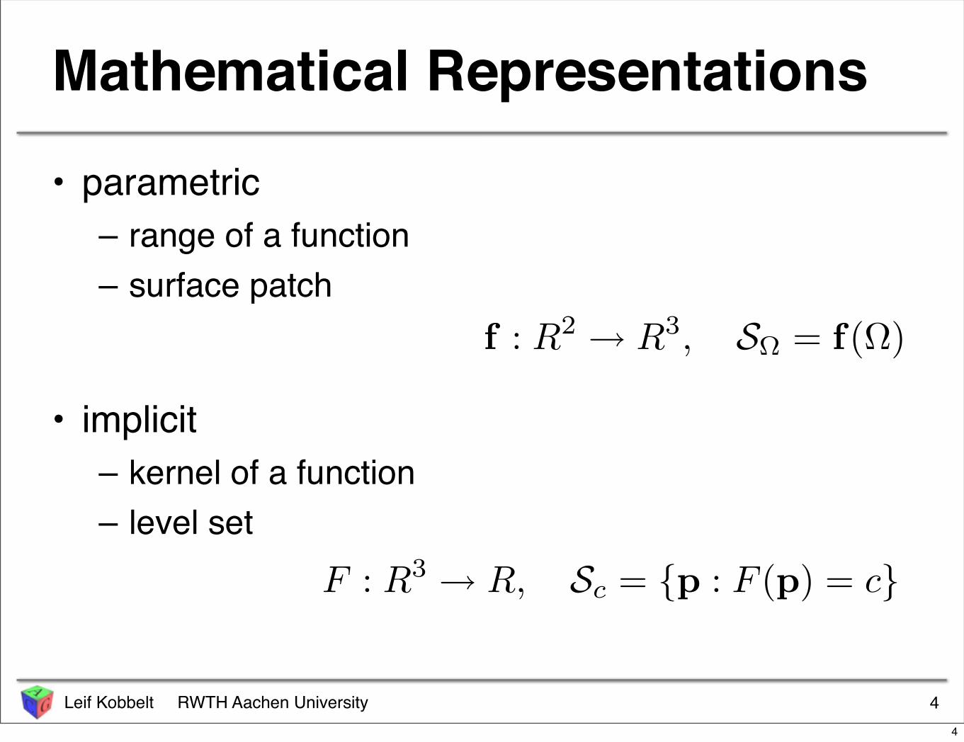
Mathematical Representations
• parametric– range of a function– surface patch
• implicit– kernel of a function– level set
4
f : R2→ R3, SΩ = f(Ω)
F : R3 → R, Sc = p : F (p) = c
4
Leif Kobbelt RWTH Aachen University
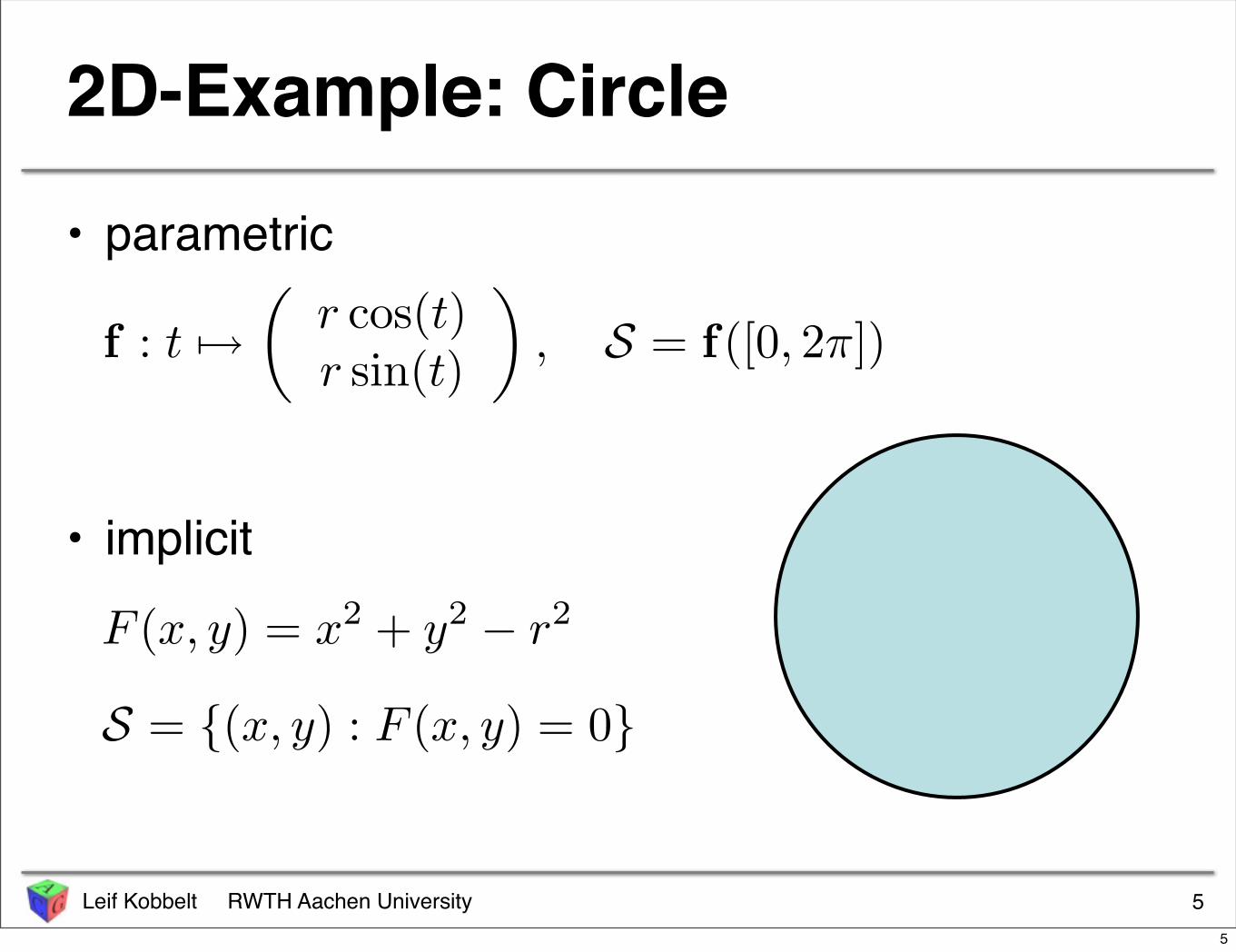
2D-Example: Circle
• parametric
• implicit
5
f : t !→
(
r cos(t)r sin(t)
)
, S = f([0, 2π])
F (x, y) = x2 + y2− r2
S = (x, y) : F (x, y) = 0
5
Leif Kobbelt RWTH Aachen University
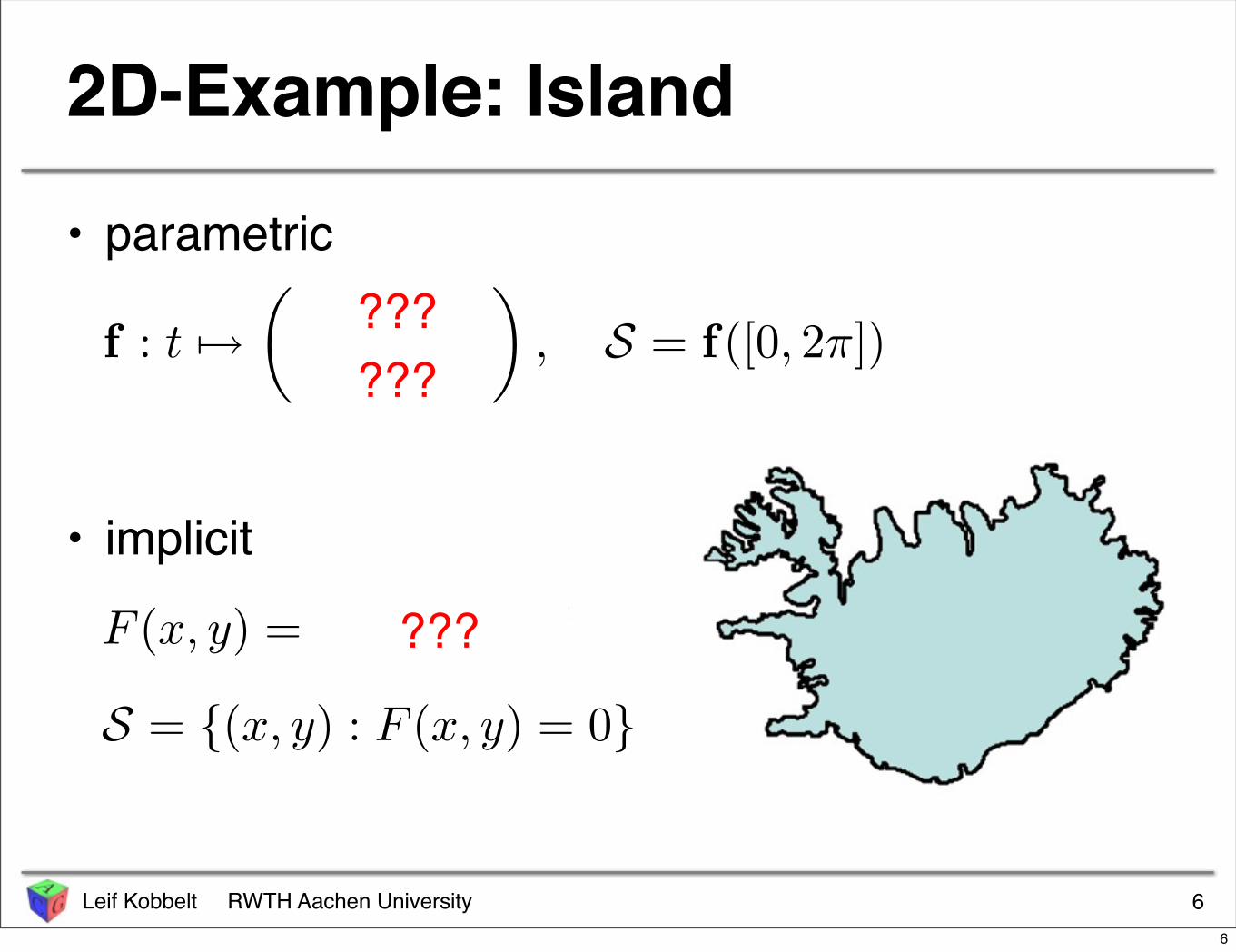
• parametric
• implicit
2D-Example: Island
6
f : t !→
(
r cos(t)r sin(t)
)
, S = f([0, 2π])
F (x, y) = x2 + y2− r2
S = (x, y) : F (x, y) = 0
??????
???
6
Leif Kobbelt RWTH Aachen University
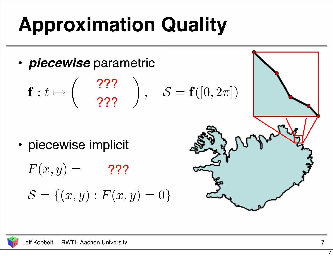
• piecewise parametric
• piecewise implicit
Approximation Quality
7
f : t !→
(
r cos(t)r sin(t)
)
, S = f([0, 2π])
F (x, y) = x2 + y2− r2
S = (x, y) : F (x, y) = 0
??????
???
7
Leif Kobbelt RWTH Aachen University
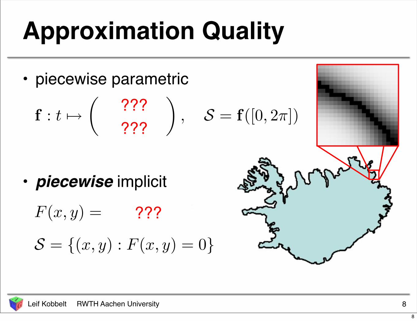
• piecewise parametric
• piecewise implicit
Approximation Quality
8
f : t !→
(
r cos(t)r sin(t)
)
, S = f([0, 2π])
F (x, y) = x2 + y2− r2
S = (x, y) : F (x, y) = 0
??????
???
8
Leif Kobbelt RWTH Aachen University
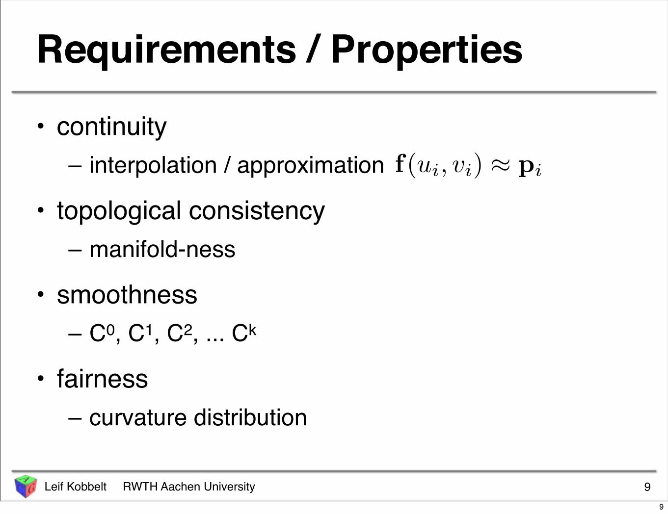
Requirements / Properties
• continuity– interpolation / approximation
• topological consistency– manifold-ness
• smoothness– C0, C1, C2, ... Ck
• fairness– curvature distribution
9
f(ui, vi) ≈ pi
9
Leif Kobbelt RWTH Aachen University
• continuity– interpolation / approximation
• topological consistency– manifold-ness
• smoothness– C0, C1, C2, ... Ck
• fairness– curvature distribution
Requirements / Properties
10
f(ui, vi) ≈ pi
10
Leif Kobbelt RWTH Aachen University
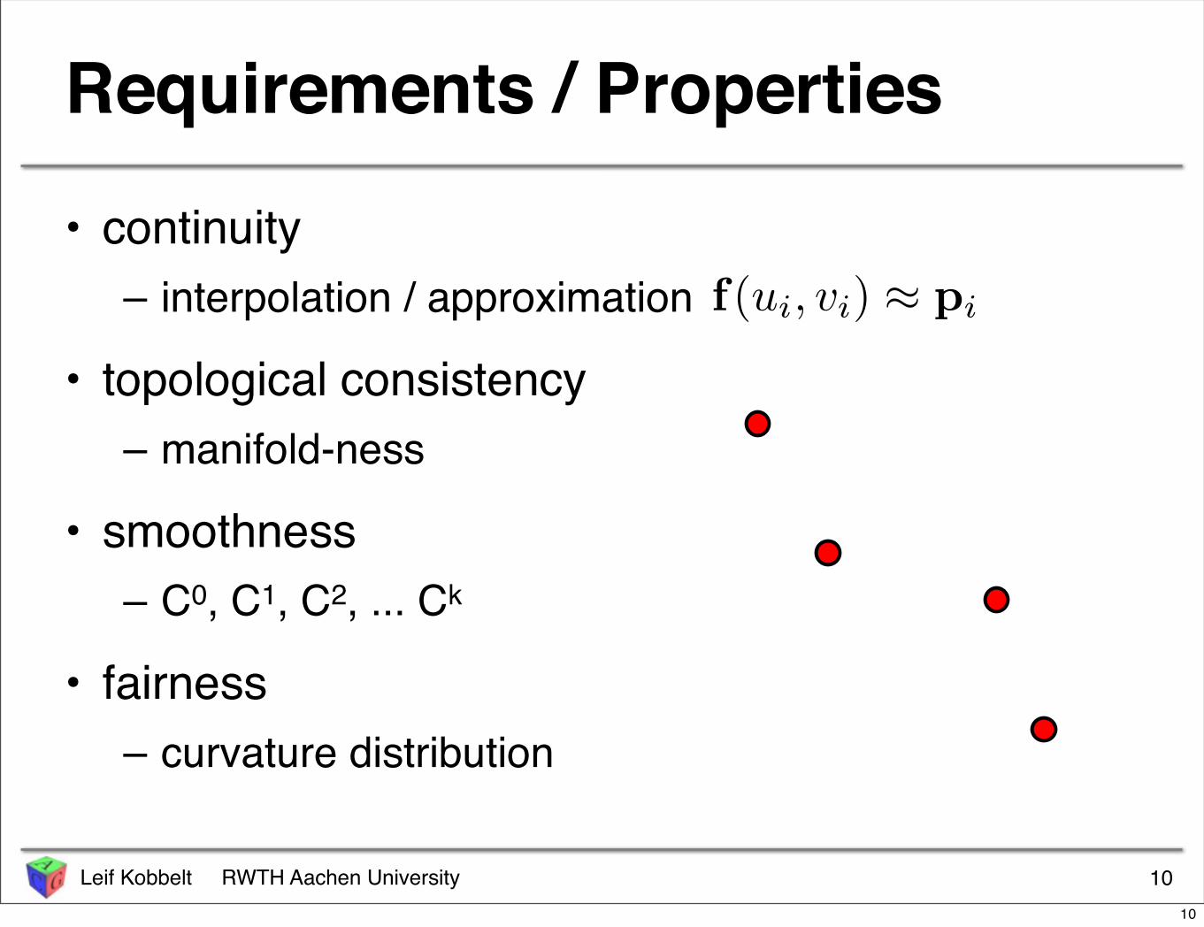
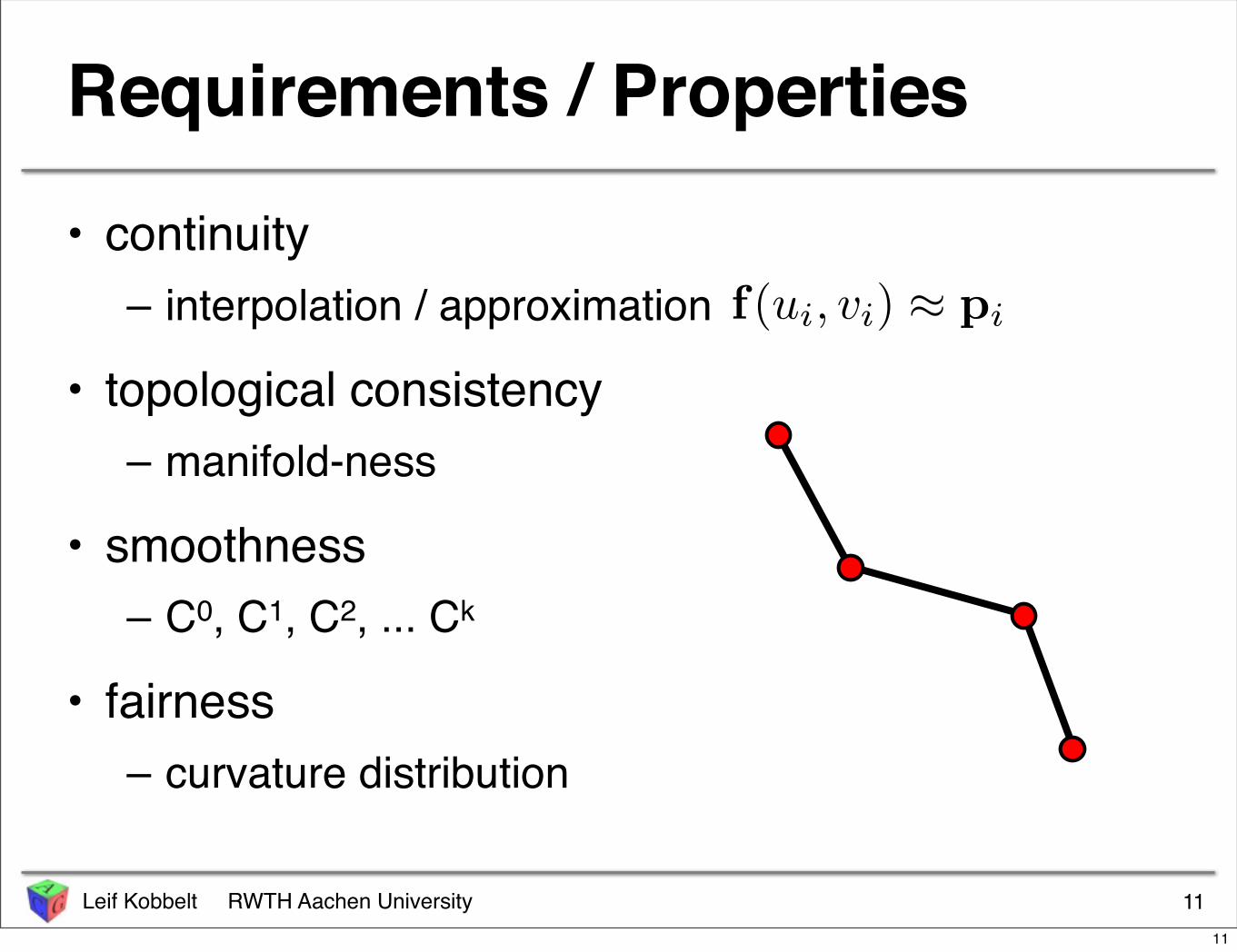
Requirements / Properties
• continuity– interpolation / approximation
• topological consistency– manifold-ness
• smoothness– C0, C1, C2, ... Ck
• fairness– curvature distribution
11
f(ui, vi) ≈ pi
11
Leif Kobbelt RWTH Aachen University
• continuity– interpolation / approximation
• topological consistency– manifold-ness
• smoothness– C0, C1, C2, ... Ck
• fairness– curvature distribution
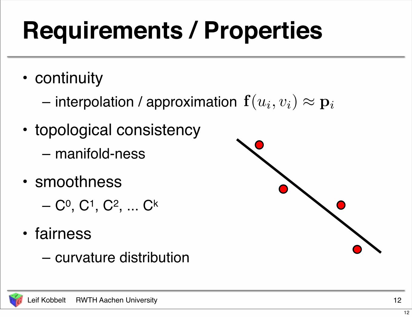
Requirements / Properties
12
f(ui, vi) ≈ pi
12

Leif Kobbelt RWTH Aachen University
• continuity– interpolation / approximation
• topological consistency– manifold-ness
• smoothness– C0, C1, C2, ... Ck
• fairness– curvature distribution
Requirements / Properties
13
f(ui, vi) ≈ pi
13
Leif Kobbelt RWTH Aachen University
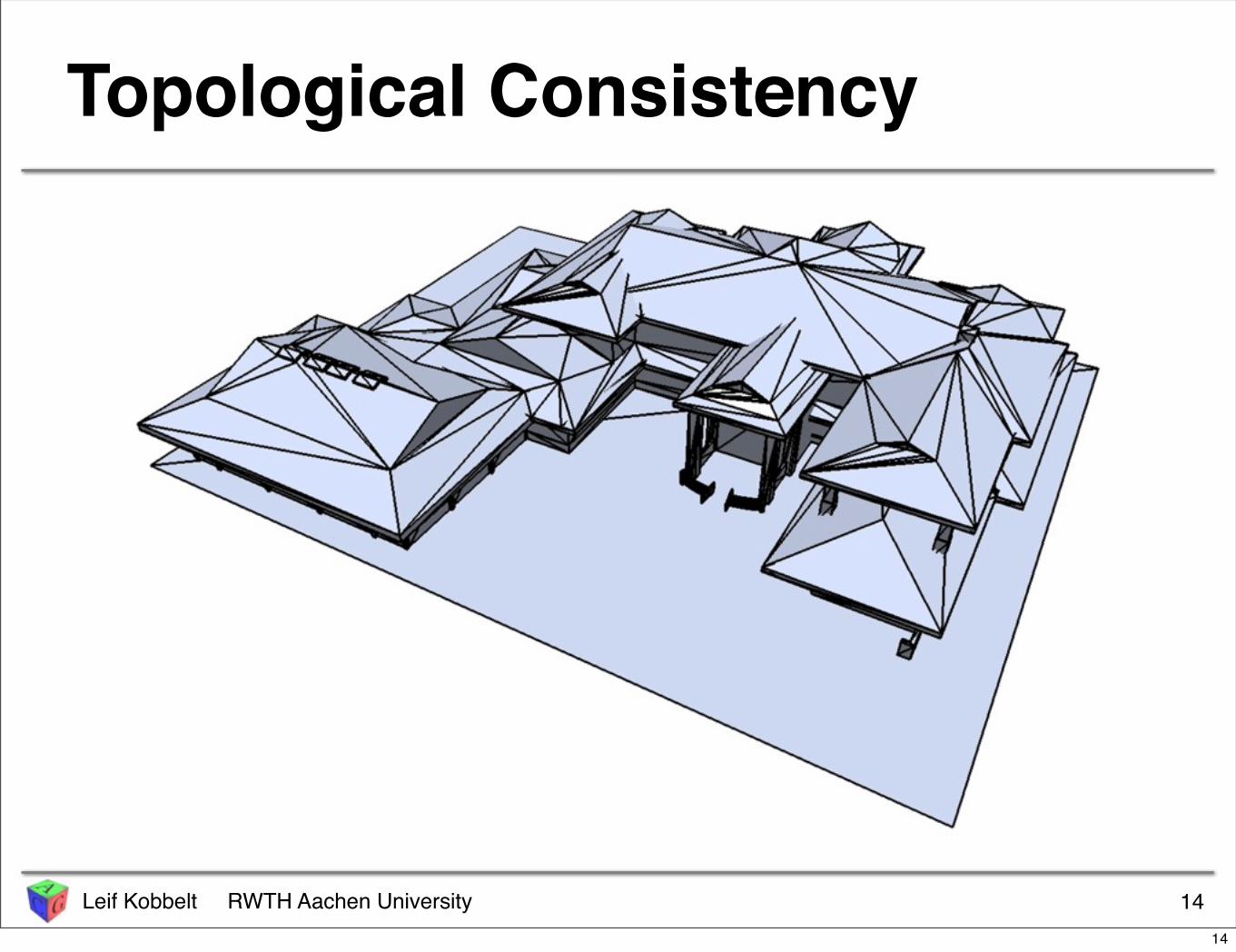
Topological Consistency
1414

Leif Kobbelt RWTH Aachen University
Topological Consistency
1414

Leif Kobbelt RWTH Aachen University
Topological Consistency
14
Mesh Repair ...
14

Leif Kobbelt RWTH Aachen University
Closed 2-Manifolds
• parametric– disk-shaped neighborhoods– + injectivity
• implicit– surface of a “physical” solid–
15
f(Dε[u, v]) = Dδ[f(u, v)]
F (x, y, z) = c, ‖∇F (x, y, z)‖ #= 0
15
Leif Kobbelt RWTH Aachen University
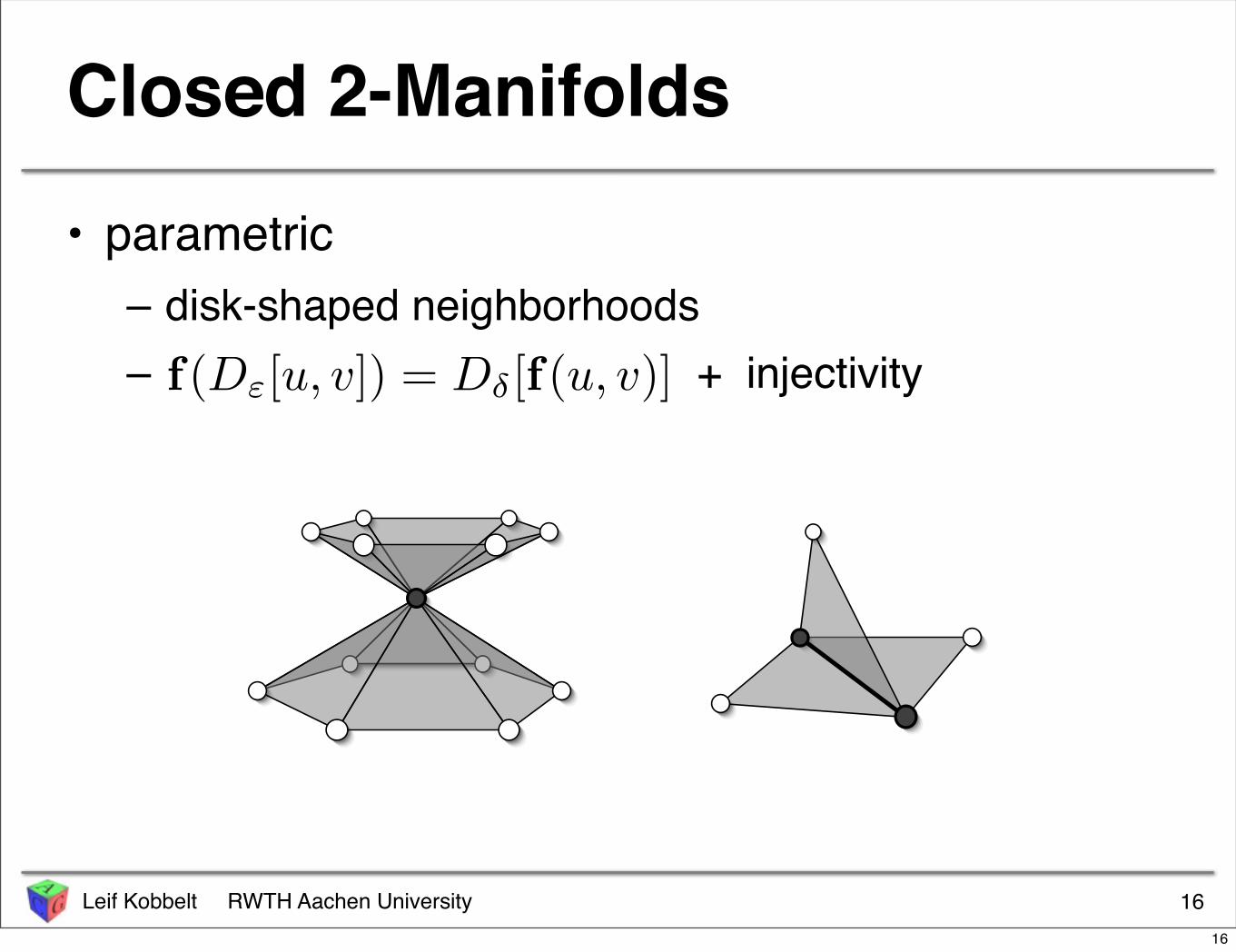
Closed 2-Manifolds
• parametric– disk-shaped neighborhoods– + injectivity
• implicit– surface of a “physical” solid–
16
f(Dε[u, v]) = Dδ[f(u, v)]
F (x, y, z) = c, ‖∇F (x, y, z)‖ #= 0
16
Leif Kobbelt RWTH Aachen University
Closed 2-Manifolds
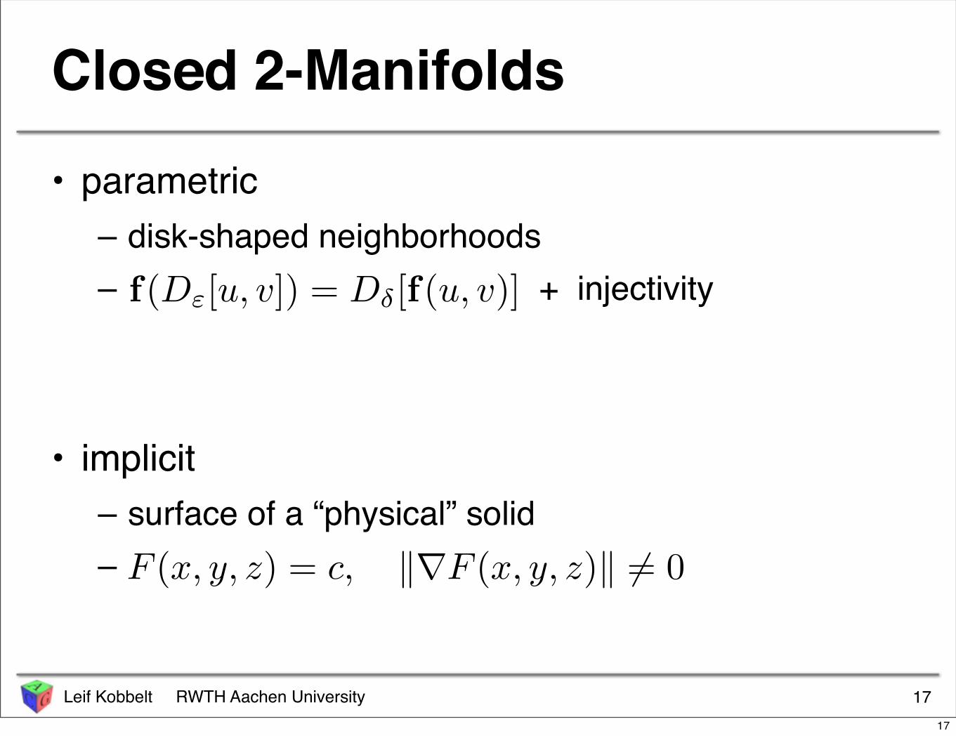
• parametric– disk-shaped neighborhoods– + injectivity
• implicit– surface of a “physical” solid–
17
f(Dε[u, v]) = Dδ[f(u, v)]
F (x, y, z) = c, ‖∇F (x, y, z)‖ #= 0
17

Leif Kobbelt RWTH Aachen University
Closed 2-Manifolds
• parametric– disk-shaped neighborhoods–
• implicit– surface of a “physical” solid–
18
f(Dε[u, v]) = Dδ[f(u, v)]
F (x, y, z) = c, ‖∇F (x, y, z)‖ #= 0
18
Leif Kobbelt RWTH Aachen University
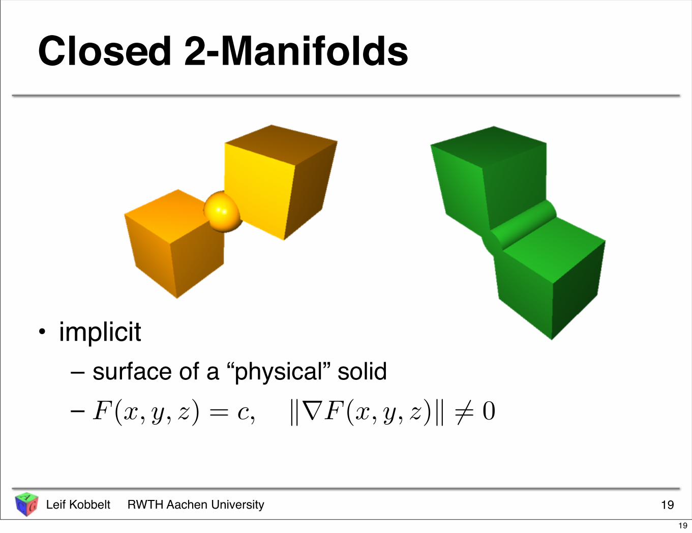
Closed 2-Manifolds
• parametric– disk-shaped neighborhoods–
• implicit– surface of a “physical” solid–
19
f(Dε[u, v]) = Dδ[f(u, v)]
F (x, y, z) = c, ‖∇F (x, y, z)‖ #= 0
19

Leif Kobbelt RWTH Aachen University
Smoothness
• position continuity : C0
• tangent continuity : C1
• curvature continuity : C2
2020
Leif Kobbelt RWTH Aachen University
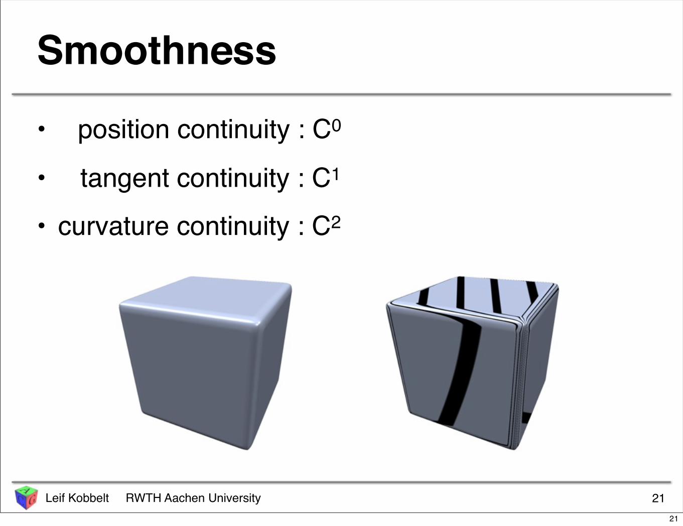
Smoothness
• position continuity : C0
• tangent continuity : C1
• curvature continuity : C2
2121
Leif Kobbelt RWTH Aachen University
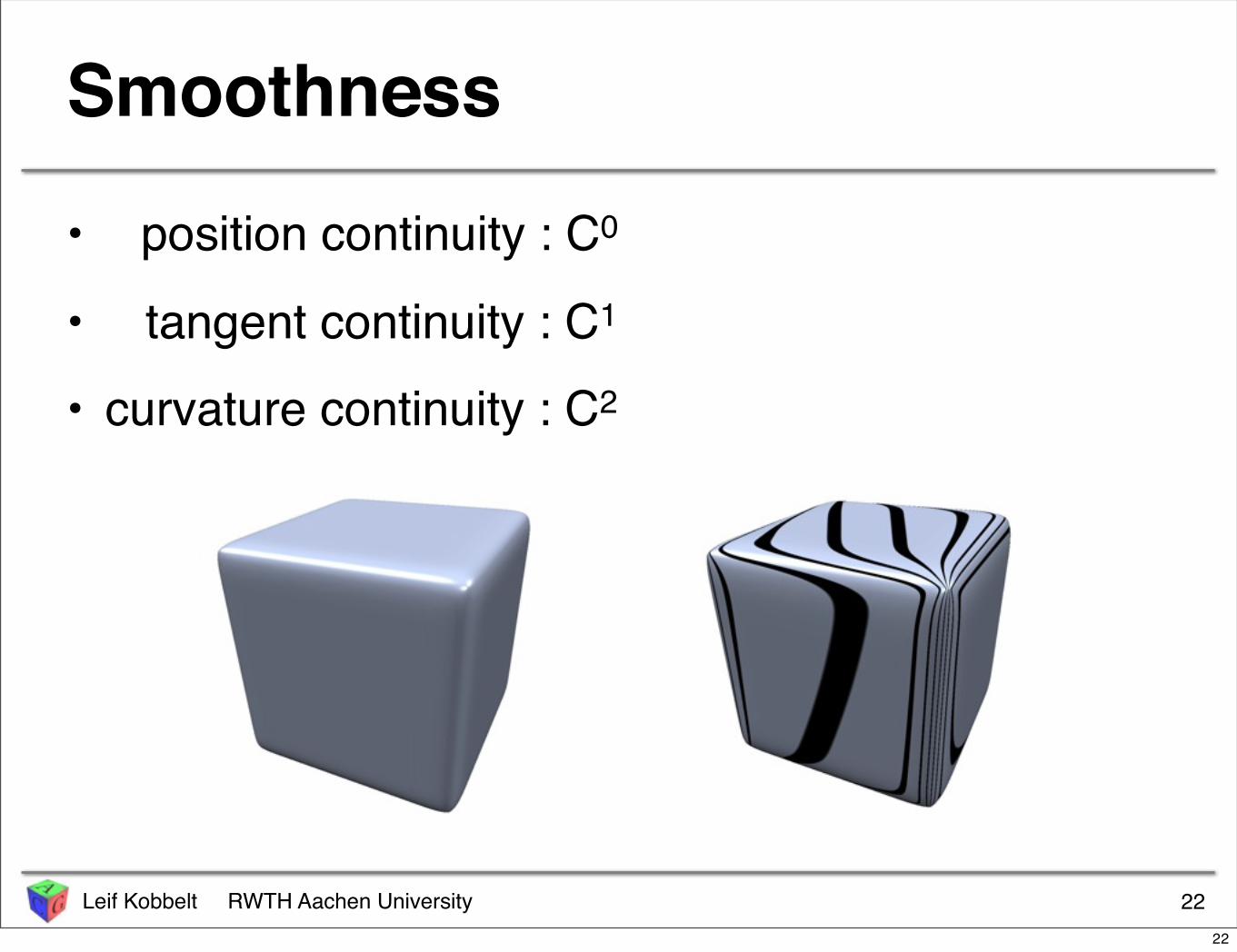
Smoothness
• position continuity : C0
• tangent continuity : C1
• curvature continuity : C2
2222
Leif Kobbelt RWTH Aachen University
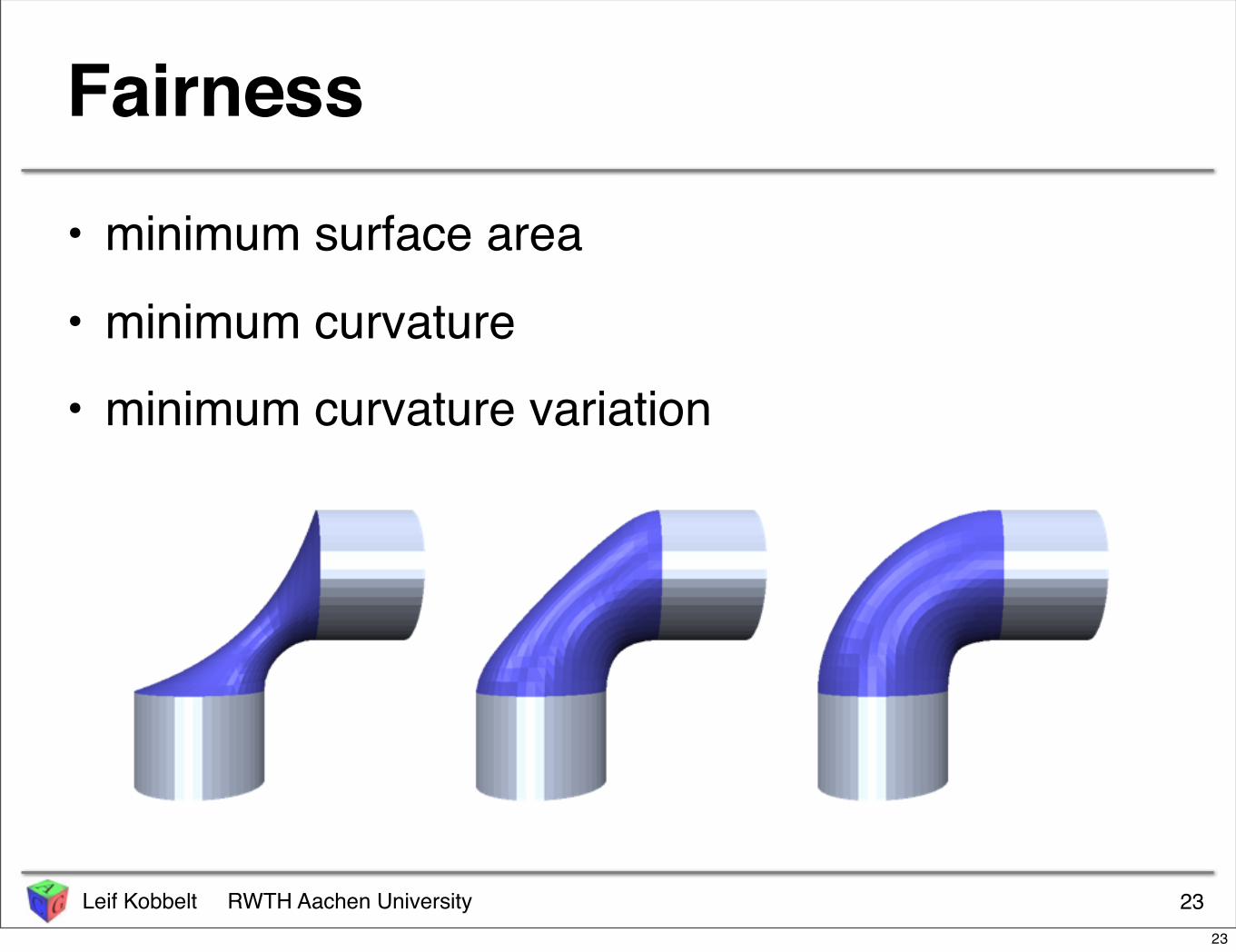
Fairness
• minimum surface area
• minimum curvature
• minimum curvature variation
2323

Leif Kobbelt RWTH Aachen University
• (mathematical) geometry representations– parametric vs. implicit
• approximation properties• types of operations
– distance queries– evaluation– modification / deformation
• data structures
Outline
2424
Leif Kobbelt RWTH Aachen University
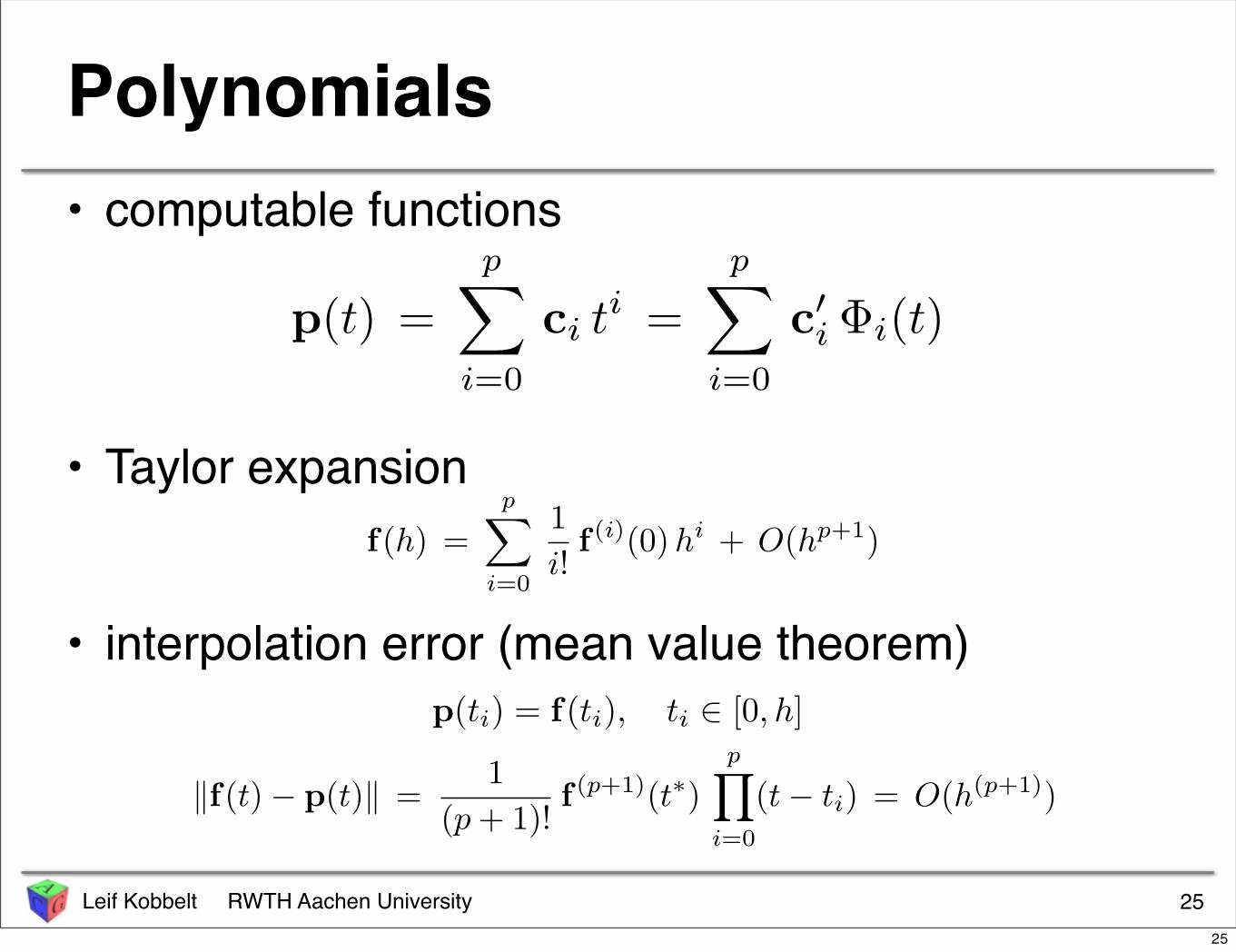
Polynomials• computable functions
• Taylor expansion
• interpolation error (mean value theorem)
25
p(t) =p∑
i=0
ci ti =
p∑
i=0
c′
i Φi(t)
p(ti) = f(ti), ti ∈ [0, h]
f(h) =p∑
i=0
1
i!f(i)(0)h
i + O(hp+1)
‖f(t) − p(t)‖ =1
(p + 1)!f (p+1)(t∗)
p∏
i=0
(t − ti) = O(h(p+1))
25
Leif Kobbelt RWTH Aachen University
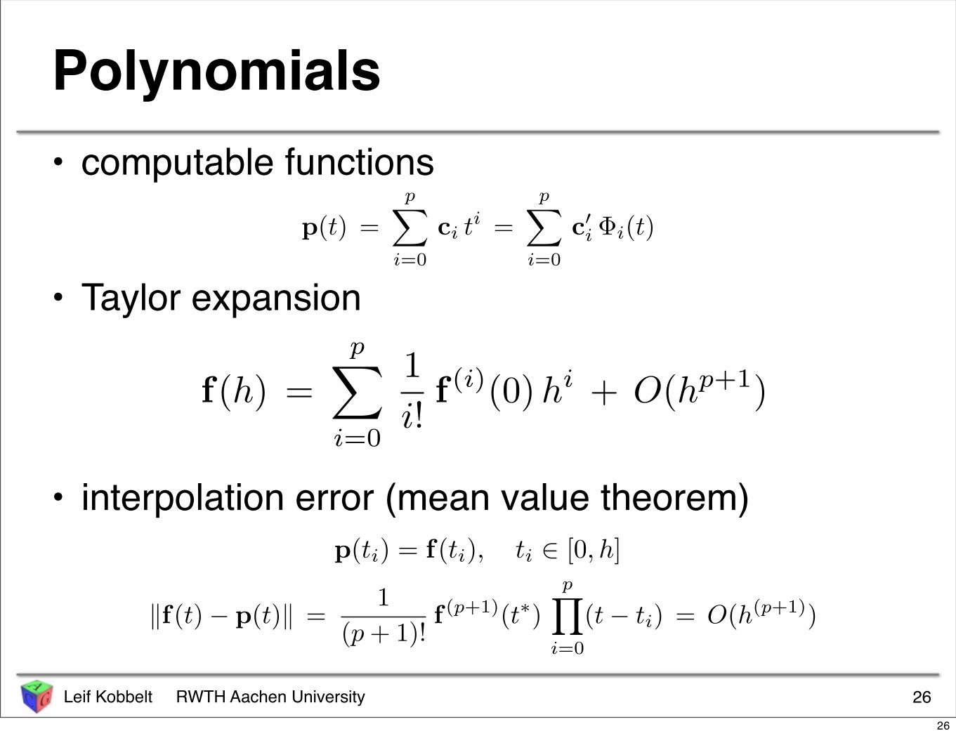
• computable functions
• Taylor expansion
• interpolation error (mean value theorem)
Polynomials
26
p(ti) = f(ti), ti ∈ [0, h]
p(t) =p∑
i=0
ci ti =
p∑
i=0
c′
i Φi(t)
‖f(t) − p(t)‖ =1
(p + 1)!f (p+1)(t∗)
p∏
i=0
(t − ti) = O(h(p+1))
f(h) =p∑
i=0
1
i!f(i)(0)h
i + O(hp+1)
26
Leif Kobbelt RWTH Aachen University
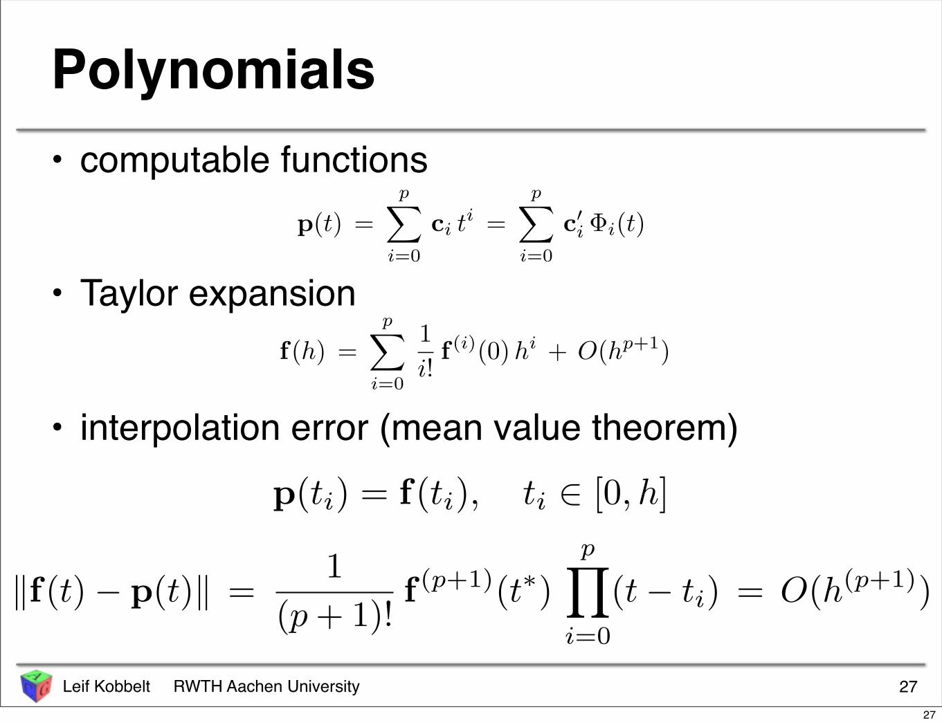
Polynomials• computable functions
• Taylor expansion
• interpolation error (mean value theorem)
27
p(ti) = f(ti), ti ∈ [0, h]
p(t) =p∑
i=0
ci ti =
p∑
i=0
c′
i Φi(t)
f(h) =p∑
i=0
1
i!f(i)(0)h
i + O(hp+1)
‖f(t) − p(t)‖ =1
(p + 1)!f (p+1)(t∗)
p∏
i=0
(t − ti) = O(h(p+1))
27
Leif Kobbelt RWTH Aachen University
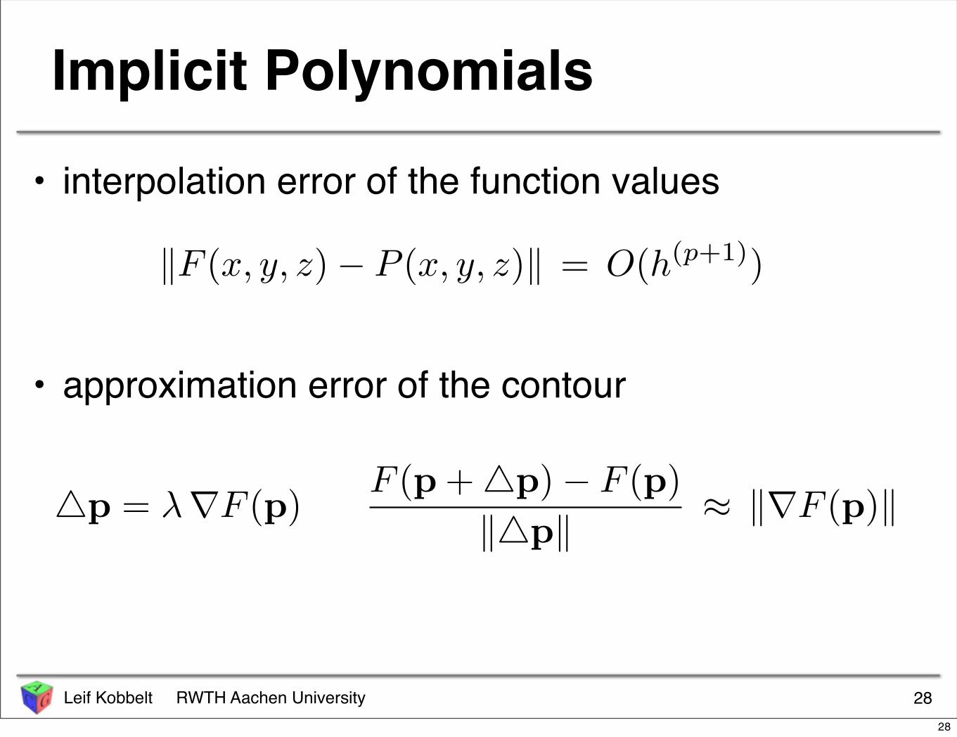
Implicit Polynomials
• interpolation error of the function values
• approximation error of the contour
28
F (p + !p) − F (p)
‖!p‖≈ ‖∇F (p)‖!p = λ∇F (p)
‖F (x, y, z) − P (x, y, z)‖ = O(h(p+1))
28
Leif Kobbelt RWTH Aachen University
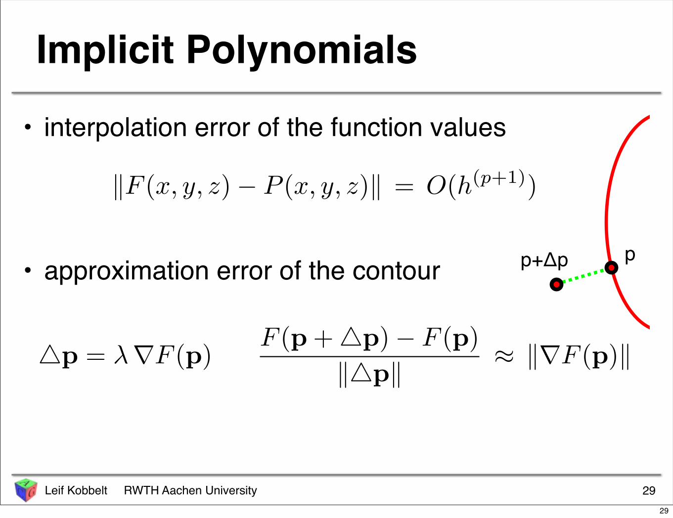
Implicit Polynomials
• interpolation error of the function values
• approximation error of the contour
29
F (p + !p) − F (p)
‖!p‖≈ ‖∇F (p)‖!p = λ∇F (p)
‖F (x, y, z) − P (x, y, z)‖ = O(h(p+1))
pp+Δp
29
Leif Kobbelt RWTH Aachen University
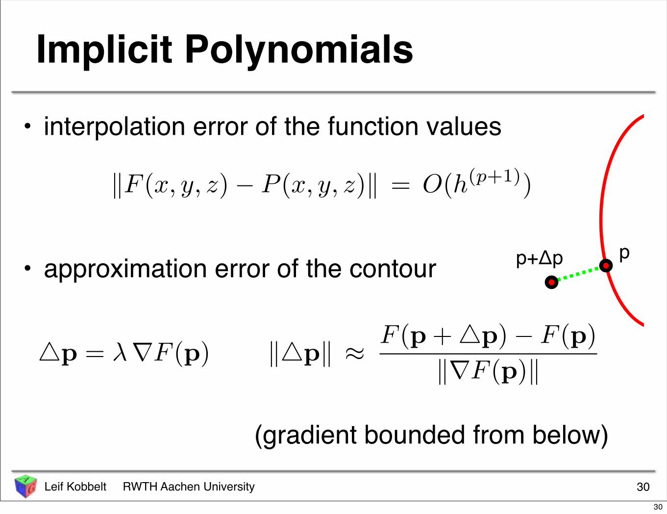
Implicit Polynomials
• interpolation error of the function values
• approximation error of the contour
30
‖"p‖ ≈F (p + "p) − F (p)
‖∇F (p)‖!p = λ∇F (p)
(gradient bounded from below)
‖F (x, y, z) − P (x, y, z)‖ = O(h(p+1))
pp+Δp
30
Leif Kobbelt RWTH Aachen University
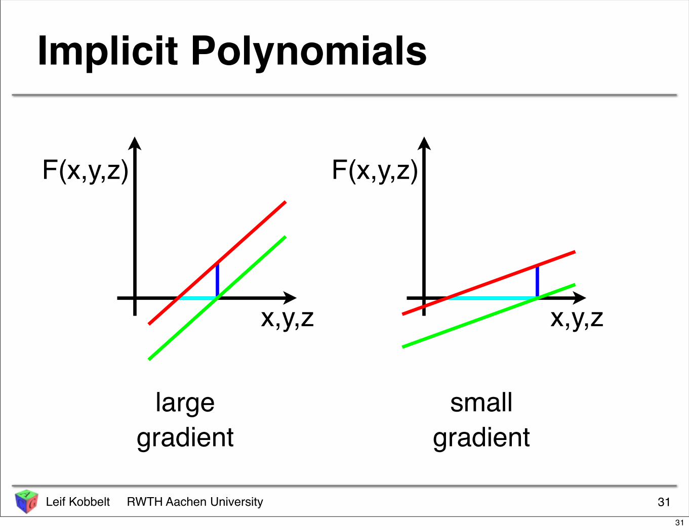
Implicit Polynomials
31
largegradient
smallgradient
F(x,y,z) F(x,y,z)
x,y,z x,y,z
31
Leif Kobbelt RWTH Aachen University
Polynomial Approximation
• approximation error is O(hp+1)
• improve approximation quality by– increasing p ... higher order polynomials– decreasing h ... smaller / more segments
• issues– smoothness of the target data ( maxt f(p+1)(t) )– handling higher order patches (e.g. boundary conditions)
3232
Leif Kobbelt RWTH Aachen University
Polynomial Approximation
• approximation error is O(hp+1)
• improve approximation quality by– increasing p ... higher order polynomials– decreasing h ... smaller / more segments
• issues– smoothness of the target data ( maxt f(p+1)(t) )– handling higher order patches (e.g. boundary conditions)
33
MOTD: p = 1
MOTD: p = 1
33
Leif Kobbelt RWTH Aachen University
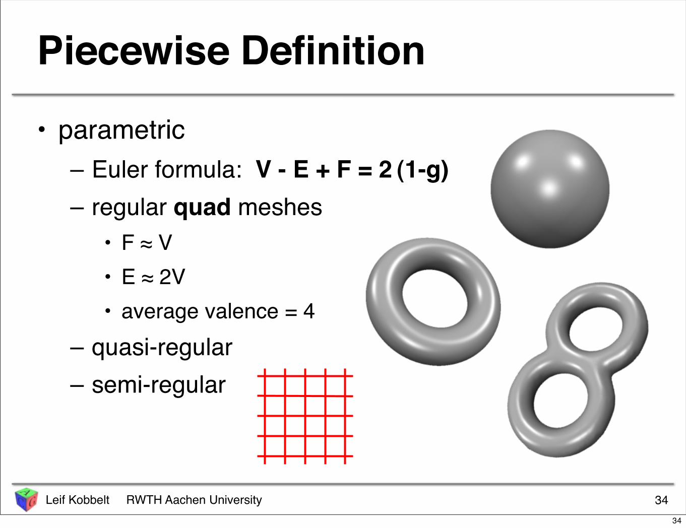
Piecewise Definition
• parametric– Euler formula: V - E + F = 2 (1-g)– regular quad meshes
• F ≈ V• E ≈ 2V• average valence = 4
– quasi-regular– semi-regular
3434
Leif Kobbelt RWTH Aachen University
Piecewise Definition
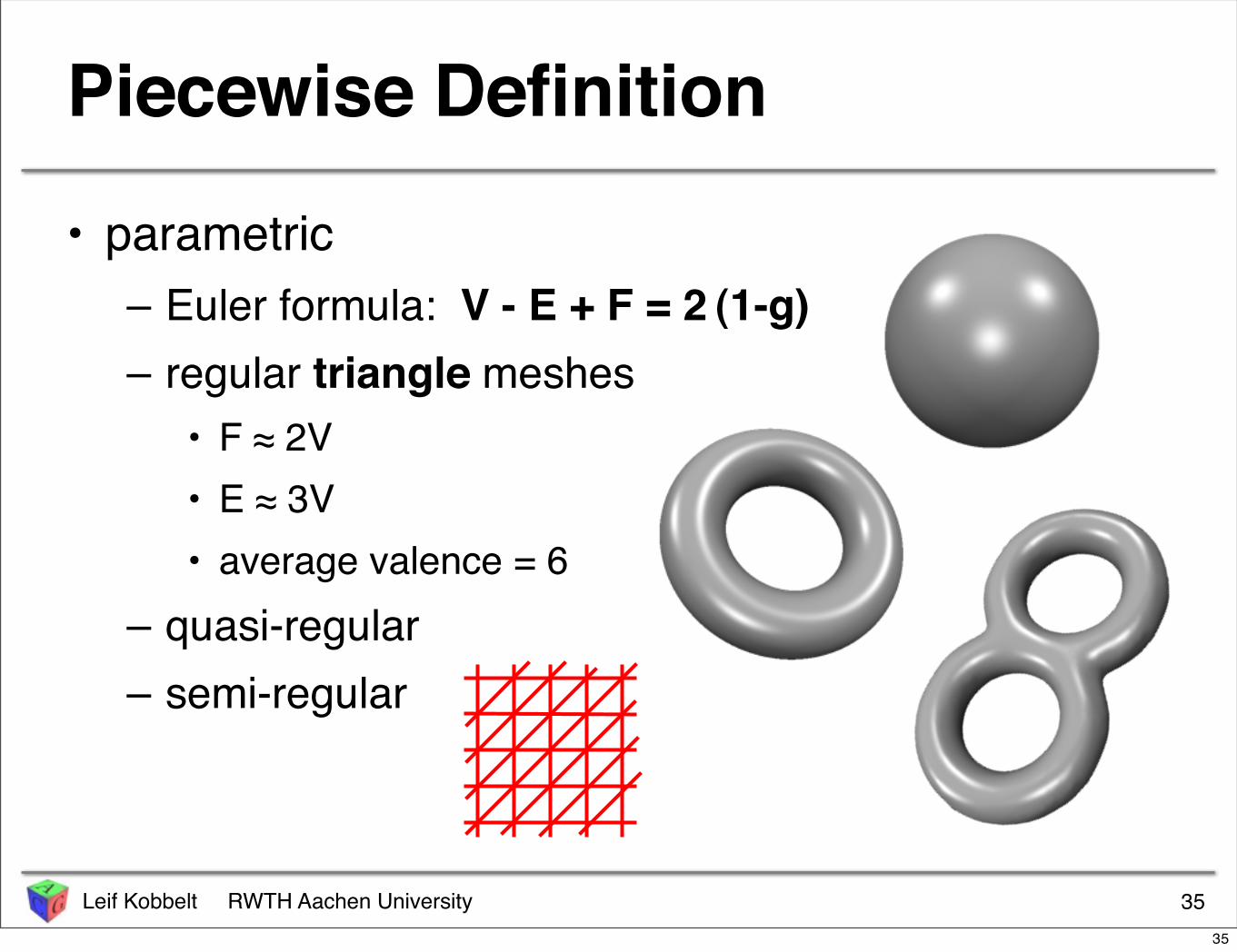
• parametric– Euler formula: V - E + F = 2 (1-g)– regular triangle meshes
• F ≈ 2V• E ≈ 3V• average valence = 6
– quasi-regular– semi-regular
3535
Leif Kobbelt RWTH Aachen University
Piecewise Definition
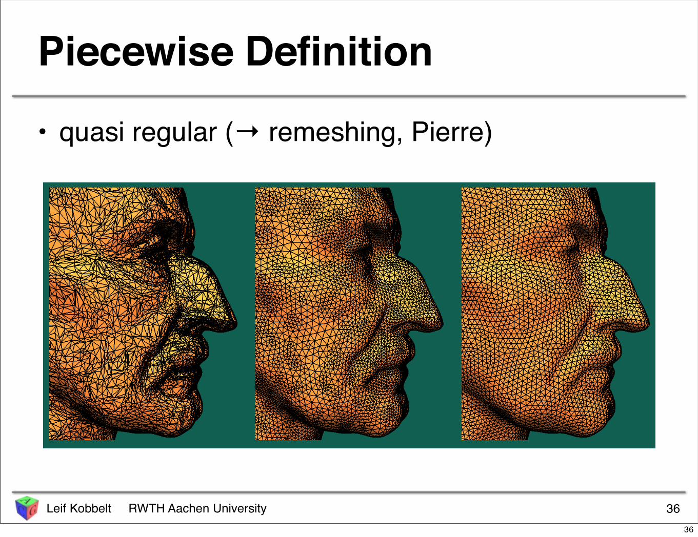
• quasi regular (→ remeshing, Pierre)
36
Computer Graphics GroupMario Botsch
Remeshing Results
Original(
1
2, 2
) (
4
5,
4
3
)
36
Leif Kobbelt RWTH Aachen University
Piecewise Definition
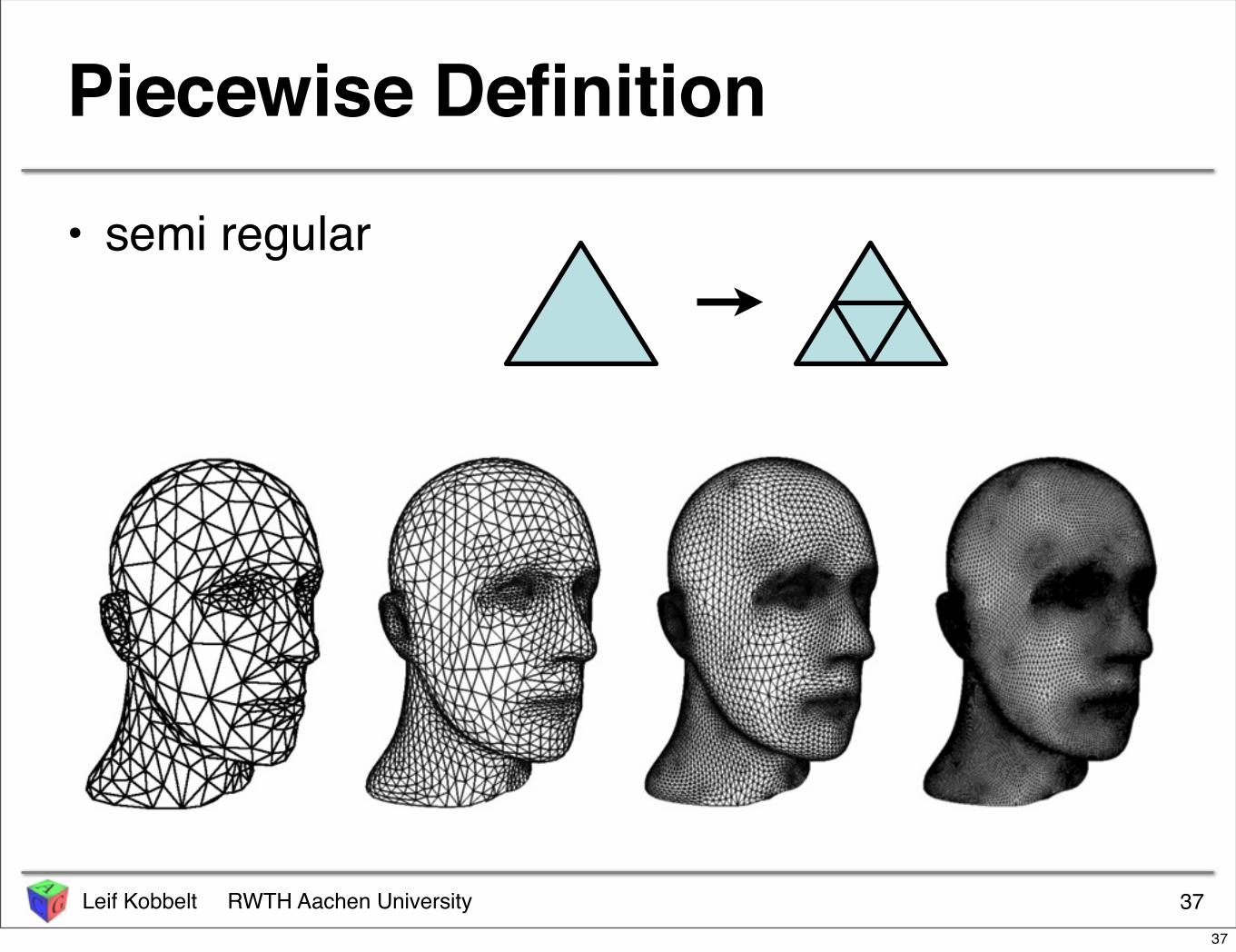
• semi regular
3737
Leif Kobbelt RWTH Aachen University
Piecewise Definition
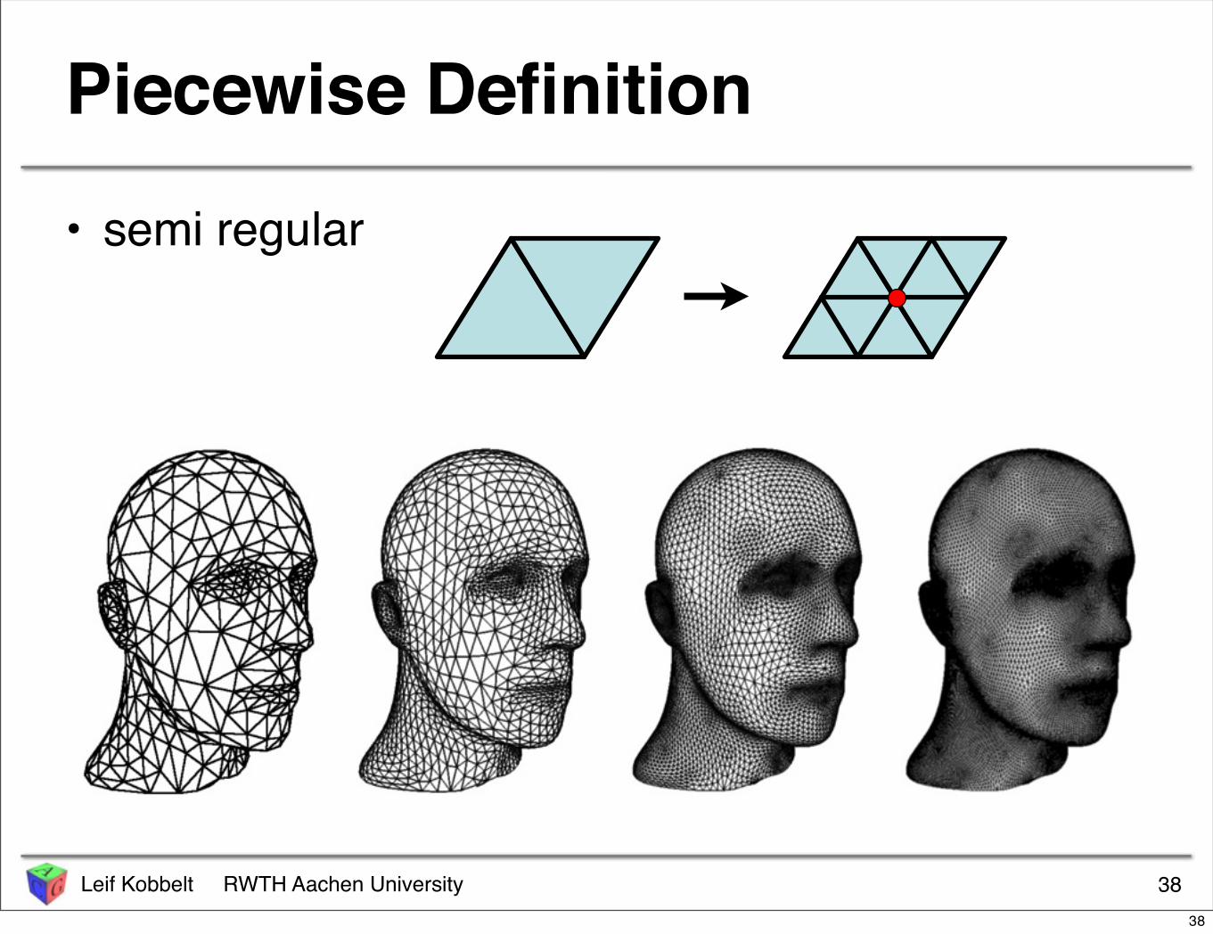
• semi regular
3838
Leif Kobbelt RWTH Aachen University
Piecewise Definition
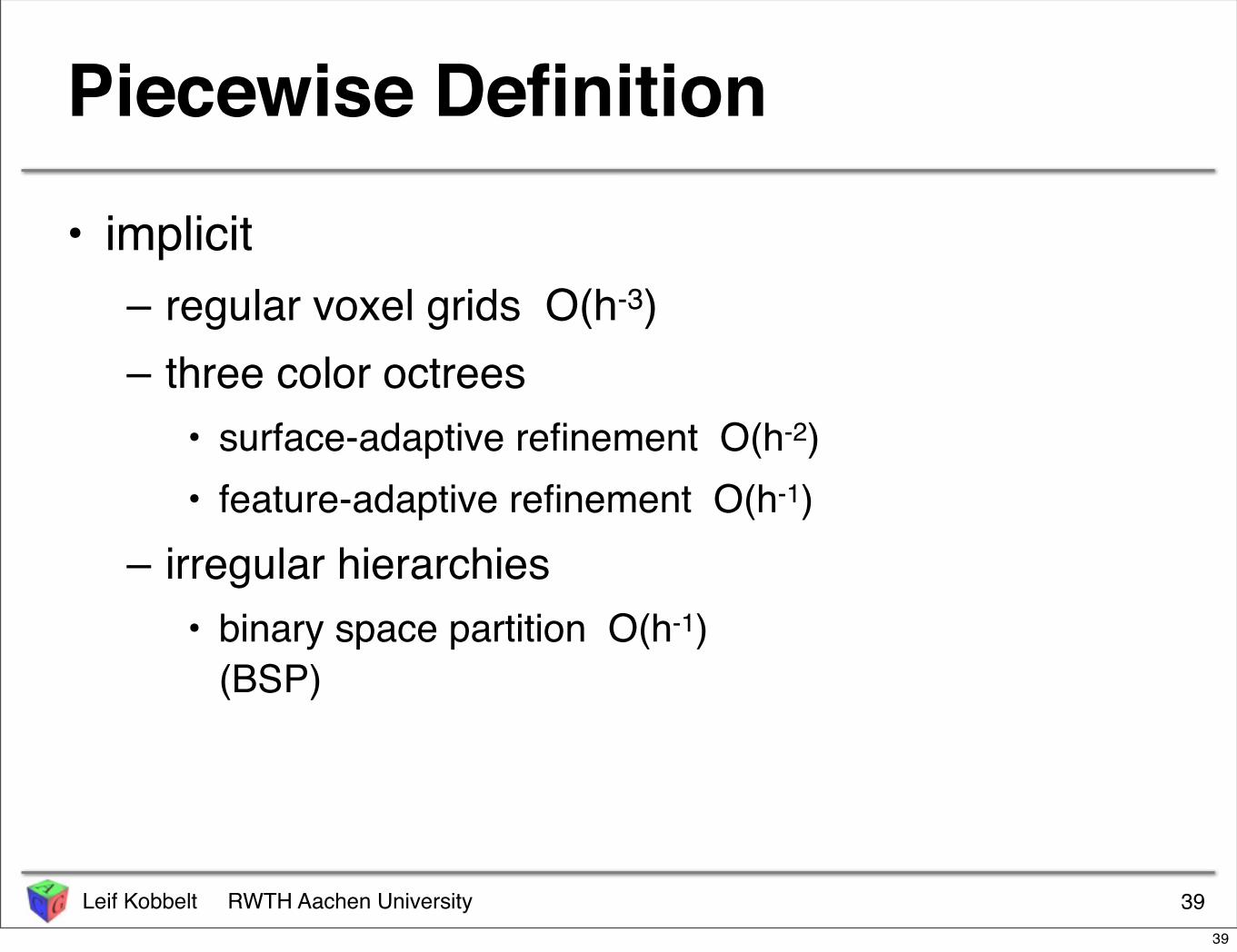
• implicit– regular voxel grids O(h-3)– three color octrees
• surface-adaptive refinement O(h-2)• feature-adaptive refinement O(h-1)
– irregular hierarchies• binary space partition O(h-1)
(BSP)
3939
Leif Kobbelt RWTH Aachen University
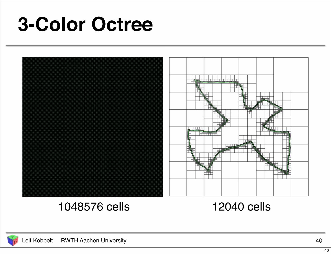
3-Color Octree
40
12040 cells1048576 cells
40

Leif Kobbelt RWTH Aachen University
Adaptively Sampled Distance Fields
41
12040 cells 895 cells
41

Leif Kobbelt RWTH Aachen University
Binary Space Partitions
42
254 cells895 cells
42
Leif Kobbelt RWTH Aachen University
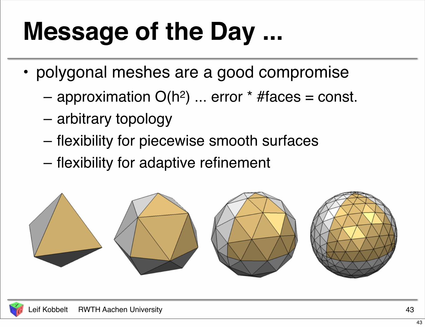
Message of the Day ...• polygonal meshes are a good compromise
– approximation O(h2) ... error * #faces = const.– arbitrary topology– flexibility for piecewise smooth surfaces– flexibility for adaptive refinement
4343

Leif Kobbelt RWTH Aachen University
Message of the Day ...• polygonal meshes are a good compromise
– approximation O(h2) ... error * #faces = const.– arbitrary topology– flexibility for piecewise smooth surfaces– flexibility for adaptive refinement
4444
Leif Kobbelt RWTH Aachen University
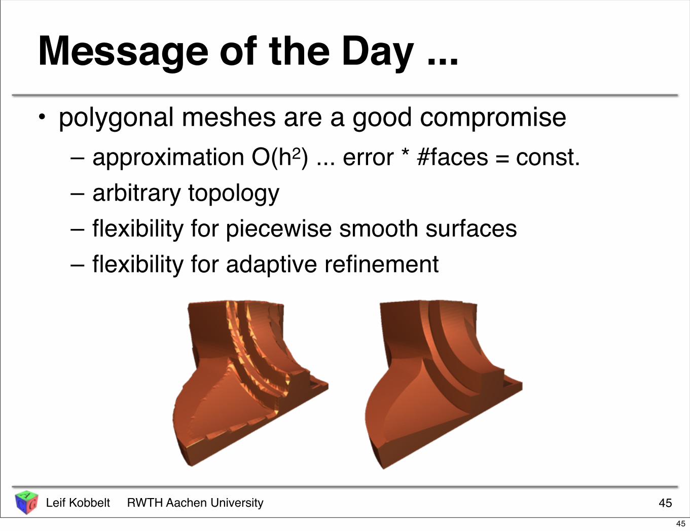
Message of the Day ...• polygonal meshes are a good compromise
– approximation O(h2) ... error * #faces = const.– arbitrary topology– flexibility for piecewise smooth surfaces– flexibility for adaptive refinement
4545
Leif Kobbelt RWTH Aachen University
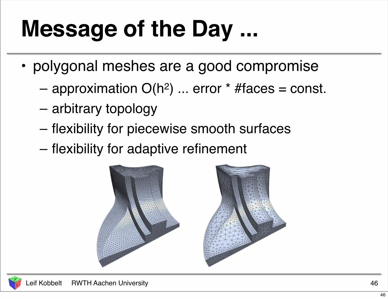
Message of the Day ...• polygonal meshes are a good compromise
– approximation O(h2) ... error * #faces = const.– arbitrary topology– flexibility for piecewise smooth surfaces– flexibility for adaptive refinement
4646
Leif Kobbelt RWTH Aachen University
Message of the Day ...• polygonal meshes are a good compromise
– approximation O(h2) ... error * #faces = const.– arbitrary topology– flexibility for piecewise smooth surfaces– flexibility for adaptive refinement– efficient rendering
4747
Leif Kobbelt RWTH Aachen University
Message of the Day ...• polygonal meshes are a good compromise
– approximation O(h2) ... error * #faces = const.– arbitrary topology– flexibility for piecewise smooth surfaces– flexibility for adaptive refinement– efficient rendering
• implicit representation can support efficient access to vertices, faces, ....
4848
Leif Kobbelt RWTH Aachen University
• (mathematical) geometry representations– parametric vs. implicit
• approximation properties• types of operations
– evaluation– distance queries– modification / deformation
• data structures
Outline
4949
Leif Kobbelt RWTH Aachen University
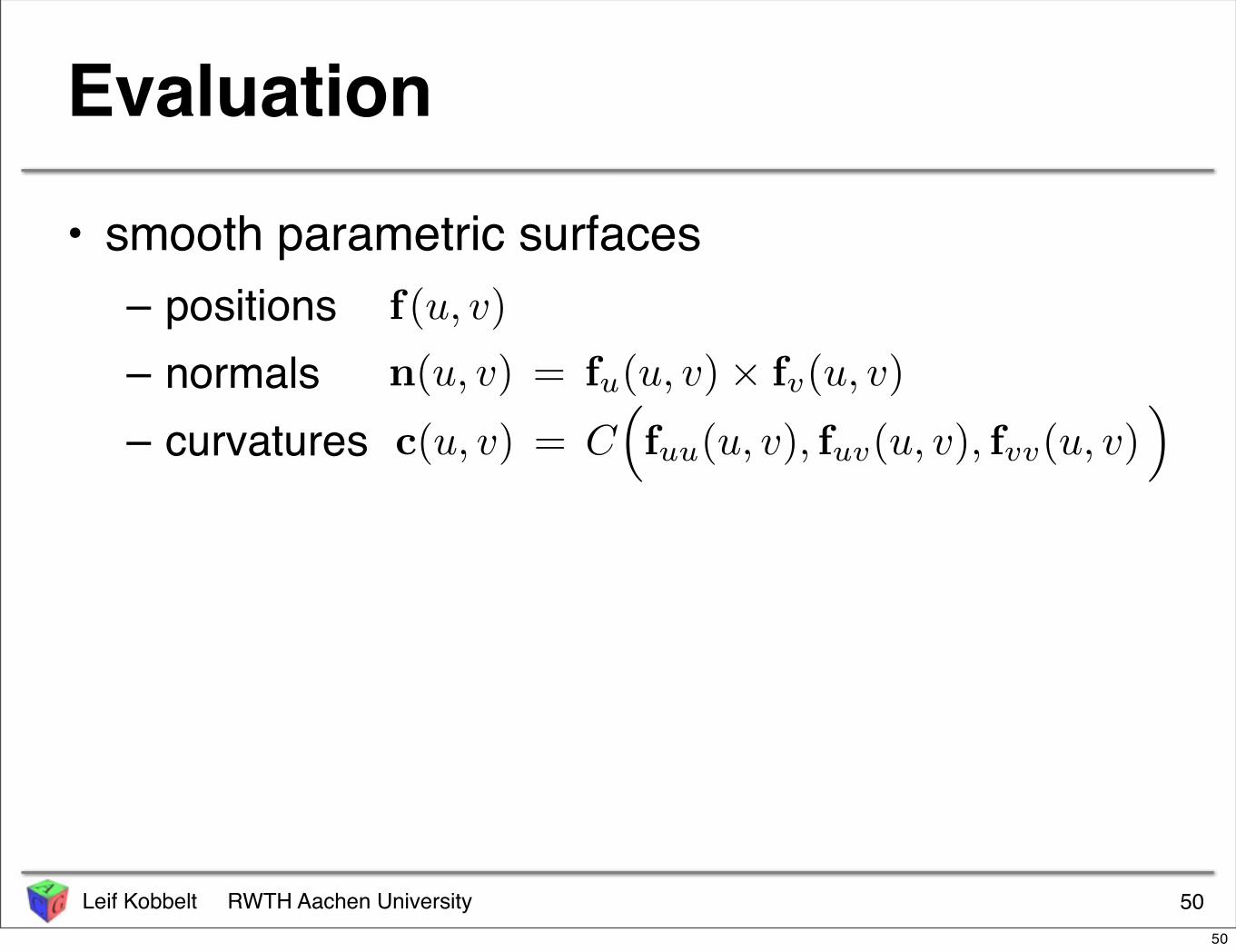
Evaluation
• smooth parametric surfaces– positions– normals– curvatures
50
f(u, v)
n(u, v) = fu(u, v) × fv(u, v)
c(u, v) = C(
fuu(u, v), fuv(u, v), fvv(u, v))
50
Leif Kobbelt RWTH Aachen University
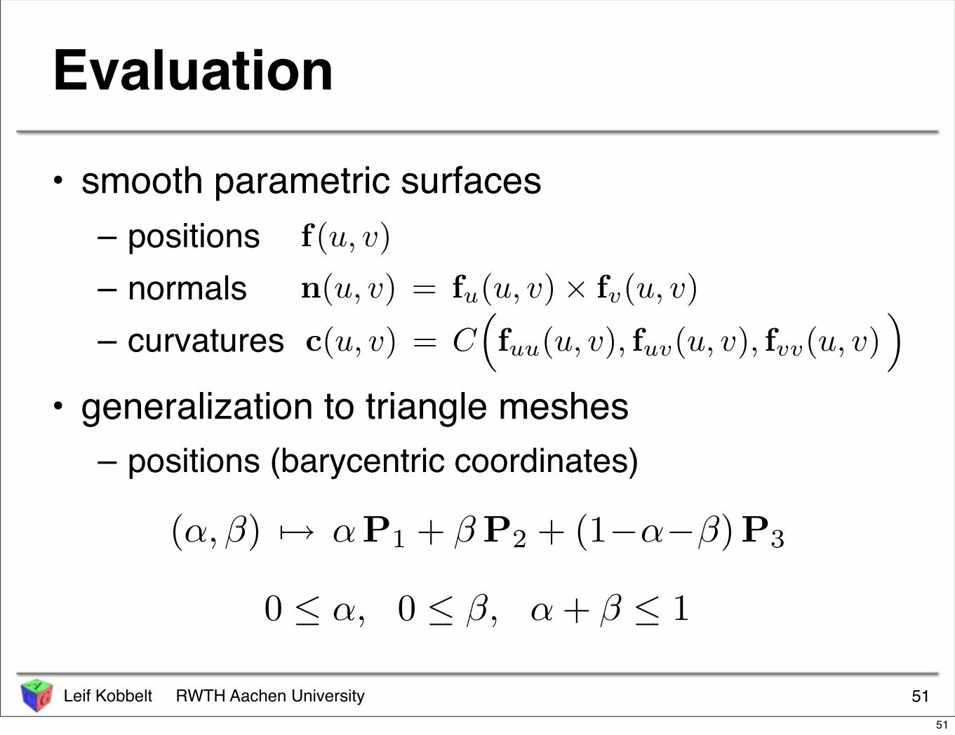
Evaluation
• smooth parametric surfaces– positions– normals– curvatures
• generalization to triangle meshes– positions (barycentric coordinates)
51
(α,β) !→ αP1 + β P2 + (1−α−β)P3
f(u, v)
n(u, v) = fu(u, v) × fv(u, v)
c(u, v) = C(
fuu(u, v), fuv(u, v), fvv(u, v))
0 ≤ α, 0 ≤ β, α + β ≤ 1
51
Leif Kobbelt RWTH Aachen University
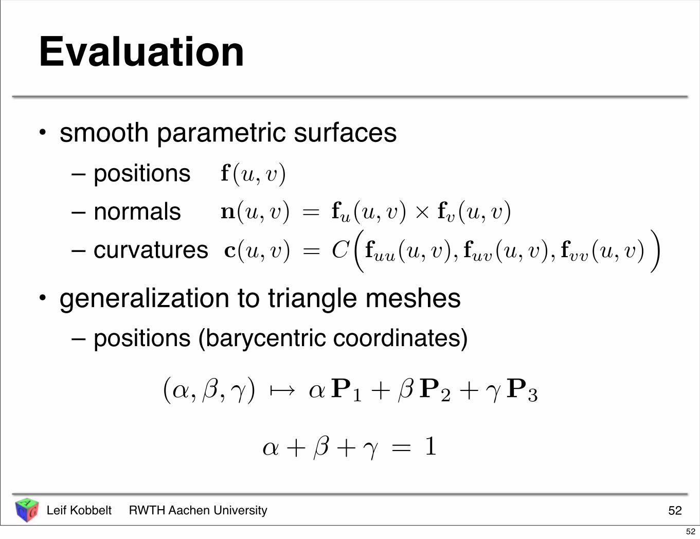
Evaluation
• smooth parametric surfaces– positions– normals– curvatures
• generalization to triangle meshes– positions (barycentric coordinates)
52
(α,β, γ) !→ αP1 + β P2 + γ P3
f(u, v)
n(u, v) = fu(u, v) × fv(u, v)
c(u, v) = C(
fuu(u, v), fuv(u, v), fvv(u, v))
α + β + γ = 1
52

Leif Kobbelt RWTH Aachen University
Evaluation
• smooth parametric surfaces– positions– normals– curvatures
• generalization to triangle meshes– positions (barycentric coordinates)
53
αu + β v + γ w !→ αP1 + β P2 + γ P3
f(u, v)
n(u, v) = fu(u, v) × fv(u, v)
c(u, v) = C(
fuu(u, v), fuv(u, v), fvv(u, v))
α + β + γ = 0
53
Leif Kobbelt RWTH Aachen University
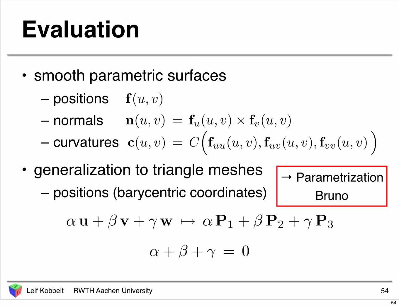
Evaluation
• smooth parametric surfaces– positions– normals– curvatures
• generalization to triangle meshes– positions (barycentric coordinates)
54
αu + β v + γ w !→ αP1 + β P2 + γ P3
f(u, v)
n(u, v) = fu(u, v) × fv(u, v)
c(u, v) = C(
fuu(u, v), fuv(u, v), fvv(u, v))
α + β + γ = 0
→ ParametrizationBruno
54
Leif Kobbelt RWTH Aachen University
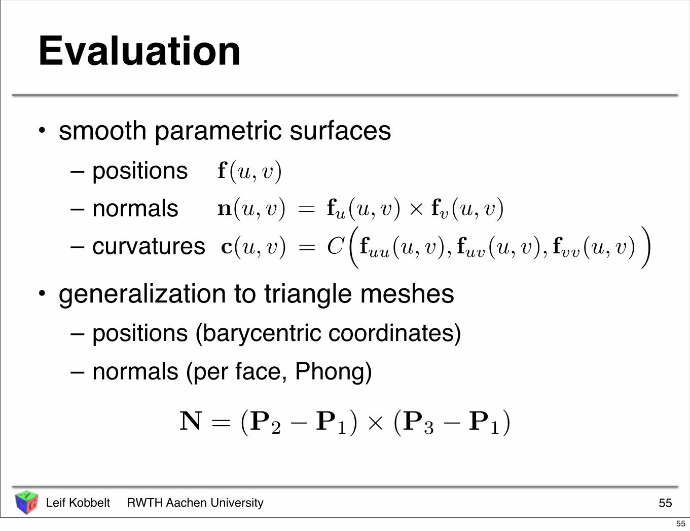
Evaluation
• smooth parametric surfaces– positions– normals– curvatures
• generalization to triangle meshes– positions (barycentric coordinates)– normals (per face, Phong)
55
f(u, v)
n(u, v) = fu(u, v) × fv(u, v)
c(u, v) = C(
fuu(u, v), fuv(u, v), fvv(u, v))
N = (P2 − P1) × (P3 − P1)
55
Leif Kobbelt RWTH Aachen University
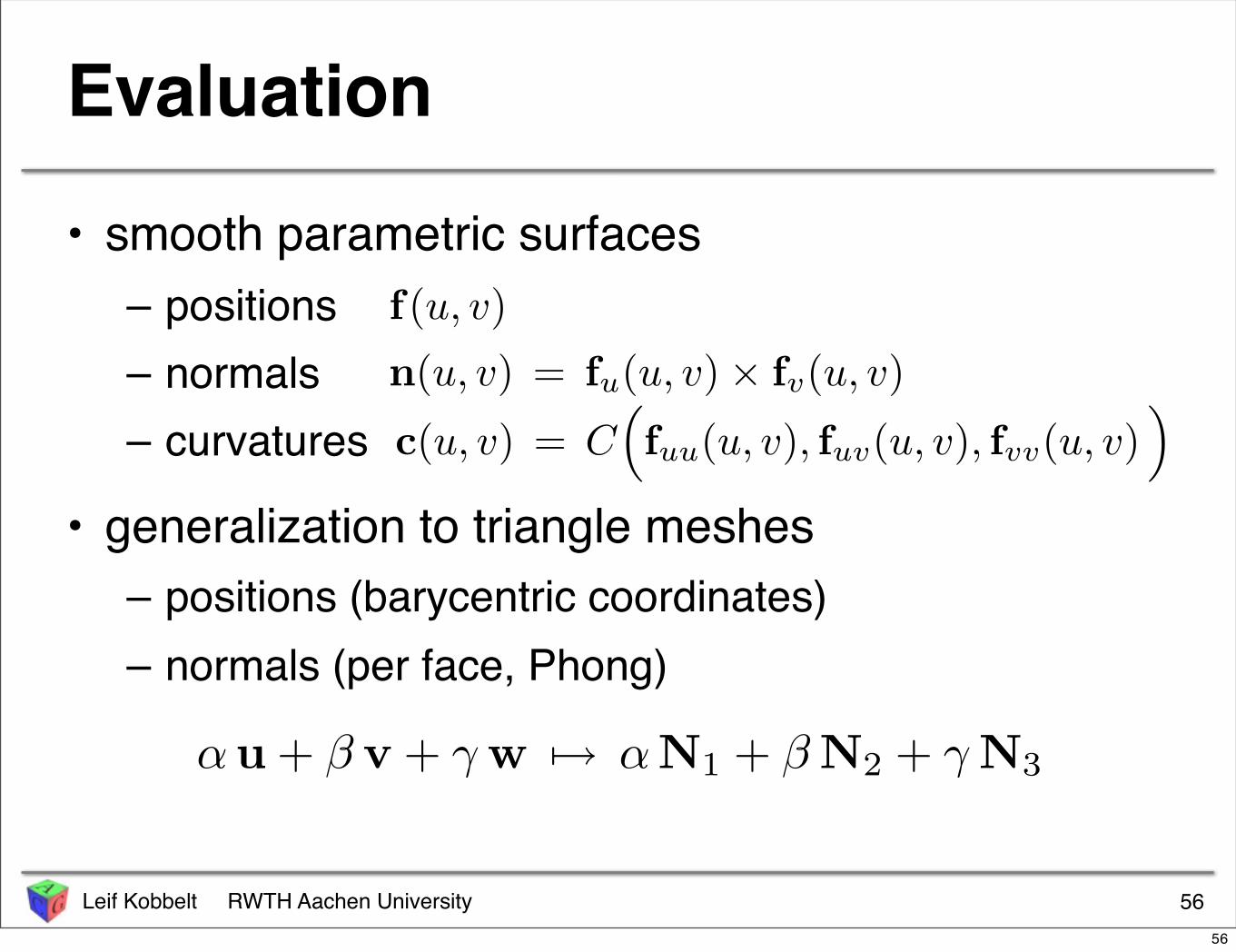
Evaluation
• smooth parametric surfaces– positions– normals– curvatures
• generalization to triangle meshes– positions (barycentric coordinates)– normals (per face, Phong)
56
f(u, v)
n(u, v) = fu(u, v) × fv(u, v)
c(u, v) = C(
fuu(u, v), fuv(u, v), fvv(u, v))
αu + β v + γ w !→ αN1 + β N2 + γ N3
56
Leif Kobbelt RWTH Aachen University
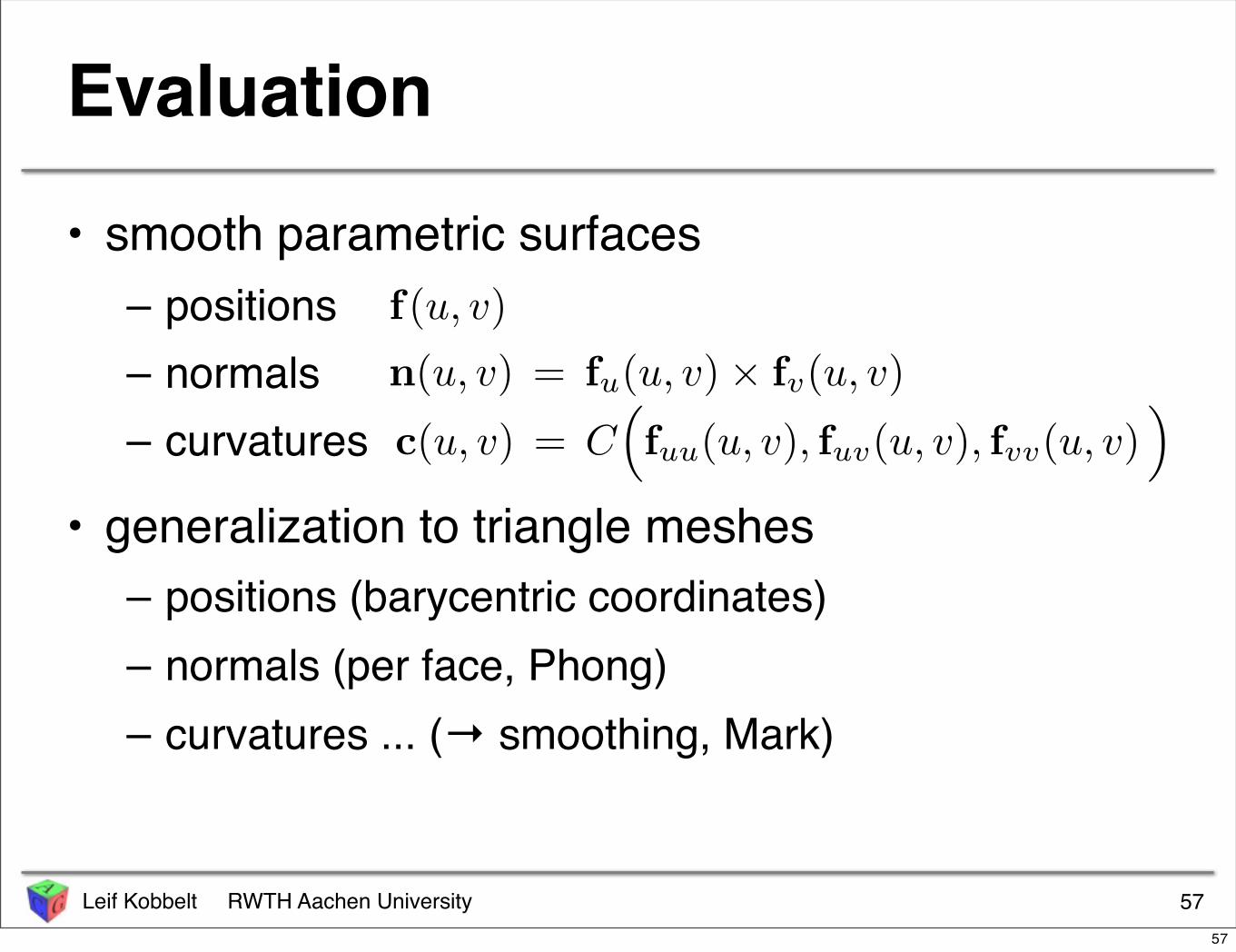
Evaluation
• smooth parametric surfaces– positions– normals– curvatures
• generalization to triangle meshes– positions (barycentric coordinates)– normals (per face, Phong)– curvatures ... (→ smoothing, Mark)
57
f(u, v)
n(u, v) = fu(u, v) × fv(u, v)
c(u, v) = C(
fuu(u, v), fuv(u, v), fvv(u, v))
57
Leif Kobbelt RWTH Aachen University
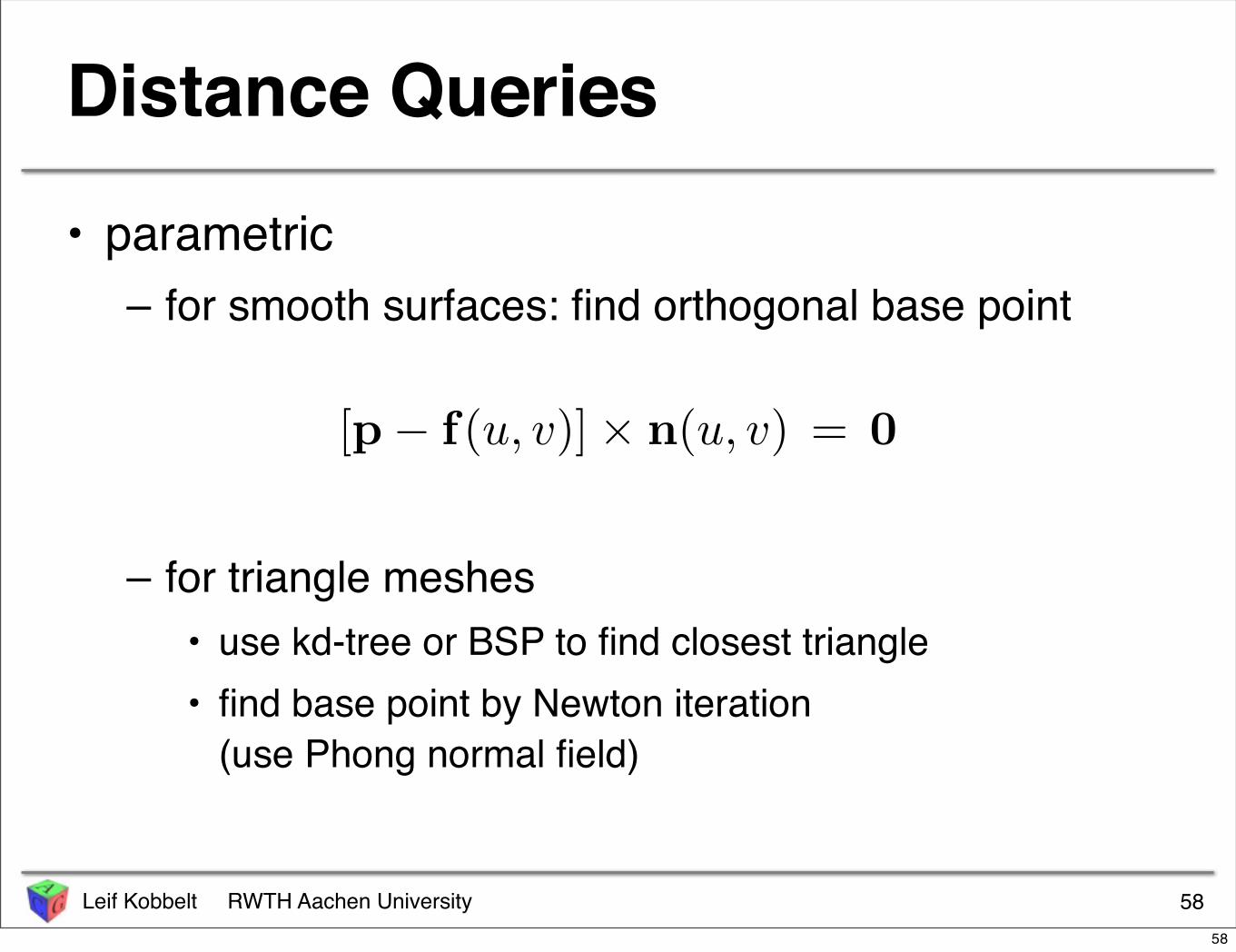
Distance Queries
• parametric– for smooth surfaces: find orthogonal base point
– for triangle meshes• use kd-tree or BSP to find closest triangle• find base point by Newton iteration
(use Phong normal field)
58
[p − f(u, v)] × n(u, v) = 0
58
Leif Kobbelt RWTH Aachen University
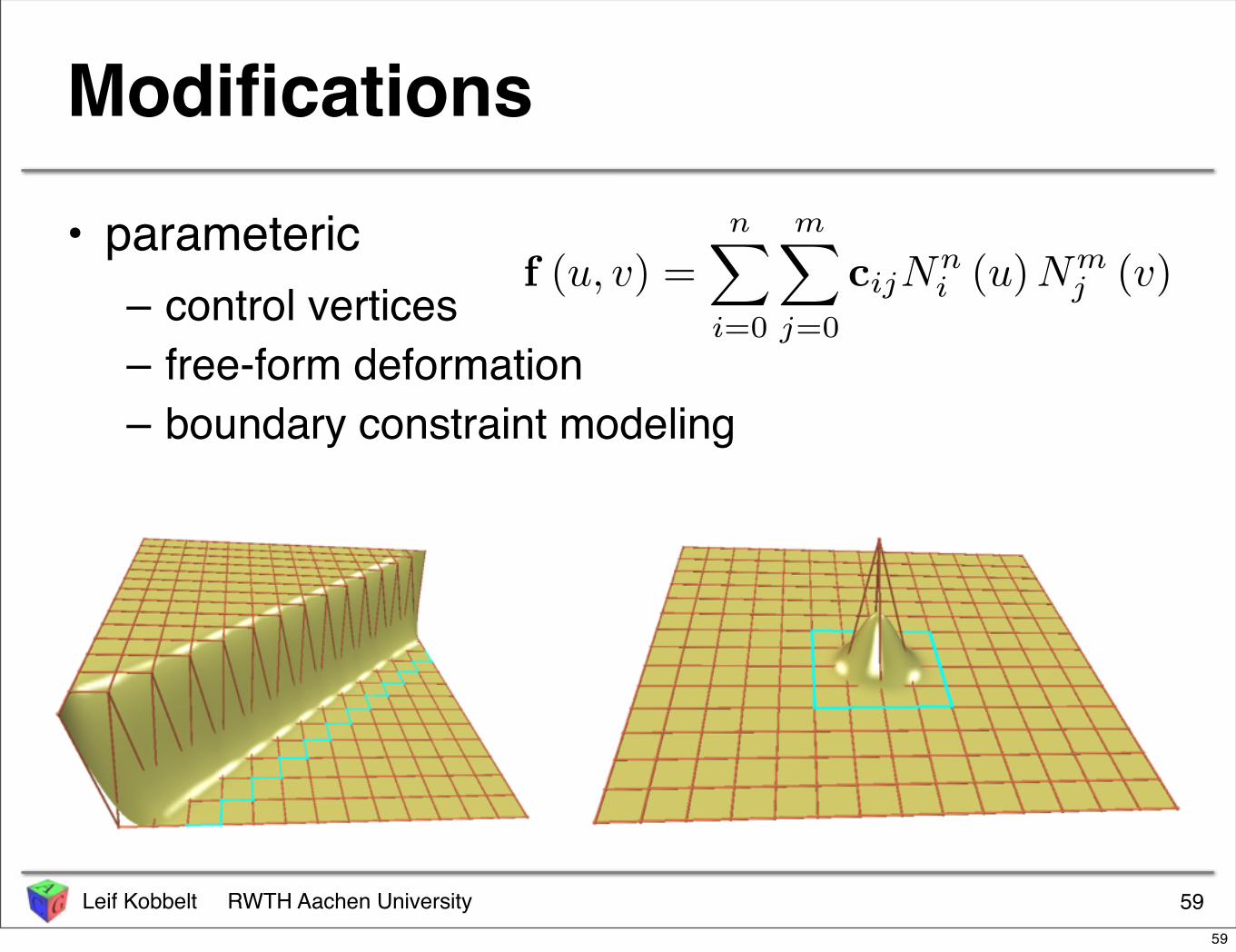
Modifications
• parameteric– control vertices– free-form deformation– boundary constraint modeling
59
f (u, v) =n∑
i=0
m∑
j=0
cijNni (u) Nm
j (v)
59
Leif Kobbelt RWTH Aachen University
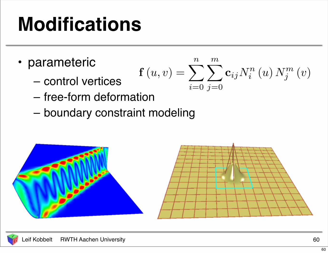
Modifications
• parameteric– control vertices– free-form deformation– boundary constraint modeling
60
f (u, v) =n∑
i=0
m∑
j=0
cijNni (u) Nm
j (v)
60
Leif Kobbelt RWTH Aachen University
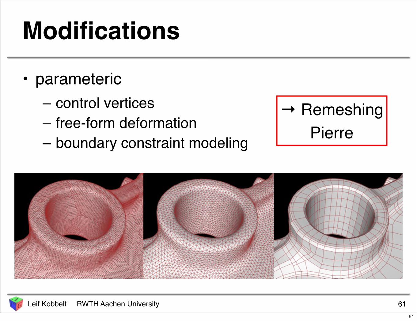
• parameteric– control vertices– free-form deformation– boundary constraint modeling
Modifications
61
→ RemeshingPierre
61

Leif Kobbelt RWTH Aachen University
• parameteric– control vertices– free-form deformation– boundary constraint modeling
Modifications
6262
Leif Kobbelt RWTH Aachen University
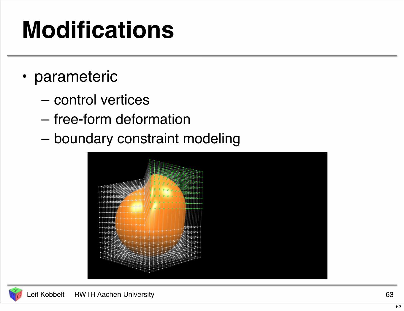
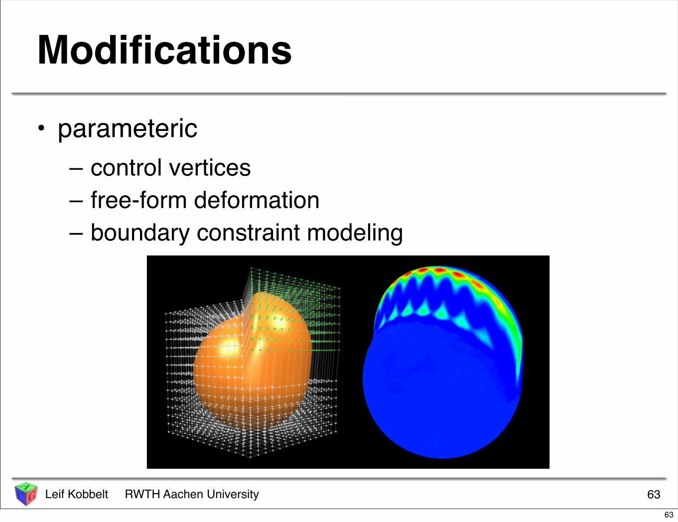
• parameteric– control vertices– free-form deformation– boundary constraint modeling
Modifications
6363
Leif Kobbelt RWTH Aachen University
• parameteric– control vertices– free-form deformation– boundary constraint modeling
Modifications
6363

Leif Kobbelt RWTH Aachen University
• parameteric– control vertices– free-form deformation– boundary constraint modeling
Modifications
64
→ Mesh EditingMario
64

Leif Kobbelt RWTH Aachen University
• (mathematical) geometry representations– parametric vs. implicit
• approximation properties• types of operations
– distance queries– evaluation– modification / deformation
• data structures
Outline
6565
Leif Kobbelt RWTH Aachen University
Mesh Data Structures
• how to store geometry & connectivity?
• compact storage– file formats
• efficient algorithms on meshes– identify time-critical operations– all vertices/edges of a face– all incident vertices/edges/faces of a vertex
6666
Leif Kobbelt RWTH Aachen University
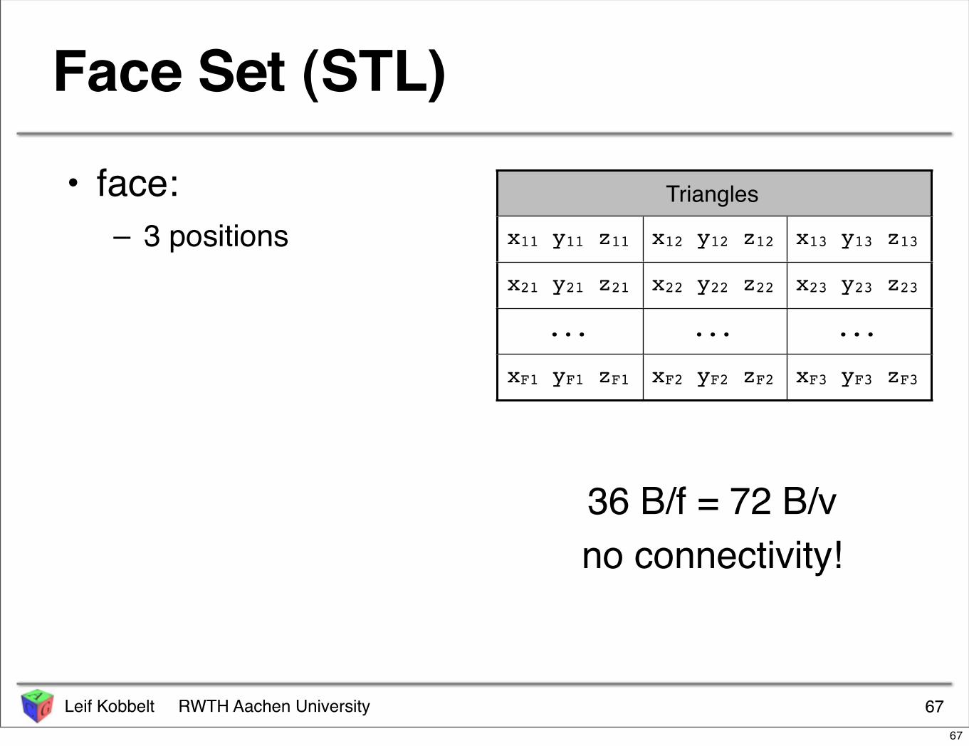
Face Set (STL)
• face:– 3 positions
67
TrianglesTrianglesTriangles
x11 y11 z11 x12 y12 z12 x13 y13 z13
x21 y21 z21 x22 y22 z22 x23 y23 z23
... ... ...
xF1 yF1 zF1 xF2 yF2 zF2 xF3 yF3 zF3
36 B/f = 72 B/vno connectivity!
67
Leif Kobbelt RWTH Aachen University
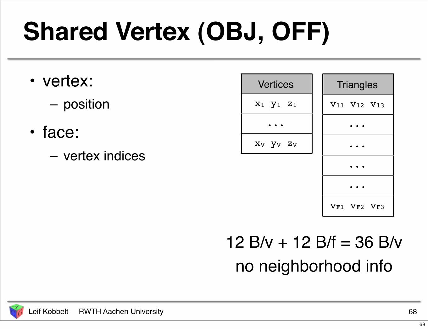
Shared Vertex (OBJ, OFF)
• vertex:– position
• face:– vertex indices
68
Vertices
x1 y1 z1
...
xV yV zV
Triangles
v11 v12 v13
...
...
...
...
vF1 vF2 vF3
12 B/v + 12 B/f = 36 B/vno neighborhood info
68
Leif Kobbelt RWTH Aachen University
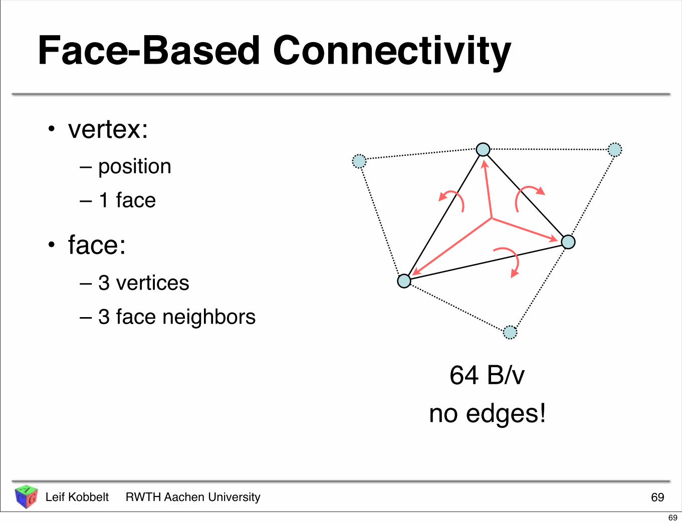
Face-Based Connectivity
• vertex:– position– 1 face
• face:– 3 vertices– 3 face neighbors
69
64 B/vno edges!
69
Leif Kobbelt RWTH Aachen University
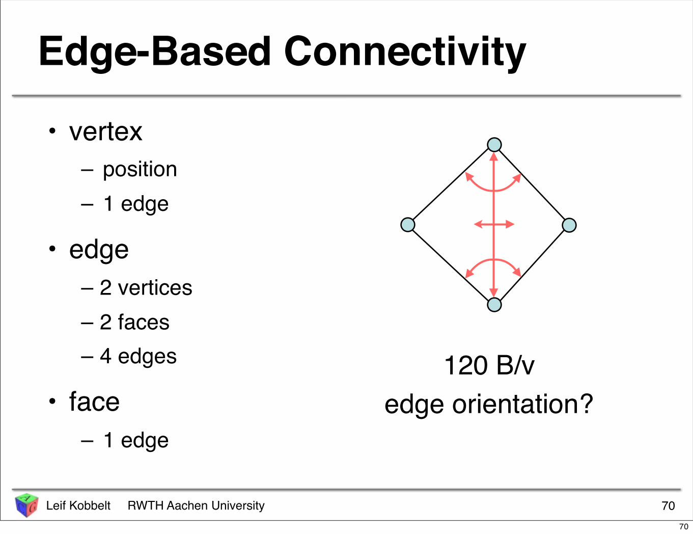
Edge-Based Connectivity
• vertex– position– 1 edge
• edge– 2 vertices– 2 faces– 4 edges
• face– 1 edge
70
120 B/vedge orientation?
70
Leif Kobbelt RWTH Aachen University
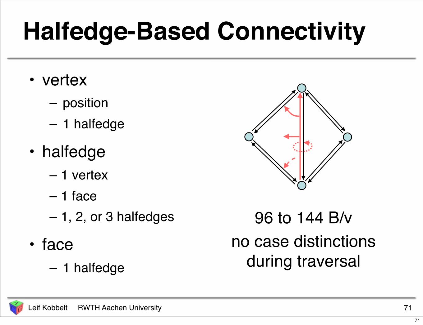
Halfedge-Based Connectivity
• vertex– position– 1 halfedge
• halfedge– 1 vertex– 1 face– 1, 2, or 3 halfedges
• face– 1 halfedge
71
96 to 144 B/vno case distinctions
during traversal
71
Leif Kobbelt RWTH Aachen University 72
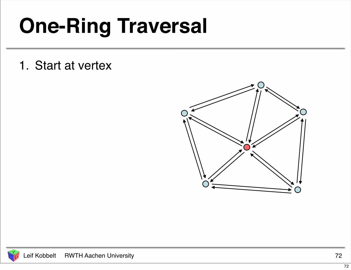
One-Ring Traversal1. Start at vertex
72
Leif Kobbelt RWTH Aachen University 73
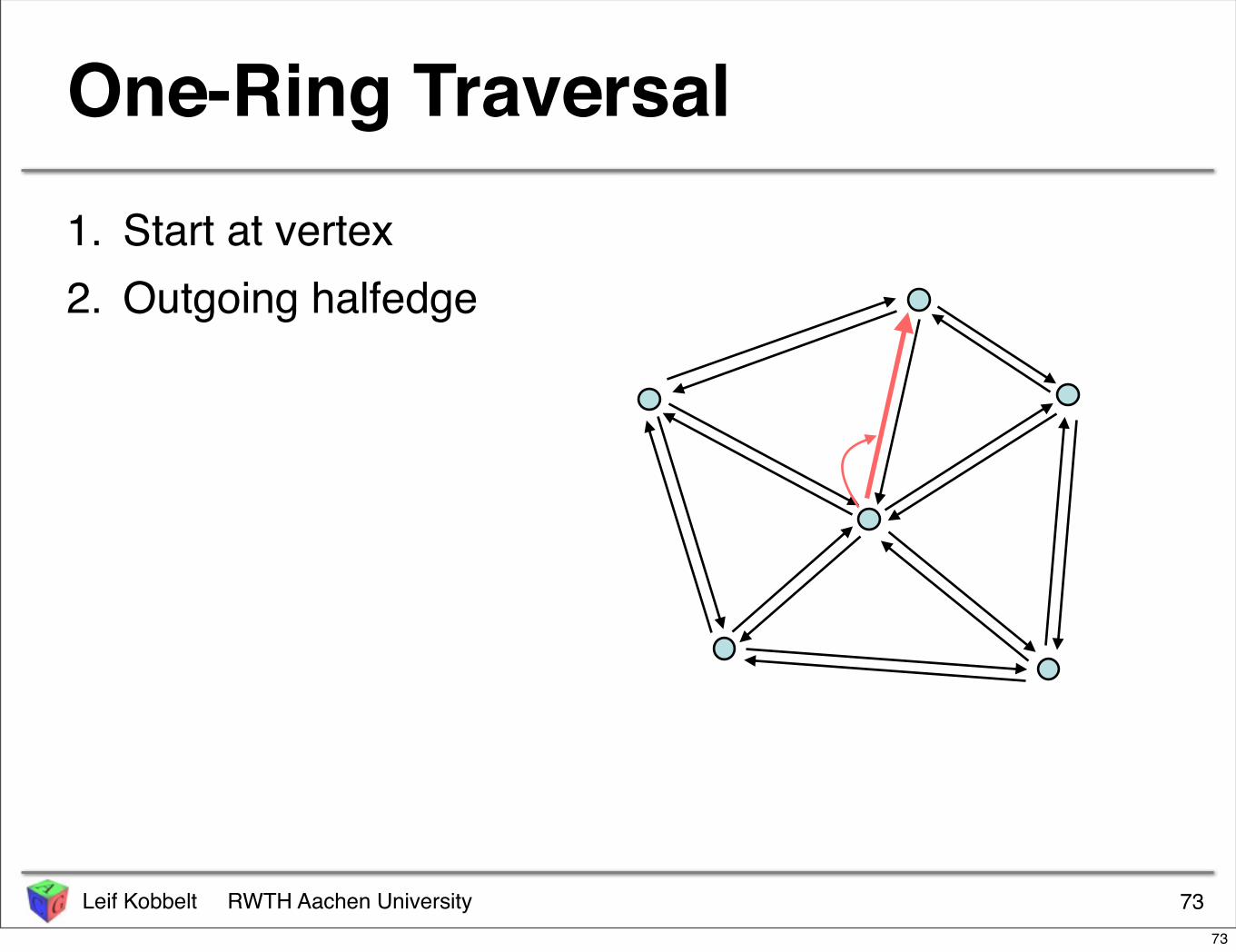
One-Ring Traversal1. Start at vertex2. Outgoing halfedge
73
Leif Kobbelt RWTH Aachen University 74
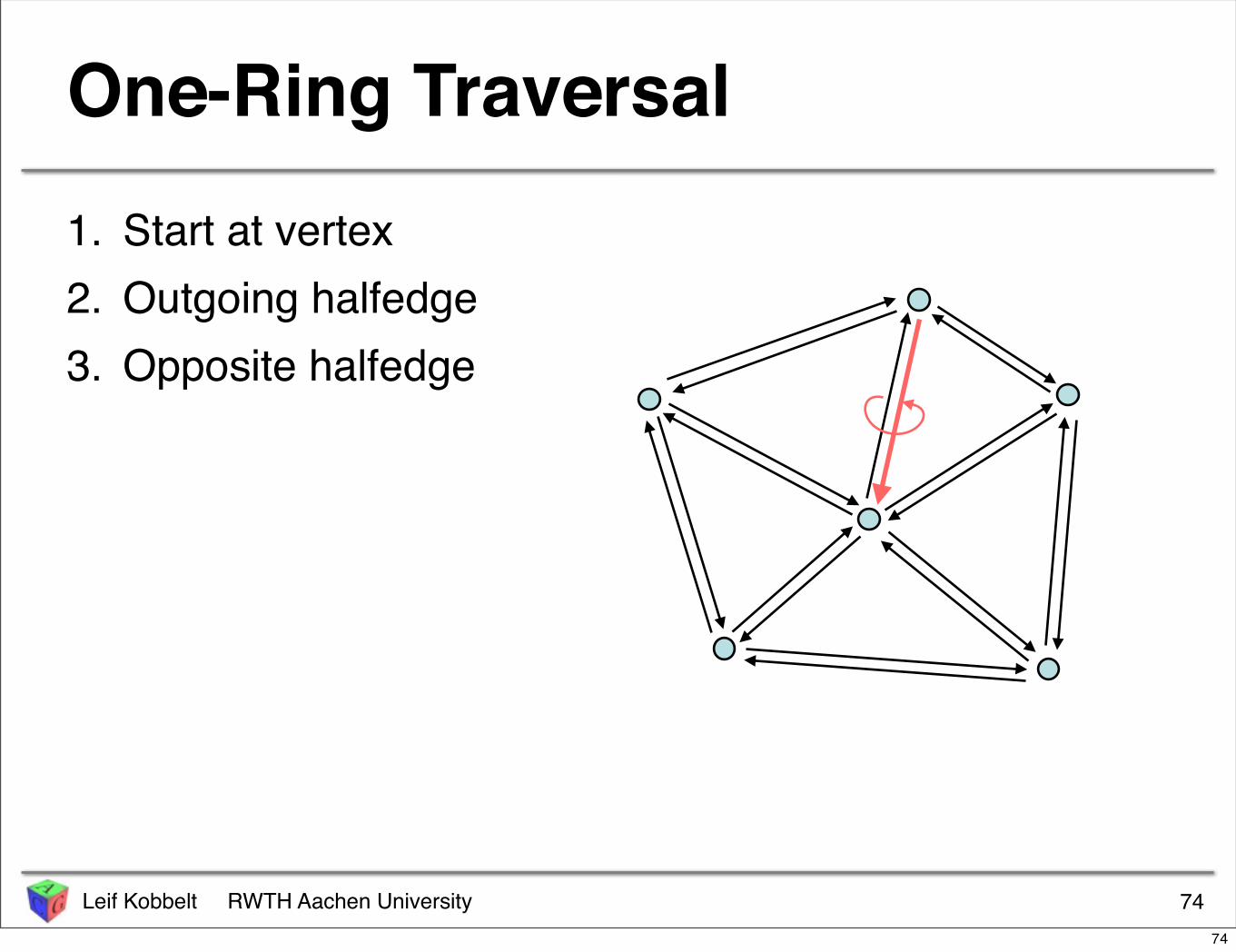
One-Ring Traversal1. Start at vertex2. Outgoing halfedge3. Opposite halfedge
74
Leif Kobbelt RWTH Aachen University 75
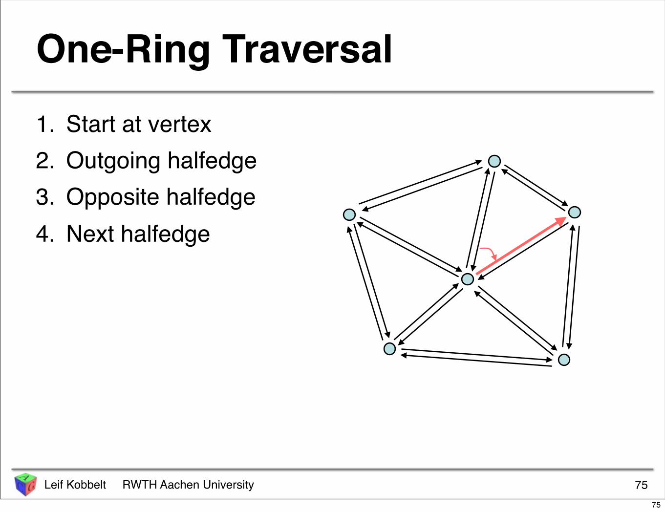
One-Ring Traversal1. Start at vertex2. Outgoing halfedge3. Opposite halfedge4. Next halfedge
75
Leif Kobbelt RWTH Aachen University 76
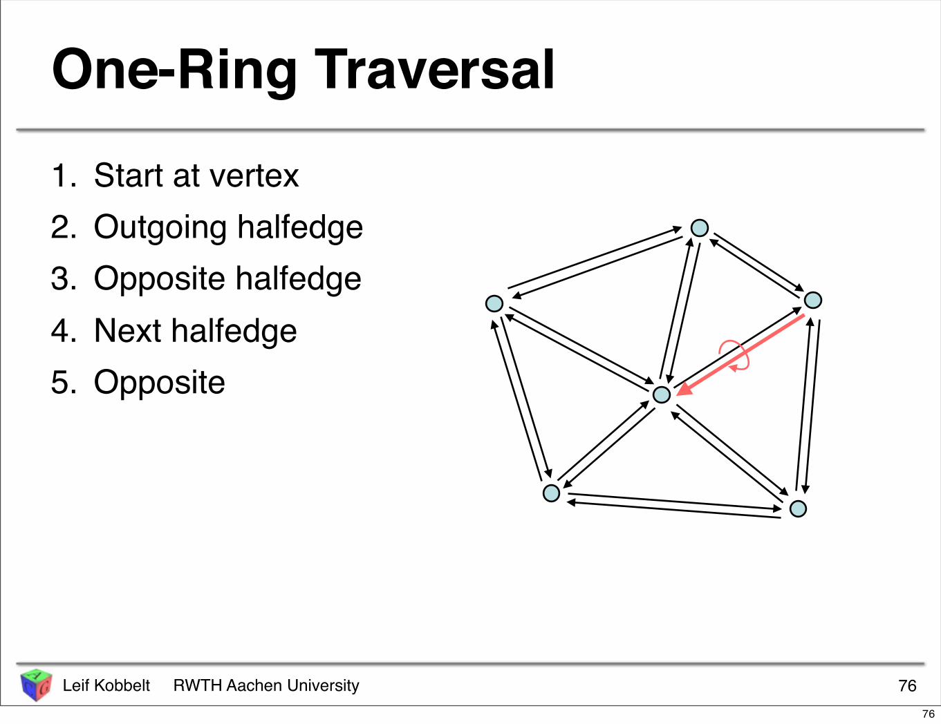
One-Ring Traversal1. Start at vertex2. Outgoing halfedge3. Opposite halfedge4. Next halfedge5. Opposite
76
Leif Kobbelt RWTH Aachen University 77
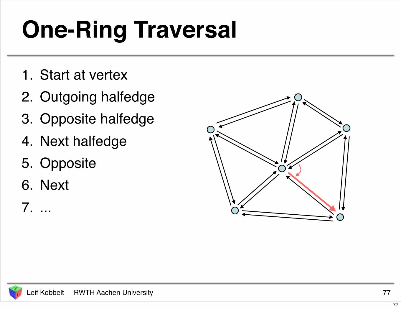
One-Ring Traversal1. Start at vertex2. Outgoing halfedge3. Opposite halfedge4. Next halfedge5. Opposite6. Next7. ...
77
Leif Kobbelt RWTH Aachen University
Halfedge-Based Libraries
• CGAL– www.cgal.org
– computational geometry– free for non-commercial use
• OpenMesh "– www.openmesh.org
– mesh processing– free, LGPL licence
7878
Leif Kobbelt RWTH Aachen University
Literature• Kettner, Using generic programming for designing a
data structure for polyhedral surfaces, Symp. on Comp. Geom., 1998
• Campagna et al, Directed Edges - A Scalable Representation for Triangle Meshes, Journal of Graphics Tools 4(3), 1998
• Botsch et al, OpenMesh - A generic and efficient polygon mesh data structure, OpenSG Symp. 2002
7979

Leif Kobbelt RWTH Aachen University
Outline
• (mathematical) geometry representations– parametric vs. implicit
• approximation properties• types of operations
– distance queries– evaluation– modification / deformation
• data structures
8080