SURFACE-SURFACE INTERSECTION WITH CRITICAL POINT DETECTION BASED ON , BEZIER NORMAL VECTOR SURFACES

Yasushi Yamaguchi Department of Graphics and Computer Science, The University of Tokyo 3-8-1, Komaba, Meguro-ku, Tokyo 153-8902, Japan yama@graco.c.u-tokyo.ac.jp

Ryuji Kamiyama NTT Telecommunications Software Headquarters 1-6, Nakase, Mihama-ku, Chiba-city, Chiba, Japan kamiyama@nwp.tsh.cae.ntt.jp

F\nnihiko Kimura Department of Precision Machinery Engineering, The University of Tokyo 7-3-1, Hongo, Bunkyo-ku, Tokyo 113-8654, Japan kimura@cim.pe.u-tokyo.ac.jp

Abstract Surface-surface intersection is one of essential techniques in geometric modeling. A relatively robust algorithm to calculate intersections of parametric surfaces is a marching method which repeatedly calculates consecutive points on an intersection curve starting with a certain point. However, it is difficult to find starting points of all branches of intersec­tions especially when the branches form small loops. It is also difficult to trace a curve near singular points. Critical points which have par­allel normals on both surfaces are key points to solve those problems. We will, first, propose a Bezier normal vector surface which can exactly represent normal vectors on a Bezier surface. Then we will explain a new algorithm to find all critical points by using Bezier normal vector surfaces. All starting points of intersection curves are obtained with the algorithm. Furthermore, intersection curves can be robustly traced by using the critical points.

Keywords: Surface-surface intersection, Critical point, Normal vector

F. Kimura (ed.), Geometric Modelling© Springer Science+Business Media New York 2001

1. Introduction Geometric modeling is a key technique for many applications such as

CAD/CAM. Surface-surface intersection is one of the toughest problems in this area, and many studies have been done on this (see Patrikalakis, 1993). For instance, Miller, 1987, studied analytic methods that calcu­late intersections of natural quadric surfaces. However, orders of inter­section curves of parametric surfaces usually become too high to solve intersection curves analytically. Surface-surface intersection algorithms usually calculate sequences of points on intersection curves.

There are mainly two approaches to calculating intersections of para­metric surfaces, i.e., recursive subdivision methods and marching meth­ods. The recursive subdivision methods recursively subdivide surfaces until the subpatches can be approximated by plane elements and cal­culate intersection curves as intersection polylines of those small plane elements (see Dokken, 1985). The methods require a lot of memory space and computation time if high precision is required. Furthermore, the methods cannot find all small intersection loops and cannot calculate intersection curves near singular points.

The marching methods trace an intersection curve by repeatedly cal­culating consecutive points on the curve (see Barnhill and Kersey, 1990). These kind of methods can robustly and quickly trace intersection curves in usual cases. However there still remain some problems. The initial point of the intersection curve is one of those problems. It is difficult to find all starting points of intersection branches to be traced, especially when a branch forms a tiny loop. The second one is a junction point. The marching methods usually assume that an intersection branch is either a simple curve segment having both its ends on the boundaries of surfaces or a closed loop inside of the surfaces. They trace intersections by approximating the surfaces with their first derivatives, i.e., with their tangential planes. So they cannot trace the intersection curve beyond a junction point because the surfaces coincide up to their first derivatives so that they have the same tangential plane. Some methods can trace the curve beyond the junction point by investigating higher order deriva­tives (see Bajaj et al., 1988; Owen and Rockwood, 1987), they are not able to determine where the junction point are, though. Those methods require the exact location of the junction point beforehand. The last one is robustness. If two intersection branches closely approach each other forming like hyperbolic curve branches, the marching method might fail to trace the branch by jumping to the other branch. A critical point is a key concept to solve these problems.

288

s

R

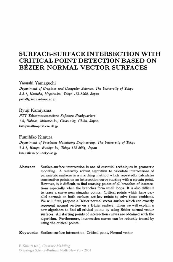
Figure 1. Critical Points.

This paper proposes a new technique to calculate all intersection curve branches ofBezier surfaces as well as to trace intersection curves robustly by using critical points. Section 2 specifies the usefulness of critical points in calculating surface-surface intersection and summarizes previ­ous studies. Section 3 explains the Bezier Normal Vector Surface which represents normal vectors on a Bezier surface and a method to calculate its control points from the original surface's control points. Section 4 proposes an algorithm for detecting all critical points based on Bezier normal vector surfaces. Section 5 shows how critical points are used to trace intersection curves robustly. Section 6 summarizes this paper.

2. Critical Points Let us consider the intersection of two surfaces S(u, v) and R(s, t).

Suppose a distance between those two surfaces is uniquely and contin­uously determined according to a point on S(u, v) so that a distance can be seen as a function of parameters u and v, r/>(u, v). Though there are several definitions of distances between two surfaces (see Cheng, 1989; Markot and Magedson, 1989; Kriezis et al., 1992; Higashi et al., 1992), the differences among them are not essential for the discussion in this section except that the distance function ¢( u, v) must be continuous in a certain domain. The function definition will be discussed in a later section. By taking the gradient of this distance function ¢( u, v), a vector field in a parametric space is defined. Critical points are defined as zero points of this vector field, V ¢( u, v).

The starting point detection problem is very similar to the intersection loop detection problem. It is enough to subdivide the surfaces such that each subdivided surface includes no intersection loops and every

289

intersection curve crosses some boundaries of subdivided surfaces. Sinha et al., 1985, and Cheng, 1989, pointed out that at least one critical point must exist inside an intersection loop as shown on the left side of Figure 1 if the distance varies continuously. It is important that the distance field must be continuous, especially inside of intersection loops. Any intersection curve is split by isoparametric lines passing through the critical points. Sederberg, Hohmeyer and others proposed several criteria for detecting intersection loops rather than for detecting critical points. There are a lot of relations among those criteria. This paper focuses on the critical point detection because critical points are useful for robust and correct tracing as well as for loop detection. Grandine and Klein IV, 1997, pointed out that "loop detection" does not guarantee the correct topology of the intersection curves and presented a method which accomplishes it. However the method is based on so called turning points which include all critical points. The critical point detection is a important premise to accomplish the robust and correct tracing.

A junction point is a critical point on intersection curves as shown on the right side of Figure 1. A critical point also exists around a near-junction point, such as somewhere between the closest points of two hyperbolic intersection branches. The marching methods that trace the intersection curves by approximating the surfaces with their first derivatives cannot trace the curves around those points where the sur­faces almost coincide up to their first derivatives. There have been some studies on tracing techniques which can trace intersection curves beyond the junction points by investigating higher order derivatives. Owen and Rockwood, 1987, showed a tracing technique which can follow intersec­tion curves of implicit surfaces including junction points. Bajaj et al., 1988, and Charrot, 1993, gave tracing techniques applicable to parara­metric surfaces. Though the techniques might not be so stable to trace the intersection curves beyond the junction points, because it is difficult to lo~ate the singular point accurately at which the techniques must in­vestigate the higher order derivatives. Both of the problems, i.e., starting point detection and tracing across singular points, are strongly related to the critical points. This paper concentrates on detecting all critical points to solve the problems.

Cheng, 1989, mentioned an algorithm for finding critical points, but it was not complete. The algorithm traces a connecting curve which connects two singular points as well as an intersection curve. It as­sumed that a connecting curve crosses an intersection curve where a dot product of the normalized normal vectors of two surfaces has a local extremum value on an intersection curve. However this assumption is not necessarily true. Wang et al., 1991, and Kushimoto and Hosaka,

290

1991, proposed methods that detect critical points as intersection points of characteristic lines on the surfaces. However, it is not so cheap to calculate intersections of characteristic lines. Furthermore, there still remains an open question of how to detect all branches of characteristic lines. Kriezis et al., 1992, proposed both the sufficient condition of criti­cal point existence based on a rotation number of a distance vector field \1</J(u, v), and an efficient algorithm to find critical points. But the algo­rithm itself cannot guarantee completeness so that every critical point is detected, because the algorithm did not specify a necessary condition of critical point existence. Ma and Luo, 1995, proposed an improved test concerning a rotation number. But it cannot guarantee the complete detection because it still gives only sufficient condition of critical point existence.

One of the most successful approaches to detect all critical points is a divide conquer method. Surfaces are subdivided until the necessary con­dition for critical points is not satisfied any more. The important char­acteristic of critical points is that a pair of critical points have parallel normal vectors. Thus, there must be points x E S(u, v) andy E R(s, t) such that the normal vector at x is parallel to the normal vector at y if the surfaces have some critical points. In other words, critical points may not exist if the Gauss maps of the surfaces do not have overlaps. The previous studies used this property as the necessary condition of critical point existence.

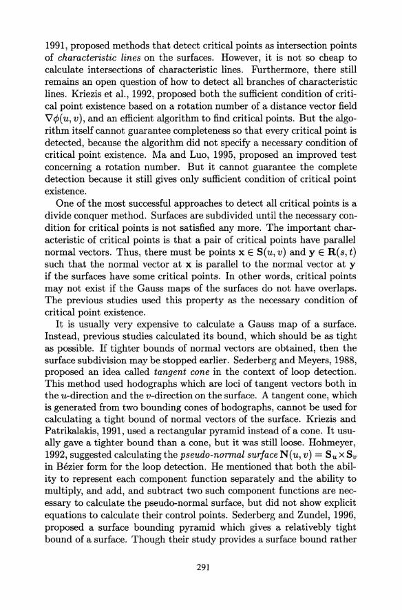
It is usually very expensive to calculate a Gauss map of a surface. Instead, previous studies calculated its bound, which should be as tight as possible. If tighter bounds of normal vectors are obtained, then the surface subdivision may be stopped earlier. Sederberg and Meyers, 1988, proposed an idea called tangent cone in the context of loop detection. This method used hodographs which are loci of tangent vectors both in the u-direction and the v-direction on the surface. A tangent cone, which is generated from two bounding cones of hodographs, cannot be used for calculating a tight bound of normal vectors of the surface. Kriezis and Patrikalakis, 1991, used a rectangular pyramid instead of a cone. It usu­ally gave a tighter bound than a cone, but it was still loose. Hohmeyer, 1992, suggested calculating the pseudo-normal surface N(u, v) = Su X Sv in Bezier form for the loop detection. He mentioned that both the abil­ity to represent each component function separately and the ability to multiply, and add, and subtract two such component functions are nec­essary to calculate the pseudo-normal surface, but did not show explicit equations to calculate their control points. Sederberg and Zundel, 1996, proposed a surface bounding pyramid which gives a relativebly tight bound of a surface. Though their study provides a surface bound rather

291

than a normal bound, it has an intimate relationship with a tighter bound of normal vectors.

Even if a tight bound of normal vectors is available, this necessary condition, i.e., parallel normal vectors, is too weak to stop the subdivi­sion process of the critical points detection algorithm. Let us imagine an intersection of a plane and a hemisphere with a circular intersection loop. There is a pair of critical points inside of the intersection loop which have parallel normal vectors. At the same time every point on a plane which does not correspond to the critical point has a parallel normal vector. This means that the Gauss maps of the subsurfaces of the plane must have an overlap however finely the subsurfaces are subdivided. The ex­istence of critical points must be determined by the relative positions of the surfaces as well as their normal vectors. The correspondence check based on both the positions and the normal vectors can be accomplished by a Minkowski sum like operation in a three-dimensional space but is very costly. An overlap test of the surfaces in a three-dimensional space does not work as the correspondence check because the separate surfaces may have critical points. This issue of the relative surface position is closely related to the issue of the surface bounding cone construction such that the compliment of a normal bounding cone does not bound the surface in a global sense. This problem was discussed by Hohmeyer, 1992, and Sederberg and Zundel, 1996, using an example of a surface shaped like a parking garage ramp.

3. Bezier Normal Vector Surface A locus of unnormalized normal vectors on a surface constructs a

surface. Hohmeyer, 1992, called it a pseudo-normal surface and pointed out the requirements for its calculation. In this paper we call this surface a normal vector surface. A normal vector surface composed of unit vectors is a Gauss map of the surface. If a normal vector surface is represented as a Bezier surface, its control polygon can tightly bound the end points of the normal vectors because of the tight convex hull property of Bezier surfaces. In this section the equation for calculating the control points of the Bezier normal vector surface from those of the original Bezier surface will be discussed in order to obtain a tighter bound of normal vectors.

A Bezier surface S(u, v) of degree nxm is defined by (n+ 1)x(m+ 1) control points P ij as below:

n m

S(u, v) = L L Bf(u)Bj(v)Pij· i=Oj=O

292

Here, Bf(u) = (7)ui(1-ut-i and Bj(u) denotes Bernstein polynomials of degree n and m respectively whose product is given as below (see de Boor, 1987):

Bn( )Bm( ) _ (7) (j) Bn+m( ) i u j u - (~tj) i+j u .

The tangent vectors in u, v-directions, Su and Sv, are given:

n-1 m

Su(u, v) = n L L B/(-1(u)B£(v)QKL, K=OL=O

n m-1

Sv(u, v) = m L L BM-(u)B7J-1(v)RMN, M=ON=O

where QKL=P(K+l) L-PKL and RMN=PM (N+l)-PMN.

(1)

The normal vector N ( u, v) of the surface S ( u, v), which is a common normal vector of the two tangent vectors, Su(u, v) and Sv(u, v), is given as below by using the product formula (1):

N(u,v) Su(u, v) X Sv(u, v)

n-1 n m m-1

nmLLLL K =0 M =0 L=O N =0

(nj/) (~) G~) Cv1) B2n-1 ( )B2m-1( ) Q R (2)

( 2n-1) (2m-1) K+M U L+N V KL X MN· K+M L+N

Equation (2) is a tensor product of Bernstein polynomials of degree 2n-l and Bernstein polynomials of degree 2m-l. This indicates that a normal vector surface N(u, v) of a Bezier surface B(u, v) can be represented as a Bezier surface of degree (2n-1)x(2m-1) defined with 2nx2m control points N ij as below:

2n-12m-1

N(u, v) = L L B;n-1 (u)Bjm-l(v)Nij· (3) i=O j=O

Thus we named this surface Bezier normal vector surface. By comparing coefficients of Equations ( 2) and ( 3), the control points N ij of the Bezier normal vector surface N(u, v) are given in the following equation:

293

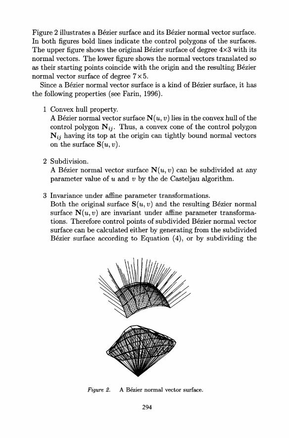
Figure 2 illustrates a Bezier surface and its Bezier normal vector surface. In both figures bold lines indicate the control polygons of the surfaces. The upper figure shows the original Bezier surface of degree 4x3 with its normal vectors. The lower figure shows the normal vectors translated so as their starting points coincide with the origin and the resulting Bezier normal vector surface of degree 7 x 5.

Since a Bezier normal vector surface is a kind of Bezier surface, it has the following properties {see Farin, 1996).

1 Convex hull property. A Bezier normal vector surface N ( u, v) lies in the convex hull of the control polygon N ij. Thus, a convex cone of the control polygon Nij having its top at the origin can tightly bound normal vectors on the surface S(u, v).

2 Subdivision. A Bezier normal vector surface N(u, v) can be subdivided at any parameter value of u and v by the de Casteljau algorithm.

3 Invariance under affine parameter transformations. Both the original surface S(u, v) and the resulting Bezier normal surface N ( u, v) are invariant under affine parameter transforma­tions. Therefore control points of subdivided Bezier normal vector surface can be calculated either by generating from the subdivided Bezier surface according to Equation {4), or by subdividing the

Figure 2. A Bezier normal vector surface.

294

Bezier normal vector surface N(u, v) with the de Casteljau algo­rithm.

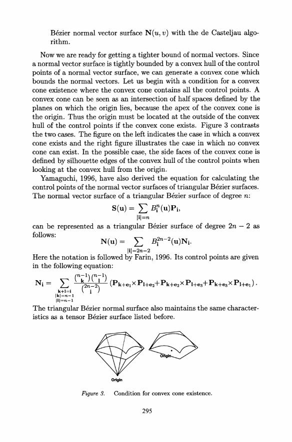
Now we are ready for getting a tighter bound of normal vectors. Since a normal vector surface is tightly bounded by a convex hull of the control points of a normal vector surface, we can generate a convex cone which bounds the normal vectors. Let us begin with a condition for a convex cone existence where the convex cone contains all the control points. A convex cone can be seen as an intersection of half spaces defined by the planes on which the origin lies, because the apex of the convex cone is the origin. Thus the origin must be located at the outside of the convex hull of the control points if the convex cone exists. Figure 3 contrasts the two cases. The figure on the left indicates the case in which a convex cone exists and the right figure illustrates the case in which no convex cone can exist. In the possible case, the side faces of the convex cone is defined by silhouette edges of the convex hull of the control points when looking at the convex hull from the origin.

Yamaguchi, 1996, have also derived the equation for calculating the control points of the normal vector surfaces of triangular Bezier surfaces. The normal vector surface of a triangular Bezier surface of degree n:

S(u) = L Bf(u)Pi, lil=n

can be represented as a triangular Bezier surface of degree 2n - 2 as follows:

N(u) = lil=2n-2

Here the notation is followed by Farin, 1996. Its control points are given in the following equation:

(n-1) (n-1) Ni = k~i (2ni2) (Pk+e1 XPI+e2+Pk+e2 XPI+e3+Pk+e3 XPI+e1 ).

lkl=n-1 lll=n-1

The triangular Bezier normal surface also maintains the same character­istics as a tensor Bezier surface listed before.

Origin

Figure 3. Condition for convex cone existence.

295

4. Critical Point Detection Algorithm In this section an efficient and complete algorithm for detecting all

critical points based on a Bezier normal vector surface will be discussed. At the end of Section 2, the importance of the correspondence check was pointed out. Overlapping Gauss maps is a too weak condition for a critical point existence. Even an overlap test of the surfaces, in addition, may not be enough. The issue of the correspondence is strongly related to the definition of distance.

4.1. Distance along a Constant Vector A distance function ¢( u, v) between two surfaces is introduced in the

section 2. There might be several different definitions of distances ac­cording to the way of measurement. Previous studies adopted a mini­mum distance between two surfaces, because it maintains C0 continuity at least. The distance field must be continuous, especially inside of in­tersection loops. Otherwise, a critical point may not exist inside of an intersection loop.

In our study, a distance is measured along a constant vector n in­stead of a minimum distance. However, it is a problem to determine the constant vector to measure the distance. The vector must be carefully selected so that there must exist corresponding points on the surfaces along the vector. The concept of a visibility cone which is a represen­tation of locally visible directions of the surface can be used to select a proper vector. This concept is very useful for various applications, such as an accessibility check for NC measurement probes, a workpiece setup for machining, an assemblability check for robot operations, and so on. Though the term visibility cone given by Kim et al., 1995, is famous for mechanical applications. The concept of a convex cone in n-dimensional space was studied by Goldman and Tucker, 1956.

A visibility cone is associated with a Gauss map. Let's consider a tangent plane of a surface and the common normal vector at that point. The tangent plane separates a whole vector space into two half spaces. And any vector starting at the point and ending at some point in the bottom half space penetrates the surface from its upside to its downside at that point. The tangent plane and the common normal vector vary on the surface simultaneously. The locus of normal vectors stands for a Gauss map. And the intersection of the half spaces stands for a visibility cone. There exists a duality of a normal cone and a visibility cone. These cones are dual so that the faces of the visibility cone are perpendicular to the edges of the normal cone and the faces of the normal cone are perpendicular to the edges of the visibility cone. Thus the visibility cone

296

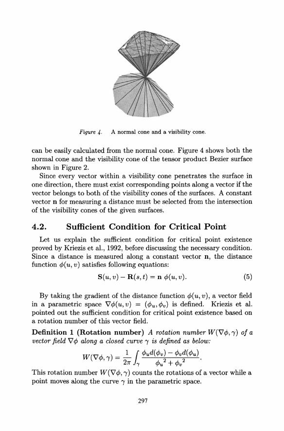
Figure 4. A normal cone and a visibility cone.

can be easily calculated from the normal cone. Figure 4 shows both the normal cone and the visibility cone of the tensor product Bezier surface shown in Figure 2.

Since every vector within a visibility cone penetrates the surface in one direction, there must exist corresponding points along a vector if the vector belongs to both of the visibility cones of the surfaces. A constant vector n for measuring a distance must be selected from the intersection of the visibility cones of the given surfaces.

4.2. Sufficient Condition for Critical Point Let us explain the sufficient condition for critical point existence

proved by Kriezis et al., 1992, before discussing the necessary condition. Since a distance is measured along a constant vector n, the distance function ¢>( u, v) satisfies following equations:

S(u, v)- R(s, t) = n <f>(u, v). (5)

By taking the gradient of the distance function ¢>( u, v), a vector field in a parametric space "V¢>(u, v) = (</>u, <f>v) is defined. Kriezis et al. pointed out the sufficient condition for critical point existence based on a rotation number of this vector field.

Definition 1 (Rotation number) A rotation number W("V¢> ,1) of a vector field "V </> along a closed curve 1 is defined as below:

W("V"' ) = J_ 1 <f>ud(</>v)- <f>vd(</>u). '~'' I 271' "Y </>u 2 + </>v 2

This rotation number W ("V ¢>, 1) counts the rotations of a vector while a point moves along the curve 1 in the parametric space.

297

u

Approximate critlcol point

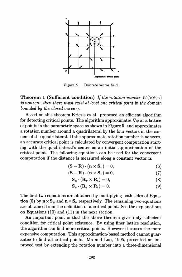
Figure 5. Discrete vector field.

Theorem 1 (Sufficient condition) If the rotation number W(\7¢, !') is nonzero, then there must exist at least one critical point in the domain bounded by the closed curve ')'.

Based on this theorem Kriezis et al. proposed an efficient algorithm for detecting critical points. The algorithm approximates \7 </> at a lattice of points in the parametric space as shown in Figure 5, and approximates a rotation number around a quadrilateral by the four vectors in the cor­ners of the quadrilateral. If the approximate rotation number is nonzero, an accurate critical point is calculated by convergent computation start­ing with the quadrilateral's center as an initial approximation of the critical point. The following equations can be used for the convergent computation if the distance is measured along a constant vector n:

(S- R) · (n x Su) = 0,

(S- R) · (n x Sv) = 0,

Su · (Rs X Rt) = 0, Sv · (Rs X Rt) = 0.

(6)

(7) (8) (9)

The first two equations are obtained by multiplying both sides of Equa­tion (5) by n x Su and n x Sv respectively. The remaining two equations are obtained from the definition of a critical point. See the explanations on Equations (10) and (11) in the next section.

An important point is that the above theorem gives only sufficient condition for critical point existence. By using finer lattice resolution, the algorithm can find more critical points. However it causes the more expensive computation. This approximation-based method cannot guar­antee to find all critical points. Ma and Luo, 1995, presented an im­proved test by extending the rotation number into a three-dimensional

298

vector field. However the rotation number is calculated with the discrete parameter space. The test cannot detect all critical points unless the ini­tial lattice crosses all of the Jacobian curves on which the Jacobian is zero. In this sense the test can be used only for the sufficiency check of the critical point existence.

4.3. Necessary Condition for Critical Point The new algorithm to be proposed in this paper is based on neces­

sary condition as well as sufficient condition. The algorithm guarantees the complete detection by subdividing the surfaces until the necessary condition is not satisfied. Before explaining the necessary condition, we have to point out that the corresponding critical points have parallel normal vectors.

Lemma 1 (Normal vectors at critical points) The corresponding crit­ical points have parallel normal vectors.

Proof. Equation (5) of the distance function ifJ( u, v) yields the fol­lowing differential equations:

ds dt Su- (Rs du + Rt d) = n ifJu,

ds dt Sv- (Rs dv + Rt dv) = n ifJv·

The terms of Rs and Rt can be eliminated by applying the multiplication of Rs x Rt to both sides of the above equations. Since a critical point is a zero point of the vector field VifJ, i.e., ifJu = ifJv = 0, a critical point satisfies the following equations:

Su · (Rs X Rt) - 0, Sv · (Rs X Rt) = 0.

(10) (11)

Equations (10) and (11) imply that the normal vector of R is also or­thogonal to tangent vectors Su and Sv respectively. 0

The necessary condition for critical point existence is given as below.

Theorem 2 (Necessary condition) If a critical point exists, then the projections along the vector n of two convex hulis of surface control poly­gons P ij of the surfaces have overlap, and the convex cones composed of the origin and control polygons Nij of the normal vector surfaces have overlap at the same time.

Proof. The definition of the distance measured along the vector n indicates that the corresponding critical points must lie on the same line parallel to the vector n. They must have parallel normal vectors according to the lemma 1. 0

299

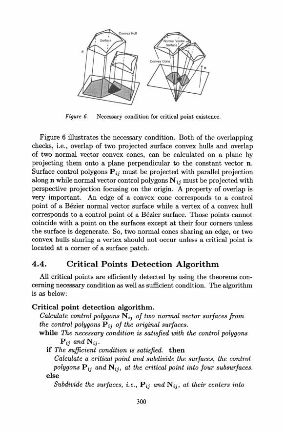
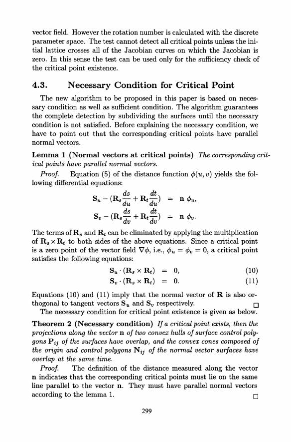
Figure 6. Necessary condition for critical point existence.

Figure 6 illustrates the necessary condition. Both of the overlapping checks, i.e., overlap of two projected surface convex hulls and overlap of two normal vector convex cones, can be calculated on a plane by projecting them onto a plane perpendicular to the constant vector n. Surface control polygons P ij must be projected with parallel projection along n while normal vector control polygons N ij must be projected with perspective projection focusing on the origin. A property of overlap is very important. An edge of a convex cone corresponds to a control point of a Bezier normal vector surface while a vertex of a convex hull corresponds to a control point of a Bezier surface. Those points cannot coincide with a point on the surfaces except at their four corners unless the surface is degenerate. So, two normal cones sharing an edge, or two convex hulls sharing a vertex should not occur unless a critical point is located at a corner of a surface patch.

4.4. Critical Points Detection Algorithm

All critical points are efficiently detected by using the theorems con­cerning necessary condition as well as sufficient condition. The algorithm is as below:

Critical point detection algorithm. Calculate control polygons Nij of two normal vector surfaces from the control polygons P ij of the original surfaces. while The necessary condition is satisfied with the control polygons

Pij and Nij·

if The sufficient condition is satisfied. then Calculate a critical point and subdivide the surfaces, the control polygons Pij and Nij, at the critical point into four subsurfaces.

else Subdivide the surfaces, i.e., Pij and Nij, at their centers into

300

II II

.t--+---i

\ -1- :x_

R= -

I =-t--

± --+---;

~ v

T

Figure 7. Critical point detection process.

four subsurfaces. endif {Find critical points on each subsurface.}

By using the sufficient condition, a critical point is detected and it becomes a corner of subsurfaces so that the detected critical point will not affect the necessary condition any more. The algorithm can stop the subdivision very quickly. Figure 7 illustrates a subdivision process for detecting all critical points of the surfaces shown in Figure 10. The detected critical points are marked with o, 11, and x. In this example the critical point marked with x accidentally coincides with the corners of the subsurfaces, which could rarely happen. Thus, it could not be found by sufficient condition and many subdivisions were required until it was finally detected by the proposed algorithm. The other critical points were detected by the sufficient condition. The program avoided further subdivision around the points.

5. Intersection Marching Algorithm An intersection marching algorithm that can robustly trace all inter­

section curves by using critical points is discussed in this section. The algorithm starts with classification of critical points by the discriminant of the second order approximation of the intersection curve and by the estimation of the size of loops and gaps between intersection branches.

5.1. Classification of Critical Points

Critical points can be classified with a discriminant D of an approxi­mate curve of second order around the critical point. By taking a Taylor series expansion of Equation (5) up to its second derivative at the critical

301

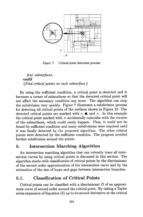
Table 1. Classification of critical points.

D>O Loop point

Touching point

D=O Parallel point

Duplicated point

D<O Hyperbolic point

Crossing point

point, where </>u = </>v = 0, the following equation is obtained:

S - R + Sudu + Svdv - R 8ds - Rtdt

+ ~ ( Suudu2 + 2Suvdudv + Svvdv2 - R 88ds2 - 2R8tdsdt- Rttdt2 )

= n ( </> + ~ ( </>uudu2 + 2</>uvdudv + </>vvdv2)) • {12)

Thus the following equation represents the approximate curve of second order, i.e., a conic section, around the critical point:

</>uudu2 + 2</>uvdudv + </>vvdv2 + 2</> = 0. (13)

The discriminant D of the conic section is given as below:

D = </>uu</>vv - </>uv 2 ,

where

</>uu = Suu ·N /TJ- ((Rss·N)<put2 - 2(Rst·N)<pus<t'ut+ {Rtt ·N)<pus2)/TJ3,

</>uv = Suv · N / TJ- ( (Rss · N) <t'ut<t'vt- (Rst · N) ( <t'us<t'vt + <t'ut<t'vs) + (Rtt · N) <t'us<t'vs) / TJ3 ,

</>vv = Svv ·N /TJ- ((Rss·N)<t'vt2 - 2(Rst·N)<t'vs<t'vt+ (Rtt·N)<pvs 2}/TJ3,

<t'us = n· (Sux R 8 ), <t'ut= n· (Sux Rt), <t'vs=n· (Sv X Rs), <t'vt=n·(SvxRt), rJ=n·N, N=R8 XRt.

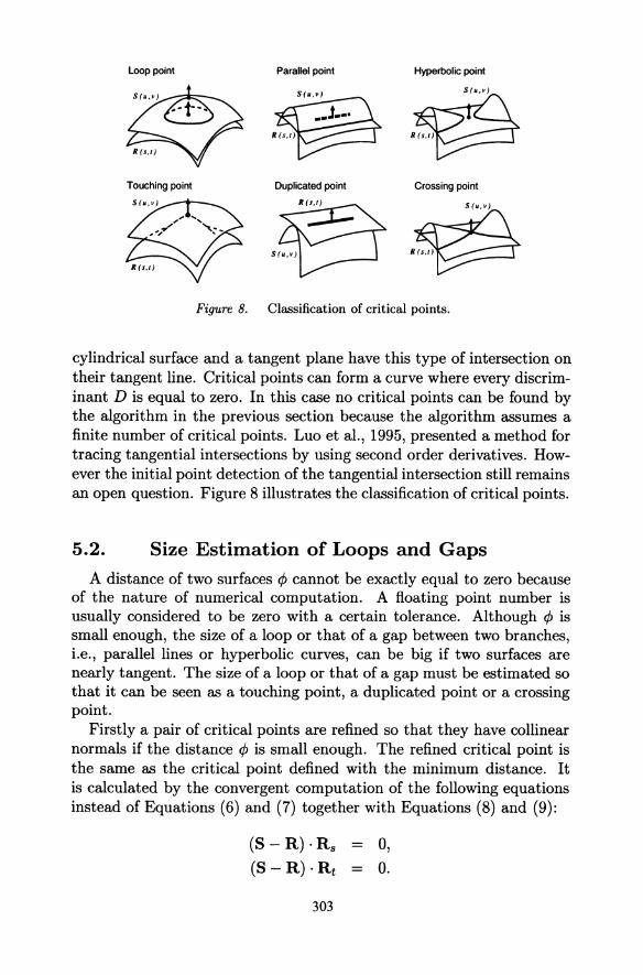
Table 1 shows the classification of critical points. The inequality</> =f 0 indicates that the critical point does not lie on the intersection curves. In this case, a critical point can be classified into either a loop point, a parallel point, or a hyperbolic point according to the discriminant D, which means that the nearest intersection curves may form either a loop, parallel lines, or hyperbolic lines respectively. The equation </> = 0 indicates that the critical point lies on the intersection. In this case, a critical point can be classified into either a touching point, a dupli­cated point, or a crossing point according to D. A touching point is a tangential point of two surfaces. A duplicated point indicates that two intersection curves completely coincide around its neighborhood. A

302

Loop point Parallel point Hyperbolic point

Touching point Duplicated point Crossing point

Figure 8. Classification of critical points.

cylindrical surface and a tangent plane have this type of intersection on their tangent line. Critical points can form a curve where every discrim­inant Dis equal to zero. In this case no critical points can be found by the algorithm in the previous section because the algorithm assumes a finite number of critical points. Luo et al., 1995, presented a method for tracing tangential intersections by using second order derivatives. How­ever the initial point detection of the tangential intersection still remains an open question. Figure 8 illustrates the classification of critical points.

5.2. Size Estimation of Loops and Gaps A distance of two surfaces ¢ cannot be exactly equal to zero because

of the nature of numerical computation. A floating point number is usually considered to be zero with a certain tolerance. Although ¢ is small enough, the size of a loop or that of a gap between two branches, i.e., parallel lines or hyperbolic curves, can be big if two surfaces are nearly tangent. The size of a loop or that of a gap must be estimated so that it can be seen as a touching point, a duplicated point or a crossing point.

Firstly a pair of critical points are refined so that they have collinear normals if the distance ¢ is small enough. The refined critical point is the same as the critical point defined with the minimum distance. It is calculated by the convergent computation of the following equations instead of Equations (6) and (7) together with Equations (8) and (9):

(S- R) · Rs 0, (S - R) · Rt = 0.

303

The first two equations indicate that the two corresponding points are lying on the normal of the surface R. The remaining two imply the points have parallel normals. The original critical point is a good first guess for the convergence.

Let's consider the approximate curve around the refined critical point. By using the collinear normal vector at the refined critical point, 1~:~~: 1 =

1 :::~:: 1 , as the constant vector n, Equation (12) of the approximate curve can be divided into three parts, i.e., the constant terms, the terms of the first derivatives, and the terms of the second derivatives. The constant terms indicate the correspondence between the points, S and R. The terms of the first derivatives govern the displacement perpendic­ular to the collinear normal, i.e., the displacement on the tangent plane, which is given by a linear transformation, S udu + Svdv. The terms of the second derivatives govern the displacement along the collinear normal, i.e., the deviation of the distance, which indicates an approximate inter­section curve of second order in a parametric space, (u, v), as shown in Equation (13). Since a conic section is mapped to another conic section with a linear transformation, we can estimate the sizes of loops and gaps with those of approximate conic sections in the real space.

5.3. Tracing Intersection Curves After classifying all detected critical points, the marching algorithm

traces all intersection lines as below:

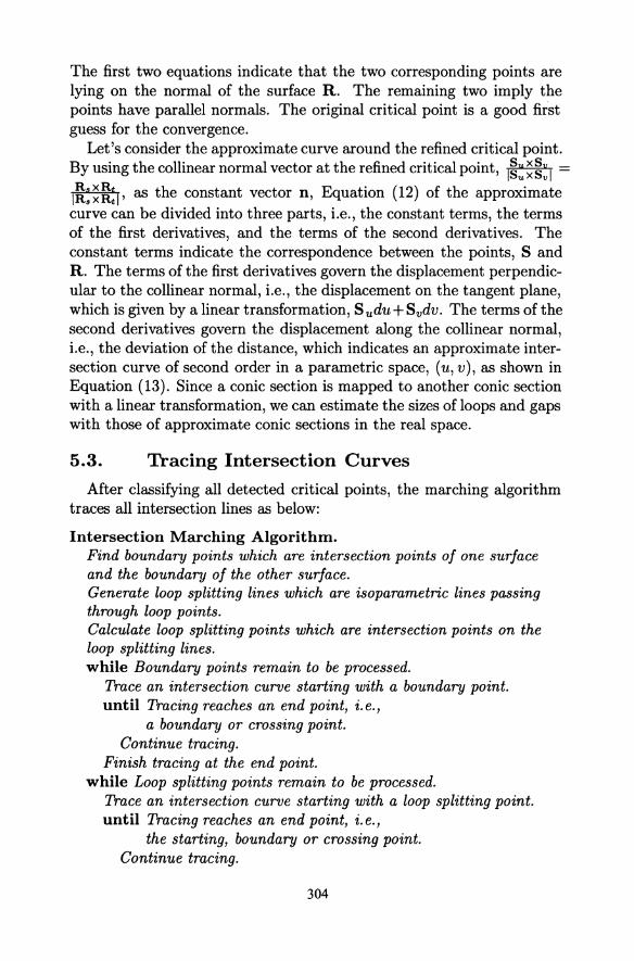
Intersection Marching Algorithm. Find boundary points which are intersection points of one surface and the boundary of the other surface. Generate loop splitting lines which are isoparametric lines passing through loop points. Calculate loop splitting points which are intersection points on the loop splitting lines. while Boundary points remain to be processed.

Trace an intersection curve starting with a boundary point. until Tracing reaches an end point, i.e.,

a boundary or crossing point. Continue tracing.

Finish tracing at the end point. while Loop splitting points remain to be processed.

Trace an intersection curve starting with a loop splitting point. until Tracing reaches an end point, i.e.,

the starting, boundary or crossing point. Continue tracing.

304

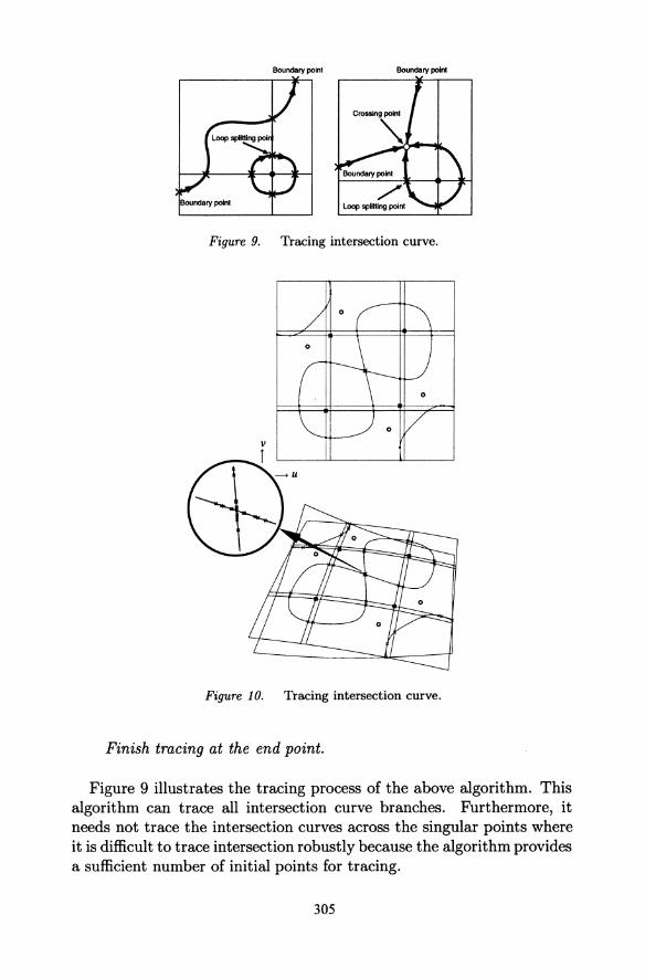
Figure 9. Tracing intersection curve.

Figure 10. Tracing intersection curve.

Finish tracing at the end point.

Figure 9 illustrates the tracing process of the above algorithm. This algorithm can trace all intersection curve branches. Furthermore, it needs not trace the intersection curves across the singular points where it is difficult to trace intersection robustly because the algorithm provides a sufficient number of initial points for tracing.

305

We have implemented the technique and examined it in several cases. Figure 10 shows a result of surface-surface intersection. The figure shows critical points, starting points for tracing, and intersection curves cal­culated by the proposed algorithms. The algorithm succeeded to find all critical points and to classify them. Hyperbolic critical points are marked with o, loop critical points are marked with ~ and a crossing critical point is marked with bold x. It also succeeded to trace the intersection curves robustly.

6. Conclusions This paper proposed a technique for solving the problems of marching

methods, i.e., starting point detection and robust tracing across singular points, which are strongly related to critical points. The advantageous characteristics of our study are as follows:

• The relationship between critical points and the problems is clari­fied.

• A Bezier normal vector surface, which has good properties, is in­troduced.

• An algorithm for detecting all critical points based on a Bezier normal vector surface is proposed.

• An algorithm for robust intersection tracing based on critical points classification is discussed.

Though the current algorithm is limited to polynomial surfaces be­cause it is based on a Bezier normal vector surface, it should be ex­tended to rational surfaces, which are commonly used in CAD systems. The normal bounds of rational surfaces are necessary for this extension Saito et al., 1995. Tangential intersection that can frequently arise in mechanical parts is also a future issue as noted in Section 5.1.

Acknowledgements This research work has been partly supported by Casio Science Pro­

motion Foundation, and Basic Research 21 for Breakthroughs in Info­Communications of Postal Services Agency.

References Bajaj, C. L., Hoffmann, C. M., and Lynch, R. W. (1988). Tracing surface intersections.

Computer Aided Geometric Design, 5(2):285-307. Barnhill, R. and Kersey, S. (1990). A marching method for parametric surface/surface

intersection. Computer Aided Geometric Design, 7(1-4):257-280.

306

Charrot, P. (January 1993). The new ACIS surface-surface intersection algorithm. Technical report, D-cubed ltd.

Cheng, K. (1989). Using plane vector fields to obtain all the intersection curves of two general surfaces. In Strasser, W. and Seidel, H.-P., editors, Theory and Practice of Geometric Modeling, pages 188-204. Springer-Verlag.

de Boor, C. (1987). B-form basics. In Farin, G., editor, Geometric Modeling: Algo­rithms and New Trends, pages 131-148. SIAM.

Dokken, T. (1985). Finding intersections of b-spline represented geometries using recursive subdivision techniques. Computer Aided Geometric Design, 2(1-3):189-195.

Farin, G. E. (1996). Curves and surfaces for computer aided geometric design. Aca­demic Press, Inc., forth edition. ISBN: 0-12-249054-1.

Goldman, A. J. and Tucker, A. W. (1956). Polyhedral convex cones. In Kuhn, H. W. and Tucker, A. W., editors, Linear Inequalities and Related Systems, pages 19-40. Princeton Univ. Press.

Grandine, T. A. and Klein IV, F. W. (1997). A new approach to the surface intersec­tion problem. Computer Aided Geometric Design, 14(2):111-134.

Higashi, M., Yatomi, H., Nozu, M., and Hosaka, M. (1992). Finding intersection pat­tern of two surfaces using their difference function. Journal of the Japan Society for Precision Engineering, 58(1):157-162. (in Japanese).

Hohmeyer, M. E. (1992). Robust and Efficient Surface Intersection for Solid Modeling. PhD thesis, University of California Berkeley.

Kim, T.-S., Paralambros, P. Y., and Woo, T. C. (1995). Tangent, normal, and visibility cones on Bezier surfaces. Computer Aided Geometric Design, 12(3):305-320.

Kriezis, G. and Patrikalakis, N. M. (1991). Rational polynomial surface intersections. In Advances in Design Automation, pages 43-53. ASME. DE-Vol.32.

Kriezis, G. A., Patrikalakis, N. M., and Wolter, F.-E. (1992). Topological and differen­tial equation methods for surface intersections. Computer-Aided Design, 24(1):41-55.

Kushimoto, T. and Hosaka, M. (1991). Methods of automatic detection of points on all separate intersection curves of two surfaces. Journal of the Japan Society for Precision Engineering, 57(9):1667-1672. (in Japanese).

Luo, R. C., Ma, Y., and McAllister, D. F. (1995). Tracing tangential surface-surface intersections. In Hoffmann, C. and Rossignac, J., editors, Symposium on Solid Modeling and Applications, pages 255-262. ACM Press.

Ma, Y. and Luo, R. C. (1995). Topological method for loop detection of surface intersection problems. Computer-Aided Design, 27(11):811-820.

Markot, R. and Magedson, R. (1989). Solutions of tangential surface and curve inter­sections. Computer-Aided Design, 21(7):421-429.

Miller, J. R. (1987). Geometric approaches to nonplanar quadric surface intersection curve. ACM Transactions on Graphics, 6(4):274-307.

Owen, J. C. and Rockwood, A. P. (1987). Intersection of general implicit surfaces. In Farin, G., editor, Geometric Modeling: Algorithms and New Trends, pages 335-345. SIAM.

Patrikalakis, N. M. (1993). Surface-to-surface intersections. IEEE Computer Graphics and Applications, 13(1):89-95.

Saito, T., Wang, G.-J., and Sederberg, T. W. (1995). Hodographs and normals of rational curves and surfaces. Computer Aided Geometric Design, 12(6):417-430.

307

Sederberg, T. W. and Meyers, R. J. (1988). Loop detection in surface patch intersec­tions. Computer Aided Geometric Design, 5(2}:161-171.

Sederberg, T. W. and Zundel, A. K. (1996). Pyramids that bound surface patches. Graphical Models and Image Processing, 58(1}:75-81.

Sinha, P., Klassen, E., and Wang, K. K. (July 1985}. Exploiting topological and geo­metric properties for selective subdivision. SIGGRAPH'85 Conf. Proc., Computer Graphics, 19(3}:39-45.

Wang, Y., Gursoz, E. L., Chen, J.-M., Prinz, F. B., and Patrikalakis, N. M. (1991). In­tersection of parametric surfaces for next generation geometric modelers. In Turner, J., Pegna, J., and Wozny, M., editors, Product Modeling for Computer-Aided De­sign and Manufacturing, pages 75-96. North-Holland.

Yamaguchi, Y. (February 1996}. Normal vectors of Bezier type surface and their bounds. Transactions of IPSJ, 37(2}:242-248. (in Japanese).

308