surfaces chiew-lan tai. surfaces 2 reading required hills section 11.11 hearn & baker, sections...
Post on 18-Dec-2015
217 views
TRANSCRIPT
SurfacesSurfaces
Chiew-Lan Tai

2
Surfaces
Reading
Required Hills Section 11.11 Hearn & Baker, sections 8.11, 8.13
Recommended Sections 2.1.4, 3.4-3.5, 3D Computer
Graphics, Watt

3
Surfaces
Mathematical surface representations Explicit z = f(x,y) (a.k.a. “height field”) What if the surface isn’t a function?
Implicit g(x,y,z) = 0 x2 + y2 + z2 = 1
Parametric S(u,v) = (x(u,v), y(u,v), z(u,v)) x(u,v) = r cos 2v sinu y(u,v) = r sin 2v sinu z(u,v) = r cos u 0≤u≤1, 0≤v≤1

4
Surfaces
Tensor product Bézier surfaces
Given a grid of control point Vij, forming a control net, construct a surface S(u,v) by:
Each row in u-direction is control points of a curve Vi(u).
V0(u), …, Vn(u) at a specific u are the control points of a curve parameterized by v (i.e. S(u,.v))

5
Surfaces
Tensor product Bezier surfaces, cont. Let’s walk through the steps:
Which points are interpolated by the surface? V0(u) and V3(u)

6
Surfaces
Tensor product Bezier surfaces, cont. Writing it out explicitly: Linear Bezier surface:
Quadratic Bezier surface?
])1[(
])1)[(1(),(
1110
0100
VV
VVS
uuv
uuvvu
])1(2)1[(
])1(2)1)[(1(2
])1(2)1[()1(),(
222
212022
122
11102
022
010022
VVV
VVV
VVVS
uuuuv
uuuuvv
uuuuvvu

7
Surfaces
Matrix form
For the case of cubic Bezier surface:

8
Surfaces
Tensor product B-spline surfaces
Like spline curves, we can piece together a sequence of Bezier surfaces to make a spline surface. If we enforce C2 continuity and local control, we get B-spline curves:

9
Surfaces
Tensor product B-spline surfaces
Use each row of B control points in u to generate Bezier control points in u. Treat each row of Bezier control points in v direction as B-spline control points to
generate Bezier control points in v direction.
u

10
Surfaces
Tangent plane and surface normal
S
S

11
Surfaces
Partial Derivatives
0
1
2
3
]1[),(
2
23 u
u
MVMvvvvuSu
TBezierBezier
1
]0123[),(2
3
2
u
u
u
MVMvvvuSv
TBezierBezier

12
Surfaces
Surface normal
S
S S
S

13
Surfaces
Other construction methods

14
Surfaces
Rotational surfaces (surface of revolution) Rotate a 2D profile curve about an axis

15
Surfaces
Profile curve, C(u)
Constructing surfaces of revolution Given a curve C(u) in the yz-plane:
Let Ry() be a rotation about the y-axis Find: A surface S(u,v) obtained by applying Ry() on C(u)
S(u,v) = Ry(v) [0, Cy(u), Cz(u), 1]t
y
xz

16
Surfaces
Surface of revolution
S(u,v) = ( Cz(u) sin(v), Cy(u), Cz(u) cos(v))
y
z
x

17
Surfaces
General sweep surface
Given a planar profile curve C(u) and a general space curve T(v) as the trajectory, sweep C(u) along the trajectory
How to orient C(u) as it moves along T(v)?

18
Surfaces
Orientating C(u) Define a local coordinate frame at any point along the trajectory The Frenet frame (t,n,b) is the natural choice
As we move along T(v), the Frenet frame (t,b,n) varies smoothly (inflection points where curvature goes to zero needs special treatment)

19
Surfaces
Sweep Surfaces
Orient the profile curve C(u) using the Frenet frame of the trajectory T(v): Put C(u) in the normal plane. Place Oc at T(v). Align xc of C(u) with b. Align yc of C(u) with n.
Sweep surface
S(u,v) = T(v) + n(v)Cx(u) + b(v) Cy(u)

20
Surfaces
Variations
Several variations are possible: Scale C(u) as it moves, possibly using length of T(v) as a
scale factor. Morph C(u) into some other curve C’(u) as it moves along
T(v)

21
Surfaces
Summary
What to take home: How to construct tensor product Bezier surfaces How to construct tensor product B-spline surfaces How to construct surfaces of revolution How to construct sweep surfaces from a profile and a
trajectory curve with a Frenet frame

22
Surfaces
Subdivision SurfacesWhat’s wrong with B-spline/NURBS surfaces?

23
Surfaces
Subdivision curves
Idea: repeatedly refine the control polygon
curve is the limit of an infinite process.
i
i
PC
PPP
lim
210

24
Surfaces
Subdivision curves

25
Surfaces
Chaikin’s algorithm In 1974, Chaikin introduced the following “corner-
cutting” scheme: Start with a piecewise linear curve Repeat
Insert new vertices at the midpoints (the splitting step)
Average two neighboring vertices (the average step)
Averaging mask(0.5, 0.5)
With this averaging mask, in the limit, the resulting curve is a quadratic B-spline curve.
26
Surfaces
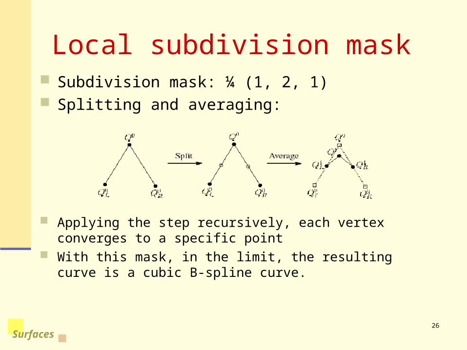
Local subdivision mask Subdivision mask: ¼ (1, 2, 1) Splitting and averaging:
Applying the step recursively, each vertex converges to a specific point
With this mask, in the limit, the resulting curve is a cubic B-spline curve.

27
Surfaces
General subdivision process
After each split-average step, we are closer to the limit surface.
Can we push a vertex to its limit position without infinite subdivision? Yes!
We can determine the final position of a vertex by applying the evaluation mask. The evaluation mask for cubic B-spline is 1/6 (1,4, 1)
28
Surfaces
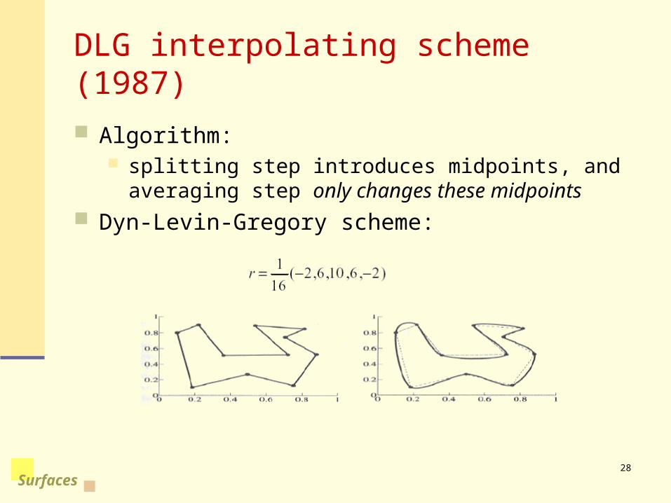
DLG interpolating scheme (1987)
Algorithm: splitting step introduces midpoints, and averaging step
only changes these midpoints Dyn-Levin-Gregory scheme:

29
Surfaces
Building Complex Models
This simple idea can be extended to build subdivision surfaces.

30
Surfaces
Subdivision surfaces Iteratively refine a control polyhedron (or control mesh) to
produce the limit surface using splitting and averaging step:
There are two types of splitting schemes: vertex schemes face schemes

31
Surfaces
Vertex schemes
A vertex surrounded by n faces is split into n subvertices, one for each face:
Doo-Sabin subdivision:

32
Surfaces
Face schemes Each quadrilateral face is split into four subfaces:
Catmull-Clark subdivision:

33
Surfaces
Face scheme, cont.
Each triangular face is split into four subfaces:
Loop subdivision:

34
Surfaces
Averaging step Averaging masks:
nn
QQQnQ n
)(
)( 1

35
Surfaces
Adding creases Sometimes, a particular feature such as a crease should be
preserved. we just modify the subdivision mask.
This gives rise to G0 continuous surfaces.

36
Surfaces
Creases
Here’s an example using Catmull-Clark surfaces: