100

Rakenteiden Mekaniikka (Journal of Structural Mechanics) Vol. 49, No 3, 2016, pp. 100-118 rmseura.tkk.fi/rmlehti/ ©The Authors 2016. Open access under CC BY-SA 4.0 license.

Surrogate-model based method and software for practical design optimization problems

Sami Pajunen, Petri Laakkonen

Summary. In a practical simulation-based design process most of the required simulations are carried out by using commercial software producing simulation responses but no gradient data. When applying mathematical optimization routines to such design process all the function evaluators must be considered as black-box solvers and the optimization can be integrated to design process efficiently using e.g. surrogate modeling techniques or heuristic optimization algorithms. In this paper we present a design optimization method that can be integrated very easily to any simulation-based design process. Special attention is paid on software implementation issues of the proposed method.

Key words: design, optimization, surrogate model Received 24 August 2015. Accepted 1 June 2016. Published online 30 December 2016.

Introduction

Throughout the history of mathematical optimization, the main focus in majority of the research projects has been the search of global optimum using various strategies. This massive research has resulted in many fine-tuned and robust optimization algorithms for different types of problems, e.g. the interior point method for linear problems [1] and sequentially quadratic method for non-linear problems [2]. In some problem categories even the finding of the global optimum can be guaranteed [3].

The practical design processes would benefit greatly from the adoption of these optimization algorithms but there are certain barriers preventing the full scale utilization of mathematical optimization methods. In industrial design environment the designers are almost without exception using commercial simulation software, i.e. black box solvers that produce only simulation results but usually not the gradient data. Hence, none of the gradient based algorithms can be used as such. On the other hand, only the biggest companies can administrate the best optimization software for every possible type of optimization problems that may appear in their design processes. There are evidently also many other reasons to the low usage of optimization in practice, but already these two

101

reasons lead us to an acute research problem statement: How to tackle in the most efficient way all kind of industrial optimization problems in all the simulation environments. In other words, how to develop a method that can be used to solve any optimization problems in any design environment. Additionally, in the industrial processes the keywords such as speed and robustness are highly appreciated and they should also be the driving forces when designing the method. It is evident, that broadening the method's capability to handle various optimization problem types will simultaneously decrease some other features of the method. Usually this means that the search of the global optimum must be replaced by the search of a better design. But at the same time the design optimization process can be done more robustly and faster than before.

In this paper we present a surrogate-model based optimization method and the associated software that can be adopted to any design process that uses parametric simulation models. The software is used to formulate the optimization problem while the simulation is carried out by using some black box solver and the generated optimization sub-problems are solved using the best available optimization algorithm libraries. In the optimization problem formulation the original simulation problem is replaced sequentially by polynomial-based metamodels [4].

The paper is organized as follows. First, the basic features and advantages of surrogate modeling techniques are concisely revised. In a subsequent section the details of the proposed optimization method and the associated software implementation issues are discussed. Two well-known benchmark problems and one industrial application problem are solved using the proposed method and finally the main conclusions of the paper are drawn.

Surrogate models in simulation-based optimization

In a practical design process the simulation models are typically rather complex, massive and time-consuming to evaluate. Thus, it is of primary interest to minimize the simulation model evaluation calls in the optimization process. Additionally, the simulation models do not usually produce sensitivity data. Due to these features, one of the most efficient strategies to apply optimization in to the design process is to replace the original simulation model with an associated surrogate model. The most widely used surrogate model techniques are the response surface method (RSM) [5], Kriging method [6], neural networks [7], radial basis function method [8] and regression splines method [9].

In general, the surrogate-model based optimization can be divided into the following four main stages [10,11]. First the required simulations are carried out with different model parameter values at the so called design-of-experiments points (or design points), then the simulated data is fitted to the selected surrogate model. Once the surrogate model is formulated to mimic the original problem, it is straightforward to formulate the optimization task and call the surrogate model whenever function evaluations are needed.

In the surrogate-model based optimization two different strategies are usually adopted: global surrogate model fit, and iterated local surrogate models. In the local strategy the surrogate model is fitted to the neighborhood of the previous optimum point

102

at every iteration cycle. This sequential strategy is used especially with the response surface method. Accuracy of the response surface method is generally sufficient to approximate only a small part of the design space [12]. As soon as the surrogate model is constructed by the desired method, also the design variable sensitivities can be estimated. Furthermore, it is noteworthy, that also discrete variables can be included in surrogate models [13].

In addition to the property that surrogate modeling simplifies greatly the original complex model it has also one fundamental advantage when used in addition to optimization. The surrogate model is constructed using the computed responses at separate design points that can be computed independently in parallel. Due to fully distributing problem the parallel computing speeds up the computation almost linearly. However, when applying surrogate modeling in optimization, one has to pay special attention to the number of design variables. When the number of design variables increases, the required amount of design points becomes rather big, when using higher-order surrogate methods. And the other hand, purely linear surrogates are computationally cheaper, but they may not be capable of predicting the model responses accurately enough but only in rather small sub-spaces. Despite of the used surrogate models, the proper formulation of the optimization problem is of primary interest and the selection of design variables must be done with great caution.

The proposed method and software implementation

Leading principles In the design of the optimization software based on the proposed method, the targets were wide applicability, superior robustness and rapidity of the optimization task set up and solution as well as prime user experience. To meet these requirements, an easy-to-use and easy-to-learn simple graphical user interface was designed. Wide applicability of the software was ensured by adopting modularity in all the implementations and enabling the use of any kind of design variables. The kernel of the optimization problem formulation was based on the successive response surface method that was found to be extremely robust in earlier studies [4]. For the optimization problems solution, the best algorithm consistent with the adopted surrogate model was chosen from existing algorithm libraries such as Gurobi [14] and SCIP [15]. Parallel computations were performed using the Techila middleware system [16]. Optimization problem formulation Implemented optimization procedure is based on successive response surface method with linear, pure quadratic or quadratic polynomial basis functions. In the design space the surrogate model is spanned sequentially into an a priori chosen subspace called the region of interest (ROI) so that approximation errors remain below a user-defined acceptance limit. To construct the surrogate model in the subspace, the required model responses are concurrently evaluated at the design points that are placed to the subspace

103

using the D-optimal design [17], and the data is fitted to selected polynomial form using the method of least squares. The optimization problem at iteration cycle i is formulated as

min 𝐟𝐟(𝐱𝐱) 𝐠𝐠(𝐱𝐱) ≤ 𝟎𝟎 𝐡𝐡(𝐱𝐱) = 𝟎𝟎

𝐱𝐱𝑖𝑖L ≤ 𝐱𝐱𝐢𝐢 ≤ 𝐱𝐱𝑖𝑖

U in which the subscript i refers to iteration cycle number and the superscripts L and U denote the lower and upper limits of the design variable vector x, respectively. In other words, the lower and upper limits define the region of interest in which the surrogate model is spanned at the current iteration cycle. The constraint functions are collected to vectors g and h and objective functions are collected in vector f. In the case of scalar optimization problem, vector f simplifies to scalar function f. In (1) all the functions in vectors f, g and h are approximated in the current region of interest 𝐱𝐱𝑖𝑖

𝐋𝐋, 𝐱𝐱𝑖𝑖𝐔𝐔 according to

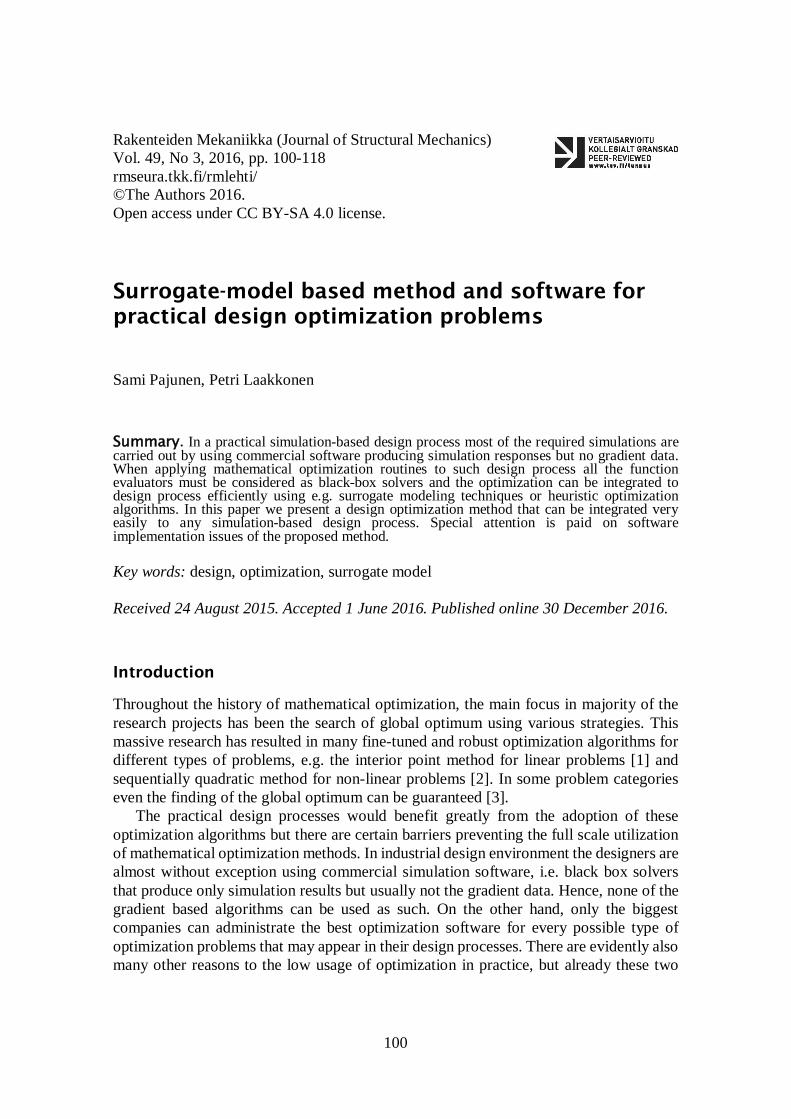
the adopted surrogate model. Once the optimization problem (1) is solved at current iteration, the next ROI is spanned in the neighborhood of the found optimum as depicted in figure 1 and the iteration is continued. The iteration is stopped either when the a priori set number of maximum iterations is exceeded or when the convergence criterion is met. The convergence criterion reads in

TolFunf

ff

i

ii ≤− −

)()()( 1

xxx

(2)

In practical design optimization problems, the objective functions rarely approach zero in the optimum, but in such case, the convergence criterion should be based on e.g. the iterative change of design variables.

More detailed derivation of the method can be found from [4]. When solving the optimization problem (1), a consistent optimization algorithm is chosen according to Table 1, in which all the implemented algorithms are introduced briefly. In the Table 1, LP denotes linear problem, MILP mixed-integer linear problem, QCQP quadratically constrained quadratic problem, MIQCQP mixed-integer quadratically constrained quadratic problem. High performance computing

In the design optimization tasks, the number of function evaluations at separate design points can be very large [17]. A distributed computation system developed by Techila is utilized to carry out parallel computation in cloud or computer clusters [16]. Techila supports the several programming interfaces as MATLAB, which has been used in the software.

(1)

104

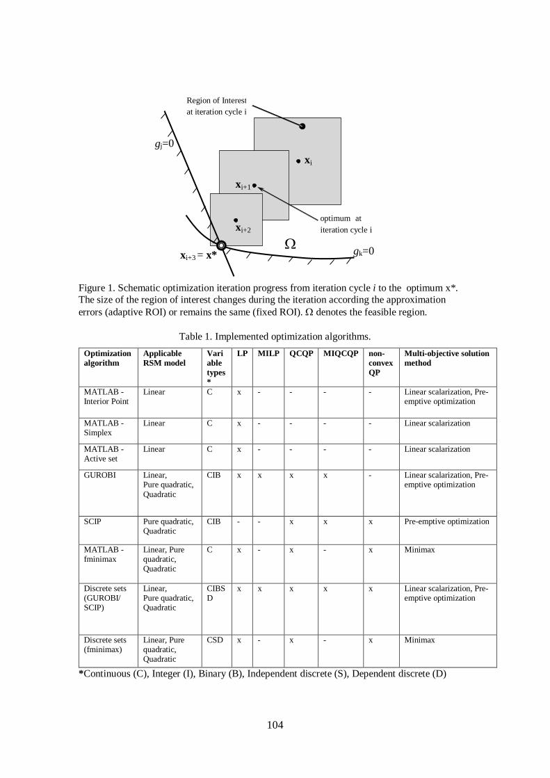
Figure 1. Schematic optimization iteration progress from iteration cycle i to the optimum x*. The size of the region of interest changes during the iteration according the approximation errors (adaptive ROI) or remains the same (fixed ROI). Ω denotes the feasible region.

Table 1. Implemented optimization algorithms. Optimization algorithm

Applicable RSM model

Variable types *

LP MILP QCQP MIQCQP non- convex QP

Multi-objective solution method

MATLAB - Interior Point

Linear C x - - - - Linear scalarization, Pre-emptive optimization

MATLAB - Simplex

Linear C x - - - - Linear scalarization

MATLAB - Active set

Linear C x - - - - Linear scalarization

GUROBI Linear, Pure quadratic, Quadratic

CIB x x x x - Linear scalarization, Pre-emptive optimization

SCIP Pure quadratic, Quadratic

CIB - - x x x Pre-emptive optimization

MATLAB - fminimax

Linear, Pure quadratic, Quadratic

C x - x - x Minimax

Discrete sets (GUROBI/ SCIP)

Linear, Pure quadratic, Quadratic

CIBSD

x x x x x Linear scalarization, Pre-emptive optimization

Discrete sets (fminimax)

Linear, Pure quadratic, Quadratic

CSD x - x - x Minimax

*Continuous (C), Integer (I), Binary (B), Independent discrete (S), Dependent discrete (D)

Ω

g j =0

g k =0

x i

x i +1

x i +2

x i +3 = x *

Region of Interest at iteration cycle i

optimum at iteration cycle i

105

GUI and interfaces

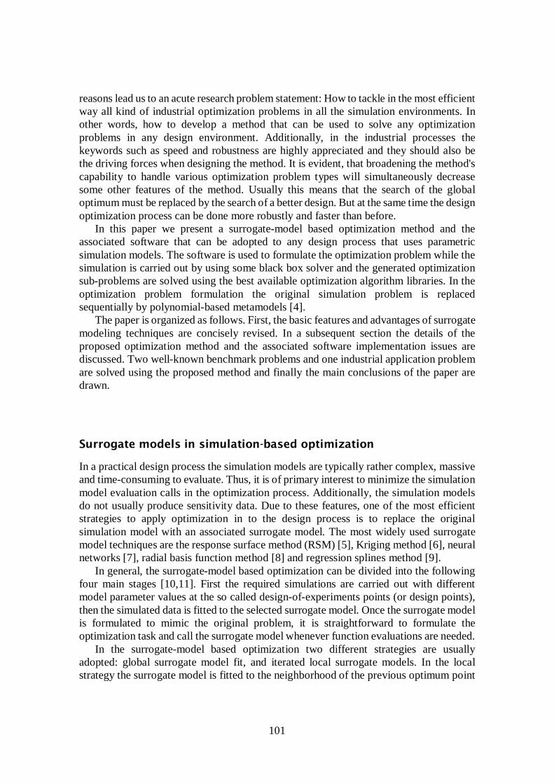
The software has been designed by following the Model-View-Controller (MVC) architectural pattern. It separates an application into three main components: the model, the view, and the controller. This makes it possible to develop these components separately [18]. In the developed software the model is a database, the view is the graphic user interface seen by the user and the controller takes care of the input given by the user. The controller's application logic also launches the actual computation code. The software and the interaction between parts are depicted at a general level in figure 2. The computation code has been put into practice by using MATLAB, but on the other hand, also Python and open source solvers could have been used instead. The figure 2 highlights the four interfaces: a graphical user interface (GUI), database, computation code and simulation software, which produces the model responses and is linked to any CAD-system. The input parameters file is edited with a user interface or text editor and is given to a computation code. When creating a new task, an output-folder to which the parameters and results of the task will be stored, is created at the same time. The parameters are also saved in the database for the user interface. The interfaces to simulation packages such as ANSYS have been made with Python. The database is implemented in SQLite.

Figure 2. Interfaces of the RapidDO software.

When designing the software, special attention was paid to the future augmentation needs by following a modular structure and to carry out functions which can be easily maintained. For the end user the software can be easily compiled to be executed in Microsoft Windows. For prime user experience the entering of the tasks is executed as proficiently as possible. The required task parameters are classified in Table 2.

106

Table 2. Task parameters needed in the optimization.

Mandatory parameters Parameters for experienced user (otherwise program-controlled)

File location of the simulation model used in the optimization (e.g. FEM-model containing two-way link to CAD-model)

Multi-objective optimization method

ID-numbers of simulation model output parameters used in objective or constraint functions

Initial radius and adaptiveness of the region of interest

ID-numbers of simulation model input parameters used as design variables and their types

Target relative error between the surrogate model and the true simulation model

Surrogate model (Linear, Quadratic or Pure quadratic)

Number of maximum iterations

Optimization algorithm (according to Table 1)

Relative convergence tolerance of the objective functions (TolFun)

Discrete sets and dependencies of discrete variables (if in use)

Constraint functions and Design variables to be visualized during the iteration

Activation of Techila parallelization Constraint tolerance for true responses Discrete problems The discrete sets are needed in practical design optimization tasks in which the variables can get only certain discrete values or value pairs. The mathematical formulation of optimization problem with discrete design variables is implemented in to the software as detailed below [19]. Discrete variable can be selected from a finite set s1,...,sm as follows.

𝑥𝑥 = ∑ 𝑢𝑢𝑖𝑖𝑠𝑠𝑖𝑖𝑚𝑚𝑖𝑖=1 (3)

in which 𝑢𝑢𝑖𝑖 ∈ 0, 1, 𝑠𝑠𝑖𝑖 ∈ 𝑅𝑅 and m is the number of discrete values. The binary variable 𝑢𝑢𝑖𝑖 is used to pick only one discrete value 𝑠𝑠𝑖𝑖 from the set according to equation (4)

∑ 𝑢𝑢𝑖𝑖𝑚𝑚𝑖𝑖=1 − 1 = 0 (4)

When discrete design variables are used, the constraint vector h in (1) is augmented with the equality constraints (4) in the standard manner [20].

Discrete models have been derived for three cases. In the first case all the design variables are chosen from discrete sets. In the second case the design variables are also discrete but dependent on each other. In other words, all the allowed combinations of design variables are defined. In practice, this often means the permitted configurations

107

that might appear e.g. in problems in which beam profile area and the second moment of area must have consistent discrete values. In the third case the design variables can be discrete and dependently discrete as above, but also continuous and integers.

Discrete values must be taken into account in the design of experiments, because the optimized target, such as a parametric FE-model may not be able to analyze the model with non-discrete values. In other words, the experimental design should be used only with allowed combinations of given discrete values and dependent variables. In the computational tool this has been solved by expanding the ROI so that sufficient number of valid discrete points is included in it, and then forming the candidate matrix in the usual manner according the D-optimal design. Multi-objective problems

There are often conflicting objectives in practical design optimization tasks. In that case the optimization problem can be formulated as multi-objective in which the solution is a Pareto optimal set instead of a single optimum point as in the case on a single-objective optimization problem. Mathematically, every Pareto optimal point is equivalent, but in practice, however, only one solution is sought. There are many strategies for selecting the final solution from the pareto-set as discussed in [21].

Three methods which appear generally in the literature are applied to the tool: The linear scalarization method (called also as weighted sum method), pre-emptive optimization method (called also as lexicographic ordering) and the minimax method as explained in brief below. In the linear scalarization the objective functions are combined into one objective function which will be then optimized as a task of one objective function. This method does not work well with non-convex tasks because it cannot detect all the Pareto optimal points. For this reason this method can be used in the computational tool only with the linear surrogate model. It can be difficult to find suitable weighting coefficients needed in the method. In the pre-emptive optimization method one objective function is minimized at a time and the other objective functions are considered as constraint functions. With this method the decision-maker must sort the objective functions carefully to the order of importance because the order has a great impact for the converging of objective functions. The minimax method minimizes the objective function having largest value. This is the most straightforward from the adopted three methods because the decision-maker does not need to make decisions before the optimization. The best results can be achieved by running the same task with different methods and settings. The user's knowledge about the behavior of responses facilitates the solving of the multi-objective optimization task. Requiring the least amount of user input, MATLAB fminimax is often a good choice to begin with.

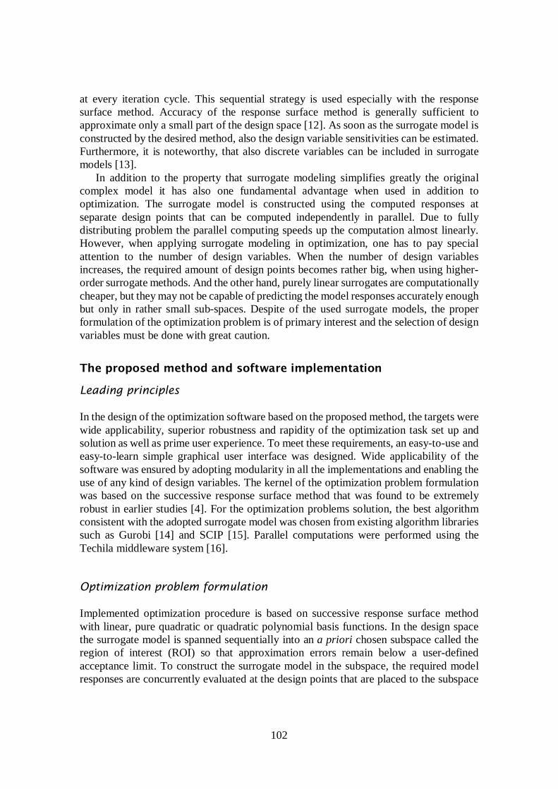
The multi-objective optimization methods used with a sequential response surface method return one pareto-optimal point at every iteration step once the iteration has found the first Pareto optimal point, thus the number of Pareto optimal points is dependent on the size of the used ROI. Therefore, in the multi-objective problems relatively small fixed radius of ROI should be used to get enough points to the Pareto optimal set. Naturally, this means more iteration cycles and at the same time more simulation calls. Figure 3

108

depicts Pareto optimal solution sets for a cantilever beam problem [22] obtained by using the proposed method with fixed and adaptive ROI.

Figure 3. Pareto front using fixed ROI (a), and adaptive ROI (b).

Results and discussion

Even though the primary goal of the proposed methodology is to solve practical simulation-based optimization problems, this chapter contains first two well-known benchmark problems for verification use. Furthermore, one practical design problem simulated by using the ANSYS FE-package and one multiobjective benchmark problem are reported Mass minimization of a pressure vessel

The first benchmark problem is a mass minimization of a pressure vessel [23]. In the problem, the function to be minimized and the associated constraints are 𝑓𝑓(𝐱𝐱) = 0.6224𝑥𝑥1𝑥𝑥3𝑥𝑥4 + 1.778𝑥𝑥2𝑥𝑥3

2 + 3.1661𝑥𝑥12𝑥𝑥4 + 19.84𝑥𝑥1

2𝑥𝑥3

(5)

𝑔𝑔1(𝐱𝐱) = −𝑥𝑥1 + 0.0193𝑥𝑥3 ≤ 0 𝑔𝑔2(𝐱𝐱) = −𝑥𝑥2 + 0.00954𝑥𝑥3 ≤ 0

𝑔𝑔3(𝐱𝐱) = −𝜋𝜋𝑥𝑥32𝑥𝑥4 −

43 𝜋𝜋𝑥𝑥3

3 + 1296000 ≤ 0 𝑔𝑔4(𝐱𝐱) = 𝑥𝑥4 − 240 ≤ 0,

x1 ∊ [0.625, 1.25], x2 ∊ [0, 0.625], x3 ∊ [45, 50], x4 ∊ [100, 120]

in which x1 is thickness of the cylindrical part of the pressure vessel and x2 is thickness of the hemispherical head. The inner diameter of the cylinder part of the container is x3 and the length is x4. All the design variables are chosen from discrete sets listed in Table 3.

109

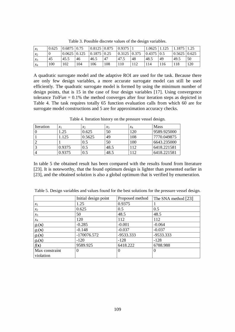
Table 3. Possible discrete values of the design variables.

x1 0.625 0.6875 0.75 0.8125 0.875 0.9375 1 1.0625 1.125 1.1875 1.25 x2 0 0.0625 0.125 0.1875 0.25 0.3125 0.375 0.4375 0.5 0.5625 0.625 x3 45 45.5 46 46.5 47 47.5 48 48.5 49 49.5 50 x4 100 102 104 106 108 110 112 114 116 118 120

A quadratic surrogate model and the adaptive ROI are used for the task. Because there are only few design variables, a more accurate surrogate model can still be used efficiently. The quadratic surrogate model is formed by using the minimum number of design points, that is 15 in the case of four design variables [17]. Using convergence tolerance TolFun = 0.1% the method converges after four iteration steps as depicted in Table 4. The task requires totally 65 function evaluation calls from which 60 are for surrogate model constructions and 5 are for approximation accuracy checks.

Table 4. Iteration history on the pressure vessel design.

Iteration x1 x2 x3 x4 Mass 0 1.25 0.625 50 120 9589.925000 1 1.125 0.5625 49 108 7770.049875 2 1 0.5 50 100 6643.235000 3 0.9375 0.5 48.5 112 6418.221581 4 0.9375 0.5 48.5 112 6418.221581

In table 5 the obtained result has been compared with the results found from literature [23]. It is noteworthy, that the found optimum design is lighter than presented earlier in [23], and the obtained solution is also a global optimum that is verified by enumeration. Table 5. Design variables and values found for the best solutions for the pressure vessel design.

Initial design point Proposed method The SNA method [23] x1 1.25 0.9375 1 x2 0.625 0.5 0.5 x3 50 48.5 48.5 x4 120 112 112 g1(x) -0.285 -0.001 -0.064 g2(x) -0.148 -0.037 -0.037 g3(x) -170076.572 -9533.333 -9533.333 g4(x) -120 -128 -128 f(x) 9589.925 6418.222 6788.988 Max constraint violation

0 0 0

110

Mass minimization of the Golinski’s speed reducer

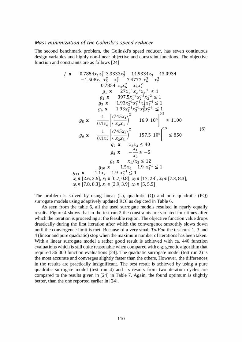
The second benchmark problem, the Golinski's speed reducer, has seven continuous design variables and highly non-linear objective and constraint functions. The objective function and constraints are as follows [24]

𝑓𝑓(𝐱𝐱) = 0.7854𝑥𝑥1𝑥𝑥2

2(3.3333𝑥𝑥32 + 14.9334𝑥𝑥3 − 43.0934)

−1.508𝑥𝑥1(𝑥𝑥62 + 𝑥𝑥7

2) + 7.4777(𝑥𝑥63 + 𝑥𝑥7

3) +0.7854(𝑥𝑥4𝑥𝑥6

2 + 𝑥𝑥5𝑥𝑥72)

(6)

𝑔𝑔1(𝐱𝐱) = 27𝑥𝑥1−1𝑥𝑥2

−2𝑥𝑥3−1 ≤ 1

𝑔𝑔2(𝐱𝐱) = 397.5𝑥𝑥1−1𝑥𝑥2

−2𝑥𝑥3−2 ≤ 1

𝑔𝑔3(𝐱𝐱) = 1.93𝑥𝑥2−1𝑥𝑥3

−1𝑥𝑥43𝑥𝑥6

−4 ≤ 1 𝑔𝑔4(𝐱𝐱) = 1.93𝑥𝑥2

−1𝑥𝑥3−1𝑥𝑥5

3𝑥𝑥7−4 ≤ 1

𝑔𝑔5(𝐱𝐱) =1

0.1𝑥𝑥63

745𝑥𝑥4

𝑥𝑥2𝑥𝑥3

2

+ (16.9)1060.5

≤ 1100

𝑔𝑔6(𝐱𝐱) =1

0.1𝑥𝑥73

745𝑥𝑥5

𝑥𝑥2𝑥𝑥3

2

+ (157.5)1060.5

≤ 850

𝑔𝑔7(𝐱𝐱) = 𝑥𝑥2𝑥𝑥3 ≤ 40 𝑔𝑔8(𝐱𝐱) = −

𝑥𝑥1

𝑥𝑥2≤ −5

𝑔𝑔9(𝐱𝐱) = 𝑥𝑥1/𝑥𝑥2 ≤ 12 𝑔𝑔10(𝐱𝐱) = (1.5𝑥𝑥6 + 1.9)𝑥𝑥4

−1 ≤ 1 𝑔𝑔11(𝐱𝐱) = (1.1𝑥𝑥7 + 1.9)𝑥𝑥5

−1 ≤ 1 x1 ∊ [2.6, 3.6], x2 ∊ [0.7, 0.8], x3 ∊ [17, 28], x4 ∊ [7.3, 8.3], x5 ∊ [7.8, 8.3], x6 ∊ [2.9, 3.9], x7 ∊ [5, 5.5]

The problem is solved by using linear (L), quadratic (Q) and pure quadratic (PQ) surrogate models using adaptively updated ROI as depicted in Table 6.

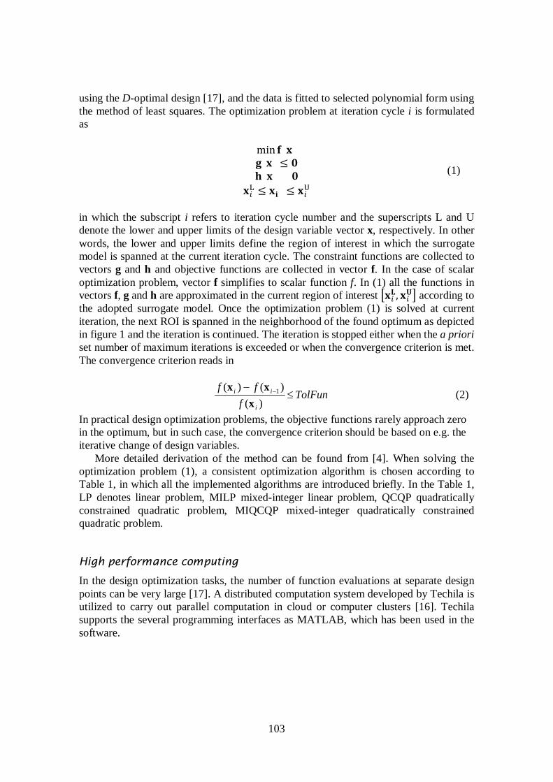
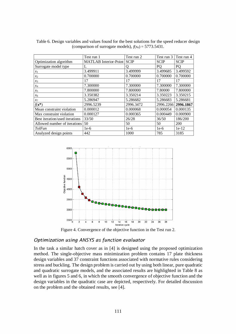
As seen from the table 6, all the used surrogate models resulted in nearly equally results. Figure 4 shows that in the test run 2 the constraints are violated four times after which the iteration is proceeding at the feasible region. The objective function value drops drastically during the first iteration after which the convergence smoothly slows down until the convergence limit is met. Because of a very small TolFun the test runs 1, 3 and 4 (linear and pure quadratic) stop when the maximum number of iterations has been taken. With a linear surrogate model a rather good result is achieved with ca. 440 function evaluations which is still quite reasonable when compared with e.g. genetic algorithm that required 36 000 function evaluations [24]. The quadratic surrogate model (test run 2) is the most accurate and converges slightly faster than the others. However, the differences in the results are practically insignificant. The best result is achieved by using a pure quadratic surrogate model (test run 4) and its results from two iteration cycles are compared to the results given in [24] in Table 7. Again, the found optimum is slightly better, than the one reported earlier in [24].

111

Table 6. Design variables and values found for the best solutions for the speed reducer design (comparison of surrogate models), f(x0) = 5773.5431.

Test run 1 Test run 2 Test run 3 Test run 4 Optimization algorithm MATLAB Interior-Point SCIP SCIP SCIP Surrogate model type L Q PQ PQ x1 3.499911 3.499999 3.499685 3.499592 x2 0.700000 0.700000 0.700000 0.700000 x3 17 17 17 17 x4 7.300000 7.300000 7.300000 7.300000 x5 7.800000 7.800000 7.80000 7.800000 x6 3.350382 3.350214 3.350223 3.350215 x7 5.286947 5.286682 5.286683 5.286681 f(x*) 2996.5239 2996.3472 2996.2266 2996.1867 Mean constraint violation 0.000012 0.000068 0.000054 0.000135 Max constraint violation 0.000127 0.000365 0.000449 0.000900 Best iteration/used iterations 33/50 26/28 36/50 186/200 Allowed number of iterations 50 50 50 200 TolFun 1e-6 1e-6 1e-6 1e-12 Analyzed design points 442 1000 785 3185

Figure 4. Convergence of the objective function in the Test run 2.

Optimization using ANSYS as function evaluator

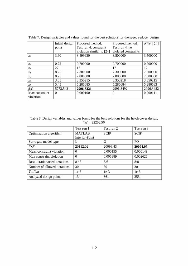
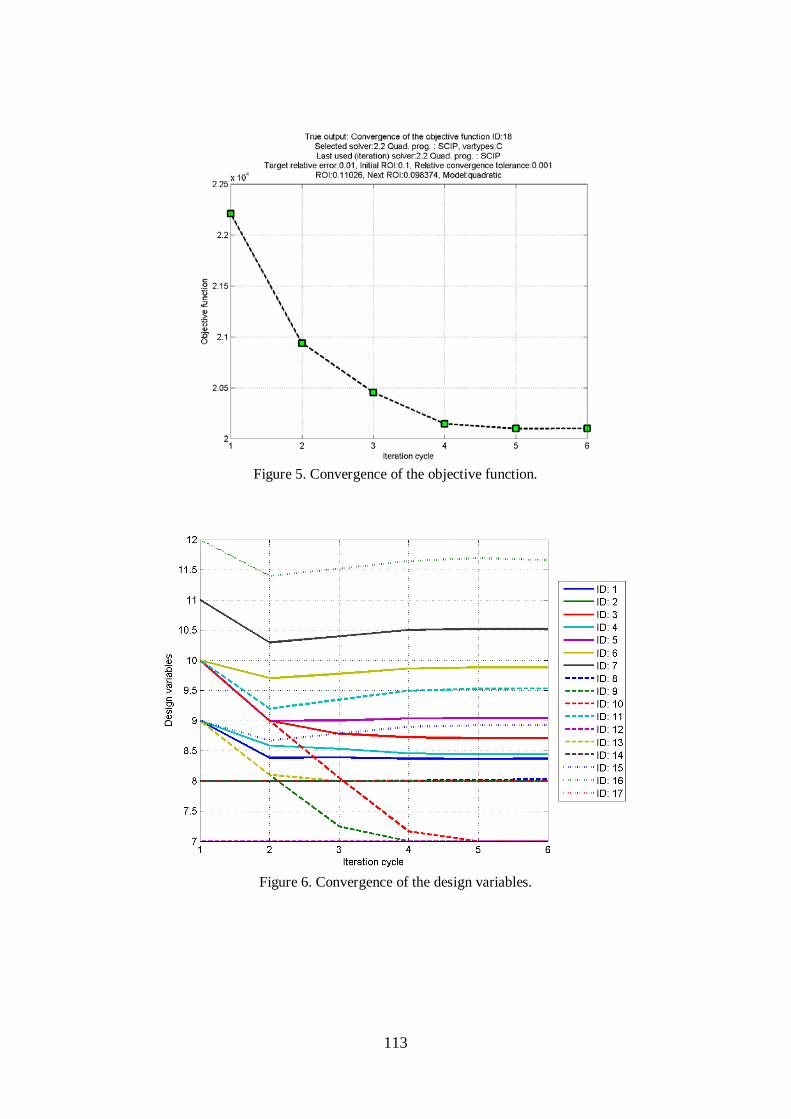
In the task a similar hatch cover as in [4] is designed using the proposed optimization method. The single-objective mass minimization problem contains 17 plate thickness design variables and 37 constraint functions associated with normative rules considering stress and buckling. The design problem is carried out by using both linear, pure quadratic and quadratic surrogate models, and the associated results are highlighted in Table 8 as well as in figures 5 and 6, in which the smooth convergence of objective function and the design variables in the quadratic case are depicted, respectively. For detailed discussion on the problem and the obtained results, see [4].

112

Table 7. Design variables and values found for the best solutions for the speed reducer design.

Initial design point

Proposed method, Test run 4, constraint violation similar to [24]

Proposed method, Test run 4, no violated constraints

APM [24]

x1 3.60 3.499930

3.500000

3.500000

x2 0.72 0.700000 0.700000 0.700000 x3 27 17 17 17 x4 8.25 7.300000 7.300000 7.300000 x5 8.25 7.800000 7.800000 7.800000 x6 3.85 3.350215 3.350218 3.350215 x7 5.45 5.286685 5.286684 5.286683 f(x) 5773.5431 2996.3221 2996.3492 2996.3482 Max constraint violation

0 0.000100 0 0.000111

Table 8. Design variables and values found for the best solutions for the hatch cover design, f(x0) = 22208.56.

Test run 1 Test run 2 Test run 3

Optimization algorithm MATLAB Interior-Point

SCIP SCIP

Surrogate model type L Q PQ f(x*) 20112.02 20098.43 20094.05 Mean constraint violation 0 0.000155 0.000149 Max constraint violation 0 0.005389 0.002626 Best iteration/used iterations 8 / 8 5/6 8/8 Number of allowed iterations 30 30 30 TolFun 1e-3 1e-3 1e-3 Analyzed design points 134 861 253

113

Figure 5. Convergence of the objective function.

Figure 6. Convergence of the design variables.

114

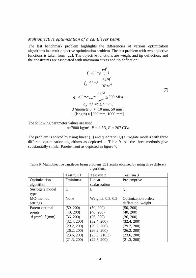
Multiobjective optimization of a cantilever beam

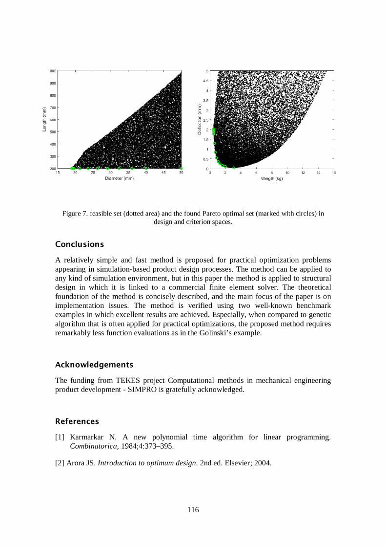
The last benchmark problem highlights the differencies of various optimization algorithms in a multiobjective optimization problem. The test problem with two objective functions is taken from [22]. The objective functions are weight and tip deflection, and the constraints are associated with maximum stress and tip deflection:

f1(d,l)=ρπd2

4l

f2(d,l)=δ=64Pl3

3Eπd4

(7)

g1(d,l)=σmax= 32Plπd3 ≤ 300 MPa

g2(d,l)=δ ≤ 5 mm, d (diameter) ∊ [10 mm, 50 mm], l (length) ∊ [200 mm, 1000 mm].

The following parameter values are used:

ρ=7800 kg/m3, P = 1 kN, E = 207 GPa The problem is solved by using linear (L) and quadratic (Q) surrogate models with three different optimization algorithms as depicted in Table 9. All the three methods give substantially similar Pareto-front as depicted in figure 7.

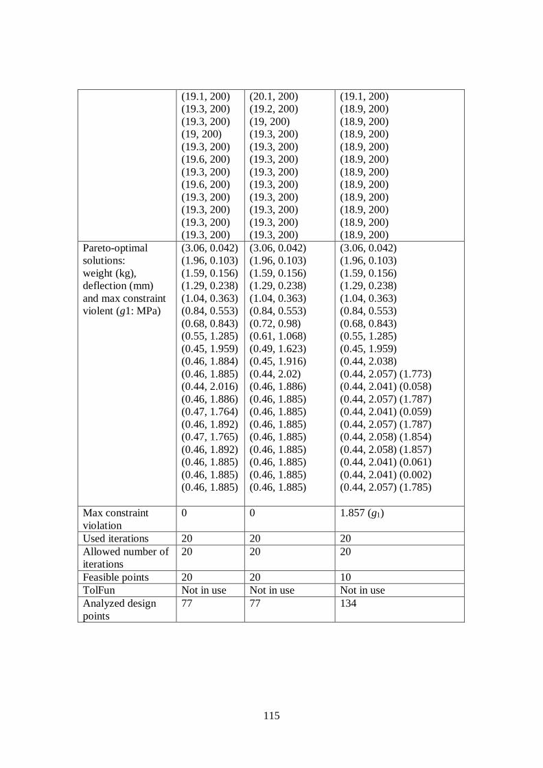
Table 9. Multiobjective cantilever beam problem [22] results obtained by using three different algorithms.

Test run 1 Test run 2 Test run 3 Optimization algorithm

Fminimax Linear scalarization

Pre-emptive

Surrogate model type

L L Q

MO-method settings

None Weights: 0.5, 0.5 Optimization order: deflection, weight

Pareto-optimal points: d (mm), l (mm)

(50, 200) (40, 200) (36, 200) (32.4, 200) (29.2, 200) (26.2, 200) (23.6, 200) (21.3, 200)

(50, 200) (40, 200) (36, 200) (32.4, 200) (29.2, 200) (26.2, 200) (23.6, 210.3) (22.3, 200)

(50, 200) (40, 200) (36, 200) (32.4, 200) (29.2, 200) (26.2, 200) (23.6, 200) (21.3, 200)

115

(19.1, 200) (19.3, 200) (19.3, 200) (19, 200) (19.3, 200) (19.6, 200) (19.3, 200) (19.6, 200) (19.3, 200) (19.3, 200) (19.3, 200) (19.3, 200)

(20.1, 200) (19.2, 200) (19, 200) (19.3, 200) (19.3, 200) (19.3, 200) (19.3, 200) (19.3, 200) (19.3, 200) (19.3, 200) (19.3, 200) (19.3, 200)

(19.1, 200) (18.9, 200) (18.9, 200) (18.9, 200) (18.9, 200) (18.9, 200) (18.9, 200) (18.9, 200) (18.9, 200) (18.9, 200) (18.9, 200) (18.9, 200)

Pareto-optimal solutions: weight (kg), deflection (mm) and max constraint violent (g1: MPa)

(3.06, 0.042) (1.96, 0.103) (1.59, 0.156) (1.29, 0.238) (1.04, 0.363) (0.84, 0.553) (0.68, 0.843) (0.55, 1.285) (0.45, 1.959) (0.46, 1.884) (0.46, 1.885) (0.44, 2.016) (0.46, 1.886) (0.47, 1.764) (0.46, 1.892) (0.47, 1.765) (0.46, 1.892) (0.46, 1.885) (0.46, 1.885) (0.46, 1.885)

(3.06, 0.042) (1.96, 0.103) (1.59, 0.156) (1.29, 0.238) (1.04, 0.363) (0.84, 0.553) (0.72, 0.98) (0.61, 1.068) (0.49, 1.623) (0.45, 1.916) (0.44, 2.02) (0.46, 1.886) (0.46, 1.885) (0.46, 1.885) (0.46, 1.885) (0.46, 1.885) (0.46, 1.885) (0.46, 1.885) (0.46, 1.885) (0.46, 1.885)

(3.06, 0.042) (1.96, 0.103) (1.59, 0.156) (1.29, 0.238) (1.04, 0.363) (0.84, 0.553) (0.68, 0.843) (0.55, 1.285) (0.45, 1.959) (0.44, 2.038) (0.44, 2.057) (1.773) (0.44, 2.041) (0.058) (0.44, 2.057) (1.787) (0.44, 2.041) (0.059) (0.44, 2.057) (1.787) (0.44, 2.058) (1.854) (0.44, 2.058) (1.857) (0.44, 2.041) (0.061) (0.44, 2.041) (0.002) (0.44, 2.057) (1.785)

Max constraint violation

0 0 1.857 (g1)

Used iterations 20 20 20 Allowed number of iterations

20 20 20

Feasible points 20 20 10 TolFun Not in use Not in use Not in use Analyzed design points

77 77 134

116

Figure 7. feasible set (dotted area) and the found Pareto optimal set (marked with circles) in design and criterion spaces.

Conclusions

A relatively simple and fast method is proposed for practical optimization problems appearing in simulation-based product design processes. The method can be applied to any kind of simulation environment, but in this paper the method is applied to structural design in which it is linked to a commercial finite element solver. The theoretical foundation of the method is concisely described, and the main focus of the paper is on implementation issues. The method is verified using two well-known benchmark examples in which excellent results are achieved. Especially, when compared to genetic algorithm that is often applied for practical optimizations, the proposed method requires remarkably less function evaluations as in the Golinski’s example.

Acknowledgements

The funding from TEKES project Computational methods in mechanical engineering product development - SIMPRO is gratefully acknowledged.

References

[1] Karmarkar N. A new polynomial time algorithm for linear programming. Combinatorica, 1984;4:373–395.

[2] Arora JS. Introduction to optimum design. 2nd ed. Elsevier; 2004.

117

[3] Nesterov Y, Nemirovsky A. Interior-point polynomial methods in convex programming, volume 13 of Studies in Applied Mathematics. SIAM: Philadelphia; 1994.

[4] Pajunen S, Heinonen O. Automatic design of marine structures by using successive response surface method. Structural and Multidisciplinary Optimization, 2014;49;863-871. DOI: 10.1007/s00158-013-1013-7

[5] Roux WJ, Stander N, Haftka RT. Response surface approximations for structural optimization. International Journal for Numerical Methods in Engineering, 1998;42:517-534. DOI: 10.1002/(SICI)1097-0207(19980615)42:3<517::AID-NME370>3.0.CO;2-L

[6] Sakata S, Ashida F, Zako M. Structural optimization using Kriging approximation. Computer Methods in Applied Mechanics and Engineering, 2003;192:923-939. doi:10.1016/S0045-7825(02)00617-5

[7] Gupta KC, Li J. Robust design optimization with mathematical programming neural networks. Computers & Structures, 2000;76:507-51. doi:10.1016/S0045-7949(99)00125-X

[8] Acar E, Guler MA, Gerceker B, Cerit ME, Bayram B. Multi-objective crashworthiness optimization of tapered thin-walled tubes with axisymmetric indentations. Thin-Walled Structures, 2011;49:94-105. doi:10.1016/j.tws.2010.08.010

[9] Friedman JH. Multivariate adaptive regression splines. Annals Statistics, 1991;19,:1–141.

[10] Barton RR, Meckesheimer M. Metamodel-based simulation optimization. In: Henderson SG. & Nelson BL (eds.). Handbooks in Operations Research and Management Science, 2006;13:535-570.

[11] Queipo NV, Haftka RT, Shyy W, Goel T, Vaidyanathan R, Tucker PK. Surrogate-based analysis and optimization. Progress in Aerospace Sciences, 2005;41:1-28. http://dx.doi.org/10.1016/j.paerosci.2005.02.001

[12] Barton RR. Simulation optimization using metamodels. In: Rossetti MD, Hill RR, Johansson B, Dunkin A & Ingalls RG (eds.). Proceedings of the 2009 Winter Simulation Conference 2009.

[13] Gary Wang G, Shan S. Review of Metamodeling Techniques in Support of Engineering Design Optimization. J Mech. Des, 2006;129:370-380. doi:10.1115/1.2429697

[14] Gurobi, documentation. 2014. Gurobi 5.6. (http://www.gurobi.com/documentation/)

118

[15] Achterberg T, SCIP: Solving constraint integer programs, Mathematical Programming Computation, 2009;1:1-41. doi:10.1007/s12532-008-0001-1

[16] Techila, documentation. 2014. Techila Fundamentals. (http://www.techilatechnologies.com/technology/technology-docs/)

[17] Myers RH, Montgomery DC, Anderson-Cook CM. Response surface methodology: process and production optimization using designed experiments, John Wiley & Sons;2009.

[18] MSDN. 2014. Microsoft Developer Network. ASP.NET MVC. (https://msdn.microsoft.com/en-us/library/dd381412(v=vs.108).aspx)

[19] Laakkonen P. Development of a computational tool for structural optimization. Master of Science Thesis. Tampere University of Technology. 159 p. 2014.

[20] Arora JS, Huang MW, Hsieh CC. Methods for optimization of nonlinear problems with discrete variables: A review. Structural optimization, 1994;8:69-85.

[21] Miettinen K. Nonlinear Multiobjective Optimization, Kluwer Academic Publishers;1999.

[22] Dep K. Multiobjective optimization using evolutionary algorithms, Wiley;2001.

[23] Hsu Y, Dong Y. Hsu M. A sequential approximation method using neural networks for nonlinear discrete-variable optimization with implicit constraints. JSME International Journal Series C, 2001;44:103-112. http://doi.org/10.1299/jsmec.44.103

[24] Lemonge, AC, Barbosa HJ, Borges CC, Silva FB. Constrained optimization problems in mechanical engineering design using a real-coded steady-state genetic algorithm. Mecánica Computacional, XXIX 2010; 95:9287-9303.

Sami Pajunen Department of Civil Engineering Tampere University of Technology P.O. Box 600 33101 Tampere sami.pajunen@tut.fi

Petri Laakkonen Sorvimo Optimointipalvelut Oy petri.laakkonen@sorvimo.com