HAL Id: hal-02432801https://hal.archives-ouvertes.fr/hal-02432801

Submitted on 8 Jan 2020

HAL is a multi-disciplinary open accessarchive for the deposit and dissemination of sci-entific research documents, whether they are pub-lished or not. The documents may come fromteaching and research institutions in France orabroad, or from public or private research centers.

L’archive ouverte pluridisciplinaire HAL, estdestinée au dépôt et à la diffusion de documentsscientifiques de niveau recherche, publiés ou non,émanant des établissements d’enseignement et derecherche français ou étrangers, des laboratoirespublics ou privés.

Surrogate Model Based on the POD Combined Withthe RBF Interpolation of Nonlinear Magnetostatic FE

ModelT. Henneron, A. Pierquin, S. Clenet

To cite this version:T. Henneron, A. Pierquin, S. Clenet. Surrogate Model Based on the POD Combined With the RBFInterpolation of Nonlinear Magnetostatic FE Model. IEEE Transactions on Magnetics, Institute ofElectrical and Electronics Engineers, 2020, 56 (1), pp.1-4. �hal-02432801�

1

Surrogate Model based on the POD combined with the RBFInterpolation of Nonlinear Magnetostatic FE model

T. Henneron1, A. Pierquin1 and S. Clenet11Univ. Lille, Centrale Lille, Arts et Metiers ParisTech, HEI, EA 2697 - L2EP, F-59000 Lille, France

The Proper Orthogonal Decomposition (POD) is an interesting approach to compress into a reduced basis numerous solutionsobtained from a parametrized Finite Element (FE) model. In order to obtain a fast approximation of a FE solution, the POD canbe combined with an interpolation method based on Radial Basis Functions (RBF) to interpolate the coordinates of the solutioninto the reduced basis. In this paper, this POD-RBF approach is applied to a nonlinear magnetostatic problem and is used with asingle phase transformer and a three-phase inductance.

Index Terms—Nonlinear magnetostatic problem, Model Order Reduction, Proper Orthogonal Decomposition, Radial BasisFunctions.

I. INTRODUCTION

THE FE method is commonly used to study low frequencyelectromagnetic devices. This approach gives accurate

results but requires large computational times due to numericalor physical features such as a high number of Degrees ofFreedom (DoF) in space and also a high number of timesteps or the nonlinear behavior of ferromagnetic materials forexample. In order to reduce the computational time especiallyfor parametrized model, model order reduction methods havebeen proposed in the litterature. One of the most popularapproach is the POD approach. Based on the solutions of theFE model for different values of parameters (called snapshots),the POD enables to approximate the solution of the FEmodel in a reduced basis [1]. Then, the initial FE systemis projected onto a reduced basis, decreasing the order ofthe numerical model to be solved for new parameter values.Another approach consists in constructing a metamodel tointerpolate directly the solution expressed into a reduced basisfor new parameter values. Different approaches can be used,as for example, based on an optimization process [2] orpolynomial functions [3]. The RBF interpolation method canbe also applied in this context. In the litterature, the POD-RBF approach has been developed for mechanical or thermalproblems [4][5] for example.In this paper, we propose to use a POD-RBF approach inorder to build a fast model of the solution of a nonlinearmagnetostatic problem. First, the numerical model of nonlinearmagnetostatic problem is brieflty presented. Secondly, thePOD-RBF approach is developed. Finally, a single phase EItransformer and a three-phase inductance are studied.

II. NONLINEAR MAGNETOSTATIC PROBLEM

Let’s consider a domain composed with Nst stranded induc-tors, each supplied by a current ij and a nonlinear magneticsubdomain. To solve the nonlinear magnetostatic problem,the vector potential formulation is used. Then, the strongformulation is

curl(ν(B)curlA) =

Nst∑j=1

Njij (1)

with ν the magnetic reluctivity depending on the magneticflux density B, A the vector potential defined by B = curlAand Nj the unit current density of the jth stranded inductor.By applying the FE method, the equation system to solve forij ∈ Ij is

M(X)X =

Nst∑j=1

Fjij (2)

with M(X) the curl-curl matrix, Fj the source vector as-sociated with the jth inductor and X ∈ RNx the vectorof components of A. For 3D problems, the potential A isdiscretized on the edge elements. For each inductor j, themagnetic linkage flux can be expressed by Φj = FtjX.

III. SURROGATE MODEL BASED ON POD COMBINED WITHRBF INTERPOLATION

From a set of solutions obtained from the evaluation ofthe FE model (2), called snapshots, for different values ofcurrent, a surrogate model is build in order to approximate thesolution for any current values. Then, the Proper OrthogonalDecomposition method is combined with the Radial BasisFunction interpolation approach. In the following, two induc-tors are considered to present the approach and the parameterset (i1, i2) is denoted by i = (i1, i2). Then, we seek for anapproximation Xap(i) of X(i) under the form

Xap(i) =

M∑l=1

ψlgl(i) (3)

with ψl ∈ RNx components of the reduced basis, so calledmodes, gl(i) a scalar function and M the size of the reducedbasis, so called number of modes.

A. Reduction of the dimension by POD

From P snapshots Xj = X(ij), j = 1, ..., P , computedfor different values of i, the vectors ψl, l = 1, ...,M , arededuced. The snapshots matrix is defined such as MX =[X1,X2, ...,XP ]. The Singular Value Decomposition (SVD)is applied to MX , such as MX = USVt with UNx×Nx

2

and VP×P orthogonal matrices and SNx×P the rectangulardiagonal matrix of the singular values ranked in a decreasingorder. This decomposition allows to obtain a reduced basisΨ = [ψl, ψ2, ..., ψM ] of size Nx ×M which corresponds tothe M first columns of U. The truncation of the first columnscan be determined by taking the M most significative singularvalues of S. Then, the solution vector X can be approximatedby Xpod under the form

X ≈ Xpod = ΨG (4)

with G the vector of components of the solution into thereduced basis.

B. RBF interpolation approach

The RBF interpolation approach is used for the determina-tion of scalar functions gl(i) for l = 1, ...,M . From the SVDof MX , we can deduce the matrix expressed in the reduced ba-sis such as MG = [G1,G2, ...,GP ] = S(1:M,1:M)V

t(1:P,1:M).

Then, each line of MG corresponds to the discrete values ofgl(ij) = Gjl for j = 1, ..., P . In fact, gl(ij) represents the lth

coordinate of the approximation of Xj in the reduced basis.From these values, the RBF interpolation is performed in orderto determine each function gl(i) under the following form

gl(i) =

P∑j=1

αljφj(i) (5)

with φj = φ(||i − ij ||) a radial function depending on theEuclidian distance between i and ij and αlj its associatedcoefficient. The coefficients αlj are calculated to interpolatethe P vectors Gk

Gkl = gl(ik) =

P∑j=1

αljφk(||ik − ij ||) (6)

for k = 1, .., P.

Then, we can define an equation system for the computationof the coefficients αlj , j = 1, ..., P , such as

Yl = BAl (7)with Yl = [G1l, ..., GPl]

t,Al = [αl1, ..., αlP ]t

and B =

φ1(i1) · · · φ1(iP )...

. . ....

φP (i1) · · · φP (iP )

.The number of equation system (7) to solve depends on thenumber of modes M (i.e. the size of the reduced basis).The error of interpolation depends on the choice for theradial function. Table I presents different examples of functionwhere a is a parameter fixed by the user, called ”shapeparameter”. Finally, for any coordinate inew, we can computean approximation Xap(inew) of the FE solution by (3).

C. Greedy algorithm

In order to optimize the size of the reduced basis Ψ andthe number of snapshots used for the interpolation, a greedyalgorithm can be applied. In this case, Q snapshots of the FE

TABLE IEXAMPLES OF RBF FUNCTION

Name φ(x)

Gaussian (G) e−(x/a)2

Multiquadric (MQ)√

1 + (x/a)2

Inverse multiquadric (IMQ)√

11+(x/a)2

Thin plate spline x2log(x)

model (2) are computed, the aim of the greedy algorithm is toselect the most significant P vectors X among the Q snapshotsto build the POD-RBF model in order to reduce the memoryrequirements, i.e. the number of coefficents αlj and the sizeof the reduced basis. We denote pk a coordinate among ij forj = 1, ..., Q, the vector of coordinates selected by the greedyalgorithm is p = [p1, ...,pP ] and εf is a criterion fixed by theuser to stop the iterative algorithm.

Algorithm 1 Greedy algorithmInput: MX = [X(i1),X(i2), ...,X(iQ)], p1

Output: M , P , Ψ and αlj- P = 0while εX > εf do

- P = P + 1if P > 1 then

- select the coordinate corresponding to the maximumof the error such as pP = argmax(e)

end if- p← [p,pP ]- MS ← [MS ,X(pP )]- from MS , update Ψ and the coefficients αlj- compute the vector e of the norm of relative errors suchas e = [ek]Qk=1 with ek =

||X(ik)−Xap(ik)||2||X(ik)||2

- compute the average of the errors εX = 1Q

∑Qk=1 ek.

end while

The average error of the magnetic linkage flux for the jth

inductor can be also defined such as

εΦj=

1

Q

Q∑k=1

eΦj,kwith eΦj,k

=|Φj(ik)− Φap,j(ik)|

|Φ(ik)|. (8)

IV. APPLICATION

Two examples of application are studied. The first one is asingle phase transformer and the second one is a three-phaseinductance.

A. Single phase transformer

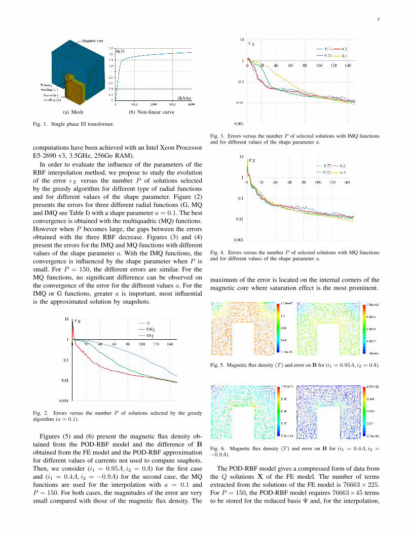
Due to the symmetries, only one eighth of the single phaseEI transformer is modeled. Figure (1) presents the mesh ofthe magnetic core and of the windings (a) and the nonlinearB(H) magnetic curve (b). The 3D mesh is composed of 67177tetrahedron elements, the number of DoF is Nx = 76663. TheFE model (2) is solved Q = 225 times with 15 equidistributedvalues Ni1 for i1 ∈ [0 : 1]A and Ni2 for i2 ∈ [−2 : 0]A.In these conditions, the computational time is 135min (all

3

(a) Mesh (b) Non-linear curve

Fig. 1. Single phase EI transformer.

computations have been achieved with an Intel Xeon ProcessorE5-2690 v3, 3.5GHz, 256Go RAM).

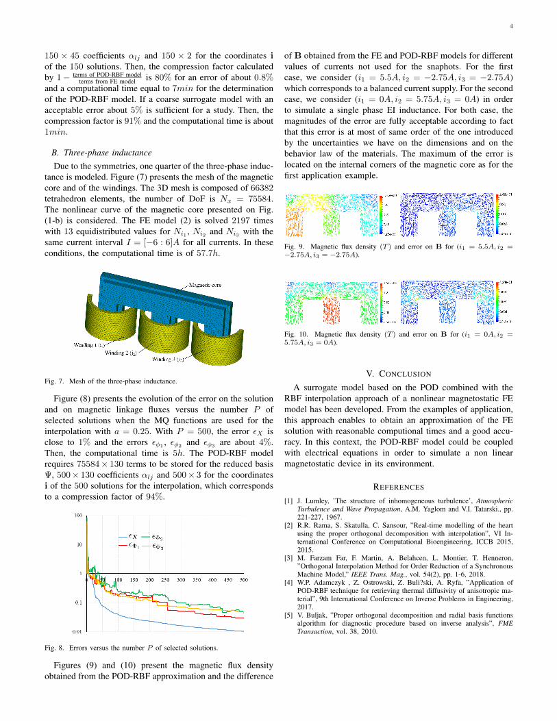
In order to evaluate the influence of the parameters of theRBF interpolation method, we propose to study the evolutionof the error εX versus the number P of solutions selectedby the greedy algorithm for different type of radial functionsand for different values of the shape parameter. Figure (2)presents the errors for three different radial functions (G, MQand IMQ see Table I) with a shape parameter a = 0.1. The bestconvergence is obtained with the multiquadric (MQ) functions.However when P becomes large, the gaps between the errorsobtained with the three RBF decrease. Figures (3) and (4)present the errors for the IMQ and MQ functions with differentvalues of the shape parameter a. With the IMQ functions, theconvergence is influenced by the shape parameter when P issmall. For P = 150, the different errors are similar. For theMQ functions, no significant difference can be observed onthe convergence of the error for the different values a. For theIMQ or G functions, greater a is important, most influentialis the approximated solution by snapshots.

Fig. 2. Errors versus the number P of solutions selected by the greedyalgorithm (a = 0.1).

Figures (5) and (6) present the magnetic flux density ob-tained from the POD-RBF model and the difference of Bobtained from the FE model and the POD-RBF approximationfor different values of currents not used to compute snaphots.Then, we consider (i1 = 0.95A, i2 = 0A) for the first caseand (i1 = 0.4A, i2 = −0.9A) for the second case, the MQfunctions are used for the interpolation with a = 0.1 andP = 150. For both cases, the magnitudes of the error are verysmall compared with those of the magnetic flux density. The

Fig. 3. Errors versus the number P of selected solutions with IMQ functionsand for different values of the shape parameter a.

Fig. 4. Errors versus the number P of selected solutions with MQ functionsand for different values of the shape parameter a.

maximum of the error is located on the internal corners of themagnetic core where saturation effect is the most prominent.

Fig. 5. Magnetic flux density (T ) and error on B for (i1 = 0.95A, i2 = 0A).

Fig. 6. Magnetic flux density (T ) and error on B for (i1 = 0.4A, i2 =−0.9A).

The POD-RBF model gives a compressed form of data fromthe Q solutions X of the FE model. The number of termsextracted from the solutions of the FE model is 76663× 225.For P = 150, the POD-RBF model requires 76663×45 termsto be stored for the reduced basis Ψ and, for the interpolation,

4

150 × 45 coefficients αlj and 150 × 2 for the coordinates iof the 150 solutions. Then, the compression factor calculatedby 1− terms of POD-RBF model

terms from FE model is 80% for an error of about 0.8%and a computational time equal to 7min for the determinationof the POD-RBF model. If a coarse surrogate model with anacceptable error about 5% is sufficient for a study. Then, thecompression factor is 91% and the computational time is about1min.

B. Three-phase inductanceDue to the symmetries, one quarter of the three-phase induc-

tance is modeled. Figure (7) presents the mesh of the magneticcore and of the windings. The 3D mesh is composed of 66382tetrahedron elements, the number of DoF is Nx = 75584.The nonlinear curve of the magnetic core presented on Fig.(1-b) is considered. The FE model (2) is solved 2197 timeswith 13 equidistributed values for Ni1 , Ni2 and Ni3 with thesame current interval I = [−6 : 6]A for all currents. In theseconditions, the computational time is of 57.7h.

Fig. 7. Mesh of the three-phase inductance.

Figure (8) presents the evolution of the error on the solutionand on magnetic linkage fluxes versus the number P ofselected solutions when the MQ functions are used for theinterpolation with a = 0.25. With P = 500, the error εX isclose to 1% and the errors εφ1

, εφ2and εφ3

are about 4%.Then, the computational time is 5h. The POD-RBF modelrequires 75584× 130 terms to be stored for the reduced basisΨ, 500× 130 coefficients αlj and 500× 3 for the coordinatesi of the 500 solutions for the interpolation, which correspondsto a compression factor of 94%.

Fig. 8. Errors versus the number P of selected solutions.

Figures (9) and (10) present the magnetic flux densityobtained from the POD-RBF approximation and the difference

of B obtained from the FE and POD-RBF models for differentvalues of currents not used for the snaphots. For the firstcase, we consider (i1 = 5.5A, i2 = −2.75A, i3 = −2.75A)which corresponds to a balanced current supply. For the secondcase, we consider (i1 = 0A, i2 = 5.75A, i3 = 0A) in orderto simulate a single phase EI inductance. For both case, themagnitudes of the error are fully acceptable according to factthat this error is at most of same order of the one introducedby the uncertainties we have on the dimensions and on thebehavior law of the materials. The maximum of the error islocated on the internal corners of the magnetic core as for thefirst application example.

Fig. 9. Magnetic flux density (T ) and error on B for (i1 = 5.5A, i2 =−2.75A, i3 = −2.75A).

Fig. 10. Magnetic flux density (T ) and error on B for (i1 = 0A, i2 =5.75A, i3 = 0A).

V. CONCLUSION

A surrogate model based on the POD combined with theRBF interpolation approach of a nonlinear magnetostatic FEmodel has been developed. From the examples of application,this approach enables to obtain an approximation of the FEsolution with reasonable computional times and a good accu-racy. In this context, the POD-RBF model could be coupledwith electrical equations in order to simulate a non linearmagnetostatic device in its environment.

REFERENCES

[1] J. Lumley, ’The structure of inhomogeneous turbulence’, AtmosphericTurbulence and Wave Propagation, A.M. Yaglom and V.I. Tatarski., pp.221-227, 1967.

[2] R.R. Rama, S. Skatulla, C. Sansour, ”Real-time modelling of the heartusing the proper orthogonal decomposition with interpolation”, VI In-ternational Conference on Computational Bioengineering, ICCB 2015,2015.

[3] M. Farzam Far, F. Martin, A. Belahcen, L. Montier, T. Henneron,”Orthogonal Interpolation Method for Order Reduction of a SynchronousMachine Model,” IEEE Trans. Mag., vol. 54(2), pp. 1-6, 2018.

[4] W.P. Adamczyk , Z. Ostrowski, Z. Buli?ski, A. Ryfa, ”Application ofPOD-RBF technique for retrieving thermal diffusivity of anisotropic ma-terial”, 9th International Conference on Inverse Problems in Engineering,2017.

[5] V. Buljak, ”Proper orthogonal decomposition and radial basis functionsalgorithm for diagnostic procedure based on inverse analysis”, FMETransaction, vol. 38, 2010.