1

Annual Status Report

FY2017 (Oct 1 2016–September 30 2017)

Sustainability of Hydraulic Fracture Conductivity

in Ductile and Expanding Shales

FWP ESD 14084

Principal Investigator: Seiji Nakagawa, (510) 486-7894, snakagawa@lbl.gov

Lawrence Berkeley National Laboratory

Submitted to: U.S. Department of Energy

National Energy Technology Laboratory DOE Project Manager: Stephen Henry

Phone: (304) 285-2083 Email Stephen.Henry@netl.doe.gov

2

1. Project Description

Hydraulic fracturing is an indispensable tool for enhancing permeability of otherwise very impermeable shales containing oil and gas. However, clay-rich, ductile shales are difficult to fracture, and the hydraulic fractures created in the rock tend to be short and have a smaller surface area. Proppant placed in these fractures tends to be embedded in the soft fracture walls, and the open space created by the fracture can be filled by mobilized clay minerals and by the expanded fracture walls if swelling clays (e.g., smectites, mixed-layer illites) are present in the rock. The primary goals of this research project are to investigate and understand (1) how hydraulic fractures produced in ductile shale behave over time to reduce in aperture and permeability, (2) how the proppant deposition characteristics (e.g., monolayer vs multilayer), grain size, and spatial distribution (isolated patches vs. connected strings and networks) affect the sustainability of the fracture conductivity impacted by fracture aperture reduction resulting from rock deformation and clay mobilization, and (3) how the near-fracture shale-matrix fluid transport is affected by the evolving conductivity of the fracture. To meet these objectives, we conduct core-scale laboratory experiments under controlled temperature and stress, using several available natural shale samples with different ductility and clay compositions. These experiments include baseline shale property characterization, micro-indentation tests, and optical and/or X-ray CT visualization of shale fracture compaction, with and without proppants. Concurrently, numerical modeling of the shale deformation and fluid transport will be performed, and prediction accuracy checked against the laboratory experiments. The modeling will employ either a discrete modeling method (TOUGH-RBSN) or a continuum modeling method (TOUGH-FLAC), depending upon the laboratory experiment being modeled and the involved physical processes.

2. Project status overview

This report summarizes our project activities and accomplishments for the first year of the current project (October 2016–September 2017). More details of the technical development and the results of the tasks can be found in corresponding task sections in the previously submitted Quarterly Reports. Similar to our preceding project on the study of hydraulic fracture creation/propagation, the current project consists of two primary components: 1. laboratory investigation of shale matrix and fracture deformation under sustained load and 2. its numerical modeling. In this report, the progress and findings from the tasks conducted under the project are briefly summarized (Task 2, laboratory experiments, and Task 3, numerical modeling).

3

Task 2.0 Laboratory Experiments

In FY2017, the laboratory experiment team focused on the development of experimental tools and sample preparation for core-scale shale fracture compaction experiments scheduled in FY2018. The key activities (subtasks) performed in the current FY are as follows:

Subtask 2.1—Designing and fabrication of shale fracture test cell

For the core-scale fracture compaction experiments in FY2018, a unique laboratory tool—uniaxial fracture compaction visualization cell—was designed and fabricated. The cell was designed so that the closure of a shale fracture can be visualized both optically through a view window and via X-ray CT through aluminum vessel walls (Figure 2-1). In Q1, initial design of the vessel was conducted in collaboration with an engineer with a pressure vessel manufacturer (Vindum Engineering, Inc., San Ramon, CA). In Q2, the design was finalized with feedback from LBNL safety department (Milestone M1). The designed pressure rating (Maximum Allowable Working Pressure) for this vessel was originally 4,500 psi based upon a standard ultimate strength of the vessel material (T6061 Aluminum alloy). However, later, this rating was upward corrected to 5,220 psi, based upon the actual strength of the material used. The fabrication of the vessel was completed at the end of Q3 (Figure 2-2), and shortly after it was pressure tested (Supplementary Q3 report) (Milestone M3)

Figure 2-1 Shale-fracture compaction visualization cell design

4

Figure 2-1 Shale-fracture compaction visualization cell design (continued)

Figure 2-2 Completed shale fracture compaction visualization cell

The pressure vessel consists of two pressure chambers separated by a piston. The upper chamber holds a shale core with an exposed fracture surface which is pressed against a transparent replica of the other half of the fracture. The flat top of the replica is pressed against an optical window (sapphire) so that the time-dependent changes in the fracture aperture distribution (with and without proppant) can be observed. The lower chamber contains hydraulic fluid which applies compaction pressure to the shale core/fracture through the piston. The displacement of the piston (and the compaction of the fracture/sample) can be monitored via an linear variable differential

5

transformer (LVDT) connected between the tube attached to the piston and the vessel base. The tube is also used to inject pore fluid into the sample from the bottom center of the shale core.

The optical visualization of a shale fracture under high confining stresses requires a large sapphire window attached to the vessel. The vessel uses a 2.00-inch diameter, 1.00-inch thick window (produced by Guild Optical Associates). During the experiment the top half of the fracture is designed to be replaced by a transparent glass plate or a fracture replica made of glass plate and optical grade epoxy resin, and the stress applied to the fracture surface will be supported by the window. The vessel also includes internal illumination consisting of an electroluminescent wire installed at the top of the sapphire window.

In Q4, we conducted a mock-up test to confirm the newly fabricated test cell’s optical and X-ray computed tomography (CT) visualization capability for rock/fracture samples undergoing compaction. A cylindrical, 2-inch-diameter Stripa Granite core was split across the core axis to produce a through-going tensile fracture. One half of this core was used to produce an optically transparent replica of the fracture using low-viscosity (visocosity~200 cP), optically transparent epoxy, with a slight mismatch with the fracture surface of the other half (Figure 2-3). Subsequently, the pair (the rock and epoxy replica samples) was introduced into the compaction visualization cell, and small axial stress was applied via an internal piston.

Optical visualization of the fracture surface was conducted through the one inch thick sapphire window. The fracture surface was illuminated by the ring-shaped, internal, electroluminescent wire which applied even light on the surface. Subsequently, the test cell containing the sample was scanned using a medical X-ray CT machine to verify the visibility of the sample through the 1 inch thick aluminum cell wall. This test clearly showed that the CT scans can image the density differences within the rock (quartz/feldspar and biotite mica), epoxy-rock boundaries, and thin (a few hundred microns thick) gap (or, a fracture) at the boundaries (Figure 2-4).

Figure 2-3 Optical visibility check for a rock fracture within a compaction visualization cell.

6

Figure 2-4 X-ray CT visibility check for a rock fracture within the compaction visualization cell.

Subtask 2.2—Test sample acquisition and preparation

In Q3, 2-inch diameter cores and small chips for five types of outcrop shale were obtained (Mancos, Marcellus, Eagle Ford, Barnett, and Niobrara). From the chip samples, small diameter cores (diameter~0.56 inches) were produced for mini indentation experiments in Subtask 2.3 and for synchrotron micro X-ray CT imaging experiments conducted by a collaborating project team [Reagan (LBNL)/Moridis (Texas A&M) project]. Because the diameter of the provided 2-inch core samples are not adequate (slightly too large) for our pressure vessel, they have to be trimmed down carefully without damaging the samples. Currently this is done using a lathe rather than a coring machine and no water or oil is used in the process.

Figure 2-5 Five types of shale samples (From the left, Barnett, Niobrara, Eagle Ford, Marcellus, and Mancos shales) used in our current experiments.

7

Subtask 2.3—Shale property characterization and ductility measurements

In this subtask, the main activity was to develop a mechanical testing system for quantitative characterization of ductile shale behavior using micro-indentation test. In Q1-Q2, an existing experimental system for micro-indentation tests was modified for the current project. This modification/improvement involved replacing a force sensor in the existing setup and adding a high-resolution capacitive sensor. Additionally, a system-controlling software was re-written in LabVIEW to accommodate the hardware changes (Figure 2-6).

a. Indentation test system b. (A part of) LabView code front panel

Figure 2-6 Modified/improved instrumented micro-indentation test system

a. Indentation load-displacement curves b. The initial part of a.

Figure 2-7 A trial test on a small (~0.55” diameter) Opalinus clay core. Compared to the capacitive sensor measurement, encoder readings from the piezo drive which moves the indenter show excess deflections of the system for high load (a). The test system is capable of measuring small loads and displacements, less than 1gf and 1 µm.

8

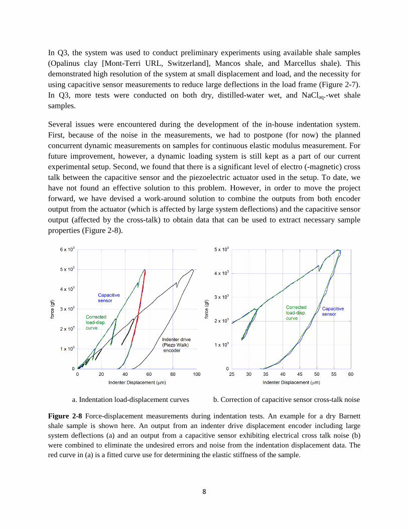
In Q3, the system was used to conduct preliminary experiments using available shale samples (Opalinus clay [Mont-Terri URL, Switzerland], Mancos shale, and Marcellus shale). This demonstrated high resolution of the system at small displacement and load, and the necessity for using capacitive sensor measurements to reduce large deflections in the load frame (Figure 2-7). In Q3, more tests were conducted on both dry, distilled-water wet, and NaClaq.-wet shale samples.

Several issues were encountered during the development of the in-house indentation system. First, because of the noise in the measurements, we had to postpone (for now) the planned concurrent dynamic measurements on samples for continuous elastic modulus measurement. For future improvement, however, a dynamic loading system is still kept as a part of our current experimental setup. Second, we found that there is a significant level of electro (-magnetic) cross talk between the capacitive sensor and the piezoelectric actuator used in the setup. To date, we have not found an effective solution to this problem. However, in order to move the project forward, we have devised a work-around solution to combine the outputs from both encoder output from the actuator (which is affected by large system deflections) and the capacitive sensor output (affected by the cross-talk) to obtain data that can be used to extract necessary sample properties (Figure 2-8).

a. Indentation load-displacement curves b. Correction of capacitive sensor cross-talk noise

Figure 2-8 Force-displacement measurements during indentation tests. An example for a dry Barnett shale sample is shown here. An output from an indenter drive displacement encoder including large system deflections (a) and an output from a capacitive sensor exhibiting electrical cross talk noise (b) were combined to eliminate the undesired errors and noise from the indentation displacement data. The red curve in (a) is a fitted curve use for determining the elastic stiffness of the sample.

9

Using this technique, in Q4, we conducted micro-indentation experiments on the five types of shale samples collected in Subtask 2.2, along with other characterization experiments (Milestone M4). These include material density and ultrasonic seismic velocity and transversely isotropic elastic moduli determination, mineralogical characterization using X-ray diffraction, and permeability measurement. Because of the time involved in the measurements, the permeability measurements are still in progress, and will continue as experiments in FY2018 are conducted. The results of the X-ray diffraction experiments indicated that the obtained samples had a good spread over the carbonate content, but the clay content was rather limited (Figure 2-9). Among the five samples, only Barnett shale showed a high clay content (over 50%) followed by Mancos shale (~20%), and none of the shales contained a significant amount swelling clays.

The determined Young’s modulus, hardness, and ductility index (a ratio between permanent work vs. maximum work [stored elastic energy + permanent work at the maximum load/displacement]) are shown in Figure 2-10. The samples are tested both in dry (oven dried at 60°C for 1 week) and in wet (exposed to 100% relative humidity air for 10 days at room temperature) conditions. (Note that during the test itself, the same samples were covered by odorless mineral spirits (Sigma Aldrich, CAS68551-17-7) to avoid evaporation loss of the water.) Clay-rich Barnett shale clearly exhibited large ductility and small elastic modulus and hardness compared to other shales, with high water sensitivity of these properties. Although the mineral composition was similar for Marcellus and Niobrara Shales, elastic modulus and hardness were water sensitive for Marcellus Shale while the Niobrara Shale was not. Mancos Shale seemed to exhibit rather large scattering among the measurements, possibly due to the strongly heterogeneous texture (layering). Correlations between the clay content and the viscoelastic (time-dependent) indentation behavior were also observed (Figure 2-11). A short-duration (30 min) indentation tests revealed creep behavior in both dry and wet samples, with the clay-rich Barnett shale exhibiting very large creep even under much smaller (1/5) of the load applied to other samples, and the clay-poor, carbonate-rich Marcellus and Niobrara shales exhibiting the smallest creep deformations.

Figure 2-9 Mineral composition analysis via XRD

10

a. Reduced Young’s modulus (sample only) b. Hardness

c. Ductility index

Figure 2-10. Reduced Young modulus (a), hardness (b), and ductility index (c) for five types of shale samples. The labels indicate: BN=Barnett shale, NB=Niobrara shale, EF=Eagle Ford shale, MR=Marcellus shale, and MN=Mancos shale. For comparison, results for aluminum (AL) and optically transparent epoxy (EP) are also shown.

One observation made during the indentation experiment is that once wet, the clay-rich Barnet Shale samples fractured easily under a single-point indenter (a ball indenter with a 1/32” diameter) (Figure 2-12). Because the maximum load on the indenter (up to 5,000 gf) was selected by considering the effective stress on a reservoir shale fracture distributed evenly among similarly sized proppant grains, we suspect that fracturing of the shale core may occur if the side wall of the core samples used in the compaction visualization experiments in FY2018 is not properly supported (as was the case for the indentation test samples). This suggests that we may need some modifications to our experimental setup.

11

a. Wet samples b. Room dry samples

Figure 2-11 30-minute Creep tests for viscoelastic property assessment. Note that the tests on Barnet shale samples were conducted at 1,000 gf while other samples at 5,000 gf.

(a) Indentation test samples (b) Fracturing occurred to wet Barnett shale sample during the test

Figure 2-12 Micro-indentation experiments on shale subcores

12

In conclusion, we have reached all the planned experimental milestones (M1, 3, 4) for FY2017. Lessons learned from the completed tasks and possible actions that will be taken in FY2018 experiments are as follows:

1. Clay-rich Barnett shale is best for investigating the impact of fracture deformation and proppant embedment on fracture permeability loss, followed by Mancos and Eagle Ford shales. Niobrara and Marcellus shales appear to be the least clay-rich and ductile samples, although indentation tests indicated the latter exhibit some water sensitivity in the hardness and Young’s modulus (but not in the viscoelastic behavior).

2. Marcellus and Niobrara shales appear to be least sensitive to water and exhibit smaller ductility. However, their sensitivity to water manifests itself in different manners (reduction in the hardness for Marcellus, and time-dependent deformations for Niobrara).

3. As observed for Barnett shale samples, indentation of asperities and proppant grains can potentially lead to splitting of shale cores along the bedding planes. This may require modifications of the experimental setup for the fracture-compaction tests. Currently, adding a thin aluminum wall to the exterior of the core is considered, to prevent tensile fracturing of the sample during the tests.

4. The epoxy used in a transparent fracture replica for optical visualization tests may be too soft, and its large viscoelastic deformations may mask the deformation of the shale itself. For this reason, we may need to replace the replica by a flat, glass plate (or quartz glass plate), and the shale fracture surface by artificially roughened surface. Although the geometry of the fracture may not look realistic, this actually will lead to better experiments and results. This is because such samples allow us to compare the behavior of the fractures in different types of shale without impacted by the macro-scale differences in the fracture geometry.

13

Task 3.0 Numerical Modeling

In FY2017, the numerical modelling team focused on the development of the models for examining proppant embedment at different scales (from the grain-scale to the block-scale). These models are tailored to capture coupled hydrological and mechanical responses of proppant-filled fractures in shale, based on previous laboratory and field studies reported in the literature. They will be refined further based on new laboratory results obtained in this project. Two codes—TOUGH-FLAC and TOUGH-RBSN—are used to solve similar but complementary problems of proppant deformation/crushing in strong, brittle shale and of rock matrix deformation/proppant embedment in ductile shale, and the related coupled multi-phase fluid flow problem. The key development and testing of these models were completed in FY2017 Q3 (Subtask 3.1, 3.2, Milestone M2). Using the developed models, in Q4, we conducted numerical simulations of laboratory indentation experiments (Subtask 3.3, Milestone M5).

Subtask 3.1— Develop grain-scale modeling approaches This subtask involves adaptation and testing of TOUGH-FLAC and TOUGH-RBSN for grain-scale modeling. We envision two types of mechanical responses depending on the clay content of shale. For a shale with high clay content, we expect ductile behavior with elasto-plastic yielding and (poro-)viscoelastic flow, whereas for a shale with low clay content, we may see more brittle mechanical response resulting in discrete fracture propagation and proppant crushing. We are using TOUGH-FLAC for simulating the ductile shale behavior with continuum elasto-plastic or visco-elastic (creep) constitutive models. In contrast, the use of TOUGH-RBSN, with which we have less experience for applying to the grain-rock matrix interaction problems, is explored for modeling the brittle behavior of a proppant-fracture system, including discrete fracturing and grain crushing.

Grain-Scale modeling with TOUGH-FLAC (Subtask 3.1a)

The grain-scale modeling with TOUGH-FLAC has been developed and tested in Q1 and Q2 of FY2017 using solid elements for shale and proppants and special interfaces for interaction between shale and proppants. We have successfully demonstrated and tested:

• Progressive proppant embedment with increasing contact between the shale and proppant. This involves contact detection in 3D as well as large strain modeling with continuous updating of the geometric configuration.

• Proppant embedment behavior using elastic and elasto-plastic (Mohr-Coulomb) constitutive models. Permanent deformations (indentation craters) resulted upon removal of the applied load at the end of the simulation.

• Swelling expansion of the shale matrix when exposed to a change in pressure or changes in saturation. The swelling resulted in significant fracture aperture changes.

14

• Creep closure of fractures over several years with progressive proppant embedment. A visco-elastic constitutive model and creep parameters from available laboratory data were used.

Figure 3-1 and 3-2 show an example of 3D simulation performed to test and demonstrate the capability of the code to model embedment of multiple proppants. The model domain was a 4 mm × 4 mm section of a fracture with a shale matrix. Four grains of proppant of different sizes were placed on the surface, which were fixed in space. Figure 3-1 shows how each proppant of different sizes were embedded into the shale sample after the matrix block was displaced downward by 0.3 mm. Figure 3-2 presents the resulting surface imprint after unloading when the upper rock sample was moved back to its original position. Maximum embedment depth is 0.28 mm, which is reasonable considering that the maximum vertical compression on the top of the rock sample was 0.3 mm. The calculated imprints of the type shown in Figure 3-2 could be compared to observed surface imprints from laboratory experiments.

Figure 3-3 and 3-4 show examples of creep-closure simulation over a 3-year period. We used elastic and creep properties from laboratory experiments on Haynseville shale. In Figure 3-3, initially an instantaneous closure due to elastic embedment is seen. Subsequently, time-dependent embedment due to creep takes place during over the 3-year simulation time. At the end, we can observe that the fracture closure by creep is dominant over the initial elastic embedment (Note that although plastic deformation is not modeled in the current simulation, it can be included in the future modeling). In Figure 3-4, the resulting deformations of the fracture and embedment of proppants are presented for simulation periods of 3 months and 3 years. These results demonstrate the simulation capabilities of the adopted grain-scale modeling approach for modeling long-term closure behavior of propped fractures in shale.

The grain-scale modeling with TOUGH-FLAC has thereby been developed and tested and the next step in FY2018 would be to conduct interpretative modeling of the actual laboratory experiments.

15

Figure 3-1 3D simulation of vertical compression of soft rock on multiple proppants of various sizes (diameters ranging from 0.7 to 1 mm). The contours show vertical stress distribution with blue areas indicating high compressive stress and red areas low compressive stress.

Figure 3-2 Plane view of the rock surface with contours of embedment depth.

16

Figure 3-3 TOUGH-FLAC simulation results of closure of fracture by elastic and creep behavior using creep properties for Haynseville shale.

Figure 3-4 TOUGH-FLAC simulation results of closure of fracture after 3 months (about 0.13 mm closure) and 3 years (about 0.34 mm closure), where initial half aperture is 0.5 mm.

17

Grain-Scale modeling with TOUGH-RBSN (Subtask 3.1b)

In FY2017, the RBSN approach was applied to grain-scale modeling of proppants pressed against relatively hard and brittle shale matrix. Main accomplishments in the RBSN modeling are as follows.

• 2D simulations were performed to confirm the capabilities of modeling proppant grain-matrix contact. Simulations successfully demonstrated local failure (fracture/crushing) near the contact.

• Improved node generation and mesh discretization algorithms were developed to represent complex geometry at the proppant grain-matrix contact

• The RBSN modeling was used in 3D simulations of proppant embedment into a matrix block. Local failure due to the contact force was well demonstrated, with a similar failure pattern as the 2D simulations.

We used the rigid-body-spring network (RBSN) approach to analyze fracture propagation near the contact between proppant grains and the rock matrix. The RBSN is limited to model contact interactions with pre-defined interfacial elements, so it is more suitable to simulate failure with small embedment in relatively stiff and brittle matrix.

For 2D simulations, a half symmetric model of a proppant grain and matrix is prepared (Figure 3-5). The diameter of the circular grain is set to be 1.0 mm, and from the grain to the matrix, the mesh size is graded (fine to coarse) for computational efficiency. Displacement boundary conditions are applied at the top of the matrix domain, while the bottom boundary of the grain is supported with symmetric boundary conditions.

Figure 3-5 A 2D half symmetric model for proppant-matrix interaction simulations.

18

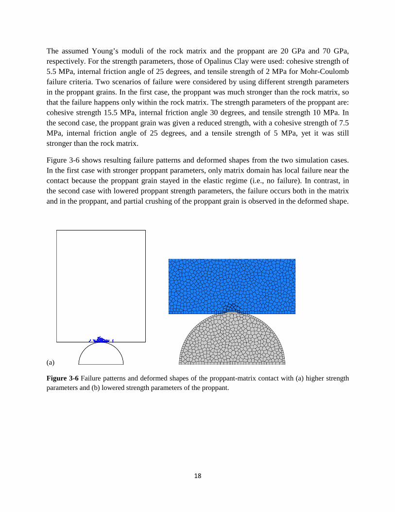
The assumed Young’s moduli of the rock matrix and the proppant are 20 GPa and 70 GPa, respectively. For the strength parameters, those of Opalinus Clay were used: cohesive strength of 5.5 MPa, internal friction angle of 25 degrees, and tensile strength of 2 MPa for Mohr-Coulomb failure criteria. Two scenarios of failure were considered by using different strength parameters in the proppant grains. In the first case, the proppant was much stronger than the rock matrix, so that the failure happens only within the rock matrix. The strength parameters of the proppant are: cohesive strength 15.5 MPa, internal friction angle 30 degrees, and tensile strength 10 MPa. In the second case, the proppant grain was given a reduced strength, with a cohesive strength of 7.5 MPa, internal friction angle of 25 degrees, and a tensile strength of 5 MPa, yet it was still stronger than the rock matrix.

Figure 3-6 shows resulting failure patterns and deformed shapes from the two simulation cases. In the first case with stronger proppant parameters, only matrix domain has local failure near the contact because the proppant grain stayed in the elastic regime (i.e., no failure). In contrast, in the second case with lowered proppant strength parameters, the failure occurs both in the matrix and in the proppant, and partial crushing of the proppant grain is observed in the deformed shape.

(a)

Figure 3-6 Failure patterns and deformed shapes of the proppant-matrix contact with (a) higher strength parameters and (b) lowered strength parameters of the proppant.

19

(b)

Figure 3-6 (Continued) Failure patterns and deformed shapes of the proppant-matrix contact with (a) higher strength parameters and (b) lowered strength parameters of the proppant

Next, we applied the TOUGH-RBSN modeling to 3D simulations of proppant-matrix interaction. Complex geometry arises in the proppant-matrix contract zone where spherical surface and flat surface are in close proximity to each other. To model each domain surface without any geometrical distortion, a sophisticated mesh generation process need to be developed. By the nature of the Voronoi discretization, the geometry of a Voronoi cell is determined not only by its nodal position but by the relative position of the neighboring nodes. Thus, it is critical to start the meshing process by carefully distributing the nodal points, which leads to proper Voronoi tiling.

To construct a spherical proppant grain discretized with irregular Voronoi cells, a group of 2 nodes (𝑁𝑁 = 2 configuration) is placed on a randomly directed ray �⃗�𝑣𝜃𝜃𝜃𝜃 from the sphere center, as shown in Figure 3-7a. The combination of different random angles 𝜃𝜃 and 𝜙𝜙 defines the ray direction. Additional nodal groups are introduced in the same way, so a sphere and the surrounding phase (e.g., interphase, shell, etc.) can be represented (Figure 3-7b).

20

Figure 3-7 Nodal placement for discretization of spherical components: (a) 𝑁𝑁 = 2 configuration; and 𝑁𝑁 = 3 configuration of layering nodal pairs.

In the first step, to model multiple spherical grains, trial spheres are randomly positioned within the domain. In the current stage, the radii of spheres are assumed to be uniform. To avoid the overlaps between grains in the 𝑁𝑁 = 2 configuration, grain placement is subject to 𝑑𝑑∗ > 2𝑎𝑎12, where 𝑑𝑑∗ is the distance between the centers of the trial sphere and the closest neighbor sphere.

Subsequently, the geometry of the contact between a proppant grain and the matrix block is formed by introducing a set of auxiliary nodal points, which is positioned at the same distance from the spherical surface and from the block surface. These auxiliary points, together with the closest nodal sets of the sphere and block domains, generate a wedge-like volume and help to form the surfaces of each domain discretized with an intended geometry.

Figure 3-8 shows an example of discretization of multiple proppant grains in contact with the matrix block for 3D simulations. It is assumed that proppant grains are placed in a single layer on the matrix block, and the example has 35 2-mm-diameter grains, randomly distributed on a 20-mm cube.

21

Figure 3-8 3D mesh for multiple proppant grains contacted on the matrix block from different perspectives.

The bottom boundary of the block domain is pushed up with a displacement control, while fixed boundary conditions are applied at the top of the grains. The embedment is simulated up to 0.02 mm displacement, and the resulting fracture/damage patterns are observed. The same mechanical properties of proppant and matrix domains as the 2D simulations are used.

As before, the two proppant/matrix failure scenarios during the proppant embedment are examined using two sets of proppant strength parameters. In the first case, proppant grains are much stronger than the rock matrix, so the failure occurs only in the matrix domain. Figure 3-9 presents the resulting failure pattern. The RBSN elements experiencing failure are marked. The matrix block has local failure near the contact zones while the proppant grains are intact. In contrast, in the second case with lowered proppant strength parameters, failure occurs both in the matrix and in the proppants (Figure 3-10).

22

(a) (b)

Figure 3-9 (a) Failure patterns with higher-strength proppants; (b) Only matrix block undergoes the local failure.

(a) (b)

Figure 3-10 (a) Failure patterns with lower-strength proppants; (b) Local failure occurs both in the matrix block and proppant grains.

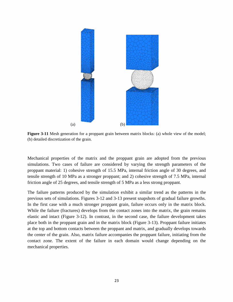
To demonstrate the failure patterns in more detail, a finer RBSN mesh was used to represent the contact zone between a single proppant grain and a matrix blocks (Figure 3-11). In this test, two 5 mm-thickness matrix blocks are propped by a 1 mm-diameter spherical grain. The top and bottom surfaces of the blocks are constrained to close the gap by displacement controlled boundary conditions. Displacements up to 0.02 mm are applied to examine deformation/ embedment of the proppant grain and any possible failure.

23

(a) (b)

Figure 3-11 Mesh generation for a proppant grain between matrix blocks: (a) whole view of the model; (b) detailed discretization of the grain.

Mechanical properties of the matrix and the proppant grain are adopted from the previous simulations. Two cases of failure are considered by varying the strength parameters of the proppant material: 1) cohesive strength of 15.5 MPa, internal friction angle of 30 degrees, and tensile strength of 10 MPa as a stronger proppant; and 2) cohesive strength of 7.5 MPa, internal friction angle of 25 degrees, and tensile strength of 5 MPa as a less strong proppant.

The failure patterns produced by the simulation exhibit a similar trend as the patterns in the previous sets of simulations. Figures 3-12 and 3-13 present snapshots of gradual failure growths. In the first case with a much stronger proppant grain, failure occurs only in the matrix block. While the failure (fractures) develops from the contact zones into the matrix, the grain remains elastic and intact (Figure 3-12). In contrast, in the second case, the failure development takes place both in the proppant grain and in the matrix block (Figure 3-13). Proppant failure initiates at the top and bottom contacts between the proppant and matrix, and gradually develops towards the center of the grain. Also, matrix failure accompanies the proppant failure, initiating from the contact zone. The extent of the failure in each domain would change depending on the mechanical properties.

24

Figure 3-12 Snapshots of failure development with a stronger proppant grain.

Figure 3-13 Snapshots of failure development with a less strong proppant grain.

25

In FY2017, the RBSN approach has been used to develop 2D and 3D grain-scale models of proppant embedment and perform test simulations. In comparison of the failure patterns obtained from 2D and 3D simulations, although general similarities are found, some differences in the details are present. The models well demonstrate the local failure due to the contact force. The fractured lattice elements are concentrated at the contact zone, and similar failure patterns were observed in the simulations so far. We confirm that the RBSN approach is capable of modeling fracture and damage behavior around a the matrix-proppant contact, especially in the problem of proppant deformation/crushing against a hard and brittle rock matrix.

Subtask 3.2 — Develop and block-scale modeling approaches (Year 1)

A block-scale model was developed and tested in Q3 of FY2017. The motivation for developing the block-scale model is that for block-scale problems (a few to tens of m’s in scale), realistically, grain-scale models cannot be used. Therefore, upscaling by using an equivalent continuum layer modeling of a proppant bed and fracture is necessary.

The effective medium modeling of a fracture/proppant bed used in this approach is based on

• Finite-thickness-element fracture representation

• Proppant bed modeled as a continuum (elasto-plastic), exhibiting stress and time-dependent changes in the permeability

• Matrix swelling into fracture considered using an internal swelling method

In Q3 of FY2017 we demonstrated the use of the block-scale modeling approach for hydraulic fracturing at 100-m scale and then tested the applicability of the approach to modeling experiments on two-inch-diameter rock cores (Figure 3-14). The core-scale model consists of a rock sample, fracture, upper plastic replica and a glass view window. The model is mechanically fixed at the top for vertical upward loading, and restricted from lateral displacements by the side boundary. In the model, the sample can be loaded from the bottom either by applying a constant stress or by applying a constant vertical velocity equivalent to displacement-controlled loading. In the simulation, the closure of the fracture and the stress normal to the fractures are monitored. We tested the model using various constitutive models, ranging from a simple, non-linear elastic closure model to elasto-plastic models for time-independent irreversible behavior, and to a creep model for long-term fracture closure.

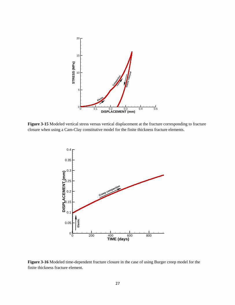
Figure 3-15 shows the results of a proppant pack modeling using an elasto-plastic constitutive model with a cap, in this case the Cam-Clay model, which can model compaction by pore-collapse rather than just shear failure. The results shown in Figure 3-15 include initial elastic compaction, followed by plastic compaction after the stress reached the pre-consolidation pressure which was set to 5 MPa. After full compaction, there is an elastic rebound. Irreversible

26

behavior is also manifested in the hysteresis of the loading loop and in the permanent offset at the end of the simulation.

We also tested modeling of fracture closure by creep. Here we used the same Burger models as we used in the previous creep simulations at the grain scale. However, in the block scale model we do not represent the stress concentrations at proppants, and the actual creep parameters need to be calibrated to obtain relevant creep deformations. Such parameters could be calibrated, again, using experimental data. Figure 3-16 shows an initial elastic closure of 0.1 mm, followed by creep deformations for another 0.2 mm closure over 3 years.

Figure 3-14 Model of laboratory experiment using a finite thickness representation of the fracture in block-scale modeling approach.

Any of the constitutive models tested for the block-scale may be used for the interpretative modeling of the experiments in FY2018 and will be a complement to the grain-scale modeling of the same experiments. The comparison between the grain-scale and the block-scale modeling of the experiments can be useful for learning how to upscale the shale fracture compaction problems. The exact choice of constitutive model to be used in these problems will be decided during the interpretative modeling of the experiments.

27

Figure 3-15 Modeled vertical stress versus vertical displacement at the fracture corresponding to fracture closure when using a Cam-Clay constitutive model for the finite thickness fracture elements.

Figure 3-16 Modeled time-dependent fracture closure in the case of using Burger creep model for the finite thickness fracture element.

DISPLACEMENT (mm)

STR

ESS

(MPa

)

0 0.1 0.2 0.3 0.4 0.50

5

10

15

20

Compa

ctio

n

Elastic

Elas

ticre

boun

d

TIME (days)

DIS

PLA

CEM

ENT

(mm

)

0 200 400 600 8000

0.05

0.1

0.15

0.2

0.25

0.3

0.35

0.4

Creep compaction

Elas

tic

28

Subtask 3.3 — Modeling of indentation experiments and material parameterization (Year 1)

In FY2017 Q4, we successfully demonstrated our modeling approach for simulating indentation tests for parametrization. There were some unexpected challenges in the modeling of the indentation tests compared to previous grain-scale modeling. In particular, the displacement and indentations were much smaller than what were previously calculated during the grain-scale modeling (shown in Q1 and Q2 reports). In the previous grain-scale modeling the embedment depth were on the order of several hundred microns with indentation diameters on the order of a millimeter. However, reference laboratory experiments conducted on a T6061T6 aluminum sample resulted in indentation depths on the order of 10 microns, with a few hundred microns of indentation diameter. As a consequence, we came to learn that modeling of laboratory indentation experiments required much finer mesh than was previously used in for the grain-scale modeling.

The current indentation model is shown in Figure 3-17. It is a half symmetric model containing half of the tungsten carbide ball indenter and central parts of the sample including its entire sample thickness and underlying aluminum plate. On top of the indenter single element, a rigid plate is placed for applying vertical compression (velocity) and for recording the total load applied on the indenter.

Figure 3-17 Half symmetric model for numerical simulations of indentation tests.

29

First, we successfully validated the model by comparing the results against the laboratory tests on an aluminum sample with known properties. In this verification, the modeling was first conducted assuming a completely elastic response, and the results were compared to analytical solutions. The analytical solution calculates the indentation depth considering the elastic properties of the sample (aluminum) and the indenter (tungsten carbide). The numerical modeling agreed exactly with the analytical solutions, providing a verification of the model and the model setup using the different model components shown in Figure 3-17. Subsequently, modeling of the actual laboratory indentation experiment on an aluminum sample was conducted, with a very good agreement as shown in Figure 3-18.

Figure 3-18 Comparison of modeling and experiment results of load-displacement curves for aluminum sample. Next simulation was done on some of the shale samples as an initial evaluation of indentation tests using elasto-plasticity with the Mohr-Coulomb strength criterion. Figure 3-19 shows a comparison of experimental and numerically simulated results for a dry Barnett sample. The simulation was conducted with E = 16.2 GPa, Poisson’s ratio of 0.33, cohesion = 8.5 MPa, and coefficient of friction of 25°. The results are in good agreement for both loading and unloading, though some disagreements are seen during unloading below 2,000 gf.

0 5 10 15 200

1000

2000

3000

4000

5000

DISPLACEMENT (µm)

LOA

D(g

f)

0 5 10 15 200

1000

2000

3000

4000

5000

ExperimentMODELING

30

Figure 3-19 Comparison of modeling and experiment results of load-displacement curves for dry Barnett sample. Overall, we found that a Mohr-Coulomb model could be used to model the experiments and to derive strength parameters to be applied for modeling fracture closure under the impact of proppant embedment. However, while the shear strength criterion provided by the Mohr-Coulomb model appears to be appropriate, more work is needed to determine whether it is possible to obtain a unique set of the failure parameters (friction angle and cohesion). Future work in FY2018 will involve modeling of all samples tested when we do the modeling of the actual proppant embedment experiments. Moreover, we will investigate whether it will be possible to determine (back-analyze) visco-elastic (creep) parameters from indentation tests involving early time-dependent response.

0 10 20 30 40 50 600

1000

2000

3000

4000

5000

DISPLACEMENT (µm)

LOA

D(g

f)

0 10 20 30 40 50 600

1000

2000

3000

4000

5000

ExperimentMODELING

31

In conclusion, we reached the planned numerical modeling milestones (M2 and M5) for FY2017. Lessons learned from the completed tasks and possible actions that will be taken in FY2018 numerical modeling are as follows:

1. Related to grain-scale modeling with TOUGH-FLAC, we found that a numerical modeling strategy using solid elements for shale and proppants and special interfaces for interaction between shale and proppants (as available in FLAC3D) works very well for modeling proppant embedment in soft shale. However, an alternate approach of discretizing rock, proppants and open fracture space with solid elements did not work, because elements tend to become too distorted by large deformations. The first approach also worked well for both elasto-plastic and creep deformation modeling. This approach will be employed in the tasks performed in FY2018.

2. TOUGH-RBSN was demonstrated for modeling proppant grain crushing. However, when using simple Voronoi discretization, we found it challenging to render the desired geometry without undesirable distortion and interference, because the geometry of a Voronoi cell is determined not only by the absolute position of the cell node but by the relative positions of the neighboring nodes. Therefore, in order to model a complex geometry, a special method has to be employed to place nodal points which results in good cell geometry. For example, for the wedge-like gap at a sphere-block contact, auxiliary points can be prescribed (although approximately) to fill the empty volume with a fictitious Voronoi cell.

3. Indentation modeling using the FLAC3D grain-scale approach turned out to be much more challenging than the previously conducted multiple-proppant-embedment modeling. Very fine mesh discretization was required for achieving accurate numerical simulations of laboratory experiments on an aluminum sample due to very small deformations and contact changes for each loading cycle. On the positive side, from the simulations of the indentation tests, we found that the Mohr-Coulomb criterion can be adopted to parameterize material strength for modeling proppant embedment. However, in FY2018, further parametric studies will be needed to investigate a possibility of a unique pair of friction angle and cohesion (Mohr-Coulomb model parameters) for the properties of test samples.

4. Block-scale modeling was successful in modeling fracture closure with and without proppants. An elasto-plastic model of a proppant pack considering pore collapse (a modified Cam-clay model) looks promising as it can replicate experimental results reported in the literature. However, we need new experimental data before deciding which approach (grain-scale or block-scale) and which constitutive models to be used. Proppant embedment in soft rock may be better represented in TOUGH-FLAC, as it is difficult to handle progressive increases of contact surfaces in TOUGH-RBSN. In FY2018, TOUGH-FLAC is expected to be used to model most experiments, whereas TOUGH-RBSN will be complementary for special cases including potential splitting of samples and grain-crushing.

32

3. Budget summary

Spending of the budget for FY2017 is summarized in the table below. Following is the current budget vs spending table (up to the FY2017 end).