DECISIONS UNDER UNCERTAINTY,CERTAINTY EQUIVALENTS,

AND GENERALIZED ENTROPY

Jointly with Aharon Ben-Tal and Marc Teboulle

Attitude towards wealth Utility

Attitude towards risk Expected utility (EU)

Axioms for EU Risk aversion (RA)

Generalizations of EU Dual theory

Bad predictions of EU Arrow-Pratt RA indices

Certainty equivalents The Recourse CE (RCE)

Sv(Z) := supz

{z + E v(Z− z)}

Meaning of v(·) Recoverability

Economic models Production, investment,

insurance

Extremal principles RCE, EU and φ–divergence

Iφ(p,q) :=∑

qi φ

(pi

qi

)

1

The St. Petersburg paradoxDaniel Bernoulli (1738)

RV Z : Prob{Z = 2n−1

}= 1

2n, (n = 1,2, . . . )

The expected value of Z:

EZ =∞∑

n=1

2n−1 1

2n=

1

2+

1

2+

1

2+ · · · = ∞

Why “paradox”?

Game with two players, A and B (= Bank).

A fair coin {H, T} is tossed until H appears.

If on trial n, B pays A : 2n−1$, (n = 1,2, . . . )

The value of the game for A is the RV Z.

What is a fair ticket price ? EZ ?

Hence the “paradox”.

Bernoulli introduced moral expectation:

The expected value to A is:

∞∑

n=1

u(2n−1

) 1

2n

where u(W ) is A’s utility of wealth W .

2

Bernoulli’s logarithmic utility

If wealth increases from W to W + ∆W ,

the utility increases by ∆u

∆u = K∆W

W

u(W ) =∫ W

cK

d W

W= K log

W

c

Back to St Petersburg: A’s EU is:

Eu(Z) = K∞∑

n=1

log(2n−1

) 1

2n

= K∞∑

n=1

n− 1

2n= K

3

Attitude towards wealth

Marginal utility ↘ ⇐⇒ u concave

- W

6

u

The Weber–Fechner law (1860)

The response to a stimulus diminishes witheach repetition of that stimulus within somespecified time period.

Sensation is a logarithmic function of stimulus

4

Axioms for EU theoryvon Neumann-Morgenstern (1947)

Preferences between RV’s X , Y:

X ∼ Y indifference

X º Y X better than Y

X ¹ Y X worse than Y

Completeness: For any X , Y,

either X º Y or X ¹ Y .

Transitivity: X º Y & Y º Z =⇒ X º Z.

Continuity: Given X º Y º Z,

there exists a probability p in [0,1] such that

Y ∼ pX + (1− p)Z

Independence: If X º Y, then

for any p ∈ [0,1] and any Z,

pX + (1− p)Z º pY + (1− p)Z

5

Existence of utility

The axioms =⇒ existence of a utility u,

(continuous, nondecreasing) such that

X º Y ⇐⇒ Eu(X) ≥ Eu(Y)

The utility u is unique up to a positive linear

transformation: For any α > 0, β, the utilities

u and αu + β

represent the same º

-

x

1

-

12

x− δ x

12

x + δ

u(x) ≥ 1

2u(x− δ) +

1

2u(x + δ)

Concavity of u ⇐⇒ Risk Aversion

6

The Allais paradox (1953)Kahneman and Tversky (1979)

Choose between:

A: 4,000 (prob. .80) B: 3,000 (certainty)

0 (prob. .20)

[20%] [80%]

C: 4,000 (prob. .20) D: 3,000 (prob. .25)

0 (prob. .80) 0 (prob. .75)

[65%] [35%]

B º A =⇒ u(3,000) > .80u(4,000)

C º D =⇒ .25u(3,000) < .20u(4,000)

7

Stochastic programming with recourse2–stage stoch. prog., Dantzig (1955)

max {f(z) : g(z) ≤ Z}

z = decision variable f(·) = profit

Z = budget g(·) = consumption

If Z is RV, the a priori decision z may violate

g(z) ≤ Z

Let y = second stage decision, with

h(y) = consumption, v(y) = profit

maxz

{f(z) + E(max

y{v(y) : g(z) + h(y) ≤ Z}

)}

If z, y are scalars, h(·) ↗, v(·) ↗,

maxz

{f(z) + E(max

y{v(y) : g(z) + y ≤ Z}

)}

maxz

{f(z) + E v(Z− g(z)) }

8

Recourse certainty equivalent (RCE)

The value of a RV Z

value of Z = max {z : z ≤ Z}Stoch. Prog. with Recourse interpretation:

supz

{z + E v(Z− z)}v(x) = current (before realization) value of x

v(·) = the value-risk function

Another interpretation:

Z = future income (RV)

z = loan against Z (unrestricted)

v(·) = utility

9

Assumptions on v(·)

(v1) v(0) = 0

(v2) v(·) is strictly increasing

(v3) v(x) ≤ x for all x

(v4) v(·) is strictly concave

(v5) v is continuously differentiable

(v1) and (v2) =⇒ v(x) < 0 for x < 0,

. .. v(·) = penalty function for

z ≤ Z

Special class of value-risk functions

U :=

{v :

v strict. ↗, strict. concavecont. diff., v(0) = 0, v′(0) = 1

}

the normalized utility functions.

For concave v the gradient inequality

v(x) ≤ v(0) + v′(0)x

shows that all v ∈ U satisfy (v3).

10

Attainment of supz

{z + E v(Z− z)}

U =

{v :

v strict. ↗, strict. concavecont. diff., v(0) = 0, v′(0) = 1

}

Lemma. Let the RV Z have finite support[zmin, zmax

].

Then ∀ v ∈ U the supremum in RCE is attained

uniquely for some z∗,

zmin ≤ z∗ ≤ zmax

which is the solution of

E v′(Z− z∗) = 1

so that

Sv(Z) = z∗ + E v(Z− z∗)

Proof. Z− zmin ≥ 0 with probability 1.

Also v′(·) ↘ ,

. .. E v′(Z− zmin

)≤ E v′(0) = 1

Similarly E v′(Z− zmax

)≥ E v′(0) = 1

11

Properties of Sv(Z) := supz {z + E v(Z− z)}

Shift additivity. For any v : IR → IR, any RV Z

and any constant c

Sv(Z + c) = Sv(Z) + c

For any function v : IR → IR,

Sv(Z + c) = supz

{z + E v(Z + c− z)}= c + sup

z{(z − c) + E v(Z− (z − c))}

= c + Sv(Z)

For any RV Z, constant S, if

Z ∼ S

then

Z + c ∼ S + c

for all constant c.

12

(v1) v(0) = 0

(v2) v(·) is strictly increasing

(v3) v(x) ≤ x for all x

(v4) v(·) is strictly concave

(v5) v is continuously differentiable

Consistency. If v satisfies (v1), (v3) then,

Sv(c) = c, ∀ constant c

Subhomogeneity. If v satisfies (v1) and (v4)

then, for any RV Z

1

λSv(λZ) is decreasing in λ , λ > 0

Sv(λZ) ≤ λ S

v(Z) , ∀λ > 1

λZ ¹ λSv(Z)

since E (λZ) = λZ

Var (λZ) = λ2Var Z > λVar Z if λ > 1

An interesting result: For v ∈ U,

limλ→0+

1

λSv(λZ) = EZ

13

(v1) v(0) = 0

(v2) v(·) is strictly increasing

(v3) v(x) ≤ x for all x

(v4) v(·) is strictly concave

(v5) v is continuously differentiable

Monotonicity. If v satisfies (v2) then, for any

RV X and any nonnegative RV Y,

Sv(X + Y) ≥ Sv(X)

If v satisfies (v1) and (v2), and if

Z ≥ zmin with probability 1,

then

Sv(Z) ≥ zmin

Take: X = zmin (degenerate RV)

Y = Z− zmin

14

(v1) v(0) = 0

(v2) v(·) is strictly increasing

(v3) v(x) ≤ x for all x

(v4) v(·) is strictly concave

(v5) v is continuously differentiable

U :=

{v :

v strict. ↗, strict. concavecont. diff., v(0) = 0, v′(0) = 1

}

Risk aversion. v satisfies (v3) iff

Sv(Z) ≤ EZ for all RV’s Z

Concavity. For any v ∈ U , RV’s X0 , X1

and 0 < α < 1,

Sv(αX1 + (1− α)X0) ≥ αS

v(X1) + (1− α)S

v(X0)

2nd order stochastic dominance. Let X , Y be

RV’s with compact support. Then

Sv(X) ≥ Sv(Y) for all v ∈ Uif and only if

E v(X) ≥ E v(Y) for all v ∈ U15

Exponential value-risk function

u(z) := 1− e−z

The optimality condition Eu′(Z− z∗) = 1

gives E e−Z+z∗ = 1 or z∗ = − log E e−Z

. .. Su(Z) = − log E e−Z

For the exponential utility u(z) = 1− e−z,

u−1Eu(Z) = − log E e−Z

Quadratic value-risk function

u(z) := z − 1

2z2 , z ≤ 1

For RV Z : zmax ≤ 1, EZ = µ, VarZ = σ2,

z∗ = µ, Su(Z) = µ− 1

2σ2

In both exponential & quadratic u(·)

Su

n∑

i=1

Zi

=

n∑

i=1

Su(Zi)

for independent RV’s {Z1,Z2, . . . ,Zn}16

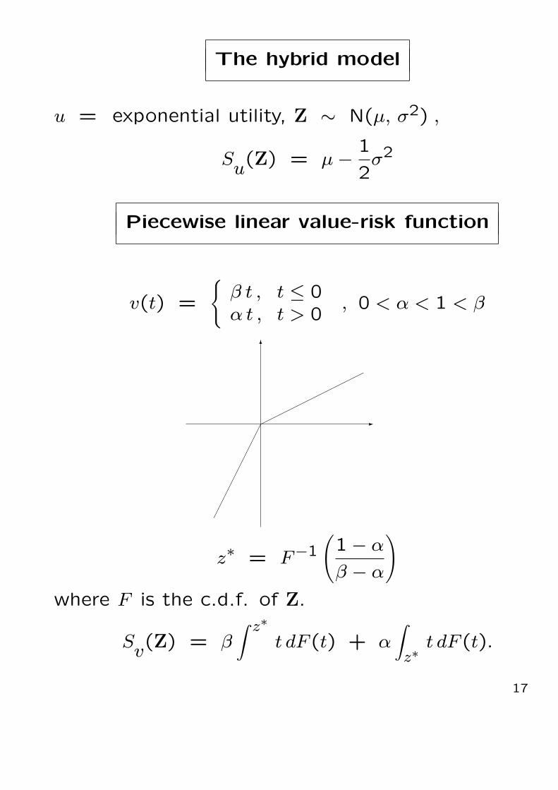
The hybrid model

u = exponential utility, Z ∼ N(µ, σ2) ,

Su(Z) = µ− 1

2σ2

Piecewise linear value-risk function

v(t) =

{β t , t ≤ 0α t , t > 0

, 0 < α < 1 < β

-

6

©©©©©©©©©©©

¢¢

¢¢

¢¢

¢¢

¢¢

z∗ = F−1(1− α

β − α

)

where F is the c.d.f. of Z.

Sv(Z) = β∫ z∗

t dF (t) + α∫

z∗t dF (t).

17

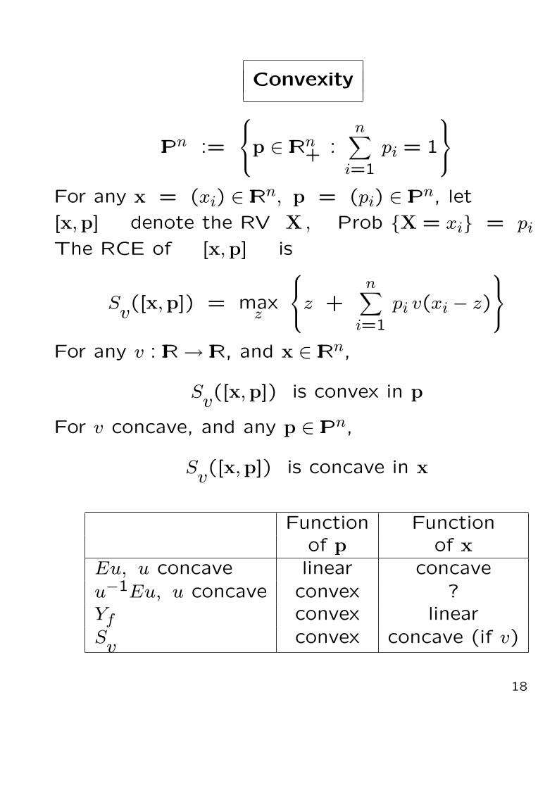
Convexity

IPn :=

p ∈ IRn

+ :n∑

i=1

pi = 1

For any x = (xi) ∈ IRn, p = (pi) ∈ IPn, let

[x,p] denote the RV X , Prob {X = xi} = pi

The RCE of [x,p] is

Sv([x,p]) = max

z

z +

n∑

i=1

pi v(xi − z)

For any v : IR → IR, and x ∈ IRn,

Sv([x,p]) is convex in p

For v concave, and any p ∈ IPn,

Sv([x,p]) is concave in x

Function Functionof p of x

Eu, u concave linear concaveu−1Eu, u concave convex ?Yf convex linearSv convex concave (if v)

18

Recoverability & meaning of v(·)

Let X = (x, p) denote the RV

X =

x, with probability p

0, with probability p = 1− p

Sv(x, p) = supz

{z + pv(x− z) + pv(−z)}

Theorem. If v ∈ U then

v(x) =∂

∂pSv(x, p)

p=0

p =∂

∂xSv(x, p)

x=0

Going from (x,0) to (x, p) changes the RCE by

∆(x, p) = Sv(x, p)− Sv(x,0)

The rate of change is

Sv(x, p)− Sv(x,0)

p≈ v(x) for p ¿ 1

19

-

6

p0 1

..

..

..

.

....

´´

´´

´´

´´

´´

´´

´´

´´

´´

´´

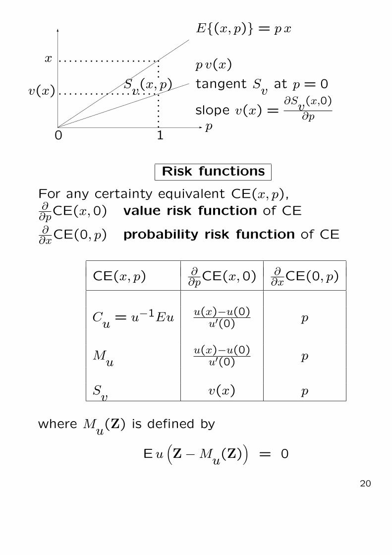
E{(x, p)} = p x

...................x

³³³³³³³³³³³³³³³³³³³³v(x) ...................S

v(x, p)

p v(x)

tangent Sv

at p = 0

slope v(x) =∂Sv(x,0)

∂p

Risk functions

For any certainty equivalent CE(x, p),∂∂pCE(x,0) value risk function of CE

∂∂xCE(0, p) probability risk function of CE

CE(x, p) ∂∂pCE(x,0) ∂

∂xCE(0, p)

Cu = u−1Eu u(x)−u(0)u′(0) p

Muu(x)−u(0)

u′(0) p

Sv

v(x) p

where Mu(Z) is defined by

Eu(Z−Mu(Z)

)= 0

20

Strong risk aversionRothschild-Stiglitz (1970,1971)

Diamond-Stiglitz (1974)

In EU Theory, risk aversion of EU, i.e.

Eu(Z) ≤ EZ , ∀ RV Z

is equivalent to the concavity of u(·).

Sv(Z) := sup

z{z + E v(Z− z)} (RCE)

In RCE Theory, risk aversion of Sv, i.e.

Sv(Z) ≤ EZ , ∀ RV Z

is equivalent to

v(x) ≤ x, ∀ x

What corresponds to v(·) concave ?

21

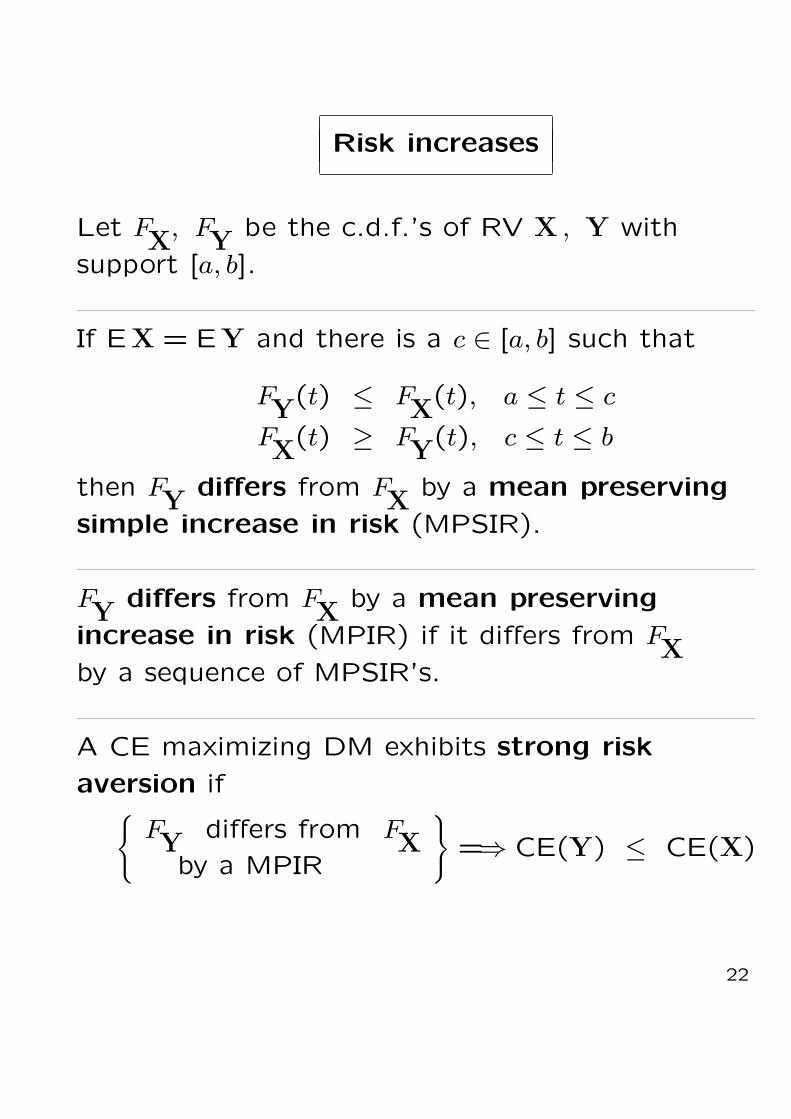
Risk increases

Let FX, FY be the c.d.f.’s of RV X , Y with

support [a, b].

If EX = EY and there is a c ∈ [a, b] such that

FY(t) ≤ FX(t), a ≤ t ≤ c

FX(t) ≥ FY(t), c ≤ t ≤ b

then FY differs from FX by a mean preserving

simple increase in risk (MPSIR).

FY differs from FX by a mean preserving

increase in risk (MPIR) if it differs from FXby a sequence of MPSIR’s.

A CE maximizing DM exhibits strong risk

aversion if{

FY differs from FXby a MPIR

}=⇒ CE(Y) ≤ CE(X)

22

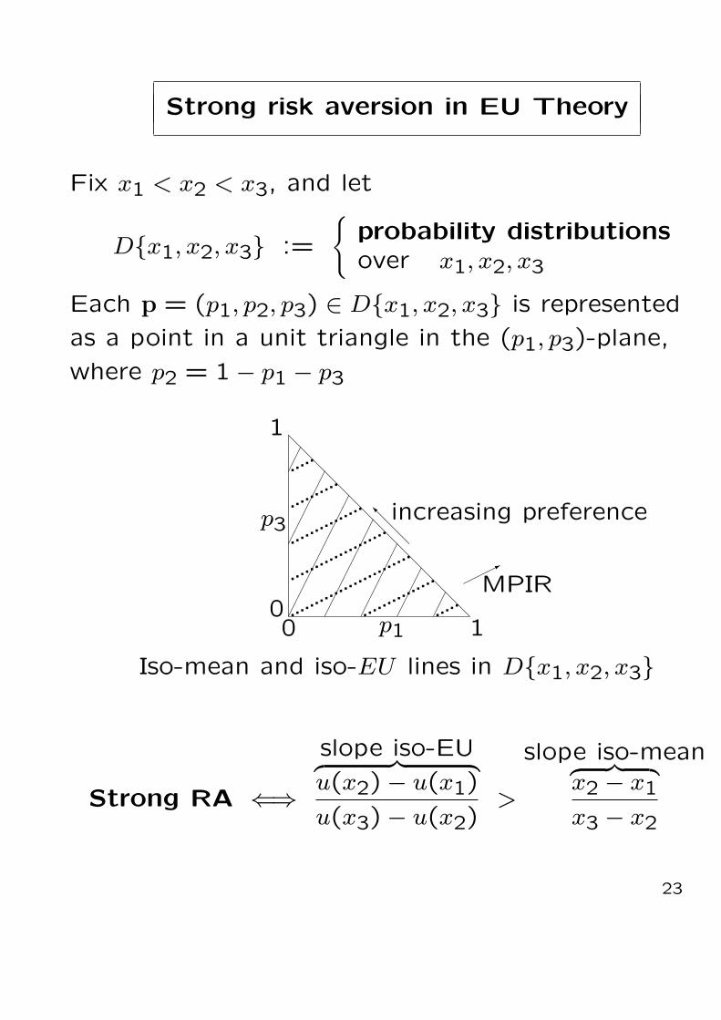
Strong risk aversion in EU Theory

Fix x1 < x2 < x3, and let

D{x1, x2, x3} :=

{probability distributionsover x1, x2, x3

Each p = (p1, p2, p3) ∈ D{x1, x2, x3} is represented

as a point in a unit triangle in the (p1, p3)-plane,

where p2 = 1− p1 − p3

@@

@@

@@

@@

@@

@@

@@

@

0 p1 1

©©©*

MPIR0

p3

1

@@

@I increasing preference

............

............

.

............

...

...........

............

..............

.............

.....

¢¢¢¢¢¢¢¢¢¢

¢¢¢¢¢¢¢¢

¢¢¢¢¢¢

¢¢¢¢

¢¢

¢¢¢¢¢¢

¢¢

Iso-mean and iso-EU lines in D{x1, x2, x3}

Strong RA ⇐⇒slope iso-EU︷ ︸︸ ︷u(x2)− u(x1)

u(x3)− u(x2)>

slope iso-mean︷ ︸︸ ︷x2 − x1

x3 − x2

23

Functionals & approximations

RV ~Z = (Zi) ∈ IRn, E ~Z = ~µµµ, Cov ~Z = Σ.

For any ~y ∈ IRn

su(~y) := Su

(~y · ~Z

)

If u ∈ U ∩ C(2), then

(a) The functional su(·) is concave, and given by

su(~y) = z∗(~y) + Eu(~y · ~Z− z∗(~y))

where z∗(~y) is the unique solution z of

E u′(~y · ~Z− z) = 1

(b) Moreover,

su(~0) = 0 , ∇su(~0) = ~µµµ, ∇2su(~0) = u′′(0)Σ

z∗(~0) = 0 , ∇z∗(~0) = ~µµµ

and if u ∈ C(3),

∇2z∗(~0) =u′′′(0)

u′′(0)Σ

su(~y) = ~µµµ · ~y +

1

2u′′(0)~y ·Σ~y + ◦

(‖ ~y ‖2

)

24

su(y) = µ · y + 12 u′′(0)y ·Σy + ◦

(‖ y ‖2

)

For n = 1 and y = 1,

Su(Z) ≈ µ +

1

2u′′(0)σ2

= µ− 1

2r(0)σ2

where r(z) = −u′′(z)u′(z)

the Arrow-Pratt absolute risk-aversion index

The approximation is exact if

(i) u is quadratic, or

(ii) u is exponential, Z is normal

Comparing with the Taylor expansion of the

classical CE

cu(y) := u−1Eu(y · Z)

we get cu(y)− su(y) = ◦(‖ y ‖2)

25

Competitive firm under price uncertaintySandmo (1971)

Π(q) = qP − c(q)−B

P = price (RV) q = production

B = fixed cost c(q) = variable cost

Π = profit

Assume:

c(0) = 0, c′ > 0, c′′ > 0

u ∈ U

maxq ≥ 0

Eu(Π(q)) (EU Model)

maxq ≥ 0

Su(Π(q)) (RCE Model)

26

Π(q) = qP − c(q)−B

EU RCE

q∗ > 0 iff µ > c′(0) same

q∗ < qcer same

q∗ ↗ as B ↗ q∗ is independentif r ↗ of B, ∀u

q∗ ↘ as B ↗if r ↘

q∗ ↗ as P → P + ε q∗ ↗ as P → P + εif r ↘ ∀u ∈ U

Profit tax (1− t)Π(q) Profit tax (1− t)Π(q)

q∗ ↗ with t if q∗ ↗ with tr = const and R ↗ or for all u ∈ Ur ↘ and R ↗r ↘ and R = const

r(z) := −u′′(z)u′(z)

, R(z) := zr(z)

27

Investment in risky & safe assetsArrow (1971)

Y (a) = A− a + (1 + X)a = A + aX

A = initial wealth, Y = final wealth.X = rate of return of risky investmenta = amount invested in risky assets

EU RCE

a∗ > 0 iff EX > 0 same

Wealth elasticity of cashbalance m = A− a∗dm/dA

m/A≥ 1 if R ↗ dm/dA

m/A≥ 1 ∀u ∈ U

X → X + h =⇒ a∗(h) ↗ same

X → (1 + h)X

=⇒ a∗(h) =a∗

1 + hsame

Tobin (1958)

28

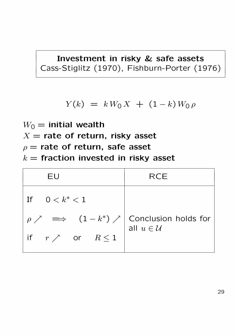
Investment in risky & safe assetsCass-Stiglitz (1970), Fishburn-Porter (1976)

Y (k) = k W0 X + (1− k)W0 ρ

W0 = initial wealth

X = rate of return, risky asset

ρ = rate of return, safe asset

k = fraction invested in risky asset

EU RCE

If 0 < k∗ < 1

ρ ↗ =⇒ (1− k∗) ↗ Conclusion holds forall u ∈ U

if r ↗ or R ≤ 1

29

InsuranceEhrlich-Becker (1972)

Lippman-McCall (1981)

n states of nature

p = (p1, . . . , pn) their probabilities

qi = premium for 1$ coverage in state i

B = insurance budget

qi = qi/∑n

j=1 qj = normalized premium

B = B/∑n

j=1 qj = normalized budget

xi = income in state i

x = (x1, . . . , xn) decision variable

n∑

i=1

qi xi = B budget constraint

The optimal value is

I∗ = maxx

Sv([x,p]) :

n∑

i=1

qi xi = B

= maxx,

∑qixi = B

maxz

z +

n∑

i=1

pi v(xi − z)

= Sv([x∗,p

])

x∗ = (x∗i ) is the optimal insurance coverage.

30

Insurace: The solution

I∗ = maxx

{Sv([x,p]) :n∑

i=1

qi xi = B}

= maxx,

∑qixi = B

maxz

{z +n∑

i=1

pi v(xi − z)}

= Sv([x∗,p

])

The optimal insurance coverage is

x∗i = B + φ

(qi

pi

)−

n∑

j=1

qj φ

(qj

pj

)

where

φ =(v′

)−1

Moreover,

I∗ = B −∑

qi φ

(qi

pi

)+

∑pi v(φ

(qi

pi

))

31

The φ–divergence functionalCsiszar (1978)

Given a convex function φ : IR+ → IR,

the φ–divergence functional,

Iφ(p,q) :=n∑

i=1

qi φ

(pi

qi

)

is a “distance function” on IPn.

φ : IR+ → IR convex

=⇒ Iφ(p,q) jointly convex in p and q.

Let φ : IR+ → IR be convex.

Then for any p, q ∈ IRn++,

Iφ(p,q) ≥

n∑

i=1

qi

φ

n∑i=1

pi

n∑i=1

qi

If φ is strictly convex, equality holds iff

p1

q1=

p2

q2= · · · = pn

qn

32

Adjoints

Let φ : IR+ → IR be convex, φ(1) = 0.

The adjoint of φ is

φ¦(t) := t φ

(1

t

), t > 0.

(a) φ¦ ¦ = φ.

(b) φ¦(·) is convex.

(c) φ¦(1) = 0

(d) For any p,q ∈ IRn++

Iφ(p,q) = Iφ¦(q,p)

(e) φ¦(t) is increasing for t > 1.

In general, Iφ(p,q) 6= Iφ(q,p).

Also Iφ(·, ·) does not satisfy triangle inequality.

To get symmetry use:

Iφ(p,q) + Iφ¦(p,q)

33

The Kullback-Leibler distance

Iφ(p,q) =n∑

i=1

pi logpi

qi

from φ(t) := t log t, t > 0,

φ¦ = t

(1

tlog

1

t

)= − log t

In particular, for p =(1n, 1

n, . . . , 1n

)

Iφ¦(p,q) = −n∑

i=1

qi log1

nqi

=n∑

i=1

qi log qi + logn

The Hellinger distance

Iφ(p,q) =n∑

i=1

(√pi −

√qi

)2

from φ(t) :=(1−

√t)2

, t > 0

φ¦ = φ

34

α–order entropy

For α > 1 let,

φ(t) := tα, t > 0

. .. Iφ(p,q) =n∑

i=1

(pi)α (qi)

1−α

the α-order entropy.

φ¦(t) = t1−α

The χ2–distance

φ(t) := (t− 1)2, t > 0,

Iφ(p,q) =n∑

i=1

(p2i − q2i

qi

)

the χ2-distance.

φ¦(t) = (√

t− 1√t)2

= t +1

t− 2

35

The variation distance

φ(t) := | t− 1 |, t > 0,

Iφ(p,q) =n∑

i=1

| pi − qi |

Indicator function

Let α < 1 < β and define

φ(t) := δ(t | [α, β]) =

0 if α ≤ t ≤ β ,

∞ otherwise ,

indicator function of the interval [α, β],

φ¦(t) = δ

(t |

[1

β,1

α

])

Iφ(p,q) =

0 if α ≤ piqi≤ β ,

∀i = 1, . . . , n∞ otherwise .

36

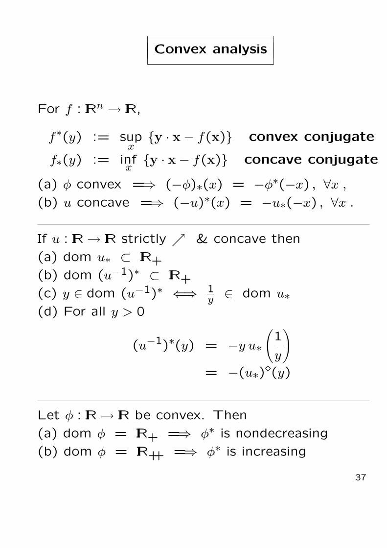
Convex analysis

For f : IRn → IR,

f∗(y) := supx

{y · x− f(x)} convex conjugate

f∗(y) := infx{y · x− f(x)} concave conjugate

(a) φ convex =⇒ (−φ)∗(x) = −φ∗(−x) , ∀x ,

(b) u concave =⇒ (−u)∗(x) = −u∗(−x) , ∀x .

If u : IR → IR strictly ↗ & concave then

(a) dom u∗ ⊂ IR+

(b) dom (u−1)∗ ⊂ IR+

(c) y ∈ dom (u−1)∗ ⇐⇒ 1y ∈ dom u∗

(d) For all y > 0

(u−1)∗(y) = −y u∗(1

y

)

= −(u∗)¦(y)

Let φ : IR → IR be convex. Then

(a) dom φ = IR+ =⇒ φ∗ is nondecreasing

(b) dom φ = IR++ =⇒ φ∗ is increasing

37

A special functional

For h : IRn → IR define h+ : IRn → IR by

h+(y) := supz ∈ IRx ∈ IRn

y · x = 0

{z + h(x− ze)}

Then for any y ∈ IRn with∑

yi 6= 0 ,

h+(y) = −h∗(

y∑

yi

)

If h is strictly concave and C(1) ,

z∗ = −vTu∗ = − yT

e · y (∇h)−1(

y

e · y

)

x∗ = u∗ + z∗e =

(I − eyT

eTy

)(∇h)−1

(y

e · y

)

= Pe⊥ (∇h)−1(

y

e · y

)

Pe⊥ := orthogonal projection ⊥ e.

−z∗e =eyT

eTy(∇h)−1

(y

e · y

)= Pe (∇h)−1

(y

e · y

)

38

Extremal principles for RCE, EU

If u : IR → IR is strictly ↗ & concave, then

φ := −u∗is convex and φ : IR+ → IR. Also

φ¦ = (u−1)∗

Conversely, for convex φ : IR+ → IR,

u(t) := −φ∗(−t)

is concave.

For any RV X = [x,p] ,

Su([x,p]) = inf

q∈ IPn

Iφ(q,p) +

n∑

i=1

qi xi

= infq∈ IPn

Iφ¦(p,q) +

n∑

i=1

qi xi

Eu ([x,p]) = infq∈ IRn

+

Iφ(q,p) +

n∑

i=1

qi xi

39

Duality

Su([x,p]) = infq∈ IPn

Iφ(q,p) +

n∑

i=1

qi xi

The RCE, in LHS, is the optimal value of

(P) sup {z : “z ≤ X”}in the sense of recourse optimization.

The RHS is the “dual” of (P),

(D) inf {z : “z ≥ X”}using a stochastic penalty function P (·) to

“enforce” the stochastic constraint

“z ≥ X”

(D1) inf {z + P (z)}

40

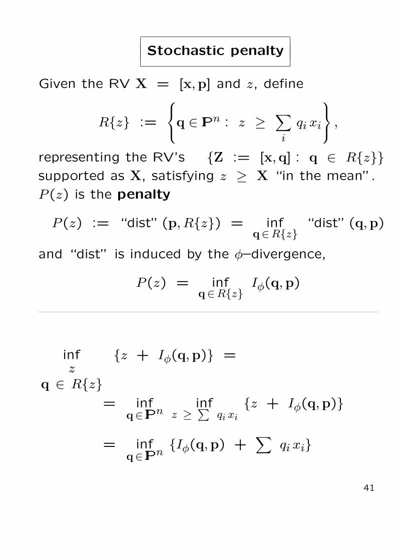
Stochastic penalty

Given the RV X = [x,p] and z, define

R{z} :=

q ∈ IPn : z ≥

∑

i

qi xi

,

representing the RV’s {Z := [x,q] : q ∈ R{z}}supported as X, satisfying z ≥ X “in the mean”.

P (z) is the penalty

P (z) := “dist” (p, R{z}) = infq∈R{z}

“dist” (q,p)

and “dist” is induced by the φ–divergence,

P (z) = infq∈R{z}

Iφ(q,p)

infz

q ∈ R{z}

{z + Iφ(q,p)} =

= infq∈ IPn

infz ≥ ∑

qi xi

{z + Iφ(q,p)}

= infq∈ IPn

{Iφ(q,p) +∑

qi xi}

41

Extremal principles for φ–divergence

Let φ : IR+ → IR convex, dom φ ⊂ IR++ . Define

u(t) := −φ∗(−t)

Then for any p,q ∈ IPn,

Iφ(q,p) = supx ∈ IRn

q · x = 0

Su([x,p])

Furthermore, if dom φ = IR++, define the function

v(x) := (φ∗)−1(x),

Then

Iφ(p,q) = supx ∈ IRn

q · x = 0

Sv([x,p])

For all p ∈ IPn, q ∈ IRn+,

Iφ(q,p) = supx ∈ IRn

n∑

i=1

pi u(xi) −n∑

i=1

qi xi

42