svm-asym-prox.pdf
TRANSCRIPT
8/11/2019 svm-asym-prox.pdf
http://slidepdf.com/reader/full/svm-asym-proxpdf 1/8
Support Vector Machine Classifiers for
Asymmetric Proximities
Alberto Munoz1
, Isaac Martın de Diego1
, and Javier M. Moguerza2
1 University Carlos III de Madrid, c/ Madrid 126, 28903 Getafe, Spain{albmun,ismdiego}@est-econ.uc3m.es
2 University Rey Juan Carlos, c/ Tulipan s/n, 28933 Mostoles, [email protected]
Abstract. The aim of this paper is to afford classification tasks on
asymmetric kernel matrices using Support Vector Machines (SVMs). Or-dinary theory for SVMs requires to work with symmetric proximity ma-trices. In this work we examine the performance of several symmetriza-tion methods in classification tasks. In addition we propose a new methodthat specifically takes classification labels into account to build the prox-imity matrix. The performance of the considered method is evaluated ona variety of artificial and real data sets.
1 Introduction
Let X be an n × p data matrix representing n objects in IR p. Let S be the n ×nmatrix made up of object similarities using some similarity measure. Assumethat S is asymmetric, that is, sij = sji. Examples of such matrices arise whenconsidering citations among journals or authors, sociometric data, or word as-sociation strengths [11]. In the first case, suppose a paper (Web page) i cites(links to) a paper (Web page) j, but the opposite is not true. In the secondexample, a child i may select another child j to sit next in their classroom, butnot reciprocally. In the third case, word i may appear in documents where word
j occurs, but not conversely.
Often classification tasks on such data sets arise. For instance, we can have anasymmetric link matrix among Web pages, together with topic labels for some of the pages (‘computer sicence’, ‘sports’, etc). Note that there exists no Euclideanrepresentation for Web pages in this problem, and classification must be doneusing solely the cocitation matrix: we are given the S matrix, but there is noX matrix in this case. SVM parametrization [1,2] of the classification problemis well suited for this case. By the representer theorem (see for instance [ 3,8]),SVM classifiers will always take the form f (x) =
i αiK (x, xi), where K is a
positively definite matrix. Thus, if we are given the similarity matrix K = (sik)and this matrix admits an Euclidean representation (via classical scaling), thisis all we need to classify data using a SVM. In the case of asymmetric K = S ,Scholkopf et al [9] suggest to work with the symmetric matrix S T S . Tsuda [10]
O. Kaynak et al. (Eds.): ICANN/ICONIP 2003, LNCS 2714, pp. 217–224, 2003.c Springer-Verlag Berlin Heidelberg 2003
8/11/2019 svm-asym-prox.pdf
http://slidepdf.com/reader/full/svm-asym-proxpdf 2/8
218 A. Munoz, I. Martın de Diego, and J.M. Moguerza
elaborates on the SVD of S , producing a new symmetric similarity matrix, thatserves as input for the SVM.
A standard way to achieve symmetrization is to define K ij = sij + sji
2 , taking
the symmetric part in the decomposition S = 12 (S +S T )+ 12 (S −S T ). This choicecan be interpreted in a classification setting as follows: we assign the same weight(one half) to sij and sji before applying the classifier. However, note that thischoice is wasting the information provided by classification labels. In addition,ignoring the skew-symmetric part implies a loss of information.
In next section we elaborate on an interpretation of asymmetry that could ex-plain why and when some symmetrization methods may success. In addition weshow the existing relation between the methods of Tsuda and Scholkopf and his
coworkers. In section 3 we propose a new method to build a symmetric Grammatrix from an asymmetric proximity matrix. The proposed method specificallytakes into account the labels of data points to build the Gram matrix. The dif-ferent methods are tested in section 4 on a collection of both artificial and realdata sets. Finally, section 5 summarizes.
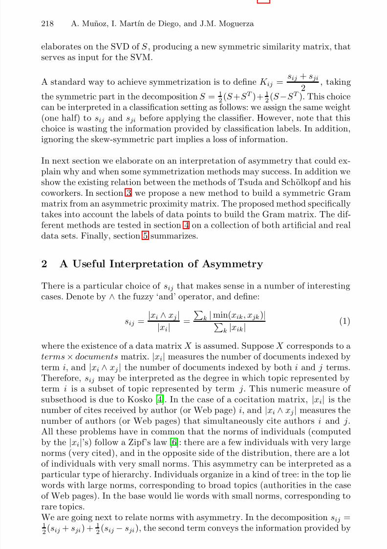
2 A Useful Interpretation of Asymmetry
There is a particular choice of sij that makes sense in a number of interestingcases. Denote by ∧ the fuzzy ‘and’ operator, and define:
sij = |xi ∧ xj |
|xi| =
k |min(xik, xjk)|
k |xik| (1)
where the existence of a data matrix X is assumed. Suppose X corresponds to aterms× documents matrix. |xi| measures the number of documents indexed byterm i, and |xi ∧ xj | the number of documents indexed by both i and j terms.Therefore, sij may be interpreted as the degree in which topic represented byterm i is a subset of topic represented by term j. This numeric measure of subsethood is due to Kosko [4]. In the case of a cocitation matrix, |xi| is thenumber of cites received by author (or Web page) i, and |xi ∧ xj | measures thenumber of authors (or Web pages) that simultaneously cite authors i and j.All these problems have in common that the norms of individuals (computedby the |xi|’s) follow a Zipf’s law [6]: there are a few individuals with very largenorms (very cited), and in the opposite side of the distribution, there are a lotof individuals with very small norms. This asymmetry can be interpreted as aparticular type of hierarchy. Individuals organize in a kind of tree: in the top liewords with large norms, corresponding to broad topics (authorities in the caseof Web pages). In the base would lie words with small norms, corresponding torare topics.We are going next to relate norms with asymmetry. In the decomposition sij =12
(sij + sji) + 12
(sij − sji), the second term conveys the information provided by

8/11/2019 svm-asym-prox.pdf
http://slidepdf.com/reader/full/svm-asym-proxpdf 3/8

8/11/2019 svm-asym-prox.pdf
http://slidepdf.com/reader/full/svm-asym-proxpdf 4/8
220 A. Munoz, I. Martın de Diego, and J.M. Moguerza
K ij =
max (sij, sji), if i and j belong to the same classmin (sij, sji), if i and j belong to different classes
(3)
In this way, if i and j are in the same class, it is guaranteed that K ij will be the
largest possible, according to the available information. If i and j belong to dif-ferent classes, we can expect a low similarity between them, and this is achievedby the choice K ij = min(sij , sji). This kernel matrix K is now symmetric andreduces to the usual case when S is symmetric. However, positive definitenessis not assured. In this case, K should be replaced by K + λI , for λ > 0 largeenough to make all the eigenvalues of the kernel matrix positive. We will callthis method the pick-out method.Note that this kernel makes sense only for classification tasks, since we needclass labels to build it.
4 Experiments
In this section we show the performance of the preceding methods on bothartificial and real data sets. The testing methodology will follow the next scheme:After building the K matrix, we have a representation for point xi given by(K (xi, x1), . . . , K (xi, xn)). Consider the X matrix defined as (K (xi, xj))ij . Next,we produce Euclidean coordinates for data points from matrix X by a classicscaling process. The embedding in a Euclidean space is convenient to make the
notion of separating surface meaningful, and allows data visualization. Next, weuse a linear SVM on the resulting data set and finally, classification errors arecomputed. For all the methods, we use 70% of the data for training and 30% fortesting.Regarding the pick-out method, we need a wise to calculate K (x, xi) for non-labelled data points x. Given a point x, we will build two different sets of K xi =K (x, xi). The first, assuming x belongs to class C 1, and the second assuming xbelongs to class C 2. Suppose you have trained a SVM classifier with labelled datapoints. Now, calculate the distance of the two Euclidean representations of x to
the SVM hyperplane. Decide x to belong to class C 1 if the second representationis the closest to this hyperplane, and to belong to C 2 in the other case.
4.1 Artificial Data Sets
The two-servers data base. This data set contains 300 data points in IR2.There are two groups linearly separable. At the beginning, there is a kernelmatrix defined by: sij = 1 − dij/ max{dij}, where dij denotes Euclidean dis-tance. Suppose that entries of the matrix are corrupted at random: for each pair(i, j), one element of the pair (sij , sji) is substituted by a random number in[0, 1]. This data set illustrates the situation that happens when there are twogroups of computers (depending on two servers) sending e-mails among them:dij corresponds to the time that a message takes to travel from computer i tocomputer j. The asymmetry between dij and dji is explained by two different

8/11/2019 svm-asym-prox.pdf
http://slidepdf.com/reader/full/svm-asym-proxpdf 5/8
Support Vector Machine Classifiers for Asymmetric Proximities 221
ways of travelling information between i and j. The randomness is introducedbecause it is not always true that dij < dji or conversely. Therefore, it is notpossible to find kernels K 1 and K 2 that allow to express the kernel in the formK = λ1K 1 + λ2K 2.
We run the four methods and the average results are shown in table 1.
Table 1. Classification errors for the two-servers database.
Method Train error Test error
Pick-out 6.6 % 8.0 %
1/2(S + S T ) 10.0 % 11.5 %
S T S 21.3 % 23.1 %
Tsuda 14.0 % 15.9 %
The pick-out method achieves the best performance. Since we are introducinginformation about labels in the pick-out kernel, we expect this kernel will bemore useful than the others for data visualization. To check this conjecture, werepresent the two first coordinates obtained by multidimensional scaling for eachof the methods. The result is shown in figure 1, and confirms our supposition.
−0.4 −0.2 0.0 0.2
− 0 . 3
− 0 . 2
− 0 . 1
0 . 0
0 . 1
0 . 2
0 . 3
(a) MDS for Pick−out matrix
+
+++
++
+
+
+
+
+
+
+
+
+
+
+
++
+
+
+
+
+
+
+
+
+
+
++
+
++
+
+
+
+
+
+
+
+
+
+
+
++
++
+
+
+
+
++
+
++
+
+
+
+
+
+
++
++
+
+
++
+
+
+
+
+
++
+++
+
+
+
+
+
+
++
+
+
+
+
+
+
+
+
+
+
+
+
+
+
+
−0.3 −0.1 0.1 0.3
− 0 . 3
− 0 .
2
− 0 .
1
0 . 0
0 . 1
0 .
2
0 . 3
(b) MDS for 1/2(S +ST) matrix
+
+++ +
++
+
+
+
+
+
+
+
+
+
+
++
+
+
+
+
+
+
+
+
+
+
+
+
+
+
+
+
+
+
+
+
+
+
+
+
++
+
+
++
+
+
+
+
++
+
+ +
+
+
+
+
+
+
+
+++
+
+
+
+
+
+
+
+
+
++
++ +
+
+
+
+
+
+
+ +
+
+
+
+ +
+
+
+
+
++
+
+
+
+
−0.10 0.00 0.05 0.10
− 0 . 1
0
− 0 . 0
5
0 .
0 0
0 . 0
5
0 . 1
0
(c) MDS for STS matrix
+
+++
+
++
+
+
+
+
+
+
+
+
+
+
++
+
+
++
+
+
+ +
+
+
+
+
+ ++
+
+
+
+
+
+
+
+
+
++ +
+
+
+
+
++
+
++
+
++
+
++
+
+
++++
+
++
+
+
+
+
+
+
+
+
+
+
+ +
+
+
+
+
+
++ +
+
+
++
++
+
+
+
+ +
+
+
+
+
−0.2 0.0 0.1 0.2
− 0 . 2
− 0 . 1
0 . 0
0 . 1
0 .
2
(d) MDS for Tsuda’s matrix
+
+
+
++
+
+
+
+
+
++
+
+
+
+
+
+
+
++
+
+
+
+
+
+
++
+
+
+
+
+
+
+
+
+
+
+
+
++
+
+
+
+
+
+
++
++
+ +
+
++
+
++
+
+
+
+
+
+
+
++
+
+
+
+
+
+
+
++ +
+
+
+
+
+
+
+
+
+
+
+
+
+
+
+
++
+
++
++
+
++
Fig. 1. Multidimensional scaling (MDS) representation of symmetrized kernels.

8/11/2019 svm-asym-prox.pdf
http://slidepdf.com/reader/full/svm-asym-proxpdf 6/8

8/11/2019 svm-asym-prox.pdf
http://slidepdf.com/reader/full/svm-asym-proxpdf 7/8
Support Vector Machine Classifiers for Asymmetric Proximities 223
common words present in records of the two classes. The task is to classifydatabase terms using the information provided by the matrix (sij). Note thatwe are dealing with about 1000 points in 600 dimensions, and this is a nearempty set. This means that it will be very easy to find a hyperplane that dividesthe two classes. Notwithstanding, the example is still useful to guess the relativeperformance of the proposed methods.
Following the same scheme of the preceding examples, table 3 shows the resultof classifying terms using the SVM with the symmetrized matrices returned bythe four studied methods.
Table 3. Classification errors for the term data base.
Method Train error Test error
Pick-out 2.0 % 2.2 %1/2(S + S T ) 2.1 % 2.4 %
S T S 3.8 % 4.2 %
Tsuda 3.3 % 3.6 %
−0.6 −0.2 0.0 0.2 0.4 0.6
− 0 . 2
0 . 0
0 . 2
0 .
4
0 . 6
(a) MDS for Pick−out matrix
++
+
++
++
++
+
+
++
+
+
+
+
++
++
++
+
++
+
++
++
+
++
+
+
+
+
+
+
++
+
+
+
+
+
+
+
+
++
+
+
+
+
++
+
+
+
+
++++
+
++
+
++
+
+
+
++
+
+
++
+
++
+++++
+
+
+
+
+++
+
++++++
+
++
+
+
+
+
++
+
+
++
+
+
+
+
+
+++
++
+
+
+
++
+
+
+
++
++
+
++
+++
++
+
+
++
+
+
++++
+
++
+
+
++
+++++
+
+
++ +++
+
+
+
+
++
++
++
+
++
+
+
+++
++
+
+
++
+
+
+++++
+
+
+
+
+
+
+
++
+
+++++
+
+
+
+
+
++
+
+
+
++
+
++
+
+
+
+
+
+
++
+
+
+
+
++
+++
++
++
+
+
+
+
++
+
+
++
+
++
+++
+
+++
++
+
+
+
+
+
+
+
++
+++ +
++
+
+
++
+
++
+++
+
+
+++
+
+
+
++
+
+
+
+
+
+
+
++
++++
+
+
+
+
+
+
+++
+
++
+
+++++
+++
++
+
++ +
+
+++
+
+
+
+
++++
+
+
+
+
+
++
+
+
+
+
+
+
+
++
+++
+
+
+
+
+
+
+
+++++++
+
+
+
++
+
+
+
+
+
++
++
+
++
+
+
+
+
++
+++
+
+
+
+
+++
+
+++
++
+
++
+++
+
+++
+
+
+
++
++
+ +
++
+
+
+
+
++
+
+
++
+
+
+++++
+
+
++
+
++
++
+++
+
++
++
++
++++
++
−0.6 −0.2 0.2 −
0 . 4
− 0 . 2
0 . 0
0 .
2
0 .
4
0 .
6
(b) MDS for 1/2(S +ST) matrix
++
+++
+
+
++
++
+
+
+
+ ++
+
+
+ ++
+
+
+
++
++
+
++ +
++
++
++
+
+
++
+
+
+
++
+++
++
++ +++
++
++++ +
+++++
++
+
+
+
++
+++
+
+++
+
+
+
+
+
++
+
+
+
++
+
+++
++
++
+
++
+
+ +
+
+
++++ +
++
+
++
++ +
+ +
+ +++
+
++
+
+ +++
+++
+
+++ +
+
+++
+
++ +
+
++
+
+ ++
+++
+++
+
++
+
++
++
+
+++
++
+
+
+
+
+
+
+ +++
++
++
++
+
++
+ ++
++
+
++
++
+
+++
+
++
+++
+
++ +++
+
+
+
+
+
+
++
+
+
+
+
++
+
++
++
+
+ ++
++
++
+ +++
+
+
+
++
++
+
+
+
++
++
+
+
+
++
++
+
+
+
+++++++
+
++
++
++
+++
++ +
+
+++
++++++ +++++
+
+
++
++ +
+
++++ +
+++
+++ ++
++
+ ++++
+
+
+
+
++++
++ +++
+
++
+
+++
++++++
++
+++
+
+
+
++
++
++ +
+
+
+
+
+
+
+
+
+
+++
++ ++ +
+
++
+
+
+
+++
++
+++++
++
+
++
+ +++ +
+ ++
+
+
++
+
++
+++
+ +
+
+
+
+
++
+
+++
++ +
+
+
+
+ ++
+
+
+
+++++
+ +
+++
++++
++++
+
+
+
+
+ ++
++
+
+
+
+++
++
−0.6 −0.4 −0.2 0.0 −
0 .
5
− 0 . 4
− 0 . 3
− 0 .
2
− 0 . 1
0 . 0
0 .
1
(c) MDS for STS matrix
++
+++
++++
++
+ +++
+
+
+
+++ ++
+++
+++
+
+
+
++++
+ ++ ++++
+
+ ++++
+ ++
+
+
+
+
+++++++++++ + ++
+++
+ +
+++
++++
+++ +++++++
+
+ ++++++
+ ++
+
++++
+
+
+++
+++
++ ++ ++++
+ +++
+ ++++
+++
++++++++
+ +
+ ++++
+
++
+++
++
+++++ ++++
+
++++
++ +++
+
+++
+++
+++++++++
+++
++
+++++
+ +
++
+
+++ ++++
++ ++++ +++ + ++
+
+++++
+++++++++
+ ++ ++
+
+++
++
+
+++
+ ++ +++++ +++++++ +++
+ ++++ + +++++++++
++
+
+
++++
+
++ ++ ++++++++
+ ++
++
+++
+
++
+
+
++++
+++
+++
++
+ ++++ ++
+
+ ++++++
++ +++++++
+++++++ +
+++
+
++ ++++
+++ ++++
+
++
+
+++
+ ++ +++ ++ +
+++
++
+++++
+++
+ +++
+++ +++ +
++++++++ +
+
++ +++++++++
+++
+
+ +++++
++
+++
++
++++
++ +++++
+ +++++++++
++++
++ +++
+
+
++
+
++
−0.1 0.1 0.3 0.5
− 0 . 5
− 0 . 4
− 0 . 3
− 0 . 2
− 0 . 1
0 . 0
0 .
1
(d) MDS for Tsuda’s matrix
+
++
++
+
++++
+
+
+
+
++
+
+ +
+
++++
+
+++
+++
+
+++
+
++
+
+++++
++
+
+++
+
+
+
++++++
+++++
+
++
+
+
++
++
+
++ +++
+
+++
+
+++
+
+
+
++++
+++
+
+
+
+
+
+
+
++++++
+
++
+
+
+
+++++
++
+
++++
+
++
++++++++++++
+
+
++++
+
+++
+
++
+++
+
+
+
+
+
++++
++
+
+
+
++
+++
++
+
++++
+
Fig. 2. MDS representation of symmetrized kernels.
The best results are obtained for the pick-out method. The MDS representationof the symmetrized kernel matrix for each method is shown in figure 2. The

8/11/2019 svm-asym-prox.pdf
http://slidepdf.com/reader/full/svm-asym-proxpdf 8/8
224 A. Munoz, I. Martın de Diego, and J.M. Moguerza
symmetrization methods achieves a similar performance for this data set. Thisfact is due to the high sparseness of the data set, as explained above. The bestvisualization is obtained when using the pick-out kernel matrix. Working withlarger textual data sets [5,7], the method using K = 1/2(S + S T ) seems to givepoor results, due to the loss of the skew-symmetric part of the similarity matrix.
5 Conclusions
In this work on asymmetric kernels we propose a new technique to build a sym-metric kernel matrix from an asymmetric similarity matrix in classification prob-lems. The proposed method compares favorably to other symmetrization meth-ods proposed in the classification literature. In addition, the proposed schemeseems appropriate for data structure visualization. Further research will focus
on theoretical properties of the method and extensions.
Acknowledgments. This work was partially supported by DGICYT grantBEC2000-0167 and grant TIC2000-1750-C06-04 (Spain).
References
1. C. Cortes and V. Vapnik. Support Vector Networks. Machine Learning, 20:1–25,
1995.2. N. Cristianini and J. Shawe-Taylor. An Introduction to Support Vector Machines.
Cambridge University Press, 2000.3. T. Evgeniou and M. Pontil and T. Poggio. Statistical Learning Theory: A Primer.
International Journal of Computer Vision, vol. 38, no. 1, 2000, pages 9–13.4. B. Kosko. Neural Networks and Fuzzy Systems: A Dynamical Approach to Machine
Intelligence. Prentice Hall, 1991.5. M. Martin-Merino and A. Munoz. Self Organizing Map and Sammon Mapping for
Asymmetric Proximities. Proc. ICANN (2001), LNCS, Springer, 429–435.6. A. Munoz. Compound Key Words Generation from Document Data Bases using a
Hierarchical Clustering ART Model. Journal of Intelligent Data Analysis, vol. 1,no. 1, 1997.7. A. Munoz and M. Martin-Merino. New Asymmetric Iterative Scaling Models for the
Generation of Textual Word Maps. Proc. JADT (2002), INRIA, 593–603. Avail-able from Lexicometrica Journal at www.cavi.univ-paris3.fr/lexicometrica/index-gb.htm.
8. B. Scholkopf, R. Herbrich, A. Smola and R. Williamson. A Generalized Representer
Theorem. NeuroCOLT2 TR Series, NC2-TR2000-81, 2000.9. B. Scholkopf, S. Mika, C. Burges, P. Knirsch, K. Muller, G. Ratsch and A. Smola.
Input Space versus Feature Space in Kernel-based Methods. IEEE Transactions on
Neural Networks 10 (5) (1999) 1000–1017.10. K. Tsuda. Support Vector Classifier with Asymmetric Kernel Function. Proc.
ESANN (1999), D-Facto public., 183–188.11. B. Zielman and W.J. Heiser. Models for Asymmetric Proximities. British Journal
of Mathematical and Statistical Psychology, 49:127–146, 1996.