1

Swilling, shooting and swallowing

1. Introduction Stimulants like alcohol, caffeine and nicotine, but also hallucinogenic drugs like cannabis, mushrooms and ecstasy do a lot to your body. How interesting this is in itself, we will not dis-cuss the damaging effects of such biologically active substances to the human body in this lesson material. What will the lessons be about? Our attention goes to pharmacokinetics, the science field that deals with the extent and speed in which a body absorbs, distributes, and eliminates substances. You will study simple mathematical models that describe the time course of the concentration of medicines and stimulants in blood or urine. This will also give you an impression of how a dosage regimen in therapeutic drug use is established and of the risk of overmedication. Although the intake and clearance of a pharmacon, i.e., the active in-gredient of a therapeutic drug or a stimulant, in the human body or the animal body is a con-tinuous process, we will choose a discrete mathematical approach. In this way you can build and simulate in the computer learning environment Coach 6 various mathematical models and compare results from computer simulations with concentrations measured in reality.

2. Mathematics under influence: a linear model of alcohol clearance

The active ingredient of an alcoholic drank is ethanol, but to make things easy we will use mostly the generic name “alcohol” and speak of alcohol clearance in the human body. In the first model we restrict ourselves to the elimination of alcohol from the body. For the moment we will not take into account how alcohol gets into the bloodstream and is further distributed in the human body over the body water after consumption of an alcoholic drink. In other words, we do as if alcohol is absorbed immediately into the body system after consumption and distributes super-fast via the bloodstream into the body water.

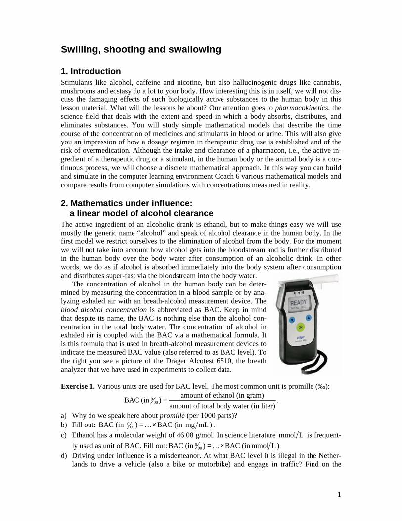
The concentration of alcohol in the human body can be deter-mined by measuring the concentration in a blood sample or by ana-lyzing exhaled air with an breath-alcohol measurement device. The blood alcohol concentration is abbreviated as BAC. Keep in mind that despite its name, the BAC is nothing else than the alcohol con-centration in the total body water. The concentration of alcohol in exhaled air is coupled with the BAC via a mathematical formula. It is this formula that is used in breath-alcohol measurement devices to indicate the measured BAC value (also referred to as BAC level). To the right you see a picture of the Dräger Alcotest 6510, the breath analyzer that we have used in experiments to collect data. Exercise 1. Various units are used for BAC level. The most common unit is promille (‰):

000

amount of ethanol (in gram)BAC (in )

amount of total body water (in liter)= .

a) Why do we speak here about promille (per 1000 parts)? b) Fill out: 0

00BAC (in ) BAC (in mg mL)= ×… .

c) Ethanol has a molecular weight of 46.08 g/mol. In science literature mmol L is frequent-

ly used as unit of BAC. Fill out: 000BAC (in ) BAC (in mmol L)= ×…

d) Driving under influence is a misdemeanor. At what BAC level it is illegal in the Nether-lands to drive a vehicle (also a bike or motorbike) and engage in traffic? Find on the

2

Internet at what BAC level the driving license of a drunken driver of a motor vehicle is confiscated?

The picture to the right suggests that the amount of alco-hol entering the human body when drinking a glass of beer is the same as the amount when drinking a glass of red wine or a glass containing a cocktail drink. The measure of capacity of a glass fits to the sort of drink. Beer is in a large glass, wine in a medium sized glass and gin in a small glass. In this way standard beer glass contains as much alcohol as a standard wine or a standard gin glass. Breezers are sold mostly in a bottle or a can. For a breezer there exists no standard glass. A Dutch standard glass in the catering industry for alcoholic drinks contains about 12 mL ethanol. The liquid density of alcohol at a temperature of 17 °C is equal to 0.792g mL. Use these data to answer the following questions: e) The volume of a standard glass of lager with an alcohol percentage of 5 % is equal to 25

cL. How many grams of alcohol contains a standard glass for this kind of beer? f) How many standard glasses are in a beer can of 33 cL with an alcohol percentage

of 5 %? g) Henceforth we assume that a standards glass contains by definition 10 gram

ethanol. Suppose that you buy a Bacardi Breezer with rum and fruit taste in a bottle with contents of 27.5 cL and an alcohol percentage of 5.6 %. How many grams of alcohol contains this bottle and with how many standard glasses is this equivalent?

h) The alcohol percentage of gin is 35 %. Compute the volume capacity of a standard gin glass.

We will build a simple mathematical model with which you can easily determine the BAC

level after consumption of alcoholic drinks and can predict the time course of the BAC level. Exercise 2. What factors could play a role in the maximal BAC level and in the time course of the BAC level? Always indicate whether you expect a variable to increase or decrease the maximal BAC level, and whether you expect it to speed up or slow down changes in alcohol concentration. Exercise 3. Assume that John, how unrealistic it may seem, drinks a whole beer bottle of size 75 cL containing Kasteelbier Blond, a beer of quadruple type with an extremely high alcohol percentage of 11 % and originating from the Belgian brewery of Honsebrouck, bottoms up, i.e., John empties the beer bottle in one draught. Also assume that the total amount of alcohol at a certain moment, say at time 0t = , is completely absorbed in the body. a) Compute how many grams of ethanol are assumed present in John’s body at 0t = . b) Suppose that John’s weight is equal to 80 kg and that the amount of body water (in liter) is

equal to 68 % of his weight (in kg). Compute the BAC level at 0t = . c) Suppose that John’s BAC level decrease 0,15 ‰ per hour. Fill out the BAC levels in the

table below:

t (in hours) 0 1 2 3 4 5 BAC (in ‰)

3

d) Let nC denote John’s BAC level after n hours ( 0,1,2,n = … ). Which phrase in the text in

corresponds with the recursive formula 1 βn nC C −= − and what value must be substituted

in the constant β ?

e) What direct formula for the blood alcohol concentration nC can you write down? Is this mathematical formula applicable for every integer value of n?

f) Suppose that you do not want to describe John’s BAC lever per hour, but per minute. Again, you could write the recursive formula 1 βt tC C −= − , but now with time t in minutes.

What value of the elimination rate β must you take for John? The BAC formula that you used in the previous exercise is based upon

t=0BAC BAC β t = β tD

V= − × − × ,

where the amount of alcohol consumed (in gram),

the volume of the body water into which the alcohol is absorbed and distributed (in liter),

β the elimination rate (in gram per liter per hour),

the time (

D

V

t

==== in hour) elapsed after consumption.

Note that the units used in the practical application do matter, in contrast with the usual approach in mathematics.

The Swedish physiologist Erik P. Widmark (1889-1945) pub-lished the above BAC formula in 1932 in a somewhat different form. He postulated that the volume of the total body water (in liter) is a fraction r of the body weight (in kilogram). Thus, the Widmark formula is:

BAC β tD

r G= − ×

× (2.1)

where G is the body weight (in kg) and r is called the Widmark factor (in L kg ). The Widmark factor is different for men and women. In general, women have more bones en fatty tissue, in which alcohol does not dissolve, so that for them the Widmark factor is lower. Reference values are:

0.68 0.085 L kg (men), 0.55 0.055 L kg (women),r r= ± = ± The elimination rate is also individual (for instance, different for men and women, different for occasional, social drinkers and alcoholics, age-dependent, and so on.) and it depends on circumstances (for example, drinking before or after a meal). Its value is between 0.10 and 0.20 1 1g L h− −⋅ ⋅ . The BAC formula exits for a long time and it is still used in forensic science and in ‘driving under the influence of alcohol’ trials in which expert witnesses are asked to extrapolate blood alcohol concentration at a previous time based on laboratory BAC results or to predict a BAC based on a particular drinking scenario. Exercise 4. What does 0.085 ±… mean in the formula 0.68 0.085 L kg (men)r = ± ? Exercise 5. In exercise 2 you have thought some factor that could play a role in the time course of blood alcohol concentration. Which of these factors do you encounter implicitly in the Widmark formula and which one(s) not?

4

Exercise 6. Many people use for alcohol usage in traffic the following rules of thumb: [1] One glass of some alcoholic beverage is eliminated from the human body in about 1 hour and [2] The maximum number of glasses of alcoholic drinks that you may consume and still be within legal limits is equal to two. Are these rules of thumbs in agreement with the Widmark formula? Exercise 7. In this exercise we will approach the Widmark formula in a different way. Let tC

be the blood alcohol concentration at time t. Now look a small time step t∆ further. Assume that the BAC decreases per time step with a fixed amount β. a) What is the relation between t tC +∆ and tC ?

b) Show that the difference quotient of tC in this mathematical model is equal to β− .

Exercise 8. Write down the Widmark formula for a person who consumed n standard glasses of some alcoholic beverage. Use in your formula the letter d for the amount of alcohol (in gram) in one standard glass. How could you adapt this formula if you want to take into account that it takes some time, say half an hour, before the alcohol is absorbed from the stomach into the total body water? Use your own version of the Widmark formula from exercise 8 in the next exercise. Exercise 9. John and Mary, who weigh both 75 kg, have something to celebrate and both drink in two hours time four glasses wine. What peak value of the blood alcohol concentration do you expect for each person, lacking more data? Exercise 10. Seidl, Jensen and Alt (2000) have investigated how the Widmark factor depends on height and weight of the person drinking alcohol. They found the following formula:

(men) 0.3161 0.004821 0.004632

(women) 0.3122 0.006446 0.004466

r W H

r W H

= − × + ×= − × + ×

(2.2)

where H is the body height (in cm) and H the body weight (in kg). From the most recent Dutch Growth Study (1997) we know that the average height and weight of a 21 year-old man of Dutch origin are 184.0 cm and 75.28 kg, respectively, and that the average height and weight of a 21 year-old woman of Dutch origin are 170.6 cm and 64.85 kg, respectively. a) What Widmark factors would follow for Dutch persons according to the three scientists

mentioned? b) Use the Widmark factors found in the previous item to compute after how many standard

glasses the average Dutch male and female person aged 21 years reach by alcohol consumption a blood alcohol concentration of 0.5 ‰?

c) Use a calculator, ‘normal body data’, and the Seidl formulas to make a reasonable case for the statement that a person drinking the same amount of alcohol reaches a lower peak value of BAC when his or her body weight would be larger.

We will now build a computer model with the modeling tool of Coach 6 for the Widmark

model and so a number of simulations to better understand the rime course of blood alcohol concentration and to investigate some drinking scenarios. We do not only carry out computer simulation for fun: we also compare results of computer simulations with experimental data collected in real experiments of alcohol consumption and evaluate the mathematical models.

Coach activity 11. The screen shot of a Coach 6 activity in Figure 1 shows on the left-hand side a table of measured BAC levels for a test subject after drinking 3 glasses of red wine in

5

one draught on an empty stomach early in the morning. Note: these are data measured in real-ity and not numbers that have been made up. The corresponding diagram to the right suggests that it takes indeed half an hour before the alcohol is absorbed and distributed in the body.

Figure 1. Table and graph of BAC measurements after drinking 3 glasses of red wine.

a) Open the corresponding Coach 6 activity and remove the data of the first half hour. b) The remaining data could lie on a straight line. Use the menu item Function Fit to find the

straight line that matches best the data points. Add this line to the diagram. c) What is the equation of the line found in part b)? d) What hypothetical BAC formula have you found with Function Fit? Is your answer in

agreement with the Widmark formula, combined with the Seidl formula (2.2), when you know that the test subject has a body weight of 85 kg and a height of 180 cm?

e) What elimination rate have you found with Function Fit and is this in agreement with reference values?

f) Save your work in a Coach 6 result file. Coach activity 12. The screen shot of a Coach 6 activity in Figure 2 shows on the left-hand side a graphical model for time course of BAC after alcohol consumption as described in the previous Coach activity . The computer model represents the following difference equation:

0BAC BAC β , BAC ,t t td

Dt

V+∆ = − × ∆ = (2.3)

where the amount of alcohol consumed (in gram),

the volume of the body water into which the alcohol is absorbed and distributed (in liter),

β the elimination rate (in gram per liter per hour),

the time (

D

V

t

==== in hour) elapsed after consumption.

In the graphical model you specify which quantities in the mathematical model play a role (distinguishing between parameters and state variables), how they depend on each other, which formulas for quantities are used and which values parameters have. The graphical model is automatically translated into a system of equations that is used in a computer -simulation, i.e., in running the model. In our model is the blood alcohol concentration a state variable that depends on time t. By default, the time variable does not explicitly appear in the graphical model, but only as icon in the icon bar. After clicking on this icon you can change the name and the unit of the time variable. The dose D of consumed alcohol, the volume of distribution dV and the elimination rate β are parameters in the model: the two handles on both sides of the circle in the parameter icon suggest that these variables have a constant value during a simulation (unless they are manually changed during a simulation

6

run). The initial concentration is the quotient of D and dV ; we have introduces the auxiliary variable BAC_0 for this purpose. The dashed arrow from BAC_0 to BAC indicates that this auxiliary variable is used to specify the concentration at time t = 0. The double arrow away from the state variable BAC with a pointed arrow in the middle represents the rate of change of BAC, so to say (a piece of) the difference quotient of BAC. An outgoing arrow means that the formula contributes negatively to the difference quotient. The rate of change of BAC is in our simple model equal to the elimination rate β .

Figure 2. Model and simulation of time course of BAC after drinking 3 glasses of red wine.

Now that you know how to interpret the Coach 6 model of Figure 2, you can try to build it yourself: a) Build the Coach 6 model of Figure 2, do a simulation and plot the computed BAC against

time. b) Even if you got in the previous part a straight line as graph of BAC versus time, the

diagram does not have to look like the right-hand side of Figure 2. To ensure that the graph hardly gets below the horizontal axis, you can specify in the model settings (stopwatch icon) a stop condition and choose a small time step. As stop condition you could choose: BAC 0≤ . In the same dialog window of model settings you can set the starting time of the model at half an hour. Adjust your model if necessary.

c) Import from the result file that you created in the previous Coach activity the measured BAC levels as background graph and try to find such model parameters that the straight line of your computer model matches well with the measurement data.

The assumptions used so far about absorption of alcohol in the human body are

unrealistic. Two assumptions that we have used until now were: 1. alcohol is immediately absorbed and distributed in the total body water upon intake; 2. absorption and distribution is delayed for half an hour after consumption of an alcoholic

drink, but after this half hour it is instantly present in the body fluids. Already somewhat better works the assumption that there is a certain time span 0T , say of 30

minutes, in which the at time 0t = consumed amount of alcohol gets into the systemic circulation of the human body with constant rate of absorption and is further distributed in the total body water. We will adapt the computer model of the previous Coach activity so that we can run the model starting from time 0t = on without being blushed with shame. Coach activity 13. a) Assuming an absorption and distribution of alcohol in the human body over the total body

water, which has a volume of distribution dV , with constant speed during a time span 0T

after consumption of a certain amount D of alcohol, what must be this speed in the model during this time interval?

7

b) What is actually the corresponding difference equation if you adapt the Widmark model? c) Have a look again at the Widmark model implemented in Coach 6 for drinking 3 standard

glasses of red wine in one draught, early in the morning on an empty stomach. But now specify in the graphical computer model the absorption of the alcohol into the systemic circulation of the human body via a short period (30 minutes) of absorption and distribu-tion at constant speed.

So you need in Coach 6 a function that takes some constant value during some time interval and is equal to zero elsewhere. Such a function exists in Coach 6 and is called Pulse. The graph of Pulse(x; b; l; h) as a function of x (Note: Coach uses semicolons to separate arguments of functions) looks as follows:

Figure 3. Graph of the Coach function Pulse(x; b; l; h).

Use this function to build your new model. Hereafter import the measured BAC levels from the result file that you created in Coach activity 11 as a background graph and try to find suitable model parameters so that your computer model matches rather well with the measured data.

d) Although the absorption and distribution of alcohol in the human body is already better described in this new model, there remains one big shortcoming of this model concerning the absorption and distribution. By looking at your computed BAC curve, have you any idea what shortcoming it could be?

Next you will model the results of an experiment in which a test subject emptied eight

glasses of red wine, each glass with an estimated amount of 14 gram alcohol, in one draught every half hour. For the specification of the absorption and distribution of alcohol in the human body you can do this similarly to the work in the previous Coach activity, on the understanding that the RepeatedPulse function in Coach is very useful now. The graph of RepeatedPulse(x; b; l; i; h) as a function of x looks as follows:

Figure 4. Graph of the Coach function RepeatedPulse(x; b; l; i; h).

Coach activity 14. a) Adapt your Coach model from the previous activity to the experiment of a test subject

emptying at regular intervals a glass of some alcoholic drink in one draught. Introduce as new parameters in your model the number of glasses emptied and the time interval between consecutive drinks.

b) Import from the Coach 6 result file that belongs to the experiment with 8 glasses of wine the measured BAC levels as background graph and try to find such model parameters that your computed BAC curve matches reasonably well with the measurement data. Ensure at least that the results computed in your model and the measured BAC levels after drinking the final glass match well. The screen shot below may inspire you:

8

Figure 5. Screen shot of the Widmark computer model for regular consumption of 8 alcoholic drinks, with measured BAC levels in the background graph.

c) Watson et al. (1980) have refined the Widmark formula concerning the amount of total body water in the human body. They have taken age, body weight and body height into account for the determination of the volume of distribution. They have presented the following formulas amongst others:

0.8 (men) 0.3626 0.1183 20.03,

0.8 (women) 0.2549 14.46,d

d

V W AGE

V W

× = × − × +× = × +

(2.4)

where W is the body weight in kg and AGE is the age in years. Adapt the model built in part b) to the usage of the Watson formulas for the volume of distribution dV . In order to

compare the measured BAC level with computer simulations, you must know that the test subject was a 49 years old man.

d) Use the model of part c) to simulate the time course of BAC for some drinking scenarios: [1] Consuming the same amount of alcoholic drinks but with sort or longer time intervals

between drinks. [2] Drinking at a slower pace: 16 drinks every quarter of an hour but also with half of the

amount per drink [3] Use another drinking scenario that interests you.

3. Painless mathematics: exponential model of the elimination of pain-alleviating drugs The way a substance is administered to the human body plays an important role in pharmaco-kinetics. For example, the pain-alleviating drug morphine can be administered via various routes to a patient: orally, sublingually, or rectally (via a tablet or capsule), via injections (subcutaneous, intramuscular or venous) or via an infusion. This has consequences for absorption, distribution, and effect of the substance in the body. In an oral administration of morphine this substance must first pass the liver, but this organ lets only a fraction pass to the systemic circulation of the human body. In other words, the biological availability at oral administration of morphine is small (about 40 %), certainly in comparison with intravenous bolus administration, i.e., a rapid intravenous injection, which has a biological availability of almost 100 %. Figure 6 illustrates another example: de route how cocaine is used plays a big role in the time course of the concentration of the active substance in the blood plasma. By taking a shot and by smoking a high peak value of the plasma concentration is already reached after a few minutes, whereas oral administration only leads to an increase of plasma concentration after half an hour and the peak value is sometimes reached only after one hour.

9

Figure 6. Time course of plasma levels of cocaine after various routes of administration.

In this section we will study a simple pharmacokinetic model for a single intravenous bolus injection of a pain-alleviating drug. We do this amongst other things on the basis of data obtained in a clinical study (Camu et al., 1982) about the pharmacokinetics of alfentanil, a morphine-like painkiller and analgesic developed and produced by Janssen Pharmaceutica. Figure 7 shows the table and the graph of the mean plasma levels measured in the tests subjects in this study, who were given 120 µg alfentanil per body weight (in kg) as bolus in 30 seconds into an antecubital vein. In Figure 7 is also shown a rather successful regression curve of the plasma levels. How we obtained such a nice mathematical description of the measured data will be revealed in this section.

Figure 7. Plasma level (C) after a bolus injection of alfentanil and a regression curve.

Let ( )C t be the plasma concentration of a drug at time t after the drug was rapidly injected into a vein and was rapidly distributed in the systemic circulation, so fast that we may assume that at time 0t = the maximum plasma concentration of the drug has already been reached. Hereafter we measure the plasma level at regular times 0, ,2 ,3 ,t h h h= … , with fixed time

interval h. Let nC be the measured plasma level of the drug after n time intervals. We assume

that the rate of change with which the plasma level decreases in a certain time interval is proportional to the plasma level at the beginning of the particular time interval:

1n nn

C Ck C

h+ − = − ⋅ (3.1)

We speak of first-order kinetics with elimination rate k. It holds:

( )0 1n

nC C k h= ⋅ − ⋅ (3.2)

10

Exercise 15. Verify the correctness of formula 3.2. We rewrite formula 3.2:

( ) ( ) ( )1 1

0 01 1n h

n hh hC n h C k h C k h

⋅⋅ ⋅ ⋅ = ⋅ − ⋅ = ⋅ − ⋅

(3.3)

The reason to rewrite the formula in this form (3.3) will become clear in the next exercise. Exercise 16. a) Take 1k = and check with a graphical calculator that for small values of h the expression

1

(1 )hh− takes a value that is close to the number 0.3678794412. b) Take 2k = and check with a graphical calculator that for small values of h the expression

1

(1 2 )hh− ( )1

1 2 hh− takes a value that is close to the number 0.1353352832.

c) Take 0.5k = and check with a graphical calculator that for small values of h the expression

( )1

1 0.5 hh− ⋅ takes a value that is close to the number 0.6065306597.

d) Take 1k = − and check with a graphical calculator that for small values of h the expression 1

(1 )hh+ takes a value that is close to the number 2.718281828.

Thus, for small h it holds that 1

(1 )hk h− ⋅ can be taken equal to some number g and that formula 3.3 can be rewritten as ( ) 0 ,tC t C g= ⋅ (3.4)

for a certain number g and times t take from the sequence 0, ,2 ,3 ,h h h… . But then we can use this formula also for any value of time t. For positive k it holds that 0 1g< < . So it is a matter

of exponential decay of the plasma level, where g is the growth factor per time unit and 0C is

the initial plasma level. There exists a relation between the growth factor g and the elimi-nation rate k. Without proof or motivation we postulate that kg e−= (3.5) and ( )lnk g= − , (3.6)

where ln is a function called the natural logarithm and e 2,718281828≈ is called the base of the natural logarithm. The natural logarithm is a mathematical function that is available on your graphical calculator, just like the exponential function xe . Coach activity 17. Equation 3.1 for the plasma level of a drug that is administered at time 0t = as an IV bolus injection can be rewritten with a time stept△ as follows: ( ) ( )( )C t t C t k C t t+ − = − ⋅ ⋅△ △ (3.7)

for 0, , 2 , 3 ,t t t t= △ △ △ …

11

a) Build a Coach model for this mathematical model and use it to compute plasma levels during10 minutes, taking 1t∆ = as time step, 10,5mink −= for the elimination rate and the

initial concentration 0 10 mg LC = (immediately after administration of the drug). Plot the time course of the computed concentration.

b) Check in the equations mode that the generated computer program corresponds with the difference equation 3.7.

c) Decrease the time step to 0.1t∆ = and let the computed concentration be stored during the simulation after every 10 time steps. The graph of the time course of the computed concentration differs from the one found in part a). How can you explain this?

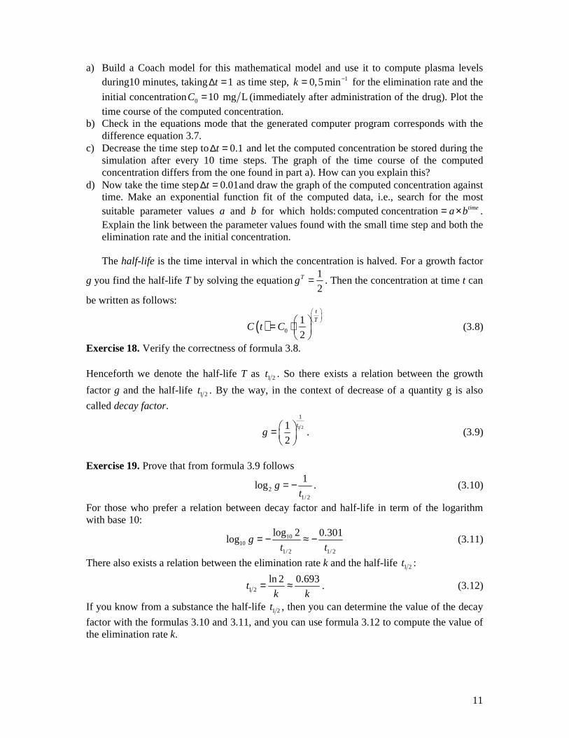
d) Now take the time step 0.01t∆ = and draw the graph of the computed concentration against time. Make an exponential function fit of the computed data, i.e., search for the most suitable parameter values a and b for which holds: computed concentration timea b= × . Explain the link between the parameter values found with the small time step and both the elimination rate and the initial concentration. The half-life is the time interval in which the concentration is halved. For a growth factor

g you find the half-life T by solving the equation1

2Tg = . Then the concentration at time t can

be written as follows:

( ) 0

1

2

t

TC t C

= ⋅

(3.8)

Exercise 18. Verify the correctness of formula 3.8. Henceforth we denote the half-life T as 1 2t . So there exists a relation between the growth

factor g and the half-life 1 2t . By the way, in the context of decrease of a quantity g is also

called decay factor.

1 2

1

1

2

tg =

. (3.9)

Exercise 19. Prove that from formula 3.9 follows

21/ 2

1log g

t= − . (3.10)

For those who prefer a relation between decay factor and half-life in term of the logarithm with base 10:

1010

1/ 2 1/ 2

log 2 0.301log g

t t= − ≈ − (3.11)

There also exists a relation between the elimination rate k and the half-life 1 2t :

1 2

ln 2 0.693t

k k= ≈ . (3.12)

If you know from a substance the half-life 1 2t , then you can determine the value of the decay

factor with the formulas 3.10 and 3.11, and you can use formula 3.12 to compute the value of the elimination rate k.

12

Sir James Black, the scientist who invented propranolol. In 1988 he won the Nobel prize of Medicine for this achieve-ment, but even more for his pioneering work in pharma-cology that lead to the basic principles of the science field. See also (Stapleton, 1997).

Coach activity 20. Propranolol is a beta-blocker this is used amongst other this to reduce blood pressure. Open the Coach activity in which data from a study about plasma concentrations after intravenous administration of propra-nolol (Fagan et al., 1982) have already been tabulated. The test subject was a health young man with a body weight of 82 kg, who get a dose of 4.1 mg administered via intra-venous infusion with an infusion rate of 1 mg/min. We set time = 0 for the moment when the administration of propra-nolol stops and we investigate the following data measured during some hours:

time C h µg/L 1 8.25 2 6.46 3 4.63 4 4.03 6 2.11 8 1.41

a) Make a diagram window in which the plasma level C is plotted against time and save what you have now in a result file (to be used in Coach activity 21).

b) Make a function fit that matches a model of exponential decay (Hint: in Coach, this function fit is offered via the function type f(x)=ab^x+c. Let Coach first make an estimate of the parameter values and hereafter refine the intermediate result. Next set the coefficient c to 0 and place the checkmark to indicate that this parameter may not change anymore but has to stay fixed in any further refinement. In this way you get the best function fit of the form f(x)=ab^x. The screen shot below shows that the function fit, also known as regression curve, matches well with the measured data and that the concentra-tion gets close to zero only after 24 hours.

c) Read from the Create/Edit dialog of a table or diagram window the mathematical formula

of the regression curve and determine the decay factor per hour and the initial concentra-tion of propranolol.

d) Compute the half-life propranolol with a graphical or scientific calculator. Is your value in agreement with the literature value of 2.8 h (Evans et al. 1973)?

e) Coach 6 has not yet a graphics option for logarithmic scaling of axes. But as an alternative for logarithmic paper you can draw the graph of the logarithm of a quantity: 10log is de-

13

noted in Coach 6 as log. Make a new table and graph of the logarithm (with base 10) of the plasma level versus time.

f) Determine the best straight line fit of 10log C plotted against time.

g) The directional coefficient of the previously found straight line is equal to 10log g . Use formula 3.11 and your calculator to compute the half-life. Is your value in agreement with the value found in part d of the activity?

h) The straight-line regression curve of 10log C intersects the y-axis in 1.027y ≈ (check!).

Use this value to compute with your calculator the initial concentration of propranonol. Is your value in agreement with the value found in part c of the activity?

i) 4.1 mg propranolol has been administered to the test subject. Suppose that this person has 5 liter blood. What initial concentration of propranolol do you then expect in the systemic circulation? Suppose that the concentration of propranolol in the blood is equal to 85 % the concentration of propranolol in the blood plasma, what value of the plasma level (in µg/L) would you expect immediately after the administration of the drug has stopped, under the assumption that no distribution in body water or tissues and no elimination takes place during administration of the drug?

In the last two parts of the previous Coach activity a big contradiction seems to pop up:

the plasma level of the pharmacon seems to deviate substantially from the concentration that can be computed from a realistic estimate of the amount of blood in which the substance circulates. Like in the case of alcohol metabolism, you must realize that a pharmacon after being absorbed into the systemic circulation is further distributed in the human body, for instance in the total body water, in the fatty tissues, or in complexes formed with tissue proteins. Thus, the volume in which the pharmacon is distributed, the volume of distribution, is much larger than that of the systemic circulation alone. The volume of distribution is the apparent volume dV of the bodily compartment in which the pharmacon is distributed such

that the initial concentration0C of the pharmacon in the sampling compartment (in most cases

the blood plasma) for a given dose D can be computed by

0d

DC

V= . (3.13)

Pharmacologists also speak about the volume of distribution as the volume of the central compartment that would be required to provide the observed dilution of the loading dose of a pharmacon. The model that they use then is called in their jargon an open, one-compartment model and is symbolized by the following picture:

Figure 7. Graphical representation of an open one-compartment model.

This picture resembles the graphical computer model in Figure 8. Coach activity 21. a) Build the Coach 6 model of Figure 8, do a simulation run and plot the computed concen-

tration against time. Try to preselect parameter values that correspond with the time cour-se of the propranolol concentration described in the previous Coach activity.

14

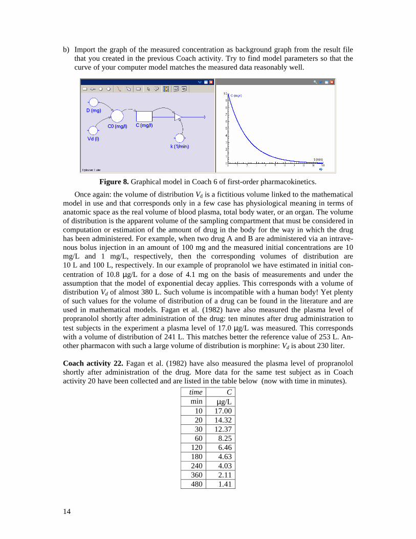
b) Import the graph of the measured concentration as background graph from the result file that you created in the previous Coach activity. Try to find model parameters so that the curve of your computer model matches the measured data reasonably well.

Figure 8. Graphical model in Coach 6 of first-order pharmacokinetics.

Once again: the volume of distribution Vd is a fictitious volume linked to the mathematical model in use and that corresponds only in a few case has physiological meaning in terms of anatomic space as the real volume of blood plasma, total body water, or an organ. The volume of distribution is the apparent volume of the sampling compartment that must be considered in computation or estimation of the amount of drug in the body for the way in which the drug has been administered. For example, when two drug A and B are administered via an intrave-nous bolus injection in an amount of 100 mg and the measured initial concentrations are 10 mg/L and 1 mg/L, respectively, then the corresponding volumes of distribution are 10 L and 100 L, respectively. In our example of propranolol we have estimated in initial con-centration of 10.8 µg/L for a dose of 4.1 mg on the basis of measurements and under the assumption that the model of exponential decay applies. This corresponds with a volume of distribution Vd of almost 380 L. Such volume is incompatible with a human body! Yet plenty of such values for the volume of distribution of a drug can be found in the literature and are used in mathematical models. Fagan et al. (1982) have also measured the plasma level of propranolol shortly after administration of the drug: ten minutes after drug administration to test subjects in the experiment a plasma level of 17.0 µg/L was measured. This corresponds with a volume of distribution of 241 L. This matches better the reference value of 253 L. An-other pharmacon with such a large volume of distribution is morphine: Vd is about 230 liter. Coach activity 22. Fagan et al. (1982) have also measured the plasma level of propranolol shortly after administration of the drug. More data for the same test subject as in Coach activity 20 have been collected and are listed in the table below (now with time in minutes).

time C min µg/L

10 17.00 20 14.32 30 12.37 60 8.25

120 6.46 180 4.63 240 4.03 360 2.11 480 1.41

15

Open the corresponding Coach activity. a) Make a diagram window in which the plasma level C is plotted against time. b) Zoom in on the time interval between 60 and 480 minutes. Make a function fit that

matches a model of exponential decay for the data you are currently looking at. c) Read from the Create/Edit dialog of a table or diagram window the mathematical formula

of the regression curve and determine the decay factor per minute. d) Is your result in part c in agreement with the decay factor per hour, that you determined

Coach activity 20 c. e) Zoom out to the whole dataset: You see that the exponential model does not match well

with the dataset as a whole. Try to make a function fit that matches a model of exponential decay for the whole dataset (do not add the graph to the diagram). You will notice that this does not work well.

f) Make a new table and graph of the logarithm (with base 10) of the plasma level versus time. How can you see from this graph that the exponential decay model for the time course of the plasma level after 10 minutes does not work well?

g) A mathematical model that describes better the time course of the plasma level for the whole time interval in which data have been collected is a so-called biexponential model. The time course of the plasma level is then not described with one exponential function,

but with two function of this kind: ( ) ( )1 1 2 2

time timeC A g A g= × + × . Often you can find suit-

able parameter values via the method of peeling functions (also known as ‘curve strip-ping’). The steps are the following: [1] For large values of time (after 1 hour in our case) the concentration decays exponen-

tially. Determine for this time interval the decay factor g2 and the constant A2. [2] Substract the regression curve found in step [1] from the measured values. This yields

a second dataset of residuals, with the contribution of the exponential decay removed. [3] The dataset of residuals found in step [2] can on its turn be fitted to an exponential

decay model. This yields the decay factor g1 and constant A1. Try to make the biexponential model for the time course of the plasma level after intrave-nous drug administration based on your intermediate result of part c in this activity. In the previous Coach activity we have seen that the biexponential model for the time

course of a drug after an intravenous bolus injection describes the elimination of the drug better than the exponential decay model. The biexponential function 1 1 2 2( ) t tC t A g A g= × + × , (3.14)

where g1 are g2 decay factors, actually describes two processes: (1) the distribution of the pharmacon from the systemic circulation into the tissue compartment or peripheral compartment and backwards (at a fast rate, thus small value of g1) and (2) the elimination of the drug from the body (slowly, thus g2 greater than g1), after the distribution of the drug in the body has been settled. You can also consider it as a model that consists of two compartments between which ex-change of the drug takes places (see the figure to the right; parameters k12 and k21 determine the drug ex-change). In this lesson material we will not pursue this further, but many-compartment models can easily be implemented in Coach 6.

16

Coach activity 23. Cannabis is more and more applied for therapeutic reasons and in particular for pain alleviation. The active substance is also known as THC. Open the corresponding Coach activity in which the data used in a study about elimination of THC from the human body (Näf, 2004) have already been tabulated. It concerns the time course of the plasma level of THC for test subjects who got a dose via intravenous administration (to be precise, 0.053 µg THC per kg body weight).1

time C min ng/mL

5 271.5 10 95.6 20 38.3 60 20.1

120 9.0 240 5.0 480 0.9

a) Build a Coach model for the biexponential model of the time course of the plasma level of THC that matches well with the measured dataset. First describe the time course of the plasma level after 20 minutes with an exponential decay model and hereafter take the first two data point into account in the modeling process.

b) Compute the half-life of each of the two phases in the elimination process (distribution, clearance) and compare your answers with those of the researcher: 2.47 and 54.0 minutes.

Scientists do not confine to exponential and biexponential models. In pharmacokinetical

studies they often make use of a triexponential model for the time course of the plasma level of a pharmacon after intravenous administration, too. The tri-exponential function 1 1 2 2 3 3( ) t t tC t A g A g A g= × + × + × , (3.15)

where g1, g2 en g3 are decay factors, actually describes three processes: (1) a fast distribution of the pharmacon from the systemic circulation into the peripheral compartment (leading to a rapid decay, thus small g1), (2) elimination (a slow decay, so g2 is greater than g1) when the distribution of the pharmacon in the body is in near equilibrium, and (3) a slow rate-determining exchange of the pharmacon between a deep tissue compartment and the central compartment (leading to a very slow decay, thus g3 greater than g2). So, the mathematical model consists of three compartments between which there is continuously an exchange of the pharmacon: see the figure to the right, in which the parameters k12 and k21 determine the exchange of the drug between the central compartment and the ‘rapid’ tissue compartment, and in which parame-ters k13 and k31 determine the exchange of the drug between the central compartment and the ‘slow’ deep tissue compartment. Such a model is for example quite often used in pharmacokinetic studies of anesthesia and pain-alleviating drugs. It is the last term in the triexponential function that is causing the effect that a pharmacon long after administration has stopped is still available in low

1 The last two data have been estimated from a graph in the research report.

17

concentration in the human body through delivery from the deep tissue compartment. This may explain the prolonged side effects of anesthesia that some patients experience. In the next Coach activity you can apply the triexponential model to intravenous administration of the painkiller Alfentanil and compare your results with those found by researchers. Coach activity 24. Open the corresponding Coach activity in which the data used in a study about elimination of alfentanil from the human body (Camu et al., 1992) have already been tabulated.

time C min ng/mL

2 565.0 5 399.0

10 302.0 15 229.0 30 145.0 45 106.0 60 81.3 90 48.7

120 43.8 180 26.8 240 17.7 300 12.4

a) Make a diagram window in which the plasma level C is plotted against time. b) Make a second window with the logarithm of C, i.e., 10log C , plotted against time.

c) In the graph of 10log C versus time you can recognize the three phases of the triexponential

model because the time interval can be split into three pieces for which the data points each seem to lie on a straight line. Which pieces in the time domain can you choose best for this purpose?

d) Select the piece of the time domain that corresponds with the last part of the alfentanil elimination from the body and find the best straight-line fit. The directional coefficient of this line is equal to the logarithm of the corresponding decay factor. Read from the Create/Edit dialog of the diagram window the value of 10 3log g and compute then the value of g3.

e) Compute the half-life of the last part of the elimination of alfentanil and compare your answer with the literature value of 94 ± 38 min.

f) Select the same piece of the time domain as in part d and fit an exponential model for the data points in this time interval. What decay factor do you find in this way and is your answer in agreement with the value determined in part d.

g) Subtract the exponential function that describes the last part of the elimination phase from the measured concentration. Fit an exponential model for the next part of the time domain that you determined in part c and determine the decay factor g2.

h) Peel the second exponential function from the intermediate result and determine the third exponential function in the triexponential model. What value of the decay factor g1 have you found?

i) Plot the graph of your triexponential model in the diagram with the measured data points. j) Compute with a graphical or scientific calculator the half-lives that correspond with g1,

g2, and g3, and compare them with the literature values 3.5 ± 1.3 min, 16.8± 6.4 min en 94 ± 38 min.

18

We return to the exponential model of the elimination of a pharmacon after an intravenous bolus injection in order to discuss more pharmacokinetic indicators. You encountered already the terms volume of distribution Vd, elimination rate k, growth factor and decay factor g, half-life t1/2, and biological availability (often denoted with the character F). Two important indi-cators that are still missing are clearance (Cl) and area under the curve (AUC). These phar-macokinetic indicators for drugs can be found in information texts that are registered by organization like the Dutch ‘College ter Beoordeling van Geneesmiddelen’ and the United States Food and Drug Administration (FDA); See for example the websites www.cbg-meb.nl, www.geneesmiddelenrepertorium.nl, www.fda.gov, www.druglib.com, and www.drugs.com. Also Wikipedia contains such information for many substances.With the pharmacokinetic properties of a drug you can in principle compute plasma level-time curves and you are pre-pared to determine dosage regimens.

The total body clearance of a pharmacon, in short clearance and denoted as Cl, is defined as the ratio of the amount of pharmacon eliminated from the body per time unit and the plasma level C. So, the unit van clearance is volume per time unit (L/h, mL/min, etc.), but clearance is often tabulated as the volume per time unit per 70 kg body weight. In terms of decay of the amount Dt of the pharmacon in the human body clearance can be described as

CltDC

t− = ×△

△

. (3.16)

For an exponential model of the time course of the plasma level after intravenous bolus injec-tion holds (see formula 3.7):

C

k Ct

= − ×△

△

. (3.17)

The ratio of the amount Dt of the pharmacon present in the body and the plasma level C is by definition equal to the volume of distribution Vd. Thus formula (3.16) can be rewritten as

1

Cld

CC

V t× = − ×△

△

. (3.18)

For an open one-compartment model with first-order elimination kinetics the clearance can then be determined via: Cl dk V= × , (3.19)

where k is the elimination rate. This formula c be rewritten, using formula 3.12, in terms of half-life t1/2:

1 2 1 2

ln 2 0,693Cl d dV V

t t

×= ≈ . (3.20)

The total body clearance is a measure for the speed with which a pharmacon is removed form the human body. How this process takes place does not play a role. In case one wants to include the elimination routes, one distinguished in general drug excretion in the urine via the kidneys (renal clearance) and biotransformation via the level followed by excretion in the bile (hepatic clearance)

The mathematical model of the time course of the plasma level plays an important role in formula 3.19. For the open one-compartment model after an intravenous bolus injection one can prove that the area under the plasma level-time curve for an infinitely long process, abbre-

viated with AUC, is equal to d

D

k V×. This relation between AUC, dose D and clearance Cl is a

special case of the following relationship that we can apply for any form of drug administra-tion:

AUCCl

F D×= , (3.21)

19

where F is the bioavailability of the drug (F = 1 for intravenous bolus administration), D is the administered dose and Cl represents the clearance. For first-order elimination kinetics you can write this as

AUCd

F D

k V

×=×

. (3.22)

The last formula can also be used to determine the bioavailability of a drug for any form of administration. For example for oral administration, compare the area under the curve in an oral administration with the AUC after intravenous bolus administration of the same dose:

, i.v.oraaloraal

i.v. , oraal

AUC

AUCd

d

VF

V= × . (3.23)

Of course you cannot measure plasma level for an infinite amount of time to determine the AUC. In first-order elimination kinetics you can estimate the AUC by the area under the measured plasma level-time curve and add to this the quotient of the last measured plasma level and the elimination rate.

In the below exercises and Coach activities we assume an open one-compartment model with fist-order elimination kinetics. Or stated differently, we assume an exponential model after intravenous bolus administration.

Exercise 25. Suppose that an 80-kg person is given a single intravenous bolus injection of a drug at a dose of 60 mg. The volume of distribution of the drug is equal to 100 liter / 70 kg body weight and the clearance is equal to 775 ml / min / 70 kg body weight a) Compute the elimination rate (in min-1). b) Compute the half-life (in hr). c) Compute the plasma level (in ng / mL) after six hours. d) What will happen if an alternative drug with the same volume of distribution is given at

the same dose, but the clearance of the new drug is larger? What will happen with the initial concentration and the half-life?

e) What will happen if an alternative drug with the same clearance is given at the same dose, but the volume of distribution of the new drug is smaller? What will happen with the initial concentration and the half-life?

Coach activity 26. Open the corresponding Coach activity in which the dataset used in a study about the time course of the serum concentration of the antibiotic drug ceftazidime (Demotes-Mainard et al., 1993) has already been tabulated. Each patient in this study suffered from chronical renal insufficiency and was given 1 gram via intravenous administration. On the basis of the measurements you will determine with Coach and a graphical or scientific calculator some pharmacokinetic indicators and you will set up a simple dosage regimen.

time C h mg/L

1 50 2 45 4 38

24 21 36 14 48 11 60 8 72 4

20

a) Make a diagram window in which the serum level C is plotted against time and save what you have until now in a result file (to be used in Coach activity 27).

b) Determine the decay factor g per hour. c) Determine the elimination rate k (in h-1). d) Determine the half-life t1/2 (in hours). e) Use the computer model to estimate the serum concentration immediately after the injec-

tion has been given. f) Estimate the area under the curve (AUC in mg·L-1·h). g) Determine the clearance Cl (in L/h). h) Determine the volume of distribution Vd (in L). i) Suppose that the threshold value for drug activity is equal to 10 mg/L. After how many

hours must the next doe be administered according to your model? j) After 24 hour the serum concentration is according to the measurements equal to 21 mg/L.

Suppose that you administer the drug intravenously at the double dose (2 g), how long will it take according to your model before the serum concentration has decreased to the value of 21 mg/L?

Coach activity 27. a) Build the Coach 6 model of Figure 9, do a simulation run and plot the computed concen-

tration against time. Try to preselect parameter values that correspond with the time cour-se of the ceftazidime concentration described in the previous Coach activity.

b) Import the graph of the measured concentration as background graph from the result file that you created in the previous Coach activity. Try to find model parameters so that the curve of your computer model matches the measured data reasonably well.

Figure 9. Graphical model of first-order elimination pharmacokinetics of ceftazidime.

4. Painless mathematics: a model of repeated intravenous administration

Instead of a single intravenous bolus injection of a drug that is rapidly distributed in the human body, we will investigate in this section the effect of multiple doses of a drug. We consider a series of bolus injections with the same dose and administered in regular time intervals. Henceforth we denote the dosing interval as τ.

Let us first simulate a practical case in Coach 6: administration of intravenous bolus injec-tions of ceftazidime in a regular multiple-dosage regimen to patients who suffer from renal insufficiency. The next two Coach functions can make the implementation of the regular

21

dosing interval in the computer model easier: Pulse and RepeatedPulse. Pulse is a function that takes a fixed value during a certain interval and is equal to zero elsewhere. The graph of Pulse(x; b; l; h) as a function of x (Note: Coach uses semicolons to separate arguments of functions) looks as follows:

Figure 10. Graph of the Coach function Pulse(x; b; l; h).

The graph of RepeatedPulse(x; b; l; i; h) as a function of x looks as follows:

Figure 11. Graph of the Coach function RepeatedPulse(x; b; l; i; h).

Coach activity 28. a) Build the Coach 6 model of Figure 9, in case you have not done yet the corresponding

activity, and do a simulation run using the following realistic parameter values for cefta-zidime: D = 1000 mg, Vd = 20.6 L and k = 0.0337 h-1.

b) Adapt your model so that it mimics the one in Figure 12 and do a simulation run with a dosing interval τ equal to 24 hours. Take the number of bolus injections equal to 10 and plot the serum level-time graph for 300 hours. The instantaneous increase of serum level after each intravenous bolus administration is implemented via the RepeatedPulse function and the drug administration is brought to a stop via a conditional program structure. The computer code that does the job (in case the time step dt is small enough) looks as follows:

If t >= (number_of_injections-1)*tau Then intake_rate := 0 Else intake_rate := RepeatedPulse(t; -dt; dt; tau; C0/dt) EndIf

Figure 12. Graphical model of repeated intravenous administration of ceftazidime.

Answer the next questions by using the simulation tool in the menu of the model window.

22

c) What do you notice in the serum level-time graph? d) What happens when you halve the dosing interval τ ? e) What happens when you double the dosing interval τ ? f) What happens when you choose the dosing interval τ equal to the half-life t1/2? g) What happens when you start with an initial concentration of 100 mg/L? (for example,

because you change the dosage regimen.) h) How would the serum-level-time curve look like if the 3rd bolus injection is forgotten and

compensated by a double dose in the 4th injection?

Figure 12 illustrates that with a repeated administration of a pharmacon, with equal doses given at equal time intervals, the blood concentration fluctuates after some time between two levels, the so-called peak level and trough level. What a physician often wants to achieve at prescription of a medicine is that o the peak level remains under the minimum toxic concentration (MTC), o the trough level is above the minimum effective concentration (MEC, a threshold level for

drug activity), and that o the therapeutic window (range of concentration between MEC and MTC) is reached as

fast as possible. Mathematical models can help to find the best dosage regimen. The following exercises will illustrate this. Exercise 29. Let us look at a theoretical example in which we can easily compute the change of drug concentrations. Let us assume that the dosing interval is equal to the half-life of the pharmacon, i.e., 1 2τ t= . Let nC be the plasma level immediately after administration of the

( )th1n + intravenous bolus injection and the rapid distribution of the pharmacon in the body.

The dose that is given with each injection is assumed to have the effect that the plasma level is increased with the initial concentration C0.

a) Verify that 1 0

3

2C C= and 2 0

7

4C C= .

b) Explain that that the concentration1nC + depends in the following way on the value of nC :

1 0

1

2n nC C C+ = + , for all n.

c) What is the plasma level after 5 doses?

d) Prove:2

0

1 1 11

2 2 2

n

nC C = + + + +

⋯

e) Prove: 0

12

2

n

nC C = −

.

f) For large value of n the plasma level fluctuates between a minimum and maximum level in the period between two doses. Which trough and peak level do we mean here?

Let us now look at the general case. Exercise 30. We take an arbitrarily selected value for the dosing interval τ and we use the exponential model with decay factor g for the drug elimination. We define τf g= . Again, nC

is the plasma level immediately after administration of the( )th1n + intravenous bolus injection.

23

a) Verify that ( )1 0 1C C f= + and ( )22 0 1C C f f= + + .

b) Explain that that the concentration1nC + depends in the following way on the value of nC :

1 0n nC f C C+ = ⋅ + , for all n.

c) Prove: ( )20 1 n

nC C f f f= + + + +⋯ .

d) Prove:1

0

1

1

n

n

fC C

f

+−= ⋅−

.

e) In the limit case of an infinite number of doses the blood concentration reaches a range in which it fluctuates between two levels, the so-called peak level and trough level, in the period between consecutive doses. Determine explicit mathematical formulas for these concentrations? We denote the peak level as maxC and the trough level as minC .

f) Suppose that the first given dose is chosen such that the plasma level at time 0t = is immediately equal tomaxC . Prove that the plasma level immediately after each injection is

equal to maxC . This suggests that for any initial blood concentration a so-called steady state

is reached. g) Prove that during steady state the following holds:

1 2

τ

max

min

2tC

C

= (4.1)

h) What happens with the fluctuations in the concentration when the dosing interval is de-creased?

The logarithmic mean2 of the peak and trough level in steady state is called the steady

state concentration Css. It can be proved mathematically that the steady state concentration is equal to the mean plasma level in a doing interval during steady state and that the steady state concentration can be determined by the following formula:

τ Clss

DC =

⋅, (4.2)

where D is the dose of the pharmacon given per intravenous bolus injection, τ is the dosing interval, and Cl is the clearance of the pharmacon. From this formula is immediately clear that the steady state concentration is doubled when you double the dose D or halve the dosing interval. The time at which steady state is reached is about 4 or 5 half-lives and does not depend on the dosage or the dosing frequency.

Formula (4.1) enables us to estimate the maximum dosing interval τmax for a pharmacon of which the therapeutic window, i.e., MTC and MEC, is known:

max

1 2

τ

max

min

2tCMTC

MEC C

≥ = ,

or in other words

10

max 1 210

logτ

log 2

MTC

MECt

= ⋅ (4.3)

τmax is the maximum dosing interval for which the drug concentration stays within the therapeutic window, but the dosage regimen may not be practical with real patients. Dosing

2 The logarithmic mean of two values A and B is defined as( ) ( )lnB A B A−

24

frequencies are often once a day, twice a day, or three times per day, and then only during daytime, perhaps around meals, to minimize the inconvenience for patients. Exercise 31. A new medicine in this exercise has a volume of distribution 41.7 LdV = , body

clearance Cl 3.4L / h= , and a therapeutic window of 10-20 mg/L . a) Estimate the steady state concentration on the basis of the therapeutic window in.

b) Determine the dosing speedτ

D necessary to reach the steady state concentration of part a.

c) Estimate what maximum dosing interval τ is allowed. d) What is according to you a dosing frequency that works in practice and what is then the

required dosage? e) Compute the peak and trough level that corresponds with this dosing frequency and dose. f) What initial dose must be given so that the steady state is immediately reached?

5. Painless mathematics: a model of intravenous infusion

Coach activity 32. In Exercise 31 you have investigated the pharma-cokinetics of a new medicine that is administered via repeated intravenous bolus injections. Pharmacokinetic parameters were: volume of distribution 41LdV = , clearance Cl 3.4L / h= , and a therapeutic window of 10-20

mg/L. From these data you have computed the steady state concentration and hopefully found that it is equal to 14.4 mg/L, you determined the elimination rate constant k as 10.0815hk −=

and the half-life as 1 2 8.5ht = , and you may have concluded that a repeated dose of 400 mg is

required every 8 hours. a) Build a computer model like the one shown below with which you can run a simulation of

a repetitive dosage regimen of 12 injections. b) You can also administer the drug via intravenous infusion. This type of drug

administration can be considered as a repeated dosage regimen via intravenous bolus injection with a high dosing frequency but with a small dose each time. Compare the simulation run part a) with a simulation run in which the dosing interval and the dose are chosen 100 times smaller and the number of injections is 100 times larger (So: dosing interval = 0.08 h, dose D = 4 mg and the number of injections = 1200). Is the steady state concentration that is reached in this way in agreement with the theoretical value of 14.4 mg/L?

Figure 13. Graphical model that describes the time course of the concentration after intra-venous infusion via a repeated administration with high dosing frequency and small dose.

25

Obviously, a better approach is to describe the pharmacokinetic process with a model in which intake of the drug at constant speed is combined with first-order elimination kinetics.

We begin with a description of a discrete model. Let ( )A t and ( )C t be the amount and con-

centration of a drug, respectively, at time t. We assume that the infusion starts at time 0t = with a constant infusion rateinfR (mass/time, e.g. µg/min). We measure the plasma level at

regular times 0, , 2 ,3 ,t h h h= … , with fixed time interval h. Let nA and nC be the measured amount and concentration of the drug, respectively, after n time intervals. We also assume that that the rate with which the drug concentration decreases in a time interval is proportional to the concentration at the start of the time interval. Recalling that the constant of proportion-ality is in fact the clearance Cl, we obtain the following equations:

1inf Cln n

n

A AR C

h+ − = − ⋅ (5.1)

and

1inf

n nn

A AR k A

h+ − = − ⋅ (5.2)

where k is the elimination rate is. The clearance Cl and the elimination rate k are related to each other via the volume of distribution Vd in the equationCl dk V= ⋅ .

Exercise 33. a) Using formula (5.1), reason why the amount of the drug in the body initially increases and

hereafter flattens to a constant value. When the amount of drug in the body remains nearly constant we speak about a steady state.

b) Give the direct mathematical formula for the concentration ssC of the drug when the steady state has been reached.

Exercise 34.

Define infn n

RB A

k= − .

a) Prove that the value of 1nB + depends in the following way on the value ofnB :

1n nn

B Bk B

h+ − = − ⋅ , for all n.

b) Find the direct mathematical formula fornB .

c) What mathematical formula can you write down fornA ?

d) Prove that the height of the steady state level is only determined by the infusion rate and the body clearance of the pharmacon.

e) Prove that in case the time step is chosen very small and we thus investigate in reality a

continuous process the time course of the concentration is given by ( )( ) 1 tssC t C g= ⋅ − .

f) After how much time (with half-life as time unit) has the plasma level reached 87.5% of the steady state value?

g) From what quantities does the time that it takes to reach the steady state depend mostly? h) What loading dose can you give at the beginning of an intravenous infusion so that the

steady state concentration is reached immediately? Coach activity 35. Build in Coach a model for an intravenous infusion of a pharmacon, for which the infusion time is finite but long enough so that steady state is reached. Take the infusion rate equal to 20 mg/h, the volume of distribution equal to 10L and the elimination

26

rate equal to 0.2 h-1. Do a simulation run on the basis of these parameters and plot the graph of concentration against time. Investigate what happens with the results of your computer model when you vary pharmacokinetic parameters such as clearance, infusion rate and elimination rates and check each time if the result of a simulation is in agreement with your expectations. Exercise 36. A physician want to administer a drug via intravenous infusion to a patient with a body weight of 80 kg. According to professional literature is the concentration for which the activity of the pharmacon is optimal equal to 14 mg/L, is the half-life of the drug 2 hours, and is the volume of distribution equal to 1.25 L per kg body weight. The drug is available as a solution with concentration 150 mg/mL. a) What is the infusion rate (in mg/h) that is required to reach the optimal concentration? b) What is the infusion rate (in mL/h) if the available solution is used? c) What loading dose do you advise to the physician?

6. Mind-expanding mathematics: a simple model of oral administration Until now we have hardly paid any attention to the way the intake of a pharmacon into the body takes place; we have only looked at administration via an intravenous bolus injection, in single or multiple dosage regimens, and via intravenous infusion. However, most medicines are administered differently. The oral administration, i.e., swallowing of tablets and pills or drinking of a medicinal drink, is the most common administration of a pharmacon. The drug first enters the stomach. After some delay the pharmacon enters the gastrointestinal (GI) tract; the delay is visible in the plasma level-time graph because there is an initial lag period (tlag) after oral administration that occurs before drug concentration is measurable in plasma (due to stomach-emptying time and intestinal motility). From the small intestine the pharmacon gets through a diffusion process via the portal vein into the liver. The absorption process follows in this step predominantly first-order kinetics because of passive diffusion. The liver lets only a fraction of the amount of drug pass untransformed into the systemic circulation of the body. Via the general blood circulation the pharmacon is further distributed in the human body and can have its therapeutic effect.

As soon as the absorbed pharmacon is distributed in the body it also undergoes the process of elimination. At the beginning the drug entry into the systemic circulation exceeds drug removal by distribution to tissues, metabolism, and excretion, and consequently the plasma level rises. At maximum plasma level the drug entry and removal are the same. After a while, when the absorption comes to the end, drug removal is the dominating process; the drug concentration decreases in the course of time. The graph below (Figure 14) illustrated the typical shape of the concentration-time curve for an orally administered drug.

In the Dutch pharmacological literature, the bioavailability is defined as the fraction of the administered pharmacon that enters unchanged into the systemic circulation. Bioavailability is in formulas mostly denoted by the capital character F. Besides the fraction of the pharmacon that appears in the systemic circulation, the absorption rate plays a role in the therapeutic quality of a drug. The American definition of bioavailability takes both the rate and extent to which the pharmacon is absorbed and becomes available in the systemic circulation into account. Then the term absolute bioavailability is reserved for the fraction of the pharmacon absorbed. A low bioavailability of a pharmacon may be caused by poor solvability of the drug in water (leading to incomplete dissolution of the substance), by dissociation of the drug in the gastro-intestinal tract, by incomplete absorption because of inadequate administration, by ‘first-pass metabolism’ in the liver (i.e., biotransformation after first or multiple passes through the liver), by interaction with other substances in the body (e.g., other drugs), and so on. The bioavailability of a pharmacon that is sensitive to fast biotransformation during

27

passage through the surface of the intestinal mucosa and passage through the liver will be low. For example, 60 to 80 % of an oral dose of the beta-blocker propranolol will be blocked during the first pass through the liver.

To determine the bioavailability of a pharmacon one usually takes the time course of the concentration in the blood, serum or plasma as starting point and in particular the area under the concentration-time curve (AUC, ‘area under the curve’). The area under the curve from zero until infinity is a much-used measure for the biological activity of a drug. The formula used for a one-compartment model is:

AUC Cl

FD

×= , (6.1)

where D is the administered dose and Cl is the clearance of the pharmacon. As measures of the absorption rate of a pharmacon one usually takes the peak value of the

plasma level maxC and the time maxt it takes to reach the peak value (see Figure 14).

Figure 14. Hypothetical concentration-time graph after oral administration of a pharmacon.

Henceforth in this section we will assume an open one-compartment model with first-

order kinetics for both the absorption and elimination process, with absorption rate constant

ak and elimination rate constant k for the drug. This means that we can use again the pharma-

cokinetic indicators that were introduced in the sections about intravenous bolus administra-tion and intravenous infusion. Under the condition that the absorption rate constant is greater than the elimination rate constant, he time course a the plasma level of a pharmacon can be described mathematically by a biexponential function, with one term for absorption and an-other one for elimination:

( )( ) t taa

d a

kF DC t g g

V k k

⋅= ⋅ ⋅ −−

, (6.2)

where ag is the growth factor for absorption and g is the decay factor for elimination (for

further information: 10ln 2.301 logk g g= − ≈ − × en 10ln 2.301 loga a ak g g= − ≈ − × ). We will

not really use this formula to model measured data via regression, but it underpins the function fit of data with two exponential functions via the method of peeling functions (also known as curve stripping), just as we have done in Exercises 22 and 23. Mathematical formulas for the peak value of the plasma levelmaxC and the time maxt it takes to reach this

peak value can be derived, but is beyond our grasp:

max

a

k

k ka

d

kF DC

V k

−⋅ = ⋅

(6.3)

28

( ) ( ) 10

max

2.301 logln ln l

ln

a

a a

a a a

kk k k k

tk k k k k k k

× − = = × ≈ − − − (6.4)

The time for peak drug concentration depends in this mathematical model only on the absorption rate constant and the elimination rate constant, or in other words on the growth factor for absorption and the decay factor for elimination. Furthermore, the peak drug concen-tration depends on the bioavailability, the administered dose and the volume of distribution. More precisely, the formula for the peak drug concentration implies that the peak value is proportional to the administered dose and the bioavailability and inversely proportional to the volume of distribution. When absorption is (almost) completed, formula 6.2 for the plasma concentration gives almost the same results as the formula for exponential decay.

To be honest, we do not really need formulas 6.2 to 6.4 because we have a powerful alternative at our disposal: a discrete dynamical model that can be easily implemented in Coach. The graphical representation of the one-compartment model for oral administration of a drug following first-order absorption and elimination kinetics is displayed in Figure 15:

Figure 15. Graphical model of oral drug administration following first-order kinetics.

The above picture represents the following: The pharmacon is absorbed from the gastro-intestinal tract (GI tract) and partly enters via the liver into the systemic circulation. For the decrease of the amount of pharmacon in solution in the GI tract we use an exponential model with decay rate constant ak . Thus:

GI tractGI tracta

Ak A

t= − ⋅

△

△

, (6.5)

where GI tractA is the amount of pharmacon in the GI tract. The velocity with which it enters the

systemic circulation has oppositie sign and only a fraction F of the pharmacon passes the GI tract and the liver. The formula for the absorption component of the rate of change of the amount of pharmacon in the central compartment is equal to the following:

central compartmentGI tract

absorption

a

AF k A

t

= ⋅ ⋅

△

△

(6.6)

The first-order elimination kinetics is described mathematically by the following formula:

central comparmentcentral compartment

elimination

Ak A

t

= − ⋅

△

△

(6.7)

Adding formulas 6.6 and 6.7 leads to a formula for the rate of change of the pharmacon in the conetral compartment and, in combination with formula 6.5, to two coupled equations that describe mathematically the rate of change of the pharmacon in the GI tract and the central component:

GI tractGI tract

central compartmentGI tract central compartment

a

a

Ak A

tA

F k A k At

= − ⋅ = ⋅ ⋅ − ⋅

△

△

△

△

(6.8)

Division by the volume of distribution dV of the central compartment gives the system of

equations in terms of the amount of pharmacon in the GI tract and the plasma level C:

29

GI tractGI tract

GI tract

a

a

d

Ak A

tF kC

A k Ct V

= − × × = × − ×

△

△

△

△

(6.9)

A corresponding graphical computer model in Coach 6 is shown in Figure 16. In this compu-ter model, the plasma level of a pharmacon has been computed for the following pharmaco-kinetic parameters: oral dose = 500 mg, 11.0 hak −= , 10.2 hk −= , 10 LdV = , and 0.5F = .

Coach activity 37. a) Build the Coach 6 model of Figure 16, do a simulation run for the above parameter values

and plot the computed concentration against time. b) Investigate the influence of some parameter choice on the peak drug concentration and the

time it takes to reach the peak value.

Figure 16. Graphical computer model and simulation of oral drug administration.

In the following Coach activities we will look at some concrete examples of pharmaco-

kinetic models and computer simulations coming from scientific studies. In this way you get an impression of what can be learned from clinical studies. Coach activity 38. Let us first practice with the method of peeling functions to verify that the model for oral drug administration shown in Figure 16 leads to a biexponential function for the plasma level. a) Build the Coach 6 model of Figure 16, do a simulation run for the above parameter values

and plot the computed concentration against time. b) Zoom in on the right part of the concentration-time curve, when absorption is almost

finished, and make a function fit of the curve using an exponential function. In other words, fit the selected part of the graph with a function of the form xy a b= ⋅ . Determine the elimination rate constant k from the calculated value of b.

c) Subtract the exponential function that describes the last part of the elimination phase from the concentration. Fit an exponential model for the resulting curve and determine the growth factor ga and corresponding absorption rateak .

d) Add the function fits found in the previous parts of the activity to obtain a biexponential approximation of the time course of the drug concentration after oral administration.

30

Coach activity 39. Tetracycline HCl is an antibiotic that is mainly used to cure bacterial infection diseases, but in combi-nation with other drugs also for treatment of acne. Open the Coach activity in which data from a study about serum concentrations after oral drug administration of 250 mg after breakfast (Wagner, 1967) have already been tabulated.

time C h µg/mL 1 0.7 2 1.2 3 1.4 4 1.4 6 1.1 8 0.8 10 0.6 12 0.5 16 0.3

a) Approximate the plasma concentration with a biexponential function using the method of peeling functions and determine in this way the absorption rate constant and the elimination rate constant. Also determine the half-life of the pharmacon.

b) Determine with the results of part a) and with formule 6.4 the time at which the peak drug concentration is reached. Is your answer in agreement with the concentration-time curve?

c) The biexponential function that you obtained via the curve-stripping method in part a) is not necessarily the best regression curve with a biexponential function, but it forms the starting point for other methods to find more appropriate parameter values. Shah (1976) has found the following function fit ( ) 2.817 0.8617 3.559 0.4888t tC t = × − × for the above data set. Draw the graph of this function in the diagram window and compare it with the approximation that you found in part a).

d) Estimate the AUC (recall: AUC ≈ area under the measured curve + the last measurement of the concentration divided by the elimination rate constant).

e) Taking a biovailability of 70%, determine the volume of distribution and the clearance of the orally administered pharmacon using formula 6.1 and the result found in part b).

f) Using the approximation found in part a), estimate the lag time (lagt ) and approximate the

serum concentration with a biexponential function of the form

( )lag lag( ) t t t taa

d a

kF DC t g g

V k k− −⋅= ⋅ ⋅ −

−.

Coach activity 40. Build the Coach 6 model of Figure 16 and do a simulation run for parameter values that match well with the measured data for oral administration of tetracycline HCL given in the previous activity (hint: also think of the lag time tlag).

Coach activity 41. Let us study again the pharmacokinetics of the beta-blocker propranolol (see activities 20-22), but this time for oral administration. Open the corresponding Coach activity in which data from a study about plasma concentrations after simultaneous oral and intravenous drug administration (Olanoff et al., 1986) have already been tabulated. The test subject was a healthy young man with a body weight of 82 kg, who received an oral dose of 80 mg.

31

time C h µg/L 0.5 9.15

1 44.82 1.5 56.29

2 51.33 3 36.43 5 22.89 7 13.06 9 7.21

a) Approximate the plasma concentration with a biexponential function and determine the absorption and elimination rate constants. Compute the half-life of the orally administered pharmacon, too.

b) Determine with the results of part a) the time at which the peak drug concentration is reached. Is your answer in agreement with the concentration-time curve?

c) Estimate the AUC. d) Taking a bioavailability of 60%, determine the volume of distribution and the clearance of

the orally administered pharmacon. Coach activity 42. Build a Coach 6 model based on oral administration with first-order pharmacokinetics and do a simulation run for parameter values that match well with the measured data for administration of propranolol given in the previous activity. Coach activity 43. Theophylline is a drug that is used for patients suffering from COPD and asthma. Open the corresponding Coach activity in which data from a study about plasma concentrations after oral administration of 320 mg theophylline (Pinheiro & Bates, 1995) have already been tabulated. The bioavailability of theophylline is almost 100 %. The therapeutic window for orally administered theophylline is 8 – 20 mg/L.

time C h mg/L

0.00 0.00 0.25 4.86 0.57 7.24 1.12 8.00 2.02 6.81 3.82 5.87 5.10 5.22 7.03 4.45 9.05 3.62

12.12 2.69 24.37 0.86

a) Approximate the plasma level with a biexponential function and determine the absorption and elimination rate constants. What is the half-life of propranolol after oral administra-tion?

b) Determine with the results of part a) the time at which the peak drug concentration is reached. Is your answer in agreement with the concentration-time curve?

c) Estimate the AUC. d) Determine the volume of distribution and the clearance.

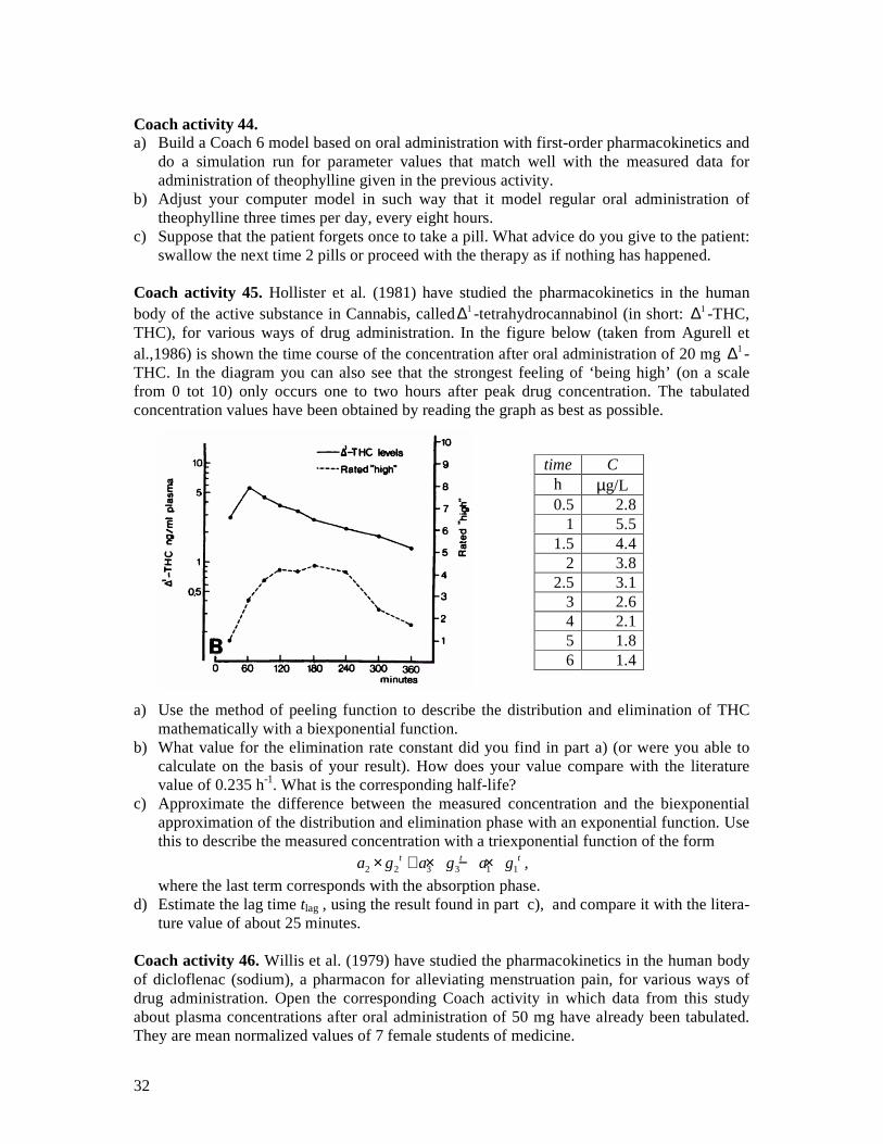
32

Coach activity 44. a) Build a Coach 6 model based on oral administration with first-order pharmacokinetics and

do a simulation run for parameter values that match well with the measured data for administration of theophylline given in the previous activity.

b) Adjust your computer model in such way that it model regular oral administration of theophylline three times per day, every eight hours.

c) Suppose that the patient forgets once to take a pill. What advice do you give to the patient: swallow the next time 2 pills or proceed with the therapy as if nothing has happened.

Coach activity 45. Hollister et al. (1981) have studied the pharmacokinetics in the human body of the active substance in Cannabis, called1∆ -tetrahydrocannabinol (in short: 1∆ -THC, THC), for various ways of drug administration. In the figure below (taken from Agurell et al.,1986) is shown the time course of the concentration after oral administration of 20 mg 1∆ -THC. In the diagram you can also see that the strongest feeling of ‘being high’ (on a scale from 0 tot 10) only occurs one to two hours after peak drug concentration. The tabulated concentration values have been obtained by reading the graph as best as possible.

a) Use the method of peeling function to describe the distribution and elimination of THC mathematically with a biexponential function.

b) What value for the elimination rate constant did you find in part a) (or were you able to calculate on the basis of your result). How does your value compare with the literature value of 0.235 h-1. What is the corresponding half-life?

c) Approximate the difference between the measured concentration and the biexponential approximation of the distribution and elimination phase with an exponential function. Use this to describe the measured concentration with a triexponential function of the form

2 2 3 3 1 1t t ta g a g a g× + × − × ,

where the last term corresponds with the absorption phase. d) Estimate the lag time tlag , using the result found in part c), and compare it with the litera-

ture value of about 25 minutes. Coach activity 46. Willis et al. (1979) have studied the pharmacokinetics in the human body of dicloflenac (sodium), a pharmacon for alleviating menstruation pain, for various ways of drug administration. Open the corresponding Coach activity in which data from this study about plasma concentrations after oral administration of 50 mg have already been tabulated. They are mean normalized values of 7 female students of medicine.

time C h µg/L 0.5 2.8

1 5.5 1.5 4.4

2 3.8 2.5 3.1

3 2.6 4 2.1 5 1.8 6 1.4

33

time C h µg/mL 1.5 0 2.0 0.046 2.5 2.014 3.0 0.694 3.5 0.257 4.0 0.137 4.5 0.089 5.0 0.053 5.5 0.035 6.0 0.025 6.5 0.012 7.0 0.008 8.0 0.005 9.0 0.002

a) Use the method of peeling function to describe the distribution and elimination of diclofenac mathematically with a biexponential function.

b) What value for the elimination rate constant did you find in part a) (or were you able to calculate on the basis of your result). How does your value compare with the literature value of 0.66 h-1. What is the corresponding half-life?

c) Approximate the difference between the measured concentration and the biexponential approximation of the distribution and elimination phase with an exponential function. Use this to describe the measured concentration with a triexponential function of the form

2 2 3 3 1 1t t ta g a g a g× + × − × ,

where the last term corresponds with the absorption phase. e) Estimate the lag time tlag , using the result found in part c), and compare it with the litera-

ture value of about 1.9 hours. f) Estimate the AUC and compare it with the literature value of 1,67 µg·mL-1·h. a) The bioavailability of diclofenac is equal to 50% beause of first-pass metabolism in the

liver. Determine the volume of distribution and the clearance. Compare your answer for clearance with the literature value of 263 ± 56 mL/min.

Coach activity 47. Like amphetamine, methamphetamine is sometimes sold under the name of speed. Methamfetamine is the same as methylamphetamine and is also called yaba, crystal (meth) or ice. Methamphetamine works for about 12 hours. Its user feels him/herself temporarily indefatigable and euphoric. When the pharmacon has lost its effect a crash follows: the users feels depressed and tired. The effect of methamphetamine is stronger and more addictive than that of amphetamine. Use of the drug may cause brain damage. Open the corresponding Coach activity in which data from a study (Cook, 1991) about plasma concentrations after oral administration of 0.250 mg/kg body weight (on average 21 mg) have already been tabulated.

time C h µg/L 0.5 0.5 1.0 15.5 1.5 30.0 2.0 35.5

34

2.5 36.0 3.0 38.5 3.5 34.5 4.0 35.5 5.0 33.5 6.0 32.0 8.0 29.0

Make a graphical computer model that describes this dataset with an open, one-compartment model for which first-order kinetics applies for absorption, distribution and elimination. First find appropriate parameter values via regression and compare your results with the following literature values of a biexponential model: tlag = 0.524 h, absorption rate constant ka= 1.083 h-1, elimination rate constant k = 0.0680 h-1, half-life t1/2 = 3.1 h, clearance Cl = 496 mL/min, Cmax=39.8 µg/L and tmax = 3.1 h. Schepers et al. (2003) report the following values of pharmacokinetic indicators: tlag = 1.1±0.5 h, t1/2 = 11.1±7.2 h, Cl = 33.5±15.9 L/h, AUC = 468.1±151.8, Cmax = 32.4±7.7 µg/L and tmax = 7.5±3.4 h. Build hereafter the graphical model, run a simulation and check whether the computer model matches well with the dataset. Coach activity 48. Ecstacy or XTC, with the chemical substance name MDMA, belongs to the family of amphetamines, but it has next to its energizing effect also a psychotomatic effect. XTC is primarily used during weekends and feasts. MDMA was synthesized for the first time in 1898 by the firm Merck Pharmaceuticals as side product in the synthesis of another chemical substance and patented in 1914. Subsequently, the drug was forgotten until the early seventies, when ecstacy ‘resurfaced’ for psychotherapeutic purposes. But this usage is not popular anymore because of negative side effects. In the early eighties a new musical style emerged in the dance club Warehouse in Chicago. Some musicians swallowed XTC pills and started in this way the use of ecstacy for recreational purposes. In November 1988, XTC was put on the list of hard drugs in the opium act. Since then the popularity of XTC has only grown: in 2001 13% of young adults in the age between 20 and 24 years had at least once used ecstacy and in some groups (early school leavers, frequent visitors of bars, clubs and feast) percentages were in 2003 between 35 and 50 % (van Laar et al., 2006). The Netherlands is an important country for the production and distribution of ecstasy. By the way, the interest in therapeutic usage of ecstasy, for example with patients in advanced stage of cancer disease, has increased again. Longstanding and frequent use of ecstacy or any other party drug that contains MDMA in combination with other substances has negative effects like depressions, psychoses, serious brain damage (in particular loss of memory), liver and/or kidney damage (Jager, 2006). Open the corresponding Coach activity in which data from a study (Mas et al., 1999) about plasma concentrations after oral admini-stration of 125 mg MDMA have already been tabulated.

time C h µg/L

0.25 0.0 0.5 19.2

0.75 74.6 1.0 125.0 1.5 200.0 2.0 223.1 3.0 215.4

35

4.0 192.3 6.0 157.7 8.0 130.8

10.0 115.4 24.0 38.5

Make a graphical computer model that describes this dataset with an open, one-compartment model for which first-order kinetics applies for absorption, distribution and elimination. First find appropriate parameter values via regression and compare your results with the following literature values of a biexponential model: absorption rate constant ka = 2.125 ± 1.100 h-1, elimination rate constant k = 0.0923 ± 0.043 h-1, half-life t1/2 = 8.73 ± 3.29 h, lag time tlag = 0,42 h, area under the curve AUC(0-24h) = 2623.7 ± 572.9 µg·L-1·h, AUC(0- ∞) = 3190.7 ± 1953.2 µg·L-1·h, peak plasma level Cmax = 236.4 ± 58.0 µg/L and tmax = 2.4 ± 0.98 h. Assume a bioavailablity of 84% (Yang et al, 2006; Cone & Huestis, 2007) for the calculation of the clearance and volume of distribution. Build hereafter the graphical model, run a simulation and check whether the computer model matches well with the dataset.

7. Mathematics under influence: more realistic models of intake and clearance of alcohol In the second section you became familiar with a linear model for the intake and clearance of alcohol in the human body, viz., the Widmark model. The formula for the blood alcohol concentration (BAC) that corresponds with the simplest version of this model in which only elimination is modeled is equal to

t=0BAC BAC β t = β t,d

D

V= − × − × (7.1)

t=0BAC BAC β t = β tD

V= − × − × ,

where the amount of alcohol consumed (in gram),

the volume of the body water into which the alcohol is absorbed and distributed (in liter),

β the elimination rate (in gram per liter per hour),

the time (

D

V

t

==== in hour) elapsed after consumption.

Widmark postulated that Vd is equal to the product r W⋅ , where W is the body weight and r is the so-called Widmark factor. The Widmark factor is individual and depends primarily of the body composition. Reference values are for men 0.68 (with standard deviation 0.085) and for women 0.55 (with standard deviation 0.055). The lower value for women can be explained because they have in general a larger percentage of fatty tissue than men and thus less body water into which alcohol can dissolve.

In Exercise 13 you have taken absorption into account in the Widmark model: you have investigated how the assumption that there exist a certain time span T0, of say 30 minutes, in which the at time t = 0 consumed amount of alcohol is absorbed with constant absorption rate into the central blood circulation en further distributed in the total body water works in practice. Maybe you have not obtained a result similar to the one shown in the screen shot below. The measured data come form a real experiment in which a test subject drank 3 standard glasses of an alcoholic beverage in one draught early in the morning on an empty stomach.

36

Figure 17. Linear model of intake and clearance of alcohol in the human body.

In this simple mathematical model two weak point catch the eye: (1) The abrupt transition from intake to elimination of alcohol in the human body and (2) the unrealistic behavior of the model curve that could lead in principle to negative BAC levels and does not match well with measurements of low BAC levels. The first minus can we take away by incorporating the absorption of alcohol into the systemic circulation via a model of exponential decay from the gastrointestinal tract. For taking away the second minus we must switch to more realistic, nonlinear models. This is what we will do in this section.

7.1. First-order absorption kinetics We assume that alcohol is absorbed via the gastrointestinal tract and gets via the portal vein through the liver into the systemic circulation. For the decrease of alcohol from the gastrointestinal tract we use an exponential decay model with elimination rate ak . Thus:

GI tractGI tracta

Ak A

t= − ⋅△

△

, (7.2)

where GI tractA is the amount of alcohol in the gastrointestinal tract. The rate of change with

which the alcohol gets into the systemic circulation has opposite sign and we assume that all alcohol passes the gastrointestinal tract and the lever unchanged. In terms of a mathematical formula, the absorption component of the rate of change of the amount of alcohol in the central compartment, which consists of the systemic circulation and the highly perfused tissues, is equal to

central compartmentGI tract

absorption

a

Ak A

t

= ⋅

△

△

(7.3)

37

The zero-order elimination kinetics according to the Widmark model is expressed in mathe-matical language as:

central compartment

elimination

Ab

t

= −

△

△

, (7.4)

where b is a constant. Adding (7.3) and (7.4) gives the formula for the rate of change of the amount o alcohol in the central compartment and, together with formula (7.2), a set of equations that describe together the rate of change of the amount of alcohol in the gastrointestinal tract and the central compartment:

GI tractGI tract

central compartmentGI tract

a

a

Ak A

tA

k A bt

= − ⋅ = ⋅ −

△

△

△

△

(7.5)

Division by the volume of distribution Vd of the central compartment leads to the following set of equations for the amount of alcohol in the gastrointestinal tract and the blood alcohol concentration:

GI tractGI tract

GI tract

BACβ

a

a

d

Ak A

tk

At V

= − × = × −

△

△

△

△

(7.6)

Here β is the elimination rate. A corresponding graphical computer model in Coach 6 is shown in Figure 18. In this example, BAC is computed using the following pharmacokinetic parameters:

dose = 30 g, 16 hak −= , 1β 0.2 h−= , 44 LV = .

It is still about the experiment in which a test subject empties three glasses of red wine in one draught early in the morning on an empty stomach.

Figure 18. Computer model and simulation of alcohol metabolism with first-order absorption kinetics and zero-order elimination kinetics.

This model gets simpler if you consider the quotient of the amount of alcohol in the gastro-intestinal tract and the volume of distribution Vd. Let us call this the concentration CGI tract. The set of equation is then rewritten as:

38

GI tractGI tract

GI tract

BACβ

a

a

Ck C

t

k Ct

= − × = × −

△

△

△

△

(7.7)

Now the rate of change of CGI tract is opposite to the absorption component of the rate of change of BAC. This fits the following graphical description of a compartmental model:

Figure 19. Two-compartment model of alcohol metabolism.

Figure 20 shows an implementation of this two-compartment model in Coach 6, together with the result of a simulation with measured data in the background. As initial value of CGI tract we choose the quotient of the amount of alcohol consumed and the volume of distribution.

Figure 20. Coach implementation of a two-compartment model of alcohol metabolism.

Coach activity 49. In this activity you use the measured BAC levels of the experiment in which a test person empties three standard glasses of red wine in one draught early in the morning on an empty stomach. You model the intake and clearance of alcohol in Coach 6 with a model of first-order absorption kinetics and zero-order elimination kinetics. a) Build the graphical model of Figure 18 and do a simulation with parameter values that fit

the imported measurement data in the background (A Coach result file with measured BAC levels is made available for this purpose).

b) Build the graphical model of Figure 20 and do a simulation with parameter values that fit the imported measurement data in the background (A Coach result file with measured BAC levels is made available for this purpose).

In the next Coach activity you will use measured data from an experiment in which a test

subject empties three standard glasses of red wine in one draught early in the morning on an empty stomach: one at the start of the experiment, one after 40 minutes, and the third drink 50 minutes later. The intake and clearance of alcohol is described with a model of first-order ab-sorption kinetics and zero-order elimination kinetics. Each consumption of an alcoholic drink has an immediate effect on the value of the state variable CGI tract in the mathematical model.

Unit now we have implemented sudden changes in Coach 6 via the Pulse function and via the RepeatedPulse function (see Coach activity13 and 14). But when the sudden changes in the state variables can be counted on the finger of one hand, then is an implementation via

39

discrete events the easiest approach. In the graphical modeling tool of Coach 6 exists an icon, viz., a rhomb with a thunderbolt inside, that represents an event and in which arrows indicate which state variables change because of the occurrence of the event and on which variables these changes depend. Look at Figure 21 below in which a screen shot of a graphical model and results of a simulation with real data in the background are visible. Behind each events icon is a piece of computer code hidden that describes exactly what should change in the simulation as soon as the event occurs. In the modeled alcohol experiment there are two discrete events: consumption of a drink after forty and after ninety minutes. In both cases the concentration CGI tract must suddenly be increased with the quotient of the amount of alcohol present in the glass and the volume of distribution. The computer code for the event drink_2 is for example:

Once (t>40) Do C := C + C_per_drink EndDo

Figure 21. Graphical model of intake and clearance of alcohol via discrete events.

Coach activity 50. Build the graphical model of Figure 21 and do a simulation with parameter values that fit the imported measurement data in the background (A Coach result file with measured BAC levels is made available for this purpose). Much better results than shown in Figure 21 cannot be achieved: the measured BAC levels are closely after intake of alcohol always greater than the simulation results. The main reason is that the mathematical model used is in fact too simple is to describe all effect of alcohol kinetics well. For this one needs amongst other things more compartments in the mathematical model (see Heck, 2007).

7.2. Nonlinear kinetics of alcohol clearance In the Widmark model it is assumed that the elimination rate is constant. Of course this cannot be the whole story because then the blood alcohol concentration would be negative after some time. In reality this cannot happen and we have avoided this in our computer models by introducing a stop condition of ending the simulation when the blood alcohol concentration becomes smaller or equal to zero. Figures 20 and 21 show that the BAC after intake of alcohol seems to decrease at high BAC levels with a constant rate, but not anymore when BAC level get small. Thus we have two reasons for improving the mathematical model with respect to elimination. We will investigate three models.

7.2.1. A combination of zero-order and first-order elimination kinetics An exponential decay of BAC after alcohol consumption, as we have applied in previous sec-tions on pharmacokinetics, does not lead to a satisfying model because BAC measurements

40

really show that the rate of change is nearly constant at high BAC levels and does not follow an exponential decay course. A simple adaptation of the Widmark model is switch to an ex-ponential model only when the blood alcohol concentration gets less than some threshold value. An important issue to take into account in this case is to make sure that the BAC curve constructed is as smooth as possible. Coach activity 51. In this activity you use the measured BAC levels of the experiment in which a test person empties three standard glasses of red wine in one draught early in the morning on an empty stomach. You model the intake of alcohol with a model of first-order absorption kinetics. You model the clearance of alcohol with a model of first-order elimina-tion kinetics in case the BAC level is less than or equal to the threshold value δ and with zero-order elimination kinetics given by the following equations:

GI tractGI tract

GI tract

GI tract

β if BACBACBAC if BAC

a

a

a

Ck C

tk C

k C kt

δδ

= − × × − > = × − × ≤

△

△

△

△

(7.8)

where ka is the absorption rate, k is the first-order elimination rate for BAC levels less than or equal to the threshold value δ and β is the zero-order elimination rate in case BAC is greater than the threshold δ. a) Prove that for a given zero-order elimination rate β and a given threshold value δ you only

get a smooth BAC curve if you choose the first-order elimination rate equal to β

δ. (Hint:

smoothness means that the rate of change of BAC according to linear Widmark model and the rate of change of BAC according to the model of exponential decay are equal to each other when the BAC level is equal to the threshold value δ).

b) Build a graphical model with combined zero-order and first-order elimination kinetics and do a simulation with parameter values that fit the imported measurement data in the background (A Coach result file with measured BAC levels is made available for this purpose). To inspire you and to show that such a model is also realizable we show below a screen shot coming from a simulation based on this mathematical model.

7.2.2. The Wagner model You may of course ask whether the rate of change of BAC cannot be described in a satisfying way with a single mathematical function. The graph of such a function should look like a straight line through the origin for small values and approach some constant value. A rational

41

function of the form ( )a x

f xb x

⋅=+

, with positive parameter values for a and b satisfies these

criteria. Wagner has described a model that predicts in this way the blood alcohol concentration for the first time in 1972. Just like the Widmark model it is in fact an open one-compartment model, but the difference is that the elimination of alcohol is described by the so-called Michaelis-Menten kinetics. This means that after alcohol absorption, the change in the blood alcohol concentration is given by the following formula:

max BACBAC

t BACdm

vV

k

⋅⋅ = −+

△

△

, (7.9)

where dV is the volume of distribution, mk is thee Michaelis-Menten constant andmaxv is the

maximum elimination rate. In the common terminology of pharmacokinetics we deal with a models in which the clearance Cl is given by the following rational expression:

max

BACm

vCl

k=

+. (7.10)

When the BAC level is high, then the elimination rate is almost equal to the maximum elimination ratemaxv (about 140 mg/min) and the graph of BAC against time is nearly a straight

line. The curvature of the BAC curve is clearly visible when the BAC level reaches half of the maximum elimination rate. At that moment BAC is equal to km and this value is mostly between 5 and 50 mg/L. Coach activity 52. Apply the Wagner model to the measurements in the experiment in which a test person empties three standard glasses of red wine in one draught early in the morning on an empty stomach. Assume first-order absorption kinetics.

7.2.3. The Pieters model Pieters et al. (1990) modeled alcohol clearance in humans with a semi-physiological three-compartment model. Their model considers the central compartment, in which alcohol is metabolized following Michaelis-Menten kinetics, the stomach and the small intestine. The alcohol goes into the stomach first, hereafter into the small intestine, and finally from there it is absorbed into the bloodstream and rapidly distributed in the central compartment. For the last two mentioned compartments they specify first-order absorption kinetics. The scheme below illustrates the model.

Figure 22. Scheme for the Pieters model of alcohol intake and clearance.

The model equations are:

3 max1 1 2 11 1 2 2 2 2 32 2

1 1 3

, , ,1 1 m

C vC k C kC C k C k C C

t a C t a C t k C= − ⋅ = ⋅ − ⋅ = ⋅ − ⋅

+ ⋅ + ⋅ +△△ △

△ △ △

with initial conditions [ ] [ ]1 2 3 0(0), (0), (0) ,0,0 ,C C C C=

42

where C0 = D0 / V, the initial amount of alcohol D0, divided by the volume of distribution V of the central compartment, and where C1, C2, and C3 are the alcohol concentrations in the stomach, small intestine and central compartment, respectively, related to the volume of distribution of the third compartment. Suitable parameter values for an experiment in which a test subject drank 28,5 g alcohol early in the morning on an empty stomach are tabulated below (Pieter et al., 1990):

Average values parameter unit male female

maxv 1 1g l h− −⋅ ⋅ 0.470 0.480

mk 1g l−⋅ 0.380 0.405

0C 1g l−⋅ 0.455 0.703

1k 1h− 5.55 4.96

2k 1h− 7.05 4.96

a 2 2l g−⋅ 0.42 0.75

Table 1. Parameter values for the Pieters 3-compartment model.

The first differential equation in the Pieters 3-compartment model, which models emptying of the stomach, does not represent a simple first-order process, but a feedback control is built-in that depends on the instantaneous concentration in the stomach, C1. The parameter a in the quadratic term of the denominator determines whether gastric emptying is faster (negative a) or slower (positive a) than the first order rate k1 under normal conditions. So, the effect of an empty or full stomach on alcohol clearance can be taken into account mathematically (Wedel et al., 1991). By the way, food promotes alcohol clearance, even when alcohol intake takes place via an intravenous infusion (Hahn et al., 1994). The Pieters model cannot explain this. Coach activity 53. Apply the Pieters model to the measurements in the experiment in which a test person empties three standard glasses of red wine in one draught early in the morning on an empty stomach. Also draw the graphs of the computed alcohol concentrations in the stomach and the small intestine.

References Agurell, S., Halldin, M., Lindgren, J-E, Ohlson, A., Widman, M., Gillespie, H. & Hollister, L.

(1986). Pharmacokinetics and Metabolism of 1∆ -Tetrahydrocannabinol and Other Canna-binoids with Emphasis on Man. Pharmacological Reviews, 39 (1) 21-43.

Atkinson, A.J., Abernethy, D.R., Daniels, C.E., Dedrick, R.L. & Markey, S.P. (2007). Principles of Clinical Pharmacology. Academic Press: New York.

Camu, F., Gepts,E., Rucquoi, M. & Heykants, J. (1982). Pharmacokinetics of Alfentanil in Man. Anesthesia and Analgesia, 61 (8) 657-661.

Cone, E.J. & Huestis, M. (2007). Interpretation of Oral Fluid Tests for Drugs of Abuse. Annals of The New York Academy of Sciences, 1098, 51-103.

Cook, C.E. (1991). Pyrolytic Characteristics, Pharmacokinetics, and Bioavailability of Smoked Heroin, Cocaine, Phencyclidine, and Methamphetamine. In: M.A. Miller & N.J. Kozel (red.) Methamphetamine Abuse: Epidemiologic Issues and Implications. National Institute on Drug Abuse, Research Monograph Series, No. 115, pp. 6-23. www.nida.nih.gov/pdf/monographs/115.pdf

M.A.Demotes-Mainard, F., Vincon, G., Ragnaud, J.M., Morlat, P., Bannwarth, B. & Dangoumau, J. (1993) Journal of Clinical Pharmacology, 33, 475-479.

43

Evans, G.H, Nies, A.S. & Shand, D.G. (1973). The disposition of propranolol. III. Decreased half-time and volume of distribution as a result of plasma binding in man, monkey, dog and rat. The Journal of Pharmacology and Experimental Therapeutics, 186 (1) 114-122.

Fagan, T.C, Walle, T., Walle, U.K., Conradi, E.C, Harmon, G. & Gaffney, T.E. (1982). Early Kinetics of Intravenous Propranolol. British Journal of Clinical Pharmacology 13, 571-574.

Hahn RG, et al. (1994). Eating a meal increases the clearance of ethanol given by intravenous infusion. Alcohol Alcohol 29, 673-677.

Heck, A. (2007). Getting Drunk and Sober Again. In: Modeling in Physics and Physics Education. Electronic Proceedings of the GIREP 2006 Conference, Amsterdam, August 20-25, 2006. Preprint: www.science.uva.nl/~heck/Research/alcohol/HECK259.pdf

Hollister, L.K., Gillespie, H.K, Ohlsen, A., Lindergren, E.-J., Wahlen , A. & Agurell, S. (1981). Do plasma concentrations of delta 9-tetrahydrocannabinol reflect the degree of intoxication? The Journal of Clinical Pharmacology, 21, S171-S177.

Gerry Jager (2006). Functional MRI studies in human Ecstasy and cannabis users. Proef-schrift, Universiteit Utrecht. igitur-archive.library.uu.nl/dissertations/2006-1031-200808/

Laar, van M., Cruts, A., Verdurmen, J., Ooyen, van M., Meijer, R. (2006, red.). De Nationale Drug Monitor. Jaarbericht 2005. trimbos.nl/Downloads/Producten/Jaarbericht 2005 NDM - definitieve versie.pdf

Mehvar, R. (1998). Pharmacokinitc-Based Design and Modification of Dosage Regimens. American Journal of Pharmaceutical Education, 62, 189-195.

Näf, M. (2004). Pharmacokinetics and Analgesic Potency of ∆9-Tetrahydrycanabinol (THC). Proefschrift, Universiteit van Basel. www.unibas.ch/diss/2004/DabsB_6910.pdf

Olanoff, L.S., Walle, T., Cowart, T.D., Oexmann, M.J & Conradi, E.C. (1986). Food effects on propranolol systemic and oral clearance: support for a blood flow hypothesis. Clinical Pharmacology and Therapeutics, 40, 408-414.

Pieters, J.E., Wedel, M., Schaafsma, G.J (1990). Parameter estimation in a three-compartment model for blood alcohol curves. Alcohol & Alcoholism 25 (1) 17-24.

Pinheiro, J.C. & Bates, D.M. (1995). Approximations to the Log-likelihood Function in the Nonlinear Mixed-effects Model. Journal of Computational and Graphical Statistics, 4, 12-35.

Schepers, R.J.F, Oyler, J.M, Joseph, R.E., Cone, E.J., Moolchan, E.T., Huestis, M.A. (2003). Methamphetamine and Amphetamine Pharmacokinetics in Oral Fluid and Plasma after Controlled Oral Methamphetamine Administration to Human Volunteers. Clinical Chemistry, 49 (1) 121-132. www.clinchem.org/cgi/reprint/49/1/121.pdf

Seidl, S., Jensen, U. & Alt, A. (2000). The calculation of blood ethanol concentrations in males and females. International Journal of Legal Medicine, 114, 71-77.

Shah, B.K. (1976). Data Analysis Problems in the Area of Pharmacokinetics Research. Bio-metrics, 32 (1) 145-157.

Shargel, L., Wu-Pong, S., Yu, A.B.C. (2005). Applied Biopharmaceutics & Pharmacokinetics. Fifth Edition (2005). Mc Graw-Hill, Medical Publishing Division: New York.

Stapleton, M.P. (1997). Sir James Black and Propranolol. The role of the Basic Sciences in the History of Cardiovascular Pharmacology. Texas Heart Institute Journal, 24(4) 336-342. www.pubmedcentral.nih.gov/picrender.fcgi?artid=325477&blobtype=pdf

Thijssen, H.H.W. & de Wildt, D.J. (2006). Kwantitatieve farmacokinetiek. In: Ree, van J.M & Breimer, D.D. (red). Algemene farmacologie (tweede druk). Elsevier Gezondheidszorg: Maarssen.

Yang, J., Jamei, M., Heydari, A., Yeo, K., de la Torre, R., Farré, M., Tucker, G. & Rostami-Hodjegan, A. (2006). Implications of mechansim-based inhibition of CYP2D6 for the pharmacokinetics and toxity of MDMA. Journal of Psychopharmacology, 20, 842-849.

44

Wagner, J.G. & Patel, J.A. (1972). Variations in absorption and elimination rates of ethyl alcohol in a single subject. Research Communications in Chemical Pathology & Pharma-cology 4, 61-76.

Watson, P.E, Watson, I.D. & Batt, R.D. (1980). Total body water volumes for adult males and females estimated from simple anthropometric measurements American Journal of Clini-cal Nutrition 33 (1) 27-39.

Wedel, M., Pieters, J.E., Pikaar, N.A., Ockhuizen, Th. (1991). Application of a three-compart-ment model to a study of the effects of sex, alcohol dose and concentration, exercise and food consumption on the pharmacokinetics of ethanol in healthy volunteers. Alcohol & Alcoholism 26 (3) 329-336.

Willis, J.V., Kendall, M.J., Flinn, R.M., Thornhill, D.P. & Welling, P.G. (1979). The Pharma-cokinetics of Diclofenac Sodium Followning Intravenous and Oral Administration. Euro-pean Journal of Clinical Pharmacology, 16, 405-410.

Copyright & Author © 2007 ITS Academy, Amsterdam. All rights reserved. This lesson material has been developed by André Heck (AMSTEL,UvA). He would like to thank Harm Houwing, Merel Hoogvliet (GSG Schagen), Mostapha Iallouchen (Bertrand Russell College, Krommenie), Suzanne Smit, José Spaan (Bonhoeffercollege, Castricum), Joost Hulshof, Jacqueline van Muijlwijk-Koezen, Jan Commandeur (Vrije Universiteit Amsterdam) and Jan van de Craats (UvA) for their comments on earlier versions and their suggestions.