- 33 -

2. Mathematical Description of the Model Components

In this chapter a mathematical description of all model components is given. First,hydrological processes are described in Section 2.1, followed by vegetation/crop growthprocesses (Section 2.2), nutrient dynamics processes (Section 2.3), and erosion (Section2.4). After that a description of the channel routing processes is given in Section 2.5. Thischapter is based mostly on the SWAT User Manual (Arnold et al., 1994) and the MATSALUmodel description (Krysanova et al., 1989a).

- 34 -

2.1 Hydrological Processes

The hydrological submodel in SWIM is based on the following water balance equation

where SW(t) is the soil water content in the day t, PRECIP – precipitation, Q – surfacerunoff, ET - evapotranspiration, PERC - percolation, and SSF – subsurface flow.

All values are the daily amounts in mm. Here the precipitation is an input, assuming thatprecipitation may differ between sub-basins, but it is uniformly distributed inside the sub-basin. The melted snow is added to precipitation.

The surface runoff, evapotranspiration, percolation below root zone and subsurface floware described below. Some river basins, especially in the semiarid zone, have alluvialchannels that abstract large quantities of stream flow. The transmission losses reducerunoff volumes when the flood wave travels downstream. This reduction is taken intoaccount by a special module that accounts for transmission losses.

2.1.1 Snow Melt

If air temperature is below 0, precipitation occurs as snow, and snow is accumulated. Ifsnow is present on soil, it may be melted when the temperature of the second soil layerexceeds 0°C (according to the model requirements, the depth of the first soil layer must bealways set to 10 mm). The approach used is similar to that of CREAMS model (Knisel,1980). Snow is melted as a function of the snow pack temperature in accordance with theequation

where SML is the snowmelt rate in mm d-1, SNO is the snow in mm of water, TMX is themaximum daily air temperature in °C.

Melted snow is treated the same as rainfall for estimating runoff volume and percolation,but rainfall energy is set to 0.

2.1.2 Surface Runoff

The model takes the daily rainfall amounts as input and simulates surface runoff volumesand peak runoff rates. Runoff volume is estimated by using a modification of the SoilConservation Service (SCS) curve number technique (USDA-SCS, 1972; Arnold et al.,1990). The technique was selected for use in SWIM as well as in SWAT due to severalreasons:(a) it is reliable and has been used for many years in the United States and worldwide;(b) the required inputs are usually available;(c) it relates runoff to soil type, land use, and management practices; and(d) it is computationally efficient.

( ) ( ) SSFPERCETQPRECIP+ tSW1tSW −−−−=+ (1)

SNO SML 0.

TMX574 SML

≤≤⋅= .

(2)

- 35 -

The use of daily precipitation data is a particularly important feature of the techniquebecause for many locations, and especially at the regional scale, more detailedprecipitation data with time increments of less than one day are not available.

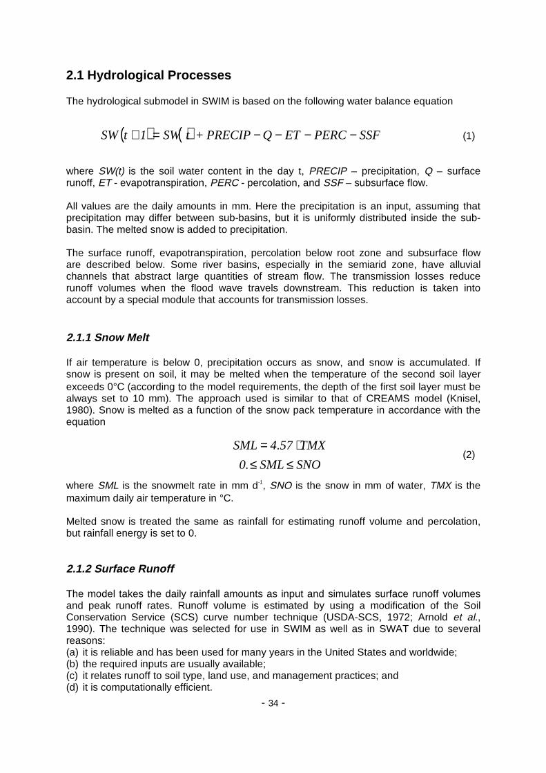
Surface runoff is estimated from daily precipitation taking into account a dynamic retentioncoefficient SMX by using the SCS curve number equation

where Q is the daily runoff in mm, PRECIP is the daily precipitation in mm, and SMX is aretention coefficient.

The retention coefficient SMX varies a) spatially, because soils, land use, management,and slope vary, and b) temporally, because soil water content is changing. The retentioncoefficient SMX is related to the curve number CN by the SCS equation

To illustrate the approach, Fig. 2.1 shows estimation of surface runoff Q from dailyprecipitation with equations (3) and (4) assuming different CN values.

Fig. 2.1 Estimation of surface runoff, Q, from daily precipitation, PRECIP, for differentvalues of CN (equations 3 and 4)

( )

SMX20PRECIP 0Q

SMX20PRECIP SMX80PRECIP

SMX20PRECIPQ

2

⋅≤=

⋅>⋅+⋅−=

.,

.,.

.(3)

1 - CN

100254SMX

⋅= (4)

0

20

40

60

80

100

120

0 10 20 30 40 50 60 70 80 90 100

PRECIP, mm

Q, m

m

CN=50CN=60CN=70CN=80CN=90CN=100

- 36 -

The parameter CN is defined in three variations:• for moisture condition 1 (or dry conditions) as CN1

• for moisture condition 2 (or average conditions) as CN2 and• for moisture condition 3 (or wet conditions) as CN3.

CN2 can be obtained from the SCS hydrology handbook (USDA-SCS, 1972) for a set ofland use types, hydrologic soil groups and management practices (see also Tab. 3.20 inChapter 3 of the Manual). The corresponding values of CN1 and CN3 are also tabulated inthe handbook. For computing purposes, CN1 and CN3 were related to CN2 with theequations (see also Fig. 2.2)

or an approximation of equation 5:

and

Fig. 2.2 Correspondence between CN1, CN2 and CN3 (equations 6, 7)

( )( )[ ]22

221 CN100063605332CN100

CN10020CNCN

−⋅−+−−⋅−=

..exp(5)

32

2221 CN000117720CN0137930CN3481191116CN ⋅+⋅−⋅+−= .... (6)

( )[ ]223 CN100006730CNCN −⋅⋅= .exp (7)

0

20

40

60

80

100

120

30 40 50 60 70 80 90 100CN1

CN1CN2CN3

- 37 -

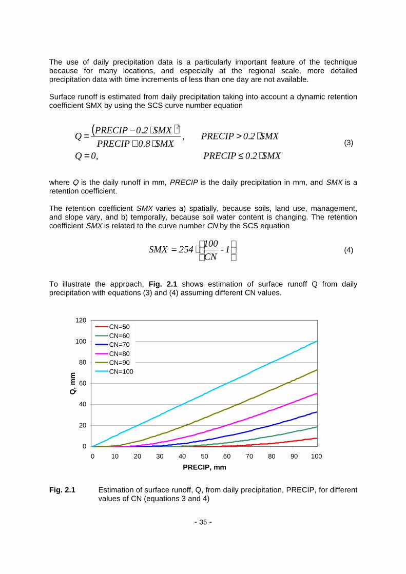
The values of CN1, CN2 and CN3 are related to land use types, hydrologic soil groups andmanagement practices. An additional assumption was made to relate curve numbers toslope. Namely, it was assumed that the CN2 value is appropriate for a 5% slope, thefollowing equation was derived (Arnold et al., 1994) to adjust it for lower and higher slopes(see also Fig. 2.3):

where CN2s is the adjusted CN2 value, and SS is the slope steepness in m m-1.

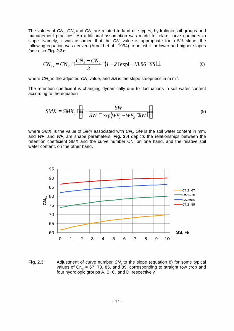
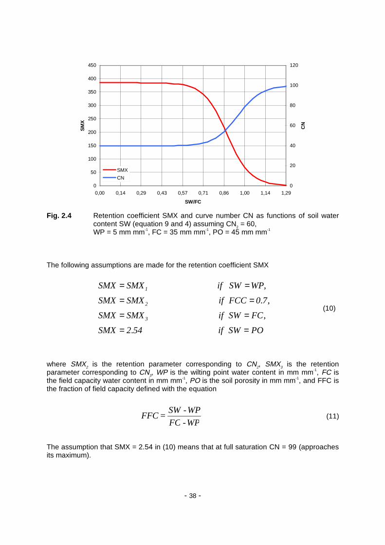
The retention coefficient is changing dynamically due to fluctuations in soil water contentaccording to the equation

where SMX1 is the value of SMX associated with CN1, SW is the soil water content in mm,and WF1 and WF2 are shape parameters. Fig. 2.4 depicts the relationships between theretention coefficient SMX and the curve number CN, on one hand, and the relative soilwater content, on the other hand.

Fig. 2.3 Adjustment of curve number CN2 to the slope (equation 8) for some typicalvalues of CN2 = 67, 78, 85, and 89, corresponding to straight row crop andfour hydrologic groups A, B, C, and D, respectively

( )( )SS8613213

CNCNCNCN 23

2s2 ⋅−⋅−⋅−

+= .exp (8)

( ) SWWFWFSW

SW1SMXSMX

211

⋅−+

−⋅=exp

(9)

60

65

70

75

80

85

90

95

0 1 2 3 4 5 6 7 8 9 10

SS, %

CN

2s

CN2=67

CN2=78

CN2=85

CN2=89

- 38 -

Fig. 2.4 Retention coefficient SMX and curve number CN as functions of soil watercontent SW (equation 9 and 4) assuming CN2 = 60,WP = 5 mm mm-1, FC = 35 mm mm-1, PO = 45 mm mm-1

The following assumptions are made for the retention coefficient SMX

where SMX2 is the retention parameter corresponding to CN2, SMX3 is the retentionparameter corresponding to CN3, WP is the wilting point water content in mm mm-1, FC isthe field capacity water content in mm mm-1, PO is the soil porosity in mm mm-1, and FFC isthe fraction of field capacity defined with the equation

The assumption that SMX = 2.54 in (10) means that at full saturation CN = 99 (approachesits maximum).

POSWif542SMX

FCSWifSMXSMX

70FCCifSMXSMX

WPSWifSMXSMX

3

2

1

==

==

==

==

.

,

,.

,

(10)

WP - FC

WP - SW = FFC (11)

0

50

100

150

200

250

300

350

400

450

0,00 0,14 0,29 0,43 0,57 0,71 0,86 1,00 1,14 1,29

SW/FC

SM

X

0

20

40

60

80

100

120

CN

SMX

CN

- 39 -

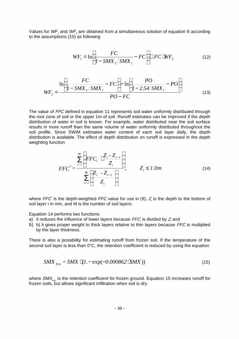
Values for WF1 and WF2 are obtained from a simultaneous solution of equation 8 accordingto the assumptions (10) as following

The value of FFC defined in equation 11 represents soil water uniformly distributed throughthe root zone of soil or the upper 1m of soil. Runoff estimates can be improved if the depthdistribution of water in soil is known. For example, water distributed near the soil surfaceresults in more runoff than the same volume of water uniformly distributed throughout thesoil profile. Since SWIM estimates water content of each soil layer daily, the depthdistribution is available. The effect of depth distribution on runoff is expressed in the depthweighting function

where FFC* is the depth-weighted FFC value for use in (9), Zi is the depth to the bottom ofsoil layer i in mm, and M is the number of soil layers.

Equation 14 performs two functions:a) it reduces the influence of lower layers because FFCi is divided by Zi andb) b) it gives proper weight to thick layers relative to thin layers because FFC is multiplied

by the layer thickness.

There is also a possibility for estimating runoff from frozen soil. If the temperature of thesecond soil layer is less than 0°C, the retention coefficient is reduced by using the equation

where SMXfroz is the retention coefficient for frozen ground. Equation 15 increases runoff forfrozen soils, but allows significant infiltration when soil is dry.

FCPO

POSMX5421

POFC

SMXSMX1

FC

WF 1132 −

−

−−

−

−=

.lnln

(13)

213

1 WFFCFCSMXSMX1

FCWF ⋅+

−

−= ln (12)

m01Z ,

Z

Z - Z

Z

Z- Z FFC

= FFC i

i

1iiM

1=i

i

1iii

M

1=i* .≤

⋅

−

−

Σ

Σ(14)

)).exp(.( SMX00086201 SMX=SMX froz ⋅−−⋅ (15)

- 40 -

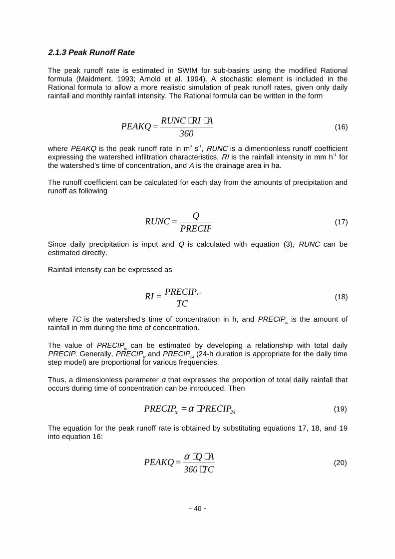
2.1.3 Peak Runoff Rate

The peak runoff rate is estimated in SWIM for sub-basins using the modified Rationalformula (Maidment, 1993; Arnold et al. 1994). A stochastic element is included in theRational formula to allow a more realistic simulation of peak runoff rates, given only dailyrainfall and monthly rainfall intensity. The Rational formula can be written in the form

where PEAKQ is the peak runoff rate in m3 s-1, RUNC is a dimentionless runoff coefficientexpressing the watershed infiltration characteristics, RI is the rainfall intensity in mm h-1 forthe watershed’s time of concentration, and A is the drainage area in ha.

The runoff coefficient can be calculated for each day from the amounts of precipitation andrunoff as following

Since daily precipitation is input and Q is calculated with equation (3), RUNC can beestimated directly.

Rainfall intensity can be expressed as

where TC is the watershed’s time of concentration in h, and PRECIPtc is the amount ofrainfall in mm during the time of concentration.

The value of PRECIPtc can be estimated by developing a relationship with total dailyPRECIP. Generally, PRECIPtc and PRECIP24 (24-h duration is appropriate for the daily timestep model) are proportional for various frequencies.

Thus, a dimensionless parameter α that expresses the proportion of total daily rainfall thatoccurs during time of concentration can be introduced. Then

The equation for the peak runoff rate is obtained by substituting equations 17, 18, and 19into equation 16:

360

ARIRUNC = PEAKQ

⋅⋅(16)

PRECIP

Q = RUNC (17)

TCPRECIP = RI tc (18)

24tc PRECIPPRECIP ⋅=α (19)

TC360

AQ = PEAKQ

⋅⋅⋅α

(20)

- 41 -

The time of concentration can be estimated by adding the surface and channel flow times

where TCch is the time of concentration for channel flow in h, and TCov is the time ofconcentration for overland surface flow in h.

The time of concentration for channel flow can be calculated by the equation

where CHFL is the average channel flow length for the basin in km and CHV is the averagechannel velocity in m s-1.

The average channel flow length can be estimated by the equation

where CHL is the channel length from the most distant point to the watershed outlet in kmand CHLcen is the distance from the outlet along the channel to the watershed centroid inkm. We can assume that CHLcen=0.5 CHL.

Average velocity can be estimated by using Manning’s equation and assuming atrapezoidal channel with 2:1 side slopes and a 10:1 bottom width to depth ratio.Substitution of these estimated and assumed values, and conversion of units gives thefollowing estimation of the time of concentration for channel

where CHN is Manning’s n, QAV is the average flow rate in mm h-1, and CHS is the averagechannel slope in m m-1.

The average flow rate is obtained from the estimated average flow rate from a unit sourcein the watershed (1 ha area) and the relationship

where QAV0 is the average flow rate from a 1 ha area in mm h-1.

ovch TCTCTC += (21)

CHV63

CHFLTCch ⋅

=.

(22)

cenCHLCHLCHFL ⋅= (23)

( ) 3750250

750

chCHSAQAV

CHNCHL620TC

..

..

⋅⋅⋅⋅= (24)

500 AQAVQAV .−⋅= (25)

- 42 -

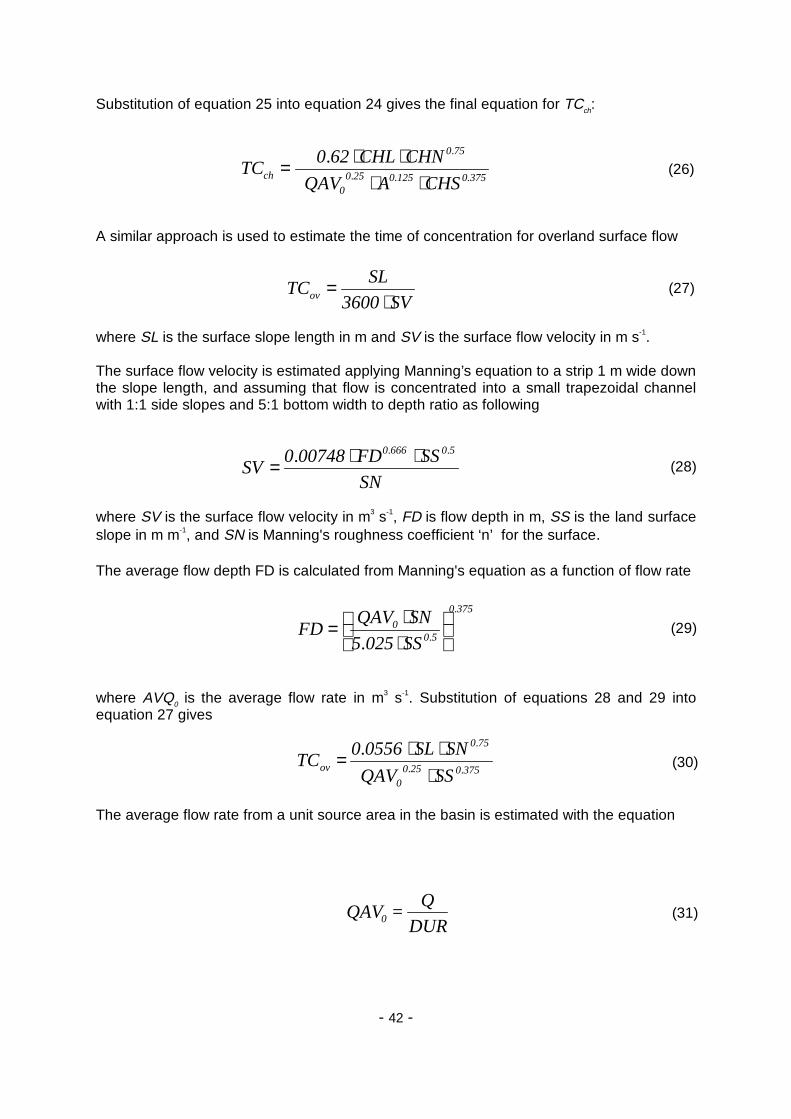
Substitution of equation 25 into equation 24 gives the final equation for TCch:

A similar approach is used to estimate the time of concentration for overland surface flow

where SL is the surface slope length in m and SV is the surface flow velocity in m s-1.

The surface flow velocity is estimated applying Manning’s equation to a strip 1 m wide downthe slope length, and assuming that flow is concentrated into a small trapezoidal channelwith 1:1 side slopes and 5:1 bottom width to depth ratio as following

where SV is the surface flow velocity in m3 s-1, FD is flow depth in m, SS is the land surfaceslope in m m-1, and SN is Manning's roughness coefficient ‘n’ for the surface.

The average flow depth FD is calculated from Manning's equation as a function of flow rate

where AVQ0 is the average flow rate in m3 s-1. Substitution of equations 28 and 29 intoequation 27 gives

The average flow rate from a unit source area in the basin is estimated with the equation

375012502500

750

chCHSAQAV

CHNCHL620TC

...

..

⋅⋅⋅⋅= (26)

SV3600

SLTCov ⋅

= (27)

SN

SSFD007480SV

506660 ... ⋅⋅= (28)

SS0255

SNQAVFD

3750

500

.

..

⋅⋅= (29)

SSQAV

SNSL05560TC

37502500

750

ov ..

..

⋅⋅⋅= (30)

DUR

Q =QAV0 (31)

- 43 -

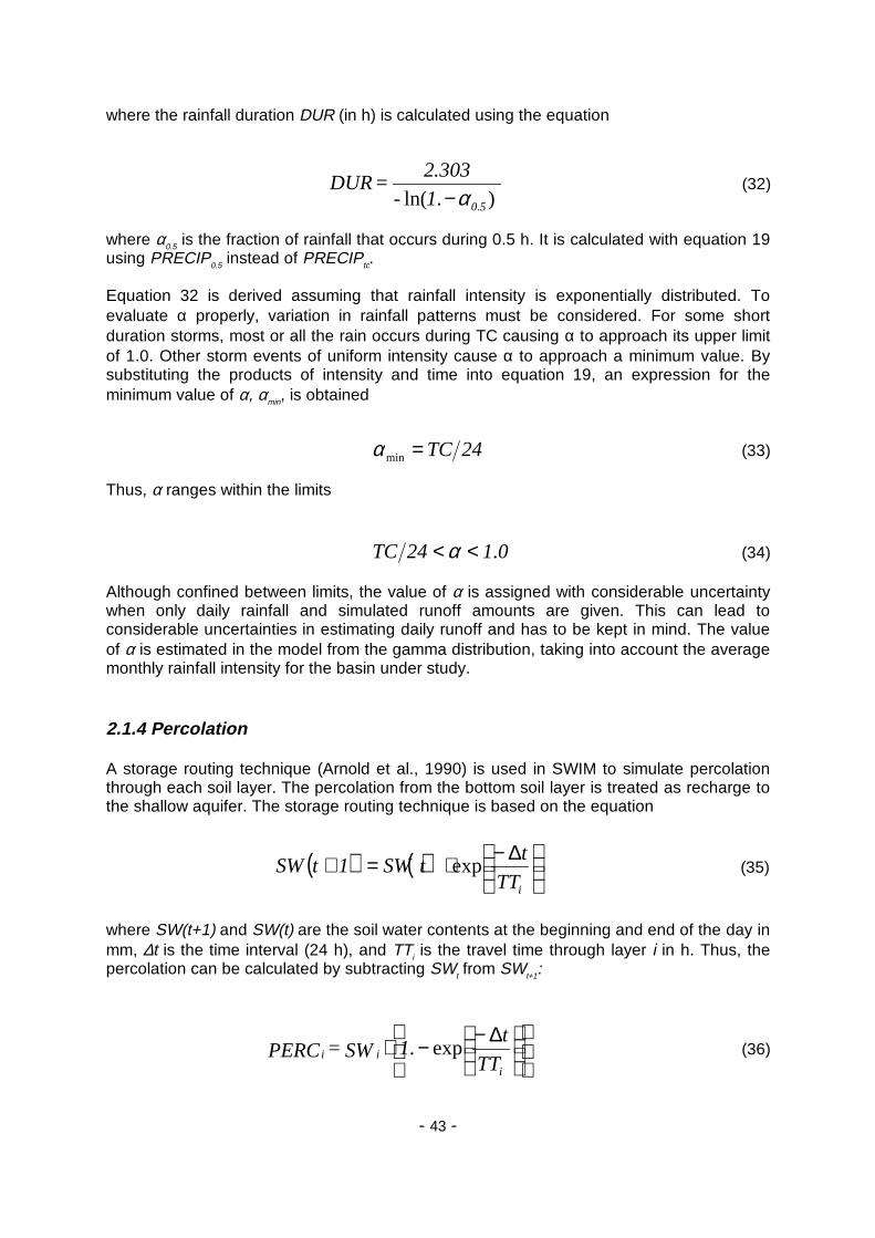
where the rainfall duration DUR (in h) is calculated using the equation

where α0.5 is the fraction of rainfall that occurs during 0.5 h. It is calculated with equation 19using PRECIP0.5 instead of PRECIPtc.

Equation 32 is derived assuming that rainfall intensity is exponentially distributed. Toevaluate α properly, variation in rainfall patterns must be considered. For some shortduration storms, most or all the rain occurs during TC causing α to approach its upper limitof 1.0. Other storm events of uniform intensity cause α to approach a minimum value. Bysubstituting the products of intensity and time into equation 19, an expression for theminimum value of α, αmin, is obtained

Thus, α ranges within the limits

Although confined between limits, the value of α is assigned with considerable uncertaintywhen only daily rainfall and simulated runoff amounts are given. This can lead toconsiderable uncertainties in estimating daily runoff and has to be kept in mind. The valueof α is estimated in the model from the gamma distribution, taking into account the averagemonthly rainfall intensity for the basin under study.

2.1.4 Percolation

A storage routing technique (Arnold et al., 1990) is used in SWIM to simulate percolationthrough each soil layer. The percolation from the bottom soil layer is treated as recharge tothe shallow aquifer. The storage routing technique is based on the equation

where SW(t+1) and SW(t) are the soil water contents at the beginning and end of the day inmm, ∆t is the time interval (24 h), and TTi is the travel time through layer i in h. Thus, thepercolation can be calculated by subtracting SWt from SWt+1:

1 -

303.2 = DUR

50 ).ln( .α− (32)

24TC=minα (33)

0124TC .<< α (34)

( ) ( ) TT

ttSW1tSW

i

∆−⋅=+ exp (35)

∆−−⋅i

iiTT

t1 SW = PERC exp. (36)

- 44 -

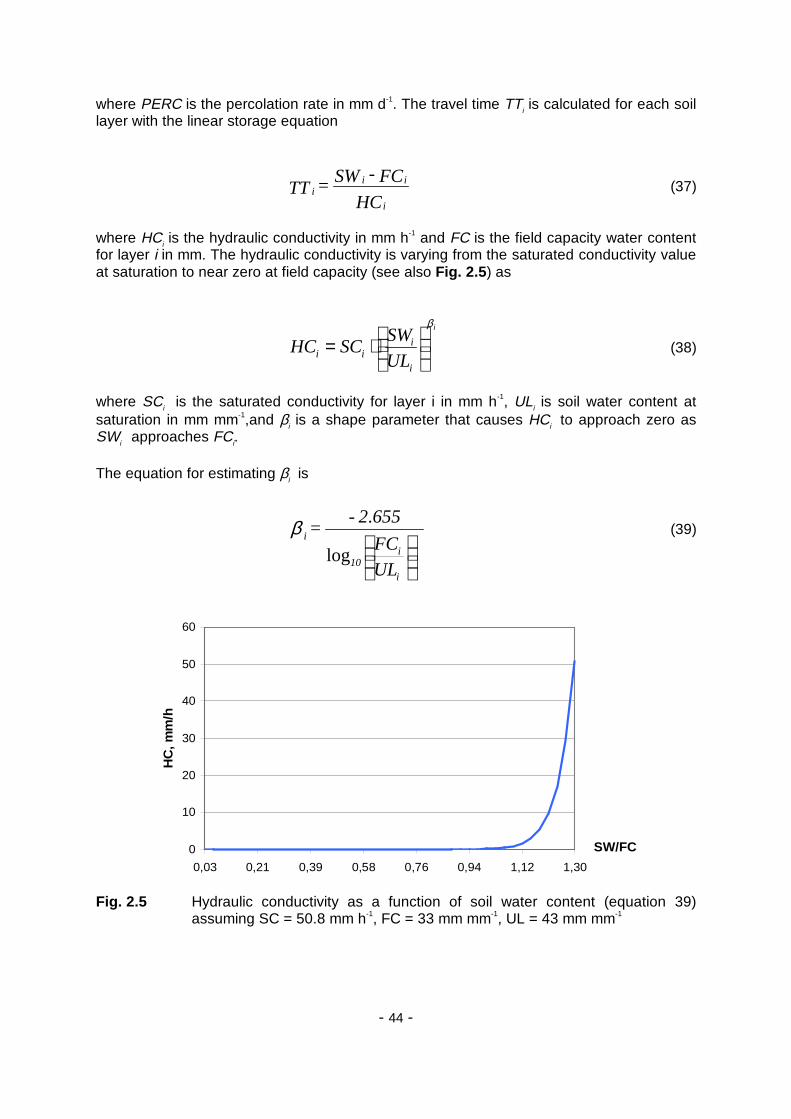
where PERC is the percolation rate in mm d-1. The travel time TTi is calculated for each soillayer with the linear storage equation

where HCi is the hydraulic conductivity in mm h-1 and FC is the field capacity water contentfor layer i in mm. The hydraulic conductivity is varying from the saturated conductivity valueat saturation to near zero at field capacity (see also Fig. 2.5) as

where SCi is the saturated conductivity for layer i in mm h-1, ULi is soil water content atsaturation in mm mm-1,and βi is a shape parameter that causes HCi to approach zero asSWi approaches FCi.

The equation for estimating βi is

Fig. 2.5 Hydraulic conductivity as a function of soil water content (equation 39)assuming SC = 50.8 mm h-1, FC = 33 mm mm-1, UL = 43 mm mm-1

HC

FC - SW = TTi

iii (37)

UL

SWSCHC

i

i

iii

β

⋅= (38)

UL

FC

6552- =

i

i10

i

log

.β (39)

0

10

20

30

40

50

60

0,03 0,21 0,39 0,58 0,76 0,94 1,12 1,30

SW/FC

HC

, mm

/h

- 45 -

The constant in equation 39 is set to –2.655 to assure that at field capacity

Water flow through a soil layer may occur until the lower layer is not saturated. If the layerbelow the layer being considered is saturated, no flow can occur. The effect of lower layerwater content is expressed by the equation

where PERCic is the percolation rate for layer i in mm d-1 corrected for layer i+1 watercontent and PERCi is the percolation calculated with equation 36.

Percolation is also affected by soil temperature. If the temperature in a particular layer isO°C or below, no percolation is allowed from that layer.

Since the one-day time interval is relatively low for routing flow through the soil root zone,the water is divided into several portions for routing through soil. This is necessary becauseflow rates are dependent upon soil water content, which is continuously changing. Forexample, if the soil is extremely wet, equations 36, 37, and 38 may overestimatepercolation, if only one routing is performed. To overcome this problem, each layer's inflowis divided into 4-mm slugs for routing.

Besides, when the inflow is divided into 4-mm slugs and each slug is routed individuallythrough the layers, the relationship taking into account the lower layer water content(equation 41) works more realistically.

2.1.5 Lateral Subsurface Flow

The kinematic storage model developed by Sloan et al. (1983) uses the mass continuityequation for the entire soil profile, considering it as the control volume. The mass continuityequation in the finite difference form for the kinematic storage model is

where SUP is the drainable volume of water stored in the saturated zone m m-1 (waterabove field capacity), t is time in h, SSF is the lateral subsurface flow in m3 h-1, WIR is therate of water input to the saturated zone in m2 h-1, SL is the hillslope length in m, andsubscripts 1 and 2 refer to the beginning and end of the time step, respectively. Thedrainable volume of water stored, SUP, is updated daily.

SC0020HC ii ⋅= . (40)

1UL

1SW1PERCPERC

i

iiic +

+−⋅= (41)

2

SSFSSFSLWIR

tt

SUPSUP 21

12

12 +−⋅=−−

(42)

- 46 -

The lateral flow at the hillslope outlet is given by

where VEL is the velocity of flow at the outlet in mm h-1, SLW is the hillslope width in m, andPORD is the drainable porosity of the soil in m m-1. Velocity at the outlet is estimated as

where SC is the saturated conductivity in mm h-1, and ν is the hillslope steepness in m m-1 .Combination of equations 43 and 44 gives

where SSF is in mm d-1, SUP in m m-1, γ in m m-1, PORD in m m-1, and SL in m.

If the saturated zone rises above the soil layer, water is allowed to flow to the layer above.The amount of flow upward is estimated as a function of saturated conductivity SC and thesaturated slope length

where QUP is the upward flow in mm d-1, and Slsat is the saturated slope length in m.

To account for multiple layers, the model is applied to each soil layer independently startingat the upper layer to allow for percolation from one soil layer to the next.

2.1.6 Potential Evapotranspiration

The method of Priestley-Taylor (1972) is used in the model for estimation of potentialevapotranspiration, which requires only solar radiation, air temperature, and elevation asinputs. Instead, the method of Penman-Monteith (Monteith, 1965) can be used, if additionalinput data are available. The Penman-Monteith method requires solar radiation, airtemperature, wind speed, and relative humidity as input.

The Priestley-Taylor method estimates potential evapotranspiration as a function of netradiation as following

SLPORD

SLWVELSUP2SSF

⋅⋅⋅⋅= (43)

)sin(ν⋅= SCVEL (44)

SLPORD

SCSUP20240SSF

⋅⋅⋅⋅⋅= )sin(

.ν

(45)

SL

SLSC24QUP sat⋅⋅= (46)

HV

RAD281EO

+⋅

⋅=

γδδ

. (47)

- 47 -

where EO is the potential evaporation in mm, RAD is the net radiation in MJ m-2, HV is thelatent heat of vaporization in MJ kg-1, δ is the slope of the saturation vapor pressure curve inkPa C-1, and γ is a psychrometer constant in kPa C-1.

The latent heat of vaporization is estimated as a function of the mean daily air temperatureT in °C

The saturation vapor pressure VP is also estimated as a function of temperature

Then the slope of the saturation vapor pressure curve is calculated with the equation

The psychrometer constant γ is calculated as a function of barometric pressure BP (in kPa)

The barometric pressure is estimated as a function of elevation ELEV (in m)

If actual net radiation is not available, in can be estimated from the maximum solar radiationas following. First, the maximum possible solar radiation RAM in Ly is calculated as

where D is the earth’s radius vector in km, φ is the sun’s half day length in radians, LAT isthe latitude of the site in degrees, and θ is the sun's declination angle in radians.

T0022052HV ⋅−= .. (48)

( ) 273T

6791273T035885410VP

+−+⋅−⋅= ln..exp. (49)

035273T

6791

273T

VP

−

+⋅

+= .δ (50)

BP1066 4 ⋅⋅= −.γ (51)

ELEV10445ELEV01150101BP 27 ⋅⋅+⋅−= −.. (52)

( ) ( ) ( )

⋅⋅

⋅⋅+⋅

⋅⋅⋅⋅=

=

φθπθπφ sincoscossinsin360

LAT2

360

LAT2

D

711

RAM

2

(53)

- 48 -

The earth’s radius vector D can be calculated for any day t as

The sun's declination angle is calculated with the equation

The sun’s half day length is calculated as

Then the net radiation is estimated with the equation

where RAD is the solar radiation in MJ m-2 and ALB is albedo.

The albedo is estimated by considering the soil, crop/vegetation cover, and snow cover.When crops are growing, albedo is determined by using the equation

where 0.23 is the albedo for plants, ALBsoil is the soil albedo, and SCOV is a soil coverindex.

The value of the soil cover index SCOV ranges from 0 to 1.0 according to the equation

where BMR is the sum of the above ground biomass and crop residue in t ha-1.

+⋅⋅⋅+

=

365

288t2033501

1D

).(sin..

π (54)

( )

365

2580t241020

−⋅⋅⋅= .

sin.πθ (55)

( )

1 ,

1 ,0

1 1 ,360

LAT21

−≤=

>=

≤≤−

⋅

⋅⋅= −

θπφ

θφ

θθπφ tantancos

(56)

( )ALB1RAMRAD −⋅= . (57)

( ) SCOVALBSCOV1230ALB soil ⋅+−⋅= .. (58)

( )BMR050SCOV ⋅−= .exp (59)

- 49 -

Fig. 2.6 An example of the annual dynamics of soil albedo (equations 58, 59)

If a snow cover exists with 5 mm or greater water content, the value of albedo is set to 0.8.If the snow cover is less than 5 mm and no crop is growing, the soil albedo is set to theinput value (default value = 0.15). An example on Fig. 2.6 shows possible seasonaldynamics of albedo in a temperate zone with a maximum 0.8 in winter (snow cover),minimum in march and september (equal to the bare soil albedo), and increasing up to 0.23in summer (crop growth).

2.1.7 Soil Evaporation and Plant Transpiration.

The model calculates evaporation from soils and transpiration by plants separately using anapproach similar to that of Ritchie (1972). The plant transpiration is calculated as

where EO is the potential evapotranspiration in mm d-1 estimated by equation (47), EP isthe plant water transpiration rate in mm d-1 and LAI is the leaf area index (area of plantleaves relative to the soil surface area).

If soil water is limited, plant water transpiration is reduced. The approach is described insection 2.2.2 about water stress.

3.0 LAI ,EOEP

3.0 LAI 0 ,3

LAIEOEP

>=

≤≤⋅=(60)

0

0,2

0,4

0,6

0,8

1

1 2 3 4 5 6 7 8 9 10 11 12month

- 50 -

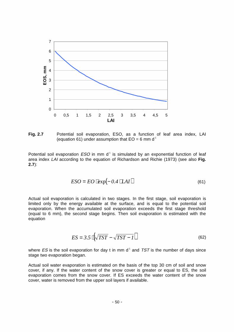
Fig. 2.7 Potential soil evaporation, ESO, as a function of leaf area index, LAI(equation 61) under assumption that EO = 6 mm d-1

Potential soil evaporation ESO in mm d-1 is simulated by an exponential function of leafarea index LAI according to the equation of Richardson and Richie (1973) (see also Fig.2.7):

Actual soil evaporation is calculated in two stages. In the first stage, soil evaporation islimited only by the energy available at the surface, and is equal to the potential soilevaporation. When the accumulated soil evaporation exceeds the first stage threshold(equal to 6 mm), the second stage begins. Then soil evaporation is estimated with theequation

where ES is the soil evaporation for day t in mm d-1 and TST is the number of days sincestage two evaporation began.

Actual soil water evaporation is estimated on the basis of the top 30 cm of soil and snowcover, if any. If the water content of the snow cover is greater or equal to ES, the soilevaporation comes from the snow cover. If ES exceeds the water content of the snowcover, water is removed from the upper soil layers if available.

( )LAI40EOESO ⋅−⋅= .exp (61)

( )1TSTTST53ES −−⋅= . (62)

0

1

2

3

4

5

6

7

0 0,5 1 1,5 2 2,5 3 3,5 4 4,5 5LAI

EO

S, m

m

- 51 -

2.1.8 Groundwater Flow

The groundwater submodel in the integrated river basin model like SWIM is intended forgeneral use in regions where extensive field measurements are not available. Thus, thegroundwater component has to be parameterized using readily available inputs. Also, itmust have the level of sophistication similar to those of the other components. Therefore adetailed numerical model is not justified for this case, and a relatively simple yet realisticapproach was chosen for use in SWAT and SWIM.

The simulated hydrological system consists of four control volumes that include:• the soil surface,• the soil profile or root zone,• the shallow aquifer, and• the deep aquifer.

The percolation from the soil profile is assumed to recharge the shallow aquifer. Thesurface runoff, the lateral subsurface flow from the soil profile, and return flow from theshallow aquifer contribute to the stream flow. The water balance equation for the shallowaquifer is

where SAW(t) is the shallow aquifer storage in the day t, RCH is the recharge, REVAP isthe water flow from the shallow aquifer back to the soil profile, GWQ is the return flow orgroundwater contribution to streamflow, SEEP is the percolation or seepage to the deepaquifer (all – in mm d-1), and t is the day.

REVAP is defined as water that raises from the shallow aquifer to the soil profile and is lostto the atmosphere by soil evaporation or plant root uptake.

The approach of Smedema and Rycroft (1983), who derived the non-steady-state responseof groundwater flow to periodic recharge from Hooghoudt's (1940) steady-state formula, isused

where KD is the hydraulic conductivity of groundwater in mm d-1, DS is the drain spacing inm, and GWH is the water table height in m.

Assuming that the shallow aquifer is recharged by seepage from stream channels,reservoirs, or the soil profile (rainfall and irrigation), and is depleted by the return flow to thestream, fluctuations of water table can be estimated using the equation of Smedema andRycroft (1983)

where SY is the specific yield.

( ) ( ) SEEPGWQREVAPRCHtSAW1tSAW −−−+=+ (63)

2DS

GWHKD8GWQ

⋅⋅= (64)

SY80

GWQRCH

dt

GWHd

⋅−=

.)(

(65)

- 52 -

The return flow can be estimated assuming that its variation with time is also linearly relatedto the rate of change of the water table height:

where RF is the constant of proportionality or the reaction factor for groundwater.

Integration of equation 66 gives

The relationship for the water table height is derived combining equations 64 and 67. Itresults in the following relationship

The percolation from the soil profile is assumed to recharge the shallow aquifer. The delaytime or drainage time of the aquifer is used to correct the recharge. Sangrey et al. (1984)used an exponential decay weighting function proposed by Venetis (1969) to estimate thedelay time for return flow in their precipitation / groundwater response model

where DEL is the delay time or drainage time of the aquifer in days (Sangrey et al., 1984).This equation will affect only the timing of the return flow and not the total volume. Theequation (69) is used in SWIM to correct the recharge.

The volume of water flow from the shallow aquifer back to the soil profile, REVAP, isestimated with the equations

where ET is the actual evapotranspiration occurring in the soil profile, CR is the revapcoefficient, and RST is the revap storage in mm.

( ) ( )GWQRCHRFDSSY

GWQRCHKD10

dt

GWQd2

−⋅=⋅

−⋅⋅=)((66)

( ) ( ) ( ) ( )[ ] tRF1RCHtRFtGWQ1tGWQ ∆⋅−−⋅+∆⋅−⋅=+ expexp (67)

( )

( ) ( ) ( )( ) tRF1

RFSY80

RCHtRFtGWH

1tGWH

∆⋅−−⋅⋅⋅

+∆⋅−⋅=

=+

exp..

exp(68)

( )

( ) ( )tRCHDEL

11tRCH

DEL

11

1tRCH

⋅

−++⋅

−−=

=+

expexp.(69)

RSTREVAP ,0REVAP

RSTREVAP ,ETCRREVAP

≤=

>⋅=(70)

- 53 -

The amount of percolation or seepage from the shallow aquifer (recharge to the deepaquifer) is estimated as a linear function

where CS is the seepage coefficient.

2.1.9 Transmission Losses

Many watersheds, especially in semiarid areas, have alluvial channels that abstract largequantities of stream flow (Lane, 1982). The abstractions, or transmission losses, reducerunoff volumes because water is lost when the flood wave travels downstream.

A procedure for estimating transmission losses for ephemeral streams is described by Lanein the SCS Hydrology Handbook (USDA, 1983, chapter 19). The procedure is based onderived regression equations for estimation of transmission losses in the absence ofobserved inflow-outflow data. It enables the user to estimate transmission losses for similarchannels of arbitrary length and width using channel geometry parameters (width anddepth) and Manning’s "n". This procedure is used in SWIM as well as in SWAT to estimatetransmission losses.

The unit channel intercept and slope, and the decay factor are estimated with regressionequations obtained from the analysis of observed data in different conditions:

where AR is the unit channel intercept in m3, CHK is the effective hydraulic conductivity ofthe channel alluvium in mm h-1 (Lane, 1982; USDA, 1983 update), DU is the duration ofstreamflow in h, DEC is the decay factor in m km-1, VOLQin is inflow volume of m3, and BR isthe unit channel regression slope.

The inflow volume is assumed to be equal to the surface runoff from the sub-basin. Theflow duration DU in h is estimated from

where Q is the surface runoff volume in mm, A is the drainage area in ha, and PEAKQ isthe peak flow rate in m3 s-1.

RCHCSSEEP ⋅= (71)

VOLQ

DUCHK264901091DEC

in

⋅⋅−⋅−= ..ln. (73)

( )DECBR −= exp (74)

DUCHK0018310AR ⋅⋅−= . (72)

PEAKQ81AQ

DU⋅

⋅=.

(75)

- 54 -

The regression parameters are estimated as

where AX is the regression intercept in m km-1, BX is the regression slope, CHW is averagewidth of flow in m, CHL is length of channel in km, and THo is the threshold volume for aunit channel in m3.

Then the final equation for runoff volume after losses, VOLQtr, is

The final equation for peak discharge after losses PEAKQtr, is

where PEAKQin is the initial peak runoff rate.

( )[ ] ( ) CHLBR1BR1ARAX ⋅−⋅−⋅= (76)

( )DEC042CHWCHLBX ⋅−⋅⋅= .exp (77)

BX

AXTH0 −= (78)

0intr

0inintr

THVOLQ 0VOLQ

THVOLQ VOLQBXAXVOLQ

<=

>⋅+−=(79)

( ) 0 > VOLQ PEAKQBXVOLQBX1DU

AX112PEAKQ in

inintr ,

.

⋅+⋅−−⋅= (80)

- 55 -

2.2 Crop / Vegetation Growth

2.2.1 Crop Growth

The crop model in SWIM and SWAT is a simplification of the EPIC crop model (Williams etal., 1984). The SWIM model uses• a concept of phenological crop development based on daily accumulated heat units,• Monteith’s approach (1977) for potential biomass,• water, temperature, and nutrients stress factors, and• harvest index for partitioning grain yield.However, the more detailed EPIC root growth and nutrient cycling modules are notincluded.

A single model is used for simulating all the crops and natural vegetation considered (seeTable 3.14 in Chapter 3). The model is capable of simulating crop growth for both annualand perennial plants. Annual crops grow from planting date to harvest date or until theaccumulated heat units equal the potential heat units for the crop. Perennial crops maintaintheir root systems throughout the year, although the plant may become dormant after frost.Later the term ‘crop’ will be used instead of ‘crop or natural vegetation’.

Phenological development of the crop is based on accumulation of daily heat units. Thevalue of heat units accumulated in the day t, HUNA, is calculated as

where TMX and TMN are the maximum and minimum temperature in °C, and TB is thecrop-specific base temperature in °C assuming that no growth occurs at or below TB.

Then the heat unit index IHUN ranging from 0 at planting to 1 at physiological maturity iscalculated as

where PHUN is the value of potential heat units required for the maturity of the crop. Thevalues of PHUN for different crops are provided in the crop database supplemented withthe model.

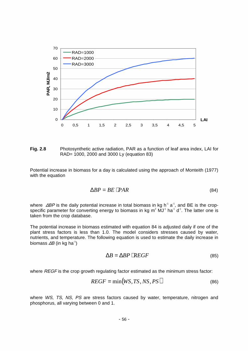
Interception of solar radiation is estimated with Beer’s law equation (Monsi and Saeki,1953) as a function of photosynthetic active radiation and leaf area index (see Fig. 2.8)

where PAR is the photosynthetic active radiation in MJ m-2, RAD is solar radiation in Ly, andLAI is the leaf area index.

( ) 0HUNA ,TB2

TMNTMXtHUNA ≥−

+= (81)

( )

PHUN

tHUNAIHUN t

∑= (82)

( )[ ]LAI6501RAD020920PAR ⋅−−⋅⋅= .exp. (83)

- 56 -

Fig. 2.8 Photosynthetic active radiation, PAR as a function of leaf area index, LAI forRAD= 1000, 2000 and 3000 Ly (equation 83)

Potential increase in biomass for a day is calculated using the approach of Monteith (1977)with the equation

where ∆BP is the daily potential increase in total biomass in kg h-1 a-1, and BE is the crop-specific parameter for converting energy to biomass in kg m2 MJ-1 ha-1 d-1. The latter one istaken from the crop database.

The potential increase in biomass estimated with equation 84 is adjusted daily if one of theplant stress factors is less than 1.0. The model considers stresses caused by water,nutrients, and temperature. The following equation is used to estimate the daily increase inbiomass ∆B (in kg ha-1)

where REGF is the crop growth regulating factor estimated as the minimum stress factor:

where WS, TS, NS, PS are stress factors caused by water, temperature, nitrogen andphosphorus, all varying between 0 and 1.

PARBEBP ⋅=∆ (84)

REGFBPB ⋅∆=∆ (85)

( )PSNSTSWSREGF ,,,min= (86)

0

10

20

30

40

50

60

70

0 0,5 1 1,5 2 2,5 3 3,5 4 4,5 5LAI

PA

R, M

J/m

2RAD=1000

RAD=2000RAD=3000

- 57 -

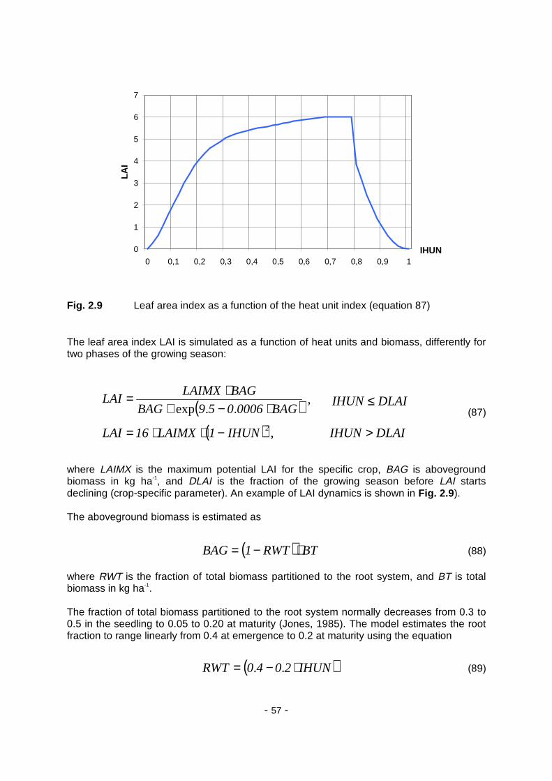
Fig. 2.9 Leaf area index as a function of the heat unit index (equation 87)

The leaf area index LAI is simulated as a function of heat units and biomass, differently fortwo phases of the growing season:

where LAIMX is the maximum potential LAI for the specific crop, BAG is abovegroundbiomass in kg ha-1, and DLAI is the fraction of the growing season before LAI startsdeclining (crop-specific parameter). An example of LAI dynamics is shown in Fig. 2.9).

The aboveground biomass is estimated as

where RWT is the fraction of total biomass partitioned to the root system, and BT is totalbiomass in kg ha-1.

The fraction of total biomass partitioned to the root system normally decreases from 0.3 to0.5 in the seedling to 0.05 to 0.20 at maturity (Jones, 1985). The model estimates the rootfraction to range linearly from 0.4 at emergence to 0.2 at maturity using the equation

( )( ) DLAIIHUNIHUN1LAIMX16LAI

DLAIIHUN ,BAG0006059BAG

BAGLAIMXLAI

2 >−⋅⋅=

≤⋅−+⋅=

,

..exp (87)

( ) BTRWT1BAG ⋅−= (88)

( )IHUN2040RWT ⋅−= .. (89)

0

1

2

3

4

5

6

7

0 0,1 0,2 0,3 0,4 0,5 0,6 0,7 0,8 0,9 1IHUN

LA

I

- 58 -

2.2.2 Growth Constraint: Water Stress

The water stress factor is calculated by considering water supply and water demand withthe following equation

where WUi is plant water use in layer i in mm. The value of potential plant transpiration EPis calculated in the evapotranspiration module.

The plant water use is estimated using the approach of Williams and Hann (1978) forsimulating plant water uptake. First, the root depth is calculated with the equation

where RD is the fraction of the root zone that contains roots and RDMX is the maximumroot depth in m (crop-specific parameter).

Then the potential water use in each soil layer is estimated with the equation

where WUPi is the potential water use rate from layer i in mm d-1, RDP is the rate-depthparameter, and RZDi is the root zone depth parameter for the layer i in mm.

The latter one is defined as

The value of RDP used in the model (3.065) was determined assuming that about 30% ofthe total water use comes from the top 10% of the root zone. The details of evaluating RDPare given in Williams and Hann (1978). Equation 92 allows roots to compensate for waterdeficits in certain layers by using more water in layers with adequate supply.

EP

WUWS

M

1ii∑

== (90)

RDMXIHUN52RD ⋅⋅= . (91)

( )

⋅−−⋅

−=

RD

RZDRDP1

RDP1

EPWUP i

i expexp

(92)

≤

>=

i

ii

i

ZRDRD

ZRDZRZD

,

,(93)

- 59 -

Then the potential water use must be adjusted for water deficits to obtain the actual wateruse WU for each layer:

After the calculation of actual water use by plants, the plant transpiration EP is adjusted.

2.2.3 Growth Constraint: Temperature Stress.

The temperature stress factor is calculated as an asymmetrical function, differently fortemperature below the optimal temperature TO, and above it. The equation for thetemperature stress factor TS for temperatures below TO is

where CTSL is the temperature stress parameter for temperatures below TO, and T is thedaily average air temperature in °C. The temperature stress parameter CTSL is evaluatedas

where TB is the base temperature for the crop in °C. Equation 96 assures that TS=0.9when the air temperature is (TO+TB)/2.

For the temperatures higher than TO

where the temperature stress parameter for temperatures higher than TO, CTSH, isevaluated as

An example of the temperature stress factor calculated with equations 96 and 98 is shownin Fig. 2.10.

FC250SW ,WUPWU iiii ⋅>= . (95)

iii

iii FC250SW ,

FC250

SWWUPWU ⋅≤

⋅⋅= .

.(94)

( ) ( )TOT

101T

TTOCTSL90TS

2

6≤

⋅+−⋅⋅= −.

.lnexp (96)

TBTO

TBTOCTSL

−+= (97)

( ) ,.

.lnexp TOT101CTSH

TTO90TS

2

6>

⋅+−⋅= −

(98)

TBTTO2CTSH −−⋅= (99)

- 60 -

Fig. 2.10 Temperature stress factor as a function of average daily air temperature(equations 96 and 98), assuming TO = 25° C and TB = 3° C

2.2.4 Growth Constraints: Nutrient Stress

Estimation of nutrient stress factors is based on the ratio of simulated plant N and Pcontents to the optimal values of nutrient content. The stress factors vary non-linearly from0 when N or P is half the optimal level to 1.0 at optimal N and P contents (Jones et al.,1984).

Let us consider the N stress factor first. As an initial step, the scaling factor SFN iscalculated as

where UN(t) is the crop N uptake on day t in kg ha-1, CNB is the optimal N concentration forthe crop, BT is the accumulated total biomass in kg ha-1.

Then the N stress factor is calculated with the equation (see also Fig. 2.11)

The P stress factor, PS, is calculated analogously, using the optimal P concentration, COP,instead.

( ) 50

BTCNB

tUN200SFN

−

⋅⋅= ∑ . (100)

( ) 0SFNifSFN0260523SFN

SFNNS >

⋅−+= ,

..exp(101)

0

0.2

0.4

0.6

0.8

1

1.2

1 4 7 10 13 16 19 22 25 28 31 34

T

TS

- 61 -

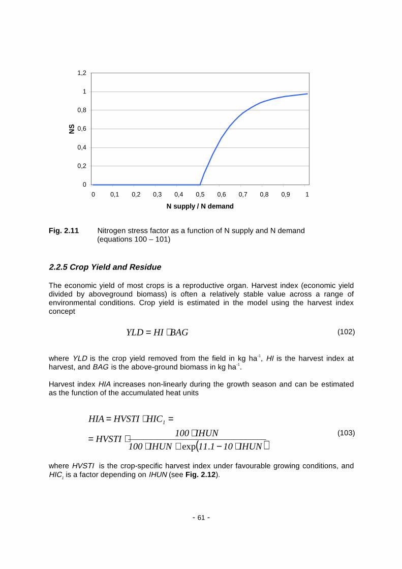
Fig. 2.11 Nitrogen stress factor as a function of N supply and N demand (equations 100 – 101)

2.2.5 Crop Yield and Residue

The economic yield of most crops is a reproductive organ. Harvest index (economic yielddivided by aboveground biomass) is often a relatively stable value across a range ofenvironmental conditions. Crop yield is estimated in the model using the harvest indexconcept

where YLD is the crop yield removed from the field in kg ha-1, HI is the harvest index atharvest, and BAG is the above-ground biomass in kg ha-1.

Harvest index HIA increases non-linearly during the growth season and can be estimatedas the function of the accumulated heat units

where HVSTI is the crop-specific harvest index under favourable growing conditions, andHIC1 is a factor depending on IHUN (see Fig. 2.12).

BAGHIYLD ⋅= (102)

( )

IHUN10111IHUN100

IHUN100HVSTI

HICHVSTIHIA 1

⋅−+⋅⋅⋅=

=⋅=

.exp

(103)

0

0,2

0,4

0,6

0,8

1

1,2

0 0,1 0,2 0,3 0,4 0,5 0,6 0,7 0,8 0,9 1

N supply / N demand

NS

- 62 -

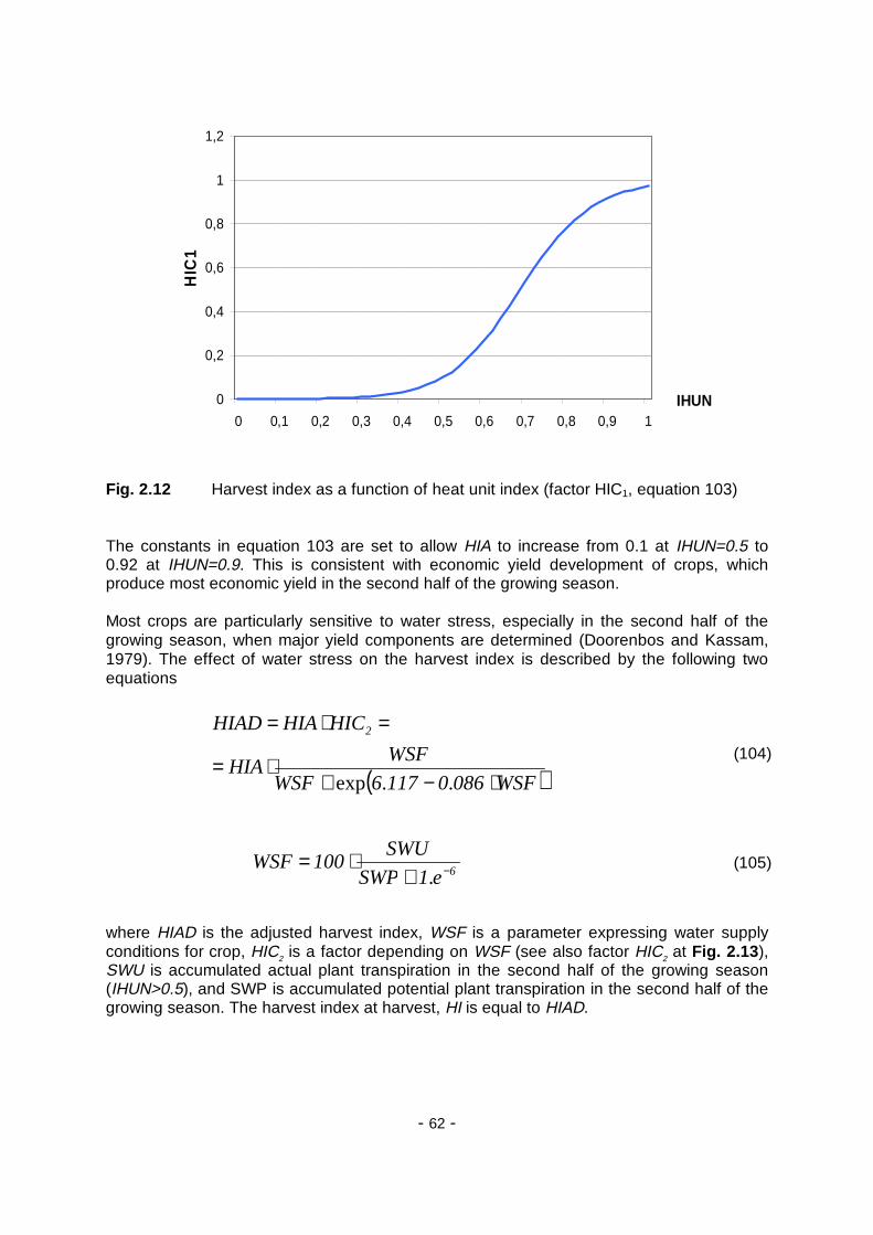
Fig. 2.12 Harvest index as a function of heat unit index (factor HIC1, equation 103)

The constants in equation 103 are set to allow HIA to increase from 0.1 at IHUN=0.5 to0.92 at IHUN=0.9. This is consistent with economic yield development of crops, whichproduce most economic yield in the second half of the growing season.

Most crops are particularly sensitive to water stress, especially in the second half of thegrowing season, when major yield components are determined (Doorenbos and Kassam,1979). The effect of water stress on the harvest index is described by the following twoequations

where HIAD is the adjusted harvest index, WSF is a parameter expressing water supplyconditions for crop, HIC2 is a factor depending on WSF (see also factor HIC2 at Fig. 2.13),SWU is accumulated actual plant transpiration in the second half of the growing season(IHUN>0.5), and SWP is accumulated potential plant transpiration in the second half of thegrowing season. The harvest index at harvest, HI is equal to HIAD.

( )WSF08601176WSF

WSFHIA

HICHIAHIAD 2

⋅−+⋅=

=⋅=

..exp

(104)

e1SWP

SWU100WSF

6−+⋅=

.(105)

0

0,2

0,4

0,6

0,8

1

1,2

0 0,1 0,2 0,3 0,4 0,5 0,6 0,7 0,8 0,9 1IHUN

HIC

1

- 63 -

Fig. 2.13 Harvest index as a function of soil water content (factor HIC2, equation 104)

The residue RSD is estimated at harvest as

where RWT is the fraction of roots, and BT is the total biomass. This relationship can bemodified for some crops if residue come from the roots.

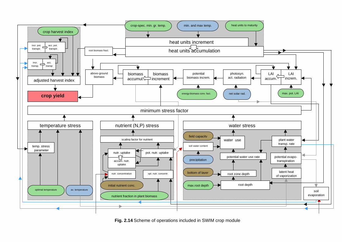
All processes described in Sections 2.2.1 – 2.2.5 are presented graphically in Fig. 2.14.There are three basic blocks in the crop module (depicted by the grey coloured boxes) thatare used to estimate the crop yield: accumulated heat units (top middle), stress factors(lower half), and harvest index (top left). The stress factors include temperature stress,nutrient stress (nitrogen and phosphorus), and water stress. The crop growth regulatingfactor is estimated as the minimum of these four factors. Nutrient stress is determined fromthe actual and potential nutrient uptake. Water stress is induced from water use and planttranspiration. The heat units accumulation is estimated from the crop specific minimumgrowth temperature, the daily minimum and maximum air temperatures and the assumedaccumulated heat units. The adjusted harvest index is evaluated from the actual andpotential transpiration and the crop specific harvest index. The small rectangles denotedependent variables, whereas the coloured ovals refer to model parameters independentfrom the others computed within the module. They describe the specifications of crop(green), climate (blue) and soil (brown).

( ) HIBTRWT1RSD ⋅⋅−= (106)

0

0.2

0.4

0.6

0.8

1

1.2

0 0.1 0.2 0.3 0.4 0.5 0.6 0.7 0.8 0.9 1

SWU/SWP

HIC

2

LAIincrem.

temperature stress nutrient (N,P) stress water stress

min. and max temp.

max. pot. LAIenergy-biomass conv. fact. net solar rad.

temp. stress parameter

optimal temperature av. temperature

potential water use rate

root depth

root zone depth

max.root depth

scaling factor for nutrient

crop yield

nutr. uptake

precipitation

bottom of layer

water use

latent heatof vaporization

crop-spec. min. gr. temp. heat units to maturity

crop harvest index

acc. pot. transpir.

acc.transp

adjusted harvest index

plant watertransp. rate

soil water content

field capacity

biomassincrement

potentialbiomass increm.

photosyn.act. radiation

biomassaccumul.

heat units accumulation

heat units increment

root biomass fract.

minimum stress factor

incr. pot.transpir.

incr.transp.

potential evapo-transpiration

LAIaccum.

soilevaporation

above-groundbiomass

pot. nutr. uptake

accum. nutr.uptake

nutrient fraction in plant biomass

opt. nutr. concentr.nutr. concentration

initial nutrient conc.

Fig. 2.14 Scheme of operations included in SWIM crop module

- 65 -

2.2.6 Adjustment of Net Photosynthesis to Altered CO2

Different approaches for the adjustment of net photosynthesis and evapotranspiration toaltered atmospheric CO2 concentration have been used in modelling studies (Goudrian etal., 1984; Rotmans et al., 1993). Detailed results about the interaction of higher CO2 andwater use efficiency are described in (Easmus, 1991; Grossman et al., 1995; Kimball et al.,in press).

Two different approaches can be used in SWIM for the adjustment of net photosynthesis(factor ALFA):1) an empirical approach based on adjustment of the biomass-energy factor as suggested

in EPIC and SWAT models (Arnold et al., 1994), and2) a new semi-mechanistic approach derived by F. Wechsung from a mechanistic model

for leaf net assimilation (Harley et al., 1992), which takes into account the interactionbetween CO2 and temperature.

The second method and its application for climate change impact study with SWIM isdescribed in Krysanova, Wechsung et al., 1999)

The factor ALFA is defined as

where AS1 and AS2 are net leaf assimilation rates (µmol m-2 s-1) in two periods,corresponding to two different CO2 concentrations.

In the first method ALFA is estimated as

where BE is the biomass-energy factor as in equation (83), CA is the current atmosphericCO2 concentration (µmol mol-1), and SHP1 and SHP2 are the coefficients of the S-shapecurve, describing the assumed change in BE for two different CO2 concentrations.

For the CO2 doubling, 1.1 times increase in BE is assumed for maize, and 1.3 timesincrease for wheat and barley (see Fig. 2.15).

AS

ASALFA

1

2= (107)

( )( ) SHPCASHPCABE

CA100ALFA

21 ⋅−+⋅⋅=

exp(108)

- 66 -

Fig. 2.15 Factor ALFA as a function of CO2 concentration for wheat and maizeestimated using the first method (equations 108, 109, 110) and assuming BE= 30 kg m2 MJ-1 ha-1 d-1 for wheat and BE = 40 kg m2 MJ-1 ha-1 d-1 for maize.The CO2 concentration is changing from 330 to 660 ppm

If CO2 concentration CA is changing from CA1 to CA2, and BE is changing from BE1 to BE2,the coefficients SHP1 and SHP2 can be estimated as following:

In the second method a temperature-dependent enhancement factor α was derived fromHarley et al., 1992 for cotton

where TL is the leaf temperature (°C), CL1 and CL2 are the current and future CO2

concentration inside leaves (µmol mol-1), and coefficients P1 = 0.3898⋅10-2 , P2 = 0.3769⋅10-5,and P3 = 0.3697⋅10-4.

( ) ( )

CACA

CABECA100CABECA100SHP

12

2221112 −

−⋅−−⋅= loglog(109)

( ) SHPCACABECA100SHP 211111 ⋅+−⋅= log (110)

( ) ( ) ( )( ) ( )[ ] CLCLTLPCLCLPCLCLP

ALFA

1232

12

22121 −⋅⋅+−⋅−−⋅=

=

exp

cot(111)

1

1,05

1,1

1,15

1,2

1,25

1,3

1,35

330 380 430 480 530 580 630

CO2, ppm

AL

FA

wheat

maize

- 67 -

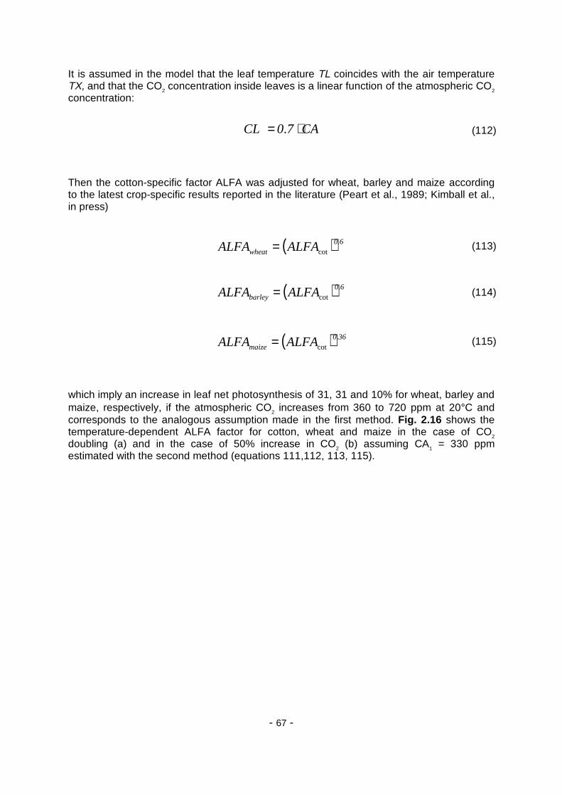
It is assumed in the model that the leaf temperature TL coincides with the air temperatureTX, and that the CO2 concentration inside leaves is a linear function of the atmospheric CO2

concentration:

Then the cotton-specific factor ALFA was adjusted for wheat, barley and maize accordingto the latest crop-specific results reported in the literature (Peart et al., 1989; Kimball et al.,in press)

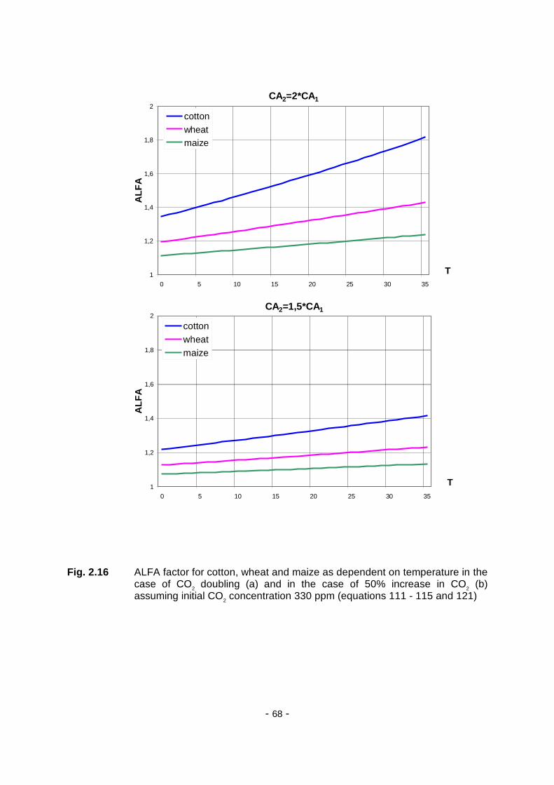
which imply an increase in leaf net photosynthesis of 31, 31 and 10% for wheat, barley andmaize, respectively, if the atmospheric CO2 increases from 360 to 720 ppm at 20°C andcorresponds to the analogous assumption made in the first method. Fig. 2.16 shows thetemperature-dependent ALFA factor for cotton, wheat and maize in the case of CO2

doubling (a) and in the case of 50% increase in CO2 (b) assuming CA1 = 330 ppmestimated with the second method (equations 111,112, 113, 115).

CA70CL ⋅= . (112)

( ) ALFAALFA 60barley

.cot= (114)

( ) ALFAALFA 360maize

.cot= (115)

( ) ALFAALFA 60wheat

.cot= (113)

- 68 -

Fig. 2.16 ALFA factor for cotton, wheat and maize as dependent on temperature in thecase of CO2 doubling (a) and in the case of 50% increase in CO2 (b)assuming initial CO2 concentration 330 ppm (equations 111 - 115 and 121)

CA2=2*CA1

1

1,2

1,4

1,6

1,8

2

0 5 10 15 20 25 30 35

T

AL

FA

cottonwheatmaize

CA2=1,5*CA1

1

1,2

1,4

1,6

1,8

2

0 5 10 15 20 25 30 35

T

AL

FA

cottonwheatmaize

- 69 -

2.2.7 Adjustment of Evapotranspiration to Altered CO2

Additionally, a possible reduction of potential leaf transpiration due to higher CO2 (factorBETA) derived directly from the enhancement of photosynthesis (factor ALF) was taken intoaccount in combination with both methods for the adjustment of net photosynthesis. Themethod was suggested by F. Wechsung.

The factor BETA is defined as

where EPO1 and EPO2 are potential plant transpiration rates (mol m-2 s-1) in two periods,corresponding to two different CO2 concentrations.

Assuming that

where VPD is the vapour pressure deficit (kPa), RESC is the total leaf resistance to CO2

transfer (m2 s mol-1), RESW is the total leaf resistance to water vapour transfer (m2 s mol-1).

From definitions 107 and116 and equation 117 the ratio can be estimated

The following assumptions can be accepted for a given plant (see, e.g. Morrison, 1993)

and

Then the following estimation is derived for BETA from equations 112, 118, 119 and 120

EPO

EPOBETA

1

2= (116)

RESC

RESW

VPD

CLCA

EPO

AS ⋅−= (117)

RESW

RESC

RESC

RESW

VPD

VPD

CLCA

CLCA

BETA

ALFA

1

1

2

2

2

1

11

22 ⋅⋅⋅−−= (118)

RESC

RESW

RESC

RESW

1

1

2

2 ≈ (119)

VPDVPD 12 ≈ (120)

CA

CAALFABETA

2

1⋅= (121)

- 70 -

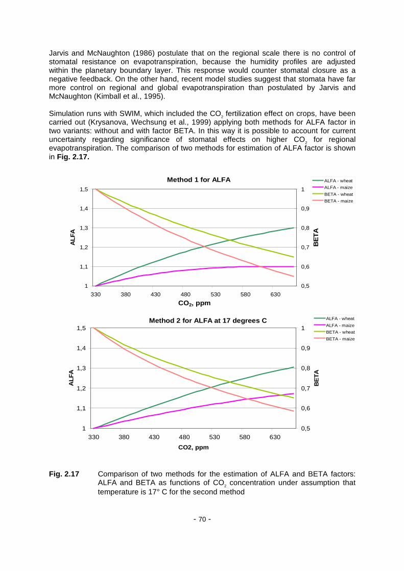
Jarvis and McNaughton (1986) postulate that on the regional scale there is no control ofstomatal resistance on evapotranspiration, because the humidity profiles are adjustedwithin the planetary boundary layer. This response would counter stomatal closure as anegative feedback. On the other hand, recent model studies suggest that stomata have farmore control on regional and global evapotranspiration than postulated by Jarvis andMcNaughton (Kimball et al., 1995).

Simulation runs with SWIM, which included the CO2 fertilization effect on crops, have beencarried out (Krysanova, Wechsung et al., 1999) applying both methods for ALFA factor intwo variants: without and with factor BETA. In this way it is possible to account for currentuncertainty regarding significance of stomatal effects on higher CO2 for regionalevapotranspiration. The comparison of two methods for estimation of ALFA factor is shownin Fig. 2.17.

Fig. 2.17 Comparison of two methods for the estimation of ALFA and BETA factors:ALFA and BETA as functions of CO2 concentration under assumption thattemperature is 17° C for the second method

Method 1 for ALFA

1

1,1

1,2

1,3

1,4

1,5

330 380 430 480 530 580 630

CO2, ppm

AL

FA

0,5

0,6

0,7

0,8

0,9

1

BE

TA

ALFA - wheat

ALFA - maize

BETA - wheat

BETA - maize

Method 2 for ALFA at 17 degrees C

1

1,1

1,2

1,3

1,4

1,5

330 380 430 480 530 580 630

CO2, ppm

AL

FA

0,5

0,6

0,7

0,8

0,9

1

BE

TAALFA - wheat

ALFA - maize

BETA - wheat

BETA - maize

- 71 -

2.3 Nutrient Dynamics

Sub-basin nutrient cycling modules were taken from MATSALU and SWAT, and modifiedwhere necessary. The approach used in SWAT was modified from the EPIC model(Williams et al., 1984). The model simulates water, sediment and nutrients dynamics inevery hydrotope, aggregates results for sub-basins, and then routes the water, sediment,and nutrients with lateral flow from the sub-basin outlet to the basin outlet.

2.3.1 Soil Temperature

Several processes of nutrient transformation, like mineralisation, are of microbial character,therefore estimation of soil temperature is necessary. Daily average soil temperature isdefined at the center of each soil layer. The basic soil temperature equation is

where TSO(Z,t) is the soil temperature at the depth Z in the day t in °C, Z is depth from thesoil surface in mm, t is time d, TAV is the average annual air temperature in °C, AMP is theannual amplitude in daily average temperature in °C, and DD is the damping depth for thesoil in mm.

The damping depth DD can be defined as a function of soil bulk density BD and watercontent SW as expressed in the following equations

where DP is the maximum damping depth for the soil in mm, BD is the soil bulk density in tm-3, ZM is the distance from the bottom of the lowest soil layer to the surface in mm, andSPD is a scaling parameter.

Equation (122) reflects average conditions, if only TAV and AMP parameters are used.Since air temperature is provided as input, the soil temperature module can use the airtemperature as driver to correct equation 122.

( ) DD

Z

DD

Z200t

365

2

2

AMPTAVtZTSO

−⋅

−−⋅⋅⋅+= expcos),(

π(122)

+−⋅

⋅=

2

SPD1

SPD1

DP

500DPDD lnexp (123)

( ) BD635686BD

BD25001000DP

⋅−⋅+⋅+=

.exp(124)

( ) ZMBD14403560

SWSPD

⋅⋅−=

..(125)

- 72 -

First, the bare soil surface temperature is estimated as

where TGB(t) is the bare soil surface temperature in °C in the day t, TMX, T, and TMN arethe maximum, average and minimum daily air temperature in °C, and WFT is a proportionof rainy days in a month.

Equation 127 uses the minimum air temperature as a base to estimate surface temperatureon rainy days. Higher temperatures are estimated on dry days using equation 126. Thevalue of WFT is determined by considering the number of rainy days in this month:

where NDD is the number of days in a month, and NRD is the number of rainy days in amonth.

The soil surface temperature is also affected by residue and snow cover. This effect isintroduced by lagging the predicted base surface temperature with the equation

where BCV is a lagging factor for simulating residue and snow cover effects on surfacetemperature. The value of BCV is 0 for bare soil and approaches 1.0 as cover increased asexpressed in the equation

where COV is the land cover, or the sum of above ground biomass and crop residue in kgha-1 and SNO is the water content of the snow cover in mm.

Then the soil temperature at any depth is estimated with equation 122 by substituting TG(t)for TS(0,t). TG(t) is a better estimate of the surface temperature than T(0,t), becausecurrent weather and cover conditions are considered. At the soil surface (Z=0), the propersubstitution can be accomplished by adding TG(t) and subtracting TS(0,t) from equation122. Differences between TG(t) and TS(0,t) are damped as Z increases. So, the finalequation for estimating soil temperature at any depth is

( ) ( ) 0 = PRECIP ,TTTMXWFTtTGB +−⋅= (126)

( ) ( ) 0 PRECIP ,TMNTMNTWFTtTGB >+−⋅= (127)

NDD

NRDWFT = (128)

( ) ( ) ( ) ( ) tTGBBCV11tTGBBCVtTG ⋅−+−⋅= (129)

( )

( )

SNO302200556SNO

SNO

COV1029715637COV

COV

BCV4

⋅−+

⋅⋅−+=

−

..exp

,..exp

max (130)

Fig. 2.18 An example of soil temperature dynamics in five soil layers simulated with SWIM using equation 131

-15

-10

-5

0

5

10

15

20

25

30

1 61 121 181 241 301 361 56 116 176 236 296 356 51 111 171 231 291 351day

deg

ree

C

lay1

lay2

lay3

lay4

lay5

- 74 -

An example of soil temperature dynamics as simulated by SWIM using equation 131 isshown in Fig. 2.18.

2.3.2 Fertilization and Input with Precipitation

Fertilization in form of mineral and active organic N and P is treated as input information inSWIM. The amounts and dates should be specified in advance. The amounts of fertilizersapplied can be either strict or calculated values, depending on whether the strict or flexiblefertilization scheme is applied. In the latter case the amounts of applied N and P depend onthe actual concentration of mineral N and P in soil.

To estimate the N contribution from rainfall, SWIM uses an average rainfall N and Pconcentration, specific for the region. The amount of N and P in precipitation is estimatedas the product of rainfall amount and concentration.

2.3.3 Nitrogen Mineralisation

The nitrogen mineralisation model is a modification of the PAPRAN mineralisation model(Seligman and van Keulen, 1981). The model considers two sources of mineralisation:(a) fresh organic N pool, associated with crop residue, and(b) the active organic N pool, associated with the soil humus.

Step 1. When the model is initialized, organic N associated with humus is divided into twopools: active or readily mineralisable organic nitrogen ANOR and stable organic nitrogenSNOR (in kg ha-1) by using the equation

where ANFR is the active pool fraction (set to 0.15), NOR is the total organic N in kg ha-1

estimated from the initial soil data.

Organic N flow between the active and stable pools is described with the equilibriumequation

where ASNFL is the flow in kg ha-1 d-1 between the active and stable organic N pools,CASN is the rate constant (10-4 d-1). The daily flow of humus-related organic N, ASNFL, isadded to the stable organic N pool and subtracted from the active organic N pool.

( ) ( ) ( )

DD

Zt0TStTG

DD

Z200t

365

2

2

AMP

TAVtZTSO

−⋅

−+

−−⋅⋅⋅+

+=

exp,cos

),(

π (131)

NORANFRANOR ⋅= (132)

−⋅= SNOR

ANFR

ANORCASNASNFL (133)

- 75 -

Step 2. The residue is decomposed daily in accordance with the equation

where DECR is the decomposition rate. Fresh organic N pool FON is associated withresidue. It is recalculated with the same equation daily:

and N mineralisation flow from fresh organic N in kg ha-1 d-1, FOMN, is estimated as

The decomposition rate DECR is a function of C:N ratio, C:P ratio, temperature, and watercontent in soil

where CNRF and CPRF are the C:N and C:P ratio factors of mineralisation, respectively,and TFM2 and WFM are the temperature and soil water factors of mineralisation,respectively. The values of CNRF and CPRF are calculated with the equations

where CNR is the C:N ratio and CPR is the C:P ratio.The CNR and CPR are calculated with the equations

( ) DECR1RSDRSD −⋅= (134)

( ) DECR1FONFON −⋅= (135)

FONDECRFOMN ⋅= (136)

( ) WFMTFMCPRFCNRF050DECR 2 ⋅⋅⋅= ,min. (137)

( )

−⋅−=

25

25CNR6930CNRF

.exp (138)

( )

−⋅−=

200

200CPR6930CPRF

.exp (139)

NMINFON

RSD580CNR

+⋅= .

(140)

PLABFOP

RSD580CPR

+⋅= .

(141)

- 76 -

where FON is the amount of fresh organic N in kg ha-1 , FOP is the amount of fresh organicP in kg ha-1, NMIN is the amount of mineral nitrogen (or nitrate nitrogen plus ammoniumnitrogen) in kg ha-1, and PLAB is the amount of labile P in kg ha-1.

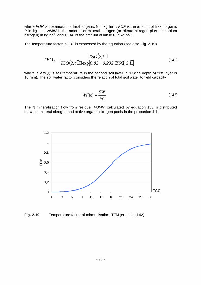
The temperature factor in 137 is expressed by the equation (see also Fig. 2.19)

where TSO(2,t) is soil temperature in the second soil layer in °C (the depth of first layer is10 mm). The soil water factor considers the relation of total soil water to field capacity

The N mineralisation flow from residue, FOMN, calculated by equation 136 is distributedbetween mineral nitrogen and active organic nitrogen pools in the proportion 4:1.

Fig. 2.19 Temperature factor of mineralisation, TFM (equation 142)

( )( ) ( )[ ]

t2TSO2320826t2TSO

t2TSOTFM 2 ,..exp,

,

⋅−+= (142)

FC

SWWFM = (143)

0

0,2

0,4

0,6

0,8

1

1,2

0 3 6 9 12 15 18 21 24 27 30

TSO

TF

M

- 77 -

Step 3. The stable organic N pool is not subjected to mineralisation. Only the active pool oforganic N in soil is exposed to mineralisation. The mineralisation from the active organic Nis expressed by the equation

where HUMNi is the mineralisation rate in kg ha-1 d-1 for the active organic N pool in layer i,COMN is the humus rate constant for N (0.0003 d-1), and TFMi and WFM i are thetemperature and water factors of mineralisation for the layer i.

The temperature and water factors are calculated for any soil layer the same as for residuedecomposition using equations 142 and 143. At the end of the day, the humusmineralisation is subtracted from the active organic N pool and added to the mineral N pool.

2.3.4 Phosphorus Mineralisation

The phosphorus mineralisation model is structurally similar to the nitrogen mineralisationmodel, with some differences as explained below.

Step 1. Fresh organic P pool FOP is associated with residue. It is recalculated daily as

Then the P mineralisation flow from fresh organic P in kg ha-1 d-1, FOMP, is estimated as

where the rate DECR is calculated the same as for nitrogen using equation 137.

Step 2. Mineralisation of organic P associated with humus is estimated for each soil layerwith the following equation

where HUMPi is the mineralisation rate in kg ha-1 d-1 i, COMP is the humus mineralisationrate constant for P, and POR is the P organic pool in soil layer i.

To maintain the P balance at the end of a day, the mineralized humus is subtracted fromthe organic P pool and added to the mineral P pool, and the mineralized residue issubtracted from the FOP pool. Then 1/5 of FOMP is added to the POR pool, and 4/5 ofFOMP is added to labile P pool, PLAB.

ANORWFMTFMCOMNHUMN iiii ⋅⋅⋅= (144)

( ) DECR1FOPFOP −⋅= (145)

FOPDECRFOMP ⋅= (146)

PORWFMTFMCOMPHUMP iiii ⋅⋅⋅= (147)

- 78 -

2.3.5 Phosphorus Sorption / Adsorption

Mineral phosphorus is distributed between three pools: labile phosphorus, PLAB, activemineral phosphorus, PMA and stabile mineral phosphorus, PMS. Mineral P flow betweenthe active and stable mineral pools is governed by the equilibrium equation

where ASPFL is the flow in kg ha-1 d-1 between the active and stable mineral P pools, CASPis the rate constant (0.0006 d-1). The daily flow ASPFL is added to the stable mineral pooland subtracted from the active mineral pool.

Mineral P flow between the active and labile mineral pools is governed by the equilibriumequation

where ALPFL is the flow in kg ha-1 d-1 between the active and labile mineral P pools, CALPis the equilibrium constant (default: 1.). The daily flow ALPFL is added to the active mineralpool and subtracted from the labile mineral pool.

2.3.6 Denitrification

Denitrification causes NO3 to be volatilized from soil. The denitrification occurs only in theconditions of oxygen deficit, which usually is associated with high water content. Besides,as one of the microbial processes, denitrification is a function of temperature and carboncontent. The equation used to estimate the denitrification rate is

where DENIT is the denitrification flow in layer i in kg ha-1 d-1, WFD is the soil water factor ofdenitrification, and TCFD is the combined temperature-carbon factor.

The soil water factor considers total soil water and is represented by the exponentialequation (see Fig. 2.20)

where SWi is the soil water content in layer i in mm and FCi is the field capacity in mm mm-1.

( )PMSPMA4CASPASPFL −⋅⋅= (148)

PMACALPPLABALPFL ⋅−= (149)

90FCSW0DENIT

90FCSWNITTCFDWFDDENIT

ii

iiiiii

..

.,

<=

≥⋅⋅=(150)

⋅⋅=

FC

SW3060WFD i

i exp. (151)

- 79 -

Fig. 2.20 Soil water factor of denitrification (equation 151)

The combined temperature and carbon factor is expressed by the equation

where CDN is a shape coefficient, TFMi coincides with the temperature factor ofmineralisation, and CBNi is the carbon content, and subscript i refers to the layers.

2.3.7 Nutrient Uptake by Crops

Nitrogen uptake by crop is estimated using a supply and demand approach. The daily (dayt) crop N demand can be computed using the equation

where NDEM(t) is the N demand of the crop in kg ha-1, CNB(t) is the optimal Nconcentration in the crop biomass, and BT(t) is the accumulated biomass in kg ha-1. Threeparameters BN1, BN2, and BN3 are specified for every crop in the crop database, whichdescribe: BN1 - normal fraction of nitrogen in plant biomass excluding seed at emergence,BN2 – at 0.5 maturity, and BN3 - at maturity.

( )iii CBNTFMCDN1TCFD ⋅⋅−= exp (152)

( ) ( ) ( ) ( ) ( ) 1tBT1tCNBtBTtCNBtNDEM −⋅−−⋅= (153)

0

0,5

1

1,5

2

2,5

0 0,2 0,4 0,6 0,8 1 1,2

SW/FC

WF

D

- 80 -

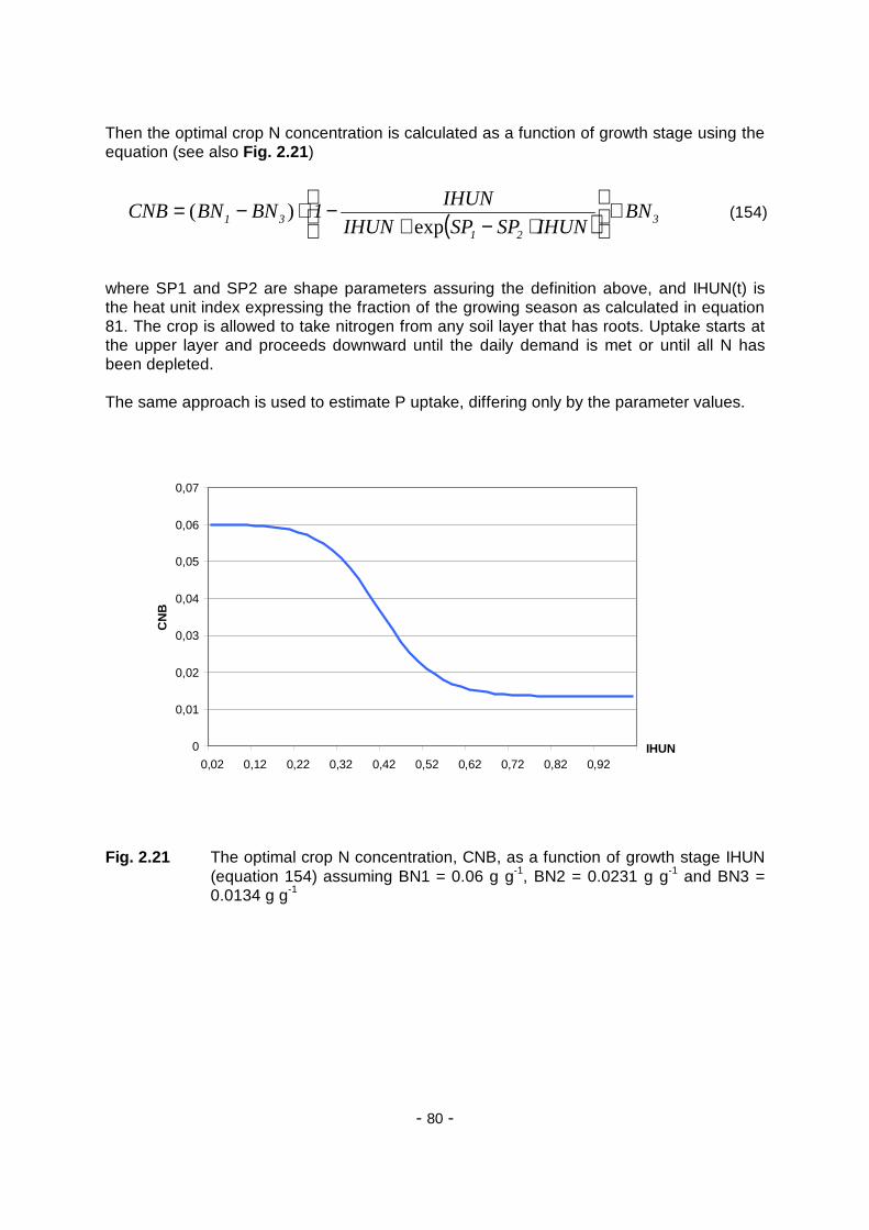
Then the optimal crop N concentration is calculated as a function of growth stage using theequation (see also Fig. 2.21)

where SP1 and SP2 are shape parameters assuring the definition above, and IHUN(t) isthe heat unit index expressing the fraction of the growing season as calculated in equation81. The crop is allowed to take nitrogen from any soil layer that has roots. Uptake starts atthe upper layer and proceeds downward until the daily demand is met or until all N hasbeen depleted.

The same approach is used to estimate P uptake, differing only by the parameter values.

Fig. 2.21 The optimal crop N concentration, CNB, as a function of growth stage IHUN(equation 154) assuming BN1 = 0.06 g g-1, BN2 = 0.0231 g g-1 and BN3 =0.0134 g g-1

( ) 321

31 BNIHUNSPSPIHUN

IHUN1BNBNCNB +

⋅−+

−⋅−=exp

)( (154)

0

0,01

0,02

0,03

0,04

0,05

0,06

0,07

0,02 0,12 0,22 0,32 0,42 0,52 0,62 0,72 0,82 0,92IHUN

CN

B

- 81 -

2.3.8 Nitrate Loss in Surface Runoff and Leaching to Groundwater

The total amount of water lost from the soil layer i is the sum of surface runoff, lateralsubsurface flow (or interflow), and percolation from this layer:

where WTOT is the total water lost from the soil layer in mm, Q is the surface runoff in mm,SSF is the lateral subsurface flow in mm, and PERC is the percolation in mm, and i is thelayer.

The amount of nitrate nitrogen lost with WTOTi is the product of NO3-N concentration andwater loss as expressed by the equation

where NFLi is the amount NO3-N lost from the layer i in kg ha-1 and CONi is theconcentration of NO3-N in the layer i in kg ha-1.

The amount of NO3-N left in the layer is adjusted daily as

where NMIN(t-1) and NMIN(t) are the amounts of NO3-N contained in the layer at thebeginning and end of the day (in kg ha-1).

Then the NO3-N concentration can be estimated by dividing the weight of NO3-N by thewater storage in the layer:

where CONi(t) is the concentration of NO3-N at the end of the day in kg ha-1, PO is the soilporosity in mm mm-1, and WP is the wilting point water content for soil layer in mm mm-1.

Equation 158 is a finite different approximation of the exponential equation

iiii PERCSSFQ WTOT ++= (155)

iii CONWTOTNFL ⋅= (156)

( ) ( ) ii CONWTOT1tNMINtNMIN ⋅−−= (157)

( ) ( )

−

−⋅−−−=ii

iiii WPPO

WTOT1tCON1tCONtCON )( (158)

( ) ( )

−

−−−=ii

iii WPPO

WTOT1tCONtCON exp (159)

- 82 -

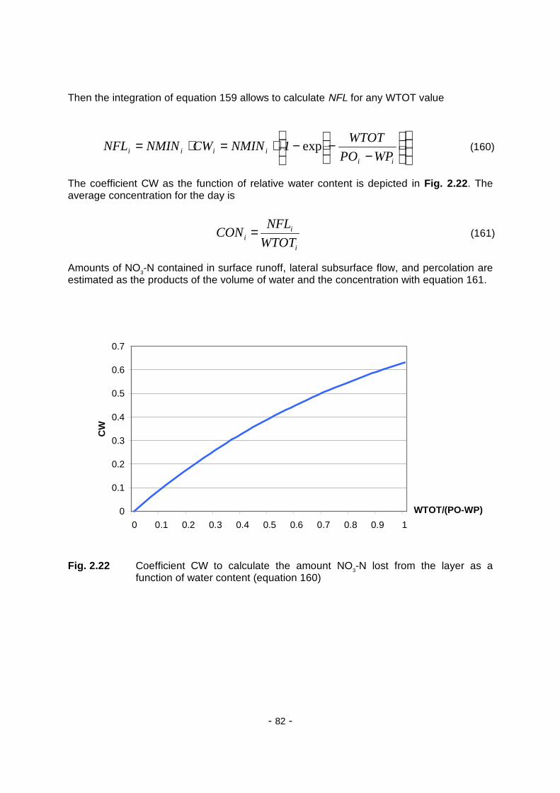
Then the integration of equation 159 allows to calculate NFL for any WTOT value

The coefficient CW as the function of relative water content is depicted in Fig. 2.22. Theaverage concentration for the day is

Amounts of NO3-N contained in surface runoff, lateral subsurface flow, and percolation areestimated as the products of the volume of water and the concentration with equation 161.

Fig. 2.22 Coefficient CW to calculate the amount NO3-N lost from the layer as afunction of water content (equation 160)

WPPO

WTOT1NMINCWNMINNFL

ii

iiii

−

−−⋅=⋅= exp (160)

i

ii WTOT

NFLCON = (161)

0

0.1

0.2

0.3

0.4

0.5

0.6

0.7

0 0.1 0.2 0.3 0.4 0.5 0.6 0.7 0.8 0.9 1

WTOT/(PO-WP)

CW

- 83 -

2.3.9 Soluble Phosphorus Loss in Surface Runoff

Phosphorus in soil is mostly associated with the sediment phase. Therefore the soluble Prunoff equation can be expressed in the simple form

where PFL is the soluble P in kg ha-1 d-1 lost with surface runoff, Q is the surface runoff inmm, COP is the concentration of labile phosphorus in soil layer in g t-1, and CSW is the Pconcentration in the sediment divided by that of the water in m3 t-1. The value of COP isinput to the model and remains constant. The default value of CSW used in the model is175.

All processes described in Sections 2.3.1 – 2.3.9 are presented graphically in Figs. 2.23(for nitrogen cycle) and 2.24 (for phosphorus).

The nitrogen module operates with four main pools depicted by the blue rectangles in Fig.2.23: nitrate, stable organic N, mineralisable organic N and fresh organic N (crop residue).The nitrate pool is influenced by the following flows (depicted as flags): N fertilizerapplication, N precipitation input, N leaching, potential N uptake by plants anddenitrification. The latter one is subject to the impact of the following variables andparameters: soil water content, field capacity, shape coefficient, temperature factor ofmineralisation and carbon content. The exchange between stable and mineralisableorganic nitrogen pools, whose intensity depends on the size of these pools and the rateconstant, is shown on the right-hand side. The mineralisation is a function of soiltemperature, soil water content, field capacity and the humus rate constant.

The phosphorus module (Fig. 2.24) consists of five pools, namely fresh organic P (cropresidue), organic P, labile P, active and stable mineral P. Labile P is influenced by thefollowing five flows: decomposition, mineralisation, potential nutrient uptake, P loss byleaching and P exchange with the active mineral phosphorus pool. The size of the lattertwo flows is modulated by the amount of P in the concerned pools. The two-directionalinfluence we meet in the case of the exchange flow between active and stable mineral P,and the mineralisation and decomposition flows (also pictured as flags). Mineralisation,decomposition, and soil erosion control the amount of organic P. The same as for thenitrogen cycle, mineralisation is influenced by soil temperature, soil water content, fieldcapacity and the humus rate constant, whereas the decomposition rate essentially dependson the C-N-ratio, C-P-ratio and soil temperature.

CSW

QCOP010PFL

⋅⋅= .(162)

- 74 -

nitrate (ano3)

soil water factor ofdenitrification

combined temp.-carbon factor ofdenitrification

fieldcapacity

soil watercontent

shapecoefficient

temp. factor

of mineral.

C contentin the layer

active or readilymineralizable

organic N(anora)

active poolfraction (0.15)

stableorganic N(anors)

rate constant

denitrification (denit)

fresh organic Nfrom crop

residue (fon) decomposition

rate (decr)

soil water fact. of mineralization

temperature factorof mineralization

C:N ratio factor ofmineralization

C:P ratio factor ofmineralization

C:N ratio

C:P ratio

amount oflabile P (plab)

amount ofminer. N insoil (nmin)

soiltemperature

crop residue

mineralization(humn)

humus rateconstant for N

input with precip.(qip)

leaching(vno3)

N appl. with fertil.(fen)

flow between active& stable org. N pool(asnflow)

pot. nutr. uptake(uno3)

decomposition(fomn)

fresh organic P (fop)

Fig. 2.23 Scheme of operations included in SWIM nitrogen module

- 75 -

fieldcapacity

soil watercontent

activemineral P

(pma)

stablemineral P

(pms)

decompositionrate (decr)

soil water fac. of mineralization

temperature factorof mineralization

C:N ratio factor ofmineralization

C:P ratio factor ofmineralization

C:N ratio

C:P ratio

amount ofminer. N insoil (nmin)

soiltemperature

crop residue

mineralization(hump)

humus rateconstant for P

flow between active& stable org. P pools

(aspflow)

decomposition(fomp)

fresh organic Pfrom crop

residue (fop)

organic P(porg)

erosion(yphe)

flow between active& labile P pools

(alpflow)

amount oflabile P (plab)

soluble P lossby leaching (ysp)

pot. nutr. uptake(uap)

Fig. 2.24 Scheme of operations included in SWIM phosphorus module

- 86 -

2.4 Erosion

2.4.1 Sediment Yield

Sediment yield is calculated for each sub-basin with the Modified Universal Soil LossEquation (MUSLE) (Williams and Berndt, 1977), practically the same as in SWAT:

where YSED is the sediment yield from the sub-basin in t, VOLQ is the surface runoffcolumn for the sub-basin in m3, PEAKQ is the peak flow rate for the sub-basin in m3 s-1, K isthe soil erodibility factor, C is the crop management factor, ECP is the erosion controlpractice factor, and LS is the slope length and steepness factor.

The only difference between SWAT and SWIM in the erosion module is that the surfacerunoff, the soil erodibility factor K and the crop management factor C are estimated inSWIM for every hydrotope, and then averaged for the sub-basin (weighted areal average).In SWAT there are two options: option 1 based on two-level disaggregation “basin – sub-basins”, when the above mentioned factors are first estimated for the sub-basins, andoption 2 similar to that of SWIM, when the factors are estimated first for HRUs (HydrologicResponse Units).

The soil erodibility factor K is estimated from the texture of the upper soil layer or is takenfrom a database.

The crop management factor, C, is evaluated with the equation,

where COV is the soil cover (above ground biomass + residue) in kg ha-1 and CMN is theminimum value of C.

The value of CMN is estimated from the average annual value of C factor, CAV, using theequation

The value of CAV for each crop is determined from tables prepared by Wischmeier andSmith (1978).

The erosion control practice is estimated as default value of 0.5, if no other data areavailable (which is usually the case for mesoscale basins and regional case studies).

( ) LSECPCKPEAKQVOLQ811YSED 560 ⋅⋅⋅⋅⋅⋅= .. (163)

( ) ( )[ ] COV001150CMN22310CMNC ⋅−⋅−−+= .exp.exp (164)

( ) 10340CAV4631CMN .ln. +⋅= (165)

- 87 -

Fig. 2.25 The LS factor calculated as a function of slope steepness SS for differentslope lengths SL (equations 166-167)

The LS factor is estimated with the equation (Wischmeier and Smith, 1978) (see Fig. 2.25)

where SL is the slope length, SS is the slope steepness, and the exponent ξ varies withslope and is computed with the equation

The slope length and slope steepness are calculated in SWIM/GRASS interface for everysub-basin.

( )0650SS5654SS4165122

SLLS 2 ...

.+⋅+⋅⋅

=

ξ

(166)

( )[ ] SS83535160 ⋅−−⋅= .exp.ξ (167)

0

10

20

30

40

50

0 0,1 0,2 0,3 0,4 0,5

SS

LS

fac

tor

SL=100

SL=75SL=50

- 88 -

2.4.2 Organic Nitrogen Transport by Sediment

A loading function developed by McElroy et al. (1976) and modified by Williams and Hann(1978) for application to individual runoff events is used to estimate organic N loss for eachsub-basin. The loading function is

where YON is the organic N runoff loss at the sub-basin outlet in kg ha-1, CNOR is theconcentration of organic N in the top soil layer in g t-1, and ER is the enrichment ratio. Thevalue of CNOR is input to the model and is constant throughout the simulation.

The enrichment ratio is the concentration of organic N in sediment divided by that of thesoil. Enrichment ratios are logarithmically related to sediment concentration as described byMenzel (1980). An individual event enrichment sediment concentration relationship wasdeveloped considering upper and lower bounds. The upper bound of the enrichment ratio isthe inverse of the sediment delivery ratio DR (sub-basin sediment yield divided by grosssheet erosion): ER<1/DR. Exceeding the inverse of the delivery ratio implied that moreorganic N leaves the watershed than is dislodged from the soil.

The delivery ratio is estimated for each runoff event using the equation

where DR is the sediment delivery ratio, PEAKQ is the peak runoff rate in mm h-1, andPRER is the peak rainfall excess rate in mm h-1.

Equation 169 is based on sediment yield estimated using MUSLE (Williams, 1975). Therainfall excess rate cannot be evaluated directly because the model uses only the total dailyrunoff volume, and not the event rainfall. An estimation of PRER can be obtained, however,using the equation

where PRR is the peak rainfall rate in mm h-1 and AIR is the average infiltration rate in mmh-1.

The peak rainfall rate can be calculated with the equation

ERCNORYSED0010YON ⋅⋅⋅= . (168)

PRER

PEAKQDR

560.

= (169)

AIRPRRPRER −= (170)

−

⋅⋅=501

1PRECIP2PRR

.

logα

(171)

- 89 -

The average infiltration rate can be calculated with the equation

where DUR is the rainfall duration in h, and PRECIP is rainfall in mm.

The rainfall duration is estimated the same as in equation 32 according to Williams et al.(1984).

The enrichment ratio is estimated with the logarithmic equation

where SEDC is the sediment concentration in g m-3, and PCON and PEXP are parametersset by the upper and lower limits.

To approach the lower limit for the enrichment ratio, 1.0, the sediment concentration shouldbe extremely high. Conversely, a very low sediment concentration would cause theenrichment ratio to approach 1/DR. The simultaneous solution of equation 174 at theboundaries assuming that sediment concentrations range from 500 to 250000 g m-3 givesthe following estimations for PEXP and PCON

2.4.3 Phosphorus Transport by Sediment

Phosphorus transport with sediments is simulated with a loading function similar to thatdescribed in 2.4.2 for the organic N transport. The loading function for phosphorus is

where YP is the sediment phase of P loss in runoff in kg ha-1, and POR1 is the concentrationof organic P in the top soil layer in g t-1.

DUR

QPRECIPAIR

−= (172)

( )501

30252

PRR

PRECIP6054DUR

.log(

..

α−−=⋅= (173)

PEXPSEDCPCONER ⋅= (174)

6992DR

1

PEXP.

log

=(175)

250

1PCON

PEXP.= (176)

ERPORYSED010 YP 1 ⋅⋅⋅= . (177)

- 90 -

2.5 River Routing

2.5.1 Flow Routing

The model uses the Muskingum flow routing method (see Maidment, 1993 and Schulze,1995). For a given reach, the continuity equation may be expressed as:

where d(STOR)/dt is the rate of change of storage within the reach (m3 s-1), QIN(t) is theinflow rate (m3 s-1) at time t, and QOUT(t) is the outflow rate (m3 s-1) at time t.

The Muskingum method assumes a variable discharge storage equation:

where STOR(t) is the storage (m3) in river reach at time t, KST is the storage time constantfor the reach (s), and X is the dimentionless weighting factor in river reach routing.

Here KST is the ratio of storage to discharge and has the dimention of time. In physicalterms, KST is considered to be an average reach travel time for a flood wave, and Xindicates the relative importance of the input QIN and outflow QOUT in determining thestorage in a reach. The lower and upper limits for X are 0 and 0.5, respectively. Typicalvalues of X for a river reach range between 0.0 and 0.3, with a mean value near 0.2.

Thus, from 179 the change in storage over time ∆t is given as

The Muskingum equation is derived from the finite difference form of the continuity equation178 and equation 180 as the following:

( ) ( ) ( )tQOUTtQINdt

STORd −= (178)

( ) ( ) ( ) ( )[ ]tQOUTX1tQINXKSTtSTOR ⋅−+⋅⋅= (179)

( ) ( )( ) ( ) ( )[ ]( ) ( ) ( )[ ]tQOUTX1tQINXKST

1tQOUTX11tQINXKST

tSTOR1tSTOR

⋅−+⋅⋅−−+⋅−++⋅⋅=

=−+(180)

( ) ( ) ( ) ( )tQOUTCtQINC1tQINC1tQOUT 321 ⋅+⋅++⋅=+ (181)

- 91 -

where the parameters C1, C2 and C3 are determined as (see also Fig. 2.26)

Here KST and ∆t must have the same time units and the three coefficients C1, C2 and C3

sum to 1.0. Numerical stability is attained and the computation of negative outflows isavoided if the following condition is fulfilled

Fig. 2.26 Coefficients C1, C2 and C3 as functions of parameter KST as used tocalculate flow routing with the Muskingum equations 182-184 assuming thatX = 0.2 and ∆t = 1

t50XKSTKST

t50XKSTC1 ∆⋅+⋅−

∆⋅+⋅−=.

.(182)

t50XKSTKST

t50XKSTC2 ∆⋅+⋅−

∆⋅+⋅=.

.(183)

t50XKSTKST

t50XKSTKSTC3 ∆⋅+⋅−

∆⋅−⋅−=..

(184)

( )X1KST2tXKST2 −⋅⋅<∆<⋅⋅ (185)

0

0,1

0,2

0,3

0,4

0,5

0,6

0,7

0,625 0,925 1,225 1,525 1,825 2,125 2,425

KST

C1C2

C3

- 92 -

Estimation of KST is based on the reach geometry

where CHL is the reach length, and CLR is the wave celerity.

The celerity may be estimated by using the Manning formula with an adjusting coefficientfor a certain reach shape. For the wide rectangular reach the celerity may be estimated(Schulze, p. AT13-9) as

where CHV is the average stream velocity in m s-1. The average velocity is estimated fromthe Manning formula as

where HR is hydraulic radius, CHS is channel bottom slope, CHN is the Manning’sroughness N. The value of X is set in the model to 0.2.

2.5.2 Sediment Routing

The sediment routing model consists of two components operating simultaneously –deposition and degradation in the streams. Deposition in the stream channel is based onthe stream velocity in the channel, which is estimated as a function of the peak flow rate,the flow depth, and the average channel width with the equation

where CHV is the stream velocity in the channel in m s-1, PEAKQ is the peak flow rate in m3

s-1, FD is the flow depth in m, and CHW is the average channel width in m.

CLR

CHLKST = (186)

3

CHV5CLR

⋅= (187)

CHN

CHSHRCHV

32 ⋅= (188)

CHWFD

PEAKQCHV

⋅= (189)

- 93 -

The flow depth is calculated using the Manning’s formula as

where CHN is the channel roughness, N, and CHS is the channel slope in m m-1.

The sediment delivery ratio DELR through the reach is described by the logarithmicequation suggested by J. Williams (similar to equation 174)

where YSEDin is the sediment amount entering the reach, and the parameters SPCON(between 0.0001 and 0.01) and SPEXP (between 1.0 and 1.5) can be used for calibration.The power function in 191 is shown in Fig. 2.27 for different combinations of SPCON andCHV.

If DELR < 1.0, the degradation is zero, and deposition is estimated from the sediment inputas

Otherwise, if DELR≥1. the deposition is zero, and the degradation is calculated from thesediment input as

where CHK is the channel K factor or the effective hydraulic conductivity of the channelalluvium (see also equation 71), and CHC is the channel C factor.

Finally, the amount of sediment reaching the sub-basin outlet, YSEDout, is

60

CHSCHW

CHNPEAKQFD

.

⋅⋅= (190)

expsp

in

CHVSPCONYSED

QDELR ⋅⋅= (191)

( ).

,

0DEGR

DELR1YSEDDEP in

=−⋅=

(192)

( ) CHCCHK1DELRYSEDDEGR

0DEP

in ⋅⋅−⋅== .

(193)

DEGRDEPYSEDYSED inout +−= (194)

- 94 -

Fig. 2.27 Function SPCON⋅CHVspexp to estimate the sediment delivery ratio DELR(equation 191) for different combinations of (CHV, SPCON)

2.5.3 Nutrient Routing

Nitrate nitrogen and soluble phosphorus are considered in the model as conservativematerials for the duration of an individual runoff event (Williams, 1980). Thus they arerouted by adding contributions from all sub-basins to determine the basin load.

0,000

0,010

0,020

0,030

0,040

0,050

0,000 0,002 0,004 0,006 0,008

spexp

(1.5,1.)

(1.5,1.25)

(1.5,1.5)

(2.5,1)(2.5,1.25)

(2.5,1.5)

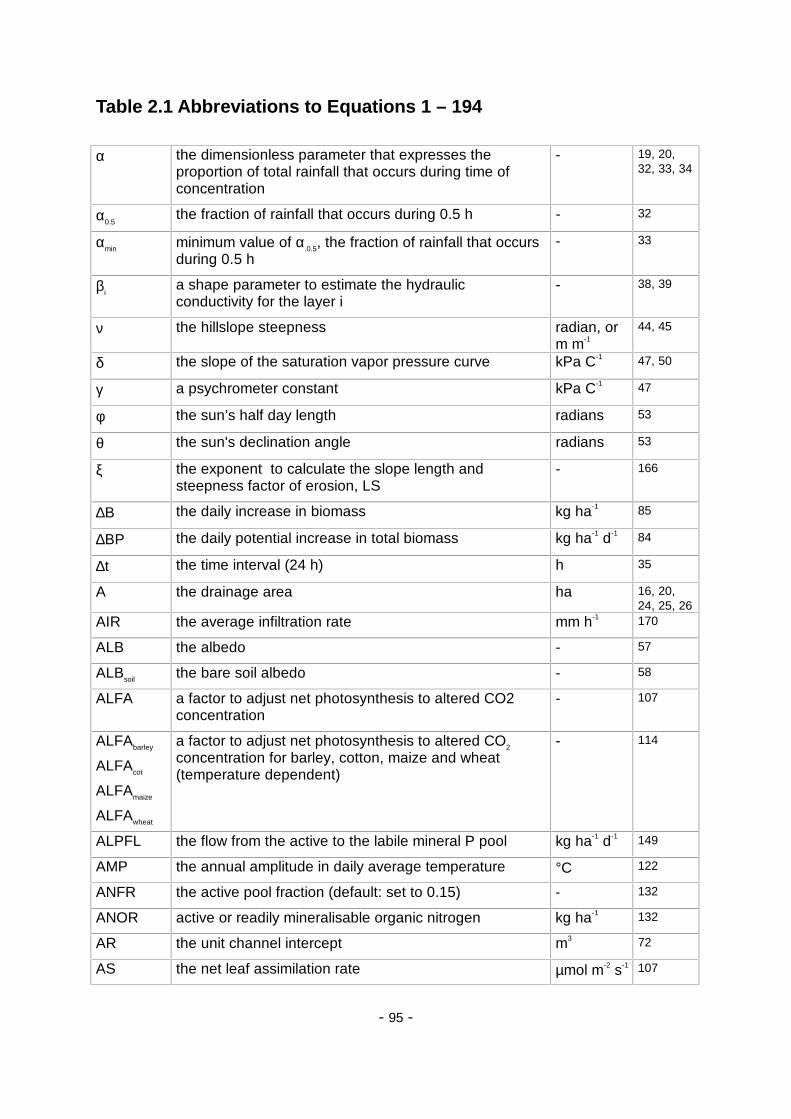
- 95 -

Table 2.1 Abbreviations to Equations 1 – 194

α the dimensionless parameter that expresses theproportion of total rainfall that occurs during time ofconcentration

- 19, 20,32, 33, 34

α0.5the fraction of rainfall that occurs during 0.5 h - 32

αmin minimum value of α.0.5, the fraction of rainfall that occursduring 0.5 h

- 33

βia shape parameter to estimate the hydraulicconductivity for the layer i

- 38, 39

ν the hillslope steepness radian, orm m-1

44, 45

δ the slope of the saturation vapor pressure curve kPa C-1 47, 50

γ a psychrometer constant kPa C-1 47

φ the sun’s half day length radians 53

θ the sun's declination angle radians 53

ξ the exponent to calculate the slope length andsteepness factor of erosion, LS

- 166

∆B the daily increase in biomass kg ha-1 85

∆BP the daily potential increase in total biomass kg ha-1 d-1 84

∆t the time interval (24 h) h 35

A the drainage area ha 16, 20,24, 25, 26

AIR the average infiltration rate mm h-1 170

ALB the albedo - 57

ALBsoil the bare soil albedo - 58

ALFA a factor to adjust net photosynthesis to altered CO2concentration

- 107

ALFAbarley

ALFAcot

ALFAmaize

ALFAwheat

a factor to adjust net photosynthesis to altered CO2

concentration for barley, cotton, maize and wheat(temperature dependent)

- 114

ALPFL the flow from the active to the labile mineral P pool kg ha-1 d-1 149

AMP the annual amplitude in daily average temperature °C 122

ANFR the active pool fraction (default: set to 0.15) - 132

ANOR active or readily mineralisable organic nitrogen kg ha-1 132

AR the unit channel intercept m3 72

AS the net leaf assimilation rate µmol m-2 s-1 107

- 96 -

ASNFL the flow from the active to the stable organic N pool kg ha-1 d-1 133

ASPFL the flow from the active to the stable mineral P pool kg ha-1 d-1 148

AX the regression intercept to estimate the thresholdvolume for a unit channel

m km-1 76

BAG the aboveground biomass kg ha-1 87

BCV a lagging factor for simulating residue and snow covereffects on surface temperature

- 129

BD the soil bulk density t m-3 124

BE the crop-specific parameter for converting energy tobiomass

kg m2 MJ-1

ha-1 d-1

84

BETA a factor to adjust potential leaf transpiration to CO2

concentration116

BMR the sum of the above ground biomass and crop residue t ha-1 59

BN1 the normal fraction of nitrogen in plant biomass atemergence (excluding seeds)

g g-1 154

BN2 the normal fraction of nitrogen in plant biomass at 0.5maturity.

g g-1 154

BN3 the normal fraction of nitrogen in plant biomass atmaturity

g g-1 154

BP the barometric pressure kPa 51, 52

BR the unit channel regression slope - 74

BT the accumulated total biomass kg ha-1 88

BX the regression slope - 77

C the crop management factor, - 163

C1 a parameter to calculate river routing - 181

C2 a parameter to calculate river routing - 181

C3 a parameter to calculate river routing - 181

CA the current atmospheric CO2 concentration µmol mol-1 108

CALP the equilibrium constant between the active and labilemineral P pools (default: 1.)

- 149

CASN the rate constant for the flow from the active to stableorganic N pool

d-1 133

CASP the rate constant for the flow between the stable andactive mineral P pools (default: 0.006)

d-1 148

CAV the average annual value of C factor - 165

CBNi the carbon content in the layer i kg ha-1 152

CDN a shape coefficient to estimate the combinedtemperature-carbon factor of denitrification, TCFD

- 152

- 97 -

CHC the channel C factor - 193

CHFL the average channel flow length for the basin km 22, 23

CHK the effective hydraulic conductivity of the channelalluvium in

mm h-1 72

CHL the channel length from the most distant point to thewatershed outlet

km 23, 24, 26

CHLcen the distance from the outlet along the channel to thewatershed centroid

km 23

CHN Manning’s roughness coefficient n for the channel - 24, 26

CHS the average channel slope m m-1 24, 26

CHV the average stream velocity in the channel m s-1 22

CHW the average channel width m 77

CL1 the current CO2 concentration inside leaves µmol mol-1 111

CL2 the future CO2 concentration inside leaves µmol mol-1 111

CLR the stream wave celerity m s-1 186

CMN the minimum value of C - 164

CN the curve number - 4

CN1 the curve number for soil moisture condition 1 (dry) - 5, 6

CN2 the curve number for soil moisture condition 2 (average) - 5, 7, 8

CN2s the curve number for soil moisture condition 2 adjustedfor slope

- 8

CN3 the curve number for soil moisture condition 3 (wet) - 7, 8

CNB the optimal N concentration for the crop g g-1 100

CNOR the concentration of organic N in the top soil layer g t-1 168

CNR the C:N ratio - 138, 140

CNRF the C:N ratio factor of mineralisation - 137

COMN the humus rate constant for N (default: 0.0003) d-1 144

COMP the humus mineralisation rate constant for P kg ha-1 d-1 147

CONi(t) the concentration of NO3-N in the layer i on the day t kg ha-1 mm-

1

156

COP the concentration of labile phosphorus in soil layer g t-1 162

COV the land cover, or the sum of above ground biomassand crop residue

kg ha-1 130

CPR the C:P ratio - 139, 141

CPRF the C:P ratio factor of mineralisation - 137

CR the revap coefficient - 70

CS the seepage coefficient - 71

- 98 -

CSW the P concentration in the sediment divided by that ofthe water

m3 t-1 162

CTSH the temperature stress parameter for the crop fortemperatures above TO

- 98, 99

CTSL the temperature stress parameter for the crop fortemperatures below TO

- 96, 97

D the earth’s radius vector km 53

DD the damping depth for the soil mm 122

DEC the decay factor m km-1 73

DECR the residue decomposition rate - 134

DEGR the degradation in stream t 192, 193

DEL the delay time or drainage time of the aquifer day 69

DELR the sediment delivery ratio through the reach - 191

DENIT the denitrification flow in layer i kg ha-1 d-1 150

DEP the deposition in stream t 192, 193

DLAI the fraction of the growing season before LAI startsdeclining

- 87

DP the maximum damping depth for the soil mm 123

DR the sediment delivery ratio - 169

DS the drain spacing m 64

DU the duration of streamflow h 72

DUR the rainfall duration h 31, 32

ECP the erosion control practice factor, - 163

ELEV the elevation of the site m 52

EO the potential evaporation mm 47

EP the plant water transpiration rate mm d-1 60

EPO the potential plant transpiration rates mol m-2 s-1 116

ER the enrichment ratio - 168

ES the soil evaporation for day t mm d-1 62

ESO the potential soil evaporation mm d-1 61

ET the evapotranspiration mm d-1 1

FC the field capacity water content vol % ormm mm-1

10, 11,12, 13,37, 39

FD the flow depth m 28, 29

FFC the fraction of field capacity - 10, 11, 14

FFC* the depth-weighted FFC value - 14

FOMN N mineralisation flow from fresh organic N kg ha-1 d-1 136

- 99 -

FOMP P mineralisation flow from fresh organic P kg ha-1 d-1 146

FON the fresh organic N pool kg ha-1 135

FOP the amount of fresh organic P kg ha-1 141

GWH the water table height m 64

GWQ the return flow mm d-1 63

HCi the hydraulic conductivity mm h-1 37, 38, 40

HI the harvest index at harvest - 102

HIAD the adjusted harvest index - 104

HIC1 the factor to estimate harvest index as depending onIHUN

103

HIC2 the factor to estimate harvest index as depending onWSF

104

HR the hydraulic radius m 188

HUMNi the mineralisation rate for the active organic N pool inlayer i,

kg ha-1 d-1 144

HUMPi the mineralisation rate in the layer i kg ha-1 d-1 147

HUNA the value of heat units accumulated in the day t °C 81

HV the latent heat of vaporization MJ kg-1 47, 48

HVSTI the crop-specific harvest index - 103

i the soil layer - 14

IHUN the heat unit index - 82

K the soil erodibility factor - 163

KD the hydraulic conductivity in shallow aquifer mm d-1 64

KST the storage time constant for the reach s 179

LAI the leaf area index - 60

LAIMX the maximum potential LAI for the specific crop - 87

LAT the latitude of the site degrees 53

LS the slope length and steepness factor - 163

M the number of soil layers - 14

NDD the number of days in a month d 128

NDEM(t) the N demand of the crop kg ha-1 153

NFLi the amount NO3-N lost from the layer i kg ha-1 156

NMIN the amount of mineral nitrogen (or nitrate nitrogen plusammonium nitrogen) in soil

kg ha-1 140

NOR the total organic N pool kg ha-1 132

NRD the number of rainy days in a month d 128

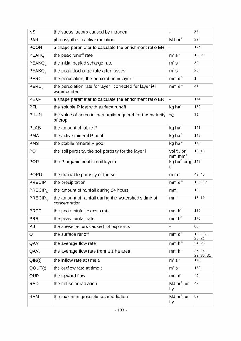
- 100 -

NS the stress factors caused by nitrogen - 86

PAR photosynthetic active radiation MJ m-2 83

PCON a shape parameter to calculate the enrichment ratio ER - 174

PEAKQ the peak runoff rate m3 s-1 16, 20

PEAKQin the initial peak discharge rate m3 s-1 80

PEAKQtr the peak discharge rate after losses m3 s-1 80

PERC the percolation, the percolation in layer i mm d-1 1

PERCic the percolation rate for layer i corrected for layer i+lwater content

mm d-1 41

PEXP a shape parameter to calculate the enrichment ratio ER - 174

PFL the soluble P lost with surface runoff kg ha-1 162

PHUN the value of potential heat units required for the maturityof crop

°C 82

PLAB the amount of labile P kg ha-1 141

PMA the active mineral P pool kg ha-1 148

PMS the stabile mineral P pool kg ha-1 148

PO the soil porosity, the soil porosity for the layer i vol % ormm mm-1

10, 13

POR the P organic pool in soil layer i kg ha-1 or gt-1

147

PORD the drainable porosity of the soil m m-1 43, 45

PRECIP the precipitation mm d-1 1, 3, 17

PRECIP24 the amount of rainfall during 24 hours mm 19

PRECIPtc the amount of rainfall during the watershed’s time ofconcentration

mm 18, 19

PRER the peak rainfall excess rate mm h-1 169

PRR the peak rainfall rate mm h-1 170

PS the stress factors caused phosphorus - 86

Q the surface runoff mm d-1 1, 3, 17,20, 31

QAV the average flow rate mm h-1 24, 25

QAV0 the average flow rate from a 1 ha area mm h-1 25, 26,29, 30, 31

QIN(t) the inflow rate at time t, m3 s-1 178

QOUT(t) the outflow rate at time t m3 s-1 178

QUP the upward flow mm d-1 46

RAD the net solar radiation MJ m-2, orLy

47

RAM the maximum possible solar radiation MJ m-2, orLy

53

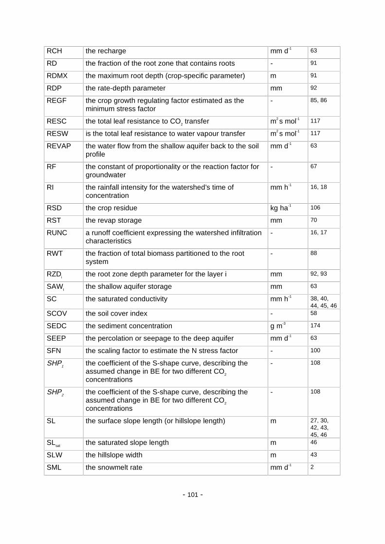
- 101 -

RCH the recharge mm d-1 63

RD the fraction of the root zone that contains roots - 91

RDMX the maximum root depth (crop-specific parameter) m 91

RDP the rate-depth parameter mm 92

REGF the crop growth regulating factor estimated as theminimum stress factor

- 85, 86

RESC the total leaf resistance to CO2 transfer m2 s mol-1 117

RESW is the total leaf resistance to water vapour transfer m2 s mol-1 117

REVAP the water flow from the shallow aquifer back to the soilprofile

mm d-1 63

RF the constant of proportionality or the reaction factor forgroundwater

- 67

RI the rainfall intensity for the watershed’s time ofconcentration

mm h-1 16, 18

RSD the crop residue kg ha-1 106

RST the revap storage mm 70

RUNC a runoff coefficient expressing the watershed infiltrationcharacteristics

- 16, 17

RWT the fraction of total biomass partitioned to the rootsystem

- 88

RZDi the root zone depth parameter for the layer i mm 92, 93

SAWt the shallow aquifer storage mm 63

SC the saturated conductivity mm h-1 38, 40,44, 45, 46

SCOV the soil cover index - 58

SEDC the sediment concentration g m-3 174

SEEP the percolation or seepage to the deep aquifer mm d-1 63

SFN the scaling factor to estimate the N stress factor - 100

SHP1 the coefficient of the S-shape curve, describing theassumed change in BE for two different CO2

concentrations

- 108

SHP2 the coefficient of the S-shape curve, describing theassumed change in BE for two different CO2

concentrations

- 108

SL the surface slope length (or hillslope length) m 27, 30,42, 43,45, 46

SLsat the saturated slope length m 46

SLW the hillslope width m 43

SML the snowmelt rate mm d-1 2

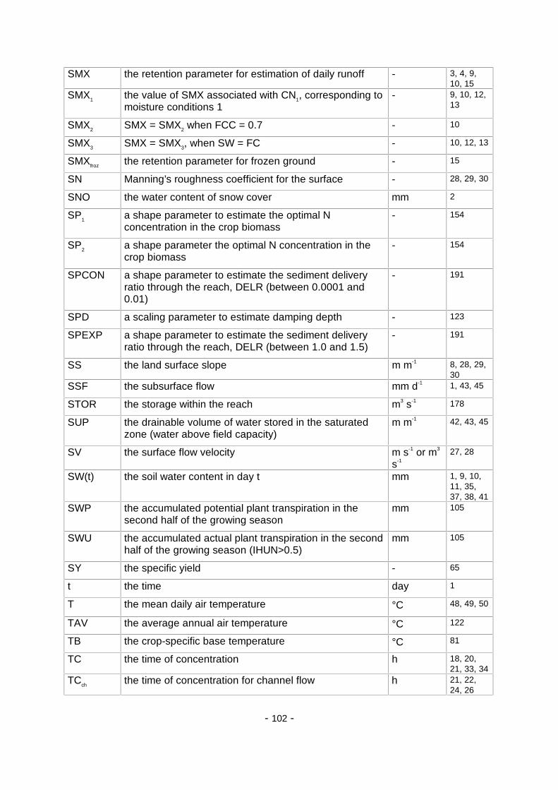
- 102 -

SMX the retention parameter for estimation of daily runoff - 3, 4, 9,10, 15

SMX1 the value of SMX associated with CN1, corresponding tomoisture conditions 1

- 9, 10, 12,13

SMX2 SMX = SMX2 when FCC = 0.7 - 10

SMX3 SMX = SMX3, when SW = FC - 10, 12, 13

SMXfroz the retention parameter for frozen ground - 15

SN Manning’s roughness coefficient for the surface - 28, 29, 30

SNO the water content of snow cover mm 2

SP1 a shape parameter to estimate the optimal Nconcentration in the crop biomass

- 154

SP2 a shape parameter the optimal N concentration in thecrop biomass

- 154

SPCON a shape parameter to estimate the sediment deliveryratio through the reach, DELR (between 0.0001 and0.01)

- 191

SPD a scaling parameter to estimate damping depth - 123

SPEXP a shape parameter to estimate the sediment deliveryratio through the reach, DELR (between 1.0 and 1.5)

- 191

SS the land surface slope m m-1 8, 28, 29,30

SSF the subsurface flow mm d-1 1, 43, 45

STOR the storage within the reach m3 s-1 178

SUP the drainable volume of water stored in the saturatedzone (water above field capacity)

m m-1 42, 43, 45

SV the surface flow velocity m s-1 or m3

s-1

27, 28

SW(t) the soil water content in day t mm 1, 9, 10,11, 35,37, 38, 41

SWP the accumulated potential plant transpiration in thesecond half of the growing season

mm 105

SWU the accumulated actual plant transpiration in the secondhalf of the growing season (IHUN>0.5)

mm 105

SY the specific yield - 65

t the time day 1

T the mean daily air temperature °C 48, 49, 50

TAV the average annual air temperature °C 122

TB the crop-specific base temperature °C 81

TC the time of concentration h 18, 20,21, 33, 34

TCch the time of concentration for channel flow h 21, 22,24, 26

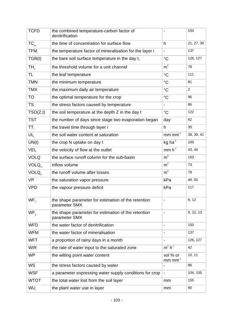
- 103 -

TCFD the combined temperature-carbon factor ofdenitrification

- 150

TCov the time of concentration for surface flow h 21, 27, 30

TFMi the temperature factor of mineralisation for the layer i - 137

TGB(t) the bare soil surface temperature in the day t, °C 126, 127

THo the threshold volume for a unit channel m3 78

TL the leaf temperature °C 111

TMN the minimum temperature °C 81

TMX the maximum daily air temperature °C 2

TO the optimal temperature for the crop °C 96

TS the stress factors caused by temperature - 86

TSO(Z,t) the soil temperature at the depth Z in the day t °C 122

TST the number of days since stage two evaporation began day 62

TTi the travel time through layer i h 35

ULi the soil water content at saturation mm mm-1 38, 39, 41

UN(t) the crop N uptake on day t kg ha-1 100

VEL the velocity of flow at the outlet mm h-1 43, 44

VOLQ the surface runoff column for the sub-basin m3 163

VOLQin inflow volume m3 73

VOLQtr the runoff volume after losses m3 79

VP the saturation vapor pressure kPa 49, 50

VPD the vapour pressure deficit kPa 117

WF1 the shape parameter for estimation of the retentionparameter SMX

- 9, 12

WF2 the shape parameter for estimation of the retentionparameter SMX

- 9, 12, 13

WFD the water factor of denitrification - 150

WFM the water factor of mineralisation - 137

WFT a proportion of rainy days in a month - 126, 127

WIR the rate of water input to the saturated zone m2 h-1 42

WP the wilting point water content vol % ormm mm-1

10, 11

WS the stress factors caused by water - 86

WSF a parameter expressing water supply conditions for crop - 104, 105

WTOT the total water lost from the soil layer mm 155

WUi the plant water use in layer mm 90

- 104 -

WUPi the potential water use rate from layer i mm d-1 92

X a dimentionless weighting factor in river reach routing - 179

YLD the crop yield removed from the field kg ha-1 102

YON the organic N runoff loss at the sub-basin outlet kg ha-1 168

YP the sediment phase of P loss in runoff kg ha-1 177

YSED the sediment yield from the sub-basin t 163

YSEDin the sediment amount entering the reach t 191

YSEDout the amount of sediment reaching the sub-basin outlet t 194

Zi the depth to the bottom of soil layer i mm 14

ZM the distance from the bottom of the lowest soil layer tothe surface

mm 125