Syddansk Universitet

Fundamental Composite (Goldstone) Higgs Dynamics

Cacciapaglia, G.; Sannino, Francesco

Published in:Journal of High Energy Physics (JHEP)

DOI:10.1007/JHEP04(2014)111

Publication date:2014

Citation for pulished version (APA):Cacciapaglia, G., & Sannino, F. (2014). Fundamental Composite (Goldstone) Higgs Dynamics. Journal of HighEnergy Physics (JHEP), [111]. DOI: 10.1007/JHEP04(2014)111

General rightsCopyright and moral rights for the publications made accessible in the public portal are retained by the authors and/or other copyright ownersand it is a condition of accessing publications that users recognise and abide by the legal requirements associated with these rights.

• Users may download and print one copy of any publication from the public portal for the purpose of private study or research. • You may not further distribute the material or use it for any profit-making activity or commercial gain • You may freely distribute the URL identifying the publication in the public portal ?

Take down policyIf you believe that this document breaches copyright please contact us providing details, and we will remove access to the work immediatelyand investigate your claim.

Download date: 14. Feb. 2017

arX

iv:1

402.

0233

v2 [

hep-

ph]

17

Mar

201

4

Fundamental Composite (Goldstone) Higgs Dynamics

Giacomo Cacciapaglia1, ∗ and Francesco Sannino2, †

1Universite de Lyon, F-69622 Lyon, France: Universite Lyon 1, Villeurbanne

CNRS/IN2P3, UMR5822, Institut de Physique Nucleaire de Lyon.

2CP 3-Origins & Danish Institute for Advanced Study DIAS,

University of Southern Denmark, Campusvej 55, DK-5230 Odense M, Denmark

Abstract

We provide a unified description, both at the effective and fundamental Lagrangian level, of

models of composite Higgs dynamics where the Higgs itself can emerge, depending on the way the

electroweak symmetry is embedded, either as a pseudo-Goldstone boson or as a massive excitation

of the condensate. We show that, in general, these states mix with repercussions on the electroweak

physics and phenomenology. Our results will help clarify the main differences, similarities, benefits

and shortcomings of the different ways one can naturally realize a composite nature of the elec-

troweak sector of the Standard Model. We will analyze the minimal underlying realization in terms

of fundamental strongly coupled gauge theories supporting the flavor symmetry breaking pattern

SU(4)/Sp(4) ∼ SO(6)/SO(5). The most minimal fundamental description consists of an SU(2)

gauge theory with two Dirac fermions transforming according to the fundamental representation

of the gauge group. This minimal choice enables us to use recent first principle lattice results to

make the first predictions for the massive spectrum for models of composite (Goldstone) Higgs

dynamics. These results are of the utmost relevance to guide searches of new physics at the Large

Hadron Collider.

Preprint: CP3-Origins-2014-003 DNRF90, DIAS-2014-3, LYCEN-2014-02

∗Electronic address: g.cacciapaglia@ipnl.in2p3.fr†Electronic address: sannino@cp3-origins.net

1

I. UNIFIED FUNDAMENTAL COMPOSITE HIGGS DYNAMICS

It is a fact that the Standard Model (SM) of particle interactions continues to be a very

successful description of Nature. The discovery of the Higgs particle can be viewed as the

crown jewel of its success. Nevertheless, if not from the experimental point of view, at least

theoretically the Higgs sector of the SM is, to put it mildly, unappealing. Spontaneous

symmetry breaking is not explained but simply modeled. Furthermore there is no field-

theoretical consistent way to shield the electroweak scale from higher scales. This is the SM

naturalness problem. For a mathematical classification of different degrees of naturality we

refer to [1].

A time-honored avenue to render the SM Higgs sector natural is to replace it with a

fundamental gauge dynamics featuring fermionic matter fields. The new dynamics is free

from the naturalness problem. The oldest incarnation of this idea goes under the name of

Technicolor [2, 3]. In these models the Higgs-sector, and therefore the Higgs boson itself,

are made by new fundamental dynamics. Variations on the theme appeared later in the

literature [4, 5].

In the traditional Technicolor setup, the electroweak symmetry breaks thanks to the gauge

dynamics of the new underlying gauge theory. The Technicolor Higgs is then identified

with the lightest scalar excitation of the fermion condensate responsible for electroweak

symmetry breaking. However the Technicolor theory per se is not able to provide mass

to the SM fermions and therefore a new sector must be introduced. This new sector is

important and can modify the physical mass of the Technicolor Higgs, typically reducing

it [6]. Another possibility is that the gauge dynamics underlying the Higgs sector does

not break the electroweak symmetry but breaks a global symmetry of the new fermions: a

Higgs-like state is therefore identified with one of the Goldstone Bosons (GB) of the global

symmetry breaking. In this case the challenges are not only to provide masses to the SM

fermions but also to break the electroweak symmetry in the first place via another sector

which, in turn, should also contribute to give mass to the would–be pseudo-GB Higgs. In

any event a true improvement with respect to the SM Higgs sector shortcomings would arise

only if a more fundamental description exists.

In this work we provide a first unified description of models of composite dynamics

for the electroweak sector of the SM. This description will clarify the main differences,

2

similarities, interplay, and shortcomings of the approaches. We will also provide specific

underlying realizations in terms of fundamental strongly coupled gauge theories. This will

permit us to use recent first principle lattice results to make the first predictions for the

massive spectrum, which is of the utmost relevance to guide searches of new physics at the

Large Hadron Collider (LHC). Furthermore we will also demonstrate that, for a generic

vacuum alignment, the observed Higgs is neither a purely pGB state nor the technicolor

Higgs, but rather a mixed state. This fact impacts on its physical properties and associated

phenomenology.

As possible underlying gauge theories we will consider those featuring fermionic matter.

The pattern of chiral symmetry breaking depends on the underlying gauge dynamics [7–9].

Of course, the initial hypothesis that the global symmetry breaks dynamically should be

verified. In fact we know that, depending on the number of matter fields, the choice of the

underlying gauge group and the dimension of the gauge group (e.g. the number of underlying

fermionic matter), the symmetry might not break at all because the theory can develop

large distance conformality, as discussed in [10] for fermions in two-index representations,

in [11] for a universal classification for SU(N) gauge theories and their applications to

Technicolor and composite dark matter models, in [12] for orthogonal and symplectic groups,

and in [13] for exceptional underlying gauge groups. Furthermore, even assuming global

chiral symmetry breaking, it remains to be seen if the breaking is to the maximal diagonal

subgroup. We shall see that for certain phenomenologically relevant gauge theories, using

first principle lattice simulations, there has been substantial progress to answer precisely

these questions [14–27]. We note that the classification of relevant underlying gauge theories

for Technicolor models appeared in [11], while a classification of the symmetry breaking

patterns relevant for composite models of the Higgs as a pGB can be found in [28, 29].

The first relevant observation is that the non-abelian global quantum unbroken flavor

symmetries, for any underlying gauge theory with one Dirac species of fermions, are bound

to be SU(2Nf ) or SU(Nf)×SU(Nf ), depending on whether the underlying fermion repre-

sentation is (pseudo-)real or complex.

An SU(2Nf ) flavor symmetry can be achieved only if the new fermions belong to a real

(like the adjoint) or pseudo-real (like the fundamental of SU(2) = Sp(2)) representation of

the underlying gauge group. In either case, both left-handed fermions and charge-conjugated

right-handed anti-fermions can be recast, via a similarity transformation, to transform ac-

3

cording to the same representation of the underlying fundamental gauge group. One can

organize the two fermion components as a 2Nf column with complex Weyl fermions indicated

by the vector ψfc with f = 1, .., 2Nf and c the new color index. At this point, the simplest

gauge invariant fermion bilinear we can construct is ψfc ψf ′

c′ with the color contracted either

via a delta function for real representations or an antisymmetric epsilon term for pseudo-

real ones. As fermions anticommute, a non vanishing condensate can be formed only if the

full wave-function is completely antisymmetric with respect to spin, new color and flavor.

Since Lorentz symmetry is conserved, the spin indices are contracted via an antisymmmetric

tensor and therefore, according to the reality or pseudo reality of the representation we can

have the following two patterns of chiral symmetry breaking:

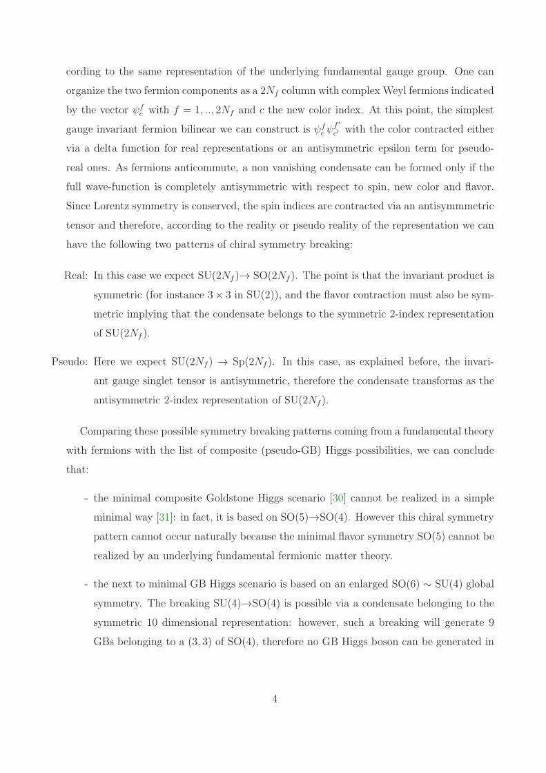
Real: In this case we expect SU(2Nf )→ SO(2Nf). The point is that the invariant product is

symmetric (for instance 3× 3 in SU(2)), and the flavor contraction must also be sym-

metric implying that the condensate belongs to the symmetric 2-index representation

of SU(2Nf ).

Pseudo: Here we expect SU(2Nf ) → Sp(2Nf). In this case, as explained before, the invari-

ant gauge singlet tensor is antisymmetric, therefore the condensate transforms as the

antisymmetric 2-index representation of SU(2Nf).

Comparing these possible symmetry breaking patterns coming from a fundamental theory

with fermions with the list of composite (pseudo-GB) Higgs possibilities, we can conclude

that:

- the minimal composite Goldstone Higgs scenario [30] cannot be realized in a simple

minimal way [31]: in fact, it is based on SO(5)→SO(4). However this chiral symmetry

pattern cannot occur naturally because the minimal flavor symmetry SO(5) cannot be

realized by an underlying fundamental fermionic matter theory.

- the next to minimal GB Higgs scenario is based on an enlarged SO(6) ∼ SU(4) global

symmetry. The breaking SU(4)→SO(4) is possible via a condensate belonging to the

symmetric 10 dimensional representation: however, such a breaking will generate 9

GBs belonging to a (3, 3) of SO(4), therefore no GB Higgs boson can be generated in

4

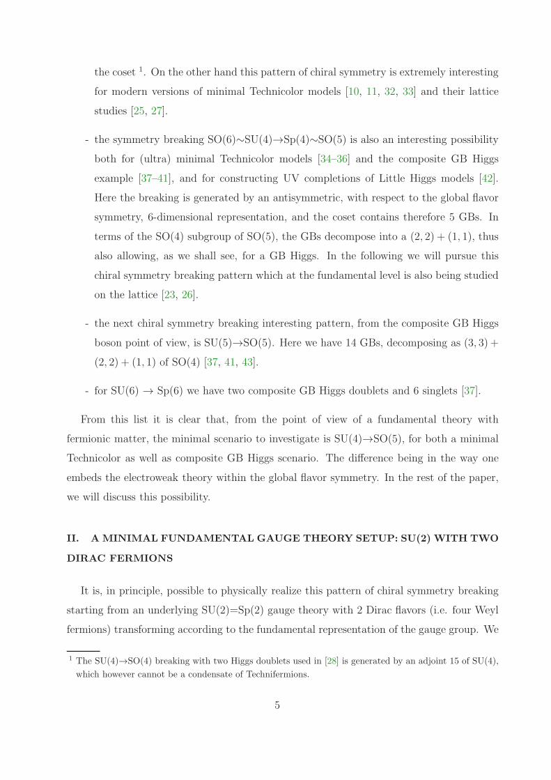
the coset 1. On the other hand this pattern of chiral symmetry is extremely interesting

for modern versions of minimal Technicolor models [10, 11, 32, 33] and their lattice

studies [25, 27].

- the symmetry breaking SO(6)∼SU(4)→Sp(4)∼SO(5) is also an interesting possibility

both for (ultra) minimal Technicolor models [34–36] and the composite GB Higgs

example [37–41], and for constructing UV completions of Little Higgs models [42].

Here the breaking is generated by an antisymmetric, with respect to the global flavor

symmetry, 6-dimensional representation, and the coset contains therefore 5 GBs. In

terms of the SO(4) subgroup of SO(5), the GBs decompose into a (2, 2) + (1, 1), thus

also allowing, as we shall see, for a GB Higgs. In the following we will pursue this

chiral symmetry breaking pattern which at the fundamental level is also being studied

on the lattice [23, 26].

- the next chiral symmetry breaking interesting pattern, from the composite GB Higgs

boson point of view, is SU(5)→SO(5). Here we have 14 GBs, decomposing as (3, 3) +

(2, 2) + (1, 1) of SO(4) [37, 41, 43].

- for SU(6) → Sp(6) we have two composite GB Higgs doublets and 6 singlets [37].

From this list it is clear that, from the point of view of a fundamental theory with

fermionic matter, the minimal scenario to investigate is SU(4)→SO(5), for both a minimal

Technicolor as well as composite GB Higgs scenario. The difference being in the way one

embeds the electroweak theory within the global flavor symmetry. In the rest of the paper,

we will discuss this possibility.

II. A MINIMAL FUNDAMENTAL GAUGE THEORY SETUP: SU(2) WITH TWO

DIRAC FERMIONS

It is, in principle, possible to physically realize this pattern of chiral symmetry breaking

starting from an underlying SU(2)=Sp(2) gauge theory with 2 Dirac flavors (i.e. four Weyl

fermions) transforming according to the fundamental representation of the gauge group. We

1 The SU(4)→SO(4) breaking with two Higgs doublets used in [28] is generated by an adjoint 15 of SU(4),

which however cannot be a condensate of Technifermions.

5

will discuss the lattice results [23, 26] supporting the breaking of the global SU(4) symmetry

to Sp(4) (locally isomorphic to SO(5)) via the formation of a non-perturbative fermion

condensate in section VI. The underlying Lagrangian, in Dirac notation, is

L = −1

4F aµνF

aµν + U(iγµDµ −m)U +D(iγµDµ −m)D , (1)

where U and D are the two new fermion fields having a common bare mass m, F aµν is the

field strength, and Dµ is the covariant derivative. The Dirac and SU(2) gauge indices of

U and D are not shown explicitly. Lattice simulations can extrapolate to the zero fermion

mass case, and in that limit the Lagrangian has a global SU(4) symmetry corresponding to

the four chiral fermion fields

UL =1

2(1− γ5)U , UR =

1

2(1+ γ5)U , DL =

1

2(1− γ5)D , DR =

1

2(1+ γ5)D . (2)

For m 6= 0, the SU(4) symmetry is explicitly broken to a remaining Sp(4) subgroup as

follows. The Lagrangian from (1) can be rewritten as

L = −1

4F aµνF

aµν+iUγµDµU+iDγµDµD+m

2QT (−iσ2)C EQ+

m

2

(QT (−iσ2)C EQ

)†, (3)

where

Q =

UL

DL

UL

DL

, E =

0 0 1 0

0 0 0 1

−1 0 0 0

0 −1 0 0

, (4)

C is the charge conjugation operator acting on Dirac indices, and the Pauli structure −iσ2

is the standard antisymmetric tensor acting on color indices. We also have UL = −iσ2CUT

R

and DL = −iσ2CDT

R. Under an infinitesimal SU(4) transformation defined by

Q→(1 + i

15∑

n=1

αnT n

)Q , (5)

the Lagrangian (3) becomes

L → L+im

2

15∑

n=1

αnQT (−iσ2)C(ET n + T nTE

)Q + h.c. , (6)

where T n denotes the 15 generators of SU(4) and αn is a set of 15 constants. The only

generators that leave the Lagrangian invariant are those that obey

ET n + T nTE = 0 (7)

6

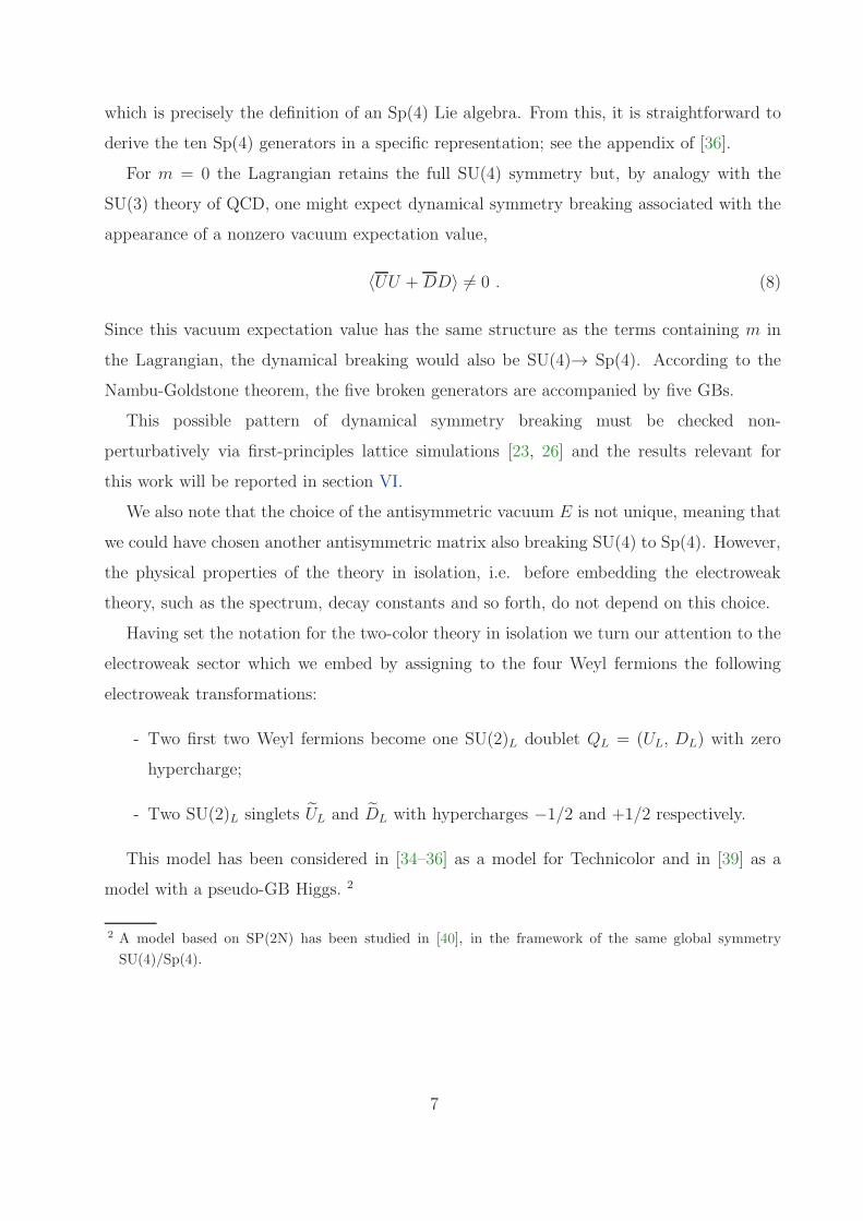
which is precisely the definition of an Sp(4) Lie algebra. From this, it is straightforward to

derive the ten Sp(4) generators in a specific representation; see the appendix of [36].

For m = 0 the Lagrangian retains the full SU(4) symmetry but, by analogy with the

SU(3) theory of QCD, one might expect dynamical symmetry breaking associated with the

appearance of a nonzero vacuum expectation value,

〈UU +DD〉 6= 0 . (8)

Since this vacuum expectation value has the same structure as the terms containing m in

the Lagrangian, the dynamical breaking would also be SU(4)→ Sp(4). According to the

Nambu-Goldstone theorem, the five broken generators are accompanied by five GBs.

This possible pattern of dynamical symmetry breaking must be checked non-

perturbatively via first-principles lattice simulations [23, 26] and the results relevant for

this work will be reported in section VI.

We also note that the choice of the antisymmetric vacuum E is not unique, meaning that

we could have chosen another antisymmetric matrix also breaking SU(4) to Sp(4). However,

the physical properties of the theory in isolation, i.e. before embedding the electroweak

theory, such as the spectrum, decay constants and so forth, do not depend on this choice.

Having set the notation for the two-color theory in isolation we turn our attention to the

electroweak sector which we embed by assigning to the four Weyl fermions the following

electroweak transformations:

- Two first two Weyl fermions become one SU(2)L doublet QL = (UL, DL) with zero

hypercharge;

- Two SU(2)L singlets UL and DL with hypercharges −1/2 and +1/2 respectively.

This model has been considered in [34–36] as a model for Technicolor and in [39] as a

model with a pseudo-GB Higgs. 2

2 A model based on SP(2N) has been studied in [40], in the framework of the same global symmetry

SU(4)/Sp(4).

7

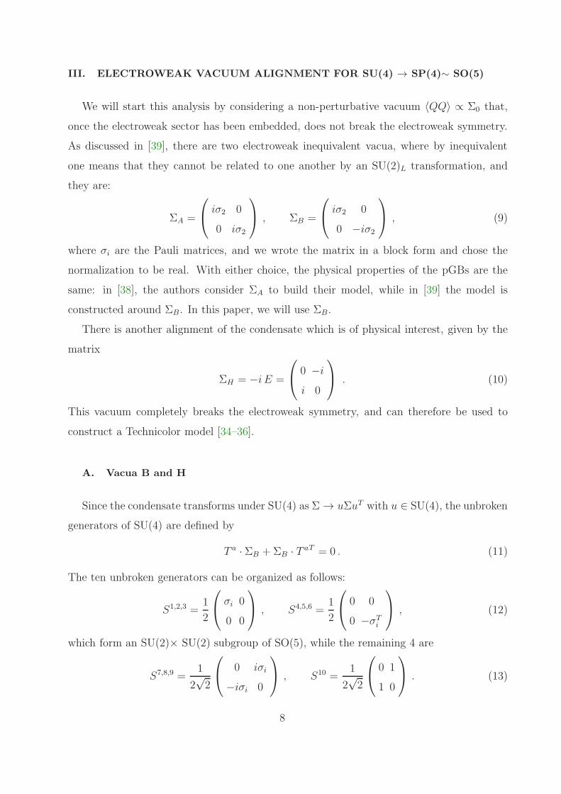
III. ELECTROWEAK VACUUM ALIGNMENT FOR SU(4) → SP(4)∼ SO(5)

We will start this analysis by considering a non-perturbative vacuum 〈QQ〉 ∝ Σ0 that,

once the electroweak sector has been embedded, does not break the electroweak symmetry.

As discussed in [39], there are two electroweak inequivalent vacua, where by inequivalent

one means that they cannot be related to one another by an SU(2)L transformation, and

they are:

ΣA =

iσ2 0

0 iσ2

, ΣB =

iσ2 0

0 −iσ2

, (9)

where σi are the Pauli matrices, and we wrote the matrix in a block form and chose the

normalization to be real. With either choice, the physical properties of the pGBs are the

same: in [38], the authors consider ΣA to build their model, while in [39] the model is

constructed around ΣB. In this paper, we will use ΣB.

There is another alignment of the condensate which is of physical interest, given by the

matrix

ΣH = −i E =

0 −ii 0

. (10)

This vacuum completely breaks the electroweak symmetry, and can therefore be used to

construct a Technicolor model [34–36].

A. Vacua B and H

Since the condensate transforms under SU(4) as Σ → uΣuT with u ∈ SU(4), the unbroken

generators of SU(4) are defined by

T a · ΣB + ΣB · T aT = 0 . (11)

The ten unbroken generators can be organized as follows:

S1,2,3 =1

2

σi 0

0 0

, S4,5,6 =

1

2

0 0

0 −σTi

, (12)

which form an SU(2)× SU(2) subgroup of SO(5), while the remaining 4 are

S7,8,9 =1

2√2

0 iσi

−iσi 0

, S10 =

1

2√2

0 1

1 0

. (13)

8

The generators of the electroweak symmetry are identified with: S1,2,3 for SU(2)L and S6

for U(1)Y . The SU(2)×SU(2) group generated by S1,...6 can therefore be thought of as the

custodial symmetry of the SM Higgs potential. The 5 broken generators, associated with

the GBs are:

X1 = 12√2

0 σ3

σ3 0

, X2 = 1

2√2

0 i

−i 0

, X3 = 1

2√2

0 σ1

σ1 0

, (14)

X4 = 12√2

0 σ2

σ2 0

, X5 = 1

2√2

1 0

0 −1

. (15)

Using the above decomposition, one can move in the quotient SU(4)/Sp(4) ∼ SU(4)/SO(5)

around the vacuum ΣB as follows:

Σ = eiφifXi · ΣB ∼ ΣB +

1

2√2f

0 iφ5 φ4 + iφ3 φ2 − iφ1

−iφ5 0 −φ2 − iφ1 φ4 − iφ3

−φ4 − iφ3 φ2 + iφ1 0 iφ5

−φ2 + iφ1 −φ4 + iφ3 −iφ5 0

+O(φ2) .

(16)

The interactions of the GBs with the electroweak gauge bosons are obtained via the minimal

coupling following the standard procedure. The associated Lagrangian term is:

TrDµΣ†DµΣ . (17)

However, given that the S generators satisfy (11), this operator is unable to provide a mass

to the observed massive SM gauge bosons. We have also chosen S6 as the hypercharge

generator in such a way that the electric charge generator is Q = T 3 + Y = S3 + S6. It is

straightforward to show that Q satisfies the relation Q · ΣH + ΣH ·QT = 0 with

ΣH = −i E =

0 −ii 0

, ΣH = 2√2 iX4 · ΣA . (18)

This implies that if φ4 acquires a non vanishing vacuum expectation value 〈φ4〉 = v, due

to some yet unspecified dynamical source, then the electroweak symmetry breaks with Q

being the correct electric charge operator. Also, the fields φ1,2,3 are the GBs eaten by the

massive W and Z. The fluctuation around the vacuum of φ4 is identified with the Higgs

9

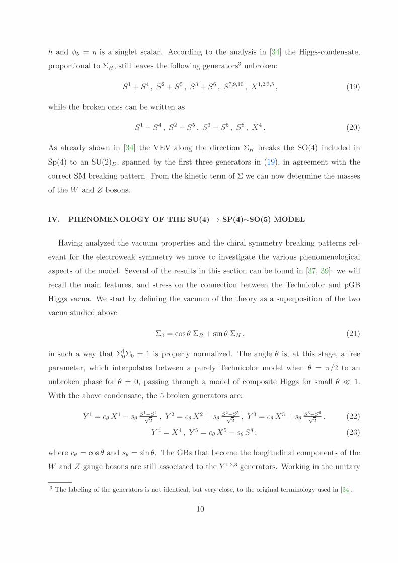
h and φ5 = η is a singlet scalar. According to the analysis in [34] the Higgs-condensate,

proportional to ΣH , still leaves the following generators3 unbroken:

S1 + S4 , S2 + S5 , S3 + S6 , S7,9,10 , X1,2,3,5 , (19)

while the broken ones can be written as

S1 − S4 , S2 − S5 , S3 − S6 , S8 , X4 . (20)

As already shown in [34] the VEV along the direction ΣH breaks the SO(4) included in

Sp(4) to an SU(2)D, spanned by the first three generators in (19), in agreement with the

correct SM breaking pattern. From the kinetic term of Σ we can now determine the masses

of the W and Z bosons.

IV. PHENOMENOLOGY OF THE SU(4) → SP(4)∼SO(5) MODEL

Having analyzed the vacuum properties and the chiral symmetry breaking patterns rel-

evant for the electroweak symmetry we move to investigate the various phenomenological

aspects of the model. Several of the results in this section can be found in [37, 39]: we will

recall the main features, and stress on the connection between the Technicolor and pGB

Higgs vacua. We start by defining the vacuum of the theory as a superposition of the two

vacua studied above

Σ0 = cos θ ΣB + sin θ ΣH , (21)

in such a way that Σ†0Σ0 = 1 is properly normalized. The angle θ is, at this stage, a free

parameter, which interpolates between a purely Technicolor model when θ = π/2 to an

unbroken phase for θ = 0, passing through a model of composite Higgs for small θ ≪ 1.

With the above condensate, the 5 broken generators are:

Y 1 = cθX1 − sθ

S1−S4√2, Y 2 = cθX

2 + sθS2−S5√2, Y 3 = cθX

3 + sθS3−S6√2. (22)

Y 4 = X4 , Y 5 = cθX5 − sθ S

8 ; (23)

where cθ = cos θ and sθ = sin θ. The GBs that become the longitudinal components of the

W and Z gauge bosons are still associated to the Y 1,2,3 generators. Working in the unitary

3 The labeling of the generators is not identical, but very close, to the original terminology used in [34].

10

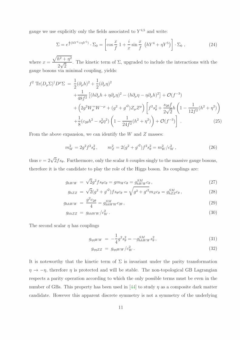
gauge we use explicitly only the fields associated to Y 4,5 and write:

Σ = eif(hY 4+ηY 5) · Σ0 =

[cos

x

f1 +

i

xsin

x

f

(hY 4 + ηY 5

)]· Σ0 , (24)

where x =

√h2 + η2

2√2

. The kinetic term of Σ, upgraded to include the interactions with the

gauge bosons via minimal coupling, yields:

f 2 Tr(DµΣ)†DµΣ =

1

2(∂µh)

2 +1

2(∂µη)

2

+1

48f 2

[(h∂µh+ η∂µη)

2 − (h∂µη − η∂µh)2]+O(f−3)

+(2g2W+

µ W−µ + (g2 + g′

2)ZµZ

µ) [

f 2s2θ +s2θf

2√2h

(1− 1

12f 2(h2 + η2)

)

+1

8(c2θh

2 − s2θη2)

(1− 1

24f 2(h2 + η2)

)+O(f−3)

]. (25)

From the above expansion, we can identify the W and Z masses:

m2W = 2g2f 2s2θ , m2

Z = 2(g2 + g′2)f 2s2θ = m2

W/c2W , (26)

thus v = 2√2fsθ. Furthermore, only the scalar h couples singly to the massive gauge bosons,

therefore it is the candidate to play the role of the Higgs boson. Its couplings are:

ghWW =√2g2fsθcθ = gmW cθ = gSMhWW cθ , (27)

ghZZ =√2(g2 + g′

2)fsθcθ =

√g2 + g′2mZcθ = gSMhZZcθ , (28)

ghhWW =g2c2θ4

= gSMhhWWc2θ , (29)

ghhZZ = ghhWW/c2W . (30)

The second scalar η has couplings

gηηWW = −1

4g2s2θ = −gSMhhWWs

2θ , (31)

gηηZZ = gηηWW/c2W . (32)

It is noteworthy that the kinetic term of Σ is invariant under the parity transformation

η → −η, therefore η is protected and will be stable. The non-topological GB Lagrangian

respects a parity operation according to which the only possible terms must be even in the

number of GBs. This property has been used in [44] to study η as a composite dark matter

candidate. However this apparent discrete symmetry is not a symmetry of the underlying

11

theory. The breaking of this symmetry manifests itself at the effective Lagrangian level via

topological-induced terms. These have been constructed explicitly for the chiral symmetry

breaking pattern envisioned here in [35]. Here one finds also the correct gauging of the

topological terms useful to consider the interaction with the gauge bosons.

A. Loop induced Higgs potential

While the dynamics does not have any preference to where the condensate is aligned in

the SU(4) space, gauge interactions do because they only involve a subgroup of the flavor

symmetry. The same is true, as we will see, for the top Yukawa, or generically the mechanism

that will generate a mass for the top. The breaking of the flavor symmetry will then be

communicated to the GBs via loops, which will therefore induce a potential determining

the value of the angle θ. The loop-induced potential for this model has been computed

in [37, 39], here we will simply recap the origin of the main components and discuss their

physical interpretation.

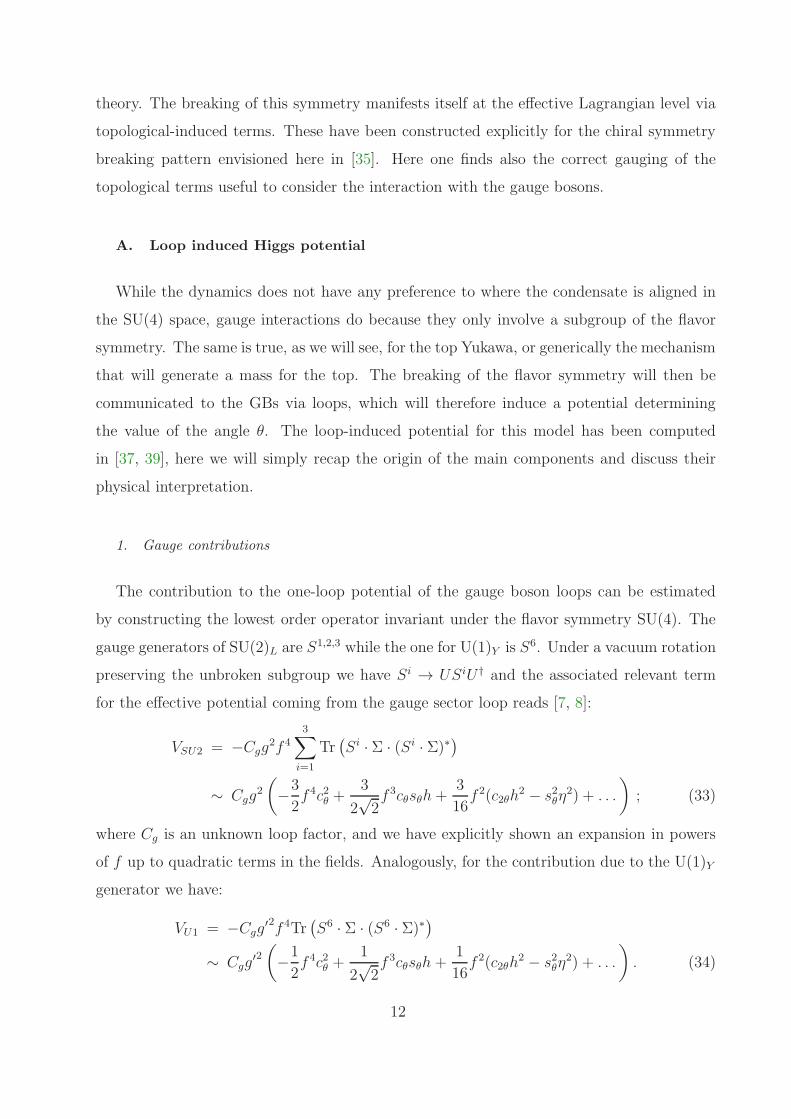
1. Gauge contributions

The contribution to the one-loop potential of the gauge boson loops can be estimated

by constructing the lowest order operator invariant under the flavor symmetry SU(4). The

gauge generators of SU(2)L are S1,2,3 while the one for U(1)Y is S6. Under a vacuum rotation

preserving the unbroken subgroup we have Si → USiU † and the associated relevant term

for the effective potential coming from the gauge sector loop reads [7, 8]:

VSU2 = −Cgg2f 43∑

i=1

Tr(Si · Σ · (Si · Σ)∗

)

∼ Cgg2

(−3

2f 4c2θ +

3

2√2f 3cθsθh+

3

16f 2(c2θh

2 − s2θη2) + . . .

); (33)

where Cg is an unknown loop factor, and we have explicitly shown an expansion in powers

of f up to quadratic terms in the fields. Analogously, for the contribution due to the U(1)Y

generator we have:

VU1 = −Cgg′2f 4Tr(S6 · Σ · (S6 · Σ)∗

)

∼ Cgg′2(−1

2f 4c2θ +

1

2√2f 3cθsθh +

1

16f 2(c2θh

2 − s2θη2) + . . .

). (34)

12

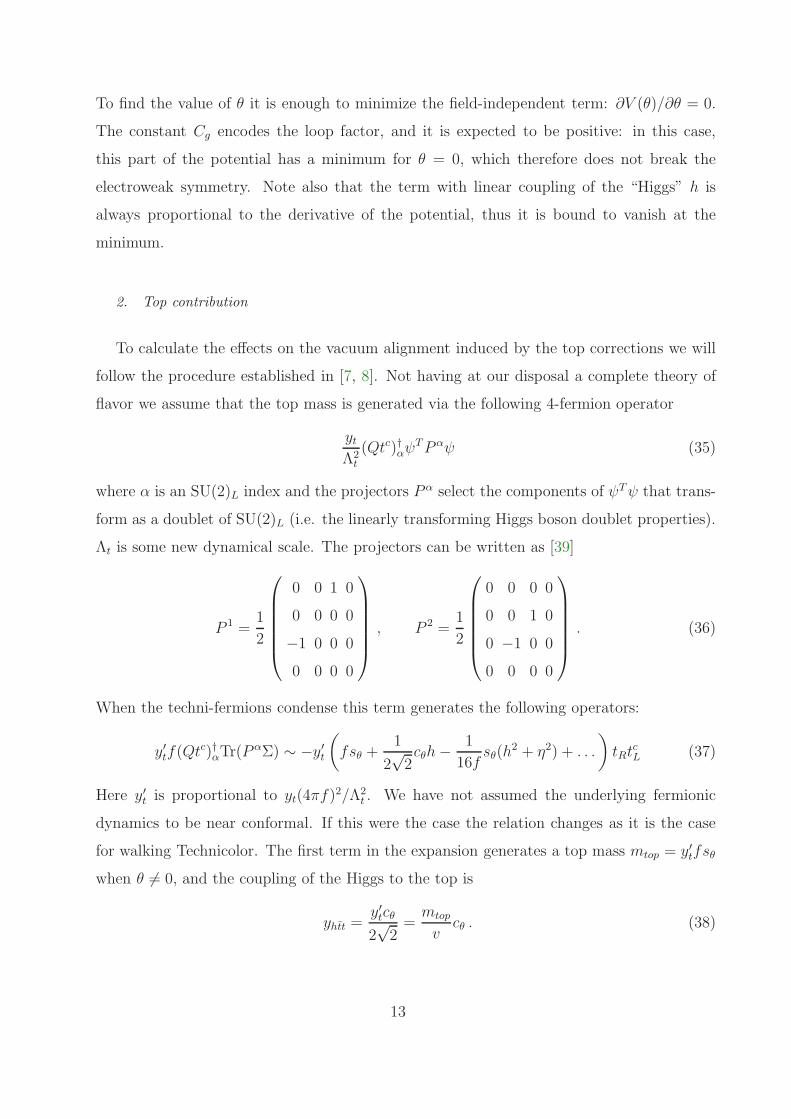
To find the value of θ it is enough to minimize the field-independent term: ∂V (θ)/∂θ = 0.

The constant Cg encodes the loop factor, and it is expected to be positive: in this case,

this part of the potential has a minimum for θ = 0, which therefore does not break the

electroweak symmetry. Note also that the term with linear coupling of the “Higgs” h is

always proportional to the derivative of the potential, thus it is bound to vanish at the

minimum.

2. Top contribution

To calculate the effects on the vacuum alignment induced by the top corrections we will

follow the procedure established in [7, 8]. Not having at our disposal a complete theory of

flavor we assume that the top mass is generated via the following 4-fermion operator

ytΛ2t

(Qtc)†αψTP αψ (35)

where α is an SU(2)L index and the projectors P α select the components of ψTψ that trans-

form as a doublet of SU(2)L (i.e. the linearly transforming Higgs boson doublet properties).

Λt is some new dynamical scale. The projectors can be written as [39]

P 1 =1

2

0 0 1 0

0 0 0 0

−1 0 0 0

0 0 0 0

, P 2 =

1

2

0 0 0 0

0 0 1 0

0 −1 0 0

0 0 0 0

. (36)

When the techni-fermions condense this term generates the following operators:

y′tf(Qtc)†αTr(P

αΣ) ∼ −y′t(fsθ +

1

2√2cθh−

1

16fsθ(h

2 + η2) + . . .

)tRt

cL (37)

Here y′t is proportional to yt(4πf)2/Λ2

t . We have not assumed the underlying fermionic

dynamics to be near conformal. If this were the case the relation changes as it is the case

for walking Technicolor. The first term in the expansion generates a top mass mtop = y′tfsθ

when θ 6= 0, and the coupling of the Higgs to the top is

yhtt =y′tcθ

2√2=mtop

vcθ . (38)

13

From the form of the operator above, the contribution of the top loop can be estimated as

Vtop = −Cty′t2f 4

2∑

α=1

[Tr(P αΣ)]2

∼ −Cty′t2

[f 4s2θ +

1√2f 3cθsθh+

1

8f 2(c2θh

2 − s2θη2) + . . .

](39)

where again we expect the coefficient Ct to be positive. In this case, the minimum is located

at θ = π/2, which would break the electroweak symmetry at the condensate scale. The

vacuum preferred by the top corrections therefore corresponds to the standard Technicolor-

like limit [11, 34, 36].

This Technicolor vacuum limit is quite interesting: in fact, one would have that all the

linear couplings of h to gauge bosons and to the top vanish, the reason being that in this limit

an extra U(1) symmetry remains unbroken upon gauging the electroweak symmetry. This

global U(1) symmetry is reminiscent of the QCD-like underlying techni-baryon symmetry

linking h and η into a complex di-techni-quark GB. Intriguingly a similar decoupling property

for the would be composite Higgs GB was observed in the Hosotani model [45]. Here too,

in the decoupling limit, the near decoupled state becomes a dark matter candidate. This

property of the Technicolor vacuum has been used extensively for dark matter model building

[33, 36, 46–50] and it is supported also by recent pioneering lattice investigations [23, 25, 26].

In the Technicolor limit, the pGB h ceases to be a Higgs-like particle: the physical Higgs-

like state now becomes the lightest techni-flavor (and SM) singlet composite scalar state

associated with the fluctuations of the condensate orthogonal to the GB directions. The

coupling of this state to the gauge bosons and fermions does not vanish for θ = π/2: we will

investigate the properties of this state in the following section.

In this vacuum, as explained before, η and h are degenerate and acquire the following

loop-induced mass term:

m2DM = m2

h = m2η =

f 2

4

(Cty

′t2 − Cg

3g2 + g′2

2

). (40)

There is, in principle, another possible contribution to the mass of the dark matter candidate

above coming from a different source of explicit SU(4) symmetry breaking discussed in [36].

This breaking term reinforces the alignment of the vacuum in the Technicolor direction.

Interestingly the weak interactions like to misalign the Technicolor vacuum while the top

corrections tend to re-align the vacuum in the Technicolor direction providing a positive

14

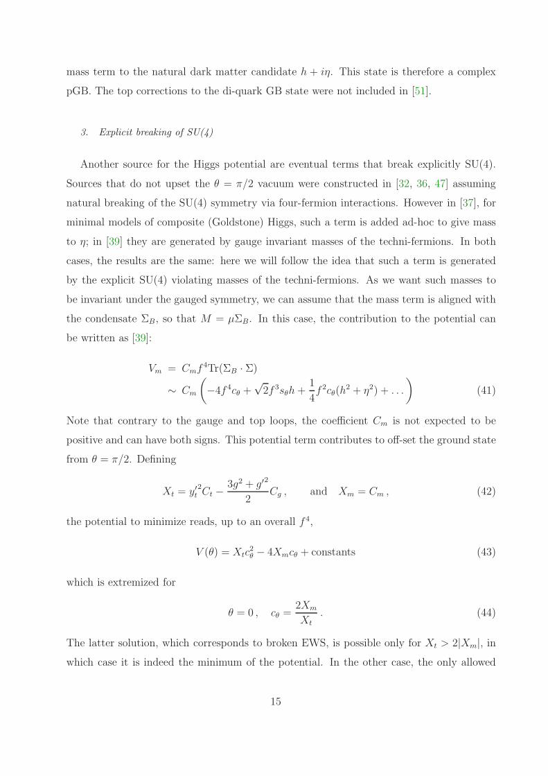
mass term to the natural dark matter candidate h + iη. This state is therefore a complex

pGB. The top corrections to the di-quark GB state were not included in [51].

3. Explicit breaking of SU(4)

Another source for the Higgs potential are eventual terms that break explicitly SU(4).

Sources that do not upset the θ = π/2 vacuum were constructed in [32, 36, 47] assuming

natural breaking of the SU(4) symmetry via four-fermion interactions. However in [37], for

minimal models of composite (Goldstone) Higgs, such a term is added ad-hoc to give mass

to η; in [39] they are generated by gauge invariant masses of the techni-fermions. In both

cases, the results are the same: here we will follow the idea that such a term is generated

by the explicit SU(4) violating masses of the techni-fermions. As we want such masses to

be invariant under the gauged symmetry, we can assume that the mass term is aligned with

the condensate ΣB, so that M = µΣB. In this case, the contribution to the potential can

be written as [39]:

Vm = Cmf4Tr(ΣB · Σ)

∼ Cm

(−4f 4cθ +

√2f 3sθh+

1

4f 2cθ(h

2 + η2) + . . .

)(41)

Note that contrary to the gauge and top loops, the coefficient Cm is not expected to be

positive and can have both signs. This potential term contributes to off-set the ground state

from θ = π/2. Defining

Xt = y′t2Ct −

3g2 + g′2

2Cg , and Xm = Cm , (42)

the potential to minimize reads, up to an overall f 4,

V (θ) = Xtc2θ − 4Xmcθ + constants (43)

which is extremized for

θ = 0 , cθ =2Xm

Xt

. (44)

The latter solution, which corresponds to broken EWS, is possible only for Xt > 2|Xm|, inwhich case it is indeed the minimum of the potential. In the other case, the only allowed

15

solution is θ = 0. The masses for the scalar fields are given by

m2h =

f 2

4(Xt(1− 2c2θ) + 2Xmcθ) , (45)

m2η =

f 2

4(Xt(1− c2θ) + 2Xmcθ) . (46)

On the solution cθ = 2Xm/Xt, the masses read

m2h =

f 2

4

X2t − 4X2

m

Xt

=f 2

4s2θXt , (47)

m2η =

f 2

4Xt . (48)

We see that m2h > 0 for Xt > 2|Xm|, for which there is always a solution for cθ. Furthermore,

we recover the relation m2η = m2

h/s2θ [39].

On the other solution θ = 0, where the electroweak symmetry is unbroken, the masses

read

m2h =

f 2

4(2Xm −Xt) , m2

η =f 2

2Xm . (49)

This solution is a stable minimum for Xt < 2Xm.

More on the Higgs mass and fine tuning

Using the expressions for the top and gauge masses, the composite GB Higgs can be

rewritten as

m2h =

f 2s2θ4

(y′t

2Ct −

3g2 + g′2

2Cg

)=Ctm

2t

4

(1− 2m2

W +m2Z

4m2t

CgCt

)∼ Ctm

2t

4

(1− 0.18

CgCt

).

(50)

This shows explicitly that the contribution of the gauge loops is typically smaller than the

top one, even assuming Cg ∼ Ct. Also, neglecting the gauge contribution, to fit the observed

Higgs mass mh = 125 GeV, we would need

Ct ∼ 2 . (51)

Another interesting point is related to the value of θ: in fact, this angle parametrizes the

corrections to the Higgs couplings to the gauge bosons, which are by now well constrained

16

by LHC data. Therefore, a realistic model would require θ to be small. In order to achieve

this, we would need:

cθ ∼ 1 ⇒ Xt ∼ 2Xm . (52)

In other words, a realistic model would require a non-trivial fine tuning between the con-

tribution of the top loops, and the contribution of the explicit breaking of SU(4), which is

induced by a completely different mechanism.

4. Variation on the theme

We can now explore some variations of the above scenario. For example we can gauge

an extra U(1). The only possibility is to gauge the symmetry generated by X5 which

commutes with both SU(2)L and U(1)Y . The new gauge boson Xµ will contribute to the

effective potential as follows

VX = −Cgg2Xf 4Tr(X5 · Σ · (X5 · Σ)∗

)

∼ Cgg2X

(1

2f 4(2c2θ − 1)− 1√

2f 3cθsθh−

1

8f 2(c2θh

2 − s2θη2) + . . .

)(53)

Although this contribution has the familiar form of the contribution coming from the elec-

troweak gauge terms, the preferred minimum is at cθ = 0. This happens because the

Technicolor ground state does not break the U(1)X symmetry thus leaving Xµ massless. In

fact:

m2X = 4g2Xf

2c2θ . (54)

The net effect of this contribution would therefore be to add to the top loop.

Another variant is to generate a mass for the top via a heavy mediator Ψ. The idea is to

complement the theory with a new fermion belonging to a complete representation of SU(4),

and couple it to Σ in an SU(4) invariant way; the mass is then communicated to the top

sector by an SU(4) violating mixing term of the form [37]

λ1fΨΣΨ + λ2fQψQ+ λ3fTψtc (55)

where Qψ and Tψ are components of Ψ with the same quantum numbers as the quark doublet

and the right-handed top singlet. However, it is not possible to find a representation of SU(4)

17

which contains a doublet and a singlet with the correct hypercharge, following the embedding

of the hypercharge generator discussed above. One may think of embedding the U(1)Y as

a superposition of the two possible U(1)’s, i.e. Y = cαS6 + sαX

5. However, there is no

vacuum that can preserve both S6 and X5 and as a consequence there would be no QED

unbroken U(1). This is interesting as it allows us to discard the construction used in [37]

to generate the top mass. In [38], the global flavor symmetry is extended to SU(4)×U(1)

and the hypercharge is identified with a linear combination of S6 and the external U(1):

this is a trick commonly used in models of composite pseudo-GB Higgs. However, it is very

unlikely that the condensate in any realistic fundamental theory, featuring fundamental

vector-like fermionic matter, can break SU(4)×U(1)→SO(5). In fact, one could imagine

to generate the extra U(1) by adding a single fermion in the adjoint representation, which

carries hypercharge. However, the two sectors of fermions do not talk to each other, and the

dynamics will generate, at first, two condensates: one breaking SU(4) and the other breaking

U(1) independently. Gauge dynamics for vector-like theories with several fermionic matter

fields were investigated in [52, 53]. To achieve the desired symmetry breaking pattern, for

these theories, one would need to introduce fields transforming simultaneously under the

two flavor symmetries. Fundamental scalar fields can easily accommodate this patterns

at the price of introducing unnatural scenarios. On the other hand, chiral gauge theories

(where a mass term for the fermions is prohibited) can break simultaneously different global

symmetries as well as the underlying gauge dynamics and would constitute and interesting

avenue to explore [54].

V. INTRODUCING THE TECHNI-HIGGS (THE σ)

As already mentioned above, the dynamics contains a would-be Higgs boson, besides

the GB of the flavor symmetry breaking, which behaves like the σ particle in QCD and

is a singlet under the flavor symmetry. To study its effect, we add its contribution to the

potential for the GBs:

L =1

2(∂µσ)

2 − 1

2κM(σ)M2σ2 + κG(σ) f

2 Tr(DµΣ)†DµΣ + κt(σ) y

′tf(Qt

c)†αTr(PαΣ) , (56)

where we have introduced the field σ with a potential term, together with the modified GB

kinetic term and the top Yukawa operator. The dynamics generates the couplings of σ to

18

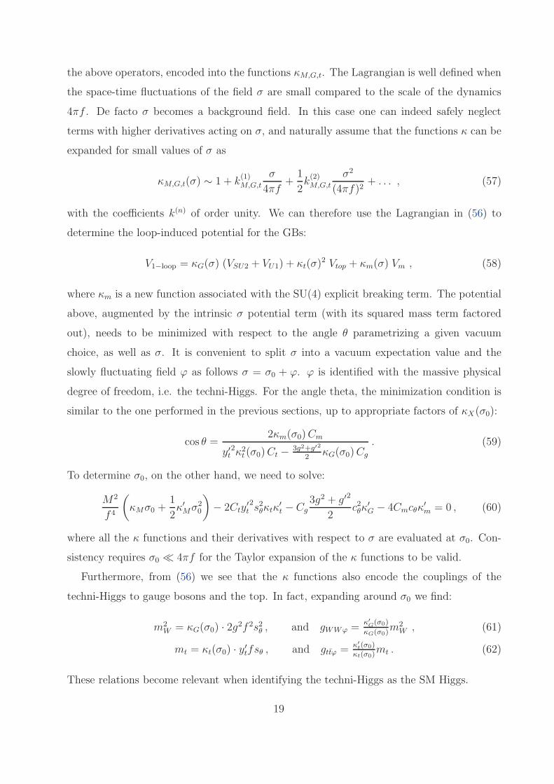
the above operators, encoded into the functions κM,G,t. The Lagrangian is well defined when

the space-time fluctuations of the field σ are small compared to the scale of the dynamics

4πf . De facto σ becomes a background field. In this case one can indeed safely neglect

terms with higher derivatives acting on σ, and naturally assume that the functions κ can be

expanded for small values of σ as

κM,G,t(σ) ∼ 1 + k(1)M,G,t

σ

4πf+

1

2k(2)M,G,t

σ2

(4πf)2+ . . . , (57)

with the coefficients k(n) of order unity. We can therefore use the Lagrangian in (56) to

determine the loop-induced potential for the GBs:

V1−loop = κG(σ) (VSU2 + VU1) + κt(σ)2 Vtop + κm(σ) Vm , (58)

where κm is a new function associated with the SU(4) explicit breaking term. The potential

above, augmented by the intrinsic σ potential term (with its squared mass term factored

out), needs to be minimized with respect to the angle θ parametrizing a given vacuum

choice, as well as σ. It is convenient to split σ into a vacuum expectation value and the

slowly fluctuating field ϕ as follows σ = σ0 + ϕ. ϕ is identified with the massive physical

degree of freedom, i.e. the techni-Higgs. For the angle theta, the minimization condition is

similar to the one performed in the previous sections, up to appropriate factors of κX(σ0):

cos θ =2κm(σ0)Cm

y′t2κ2t (σ0)Ct − 3g2+g′2

2κG(σ0)Cg

. (59)

To determine σ0, on the other hand, we need to solve:

M2

f 4

(κMσ0 +

1

2κ′Mσ

20

)− 2Cty

′t2s2θκtκ

′t − Cg

3g2 + g′2

2c2θκ

′G − 4Cmcθκ

′m = 0 , (60)

where all the κ functions and their derivatives with respect to σ are evaluated at σ0. Con-

sistency requires σ0 ≪ 4πf for the Taylor expansion of the κ functions to be valid.

Furthermore, from (56) we see that the κ functions also encode the couplings of the

techni-Higgs to gauge bosons and the top. In fact, expanding around σ0 we find:

m2W = κG(σ0) · 2g2f 2s2θ , and gWWϕ =

κ′G(σ0)

κG(σ0)m2W , (61)

mt = κt(σ0) · y′tfsθ , and gttϕ =κ′t(σ0)

κt(σ0)mt . (62)

These relations become relevant when identifying the techni-Higgs as the SM Higgs.

19

A. The Technicolor vacuum

Let us now focus on the Technicolor vacuum, i.e. θ = π/2, which is obtained in the limit

Cm = 0. In this case the SM Higgs can only be played by the techni-Higgs scalar ϕ, while

the two pseudo-GBs h and η become degenerate. The associated complex state is stable

and can play the role a complex dark matter state. Phenomenology requires the couplings

of ϕ to the gauge bosons to be close to the SM ones, yielding the following constraints on

the function κG:

κ′G(σ0)

κG(σ0)∼ k

(1)G

4πf≈ 2

v=

1√2f

⇒ k(1)G ∼ 2

√2π , (63)

where we are neglecting higher order terms in σ0/(4πf). The same analysis for the top

would imply

κ′t(σ0)

κt(σ0)∼ k

(1)t

4πf≈ 1

v=

1

2√2f

⇒ k(1)t ∼

√2π . (64)

We now consider the various contributions to the physical mass for the would-be Higgs

ϕ, and to the one of the complex dark matter particle formed by the two GBs. Truncating

the Taylor expansion of the κ function to the first relevant orders we find:

m2ϕ = M2

(1 + 3k

(1)M

σ04πf

)−

((k

(1)t )2 + k

(2)t

)

2π2

Cty′t2f 2

4, (65)

m2DM =

Cty′t2f 2

4

[1− 3g2 + g′2

2y′t2

CgCt

+

(2k

(1)t − k

(1)G CgCt

3g2 + g′2

2y′t2

)σ0

4πf

]. (66)

In our calculation, σ0 ≪ 4πf , therefore, at leading order the dark matter mass is the same

as we obtained in the previous section

m2DM ∼ Cty

′t2f 2

4≃ Ct

4m2t , (67)

where mt = y′tf for θ = π/2 and κt(σ0) ∼ 1. Analogously, neglecting terms suppressed by

σ0/(4πf), the techni-Higgs mass is given by

m2ϕ ≃M2 −

((k

(1)t )2 + k

(2)t

)

2π2m2DM ∼ M2 − Ct

((k

(1)t )2 + k

(2)t

)

8π2m2t . (68)

The above formula provides a nice correlation between the would-be Higgs mass, the mass

of the dark matter candidate and the top mass under the assumption that no other ex-

plicit SU(4) breaking terms are present in the theory. In particular, this formula shows the

20

possibility that a potentially large value of M generated by the strong dynamics, may be

cancelled by the mass of the dark matter candidate, which is generated by the top loop as

suggested in [6].

Finally, we need to check the consistency of our calculation by checking the value of σ0,

and making sure that it is not too big to invalidate the expansion. An approximate solution

for σ0 reads:

σ0 ∼4πf 3k

(1)t Cty

′t2

8π2M2 −((k

(1)t )2 + k

(2)t

)Cty′t

2f 2∼ 2

√2f · k

(1)t√2π

m2DM

m2ϕ

. (69)

From this equation we see that a small correction σ0 ≪ 4πf would require either mDM <

mϕ, or small k(1)t <

√2π thus implying that the techni-Higgs has a coupling to the top

smaller that the SM expectation (see Eq.(64)). Nevertheless, this analysis does not exclude

the possibility to achieve a light techni-Higgs within a consistent dynamical framework.

Furthermore the resulting value of the techni-Higgs mass can be further lowered because the

intrinsic value of M itself can be small with respect to 4πf . The most discussed example in

the literature is the one according to which M is reduced because the underlying dynamics

is near conformal. In this case the techni-Higgs is identified with the techni-dilaton [55–

57]. Several model computations have been used to estimate M ranging from the use of the

truncated Schwinger-Dyson equations [58–66] to computations making use of orientifold field

theories [67, 68]. Perturbative examples have proven useful to demonstrate the occurrence of

a calculable dilaton state parametrically lighter than the other states in the theory [69–71].

Last but not the least recent first principle lattice simulations [72, 73] support this possibility

for certain fundamental gauge theories put forward in [11, 56, 68].

B. The pseudo-Goldstone Higgs vacuum and beyond

We now consider the general θ case, including also the explicit SU(4) breaking term, and

determine the masses of the 3 scalars. The η state does not mix, to the quadratic order,

with the other two states, while h and ϕ do mix with each others. To the lowest order in

21

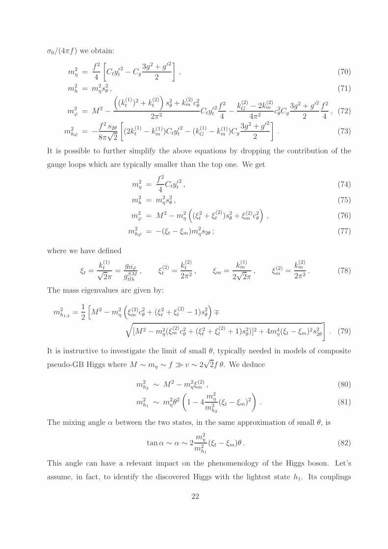
σ0/(4πf) we obtain:

m2η =

f 2

4

[Cty

′t2 − Cg

3g2 + g′2

2

], (70)

m2h = m2

ηs2θ , (71)

m2ϕ = M2 −

((k

(1)t )2 + k

(2)t

)s2θ + k

(2)m c2θ

2π2Cty

′t2 f

2

4− k

(2)G − 2k

(2)m

4π2c2θCg

3g2 + g′2

2

f 2

4, (72)

m2hϕ = −f

2 s2θ

8π√2

[(2k

(1)t − k(1)m )Cty

′t2 − (k

(1)G − k(1)m )Cg

3g2 + g′2

2

]. (73)

It is possible to further simplify the above equations by dropping the contribution of the

gauge loops which are typically smaller than the top one. We get

m2η =

f 2

4Cty

′t2, (74)

m2h = m2

ηs2θ , (75)

m2ϕ = M2 −m2

η

((ξ2t + ξ

(2)t )s2θ + ξ(2)m c2θ

), (76)

m2hϕ = −(ξt − ξm)m

2ηs2θ ; (77)

where we have defined

ξt =k(1)t√2π

=gttϕgSMtth

, ξ(2)t =

k(2)t

2π2, ξm =

k(1)m

2√2π

, ξ(2)m =k(2)m

2π2. (78)

The mass eigenvalues are given by:

m2h1,2

=1

2

[M2 −m2

η

(ξ(2)m c2θ + (ξ2t + ξ

(2)t − 1)s2θ

)∓

√[M2 −m2

η(ξ(2)m c2θ + (ξ2t + ξ

(2)t + 1)s2θ)]

2 + 4m4η(ξt − ξm)2s22θ

]. (79)

It is instructive to investigate the limit of small θ, typically needed in models of composite

pseudo-GB Higgs where M ∼ mη ∼ f ≫ v ∼ 2√2f θ. We deduce

m2h2

∼ M2 −m2ηξ

(2)m , (80)

m2h1

∼ m2ηθ

2

(1− 4

m2η

m2h2

(ξt − ξm)2

). (81)

The mixing angle α between the two states, in the same approximation of small θ, is

tanα ∼ α ∼ 2m2η

m2h1

(ξt − ξm)θ . (82)

This angle can have a relevant impact on the phenomenology of the Higgs boson. Let’s

assume, in fact, to identify the discovered Higgs with the lightest state h1. Its couplings

22

must be close to the SM ones. However, the couplings of h1 will get a contribution from the

couplings of ϕ via the mixing angle α. After having defined the quantity ξG =k(1)G

2√2π

=gWWϕ

gSMWWh

,

we have

gWWh1

gSMWWh

∼ 1 + ξG 2m2η

m2h1

(ξt − ξm)θ +O(θ2) , (83)

gtth1gSMtth

∼ 1 + ξt 2m2η

m2h1

(ξt − ξm)θ +O(θ2) . (84)

The mixing with ϕ has generated a correction of order θ to the couplings, while the con-

tribution of the pseudo-GB nature of the Higgs arises at the θ2 level. Hence the bounds

on θ, and therefore the required fine tuning between the top loop and the explicit SU(4)

breaking, are sensitive to the presence of the σ state and its correction cannot, in general,

be neglected.

As a consistency check one can determine again σ0 (neglecting also the gauge loops) and

one finds

σ0 ∼ f 3Cty′t2

2π

k(1)t s2θ + k

(1)m c2θ

M2 +f2Cty′y

2

8π2

(((k

(1)m )2 − 2k

(1)m k

(1)t − k

(2)m )c2θ − ((k

(1)t )2 + k

(2)t )s2θ

)

∼ 2√2f

2ξmm2η

m2h2

+ 4ξm(ξm − ξt)m2η

. (85)

therefore, for consistency, we shall either have small ξm, or mη ≪M .

VI. CHIRAL SYMMETRY BREAKING AND PREDICTIONS FOR THE SPIN

ONE SPECTRUM FROM THE LATTICE

Without the specific knowledge of an underlaying gauge theory it is impossible to provide

a reasonable prediction for the energy scale when the spin-one spectrum of the theory will

become accessible at colliders. The coefficients of the effective Lagrangians are all unknown

allowing, at best, order unity predictions for low energy processes. Furthermore, for the

phenomenological analyses presented above, whether they were meant for composite Higgs

models of pseudo-GB or non-GB nature, it was assumed that a specific pattern of chiral

symmetry breaking, namely SU(4) breaking to Sp(4)∼ SO(5), occurs via a more fundamen-

tal dynamics. This pattern was assumed to occur before embedding the electroweak sector,

before extending the model in order to provide masses to the SM fermions and, last but not

23

the least, before the further explicit breaking of the original SU(4) symmetry. The conspir-

acy of these different ingredients is required to provide a successful model of electroweak

symmetry breaking and fermion mass generation.

The first question to answer is therefore: Does it exist a fundamental gauge theory

example, not suffering from quadratic divergences, that supports the dynamical breaking of

SU(4) to Sp(4)∼ SO(5)?

The answer, from lattice simulations, is positive [23, 26]. The dynamics studied is indeed

an SU(2) gauge theory with two dynamical Dirac fermions transforming according to the

fundamental representation of the gauge group. Using the Wilson formulation of the lattice

action in [23] clear signs, further analyzed in [26], of chiral symmetry breaking have appeared.

They consist in having shown that the GB squared mass vanishes linearly with the underlying

common fermion masses, that the GB decay constant f divided by Za (the axial current

renormalisation factor4), does not vanish in the chiral limit. Furthermore the spectrum of

spin-one vector and axial resonances is well separated from the GBs with the ratio of the

spin-one masses to the GB masses growing to infinity towards the chiral limit.

We now provide the local operators, and the associated two-point correlators, studied on

the lattice [23, 26] in the Dirac notation. For the QCD-like meson degrees of freedom the

local operators are

O(Γ)

UD(x) = U(x)ΓD(x) , (86)

O(Γ)

DU(x) = D(x)ΓU(x) , (87)

O(Γ)

UU±DD(x) =1√2

(U(x)ΓU(x)±D(x)ΓD(x)

), (88)

where Γ denotes any product of Dirac matrices. Di-quarks in the SU(2) color theory couple

to the following local operators

O(Γ)UD(x) = UT (x)(−iσ2)CΓD(x) , (89)

O(Γ)DU(x) = DT (x)(−iσ2)CΓU(x) , (90)

O(Γ)UU±DD(x) =

1√2

(UT (x)(−iσ2)CΓU(x)±DT (x)(−iσ2)CΓD(x)

), (91)

where the Pauli structure −iσ2 acts on color indices while the charge conjugation operator

C acts on Dirac indices. In [23, 26] the meson masses were extracted from the two-point

4 The perturbative lattice determination of Za and the vector renormalisation factor Zv for any SU(N)

gauge theory and any matter representation can be found in [16].

24

correlation functions

C(Γ)

UD(ti − tf ) =

∑

~xi,~xf

⟨O(Γ)UD(xf )O

(Γ)†UD (xi)

⟩.

=∑

~xi,~xf

Tr ΓSDD(xf , xi)γ0Γ†γ0SUU(xi, xf ), (92)

where SUU(x, y) = 〈U(x)U(y)〉. The quantities of interest are pseudoscalar Γ = γ5, vector

Γ = γk (k = 1, 2, 3), and axial vector Γ = γ5γk mesons.

The second point to answer is: At what energy scale one can hope to discover new states

such as spin-one resonances?

Having both a well defined underlying gauge theory as well as its lattice simulations we

can provide the first preliminary predictions [26]. In units of 2√2f ≃ (246/sθ) GeV we have

mρ

2√2 f

≃ 10.20(0.16)(1.14)(1.22) ,mA

2√2f

≃ 13.20(0.53)(1.50)(1.50) , (93)

where the first error is statistical, the second comes from the continuum extrapolation and

the third from the uncertainty in Za [26]. In electroweak physical units

mρ ≃ 2510(40)(280)(300) GeV/sθ , mA ≃ 3270(130)(370)(370) GeV/sθ . (94)

The phenomenological lightest vector mesons occur for θ = π/2 associated to the Technicolor

direction while for small θ, which is the direction associated to a prevalently pseudo-GB

Higgs, the vectors become very heavy to be easily detectable even for the next generation

of colliders.

One can imagine to use a more involved gauge theory dynamics by, for example, adding

new type of matter singlet with respect to the electroweak interactions as advocated in

[11] in order to reach near-conformal dynamics. An explicit construction involving directly

the SU(2) gauge group which besides two Dirac fermions in the fundamental also features

fermions in the adjoint representation was considered explicitly in [36]. These theories might

feature parametrically lighter non-GB states because they might feel the presence of a nearby

infrared fixed point5. Lattice investigations of this type of dynamics are underway [72].

5 This behavior requires that, as function of the parameter space of the theory, such as the number of

flavors, the transition to conformality is smooth, i.e. no jumping phenomenon exists [74] in the form of a

first-order phase transition.

25

VII. CONCLUSIONS AND OUTLOOK

Models of composite (Goldstone) Higgs are relevant alternatives to supersymmetric ex-

tensions of the SM. In this paper we have explicitly shown that by providing an explicit

UV completion, even if only partial, for models of composite Higgs, based on a strongly

interacting gauge theory with fermionic matter fields, offers a unified framework where one

can study simultaneously models of pseudo-GB Higgses and Technicolor models. In the

Technicolor limit the Higgs is identified with the lightest scalar resonance of the dynam-

ics. We can, therefore, answer several questions that cannot be otherwise addressed via the

mere knowledge of the global symmetries of the effective theory such as: How heavy are the

vector-mesons? Is it there a stable dark matter candidate? Does the global symmetry break

according to the phenomenologically desired pattern?

We focused on the well known example of the flavor symmetry

SU(4)/Sp(4)∼SO(6)/SO(5) breaking pattern. The most minimal strongly coupled

gauge theory able to achieve this breaking pattern is the SU(2) gauge theory with 4 Weyl

fermions transforming according to the fundamental representation of the gauge group.

Henceforth, seen from a fundamental dynamics point of view, this is also the minimal

symmetry breaking pattern to serve as foundation for a pseudo-GB Higgs model as well

as minimal models of Technicolor. The coset space contains 5 pGBs, three of which are

eaten by the massive W and Z assuming that a chiral condensate develops breaking

spontaneously the electroweak symmetry. The fate of the remaining pGBs depends on

the way the complete dynamics aligns the electroweak theory with respect to the vacuum

condensate of the theory: in the Technicolor alignment, they form a complex stable

dark matter candidate, while in the pGB Higgs alignment one state plays the role of the

discovered Higgs boson and the other state remains neutral with respect to the electroweak

symmetry but it is not expected to be stable. Our analysis shows that the Technicolor

alignment is more natural as it is preferred by the top loop corrections, while to achieve the

pGB Higgs vacuum one needs to introduce yet another explicit SU(4) symmetry breaking

operator with an ad-hoc tuned coupling.

On general grounds, however, there is no reason to expect the condensate to align in

either the pure Technicolor or pGB Higgs limit. We should rather conclude that, in the

absence of a complete theory of SM mass generation a well as explicit breaking of the SU(4)

26

symmetry, the vacuum alignment angle θ can assume any value between 0 and π/2. For a

generic alignment there is a relevant mixing between the pGB and the techni-Higgs. In this

case neither the pure pGB nor the techni-Higgs state can be identified with the observed

Higgs, but will be the lightest eigenstate. We have also demonstrated that this mixing affects

the physical couplings of the new Higgs and argued that the additional singlet cannot play

the role of a stable dark matter candidate unless the condensate is aligned mostly in the

Technicolor vacuum. Last but not the least, having a well defined UV completion allowed

to use recent lattice computations to predict masses and couplings of heavy states, like for

instance the lightest spin-one resonances (techni-ρ and techni-axial), for a generic vacuum

alignment. It turns out that the lightest state is the techni-ρ but it is already rather heavy,

with a mass above 2.5 TeV (the heavier the closer to the pGB Higgs alignment). We could

therefore argue that, for the LHC, the scalar sector can be more directly tested while the

spin-one states are rather challenging to explore.

Our analysis can be applied to other patterns of symmetry breaking, like for instance

SU(6)→Sp(6), which is the minimal case with two pseudo-GB Higgs doublets.

We aimed at bridging the gap among different models of composite dynamics at the

electroweak scale both at the effective model description as well as at a more fundamental

level. Having at our disposal the fundamental description of, at least, one relevant piece

of the composite gauge dynamics, we were able to make relevant physical predictions for

the most elusive part of any low energy effective description, i.e. the mass scale of the new

spin-one states to be discovered at colliders.

Much remains to be investigated, at the fundamental level, from a model building point

of view and last but not the least experimentally in order to rule-out models of composite

dynamics at the electroweak scale.

Acknowledgments

The work of F.S. is partially supported by the Danish National Research Foundation

under the grant number DNRF:90. G.C. acknowledges partial support from the Labex-LIO

(Lyon Institute of Origins) under grant ANR-10-LABX-66. G.C. would also like to thank

the ESF Holograv Programme for supporting his participation to workshops in Edinburgh

27

and Swansea, where the inspiration for this work was born.

[1] O. Antipin, M. Mojaza and F. Sannino, arXiv:1310.0957 [hep-ph].

[2] S. Weinberg, Phys. Rev. D 13, 974 (1976).

[3] L. Susskind, Phys. Rev. D 20, 2619 (1979).

[4] D. B. Kaplan and H. Georgi, Phys. Lett. B 136, 183 (1984).

[5] D. B. Kaplan, H. Georgi and S. Dimopoulos, Phys. Lett. B 136, 187 (1984).

[6] R. Foadi, M. T. Frandsen and F. Sannino, Phys. Rev. D 87, 095001 (2013) [arXiv:1211.1083

[hep-ph]].

[7] M. E. Peskin, Nucl. Phys. B 175, 197 (1980).

[8] J. Preskill, Nucl. Phys. B 177, 21 (1981).

[9] D. A. Kosower, Phys. Lett. B 144, 215 (1984).

[10] F. Sannino and K. Tuominen, Phys. Rev. D 71, 051901 (2005) [hep-ph/0405209].

[11] D. D. Dietrich and F. Sannino, Phys. Rev. D 75, 085018 (2007) [hep-ph/0611341].

[12] F. Sannino, Phys. Rev. D 79, 096007 (2009) [arXiv:0902.3494 [hep-ph]].

[13] M. Mojaza, C. Pica, T. A. Ryttov and F. Sannino, Phys. Rev. D 86, 076012 (2012)

[arXiv:1206.2652 [hep-ph]].

[14] S. Catterall and F. Sannino, Phys. Rev. D 76, 034504 (2007) [arXiv:0705.1664 [hep-lat]].

[15] S. Catterall, J. Giedt, F. Sannino and J. Schneible, JHEP 0811, 009 (2008) [arXiv:0807.0792

[hep-lat]].

[16] L. Del Debbio, M. T. Frandsen, H. Panagopoulos and F. Sannino, JHEP 0806, 007 (2008)

[arXiv:0802.0891 [hep-lat]].

[17] L. Del Debbio, A. Patella and C. Pica, Phys. Rev. D 81, 094503 (2010) [arXiv:0805.2058

[hep-lat]].

[18] S. Catterall, J. Giedt, F. Sannino and J. Schneible, arXiv:0910.4387 [hep-lat].

[19] A. J. Hietanen, K. Rummukainen and K. Tuominen, Phys. Rev. D 80, 094504 (2009)

[arXiv:0904.0864 [hep-lat]].

[20] L. Del Debbio, B. Lucini, A. Patella, C. Pica and A. Rago, Phys. Rev. D 80, 074507 (2009)

[arXiv:0907.3896 [hep-lat]].

[21] J. B. Kogut and D. K. Sinclair, Phys. Rev. D 81, 114507 (2010) [arXiv:1002.2988 [hep-lat]].

28

[22] T. Karavirta, J. Rantaharju, K. Rummukainen and K. Tuominen, JHEP 1205, 003 (2012)

[arXiv:1111.4104 [hep-lat]].

[23] R. Lewis, C. Pica and F. Sannino, Phys. Rev. D 85, 014504 (2012) [arXiv:1109.3513 [hep-ph]].

[24] A. Hietanen, C. Pica, F. Sannino and U. I. Sondergaard, PoS LATTICE 2012, 065 (2012)

[arXiv:1211.0142 [hep-lat]].

[25] A. Hietanen, C. Pica, F. Sannino and U. I. Sondergaard, Phys. Rev. D 87, no. 3, 034508

(2013) [arXiv:1211.5021 [hep-lat]].

[26] A. Hietanen, R. Lewis, C. Pica and F. Sannino, arXiv:1308.4130 [hep-ph]. Extended version

to appear.

[27] A. Hietanen, C. Pica, F. Sannino and U. Søndergaard, arXiv:1311.3841 [hep-lat].

[28] J. Mrazek, A. Pomarol, R. Rattazzi, M. Redi, J. Serra and A. Wulzer, Nucl. Phys. B 853

(2011) 1 [arXiv:1105.5403 [hep-ph]].

[29] B. Bellazzini, C. Csaki and J. Serra, arXiv:1401.2457 [hep-ph].

[30] K. Agashe, R. Contino and A. Pomarol, Nucl. Phys. B 719 (2005) 165 [hep-ph/0412089].

[31] F. Caracciolo, A. Parolini and M. Serone, JHEP 1302 (2013) 066 [arXiv:1211.7290 [hep-ph]].

[32] R. Foadi, M. T. Frandsen, T. A. Ryttov and F. Sannino, Phys. Rev. D 76, 055005 (2007)

[arXiv:0706.1696 [hep-ph]].

[33] M. T. Frandsen and F. Sannino, Phys. Rev. D 81, 097704 (2010) [arXiv:0911.1570 [hep-ph]].

[34] T. Appelquist, P. S. Rodrigues da Silva and F. Sannino, Phys. Rev. D 60, 116007 (1999)

[hep-ph/9906555].

[35] Z. -y. Duan, P. S. Rodrigues da Silva and F. Sannino, Nucl. Phys. B 592, 371 (2001)

[hep-ph/0001303].

[36] T. A. Ryttov and F. Sannino, Phys. Rev. D 78, 115010 (2008) [arXiv:0809.0713 [hep-ph]].

[37] E. Katz, A. E. Nelson and D. G. E. Walker, JHEP 0508 (2005) 074 [hep-ph/0504252].

[38] B. Gripaios, A. Pomarol, F. Riva and J. Serra, JHEP 0904 (2009) 070 [arXiv:0902.1483

[hep-ph]].

[39] J. Galloway, J. A. Evans, M. A. Luty and R. A. Tacchi, JHEP 1010 (2010) 086

[arXiv:1001.1361 [hep-ph]].

[40] J. Barnard, T. Gherghetta and T. S. Ray, arXiv:1311.6562 [hep-ph].

[41] G. Ferretti and D. Karateev, arXiv:1312.5330 [hep-ph].

[42] P. Batra and Z. Chacko, Phys. Rev. D 77 (2008) 055015 [arXiv:0710.0333 [hep-ph]].

29

[43] L. Vecchi, arXiv:1304.4579 [hep-ph].

[44] M. Frigerio, A. Pomarol, F. Riva and A. Urbano, JHEP 1207 (2012) 015 [arXiv:1204.2808

[hep-ph]].

[45] Y. Hosotani, P. Ko and M. Tanaka, Phys. Lett. B 680 (2009) 179 [arXiv:0908.0212 [hep-ph]].

[46] S. B. Gudnason, C. Kouvaris and F. Sannino, Phys. Rev. D 73, 115003 (2006)

[hep-ph/0603014].

[47] S. B. Gudnason, C. Kouvaris and F. Sannino, Phys. Rev. D 74, 095008 (2006)

[hep-ph/0608055].

[48] E. Nardi, F. Sannino and A. Strumia, JCAP 0901, 043 (2009) [arXiv:0811.4153 [hep-ph]].

[49] R. Foadi, M. T. Frandsen and F. Sannino, Phys. Rev. D 80, 037702 (2009) [arXiv:0812.3406

[hep-ph]].

[50] E. Del Nobile, C. Kouvaris and F. Sannino, Phys. Rev. D 84, 027301 (2011) [arXiv:1105.5431

[hep-ph]].

[51] D. D. Dietrich and M. Jarvinen, Phys. Rev. D 79, 057903 (2009) [arXiv:0901.3528 [hep-ph]].

[52] T. A. Ryttov and F. Sannino, Int. J. Mod. Phys. A 25, 4603 (2010) [arXiv:0906.0307 [hep-ph]].

[53] N. Chen, T. A. Ryttov and R. Shrock, Phys. Rev. D 82, 116006 (2010) [arXiv:1010.3736

[hep-ph]].

[54] T. Appelquist, Z. -y. Duan and F. Sannino, Phys. Rev. D 61, 125009 (2000) [hep-ph/0001043].

[55] K. Yamawaki, M. Bando and K. -i. Matumoto, Phys. Rev. Lett. 56 (1986) 1335.

[56] D. D. Dietrich, F. Sannino and K. Tuominen, Phys. Rev. D 72 (2005) 055001

[hep-ph/0505059].

[57] T. Appelquist and Y. Bai, Phys. Rev. D 82 (2010) 071701 [arXiv:1006.4375 [hep-ph]].

[58] V. P. Gusynin and V. A. Miransky, Sov. Phys. JETP 68 (1989) 232 [Zh. Eksp. Teor. Fiz. 95

(1989) 410].

[59] B. Holdom and J. Terning, Phys. Lett. B 187 (1987) 357.

[60] B. Holdom and J. Terning, Phys. Lett. B 200 (1988) 338.

[61] M. Harada, M. Kurachi and K. Yamawaki, Phys. Rev. D 68 (2003) 076001 [hep-ph/0305018].

[62] M. Kurachi and R. Shrock, JHEP 0612 (2006) 034 [hep-ph/0605290].

[63] A. Doff, A. A. Natale and P. S. Rodrigues da Silva, Phys. Rev. D 77 (2008) 075012

[arXiv:0802.1898 [hep-ph]].

[64] A. Doff and A. A. Natale, Phys. Lett. B 677 (2009) 301 [arXiv:0902.2379 [hep-ph]].

30

[65] A. Doff, A. A. Natale and P. S. Rodrigues da Silva, Phys. Rev. D 80 (2009) 055005

[arXiv:0905.2981 [hep-ph]].

[66] A. Doff and A. A. Natale, Phys. Rev. D 81 (2010) 095014 [arXiv:0912.1003 [hep-ph]].

[67] F. Sannino and M. Shifman, Phys. Rev. D 69 (2004) 125004 [hep-th/0309252].

[68] D. K. Hong, S. D. H. Hsu and F. Sannino, Phys. Lett. B 597 (2004) 89 [hep-ph/0406200].

[69] B. Grinstein and P. Uttayarat, JHEP 1107 (2011) 038 [arXiv:1105.2370 [hep-ph]].

[70] O. Antipin, M. Mojaza and F. Sannino, Phys. Lett. B 712 (2012) 119 [arXiv:1107.2932 [hep-

ph]].

[71] O. Antipin, M. Mojaza and F. Sannino, Phys. Rev. D 87 (2013) 096005 [arXiv:1208.0987

[hep-ph]].

[72] Z. Fodor, K. Holland, J. Kuti, D. Nogradi and C. H. Wong, arXiv:1401.2176 [hep-lat].

[73] Z. Fodor, K. Holland, J. Kuti, D. Nogradi, C. Schroeder and C. H. Wong, PoS LATTICE

2012 (2012) 024 [arXiv:1211.6164 [hep-lat]].

[74] F. Sannino, Mod. Phys. Lett. A 28, 1350127 (2013) [arXiv:1205.4246 [hep-ph]].

31