symbolic analysis - purdue university · 2 cs510 s o f t w a r e e n g i n e e r i n g what is...
TRANSCRIPT

Symbolic Analysis
Xiangyu Zhang

2
CS510 S o f t w
a r e E n g i n e e r i n g
What is Symbolic Analysis
Static analysis considers all paths are feasibleDynamic considers one path or a number of pathsSymbolic analysis reasons about path feasibility
Much more preciseScalability is an issue
A lot of security applicationsExploit generationVulnerability detectionExpose hidden behaviorVerificationEquivalence checking for analyzing obfuscated code

3
CS510 S o f t w
a r e E n g i n e e r i n g
An Example
1: x=input()2: if (x>0) 3: y=…;4: else 5: y=…;6: if (x>10)10: z=y

4
CS510 S o f t w
a r e E n g i n e e r i n g
Basic Idea
Explore individual paths in the program; models the conditions and the symbolic values along a path to a symbolic constraint; a path is feasible if the corresponding constraint is satisfiable (SAT)Similar to our per-path static analysis, a worklist is used to maintain the paths being exploredUpon a function invocation, the current worklist is pushed to a stack and a new worklist is initialized for path exploration within the calleeUpon a return, the symbolic value of the return variable is passed back to the caller

5
CS510 S o f t w
a r e E n g i n e e r i n g
Another Example
1: x=input()2: if (x>0) 3: y=…;4: else 5: y=…;6: t= f (x)7: if (t>0)8: z=y
10: f (k) {11: if (k<=-10) 12: return k+10;13: else 14: return k;

6
CS510 S o f t w
a r e E n g i n e e r i n g
Language

7
CS510 S o f t w
a r e E n g i n e e r i n g
Definitions

8
CS510 S o f t w
a r e E n g i n e e r i n g
Symbolic Execution Semantics

9
CS510 S o f t w
a r e E n g i n e e r i n g
Symbolic Execution Semantics

10
CS510 S o f t w
a r e E n g i n e e r i n g
Symbolic Execution Semantics
{ }↓

11
CS510 S o f t w
a r e E n g i n e e r i n g
Technical Challenges
How to encode a program to constraintsArrays, loops, heap, strings
How to solve constraintsPropositional logic and SAT/SMT solving

Propositional logic
Programming and Modal Logic 2006-2007 4

Syntax of propositional logic
F ::= (P ) | (¬F ) | (F ∨ F ) | (F ∧ F ) | (F → F )P ::= p | q | r | . . .
• propositional atoms: p, q, r, . . . for describing declarative sentences such as:
◦ All students have to follow the course Programming and Modal Logic
◦ 1037 is a prime number
• connectives:
Connective Symbol Alternative symbols
negation ¬ ∼disjunction ∨ |conjunction ∧ &
implication → ⇒, ⊃, ⊇
Sometimes also bi-implication (↔, ⇔, ≡) is considered as a connective.
Programming and Modal Logic 2006-2007 6

Syntax of propositional logic
Binding priorities
¬
∨ ∧
→ (↔)
for reducing the number of brackets.
Also outermost brackets are often omitted.
Programming and Modal Logic 2006-2007 7

Semantics of propositional logic
The meaning of a formula depends on:
• The meaning of the propositional atoms (that occur in that formula)
• The meaning of the connectives (that occur in that formula)
Programming and Modal Logic 2006-2007 8

Semantics of propositional logic
The meaning of a formula depends on:
• The meaning of the propositional atoms (that occur in that formula)
◦ a declarative sentence is either true or false
◦ captured as an assignment of truth values (B = {T, F}) to the propositional atoms:
a valuation v : P → B
• The meaning of the connectives (that occur in that formula)
◦ the meaning of an n-ary connective ⊕ is captured by a function f⊕ : Bn → B
◦ usually such functions are specified by means of a truth table.
A B ¬A A ∧ B A ∨ B A→ B
T T F T T TT F F F T FF T T F T TF F T F F T
Programming and Modal Logic 2006-2007 9

Exercise
Find the meaning of the formula (p→ q) ∧ (q → r) → (p→ r) by constructinga truth table from the subformulas.
Programming and Modal Logic 2006-2007 10

Exercise
Find the meaning of the formula (p→ q) ∧ (q → r) → (p→ r) by constructinga truth table from the subformulas.
(p→ q) (p→ q) ∧ (q → r)
p q r p→ q q → r ∧ p→ r →(q → r) (p→ r)
T T T T T T T TT T F T F F F TT F T F T F T TT F F F T F F TF T T T T T T TF T F T F F T TF F T T T T T TF F F T T T T T
Programming and Modal Logic 2006-2007 11

Exercise
Find the meaning of the formula (p→ q) ∧ (q → r) → (p→ r) by constructinga truth table from the subformulas.
(p→ q) (p→ q) ∧ (q → r)
p q r p→ q q → r ∧ p→ r →(q → r) (p→ r)
T T T T T T T TT T F T F F F TT F T F T F T TT F F F T F F TF T T T T T T TF T F T F F T TF F T T T T T TF F F T T T T T
Formally (this is not in the book) [[ ]] : F → ((P → B) → B)
[[p]](v) = v(p) [[φ ∧ ψ]](v) = f∧([[φ]](v), [[ψ]](v))
[[¬φ]](v) = f¬([[φ]](v)) [[φ ∨ ψ]](v) = f∨([[φ]](v), [[ψ]](v))
[[φ→ ψ]](v) = f→([[φ]](v), [[ψ]](v))
Programming and Modal Logic 2006-2007 12

Deciding validity and satisfiability of propositional formulas
• Validity: A formula φ is valid if for any valuations v, [[φ]](v) = T.
• Satisfiability: A formula φ is satisfiable if there exists a valuation v suchthat [[φ]](v) = T.
Programming and Modal Logic 2006-2007 33

Deciding validity and satisfiability of propositional formulas
• Validity: A formula φ is valid if for any valuations v, [[φ]](v) = T.
• Satisfiability: A formula φ is satisfiable if there exists a valuation v suchthat [[φ]](v) = T.
Examples
p ∧ q valid? satisfiable?p→ (q → p) valid? satisfiable?p ∧ ¬p valid? satisfiable?
Programming and Modal Logic 2006-2007 34

Deciding validity and satisfiability of propositional formulas
• Validity: A formula φ is valid if for any valuations v, [[φ]](v) = T.
• Satisfiability: A formula φ is satisfiable if there exists a valuation v suchthat [[φ]](v) = T.
Examples
p ∧ q satisfiablep→ (q → p) validp ∧ ¬p unsatisfiable
Given a propositional formula φ, how to check whether it is valid? satisfiable?
Programming and Modal Logic 2006-2007 35

SAT Solver
• Finding satisfying valuations to a propositionFinding satisfying valuations to a propositionalformula.

Forcing laws { negation
� :�T FF T
xxx : TKS
��� F
xxx : FKS
��� T

Forcing laws { conjunction
� � ^ T T TT F FF T FF F F
T
|� �����
����� ^
�����
::::
:
�"===
==
====
=
T � � T
T<D
�����
����� ^
�����
::::
: Zb==
===
====
=
T � � T
F<D
�����
����� ^
�����
::::
:
�"===
==
====
=
F � � T
F<D
�����
����� ^
�����
::::
: Zb<<
<<<
<<<<
<
T � � F
Other laws possible,but : and ^are adequate
F^
�����
::::
:
�"<<<
<<
<<<<
<
T � +3 � F
F<D
�����
����� ^
�����
::::
:
F � �+3 T

Using the SAT solver
1. Convert to : and ^.
T (p) = p T (:�) = :T (�)
T (� ^ ) = T (�) ^ T ( ) T (� _ ) = :(:T (�) ^ :T ( ))
T (�! ) = :(T (�) ^ :T ( ))
Linear growth in formula size (no distributivity).
2. Translate the formula to a DAG, sharing common subterms.
3. Set the root to T and apply the forcing rules.
Satis�able if all nodes are consistently annotated.

Example: satis�ability
Formula: p ^ :(q _ :p) � p ^ ::(:q ^ ::p)
p2T q 6T
: 6F
:5T : 5T
^ 4T
: 3F
: 2T
^1TSSSS
SSSSSS
|||| BBB
B
oooooo
oooooo
oo
Satis�able?

Example: satis�ability
Formula: p ^ :(q _ :p) � p ^ ::(:q ^ ::p)
p2T q 6T
: 6T
:5T : 5T
^ 4T
: 3F
: 2T
^1TSSSS
SSSSSS
|||| BBB
B
oooooo
oooooo
oo
Satis�able?

Example: satis�ability
Formula: p ^ :(q _ :p) � p ^ ::(:q ^ ::p)
p2T q 6T
: 6T
:5T : 5T
^ 4T
: 3F
: 2T
^1TSSSS
SSSSSS
|||| BBB
B
oooooo
oooooo
oo
Satis�able?

Example: satis�ability
Formula: p ^ :(q _ :p) � p ^ ::(:q ^ ::p)
p2T q 6T
: 6T
:5T : 5T
^ 4T
: 3F
: 2T
^1TSSSS
SSSSSS
|||| BBB
B
oooooo
oooooo
oo
Satis�able?

Example: satis�ability
Formula: p ^ :(q _ :p) � p ^ ::(:q ^ ::p)
p2T q 6T
: 6T
:5T : 5T
^ 4T
: 3F
: 2T
^1TSSSS
SSSSSS
|||| BBB
B
oooooo
oooooo
oo
Satis�able?

Example: satis�ability
Formula: p ^ :(q _ :p) � p ^ ::(:q ^ ::p)
p2T q 6F
: 6F
:5T : 5T
^ 4T
: 3F
: 2T
^1TSSSS
SSSSSS
|||| BBB
B
oooooo
oooooo
oo
Satis�able?

Example: satis�ability
Formula: p ^ :(q _ :p) � p ^ ::(:q ^ ::p)
p2T q 6F
: 6F
:5T : 5T
^ 4T
: 3F
: 2T
^1TSSSS
SSSSSS
|||| BBB
B
oooooo
oooooo
oo
Satis�able?

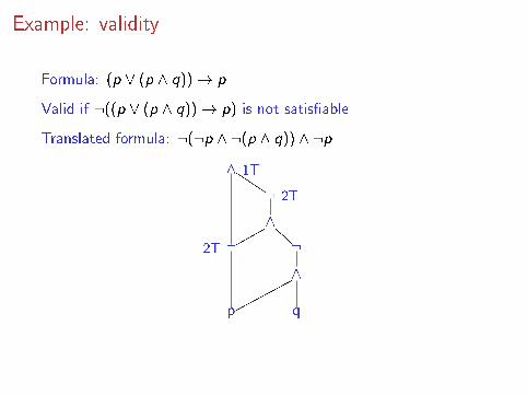
Example: validity
Formula: (p _ (p ^ q))! p
Valid if :((p _ (p ^ q))! p) is not satis�able
Translated formula: :(:p ^ :(p ^ q)) ^ :p
p3F q
^ 1T
: 2T
^ 3F
:2T : 4F
^ 5T
JJJJJ
qqqqq BBB
B
pppppp
ppp
Contradiction.

Example: validity
Formula: (p _ (p ^ q))! p
Valid if :((p _ (p ^ q))! p) is not satis�able
Translated formula: :(:p ^ :(p ^ q)) ^ :p
p3F q
^ 1T
: 2T
^ 3F
:2T : 4F
^ 5T
JJJJJ
qqqqq BBB
B
pppppp
ppp
Contradiction.
Example: validity
Formula: (p _ (p ^ q))! p
Valid if :((p _ (p ^ q))! p) is not satis�able
Translated formula: :(:p ^ :(p ^ q)) ^ :p
p3F q
^ 1T
: 2T
^ 3F
:2T : 4F
^ 5T
JJJJJ
qqqqq BBB
B
pppppp
ppp
Contradiction.

Example: validity
Formula: (p _ (p ^ q))! p
Valid if :((p _ (p ^ q))! p) is not satis�able
Translated formula: :(:p ^ :(p ^ q)) ^ :p
p3F q
^ 1T
: 2T
^ 3F
:2T : 4F
^ 5T
JJJJJ
qqqqq BBB
B
pppppp
ppp
Contradiction.

Example: validity
Formula: (p _ (p ^ q))! p
Valid if :((p _ (p ^ q))! p) is not satis�able
Translated formula: :(:p ^ :(p ^ q)) ^ :p
p3F q
^ 1T
: 2T
^ 3F
:2T : 4F
^ 5T
JJJJJ
qqqqq BBB
B
pppppp
ppp
Contradiction.

Example: validity
Formula: (p _ (p ^ q))! p
Valid if :((p _ (p ^ q))! p) is not satis�able
Translated formula: :(:p ^ :(p ^ q)) ^ :p
p3F q
^ 1T
: 2T
^ 3F
:2T : 4F
^ 5T
JJJJJ
qqqqq BBB
B
pppppp
ppp
Contradiction.

Example: validity
Formula: (p _ (p ^ q))! p
Valid if :((p _ (p ^ q))! p) is not satis�able
Translated formula: :(:p ^ :(p ^ q)) ^ :p
p3F q
^ 1T
: 2T
^ 3F
:2T : 4F
^ 5T
JJJJJ
qqqqq BBB
B
pppppp
ppp
Contradiction.

Example: satis�ability
Formula: (p _ (p ^ q))! p � :(:(:p ^ :(p ^ q)) ^ :p)
p q
^ 2F
:
^
: :
^
:1T
JJJJJ
qqqqq BBB
B
pppppp
ppp
Now what?

Example: satis�ability
Formula: (p _ (p ^ q))! p � :(:(:p ^ :(p ^ q)) ^ :p)
p q
^ 2F
:
^
: :
^
:1T
JJJJJ
qqqqq BBB
B
pppppp
ppp
Now what?

Example: satis�ability
Formula: (p _ (p ^ q))! p � :(:(:p ^ :(p ^ q)) ^ :p)
p q
^2F
:
^
: :
^
:1T
JJJJJ
qqqqq BBB
B
pppppp
ppp
Now what?

Example: satis�ability
Formula: (p _ (p ^ q))! p � :(:(:p ^ :(p ^ q)) ^ :p)
p q
^2F
:
^
: :
^
:1T
JJJJJ
qqqqq BBB
B
pppppp
ppp
Now what?

Limitation of the SAT solver algorithm
Fails for all formulas of the form :(�1 ^ �2).
�1? �2 ?
^ F
: T
||| BBB
Some are valid, and thus satis�able:
>� p ! p � :(p ^ :p)
Some are not valid, and thus not satis�able:
? � :> � :(> ^>) � :(p ! p ^ p ! p) � :(:(p ^ :p) ^ :(p ^ :p))

Limitation of the SAT solver algorithm
Fails for all formulas of the form :(�1 ^ �2).
�1? �2 ?
^ F
: T
||| BBB
Some are valid, and thus satis�able:
> � p ! p� :(p ^ :p)
Some are not valid, and thus not satis�able:
? � :> � :(> ^>) � :(p ! p ^ p ! p) � :(:(p ^ :p) ^ :(p ^ :p))

Limitation of the SAT solver algorithm
Fails for all formulas of the form :(�1 ^ �2).
�1? �2 ?
^ F
: T
||| BBB
Some are valid, and thus satis�able:
> � p ! p � :(p ^ :p)
Some are not valid, and thus not satis�able:
? � :> � :(> ^>) � :(p ! p ^ p ! p) � :(:(p ^ :p) ^ :(p ^ :p))

Limitation of the SAT solver algorithm
Fails for all formulas of the form :(�1 ^ �2).
�1? �2 ?
^ F
: T
||| BBB
Some are valid, and thus satis�able:
> � p ! p � :(p ^ :p)
Some are not valid, and thus not satis�able:
?� :> � :(> ^>) � :(p ! p ^ p ! p) � :(:(p ^ :p) ^ :(p ^ :p))

Limitation of the SAT solver algorithm
Fails for all formulas of the form :(�1 ^ �2).
�1? �2 ?
^ F
: T
||| BBB
Some are valid, and thus satis�able:
> � p ! p � :(p ^ :p)
Some are not valid, and thus not satis�able:
? � :>� :(> ^>) � :(p ! p ^ p ! p) � :(:(p ^ :p) ^ :(p ^ :p))

Limitation of the SAT solver algorithm
Fails for all formulas of the form :(�1 ^ �2).
�1? �2 ?
^ F
: T
||| BBB
Some are valid, and thus satis�able:
> � p ! p � :(p ^ :p)
Some are not valid, and thus not satis�able:
? � :> � :(>^>)� :(p ! p ^ p ! p) � :(:(p ^ :p) ^ :(p ^ :p))

Limitation of the SAT solver algorithm
Fails for all formulas of the form :(�1 ^ �2).
�1? �2 ?
^ F
: T
||| BBB
Some are valid, and thus satis�able:
> � p ! p � :(p ^ :p)
Some are not valid, and thus not satis�able:
? � :> � :(>^>) � :(p ! p^p ! p)� :(:(p ^ :p) ^ :(p ^ :p))

Limitation of the SAT solver algorithm
Fails for all formulas of the form :(�1 ^ �2).
�1? �2 ?
^ F
: T
||| BBB
Some are valid, and thus satis�able:
> � p ! p � :(p ^ :p)
Some are not valid, and thus not satis�able:
? � :> � :(>^>) � :(p ! p^p ! p) � :(:(p^:p)^:(p^:p))

Extending the algorithm
Formula: :(q ^ r) ^ :(:(q ^ r) ^ :(:q ^ r))
q8F 6T
q8F 6T r7T 6T :7T r7T 6T
^5F 5T ^6T
q8F 6T r7T 6T :4T 4F :5F
^3F ^ 3F
:2T : 2T
^ 1Tllll
lllWWWWW
WWWWWW
|||| BB
BBllll
lll RRRRRRR
|||| BB
BB|||| BB
BB
Idea: pick a node and try both possibilities

Extending the algorithm
Formula: :(q ^ r) ^ :(:(q ^ r) ^ :(:q ^ r))
q8F 6T
q8F 6T r7T 6T :7T r7T 6T
^5F 5T ^6T
q8F 6T r7T 6T :4T 4F :5F
^3F ^ 3F
:2T : 2T
^ 1Tllll
lllWWWWW
WWWWWW
|||| BB
BBllll
lll RRRRRRR
|||| BB
BB|||| BB
BB
Idea: pick a node and try both possibilities

Extending the algorithm
Formula: :(q ^ r) ^ :(:(q ^ r) ^ :(:q ^ r))
q8F 6T
q8F 6T r7T 6T :7T r7T 6T
^5F 5T ^6T
q8F 6T r7T 6T :4T 4F :5F
^3F ^ 3F
:2T : 2T
^ 1Tllll
lllWWWWW
WWWWWW
|||| BB
BBllll
lll RRRRRRR
|||| BB
BB|||| BB
BB
Idea: pick a node and try both possibilities

Extending the algorithm
Formula: :(q ^ r) ^ :(:(q ^ r) ^ :(:q ^ r))
q8F 6T
q8F 6T r7T 6T :7T r7T 6T
^5F 5T ^6T
q8F 6T r7T 6T :4T 4F :5F
^3F ^ 3F
:2T : 2T
^ 1Tllll
lllWWWWW
WWWWWW
|||| BB
BBllll
lll RRRRRRR
|||| BB
BB|||| BB
BB
Idea: pick a node and try both possibilities

Extending the algorithm
Formula: :(q ^ r) ^ :(:(q ^ r) ^ :(:q ^ r))
q8F 6T
q8F 6T r7T 6T :7T r7T 6T
^5F 5T ^6T
q8F 6T r7T 6T :4T 4F :5F
^3F ^ 3F
:2T : 2T
^ 1Tllll
lllWWWWW
WWWWWW
|||| BB
BBllll
lll RRRRRRR
|||| BB
BB|||| BB
BB
Idea: pick a node and try both possibilities

Extending the algorithm
Formula: :(q ^ r) ^ :(:(q ^ r) ^ :(:q ^ r))
q8F 6T
q8F 6T r7T 6T :7T r7T 6T
^5F 5T ^6T
q8F 6T r7T 6T :4T 4F :5F
^3F ^ 3F
:2T : 2T
^ 1Tllll
lllWWWWW
WWWWWW
|||| BB
BBllll
lll RRRRRRR
|||| BB
BB|||| BB
BB
r is true in both casesIdea: pick a node and try both possibilities

Using the value of r
Formula: :(q ^ r) ^ :(:(q ^ r) ^ :(:q ^ r))
q5F
q5F r 4T :6T r 4T
^ 6F ^7T
q5F r 4T :7T : 8F
^3F ^ 3F
:2T : 2T
^ 1Tllll
lllWWWWW
WWWWWW
|||| BB
BBllll
lll RRRRRRR
|||| BB
BB|||| BB
BB
Idea: pick a node and try both possibilities

Using the value of r
Formula: :(q ^ r) ^ :(:(q ^ r) ^ :(:q ^ r))
q5F
q5F r 4T :6T r 4T
^ 6F ^7T
q5F r 4T :7T : 8F
^3F ^ 3F
:2T : 2T
^ 1Tllll
lllWWWWW
WWWWWW
|||| BB
BBllll
lll RRRRRRR
|||| BB
BB|||| BB
BB
Idea: pick a node and try both possibilities

Using the value of r
Formula: :(q ^ r) ^ :(:(q ^ r) ^ :(:q ^ r))
q5F
q5F r 4T :6T r 4T
^ 6F ^7T
q5F r 4T :7T : 8F
^3F ^ 3F
:2T : 2T
^ 1Tllll
lllWWWWW
WWWWWW
|||| BB
BBllll
lll RRRRRRR
|||| BB
BB|||| BB
BB
Idea: pick a node and try both possibilities

Using the value of r
Formula: :(q ^ r) ^ :(:(q ^ r) ^ :(:q ^ r))
q5F
q5F r 4T :6T r 4T
^ 6F ^7T
q5F r 4T :7T : 8F
^3F ^ 3F
:2T : 2T
^ 1Tllll
lllWWWWW
WWWWWW
|||| BB
BBllll
lll RRRRRRR
|||| BB
BB|||| BB
BB
Idea: pick a node and try both possibilities

Using the value of r
Formula: :(q ^ r) ^ :(:(q ^ r) ^ :(:q ^ r))
q5F
q5F r 4T :6T r 4T
^ 6F ^7T
q5F r 4T :7T : 8F
^3F ^ 3F
:2T : 2T
^ 1Tllll
lllWWWWW
WWWWWW
|||| BB
BBllll
lll RRRRRRR
|||| BB
BB|||| BB
BB
Satis�able.Idea: pick a node and try both possibilities

Extended algorithm
Algorithm:1. Pick an unmarked node and add temporary T and F marks.
2. Use the forcing rules to propagate both marks.
3. If both marks lead to a contradiction, report a contradiction.
4. If both marks lead to some node having the same value,permanently assign the node that value.
5. Erase the remaining temporary marks and continue.
Complexity O(n3):1. Testing each unmarked node: O(n)
2. Testing a given unmarked node: O(n)
3. Repeating the whole thing when a new node is marked: O(n)
Why isn't it exponential?

An optimization
Formula: :(q ^ r) ^ :(:(q ^ r) ^ :(:q ^ r))
q8F 6T
q8F 6T r7T 6T :7T r7T 6T
^5F 5T ^6T
q8F 6T r7T 6T :4T 4F :5F
^3F ^ 3F
:2T : 2T
^ 1Tllll
lllWWWWW
WWWWWW
|||| BB
BBllll
lll RRRRRRR
|||| BB
BB|||| BB
BB
We could stop here: red values give a complete and consistentvaluation.

Another optimization
q8F 6T
q8F 6T r7T 6T :7T r7T 6T
^5F 5T ^6T
q8F 6T r7T 6T :4T 4F :5F
^3F ^ 3F
:2T : 2T
^ 1Tllll
lllWWWWW
WWWWWW
|||| BB
BBllll
lll RRRRRRR
|||| BB
BB|||| BB
BB
I Contradiction in the leftmost subtree.I No need to analyze q, etc.I Permanently mark \4T4F" as T.

Basic DLL Search
(a + c + d)
(a + c + d’)
(a + c’ + d)
(a + c’ + d’)
(a’ + b + c)
(b’ + c’ + d)
(a’ + b + c’)
(a’ + b’ + c)
M. Davis, G. Logemann, and D. Loveland. A machine program
for theorem-proving. Communications of the ACM, 5:394–397,
1962
Perform backtracking search
over values of variables
Try to satisfy each clause
19
Slides from Aarti Gupta

Basic DLL Search
Performs backtracking search over variable assignments
Basic definitions
Under a given partial assignment (PA) to variables• A variable may be
• assigned (true/false literal)
• unassigned.
• A clause may be
• satisfied (≥1 true literal)
• unsatisfied (all false literals)
• unit (one unassigned literal, rest false)
• unresolved (otherwise)
20

Basic DLL Search
(a + c + d)
(a + c + d’)
(a + c’ + d)
(a + c’ + d’)
(a’ + b + c)
(b’ + c’ + d)
(a’ + b + c’)
(a’ + b’ + c)
a
21

Basic DLL Search
a0
(a + c + d)
(a + c + d’)
(a + c’ + d)
(a + c’ + d’)
(a’ + b + c)
(b’ + c’ + d)
(a’ + b + c’)
(a’ + b’ + c)
Decision→
→→
22

Basic DLL Search
a
0(a + c + d)
(a + c + d’)
(a + c’ + d)
(a + c’ + d’)
(a’ + b + c)
(b’ + c’ + d)
(a’ + b + c’)
(a’ + b’ + c)
b
0 Decision
→
23

Basic DLL Search
a
0(a + c + d)
(a + c + d’)
(a + c’ + d)
(a + c’ + d’)
(a’ + b + c)
(b’ + c’ + d)
(a’ + b + c’)
(a’ + b’ + c)
b
0
c
0 Decision
→→
24

Basic DLL Search
a
0(a + c + d)
(a + c + d’)
(a + c’ + d)
(a + c’ + d’)
(a’ + b + c)
(b’ + c’ + d)
(a’ + b + c’)
(a’ + b’ + c)
b
0
c
0
d=1
c=0
(a + c + d)a=0
Implication Graph
Unit →
d=1
BCP: Boolean Constraint Propagation
repeatedly applies Unit Clause Rule
lit clause[lit’]
clause[⟘]d is implied25

Basic DLL Search
a
0(a + c + d)
(a + c + d’)
(a + c’ + d)
(a + c’ + d’)
(a’ + b + c)
(b’ + c’ + d)
(a’ + b + c’)
(a’ + b’ + c)
b
0
c
0
d=1
c=0
(a + c + d)a=0
d=0(a + c + d’)
Implication Graph
Unit→→
d=1,d=0
26

Basic DLL Search
a
0(a + c + d)
(a + c + d’)
(a + c’ + d)
(a + c’ + d’)
(a’ + b + c)
(b’ + c’ + d)
(a’ + b + c’)
(a’ + b’ + c)
b
0
c
0
d=1
c=0
(a + c + d)a=0
d=0(a + c + d’)
Conflict!Implication Graph
→→
Conflict!
d=1,d=0
27

Basic DLL Search
a
0(a + c + d)
(a + c + d’)
(a + c’ + d)
(a + c’ + d’)
(a’ + b + c)
(b’ + c’ + d)
(a’ + b + c’)
(a’ + b’ + c)
b
0
c
0
Backtrack
→→→→
28

Basic DLL Search
a
0(a + c + d)
(a + c + d’)
(a + c’ + d)
(a + c’ + d’)
(a’ + b + c)
(b’ + c’ + d)
(a’ + b + c’)
(a’ + b’ + c)
b
0
c
0 1 Forced Decision
→→
29

Basic DLL Search
a
0(a + c + d)
(a + c + d’)
(a + c’ + d)
(a + c’ + d’)
(a’ + b + c)
(b’ + c’ + d)
(a’ + b + c’)
(a’ + b’ + c)
b
0
c
0
d=1
c=1
(a + c’ + d)a=0
d=0(a + c’ + d’)
Conflict!
1 Forced Decision
Implication Graph
→→
d=1,d=0
30

Basic DLL Search
a
0(a + c + d)
(a + c + d’)
(a + c’ + d)
(a + c’ + d’)
(a’ + b + c)
(b’ + c’ + d)
(a’ + b + c’)
(a’ + b’ + c)
b
0
c
0 1
Backtrack
→→→→→
31

Basic DLL Search
a
0(a + c + d)
(a + c + d’)
(a + c’ + d)
(a + c’ + d’)
(a’ + b + c)
(b’ + c’ + d)
(a’ + b + c’)
(a’ + b’ + c)
b
0
c
0 1
Backtrack
32

Basic DLL Search
a
0(a + c + d)
(a + c + d’)
(a + c’ + d)
(a + c’ + d’)
(a’ + b + c)
(b’ + c’ + d)
(a’ + b + c’)
(a’ + b’ + c)
b
0
c
0 1
1 Forced Decision
33

Basic DLL Search
a
0(a + c + d)
(a + c + d’)
(a + c’ + d)
(a + c’ + d’)
(a’ + b + c)
(b’ + c’ + d)
(a’ + b + c’)
(a’ + b’ + c)
b
0
c
0
d=1
c=0
(a + c’ + d)a=0
d=0(a + c’ + d’)
Conflict!
1
c
0
1
Decision
Implication Graph
→→→→→ d=1,d=0
34

Basic DLL Search
a
0(a + c + d)
(a + c + d’)
(a + c’ + d)
(a + c’ + d’)
(a’ + b + c)
(b’ + c’ + d)
(a’ + b + c’)
(a’ + b’ + c)
b
0
c
0 1
c
0
1
Backtrack
→→→→→
35

Basic DLL Search
a
0(a + c + d)
(a + c + d’)
(a + c’ + d)
(a + c’ + d’)
(a’ + b + c)
(b’ + c’ + d)
(a’ + b + c’)
(a’ + b’ + c)
b
0
c
0
d=1
c=1
(a + c’ + d)a=0
d=0(a + c’ + d’)
Conflict!
1
c
0 1
1
Forced Decision
Implication Graph
→→→ d=1,d=0
36

Basic DLL Search
a
0(a + c + d)
(a + c + d’)
(a + c’ + d)
(a + c’ + d’)
(a’ + b + c)
(b’ + c’ + d)
(a’ + b + c’)
(a’ + b’ + c)
b
0
c
0 1
c
0 1
1
Backtrack→→→→→→→→
37

Basic DLL Search
a
0(a + c + d)
(a + c + d’)
(a + c’ + d)
(a + c’ + d’)
(a’ + b + c)
(b’ + c’ + d)
(a’ + b + c’)
(a’ + b’ + c)
b
0
c
0 1
c
0 1
1
1 Forced Decision→→→→
38

(a’ + b’ + c)
Basic DLL Search
a
0(a + c + d)
(a + c + d’)
(a + c’ + d)
(a + c’ + d’)
(a’ + b + c)
(b’ + c’ + d)
(a’ + b + c’)
b
0
c
0 1
c
0 1
1
1
b
1
a=1
b=1
c=1(a’ + b’ + c)
Decision
Implication Graph
→
→→
c=1
39

(a’ + b’ + c)
Basic DLL Search
a
(a + c + d)
(a + c + d’)
(a + c’ + d)
(a + c’ + d’)
(a’ + b + c)
(b’ + c’ + d)
(a’ + b + c’)
b
0
c
0 1
c
0 1
1
1
b
1
a=1
b=1
c=1(a’ + b’ + c) (b’ + c’ + d)
d=1
0
→
c=1,d=1
Implication Graph
40

Basic DLL Search
a
(a + c + d)
(a + c + d’)
(a + c’ + d)
(a + c’ + d’)
(a’ + b + c)
(b’ + c’ + d)
(a’ + b + c’)
(a’ + b’ + c)
b
0
c
0 1
c
0 1
1
1
b
1
a=1
b=1
c=1(a’ + b’ + c) (b’ + c’ + d)
d=1
SAT
0
→
c=1,d=1
Implication Graph
Unit-clause rule with
backtrack search 41

DPLL SAT Solver
42
DPLL(F)
G ← BCP(F)
if G = ⟙ then return true
if G = ⟘ then return false
p ← choose(vars(G))
return DPLL(G{p ↦ ⟙}) = “SAT” or DPLL(G{p ↦ ⟘})
unit clause rule
decision heuristics
backtracking search

Satisfiability Modulo Theories
(SMT)
Slides modified from those by Aarti Gupta
1
Textbook: The Calculus of Computation by A. Bradley and Z. Manna

Satisfiability Modulo Theory (SMT)
This lecture:
Theories, theory solvers
Next lecture: DPLL(T)
x = f(y)
(b >> 1) & c = d
10x + z < 20
a[i] = y
SMT Solver
FOL
Formulae
Theories
¬, ∧, ∨,
⇒, ⇔,
∀, ∃
Satisfiable?
theory
solver
theory
solver
DPLL(T)
. . .
5

First-Order Theories
Software manipulates structures• Numbers, arrays, lists, bitvectors,…
Software (and hardware) verification• Involve reasoning about such structures
First-order theories• Formalize structures to enable reasoning about them
• Validity is sometimes decidable
• Note: Validity of FOL is undecidable
6

First-order theoriesRecall: FOL
• Logical symbols
• Connectives: ¬, ∧, ∨, ⇒, ⇔
• Quantifiers: ∀, ∃
• Non-logical symbols
• Variables: x, y, z
• N-ary functions: f, g
• N-ary predicates: p, q
• Constants: a, b, c
First-order theory T is defined by:
• Signature T
• set of constant, function, and predicate symbols
• Set of T-Models
• models that fix the interpretation of symbols of T
• alternately, can use Axioms AT (closed T formulae) to provide
meaning to symbols of T 7
-Every dog has its day-Some dogs have more days than others-All cats have more days than dogs-Triangle length theory
Interpretation of a FOL formula:∀x∀y x>0 ∧ y>0 ⇒ add(x,y)>0

Examples of FO theories
Equality (and uninterpreted functions)• = stands for the usual equality
• f is not interpreted in T-model
Fixed-width bitvectors• >> is shift operator (function)
• & is bit-wise-and operator (function)
• 1 is a constant
Linear arithmetic (over R and Z)• + is arithmetic plus (function)
• < is less-than (predicate)
• 10 and 20 are constants
Arrays• a[i] can be viewed as select(a, i) that selects the
i-th element in array a
x = f(y)
(b >> 1) & c = d
a[i] = y
10x + z < 20
8

Satisfiability Modulo Theory
First-order theory T is defined by:
• Signature T
• set of constant, function, and predicate symbols
• Set of T-Models
• models that fix the interpretation of symbols of T
• alternately, can use Axioms AT (closed T formulae) to provide
meaning to symbols of T
A formula F is T-satisfiable
(satisfiable modulo T) iff
M ⊨ F for some T-model M.
A formula F is T-valid
(valid modulo T) iff
M ⊨ F for all T-models M.
Theory T is decidable
if validity modulo T is decidable
for every T -formula F.
There is an algorithm
that always terminates
with “yes” if F is T-valid,
and “no” if F is T-invalid.9

Fragment of a Theory
Fragment of a theory T
is a syntactically restricted subset of formulae of the theory
Example• Quantifier-free fragment (QFF) of theory T is the set of formulae
without quantifiers
• Quantifier-free conjunctive fragment of theory T is the set of formulae
without quantifiers and disjunction
Fragments • can be decidable, even if the full theory isn’t
• can have a decision procedure of lower complexity than for full theory
10

Theory of Equality TE
Signature
E : {=, a, b, c,…,f, g, h,…,p, q, r,…}
consists of • a binary predicate “=“ that is interpreted using axioms
• constant, function, and predicate symbols
11

1. ∀x. x=x (reflexivity)
2. ∀x,y. x=y y=x (symmetry)
3. ∀x,y,z. x=y ˄ y=z x=z (transitivity)
4. for each n-ary function symbol f,
∀x1,…,xn,y1,…,yn. ˄i (xi=yi)
f(x1,…,xn) = f(y1,…,yn) (function congruence)
5. for each n-ary predicate symbol p,
∀x1,…,xn,y1,…,yn. ˄i (xi=yi)
(p(x1,…,xn) ↔ p(y1,…,yn)) (predicate congruence)
Axioms of TE
12

Decidability of TE
Bad news• TE is undecidable
Good news• Quantifier-free fragment of TE is decidable
• Very efficient algorithms for QFF conjunctive fragment
• Based on congruence closure
13

Theory solver for TE
• In 1954 Ackermann showed that the theory of equality
and uninterpreted functions is decidable.
• In 1976 Nelson and Oppen implemented an O(m2)
algorithm based on congruence closure computation.
• Modern implementations are based on the union-find
data structure (data structures again!)
• Efficient: O(n log n)
27

a = b, b = c, d = e, b = s, d = t, a e, a s
a b c d e s t
Deciding Equality
Note: Quantifier-free, Conjunctive
28

Deciding Equality
a = b, b = c, d = e, b = s, d = t, a e, a s
a b c d e s ta,b
29

Deciding Equality
a = b, b = c, d = e, b = s, d = t, a e, a s
c d e s ta,b a,b,c
30

Deciding Equality
d,e
a = b, b = c, d = e, b = s, d = t, a e, a s
d e s ta,b,c
31

Deciding Equality
a,b,c,s
a = b, b = c, d = e, b = s, d = t, a e, a s
s ta,b,c d,e
32

Deciding Equality
a = b, b = c, d = e, b = s, d = t, a e, a s
td,ea,b,c,s d,e,t
33

Deciding Equality
a = b, b = c, d = e, b = s, d = t, a e, a s
a,b,c,s d,e,t
34

Deciding Equality
a = b, b = c, d = e, b = s, d = t, a e, a s
a,b,c,s d,e,t
Unsatisfiable
35

Deciding Equality +
(uninterpreted) Functions
a = b, b = c, d = e, b = s, d = t, f(a, g(d)) f(b, g(e))
a,b,c,s d,e,t g(d) f(a,g(d))g(e) f(b,g(e))
Congruence Rule:
x1 = y1, …, xn = yn implies f(x1, …, xn) = f(y1, …, yn)
36

Deciding Equality +
(uninterpreted) Functions
a,b,c,s d,e,t g(d) f(a,g(d))g(e) f(b,g(e))
Congruence Rule:
x1 = y1, …, xn = yn implies f(x1, …, xn) = f(y1, …, yn)
g(d),g(e)
Deciding Equality +
(uninterpreted) Functions
a = b, b = c, d = e, b = s, d = t, f(a, g(d)) f(b, g(e))
37

a,b,c,s d,e,t f(a,g(d)) f(b,g(e))
Congruence Rule:
x1 = y1, …, xn = yn implies f(x1, …, xn) = f(y1, …, yn)
g(d),g(e)
Deciding Equality +
(uninterpreted) Functions
a = b, b = c, d = e, b = s, d = t, f(a, g(d)) f(b, g(e))
38
f(a,g(d)),f(b,g(e))

a,b,c,s d,e,t f(a,g(d)) f(b,g(e))g(d),g(e) f(a,g(d)),f(b,g(e))
Deciding Equality +
(uninterpreted) Functions
a = b, b = c, d = e, b = s, d = t, f(a, g(d)) f(b, g(e))
Unsatisfiable
Efficient implementation using Union-Find data structure
39

int fun1(int y) {int x, z;z = y;y = x;x = z;return x*x;
}
int fun2(int y) {return y*y;
}
TE formula that is satisfiable iff
programs are not equivalent:
(z1 = y0 ∧ y1 = x0 ∧ x1 = z1 ∧ r1 = x1*x1) ∧(r2 = y0* y0) ∧¬(r2 = r1)
Using 32-bit integers,
and interpreting * as multiplication,
a SAT solver fails to return an answer
in 1 minute.
Example: program equivalence
14
quantifier-free
conjunctive fragment

int fun1(int y) {int x, z;z = y;y = x;x = z;return x*x;
}
int fun2(int y) {return y*y;
}
TE formula that is satisfiable iff
programs are not equivalent:
(z1 = y0 ∧ y1 = x0 ∧ x1 = z1 ∧ r1 = sq(x1) ∧(r2 = sq(y0)) ∧¬(r2 = r1)
Using TE (with uninterpreted functions),
SMT solver proves unsat
in a fraction of a second.
uninterpreted
function symbol sq
(abstraction of *)
Example: program equivalence
15

Example: program equivalence
int fun1(int y) {int x, z;x = x ^ y;y = x ^ y;x = x ^ y;return x*x;
}
int fun2(int y) {return y*y;
}
Is the uninterpreted function abstraction
going to work in this case?
No, we need the theory of fixed-width
bitvectors to reason about ^ (xor).
16

Theory of fixed-width bitvectors TBV
Signature• constants
• fixed-width words (bitvectors) for modeling machine ints, longs, etc.
• arithmetic operations (+, -, *, /, etc.) (functions)
• bitwise operations (&, |, ^, etc.) (functions)
• comparison operators (<, >, etc.) (predicates)
• equality (=)
Theory of fixed-width bitvectors is decidable• Bit-flattening to SAT: NP-complete complexity
17

Bit-Vector Logic: Syntax
formula : formula ∨ formula | ¬formula | atomatom : term rel term | Boolean-Identifier | term[ constant ]
rel : = | <
term : term op term | identifier | ∼ term | constant |atom?term:term |term[ constant : constant ] | ext( term )
op : + | − | · | / | << | >> | & | | | ⊕ | ◦
∼ x: bit-wise negation of x
ext(x): sign- or zero-extension of x
x << d: left shift with distance d
x ◦ y: concatenation of x and y
D. Kroening, O. Strichman (ETH/Technion) Decision Procedures Version 1.0, 2007 6 / 24

A simple decision procedure
Transform Bit-Vector Logic to Propositional Logic
Most commonly used decision procedure
Also called ’bit-blasting’
Bit-Vector Flattening
1 Convert propositional part as before
2 Add a Boolean variable for each bit of each sub-expression (term)
3 Add constraint for each sub-expression
We denote the new Boolean variable for i of term t by µ(t)i.
D. Kroening, O. Strichman (ETH/Technion) Decision Procedures Version 1.0, 2007 18 / 24

Bit-vector flattening
What constraints do we generate for a given term?
This is easy for the bit-wise operators.
Example for a|[l]b:l−1∧i=0
(µ(t)i = (ai ∨ bi))
(read x = y over bits as x ⇐⇒ y)
We can transform this into CNF using Tseitin’s method.
D. Kroening, O. Strichman (ETH/Technion) Decision Procedures Version 1.0, 2007 19 / 24

Flattening bit-vector arithmetic
How to flatten a + b?
−→ we can build a circuit that adds them!
FA
iba
so
Full Adder
s ≡ (a + b + i ) mod 2 ≡ a⊕ b⊕ i
o ≡ (a + b + i ) div 2 ≡ a · b + a · i + b · i
The full adder in CNF:
(a ∨ b ∨ ¬o) ∧ (a ∨ ¬b ∨ i ∨ ¬o) ∧ (a ∨ ¬b ∨ ¬i ∨ o)∧(¬a ∨ b ∨ i ∨ ¬o) ∧ (¬a ∨ b ∨ ¬i ∨ o) ∧ (¬a ∨ ¬b ∨ o)
D. Kroening, O. Strichman (ETH/Technion) Decision Procedures Version 1.0, 2007 20 / 24

Flattening bit-vector arithmetic
Ok, this is good for one bit! How about more?
8-Bit ripple carry adder (RCA)
i
FA FA FA FA FA FA FA FA
a7b7 a6b6 a5b5 a5b4 a4b3 a3b2 a2b1 a0b0
os7 s6 s5 s4 s3 s2 s1 s0
Also called carry chain adder
Adds l variables
Adds 6 · l clauses
D. Kroening, O. Strichman (ETH/Technion) Decision Procedures Version 1.0, 2007 21 / 24

Multipliers
Multipliers result in very hard formulas
Example:a · b = c ∧ b · a 6= c ∧ x < y ∧ x > y
CNF: About 11000 variables, unsolvable for current SAT solvers
Similar problems with division, modulo
Q: Why is this hard?
Q: How do we fix this?
D. Kroening, O. Strichman (ETH/Technion) Decision Procedures Version 1.0, 2007 22 / 24

Multipliers
Multipliers result in very hard formulas
Example:a · b = c ∧ b · a 6= c ∧ x < y ∧ x > y
CNF: About 11000 variables, unsolvable for current SAT solvers
Similar problems with division, modulo Q: Why is this hard?
D. Kroening, O. Strichman (ETH/Technion) Decision Procedures Version 1.0, 2007 22 / 24

Theories for Arithmetic
Natural numbers ℕ = {0,1,2,…}
Integers ℤ = {…,-2,-1,0,1,2,…}
Three theories: (Axioms in [BM Ch. 3])
Peano arithmetic TPA
• Natural numbers with addition (+), multiplication (*), equality (=)
• TPA-satisfiability and TPA-validity are undecidable
Presburger arithmetic Tℕ• Natural numbers with addition (+), equality (=)
• Tℕ-satisfiability and Tℕ-validity are decidable
Theory of integers Tℤ• Integers with addition (+), subtraction (-), comparison (>),
equality (=), multiplication by constants
• Tℤ-satisfiability and Tℤ-validity are decidable
18

Theory of Integers Tℤ
ℤ : {…,-2,-1,0,1,2,…,-3*,-2*,2*,3*,…,+,-,=,>}
where• …,-2,-1,0,1,2,… are constants
• …,-3*,-2*,2*,3*,… are unary functions
(intended meaning: 2*x is x+x, -3*x is -x-x-x)
• +,-,>,= have the usual meaning
Tℕ and Tℤ have the same expressiveness• Every ℤ-formula can be reduced to ℕ-formula
• Every ℕ-formula can be reduced to ℤ-formula
19

Example: compiler optimization
for (i=1; i<=10; i++) {a[j+i] = a[j];
}
int v = a[j];for (i=1; i<=10; i++) {
a[j+i] = v;}
A Tℤ formula that is satisfiable
iff this transformation is invalid:
(i ≥ 1) ∧ (i ≤ 10) ∧(j + i = j)
20
quantifier-free
conjunctive fragment

Theory of Reals Tℝ and
Theory of Rationals Tℚ
ℝ : {0, 1, +, –, *, =, ≥ } with multiplication
ℚ : {0, 1, +, –, =, ≥ } without multiplication
Both are decidable
• High time complexity
Quantifier-free fragment of Tℚ is efficiently decidable
21

Theory of Arrays TA
A : {select, store, =}
where• select(a,i) is a binary function:
• read array a at index i
• store(a,i,v) is a ternary function:
• write value v to index i of array a
Axioms of TA
1.∀a,i,j. i = j select(a,i) = select(a,j) (array congruence)
2.∀a,v,i,j. i = j select(store(a,i,v),j) = v (select-store 1)
3.∀a,v,i,j. i j select(store(a,i,v),j) = select(a,j) (select-store 2)
TA is undecidable
Quantifier-free fragment of TA is decidable22

Note about TA
Equality (=) is only defined for array elements…• Example:
select(a,i) = e ∀j. select( store(a,i,e), j) = select(a,j)
is TA-valid
…and not for whole arrays• Example:
select(a,i)=e store(a,i,e)=a
is not TA-valid
23
A program:A[1]=-1;A[2]=1;k=unknown( );if (A[k]==1) ...

Summary of Decidability Results
Theory Quantifiers
Decidable
QFF
Decidable
TE Equality NO YES
TPA Peano Arithmetic NO NO
Tℕ Presburger Arithmetic YES YES
Tℤ Linear Integer Arithmetic YES YES
Tℝ Real Arithmetic YES YES
Tℚ Linear Rationals YES YES
TA Arrays NO YES
QFF: Quantifier Free Fragment
25
[BM Ch. 3, Page 90]

Summary of Complexity Results
Theory Quantifiers QF
Conjunctive
TE Equality – O(n log n)
Tℕ Presburger Arithmetic O(2^2^2^(kn)) NP-complete
Tℤ Linear Integer Arithmetic O(2^2^2^(kn)) NP-complete
Tℝ Real Arithmetic O(2^2^(kn)) O(2^2^(kn))
Tℚ Linear Rationals O(2^2^(kn)) PTIME
TA Arrays – NP-complete
n – input formula size; k – some positive integer
Note: Quantifier-free Conjunctive fragments look good!26
[BM Ch. 3, Pages 90, 91]

Combination of Theories
theory
solver
combination
solver ?
theory
solver
Undecidable for arbitrary T1, T2
but
Decidable under Nelson-Oppen
restrictions40

Nelson-Oppen Procedure for deciding satisfiability• If both T1 and T2 are quantifier-free (conjunctive) fragments
• If “=“ is the only symbol common to their signatures
• If T1 and T2 meet certain other technical restrictions
Decision Procedure for
Combination of Theories
theory
solver
combination
solver ?
theory
solver
Note: Quantifier-free Conjunctive fragments look good!41

Theories in SMT Solvers
Modern SMT solvers support many useful theories• QF_UF: Quantifier-free Equality with Uninterpreted Functions
• QF_LIA: Quantifier-free Linear Integer Arithmetic
• QF_LRA: Quantifier-free Linear Real Arithmetic
• QF_BV: Quantifier-free Bit Vectors (fixed-width)
• QF_A: Quantifier-free Arrays
… and many combinations
Check out more info at
http://smtlib.cs.uiowa.edu/index.shtml
http://smtlib.cs.uiowa.edu/logics.shtml
42

summary
This lecture: Theory solvers
for QF Conjunctive fragments
Next lecture: DPLL(T)
x = f(y)
(b >> 1) & c = d
10x + z < 20
a[i] = y
SMT Solver
FOL
Formulae
Theories
¬, ∧, ∨,
⇒, ⇔,
∀, ∃
Satisfiable?
theory
solver
theory
solver
DPLL(T)
. . .
43

Z3 SMT Solver
http://rise4fun.com/z3/
Input format is an extension of SMT-LIB standard
Commands• declare-const – declare a constant of a given type
• declare-fun – declare a function of a given type
• assert – add a formula to Z3’s internal stack
• check-sat – determine if formulas currently on stack are
satisfiable
• get-model – retrieve an interpretation
• exit
45

SMT solvers: DPLL(T)
Main idea: combine DPLL SAT solving with theory solvers• DPLL-based SAT over the Boolean structure of the formula
• theory solver handles the conjunctive fragment
• Recall: SAT solvers use many techniques to prune the exponential
search space
This is called DPLL(T) • T could also be a combination of theories (using Nelson-Oppen)
8

DPLL(T): main idea
SAT solver handles Boolean structure of the formula• Treats each atomic formula as a propositional variable
• Resulting formula is called a Boolean abstraction (B)
Example
F: (x=z) ˄ ((y=z ˄ x = z+1) ˅ ¬ (x=z))
• B(F): b1 ˄ ((b2 ˄ b3) ˅ ¬b1)
• Boolean abstraction (B) defined inductively over formulas
• B is a bijective function, B-1 also exists
• B-1 (b1 ˄ b2 ˄ b3): (x=z) ˄ (y=z) ˄ (x=z+1)
• B-1 (b1 ˅ b2’): (x=z) ˅ ¬(y=z)
9
b1 b2 b3 b1

DPLL(T): main idea
Example
F: (x=z) ˄ ((y=z ˄ x = z+1) ˅ ¬ (x=z))
• B(F): b1 ˄ ((b2 ˄ b3) ˅ ¬b1)
• Use DPLL SAT solver to decide satisfiability of B(F)• If B(F) is Unsat, then F is Unsat
• If B(F) has a satisfying assignment A, F may still be Unsat
Example• SAT solver finds a satisfying assignment A: b1 ˄ b2 ˄ b3
• But, B-1(A) is unsatisfiable modulo theory
• (x=z) ˄ (y=z) ˄ (x=z+1) is not satisfiable10
b1 b2 b3 b1
B(F) is an over-approximation of F
F
B(F)

DPLL(T): main idea
Example
F: (x=z) ˄ ((y=z ˄ x = z+1) ˅ ¬ (x=z))
• B(F): b1 ˄ ((b2 ˄ b3) ˅ ¬b1)
• Use DPLL SAT solver to decide satisfiability of B(F)• If B(F) is Unsat, then F is Unsat
• If B(F) has a satisfying assignment A
• Use theory solver to check if B-1(A) is satisfiable modulo T• Note B-1(A) is in conjunctive fragment
• If B-1(A) is satisfiable modulo theory T, then F is satisfiable
12
b1 b2 b3 b1
B(F) is an over-approximation of F
F
B(F)

Like a conflict clause (due to a theory conflict)
DPLL(T): simple version
• Generate a Boolean abstraction B(F)
• Use DPLL SAT solver to decide satisfiability of B(F)
• If B(F) is Unsat, then F is Unsat
• If B(F) has a satisfying assignment A
• Use theory solver to check B-1(A) is satisfiable modulo T
• If B-1(A) is satisfiable modulo theory T, then F is satisfiable
• Because A satisfies the Boolean structure, and is consistent with T
• What if B-1(A) is unsatisfiable modulo T? Is F Unsat?
• No!
• There may be other assignments A’ that satisfy the Boolean structure and
are consistent with T
• Add ¬A to B(F), and backtrack in DPLL SAT to find other assignments
• Until there are no more satisfying assignments of B(F)
13
F
B(F)
A
A’

DPLL(T): simple version recap
1. Generate a Boolean abstraction B(F)
2. Use DPLL SAT solver to decide satisfiability of B(F)• If B(F) is Unsat, then F is Unsat
• Otherwise, find a satisfying assignment A
3. Use theory solver to check if B-1(A) is satisfiable modulo T • If B-1(A) is satisfiable modulo theory T, then F is satisfiable
• Otherwise, B-1(A) is unsatisfiable modulo T
Add ¬A to B(F), and backtrack in DPLL SAT
Repeat (2, 3) until there are no more satisfying assignments
14

DPLL(T): simple version example
• Example F: (x=z) ˄ ((y=z ˄ x = z+1) ˅ ¬ (x=z))• B(F): b1 ˄ ((b2 ˄ b3) ˅ ¬b1)
• DPLL finds A: b1 ˄ b2 ˄ b3, B-1(A): (x=z) ˄ (y=z) ˄ (x=z+1)
• Theory solver checks B-1(A), this is unsat modulo T, therefore add ¬A
• DPLL finds B(F) ˄ ¬A: b1 ˄ ((b2 ˄ b3) ˅ ¬b1) ˄ (b1’ + b2’ + b3’) is Unsat
• Therefore, F is Unsat
15
theory
solver
DPLL(T)
. . .
B(F)
Sat AB-1(A)
Add ¬A UnsatF is Unsat
Sat
Unsat
F is Sat

DPLL(T): simple version
• Correctness
• When it says “F is Sat”, there is an assignment that satisfies the Boolean
structure and is consistent with theory
• When it says “F is Unsat”, the formula is unsatisfiable because B(F) ˄ ¬A
is also an over-approximation of F
• B-1(A) is not consistent with T, i.e., B-1(¬A) is T-valid 16
theory
solver
DPLL(T)
. . .
B(F)
Sat AB-1(A)
Add ¬A UnsatF is Unsat
Sat
Unsat
F is Sat

DPLL(T): simple version
• Termination
• B(F) has only a finite number of satisfying assignments
• When ¬A is added to B(F), the assignment A will never be generated again
• Either some satisfying assignment of B(F) is also T-satisfiable (F is SAT),
or all satisfying assignments of B(F) are not T-satisfiable (F is Unsat)
17
theory
solver
DPLL(T)
. . .
B(F)
Sat AB-1(A)
Add ¬A UnsatF is Unsat
Sat
Unsat
F is Sat

An Example of Symbolic Analysis and DPLL(T)
1. m=getstr();2. n=getstr();3. i=getint();4. x=strcat(“abc”,m)5. if (strlen(m)+i>5)6. y=“abcd”7. else 8. y=strcat(“efg”,n);9. if (x==y) …
)!(:1 21 eeassertPath
),"(":1 mabcconcatxe
),"(":3 nefgconcatye "":4 abcdye
yxe :5
5)(:2 imstrlene

An Example of Symbolic Analysis and DPLL(T)
{}
{e1=T}{e1=T, e2=T}
S0
S1
{e1=T, e2=T, e5=T, e4=T}
{e1=T, e2=T, e4=T}
S2
S3 S5
state∙∙∙ facts∙∙∙ new axiom
try
backtrack
interaction withstring pluginAdd:
{e1=T, e2=T, e3=T, e4=T,
e5=T}
S6"":5 dme
1)(""),"("
5
5
mstrleneeabcdmabcconcat
)(:2 5421 eeeeassertPath
),"(":1 mabcconcatxe
),"(":3 nefgconcatye "":4 abcdye
yxe :5
5)(:2 imstrlene

12
CS510 S o f t w
a r e E n g i n e e r i n g
Recent Trends
Hybrid analysisModel counting
Quantifying information flowSide channel analysis
Develop specialized theoriesE.g., theories for regular expressions

13
CS510 S o f t w
a r e E n g i n e e r i n g
In-class Exercise 1
Model the following statement to a formula. Decide its validity by formulating it as a satisfiability problem and solving it. Please show the parse tree and the value assignment process.
If I study, then I will not fail basket weaving 101. If I do not play cards to often, then I will study. I failed basket weaving 101. Therefore, I played cards too often.

14
CS510 S o f t w
a r e E n g i n e e r i n g
In-class Exercise 2
Describe the execution of DPLL on the following formulae