Symmetric Quasi-Definite Matrices

Robert J. Vanderbei

Program in Statistics & Operations ResearchPrinceton UniversityPrinceton, NJ 08544

Abstract

We say that a symmetric matrix K is quasi-definite if it has theform

K =

[−E AT

A F

]where E and F are symmetric positive definite matrices. Althoughsuch matrices are indefinite, we show that any symmetric permutationof a quasi-definite matrix yields a factorization LDLT .

We apply this result to obtain a new approach for solving the sym-metric indefinite systems arising in interior-point methods for linearand quadratic programming. These systems are typically solved eitherby reducing to a positive definite system or by performing a Bunch-Parlett factorization of the full indefinite system at every iteration.Ours is an intermediate approach based on reducing to a quasi-definitesystem. This approach entails less fill-in than further reducing to apositive definite system but is based on a static ordering and is there-fore more efficient than performing Bunch-Parlett factorizations of theoriginal indefinite system.

1 Introduction.

We call a symmetric matrix K quasi-definite if it has the form

K =

[−E AT

A F

],

where E ∈ <n×n and F ∈ <m×m are positive definite matrices with m, n ≥ 0.

The fact that quasi-definite matrices are nonsingular is trivial. To see it,

consider the following system of equations:[−E AT

A F

] [xy

]=

[bc

]. (1.1)

The positive definiteness of E allows us to use the first set of equations to

solve for x in terms of y:

x = −E−1(b− AT y). (1.2)

Substituting for x into the second set of equations yields

y = (F + AE−1AT )−1(c + AE−1b). (1.3)

Again, the positive definiteness of E and F assures that the matrix S :=

F + AE−1AT in (1.3) is also positive definite (and therefore nonsingular).

Hence, there exists a unique solution to (1.1) for any b and c, which implies

that K is nonsingular.

The above argument suggests an algorithm for solving (1.1). Namely, first

solve for y using (1.3) and then solve for x using (1.2). However, when K is

1

large and sparse, computational efficiency critically depends on maintaining

sparsity in the matrix to be inverted in (1.3). Unfortunately, forming S can

entail considerable fill-in. For example, if A has a single dense column, this

matrix is completely full. Of course, one could try to solve the system in the

other order, first solving for x directly and then solving for y as a function

of x, but this approach encounters analogous inefficiencies when A has dense

rows. In fact, both methods perform poorly when A has dense columns and

dense rows.

A preferable approach is to apply an ordering heuristic (such as minimum-

degree or minimum-local-fill) that prevents fill-in during the factorization of

the entire matrix K. The caveat, however, is that general indefinite matri-

ces are not guaranteed to be factorizable. The quasi-definite matrix K is

indefinite, and so it is not clear a priori that one can (symmetrically) re-

arrange its rows and columns and factor the system in the resulting order.

The fundamental result in this paper is that any symmetric permutation of

a quasi-definite matrix is guaranteed to be factorizable.

It should be emphasized that no claim is made that all possible factor-

izations are equally stable numerically. Indeed, it is simple to give examples

where one factorization is much worse than another (see Section 2). However,

our aim is to apply the results presented here to the efficient implementation

of interior-point methods for linear and quadratic programming, and in such

cases we shall argue that there is not much disparity in the quality of the

2

possible factorizations (where quality is measured by the relative sizes of the

elements of the factorization). In fact, in the end they are all bad and yet

it is rather remarkable that it is not difficult to obtain results with precision

approximately equal to the square root of machine precision.

In situations where the relative sizes of the elements of a matrix fac-

torization vary widely, it is important to limit the mixing of addition and

subtraction operations in the calculation of the factors. This observation

implies that, in the interior-point context, one should pivot out all the ele-

ments in either the upper left block (or the lower right block) first. While

it is true that such strategies (which were called conservative strategies in

[24]) are the safest, it is often possible to allow a little mixing in cases where

such an allowance has a significant impact on the efficiency of the algorithm.

The main result of this paper is that mathematically this poses no problem

(but on a finite-precision machine one must be cautious about the degree of

mixing allowed).

We end this section with a simple but important result:

Theorem 1 The inverse of a quasi-definite matrix is quasi-definite.

Proof. Simple calculations show that[−E AT

A F

]−1

=

[−E AT

A F

]

3

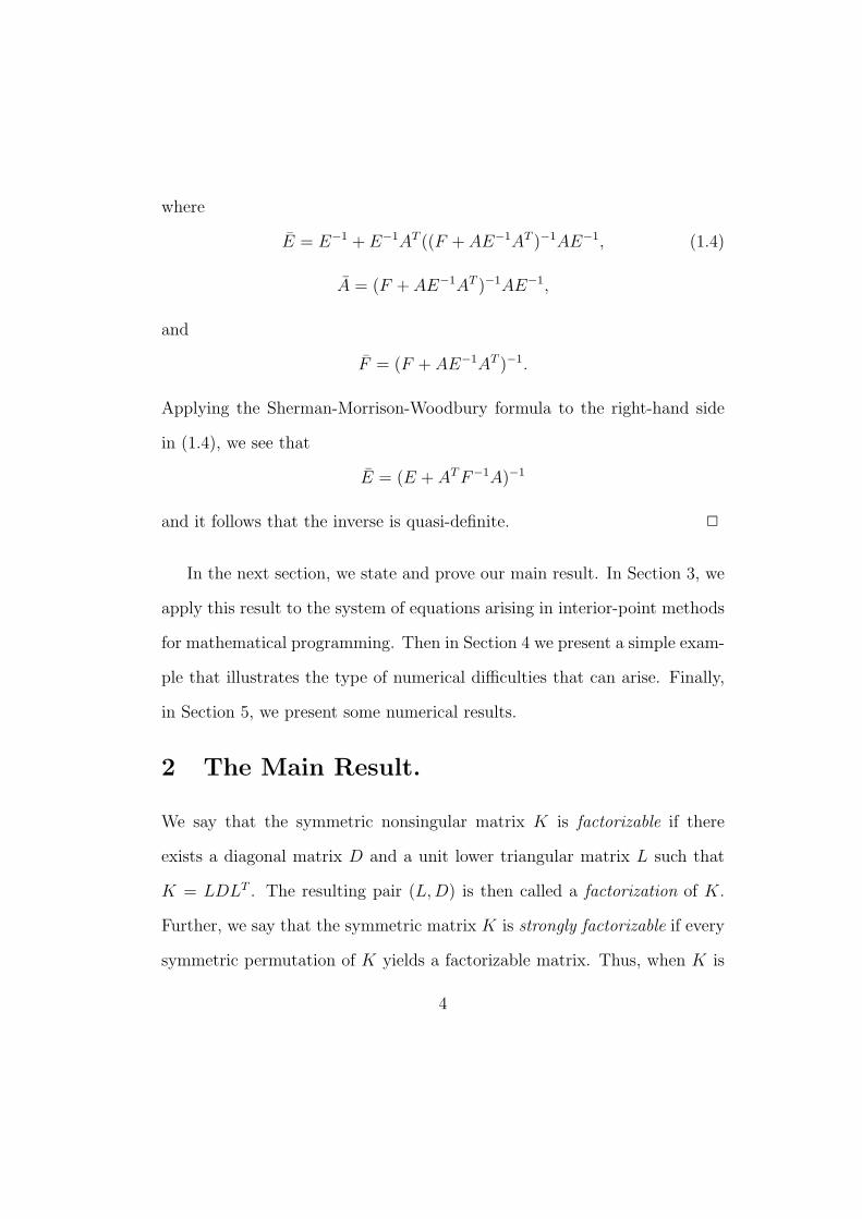
where

E = E−1 + E−1AT ((F + AE−1AT )−1AE−1, (1.4)

A = (F + AE−1AT )−1AE−1,

and

F = (F + AE−1AT )−1.

Applying the Sherman-Morrison-Woodbury formula to the right-hand side

in (1.4), we see that

E = (E + AT F−1A)−1

and it follows that the inverse is quasi-definite. 2

In the next section, we state and prove our main result. In Section 3, we

apply this result to the system of equations arising in interior-point methods

for mathematical programming. Then in Section 4 we present a simple exam-

ple that illustrates the type of numerical difficulties that can arise. Finally,

in Section 5, we present some numerical results.

2 The Main Result.

We say that the symmetric nonsingular matrix K is factorizable if there

exists a diagonal matrix D and a unit lower triangular matrix L such that

K = LDLT . The resulting pair (L, D) is then called a factorization of K.

Further, we say that the symmetric matrix K is strongly factorizable if every

symmetric permutation of K yields a factorizable matrix. Thus, when K is

4

strongly factorizable, there exists a factorization PKP T = LDLT for any

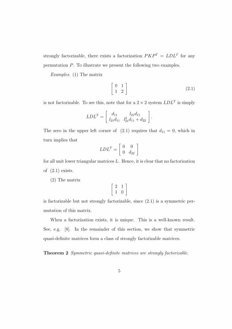
permutation P . To illustrate we present the following two examples.

Examples. (1) The matrix [0 11 2

](2.1)

is not factorizable. To see this, note that for a 2× 2 system LDLT is simply

LDLT =

[d11 l21d11

l21d11 l221d11 + d22

].

The zero in the upper left corner of (2.1) requires that d11 = 0, which in

turn implies that

LDLT =

[0 00 d22

]

for all unit lower triangular matrices L. Hence, it is clear that no factorization

of (2.1) exists.

(2) The matrix [2 11 0

]

is factorizable but not strongly factorizable, since (2.1) is a symmetric per-

mutation of this matrix.

When a factorization exists, it is unique. This is a well-known result.

See, e.g. [8]. In the remainder of this section, we show that symmetric

quasi-definite matrices form a class of strongly factorizable matrices.

Theorem 2 Symmetric quasi-definite matrices are strongly factorizable.

5

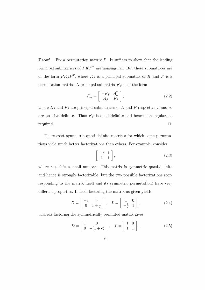
Proof. Fix a permutation matrix P . It suffices to show that the leading

principal submatrices of PKP T are nonsingular. But these submatrices are

of the form PKSP T , where KS is a principal submatrix of K and P is a

permutation matrix. A principal submatrix KS is of the form

KS =

[−ES AT

S

AS FS

], (2.2)

where ES and FS are principal submatrices of E and F respectively, and so

are positive definite. Thus KS is quasi-definite and hence nonsingular, as

required. 2

There exist symmetric quasi-definite matrices for which some permuta-

tions yield much better factorizations than others. For example, consider[−ε 11 1

], (2.3)

where ε > 0 is a small number. This matrix is symmetric quasi-definite

and hence is strongly factorizable, but the two possible factorizations (cor-

responding to the matrix itself and its symmetric permutation) have very

different properties. Indeed, factoring the matrix as given yields

D =

[−ε 00 1 + 1

ε

], L =

[1 0−1

ε1

], (2.4)

whereas factoring the symmetrically permuted matrix gives

D =

[1 00 −(1 + ε)

], L =

[1 01 1

]. (2.5)

6

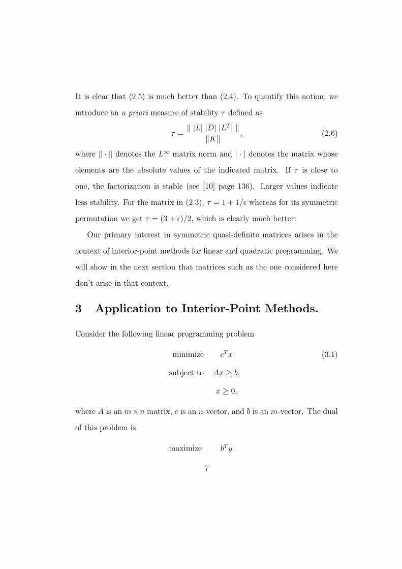
It is clear that (2.5) is much better than (2.4). To quantify this notion, we

introduce an a priori measure of stability τ defined as

τ =‖ |L| |D| |LT | ‖

‖K‖, (2.6)

where ‖ · ‖ denotes the L∞ matrix norm and | · | denotes the matrix whose

elements are the absolute values of the indicated matrix. If τ is close to

one, the factorization is stable (see [10] page 136). Larger values indicate

less stability. For the matrix in (2.3), τ = 1 + 1/ε whereas for its symmetric

permutation we get τ = (3 + ε)/2, which is clearly much better.

Our primary interest in symmetric quasi-definite matrices arises in the

context of interior-point methods for linear and quadratic programming. We

will show in the next section that matrices such as the one considered here

don’t arise in that context.

3 Application to Interior-Point Methods.

Consider the following linear programming problem

minimize cT x (3.1)

subject to Ax ≥ b,

x ≥ 0,

where A is an m×n matrix, c is an n-vector, and b is an m-vector. The dual

of this problem is

maximize bT y

7

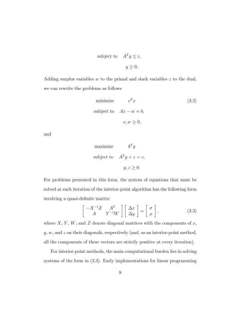
subject to AT y ≤ c,

y ≥ 0.

Adding surplus variables w to the primal and slack variables z to the dual,

we can rewrite the problems as follows

minimize cT x (3.2)

subject to Ax− w = b,

x, w ≥ 0,

and

maximize bT y

subject to AT y + z = c,

y, z ≥ 0.

For problems presented in this form, the system of equations that must be

solved at each iteration of the interior-point algorithm has the following form

involving a quasi-definite matrix:[−X−1Z AT

A Y −1W

] [∆x∆y

]=

[σρ

], (3.3)

where X, Y , W , and Z denote diagonal matrices with the components of x,

y, w, and z on their diagonals, respectively (and, as an interior-point method,

all the components of these vectors are strictly positive at every iteration).

For interior-point methods, the main computational burden lies in solving

systems of the form in (3.3). Early implementations for linear programming

8

did not operate on system (3.3) directly, but rather dealt with the symmetric

positive definite system obtained from (3.3) by solving for ∆x in terms of ∆y

using the first set of equations and then eliminating ∆x from the second set:

∆x = −XZ−1(σ − AT ∆y) (3.4)

and

(AXZ−1AT + Y −1W )∆y = (ρ + AXZ−1σ). (3.5)

The advantage of this approach is that the matrix AXZ−1AT + Y −1W is

symmetric and positive definite, so that well-known and well-behaved meth-

ods such as Cholesky factorization (which was used in the implementations

described in [14], [4], [17], [15], [18], [12], [23], [21], [13]) or preconditioned

conjugate gradient (used in the implementations described in [4], [11], [16])

can be used to solve systems involving this matrix. However, the disadvan-

tage is that AXZ−1AT can be quite dense compared to A if A has dense

columns.

Recent papers have suggested that it might be better to solve indefinite

systems such as (3.3) at every iteration. This suggestion was first put forth by

researchers in Stanford’s Systems Optimization Laboratory ([5], [19], [9]) and

by Turner [20]. Subsequently, Fourer and Mehrotra [6] began experimenting

with the indefinite system approach. All of these papers rely on doing a

Bunch-Parlett ([3], [2]) factorization of the indefinite system.

Solving the indefinite system mitigates the fill-in caused when dense

columns are present, but Bunch-Parlett factorizations tend to be more com-

9

putationally burdensome. As such, solving the indefinite system offers an

advantage when dense columns are present, but tends to be slower on most

other problems.

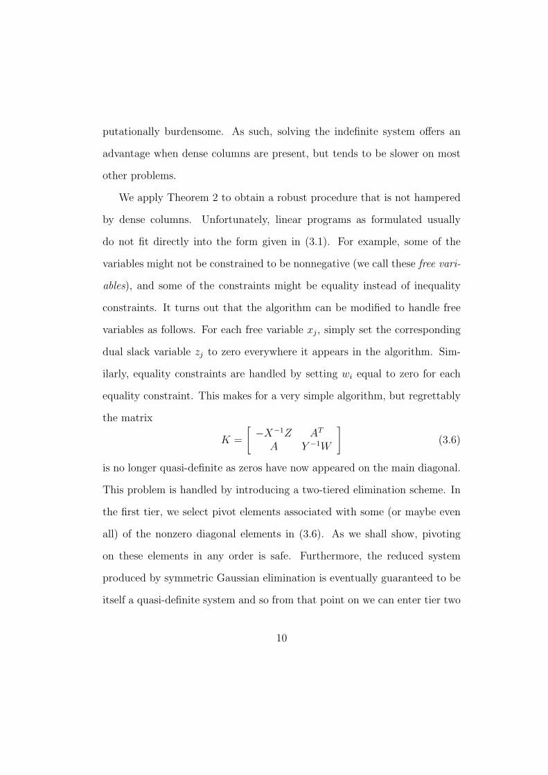
We apply Theorem 2 to obtain a robust procedure that is not hampered

by dense columns. Unfortunately, linear programs as formulated usually

do not fit directly into the form given in (3.1). For example, some of the

variables might not be constrained to be nonnegative (we call these free vari-

ables), and some of the constraints might be equality instead of inequality

constraints. It turns out that the algorithm can be modified to handle free

variables as follows. For each free variable xj, simply set the corresponding

dual slack variable zj to zero everywhere it appears in the algorithm. Sim-

ilarly, equality constraints are handled by setting wi equal to zero for each

equality constraint. This makes for a very simple algorithm, but regrettably

the matrix

K =

[−X−1Z AT

A Y −1W

](3.6)

is no longer quasi-definite as zeros have now appeared on the main diagonal.

This problem is handled by introducing a two-tiered elimination scheme. In

the first tier, we select pivot elements associated with some (or maybe even

all) of the nonzero diagonal elements in (3.6). As we shall show, pivoting

on these elements in any order is safe. Furthermore, the reduced system

produced by symmetric Gaussian elimination is eventually guaranteed to be

itself a quasi-definite system and so from that point on we can enter tier two

10

and choose the remaining pivots in any order.

To make the above explanation more precise, we partition X−1Z and

Y −1W into 2× 2 blocks

X−1Z =

[E1

E2

],

Y −1W =

[F1

F2

],

putting all the zero elements (and perhaps some nonzeros) of X−1Z into E2

and all the zero elements (and perhaps some nonzeros) of Y −1W into F2.

Then we partition system (3.3):−E1 AT

11 AT21

−E2 AT12 AT

22

A11 A12 F1

A21 A22 F2

∆x1

∆x2

∆y1

∆y2

=

σ1

σ2

ρ1

ρ2

. (3.7)

Since E1 and F1 are positive definite, we move those blocks to the upper

left-hand corner:−E1 AT

11 AT21

A11 F1 A12

AT12 −E2 AT

22

A21 A22 F2

∆x1

∆y1

∆x2

∆y2

=

σ1

ρ1

σ2

ρ2

. (3.8)

Now, the upper left 2× 2 block is quasi-definite and so can be used to solve

(with pivots in any order) for ∆x1 and ∆y1:[∆x1

∆y1

]=

[−E1 AT

11

A11 F1

]−1 ([σ1

ρ1

]−[

AT21

A12

] [∆x2

∆y2

]).

Substituting this into the last equations in (3.8), we get the following system

for ∆x2 and ∆y2:[ −E2 AT22

A22 F2

]−[

AT12

A21

] [−E1 AT

11

A11 F1

]−1 [AT

21

A12

][ ∆x2

∆y2

]

11

=

[σ2

ρ2

]−[

AT12

A21

] [−E1 AT

11

A11 F1

]−1 [σ1

ρ1

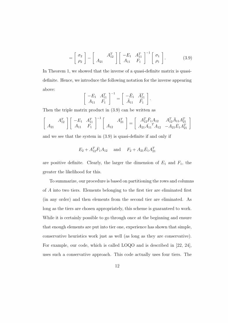
]. (3.9)

In Theorem 1, we showed that the inverse of a quasi-definite matrix is quasi-

definite. Hence, we introduce the following notation for the inverse appearing

above: [−E1 AT

11

A11 F1

]−1

=

[−E1 AT

11

A11 F1

].

Then the triple matrix product in (3.9) can be written as[AT

12

A21

] [−E1 AT

11

A11 F1

]−1 [AT

21

A12

]=

[AT

12F1A12 AT12A11A

T21

A21A11TA12 −A21E1A

T21

]

and we see that the system in (3.9) is quasi-definite if and only if

E2 + AT12F1A12 and F2 + A21E1A

T21

are positive definite. Clearly, the larger the dimension of E1 and F1, the

greater the likelihood for this.

To summarize, our procedure is based on partitioning the rows and columns

of A into two tiers. Elements belonging to the first tier are eliminated first

(in any order) and then elements from the second tier are eliminated. As

long as the tiers are chosen appropriately, this scheme is guaranteed to work.

While it is certainly possible to go through once at the beginning and ensure

that enough elements are put into tier one, experience has shown that simple,

conservative heuristics work just as well (as long as they are conservative).

For example, our code, which is called LOQO and is described in [22, 24],

uses such a conservative approach. This code actually uses four tiers. The

12

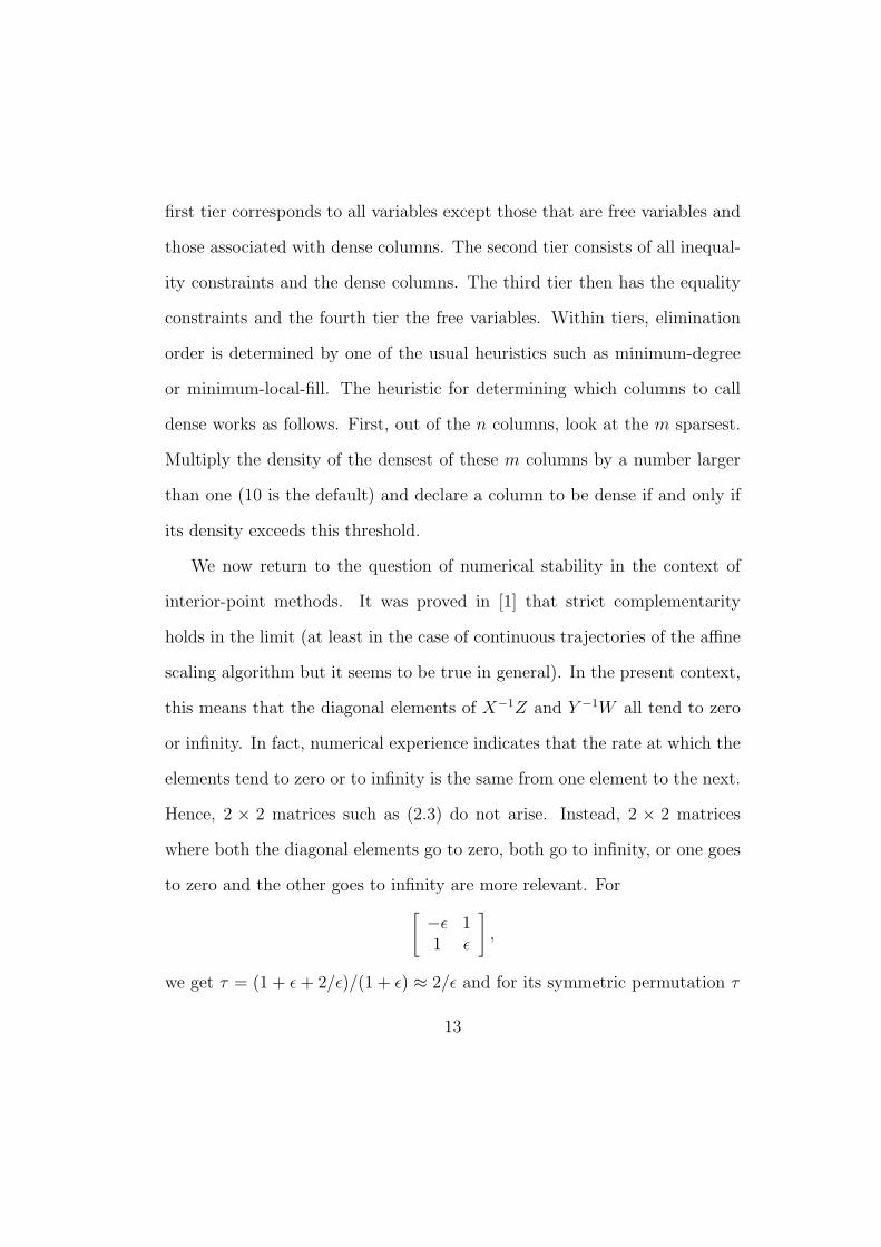
first tier corresponds to all variables except those that are free variables and

those associated with dense columns. The second tier consists of all inequal-

ity constraints and the dense columns. The third tier then has the equality

constraints and the fourth tier the free variables. Within tiers, elimination

order is determined by one of the usual heuristics such as minimum-degree

or minimum-local-fill. The heuristic for determining which columns to call

dense works as follows. First, out of the n columns, look at the m sparsest.

Multiply the density of the densest of these m columns by a number larger

than one (10 is the default) and declare a column to be dense if and only if

its density exceeds this threshold.

We now return to the question of numerical stability in the context of

interior-point methods. It was proved in [1] that strict complementarity

holds in the limit (at least in the case of continuous trajectories of the affine

scaling algorithm but it seems to be true in general). In the present context,

this means that the diagonal elements of X−1Z and Y −1W all tend to zero

or infinity. In fact, numerical experience indicates that the rate at which the

elements tend to zero or to infinity is the same from one element to the next.

Hence, 2 × 2 matrices such as (2.3) do not arise. Instead, 2 × 2 matrices

where both the diagonal elements go to zero, both go to infinity, or one goes

to zero and the other goes to infinity are more relevant. For[−ε 11 ε

],

we get τ = (1 + ε + 2/ε)/(1 + ε) ≈ 2/ε and for its symmetric permutation τ

13

is the same. On the other hand, for[−ε 11 1

ε

],

we get τ = (1+3/ε)/(1+1/ε) ≈ 3 and for its symmetric permutation τ = 1.

The other cases are similar. What one observes is that the level of instability

is essentially independent of the permutation.

However, the value of τ does not tell the whole story. In the next section,

we consider a specific example that illustrates the situations that can arise.

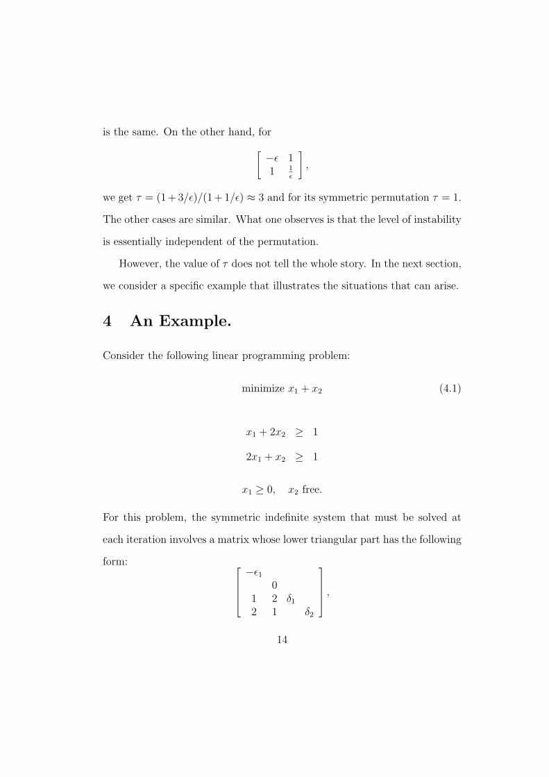
4 An Example.

Consider the following linear programming problem:

minimize x1 + x2 (4.1)

x1 + 2x2 ≥ 1

2x1 + x2 ≥ 1

x1 ≥ 0, x2 free.

For this problem, the symmetric indefinite system that must be solved at

each iteration involves a matrix whose lower triangular part has the following

form: −ε1

01 2 δ1

2 1 δ2

,

14

where ε1, δ1 and δ2 are all positive and tending to zero (at roughly the same

rate) as the iterations progress (the zero on the second diagonal position

arises from the fact that x2 is a free variable). The zero diagonal element

could pose a problem and so any static ordering must anticipate this and

defer this pivot till the end. Therefore, the lower triangular part of the

matrix becomes −ε1

1 δ1

2 δ2

2 1 0

.

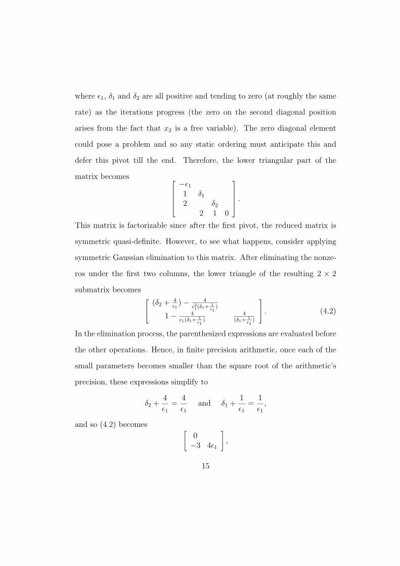
This matrix is factorizable since after the first pivot, the reduced matrix is

symmetric quasi-definite. However, to see what happens, consider applying

symmetric Gaussian elimination to this matrix. After eliminating the nonze-

ros under the first two columns, the lower triangle of the resulting 2 × 2

submatrix becomes (δ2 + 4ε1

)− 4ε21(δ1+ 1

ε1)

1− 4ε1(δ1+ 1

ε1)

4(δ1+ 1

ε1)

. (4.2)

In the elimination process, the parenthesized expressions are evaluated before

the other operations. Hence, in finite precision arithmetic, once each of the

small parameters becomes smaller than the square root of the arithmetic’s

precision, these expressions simplify to

δ2 +4

ε1

=4

ε1

and δ1 +1

ε1

=1

ε1

,

and so (4.2) becomes [0−3 4ε1

],

15

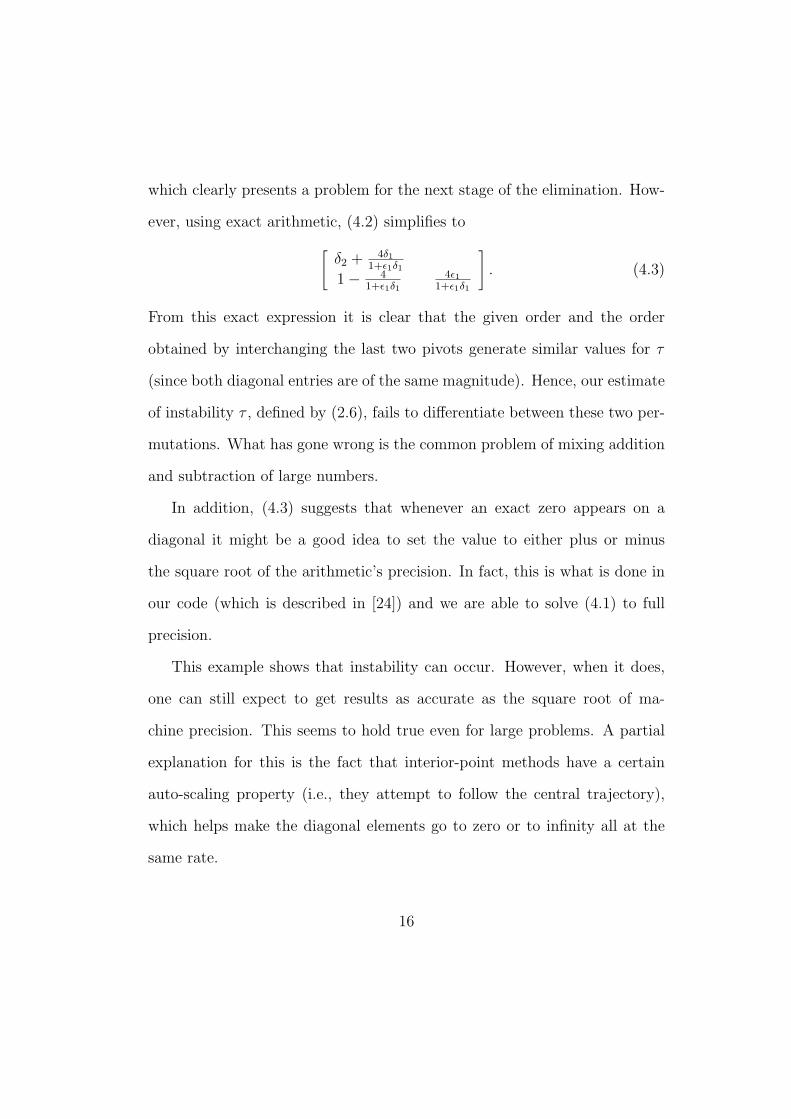
which clearly presents a problem for the next stage of the elimination. How-

ever, using exact arithmetic, (4.2) simplifies to[δ2 + 4δ1

1+ε1δ1

1− 41+ε1δ1

4ε11+ε1δ1

]. (4.3)

From this exact expression it is clear that the given order and the order

obtained by interchanging the last two pivots generate similar values for τ

(since both diagonal entries are of the same magnitude). Hence, our estimate

of instability τ , defined by (2.6), fails to differentiate between these two per-

mutations. What has gone wrong is the common problem of mixing addition

and subtraction of large numbers.

In addition, (4.3) suggests that whenever an exact zero appears on a

diagonal it might be a good idea to set the value to either plus or minus

the square root of the arithmetic’s precision. In fact, this is what is done in

our code (which is described in [24]) and we are able to solve (4.1) to full

precision.

This example shows that instability can occur. However, when it does,

one can still expect to get results as accurate as the square root of ma-

chine precision. This seems to hold true even for large problems. A partial

explanation for this is the fact that interior-point methods have a certain

auto-scaling property (i.e., they attempt to follow the central trajectory),

which helps make the diagonal elements go to zero or to infinity all at the

same rate.

16

5 Numerical Experiments and Conclusions.

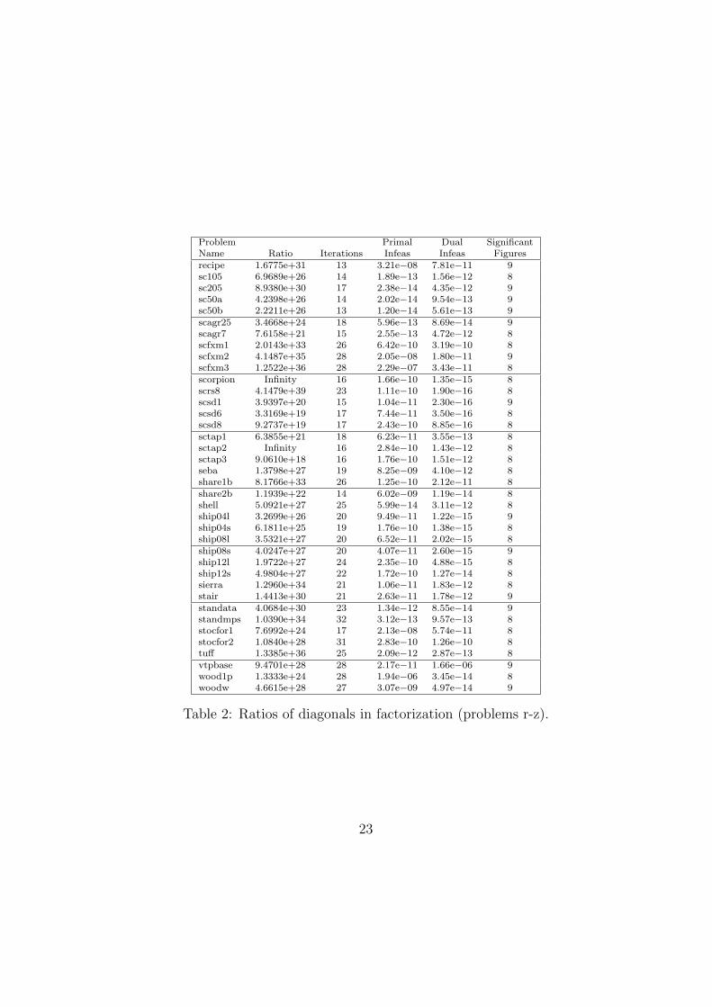
Using our code, we computed the ratio of the largest to the smallest of the

absolute values of the diagonal elements of D on the last iteration of the

algorithm. On the eighty or so test problems in the NETLIB suite [7] this

ratio ranged between 1.0e+19 and infinity (infinity means that an exact zero

appeared on the diagonal, which can happen when rank deficiency occurs

due to primal degeneracy). These ratios are tabulated in Tables 1 and 2.

Given such large values for this ratio, it is quite remarkable that the code

was able to solve all but 2 problems (greenbeb and pilot87) to 8 significant

figures of accuracy (and pilot87 stopped just short with 7 significant figures).

These tests were performed on an IBM RS 6000, which implements the IEEE

floating-point standard and therefore has 15 digits of precision (53 bits). It

is also interesting to note that the two that ran into numerical trouble were

not necessarily the ones with the largest ratios. It turns out that for many

problems in this suite the matrix to which K in (3.6) is converging is actu-

ally a singular matrix (due to primal or dual degeneracy) and so numerical

difficulties will exist regardless of the ordering.

We also computed the value of τ , defined by (2.6), for each of the test

problems. For these computations, we scaled the matrix K by dividing each

row and each column by the maximum between 1.0 and the square root of

the corresponding diagonal element. Tables 3 and 4 show the value of τ on

the last iteration. It turns out that in every case this was the largest value

17

over all iterations of the algorithm. Again there seems to be no correlation

between those problems that encountered numerical difficulties and those

that had large τ values. This lack of correlation gives credence to the notion

that numerical difficulty arises primarily from primal and dual degeneracy.

Acknowledgement: The author would like to thank Tami Carpenter and

Michael Saunders, the associate editor, for carefully reading the paper and

suggesting several improvements. He also wishes to acknowledge an anony-

mous referee who suggested the proof given for Theorem 2, which is shorter

than the author’s original proof, as well as other important improvements.

18

References

[1] I. Adler and R.D.C. Monteiro. Limiting behavior of the affine scalingcontinuous trajectories for linear programming. Technical Report ESRC88-9, Engineering Systems Research Center, University of California -Berkeley, 1988.

[2] J.R. Bunch and L.C. Kaufman. Some stable methods for calculatinginertia and solving symmetric linear equations. Mathematics of Compu-tation, 31:163–179, 1977.

[3] J.R. Bunch and B.N. Parlett. Direct methods for solving symmetric in-definite systems of linear equations. SIAM Journal on Numerical Analy-sis, 8:639–655, 1971.

[4] Y.C. Cheng, D.J. Houck, J.M.Liu, M.S. Meketon, L. Slutsman, R.J.Vanderbei, and P. Wang. The AT&T KORBX system. AT&T Tech.Journal, 68:7–19, 1989.

[5] A.L. Forsgren and W. Murray. Newton methods for large-scale linearequality-constrained minimization. Technical Report SOL 90-6, Depart-ment of Operations Research, Stanford University, 1990.

[6] R. Fourer and S. Mehrotra. Performance of an augmented system ap-proach for solving least-squares problems in an interior-point method forlinear programming. Dept. of Ind. Eng. and Mgmt. Sci., NorthwesternUniv., Evanston, IL, 1991.

[7] D.M. Gay. Electronic mail distribution of linear programming test prob-lems. Mathematical Programming Society COAL Newslettter, 13:10–12,1985.

[8] A. George and J. Liu. Computer Solution of Large Sparse Positive Def-inite Systems. Prentice-Hall, 1981.

[9] P.E. Gill, W. Murray, D.B. Ponceleon, and M.A. Saunders. Precondi-tioners for indefinite systems arising in optimization. SIAM J. MatrixAnal. Appl., 13(1), 1992.

[10] G.H. Golub and C.F. VanLoan. Matrix Computations. The Johns Hop-kins University Press, 2 edition, 1989.

[11] N.K. Karmarkar and K.G. Ramakrishnan. Implementation and com-putational results of the Karmarkar algorithm for linear programming,using an iterative method for computing projections. Technical report,AT&T Bell Labs, Murray Hill, NJ, 1989.

19

[12] I.J. Lustig, R.E. Marsten, and D.F. Shanno. On implementing Mehro-tra’s predictor-corrector interior point method for linear programming.Technical Report SOR 90-03, Dept. of Civil Engineering and OperationsResearch, Princeton Univ., April 1990.

[13] I.J. Lustig, R.E. Marsten, and D.F. Shanno. Computational experiencewith a primal-dual interior point method for linear programming. Lin.Alg. and Appl., 152:191–222, 1991.

[14] R.E. Marsten, M.J. Saltzman, D.F. Shanno, G.S. Pierce, and J.F.Ballintijn. Implementation of a dual interior point algorithm for lin-ear programming. ORSA Journal on Computing, 1:287–297, 1989.

[15] K.A. McShane, C.L. Monma, and D.F. Shanno. An implementationof a primal-dual interior point method for linear programming. ORSAJournal on Computing, 1:70–83, 1989.

[16] S. Mehrotra. Implementations of affine scaling methods: Approximatesolutions of systems of linear equations using preconditioned conjugategradient methods. Technical Report 89-04, Dept. of Ind. Eng. and Mgmt.Sci., Northwestern Univ., Evanston, IL, 1989.

[17] S. Mehrotra. Implementations of affine scaling methods: towards fasterimplementations with complete Cholesky factor in use. Technical Report89-15, Dept. of Ind. Eng. and Mgmt. Sci., Northwestern Univ., Evanston,IL, 1989.

[18] S. Mehrotra. On the implementation of a (primal-dual) interior pointmethod. Technical Report 90-03, Dept. of Ind. Eng. and Mgmt. Sci.,Northwestern Univ., Evanston, IL, 1990.

[19] D.B. Ponceleon. Barrier methods for large-scale quadratic programming.Technical Report SOL 91-2, Stanford University, October 1991.

[20] K. Turner. Computing projections for the Karmarkar algorithm. LinearAlgebra and Its Applications, 152:141–154, 1991.

[21] R.J. Vanderbei. A brief description of ALPO. OR Letters, pages 531–534, 1991.

[22] R.J. Vanderbei. Loqo users manual. Technical Report SOR 92-5, Prince-ton, University, 1992.

[23] R.J. Vanderbei. ALPO: Another linear program optimizer. ORSA Jour-nal on Computing, 1993. To appear.

20

[24] R.J. Vanderbei and T.J. Carpenter. Symmetric indefinite systems forinterior-point methods. Mathematical Programming, 58:1–32, 1993.

21

Problem Primal Dual SignificantName Ratio Iterations Infeas Infeas Figures25fv47 5.8709e+37 29 4.61e−13 2.56e−13 880bau3b Infinity 43 6.43e−10 1.28e−11 8adlittle 2.2458e+21 14 8.87e−11 1.74e−16 8afiro 4.1738e+24 13 6.00e−14 8.98e−14 8agg 7.8694e+41 26 3.98e−12 3.62e−09 8agg2 1.1431e+32 22 1.09e−14 4.99e−12 8agg3 4.8834e+34 22 5.34e−15 5.24e−12 8bandm 8.6392e+27 20 8.74e−11 5.95e−13 9beaconfd 1.9200e+28 14 7.95e−11 6.14e−12 8blend 5.8329e+24 14 1.90e−12 6.75e−11 9bnl1 1.0244e+35 35 2.39e−12 2.23e−12 8bnl2 3.4315e+54 40 1.62e−09 1.94e−11 8boeing1 1.0681e+41 28 1.26e−08 2.09e−13 9boeing2 5.1782e+38 28 1.47e−15 1.71e−10 8bore3d Infinity 17 1.72e−08 2.48e−16 8brandy 3.3141e+31 22 7.33e−08 1.97e−11 9capri 8.8349e+27 23 1.07e−12 4.52e−11 8cycle 6.2422e+36 32 5.75e−09 3.27e−11 9czprob 6.7245e+30 38 1.15e−11 1.08e−13 8d2q06c 2.8169e+47 38 2.24e−10 1.50e−09 8degen2 1.0067e+20 14 5.94e−10 3.75e−16 8degen3 Infinity 17 9.54e−10 2.94e−12 8e226 8.4768e+33 22 5.12e−13 9.02e−14 9etamacro 2.0071e+31 30 3.19e−13 1.62e−14 8fffff800 1.7007e+39 36 3.97e−13 2.53e−08 8finnis 8.9977e+33 26 1.00e−13 4.91e−14 8fit1d 1.6286e+22 21 4.81e−08 3.61e−15 9fit1p 3.5353e+24 26 5.68e−10 5.52e−12 8fit2d 5.1893e+19 24 1.50e−08 1.70e−16 8fit2p 6.3007e+23 24 4.24e−11 1.86e−12 8forplan 4.8253e+40 29 7.28e−14 1.33e−10 8ganges 3.3747e+33 23 5.06e−12 3.88e−11 9gfrdpnc 2.9347e+25 19 1.82e−10 3.61e−14 8greenbea 8.1336e+44 50 2.30e−06 2.86e−12 8greenbeb 2.8818e+28 30 1.80e−06 1.82e−10 3grow15 2.3749e+33 23 2.35e−06 7.18e−14 10grow22 3.1747e+33 27 7.99e−06 9.88e−15 10grow7 6.0359e+31 20 2.62e−06 3.69e−13 10israel 5.7337e+28 28 3.58e−16 4.36e−15 9kb2 3.7487e+26 20 2.54e−06 5.84e−10 8lotfi 1.1710e+44 25 1.83e−14 7.60e−12 8maros 9.9261e+31 28 3.27e−10 9.37e−10 8nesm 3.3790e+25 37 9.48e−13 2.61e−14 8perold 1.7497e+36 39 1.79e−13 5.11e−11 9pilot4 5.9526e+36 38 1.81e−11 1.51e−10 8pilot87 1.7318e+50 45 3.45e−12 7.84e−10 7pilotja 1.1399e+37 38 3.06e−12 5.56e−10 8pilotnov 1.1636e+36 29 2.24e−11 6.77e−11 8pilots 1.1568e+45 44 5.17e−12 1.07e−08 8pilotwe 2.8908e+32 39 7.47e−12 2.37e−14 8

Table 1: Ratios of diagonals in factorization (problems 1-p).

22

Problem Primal Dual SignificantName Ratio Iterations Infeas Infeas Figuresrecipe 1.6775e+31 13 3.21e−08 7.81e−11 9sc105 6.9689e+26 14 1.89e−13 1.56e−12 8sc205 8.9380e+30 17 2.38e−14 4.35e−12 9sc50a 4.2398e+26 14 2.02e−14 9.54e−13 9sc50b 2.2211e+26 13 1.20e−14 5.61e−13 9scagr25 3.4668e+24 18 5.96e−13 8.69e−14 9scagr7 7.6158e+21 15 2.55e−13 4.72e−12 8scfxm1 2.0143e+33 26 6.42e−10 3.19e−10 8scfxm2 4.1487e+35 28 2.05e−08 1.80e−11 9scfxm3 1.2522e+36 28 2.29e−07 3.43e−11 8scorpion Infinity 16 1.66e−10 1.35e−15 8scrs8 4.1479e+39 23 1.11e−10 1.90e−16 8scsd1 3.9397e+20 15 1.04e−11 2.30e−16 9scsd6 3.3169e+19 17 7.44e−11 3.50e−16 8scsd8 9.2737e+19 17 2.43e−10 8.85e−16 8sctap1 6.3855e+21 18 6.23e−11 3.55e−13 8sctap2 Infinity 16 2.84e−10 1.43e−12 8sctap3 9.0610e+18 16 1.76e−10 1.51e−12 8seba 1.3798e+27 19 8.25e−09 4.10e−12 8share1b 8.1766e+33 26 1.25e−10 2.12e−11 8share2b 1.1939e+22 14 6.02e−09 1.19e−14 8shell 5.0921e+27 25 5.99e−14 3.11e−12 8ship04l 3.2699e+26 20 9.49e−11 1.22e−15 9ship04s 6.1811e+25 19 1.76e−10 1.38e−15 8ship08l 3.5321e+27 20 6.52e−11 2.02e−15 8ship08s 4.0247e+27 20 4.07e−11 2.60e−15 9ship12l 1.9722e+27 24 2.35e−10 4.88e−15 8ship12s 4.9804e+27 22 1.72e−10 1.27e−14 8sierra 1.2960e+34 21 1.06e−11 1.83e−12 8stair 1.4413e+30 21 2.63e−11 1.78e−12 9standata 4.0684e+30 23 1.34e−12 8.55e−14 9standmps 1.0390e+34 32 3.12e−13 9.57e−13 8stocfor1 7.6992e+24 17 2.13e−08 5.74e−11 8stocfor2 1.0840e+28 31 2.83e−10 1.26e−10 8tuff 1.3385e+36 25 2.09e−12 2.87e−13 8vtpbase 9.4701e+28 28 2.17e−11 1.66e−06 9wood1p 1.3333e+24 28 1.94e−06 3.45e−14 8woodw 4.6615e+28 27 3.07e−09 4.97e−14 9

Table 2: Ratios of diagonals in factorization (problems r-z).

23

Problem ‖K‖ ‖L‖ ‖D‖ last τ25fv47 4.32e+02 1.08e+19 1.08e+19 2.51e+1680bau3b 2.16e+02 3.98e+13 3.96e+13 7.28e+11adlittle 1.03e+02 1.76e+09 3.03e+10 3.24e+08afiro 3.36e+00 2.87e+12 2.04e+12 4.04e+12agg 4.28e+02 3.62e+14 5.54e+16 4.68e+14agg2 4.29e+02 1.20e+14 6.50e+13 2.14e+12agg3 4.29e+02 2.08e+14 1.13e+14 3.68e+12bandm 1.06e+03 1.38e+13 7.63e+13 9.54e+11beaconfd 1.10e+03 2.72e+13 2.09e+15 5.00e+12blend 1.05e+02 2.54e+12 2.42e+12 1.09e+11bnl1 4.18e+02 1.45e+14 9.67e+13 9.55e+11bnl2 5.07e+02 4.51e+26 4.51e+26 2.63e+24boeing1 9.92e+02 5.93e+17 1.49e+14 1.03e+12boeing2 1.03e+03 1.50e+14 1.29e+14 5.81e+11bore3d 3.13e+03 2.98e+14 3.33e+14 2.51e+11brandy 9.43e+02 9.69e+16 7.65e+15 3.85e+15capri 5.61e+02 1.06e+14 1.05e+14 5.63e+11cycle 3.37e+03 2.16e+18 2.03e+15 2.24e+15czprob 1.48e+02 1.24e+13 1.20e+13 9.19e+10d2q06c 7.32e+03 1.88e+19 1.48e+18 5.42e+15degen2 3.51e+01 4.44e+08 1.29e+08 1.70e+08degen3 9.37e+01 6.28e+09 3.33e+09 1.25e+09e226 9.84e+02 1.74e+13 1.33e+13 1.71e+11etamacro 3.08e+03 9.76e+12 1.91e+13 7.12e+10fffff800 1.13e+05 8.10e+15 6.53e+15 8.91e+10finnis 3.95e+01 1.34e+17 1.34e+17 3.39e+15fit1d 3.25e+03 4.78e+10 7.31e+12 1.67e+10fit1p 1.42e+05 1.50e+11 5.17e+11 3.24e+07fit2d 3.22e+03 4.68e+08 8.24e+09 1.24e+08fit2p 2.73e+05 7.94e+11 7.94e+11 2.90e+06forplan 3.09e+03 1.83e+17 2.44e+20 2.35e+17ganges 1.20e+01 6.84e+16 6.29e+16 2.02e+16gfrdpnc 2.35e+03 7.44e+12 6.01e+12 1.12e+10greenbea 1.00e+02 3.21e+22 3.61e+22 8.68e+20greenbeb 1.41e+02 3.01e+14 2.39e+14 8.63e+12grow15 5.21e+00 5.86e+16 4.01e+16 2.54e+16grow22 5.21e+00 5.67e+16 5.51e+16 2.60e+16grow7 5.21e+00 9.28e+15 6.36e+15 3.72e+15israel 9.22e+03 3.11e+12 3.82e+12 1.86e+09kb2 6.02e+02 1.48e+13 2.55e+13 1.55e+11lotfi 4.83e+03 1.53e+22 1.53e+24 3.17e+20maros 5.10e+04 1.58e+16 1.23e+16 4.56e+13nesm 9.35e+01 1.21e+12 1.21e+12 5.46e+10perold 7.85e+04 1.83e+17 1.91e+19 2.12e+15pilot4 6.85e+04 1.02e+17 4.35e+17 6.18e+14pilot87 1.10e+03 1.90e+16 7.55e+16 1.01e+14pilotja 1.56e+06 1.36e+17 2.20e+18 4.55e+13pilotnov 1.19e+07 2.06e+17 2.84e+18 1.64e+13pilots 2.66e+02 9.69e+15 1.04e+16 9.73e+13pilotwe 7.50e+03 2.27e+15 2.54e+17 8.56e+13

Table 3: A Priori Test of Stability (problems 1-p).

24

Problem ‖K‖ ‖L‖ ‖D‖ last τrecipe 9.15e+02 5.90e+15 5.68e+15 3.15e+13sc105 5.52e+00 3.66e+13 3.66e+13 3.83e+13sc205 5.52e+00 1.88e+15 1.88e+15 1.88e+15sc50a 5.50e+00 1.50e+13 1.29e+13 1.24e+13sc50b 1.00e+01 6.51e+12 6.51e+12 3.24e+12scagr25 1.70e+01 1.99e+12 1.90e+12 3.61e+11scagr7 1.70e+01 1.43e+11 9.15e+10 5.38e+10scfxm1 8.26e+02 1.86e+16 9.30e+17 2.34e+15scfxm2 8.24e+02 9.11e+17 4.55e+19 1.15e+17scfxm3 8.26e+02 1.57e+18 7.87e+19 1.98e+17scorpion 6.85e+00 6.49e+07 6.34e+07 2.47e+07scrs8 3.59e+02 8.15e+19 8.08e+19 4.80e+17scsd1 4.32e+00 2.30e+09 2.30e+09 2.00e+09scsd6 5.79e+00 2.43e+09 2.09e+09 1.43e+09scsd8 4.31e+00 1.62e+10 1.04e+10 1.15e+10sctap1 2.89e+02 7.26e+09 2.58e+09 1.37e+09sctap2 4.65e+02 4.63e+09 1.46e+10 9.49e+08sctap3 4.65e+02 5.09e+09 1.76e+10 1.04e+09seba 1.34e+03 3.71e+13 3.71e+13 2.78e+10share1b 2.05e+03 7.36e+16 1.12e+17 2.26e+14share2b 7.89e+02 5.47e+11 3.43e+11 2.68e+11shell 1.80e+01 6.40e+11 4.88e+11 1.55e+11ship04l 7.10e+01 6.57e+09 3.25e+08 3.86e+08ship04s 4.90e+01 8.03e+08 1.42e+07 6.86e+07ship08l 7.10e+01 2.08e+08 1.53e+08 5.21e+06ship08s 4.10e+01 7.76e+08 1.01e+08 5.76e+07ship12l 5.70e+01 1.93e+09 5.94e+08 9.70e+07ship12s 3.10e+01 3.18e+08 1.44e+08 2.70e+07sierra 1.00e+05 4.82e+10 4.68e+10 1.43e+06stair 3.40e+01 1.70e+15 1.70e+15 2.00e+14standata 1.34e+02 6.19e+13 6.14e+13 5.43e+11standmps 1.05e+03 8.54e+12 8.48e+12 9.36e+09stocfor1 1.10e+03 2.22e+12 3.48e+12 1.05e+10stocfor2 1.20e+03 8.15e+13 1.33e+14 5.46e+11tuff 1.92e+03 5.09e+17 1.16e+17 1.31e+15vtpbase 2.91e+02 2.41e+14 2.32e+14 1.16e+12wood1p 1.91e+04 5.40e+12 6.54e+13 7.57e+11woodw 6.24e+04 6.61e+12 3.16e+15 3.55e+11

Table 4: A Priori Test of Stability (problems r-z).

25