Symmetric Responses to Threshold Policies:

The Impact of Temporary Drought Restrictions

Bryan Pratt∗

January 31, 2018

The most recent version is available here.

Abstract

This paper examines a quota-and-�ne policy implemented to curtail residential water consumption

during a period of drought. Leveraging an arbitrary border between two water districts which im-

plemented divergent policies, this research is able to isolate the e�ects of the quota-and-�ne policy,

speci�cally, and estimate the induced reductions at around 18 percent in the �rst year and 3 percent in

the second year. These reductions are in addition to large global reductions from general drought cur-

tailment. There appear to be strong non-price channels at work, with accounts that never exceeded 40

percent of the allotment before the policy also curtailed usage by a statistically signi�cant amount. More

broadly, this research �nds reductions in consumption beyond what a price e�ect alone would induce,

but it fails to �nd any persistence in these e�ects beyond the general drought curtailment also found in

the control group. Furthermore, these e�ects appear to be consistent with the previous imposition of

such a policy in the same service area in 1990.1

1 Introduction

The state of California has long dealt with periods of severe drought, and water scarcity is poised to be oneof the most important challenges of the 21st century.2 In its Fifth Assessment Report, the IntergovernmentalPanel on Climate Change (IPCC) notes the serious threat of increasing drought prevalence throughout theworld and the potential challenges this will pose for urban water systems, in particular (IPCC, 2014). Con-sidering this need for reducing water consumption, it is increasingly important to consider the e�ectivenessof various drought policies.

While residential water consumption is only a relatively small percentage of total water consumption, theburden of reducing water usage typically falls �rst and foremost on the residential sector, as agricultural andeconomic uses of water are explicitly prioritized over residential use. For example, water utilities in Californiamay exclude water delivered for commercial agricultural use for complying with mandated reductions.3 Whilehealth and safety is the highest priority in the quota-and-�ne district studied in this paper, residential outdooruse is considered the lowest priority (SCMU 2015).

Despite this particular policy relevance, this appears to be the �rst study to use account-level paneldata and a robust counterfactual to isolate the impact of quota-and-�ne policies, also called mandatoryrestrictions or rationing. This paper examines the e�ectiveness and mechanisms of a quota-and-�ne policyimplemented in Santa Cruz County, California. I �nd that the policy was successful both through puredemand elasticity to prices and an aversion to �nes. That is, households whose consumption was subject to

∗University of California, Santa Cruz1Many thanks to feedback from Carlos Dobkin, George Bulman, Justin Marion, Jon Robinson, Jeremy West, Alan Spearot,

Brent Haddad, Dahyeon Jeong, Dylan Brewer, John Creamer, and UC Santa Cruz Microeconomics Workshop participants.The panel regressions in this paper make use of the reghdfe package, created by Sergio Correia.

2For a relatively comprehensive history of California, drought, and relevant policy, see: Hundley (2001). For an overview ofthe current future challenges facing California, see: Mount et al. (2016).

3�Agricultural Water Use Exclusion Certi�cation.� California State Water Resources Control Board.http://www.waterboards.ca.gov/water_issues/programs/conservation_portal/agriculture/

1

a quota-and-�ne policy reduced consumption relative to similar households in the neighboring district, evenwhen they were highly unlikely to ever exceed their quota. A�ected households responded with statisticallysigni�cant reductions even when less than 10 percent of similar households in the neighboring district wouldgo on to consume beyond their placebo allotment.

1.1 Mandatory Water Restrictions

The study which comes closest to analyzing this type of quota-and-�ne policy is Kenney et al. (2004).Their study evaluates municipal programs responding to drought in Colorado in 2002, which is very similarto the proposed research presented here. However, none of the municipalities they studied enforced thesame type of mandatory (�ne-based) restrictions on total water consumption the way Santa Cruz did. Themain mandatory restriction put in place in these municipalities was mandatory lawn watering restrictions.Furthermore, Kenney et al. (2004) are working only with historical or forecast demand, rather than a controlgroup counterfactual. Applying similar techniques to the policy studied in this paper yields substantiallyoverstated reductions.

In addition, multiple studies have examined mandatory outdoor water restrictions in Australia during adrought. Grafton &Ward (2008) explore whether mandatory outdoor watering restrictions generate a greaterloss for consumers than pricing schedules designed to induce the same cutbacks. While Hensher et al. (2006)�nd that consumers seem uninterested in paying to avoid water restrictions, Grafton & Ward (2008) �nd thatthey would be better o� paying higher prices. It is important to remember, however, that this only applies tooutdoor water use restrictions. Unlike mandatory outdoor water restrictions, mandatory allotments for totalusage can be coerced into a price framework, with the penalties augmenting the marginal price of water.Moreover, I observe many accounts paying the price necessary to consume beyond the allotment.

Studying the 1976-1977 California drought, widely considered the most severe drought, Bruvold (1979)presents key evidence on residential consumers' perceptions of mandatory drought restrictions and otherrigorous drought policies. Bruvold �nds extensive evidence of higher curtailment in utility service areaswith more rigorous restrictions. However, Bruvold (1979) is still comparing treated aggregate consumptionto pre-treatment consumption, rather than to a control group. That study was able to include estimatesfrom both mild and rigorous policies, which might enable a similar di�erence-in-di�erence examination ofthe 1976-1977 drought, if the parallel trends assumption holds across districts selecting di�erent policies.However, Bruvold's work contributed more speci�cally to public perceptions. As a result, the researchin this paper extends our understanding of the impact of quota-and-�ne policies separately from generalcurtailment e�ects of statewide pressure to conserve.

1.2 Non-Price Channels in Utilities Markets

A key component of emergency conservation measures can be the non-price channels through which theymight achieve their goals. The current literature has produced con�icting �ndings regarding the relative andabsolute magnitude and persistence of e�ects from price and non-price interventions.

One potential non-price channel is social norms and the comparison of usage to peers or an externallydetermined benchmark. Many studies have demonstrated modest but established reductions from purelynon-price interventions. Allcott (2011) demonstrates that providing home energy reports comparing house-hold electricity usage to neighbors reduced consumption by at least two percent, with signi�cant persistence.Similarly, Asensio & Delmas (2015) �nd reductions around eight percent for conservation messaging basedon the adverse health impacts of local electricity generation and demand. Both of these studies �nd in-signi�cant reductions, or even increases, among low users, with high users responding heavily. Ito et al.(forthcoming) contrast non-price interventions with price interventions. While home energy reports appearto engender persistence, Ito et al. (forthcoming) �nd diminishing e�ects of moral suasion over time and afterrepeated intervention. In their study, economic incentives produce larger and persistent e�ects, inducinghabit formation beyond the �nal interventions. Examining conservation messaging in the water utility mar-ket, Datta et al. (2015), Ferraro & Price (2013), Fielding et al. (2012), and others have found evidence thatboth simple information and behavioral norms interventions can yield modest reductions in residential waterconsumption.

2

Gerard (2013) studies the impact and persistence of particularly ambitious conservation programs. Exam-ining the 2001 Brazilian electricity crisis, he studies a similar combination of �nes and conservation appealsin the context of supply shortages exceeding 20 percent. While substantially similar, the Brazilian policyactually included more policy instruments, such as billing bonuses (credits) for consuming below allotments,and more individually targeted, with quotas depending on baseline usage. Gerard (2013) �nds signi�cantpersistence in treatment e�ects but is unable to partition these treatment e�ects to identify the impacts ofeach policy. This paper highlights that pleas for conservation appear to have signi�cant, persistent impacts,but speci�c economic incentives, such as a quota-and-�ne policy, have more transient e�ects.

An important layer of the current study's intervention is the labeling of use beyond one's allotment asexcessive use, a violation of municipal policy that enabled the local paper to release the names and addressesof violators, their consumption, and their allotment. As a result, the e�ectiveness of the policy studied herebeyond mere price elasticity re�ects a non-price channel through which it was able to generate increasedreductions. As above, this research �nds lower e�ects for low users; however, statistically and economicallysigni�cant reductions appear even for households with a very low likelihood of being �ned.

1.3 Non-Linear Pricing and Average Price Demand

An additional area of interest is the non-linear price schedules common among utilities and present in thisresearch. Seminal work from Ito (2013; 2014) establishes the fact that consumers do not always behaveas predicted by standard utility maximization when faced with non-linear pricing schedules for water andelectricity. This is important to consider not only for the underlying four- and �ve-tiered pricing schedulespresent in the two water districts studied here, but also for the evaluation of the quota-and-�ne policy. Understandard economic theory, the imposition of a quota-and-�ne structure is equivalent to the restructuring ofrates to incorporate higher marginal prices above the quota threshold. Beyond the non-price e�ects oflabeling the threshold a mandatory allotment and the additional price a �ne, which one might predict tohave signi�cant impacts, a growing literature also suggests that consumers may not be considering marginalprices. Rather, Ito (2013; 2014) and others �nd that utility consumers appear to respond to average prices,instead of marginal prices. Ito presents convincing evidence during a non-drought period showing that amodel of demand based on average price is more appropriate than a model in which consumers set marginalbene�t equal to marginal price.

In related research, Ito (2015) considers the asymmetry generated by subsidizing energy conservationwithout similarly taxing excessive energy usage. These subsidies generate a discrete jump in marginal pricesfor conservation, particularly during summer months and with air conditioning, and a discrete change in theincentives to conserve. Ito �nds no e�ects in service areas without a serious need for air conditioning, buthe �nds signi�cant e�ects in hotter inland service areas. While the research presented here �nds treatmente�ects distributed smoothly across the incentive threshold, Ito (2015) �nds treatment e�ects concentratedamong users close to the threshold. The �ndings from the quota-and-�ne policy suggest that such a policymay not be empirically less e�ective than �rst-best policy, which would be charging the marginal social costof water consumption.

1.4 Information Channels

A separate and additional factor to consider is the frequency and detail with which water users receiveinformation about their consumption. At the time of policy implementation in this study, all customers hadrecently migrated to monthly billing, instead of bimonthly billing. Wichman (2015) found that an exogenousmigration to monthly billing from bimonthly billing induced an increase in consumption of approximately �vepercent. While this would be a concern for the analysis presented here, both the treatment and control groupsfor the primary results shifted from bimonthly to monthly billing around the same time. Wichman positsthat these results derive from removing a wedge between perceived price and actual price. This uncertaintyaround the actual price of water could similarly drive the results from this paper, which demonstrate thatusers unlikely to exceed their allotment still respond to penalties. One explanation for this behavior is thatconsumers either do not completely understand the amount they consume, the policy being imposed, orboth.

3

Figure 2.1: Annual Rainfall by Water Year, 1906-2016 (inches), Santa Cruz Weather Station

Source: California Department of Water Resources

2 The Setting

2.1 Drought and Santa Cruz County

As in much of California, rainfall in Santa Cruz County during the fall and winter months provides water forthe subsequent spring and summer. The most appropriate measure of annual rainfall is total precipitationduring the California Water Year, which runs from October 1 through September 30. For example, the 2016water year runs from October 1, 2015, through September 30, 2016.

Since a peak in the 1990s, annual precipitation in the City of Santa Cruz, CA, has been declining. Notonly has water-year rainfall been historically low, total calendar-year rainfall in 2013 was the lowest sincerecords began at the CRZ weather station in 1905, and 2007 and 2015 were two of the ten driest years onrecord.4 Figure 2.1 provides a visual presentation of precipitation trends measured by the weather stationover the past 110 years.

The drought of the 1987-1992 is worth noting, as it is the last time drought restrictions were enforcedin this area. Much of the state has been in an increasing state of drought since January 2012, and nearlytwo-thirds of the state was still listed as in extreme drought in April, 2016.5 Figure 2.2 plots the geographiccoverage of the drought over time. However, while the drought studied here was lengthy and acute, it isimportant to understand that the drought in Santa Cruz was not exceptional. As a result, the �ndings fromthis research could have very immediate policy implications for water management.

Another reason to focus on residential consumers is that, within areas like Santa Cruz, residential waterconsumption comprises the majority of utility-serviced water consumption. Table 2.1 illustrates the factthat residential consumption accounts for more than one-half of the utilities' production and single-familyresidential consumption represents more than 40 percent of production. State and local political pressures,as mentioned in the following sub-section, have generated substantial demand for utilities to demonstratereductions in consumption, without compromising economic growth and vitality. Consequently, reducingresidential consumption is a top priority.

2.2 Divergent Responses to a Stage 3 Water Emergency

In response to this most recent drought, the Governor of California set forth increasingly ambitious goals forwater conservation. On April 1, 2015, the Governor mandated a 25 percent reduction in water use for cities

4California Department of Water Resources. http://cdec.water.ca.gov/cgi-progs/staMeta?station_id=CRZ5Data on drought severity are available from the National Oceanic and Atmospheric Administration (NOAA). NOAA also

provides an explanation of the drought indices. See (NOAA, 2015).

4

Table 2.1: Total Consumption by Sector, July - December 2013Total Consumption Share

Account Type (Million Gallons) (%)Residential (Single-Family) 684 41Residential (Multi-Family) 366 22

Business (General) 246 15University 91.2 6

Irrigation (Golf) 73.0 4Irrigation (Business) 51.6 3Business (Hotel) 45.4 3

Irrigation (Residential) 30.3 2Industrial 28.0 2

Business (Restaurant) 20.9 1Irrigation (North Coast) 17.5 1

Construction 0.592 <1Total 1,654 100

and towns across the state, and this reduction mandate has largely been met (Kostyrko, 2015). Locally,the two water districts in the greater Santa Cruz - Capitola metropolitan area chose distinct responses tothe drought. One chose a quota-and-�ne policy, while the other raised marginal rates under an emergencyrate schedule. The rate systems for both Santa Cruz Municipal Utilities (�West�) and Soquel Creek WaterDistrict (�East�) customers are shown in Figure 2.4. Additionally, the boundaries of these water districts arepresented in Figure 2.3.

Taking a quantity-oriented approach, the West district imposed volumetric restrictions in 2014 and 2015,but these restrictions were removed from November of 2014 through April of 2015 (SCMU, 2014; 2015). Thestated policy was that these restrictions would be removed inde�nitely, and their reinstatement was onlyannounced in April of 2015. The restrictions were lifted as of November 1, 2015, with the shift announcedon October 28, 2015 (Gomez, 2015).

While framed as a quota system, the penalty for using water beyond one's allocation is a �ne. Therestrictions are as follows:

• Consumers are given monthly water allotments, which were the same in both the 2014 and 2015rounds of restrictions.

• Single family residential accounts are assigned a monthly water allotment of 1,000 cubic feet of water(10 CCF)6

• Every CCF beyond the allotment is charged an additional �ne beyond the tiered structure. These aretermed excessive water use penalties:

6CCF is the standard billing unit of water, and it represents a �centi-cubic foot� of water, or 100 cubic feet of water. OneCCF is equivalent to 748 gallons of water.

Figure 2.2: California Drought Conditions, April 2013 - April 2016

5

Figure 2.3: Water District Service Areas

Figure 2.4: Marginal Rate Comparison Over TimeBefore the Stage 3 Declaration After Fines Introduced After East Rate Hike

� For the �rst 10% beyond the allotment (one CCF for a single family residential account), the �neis $25 per CCF

� For every CCF beyond the �rst 10%, the �ne is $50 per CCF

• Instead of paying the �ne, a customer may elect to attend water school, a one-time class where violatorslearn about conserving water and why the restrictions are in place. However, this avoidance can onlybe done once.

It is important to note that the imposed restriction for the average consumer is 1,000 cubic feet of water(10 CCF), which is near the threshold between tiers 2 and 3 of the �ve-tiered system in the West servicearea. Moreover, when compared to the existing marginal price increase at the the nearby cuto�, the newincrease is more than 20 times as large. Indeed, the �nes can change the price of a monthly water bill byorders of magnitude for violators. Another important consideration is the fact that violators can choose toattend water school instead of paying a �ne, if it is the �rst violation. According to Gomez (2015), �[a]lmost400 people opted to attend water school rather than pay �nes.� Regardless, the treatment is a clear punitivemeasure incurred by crossing an arbitrary threshold that does not coincide with a marginal price change inthe tiered pricing structure. An example bill is provided in the Appendix, in Figure A.1.

Notably, the two districts share a border that runs through the heart of a commercial district and isindependent of political boundaries. Both service areas have tiered pricing, but the East district implementedhigher marginal rates instead of a quota-and-�ne system. A quota system was proposed, but it was not

6

Table 3.1: Single-Family Residential Accounts by DistrictWest East

North Coast 34 0Santa Cruz 20,465 0

Uninc. SC County 9,173 448Capitola 213 2,972Soquel 37* 2,285Aptos 0 10,922

La Selva Beach 0 190Watsonville 0 1,133

Total 29,922 17,955**

* Author's adjustment, based on zone boundaries

** The locations of �ve East accounts were

impossible to accurately verify

enacted.7 Instead, the Stage 3 emergency declaration led to the district increasing rates by approximately19 percent. In 2015, the East district increased rates slightly for January and by approximately 15 percent inJuly. Notably, the West rate schedule increased, independent of the quota and penalty system. This paperwill leverage these events and the arbitrary boundary to assess the aggregate impacts of the policies and theindividual impact of �nes on �ned households.

3 Data

This paper leverages datasets from each service area. For West customers, the main dataset is the universe ofbilling records from January 1, 2013, through October 25, 2016. To incorporate long-run seasonality trends,I also take advantage of monthly aggregate consumption by consumer type, beginning with 2009. Separateinformation regarding price schedules, aggregate and individual �ne data, and water school also informsthe paper. For East customers, the main dataset is all single-family billing records from January 1, 2013,through June 30, 2016. Aggregate data from previous years is not currently available for East. However,East data also includes rebates, as well as price schedules.

Notably, the two water districts do not have purely comparable customers. However, there is a subsetof the districts which include a common geographic span centered around the cities of Capitola and Soquel,as shown in Table 3.1. While not formally delineated, 37 of the West accounts labeled as unincorporatedSanta Cruz County are part of the Soquel jurisdiction. An additional �ve accounts for East are currentlynot paired with a city.

The billing records for the East district include the date of the reading but not the number of days billed,which leads to an interpolated number for days billed. As a consequence, a small number of observationsappear to be unreasonable, and I verify that results with daily consumption are generally re�ecting con-sumption changes rather than changes in interpolated billed days. I drop eight infeasible observations ofover 10,000 gallons per day, as a result, all in the East district.

3.1 Balance across the Border

This paper leverages an arbitrary boundary between two neighboring water districts. While this boundary iscompletely independent of other administrative and legal boundaries, one might wonder whether householdsmight sort on the basis of water district policy. This is highly unlikely, given that water and sewer chargescomprise a small part of most households' budgets. However, Table 3.2 demonstrates that there appears tobe balance running East-to-West across the boundary in key metrics. I cannot currently provide accuratestatistical tests of di�erence, as these measures refer to population-weighted aggregations of the census block

7http://www.kionrightnow.com/news/local-news/soquel-creek-customers-face-rate-increases-and-water-rationing/26563910http://www.santacruzsentinel.com/general-news/20140617/soquel-creek-water-district-water-emergencies-declaredhttp://aptoscommunitynews.org/news/2014/03/19/water-rationing-rate-increases-coming-soon/

7

Table 3.2: Balance, within Border SampleWest East

Pct Owner Occupied 48.04 48.61

Pct Renter Occupied 42.05 38.62

Pct Seasonal 5.51 6.60

Median Income $64,940.42 $71,138.07

Per Capita Income $34,207.55 $38,512.50Source: American Community Survey, 5-year estimates at the block

group level, 2009-2014. Household-weighted averages of census

block group estimates. Standard errors currently unavailable.

Figure 3.1: Single-Family Residential Consumption by District, Border Sample Only

groups on either side of the boundary in the border area shown in Figure 2.3. Additional �gures not shownillustrate that there is substantial balance on the majority of available demographic and housing measures.Moreover, while one might expect the divergence in policy to be the result of divergent circumstances, thetwo districts share many things in common. Among other things, the water districts share their main aquifer,with each district also utilizing additional sources.

Figure 3.1 provides consumption data for single-family residential households by district. The points inthe graph are averages by week and district, weighted by the number of bills they represent. The West districtgenerally bills less than one percent of customers in the last week of each month, leading to approximatelyone low and small dot for each month. Several key points are visible in this graph. First, consumers in thetwo water districts are strikingly similar before the application of the Stage 3 Water Emergency declaration.Second, during the drought period, water consumption decreased in both water districts. Third, waterconsumption is highly seasonal, and without a convincing counterfactual, any evidence of the policy's e�ectwould be di�cult to assess.

4 Estimation

In a traditional setting, the imposition of a quota-and-�ne policy like the one described here would behypothesized to have almost exclusively a price e�ect. The water district raised the marginal rate of con-

8

sumption above a certain quantity, and high users should be expected to curtail as they maximize theirutility subject to a budget constraint. However, water utility customers generally do not understand theirusage with precision. In other words, a key element of this market is imperfect information. Usage datais generally only available once per month (or once every two months when billing bimonthly), and thisinformation provides a single total number for that period. By contrast, usage choices are made daily. Ifthis information asymmetry is su�cient, it may induce otherwise seemingly irrational responses.

In this paper, I �nd not only that some consumers act as if they were surprised to be �ned in the�rst month of implementation, reacting by strongly curtailing their usage, but also that many consumerswho are essentially inframarginal also respond to the penalties by curtailing their usage. Speci�cally, I �ndstatistically signi�cant curtailment among accounts with less than a 10 percent chance of being �ned underbusiness-as-usual.

All of the results presented in this paper use two-way �xed e�ects and two-way clustering with the reghdfepackage authored by Sergio Correia, as described in Correia (2016). While the �xed e�ects are by accountand week, the clustering is by account and day, to ensure there are enough clusters for inference. Withaccount and week clustering, there are only about 50 clusters, but there are over 200 with account and dayclusters.8 Furthermore, the command drops singleton clusters to avoid overstating statistical signi�cance,as noted in Correia (2015). For comparison across speci�cations and to ensure appropriate inference, allregression results are restricted to accounts that are not missing a bill during the �rst bill of the quota-and-�ne policy. While additional accounts may serve as appropriate control or treated units, the key to inferencein this panel setting is the behavior of individuals across time.

4.1 Impacts on Aggregate Consumption

The �rst e�ect to consider is the impact on aggregate consumption among accounts in the West district.Since identi�cation rests on the parallel trends assumption, the treatment e�ect should be identi�ed usingequation 4.1, where consumption will be measured in gallons at the daily level. This ensures an accuratecomparison across billing cycles with di�ering lengths. For ease of interpretation, the regressions will utilizethe log of daily consumption to estimate a treatment e�ect, δ̂, that represents the percent curtailment.The policy variable is de�ned based on the water district's implementation guidelines, with bills having allconsumption within the policy period being subject to �nes. Controls are weather measures, with only onerelevant weather station for all observations. In addition, account and week-of-time �xed e�ects are included.Standard errors are clustered by account and day, as discussed previously.

Consi,t = α+ δPolicyi,b ×Westi + βXi,t + γi + ψw + εi,t (4.1)

In order to provide the most consistent estimates, I restrict the sample to accounts between the easternboundary of the City of Santa Cruz and the eastern boundaries of Soquel and Capitola. While this restrictionreduces power, it is an attempt to provide a homogeneous group of accounts.9 Using single-family accountsin this restricted sample, I �nd that the quota-and-�ne policy reduced water consumption by an averageof 18 percent in 2014 and approximately three percent in 2015. Importantly, these results are measures ofrelative reduction in comparison to East households, which will be discussed further below. Columns 1 and 4in Table 4.1 present aggregate treatment e�ects for the border sample with full weather controls. Table B.1in the Appendix provides evidence regarding the robustness of these estimates to the inclusion of weathercontrols.

It is noteworthy to recall that the East district imposed a mild rate increase for all tiers and accountsapproximately two months into the quota-and-�ne policy. As Figure 4.1 demonstrates, the policy continuedto elicit reductions throughout the summer months, but its e�ect was somewhat attenuated after the Eastdistrict's policy change. Unfortunately, it is di�cult to entirely disentangle whether this is a declining e�ector attenuation from a response in the control group.

8Fifty clusters is generally considered the bare minimum for accurate clustered standard errors.9There are approximately 10,000 households in the restricted sample.

9

Table 4.1: Di�erence-in-Di�erence ResultsDependent Var: Log of Daily Consumption (Gallons)2014 2015

Treated -0.178*** -0.162*** -0.171*** -0.0305*** -0.0213* -0.0297**(0.0393) (0.0394) (0.0394) (0.0115) (0.0119) (0.0116)

Fined -0.174*** -0.141***(First Month) (0.0396) (0.0392)

Fine in USD -0.000368** -0.000108(First Month) (0.000168) (0.0000974)

Over Allotment 0.107*** 0.102***(First Month) (0.0300) (0.0281)

Percent Over Allotment 0.101** -0.0000962**(First Month) (0.0410) (0.0000401)

Controls Precipitation, Max Temp,Min Temp, Evapotranspiration

East Mean 149.73 135.21(Post Period) (121.08) (107.27)FE Account, WeekClustered SE Account, DayR2 0.713 0.714 0.714 0.718 0.719 0.718Obs. 87342 87342 87342 91871 91871 91871

Sample restricted to �ve months before and after the month of implementation, but excludes the month of implementation

Standard errors in parentheses

* p < 0.10, ** p < 0.05, *** p < 0.01

Figure 4.1: Monthly Aggregate Treatment Estimates

10

Figure 4.2: Fine E�ects Over TimeFined (Indicator) Fined (Dollars)

4.2 E�ects of Being Fined

The most direct way to assess the e�ect of being �ned would be to measure the reduction in consumptioninduced by the �ne in the following month.

Consi,t = α+ f (�nei,b−1) + δPolicyi,b ×Westi + βXi,t + γi + ψw + εi,t (4.2)

We can also control for the e�ect of simply being over a placebo allotment, estimated from the Easthouseholds, and we can run this regression for a variety of functions of the �ne. This controls for meanreversion if we assume households in each district revert similarly. However, there is still a �aw in using thisapproach. If we believe consumers are rational, they will adjust to the policy. To estimate the impact of a�ne, we want to know one (or both) of two things. The �rst is what would a household do in response to anunexpected �ne. I will address this below. The second is what would a household do in anticipation of anexpected �ne. I will seek to examine this impact through a more structural approach in future work.

Assuming that not everyone is cognizant of the �nes being introduced, I can examine the data for cluesas to how households reacted to a �ne in the �rst month of �nes. Under the assumption that, for at leastsome segment of the population, the �nes come as a surprise, we can examine an intent-to-treat estimator ofthe impact of such �nes. This requires only the supposition that households either are not aware of the �nesor are not aware of where their consumption falls in the rate schedule. We can then estimate the impact ofbeing �ned unexpectedly with the following regression:

lnConsi,t = α+ f (�nei,b=fm) + δPolicyi,b ×Westi + βXi,t + γi + ψw + εi,t (4.3)

I estimate this equation without the �rst month of the policy (fm) to avoid endogeneity, and I useonly �ve months before and after implementation. Prior to that period, too many accounts were billedbimonthly, while after six months, the policy was temporarily removed for the winter. In addition, I onlyconsider households near the border between the two water districts, as previously noted. Section B.1 in theAppendix demonstrates that these estimates are smaller but qualitatively similar when using the full districtsamples.

The results from Table 4.1 imply that many households may have been unaware of the impending�ne policy or of their own consumption. Columns 2 and 5 provide estimates for an indicator function,f (�nei,b=fm) = 1 (�ned)i,b=fm, for 2014 and 2015, respectively. Columns 3 and 6 provide the estimatesfor f (�nei,b=fm) = �nei,b=fm. In addition to providing estimates for the responsiveness to �nes, Table 4.1provides a glimpse into how - and why - the quota-and-�ne policy worked. In 2014, the aggregate impact ofthe policy on households that were not �ned in the �rst month of the policy was a reduction of 16 percent.On the contrary, these estimates imply a small two percent relative aggregate e�ect on households thatwere not �ned in the second year of the policy. Moreover, this suggests that, while some of the reductionsin 2014 stem from avoidance behavior and adjustment, this behavior may have persisted through 2015. Aconfounding factor in this analysis is the implementation of additional rate hikes in 2015.

Figure 4.2 provides estimates of the impact of being �ned (left panel) and dollars �ned (right panel) onconsumption in subsequent months. The impact of the 2014 �ne appears to last through the summer but

11

Figure 5.1: Responses to Fines across the Distribution, West v East

collapse with the removal of the policy. Unlike the avoidance behavior indicated earlier, �ne e�ects appearto have limited persistence or no e�ect beyond the threat of an additional �ne.

5 Discussion

5.1 Fine Aversion and Price Elasticity

While aggregate consumption fell with the implementation of the quota-and-�ne policy, there are severalpotential mechanisms and alternative explanations available. The traditional rational consumer model wouldpredict that only households that would be �ned under the policy will respond. Moreover, such a modelwould predict that these households respond by adjusting to set the new marginal price of water equal to theirmarginal bene�t of water consumption. An alternate prediction is that consumers have limited informationor understanding of their water consumption. A rational consumer operating under traditional uncertaintywould respond with reductions proportional to their perceived probability of being �ned.

Examining the behavior of households on either side of the border with varying levels of consumptionfor the bill prior to policy implementation, Figure 5.1 illustrates that the response to the policy scales withconsumption prior to the policy. Figure 5.2 plots the di�erence-in-di�erence coe�cient estimates, and their95 percent con�dence intervals, for the e�ect of �nes by pre-policy consumption level. Something importantto understand about the results in Figure 5.2 is that many of the households that are responding wouldnot have been �ned if they had followed their neighbors across the border, as shown in Table 5.1. Thiswould imply that consumers do not understand their consumption or that they fear �nes. In other words,consumers over-estimate their probability of being �ned under business-as-usual, or they have a signi�cantdisutility of being �ned akin to loss aversion. Each of these behavioral explanations suggest pathways bywhich the quota-and-�ne policy can impact consumption beyond the conventional price channel.

12

Figure 5.2: E�ect of Fines by Pre-Implementation Consumption Level

Table 5.1: Inframarginality of Pre-Policy Bins, Border Sample OnlyPrior % Accounts Exceeding Allotment during Summer 2014

Consumption East West di�. p-value nEast nWest

3 5.90 4.77 -1.13 0.372 542 7334 7.97 6.93 -1.04 0.475 552 7655 13.5 7.53 -6.01*** 0.000 502 7706 20.5 16.6 -3.92 0.110 409 6267 30.1 25.0 -5.12 0.110 322 4768 47.1 29.8 -17.3*** 0.000 257 3869 61.7 47.4 -14.3*** 0.006 141 25310 65.9 64.2 -1.74 0.759 129 15911 77.3 67.5 -9.85 0.139 75 12312 87.0 83.7 -3.34 0.589 54 92

Prior consumption is the billed 100 cubic feet in the bill before the policy was implemented.

Data is collapsed at the account level and includes only accounts with a bill during the �rst month of the policy

for variable construction purposes.

13

Figure 5.3: Treatment E�ect by Pre-Policy Maximum Consumption, Border Sample

5.2 Behavioral Mechanisms

One possible explanation for curtailment among non-targeted households is risk aversion. Households per-ceive some probability of consumption exceeding their allotment, and this translates to a probability-weightedexpectation of dollars �ned, moral disutility, or both. However, if households are informed, rational actorswould assign a negligible probability to consumption well above their maximum historical consumption. Fig-ure 5.3 provides estimates of curtailment during the West policy period in 2014 by maximum consumptionpre-policy. Contrary to the risk aversion prediction with informed households, Figure 5.3 demonstrates thathouseholds never consuming more than 40 percent of their allotment before the policy conserved an amountstatistically indistinguishable from the conservation e�orts of households having consumed over twice theallotment at least once before.

As a result, there are two primary alternate explanations. The �rst explanation is that the householdsare not informed. If households are not aware that the policy does not impact them, they may behave as ifit does. A second explanation is that households perceive social pressure to curtail usage as a result of thepolicy. While the estimates control for social norm responses to the declaration of a Stage 3 Emergency andresponses to statewide and local calls for conservation, the imposition of �water rationing� may have beeninterpreted as a signal of the severity of the water shortage. Future work will seek to identify the plausibilityand relative importance of these mechanisms using a theoretical model.

5.3 Historical Comparison

In 1990, the West district applied a similar water rationing program. Using monthly aggregate data for 30years and business consumption as a control, I �nd similar estimates for 1990 and 2014, as shown in Figure5.4. Notably, these estimates are from regressions controlling for the Palmer Drought Index of the area, bymonth.10 However, the drought index becomes statistically insigni�cant when including indicator variablesfor these three policies, as well as an indicator for high-use penalties in 1991 and 1992. Given the less precisecounterfactual of using business consumption, the e�ects are both imprecise and slightly overstated for 2014and 2015. As a result, one might expect the true reductions achieved in 1990 to similarly be slightly smaller.Appendix B.4 provides additional information on the methodology behind these estimates.

10The Palmer Drought Index is widely-used standard for measuring meteorological drought, see: Palmer (1965)

14

Figure 5.4: Aggregate E�ects of Mandatory Reductions, 1990 vs 2014/2015

6 Conclusion

This paper identi�es important price and non-price channels through which a quota-and-�ne drought policygenerated signi�cant residential consumption reduction. The evidence provided here suggests that quota-and-�ne policies can generate reductions beyond the price response of directly a�ected consumers. Whileconsumers may be responding irrationally to over-estimated probabilities of adverse outcomes, this reactionmay be socially optimal when the social cost of consumption is high. While direct estimates of the socialcost of consuming water do not exist, the social cost is a direct function of the impact consumption has onthe probability of future water scarcity. In drought periods, the marginal social cost of consuming a gallonof water rises with the falling reservoir levels. As such, a quota-and-�ne policy that generates reductionsbeyond the price response may be an e�ective second-best policy, especially when more far-reaching rateincreases are legally or politically infeasible.

However, while the overall curtailment of both districts in response to the drought has shown persis-tence, the summer-only policy in the West district did not generate persistence through the winter nor intosubsequent summers. As a result, this paper �nds no evidence that temporary drought restrictions are ableto generate more permanent curtailment. For more permanent usage reductions, alternate policies may benecessary.

References

2014. Water Rationing Begins May 1. SCMU Review, Santa Cruz Municipal Utilities.http://www.cityofsantacruz.com/home/showdocument?id=44394.

2015. Historical Palmer Drought Indices. National Oceanic and Atmospheric Administration.http://www.ncdc.noaa.gov/temp-and-precip/drought/historical-palmers/psi/199512-201511.

2015. Santa Cruz Water School Presentation. City of Santa Cruz.http://www.cityofsantacruz.com/departments/water/drought/water-school.

2015. Stage 3 Water Shortage Emergency: 2015 Update for Santa Cruz Municipal Utility Customers. Cityof Santa Cruz. http://cityofsantacruz.com/home/showdocument?id=36799.

Allcott, Hunt. 2011. Social Norms and Energy Conservation. Journal of Public Economics, 95, 1082�1095.

Asensio, Omar I., & Delmas, Magali A. 2015. Nonprice incentives and energy conservation. Proceedings ofthe National Academy of Sciences, 112(6), E510�E515.

15

Bruvold, William. 1979. Residential Response to Urban Drought in Central California. Water ResourcesResearch, 15(6).

Correia, Sergio. 2015. Singletons, Cluster-Robust Standard Errors and Fixed E�ects: A Bad Mix. WorkingPaper.

Correia, Sergio. 2016. A Feasible Estimator for Linear Models with Multi-Way Fixed E�ects. Working Paper.

Datta, Suagato, Darling, Matthew, Lorenzana, Karine, Gonzalez, Oscar Calvo, Miranda, Juan Jose, &de Castro Zoratto, Laura. 2015. A Behavioral Approach to Water Conservation: Evidence from a Ran-domized Evaluation in Costa Rica. Tech. rept. ideas42 and the World Bank.

Ferraro, Paul, & Price, Michael. 2013. Using Nonpecuniary Strategies to In�uence Behavior: Evidence froma Large-Scale Field Experiment. The Review of Economics and Statistics, 95(1), 64�73.

Fielding, Kelly, Spinks, Anneliese, Russell, Sally, Mankad, Aditi, McCrea, Rod, & Gardner, John. 2012.Water Demand Management: Interventions to Reduce Household Water Use. techreport 94. Urban WaterSecurity Research Alliance.

Gerard, François. 2013. The Impact and Persistence of Ambitious Energy Conservation Programs: Evidencefrom the 2001 Brazilian Electricity Crisis. Working Paper, 2013(May).

Gomez, Phil. 2015. Water restrictions in Santa Cruz lifted. KSBW News.http://www.ksbw.com/news/watrer-restrictions-in-santa-cruz-lifted/36096802.

Grafton, R. Quentin, &Ward, Michael B. 2008. Prices versus Rationing: Marshallian Surplus and MandatoryWater Restrictions. Economic Record, 84(Special Issue), S57�S65.

Hensher, David, Shore, Nina, & Train, Kenneth. 2006. Water Supply Security and Willingness to Pay toAvoid Drought Restrictions. Economic Record, 82(256), 56�66.

Hundley, Jr., Norris. 2001. The Great Thirst: Californians and Water: A History. Revised edition edn.University of California Press.

IPCC. 2014. Climate Change 2014: Synthesis Report. Contribution of Working Groups I, II and III to theFifth Assessment Report of the Intergovernmental Panel on Climate Change. R.K. Pachauri and L.A.Meyer (eds.), Geneva, Switzerland.

Ito, Koichiro. 2013. How Do Consumers Respond to Nonlinear Pricing? Evidence from Household WaterDemand. Working Paper.

Ito, Koichiro. 2014. Do Consumers Respond to Marginal or Average Price? Evidence from NonlinearElectricity Pricing. American Economic Review, 104(2), 537�563.

Ito, Koichiro. 2015. Asymmetric Incentives in Subsidies: Evidence from a Large-Scale Electricity RebateProgram. American Economic Journal: Economic Policy, 7(3), 209�237.

Ito, Koichiro, Ida, Takanori, & Tanaka, Makoto. forthcoming. The Persistence of Moral Suasion and Eco-nomic Incentives: Field Experimental Evidence from Energy Demand. American Economic Journal:Economic Policy, January.

Kenney, Douglas S., Klein, Roberta A., & Clark, Martyn P. 2004. Use and E�ectiveness of Municipal WaterRestrictions During Drought in Colorado. Journal of the American Water Resources Association, 40(1),77�87.

Kostyrko, George. 2015. Top Story: California's Cumulative Water Savings Continue to Meet Governor'sOngoing Conservation Mandate. State of California. http://ca.gov/drought/topstory/top-story-51.html.

Mount, Je�rey, Escriva-Bou, Alvar, Hanak, Ellen, Lund, Jay, Cayan, Daniel, Davis, Frank, DeShazo, J.R.,Frank, Richard, Ullrich, Paul, & Wilkinson, Robert. 2016. California's Water. Tech. rept. Public PolicyInstitute of California.

16

Figure A.1: West Bill

Palmer, Wayne. 1965. Meteorological Drought. Research Paper 45. US Department of Commerce, USWeatherBureau, O�ce of Climatology.

Wichman, Casey. 2015. Information Provision and Consumer Behavior: A Natural Experiment in BillingFrequency. Discussion Paper 15-35. Resources for the Future.

A Quota-and-Fine Policy Details

Figure A.1 provides an example bill presented during the Water School that violators could attend (SCMU2015). While the bill lists an excessive use penalty, this bill was not actually assessed an excessive usepenalty, as �nes were temporarily suspended. It is important to note, however, that the red line in the usageplot remained even while �nes were suspended. In other words, the allotment remained even when it wasnot enforced.

B Robustness

Tables B.1 and B.2 demonstrate robustness of the aggregate estimates and �ne estimates to the inclusionof weather controls. Since the weather controls appear to slightly attenuate the estimates, all estimatesshown in the main sections of the paper include weather controls. Precipitation controls for the sum of totalprecipitation during the previous 30 days. Evapotranspiration and maximum and minimum temperaturerefer to the average of the respective measure over the previous 30 days.

B.1 Full District Estimates

As discussed in Subsection 3.1, this paper relies on the assumption that sorting across an arbitrary districtboundary is as good as random assignment. However, we could also consider a di�erence-in-di�erence

17

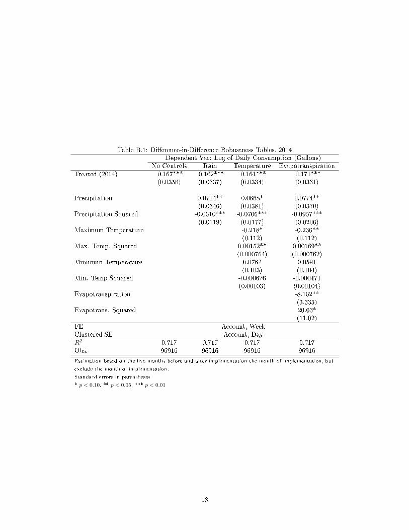
Table B.1: Di�erence-in-Di�erence Robustness Tables, 2014Dependent Var: Log of Daily Consumption (Gallons)

No Controls Rain Temperature EvapotranspirationTreated (2014) -0.167*** -0.162*** -0.161*** -0.171***

(0.0356) (0.0337) (0.0334) (0.0331)

Precipitation 0.0714** 0.0668* 0.0774**(0.0346) (0.0381) (0.0370)

Precipitation Squared -0.0610*** -0.0766*** -0.0957***(0.0119) (0.0177) (0.0206)

Maximum Temperature -0.218* -0.236**(0.112) (0.112)

Max. Temp. Squared 0.00152** 0.00169**(0.000764) (0.000762)

Minimum Temperature 0.0762 0.0591(0.103) (0.104)

Min. Temp Squared -0.000676 -0.000471(0.00103) (0.00104)

Evapotranspiration -8.162**(3.335)

Evapotrans. Squared 20.63*(11.02)

FE Account, WeekClustered SE Account, DayR2 0.717 0.717 0.717 0.717Obs. 96916 96916 96916 96916

Estimation based on the �ve months before and after implementation the month of implementation, but

exclude the month of implementation.

Standard errors in parentheses

* p < 0.10, ** p < 0.05, *** p < 0.01

18

Table B.2: Di�erence-in-Di�erence Robustness Tables, with Fines, 2014Dependent Var: Log of Daily Consumption (Gallons)

No Controls Rain Temperature EvapotranspirationTreated (2014) -0.150*** -0.147*** -0.145*** -0.162***

(0.0414) (0.0393) (0.0389) (0.0394)Fined -0.174*** -0.175*** -0.175*** -0.174***(First Month, 2014) (0.0396) (0.0395) (0.0397) (0.0396)

Over 0.105*** 0.106*** 0.106*** 0.107***(First Month, 2014) (0.0299) (0.0299) (0.0301) (0.0300)

Precipitation 0.0731** 0.0679* 0.0833**(0.0345) (0.0378) (0.0379)

Precipitation Squared -0.0594*** -0.0772*** -0.100***(0.0114) (0.0177) (0.0208)

Maximum Temperature -0.244** -0.258**(0.115) (0.115)

Max. Temp. Squared 0.00169** 0.00185**(0.000782) (0.000785)

Minimum Temperature 0.0791 0.0549(0.104) (0.106)

Min. Temp Squared -0.000685 -0.000385(0.00104) (0.00107)

Evapotranspiration -10.19***(3.885)

Evapotrans. Squared 26.70**(12.56)

FE Account, WeekClustered SE Account, DayR2 0.713 0.714 0.714 0.714Obs. 87342 87342 87342 87342

Estimation based on the �ve months before and after implementation the month of implementation, but

exclude the month of implementation.

Standard errors in parentheses

* p < 0.10, ** p < 0.05, *** p < 0.01

19

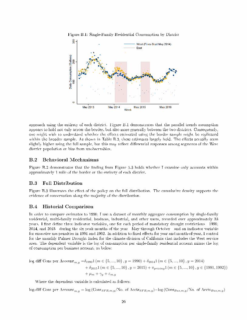
Figure B.1: Single-Family Residential Consumption by District

approach using the entirety of each district. Figure B.1 demonstrates that the parallel trends assumptionappears to hold not only across the border, but also more generally between the two districts. Consequently,one might wish to understand whether the e�ects estimated using the border sample might be replicatedwithin the broader sample. As shown in Table B.3, these estimates largely hold. The e�ects actually seemslightly higher using the full sample, but this may re�ect di�erential responses among segments of the Westdistrict population or bias from unobservables.

B.2 Behavioral Mechanisms

Figure B.2 demonstrates that the �nding from Figure 5.3 holds whether I examine only accounts withinapproximately 1 mile of the border or the entirety of each district.

B.3 Full Distribution

Figure B.3 illustrates the e�ect of the policy on the full distribution. The cumulative density supports theevidence of conservation along the majority of the distribution.

B.4 Historial Comparison

In order to compare estimates to 1990, I use a dataset of monthly aggregate consumption by single-familyresidential, multi-family residential, business, industrial, and other users, recorded over approximately 33years. I �rst de�ne three indicator variables, one for each period of mandatory drought restrictions - 1990,2014, and 2015 - during the six peak months of the year - May through October - and an indicator variablefor excessive use penalties in 1991 and 1992. In addition to �xed e�ects for year and month-of-year, I controlfor the monthly Palmer Drought Index for the climate division of California that includes the West servicearea. The dependent variable is the log of consumption per single-family residential account minus the logof consumption per business account, as below:

log-di� Cons per Accountm,y =δ19901 (m ∈ {5, ..., 10} , y = 1990) + δ20141 (m ∈ {5, ..., 10} , y = 2014)

+ δ20151 (m ∈ {5, ..., 10} , y = 2015) + πpricing1 (m ∈ {5, ..., 10} , y ∈ {1991, 1992})+ µm + γy + εm,y

Where the dependent variable is calculated as follows:

log-di� Cons per Accountm,y = log (ConsSFR,m,y/No. of AcctsSFR,m,y)−log (ConsBus,m,y/No. of AcctsBus,m,y)

20

Figure B.2: Treatment E�ect by Pre-Policy Maximum Consumption, Sample Robustness

Border Sample (Within 2 Miles)

Within 0.5 Miles Within 1 Mile

Within 1.5 Miles Whole Sample

21

Figure B.3: Impacts on the Full Distribution

Summer 2013 v Summer 2014, Full SampleDensity Cumulative Density

Five Months Before and After Policy Implementation, Full SampleDensity Cumulative Density

22

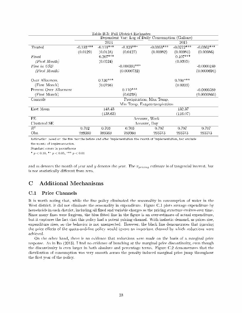
Table B.3: Full District EstimatesDependent Var: Log of Daily Consumption (Gallons)

2014 2015Treated -0.133*** -0.111*** -0.123*** -0.0363*** -0.0272*** -0.0362***

(0.0129) (0.0128) (0.0127) (0.00982) (0.00981) (0.00986)Fined -0.207*** -0.107***(First Month) (0.0224) (0.0303)

Fine in USD -0.000391*** -0.0000180(First Month) (0.0000732) (0.0000694)

Over Allotment 0.136*** 0.100***(First Month) (0.0198) (0.0203)

Percent Over Allotment 0.110*** -0.0000580(First Month) (0.0238) (0.0000866)

Controls Precipitation, Max Temp,Min Temp, Evapotranspiration

East Mean 148.43 132.37(138.63) (116.07)

FE Account, WeekClustered SE Account, DayR2 0.702 0.703 0.703 0.707 0.707 0.707Obs. 289360 289360 289360 293513 293513 293513

Estimation based on the �ve months before and after implementation the month of implementation, but exclude

the month of implementation.

Standard errors in parentheses

* p < 0.10, ** p < 0.05, *** p < 0.01

and m denotes the month of year and y denotes the year. The πpricing estimate is of tangential interest, butis not statistically di�erent from zero.

C Additional Mechanisms

C.1 Price Channels

It is worth noting that, while the �ne policy eliminated the seasonality in consumption of water in theWest district, it did not eliminate the seasonality in expenditure. Figure C.1 plots average expenditure byhouseholds in each district, including all �xed and variable charges as the pricing structure evolves over time.Since many �nes were forgiven, the blue �tted line in the �gure is an over-estimate of actual expenditure,but it captures the fact that this policy had a potent pricing channel. With inelastic demand, as prices rise,expenditure rises, so the behavior is not unexpected. However, the black line demonstrates that ignoringthe price e�ects of the quota-and-�ne policy would ignore an important channel by which reductions wereachieved.

On the other hand, there is no evidence that reductions were made on the basis of a marginal priceresponse. As in Ito (2013), I �nd no evidence of bunching at the marginal price discontinuity, even thoughthe discontinuity is even larger in both absolute and percentage terms. Figure C.2 demonstrates that thedistribution of consumption was very smooth across the penalty-induced marginal price jump throughoutthe �rst year of the policy.

23

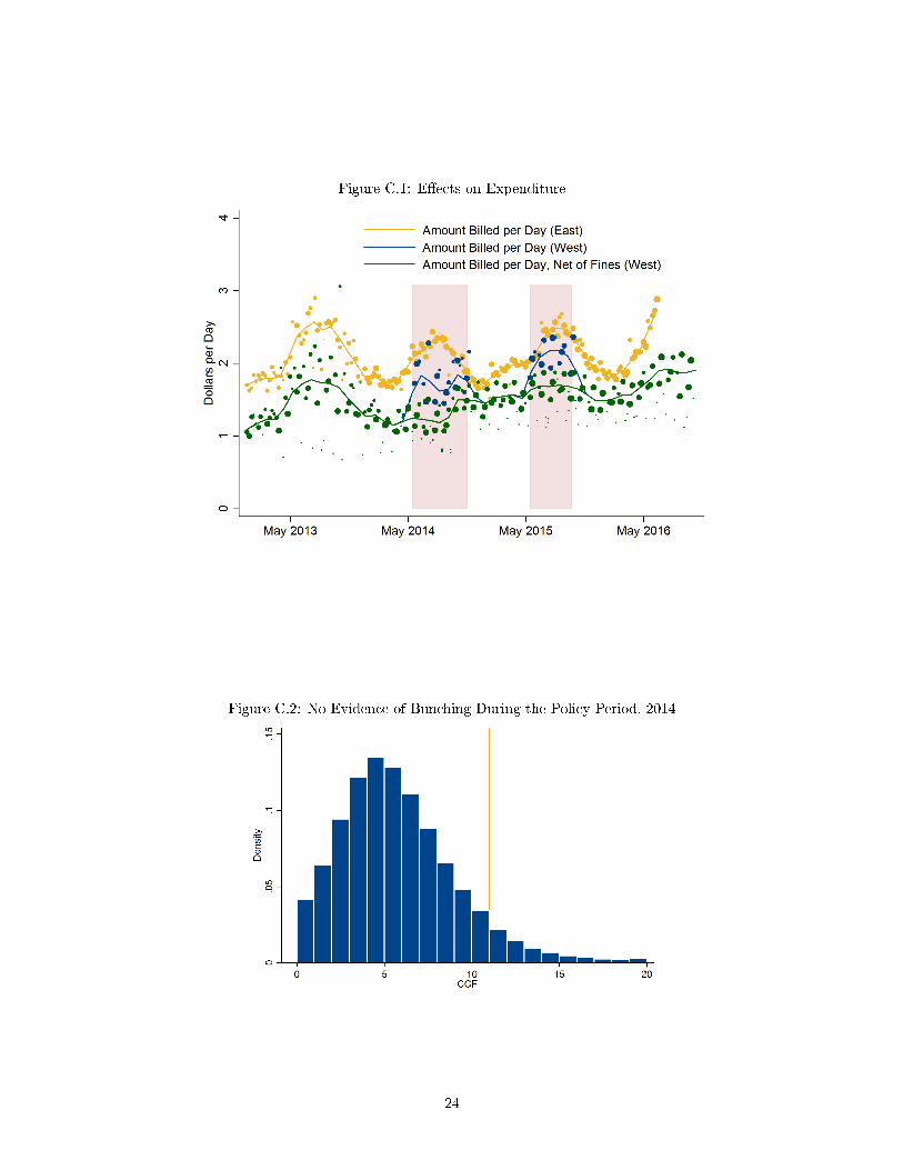
Figure C.1: E�ects on Expenditure

Figure C.2: No Evidence of Bunching During the Policy Period, 2014

24