Symmetry breaking in a bull and bear �nancial market model

Iryna Sushko,a�Fabio Tramontana,b, Frank Westerho¤,c Viktor Avrutind

aInstitute of Mathematics, National Academy of Sciences of Ukraine, 3 Tereshchenkivska st., 01601 Kyiv, Ukraine

bDepartment of Economics and Management, University of Pavia, via S.Felice 5, 27100 Pavia, Italy

cDepartment of Economics, University of Bamberg, Feldkirchenstrasse 21, 96045 Bamberg, Germany

dDESP, University of Urbino, via Sa¢ 42, 61029 Urbino, Italy

Abstract

We investigate bifurcation structures in the parameter space of a one-dimensional piecewise linear map with two

discontinuity points. This map describes endogenous bull and bear market dynamics arising from a simple asset-

pricing model. An important feature of our model is that some speculators only enter the market if the price is

su¢ ciently distant to its fundamental value. Our analysis starts with the investigation of a particular case in which

the map is symmetric with respect to the origin, associated with equal market entry thresholds in the bull and bear

market. We then generalize our analysis by exploring how novel bifurcation structures may emerge when the map�s

symmetry is broken.

1 Introduction

Research in �nancial market models with interacting chartists and fundamentalists has made considerable progress

in recent years. For surveys, see Chiarella et al. (2009), Hommes and Wagener (2009), Lux (2009) and Westerho¤

(2009). According to these models, the dynamics of �nancial markets is not caused solely by the arrival of exogenous

fundamental shocks, but also depends on the endogenous trading activity of heterogeneous speculators. These models,

some of which are able to mimic a number of important stylized facts of �nancial markets, including bubbles and crashes

�Corresponding author: Institute of Mathematics, National Academy of Sciences of Ukraine, 3 Tereshchenkivska st., 01601 Kyiv, Ukraine,

email: sushko@imath.kiev.ua

1

and excess volatility, clearly help us to gain a better understanding of how �nancial markets function. The dynamics of

these models is usually due to some kind of non-linearity which arises from speculators�trading behavior. For instance,

in the models of Day and Huang (1990), Chiarella (1992) and Tramontana et al. (2009), speculators follow non-linear

technical or fundamental trading rules and, as a consequence, complex price dynamics may arise. Non-linearities may

also arise if speculators switch between technical and fundamental trading rules, as in the models of Kirman (1991),

Brock and Hommes (1998), and Lux and Marchesi (1999), or if they switch between di¤erent markets, as in Westerho¤

(2004), Chiarella et al. (2005, 2007), and Huang and Chen (2014).

Only a few models are represented by piecewise linear maps. This is surprising since piecewise linear maps enable

very in-depth analytical investigation of dynamic properties of a model. Contributions in this direction include Huang

and Day (1993), Day (1997), Tramontana et al. (2010), Huang et al. (2010) and Huang and Zheng (2012). Recently, we

therefore started to consider �nancial market models in which some speculators are always active in the market while

others only become active if mispricing, i.e. the distance between the current price of an asset and its fundamental

value, is large enough (see Tramontana et al. 2010, 2013, 2014). Assuming that speculators�trading rules are otherwise

linear, such a perspective leads to simple models which possess piecewise linear structures. Until now, we have only

considered cases in which the threshold value of the misalignment in the bull market is the same as the corresponding

threshold value in the bear market. In this way, we obtained a one-dimensional piecewise linear map (1D PWL map

for short) with three linear branches and two symmetric discontinuity points. In this paper we remove this simplifying

assumption by considering a �nancial market model in which the two threshold values di¤er.

To be precise, the model considered in the present paper is de�ned by a 1D PWL map f with three linear branches

and two (not necessarily symmetric) discontinuity points. We are interested in the bifurcation structure of the map�s

parameter space. In particular, we study parameter regions called periodicity regions, related to attracting cycles of

di¤erent periods. Obviously, in the presence of two discontinuity points, the bifurcation structure may be much more

complicated than those observed in the parameter space of a map with one discontinuity point. In fact, the dynamics of

a generic 1D PWL map with one discontinuity point, say, map g, are relatively well understood (see, e.g., Keener 1980,

Gardini et al. 2010, Gardini et al. 2014, and references therein). For instance, there are two basic bifurcation structures

for the periodicity regions of map g, namely the period adding structure and the period incrementing structure.

The period adding structure is associated with the invertibility of map g on its absorbing interval, in which case map

2

g can only have attracting cycles and quasiperiodic orbits, but no chaotic attractors. We observe such a bifurcation

structure in the parameter space of map g when its linear branches are both increasing functions. The period adding

structure is formed by periodicity regions which are ordered in the parameter space according to the Farey summation

rule applied to the rotation numbers of the related cycles. For example, between two periodicity regions related to

cycles with rotation numbers 1=2 and 1=3 there is a region corresponding to cycles with rotation number 2=5. Similar

structures, also called Arnold tongues or mode-locking tongues, are observed in the parameter space of two- and higher-

dimensional maps near a Neimark-Sacker bifurcation boundary, in a certain class of circle maps, in 1D PWL continuous

bimodal maps, etc. The boundaries of the periodicity regions belonging to the period adding structure are de�ned by

the conditions of border collision bifurcations of the related cycle occurring when a point of the cycle collides with a

discontinuity point under parameter variation. In contrast, the period incrementing structure is much simpler. It is

associated with increasing and decreasing branches of map g, and is formed by periodicity regions related to basic cycles,

ordered according to increasing periods, with overlapping parts of two neighboring regions and bistability. Recall that

a basic cycle has only one point in the left (right) partition of the map while all its other points are located in the right

(left) partition of the map.

It is clear that the parameter space of a 1D PWL map with two discontinuity points contains regions, associated

with absorbing intervals involving only one discontinuity point, in which case the aforementioned period adding and the

period incrementing structures can be observed. However, there are also more complicated bifurcation structures that

involve both discontinuity points. In fact, for map f considered in the symmetric case (z� = z+), studied in Tramontana

et al. (2013), four bifurcation structures are observed. Two of these can be explained on the basis of standard period

adding and period incrementing structures, while two other structures, associated with both discontinuity points, are

non-standard. Namely, there is an even-period incrementing structure and a particular period adding structure, the

explicit description of which was left for future work. In the present paper, we �rst describe these structures in detail

and then break the symmetry of the map by considering that z+ = z� + " for some small " > 0; in order to �nd

possible distortions of the aforementioned bifurcation structures. We show that there are parameter regions in which

the period adding and period incrementing structures are preserved, being only quantitatively modi�ed. However, new

substructures also appear which are related to the two discontinuity points.

Overall, our simple asset-pricing model possesses a surprisingly rich bifurcation structure. Note that the cycles we

3

study in our paper imply excess volatility, since the fundamental value of the asset is constant. Moreover, the cycles can

be located in the bull or bear market, or they can stretch over bull and bear markets. Economically, this means that

the model is able to explain periods of persistent misalignments and the emergence of endogenous bubbles and crashes.

Without question, the primary goal of our paper is to contribute to the bifurcation theory of 1D PWL maps with two

discontinuity points. However, the fact that our analysis also o¤ers valuable insights into the functioning of �nancial

markets should not be overlooked. Bubbles and crashes and excess volatility can have very negative consequences for

the real economy. It is therefore crucial for us to understand what drives these two phenomena.

The rest of our paper is organized as follows. In Section 2, we introduce our �nancial market model. In Section 3, we

recap what is known about its bifurcation structure in the symmetric case (i.e. z� = z+), and consider in more detail

a particular period adding structure, associated with two discontinuity points, for which only few preliminary results

exist as yet. In Section 4, we explore how the bifurcation structures are modi�ed when the map�s symmetry is broken

(i.e. z� 6= z+). Section 5 concludes our paper and identi�es a few avenues for future research.

2 A simple piecewise linear �nancial market model

Our model may be regarded as a generalization of the models of Huang and Day (1993) and Tramontana et al. (2013).

In a nutshell, the model�s structure may be summarized as follows. We assume that there are chartists, fundamentalists

and market makers who can trade one risky asset. Chartists bet on the persistence of bull and bear markets while

fundamentalists believe in mean reversion. Market makers clear the market and adjust the price of the asset with

respect to speculators� excess demand. What makes the model interesting is that there are two types of chartists

and fundamentalists: type 1 chartists and type 1 fundamentalists are always active while type 2 chartists and type

2 fundamentalists only enter the market if the asset�s mispricing exceeds a certain critical threshold. We present the

model�s building blocks in Section 2.1 and derive its dynamical system in Section 2.2.

2.1 The setup of the model

Market makers adjust the price of the asset on the basis of a linear price-adjustment rule. Accordingly, they quote the

price of the asset for period t+ 1 as

Pt+1 = Pt + a�DC;1t +DF;1

t +DC;2t +DF;2

t

�: (1)

4

The four terms in the bracket on the right-hand side of (1) capture the orders placed by type 1 chartists, type 1

fundamentalists, type 2 chartists and type 2 fundamentalists, respectively. Moreover, parameter a is a positive price

adjustment parameter that determines how strongly market makers adjust the price of the asset with respect to excess

demand. Without loss of generality, we set a = 1.

Chartists classify a bull (bear) market as a market in which the price of the asset is above (below) its fundamental

value. When prices are in the bull (bear) region, chartists optimistically (pessimistically) buy (sell) assets. Let F be the

asset�s fundamental value. Type 1 chartists are always active, and their orders can be represented as

DC;1t = c1(Pt � F ): (2)

Reaction parameter c1 is positive, and indicates how aggressively type 1 chartists react to their price signals. Type 2

chartists wait for a stronger price signal before they enter the market. Their orders are formalized as

DC;2t =

8>>>>>><>>>>>>:c2(Pt � F ) + c3 for Pt � F � z+;

0 for �z� < Pt � F < z+;

c2(Pt � F )� c3 for Pt � F � �z�:

(3)

Parameters z+ and z� are positive, and capture how large the deviation between the current price and its fundamental

value must be for type 2 chartists to enter the market in the bull market and bear market, respectively. Reaction

parameter c2 > 0 controls the trading intensity of type 2 chartists with respect to their price signals. Parameter c3

enables type 2 chartists�transactions to be adjusted such that they are non-negative in a bull market and non-positive

in a bear market. In this paper, we achieve this by assuming that c3 � max [�c2z+;�c2z�].

Orders placed by type 1 and type 2 fundamentalists are formulated similarly except for the fact that they buy assets

in undervalued markets and sell assets in overvalued markets. Orders placed by type 1 and type 2 fundamentalists are

given as

DF;1t = f1(F � Pt) (4)

and

DF;2t =

8>>>>>><>>>>>>:f2(F � Pt)� f3 for Pt � F � z+;

0 for �z� < Pt � F < z+;

f2(F � Pt) + f3 for Pt � F � �z�;

(5)

5

respectively. Note that f1 and f2 are positive reaction parameters, determining the aggressiveness of type 1 and type

2 fundamentalists, while parameter f3 � max [�f2z+;�f2z�] ensures that the orders placed by type 2 fundamentalists

are non-positive in overvalued markets and non-negative in undervalued markets.

2.2 The model�s map and some preliminary remarks

By inserting the four demand functions (2-5) into the price adjustment rule (1), we obtain, after rearranging

Pt+1 =

8>>>>>><>>>>>>:Pt + (c1 + c2 � f1 � f2)(Pt � F ) + c3 � f3 for Pt � F � z+;

Pt + (c1 � f1)(Pt � F ) for �z� < Pt � F < z+;

Pt + (c1 + c1 � f1 � f2)(Pt � F )� c3 + f3 for Pt � F � �z�:

(6)

It is convenient to express our model in terms of deviations from the asset�s fundamental value by introducing the new

variable xt = Pt � F . Moreover, let us simplify the notation by de�ning s1 = c1 � f1, s2 = c2 � f2 and m = c3 � f3.

Our model then turns into the following 1D PWL map

f : x! f(x) =

8>>>>>><>>>>>>:fR(x) = (1 + s1 + s2)x+m for x � z+;

fM (x) = (1 + s1)x for �z� < x < z+;

fL(x) = (1 + s1 + s2)x�m for x � �z�:

(7)

In Tramontana et al. (2013), the dynamics of map f is explored for the case z+ = z�, i.e. for the case in which the

market entry thresholds for type 2 chartists and type 2 fundamentalists are symmetrically located around the asset�s

fundamental value. Moreover, they assume that s1 > 0 so that the slope of fM (x) is greater than 1. In the present

paper, we retain the assumption of s1 > 0; but study how the bifurcation structures in the (m; s2)-parameter plane

change if the symmetry of market entry thresholds is broken. Our focus is on regular dynamics, that is, on bifurcation

structures formed by parameter regions called periodicity regions, related to attracting cycles of map f .

In order to describe a cycle of map f; it is convenient to use its symbolic representation. To this end, we �rst associate

symbol L with partition IL = (�1;�z�); M� with IM� = (�z�; 0); M+ with IM+ = (0; z+) and R with IR = (z+;1).

Then the symbolic representation of an n-cycle fxigni=1 ; where xi 2 I�i , �i 2 fL;M�;M+; Rg; is the symbolic sequence

� = �1�2:::�n.

Recall that a boundary of a periodicity region related to an attracting n-cycle of a 1D piecewise linear discontinuous

map is de�ned either by the condition of a border collision bifurcation (BCB for short) of the cycle occurring when

6

a point of the cycle collides with a discontinuity point, or by the condition of a degenerate �ip bifurcation (DFB) of

the cycle associated with its eigenvalue crossing �1; or by the condition of a degenerate bifurcation associated with its

eigenvalue crossing +1 (DB+1). For details concerning degenerate bifurcations, we refer to Sushko and Gardini (2010).

A BCB of an n-cycle of the considered map f occurs if one of the periodic points collides with either x = �z�

or x = z+: Such a periodic point is called the colliding point. If a colliding point approaches the discontinuity point

x = �z� or x = z+ from the left, then the BCB condition is fn�1(fL(�z�)) = �z� or fn�1(fM (z+)) = z+; respectively.

If a colliding point approaches the discontinuity point from the right, then the BCB condition is fn�1(fM (�z�)) = �z�

or fn�1(fR(z+)) = z+; respectively. Moreover, a BCB condition of an n-cycle can be written as f�(z) = z, where

z 2 f�z�; z+g is the related discontinuity point and f� denotes a composite function associated with the colliding point:

f�(x) = f�1 � f�2 � ::: � f�n(x) (note that fM� = fM+ = fM ). The limiting values of f at the discontinuity points are

called critical points and denoted as follows:

c�L = fL(�z�); c�M = fM (�z�);

c+M = fM (z+); c+R = fR(z

+):

3 Symmetric case

Let us �rst recall what is known about the bifurcation structure of the parameter space of map f in the case of symmetric

market entry thresholds z+ = z� = z (see Tramontana et al. (2013) for details). After a suitable rescaling of x, map f

can, in the symmetric case, be written as follows:

fs : x! fs(x) =

8>>>>>><>>>>>>:fL(x) = (1 + s1 + s2)x�m for x � �1;

fM (x) = (1 + s1)x for �1 < x < 1;

fR(x) = (1 + s1 + s2)x+m for x � 1:

(8)

A 2D bifurcation diagram of map fs in the (m; s2)-parameter plane is shown in Fig. 1. Here, the dark gray regions

are related to divergence of a generic orbit; white regions are related to chaotic attractors; colored regions are associated

with attracting cycles of di¤erent periods where the correspondence of colors and periods is given in the color bar; and,

the overlapping parts of some neighboring regions are light gray. Note that one of the characteristic features of map

fs is its symmetry with respect to the origin, which leads to a simple conclusion being drawn: any invariant set A of

f is either symmetric with respect to the origin, or there exists another invariant set A0 which is symmetric to A. In

7

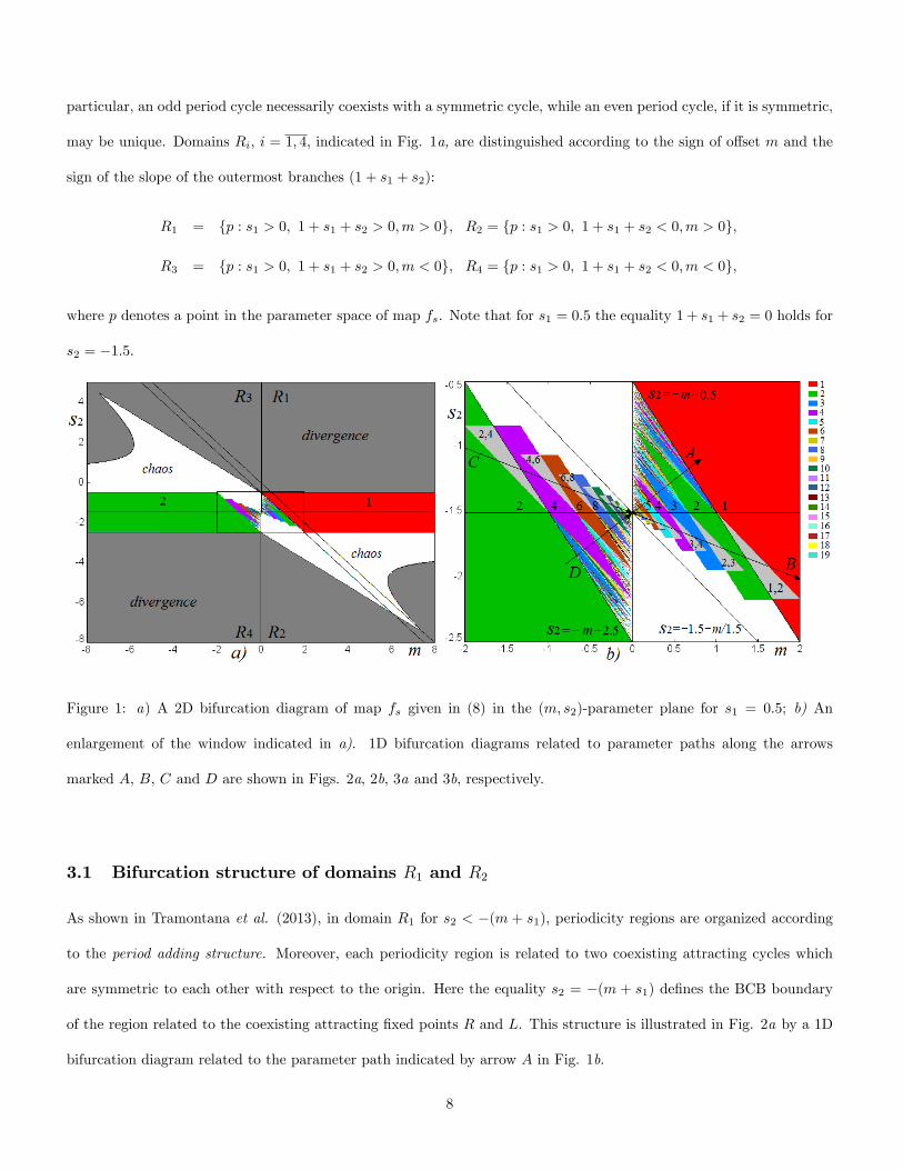
particular, an odd period cycle necessarily coexists with a symmetric cycle, while an even period cycle, if it is symmetric,

may be unique. Domains Ri; i = 1; 4; indicated in Fig. 1a, are distinguished according to the sign of o¤set m and the

sign of the slope of the outermost branches (1 + s1 + s2):

R1 = fp : s1 > 0; 1 + s1 + s2 > 0;m > 0g; R2 = fp : s1 > 0; 1 + s1 + s2 < 0;m > 0g;

R3 = fp : s1 > 0; 1 + s1 + s2 > 0;m < 0g; R4 = fp : s1 > 0; 1 + s1 + s2 < 0;m < 0g;

where p denotes a point in the parameter space of map fs. Note that for s1 = 0:5 the equality 1 + s1 + s2 = 0 holds for

s2 = �1:5:

Figure 1: a) A 2D bifurcation diagram of map fs given in (8) in the (m; s2)-parameter plane for s1 = 0:5; b) An

enlargement of the window indicated in a). 1D bifurcation diagrams related to parameter paths along the arrows

marked A; B, C and D are shown in Figs. 2a, 2b, 3a and 3b, respectively.

3.1 Bifurcation structure of domains R1 and R2

As shown in Tramontana et al. (2013), in domain R1 for s2 < �(m + s1); periodicity regions are organized according

to the period adding structure. Moreover, each periodicity region is related to two coexisting attracting cycles which

are symmetric to each other with respect to the origin. Here the equality s2 = �(m + s1) de�nes the BCB boundary

of the region related to the coexisting attracting �xed points R and L. This structure is illustrated in Fig. 2a by a 1D

bifurcation diagram related to the parameter path indicated by arrow A in Fig. 1b.

8

In fact, for the considered parameter region, map fs has two disjoint (symmetric to each other) absorbing intervals

bounded by the related critical points, I� = [c�M ; c�L ] and I+ = [c+R; c

+M ]; on each of which the map is invertible and

de�ned by two increasing functions. It is known (see e.g., Gardini et al. (2014)) that for this class of maps (also called

gap maps) the periodicity regions are organized in the period adding structure. Fig. 2a reveals two such structures: one

of them is associated with discontinuity point x = �1; and the symbolic sequences of related cycles contain the symbols

L and M� only (highlighted red in Fig. 2a). In particular, cycles of complexity level one (also called basic cycles) form

two families,

��1;1 =�LMn

�n�1 ; �

�1;2 = fM�L

ngn�1 :

The second period adding structure (highlighted blue in Fig. 2a) is associated with discontinuity point x = 1 and the

symbols M+, R, where cycles of complexity level one form the following families:

�+1;1 =�RMn

+

n�1 ; �

+1;1 = fM+R

ngn�1 :

Symbolic sequences of complexity level two are obtained using consecutive concatenations starting from two neighboring

sequences of complexity level one, leading to 22 families:

��2;1 =�(LMn

�)mLMn+1

�n;m�1 ; �

�2;2 =

�LMn

�(LMn+1� )m

n;m�1 ;

��2;3 =�(M�L

n)mM�Ln+1

n;m�1 ; �

�2;4 =

�M�L

n(M�Ln+1)m

n;m�1 :

In order to obtain 2K families of complexity level K � 3; similar concatenation procedures can be applied to sequences of

families of complexity level K � 1 (see Leonov (1959), Leonov (1962), Gardini et al. (2014)). Another way to determine

all families of the period adding structure is to apply the map replacement technique, as described in Avrutin et al.

(2010), and Gardini et al. (2010). This method also helps to simplify the calculation procedure for expressions of the

boundaries of related periodicity regions.

Families �+2;i; i = 1; 4; of complexity level two related to the second period adding structure are obviously obtained

by substituting R instead of L; and M+ instead of M� in families ��2;i related to the �rst period adding structure.

Families of higher complexity levels are obtained in the same way.

Let �0 denote the symbolic sequence obtained from � by interchanging R and L; as well as M+ and M�: Sequence

�0 of the cycle symmetric (with respect to the origin) to the cycle of symbolic sequence �. Let P� denote the periodicity

region corresponding to the attracting cycle with symbolic sequence �.

9

If one compares periodicity regions P� and P�0 ; related to symmetric cycles (and, thus, associated with the two

aforementioned period adding structures) then, due to the symmetry of the map, these periodicity regions have the same

boundaries. That is, in domain R1 we observe just one period adding structure associated with coexisting symmetric

cycles. Consider, for example, a cycle with symbolic sequence � containing the symbols M+ and R: One of the BCB

boundaries of periodicity region P� is obtained from f�(z+) = z+, where � is the symbolic sequence associated with the

colliding periodic point. For map fs; it holds that fR(x) = � fL(�x); fM+(x) = �fM�(�x); thus, f�(x) = � f�0(�x);

so that from f�(z+) = z+ we get �f�0(�z+) = z+, and, �nally, f�0(�z�) = �z�; which corresponds to the condition of

the BCB boundary of P�0 . That is, conditions f�(z+) = z+ and f�0(�z�) = �z� are equivalent in terms of parameters.

For example, the two BCB boundaries of region PRMn+; n � 1, related to the basic cycle RMn

+; are obtained from

fR � fnM+(z+) = z+; (9)

fM+� fR � fn�1M+

(z+) = z+: (10)

The conditions de�ning the BCB boundaries of PLMn�are obviously the same up to substitution R by L; M+ by M�

and z+ by �z�: Hence we can use the unique notation PLMn�; RM

n+for the related region. Similarly, we use the notation

P�; �0 for a generic region of the period adding structure corresponding to two symmetric cycles. It is obvious that if

the symmetry z� = z+ is broken, then periodicity regions of two period adding structures will no longer have the same

boundaries, as we will discuss in the next section. In fact, for z+ 6= z� the BCB conditions fL � fnM�(�z�) = �z� and

fM� � fL � fn�1M�(�z�) = �z� become di¤erent to those given in (9) and (10), and the same occurs for cycles of all other

complexity levels.

Note that for m = 0; 0 < (1 + s1 + s2) < 1; corresponding to segment f(m; s2) : m = 0;�1:5 < s2 < �0:5g in Fig. 1,

map fs is topologically conjugate on both absorbing intervals I� and I+ to a circle map on which a linear rotation with

a rational or irrational rotation number is de�ned. Any point of this segment related to a rational rotation is an issue

point of the corresponding periodicity region.

Periodicity regions in domain R2 are organized in a period incrementing structure. It is illustrated by the 1D

bifurcation diagram presented in Fig. 2b which is related to the parameter path indicated by arrow B in Fig. 1b. It

can be shown that if m > �(1 + s1 + s2)(1 + s1) (in Fig. 1b the related region is de�ned by s2 > �1:5�m=1:5), map

fs has two disjoint (symmetric to each other) absorbing intervals, I� = [c�M ; fL(c

�M )] and I+ = [fR(c

+M ); c

+M ]; on both

of which the map is de�ned by increasing and decreasing functions. It is known that such a map is characterized (in

10

Figure 2: 1D bifurcation diagrams of map fs given in (8) illustrating in a) two coexisting period adding structures, and

in b) period incrementing structures. Here s1 = 0:5 and in a) s2 = 0:5m� 1:5; 0 < m < 0:8 (see path marked A in Fig.

1b), while in b) s2 = �0:25m� 1:5; 0 < m < 2 (see path marked B in Fig. 1b).

the stability regime) by period incrementing structures formed by periodicity regions related to the basic cycles, with

overlapping parts of each two neighboring regions. As illustrated in Fig. 2b, there are two such structures. The �rst

(highlighted red and green), associated with discontinuity point x = �1; is formed by the periodicity regions PLMn�

related to basic cycles, with overlapping parts of each two neighboring regions, PLMn�and PLMn+1

�; which correspond

to coexisting cycles LMn� and LM

n+1� : The second period incrementing structure (highlighted blue and magenta in Fig.

2b) is associated with discontinuity point x = 1; and is formed by the periodicity regions PRMn+of basic cycles, with

overlapping parts of each two neighboring regions.

As already discussed, the symmetry of the map with respect to zero leads to the fact that the BCB boundaries

of PLMn�and PRMn

+coincide in the parameter space, meaning that we see just one period incrementing structure in

domain R2; and each region of this structure is denoted by PLMn�; RM

n+: In contrast to the periodicity regions of the

period adding structure, having only BCB boundaries, any region PLMn�; RM

n+of the period incrementing structure also

has a DFB boundary de�ned by

(1 + s1 + s2)(1 + s1)n�1 = �1

(obviously, the DFB boundaries of PLMn�and PRMn

+coincide as well). Hence, each region PLMn

�; RMn+is related to

11

two coexisting cycles, LMn� and RM

n+, while its part that overlaps with neighboring region PLMn+1

� ; RMn+1+

is related

to four coexisting cycles, LMn�; LM

n+1� ; RMn

+ and RMn+1+ : Obviously, if the symmetry z� = z+ is broken, then the

BCB boundaries of periodicity regions of the two period incrementing structures become di¤erent.

Note that at the border between domains R1 and R2 de�ned by (1+s1+s2) = 0, periodicity regions are organized in

period incrementing structure without overlapping, and each region corresponds to coexisting superstable basic cycles

LMn� and RM

n+, n � 0:

3.2 Bifurcation structure of domains R3 and R4

As we have seen, the period adding structure in domain R1 and the period incrementing structure in domain R2 are well

known. The basic mechanisms of their formation can be described using symbolic sequences consisting of two symbols

only. The bifurcation structures observed in domains R3 and R4 are associated with four symbols; such structures have

been studied to a much lesser extent (see, e.g., Tramontana et al. (2012), Tramontana et al. (2015)).

Let us recall �rst how the periodicity regions in domain R3 are organized. Fig. 3a shows the 1D bifurcation diagram

corresponding to the parameter path indicated by arrow C in Fig. 1b. As shown in Tramontana et al. (2013), periodicity

regions in this domain are organized in an even-period incrementing structure formed by regions PLMn+RM

n�; n � 0;

related to the cycle of even period 2(n + 1), with overlapping parts of each two neighboring regions corresponding to

coexisting cycles LMn+RM

n� and LM

n+1+ RMn+1

� .

In fact, in domain R3 for m < �(1 + s1 + s2)(1 + s1) (in Fig. 1b this condition corresponds to s2 < �1:5�m=1:5),

map fs has an invariant absorbing set consisting of two intervals: I =�c�M ; fR(c

+M )�[�fL(c

�M ); c

+M

�: The condition

m < �(1 + s1 + s2)(1 + s1) is obtained from the condition fR(c+M ) < 0 or, equivalently, fL(c

�M ) > 0; in which case

the two intervals mentioned above are disjoint. Two BCB boundaries of the periodicity region PLMn+RM

n�; n � 1, are

obtained from

fR � fnM� � fL � fnM+(z+) = z+ (11)

(or, equivalently, fL � fnM+� fR � fnM�

(�z�) = �z�) and

fM+� fR � fnM� � fL � f

n�1M+

(z+) = z+ (12)

(or equivalently, fM� � fL � fnM+� fR � fn�1M�

(�z�) = �z�), while the DB+1 boundary is de�ned by

(1 + s1 + s2)(1 + s1)n = 1:

12

Figure 3: 1D bifurcation diagrams of map fs given in (8) illustrating in a) an even-period incrementing structure and

in b) a period adding structure, with coexisting cycles of odd periods. Here s1 = 0:5 and in a) s2 = �0:25m � 1:5;

�2 < m < 0 (see path marked C in Fig. 1b), while in b) s2 = 0:5m � 1:5; �0:8 < m < 0 (see path marked D in Fig.

1b).

(Obviously, when the symmetry z+ = z� is broken, the conditions associated with z� are no longer equivalent to those

given in (11) and (12).) Periodicity region PLR is bounded by the BCB boundary obtained from fR � fL(z+) = z+ (or,

equivalently, fL � fR(�z�) = �z�), that holds for s2 = �m� 2� s1 or for s2 = �s1 (i.e. s2 = �m� 2:5 and s2 = �0:5

in Fig. 1), and the DB+1 boundary de�ned by (1 + s1 + s2) = 1; that is, s2 = �s1: Note that region PLR also extends

to domain R4; where it has one more stability boundary, related to the DFB of cycle LR, de�ned by (1+ s1+ s2) = �1;

that is, s2 = �2� s1 (in Fig. 1 this boundary is given by s2 = �2:5).

Comparing the period incrementing structure in domain R2 with that in R3 (see Fig. 1b; cf also Fig. 2b and Fig.

3a), one can note the symmetry of these structures with respect to the parameter point

S = (m; s2) = (0;�(1 + s1)) (13)

associated with fL(x) = fR(x) � 0: However, the symmetric parameter regions are related to di¤erent cycles, namely,

region PLMn�; RM

n+� R2; n � 0; is symmetric with respect to S to region PLMn

+RMn�� R3. To prove this, recall

that one BCB boundary of PLMn�; RM

n+� R2 is de�ned by the condition fR � fnM+

(z+) = z+; moreover, the condition

fL � fnM�(�z�) = �z� also holds. Let parameter point p� = (m�; s�2) 2 R2 satisfy the condition fR � fnM+

(z+) = z+:

13

Then it is easy to show that at parameter point p0 = (�m�;�2(1+s1)�s�2) 2 R3; which is symmetric to p� with respect

to S; it holds that fR � fnM�(z+) = �z� and fL � fnM�

(�z�) = z+: Therefore, parameter point p0 satis�es the condition

fR�fnM��fL�fnM+

(z+) = z+; which is related to the BCB boundary of PLMn+RM

n�� R3. Similarly, it can be shown that

the second BCB boundary of PLMn�; RM

n+� R2 is symmetric to the second BCB boundary of PLMn

+RMn�� R3: Finally,

the DFB boundary of PLMn�; RM

n+is obviously symmetric with respect to S to the DB+1 boundary of PLMn

+RMn�.

Now let us consider the bifurcation structure of domain R4; illustrated in Fig. 3b by the 1D bifurcation diagram

corresponding to parameter path D shown in Fig. 1b. One can see a particular period adding structure where any

odd period cycle coexists with the symmetric (with respect to the origin) cycle, while any even period cycle is a unique

attractor, being symmetric itself. Tramontana et al. (2013) left an explicit description of this structure for future work,

hence it is discussed below in more detail.

In fact, in domain R4 map fs has an invariant absorbing set consisting of two symmetric intervals, I =�c�M ; c

+R

�[�

c�L ; c+M

�. The condition fM (c

+R) < fR(c

+M ); as well as fM (c

�L ) > fL(c

�M ), equivalent to ms1 < 0, obviously holds in R4;

thus, fs is a gap map on I (that is, it is invertible in I), which is known to be unable to have chaotic attractors, but only

attracting cycles and quasiperiodic orbits (so-called Cantor set attractors). Similar to the case of the period adding struc-

ture observed in domain R1, the period adding structure in R4 originates from the straight line withm = 0; namely, from

its segment with �2�s1 < s2 < �1�s1 (in Fig. 1b it corresponds to the segment f(m; s2) : m = 0; �2:5 < s2 < �1:5g),

at which the condition fM (c+R) = fR(c

+M ) holds (as well as fM (c

�L ) = fL(c

�M )). For parameter values belonging to this

segment, map fs is topologically conjugate to a circle map with a rational or irrational rotation number. Each point

of the segment related to rational rotation is an issue point of the related periodicity region in R4. For example, point

(m; s2) � (0;�2:3165) is an issue point of the periodicity region related to cycles with rotation number 1=3 (see Fig.

4a), or point (m; s2) � (0;�2:1662) is an issue point of the periodicity region corresponding to cycles with rotation

number 1=4 (see Fig. 5a). If a parameter point enters a periodicity region related to an odd period cycle, then two

symmetric cycles of this period are born, as shown, for example, in Fig. 4b. Obviously, due to the symmetry of fs,

BCBs of these cycles occur at the same parameter values, which is why we observe just one periodicity region for each

pair of odd period cycles. If a parameter point enters a periodicity region related to even period, then only one cycle of

this period is born, which itself is symmetric with respect to the origin (see, e.g., Fig. 5b).

In order to obtain the symbolic sequences of the cycles of fs associated with the period adding structure in domain

14

Figure 4: a) Map fs and f3s for s1 = 0:5; s2 = �2:3165; m = 0; when any point of I =�c�M ; c

+R

�[�c�L ; c

+M

�is 3-periodic;

b) fs, f3s and two coexisting 3-cycles for s1 = 0:5; s2 = �2; m = �0:4.

Figure 5: a) Map fs and f4s for s1 = 0:5; s2 = �2:1662; m = 0; when any point of I =�c�M ; c

+R

�[�c�L ; c

+M

�is 4-periodic;

b) fs; f4s and attracting 4-cycle for s1 = 0:5; s2 = �1:8; m = �0:4.

R4; �rst note that there is a rule to check the admissibility of such symbolic sequences: it is easy to see that a point

x0 2 IL (x0 2 IR) is mapped in one iteration either to a point x1 2 IR (x1 2 IL) or x1 2 IM+ (x1 2 IM�), while a point

x0 2 IM+(x0 2 IM�) is mapped either to a point x1 2 IM+

(x1 2 IM�), or x1 2 IR (x1 2 IL) (see, for example, Fig.

5). That is, in a symbolic sequence �; symbol L (R) is necessarily followed by R or M+ (L or M�), while M+ (M�) is

followed by M+ or R (M� or L).

Similar to the symmetry of the period incrementing structures in R2 and R3 with respect to parameter point S given

15

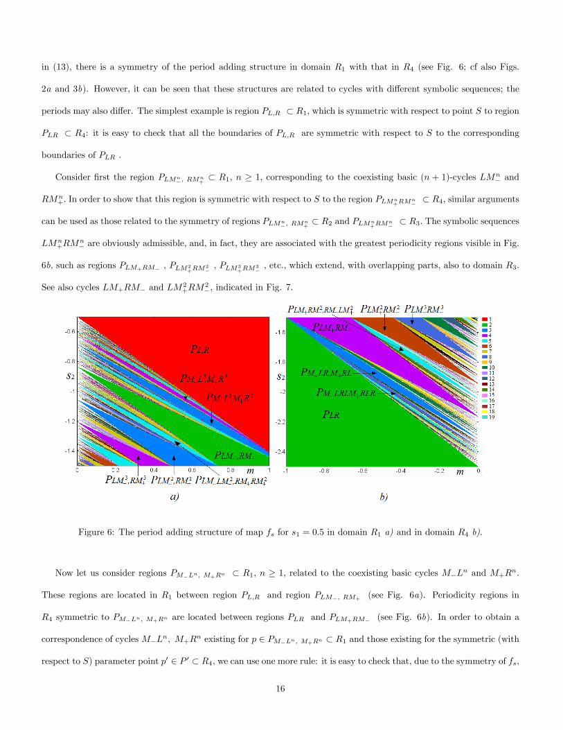
in (13), there is a symmetry of the period adding structure in domain R1 with that in R4 (see Fig. 6; cf also Figs.

2a and 3b). However, it can be seen that these structures are related to cycles with di¤erent symbolic sequences; the

periods may also di¤er. The simplest example is region PL;R � R1; which is symmetric with respect to point S to region

PLR � R4: it is easy to check that all the boundaries of PL;R are symmetric with respect to S to the corresponding

boundaries of PLR .

Consider �rst the region PLMn�; RM

n+� R1, n � 1; corresponding to the coexisting basic (n + 1)-cycles LMn

� and

RMn+: In order to show that this region is symmetric with respect to S to the region PLMn

+RMn�� R4; similar arguments

can be used as those related to the symmetry of regions PLMn�; RM

n+� R2 and PLMn

+RMn�� R3: The symbolic sequences

LMn+RM

n� are obviously admissible, and, in fact, they are associated with the greatest periodicity regions visible in Fig.

6b, such as regions PLM+RM� ; PLM2+RM

2�; PLM3

+RM3�; etc., which extend, with overlapping parts, also to domain R3.

See also cycles LM+RM� and LM2+RM

2�; indicated in Fig. 7.

Figure 6: The period adding structure of map fs for s1 = 0:5 in domain R1 a) and in domain R4 b).

Now let us consider regions PM�Ln; M+Rn � R1; n � 1; related to the coexisting basic cycles M�Ln and M+R

n:

These regions are located in R1 between region PL;R and region PLM�; RM+(see Fig. 6a). Periodicity regions in

R4 symmetric to PM�Ln; M+Rn are located between regions PLR and PLM+RM� (see Fig. 6b). In order to obtain a

correspondence of cycles M�Ln; M+R

n existing for p 2 PM�Ln; M+Rn � R1 and those existing for the symmetric (with

respect to S) parameter point p0 2 P 0 � R4; we can use one more rule: it is easy to check that, due to the symmetry of fs;

16

it holds that fL � fL(x)jx 2 IL; p 2 PM�Ln; M+Rn= fR � fL(x)jx 2 IL; p0 2 P 0 ; and fR � fR(x)jx 2 IR; p 2 PM�Ln; M+Rn

=

fL � fR(x)jx 2 IR; p0 2 P 0 : Hence, if one takes a parameter point p 2 PM�Ln; M+Rn where n � 2 is even (that is, at p the

number of applications of fL or fR is even), then point p0 is related to two coexisting (n + 1)-cycles M� (LR)n=2 and

M+ (RL)n=2

: That is, region PM�Ln; M+Rn � R1 for even n � 2 is symmetric to region P 0 = PM�(LR)n=2; M+(RL)

n=2 �

R4:As an example, one can compare the region PM�L2; M+R2 � R1; indicated in Fig. 6a, with the region PM�LR; M+RL �

R4 symmetric to it, indicated in Fig. 6b (see also Fig. 7 where cycles M�LR; M+RL are visible). In the meantime, if

p 2 PM�Ln; M+Rn where n � 1 is odd (that is, the number of applications of fL or fR is odd), then the symmetric point

p0 2 P 0 � R4 is related to one 2(n + 1)-cycle M� (LR)(n�1)=2

LM+ (RL)(n�1)=2

R: That is, region PM�Ln; M+Rn � R1

for odd n � 1 is symmetric to region PM�(LR)(n�1)=2LM+(RL)

(n�1)==2R � R4: One can compare, for example, region

PM�L3; M+R3 � R1 in Fig. 6a and region PM�LRLM+RLR � R4 in Fig. 6b (see also Fig. 7 where cycleM�LRLM+RLR

is shown).

Figure 7: An enlargement of the 1D bifurcation diagram shown in Fig. 3b.

Now let us consider region PLMn�LM

n+1� ; RMn

+RMn+1+

� R1; n � 1, associated with two coexisting cycles of complexity

level two. Such regions are located between regions PLMn� ; RMn

+and PLMn+1

� ; RMn+1+

: The periodicity region P 0 � R4

symmetric to PLMn�LM

n+1� ; RMn

+RMn+1+

� R1 with respect to S is located between regions PLMn+RM

n�and PLMn+1

+ RMn+1�

:

It can be shown that P 0 = PLMn+RM

n+1� ; RMn

�LMn+1+

� R4; n � 0. Compare, for example, region PLM�LM2�; RM+RM2

+�

R1 indicated in Fig. 6a with region PLM+RM2�; RM�LM2

+� R4 shown in Fig. 6b (see also the coexisting cycles

17

LM+RM2�; RM�LM

2+ visible in Fig. 7).

Hence, for the period adding structure observed in domain R4; we obtain the following families of complexity level

one related to cycles with one point in IL and another in IR :

�LMn

+RMn�;�LMn

+RMn+1� ; RMn

�LMn+1+

; for n � 0;

as well as the following �rst complexity level families related to cycles with one point in M� and another in M+ :

nM� (LR)

n=2; M+ (RL)

n=2o; for even n � 2;n

M� (LR)(n�1)=2

LM+ (RL)(n�1)=2

Ro; for odd n � 1:

The correspondence of other periodicity regions in R4 with the symmetric one in R1 can be described similarly.

However, it is clear that a generic procedure to obtain symbolic sequences of all complexity levels is more complicated

than in the case of a period adding structure based on two symbols.

4 Symmetry breaking

Let us now study how the bifurcation structures of domains Ri; i = 1; 4; described in the previous section, change when

the equality z� = z+ in the de�nition of map f given in (7) does not hold, that is, when the map is no longer symmetric

with respect to the origin. To this end, let us consider map f and assume that z� = 1; z+ = 1 + "; for some " > 0. As

we shall see, it is rather easy to explain how the period adding and period incrementing structures in domains R1 and

R2; respectively, are modi�ed because disjoint absorbing intervals, each of which includes only one discontinuity point,

persist for such parameter regions. Obviously, qualitatively similar structures are observed for " < 0 as well (note that

to have z+ > 0; it must hold " > �1). By contrast, the distortion of bifurcation structures of domains R3 and R4 is

more complicated given that both discontinuity points are involved into absorbing intervals.

4.1 Distortion of bifurcation structures in domains R1 and R2

Consider �rst how the period adding structure in R1 is modi�ed if z� < z+: In this case, similar to the symmetric case

z� = z+; map f has two disjoint absorbing intervals, I� = [c�M ; c

�L ] and I+ = [c

+R; c

+M ]; and there are two period adding

structures associated with these two intervals. However, now the BCB boundaries of the related periodicity regions no

longer coincide, and two coexisting cycles may have di¤erent periods.

18

The bifurcation structure in R1 is illustrated in Fig. 8 for z� = 1; z+ = 1:2. Fig. 8a shows gray n-periodicity regions,

n = 1; 5; of the period adding structure related to discontinuity point x = �z� = �1. Let for each cycle associated

with periodicity region P� the symbolic sequence �� / �+ (consisting of the symbols L and M�) be associated with the

periodic point colliding with discontinuity point x = �1 from the left/right. Then one BCB boundary of P� is related

to the condition f��(�z�) = �z� (these boundaries are colored red in Fig. 8a), and the second BCB boundary of P� is

related to the condition f�+(�z�) = �z� (these boundaries are colored green in Fig. 8a). The complete period adding

structure associated with x = �1 is obviously the same as that observed in domain R1 in the symmetric case (see Fig. 1b

or Fig. 6a). As for the period adding structure associated with discontinuity point x = z+ = 1:2; in Fig. 8a the related

n-periodicity regions are not colored, while their boundaries related to condition f�0+(z+) = z+ are colored blue, and

those related to the condition f�0+(z+) = z+ are given in magenta. Here, for each cycle related to periodicity region P�0 ;

the symbol �0+ / �0� (consisting of symbols R and M+) is associated with the periodic point colliding with discontinuity

point x = 1:2 from the right/left. It is easy to show that periodicity region P�0 of this period adding structure issues

from the same point of the line m = 0 as region P� (recall that �0 is obtained from � substituting L with R and M�

with M+). However, the overall period adding structure is expanded with respect to the �rst structure.

The two period adding structures can be compared by means of the 1D bifurcation diagram shown in Fig. 8b. For

example, for the values of m indicated by gray arrows (see also a segment bounded by points A and B in Fig. 8a)

attracting �xed point L (to which any initial point x0 < 0 is attracted) coexists with the cycles colored blue (to which

any initial point x0 > 0 is attracted).

The distortion of the period incrementing structure in domain R2 is illustrated in Fig. 9 for z� = 1 and z+ = 1:1: It

is easy to see that for m > �(1 + s1 + s2)(1 + s1)z+ (in Fig. 9a the related region is de�ned by s2 > �1:5�m=1:5z+)

map f has two disjoint absorbing intervals, I� = [c�M ; fL(c�M )] and I+ = [fR(c

+M ); c

+M ]; on each of which the map is

de�ned by increasing and decreasing functions. Thus, two period incrementing structures can be observed, associated

with these intervals. Obviously, the period incrementing structure related to discontinuity point x = �z� = �1 is the

same as in the symmetric case described in the previous section (see Fig. 1b). In Fig. 9a periodicity regions PLMn�;

n = 0; 4; belonging to this structure, are colored light gray with overlapping parts of two neighboring regions given in

dark gray. For each region PLMn�its BCB boundary related to the condition fLMn

�(z�) = z� is colored red and that

related to the condition fM�LMn�1�

(�z�) = �z� is given in green. DFB boundaries are obviously de�ned by the same

19

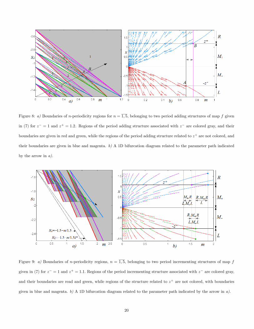
Figure 8: a) Boundaries of n-periodicity regions for n = 1; 5, belonging to two period adding structures of map f given

in (7) for z� = 1 and z+ = 1:2. Regions of the period adding structure associated with z� are colored gray, and their

boundaries are given in red and green, while the regions of the period adding structure related to z+ are not colored, and

their boundaries are given in blue and magenta. b) A 1D bifurcation diagram related to the parameter path indicated

by the arrow in a).

Figure 9: a) Boundaries of n-periodicity regions, n = 1; 5; belonging to two period incrementing structures of map f

given in (7) for z� = 1 and z+ = 1:1: Regions of the period incrementing structure associated with z� are colored gray,

and their boundaries are read and green, while regions of the structure related to z+ are not colored, with boundaries

given in blue and magenta. b) A 1D bifurcation diagram related to the parameter path indicated by the arrow in a).

20

condition as in the symmetric case, that is, by the condition (1+ s1+ s2)(1+ s1)n = �1. As for the period incrementing

structure associated with discontinuity point z+ = 1:1, in Fig. 9a only the boundaries of periodicity regions PRMn+;

n = 0; 4; belonging to this structure, are colored: the BCB boundary of PRMn+related to the condition fRMn

+(z+) = z+

is colored magenta and that related to the condition fM+RMn�1+

(z+) = z+ is given in blue. The overlapping part of

PRMn+and PRMn+1

+is associated with coexisting cycles RMn

+ and RMn+1+ . The condition related to the DFB boundary

of PRMn+is obviously the same as for region PLMn

�: Comparing these two period incrementing structures by means of

1D bifurcation diagram, it is easy to conclude which cycles may coexist, such as those indicated in Fig. 9b.

4.2 Distortion of the bifurcation structures in domains R3 and R4

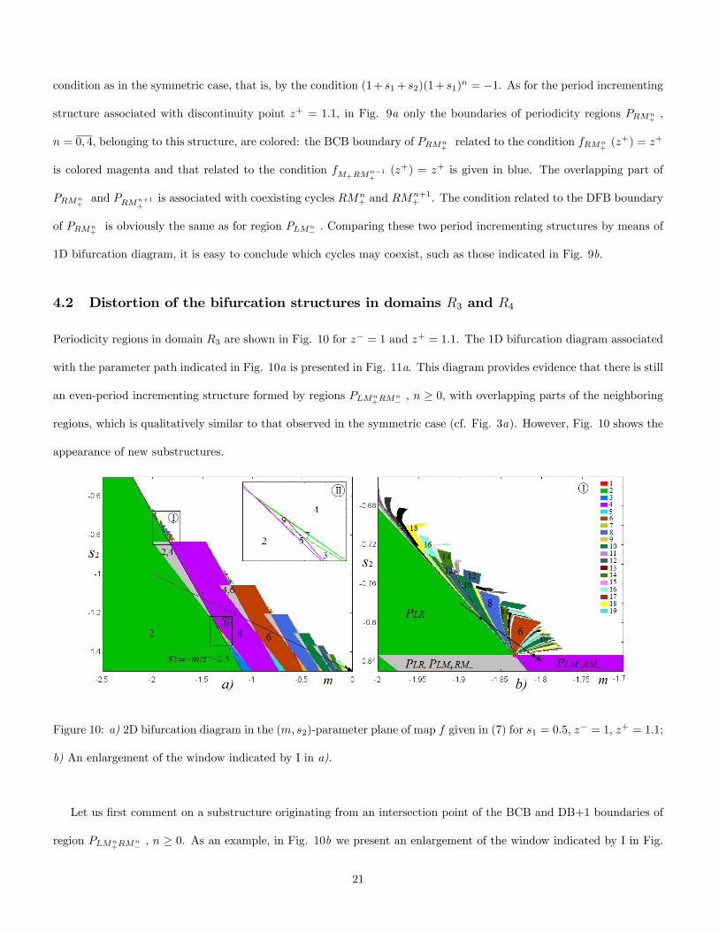
Periodicity regions in domain R3 are shown in Fig. 10 for z� = 1 and z+ = 1:1. The 1D bifurcation diagram associated

with the parameter path indicated in Fig. 10a is presented in Fig. 11a. This diagram provides evidence that there is still

an even-period incrementing structure formed by regions PLMn+RM

n�; n � 0; with overlapping parts of the neighboring

regions, which is qualitatively similar to that observed in the symmetric case (cf. Fig. 3a). However, Fig. 10 shows the

appearance of new substructures.

Figure 10: a) 2D bifurcation diagram in the (m; s2)-parameter plane of map f given in (7) for s1 = 0:5; z� = 1; z+ = 1:1;

b) An enlargement of the window indicated by I in a).

Let us �rst comment on a substructure originating from an intersection point of the BCB and DB+1 boundaries of

region PLMn+RM

n�, n � 0. As an example, in Fig. 10b we present an enlargement of the window indicated by I in Fig.

21

10a. It shows a period adding structure on the base of cycles LR and LM+RM�, which issues from the intersection

point of the BCB boundary of PLR given by s2 = �m=z+ � (2 + s1) and the DB+1 boundary of PLM+RM� given by

(1 + s1 + s2)(1 + s1) = 1. In Fig. 10 the BCB boundary is de�ned by s2 = �m=1:1 � 2:5; the DB+1 boundary by

s2 = �5=6, and their intersection point is (m; s2) = (�11=6;�5=6) (shown in Fig. 10b by a red point). The period

adding structure issuing from this point is illustrated in Fig. 12, which shows the 1D bifurcation diagram with an

enlargement, related to the parameter path indicated in Fig. 10b. In order to see that the observed structure, is indeed

a period adding structure �rst note that the DB+1 boundary of PLM+RM� also satis�es the condition of a BCB of

cycle LM+RM�. In fact, for parameter values belonging to this DB+1 boundary, map f has four invariant intervals,

each point of which is 4-periodic. Hence, the point (m; s2) = (�11=6;�5=6) can be seen as an intersection point of two

BCB boundaries: one is related to cycle LR and the other to cycle LM+RM�: It is known that such a point, called the

big bang bifurcation point (or organizing center), is an issue point of a period adding structure under certain additional

conditions which are satis�ed for the considered case (for details, see Gardini et al. (2014)). Similar structures are also

described in Tramontana et al. (2012).

Figure 11: 1D bifurcation diagram of map f given in (7) for s1 = 0:5; z� = 1; z+ = 1:1 and a) s2 = �0:25m � 1:5,

�2 < m < 0 (see the path indicated in Fig. 10a); b) s2 = �1:5; �2 < m < 0.

One more di¤erence with respect to the symmetric case z� = z+ concerns dynamics occurring for the parameter

values belonging to the straight line s2 = �(1 + s1); m < 0, associated with zero slope of the outermost branches of

map f . For parameter values belonging to this line, one observes a period incrementing structure without overlapping,

22

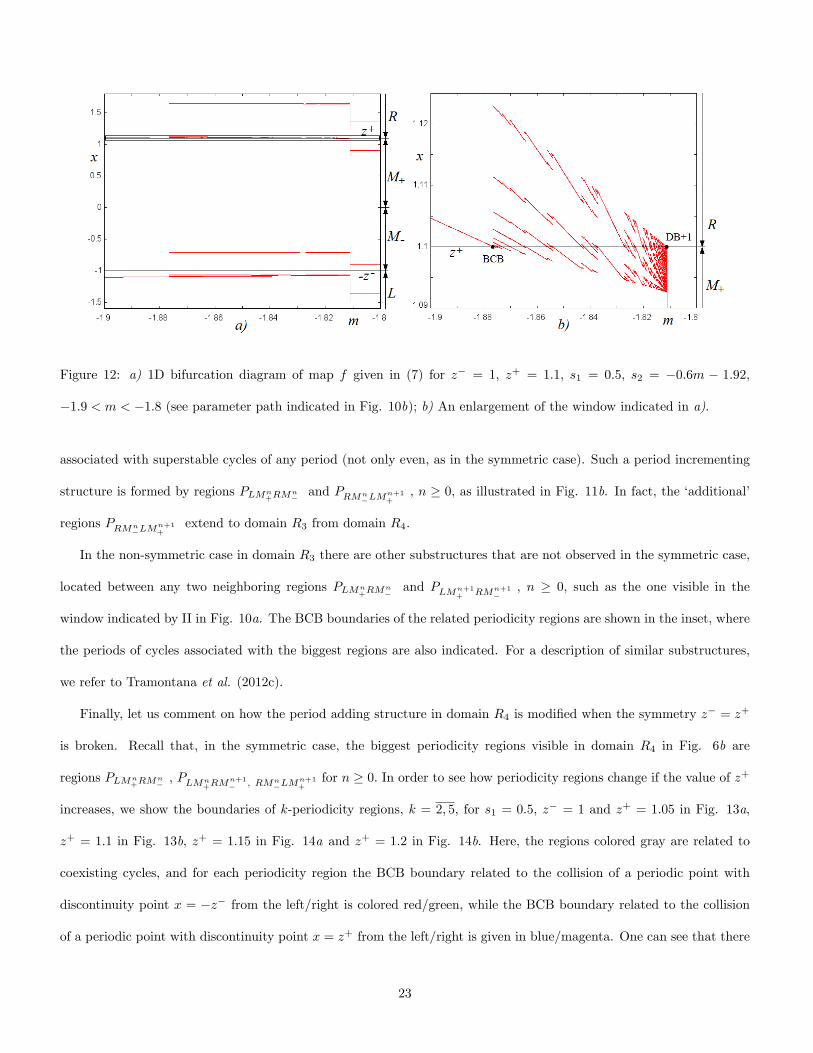
Figure 12: a) 1D bifurcation diagram of map f given in (7) for z� = 1; z+ = 1:1; s1 = 0:5; s2 = �0:6m � 1:92,

�1:9 < m < �1:8 (see parameter path indicated in Fig. 10b); b) An enlargement of the window indicated in a).

associated with superstable cycles of any period (not only even, as in the symmetric case). Such a period incrementing

structure is formed by regions PLMn+RM

n�and PRMn

�LMn+1+

; n � 0, as illustrated in Fig. 11b. In fact, the �additional�

regions PRMn�LM

n+1+

extend to domain R3 from domain R4.

In the non-symmetric case in domain R3 there are other substructures that are not observed in the symmetric case,

located between any two neighboring regions PLMn+RM

n�and PLMn+1

+ RMn+1�

, n � 0, such as the one visible in the

window indicated by II in Fig. 10a. The BCB boundaries of the related periodicity regions are shown in the inset, where

the periods of cycles associated with the biggest regions are also indicated. For a description of similar substructures,

we refer to Tramontana et al. (2012c).

Finally, let us comment on how the period adding structure in domain R4 is modi�ed when the symmetry z� = z+

is broken. Recall that, in the symmetric case, the biggest periodicity regions visible in domain R4 in Fig. 6b are

regions PLMn+RM

n�; PLMn

+RMn+1� ; RMn

�LMn+1+

for n � 0: In order to see how periodicity regions change if the value of z+

increases, we show the boundaries of k-periodicity regions, k = 2; 5, for s1 = 0:5, z� = 1 and z+ = 1:05 in Fig. 13a,

z+ = 1:1 in Fig. 13b, z+ = 1:15 in Fig. 14a and z+ = 1:2 in Fig. 14b. Here, the regions colored gray are related to

coexisting cycles, and for each periodicity region the BCB boundary related to the collision of a periodic point with

discontinuity point x = �z� from the left/right is colored red/green, while the BCB boundary related to the collision

of a periodic point with discontinuity point x = z+ from the left/right is given in blue/magenta. One can see that there

23

are coexisting cycles not only of odd periods, as in the symmetric case, but also of even periods. Moreover, if the value

of z+ is incresed, the bistability regions associated with odd periods decrease while those with even periods increase.

In Fig. 15 we present a 1D bifurcation diagram for z+ = 1:1, m = �0:2 and �2:2 < s2 < �1:8 (see the parameter

path shown in Fig. 13b). One can suggest that for z+ = z�+ " for some su¢ ciently small " > 0 each region PLMn+RM

n�;

n � 1, includes region PLMn+1+ RMn�1

�; and each region PRMn

�LMn+1+

includes regions PLMn+RM

n+1�

. We leave the

detailed investigation of this bifurcation structure for future work.

Figure 13: Boundaries of k-periodicity regions, k = 2; 5, in the (m; s2)-parameter plane of map f for s1 = 0:5, z� = 1

and z+ = 1:05 in a), z+ = 1:1 in b).

Figure 14: Boundaries of k-periodicity regions, k = 2; 5, in the (m; s2)-parameter plane of map f for s1 = 0:5, z� = 1

and z+ = 1:15 in a), z+ = 1:2 in b).

24

Figure 15: 1D bifurcation diagram of map f for s1 = 0:5, z� = 1, z+ = 1:1, m = �0:2 and �2:2 < s2 < �1:8 (the

related parameter path is indicated in Fig. 13b by an arrow).

Only a few examples of the distortion of the bifurcation structures of domains R3 and R4 were discussed above:

Examples of bifurcation structures of these domains for larger " are presented in Fig.16. It is a challenging task to

provide a complete description of the structures that may appear in these domains increasing ", which will be left for

future work.

Figure 16: 2D bifurcation diagram in the (m; s2)-parameter plane of map f given in (7) for a) s1 = 0:5; z� = 1; z+ = 1:4;

b) s1 = 0:5; z� = 1; z+ = 3:

25

A few �nal economic remarks seem to be in order. To study the dynamics of our model, we neglect possible exogenous

shocks. The analysis of regions R1 to R4 in this section reveals that a symmetry breaking of our map can greatly increase

the complexity of the model�s bifurcation structure. This is clearly witnessed by Figs. 10 to 15. Of course, the behavior

of real market participants is random to some degree. Translated to our model, this means, in particular, that the

model parameters will change over time and that the model dynamics will be subject to exogenous shocks. Consider,

for instance, the situation depicted above the big bang bifurcation point in Fig. 10b. Apparently, even modest changes

in parameters m and s2 can turn the period-6 cycle, say, into a period-14 cycle, or into a period-2 cycle. Note that these

cycles are associated with di¤erent volatilities and mispricings. In addition, exogenous shocks can push the dynamics

from one attractor to another, making it even more di¢ cult to predict the price dynamics. These observations suggest

that our simple deterministic asset-pricing model, enriched by random components, can be useful for explaining the

dynamics of real �nancial markets. While random forces are necessary to obtain a good �t of actual market dynamics, it

is clear that the core of the dynamics will still depend on the model�s (complex) bifurcation structure. For more details

in this direction, see Tramontana et al. (2015).

5 Conclusions

The model studied in the present paper is de�ned by a 1D PWL map f with two discontinuity points. In Tramontana et

al. (2013), the dynamics of this map was investigated for the special case z� = z+, implying that the map is symmetric

with respect to the origin. This assumption considerably simpli�ed the investigation of the bifurcation structures in the

parameter space of the map, enabling four distinct bifurcation structures to be indenti�ed: the period adding and period

incrementing structures typical for maps with one discontinuity point, the even-period incrementing structure associated

with two discontinuity points, and a particular period adding structure, which is also associated with two discontinuity

points, the explicit description of which was left for future work. In the present paper, we consider this period adding

structure in further detail. In particular, we obtain symbolic sequences of cycles of the �rst complexity level on the

basis of which symbolic sequences of cycles of other complexity levels can be obtained. The main part of the paper is

related to the symmetry breaking of the map. Accordingly, we investigate how the bifurcation structures existing in the

symmetric case are modi�ed when z+ = z� + " for some small " > 0: We show that the standard period adding and

period incrementing structures persist, being only quantitatively modi�ed, while the bifurcation structures related to

26

two discontinuity points give rise to new substructures. In this way, the present paper contributes to the investigation

of the overall bifurcation structure of the parameter space of a generic 1D PWL map with two discontinuity points, the

complete description of which remains a challenging task with many unresolved problems.

However, we believe that our paper also makes a number of relevant economic contributions. Two of the most

intriguing asset-pricing puzzles are associated with the observations that asset prices may persistently deviate from

their fundamental values and that they are much more volatile than warranted by changes in their fundamental values.

Apparently, these puzzles must have endogenous explanations. Our starting point is that the dynamics of �nancial

markets is due largely to the behavior of its market participants. Indeed, the �nancial market model we present in this

paper highlights interactions between chartists, fundamentalists and market makers, and is able to produce bubbles,

crashes and excess volatility. We hope that our detailed analysis of the model�s bifurcation structures �which reveal

the existence and coexistence of cycles of di¤erent length, either located in the bull market, the bear market or even

stretched over bull and bear markets �provide us with some novel insights to address these important puzzles.

Our paper may be extended in various directions. Let us brie�y mention two of them. First, the dynamics of a

stochastic version of our model can be studied. For example, one may assume that the reaction parameters of market

participants and/or their market entry levels, (infrequently) change over time. The dynamics of such a model would

then be the result of a combination of transients and cycles with di¤erent lengths and positions. In such a setup, a low

volatility cycle may turn into a high volatility cycle, or a cycle located in the bull market may turn into a cycle involving

bull and bear markets. Second, the 1D PWL map we study in our paper only contains the o¤set parameter m. By

assuming that the price-independent demand of type 2 chartists and type 2 fundamentalists may di¤er in bull and bear

markets, the map would have two di¤erent o¤set parameters, say m1 and m2. Of course, this would greatly complicate

the analysis, which is why we started our analysis of the case with one o¤set parameter.

To conclude, we hope that our analysis is of use to other researchers studying 1D PWL maps. It is truly astonishing

to see how rich the dynamics of a 1D PWL map can be. Obviously, such maps can be used to study many important

economic and non-economic problems. In order to do so, however, more research is required in this exciting direction.

AcknowledgmentsThe authors express their gratitude to Laura Gardini for the valuable discussions they had with her. The work of

I. Sushko and F. Westerho¤ was performed under the auspices of COST Action IS1104 "The EU in the new complex

27

geography of economic systems: models, tools and policy evaluation". The work of V. Avrutin was supported by

the European Community within the scope of the project "Multiple-discontinuity induced bifurcations in theory and

applications" (Marie Curie Action of the 7th Framework Programme, Contract Agreement N. PIEF-GA-2011-300281).

ReferencesAvrutin, V., Schanz, M. and Gardini, L. (2010): Calculation of bifurcation curves by map replacement. Int. J.

Bifurcation and Chaos 20(10), 3105-3135.

Brock, W. and Hommes, C. (1998): Heterogeneous beliefs and routes to chaos in a simple asset pricing model.

Journal of Economic Dynamics Control, 22, 1235-1274.

Chiarella, C. (1992): The dynamics of speculative behavior. Annals of Operations Research, 37, 101-123.

Chiarella, C., Dieci, R. and Gardini, L. (2005): The dynamic interaction of speculation and diversi�cation. Applied

Mathematical Finance, 12, 17-52.

Chiarella, C., Dieci, R. and He, X.-Z. (2007): Heterogeneous expectations and speculative behaviour in a dynamic

multi-asset framework. Journal of Economic Behavior and Organization 62, 408-427.

Chiarella, C., Dieci, R. and He, X.-Z. (2009): Heterogeneity, market mechanisms, and asset price dynamics. In:

Hens, T. and Schenk-Hoppé, K.R. (Eds.): Handbook of Financial Markets: Dynamics and Evolution. North-Holland,

Amsterdam, 277-344.

Day, R. and Huang, W. (1990): Bulls, bears and market sheep. Journal of Economic Behavior and Organization,

14, 299-329.

Day, R. (1997): Complex dynamics, market mediation and stock price behavior. North American Actuarial Journal,

1, 6-21.

Gardini, L., Avrutin, V., and Sushko, I. (2014): Codimension-2 Border Collision Bifurcations in One-Dimensional

Discontinuous Piecewise Smooth Maps. Int. J. of Bifurcation and Chaos 24(2) 1450024 (30 pages).

Gardini, L., Tramontana, F., Avrutin, V. and Schanz, M. (2010): Border Collision Bifurcations in 1D PWL map

and Leonov�s approach. Int. J. Bifurcation and Chaos, 20(10), 3085-3104.

Gardini, L. and Tramontana, F. (2010): Border Collision Bifurcations in 1D PWL map with one discontinuity and

negative jump. Use of the �rst return map. Int. J. Bifurcation and Chaos, 20(11), 3529-3135.

Hommes, C. and Wagener, F. (2009): Complex evolutionary systems in behavioral �nance. In: Hens, T. and

28

Schenk-Hoppé, K.R. (Eds.): Handbook of Financial Markets: Dynamics and Evolution. North-Holland, Amsterdam,

217-276.

Huang, W. and Day, R. (1993): Chaotically switching bear and bull markets: the derivation of stock price distribu-

tions from behavioral rules. In: Day, R. and Chen, P. (Eds.): Nonlinear Dynamics and Evolutionary Economics, Oxford

University Press, Oxford, 169-182.

Huang, W., Zheng, H. and Chia, W.M. (2010): Financial crisis and interacting heterogeneous agents. Journal of

Economic Dynamics and Control, 34, 1105-1122.

Huang, W. and Zheng, H. (2012): Financial crisis and regime-dependent dynamics. Journal of Economic Behavior

and Organization, 82, 445-461.

Huang, W. and Chen, Z. (2014): Modelling regional linkage of �nancial markets. Journal of Economic Behavior and

Organization, 99, 18-31.

Keener J.P. (1980): Chaotic behavior in piecewise continuous di¤erence equations. Trans. Amer. Math. Soc. 261(2)

589-604.

Kirman, A. (1991): Epidemics of opinion and speculative bubbles in �nancial markets. In: Money and Financial

Markets, edited by Mark Taylor, 354-368. Oxford: Blackwell.

Leonov, N.N. (1959): On a pointwise mapping of a line into itself. Radio�sica 2(6), 942-956.

Leonov, N.N. (1962): On a discontinuous pointwise mapping of a line into itself. Dokl. Acad. Nauk SSSR 143(5),

1038-1041.

Lux, T. and Marchesi, M. (1999): Scaling and criticality in a stochastic multi-agent model of a �nancial market.

Nature 397, 498-500.

Lux, T. (2009): Stochastic behavioural asset-pricing models and the stylized facts. In: Hens, T. and Schenk-Hoppé,

K.R. (Eds.): Handbook of Financial Markets: Dynamics and Evolution. North-Holland, Amsterdam, 161-216.

Sushko I., and Gardini L. (2010): Degenerate Bifurcations and Border Collisions in Piecewise Smooth 1D and 2D

Maps. International Journal of Bifurcation & Chaos, 20(7) 2045-2070.

Tramontana, F., Gardini, L., Dieci, R. and Westerho¤, F. (2009): The emergence of �bull and bear�dynamics in a

nonlinear 3d model of interacting markets. Discrete Dynamics in Nature and Society, Vol. 2009, Article ID 310471, 30

pages.

29

Tramontana, F., Westerho¤, F. and Gardini, L. (2010): On the complicated price dynamics of a simple one-

dimensional discontinuous �nancial market model with heterogeneous interacting traders. Journal of Economic Behavior

and Organization, 74, 187-205.

Tramontana, F., Gardini L., Avrutin V. and Schanz M. (2012): Period Adding in Piecewise Linear Maps with Two

Discontinuities. International Journal of Bifurcation & Chaos, 22(3) (2012) 1250068 (1-30).

Tramontana, F., Westerho¤, F., Gardini, L. (2013). The bull and bear market model of Huang and Day: Some

extensions and new results. Journal of Economic Dynamics & Control 37, 2351-2370.

Tramontana, F., Westerho¤, F. and Gardini, L. (2015): A simple �nancial market model with chartists and funda-

mentalists: market entry levels and discontinuities. Mathematics and Computers in Simulation, Vol. 108, 16-40.

Tramontana, F., Westerho¤, F. and Gardini, L. (2014): One-dimensional maps with two discontinuity points

and three linear branches: mathematical lessons for understanding the dynamics of �nancial markets. Decisions in

Econonomics and Finance, 37, 27-51.

Westerho¤, F. (2004): Multiasset market dynamics. Macroeconomic Dynamics 8, 596-616.

Westerho¤, F. (2009): Exchange rate dynamics: a nonlinear survey. In: Rosser, J.B., Jr. (Ed): Handbook of

Research on Complexity. Edward Elgar, Cheltenham, 287-325.

30