symplectic integration of constrained … integration of constrained hamiltonian systems ......

MATHEMATICS OF COMPUTATIONVOLUME 63, NUMBER 208OCTOBER 1994, PAGES 589-605

SYMPLECTIC INTEGRATIONOF CONSTRAINED HAMILTONIAN SYSTEMS

B. LEIMKUHLER AND S. REICH

Abstract. A Hamiltonian system in potential form (H(q, p) = p'M~ 'p/2 +

E(q)) subject to smooth constraints on q can be viewed as a Hamiltonian

system on a manifold, but numerical computations must be performed in R" .

In this paper, methods which reduce "Hamiltonian differential-algebraic equa-

tions" to ODEs in Euclidean space are examined. The authors study the con-

struction of canonical parametrizations or local charts as well as methods based

on the construction of ODE systems in the space in which the constraint mani-

fold is embedded which preserve the constraint manifold as an invariant man-

ifold. In each case, a Hamiltonian system of ordinary differential equations

is produced. The stability of the constraint-invariants and the behavior of the

original Hamiltonian along solutions are investigated both numerically and an-

alytically.

1. Introduction

Consider a Hamiltonian system of the form

(1) q = M~xp,

(2) p = -VF(q),

where q, p e R", F : R" —> R is C2, and M is a symmetric, positive def-inite n x n mass matrix. With the scaling q i-+ Mxl2q, p i-+ Mxl2p we can

reduce ( 1 )-(2) to an equivalent system with M — I, so we will always assume

this simplification in the remainder of the paper. All of the essential results ofthis paper could be extended to the separable case (H(q, p) - T(p) + F(q)).

The system (l)-(2) arises in numerous practical applications (e.g., moleculardynamics [12]). The flow of a Hamiltonian system like (l)-(2) is symplectic,

meaning that it conserves the two-form dq A dp .x A growing body of numer-

ical evidence suggests that the integration of (l)-(2) over long time intervals

is best performed by canonical discretization schemes [20] which maintain thesymplectic structure of the flow.

A natural question is what happens when (l)-(2) is constrained by algebraic

equations in q and/or p . In this paper, we primarily restrict ourselves to the

Received by the editor September 25, 1992 and, in revised form, September 2, 1993.

1991 Mathematics Subject Classification. Primary 65L05.Key words and phrases. Differential-algebraic equations, constrained Hamiltonian systems,

canonical discretization schemes, symplectic methods.

1 dq A dp = Y.i d<Ii A ¿Pi ■ The wedge product A is a bilinear and skew-symmetric form [2].

©1994 American Mathematical Society0025-5718/94 $1.00+ $.25 per page

589

License or copyright restrictions may apply to redistribution; see http://www.ams.org/journal-terms-of-use

590 B. LEIMKUHLER AND S. REICH

Error

otW

c

Si<

10 20 30 40 50 60 70 80 90 100

time

Figure 1. Energy error in BDF-2 solution vs. time

case when the constraints are holonomic (i.e., essentially dependent on q only)

as in many mechanical systems, in which case, starting from a Lagrangian varia-

tional principle, one would arrive at a system of differential-algebraic equationsof the form

(3)

(4)

q=p,

p = -VF(q)-G(q)'X,

(5) 0 = g(q),

where g: R" -» Rm, G(q) = g'(q) e Rmx" has full rank, and we have taken

M = I. Furthermore, X e Rm is a vector of Lagrange multipliers. This system

generates a flow on the (2« - 2m)-dimensional manifold Jf — {(q, p) : g(q) =

0, Gp = 0} . (For notational simplicity, we write G for G(q), etc.)A standard (nonsymplectic) approach to solving the constrained system (3)-

(5) is based on direct discretization with backward differentiation formulas(BDF methods) [5]. In Figure 1, we have indicated the typical growth in energy

error in the solution of a simple plane pendulum (12)—( 14) computed with thesecond-order BDF method (fixed stepsize h — .05). Here, the initial energy

was E(0) = .5, so we have completely lost the conservative character of the

problem after only a small number of periods.Other approaches to solving (3)-(5) are based on the construction of vari-

ous families of ODEs in Euclidean space: the underlying and state-space formODEs. An example of an underlying ODE is obtained by first differentiating

the constraint g(q) = 0 and using (3):

Gq = 0 = Gp.

Then differentiating again yields

Gp + Gq(p, p) = 0.

(We use the notation GQ(p, w) to denote the derivative of G—the tensor sec-

ond derivative of g—operating on vectors p and w.) Next we substitute (4)and solve the resulting equations for X in terms of q and p :

X = A(q,p) = (GG')-x(-GVF(q) + Gq(p, p)),


SYMPLECTIC INTEGRATION OF HAMILTONIAN SYSTEMS 591

which, upon reintroduction in (4), gives

(6) p = -(I-^)VF(q)-Gt(GG'rlGq(p,p),

where ßf — G'(GG')~XG is the orthogonal projector onto the orthogonal com-

plement of the null space of G. We term the ODE system comprising q = p

together with (6) the standard underlying ODE; it has the feature that the flow itgenerates reduces to the flow of (3)-(5) along the constraint manifold J!. On

the other hand, without enforcing the constraint, (3), (6) actually define a flow

in R2" . Numerical methods applied directly to this underlying ODE typically

drift from the constraint manifold into R2" during the course of integration,but a popular approach to short-time-interval computations incorporates nu-

merical discretization of (3), (6) and frequent projection onto the constraints

[9, 3].While (3), (6) define a particular underlying ODE, there is an entire family

of ODEs whose dynamics reduce to those of the constrained system along Jf.

While (3), (6) is not a Hamiltonian system away from Jf, Hamiltonian ODE

systems can be found in the family of underlying ODEs; such systems are de-

veloped in §3, using the Poisson bracket formalism of Dirac [8] for constrained

Hamiltonian systems.

The second family of ODEs associated with the DAE (3)-(5) is constructedvia a parametrization of the constraint (5). Suppose there is a function 4>: R"-m-* R" with a full rank Jacobian satisfying, for all S e Rn~m,

g(<p(S)) = 0;

then, with S, 6 e Rn~m , the equations

q = <KS), P = <l>'(S)0

define an invertible map from Jf to R2"-2m . This results in equations in the

new variables of the form

<p'(ô)è = <p'(S)d,

<p'(ô)Ô + ̂ P¿ = -VF(<b(ô)) + G'X.

Now multiplying both equations on the left by (</>"</>')-'</>" results in

6 = 6, 6 = -( W V'(V*W)) - <p"{6, 6)).

A state space form constructed along these lines will rarely be Hamiltonian. Onthe other hand, by searching among all parametrizations of J? (which do not

necessarily maintain the relation S = 6), one can find a family of canonical

state space forms for the constrained problem. This is the approach taken in §2.An alternative approach would be based on direct canonical discretization

of the constrained system (see Leimkuhler and Skeel [12], Reich [18], and Jay

[10]).

2. Hamiltonian state space forms

The following theorem shows that there is a family of canonical state spaceforms based on parametrizations of the constraints. Throughout this section,

we are concerned with a Hamiltonian of the form H = F(q) + p'p/2.



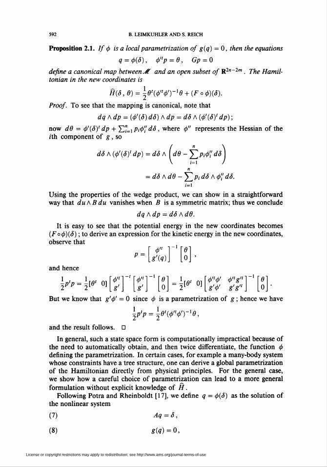
Proposition 2.1. If tp is a local parametrization of g(q) = 0, then the equations

q = <KS), <PllP = e, Gp = 0

define a canonical map between Jf and an open subset of R2"-2m . The Hamil-

tonian in the new coordinates is

H(o,d)=l-e'(<t>"<t>')-l0 + (F°<t>)(S)-

Proof. To see that the mapping is canonical, note that

dqAdp = {<t>'(ô) dÔ) A dp = dô A (<f>'(ô)< dp) ;

now dd = (p'(ô)' dp + YX=i Pifti dô , where <p" represents the Hessian of the

ith component of g, so

do A (<p'(ô)' dp) = doA¡d6- ¿/>,■#' dô )

n

= dôAdd-YiPidôA<p'i'dô.i=i

Using the properties of the wedge product, we can show in a straightforward

way that du AB du vanishes when B is a symmetric matrix; thus we conclude

dq A dp = dô A dO.

It is easy to see that the potential energy in the new coordinates becomes(Fo(j))(ô) ; to derive an expression for the kinetic energy in the new coordinates,

observe that

and hence

~p'p = W 0]g'

P =

<f>"g'

cp"

g'(q)

-i

= jie' o]g'V g'g"

But we know that g'tp' = 0 since <j> is a parametrization of g ; hence we have

^p^öwr'ö,and the result follows. □

In general, such a state space form is computationally impractical because of

the need to automatically obtain, and then twice differentiate, the function <j>

defining the parametrization. In certain cases, for example a many-body system

whose constraints have a tree structure, one can derive a global parametrization

of the Hamiltonian directly from physical principles. For the general case,

we show how a careful choice of parametrization can lead to a more general

formulation without explicit knowledge of H.Following Potra and Rheinboldt [17], we define q = <f>(ô) as the solution of

the nonlinear system

(7) Aq = ô,

(8) g(q) = 0,



where the constant matrix A e R("-m)xn is chosen so that R = [^] is a nonsin-

gular matrix. Typically, A is treated as a piecewise constant function of time.Previous authors have used the induced state space form obtained by settingô' - 6 to solve multibody dynamics problems, but instead, we here choose 6

according to Proposition 2.1 to insure a canonical map.

If the mapping <j> = qb(6) in Proposition 2.1 is defined by (7)-(8), then <j>'can be written explicitly as

tj)1 = R~x

Hence, the equations determining 6 boil down to

[/ 0]R-'p = 6, Gp = 0.

Thus, we must haver a~\

-.b

for some O; hence p = R'b = Al6 + G'Q. Now by virtue of Gp = 0, weobtain

(9) p = (I-ß?)A<6

with %f = Gt(GGt)~xG.

Theorem 2.2. Suppose a parametrization of g(q) = 0 ¿s defined via (7)-(8).

Then the corresponding Hamiltonian state space form is characterized by

(10) o = A(I-ß?)A'd,

(11) A(I- ß?)A'd = -A(I - ßT)VF(q) + A(I - ßf)ß?q(p, A'6),

since A(I - ß?)A' is nonsingular.

Proof. Differentiating (7) with respect to time and using (9) yields

S = Aq = Ap = A(I - ß?)A'0.

Next differentiate (9) with respect to time, replace p by (6), and premultiplyby A(I - %?) to obtain equation (11). □

It must be pointed out that although we began this section treating a problem

with a separable Hamiltonian (i.e., H(q, p) — T(p)+V(q)), the Hamiltonian of

the canonical state space form ODE is not separable. Since no explicit symplec-

tic discretizations are available for a general Hamiltonian, it would be necessaryto employ an implicit scheme. In [11], it is shown that the mixed set of equa-

tions (7)-(l 1) in q, p, ô, and 6 can be solved effectively with Gauss-Legendre

Runge-Kutta discretization by an algorithm based on functional iteration. How-

ever, there is a more serious and perhaps insurmountable problem with using

the discretized state space form for symplectic integration.

Recent results (see, e.g., Sanz-Serna [20]) indicate that an integrator for a

Hamiltonian system should consist of the iteration of one and the same sym-

plectic map. In this case, it can be shown that there is a nearby Hamiltonian

for which the numerical solution is nearly the exact flow. In terms of our state

space form this means that the matrix A must be held constant; in other words,A must define a parametrization valid along the entire trajectory.



xlO

Figure 2. Energy error in numerically computed state space

form vs. time

To illustrate the difficulty when the parametrization changes along a trajectory

(i.e., when we switch from one local chart of the manifold to another), we

consider the plane pendulum with unit length and mass, where for q, p Ç.R2 ,we have

H(q , p) = \plp + gq2 ,

(12)

(13)

(14)

q = p,

p =o

-g - Xq.

10 = ^0-1).

We parametrized the unit circle in four charts, Q,, i = 1, ... , 4, usingalternately x and y as parameter, and following the program of Theorem

2.2. The chart was changed when y crossed the threshold values ±\/2/2.

For our experiment, we took g = 0 and set (qx(0), q2(0), px(0), p2(0)) =

(1,0,0,-2). In each chart, we applied the implicit midpoint method. Thisresulted in correct dynamics on bounded intervals as h —► 0.

As illustrated in Figure 2 (with h = .01), we observed an undesirable drift in

the energy of the numerical solution. Such behavior would not be anticipated

from fixed stepsize symplectic integration of a single Hamiltonian vector field.

Nevertheless, the numerical results for the Hamiltonian state space form werea vast improvement over the results with BDF-2.

3. Hamiltonian underlying ODEs

We now examine the possibility of obtaining Hamiltonian underlying ODEs

as an alternative to the computation of the state space form. In case the con-

straint is linear, Gq = 0, with G constant, the standard underlying ODE ( 1 )-

(2) reduces to

q=p, p = -(I-JT)VF(q).

This ODE system is not Hamiltonian because the projection of VF is not

necessarily the gradient of any function; however, it is easy to construct an



underlying ODE which is Hamiltonian: we simply note that if q lies on Gq =

0, then (/ - ßf)q = q , so that

q=P, p = -(I-^)VF((I-^)q)

is also an underlying ODE—and this one is a Hamiltonian system.

For the nonlinearly constrained case, we make use of Dirac's theory of con-

strained Hamiltonian systems [8].

3.1. Nonlinearly constrained Hamiltonians. In this subsection, we will derive

a modified, unconstrained Hamiltonian with the property that on Jf the mod-ified and the original Hamiltonian are identical and that Jf is an invariantmanifold of the flow corresponding to the modified Hamiltonian. As a result,we will obtain a Hamiltonian ODE whose flow on Jf reduces to the flow of

(3)-(5). The main idea in the construction of the modified Hamiltonian is the

following: for a Hamiltonian function H = H(q, p) and a scalar-valued func-

tion 0 = <p{q, p), the condition for tf> to be an invariant under the flow of the

Hamiltonian system derived from H is just that the Poisson bracket [17] of <j>

with H vanishes, i.e.,

^tWidp--diidq-=-{((>'H} = 0-

Following Dirac [8], we make a distinction between two types of invariants.

<t>{q> P) = 0 is said to be a strong invariant of the flow derived from H in case{<j>, H} vanishes identically. A weak invariant is one that satisfies {(/>, H} = 0only when cp(q, p) = 0. In the latter case we will often write {</>, H} « 0.We make use of the following elementary properties of Poisson brackets for

functions <f>, y/, to: R2n —* R and real constants ax, a2 :

(i) {</>, y/} = -{y/, <j>} ,

(ii) {<£,<£} = 0,(iii) {ax<f>x + a2<t>2 , y/} = ax{4>x, y/} + a2{4>2, y/};

W, cxx<t>x + a2<t>2} = ax{y/, <j>x} + a2{\p, cj>2} ,

(iv) {4>, y/co} = {(/>, \p}œ + {4>,œ}y/.

If 0 is not an invariant of the Hamiltonian H, as in the case of constrainedHamiltonian systems with H = p'p/2 + F(q) and <j> = g, consider the adjusted

(constrained) Hamiltonian function

H(j] = H + p<f>.

Here the function p = p(q, p) plays much the same role as the Lagrange

multiplier in (3)-(5). The function p is chosen to insure </> = 0 along solutions,

which certainly holds if 0 is a weak invariant of the flow of Hj . For this to

happen, we need that

0 « {<b, H{Tl)} = {<p, H}+ {<!>, p<p) = {<!>, H} + {<p, <p}p + {</», p}<p.

Taking <p = 0 in the above, and noting that {</>,</>} = 0, we must have{(p, H} « 0. Since we assumed {<f>, H} ^ 0, we have to treat the equation

y/ = {</>, H} = 0 as a new constraint and consider the revised Hamiltonian

H(}] = H + px<p + p2y/.



If we now seek px = px(q, p) and p2 = p2(q,p) to insure that both {<f>,HT'}

« 0 and {y/, H^} « 0, we find that the key issue concerns the invertibility of

the matrix of Poisson brackets,

0 {(p,vY{y/,<fi} 0 '

When {</>, y/} / 0, then R is nonsingular, and we can solve for the functions

(px, p2) so that both </> — 0 and y/ = 0 are invariant for H^ . Furthermore,

on (j) = y/ = 0 we have HT2^ = H.

We now turn to the case of a vector-valued constraint function. The main

thing to bear in mind here is that, in the end, the constraints must be treated

all at once, not one at a time. Given a vector of constraints </> = 0, one must

first augment these constraints by all of the "hidden" constraints which arise

by taking Poisson brackets with the augmented Hamiltonians, i.e., through the

recursive differentiation of the constraints and substitution of the differential

equations derived from the Hamiltonian. This approach is taken in [13] in

deriving control laws for constrained systems, where it is shown that two steps

of the reduction process are sufficient if the constraints are independent and

holonomic, i.e., essentially only dependent on q .As an example, if we follow the reduction for H = p'p/2 + F(q) and in-

dependent constraints of the form g(q) = 0, we obtain the hidden constraints

G(q)p = 0. The next step is the construction of the modified Hamiltonian Ht

from H and the constraints; thus we set

HT(q, p) := H(q, p) + p'g(q) + n'G(q)p.

Equations for p and r\ can be derived directly by insuring that g(q) = 0and G(q)p = 0 are either weak or strong invariants of the flow derived from

Ht . A slight generalization of the Poisson bracket notation to handle multiple

constraints makes this straightforward.

Definiton 3.1. Given vector-valued functions <p: R2n -* Rl and y/: R2n -* Rm ,

the Poisson bracket of <f> and y/ is the / x m matrix whose (i, j)-component

is defined by

({</>> ¥})i,j = {<Pi> ¥j}-

The following proposition shows how the generalized Poisson bracket can be

evaluated in terms of the Jacobians of the vector functions.

Proposition 3.1. Given vector-valued functions (j>: R2n -> R' and y/: R2n -► Rm ,

let (f>q, <pp € Rlxn, y/q, y/p e Rmxn, and denote the Jacobian matrices of the

indicated function with respect to the indicated variables. Then

{</>, y/} = cj)qy/'p - <ppy/q.

Using Proposition 3.1, we can easily see that {</>, y/} = -{<p, </)}'. Proposi-

tion 3.2 is also useful in calculations:

Proposition 3.2. // <f> and y/ are as in Proposition 3.1, and X: R2n -► Rm , then

R {<P,<I>} {<P,V}{y/,(f>} {ty,H

{4>,Xly/} = {<t>, y/}X + {4>, X}y/.



Proof. We have

= {<p, y/}X + {<p, X}y/. D

The generalized Poisson bracket described here is purely a computationaldevice and not technically a Poisson bracket in the classical sense (see, e.g.,

[17]). In particular, the Poisson bracket of a vector function with itself is a

skew-symmetric matrix.To get an invariant, we require

{g, HT} = {g,H} + {g, p'g} + {g, n'Gp} = 0,

{Gp, HT} = {Gp, H} + {Gp, p'g} + {Gp, n'Gp} = 0.

Working out the Poisson brackets in the first equation, we get

(15) -{g,H} = {g,g}p + {g,p}g + {g,Gp}n + {g,n}Gp.

If we do not take the constraints to be satisfied and seek p and n so that, e.g.,

{g, Ht} = 0, then we need to solve a system of partial differential equations

which actually becomes singular along the constraints; thus it seems to be too

much to ask for strong invariance of the constraints.

On the other hand, for a weak invariant, we may assume that g = Gp = 0.

Next, note that {g, g} vanishes because g is a function of q only. Moreover,

{¿?, Gp} = GG', and thus

-{g,H} = GG'n.

This can be solved for n provided G has full rank.

The second equation can be reduced to

-{Gp, H} = -GG'p + {Gp, p}g + [(Gp)qG< - G(Gp)'q]r, - {Gp, n}Gp.

Again, for weak invariance, the terms multiplied by g and Gp drop out andwe are left with equations which uniquely determine p. Once p and n are

known, the Hamiltonian function Ht is determined and the unconstrained

equations of motion can be found by differentiating HT :

(16) q=P + Ppg + ri'pGp + G'r1,

(17) p = -VF-p'qg-G'p-n'qGp-(Gp)'qn.

From a computational point of view, it may be quite involved to formu-

late the system in this manner. In particular, we now need to compute third

derivatives of g and second derivatives of F. Below we will consider somesimplifications in the hope of improving the computational efficacy of Hamil-

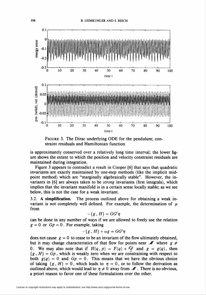
tonian formulation.In Figure 3 (next page), a numerical experiment with the Hamiltonian un-

derlying ODE for the nonlinear pendulum (12)—(14) in Cartesian coordinates

is summarized. We computed p and n as described above. Starting from theinitial configuration (qx, q2, px, p2) = (1,0,0, -2), we solved the resultingHamiltonian underlying ODE (16)—(17), using the implicit midpoint method

and h = . 1. The upper graph in Figure 3 demonstrates that the Hamiltonian



0.1 i-1-1-1-1-1-1-r

time t

time t

Figure 3. The Dirac underlying ODE for the pendulum; con-

straint residuals and Hamiltonian function

is approximately conserved over a relatively long time interval; the lower fig-

ure shows the extent to which the position and velocity constraint residuals are

maintained during integration.Figure 3 appears to contradict a result in Cooper [6] that says that quadratic

invariants are exactly maintained by one-step methods (like the implicit mid-point method) which are "marginally algebraically stable". However, the in-

variants in [6] are always taken to be strong invariants (first integrals), which

implies that the invariant manifold is in a certain sense locally stable; as we see

below, this is not the case for a weak invariant.

3.2. A simplification. The process outlined above for obtaining a weak in-

variant is not completely well defined. For example, the determination of p

from-{g,H} = GG'n

can be done in any number of ways if we are allowed to freely use the relation

g = 0 or Gp = 0. For example, taking

-{g,H} + ag = GG'n

does not cause g = 0 to cease to be an invariant of the flow ultimately obtained,but it may change characteristics of that flow for points near Jf where g ¿

0. We may also note that if H(q, p) = F(q) + ¿£ and g = g(q), then{g, H} = Gp, which is weakly zero when we are constraining with respect to

both g(q) = 0 and Gp = 0. This means that we have the obvious choiceof taking {g, H} = 0, which leads to n = 0, or to follow the derivation asoutlined above, which would lead to n ^ 0 away from Jf. There is no obvious,

a priori reason to favor one of these formulations over the other.



Figure 4. Hamiltonian function and constraint residuals for

the simplified Hamiltonian formulation

If we take n = 0, we get

HT = H + p'g,

so that, after insuring that Jf is invariant, we arrive at

(18) A-^..t

(19)

q = p + ßPg,

P = -VF-p'qg-G'p.,

where p = (GG')~X(GVF - Gq(p, p)). This system requires the computation

of third derivatives of g and second derivatives of H as before.Besides providing a simplified Hamiltonian formulation, ( 18)—( 19) has

the immediate and natural consequence of showing that along the constraint

(g — 0), the standard underlying ODE generates a Hamiltonian flow. However,

as shown in the next section, the formulation (18)—(19) can possess a some-

what surprising instability, which can be observed in computations whenever

numerical discretization induces a perturbation of the constraint. In Figure 4,

the implicit midpoint method (a canonical discretization scheme) has been ap-

plied to solve (18)—(19) for the Cartesian pendulum discussed above with fixed

stepsize h = .01 from t = 0 to t = 1 with the same initial conditions as for

Figure 3. Although the wedge product is maintained in this case, the constraint

residuals and the Hamiltonian function are very rapidly growing in time.

3.3. Stability of the constraint-invariants. Let us begin with the case of a

linearly constrained quadratic Hamiltonian with constraint <p = Gq and G



constant. Here we find that the simplified Hamiltonian system based on HT =

H + p'Gq is

q=p, p = -(I-ß?)VF + D2Fß?q,

where D2F is the Hessian matrix of F. Multiplying both equations by the

(here constant) projector ß?, we obtain

ß?q = ß?p, ß?p = ß?D2Fß?q.

Since ßf = ß?2 , we can change to variables r = ß?q, s = ßfp and write

(20) r = s,

(21) s = Br,

where B = ßfD2Fß^. Invariance of the constraints translates to r = s = 0.

If the Hessian is constant and positive definite, as is the case near a stable

equilibrium, B is positive semidefinite, and the equilibrium position in (20)-(21) will be a saddle point. In this situation, one can expect an instability under

perturbation of the constraint-invariants introduced via discretization.

If we perform a similar analysis starting from the Hamiltonian Ht = ^ +

F{q) + p'Gq + n'Gp of Dirac, we arrive at equations

q = (I- 2ß?)p, p = -(I- ß?)VF + D2Fß?q.

Multiplying the equations by ßf, we get

JTq = ß?(I - 2ß?)p = -ß?p, ß?p = ß?D2Fß?q.

Hence, the corresponding system of differential equations for the constraint

residuals is

(22) r = -s,

(23) s = Br.

Now the equilibrium position r = s = 0 has become a stable center under the

assumption that D2F is positive definite.

3.4. Nonlinear constraints. We begin the discussion by writing the equationsof motion for both formulations in the case of a single position constraint <f>.

We derive a constraint of the form y/ = {cf>, H} . Assuming {</>, y/} ^ 0, we

arrive at the Hamiltonian HT = H + p'tp + n'y/. The conditions on p and n

reduce to

{<t>,HT}nO^{(b,H}-r{<p,¥}n = 0,

{y/, HT} « 0 => {y/, H} + {y/, <f>}p + {y/, y/}r] = 0.

Since {y/, <f>} is an invertible matrix, and using {$, H} = y/, we have

n = -{tp, yf}-lyt,

ß = -{¥, 4>}~1\{V, H} - {y/, y/}{4>, y/}~xy/].



Now {(¡), 4>} = 0. Also, because the constraint is scalar, {y/, y/} = 0. Next,we write differential equations for the constraint residuals; thus

¡f> = {<p, Ht} = y/ + {<j>, -{y/, <p}-x[{y/, H} = {y/, yi}{<p, y/}-xy/]}<f)

+ {<t>,-{4>, y/}-xy/}y/ + {4>, y/}[-{<t>, ¥}~W],yj = {y,,HT} = {y,H} + {y,,-{y,,<l>}-x[{y,,H}-{y,,¥}{$,y/}-xy,\}t>

+ {¥, <!>}[-{¥, <t>}-\{V,H} - {y/, y/}{cp, ̂}"V)]

+ {y/, ~{<p, ¥}~x ¥}¥ + {¥, ¥}[-{<!>, ¥}~l¥l

This simplifies to the system

(24) ¿ = -{«/», {yv, <p}-x{¥, H}}<f>-{<p, {<p, ip}-W}¥,

(25) ¥ = -{¥, {¥,(f>r1{¥,H}}(l>-{¥, W, ¥}~l¥}¥-

Now by employing the product rule for Poisson brackets (Proposition 3.2),

we get

{(f), {</», y/}-ly/}¥ = {4>, {4>, ¥}~l}¥2 + {<P, ¥}{<P, ¥}~l¥ = ¥ + 0(y/2).

Similarly, we have

{y/, {(f>, y/}~l¥}¥ = {¥, {<t>, ¥}~]}¥2 + {¥, ¥}{<t>, V}~V = 0(y/2).

Thus, in the neighborhood of the constraint manifold, we have the following

driving differential equations for the residuals:

(26) i = -V-{<l>,{¥,<prl{¥,H}}<p,

(27) y, = -{y,,{y,,(f)}-x{y,,H}}(t>.

On the other hand, if we start with Ht = H + p''(p, then we obtain via the

same sort of calculations

(28) ^=¥-{<P,{¥,4>}-l{V,H}}4>,

(29) y, = -{y,,{y,,d>}-x{y/,H}}(f>.

Note that the only difference between (26)-(27) and (28)-(29) is the sign thatappears with y/ in the first equation of each system.

Let us turn to an example. For the Cartesian pendulum with zero gravity,

0 = (q'q - l)/2 and y/ = q'p . The Dirac Hamiltonian becomes

u i„ n\ P'P^lP'Pt„t„ n (g'P)2

and the corresponding ODE system is

(2q'q-i. 2 A

p=-7%q + 2^p-2(^)2q.(q'q)2 q'q \q'q)



Equations for 0 and 0 follow immediately:

0

¥

The term p'p is a nuisance. If we treat it as a time-dependent coefficient,

linearizing at </> = y/ = 0, we get

j>=-¥, y/ = 4p'p(p,

which makes the origin a center; this agrees with the numerical experimentshown in Figure 3.

By contrast, if we had only made use of constraints on q in formulating the

system, we would have had, after following the above analysis and linearizing,

j>=y/, y/ = 4p'p(f>,

meaning that the origin has become a saddle point; this is exactly the situationwe would expect from viewing Figure 4.

Although the general nonlinear case can be quite complicated, some gener-alization of the comparative analysis for linear systems of the first part of this

section is possible via linearization of nonlinear constraints if we bear in mind

that a potential energy function always has a positive definite Hessian at least

in the neighborhood of a stable equilibrium [7]. On the other hand, all we

can conclude from the stability of the linearized system is the absence of anexponential instability in the nonlinear system [2].

3.5. Weakly Hamiltonian underlying ODE. Dirac's process requires the dif-

ferentiation of the constraint multipliers p and n ; since p and t] depend onsecond derivatives of g and first derivatives of H, construction of a Hamilto-nian underlying ODE along the lines of Dirac's theory in general requires third

derivatives of g and second derivatives of H. However, along the constraint

manifold Jf, which is an invariant under the flow of (16)—(17), the termsmultiplying the partial derivatives of p and t] vanish, and we are left with a

simplified system:

(30) q = VpH + G'n,

(31) p = -VqH-G'p-(Gp)'qn.

This system (referred to as the "Weakly Hamiltonian Dirac formulation") be-

haves like a Hamiltonian system for initial values chosen on the constraint man-

ifold; in fact, any underlying ODE is a Hamiltonian system along the constraint

manifold. But under numerical discretization we cannot in general expect the

constraints to be maintained exactly, so that a canonical ODE discretization

scheme applied to (30)—(31) would not result in a canonical step-to-step map.On the other hand, (30)—(31) requires only the computation of second deriva-

tives of g and first derivatives of H ; hence it may be much more easily com-puted for certain problems. This formulation has been treated in the literature

— nlq'q = q'p - 2q'p +q'q - 1 „,

q'qqp -y/ +

y/(f)

q'p+p'q

0+1/2't.

= 2p'p J>

p'p i *(q'p) i q'q-■t-f +p'p - 2^-p- +p'p—.—q'q q'q q'q

¥2

0+1/2 0+1/2'



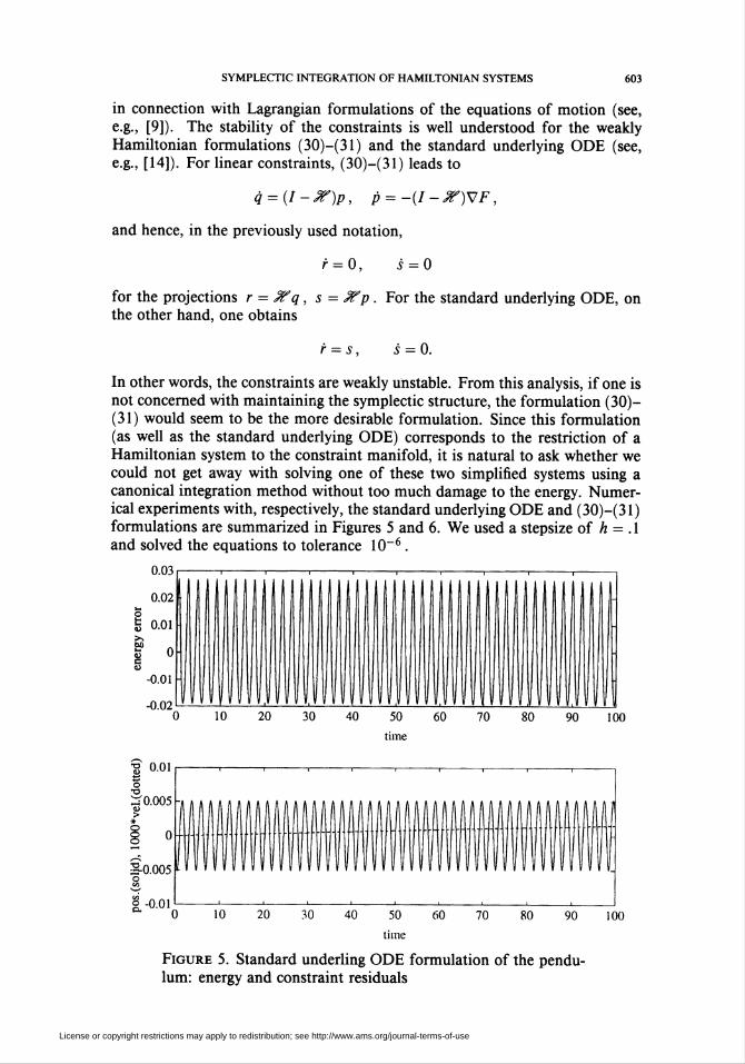
in connection with Lagrangian formulations of the equations of motion (see,

e-g-> [9])- The stability of the constraints is well understood for the weakly

Hamiltonian formulations (30)—(31) and the standard underlying ODE (see,

eg-> [14]). For linear constraints, (30)—(31) leads to

q = (I-ßT)p, p = -(I-ß?)VF,

and hence, in the previously used notation,

r = 0, 5 = 0

for the projections r = ßfq, s = ßfp . For the standard underlying ODE, onthe other hand, one obtains

r = s. ¿ = 0.

In other words, the constraints are weakly unstable. From this analysis, if one isnot concerned with maintaining the symplectic structure, the formulation (30)-

(31) would seem to be the more desirable formulation. Since this formulation

(as well as the standard underlying ODE) corresponds to the restriction of a

Hamiltonian system to the constraint manifold, it is natural to ask whether we

could not get away with solving one of these two simplified systems using a

canonical integration method without too much damage to the energy. Numer-

ical experiments with, respectively, the standard underlying ODE and (30)—(31)

formulations are summarized in Figures 5 and 6. We used a stepsize of h = . 1and solved the equations to tolerance 10-6 .

0.03

Figure 5. Standard underling ODE formulation of the pendu-lum: energy and constraint residuals



xlO-4

Figure 6. The weakly Hamiltonian Dirac formulation for the

pendulum

These experiments seem to indicate that direct integration of the weakly

Hamiltonian formulations with a canonical integrator may offer a practical, al-

though nonsymplectic, alternative to the true Hamiltonian formulation, evenon relatively long intervals. Note that the energy conservation observed in Fig-

ure 6 is far better than that observed in Figure 3, and somewhat better than

that of Figure 5. It turns out that this is exceptionally good behavior owing to

the combination of having a single quadratic constraint and using the implicit

midpoint method, since the original Hamiltonian H is a first integral of thereformulation in this case. This topic will be addressed in a future article.

Acknowledgment

We would like to thank Linda Petzold for pointing us to this problem, and

Peter Deuflhard, Jacek Szmigielski, and the referee for their useful comments.

We are especially grateful to the referee for assistance with §2.

Bibliography

1. R. Abraham and J. E. Marsden, Foundations of mechanics, 2nd ed., Benjamin, Reading,

MA, 1978.

2. V. I. Arnold, Mathematical methods of classical mechanics, Graduate Texts in Math., Vol.

60, Springer-Verlag, New York, 1975.

3. U.M. Ascher and L. R. Petzold, Stability of computational methods for constrained dynamics

systems, SIAM J. Sei. Statist. Comput. 14 (1993), 95-120.

4. J. Baumgarte, Stabilization of constraints and integrals of motion in dynamical systems,

Comp. Methods Appl. Mech. Engrg. 1 (1976), 1-16.



5. K. E. Brenan, S. L. Campbell, and L. R. Petzold, Numerical solution of initial value problems

in differential-algebraic equations, North-Holland, Amsterdam, 1989.

6. G. J. Cooper, Stability of Runge-Kutta methods for trajectory problems, IMA J. Numer.

Anal. 7(1987), 1-13.

7. R. Courant and D. Hubert, Methods of mathematical physics, Wiley, New York, 1953.

8. P. A. M. Dirac, Lectures on quantum mechanics, Belfer Graduate School Monographs, no.

3, Yeshiva University, 1964.

9. E. Eich, C. Führer, B. Leimkuhler, and S. Reich, Stabilization and projection methods for

multibody dynamics, Report A281, Helsinki Univ. of Technology, Helsinki, 1990.

10. L. Jay, Symplectic partitioned Runge-Kutta methods for constrained Hamiltonian systems,

Technical Report, Université de Genève, 1993.

11. B. Leimkuhler and S. Reich, Numerical methods for constrained Hamiltonian systems, Tech-

nical Report, Konrad Zuse Center, Berlin, 1992.

12. B. Leimkuhler and R. D. Skeel, Symplectic numerical integrators for constrained molecular

dynamics, Technical Report, Dept. of Math., University of Kansas, Lawrence KS, 1992.

13. N. H. McClamroch and A. M. Bloch, Control of constrained Hamiltonian systems and

applications to control of constrained robots, Dynamical Systems Approaches to Nonlinear

Problems in Systems and Circuits (Fathi M. A. Salam and Mark L. Levi, eds.), SIAM,

Philadelphia, PA, 1988, pp. 344-403.

14. T. Mrziglod, Zur Theorie und numerischen Realisierung von Lösungsmethoden bei Differ-

entialgleichungen mit angekoppelten algebraischen Gleichungen, Diplomarbeit, Math. Inst.,

Univ. zu Köln, 1987.

15. J. M. Sanz-Serna, Symplectic integrators for Hamiltonian problems: an overview, Acta Nu-

mer. 1 (1991).

16. P. Olver, Applications of Lie groups to differential equations, Springer-Verlag, Berlin and

New York, 1986.

17. F. Potra and W. Rheinboldt, On the numerical solution of the Euler-Lagrange equations,

NATO Advanced Research Workshop on Real-Time Integration Methods for Mechanical

System Simulation (R. Deyo and E. Haug, eds.), Springer-Verlag, Berlin and New York,

1990.

18. S. Reich, Symplectic integration of constrained Hamiltonian systems by Runge-Kutta meth-

ods, Technical Report 93-13, Dept. of Comput. Sei., University of British Columbia, 1993.

19. W. Rheinboldt, Numerical analysis of parametrized nonlinear equations, Univ. Ark. Lecture

Notes in Math. Sei., vol. 7, Wiley, New York, 1986.

20. J. M. Sanz-Serna, Runge-Kutta schemes for Hamiltonian systems, BIT 28 (1988), 877-883.

Department of Mathematics, University of Kansas, Lawrence, Kansas 66045-2142

E-mail address : le imkuhlQmath. ukan s. edu

Institute of Applied Mathematics and Statistics, Berlin O-1086, Germany

Current address: University of British Columbia, Vancouver, British Columbia, Canada

V6T 1Z2


symplectic integration of constrained … integration of constrained hamiltonian systems ......

Documents