synchronization and linearity - rocq.inria.fr · synchronization and linearity an algebra for...
TRANSCRIPT

Synchronization and LinearityAn Algebra for Discrete Event Systems
Francois BaccelliINRIA
andEcole Normale Sup´erieure, Departement d’Informatique
Paris,France
Guy CohenEcole Nationale des Ponts et Chauss´ees-CERMICS
Marne la Vallee, Franceand
INRIA
Geert Jan OlsderDelft University of Technology
Faculty of Technical MathematicsDelft, the Netherlands
Jean-Pierre QuadratInstitut National de la Recherche en Informatique et en Automatique
INRIA-RocquencourtLe Chesnay, France


Preface to the Web Edition
The first edition of this book was published in 1992 by Wiley (ISBN 0 471 93609 X).Since this book is now out of print, and to answer the request of several colleagues,the authors have decided to make it available freely on the Web, while retaining thecopyright, for the benefit of the scientific community.
Copyright Statement
This electronic document is in PDF format. One needs Acrobat Reader (availablefreely for most platforms from the Adobe web site) to benefit from the full interactivemachinery: using the packagehyperref by Sebastian Rahtz, the table of contentsand all LATEX cross-references are automatically converted into clickable hyperlinks,bookmarks are generated automatically, etc.. So, do not hesitate to click on referencesto equation or section numbers, on items of the table ofcontents and of the index, etc..
One may freely use and print thisdocument for one’s own purpose or even dis-tribute it freely, but not commercially, provided it is distributed in its entirety andwithout modifications, including this preface and copyright statement. Any use ofthe contents should be acknowledgedaccording to the standard scientific practice. Theauthors will appreciate receiving any comments by e-mail or other means; all modifica-tions resulting from these comments in future releases will be adequately and gratefullyacknowledged.
About This and Future Releases
We have taken the opportunity of this electronic edition to make corrections of mis-prints and slight mistakes we have become aware of since the book was published forthe first time. In the present release, alterations of the original text are mild and need nospecial mention: they concern typographic style (which may result in a different pagi-nation with respect to the original paper version of the book), the way some equationsare displayed, and obvious mistakes. Some sentences may even have been rephrasedfor better clarity without altering the original meaning. There are, however, no changesin the numbering of equations, theorems, remarks, etc..
Fromtime to time in the near future, we plan to offer new releases in which moresubstantial alterations of the original text will be provided. Indeed, we consider somematerial as somewhat outdated (and sometimes even wrong). These more importantmodifications will initially be listed explicitly and provided separately from the original
i

ii Synchronization and Linearity
text. In a more remote future, we may consider providing a true “second edition” inwhich these changes will be incorporatedin the main text itself, sometimes removingthe obsolete or wrong corresponding portions.
Francois Baccelli [email protected] Cohen [email protected] Jan Olsder [email protected] Quadrat [email protected]
October 2001
Contents
Preface ix
I Discrete EventSystems and Petri Nets 1
1 Intro duction and Motivation 31.1 Preliminary Remarks and Some Notation . . . . . . . . . . . . . . . 31.2 MiscellaneousExamples . . . . . . . . . . . . . . . . . . . . . . . . 8
1.2.1 Planning . . . . . . . . . . . . . . . . . . . . . . . . . . . . 91.2.2 Communication . . . . . . . . . . . . . . . . . . . . . . . . . 141.2.3 Production . . . . . . . . . . . . . . . . . . . . . . . . . . . 151.2.4 QueuingSystemwith Finite Capacity . . . . . . . . . . . . . 181.2.5 Parallel Computation . . . . . . . . . . . . . . . . . . . . . . 201.2.6 Traffic . . . . . . . . . . . . . . . . . . . . . . . . . . . . . . 221.2.7 Continuous System Subject to Flow Bounds and Mixing . . . 25
1.3 Issuesand Problems in PerformanceEvaluation . . . . . . . . . . . . 281.4 Notes . . . . . . . . . . . . . . . . . . . . . . . . . . . . . . . . . . 32
2 Graph Theory and Petri Nets 352.1 Introduction . .. . . . . . . . . . . . . . . . . . . . . . . . . . . . . 352.2 DirectedGraphs . . . . . . . . . . . . . . . . . . . . . . . . . . . . . 352.3 Graphsand Matrices . . . . . . . . . . . . . . . . . . . . . . . . . . 38
2.3.1 Composition of Matrices and Graphs. . . . . . . . . . . . . 412.3.2 MaximumCycle Mean . . . . . . . . . . . . . . . . . . . . . 462.3.3 TheCayley-Hamilton Theorem . .. . . . . . . . . . . . . . 48
2.4 Petri Nets . . . . . . . . . . . . . . . . . . . . . . . . . . . . . . . . 532.4.1 Definition . . . . . . . . . . . . . . . . . . . . . . . . . . . . 532.4.2 Subclasses andProperties of Petri Nets . . . . . . . . . . . . 59
2.5 TimedEvent Graphs . . . . . . . . . . . . . . . . . . . . . . . . . . 622.5.1 Simple Examples . . . . . . . . . . . . . . . . . . . . . . . . 632.5.2 The Basic Autonomous Equation .. . . . . . . . . . . . . . 682.5.3 Constructivenessof the Evolution Equations . . . . . . . . . 772.5.4 Standard Autonomous Equations . .. . . . . . . . . . . . . . 812.5.5 The Nonautonomous Case. . . . . . . . . . . . . . . . . . . 832.5.6 Construction of theMarking . . . . . . . . . . . . . . . . . . 872.5.7 Stochastic Event Graphs . . . . . . . . . . . . . . . . . . . . 87
2.6 Modeling Issues . . . . . . . . . . . . . . . . . . . . . . . . . . . . . 88
iii

iv Synchronization and Linearity
2.6.1 Multigraphs. . . . . . . . . . . . . . . . . . . . . . . . . . . 882.6.2 Places with Finite Capacity. . . . . . . . . . . . . . . . . . . 892.6.3 Synthesis of Event Graphsfrom Interacting Resources . . . . 90
2.7 Notes . . . . . . . . . . . . . . . . . . . . . . . . . . . . . . . . . . 97
II Algebra 99
3 Max-Plus Algebra 1013.1 Introduction .. . . . . . . . . . . . . . . . . . . . . . . . . . . . . . 101
3.1.1 Definitions . . . . . . . . . . . . . . . . . . . . . . . . . . . 1013.1.2 Notation . . . . . . . . . . . . . . . . . . . . . . . . . . . . 1033.1.3 Themin Operation in theMax-PlusAlgebra . . . . . . . . . . 103
3.2 Matrices inRmax . . . . . . . . . . . . . . . . . . . . . . . . . . . . 1043.2.1 Linearand AffineScalar Functions . . . . . . . . . . . . . . 1053.2.2 Structures . . . . . . . . . . . . . . . . . . . . . . . . . . . . 1063.2.3 Systems of Linear Equations in(Rmax)
n . . . . . . . . . . . . 1083.2.4 Spectral Theory of Matrices . . . . . . . . . . . . . . . . . . 1113.2.5 Appli cation to Event Graphs . . . . . . . . . . . . . . . . . . 114
3.3 Scalar Functions inRmax . . . . . . . . . . . . . . . . . . . . . . . . 1163.3.1 Polynomial FunctionsP(Rmax) . . . . . . . . . . . . . . . . 1163.3.2 Rational Functions . . . . . . . . . . . . . . . . . . . . . . . 1243.3.3 Algebraic Equations . . . . . . . . . . . . . . . . . . . . . . 127
3.4 Symmetrization of theMax-PlusAlgebra . . . . . . . . . . . . . . . 1293.4.1 The Algebraic StructureS . . . . . . . . . . . . . . . . . . . 1293.4.2 LinearBalances. . . . . . . . . . . . . . . . . . . . . . . . . 131
3.5 Linear Systems inS . . . . . . . . . . . . . . . . . . . . . . . . . . . 1333.5.1 Determinant . . . . . . . . . . . . . . . . . . . . . . . . . . . 1343.5.2 Solving Systems of Linear Balances by the Cramer Rule . . . 135
3.6 Polynomials with Coefficients inS . . . . . . . . . . . . . . . . . . . 1383.6.1 Some Polynomial Functions . . .. . . . . . . . . . . . . . . 1383.6.2 Factorization of Polynomial Functions. . . . . . . . . . . . . 139
3.7 Asymptotic Behavior ofAk . . . . . . . . . . . . . . . . . . . . . . . 1433.7.1 Critical Graph of aMatrix A . . . . . . . . . . . . . . . . . . 1433.7.2 EigenspaceAssociatedwith the Maximum Eigenvalue . . . . 1453.7.3 Spectral Projector . . . . . . . . . . . . . . . . . . . . . . . . 1473.7.4 Convergence ofAk with k . . . . . . . . . . . . . . . . . . . 1483.7.5 Cyclic Matrices. . . . . . . . . . . . . . . . . . . . . . . . . 150
3.8 Notes . . . . . . . . . . . . . . . . . . . . . . . . . . . . . . . . . . 151
4 Dioids 1534.1 Introduction .. . . . . . . . . . . . . . . . . . . . . . . . . . . . . . 1534.2 Basic Definitionsand Examples . . . . . . . . . . . . . . . . . . . . 154
4.2.1 Axiomatics . . . . . . . . . . . . . . . . . . . . . . . . . . . 1544.2.2 Some Examples . . . . . . . . . . . . . . . . . . . . . . . . . 1554.2.3 Subdioids. . . . . . . . . . . . . . . . . . . . . . . . . . . . 1564.2.4 Homomorphisms, Isomorphisms and Congruences. . . . . . 157

Contents v
4.3 Lattice Properties of Dioids . .. . . . . . . . . . . . . . . . . . . . . 1584.3.1 Basic Notions in Lattice Theory . .. . . . . . . . . . . . . . 1584.3.2 OrderStructure of Dioids. . . . . . . . . . . . . . . . . . . . 1604.3.3 Complete Dioids,Archimedian Dioids . . . . . . . . . . . . . 1624.3.4 Lower Bound. . . . . . . . . . . . . . . . . . . . . . . . . . 1644.3.5 Distributive Dioids . . . . . . . . . . . . . . . . . . . . . . . 165
4.4 IsotoneMappingsand Residuation . . . . . . . . . . . . . . . . . . . 1674.4.1 Isotony and Continuity of Mappings . . . . . . . . . . . . . . 1674.4.2 Elements of Residuation Theory . . . . . . . . . . . . . . . . 1714.4.3 ClosureMappings . . . . . . . . . . . . . . . . . . . . . . . 1774.4.4 Residuation of Addition and Multiplication. . . . . . . . . . 178
4.5 Fixed-Point Equations, Closure of Mappings and Best Approximation 1844.5.1 General Fixed-Point Equations . . . . . . . . . . . . . . . . . 1844.5.2 The Case�(x) = a ◦\x ∧ b . . . . . . . . . . . . . . . . . . . 1884.5.3 The Case�(x) = ax ⊕ b . . . . . . . . . . . . . . . . . . . 1894.5.4 Some Problems of Best Approximation . . . . . . . . . . . . 191
4.6 Matrix Dioids . . . . . . . . . . . . . . . . . . . . . . . . . . . . . . 1944.6.1 From ‘Scalars’ to Matrices . . . . . . . . . . . . . . . . . . . 1944.6.2 Residuation of Matrices and Invertibility . . . . . . . . . . . 195
4.7 Dioids of Polynomials and Power Series . .. . . . . . . . . . . . . . 1974.7.1 Definitions and Properties of Formal Polynomials and Power Series. 1974.7.2 Subtraction andDivisionof Power Series . . . . . . . . . . . 2014.7.3 Polynomial Matrices .. . . . . . . . . . . . . . . . . . . . . 201
4.8 Rational Closureand Rational Representations . . . . . . . . . . . . 2034.8.1 Rational Closureand Rational Calculus . . . . . . . . . . . . 2034.8.2 Rational Representations . . . . . . . . . . . . . . . . . . . . 2054.8.3 Yet Other Rational Representations . . . . . . . . . . . . . . 2074.8.4 Rational Representationsin CommutativeDioids . . . . . . . 208
4.9 Notes . . . . . . . . . . . . . . . . . . . . . . . . . . . . . . . . . . 2104.9.1 Dioids andRelated Structures . . . . . . . . . . . . . . . . . 2104.9.2 RelatedResults . . . . . . . . . . . . . . . . . . . . . . . . . 211
III Determin istic System Theory 213
5 Two-Dimensional Domain Description of Event Graphs 2155.1 Introduction . .. . . . . . . . . . . . . . . . . . . . . . . . . . . . . 2155.2 A Comparison Between Counter and Dater Descriptions .. . . . . . 2175.3 Daters and their Embedding in Nonmonotonic Functions .. . . . . . 221
5.3.1 A Dioid of Nondecreasing Mappings . . . . . . . . . . . . . 2215.3.2 γ -Transforms of Daters and Representation by Power Series inγ . . 224
5.4 Moving to theTwo-Dimensional Description . . . . . . . . . . . . . 2305.4.1 TheZmax Algebra through Another Shift Operator. . . . . . 2305.4.2 TheMax
in[[γ, δ]] Algebra . . . . . . . . . . . . . . . . . . . . . 2325.4.3 Algebra of Information about Events. . . . . . . . . . . . . 2385.4.4 M
axin[[γ, δ]] Equationsfor Event Graphs. . . . . . . . . . . . . 238
5.5 Counters. . . . . . . . . . . . . . . . . . . . . . . . . . . . . . . . . 244

vi Synchronization and Linearity
5.5.1 A First Derivation of Counters . .. . . . . . . . . . . . . . . 2445.5.2 Counters Derived from Daters . .. . . . . . . . . . . . . . . 2455.5.3 Alternative Definition of Counters. . . . . . . . . . . . . . . 2475.5.4 Dynamic Equations of Counters .. . . . . . . . . . . . . . . 248
5.6 Backward Equations . . . . . . . . . . . . . . . . . . . . . . . . . . 2495.6.1 M
axin[[γ, δ]] Backward Equations . . . . . . . . . . . . . . . . 249
5.6.2 Backward Equationsfor Daters . . . . . . . . . . . . . . . . 2515.7 Rationality, Realizability and Periodicity .. . . . . . . . . . . . . . . 253
5.7.1 Preliminaries . . . . . . . . . . . . . . . . . . . . . . . . . . 2535.7.2 Definitions . . . . . . . . . . . . . . . . . . . . . . . . . . . 2545.7.3 Main Theorem . . . . . . . . . . . . . . . . . . . . . . . . . 2555.7.4 On theCodingof Rational Elements . . . . . . . . . . . . . . 2575.7.5 Realizations byγ - andδ-Transforms . . . . . . . . . . . . . 259
5.8 Frequency Response of Event Graphs . .. . . . . . . . . . . . . . . 2615.8.1 Numerical Functions Associated with Elements ofB[[γ, δ]] . . 2615.8.2 Specialization toM
axin[[γ, δ]] . . . . . . . . . . . . . . . . . . 263
5.8.3 Eigenfunctionsof Rational Transfer Functions . . . . . . . . 2645.9 Notes . . . . . . . . . . . . . . . . . . . . . . . . . . . . . . . . . . 268
6 Max-Plus Linear System Theory 2716.1 Introduction .. . . . . . . . . . . . . . . . . . . . . . . . . . . . . . 2716.2 System Algebra . . . . . . . . . . . . . . . . . . . . . . . . . . . . . 271
6.2.1 Definitions . . . . . . . . . . . . . . . . . . . . . . . . . . . 2716.2.2 Some Elementary Systems . . . . . . . . . . . . . . . . . . . 273
6.3 Impulse Responses of Linear Systems . .. . . . . . . . . . . . . . . 2766.3.1 The Algebra of Impulse Responses. . . . . . . . . . . . . . 2766.3.2 Shift-Invariant Systems . . . . . . . . . . . . . . . . . . . . . 2786.3.3 Systems with Nondecreasing Impulse Response .. . . . . . . 279
6.4 Transfer Functions . . . . . . . . . . . . . . . . . . . . . . . . . . . 2806.4.1 Evaluation Homomorphism . . . . . . . . . . . . . . . . . . 2806.4.2 Closed Concave Impulse Responses and Inputs .. . . . . . . 2826.4.3 Closed Convex Inputs. . . . . . . . . . . . . . . . . . . . . 284
6.5 Rational Systems . . . . . . . . . . . . . . . . . . . . . . . . . . . . 2866.5.1 Polynomial, Rational and Algebraic Systems . .. . . . . . . 2866.5.2 Examples of Polynomial Systems. . . . . . . . . . . . . . . 2876.5.3 Characterization of Rational Systems . . . . . . . . . . . . . 2886.5.4 Minimal Representation andReali zation . . . . . . . . . . . . 292
6.6 Correlationsand FeedbackStabili zation . . . . . . . . . . . . . . . . 2946.6.1 Sojourn Time and Correlations. . . . . . . . . . . . . . . . . 2946.6.2 Stability and Stabilization . . . . . . . . . . . . . . . . . . . 2986.6.3 LoopShaping . . . . . . . . . . . . . . . . . . . . . . . . . . 301
6.7 Notes . . . . . . . . . . . . . . . . . . . . . . . . . . . . . . . . . . 301

Contents vii
IV Stochastic Systems 303
7 Ergodic Theory ofEvent Graphs 3057.1 Introduction . .. . . . . . . . . . . . . . . . . . . . . . . . . . . . . 3057.2 A Simple Example inRmax . . . . . . . . . . . . . . . . . . . . . . . 306
7.2.1 TheEvent Graph . . . . . . . . . . . . . . . . . . . . . . . . 3067.2.2 StatisticalAssumptions. . . . . . . . . . . . . . . . . . . . . 3077.2.3 Statement of the Eigenvalue Problem . . . . . . . . . . . . . 3097.2.4 Relation with the Event Graph . . . . . . . . . . . . . . . . . 3137.2.5 Uniquenessand Coupling . . . . . . . . . . . . . . . . . . . 3157.2.6 First-Order and Second-Order Theorems. . . . . . . . . . . 317
7.3 First-OrderTheorems . . . . . . . . . . . . . . . . . . . . . . . . . . 3197.3.1 Notation andStatisticalAssumptions . . . . . . . . . . . . . 3197.3.2 Examples inRmax . . . . . . . . . . . . . . . . . . . . . . . . 3207.3.3 Maximal Lyapunov Exponent inRmax . . . . . . . . . . . . . 3217.3.4 The Strongly Connected Case . . .. . . . . . . . . . . . . . 3237.3.5 General Graph . . . . . . . . . . . . . . . . . . . . . . . . . 3247.3.6 First-OrderTheoremsin Other Dioids . . . . . . . . . . . . . 328
7.4 Second-Order Theorems; Nonautonomous Case. . . . . . . . . . . . 3297.4.1 Notation andAssumptions . . . . . . . . . . . . . . . . . . . 3297.4.2 Ratio Equation in aGeneral Dioid . . . . . . . . . . . . . . . 3307.4.3 Stationary Solution of theRatio Equation . . . . . . . . . . . 3317.4.4 Specialization toRmax . . . . . . . . . . . . . . . . . . . . . 3337.4.5 Multiplicative Ergodic Theorems inRmax . . . . . . . . . . . 347
7.5 Second-Order Theorems; Autonomous Case. . . . . . . . . . . . . . 3487.5.1 Ratio Equation . . . . . . . . . . . . . . . . . . . . . . . . . 3487.5.2 Backward Process . . . . . . . . . . . . . . . . . . . . . . . 3507.5.3 From Stationary Ratios to Random Eigenpairs . .. . . . . . 3527.5.4 Finiteness and Coupling inRmax; PositiveCase . . . . . . . . 3537.5.5 Finiteness and Coupling inRmax; Strongly Connected Case . . 3627.5.6 Finiteness and Coupling inRmax; General Case . . . . . . . . 3647.5.7 Multiplicative Ergodic Theorems inRmax . . . . . . . . . . . 365
7.6 Stationary Marking of Stochastic Event Graphs . . . . . . . . . . . . 3667.7 Appendix on Ergodic Theorems. . . . . . . . . . . . . . . . . . . . 3697.8 Notes . . . . . . . . . . . . . . . . . . . . . . . . . . . . . . . . . . 370
8 Computational Issues in Stochastic Event Graphs 3738.1 Introduction . .. . . . . . . . . . . . . . . . . . . . . . . . . . . . . 3738.2 Monotonicity Properties . . .. . . . . . . . . . . . . . . . . . . . . 374
8.2.1 Notation for Stochastic Ordering . . . . . . . . . . . . . . . . 3748.2.2 Monotonicity Table for Stochastic Event Graphs .. . . . . . 3748.2.3 Properties of Daters . . . . . . . . . . . . . . . . . . . . . . . 3758.2.4 Properties of Counters. . . . . . . . . . . . . . . . . . . . . 3798.2.5 Properties of Cycle Times . . . . . . . . . . . . . . . . . . . 3838.2.6 Comparison of Ratios . . . . . . . . . . . . . . . . . . . . . 386
8.3 Event Graphsand BranchingProcesses . . . . . . . . . . . . . . . . 3888.3.1 StatisticalAssumptions. . . . . . . . . . . . . . . . . . . . . 389

viii Synchronization and Linearity
8.3.2 StatisticalProperties . . . . . . . . . . . . . . . . . . . . . . 3898.3.3 Simple Bounds on Cycle Times .. . . . . . . . . . . . . . . 3908.3.4 General Case . . . . . . . . . . . . . . . . . . . . . . . . . . 395
8.4 MarkovianAnalysis . . . . . . . . . . . . . . . . . . . . . . . . . . . 4008.4.1 Markov Property . . . . . . . . . . . . . . . . . . . . . . . . 4008.4.2 Discrete Distributions . . . . . . . . . . . . . . . . . . . . . 4008.4.3 Continuous Distribution Functions. . . . . . . . . . . . . . . 409
8.5 Appendix . . . . . . . . . . . . . . . . . . . . . . . . . . . . . . . . 4128.5.1 Stochastic Comparison . . . . . . . . . . . . . . . . . . . . . 4128.5.2 Markov Chains . . . . . . . . . . . . . . . . . . . . . . . . . 414
8.6 Notes . . . . . . . . . . . . . . . . . . . . . . . . . . . . . . . . . . 414
V Postface 417
9 Related Topics and Open Ends 4199.1 Introduction .. . . . . . . . . . . . . . . . . . . . . . . . . . . . . . 4199.2 About Realization Theory . .. . . . . . . . . . . . . . . . . . . . . . 419
9.2.1 The Exponential as a Tool; Another View on Cayley-Hamilton 4199.2.2 Rational Transfer Functionsand ARMA Models . . . . . . . 4229.2.3 Reali zation Theory . . . . . . . . . . . . . . . . . . . . . . . 4239.2.4 More on Minimal Reali zations . . . . . . . . . . . . . . . . . 425
9.3 Control of Discrete Event Systems . . . . . . . . . . . . . . . . . . . 4279.4 Brownian and Diffusion DecisionProcesses . . . . . . . . . . . . . . 429
9.4.1 Inf-Convolutionsof Quadratic Forms . . . . . . . . . . . . . 4309.4.2 Dynamic Programming . . . . . . . . . . . . . . . . . . . . . 4309.4.3 Fenchel and Cramer Transforms . . . . . . . . . . . . . . . . 4329.4.4 Law of Large Numbers in Dynamic Programming . . . . . . 4339.4.5 Central Limit Theoremin Dynamic Programming . . . . . . . 4339.4.6 TheBrownianDecisionProcess . . . . . . . . . . . . . . . . 4349.4.7 DiffusionDecisionProcess . . . . . . . . . . . . . . . . . . . 436
9.5 Evolution Equationsof General TimedPetri Nets . . . . . . . . . . . 4379.5.1 FIFO TimedPetri Nets . . . . . . . . . . . . . . . . . . . . . 4379.5.2 Evolution Equations . . . . . . . . . . . . . . . . . . . . . . 4399.5.3 Evolution Equationsfor Switching . . . . . . . . . . . . . . . 4449.5.4 Integration of theRecursive Equations. . . . . . . . . . . . . 446
9.6 Min-MaxSystems . . . . . . . . . . . . . . . . . . . . . . . . . . . . 4479.6.1 General Timed Petri Netsand Descriptor Systems . . . . . . . 4499.6.2 Existenceof Periodic Behavior . . . . . . . . . . . . . . . . . 4509.6.3 Numerical Proceduresfor theEigenvalue . . . . . . . . . . . 4529.6.4 Stochastic Min-Max Systems . . . . . . . . . . . . . . . . . 455
9.7 About Cycle Times in General Petri Nets. . . . . . . . . . . . . . . 4569.8 Notes . . . . . . . . . . . . . . . . . . . . . . . . . . . . . . . . . . 458
Bibliography 461
Notation 471

Preface
The mathematical theory developed in this book finds its initial motivation in the mod-eling and the analysis of the time behavior of a class of dynamic systems now oftenreferred to as ‘discrete event (dynamic) systems’ (DEDS). This class essentially con-tains man-made systems that consist of a finite number of resources (processors ormemories, communication channels, machines) shared by several users (jobs, packets,manufactured objects) which all contribute to the achievement of some common goal(a parallel computation, the end-to-end transmission of a set of packets, the assemblyof a product in an automated manufacturing line). The coordination of the user ac-cess to these resourcesrequires complex control mechanisms which usually make itimpossible to describe the dynamic behavior of such systems in terms of differentialequations, as in physical phenomena. The dynamics of such systems can in fact bedescribed using the two (Petri net like) paradigms of ‘synchronization’ and ‘concur-rency’ . Synchronization requires the availability of several resources or users at thesametime, whereas concurrency appears for instance when, at a certain time, someuser must choose among several resources. The following example only contains thesynchronization aspect which is the main topic of this book.
Consider a railway station. A departing train must wait for certain incoming trainsso as toallow passengers to change, which reflects the synchronization feature. Con-sider anetwork of such stations where the traveling times between stations are known.The variables of interest are thearrival and departure times, assuming that trains leaveas soon as possible. The departure time of a train is related to the maximum of thearrival times of the trains conditioning this departure. Hence the max operation is thebasic operator through which variables interact. The arrival time at a station is the sumof the departure time from the previous station and the traveling time. There is noconcurrency since it has tacitly been assumed thateach train has been assigned a fixedroute.
The thesis developed here is that there exists an algebra in which DEDS that do notinvolve concurrency can naturally be modeled as linear systems. A linear model is aset of equations in which variables can be added together and in which variables canalsobemultiplied by coefficients which are a part of the data of the model. The trainexample showed that the max is the essential operation that captures the synchroniza-tion phenomenon by operating on arrival times to compute departure times. Thereforethe basic idea is to treat the max as the ‘addition’ of the algebra (hence this max willbe written⊕ to suggest ‘addition’). The same example indicates that we also needconventional addition to transform variables from one end of an arc of the network to
ix

x Synchronization and Linearity
the other end (the addition of the traveling time, the data, to the departure time). Thisis why+ will be treated as multiplication in this algebra (and it will be denoted⊗).Theoperations⊕ and⊗ will play their own roles and inother examples they are notnecessarily confined to operate as max and+, respectively.
The basic mathematical feature of⊕ is that it is idempotent:x ⊕ x = x . Inpractice, it may be the max or the min of numbers, depending on the nature of thevariables which are handled (either the times at which events occur, or the numbers ofeventsduring given intervals). But the main feature is again idempotency of addition.The role of⊗ is generallyplayed by conventional addition, but the important thingis that it behaves well with respect to addition (e.g. that it distributes with respect to⊕). The algebraic structure outlined is known under the name of ‘dioid’, among othernames. It has connections with standard linear algebra with which it shares many com-binatorial properties (associativity and commutativity of addition, etc.), but also withlattice-ordered semigroup theory for, speaking of an idempotent addition is equivalentto speaking of the ‘least upper bound’ in lattices.
Conventional system theory studies networks of integrators or ‘adders’ connectedin series, parallel and feedback. Similarly, queuing theory or Petri net theory build upcomplex systems from elementary objects (namely, queues, or transitions and places).The theory proposed here studies complex systems which are made up of elementarysystems interacting through a basic operation, called synchronization, located at thenodes of a network.
The mathematical contributions of the book can be viewed as the first steps to-ward the development of a theory oflinear systems on dioids. Both deterministic andstochastic systems are considered. Classical concepts of system theory such as ‘statespace’ recursive equations, input-output (transfer) functions, feedback loops, etc. areintroduced. Overall, this theory offers a unifying framework for systems in which thebasic ‘engine’ of dynamics is synchronization, when these systems are considered fromthepoint of view of performance evaluation. In other words, dioid algebra appears to bethe right tool to handle synchronization in alinear manner, whereasthis phenomenonseems to be very nonlinear, or even nonsmooth, ‘through the glasses’ of conventionalalgebraic tools. Moreover, this theory may be a good starting point to encompass otherbasic features of discrete event systems such as concurrency, but at the price of consid-ering systems which arenonlinear even inthis new framework. Some perspectives areopened in this respect in the last chapter.
Although the initial motivation was essentially found in the study of discrete eventsystems, it turns outthat this theory may be appropriate for other purposes too. Thishappens frequently with mathematical theories which often go beyond their initialscope, as long as other objects can be found with the same basic features. In thisparticular case the common feature may be expressed by saying that the input-outputrelation has the form of an inf- (or a sup-) convolution. In the same way, the scopeof conventional system theory is the study of input-output relations which are convo-lutions. In Chapter 1 it is suggested that this theory is also relevant for some systemswhich either are continuous or do not involve synchronization. Systems which mix

Preface xi
fluids in certain proportions and which involve flow constraints fall in the former cate-gory. Recursive ‘optimization processes’, of which dynamic programming is the mostimmediate example, fall in the latter category. All these systems involve max (or min)and+ as the basic operations. Another situation where dioid algebra naturally showsup is the asymptotic behavior of exponential functions. In mathematical terms, theconventional operations+ and× over positivenumbers, say, are transformed into maxand+, respectively, bythe mapping: x �→ lims→+∞ exp(sx). This is relevant, forexample, in the theory of large deviations, and, coming back to conventional systemtheory, when outlining Bode diagrams by their asymptotes.
There are numerous concurrent approaches for constructing a mathematical frame-work for discrete event systems. An important dichotomy arises depending on whetherthe framework is intended to assess the logical behavior of the system or its temporalbehavior. Among the first class, we would quote theoretical computer science lan-guages like CSPor CCSand recent system-theoretic extensions of automata theory[114]. The algebraic approach that is proposed here is clearly of the latter type, whichmakes it comparable with such formalisms as timed (or stochastic) Petri nets [1], gen-eralized semi-Markov processes [63] and ina sensequeuing network theory. Anotherapproach, that emphasizes computational aspects, is known as Perturbation Analysis[70].
A natural question of interest concerns the scope of the methodology that we de-velop here. Most DEDS involve concurrency at an early stage of their design. However,it is often necessary to handle this concurrency by choosing certain priority rules (byspecifying routing and/or scheduling, etc.), in order to completely specify their behav-ior. The theory developed in this book may then be used to evaluate the consequencesof these choices interms of performance. If the delimitation of the class of queuingsystems that admit a max-plus representation is not an easy task within the frame-work of queuing theory, the problem becomes almost transparent within the setting ofPetri networks developed in Chapter 2: stochastic event graphs coincide with the classof discrete event systems that have a representation as a max-plus linear system in arandom medium (i.e. the matrices of the linear system are random); any topologicalviolation of the event graph structure, be it a competition like in multiserver queues,or a superimposition like in certain Jackson networks, results in a min-type nonlinear-ity (see Chapter 9). Although it is beyond the scope of the book to review the list ofqueuing systems that are stochastic event graphs, several examples of such systems areprovided ranging from manufacturing models (e.g. assembly/disassembly queues, alsocalled fork-join queues, jobshop and flowshop models, production lines, etc.) to com-munication and computer science models (communication blocking, wave front arrays,etc.)
Another important issue is that of the design gains offered by this approach. Themost important structural results are probably those pertaining to the existence of pe-riodic and stationary regimes. Within the deterministic setting, we would quote theinterpretation of the pair (cycle time, periodic regime) in terms of eigenpairs togetherwith the polynomial algorithms that can be used to compute them. Moreover, because

xii Synchronization and Linearity
bottlenecks of the systems are explicitly revealed (through the notion of critical cir-cuits), this approach provides an efficientwaynot only to evaluate the performance butalso to assess certain design choices made at earlier stages. In the stochastic case, thisapproach first yields new characterizations of throughput or cycle times as Lyapunovexponents associated with the matrices of the underlying linear system, whereas thesteady-state regime receives a natural characterization in terms of ‘stochastic eigenval-ues’ in max-plus algebra, very much in the flavor of Oseledec¸’s multiplicative ergodictheorems. Thanks to this, queuing theory and timed Petri nets find some sort of (linear)garden where several known results concerning small dimensional systems can be de-rived from a few classical theorems (or more precisely from the max-plus counterpartof classical theorems).
The theory of DEDS came into existence only at the beginning of the 1980s, thoughit is fair to say that max-plus algebra is older, see [49], [130], [67]. The field of DEDS isin full development and this book presents in a coherent fashion the results obtained sofar by this algebraic approach. The book can be used as a textbook, but it also presentsthe current state of the theory. Short historical notes and other remarks are given in thenote sections at the end of most chapters. The book should be of interest to (applied)mathematicians, operations researchers, electrical engineers, computer scientists, prob-abilists, statisticians, management scientists and in general to those with a professionalinterest in parallel and distributed processing, manufacturing, etc. An undergraduatedegree in mathematics should be sufficient to follow the flow of thought (though someparts go beyond this level). Introductory courses in algebra, probability theory and lin-earsystem theory form an ideal background. For algebra, [61] for instance providessuitable background material; for probability theory this role is for instance played by[20], and for linear system theory it is [72] or the more recent [122].
The heart of the book consists of four main parts,each of which consists of twochapters. Part I (Chapters 1 and 2) provides a natural motivation for DEDS, it isdevoted to a general introduction and relationships with graph theory and Petri nets.Part II (Chapters 3 and 4) is devoted to the underlying algebras. Once the reader hasgone through this part, he will also appreciate the more abstract approach presentedin Parts III and IV. Part III (Chapters 5 and 6) deals with deterministic system theory,where the systems are mostly DEDS, but continuous max-plus linear systems also arediscussed in Chapter 6. Part IV (Chapters 7 and 8) deals with stochastic DEDS. Manyinterplays of comparable results between the deterministic and the stochastic frame-work are shown. There is a fifth part,consisting of onechapter (Chapter 9), whichdeals with related areas and some open problems. The notation introduced in Parts Iand II i s used throughout the other parts.
The idea of writing this book took form during the summer of 1989, during whichthe third author (GJO) spent a mini-sabbatical at the second author’s (GC’s) institute.The other two authors (FB and JPQ) joined in the fall of 1989. During the processof writing, correcting, cutting, pasting, etc., the authors met frequently, mostly inFontainebleau, the latter being situated close to the center of gravity of the authors’own home towns. We acknowledge the working conditions and support of our home

Preface xiii
institutions that made this project possible. The Systems and Control Theory Net-work in the Netherlands is acknowledged for providing some financial support for thenecessary travels. Mr. J. Schonewille of Delft University of Technology is acknowl-edged for preparing many of the figures using Adobe Illustrator. Mr. G. Ouanounouof INRIA-Rocquencourt deserves also many thanks for his help in producing the finalmanuscript using the high-resolution equipment of this Institute. The contents of thebook have been improved by remarks of P. Bougerol of the University of Paris VI, andof A. Jean-Marie and Z. Liu of INRIA-Sophia Antipolis who were all involved in theproofreading of some parts of the manuscript. The authors are grateful to them. Thesecond (GC) and fourth (JPQ) authors wish to acknowledge the permanent interactionwith the other past or present membersof the so-called Max Plus working group atINRIA-Rocquencourt. Among them, M. Viot and S. Gaubert deserve special mention.Moreover, S. Gaubert helped us to check some examples included in this book, thanksto his handy computer software MAX manipulating theMax
in[[γ, δ]] algebra. Finally,the publisher, in the person of Ms. Helen Ramsey, is also to be thanked, specificallybecause of her tolerant view with respect to deadlines.
We would like to stress that the material covered in this book has been and is stillin fast evolution. Owing to our different backgrounds, it became clear to us that manydifferent cultures within mathematics exist with regard to style, notation, etc. We didour best to come up with one, uniform style throughout the book. Chances are, how-ever, that, when the reader notices a higher density of Theorems, Definitions, etc., GCand/or JPQ were the primary authors of the corresponding parts1. As a lastremark,the third author can always be consulted on the problem of coping with three Frenchco-authors.
Francois Baccelli, Sophia AntipolisGuy Cohen, FontainebleauGeert Jan Olsder, DelftJean-Pierre Quadrat, Rocquencourt
June 1992
1GC: I donot agree. FB is more prone to that than any of us!

xiv Synchronization and Linearity

Part I
Discrete Event Systems andPetri Nets
1

Chapter 1
Intro duction and Motivation
1.1 Preliminary Remarks and Some Notation
Probably the most well-known equation in the theory of difference equations is
x(t + 1) = Ax(t) , t = 0, 1, 2, . . . . (1.1)
The vectorx ∈ Rn represents the ‘state’ of an underlying model and this state evolves
in time according to this equation;x(t) denotes the state at timet . The symbol Arepresents a givenn × n matrix. If an initial condition
x(0) = x0 (1.2)
is given, then the whole future evolution of (1.1) is determined.Implicit in the text above is that (1.1) is a vector equation. Written out in scalar
equations it becomes
xi (t + 1) =n∑
j=1
Ai j x j(t) , i = 1, . . . , n ; t = 0, 1, . . . . (1.3)
The symbol xi denotes thei-th component of the vectorx ; the elementsAi j are theentries of the square matrixA. If Ai j , i, j = 1, . . . , n, andx j (t), j = 1, . . . , n, aregiven, thenx j (t + 1), j = 1, . . . , n, can be calculated according to (1.3).
Theonly operations used in (1.3) are multiplication (Ai j × x j (t)) andaddition (the∑symbol). Most of this book can be considered as a study of formulæ of the form
(1.1), in which the operations are changed. Suppose that the two operations in (1.3)are changed in thefollowing way: addition becomes maximization and multiplicationbecomes addition. Then (1.3) becomes
xi (k + 1) = max(Ai1 + x1(k), Ai2 + x2(k), . . . , Ain + xn(k))= maxj (Ai j + x j (k)) , i = 1, . . . , n .
(1.4)
If the initial condition (1.2) also holds for (1.4), then the time evolution of (1.4) iscompletely determined again. Of course the time evolutions of (1.3) and (1.4) will bedifferent in general. Equation (1.4), as it stands, is a nonlinear difference equation. As
3

4 Synchronization and Linearity
an example taken = 2, suchthat A is a 2× 2 matrix. Suppose
A =(
3 72 4
)(1.5)
and that the initial condition is
x0 =(
10
). (1.6)
Thetime evolution of (1.1) becomes
x(0) =(
10
), x(1) =
(32
), x(2) =
(2314
), x(3) =
(167102
), . . .
and thetime evolution of (1.4) becomes
x(0) =(
10
), x(1) =
(74
), x(2) =
(119
), x(3) =
(1613
), . . . . (1.7)
We are used to thinking of the argumentt in x(t) as time; at timet the state isx(t). With respect to (1.4) we will introduce a different meaning for this argument.In order to emphasize this different meaning, the argumentt has been replaced byk.For this new meaning we need to think of a network, which consists of a number ofnodes and some arcs connecting these nodes. The network corresponding to (1.4) hasn nodes; one foreach componentxi . Entry Ai j corresponds to the arc from nodej tonodei. In terms ofgraph theory such a network is called a directed graph (‘directed’because the individual arcs between thenodes are one-way arrows). Therefore the arcscorresponding toAi j and A ji , if both exist, are considered to be different.
Thenodes in the network can perform certain activities;eachnode has its own kindof activity. Such activities take a finite time, called the activity time, to be performed.These activity timesmay be different for different nodes. It is assumed that an activityat a certain node can only start when all preceding (‘directly upstream’)nodes havefinished their activities and sent the results of these activities along the arcs to thecurrent node. Thus, the arc corresponding toAi j can be interpreted as an output channelfor node j and simultaneously as an input channel for nodei. Suppose that this nodeistarts its activity as soon as all precedingnodes have sent their results (the rather neutralword ‘results’ is used, it could equally have been messages, ingredients or products,etc.) to nodei, then (1.4) describes when theactivities take place. The interpretationof the quantities used is:
• xi (k) is theearliest epoch at which nodei becomes active for thek-th time;
• Ai j is the sum of the activity time of nodej and the traveling time from nodejto nodei (the rather neutral expression ‘traveling time’ is used instead of, forinstance, ‘transportation time’ or ‘communication time’).
The fact that we writeAi j ratherthan A ji for a quantity connected to the arc fromnode j to nodei has to do with matrix equations which will be written in the classical

1.1. Preliminary Remarks and Some Notation 5
3 4
node 1 node 2
2
7
Figure 1.1: Network corresponding to Equation (1.5)
way with column vectors, as will be seen later on. For the example given above, thenetwork has two nodes and four arcs, as given in Figure 1.1. The interpretation of thenumber 3 in this figure is that if node 1 has started an activity, the next activity cannotstart within the next 3 time units. Similarly, the time between two subsequent activitiesof node 2 is at least 4 time units. Node 1 sends its results to node 2 and once an activitystarts in node 1, it takes 2 time units before the result of this activity reachesnode 2.Similarly it takes 7 time units after the initiation of an activity of node 2 for the resultof that activity to reachnode 1. Suppose that an activity refers to some production. Theproduction time of node 1 could for instance be 1 time unit; after that, node 1 needs2 time units for recovery (lubrication say) and the traveling time of the result (the finalproduct) from node 1 to node 2 is 1 time unit. Thus the numberA11 = 3 is made upof a production time 1 and a recovery time 2 and the numberA21 = 2 is made up ofthe same production time 1 and a traveling time 1. Similarly, if the production time atnode 2 is 4, then this node does not need any time for recovery (becauseA22 = 4), andthe traveling time from node 2 to node 1 is 3 (becauseA12 = 7= 4+ 3).
If we now look at the sequence (1.7) again, the interpretation of the vectorsx(k) isdifferent from theinitial one. The argumentk is no longer a time instant but a counterwhich states how many timesthe various nodes have been active. At time 14, node 1has been active twice (more precisely, node 1 has started two activities, respectively attimes7 and 11). At the same time 14, node 2 has been active three times (it startedactivities at times 4, 9 and 13). The counting of the activities is such that it coincideswith the argument of thex vector. The initial condition is henceforth considered to bethezeroth activity.
In Figure 1.1 there was an arc from any node to any other node. In many networksreferring to more practical situations, this will not be the case. If there is no arc fromnode j to nodei, then nodei does not need any result from nodej . Therefore nodejdoes not have a direct influence on the behavior of nodei. In such a situation it is usefulto consider the entryAi j to be equal to−∞. In (1.4) the term−∞ + x j(k) does notinfluencexi (k + 1) as long asx j(k) is finite. The number−∞ will occur frequently inwhat follows and will be indicated byε.
For reasonswhich will become clear later on, Equation (1.4) will be written as
xi (k + 1) =⊕
j
Ai j ⊗ x j(k) , i = 1, . . . , n ,

6 Synchronization and Linearity
or in vector notation,
x(k + 1) = A⊗ x(k) . (1.8)
The symbol⊕
j c( j ) refers to the maximum of the elementsc( j ) with respect to allappropriatej , and⊗ (pronounced ‘o-times’) refers to addition. Later on the symbol⊕(pronounced ‘o-plus’) will also be used;a ⊕ b refers to the maximum of the scalarsaandb. If the initial condition for (1.8) isx(0) = x0, then
x(1) = A⊗ x0 ,
x(2) = A⊗ x(1) = A ⊗ (A ⊗ x0) = (A ⊗ A) ⊗ x0 = A2 ⊗ x0 .
It will be shown in Chapter 3 that indeedA ⊗ (A ⊗ x0) = (A ⊗ A) ⊗ x0. For theexample given above it is easy to check this by hand. Instead ofA⊗ A we simply writeA2. Weobtain
x(3) = A ⊗ x(2) = A ⊗ (A2 ⊗ x0) = (A ⊗ A2)⊗ x0 = A3 ⊗ x0 ,
and in general
x(k) = (A ⊗ A ⊗ · · · ⊗ A︸ ︷︷ ︸k times
)⊗ x0 = Ak ⊗ x0 .
The matricesA2, A3, . . . , can be calculated directly. Let us consider theA-matrix of(1.5) again, then
A2 =(
max(3+ 3, 7+ 2) max(3+ 7, 7+ 4)max(2+ 3, 4+ 2) max(2+ 7, 4+ 4)
)=(
9 116 9
).
In general
(A2)i j =⊕
l
Ail ⊗ Al j = maxl
(Ail + Al j ) . (1.9)
An extension of (1.8) is
x(k + 1) = (A ⊗ x(k)) ⊕ (B ⊗ u(k)) ,
y(k) = C ⊗ x(k) .
}(1.10)
The symbol⊕ in this formula refers to componentwise maximization. Them-vectoru is called the input to the system; thep-vector y is the output of the system. Thecomponents ofu refer to nodes which have no predecessors. Similarly, the componentsof y refer to nodes with no successors. The components ofx now refer to internalnodes, i.e. to nodes which have both successors and predecessors. The matricesB ={Bi j } andC = {Ci j } havesizesn × m and p × n, respectively. The traditional way ofwriting (1.10) would be
xi (k + 1) = max(Ai1 + x1(k), . . . , Ain + xn(k),Bi1 + u1(k), . . . , Bim + um(k)) , i = 1, . . . , n ;
yi(k) = max(Ci1 + x1(k), . . . ,Cin + xn(k)) , i = 1, . . . , p .

1.1. Preliminary Remarks and Some Notation 7
Sometimes (1.10) is written as
x(k + 1) = A ⊗ x(k) ⊕ B ⊗ u(k) ,
y(k) = C ⊗ x(k) ,
}(1.11)
where it isunderstood that multiplication has priority over addition. Usually, however,(1.10) is written as
x(k + 1) = Ax(k) ⊕ Bu(k) ,
y(k) = Cx(k) .
}(1.12)
If it is clear where the ‘⊗’-symbols are used, they are sometimes omitted, asshown in (1.12). This practice is exactly the same one as with respect to themore common multiplication ‘ × ’ or ‘ . ’ symbol in conventional algebra. Inthe same vein, in conventional algebra 1×x is the same as 1x , which isusuallywritten asx . Within the context of the⊗ and⊕ symbols, 0⊗ x is exactly thesame asx . The symbol ε is the neutral element with respect to maximization;its numerical value equals−∞. Similarly, the symbole denotes the neutralelement with respect to addition; it assumes the numerical value 0. Also notethat 1⊗ x is differentfrom x .
If one wants to think in terms of a network again, thenu(k) is a vector indicating whencertain resources become available for thek-th time. Subsequently it takesBi j timeunits before the j -th resource reachesnodei of the network. The vectory(k) refers tothe epoch at which the final products of the network are delivered to the outside world.
Take for example
x(k + 1) =(
3 72 4
)x(k) ⊕
(ε
1
)u(k) ,
y(k) = ( 3 ε )x(k) .
(1.13)
The corresponding network is shown in Figure 1.2. BecauseB11 = ε ( = −∞), the
3 41
7
23
u(k )
y(k )
Figure 1.2: Network with input and output
inputu(k) only goes to node 2. If one were to replaceB by ( 2 1 )′ for instance,

8 Synchronization and Linearity
where the prime denotes transposition, then each input would ‘spread’ itself over thetwo nodes. In this example from epochu(k) on, it takes 2 time units for the input toreachnode 1 and 1 time unit to reachnode 2. In many practical situations an input willenter the network through one node. That is why, as in this example, only oneB-entryper column is different fromε. Similar remarks can be made with respect to the output.Suppose that we have (1.6) as an initial condition and that
u(0) = 1 , u(1) = 7 , u(2) = 13 , u(3) = 19 , . . . ,
then it easily follows that
x(0) =(
10
), x(1) =
(74
), x(2) =
(119
), x(3) =
(1614
), . . . ,
y(0) = 4 , y(1) = 10 , y(2) = 14 , y(3) = 19 , . . . .
We started this section with the difference equation (1.1), which is a first-orderlinear vector difference equation. It is well known that a higher order linear scalardifference equation
z(k + 1) = a1z(k) + a2z(k − 1)+ · · · + anz(k − n + 1) (1.14)
canbe written in the form of Equation (1.1). If we introduce the vector(z(k), z(k −1), . . . , z(k − n + 1))′, then (1.14) canbewritten as
z(k + 1)z(k)......
z(k − n + 2)
=
a1 a2 . . . . . . an
1 0 . . . . . . 00...
0 . . . 0 1 0
z(k)z(k − 1)......
z(k − n + 1)
. (1.15)
This equation has exactly the form of (1.1). If we change the operations in (1.14) in thestandard way, addition becomes maximization and multiplication becomes addition;then the numerical evaluation of (1.14) becomes
z(k + 1) = max(a1 + z(k), a2 + z(k − 1), . . . , an + z(k − n + 1)) . (1.16)
This equation can also be written as a first-order linear vector difference equation. Infact this equation is almost Equation (1.15), which must now be evaluated with theoperations maximization and addition. The only difference is that the 1’s and 0’s in(1.15) must be replaced bye’s andε’s, respectively.
1.2 Miscellaneous Examples
In this section, seven examples from different application areas are presented, with aspecial emphasis on the modeling process. The examples can be read independently.

1.2. Miscellaneous Examples 9
It is shown that all problems formulated lead to equations of the kind (1.8), (1.10),or related ones. Solutions to the problems which are formulated are not given in thissection. To solve these problems, the theory must first be developed and that will bedone in the next chapters. Although some of the examples deal with equations with thelook of (1.8), the operations used will again be different. The mathematical expressionsare the same for many applications. The underlying algebra, however, differs. Theemphasis of this book is on these algebras and their relationships.
1.2.1 Planning
Planning is one of the traditional fields in which the max-operation plays a crucialrole. In fact, many problems in planning areas are more naturally formulated withthe min-operation than with the max-operation. However, one can easily switch fromminimization to maximization and vice versa. Two applicationswill be considered inthis subsection; the first one is the shortestpath problem, the second one is a schedulingproblem. Solutions to such problems have been known for some time, but here theemphasis is on the notation introduced in§1.1 and on some analysis pertaining to thisnotation.
1.2.1.1 Shortest Path
Consider a network ofn cities; these cities are the nodes in a network. Between somecities there are road connections; the distance between cityj and city i is indicatedby Ai j . A road corresponds to an arc in the network. If there is no road fromj to i,then we setAi j = ε. In this exampleε = +∞; nonexisting roads get assigned a value+∞ ratherthan−∞. The reason is that wewill deal with minimization rather thanmaximization. Owing to the possibility of one-way traffic, it is allowed thatAi j = A ji .Matrix A is defined asA = (Ai j ).
The entryAi j denotes the distance betweenj and i if only one link is allowed.Sometimes it may be more advantageous to go fromj to i via k. This will be the caseif Aik + Akj < Ai j . The shortest distance fromj to i using exactly two links is
mink=1,... ,n
(Aik + Akj ) . (1.17)
When we use the shorthand symbol⊕ for the minimum operation, then (1.17) becomes
⊕
k
Aik ⊗ Akj .
Note that⊕
has been used for both the maximum and the minimum operation.It should be clear from the context which is meant. The symbol⊕ will be usedsimilarly. The reason for not distinguishing between these two operations is that(R ∪ {−∞},max,+) and (R ∪ {+∞},min,+) are isomorphic algebraic structures.Chapters 3 and 4 will deal with such structures. It is only when the operations maxand min appear in the same formulathat this convention would lead to ambiguity. Thissituation will occur in Chapter 9 and different symbols for the two operations will be

10 Synchronization and Linearity
used there. Expression (1.17) is thei j -th entry ofA2:
(A2)i j =⊕
k
Aik ⊗ Akj .
Note that the expressionA2 can have different meanings also. In (1.9) the max-operation was used whereas the min-operation is used here.
If one isinterested in the shortest path fromj to i using oneor two links, then thelength of the shortest path becomes
(A ⊕ A2)i j .
If we continue, and if one, two or three links are allowed, then the length of the shortestpath from j to i becomes
(A ⊕ A2 ⊕ A3)i j ,
whereA3 = A2 ⊗ A, and soon for more than three links. We want to find the shortestpath whereby any number of links is allowed. It is easily seen that a road connectionconsisting of more thann − 1 links can never be optimal. If it were optimal, thetraveler would visit one city at least twice. The road from this city to itself forms a partof the total road connection and is called a circuit. Since it is (tacitly) assumed thatall distances are nonnegative, this circuit adds to the total distance and can hence bedisregarded. The conclusion is that the length of the shortest path fromj to i is givenby
(A ⊕ A2 ⊕ · · · ⊕ An−1)i j .
Equivalently one can use the following infinite series for the shortest path (the termsAk , k ≥ n do not contribute to the sum):
A+ def= A⊕ A2 ⊕ · · · ⊕ An ⊕ An+1 ⊕ · · · . (1.18)
The matrixA+, sometimes referred to as theshortest path matrix, also showsup inthescheduling problem that we define below shortly.
Notethat(A+)ii refers to a path which first leaves nodei and then comes back to it.If one wants to include the possibility of staying at a node, then the shortest path matrixshould be defined ase⊕ A+, wheree denotesthe identity matrix of the same size asA.An identity matrix in this set-up has zeros onthe diagonal and the other entries havethe value+∞. In general,e is an identity matrix of appropriate size.
The shortest path problem can also be formulated according to a difference equationof the form (1.8). To that end, consider ann × n matrix X : the i j -th entry ofX refersto a connection from cityj to city i, Xi j (k) is the minimum length with respect to allroads fromj to i with k li nks. Then it is not difficult to see that this vector satisfies theequation
Xi j (k) = minl=1,... ,n
(Xil (k − 1)+ Al j ) , i, j = 1, . . . , n . (1.19)

1.2. Miscellaneous Examples 11
Formally this equation can be written as
X (k) = X (k − 1)A = X (k − 1)⊗ A ,
but it cannot be seen from this equation that the operations to be used are minimizationand addition. Pleasenote that the matrixA in the last equation, which is of sizen2×n2,is different from the originalA, of sizen × n, as introduced at the beginning of thissubsection. The principle of dynamic programming can be recognized in (1.19). Thefollowing formula gives exactlythe same results as (1.19):
Xi j (k) = minl=1,... ,n
(Ail + Xl j (k − 1)) , i, j = 1, . . . , n .
The difference betweenthis formula and (1.19) is that one uses the principle of forwarddynamic programming and the other one uses backward dynamic programming.
1.2.1.2 Scheduling
Consider a project which consists of various tasks. Some of these tasks cannot bestarted before some others have been finished. The dependence of these tasks can begiven in a directed graph in which eachnode coincides with a task (or, equivalently,with an activity). Asan example, consider the graph of Figure 1.3. There are six
1
2
212
4
54
3
8 6
4
5
3
5
Figure 1.3: Ordering of activities in a project
nodes, numbered 1, . . . , 6. Node 1 represents the initial activity and node 6 representsthe final activity. It is assumed that the activities, except the final one, take a certaintime to be performed. In addition, there may be traveling times. The fact that the finalactivity has a zero cost is not a restriction. If it were to have a nonzero cost, a fictitiousnode 7 could be added to node 6. Node 7 would represent the final activity. The arcsbetween the nodes in Figure 1.3 denote the precedence constraints. For instance,node4 cannot start before nodes 2 and 5 have finished their activities. The numberAi j
associated with the arc from nodej to nodei denotes the minimum time that shouldelapsebetween the beginning of an activity at nodej and thebeginning of an activityat nodei.
By means of the principle of dynamic programming it is not difficult to calculatethe critical path in the graph. Critical hererefers to ‘slowest’. The total duration of
12 Synchronization and Linearity
the overall project cannot be smaller than the summation of all numbersAi j along thecritical path.
Another way of finding the time at which the activity at nodei can start at theearliest, whichwill be denotedxi , is the following. Suppose activity 1 can start atepochu at the earliest. This quantityu is an input variable which must be given fromtheoutside. Hencex1 = u. For the otherxi ’s we can write
xi = maxj=1,... ,6
(Ai j + x j) .
If there is no arc from nodei to j , then Ai j gets assigned the valueε (= −∞). Ifx = (x1, . . . , x6)
′ and A = (Ai j ), then wecan compactly write
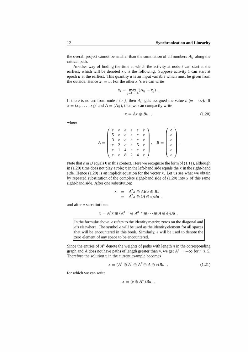
x = Ax ⊕ Bu , (1.20)
where
A =
ε ε ε ε ε ε
5 ε ε ε ε ε
3 ε ε ε ε ε
ε 2 ε ε 5 ε
ε 1 4 ε ε ε
ε ε 8 2 4 ε
, B =
eε
ε
ε
ε
ε
.
Notethate in B equals 0 in this context. Here we recognize the form of (1.11), althoughin (1.20) timedoes not play a role;x in the left-hand side equals thex in the right-handside. Hence (1.20) is an implicit equation for the vectorx . Let us see what weobtainby repeated substitution of the complete right-hand side of (1.20) intox of this sameright-hand side. After one substitution:
x = A2x ⊕ ABu ⊕ Bu= A2x ⊕ (A ⊕ e)Bu ,
and aftern substitutions:
x = An x ⊕ (An−1 ⊕ An−2 ⊕ · · · ⊕ A⊕ e)Bu .
In the formulæ above,e refers to the identity matrix; zeros on the diagonal andε’s elsewhere. The symbol e will be used as the identity element for all spacesthat will be encountered in this book. Similarly,ε will be used todenote thezero element of any space to be encountered.
Since the entries of An denote the weights of paths with lengthn in the correspondinggraph andA does not have paths of length greater than 4, we getAn = −∞ for n ≥ 5.Therefore the solution x in the current example becomes
x = (A4 ⊕ A3 ⊕ A2 ⊕ A ⊕ e)Bu , (1.21)
for whichwe can write
x = (e ⊕ A+)Bu ,
1.2. Miscellaneous Examples 13
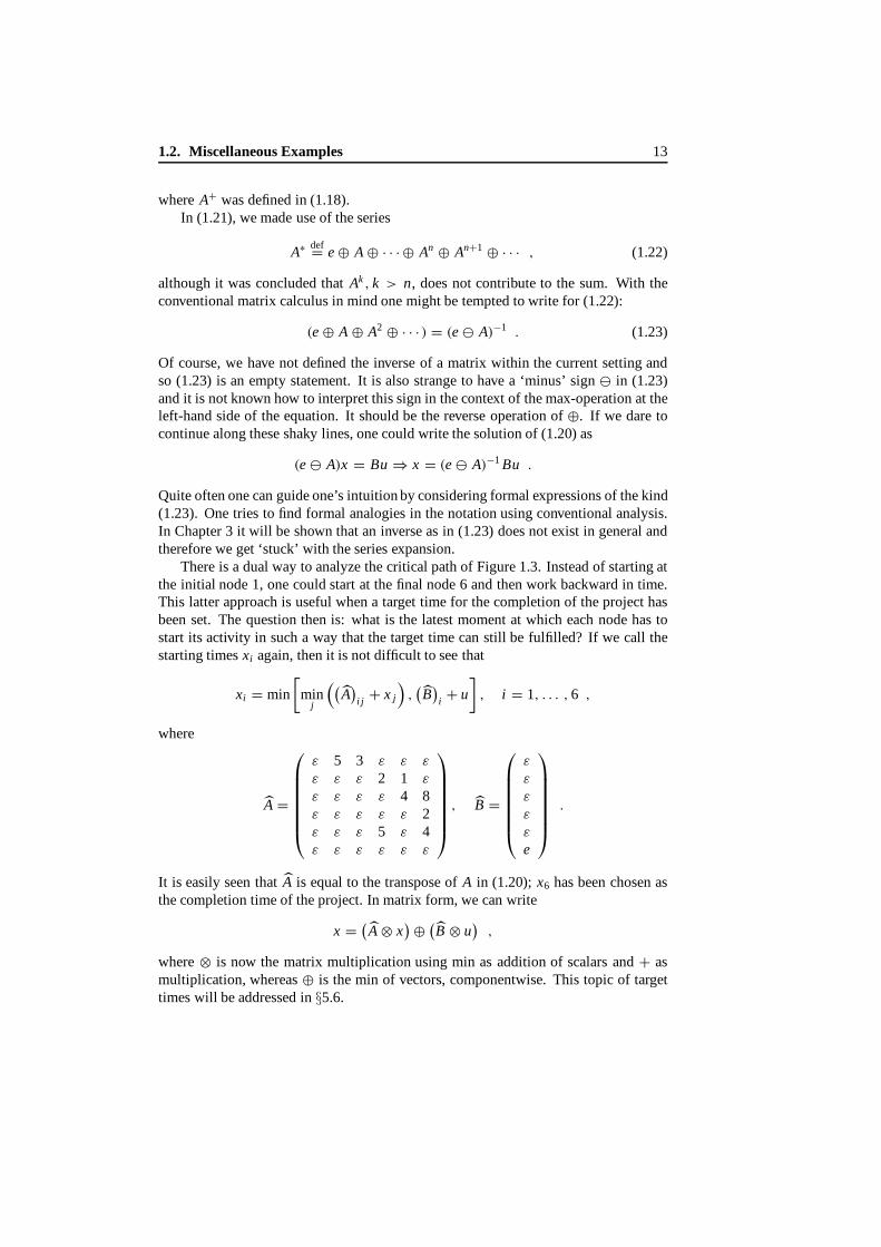
whereA+ was defined in (1.18).In (1.21), we made use of the series
A∗ def= e⊕ A⊕ · · · ⊕ An ⊕ An+1 ⊕ · · · , (1.22)
although it was concluded thatAk , k > n, does not contribute to the sum. With theconventional matrix calculus in mindone might be tempted to write for (1.22):
(e ⊕ A ⊕ A2 ⊕ · · · ) = (e � A)−1 . (1.23)
Of course, we have not defined the inverse of a matrix within the current setting andso (1.23) is anempty statement. It is also strange to have a ‘minus’ sign� in (1.23)and it isnot known how to interpret this sign in the context of the max-operation at theleft-hand side of the equation. It should be the reverse operation of⊕. If we dare tocontinue along these shaky lines, one could write the solution of (1.20) as
(e � A)x = Bu ⇒ x = (e � A)−1 Bu .
Quite often one can guide one’s intuition by considering formal expressions of the kind(1.23). One tries to find formal analogies in the notation using conventional analysis.In Chapter 3it will be shown that an inverse as in(1.23) does not exist in general andtherefore we get ‘stuck’ with the series expansion.
There is a dual way to analyze the critical path of Figure 1.3. Instead of starting atthe initial node 1, one could start at the final node 6 and then work backward in time.This latter approach is useful when a target time for the completion of the project hasbeen set. The question then is: what is the latest moment at which eachnode has tostart its activity in such a way that the target time can still be fulfilled? If we call thestarting timesxi again, then itis not difficult to see that
xi = min
[min
j
((A)
i j+ x j
),(B)
i+ u
], i = 1, . . . , 6 ,
where
A =
ε 5 3 ε ε ε
ε ε ε 2 1 ε
ε ε ε ε 4 8ε ε ε ε ε 2ε ε ε 5 ε 4ε ε ε ε ε ε
, B =
ε
ε
ε
ε
ε
e
.
It is easily seen thatA is equal to the transpose ofA in (1.20); x6 has been chosen asthe completion time of theproject. In matrix form, we can write
x = ( A⊗ x)⊕ (B ⊗ u
),
where⊗ is now the matrix multiplication using min as addition of scalars and+ asmultiplication, whereas⊕ is the min of vectors, componentwise. This topic of targettimes will be addressed in§5.6.

14 Synchronization and Linearity
1.2.2 Communication
This subsection focuses on the Viterbi algorithm. It can conveniently be described bya formulaof the form (1.1). The operations to be used this time are maximization andmultiplication.
The stochastic process of interest in this section,ν(k), k ≥ 0, is a time homoge-neous Markov chain with state space{1, 2, . . . , n}, defined on some probability space(�,F,P). The Markovproperty means that
P[ν(k + 1) = ik+1 | ν(0) = i0, . . . , ν(k) = ik
] = P[ν(k + 1) = ik+1 | ν(k) = ik
],
whereP [A | B] denotesthe conditional probability of the eventA given the eventBandA andB are inF. Let Mi j denote thetransition probability1 from state j to i. Theinitial distribution of the Markov chain will be denotedp.
The processν = (ν(0), . . . , ν(K )) is assumed to be observed with some noise.This means that there exists a sequence of{1, 2, . . . , n}-valued random variables
z(k), k = 0, . . . , K , called theobservation, and such that Nik jkdef= P[z(k) = ik |
ν(k) = jk] does not depend onk and such that the joint law of (ν, z), wherez = (z(0), . . . , z(K )), is given by the relation
P[ν = j, z = i] =(
K∏
k=1
Nik jk M jk jk−1
)Ni0 j0 p j0 , (1.24)
wherei = (i0, . . . , iK ) and j = ( j0, . . . , jK).Given such asequencez of observations, the question to be answered is to find
the sequencej for which the probabilityP [ν = j | z] is maximal. This problem is ahighly simplified version of a text recognition problem. A machine reads handwrittentext, symbol after symbol, but makes mistakes (the observation errors). The underlyingmodel of thetext is such that after having read a symbol, the probability of the occur-rence of the next one is known. More precisely, the sequence of symbols is assumed tobe produced by a Markov chain.
Wewant to compute the quantity
x jK (K ) = maxj0,... , jK−1
P [ν = j, z = i] . (1.25)
This quantity is also a function ofi, but this dependence will not be made explicit. Theargument that achieves the maximum in the right-hand side of (1.25) is the most likelytext up to the(K−1)-st symbol for the observationi; similarly, the argumentjK whichmaximizesx jK (K ) is the most likelyK -th symbol given that the firstK observationsarei. From (1.24), we obtain
x jK (K ) = maxj0,... , jK−1
(K∏
k=1
(Nik jk M jk jk−1
)Ni0 j0 p j0
)
= maxjK−1
((NiK jK M jK jK−1
)x jK−1(K − 1)
),
1Classically, in Markov chains,Mij would rather be denotedM ji .

1.2. Miscellaneous Examples 15
with initial conditionx j0(0) = Ni0 j0 p j0. The reader will recognize the above algorithmas a simple version of (forward) dynamic programming. IfNik jk M jk jk−1 is denotedA jk jk−1, then the general formula is
xm(k) = max�=1,... ,n
(Am�x�(k − 1)) , m = 1, . . . , n . (1.26)
This formula is similar to (1.1) if addition is replaced by maximization and multiplica-tion remains multiplication.
The Viterbi algorithmmaximizesP[ν, z] as given in (1.24). If we take the logarithmof (1.24), and multiply the result by−1, (1.26) becomes
− ln(xm(k)) = min�=1,... ,n
[− ln(Am�)− ln(x�(k − 1))] , m = 1, . . . , n .
The form of this equation exactly matches (1.19). Thus the Viterbi algorithm is identi-cal to an algorithm which determines the shortest path in a network. Actually, it is thislatter algorithm—minimizing− ln(P[ν | z])—which is quite often referred to as theViterbi algorithm, rather than the one expressed by (1.26).
1.2.3 Production
Consider a manufacturing system consisting of three machines. It is supposed to pro-duce three kinds of parts according to a certain product mix. The routes to be followedby each part and each machine are depicted in Figure 1.4 in whichMi , i = 1, 2, 3,are the machines andPi , i = 1, 2, 3, are the parts. Processing times are given in
P1
P3
P2
M 3M 2M 1
Figure 1.4: Routing of parts along machines
Table 1.1. Note that this manufacturing system has a flow-shop structure, i.e. all partsfollow the same sequence on the machines (although they may skip some) and everymachine is visited at most once by each part. We assume that there are no set-up timeson machines when they switch from one part type to another. Parts are carried on alimited number of pallets (or, equivalently, product carriers). For reasons of simplicityit is assumed that
1. only onepallet is available for each part type;
2. the final product mix is balanced in the sense that it can be obtained by means ofa periodic input of parts, here chosen to beP1, P2, P3;
3. there are no set-up times or traveling times;

16 Synchronization and Linearity
Table 1.1: Processing times
P1 P2 P3
M1 1 5M2 3 2 3M3 4 3
4. the sequencing of part types on the machines is known and it is(P2, P3) on M1,(P1, P2, P3) on M2 and(P1, P2) on M3.
The lastpoint mentioned is not for reasons of simplicity. If any machine were to startworking on the part which arrived first instead of waiting for the appropriate part, themodeling would be different. Manufacturing systems in which machines start workingon the first arriving part (if it has finished its current activity) will be dealt with inChapter 9. We can draw a graph in which eachnode corresponds to a combination ofa machine and a part. SinceM1 works on 2 parts,M2 on 3 andM3 on 2, this graph hasseven nodes. The arcs between the nodes express the precedence constraints betweenoperationsdue to the sequencing of operations on the machines. To eachnodei inFigure 1.5 corresponds a numberxi which denotes the earliest epoch at which the nodecanstart its activity. In order to be able to calculate these quantities, the epochs at whichthe machines and parts (together called the resources) are available must be given. Thisis done by means of a six-dimensional input vectoru (six since there are six resources:three machines and three parts). There is an output vector also; the components ofthe six-dimensional vectory denote the epochs at which the parts are ready and themachines have finished their jobs (for one cycle). The model becomes
x = Ax ⊕ Bu ; (1.27)
y = Cx , (1.28)
in which the matrices are
A =
ε ε ε ε ε ε ε
1 ε ε ε ε ε ε
ε ε ε ε ε ε ε
1 ε 3 ε ε ε ε
ε 5 ε 2 ε ε ε
ε ε 3 ε ε ε ε
ε ε ε 2 ε 4 ε
; B =
e ε ε ε e ε
ε ε ε ε ε eε e ε e ε ε
ε ε ε ε ε ε
ε ε ε ε ε ε
ε ε e ε ε ε
ε ε ε ε ε ε
;

1.2. Miscellaneous Examples 17
C =
ε 5 ε ε ε ε ε
ε ε ε ε 3 ε ε
ε ε ε ε ε ε 3ε ε ε ε ε 4 ε
ε ε ε ε ε ε 3ε ε ε ε 3 ε ε
.
Equation (1.27) is an implicit equation inx which can be solved as we did in the
1 2
3 4 5
6 7M 3
u3
M 2u2
M 1
P2
y4
y2
y1u4
u1
u5 u6
P3P1
y6y3
y5
Figure 1.5: Theorderingof activities in the flexible manufacturing system
subsection on Planning;
x = A∗Bu .
Now we add feedbackarcsto Figure 1.5 as illustrated in Figure 1.6. In this graph
Figure 1.6: Production system with feedback arcs
the feedback arcs are indicated by dotted lines. The meaning of these feedback arcs isthe following. After a machine has finished a sequence of products, it starts with thenext sequence. If the pallet on which productPi was mounted is at the end, the finishedproduct is removed and the empty pallet immediately goes back to the starting pointto pick up a new partPi . If it is assumed that the feedback arcs have zero cost, thenu(k) = y(k − 1), whereu(k) is thek-th input cycle andy(k) thek-th output. Thus we

18 Synchronization and Linearity
can write
y(k) = Cx(k) = C A∗ Bu(k)= C A∗ By(k − 1) .
(1.29)
The transition matrix from y(k − 1) to y(k) canbe calculated (it can be done by hand,but a simplecomputerprogram does the job also):
Mdef= C A∗B =
6 ε ε ε 6 59 8 ε 8 9 86 10 7 10 6 ε
ε 7 4 7 ε ε
6 10 7 10 6 ε
9 8 ε 8 9 8
.
This matrix M determines the speed with which the manufacturing system can work.We will return to this issue in§1.3
1.2.4 Queuing System with Finite Capacity
Let us consider four servers,Si, i = 1, . . . , 4, in series(see Figure 1.7). Each cus-
S 1 S 2 S 3 S 4
Figure 1.7: Queuing system with four servers
tomer is to be served byS1, S2, S3 andS4, and specifically in this order. It takesτi (k)time units forSi to serve customerk (k = 1, 2, . . . ). Customerk arrives at epochu(k)into the buffer associated withS1. If this buffer is empty andS1 is idle, then thiscustomer is served directly byS1. Between the servers there are no buffers. The con-sequence is that ifSi, i = 1, 2, 3, has finished serving customerk, but Si+1 is still busyserving customerk − 1, thenSi cannot start serving the new customerk + 1. He mustwait. To complete the description of the queuing system, it is assumed that the travel-ing times between the servers are zero. Letxi (k) denote the beginning of the serviceof customerk by serverSi . BeforeSi can start serving customerk + 1, the followingthree conditions must be fulfilled:
• Si must have finished serving customerk;
• Si+1 must be idle (for i = 4 this condition is an empty one);
• Si−1 must have finished serving customerk + 1 (for i = 1 this condition is anempty one and must be related to the arrival of customerk + 1 in thequeuingsystem).

1.2. Miscellaneous Examples 19
It is not difficult to see that the vectorx , consisting of the fourx-components, satisfies
x(k + 1) =
ε ε ε ε
τ1(k + 1) ε ε ε
ε τ2(k + 1) ε ε
ε ε τ3(k + 1) ε
x(k + 1)
(1.30)
⊕
τ1(k) e ε ε
ε τ2(k) e ε
ε ε τ3(k) eε ε ε τ4(k)
x(k) ⊕
eε
ε
ε
u(k + 1) .
We will not discuss issues related to initial conditions here. For those questions, thereader is referred to Chapters 2 and 7. Equation (1.30), which we write formally as
x(k + 1) = A2(k + 1, k + 1)x(k + 1)⊕ A1(k + 1, k)x(k) ⊕ Bu(k + 1) ,
is an implicit equation inx(k + 1) which can be solved again, as done before. Theresult is
x(k + 1) = (A2(k + 1, k + 1))∗ (A1(k + 1, k)x(k) ⊕ Bu(k + 1)) ,
where(A2(k + 1, k + 1))∗ equals
e ε ε ε
τ1(k + 1) e ε ε
τ1(k + 1)τ2(k + 1) τ2(k + 1) e ε
τ1(k + 1)τ2(k + 1)τ3(k + 1) τ2(k + 1)τ3(k + 1) τ3(k + 1) e
.
The customers who arrive in the queuing system and cannot directly be served byS1, wait in thebufferassociated withS1. If one isinterested in the buffer contents, i.e.the number of waiting customers, at a certain moment, one should use a counter (ofcustomers) at the entry of the buffer and one at the exit of the buffer. The difference ofthe two counters yields the buffer contents, but this operation is nonlinear in the max-plus algebra framework. In§1.2.6 we will return to the ‘counter’-descriptionof discreteevent systems. The counters just mentioned are nondecreasing with time, whereas thebuffercontentsitself is fluctuating as a function of time.
The design of buffer sizes is a basic problem in manufacturing systems. If the buffercontents tends to go to∞, one speaks of an unstable system. Of course, an unstablesystem is an example of abadly designed system. In the current example, bufferingbetween the servers was not allowed. Finite buffers can also be modeled within themax-plus algebra context as shown in the next subsection and more generally in§2.6.2.Another useful parameter is the utilization factor of a server. It is defined by the ‘busytime’ divided by the total time elapsed.
Notethat we didnot make any assumptions on the service timeτi(k). If oneis facedwith unpredictable breakdowns (and subsequently a repair time) of the servers, thenthe service times might be modeled stochastically. For a deterministic and invariant(‘customer invariant’) system, the serving times do not, by definition, depend on theparticular customer.

20 Synchronization and Linearity
1.2.5 Parallel Computation
The application of this subsection belongs to the field of VLSI array processors (VLSIstands for ‘Very Large Scale Integration’). The theory of discrete events provides amethod for analyzing the performances of so-called systolic and wavefront array pro-cessors. In both processors, the individual processing nodes are connected together ina nearest neighbor fashion to form a regular lattice. In the application to be described,all i ndividual processing nodes perform the same basic operation.
The difference between systolic and wavefront array processors is the following.In a systolic array processor, the individual processors, i.e. the nodes of the network,operate synchronously and the only clock required is a simple global clock. The wave-front array processor does not operate synchronously, although the required processingfunction and network configuration are exactly the same as for the systolic processor.The operation of each individual processor in the wavefront case is controlled locally.It depends on the necessary input data available and on the output of the previous cyclehaving been delivered to the appropriate (i.e. directly downstream) nodes. For thisreason a wavefront array processor is also called a data-driven net.
Wewill consider a network in which the execution times of the nodes (the individ-ual processors) depend on the input data. In the case of a simple multiplication, thedifference in execution time is a consequence of whether at least one of the operands isazero or aone. We assumethat if one of the operands is a zero or a one, the multiplica-tion becomes trivial and, more importantly, faster. Data driven networks are at least asfast as systolic networks since in the latter case the period of the synchronization clockmust be large enough to include the slowest local cycle or largest execution time.
1 2
3 4
0 0
0 0. . . ;A 22;A 21
. . . ;A 12;A 11
...B 21
B 11
...B 22
B 12
Figure 1.8: Thenetwork which multiplies two matrices
Consider the network shown in Figure 1.8. In this network four nodes are connec-ted. Each of these nodes has an input/output behavior as given in Figure 1.9. Thepurpose of this network is to multiply two matricesA and B; A has size 2× n andBhas sizen× 2. The numbern is large (� 2), but otherwise arbitrary. The entries of therows of A are fedinto the network as indicated in Figure 1.8; they enter the two nodeson the left. Similarly, the entries ofB enter the two top nodes. Each node will startits activity as soon as each of the input channels contains a data item, provided it has

1.2. Miscellaneous Examples 21
...
ηγ
. . .
......
. . .. . . , Ai,j +1, Aij
Bl+1,m
Blm
Bl−©1,m
ηγ+Aij Blm
Ai,j +1 Aij ,
Blm
Bl−©1,m
...Bl+1,m
Ai, j−©1 Ai,j −©1 . . .
Figure 1.9: Input and output of individual node, before and after one activity
finishedits previous activity and sent theoutput of that previous activity downstream.Note that in the initial situation—see Figure 1.8—not all channels contain data. Onlynode 1 can start its activity immediately. Also note that initially all loops contain thenumber zero.
The activities will stop when all entries ofA and B have been processed. Theneach of the fournodes contains an entry of the productAB. Thus for instance, node 2contains(AB)12. It is assumed that eachnode has a local memory ateach of its inputchannels which functions as a buffer and in which at most one data item can be storedif necessary. Such a necessity arises when the upstream node has finished an activityand wants to send the result downstream while the downstream node is still busy withan activity. If the buffer is empty, the output of the upstream node can temporarilybe stored in this buffer and the upstream node can start a new activity (provided theinput channels contain data). If the upstream node cannot send out its data becauseone or more of the downstream buffers are full, then it cannot start a new activity (it is‘blocked’).
Since it is assumed that eachnode starts its activities as soon as possible, the net-work of nodes can be referred to as a wavefront array processor. The execution time ofa node is eitherτ1 or τ2 units oftime. It isτ1 if at least one of the input items, from theleft and from above (Ai j andBi j ), is a zero or a one. Then the product to be performedbecomes a trivial one. The execution time isτ2 if neither input contains a zero or a one.
It is assumed that the entryAi j of A equals zero or one with probabilityp, 0 ≤p ≤ 1, and thatAi j is neither zero nor one with probability 1− p. The entries of Bare assumed to be neither zero nor one (or,if such anumber would occur, it will not bedetected and exploited).
If xi (k) is the epoch at which nodei becomes active for thek-th time, then it followsfrom the description above that
x1(k + 1) = α1(k)x1(k) ⊕ x2(k − 1)⊕ x3(k − 1) ,
x2(k + 1) = α1(k)x2(k) ⊕ α1(k + 1)x1(k + 1)⊕ x4(k − 1) ,
x3(k + 1) = α2(k)x3(k) ⊕ α1(k + 1)x1(k + 1)⊕ x4(k − 1) ,
x4(k + 1) = α2(k)x4(k) ⊕ α1(k + 1)x2(k + 1)⊕ α2(k + 1)x3(k + 1) .
(1.31)
In these equations, the coefficientsαi(k) are eitherτ1 (if the entry is either azero or a

22 Synchronization and Linearity
one) orτ2 (otherwise);αi(k + 1) have the same meaning with respect to the next entry.Systems of this type will be considered in Chapter 7.
There is a correlation among the coefficients of (1.31) during different time steps.By replacingx2(k) andx3(k) by x2(k+1) andx3(k+1), respectively,x4(k) by x4(k+2)andα2(k) by α2(k + 1), weobtain
x1(k + 1) = α1(k)x1(k) ⊕ x2(k) ⊕ x3(k) ,
x2(k + 1) = α1(k − 1)x2(k) ⊕ α1(k)x1(k) ⊕ x4(k) ,
x3(k + 1) = α2(k)x3(k) ⊕ α1(k)x1(k) ⊕ x4(k) ,
x4(k + 1) = α2(k − 1)x4(k) ⊕ α1(k − 1)x2(k) ⊕ α2(k)x3(k) .
(1.32)
The correlation between some of theαi -coefficients still exists. The standard proce-dure to avoid problems connected to this correlation is to augment the state vectorx .Two new state variables are introduced:x5(k + 1) = α1(k) andx6(k + 1) = α2(k).Equation (1.32) can now be written as
x1(k + 1)= α1(k)x1(k) ⊕ x2(k) ⊕ x3(k) ,
x2(k + 1)= x5(k)x2(k) ⊕ α1(k)x1(k) ⊕ x4(k) ,
x3(k + 1)= α2(k)x3(k) ⊕ α1(k)x1(k) ⊕ x4(k) ,
x4(k + 1)= x6(k)x4(k) ⊕ x5(k)x2(k) ⊕ α2(k)x3(k) ,
x5(k + 1)= α1(k) ,
x6(k + 1)= α2(k) .
(1.33)
The correlation in time of the coefficientsαi has disappeared at the expense of a largerstate vector. Alsonote that Equation (1.33) has termsx j (k) ⊗ xl(k), which cause theequation to become nonlinear (actually, bilinear). For our purposes of calculating theperformance of the array processor, this does not constitute basic difficulties, as willbe seen in Chapter 8. Equation (1.32) is non-Markovian and linear, whereas (1.33) isMarkovian and nonlinear.
1.2.6 Traffic
In a metropolitan area there are three railway stations,S1, S2, andS3, which are con-nected by a railway system as indicated in Figure 1.10. The railway system consists oftwo inner circles, along which the trains run in opposite direction, and of three outercircles. The trains on these outer circles deliver and pick up passengers at local stations.These local stationshave not been indicated in Figure 1.10 since they do not play anyrole in the problem tobe formulated.
There are nine railway tracks. TrackSi S j denotes the direct railway connectionfrom station Si to stationS j ; trackSi Si denotes the outer circleconnected to stationSi .Initially, a train runs alongeach of these nine tracks. At each station the trains mustwait for the trains arriving from the other directions (except for the trains coming fromthe direction the current train is heading for) in order to allow for transfers. Anotherassumption to be satisfied is that trains on the same circle cannot bypass one another.If xi(k) denotes thek-th departuretime of the train in directioni (see Figure 1.10) thenthese departure times are described byx(k + 1) = A1 ⊗ x(k), whereA1 is the 9× 9

1.2. Miscellaneous Examples 23
6
9
8
5
1
74
3
2
S 1
S 3 S 2
Figure 1.10: The railway system, routing no. 1
matrix
A1 =
e ε s31 ε ε ε s11 ε ε
s12 e ε ε ε ε ε s22 ε
ε s23 e ε ε ε ε ε s33
ε ε ε e s21 ε s11 ε ε
ε ε ε ε e s32 ε s22 ε
ε ε ε s13 ε e ε ε s33
ε ε s31 ε s21 ε s11 ε ε
s12 ε ε ε ε s32 ε s22 ε
ε s23 ε s13 ε ε ε ε s33
.
An entrysi j refers to the traveling time on trackSi S j . Thesequantities include transfertimesat the stations. The diagonal entriese prevent trains from bypassing one anotheron the same track at a station. The routing of the trains was according to Figure 1.10;trainson the two inner circles stay on these inner circles and keep the same direction;trainson the outer circles remain there. Other routings of the trains are possible; twosuch different routings are given inFigures 1.11 and 1.12. Ifxi (k) denotes thek-thdeparture time from the same station as given in Figure 1.10, then the departure timesare described again by a model of the formx(k + 1) = A ⊗ x(k). The A-matrixcorresponding to Figure 1.11 is indicated byA2 and theA-matrix corresponding toFigure 1.12 byA3. If we definematricesFi of size 3× 3 in the following way:
F1 =
ε ε ε
ε ε ε
ε ε ε
, F2 =
ε ε s31
s12 ε ε
ε s23 ε
,
F3 =
s11 ε ε
ε s22 ε
ε ε s33
, F4 =
ε s21 ε
ε ε s32
s13 ε ε
,

24 Synchronization and Linearity
S 1
S 3 S 2
Figure 1.11: Routing no. 2
S 1
S 3 S 2
Figure 1.12: Routing no. 3
then the matricesA1, A2 and A3 canbecompactly written as
A1 =
e ⊕ F2 F1 F3
F1 e⊕ F4 F3
F2 F4 F3
, A2 =
e⊕ F2 F4 F3
F2 e ⊕ F4 F3
F2 F4 F3
,
A3 =
e ⊕ F2 F1 F3
F1 e F3
F2 F4 e
.
It is seen that for different routing schemes, different models are obtained. In gen-eral, depending on the numerical values ofsi j , thetime evolutions of these three modelswill be different. One needs a criterion for deciding which of the routing schemes ispreferable.
Depending on the application, it may be more realistic to introduce stochasticsi j -quantities. Suppose for instance that there is a swing bridge in the railway track fromS3 to S1 (only in this track; there is no bridge in the track fromS1 to S3). Each timea trainruns fromS3 to S1 there is a probabilityp, 0 ≤ p ≤ 1, thatthe train will bedelayed, i.e.s31 becomes larger. Thus the matricesAi becomek-dependent;Ai (k).The system has becomestochastic. In this situation one may also have a preference forone of the three routings, or for another one.
The last part of the discussion of this example will be devoted to thedeterministicmodel of routing no. 1 again. However, to avoid some mathematical subtleties whichare not essential at this stage, we assume that there is at least a difference ofτ timeunits between two subsequent departures of trains in the directions 1 to 6 (τ > e).Consequently, the equations are nowx(k + 1) = A1 ⊗ x(k), where A1 equalsthepreviousA1 except for the first six diagonal entries that are replaced byτ (instead ofeearlier), and the last three diagonal entriessii that are replaced bysii ⊕ τ respectively.
Wethen introduce a quantityχi (t) which is related toxi (k). The argumentt of χi (t)refers to the actual clocktime andχi (t) itself refers to the number of train departures

1.2. Miscellaneous Examples 25
in the directioni which have occurred up to (and including) timet . The quantity χi
can henceforth only assume the values 0, 1, 2, . . . . At an arbitrary time t , thenumberof trains which left in the direction 1 can exceed at most by one:
• the samenumber of trainsτ units oftime earlier;
• thenumber of trains that left in the direction 3s31 time units earlier (recall thatinitially a train was already traveling oneach track);
• thenumber of trains that left in the direction 7s11 time units earlier.
Therefore, we have
χ1(t) = min (χ1(t − τ )+ 1, χ3(t − s31)+ 1, χ7(t − s11)+ 1) .
Forχ2 one similarly obtains
χ2(t) = min (χ1(t − s12)+ 1, χ2(t − τ )+ 1, χ8(t − s2)+ 1) ,
etc. If all quantitiessi j andτ are equal to 1, then one can compactly write
χ(t) = A ⊗ χ(t − 1) ,
whereχ(t) = (χ1(t), . . . , χ9(t))′, and where the matrix A is derived from A1 byreplacing all entries equal toε by+∞ and theother entries by 1. This equation mustbe read in the min-plus algebra setting. In case we want something more general thansi j andτ equal to 1, we will consider the situation when all these quantities are integermultiples of a positive constantgc; thengc can be interpreted as the time unit alongwhich the evolution will be expressed. One then obtains
χ(t) = A1⊗ χ(t − 1)⊕ A2⊗ χ(t − 2)⊕ · · · ⊕ Al ⊗ χ(t − l) (1.34)
for some finitel. The latter equation (in the min-plus algebra) andx(k+1) = A1⊗x(k)(in the max-plus algebra) describe the same system. Equation (1.34) is referred to asthe counter description and theother one as thedater description. The word‘dater’mustbe understood as ‘timer’, but since the word ‘time’ and its declinations are alreadyused in various ways in this book, we will stick to the word ‘dater’. The awareness ofthese two different descriptions for the same problem has far-reaching consequencesas will be shown in Chapter 5.
The reader should contemplate that the stochastic problem (in which some of thesi j are random) is more difficult to handle in the counter description, since the delaysin (1.34) become stochastic (see§8.2.4).
1.2.7 Continuous System Subject to Flow Bounds and Mixing
So far, the examples have been related to the realm of discrete eventsystems, and dy-namic equations have been obtained under the form of recursive equations involvingmax (or min) and+-operations. We close this section by showing that a continuous-time system may naturally lead to essentially the same type of equations whenever

26 Synchronization and Linearity
someflow limitation and mixing phenomena are involved. Had we adopted the pointof view of conventional system theory, the model of such a system in terms of differ-ential equations would have exhibited very complex nonlinearities. With the followingapproach, we will see that this system is ‘linear’ in a precise mathematical sense (seeChapter 6). An analogous discrete event model will be discussed in Example 2.48.
In Figure 1.13, a fluid is poured through a long pipe into a first reservoir (empty
Figure 1.13: A continuous system
at time t = 0). The inputu(t) denotes thecumulated flow at theinlet of the pipeup to time t (hence u(t) is a nondecreasing time function andu(t) = 0 for t ≤ 0).It is assumed that it takes a delay of 2 units of time (say, 2 seconds) for the fluid totravel through the pipe. From the first reservoir, the fluid drops into a second reservoirthrough an aperture which limits the instantaneous flow to a maximum value of, say,0.5 liter per second. The volume of fluid at timet in this second reservoir is denotedy(t), and itis assumed thaty(0) = 3 liters.
Let us establish dynamic equations for such a system relating the outputy to theinputu. Because of the flow limitation into the second reservoir, we have:
∀t , ∀s ≥ 0 , y(t + s) ≤ y(t)+ 0.5s . (1.35)
Onthe otherhand, since there is a delay of 2 seconds caused by the pipe,y(t) should becompared withu(t − 2), andbecause there is a stock of 3liters in the second reservoirat t = 0, we have:
∀t , y(t) ≤ u(t − 2)+ 3 . (1.36)
It follows that
∀t , ∀s ≥ 0 , y(t) ≤ y(t − s) + 0.5s
≤ u(t − 2− s)+ 3+ 0.5s ,
hence,
∀t , y(t) ≤ infs≥0
[u(t − 2− s)+ 3+ 0.5s]
= infτ≥2
[u(t − τ )+ 3+ 0.5(τ − 2)] . (1.37)

1.2. Miscellaneous Examples 27
Let
h(t)def={
3 if t ≤ 2;
3+ 0.5(t − 2) otherwise.(1.38)
and consider
∀t , y(t)def= inf
τ∈R
[u(t − τ )+ h(τ )] . (1.39)
Indeed, in (1.39), the range ofτ may belimited to τ ≥ 2 since, for τ < 2, h(τ )remains equal to 3 whereasu(t − τ ) ≥ u(t −2) (remember thatu(·) is nondecreasing).Therefore, comparing (1.39) with (1.37), it is clear thaty(t) ≤ y(t), ∀t .
Moreover, choosingτ = 2 at the right-hand side of (1.39), we see thaty satisfies(1.36). In addition, since for alls and allϑ ≥ 0, h(s + ϑ) ≤ h(s) + 0.5ϑ , then
∀t , ∀θ ≥ 0 , y(t + ϑ) = infτ∈R
[u(t + ϑ − τ )+ h(τ )]
= infs∈R
[u(t − s)+ h(s + ϑ)]
≤ infs∈R
[u(t − s)+ h(s)] + 0.5ϑ
= y(t)+ 0.5ϑ .
Thus,y satisfies (1.35).
Finally, we have proved thaty is the maximum solution of (1.35)–(1.36). It canalso be checked that (1.39) yieldsy(t) = 3, ∀t ≤ 2. Therefore,y is the solution whichwill be physically realized if we assume that, subject to (1.37)–(1.39), the fluid flowsasfast as possible. This output trajectory is related to the input historyu by an ‘inf-convolution’ (see Equation (1.39)). In order to make this inf-convolution more visible,the inf-operator should be viewed as an ‘integration’ (which is nothing else than the⊕-operator ranging over the real numbers). If moreover+ in (1.39) is replaced by⊗one obtains the appearance of the conventional convolution. The same kind of input-output relationship (indeed, a ‘sup-convolution’ in that context) can be obtained fromthe recursive equations (1.12) by developing the recursion from any initial condition.
As a final remark, observe that if wehave two systems similar to the one shown inFigure 1.13, one producing a red fluid and the other producing a white fluid, and if wewant to produce a pink fluid by mixing them in equal proportions, then the new outputis related to the two inputs by essentially the same type of equations. More specifically,let yr(t) andyw(t) be the quantities of red and white fluids that have been produced inthe two downstream reservoirs up to timet (including the initial reserves). Supposethat the two taps at their outlets are opened so that the same (very large) outflow of redand white liquids canbe obtained unless one of the two reservoirs is empty, in whichcase the two taps are closed immediately. Then, min(yr(t), yw(t)) is directly related tothe quantityyp(t) of pink fluid produced up to timet . Therefore, this mixing operationdoes not introduce new mathematical operators.

28 Synchronization and Linearity
1.3 Issues and Problems in Performance Evaluation
In the previous sections we dealt with equations of the formx(k+1) = Ax(k), or moregenerallyx(k+1) = A(k)x(k)⊕ B(k)u(k). In the applicationsthree different interpre-tations in terms of the operations were given: maximization and addition, minimizationand addition and lastly, maximization and multiplication. In this section only the firstinterpretation will be considered (we will say that the system under consideration is inthe max-plus algebra framework). Before that a brief introduction to the solution of theconventional equation (1.1) is needed.
Assumethat the initial vector (1.2) equals an eigenvector ofA; the correspondingeigenvalueis denoted byλ. Thesolution of (1.1) can be written as
x(t) = λt x0 , t = 0, 1, . . . . (1.40)
More generally, if the initial vector can be written as a linear combination of the set oflinearly independent eigenvectors,
x0 =∑
j
c jv j , (1.41)
wherev j is the j -th eigenvector with corresponding eigenvalueλ j , thec j are coeffi-cients, then
x(t) =∑
j
c jλtjv j .
If the matrix A is diagonalizable, then the set of linearly independent eigenvectorsspansRn , and any initial conditionx0 can be expressed as in (1.41). IfA is not diag-onalizable, then one must work with generalized eigenvectors and the formula whichexpressesx(t) in terms of eigenvalues andx0 is slightly more complicated. This com-plication does not occur in the max-plus algebra context and therefore will not be dealtwith explicitly.
In Chapter 3 it will be shown that under quite general conditions an eigenvalue(λ) and corresponding eigenvector (v) also existin the max-plus algebra context for asquare matrix ( A). The definition is
A⊗ v = λ⊗ v .
To exclude degenerate cases, it is assumed that not all components ofv are identical toε. As an example of a (nondegenerate) eigenvalue:
(3 72 4
)(2.5e
)= 4.5
(2.5e
).
Thus itis seen that the matrixA of (1.5) has an eigenvalue 4.5. Equation (1.40) is alsovalid in the current setting. Ifx0 is aneigenvectorof A, with corresponding eigenvalueλ, then thesolution of the difference equation (1.8) can be written as
x(k) = λkx0 ( = λk ⊗ x0) , k = 0, 1, . . . . (1.42)

1.3. Issues and Problems in Performance Evaluation 29
The numerical evaluation ofλk in this formula equalskλ in conventional analysis. Theeigenvalueλ canbe interpreted as the cycle time (defined as the inverse of the through-put) of the underlying system;eachnode of the corresponding network becomes activeeveryλ units of time, since it follows straightforwardly from (1.42). Also, the relativeorder in which the nodes become active for thek-th time, as expressed by the compo-nentsxi(k), is exactly the same as the relative order in which the nodes become activefor the (k + 1)-st time. More precisely, Equation (1.42) yields
xl(k + 1)− x j (k + 1) = xl(k) − x j(k) , j, l = 1, . . . , n .
Thus the solution (1.42) exhibits a kind of periodicity. Procedures exist for the calcula-tion of eigenvalues and eigenvectors; an efficient one is the procedure known as Karp’salgorithm for which the reader is referred to Chapter 2. More discussion about relatedissues can be found in Chapter 3. Under suitable conditions the eigenvalue turns out tobe unique (which differs from the situation in conventional analysis). It can be shownfor instance thatA of (1.5) has only one eigenvalue. Similarly, the matrixM of §1.2.3also has aunique eigenvalue:
6 ε ε ε 6 59 8 ε 8 9 86 10 7 10 6 ε
ε 7 4 7 ε ε
6 10 7 10 6 ε
9 8 ε 8 9 8
e33.50.53.53
= 9.5
e33.50.53.53
.
It follows that the eigenvalue equals 9.5, which means in more practical terms that themanufacturing system ‘delivers’ an item (a product or a machine) at all of its outputchannels every 9.5 units of time. The eigenvector of this example is also unique, apartfrom adding the same constant to all components. Ifv is aneigenvector, thencv, wherec is a scalar, also is an eigenvector, as it follows directly from the definition of eigen-value. Itis possible that several eigenvectors can be associated with the only eigenvalueof a matrix, i.e. eigenvectors may not be identical up to an additional constant.
Suppose that we deal with the system characterized by the matrix of (1.5); thenit is known from earlier that the ‘cycle time’ is 9/2 units of time. The throughputis defined as the inverse of the cycle time and equals 2/9. If we had the choice ofreducing one arbitrary entry ofA by 2, which entry should we choose such that thecycletime becomes as small as possible? To put it differently, if a piece of equipmentwere available which reduces the traveling time at any connection by 2, where shouldthis piece of equipment be placed? By trial and error it is found that eitherA12 or A21
should be reduced by 2; in both cases the new cycle time becomes 4. If one reducesA11 or A22 by this amount instead ofA12 or A21, then the cycletime remains 9/2. Theconsequences of the four potential ways of reduction are expressed by(
1 72 4
)(2.5e
)= 4.5
(2.5e
);(
3 52 4
)(1e
)= 4
(1e
);
(3 70 4
)(3e
)= 4
(3e
);
(3 72 2
)(2.5e
)= 4.5
(2.5e
).

30 Synchronization and Linearity
To answer thequestion of which ‘transportation line’ to speed up for more generalnetworks, application of the trial and error method as used above would become verylaborious. Fortunately more elegant and more efficient methods exist. For those oneneeds the notion of a critical circuit, which is elaborated upon in Chapters 2 and 3.Without defining such a circuit in this section formally let us mention that, in Fig-ure 1.1, this critical circuit consists of the arcs determined byA12 and A21. Note that(A12 + A21)/2= λ = 9/2, and this equality is not a coincidence.
Stochastic extensions are possible. Towards that end, consider
x(k + 1) = A(k)x(k) ,
where thematrix A now depends onk in a stochastic way. Assume thatx ∈ R2 and
that for eachk the matrixA is one of the following two matrices:(
3 72 4
),
(3 52 4
).
Both matrices occur with probability 1/2 and there is no correlation in time. A suitabledefinition of cycle time turns out to be
limk→∞
E [xi (k + 1)− xi(k)] ,
whereE denotes mathematical expectation. Application of the theory presented inChapters 7 and 8 shows that this cycle time is independent ofi and is equal to 13/3.
Conventional linear systems with inputs and outputs are of the form (1.10), al-though (1.10) itself has the max-plus algebra interpretation. This equation is a rep-resentation of a linear system in the time domain. Its representation in thez-domainequals
Y (z) = C(z I − A)−1 BU (z) ,
whereY (z) andU (z) are defined by
Y (z) =∞∑
i=0
y(i)z−i , U (z) =∞∑
i=0
u(i)z−i ,
where it is tacitly assumed that the system was at rest fort ≤ 0. The matrixH (z)def=
C(z I − A)−1 B is called the transfer matrix of the system. HereI refers to the identitymatrix in conventional algebra. The notion of transfer matrix is especially useful whensubsystems are combined to build larger systems, by means of parallel, series andfeedback connections.
In the max-plus algebracontext, the z-transform also exists (see [72]), but herewe will rather refer to theγ -transform whereγ operates asz−1. For instance, theγ -transform ofu is defined as
U (γ ) =∞⊕
i=0
u(i) ⊗ γ i ,

1.3. Issues and Problems in Performance Evaluation 31
andY (γ ) andX (γ ) are defined likewise. Multiplication of (1.12) byγ k yields
γ −1x(k + 1)γ k+1 = A ⊗ x(k)γ k ⊕ B ⊗ u(k)γ k ,
y(k)γ k = C ⊗ x(k)γ k .
}(1.43)
If these equations are summed with respect tok = 0, 1, . . . , then weobtain
γ −1X (γ ) = A ⊗ X (γ )⊕ B ⊗U (γ )⊕ γ −1x0 ,
Y (γ ) = C ⊗ X (γ ) .
}(1.44)
The first of these equations can be solved by first multiplying (max-plus algebra),equivalently adding (conventional) the left- and right-hand sides byγ and then repeat-edly substituting the right-hand side forX (γ ) within this right-hand side. This resultsin
X (γ ) = (γ A)∗(γ BU (γ )⊕ x0) .
Thus we obtainY (γ ) = H (γ )U (γ ), provided thatx0 = ε, and where the transfermatrix H (γ ) is defined by
H (γ ) = C ⊗ (γ A)∗ ⊗ γ ⊗ B = γC B ⊕ γ 2C AB ⊕ γ 3C A2 B ⊕ · · · . (1.45)
The transfer matrix is defined by means of an infinite series and the convergence de-pends on the value ofγ . If the series isconvergent forγ = γ ′, then it is also convergentfor all γ ’s which are smaller thanγ ′. If theseriesdoesnotconverge, it still has a mean-ing as a formal series.
Exactly asin conventional system theory, the product of two transfer matrices (inwhich it is tacitly assumed that the sizes of these matrices are such that the multiplica-tion is possible), is a new transfer matrix which refers to a system which consists of theoriginal systems connected in series. In the same way, the sum of two transfer matricesrefers to two systemsput in parallel. This section will be concluded by an example ofsuch a parallel connection.
We are given two systems. The first one is given in (1.13), and is characterized bythe 1× 1 transfer matrix
H1 = εγ ⊕ 11γ 2⊕ 15γ 3⊕ 20γ 4⊕ 24γ 5⊕ 29γ 6⊕ · · · .
It is easily shown that this series converges forγ ≤ −4.5; the number 4.5 correspondsto the eigenvalue ofA. The second system is given by
x(k + 1) =
e ε 41 1 ε
ε 6 3
x(k) ⊕
ε
2e
u(k) ,
y(k) = ( 1 1 4 )x(k) ,
andits transfer matrix is
H2 = 4γ ⊕ 12γ 2⊕ 15γ 3⊕ 18γ 4⊕ 23γ 5⊕ 26γ 6⊕ · · · .

32 Synchronization and Linearity
The transfer matrix of the two systems put in parallel has size 1×1 again (one cantalkabout a transfer function) and is obtained as
Hpar= H1⊕ H2 = 4γ ⊕ 12γ 2⊕ 15γ 3⊕ 20γ 4⊕ 24γ 5⊕ 29γ 6⊕ · · · . (1.46)
A transfer function caneasily be visualized. IfH (γ ) is a scalar function, i.e. the systemhas one input and one output, then it is a continuous and piecewise linear function.As an example, the transfer function of the parallel connection considered above ispictured in Figure 1.14.
Above it was shown how to derive the transfer matrix of a system if the represen-tation of the system in the ‘time domain’ is given. This time domain representation ischaracterized by the matricesA, B andC. Now one could pose the opposite question:How can we obtain a time domain representation, or equivalently, how can we findA, B andC if the transfer matrix is given? A partial answer to this question is given in[103]. For the example above, one would like to obtain a time domain representationof the two systems put in parallel starting from (1.46). This avenue will not be pursuednow. Instead, one can always obtain such a representation by connecting the underly-ing networks of the two original systems in the appropriate (‘parallel’) way and thenderive the state equations directly. In this way one gets for the above example,
x(k + 1) =
3 7 ε ε ε
2 4 ε ε ε
ε ε e ε 4ε ε 1 1 ε
ε ε ε 6 3
x(k) ⊕
ε
1ε
2e
u(k) ,
y(k) = ( 3 ε 1 1 4 )x(k) .
1.4 Notes
A few times, reference has been made to (linear) system theory. Classic texts are [81], [32] or[72]. A few examples could be phrased in terms of dynamic programming. There are manyelementary texts which explain the theory of dynamic programming. A more advanced text is[18]. Systems in the context of max-plus algebra were probably first described in [49], thoughmost theory in this book is algebraically rather than system oriented. It was in [39] where therelation between system theory and max-plus algebra was clearly shown. The shortest pathproblem is a standard example in dynamic programming texts. The Viterbi algorithm was foundin [59]. The example on production was presented in [38], the examples of parallel computationand traffic can be found in [97]. Other simple examples can be found in [101]. A max-plusmodeling of the Dutch intercity railway net is given in [27]. An application to chemical batchprocessing is given in [107]. A good introductory text to design methods of processors forparallel computation is [79]. The relation between eigenvalue and cycle time was developed in[39]. Stochastic extensions were given in [104]. The connection between transfer matrices andstate equations in the max-plus algebra context was investigatedin [103]; see also§9.2.3.

1.4. Notes 33
−©4
−©6
−©
−©2
0
2
4
6
Hpar
33γγ7
33γγ7
29γγ6
29γγ6
24γγ5
24γγ5
20γγ4
20γγ4
15γγ3
15γγ3
12γγ2
4γγ
4−©6−©8 −©2
Figure 1.14: The transfer functionHpar as a function ofγ

34 Synchronization and Linearity

Chapter 2
Graph Theory and Petri Nets
2.1 Introduction
An overview of various results in the theories of graphs and Petri nets will be given.Several properties of DEDS can be expressed in terms of graph-theoretic notions suchas strong connectedness and critical circuits.
A rich relationship exists between graphs and matrices, about which many bookshave beenwritten. Here, we will emphasize some of these relationships between di-rected graphs and matrices, together with their consequences if such matrices andgraphs are composed to build larger ones. The way to construct such compositionsis by means of parallel and series connections.
Petri nets, which describe DEDS pictorially, can be viewed as bipartite graphs.An essential feature of Petri nets, not present in conventional graphs, is that they aredynamic systems. Tokens are used to reflect this dynamic behavior.
There is an equivalence between DEDS without concurrency and a subclass ofPetri netscalled ‘event graphs’. For any timed event graph, we will show how to ob-tain a mathematical model in terms of recurrence equations. In the proper algebraicframework, these equations are linear and the model offers a strong analogy with con-ventional linear dynamic systems.
In the last part of this chapter, starting from the point of view of resources involvedin DEDS, we propose a methodolgy to go from the specifications of a concrete systemto its modeling by eventgraphs.
2.2 Directed Graphs
A directed graph G is definedas a pair(V, E), whereV is a set ofelements callednodesand whereE is a set the elements of which are ordered (not necessarily different) pairsof nodes, calledarcs. The possibilityof several arcs between two nodes exists (one thenspeaks about a multigraph); in this chapter, however, we almost exclusively deal withdirected graphs in which there is at most one (i.e. zero or one) arc between any twonodes. One distinguishes graphs and directed graphs. The difference between the twois that in a graph the elements ofE arenot ordered while they are in a directed graph.Instead of nodes and arcs, one also speaks about vertices and edges, respectively. Theorigin of the symbolsV andE in the definition of a (directed) graph is due to the first
35

36 Synchronization and Linearity
letters of the latter two names. Instead of directed graph one often uses the shorterword ‘digraph’, or even ‘graph’ if it is clear from the context that digraph is meant. Inthis chapter we will almost exclusively deal with digraphs (hence also called graphs).
Denote the number of nodes byn, and number the individual nodes 1, 2, . . . , n.If (i, j ) ∈ E , theni is called the initial node or the origin of the arc(i, j ), and j thefinal node or the destination of the arc(i, j ). Graphically, the nodes are represented bypoints, and the arc(i, j ) is represented by an ‘arrow’ from i to j .
We now give alist of conceptsof graph theory which will be used later on.
Predecessor, successor.If in a graph(i, j ) ∈ E , then i is called a predecessor ofjand j is called a successor ofi. The set of allpredecessors ofj is indicated byπ( j ) and the set of all successors ofi is indicated byσ(i). A predecessor is alsocalled anupstream node and a successor is also called adownstream node.
Source, sink. If π(i) = ∅, then nodei is called a source; ifσ(i) = ∅ theni is calleda sink. Depending on the application, a source, respectively sink, is also calledan input(-node), respectively anoutput(-node) of the graph.
Path, circuit, loop, length. A path ρ is a sequence of nodes(i1, i2, . . . , ip), p > 1,suchthat i j ∈ π(i j+1), j = 1, . . . , p − 1. Nodei1 is the initial node andip isthe finalone of this path. Equivalently, one also says that a path is a sequence ofarcswhich connects a sequence of nodes. Anelementary path is a path in whichno node appears more than once. When the initial and the final nodes coincide,one speaks of acircuit. A circuit (i1, i2, . . . , ip = i1) is anelementary circuit ifthe path(i1, i2, . . . , ip−1) is elementary. Aloop is a circuit(i, i), that is,a circuitcomposed of a single node which is initial and final. This definition assumes thati ∈ π(i), that is, there does exist an arc fromi to i. The length of a path ora circuit is equal to the sum of the lengths of the arcs of which it is composed,the lengths of the arcs being 1 unless otherwise specified. With this convention,the length of a loop is 1. The length of pathρ is denoted|ρ|l . The subscript ‘l’here refers to the word ‘length’ (later on, another subscript ‘w’ will appear for adifferent concept). The set of all paths and circuits in a graph is denotedR. Adigraph is said to beacyclic if R contains no circuits.
Descendant, ascendant.The set ofdescendantsσ+(i) of nodei consists of all nodesj such that a path exists fromi to j . Similarly the set of ascendantsπ+(i) ofnodei is the set of all nodesj such that a path exists fromj to i. Onehas, e.g.,π+(i) = π(i) ∪ π(π(i)) ∪ . . . . The mapping i �→ π∗(i) = {i} ∪ π+(i) is thetransitive closure ofπ ; the mapping i �→ σ ∗(i) = {i} ∪ σ+(i) is the transitiveclosure ofσ .
Subgraph. Given a graphG = (V, E), a graphG′ = (V ′, E ′) is said to be a subgraphof G if V ′ ⊂ V and ifE ′ consists of the set of arcs ofG which have their originsand destinations inV ′.
Chain, connected graph. A graph is called connected if for all pairs of nodesiand j there exists achain joining i and j . A chain is a sequence of nodes(i1, i2, . . . , ip) such that between each pair of successivenodes either the

2.2. Directed Graphs 37
arc (i j , i j+1) or the arc(i j+1, i j ) exists. If one disregards the directions of thearcsin the definition of a path, one obtains a chain.
Strongly connected graph.A graph is called strongly connected if for any two dif-ferent nodesi and j there exists a pathfrom i to j . Equivalently, i ∈ σ ∗( j ) forall i, j ∈ V, with i = j . Note that, according to this definition, an isolated node,with or without a loop, is a strongly connected graph.
Bipartit e graph. If the set of nodesV of a graphG canbepartitioned into two disjointsubsetsV1 andV2 such that every arc ofG connects an element of V1 with oneof V2 or the other way around, thenG is called bipartite.
In §2.3, it will be useful to introduce the notion of an ‘empty circuit’ the lengthof which is equal to 0 by definition. An empty circuit contains no arcs. Thecircuit (i) is anempty circuit which should not be confused with the loop(i, i)of length 1 (the latter makes sense only if there exists an arc from nodei toitself). Empty circuits arenot included in the setR of paths.
To exemplify the various concepts introduced, consider the graph presented in Fig-ure 2.1. It is a digraph since the arcs are indeed directed. The graph has seven nodes.Node 3 is a predecessor of node 6; 3∈ π(6). Similarly, 6 ∈ σ(3). The sequence ofnodes 1, 3, 6, 4, 3, 2 is a nonelementary path. The arc(1, 1) is a loop and the sequenceof nodes 3, 6, 4, 3 is an elementary circuit of length 3. The sequence of nodes 2, 3, 6 isa chain. It should be clear that the graph of Figure 2.1 is connected.
Definition 2.1 (Equivalence relationR ) Let i, j ∈ V be two nodes of a graph. Wesay that iR j , if either i = j or there exist paths from i to j and from j to i.
ThenV is split up into equivalence classesV1, . . . ,Vq , with respect to the relationR.Note that if nodei belongs toV�, thenV� = σ ∗(i) ∩ π∗(i). To each equivalence classV� corresponds a subgraphG� = (V�, E�), whereE� is the restriction ofE to V�, whichis strongly connected.
Definition 2.2 (Maximal strongly connected subgraphs–m.s.c.s.)The subgraphsGi = (Vi , Ei ) corresponding to the equivalence classes determined by R are themaximal strongly connected subgraphsof G.
Notation 2.3
• The subset of nodes of the m.s.c.s. containing nodei (and possibly reduced toi)is denoted [i].
• The subset of nodes⋃
j∈π∗(i)[ j ] is denoted [≤ i].
• The symbol [< i] represents the subset of nodes [≤ i] \ [i].
The graph of Figure 2.1 has two m.s.c.s.’s, namely the subgraphs consisting of thenodes 1, 3, 6, 4 and 2, 5, 7, respectively. If one ‘lumps’ the nodes ofeach m.s.c.s. intoa single node, one obtains the so-calledreduced graph.

38 Synchronization and Linearity
72
4
1
36
5
Figure 2.1: A digraph Figure 2.2: The reduced graph
Definition 2.4 (Reduced graph) The reduced graph of G is the graph with nodes V def={1, . . . , q} (one node per m.s.c.s.), and with arcs E, where (i, j ) ∈ E if (k, l) ∈ E forsome node k of Vi and some node l of V j .
Figure 2.2 shows the reduced graph of the graph in Figure 2.1.
Notation 2.5 A nodei of the reduced graph corresponds to a collection of nodes ofthe original graph. Letx be a vector the entries of which are associated with nodes ofthe original graph. If we want to refer to the subvector associated with the nodes ofm.s.c.s.i, we will use the notationx(i). Similarly, for a matrix A, A(i)( j) is the blockextracted fromA by keeping the rows associated with the nodes of m.s.c.s.i and thecolumns associatedwith thenodes of m.s.c.s.j . If node� of the original graph belongsto m.s.c.s.i, thenotationx[�] is equivalent tox(i). Similarly, x(<i), respectivelyx(≤i), isequivalent tox[<�], respectivelyx[≤�].
Lemma 2.6 The reduced graph is acyclic.
Proof If there is a path fromk ∈ Vi to l ∈ V j , then there is no path from any node ofV j to any node ofVi (otherwise,k andl would be in the same m.s.c.s.).
Denote the existence of a path from one subgraphGi to another oneG j by the binaryrelation R′; GiR′G j . Then these subgraphsG1, . . . ,Gq, together with the relationR′
form a partially ordered set, see Chapter 4 and also [85].
2.3 Graphs and Matrices
In this section we consider matrices with entries belonging to an abstract alphabetC in which some algebraic operations will be defined in§2.3.1. Some relationshipsbetween these matrices and ‘weighted graphs’ will be introduced. Consider a graphG = (V, E) and associate an elementAi j ∈ C with each arc( j, i) ∈ E : thenG is calleda weighted graph. The quantity Ai j is called theweight of arc ( j, i). Note that thesecond subscript ofAi j refers to the initial (and not the final) node. The reason is that,in the algebraic context, we will work with column vectors (and not with row vectors)

2.3. Graphs and Matrices 39
later on. In addition, we will also consider compositions of matrices and the resultingconsequences for the corresponding graphs.
The alphabetC contains a special symbolε the properties of which will be given in§2.3.1.
Definition 2.7 (Transition graph) If an m × n matrix A = (Ai j ) with entries in C isgiven, the transition graphof A is a weighted, bipartite graph with n+m nodes, labeled1, . . . ,m,m+1, . . . ,m+n, such that each row of A corresponds to one of the nodes1, . . . ,m; each column of A corresponds to one of the nodes m + 1, . . . ,m + n. Anarc from j to n + i, 1 ≤ i ≤ m, 1 ≤ j ≤ n, is introduced with weight Ai j if Ai j = ε.
As an example, consider the matrix
A =
3 ε ε 7 ε ε ε
ε ε 2 ε ε ε 1e ε ε 2 ε ε ε
ε ε ε ε ε 5 ε
ε 4 ε ε ε 8 64 ε 1 ε ε ε ε
ε ε ε ε e ε ε
. (2.1)
Its transition graph is depicted in Figure 2.3.
1
2
3
4
5
6
7
8
9
10
11
12
13
14
30
7
2
50
6
18
2
1
4
4
Figure 2.3: Thetransition graph ofA
Defini tion 2.8 (Precedence graph)The precedence graph of a squaren× n matrix Awith entries in C is a weighted digraph with n nodes and an arc ( j, i) if Ai j = ε, inwhich case the weight of this arc receives the numerical value of Ai j . The precedencegraph is denoted G(A).
It is not difficult to see that any weighted digraphG = (V, E) is the precedence graphof an appropriately defined square matrix. The weightAi j of the arc from nodej to

40 Synchronization and Linearity
nodei defines thei j -th entry of a matrixA. If an arc does not exist, the correspondingentry of A is set toε. The matrix A thus defined hasG as its precedence graph.
The transition graph of a squaren × n matrix, which has 2n nodes, can be trans-formed into a precedence graph ofn nodes. Towards that end, one combines the nodesi and n + i of the transition graph into one single node for the precedence graph,i = 1, . . . , n. As an example, Figure 2.4 gives the precedence graph of the matrixA
3
2
44 1
82
71
5
0
61
23
547
0
6
Figure 2.4: The precedence graph ofA
defined in (2.1). One directly recognizes the relation of this graph with the transitiongraph in Figure 2.3. The latter graph has been ‘folded’ so as to obtain the precedencegraph.
It may be convenient to considerthat entriesAi j equal to ε definedummy arcs(which are not drawn) in the associated precedence or transition graph. Later, a pathincluding a dummy arc will be called a dummy path. Dummy paths are not includedin the setR of paths (which were taken into account in Definition 2.1; therefore thesedummypaths are not involved in the definition of m.s.c.s.’s). The interest of the notionof dummy arcs is that these arcs may be considered as being of the same length as arcsassociated with entriesAi j = ε (generally this length is 1); hence arcs of the samelength can be associated with all entries of a matrix.
Notation 2.9 The number of m.s.c.s.’s ofG(A) is denotedNA.
For later reference, the following definitions are given.
Definition 2.10 (Incidence matrix) The incidence matrixF = (Fi j ) of a graph G =(V, E) is a matrix the number of columns of which equals the number of arcs and thenumber of rows of which equals the number of nodes of the graph. The entries of Fcan take the values 0, 1 or −1. If l = (i, j ) ∈ E , i = j , then Fil = 1, Fjl = −1 andthe other entries of column l are 0. If l = (i, i) ∈ E , then Fil = 0.
Definition 2.11 (Adjacency matrix) The adjacency matrixG = (Gi j ) of a graph G =(V, E) is a matrix the numbers of rows and columns of which are equal to the numberof nodes of the graph. The entry Gi j is equal to 1 if j ∈ π(i) and to 0 otherwise.
Notethat if G = G(A), thenGi j = 1 if andonly if Ai j = ε (G describes the ‘support’of A).

2.3. Graphs and Matrices 41
2.3.1 Composition of Matrices and Graphs
We now study two kinds of compositions of matrices, and the relation between thetransition graph of these compositions and the original transition graphs. These com-positions are, respectively, theparallel composition, denoted⊕, and theseries compo-sition, denoted⊗. These compositions will be defined by means of the correspondingcomposition operations of elements in the alphabetC, for which the samesymbols⊕and⊗ will be used. The operation⊕ is usually referred to as ‘addition’ or ‘sum’, andthe operation⊗ as‘multiplication’ or ‘product’. The alphabetC includes twospecialelementsε ande with specific properties to be defined in the following set of axioms:
Associativity of addition:
∀a, b, c ∈ C , (a ⊕ b)⊕ c = a ⊕ (b ⊕ c) .
Commutativity of addition:
∀a, b ∈ C , a ⊕ b = b ⊕ a .
Associativity of multiplication:
∀a, b, c ∈ C , (a ⊗ b)⊗ c = a ⊗ (b ⊗ c) .
Right and left distributivity of multiplication over addition:
∀a, b, c ∈ C , (a ⊕ b)⊗ c = (a ⊗ c)⊕ (b ⊗ c) ,
∀a, b, c ∈ C , c⊗ (a ⊕ b) = (c ⊗ a)⊕ (c ⊗ b) .
Existence of a zero element:
∃ε ∈ C : ∀a ∈ C , a ⊕ ε = a .
Absorbing zero element:
∀a ∈ C , a ⊗ ε = ε .
Existence of an identity element:
∃e ∈ C : ∀a ∈ C , a ⊗ e = e ⊗ a = a .
In Chapter 3 other related axioms will be discussed in detail. There the notion of asemifield will be introduced and its relation to axioms of this type will be made clear.
Theparallel composition⊕ of matrices is defined for matrices of the same size bythe following rule: if A = (Ai j ) andB = (Bi j ) have the same size, then
(A ⊕ B)i j = Ai j ⊕ Bi j .

42 Synchronization and Linearity
A transition graph can of course be associated with the matrixC = A ⊕ B. Thistransition graph has the same set of nodes as the transition graph ofA (and thereforeof B) and there exists a (nondummy) arc from nodej to nodei if and only if at leastoneof the transition graphs ofA and B has a (nondummy) arc fromj to i. This isa consequence of the axiomAi j ⊕ ε = Ai j . In general, this arc receives the weightAi j ⊕ Bi j . It may beviewedasthe arc resulting from the merging of two parallel arcs(if both Ai j and Bi j are different fromε). The symbolε is called thezero element ofthe operation⊕. Two other axioms are that⊕ is associative and commutative and theyhave obviousconsequencesfor theparallel composition of transition graphs.
Theseries composition⊗ of matricesA andB is definedonly when the number ofcolumns ofA equals the number of rows ofB (say,A is m × n andB is n × p) by thefollowing rule:
(A ⊗ B)i j =n⊕
k=1
Aik ⊗ Bkj . (2.2)
A transition graph can be associated with the matrixC = A ⊗ B of sizem × p. Withthe help of Figure 2.5, we explain how this graph is obtained. First, the transition
B A
j
k i
p nodes n nodes m nodes
Figure 2.5: Theseriescomposition of two transition matrices
graphs of matricesB andA are concatenated. Thegraph so obtained isnota transitiongraph since it hasn intermediate nodes in addition of itsp input nodes and itsmoutput nodes. These intermediate nodes are removed, and an arc from nodej to nodeiexists in the transition graph ofC if and only if there exists at least one (nondummy)path from nodej to nodei in the concatenated graph shown inFigure 2.5. This arcreceives the weight indicated by Equation (2.2). In order to interpret this formula, letus first define the weight of a pathρ = (i1, . . . , ip) in a weighted graph as the productAip ,ip−1 ⊗ · · · ⊗ Ai2 ,i1 of weights of arcs composing this path (observe the order). Thisweight is denoted|ρ|w, where the subscript w refers to the word ‘weight’. Notethat adummy path always has a weightε thanks to the absorbing property ofε in products.Then, each term of the sum in (2.2) can be interpreted as the weight of some parallelpath of length 2 from nodej to nodei, characterized by the intermediate nodek itpasses through (see Figure 2.5). The previous rule pertaining to the weights of parallelcompositions of arcs is thus extended to parallel paths. Sinceε is the zero element foraddition, dummy paths do not contribute to (nonzero) weights in parallel compositions.

2.3. Graphs and Matrices 43
For theseriescomposition of matrices, we have(A⊗ B)⊗C = A⊗ (B⊗C). Thisassociativity property of matrix multiplication is a direct consequence of the axiomsgiven above, namely the associativity of⊗ and the right and left distributivity of ⊗over⊕. It is easily seen that these right and left distributivities also hold for matricesof appropriate sizes.
The notion (Ap ) j i, p = 1, 2, . . . , whereA is square, is defined by(Ap ) j i = (A ⊗Ap−1) j i . Observe that this involves the enumeration and the sums of weights of allpaths of lengthp with initial nodei and final nodej . This definition makes sense forboth thetransition graph ofA, concatenatedp times, and the precedence graph ofA.We get
(Ap ) j i =⊕
{ρ| |ρ|l=p;i0=i;ip= j}Aip ,ip−1 ⊗ Aip−1 ,ip−2 ⊗ · · · ⊗ Ai1,i0 .
Because we removed the intermediatenodes in the graph of Figure 2.5 in order toobtain thetransition graph ofC = A ⊗ B, and similarly whenone considers the tran-sition graph of a matrixC equal toAp , the information that weights of the graph ofChave been obtained as weights of paths of length larger than 1 (namely 2 andp, respec-tively) hasbeen lost. In order to keep track of this information, one may introduce thenotion of length of a transition graph. This length is an integer number associated withthe transition graph and hence also with all its individual arcs, including dummy arcs,and finally with the matrix associated with this graph. These considerations explainwhy the lengths of arcs may be taken greater than 1 and why dummy arcs may alsohave a nonzero length.
We now consider the transition graph corresponding to matricesA0 whereA is ann × n matrix. In the same way asAp , for p ≥ 1, describes the weights of paths oflength p, A0 should describe the weights of paths of length 0, that is, empty circuits(i) corresponding to ‘no transition at all’. Pictorially, the corresponding transitiongraph of such matrices has the special form depicted in Figure 2.6a in which input
�
(a) (b) (c)
e
e
e
Figure 2.6: Thetransition graphs ofA0, ε ande
and output nodes are not distinguishable. This transition graph must not be confusedeither with that of the ‘zero matrix’ (with all entries equal toε) or with that of the‘identity matrix’ (with diagonal entries equal toe and all off-diagonal entries equalto ε). The transition graph of the zero matrix is depicted in Figure 2.6b: all its arcsare dummy with length 1. The transition graph of the identity matrix is depicted inFigure 2.6c: weights are indicated in the figure and the length is 1 for all dummy andnondummy arcs. The length associated with all entries ofA0 is 0, that is, the series
44 Synchronization and Linearity
composition of the transition graph ofA0 with any other bipartite graph do not modifythe lengths of paths. In the same way, we would like the weights not to be modified inthat operation: this requires that the entries ofA0 bethe same as those of the identitymatrix e. Butagain therespective lengthsand transition graphs ofA0 ande are different(see Figure 2.6a–c). Also, dummy loops(i, i) of the transition graph of the zero matrixshould not be confused with empty circuits(i) (see Figure 2.6a–b) even if it is difficultto distinguish them with the help of precedence, rather than transition, graphs.
In Chapter 1we already met several examples of⊕ and⊗ operations which satisfythe axioms just stated. A particular example is thatC equalsR, e = 0, ε = −∞, ⊕equals maximization and⊗ equals addition. Note that the max-operation is idempotent,i.e. a ⊕ a = a, but this property is not (yet) assumed as an axiom.
Remark 2.12 An example of operations which donot satisfy some ofthe axioms isone where⊕ is addition and⊗ is minimization. The axioms of distributivity are notsatisfied. Indeed,
min(5, 3+ 6) = min(5, 3)+min(5, 6) .
As a consequence, associativity of multiplication with respect to matrices does nothold. If for instance,
A =(
1 32 2
), B =
(3 21 5
), C =
(4 22 5
),
then(
4 65 6
)= (AB)C = A(BC) =
(4 44 4
).
A practical interpretation of a system with these operations is in terms of the calcula-tion of the capacity of a network in which the arcs are pipes through which there is acontinuous flow. The capacity of a pipe is assumed to be proportional to the diameterof this pipe. Then it is easilyseen that the capacity of two pipes in parallel equals thesum of thetwo capacities. Similarly, the capacity of two pipes in series equals the min-imum of their capacities. The reader should contemplate the physical consequences ofthe lack of associativity.
Defini tion 2.13 (I rr educibility) The (square) matrix A is called irreducible if no per-mutation matrix P exists such that the matrix A, defined by
A = P ′AP ,
has an upper triangular block structure.
The reader should be aware of the fact that this definition is invariant with respect tothe algebra used. Premultiplication ofA by P ′ and postmultiplication by P simplyrefers to a renumbering of the nodes of the corresponding graph. Hence renumberingof the nodes of the same graph leads to differentA-matrices. In an upper triangularblock structure, diagonal blocks with non-ε entries are allowed.If one also wantsthe diagonal blocks to haveε-entries only, one should speak about a strictly uppertriangular block structure.

2.3. Graphs and Matrices 45
Theorem 2.14 A necessary and sufficient condition for the square matrix A to be irre-ducible is that its precedence graph be strongly connected.
Proof Suppose thatA is such that by an appropriate renumbering of the nodes,A hasan upper triangular block structure. Call the diagonal blocksAd
1, . . . , Adq . If Ad
q hassizenq×nq , then there are no paths from any of the (renumbered) nodes 1, . . . , n−nq,
to any of the nodesn − nq + 1, . . . , n. Hencethis graph is not strongly connected.On the other hand, if the graph is not strongly connected, determine its m.s.c.s.’s
Gi , i = 1, . . . , q. These subgraphs form a partially ordered set. Number the individualnodes ofV in such a way that if GiR′G j , then the nodes ofVi have lower indicesthan those ofV j (R′ was defined in§2.2). With this numbering of the nodes, thecorresponding matrixA will be upper block triangular.
Definition 2.15 (Aperiodicity) The square matrix A is aperiodic if there exists an in-teger N such that for all n ≥ N and for all i, j , (An)i j = ε.
Theorem 2.16 An irreducible matrix A such that A j j = ε for all j is aperiodic.
Proof FromTheorem 2.14, the irreducibility assumption implies that for alli, j , thereexists n suchthat (An)i j = ε. This together with the assumptionA j j = ε in turn im-plies that(Am )i j = ε for all m ≥ n. The assertion of the theorem follows immediatelyfrom this since the number of nodes is finite.
Definition 2.17 A digraph is called a treeif there exists a single node such that thereis a unique path from this node to any other node.
16
4 0 72
2 4
7 5
4
3
1
3 6
2
5
08
1
Figure 2.7: Weighted digraph consisting of two m.s.c.s.’s
In order to determine whetherA is irreducible, one can calculateA+ (see (1.18)).Matrix A is irreducible if and only if all entries ofA+ are different from ε. Thisalgorithm for determining whetherA is irreducible can be simplified by consideringonly Boolean variables. ReplaceA by the adjacency matrixG of its precedence graph(seeDefinition 2.11), except that 0 and 1 are replaced byε ande, respectively, in thepresent context. ThenA is irreducible if and only if all entries ofG+ are identical toe.

46 Synchronization and Linearity
As an example, consider the matrix given in (2.1). The matrixG+ becomes
e ε e e ε e ε
e e e e e e ee ε e e ε e ε
e ε e e ε e ε
e e e e e e ee ε e e ε e ε
e e e e e e e
. (2.3)
HenceA is not irreducible. In fact it follows directly from (2.3) that the nodes 1, 3, 4and 6 form a m.s.c.s., as do the nodes 2, 5 and 7. If one rearranges the nodes andarcs of Figure 2.4, one obtains Figure 2.7, in which the weights of the arcs have beenindicated, and the two m.s.c.s.’s are clearly visible. Figure 2.7 is identical to Figure 2.1apart from the fact that weights are given.
2.3.2 Maximum Cycle Mean
In this subsection the maximum cycle mean will be defined and some of its propertieswill be derived. The maximum cycle mean has aclear relation with eigenvalues ofmatrices within the context of the max algebra and with periodic regimes of systemsdescribed by linear equations, also within the same context. These relationships willbe described in Chapter 3.
Let G = (V, E) be a weighted digraph withn nodes. The weights are real numbershere and are given by means of then× n matrix A. As discussed before, the numericalvalue of Ai j equals the weight of the arc from nodej to nodei. If no such arc exists,then Ai j = ε. It is known from Chapter 1 that the entry(i, j ) of Ak = A ⊗ · · · ⊗ A,
considered within the algebraic structureRmaxdef= (R ∪ {−∞},max,+), denotes the
maximum weight with respect to all paths of lengthk which go from nodej to nodei.If no such pathexists, then(Ak )i j = ε. Within this algebraic structure,ε gets assignedthenumerical value−∞ ande = 0. In this subsection we will confine ourselves to thealgebraic structure Rmax.
Definition 2.18 (Cycle mean)The mean weightof a pathis defined as the sum of theweights of the individual arcs of this path, divided by the length of this path. If the pathis denoted ρ, then the mean weight equals |ρ|w/|ρ|l. If such a path is a circuit onetalks about the mean weight of the circuit, or simply the cycle mean.
We are interested in the maximum of these cycle means, where the maximum is takenover all circuits in the graph (empty circuits are not considered here). Consider ann × n matrix A with corresponding precedence graphG = (V, E). The maximumweight of all circuits of lengthj which pass through nodei of G can be written as(A j )ii . The maximum of these maximum weights over all nodes is
⊕ni=1(A j )ii which
canbewritten trace(A j ). The average weight isobtained by dividing this number byjin the conventional sense, but this can be written(trace(A j ))1/j in the max-plus algebranotation. Finally, we have to take the maximum with respect to the lengthj . It is notnecessary to consider lengths larger than the numbern of nodes since it is enough to

2.3. Graphs and Matrices 47
limit ourselves to elementary circuits. It follows that a formula for the maximum cyclemeanλ in the max-plus algebra notation is
λ =n⊕
j=1
(trace(A j ))1/j .
The following theorem provides an expression, due to R. Karp, for this maximumvalue. All circuits with a cycle mean equal to the maximum cycle mean are calledcritical circuits. Karp’s theorem does not give the critical circuit(s).
Theorem 2.19 (Karp’s theorem) Given is an n × n matrix A with correspondingprecedence graph G = (V, E). The maximum cycle mean is given by
λ = maxi=1,... ,n
mink=0,... ,n−1
(An )i j − (Ak )i j
n − k, ∀ j . (2.4)
In this equation, An and Ak are to be evaluated in Rmax; the other operations areconventional ones.
Proof Notethat the indexj in (2.4) is arbitrary (it will be shown in this proof that onecan take anyj ∈ {1, . . . , n}). The resulting value ofλ is independent ofj .
Without loss of generality, we may assume thatG is strongly connected. If it werenot, we would consider each of its m.s.c.s.’s—sinceG is assumed to be finite, there areonly a finite number of such m.s.c.s.’s—and determine the maximum cycle mean ofeach of them and then take the maximum one.
We first assume thatthe maximum cycle mean is 0. Then it must be shown that
maxi=1,... ,n
mink=0,... ,n−1
(An )i j − (Ak )i j
n − k= 0 .
Sinceλ = 0 there exists a circuit of weight 0 and there exists no circuit with posi-tive weight. Because there are no circuits (or loops) with positive weight, there is amaximum weight of all paths from nodej to nodei which is equal to
χi jdef= max
k∑
l=1
Ail ,il−1 , subject to i0 = j , ik = i ,
where the maximum is taken with respect to all paths and allk. Since fork ≥ n the pathwould contain a circuit and since all circuits have nonpositive weight, we can restrictourselves tok < n. Therefore we get
χi j = maxk=0,... ,n−1
(Ak )i j .
Also, (An )i j ≤ χi j , andhence
(An )i j − χi j = mink=0,... ,n−1
(An )i j − (Ak )i j ≤ 0 .

48 Synchronization and Linearity
Equivalently,
mink=0,... ,n−1
(An )i j − (Ak )i j
n − k≤ 0 . (2.5)
Equality in (2.5) will only hold if (An )i j = χi j . It will be shown that indeed an indexi exists such that this is true. Letζ be a circuit of weight 0 and letl be a node ofζ .Let ρl j be a path fromj to l with corresponding maximum weight|ρl j |w = χl j . Nowthis path is extended by appending to it a number of repetitions ofζ such that the totallength of this extended path, denotedρe, becomes greater than or equal ton. This isagain a path of maximum weight from j to l. Now considerthe path consisting of thefirst n arcs ofρe; its initial node is j and denote its final nodel ′. Of coursel ′ ∈ ζ .Since any subpath of any path of maximum weight is of maximum weight itself, thepath from j to l ′ is of maximum weight. Therefore(An )l′ j = χl′ j . Now choosei = l ′
and we get
maxi=1,... ,n
[min
k=0,... ,n−1
(An)i j − (Ak )i j
n − k
]= 0 .
This completes the part of the proof withλ = 0.Now consideran arbitrary finiteλ. A constantc isnow subtracted from each weight
Ai j . Then clearlyλ will be reduced byc. Since(Ak )i j is reduced bykc, we getthat
(An )i j − (Ak )i j
n − k
is reduced byc, for all i, j andk, andhence
maxi=1,... ,n
mink=0,... ,n−1
(An )i j − (Ak )i j
n − k
is also reduced byc. Hence both sides of (2.4) are affected equally when all weightsAi j are reduced by the same amount. Now choose this amount such thatλ becomes 0and then we are back in the previous situation whereλ = 0.
2.3.3 The Cayley-Hamilton Theorem
The Cayley-Hamilton theorem states that, in conventional algebra, a square matrixsatisfies its own characteristic equation. In mathematical terms, letA be ann × nmatrix and let
pA(x)def= det(x I − A) = xn + c1xn−1 + · · · + cn−1x + cn x0 , (2.6)
where I is the identity matrix, be its characteristic polynomial. The termx0 in thepolynomial equals 1. ThenpA(A) = 0, where 0 isthezero matrix. The coefficientsci , i = 1, . . . , n, in (2.6) satisfy
ck = (−1)k∑
i1<i2<···<ik
det
Ai1 ,i1 . . . Ai1 ,ik...
...
Aik ,i1 . . . Aik ,ik
. (2.7)

2.3. Graphs and Matrices 49
The reason for studying the Cayley-Hamilton theorem is the following. In con-ventional system theory, this theorem is used for the manipulation of different systemdescriptions and for analyzing such properties as controllability (see [72]). In the con-text of discrete event systems, a utilization of this theorem will be shown in§9.2.2.
In this section it will be shown that a Cayley-Hamilton theorem also exists in analgebraic structure defined by a setC of elements supplied with two operations denoted⊕ and⊗ whichobey some of the axioms given in§2.3.1, namely
• associativityof addition,
• commutativity of addition,
• associativity of multiplication,
• both right and left distributivity of multiplication over addition,
• existence of an identity element,
provided wealso have
Commutativity of multiplication:
∀a, b ∈ C , a ⊗ b = b ⊗ a .
Notethat the existence of a zero element (and its absorbing property) is not required inthis subsection.
A partial permutation of {1, . . . , n} is a bijectionς of a subset of{1, . . . , n} ontoitself. Thedomain ofς is denoted by dom(ς) and its cardinality is denoted|ς |l . A par-tial permutationς for which|ς |l = n is called a complete permutation. The completionς of a partial permutationς is defined by
ς (i) ={
ς(i) if i ∈ dom(ς) ,
i if i ∈ {1, . . . , n} \ dom(ς) .
Thesignature ∗ of a partial permutationς , denoted sgn∗(ς), is defined by
sgn∗(ς) = sgn(ς)(−1)|ς |l ,
where sgn(ς), sometimes also written as(−1)ς , denotes the conventional signature ofthe permutationς , see [61].
Every (partial) permutation has a unique representation as a set of disjoint circuits.For example, thepermutation
(1 2 3 4 5 64 6 3 5 1 2
)
has the circuit representation
{(1, 4, 5), (3), (2, 6)} .

50 Synchronization and Linearity
With the graph-theoretic interpretation of permutations in mind, these disjoint circuitscorrespond to m.s.c.s.’s. The unique partial permutation of cardinality 0 has the emptyset asits circuit representation. If ς is a partial permutation with cardinalityk consist-ing of a single circuit, then sgn∗ = (−1)k−1(−1)k = −1. It easily follows that for anypartial permutationς , sgn∗ = (−1)r , wherer is the number of circuits appearing inthe circuit representation ofς .
Given ann × n matrix A = (Ai j ), the weight ofς is defined by
|ς |w =⊗
i∈dom(ς)
Aς(i),i .
The weight of the partial permutation with cardinality 0 equalse, in accordance withthe theory presented in§2.3.1. Let 1≤ i, j ≤ n and letT+j i be the set ofall pairs(ς, ρ)whereς is a partial permutation and whereρ is a path from i (the initial node) toj (thefinal node) in such a way that
|ς |l + |ρ|l = n , sgn∗(ς) = 1 .
The setT −j i is defined identically except for the fact that the condition sgn∗(ς) = 1 isreplaced by sgn∗(ς) = −1.
Lemma 2.20 For each pair ( j, i), with 1 ≤ i, j ≤ n, there is a bijection η j i : T+j i →T −j i in such a way that η j i (ς, ρ) = (ς ′, ρ ′) implies |ς |w ⊗ |ρ|w = |ς ′|w ⊗ |ρ ′|w.
Proof Each pair(ς, ρ) ∈ T +j i ∪ T −j i is represented by a directed graph with nodes{1, . . . , n}. The set of arcs consists oftwo classes of arcs:
E ς = {(i, ς(i)) | i ∈ dom(ς)} , Eρ = {(l, k) | (l, k) is anarc ofρ} .
This graph will, in general, contain multiple arcs, sinceρ may traverse the same arcmore than once, or the same arc may appear in bothE ς andEρ. The expression|ς |w⊗|ρ|w is the series composition, with multiplicities taken intoaccount, of all theAlk forwhich (k, l) is anarc of the graph associated with(ς, ρ).
Let ρ be the path connecting the nodesi0, i1, . . . , iq , in this order. There is asmallestintegerv ≥ 0 such that either iu = iv for someu < v, or iv ∈ dom(ς). If suchav did not exist, thenρ must have|ρ|l +1 distinct nodes (because there are nou andvwith iv = iu ). But then there are at least|ς |l+|ρ|l +1 = n+1 distinct nodes (becauseς andρ do not have any node in common), which is a contradiction. Furthermore,it is easily seen that this smallest integerv cannot have both properties. Hence eitheriu = iv for someu < v or iv ∈ dom(ς). An exampleof the first property is given inFigure 2.8 and an example of the second property is given in Figure 2.9. The dashedarcs refer to the setE ς and the solid arcs refer to the setEρ. In Figure 2.8,v equals 3,and in Figure 2.9,v equals 1 (i.e. i1 = 2).
Consider the situation with the first property such as pictured in Figure 2.8. Wehaveiu = iv for someu andv. The circuit passing throughiu is removed fromρ andadjoined as a new circuit toς . Thenew path fromi0 to iq is denotedρ ′ and thenew,longer, partial permutation is denotedς ′. The mappingη j i is defined asη j i(ς, ρ) =

2.3. Graphs and Matrices 51
1 23
4 5 6
Figure 2.8: Example of a graph withthe first property
1 2 3
4 5 6
Figure 2.9: Example of a graph withthe second property
1 23
4 5 6
Figure 2.10:η31 applied to Figure 2.8
1 2 3
4 5 6
Figure 2.11:η31 applied to Figure 2.9
(ς ′, ρ ′). Application of themappingη31 to Figure 2.8 isgiven in Figure 2.10. Sincethe number of circuits ofς ′ and ofς differ by one, we have sgn∗(ς ′) = −sgn∗(ς) andthereforeη j i mapsT+j i into T −j i and vice versa.
Consider next the situation with the second property such as pictured in Figure 2.9.The mapping η j i(ς, ρ) = (ς ′, ρ ′) is obtained by removing the circuit containingivfrom ς and adjoining it toρ. Application of η31 to Figure 2.9 is given in Figure 2.11.Also in this situation, the numbers of circuits ofς ′ and ofς differ by one, and againwe have sgn∗(ς ′) = −sgn∗(ς) which results in the fact thatη j i mapsT+j i into T −j i andvice versa. In both situations|ς |w ⊗ |ρ|w = |ς ′|w ⊗ |ρ ′|w, sincenothing has changedin the graph of(ς, ρ). It is in thederivation of this equality that the associativity andcommutativity of multiplication, and the existence of an identity element, have beenused. What remains to be shown is that the mappingη j i is surjective. For this reasonconsiderthe iterationη j i◦η j i . It easily follows that this mapping is the identity onT +j i ∪ T−j i , which isonly possible ifη j i is surjective.
Definition 2.21 (Characteristic equation) The characteristic equation is given by
p+A (x) = p−A (x) , (2.8)
where
p+A (x) =n⊕
k=0
⊕
|ς |l=k,sgn∗(ς)=1
⊗
i∈dom(ς)
Aς(i),i
xn−k ,
and
p−A(x) =n⊕
k=0
⊕
|ς |l=k,sgn∗(ς)=−1
⊗
i∈dom(ς)
Aς(i),i
xn−k .

52 Synchronization and Linearity
It is easily verified that this characteristic equation, if considered the conventional alge-bra, coincides with the equation obtained by setting the characteristic polynomial (2.6)equal to zero. The crucial feature of (2.8) is that there are no terms with ‘negative’coefficients (in contrast with the conventional characteristic equation, which can havenegative coefficients). Sincethe inverse of⊕ does not exist, the terms in (2.8) cannotfreely be moved from one side to the other side of the equation.
Theorem 2.22 (The Cayley-Hamilton theorem)The following identity holds true:
p+A(A) = p−A (A) .
Proof For k = 0, . . . , n,
(An−k ) j i =⊕
|ρ|l = n−kinitial node ofρ equalsifinal node ofρ equals j
|ρ|w .
It follows that
p+A (A) j i =⊕
(ς,ρ)∈T+j i
|ς |w ⊗ |ρ|w , p−A(A) j i =⊕
(ς,ρ)∈T−j i
|ς |w ⊗ |ρ|w .
Owing to Lemma 2.20, these two sums are identical. It is in these two equalities thatthe associativity and commutativity of addition, the distributivity and the existence ofanidentity element have been used.
Let us give an example. For the 3× 3 matrix A = (Ai j ), the characteristic equation isp+A (x) = p−A(x), where
p+A(x) = x3⊕ (A11A22⊕ A11A33⊕ A22A33)x ⊕ A13A22A31
⊕ A12A21A33⊕ A11A32A23 ,
p−A(x) = (A11⊕ A22⊕ A33)x2 ⊕ (A12A21⊕ A13A31⊕ A23A32)x⊕ A11A22A33⊕ A12A23A31⊕ A21A13A32 ,
where, as usual, the⊗-symbols have beenomitted. If we consider
A =
1 2 34 1 ε
e 5 3
in the algebraic structureRmax, then the characteristic equation becomes
x3⊕ 4x ⊕ 9= 3x2⊕ 6x ⊕ 12 ,
whichcan be simplified to
x3 = 3x2⊕ 6x ⊕ 12 ,

2.4. Petri Nets 53
since the omitted terms are dominated by the corresponding terms at the other side ofthe equality. A simple calculation shows that if one substitutesA in the latter equation,oneobtainsanidentity indeed:
12 11 910 12 1012 11 12
=
9 11 98 9 10
12 11 9
⊕
7 8 9
10 7 ε
6 11 9
⊕
12 ε ε
ε 12 ε
ε ε 12
.
This section will be concluded with some remarks on minimal polynomial equa-tions. The Cayley-Hamilton theorem shows that there exists at least one polynomialequation satisfied by a givenn × n matrix A. This polynomial equation is of degreen.For example, ifA is the 3× 3 identity matrix, then
p+A(x) = x3⊕ x , p−A (x) = x2⊕ e ,
and A satisfies the equationA3 ⊕ A = A2 ⊕ e. There may exist equations of lowerdegree also satisfied byA. With the previousA, we also haveA = e andx = e is apolynomial equation of degree 1 also satisfied by the identity matrix. A slightly lesstrivial exampleis obtained for
A =
ε 1 ε
1 ε ε
ε ε 1
.
The characteristic equation is
x3⊕ 3= 1x2⊕ 2x .
It is easily seen thatA satisfies bothx3 = 2x and 3= 1x2. These equations have beenobtained by a ‘partitioning’ of the characteristic equation; ‘adding’ these partitionedequations, one obtains the characteristic equation again. In this case, 3= 1x2 is ofdegree 2. We may call a polynomial equation of least degree satisfied by a matrix,with the additional requirement that the coefficient of thehighest power be equal toe, a minimal polynomial equation of this matrix. This is the counterpart of the notionof the minimal polynomial in conventional algebra and it is known that this minimalpolynomial is a divisor of the characteristic polynomial [61]. In the present situation,it is not clear whether the minimal polynomial equation of a matrix is unique and howto extend the idea of division of polynomials to polynomial equations. In Chapter 3, amore detailed discussion on polynomials is given.
2.4 Petri Nets
2.4.1 Definition
Petri nets are directed bipartite graphs. They are named after C.A. Petri, see [96].The set of nodesV is partitioned into two disjoint subsetsP andQ. The elementsof P are called places and those ofQ are called transitions. Places will be denoted

54 Synchronization and Linearity
pi , i = 1, . . . , |P|, and transitions,q j , j = 1, . . . , |Q|. Thedirected arcs go from aplaceto a transition or vice versa. Since a Petri net is bipartite, there are no arcs fromplaceto place or from transition to transition. In the graphical representation of Petrinets, places are drawn as circles and transitions asbars (the orientation of these barscan be anything). An example of a Petri net is given in Figure 2.12.
Figure 2.12: A Petri net with sources and sinks
In order to complete theformal definition of a Petri net, an initial marking must beintroduced. The initial marking assigns a nonnegative integerµi to each placepi . It issaidthat pi is marked withµi initial tokens. Pictorially,µi dots (the tokens) areplacedin the circle representing placepi . The componentsµi form the vectorµ, called theinitial marking of the Petri net.
Definition 2.23 A Petri net is a pair (G, µ), where G = (V, E) is a bipartite graphwith a finite number of nodes (the set V) which are partitioned into the disjoint sets Pand Q; E consists of pairs of the form (pi , q j) and (q j , pi), with pi ∈ P and q j ∈ Q;the initial marking µ is a |P|-vector of nonnegative integers.
Notation 2.24 If pi ∈ π(q j ) (or equivalently (pi , q j) ∈ E), then pi is anupstreamplace forq j . Downstream places are defined likewise. The following additional nota-tion will also be used when we have to play with indices: ifpi ∈ π(q j ), we writei ∈ πq( j ), i = 1, . . . , |P|, j = 1, . . . , |Q|; similarly, if q j ∈ π(pi ), we writej ∈ π p(i), with ananalogous meaning forσ p or σ q .
Roughly speaking, places represent conditions and transitions represent events. A tran-sition (i.e. an event) has a certain number of input and output places representing thepre-conditions and the post-conditions of the event, respectively. The presence of a to-ken in aplaceis interpreted as the condition associated with that place being fulfilled.In another interpretation,µi tokens are put into a place to indicate thatµi dataitems orresourcesare available. If a token represents data, then a typical example of a transitionis a computation step for which these data are needed as an input. In Figure 2.13, thePetri net of the production example in§1.2.3 is given. The tokens in this figure arelocated in such a way that machineM1 starts working on productP2 and M2 on P1.Notethat M1 cannot work onP3 in Figure 2.13.

2.4. Petri Nets 55
5
1
531
3
2
32
3
4
43
3
q6 q7
q3 q4 q5
q1 q2
Figure 2.13: Petri net of the manufacturing system of§1.2.3
Within the classical Petri-net setting, the marking of the Petri net is identified withthe state. Changes occur according to the following rules:
• A transition is said to beenabled if each upstream place contains at least onetoken.
• A firing of an enabled transition removes one token fromeach of its upstreamplaces and adds one token to each of its downstream places.
Remark 2.25 The enabling rule given above is not the most general one. Sometimesinteger valued ‘weights’ are attached to arcs. A transition is enabled if the upstreamplace contains at least the number of tokens given by the weight of the connecting arc.Similarly, after the firing of a transition, a downstream place receives the number of to-kens given by the weight of the connecting arc. Instead of talking about such ‘weights’,one sometimes talks about multi-arcs; the weight equals the number of arcs betweena transition and a place or between a place and a transition. In terms of ‘modelingpower’, see [96] and [108] for a definition, this generalization is not more powerfulthan the rules which will beused here. The word ‘weight’ of an arc will be used in adifferent sense later on.
For q j to be enabled, we need that
µi ≥ 1 , ∀ pi ∈ π(q j ) .
If the enabled transitionq j fires, then anew markingµ is obtained with
µi =
µi − 1 if pi ∈ π(q j ) ,
µi + 1 if pi ∈ σ(q j ) ,
µi otherwise.

56 Synchronization and Linearity
In case bothpi ∈ π(q j ) and pi ∈ σ(q j ) for the same placepi , thenµi = µi .In Figure 2.13, onceM1 has completed its work onP2 andM2 its work onP1, then
Figure 2.14 is obtained. The next transitions that are now enabled are described by the
5
1
531
3
2
32
3
4
43
3
q6 q7
q3 q4 q5
q1 q2
Figure 2.14: The tokens after the firing ofq1 andq3
combinations(M1, P3), (M2, P2) and(M3, P1). Note that in general the total amountof tokens in the net is not left invariant by the firing of a transition, although this doesnot happen in Figure 2.13. If we have a ‘join’-type transition (Figure 2.15), whichis called anand-convergence, or a ‘fo rk’-t ypetransition (Figure 2.16), called anand-divergence, then clearly the number of tokens changes after a firing has taken place. In
Figure 2.15: And-convergence beforeand after firing
Figure 2.16: And-divergence beforeand after firing
the same vein, anor-convergence refers to two or more arcs entering one place, and anor-divergence refers to two or more arcs originating from oneplace.
A transition without predecessor(s) iscalled a source transition or simply a source;it is enabled by the outside world. Similarly, a transition which does not have succes-sor(s), is called a sink (or sink transition). Sink transitions deliver tokens to the outsideworld. In Figure 2.12 there are two transitions which are sources and there is one tran-sition which is a sink. If there are no sources in the network, as in Figure 2.17, then wetalk about anautonomous network. It is assumed that only transitions can be sourcesor sinks. This is no loss of generality, since one can always add a transition upstream

2.4. Petri Nets 57
or downstream of a place if necessary. A source transition is an input of the network, asink transition is an output of the network.
The structure of a placepi having two or more output transitions, as shown inFigure 2.18, is referred to as aconflict, sincethe transitions are competing for the
Figure 2.17: An autonomous Petri netFigure 2.18: Part of a Petri net
with a conflict
token in theplace. The transitions concerned will be said to berivals. There are nogeneral rules as to which transition should fire first. One says that a Petri net with suchanor-divergence exhibits nondeterminism. Depending on the application, one can alsotalk about a choice (between the transitions) or a decision.
The firing of an enabled transition will change the distribution of tokens. A se-quence of firings will result in a sequence of markings. A markingµ is said to bereachable from a markingµ if there exists a sequence of enabled firings that trans-formsµ intoµ.
Defini tion 2.26 (Reachability tree) The reachability tree of a Petri net (G, µ) is a treewith nodes in N
|P| which is obtained as follows: the initial marking µ is a node of thistree; for each q enabled in µ, the marking µ obtained by firing q is a new node ofthe reachability tree; arcs connect nodes which are reachable from one another in onestep; this process is applied recursively from each such µ.
Defini tion 2.27 (Reachability graph) The reachability graph is obtained from thereachability tree by merging all nodes corresponding to the same marking into a singlenode.
Take as an example the Petri net depicted in Figure 2.19. The initial marking is(1, 1, 1, 1). Both transitions are enabled. Ifq1 fires first, the next marking is(1, 1, 0, 2).If q2 fires instead, the marking becomes(1, 1, 2, 0). From(1, 1, 0, 2), only the initialmarking can be reached immediately by firingq2; starting from(1, 1, 2, 0), only q1 canfire,which also leads to the initial marking. Thus it has been shown that there are threedifferent markings in the reachability graph of (1, 1, 1, 1).

58 Synchronization and Linearity
(1,1,1,1)
(1,1,0,2) (1,1,2,0)
(1,1,1,1)(1,1,1,1)
(1,1,0,2) (1,1,0,2)(1,1,2,0) (1,1,2,0)
(1,1,0,2) (1,1,2,0)
(1,1,1,1)
p1 p2
p3
p4
q1 q2
Figure 2.19: A Petri net with corresponding reachability graph and reachability tree
Definition 2.28 For a Petri net with n transitions and m places, the incidence matrixG = (Gi j ) is an n ×m matrix of integers−1, 0 and +1. The entry Gi j is defined by
Gi j = Gouti j − G in
i j ,
where Gouti j = 1 (0) if there is an (no) arc from qi to p j and G in
i j = 1 (0) if there isan (no) arc from p j to qi . Matrices Gout and G in are defined as Gout = (Gout
i j ) andG in = (G in
i j ), respectively.
Note that G does not uniquely define a Petri net since, ifGii = 0, a path includingexactly one place around the transitionqi is also possible. A circuit consisting of onetransition and one place is called aloop in the context of Petri nets. If each place inthe Petri net hadonly one upstream and one downstream transition, then the incidencematrix G would reduce to the well-known incidence matrixF introduced in Defini-tion 2.10 by identifying each placep with theunique arc fromπ(p) to σ(p).
Transition q j is enabled if and only if a markingµ is given such that
µ ≥ (G in)′e j ,
wheree j = (0, . . . , 0, 1, 0, . . . , 0)′, with the 1 being thej -th component. If thistransition fires, then the next markingµ is given by
µ = µ+ G′e j .
A destination markingµ is reachable fromµ if a firing sequencee j1, . . . , e jd existssuchthat
µ = µ+ G′d∑
l=1
e jl .
Hence a necessary condition for µ to be reachable fromµ is that ann-vector x ofnonnegative integers exists such that
G′x = µ− µ . (2.9)

2.4. Petri Nets 59
The existence of such a vectorx is not a sufficient condition; for a counterexample seefor instance [108]. The vectorx does not reflect the order in which the firings takeplace. In the next subsection a necessary and sufficient condition for reachability willbe given for a subclass of Petri nets. An integer solutionx to (2.9), with its componentsnot necessarily nonnegative, exists if and only ifµ′y = µ′ y, for any y that satisfiesGy = 0. The necessity of this statement easily follows if one takes the inner productsof the left- and right-hand sides of (2.9) with respect toy. The sufficiency is easilyshown if one assumes thatx does not exist, i.e. rank[G] <rank[G, µ−µ]—the notation[G, µ − µ] refers to the matrix consisting ofG and the extra columnµ − µ. Then avectory exists with y′G′ = 0 andy′(µ− µ) = 0, which is a contradiction.
2.4.2 Subclasses and Properties of Petri Nets
In this subsection we introduce some subclasses of Petri nets and analyze their basicproperties. Not all of these properties areused later on;this subsection is also meantto give some background information on distinct features of Petri nets. The emphasiswill be on event graphs.
Definition 2.29 (Event graph) A Petri net is called an event graph if each place hasexactly one upstream and one downstream transition.
Definition 2.30 (State machine)A Petri net is called a state machine if each transitionhas exactly one upstream and one downstream place.
Event graphs have neither or-divergences nor or-convergences. In event graphs eachplace together with its incoming and outgoing arcs can be interpreted as an arc itself,connecting the upstream and downstream transition, directly.
In the literature, event graphs are sometimes also referred to asmarked graphs orasdecision free Petri nets. Figure 2.20 shows both a state machine which is not an
Figure 2.20: A state machine and an event graph
event graphand an eventgraph which is not a state machine. An event graph doesnot allow and cannot model conflicts; a token in a place can be consumed by onlyonepredetermined transition. In an event graph several places can precede a giventransition. It is said that event graphs canmodel synchronization. State machines do

60 Synchronization and Linearity
notadmit synchronization; however, they do allow competition. The number of tokensin an autonomous state machine never changes (Petri nets in which the number oftokens remains constant are called strictly conservative; a discussion follows later).
It can be shown [108] that state machines are equivalent to the finite state machinesor automata in theoretical computer science. Each automaton can be rephrased as astate machine Petri net. This shows that Petri nets have more modeling power thanautomata.
Basic definitions and properties of Petri nets are now given.
Definition 2.31 (Bounded and safe nets)A Petri net, with initial marking µ, is saidto be k-bounded if the number of tokens in each place does not exceed a finite numberk for any marking reachable from µ. Instead of 1-bounded (k = 1) Petri nets, onespeaks of safe Petri nets.
Concerning (practical) applications, it is important to know whether one deals with abounded or safe Petri net, since one is then sure that there will be no overflows in thebuffers or registers, no matter what thefiring sequence will be.
Definition 2.32 (Live net) A Petri net is said to be live for the initial marking µ if foreach marking ν reachable from µ and for each transition q, there exists a marking owhich is reachable from ν and such that q is enabled on o. A Petri net which is not liveis called deadlocked.
A Petri net is deadlocked if its reachability tree has a marking where a transition, or a setof transitions, can never fire whatever the firing sequences of the other transitions. Fora live Petri net, whatever the finite initial sequence of firings, from that point onwards,any arbitrary transition can be fired an infinite number of times.
An example of a live net is a state machine the underlying graph of which is stronglyconnectedand theinitial marking of which has at least one token.
Definition 2.33 (Consistent net)A Petri net is called consistent(weakly consistent) ifthere exists a firing sequence, characterized by the x-vector with positive (nonnegative)integers as components, such that G′x = 0, where G is the incidence matrix.
In a consistent Petri net we can choose a finite sequence of firings such that repeatingthis sequence results in a periodic behavior.
Definition 2.34 (Synchronous net)A consistent net is called synchronousif the onlysolutions x of G′x = 0 are of the form x = k(1, 1, . . . , 1)′.
Definition 2.35 (Strictly conservative net) A Petri net with initial marking µ is calledstrictly conservativeif, for all reachable markings µ, we have
∑pi∈P µi =
∑pi∈P µi .
Definition 2.36 (Conservative net)A Petri net with initial marking µ is called con-servativeif positive integers ci exist such that, for all reachable markings µ, we have∑
pi∈P ciµi =∑
pi∈P ciµi .
Theorem 2.37 The number of tokens in any circuit of an event graph is constant.

2.4. Petri Nets 61
Proof If a transition is part of an elementary circuit, then exactly one of its incomingarcs and one of its outgoing arcs belong to the circuit. The firing of the transitionremoves one token from the upstream place connected to the incoming arc (it mayremove tokens from other places as well, but they do not belong to the circuit) andit adds one token to the downstream place connected to the outgoing arc (it may addtokensto other downstream places as well, but they do not belong to the circuit).
An event graphis not necessarily strictly conservative. Consider an and-convergence,where two circuits merge. The firing of this transition removes one tokenfrom each of the upstream places and adds one token to the only downstream place.At anand-divergence,where two circuits split up, the firing of the transition removesonetoken from theonly upstream place and adds one token to each of the downstreamplaces.
Theorem 2.38 An autonomous event graph is live if and only if every circuit containsat least one token with respect to the initial marking.
Proof
Only if part: If there are no tokens in a circuit of the initial marking of an event graph,then this circuit will remain free of tokens and thus all transitions along thiscircuit never fire.
If part: If a transition is never enabled by any firing sequence, then by backtrackingtoken-free places, one can find a token-free circuit. Indeed, if in an event grapha transition never fires, there is at least one upstream transition that never firesalso(this statement cannot be made for general Petri nets). This backtracking isonly possible if each place has a transition as predecessor and each transition hasat least one place as predecessor. This holds for autonomous event graphs. Thusthe theorem has been proved.
Theorem 2.39 For a connected event graph, with initial marking µ, a firing sequencecan lead back to µ if and only if it fires every transition an equal number of times.
Proof In a connected event graph all transitions are either and-divergences, and-convergences or they are simple, i.e. they have one upstream place as well as onedownstream place. These categories may overlap one another. If an and-divergence isenabled and it fires, then the number of tokens in all downstream places is increasedby one. In order to dispose of these extra tokens, the downstream transitions in eachof these places must fire also (in fact, they must fire as many times as the originallyenabled transition fired in order to keep the number of tokens of the places in betweenconstant). If an and-convergence wants to fire, then the upstream transitions of its up-stream places must fire first in order that the number of tokens of the places in betweendo not change. Lastly, if a transition is simple and it can fire, both the unique down-streamtransition and upstream transition must fire the same number of times in orderthat the number of tokens in the places in between do not change. The reasoning aboveonly fails for loops. Since loops are connected to the event graph also and since a firing

62 Synchronization and Linearity
of a transition in a loop does not change the number of tokens in the place in the loop,these loops can be disregarded in the above reasoning.
This theorem states that the equationG′x = 0 hasonly one positive independent solu-tion x = (k, . . . , k)′. An immediate consequence is that every connected event graphis synchronous.
Theorem 2.40 Consider an autonomous live event graph. It is safe if and only if thetotal number of tokens in each circuit equals one.
Proof The if part of the proof is straightforward. Now consider the only if part. As-sume thatthe graph is safe and that the total number of tokens in a circuitζk , indicatedbyµ(ζk ), is not necessarily one. Consider all circuits(ζ1, ζ2, . . . , ζm) passing througha placepi and its upstream transitiont j . Bringas many tokens as possible to each of theupstream places oft j and subsequently firet j as many times as possible. It can be seenthat the maximum number of tokens that can be brought inpi is bounded from aboveby min{µ(ζ1), µ(ζ2), . . . , µ(ζm )}. In particular, if this minimumequals one, then thismaximumnumber of tokens is less than or equal to one. Since the event graph is live,t j can be enabled, and therefore this maximum equals one.
The following theorem is stated in [95].
Theorem 2.41 In a live event graph µ is reachable from µ if and only if µ′y = µ′y,for any y that satisfies Gy = 0.
This last theorem sharpens the resultmentioned at the end of§2.4.1, where the condi-tionµ′y = µ′ y wasonly a necessary condition.
2.5 Timed Event Graphs
The original theory of Petri nets deals with the ordering of events, and questions per-taining to when events take place are not addressed. However, for questions related toperformance evaluation (how fast can a network produce?) it is necessary to introducetime. This can be done in two basic ways by associating durations with either transitionfiringsor with the sojourn of tokensin places.
Durations associated with firing times can be used to represent production timesin a manufacturing environment, where transitions represent machines, the length of acode in a computer science setting, etc. We adopt the following definition.
Definition 2.42 (Firing time) The firing time of a transition is the time that elapsesbetween the starting and the completion of the firing of the transition.
We alsoadopt the additional convention that the tokens to be consumed by a transitionremain in the preceding places during the firing time; they are calledreserved tokens.
Durationsassociated with places can be used to represent transportation or commu-nication time. When a transition produces a token into a place, this token cannot im-mediately contribute to the enabling of the downstream transitions; it must first spendsomeholding time in that place, which actually represents the time it takes to transportthis token from the initial transition to the place.
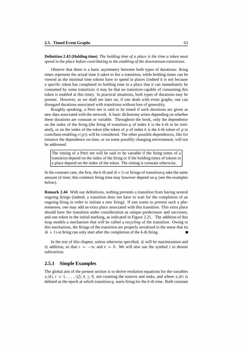
2.5. Timed Event Graphs 63
Definition 2.43 (Holding time) The holding time of a place is the time a token mustspend in the place before contributing to the enabling of the downstream transitions.
Observe that there is a basic asymmetry between both types of durations: firingtimes represent the actual time it takes to fire a transition, while holding times can beviewed as the minimal time tokens have to spend in places (indeed it is not becausea specific token has completed its holding time in a place that it can immediately beconsumed by some transition; it may be that no transition capable of consuming thistoken is enabled at this time). In practical situations, both types of durations may bepresent. However, as we shall see later on, if one deals with event graphs, one candisregard durations associated with transitions without loss of generality.
Roughly speaking, a Petri net is said to be timed if such durations are given asnew data associated with the network. A basic dichotomy arises depending on whetherthese durations are constant or variable. Throughout the book, only the dependenceon the index of the firing (the firing of transitionq of index k is thek-th to be initi-ated), or on the index of the token (the token ofp of indexk is thek-th token of p tocontribute enablingσ(p)) will be considered. The other possible dependences, like forinstance the dependence on time,or on some possibly changing environment, will notbe addressed.
The timing of a Petri net will be said to be variable if the firing times of atransition depend on the index of the firing or if the holding times of tokens ina place depend on the index of the token. The timing is constant otherwise.
In the constant case, the first, thek-th and(k+1)-st firingsof transitionq take the sameamount of time; this common firing time may however depend onq (see the examplesbelow).
Remark 2.44 With our definitions, nothing prevents a transition from having severalongoing firings (indeed, a transition does not have to wait for the completion of anongoing firing in order to initiate a new firing). If one wants to prevent such a phe-nomenon, one may add an extra place associated with this transition. This extra placeshould have the transition under consideration as unique predecessor andsuccessor,and onetoken in the initial marking, as indicated in Figure 2.21. The addition of thisloop models a mechanism that will be called arecycling of the transition. Owing tothis mechanism, the firings of the transition are properly serialized in the sense that its(k + 1)-st firing can only start after the completion of thek-th firing.
In the rest of this chapter,unless otherwise specified,⊕ will be maximization and⊗ addition, so thatε = −∞ ande = 0. We will also use the symbol◦/ to denotesubtraction.
2.5.1 Simple Examples
The global aim of the present section is to derive evolution equations for the variablesxi (k), i = 1, . . . , |Q|, k ≥ 0, not counting the sources and sinks, and wherexi(k) isdefinedasthe epoch at which transitionqi startsfiring for thek-th time. Both constant

64 Synchronization and Linearity
or
p1
q1
p2
q1
p2
p1
Figure 2.21: Recycling of a transition
and variabletimings will be considered. Forgeneral Petri nets, such equations aredifficult to derive. This problem will only be addressed in Chapter 9. For the moment,we shall confine ourselves to event graphs. We start with some simple examples withconstant timing before addressing the general case. The issue of the initial conditionwill not be addressed in these simple examples either (see§2.5.2.1). The general rule(to which we will return in the next subsection) is that transitions start firing as soon asthey are enabled.
Example 2.45 (An autonomous timed event graph) The first exampledeals withthemanufacturing system of§1.2.3, as depicted in Figure 1.5. The related Petri net, givenin Figure 2.13, is the starting point for discussing the way the evolution equations arederived. The timing under consideration is limited to constant holding times on places,which areindicated in the figure. The firing times are all assumed to be 0. We have thefollowing evolution equations:
x1(k + 1) = 5x2(k) ⊕ 3x7(k) ,
x2(k + 1) = 1x1(k + 1)⊕ 3x5(k) ,
x3(k + 1) = 3x5(k) ⊕ 4x6(k) ,
x4(k + 1) = 1x1(k + 1)⊕ 3x3(k + 1) ,
x5(k + 1) = 5x2(k + 1)⊕ 2x4(k + 1) ,
x6(k + 1) = 3x3(k + 1)⊕ 3x7(k) ,
x7(k + 1) = 2x4(k + 1)⊕ 4x6(k + 1) .
In order to get this set of equations, one must first observe that owing to our assumptionthat holding times are constant, overtaking of tokens in places is not possible: thek-th token to enter a place will be thek-th token to leave that place (at least if theinitial marking in that place is 0). If one uses this observation, the equation forx6 (forinstance) is obtained as follows: q6 is enabled for the(k +1)-st time at the latest of thetwo epochs when the(k + 1)-st token to enterthe placebetweenq3 andq6 completesits holding time there, and when thek-th token to enterthe placebetweenq7 andq6
completes its holding time. The difference between the argumentsk andk + 1 comesfrom the factthat the place betweenq7 andq6 has onetoken in the initial marking. Ifonenow uses thedefinition of holding times, it is easily seen that the first of these two

2.5. Timed Event Graphs 65
epochs isx3(k + 1)+ 3, while the second one isx7(k)+ 3, which concludes the proof.There are clearly some further problems to be addressed regarding the initial condition,but let usforget them for the moment. In matrix form this equation can be written as
x(k + 1) = A0x(k + 1)⊕ A1x(k) , (2.10)
where
A0 =
ε ε ε ε ε ε ε
1 ε ε ε ε ε ε
ε ε ε ε ε ε ε
1 ε 3 ε ε ε ε
ε 5 ε 2 ε ε ε
ε ε 3 ε ε ε ε
ε ε ε 2 ε 4 ε
, A1 =
ε 5 ε ε ε ε 3ε ε ε ε 3 ε ε
ε ε ε ε 3 4 ε
ε ε ε ε ε ε ε
ε ε ε ε ε ε ε
ε ε ε ε ε ε 3ε ε ε ε ε ε ε
.
The equation is written in a more convenient way as
x(k + 1) = Ax(k) , (2.11)
whereA = A∗0 A1 (see(1.22)), or, written out,
A =
ε 5 ε ε ε ε 3ε 6 ε ε 3 ε 4ε ε ε ε 3 4 ε
ε 6 ε ε 6 7 4ε 11 ε ε 8 9 9ε ε ε ε 6 7 3ε 8 ε ε 10 11 7
.
Remark 2.46 Both equations (2.11) and (1.29) describe the evolution of the firingtimes, the first equation with respect to the statex , the second one with respect totheoutputy. Using thenotation of§1.2.3, one cancheck that
y(k + 1) = Cx(k + 1) = C Ax(k)
and that
y(k + 1) = M y(k) = MCx(k) ,
whereA is definedabove, and whereC A equalsMC.
Conversely, it is easy to derive a Petri net from (2.11); such a net has 7 transitions(thedimension of the state vector) and 22 places (the number of entries inA which arenot equal toε). Each of these places has a token in the initial marking. The holdingtime associated with the place connecting transitionj to transitioni is given by the

66 Synchronization and Linearity
u1 u2
x 2x 1
x 3
y
1 3
4
42
2 0
5
3
Figure 2.22: Petri net of Example 2.47
appropriateAi j entry. Thus at least two different Petri nets exist which both yield thesame set of evolution equations. In this sense these Petri nets are equivalent.
Example 2.47 (A nonautonomous timed event graph)The starting point for thenext example is Figure 2.22, which coincides with Figure 2.12 with an initial markingadded. The timing is again limited to places. The evolution equations are given by
x(k + 1) = A0x(k + 1)⊕ A1x(k) ⊕ A2x(k − 1)⊕ B0u(k + 1)⊕ B1u(k) ,
y(k) = C0x(k) ⊕ C1x(k − 1) ,
where
A0 =
ε ε ε
3 ε ε
3 4 ε
, A1 =
ε 4 ε
ε ε ε
ε ε ε
, A2 =
ε ε ε
ε ε ε
ε ε 2
,
B0 =
1 ε
ε ε
ε ε
, B1 =
ε ε
ε 5ε ε
,
C0 = ( ε ε 2 ) , C1 =(ε e ε
).
If one usesA∗0, this system can be written as
x(k + 1) =
ε 4 ε
ε 7 ε
ε 11 ε
x(k) ⊕
ε ε ε
ε ε ε
ε ε 2
x(k − 1)
⊕
1 ε
4 ε
8 ε
u(k + 1)⊕
ε ε
ε 5ε 9
u(k) ,
y(k) = (ε ε 2
)x(k) ⊕ ( ε e ε
)x(k − 1) .

2.5. Timed Event Graphs 67
This equation can be put into standard form by augmenting the state space: if onedefines
x(k) = (x1(k), x1(k − 1), x2(k), x2(k − 1), x3(k), x3(k − 1), u1(k), u2(k))′ ,
the system can be written as
x(k + 1) = Ax(k) ⊕ Bu(k + 1) ,
y(k) = C x(k) ,(2.12)
where
A =
ε ε 4 ε ε ε ε ε
e ε ε ε ε ε ε ε
ε ε 7 ε ε ε ε 5ε ε e ε ε ε ε ε
ε ε 11 ε ε 2 ε 9ε ε ε ε e ε ε ε
ε ε ε ε ε ε ε ε
ε ε ε ε ε ε ε ε
, B =
1 ε
ε ε
4 ε
ε ε
8 ε
ε ε
e ε
ε e
,
and
C = ( ε ε ε e 2 ε ε ε)
.
Further simplifications are possible in this equation. Sincex1 is not observable (see[72]) and since it does not influence the dynamics ofx2 or x3 either, it can be discardedfrom the state, as canu1. Thus a five-dimensional state vector suffices. Equation (2.12)is still not in the standard form since the argument ofu is k + 1 instead ofk. If oneinsists on the ‘precise’ standard form, it can be shown that (2.12) and
x(k + 1) = Ax(k) ⊕ ABu(k) ,
y(k) = C x(k) ⊕ C Bu(k) ,(2.13)
are identical in the sense that theirγ -transforms (see Chapter 1) are identical. Thisis left as an exercise to the reader. The latter equation does have the standard form,though there is a direct throughput term (the inputu(k) has a direct influence on theoutputy(k)).
Example 2.48 (Discrete analogue of the system of§1.2.7)Thepurpose of this exam-ple is to play again with the ‘counter’ description already alluded to in Chapter 1, andto show that discrete event systems may obey similar equations as some continuoussystems, up to the problem of ‘quantization’. Figure 2.23 (left-hand side) representsa simple event graph: the three transitions are labelledu, x and y, holding times ofplaces are indicated by numbers (firing times are all zero) and an initial marking isshown. With each transition, e.g. x , is associated a function of time t having the samename, e.g.t �→ x(t), with the following meaning:x(t) represents the number of firings
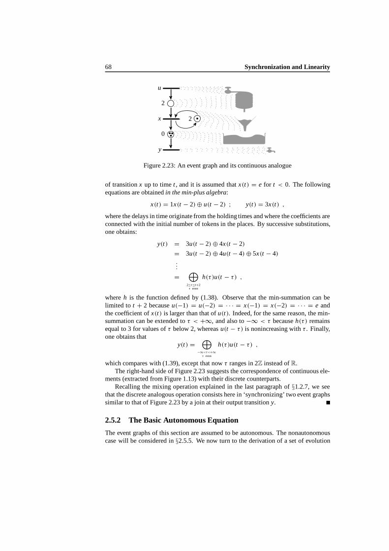
68 Synchronization and Linearity
u
x
y
0
2
2
Figure 2.23: An event graph and its continuous analogue
of transitionx up to time t , and itis assumed thatx(t) = e for t < 0. The followingequations are obtainedin the min-plus algebra:
x(t) = 1x(t − 2)⊕ u(t − 2) ; y(t) = 3x(t) ,
where thedelays in time originate from the holding times and where the coefficients areconnectedwith the initial number of tokens in the places. By successive substitutions,one obtains:
y(t) = 3u(t − 2)⊕ 4x(t − 2)
= 3u(t − 2)⊕ 4u(t − 4)⊕ 5x(t − 4)...
=⊕
2≤τ≤t+2τ even
h(τ )u(t − τ ) ,
whereh is the function defined by (1.38). Observe that the min-summation can belimited to t + 2 becauseu(−1) = u(−2) = · · · = x(−1) = x(−2) = · · · = e andthe coefficient ofx(t) is larger than that ofu(t). Indeed, for the same reason, the min-summation can beextended toτ < +∞, and also to−∞ < τ becauseh(τ ) remainsequal to 3 for values ofτ below 2, whereasu(t − τ ) is nonincreasing withτ . Finally,one obtains that
y(t) =⊕
−∞<τ<+∞τ even
h(τ )u(t − τ ) ,
which compares with (1.39), except that nowτ ranges in 2Z instead ofR.The right-hand side of Figure 2.23 suggests the correspondence of continuous ele-
ments (extracted from Figure 1.13) with their discrete counterparts.Recalling the mixing operation explained in the last paragraph of§1.2.7, we see
that the discrete analogous operation consists here in ‘synchronizing’ two event graphssimilar to that of Figure 2.23 by a join at their output transitiony.
2.5.2 The Basic Autonomous Equation
The event graphs of this section are assumed to be autonomous. The nonautonomouscase will be considered in§2.5.5. We now turn to the derivation of a set of evolution

2.5. Timed Event Graphs 69
equations for event graphs with variable timing, under the general assumptions that
• the transitions start firing as soon as they are enabled;
• the tokens of a place start enabling the transitions downstream as soon as theyhave completed their holding times.
The problems that arise with variable timing are slightly more complex than in thepreceding examples. The main reason for this lies in the fact that tokens can thenovertake one another when traversing places or transitions. As we will see in Chapter 9,this precludes a simpleordering of events to hold, and event graphs with overtaking losethe nice linearity property emphasized in the preceding examples. The discussion willhence be limited to thecase of event graphs with First In First Out (FIFO) places andtransitions, where the ordering of events preserves linearity.
2.5.2.1 Initial Condition
We start with a first discussion of theinitial condition which is here understood as aset of initial delays attached to the tokens of the initial marking in a way that general-izeswhat is often done in queuing theory. This topic will be revisited in§5.4.4.1 and§5.4.4.2, and further considered from a system-theoretic point of view in§5.4.4.3.
Assumethat one starts looking at the system evolution at timet = 0, and that thepiecewise constant functionNi (t) describing the evolution of the number of tokenspresent in pi , i = 1, . . . , |P|, at time t ∈ R, is right continuous. LetNi (0) = µi ,whereµi denotesthe initial marking in placepi .
The general idea behind the initial condition is as follows: theNi (0) ( = µi ) tokensvisible at timet = 0 in pi are assumed to have enteredpi beforetime 0; at time 0, eachtoken is completing its holding time or it is being consumed by the transition (namelyit is a reserved token), or it is ready to be consumed. We can equivalently define theinitial condition through the entrance times of the initial tokens, or through the vectorof R-valuedlag times, where
Definition 2.49 (Lag time) The lag time of a token of the initial marking of pi is theepoch when this token starts contributing to enabling σ(pi ).
However, these lag times should be compatible with the general rules that transitionsfire as soonasthey are enabled and that tokens start enabling the transition downstreamas soon as they have completed their holding times. For instance
• if the lag time of an initial token exceeds its holding time, this token cannot haveentered the placebefore time 0;
• if the lag times (whichare possibly negative) are such that one of the transitionscompletes firing and consumes tokens of the initial marking beforet = 0, thesetokens cannot be part of the marking seen at time 0 since they must have leftbefore time 0.
Definition 2.50 (Weakly compatible initial condition) The initial condition of atimed event graph consists of an initial marking and a vector of lag times. This ini-tial condition is weakly compatible if

70 Synchronization and Linearity
1. the lag time of each initial token does not exceed its holding time;
2. the first epoch when a transition completes firing is nonnegative.
2.5.2.2 FIFO Places and Transitions
A basic assumption that will be made throughout the chapter is that both places andtransitions are First In First Out (FIFO) channels.
Definition 2.51 (FIFO place) A place pi is FIFO if the k-th token to enter this placeis also the k-th which becomes available in this place.
In view of the interpretation of holding times as communication or transportation times,this definition just means that the transportation or communication medium is overtakefree. For instance, a place with constant holding times is FIFO.
Definition 2.52 (FIFO transition) A transition q j is FIFO if the k-th firing of q j tostart is also the k-th to complete.
The interpretation is that tokens cannot overtake one another because of the firingmechanism, namely the tokens produced by the(k + 1)-st firing of q j to be initi-atedcannot enter the places ofσ(q j ) earlier than those of thek-th firing. For instance,a transition with constant firing times is always FIFO. If a transition is recycled, its(k + 1)-st firing cannot start before the completion of thek-th one, so that a recycledtransition is necessarily FIFO, regardless of the firing times.
Definition 2.53 (FIFO event graph) An event graph is FIFO if all its places and tran-sitions are FIFO.
A typical example of a FIFO timed event graph is that of a system with constant holdingtimes and recycled transitions with possibly variable firing times. An event graph withconstant holding and firing times is always FIFO, even if its transitions are not recycled.Since the FIFOproperty is essential in order to establish the evolution equations of thepresent section,it is important to keep in mind that:
The classes of timedevent graphs considered throughout the book are thosewith
1. constant firing and holding times;
2. constant holding times and variable firing times, provided all transitionsare recycled.
2.5.2.3 Numbering of Events
The following way of numbering the tokens that traverse a place and the firings of atransition will be adopted.

2.5. Timed Event Graphs 71
By convention, thek-th token,k ≥ 1, of placepi is thek-th token to contributeenablingσ(pi ) during the evolution of the event graph, including the tokensof the initial marking. Thek-th firing, k ≥ 1, of transitionqi is thek-th firingof qi to be initiated, including the firings that consume initial tokens.
It may happen that two tokens inpi contribute enablingσ(pi ) at the same epoch, orthat two firings of a transition are initiated at the same time (when the transition is notrecycled). In thiscase, some ordering of these simultaneous events is chosen, keepingin mind that it should be compatible with the FIFO assumptions.
2.5.2.4 Dynamics
In what follows, the sequences of holding timesαi(k), i = 1, . . . , |P|, k ∈ Z, and offiring timesβ j (k), j = 1, . . . , |Q|, k ∈ Z, are assumed to be givennonnegative andfinite real numbers. Initially, only the restriction of these sequences tok ≥ 1 will beneeded. However, we assume that these sequences can be continued tok ≤ 0. Such acontinuation is clear in the case of a constant timing, and we will see in due time howto define the continuation in more general circumstances (see§2.5.7).
Weare now in a position to define the dynamics of the event graph more formally.
• Thek-th token of placepi incurs theholding timeαi(k).
• Once thek-th firingof transitionq j is enabled, the time forq j to complete itsk-thfiring is thefiring timeβ j (k). When this firing is completed, the reserved tokenis removed from each of the places ofπ(q j ), and each place ofσ(q j ) receivesone token.
We now state a few basic properties of thenumbering in a FIFO event graph with aweakly compatible initial condition. Fori suchthatµi ≥ 1, denotewi(1) ≤ wi(2) ≤· · · ≤ wi(µi ) ∈ R, the lag times of the initial tokens of placepi ordered in a nonde-creasing way.
Lemma 2.54 If the initial condition is weakly compatible and if the timed event graphis FIFO, then for all i and for all k such that 1≤ k ≤ µi and µi ≥ 1, the initial tokenwith lag time wi(k) is also the k-th token of place pi (that is the k-th token to enableσ(pi )).
Proof If this last property does not hold for some placepi , then a token which does notbelong to the initial marking ofpi , and which hence enterspi after time 0 (the initialcondition is weakly compatible), contributes to enablingσ(pi ) before one of the tokensof the initial marking does. Since the tokens of the initial marking enterpi before time0 (the initial condition is weakly compatible), this contradicts the assumption thatpi isFIFO.
Lemma 2.55 The firing of q j that consumes the k-th token of pi (for all pi ∈ π(q j ))is the k-th firing of qi .

72 Synchronization and Linearity
Proof Owing tothenumbering convention, the set ofk-th tokens ofpi ∈ π(q j) enablesq j before the set of(k + 1)-st tokens.
Lemma 2.56 The completion of the k-th firing of q j , k ≥ 1, produces the (k + µi )-thtoken of pi , for all pi ∈ σ(q j ).
Proof The FIFO assumptionson transitions imply that the completion of thek-th firingof q j produces thek-th token to enter the places that followpi . Theproperty followsimmediately from the FIFO assumption on places and from Lemma 2.54.
2.5.2.5 Evolution Equations
Definition 2.57 (Statevariables, daters) The state variable x j(k), j = 1, . . . , |Q|,k ≥ 1, of the event graph is the epoch when transition q j starts firing for the k-th time,with the convention that for all qi , xi (k) = ∞ if qi fires less than k times. These statevariables will be called daters.
These state variables are continued to negative values ofk by the relation x j (k) = ε,for all k ≤ 0. Let
M = maxi=1,... ,|P|
µi . (2.14)
In what follows, we will adopt the convention that the⊕-sumover an empty set isε.Define the|Q| × |Q|matricesA(k, k), A(k, k − 1), . . . , A(k, k − M), by
A jl (k, k −m)def=
⊕
{i∈πq ( j)|π p(i)=l,µi=m}αi(k)
⊗ βl (k −m) , (2.15)
and the|Q|-dimensional vectorv(k), k = 1, . . . , M, by
v j (k)def=
⊕
{i∈πq ( j)|µi≥k}wi(k) . (2.16)
Theorem 2.58 For a timed event graph with recycled transitions, the state vectorx(k) = (x j (k)) satisfies the evolution equations:
x(k) = A(k, k)x(k) ⊕ A(k, k − 1)x(k − 1)⊕ · · · ⊕ A(k, k − M)x(k − M) ,
k = M + 1, M + 2, . . . , (2.17)
with the initial conditions
x(k) = A(k, k)x(k) ⊕ · · · ⊕ A(k, k − M)x(k − M)⊕ v(k) ,
k = 1, 2, . . . , M , (2.18)
where x j(k)def= ε for all k ≤ 0.

2.5. Timed Event Graphs 73
Proof We first prove thatthe variablesx j (k), j = 1, . . . , |Q|, satisfy the evolutionequations:
x j(k) =⊕
{i∈πq ( j)|k>µi }
(αi(k) ⊗ βπ p (i)(k − µi )⊗ xπ p (i)(k − µi )
)
⊕
⊕
{i∈πq ( j)|k≤µi }wi(k)
, k = 1, 2, . . . . (2.19)
Thek-th firing,k ≥ 1, of transitionq j startsas soon as, for alli ∈ πq( j ), thek-th tokenof pi contributes to enablingq j . In view of Lemmas 2.55 and 2.56, fork > µi , thisk-thtoken is produced by the(k − µi )-th firingof transitionπ(pi ), so that the epoch whenthis token contributes enablingσ(pi ) is αi (k) ⊗ βπ p (i)(k − µi ) ⊗ xπ p (i)(k − µi ). Fork ≤ µi , this event takes place at timewi(k), in view of Lemma 2.54, which completesthe proof of (2.19).
We now use associativity and commutativity of ⊕, together with ourconvention on⊕-sumsover emptysets, to rewrite x j(k), k > M, as
M⊕
m=0
|Q|⊕
l=1
⊕
{i∈πq ( j)|π p(i)=l, µi=m}αi(k) ⊗ βl (k − m)⊗ xl (k − m) .
The distributivity of ⊗ with respect to⊕ implies in turn
x j (k) =M⊕
m=0
|Q|⊕
l=1
⊕
{i∈πq ( j)|π p(i)=l, µi=m}αi (k)
⊗ βl (k − m)⊗ xl (k − m) ,
which completes the proof of (2.17), in view of the definition ofA.The proof of (2.18) follows the same lines (using the continuation of the functions
x j (k) to ε for k ≤ 0).
Remark 2.59 Owing to the dynamics, the first transition to complete its firing is nec-essarily within the set of transitionsq j havingat least one token in the initial markingof pi for all pi ∈ π(q j). Sincethe set of tokens with the smallest lag times is thefirst to be consumed, the second weak compatibility condition in Definition 2.50 canbe translated intothe requirement that
β j (1)⊗ v j (1) ≥ e , (2.20)
for all j suchthatµi ≥ 1 ∀ pi ∈ π(q j ), which can be seen as a first set of linearconstraints on the lag times in view of (2.16). Similarly, the first weak compatibilityrelation is translated into the followingadditional set of linear constraints:
wi(k) ≤ αi(k) , i = 1, . . . , |P| , 1≤ k ≤ µi . (2.21)
For instance, if wi(k) = αi (k) for all i = 1, . . . , |P|, 1 ≤ k ≤ µi , then the initialcondition is weakly compatible, provided the conditionwi(1) ≤ wi(2) ≤ . . . ≤ wi(µi )
is satisfied.

74 Synchronization and Linearity
q3
q1 q2q4
α14(k )
α31(k )
α21(k )
α43(k )
α42(k )
α11(k ) α44(k )
Figure 2.24: Event graph of Example 2.60
Example 2.60Consider the timed event graph of Figure 2.24. The firing times are as-sumed to be equal toe. Theplace connecting q j to ql is denotedpl j . Theholding timesin this placeare denotedαl j (k), and the lag times of the initial tokenswl j (k). In orderto have a FIFO event graph, places should be overtake free. This will always be truefor p11 and p22, regardless of the holding time sequences in these places (since there isalways at most one token each of these places). A simple sufficient condition ensuringthat the other places are overtake free is that the associated holding time sequences arenon decreasing ink (for instance constant). Under the assumption that the event graphis FIFO, the matrices and vectors involved in the evolution equations are
A(k, k) =
ε ε ε ε
ε ε ε ε
ε ε ε ε
ε α42(k) α43(k) ε
, A(k, k − 1) =
α11(k) ε ε α14(k)α21(k) ε ε ε
ε ε ε ε
ε ε ε α44(k)
,
A(k, k − 2) =
ε ε ε ε
ε ε ε ε
α31(k) ε ε ε
ε ε ε ε
,
and
v(1) =
w11(1)⊕w14(1)w21(1)w31(1)w44(1)
, v(2) =
ε
ε
w31(2)ε
.
The constraints (2.21) and (2.20) are translated into the boundswl j (k) ≤ αl j (k), andw11(1)⊕w14(1) ≥ e, w21(1) ≥ e, w31(1) ≥ e.
2.5.2.6 Simplifications
Firing Times The evolution equations (2.19) are unchanged if one sets all the firingtimes equal toe and ifαi(k) receives the valueαi (k) ⊗ βπ p (i)(k − µi ). Thus, one can

2.5. Timed Event Graphs 75
always modify the holding times in order to get an ‘equivalent’ event graph with firingtimes of duratione, where equivalence means that the epochs when transitions fire arethe same in both systems.
It may be assumed without loss of generality that the firing times are equal toe = 0.
Observe that under this assumption the state variablex j (k) is also the epoch whentransitionq j completes itsk-th firing. Graphically, this is exemplified in Figure 2.25.If a firing time were assigned to a transition within an event graph, then this time canalways be assigned to (i.e. added to) the holding times of all the upstream places.Consider Figure 2.25a, in which the transition has a firing time of 5 time units. The
3 4
6
(a) (b) (c)
11
0 0
6
8 9 3 4
5
5
(e)
0
3 4
6
5
(d)
3 4
6
Figure 2.25: Firing times set toe
holdingtimes of the places are 3, 4 and 6 as indicated in this figure. Figure 2.25b showsassignment of the firing time to the places. The firing of the transition in Figure 2.25b,which is instantaneous, corresponds to the completion of the firing of the transition inFigure 2.25a. Another, similar, solution is provided in Figure 2.25c, where the holdingtime has been assigned to all the downstream places. The firing of the transition in thisfigure corresponds to the initiation of the firing of the transition in Figure 2.25a.
A different solution is provided in Figure 2.25d. In this figure, both the beginningand completion of the firing are now explicitly represented. In Figure 2.25e, the holdingtime at the transitions is also 0, but in contrast to the previous solutions the transitionscannot fire twice (or more times) within 5 time units. The transitions cannot be engagedin (partly) parallel activities.
In what follows, we shall therefore often assume that the firing times are zero. Thepractical implication of this mathematical simplification is clear in the constant firingand holding time case. In the variable case, one should however always keep in mindthat the only meaningful initial situation is that of variable firing times (on recycledtransitions) and constant holding times.
Init ial Condition The end of this subsection is devoted to a discussion of the initialcondition. It is shown that Equation (2.18), defining the initial condition, can be furthersimplified whenever the lag times satisfy certain additional and natural constraints.

76 Synchronization and Linearity
For all i suchthatµi > 0, denote byyi(k), k ≤ 0, theentrance time functionassociated with placepi , defined by the relation
yi(k − µi )def={wi (k)◦/αi(k) if 1 ≤ k ≤ µi ;
ε if k > µi ,(2.22)
where we recall that◦/ denotes conventional subtraction.The initial condition is said to becompatible if it is wealky compatible and if for
any pair of placespi and p j which follow the same transition, the entrance timesyi (k)andy j(k) coincide providedk ≥ min(µi , µ j ).
Definition 2.61 (Compatible initial condition) The initial condition is compatible ifit is weakly compatible and if there exist functions z j(k), j = 1, . . . , |Q|, k ≤ 0, suchthat
yi(k) = zπ p (i)(k) , ∀i, k such that − µi + 1≤ k ≤ 0 . (2.23)
This condition is quite natural, should the initial condition result from a past evolutionof the event graph: for instance, the last tokens of the initial marking to enter two placespi and pi ′ that follow the same transitionq j , have then been produced at the same timez j (0) by a firing ofq j .
LetM j
def= maxi∈σ q ( j)
(µi ) .
Observe that the functionz j (k) is only defined through (2.23) for−M j < k ≤ 0,providedM j ≥ 1. For othervalues ofk, or if M j = 0, we takez j (k) = ε.
Instead of the former continuation ofx(k) to k ≤ 0 (which consisted in takingx j (k) = ε for k ≤ 0), we now take
x j (k) = z j(k) , ∀k ≤ 0 , j = 1, . . . , |Q| . (2.24)
Corollary 2.62 For a FIFO timed event graph with a compatible initial condition, thestate vector x(k) = (x j (k)) satisfies the evolution equations:
x(k) = A(k, k)x(k) ⊕ A(k, k − 1)x(k − 1)⊕ · · · ⊕ A(k, k − M)x(k − M) ,
k = 1, 2, . . . , (2.25)
provided the continuation of x(k) to negative values of k is the one defined by (2.24).
Proof By successively using (2.22) and (2.23), one gets
⊕
{i∈πq ( j)|k≤µi }wi(k) =
⊕
{i∈πq ( j)|k≤µi }αi(k) ⊗ yi(k − µi )
=⊕
{i∈πq ( j)|k≤µi }αi(k) ⊗ zπ p(i)(k − µi ) ,

2.5. Timed Event Graphs 77
for all k = 1, 2, . . . , so thatone can rewrite (2.19) as
x j(k) =⊕
{i∈πq ( j)}
(xπ p (i)(k − µi )⊗ αi (k)
), k = 1, 2, . . . , (2.26)
when using the continuation ofx proposed in (2.24). Equation (2.25) follows immedi-ately from (2.26).
Remark 2.63 A simple example of compatible initial condition is obtained whenchoosingwi(k) = αi (k) for all 1 ≤ k ≤ µi . Practically speaking, this means thatall the initial tokens enter at time 0. This corresponds to the continuation
x j(k) ={
e if −M j < k ≤ 0 ;
ε if k ≤ M j .(2.27)
Example 2.64 (Example 2.60 continued)If the initial condition is compatible, let
z1(0)def= w11(1)◦/α11(1) = w21(1)◦/α21(1) = w31(2)◦/α31(2) ,
z1(−1) def= w31(1)◦/α31(1) ,
z4(0)def= w14(1)◦/α14(1) = w44(1)◦/α44(1) .
Define
x(0) =
z1(0)ε
ε
z4(0)
, x(−1) =
z1(−1)ε
ε
ε
.
It is easily checked thatv(2) = A(2, 0)x(0)
and thatv(1) = A(1, 0)x(0) ⊕ A(1,−1)x(−1) .
Thus
x(k) = A(k, k)x(k) ⊕ A(k, k − 1)x(k − 1)⊕ A(k, k − 2)x(k − 2), k = 1, 2, . . . .
2.5.3 Constructiveness of the Evolution Equations
The first naturalquestion concerning Equation (2.17) is: is it implicit or constructive?The main result of this section establishes that the evolution equations (2.17) are notimplicit and that they allow one to recursively define the value ofx j(k) for all j =1, . . . , |Q|, andk ≥ 1, provided the event graph under consideration is live.

78 Synchronization and Linearity
Lemma 2.65 The event graph is live if and only if there exists a permutation P of thecoordinates for which the matrix P
′A(k, k)P is strictly lower triangular for all k.
Proof If the matrix P′A(k, k)P is strictly lower triangular for some permutationP,
then there is no circuit with 0 initial marking, in view of the definition ofA(k, k) (see(2.15)). Conversely, if the event graphis live, the matrixA(k, k) has no circuit, andthere exists apermutation of the coordinates that makesA strictly lower triangular. Theproof is then concluded from Theorem 2.38.
Observe that the fact thatP does not depend onk comes from the fact that thesupport of A(k, k) does not depend onk (by ‘the support’ of matrixA we mean thematrix S with the same dimension asA defined bySi j = 1Aij =ε).
If the matrix P ′A(k, k)P is strictly lower triangular,An(k, k) = ε for n ≥ |Q|, andthe matrix
A∗(k, k)def= e ⊕ A(k, k) ⊕ A2(k, k) ⊕ · · ·
is finite. Let
A(k, k − l)def= A∗(k, k)A(k, k − l) , k ∈ Z , l = 1, . . . , M , (2.28)
andv(k)
def= A∗(k, k)v(k) , k ∈ Z ,
with v j (k)def= ε for k ≤ 0 or k > M.
Theorem 2.66 If the event graph is live, the evolution equations (2.17) and (2.18) canbe rewritten as
x(k) = A(k, k − 1)x(k − 1)⊕ · · · ⊕ A(k, k − M)x(k − M)⊕ v(k) ,
k = 1, 2, . . . , (2.29)
where x j(k)def= ε, for all k ≤ 0.
Proof From (2.17) and (2.18), we obtain by induction onn that
x(k) = An+1(k, k)x(k)
⊕(
n⊕
m=0
Am (k, k)
) (M⊕
l=1
A(k, k − l)x(k − l)⊕ v(k)
), k = 1, 2, . . . .
Equation (2.29) follows from the last relation by lettingn go to∞.
Remark 2.67 If the initial condition is compatible and if one now takes the continu-ation of x(k) for k ≤ 0, as defined in (2.24), the same type of arguments shows that(2.25) becomes
x(k) =M⊕
l=1
A(k, k − l)x(k − l) , k = 1, 2, . . . .

2.5. Timed Event Graphs 79
Corollary 2.68 If the event graph is live and if the holding times and the lag times areall finite, so are the state variables x j (k), j = 1, . . . , |Q|, k ≥ 1.
Proof The proof is by induction based on (2.29).
Remark 2.69 The matrixA(k, k−l), l ≥ 1, has a simple graph-theoretic interpretation.Let S( j ′, j, l) be the set of paths in the graphG of the event graph, of length at least 2,with initial transitionq j ′, with final transitionq j , and suchthat the first two transitionsof the path are connected by a place with initial marking equal tol, while the othertransitions are connected by places with 0 initial marking. It is easily checked, usingthe results of§2.4, thatA j j ′(k, k − l) is defined by the relation
A j j ′(k, k − l) =⊕
{ρ=( j1,i1, j2,i2··· ,ih−1, jh)∈S( j ′, j,l)}
h−1⊗
n=1
αin (k) , (2.30)
with the usual convention if the setS( j ′, j, l) is empty. The entryA j j ′(k, k − l) ishence simply the longest path inS( j ′, j, l).
Example 2.70 (Example 2.60 continued)We have
A∗(k, k) =
e ε ε ε
ε e ε ε
ε ε e ε
ε α42(k) α43(k) e
,
so that
A(k, k − 1) =
α11(k) ε ε α14(k)α21(k) ε ε ε
ε ε ε ε
α42(k)α21(k) ε ε α44(k)
,
A(k, k − 2) =
ε ε ε ε
ε ε ε ε
α31(k) ε ε ε
α43(k)α31(k) ε ε ε
,
and
v(1) =
w11(1)⊕w14(1)w21(1)w31(1)
w21(1)α42(1)⊕ w31(1)α43(1)⊕w44(1)
, v(2) =
ε
ε
w31(2)w31(2)α43(2)
.
Remark 2.71 (Equivalent event graph with positive initial marking) With the evo-lution equation (2.29), one canassociate aderived event graphwith the same set oftransitions as the initial event graph, and where the initial marking is such thatµi > 0
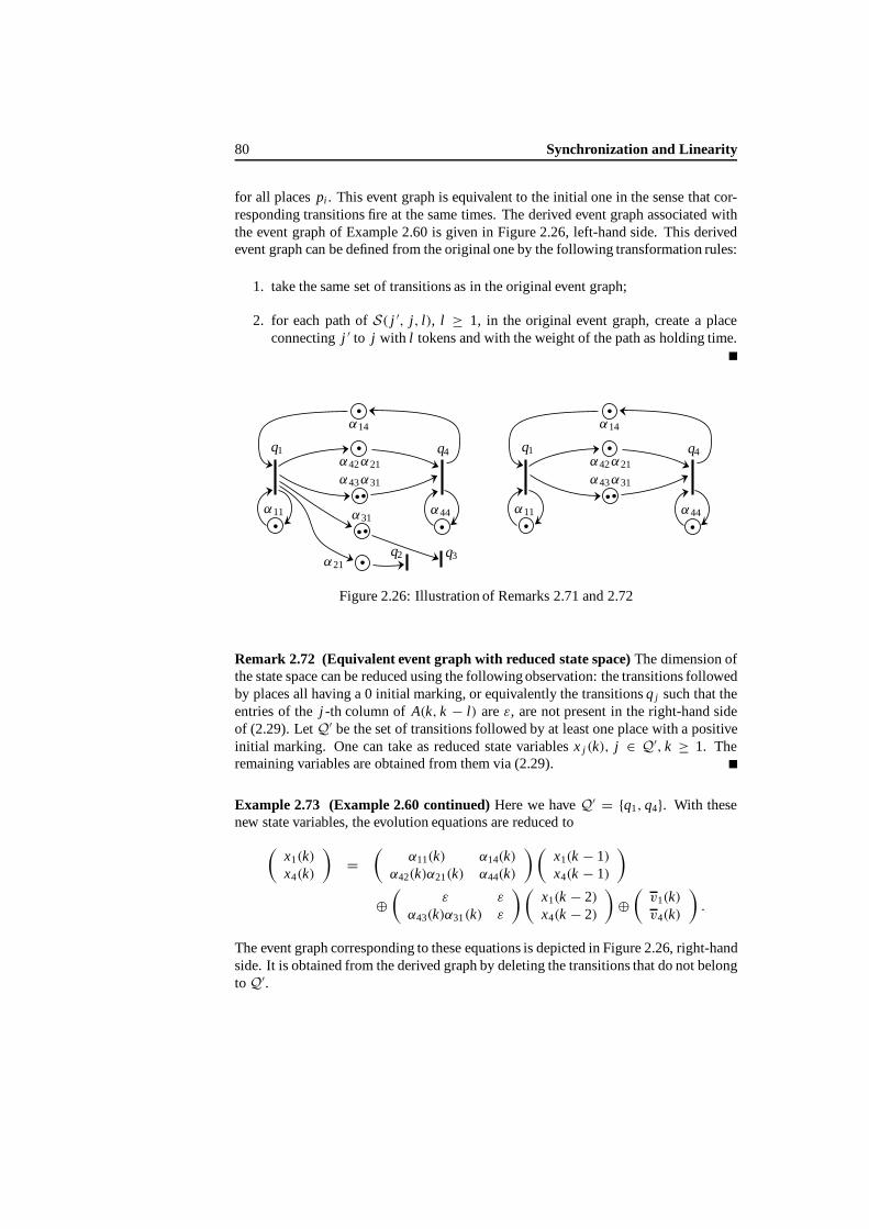
80 Synchronization and Linearity
for all placespi . This event graph is equivalent to the initial one in the sense that cor-responding transitions fire at the same times. The derived event graph associated withthe eventgraph of Example 2.60 is given in Figure 2.26, left-hand side. This derivedevent graphcan be defined from theoriginal one by the following transformation rules:
1. take the same set of transitions as in the original event graph;
2. for each path ofS( j ′, j, l), l ≥ 1, in the original event graph, create a placeconnectingj ′ to j with l tokens and with the weight of the path as holding time.
q3
q1
q2
q4
α14
α31
α21
α11 α44
α43α31
α42α21
q1 q4
α14
α11 α44
α43α31
α42α21
Figure 2.26: Illustration of Remarks 2.71 and 2.72
Remark 2.72 (Equivalent event graph with reduced state space)The dimensionofthe state space can be reduced using the followingobservation: the transitions followedby places all having a 0 initial marking, or equivalently the transitionsq j such that theentries of the j -th column of A(k, k − l) areε, arenot present in the right-hand sideof (2.29). LetQ′ be the set of transitions followed by at least one place with a positiveinitial marking. One can take as reduced state variablesx j (k), j ∈ Q′, k ≥ 1. Theremaining variables are obtained from them via (2.29).
Example 2.73 (Example 2.60 continued)Here we haveQ′ = {q1, q4}. With thesenew state variables, the evolution equations are reduced to
(x1(k)x4(k)
)=(
α11(k) α14(k)α42(k)α21(k) α44(k)
)(x1(k − 1)x4(k − 1)
)
⊕(
ε ε
α43(k)α31(k) ε
)(x1(k − 2)x4(k − 2)
)⊕(
v1(k)v4(k)
).
The event graph corresponding to these equations is depicted in Figure 2.26, right-handside. It isobtained from the derived graph by deleting the transitions that do not belongtoQ′.

2.5. Timed Event Graphs 81
The other state variables are obtained from the reduced state variables by the rela-tion
(x2(k)x3(k)
)=(
α21(k) ε
ε ε
)(x1(k − 1)x4(k − 1)
)
⊕(
ε ε
α31(k) ε
)(x1(k − 2)x4(k − 2)
)⊕(
v2(k)v3(k)
).
The variables(x2(k), x3(k)) areoutput variables in the derived event graph. Equiva-lently, transitionsq2 andq3 are sinks of the derived event graph.
2.5.4 Standard Autonomous Equations
The data of this section is a live event graphsatisfying the evolution equations (2.29),with the reduction of the state space mentioned in Remark 2.72. We will assume thatthe transitionsof Q′ arenumbered 1, . . . , |Q′|, which introduces no loss of generality.
It may be desirable to replace the initial recurrence (2.29), which is of orderM,by an equivalent recurrence of order 1. This is done by using the standard techniquewhich consists in extending the state vector. As a new state vector, take the
(|Q′| × M)-
dimensional vector
x(k)def=
x(k)x(k − 1)
...
x(k + 1− M)
.
Let A(k), k ∈ Z, be the(|Q′| × M)× (|Q′| × M) matrix defined by the relation
A(k) =
A(k + 1, k) A(k + 1, k − 1) . . . . . . A(k + 1, k + 1− M)
e ε . . . ε ε
ε e. . .
......
.... . . e ε ε
ε . . . ε e ε
,
wheree andε denote the|Q′| × |Q′| identity and zero matrices, respectively, and letv(k) be the
(|Q′| × M)-dimensional vector
v(k)def=
v(k + 1)ε...
ε
,
whereε represents here the|Q′|-dimensionalzero vector.Adopting the convention thatx j (k) andv j (k) are equal toε for k ≤ 0, it should be
clearthat Equation (2.31) in the following corollary is a mere rewriting of the evolutionequations (2.29).

82 Synchronization and Linearity
Corollary 2.74 The extended state space vector x(k) satisfies the(M × |Q′|)-
dimensional recurrence relation of order 1
x(k + 1) = A(k)x (k) ⊕ v(k) , k = 1, 2, . . . . (2.31)
Equation (2.31) will be referred to as thestandard form of the evolution equations ofanautonomous timed event graph satisfying (2.29).
Remark 2.75 In the particular case of a compatible initial condition, these equationsread
x(k + 1) = A(k)x (k) , k = 1, 2, . . . , (2.32)
providedthe continuation ofx j(k) for k ≤ 0, is that of Equation (2.24). Whenever theentrance times of the tokens of the initial marking are all equal toe (see Remark 2.63),it is easily checked from (2.27) that in this case
xl|Q′ |+ j (0) ={
e if 0 ≤ l < M j ;
ε for l ≥ M j ,(2.33)
for l = 0, . . . , M − 1; j = 1, . . . , |Q′|.
Example 2.76 (Example 2.60 continued)Here we have
x(k) =
x1(k)x4(k)
x1(k − 1)x4(k − 1)
, v(k) =
v1(k + 1)v4(k + 1)
ε
ε
,
and
A(k) =
α11(k + 1) α14(k + 1) ε ε
α42(k + 1)α21(k + 1) α44(k + 1) α43(k + 1)α31(k + 1) ε
e ε ε ε
ε e ε ε
.
In the special case mentioned at the end of the preceding remark, we havex(0) =(e, e, e, ε)′.
Remark 2.77 (Equivalent net with at most one token in the initial marking) Onecan associate a timed event graph with the evolution equations (2.31). The interest-ing property of this event graph is that its initial marking is such thatM = 1 (moreprecisely, eachµi in this event graph is 1).
In view of Corollary 2.74, one can hence state that for any timed event graph, onecanconstruct another ‘equivalent’ event graph with initial marking equal to 1 every-where. The equivalence means here that one can find a bijective mapping from theset of transitions of the initial event graph to a subset of the transitions of the second

2.5. Timed Event Graphs 83
one, such that two corresponding transitions fire at the same time. In particular, anyobservation of these transitions will be identical.
For instance, in the case of a compatible initial condition, this event graph can beobtained from the original one by first transforming it into an event graph with positiveinitial marking (as it was done in Remark 2.71), and by then applying the followingtransformation rules:
1. for each transition q j of Q′ in the original event graph, createM transitionsq jl, l = 0, . . . , M − 1;
2. for eachq jl , l = 0, . . . , M − 2, create a place that connectsq jl to qi,l+1, with 0holdingtimes. Put one token in its initial marking, with initial lag timez j(−l);
3. for each place connectingqi ∈ Q′ to q j , andwith l + 1 initial tokens,l ≥ 0,in the original system, create a place with one token with initial lag timezi(−l),and with the same holding times sequence as the original place. This new placehasqil asinput transition, andq j0 asoutput transition.
For Example 2.60, the corresponding event graph is given in Figure 2.27. The behaviorof q10 in this graph is the same as that ofq1 in Figure 2.24. The same property holdsfor q40 andq4 respectively.
00
z4(0)
z1(0) z1(−1)
q10 q40 q41
α11 α44
α43α31q11
α42α21
α14
Figure 2.27: Illustration of Remark 2.77
2.5.5 The Nonautonomous Case
This subsection focuses on FIFO timed event graphs with external inputs. The firingtimes can be taken equal to 0, without loss of generality.
To theframework of the preceding sections, we add a new class of transitions calledinput transitions. This setof transitions will be denotedI.
Definition 2.78 (Input transition) An input transition consists of a source transitionand of a nondecreasing real valued sequence, called the input sequence .
84 Synchronization and Linearity
The input sequence associated with transitionq j ∈ I will be denotedu j (k), k ≥ 1; theinterpretation of this sequence is thatu j (k), k ≥ 1, gives the epoch whenq j fires forthek-th time, due to some external trigger action. The input sequences are assumed tobe given.
Definition 2.79 (Weakly compatible input sequence)The input sequence u j (k), k ∈Z, is weakly compatible if u j (1) ≥ 0.
In what follows, all input sequences will be assumed to be weakly compatible. As inthe autonomous case, the initial condition is said to be weakly compatible if in addition
• the entrance times of the tokens of the initial marking are nonpositive;
• the firings which consume tokens of the initial marking complete at nonnega-tiveepochs (the assumption that the input sequences are weakly compatible maycontribute ensuring that this holds).
The definition of compatibility is the same as in the autonomous case. For instance,if the lagtimesof a nonautonomous event graph are compatible, one can continue theinput sequence{u j (k)} (with j ∈ I) to a nondecreasing sequence{u j (k)}k∈Z , withu j (0) ≤ 0, such that for all pi ∈ σ(q j ) with µi ≥ 1,
wi(k) = αi(k) ⊗ u j (k − µi ) , ∀k : 1≤ k ≤ µi . (2.34)
2.5.5.1 Basic Nonautonomous Equations
The derivation of theevolution equations is based on the same type of assumptions asin the autonomous case, namely the event graph is FIFO and the initial condition isweakly compatible.
Define the|Q| × |I|matricesB(k, k), . . . , B(k, k − M) by
B jl (k, k − m)def=
⊕
{i∈πq ( j)|π p(i)=l,µi=m}αi(k) , (2.35)
and the|I|-dimensional vectoru(k) = (u1(k), . . . , u|I|(k)), k = 1, 2, . . . . Using thesame argumentsas in Theorem 2.58, we get the following result.
Theorem 2.80 Under the foregoing assumptions, the state vector x(k) =(x1(k), . . . , x|Q|(k))′ satisfies the evolution equations:
x(k) = A(k, k)x(k) ⊕ · · · ⊕ A(k, k − M)x(k − M)⊕ B(k, k)u(k)⊕ · · · ⊕ B(k, k − M)u(k − M)⊕ v(k) , k = 1, 2, . . . ,
(2.36)
where x j (k)def= ε and u j (k) = ε for all k ≤ 0; v j (k) is defined as in (2.16) for
1 ≤ k ≤ M and it is equal to ε otherwise.

2.5. Timed Event Graphs 85
If the initial lag times and the input sequences are both compatible, this equation canbe simplified by using the same arguments as in Corollary 2.62, which leads to theequation
x(k) = A(k, k)x(k) ⊕ · · · ⊕ A(k, k − M)x(k − M)⊕ B(k, k)u(k)⊕ · · · ⊕ B(k, k − M)u(k − M) , k = 1, 2, . . . ,
(2.37)
where thecontinuations that are taken forx(k) andu(k), k ≤ 0, are now those definedin Corollary 2.62and Equation 2.34, respectively.
In what follows, we will say that the nonautonomous event graph is live if theassociated autonomous event graph (namely the one associated with the equationx(k) = A(k, k)x(k) ⊕ · · · ⊕ A(k, k − M)x(k − M)) is live. Let
B(k, k − l)def= A∗(k, k)B(k, k − m) , k ∈ Z , l = 0, . . . , M .
The following theorem is proved like Theorem 2.66.
Theorem 2.81 If the event graph is live, the evolution equations (2.36) can be rewrit-ten as
x(k) = A(k, k − 1)x(k − 1)⊕ · · · ⊕ A(k, k − M)x(k − M)
⊕ B(k, k)u(k) ⊕ · · · ⊕ B(k, k − M)u(k − M)⊕ v(k) ,
k = 1, 2, . . . ,(2.38)
with the same simplification as in Corollary 2.62, provided the initial lag times and theinput sequences are compatible.
The graph theoretic interpretation ofB j j ′(k, k−l) isagain the longest path inS( j ′, j, l)(see Remark 2.69).
2.5.5.2 Standard Nonautonomous Equations
Define the(M × |I|)-dimensional vector
u(k)def=
u(k + 1)u(k)...
u(k + 2− M)
,
and the(|I| × M)× (|Q′| × M) matrix
B(k) =
B(k + 1, k + 1) B(k + 1, k) . . . B(k + 1, k + 2− M)
ε ε . . . ε...
......
...
ε ε . . . ε
.

86 Synchronization and Linearity
Corollary 2.82 (Standard nonautonomous equation)The extended state space vec-tor x(k) satisfies the
(M × |Q′|)-dimensional recurrence of order 1:
x(k + 1) = A(k)x (k) ⊕ B(k)u(k) ⊕ v(k) , k = 1, 2, . . . , (2.39)
with the same simplification as in Corollary 2.62, provided the initial lag times and theinput sequences are compatible.
Remark 2.83 Formally, the autonomous equation (2.17) can also be seen as that ofa nonautonomous event graph with a set of input transitionsI = {q ′1, q ′2, . . . } of thesamecardinality as the setQ′, with input sequence vectorv(k), andwith B(k, k) = e,B(k, k − l) = ε for l = 1, . . . , M (the input transitionq ′j is connected tothe internaltransitionq j by a single place with 0 initial marking).
However, the requirement that an input sequence should be nondecreasing con-tradicts our foregoing assumption onv(k) (with our definitions,v j (k) eventually be-comesε for k large,as it can be seen from (2.16)). However, when using the fact thatthe sequencesx j(k) are nondecreasing, it is easy to check that one can take the inputsequenceu j (k) defined by the function
u j (k)def={v j (k) if 1 ≤ k ≤ M j ;
v j (M j ) if k ≥ M j ,
instead ofv(k), without altering the values ofx(k).This representation of an autonomous event graph as a nonautonomous one, where
all i nitial lag times can be taken equal toε, is exemplified on the eventgraph of Exam-ple 2.60 in Figure 2.28.
q1 q4q2
q3
u2(k ) = w21(1) , k ≥ 1
u4(k ) = w44(1)k ≥ 1
u3(1) = w31(1)u3(k ) = w31(2) k ≥ 2,
u1(k ) = w14(1)⊕w11(1)k ≥ 1
Figure 2.28: Illustration of Remark 2.83

2.5. Timed Event Graphs 87
2.5.6 Construction of the Marking
This subsection is concerned with the construction of the marking from the state vari-ables. We will limit ourselves to the construction of the marking at certain epochs forwhich their expression is quite simple. However, the formulæ that are obtained arenonlinearin the max-plus algebra. We will therefore return to classicalalgebra, at leastin this subsection. For the sake of simplicity, it is assumed that the initial condition iscompatible. Pick some placepi in P, and letq j = π(pi ), ql = σ(pi ). Let Ni (t) be thenumber of tokens in placepi at time t, t ≥ 0, with the convention that this piecewiseconstant function is right-continuous.
Let
N−i (k)
def= Ni(xπ p (i)(k)
), k ≥ 1 , (2.40)
N+i (k)
def= Ni(xσ p(i)(k)
), k ≥ 1 . (2.41)
Owing toour definitions,N−i (k) is the number of tokens inpi just after thek-th token
entrance intopi after t = 0, while N+i (k) is thenumber of tokenspi just after the
departure of thek-th token to leavepi aftert = 0.
Lemma 2.84 Under the foregoing assumptions,
N−i (k) =
k+µi∑
h=1
1{xl(h)>x j (k)} , k = 1, 2, . . . , (2.42)
N+i (k) =
∞∑
h=k+1−µi
1{xl(k)≥x j (h)} , k = 1, 2, . . . . (2.43)
Proof The tokens present inpi at time (just after)x j (k) are those that arrived intopi
no later thanx j(k) and which are still in pi at time x j (k). The tokens that arrived nolater thanx j(k) are those with indexh with respect to this place, with 1≤ h ≤ k+ µi .Among these tokens, those which satisfy the relationxl(h) > x j (k) are still in pi attime x j(k). Similarly, the only tokens that can be present in placepi just after timexl (k) are those with indexh > k with respect topi . The token of indexh with respectto pi is the token produced by transitionj at time x j(h − µi ) (where the continuationof x j (k) to k ≤ 0 is theone defined in§2.5.2.6). Among these tokens, those whichenteredpi no later than timexl(k) are in pi at time xl (k).
2.5.7 Stochastic Event Graphs
Definition 2.85 (Stochastic event graph)A timed event graph is a stochastic eventgraph if the holding times, the firing times and the lag times are all random variablesdefined on a common probability space.
Different levels of generality can be considered. The most general situation thatwill be considered in Chapters 7 and 8 is the case when the sequences{αi (k)}k∈Z ,
i = 1, . . . , |P|, and {β j (k)}k∈Z , j = 1, . . . , |Q|, are jointly stationary and ergodic

88 Synchronization and Linearity
sequences of nonnegative and integrable random variables defined on a common prob-ability space(�,F,P). Similarly, the lag timeswi (k − µl ), 1≤ k ≤ µi , are assumedto be finite and integrable random variables defined on(�,F,P).
More specific situations will also be considered, like for instance the case whenthe sequences{αl (k)}k∈N , l = 1, . . . , |P|, and{βi (k)}k∈N , i = 1, . . . , |Q|, are mutu-ally independent sequences of independent and identically distributed (i.i.d.) randomvariables. For instance, all these variables could be exponentially distributed, with aparameter that depends onl or i, namely
P[αl (k) ≤ x ] ={
1− exp(al x) if x ≥ 0 ;
0 otherwise,(2.44)
and
P[βi (k) ≤ x ] ={
1− exp(bi x) if x ≥ 0 ;
0 otherwise,(2.45)
wherea j > 0 andb j > 0. Another particular case arises when all the sequences areconstant and deterministic, and the case withconstant timing is thusa special (anddegenerate) case of the i.i.d. situation.
2.6 Modeling Issues
In this section some issues related to the modeling of Petri nets will be described briefly.
2.6.1 Multigraphs
Multigraphs are graphs in which more than one arc between two nodes is allowed. Thefact that in this chapter no such multigraphs have been considered is twofold.
The first reason is that the modeling power of Petri nets with multiple arcs andPetri nets with single arcs is the same [108]. This ‘modeling power’ is defined in termsof ‘reachability’, as discussed in§2.4.1. Petri nets with multiple arcs can straightfor-wardly be represented by Petri nets with single arcs, as shown in Figure 2.29. Note,
Figure 2.29: The changeof multiple arcs into single arcs
however, that in the second of these figures a conflict situation has arisen. In order that

2.6. Modeling Issues 89
this single arc representation of the originally multiple arc from place to transition be-haves in thesameway as this multiple arc, it is necessary that the tworival transitionsreceive tokens alternately.
The second reason is that it is not at all clear how toobtain equations for timedPetri nets in which there are multiple arcs. Observe that such nets are not event graphs,as is directly seen from Figure 2.29. It seems that some transitions fire in the long runtwice as often as some other transitions; the 2k-th enabling of such a ‘fast’ transition iscaused by thek-th firing (approximately) of such a ‘slow’ transition.
2.6.2 Places withFinite Capacity
For the rule for enabling transitions it has tacitly been assumed thateach place canaccommodate an unlimited number of tokens. For the modeling of manyphysicalsystems it is natural to consider an upper limit for the number of tokens thateach placecan hold. Such a Petri net is referred to as a finite capacity net. In such a net, each placehas an associated capacityKi , being the maximumnumber of tokens thatpi can holdat any time. For a transition in a finite capacity net to be enabled, there is the additionalcondition that the number of tokens ineachpi ∈ σ(q j ) cannot exceed its capacity afterthe firing ofq j .
In the discussion to come we confine ourselves to event graphs, although the ex-tension to Petri nets is quite straightforward, see [96]. Suppose that placepi has acapacity constraintKi , then the finite capacity net will be ‘remodeled’ as another eventgraph, without capacity constraints. Ifπ(pi) ∩ σ(pi ) = ∅, then there is a loop. Thenumber of tokens in a loop before and after the firing is the same and hence the capac-ity constraint is never violated (provided the initial number of tokens was admissible).Assume now that π(pi) ∩ σ(pi ) = ∅. Add another placepi ′ to the net. This newplace will haveµi ′ = Ki − µi tokens. Add an arc fromσ(pi ) to pi ′ and an arcfrompi ′ to π(pi ). Thenumber of tokensin this new circuit is constant according to Theo-rem 2.37. The liveness of theevent graph is not influenced by the addition of such anew circuit, see Theorem 2.38. An example is provided in Figure 2.30 whereKi = 3.
K i = 3pi
pi
p′i
Figure 2.30: Node with and without a capacity constraint
It is easily verified that this newly constructed Petri net, without capacity constraints,behaves in exactly the same way in terms of possible firing sequences as the originalfinite capacity net. In this sense the nets are ‘equivalent’.

90 Synchronization and Linearity
2.6.3 Synthesis of Event Graphs from Interacting Resources
This aim of this subsection is to show how, starting from the physical understandingof ‘resources’, and some assumptions, one can build up event graphs in a somewhatsystematic way. This approach leads to a subclass of event graphs (essentially restrictedby the kind of initial marking they can receive) for which the issue of initial conditionsis transparent.
2.6.3.1 General Observations
The exercise of modeling is more an art than an activity which obeys rigid and preciserules. For example, the degree of detailsretained in a model is a matter of appraisalwith respect to future uses of the model. Models may be equivalent in some respects butthey may differ in the physical insights they provide. These observations are classicalin conventional system theory: it is well known that different state space realizations,evenwith different dimensions, may yield the same input-output behavior, but some ofthese reali zations may capture a physical meaning of the state variables whereas othersmaynot.
To be more specific, a clear identification of what corresponds to ‘resources’ in anabstract Petri net model may not be crucial if available resources are given once and forall and ifthe problem only consists in evaluating the performance of a specified system,but it may become a fundamental issue when resource quantities enter the decisionvariables,e.g. in optimal resource sizing at the design stage. It has already been noticedthat, in an event graph, although the number of tokens ineach circuit is invariant duringthe evolution of the system, this is notgenerally the case of thetotal number of tokensin the system, even if the graph is strongly connected and autonomous. In this case, itis unclear how tokens and physical resources are related toeach other.
Figure 2.31 shows the simplest example of this type for which there are only twodistinct situations for the distribution of tokens, the total number of tokens being eitherone or two. Indeed, if we redraw this event graph as in Figure 2.32, it becomes pos-
(a) (b)
Figure 2.31: Merging two resources
(a) (b)
Figure 2.32: An alternative model
sible to interpret the two tokens as two resourcescirculating in the system sometimesalone (case (a)) and sometimes jointly (case (b)). The problem with the former modelof Figure 2.31 is that, when they stay together (case (b)), the two resources are rep-resented by a single token. Obviously, these two models are equivalent if one is only
2.6. Modeling Issues 91
interested in the number of transition firings within a certain time (assuming that someholding times have been defined properly in corresponding places), but the differencebecomes relevant if oneis willing to play with individual resource quantities in orderto ‘optimize’ the design.
As long as modeling is an art, what is described hereafter should be considered asa set of practical guidelines—rather than as a rigorous theory—which should help intrying to construct models which capture as much physical meaning as possible. Thedynamic systems we have in mind are supposed to involve the combined evolution ofseveral interacting resources designed to achieve some specific overall task or service.Our approach isin three stages:
1. we first describethe evolution of each type of resource individually;
2. then we describe the mechanism of interaction between resources;
3. finally, we discuss the problem of initialization.
2.6.3.2 State Evolution of Individual Resources
The word ‘resource’ should be understood in the broadest sense: a machine, a tool, apart, achannel, a transportation link, a position in a storage or in a buffer, etc. are allresources. Of course, in practice, it is worthwhile modeling a resource explicitly aslong as it is a ‘scarce’ resource, that is a resource the limited availability of which mayhave some influence on the evolution of the system at some time. The capacity of abuffer may be large enough for the buffer to behave as if it were infinite. Again, it isa matter of feeling to decide whether an explicit model of the finite capacity is a priorineeded or not.
The evolution of each resource in the system is modeled by a sequence of ‘stages’.What is considered a ‘stage’ is a matter of judgment since severalconsecutive stagesmay be aggregated intoa single stage. For example, considering the evolution of a partin a workshop, traveling to the next machine and then waiting for the temperature to becool enough before entering this next machine may be considered a single stage. Weassume that
• the nature and the order of the stages experienced by each type of resource areknown in advance;
• for agiven resource, every stage is preceded (followed)—if it is not the first (last)stage—by asingle other stage.
Consequently, for a given type of resource, if we draw a graph such that nodes (drawnas places in a Petri net) represent stages, and arcs indicate precedence of the upstreamstages over the downstream stages, then this graph is a path (i.e. it has neither circuitsnor branches) and itreflects the total order of stages.
Obviously, in a workshop, this assumes that a ‘deterministic scheduling’ of oper-ations has been defined a priori. For example, a machine is supposed to work on aspecified sequence of parts in a specified order, each operation being represented by aparticular stage. If the stage ‘idle’ is possible between two such operations (i.e. the

92 Synchronization and Linearity
machine may deliver the part it holds without receiving its next part—hence it staysalone for a while), then additional stages should be introduced in between. Notice that
• the stage ‘idle’ isnot represented by aunique node, but that a node of this typeis introduced if necessary betweenany two successive operations;
• a machine may be idle, while still holding the part it was working on, becausethere is no storage available downstream, and the next operation of this machinecannot be undertaken before the downstream machine can absorb the presentpart. In this case, it is not necessary to introduce an additional stage, that is,the stage ‘working’ and the stage ‘waiting for downstream delivery’ need not bedistinguished.
For a part, it is also assumed that the sequence of machines visited is specified inadvance, but notice that storages visited should be considered as an operation of thesame type as machines visited. Therefore, a storage position, if it is common to severaltypes of parts, must know in advance the order in which it will be visited by thesedifferent parts, which is certainly a restrictive constraint in the modeling phase, but thisis the price to pay for remaining eventually in the class of event graphs.
Finally, the evolution of a resource is simplya path (inother words, this evolutionis represented by a serial automaton). For convenience, each arc will be ‘cut’ by a barresembling a transition, which will serve later on for synchronization purposes. Eachstage receives a sequence of holding times representingminimal times spent in thisstage by the successive resources. For example, waiting in a storage should involve aminimal time equal to 0. At any time, the present stage of a given resource is repre-sented by a token marking the corresponding place. Transitions represent changes ofstages and they are instantaneous.
Resources may enter the system and leave it after a while (nonreusable resources)or they may revisit the same stages indefinitely because they are ‘recycled’ (reusableresources). For example, raw materials come in a workshop and leave after a trans-formation, whereas machines may indefinitely resume their work on the same repeti-tive sequences of parts. Sometimes, nonreusable resources are tightly associated withreusable resources so that it is only important to model these reusable resources: forexample, parts may be fixed on pallets that are recycled after the parts leave the work-shop. For reusable resources, we introduce an additional stage called the ‘recyclingstage’, and we put an arc from the last stage (of an elementary sequence) to this recy-cling stage and another arc from the recycling stage to the first stage. Hence we obtain acircuit. Physically, the recycling stage mightrepresent a certain ‘reconditioning’ oper-ation (possibly involving other resources too), and therefore it might receive anonzeroholding time (transportationtime, set-up time, etc.). However, it will be preferable tosuppose that the recycling stage of any resource corresponds to an abstract operationwhich involvesonly this resource, and which is immediate (holding time 0). The posi-tioning of this recycling stage with respect to the true reconditioning operation (beforeor after it) is left to the appraisal of the user in each specific situation. Indeed, eachstage along the circuit of the reusable resource where this resource stands alone maybe a candidate to play the role of the recycling stage, a remark which should be kept in

2.6. Modeling Issues 93
mind when we speak of canonical initialization later on (this is related to the issue ofthepoint at which one starts a periodic behavior).
2.6.3.3 Synchronization Mechanism
Any elementaryoperation may involve only one particular type of resource, or it mayalso involve several different resources. For example, a part waiting in a storage in-volves both the part and the storage position (whereas an idle machine involves onlythis machine). It should be realized that, so far, the same physical operation, as longas it involvesn different resources simultaneously, has been represented byn differentplaces.
If two stages belonging to two distinct resource paths (or circuits) correspond tothe same operation, we must express that these stages are entered and left simultane-ously by the two resources (moreover, the holding times of these stages should be thesame). This may be achieved by putting two synchronization circuits, one connectingthe ‘beginning’ transitions, the other connecting the ‘end’ transitions, as indicated inFigure 2.33. In order to comply with the standard event graph representation, we haveput new places—represented here in grey color—over the arcs of these circuits. How-ever, these grey places do not represent ‘stages’ as other places do. They are nevermarked with tokens and they have holding times equal to 0. Then, it is realized thatthese circuits involving no tokens and having a total holding time equal to 0 expresssimultaneity of events, that is entering or leaving the considered stage by anyone of thetwo resources precedes the same type of event achieved by the other resource and viceversa.
Remark 2.86 What we have just done here is nonstandard from the point of view ofPetri net theory, although it is mathematically correct for the purpose of expressingsimultaneity. Indeed, having alive Petri net which includes circuits with no tokensseems to contradict Theorem 2.38. More specifically, every transition having a ‘greyplace’ upstream (which will never receive tokens) will never fire if we stick to thegeneral rule about how transition firings are enabled. We propose the following (tricky)adaptation of this rule to getout of this contradiction:‘in a timedPetri net, a transitionmay “borrow” tokens to enable its own firing during a duration of 0 time units, that is,provided that it can “return” the same amount of tokens immediately’. This conditionis satisfied for transitions preceded and followed by (the same number of) ‘grey places’since tokensmay be ‘borrowed’ in upstream ‘grey places’ only at the epoch of firing(since those tokens are then immediately available—holding time 0), and, for the samereason, tokens produced in downstream ‘grey places’ can immediately be ‘returned’after firing(they are immediately available when produced).
Mathematically, consider the pair of transitions at the left-hand side of Figure 2.33and letx1(k) andx2(k) denote their respective daters (see Definition 2.57). The ‘greycircuit’ translates into the following two inequalities:
x1(k) ≥ x2(k) and x2(k) ≥ x1(k) ,
which imply equality: this is exactly what we want and everything is consistent.

94 Synchronization and Linearity
Onthe contrary, the reader should think of what happens if one of the holding timesputon‘grey places’ is strictly positive and there are still no tokens in the initial markingof these places.
To avoid this discussion, two alternative solutions can be adopted. The first oneconsists in merging the simultaneous transitions as shown by Figure 2.34, which re-
Figure 2.33: Synchronization mecha-nism
Figure 2.34: Alternative representationof synchronization
moves the synchronization circuits and the ‘grey places’. We then come up with a rep-resentation similar to that of Figure 2.32.A further step towards simplification wouldbeto merge the places and arcs in between so as to arrive at a representation similar tothat of Figure 2.31, but then the resource interpretation would be obscured.
The second solution involves the introduction of fake transitionsx ′1 andx ′2 upstreamthe real transitions to be synchronized. This mechanism is explained by Figure 2.35with the equations proving that the firing times ofx1 andx2 (denoted after the name ofthe transitions) are equal.
x1 = x ′1x ′1 ⊕ x ′2
x2
x1
x2= x ′1⊕ x ′2x ′2
}⇒ x1 = x2
Figure 2.35: Another synchronization mechanism
Notice that the holding times of two synchronized stages, which were equal byconstruction, can now be different—e.g. one of the two may be taken to be 0—sinceonly the greater holding time is important. All the above considerations extend to the

2.6. Modeling Issues 95
case ofn, rather than 2, resources simultaneously. It is realized that, withthis approach,every transition has as many output arcs as it has input arcs. A problem arises withresources which are physically merged into a single product (assembly) or split up intotwo or more products (disassembly). That is, the end nodes of a resource path do notcorrespond to inlet or outlet nodes of the system. There is a choice of considering thata cluster of two resources that enter the system separately is still made of two resourcestraveling together (which amounts to doubling all arcs and places after the assemblyoperation)or to accept that the number of output arcs at some transition (representingthe beginning of an assembly operation) be less than the number of input arcs (whichmeans that anew type of resource starts its life at that point of the system). Dualconsiderations apply to the problem of disassembly.
2.6.3.4 Initialization
As already indicated, during the evolution of the system the present stage of each re-source will be marked on the graph by a token in a certain place along the path or thecircuit of that resource. Two resources of the same type, e.g. two machines performingexactly the same sequence of operations, may use the same path or circuit as long astheynever need to be distinguished. For example, a storage withn positions, and whichis dedicated to a single type of stored resource, will be represented by a circuit with twostages, ‘occupied’ and ‘available’ (the only distinguishable stages of a single position),and with n tokens the distribution of which in the circuit indicates how many positionsare available at any time. For a storage accommodating several types of resources, werefer the reader to the example at the end of this section.
Epochs at which resources move from one stage to the next one will be given by thedater attached to the transition in between. We now define a canonical initial condition.For reusable resources, it corresponds to all tokens put at the corresponding recyclingstages. As discussed earlier, these recycling stages are supposed to involve a single typeof resource each, and a holding time equal to 0 (therefore, it is irrelevant to know whenthe tokens had been put there). For any nonreusable resource, since it passes throughthe system, we first complete its path by adding an inlet transition (upstream from thefirst place) and an outlet transition (downstream from the last place) so as to attachthe epochs of inputs and outputs to these transitions (unless one of these transitionsis already represented because the resource participates in an assembly operation, orbecause it is issued from a disassembly operation). The canonical initial conditionfor nonreusable resources corresponds to their paths beingempty: all tokens must beintroduced at the inlet transitionsafter the origin of time. Observe that the canonicalinitial condition is compatible in the sense of Definition 2.61.
From this given canonical initial condition, and given a sequence of epochs at allinput transitions at which tokens are introduced into the system (see Definition 2.78),tokenswill evolvewithin the system (whereas other tokens will leave) according to thegeneral rules of timed event graphs, and they will reach some positions at some othergiven epoch. Obviously, all situations thus obtained, which we may call ‘reachableconditions’, are also acceptable ‘initial conditions’ by changing the origin of time tothe present time. Such a candidate to play the role of an initial condition obviouslyfulfills some constraints (see hereafter), and it is not defined only by the positions of

96 Synchronization and Linearity
(a) (b)
Figure 2.36: Two plus one resources
tokens (called the ‘initial marking’): the time already spent byeach token of the initialmarking in this position before the (new) origin of time is also part of the definitionof the ‘initial condition’ (at least for places where the holding time isnonzero). Alter-natively, thefirst epoch at which each token of the initial marking may be consumedmust be given: this corresponds to the notion of lag time introduced in Definition 2.49.Necessary, but maybe not sufficient, requirements of reachability from the canonicalinitial condition can be stated for all places included between any pair of synchronized(Figure 2.33) or merged (Figure 2.34) transitions. Say there aren such places, then thesame number of tokens must mark all these places, sayp tokensper place, and theremust existp n-tuples of tokens (with one token per place) with the same differencebetween their holding times and theirlag times. This assumption that there must existexactly the same numberp of tokens in each of then places makes this notion of an‘initial condition reachable from the canonical initial condition’ even more restrictivethan the notion of a ‘compatible initial condition’ of Definition 2.61.
For example, if we return to thegraph of Figure 2.32, with the interpretation oftwo reusable resources, position (a) corresponds to the canonical initial condition, po-sition (b) is anotheracceptable initial marking. Suppose now that we add an additionalexemplary of the resource represented by the left-hand circuit. Figure 2.36a repre-sents an initial marking which we can interpret, but Figure 2.36b does not, althoughit is perfectly correct from the abstract point of view of event graphs. Moreover, itmay be noted that the graph of Figure 2.36b is not reducible to something similar toFigure 2.31.
2.6.3.5 An Example
We consider two types of parts, say♠ and♥, which can waitin separate buffers oflarge capacities before being heated individually by a furnace. The furnace deals withparts♠ and♥ alternately. The parts can then waitin a stove having the room for threeparts, each one of either type, the purpose being to maintain the temperature of theparts until they are assembled in pairs(♠,♥) by a machine. Finally, partsleave theworkshop. A part must stay in the furnace if it cannot enter the stove. In the same way,parts can leave the stove in pairs(♠,♥) only when the assembly machine can handlethem.
Figure 2.37 represents the stage sequences of parts♠ and♥ as vertical paths on

2.7. Notes 97
Table 2.1: An example: stage interpretation
Stage label Stage interpretation Holding timeA Part♠ waits in buffer 0B Part♠ stays in furnace α1
C Part♠ waits in stove 0D Part♠ is assembled with part♥ α2
E Part♥ waits in buffer 0F Part♥ stays in furnace α3
G Part♥ waits in stove 0H Part♥ is assembled with part♠ α2
I Furnace waits for part of type♠ 0J Furnace holds part of type♠ α1
K Furnace waits for part of type♥ 0L Furnace holds part of type♥ α3
M Oneposition in stove waits for part of type♠ 0N Oneposition in stove holds part of type♠ 0O Oneposition in stove waits for part of type♥ 0P Oneposition in stove holds part of type♥ 0Q Machine assembles a pair(♠,♥) α2
R Machine waits for a pair(♠,♥) 0
the left-hand and right-hand sides, respectively. In the middle, from top to bottom,the three circuits represent the stage sequences of the furnace, of the stove and of themachine. Each stage is labeled by a letter and Table 2.1 gives the interpretation of thesestages together with their holding times.
The transitions which are synchronized are connected by a dotted line. The initialmarking assumes that the furnace starts with a part♠ and that two positions out of thethree in thestoveaccept a part♠ first.
Figure 2.38 shows the reduced event graph obtained by merging the synchronizedtransitions and the stages representing the same operation. However, we keep multiplelabels when appropriate so that the order of multiplicity of places between synchro-nized transitions is still apparent. Single labels on places in circuits indicate possi-ble recycling stages. Observe that, for any transition, the total number of labels ofplaces upstream balances the total number of labels of places downstream. Indeed, thePetri net of Figure 2.37 (with transitions connectedby dottedlines merged together) isstrictly conservative (Definition 2.35) whereas that of Figure 2.38 is conservative (Def-inition 2.36) with weights (used in that definition) indicated by the number of labels.
2.7 Notes
Graph theory is a standard course in many mathematical curricula. The terminology varies, how-ever. Here we followed the terminology as used in [67] as much as possible. Karp’s algorithm,

98 Synchronization and Linearity
A E
F
G
HRQD
C
B
N M O P
J L
KI
Figure 2.37: Expanded model
M
E
BJ FLI K
O
DHQ R
CN GP
A
Figure 2.38: Reduced model
the subject of§2.3.2, was first published in [73]. The proof of the Cayley-Hamilton theorem in§2.3.3 is due to Straubing [124]. Since the 1970s, a lot of attention has been paid to the theoryof Petri nets. This theory has the potential of being suitable as an excellent modeling aid inmany fields of application. Its modeling power is larger than the one of automata. If one were toallow inhibitor arcs, see [1], then the modeling power is the same as that of Turing machines. A‘system theory’ including maximization, addition as well as negation (which is what an inhibitorarc represents), has not yet been developed. An excellent overview of the theory of Petri nets isgiven in [96], where also many other references can be found. The section on timed Petri nets,however, is rather brief in [96]. Some material on cycle times can be found in [47] and [115],which is also discussed in Chapter 9. A good, though somewhat dated, introduction to Petri netsis [108]. Other sources which contain a lot of material on Petri nets are [30] and [29]. For arecent discussion on modeling power related to Petri nets, see [82]. Section 2.5 on equations fortimed Petri nets is mainly based on [39] for the constant timing case and on [11] for the generalcase. Equivalence of systems represented by different graphs is also discussed in [84]. This ref-erence, however, deals with systolic systems,in which there is a fixed clock frequency. Some ofthe results obtained there also seem plausible within the timed event graph setting. Relationshipsbetween graphs and binary dynamic systems are described in [25].
In [92] a novel scheme, calledkanban, is described and analyzed for the coordination oftokens in an event graph. The essence is that the introduction of a new circuit with enoughtokens regulates the ‘speed’ of the original event graph and it controls the number of tokens invarious places.
For a recent development in continuous Petri nets, where the the number of tokens is realrather than integer valued, see [53] and [99]. In the latter reference some results given in Chap-ter 3 for ‘discrete’ Petri nets are directly extended to continuous ones.

Part II
Algebra
99


Chapter 3
Max-Plus Algebra
3.1 Introduction
In this chapter we systematically revisit the classical algebraic structures used in con-ventional calculus and we substitute the idempotent semifieldRmax (the set of realnumbers endowed with the operations max and plus) for the field of scalars. The pur-pose is to provide the mathematical tools needed to study linear dynamical systems in(Rmax)
n .This chapter is dividedin three main parts. In the first part we study linear systems
of equations and polynomial functions inRmax. In the second part we consider a moreadvanced topic which can beskipped in a first reading. Thistopic is the problem ofthe linear closure ofRmax andits consequences for solving systems of linear and poly-nomial equations (the linear closure is the extension of a set in such a way that anynondegenerated linear equation has one and only one solution). The third part is con-cerned with a max-plus extension of the Perron-Frobenius theory. It gives conditionsunder which event graphs reach a periodic behavior and it characterizes their periodici-ties. It can be seen as a more advanced topic of the spectral theory of max-plus matricesgiven in the first part of this chapter.
Wefirst introduce the algebraic structureRmax and we study its basic properties.
3.1.1 Definitions
Definition 3.1 (Semifield) A semifieldK is a set endowed with two operations⊕ and⊗ such that:
• the operation⊕ is associative, commutative and has a zero elementε;
• the operation⊗ defines a group on K ∗def= K \ {ε}, it is distributive with respect
to ⊕ and its identity elemente satisfies ε ⊗ e = e ⊗ ε = ε.
We say that the semifield is
• idempotentif the first operation is idempotent, that is, if a ⊕ a = a, ∀a ∈ K;
• commutative if the group is commutative.
101

102 Synchronization and Linearity
Theorem 3.2 The zero element ε of an idempotent semifield is absorbingfor the secondoperation, that is ε ⊗ a = a ⊗ ε = ε, ∀a ∈ K.
Proof We have that
ε = εe = ε(ε ⊕ e) = ε2⊕ ε = ε2 ,
and then,
∀a ∈ K ∗ , ε = εe = εa−1a = ε(a−1⊕ ε)a = εa−1a ⊕ ε2a = ε2a = εa .
Definition 3.3 (The algebraic structure Rmax) The symbol Rmax denotes the set R ∪{−∞} with maxand + as the two binary operations⊕ and ⊗, respectively.
We call this structurethe max-plus algebra. Sometimes this is also called an orderedgroup. We remark that the natural order onRmax may be defined using the⊕ operation
a ≤ b if a ⊕ b = b .
Definition 3.4 (The algebraic structure Rmax) The set R ∪ {−∞} ∪ {+∞} endowedwith the operations maxand + as⊕ and ⊗ and with the convention that (−∞)+∞ =−∞ is denoted Rmax. The element +∞ is denoted �.
Theorem 3.5 The algebraic structure Rmax is an idempotent commutative semifield.
The proof is straightforward. If we compare the properties of⊕ and⊗ with those of+and×, we seethat:
• wehave lost the symmetry of addition (for a givena, an elementb does not existsuch that max(b, a) = −∞ whenevera = −∞);
• we havegained the idempotency of addition;
• there areno zero divisors inRmax (a ⊕ b = −∞ ⇒ a = −∞ or b = −∞).
If we try to make some algebraic calculations in this structure, we soon realize thatidempotency is as useful as the existence of a symmetric element in the simplificationof formulæ. For example, the analogue of the binomial formula
(a + b)n =(
n0
)an +(
n1
)an−1b + · · · +
(n
n − 1
)abn−1+
(n0
)bn
is n max(a, b) = max(na, nb), which is much simpler. On the other hand, we nowface the difficulty that the max operation is no longer cancellative, e.g. max(a, b) = bdoes not imply thata = −∞.

3.1. Introduction 103
3.1.2 Notation
First of all, to emphasize the analogy with conventional calculus, max has been denoted⊕ , and+ has been denoted⊗. We also introduce the symbol◦/ for the conventional− (the inverse operation of+ which plays the role of multiplication, that is, the ‘di-vision’). Hencea◦/b meansa − b. Another notation fora◦/b is the two-dimensionaldisplay notation
a
b.
We will omit the sign⊗ if this does not leadto confusion. To prevent mistakes, weuseε and e for the ‘zero’ and the ‘one’, that is, the neutral elements of⊕ and⊗,respectively, namely−∞ and 0. To get the reader acquainted with this new notation,we propose the following table.
Rmax notation Conventional notation =2⊕ 3 max(2, 3) 3
1⊕ 2⊕ 3⊕ 4⊕ 5 max(1, 2, 3, 4, 5) 52⊗ 3 = 5 2+ 3 5
2⊕ ε max(2,−∞) 2ε = ε ⊗ 2 −∞+ 2 −∞(−1) ⊗ 3 −1+ 3 2
e⊗ 3 0+ 3 332 = 23 = 3⊗ 3= 2⊗ 2⊗ 2 3× 2= 2× 3= 3+ 3= 2+ 2+ 2 6
e = e2 = 20 0× 2 = 2× 0 0(2⊗ 3)◦/(2⊕ 3) (2+ 3)−max(2, 3) 2
(2⊕ 3)3 = 23⊕ 33 3×max(2, 3) = max(3× 2, 3× 3) 96◦/e 6− 0 6e◦/3 0− 3 −3
2√
8 8/2 45√
15 15/5 3
There is no distinction, hence there are risks of confusion, between the twosystems of notation as far as the power operation is concerned. As a generalrule, a formula is written in one system of notation. Therefore if, in a formula,an operator of the max-plus algebra appears explicitly, then usually all theoperators of this formula are max-plus operators.
3.1.3 The min Operation in the Max-Plus Algebra
It is possible to derive the min operation from the two operations⊗ and⊕ as follows:
min(a, b) = ab
a ⊕ b.
Let us now prove the classical properties of the min by pure rational calculations in themax-plus algebra.

104 Synchronization and Linearity
• −min(a, b) = max(−a,−b):
eab
a ⊕ b
= a ⊕ b
ab= e
b⊕ e
a;
• −max(a, b) = min(−a,−b):
e
a ⊕ b=
e
aba ⊕ b
ab
=e
a⊗ e
be
a⊕ e
b
;
• min(a,min(b, c)) = min(min(a, b), c):
abc
b ⊕ c
a ⊕ bc
b ⊕ c
= abc
ab⊕ ac⊕ bc
and the symmetry of the formula with respect toa, b andc proves the result;
• max(c,min(a, b)) = min(max(c, a),max(c, b)):{
c⊕ ab
a ⊕ b= (c ⊕ a)(c ⊕ b)
(c ⊕ a)⊕ (c ⊕ b)
}⇔{
ca ⊕ cb ⊕ ab
a ⊕ b= (c ⊕ a)(c ⊕ b)
a ⊕ b⊕ c
}
⇔ {(ca ⊕ cb ⊕ ab)(a ⊕ b ⊕ c) = (c ⊕ a)(c ⊕ b)(a ⊕ b)} .
To check the last identity, we consider the expressions in both sides as polyno-mials inc and we first remark that the coefficient ofc2, namely a⊕b, is the samein both sides. The coefficient of c0, namely ab(a ⊕ b), also is thesame inbothsides. Now, considering the coefficient ofc, it is equal to(a ⊕ b)2 ⊕ ab in theleft-hand side, and to(a ⊕ b)2 in the right-hand side: these two expressions areclearly always equal.
• min(c,max(a, b)) = max(min(c, a),min(c, b)):{
c(a ⊕ b)
c ⊕ a ⊕ b= ca
c ⊕ a⊕ cb
c⊕ b
}⇔{
a ⊕ b
c⊕ a ⊕ b= a
c⊕ a⊕ b
c ⊕ b
}.
The latter identity is amenable to the same verification as earlier.
3.2 Matrices in Rmax
In this section we are mainly concerned with systems of linear equations. There are twokinds of linear systems inRmax for which we are able to compute solutions:x = Ax⊕band Ax = b (the general system beingAx ⊕ b = Cx ⊕ d). We alsostudy the spectraltheory of matrices. There exist good notions of eigenvalue and eigenvector but there isoften only oneeigenvalue: this occurs when the precedence graph associated with thematrix is strongly connected (see Theorem 2.14).

3.2. Matrices inRmax 105
3.2.1 Linear and Affine Scalar Functions
Definition 3.6 (Linear function) The function f : Rmax→ Rmax is linearif it satisfies
f (c) = c ⊗ f (e) , ∀c ∈ Rmax .
Thus any linear function is of the formy = f (c) = a ⊗ c, wherea = f (e). Thegraph of such a function consists of a straight line with slope equal to one and whichintersects they-axis ata (see Figure 3.1).
Definition 3.7 (Affine function) The function f : Rmax→ Rmax, f (c) = ac⊕ b, a ∈Rmax, b ∈ Rmax is called affine.
Observe that, as usual,b = f (ε) anda = limc→∞ f (c)◦/c, but here thelimit is reachedfor a finite value ofx (see Figure 3.2).
Rmax
Rmax
y=
ac
a
slope
=1
0
Figure 3.1: A linear function
0
a
b
Rmax
Rmax
y =ac ⊕
b
Figure 3.2: An affine function
In the primary school, the first algebraic problem that we have to solve is to findthe solution of a scalar affine equation.
Definition 3.8 (Affine equation) The general scalar affine equationis
ax ⊕ b = a′x ⊕ b′ . (3.1)
Indeed, since⊕ has no inverse, Equation (3.1) cannot be reduced to the usual formax ⊕ b = ε, whichmotivates the definition above.
Theorem 3.9 The solution of the general scalar affine equation is obtained as follows:
• if
((a′ < a) and (b < b′)) or ((a < a′) and (b′ < b)) (3.2)
hold true, then the solution is unique and it is given by x = (b ⊕ b′)◦/(a ⊕ a′);
• if a = a′, b = b′, and (3.2) does not hold, no solutions exist in Rmax;
• if a = a′ and b = b′, the solution is nonunique and all solutions are given byx ≥ (b ⊕ b′)◦/a;
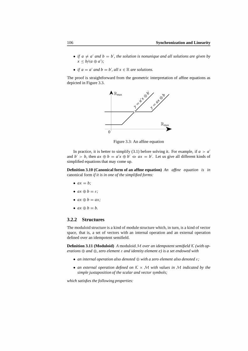
106 Synchronization and Linearity
• if a = a′ and b = b′, the solution is nonunique and all solutions are given byx ≤ b◦/(a ⊕ a′);
• if a = a′ and b = b′, all x ∈ R are solutions.
The proof is straightforward from the geometric interpretation of affine equations asdepicted in Figure 3.3.
0
Rmax
Rmax
y =ax ⊕
b
y =a′ x ⊕
b′
Figure 3.3: An affine equation
In practice, it is better to simplify (3.1) before solving it. For example, ifa > a′
andb′ > b, thenax ⊕ b = a′x ⊕ b′ ⇔ ax = b′. Let usgive all different kinds ofsimplified equations that may come up.
Definition 3.10 (Canonical form of an affine equation)An affine equation is incanonical formif it is in one of the simplified forms:
• ax = b;
• ax ⊕ b = ε;
• ax ⊕ b = ax;
• ax ⊕ b = b.
3.2.2 Structures
The moduloid structure is a kind of module structure which, in turn, is a kind of vectorspace, that is, a set of vectors with an internal operation and an external operationdefined over an idempotent semifield.
Definition 3.11 (Moduloid) A moduloidM over an idempotent semifield K (with op-erations⊕ and ⊗, zero element ε and identity element e) is a set endowed with
• an internal operation also denoted ⊕ with a zero element also denoted ε;
• an external operation defined on K × M with values in M indicated by thesimple juxtaposition of the scalar and vector symbols;
which satisfies the following properties:

3.2. Matrices inRmax 107
• ⊕ is associative, commutative;
• α(x ⊕ y) = αx ⊕ αy;
• (α ⊕ β)x = αx ⊕ βx;
• α(βx) = (αβ)x;
• ex = x;
• εx = ε;
for all α, β ∈ K and all x, y ∈M.
We will only be concerned with somespecial cases of such a structure.
Example 3.12 (Rmax)n is a moduloid overRmax. Its zero element is(ε, . . . , ε)′.
Other examples of moduloids will be presented later on.
Definition 3.13 (Idempotent algebra) A moduloid with an additional internal oper-ation also denoted ⊗ is called an idempotent algebraif ⊗ is associative, if it has anidentity element also denoted e, and if it is distributive with respect to ⊕.
This idempotent algebra is the main structure in which the forthcoming system theoryis going to be developed.
Example 3.14 Let (Rmax)n×n be the set ofn × n matrices withcoefficients inRmax
endowed with the following two internal operations:
• the componentwise addition denoted⊕;
• the matrix multiplication already used in Chapters 1 and 2 denoted⊗:
(A ⊗ B)i j =n⊕
k=1
Aik ⊗ Bkj ;
and the external operation:
• ∀α ∈ Rmax, ∀A ∈ (Rmax)n×n , αA = (αAi j ).
The set(Rmax)n×n is an idempotent algebra with
• thezero matrix, again denotedε, whichhas allits entries equal toε;
• the identity matrix, again denotede, which has the diagonal entries equal toeand theother entries equal toε.

108 Synchronization and Linearity
3.2.3 Systems of Linear Equations in(Rmax)n
In this subsection we are mainly interested in systems of linear equations. To definesuch systems, we use matrix notation. A linear mapping(Rmax)
n → (Rmax)n will be
represented by a matrix as it was done in the previous chapters. With the max-plusalgebra, the general system of equations is
Ax ⊕ b = Cx ⊕ d ,
whereA andC aren × n matrices andb andd aren-vectors. This system can be putin canonical form in the same way as we have done in the scalar case.
Definition 3.15 (Canonical form of a system of affine equations) The systemAx ⊕ b = Cx ⊕ d is said to be in canonical formif A,C, b, and d satisfy
• Ci j = ε if Ai j > Ci j , and Ai j = ε if Ai j < Ci j ;
• di = ε if bi > di , and bi = ε if bi < di .
Example 3.16 Consider the system
(3 2ε 2
)(x1
x2
)⊕(
12
)=(
4 11 1
)(x1
x2
)⊕(
e3
),
whichcan be simplified as follows:
(ε 2ε 2
)(x1
x2
)⊕(
1ε
)=(
4 ε
1 ε
)(x1
x2
)⊕(
ε
3
),
which implies
2x2⊕ 1= 4x1
2x2 = 1x1⊕ 3
}⇒ 4x1 = 1x1⊕ 3⇒ 4x1 = 3⇒ x1 = −1⇒ x2 = 1 .
This system has a solution. In general, a linear system may or may not have a solution.Moreover, even if a solution exists, it may be nonunique.
There are two classes of linear systems for which we have a satisfactory theory,namely,
• x = Ax ⊕ b;
• Ax = b.
Let us study the former case first.

3.2. Matrices inRmax 109
3.2.3.1 Solution ofx = Ax ⊕ b
Theorem 3.17 If there are only circuits of nonpositive weight in G(A), there is a so-lution to x = Ax ⊕ b which is given by x = A∗b. Moreover, if the circuit weights arenegative, the solution is unique.
The reader should recall the definition of A∗ as given by (1.22).
Proof If A∗b does exist, it is a solution; as a matter of fact,
A(A∗b)⊕ b = (e ⊕ AA∗ )b = A∗b .
Existence ofA∗b. The meaning of(A∗)i j is the maximum weightof all paths of anylength from j to i. Thus, anecessary and sufficient condition for the existence of(A∗)i j is thatno strongly connected components ofG(A) have a circuit with pos-itive weight. Otherwise, there would exist a path fromj to i of arbitrarily largeweight for all j andi belonging to the strongly connected component which in-cludes the circuit of positive weight (by traversing this circuit a sufficient numberof times).
Uniqueness of the solution.Suppose thatx is a solution ofx = Ax ⊕ b. Then xsatisfies
x = b ⊕ Ab ⊕ A2x ,
x = b ⊕ Ab ⊕ · · · ⊕ Ak−1b ⊕ Ak x , (3.3)
and thus x ≥ A∗b. Moreover, if all thecircuits of the graphhave negativeweights, thenAk → ε whenk → ∞. Indeed, the entries ofAk are the weightsof the paths of lengthk which necessarilytraverse some circuits ofA anumber oftimes going to∞ with k, but the weights of these circuits are all negative. Usingthis property in Equation (3.3) fork large enough, we obtain thatx = A∗b.
Remark 3.18 If the maximum circuit weight is zero, a solution does exist, but thereis nouniqueness anymore. For example, the equationx = x ⊕ b admits the solutionx = a∗b = b but all x > b are solutions too.
Example 3.19 Consider the two-dimensional equation
x =( −1 2−3 −1
)x ⊕(
e2
).
Then,
b =(
e2
), Ab =
(41
), A2b =
(31
), A3b =
(3e
), A4b =
(2e
). . . .
Thus,
x =(
e2
)⊕(
41
)⊕(
3e
)⊕(
2e
)⊕ · · · =
(42
).
This is theunique solution.

110 Synchronization and Linearity
Theorem 3.20 If G(A) has no circuit with positive weight, then
A∗ = e⊕ A ⊕ · · · ⊕ An−1 ,
where n is the dimension of matrix A.
Proof All the paths of length greater than or equal ton are necessarilymadeup of acircuit and of a path with length strictly less thann. Therefore, because the weights ofcircuits are nonpositive by assumption, we have
∀m ≥ n , Am ≤ e⊕ · · · ⊕ An−1 .
Returning to Example 3.19, we remark thatA2b, A3b, . . . are less thanb ⊕ Ab.
3.2.3.2 Solution ofAx = b
The second class of linear systems for which wecan obtain a general result consists ofthe systemsAx = b. However, we must first consider the problem inRmax ratherthanin Rmax, and second, we must somewhat weaken the notion of ‘solution’. Asubsolutionof Ax = b is anx which satisfies Ax ≤ b, where the order relation on the vectors canalso bedefined byx ≤ y if x ⊕ y = y.
Theorem 3.21 Given an n × n matrix A and an n-vector b with entries in Rmax, thegreatest subsolution of Ax = b exists and is given by
−x j = maxi
(−bi + Ai j ) .
For reasons that will become apparent in§4.4.4 and§4.6.2, the vector form of thisformulacanbewrittene◦/x = (e◦/b)A.
Proof We have that
{Ax ≤ b} ⇔
⊕
j
Ai j x j ≤ bi , ∀i
⇔ {x j ≤ bi − Ai j , ∀i, j
}
⇔{
x j ≤ mini
(bi − Ai j
), ∀ j
}
⇔{−x j ≥ max
i
(−bi + Ai j)
, ∀ j
}.
Conversely, it can be checked similarly that the vectorx defined by−x j =maxi(−bi + Ai j
), ∀ j, is a subsolution. Therefore, it is the greatest one.
As a consequence, in order to attempt to solve the systemAx = b, we may firstcompute its greatest subsolution and then check by inspection whether it satisfies theequality.

3.2. Matrices inRmax 111
Example 3.22 Let us compute thegreatest subsolution of the following equality:(
2 34 5
)(x1
x2
)=(
67
).
According to the preceding considerations, let us first compute
(e◦/b)A = ( −6 −7)( 2 3
4 5
)= ( −3 −2
).
Then the greatest subsolution is(x1, x2) = (3, 2); indeed,(
2 34 5
)(32
)=(
57
)≤(
67
).
It is easily verified that the second inequality would not be satisfied if we increasex1
and/orx2. Therefore, the first inequality cannot be reduced to an equality.
3.2.4 Spectral Theory of Matrices
Given amatrix A with entries inRmax, we consider the problem of existence of eigen-valuesand eigenvectors, that is, the existence of (nonzero)λ andx suchthat
Ax = λx . (3.4)
The main result is as follows.
Theorem 3.23 If A is irreducible, or equivalently if G(A) is strongly connected, thereexists one and only one eigenvalue (but possibly several eigenvectors). This eigenvalueis equal to the maximum cycle mean of the graph (see § 2.3.2):
λ = maxζ
|ζ |w|ζ |l ,
where ζ ranges over the set of circuits of G(A).
Proof
Existence ofx and λ. Consider matrix B = A◦/λ def= (e◦/λ)A, where λ =maxζ |ζ |w/|ζ |l . The maximum circuit weight ofG(B) is e. Hence B∗ andB+ = B B∗ exist. Matrix B+ has some columns with diagonal entries equal toe.To prove this claim, pick a nodek of a circuit ξ suchthatξ ∈ arg maxζ |ζ |w/|ζ |l .The maximumweight of paths fromk to k is e. Therefore we havee = B+kk . LetB·k denote thek-th column ofB. Then, since, generally speaking,B+ = B B∗
andB∗ = e ⊕ B+ (e the identity matrix), for thatk,
B+·k = B∗·k ⇒ B B∗·k = B+·k = B∗·k ⇒ AB∗·k = λB∗·k .
Hencex = B∗·k = B+·k is aneigenvectorof A corresponding to the eigenvalueλ. The set of nodes ofG(A) corresponding to nonzero entries ofx is called thesupport of x .

112 Synchronization and Linearity
Graph interp retation of λ. If λ satisfies Equation (3.4), there exists a nonzero com-ponent ofx , sayxi1. Then we have(Ax)i1 = λxi1 and there exists an indexi2suchthat Ai1 i2 xi2 = λxi1. Hence xi2 = ε and A1i2 = ε. We can repeat thisargument and obtain a sequence{i j } suchthat Aij−1 i j xi j = λxi j−1 , xi j = ε andAij−1 i j = ε. At some stage we must reach an indexil already encountered inthe sequence since the number of nodes is finite. Therefore, we obtain a circuitβ = (il , im, . . . , il+1, il ). By multiplication along this circuit, we obtain
Ail il+1 Ail+1 il+2 . . . Aim il xil+1 xil+2 . . . xim xil = λm−l+1xil xil+1 . . . xim .
Sincexi j = ε for all i j , we may simplify the equation above which shows thatλm−l+1 is the weight of the circuit of lengthm − l + 1, or, otherwise stated,λ isthe average weight of circuitβ. Observe that this partof the proof did not usethe irreducibility assumption.
If A is irreducible, all the components ofx are different from ε. Suppose that thesupport ofx does not cover the whole graph. Then, there are arcs going fromthe support ofx to other nodes because the graphG(A) has only one stronglyconnected component. Therefore, the support ofAx is larger thanthe support ofx , whichcontradicts Equation (3.4).
Uniqueness in the irreducible case.Consider any circuitγ = (i1, . . . , ip, i1) suchthat its nodes belong to the support ofx (here any node ofG(A)). We have
Ai2 i1 xi1 ≤ λxi2 , . . . , Aip ip−1 xip−1 ≤ λxip , Ai1 ip xip ≤ λxi1 .
Hence, by the same argument as in theparagraph on the graph interpretationof λ, we seethatλ is greater than the average weight ofγ . Therefore λ is themaximum cycle meanand thus it is unique.
It is important to understand the role of the support ofx in the previous proof. IfG(A)is not strongly connected, the support ofx is not necessarily the whole set of nodesand, in general, there is no unique eigenvalue (see Example 3.26 below).
Remark 3.24 The part of theproof on the graph interpretation ofλ indeed showedthat, fora general matrixA, any eigenvalue is equal to some cycle mean. Therefore themaximum cycle mean is equal to the maximum eigenvalue of the matrix.
Example 3.25 (Nonunique eigenvector)With the only assumption of Theorem 3.23onirreducibility, the uniqueness of the eigenvector is not guaranteed as is shown by thefollowing example:
(1 ee 1
)(e
−1
)=(
1e
)= 1
(e
−1
),
and (1 ee 1
)( −1e
)=(
e1
)= 1
( −1e
).
The two eigenvectors are obviously not ‘proportional’.

3.2. Matrices inRmax 113
Example 3.26 (A not irreducible)
• The followingexample is a trivial counterexample to the uniqueness of the eigen-value whenG(A) is not connected:
(1 ε
ε 2
)(eε
)= 1
(eε
),
(1 ε
ε 2
)(ε
e
)= 2
(ε
e
).
• In the following exampleG(A) is connected but not strongly connected. Never-theless there isonly one eigenvalue:
(1 eε e
)(eε
)= 1
(eε
),
but (1 eε e
)(ae
)= λ
(ae
)
has no solutionsbecause the second equation impliesλ = e, and thenthe firstequation has no solutions for the unknowna.
• In the following exampleG(A) is connected but not strongly connected and thereare two eigenvalues:
(e eε 1
)(eε
)= e
(eε
),
(e eε 1
)(e1
)= 1
(e1
).
More generally, consider the block triangular matrix
F =(
A ε
B C
),
whereG(A) andG(C) are strongly connected, andG(C) is downstream ofG(A). LetλA andλC , be the eigenvalues of blocksA andC, respectively, and letx A andxC bethe corresponding eigenvectors. Observe that
(ε xC
)′is aneigenvectorof F for the
eigenvalueλC . In addition, if λA > λC , the expression(C◦/λA)∗ is well-defined. The
vector (x A
(C◦/λA)∗(B◦/λA)x A
)
is aneigenvector of F for the eigenvalueλA. In conclusion,F has two eigenvaluesif the upstream m.s.c.s. is ‘slower’ than the downstream one. Clearly this kind ofresult can be generalized to a decomposition into an arbitrary number of blocks. Thisgeneralization will not be considered here (see [62]).

114 Synchronization and Linearity
3.2.5 Application to Event Graphs
Consider an autonomous event graph withn transitions, that is, an event graph withoutsources, with constant holding times and zero firing times. In§2.5.2 we sawthatit canbe modeled by
x(k) =M⊕
i=0
A(i)x(k − i) , (3.5)
where theA(i) are n × n matrices with entries inRmax. We assume thatthe eventgraph (in which transitions are viewed as the nodes and places as the arcs) is stronglyconnected. In§2.5.4, it was shown that an equation in the standard form
x(k + 1) = Ax(k) (3.6)
canalsodescribe the same physical system. A new event graph (with a different num-ber of transitionsin general) can be associated with (3.6). In this new event graph, eachplacehas exactly one token in the initial marking. Therefore, in this graph, the lengthof a circuit or path can either be defined as the total number of arcs, or as the totalnumber of tokensin the initial marking along this circuit or path.
We refer the reader to the transformations explained in§2.5.2 to§2.5.4 to see thatsome transitions in the two graphs can be identified to each other and that the circuitsare in one-to-one correspondence. Since the original event graph is assumed to bestrongly connected, the new event graph can also be assumed to be strongly connected,provided unnecessary transitions (not involved in circuits) becanceled. ThenA isirreducible. Hence there exists a unique eigenvalueλ, and at least one eigenvectorx . By starting the recurrence in (3.6) with the initial valuex(0) = x , we obtain thatx(k) = λkx for all k in N. Therefore, a token leaves each transition everyλ units oftime,or, otherwise stated, the throughput ofeach transition is 1/λ.
It was shown thatλ can be evaluated as the maximum cycle mean ofG(
A), that
is, as the maximum ratio‘weight divided by length’ over all the circuits ofG(A). The
purpose of the following theorem is to show thatλ can also be evaluated as the samemaximum ratio over the circuits of theoriginal graph, provided the length of an arc beunderstood as the number of tokens in the initial marking of the corresponding place(theweight is still defined as the holding time).
Let us return to (3.5). The graphG(A(i)) describes the subgraph of the originalgraph obtained by retaining only the arcs corresponding to places marked withi tokens.SinceA(i) is ann × n matrix, all original nodes are retained in this subgraph which ishowever not necessarily connected. Consider the followingn × n matrix:
B(λ)def=
M⊕
i=0
λ−i A(i) ,
whereλ is any real number.
Remark 3.27 For a given value ofλ, a circuit of B(λ) can bedefined by a sequenceof nodes (in which the last node equals the first). Indeed, once this sequence of nodes

3.2. Matrices inRmax 115
is given, the arc between a pair of successive nodes(a, b) is selected by the argumentiλ(a, b) of the maxi which is implicit in the expression of(B(λ))ba . If this iλ(a, b) isnot unique, it does not matter which one is selected since any choice leads to the sameweight. Therefore, the set of circuits of G(B(λ)) is a subset of the set of circuits ofthe original graph (a circuit of the original graph can be specified by a given sequenceof nodesand by a mapping(a, b) �→ i(a, b) in order to specify one of the possibleparallel arcs between nodesa andb). The set of circuits ofG(B(λ)) is thus changingwith λ. However, for any given value ofλ, if we areonly interested in the maximumcircuit weight ofG(B(λ)) (or in the maximum cycle mean, assuming that the length ofa circuit is defined as thenumber of arcs inG(B(λ))), the maximum can be takenoverthe whole set of circuits of the original graph (this set is independent ofλ). Indeed,the additional circuits thus considered donot contribute to the maximum since theycorrespond to choices ofi(a, b) which are not optimal.
Theorem 3.28 We assume that
1. G(B(e)) is strongly connected;
2. G(A(0)) has circuits of negative weight only;
3. there exists at least one circuit of G(B(λ)) containing at least one token.
Then, there exist a vector x and a unique scalar λ satisfying x = B(λ)x. The graphinterpretation of λ is
λ = maxζ
|ζ |w|ζ |t , (3.7)
where ζ ranges over the set of circuits of the original event graph and |ζ |t denotes thenumber of tokens in circuit ζ .
Proof To solve theequationx = B(λ)x , we must find λ and x suchthat e is aneigenvalue of the matrixB(λ). ThegraphG(B(e)) being strongly connected,G(B(λ))is alsostrongly connected for any real value ofλ and thereforeB(λ) admits auniqueeigenvalue�(λ). Owing tothe graph interpretation of�(λ), �(λ) = maxζ |ζ |w/|ζ |l ,whereζ ranges over the set of circuits ofG(B(λ)). However, Remark 3.27 showedthat wecan as well consider thatζ ranges over the set of circuits of the original graph.Hence, in conventionalnotation, we have
�(λ) = maxζ
1
|ζ |l∑
(a,b)∈ζ(B(λ))ba
= maxζ
1
|ζ |l∑
(a,b)∈ζmax
i∈{1,... ,M}((A(i))ba − i × λ)
= maxζ
1
|ζ |l maxi(a,b)
∑
(a,b)∈ζ((A(i(a, b))ba − i(a, b) × λ)
. (3.8)

116 Synchronization and Linearity
If we assume that there exists aλ suchthat�(λ) = e = 0, then, forany circuitζ ofthe original graph, and thus for any mappingi(·, ·) which completes the specificationof the circuit, we have
λ ≥∑
(a,b)∈ζ (A(i(a, b)))ba∑(a,b)∈ζ i(a, b)
,
and theequality is obtained for some circuitζ . This justifies the interpretation (3.7)of λ.
Let us nowprove that�(λ) = e has a uniquesolution. Because of (3.8), andsince, according to Remark 3.27, the mappingsi(·, ·) can be viewed asranging in a setindependent ofλ, �(·) is theupper hull of a collection of affine functions (ofλ). Eachaffine function has a nonpositive slope which, in absolute value, equals the numberof tokens in a circuit divided by the number of arcs in the circuit. Therefore,� is anonincreasing function ofλ. Moreover, due tothe third assumption of the theorem,there is at least one strictly negative slope. Hence limλ→−∞�(λ) = +∞. On theotherhand, owing to the second assumption, and since the affine functions with zero slopestem necessarilyfrom the circuits ofA(0), limλ→+∞�(λ) < 0. Finally� is a convexnonincreasing function which decreases from+∞ to a strictly negative value, and thusits graph crosses thex-axis at a single point.
It is easy to see that if we start the recurrence (3.5) withx(0) = x, x(1) = λ ⊗x, . . . , x(M) = λM ⊗ x, thenx(k) = λk ⊗ x for all k. Hence 1/λ is the throughput ofthe system at theperiodic regime. At the end of this chapter, we will give conditionsunder which this regime is asymptotically reached, and conditions under which it isreached after a finite time, whatever the initial condition is.
3.3 Scalar Functions inRmax
In this section we discuss nonlinear real-valued functions of one real variable, consid-ered as mappings fromRmax into Rmax. We classify them in polynomial, rational andalgebraic functions in the max-plus algebrasense.
3.3.1 Polynomial FunctionsP(Rmax)
Polynomial functions are a subset of piecewise linear functions (in the conventionalsense) for which we have the analogue of the fundamental theorem of algebra. Thisset is not isomorphic to the set of formal polynomials ofRmax, that is, the set offinitesequences endowed with a product which is the sup-convolution of sequences.
3.3.1.1 Formal Polynomials and Polynomial Functions
Definition 3.29 (Formal polynomials) We consider the set of finite real sequences ofany length
p = (p(k), . . . , p(i) . . . p(n)) , k, i, n ∈ N , p(i) ∈ Rmax .

3.3. Scalar Functions inRmax 117
If the extreme values k and n are such that p(k) and p(n) are different from ε, then
val(p)def= k is called the valuation of p, and deg(p)
def= n is called the degreeof p.This set is endowed with the following two internal operations:
• componentwise addition⊕;
• sup-convolution⊗ of sequences, that is,
(p ⊗ q)(l)def=
⊕
i+ j=lval(p)≤i≤deg(p)val(q)≤ j≤deg(q)
p(i)q( j ) ,
and with the following external operation involving scalars in Rmax:
• multiplication of all the elements of the sequence p by the same scalar of Rmax,
We thus define Rmax[γ ] which is called the set of formal polynomials.
Note that if thepolynomialγ is defined by
γ (k) ={
e if k = 1 ;
ε otherwise,
thenany polynomial ofRmax[γ ] canbewritten asp =⊕nl=k p(l)γ l .
Let us give alist of definitions related to the notion of formal polynomials.
Definition 3.30
Polynomial functions: associated with a formal polynomial p, we define the polyno-mial function by
p : Rmax→ Rmax , c �→ p(c) = p(k)ck ⊕ · · · ⊕ p(n)cn .
The set of polynomial functions is denoted P(Rmax).
Support: the support supp(p) is the set of indices of the nonzero elements of p, thatis, supp(p) = {i | k ≤ i ≤ n, p(i) = ε}.
Monomial: a formal polynomial reduced to a sequence of one element is called amonomial1.
Head monomial: the monomial of highest degree one can extract from a polynomialp, that is p(n)γ n, is called the head monomial.
Tail monomial: the monomial of lowest degree out of p, that is, p(k)γ k , is called thetail monomial.
1We do not to make the distinction between formal monomials and monomial functions because, unlikepolynomials-see Remark 3.34 below-a formal monomial is in one-to-one correspondence with its associatedfunction.

118 Synchronization and Linearity
Full Support: we say that a formal polynomial has a full support if
p(i) = ε , ∀i : k ≤ i ≤ n .
The following two theorems are obvious.
Theorem 3.31 The set of formal polynomials Rmax[γ ] is an idempotent algebra.
Remark 3.32 Because we can identify scalars with monomials of degree 0, this idem-potent algebra can be viewed as the idempotent semiring obtained by considering thetwo internal operations only, since the external multiplication by a scalar is amenableto the internal multiplication by a monomial.
Theorem 3.33 The set of polynomial functionsP(Rmax) endowed with the two internaloperations:
• pointwise addition denoted⊕, that is, ( p ⊕ q)(c)def= p(c)⊕ q(c);
• pointwise multiplication denoted ⊗, that is, ( p ⊗ q)(c)def= p(c)⊗ q(c),
and the external operation over Rmax× P(Rmax), namely,
• (b p)(c)def= b ⊗ p(c),
is an idempotent algebra.
The same remark as above applies to this idempotent algebra too.Polynomial functions are convex piecewise linear integer-sloped nondecreasing
functions (see Figure 3.4). Indeed the monomialp(i)ci is nothing but the conventionalaffine functionic+ p(i). Owing to the meaning of addition of monomials, polynomialfunctions are thus upper hulls of such affine functions.
Remark 3.34 There is no one-to-one correspondence between formal polynomials andpolynomial functions. For example,
∀c , c2⊕ 2 = (c ⊕ 1)2 = c2⊕ 1c⊕ 2 .
The monomial 1c is dominated byc2⊕ 2. In other words, 1c does not contribute to thegraph ofc2⊕ 1c ⊕ 2 (see Figure 3.5), and thus, two different formal polynomials areassociated with the same function.
The following lemma should be obvious.
Lemma 3.35 (Evaluation homomorphism)Consider the mapping F : Rmax[γ ] →P(Rmax), p �→ p. Then, F is a homomorphism between the algebraic structures de-fined in Theorems 3.31 and 3.33. It will be referred to as the evaluation homomorphism.

3.3. Scalar Functions inRmax 119
−1
1
0
2
Rmax
Rmax
Figure 3.4: The graph ofy = (−1)c2⊕1c⊕2
0
2
1
Rmax
Rmax
Figure 3.5: The graph ofy = (c ⊕ 1)2
Unlike in conventional algebra, the evaluation homomorphism is not a one-to-one cor-respondence, as shown in Remark 3.34. More precisely, it is surjective but not injective.This is why it is important to distinguish between formal objects and their associatednumerical functions.
Remark 3.36 The mappingF is in factclosely related to the Fenchel transform [58].In convexity theory [119],with a numerical functionf over a Hilbert spaceV , theFenchel transformFe associates a numerical functionFe( f ) over thedual Hilbert spaceV ∗ as follows:
∀c ∈ V ∗ , [Fe( f )] (c) = supz∈V
(〈c, z〉 − f (z)) ,
where〈·, ·〉 denotes the duality product overV ∗ × V . If we consider the formal poly-nomial p as a function fromN into Rmax, p : l �→ p(l) (the domain of which can beextended to the wholeN by setting p(l) = ε if l < val(p) or l > deg(p)), then,
p(c) = maxl∈N
(lc + p(l)) = Fe(−p)(c) . (3.9)
Before studying the properties ofF and the equivalence relation it induces inRmax[γ ], let us first give some terminology related to convexity that we will use lateron.
Definition 3.37
Convex set in a disconnected domain: we say that a subset F ⊂ E = N × R isconvex if, for all µ ∈ [0, 1] and for all x, y ∈ F for which µx + (1− µ)y ∈ E,it follows that µx + (1− µ)y ∈ F.
Hypograph and epigraph of a real function f : X → R: these are the sets definedrespectively by
hypo( f )def= {(x, y) | x ∈ X, y ∈ R, y ≤ f (x)} ,

120 Synchronization and Linearity
epi( f )def= {(x, y) | x ∈ X, y ∈ R, y ≥ f (x)} .
Convex (concave) mapping: a function f : X → R is convex (respectively concave)if its epigraph (respectively its hypograph) is convex.
Extremal point of a convex setF : it is a point which is not a convex combination oftwo other distinct points of F.
Theorem 3.38 Consider the equivalence relation
∀p, q ∈ Rmax[γ ] , pF≡ q ⇔ p = q ⇔ q ∈ F−1 ( p) .
1. With a given p ∈ Rmax[γ ], we associate two other elements of Rmax[γ ] denotedp�
1 and p�
2, such that, for all l ∈ N,
p�
1(l)def= max
0≤µ≤1i, j∈N
(µp(i) + (1− µ)p( j )) ,
subject to l = µi + (1− µ) j ,
(3.10)
p�
2(l)def= min
c∈Rmax
( p(c)− lc) . (3.11)
Then p�1 = p�
2 (denoted simply p�) and p� belongs to the same equivalence classas p of which it is the maximum element. The mapping l �→ p�(l) is the concaveupper hull of l �→ p(l). Hence hypo
(p�)
is convex.
2. Let now p� ∈ Rmax[γ ] be obtained from p by canceling the monomials of pwhich do not correspond to extremal points of hypo
(p�). Then p� belongs to the
same equivalence class as p of which it is the minimum element.
3. Two members p and q of the same equivalence class have the same degree andvaluation. Moreover p� = q� and p� = q�.
Proof
1. Using (3.10) with the particular valuesµ = 1, hencel = i, we first prove thatp�
1 ≥ p for the pointwise conventional order (which is also the natural orderassociatedwith the addition inRmax[γ ]). Combining (3.9) (written forp�
1) with(3.10), we obtain
p�
1(c) = maxl
(lc + max
0≤µ≤1, i, j∈N
(µp(i) + (1− µ)p( j ))
)
subject to l = µi + (1− µ) j
= max0≤µ≤1
(µmax
i(ic + p(i)) + (1− µ)max
j( j c+ p( j ))
)
= max0≤µ≤1
(µ p(c) + (1− µ) p(c))
= p(c) .

3.3. Scalar Functions inRmax 121
This shows thatp�
1 belongs to the same equivalence class asp and that it isgreater than any suchp, hence it is the maximum element in this equivalenceclass.
On the other hand, combining (3.11) with (3.9), we get
p�
2(l) = minc∈Rmax
(maxm∈N
(mc+ p(m)) − lc
).
By choosing particular valuem = l, it is shown thatp�
2 ≥ p. SinceF is a
homomorphism, it preserves the order, and thusp�
2 ≥ p. But, if we combine(3.9) (written for p�
2) with (3.11), we get
p�
2(c) = maxl∈N
(lc + min
c′∈Rmax
(p(c′)− lc′
)).
By picking the particular valuec′ = c, it is shown thatp�
2 ≤ p. Hence, we have
proved thatp�
2 = p and thatp�
2 ≥ p. Therefore p�
2 is the maximumelement inthe equivalence class ofp. Sincethe maximumelement is unique (see§ 4.3.1),it follows that p�
1 = p�
2.
From (3.11), it is apparent thatp�
2 is concave as the lower hull of a family ofaffine functions. Hence, since it is greater thanp, it is greater than its concaveupper hull, but (3.10) shows that indeed it coincides with this hull.
2. It is now clearthat the equivalence class ofp can be characterized byp�, orequivalently by its hypograph which is a convex set. Since a convex set is fullycharacterized by the collection of its extreme points, this collection is anothercharacterization of the class. Sincep� has precisely been defined from this col-lection of extreme points, it is clearly anelement of the same class and the min-imum one (dropping any further monomial would change the collection of ex-tremepoints and thus the equivalence class).
3. In particular, the head and tail monomials of a givenp correspond to members ofthe collection of extreme points. Therefore, all elements of an equivalence classhave the same degree and valuation.
Definition 3.39 (Canonical forms of polynomial functions)According to the previ-ous theorem, we may call p� and p� the concavified polynomialand the skeletonof p,respectively.
• The skeleton p� is also called the minimum canonical formof the polynomialfunction p;
• the concavified polynomial p� is also called the maximum canonical formof p.
Figure 3.6 illustrates these notions. It should be clear that necessarilyp� has full sup-port.

122 Synchronization and Linearity
Example 3.40 For p = γ 2⊕ γ ⊕ 2, we havep� = γ 2⊕ 2. For p = γ 3⊕ 3, we havep� = γ 3⊕ 1γ 2⊕ 2γ ⊕ 3.
Lemma 3.41 A formal polynomial p of valuation k and degree n is a maximal canon-ical form of a polynomial function p, that is, p = p�, if and only if p has full support(hence p(l) = ε, for l = k, . . . , n), and
p(n − 1)
p(n)≥ p(n − 2)
p(n − 1)≥ · · · ≥ p(k)
p(k + 1). (3.12)
Proof The fact that a maximal canonical form must have full support has been es-tablished earlier and this ensures that the ‘ratios’ in (3.12) are well defined. In theproof of Theorem 3.38 it has also been shown thatp� is the concave upper hull ofthe functionl �→ p(l) (concavity in the sense of Definition 3.37). Conversely, ifpis concave, it is equal to its own concave upper hull, and thusp = p�. Now, (3.12)simply expresses that the slopes of the lines defined by the successive pairs of points((l − 1, p(l − 1)), (l, p(l))) are decreasing withl, which isobviously a necessary andsufficient condition for p to be concave.
3.3.1.2 Factorization of Polynomials
Let us now show that polynomial functions and concave formal polynomials can befactored into a product of linear factors.
Definition 3.42 (Corners, multiplicity) The nonzero cornersof a polynomial functionp are the abscissæ of the extremal points of the epigraph of p. Since p is convex,at such a corner, the (integer) slope increases by some integer which is called themultiplicity of the corner. A corner is called multiple if the multiplicity is larger thanone.
The zero cornerexists if the least slope appearing in the graph of p is nonzero: themultiplicity of this zero corner is then equal to that (integer) slope.
Figure 3.7 shows anonzero corner of multiplicity 2.
N0
p�
p�
p
Rmax
Figure 3.6: The functionsp, p� and p�
0
Corner of multiplicity 2
Rmax
Rmax
Figure 3.7: Corner of apolynomial function

3.3. Scalar Functions inRmax 123
Theorem 3.43 (Fundamental theorem of algebra)
1. Any formal polynomial of the form p = p(n)⊗n
i=1(γ ⊕ ci ) (where some ci maybe equal to ε) satisfies p = p�.
2. Conversely, if a formal polynomial p = p(k)γ k ⊕ p(k+1)γ k+1⊕ · · ·⊕ p(n)γ n
is such that p = p�, then it has full support, the numbers ci ∈ Rmax defined by
cidef={
p(n − i)◦/ p(n − i + 1) for 1≤ i ≤ n − k ;
ε for n − k < i ≤ n ,(3.13)
are such that
c1 ≥ c2 ≥ · · · ≥ cn , (3.14)
and p can be factored as p = p(n)(⊗n
i=1(γ ⊕ ci )).
3. Any polynomial function p can be factored as
p(c) = p(n)
(n⊗
i=1
(c ⊕ ci )
),
where the ci are the zero and/or nonzero corners of the polynomial function prepeated with their order of multiplicity. These corners are obtained by Equa-tion (3.13) using the maximum canonical form.
Proof
1. Let p = ⊗ni=1 p(n)(γ ⊕ ci ) and assume without loss of generality that theci
have been numbered in such a way that (3.14) holds. We consider the nontrivialcasep(n) = ε. By direct calculation, it can be seen thatp(n − k) = p(n)σk ,whereσk is thek-th symmetric product of the cornersci , that is,
σ1 =n⊕
i=1
ci , σ2 =⊕
i = j=1
ci c j , . . . .
Owing toour assumption on the ordering of theci , it is clear thatσk =⊗k
i=1 c j .Therefore,
pn−k
pn−k+1= σk
σk−1= ck ≤ ck−1 = pn−k+1
pn−k+2.
Thus p = p� by Lemma 3.41.
2. If p = p�, theci canbe defined by (3.13) unambiguously and then (3.14) followsfrom Lemma 3.41. The fact thatp can be factored as indicated is checked aspreviously by direct calculation.

124 Synchronization and Linearity
3. Fromthe preceding considerations, provided that we representp with the help ofits maximum canonical form, the factored form can be obtained if we define theci with Equation (3.13). To complete the proof, it must be shown that any suchci
is a corner in the sense of Definition 3.42 and that, if aci appearski times, thenthe slope jumps byki at ci . To see this, rewrite the factored form in conventionalnotation, which yields
p(c) =n∑
i=1
max(c, ci ) .
Each elementary termc ⊕ ci has a graph represented in Figure 3.2 with a slopediscontinuity equal to one atci . If a ci appearski times, the termki ×max(c, ci )
causes aslope discontinuity equal toki . All other terms with c j = ci do notcause any slope discontinuity at ci .
Example 3.44 The formal polynomialγ 2 ⊕ 3γ ⊕ 2 is amaximum canonical formbecausec1 = 3◦/e = 3 ≥ c2 = 2◦/3 = −1, and therefore itcan be factored into(γ ⊕ 3)(γ ⊕ (−1)). The formal polynomial(γ 2⊕ 2)� = γ 2⊕ 1γ ⊕ 2 can be factoredinto (γ ⊕ 1)2.
3.3.2 Rational Functions
In this subsection we study rational functions in theRmax algebra. These functionsare continuous, piecewise linear, integer-sloped functions. We give the multiplicativeform of such functions, which completely defines the points where the slope changes.Moreover, we show that the Euclidean division and the decomposition into simpleelements is not always possible.
3.3.2.1 Definitions
Definition 3.45 Given p(0), . . . , p(n), q(0), . . . , q(m) ∈ Rmax, p(n) and q(m) = ε,the rational functionr , associated with these coefficients, is given by
r : Rmax→ Rmax , c �→ r(c) = p(0)⊕ · · · ⊕ p(n)cn
q(0)⊕ · · · ⊕ q(m)cm.
Sucha function is equal to the difference of two polynomial functions (see Figure 3.8):hence it is still continuous, piecewise linear, integer-sloped, but it is neither convex norincreasing anymore.
Definition 3.46 The corners of the numerator are called zero cornersor root corners,and the corners of the denominator are called pole corners.
Using the fundamental theorem of algebra, we can write any rational functionr as
r(c) = a
⊗ni=1(c ⊕ ci )⊗mj=1(c ⊕ d j)
,

3.3. Scalar Functions inRmax 125
where thezero and pole corners are possibly repeatedwith their order of multiplicity.At a zero corner of multiplicity ki , the change of slope iski (unless this zero cornercoincides with some pole corner). At a pole corner of multiplicityl j , the change ofslope is−l j (see Figure 3.9).
y c 2 ⊕ 2c ⊕ 3=
y = e◦/(1c2⊕ 4c⊕ 5)
0
Rmax
Rmax
Figure 3.8: Graph ofy = (c2 ⊕ 2c⊕ 3)◦/(1c2 ⊕ 4c⊕ 5)
max
max
0
root corner
pole corner
k i
lj
R
R
Figure 3.9: Root and pole corners
3.3.2.2 Euclidean Division
In general, a polynomialp cannot be expressed asbq ⊕ r with deg(r ) < deg(b) forsomegiven polynomialb as shown by Example3.47. Nevertheless, sometimes we canobtain such a decomposition, as shown by Example 3.48.
Example 3.47 The equationc2 ⊕ e = q(c ⊕ 1) ⊕ r has no solutions. Indeed,qmust beof degree 1 andr of degree 0; thusq = q(1)γ ⊕ q(0), r = r(0), withq(0), q(1), r(0) ∈ Rmax. By identifying the coefficients of degree 2 in both sides, wemust haveq(1) = e. Now, since the maximal canonical form in the left-hand side isc2 ⊕ c ⊕ e, by considering the coefficient of degree 1 in the right-hand side, we musthaveq(0)⊕ 1q(1) ≤ e, whichcontradictsq(1) = e.
Example 3.48 For p(c) = c2⊕ 3 andb = c⊕ 1, we have
c2⊕ 3 = (c ⊕ 1)2⊕ 3= (c ⊕ 1)(c ⊕ 1.5)⊕ 3 .
As in conventional algebra, this issue of the Euclidean division leads to solving atriangular system of linear equations. However, inRmax, thedifficulty dwells in thefact that a triangular system of linear equations with nonzero diagonal elements mayhave no solutions.
Example 3.49 The system(x1 = 1, x1⊕ x2 = e) has no solutions inRmax.

126 Synchronization and Linearity
3.3.2.3 Decomposition of a Rational Function into Simple Elements
Definition 3.50 A proper rational functionr ◦/q is a rational function which satisfiesdeg(r ) < deg(q).
In general, it is not possible to express a rational functionp◦/q ass⊕ r◦/q, wherer◦/q isproper ands is a polynomial function. Nevertheless, given a proper rational function,we may attempt to decompose it into simple elements.
Definition 3.51 A proper rational function r is decomposableinto simple elementsifit can be written as
r =n⊕
i=1
Ki⊕
k=1
aik◦/(c ⊕ ci )k ,
where the aik are constants.
Such a decomposition is not always possible.
Example 3.52 We first consider a rational function for which the decomposition intosimple elements is possible:
c⊕ 1
(c ⊕ e)2= c ⊕ e
(c ⊕ e)2⊕ 1
(c ⊕ e)2= e
c ⊕ e⊕ 1
(c ⊕ e)2.
The rational function(c⊕e)◦/(c⊕1)2, however, cannot be decomposed. Indeed, if sucha decomposition exists, we would have
c ⊕ e
(c⊕ 1)2= a
c ⊕ 1⊕ b
(c⊕ 1)2.
Thena(c ⊕ 1) ⊕ b = c ⊕ e, hence a = e, and alsoa1⊕ b = 1⊕ b = e, which isimpossible.
The graphof a proper rational function which can be decomposed into simple ele-ments is necessarily nonincreasing because it is theupper hull of nonincreasing func-tions. But a rational function with the degree of thenumerator lower than the degree ofthe denominator is not always nonincreasing: this depends on the relative ordering ofits pole and zero corners.
Example 3.53 The functiony = 2(c ⊕ e)◦/(c ⊕ 1)2 is proper but not monotonic (seeFigure 3.10).
However, being nonincreasing is a necessary but not a sufficient condition to bedecomposable into simple elements as shown by the following example.
Example 3.54 The function r(c) = e◦/(c2 ⊕ c), thegraph of which is displayed inFigure 3.11, cannot be decomposed into simple elements. Indeed,
{r (c) = a
c⊕ b
c ⊕ e
}⇒ {a(c ⊕ e)⊕ bc = e} ⇒
{a ⊕ b = ε
a = e
},
which is impossible inRmax.

3.3. Scalar Functions inRmax 127
max
Rmax
0 1 2
1
R
Figure 3.10: Graph ofy = 2(c ⊕ e)◦/(c ⊕ 1)2
01
− 1
− 2
1Rmax
Rmax
Figure 3.11: Graph ofy = e◦/(c2⊕c)
Theorem 3.55 A proper rational function has a simple element decomposition if andonly if it has general root corners and special pole corners which are at the intersectionof a zero-sloped line and a negative-integer-sloped line (Figure 3.12).
Proof If r is decomposable, it can be written asr =⊕ ri with
ri (c) =Ki⊕
k=1
aik ◦/(c ⊕ ci )k .
Reducing the right-hand side to a common denominator(c ⊕ ci )Ki , we obtain ri =
p(c⊕ci )◦/(c⊕ci )Ki , wherep isapolynomial function of degreeKi−1. The polynomial
function p is characterized by the fact that the abscissæ of its corners are greater thanci . Therefore ri (c) is constant on the left-hand side ofci , has apole corner of orderKi
at ci , and a root corner on the right-hand side ofci . Conversely, a function having thisshapecan easily be realized by anri . Theproof is completed by considering the factthat r is the supremumof a finite number of suchri .
3.3.3 Algebraic Equations
Definition 3.56 (Polynomial equation)Given two polynomial functions p and q ofdegree n and m, respectively, the equality p(c) = q(c) is called a polynomial equation.Solutions to this equation are called roots. The degreeof the polynomial equation isthe integer max(n,m).
Somepolynomial equations have roots, some do not. For example,cn = a has therootc = n
√a, that is,c = a/n in conventional algebra. On the other hand, the equation
p(c) = ε has no roots whenp is a general polynomial of degreen ≥ 1.
3.3.3.1 Canonical Form of an Equation
Before studying equations, it is useful to write them in their simplest form. An equationp(c) = q(c) can generally be simplified even if it is in the formp�(c) = q�(c). Indeed,

128 Synchronization and Linearity
if two monomialsp�(k)γ k andq�(k)γ k of the same degree appear simultaneously, andif p�(k) < q�(k), we can further simplify the equation by canceling the monomialp�(k)γ k .
Example 3.57The equationc2⊕3c⊕2= 3c2⊕2c⊕e can be reduced to 3c⊕2= 3c2
(see Figure 3.13).
rootcorners admissible
corner
0
pole
Rmax
Rmax
Figure 3.12: A rational functiondecomposableinto simple elements
0
Rmax
y=
3c2⊕
2c⊕
e
y =c2 ⊕ 3c
⊕ 2
Rmax
Figure 3.13: Equationc2⊕3c⊕2= 3c2⊕2c⊕ e
Definition 3.58 If there exist two identical monomials on both sides of the equation,we say that the equation is degenerated. The nondegenerated equation p(c) = q(c) isin minimal canonical formif (p ⊕ q)� = p ⊕ q.
In the case of a degenerated equation, there is a segment of solutions.
3.3.3.2 Solving Polynomial Equations
Theorem 3.59 Any root of the nondegenerated equation p(c) = q(c) is a corner ofp ⊕ q.
Proof Let us take the canonical form of the equation. Any root ofp(c) = q(c) is thesolution of p(k)ck = q(l)cl for some differentk andl and thus it is a corner ofp ⊕ qbecause the equation is in minimal canonical form.
The converse of this theorem is not true, i.e. a corner is not always a root of the equationp(c) = q(c).
Example 3.60 The polynomial equation 3c ⊕ 2 = 3c2 has the cornerc = −1 whichis not a root (3(−1)⊕ 2 = 2, 3(−1)2 = 1).

3.4. Symmetrization of the Max-Plus Algebra 129
Now we give a characterization of the situation where the polynomial equation ofdegreen has exactlyn roots.
Theorem 3.61 Suppose that n is even (the case when n is odd is similar). Let
p(c) = p(0)⊕ p(2)c2 ⊕ · · · ⊕ p(2k)c2k ,
q(c) = p(1)c ⊕ p(3)c3 ⊕ · · · ⊕ p(2k − 1)c2k−1 ,
and suppose that p(c) = q(c) is a nondegenerated equation in canonical form, then
cidef= p(i − 1)◦/p(i), i = 1, . . . , n, are the n roots of the equation.
Proof No corner of p ⊕ q is multiple. Henceeach one is obtained as the intersection oftwo monomials of consecutive degrees. Therefore, these monomials belong to differentsides of the equation. Thus the corresponding corners are roots of the equation.
Conversely if the equation hasn roots, p ⊕ q hasn corners which therefore aredistinct. But each of these corners is a root, hence these corners are characterizedby the intersection of two monomial functions of consecutive degrees, the monomialsbeing in different sides of the equation.
3.4 Symmetrization of the Max-Plus Algebra
We have seen that the theory of linear system ofequations in the max-plus algebra isnot satisfactory at all, not even inthe scalar case. We now extendRmax to a largersetS for which Rmax can be viewed as the positive part. The construction is similarto the construction ofZ as an extension ofN in conventional algebra, but we cannotavoid some complications coming from the idempotency of the max operator. Withthis new set, wecan generalize the notion of an equation that we call a balance. Thenall nondegenerated scalar linear balances have a unique solution. Thus a linear closureof Rmax has been achieved.
3.4.1 The Algebraic StructureS
A natural approach toour problem is to embed the max-plus algebra into a structure inwhich every nontrivial scalar linear equation has at least one solution. In particular wewould like to have a solution to the equationa⊕ x = ε, that is, wewould like to find asymmetric element toa. But this not possible, as shown by the following theorem.
Theorem 3.62 Every idempotent group is reduced to the zero element.
Proof Assume thatthe group(G,⊕) is idempotent with zero elementε. Let b be thesymmetric element ofa ∈ G. Then
a = a ⊕ ε = a ⊕ (a ⊕ b) = (a ⊕ a)⊕ b = a ⊕ b = ε .
Nevertheless we canadapt the idea of the construction ofZ from N to build a ‘bal-ancing’ element rather than a symmetricone. This is the purpose of the followingsubsections.
130 Synchronization and Linearity
3.4.1.1 The Algebra of Pairs
Let us consider the set of pairsR2max endowed with the natural idempotent semifield
structure:(x ′, x ′′)⊕ (y′, y′′) = (x ′ ⊕ y′, x ′′ ⊕ y′′) ,
(x ′, x ′′)⊗ (y′, y′′) = (x ′y′ ⊕ x ′′y′′, x ′y′′ ⊕ x ′′y′) ,
with (ε, ε) as the zero element and(e, ε) asthe identity element.Let x = (x ′, x ′′) and define theminus sign as�x = (x ′′, x ′), theabsolute value of
x as|x | = x ′ ⊕ x ′′ and thebalance operator asx• = x � x = (|x |, |x |). Clearly, theseoperators have the following properties:
1. a• = (�a)•;
2. a•• = a•;
3. ab• = (ab)•;
4. �(�a) = a;
5. �(a ⊕ b) = (�a)⊕ (�b);
6. �(a ⊗ b) = (�a)⊗ b.
These properties allow us to writea ⊕ (�b) = a � b as usual.
3.4.1.2 Quotient Structure
Definition 3.63 (Balance relation)Let x = (x ′, x ′′) and y = (y′, y′′). We say that xbalances y (which is denoted x ∇ y) if x ′ ⊕ y′′ = x ′′ ⊕ y′ .
It is fundamental to notice that∇ is not transitive and thus is not anequivalence relation.For instance, consider(e, 1)∇ (1, 1), (1, 1)∇ (1, e), but(e, 1) ∇ (1, e)! Since∇ cannotbe an equivalence relation, it is not possible to define the quotient structure ofR
2max by
means of∇ (unlike in conventional algebrain which N2/ ∇ Z). However, we can
introduce the equivalence relationR on R2max closely related to the balance relation,
namely,
(x ′, x ′′)R(y′, y′′)⇔{
x ′ ⊕ y′′ = x ′′ ⊕ y′ if x ′ = x ′′, y′ = y′′ ,
(x ′, x ′′) = (y′, y′′) otherwise.
It is easy to check thatR is compatible with the addition and multiplication ofR2max,
the balance relation∇, and the�, | · | and• operators.
Definition 3.64 The symmetrizedalgebraR2max/R of Rmax is called S.
We distinguish three kinds of equivalence classes:
(t,−∞) = {(t, x ′′) | x ′′ < t} , called positive elements;(−∞, t) = {(x ′, t) | x ′ < t} , called negative elements;(t, t) = {(t, t)} , called balanced elements.

3.4. Symmetrization of the Max-Plus Algebra 131
By associating(t,−∞) with t ∈ Rmax, we can identifyRmax with the semifield ofpositive or zero classes denotedS
⊕. The set of negative or zero classes (of the form�x for x ∈ S
⊕) will be denotedS�. This set is not stable by multiplication and thus itis not a semifield. The set of balanced classes (of the formx•) is denotedS
•; it is alsoisomorphic toRmax. This yields the decomposition
S = S⊕ ∪ S
� ∪ S• . (3.15)
The elementε is theonly element common toS⊕ andS� andS
•. This decompositionof S should be compared withZ = N
+ ∪ N−. This notation allows us to write 3� 2
instead of(3,−∞) ⊕ (−∞, 2). We thus have 3� 2 = (3, 2) = (3,−∞) = 3. Moregenerally, calculations inS can be summarized as follows:
a � b = a , if a > b ;b � a = �a , if a > b ;a � a = a• .
(3.16)
Because of its importance, we introduce the notationS∨ for the setS⊕ ∪ S� and
S∨� = S
∨ \{ε}. The elements ofS∨ are calledsigned elements. They are either positive,negative or zero.
Theorem 3.65 The set S∨� = S \ S
• is the set of all invertible elements of S.
Proof The obvious identityt ⊗ (−t) = (�t)⊗ (�− t) = e for t ∈ Rmax\ {ε} impliesthat every nonzero element of S
∨ is invertible. Moreover, the absorbing properties ofthe balance operator show thatS∨ is absorbing for the product. Thus,x•y = e for ally ∈ S sincee ∈ S
•.
Remark 3.66 Thus, inS, with each elementa ∈ S∨, wecan associate an element�a
suchthatb = a � a ∈ S• but in generalb = ε. This is the maindifference with the
usual symmetrization. Here the whole setS• plays the role of the usual zero element.
3.4.2 Linear Balances
Before solving general linear balances, we need to understand the meaning of the gen-eralization of equations inRmax by balances inS. This can be done by studying theproperties of balances.
Theorem 3.67 The relation ∇ satisfies the following properties:
1. a ∇ a;
2. a ∇ b ⇔ b ∇ a;
3. a ∇ b ⇔ a � b ∇ ε;
4. {a ∇ b, c∇ d} ⇒ a ⊕ c ∇ b ⊕ d;
5. a ∇ b ⇒ ac ∇ bc.

132 Synchronization and Linearity
Proof Let us prove Property 5. Obviously, a ∇ b ⇔ a � b ∈ S• and, sinceS
• isabsorbing,(a � b)c = ac � bc ∈ S
•, i.e. ac ∇ bc.
Although∇ is not transitive, when some variables are signed, we can manipulate bal-ances in the same way as we manipulate equations.
Theorem 3.68
1. Weak substitution If x ∇ a, cx ∇ b and x ∈ S∨, we have ca ∇ b.
2. Weak transitivity If a ∇ x, x ∇ b and x ∈ S∨, we have a ∇ b.
3. Reduction of balancesIf x ∇ y and x, y ∈ S∨, we have x = y.
Proof
1. We have eitherx ∈ S⊕ or x ∈ S
�. Assume for instance that x ∈ S⊕, that is,
x = (x ′, ε). With the usual notation,x ′ ⊕ a′′ = a′ andc′x ′ ⊕ b′′ = c′′x ′ ⊕ b′.Addingc′a′′ ⊕ c′′a′′ to the last equality, we get
c′x ′ ⊕ c′a′′ ⊕ c′′a′′ ⊕ b′′ = c′′x ′ ⊕ c′a′′ ⊕ c′′a′′ ⊕ b′ ,
which yields, by usingx ′ ⊕ a′′ = a′,
c′a′ ⊕ c′′a′′ ⊕ b′′ = c′′a′ ⊕ c′a′′ ⊕ b′ ,
that is,ca ∇ b.
2. This a consequence of the weak substitution forc = e.
3. This point is trivial but is important in order to derive equalities from balances.
The introduction of these new notions is justified by the fact that any linear balance(which is not degenerated) has one and only one solution inS
∨.
Theorem 3.69 Let a ∈ S∨� and b ∈ S
∨, then x = �a−1b is the unique solution of thebalance
ax ⊕ b ∇ ε , (3.17)
which belongs to S∨.
Proof From the properties of balances it follows thatax⊕b∇ ε⇔ x∇ � a−1b. Thenusing the reduction property and the fact that�a−1b ∈ S
∨, weobtainx = �a−1b.
Remark 3.70 If b ∈ S∨, we lose the uniqueness of signed solutions. Everyx such
that |ax | ≤ |b| (i.e. |x | ≤ |a−1b|) is a solution of the balance (3.17). Ifa ∈ S∨, we
again lose uniqueness. Assumeb ∈ S∨ (otherwise, the balance holds for all values of
x), theneveryx suchthat|ax | ≥ |b| is a solution.

3.5. Linear Systems inS 133
Remark 3.71 We can describe all the solutions of (3.17). For allt ∈ Rmax, we obvi-ously haveat • ∇ ε. Adding this balance toax ⊕ b ∇ ε, wherex is the unique signedsolution, we obtaina(x ⊕ t •)⊕ b ∇ ε. Thus,
xt = x ⊕ t • (3.18)
is a solution of (3.17). If t ≥ |x |, thenxt = t • is balanced. Conversely, it can bechecked that every solution of (3.17) may be written as in (3.18). Finally theuniquesigned solutionx is also the least solution.
Remark 3.72 Nontrivial linear balances (withdatain S∨) always have solutions inS;
this is whyS may be considered as alinear closure of Rmax.
3.5 Linear Systems inS
It is straightforward to extend balances to the vector case. Theorems 3.67 and 3.68still hold whena, b, x, y andc are matrices with appropriatedimensions, provided wereplace ‘belongs toS∨’ by ‘every entry belongs toS∨’. Therefore, we say that a vectoror a matrix issigned if all its entries are signed.
We now consider a solutionx ∈ Rmax of the equation
Ax ⊕ b = Cx ⊕ d . (3.19)
Thenthe definition of the balance relation implies that
(A � C)x ⊕ (b � d) ∇ ε . (3.20)
Conversely, assuming thatx is a positive solution of (3.20), we obtain
Ax ⊕ b ∇ Cx ⊕ d ,
with Ax ⊕ b andCx ⊕ d ∈ S⊕. Using Theorem 3.68, we obtain
Ax ⊕ b = Cx ⊕ d .
Therefore we have the following theorem.
Theorem 3.73 The set of solutions of the general system of linear equations (3.19)in Rmax and the set of positivesolutions of the associated linear balance (3.20) in S
coincide.
Hence, studying Equation (3.19) is reduced to solving linear balances inS.
Remark 3.74 The case when a solution x of (3.20) has some negative and somepositive entries is also of interest. We writex = x+ � x− with x+, x− ∈ (S⊕)n .Partitioning the columns ofA andC according to the sign of the entries ofx , weobtainA = A+⊕ A−, C = C+⊕C−, so thatAx = A+x+� A−x− andCx = C+x+�C−x−.We can thus claim the existence of a solution inRmax to the newproblem
A+x+ ⊕ C−x− ⊕ b = A−x− ⊕ C+x+ ⊕ d .
The solution of nondegenerated problems is not unique, but the set of solutions formsa single class ofR2
max (for the equivalence relationR ).

134 Synchronization and Linearity
3.5.1 Determinant
Before dealing with general systems, we need to extend the determinant machinery totheS-context. We define the signature of a permutationσ by
sgn(σ) ={
e if σ is even;
�e otherwise.
Then the determinant of ann × n matrix A = (Ai j ) is given (asusual) by
⊕
σ
sgn(σ)n⊗
i=1
Aiσ (i) ,
and is denoted either|A| or det(A). The transpose of the matrix of cofactors is denoted
A� ((
A�)
i j
def= cof j i(A)). The classical properties of the determinant are still true.
Theorem 3.75 The determinant has the following properties:
linearity:
|(u1, . . . , λui ⊕µvi , . . . , un)| = λ|(u1, .. , ui , .. , un)|⊕µ|(u1, .. , vi , .. , un)| ;
antisymmetry:|(uσ (1), . . . , uσ (n))| = sgn(σ)|(u1, . . . , un)| ;
and consequently
|(u1, . . . , v, . . . , v, . . . , un)| ∇ ε ;
expansion with respect to a row:
|A| =n⊕
k=1
aikcofik (A) ;
transposition: |A| = |A′ |.A direct consequence is that some classical proofs lead to classical identities in thisnew setting. Sometimes weak substitution limits the scope of this approach.
Theorem 3.76 For an n × n matrix A with entries in S, we have
Cramer formula: AA� ∇ |A|e, and if |A| is signed, then the diagonal of AA� issigned;
recursive computation of the determinant:
|A| =∣∣∣∣(
F GH ann
)∣∣∣∣ = |F |ann � H F �G
for a partition of matrix A where ann is a scalar;

3.5. Linear Systems inS 135
Cayley-Hamilton theorem: p being the characteristic polynomial of matrix A, i.e.
p(λ)def= |A� λe|, we have p(A) ∇ ε.
Remark 3.77 We define the positive determinant of a matrixA, denoted|A|+, by thesum of terms
⊗i Aiσ (i) where the sum islimited to even permutations, and a negative
determinant, denoted|A|−, by the samesumlimited to odd permutations. The matrixof positive cofactors is defined by
(A�+)
i j={|A ji |+ if i + j is even,
|A ji |− if i + j is odd,
where A ji denotes the matrix derived from A by deleting row j and column i. Thematrix of negative cofactorsA�− is defined similarly. With this notation, Theorem 3.76canberewritten as follows:
AA�+ ⊕ |A|−e = AA�− ⊕ |A|+e .
This formula does not use the� sign and is valid in any semiring. The symmetrizedalgebra appears to be a natural way of handling such identities (and giving proofs in analgebraic way).
3.5.2 Solving Systems of Linear Balances by the Cramer Rule
In this subsection we study solutions of systems of linear equations with entries inS.We only consider the solutions belonging to(S∨)n , that is, weonly considersignedsolutions. Indeed, in a more general setting we cannot hope to have a result of unique-ness; see Remark 3.70. We can now state the fundamental result for the existence anduniqueness of signed solutions of linear systems.
Theorem 3.78 (Cramer system) Let A be an n×n matrix with entries in S, |A| ∈ S∨� ,
b ∈ Sn and A�b ∈ (S∨)n . Then, in S
∨ there exists a unique solution of
Ax ∇ b , (3.21)
and it satisfies
x ∇ A�b◦/|A| . (3.22)
Proof By right-multiplying the identityAA� ∇ |A|e by |A|−1b, we seethat x is asolution. Let us now prove uniqueness. The proof is by induction on the size of thematrix. It is based on Gauss elimination in which we manage the balances using weaksubstitution. Let us prove (3.22) for the last row, i.e.|A|xn ∇ (A�b)n . Developing|A| with respect to the last column,|A| =⊕n
k=1 akncofkn(A), we see that at least oneterm is invertible, saya1ncof1n(A). We now partition A, b andx in sucha way that thescalara1n becomes a block:
A =(
H a1n
F G
), b =
(b1
B
), x =
(Xxn
).
136 Synchronization and Linearity
Then Ax ∇ b canbewritten as
H X ⊕ a1nxn ∇ b1 , (3.23)
F X ⊕ Gxn ∇ B . (3.24)
Since|F | = (�e)n+1cof1n(A) is invertible, we can apply the induction hypothesis to(3.24). This implies that
X ∇ |F |−1F �(B � Gxn) .
Using the weak substitution property, we can replaceX ∈ (S∨)n−1 in Equation (3.23)to obtain
|F |−1H F �(B � Gxn)⊕ a1nxn ∇ b1 ,
that is,xn(|F |a1n � H F �G) ∇ |F |b1� H F �B .
Here we recognize the developments of|A| and(A�b)n , therefore
xn ∇ (A�b)n◦/|A| .
Since the same reasoning can be applied to the entries ofx other thann, this concludesthe proof.
Remark 3.79 Let us write Di for the determinant of the matrix obtained by replacing
thei-th column ofA by the column vectorb; thenDi = (A�b)i . Assume thatDdef= |A|
is invertible, then Equation (3.22) is equivalent to
xi ∇ D−1Di , ∀i .
If A�b ∈ (S∨)n , then by using the reduction of balances (see Theorem 3.68), we obtain
xi = D−1Di ,
which is exactly the classical Cramer formula.
Example 3.80 TheRmax equation(
e −43 2
)⊗(
x1
x2
)⊕(
1−5
)=( −1 1
ε 2
)⊗(
x1
x2
)⊕(
27
), (3.25)
corresponds to the balance(
e �13 2•
)(x1
x2
)∇(
27
). (3.26)
Its determinant is D = 4.
D1 =∣∣∣∣(
2 �17 2•
)∣∣∣∣ = 8 , D2 =∣∣∣∣(
e 23 7
)∣∣∣∣ = 7 ,
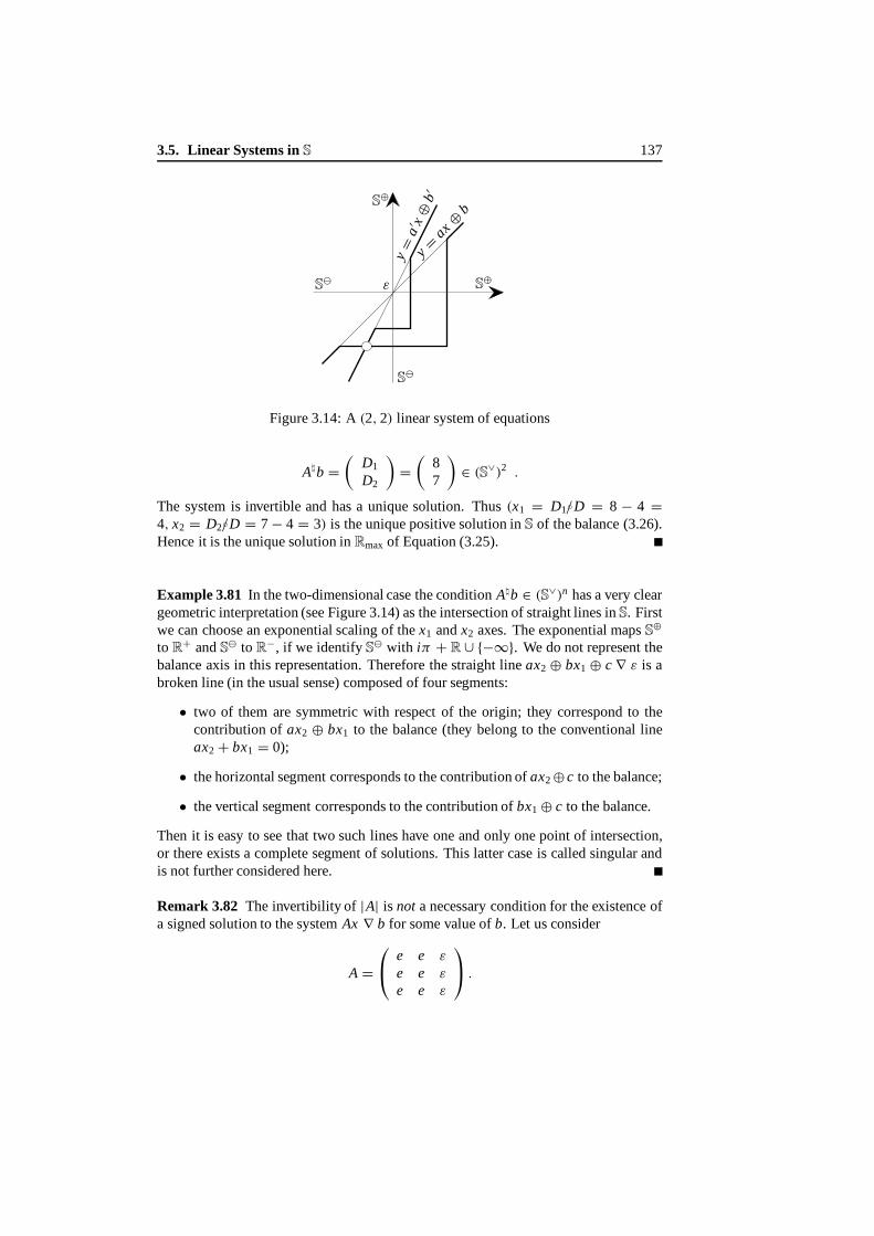
3.5. Linear Systems inS 137
ε
y=
a′ x⊕
b′
y =ax ⊕
b
�S
�S
S⊕
S⊕
Figure 3.14: A(2, 2) linear system ofequations
A�b =(
D1
D2
)=(
87
)∈ (S∨)2 .
The system is invertible and has a unique solution. Thus(x1 = D1◦/D = 8 − 4 =4, x2 = D2◦/D = 7− 4 = 3) is the unique positive solution inS of the balance (3.26).Hence it is the unique solution inRmax of Equation (3.25).
Example 3.81 In the two-dimensional case the conditionA�b ∈ (S∨)n has a very cleargeometric interpretation (see Figure 3.14) as the intersection of straight lines inS. Firstwe canchoose an exponential scaling of thex1 andx2 axes. The exponential mapsS⊕
to R+ andS
� to R−, if we identify S
� with iπ + R ∪ {−∞}. We donot represent thebalance axis in this representation. Therefore the straight lineax2⊕ bx1⊕ c ∇ ε is abroken line (in the usual sense) composed of four segments:
• two of them are symmetric with respect of the origin; they correspond to thecontribution ofax2 ⊕ bx1 to the balance (they belong to the conventional lineax2+ bx1 = 0);
• thehorizontal segment corresponds to the contribution ofax2⊕ c to the balance;
• the vertical segment corresponds to the contribution ofbx1⊕ c to the balance.
Then it is easy to see that two suchlines haveone and only one point of intersection,or there exists a complete segment of solutions. This latter case is called singular andis not further considered here.
Remark 3.82 The invertibility of |A| is not a necessary condition for the existence ofa signed solution to the systemAx ∇ b for some value ofb. Let usconsider
A =
e e ε
e e ε
e e ε
.

138 Synchronization and Linearity
Because|A| = ε, the matrix A is not invertible. Lett ∈ S∨ be suchthat |bi | ≤ |t | for
all i, and letx = ( t �t ε)′
. ThenAx ∇ b. But in this case, the signed solution isnot unique.
Remark 3.83 As already noticed, in [65] for example, determinants have a naturalinterpretation in terms of assignment problems. So the Cramer calculations have thesame complexity asn + 1 assignment problems, which can be solved using flow algo-rithms.
3.6 Polynomials with Coefficients inS
We havebuilt the linear closureS of Rmax. Therefore anylinear equation inS has ingeneral a solution in this set. The purpose of this section is to show thatS is almostalgebraically closed, that is, any ‘closed’ polynomial equation of degreen in S hasn solutions. The term ‘closed’ refers to the fact that the class of formal polynomialshaving the same polynomial function defined onS isnot always closed (in a topologicalsense that will be made precise later). We will see thatS is algebraically closed only forthe subset of ‘closed’ polynomial equations. Moreover, we will see that any polynomialfunction can be transformed into a closed function by modifying it in a finite numberof points.
3.6.1 Some Polynomial Functions
We cangeneralize the notions of formal polynomials and of polynomial functions to
the setS. We restrict our study to polynomial functions inP(S∨) def= F(S∨[γ ]), whereS∨[γ ] denotes the class of formal polynomials with coefficients inS
∨ andF is thestraightforward extension of the evaluation homomorphism introduced in Lemma 3.35.We will see that such functions assume values inS
∨ when their argument ranges inS∨,except perhaps at a finite number of points. For the more general class of polynomialfunctions with coefficients inS, denotedP(S), it may happen that the function takes abalanced value on a continuous set of points ofS
∨ (in which case we say that we havea balanced facet). Because we are mainly interested in the analogy with conventionalpolynomials, we do not deal with this latter situation.
To get a better understanding of polynomial functions onS we study someparticu-lar cases. Let us start by plotting the graphs of polynomial functions of degree one, twoand three (see Figure 3.15). We must study the graphs over each of the three compo-nentsS⊕ , S� andS
•. The value of the functionitself, however,is anelement ofS whichalso belongs to one of these components. Therefore the plot is quite complicated. Inorder to simplify the study, only the plot overS
∨ is considered. Moreover we will usethe exponential system of coordinates that we have discussed in the previous section.Figure 3.15 shows the points of discontinuity of the three component functions. Thesediscontinuities always appear at abscissæ which are symmetric with respect to cornerabscissæ. At these discontinuities the polynomial functions take balanced values (inthe graph, we see sign changes). They correspond to what we call ‘roots’ of polyno-

3.6. Polynomials with Coefficients inS 139
�
� �
� �
�
⊕ ⊕ ⊕
⊕⊕S
ε
y = ax ⊕b
ε ε
y = ax 2⊕ bx⊕c y = ax 3⊕bx 2⊕cx ⊕d
S⊕
S S S
S
SS S
SS S
Figure 3.15: Polynomial functions of degree one, two and three
mial functions. If a polynomial is of degreen, it has ingeneraln corners andn pointsin S
∨ where the polynomial function takes balanced values.Let us study the polynomial functions of degree two in more detail. We consider
p(c) = p(0)⊕ p(1)c ⊕ p(2)c2 , p(i) ∈ S∨ , i = 0, 1, 2 .
The polynomial function| p| ∈ P(Rmax) is defined as p(c) = |p(0)| ⊕ |p(1)|c ⊕|p(2)|c2. We will later prove, but it should be clear, that ifc is a root of p, then|c| isa corner of |p|. Owing to Theorem 3.43,| p| canbe factored into the product of twolinear polynomials. We have the following four possibilities:
1. If |p(1)◦/p(2)| > |p(0)◦/p(1)|, then| p| has two distinct cornersc1 = |p(1)◦/p(2)|andc2 = |p(0)◦/p(1)|. It can be checked thatp = p(2)(c ⊕ p(1)◦/p(2))(c ⊕p(0)◦/p(1)) and that this factorization is unique. In addition, the moduli of theroots arec1 andc2.
2. If |p(1)◦/p(2)| = |p(0)◦/p(1)|, then | p| has a corner c1 = |p(0)◦/p(2)|1/2 ofmultiplicity 2 and the roots ofp = p(2)(c ⊕ p(1)◦/p(2))(c ⊕ p(0)◦/p(1)) havemodulusc1.
3. If |p(1)◦/p(2)| < |p(0)◦/p(1)| and p(2)p(0) ∈ S⊕, then| p| has a corner c1 =
|p(0)◦/p(2)|1/2 of multiplicity 2 and p cannot be factored. Indeed atc1 and�c1,p has signed values. We havep = p(2)(c2 ⊕ p(0)◦/p(2)).
4. If |p(1)◦/p(2)| < |p(0)◦/p(1)| and p(2)p(0) ∈ S�, then the polynomial| p| has a
cornerc1 = |p(0)◦/p(2)|1/2 of multiplicity 2. We havep = p(2)(c⊕ c1)(c� c1)
and thus p has been factored.
This discussion suggests that if the corners of| p| (now a polynomial function of de-green) are distinct, then there aren roots; but if| p| has multiple corners, then we arenot guaranteed to have a factorization in linear factors. We now study the situation inmore detail.
3.6.2 Factorization of Polynomial Functions
We canconsider formal polynomialsS[γ ] and polynomial functionsP(S) with coef-ficients inS aswe have done for polynomials with coefficients inRmax. They define

140 Synchronization and Linearity
algebras. The following mapping fromP(S) intoP(Rmax)
p = p(k)γ k ⊕ · · · ⊕ p(n)γ n �→ |p| = |p(k)|γ k ⊕ · · · ⊕ |p(n)|γ n
is a surjective morphism.
Definition 3.84 (Root) The root of a polynomial function p ∈ P(S) is an elementc ∈ S
∨ such that p(c) ∇ ε.
Remark 3.85 It should be clear that the computation of the linear factors of a polyno-mial yieldsits roots. Indeed we have
⊗
i
(c � ci ) ∇ ε ⇔ c � ci ∇ ε .
Lemma 3.86 If, for a polynomial p ∈ P(S∨), c is a root of p(c), then |c| is a cornerof |p|.
Proof If c is a root, then p(c) is balancedand hence| p(c)| = | p(|c|)| is a quantitywhich isachieved by twodistinct monomials ofp since, by assumption, the coefficientsof p belong toS
∨. Thus|c| is a corner of|p|.
For the same reason as in theRmax case, the mapping
F : S[γ ] → P(S) , p �→ p ,
is not injective. In order to study the set valued-inverse mappingF−1, we introduce thenotion of a closed polynomial function.
Definition 3.87 (Closed polynomial function)We say that the polynomial functionp ∈ P(S∨) is closed if F−1( p) admits a maximum element denoted p� ∈ P(S). Thiselement is called the maximum representative of p.
Example 3.88 Thepolynomial functionc2� e is closed because it has the same graphas c2 ⊕ e•c � e. The polynomial functionc2 ⊕ e is not closed because its graph isdifferent from that of any polynomialpa = c2⊕ ac⊕ e with a ∈ {e,�e, e•} althoughit is the same for alla < e.
The notion of closed polynomial function is relevant because the inverse of the evalua-tion homomorphismis simple for this class, and because this class is exactly the set ofpolynomial functions which can be factored into linear factors.
Theorem 3.89 A polynomial function p ∈ P(S∨) can be factored in linear factors ifand only if it is closed.

3.6. Polynomials with Coefficients inS 141
ProofAny polynomial which can be factored is closed.Let us suppose that the degree ofp is n, its valuation 0, and the coefficient of its head monomial ise (the proof can begeneralized to avoid these assumptions). Let us suppose that the degree ofp is n, itsvaluation 0, and the coefficient of its head monomial ise (the proof can be adapted tothe general case). Letci , i = 1, . . . , n, denote the roots ofp numbered according tothe decreasing order of their modulus. If theci are all distinct, we have
p(c) =n⊕
i=0
mi with midef=
i⊗
j=1
c j
cn−i .
Becausemi > m j , ∀ j > i , ∀c : ci+1 < c < ci ,
we cannot increase the coefficient of a monomial without changing the graph ofp andtherefore it is closed. The situation is more complicated when there is a multiple rootbecause then at least three monomials take the same value in modulus at this root. Tounderstand what happens at such a multiple root, let us consider the case whenp hasonly the rootse or �e, that is, p(c) = (c ⊕ e)n−m (c � e)m . The expansion of thispolynomial gives five kinds of polynomials:
• cn ⊕ cn−1⊕ · · · ⊕ e ;• cn � cn−1⊕ cn−2 · · · ⊕ e ;• cn � cn−1⊕ cn−2 · · · � e ;• cn ⊕ e•cn−1⊕ e•cn−2 · · · ⊕ e ;• cn ⊕ e•cn−1⊕ e•cn−2 · · · � e .
By inspection, we verify that we cannot increase any coefficient of these polynomialswithout changing their graphs. Therefore, they are closed.
Weremark that some polynomials considered in this enumeration do not belong toP(S∨). For example, it is the case of(c � e)2(c ⊕ e). Some other polynomials havetheir coefficients inS
• and do not seem to belong to the class that we study here, butthey haveother representatives inP(S∨). For example, we have
(c� e)(c ⊕ e) = c2⊕ e•c� e = c2� e .
Any closed polynomial can be factored. If p is closed, let p denote its maximumrepresentative. Its coefficientsci = p(n − i)◦/ p(n − i + 1) are nonincreasing withi in modulus. Indeed, if that were not the case, there would existi and k suchthat|ci−k | > |ci+1| > |ci |. Then it would be possible to increasepn−i while preserving theinequalities|ci−k | > |ci+1| > |ci |. Because this operation would not change the graphof p, we would have contradictedthe maximality ofp.
Now, if the |ci | arestrictly decreasing withi, we directly verify by expansion thatp(c) = ⊗i (c ⊕ ci ). If the ci are simply nonincreasing, we will only examine theparticular case when theci have their modulus equal toe. There are four subcases:

142 Synchronization and Linearity
1. p(e) ∇ ε and p(�e) ∇ ε;
2. p(e) ∇ ε and p(�e) ∇ ε;
3. p(e) ∇ ε and p(�e) ∇ ε;
4. p(e) ∇ ε and p(�e) ∇ ε.
The first case can appear only ifn is evenand
p(c) = cn ⊕ cn−2 ⊕ · · · ⊕ e ,
which contradicts the fact theci are nonincreasing. The other cases correspond to afactorization studied in the first part of the proof.
Corollary 3.90 A sufficient condition for p ∈ P(S∨) to be closed is that |p| has dis-tinct corners.
Example 3.91
• c2⊕ e is always positive and therefore cannot be factored;
• c2⊕ c⊕ e is closed and can be factored into(c ⊕ e)2;
• (γ � e)(γ ⊕ e)2 = (γ ⊕ e)(γ � e)2 = γ 3 ⊕ e•γ 2 ⊕ e•γ ⊕ e is a maximumrepresentative of a closed polynomial;
• γ 3⊕ e•γ 2⊕ eγ ⊕ e is not a maximum representative of a closed polynomial.
In the following theorem the form of the inverse function ofF , which is a set-valued mapping, is made precise.
Theorem 3.92 The set F−1 ( p), with p ∈ P(S∨), admits the minimum element p� ∈S∨[γ ] and the maximum element p� ∈ S[γ ] which satisfy
• p� ≤ F−1( p) ≤ p�;
• p�, p� ∈ F−1( p);
• |p�| = |p|�;• |p�| = |p|�.
Proof The proof follows from the epimorphism property ofp �→ |p|, from the corre-sponding result inRmax, and from the previous result on closed polynomial functions.
Example 3.93 For p = c2 ⊕ 1c ⊕ e we havep� = p� = γ 2 ⊕ 1γ ⊕ e. For p =c2 ⊕ (−1)c ⊕ e we havep� = γ 2⊕ e, but p� does not exist in this case.

3.7. Asymptotic Behavior ofAk 143
3.7 Asymptotic Behavior of Ak
In this section we prove a max-plus algebra analogue of the Perron-Frobenius theorem,that is, we study the asymptotic behavior of the mappingk �→ Ak , whereA is ann× nmatrix with entries inRmax. Wecan restrict ourselves to the case whenG(A) containsat least a circuit since, otherwise,A is nilpotent, that is,Ak = ε for k sufficiently large.
We suppose that the maximum cycle mean is equal toe. If this is not thecase,the matrixA is normalizedby dividing all its entries by the maximum cycle meanλ.Then the behavior of the general recurrent equation is easily derived from the formulaAk = λk(λ−1A)k . Therefore, in this section all circuits have nonpositive weights andsome dohave a weight equal toe = 0 which isalso the maximum cycle mean. Werecall that, in this situation,e is the maximumeigenvalueof A (see Remark 3.24).
3.7.1 Critical Graph of a Matrix A
Definition 3.94 For an n × n normalized matrix A, the following notions are defined:
Crit ical circuit: a circuit ζ of the precedence graph G(A) is called critical if it hasmaximum weight, that is, |ζ |w = e.
Crit ical graph: the critical graph Gc(A) consists of those nodes and arcs of G(A)which belong to a critical circuit of G(A). Its nodes constitute the set Vc.
Saturation graph: given an eigenvector y associated with the eigenvalue e, the sat-uration graph S(A, y) consists of those nodes and arcs of G(A) such thatAi j y j = yi for some i and j with yi , y j = ε.
Cyclicity of a graph: the cyclicity of a m.s.c.s. is the gcd (greatest common divisor)of the lengths of all its circuits. The cyclicity c(G) of a graph G is the lcm (leastcommon multiple) of the cyclicities of all its m.s.c.s.’s.
Example 3.95 Consider the matrix
A =
e e ε ε
−1 −2 ε ε
ε −1 −1 eε ε e e
.
• Its precedence graphG(A) has three critical circuits{1}, {3, 4},{4}.
• Its criti cal graph is the precedence graph of the matrix
C =
e ε ε ε
ε ε ε ε
ε ε ε eε ε e e
.

144 Synchronization and Linearity
• Matrix A has the eigenvector(
e −1 −2 −2)′
associated with the eigen-valuee. The corresponding saturation graph is the precedence graph of the ma-trix
S =
e ε ε ε
−1 ε ε ε
ε −1 ε eε ε e e
.
• The cyclicity of the critical graph is 1. Indeed, the critical graph has two m.s.c.s.’swith nodes{1} and{3, 4}, respectively. The second one has two critical circuits,{4} and{3, 4}, of length 1 and 2, respectively. The cyclicity of the first m.s.c.s.is 1, the cyclicity of the second m.s.c.s. is gcd(1, 2) = 1. Therefore the cyclicityof Gc(A) is lcm(1, 1) = 1.
Let us give now somesimple results about these graphs which will be useful in thefollowing subsections.
Theorem 3.96 Every circuit of Gc(A) is critical.
Proof If this were not thecase, we could find a circuitζ , composed of subpathsζi ofcritical circuitsγi , with a weightdifferent from e. If this circuit had a weight greaterthane, it would contradict the assumption that the maximum circuit weight ofG(A)is e. If the weight of ζ were less thane, the circuit ζ ′ composedof the union of thecomplements ofζi in γi would be a circuit of weight greater thane and this would alsobe a contradiction.
Corollary 3.97 Given a pair of nodes (i, j ) in Gc(A), all paths connecting i to j inGc(A) have the same weight.
Proof If there exists a pathp from i to j in Gc(A), it can be completed by a pathp′
from j to i also inGc(A) to form a critical circuit. If there exists another pathp′′ fromi to j in Gc(A), the concatenations ofp and p′ on the one hand, and ofp′′ and p′ onthe other hand, form two critical circuits with the same weight. Hencep and p′′ musthave the same weight.
Theorem 3.98 For each node in a saturation graph, there exists a circuit upstream inthis graph. The circuits of any saturation graph belong to Gc(A).
Proof Indeed, if i is one of its nodes, there exists another nodej , upstreamwithrespect to i, such that yi = Ai j y j ; yi, y j = ε. The same reasoning shows that thereexists another node upstream with respect toj , etc. Because the number ofnodes ofS(A, y) is finite, the path(i, j, . . . ) obtained by this construction contains a circuit. Acircuit (i0, i1, . . . , ik , i0) of a saturation graphS(A, y) satisfies
yi1 = Ai1 i0 yi0 , . . . , yi0 = Ai0 ik yik .
The multiplication of all these equalities shows that the weight of the circuit(i, i1, . . . , ik, i) is e.

3.7. Asymptotic Behavior ofAk 145
Example 3.99 In Example 3.95, node 2 has the critical circuit (indeed a loop){1}upstream.
3.7.2 Eigenspace Associated with the Maximum Eigenvalue
In this subsection we describe the set of eigenvectors of matrixA associated with theeigenvaluee. Clearly, this set is a moduloid. We characterize a nonredundant set ofgenerators of this moduloid as a subset of the columns ofA+.
Here the word ‘eigenvector’ must be understood as ‘eigenvector associatedwith the eigenvaluee’. We will use the notationAp
i j for (Ap)i j and A+i j for(A+)i j .
Theorem 3.100 If y is an eigenvector of A, it is also an eigenvector of A+ . It is thelinear combination of the columns A+·i , i ∈ Vc. More precisely,
y =⊕
i∈Vc
yi A+·i . (3.27)
Proof The first part of the theorem is trivial. Let usprove Formula (3.27). Considertwo nodesi and j in the same m.s.c.s. of the saturation graphS(A, y). There exists apath(i, i1, . . . , ik, j ) which satisfies
yi1 = Ai1 i yi , . . . , y j = A jik yik .
Therefore,y j = wyi with
w = A jik · · · Ai1 i ≤ A+j i ,
and we have
A+l j y j = A+l jwyi ≤ A+l j A+j i yi ≤ A+li yi , ∀l . (3.28)
We could have choseni in a circuit of the saturation graph according to Theorem 3.98.This i will be calledi( j ) in the following. We have
yl =⊕
j∈S(A,y)
A+l j y j (by definition of S(A, y)
≤⊕
j∈S(A,y)
A+li( j) yi( j) (by (3.28))
≤⊕
i∈Vc
A+li yi , ∀l ,
where thelast inequality stems from the fact thati( j ), belonging to a circuit of a sat-uration graph, belongs also toVc by Theorem 3.98. The reverseinequality is derivedimmediately from the fact thaty is aneigenvectorof A+.

146 Synchronization and Linearity
Theorem 3.101 Given a matrix A with maximum circuit weight e, any eigenvectorassociated with the eigenvalue e is obtained by a linear combination of Nc
A columns ofA+ , where Nc
A denotes the number of m.s.c.s.’s of Gc(A). More precisely we have
1. the columns A+·i , i ∈ Vc, are eigenvectors;
2. if nodes i and j belong to the same m.s.c.s. of Gc(A) , then A+·i and A+· j are‘proportional’;
3. no A+·i can be expressed as a linear combination of columns A+· j which onlymakes use of nodes j belonging to m.s.c.s.’s of Gc(A) distinct from [i].
Proof The first statementhas already been proved in Theorem 3.23. Consider now thesecond statement: sinceA+A+ ≤ A+ and A+i j A+j i = e, if nodesi and j belong to thesame m.s.c.s. ofGc(A), hence to the same critical circuit by Theorem 3.96, we have
A+l j A+j i ≤ A+li = A+li A+i j A+j i ≤ A+l j A+j i , ∀l ,
which shows that
A+l j A+j i = A+li , ∀l .
This result, together with (3.27), show thatNcA columns ofA+ are sufficient to generate
all eigenvectors.The third statement of the theorem claims that we cannot further reduce this num-
ber of columns. Otherwise, one column ofA+, sayi, could be expressed as a linearcombination of other columns ofA+ selected in other m.s.c.s.’s ofGc(A). Let K de-note the set of columns involved in this linear combination. Then, construct a matrixB as follows. LetJ = K ∪ {i}. Matrix B is obtained fromA+ by deleting all rows andcolumns with indices outof J . By construction,Bkk = e, ∀k, and the weights of all cir-cuits of G(B) are less than or equal toe. Thelinear combination of the columns ofA+
is preserved when restricting this combination to matrixB. Owing to the multilinear-ity and antisymmetry of the determinant, and to the decomposition of any permutationinto circular permutations, detB = e•. Since
⊗k Bkk = e, there must exist another
permutationς suchthat⊗
k Bkς(k) = e. Stated differently, there must exist a criticalcircuit connecting some m.s.c.s.’s ofGc(A) and this yields a contradiction.
Example 3.102 If we return to Example 3.95,matrix A+ is equal to
e e ε ε
−1 −1 ε ε
−2 −1 e e−2 −1 e e
.
Nodes 1, 3, 4 belong toGc(A) which hastwo m.s.c.s.’s, namely{1} and {3,4}.Columns 1 and 3 are independent eigenvectors. Column 4 is equal to column 3.

3.7. Asymptotic Behavior ofAk 147
3.7.3 Spectral Projector
In this subsection we build the spectral projector on the eigenspace (invariant modu-loid) associated with the eigenvaluee.
Definition 3.103 (Spectral proj ector) A matrix Q satisfying AQ = Q A = Q2 iscalled a spectral projector of A associated with the eigenvalue e.
Theorem 3.104The matrices
Qidef= A+·i A+i· , i ∈ Vc , (3.29)
are spectral projectors of A.
Proof The propertiesAQi = Qi A = Qi follow from the fact that the columnsA+·i , i ∈Vc, are eigenvectors ofA (from which we deduce by transposition that the rows ofA+
suchthat A+ii = e are left eigenvectors). Let us prove thatQ2i = Qi , that is,
A+·i A+i· =⊕
k
A+·i A+ik A+ki A+i· .
This relation is true becauseA+ii = e implies⊕
k A+ik A+ki = e.
Theorem 3.105The matrix Qdef= ⊕i∈Vc Qi , where the matrices Qi are defined by
(3.29), is a spectral projector.
Proof The only nontrivial fact to prove is thatQ2 = Q. This relation will be proved ifwe prove thatQi Q j ≤ Qi ⊕ Q j . This last inequality is true because it means that thegreatest weight of the paths connecting a pair of nodes and traversingi and j is lessthanthe maximum weight of the paths connecting the same pair of nodes and traversingeither i or j .
Example 3.106 Continuing with Example 3.95, we obtain two elementary spectralprojectors:
Q1 =
e−1−2−2
(
e e ε ε) =
e e ε ε
−1 −1 ε ε
−2 −2 ε ε
−2 −2 ε ε
,
Q2 =
ε
ε
ee
( −2 −1 e e
) =
ε ε ε ε
ε ε ε ε
−2 −1 e e−2 −1 e e
,
Q = Q1⊕ Q2 =
e e ε ε
−1 −1 ε ε
−2 −1 e e−2 −1 e e
.

148 Synchronization and Linearity
3.7.4 Convergence ofAk with k
In this subsection we give a necessary and sufficient condition for the convergence ofthe powers of matrix A. To achievethis goal, we equipRmax with the topology: whenn →+∞,
xn → x ⇔ |xn − x |e def= | exp(xn)− exp(x)| → 0 .
The purpose of this topology is to simplify the study of the convergence towardsε.Indeed, because exp(ε) = e, limn |xn − ε|e = 0 andlimn |x ′n − ε|e = 0 imply thatlimn |xn − x ′n|e = 0. This property, which is not truewith respect to the usual absolutevalue inR, is useful for the asymptotic cyclicity notion that we will introduce later on.We first recall the following result on the diophantine linear equation (see [33]).
Lemma 3.107 For all p and n which are coprime and for all q ≥ (p − 1)(n − 1),there exist two integers a(q) and b(q) such that q = a(q)p + b(q)n.
Theorem 3.108 A necessary and sufficient condition to have limk→∞ Ak = Q is thatthe cyclicity-see Definition 3.94-of each m.s.c.s. of Gc(A) is equal to 1.
Proof Let us prove the sufficient condition first. Consider a nodei in Gc(A). For anyother nodej , there exists a path fromi to j of maximum weight (possibly equal toε).If there happens to be more than one such path, we take the one with the least lengthand call this lengthp(i, j ) which is less thann − 1 if A is ann × n matrix. If themaximum weight isε, we consider that the length is equal to 1. By Lemma 3.107 andthe assumption on cyclicity, there exists some integerM(i) such that, for allm greaterthan M(i), there exists a critical circuit of lengthm in [i]Gc(A) (the m.s.c.s. ofGc(A)to which i belongs). Therefore, because the maximum weight of the circuits ise, anymaximum-weight path fromi to j of lengthq greater thanM(i) + p is composed of acritical circuit of lengthq − p traversingi and a maximum-weight path fromi to j (ofany length). ThereforeAq
ji = A+j i for all q greater thanp+ M(i) and thisholds for alli in Gc(A). SinceA+ii = e, we also haveAq
ji = A+j i A+ii .Consider now another nodel which does not belong toGc(A). Let i be a node in
Gc(A), let q be large enough and letp ≤ n be suchthat Apil = A+il (such ap exists
because circuits have weights less thane, hence the lengths of maximum-weight pathsbetween any two nodes do not need to exceedn). We have
Aqjl ≥ Aq−p
j i Apil = A+j i A+il ,
where the inequality is a consequence of the matrix product inRmax whereas the equal-ity arises from the previous part of the proof and from the property ofp. If we havea strict inequality, it means that the paths with maximum weight fromj to l do nottraversei, and since this is true for anyi in Gc(A), thesepaths do not traverseGc(A).On the other hand, forq large enough, they must traverse some circuits which thereforehave a strictly negative weight. Whenq increases, these paths have weights arbitrarilyclose toε. Finally, this situation is possible only if there is no node ofGc(A) locateddownstream ofl in G(A). In thiscaseA+il = ε for all i in Gc(A) and therefore
limq→∞ Aq
jl = ε =⊕
i∈Vc
A+j i A+il .

3.7. Asymptotic Behavior ofAk 149
By collecting all the above results, we have proved that
limq→∞ Aq
jl =⊕
i∈Vc
A+j i A+il , ∀ j, l ∈ G(A) .
Conversely, suppose that the above limit property holds true and that at the sametime the cyclicity ofGc(A) is strictly greater than 1. Let us consider a nodei ∈ Gc(A)(hence A+ii = e). We have
exp(Ak×dii ) = exp(e) = exp(Ak×d+1
ii )+ η ,
whereη can be arbitrarily small because of the assumed limit. ButAk×d+1ii = Ap
iifor 0 ≤ p ≤ n (again because circuits havenonpositive weights). Therefore,Ak×d+1
iicanassume valuesout of a finite set. From the relation above, it should be clear thatAk×d+1
ii = e. This means that there exists a circuit of lengthk × d + 1. But the gcd ofkd andk × d + 1 is 1, which is a contradiction.
Theorem 3.109Suppose that G(A) is strongly connected. Then there exists a K suchthat
∀k ≥ K , Ak = Q ,
if and only if the cyclicity of each m.s.c.s. of Gc(A) is equal to 1.
Proof The proof is similar to the previous one. The only difference lies in the secondpart of the ‘if’ part. Under the assumption thatG(A) is strongly connected, a pathof maximum weight froml to j with length large enough necessarilycrossesGc(A).Therefore, forq large enough we have
Aqjl = A+j i A+il ,
wherei belongs toGc(A).
Example 3.110
• Using Example 3.95 once more, we have
A2 =
e e ε ε
−1 −1 ε ε
−2 −2 e eε −1 e e
,
A3 = A4 = · · · =
e e ε ε
−1 −1 ε ε
−2 −1 e e−2 −1 e e
.
ThereforeAn , n ≥ 3, is equal toQ1⊕ Q2 given in Example 3.106.

150 Synchronization and Linearity
• In the previousexample the periodic regime is reached after a finite number ofsteps. This is true for the submatrix associated with the nodes of the criticalgraph but it is not true in general for the complete matrix. To show this, take theexample
A =( −1 ε
ε e
).
• In the previous example there is an entry which goes toε. When allentriesconverge to a finite number, the periodic regime can be reached also, but thetime neededmay be arbitrarily long. Consider the matrix
A =( −η −1
e e
).
The matrixAk converges to the matrix( −1 −1
e e
)
if η is a small positivenumber. But we have to wait for a power of order 1/η toreach the asymptote.
3.7.5 Cyclic Matrices
In this subsection we use the previous theorem to describe the general behavior of thesuccessive powers of matrixA which turns out to be essentially cyclic.
Definition 3.111
Cyclicity of a matrix: a matrix A is said to be cyclic if there exist d and M such that∀m ≥ M, Am+d = Am . The least such d is called the cyclicity of matrix A andA is said to be d-cyclic.
Asymptotic cyclicity: a matrix A is said to be asymptotically cyclic if there ex-ists d such that, for all η > 0, there exists M such that, for all m ≥ M,supi j |(Am+d )i j−(Am )i j |e ≤ η. The least such d is called the asymptotic cyclicityof matrix A and A is said to be d-asymptotically cyclic.
Theorem 3.112 Any matrix is asymptotically cyclic. The asymptotic cyclicity d of ma-trix A is equal to the cyclicity ρ of Gc(A). Moreover if G(A) and G(Aρ ) are connected,the matrix is ρ-cyclic.
Proof This result has already been proved in the caseρ = 1. For anymatrix A, ifwe considerB = Aρ , then the asympoticcyclicity ρ ′ of B is equal to 1. Indeed, thenodes of the critical graph ofB are a subset ofGc(A), and aroundeach suchnodethere exists a loop. The necessary and sufficient conditions of convergence of thepowers of a matrix can be applied toB (see Theorems 3.108 and 3.109). They showthe convergence (possibly in a finite number of stages) ofBk = Ak×ρ to the spectral

3.8. Notes 151
projector Q associated withB. Because anym can be written h + k × ρ, Am =Ah+k×ρ = Ah Bk converges toAh Q whenk goes to infinity. This is equivalent to sayingthat matrixA is d-asymptotically-cyclic (ord-cyclic in the case of finite convergence),with d ≤ ρ.
Let us prove thatthe asymptotic cyclicityd of matrix A is greater than or equal toρ (hence it is equal toρ). The proof when the matrix isnot only asymptotically cyclicbut cyclic is similar. Consider a node of the m.s.c.s.l = [i]Gc(A) of Gc(A) and letρl
denote its cyclicity. By definition ofd, we have
exp(
Ak×ρlii
)= exp(e) = exp(Ak×ρl+d
ii )+ η ,
for η arbitrarily small and fork large enough. ThereforeAk×ρl
ii = Ak×ρl+dii and there is
a circuit of lengthd in the m.s.c.s.l of Gc(A). Thereforeρl dividesd. But this is truefor all m.s.c.s.’s ofGc(A) and therefored is divided by the lcm of all theρl which isρ.
Example 3.113 The matrix
A =
−1 ε ε
ε ε eε e ε
has cyclicity 2. Indeed,
A2n =
−2n ε ε
ε e ε
ε ε e
, A2n+1 =
−(2n + 1) ε ε
ε ε eε e ε
.
3.8 Notes
The max-plus algebra is a special case of a more general structure which is called a dioid struc-ture. This is the topic of the next chapter. Nevertheless the max-plus algebra, and the algebras ofvector objects built up on it, are important examples of dioids for this book because they are per-fectly tailored to describe synchronization mechanisms. They were also used to compute pathsof maximum length in a graph in operations research. This is why they are sometimes called‘path algebra’ [ 67].
Linear systems of equations in the max-plus algebra were systematically studied in [49].Some other very interesting references on this topic are [67], [130]. In these references theGauss elimination algorithm can be found. It was not discussed here. Linear dependence hasbeen studied in [49], [65], [93], [126] and [62]. Several points of view exist but none of them iscompletely satisfactory. Moreover the geometry of linear manifolds in the max-plus algebra isnot well understood (on this aspect, see [126]).
The only paper that we know on a systematic study of polynomial and rational functions inthe max-plus algebra is [51]. In this paperone can find some results on rational functions notdetailed in this book.

152 Synchronization and Linearity
The symmetrization of the max-plus algebra was discussed earlier in [109] and [110]. Thepresentation given here is based on these references. This symmetrization is more deeply studiedin [62]. Reference [65] has been an important source of ideas even though symmetrization hasbeen avoided in this paper. The proof of the Cramer formula is mainly due to S. Gaubert andM. Akian. Relevantreferences are [118], [124], [93].
The attempt made here to discuss polynomials inS is new. It could give a new insight intothe eigenvalue problem. Because of the lack of space this discussion has not been continuedhere.
The section on the max-plus Perron-Frobenius theorem is a new version of the report [37].The proof is mainly due to M. Viot. Some other relevant references are [64], [49], [127].

Chapter 4
Dioids
4.1 Introduction
In previous chapters, the setR ∪ {−∞} (respectively R ∪ {+∞}) endowed with themax (respectively the min) operation as addition and the usual addition as multipli-cation has appeared as a suitable algebraic structure for obtaining ‘linear’ models ofsome discrete event systems. In Chapter 5 it will be shown that another slightly morecomplex structure is also appropriate for the sameclass of systems.
All these algebraic structures share some common features that will be studiedin the present chapter. However, there is yet nouniversal name nor a definite set ofaxiomseverybody agrees upon in this general field. We refer the reader to the notes atthe end of this chapter where some related works are briefly discussed. Here we adoptthe following point of view: we introduce a first ‘minimal’ set of axiomsaccordingto what seems to be the intersection of axioms generally retained in the works alludedto above, and also according to what seems to be appropriate for the linear systemtheory wearegoing to develop in Chapter 5. Starting from this minimal set of axioms,we derive some basic results. To obtain further results we may need to introduce someadditional assumptions or properties, which we do only when necessary: it is then clearwhere this added structure is really needed.
We use the word ‘dioid’ as the generic name for the algebraic structure studied inthis chapter. The linguistic roots of this name and its introduction in the literature arediscussed in the notes section.
Dioids are structures that lie somewhere between conventional linear algebra andsemilattices endowed with an internal operation generally called multiplication. Withthe former, it shares combinatorial properties such as associativity and commutativityof addition, associativity of multiplication, distributivity of multiplication with respectto addition, and of course the existence of zero and identity elements. With the latter,it sharesthe features of an ordered structure (adding is then simply taking the upperbound) endowed with another ‘compatible’ operation. Therefore one may expect thatthe results of linear algebra which depend only on combinatorial properties will gen-eralize to dioids. A typical case is the Cayley-Hamilton theorem. On the other hand,since neither addition nor multiplication are invertible in general dioids (in this respectthe max-plus algebra isspecial since the structure associated with+ is a group), oneappeals to theclassical theory of residuation in lattice structures to provide alternative
153

154 Synchronization and Linearity
notions of inversion of the basic operations and of other order-preserving mappings.This yields a way to ‘solve’ some equations in a certain sense related to the orderstructure even if there isno solution in a more classical sense.
A section of this chapter is devoted to rational calculus, in the sense in which thisexpression is used in automata and formal languages theory. The motivation in termsof system theory and especially in terms of realization theory should be clear and thiswill be illustrated by Chapter 5. However, the problem ofminimal realization is yetunsolved in the present framework (see also Chapters 6 and 9).
In this chapter we will also be interested in constructing more elaborate dioidsfrom given basic dioids. This is generally done by considering the quotient of simpledioids by certain ‘congruences’ (equivalence relations which are compatible with theoriginal dioid structure). Particular congruences will be considered for their usefulnessregarding the developments in Chapter 5. As a motivation, the reader may think of thisquotient operation yielding a ‘coarser’ dioid as a way to ‘filter’ elements of the originaldioid that are ‘undesirable’ for the system theory one is concerned with. For example,if trajectories of discrete event systems are the basic objects, one is often interestedin nondecreasing trajectories whereas the basic dioid may also contain nonmonotonictrajectories. Nonmonotonic trajectories are then mapped to nondecreasing ones in acanonical way by special congruences.
4.2 Basic Definitions and Examples
4.2.1 Axiomatics
Definition 4.1 (Dioid) A dioid is a set D endowed with two operations denoted ⊕ and⊗ (called ‘sum’ or ‘addition’, and ‘product’ or ‘multiplication’) obeying the followingaxioms:
Axiom 4.2 (Associativity of addition)
∀a, b, c ∈ D , (a ⊕ b)⊕ c = a ⊕ (b ⊕ c) .
Axiom 4.3 (Commutativity of addition)
∀a, b ∈ D , a ⊕ b = b ⊕ a .
Axiom 4.4 (Associativity of multiplication)
∀a, b, c ∈ D , (a ⊗ b)⊗ c = a ⊗ (b ⊗ c) .
Axiom 4.5 (Distributivity of multiplication with respect to addition)
∀a, b, c ∈ D , (a ⊕ b)⊗ c = (a ⊗ c)⊕ (b ⊗ c) ,
c⊗ (a ⊕ b) = c ⊗ a ⊕ c ⊗ b .
This is right, respectively left, distributivity of product with respect to sum. One state-ment does not follow from the other since multiplication is not assumed to be commu-tative.

4.2. Basic Definitions and Examples 155
Axiom 4.6 (Existence of a zero element)
∃ε ∈ D : ∀a ∈ D , a ⊕ ε = a .
Axiom 4.7 (Absorbing zero element)
∀a ∈ D , a ⊗ ε = ε ⊗ a = ε .
Axiom 4.8 (Existence of an identity element)
∃e ∈ D : ∀a ∈ D , a ⊗ e = e ⊗ a = a .
Axiom 4.9 (Idempotency of addition)
∀a ∈ D , a ⊕ a = a .
Definition 4.10 (Commutative dioid) A dioid is commutative if multiplication iscommutative.
Most of the time, the symbol ‘⊗’ i s omitted as is the case in conventionalalgebra. Moreover,ak, k ∈ N, will of course denotea ⊗ · · · ⊗ a︸ ︷︷ ︸
k times
anda0 = e.
With thenoticeable exception of Axiom 4.9, most of the axioms of dioids are requiredfor rings too. Indeed, Axiom 4.9 is the most distinguishing feature of dioids. Becauseof this axiom, addition cannot be cancellative, that is,a ⊕ b = a ⊕ c does not implyb = c in general, for otherwiseD would be reduced toε (see Theorem 3.62). In fact,Axiom 4.9 is at the basis of the introduction of an order relation; as mentioned in theintroduction, this is the other aspect of dioids, their lattice structure. This aspect is dealtwith in §4.3.
Multiplication is not necessarily cancellative either (of course, because of Ax-iom 4.7, cancellation would anyway only apply to elements different fromε). Werefer the reader to Example 4.15 below. A weaker requirement would be that the dioidbe ‘entire’.
Definition 4.11 (Entire dioid) A dioid is entire if
ab = ε⇒ a = ε or b = ε .
If a = ε, b = ε, andab = ε, thena andb are calledzero divisors. Hence, an entiredioid is a dioid which does not contain zero divisors. Not every dioid is entire (seeExample 4.81 below). If multiplication is cancellative, the dioid is entire. As a matterof fact,ab = ε ⇒ ab = aε ⇒ b = ε if a = ε by cancellation of a.
4.2.2 Some Examples
For the following examples of dioids, we let the reader check the axioms and definewhatε ande should be. All of them are commutative dioids.

156 Synchronization and Linearity
Example 4.12 The first example of a dioid encountered in this book wasR ∪ {−∞}with max as⊕ and+ as⊗. It wasdenotedRmax.
Example 4.13 (R∪ {+∞},min,+) is another dioid which is isomorphic—this termi-nology is precisely defined later on—to the previous one by the compatible bijection:x �→ −x . It will be denotedRmin.
Example 4.14 Using the bijection x �→ exp(x), R ∪ {−∞} is mapped ontoR+. Forthis bijection to preserve the dioid structure ofRmax, one has to define⊕ in R
+ as maxagain and⊗ as× (the conventional product). This yields the dioid(R+,max,×).
Example 4.15 Consider the setR ∪ {−∞} ∪ {+∞} and define⊕ as max and⊗ asmin.
Example 4.16 In the previous example, replace the set by{0, 1} and keep the sameoperations: this is the Boole algebra and also the unique dioid (up to an isomorphism)reduced to{ε, e}.
Example 4.17 Let 2R2
denote the set of all subsets of theR2 plane, including∅ and
the wholeR2 itself. Then define⊕ as∪ and⊗ as+, that is, the ‘vector sum’ of subsets
∀A, B ⊆ R2 , A⊗ B = A + B = {x ∈ R
2 | x = y + z, y ∈ A, z ∈ B}
.
Example 4.18A similar example in dimension 1 is provided byconsidering the subsetof 2R consisting only of half-lines infinite to the left, that is, intervals(−∞, x ] for allx ∈ R, including∅ but not R itself, with again∪ as⊕ and+ as⊗. Observe thatthis subset of half-lines is closed—see below—for these two operations. This dioid isisomorphic toRmax by the bijectionx ∈ R �→ (−∞, x ] ∈ 2R andε = −∞ �→ ∅.
In all the examples above, except Examples 4.15 and 4.17,⊗ induces a group struc-ture onD \ {ε} (D minusε). This implies of course that⊗ is cancellative. Obviously⊗ is not cancellative in Example 4.15. Thisis also true for Example 4.17: this factfollows from Theorem 4.35 below. However, inboth cases the dioid is entire.
4.2.3 Subdioids
Definition 4.19 (Subdioid) A subset C of a dioid is called a subdioidof D if
• ε ∈ C and e ∈ C;
• C is closed for⊕ and⊗.
The second statement means that∀a, b ∈ C, a ⊕ b ∈ C anda ⊗ b ∈ C. We emphasizethe first condition. For example, the dioid in Example 4.16 (Boole algebra) isnot asubdioid of the one in Example 4.15. The dioid(N ∪ {−∞},max,+) is a subdioidof Rmax.

4.2. Basic Definitions and Examples 157
4.2.4 Homomorphisms, Isomorphisms and Congruences
Most of the material in this subsection is notvery specific tothe dioid structure and canbe found in elementary textbooks on algebra. Here, we reconsider this material in theframework of dioids.
Definition 4.20 (Homomorphism) A mapping � from a dioid D into another dioid Cis a homomorphismif
∀a, b ∈ D , �(a ⊕ b) = �(a)⊕�(b) and �(ε) = ε , (4.1)
�(a ⊗ b) = �(a)⊗�(b) and �(e) = e . (4.2)
Of course the operations and neutral elements on the left-hand (respectively right-hand)side are those ofD (respectively C). If � is surjective, it is clear that the former part of(4.1) (respectively (4.2)) implies the latter part which is thus redundant.
A mapping having only property (4.1) will be called ‘a⊕-morphism’, and a map-ping having property (4.2) will be called ‘a⊗-morphism’.
Definition 4.21 (Isomorphism) A mapping � from a dioid D into another dioid C isan isomorphismif �−1 is defined over C and � and �−1 are homomorphisms.
Lemma 4.22 If � is a homomorphism from D to C and if it is a bijection, then it is anisomorphism.
Proof It suffices to prove that�−1 satisfies (4.1)–(4.2). Applying (4.1) toa =�−1(x), x ∈ C andb = �−1(y), y ∈ C, we get
�(�−1(x)⊕�−1(y)
) = �(�−1(x)
) ⊕�(�−1(y)
) = x ⊕ y ,
and therefore�−1(x)⊕�−1(y) = �−1(x ⊕ y) .
Also�(ε) = ε⇒ ε = �−1(ε) ,
which proves that�−1 is a⊕-morphism. The same reasoning can be applied to (4.2).
Definition 4.23 (Congruence)A congruencein a dioid D is an equivalence relation(denoted ≡) in D which is compatible with⊕ and ⊗, that is,
∀a, b, c ∈ D , a ≡ b ⇒ a ⊕ c ≡ b ⊕ c ,
and the same for⊗.
Lemma 4.24 The quotient of D by a congruence (that is, the set of equivalenceclasses) is a dioid for the addition and multiplication induced by those of D.

158 Synchronization and Linearity
Proof The main difficulty here is to show how⊕ and⊗ can beproperly defined in thequotient. Let [a] denote the equivalence class ofa (b ∈ [a] ⇔ b ≡ a ⇔ [b] = [a]).Then define [a] ⊕ [b] by [a ⊕ b]. This definition is correct because ifa′ ∈ [a] andb′ ∈ [b], then [a′ ⊕ b′] = [a ⊕ b] from thecompatibility of ≡ with⊕, that is, [a ⊕ b]only depends on [a] and [b], not on particular representatives of these classes. Thesame considerations apply to⊗ too.
Example 4.25 One special instance of a congruence is the following. Let� be ahomomorphism from a dioidD to another dioidC. We can define an equivalencerelation inD as follows:
∀a, b ∈ D , a�≡ b ⇔ �(a) = �(b) . (4.3)
Corollary 4.26 If � is a homomorphism,�≡ is a congruence. Therefore, the quotient
set denoted D/� is a dioid; it is isomorphic to �(D).
The proof is straightforward. Of course,D/� is isomorphic toD if � is injective.
4.3 Lattice Properties of Dioids
4.3.1 Basic Notions in Lattice Theory
Hereafter, we list a few basic notions from lattice theory, the main purpose being tomake our vocabulary more precise, especially when there are some variations withrespect to other authors. The interested reader may refer to [22] or [57]. In a set, weadopt the following definitions.
Order rel ation: a binary relation (denoted≥) which is reflexive, transitive and anti-symmetric.
Total (part ial) order: the order istotal if for each pair of elements(a, b), theorderrelation holds true either for(a, b) or for (b, a), or otherwisestated, if a andbare always ‘comparable’; otherwise, the order ispartial.
Ordered set: a setendowed with an order relation; it is sometimes useful to representan ordered set by an undirected graph the nodes of which are the elements ofthe set; two nodes are connected by an arc if the corresponding elements arecomparable, the greater onebeing higher in the diagram; the minimal number ofarcs is represented, the other possible comparisons being derived by transitivity.Figure 4.1 below gives an example of such a graph called a‘Hasse diagram’.
Chain: a totally ordered set; its Hasse diagram is ‘linear’.
Please note that the following elements do not necessarily exist.
Top element (of an ordered set): an element which is greater than any other elementof the set (elsewhere also called ‘universal’).
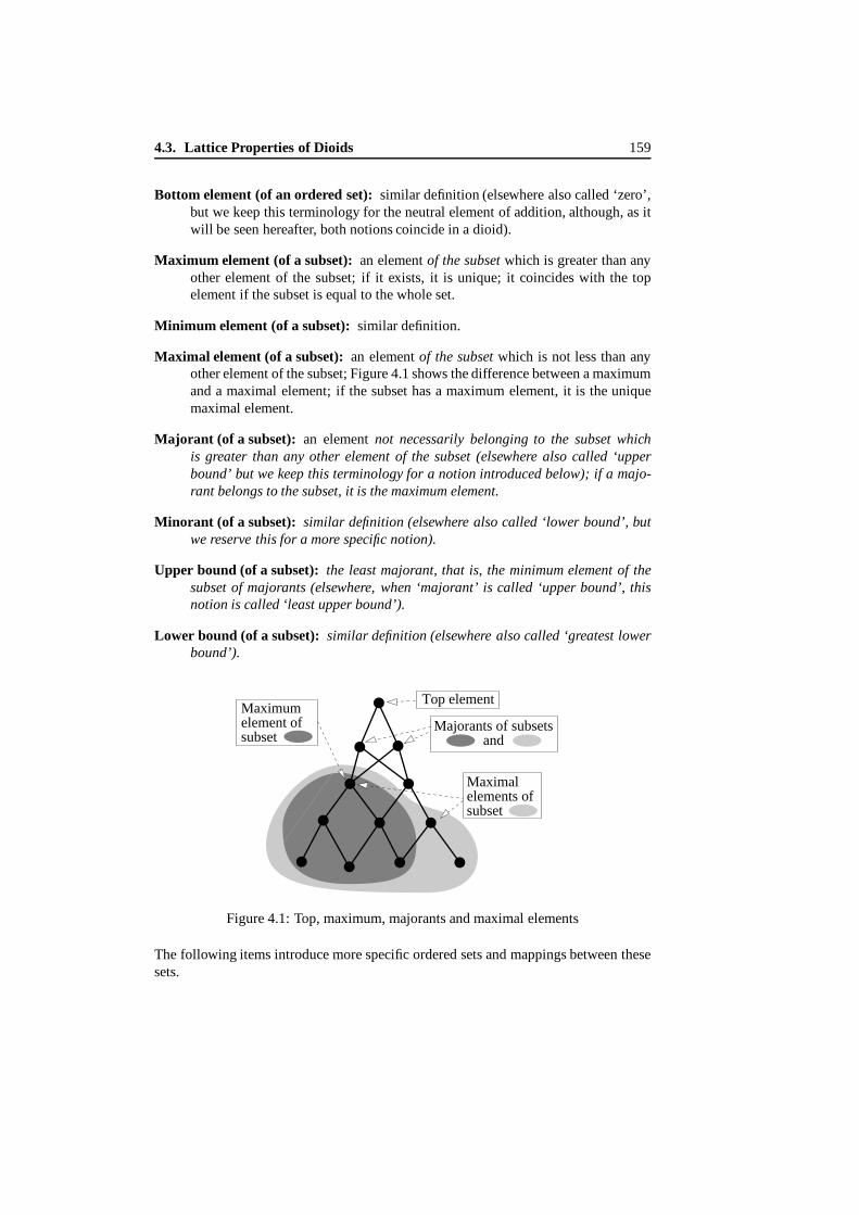
4.3. Lattice Properties of Dioids 159
Bottom element (of an ordered set):similar definition (elsewhere also called ‘zero’,but we keepthis terminology for the neutral element of addition, although, as itwill be seen hereafter, both notions coincide in a dioid).
Maximum element (of a subset):an elementof the subset which is greater than anyother element of the subset; if it exists, it is unique; it coincides with the topelement if the subset isequal to the whole set.
Minimum element (of a subset): similar definition.
Maximal element (of a subset):an elementof the subset which is not lessthananyother element of the subset; Figure 4.1 shows the difference between a maximumand a maximal element; if the subset has a maximum element, it is the uniquemaximal element.
Majorant (of a subset): an elementnot necessarily belonging to the subset whichis greater than any other element of the subset (elsewhere also called ‘upperbound’ but we keep this terminology for a notion introduced below); if a majo-rant belongs to the subset, it is the maximum element.
Minorant (of a subset): similar definition (elsewhere also called ‘lower bound’, butwe reserve this for a more specific notion).
Upper bound (of a subset): the least majorant, that is, the minimum element of thesubset of majorants (elsewhere, when ‘majorant’ is called ‘upper bound’, thisnotion is called ‘least upper bound’).
Lower bound (of a subset): similar definition (elsewhere also called ‘greatest lowerbound’).
Maximalelements ofsubset
Majorants of subsetsand
Top elementMaximumelement ofsubset
Figure 4.1: Top, maximum, majorants and maximal elements
The following items introduce more specific ordered sets and mappings between thesesets.
160 Synchronization and Linearity
Sup-semilattice: anordered set such that there exists an upper bound foreach pair ofelements.
In f-semilattice: similar definition.
Lattice: an ordered set which is both a sup- and an inf-semilattice.
Complete sup-semilattice: an ordered set such that there exists an upper bound foreach finite or infinite subset.
Complete inf-semilattice: similar definition.
Complete lattice: obvious definition.
Distributive lattice: let a ∨ b (respectively, a ∧ b) denote the upper (respectively,lower) bound ofa andb in a lattice; then the lattice isdistributive if
∀a, b, c , a ∨ (b ∧ c) = (a ∨ b)∧ (a ∨ c) ;
in fact, as shown in [57, p. 188], if this equality holds true, the same equalitywith ∨ and∧ interchanged also holds true, and conversely.
Isotone mapping: a mapping� from an ordered setD into an ordered setC suchthat
∀a, b ∈ D , a ≥ b ⇒ �(a) ≥ �(b) .
We conclude this brief enumeration (more facts from lattice theory will be recalledlater on) by mentioning a fundamental result [57, pp. 175–176].
Theorem 4.27 A complete sup-semilattice having a bottom element is a complete lat-tice.
Proof Let C bea subset of a complete sup-semilatticeD; we must provethat it admitsa lowerbound. Consider the subsetT of minorants ofC. This subset is nonempty sinceit contains at least the bottom element. Letc be the upper bound ofT , which existssinceD is a complete sup-semilattice. Let us check whetherc obeys the definition ofthe lower bound ofC. First,c itself is belowC (that is, it belongs toT —it is thus themaximum element ofT ). As a matter of fact,T is bounded from above by allb ∈ C(by definition). Sincec is less than, or equal to, every element greater thanT (bydefinition of the upper bound),c ≤ b, ∀b ∈ C, hencec ∈ T . Therefore, c is less than,or equal to, all elements ofC and greater than every other element belowC, namely theelements inT . Henceit is the lowerbound ofC.
4.3.2 Order Structure of Dioids
Theorem 4.28 (Order relation) In a dioid D, one has the following equivalence:
∀a, b : a = a ⊕ b ⇔ ∃c : a = b ⊕ c .

4.3. Lattice Properties of Dioids 161
Moreover these equivalent statements define a (partial) order relation denoted ≥ asfollows:
a ≥ b ⇔ a = a ⊕ b .
This order relation is compatible with addition, namely
a ≥ b ⇒ {∀c , a ⊕ c ≥ b ⊕ c} ,
and multiplication, that is,
a ≥ b ⇒ {∀c , ac ≥ bc}
(the same for the left product). Two elements a and b in D always have an upperbound, namely a ⊕ b, and ε is the bottom element of D.
Proof
• Clearly, ifa = a⊕b, then∃c : a = b⊕c, namely c = a. Conversely, ifa = b⊕c,thenaddingb onboth sides of this equality yieldsa⊕b = b⊕(b⊕c) = b⊕c = a.
• The relation≥ is reflexive (a = a⊕a from Axiom 4.9), antisymmetric (a = a⊕bandb = b ⊕ a impliesa = b), and transitive since
{a = a ⊕ bb = b ⊕ c
}⇒
a ⊕ c = a ⊕ b ⊕ cb = b ⊕ ca = a ⊕ b
⇒{
a ⊕ c = a ⊕ ba = a ⊕ b
}⇒ {a ⊕ c = a
}.
Therefore≥ is an order relation.
• The compatibility of ≥ with addition is a straightforward consequence of Ax-ioms 4.2 and 4.3. The compatibility of multiplication involves Axiom 4.5. Theexpression ‘the(left or right) multiplication is isotone’ is also used for this prop-erty. But, as will be discussed in§4.4.1, the mappingx �→ ax is more thansimply isotone: it is a⊕-morphism.
• Obviously,a ⊕ b is greater thana andb. Moreover, if c ≥ a andc ≥ b, thenc = c⊕ c ≥ a ⊕ b. Hencea ⊕ b is theupper bound ofa andb.
• Finally,{∀a , a = a ⊕ ε} ⇔ {∀a , a ≥ ε} ,
which means thatε is the bottom element ofD.
Notation 4.29 As usual, we may usea ≤ b as an equivalent statement forb ≥ a, andb > a (or a < b) as an equivalent statement for [b ≥ a and b = a].
The following lemma deals with the problem ofwhether the order relation induced by⊕ is total or only partial.

162 Synchronization and Linearity
Lemma 4.30 (Total order) The order relation defined in Theorem 4.28 is total if andonly if
∀a, b ∈ D , a ⊕ b = either a or b .
Proof It is just a matter of rewriting the claim ‘eithera ≥ b or b ≥ a’ using⊕ and thevery definition of ≥.
Let us revisit the previous examples of dioids and discover what is the order relationassociated with⊕. It is the conventional orderof numbers for Examples 4.12, 4.14,4.15 and 4.16. However, in Example 4.13 it is thereversed order: 2≥ 3 in this dioidsince 2= 2⊕ 3. As for Examples 4.17 and 4.18,≥ is simply⊇. All these dioids arechains except for Example 4.17.
Theorem 4.28 essentially shows that an idempotent addition inD induces a struc-ture of sup-semilattice overD. But we could have done it the other way around: con-sidering a sup-semilattice, we can define the result of the addition of two elements astheir upper bound; this obviously defines an idempotent addition. The sup-semilatticehas then to be endowed with another operation called⊗. This multiplication should beassumed notonly isotone but also distributive,except that isotony is sufficient ifD isa chain (see§4.4.1). We now present a counterexample to the statement that isotonyof multiplication implies distributivity (and therefore of the statement that isotony of amapping would imply that this mapping is a⊕-morphism).
Example 4.31 Consider Example 4.17 again but change addition to∩ instead of∪.Now A ≥ B meansA ⊆ B and it is true that this implies A⊗C ≥ B⊗C or equivalentlyA + C ⊆ B + C. Since⊗ = + is isotone, we do have, as a translation of (4.12),
(B ∩ C) + D ⊆ (B + D) ∩ (C + D) (4.4)
(because here≥ is⊆, not⊇!), but equality does not hold in general, as shown by theparticular case:B is the subsetreduced to the point(1, 0) ∈ R
2, C is similarly reducedto thepoint (0, 1), whereasD is the square [−1, 1] × [−1, 1]. Clearly, the left-handsideof (4.4) is equal to∅, whereas the right-hand side is thesquare [0, 1]× [0, 1] (see
Figure 4.2). In conclusion,(2R
2,∩,+)
is not a dioid.
4.3.3 Complete Dioids, Archimedian Dioids
In accordance with the definition of complete sup-semilattices, we adopt the followingdefinition.
Definition 4.32 (Complete dioid) A dioid is complete if it is closed for infinite sumsand Axiom 4.5 extends to infinite sums.
With the former requirement, the upper bound of any subset is simply the sum ofall its elements. The latter requirement may be viewed as a property of ‘lower-semicontinuity’ of multiplication.

4.3. Lattice Properties of Dioids 163
︸ ︷︷ ︸
D
C + D
B + D︷ ︸︸ ︷
Figure 4.2:+ is not distributive with respect to∩
In a complete dioid the top element of the dioid, denoted�, exists and is equal tothe sumof all elements inD. Thetop element is always absorbing for addition sinceobviously∀a,�⊕ a = �. Also
�⊗ ε = ε , (4.5)
because of Axiom 4.7.If we consider our previous examples again, Examples 4.12, 4.13, 4.14 and 4.18
are not complete dioids, whereas Examples 4.15, 4.16 and 4.17 are. ForRmax to becomplete, we should add the top element� = +∞ with the rule−∞ +∞ = −∞which is atranslation of (4.5). This completed dioid is calledRmax andR denotesR ∪ {−∞} ∪ {+∞}. Similarly, the dioid in Example 4.18 is not complete but can becompleted by adding the ‘half-line’R itself to theconsidered set. However somethingis lost when doing this completion since multiplication does not remain cancellative(see Theorem 4.35 below). Of course, a subdioid of a complete dioid may not becomplete. For example(Q ∪ {−∞} ∪ {+∞},max,+) is a subdioid ofRmax which isnot complete.
Thequestion arises whether� is in general absorbing for multiplication, that is,
∀a ∈ D , a = ε , �⊗ a = a ⊗� = � ? (4.6)
Property (4.6) can be proved for ‘Archimedian’ dioids.
Definition 4.33 (Archimedian dioid) A dioid is Archimedianif
∀a = ε , ∀b ∈ D , ∃c and d ∈ D : ac ≥ b and da ≥ b .
Theorem 4.34 In a complete Archimedian dioid, the absorbing property (4.6) holdstrue.
Proof We give the proof only for right multiplication by�. From Definition 4.33,givena, for all b, thereexistscb suchthatacb ≥ b. Onehas that

164 Synchronization and Linearity
a� = a
(⊕
b∈Db
)≥ a
(⊕
b∈Dcb
)=⊕
b∈Dacb ≥
⊕
b∈Db = � .
Among our previous examples, all dioids, except for the one in Example 4.15, areArchimedian, but only Examples 4.16 and 4.17 correspond to complete dioids forwhich (4.6) holds true. Example 4.15 is a case of a dioid which is complete but notArchimedian, and (4.6) fails to be true.
Theorem 4.35 If a dioid is complete, Archimedian, and if it has a cancellative multi-plication, then it is isomorphic to the Boole algebra.
Proof Since (4.6) holds true and since⊗ is cancellative, it is realized that every elementdifferentfrom ε is equal to�. Hence, the dioid is reduced to{ε,�}.
4.3.4 Lower Bound
Since a complete dioid is a complete sup-semilattice, and since there is also a bottomelementε, the lower bound can be constructed for any subsetC of elements ofD andthe semilattice becomes then a complete lattice (Theorem 4.27). IfC = {x, y, z, . . . },its lower bound is denotedx ∧ y ∧ z ∧ . . . . In general, we use the notation
∧x∈C x .
One has the following equivalences:
a ≥ b ⇔ a = a ⊕ b ⇔ b = a ∧ b . (4.7)
This operation∧ is alsoassociative, commutative, idempotent and has� as neutralelement (� ∧ a = a, ∀a). The following property, called ‘absorption law’, holds true[57, p. 184]:
∀a, b ∈ D , a ∧ (a ⊕ b) = a ⊕ (a ∧ b) = a .
Returning to our examples, the reader should apply the formal construction of thelower bound recalled in Theorem4.27 to Example 4.17 (a complete dioid) and provethat∧ is simply∩ in this case. As for the other examples, since all of them are chains,and even when thedioid isnotcomplete, a simpler definition ofa ∧ b canbe adopted:indeed, owing to Lemma 4.30, (4.7) may serve as a definition. Moreover, in the caseof a chain, since a lower bound can be defined anyway, and because there exists abottom elementε, thedioid is acomplete inf-semilattice even if it is not a completesup-semilattice.
Equivalences (4.7) may leave the impression that⊕ and∧ play symmetric roles ina complete dioid. This is true from the lattice point of view, but this is not true whenconsidering the behavior with respect to the other operation of the dioid, namely⊗.Since multiplication is isotone, from Lemma 4.42 in§4.4.1 below itfollows that
(a ∧ b)c ≤ (ac) ∧ (bc) (4.8)
(similarly for left multiplication) what we may call ‘subdistributivity’ of⊗with respectto∧. The same lemma shows that distributivityholds true for chains. But this is not true

4.3. Lattice Properties of Dioids 165
in general for partially-ordered dioids. A counterexample is provided by Example 4.17(⊕ is∪,⊗ is+ and∧ is∩). In Example 4.31 we showed that+ is not distributive withrespect to∩. There are, however, situations in which distributivity of⊗ with respect to∧ occurs forcertain elements. Here is such a case.
Lemma 4.36 If a admits a left inverse b and a right inverse c, then
• b = c and this unique inverse is denoted a−1;
• moreover, ∀x, y, a(x ∧ y) = ax ∧ ay.
The same holds true for right multiplication by a, and also for right and left multipli-cation by a−1.
Proof
• One hasb = b(ac) = (ba)c = c, proving uniqueness of a right and left inverse.
• Then,∀x, y, defineξ andη according to(ξ = ax, η = ay), whichis equivalentto (x = a−1ξ, y = a−1η). Onehas
ξ ∧ η = aa−1(ξ ∧ η) ≤ a[a−1ξ ∧ a−1η] = a[x ∧ y] ≤ ax ∧ ay = ξ ∧ η .
Hence equality holds throughout.
4.3.5 Distributive Dioids
Once the lower bound has been introduced, this raises the issue of the mutual behav-ior of ⊕ and∧. In fact,∧ is not necessarily distributive with respect to⊕ and con-versely, except again for chains. The following inequalities are again consequences ofLemma 4.42 in§4.4.1 below, and of the fact thatx �→ x⊕c andx �→ x∧c are isotone:
∀a, b, c ∈ D ,(a ∧ b)⊕ c ≤ (a ⊕ c) ∧ (b ⊕ c) ,
(a ⊕ b) ∧ c ≥ (a ∧ c)⊕ (b ∧ c) ,
which means that⊕ is subdistributive with respect to∧, and∧ is superdistributive withrespect to⊕.
As already defined, a lattice is distributive when equality holds true in the twoinequalities above.
Example 4.37 Here is an example of a complete lattice which is not distributive.Consider all the intervals ofR (including∅ andR itself) with⊆ as≤. The upper bound⊕ of any (finite orinfinite) collection of intervals is the smallest interval which containsthe whole collection, that is, it is the convex hull of the union of all the intervals in thecollection. The lower bound∧ is simply∩. Then, considera = [−3,−2], b = [2, 3]andc = [−1, 1]. We have that(a ⊕ b)∧ c = c, whereas(a ∧ c)⊕ (b ⊕ c) = ∅.
The following theorem can be found in [57, p. 207].

166 Synchronization and Linearity
Theorem 4.38 A necessary and sufficient condition for a lattice to be distributive isthat
∀a, b ,
{∃c :
a ∧ c = b ∧ ca ⊕ c = b ⊕ c
}⇒ {a = b} .
In [57] it is also shown that ifG is a multiplicative ‘lattice-ordered group’, which meansthat, in addition to being a group and a lattice, the multiplication is isotone, then
• the multiplication is necessarily distributive with respect to both the upper andthe lowerbounds (G is called a ‘reticulated group’),
• moreover, the lattice is distributive (that is, upper and lower bounds are distribu-tive with respectto one another).
Also, one has the remarkable formulæ:
(a ∧ b)−1 = a−1⊕ b−1 , (4.9)
(a ⊕ b)−1 = a−1 ∧ b−1 , (4.10)
a ∧ b = a(a ⊕ b)−1b , (4.11)
which should remind us of the De Morgan laws in Boolean algebra, and also the sim-ple formula min(a, b) = −max(−a,−b). However, this situation is far from beingrepresentative for the general case as shown by Examples 4.15 (total order) and 4.17(partial order). Nevertheless, these examples correspond to ‘distributive dioids’ in thefollowing sense.
Definition 4.39 (Distributive dioid) A dioid D is distributiveif it is complete and, forall subsets C of D,
∀a ∈ D ,
(∧
c∈Cc
)⊕ a =
∧
c∈C(c ⊕ a) ,
(⊕
c∈Cc
)∧ a =
⊕
c∈C(c ∧ a) .
Notice that here distributivity is required to extend to infinite subsets. Both propertiesshould be required now since one does not imply the other in the infinite case [57,p. 189]. Using the terminology of§4.4.1, we may state the preceding definition inother words by saying that a dioid is distributive if and only if the mappingsx �→ a∧ xandx �→ a ⊕ x are both continuous for everya. All complete dioids considered so farare distributive. Example 4.37 can be extended to provide a nondistributive dioid. Itsuffices to define⊗ as the ‘sum’ of intervals (conventional arithmetic sum). Of course,⊕ is theupper bound as defined in that example (the reader may check the distributivityof ⊗ with respect to⊕).

4.4. IsotoneMappings and Residuation 167
Remark 4.40 A distributive dioid may also be considered as a dioid with the two
operations⊕ def= ⊕ and⊗ def= ∧. But one can also choose⊕ def= ∧ and⊗ def= ⊕. Specialfeatures of these dioid structures are that∀x, ε ≤ x ≤ e and that multiplication iscommutative and idempotent. Examples 4.15 and 4.16 are instances of such dioids.
4.4 Isotone Mappings and Residuation
Most of the material in this section is classical in Lattice Theory. The structure addedby⊗ in dioids plays virtually no role, except of course when the mappings consideredthemselves involve multiplication (for example when considering the residual of themappingx �→ ax). A basic reference is the book by Blyth and Janowitz [24].
4.4.1 Isotony and Continuity of Mappings
We are going to characterize isotone mappings in terms of ‘lower’ and ‘upper sets’.
Definition 4.41 (Lower, upper set) A lower setis a nonempty subset L of D such that
(x ∈ L andy ≤ x)⇒ y ∈ L .
A closed lower set(generated by x) is a lower set denoted [←, x ] of the form{y | y ≤ x}. An upper setis a subset U such that
(x ∈ U andy ≥ x)⇒ y ∈ U .
A closed upper set(generated by x) is an upper set denoted [x,→] of the form{y | y ≥ x}.The names ‘(principal) ideal’ and ‘(principal) filter’ are used for ‘(closed) lower set’and ‘(closed) upper set’, respectively, in [24].
A closed lower set is alower set which contains the upper bound of its elements.Similarly, a closed upper set is an upper set containing the lower bound of its elements.For a chain, sayRmax, closed lowersetscorrespond to closed half-lines(−∞, x ], lowersets are open or closed half-lines, whereas closed upper sets are of the type [x,+∞).Figure 4.3 gives examples of such sets in a partially-ordered lattice.
Obviously, if � is a⊕- or a∧-morphism, it is isotone (see§4.3.1). For example,for everya ∈ D, the mappingx �→ ax fromD into itself is a⊕-morphism, hence it isisotone. But, conversely, if� is isotone, it is neither necessarily a⊕- nor necessarily a∧-morphism.
Lemma 4.42 Let � be a mapping from a dioid D into another dioid C. The followingstatements are equivalent:
1. the mapping � is isotone;
2. the ‘pre-image’ �−1([←, x ]) of every closed lower set is a lower set or it isempty;
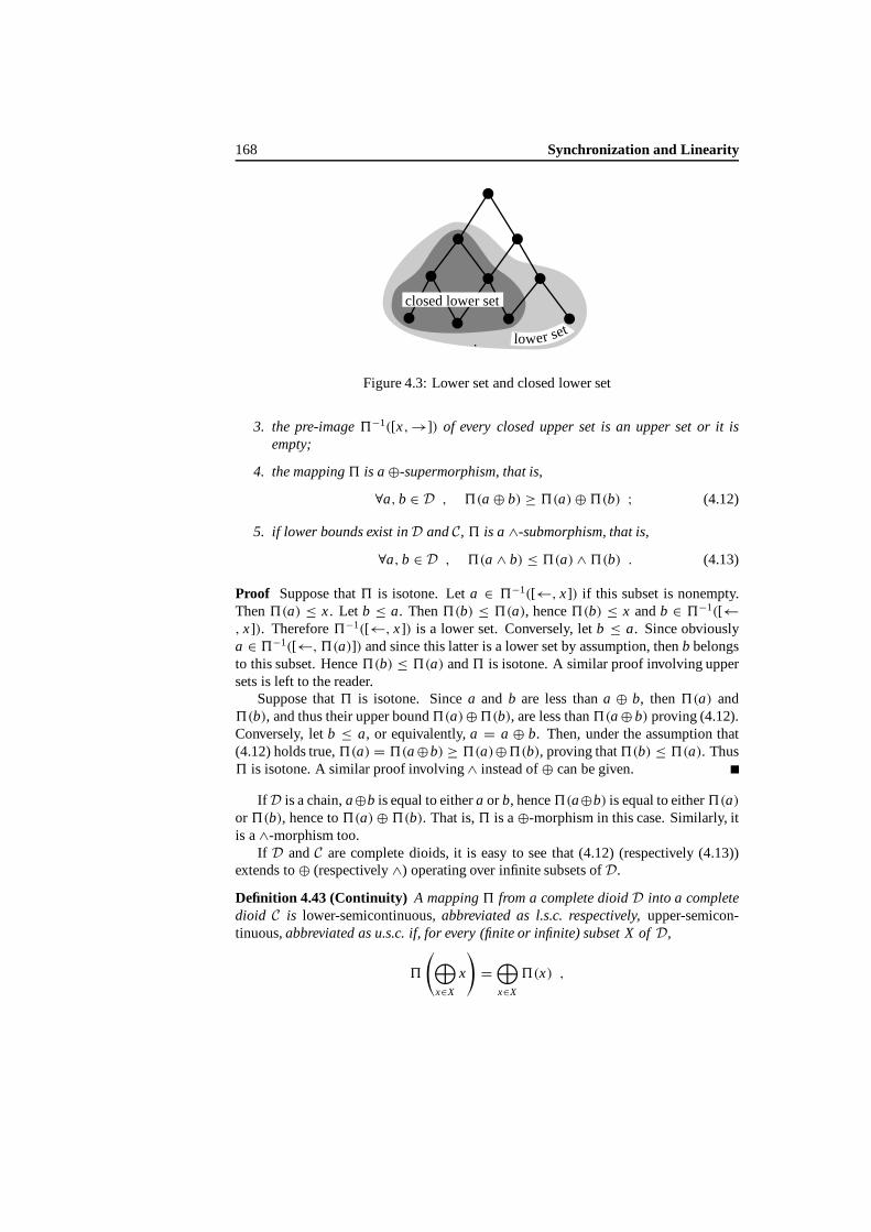
168 Synchronization and Linearity
lower set
closed lower set
Figure 4.3: Lower set and closedlower set
3. the pre-image �−1([x,→]) of every closed upper set is an upper set or it isempty;
4. the mapping � is a ⊕-supermorphism, that is,
∀a, b ∈ D , �(a ⊕ b) ≥ �(a)⊕�(b) ; (4.12)
5. if lower bounds exist in D and C, � is a ∧-submorphism, that is,
∀a, b ∈ D , �(a ∧ b) ≤ �(a)∧�(b) . (4.13)
Proof Suppose that� is isotone. Leta ∈ �−1([←, x ]) if this subset is nonempty.Then�(a) ≤ x . Let b ≤ a. Then�(b) ≤ �(a), hence�(b) ≤ x andb ∈ �−1([←, x ]). Therefore�−1([←, x ]) is a lower set. Conversely, letb ≤ a. Since obviouslya ∈ �−1([←, �(a)]) and since this latter is a lower set by assumption, thenb belongsto this subset. Hence�(b) ≤ �(a) and� is isotone. A similar proof involving uppersetsis left to the reader.
Suppose that� is isotone. Sincea and b are less thana ⊕ b, then�(a) and�(b), and thus their upper bound�(a)⊕�(b), are less than�(a⊕ b) proving (4.12).Conversely, let b ≤ a, or equivalently, a = a ⊕ b. Then, under the assumption that(4.12) holds true,�(a) = �(a⊕b) ≥ �(a)⊕�(b), proving that�(b) ≤ �(a). Thus� is isotone. A similar proof involving∧ instead of⊕ can begiven.
If D is a chain,a⊕b is equal to eithera or b, hence�(a⊕b) is equal to either�(a)or�(b), hence to�(a)⊕�(b). That is,� is a⊕-morphism inthis case. Similarly, itis a∧-morphism too.
If D andC are complete dioids, it is easy to see that (4.12) (respectively (4.13))extends to⊕ (respectively ∧) operating over infinite subsets ofD.
Definition 4.43 (Continuity) A mapping � from a complete dioid D into a completedioid C is lower-semicontinuous, abbreviated as l.s.c. respectively, upper-semicon-tinuous, abbreviated as u.s.c. if, for every (finite or infinite) subset X of D,
�
(⊕
x∈X
x
)=⊕
x∈X
�(x) ,

4.4. IsotoneMappings and Residuation 169
respectively,
�
(∧
x∈X
x
)=∧
x∈X
�(x) .
The mapping � is continuousif it is both l.s.c. and u.s.c.
Of course, a l.s.c. (respectively an u.s.c.) mapping is a⊕- (respectively a∧-) morphism.If � is a⊕-morphism, it is isotone and thus it is a∧-submorphism, but not necessarilya∧-morphism. This hasalready beenillustrated by Example 4.31.
To justify the terminology ‘l.s.c.’, one should consider the example of anondecreas-ing mapping� from R to itself (because here we are interested inisotone mappingsbetween ordered sets), and check that, in this case, the lower-semicontinuity in theprevious sense coincides with the conventional notion of lower-semicontinuity (whichrequires that lim infxi→x �(xi) ≥ �(x)). The same observation holds true for upper-semicontinuity.
Lemma 4.44 One has the following equivalences:
• � is l.s.c.;
• the pre-image �−1([←, x ]) of every closed lower set is a closedlower set or itis empty.
Similarly, the following two statements are equivalent:
• � is u.s.c.;
• the pre-image �−1([x,→]) of every closed upper set is a closedupper set or itis empty.
Proof Weprove the former equivalence only. Suppose that� is l.s.c. In particular it isisotone and the pre-imageX = �−1([←, x ]) of every closed lower set, if nonempty,is a lower set. Ifa ∈ X , then�(a) ≤ x . Thus
�
(⊕
a∈Xa
)=⊕
a∈X�(a) ≤ x .
Hence the upper bound ofX belongs toX : X is closed.Conversely, suppose that the pre-image of every closed lower set is a closed lower
set. In particular, according to Lemma 4.42,� is isotone and for every nonemptysubsetX ⊆ D, one has that
�
(⊕
x∈Xx
)≥⊕
x∈X�(x) . (4.14)
On the other hand, it isobvious that
X ⊆ �−1
([←,⊕
x∈X�(x)]
).

170 Synchronization and Linearity
But the latter subset is a closed lower set by assumption, hence it contains the upperbound of its elements and a fortiori it contains the upper bound ofX . This implies thereverse inequality in (4.14). Therefore equality holds true and� is l.s.c.
Example 4.45 Let D = Rmax andC = Nmax, let� : D→ C defined by
� : x �→ y =⊕
y∈C,y≤x
y ,
where thesymbol ≤ has its usual meaning. Indeed,� is the residual of the mappingx �→ x from C intoD (not fromD to C!)—see§4.4.2 below. More simply,�(x) is justthe integerpart of the real numberx . Then, � is a⊕- and a∧-morphism, it is u.s.c.(this is a consequence of being a residual) but not l.s.c.
Lemma 4.46 The set of l.s.c. mappings from a complete dioid D into itself is a com-plete dioid when endowed with the following addition ⊕ and multiplication ⊗:
�⊕� : x �→ �(x)⊕�(x) ;�⊗� : x �→ �(�(x)) .
(4.15)
Similarly, the set of u.s.c. mappings from D into D is a complete dioid when endowedwith the following addition ⊕ and multiplication ⊗:
�⊕� : x �→ �(x)∧ �(x) ;�⊗� : x �→ �(�(x)) .
(4.16)
Proof We only prove the former statement. It is easy to check thatl.s.-continuityis preserved by addition and composition of mappings. The other axioms of dioidsare also easily checked. In particular,ε is the mapping identically equal toε ande = ID (identity of D). Distributivity of right multiplication with respect to additionis straightforward from the very definitions of⊕ and ⊗, whereas left distributivityinvolves the assumption of l.s.-continuity.
Remark 4.47 Observe that since Lemma 4.46 defines a complete dioid structure forthe set of l.s.c.mappings from a complete dioidD into itself, this dioid of mappingshas a lower bound operation (Theorem 4.27) also denoted∧. However, in general, fortwo mappings� and�, (� ∧ �)(x) = �(x) ∧ �(x) since the right-hand side is ingeneral not a l.s.c. function ofx .
Example 4.48 ConsiderD =(Rmax
)2(operations ofD are those ofRmax operating
componentwise). LetC =(R
2, ⊕,⊗
)for which the underlying set is the same as that
of D and⊗ is also the same. But⊕ is defined as follows:
∀x, y ∈ R2, x⊕y =
{x if (x1 > y1) or (x1 = y1 andx2 ≥ y2) ;y if (x1 < y1) or (x1 = y1 andx2 ≤ y2) .

4.4. IsotoneMappings and Residuation 171
The order inD is the usual partial order inR2
whereasC is totally ordered by thelexicographic order. Let� : D → C be simply the canonical bijectionx �→ x . Thisis an isotone mapping sincex ≤ y in D implies x ≤ y in C. However, this mappingis neither l.s.c. nor u.s.c. Figure 4.4 depicts the shape of a closed lower set generatedby the pointx = (2, 3) in C (shaded area). It is a half-plane including the border
Figure 4.4: A closed lower set for the lexicographic order
for x2 ≤ 3 but not for x2 > 3. Since�−1 is also the canonical bijection inR2, the
pre-image of this closed lower set is itself and it is not a closed lower set inD: closedlower sets inD consist ofclosed south-west orthants. Hence� is not l.s.c.
This example is also interesting because it shows that an isotone bijection� mayhave an inverse mapping�−1 which is not isotone. As a matter of fact,x ≤ y in Cdoes not imply the same inequality inD in general. However, we leave to thereaderto prove that an isotone bijection from atotally ordered dioid D onto another dioidChas an isotone inverse and, moreover, if both dioids are complete, the mapping and itsinverse are continuous.
Lemma 4.49 Let D and C be complete dioids and � be a homomorphism from D intoC. Consider the congruence defined in Example 4.25. If � is l.s.c. (respectively u.s.c.),then every equivalence class has a maximum (respectively minimum) element, which istherefore a canonical representative of the equivalence class.
Proof We consider the case of a l.s.c. mapping. Let [x ] denote the equivalence class
of anyx ∈ D, then︷︷x
def=⊕y∈[x] y is theupper bound of [x ], and it belongs to [x ] since,by lower-semicontinuity,
�(︷︷x) = �
⊕
y∈[x]
y
=⊕
y∈[x]
�(y) = �(x) .
4.4.2 Elements of Residuation Theory
Residuation has to do with ‘inverting’ isotone mappings and with solving equations.Let � be an isotone mapping from a dioidD into another dioidC. To guarantee the

172 Synchronization and Linearity
existence of upper and lower bounds, we assume throughout this subsection thatDandC are complete. If� is not surjective, the equation inx : �(x) = b will haveno solution for some values ofb, and if � is not injective, the same equation mayhave nonunique solutions. One way to always give a unique answer to this problem ofequation solving is to consider the subset of so-called ‘subsolutions’, that is, values ofx satisfying �(x) ≤ b, if this subset is nonempty, and then to take the upper boundof the subset, if it exists: it remains to be checked whether the upper bound itself isa subsolution, namely, that it is the maximum element of the subset of subsolutions,which hasto do with l.s.-continuity of�. In thiscase, this maximum elementwill bedenoted��(b) and we have
��(b) =⊕
{x|�(x)≤b}x and �
(��(b)) ≤ b . (4.17)
Dually, one may consider ‘supersolutions’ satisfying�(x) ≥ b, if again this subsetis nonempty, and then take the lower bound assuming it exists: again it remains tocheckwhether the lower bound is itself a supersolution, namely, that it is the minimumelement of the subset of supersolutions, which has to do with u.s.-continuity of�. Inthis case this minimum element will be denoted��(b) and we have
��(b) =∧
{x|�(x)≥b}x and �
(��(b)) ≥ b . (4.18)
Theorem 4.50 Let � be an isotone mapping from the complete dioid D into the com-plete dioid C. The following three statements are equivalent:
1. For all b ∈ C, there exists a greatest subsolution to the equation �(x) = b(by this we mean that the subset of subsolutions is nonempty and that it has amaximum element).
2. �(ε) = ε and � is l.s.c. (or equivalently, the pre-image of every closed lowerset is nonempty and it is a closed lower set).
3. There exists a mapping �� from C into D which is isotone and u.s.c. such that
�◦�� ≤ IC (identity of C) ; (4.19)
��◦� ≥ ID (identity of D) . (4.20)
Consequently, �� is unique. When � satisfies these properties, it is said to be residu-atedand �� is called its residual.
Proof First of all, it should be clear that the two statements in ‘2.’ above are equivalent.In the rest of the proof, we always refer to the former of these two statements.
1⇒ 3: As a matter of fact,∀b ∈ C, there exists a greatest subsolution that we de-note��(b). It is obvious that the mapping�� thus defined is isotone. Inequal-ity (4.19) is immediate from the definition of a subsolution. Now,∀x ∈ D, let

4.4. IsotoneMappings and Residuation 173
b = �(x). Sincex is a subsolution corresponding to thatb, from thedefinitionof ��(b), x ≤ ��(b) = ��◦�(x), from which (4.20) follows.
We now prove that�� is u.s.c. Since�� is isotone, using (4.13), for a subsetB ⊆ C, one has that
��
(∧
b∈B
b
)≤∧
b∈B
��(b) . (4.21)
Using (4.13) again, we obtain
�
(∧
b∈B
��(b)
)≤∧
b∈B
�◦��(b) ≤∧
b∈B
b ,
in which the latter inequality follows from (4.19). Hence∧
b∈B ��(b) is a subso-lution corresponding to the right-hand side
∧b∈B b. Thus, thereverse inequality
alsoholdstrue in (4.21), and equality is obtained, proving that�� is u.s.c.
3⇒ 2: From (4.19),�◦��(ε) ≤ ε ⇒ �◦��(ε) = ε. But��(ε) ≥ ε ⇒ �◦��(ε) ≥�(ε). If we combine the two facts, it follows thatε ≥ �(ε), provingthe equalityof the two sides.
Let X ⊆ D. Since� is isotone, it follows from (4.12) that
⊕
x∈X
�(x) ≤ �
(⊕
x∈X
x
). (4.22)
For all x ∈ X , let bx = �(x). Because of (4.20),��(bx) ≥ x , hence
�
(⊕
x∈X
x
)≤ �
(⊕
x∈X
��(bx )
)≤ �◦��
(⊕
x∈X
bx
)≤⊕
x∈X
bx =⊕
x∈X
�(x) ,
where we used (4.12) for�� and then (4.19). This is thereverse inequality of(4.22), henceequality holds true and the l.s.-continuity of� is proved.
2⇒ 1: Since�(ε) = ε, the subset of subsolutionsXb ⊆ D is nonempty∀b ∈ C.Then, by l.s.-continuity of�, and since everyx ∈ Xb is a subsolution,
�
⊕
x∈Xb
x
=⊕
x∈Xb
�(x) ≤ b .
This proves that⊕
x∈Xbx is a subsolution too.
Finally, since the greatest subsolution isunique by definition, the equivalences aboveimply that�� is unique as well.
Remark 4.51 It is clear that�−1([←, x ]) = [←, ��(x)]. Moreover, since�(�) ≤�, then��(�) ≥ �, hence��(�) = �.
Now, instead of being interested in the greatest subsolution, we may search for theleast supersolution. This is dual residuation. The dual of Theorem 4.50 can be stated.

174 Synchronization and Linearity
Theorem 4.52 Let � be an isotone mapping from the complete dioid D into the com-plete dioid C. The following three statements are equivalent:
1. For all b ∈ C, there exists a least supersolution to the equation�(x) = b (by thiswe mean that the subset of supersolutions is nonempty and that it has a minimumelement).
2. �(�) = � and � is u.s.c. (or equivalently, the pre-image of every closed upperset is nonempty and it is a closed upper set).
3. There exists a mapping �� from C into D which is isotone and l.s.c. such that
�◦�� ≥ IC (identity of C) ; (4.23)
��◦� ≤ ID (identity of D) . (4.24)
Consequently, �� is unique. When � satisfies these properties, it is said to be duallyresiduatedand �� is called its dual residual.
Remark 4.53 One hasthat
�−1([x,→]) = [��(x),→] ,
and��(ε) = ε .
It should also be clear that if� is residuated, itsresidual is dually residuated and
(��)� = � .
Example 4.54An example of a residuated mapping was encountered in Example 4.45.Indeed, if we letD = Nmax andC = Rmax, the canonical injection fromN into R isresiduated and its residual is the mapping described in that example, that is, the ‘integerpart’ of a real number ‘from below’. The same injection is also dually residuated andits dual residual is the ‘integer part from above’.
Example 4.55 Another interesting example is provided by the mapping� : x �→(x, x) from a complete dioidD into D2. This mapping again is residuated and duallyresiduated and it is easy to check that
��(x, y) = x ∧ y and ��(x, y) = x ⊕ y .
Subsection 4.4.4 provides other examples on residuation. The following theorem listsadditional properties of residuated mappings and residuals, and dual properties whenappropriate.

4.4. IsotoneMappings and Residuation 175
Theorem 4.56
• If � is a residuated mapping from D into C, then
�◦��◦� = � ; (4.25)
��◦�◦�� = �� . (4.26)
One has the following equivalences:
��◦� = ID ⇔ � injective⇔ �� surjective ; (4.27)
�◦�� = IC ⇔ �� injective⇔ � surjective . (4.28)
The same statements hold true for dually residuated mappings by changing �
into �.
• If � : D → C and � : C → B are residuated mappings, then �◦� is alsoresiduated and
(�◦�)� = ��◦�� . (4.29)
Again, the same statement holds true with � instead of �.
• If �,�,� and � are mappings from D into itself, and if � and � are residu-ated, then
�◦� ≤ �◦�⇔ �◦�� ≤ ��◦� . (4.30)
As corollaries, one has that
� ≤ �⇔ �� ≤ �� , (4.31)
and
� ≤ ID ⇔ �� ≥ ID , (4.32)
� ≥ ID ⇔ �� ≤ ID . (4.33)
Similar statements hold true for dual residuals with appropriate assumptions; inparticular, the analogue of (4.30) is
�◦� ≤ �◦� ⇔ ��◦� ≤ �◦�� . (4.34)
• If � and � are two residuated mappings from a dioid D (in which ∧ exists) intoitself, then �⊕� is residuated and
(�⊕�)� = �� ∧�� . (4.35)
If � and � are dually residuated, then �∧ � is dually residuated and
(� ∧�)� = �� ⊕�� . (4.36)

176 Synchronization and Linearity
• If � and � are two residuated mappings from a dioid D (in which ∧ exists) intoitself and if �∧ � is residuated, then
(�∧ �)� ≥ �� ⊕�� . (4.37)
With dual assumptions,
(�⊕�)� ≤ �� ∧�� . (4.38)
Proof
About (4.25)–(4.26):One hasthat
�◦��◦� = �◦(��◦�) ≥ � ,
which follows from (4.20). But one also has that
�◦��◦� = (�◦��)◦� ≤ � ,
by making use of (4.19), hence (4.25) follows. Equation (4.26) is similarlyproved by remembering that�� is isotone.
About (4.27)–(4.28):Assume that��◦� = ID and suppose that�(x) = �(y).Applying ��, we conclude thatx = y, hence � is injective. Also, since��◦�(x) = x , it means that everyx belongs to Im��, hence�� is surjective.Conversely, if��◦� = ID, thereexists y suchthatx = ��◦�(y) = y. However,because of (4.25),�(x) = �(y). Hence� cannot be injective. On the otherhand, if�� is surjective,∀x ∈ D, ∃b ∈ C : ��(b) = x . Sincex is a subsolutioncorresponding to the right-hand sideb,�(x) ≤ b, hence��◦�(x) ≤ ��(b) = x .We conclude that��◦� ≤ ID, but equality must hold true because of (4.20).This completes the proof of (4.27). The proof of (4.28) is similar.
About (4.29): Asalready noticed l.s.- or u.s.-continuity is preserved by composition oftwo similarly semicontinuous mappings and the same holds true for the propertyof being residuated (consider the conditions stated in item 2 of Theorem 4.50).Also��◦�� is an isotone and u.s.c. mapping. Finally,
�◦�◦��◦�� = �◦(�◦��)◦�� ≤ �◦�� ≤ IC ,
by repeated applications of (4.19), showing that��◦�� satisfies (4.19) togetherwith �◦�. Likewise, it can beproved that (4.20) is met by the two composedfunctions. From the uniqueness of the residual, we conclude that (4.29) holdstrue.
About (4.30)–(4.34): If �◦� ≤ �◦�, then(��◦�)◦�◦�� ≤ ��◦�◦
(�◦��)
whichimplies that�◦�� ≤ ��◦� using (4.19)–(4.20). The converse proof is left to thereader (use a dual trick). Then (4.31) is obvious whereas to prove (4.32)–(4.33),we use the straightforward fact thatID is residuated and is its own residual. Theproof of (4.34) is similar to that of (4.30).

4.4. IsotoneMappings and Residuation 177
About (4.35)–(4.36):We give a proof of (4.35) only. First it is clear that the sum oftwo residuated mappings is residuated (l.s.-continuity is preserved by⊕). Nowconsider the composition� = �3◦�2◦�1 of the following three mappings:
�1 : D → D2 , x �→ (x x
),
�2 : D2 → D2 ,(
x y) �→ (
�(x) �(y))
,
�3 : D2 → D ,(
x y) �→ x ⊕ y .
Thus� : D→ D , x �→ (�⊕�)(x) .
Then,
��1 : D2 → D ,
(x y
) �→ x ∧ y (see Example 4.55),�
�
2 : D2 → D2 ,(
x y) �→ ( ��(x) ��(y)
)(trivial),
��
3 : D→ D2 , x �→ ( x x)
,
the last statement following also from Example 4.55 since it was explained therethat(��
3)� is indeed�3. Then, it suffices to calculate�� by using (4.29) repeat-
edly to prove (4.35).
About (4.37)–(4.38):We prove (4.37)only. Observe first that it is necessary toassumethat�∧ � is residuated since this is not automatically true. Then
(� ∧�) ◦(�� ⊕��
) = (�∧ �) ◦�� ⊕ (� ∧�) ◦�� ,
since�∧� is assumed residuated and hence l.s.c. The former term at the right-hand side is less than�◦�� which is less thanID; the latter term is less than�◦�� which again is less thanID, and so isthe left-hand side. This suffices toprove (4.37).
Remark 4.57 Returning to Lemma 4.49, if� is residuated, it should be clear that︷︷x
considered inthe proof of this lemma is nothing but��◦�(x).
4.4.3 Closure Mappings
Here we study a special class of mappings of a dioid into itself which will be of interestlater on.
Definition 4.58 (Closure mapping) Let D be an ordered set and � : D → D be anisotone mapping such that � = �◦� ≥ ID , then � is a called a closure mapping. If� = �◦� ≤ ID , then � is called a dual closure mapping.
Theorem 4.59 If � : D → D is a residuated mapping, then the following four state-ments are equivalent:
�◦� = � ≥ ID (i.e. � is a closure mapping), (4.39)
��◦�� = �� ≤ ID (i.e. �� is a dual closure mapping), (4.40)
�� = �◦�� , (4.41)
� = ��◦� . (4.42)

178 Synchronization and Linearity
Proof
(4.39)⇒ (4.40): This follows from (4.29) and (4.33).
(4.40)⇒ (4.41): From (4.40) it follows that�◦��◦�� = �◦��. The left-hand side isless than orequal to�� because of (4.19). The right-hand side is greater than orequal to�� because�� ≤ ID ⇒ � ≥ ID (see (4.33)). Hence (4.41) is proved.
(4.41)⇒ (4.42): From (4.41), it follows that�◦��◦� = ��◦�. But the left-hand sideis equal to� (see (4.25)). Hence (4.42) results.
(4.42)⇒ (4.39): Since� = ��◦�, then� ≥ ID because of (4.20). On the otherhand, (4.42)⇒ �◦��◦� = �◦� but the left-hand side is equal to� (see (4.25)).
Theorem 4.59 states thatall residuated closure mappings can be expressed as in (4.42).Indeed,all closure mappings� onD can be factored as��◦� for some� : D → C,whereC is another ordered set [24, Theorem 2.7]. Another characterization of l.s.c.closure mappings will be given in Corollary 4.69.
Theorem 4.60 If � : D→ D is a dually residuated mapping, then the following fourstatements are equivalent:
�◦� = � ≤ ID (i.e. � is a dual closure mapping), (4.43)
��◦�� = �� ≥ ID (i.e. �� is a closure mapping), (4.44)
� = �◦�� , (4.45)
�� = ��◦� . (4.46)
Lemma 4.61 If � and � are closure mappings on D and if they are ∧-morphisms,then �∧� also is a closure mapping. Likewise, if � and � are dual closure mappingsand if they are⊕-morphisms, then �⊕� is a dual closure mapping. These statementsextend to infinite numbers of mappings if the mappings are u.s.c., respectively l.s.c.
Proof Let us prove the former statement. Clearly,� ∧� ≥ ID. Moreover,
(� ∧ �)◦(� ∧�) = � ∧�◦� ∧ �◦� ∧� = � ∧ � ,
since� and� are greater thanID.
4.4.4 Residuation of Addition and Multiplication
In this subsection we consider the following mappings from a dioidD into itself:
Ta : x �→ a ⊕ x (translation by a);La : x �→ a ⊗ x (left multiplication by a);Ra : x �→ x ⊗ a (rightmultiplication by a).
Observe that
Ta◦Tb = Tb◦Ta = Ta⊕b = Ta ⊕ Tb . (4.47)

4.4. IsotoneMappings and Residuation 179
Moreover, ifD is a distributive dioid,
Ta ∧ Tb = Ta∧b . (4.48)
As for multiplication, the associativity of⊗ implies that
La◦Lb = Lab , (4.49)
and also that
La◦Rb = Rb◦La . (4.50)
The distributivity of ⊗ with respect to⊕ implies that
La ⊕ Lb = La⊕b , (4.51)
and also that
La◦Tb = Tab◦La . (4.52)
Observe thatLa is l.s.c. if and only if (left) multiplication is distributivewith respectto addition of infinitely many elements, which we assume here, and, since moreoverLa(ε) = ε, La is residuated. The same considerations apply to right multiplicationRa .
Notation 4.62 We use the one-dimensional display notationL �a(x) = a ◦\x (‘left divi-
sion’ by a—reads ‘a (left) dividesx ’), respectively,R�a(x) = x◦/a (‘right division’ by
a—reads ‘x (right) divided bya’), and the two-dimensional display notation
L �a(x) =
x
a, R�
a(x) =x
a.
As for Ta , sinceTa(ε) = ε unlessa = ε, this mapping is not residuated. Actually,by restraining the range ofTa to a ⊕ D, that is, tothe subset of elements greater thanor equal toa (call this new mappingAa : D → a ⊕ D), we could define a residualA�
a with domain equal to a ⊕ D. However, this is not very interesting sinceA�a is
simply the identity ofa ⊕ D. Indeed, sinceAa is surjective (by definition), Aa ◦A�a is
the identityaccording to (4.28). On the other hand, sinceAa is obviously a closuremapping, Aa ◦ A�
a = A�a (see (4.41)). Thisis why we assume thatD is a distributive
dioid—see Definition 4.39—and, as a consequence of that,Ta is u.s.c.Since moreoverTa(�) = �, Ta is dually residuated.
Notation 4.63 We use the notationT �a (x) = x ◦− a.
It should be clear that:x ◦− a = ε⇔ a ≥ x .
We aregoing to list a collection of formulæ and properties for these two new op-erations, ‘division’ and ‘subtraction’, which are direct consequences of the generalproperties enumerated in§4.4.2. For the sake of easy reference, the main formulæ havebeengathered in Tables 4.1 and 4.2. In Table 4.1, left and right multiplication anddivision are both considered.

180 Synchronization and Linearity
Remember that, when we consider properties involving◦− , the dioid D istacitly assumed to be complete (hence multiplication is infinitely distributive)and also distributive.
Table 4.1: Formulæinvolving division
x ∧ y
a= x
a∧ y
a
x ∧ y
a= x
a∧ y
a(f.1)
x ⊕ y
a≥ x
a⊕ y
a
x ⊕ y
a≥ x
a⊕ y
a(f.2)
x
a ⊕ b= x
a∧ x
b
x
a ⊕ b= x
a∧ x
b(f.3)
x
a ∧ b≥ x
a⊕ x
b
x
a ∧ b≥ x
a⊕ x
b(f.4)
ax
a≤ x
x
aa ≤ x (f.5)
ax
a≥ x
xa
a≥ x (f.6)
aax
a= ax
xa
aa = xa (f.7)
a(a ◦\x)
a= x
a
(x◦/a)a
a= x
a(f.8)
x
ab= a ◦\x
b
x
ba= x◦/a
b(f.9)
a ◦\xb
= x◦/b
a
x◦/a
b= b ◦\x
a(f.10)
bx
a≤ x
a◦/b
x
ab ≤ x
b ◦\a (f.11)
x
ab ≤ xb
ab
x
a≤ bx
a(f.12)
x
a⊕ b ≤ x ⊕ ab
a
x
a⊕ b ≤ x ⊕ ba
a(f.13)
For Table 4.1, we only prove the left-hand side versions of the formulæ. Formulæ (f.1)and (f.2) are consequences of the fact thatL �
a is u.s.c.and isotone. Dually, For-mulæ(f.14) and (f.15) result fromT �
a being l.s.c. and isotone. Inequalities (4.19)–(4.20) imply (f.5)–(f.6). However, if multiplication is cancellative, thenLa is injectiveand (see (4.27)) a ◦\(ax) = x and x �→ a ◦\x is surjective. If a is invertible, then

4.4. IsotoneMappings and Residuation 181
Table 4.2: Formulæinvolving subtraction
(x ⊕ y) ◦− a = (x ◦− a)⊕ (y ◦− a) (f.14)
(x ∧ y) ◦− a ≤ (x ◦− a)∧ (y ◦− a) (f.15)
(x ◦− a)⊕ a = x ⊕ a (f.16)
(x ⊕ a) ◦− a = x ◦− a (f.17)
x ◦− (a ⊕ b) = (x ◦− a) ◦− b = (x ◦− b) ◦− a (f.18)
x ◦− (a ∧ b) = (x ◦− a)⊕ (x ◦− b) (f.19)
ax ◦− ab ≤ a(x ◦− b) (f.20)
x = (x ∧ y)⊕ (x ◦− y) (f.21)
a ◦\x = a−1x . Dually, (4.23)–(4.24) yields
(x ◦− a)⊕ a ≤ x and (x ⊕ a) ◦− a ≤ x .
But this is weaker than what results from Theorem 4.60. ClearlyTa is a closure map-ping, hence from (4.44),
(x ◦− a) ◦− a = x ◦− a ,
and one alsogets (f.16)–(f.17) from (4.45)–(4.46). It follows that
x ≥ a ⇒ (x ◦− a)⊕ a = x and (x ≥ a, y ≥ a, x ◦− a = y ◦− a)⇒ (x = y) ,
which mayalso be viewed as consequences of the dual of (4.28) by observing thatTa
is surjective if its range is restrained toa ⊕D.Formulæ(f.7)–(f.8) are consequences of (4.25)–(4.26). The dual result stated for
⊕ and ◦− is weaker than (f.16)–(f.17).As a consequence of (4.31) or its dual,
a ≤ b ⇔{ x
a≥ x
b, ∀x
}⇔ {x ◦− a ≥ x ◦− b , ∀x} .
In particular,a ≥ e ⇔ a ◦\x ≤ x, ∀x andx ◦− a ≤ x, ∀a, ∀x sincea is alwaysgreaterthan orequal toε andx ◦− ε = x .
Using (4.29) and (4.49), one gets (f.9). Dually, using (4.47), Formula (f.18) isderived. Formula (f.10) is a consequence of (4.50) and (4.29). To obtain (f.12), onemakes useof (4.30) with� = � = La and� = � = Rb , and alsoof (4.50). Theproof of (f.11) essentially uses (f.5) twice:x ≥ a (a ◦\x) ≥ (a◦/b) b (a ◦\x) (the latterinequality arising from the version of (f.5) written forright multiplication and divisionapplied to the pair(a, b) instead of(x, a)); by associativity of the product, and fromthe very definition ofL �
a◦/b(x), one obtains (f.11).

182 Synchronization and Linearity
Equations (4.35) and (4.51) yield Formula (f.3) (which should be compared with(4.10)), whereas (4.36) and (4.48) yield (f.19). Because of (4.8),La∧b ≤ La ∧ Lb.If La ∧ Lb were residuated, we could use Inequality (4.37) to get thatL �
a∧b ≥(La ∧ Lb)
� ≥ L �a ⊕ L �
b, which would prove (f.4). Unfortunately,La ∧ Lb is not resid-uated in general, unless multiplication is distributive with respect to∧. A direct proofof (f.4) is as follows: La∧b ≤ La, hence L �
a∧b ≥ L �a; similarly L �
a∧b ≥ L �b; hence
L �
a∧b ≥ L �a ⊕ L �
b.As for (4.38) applied toTa⊕Tb , it would yield a weaker result than Equality (f.18).
Finally, consider (4.52) and use (4.30) with� = � = La, � = Tb, � = Tab; thisyields(f.13). Considering (4.52) again, but now in connection with (4.34), and setting� = � = La, � = Tb, � = Tab yield (f.20).
An interesting consequence of some of these formulæ is the decomposition of anyx with respect to anyy as given by (f.21). Indeed,
(x ∧ y)⊕ (x ◦− y) = (x ⊕ (x ◦− y)) ∧ (y ⊕ (x ◦− y))
= x ∧ (x ⊕ y)
= x ,
the first equality following from the assumption of distributivity, the second based onthe fact thatx ◦− y ≤ x on the one hand, and (f.16) on the other hand, the last equalitybeing obvious. As a corollary,
x ⊕ y = (x ◦− y)⊕ (x ∧ y)⊕ (y ◦− x) ,
which is straightforward using the decompositions ofx with respect toy and ofy withrespect tox .
Remark 4.64 Formula (f.3) canbewritten L �
a⊕b(x) = La(x)� ∧ L �
b(x), whereas (f.9)
can be written L �ab(x) = L �
b◦L�a(x). Then considering the dioid structure of u.s.c.
mappings fromD into D described in Lemma 4.46 (see (4.16)), it is realized that themappinga �→ L �
a is ahomomorphism fromD into that dioid of u.s.c. mappings.Likewise, (f.19) canbewritten T �
a∧b(x) = T �a (x) ⊕ T �
b (x), whereas (f.18) can bewrittenT �
a⊕b(x) = T �b (x)◦T
�a (x). Remember that nowD is supposed to be a distributive
dioid. Consider the dioid of l.s.c. mappings with the operations defined by (4.15).Observe that⊗ is commutative and idempotent when restricted to elements of the formT �
a . For the mapping a �→ T �a to be a homomorphism, we must supplyD with the
addition⊕ def= ∧ and themultiplication⊗ def= ⊕ (see Remark 4.40).
Example 4.65 Let us consider the complete dioid Rmax. From thevery definition of◦− , we have that
∀a, b ∈ R , a ◦− b ={
a if b < a ;
ε otherwise.
As for a◦/b (or b ◦\a, which is the same since the multiplication is commutative), itis equal toa − b (conventional subtraction) whenever there is no ambiguity in thisexpression, that is, in all cases except whena = b = ε = −∞ and whena = b =

4.4. IsotoneMappings and Residuation 183
� = +∞. Returning to the definition of◦/, it should be clear thatε◦/ε = �◦/� = �,which yields the rule∞−∞ = +∞ in conventional notation.
Note that the conventional notation should be avoided because it may be mislead-ing. As a matter of fact, we also have that�⊗ ε = ε (according to Axiom 4.7), whichyields the rule∞−∞ = −∞: this seems to contradict the previous rule, at least whenusing conventional notation.
Example 4.66 In order to illustrate the operations◦− and◦/ in the case of thecommu-tative dioid of Example 4.17, consider first Figure 4.5 in whichA andB are two disks(respectively, transparent and grey). The subsetC = B ◦− A is the smallest subset suchthatC ∪ A ⊇ B: it is depicted in the figure which also illustrates Formula (f.16) in thisparticular case. Consider now Figure 4.6 in whichA is a disk centered at the origin,whereasB is a square. Then,C = B◦/A is the largest subset such thatC + A ⊆ B: itis the dark small square in the middle of thefigure. The right-hand side of this figureillustrates Formula (f.5) (written here forright divisionand multiplication).
(B ◦− A )⊕ A = B ⊕ AB ◦− AA B
Figure 4.5: The operation◦− in(2R
2,∪,+)
B
A
B ◦/A (B ◦/A )⊗ A ≤ B
Figure 4.6: The operation◦/ in(2R
2,∪,+)
We conclude this subsection by considering the problem of ‘solving’ equations ofthe form
ax ⊕ b = c (4.53)
in the senseof the greatest subsolution. This amounts to computing��(c) with � =Ab ◦La . Notice that, as discussed at the beginning of this subsection, we have to restrainthe image of Tb to b ⊕ D for the mappingAb to be residuated. More directly, it is

184 Synchronization and Linearity
obvious that the subset of subsolutions of (4.53) is nonempty if and only ifc ≥ b.Then��(c) = L �
a because of (4.29) and sinceA�
b = Ib⊕D as already discussed. Wesummarize this discussionin the following lemma.
Lemma 4.67 There exists a greatest subsolution x to (4.53) if and only if b ≤ c. Thenx = a ◦\c.
Of course, other similar equations may be considered as well, for example those in-volving the residuated mappingsT �
b ◦La andLa◦T�
b , or thedually residuated mappingsTb◦L
�a andL �
a◦Tb .
4.5 Fixed-Point Equations, Closure of Mappings andBest Approximation
In this section we first study general fixed-point equations in complete dioids. Thegeneral results are then applied to specialcases of interest. These special cases aremotivated by some problems of ‘best approximation’ of elements of a dioid by otherelements subject to ‘linear constraints’. This kind ofquestions will arise frequently inChapter 5 and therefore they are discussed here in some detail.
4.5.1 General Fixed-Point Equations
Let D be a complete dioid and consider the following ‘fixed-point’ equation and in-equalities:
�(x) = x , (4.54)
�(x) ≤ x , (4.55)
�(x) ≥ x , (4.56)
where� is an isotone mapping fromD intoD. Observe that the notion of ‘inequality’is somewhat redundant in complete dioids: indeed, Inequalities (4.55) and (4.56) canbewritten as equations, namely�(x)⊕ x = x and�(x) ∧ x = x , respectively.
Let us again consider the operations defined by (4.15) or (4.16). We will use⊕instead of⊕ and∧ instead of⊕. Accordingly,� ≥ � will mean� = �⊕�, or else� = � ∧� (which would not be the case if∧ were considered as the ‘sum’);�k willdenote�◦ . . . ◦�︸ ︷︷ ︸
k times
and�0 = ID. We introduce the following additional notation:
�∗ =+∞⊕
k=0
�k ; �∗ =+∞∧
k=0
�k . (4.57)
Although (4.15) (respectively (4.16)) has been defined only for l.s.c. (respectivelyu.s.c.) mappings, there is no difficulty in defining�∗ or �∗ for mappings� whichare neither l.s.c. nor u.s.c. We will also use the following notation:
�+ =+∞⊕
k=1
�k ; �+ =+∞∧
k=1
�k .

4.5. Fixed-Point Equations, Closure of Mappings and Best Approximation 185
Obviously
�∗ = ID ⊕�+ , hence �∗ ≥ �+ , (4.58)
but equality holds true if� ≥ ID. Also, because of (4.12),
�◦�∗ ≥ �∗◦� = �+ , (4.59)
but equality holds true if� is l.s.c. Similarly,
�∗ = ID ∧�+ , hence �∗ ≤ �+ , (4.60)
but equality holds true if� ≤ ID. Also, because of (4.13),
�◦�∗ ≤ �∗◦� = �+ , (4.61)
but equality holds true if� is u.s.c.If � is a closuremapping, then�∗ = �, and if� is a dual closure mapping, then
�∗ = �. Indeed, when� is not a closure(respectively dual closure) mapping,�∗
(respectively �∗) is its ‘closure’ (respectively ‘dual closure’) under a semicontinuityassumption.
Lemma 4.68 Let � be a mapping from a complete dioid D into itself. If � is l.s.c.,then �∗ is the least closure mapping which is greater than �. Likewise, if � is u.s.c.,then �∗ is the greatest dual closure mapping which is less than �.
Proof We give the proof of the first statement only. By direct calculations using theassumption of lower-semicontinuity, it is first checked that
(�∗)2 = �∗ . (4.62)
Since moreover �∗ ≥ ID, �∗ meets properties (4.39) and it is a closure mappinggreater than�.
Then, assume that� is another closure mapping greater than�. We have� ≥ ID,and successively,� ≥ �, � = �2 ≥ �◦� ≥ �2 and�k ≥ �k, ∀k ∈ N. Therefore,by summingup these inequalities,
� ≥+∞⊕
k=0
�k = �∗ ,
which completes the proof.
Corollary 4.69 Let � be a mapping from a complete dioid D into itself. If � is l.s.c.,then
� is a closure mapping⇔ � = �∗ .
If � is u.s.c., then
� is a dual closure mapping⇔ � = �∗ .

186 Synchronization and Linearity
This corollary provides an additional equivalent statement to Theorem 4.59, respec-tively Theorem 4.60.
We now return to (4.54), (4.55) and (4.56) and we set
D�� = {x | �(x) = x}, D
�� = {x | �(x) ≤ x}, D
�� = {x | �(x) ≥ x}. (4.63)
Obviously, D�
� = D�
� ∩ D�
�. With the only assumption that� is isotone, Tarski’sfixed-point theorem (see [22]) states thatD�
� is nonempty (thus,D�� andD
�� are also
nonempty).
Theorem 4.70
1. Given two mappings � and � , if � ≥ � , then D�� ⊆ D
�� .
2. If C ⊆ D��, then
∧x∈C x ∈ D
��; otherwise stated, the set D
�� with the order
induced by that of D is a complete inf-semilattice having the same lower boundoperation ∧ as D. Moreover, � ∈ D
�
�. Hence (by Theorem 4.27, or rather byits dual), D
�� is also a complete lattice, but the upper bound operation does not
need to be the same as that of D, the latter being denoted ⊕.
3. If � is l.s.c., then C ⊆ D�� implies
⊕x∈C x ∈ D
��; otherwise stated, the set
D�� with the order induced by that of D is a complete sup-semilattice having the
same upper bound operation⊕ as D.
4. Statement 3 holds true also for D��.
5. In general, D�� = D
��∗ = D
��∗ . Otherwise stated,
�(x) ≤ x ⇔ �∗(x) ≤ x ⇔ �∗(x) = x . (4.64)
6. If � is l.s.c., then D�
� = �∗(D). The minimum element is �∗(ε) which alsobelongs to D
��, and thus is the minimum element of this subset too.
Proof
1. Straightforward.
2. Since� is isotone, if x, y ∈ D��, thenx ∧ y ≥ �(x) ∧�(y) ≥ �(x ∧ y) (see
(4.13)). Hencex ∧ y ∈ D��. This result obviously extendsto any finite or infinite
subset ofD�
�. Also � ≥ �(�), hence� ∈ D�
�. The dual of Theorem 4.27shows that any (finite or infinite) number of elements ofD�
� admit an upperbound inD
��. But this does not mean that, ifx, y ∈ D
��, thenx ⊕ y ∈ D
��,
where of course⊕ denotesthe addition ofD.
3. Since� is assumed to be l.s.c., forx, y ∈ D��, x⊕y ≥ �(x)⊕�(y) = �(x⊕y).
Hencex ⊕ y ∈ D�
�. This result obviously extends to any finite or infinite subsetof D
��.

4.5. Fixed-Point Equations, Closure of Mappings and Best Approximation 187
4. Same argument.
5. If � ≥ ID and if x ∈ D�
� , thenx ≥ �(x) ≥ x , hence x = �(x) andx ∈ D�
� ,thusD
�� = D
�� . In particular, this is true for� = �∗. Now, if x ∈ D
��,
x ≥ �(x) ≥ �2(x) ≥ · · · , andby summing up,x ≥ �∗(x), hencex ∈ D�
�∗ andD
�� ⊆ D
��∗ . But since�∗ ≥ �, the reverse inclusion also holds true and thus
D�� = D
��∗ = D
��∗ .
6. From its very definition,D��∗ ⊆ �∗(D). On theother hand, letx ∈ �∗(D),
hence∃y ∈ D : x = �∗(y). Then, �(x) = �◦�∗(y) = �+(y), the latterequality being true because� is assumed to be l.s.c. From (4.58), it follows that�(x) = �+(y) ≤ �∗(y) = x , hence x ∈ D
�� and�∗(D) ⊆ D
��. But since it
has been proved thatD�� = D
��∗ , finally D
�� = D
��∗ = D
��∗ = �∗(D).
Sinceξ = �∗(ε) is clearly the minimum element of�∗(D), it is also that ofD�
�,but sinceD�
� ⊆ D��, ξ is a minorant ofD�
�. It remains tobe proved thatξ indeedbelongs toD�
�. This follows from the fact that�∗(ε) = �+(ε) = �◦�∗(ε),henceξ = �(ξ).
Lemma 4.71 If � is residuated, then �∗ is also residuated, and[x ≥ �(x)⇔ ��(x) ≥ x
], that is, D
�� = D
�
�� . (4.65)
Moreover,(�∗)� = (��
)∗ . (4.66)
Proof If � is residuated, the fact that�∗ is also residuated is immediate from itsdefinition. Then (4.65) is a direct consequence of (4.19)–(4.20). Equality (4.66) can beproved using (4.29) and (4.35) (or rather its extension to infinitely many operations⊕and∧).
The following dual of Theorem 4.70 is stated without proof.
Theorem 4.72
1. If � ≥ � , then D�
� ⊇ D�
� .
2. If C ⊆ D��, then
⊕x∈C x ∈ D
��; otherwise stated, the set D
�� with the order
induced by that of D is a complete sup-semilattice having the same upper boundoperation ⊕ as D. Moreover, ε ∈ D
��. Hence (by Theorem 4.27), D
�� also is a
complete lattice, but the lower bound operation does not need to be the same asthat of D, the latter being denoted ∧.
3. If � is u.s.c., then C ⊆ D�
� implies∧
x∈C x ∈ D�
�; otherwise stated, the set D�
�
with the order induced by that of D is a complete inf-semilattice having the samelower bound operation ∧ as D.
4. The same statement holds true for D��.
188 Synchronization and Linearity
5. In general, D�
� = D�
�∗ = D�
�∗ .
6. If � is u.s.c., then D�� = �∗(D). The maximum element is �∗(�) which also
belongs to D��, and thus is the maximum element of this subset too.
4.5.2 The Case�(x) = a ◦\x ∧ b
Givena andb in a complete dioidD, we considerthe equation
x = a ◦\x ∧ b , (4.67)
and theinequality
x ≤ a ◦\x ∧ b . (4.68)
We may useall the conclusions of Theorem 4.72 since the corresponding� is u.s.c.(� is the composition of two u.s.c. mappings, namelyL �
a introduced in§4.4.4, andx �→ x ∧ b). Let us evaluate�∗(x). By using(f.1) and (f.9) of Table 4.1, it followsthat
�2(x) = a ◦\x ∧ b
a∧ b = x
a2∧ b ∧ b
a,
...
�k(x) = x
ak∧ b ∧ b
a∧ · · · ∧ b
ak−1.
Taking the lower bound on both sides of these equalities fork = 0, 1, 2, . . . , andusing(f.3) (more properly, using its extension to infinitely many operations), it follows that
�∗(x) = x ∧ x
a∧ x
a2∧ · · · ∧ b ∧ b
a∧ b
a2∧ · · ·
= x
e⊕ a ⊕ a2⊕ · · · ∧b
e⊕ a ⊕ a2⊕ · · ·= x ∧ b
e⊕ a ⊕ a2⊕ · · ·= x ∧ b
a∗, (4.69)
with
a∗ = e ⊕ a ⊕ a2⊕ · · · . (4.70)
Returning to Theorem 4.72, we know that�∗(�) = a∗ ◦\b is the maximum elementof both subsets of solutions to (4.67) and (4.68). On the other hand,ε solves (4.68),but it also solves (4.67), unlessa = ε andb = ε (note thatε ◦\ε = �). Because ofstatement 5 of Theorem 4.72, ifx solves (4.68), and a fortiori if itsolves (4.67), thatis, if x ∈ D
�
�, thenx ∈ D�
�∗ , that is,x = �∗(x) = a∗ ◦\(x ∧ b). This implies thatx = a∗ ◦\x sincex ≤ b as a solution of (4.68). We summarize these results in thefollowing theorem.

4.5. Fixed-Point Equations, Closure of Mappings and Best Approximation 189
Theorem 4.73 Consider Equation (4.67) and Inequality (4.68) with a and b given ina complete dioid D. Then,
1. a∗ ◦\b is the greatest solution of (4.67) and (4.68);
2. every solution x of (4.67) and (4.68) satisfies x = a∗ ◦\x;
3. ε is the least solution of (4.68), and it is also the least solution of (4.67) providedthat a = ε or b = ε.
Remark 4.74 (Some identities involvinga∗) Observe that the notationa∗ of (4.70)may be justified by the fact that
L∗a = La∗ , (4.71)
which is a consequence of (4.57), (4.49) and (4.51). SinceL∗a is a closure mapping,(L∗a)2 = L∗a and with (4.49) and (4.71), it follows that
(a∗)2 = a∗, hence (a∗)∗ = a∗ . (4.72)
Consideragain�(x) = a ◦\x (derived from the previous� by letting b = �). Thismapping� is nothing butL �
a. By using (4.69) in this case, we see that
(L �a)∗ = (La∗)
� = (L∗a)�
, (4.73)
the latter equality following from (4.71). Indeed, this is a particular instance of Equa-tion (4.66). Since
(L∗a)�
is a dual closuremapping, it is equal to its square, hence, with(4.73),
∀x ,x
a∗= a∗ ◦\x
a∗. (4.74)
SinceLa∗ is a closure mapping, and since its residual is(La∗)�, from (4.42), it follows
that
∀x , a∗x = (a∗x)a∗
(in particular, a∗ = a∗
a∗
). (4.75)
From (4.41), weobtain
∀x ,x
a∗= a∗( x
a∗
). (4.76)
4.5.3 The Case�(x) = ax ⊕ b
Givena andb in a complete dioidD, we considerthe equation
x = ax ⊕ b , (4.77)

190 Synchronization and Linearity
and theinequality
x ≥ ax ⊕ b . (4.78)
We may useall the conclusions of Theorem 4.70 since the corresponding� is l.s.c. Adirect calculation shows that
�∗(x) = a∗(x ⊕ b) .
Then,�∗(ε) = a∗b is the minimum element of both subsets of solutions to (4.77) and(4.78). On the other hand,� solves (4.78), but it also solves (4.77) ifD is Archimedian,unlessa = ε andb = �. Because of (4.64), ifx solves (4.78), and a fortiori if it solves(4.77), thenx = a∗(x ⊕ b). This implies thatx = a∗x sincex ≥ b as a solution of(4.78). We summarizethese results in the following theorem.
Theorem 4.75 Consider Equation (4.77) and Inequality (4.78) with a and b given ina complete dioid D. Then,
1. a∗b is the least solution of (4.77) and (4.78);
2. every solution x of (4.77) and (4.78) satisfies x = a∗x;
3. � is the greatest solution of (4.78), and, if D is Archimedian, it is also thegreatest solution of (4.77) provided that a = ε or b = �.
We conclude this subsection by showing a result which is analogous to a classicalresultin conventional linear algebra. Namely, in conventional algebra, letA be ann×nmatrix and b be ann-dimensional column vector, it is known that all the solutions ofAx = b can beobtained by summing up a particular solution of this equation with allsolutions of the ‘homogeneous’ equationAx = 0. More precisely, ifAx = b and ifAy = 0, then, by summing up the two equations, one obtainsA(x + y) = b. Thisstatement and proof also hold true for equation (4.77) in a dioid, where
x = ax (4.79)
plays the part of the homogeneous equation.Conversely, in conventional algebra, ifAx = b and Ax ′ = b, by subtraction,
y = x − x ′ satisfies Ay = 0. This latter argument cannot be translated straightfor-wardly to the dioid situation. Indeed, one should first observe that, since ‘adding’ alsomeans ‘increasing’ in a dioid, one cannot recoverall solutions of (4.77) by addingsomething to a particular solution,unless this is the least solution. Moreover, the proofby subtraction has to be replaced by another argument. We are going to see that the‘minus’ operation◦− indeed plays a part in proving essentially the expected result, al-though, admittedly, things are somewhat more tricky. Since we are playing with◦− ,we recall thatD has to be assumed distributive.
Theorem 4.76 Let D be a distributivedioid (which may as well be a matrix dioid—see§4.6). A necessary and sufficient condition for x to be a solution of (4.77) is that x canbe written y ⊕ a∗b, where y is a solution of (4.79).
4.5. Fixed-Point Equations, Closure of Mappings and Best Approximation 191
Proof Let x be a solution of (4.77). Consider the decomposition ofx with respect toa∗b (see (f.21) of Table 4.2), that is,
x = (x ∧ a∗b)⊕ (x ◦− a∗b)= a∗b ⊕ (x ◦− a∗b)
sincex ≥ a∗b by Theorem 4.75. Letr = x ◦− a∗b. Onehas that
r = (ax ⊕ b) ◦− a∗b owing to (4.77),= (ax ◦− a∗b)⊕ (b ◦− a∗b) using (f.14),= ax ◦− a∗b sinceb ◦− a∗b = ε becausee ≤ a∗,≤ ax ◦− a+b sincea∗ ≥ a+,≤ a(x ◦− a∗b) = ar using (f.20).
Sincex = a∗b ⊕ r, one also hasa∗x = a∗a∗b ⊕ a∗r = a∗b ⊕ a∗r from (4.62). But
x = a∗x (by Theorem 4.75) and thusx = a∗b ⊕ y with ydef= a∗r. Observe that
y = a∗y (from (4.62) again). Sincer ≤ ar, theny ≤ ay, and hence,multiplying bya∗, weobtainy = a∗y ≤ a+y ≤ a∗y = y. Finally, we have proved thaty = ay andthatx = a∗ ⊕ y.
4.5.4 Some Problems of Best Approximation
Let us give thepractical rationale behind solving inequalities such as (4.68) or (4.78)in the sense of finding an ‘extremal’ solution (respectively the maximum or the mini-mum). This motivation will be encountered several times in Chapter 5. In a completedioid D, for somegiven a, D
�
Lais the subset{x ∈ D | x ≥ ax} . Such subsets en-
joy nice properties that willbe described later on. LetI be the ‘canonical injection’from D
�La
into D, namely I : x �→ x . Givenany b, if b ∈ D�La
, thereis no solution
to I(x) = b, x ∈ D�
La. However, residuation theory provides an answer by looking
for the maximum element in D�La
which is less thanb, or the minimum element inD�La
which is greater thanb, as long asI is both residuated and dually residuated (which wewill check later on). In some sense, these solutions canbe viewed as ‘best approxima-tions from above or from below’ ofb by elements ofD�
La. It will be shown that these
two residuation problems are directly related to the problems of§4.5.2 and§4.5.3.We firststudy several equivalent characterizations ofD�
Laand the structure of this
subset.
Lemma 4.77
1. We have the following equivalences:
x ≥ ax︸ ︷︷ ︸(i)
⇔ x = a∗x︸ ︷︷ ︸(ii)
⇔ x ≤ a ◦\x︸ ︷︷ ︸(iii )
⇔ x = a∗ ◦\x︸ ︷︷ ︸(iv)
. (4.80)
2. The subset D�
Lacontains ε and �; it is closed for addition; it is a left multiplica-
tive ideal, that is,
∀x ∈ D�La
, ∀y ∈ D , x y ∈ D�La;
a fortiori, it is closed for multiplication.

192 Synchronization and Linearity
3. The subset D�
Lais the image of D by La∗ and also by (La∗)
�, that is, ∀y ∈ D,
a∗y ∈ D�La
and a∗ ◦\y ∈ D�La
; the subset D�La
is a complete dioid with a∗ as its
identity element (it is a subdioid of D only if a ≤ e and D�
La= D).
Proof
1. The equivalences(i) ⇔ (ii ) and(iii ) ⇔ (iv) are direct consequences of Theo-rems 4.70 and 4.72 (statement 5), respectively, applied to� = La and� = L �
a.The equivalence(i)⇔ (iii ) comesfrom (4.65).
2. We may use any of the equivalent characterizations ofD�La
to prove the rest ofthe statements of this lemma. For each statement, we choose the most adequatecharacterization, but, as an exercise, we invite the reader to use the other onesto prove the same statements. Of courseε ≥ aε and� ≥ a�. We have [x ≥ax, y ≥ ay] ⇒ x ⊕ y ≥ a(x ⊕ y). Also x ≥ ax ⇒ ∀y ∈ D, x y ≥ a(x y).
3. The first part of the statement is a direct consequence of statements 6 of Theo-rems 4.70 and 4.72 (applied to� = La and to� = L �
a , respectively), andof(4.73). For allx ∈ D
�
La, a∗x = x , andhencea∗ behaves as theidentity element
in D�La
. Therefore, D�La
satisfies all the axioms of a dioid; it is even a completedioid since it is also closed for infinite sums. It is a subdioid ofD if a∗ coincideswith e. Sincea ≤ a∗, this implies thata ≤ e. In this case,D�
Lacoincides with
D, which isa rather trivial situation.
SinceD�
La= La∗(D), from now on we will prefer the more suggestive notationa∗D
instead ofD�La
.Let us now return to the problem of the best approximation ofb by the ‘closest’
element ofa∗D among those which are either ‘below’ or ‘above’b. More precisely,we look for the greatestx ∈ a∗D suchthatI(x) ≤ b or for the leastx ∈ a∗D suchthatI(x) ≥ b. Such problems are well-posed ifI is residuated ordually residuatedrespectively. This is indeed the case thanks to the fact thata∗D is a complete dioidcontainingε and� which aremapped to the same elements ofD (and all continuityassumptions needed are satisfied byI).
Consider the former problem of approximation from below, the solution of whichis I�(b) by definition. We show that this problem is the same as that of finding thegreatest element ofD�
� with �(x) = a ◦\x ∧ b. Indeed,x must be less thanb; it mustalso belong toa∗D, hence x ≤ a ◦\x , thusx ≤ a ◦\x ∧ b. Conversely, this inequalityimplies thatx is less thanb and less thana ◦\x , hence it belongs toa∗D. Therefore,from the results of§4.5.2, we conclude thatI�(b) = a∗ ◦\b.
Similarly, it can be shown that findingI�(b) is the same problem as finding theleast elementof D
�� with �(x) = ax ⊕ b. The solution hasbeen given in§4.5.3 and
thereforeI�(b) = a∗b.We consider the mapping which associates with anyb ∈ D its bestapproximation
from below (or from above) ina∗D. This mapping is of course surjective (any elementof a∗D is its own approximation) but not injective: severalb having the same bestapproximation are said to be ‘equivalent’. We can partitionD into equivalence classes.The following theorem summarizes and completes this discussion.

4.5. Fixed-Point Equations, Closure of Mappings and Best Approximation 193
Theorem 4.78
1. Let I : a∗D → D be such that I(x) = x. The canonical injection I is bothresiduated and dually residuated and
I�(b) = b
a∗, I�(b) = a∗b .
2. The mapping I� : D→ a∗D is a surjective l.s.c. dioid homomorphism. Consid-
ering the equivalence relationI�
≡ in D (see (4.3)), then for any b ∈ D, its equiv-alence class [b] contains one and only one element which can also be viewed asan element of a∗D and which, moreover, is the maximum element in [b]. Thiselement is precisely given by I
(I�(b)) = a∗b.
3. The mapping I� : D→ a∗D is surjective and u.s.c. (it is not a homomorphism).
Considering the equivalence relationI�
≡ in D, then for any b ∈ D, its equiva-lence class [b] contains one and only one element which can also be viewed asan element of a∗D and which, moreover, is the minimum element in [b]. Thiselement is precisely given by I
(I�(b)) = a∗ ◦\b.
Proof
1. Already done.
2. The fact thatI� is ahomomorphism is obvious from its explicit expression; it isl.s.c. (as adual residual) and surjective as already discussed. Each equivalence
class byI�
≡ has a maximum element︷︷
b by Lemma 4.49, and an explicit expressionfor
︷︷b has been given in Remark 4.57: here� = I� and hence�� = I, thus
︷︷b = I(a∗b). Clearly,
︷︷b may be considered as an element ofa∗D. If anotherb′
belongs at the same time to [b] (hencea∗b′ = a∗b) and toa∗D (henceb′ = a∗b′),thenb′ = a∗b = a∗
︷︷
b =︷︷
b andb′ coincides with︷︷
b.
3. Dual arguments can be used here. The main difference is thatI�
≡ is not a congru-ence becauseI� is only a∧-morphism (indeed it is u.s.c.), but it does not behavewell with respect to⊕ and⊗.
Concrete applications of these results will be given in Chapter 6 and 5.
Remark 4.79 Most of the results of this subsection can be generalized to the situationwhen the subseta∗D characterized by (4.80) is replaced byD
�
� (see (4.63)) with �
residuated. Theorems 4.70 and 4.72, and Lemma 4.71 show that other characterizationsof D
�� are
x = �∗(x)⇔ x ≤ ��(x)⇔ x = (��)∗ (x) =
(�∗)� (x) ;
that this subset containsε and�; that it is closed for addition (but it is no longer a leftmultiplicative ideal, unless� satisfies�(x)y ≥ �(x y), ∀x, y, which isequivalent to

194 Synchronization and Linearity
��(x)y ≤ ��(x y)); thatit is the image of the wholeD by �∗ and also by (�∗)�. Thebest approximation of someb from above inD�
� is given by�∗(b). It is themaximum
representative of the equivalence class [b] of b for the equivalence relation�∗≡ and the
only element in [b] ∩D��. Dual statementshold true for the best approximation from
below given by(�∗)� (b).
4.6 Matrix Dioids
4.6.1 From ‘Scalars’ to Matrices
Starting from a ‘scalar’ dioidD, consider squaren× n matrices with entries inD. Thesum and product of matrices are defined conventionally after the sum and product ofscalars inD.
The set ofn × n matrices endowed with these two operations is also a dioid whichis denotedDn×n . The only point that deserves some attention is the existence of anidentity element. Thanks to Axiom 4.7, the usual identity matrix with entries equal toeon the diagonal and toε elsewhere is theidentity element ofDn×n . This identity matrixwill also bedenotede and the zero matrix will simply be denotedε.
Remark 4.80 We prefer to move from ‘scalars’ directly to square matrices. In this waythe product of two matrices is a matrix of the same type andDn×n can begiven a dioidstructure too (multiplication remains an ‘internal’ operation). In fact, from a practicalpoint of view and for most issues that will be considered later on, in particular linearequations, we can deal with nonsquare matrices, and especially with row or columnvectors, as well. This is just a matter of completing the nonsquare matrices by rowsor columns with entries equal toε in order to convert them into square matrices, andto check that, for the problem considered, this artificial part does not interfere with thereal part of the problem and that it only adds a trivial part to that problem.
Notice that ifD is a commutative dioid, this is not the case forDn×n in general.Even ifD is entire,Dn×n is not so.
Example 4.81 Let n = 2 and
A =(
ε aε ε
).
Then A2 = A ⊗ A = ε althoughA = ε.
Of course
A ≥ B in Dn×n ⇔ {Ai j ≥ Bi j in D , i = 1, . . . , n , j = 1, . . . , n} .
Even ifD is a chain,Dn×n is only partiallyordered. IfD is complete,Dn×n is completetoo. Moreover
(A ∧ B)i j = Ai j ∧ Bi j .

4.6. Matrix Dioids 195
If D is distributive,Dn×n is also distributive. Even if D is Archimedian,Dn×n is notArchimedian. Here is a counterexample.
Example 4.82 Let n = 2 and considerthe matrices
A =(
a ε
ε ε
)and B =
(ε ε
ε b
).
Then there is obviously no matrixC suchthat AC ≥ B.
In §2.3 it was shown how weighted graphscan be associated with matrices, andmoreover, inthe case when the entries lie in sets endowed with two operations⊕ and⊗ satisfying certain axioms, how the sum and the product of two matrices can beinterpreted in termsof those graphs (see§2.3.1). These considerations are valid formatriceswith entries belonging to a general dioid. The only point that deserves someattention is the notion of ‘circuit of maximum weight’ in the case when the underlyingdioid is not a chain. We will discuss this issue in the case of polynomial matrices in§4.7.3.
4.6.2 Residuation of Matrices and Invertibility
We consider the mappingL A from Dn intoDn defined byx �→ Ax , whereA ∈ Dn×n
andD is a dioid in which∧ exists. Returning to Remark 4.80, we could rather definea mapping fromDn×n (which is a dioid unlikeDn) intoDn×n , namely X �→ AX andthen use it for X ∈ Dn×n having its first column equal tox ∈ Dn andits n − 1 lastcolumns identically equal toε. Thepurpose here is to establish a formula forL �
A andthen to study conditions of exact invertibility to the left of matrixA.
Indeed, it is not more difficult to consider a ‘matrix of operators’ in the followingway. To keep notation simple,we taken = 3 but the generalization is straightforward.Then, considersix dioids{Di }i=1,2,3 and{C j } j=1,2,3 and nine residuated mappings�i j
from D j to Ci . The mapping� mapsD1 × D2 ×D3 into C1 × C2 × C3 and is definedas follows:
� : x =
x1
x2
x3
�→ y =
y1
y2
y3
=
�11(x1)⊕�12(x2)⊕�13(x3)
�21(x1)⊕�22(x2)⊕�23(x3)
�31(x1)⊕�32(x2)⊕�33(x3)
.
It is interesting to consider� as the sumof the following three mappings:
�1(x) =
�11(x1)
�22(x2)
�33(x3)
, �2(x) =
�12(x2)
�23(x3)
�31(x1)
, �3(x) =
�13(x3)
�21(x1)
�32(x2)
.
The reason for considering these mappings is that their residuals should be obvioussince eachyi depends upon a singlex j (or otherwise stated, they are ‘diagonal’ up to apermutation of ‘rows’). For instance,
x = ��
3(y) =
�
�
21(y2)
��
32(y3)
��
13(y1)
.

196 Synchronization and Linearity
Then, since� = �1⊕�2⊕�3, by application of (4.35), one obtains
��(y) =
�
�
11(y1) ∧��
21(y2) ∧��
31(y3)
��12(y1) ∧�
�22(y2) ∧�
�32(y3)
��
13(y1) ∧��
23(y2) ∧��
33(y3)
.
Returning to the mappingL A : x �→ Ax , we will use the natural notationA ◦\y forL �
A(y). It should be kept in mind thatL �
A is not a ‘linear’ operator in general, that is, itis not expressible as the left product by some matrix. The following lemma is indeedjust a corollary of the considerations just made.
Lemma 4.83 If A = (Ai j) ∈ Dn×n where D is a dioid in which ∧ exists, and y ∈
Dn×1, then
(A ◦\y)i =n∧
j=1
(A ji ◦\y j
). (4.81)
Therefore, calculatingA ◦\y amounts to performing a kind of (left) matrix product ofthe vector y by the transpose of matrix A where multiplication is replaced by (left)division and addition is replaced by lowerbound. Recall that ◦\ is distributive withrespect to∧ as shown by Formula(f.1).
With A, D ∈ Dm×n, B ∈ Dm×p,C ∈ Dn×p , it is straightforward to obtain thefollowing more general formulæ forC = A ◦\B andD = B◦/C:
Ci j =m∧
k=1
(Aki ◦\Bkj
), Di j =
p∧
k=1
(Bik◦/C jk
). (4.82)
We now consider conditions under which there exists a left inverse toA ∈ Dn×n ,that is, an operatorB from Dn to Dn suchthat B◦A = I (here we useI instead ofIDn to denote identity). IfD is a commutative dioid, andB ∈ Dn×n (as A does),Reutenauer and Straubing [118] proved thatB A = I ⇔ AB = I . In what follows wedo not assume that the operatorB canbe expressed as the left product by a matrix (seeRemark 4.85 below) nor that there exists a right inverse toA.
Lemma 4.84 Let D be a complete Archimedian dioid and let A be an n × n matrixwith entries in D. A necessary and sufficient condition for the existence of a left inverseoperator to A is that there is one and only one entry in each row and column of A whichis different from ε and each such an entry has a left inverse.
Proof Notice first that ifB◦A = I , it can beproved thatA is injective by using a similarargument as that used in the proof of (4.27). Then (4.27) again shows thatA ◦\A = I .Hencex = A ◦\(Ax), ∀x . Fix any i ∈ {1, . . . , n} and setxi = ε andx j = �, ∀ j = i.Using (4.81) and the conventional matrix product formula, one obtains
xi = ε =n∧
k=1
( ⊕j =i Akj x j
Aki
). (4.83)

4.7. Dioids of Polynomials and Power Series 197
For the lower bound, we can limit ourselves to the indicesk ∈ K (i), whereK (i) ={k | Aki = ε}, sinceAki = ε ⇒ (Aki ◦\y = �, ∀y). This subset is nonempty for alli since otherwise the right-hand side of (4.83) would be equal to� for the reasonjust given, yielding a contradiction (or equivalently, becauseA is injective and thereis no column ofA which is identically equal toε). For all k ∈ K (i), we considerJ (i, k) = { j | j = i, Akj = ε
}. If none of theseJ (i, k) was empty, we would again
reach a contradiction since the right-hand side of (4.83) would again be equal to�.Therefore we have proved that for every columni, there exists at least one rowk
suchthat Aki = ε and all other entries in the same row are equal toε. Since such a rowcan obviously be associated with only one indexi, there are exactly n rows in A witha single nonzero entry. HenceA contains exactlyn nonzero entries, but since it hasno column identically zero, each column must also contain exactly onenonzero entry.Therefore, up to a permutation of rows and columns,A is a diagonal matrix. Then,using vectorsx which are columns of the identity matrix, it is easy to prove thateachdiagonal term has a left inverse.
This result generalizes similar results by Wedderburn [128] and Rutherford [120]for Boolean matrices (observe that the Boole algebra is a complete Archimedian dioid).Other extensions using different assumptions on the dioidD are discussed in the notessection.
Remark 4.85 Of course, the mappingy �→ A ◦\y (denotedA ◦\·) is a∧-morphism, butwhen A has a leftinverse,A ◦\· is also a⊕-morphism when restricted to the image ofA. As a matter of fact,
x ⊕ y = A ◦\(Ax ⊕ Ay) ≥ A ◦\(Ax) ⊕ A ◦\(Ay) ,
since A ◦\· is isotone. But the last term is also equal tox ⊕ y, hence equality holdsthroughout. However, whenD is not commutative, this isnot sufficient to associate amatrix with this operator.
4.7 Dioids of Polynomials and Power Series
4.7.1 Definitions and Properties of Formal Polynomials and PowerSeries
Starting from a ‘scalar’ dioidD, we can consider the set of formal polynomials andpower series in one or several variables with coefficients inD. If several variables areinvolved (e.g.z1 andz2), we only considerthe situation ofcommutative variables (e.g.z1z2 andz2z1 are considered to be the same object). Exponentski of zi can be taken inN or in Z: in the latter case, one usually speaks of ‘Laurent series’.
Definition 4.86 (Formal power series)A formal power seriesin p (commutative) vari-ables with coefficients in D is a mapping f from N
p or Zp into D: ∀k = (k1, . . . , kp)

198 Synchronization and Linearity
∈ Np or Z
p, f (k) represents the coefficient of zk11 . . . z
kpp . Another equivalent represen-
tation is
f =⊕
k∈Np or Zp
f (k1, . . . , kp)zk11 . . . z
kpp . (4.84)
Remember that e.g. f (3) denotes the coefficient ofz3, not the ‘numerical’value of theseriesfor z = 3. First,this has no meaning ifD is not a dioid ofnumbers but just an abstract dioid. Second, even ifD is a setof numbers, weare not dealing here withnumerical functions defined by either polynomialsor series, we only deal withformal objects. The relationship between a formalpolynomial and its related numerical function was discussed in Chapter 3.
Definition 4.87 (Support, degree, valuation)The support supp( f ) of a series f in pvariables is defined as
supp( f ) = {k ∈ Zp | f (k) = ε
}.
The degree deg( f ) (respectively valuation val( f )) is the upper bound (respectivelylower bound) of supp( f ) in the completed lattice Z
p, where Z denotes Z ∪ {−∞} ∪
{+∞}.
Example 4.88 For p = 2 and f = z1z42⊕ z2
1z32, deg( f ) = (2, 4) and val( f ) = (1, 3).
Definition 4.89 (Polynomial, monomial)A polynomial(respectively a monomial) isa series with a finite support (respectively with a support reduced to a singleton).
The set of formal series is endowed with the following two operations:
f ⊕ g : ( f ⊕ g)(k) = f (k) ⊕ g(k) ,
f ⊗ g : ( f ⊗ g)(k) =⊕
i+ j=k
f (i) ⊗ g( j ) .
(4.85)
These are the conventional definitions of sum and product of power series. The productis nothing other than a ‘convolution’. As usual, there is no ambiguity in using the same⊕ symbol in (4.84) and for the sum of series. It is easy to see that the set of seriesendowed with these two operations is a dioid denotedD[[ z1, ..., z p ]]. In particular, itszero element, still denotedε, is defined byf (k) = ε, ∀k, and its identity elementecorresponds tof (0, . . . , 0) = e and f (k) = ε otherwise. Most ofthe time, we willconsider exponentski ∈ Z; we will not use a different notation whenki ∈ N but we willstate it explicitly when necessary. Notice that whenk lies inZ
p, thedefinition of f ⊗ ginvolves infinite sums: for this definition to make sense, it is then necessary toassumethatD is complete. This is not required for polynomials. The subset of polynomials isa subdioid ofD[[z1, ..., z p ]] denotedD[z1, ..., z p ].
One hasthatf ≥ g ⇔ { f (k) ≥ g(k) , ∀k} .

4.7. Dioids of Polynomials and Power Series 199
Of course,D[[ z1, ..., z p ]] is only partially ordered even ifD is a chain. The dioidD[[ z1, ..., z p ]] is commutative if D is commutative (this holds true because we con-sider commutative variablesonly). If D is complete,D[[ z1, ..., z p ]] is complete, butD[z1, ..., z p ] i snot. Here is a counterexample.
Example 4.90 For p = 1, consider the infinite subset of polynomials{zk}
k∈N. Their
sum isnot a polynomial.
However, if lower bounds can be defined inD, in particular whenD is complete,these lower bounds extend toD[z1, ..., z p ] andD[[ z1, ..., z p ]] ‘coefficientwise’. Dis-tributivity of D implies distributivity ofD[[ z1, ..., z p ]]. But even ifD is Archimedian,D[[ z1, ..., z p ]] andD[z1, ..., z p ] are not necessarily so when exponents are inN
p . Hereis a counterexample.
Example 4.91 Let p = 1, f = z and g = e. Obviously, there is noh suchthatf h ≥ g, sincez is alwaysa factorof f h, that is,( f h)(0) = ε, which cannot dominateg(0) = e.
Lemma 4.92 If D is Archimedian, D[z1, ..., z p ] and D[[ z1, ..., z p ]] are Archimediantoo provided the exponents lie in Z
p.
Proof Given f = ε and g (Laurent series or polynomials), we must findh suchthat f h ≥ g. Since f = ε, there exists at least one� suchthat f (�) = ε. Letf ′ denote the corresponding monomial, that is,f ′(�) = f (�) and f ′(k) = ε whenk = �. Of course, f ≥ f ′, hence it suffices to findh suchthat f ′h ≥ g. Onehas that( f ′h)(k) = f ′(�)h(k − �). SinceD is Archimedian, for allk, there exists anak suchthat f ′(�)ak ≥ g(k). It suffices to seth(k) = ak+�. Of course, ifg is a polynomial,hcanbe a polynomial too.
Lemma 4.93 We consider supp(.) as a mapping from the dioid D[[ z1, ..., z p ]] into thedioid(2Z
p,∪,+) in which ∧ is ∩, and deg(.) and val(.) as mappings from the dioid
D[[ z1, ..., z p ]] into the dioid(Z,max,+
)pin which all operations are componentwise,
in particular ∧ is min componentwise. Then
supp( f ⊕ g) = supp( f )⊕ supp(g) , (4.86)
supp( f ∧ g) = supp( f ) ∧ supp(g) , (4.87)
supp( f ⊗ g) ≤ supp( f )⊗ supp(g) , (4.88)
deg( f ⊕ g) = deg( f )⊕ deg(g) , (4.89)
deg( f ∧ g) = deg( f )∧ deg(g) , (4.90)
deg( f ⊗ g) ≤ deg( f )⊗ deg(g) , (4.91)
val( f ⊕ g) = val( f ) ∧ val(g) , (4.92)
val( f ∧ g) = val( f )⊕ val(g) , (4.93)
val( f ⊗ g) ≥ val( f )⊗ val(g) . (4.94)

200 Synchronization and Linearity
Of course, equalities and inequalities involving the lower bound in D[[ z1, ..., z p ]] aremeaningful only if this lower bound exists. Moreover, all inequalities become equalitiesif D is entire, and then suppand degare homomorphisms, whereas val would be a
homomorphism if considered as a mapping from D[[z1, ..., z p ]] into(Z,min,+
)p.
Proof Equation (4.86)—respectively, (4.87)—results from the fact that
f (k) ⊕ g(k) = ε ⇔ { f (k) = ε or g(k) = ε}—respectively,
f (k) ∧ g(k) = ε⇔ { f (k) = ε andg(k) = ε} .
Inequality (4.88) results from the fact that
( f ⊗ g)(k) = ε ⇒ {∃i, j : i + j = k , f (i) = ε , g( j ) = ε} .
But the converse statement is also true ifD is entire, proving equality in (4.88).Now, to prove the corresponding statements for deg (respectively, val), it suffices to
take the upper bound (respectively, the lower bound) at both sides of (4.86)–(4.88) and
to observe that, in theparticular case of(Z,max,+
)p, ⊕,⊗,∧ are distributive with
respect to one another.
Remark 4.94 Since⊕, and therefore≤, operate componentwise for power series, it isclear that∧ operates also componentwise, as was claimed in Lemma 4.93. However,there is another interesting way of viewing this question. Consider a family{ f j } j∈J ⊆D[[ z]] (we limit ourselves to a single variablez simplyto alleviate thenotation) and theexpression ∧
j∈J
f j =∧
j∈J
⊕
k∈Z
f j (k)zk .
Notethat the general formula of distributivity of any abstract operation∏
with respectto some other operation
∐is∏
j∈J
∐
k∈K
a jk =∐
ϕ∈K J
∏
j∈J
a jϕ( j) , (4.95)
whereK J is the set ofmappings fromJ into K . Applying this formula to our situation,we obtain ∧
j∈J
f j =⊕
ϕ∈ZJ
∧
j∈J
f j (ϕ( j ))zϕ( j) .
Then, since for anya, b ∈ D, azk ∧ bz� = ε wheneverk = �, we can limit ourselvesto constant mappingsϕ in the above formula. Therefore, we finally obtain
∧
j∈J
f j =⊕
k∈Z
∧
j∈J
f j (k)zk , (4.96)
which is the expected result.

4.7. Dioids of Polynomials and Power Series 201
4.7.2 Subtraction and Division of Power Series
Since⊕ operates componentwise, so does◦− for power series. Let usconsider ◦\which is more involved since⊗ is a ‘convolution’. We again limit ourselves to a singlevariablez without loss of generality. We also assume that the exponentk ranges inZratherthan inN. A power seriesf with exponents inN is nothing but a series withexponents inZ for which f (k) = ε for k < 0. However, if one considersf = z, forexample, it should be clear, from the very definition of◦\, thatz ◦\e = z−1 if exponentsare allowed to range inZ andz ◦\e = ε if exponents are restricted to belong toN.
Since we considerk ∈ Z, recall thatD should be complete.
Lemma 4.95 Under the foregoing assumptions, for any given f and h in D[[ z]] , onehas
gdef= h
f=⊕
k∈Z
∧
�∈Z
h(�)
f (� − k)zk . (4.97)
Proof This is another consequence of the considerations preceding Formula (4.81).If h = f ⊗ g, thenh(�) = ⊕k ��k(g(k)), where��k(x) = f (� − k)x . Therefore,g(k) =∧� �
��k(h(�)), whichyields (4.97).
Remark 4.96 There is another way to derive (4.97), which makes use of Formula (f.3)of Table 4.1, plus a remark concerning the division by monomial, namely:
⊕� h(�)z�
f (m)zm=⊕
�
h(�)
f (m)z�−m . (4.98)
This formula should be obvious, but note that it is stronger than theinequality derivedfrom (f.2). Now, to derive (4.97), we have
⊕k g(k)zk =
⊕n h(n)zn
⊕m f (m)zm by definition,
=∧m
⊕n h(n)zn
f (m)zm by (f.3),
=∧m
⊕n
h(n)f (m)
zn−m by (4.98),
=∧m
⊕k
h(m+k)f (m)
zk by setting n = m + k,
=⊕k
∧m
h(m+k)f (m)
zk by (4.96),
=⊕k
∧�
h(�)f (�−k) zk by setting m = �− k.
4.7.3 Polynomial Matrices
SinceD[z1, ..., z p ] is a dioid, we may consider squaren × n matrices with entries
in this dioid: this is the dioid(D[z1, ..., z p]
)n×n. Here, we justwant toreturnto the

202 Synchronization and Linearity
interpretation of such matrices in terms of precedence graphs, and discuss the issue of‘path or circuit of maximum weight’ through an example.
Example 4.97 SupposeD is the dioid of Example 4.12 and letp = 1 andn = 2.Consider the matrix
A =(
ε e⊕ z3⊕ z e ⊕ 2z
),
Figure 4.7 features the weighted graphG(A). We have
node 2node 1
3⊕ z
e ⊕ z
e ⊕ 2z
Figure 4.7: A graph representation of a polynomial matrix
A2 =(
3⊕ 3z⊕ z2 e ⊕ 2z ⊕ 2z2
3⊕ 5z ⊕ 2z2 3⊕ 3z ⊕ 4z2
).
The term(A2)22 = 3⊕ 3z⊕ 4z2 gives the upper bound of weights of circuits of length2 passing through node 2. Butno circuit of length 2 corresponds to this weight in Fig-ure 4.7. This is due to the fact thatD[z1, ..., z p ] is only partially ordered. To figure outwhathappens, one may adopt the alternative representation shown in Figure 4.8, whichamounts to viewingA as being equal to the sumB⊕C of two matrices withmonomial
node 2node 1
3
z
z
e
e2z
Figure 4.8: Another graph representation of the same matrix
entries (according to the rule of parallel composition of graphs explained in§2.3.1—the pair(B,C) is of course not uniquely defined). The advantage is that monomials ofthe same degree can always be compared. It is then seen that the monomial 3 of(A2)22
is obtained by going from node 2 to node 1 using the arc weighted 3 and coming backusing the arc weightede; the monomial 3z of (A2)22 is obtained by going from node 2

4.8. Rational Closure and Rational Representations 203
to node 1 using the arc weighted 3 and coming back using the arc weightedz; finally,the monomial 4z2 is obtained by using the loop weighted 2z twice.
Therefore, each entry ofA2 can always be interpreted as the weight of a path or acircuit made up of arcs belonging to eitherG(B) or G(C).
4.8 Rational Closure and Rational Representations
The main motivation of this section arises from system theory over dioids, and in par-ticular from realization theory. Therefore, this material forms a bridge to Chapter 5.However, since the results hold true in general dioids, this theory of rational calculushas its natural place in the present chapter.
4.8.1 Rational Closure and Rational Calculus
We consider a complete dioidD and a subsetT ⊆ D which containsε ande. Forexample, think of D as the set of formal power series in one or several variables withcoefficients in a complete dioid, and ofT asthe corresponding subset of polynomials.In general,T does not need to be a subdioid.
Definition 4.98 (Dioid closure) The dioid closureof a subset T of a dioid D, denotedT %, is the least subdioid of D containing T .
This definition is well-posed since the set of subdioids containingT is nonempty (itcontainsD itself) and this set has a minimum element (for the order relation⊆) sincethe intersection (lower bound) of a collection of subdioids is a subdioid. The termi-nology ‘closure’ i s justified becauseT % ⊇ T andT %% = T %. Notice that we donotrequireT % to be complete. It should be clear thatT % contains, and is indeed reduced to,all elements ofD whichcan beobtained byfinite sets ofoperations⊕ and⊗ involvingelements ofT only.
The idea is now to consider ‘scalar’ equations like (4.77), subsequently called‘affine equations’, with dataa and b in T (or, equivalently, in T %). The least solu-tion a∗b exists in D sinceD is complete, but it doesnot necessarily belong toT %since the star operation involves an infinite sum. Thus, one may produce elements outof T % from data inT or T %. Onecan then use these new elements as data of otheraffine equations, and so on and so forth. The ‘rational closure’ ofT , hereafter de-fined, is essentially the stable structure that contains all elements one can produce byrepeating these operations afinite number of times. We shall see that if we considermatrix, instead ofscalar, affine equations (with data inT ), but of arbitrary large, albeitfinite, dimensions, it isnot necessary to repeat the process of using solutions as datafor further equations. In the case whenD is a commutative dioid, it is even enough tolimit ourselves to weighted sums of solutions to sets of decoupled scalar equations (theweights belonging toT ).
Definition 4.99 (Rational closure) The rational closureof a subset T of a completedioid D, denoted T �, is the least subdioid of D containing T and all finite sums,products and star operations over its elements. A subset T is rationally closedif T � =T .

204 Synchronization and Linearity
This definition is well-posed for the same reason as previously. Moreover, it is clearthat(T %)� = T � and thatT �� = T � (hence the terminology ‘closure’).
If we go from scalars to matrices, we may first consider the subsetT n×n ⊆ Dn×n
of n × n matrices with entries inT andits rational closure(T n×n)�
. This is a subdioidof Dn×n . On the other hand, we may consider the subdioid(T �)n×n ⊆ Dn×n . We statea first result which will be needed soon in itspresent form, but which will be improvedlater on (Theorem 4.104).
Lemma 4.100 The subdioid(T n×n)�
is included in the subdioid (T �)n×n .
The proof is based on the following technical lemma.
Lemma 4.101 For a ∈ Dn×n partitioned into four blocks, namely
a =(
a11 a12
a21 a22
), (4.99)
a∗ is equal to(
a∗11⊕ a∗11a12(a21a∗11a12⊕ a22)∗a21a∗11 a∗11a12(a21a∗11a12⊕ a22)
∗
(a21a∗11a12⊕ a22)∗a21a∗11 (a21a∗11a12⊕ a22)
∗
). (4.100)
Proof We use the fact thata∗ is the least solution of equationx = ax⊕e, whichyieldsthe system
x11 = a11x11⊕ a12x21⊕ e , (4.101)
x12 = a11x12⊕ a12x22 , (4.102)
x21 = a21x11⊕ a22x21 , (4.103)
x22 = a21x12⊕ a22x22⊕ e . (4.104)
We can solve this system in a progressive manner, using Gaussian elimination. From(4.101) and (4.102), we first calculate
x11= a∗11(a12x21⊕ e) and x12= a∗11a12x22 ,
which we substitute into (4.103)–(4.104). These equations are then solved forx21, x22,and the solutions are placed back in the equations above, yielding the claimed formulæ.Note that placing partial least solutions in other equations preserves the objective ofgetting overall least solutions since all operations involved are isotone.
Another path to solve the system is to first getx21 andx22 from (4.103)–(4.104), andthen to calculatex11 andx12. This amounts to interchanging the roles ofa11 anda12
with those ofa22 anda21, respectively. Identifying the expressionof the solution whichonegets in this way with the previous expression, the following identity is obtained:
(a21a∗11a12⊕ a22)∗ = a∗22⊕ a∗22a21(a12a∗22a21⊕ a11)
∗a12a∗22 . (4.105)
Proof of Lemma 4.100The sums and products of matrices inT n×n belong to(T �)n×n .To prove that
(T n×n)�
is included in(T �)n×n , it remains tobe proved that one stays

4.8. Rational Closure and Rational Representations 205
in (T �)n×n when performing star operations over elements ofT n×n . This is done byinduction over the dimensionn. The statementholds true forn = 1. Assuming itholds true up to somen − 1, let us prove it is also true forn. It suffices to consider apartitioning of an element ofT n×n into blocks as in (4.99) such thata11 is (n − 1) ×(n− 1)-dimensional. By inspection of (4.100), and by using the induction assumption,the proof is easily completed.
4.8.2 Rational Representations
We aregoing to establish some results on representations of rational elements. Herethe connection with realization theory of rational transfer functions should be clear.For reasons that will become more apparent in Chapter 5, we distinguish two particularsubsets ofT , namely B andC. There is no special requirement about these subsetsexcept that they both must containε ande. Hence, we allowB andC to beoverlappingand even identical. The extreme cases areB = C = {ε, e} andB = C = T .
Theorem 4.102The rational closure T � coincides with the set of elements x whichcan be written as
x = cx A∗x bx , (4.106)
where Ax ∈ T nx×nx , bx ∈ Bnx×1 (column vector), and cx ∈ C1×nx (row vector). Thedimension nx is finite but may depend on x. For short, a representation of x like in(4.106) will be called a (B, C)-representation.
Proof Let F be the subset of all elements ofD having a(B, C)-representation. Thissubset includesT because of the following identity:
x = ( e ε) ( ε x
ε ε
)∗ (ε
e
).
Suppose that we have already proved thatF is stable by addition, multiplication andstaroperation, which we postpone to the end of this proof, thenF is of course equal toits rational closureF �. SinceF includesT , F � = F includesT �. On theother hand,from Lemma 4.100,A∗x hasits entries inT �. From (4.106), it is thus clear thatF isincluded inT �. Finally, we conclude thatF = F � = T �.
For theproof to be complete, we have to show that, considering two elements ofF , sayx andy, which, by definition, have(B, C)-representations,x ⊕ y, x ⊗ y andx∗
also have(B, C)-representations. This is a consequence of the following formulæ:
cx A∗x bx ⊕ cy A∗yby =(
cx cy) ( Ax ε
ε Ay
)∗ (bx
by
),
cx A∗x bx ⊗ cy A∗yby =(
cx ε ε)
Ax bx ε
ε ε cy
ε ε Ay
∗
ε
ε
by
,

206 Synchronization and Linearity
(cx A∗x bx)∗ = ( ε e
)( Ax bx
cx ε
)∗ (ε
e
).
These formulæ can be proved by making repeated use of (4.100). However, the readeralready familiar with system theory will have recognized the arithmetics of transferfunctions in parallel, series and feedback.
Remark 4.103 As already mentioned,B andC can be any subsets ofT ranging from{ε, e} to T itself. Let B = {ε, e}. For a fixedx ∈ T �, and for two pairs(B′, C′) and(B, C) suchthatB′ ⊆ B andC′ ⊆ C, a (B′, C′)-representation can also be consideredas a(B, C)-representation. Conversely, every(B, C)-representation can yield a(B,B)-representation thanks to the formula (which is again a consequence of (4.100) usedrepeatedly)
cA∗b = ( ε ε e)
A b ε
ε ε ε
c ε ε
∗
ε
eε
.
However, we note that the corresponding inner dimensionn increases when passingfrom the(B, C)- to the(B,B)-representation (which is also a(B′, C′)-representation).
In fact, this discussion cannot be pursued satisfactorily until one is able to clarifythe issue of ‘minimal representation’, that is, for a given pair(B, C), and for agivenx ∈ T �, arepresentation yielding the minimal (canonical) value ofnx . This problem isyet unsolved.
Theorem 4.104 The subdioids(T n×n)�
and (T �)n×n are identical. Consequently,(T �)n×n is rationally closed.
Proof The inclusion in one direction has been stated in Lemma 4.100. Therefore, weneed only to prove the reverse inclusion. LetX ∈ (T �)n×n and assume thatn = 2 forthe sake of simplicity and without loss of generality. ThenX canbewritten as
X =(
x1 x2
x3 x4
)
with entriesxi ∈ T �. Every xi has a(B, C)-representation consisting of a triple(Axi , bxi , cxi ), with Axi ∈ T ni×ni . Then
X =(
cx1 A∗x1bx1 cx2 A∗x2
bx2
cx3 A∗x3bx3 cx4 A∗x4
bx4
)
=(
cx1 cx2 ε ε
ε ε cx3 cx4
)
Ax1 ε ε ε
ε Ax2 ε ε
ε ε Ax3 ε
ε ε ε Ax4
∗
bx1 ε
ε bx2
bx3 ε
ε bx4
.
The inner dimension is∑4
i=1 ni , but it can be artificially augmented to the next multipleof 2 (and more generally ofn) by adding enough rows and columns with entries equalto ε in the matrices. Then, since the outer dimension is 2 and the inner dimension

4.8. Rational Closure and Rational Representations 207
is now a multiple of 2, by appropriately partitioning these matrices in 2× 2 blocks,one may consider thisrepresentation as a
(B2×2, C2×2
)-representation.Application of
Theorem 4.102 inthe dioidD2×2 proves thatX belongs to(T 2×2)�
.
4.8.3 Yet Other Rational Representations
So far, we haveconsidered representations of elements ofT � by triples(A, b, c), suchthat the entries ofA are taken inT , whereas those ofb andc are allowed to lie in subsetsB andC of T which are arbitrary, up to the fact that they must containB = {ε, e}.Recall thatB andC need to be neither distinct nor disjoint.
As an example to be encountered in Chapter 5, consider againT as the subset ofpolynomials ofD which is thedioid of formal power series in one or several variables.ThenB andC may be subsets of particular polynomials, or they may be reduced toB.Since formal variables are going to be interpreted as ‘shift’ or ‘delay’ operators in thesystem theory setting, it means that no ‘dynamics’ is allowed inb andc in the lattercase, whereas‘some’ dynamics is allowed in the former case. In Chapter 5, we are go-ing to consider a two-dimensional domain description involving two shift operatorsγ
andδ in the event, respectively the time, domain. To describe the connection betweenthis two-dimensional description and the more classical one-dimensional description(either in the event or in the time domain), it is necessary to study other rational rep-resentations. They correspond to other choices for the subsets in which the entries ofA, b, c assume their values.
Let us introduce the following notation. For two subsetsU andV of D, let
U� ⊗ V def={
x
∣∣∣∣∣ ∃k ∈ N : x =k⊕
i=1
ci bi , ci ∈ U�, bi ∈ V}
.
ThenotationV⊗U� is similarly defined. Notice thatε belongs to the subsets so defined.We now consider a ‘covering’(U,V) of T (that is,T = U ∪ V butU ∩ V does not
need to be empty). We always assume thatB ⊆ U whenconsideringU�.
Theorem 4.105The rational closure T � coincides with the set of elements x whichcan be written as in (4.106), but with entries of Ax lying in U� ⊗ V, those of bx inU� ⊗ B and those of cx in C (we call this an observerrepresentation).
Alternatively, there exist other representations such that the entries of Ax are inV ⊗ U�, those of bx are in B, and those of cx are in C ⊗ U� (we call these controllerrepresentations).
Proof Only the former statement will be proved. The latter can be proved similarly.We first prove that if x ∈ T �, then x does have an observer representation. FromTheorem 4.102, we know thatx has a(B, C)-representation, say(A, b, c). The matrixA can be written AV ⊕ AU in such a way that AV contains only entries which areelements ofV, andAU only elements ofU . If V ∩ U is nonempty, entries ofA whichlie in the intersection of those sets may be arbitrarily put either inAV or in AU , oreven inboth matrices thanks to Axiom 4.9. Therefore, we havex = c (AV ⊕ AU )
∗ b.

208 Synchronization and Linearity
Consider (4.105) witha11 = ε, a12= e, a21= a anda22 = b. Weobtain
(a ⊕ b)∗ = b∗ ⊕ b∗a(b∗a)∗b∗ ,
= (e ⊕ (b∗a)+)b∗ ,
hence theidentity
(a ⊕ b)∗ = (b∗a)∗b∗ . (4.107)
If we use this witha = AV andb = AU , weobtain
x = c(
A∗U AV)∗
A∗Ub ,
which is an observer representation.Conversely, ifx has an observer representation(Ax , bx, cx), thenx ∈ T �. As a
matter of fact, it is easy to realize that the entries ofAx , bx, cx lie in subsets ofT � (inparticular, remember thatT �� = T �). The conclusion follows from Theorem 4.102.
Remark 4.106 Another form of (4.107) isobtained by letting a11= ε, a21= e, a12=a, a22= b in (4.105), which yields
(a ⊕ b)∗ = b∗(ab∗)∗ . (4.108)
If we return to our example ofD being the dioid of power series in two variablesγ
andδ (say, with exponents inN), we may for example assume thatT = {ε, e, γ, δ}—the dioid closure of which is the dioid of polynomials inγ, δ—and we may chooseB = C = {ε, e}, U = {ε, e, γ } andV = {δ}. A more explicit interpretation of thissituation will be discussed in Chapter 5.
4.8.4 Rational Representations in Commutative Dioids
We havedefined ‘rational elements’ (i.e. elements ofT �) as those elements whichcan be obtained by a finite number of operations such as sums, products and stars,starting from elements ofT . This can also be viewed as the process of obtaining(least) solutions from equations like (4.77), which in turn serve as coefficients of furtherequations of the same type, this process being repeated a finite number of times, startingwith coefficients inT . The results of the previous subsections showed that, indeed, allrational elements can also be obtained by solving equations with coefficients inT onlyonce, but these should bematrix equations—or systems of equations—of arbitrary,albeit finite, dimensions.
What we are goingto discuss here is the possibility, in the context of commutativedioids (Definition 4.10), of limiting ourselves to linear combinations of solutions ofscalar equations with coefficients inT , or otherwisestated, of solving only ‘decoupled’systems of equations with coefficients inT .
4.8. Rational Closure and Rational Representations 209
Lemma 4.107 Let D be a complete commutative dioid, then
∀a, b ∈ D , (a ⊕ b)∗ = a∗b∗ . (4.109)
Proof One wayto prove this is by direct calculations, starting from the very definitionof the left-hand side above, and reducing it to the right-hand side using commutativity.Alternatively, one may start from (4.107) (for scalars) and remark that(a ⊕ b)∗ =(b∗a)∗b∗ = (b∗a∗)b∗ = a∗(b∗)2 = a∗b∗ whencommutativity holds true.
A third, maybe more involved, but interesting, argument is based on considering anequationlike (4.54) with�(x) = ax ⊕ xb ⊕ c. With or without commutativity, theleast solution�∗(ε) is easily proved to be equal toa∗cb∗. But, with commutativity, thesameequation can be writtenx = (a⊕b)x⊕c, the least solution of which is(a⊕b)∗c.Setting c = e, we obtain the identity (4.109).
With this formula at hand, (4.100) can be given a new useful form, at least whena22 is a scalar (i.e. a 1× 1 block).
Lemma 4.108 In a commutative dioid, for a matrix a partitioned into four blocks asin (4.99), where a22 is 1× 1, and a12 and a21 are respectively column and row vectors,then a∗ is equal to
(a∗11(e ⊕ a∗22a12a21(a11⊕ a12a21)
∗) a∗22(a11⊕ a12a21)∗a12
a∗22a21(a11⊕ a12a21)∗ a∗22(e⊕ a21(a11⊕ a12a21)
∗a12)
). (4.110)
Proof Sincea22 anda21a∗11a12 are scalars, using (4.109), one obtains
(a21a∗11a12⊕ a22)
∗ = (a21a∗11a12)
∗a∗22 .
Moreover, from (4.105) witha22 = ε, we find that
(a21a∗11a12)
∗ = e⊕ a21(a11⊕ a12a21)∗a12 .
Therefore(a21a∗11a12⊕ a22)
∗ = a∗22⊕ a∗22a21(a11⊕ a12a21)∗a12 .
These are the lower right-hand blocks of (4.100) and (4.110), respectively.Consider now the upper right-hand block of (4.100) which is equal (see (4.100)) to
the lower right-hand block premultiplied bya∗11a12. Using (4.108),
a∗11a12(a21a∗11a12⊕ u)∗ = a∗22a
∗11a12(e⊕ a21(a11⊕ a12a21)
∗a12)
= a∗22a∗11a12(e⊕ a21a
∗11(a12a21a
∗11)
∗a12)
= a∗22a∗11
(e⊕ (a12a21a
∗11)
+) a12
= a∗22a∗11(a12a21a
∗11)∗a12
= a∗22(a∗11⊕ a12a21)
∗a12 .
Similar calculations yield the left-hand blocks of (4.110).

210 Synchronization and Linearity
Theorem 4.109 Let a ∈ Dn×n where D is a complete commutative dioid. Then allentries of a∗ are finite sums of the form
⊕i ci (bi )
∗, where each ci is a finite product ofentries of a and each bi is a finite sum of weights of circuits of the precedence graphG(a).
Proof The proof is by induction. The statement is true forn = 1. Suppose that it alsoholds true up to dimensionn−1. Consider the partitioning (4.99) ofA with a22 scalar.In the graph associated witha, matrixa12a21 describes the weights of paths of length 2which start from one of the firstn−1 nodes, then go to then-th node, and finally comeback to one of the firstn − 1 nodes. The paths coming back to their initial nodes arecircuits of length 2, among other circuits of the graph associated witha. Matrix a12a21
can be considered as describing a graph withn − 1 nodes in which the previous pathsor circuits of length 2 can be considered as arcs (i.e. paths of length 1) or loops. As fora11, it describesthe subgraph associated with the firstn−1 nodes. Matrixa11⊕ a12a21
corresponds to a graph with the samen− 1 nodes but with weights calculated as upperbounds of the weights of the two previous graphs. The weights of paths of this graphare among the weights of paths of the graph ofa. The induction assumption applies to(a11 ⊕ a12a21)
∗. The conclusion follows easily by considering the expressions of thefour blocks in (4.110) and by remembering that products of stars of scalar elements canbe converted to stars of sums of these elements using (4.109).
Theorem 4.110 Let T be a subset of the complete commutative dioid D. Then, T �
coincides with the set of elements x which can be written as
x =kx⊕
i=1
ci (bi )∗ , (4.111)
where kx is an arbitrary finite integer and ci , bi ∈ T % (the dioid closure of T ).
This is a straightforward consequence of Theorems 4.60 and 4.109.
4.9 Notes
4.9.1 Dioids and Related StructuresDioids, as defined and studied in this chapter, are members of a larger family of algebraic struc-tures that stem from various fields of mathematics and from several works motivated by a widerange of applications. We shall not attempt to be exhaustive in describing the origins of thesetheories. The interested may refer e.g. to [66] where some references are given. In all theseworks, the setof axioms and the terminology are subject to some variations. The notion of‘semiring’ has already been defined in Chapter 3. ‘Absorbing semiring’ is sometimes used whenthe first operation is supposed to be idempotent (Axiom 4.9), but ‘idempotent semiring’ wouldbe a more appropriate denomination in this case. As already discussed, this axiom prevents theaddition from being cancellative. This is why Gondran and Minoux reject the name ‘semiring’which may suggest that the structure can be embedded into that of a ring. Hence they proposethe appellation ‘dioid’ which they attribute to Kuntzmann [80]. In French (or Latin), ‘di’ is aprefix for ‘two’ as ‘mono’ is a prefix for ‘one’. A ‘dioid’ is thus ‘twice a monoid’.
4.9. Notes 211
As discussed in§4.3.2, Axiom 4.9 is closely related to the introduction of a partial orderrelation and to a semilattice structure. However, weaker axioms may serve the same purpose.The following axiom is proposed in [66]:
{a = b ⊕ c and b = a ⊕ d} ⇒ a = b , (4.112)
and this axiom is sufficient for stating Theorem 4.28. We retained Axiom 4.9 because all dioidsof interest to us naturally satisfy it. An example of a dioid satisfying (4.112) but not Axiom 4.9is (R+,+,×). However, this example corresponds to a cancellative addition and it is natural toembed this structure in(R,+,×), that is, inthe conventional algebra.
Helbig [69], whohimself refers to Zimmermann [130], defines an ‘extremal algebra’ withaxioms which are very close to but stronger than ours on two points:
• the multiplication is commutative;
• Axiom 4.9 is replaced by the stronger one:
x ⊕ y = either x or y .
As stated by Lemma 4.30, the latter axiom corresponds to a total order.Cuninghame-Green [49] studies structures that we calledRmax andRmin under the name of
‘minimax algebra’. The term ‘path algebra’ may also be found, owing to the relevance of theseparticular dioids in graph theory. Reference [34] is about ‘incline algebra’ which is a structureclose to our dioid algebra, but with the following additional axiom:
∀a, b , a ⊕ ab = a , (4.113)
which says thatab ≤ a. This suggests that the multiplication is close to the lowerbound(although these two operations may be different), and that every element is less thane (theidentity element—although the existence of an identity element is not required a priori). Indeed,Proposition 1.1.1 of [34] states that an incline algebra is exactly a distributive lattice (that is,multiplication and lowerbounds are the same) ifa2 = a (that is, the multiplication itself isidempotent). The dioid of Example 4.15 is an incline algebra. The structure([0, 1],max,×)is an example of an incline algebra for which multiplication and lowerbound do not coincide.Observe that Axiom (4.113) prevents the corresponding dioid from being Archimedian, unless itis isomorphic to the Boole algebra (Example 4.16).
Finally, since an idempotent addition can indirectly be introduced through the introductionof a semilattice or a lattice structure, in the literature on ordered sets, owing to the propertiesof the second operation (multiplication), the name ‘lattice-ordered semigroup’ is frequently en-countered.
4.9.2 Related ResultsResults of §4.3 and§4.4, which are not very specific to dioid theory, are largely based on the cor-responding quoted references, with a few variations with respect to terminology (these variationshave been indicated) and to presentation.
The main topic of§4.5 is about solving implicit equations likex = ax ⊕ b for example.Unlike [67] or Chapter 3 of this book, we only considered the case of complete dioids (in whicha∗ always exists), which makes the problem of the existence of a solution easier, but at the priceof losing uniqueness in general (for example, in an Archimedian dioid,� is a trivial solutionof x = ax ⊕ b). Theorem 4.76 is an original result, first published in [44] with a slightlydifferent proof. In this same reference, a discussion of the form of the general solution of thehomogeneous equation (4.79) can be found.

212 Synchronization and Linearity
The problem of invertibility of matrices (§4.6.2) has been considered by several authors, firstfor Boolean matrices ([128], [120]), then for more general dioids ([23], [34]). Formula (4.81)appears in [49] in the special case ofRmax. As for the condition of exact invertibility (seeLemma 4.84 which appears here for the first time), it is similar to that obtained in the abovementioned references, but under quite different assumptions: like [34], reference [23] is more orless in the context of an incline algebra—or at least of an algebra in which every element liesbetweenε ande—whereas our result deals with Archimedian dioids.
Finally, the rational theory of§4.8, which appeared first in [44], is largely inspired by theuse of it we are going to make in Chapter 5 in a system theoretic context.

Part III
Deterministic System Theory
213

Chapter 5
Two-Dimensional Domain Descriptionof Event Graphs
5.1 Introduction
In Chapter 2 a class of Petri nets called event graphs has been discussed. This class pic-torially describes discrete event systems. The dynamics of such systems is essentiallydriven by synchronization phenomena. In§2.5, it was shown that linear equations canbe obtained for event graphs by appealing to some descriptive variables and to someassociated dioid algebras.
To beprecise, we will call an ‘event’ any occurrence which is instantaneous, suchasthe beginning of a transition firing, the end of a transition firing (these two eventsare simultaneous if transition firings are themselves immediate), the arrival of a tokenat, or the departure of a token from, a place, etc. In fact, we distinguish ‘events’, whichare uniquesince they occur only once, from ‘types of events’ which refer to familiesof events of the same nature. For example, ‘a message pops up on the screen of mycomputer’ is a type of event, whereas ‘a message pops up on the screen of my computerat five o’clock’ is a particular event of this type. In the context of event graphs, a typeof event will very often correspond to the successive firings of a particular transition(we assume that firings have a zero duration).
In the ‘dater’ description, one essentially deals with variablesd(k) associated withtypes of events such that, for a given type:
• k is an index inZ which numbers successive events of this type (from an initial,possibly negative, value onwards);
• d(k) is the epoch (or ‘date’) at which the event numberedk takes place.
The mappingk �→ d(k) is called thedater associated with the type of event. Becauseof the meaning of the indexk, one may call this an ‘event-domain description’. Forthis description, the appropriate underlying dioid isRmax in continuous time orZmax
in discrete time. Using theγ -transform (which is analogous to thez-transform of con-ventional system theory—see Chapter 1), daters can be represented by formal powerseries with exponents inZ and with coefficients inRmax or Zmax.
In conventional system theory, a ‘time-domain’ description is rather used. For eventgraphs, this description involves variablesc(t) such that:
215

216 Synchronization and Linearity
• t has the usual meaning of time (either in a continuous or in a discrete domain);
• c(t) is thenumber1 of the last event of the considered type which happens beforeor at time t .
In fact, there is a discrepancy between the definitions of daters and counters. Toeachk, at least from a certaink0 (the initial value of the numbering process) to a certaink1 which can be infinite, corresponds a uniqued(k) which is well defined. On thecontrary, for anyt , it may be that no event takes place att , a single event happensat t , or several events occur simultaneously att . Consequently, the definition ofc(t)adopted above is just one among several possible definitions. A purpose of this chapteris to discuss two ‘canonical’ definitions and their relationship with daters. In any case,the mapping t �→ c(t), definedover the whole time domain, will be called acounter.The appropriate dioid algebra of counters turns out to beZmin (seee.g. Example 2.48).In order to enhance the symmetry between counter and dater descriptions, from nowon in this chapter, time will be discrete. Then, theδ-transform ofc(·) is classicallydefinedas the formal power series
⊕t∈Z
c(t)δt with coefficients inZmin.
In viewof what happensin conventional system theory, this dual possibility of de-scribingevent graphsby models written down either in the event domain or in the timedomain is not usual. This arises because of the fact that trajectories exhibit a mono-tonic behavior, due to the numbering of events in the order they take place. Roughlyspeaking, the mappingsk �→ d(k) andt �→ c(t) are inverses of each other. Indeed, togive to this statement a precise meaning, it will be necessary to appeal to residuationtheory(see§4.4). Anyway, thisinversion is a nonlinear operation. Nevertheless, thedater and counter descriptions are both ‘linear’, but of course not in the same dioid.
We will discuss the fact that neither description has a definite superiority over theother one. Then, we will study another description, namely in a two-dimensional do-main which is the cartesian product of the event and time domains. In this new domain,a description involving formal power series in(γ, δ) will be proposed. UnlikeZmax andZmin, the corresponding dioid is no longer totally ordered, and it is not the straightfor-ward product of these two dioids.
Section 5.6 addresses the issue of obtaining equations for ‘dual’ systems. We as-sume that desired outputs of an event graph are given and we wish to find the ‘bestpossible’ inputs which meet this target, that is, to compute the latest input dates whichcause output dates to be less than or equal to the given target. This problem of ‘invert-ing a system’ is solved via residuation and the equations so obtained are reminiscent ofadjoint- or co-state equations in conventional optimal control.
Section 5.7 discusses the equivalence of three notions related to transfer functions,namely rationality, periodicity and realizability. Finally,§5.8 studies the response of ra-tional systems to some periodic inputs which are shown to be eigenfunctions of rationaltransfer functions (in the same way as sine functions are eigenfunctions in conventionalsystem theory). Thenotions of phase shift, amplification gain and Black plots can thenbe demonstrated for timed event graphs.
1In French, ‘numero’ rather than ‘nombre’, the former being a numerical label assigned to each event.

5.2. A Comparison Between Counter and Dater Descriptions 217
5.2 A Comparison Between Counter and Dater Des-cript ions
We consider the simple example of Figure 5.1 and we compare the equations obtained
y
u
x1 x2
Figure 5.1: An event graph
for daters and counters.
Bars in places indicate the holding times of these places (in time units). Eachtransition receives a name (indicated in the figure) and this name is also thatof the descriptive variable attached to this transition, be it a dater or a counter.The name of the argument, eitherk or t , will indicate whether we are dealingwith a dater or with a counter description. It should also be remembered thatthe symbol ‘⊕’ has a different meaning in each context: it stands for the maxoperation when used in conjunction with daters, and for the min operation inconjunction with counters.
According to§5.1, we consider that, e.g.,x(t) is the number of the last firing of tran-sition x occurring before or at timet . Thenumbering of firings starts with 1, say, forall transitions. For the event graph of Figure 5.1, the following equations are then ob-tained (we do not discuss the issue of initial conditions at this moment—see§5.4.4.1,page 241).
Dater equations:x1(k) = 1x1(k − 2)⊕ 1x2(k − 1)⊕ 1u(k) ;x2(k) = 1x1(k − 1)⊕ 2u(k) ;y(k) = x1(k) ⊕ x2(k) .
(5.1)
Counter equations:x1(t) = 2x1(t − 1)⊕ 1x2(t − 1)⊕ u(t − 1) ;x2(t) = 1x1(t − 1)⊕ u(t − 2) ;y(t) = x1(t)⊕ x2(t) .
(5.2)

218 Synchronization and Linearity
Using the former representation,we derive
y(k) = x1(k) ⊕ x2(k)
= 1(x1(k − 1)⊕ x1(k − 2))⊕ 1x2(k − 1)⊕ (1⊕ 2)u(k)
= 1x1(k − 1)⊕ 1x2(k − 1)⊕ 2u(k)
= 1y(k − 1)⊕ 2u(k) .
Thus a first order input-output relation has been obtained. It should be noticed thatwe haveused two different rules in our simplifications. On the one hand, 2⊕ 1 = 2because we are working with the dioidZmax. On theother hand, we have used thatx1(k − 1)⊕ x1(k − 2) = x1(k − 1) because we are interested only in trajectories ofx1
which are nondecreasing functions ofk.
Remark 5.1 The nondecreasingness is not an intrinsic property of solutions of (5.1).For example, ifu(k) = ε for k < 0 andu(k) = e( = 0) for k ≥ 0 (such inputs will beinterpreted as ‘impulses’ in§5.4.4.1), then one can check that
∀k ∈ Z ,(
x1(k) x2(k))′ =
(k + 1 k + 3
)′if k even;
(k + 3 k + 1
)′if k odd,
is anonmonotonic solution to (5.1).
In terms ofγ -transforms, the preceding simplification rules can be summarized asfollows:
tγ � ⊕ τγ � = max(t, τ )γ � ; tγ �⊕ tγ m = tγ min(�,m) . (5.3)
In terms of event graphs, this corresponds to the graph reductions displayed in Fig-ure 5.2.
Figure 5.2: Two rules for graph reduction
Remark 5.2 Since we left apart the issue of initial conditions, one should be awareof the fact that the reduction shown on the right-hand side of Figure 5.2 is only validfor certain initial conditions (in particular, it holds true for canonical initial conditionsdiscussed at§5.4.4.1, page 241).

5.2. A Comparison Between Counter and Dater Descriptions 219
Now, using the counter representation, we derive
y(t) = x1(t)⊕ x2(t)
= (2⊕ 1)x1(t − 1)⊕ 1x2(t − 1)⊕ u(t − 1)⊕ u(t − 2)
= 1(x1(t − 1)⊕ x2(t − 1))⊕ u(t − 2)
= 1y(t − 1)⊕ u(t − 2) .
We haveused that 1⊕2= 1 inZmin, and thatu(t−1)⊕u(t−2) = u(t−2) becauseu isanondecreasing function oft . In terms ofδ-transforms, these rules can be summarizedby
kδτ ⊕ �δτ = min(k, �)δτ ; kδτ ⊕ kδθ = kδmax(τ,θ) . (5.4)
These rules are similar to those of (5.3) but the roles of the exponents and coefficientsare, roughly speaking, interchanged. In terms of event graphs, the rules (5.4) alsoexpress the graph reductions of Figure 5.2 (in reverse order).
The above example also shows that in both approaches we reach a kind of ‘ARMA’(Auto-Regressive-Moving-Average) equation which, in this specific case, involves thesame delay in the AR part in both representations, but different delays in the MA part.Consequently, we would need state vectors of different dimensions in both cases toconvert this ARMA equation into standard state space equations (with only unit delayson the right-hand side). Otherwise stated, the same physical system appears to be of adifferent order in the dater and in the counter descriptions.
These discrepancies and dissymmetries are not very satisfactory and we could fur-ther accumulate remarks in the same vein. Let us just mention another intriguing fact.Figure 5.3 represents an event graph before and after the firing of the transition namedx1 or ξ1. The following equations are obtained for the dater description before and afterfiring.
Before firing After firingx1(k) = 1x1(k − 1)⊕ x2(k − 1) , ξ1(k) = 1ξ1(k − 1)⊕ ξ2(k) ,
x2(k) = x1(k) ⊕ u(k) , ξ2(k) = ξ1(k − 1)⊕ u(k) ,
y(k) = x2(k) , y(k) = ξ2(k) .
Somesubstitutions yield the following equivalent descriptions:
Before firing(x1(k)x2(k)
)=(
1 e1 e
)(x1(k − 1)x2(k − 1)
)⊕(
ε
e
)u(k) ,
y(k) = ( ε e) ( x1(k)
x2(k)
),
After firing(ξ1(k)ξ2(k)
)=(
1 ε
e ε
)(ξ1(k − 1)ξ2(k − 1)
)⊕(
ee
)u(k) ,
y(k) = ( ε e) ( ξ1(k)
ξ2(k)
).

220 Synchronization and Linearity
These are two state space realizations of the sameγ -transfer function (which can beproved to be equal toe⊕γ (1γ )∗ provided that all possible simplification rules be used).In matrix notation, we have
before firing after firing
uu
x 1 x 2 ξ1 ξ2
y y
Figure 5.3: Firing a transition
x(k) = Ax(k − 1)⊕ Bu(k) , y(k) = Cx(k) ,
ξ(k) = Aξ(k − 1)⊕ Bu(k) , y(k) = Cξ(k) .
But one cannot find a linear coordinate transformation to pass from one realization tothe other. As a matter of fact, this would require that an invertible 2×2 matrixT existssuchthatx = T ξ , implying for example that
B = T B , i.e.
(ε
e
)=(
T11 T12
T21 T22
)(ee
).
The first row of this matrix relation implies thatT11⊕ T12 = ε, hence T11 = T12 = ε,which isnot compatible with the fact thatT is invertible.
Indeed, from the physical interpretation of this situation (remember that an inter-nal transition fired once), or directly from the equations, it is apparent that the truerelationship betweenξ andx is ξ2(k) = x2(k); ξ1(k) = x1(k + 1). However, thiscan-not becaptured by a (static) linear change of basis in the state space. Because, in thecounter description, coefficients and delays are, roughly speaking, exchanged, this is-sue of finding a linear change of basis in the state spacecan be solved positively whenmoving to the counter description for the same example. In this description, entriesof matrices correspond to numbers of tokens in the initial marking. Firing an internaltransition removes one token fromeach upstream place: this subtracts 1—in conven-tional algebra—from each entry of the row of matrixA corresponding to that transition,and it does the same on the corresponding row ofB. Similarly, the same transition fir-ing addsonetoken to each downstream place: algebraically, this adds 1 to each entryof the corresponding column ofA andC. Theseoperations can be realized inZmin bypre-, respectively post-multiplicationby appropriate matrices which are inverse ofeachother. For theaboveexample, the pre-multiplication involves the matrix:
( −1 ε
ε e
).

5.3. Daters and theirEmbedding in Nonmonotonic Functions 221
We let the reader works out this example completely in the counter description andcheck this claim.
Remark 5.3 From the above example, one should not conclude any superiority of thecounter over the dater description. When it is possible, consider removing one bar fromall places upstream of a giveninternal transition, and adding one bar to all downstreamplaces: this leaves the input-output relation unchanged, and this is indeed the dualsituation of firing a transition (which moves tokens instead of bars). Therefore, playingwith bars instead of tokens will correspond to a change of basis in the dater description,but not in the counter description.
In the next sections we move smoothly to a two-dimensional description in which,roughly speaking, monomials such astγ k in γ -transforms andkδt in δ-transforms willbe represented by monomials of the formγ kδt ; thebasic objects will be power series in(γ, δ) with Boolean coefficients; and, in addition to the conventional sum and productof series, we will be allowed to use the rules
γ kδt ⊕ γ �δt = γ min(k,�)δt , γ kδt ⊕ γ kδτ = γ kδmax(t,τ ) , (5.5)
which arejust the synthesis of (5.3) and (5.4). However, this requires an algebraicfoundation which appeals to isomorphisms, quotients of dioids by congruences andresiduation theory. As an introduction to these algebraic manipulations, the next sec-tion discusses how the set of daters can be embedded into a more general set of non-monotonic functions fromZ to Zmax.
5.3 Daters and theirEmbedding in Nonmonotonic Func-tions
5.3.1 A Dioid of Nondecreasing Mappings
Recall that with each type of event is associated a numbering mechanism which assignsa number to each event of this type in the order of these events taking place, startingfrom an initial finite (but possibly negative) valuek0 ∈ Z. We also consider a specialtype of event which corresponds to ticks of an absolute clock. These ticks are alsonumbered in increasing order, starting from an initial valuet0 ∈ Z (the originof time).At each event of a given type, the current clock value is instantaneously read and thepair (event number, clock value) is saved. The dater associated with a type of event isjust the mapping fromZ into Z the graphof which is the set of all such pairs.
Obviously, daters are nondecreasing functions, but they may not be strictly increas-ing since several events of the sametype may occur simultaneously. We used as ageneric notation for a dater. Strictly speaking, the functiond is definedover an inter-val of Z possibly extending to infinity to the right (if events of the same type occurinfinitely often), and, wherever it is defined,d assumes finite, but a priori unboundedvalues inZ. Indeed, in order to extend the definition ofd to the wholedomainZ, it is
222 Synchronization and Linearity
convenient to assumethat the range set isZdef= Z ∪ {−∞} ∪ {+∞}. The convention is
that
d(k) =
−∞ if k < k0 (theinitial value of the numbering);
+∞ if the k-th event of the considered type never
tookplace;
any finite value otherwise.
From a mathematical point of view, it may sometimes be useful to see daters as map-pings from a complete dioid into a complete dioid. For this reason, we may extend thedomain ofd by setting
d(−∞) = −∞ and d(+∞) = +∞ . (5.6)
Obviously, these end-point conditions are always compatible with the nondecreasing-ness property ofd.
As already discussed, the natural algebra for the range space ofd is Zmax, that is,(Z,max,+
). It should be remembered that, inZmax,
(−∞) + (+∞) = ε ⊗� = ε = −∞ (5.7)
according to Axiom 4.7. As for the domain space ofd, the algebraic structure we needconsists of the conventional order relation ofZ (this is necessary in order to speak of thenondecreasingness property ofd), and theconventional addition (which will be neededfor defining the product of daters). At this stage, it is immaterial to decide whether thedomain will be called Zmin or Zmax. Indeed, if we adopt the former option, the onlyconsequence is that we should speak of ‘nonincreasing’, rather than ‘nondecreasing’functionsd with regardto the order relations implied by the dioid structures in thedomain and in the range. There is however a more important criterion to decide whichname is to be given to the domain of daters. In this dioid, do we wish that+∞−∞ =+∞⊗ (−∞) = −∞ or +∞? Thisquestion involves+, i.e.⊗, rather than⊕ whichis related to the order relation. We leave the answer open until Remark 5.4 below.
The next stage is to endow the set of daters with a dioid structure which alreadyappeared to be appropriate for our purpose. Namely,
• addition is just the conventional pointwise maximum, or otherwise stated
∀k ∈ Z , (d1⊕ d2)(k) = d1(k) ⊕ d2(k) ,
in which thesymbol ‘⊕’ on the left-hand side denotes the addition of daters,whereasit denotes addition in the range dioidZmax on the right-hand side; thisdefinition is extended to infinite sums without difficulty since the range is a com-plete dioid;
• multiplication is the conventional ‘sup-convolution’, that is, for allk ∈ Z,
(d1⊗ d2)(k) =⊕
�∈Z
(d1(�)⊗ d2(k − �)) = sup�∈Z
(d1(�) + d2(k − �)) .
5.3. Daters and theirEmbedding in Nonmonotonic Functions 223
Remark 5.4 The aboveformulacanbewritten
(d1⊗ d2)(k) =sup
(d1(−∞) + d2(k +∞), d1(+∞) + d2(k −∞), sup
�∈Z
(d1(�) + d2(k − �))
).
Using (5.6) and (5.7), it can be proved by inspection that
• for finite k,(d1⊗ d2)(k) = sup
�∈Z
(d1(�) + d2(k − �)) ,
that is, the result is the same whether we consider that the domain isZ or Z;
• for k = −∞, weobtain(d1 ⊗ d2)(−∞) = −∞, whatever we decide upon thevalue to be given to+∞−∞ in the domain of� (event domain);
• for k = +∞, one has that
(d1⊗ d2)(+∞) = sup
(−∞,+∞ + d2(+∞−∞), sup
�∈Z
(d1(�)+∞)
).
For the class of functions satisfying (5.6) to be closed by multiplication (it isobviously closed by addition), we want to ensure that(d1 ⊗ d2)(+∞) = +∞,even ifd1(�) = −∞, ∀� < +∞. Then, wemust decide that
+∞−∞ = +∞ in the event domain. (5.8)
In conclusion,
• we should consider that the event domain isZmin ratherthanZmax (however, wewill keep on speaking of ‘nondecreasing’ functions);
• we also observed that one may first consider that addition and multiplicationoperate on functions fromZ (instead ofZ) into Zmax, and thencomplete theresults of these operations by the end-point conditions (5.6).
We summarize this subsection with the following definition.
Definition 5.5 (Daters) Daters are nondecreasing mappings from Zmin into Zmaxobey-ing the end-point conditions (5.6) (‘nondecreasing’ refers to the conventional order ofZ in both the domain and the range). The set of daters is endowed with the pointwisemaximum of functions as the addition, and with the sup-convolution as the multiplica-tion.
Onecancheckthat the zero and identity elements of the dioid of daters are respectively:
ε(k) ={−∞ if k < +∞ ;
+∞ otherwise;e(k) =
−∞ if k < 0 ;
0 if 0 ≤ k < +∞ ;
+∞ otherwise.
(5.9)

224 Synchronization and Linearity
5.3.2 γ -Transforms of Daters and Representation by Power Seriesin γ
5.3.2.1 Power Series inγ and the Nondecreasingness Property
A convenient way to manipulate daters is to encode them using theirγ -transforms.This yields formal power series with coefficients inZmax. As for exponents, owing tothe last observation in Remark 5.4, we may restrict them to belong toZ. For a daterd,D will denote itsγ -transform and we have
D =⊕
k∈Z
d(k)γ k .
As is usual, if some monomialγ k is missing in the explicit expression of someD, this just means that the corresponding coefficient is ‘zero’, that is, it isequal toε.
If the set ofγ -transforms of daters is endowed with the addition and multiplicationintroduced in Chapter 4 (see (4.85)), then daters and theirγ -transforms constitute two,isomorphic dioids. The latter will be denotedD[[γ ]]. In D[[γ ]], the zero element canbe denoted simplyε because, owing to (5.9), it is the zero series with all coefficientsequal toε = −∞. As for the identity element, it is theγ -transform ofe given in (5.9),and this isγ ∗ = γ 0⊕ γ ⊕ γ 2⊕ · · · .
Remark 5.6 Observe that the interpretation ofγ is that of the ‘backward shift operatorin numbering’ (or ‘in the event domain’) since the seriesγ D corresponds to theγ -transform of the daterk �→ d(k − 1). The expression ‘backward shift’ is traditionalin system theory as is the name ‘forward shift’ for the operatorz (see [72]). However,this appellation is somewhat misleading since it should be realized that, if we plot thegraphs ofk �→ d(k) andk �→ d(k−1), then the latter is shiftedto the right with respectto the former.
Note that γ itself, viewed as a formal power series which has all its coefficientsequal toε except that ofγ 1 which is equal toe, may beconsidered as theγ -transformof the function
k �→ γ (k)def={
e if k = 1 ;
ε otherwise.(5.10)
Shifting a dater may be considered as achieving its sup-convolution withγ ; with γ -transforms, this operation amounts to ‘multiplying byγ ’. Of course, the functionγitself i s not a dater since it is not monotonic, henceγ ∈ D[[γ ]]. Therefore, to givea meaning to this ‘multiplication byγ ’, we must embed elements ofD[[γ ]] in to alarger set, namely the set of(general) formal power series with coefficients inZmax andexponents inZ. According to§4.7.1, once endowed with the same operations asD[[γ ]](see (4.85)), this set is a complete commutative distributive Archimedian dioid denotedZmax[[γ ]].
5.3. Daters and theirEmbedding in Nonmonotonic Functions 225
The zero elementε of Zmax[[γ ]] is again the zero series (all coefficients equal toε), but the identity elemente of Zmax[[γ ]] is the series which hasonly one coefficientdifferentfrom ε, namely that ofγ 0 which is equal toe = 0 (in Zmax). It is reali zed thatthise = γ 0 of Zmax[[γ ]] is not formally equal toγ ∗ which is the identity element in thedioidD[[γ ]]. HenceD[[γ ]] is not a subdioid ofZmax[[γ ]].
Actually, this situation is pretty much related to that considered in Theorem 4.78.To show this, let us firstobserve that the property of a functionf : Z → Zmax to benondecreasing can be characterized by
∀k ∈ Z , f (k) ≥ f (k − 1) .
In terms of theγ -transformF ∈ Zmax[[γ ]], this translates into
f nondecreasing⇔ F ≥ γ F . (5.11)
This should be compared with (4.80) which provides other characterizations of nonde-creasing functions.
Remark 5.7 If we let k range inZ instead ofZ, without imposing the end-pointconditions (5.6), then (5.11) is no longer a characterization of nondecreasing functions.For instance, consider the functionf suchthat f (−∞) = 2 and f (k) = 1 for k >
−∞: it satisfies f (k) ≥ f (k−1), and thus also (5.11), although it isnot nondecreasingover Z. If (5.11) cannot be retained as a characterization of nondecreasing functions,then it is not clear how to solve in a simple way the best approximation problemsaddressed below.
It is thus realized that, as a subset of elements ofZmax[[γ ]] meeting condition (5.11),D[[γ ]] is nothing but what we have denotedγ ∗Zmax[[γ ]] in §4.5.4. The following theo-rem is just a rephrasing of Theorem 4.78 in the present context.
Theorem 5.8 Let I denote the canonical injection from D[[γ ]] into Zmax[[γ ]] , and con-sider some F ∈ Zmax[[γ ]] .
1. The greatest element︸︸F in I (D[[γ ]]) which is less than or equal to F is given by
︸︸F = γ ∗ ◦\F = F ∧ γ −1F ∧ γ −2F ∧ · · · . (5.12)
In the equivalence class of elements F of Zmax[[γ ]] which have the same ‘bestapproximation from below’
︸︸F, this
︸︸F is the unique element which belongs to
I (D[[γ ]]) and it is also the minimum representative in the equivalence class.
2. The least element︷︷
F in I (D[[γ ]] ) which is greater than or equal to F is given by
︷︷
F = γ ∗F . (5.13)
In the equivalence class of elements F of Zmax[[γ ]] which have the same ‘bestapproximation from above’
︷︷
F, this︷︷
F is the unique element which belongs toI (D[[γ ]]) and it is also the maximum representative in the equivalence class.

226 Synchronization and Linearity
Corollary 5.9 The greatest dater︸︸f which is less than or equal to a given (not nec-
essarily monotonic) mapping f from the event domain into Zmax is obtained by theformula
∀k ∈ Z ,︸︸f (k) =
∧
�≥k
f (�) = inf�≥k
f (�) . (5.14)
The least dater︷︷f which is greater than or equal to f is obtained by
∀k ∈ Z ,︷︷f (k) =
⊕
�≤k
f (�) = sup�≤k
f (�) . (5.15)
Of course, these formulæ should be completed by the end-point conditions (5.6).
Proof The formulæ (5.14) and (5.15) are straightforward consequences of (5.12) and(5.13).
The mapping I� which associates withF ∈ Zmax[[γ ]] its best approximation frombelow inD[[γ ]] is u.s.c., but it is neither a⊕- nor a⊗-morphism. On the contrary,the mappingI� which selects thebest approximation from above is a l.s.c. surjectivedioid homomorphism. This is why in what follows we concentrate on this type ofapproximation.
Remark 5.10 Because of (5.13) and of Lemma 4.77, statement 2, it should be clearthatD[[γ ]] is a multiplicative ideal and that
∀F, G ∈ Zmax[[γ ]] ,︷ ︷F ⊗ G =
︷︷
F ⊗︷︷
G = F ⊗︷︷
G =︷︷
F ⊗ G .
Figure 5.4 explains how to geometrically construct the graph of the mappingk �→
Figure 5.4: Featuring the construction ofγ ∗F
︷︷f (k) associated with the power series
︷︷
F for a given F (represented by the graph ofk �→ f (k)): to each point of this discrete graph is attached a ‘horizontal half line’extending to the right (corresponding to the multiplication byγ ∗) and then, the graph
5.3. Daters and theirEmbedding in Nonmonotonic Functions 227
of︷︷f is obtained as the ‘upper hull’ of this set of half lines. Of course, when we speak
of ‘lines’, only the trace of those lines overZ2 is significant.
The practical consequence of the preceding results is that an element ofD[[γ ]] canbe viewed as a particular representative (indeed the maximum one) of an equivalenceclass of elements ofZmax[[γ ]] for the equivalence relation
F ≡ G ⇔ γ ∗F = γ ∗G . (5.16)
Calculations inD[[γ ]] can beperformed using the general rules of power series withanyrepresentative of an equivalence class (i.e. not necessarily a series with nondecreasingcoefficients); however, the second simplification rule (5.3) is now available (the firstone is of course also valid since it arisesfrom the fact that the coefficientslie in Zmax).The symbol ‘=’ i n the second rule must be understood as the fact that both sides are inthe same equivalence class.
Because of (5.16), there is no meaning in speaking of the degree of an elementof D[[γ ]] , because an element is an equivalence class, and two representatives of thesame class may have different degrees. For example,e = γ 0 (which is of degree zeroin Zmax[[γ ]]) and γ ∗ (which is of infinite degree inZmax[[γ ]]) are the same element inD[[γ ]]. The situation is better for the valuation which is invariant in an equivalenceclass. This is stated by the next lemma which also exhibits another invariant of equiv-alence classes.
Lemma 5.11 Consider F =⊕k∈Zf (k)γ k and G =⊕k∈Z
g(k)γ k in Zmax[[γ ]] . If Fand G are in the same equivalence class, then
1. val(F) = val(G), i.e. inf{k | f (k) = ε} = inf{k | g(k) = ε};2.⊕
k∈Zf (k) =⊕k∈Z
g(k), i.e. supk∈Zf (k) = supk∈Z
g(k).
Proof
1. We haveγ ∗F = γ ∗G. But val(γ ∗F) = val(γ ∗)⊗ val(F) from (4.94) (equalityholds true sinceZmax is entire), but val(γ ∗) = e and hence val(F) = val(γ ∗F) =val(γ ∗G) = val(G).
2. Since the two formal power series in (5.16) must be equal, the correspondingvalues inZmax, obtained by substituting a numerical value inZmax for γ , mustalso be the same. Therefore, setγ = e and the result follows.
5.3.2.2 Minimum Representative
In general, there is no minimum representative of an equivalence class becauseI� isnot a∧-morphism (check thatI�(F ∧ G) < I�(F) ∧ I�(G) with F = e ⊕ 1γ andG = 1⊕ γ ). However, it turns outthat some equivalence classes do have a minimumrepresentative. We address this question now. LetF define an equivalence class. Ifthere were to exist a minimum member, sayF , of that equivalence class, then wewould have that
γ ∗F = γ ∗ F = F ⊕ γ γ ∗ F = F ⊕ γ γ ∗F ,

228 Synchronization and Linearity
where thefollowing identities have been used:
γ ∗ = e⊕ γ + and γ + = γ γ ∗ . (5.17)
Hence, if such anF were to exist, it should be the smallest one satisfyingγ ∗F =F ⊕ γ +F , and therefore it should be equal toγ ∗F ◦− γ +F .
Theorem 5.12 (Minimum representative) Let F =⊕ f (k)γ k ∈ Zmax[[γ ]] and Fdef=
γ ∗F ◦− γ +F. Then, one also has that
F = F ◦− γ +F (5.18)
(equality in Zmax[[γ ]]). Moreover, this F depends only on the equivalence class of Fof which it is a minorant. Finally, the following three statements are equivalent:
1. F belongs to the equivalence class of F of which it is the minimum representa-tive;
2. val(F) = val(F);
3. limk→−∞ f (k) = ε.
Before giving a proof, let us consider Figure 5.5 which illustrates howF is obtainedin practice using a geometric construction ofγ ∗F ◦− γ +F : theblack graph represents
Points belonging tothe graph of the
minimal representative
Figure 5.5: Featuring the construction ofγ ∗F ◦− γ +F
γ ∗F (a nondecreasing mapping fromZ to Z); the grey graph representsγ +F andis obtained from the previous one by a unit shift along thex-axis; finally, only thecoefficients corresponding to points where the black graph differs from the grey graphare nonzero coefficients ofF .
Proof of Theorem 5.12 First, wehave that
F = γ ∗F ◦− γ +F = (F ⊕ γ +F) ◦− γ +F = F ◦− γ +F
according to Formula (f.17) of Table 4.2.The former expression shows thatF depends only on the equivalence class ofF
(sinceγ +F = γ γ ∗F andγ ∗F characterizes an equivalence class). The latter expres-sion shows thatF ≤ F , hence F is a minorant of the equivalence class ofF since thisinequality can be obtained for anyF in this subset.

5.3. Daters and theirEmbedding in Nonmonotonic Functions 229
1⇒ 2 If F belongs to the equivalence class ofF , then Lemma 5.11 shows that val(F) =val(F).
2⇒ 3 Suppose that val(F) = val(F). We also assume thatF = ε since otherwiseF = ε and the theorem is trivial. Then, either val(F) > −∞ —in this casethe equality with val(F) need not be assumed since it can indeed be proved, seeRemark 5.13 below—or it is equal to−∞. In the formercase, clearlyf (k) = ε
for all k < val(F) and statement 3 is trivially true. In the latter case, we aregoing to prove that statement 3 also holds true. Indeed, since val(F) = −∞, forall k0, thereexists k′0 ≤ k0 suchthat f (k′0) > ε. Since (5.18) says thatf (k′0) =f (k′0) ◦− sup�≤k′0−1 f (�), it is necessary that sup�≤k′0−1 f (�) ≤ f (k′0) − 1. Letk1 = k′0 − 1 < k0. By repeating the same argument, we can construct a strictlydecreasing subsequence{ki } such that sup�≤ki
f (�) ≤ f (ki +1)−1. Thisclearlyshows thatlimki→−∞ sup�≤ki
f (�) = ε, and since the mappingk �→ sup�≤k f (l)is nondecreasing, then limk→−∞ sup�≤k f (�) = ε. This property is equivalent tostatement 3.
3⇒ 1 Statement 1 is equivalent to the fact thatA = B with Adef= γ ∗ F andB
def= γ ∗F ,which is also equivalent to the fact thatB ◦− A = ε becauseF ≤ F and thusA ≤ B. From (5.17), we have thatA = γ A⊕ F andB = γ B⊕F . With the helpof Formula (f.16) of Table 4.2, we have thatB = γ B ⊕ (F ◦− γ B) = γ B ⊕ F .Moreover,
B ◦− A = (γ B ⊕ F) ◦− (γ A⊕ F)
= (γ B ◦− (γ A⊕ F))⊕ (F ◦− (γ A ⊕ F)) using (f.14),= γ B ◦− (γ A ⊕ F) sinceF ◦− (γ A⊕ F) = ε,
= (γ B ◦− γ A) ◦− F using (f.18),≤ γ (B ◦− A) ◦− F using (f.20),≤ γ (B ◦− A) (obvious).
It follows thatXdef= B ◦− A satisfiesX ≤ γ X which means thatx(·) = b(·) ◦− a(·)
is nonincreasing. In addition, for all k,
x(k) ≤ b(k) = sup�≤k
f (�) and limk→−∞
b(k) = ε
from the assumption that statement 3 holds true. Therefore,x being nonincreas-ing and tending toε at−∞ is alwaysequal toε.
Remark 5.13 If −∞ < val(F) < +∞, then val(γ +F) = val(γ +) ⊗ val(F) =1+ val(F) > val(F). From (5.18), we have thatF ≤ γ +F ⊕ F , hence, with (4.92),val(F) ≥ min(val(γ +F), val(F)). But val(γ +F) > val(F), hence val(F) ≥ val(F).On the other hand, sinceF ≤ F , val(F) ≥ val(F) and finally val(F) = val(F). Ifval(F) = +∞, then F = F = ε. Therefore, statement 2 of the theorem can bereplaced by the statement{val(F) = −∞ ⇒ val(F) = −∞}.

230 Synchronization and Linearity
5.4 Moving to the Two-Dimensional Description
In (5.3), the simplification rule on exponents is dual to the one which applies to coeffi-cients. Therefore, it seems more natural to preserve the symmetry between exponentsand coefficients. This is realizedby a new coding of daters usingtwo shift operatorsinstead ofone, the so-called two-dimensional domain description. Then a nice inter-pretation of this new coding will be given in terms of ‘information’ about events.
5.4.1 TheZmax Algebra through Another Shift Operator
In Examples 4.17 and 4.18 we observed that a dioid of vectors or scalars can be madeisomorphic to a dioid of some subsets of this vector or scalar set in which∪ plays therole of addition and+ (‘vector sum’) that of multiplication. For our present purpose,we considerZmax on the one hand, and(L,∪,+) on the other hand, whereL is thesubset of 2Z consisting of ‘half lines ofZ’ extending to the left, and including∅ andZ
itself. More precisely, we consider the mapping
� : Z → 2Z , t �−→
{s ∈ Z | s ≤ t} if t ∈ Z ;
∅ if t = ε = −∞ ;
Z if t = � = +∞ .
(5.19)
Hence�(Z
)= L and� is a dioid isomorphism between the two complete dioids
Zmax and(L,∪,+) (in thelatter,ε = ∅ ande = (−∞, 0]).We now consider the set of power series in one variableδ, with ‘Booleancoeffi-
cients’ (denotedε ande) belonging to the dioid of Example 4.16, and with exponentsin Z, this set of series being endowed with the conventional sum and product of series;this dioid is denotedB[[δ]]. With any subsetS of Z, we associate a power series via themapping
S = {t}t∈JS �→⊕
t∈JS
δt . (5.20)
This expression should be interpreted as a series in which only coefficients equal toe are explicitly mentioned, the missing monomials having a coefficient equal toε.Clearly,S ∪ S′ is represented by the series obtained by summing up the series relatedto S andS′. The empty subset is represented by the zero series (all coefficients equalto ε) and the subsetZ is represented by the series� having all coefficients equal toe.Also, if
S ⊗ S′ def= S + S′ = {t + t ′ | t ∈ JS, t ′ ∈ JS ′}
,
then the product of the series associated withS and S′ is the series associated withS ⊗ S′. Theidentity element consists of the subset{0}, and is represented by the seriesδ0 also denotede.
The mapping (5.20) is an isomorphism between the two complete dioids(2Z,∪,+)
andB[[δ]]. ThesubsetL of 2Z is mapped to some subset ofB[[δ]] which we are going tocharacterize. Note first thatδ is the series representing the subset{1}, and ‘multiplying

5.4. Moving to the Two-Dimensional Description 231
by δ’ amounts to shifting a subset to the right by one (later on,δ will be called a‘backward shift operator in timing’ or ‘in the time domain’ for reasons akin to thoseput forward in Remark 5.6). Then, a half lineL ∈ L is a subsetcharacterized by thefact that it is included in its own image obtained by translation to the right: in termsof associated series, and keeping the same letter to denote the half line and its codingseries, this means thatL ≤ δL or
L ≥ δ−1L . (5.21)
Given any subsetS, we may look for the smallest half lineL larger than (i.e. contain-ing) S: in the algebraic setting, this amounts to solving the algebraic problem of the‘best approximation from above’ of a seriesS by a seriesL satisfying (5.21). By directapplication of Theorem 4.78, the solution of this problem is obtained by using the for-mulaL = (δ−1)∗S. ThedioidL[[δ]] of seriesrepresenting half linesL is isomorphic tothequotient ofB[[δ]] by the congruence
∀S, S′ ∈ B[[δ]] , S ≡ S′ ⇔ (δ−1)∗S = (δ−1)∗S′ , (5.22)
and it is also isomorphic to the multiplicative ideal(δ−1)∗B[[δ]]. Calculations inL[[δ]],which amount to manipulations of half lines—and hence also of numbers inZmax ac-cording to the mapping (5.19)—can be done with any representative of an equivalenceclass inB[[δ]], provided that the following simplification rule be remembered (whichshould remind us of the second rule in (5.4)):
δt ⊕ δτ = δmax(t,τ ) .
This indeed expresses the equivalence of both sides of the equation.
Remark 5.14 The composition of (5.19) and (5.20) (direct correspondence fromZmax
to (δ−1)∗B[[δ]]) is given by
t �→
δt(δ−1)∗ if t ∈ Z ;
ε (zero series) ift = ε = −∞ ;
(δ−1)∗δ∗ = (δ−1⊕ δ)∗ = (δ−1)∗ ⊕ δ∗ if t = � = +∞ .
(5.23)
In the first two cases there exist minimum representatives in the corresponding equiv-alence classes ofB[[δ]] which are respectively δt andε (the latter class contains onlythis element), but there is no minimum representative in the class of� (the lastcase).If we attempt to allow infinite exponents for power series inB[[δ]] in order to say thatδ+∞ is a minimum representative of�, then expression (5.22) of the congruence isno longer valid sinceδ+∞ andδ∗, which should both represent�, donot appear to bealgebraically equivalent through (5.22), that is,δ+∞
(δ−1)∗ = δ∗
(δ−1)∗
. The reason isthat a subset ofZ which is aleft half line can no longer be characterized by the fact thatthis subset is included in its image by a right unit shift: this fails for the subset{+∞}.Thisobservation is similar to that of Remark 5.7.

232 Synchronization and Linearity
5.4.2 TheMaxin [[γ, δ]] Algebra
We startfrom the set of formal powerseries intwo variables(γ, δ) with Booleancoef-ficients and with exponents inZ, this set being endowed with the conventional additionand multiplication of series: this dioid is calledB[[γ, δ]]. In two stages, that is, by twosuccessive quotients by equivalence relations, we reach an algebraic structure, calledM
axin[[γ, δ]] (pronounced ‘min maxγ δ’), which is isomorphic toD[[γ ]] (the dioid of
γ -transforms ofnondecreasing functions fromZ to Zmax). At the first stage, we reacha dioid which is isomorphic toZmax[[γ ]] (γ -transforms ofgeneral functions). We alsoshow that the two steps can be combined into a single one. For each stage, we givealgebraic and geometric points of view.
5.4.2.1 From Sets of Points in the Plane to Hypographs of Functions
The dioid B[[γ, δ]] is complete, commutative, distributive and Archimedian. It is iso-
morphic to the dioid(2Z
2,∪,+)
via the one-to-one correspondence:
F ∈ 2Z2, F = {(k, t)}(k,t)∈JF �−→
⊕
(k,t)∈JF
γ kδt ∈ B[[γ, δ]] . (5.24)
The lowerbound operation∧ in B[[γ, δ]] corresponds to the intersection∩ in 2Z2.
Instead of subsets of points inZ2, wecan manipulate their indicator functions overZ
2 which assumethe valuee at a point belonging to the corresponding subset andthe valueε elsewhere. This set of Boolean functions is a complete dioid once endowedwith the pointwise maximum as the addition and the two-dimensional max-convolutionasthe multiplication. Then, elements ofB[[γ, δ]] appear as(γ, δ)-transforms of thesefunctions in an obvious sense.
From analgebraic point of view,B[[γ, δ]] is alsoisomorphic toB[[δ]][[ γ ]] which isthe dioid of power series in one variableγ with coefficients inB[[δ]]. The equivalencerelation (5.22) can be extended to elements ofB[[γ, δ]] by using the same definition(note that(δ−1)∗ is another notation for(δ−1)∗γ 0 in B[[γ, δ]]). The quotient ofB[[γ, δ]]by this equivalence relation, denoted(δ−1)∗B[[γ, δ]] because it is isomorphic to thismultiplicative ideal, is also isomorphic to
((δ−1)∗B[[δ]]
)[[γ ]] which is thedioid of power
series inγ with coefficients in(δ−1)∗B[[δ]]. Since this one is isomorphic toZmax bythe correspondence (5.23), we are back to the dioidZmax[[γ ]]. We summarize theseconsiderations withthe following lemma.
Lemma 5.15 The dioids (δ−1)∗B[[γ, δ]] and Zmax[[γ ]] are isomorphic.
Geometrically, if one starts from a collection of points inZ2 (coded by an elementof B[[γ, δ]] as indicated by (5.24)), the quotient by (5.22) corresponds to ‘hanging avertical half line’ (extending downwards) at each point as shown in Figure 5.6. Thisoperation is the counterpart of the isomorphism described in§5.4.1 whichassociatesa half line extending to the left with each number ofZmax (but nowZmax is disposedvertically along they-axis). All the subsets ofZ2 yielding the same collection of pointsunder this transformation are equivalent. We obtain the geometric representation ofan element of
((δ−1)∗B[[δ]]
)[[γ ]] (in f act, a maximum representative of an equivalence

5.4. Moving to the Two-Dimensional Description 233
Figure 5.6: Hypograph
class). Since((δ−1)∗B[[δ]]
)[[γ ]] is isomorphic toZmax[[γ ]], this geometric figure is in
turn in one-to-one correspondence with theγ -transform of some functionk �→ f (k)of which it is the ‘hypograph’ (see Definition 3.37). This function is determined by
f : k �→ f (k) = sup(k,t)∈JF
t . (5.25)
Conversely, given a functionf : Z → Zmax, it follows from (5.23) that one represen-tativeof the corresponding elementF ∈ (δ−1)∗B[[γ, δ]] is obtained by
F =
⊕
{k|−∞< f (k)<+∞}γ kδ f (k)
⊕
⊕
{k| f (k)=+∞}γ kδ∗
. (5.26)
5.4.2.2 From Hypographs of General Functions to Hypographs of Nondecreas-ing Functions
The next step is to restrict ourselves tonondecreasing functions. This amounts tomaking the quotient of(δ−1)∗B[[γ, δ]]—isomorphic toZmax[[γ ]]—by the equivalencerelation (5.16): the result is isomorphic to the multiplicative idealγ ∗(δ−1)∗B[[γ, δ]],and it will be denotedMax
in[[γ, δ]]. This dioid is isomorphic toD[[γ ]].
Lemma 5.16 The dioids D[[γ ]] (dioid of γ -transforms of daters) and Maxin[[γ, δ]]
def=γ ∗(δ−1)∗B[[γ, δ]] are isomorphic.
Geometrically, this new quotient amounts to attaching a horizontal right half lineto each point of thehypograph of a general function (as we did in Figure 5.4) to obtainthehypograph of a nondecreasing functiond which is determined by
d : k �→ d(k) = sup(�,t)∈JF
�≤k
t . (5.27)
This formula is derived from (5.25) and (5.15). Conversely, given a nondecreasingfunctiond, one representative inM
axin[[γ, δ]] of this dater isobtained by (5.26) withd
replacing f , that is,
F =
⊕
{k|−∞<d(k)<+∞}γ kδd(k)
⊕
⊕
{k|d(k)=+∞}γ kδ∗
. (5.28)

234 Synchronization and Linearity
5.4.2.3 Directly from B[[γ, δ]] to Maxin[[γ, δ]]
It is realized that the quotients associated with(δ−1)∗ and with γ ∗ done sequentiallycanbe condensed into a single one using the new equivalence relation inB[[γ, δ]]:
∀A, B ∈ B[[γ, δ]] , A ≡ B ⇔ γ ∗(δ−1)∗ A = γ ∗(δ−1)∗B . (5.29)
Because of Formula (4.109),Maxin[[γ, δ]] is alsoequal to(γ ⊕ δ−1)∗B[[γ, δ]].
Geometrically, starting from a collection of points inZ2 (in one-to-one correspon-dence with anelement ofB[[γ, δ]]), onefirstattaches vertical half lines down from eachpoint, and then horizontal right half lines to all the points so obtained: this amounts tofixing a cone extending in south-east directions with vertical and horizontal borders toeach original point. Note that the cone with its vertex at the origin is coded byγ ∗(δ−1)∗
in B[[γ, δ]] ; it corresponds to the identity element in the quotient dioid.
Notation 5.17 Weintroduce the following notation:∀(k, t), (�, τ ) ∈ Z2,
{(�, τ ) & (k, t) or (k, t) ' (�, τ )} ⇔ {� ≥ k andτ ≤ t} ,
{(�, τ ) ≺ (k, t) or (k, t) ) (�, τ )} ⇔ {(�, τ ) & (k, t) and(�, τ ) = (k, t)} .
Geometrically, the point (�, τ ) lies in a south, east or south-east direction withrespect to(k, t). The elements ofMax
in[[γ, δ]] could have been obtained by raising thegeometric problem of finding the smallest set of points inZ
2 containing a given set ofpoints and closed by translations to the right and downwards (that is, a set containing itsown images by these translations). The corresponding algebraic formulation inB[[γ, δ]]is the following: for a givenA ∈ B[[γ, δ]], find the ‘best approximation from above’ bya B satisfying
B ≥ γ B , B ≥ δ−1B or equivalently B ≥ (γ ⊕ δ−1)B .
By application of Theorem 4.78, thisB is equal toγ ∗(δ−1)∗A and it is themaximumrepresentative of the equivalence class ofA. Theproblem of minimum representativesis addressed later on.
Note that there is another path to obtainMaxin[[γ, δ]] from B[[γ, δ]]: it consists in
making the quotient byγ ∗ first, followed by thequotient by(δ−1)∗. This proceduremay be interpretedin terms of functionst �→ g(t), which amounts to inverting the roleof thex- andy-axes. This is what we will do when considering counter descriptions in§5.5. Finally, we obtain the commutative diagram of Figure 5.7.
The practical rule for manipulating elements ofMaxin[[γ, δ]] is to use any represen-
tative in each equivalence class and the usual rules of addition and multiplication ofpower series in two variables plus the rules (5.5) which should be understood as equiv-alenceswith respect to the congruence (5.29). The symbolM
axin[[γ, δ]] is supposed to
suggest the rules (5.5) which involve min and max. These rules can be summarized bythe followingone:
(�, τ ) & (k, t)⇒ γ kδt ⊕ γ �δτ = γ kδt . (5.30)
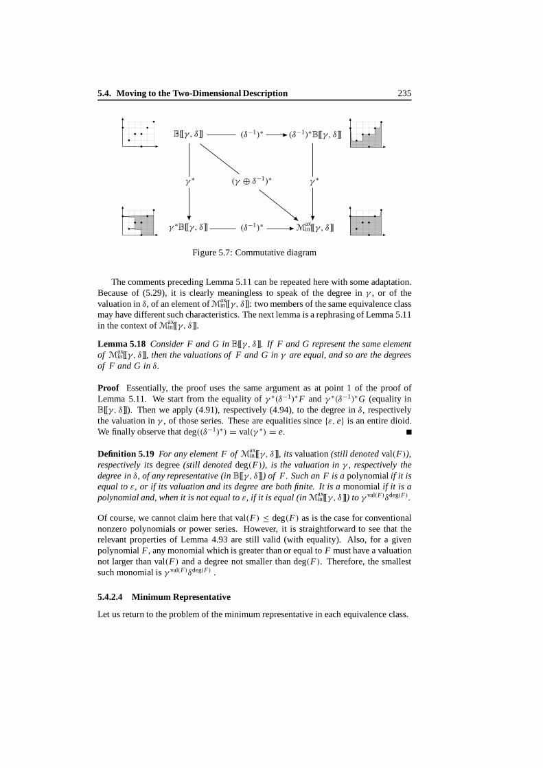
5.4. Moving to the Two-Dimensional Description 235
γ ∗
γ ∗ γ ∗
B[[γ, δ]]
B[[γ, δ]] (δ−1)∗(δ−1)∗
(δ−1)∗
B[[γ, δ]]
γ, δ
(γ ⊕ δ−1)∗
Maxin[[ ]]
Figure 5.7: Commutative diagram
The comments preceding Lemma 5.11 can be repeated here with some adaptation.Because of (5.29), it is clearly meaningless to speak of the degree inγ , or of thevaluation in δ, of an elementof Max
in[[γ, δ]]: two members of the same equivalence classmay have different such characteristics. The next lemma is a rephrasing of Lemma 5.11in the context ofMax
in[[γ, δ]].
Lemma 5.18 Consider F and G in B[[γ, δ]] . If F and G represent the same elementof M
axin[[γ, δ]] , then the valuations of F and G in γ are equal, and so are the degrees
of F and G in δ.
Proof Essentially, the proof uses the same argument as at point 1 of the proof ofLemma 5.11. We start from the equality ofγ ∗(δ−1)∗F andγ ∗(δ−1)∗G (equality inB[[γ, δ]]). Then weapply (4.91), respectively (4.94), to the degree inδ, respectivelythe valuation inγ , of those series. These are equalities since{ε, e} is an entire dioid.We finally observe that deg((δ−1)∗) = val(γ ∗) = e.
Definition 5.19 For any element F of Maxin[[γ, δ]] , its valuation (still denoted val(F)),
respectively its degree(still denoted deg(F)), is the valuation in γ , respectively thedegree in δ, of any representative (in B[[γ, δ]] ) of F. Such an F is a polynomialif it isequal to ε, or if its valuation and its degree are both finite. It is a monomialif it is apolynomial and, when it is not equal to ε, if it is equal (in M
axin[[γ, δ]]) to γ val(F)δdeg(F).
Of course, we cannot claim here that val(F) ≤ deg(F) as is the case for conventionalnonzero polynomials or power series. However, it is straightforward to see that therelevant properties of Lemma 4.93 are still valid (with equality). Also, for a givenpolynomialF , any monomial which is greater than or equal toF must have a valuationnot largerthan val(F) and a degree not smaller than deg(F). Therefore, the smallestsuch monomial isγ val(F)δdeg(F) .
5.4.2.4 Minimum Representative
Let us return to the problem of the minimum representative in each equivalence class.
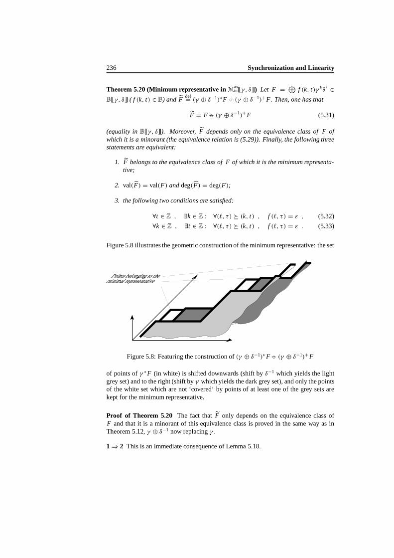
236 Synchronization and Linearity
Theorem 5.20 (Minimum representative inMaxin[[γ, δ]]) Let F = ⊕ f (k, t)γ kδt ∈
B[[γ, δ]] ( f (k, t) ∈ B) and Fdef= (γ ⊕ δ−1)∗F ◦− (γ ⊕ δ−1)+F. Then, one has that
F = F ◦− (γ ⊕ δ−1)+F (5.31)
(equality in B[[γ, δ]]). Moreover, F depends only on the equivalence class of F ofwhich it is a minorant (the equivalence relation is (5.29)). Finally, the following threestatements are equivalent:
1. F belongs to the equivalence class of F of which it is the minimum representa-tive;
2. val(F) = val(F) and deg(F) = deg(F);
3. the following two conditions are satisfied:
∀t ∈ Z , ∃k ∈ Z : ∀(�, τ ) ' (k, t) , f (�, τ ) = ε , (5.32)
∀k ∈ Z , ∃t ∈ Z : ∀(�, τ ) ' (k, t) , f (�, τ ) = ε . (5.33)
Figure 5.8 illustrates the geometric construction of the minimum representative: the set
Points belonging to theminimal representative
Figure 5.8: Featuring the construction of(γ ⊕ δ−1)∗F ◦− (γ ⊕ δ−1)+F
of points ofγ ∗F (in white) is shifted downwards (shift byδ−1 which yields the lightgrey set) and to the right (shift byγ which yields the darkgrey set), and only the pointsof the white set which are not ‘covered’ by points of at least one of the grey sets arekept for the minimum representative.
Proof of Theorem 5.20 The fact thatF only depends on the equivalence class ofF and that it is a minorant of this equivalence class is proved in the same way as inTheorem 5.12,γ ⊕ δ−1 now replacingγ .
1⇒ 2 This is an immediate consequence of Lemma 5.18.

5.4. Moving to the Two-Dimensional Description 237
2⇒ 3 Weconsider the equality of valuations and show that it implies (5.32). A similarproof, not given here, canbemade for theequality of degrees implying (5.33).The case whenF = ε is trivial. Moreover, when val(F) is finite, itcan beproved,as shown in Remark 5.13, that this implies that val(F) is equal to it,and (5.32) isagain obvious. Finally, suppose that val(F) = val(F) = −∞ and F = ε. Picksomek0; there mustexist somek′0 ≤ k0 and somet ′0 suchthat f (k′0, t ′0) = e,which implies that f (k′0, t ′0) = e and, for all (�, τ ) ) (k′0, t ′0), f (�, τ ) = ε,since otherwisef (k′0, t ′0) would be equal toε by (5.31). Set(k1, t1) = (k′0 −1, t ′0 − 1). We can repeat the same argument and find some(k′1, t ′1) suchthatk′1 ≤ k1, f (k′1, t ′1) = e and, for all (�, τ ) ) (k′1, t ′1), f (�, τ ) = ε. Necessarily,t ′1 ≤ t ′0 − 1 since otherwise, we would have found a(k′1, t ′1) ) (k′0, t ′0) suchthat f (k′1, t ′1) = e, which is a contradiction. Hence we can construct a sequence{(k′i , t ′i )
}with the mentioned property and such thatk′i+1 < k′i and t ′i+1 < t ′i .
Hence(k′i , t ′i ) → (−∞,−∞) as i → +∞. Let any t be given. Pick the next(k′i , t ′i) suchthatt ′i ≤ t . Setk = k′i −1. Thisk fulfills the condition expressed by(5.32).
3⇒ 1 Let Xdef= B ◦− A with A
def= (γ ⊕ δ−1)∗ F and Bdef= (γ ⊕ δ−1)∗F . To prove
that F belongs to the equivalence class determined byF , we need to prove thatA = B. Since weknow thatA ≤ B, it suffices to prove thatX = ε. In a waysimilar to that of theproof of Theorem 5.12, it can be proved that
X ≤ (γ ⊕ δ−1)X . (5.34)
Suppose that there exists(k0, t0) suchthatx(k0, t0) = e. Then, because of (5.34),either x(k, t + 1) or x(k − 1, t) is alsoequal toe. Call this newpoint (k1, t1),wherex assumes the valuee. This argument can be repeated at the point(k1, t1),providing the next point(k2, t2) ) (k1, t1) at whichx is equal toe, etc. Therefore,we can construct an infinite sequence of points such that(ki+1, ti+1) ) (ki , ti)
and at each pointx(ki , ti) = e, which also implies thatb(ki , ti) = e, sincex = b ◦− a. Oneof the following three possibilities must then occur:
• the sequence {ti} is bounded from above, hence it stays at some value t fori large enough; thenki must go to−∞ when i increases; consequently,there existarbitrarily small values ofk suchthat b(k, t) = e; on theotherhand, according to (5.32), there exists ak suchthat f (�, τ ) = ε for all
(�, τ ) ' (k, t) which also implies thatb(�, t)def=⊕(�′,τ ′)'(�,t) f (�′, τ ′) = ε;
this yields a contradiction;
• the sequence {ki } is bounded from below, hence it stays at some value kfor i large enough; thenti must go to+∞ wheni increases; consequently,there exist arbitrarily large values oft suchthat b(k, t) = e; on theotherhand, according to (5.33), there exists at suchthat f (�, τ ) = ε for all
(�, τ ) ' (k, t) which also implies thatb(k, τ )def= ⊕(�′,τ ′)'(k,τ ) f (�′, τ ′) =
ε; this yields a contradiction;
• the sequences {ki } and {ti } are both unbounded and converge to −∞ and+∞, respectively; this again yields a contradiction with both (5.32) and(5.33).

238 Synchronization and Linearity
Finally, x cannot assume the valuee anywhere.
Remark 5.21 With the aid of (5.27), it is seen that the condition (5.32) is equivalent tothe fact that limk→−∞ d(k) = ε which is statement 2 of Theorem 5.12. But now thereis an extra condition, namely (5.33), which is equivalent to saying thatd(k) remainsfinite for all finite k. Thereason for this extra condition is that, inZmax[[γ ]], the point+∞ does belong to they-axis, whereas inB[[γ, δ]] it does not. About this issue, thereader should refer to Remark 5.14.
5.4.3 Algebra of Information about Events
We aregoing to provide an interpretation of the algebraic manipulation of power seriesof B[[γ, δ]] using the additional rule (5.30) in terms of the manipulation of informationabout events. Consequently, the relation order& introduced earlier will be interpretedas the domination of pieces of information over one another.
Given a power seriesF (see (5.24)), we may view each pair(k, t) ∈ JF as thecoordinates of a ‘pixel’ inZ2 which is ‘on’ (whereas pairs of exponents of(γ, δ) cor-responding to zero coefficients inF represent pixels which are ‘off’). Each such pixelwhich is ‘on’ gives a piece of information about the associated daterd evaluated by(5.27): it says that∀� ≥ k, d(�) ≥ t , or, in words, ‘the event numberedk and thesub-sequent ones take place atthe earliest at timet ’. Geometrically, the graph ofd cannotcross the region ofZ2 delineated by the south-east cone{(ell, τ ) | (�, τ ) & (k, t − 1)}.
Now, given two pixels(k1, t1) and (k2, t2), the forbidden region is of course theunion of the two corresponding cones. Obviously, if(k1, t1) & (k2, t2), thepiece ofinformation associated with the latter pixel is at least as informative as the two piecesof information together (for one cone is included in the other one) and hence the latterpiece of information only may be kept. Indeed, we are just rephrasing the rule (5.30). Insummary, power series inMax
in[[γ, δ]] can be interpreted as representations of collectionsof pieces of information about events, and summing up two power series consists ingathering all the pieces of information brought by the two series about the same type ofevent. At any stage, the reduction of the representation using the rule (5.30) amounts tocanceling the pieces of information which are redundant. The relation order associatedwith this idempotent addition expresses the domination of collections of informationover one another. The particularelementε, which corresponds to the power series withzero coefficients, has all its pixels ‘off’ andtherefore it brings no information at all. Itis the neutral element for the addition of information.
To complete our interpretation of the manipulations inMaxin[[γ, δ]], we discuss the
product operation in the next subsection in which we return to event graphs.
5.4.4 Maxin [[γ, δ]] Equations for Event Graphs
5.4.4.1 Transfer Function
Let us refer back to Figure 5.1. With each transition is associated a power series inM
axin[[γ, δ]] (with the same name as the transition itself) which encodes the information
available about the corresponding dater trajectory. For the sake of simplicity, in the
5.4. Moving to the Two-Dimensional Description 239
same way as we have assumed that there is a global clock delivering the ticks num-beredt for all the transitions, we assume that there is acommon initial value of thenumbering mechanisms at all transitions (assigning numbersk at successive transitionfirings). Then, each arc between two transitions, indeed the place on this arc, trans-mits information from upstream to downstream, but this information is ‘shifted’ by thenumber of ‘bars’ in terms of timing and by the number of ‘dots’ in terms of number-ing. Algebraically, this shift is obtained by multiplication of the corresponding seriesby the appropriate monomial. For example, since the place betweenu andx1 has onebar, and since e.g. u denotes the information available about the transition with thesame name, the arcu → x1 carries the informationδu. Hence x1 ≥ δu, that is, theinformation available atx1 is at least δu. In the same way,x1 ≥ γ 2δx1 andx1 ≥ γ δx2.The transition x1 gathers the information brought by all incoming arcs. Finally,
x1 ≥ γ 2δx1⊕ γ δx2⊕ δu .
In the same way, we can obtain inequalities forx2 and y. In matrix form (rememberthatall elements belong toM
axin[[γ, δ]]), we obtain
(x1
x2
)≥(
γ 2δ γ δ
γ δ ε
)(x1
x2
)⊕(
δ
δ2
)u ,
y ≥ ( e e) ( x1
x2
),
of the general form
x ≥ Ax ⊕ Bu , y ≥ Cx . (5.35)
These inequalities should be compared with the equations obtained in§5.2.
Remark 5.22 Without our assumption of a common initial value of all the numberingmechanisms, corrections should have been made as for the exponent ofγ in the shiftoperator associated with each place in order to account for the difference in numberinginitial values between the upstream and downstream transitions of this place.
We make the following assumption which is different from that made in§2.5.2.3,but which will find a justification later on in this section.
The initial global clock value ist = 0 by convention, and the numberingmechanism at each transition assigns the valuek = 0 to the first transitionfiring occurring at or after time 0.
This convention does not mean that tokens cannot be brought from the outside worldbefore time 0: it suffices to include these tokens in the initial marking of the placeconnecting the input transition with other internal transitions.
Remark 5.23 (Interpretation of ε inputs) Becauseε is the bottom element, anε inputis the least constraining input possible: it is less constraining than any inputγ nδ−t for
240 Synchronization and Linearity
arbitrarily large n andt . Therefore, one may viewε inputs as those which correspondto bringing an infinity of tokens at time−∞.
Sofar, only the inequalities (5.35) have been obtained. Without further information,the behavior of the system is not completely specified andnothing more can be said.In particular, lag times of tokens of the initial marking (see Definition 2.49) have notbeen stipulated. For the time being, we give a mathematical answer to this lack ofinformation by selecting a ‘canonical’ solution to the system of inequalities. Later on,a more concreteinterpretation of this uniquely defined solution in terms of arrival timesof tokens of the initial marking in places will be given.
From Theorem 4.75, we know that the least solution of (5.35) is given by
x = A∗Bu , y = Cx = C A∗ Bu , (5.36)
and that it satisfies the equalities in (5.35). This solution corresponds to the earliestpossible occurrences of all events. For the time being, let us assume thatthe leastsolution is indeed the one of interest. We will return to this issue later on. As an exer-cise, the reader may try to evaluate the expressionC A∗ B for the considered example.This canbe done either by Gaussian elimination (hint: first expressx2 with respect tox1 andu, then solve a fixed-point equation inx1), or, equivalently, by using the for-mulæ (4.100), or preferably (4.110), and (4.109), plus the simplification rules (5.5).Finally, oneobtains
y = δ2(γ δ)∗u . (5.37)
Under the assumption that the earliest possible behavior is the one which will occur,we reach the conclusion that the input-output relation of the event graph of Figure 5.1is given by (5.37): in generalC A∗B will be called thetransfer function of the system(for single-input-single-output (SISO) systems).
NotethatC A∗B encodes the output dater caused by the input datere. Onepossiblerepresentation of e is δ0(γ 0⊕ γ 1⊕ γ 2⊕ · · · ). Due to the convention adopted earlierregarding the initial time and the initial numbering value of events, the inpute may beinterpreted as the action of firing the transitionu an infinite number of times at time 0(or putting an infinite amount of tokens at time 0 at the inlet of this transition)2. Thisis the analogue of animpulse in conventional system theory, and therefore the transferfunction may be viewed as the coding of theimpulse response.
We now return to the issue of selecting the ‘earliest possible solution’ of (5.35).This solution corresponds to the least constraining conditions. It does not only meanthat transitions are fired immediately after being enabled, but also that ‘the best initialcondition’ must be selected: this concerns the time at which tokens of the initial mark-ing are available; these tokens must not determine the firing epochs of transitions theycontribute to enable, whatever the inputu is, and whatever the holding times are. Forthe relations (5.36) to be valid for allu, irrespective of theinitial marking and holdingtimes, we thus assume the following condition.
2With the convention of§2.5.2.3 regarding the numbering of events, the same sequence of events wouldbe coded byδ0(γ 1 ⊕ γ 2⊕ · · · ) = γ .

5.4. Moving to the Two-Dimensional Description 241
Tokensof the initial marking are available at time−∞.
This convention corresponds to always choosing lag times equal to−∞. These lagtimes may fail to fulfill item 2 of Definition 2.50 of weakly compatible lag times. Ifother lag times are desired, there is a way to introduce them without changing the aboveconvention. This is the topic of the following discussion.
5.4.4.2 Introduction of More General Lag Times
Considera placep of anevent graphwith, say, two tokens in the initial marking and aholding time equal to two time units (see Figure 5.9a). Suppose that for the two tokens
x 1 x 2x 1 x 2p p
w
(a) (b)
Figure 5.9: The introduction of lag times
of the initial marking, we wish to have the lag timesw(0) andw(1), respectively. Thenthe event graph is modified locally in such a way as to introduce an additional placeand two additional transitions, one of which is an input transition (labeledw) as shownin Figure 5.9b. The new additional place keeps the original initial marking and holdingtime. The original placep is now free of any initial marking and holding time. The lagtimesare forced by the additional input
w = γ 0δw(0) ⊕ γ 1δw(1)(⊕ γ 2δw(1) ⊕ · · · ) , (5.38)
that is, the first token is introducedat time w(0) and infinitely many tokens are in-troducedat time w(1). Since the convention that tokens of the initial marking areavailable since−∞ is still assumed, it is seen that indeed the first token of the initialmarking starts enabling transitionx2 at timew(0) and the second token does the sameat timew(1), which is consistent with the definition of lag times. After timew(1), theinput defined by (5.38) is no longer constraining for the rest of the life of the system.
Consider again Figure 5.9a, and assume now that this figure represents an isolatedevent graph, instead of a part of a larger event graph (that is, grey arrows are discarded).Renamex1 andx2 asu andy, respectively. The input-output relation of such a systemis y = γ 2δ2u. If, say, u = e (u is an impulse at time 0),then weobtain that thecorresponding output is equal to
y = δ2(γ 2⊕ γ 3⊕ · · · ) . (5.39)
In terms of information, we thus learn that thethird token (numbered 2) and the nextones get out at time 2. Nothing is said about the first two tokens (those of the initial
242 Synchronization and Linearity
marking). Alternatively, by completing the missing information in a canonical way(behavior ‘at the earliest possible time’), it can be said that these two initial tokenswent out at−∞. This contradicts the fact that they are part of the initial marking, ifthis initial marking is meant to represent the exact position of tokens at time 0. Thisparadoxoccurs because the lag times, equal to−∞ after our convention, are not weaklycompatible in this case (transitiony is enabled twicebefore the initial time). We nowdiscuss two different ways of resolving this contradiction. The first one is describedbelow. The second one is the topic of the next paragraph.
Along the lines of Chapter 2, we consider the modification shown in Figure 5.9b,and we only accept weakly compatible lag times (they serve to determine the additionalinputw asin (5.38)). In this specific case, these lag times must be nonnegative and lessthan orequal to 2, the holding time ofp. Then, the input-output relation is given by
yw = γ 2δ2u ⊕w . (5.40)
Notice that this is now anaffine, rather than alinear, function ofu. Foru = e and forw given by (5.38), we obtain the information already provided by (5.39) for the outputtokens numbered 2, 3,. . . , but weobtain additional information regarding the epochsat which tokens numbered 0 and 1 get out. We see thatyw, given by (5.40), is notless thany, given by (5.39), from both theMax
in[[γ, δ]] (algebraic) and the informationalpoints of view (of course, these two points of view are consistent according to§5.4.3).
The input-output relation (5.40) can be considered to be linear, rather than affine,if we restrict ourselves to inputsu not lessthanγ −2δ−2w (w being given by (5.38)),which amounts to considering that the two tokens of the initial marking have also beenproduced by the input: this discussion will not be pursued further here but it obviouslyrelated to the notion of acompatible initial condition (seeDefinition 2.61).
5.4.4.3 System-Theoretic View of Event Graphs
From a different point of view, we may consider event graphs as playing the role ofblock-diagrams in conventional system theory. Recall that, for block-diagrams, the‘initial conditions’ are not directly related to the operators shown in the blocks of thediagram, but they are either set to zero canonically (in which case the input-outputrelation is indeed linear), or they are forced by additional (Dirac-like) inputs whichmake the ‘states’ (i.e. the initial values of the integrators in continuous time models)jump to nonzero values at the initial time.
In an analogous way, we may view places of event graphs as serving the onlypurpose of representing elementary shift operators in the event domain (number of‘dots’) and in the time domain (number of ‘bars’) in a pictorial way. In this more ab-stract (or more system-theoretic) point of view, there is no notion of ‘circulation oftokens’ involved, and therefore no applicability of any ‘initial position of tokens’. Theconventional rules of Petri nets which make tokens ‘move’ inside the net (and pos-sibly get outside) are not viewed as describing any dynamic evolution, but they areratherconsidered as transformation rules affecting the internal representation but notthe input-output relation (at least when tokens do not get outside the system; they add
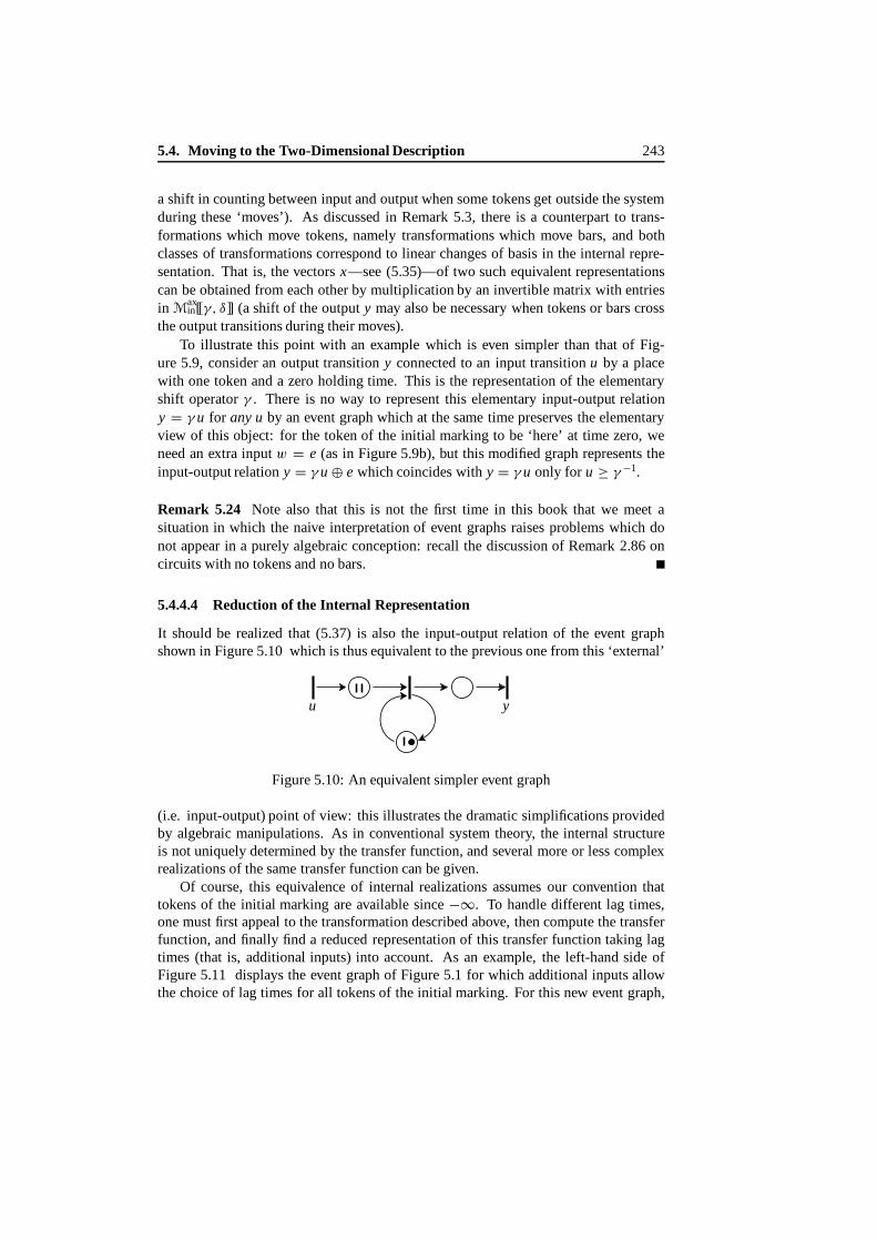
5.4. Moving to the Two-Dimensional Description 243
a shift in counting between input and output when some tokens get outside the systemduring these ‘moves’). As discussed in Remark 5.3, there is a counterpart to trans-formations which move tokens, namely transformations which move bars, and bothclasses of transformations correspond to linear changes of basis in the internal repre-sentation. That is, the vectorsx—see (5.35)—of twosuchequivalent representationscan be obtained from each other by multiplication by an invertible matrix with entriesin M
axin[[γ, δ]] (a shift of the outputy may also be necessary whentokens or bars cross
theoutput transitions during their moves).To illustrate this point with an example which is even simpler than that of Fig-
ure 5.9, consider an output transitiony connected to an input transitionu by a placewith one token and a zero holding time. This is the representation of the elementaryshift operatorγ . There is no way to represent this elementary input-output relationy = γ u for any u by an event graph which at the sametime preserves the elementaryview of this object: for the token of the initial marking to be ‘here’ at time zero, weneed an extra inputw = e (as in Figure 5.9b), but this modified graph represents theinput-output relationy = γ u ⊕ e which coincides with y = γ u only for u ≥ γ −1.
Remark 5.24 Note also that this is not the first time in this book that we meet asituation in which the naive interpretation of event graphs raises problems which donot appear in a purely algebraic conception: recall the discussion of Remark 2.86 oncircuits with no tokens and no bars.
5.4.4.4 Reduction of the Internal Representation
It should be realized that (5.37) is also the input-output relation of the event graphshown in Figure 5.10 which is thus equivalent to the previous one from this ‘external’
u y
Figure 5.10: An equivalent simpler event graph
(i.e. input-output) point of view: this illustrates the dramatic simplifications providedby algebraic manipulations. As in conventional system theory, the internal structureis not uniquely determined by the transfer function, and several more or less complexrealizations of the same transfer function can be given.
Of course, this equivalence of internal realizations assumes our convention thattokens of the initial marking are available since−∞. To handle differentlag times,one must first appeal to the transformation described above, then compute the transferfunction, and finally find a reduced representation of this transfer function taking lagtimes (that is, additional inputs) intoaccount. As an example, the left-hand side ofFigure 5.11 displays the event graph of Figure 5.1 for which additional inputs allowthe choice of lag times for all tokens of the initial marking. For this new event graph,

244 Synchronization and Linearity
y
x2x1
x3
x5x 4
y
uw1 w2 w3 u w1 w2 w3
Figure 5.11: Event graph with lag times and its reduced representation
the input-output relation turns out to bey = (γ δ)∗(δ2u ⊕w1⊕w2⊕ w3
): another
simpler eventgraph which has the same transfer function.
Remark 5.25 (Multiple-Input Multiple-Output—MIMO—systems) All t he no-tions presented in this section extend without difficulty to the case when the inputuand theoutputy are (column) vectors of respective dimensionm and p. In particular,C A∗ B (see (5.36)) is then ap × m matrix (called the transfer matrix), the entries ofwhich are polynomial elements ofMax
in[[γ, δ]].
5.5 Counters
5.5.1 A First Derivation of Counters
As already mentioned in§5.1, discrete event systems, and in particular event graphs,canbe described in the event domain by daters, or in the time domain by counters. Wealso mentioned that for a countert �→ c(t) associated with some type of event, theprecise meaning given toc(t) deserves some attention: roughly speaking, it representsthe value reached by the corresponding numbering mechanism of events at timet ;however, several events may take place simultaneously at timet . On the contrary,there is no ambiguity in speaking of the epochd(k) of the event numberedk. Froma mathematical point of view, this issue about counters will receive a natural solutionin this section. Yet, from an intuitive point of view, the interpretation given toc(t)might not appear as the most natural one. This interpretation will be given only afterthe relationship with the corresponding dater has been established.
At this stage, we can discuss the two possibilities of describing event graphs, bydaters or by counters, from an abstract point of view. Consider two different ways ofmoving from the upper left-hand corner to the lower right-hand corner of the commu-tative diagram of Figure 5.7, namely via the eastern then southerndirections on theone hand, and via the southern then eastern directions on the other hand. The former

5.5. Counters 245
path has been described in some detail: the first move is developed in§5.4.2.1, and thesecond move in§5.4.2.2.
Wecan interpret the latter path in the same way. The first move goes fromB[[γ, δ]]to γ ∗B[[γ, δ]] which is isomorphic to(γ ∗B[[γ ]] ) [[δ]]. For reasonsdual to those given in§5.4.1,γ ∗B[[γ ]] is isomorphic toZmin by the correspondence fromZmin to γ ∗B[[γ ]]:
k �→
γ kγ ∗ if k ∈ Z ;
ε (zero series) ifk = ε = +∞ ;
(γ −1)∗γ ∗ = (γ −1⊕ γ )∗ = (γ −1)∗ ⊕ γ ∗ if k = � = −∞ ,
(5.41)
which is the counterpart of (5.23). Therefore,(γ ∗B[[γ ]])[[δ]] can be viewed as the subsetof B[[γ, δ]] (the latter encodes collections of points inZ2) corresponding to epigraphsof mappingsg : t �→ g(t) from Z into Zmin, or alternatively, as the set ofδ-transformsof those mappingsg.
Remark 5.26 Westill speak of ‘epigraph’, that is the part of the plane above the graph(see Definition 3.37), although, inZmin, thedioid order is reversed with respect to theconventional order.
The second move in the diagram, namely that going fromγ ∗B[[γ, δ]] to Maxin[[γ, δ]]
through the south, corresponds to selecting only the nondecreasing mappings fromZ toZmin which are precisely the counters. The approximation of nonmonotonic functionsby nondecreasing ones is ‘from below’. Again, the words ‘nondecreasing’ and ‘frombelow’ should be understood with reference to the conventional order.
These two movescanbe summarized by the following formulæ which are the coun-terparts of (5.25) and (5.27): the mappingsg andc defined by
g : t �→ g(t) = inf(k,t)∈JF
k , c : t �→ infs≥t
g(s) = inf(k,s)∈JF
s≥t
k (5.42)
are successively associated with a power seriesF ∈ B[[γ, δ]] , or with the correspondingcollection of points inZ
2 (see (5.24)). In terms of ‘information’, a pixel(k, t) ∈ JF ,tells that,at time t , the counter reaches at most the value k (since, from (5.42),c(s) ≤ kfor all s ≤ t ). Conversely, to a counterc : Z → Zmin corresponds a power series inM
axin[[γ, δ]], namely
⊕
{t |−∞<c(t)<+∞}γ c(t)δt
⊕
⊕
{t |c(t)=−∞}(γ −1)∗δt
, (5.43)
a formula which follows from (5.41). This formula is the counterpart of (5.28).
5.5.2 Counters Derived from Daters
Let us now discuss the relationship that exists between the dater and the counter as-sociated with the same type of event. We are going to prove that under some mildcondition, the counter is the dual residual of the dater, i.e.c = d �.

246 Synchronization and Linearity
However, for this to be possible,d must first beconsidered as anisotone functionbetween two complete dioids. Indeed, as already discussed,d is a monotonic mappingfrom Zmin into Zmax; as such, it is antitone ratherthan isotone (that is, with the dioidorders in the domain and the range, it is ‘decreasing’ rather than ‘increasing’). How-ever, we may as well consider the mappingd from Z (with the natural order) into itselfhaving the same graph asd. This d is an isotone mapping from a complete lattice intoitself. Because of the end-point conditions (5.6) that we imposed on purpose,d can beboth residuated and dually residuated, provided that the required semicontinuity con-ditions be fulfilled (see Theorems 4.50 and 4.52, statements 2). The following theoremdiscusses the dual residuation. By abuse of expression, we speak of the residuation ofd ratherthan ofd.
Theorem 5.27 A dater d is dually residuated if and only if
limk→−∞
d(k) = −∞ . (5.44)
Then, if a power series in Maxin[[γ, δ]] is associated with d by (5.28), and if c is derived
from this series by (5.42), then c = d �.
Proof Sinced is a mapping between two totally ordered and discrete sets, the requiredupper-semicontinuity condition (see Definition 4.43) has to be checked only for subsets{ki } suchthat
∧i ki = −∞. Since weimposedd(−∞) = −∞, condition (5.44)
follows.Then, the set of pixels{(k, t)} defined by
⋃
−∞<d(k)<+∞(k, d(k))
∪
⋃
d(k)=+∞τ≥0
(k, τ )
is associated withd. Indeed, this isone possible collection, since a south-east conecan be attached to any pixel of the collection. The above formula follows from (5.28).Finally, looking at (5.42), it should be clear that
c(t) = infd(k)≥t
k , (5.45)
which is nothing but a possible definition ofd � (see statement 1 of Theorem 4.52).
Remark 5.28 If (5.44) is satisfied, then it follows from (4.23) and (4.24) that
∀t , d(c(t)) ≥ t and ∀k , c(d(k)) ≤ k . (5.46)
Moreover, sincec = d �, thend = c�, hence
d(k) = supc(t)≤k
t . (5.47)
Relation (5.45) always holds true, even if condition (5.44) is not fulfilled. But then,wecannot say thatc is the dual residual ofd since the other statements of Theorem 4.52

5.5. Counters 247
do not hold true, in particular (5.46) and (5.47) may be wrong. For example, considerthe mapping defined by (5.6) andd(k) = 0 for all finite k. Then the correspondingcis such thatc(t) = +∞ for t > 0 andc(t) = −∞ otherwise.Therefore,d(c(0)) =d(−∞) = −∞ < 0, in contradiction with (5.46). Also, supc(t)≤−∞ t = 0 > d(−∞) =−∞, in contradiction with (5.47).
However, this discussion isof purely mathematical interest since, given our con-ventions, any realistic dater, even after somefinite shift in numbering due to the initialmarking, will be such thatd(k) = −∞, ∀k < k0 for some finitek0. That is, condi-tion (5.44) will always be satisfied in practice.
Remark 5.29 (Interpretati on of counters) In words, the relation (5.45) expressesthat c(t) is the smallest value the numbering mechanism will reach at or after timet ; otherwisestated, c(t) is the number of the next event to come at or after time t .This explains the inequalities (5.46) which may seem counterintuitive at first sight. Analternative definition of counters is considered in the next subsection.
5.5.3 Alternative Definition of Counters
Another possible definition of counters isc = d�, provided thatd be residuated. Anecessary and sufficient condition is thatd be l.s.c., which here is implied by the dualcondition of (5.44), namely
limk→+∞
d(k) = +∞ . (5.48)
This condition means that no infinite numbers of events occur in finite time. Then, theresiduated mappingc of d is, by definition, equal to
c(t) = supd(k)≤t
k . (5.49)
Even if (5.48) is not fulfilled, we can take (5.49) as the definition ofc (but then, wecannot say that, conversely,d(k) = infc(t)≥k t ). The meaning of this new counterc(t)is the number of the last event which occurs before or at t . This might seem a morenatural definition for counters than the one corresponding toc(t). However, from amathematical pointof view, there is a drawback in manipulating this alternative notionof counters. To explain this point, we first establish the following result.
Lemma 5.30 If c and c are derived from the same d by (5.45) and (5.49), respectively,then
∀t , c(t) = c(t − 1)+ 1 .
Proof Let us startfrom (5.45). A c(t) so defined ischaracterized by the fact thatd(c(t)) ≥ t but alsod(c(t) − 1) < t , that is,d(c(t) − 1) ≤ t − 1. Observe that if we
setk def= c(t)− 1, these inequalities also tell us thatk = supd(�)≤t−1 �, which isnothingbut c(t − 1).

248 Synchronization and Linearity
Given c, a two-dimensional representative inMaxin[[γ, δ]] can be associated withc
by (5.43). Therefore, owing to the above lemma, givenc, the corresponding two-dimensional representative is given by
⊕
{t |−∞<c(t)<+∞}γ c(t)+1δt+1
⊕
⊕
{t |c(t)=−∞}(γ −1)∗δt+1
,
which is of course not as convenient as withc.
5.5.4 Dynamic Equations of Counters
We return to the definition (5.45) of counters. We introduce the following notation:
• Equation (5.45) defines a functionalZ from the set of nondecreasing mappingsd : Z → Zmax (referred to as the ‘dater set’) to the set of nondecreasing map-pingsc : Z → Zmin (referred to as the ‘counter set’); if we restrict ourselvesto mappingsd which satisfy (5.6) and(5.44), thenZ (d) is simplyd � (and then,Z−1(c) = c�);
• in the dater set, the pointwise addition of mappings (denoted⊕) is theoperationof upper hull; in the counter set, the pointwise addition (denoted⊕) is the lowerhull;
• in the dater set, the ‘shift’{k �→ d(k)} �→ {k �→ d(k − 1)} is denotedγ forobvious reasons (see Remark 5.6); similarly, the same kind of shift in the counterset is denotedδ;
• in the dater set, the ‘gain’{k �→ d(k)} �→ {k �→ d(k) + 1} is denoted1d; theanalogous unit gain in the counter set is denoted1c.
Lemma 5.31 With the previous notation, we have, for all d or di in the dater set:
Z (d1⊕ d2) = Z (d1)⊕Z (d2) , (5.50)
Z (γ d) = 1cZ (d) , (5.51)
Z (1dd) = δZ (d) . (5.52)
Proof A proof canbegiven by playing with Definition (5.45) ofZ and with the mean-ing of thenotationγ , δ, . . . . A smarter proof is obtained in the following way. For agivend, let D denote the element inMax
in[[γ, δ]] definedby the right-hand side of (5.28).Similarly, for a givenc, let C denote the element inMax
in[[γ, δ]] definedby (5.43). Ifc = Z (d), it should be clear thatC = D in M
axin[[γ, δ]] (that is, C and D are two rep-
resentatives of the same equivalence class). The seriesγ D corresponds to the daterγ d, hence the series associated with the counterZ (γ d) must beγC, but this seriescorresponds, through (5.43), to the series associated with the counter1cc = 1cZ (d).This proves (5.51). Formula (5.52) can be similarly proved (by noticing that the seriesassociated with1dd is δD).

5.6. Backward Equations 249
As for (5.50), let Di , i = 1, 2, be the series associated with the datersdi , i = 1, 2.Then, because of the second rule (5.5), which can be used inM
axin[[γ, δ]], D1 ⊕ D2
(here⊕ is the addition inMaxin[[γ, δ]]) is associated withd1⊕ d2 (pointwise maximum
of the mappingsd1 andd2). Similarly, for counters,C1 ⊕ C2 is associated withc1⊕c2
because of the first rule (5.5). With these observations at hand, the proof of (5.50) iseasily completed.
Remark 5.32 In the case whenZ (d) = d �, and with the necessary adaptation ofnotation, (5.50) can be viewed as a stronger version of (4.38).
As a consequence of Lemma 5.31, Equations (5.2) can be derived from (5.1). Forexample, 1x1(k−2) is the value atk of the dater1dγ
2x1 with which the counterδ(1c)2x1
is associated according to (5.51)–(5.52) (here, the dater and its associated counter aredenoted with the same symbol, as we did in§5.2). Therefore, the term 2x1(t − 1)corresponds to the term 1x1(k − 2) in the counter equations. And⊕ in dater equa-tions (that is, max) is converted to⊕ in counter equations (that is, min)according to(5.50). Afterwards,it is realized that1d, respectively 1c, could have been denotedδ,respectivelyγ .
Using Lemma 5.30, once Equations (5.2) have been established using one notionof counters (given by (5.45)), it is clear that these equations are also valid with thealternative notion of counters (given by (5.49)).
5.6 Backward Equations
Sofar we have been interested in computing outputs produced by given inputs. In thedater description, outputs are sequences of theearliest dates at which events (numberedsequentially) can occur. Sometimes, it may also be useful to derive inputs from outputs,which, roughly speaking, corresponds to ‘inverse’ the system. More precisely, and stillin the dater setting, we may be given a sequence of dates at which one would like tosee events occur at the latest, and we are asked to provide thelatest input dates thatwould meet this objective. It is the topic of this section to discuss this problem.
From a mathematical point of view, as long as the transfer function (matrix, in theMIMO case) has to be inverted, it is no surprise that residuation plays an essentialrole. This inversion translates into the fact that recurrent equations in the event domainfor daters, respectively in the time domain for counters, now proceed backwards ineventnumbering, respectively in time. Moreover, the ‘algebra’(∧, ◦\) is substituted for(⊕,⊗) in these backward equations. These equations offer a strong analogy with theadjoint-state (or co-state) equations of optimal control theory.
5.6.1 Maxin [[γ, δ]] Backward Equations
Consider a system inMaxin[[γ, δ]] described by Equation (5.35) or (5.36) (recall that
(5.36) yields the least solutiony of (5.35)with either inequalities or equalities). Lety

250 Synchronization and Linearity
be given. The greatestu suchthat
z = Hudef= C A∗ Bu ≤ y (5.53)
is, by definition, obtained as
u = H �y = C A∗B ◦\y . (5.54)
From the previous results, in practice (5.53) means that, in the dater description, theoutput events produced byu occur not later than those described byy; moreover, ubeing the ‘greatest’ input having property (5.53), the input events corresponding touoccurnot earlier thanwith any other input having property (5.53).
Recall thaty = C A∗ Bu can be also described as the least solution of
x = Ax ⊕ Bu ,
y = Cx .
}(5.55)
We aregoing to give a similar ‘internal’ representation for the mappingH � defined by(5.54).
Lemma 5.33 Let u be derived from y by Equation (5.54). Then u is the greatest solu-tion of the system
ξ = ξ
A∧ y
C, (5.56)
u = ξ
B. (5.57)
This is equivalent to saying that ξ must be selected as the greatest solution of (5.56).Moreover, the symbol ‘=’ can be replaced by ‘≤’ in (5.56)–(5.57).
Proof We have
u = C A∗B ◦\y owing to (5.54),= A∗B ◦\ (C ◦\y) thanks to(f.9),= B ◦\ (A∗ ◦\ (C ◦\y)) (same reason).
Let ξdef= A∗ ◦\ (C ◦\y). By Theorem 4.73, we know thatξ is the greatest solution of
(5.56)with equality or with the inequality≤.
If x (hence ξ ) is n-dimensional, and if u, respectively y, is p-dimensional, re-spectively m-dimensional, then, by using Formula (4.81), (5.56)–(5.57) can be moreexplicitly written as
∀i = 1, . . . , n , ξi =
n∧
j=1
ξ j
A ji
∧(
p∧
r=1
yr
Cri
),
∀� = 1, . . . ,m , u� =n∧
s=1
ξs
Bs�.
(5.58)

5.6. Backward Equations 251
Observe again the transposition of matrices and the substitution of the operation∧,respectively ◦\, to theoperation⊕, respectively⊗. However, theseequations are not‘linear’. Owing to (f.1) and (f.9), the mappingH � rather obeys the dual properties:
H �(y ∧ z) = H �(y) ∧ H �(z) , H �(α ◦\y) = α ◦\H �(y) ,
whereα is a ‘scalar’ (i.e.α ∈Maxin[[γ, δ]]).
5.6.2 Backward Equations for Daters
Weare going to translate the preceding equations in the setting of the dater description.Consider a system described by equations of the form (2.36), but with matrices (thatis, holding times) which do not depend on the event numberk (hence wewill writee.g. A(�) for A(k, k − �)). More specifically, we consider a system described byRmax
equations of the form:
x(k) = A(0)x(k) ⊕ · · · ⊕ A(M)x(k − M)
⊕ B(0)u(k) ⊕ · · · ⊕ B(M)u(k − M) ,
y(k) = C(0)x(k) ⊕ · · · ⊕ C(M)x(k − M) .
(5.59)
There is of courseno loss of generality in assuming that there is the same delayM forx andu and in both equations (this possibly amounts to completing the expressionswith terms having zero matrix coefficients). Theγ -transforms of these equations yield(5.55) wherex , u, y now denote theγ -transforms of signals, and similarly, e.g.
A =M⊕
�=1
A(�)γ � .
In the same way, (5.56)–(5.57) are still valid with the new interpretation of notation.Using (4.97), we can write these equations more explicitly in terms of power seriesin γ . Taking into account thatA, B, C are in factpolynomials, i.e. power series forwhich coefficients areε for powers ofγ out of the set{0, . . . , M}, we finally obtainthe relations, for allk:
ξ(k) = ξ(k)
A(0)∧ . . . ∧ ξ(k + M)
A(M)∧ y(k)
C(0)∧ . . . ∧ y(k + M)
C(M),
u(k) = ξ(k)
B(0)∧ . . . ∧ ξ(k + M)
B(M).
(5.60)
From these equations, the backward recursion is clear. To alleviate notation, let us nowlimit ourselves toM = 1, that is, consider the standard form (2.39), namely,
x(k + 1) = Ax(k) ⊕ Bu(k) ; y(k) = Cx(k) . (5.61)

252 Synchronization and Linearity
Then, combining (5.60) with (5.58), we obtain
∀i = 1, . . . , n , ξi (k) =
n∧
j=1
ξ j (k + 1)
A ji
∧(
p∧
r=1
yr (k + 1)
Cri
),
∀� = 1, . . . ,m , u�(k) =n∧
s=1
ξs(k)
Bs�.
(5.62)
Let us rewrite these equations with conventionalnotation. We refer the reader to Ex-ample 4.65, to the rule regarding the ambiguous expression∞−∞ that may show upif ratios such asε ◦\ε are encountered, and finally to the warning about the ambiguity ofconventionalnotation since the expression∞−∞may also beobtained as the result ofε⊗� which yields a different value. With this warning in mind, (5.62) can be written:
ξi (k) = min
[n
minj=1
(ξ j (k + 1)− A ji
),
pminr=1
(yr (k + 1)− Cri )
],
u�(k) =n
mins=1
(ξs(k) − Bs�) .
(5.63)
The reader is invited to establish these equations by a direct reasoning with an eventgraph for which the sequence{y(k)}k∈Z of desired output dates is given. It is thenrealized that the recursion is not only backward in event numbering (indexk) but alsobackward in the graph (from output transitions to input transitions through internaltransitions).
A fewwords are in order regarding ‘initial conditions’ of the recursion (5.63). Thisproblem arises when the backward recursion starts at some finite event number, saykf (‘f ’ f or ‘fi nal’), because desired objectives{y(k)} areonly given up to this numberkf . In accordance with the idea of finding the ‘latest input dates’, that is the greatestsubsolution ofC A∗Bu ≤ y assupposed by residuation theory, the missing informationmust be set to the maximum possible value. This amounts to saying thaty(k) must beset to� = +∞ beyondkf , and more importantly ξ(k) = � for k > kf . As forthe tokens of the initial marking, they are still supposed to be available at time−∞(see page 241) since this is the assumption under which the ‘direct’ system obeys theinput-output relation at the left-hand side of Inequality (5.53).
At the end of this section, let us consider the following situation. Suppose thatsomeoutput trajectoryy(·) has been produced by processing some inputv(·) througha systemobeying Equations (5.61). This output trajectory is taken as the desired latestoutput trajectory. Of course, it is feasible since it is an actual output of the system.Then, if we compute the latest possible input, sayu, that meets thegiven objective byusing Equations (5.62), thisu will alsoproduce the outputy, and it will be greater thanor equal tov. Therefore, the pairs(v, y) and (u, y) areboth solutions of (5.61), buttwo different internal state trajectories, sayx and x , respectively, would beobtainedwith x ≤ x . Moreover, the trajectoryx is also different fromξ which is computedby (5.62) usingy asthe input. The differencesξi(k) − xi(k), i = 1, . . . , n; k ∈ Z,
are nonnegative since (5.62) corresponds to the backward operation at ‘the latest time’

5.7. Rationality, Realizability and Periodicity 253
whereas(5.61) describes the forward operation ‘at the earliest time’ for the same input-output pair(u, y). For thek-th firing of thei-th transition, the differenceξi(k) − xi (k)indicates the time margin which is available, that is, the maximum delay by whichthis firing may be postponed, with respect to its earliest possible occurrence, withoutaffecting the output transition firing. This kind of information is of course very usefulin practical situations.
Let us finally summarize the equations satisfied by the pair(x, ξ ). The following isderived from (5.61)–(5.62) in whichu andy are replaced by their expressions, namelyu = B ◦\ξ andy = Cx , respectively. Then we obtain the system
x(k + 1) = Ax(k) ⊕ Bξ(k)
B,
ξ(k) = Cx(k + 1)
C∧ ξ(k + 1)
A.
(5.64)
This system is veryreminiscent of state/co-state (or Hamiltonian) equations derivedfor example from Pontryagin’s minimum principle for optimal control problems inconventional control theory. Moreover, the differenceξi(k)− xi(k) alluded to above isthei-th diagonal entry of the matrixξ(k)◦/x(k). Pursuing the analogy withconventionalcontrol problems, it is known that introducing the ‘ratio’ of the co-state vector by thestate vector yields a matrix which satisfies a Riccati equation.
5.7 Rationality, Realizability and Periodicity
5.7.1 Preliminaries
At this point, we know that event graphs can be described by general equations ofthe form (5.55) in which the mathematical form ofu, x, y, A, B,C depends on thedescription adopted. Essentiallyu, x, y may be:
• power series inγ with coefficients inZmax;
• power series inδ with coefficients inZmin;
• power series in(γ, δ) with coefficients in{ε, e}.As for A, B,C, they are matrices with polynomial entries of the same nature as thepower seriesu, x, y, but with only nonnegative exponents since tokens of the initialmarking and holding times introduce nonnegative ‘backward’ shifts (see Remark 5.6)in event numbering, respectively in time. The input-output relationu �→ y is givenby y = C A∗Bu, hence the entries of this so-called transfer matrix belong to the ratio-nal closure (see Definition 4.99) of the corresponding class of polynomials with non-negative exponents. One purpose of this section is to study the converse implication,namelythat a system with a ‘rational’ transfer matrix does have a finite-dimensional‘realization’ of the form (5.55) with polynomial matrices. In fact, this is an immediateconsequence of Theorem 4.102. Moreover, playing with the various possibilities of

254 Synchronization and Linearity
realizations provided by Theorem 4.105, we will recover essentially the three possibledescriptions of systems alluded to above by starting from a single framework, namelytheone offered by theMax
in[[γ, δ]] algebra.
Remark 5.34 In an event graph, if there are direct arcs from input to output transitions,one obtains an output equation of the formy = Cx ⊕ Du and a transfermatrix of theform C A∗B ⊕ D. However, by redefining the ‘state’ vector asx = ( x ′ u′
)′, it
is possible to come back tothe formC A∗ B with C = ( C D), B ′ = ( B ′ e
)
and A = diag(A, ε), but at the price of increasing the ‘state’ dimensionality. Indeed,in what follows the issue of the ‘minimal’ realization will not be addressed since onlypartial results have been obtained so far.
The equivalence between rationality of the transfer matrix and its ‘realizability’ isa classical result in both conventional linear system theory and in automata and formallanguage theory. However, there is here a third ingredient coming in: rationality isalso equivalent to some ‘periodicity’ property of the transfer function or the impulseresponse. This is analogous to the situation of rational numbers which have a periodicdecimal expansion.
We will only address the SISO case. The MIMO case (e.g. 2 inputs, 2 outputs)can be dealt with in a trivialmanner by considering all the individual scalar transferfunctionsHi j : u j �→ yi , j = 1, 2, i = 1, 2, first. Suppose that 3-tuples(Ai j , Bi j ,Ci j )
have been found to realizeHi j in the form (5.55) (Ai j is in general a matrix, not ascalar). Then, it is easy to check that the 3-tuple
A =
A11 ε ε ε
ε A12 ε ε
ε ε A21 ε
ε ε ε A22
, B =
B11 ε
ε B12
B21 ε
ε B22
,
C =(
C11 C12 ε ε
ε ε C21 C22
),
is a realization of the 2×2 transfer matrix. Of course, this way of handling MIMO sys-tems does not consider the dimensionality of the realization explicitly. In the following,we will comment on the MIMO case when appropriate.
5.7.2 Definitions
We start with the following definitions.
Definition 5.35 (Causality) An element h of Maxin[[γ, δ]] is causaleither if h = ε or if
val(h) ≥ 0 and h ≥ γ val(h) .
This definition is somewhat technical, due to the fact thath, as an elementof Maxin[[γ, δ]],
has various formal representations, and among them e.g. the maximal one which in-volves the multiplication by(δ−1)∗ (hence it may have monomials with negative ex-ponents inδ). However, the definition, while using the language ofM
axin[[γ, δ]], clearly

5.7. Rationality, Realizability and Periodicity 255
says thatthe graph of the associated dater lies in the right-half plane and above thex-axis. It can then be formally checked that the set of causal elements ofM
axin[[γ, δ]]
is a subdioid ofMaxin[[γ, δ]]. For example, if p andq are causal, then val(p ⊕ q) =
min(val(p), val(q)) ≥ 0, andγ val(p⊕q) = γ min(val(p),val(q)) = γ val(p) ⊕ γ val(q) ≤ p ⊕ q,proving thatp ⊕ q is also causal. A similar proof can be given forp ⊗ q.
Definition 5.36 (Rationality) An element of Maxin[[γ, δ]] is rationalif it belongs to the
rational closure of the subset T def= {ε, e, γ, δ}. A vector or matrix is rational if itsentries are all rational.
Indeed, because of the choice of the basic set, the rational elements will also be causal.
Defini tion 5.37 (Realizability) A matrix H ∈ (Maxin[[γ, δ]]
)p×mis realizableif it can
be written as
H = C(γ A1 ⊕ δA2)∗B (5.65)
where A1 and A2 are n× n matrices, n being an arbitrary but finite integer (dependingon H), C and B are n × m and p × n matrices respectively, and each entry of thesematrices is equal to either ε or e.
Definition 5.38 (Periodicity) An element h of Maxin[[γ, δ]] is periodicif there exist two
polynomials p and q and a monomial m (all causal) such that
h = p ⊕ qm∗ . (5.66)
A matrix H is periodic if its entries are all periodic.
Here, we adopt a ‘mild’ definition of periodicity. It is however mathematically equiv-alent to seemingly other more sophisticated definitions which put further constraintson the polynomialsp andq. This point will be discussed in§5.7.4. At this stage, itsufficesto understand that, if one considersh as the(γ, δ)-transform of a trajectory,say an impulse response, the intuitive meaning of Formula (5.66) is that a certain pat-ternrepresented byq is reproduced indefinitely, since the multiplication bym = γ rδs
represents a shift byr units along thex-axis—event domain—ands units along they-axis—time domain—andqm∗ = q ⊕ qm ⊕ qm2 ⊕ · · · is the union of all theseshifted versions ofq. This periodic behavior occurs after a certain transient which isessentially (but not always exactly, as we shall see) represented byp. The ratio s/rrepresentsthe asymptotic slope of the graph of the dater associated withh, and thus theasymptotic output rate: on the average,r events occur everys time units. The extremecasess = 0 andr = 0 will be discussed in§5.7.4.
5.7.3 Main Theorem
Theorem 5.39 For H ∈ (Maxin[[γ, δ]]
)p×m, the following three statements are equiva-
lent

256 Synchronization and Linearity
(i) H is realizable;
(ii) H is rational;
(iii) H is periodic.
Proof The implication (i) ⇒ (ii) is straightforward. The converse (ii)⇒ (i) follows,at least for the SISO case, from Theorem 4.105 withB = C = U = B = {ε, e} andV = {γ, δ}. We then observethatU� = U henceU� ⊗ V = {ε, γ, δ, γ ⊕ δ}. It remainsto split up matrixAx , whichappears in the(B, C)-representation (4.106) (with entriesin U� ⊗ V), into γ A1⊕ δA2, whichoffers no difficulty. The MIMO case is handled asindicated previously.
We now outline the proof of the equivalence (ii)⇔ (iii). Since the definitions ofperiodicity and rationality refer to the entries ofH individually, it suffices to deal withthe SISO case. The implication (iii)⇒ (ii) is obvious: if h canbewritten as in (5.66),thenclearly h ∈ T �. Conversely, ifh is rational, sinceMax
in[[γ, δ]] is a commutativedioid, we can use Theorem 4.110 (applied to the dioid closure ofT ) to seethath canbewritten as
h =⊕
i∈I
γ αiδβi
⊕
j∈Ji
γ r j δs j
∗
=⊕
i∈I
γ αiδβi⊗
j∈Ji
(γ r j δs j)∗
, (5.67)
where I and theJi are finite sets,αi , βi , r j , s j are nonnegative integers, and (5.67)follows from (4.109). The proof is then completed by showing that (5.67) is amenableto the form (5.66) wherem is essentially the monomialγ r j δs j with maximal ‘slope’s j/r j . Indeed, the term(γ r j δs j )∗ tends to asymptotically dominate all other similarterms in sums and products. When the monomial with maximal slope is nonunique,the precise rules for obtaining the monomialm used in (5.66) will be given in the proofof Theorem 6.32 in the next chapter. The precise derivation of this last part of the proof,which is rather technical, will be skipped here. The reader is referred to [44] for a moredetailed outline and to [62] for a full treatment.
In the above proof, instead of attempting to prove the implication (ii)⇒ (iii), wemight have proved the implication (i)⇒ (iii) using Theorem 4.109 and Formula (4.110).This would have provided some insight into how the monomialmi j appearing in therepresentation (5.66) of eachHi j (in the form ofm∗
i j ) is related to the weights of cir-cuits of G(A), whereA = γ A1 ⊕ δA2 appears in (5.65). The graphG(A) is drawn asexplained in§4.7.3 (see Figure 4.8). Then, for an input-output pair(u j , yi), we con-sider all (oriented) paths connecting these transitions and all circuits which have at leastone node in common with those paths. These are the circuits of interest to determinethe maximal ratiosi j /ri j . If there is no such circuit, this means that the polynomialq of (5.66) isε and thusmi j is irrelevant. As a consequence, if matrixA is stronglyconnected (which in particular precludes any direct path from the input to the output,

5.7. Rationality, Realizability and Periodicity 257
given that we have not included a termDu — see Remark5.34), then the ratiossi j /ri j
take aunique value for all themi j .Wecould also have proved that (iii)⇒ (i) directly by providing an explicit realiza-
tion of a periodic element. This essentially follows the scheme illustrated by Figure 6.4in the next chapter.
5.7.4 On the Coding of Rational Elements
In this subsection, it is helpful to use the pictorial representation of (causal) elementsof M
axin[[γ, δ]] by collection of points in theN
2-plane: a monomialγ kδt is representedby a point with coordinates(k, t) and we assume that polynomials are represented bytheir minimum representatives (which do exist—see Theorem 5.20).
Let the monomialm involved in (5.66) be equal toγ r δs.
• If s = 0, thena = p⊕ qm∗ = p⊕ q sincem∗ = (γ r )∗ = e, that is, the impulseresponsea is a polynomial : this is the behavior of an event graph having eitherno circuits or only circuits with zero holding time. Such a system is able to workat infinite speed. This ‘finite’ impulse response thus corresponds to the situationwhenan infinite number of tokens get out at timet = deg(a); the first tokensget out earlier as described by p ⊕ q. From thepoint of view of the minimumcoding ofa, thereno way but to retain the minimum representative ofp ⊕ q.
• If s = 0 but r = 0 (andq = ε), and since m∗ = (δs)∗ corresponds to aninfinite slope, the impulse response is ‘frozen’ after a transient during whichsome tokens get out (those numbered from 0 to val(q) − 1): this is indeed thekind of behavior one would like to call a ‘finite response’. It happens whenthere is acircuit without tokens but with a positive holding time: the system is‘deadlocked’. The nontrivial part ofa is provided byp ◦− γ val(q)δ∗ (the part ofthe plot ofa which lies at the left hand of the vertical asymptote) which shouldagain be coded by its minimum representative.
These two particular cases will no longer be considered in detail. Hence, from now on,we assume thatr > 0 ands > 0 unless stated otherwise.
With (5.66), we have adopted a characterization of rational (or periodic) elementswhich is mathematically simple. The forthcoming lemma shows that this characteri-zation is equivalent to another one which puts further constraints on the polynomialsp andq. The latter definition will be used in Chapter 6 (see Theorem 6.32). It hasthe advantageof making the interpretation of the newp as the transientpart and of thenew q as the periodic pattern (see Figure 6.2) possible. Indeed,p can then be repre-sentedby points contained in a box of widthν − 1 andheightτ − 1 with its lowerleft-hand corner located at the origin. The periodic patternq can be encapsulated in abox of widthr − 1 andheights − 1 with its lower left-hand corner located at the point(ν, τ ). Thisbox istranslated indefinitely by the vector(r, s). These conditions are nowexpressed mathematicallyin the following lemma.
Lemma 5.40 An element a ∈Maxin[[γ, δ]] is rational if and only if it is a polynomial, or
an element of the form p ⊕ γ νδ∗ (p is a polynomial), or if there exist positive integers

258 Synchronization and Linearity
r and s, nonnegative integers ν and τ , and polynomials
p =⊕
(k,t)∈Jp
γ kδt with k ≤ ν − 1, t ≤ τ − 1, ∀(k, t) ∈ Jp ,
q =⊕
(κ,θ)∈Jq
γ κδθ with ν ≤ κ ≤ ν + r − 1, τ ≤ θ ≤ s + τ − 1, ∀(κ, θ) ∈ Jq ,
(Jp and Jq are necessarily finite) such that a = p ⊕ q (γ rδs)∗.
Proof Only thecase whenr > 0, s > 0 andq = ε is of interest here. Moreover, sincethe new characterization of rational elements is a particular case of (5.66), it suffices toprove that, conversely, (5.66)is amenable to the new characterization. Considera =p⊕q(γ r δs)∗ for any polynomialsp andq. Let τ
def= max(deg(p)+1, deg(q)− s +1).For any(k, t) ∈ Jq , there exists aunique�(k,t) ∈ Z suchthatτ ≤ t+�(k,t)s ≤ τ+s−1.Because deg(q) ≤ τ + s − 1 ands > 0, necessarily�(k,t) ≥ 0. We consider
qdef=⊕
(k,t)∈Jq
γ k+�(k,t)r δt+�(k,t)s . (5.68)
In addition, letα def= max(k,t)∈Jq �(k,t) andν def= val (q). Observe that all points rep-resenting monomials appearing at the right-hand side of (5.68) lie in a strip of heights − 1 delimited by the horizontal linesy = τ andy = τ + s − 1, and at the right-handclosed halfplane bordered by the vertical line atx = ν.
Let a minimum representative ofa bewritten⊕
(k,t)∈Jaγ kδt (Ja is countably infi-
nite). This minimum representative does exist since we deal with causal elements andsince we assume thatr > 0 (see Theorem 5.20). Consider any(k, t) ∈ Ja . If t ≥ τ ,then the corresponding monomial cannot belong top sinceτ > deg(p). Hence, itnecessarily belongs to someqmn . If t < τ , then this monomial may belong to eitherp or to someqmn but thenn < α: indeed, forn ≥ α, we have by construction that
t ≥ τ . Hence, if we setp def= p ⊕ q ⊕ qm ⊕ · · · ⊕ qmα−1, we can consider all pairs(k, t) ∈ Ja with t < τ as coming fromp. We now prove thatthe other pairs can beexplained by monomials ofqm∗. If (k, t) ∈ Ja andt ≥ τ , then there exist
(k, t) ∈ Jq
and� ≥ 0 such that(k, t) = (k, t)+ �× (r, s). Moreover,� ≥ �(k ,t), hence
(k, t) = (k, t)+(�− �(k,t)
)× (r, s) ,
whereγ kδ t is one of the polynomials involved in (5.68).At this point, we have proved that all monomials ofa = p ⊕ qm∗ are among the
monomials ofp ⊕ qm∗, hencea ≤ p ⊕ qm∗. But the converse statement is also truesince the monomials inp andq have been obtained froma. Hence p⊕ qm∗ is anotherexpression fora.
To complete the proof, we must delete monomials which are useless from thisexpression (because they are dominated by other polynomials in the same expressionin the sense of the order relation ofM
axin[[γ, δ]]). Firstly, concerningp, if monomials of

5.7. Rationality, Realizability and Periodicity 259
p, thus also ofa, have a degree greaterthan orequal toτ , theycan also be obtained byother monomials ofqm∗ (proceed as previously) and thus they can be dropped fromp. Let m = γ νδτ be the monomial ofq with valuationν (recall thatν = val (q)).Observe thatτ ≥ τ . This monomial dominates the monomialsγ kδt of p with t < τ
butk ≥ ν which canthus also be dropped fromp. Finally, thenew p stays in the lowerleft-hand part of the plane delimited by the horizontal liney = τ − 1 and the verticalline x = ν − 1. Secondly, concerningq, consider the monomials ofq with valuationgreater thanν+s−1: their degree beingnecessarilyless thanτ+s, they aredominatedby the monomialγ ν+rδτ+s contained inqm. This observation is of course preservedby the successivetranslations(r, s). Therefore, a newq can be used which staysin thebox given in the statement of the lemma.
We refer the reader to [62] in which an algorithm is provided to obtain the ‘best’possible representation of the type described by the lemma. The following exampleshows that by redefining not onlyp andq but alsom, more compact representationsmay be obtained (the reader is invited to make the drawing corresponding toeachexample, which is thebest way to quickly grasp the situation).
Example 5.41 The expression(e ⊕ γ δ)(γ 2δ2)∗ is already in the form of Lemma 5.40but it can be simplified to(γ δ)∗ by redefiningm asγ δ instead ofγ 2δ2.
Consider now the following example.
Example 5.42 Let a = p ⊕ qm∗ with p = e⊕ γ 2δ2⊕ γ 5δ3⊕ γ 6δ4⊕ γ 8δ6⊕ γ 11δ7,q = γ 12δ8(e ⊕ γ 2δ) andm = γ 3δ2. Another representation ofa as p ⊕ qm∗ involvesp = γ 2δ2⊕ γ 8δ6 andq = e ⊕ γ 2δ.
In this example, what happens is thatp can partlybe explained by ‘noncausal shifts’qm−l of q. Algebraically, there exists somen (heren = 4) such that addingb =⊕n
l=1 qm−l to a does not changea. Hence
a = a ⊕ b = p ⊕ qm∗ ⊕ b = (p ◦− b)⊕ b ⊕ qm∗ = p ⊕ qm∗ ,
where p = p ◦− b andq = qm−n . Now p does not any longer appear as the transientpart, but rather as a transient perturbation of the periodic regime. Now the contributionsof p andq to the transient partare interweaved.
5.7.5 Realizations byγ - and δ-Transforms
In the proof of Theorem 5.39, Theorem 4.105 has been used with the choiceB = C =U = B andV = {γ, δ}. Other possibilities have been suggested at the end of§4.8.3.
5.7.5.1 Dater Realization
If we consider the possibilityB = C = B, U = B ∪ {δ} and V = {γ }, thenU� = {ε, e, δ, δ2, . . . , δ∗} since all sums of such elements are reducible to one ofthem by the ruleδt ⊕ δτ = δmax(t,τ ). HenceU�, beingobviously a complete dioid in

260 Synchronization and Linearity
this case, is isomorphic to (and will be identified with)Nmax (with δ∗ identified with� = +∞). Consequently, in an observer representation(C, A, B) of a rational matrixH as provided by Theorem 4.105, B hasits entries inNmax and A = γ A where Ais also a matrix with entries inNmax; C is a Boolean matrix. This realization may beinterpreted as the one directly derived, by theγ -transform, from the dater equations
x(k) = Ax(k − 1)⊕ Bu(k) , y(k) = Cx(k) ,
where in addition y is a subvectorof x (hence the name ‘observer representation’).For a controller representation,B is a Boolean matrix whereasC makes any linear
combination of thexi with weights inNmax.
Remark 5.43 It is thus always possible, starting from any timed event graph, to obtainanequivalent event graph with a structure corresponding to the observer (respectively,the controller) representation, that is, the initial marking consists of exactly one tokenin internal places, no tokens in the input and output places, and in addition, zeroholdingtimesfor the output (respectively, the input) places.
It should be realized that there is a trick here to represent deadlocked systems in thisway, i.e. event graphs circuitswith no tokens and positive holding times. These systemswill berealized in ‘state space’ form by matricesA, B or C having some entries equalto δ∗. Indeed, an arc with weight δ∗ introduces an unbounded holding time, which issufficient to block some parts of the system. For example, for the graph of Figure 5.12(the transfer function of which isδ∗), an observer (dater) realization isC = e, A = γ ,
xu y
Figure 5.12: A deadlocked event graph
B = δ∗.
5.7.5.2 Counter Realization
The counter realization corresponds to the dual possibility offered by Theorem 4.105,namely to chooseU = B ∪ {γ } andV = {δ}. ThenU� = {ε, e, γ, γ 2, . . . }. This isa complete dioid. Due to the ruleγ k ⊕ γ κ = γ min(k,κ), thisU� is now identified withNmin (note also thatγ ∗ = e).
Remark 5.44 In Nmax, all elements are greater thane exceptε. In Nmin, all elementslie betweenε = +∞ and� = e = 0.
In this new context, the realizations one obtains appear to be derived, by theδ-transform, from counter equations in ‘state space’ form with, in addition, BooleanmatricesC or B.

5.8. Frequency Response of Event Graphs 261
Deadlocked systems can be represented directly since a weight ofe means no to-kens in the corresponding place (or arc). For the graph of Figure 5.12, an observer(counter) realization isC = B = e and A = δ.
5.8 Frequency Response of Event Graphs
In conventional system theory, with a continuous time-domain, rational transfer func-tions may be viewed as rational expressions of a formal operator denoteds, which canbe interpreted as the derivative with respect to time. However, transfer functions, sayH (s), are alsousedas numerical functions when an imaginary numerical valuejωis substituted fors. It is well known that when a signal of pure frequencyω is usedasthe input of a (stable) linear time-invariant system, the corresponding output is, af-ter a possible transient, a signal of the same frequencyω which is phase-shifted byargH ( jω) and amplified by the gain|H ( jω)| with respect to the input. The transientcan be avoided by starting at time−∞. Then sine functions of any frequencyω appearas eigenfunctions of any rational transfer functionH with corresponding eigenvalueH ( jω).
The main purpose of this section is to discuss analogous results for event graphs.We will confine ourselves to the SISO case. Since we can consider transfer func-tions under three different forms as recalled at thebeginning of§5.7 (referred to asdater, counter or two-dimensional representations), the following developments couldbe made from these three different points of view. We will favor the two-dimensionalpoint of view, but the analogy of certain quantities to phase shift or amplification gaindepends on which of the first two points of view is adopted. In§6.4, this topic will berevisited from the dater point of view and with a continuous domain.
5.8.1 Numerical Functions Associated with Elements ofB[[γ, δ]]
In this section,an elementF of B[[γ, δ]] or of Maxin[[γ, δ]] will be written either as
⊕
(k,t)∈JF
γ kδt (5.69)
or as
⊕
(k,t)∈Z2
F(k, t)γ kδt with F(k, t) ={
e if (k, t) ∈ JF ;
ε otherwise.(5.70)
Guided bythe analogy with conventional system theory alluded to above, we aregoing to use such a formal expression as a numerical function. This means that numer-ical integer values will be substituted for the formal variablesγ andδ, and the quantitythus obtained will be evaluated numerically. Therefore, the symbols⊕ and⊗ (the latterbeing implicit in the above expressions) must be given a meaning in order to operate onnumbers. We choose the max-plus interpretation, that is,⊕ will be interpreted as max(or sup) and⊗ as+. Consistently, a coefficiente is interpreted as 0 andε as−∞. For

262 Synchronization and Linearity
the time being, let us considerF as an element ofB[[γ, δ]] and define the associatednumerical function, denotedF(F), as the mapping fromZ
2 into Z:
(g, d) �→⊕
(k,t)∈Z2
F(k, t)gkdt = sup(k,t)∈Z2
(F(k, t)+ gk + dt)
= sup(k,t)∈JF
(gk + dt) .(5.71)
In this section, according to our general convention, the multiplication, de-noted by mere juxtaposition of elements, must be interpreted as the conven-tional× when the+, −, supor inf symbols are involved in the same expres-sion.
Lemma 5.45 The set of mappings from Z2 into Z endowed with the pointwise max-
imum as addition, and the pointwise (conventional) addition as multiplication, is acomplete dioid. The mapping F introduced above is a l.s.c. dioid homomorphism fromB[[γ, δ]] into this dioid of numerical functions.
The proof is straightforward.The mappingF will be referred to as theevaluation homomorphism in this chapter
and thenext one (see§6.4.1), although the context is somewhat different in the twochapters. Equations (5.71) show that not all numerical functions are in the range ofFfor at least two reasons.
• If the functionF(F) was extended to the continuous domainR2 instead ofZ2
(with range inR instead ofZ) in an obvious manner, then it would be aconvexfunction as the supremum of a family of linear functions.
• The functionF(F) is positively homogeneous of degree 1, thatis, [F(F)](a ×g, a × d) = a × [F(F)](g, d) for any nonnegative (integer) numbera (in par-ticular, [F(F)](0, 0) = 0).
For the latter reason, it suffices practically to know the value ofF(F) for all values ofthe ratiog/d which ranges inQ.
From the geometric point of view, since an elementF of B[[γ, δ]] encodes a subsetof pointsJF in theZ
2 plane, it is realized thatF(F) isnothing but the so-called ‘supportfunction’ of this subset [119]. It is well known that support functions characterize onlythe convex hulls of subsets: this amounts to saying thatF is certainly not injective; itsvalue atF depends only on the extreme points of the subset associated withF .
Being l.s.c. and such thatF(ε) = ε, the mappingF is residuated.
Lemma 5.46 Let F be a mapping from Z2 into Z. If F is positively homogeneous of
degree 1, then F = F �(F)
is obtained by
F(k, t) = inf(g,d)∈Z2
(F(g, d)− gk − dt
). (5.72)

5.8. Frequency Response of Event Graphs 263
Proof Recall thatF is the largestelement inB[[γ, δ]] such thatF(F) ≤ F . Becauseof (5.71), for all(k, t) ∈ Z
2, we must have
∀(g, d) ∈ Z2 , F(k, t) ≤ F(g, d)− (gk + dt) ,
hence,
F(k, t) ≤ inf(g,d)∈Z2
(F(g, d)− (gk + dt)
). (5.73)
The largest suchF is defined by the equality in (5.73). For thisF , we must prove that:
1. F(k, t) assumes only the values−∞ and 0;
2. the inequalityF(F) ≤ F is still verified for thisF .
The first fact stemsfrom the homogeneity ofF . Indeed, if we setg = d = 0 at theright-hand side of (5.73), this shows thatF(k, t) ≤ 0. Then, it suffices to realize thatthe inf cannot be equal to anyfinite and strictly negative value: as a matter of fact, foranypositively homogeneous functionϕ, we have
inf(g,d)∈Z2
ϕ(g, d) = infa∈N
(a ×[
inf(g,d)∈Z2
ϕ(g, d)
]),
and a contradiction would be obtained for any value of this inf different from 0 and−∞.
As for item 2above, according to (5.71) and the definition of F , weobtain
[F(F)] (g, d) = sup(k,t)∈Z2
(gk + dt + inf
(g,d)
(F(g, d)− gk − dt
))
≤ inf(g,d)
sup(k,t)∈Z2
((g − g)k + (d − d)t + F(g, d)
)
= F(g, d) .
5.8.2 Specialization toMaxin [[γ, δ]]
We are now interested in redefining a similar evaluation homomorphism, but for el-ements ofMax
in[[γ, δ]]. We have seen that elements ofMaxin[[γ, δ]], which are indeed
equivalence classes, may be represented by different formal expressions inB[[γ, δ]].All these expressions are characterized by the fact that they yield the same element ofB[[γ, δ]] (themaximum representative)whenthey are multiplied byγ ∗(δ−1)∗. By mereapplication of (5.71), we have that
[F(γ ∗(δ−1)∗
)](g, d) =
{0 if g ≤ 0 andd ≥ 0 ;
+∞ otherwise.

264 Synchronization and Linearity
Therefore, by application of the homomorphism property ofF , it is seen that, for all(g, d) suchthatg ≤ 0 (denotedg ∈ (−N)) andd ≥ 0,
Fγ ∗(δ−1)∗ = Gγ ∗(δ−1)∗ (in B[[γ, δ]]) ⇒ [F(F)](g, d) = [F(G)](g, d) .
It is readily checked that we can repeat all the proofs and results of§5.8.1, using anyrepresentatives inB[[γ, δ]] of elements inMax
in[[γ, δ]], provided that we restrict the pairs(g, d) to belong to(−N) × N.
Remark 5.47 For (g, d) ∈ (−N) × N, the value ofF(F) can consistently be set to+∞ wheneverF is considered as an element ofMax
in[[γ, δ]], except if F = ε, for this isthe value obtained with the maximum representative ofF . This maybe explained byrecalling the geometric interpretation ofF(F) asa support function of a subset, andby observing that the ‘cones of information’ introduced in§5.4.3 extend indefinitely inthe South and East directions (characterized byg > 0 or d < 0).
Observe that the subset of numerical functions equal to+∞ outside(−N) × N,plus the functionε equal to−∞ everywhere, is also a complete dioid for the operationsdefined at Lemma 5.45.
We will keep on using the notationF for this mapping defined overMaxin[[γ, δ]]
(since the previousF definedover B[[γ, δ]] will no longer be in use). The followingdefinition and lemma, which should now be clear, summarizes the situation.
Definition 5.48 (Evaluation homomorphism) The mapping F from Maxin[[γ, δ]] into
the dioid of numerical functions (introduced at Lemma 5.45) is defined as follows:
• F(ε) = ε;
• if F = ε,
– if (g, d) ∈ (−N) × N, then [F(F)](g, d) is defined by Equations (5.71)using any representative of F;
– if (g, d) ∈ (−N)× N, then [F(F)](g, d) = +∞.
Lemma 5.49 The mappingF just defined is a l.s.c. dioid homomorphism over Maxin[[γ, δ]]
which is residuated, and F � can be defined by (5.72) in which the inf is restricted tog ∈ (−N) and d ∈ N.
5.8.3 Eigenfunctions of Rational Transfer Functions
We now introduce particular elements ofMaxin[[γ, δ]] which will be shown to play the
role of sine functions in conventional system theory.
Definition 5.50 For two positive integers k and t , we set
L (k,t)def= F �(F((γ kδt ⊕ γ −kδ−t
)∗)).

5.8. Frequency Response of Event Graphs 265
It is easy to check that
M(k,t)def= (γ kδt ⊕ γ −kδ−t
)∗ = (γ kδt)∗ (
γ −kδ−t)∗ = (γ kδt
)∗ ⊕ (γ −kδ−t)∗
.
Lemma 5.51 The element L (k,t) depends only on the ratio c = t/k > 0 (therefore itwill be denoted simply Lc with c > 0) and it is given explicitly by
Lc =⊕
s≤c×l
γ lδs .
If one draws the line of slopec > 0 in theR2-plane,Lc is the coding of the points ofZ2
which lie below this line.In other words,Lc representsthe best discrete approximationof this line from below. For example, withk = 3 and t = 2 hence c = 2/3 (seeFigure 5.13), then
Lc = (e ⊕ γ 2δ)(γ 3δ2)∗ (γ −3δ−2)∗ .
Figure 5.13: A ‘linear’ function
Proofof Lemma 5.51We haveM(k,t)(l, s) = e if (l, s) = (n × k, n × t) with n ∈ Z
andM(k,t)(l, s) = ε otherwise. Then, according to (5.71),
[F(M(k,t))](g, d) = sup
n∈Z
n(gk + dt) ={
0 if gk + dt = 0 ;
+∞ otherwise.
Obviously, this expression depends only on the ratioc = t/k. Finally, according toLemma5.49,
[F �(F(M(k,t)
))](l, s) = inf
g∈(−N),d∈N
gk+dt=0
(−(gl + ds))
= infd∈N
d(lc − s) (5.74)
={
0 if s ≤ cl ;
−∞ otherwise.

266 Synchronization and Linearity
The elementLc describes a sequence of events which occurs at the average rate of1/c events perunit of time. Consider a SISO event graph with transfer functionH .SinceH is realizable, hence periodic (see Definition 5.38), it can be written asP ⊕Q(γ kδt)∗
(P and Q are polynomials). We will confine ourselves to the nontrivial
cases whenQ = ε andk > 0, t > 0. The ratio k/t (the inverse of the asymptotic‘slope’ of the impulse response) characterizes the limit of the rate of events the systemcan process. IfLc is used as the input of the event graph, and if 1/c exceeds this limit,then there will be an indefinite accumulation of tokens inside the system and the outputis indefinitely delayed with respect to the input. Otherwise, the following theoremstates that, usingLc asthe input produces an outputγ κcδθc Lc, that is,essentially thesame trajectory as the input up to shifts byκc along thex-axis (event domain) andθc along they-axis (time domain). The theorem also shows how(κc, θc) is related to[F(H )](g, d) for any(g, d) suchthatg = −d × c.
Theorem 5.52 Consider a SISO system with rational transfer function H = P ⊕Q(γ kδt)∗
, where P and Q are polynomials in Maxin[[γ, δ]] , Q is supposed to be differ-
ent from ε, and k and t are supposed to be strictly positive. Then,
1. for all g ≤ 0 and d ≥ 0, [F(H )](g, d) is different from +∞ if and only if
c = −g/d ≥ t/k , (5.75)
and then
[F(H )](g, d) = [F(P ⊕ Q)](g, d) = κcg + θcd (5.76)
for some finite nonnegative integers κc and θc;
2. those κc and θc are not necessarily unique, but any selection yields nonincreasingfunctions of c;
3. let cdef= t/k and assume that c satisfies (5.75); then we have
H Lc = γ κcδθc Lc . (5.77)
Proof
1. Let R =(γ kδt)∗
. Since for theminimum representative ofR, R(l, s) = e when
(l, s) = n(k, t) with n ∈ N, andR(l, s) = ε otherwise, we have that
[F(R)](g, d) = supn∈N
n(gk + dt
) ={
0 if (g, d) satisfies (5.75);
+∞ otherwise.
Onthe otherhand, for a polynomial, sayP, the minimum representative involvesa finite number of points, andF(P) is the convex hull of a finite number oflinear functions. Therefore, by the homomorphism property ofF , F(H ) =F(P) ⊕ F(Q) ⊗ F(R), and since Q = ε, [F(H )](g, d) is finite if and only
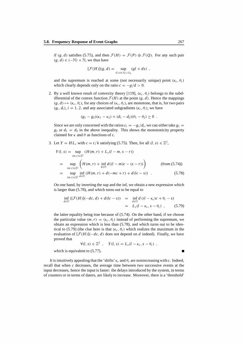
5.8. Frequency Response of Event Graphs 267
if (g, d) satisfies (5.75), and thenF(H ) = F(P) ⊕ F(Q). For any such pair(g, d) ∈ (−N) ×N, we thus have
[F(H )](g, d) = sup(l,s)∈JP∪JQ
(gl + ds) ,
and the supremum is reached at some (not necessarily unique) point(κc, θc)
which clearly depends only on the ratioc = −g/d > 0.
2. By a well known result of convexity theory [119],(κc, θc) belongs to the subd-ifferential of the convex functionF(H ) at thepoint (g, d). Hence the mappings(g, d) �→ (κc, θc), for any choices of(κc, θc), are monotone, that is, for two pairs(gi , di), i = 1, 2, and any associatedsubgradients(κi , θi ), we have
(g1 − g2)(κ1 − κ2)+ (d1 − d2)(θ1 − θ2) ≥ 0 .
Since we areonly concerned with the ratiosci = −gi/di , wecan either takeg1 =g2 or d1 = d2 in the above inequality. This shows the monotonicity propertyclaimed forκ andθ as functions ofc.
3. Let Y = H Lc with c = t/k satisfying (5.75).Then, for all(l, s) ∈ Z2,
Y (l, s) = sup(m,r)∈Z2
(H (m, r) + Lc(l − m, s − r))
= sup(m,r)∈Z2
(H (m, r) + inf
d∈N
d((l − m)c − (s − r))
)(from (5.74))
= sup(m,r)∈Z2
infd∈N
(H (m, r) + d(−mc + r) + d(lc − s)) . (5.78)
Onone hand, by inverting the sup and the inf, we obtain a new expression whichis larger than (5.78), and which turns out to be equal to
infd∈N
([F(H )](−dc, d)+ d(lc − s)) = infd∈N
d ((l − κc)c + θc − s)
= Lc(l − κc, s − θc) , (5.79)
the latter equality being true because of (5.74). On the other hand, if we choosethe particular value(m, r) = (κc, θc) instead ofperforming the supremum, weobtain an expression which is less than (5.78), and which turns out to be iden-tical to (5.79) (the clue here is that(κc, θc) which realizes the maximum in theevaluation of [F(H )](−dc, d) does not depend ond indeed). Finally, we haveproved that
∀(l, s) ∈ Z2 , Y (l, s) = Lc(l − κc, s − θc) ,
which is equivalent to (5.77).
It is intuitively appealing that the ‘shifts’κc andθc arenonincreasing withc. Indeed,recall that whenc decreases, the average time between two successive events at theinput decreases, hence the input is faster: the delays introduced by the system, in termsof counters or in terms of daters, are likely to increase. Moreover, there is a ‘threshold’
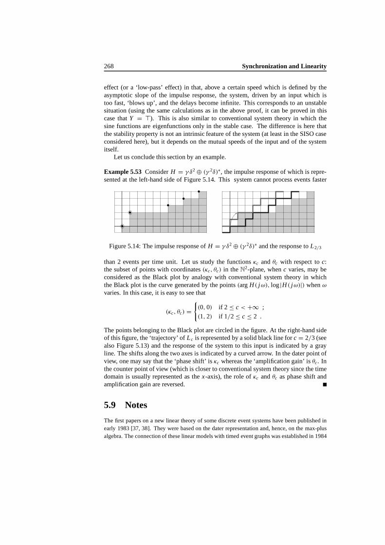
268 Synchronization and Linearity
effect (or a ‘low-pass’ effect) in that, above a certain speed which is defined by theasymptotic slope of the impulse response, the system, driven by an input which istoo fast, ‘blows up’, and the delays become infinite. This corresponds to an unstablesituation (using the same calculations as inthe above proof, it can be proved in thiscase thatY = �). This is also similar to conventional system theory in which thesine functions are eigenfunctions only in the stable case. The difference is here thatthe stability property is not an intrinsic feature of the system (at least in the SISO caseconsidered here), but it depends on the mutual speeds of the input and of the systemitself.
Let us conclude thissection by an example.
Example 5.53 ConsiderH = γ δ2⊕ (γ 2δ)∗, the impulse response of which is repre-sented at the left-hand side of Figure 5.14. This system cannot process events faster
Figure 5.14: The impulse response ofH = γ δ2⊕ (γ 2δ)∗ and the response toL2/3
than 2 events per time unit. Let us study the functionsκc andθc with respect toc:the subset of points with coordinates(κc, θc) in theN
2-plane, whenc varies, may beconsidered as the Black plot by analogy with conventional system theory in whichthe Black plot is the curvegenerated by the points(argH ( jω), log|H ( jω)|) whenωvaries. In thiscase, it is easy to see that
(κc, θc) ={(0, 0) if 2 ≤ c < +∞ ;
(1, 2) if 1/2≤ c ≤ 2 .
The points belonging to the Black plot are circled in the figure. At the right-hand sideof this figure, the ‘trajectory’ ofLc is represented by a solid black line forc = 2/3 (seealso Figure 5.13) and the response of the system to this input is indicated by a grayline. The shifts along the two axes is indicated by a curved arrow.In the dater point ofview, one may say thatthe ‘phase shift’ isκc whereas the ‘amplification gain’ isθc. Inthe counter point of view (which is closer to conventional system theory since the timedomain is usually represented as thex-axis), the role ofκc andθc asphase shift andamplification gain are reversed.
5.9 Notes
The first papers on a new linear theory of some discrete event systems have been published inearly 1983 [37, 38]. They were based on the dater representation and, hence, on the max-plusalgebra. The connection of these linear models with timed event graphs was established in 1984

5.9. Notes 269
[41]. In 1985, it has been realized that specific algebraic problems arise from the fact that daters,as time sequences, are nondecreasing [42]. At about the same time, the idea of the counterrepresentation has been introduced by Caspi and Halbwachs [35] to whom this terminology isdue. This finally resulted in the two-dimensional representation first published in [43]. A moredetailed account of the so-calledM
axin [[γ, δ]] algebra was given in [44] together with some of the
formulæ about residuation of⊕ and⊗. A large part of thematerial ofthis (and the previous)chapter(s) is based on that paper—e.g. the sections on backward equations and on rationality,realizability and periodicity—although the presentation has been somewhat improved here. Inparticular, the role of residuation theory has been clarified in the process of establishing backwardequations, and in the relationships between dater and counter representations. Only the resultson ‘minimum representatives’ appear for the first time in this book. The idea of using the formaltransfer function as a numerical function, the fact that the Fenchel transform plays a role similarto that played by the Laplace transform in conventional system theory, the parallel notion ofeigenfunctions of linear transfer functions in discrete event and conventional system theories,. . . , were all discovered and published in 1989 [40]. However, here, the presentation has beenmore tightly confined in the two-dimensional point of view.

270 Synchronization and Linearity

Chapter 6
Max-Plus Linear System Theory
6.1 Introduction
In this chapter a linear system theory is developed for a class of max-plus linear systemswith discrete or continuous domain and range. This class provides a generalization ofthe class of event graphs which have been considered in Chapter 2. We will start withan input-output point of view. We will view a max-plus linear system as a max-pluslinearoperator mapping an input, which is a function over some domain, to an output,which is another function over the same domain. For this max-plus linear operator, wewill review the classical notions of conventional linear system theory. In particular, thenotions of causality, shift-invariance, impulseresponse, convolution, transfer function,rationality, realization and stability will be considered.
The outline of the chapter is as follows. In§6.2 we give general definitions, wepresent the system algebra and we discuss some fundamental elementary systems. In§6.3 we define some subalgebras of the system algebra by progressively specializ-ing the systems, starting with the most general ones, and finishing with causal shift-invariant systems with nondecreasing impulse responses. Most practical examples ofdiscrete event systemsfall into this last category. In the dater description, their output isthe result of a sup-convolution between their input and their impulse response. In§6.4weintroduce the notion of transfer functions which are related to impulse responses bymeans of theFenchel transform. In§6.5 we discuss rationality in the max-plus con-text, and characterize rational elements in terms of periodicity. We also discuss theproblem of minimal realization of these max-plus systems. In§6.6 we give adefinitionof internally stable systems andcharacterize them in terms of equations which are theanalogue of the conventional Lyapunov equation. In this chapter, mainly single-inputsingle-output (SISO) linear max-plus systems are considered.
6.2 System Algebra
6.2.1 Definitions
Definition 6.1 (Signal) A signalu is a mapping from R into Rmax. When a signal is anondecreasing function it is called a dater.
The signal set isRR
max. This signal set is endowed with two operations, namely
271

272 Synchronization and Linearity
• pointwise maximum of signals which plays the role of addition:
∀k ∈ R , ∀u, v ∈ RR
max , (u ⊕ v)(k)def= u(k) ⊕ v(k) = max(u(k), v(k)) ;
• addition of a constant to a signal, which plays the role of the external product ofa signal by a scalar:
∀k ∈ R , ∀a ∈ Rmax , ∀u ∈ RR
max , (au)(k)def= a ⊗ u(k) = a + u(k) .
Therefore the set of signals is endowed with a moduloid structure. This algebraicstructure iscalled U .
In previous chapters the domain of signals wasZ (event domain) and trajectorieswere nondecreasing. In this chapter we develop the theory in the more general frame-work of Definition 6.1.
Definition 6.2 (Max-plus linear system) A systemis an operator S : U → U, u �→y. The signal u (respectively y) is called the input(respectively output) of the system.We say that the system is max-plus linearwhen the corresponding operator satisfies
S
(⊕
i∈I
ui
)=⊕
i∈I
S(ui ) , (6.1)
for any finite or infinite set {ui }i∈I , and
S(au) = aS(u) , ∀a ∈ Rmax , ∀u ∈ U .
Remark 6.3 Equation (6.1) is indeed the requirement of lower-semicontinuity ofSandnot only the requirement thatS is an⊕-morphism. Here is an example of a systemwhich is an⊕-morphism but which fails to be l.s.c.:
[S(u)](t) = lim sups→t
u(s) .
This system is clearly an⊕-morphism, but to show that it is not l.s.c., consider
∀n ≥ 1, un(k) =
0 if k ≤ 0 ;
n × k if 0 < k < 1n ;
1 if 1n ≤ k .
For all n ≥ 1, we have [S(un)](0) = 0, and
⊕
n≥1
un(t) ={
0 if t ≤ 0 ;
1 otherwise.
This yields[S(⊕
n un
)](0) = 1, which is different from
[⊕n S(un)
](0) = 0 .
The set of linear systems is endowed with two internal and one external operations,namely

6.2. System Algebra 273
parallel composition: S = S1⊕ S2 is defined as follows:
[S(u)](k) = [S1(u)](k) ⊕ [S2(u)](k) ; (6.2)
series composition: S = S1⊗ S2, 1 or more briefly,S1S2 is defined as follows:
[S(u)](k) = [S1(S2(u))](k) ; (6.3)
amplification: T = a ⊗ S, a ∈ Rmax is definedby:
T (k) = a ⊗ S(k) .
In addition to these basic operations, we have another important one, the feedback:
feedback: S∗ defined by the mapping fromU intoU : u �→ y, wherey (see Figure 6.1)is the least solution of
y = S(y)⊕ u . (6.4)
The notationS∗ is justified by the fact that the least solution of (6.4) does exist byTheorem 4.75 andit is given byu ⊕ S(u)⊕ S(S(u)) ⊕ · · · .
⊕u
S
y
Figure 6.1: The feedback operationy = S∗u
The set of systems endowed with the first three operations defines an idempotentalgebra called the algebra of systems. We do not lose anything by considering only thetwo internal operations because the amplification can be realized by a series composi-tion where the downstreamsystem is what we call again in the next section. Wheneverwe speak of the set of systems endowed with the two internal operations, we refer to itas the ‘dioid of systems’. The second operation is not invertible, and therefore this setis not an idempotent semifield (see Chapter 3), it is only a dioid.
6.2.2 Some Elementary Systems
We havediscussed how we can combine systems using compositions and feedbacks.Here, we describe some elementary though fundamental systems with which morecomplex systems can be built up.
Wefirst introduce the following notation.1Wemakethe usual abuse of notation which consists in using the same symbol for external multiplication
by a scalarand for internal multiplication of systems. This will be justified later on.

274 Synchronization and Linearity
Notation 6.4 For f : R → Rmax, �∫ b
sa
f (s) denotes the supremum off (s) whens rangesin the interval [a, b] (or e.g.(a, b] if a = −∞). We may also usethe notation�
∫sR
f (s)if a = −∞ andb = +∞.
The following elementary systems are now introduced.
Zero systemε: this systemproduces the constant outputε whateverthe input is:y(k) =ε for all k. It satisfies
ε ⊕ ε = ε ⊗ ε = ε∗ = ε .
Identity e: this systemproduces an output equal to the inputy(k) = u(k) for all k. Itsatisfies
e ⊕ e = e⊗ e = e∗ = e .
Shift �g: thissystemmaps inputs to outputsaccording to the equationy(k) = u(k−g)for all k. Thenotation�g is justified by the following rule of series compositionwhich should be obvious to the reader:
�g ⊗ �g′ = �g+g′ = �g⊗g′ .
Therefore�1 may be denoted�. If we restrict ourselves to signals that arenondecreasing signals (see the discussion just above Remark 5.1), we have thesimplification rule
�g ⊕ �g′ = �min(g,g′) . (6.5)
In the context of event graphs, an initial stock ofc tokens in a place introducessuch a shift between inputs and outputs in the domain where we ‘count’ events.In the framework of the continuous system depicted in Figure 1.13, the samerole is played by the initial amount of fluid in the reservoir at the outlet. Notehowever that, in that example, equations were written in a counter, rather thanin a dater, representation, and consequently, this device operated as a gain ratherthanas a shift.
Gain "d : this system maps inputs to outputsaccording to the equationy(k) = d ⊗u(k) = d + u(k) for all k. Again, thenotation"d is justified by the followingrule of series composition:
"d ⊗"d ′ = "d+d ′ = "d⊗d ′ .
Therefore"1 may be denoted". We also have the simplification rule (whichholds true for any input signal)
"d ⊕"d ′ = "d⊕d ′ = "max(d,d ′) .
In the context of timed event graphs, this is the general input-output relationinduced by a place with holding timed. For the system of Figure 1.13,thisinput-output relation is that of along pipe at the inlet of a funnel.

6.2. System Algebra 275
Flow limiter �a : this systemmaps inputs to outputsaccording to the relation
y(k) = �∫ k
s−∞u(s)ak−s . (6.6)
Unlike �c and"d , we use thenotation�a with a as a subscript, becausea doesnot behave like an exponent. Indeed, the following parallel, series and feedbackcomposition rules can be checked by direct calculation:
�a ⊕�a′ = �a ⊗�a′ = �max(a,a′) = �a⊕a′ . (6.7)
Moreover,�a > e and hence�a = (�a)∗.
Physically, this system corresponds to the input-output relation between the cu-mulated quantities traversing a pipe which limits the flow to 1/a (of course, herea is a positive number). This is the case of the aperture of the funnel in Fig-ure 1.13 (recall that this example is worked out using counter rather than daterequations). This system plays the role of the SISO system governed by the dif-ferential equation
y = ay + u
in conventional system theory, the solution of which is
y(t) =∫ t
−∞u(s)exp(a(t − s))ds ,
which is the analogue of (6.6).
Integrator e: this is another notation for�0. It maps inputs to outputsaccording tothe equationy(k) = �
∫ ks−∞u(s). The output of such a system is always nonde-
creasing. It plays the role of an identity element for shift-invariant systems withnondecreasing impulse responses as we shall see later on. This role justifies thenotatione. It satisfies
e ⊕ e = e ⊗ e = (e)∗ = e .
Local integrator #w: this system maps inputs to outputsaccording to the relationy(k) = �
∫ ksk−wu(s). It is the analogue of a conventional system recursively av-
eraging the input in a window of widthw. The following series, parallel andfeedback compositions of local integrators can beeasily checked:
#w ⊕ #w′ = #w⊕w′ ,
#w ⊗ #w′ = #w+w′ = #w⊗w′ ,
(#w)∗ = #∞ = e , ∀w > 0 .

276 Synchronization and Linearity
6.3 Impulse Responses of Linear Systems
In this section we introduce the notion of impulse response for a max-plus linear sys-tem. The algebra of impulse responses is isomorphic to the algebra of systems. The for-mer algebra is first specialized to the case of shift-invariant systems and subsequentlyto thecase of systems with nondecreasing impulse responses.
6.3.1 The Algebra of Impulse Responses
We saw that the set of systems can be endowed with a moduloid structure. The nextstepis to introduce a kind of ‘canonical basis’ for this algebraic structure. Classically,for time functions, this basis is provided bythe Dirac function at 0, and all its shiftedversions at other time instants. Therefore, we now introduce
e(·) : k �→ e(k)def={
e if k = 0 ;
ε otherwise,(6.8)
and
γ s(·) def= �s(e(·)) i.e. γ s(k) = e(k − s) , ∀k . (6.9)
The justification of the notatione(·) will come from the fact that this particular signalis the identity element for sup-convolution which will be the internal multiplication inthe system set. Indeed, it can be checked by direct calculation that
∀u , ∀k , u(k) = �∫
sR
u(s)e(k − s) . (6.10)
In viewof (6.9), this can be rewritten
u = �∫
sR
u(s)γ s , (6.11)
which shows thatu is obtained as a linear combination of the signalsγ s . This is thedecomposition of signals with respect to the canonical basis. This decomposition isunique since, if there exists another functionv : R → Rmax suchthat u = �
∫sR
v(s)γ s ,we conclude thatv(s) = u(s), ∀s, because of Identity (6.10) applied to the functionv.
Now we can state the following theorem which introducesthe notion ofimpulseresponse.
Theorem 6.5 Let S be a linear system, then there exists a unique function h(k, s)(called the impulse response) such that y = S(u) can be obtained by
∀k , y(k) = sups∈R
[h(k, s) + u(s)] = �∫
sR
h(k, s)u(s) , (6.12)
for all input-output pairs (u,y).

6.3. Impulse Responses of Linear Systems 277
Proof We have
y(k) = [S(u)](k) =[
S
(�∫
sR
u(s)γ s
)](k) ,
which, owing to the linearity assumption, implies
y(k) = �∫
sR
([S(γ s)](k))
u(s) = �∫
sR
h(k, s)u(s) ,
where we have seth(k, s)def= [S(γ s)](k). To prove uniqueness, suppose that there
exists another functionf (·, ·) which satisfies (6.12). Then using inputsu = γ s, weobtain
h(k, s)def= [S(γ s)](k)
= �∫
τ
R
f (k, τ )γ s (τ )
= f (k, s) ,
for all s, k ∈ R, where the last equality is (6.10) applied to the functionf (k, ·).
To the series,parallel, amplification and feedback compositions of systems correspondoperations on the impulse responses.
Theorem 6.6 Given a ∈ Rmax and the systems S, S1 and S2 with respective impulseresponses h, h1 and h2, then,
• the impulse response of S1⊕ S2 is [h1⊕ h2](k, s)def= h1(k, s) ⊕ h2(k, s);
• the impulse response of S1⊗ S2 is [h1⊗ h2](k, s)def= �∫
rR
h1(k, r)h2(r, s);
• the impulse response of aS is [ah](k, s)def= ah(k, s);
• the impulse response of S∗ is h∗ def= ⊕i∈Nhi .
The set of impulse responses endowed with the first three operations (respectively thefirst two operations) defines an idempotent algebra (respectively a dioid), called thealgebra (respectively the dioid) of impulse responses which is denotedH. Impulseresponses are representations of systems written in a canonical basis, just like matricesare finite dimensional linear operators written in a particular basis.
Definition 6.7 A linear system S is causal if, for all inputs u1 and u2 with correspond-ing outputs y1 and y2,
∀s , ∀k ≤ s , u1(k) = u2(k)⇒ y1(s) = y2(s) .
Theorem 6.8 A system S is causal if its impulse response h(k, s) equals ε for k ≤ s.

278 Synchronization and Linearity
Proof If S is causal,S(γ s) = h(k, s) coincides with S(ε) = ε for k ≤ s.
Remark 6.9 The impulse responseh of a series composition of two causal systems ofimpulse responsesh1 andh2 has the simplified form
h(k, s) = �∫ k
rs
h1(k, r)h2(r, s) .
6.3.2 Shift-Invariant Systems
Let us specialize the algebraH to shift-invariant systems.
Definition 6.10 A linear system S is called shift-invariant if it commutes with all shiftoperators, that is, if
∀u , ∀c , S(�c(u)) = �c(S(u)) .
Theorem 6.11 A system S is shift-invariant if and only if its impulse response h(k, s)depends only on the difference k − s. With the usual abuse of notation, the impulseresponse is denoted h(k − s) in this case. It is equal to h(·) = [S(e)](·).
Proof We have
h(k, s)def= [S(γ s)](k) = [S(�s(e))](k) = [�s(S(e))](k) = [S(e)](k − s) .
Consequently, in the shift-invariant case, the kernel defining the impulse response isreduced to a function. The input-output relation can be expressed as follows:
y(k) = (h ⊗ u)(k)def= �∫
sR
h(k − s)u(s) .
This newoperation, also denoted⊗, isnothing but thesup-convolution which plays therole of the convolution in conventional system theory. We also note that the series com-position corresponds to the sup-convolution of the corresponding impulse responses.
Definition 6.12 The algebra of shift-invariant impulse responses, denoted S, is the set
RR
max endowed with:
• the pointwise maximum of functions denoted ⊕;
• the sup-convolution denoted ⊗;
• the external operation which consists in adding a constant to the function.
The zero elementdenotedε(·) is defined byε(k) = ε, ∀k . It is absorbingfor multipli-cation. The identity element denotede(·) is described by (6.8).

6.3. Impulse Responses of Linear Systems 279
Remark 6.13
1. This idempotent algebraS can simply be considered as a dioid.
2. Because signals and SISO systems can be represented by functions, we do nothave to distinguish them.
3. Impulse responses of shift-invariant causal systems satisfyh(k) = ε for k < 0.
Example 6.14 The elementary systemsintroduced in§6.2.2 are shift-invariant linearsystems. Their impulse responses are given later in Table 6.2. Notice thatγ 0 = δ0 =φε = e if φε denotes the pointwise limit ofφa whena goes to−∞.
6.3.3 Systems with NondecreasingImpulse Response
In the context of event graphs, input signals have the meaning of sequences of dates atwhich successive events occur, and therefore they are nondecreasing functions. In thecase of the continuous system depicted in Figure 1.13, the input and the output are alsonondecreasing.
A nondecreasing signalu canbecharacterized by the inequalityu ≥ #wu for anyarbitrary positivew. From an algebraic point of view, this situation is identical to thatdescribed by Inequality (5.11) if #w plays the role earlier played byγ , now that the
domain is continuous. Hence from Theorem 5.8, we know thatvdef= (#w)∗ v is the
best approximation from above of a signalv in the subset of nondecreasing signals.Recall that(#w)∗ = e (seeend of§6.2.2). In particular, a nondecreasing functionu ischaracterized byu = u = eu.
Consider a system with impulse responseh. Then, if only nondecreasing inputsuare considered, the outputs are also nondecreasing as shown by the following equalities:
y = h ⊗ u = h ⊗ (e ⊗ u) = e ⊗ (h ⊗ u) = e ⊗ y .
We also notice that, for this class of nondecreasing inputs, the systems with impulseresponsesh andh = e⊗ h yield the same outputs. Thish is called the ‘nondecreasingversion’ of the impulse responseh. The subset of nondecreasing signals and impulseresponses, denotedS, is adioid with the same addition and multiplication asS, but theidentity element ise.
The following are the nondecreasing versions of the impulse responses of someelementary systems encountered earlier, the nonmonotonic versions of which are givenin Table 6.2 below:
e(k) ={
e if k ≥ 0 ;
ε otherwise;γ c(k) =
{e if k ≥ c ;
ε otherwise;δd(k) =
{d if k ≥ 0 ;
ε otherwise.

280 Synchronization and Linearity
6.4 Transfer Functions
6.4.1 Evaluation Homomorphism
In this section we discuss the notion of transfer functions associated with shift-invariantmax-plus linear systems. Transfer functions are related to impulse responses by a trans-formation which plays the role of the Fourier or Laplace transform in conventionalsystem theory, and which, in our case, is similar to theFenchel transform of convexanalysis.
We saw that signals and impulse responses are functions belonging to the sameidempotent algebra and that, in the canonical basis, they can be written
f = �∫
sR
f (s)γ s .
We associate a transfer functiong, which will be a mapping fromRmax into Rmax,with suchanimpulse response viewed as a generalization of a formal polynomial intro-ducedin Chapter 3. The value at a point of this latter function is obtained by substitut-ing anumerical variable inRmax for γ in the expressionof f . Theresulting expressionis evaluated using the calculation rules ofRmax. This substitution of a numerical valuefor the generator should be compared with what one does in conventional system the-ory when substituting numerical values inC for the formal operator of the derivative(denoteds) in continuous time, or the shift operator (denotedz) in discrete time. Toformalize this notion, we introduce the idempotent algebra of convex functions. Recallthat a closed convex function is a function which is
1. l.s.c.in the conventional sense, that is, it satisfies limxn→x f (xn) ≥ f (x);
2. convex;
3. proper, that is, nowhere equal to−∞;
or a function which is always equal to−∞. It is exactly the set of the upper hulls ofcollections of affine functions [119, Theorem 12.1].
Definition 6.15 The set of closed convex functions endowed with the pointwise max-imum denoted ⊕, the pointwise addition denoted ⊗ and the addition of a scalar asexternal operation, is called the algebra of convex functions and is denoted Ccx.
Oncemore, there is no loss of generality in considering the dioid of convex functionsendowed with two internal operations only. Indeed, the product by a scalar or thepointwise product by a constant function gives the same result.
Definition 6.16 For f = �∫
sR
f (s)γ s ∈ S, let
g : R→ Rmax , c �→ �∫
sR
f (s) ⊗ cs . (6.13)

6.4. Transfer Functions 281
Then g is called the numerical transfer function2 associated with f . The transform Fwhich maps f to g is called the evaluation homomorphism(as will be justified by theforthcoming Theorem 6.17).
Five different complete and commutative idempotent algebras and dioids have beenconsidered, and consequently five different meanings of⊕ and⊗ have been used.As usual, the context should indicate which one is meantaccording to the nature ofelements on which these binary operations operate. Table 6.1 recalls the meaning ofthese operations. The application of the evaluation homomorphism to the impulse
Table 6.1: Five dioids
Dioid Rmax H S⊕ max pointwise max⊗ + max-plus kernel product sup-convolutionε −∞ ε(k, l) = −∞ , ∀k, l ε(k) = −∞ , ∀k
e 0 e(k, l) ={
0 ifk=l
−∞ otherwisee(k) =
{0 if k = 0
−∞ otherwise
Dioid S = e ⊗ S Ccx
⊕ pointwise max⊗ sup-convolution pointwiseadditionε ε(k) = −∞ , ∀k ε(c) = −∞ , ∀c
e e(k) ={
0 if k ≥ 0
−∞ otherwisee(c) = 0 , ∀c
responses of the elementary systems is given in Table 6.2.
Theorem 6.17 The evaluation homomorphism F is a l.s.c. (in the sense of Defini-tion 4.43) epimorphism (surjective homomorphism) from S onto Ccx.
Proof The homomorphism and l.s.c. properties are true by construction. Indeed,F( f ⊕ f ′) = F( f ) ⊕ F( f ′), andits extension to infinite sums is true by commu-tativity of the sup operation. FinallyF( f ⊗ f ′) = F( f )⊗F( f ′) is true by definitionof the⊗ operation inS. Surjectivity arises from the fact thatF (S) is the set of theupper hulls of families of affine functions which coincides with the set of closed convexfunctions.
Remark 6.18
1. ClearlyF is not injective, for example
c ⊕ c2 = [F (γ ⊕ γ 2)](c) =
[F(�∫ 2
s1γ s
)](c) .
2In this chapter we will call it simply a transfer function because the notion of formal transfer is not used.

282 Synchronization and Linearity
Table 6.2: Impulse responses and transfer functions of the elementary systems
System Impulse response Transfer function
ε ε(k) = ε , ∀k [F(ε)](c) = ε , ∀c
e e(k) ={
e if k = e
ε otherwise[F(e)](c) = e , ∀c
�g γ g(k) ={
e if k = g
ε otherwise[F (γ s)](c) = gc , ∀c
"d δd(k) ={
d if k = 0
ε otherwise
[F(δd)](c) = d , ∀c
�a φa(k) ={
ak if k ≥ 0
ε otherwise[F (φa)](c) =
{e if c ≤ −a
� otherwise
e e(k) ={
e
ε otherwise
[F(e)](c) ={
e if c ≤ 0
� otherwise
#w ςw(k) ={
e if w ≥ k ≥ 0
ε otherwise[F (#w)](c) =
{e if c ≤ 0
wc otherwise
2. The convex function
g(c) ={ε if c = 0 ,
� otherwise,
is not closed. Neither is it the upper hull of a set of affine functions. Indeed,eachaffine function would be belowg and therefore would be equal toε everywhere.Neverthelessthis function is l.s.c. because the subsets{c | g(c) ≤ a}, whichareequal to{0} for all a ∈ R, are closed.
3. By returning to conventional notation,F can be interpreted in terms of theFenchel transform. More precisely we have
[F( f )](c) = supk
[kc + f (k)] = [Fe(− f )](c) , (6.14)
where [Fe( f )](c)def= supk(kc − f (k)) denotes the classical Fenchel transform
of convex analysis [58]. Recalling that the Fenchel transform converts inf-convolutions into pointwise (conventional) additions, we see that the choice ofmultiplication in Ccx is consistent with this property of the Fenchel transform.
6.4.2 Closed Concave Impulse Responses and Inputs
It is well known that the Fenchel transform only characterizes closed convex functions;or otherwise stated, all functions having the same convex hull have the same Fenchel

6.4. Transfer Functions 283
transform. Rephrasing this result in terms of the evaluation homomorphism, we ob-tain that only the closed concave impulse responses are completely characterized bytheir transfer functions. For this subclass, the evaluation homomorphism is a tool aspowerful as the Laplace transform in conventional system theory.
Theorem 6.19 For g ∈ Ccx, the subset F−1(g) admits a maximum element F �(g)defined by
[F �(g)](k)
def=∧
c
g(x)◦/ck = infc
[g(c)− ck] (6.15)
(where the latter expression in conventional notation requires the convention about∞−∞ discussed in Example 4.65). Moreover, F �(g) is the concave upper hull of anyother element of F−1(g).
Proof From the preceding considerations, we see that all the assumptions required inTheorem 4.50 are fulfilled. Then (6.15) is a straightforward extension of (3.11) to thecontinuous domain case.
Definition 6.20 The subset Scv of S consists of closed concave functions, that is, thefunctions which are concave, upper-semicontinuous (u.s.c. in the conventional sense)and either nowhere equal to� or always equal to�.
Remark 6.21 The setScv is closed for multiplication (sup-convolutions of concaveu.s.c. functions yield concave u.s.c. functions), but not for addition (the upper hull ofconcave functions is not in general a concave function). It is closed for pointwiseinfimum. Therefore, this subset is not a subdioid ofS.
The next theorem tells us that the computation of the sup-convolution of two concavefunctions is equivalent to a pointwise addition and three Fenchel transforms. Knowingthat there exists a fast Fenchel transform which is the analogue of the fast Fouriertransform [31], this formula gives an efficient algorithm to compute sup-convolutions.
Theorem 6.22 We have the formula
∀ f, g ∈ Scv , h = f ⊗ g = F � (F( f )⊗F(g)) ,
which, in conventional notation, means
h(k) = supx+y=k
[ f (x)+ g(y)] = F � (F( f )+F(g)) .
Proof Equation (6.15) shows thatScv equalsF � (Ccx), since lower hulls of families ofaffine functions are closed concave functions. Therefore,
∀ f ∈ Scv , F �◦F( f ) = f .
Then, using the closedness ofScv and thehomomorphism property ofF , we have
f ⊗ g = F �◦F( f ⊗ g) = F � (F( f )⊗F(g)) .

284 Synchronization and Linearity
6.4.3 Closed Convex Inputs
In conventional system theory anyL2 function can be decomposed with respect to thebasis of sine functions. In the present situation, any closed convex function can bedecomposed with respect to conventional linear functions:
y = lc(x)def= c × x = xc ,
which may be considered as the max-plus exponentials (the last expression is in max-plus notation). This decomposition can be used to compute the outputs of a shift-invariant max-plus system driven by convex inputs. Indeed, the max-plus exponentialsare eigenvectors for any shift-invariant max-plus linear system in the same way as thesine functions are eigenvectors for any shift-invariantlinear system inconventionallinear system theory.
Definition 6.23 The subset Scx of S consists of closed convex functions. The canonicalinjection of Scx into Ccx is denoted I .
Remark 6.24
1. The difference betweenScx andCcx is the⊗ operation (see Table 6.1).
2. Unlike Scv which is closed for multiplication but not for addition,Scx is closedfor addition and multiplication. But in general the multiplication of two convexfunctions is equal to�. The only exception is the product of two affine functionswith the same slope.
3. The identity elemente(·) is not convex. Therefore,Scx is not a subdioid ofSeither.
4. The intersection ofScv andScx is the subset of weighted exponentials in themax-plus sense (b ⊗ lc(·)) or affine functions in the conventional sense.
In the max-plus framework, the decomposition of closed convex functions tells usthat these functions are integrals of weighted exponentials. Moreover, the correspond-ing weights are explicitly given by the Fenchel transform.
Theorem 6.25 For all f ∈ Scx, we have
f = I−1◦F◦F �◦I( f ) ,
which can be written
∀k , f (k) = �∫
cR
ck[F �◦I( f )
](c) = �∫
cR
kc[F �◦I( f )
](c) , (6.16)
to emphasize the exponential decomposition.

6.4. Transfer Functions 285
Proof A function f ∈ Scx may be viewed as a transfer function inCcx because it isa closed convex function. Therefore,I( f ) equals f but considered as an element ofCcx. BecauseI( f ) ∈ Ccx, we can solveF(g) = I( f ) for g. But wehave an explicitformula forg, namely g = F � (I( f )). Then using the fact thatF◦F � = ICcx, we haveproved the result.
Let us show now that the max-plus exponentials (conventional linear functions)lc areeigenvectors for the operator defined as the sup-convolution with a given impulse re-sponse.
Theorem 6.26 For all impulse responses h ∈ S and all scalars c, we have
h ⊗ lc = [F(h)](−c) lc . (6.17)
Therefore [F(h)](−c) is the eigenvalue (called the gain of h for the exponential lc )associated with the eigenvector lc of the operator g �→ h ⊗ g.
Proof The proof is the same as in conventional algebra:
[h ⊗ lc ](k) = �∫
sR
ck−sh(s) = ck�∫
sR
c−sh(s) = ck [F(h)](−c) .
Wemay usethis property of the exponentials to compute the output of a shift-invariantsystemdriven by a convex input.
Theorem 6.27 We have
∀ f ∈ Scx , ∀h ∈ S , h ⊗ f = �∫
cR
[F �◦I( f )
](c) [F(h)](−c) lc ,
where[F �◦I( f )
](c) is the weight of the exponential lc in the spectral decomposition
of f and [F(h)](−c) is the gain of h for the same exponential.
Proof Using thedistributivity of⊗ (sup-convolution inS) with respect to�∫
, we have
h ⊗ f = h ⊗�∫
cR
[F �◦I( f )
](c) lc by (6.16),
= �∫
cR
[F �◦I( f )
](c) (h ⊗ lc) by linearity,
= �∫
cR
[F �◦I( f )
](c) [F(h)](−c) lc by (6.17),
and the functionh ⊗ f alsobelongs toScx.
In conclusion, we have encountered two situations of special interest to compute theresponse of a system to an input

286 Synchronization and Linearity
• if the input and the impulse response are concave, we can use the evaluationhomomorphism to transform this inf-convolution into a pointwise conventionalsum;
• if the input is convex, we can first decompose it as a sum of exponential functions(in the dioid sense), and then, using the linearity of the system, we can sum upthe responses to these exponentials inputs.
6.5 Rational Systems
The setS is a nice algebraic structure but its elements are functions and therefore can-not be coded by finite sets of numbers in general. It is useful to consider subsets of thesefunctions which can be coded in a finite way. The algebraic functions would constitutesuch a set. Those functions are described as the solutions of a polynomial systems ofequations inS. But even inclassical system theory the study of these systems is inits infancy. Therefore we restrict ourselves to a simpler situation. We only considersystems which can be described by a finite set ofspecial linear equationsy = hy ⊕ u.These equations describe the input-output relation of systems obtained by series, paral-lel and feedback compositions of elementary systems for which the impulse responsesare explicitly known. Such systems are called rational. Clearly this notion of rational-ity depends on the elementary systems considered. Rational systems can be describedin terms of the star operation(y = h∗u). This storyis not specific to max-plus alge-bra, but the rationals of these max-plus algebras have simple characterizations in termsof their periodic asymptotic behavior which is similar to the periodicity property ofthe decimal expansion of rational numbers. The aim of this section is to characterizemax-plus rational systems by their asymptotic behavior.
6.5.1 Polynomial, Rational and Algebraic Systems
Let us consider
1. a subsetK of S which also has a structure of idempotent algebra but not nec-essarily the same identity element asS (for example, nondecreasing functionsdefine an algebrawith e asthe identity element—see§6.3.3);
2. a finite setα = {α1, . . . , α�} of elements ofS.
Let us define five subsets ofS which may beconsidered asextensions ofK and whichhave a structure of idempotent algebra:
polynomial or dioid closure K [α] of K ∪ α: its elements are obtained by combiningthe elements ofK ∪ α using a finite number of⊕ and⊗ operations;
rational closure K (α) of K ∪ α: its elements are obtained by combining the elementsof K ∪ α using a finite number of⊕,⊗ and∗ operations;

6.5. Rational Systems 287
algebraic closureK {α} of K ∪ α: its elements are obtained by combining the ele-ments ofK ∪ α using a finite number of⊕ and⊗ operations and by solvingpolynomial equations with coefficients inK ∪ α;
series closureK [[α]] of K ∪ α: its elements are obtained by combining the elementsof K ∪α using a countable number of⊕ and⊗ operations: this is the completionof the polynomial closure;
topological closureK {{α}} of K ∪ α: its elements are obtained by combining the ele-ments ofK ∪ α using an infinite number of⊕ and⊗ operations and by solvingpolynomial equations: this is the completion of the algebraic closure.
NotethatS is a subset ofRmax{{γ }}. In general we have
K ⊂ K [α] ⊂ K (α) ⊂{
K [[α]]
K {α}}⊂ K {{α}} .
For example, considerK = B = {ε, e} andα = {δ}, whereδ is the impulse responsementioned in Table 6.2. Recall that inS, δd1 ⊕ δd2 = δmax(d1,d2). In this particularcasewe have
B[δ] Nmax⊂ B(δ) = B[[δ]] Nmax⊂ B{δ} Qmax⊂ B{{δ}} Rmax ,
whereAmax for a setA meansA∪{ε} endowed withthe maxand the+ operations,A isAmax ∪ {+∞}, and the isomorphisms above identify scalarsd with impulse responsesδd .
Remark 6.28 Observe that inB[δ] it is difficult to speak of thenotion of valuation.For example, the valuation of δd1 ⊕ δd2 would formally be equal to min(d1, d2); but atthe same timeδd1 ⊕ δd2 is equal toδmax(d1,d2); the latter is a monomial the valuation ofwhich is thus the same as the degree, namely max(d1, d2).
Similarly, considerB[γ ] which is equal to e ⊗ B[γ ], and observe that the notionof degree is equally difficult to define. Indeed, owing to (6.5) which holds true fornondecreasing signals,γ g1⊕ γ g2 is equal toγ min(g1,g2), whereas it would formally havea degree equal to max(g1, g2).
The same difficulties arise in other polynomial (or dioid) closures such asB[γ , δ] =eB[γ, δ]. This dioid is isomorphic to the polynomial subdioid ofM
axin[[γ, δ]] (‘polyno-
mial’ i n thesense of Definition 5.19). Any element inB[γ , δ] can be represented, in anonunique way, as the product ofe by anelement ofB[γ, δ]: the latter may be called a‘representative’ of the former. It is thus possible to speak of the valuations and degreesin γ andδ of such a representative inB[γ, δ] of an elementof B[γ , δ]. However, thesenotions can be given an intrinsic meaning only if we restrict ourselves to the ‘minimumrepresentative’ which exists for polynomials (see Theorem 5.20).
6.5.2 Examples of Polynomial Systems
Table 6.3 gives the main examples of polynomial closures ofRmax or of B used inthisbook. They are obtained from the set of scalars (identified with impulse responsesδd

288 Synchronization and Linearity
asexplained earlier) augmented with the impulse responses of some of the elementarysystems encountered previously. We setφ = {φc1, . . . , φc�}, whereφci is defined inTable 6.2. In the following, the ci are assumed to be positive and thereforeφci isnondecreasing.
Table 6.3: Polynomial extensions.
K α h ∈ K [α] ⊂ RR
max
Rmax
B{{δ}}
{γ } h(k) = ε only for k ∈ N.
Rmaxdef=
eRmax
{γ }h(k) = ε for k ∈ R
−; overR+, h isnondecreasing and piecewiseconstant with a finite number ofdiscontinuities at integer abscissæ.
Rmax
φ
={φc1, . . . , φc�}
h(k) = ε for k ∈ R−; overR+, h is
convex, nondecreasing andpiecewise linear with slopes in{c1, . . . , c�}.
B
def=e{ε, e}
{γ , δ}h(k) = ε for k ∈ R
−; overR+, h isnondecreasing, piecewise constantand integer-valued with a finitenumber of discontinuities at integerabscissæ.
B {γ , δ} ∪ φ
h(k) = ε for k ∈ R−; overR+, h is
convex, nondecreasing, piecewiselinear with slopes in{c1, . . . , c�}and with a finite number ofdiscontinuities at integer abscissæ.
6.5.3 Characterization of Rational Systems
A characterization of elements ofK (α) is given under the assumption thatK is ratio-nally closed (see Definition 4.99); this is the representation problem. In the present

6.5. Rational Systems 289
context, we defined a rational element as an elementh obtained by a finite number of⊕, ⊗ and∗ operations applied to elements ofK ∪ α. The following result shows thatonly one∗ operation is needed with respect tothe elements inα. Consequently, it iseasy to obtain a linear system which admitsh asits impulse response.
Theorem 6.29 (Representation of rational impulse responses)We assume that K isrationally closed (for example, K is a complete dioid). Then, for all h ∈ K (α), thereexist n ∈ N, B,C ∈ K n and Ai ∈ K n×n , i = 1, . . . , �, such that
h = C′(
�⊕
i=1
αi Ai
)∗B . (6.18)
Proof Let us refer to Theorem 4.105 and setB = K , C = K , U = K andV = α. SinceK is supposed to be rationally closed, thenU� = K , U� ⊗B = K andU�⊗ V consistsof linear combinations of elements ofα with coefficients inK . Theseobservations leadto (6.18).
Example 6.30 Let us considerthe elementh of Rmax(γ ) defined byh = ((1γ 3)∗ ⊕(γ 2)∗)∗. Observe thatRmax is a complete dioid. Using (4.109) and the fact that(a∗)∗ =a∗, we haveh = ((1γ 3)∗)∗((γ 2)∗)∗ = (1γ 3)∗(γ 2)∗ = (1γ 3⊕γ 2)∗ for which we obtainthe realization
x2 = γ x1 , x3 = γ x2 , x1 = 1γ x3⊕ γ x2⊕ u , y = x1 .
In the case of nondecreasing impulse responses, the form of the rational functions maybe explicited by specializing Theorem 6.29.
Corollary 6.31 Every h ∈ Rmax(φ) can be written
h =�⊕
i=1
hiφci , hi ∈ Rmax , i = 1, . . . , � .
Proof Using Theorem 6.29 withK = Rmax (this is a complete, hence rationally closed,dioid) andα = φ, wecan write
h = c′(
�⊕
i=1
aiφci
)∗b ,
where the entries ofb, c andai belong toRmax. By expanding the∗ expression and byusing the simplification rules given in (6.7), we obtain the form claimed in the statement
of the corollary, butwith coefficientshi of theφci belonging toRmax. As such, theycanbewritten hi = ehi for somehi ∈ Rmax. On theother hand, recall that we assumedci > 0 for all i, which implies that theφci are nondecreasing. Henceeφci = φci . Thisobservation allows us to adopt thehi as the coefficients of theφci .
290 Synchronization and Linearity
Theorem 6.32 Every h ∈ B(γ , δ) can be written h = e (p ⊕ γ νδτ(γ r δs)∗q), where
• p ∈ B[γ, δ] is a polynomial of degree at most ν − 1 in γ and τ − 1 in δ;
• q ∈ B[γ, δ] is a polynomial of degree at most r − 1 in γ and s − 1 in δ.
For a given h, the ratio s/r is independent of the particular representation of this type.
The above form expresses a periodic behavior of the impulse responseh. Thepoly-nomial p represents the transient part having a ‘width’ ofν and a ‘height’ ofτ . Thepolynomialq represents a pattern having a ‘width’ ofr and a ‘height’ ofs. This patternis reproduced indefinitely after the transient part (see Figure 6.2). The ratios/r repre-sents the‘asymptotic slope’ (see Definition 6.46 below). For the extreme casesr = 0or s = 0, the reader may return to the discussion in§5.7.4.
Proof Because we are in the commutative case, we can refer to Theorem 4.110 withT = {ε, e, γ , δ} andD = B[[ γ , δ]]. In f act, in the following, we will also need touse elements ofB{γ , δ}, hence we may embed all these structures into a larger one,
namelyB{{γ , δ}}. From Theorem 4.110 we have thath = ⊕li=1 ai
(bi
)∗, for some
ai and bi which are elements ofT % = B[γ , δ] = eB[γ, δ] (see§6.3.3). Sinceai
and bi are polynomials, we may consider their minimum representatives inB [γ, δ](see Remark 6.28), denotedai andbi , respectively, and thus obtain thenew formh =e⊗l
i=1 ai(bi )∗. It remains to showthat this form can be reduced to the form given in
the theorem statement, which essentially uses the star of a single monomial in(γ, δ).This proof is outlined below.
Considering monomialsm = γ rδs, we first introduce the rational number sl(m)def=
s/r, called the ‘slope’ (with the convention that sl(e)def= 0). This notion is extended to
polynomials (or power series) as follows. Ifm1 andm2 are two monomials, then
sl(m1⊕ m2) = sl(m1)⊕ sl(m2) .
The expression of sl(m1⊗m2) is a direct consequence of the definition since the productof two monomials is also a monomial. Using these rules, we notice that, ifp is apolynomial, then sl(p∗) = sl(p) and this is the maximum slope among the monomialswhich form the polynomial.
Wenow propose the following inequalities:
xdef= eδs(γ δs/r)∗ ≥ y
def= e(γ rδs)∗ ≥ zdef= eγ r (γ δs/r)∗
(note thatδs/r is anelement of the algebraic closure ofT ). Only the inequalityy ≥ zwill be proved. The other inequality can be proved using similar calculations. Withn = αr + β, α, β ∈ N andβ < r, all the monomials ofz namelyeγ r (γ δs/r )n, n ∈ N,
canbewritten e(γ r δs)α+1γ βδ(β/r−1)s . The monomiale(γ rδs)α+1 appear iny, whereasthe multiplicative monomialeγ βδ(β/r−1)s is less thane (it has a nonnegative exponentin γ and a negative exponent inδ), owing to the simplification rules for ‘shifts’ and‘gains’ given in §6.2.2. Thus each monomial ofz is dominated by a monomial ofy.
From these inequalities and from Lemma 3.107, we can derive the following fourrules.

6.5. Rational Systems 291
Rule 1: sl(m2) < sl(m1) ⇒ p1(m1)∗ ⊕ p2(m2)
∗ = p ⊕ p1(m1)∗, wherep is apoly-
nomial depending on the given polynomialspi and monomialsmi .
Rule 2: sl(m2) = sl(m1) ⇒ (m1)∗ ⊕ (m2)
∗ = p ⊗ (lcm(m1,m2))∗, wheremi =
eγ ri δsi , lcm(m1,m2)def= eγ lcm(r1,r2)δ lcm(s1,s2), and p is a polynomial depending
on themi .
Rule 3: sl(m2) < sl(m1) ⇒ (m1)∗ ⊗ (m2)
∗ = (m1 ⊕ m2)∗ = p ⊕ q(m1)
∗, wherepandq are polynomials depending on the given monomialsmi . This rule can bederived from(m1)
∗ ⊗ (m2)∗ =⊕r mr
1m∗2.
Rule 4: sl(m2) = sl(m1) ⇒ (m1)∗ ⊗ (m2)
∗ = (m1 ⊕ m2)∗ = p ⊕ m gcd(m1,m2)
∗,where the gcd of two monomials is defined in a similar way as the lcm previously,m is a monomial andp a polynomial, both depending on themi .
The possibility of reducingh to the claimed form comes from the recursive utilizationof these four rules.
Finally, it should be clear thath cannot have two representations with differentvalues ofthe ratios/r.
Figure 6.2: An element ofB(γ , δ) Figure 6.3: An element ofB(γ , δ, φ)
Remark 6.33 The representation of rationals in Rmax(γ ) is a simple extension of
Theorem 6.32. IndeedB(γ , δ) [B
(δ)]
(γ ) Nmax(γ). Therefore we have to
generalize the situation to the case when the coefficients of power series inγ are realinstead of integer. This extension is straightforward. The result becomes: for each
h ∈ Rmax(γ ), there existp, q ∈ Rmax[γ ] of degreesν − 1 andr − 1, respectively, anda ∈ R suchthath = e (p ⊕ qγ ν(aγ r )∗). For a givenh (recall this is anondecreasingimpulse response),a can be restrained to be nonnegative, and then the nonnegativeslopea/r is independent of the particular representation chosen forh.
Finally, the following corollary is just the synthesis of the previous results.
Corollary 6.34 Every h ∈ B(γ , δ, φ) can be written as h = e(p ⊕ γ νδτ (γ r δs)∗q) ,where

292 Synchronization and Linearity
• p ∈ B[γ, δ, φ] is a polynomial of degree at most ν − 1 in γ and τ − 1 in δ, andit is linear in φci ;
• q ∈ B[γ, δ, φ] is a polynomial of degree at most r − 1 in γ and s − 1 in δ, andit is linear in φci .
This theorem describes the asymptotically periodic behavior of the impulse response,the periodic pattern being a piecewise nondecreasing convex function (see Figure 6.3).
6.5.4 Minimal Representation and Realization
The minimal representation problem can be stated in different terms depending on the
elementary subsystems that we consider. Let us discuss the two examplesRmax[φ] and
Rmax(γ ).
Definition 6.35 (Minimal representation in Rmax[φ]) Given h ∈ Rmax[φ], where φ ={φc1, . . . , φc�} (the ci are nonnegative), the minimal representation problem consists infinding a subset of φ with minimal cardinality �min such that h = ⊕�min
i=1 hiφci , withhi ∈ Rmax, i = 1, . . . , �min.
In conventional system theory, this problem corresponds to finding the minimal numberof exponentials of which the impulse response is a linear combination.
Observe that this representation directly corresponds to a realization(A, B,C) witha diagonal matrixA (see the theorem below). Indeed, in conventional system theory,the impulse response of a continuous-timeshift-invariant system may contain functionsof the formt n exp(kt). Themax-plus case is simpler becauseat = t a and therefore theimpulse response is only composed of max-plus exponentials.
Theorem 6.36 Given h =⊕�i=1 hiφci , the realization
x1 = φc1u , . . . , x� = φc�u , y = Cx ,
with C = ( h1 . . . h�
), is minimal if and only if the points (ci , hi ) ∈ R
+ ×R arethe corners of the graph of a decreasing and concave piecewise linear function.
Proof Let cimin = mini ci andcimax = maxi ci . OverR+, h is the upper hull of� affinefunctionsx �→ ci x + hi , whereash(x) = −∞ for x < 0. Since we are interestedin determining whether the� affine functions are all needed to representh, it does notmatter if we replaceh by a new functionH suchthat H (x) = h(x) for x ≥ 0 andH (x) = +∞ for x > 0. This H is convexand is fully characterized by its Fencheltransform (see Remark 3.36). This latter function also is convex and piecewise linear,and it admits some of thepoints(ci ,−hi ) as the corners of its graph. Moreover, owingto our assumption thatH (x) = +∞ for x < 0, this function is constant at the value−himin on the left ofcimin and is equal to+∞ beyondcimax. Because of the horizontalbranch of the graph at the left-hand side, the first slope is zero and the next slopes are allpositive since the slope of a convex function is nondecreasing in general, and moreoverit strictly increases when a corner is traversed. Any pair(ci ,−hi ) which isnot a corner

6.5. Rational Systems 293
of the graph of the Fenchel transform can be discarded without changing this function.The corresponding affine function ofx canalsobe discarded without changingh. Thestatement of the theorem expresses these conditions, which are obviously necessaryand sufficient, up to the change of−hi into hi .
Definition 6.37 (Minimal realization in Rmax(γ )) Given h ∈ Rmax(γ ), the minimalrealization problem consists in finding a triple (A, B,C) ∈ R
n×nmax × R
nmax× R
nmax with
minimal n such that h = C(γ A)∗B. Equivalently, if y = hu, then there exists x ∈(Rmax(γ )
)nsuch that (u, x, y) satisfy:
(xy
)= S
(xu
)= e
(A BC ε
)(xu
).
Matrix S is called the system matrix.
The problemof findinga minimal realization is still open. The previous minimal rep-resentation theorem in the case of continuous impulse responses cannot be extendedto the present discrete situation in a straightforward manner, essentially because it isdifficult to precisely identify the underlying ‘exponentials’ (that is, the expressions ofthe form(aγ ri )∗ which may contribute to the transient part of the impulse response).Many attempts to solve this problem have not been successful yet. In Chapter 9 partialresults are given. Nevertheless the following theorem gives a realization which is notnecessarily minimal but which contains only one star operation.
Theorem 6.38 (Realization inRmax(γ )) Every element of Rmax(γ ) can be realizedwith a system matrix S given by
S = e
ε γ ε · · · · ε
ε ε γ · · · · ε
· · · · · · · ·aγ ε · · γ ε · ·ε · · · · γ · ε
· · · · · · γ ε
· · · · · · · eq(r − 1) · · q(0) p(ν − 1) · p(0) ε
corresponding to the event graph given in Figure 6.4.
Proof Remark 6.33 showed that ifh ∈ Rmax(γ ), it can be represented ash =e (p ⊕ qγ ν(aγ r )∗), with p = ⊕ν−1
i=0 p(i)γ i andq = ⊕r−1j=0 q( j )γ j. By direct cal-
culation, which consists in eliminatingx in(
xy
)= S
(xu
),
with the above expression ofS, one cancheck thaty = hu with the given expressionof h.

294 Synchronization and Linearity
u ye e e e e
ax r+ν x r+ν−1 x 1x r x r−1
p(0) p(1) p(2) q(0) q(1)q(r − 1)
Figure 6.4: One-star realization of rational systems inRmax(γ )
6.6 Correlations and Feedback Stabilization
In this section we develop a second-order max-plus system theory. This theory offersalgebraic similarities with conventional second-order system theory. In the context ofevent graphs, its main application is the evaluation of sojourn times of tokens in placesor in broader portions of the graph. A notion of internal stability is introduced bysaying that a system is stable if all its sojourn times are bounded. Finally it is shownthat a structurally observable and controllable system can be stabilized by a dynamicfeedback while preserving the asymptotic open-loop performance.
6.6.1 Sojourn Time and Correlations
We consider the problem of computing the sojourn times in timed event graphs. Letv
andu be two daters associated with a pair of transitions (also namedv andu) surround-ing a place p containingµ tokens initially (v corresponds to the upstream transition,u to the downstream). The token involved in the firing of transitionu numberedk(this firing occurs at timeu(k)) corresponds to the token which was produced by thefiring of transitionv numberedk − µ (occurring atv(k −µ)). This is because we dealwith deterministic event graphs with constant holding times and the FIFO rule may beassumed for places. Therefore, we define the sojourn timeTuv (k, µ) of this token inplacep (along arc(v, u), marked with µ tokens initially) by
Tuv (k, µ) = u(k) − v(k − µ) .
More generally, for two transitionsv andu connected by a pathρ containingµρ tokensinitially (i.e. µρ = |ρ|t), Tuv (k, µρ ) = u(k) − v(k − µρ) representsthe time spentalong the pathρ by the token numberedk at u. Thesenotions can be generalized tocontinuous systems, like the one presented in§1.2.7, by considering that tokens are‘molecules’ of fluid in pipes. More formally, we introduce the following notions.
Definition 6.39 Let u, respectively v, be an n-dimensional, respectively p-dimension-al, vector with entries in S.
Sojourn-time matrix The sojourn time (Tuv )i j (k, µ) of the token participating in thek-th firing of transition ui , and using a path from v j to ui which containsµ tokensinitially, is defined as
(Tuv )i j (k, µ) = ui (k)◦/v j (k − µ) = (u(k)◦/v(k − µ))i j .

6.6. Corr elations and Feedback Stabilization 295
Here ◦/ denotes the residuation of the instantaneous matrix product. The n × pmatrix function Tuv (·, ·), which gives the sojourn times between paths going fromthe set v of p transitions to the set u of n transitions, is called the sojourn-timematrix.
Correlation matrix Let Ruv be the matrix with entries in S defined by Ruv = u◦/v.Here ◦/ is considered as the residuation of the (matrix) ‘convolution’ product inforce in S (which is similar to power series product). Therefore (see (4.97)),
∀m ∈ R, Ruv (µ) = [u◦/v](µ) =∧
k
(u(k)◦/v(k − µ)) =∧
k
Tuv (k, µ), (6.19)
This Ruv is called the correlation matrix of u with v. If u = v, it is called theautocorrelation matrix of u.
There might be parallel paths with different initial markings.
Lemma 6.40 If v ∈ S, the mappings µ �→ Tuv (k, µ) and µ �→ Ruv (µ) are nonde-creasing.
Proof Sincev is nondecreasing,
∀k , µ′ ≤ µ⇒ v(k − µ′) ≥ v(k − µ)⇒ u(k)◦/v(k − µ′) ≤ u(k)◦/v(k − µ) .
The results follow immediately.
Remark 6.41 We refer the reader to Example 4.65 forthe manipulation of◦/ in Rmax
and to§4.6.2 for the matrix formulæinvolving ◦/. It may be useful to recall the pointof view adopted in [49]. With the choice of primitives used therein, the residuationoperator can be evaluated as follows in the case of vectors overRmax. Let us firstintroduce the following notation: an overlined (square or nonsquare) matrix or vectorwill denote the transposed matrix or vector in which, moreover, the (conventional) signof all entries has been changed to the opposite. For example, ifa = ( 2 3
), then
a = ( −2 −3)′
; if h ∈ S, thenh(t) = −h(−t).3 Then we haveu◦/v = v ⊗ u andv ◦\u = u ⊗ v, where⊗ still denotes the matrix product inRmax. Theseformulæ holdalso true inRmax: we have
� = ε◦/ε = ε ⊗ ε = ε ⊗� , � = �◦/� = �⊗ � = �⊗ ε .
It is also useful to recall the De Morgan formulæ for the sup and the inf (see (4.9)–(4.11)) and in particular the following formula:
a ⊗ b = b , a ,
3Indeed, if we view the convolution as an extension of the matrix product with infinite-dimensionalelements (for special matrices in which entry(i, j ) depends only on the differencet = i − j ), thenh(t) =−h(−t) is the composition of transposition and of change of sign.

296 Synchronization and Linearity
where, denotes the matrix product based on min and+ (the absorbing element forscalar multiplication being now� = +∞: we haveε ⊗� = ε but ε ,� = �). Forexample,
a◦/b = b ⊗ a = a , b .
Remark 6.42
1. Another interesting quantity isT +uv (k, µ) = u(k) − v((k − µ)−) wherev(k−) =lims↑k v(s). ThisT+ is differentfrom T whenv is not left-continuous.
2. Let us consider the case whenu andv are scalar functions. The analogy betweenthe conventional correlation and the max-plus correlation should be clear:
Suv(µ) = limT→∞
1
2T
∫ T
−Tu(s)v(s − µ)ds , Ruv (µ) =
∧
s∈R
(u(s)◦/v(s − µ)) .
3. For finite functionsui and v j , the classical distance supk |ui (k) − v j (k)| canbe expressed as− inf
((Ruv )i j (0), (Rvu ) j i (0)
), which shows some connection
between the notions of distance and correlation.
4. From (6.19), it is clear that(Tuv )i j (k, µ) = ui (k)◦/v j (k − µ) is bounded frombelow by(Ruv )i j (µ) for all i, j, k,m. On theother hand,
(Rvu ) j i (−µ) =∧
l
v j (l)◦/ui (l + µ) =∧
k
v j (k − µ)◦/ui (k) ,
hencee◦/(v j (k − µ)◦/ui (k)
)is bounded from above bye◦/
((Rvu ) j i (−µ)
). This
would provide an upper bound for(Tuv )i j (k, µ) if it were true thate◦/(x◦/y) =y◦/x . In Rmax this equality obviously holds true wheneverx and y are scalarsassuming finite values. Otherwise it may not hold, as shown by the followingexample: letx = y = ε, thenx◦/y = �, e◦/� = ε but y◦/x = �.
Let us now give the evolution equation of the sojourn time for a shift-invariantautonomous linear system.
Theorem 6.43 For the system x(k + 1) = Ax(k), where A ∈ Rn×nmax, the sojourn time
matrix Txx (·, µ) follows the dynamics
Txx (k + 1, µ) = (ATxx (k, µ))◦/A = A(Txx (k, µ)◦/A) ,
provided that Txx (·, µ) never assumes infinite values. More generally, the followinginequalities always hold true
Txx (k + 1, µ) ≥ (ATxx (k, µ))◦/A ≥ A(Txx (k, µ)◦/A) .

6.6. Corr elations and Feedback Stabilization 297
Proof We have
Txx (k + 1, µ) = x(k + 1)◦/x(k + 1− µ) = (Ax(k))◦/(Ax(k − µ))
= ((Ax(k))◦/x(k − µ))◦/A by (f.9),
≥ (A(x(k)◦/x(k − µ))◦/A by (f.12),
≥ A((x(k)◦/x(k − µ))◦/A) by (f.12).
The two inequalities become equalities in the case whenTuv (k, µ) has finiteentriesonly. Indeed, inRmax, the only counterexamples to equality in (f.12) are the caseswhenε and/or� are involved: for example,ε = ε ⊗ (ε◦/ε) < (ε ⊗ ε)◦/ε = �.
The following result provides insight into how correlations are transformed by linearsystems.
Theorem 6.44 (Nondecreasing correlation principle) Consider a (MIMO) shift-invariant system with (matrix) impulse response H ∈ S and two inputs signals u andv with their corresponding outputs y and z, respectively. Then
y◦/z ≥ (v ◦\u)(H ◦/H ) , (6.20)
z ◦\y ≥ (v ◦\u)∧
i, j
Hi j ◦/Hi j . (6.21)
Proof Observe first that, for alli, j,
(u◦/v)i j (k) =∧
l
(ui(l)◦/v j (l − k)
) =∧
l
(v j (l − k) ◦\ui(l)
)
because⊗ is commutative for scalars. Using this equality fori = j and theobviousfact that(u◦/v)i j ≥ ε for i = j , we have thatu◦/v ≥ (v ◦\u)e, wheree is the identitymatrix. Then, we have
y◦/z = (Hu)◦/(Hv)
= ((Hu)◦/v)◦/H by (f.9),
≥ (H (u◦/v))◦/H by (f.12),
≥ ((v ◦\u)H )◦/H as explained above,
≥ (v ◦\u)(H ◦/H ) by (f.12).
This proves (6.20). Inequality (6.21) is obtained easily from (6.20) and (4.82).
Remark 6.45
1. SinceH ◦/H ≥ e, by (f.6), Inequality (6.21) implies thatz ◦\y ≥ v ◦\u, whichmeans that,in the SISO case, the correlation of output signals is not less than thecorrelation of inputs.
2. For autocorrelations, (6.20) becomesy◦/y ≥ (u ◦\u)(H ◦/H ) ≥ H ◦/H since(u ◦\u) ≥e. This is a second correlation principle, which states that the autocorrelation ofoutputs is not less than the intrinsic correlationH ◦/H of the system.
Theorem 6.44 suggests the importance of quotients of the formA◦/A. Theorem 4.59and Corollary 4.69 gave an algebraic characterization of these quotients.

298 Synchronization and Linearity
6.6.2 Stability and Stabilization
In this subsection we are concerned with what we call the internal stability of systems.The discussion will be limited to systems modeling timed event graphs. This notionof internal stability means that there is noaccumulation of tokens in places or, dually,that the sojourn times of tokens remain finite. Let us start our discussion on stability bystudying the relation between the asymptotic slopes of functions and their correlations.
Definition 6.46 (Asymptotic slope) Let h ∈ Rmax(γ ) be represented by
e(p ⊕ qγ ν(aγ r )∗)
(see Remark 6.33; without loss of generality, we assume that a is nonnegative). Then,
the asymptotic slope of h ∈ Rmax(γ ), denoted sl∞(h), is defined by the ratio a/r.
As observed in Remark 6.33, the ratioa/r is independent of the particular represen-tation of this type which waschosen forh. Note the difference between the slopeintroduced in the proof of Theorem 6.32 andthis asymptotic slope: in the context
of Rmax(γ ), the former would be the maximum ratioa(n)/n among the monomialsa(n)γ n appearing inh; the latter is the limit of such ratios whenn goes to infinity.
Theorem 6.47 Given a realization of some h ∈ Rmax(γ ) by an event graph with ‘in-ternal state’ x, for any rational input (dater) u such that u(k) = ε, ∀k < 0, the cor-responding dater x is also rational and such that x(k) = ε, ∀k < 0. The followingequivalence holds true:{(A) : ∀i, j, (Rxx )i j = ε
} ⇔ {(B) : ∀i, j, sl∞(xi ) = sl∞(x j )
}.
Proof Thecase of zero slopes must be handled separately. Suppose that for somei andj , sl∞(xi ) ≥ sl∞(x j ) and that, moreover, sl∞(xi ) > 0. Then itis easy to see that thereexists a shiftγ µ suchthatxi ≥ γ µx j . Therefore, for allk ∈ Z, xi (k) ≥ x j (k − µ) and(Rxx )i j (µ) ≥ e. Consequently, if sl∞(xi ) = sl∞(x j ) > 0, (Rxx )i j > ε and(A) holdstrue. If sl∞(xi ) = sl∞(x j ) = 0, xi andx j are then polynomials, that is, they can be(minimally) represented by a finite number of coefficients not equal toε. In this case,it is easy to conclude this partof the proof by remembering thatε◦/ε = �.
Conversely, if (B) does not hold, that is, there exists a pair(i, j ) such that sl∞(x j ) >
sl∞(x j ), then whateverµ ∈ Z, xi (k) increases to infinity strictly faster thanx j(k − µ)
whenk → +∞. Hence, for allµ ∈ Z,∧
k xi (k)◦/x j(k − µ) = ε (the∧ is obtained asa limit when k →+∞) and (A) is contradicted.
Defini tion 6.48 (Internal stability) When the equivalent conditions (A) and (B) holdtrue for all inputsof the type described in Theorem 6.47, we say that the realization isinternally stable.
Remark 6.49 Owing to Remark 6.42 (point 4), in the situation of Definition 6.47,and if all datersxi remain finite, one can obtain an upper bound for the sojourn timesof tokens in any internal path of the event graph (using appropriate shiftsµ). The

6.6. Corr elations and Feedback Stabilization 299
condition that thexi remain finite is satisfied if the inputs remain finite (no indefinite‘starving’ of tokens at the input transitions) and if the system has no deadlocks. Adeadlock would be revealed by infinite asymptotic slopes for the daters associated withtransitions belonging to the deadlocked circuits.
However, even for internally stable event graphs with finite inputs and no dead-locks, it might happen that tokens incur unbounded sojourn times: this typically occursin places which are located immediately downstream ofu-transitions (sources), whenone uses inputs which are too fast with respect to the potential throughput of the eventgraph (that is, when the asymptotic slopes of these inputs areless than the commonvalue of theasymptotic slopes of thexi ).
Corollary 6.50 Given a rational impulse response h and a realization described by atriple of matrices4 (A, B,C), this realization is internally stable if and only
∀i, j , (H ◦/H )i j = ε ,
where Hdef= e(γ A)∗B.
Proof The condition is sufficient becausex = Hu andx◦/x ≥ H ◦/H by Remark 6.45(point 2). Conversely, since(H ◦/H )i j =
∧l Hil ◦/H jl and if (H ◦/H )i j = ε, then there
exists lo suchthat Hilo◦/H jlo = ε. The systemdoes not satisfy the requirement ofDefinition 6.48 for the inputulo = e, ul = ε, l = k.
Theorem 6.51 If the internal subgraph of an event graph (that is, the subgraph ob-tained by deleting input and output transitions together with the arcs connecting themto other transitions) is strongly connected, then this system is internally stable.
Proof Indeed if the internal subgraph is strongly connected, for any pair of internalnodes(i, j ), there exists a pathρ from j to i containingµρ tokens (µρ may be equalto 0). Then we havexi (k) ≥ αρ ⊗ x j (k − µρ), whereαρ is the sum ofthe holdingtimes of the places in the pathρ (i.e. αρ = |ρ|w; αρ > ε, indeedαρ ≥ e). Therefore(Txx )i j (k, µρ ) ≥ tρ for all k. This holds for any input and Definition 6.48 is satisfied.
When a given (open-loop) event graph is not internally stable, we consider theproblem of obtaining this property by ‘closing the loop’ between inputs and outputs.By this we mean thatu will be obtained fromy by u = Fy ⊕ v, whereF is a ‘feed-
back’ matrix of appropriate dimensions with entries inRmax(γ ), andv is the new input(of the same dimension asu). The situation is depicted in Figure 6.5 from which itappears that (at least some components of)u, respectively y, do no longer correspondto sources, respectively sinks. The feedback should in general be dynamic in the sensethat F should indeed contain termsa(n)γ n with n ≥ 1 anda(n) ≥ e, in order to avoiddeadlocks in the closed-loop system. A term of this type inFi j means that there existsa pathfrom y j to ui (in grey in the figure) with a total number ofn tokens in the initialmarking anda totalholding time ofa(n) time units.
4See Definition 6.37, except that minimality is not required here.

300 Synchronization and Linearity
feedback in grey
x1 x2
u1 u2
y
v1 v2
Figure 6.5: An unstable timed event graph with a stabilizing feedback
The stabilization of event graphs by output feedback requires the introduction ofthe following notions.
Definition 6.52
Structural Controllability An event graph is structurally controllable if every inter-nal transition can be reached by a path from at least one input transition.
Structural Observability An event graph is structurally observable if, from every in-ternal transition, there exists a path to at least one output transition.
Theorem 6.53 (Feedback stabilization)Any structurally controllable and observableevent graph can be made internally stable by output feedback.
Proof The idea of the proof is to fulfill the sufficient condition of strong connectedness(mentioned in Theorem 6.51) for the internal subgraph of the closed-loop graph. Underthe assumptions of structural controllability and observability of the open-loop system,it should not be difficult to see that this sufficient condition can indeed be satisfied ifaneffective feedback connection is established from any output to any input.
Of course, one can imagine more refined strategies in orderto attempt to minimizethe number of feedback links so introduced. Obviously, input transitions which areupstream ofseveral m.s.c.s.’s of the internal subgraph must be preferably used and asimilar remark applies to output transitions.
Example 6.54 The timed event graph represented in Figure 6.5 is not internally stablein the open-loop configuration. For instance, if tokens are input throughu1 at the rateof 2 tokensper time unit, then tokens accumulate indefinitely in the place betweenx1
andx2 since the throughput ofx2 is limited to one token per time unit, whereasx1 canprocess tokens at the given input rate. On the other hand, the system can be stabilizedby the feedback shown in Figure 6.5 (grey lines).

6.7. Notes 301
6.6.3 Loop Shaping
In the previous subsection we saw how to obtain an internally stable system by closingthe loop between input and output, provided the system is structurally controllableand observable. However, this operation creates new circuits whereas it preserves thecircuits already existing in theopen-loop system. Therefore, the maximum cycle meanmayonly increase when passing from the open-loop to the closed-loop system, whichmeans that the throughput (inverse of the maximum cycle mean) may only be worse,resulting in a loss of performance.
The newly created circuits traverse the feedback arcs. If any such circuit, sayζ ,happens to be critical, it suffices to increase the number of tokens in the correspondingfeedback path in such a way that the cycle mean|ζ |w/|ζ |t ceases to be critical. Thisreasoning justifies the following theorem which improves the previous one.
Theorem 6.55 Any structurally controllable and observable event graph can be madeinternally stable by output feedback without altering its original open-loop throughput.
Another more algebraic view on this problem can be explained in the simple case ofa SISO system. Leth be its (rational) impulse response. The open-loop throughputis 1/sl∞(h). If one uses the feedback lawu = f y ⊕ v, the closed-loop system isy = (h f )∗hv. Then itcan beproved that if f = γ µ, thereexistsµ large enough suchthat sl∞ ((hγ µ)∗h) = sl∞(h).
An interesting question is to determine theminimum number of tokens (which mayrepresent costly resources practically) such that a desired throughput is achieved. Thisproblem is discussed in [62].
6.7 Notes
This chapter is based on the two articles [111] and [112]. The idea of extending the application ofthe max-plus algebra to continuous systems was proposed by R. Nikoukhah during a Max-Plus’working group meeting. It is quite natural once one realizes that time-invariant max-plus linearsystems indeed perform sup-convolutions of the inputs with their impulse responses. ContinuousPetri nets have also been studied in [14] and [99].
Formaland numerical transfer functions are isomorphic in conventional algebra, and there-fore theyare not always clearly distinguished in theliterature on system theory. The situation isquite different in the max-plus context. The terminology ‘transfer function’ was reserved for theFenchel transform of the impulse response in this chapter.
In the literature on optimization, the idea of consideringdynamic systems based on vectorsums of convex objects appeared from time to time but with no connection to the modeling ofsynchronization mechanisms.
The characterization of rational impulse responses in terms of periodicity was given for thefirst time in [41]. A program for symbolic computation based on this periodic characterization ofrational systems has been developed by S. Gaubert. It is called MAX [62]. An analogous notionof periodicity exists in the Petri net literature [36].
The second-order theory developed in the second part has two origins: the first stems from[112], the second from [4]. The first is concerned with finding a max-plus equivalent of theautocorrelation of a process, the second with describing the recurrent equation of differences.

302 Synchronization and Linearity
The application to stability provides another view on the stabilization by feedback described forthe first time in [41]. The nondecreasing correlation principle was found by S. Gaubert.
The interesting problem of the optimization of the number of tokens involved in the loopshaping issue has been solved in [62] but was not discussed here.

Part IV
Stochastic Systems
303


Chapter 7
Ergodic Theory of Event Graphs
7.1 Introduction
The main practical concerns of this chapter are the construction of the stationary regimeof stochastic event graphs and the conditions on the statistics of the holding times underwhich such a stationary regime exists. The basis for the analysis is the set of equationswhich govern the evolution of daters, established in Chapter 2. In§7.6 we will seethat this construction also allows us to determine the stationary regime of the markingprocess.
The main tool for addressing these problems is ergodic theory: the existence prob-lem is stated in termsof a ‘random eigenpair problem’ which generalizes the eigenpairproblem formulation of Chapter 3 in the deterministic case, and whichcan be seen astheRmax-analogue of that of a multiplicative ergodic theorem in conventional algebra.
Section 7.2 focuses on a simple one-dimensional nonautonomous example. Thisexample is the Petri net analogue of the classicalG/G/1 queue. Most of the basicprobabilistic tools to be used in this chapter are introduced through this simple exam-ple. These tools are based on theprobabilistic formalism of [6]. More advanced prob-abilistic material, and in particular the ergodic theorems which are used or referred toin the chapter, are gathered in§7.7.
Section 7.3 gives the basic first-order theorems which indicate how the daters growin such a stochastic framework. The growth rates given in these first-order theoremsare shownto be theRmax-analogues of Lyapunov exponents in conventional algebra,and generalizations of cycle times in the deterministic case.
Second-order theorems are concerned with the construction of the eigenpairs. Thisconstruction is based on the analysis of ratios of daters (in theRmax sense). Thissecond-order theory is first presented for multidimensional nonautonomous systemsin §7.4. It is shown that under appropriate statistical assumptions, this type of systemsadmits a unique stationary regime which is reached in finite time, regardless of theinitial condition, provided the ‘Lyapunov exponents’ of the m.s.c.s.’s are less than theasymptotic rate of the input. Section 7.5 focuses on the autonomous case. We providea simple and natural condition for the uniqueness and thereachability of the stationaryregime.
Throughout the chapter, we will consider two levels of abstraction.
• The first level isthat of stochastic Petri nets, for which wewill use the notation of
305
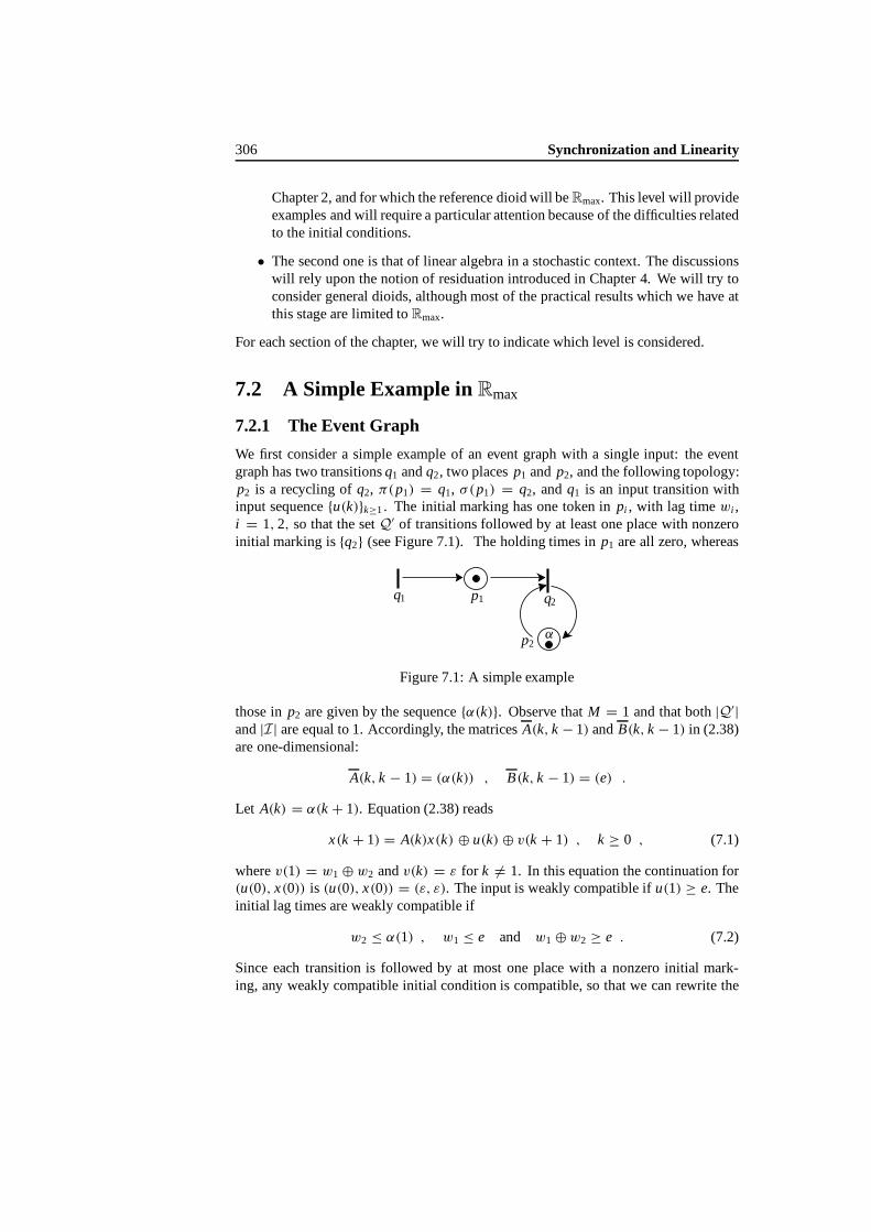
306 Synchronization and Linearity
Chapter 2, and for which the reference dioid will beRmax. This level will provideexamples and will require a particular attention because of the difficulties relatedto the initial conditions.
• The second one is that of linear algebra in a stochastic context. The discussionswill rely upon the notion of residuation introduced in Chapter 4. We will try toconsider general dioids, although most of the practical results which we have atthis stage are limited toRmax.
For each section of the chapter, we will try to indicate which level is considered.
7.2 A Simple Example inRmax
7.2.1 The Event Graph
We first consider a simple example of an event graph with a single input: the eventgraph has two transitionsq1 andq2, two placesp1 and p2, and the following topology:p2 is a recycling ofq2, π(p1) = q1, σ(p1) = q2, andq1 is an input transition withinput sequence{u(k)}k≥1. The initial marking has one token inpi , with lag timewi ,i = 1, 2, so thatthe setQ′ of transitions followed by at least one place with nonzeroinitial marking is{q2} (see Figure 7.1). The holding times inp1 are all zero, whereas
q1 q2p1
p2α
Figure 7.1: A simple example
those inp2 are given by the sequence{α(k)}. Observe thatM = 1 and that both|Q′|and|I| are equal to 1. Accordingly, the matricesA(k, k − 1) andB(k, k − 1) in (2.38)areone-dimensional:
A(k, k − 1) = (α(k)) , B(k, k − 1) = (e) .
Let A(k) = α(k + 1). Equation (2.38) reads
x(k + 1) = A(k)x(k) ⊕ u(k) ⊕ v(k + 1) , k ≥ 0 , (7.1)
wherev(1) = w1⊕ w2 andv(k) = ε for k = 1. In this equation the continuation for(u(0), x(0)) is (u(0), x(0)) = (ε, ε). The input is weakly compatible ifu(1) ≥ e. Theinitial lag times are weakly compatible if
w2 ≤ α(1) , w1 ≤ e and w1⊕w2 ≥ e . (7.2)
Since each transition is followed by at most one place with a nonzero initial mark-ing, any weakly compatible initial condition is compatible, so that we can rewrite the

7.2. A Simple Example inRmax 307
preceding equation as
x(k + 1) = A(k)x(k) ⊕ u(k) , k ≥ 0 , (7.3)
provided we now takex(0) = w2◦/α(1) andu(0) = w1.
Remark 7.1 With the statistical assumptions described in the next subsection, thissystem is very close to the FIFOG/G/1/∞ queue. TheG/G part states that boththe ratios of the input sequence (see (7.4) below) and the holding times form gen-eral stationarysequences. The 1/∞ part states that there is a single server and thatthere is an infinite buffer in front of the server. This system is also known as theproducer-consumer system in theoretical computer science. The inputu1 into transi-tion q1 features the external input stream of customers,p1 is the infinite buffer whichstorescustomers to be served,q2 features the single server, and the holding times inp2
represent the service times.
7.2.2 Statistical Assumptions
The statistical assumptions are as follows: the firing times are 0, as well as the holdingtimes in p1. The holding timesα(k), k ≥ 1, (or equivalently A(k)) and the ratios{U (k)}k≥1 of the input sequence, where
U (k)def= u(k + 1)◦/u(k) , (7.4)
form two jointly stationary and ergodic sequences on some probability space(�,F,P).This assumption can be seen as the stochastic generalization of the case of periodic in-put considered in Chapter 3: the constant ratios of the input and the constant holdingtimes in Chapter 3 are now replaced by stationary ratios. Whenever needed, we will
stress the fact thatA(k), U (k) andw def= (w1, w2) are random variables, namely mea-surable functions from� into R, by writing A(k;ω), U (k;ω) andw(ω) instead ofA(k), U (k), andw, respectively. Observe that this is tantamount to using the same no-tation for a function and for the value which ittakes at aparticular point. The contextshould always allow the reader to decide what is meant.
Before going further in the analysis of the system, we comment on the statisticalframework, and on what will be meant by joint stationarity and ergodicity of the twosequences{A(k)} and{U (k)} throughout this chapter and the next one.
Definition 7.2 (θ-shift) The mapping θ : � → � is a shift operator on (�,F,P) ifit is bijective and measurable from � onto itself, and if it is such that the probabilitylaw P is left invariant by θ , namely E[ f ] = E[ f ◦θ ], for all measurable and integrablefunctions f : � → R, where E denotes the mathematical expectation with respectto P.
By convention, the composition operator ‘◦’ has the highest priority in all for-mulæ. For instance,f ◦gh means( f ◦g)h.

308 Synchronization and Linearity
Definition 7.3 (θ-stationarity) We say that a sequence of R-valued random variables{a(k;ω)}k∈Z defined on (�,F,P) is θ-stationary if the relation
a(k;ω) = a(0; θk(ω)) (7.5)
holds for all k ≥ 0, where θk is the composition of θ by itself k times: θk+1 = θk◦θ ,and θ0 = I�, the identity.
Remark 7.4 Another way of stating the preceding definition consists in requiring thata(0)◦θk = γ −ka(0), for all k ∈ Z, whereγ is the backward shift operator on thenumbering of sequences which was defined in§5.3.2.
In the present example, wewill assume that the data of the problem, namely bothsequences{A(k)} and{U (k)}, areθ-stationary. We immediately obtain from this andfrom (7.5) that for all integersm, the relation
E[h(A(0),U (0), . . . , A(k),U (k))]
= E[h(A(m),U (m), . . . , A(m + k),U (m + k))]
holds for all measurable functionsh : R2(k+1) → R such that the expectation exists.
This is a natural property to expect from joint stationarity indeed. Starting from thisassumption, we will then be interested in proving that other quantities associated withthe event graph also satisfy theθ-stationarity property.
Similarly, the joint ergodicity of the sequences{A(k)} and{U (k)} is obtained whenassuming thatθ is P-ergodic:
Definition 7.5 (Ergodic shift) The shift θ is said to be ergodic if the almost sure (a.s.)limit
limk→∞
1
k
k∑
l=1
f ◦θ l = E[ f ] a.s. (7.6)
holds for all measurable and integrable functions f : �→ R.
Owing to (7.5),the last property implies in particular that
limk→∞
1
k
k∑
l=1
A(l) = E[ A(0)] a.s. and limk→∞
1
k
k∑
l=1
U (l) = E[U (0)] a.s.,
providedA(0) andU (0) are integrable, which corresponds to the conventional meaningof the ergodicity of both sequences. The joint ergodicity becomes more apparent fromthe formula
limk→∞
(k⊗
l=1
h (A(l),U (l))
)1/k
= E[h(A(0),U (0))] a.s.
for all measurable functionsh : R2 → R such that the expectation exists, which is also
a direct consequence of our definition.

7.2. A Simple Example inRmax 309
A measurable setA of F (an ‘event’) is said to beθ-invariant if the indicator func-tion of A, which will be denoted 1{A}, satisfies the relation 1{A}◦θ = 1{A}. We willoften make use of Birkhoff’s pointwise ergodic theorem (see [20]).
Theorem 7.6 (Birkhoff) The shift operator θ is ergodic if and only if the only sets ofthe σ -algebra F which are θ-invariant are of measure 0 or 1.
Example 7.7 (Canonical probability space)In the particular example which we con-sider, the data consist of the two sequences{A(k)} and{U (k)}. A concrete example ofsuch a shiftoperator is provided by the translation operatorγ −1 on thecanonical spaceof the two sequences, which is defined as follows:
• � is the spaceof bi-infinite sequences of the form. . . , z(−2), z(−1), z(0), z(1),z(2), . . . , wherez(k) = (s(k), t (k)) ∈ R
2 for all k ∈ Z;
• F is theσ -algebra generated by the coordinate mappingsek(ω), k ∈ Z, whereek(ω) = z(k);
• P is a probability measure on the measurable space(�,F).
On this probability space, we can then take
θ(. . . , z(−1), z(0), z(1), . . . ) = γ −1(. . . , z(−1), z(0), z(1), . . . ) ,
that isek(θ(ω)) = ek+1(ω) for all k ∈ Z. Within this framework, theθ-stationarity as-sumption boils down to the assumption that the probability lawP of the two sequencesis left invariant byγ .
If A(k;ω) denotes the first component ofek(ω), andU (k;ω) the second one, weobtain that (7.5) is indeed satisfied by both sequences.
Remark 7.8 If we consider a sequence of random variables, say{b(k;ω)}, definedon this canonical probability space, which is different from the coordinate process, itis not true ingeneral thatb(0)◦θk = b(k). It is clear thatb(0; θ(ω)) = b(0; γ −1(ω)),but in general, it is not true thatb(0; γ −1(ω)) = γ −1b(0;ω) because the translationoperator which is used at the right-hand side of the last relation has nothing to do withthe specific one used at the left-hand side, which operates on the sequences of�. Forinstance, takeb(k;ω) = k A(k;ω). We haveb(0)◦θk = 0, which clearly differs fromk A(k) unlessA(·) = 0.
7.2.3 Statement of the Eigenvalue Problem
We can rewritethe equations governing this system as{
u(k + 1) = U (k)u(k) ,
x(k + 1) = A(k)x(k) ⊕ u(k) ,
or equivalently as
X (k + 1) = D(k)X (k) , k ≥ 0 , (7.7)

310 Synchronization and Linearity
where
X (k) =(
u(k)x(k)
)and D(k) =
(U (k) ε
e A(k)
).
The variablesA(k) andU (k) are assumed to be integrable random variables, definedona probability space(�,F,P, θ), and such that
A(k) = A◦θk , U (k) = U ◦θk , k ∈ Z ,
whereAdef= A(0) andU
def= U (0). Under this assumption,D(k) = D◦θk , with D =D(0).
In the deterministic setting, we looked for periodic regimes in terms of eigenpairsassociated with theRmax matrix describing the dynamics of the event graph (see§3.7).In the stochastic setting defined above, we state the problem as the following ‘randomeigenpair’ problem.
Can we find aneigenvectorX = (X1, X2), normalizedin such a way thatX1 = e, and aneigenvalueλ, which are both random variables defined on(�,F,P, θ), and such that
DX = λX ◦θ ? (7.8)
In view of the specific form ofD, this eigenpair property reads
λ = U ,
e⊕ AX2 = U X2◦θ .
}(7.9)
So the true unknown isX2, and the equation it satisfies is a stochastic fixed pointequation. Assume that the above eigenpair is finite; whenever we takex(0) = X2 andu(0) = X1 = e in Equation (7.7), weobtain
u(1) = U ,
x(1) = e ⊕ AX2 .
}(7.10)
From (7.9) and (7.10), we seethat
x(1)− u(1) = X2◦θ +U −U = (x(0) − u(0))◦θ .
More generally, we prove inthe same way that for allk ≥ 0,
x(k) − u(k) = (x(0) − u(0))◦θk .
Therefore, if the above eigenpair problem has a finite solution, we can find an initialcondition such that the random variablesx(k) − u(k) are stationary.
Let us show that for this initial condition the marking process is also stationary: letN+(k) denote the number of tokens inp1 at the epoch when transitionq2 fires for thek-th time, namely atx(k). Within our setting,N+(k) isa random variable. For instanceN+(1) is given by the following expression (see§2.5.6):
N+(1) =∞∑
h=1
1{x(1)≥u(h)} =∞∑
h=1
1{X2◦θ≥∑h−1
l=1 U◦θ l} ,

7.2. A Simple Example inRmax 311
where∑0
1 = 0 by convention. Similarly, when using the convention∑1
2 = 0, weobtain
N+(2) =∞∑
h=2
1{x(2)≥u(h)} =∞∑
h=2
1{X2◦θ2≥∑h−1l=2 U◦θ l }
=∞∑
h=2
1{"◦θ≥∑h−1l=1 U◦θ l}◦θ = N+(1)◦θ ,
and more generallyN+(k + 1) = N+(1)◦θk .
7.2.3.1 Solution of the Eigenpair Problem
For this classical example, it is customary to take
"def= X2◦θU
asunknown, rather thanX2, mainly because this newunknown is nonnegative; indeedit is immediately seen from (7.9) that
"◦θ = e ⊕ (A◦θ◦/U") = e ⊕ F" , (7.11)
where
Fdef= A◦θ◦/U .
The construction of a solution to (7.11) is based on a backward construction which iscommon in ergodic theory, and which will be used on several occasions in this chapter.The backward process"(k), k ≥ 0, associated with (7.11) is the random process onthe probability space(�,F,P) defined by"(0) = e and
"(k + 1) = (e ⊕ F"(k)) ◦θ−1
= e⊕ F◦θ−1"(k)◦θ−1 , k ≥ 0 . (7.12)
We will return to the physical interpretation of this process in the next subsection.A nice property of the backward process is that"(k) = "(k;ω) is nondecreasing
in k for all ω. This is obtained by induction: it is true that"(1) ≥ "(0) = e; assumingthat"(k) ≥ "(k − 1), weobtain from (7.12) that
"(k + 1)◦θ = e⊕ F"(k)
≥ e⊕ F"(k − 1) = "(k)◦θ .
Let " be the a.s. limit of "(k) ask goes to∞ (thea.s. limit exists because"(k) isnondecreasing for allω). The random variable" may be finite or infinite. In bothcases we obtain that" satisfies (7.11) by lettingk go to∞ in (7.12).

312 Synchronization and Linearity
7.2.3.2 Finiteness of the Eigenvector
The main result of this subsection is the following theorem.
Theorem 7.9 (Stability condition) If E[ A] < E[U ], then the eigenvector
X = (e, ("◦/U )◦θ−1)
is P-a.s. finite.
SinceU is a.s. finite (U is assumed to have a finite mean), it follows from the verydefinition of " that X is a.s. finite if and only if" is a.s. finite. The event{" = ∞}is θ-invariant. Indeed, if"(ω) = ∞, then"(θ(ω)) = ∞, in view of (7.11) and ofthe assumption thatU (ω) < ∞ a.s. Similarly, "(θ(ω)) = ∞ implies"(ω) = ∞,since A(ω) < ∞ a.s. Therefore, in view of the ergodic assumption,P[" = ∞] iseither 0 or 1: either" is finite with probability 1, or it is infinite with probability 1 (seeTheorem 7.6).
Lemma 7.10 (Backward star) The following relation holds:
"(k) =k⊕
l=0
l⊗
h=1
F◦θ−h , (7.13)
where the⊗-product over an empty set (when l = 0) is e by convention.
Proof The proof is by induction onk. The relation holds true fork = 0 sincebothsides areequal toe. Assume the relation holds up to somek ≥ 0. Then using (7.12),we obtain
"(k + 1) = F◦θ−1⊗(
k⊕
l=0
l⊗
h=1
F◦θ−h
)◦θ−1⊕ e
=(
k+1⊕
l=1
l⊗
h=1
F◦θ−h
)⊕ e =
k+1⊕
l=0
l⊗
h=1
F◦θ−h ,
where we used thedistributivity of ⊗ with respect to⊕ and the associativity and com-mutativity of ⊕ to passfrom the first expression to the second in the last equation.
Remark 7.11 The property that"(k) is nondecreasing, which was already shown inthe preceding subsection, is obvious from (7.13), since this relation shows that"(k)consists of the maximum of an increasing set of random variables.
Proofof Theorem 7.9If E[F ] < 0 (or equivalently E[ A] < E[U ]), from the pointwiseergodic theorem we obtain that the a.s. limit
limk→∞
(k⊗
h=1
F◦θ−h
)1/k
= 1
k
k∑
h=1
(A◦θ−h+1 −U ◦θ−h) = E[ A−U ] < 0

7.2. A Simple Example inRmax 313
holds (we used the obvious property thatθ is P-ergodic if and only ifθ−1 isP-ergodic).Therefore,
S(k)def=
k∑
h=1
(A◦θ−h −U ◦θ−h)
tends to−∞ a.s. ask goes to∞, which inturn implies thatS(k) < 0 for all k greaterthana finite random integerL . Hence"(k) is a.s. finite in view of (7.13), since it isthe maximum of ana.s. finite numberL of finite random variables.
Remark 7.12 A partial converse of the preceding result is the following: ifE[ A] >
E[U ], then noP-a.s. finite solution of (7.11) exists. To prove this, it is enough to showthat" = ∞, P-a.s., and that" is the least nonnegative solution of (7.11). The latteris proved by induction. If we start with a nonnegative solution% of (7.11) for which% ≥ "(0) = e, it is easily checked that% ≥ "(k) implies% ≥ "(k + 1) (this is truebecause"(k + 1)◦θ = e ⊕ F"(k) ≤ e ⊕ F% = %◦θ). As for the proof of" = ∞,P-a.s., it follows from the fact thatS(l) then tends to∞ a.s. asl goes to∞. This inturn implies that"(k) tends to infinity as well, in view of (7.13).
Remark 7.13 The random variable" may be finite and nonintegrable. A simpleexample of this situation is provided by theM/G/1 case (namelyu(k) is thek-thepoch of a Poisson process and{α(k)} is an independent i.i.d. sequence), whenever theservice timesα(k) have infinite second moments (see [46]).
7.2.4 Relation with the Event Graph
This section focuses on the relationship between the eigenpair which was constructedin the previous section and the stochastic event graph which motivated our preliminary
example. Considerthe ‘ratios’δ(k) def= x(k + 1)◦/u(k) = x(k + 1)− u(k), k ≥ 0. Byusing (7.3), we obtain
x(k + 2)− u(k + 1) = max(A(k + 1)+ x(k + 1), u(k + 1))− u(k + 1)
= max(A(k + 1)+ x(k + 1)− u(k + 1), 0)
= max(A(k + 1)+ δ(k) −U (k), 0) ,
which corresponds to theRmax relation
δ(k + 1) = e ⊕ F(k)δ(k) , k ≥ 0 , (7.14)
where the initial conditionδ(0) is given by the relation
δ(0)def= (A(0)x(0) ⊕ u(0))◦/u(0) = (w2⊕w1)◦/w1 , (7.15)
and F(k) = A(k + 1)◦/U (k) = F◦θk , k ≥ 0. When making use of Assumption (7.2),we obtain
δ(0) = w2◦/w1 ≥ e , (7.16)

314 Synchronization and Linearity
for all weakly compatible initial lag timesw. This lower bound is achievable wheneverw1 = w2 = e.
In what follows we will emphasize the dependence on the initial condition byadding a second optional argument to theδ function: for instance,δ(k; z) will de-note the value ofδ(k) wheneverδ(0) = z. Of special interestto us will be the sequence{δ(k; e)} defined by (7.14), and by the initial conditionδ(0; e) = e.
It is immediately checked by induction that
"(k) = δ(k; e)◦θ−k , (7.17)
which shows thatδ(k; e) and"(k) have the same probability law. Indeed, this is truefor k = 0, and assuming it is true for somek ≥ 0, we obtain from (7.12) that
"(k + 1) = (e ⊕ F(δ(k; e)◦θ−k)
)◦θ−1
= (e ⊕ F(k)δ(k; e)) ◦θ−k−1
= δ(k + 1; e)◦θ−k−1 ,
where we used theproperty thatF = F(k)◦θ−k . Therefore, the random variable"(k) stands for the value ofδ(k; e), when replacing the sequenceU (0), U (1), . . .by U (−k), U (1 − k), . . . , and the sequence of holding timesA(0), A(1), . . . byA(−k), A(1− k), . . . , respectively.
Remark 7.14 Another interpretation is as follows: we go backward in time and wedefine the continuation ofu(k) by
u(k) = u(1)−0∑
l=k
U (l) , k ≤ 0 .
If we assume that the holding time of thek-th token inp2 isα(k), and thatthe entranceof the k-th token in p1 takes place at timeu(k), for all k ∈ Z, we can then interpret"(k) as the value ofx(1)◦/u(0) given that the value ofx(−k + 1)◦/u(−k) is e.
Remark 7.15 Assume" is a.s. finite. If we take the initial lag times such that
w2 = "w1 , (7.18)
thenδ(0) = ", so thatδ(1) is equal to"◦θ , in view of (7.16); more generally we haveδ(k) = "◦θk for all k ≥ 0. In words, we found initial lag times which make the ratioprocessδ(k) θ-stationary. Observe, however, that these initial lag times are not weaklycompatible in general. For instance, if we takew1 = u(0) = e (w1 andw2 areonlydefined through (7.18) up to an additive constant), and if" > α(1) with a positiveprobability, then (7.18) shows that the compatibility relationw2 ≤ α(1) cannot holdalmostsurely.
Remark 7.16 If the ratios δ(k) are finite andθ-stationary, theθ-stationarity of theratios x(k + 1)◦/x(k) is easily obtained from the following relation
x(k + 1)
x(k)= x(k + 1)
u(k)
u(k)
u(k − 1)
u(k − 1)
x(k).

7.2. A Simple Example inRmax 315
If x(k + 1)◦/u(k) = "◦θk , sinceu(k + 1)◦/u(k) = U ◦θk , we then have
x(k + 1)◦/x(k) = ("◦θk◦/U ◦θk−1) ◦/"◦θk−1 .
Thereforex(k + 1)◦/x(k) = {("◦/U ◦θ−1) ◦/"◦θ−1} ◦θk .
Remark 7.17 By computing the star operation forward (or more directly by using(7.17) and (7.13)), we obtain the expression
δ(k; e) =k⊕
l=0
k−1⊗
h=k−l
F(h) . (7.19)
The sequence{δ(k; e)} is not monotone in general.
7.2.5 Uniqueness and Coupling
The main result of this section is the following theorem.
Theorem 7.18 If the stability condition E[ A] < E[U ] is satisfied, there exists a uniquefinite random eigenvalue λ and a unique finite random eigenvector X = (X1, X2), withX1 = e, such that (7.8) holds. In addition, for all finite random initial conditionsX (0) = (X1(0), X2(0)) with X1(0) = e, there exists a finite integer-valued randomvariable K such that, for k ≥ K ,
X (k + 1) = D(k)D(k − 1) . . . D(1)DX (0) = λ(k)λ(k − 1) . . . λ(1)λ(0)X ◦θk+1 ,
(7.20)
where X and λ are defined as above.
The main tool for proving this theorem is the notion of coupling.
Definition 7.19 (Coupling) The random sequence {W (k)}k≥0 defined on the proba-bility space (�,F,P) couples in finite time(or simply couples) with the stationarysequence generated by the random variable V if there exists a finite integer-valuedrandom variable K such that
W (k) = V ◦θk, ∀k ≥ K .
We alsosay that the sequence{V ◦θk} is reached by coupling by the sequence{W (k)}.Coupling implies convergence in total variation; in particular, if{W (k)} couples withthe sequence generated byV , thenW (k) converges weakly toV ask goes to∞. (see[6, Chapter 2]). We start with the following lemma which deals with the consideredstochastic event graph.
Lemma 7.20 Assume that E[ A] < E[U ]. Then for all finite and compatible initiallag times w = (w1, w2), there exists a positive integer H (w;ω) such that for all k ≥H (w), δ(k; z) = δ(k; e), where z = z(w;ω) is the initial condition defined in (7.15).

316 Synchronization and Linearity
Proof We first prove thatH (w) = H ′(w), where
H ′(w)def= inf {k ≥ 0 | δ(k; z) = δ(k; e)} .
In words, after the first time whenδ(k; z) andδ(k; e) meet, theirpaths areidenticalforever. The proof is by induction: if for someω, δ(k; z;ω) = δ(k; e;ω), thenfrom(7.14) we obtain thatδ(k + 1; z;ω) = δ(k + 1; e;ω).
It is easily checked by induction onk that for all weakly compatible initial lag timesδ(k; z) ≥ δ(k; e) ≥ e, for all k ≥ 0.
Assume thatthe statement of the theoremdoes not hold. Then the pathsδ(k; z) andδ(k; e) never meetwith a positive probability, so that the event
A = {δ(k; z) > δ(k; e) ≥ e, ∀k ≥ 0}has apositive probability. For allω in A, weobtain
δ(k; z) = e ⊕ F(k − 1)δ(k − 1; z)
= F(k − 1)δ(k − 1; z) ,
for all k ≥ 0. Therefore, ifA has apositive probability, the relation
δ(k; z) = z ⊗k−1⊗
l=0
F◦θ l
holds with a positive probability. Owing to the ergodic assumption,∑k−1
l=0 F◦θ l tendsto −∞ a.s. ifE[ A] < E[U ]. Therefore, under the assumptionE[ A] < E[U ], the lastrelation readily implies thatδ(k; z)→ −∞ whenk →∞, with a positive probability,which is impossible sinceδ(k; z) ≥ 0.
The general coupling property for the ratio process of the event graph is summarizedin the following lemma.
Lemma 7.21 Let w be an arbitrary finite and compatible initial lag time vector. Thesequence {δ(k; z)} couples with the sequence generated by the random variable ", sothat δ(k; δ(0;w)) converges weakly to " when k tends to ∞. If E[ A] > E[U ], thenδ(k; z) converges a.s. to∞ when k tends to∞. More precisely,
limk
(δ(k, z))1/k = E[ A◦/U ] > e a.s.
Proof From Lemma 7.20, there existsa finite integerH = H (z) > 0 such that forall k ≥ H , δ(k; z) = δ(k; e) a.s. Using again Lemma 7.20, we obtain another finiteintegerH ′ = H (") such that for all k ≥ H ′, "◦θk = δ(k;") = δ(k; e) a.s. Hence,for all k ≥ max{H, H ′}, "◦θk = δ(k; z) a.s. As for the caseE[ A] > E[U ], we shoulduse the boundδ(k; z) ≥ δ(k; e) and the fact that
limk
(δ(k; e))1/k = E[ A]◦/E[U ] > e ,
which follows from (7.13), to prove that limδ(k; z) = ∞ a.s.

7.2. A Simple Example inRmax 317
Corollary 7.22 If E[ A] < E[U ], then " is the unique finite solution of (7.11).
Proof The uniqueness of the possible stationary regimes follows from the couplingproperty: if% is another stationary regime, namely a finite solution of (7.11), then wefirst obtain%◦θ ≥ e a.s. from the fact that% satisfies (7.11), so that% is necessarilynonnegative. In addition, from the coupling property we obtain that%◦θk = δ(k;%) =δ(k; e) = δ(k;%) = "◦θk , for all k ≥ max{H ("), H (%)} < ∞. Therefore" = %.
Proof of Theorem 7.18The existence partis established in§7.2.3.1–7.2.3.2. ForλandX as inthe theorem, we must haveλ = U andX2◦θU necessarilysatisfies (7.11).Therefore,X2◦θU = " in view of Corollary7.22. The last property of the theoremis a mere rephrasing of Lemma 7.21, once we notice that the coupling of{δ(k)} with{"◦θk} implies that of{x(k)◦/u(k)} with {X2◦θk}. In fact, the lastassertion is onlyproved for initial conditions such thatδ(0) ≥ e (see the proof of the Lemma 7.21); theextension to more general finite initial conditions is obtained in the same way.
Remark 7.23 The only difficulty in the preceding eigenpair problem lies in findingX2, or equivalently ". In thecase when the sequences{A(k)} and {U (k)} arebothi.i.d. (independent and identically distributed) and mutually independent, the problemof finding the distribution function ofX2 is solved using Wiener-Hopf factorization[46].
7.2.6 First-Order and Second-Order Theorems
The aim of what follows is primarily to extend Theorem 7.18 to more general classesof matricesD. Of particular interest to us will be matrices which correspond to cer-tain types of autonomous and nonautonomous event graphs, like those introduced inChapter 2.
The results generalizing the eigenpair property of Theorem 7.18 will be referred toassecond-order theorems, because they are concerned with ratios of the state variables.These theorems can be seen asRmax-instances ofmultiplicative ergodic theorems (seeTheorem 7.108).
In what follows, the constants whichcharacterize the growth rates of the state vari-ablesx j (k), and which generalize those in Theorem 7.24 below, will be referred to asLyapunov exponents; these theorems will be called first-order or rate theorems. Weconclude the section with the first-order theorem associated with our simple example.
Let (e1, e2) denote the following vectors ofR2: e1 = (e, ε) ande2 = (ε, e).
Theorem 7.24 The growth rate of X (k) is characterized by the relations
limk→∞
X1(k)1/k = lim
k→∞(e1D(k)D(k − 1) . . . D(1)D(0)X (0))1/k
= E[U ] a.s.,
and
limk→∞
X2(k)1/k = lim
k→∞(e2D(k)D(k − 1) . . . D(1)D(0)X (0))1/k
= E[ A] ⊕ E[U ] a.s.,

318 Synchronization and Linearity
regardless of the (finite) initial condition X (0).
Proof The first assertion of the theorem is trivial. As for the second, we have
limk
(x(k))1/k = limk
(u(k − 1))1/k limk
(x(k)◦/u(k − 1))1/k
= E[U ] limk
(x(k)◦/u(k − 1))1/k .
If E[ A] > E[U ], then Lemma 7.21implies that
limk
(x(k)◦/u(k − 1))1/k = E[ A]◦/E[U ] .
If E[ A] < E[U ], we obtain from the coupling property of Lemma 7.21 that
limk
(x(k)◦/u(k − 1))1/k = limk
("◦θk)1/k
= limk
(k⊕
i=1
("◦/"◦θ−1)◦θ i
)1/k
. (7.21)
If " is integrable in addition to being finite, so is"◦/"◦θ−1, and we therefore haveE["◦/"◦θ−1
] = 0; thus Birkhoff’s Theorem and (7.21) immediately imply that
limk
(x(k)◦/u(k − 1))1/k = E["◦/"◦θ−1] = 0 .
Even if " is not integrable (whichmay happen even in this simple case, see Re-mark 7.13), the random variable"◦/"◦θ−1 is integrable as canbe seen when usingthe following bounds obtained from (7.11):
F◦θ−1 ≤ "◦/"◦θ−1 ≤ A◦θ−1 .
Therefore, in this case too, when using (7.21), we also obtain that
limk
(x(k)◦/u(k − 1))1/k = E["◦/"◦θ−1
],
from Birkhoff’s Theorem. We now prove that
E["−"◦θ−1] = 0 , (7.22)
which implies that in thiscase too limk (x(k))1/k = E[U ]. In order to prove (7.22),
observethat ∣∣min(", t)−min("◦θ−1, t)∣∣ ≤ ∣∣"−"◦θ−1
∣∣ ,
for all t ∈ R+. Thus, from the Lebesgue dominated convergence theorem, we obtain
that
0 = limt→∞E
[min(", t)−min("◦θ−1, t)
]
= E
[lim
t→∞(min(", t)−min("◦θ−1, t))]= E["−"◦θ−1] .
7.3. First-Order Theorems 319
If E[ A] = E[U ], either" is a.s. finite, in which case the preceding method applies, orit is a.s. infinite. We will consider the case" = ∞ a.s. later on (see Theorem 7.36);the result is that
limk
(x(k))1/k = E[U ]
in this case too.
The proof of the following lemma is contained in the proof of the preceding theorem,and will be important in what follows.
Lemma 7.25 If " is a finite (not necessarily integrable) random variable such that" − "◦θ−1 is integrable, namely E
[∣∣"−"◦θ−1∣∣] < ∞, where |x | denotes conven-
tional absolute value in R, then E["−"◦θ−1
] = 0.
7.3 First-Order Theorems
7.3.1 Notation and Statistical Assumptions
Let D be a general dioid. ForA ∈ Dp×q , let
|A|⊕ def=p⊕
i=1
q⊕
j=1
Ai j (7.23)
and
|A|∧ def=p∧
i=1
q∧
j=1
Ai j . (7.24)
We will often use the following properties.
Lemma 7.26 For all pairs of matrices (A, B) such that the product AB is well defined,we have
|AB|⊕ ≤ |A|⊕ |B|⊕ ,
|AB|⊕ ≥ |A|∧ |B|⊕ ,
|AB|⊕ ≥ |A|⊕ |B|∧ ,
(7.25)
and
|AB|∧ ≥ |A|∧ |B|∧ ,
|AB|∧ ≤ |A|∧ |B|⊕ ,
|AB|∧ ≤ |A|⊕ |B|∧ ,
(7.26)
where ≤ is the order associated with⊕ in D.
Proof SinceAik ≤ |A|⊕ for all i, k,
⊕
i, j
⊕
k
Aik Bkj ≤ |A|⊕
⊕
j,k
Bkj
= |A|⊕ |B|⊕ .

320 Synchronization and Linearity
The proof of the other formulæ is similar.
The equation of interest in this section is
x(k + 1) = A(k)x(k) , (7.27)
whereA(k), respectively x(k), is arandom square matrix, respectively a random col-umn vector, with entries taking their values inD. We will stress the dependence ofx(k) on the initial condition by writingx(k; x0).
The random variablesA(k), k ∈ Z, and the initial conditionx0 are assumed to bedefinedona common probability space(�,F,P, θ), whereθ is a shift which leavesPinvariant, and is ergodic, with
A(k) = A◦θk , k ∈ Z . (7.28)
Most of the section will be devoted to the case whenD is Rmax. Within this setting,x(k) will be ann-dimensional column vector andA(k) ann × n matrix. In this case,each entry ofA is either a.s. equal toε or nonnegative, andeach diagonal entry ofA isnonnegative. We start with a few examples in this dioid.
7.3.2 Examples inRmax
7.3.2.1 Example 1: Autonomous Event Graphs
Consider the evolution equation of a FIFO and autonomous stochastic event graph inits standard form, as given in Equation (2.31). If the initial condition of this eventgraph is compatible, (2.31) is of the type (7.27). In addition assume that the holdingtimesαi(k), pi ∈ P, and the initial lag times of this event graph are random variablesdefined on a common probability space(�,F,P, θ), and thatthe sequence{αi(k)} isθ-stationary, i.e.
αi(k) = αi ◦θk , k ∈ Z , pi ∈ P ,
whereαi is finite, nonnegative and integrable. Then it easily checked that the matri-ces A(k) in (2.31) satisfy theθ-stationarity property and that each entry ofA is eithera.s. equal toε or nonnegative and integrable. In view of the FIFO assumption, it isalways true thatx j (k + 1) ≥ x j(k), so that the diagonal entryA j j (k) can be assumedto satisfy the boundA j j (k) ≥ e without loss of generality. Therefore, under the fore-going statistical assumptions, any FIFO and autonomous stochastic event graph withcompatible initial condition satisfies an evolution equation which falls into the frame-work considered above. Conversely, as was pointed out in§2.5.4, we can also view anyequation of the type (7.27) as the standard evolution equation of an event graph withcompatible initial condition and where the initial marking is(0, 1)-valued.
7.3.2.2 Example 2: Nonautonomous Event Graphs
Similarly, consider the evolution equation of a FIFO nonautonomous stochastic eventgraph in its standard form (2.39). If the initial condition is compatible, this equationthen reads
x(k + 1) = A(k)x (k) ⊕ B(k)u(k) . (7.29)

7.3. First-Order Theorems 321
If we defineX (k) to be the followingM(|Q| + |I|)-dimensional vector andA(k) to bethe following matrix:
X (k) =(
u(k)x(k)
), A(k) =
(U (k) ε
B(k) A(k)
), (7.30)
whereU (k) is the diagonal matrix with entries
U j j (k) = u j(k + 1)◦/u j (k) , q j ∈ I , (7.31)
then it is immediate that (2.39) can also be rewritten as
X (k + 1) = A(k)X(k) , k ≥ 1 . (7.32)
This transformation is tantamount to viewingeach input transition j as a recycledtransition where the holding times of the recycling place are given by the sequence{U j j (k)
}. If the holding timesαi(k) and theinter-input times U j j (k) satisfy the θ-
stationarity conditions
αi (k) = αi ◦θk , pi ∈ P , U j j (k) = U j j ◦θk , q j ∈ I , k ∈ Z ,
where the random variablesαi andU j j are positive and integrable, then the matricesA(k) satisfy theθ-stationarity condition (7.28) and the additional conditions mentionedabove. Hence, the framework described at thebeginning of this section also covers thenonautonomous case, provided we make additionalθ-stationarity assumptions on theinter-input times.
7.3.3 Maximal Lyapunov Exponent inRmax
Weassumethat thenonnegative entries ofA are all integrable. Under this condition thesequence{x(k; x0)} defined by (7.27) converges to∞ a.s. in a way which isquantifiedby the following theorem.
Theorem 7.27 There exists a constant e ≤ a < � = ∞ such that, for all finite initialconditions x0, the a.s. limit
limk→∞
|x(k; x0)|1/k⊕ = lim
k→∞|A(k − 1)A(k − 2) . . . A(k)A(0)x0|1/k
⊕ = a a.s. (7.33)
holds. If the initial condition is integrable, in addition we have
limk→∞
E[|x(k; x0)|1/k
⊕] = lim
k→∞E[|x(k; x0)|⊕
]1/k = a . (7.34)
Proof By induction, we obtain that|x(k; e)|⊕ is integrable for allk ≥ 0 (using theintegrability assumptions together with the fact that max(a, b) ≤ |a| + |b|, for a andbin R). Therefore we have
e ≤ E[|x(k; e)|⊕
]< � , ∀k ≥ 0 .

322 Synchronization and Linearity
Let
ξm,m+k = |x(k; e)|⊕ ◦θm , m ∈ Z , k ≥ 0 . (7.35)
Since|x(k, e)|⊕ =
∣∣A◦θk−1 . . . Ae∣∣⊕ =∣∣A◦θk−1 . . . A
∣∣⊕ ,
we obtain from Lemma 7.26 that for allk ≥ 1, and all 0≤ p ≤ k,∣∣A◦θk−1 . . . A◦θ p A◦θ p−1 . . . A
∣∣⊕ ◦θ
m ≤ ∣∣A◦θk−1 . . . A◦θ p∣∣⊕ ◦θ
m∣∣A◦θ p−1 . . . A
∣∣⊕ ◦θ
m ,
that is,ξm,m+k ≤ ξm,m+p + ξm+p,m+k, so thatξm,m+k is a nonnegative and integrablesubadditive process. From Kingman’s Theorem on subadditive ergodic processes (seeTheorem 7.106), we obtain
limk→∞
(ξ0k)1/k = lim
k→∞E[(ξ0k)
1/k] = a a.s.,
for some constanta <∞, whichconcludes the proof for|x(k; e)|⊕. From therelationx(k) = A(k − 1) . . . A(0)x0 and from (7.25), we obtain the immediate bounds
|x(k; e)|⊕ |x0|∧ ≤ |x(k; x0)|⊕ ≤ |x(k; e)|⊕ |x0|⊕ , k ≥ 0 , ∀x0 finite .
Therefore
|x(k; e)|1/k⊕ |x0|1/k
∧ ≤ |x(k; x0)|1/k⊕ ≤ |x(k; e)|1/k
⊕ |x0|1/k⊕ , (7.36)
for all k ≥ 0. Property (7.33) follows immediately when lettingk go to∞. If, in addi-tion,x0 is integrable, we first prove by induction thatx(k; x0) is integrable for allk ≥ 0.Wecan hence take expectations in (7.36) and use the fact that limk→∞ E
[(ξ0k)
1/k] = a
to obtain (7.34).
Remark 7.28 Certain representations of stochastic event graphs considered in Chap-ter 2, such as the representation of Corollary 2.62 for instance, involve initial conditionswith ε entries, for which Theorem 7.27 cannot be applied directly. However, it is easyto checkthatone can replace these entries by appropriate finite entries without alteringthe value ofx(·).
Remark 7.29 It will also be useful to know when the constanta is strictly positive. Asufficient condition for this is that there exists at least a circuit of the precedence graphof A and two nodesi0 and j0 in this circuit such thatE
[A j0i0(k)
]> e. Under this
condition the positiveness ofa is obtained from the bound
x j0(kn) ≥ A j0i0(kn − 1)xi0((k − 1)n) .
This in turn implies
E[x j0(kn; e)
] ≥ kE[
A j0i0(k)] = kC ,
with C > 0, which implies thata > e. Note that in the stochastic event graph setting,this condition is tantamount to having a circuit of the event graph with at least oneplace with a positive mean holding time.
7.3. First-Order Theorems 323
7.3.4 The Strongly Connected Case
Theframework is that of the previous section. LetG(A) denote theprecedence graph ofthe square matrixA (see§2.3). Although matrixA depends onω, the assumption thatits entries are either a.s. equal toε or a.s. finite implies thatG(A) is eithera.s.stronglyconnected or a.s. nonstrongly connected (or equivalently, eitherA is a.s. irreducible orit is a.s. nonirreducible). In this subsection we assume that we are in the former case.
Remark 7.30 The assumption thatA is irreducible and the assumption that thediago-nal entries ofA are different fromε imply that A is aperiodic (see Definition 2.15 andthe theorem which follows this definition). More precisely, the matrix
G(k)def= A(k + n− 1)A(k + n− 2) . . . A(k) , k ∈ Z , (7.37)
is such thatGi j (k) ≥ e for all pairs(i, j ) ∈ {1, . . . , n}2.
We know from thepreceding subsection that|x(k)|⊕ growslike ak. In fact, in thecase considered here, each individual state variablex j(k) has the same growth rate, asshown in the following lemma.
Corollary 7.31 If matrix A is irreducible, then for all finite initial conditions x0, andfor all j = 1, . . . , n, we have
limk→∞(x j (k; x0)
)1/k = a a.s., (7.38)
where a is the maximal Lyapunov exponent of Theorem 7.27. If the initial condition isintegrable, we also have
limk→∞
E
[(x j(k; x0)
)1/k]= a . (7.39)
Proof From Remark7.30, we obtain thatx j (k; x0) ≥ xi (k − n; x0) for all i, j =1, . . . , n, andk > n. The property (7.38) follows then from the bounds
|x(k − n)|⊕ ≤ x j (k) ≤ |x(k)|⊕ , ∀ j = 1, . . . , n , (7.40)
andfrom Theorem 7.27.
Corollary 7.32 Under the foregoing assumptions, if A is irreducible, the a.s. limits
limk→∞
|x(k)|1/k∧ = a a.s. (7.41)
and
limk→∞
|A(k − 1) . . . A(1)A(0)|1/k∧ = a a.s. (7.42)
hold.

324 Synchronization and Linearity
Proof Equation (7.41) follows from (7.40). As for the second relation, it is immediatethat
lim supk
|A(k − 1) . . . A(1)A(0)|1/k∧ ≤ a a.s.
In addition, we have
(A(k − 1+ n)A(k − 2+ n) . . . A(1)A(0)) j i
=n⊕
l=1
[(A(k − 1+ n)A(k − 2+ n) . . . A(n + 1)A(n)) jl
⊗ (A(n − 1)A(n − 2) . . . A(1)A(0)) li
].
In view of Remark 7.30, this implies
(A(k − 1+ n)A(k − 2+ n) . . . A(1)A(0)) j i
≥n⊕
l=1
(A(k − 1+ n)A(k − 2+ n) . . . A(n + 1)A(n)) jl
= ∣∣x(k, e)◦θn∣∣⊕ .
Thus the a.s. limit
lim infk
(A(k − 1) . . . A(1)A(0))1/kj i ≥ a a.s.
holds as a direct consequence of Theorem 7.27.
Remark 7.33 Thus, in the case of a strongly connected stochastic event graph, all tran-sitions have the same asymptotic firing rate; the constanta is also called thecycle timeof the strongly connected event graph. Its inversea−1 is often called itsthroughput.
7.3.5 General Graph
Consider the decomposition ofG(A) into its m.s.c.s.’s (§2.2). For the same reasons asabove, thenumberNA of its m.s.c.s.’s and their topologies are nonrandom. We willuse the notations of§2.2 for the m.s.c.s.’s and the reduced graph(V, E) of G(A). Thereduced graph is acyclic and connected (provided the precedence graph is connected,which will be assumed in the what follows). Remember that a m.s.c.s.(Vn , En) is saidto be a source subgraph if noden of the reduced graph has no predecessors, and that itis said to be a nonsource subgraph otherwise.
Remark 7.34 In the particular case when the equation of interest is that of a nonau-tonomous event graph of the form (7.32),each recycled transition associated with aninput transition will be seen as a source subgraph.
When there is no ambiguity, the notationπ , π∗ andπ+ will be used torepresentthe usual sets of predecessor nodes in thereduced graph. Without loss of generality,

7.3. First-Order Theorems 325
the numbering of the nodes is assumed to be compatible with the graph in the sensethat (m, n) ∈ E implies m < n. In particular, the source subgraphs are numbered{1, . . . , N0}. For all 1≤ n ≤ NA, we will make use of the restrictionsA(n)(m), x(n),A(≤n)(≤m), x(≤n), etc. defined in Notation 2.5.
The maximal Lyapunov exponent associated with the matrixA(n) (k)def= A(n)(n) (k)
(respectively A(≤n)def= A(≤n)(≤n) or A(<n)
def= A(<n)(<n) ) will be denoteda(n) (respec-tively a(≤n) or a(<n)).
Observe that in general,x(n)(k) does not coincide with the solution of the evolutionequation
y(k + 1) = A(n) (k)y(k) , k ≥ 0 ,
with initial condition y(0) = x(n)(0). However, the sequence{
x(≤n)(k)}
(respectively{x(<n)(k)
}) is the solution of the evolution equation
x(≤n)(k + 1) = A(≤n) (k)x(≤n) (k) ,
(respectively x(<n)(k + 1) = A(<n) (k)x(<n) (k)) , k ≥ 0 ,
with initial conditionx(≤n)(0) (respectively x(<n)(0)).
Lemma 7.35 For all finite initial conditions, the following a.s. limits hold:
limk→∞∣∣x(n)(k)
∣∣1/k
⊕ = a(≤n) a.s., (7.43)
and
limk→∞(x j (k))1/k = a(≤n) a.s., ∀ j ∈ Vn . (7.44)
If the initial condition is integrable, we also have
limk→∞
E
[∣∣x(n)(k)∣∣1/k
⊕
]= a(≤n) (7.45)
and
limk→∞
E
[(x j(k))1/k]= a(≤n) , ∀ j ∈ Vn . (7.46)
Proof It is obvious from the definition that∣∣x(n)(k)
∣∣⊕ ≤∣∣x(≤n)(k)
∣∣⊕, so that
lim infk
∣∣x(n)(k)∣∣1/k
⊕ ≤ a(≤n) .
When using the fact that there exists a path of length less thann from h to j in G(A),for all j ∈ Vn and h ∈ ⋃m∈π∗(n) Vm , together with the assumption on the diagonalentries of A, we obtain the following bound from (7.27):
x j(k + 1) ≥⊕
{h∈Vm ,m∈π∗(n)}xh(k − n) , ∀ j ∈ Vn ,

326 Synchronization and Linearity
providedk ≥ n. Therefore∣∣x(n)(k + 1)
∣∣⊕ ≥∣∣x(≤n)(k − n)
∣∣⊕, for k ≥ n, so that
lim supk
∣∣x(n)(k)∣∣1/k
⊕ ≥ a(≤n) a.s.
The proof of the individual a.s. limits in (7.44) follows the same lines as in Corol-lary 7.31. In the integrable case, the proof of the convergence of the expectations isimmediate.
Owing tothe acyclic nature of the reduced graph, the vectorx(n)(k) satisfies theequa-tion
x(n)(k + 1) = A(n) (k)x(n) (k) ⊕ s(n, k + 1) , (7.47)
where
s(n, k + 1)def= A(n)(<n) (k)x(<n) (k) . (7.48)
Equation (7.47) is the basis for proving the following property.
Theorem 7.36 The constant a(≤n) , which characterizes the growth rate of the variablesx j (k), j ∈ Vn , is obtained from the constants a(m), 1 ≤ m ≤ n, by the relation
a(≤n) =⊕
m∈π∗(n)a(m) . (7.49)
Proof We first prove that
limk→∞
|s(n, k)|1/k⊕ = a(<n) a.s., (7.50)
for all N0 < n ≤ N . From (7.48), we obtain that
|s(n, k + 1)|⊕ ≤ |A(k)|⊕
⊕
m∈π+(n)
∣∣x(m)(k)∣∣⊕
,
so that
|s(n, k + 1)|1/k⊕ ≤ |A(k)|1/k
⊕
∣∣x(<n)(k)∣∣1/k
⊕ . (7.51)
The integrability assumption onA implies that
limk|A(k)|1/k
⊕ = e a.s.
(usingthe same technique as in the proof of Theorem 7.24). Lettingk go to∞ in (7.51)then implies
lim infk→∞
|s(n, k)|1/k⊕ ≤ a(<m) a.s.
By using the same type of arguments as in Lemma 7.35, from (7.48) we obtain that
|s(n, k + 1)|⊕ ≥∣∣x(<n)(k − n)
∣∣⊕ a.s.,

7.3. First-Order Theorems 327
which in turn implieslim sup
k→∞|s(n, k)|1/k
⊕ ≥ a(<m) a.s.
This concludes the proof of (7.50).It is clear from (7.48) that
∣∣x(n)(k + 1)∣∣⊕ ≥ |s(n, k + 1)|⊕, so that necessarily
∣∣x(n)(k + 1)∣∣1/k
⊕ ≥ |s(n, k + 1)|1/k⊕ , andhencea(≤n) ≥ a(<n). Owing tothe individual
limits of Equation 7.44, for allj ∈ Vn , (x(n)) j (k) ∼ ak(≤n), whereas|s(n, k)|⊕ ∼ ak
(<n),so that if a(≤n) > a(<n), then there exists a finite integer-valued random variableK suchthat
A(n)(k)x(n) (k) ≥ s(n, k) , ∀k ≥ K .
Accordingly,Equation (7.48) reads
x(n)(k + 1) = A(n) (k)x(n) (k) ,
for k ≥ K . Let y(k; x0) denote the solution of the equation
y(k + 1) = A(n) (k)y(k) , k ≥ 0 ,
with initial conditiony(0) = (x0)(n). On{K = h}, we have
x(n)(k) = A(n) (k) . . . A(n) (h)x(n)(h)
= (A(n) (k − h) . . . A(n) (0)x(n)(h)◦θ−h)◦θh
= y(k − h; x(n)(h)◦θ−h)◦θh ,
for all k ≥ h. Thus, on the event{K = h}
limk
∣∣x(n)(k)∣∣1/k
⊕ = limk
∣∣y(k − h; x(n)(h)◦θ−h)∣∣1/k
⊕ ◦θh = a(n) a.s., (7.52)
where we used the a.s. convergence result of Theorem 7.27 applied to matrixA(n) (k).SinceK is finite,
⋃h{K = h} = �, so that
limk
(x j (k))1/k = a(n) a.s., ∀ j ∈ Vn .
Therefore,a(≤n) ≥ a(<n), anda(≤n) > a(<n) implies a(≤n) = a(n), that is,a(≤n) =a(<n) ⊕ a(n). The proof of (7.49) is obtained from the last relation by an immediateinduction onn.
Example 7.37 (Acyclic fork-join networks of queues)Consider the stochastic eventgraph of Figure 7.2. This example features an acyclic fork-join queuing networkwhich is characterized by an acyclic graphG = (V , E), with nodes{0, 1, . . . , n}. Inthis graph, π( j ) will denote the set of predecessors of nodej and σ ( j ) the set of itssuccessors. This graph has a single source node denoted 0.
With this graph, we associate a FIFO stochastic event graph, for which we usethe conventional notation. The set of transitions is{q0, q1, . . . , qn}; each transitionq j is recycled, withassociated placep j j , 0 ≤ j ≤ n; in addition, a placep ji isassociated with each pair ofnodes 0≤ i, j ≤ n suchthat i ∈ π( j ). Transition q0,

328 Synchronization and Linearity
q0
p10q1
q4
q5
q6
q2
q3
p00
p31
p41
p11
p20
p22
p33
p44
p53
p55
p62
p54p65
p66
Figure 7.2: An acyclic fork-join network of queues
which generates the input to the queuing network, is a recycled transition such thatσ(q0) = {p00, pi0}i∈σ (0), andπ(q0) = {p0}. Transition q j , which represents queuejof the queuing network, admits the set{p j j, p ji}i∈π ( j) as a predecessor set and the set{p j j , pi j }i∈σ ( j) as a successor set.
If σ ( j ) has two or more elements, one says that there is a ‘fork’ from queuej tothequeues ofσ ( j ). As a result ofthis fork, when adeparture takes place from queuej ,this creates simultaneous arrivals into successor queues. Similarly, whenπ( j ) has twoor more elements, one says that there is a ‘join’. Clearly, the effect of a join in queuejis to synchronize the outputs of the queues ofπ( j ).
Letα j(k) denote the holding times inp j j andU (k) denote those inp00, and assumethatall theother holding times are zero. For instance, the matrixA(k) associated withthe autonomous event graph of Figure 7.2 is characterized by the formula
A(k − 1) =
α0(k) e e ε ε ε ε
ε α1(k) ε e e ε ε
ε ε α2(k) ε ε ε eε ε ε α3(k) ε e ε
ε ε ε ε α4(k) e ε
ε ε ε ε ε α5(k) eε ε ε ε ε ε α6(k)
.
It is easily checked thatNA = n + 1, and that each m.s.c.s. consists of exactly onetransition, so that the firing rate of transitionj is simply
a(≤ j) =⊕
i∈π∗( j)
E[α j ] .
7.3.6 First-Order Theorems in Other Dioids
The rate theorem (Theorem 7.27) which was established in the preceding sections for⊕ = max and⊗ = + is essentially based on the following two ingredients:

7.4. Second-Order Theorems; Nonautonomous Case 329
• the relation
|AB|⊕ ≤ |A|⊕ |B|⊕ ; (7.53)
• Kingman’s subadditive ergodic theorem which relies on the fact that⊗ = +.
The first result holds in a general dioid (see Lemma 7.26).
Example 7.38 For instance, ifD = Rmin, the first relation of (7.25) translates into theproperty|AB|⊕ ≥ |A|⊕ |B|⊕ (where≥ denotes here the conventional ordering inR),since≤ corresponds to the ‘reverse’ of≤min.
In order to extend the second result to a general dioid, we need a ‘sub-⊗ ergodictheorem’ stating that anyD-valued random sequence{amn}m<n∈N which satisfies theconditions
amn ≤ amp ⊗ apn , ∀m < p < n ,
andam,m+k = a0k◦θm , ∀m, k ∈ N ,
is such that∃ lim
k→∞(a0k)
1/k = a a.s.,
wherea is some constant (the meaning of the limit will not be discussed preciselyhere). For instance, such a theorem will follow from Kingman’s subadditive ergodictheorem if⊗ is + or ×. Thus, under the same type of statistical assumptions as inTheorem 7.27, we can prove the existence of maximal Lyapunov exponents for linearsystems of thetype (7.27) inRmin.
7.4 Second-Order Theorems; Nonautonomous Case
7.4.1 Notation and Assumptions
In this section the dioidD under consideration is general. The basic equation of interestis the evolution equation
x(k + 1) = A(k)x(k) ⊕ B(k)u(k) , k ≥ 0 , (7.54)
wherex(k), u(k) and A(k) all belong toD.The sequences{A(k), B(k)}k∈Z and{u(k)}k≥0 are assumed to be given, as well as
the initial conditionx0. The sequence{u(k)} is assumed to be finite and nondecreasingin k. Let U (k) be defined by
U (k) = u(k + 1)
u(k), k ≥ 0 . (7.55)

330 Synchronization and Linearity
7.4.2 Ratio Equation in a General Dioid
As in the preliminary example, we define theratio process, which consists ofthe se-quence
δ(k) = x(k + 1)
u(k), k ≥ 0 . (7.56)
The first aim ofthis subsection is to derive an evolution equation for this ratio process.
Theorem 7.39 (Ratio Equation) The variables δ(k) satisfy the inequalities
δ(k + 1) ≥ A(k + 1)δ(k)U− (k) ⊕ B(k + 1)U+(k)U−(k) , k ≥ 0 , (7.57)
where the initial condition is δ(0) = δ0 is equal to x(1)◦/u(0), and where
U−(k)def= u(k)
u(k + 1), U+(k)
def= U (k) = u(k + 1)
u(k). (7.58)
Proof By successively using formulæ (f.2) and (f.12) of Table 4.1, we obtain
x(k + 1)
u(k − 1)= A(k)x(k) ⊕ B(k)u(k)
u(k − 1)
≥ A(k)x(k)
u(k − 1)⊕ B(k)u(k)
u(k − 1)
≥ A(k)x(k)
u(k − 1)⊕ B(k)
u(k)
u(k − 1).
From(f.5), we obtain
u(k − 1) ≥ u(k − 1)
u(k)u(k) ,
so that
x(k + 1)
u(k − 1)≤ x(k + 1)
(u(k − 1)◦/u(k)) u(k)
= x(k + 1)◦/u(k)
u(k − 1)◦/u(k),
where we used (f.9)in order to obtain the last relation. By using the notationU−(k)andU+(k) defined in the statement of the theorem, we finally obtain
δ(k)
U−(k − 1)≥ A(k)δ(k − 1)⊕ B(k)U+(k − 1) , k ≥ 1 .
Therefore,
δ(k)
U−(k − 1)U−(k − 1) ≥ A(k)δ(k − 1)U−(k − 1)
⊕ B(k)U+(k − 1)U−(k − 1) , k ≥ 1 ,

7.4. Second-Order Theorems; Nonautonomous Case 331
and theproof is completed since the left-hand side of the last expression is less thanδ(k) (owing to (f.5)).
In what follows, we will concentrate on the least solution of Inequalities (7.57).
Lemma 7.40 The least solution of (7.57) is also the solution of the set of equations
δ(k + 1) = A(k + 1)δ(k)U− (k) ⊕ B(k + 1)U+(k)U−(k) , k ≥ 0 , (7.59)
with initial condition δ(0) = x(1)◦/u(0).
Proof The minimum element of the set{x ≥ a} being a, the resultof the lemmafollows from an immediate induction.
Example 7.41 Let the dioid of scalars beRmax and letx and u be vectors in thisdioid, of dimensionn andm respectively. Taking Remark 4.80 into account, the abovecalculations are still valid. A more direct derivation of the same result is obtained bysubtractingui (k) from the j -th line of (7.54); we directly obtain
δ j i(k + 1) =n⊕
l=1
(A jl (k + 1) (xl(k + 1)◦/ui(k + 1))
)
⊕m⊕
l=1
(B jl(k + 1) (ul (k + 1)◦/ui (k + 1))
).
By using the property thata◦/a = e for all a ∈ R, a = ε, it is immediately verified thatunder the finiteness assumptions which were made onu(k), thiscanberewritten as
δ j i(k + 1) =n⊕
l=1
m⊕
p=1
(A jl (k + 1)
(xl (k + 1)◦/u p(k)
) (u p(k)◦/ui (k + 1)
))
⊕m⊕
l=1
m⊕
p=1
(B jl (k + 1)
(ul (k + 1)◦/u p(k)
) (u p(k)◦/ui (k + 1)
)),
which is a mere rephrasing of the matrix relation (7.59).
7.4.3 Stationary Solution of the Ratio Equation
Al l thedata are now assumed to be defined on a common probabilityspace(�,F,P, θ),with the usual assumptions onθ . The variablesA(k) and B(k) are assumed to beθ-stationary, with A(k) = A◦θk and B(k) = B◦θk . The dioid D is assumed to becomplete. In addition to this, it is assumed that the sequence of ratios{U+(k)} and{U−(k)} defined in (7.58) are such that
U+(k) = U+◦θk , U−(k) = U−◦θk , k ∈ Z .
As in the preliminary example, we are interested in the possibility of making the ratiosδ(k) stationary. For this, we will use a backward construction which generalizes theconstruction of the preliminary example.

332 Synchronization and Linearity
Definition 7.42 (Backward process)The backward process associated with the leastsolution of (7.57) is the sequence of variables {"(k)}k≥0 defined as the solution of theset of relations
"(0)◦θ = C ,
"(k + 1)◦θ = A◦θ"(k)U− ⊕ C , k ≥ 0 , (7.60)
where U+def= U+(0), U−
def= U−(0) and Cdef= B◦θU+U−.
Lemma 7.43 The sequence {"(k)} is coordinatewise nondecreasing in k with respectto the order in D.
Proof It is clear that"(1) ≥ C◦θ−1 = "(0). Assume now that for somek ≥ 1,"(k) ≥ "(k − 1). Then
"(k + 1)◦θ = A◦θ"(k)U− ⊕ C
≥ A◦θ"(k − 1)U− ⊕ C = "(k)◦θ ,
where we used the fact that the mappingx �→ Ax B ⊕ C is isotone.
Lemma 7.44 The random variable " =⊕k≥0 "(k) satisfies the relation
"◦θ = A◦θ"U− ⊕ C . (7.61)
Proof The sum" belongs toD because this dioid is complete. Since the mappingx �→ Ax B ⊕ C is l.s.c., we also have
"◦θ =⊕
k≥0
(A◦θ"(k)U− ⊕ C)
= A◦θ
(⊕
k≥0
"(k)
)U− ⊕ C
= A◦θ"U− ⊕ C .
Lemma 7.45 In the case when A ∈ Dn×n, U+ and U− ∈ Dm×m, and C and " ∈Dn×m , if the diagonal elements of A are greater than or equal to e and U− has finiteentries, then the event B = {|"|⊕ = �} is of probability either 0 or 1.
Proof Owing to the assumption that the diagonal elements ofA are a.s. finite, |"|⊕ =� implies|A◦θ"|⊕ = �, which inturn implies that|A◦θ"U−|⊕ = � (sinceU− has allits entries a.s. finite). Therefore,|"|⊕ = � implies that
|"◦θ |⊕ ≥ |A◦θ"U−|⊕ = � .
7.4. Second-Order Theorems; Nonautonomous Case 333
Thus, the measurable setB is such that the indicator functions 1B◦θk arenondecreasingin k. This is enough to ensure thatB is of probability 0 or 1; indeed, when using theergodicity assumption on the shiftθ , and the nondecreasingness property, we obtain
P[B] = limk→∞
1
k
k∑
l=1
1B◦θ l ≥ 1B a.s.,
so that if P[B] > 0, then the indicator function 1B is equal to 1 a.s. (an indicatorfunction which ispositiveis necessarily equal to 1).
The following expansion of the backward process generalizes the star operation ofLemma7.10.
Lemma 7.46 The relation
"(k) =k⊕
l=0
(l⊗
h=1
A(−h + 1)
)C(−l − 1)
(l⊗
h=1
U−(h − l − 1)
)(7.62)
holds, where the⊗-product over an empty set (when l = 0) is equal to e by convention,and C(k) = B(k + 1)U+(k)U−(k). This formula holds true for k = ∞ when taking"(∞) = ".
As in our previous example, the nondecreasingness of the sequence{"(k)} becomestransparent from this formula.
The mainquestion we are now interested in consists in determining the conditionsunder which the limiting value" is a.s. finite. The answer to this question is basedon ergodic theory arguments, and is therefore dependent on the specific dioid which isconsidered. We will concentrate on theRmax case for the rest of this section.
7.4.4 Specialization toRmax
7.4.4.1 Statistical Assumptions
In this subsection the underlying scalar dioid isRmax. In view of the results of the pre-ceding subsection and of those of the preliminary example, the most natural statisticalassumptions would consist in taking
• U+(k) = U+◦θk (which implies thatU−(k) = U−◦θk);
• U+ integrable (which impliesU− integrable).
We will rather take the weaker assumptions
• {U+(k)} couples with{U+◦θk }, where all the entries ofU+ are a.s. finite (whichimplies that{U−(k)} couples with{U−◦θk}, whereU− has finite entries);
• (U+)ii integrable for alli = 1, . . . ,m.

334 Synchronization and Linearity
The motivations for taking these weaker assumptions will be commented upon in thenext subsection.
Remark 7.47 Let uidef= E[(U+)ii ]. Sinceui (k) = ui(0)
⊗k−1l=0 (U+)ii (l), k ≥ 1, from
the coupling assumption and the assumptionE[(U+)ii
] = ui , weobtain that
limk→∞
(ui (k))1/k = ui a.s., ∀i = 1, . . . ,m . (7.63)
This can only be compatible with the assumption thatU+(k) couples with a stationaryand finite sequence if ui = u j for all i, j = 1, . . . ,m (sinceui (k) − u j(k) cannotcouple with a finite stationary sequence ifui = u j ). Therefore, a directconclusion ofour assumptions is that
limk→∞
|u(k)|⊕1/k = limk→∞
|u(k)|1/k∧ = u a.s. (7.64)
More general cases withE[(U+)ii ]= ui andui = u j for some pair(i, j ), are oflimitedpractical interest, as shown by the following example.
Example 7.48Matrix A has a single m.s.c.s., and its Lyapunov exponenta is such thata < ui < u j . In view of Theorem 7.36, we then have
xl (k) ∼ (a ⊕ ui ⊕ u j )k = u
kj ,
for all l = 1, . . . , n. Therefore, xl(k) − ui(k) tends a.s. to∞ for all l ask goes to∞.Thus, in such a situation, some of the ratios necessarily become infinite.
We conclude this section with an algebraic interpretation of the assumptions onU+,and a statement of theRmax-eigenvalue problem.
Lemma 7.49 Let V (k), k ≥ 0 be a sequence of m×m matrices. The two conditions
• V (k) = v(k + 1)◦/v(k), k ≥ 0, where v(k), k ≥ 0 is a sequence of finite m-dimensional vectors,
• V (k) = V ◦θk , k ≥ 0,
are equivalent to the existence of a unique finite Rm eigenvector y, with y1 = e, and a
unique eigenvalue β ∈ R such that V y = βy◦θ and V = (βy◦θ)◦/y.
Proof We first show that under the first two conditions, there exists a unique pair offinite vectors(y, z) suchthat y1 = e andV = z◦/y. We haveV = v(1)◦/v(0) = z◦/y,
whereyidef= vi (0)◦/v1(0) andzi
def= vi (1)◦/v1(0). We havey1 = e; let us show thaty andz areuniquely defined fromV : from thevery definition of ◦/, we have
Vi j = zi◦/y j .
By taking j = 1 in the last relation, we see thatz is uniquely defined fromV , sincezi = Vi1; therefore y j = zi◦/Vi j does not depend oni and isuniquely determinedfrom V .

7.4. Second-Order Theorems; Nonautonomous Case 335
Let β be the random variableβ = z1. We havez = βw, wherewi = zi ◦/β =vi (1)◦/v1(1). We now conclude the proof of the eigenpair property by showing that
w = y◦θ . We haveV ◦θ = v(2)◦/v(1) = v◦/w, wherevidef= vi (2)◦/v1(1). Sincew1 = e,
the above uniqueness property shows thatw = y◦θ indeed.Conversely, if we assume thatV = (βy◦θ)◦/y, for some finite (β, y), we obtain
V (0) = v(1)◦/v(0) with v(0) = y andv(1) = βy◦θ . More generally, we haveV (k) =v(k + 1)◦/v(k), for all k ≥ 1, when takingv(k) = βk . . . βy◦θk .
Under theassumptions listed above, the system of interest can be rewritten as
u(k + 1) = U+(k)u(k) ,
x(k + 1) = A(k)x(k) ⊕ B(k)u(k) ,
}(7.65)
or equivalently as
X (k + 1) = D(k)X (k) , k ≥ 0 , (7.66)
where
X (k) =(
u(k)x(k)
)
and
D(k) =(
U+(k) ε
B(k) A(k)
).
In view of the preceding lemma, the assumptions onD(k) can be summarized as fol-lows: the matricesD(k) couple in finite time with a stationary sequence{D◦θk}, where
D =(
U+ ε
B A
);
the matrixU+ is such that
U+ = λu◦θu
, (7.67)
where(λ, u) areuniquely defined (u is a finite random vectoru ∈ Rm with u1 = e and
λ is a nonnegative and finite random variable).The problem of interest is then similar to the random eigenpair problem of§7.2.3:
can we continue the random eigenpair propertyU+u = λu◦θ , which follows from(7.67), to the following eigenpair property ofD:
DX = λX ◦θ ? (7.68)
Remark 7.50 The assumption that(U+)i j (k) couples with a stationary sequence forall i, j = 1, . . . ,m, which is equivalent to the eigenpair property of (7.67), is neces-sary for the second-order theorems of the following subsections; in particular, if thisproperty is only satisfied by the diagonal terms(U+)ii (k) (like for instance in the for-mulation (7.30) of the evolution equation), then these stability theorems do not hold,as shown by Example7.98.

336 Synchronization and Linearity
7.4.4.2 Example: Nonautonomous Event Graphs
We know from Corollary 2.82 that a nonautonomous FIFO stochastic event graph withrecycled transitions and with a compatible initial condition in its standard form satisfiesan equation of the form (7.54) inRmax. We make thefollowing stationarity assump-tions:
• theholding timesαi(k), pi ∈ P, k ∈ Z, areθ-stationary and integrable;
• the ratiosUi j (k)def= ui(k + 1)◦/u j (k), qi , q j ∈ I, k ∈ N, are finite and couple in
finite time with aθ-stationary sequence{Ui j ◦θk
}, whichsatisfies the integrability
and rate conditions mentioned above.
As a direct consequence of the first assumption, the sequences{A(k)} and{B(k)} areboth θ-stationary and theentries of these matrices which arenot a.s. equal toε areintegrable. In particular, the diagonal entries ofA(k) are a.s. nonnegative and integrableowing to the assumptionsthat the transitions are all recycled.
Remark 7.51 We nowlist a few motivationsfor the assumptions onU+(k), whichwillbecome more apparent in§7.4.4.5. In (7.54), we would like to be able to take the inputvectoru(k) ∈ R
m equal to the output of some other stochastic event graph (incidentally,this is the most practical way of building input vectors which satisfy the conditions of§7.4.4.1). For instance, consider the vector(u(k), x(k + 1)) ∈ R
2, associated withEquation (7.3), as an output signal of the system analyzed in the preliminary example.The first assumption (coupling of U+(k) with U+◦θk) is motivated by the followingobservations:
• Even inthe stable case, the output process of a stochastic event graph is usuallynot suchthat U+(k) is θ-stationary fromk = 0 on. For instance, if we takethe specific vector mentioned above as an input vector of Equation (7.54), withm = 2, we know from the preliminary example that the corresponding sequences{U+(k)} and {U−(k)} couple with stationary sequences, provided appropriaterate conditionsare satisfied.
• More generally, for stochastic event graphs, the assumption that{U+(k)} is θ-stationary may not be consistent with the assumption that the initial condition iscompatible.
As for the second assumption (integrability of the diagonal terms only), we also knowfrom the preliminary example that the nondiagonal entries ofU+ or U− arenot inte-grable in general (see Remark 7.13).
7.4.4.3 Finiteness of the Stationary Solution of the Ratio Equation; StronglyConnected Case
Matrix A associated with (7.54) is assumed to have a strongly connected precedencegraph. Leta denote the maximal Lyapunov exponent associated withA (see Corol-lary 7.31). Let
ξ(k; x0)def= |A(k) . . . A(2)A(1)δ(0; x0)U−(0)U−(1) . . .U−(k − 1)|⊕ , (7.69)

7.4. Second-Order Theorems; Nonautonomous Case 337
wherex0 is a finite random initial condition inRn×m.
Lemma 7.52 For all finite initial conditions x0 ∈ Rn×m,
limk→∞
(ξ(k, x0))1/k = a◦/u a.s. (7.70)
Proof The property stated in (7.70) is similar to the one proved in Theorem 7.27.Indeed, from (7.25) we obtain that
|ξ(k, x0)|⊕ ≤ |A(k) . . . A(2)A(1)|⊕ |δ(0; x0)|⊕ |U−(0)U−(1) . . .U−(k − 1)|⊕ .
We know from Theorem 7.27 that
limk|A(k)A(k − 1) . . . A(2)A(1)|1/k
⊕ = a a.s.
As for the productU−(0)U−(1) . . .U−(k − 1), we cannot apply the same theorembecause the entries ofU−(k) are not assumed to be integrable anymore, and because theθ-stationarity is replaced by the coupling assumption. However, owing to the specificform of U−(k), and tothe fact that the scalar dioid isRmax, the relation
U−(0) . . .U−(k − 1) = u(0)
u(k)
holds, so thatlim
k|U−(0) . . .U−(k − 1)|1/k
⊕ = e◦/u a.s. ,
in view of (7.63). This immediately implies that
lim supk
(ξ(k; x0))1/k ≤ a◦/u a.s.
On the other hand, (7.25) and (7.26) imply that
ξ(k; x0) ≥ |(A(k − 1) . . . A(0))|⊕ |δ(0; x0)|∧(|u(0)|∧ ◦/ |u(k)|⊕
).
By using this inequality together with the above a.s. limits, we finally obtain
lim infk
(ξ(k; x0))1/k ≥ a◦/u a.s.
Let
ζ(k)def= ∣∣A . . . A◦θ−k+1C◦θ−k−1U−◦θ−k . . .U−◦θ−1
∣∣⊕ , (7.71)
whereC was defined in Definition 7.42. The following lemma is very similar to thepreceding one, although it is somewhat more difficult to prove.
Lemma 7.53 Under the foregoing assumptions
limk→∞
(ζ(k))1/k = a◦/u a.s. (7.72)

338 Synchronization and Linearity
Proof When using the same arguments as in Theorem 7.27 and Corollary 7.32 (appliedto the shiftθ−1, which is also ergodic), we obtain that for alli, j ,
limk
((A . . . A◦θ−k+1)
i j
)1/k= lim
k
∣∣A . . . A◦θ−k+1∣∣1/k
⊕
= limk
E
[∣∣A . . . A◦θ−k+1∣∣1/k
⊕
]= a
′ ,
for some positive and finite constanta′ (the first two limits are understood in the a.s.sense). Since
E
[∣∣A . . . A◦θ−k+1∣∣1/k
⊕
]= E
[∣∣A◦θk−1 . . . A∣∣1/k
⊕
],
we necessarily havea = a′. Therefore, for all i, j,
limk
((A . . . A◦θ−k+1
)i j
)1/k= a a.s. (7.73)
We now show that we also have
limk
((U−◦θ−k . . .U−◦θ−1)
i j
)1/k = e◦/u a.s., (7.74)
for all i, j = 1, . . . ,m. For this, we will use the specific forms ofU+ andU−, whichimply that there exists a unique pair of vectors(b(0), b(1)) in (Rm)2 suchthatb1(0) =e and
U+ = b(1)
b(0), U− = b(0)
b(1)
(see Lemma 7.49). Let{b(k)}k≥1 be the sequence ofRm-valued vectors defined by the
relations
b(k) = U+◦θk−1b(k − 1) = U+◦θk−1 . . .U+◦θ1b(1) , k ≥ 2 .
We have
U+◦θk = b(k + 1)
b(k), U−◦θk = b(k)
b(k + 1), k ≥ 0 . (7.75)
This implies
(U−◦θ−k . . .U−◦θ−1)
i j= (
U− . . .U−◦θk−1)i j◦θ−k (7.76)
= bi(0)◦θ−k◦/b j(k)◦θ−k . (7.77)
Therefore fori = j
(U−◦θ−k . . .U−◦θ−1)
ii=
−k⊗
l=−1
(e◦/Uii )◦θ l ,

7.4. Second-Order Theorems; Nonautonomous Case 339
so that the ergodicity of θ−1 and the assumptionE[Uii ] = u show that (7.74) holds atleast fori = j . In view of (7.76), we have
(U−◦θ−k . . .U−◦θ−1)
i j= (U−◦θ−k . . .U−◦θ−1)
j jbi (0)◦θ−k◦/b j(0)◦θ−k .
We conclude the proof of (7.74) by showing that
limk
(bi (0)◦θ−k
)1/k = e a.s. , (7.78)
for all i = 1, . . . ,m (this is immediate if the entries ofU− or U+ are integrable, butwe havenot assumed this). We know from Lemma 7.49 that
b(0)◦θ = b(1)◦/(b1(1)) . (7.79)
Therefore, for alli = 1, . . . ,m, the relation
bi(0)◦θbi (0)
= (bi (1)◦/bi (0))
(b1(1)◦/b1(0))= (U+)ii
(U+)11
holds, which shows thatbi (0)◦θ◦/bi (0) and hencebi (0)◦θ−1◦/bi(0) are integrable. Thisimplies thatE[bi(0)◦θ−1◦/bi(0)] = e (see Lemma 7.25). Since
bi(0)◦θ−k = bi(0)−k+1⊗
h=0
(bi(0)◦θ−1◦/bi(0)
)◦θh ,
this and Birkhoff’s Theorem imply that
limk
[bi(0)◦θ−k
]1/k = limk
[bi (0)
−k+1⊗
h=0
(bi(0)◦θ−1◦/bi (0)
)◦θh
]1/k
= limk
(−k+1⊗
h=0
(bi(0)◦θ−1◦/bi (0)
)◦θh
)1/k
= E[bi (0)◦θ−1◦/bi(0)
] = e . (7.80)
Finally, sinceC = B◦θU+U− = B◦θb(1)◦/b(1), weobtain from (7.79) that
C = B◦θb(1)
b(1)= B◦θ
b(1)◦/b1(1)
b(1)◦/b1(1)=(
Bb(0)
b(0)
)◦θ . (7.81)
Then either thej -th line of B is ε, andC ji (k) = ε for all i andk, or it is different fromε and (7.81), theintegrability assumption on the nonε elements ofB, and (7.78) implythat
limk→∞(C ji ◦θ−k
)1/k = e a.s. , (7.82)
for all i. Theproof of the lemma is concluded from (7.73), (7.74) and (7.82).

340 Synchronization and Linearity
Remark 7.54 When using the notation of the preceding theorem, the initial conditionfor the backward recurrence should be
"(0) = Bb(0)
b(0).
If U+(k) is stationary, then for all x0, the initial conditionδ0 of the ratio process satisfiesthe bound
δ0 = A(0)x0 ⊕ B(0)u(0)
u(0)≥ B(0)u(0)
b(0)= Bb(0)
b(0)= C◦θ−1 .
Remark 7.55 If A is not strongly connected, the proof of Lemma 7.53 allows one toconclude that
lim supk→∞
(ζ(k))1/k ≤ a◦/u a.s. , (7.83)
wherea is the maximal Lyapunov exponent ofA.
In the following theorem, which holds regardless of the strong connectedness ofA, a
is the maximal Lyapunov exponent ofA.
Theorem 7.56 If a < u, then |"|⊕ <∞ a.s., and there exists an initial condition δ(0)such that the solution δ(k) of the ratio equation (7.59) forms a stationary and ergodicprocess.
Proof From Lemma 7.45, either|"(k)|⊕ tends to∞ a.s., or"(k) tends to" with|"|⊕ < �. Assume we are in thefirst case. Then in view of (7.62),
lim supk→∞
ζ(k) = ∞ a.s.,
which contradicts (7.83) ifa < u. Therefore a < u implies that|"|⊕ < ∞ a.s., andhence" <∞ a.s. Taking δ(0) = " makesδ(k) stationary in view of (7.61).
Remark 7.57 If wereturn to the initial system (7.54), we may ask whether this systemhas an initial condition(x(0), u(0)) which renders the ratio processδ(k) stationary.The answer to this question is equivalent to the existence of a solution to the equation
Ax(0) ⊕ Bu(0)
u(0)= " ,
where the unknowns arex(0), andu(0), and where" is the random variable definedin Lemma 7.44. We will not pursue this line of thought since we will see that thestationary regime{"◦θk} is actually reached by coupling regardless of the initial con-dition δ(0).

7.4. Second-Order Theorems; Nonautonomous Case 341
Lemma 7.58 In the strongly connected case, if a > u, the variables "(k) all convergeto∞ a.s.
Proof In view of (7.62),a > u implies |"(k)|⊕ tends to∞ and hence|"|⊕ = ∞.From (7.61), weobtain
"◦θn ≥ G◦θ"H ,
where
Gdef=
n⊗
l=1
A◦θ l , Hdef=
n−1⊗
l=0
U−◦θ l .
In view of our assumptions onA, the matrix G(k) defined in (see (7.37)) is such thatGi j ≥ e for all i, j = 1, . . . , n. This togetherwith |"|⊕ = � a.s. implies" j ◦θn = �a.s. for all j = 1, . . . , n (sinceU− is a.s. finite).Thereforea > u implies" j = � a.s.for all j = 1, . . . , n.
Corollary 7.59 The random variable " is the least stationary solution of (7.61).
Proof Starting with a solution% of (7.61), we necessarily have% ≥ C◦θ−1 = "(0).It is easily checked that% ≥ "(k) implies% ≥ "(k + 1) (the proof is essentially thesame as for thepreliminary example). Therefore% ≥ ".
Hence ifa > u, there isno finite stationary regime for ratios of the typex j (k)◦/ui (k).
Remark 7.60 A few remarks are in order concerning stochastic event graphs. If thereexist initial lag timesx(0) andu(0) which make the ratio process stationary, these lagtimes are not compatible in general (see Remark 7.15).
• Nothing general can be said about the critical caseu = a. As in queuing theory,it may happen that" is finite or infinite, depending on higher order statistics.For instance, if the holding times are deterministic, the variable" is finite (seeChapter 3). In the case of i.i.d. exponentially distributed holding times, it will beinfinite.
• It is not always truethat the variables" are integrable. Simple counterexamplescanbe found in queuing theory. For instance, the stationary waiting times in theGI/GI/1 queue (see§7.2) fall in this category of ratios and are only integrableunder certain specific conditions on the second moments of the holding (serviceand interarrival) times.
• Assume thatthe constanta is fixed; what is the minimal value ofu for which thesystem can be stabilized? The preceding remarks show that the threshold is foru = a, the cycle time of the strongly connected component. In other words, theminimal asymptotic rate of the input for which the system can be stabilized, isequal to the cycle time of the system with an infinite supply of tokens ineachof the inputs. This result can then be seen as a generalization to Petri nets of aresult known as Lavenberg’s Theorem [83] in queuing theory.

342 Synchronization and Linearity
7.4.4.4 Coupling; Strongly Connected Case
Theorem 7.61 Under the statistical assumptions of §7.4.4.1, if a < u, there existsa unique random matrix " such that for all finite initial conditions δ(0), the randomvariables {δ(k; δ(0))} couple in finite time with the sequence {"◦θk}, regardless of theinitial conditions provided they are finite. If a > u, then for all j = 1, . . . , n, andi = 1, . . . ,m, δ j i(k; δ(0)) converges a.s. to∞ when k tends to∞.
The proof is based on the following lemma.
Lemma 7.62 Assume that a < u. Then for any finite initial condition δ(0), there existsa positive integer K (δ(0)) such that for all k ≥ K (δ(0)), δ(k; δ(0)) = δ(k;C◦θ−1).
Proof The proof is by contradiction. Assume thatδ(k; δ(0)) = δ(k;C◦θ−1) for allk ≥ 0. This means that for any fixedk ≥ 1, there exists a pair of integers( jk, ik),with 1 ≤ jk ≤ n and 1 ≤ ik ≤ m, such that δ jk ik (k; z1) > δ jk ik (k; z2), wherez1
is eitherz or C◦θ−1 and z2 is the other one. In view of (7.59), we necessarily haveδ jk ik (k; z1) = (A(k)δ(k − 1; z1)U−(k − 1)) jk ik , for if it were not thecase, we wouldhave
δ jk ik (k; z1) = δ jk ik (k; z2) = (B(k)U+(k − 1)U−(k − 1)) jk ik
(in Rmax, a ⊕ b = a impliesa ⊕ b = b). This in turn implies the existence of a pair ofintegers( jk−1, ik−1), with 1≤ jk−1 ≤ n and 1≤ ik−1 ≤ m, such that
δ jk ik (k; z1) = A jk jk−1(k)δ jk−1 ik−1(k − 1; z1)U−(k − 1)ik−1 ik .
It is easy to see that necessarilyδ jk−1ik−1(k − 1; z1) > δ jk−1ik−1(k − 1; z2). If this werenot true, we would then have
δ jk ik (k; z1) = A jk jk−1(k)δ jk−1 ik−1(k − 1; z1)U−(k − 1)ik−1 ik
≤ A jk jk−1(k)δ jk−1 ik−1(k − 1; z2)U−(k − 1)ik−1 ik
≤n⊕
p=1
m⊕
q=1
A jk p(k)δpq (k − 1; z2)U−(k − 1)qik
⊕ (B(k)U+(k − 1)U−(k − 1)) jk ik
= δ jk ik (k; z2) ,
which would contradict the definition ofjk andik .More generally, by using the same argument iteratively, we can find a sequence of
pairs{( jk−l, ik−l )}l=1,2,... ,k such that for all l in this range,
δ jk−l+1ik−l+1 (k − l + 1; z1) = A(k − l + 1) jk−l+1 jk−lδ(k − l; z1) jk−l ik−l U−(k − l)ik−l ik−l+1 .
Therefore, there exists a sequence of pairs such that
δ jk ik (k; z1) =k⊗
l=1
A jk−l+1 jk−l (k − l + 1)δ j0i0(0; z1)
k−1⊗
l=0
U−(l)il il+1 ,

7.4. Second-Order Theorems; Nonautonomous Case 343
which implies thatδ jk ik (k; z1) ≤ ξ(k; z1), whereξ(k; z1) is definedby (7.69). On theother hand, we know from (7.59) thatδ(k; z1) ≥ B(k)U+(k − 1)U−(k − 1); thus forsome pair( jk, ik) such that theline B jk . has some nonvanishing entries,
(ξ(k; z1))1/k ≥ [(B(k)U+ (k − 1)U−(k − 1)) jk ik
]1/k. (7.84)
Owing to (7.70),ξ(k; z1)1/k → a◦/u whenk → ∞. Similarly, our assumptions on the
rates (7.63) and on the integrability of the entries ofB imply that
limk→∞
(B(k)U+(k − 1)U−(k − 1))1/kjk ik
= limk→∞
⊕
l
(B jkl(k)
)1/k((ul(k))
1/k ◦/(uik (k))1/k)
=⊕
l
(lim
k→∞(B jkl(k)
)1/k)(
limk→∞
(ul (k))1/k ◦/ lim
k→∞(uik (k))1/k)
= e a.s.
By letting k go to∞ in (7.84), we finally obtaina◦/u ≥ e, where the contradiction isobtained, since we have assumed thata◦/u < e.
The proof of Theorem 7.61 is obtained from the last lemma using the same argumentsas inthe preliminary example (see Lemma 7.21).
Corollary 7.63 Under the stability condition a < u, Equation (7.61) admits a uniquefinite solution.
Proof Given the coupling property of Theorem 7.61, the proof is the same as the oneof Corollary 7.22.
Remark 7.64 The coupling of the ratios x(k + 1)◦/u(k) with a finiteθ-stationary se-quence implies the coupling of other ratios like x(k + 1)◦/x(k) with a θ-stationary andfinite sequence. In order to see this, write
x(k + 1)
x(k)= δ(k)U−(k)δ−(k) ,
whereδ−(k) is the matrix with entries(δ−(k))i j = e◦/δ j i (k). The coupling of {δ(k)}with a stationary sequence implies that of{δ−(k)}, which inturn implies that of{x(k +1)◦/x(k)}, provided{U−(k)} couples with a stationary sequence too.
Example 7.65 (Blocking after service) Consider a network ofn machines in series.The first machine has an infinite input buffer and is fed by an external arrival streamof items. There are no intermediate buffers between machinej and machinej + 1,1 ≤ j ≤ n− 1, and an item having completed its service in machinej is blocked thereas long as machinej + 1 isnot empty.
It is easily checked that this mechanism is adequately described by the timed eventgraph of Figure 7.3. The input transitionq0 is associatedwith the input functionu(k),

344 Synchronization and Linearity
q0 p10 q11
p12
q12 p20
p23q21
p22
p30
p33
pJ−1,3
pJ−1,0qJ−1,1 pJ−1,1
pJ−1,2
qJ−1,2
pJ 3pJ 0
qJ 1 pJ 1
pJ 2
qJ 2
Figure 7.3: Blocking after service
with inter-input timesU (k); transitionsq j1 andq j2 are associated with the behavior ofmachine j, with j = 1, . . . , n. Place p j0, which precedesq j1, represents thedevicefor transportingitems from machinej − 1 to machine j . Theholding timesassociatedwith these places (namely the transportation times) will be assumed to be identicallyequal toe. Transition q j1 represents the admittance to machinej , andq j2 the exitout of machinej . Theholding times inp j1 will be denotedα j (k) and represent theprocessing time of thek-th item to entermachinej . Finally, the feedback arc whichcontainsp j+1,3 forbids one to sendan item from machinej to machinej+1 if thelatterstill has an item (this is the blocking mechanism). Similarly, the feedback arc whichcontains p j2 preventsan item from entering machinej if this one contains anotheritem. The two placesp j2 and p j3 are assumed to have zero holding times.
Al l thesevariables are defined on the probability space(�,F,P, θ), as well as thecompatible initial lag timesv j ∈ R, wherev j is both the initial lag time of the token inp j2, and theone of the token inp j3.
It is easily checked that the state space can be reduced to the set of transitionsQ′ ={q12, . . . , qn2}, and that the corresponding canonical form of the evolution equation ofCorollary 2.82 reads
x(k + 1) = A(k)x (k) ⊕ B(k)u(k) ,
where then× n matrix A(k) is given by the relation
A j i (k) =
⊗ jl=i αl (k + 1) for i = 1, . . . , j ;
e for i = j + 1 ;
ε for i = j + 2, . . . , n ,
whereas then×1 matrix B(k) is defined byB j1(k) =⊗ j
l=1 αl(k+1), andu(k) = u(k+1). Theprecedence graph is strongly connected, and ratios of the formx j(k + 1)◦/u(k)with j = 1, . . . , n, admit aunique stationary regime ifu = E[U ] > a, wherea is thecycletime associated with matricesA(k). Theratio x j (k + 1)◦/u(k) here represents the
7.4. Second-Order Theorems; Nonautonomous Case 345
delay between the arrival of anitem in the network and the time at which it starts beingprocessed by machine j . If this rate condition is fulfilled, the unique stationary regimeis reached with coupling regardless of the initial lag times.
7.4.4.5 More on Coupling; General Case
Thenotations and the statistical assumptions of the present section are those of§7.4.4.3.The only difference concerns the precedence graph associated withA, which is notsupposed to be strongly connected here. We assume thatA hasNA m.s.c.s.’s. As in thepreceding subsections, the basic process of interest is the ratio process
η(k)def= X (k + 1)
X (k), (7.85)
where{X (k)} is the sequence defined in (7.66).For theproof of the next theorem, it will be convenient to use Equation (7.66). By
construction, the number of m.s.c.s.’s ofD is ND = NA + 1.
Remark 7.66 The δ(k) process defined in (7.56) is the ratio of the state variablesx(k + 1) and the inputu(k), whereas the ratio η(k) definedabove is
(u′(k + 1) x ′(k + 1)
)′ ◦/(
u′(k) x ′(k))′
.
The restriction of the latter matrix to the set of coordinates(> 1), (1) coincides withδ(k).
Theorem 7.67 If the Lyapunov exponents a(n) of Theorem 7.36 satisfy the condition
NA⊕
n=1
a(n) < u , (7.86)
then there exists a unique finite random (n + m) × (n + m) matrix E such that thesequence {η(k)}, defined in (7.85), couples in finite time with a uniquely defined sta-tionary and ergodic process {E◦θk}, regardless of the initial condition. If
NA⊕
n=1
a(n) > u , (7.87)
let n0 be the first n = 1, . . . , NA, such that a(n) > u. Then all ratios of the formη j i(k), j ∈ Vn0 , i ∈ Vm ,m < n0, tend to∞ a.s., for all finite initial conditions.
Proof Weprove by induction onn = 1, . . . , ND, that under the rate condition (7.86),the matrices
X (≤n)(k + 1)
X (≤n)(k),
couple in finite time with a uniquely defined and finiteθ-stationary process, and thatthe stationary regime is such that
E[(X (≤n)(k + 1)
)i◦/(X (≤n)(k)
)i] = u , ∀i .

346 Synchronization and Linearity
This induction assumption is satisfied for the source m.s.c.s. ofD, namely for n = 1,which corresponds to the set of input variables, because of the assumptions which weremade on the input functions. It is also satisfied for all source m.s.c.s.’s ofA, namelyfor all n = 2, . . . , N0+1 (thenumbering we adopt here for m.s.c.s.’s is that relative toD), in view of Theorem 7.61 and Remark 7.64.
Assumethatthe induction assumption is true up to rankn−1, wheren−1≥ N0+1and thata(n) < u. From (7.66) we obtain
X (n)(k + 1) = D(n),(n)(k)X (n) (k) ⊕ D(n),(≤n−1)(k)X (≤n−1)(k) ,
where the notation should be clear in view of our conventions. From the assumptionthat the ratios ofX (≤n−1)(k + 1)◦/X (≤n−1)(k) couple in finite time withθ-stationary se-quences, and that the rates of the coordinates ofX (≤n−1)(k) are allu, we obtain fromTheorem 7.61 that the ratiosX (n)(k + 1)◦/X (≤n−1)(k) alsocouple with a finite and sta-tionary sequence. This immediately implies that the sequence
{X (≤n)(k + 1)◦/X (≤n)(k)
}
alsocouples with aθ-stationary sequence.For all i ∈ Vn and in the stationary regime,E[Xi(k + 1)◦/Xi(k)] = u. This follows
from the rate property of Theorem 7.36, which implies that
limk→∞
(Xi (k))1/k = u a.s., (7.88)
for all i ∈ Vn , andfrom the following simpleargument: the variablesXi (k + 1)◦/Xi (k)are nonnegative (the diagonal elements ofD are all assumed to be greater thane), andcouple with aθ-stationary sequence{"ii ◦θk}; therefore, either the random variable"ii
is integrable, orE["ii ] = ∞. Since
Xi (k) = Xi(0)k⊗
l=1
(Xi (l)◦/Xi (l − 1)) ,
if E["ii ] = ∞, Birkhoff’s Theorem implies that
limk
(Xi(k))1/k = lim
k
(k⊗
l=1
Xi(l)◦/X (l − 1)i
)1/k
= limk
(k⊗
l=K
"ii ◦θ l
)1/k
= ∞ a.s.,
whereK is the coupling time ofXi (k + 1)◦/Xi(k) with its stationary regime. This is incontradiction with (7.88). Therefore"ii is integrable and necessarily of mean valueu.
Theuniqueness property follows from Corollary 7.63.
Remark 7.68 The only general statement whichcanbemadeconcerning integrabilityis as follows: ratios of the formxi (k + 1)◦/xi (k) are always integrable, whereas ratiosof the formx j (k + 1)◦/xi(k), wherei and j belong to different m.s.c.s.’s, sayi ∈ Vm
and j ∈ Vn with m = n, maybe finite and nonintegrable.

7.4. Second-Order Theorems; Nonautonomous Case 347
7.4.5 Multiplicative Ergodic Theorems inRmax
We are now in a position to answer the eigenpair problem associated with Equa-tion (7.54) and stated in (7.68). The notations concerning the m.s.c.s.’s ofA and Dare those of Theorem 7.67.
Theorem 7.69 Under the statistical assumptions of §7.4.4.1, if the stability condition⊕NAn=1 a(n) < u is satisfied, there exist a unique finite random eigenvalue λ and a unique
finite random eigenvector X ∈ Rm+n, with X1 = e, and such that (7.68) holds.
Proof Owing to (7.67), we know that the restrictionD(1),(1) = U+ of D to the firstmcoordinates, satisfies the eigenpair property
D(1),(1)u = λu◦θ ,
for a uniquely defined finite eigenpair(λ, u), with u1 = e. Therefore, the firstmcoordinates ofX andλ areuniquely defined, and in particularX (1) = u.
Let " be then×m random matrix of Lemma 7.44 (the finiteness of" is obtainedfrom Theorem 7.56). Lety be theR
n vectordefined by
y◦θ def= ("u)◦/λ , (7.89)
so that"u = λy◦θ . When multiplying (7.61) byu, weobtain
λy◦θ = A"◦θ−1U−◦θ−1u ⊕ B(U+U−)◦θ−1u . (7.90)
In viewof the definition ofU+, we have
U+U− = λu◦θu
u
λu◦θ= u◦θ
u◦θ.
Therefore(U+U−)◦θ−1u = u. Similarly,
"◦θ−1U−◦θ−1u = "◦θ−1 u◦θ−1
λ◦θ−1uu = y .
Thus, the right-hand side of (7.90) readsAy ⊕ Bu, and we conclude the proof of theexistence part by takingX (>1) = y.
Theuniqueness property follows from the following observations: ifX andX ′ aretwo different eigenvectors, they can only differ through their last coordinates (i.e. thecoordinates corresponding to(> 1)), sinceu andλ areuniquely defined. Then thereexist two different vectorsy andy′ in R
n suchthat
λy◦θ = Ay ⊕ Bu , λy′◦θ = Ay′ ⊕ Bu .
By defining
"def= λ
y◦θu
, "′ def= λy′◦θ
u,
we obtain twodifferent finite matrices which are easily shown to satisfy Equation (7.61).Since this equation has a unique finite solution, we reach a contradiction.

348 Synchronization and Linearity
We conclude this subsection by the following rewriting of the coupling property ofTheorem 7.67, which holds wheneverU+(k) is stationary, and which generalizes The-orem 7.18.
Theorem 7.70 If the stability condition⊕NA
n=1 a(n) < u is satisfied, and if the matricesU+(k) are θ-stationary, then for all finite random initial conditions X (0) with X1(0) =e, a finite integer-valued random variable K exists, such that for all k ≥ K ,
X (k + 1) = D(k) . . . D(1)D(0)X (0) = λ◦θk . . . λ◦θλX ◦θk+1 , (7.91)
where (X, λ) is the eigenpair of Theorem 7.69.
Proof Owing to the coupling property of Theorem 7.67, we have thatX (k)◦/X1(k)couples in finite time withX ◦θk . Weobtain (7.91) by⊗-multiplying the equality
X (k)◦/X1(k) = X ◦θk ,
whichholds fork greater than the couplingtime K , by
λ◦θk−1 . . . λ = X1(k)
X1(k − 1). . .
X1(1)
X1(0),
and by using the assumption thatX1(0) = e.
7.5 Second-Order Theorems; Autonomous Case
The equation of interest in this section is
x(k + 1) = A(k)x(k) , k ≥ 0 , (7.92)
with initial conditionx0, wherex(k) andA(k) have their entries ina dioid D.
7.5.1 Ratio Equation
As in the preceding sections, the basic process of interest is the ratio process1
δ(k; x0) = x(k + 1; x0)
x(k; x0). (7.93)
The aim of this subsection is to determine the condition under which this process admitsa stationary regime where
δ(k) = δ◦θk , k ≥ 0 , (7.94)
and toquantify the nature of the convergence ofδ(k; x0) to this regime.1We will use the same symbolδ(·) to represent this ratio process and the one defined in Equation (7.56)
in the nonautonomous case; the context should help determining which one is meant; in this section, theoptional argument ofδ(k) will be x0.

7.5. Second-Order T heorems; Autonomous Case 349
Lemma 7.71 The state variables δ(k; x0) satisfy the inequalities
δ(k + 1; x0) ≥ A(k + 1)δ(k)
A(k), k ≥ 0 , (7.95)
with the initial condition
δ(0; x0) = A(0)x(0)
x(0). (7.96)
Proof We have
δ(k + 1) = x(k + 2)
x(k + 1)= A(k + 1)x(k + 1)
A(k)x(k)
= (A(k + 1)x(k + 1)) ◦/x(k)
A(k)
≥ A(k + 1) (x(k + 1)◦/x(k))
A(k),
where we successively used (f.9) and (f.12) in the second and the third relations.
Example 7.72 Consider thecase of matrices with entries inRmax; matrix A(k) is suchthat
Ai j (k) = ε , ∀i, j = 1, . . . , n , k ≥ 0 .
In Rmax, if A and B are finite n × n matrices, then × n matrix X = A◦/B is given bythe relation
Xi j =n∧
k=1
Aik ◦/B jk , ∀i, j = 1, . . . , n (7.97)
(see Equation (4.82)). Using this relation and the finiteness assumption onA(k), wedirectly obtain that for allk ≥ 1, i, j = 1, . . . , n,
δ j i (k + 1; x0) = x j(k + 2; x0)◦/
n⊕
g=1
Aig(k)xg(k; x0)
=n∧
g=1
(x j(k + 2; x0)◦/
(Aig(k)xg(k; x0)
))
=n∧
g=1
n⊕
h=1
(A jh(k + 1)δhg(k; x0)
)◦/Aig (k)
=n∧
g=1
(A(k + 1)δ(k; x0)) jg ◦/Aig (k)
=(
A(k + 1)δ(k; x0)
A(k)
)
j i
.
The following lemma is proved exactly in the same way as Lemma 7.40.
350 Synchronization and Linearity
Lemma 7.73 The least solution of (7.95) is also the solution of the set of equations
δ(k + 1; x0) = A(k + 1)δ(k; x0)
A(k), (7.98)
with the initial condition δ(0; x0) = (A(0)x(0))◦/x(0).
7.5.2 Backward Process
The statistical assumptions onA(k) are those of§7.3.1. The dioidD is assumed to becomplete.
Theorem 7.74 Under the above assumption, Equation (7.98) has a θ-stationary sub-solution in the sense that there exists a random variable " satisfying the relation
"◦θ ≤ A◦θ"A
. (7.99)
This subsolution is a solution if the right division x �→ x◦/b is l.s.c.
The proof is based on the backward process defined by
"(0) = A , "(k + 1)◦θ = A◦θ"(k)
A, k ≥ 0 . (7.100)
Lemma 7.75 The sequence {"(k)} is nondecreasing.
Proof By using (f.6), we obtain
"(1)◦θ = A◦θ A
A≥ A◦θ ,
so that"(1) ≥ "(0). Assume"(k) ≥ "(k − 1), for k ≥ 1. Then
"(k + 1)◦θ = A◦θ"(k)
A
≥ A◦θ"(k − 1)
A= "(k)◦θ ,
where we used the isotony of the mappingx �→ (ax)◦/b.
Proofof Theorem 7.74Fromthe preceding lemma, we obtain that the sum
"def=⊕
k≥0
"(k) (7.101)

7.5. Second-Order T heorems; Autonomous Case 351
exists sinceD is assumed to be complete. By summing up the equations in (7.100) andby using the nondecreasingness of"(k) and the fact that the mappingx �→ (ax)◦/b isisotone, we directly obtain
" =⊕
k≥1
"(k)◦θ =⊕
k≥0
A◦θ"(k)
A≤ A◦θ"
A.
If the mappingx �→ (ax)◦/b is l.s.c., there is equality in the last relation. A sufficientcondition for this is that the right division operatorx �→ x◦/b be l.s.c.
The subsolution" satisfies the followingextremal property.
Lemma 7.76 The random variable " is less than or equal to any solution of (7.99)greater than or equal to A.
Proof Let % be an arbitrary solution of (7.99) such that% ≥ A = "(0). If % ≥ "(k),we obtain
%◦θ = A◦θ%A
≥ A◦θ"(k)
A≥ "(k + 1)◦θ .
Thus,% ≥ ".
As in the nonautonomous case, the question of finiteness of the minimal (sub)solution" will only be addressed in specific dioids. However, we have the following generalbound.
Lemma 7.77 For all k ≥ 1,
"(k)◦θ ≤ A◦θ A . . . A◦θ−k+1
A . . . A◦θ−k+1.
Proof The bound clearly holds fork = 1, in view of the definition. Assume it is truefor k ≥ 1. Then
"(k + 1)◦θ = A◦θ"(k)
A
≤ A◦θ((
AA◦θ−1 . . . A◦θ−k)◦/(
A◦θ−1 . . . A◦θ−k))
A
≤(
A◦θ A◦θ−1 . . . A◦θ−k)◦/(
A◦θ−1 . . . A◦θ−k)
A
= A◦θ A◦θ−1 . . . A◦θ−k
AA◦θ−1 . . . A◦θ−k,
where we used (f.12) and (f.9) toobtain the last two relations.

352 Synchronization and Linearity
7.5.3 From Stationary Ratios to Random Eigenpairs
In this subsection we make use of the following inequalities which hold in any dioidD.
Lemma 7.78 For all x ∈ D,
x ≤ e
x ◦\e and x ≤ e
e◦/x. (7.102)
Proof When taking x = e and a = x in Formula(f.5) of Table 4.1, we obtainx(x ◦\e) ≤ e, which immediately implies the first relation in view of the definitionof the residuation of right multiplication. The second relation is obtained in the sameway.
The results of this subsection are concerned with Equation (7.92) in a general dioidD,whereA(k) = A◦θk .
Theorem 7.79 Assume that the ratio equation associated with (7.92) admits a station-ary subsolution " in D such that
"◦θ ≤ A◦θ"A
, (7.103)
and such that
" = Ax
x, (7.104)
for some x in D. Then there exists a right super-eigenpair (λ, X) such that
AX ≥ X ◦θλ . (7.105)
Proof Let y = Ax . From (7.103), (f.12) and (f.9), we obtain
"◦θ ≤ A◦θ(y◦/x)
A≤ (A◦θy)◦/x
A= A◦θy
Ax= A◦θy
y.
Therefore"◦θy ≤ A◦θy, that is,(y◦θ)◦/(x◦θ)y ≤ A◦θy. By using (7.102), we obtainx◦θ ≤ (e◦/x◦θ) ◦\e, so that
A◦θy ≥ y◦θ(e◦/x◦θ) ◦\e y ≥ y◦θ
e
e
x◦θy ,
where we used (f.11) inorder to obtain the last relation. Sincex◦/e = x , we finallyobtain
A◦θy ≥ y◦θ( e
x◦θ
)y .
When taking
X = (Ax)◦θ−1 (7.106)

7.5. Second-Order T heorems; Autonomous Case 353
and
λ = e
xX , (7.107)
we directly obtain (7.105).
Remark 7.80 The terminology which is used in the preceding theorem comes fromthecase when the dioid of interest is a matrix dioid associated with some scalar dioidD. In thiscase, it is easily checked from (4.82) that ifA is n × n andx(k) n× 1, thenλ, defined in (7.107), is a scalar andX , defined in (7.106), is ann × 1 matrix.
7.5.4 Finiteness and Coupling inRmax; Positive Case
In this subsection,D = Rmax. By using (7.97), it is easilychecked that the right-division operator of matrices with finite entries inRmax is l.s.c., so that the subsolu-tion" of Theorem 7.74 is a solution. The statistical assumptions are those of the pre-vious section. In addition, we assume thatA is positive in the sense thatAi j (k) ≥ e forall i, j = 1 . . . , n. More general conditions will be considered in the next subsection.
7.5.4.1 Finiteness of the Minimal Stationary Solution
We start with a few preliminary lemmas.
Lemma 7.81 For all initial conditions x0, and all k ≥ 0, δ(k; x0) satisfies the bounds
A(k) ≤ δ(k; x0) , (7.108)
and for all k ≥ 1,
|δ(k; x0)|⊕ ≤ |A(k)|⊕ |A(k − 1)|⊕ . (7.109)
Proof Assume that for somek ≥ 0, δ(k; x0) ≥ A(k); this is true fork = 0 in view of(7.96) and (f.6)which imply that
δ(0) = A(0)x0
x0≥ A(0) .
Then
δ(k + 1; x0) = A(k + 1)δ(k; x0)
A(k)≥ A(k + 1)A(k)
A(k)≥ A(k + 1) ,
where we successively used the isotony of the mapping x �→ (ax)◦/b and(f.6). Thiscompletes the proof of the lower bound.
As for the upper bound, letδ−(k; x0) be the matrix
δ−(k; x0) = x(k)
x(k + 1), k ≥ 0 .

354 Synchronization and Linearity
For all k ≥ 1, we have
δ−(k; x0) = x(k)
A(k)A(k − 1)x(k − 1)= x(k)◦/x(k − 1)
A(k)A(k − 1)
= δ(k − 1; x0)
A(k)A(k − 1)≥ A(k − 1)
A(k)A(k − 1),
where we successively used (f.9) and the lower bound onδ(k). Since weare inRmax,
this reads (see Equation (4.82))
xi (k)◦/x j(k + 1) ≥n∧
l=1
Ail (k − 1)◦/ (A(k)A(k − 1)) jl ,
which can be rewritten as
x j (k + 1)◦/xi (k) ≤n⊕
l=1
(A(k)A(k − 1)) jl ◦/Ail (k − 1) .
SinceAil (k − 1) ≥ e for all i, l, we finally obtain
|δ(k)|⊕ ≤n⊕
j,l=1
(A(k)A(k − 1)) jl
= |A(k)A(k − 1)|⊕ ≤ |A(k)|⊕ |A(k − 1)|⊕ ,
which concludes the proof of the upper bound.
Lemma 7.82 For all k ≥ 0, the random variable "(k) satisfies the bounds
A ≤ "(k) , (7.110)
and
|"(k)|⊕ ≤ |A|⊕∣∣A◦θ−1
∣∣⊕ . (7.111)
Proof The fact that"(k) ≥ A is clear since"(k) is nondecreasing and"(0) = A. Inorder to prove the upper bound in (7.111), we first establish the property that for allx0,
"(k) ≤ δ(k; x0)◦θ−k , k ≥ 0 . (7.112)
The proof is by induction; the property holds fork = 0, in view of (7.108) consideredfor k = 0. By assuming it holds for somek ≥ 0, we then obtain
"(k + 1)◦θ = A◦θ"(k)
A≤ A◦θδ(k; x0)◦θ−k
A
= A◦θk+1δ(k; x0)
A◦θk◦θ−k = δ(k + 1; x0)◦θ−k ,
7.5. Second-Order T heorems; Autonomous Case 355
which concludes the proof of (7.112). From (7.112) and (7.109), we immediately ob-tain that
|"(k)|⊕ ≤ |δ(k; x0)|⊕ ◦θ−k ≤ |A|⊕∣∣A◦θ−1
∣∣⊕ , ∀k ≥ 0 .
By putting together the results obtained in this section, we see that the nondecreasingand bounded sequence{"(k)} necessarily converges to a finite and integrable limit.
Theorem 7.83 In Rmax, if A is integrable and such that Ai j ≥ e for all i, j, the equa-tion
"◦θ = A◦θ"A
(7.113)
always admit the limiting value " of the sequence {"(k)} as a finite and integrablesolution. Any other solution of (7.113) is bounded from below by ".
However, the situation is slightly different from the one encountered in the nonau-tonomous case: in particular, the equality in law"(k) = δ(k)◦θ−k has no reason tohold here (because it is not true in general that we can takeδ(0) = "(0)). Therefore,nothing ensures a priori thatδ(k) converges weakly to" ask goes to∞; theonly thingwhich weknow from Lemma 7.76 is that any stationary regime of the ratio process isbounded from below by". The conditions under which this minimal solution can be aweak limit for the ratio process are the main focus of the following subsections.
7.5.4.2 Reachability
Defini tion 7.84 (Direct reachability) A stationary solution " of (7.113) is directlyreachableif there exists an initial condition x0 for which the ratio process defined in(7.93) coincides with the stationary process {"◦θk }, in the sense that
δ(k; x0) = "◦θk , k ≥ 0 .
Lemma 7.85 The stationary solution" of (7.113) is reachable if and only if the systemof equations
" = Ax
x(7.114)
has a finite solution x ∈ Rn with x1 = e. If such a solution exists, it is unique.
Proof If such a solution exists, the ratio process (7.98) can then be made stationary byadoptingx0 = x asthe initial condition (see (7.96)). It is clear that there is no loss ofgenerality in assuming thatx1 = e. We now prove that (7.114) has at most one finitesolution with x1 = e. Indeed, for alln-dimensional column vectorsa andb with finiteentries inRmax, the relation
a◦/b
a◦/b= b
b
356 Synchronization and Linearity
holds (use (4.82) repeatedly). Therefore,
x =( x
x
)
·1=(
Ax◦/x
Ax◦/x
)
·1=(
"
"
)
·1,
so thatx is uniquely defined from".
Remark 7.86 Using theconstruction in the preceding proof, it is easy to check thatthe set {
ω
∣∣∣∣ ∃x(ω) ∈ Rn : x1(ω) = 0, "(ω) = A(ω)x(ω)
x(ω)
}
canberewritten as{ω
∣∣∣∣ "(ω) = A(ω) ("(ω) ◦\"(ω))·1("(ω) ◦\"(ω))·1
}, (7.115)
where its measurability becomes more apparent.
Similarly, a stationary solution" of (7.113) is said to bereachable by coupling if thereexists an initial conditionx0 and afinite random variableK suchthatδ(k; x0) = "◦θk ,k ≥ K . The aim of the following subsections is to give sufficient conditions underwhich theminimal stationary solution of Theorem 7.74 satisfies the above reachabilityproperties.
7.5.4.3 Conditions for Reachability
For k ≥ 0, letA(k) denote the event
A(k)def={ω
∣∣∣∣ ∃x ∈ Rn : "(k) = Ax
x
}, (7.116)
where"(k) is thenondecreasing backward process defined in (7.100), and letA be theevent
A def={ω
∣∣∣∣ ∃x ∈ Rn : " = Ax
x
}, (7.117)
where" is the a.s. limit of"(k). The following notation will be used in what follows:for all eventsB, B◦θ will denote the setB◦θ = {ω ∈ � | 1B◦θ(ω) = 1}.Lemma 7.87 For all k ≥ 0, A(k) is included in A(k+1)◦θ and A is included in A◦θ.
Proof For ω ∈ A(k), there exists a finite random vectorx suchthat"(k) = Ax◦/x .Hence,
"(k + 1)◦θ = A◦θ"(k)
A= A◦θ (Ax◦/x)
A
= (A◦θ Ax) ◦/x
A= A◦θ Ax
Ax(from (f.12) and (f.9))
= A◦θ ("(k)) ·1("(k)) ·1
,

7.5. Second-Order T heorems; Autonomous Case 357
so thatθ(ω) belongs toA(k + 1) (takex = ("(k)) ·1 ◦θ−1). The proof of the secondinclusion is similar.
Lemma 7.88 If P[A(k)] > 0 for some k, then lim supk→∞A(k) = � a.s.
Proof If P[A(k)] > 0 for somek ≥ 0, the ergodic assumption implies that
limh→∞
(h∑
m=1
1{A(k)}◦θ−m
)/h = P[A(k)] > 0 a.s.,
so that necessarilylim supm→∞A(k)◦θ−m = � a.s. From Lemma 7.87, we obtain byan immediate induction that for allm ≥ 0, A(k + m) ⊇ A(k)◦θ−m . Thus, the lastrelation implies that lim supk→∞A(k) = � a.s.
Lemma 7.89 If P[A(k)] > 0 for some k, then P[A] = 1.
Proof Let H be the subset ofRn×n defined by
H ={" ∈ R
n×n
∣∣∣∣ ∃x ∈ Rn : " = Ax
x
}.
When using (7.115), we obtain the equivalent representation
H ={" ∈ R
n×n
∣∣∣∣ " =A (" ◦\")·1(" ◦\")·1
},
from which it is immediate thatH is a closed subset ofRn×n. Owing to Lemma 7.88, ifP[A(k)] > 0 for somek, then for almost allω ∈ � there exists a sequence of integerskn ↑ ∞ suchthatω ∈ A(kn ) or equivalently such that"(kn ) ∈ H for all n ≥ 1. SinceH is closed, the a.s. limit" of "(kn ) whenn goes to∞ is also inH, so thatω ∈ A.
Let h� be a fixed integersuch that 1≤ h� ≤ n, and letB be the event
B = {A◦θ·h� Ah� · = A◦θ A} , (7.118)
or equivalently,
B ={
A jh� ◦θ Ah� i =n⊗
h=1
A jh ◦θ Ahi , ∀i, j = 1, . . . , n
}. (7.119)
Theorem 7.90 If there exists h� such that P[B] > 0, the stationary regime defined by" is directly reachable.
Proof If a is ann-dimensional row (respectively column) vector withfinite entries inRmax, then wecan use the group structure of⊗ to write
a = e
a ◦\e(
respectively a = e
e◦/a
),

358 Synchronization and Linearity
wheree is 1× 1. If c is a scalar, we havec = e◦/(e◦/c). OnB, we therefore have
"(1)◦θ = A◦θ A
A= A◦θ·h� Ah� ·
A= A◦θ·h� (e◦/ (Ah� · ◦\e))
A
= A◦θ·h� ◦/ (Ah� · ◦\e)A
= A◦θ·h�
A (Ah� · ◦\e) .
In these equalities, we used (f.12) in order to obtain the fourth equality, and (f.9) inorder to obtain the last one. Both are equalities becauseD = Rmax and the entries ofthe matrices which are dealt with are finite.
Let Z = A (Ah� · ◦\e). OnB, we have
A◦θZ = A◦θ Ae
Ah� ·= A◦θ·h� Ah� ·
e
Ah� ·= A◦θ·h� .
Therefore, onB,
"(1)◦θ = A◦θ·h�
Z= A◦θZ
Z,
so thatB ⊂ A(1)◦θ . Theproof is immediately concluded from Lemma 7.89.
Remark 7.91 Consider the particular case of an autonomous event graph for whichthe random variablesα j (k) are mutually independent. It is easily checked that a suf-ficient condition forP[B] > 0 is that there exists one transition inQ′ such that all theplaces which follow it have holding times with an infinite support. As we will see inExample 7.92, weaker conditions, like for instance having one transition followed byat least one place with infinite holding times, may be enough to ensure this property.
As in the nonautonomous case, there is no reason for the initial condition, theexistence of which is proved in Theorem 7.90, to be compatible.
Example 7.92 (Manufacturing blocking) Consider a closed cyclic network ofn ma-chines. There are no intermediate buffers between machines. The migration of itemsis controlled by manufacturing blocking, as defined in Example 7.65: when an item isfinished in machine j , 0≤ j ≤ n− 1, it enters machines( j ) = ( j + 1) modn if s( j )is empty. Otherwise it is blocked inj until s( j ) is empty. In this example, all machineindices are understood to be modulon.
A network of this type, withn = 3, is described by the timed event graph ofFigure 7.4. The interpretation of the various types of places and transitions is thesame as in Example 7.65. The only nonzero holding times are those inp j1, j =0, . . . , n, which will be denotedα j(k), representing the service time of thek-th itemin machine j . Let µ j denote the initial number of items inp j1. It is assumed thatµ j = 0 or 1, that
0 <
n−1∑
j=0
µ j < n ,
and that ifµ j = 0, then there is an initial token in placep j2 and in placep j3.
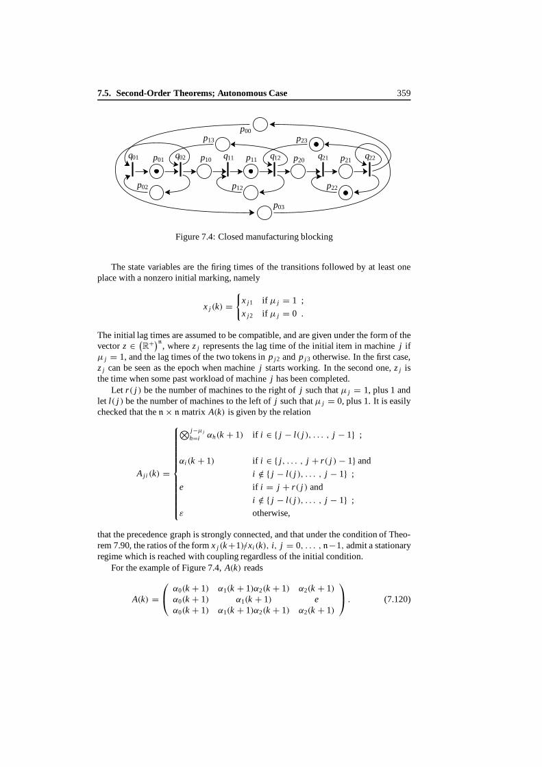
7.5. Second-Order T heorems; Autonomous Case 359
q02 p10 q11
p12
q12 p20
p23
q21
p22
q01 q22p01 p11 p21
p03
p00
p02
p13
Figure 7.4: Closed manufacturing blocking
The state variables are the firing times of the transitions followed by at least oneplacewith a nonzero initial marking, namely
x j (k) ={
x j1 if µ j = 1 ;
x j2 if µ j = 0 .
The initial lag times are assumed to be compatible, and are given under the form of thevectorz ∈ (R+)n, wherez j represents the lag time of the initial item in machinej ifµ j = 1, and the lag times of the two tokens inp j2 and p j3 otherwise. Inthe first case,z j can be seen as the epoch when machinej starts working. In the second one,z j isthe time when some past workload of machinej has been completed.
Let r( j ) be the number of machines to the right ofj suchthatµ j = 1, plus 1 andlet l( j ) be the number of machines to the left ofj suchthatµ j = 0, plus 1. It is easilychecked that then× n matrix A(k) is given by the relation
A ji (k) =
⊗ j−µ j
h=i αh(k + 1) if i ∈ { j − l( j ), . . . , j − 1} ;
αi (k + 1) if i ∈ { j, . . . , j + r( j )− 1} and
i /∈ { j − l( j ), . . . , j − 1} ;
e if i = j + r( j ) and
i /∈ { j − l( j ), . . . , j − 1} ;
ε otherwise,
that the precedence graph is strongly connected, and that under the condition of Theo-rem 7.90, the ratios of the formx j (k+1)◦/xi (k), i, j = 0, . . . , n−1, admit a stationaryregime which is reached with coupling regardless of the initial condition.
For the example of Figure 7.4,A(k) reads
A(k) =
α0(k + 1) α1(k + 1)α2(k + 1) α2(k + 1)α0(k + 1) α1(k + 1) eα0(k + 1) α1(k + 1)α2(k + 1) α2(k + 1)
. (7.120)

360 Synchronization and Linearity
Matrix A being positive, we can directly apply Theorems 7.90 and 7.93. The conditionP[B] > 0 is satisfied if the random variablesα j(k) are mutually independent and if oneof the distribution functionsS0 andS1 has an infinite support, whereS j(t) = P[α j ≤ t ],t ∈ R
+.
7.5.4.4 Coupling
The main result of this subsection is the following theorem.
Theorem 7.93 If there exists h� such that P[B] > 0, the stationary sequence {"◦θk}is the unique stationary solution of (7.98). For any initial condition x0, the sequence{δ(k; x0)} couples with this stationary sequence.
Proof Let C(k), k ≥ 1, be the event
C(k) = {A(k + 1)x(k + 1) = A·h� (k + 1)xh� (k + 1)} .
We first prove that on the eventC(k), the relation
δ(k + 1) = A·h� (k + 1)
A(k) (δh�·(k) ◦\e)(7.121)
holds. OnC(k), we have indeed
δ(k + 1) = A(k + 1)x(k + 1)
A(k)x(k)= A·h� (k + 1)xh� (k + 1)
A(k)x(k)
= A·h� (k + 1) (e◦/ (e◦/xh� (k + 1)))
A(k)x(k)= A·h� (k + 1)
A(k)x(k) (e◦/xh� (k + 1))
= A·h� (k + 1)
A(k) (x(k)◦/xh� (k + 1))= A·h� (k + 1)
A(k) (δh� ·(k) ◦\e).
Therefore, onC(k),
δ(k + 2) = A(k + 2)x(k + 2)
x(k + 2)= A(k + 2)
x(k + 2)
x(k + 2)
= A(k + 2)δ·1(k + 1)
δ·1(k + 1)= A(k + 2)
A·h� (k + 1)
A·h� (k + 1),
where the last relation follows from (7.121). This last formula shows that on theeventC(k), regardless ofx0,
δ(k + 2; x0) = φ(A(k + 1), A(k + 2)) , (7.122)
whereφ is a measurable function which we will not need in explicit form.If we can show that for allk, D◦θk ⊂ C(k), whereD is an event ofpositive prob-
ability, then Equation (7.122) implies thatδ(k)◦θ−k couples with a uniquely definedfinite stationary sequence. This result is a direct consequence of Borovkov’s renovat-ing events theorem (Theorem 7.107 shows thatC(k) is a renovating event of length 2).
7.5. Second-Order T heorems; Autonomous Case 361
The second stepof the proof consists in showing thatB◦θk ⊂ C(k). In order to do so,we first prove that
B ⊂{
Ae
Ah� ·≤ A◦θ·h�
A◦θ
}. (7.123)
The propertyA◦θ A = A◦θ·h� Ah� · implies thatA◦θ A (Ah� · ◦\e) = A◦θ·h� , which in turnimplies that A (Ah� · ◦\e) ≤ (A◦θ ◦\A◦θ·h� ), where we used the very definition of leftdivision in order to obtain the last implication. This immediately implies (7.123).
Weare now in a position to conclude the proof by showing that
B◦θk ⊂ C(k) . (7.124)
Inequality (7.109) implies
x(k + 1)
x(k + 1)= x(k + 1)
A(k)x(k)= δ(k)
A(k)≥ A(k)
A(k).
Therefore, for allh,xh(k + 1)
x(k + 1)≥ Ah· (k)
A(k),
or, equivalently,
x(k + 1)
xh(k + 1)≤ A(k)
e
Ah· (k). (7.125)
On the eventB◦θk
A(k + 1)A(k) = A·h� (k + 1)Ah� ·(k) .
By using (7.123) and (7.125), we therefore obtain that on this event,
x(k + 1)
xh� (k + 1)≤ A(k)
e
Ah� ·(k)≤ A·h� (k + 1)
A(k + 1).
From the very definition of left division, the last relation implies that
A(k + 1)x(k + 1)
xh� (k + 1)≤ A·h� (k + 1) ,
so that
A(k + 1)x(k + 1) ≤ A·h� (k + 1)xh� (k + 1) .
which concludes the proof of (7.124). Therefore, there exists a stationary sequence ofrenovating events of length 2. The coupling property is then a direct application ofBorovkov’s Theorem.

362 Synchronization and Linearity
7.5.5 Finiteness and Coupling inRmax; Strongly Connected Case
The assumptionsof this subsection are the same as in§7.5.4, except for the positivenessassumption which is replaced by the assumption that the precedence graph ofA has adeterministic topology (namely the entries which are equal toε with a positive proba-bility are a.s. equal toε) and is strongly connected. We also make the usual assumptionthat the diagonal entries are nonvanishing. Under these assumptions, the matrices
E(k)def= A(nk + n− 1)A(nk + n− 2) . . . A(nk + 1)A(nk) , k ∈ Z ,
are such that Ei j (k) ≥ e for all pairs(i, j ) (this follows from Remark 7.30 and fromthe fact thatE(k) = G(nk). In this subsection, it will also be assumed that the shift
�def= θn
is ergodic (the ergodicity ofθ does not grant the ergodicity ofθk, k > 1, in general).
Observe thatE(k) = E◦�k , whereEdef= E(0).
Let X (k) ∈ Rn be defined by the relation
X (k) = x(nk) , k ≥ 0 . (7.126)
It is easily checked from (7.92) that the state variablesX (k) satisfy the relation
X (0) = x(0) , X (k + 1) = E(k)X (k) , k ≥ 0 . (7.127)
Following our usual notation, we will stress the dependence on the initial condition
x0def= x(0) by writing X (k; x0) when needed.
Theorem 7.94 Under the assumption that there exists h� such that
P [E◦�·h� Eh� · = E◦θE ] > 0 , (7.128)
the ratios δ(k) = x(k + 1)◦/x(k) also admit a stationary regime {δ◦θk}. This stationaryregime is unique, integrable and directly reachable. Whatever the initial condition x0,δ(k; x0) couples with it in finite time.
Proof Under Assumption (7.128), the ratio processX (k + 1)◦/X (k) couples with astationary regime"◦�k , which is directly reachable (Theorems 7.90 and 7.93). There-fore, the equation
" = Ex
x(7.129)
has auniquesolution satisfying the conditionx1 = e. From the very definition, takingx asthe initial condition makes the ratios
"(k; x)def= x((k + 1)n; x)
x(kn; x)

7.5. Second-Order T heorems; Autonomous Case 363
stationary ink, and moreprecisely such that"(k; x) = "◦�k , k ≥ 0. Therefore, theratios x((k + 1)n+ 1; x)◦/x(kn+ 1; x) are stationary ink, ascanbeseenwhenwritingthemas
x((k + 1)n+ 1; x)
x(kn + 1; x)= A((k + 1)n)x((k + 1)n)
A(kn)x(kn)
= A((k + 1)n)x((k + 1)n)◦/x(kn)
A(kn)x(kn)
= A((k + 1)n)"(k, x)
A(kn)x(kn),
and when using the stationarity of"(k; x). But this ratio process is the one generatedby the event graph when taking{A(k)◦θ}k≥0 as the timing sequence, andy asthe initialcondition, wherey = x(1; x)◦/x1(1; x). In view of theuniqueness property mentionedin Theorem 7.93 we immediatelyobtain thatx(n+1; x)◦/x(1; x) = "◦θ . Sincey1 = e,this in turn implies thaty = x◦θ , owing to the uniqueness property mentioned inLemma7.85.
We show thatthe ratio processδ(k; x) satisfies (7.94). We have
δ(1; x) = A(1)x(1)
x(1)= A(1)
x(1)
x(1)
= A(1)x(1)◦/x1(1)
x(1)◦/x1(1)= A◦θ
x
x◦θ = Ax
x◦θ
= δ(0; x)◦θ , (7.130)
so thatδ(k; x) satisfies (7.94) fork = 1. In addition,δ(k) satisfies the equation
δ(k + 1) = A(k + 1)x(k + 1)
A(k)= A(k + 1)δ(k)
A(k).
From this relation and (7.130), we prove by an immediate induction thatδ(k) satisfies(7.94) for allk ≥ 0.
One proves in the same way that the coupling of the ratios"(k) with a uniquely de-fined stationary process implies the same property forδ(k). Theintegrability propertyfollows from the integrability ofx and of thefinite entries ofA andfrom the relationδ(0; x) = Ax◦/x .
Remark 7.95 If we replacen in (7.126) by another integern′, such that
• (G(n′k)i j ≥ e for all i, j = 1, . . . , n (this condition is satisfied for alln′ ≥ n);
• θn′ is ergodic,
then the whole construction is unchanged. As a consequence, whenever the variablesA associated withn do not satisfy the reachability and coupling conditions of Theo-rems 7.90 and 7.93, we still have the option to test this condition on the variablesA′
associated withn′.

364 Synchronization and Linearity
7.5.6 Finiteness and Coupling inRmax; General Case
The framework is the same as in§7.5.5, butA is not supposed to have a stronglyconnected precedence graph anymore. The notations concerning the decomposition ofthe precedence graph into m.s.c.s.’s are those of the end of§7.3.5. In particular, we willnumber the source subgraphs 1, . . . , N0 and the nonsource onesN0 + 1, . . . , N .
We know from§7.5.5 that the stationary regime of the ratio process of the sourcesubgraphs can be constructed using the techniques developed there. The only remain-ing problem consists in the construction of the stationary regime of nonsource sub-graphs.
Consider first the case when the reduced graph has a single source, namelyN0 = 1,and assume that itsatisfies the assumption of Theorem 7.94. Then we obtain from thistheorem that the ratiosx(1)(k+1)◦/x(1)(k) couple in finite time with a stationary, ergodicand integrable processδ(1)◦θk , which satisfies thepropertyE
[(δ(1))
ii
] = a(1), wherea(1) is the maximal Lyapunov exponent associated withA(1). The same technique asin the general nonautonomous case (see§7.4.4.5) allows us to prove the followingtheorem.
Theorem 7.96 If A(1) satisfies the assumptions of Theorem 7.94, and if the condition⊕Nn=2 a(n) < a(1) holds true, then a unique finite random matrix δ exists such that
the ratio process δ(k) = x(k + 1)◦/x(k) couples in finite time with the stationary andergodic process δ◦θk , regardless of the initial condition. If
⊕Nn=2 a(n) > a(1), let n0
be the first n ∈ {2, . . . , N} such that a(n) > a(1). Then all ratios of the form δ j i(k),j ∈ Vn0 , i ∈ Vm, m ∈ π+(n0) tend to∞ a.s. for all initial conditions.
Remark 7.97 Nothing general can be said with respect to the critical case, namelywhen⊕
n≥2 a(n) = a(1) (e.g. queuing theory).
Consider now the case when the reducedgraph has several sources, namelyN0 >
1. If the sources have different cycle times, it is clear that some of the ratios of theprocessesx j(k), j ∈ Vn , n = 1, . . . , N0, canneither be made stationary nor couplewith a stationary sequence. Even if all these m.s.c.s.’s have the Lyapunov exponents,nothing general can be said about the stationarity of the variablesδi j (k) for j ∈ Vn ,
i ∈ Vm, m, n = 1, . . . , N0, m = n, as exemplified inthe following simple situation.
Example 7.98 Consider a timed event graph with three recycled transitionsq1, q2 andt and five placesp1, p2, p′1, p′2 andr. Placepi (respectively r) is theplace associatedwith the recycling ofqi , i = 1, 2 (respectively t ) and p′i is the place connectingqi to t(see Figure 7.5). Within the terminology of Example 7.37, this system is ajoin queuewith one server (transitiont ) and with two sources (transitionsq1 andq2). This examplecan be seen as the simplest assembly problem in manufacturing: engines are producedby q1 and carbodies byq2, whereast is the assembly machine. With our terminology,we have two source m.s.c.s.’sGi , with Vi = {qi } andEi = (qi , qi), i = 1, 2, andonenonsource subgraphG3, with V3 = {t} andE3 = (t, t). Assume the holding times inr,p′1 and p′2 are zero and that the holding times inp1 and p2 are mutually independenti.i.d. sequences{α1(k)} and{α2(k)} with common meanλ. If the variablesα1(k) andα2(k) are deterministic, the ratiosx1(k+1)◦/x2(k) (with obvious notation) are stationary

7.5. Second-Order T heorems; Autonomous Case 365
t
q2
p2
p′1
p′2
r
q1
p1
Figure 7.5: Counterexample
and finite whatever the initial condition. However, if the two sequences are made ofexponentially distributed random variables with parameterλ, these ratios form anullrecurrent Markov chain onR which admits no invariant measure with finite mass, sothat theycannot be made stationary.
This example can also be formulated as a nonautonomous system with a two-dimensional input vector(u1(k), u2(k)) whenever we remove the recycling placepi
associated with transitionsqi , and replace it by an input functionui (k), i = 1, 2. Inthis formulation we see that in the exponential case (i.e.u1(k) andu2(k) are theepochsof two independent Poisson processes with the same intensity), the matricesU+(k) andU−(k) do not satisfy the assumptions of§7.4.4.1 (although the diagonal terms of thesematricesare stationary and integrable, the nondiagonal terms do not couple with finitestationary processes). We see that in this case, our second-order theorems do not apply.
7.5.7 Multiplicative Ergodic Theorems inRmax
We will limit ourselves to the case whenA is positive (see§7.5.4).
Theorem 7.99 If the event B = {ω | ∃h� : A◦θ A = A◦θ·h� Ah� ·} has a positive prob-ability, then there exists a unique finite eigenpair {λ, X }, with X1 = e and such thatAX = λX ◦θ . This eigenpair is integrable, and
E[λ] = a , (7.131)
where a is the maximal Lyapunov exponent of A. In addition, the following couplingproperty takes place: for all finite initial conditions x(0) = x0, with (x0)1 = e, thereexists a finite integer-valued random variable K such that, for all k ≥ K ,
x(k + 1; x0)
x(k; x0)=(λ
X ◦θX
)◦θk .
Proof Weknow from Theorem 7.90 that under the above assumptions, Equation (7.105)has a unique finite solution" for which (7.105) is satisfied with equality, and such that(7.104) has a solution. When specializing the formulæ of Theorem 7.79 to vectors andmatrices with entries inRmax as considered here, it is easily checked that whenever the

366 Synchronization and Linearity
subsolution" of (7.103) is finite and is a solution, then the super-eigenvalue inequalityof (7.105) becomes an eigenvalue equality, so that there exists a pair(λ, X) satisfyingthe eigenpair property (7.68).
First it iseasily checked that if(X, λ) is a finite eigenpair, then(AX)◦/X = (λX ◦θ)◦/Xis a solution of the ratio equation (7.113). Under the foregoing assumptions, this equa-tion has a unique solution". Sincethe equation" = (Ax)◦/x has a unique solutionxsuchthat x1 = e (Lemma 7.85), the eigenvectorX is uniquely defined if we decidethat X1 = e. The sameproperty holds forλ sinceλ(X ◦θ)◦/X = ". Property (7.131)follows from the relation
x(k + 1; X) = λ◦θk . . . λX ◦θk+1 ,
which implies that
(x1(k + 1; X))1/k =(
k⊗
h=0
λ◦θh
)1/k
.
The result follows immediately from the pointwise ergodic theorem and from Corol-lary 7.31.
7.6 Stationary Marking of Stochastic Event Graphs
In this section we consider a stochastic event graph, with all its transitions recycled,and where the places in the recycling all have positive holding times. We return to thenotation of conventional algebra.
Definition 7.100 (Stable place)A place of the event graph is said to be stable if thenumber of tokens in this place at time t (the marking at time t ), converges weakly to afinite random variable when time goes to∞. The event graph is said to be stable if allthe places are stable.
The aim of this section is to determine the conditions under which the event graph isstable and to construct the stationary regime of the marking process, under the usualstationarity and ergodicity on the holding times.
Remark 7.101 Let P0 be the subset of places connecting two transitions belongingto the same strongly connected subgraph, andP1 be the subset of places connectingtransitions which belong to no circuit. The marking of a place inP0 is bounded, andthe only places which can possibly have an infinite marking when time goes to∞ arethose ofP1 (see Chapter 2).
Pick some placepi in P and letq j = π(pi), andql = σ(pi ). Assume thatthereexists an initial conditionx0 suchthat x j(0; x0) = 0, and such that the ratiosx(k +1; x0)◦/x(k; x0) are stationary and ergodic (the conditions for such an initial conditionto exist are given in Theorems 7.67 and 7.96, respectively, for the nonautonomous andthe autonomous case). Since the sequence
b(k)def= x(k; x0)◦/x j (k; x0) , k ≥ 0 ,

7.6. Stationary Marking of Stochastic Event Graphs 367
is stationary and ergodic, it can be continued to a bi-infinite stationary and ergodic
sequence by the relationb(k) def= b◦θk , k ∈ Z, whereb = b(0). A similar continuationalsoholds for the sequence
d(k)def= δ j j (k; x0)
def= d◦θk , k ≥ 0 .
Because of the assumption thatq j is recycled and with positive holding times in therecycling,d > 0. Therefore, we can consider the sequence{d(k)} as the stationaryinter-event times of apoint process defined on(�,F,P, θ).
Definition 7.102 We define N as the marked point process on (�,F,P, θ) with inter-event times sequence {d(k)}k∈Z and with the R
|Q|-valued mark sequence{(bh(k))qh∈Q
}k∈Z
.
Namely, the k-th point of N is
t (k)def={
x j(k; x0) for k ≥ 0 ;∑−1h=k −d(k) for k < 0 ,
and its mark is {bh(k), qh ∈ Q}.The interarrival times and the marks beingθ-stationary, this point process is stationary(in its so-called Palm version). Owing to our assumptions,N has a finite intensity andno double points.
Let T (k) = (T1(k), . . . , Tn(k)), wheren = |Q|, be the sequence
Th(k)def= t (k)+ bh(k) , qh ∈ Q , k ∈ Z ,
and letN−i be the random variable
N−i =∑
k≤0
1{Tl(k+µi )>0} , (7.132)
whereql = σ(pi ). This variable is a.s. finite. Indeed,Tl (k) satisfies the relations
limk→∞
Tl (k)
k= c > 0 ,
wherec is a positiveconstant. Therefore{Tl (k)} is an increasing sequence such thatlimk→−∞ Tl (k) = −∞ a.s. Hence there exists a finite integer-valued random vari-ableH suchthatTl (k) ≤ 0 for all k ≤ −H .
Theorem 7.103Under the assumptions of Theorem 7.67 (respectively 7.96), if a(n) <
u, for all n = 1, . . . , N , (respectively a(n) < a(1), for all n = 2, . . . , N), whereN denotes the number of m.s.c.s.’s of the event graph, then the event graph is stablewhatever the initial condition, and the marking in place pi at arrival epochs convergesweakly to the random variable N−
i . Conversely, if n0 is the first n = 1, . . . , N , suchthat a{n} > u (respectively the first n = 2, . . . , N, such that a(n) > a(n)), then theplaces connecting the transitions of Q m ∪I (respectively Q m), m < n0, to transitionsof Q n0 are all unstable whatever the initial condition.

368 Synchronization and Linearity
Proof Let N−i (k) be the number of tokens inpi just after timex j (k), k ≥ 1, where
q j = π(pi ). From (2.42) we obtain that
N−i (k) =
k+µi∑
h=1
1{xl(h)>x j (k)} =k+µi∑
h=0
1{xl(k+µi−h)>x j (k)} . (7.133)
We first prove the last assertion of the theorem. Assume thatpi is the place connectinga transition of Q m ∪I (respectively Q m) to atransition ofQ n0 . Owing tothe propertythat
limk
xl (k) − x j (k)
k= a(n0) − u > 0 ,
(respectively lim
k
xl (k) − x j (k)
k= a(n0) − a(1) > 0
),
and to the increasingness of the sequences{xl (k)} and{x j (k)}, we obtain that, for allH , thereexits K such that, for all k ≥ K andh = 1, . . . , H, xl(k − h)− x j(k) ≥ 0.It follows immediately from this thatN−
i (k) ≥ H for k ≥ K . Therefore, N−i (k) tends
to∞ a.s.We now prove the first part. Weknow that the ratios ofxh(k), qh ∈ Q, couple with
their stationary regime in a finite random timeK . This implies that for all fixed h, thesequence{xl (k + µi − h)− x j (k)} couples with a stationary process. More precisely,for all k ≥ K + h, andh > µi , xl(k + µi − h)− x j (k) = −ρl(µi − h)◦θk , where
ρl(k)def=
k∑
n=−1
d◦θn − bl◦θ−k = Tj (0)− Tl (k) , k < 0 ,
in view of the uniqueness of the stationary regimes of the ratios. Define
H = inf{k | k ≥ K , xl(h)− x j (k) < 0 , ∀h = 1, . . . , K
}.
This H is a.s. finite sinceK is finite andx j (k) tends to∞ a.s. Therefore,
N−i (k) =
∑
1≤h≤k−K
1{x(k+µi−h)l−x j (k)>0} =∑
1≤h≤k−K
1{−ρl(µi−h)◦θ k>0} ,
for all k ≥ H . On theother hand,
N−i ◦θ
k =∑
0≤h
1{Tl(k+µi−h)−Tj(k)>0} =∑
0≤h
1{−ρl(µi−h)◦θ k>0} .
SinceTj (k) tends to∞ ask goes to∞, weobtain that there exists anL suchthat
∑
k−h≤K
1{Tl(k+µi−h)−Tj(k)>0} = 0 ,
for all k ≥ L . Therefore, N−i (k) = N−
i ◦θk for k ≥ max(H, L), and the stationary
regime of the marking process is reached with coupling, regardless of the initial condi-tion.

7.7. Appendix on Ergodic Theorems 369
Remark 7.104 This stationary regime is unique, owing to the uniqueness of the sta-tionary regime of the ratio process.
Remark 7.105 The preceding construction gives the Palm probability of the numberof tokens inpi at arrival epochs. The stationary distribution of the number of tokens inpi in ‘continuous time’ is then obtained via the Palm inversion formula (see [5, p. 17]).
7.7 Appendix on Ergodic Theorems
The aim of this section is to state in a concise form a few basic ergodic theorems(in conventional algebra) which are either used or referred to in this chapter. Thebasic data are a probability space(�,F,P) on which ashift operatorθ is defined (seeDefinition 7.2). This shift is assumed to be stationary and ergodic.
Theorem 7.106 (Kingman’s subadditive ergodic theorem)Let ξm,n, m > n ∈ Z bean integrable random process on (�,F,P) such that
ξm,m+p = ξ0,p◦θm , ∀m ∈ Z , ∀p > 0 (stationarity) ,
andξm,n ≤ ξm,p + ξp,n , ∀m < p < n (subadditivity) .
Assume in addition that there exists a positive constant A such that E[ξ0,p] ≥ −Ap,for all p > 0. Then there exists a constant γ such that the following two equationshold:
limp→∞
ξ0,p
p= γ a.s., lim
p→∞E[ξ0,p]
p= γ .
For theproof, see [75], [76].
Theorem 7.107 (Borovkov’s renovating events theorem)Let {u(k)} be a θ-station-ary R
n-valued sequence of random variables defined on (�,F,P). Let {x(k)} be theR
K -valued sequence of random variables defined by the recurrence relation
x(k + 1) = a(x(k), u(k)) , k ≥ 0 , (7.134)
where a is a continuous mapping RK × R
n → RK , and by the random initial condi-
tion x(0). The event A(k) ∈ F is said to be a renovating event of length m ≥ 1 and ofassociated function φ : R
mn → RK if, on A(k), the relation
x(k + m) = φ (u(k), . . . , u(k +m − 1))
holds. If the random process x(k) admits a sequence {A(k)} of renovating events,all of length m and associated function φ, such that A(k) = A(0)◦θk , ∀k ≥ 0, andP[A(0)] > 0, then, the sequence {x(k)◦θ−k} converges a.s. to a finite random variablez, which does not depend upon the initial condition x(0). The sequence {z◦θk} is afinite solution of (7.134), and the sequence {x(k)} couples with it in finite time for allfinite initial conditions.

370 Synchronization and Linearity
For theproof, see [26], [6].For anymatrix A, let |A| denote its operator norm, namely
|A| = sup‖x‖=1
‖Ax‖ ,
where‖x‖ denotes the Euclidean norm of vectorx .
Theorem 7.108 (Oseledec¸ ’s multi plicative ergodic theorem) Let {A(k)} be a sequenceof n × n random matrices with nonnegative entries, defined on the probability space(�,F,P). Assume that A(k) = A(0)◦θk , for all k ∈ Z, and that
E[max(log(|A(0)|), 0)
]<∞ .
Then there exists a constant γ (the maximal Lyapunov exponent of the sequence) suchthat
limk→∞
1
klog(|A(k) . . . A(1)|) = γ , a.s.
In addition, there exists a random eigenspace V (ω) of dimension d constant, d ≤ n,such that A(1)V = V ◦θ and such that for all random vectors x in V ,
limk→∞
1
klog(‖A(k) . . . A(1)x‖) = γ , a.s.
Whenever d = 1, there exists an eigenpair {λ, X } such that A(0)X = λX ◦θ andE[λ] = γ .
In fact, Oseledec¸’s Theorem gives the existence of othereigenvalues as well. Our state-mentof this theorem is limited to the maximal eigenvalue and its associated eigenspace(see [106], [45]).
7.8 Notes
The preliminary example of§7.2 was first analyzed by R.M. Loynes in 1962 [87]. The prob-abilistic formalism introduced in§7.2 is that developed for queues by P. Br´emaud and one ofthe coauthors in [6]. The existence of Lyapunov exponents for products of random matrices ofRmax was first proved by J.E. Cohen, in the case of matrices with nonε entries, inSubadditivity,generalized product of random matrices and operations research, SIAM Review, volume 30,number 1, pages 69–86, 1988. The extension of this result to reducible matrices, and the sec-tions on the relationship between stochastic event graphs andRmax-multiplicative ergodic theory(§7.3–7.6) are mainly basedon [11], [13]. As to the writing of thisbook, this approach providesa more or less systematic way for analyzing nonautonomous systems. The situation is somewhatless satisfactory in the autonomous case: in particular, only the case when the eigenspace associ-ated with the maximal exponent has dimension 1 was considered. This practically covers caseswith ‘sufficiently random’ entries ofA, as shownby the results of §7.5; however, we know fromthe analysis of Chapter 3 that an eigenspace of dimension 1 is rarely sufficient to handle the caseof deterministic systems. Autonomous deterministic systems can fortunately be addressed viathe spectral methods of Chapter 3. However, some systems are neither deterministic nor random

7.8. Notes 371
enough to satisfy the conditions of §7.4. Filling up this ‘theoretical gap’ between purely de-terministic and sufficiently random systems is clearly tantamount to understanding the structureof the eigenspace associated with the maximal exponent when this eigenspace is of dimensiongreater than 1.

372 Synchronization and Linearity

Chapter 8
Computational Issues in StochasticEvent Graphs
8.1 Introduction
This chapter gathers miscellaneous resultspertaining to the computation of the cycletimesand the stationary regimes of stochastic event graphs. The existence and unique-nessof these two quantities are discussed in Chapter 7: the cycle time of a stochasticevent graph is the maximal Lyapunov exponent associated with the matricesA(k) ofits standard equation, and stationary regimes correspond to stochastic eigenpairs ofA.
Section 8.2 focuses on monotonicity properties of daters and counters consideredasfunctions of the data (e.g. firing and holding times, initial marking, topology of thegraph, etc.). These results lead to the derivation of a lower bound for the cycle time,which is based on the results of Chapter 3 concerning the deterministic case. It is alsoshown that the throughput is a concave function of the initial marking, provided thatthe firing andholding times satisfy appropriate statistical properties.
Section 8.3 is concerned with the relationship between stochastic event graphs anda class of age-dependent branching processes. Large deviation techniques are used toprovide an estimate for the cycle time, which is also shown to be an upper bound.
The last section contains miscellaneous computational results which can be ob-tained in the Markovian case. Whenever the firing and the holding times have discretedistribution functions with finite support, simple sufficient conditions for the ratio pro-cess to have a finite state space Markov chain structure are given. In the continuousand infinite support case, partial results on functional equations satisfied by the station-ary distribution functions are provided. These results are then used for computing thedistribution of the stationary regime.
The sections of this chapter can be read (almost) independently. Each section hasits own prerequisites: basic properties of stochastic orders for§8.2 (see [123]); notionsof branching processes and of large deviations ([3]) in§8.3; elementary Markov chaintheory in§8.4. Throughout the whole chapter, the scalar dioid of reference isRmax,unless otherwise specified.
373
374 Synchronization and Linearity
8.2 Monotonicity Properties
8.2.1 Notation for Stochastic Ordering
Let x andx† beRn-valued random variables. Three classical stochastic ordering rela-
tions betweenx andx† will be considered in this section.
Notation 8.1
Stochastic ordering≤st: x ≤st x† if E[ f (x)] ≤ E[ f (x†)], for all nondecreasingfunctions f : R
n → R.
Convex ordering ≤cx: x ≤cx x† if E[ f (x)] ≤ E[ f (x†)], for all convex functionsf : R
n → R.
Increasing convex ordering≤icx: x ≤icx x† if E[ f (x)] ≤ E[ f (x†)], for all convexand nondecreasing functionsf : R
n → R.
Let x = {x(1), . . . , x(k), . . . } (respectively x(·) = x(t), t ∈ R+) and
x† = {x†(1), . . . , x†(k), . . . }
(respectively x†(·) = {x†(t)}t∈R+ ) be twoRn-valued stochastic sequences (respectively
processes) definedon the probability space(�,F,P). The sequencex† is said to dom-inatex (respectively theprocessx†(·) dominatesx(·)) for one of the above orderingrelations, say≤st, which isdenotedx ≤st x† (respectively x(·) ≤st x†(·)), if all corre-sponding finite dimensional distributions compare for this ordering.
For basic properties of these orderings, see§8.5.
8.2.2 Monotonicity Table for Stochastic Event Graphs
The basic model of this section is a live autonomous event graph, where all transitionsare assumed to be recycled. The nonautonomous case leads to similar results andwill not be considered in this chapter. Thenotation and basic definitions concerningstochastic event graphs are those of Chapter 2 and Chapter 7. The following concisenotation will be used:
Data
Firing times: β(k) denotes the vectorβ j (k), j = 1, . . . , |Q|, andβ the se-quence{β(k)}.
Holding times: α(k) denotes the vectorαi (k), i = 1, . . . , |P|, andα the se-quence{α(k)}.
Timing sequence: η(k) denotes the vector(β(k), α(k)) andη the sequence{η(k)}.Init ial marking: µ denotes the vectorµi , i = 1 . . . , |P|.

8.2. Monotonicity Properties 375
State Variables With each dater sequence{x j (k)}k∈N we associate theN-valued counterfunctionx j(t), t ∈ R
+, defined by the relation
x j(t) = sup{k | x j (k) ≤ t} .
Daters: x(k) denotes the vectorx j(k), j = 1, . . . |Q|, andx the sequence{x(k)}.Counters: x(t) denotes the vectorx j (t), j = 1, . . . |Q|, t ∈ R, andx(·) the
functionx(t).
The aim of the following sections is to prove various monotonicity properties of thestate variables and of their asymptotic characteristics considered as functions of thedata. By asymptotic characteristics, we mean the cycle timea of the event graph andits (conventional) inverseτ , the throughput. A typical question is as follows: if onereplaces one of the data, sayµ or β, by µ† or β† respectively, where the new dataare greater than the initial ones for some partial ordering, what result do we obtain onthe various state variables? The main properties along these lines are summarized inTable 8.1. The reader should refer to the following subsections in order to obtain thespecific assumptions under which the reported monotonicity properties hold. These as-sumptions are not always the most general ones under which these properties hold. Forinstance, we have tried to avoid the intricate issues associated with the initial condi-tions by choosing assumptions leading to short proofs, although most of the propertiesof the table extend to more general initial conditions.
Table 8.1: Monotonicity of the state variables
Data Variation Daters Cycle Counters Throughput
of data time
µ µ ≤ µ† x ≥ x† a ≥ a† x(·) ≤ x†(·) τ ≤ τ †
P ⊂ P†
G Q ⊂ Q† x ≤ x† a ≤ a† x(·) ≥ x†(·) τ ≥ τ †
E ⊂ E†
η ≤st η† x ≤st x† a ≤ a† x(·) ≥st x†(·) τ ≥ τ †
η η ≤cx η† x ≤icx x† a ≤ a† τ ≥ τ †
η ≤icx η† x ≤icx x† a ≤ a† τ ≥ τ †
8.2.3 Properties of Daters
8.2.3.1 Stochastic Monotonicity
Monotonicity wi th respect to the Timing Sequence In this paragraph, we assumethat the entrance times are all equal toe (see Remark 2.75). Letη† be another tim-ing sequence associated with the same event graph (i.e. the topology and the initial

376 Synchronization and Linearity
marking of the event graph are unchanged and each timing variable is replaced by thecorresponding dagger variable) and letx† bethe resulting daters. We first compare thesequencesx† andx , whenever the timing sequences can be compared for some integralordering.
Theorem 8.2 If η ≤st η†, then x ≤st x†.
Proof The initial conditionx(0) is untouched by the transformation of the variables,in view of the definition given in Remark 2.75. The matricesA(k) in (2.31) are nonde-creasing functions of the variablesα, β (seeEquations (2.15), (2.28) and the definitionof A(k)). Therefore, from (8.40), we obtain that
{x(0), A(0), A(1), . . . } ≤st {x†(0), A†(0), A†(1), . . . } .
We now use the canonical representation (2.31) to represent the evolution equations ofinterest as recursions of the type (8.43), where the mappinga is coordinatewise non-decreasing and such that the sequences defined in (8.44) satisfy the relation{ξ(k)} ≤st
{ξ †(k)}. Theproof is then concluded from Theorem 8.60.
In the next theorem, the timing variables are assumed to be integrable.
Theorem 8.3 If η ≤icx η†, then x ≤icx x†.
Proof The entries of matricesA(k), k ≥ 1, arenondecreasing and convex functions ofthe variablesα, β. So, the assumptionη ≤icx η† and (8.41) imply that
{x(0), A(0), A(1), . . . } ≤icx {x†(0), A†(0), A†(1), . . . } .
Since the mappinga of the preceding proof isnondecreasing and convex, the resultimmediately followsfrom Theorem 8.62.
Remark 8.4 Assume thatthe holding and firing times are all integrable. Then, itfollows from (8.42) that the ‘deterministic version’ of the event graph�, with firingtimesβ j (k) = E
[β j (k)]
andholding timesαi (k) = E [αi (k)], leads to a sequence ofdaters{x(k)} which is alower bound of{x(k)} in the≤icx sense. Inparticular, sincethe daters are integrable under these assumptions, it follows from Lemma 8.59 that forall k ≥ 1 andq j ∈ Q, E
[x j (k)] ≥ x j (k).
Example 8.5 For example, by applying Theorem 8.3 to the cyclic queuing networkwith finite buffers of Example 7.92, one obtains that the departure times from thequeues are≤icx-nondecreasing functions of the service times.
Monotonicity wi th respect to the Initial Marking Here, thediscussion will be lim-ited to the case when all initial lag times are equal toe (which is a compatible initialcondition). It will be convenient to use (2.19) as the basic evolution equation. Underourassumption on the initial lag times, this equation reads
x j(k) =⊕
{i∈πq ( j)|k>µi }βπ p (i)(k − µi )αi (k)xπ p (i)(k − µi )⊕ e , (8.1)

8.2. Monotonicity Properties 377
for k ≥ 1, wherex j (k) = ε if k ≤ 0. Consider the same event graph as above, but withthe initial markingµ†
i , pi ∈ P, in place ofµi , and let{x†(k)} denote the correspondingdater sequence.
Theorem 8.6 Under the assumption that all the initial lag times are equal to e, ifµi ≤ µ
†i , ∀pi ∈ P, then the coordinatewise inequality x ≥ x† holds.
Proof Owing to the assumption that all transitions are recycled and to the precedingconvention concerningthe continuation ofx(k) for k ≤ 0, it is easy to check that
x j(k) ≥ β j (k − 1)x j (k − 1) , ∀ j = 1, . . . , n, k ∈ Z .
Thereforex j(k) ≥ x j(k − 1) , ∀ j = 1, . . . , n, k ∈ Z ,
and
β j (k)x j (k) ≥ β j (k − 1)x j (k − 1) , ∀ j = 1, . . . , n, k ∈ Z . (8.2)
We prove thatx j(k) ≤ x†j (k) for all j = 1, . . . , n, andk ≥ 1. The proof is by induction
on ( j, k). Sincethe eventgraph is assumed to be live, the numbering of the transitionscan be chosen in such a way that for all( j, k), j = 1, . . . , n, k ≥ 1, the variablesxi (l)which are found at the right-hand side of (8.1) are always such that eitherl < k orl = k, but i < j . Therefore, there exists a way of numbering the transitions such thatthe datersx j(k) can be computed recursively in the order
x1(1), x2(1), . . . , xn(1), x1(2), . . . , xn(2), . . . , x1(k), . . . , xn(k), . . . .
Assume thatthe property holds up to( j, k) excluding this point (it holds for(1, 1)since with our assumptions, we necessarily havex1(1) = x†
1(1) = e). Then, we have
x†j (k) =
⊕
{i∈πq ( j)|k>µ†i }βπ p (i)(k − µ
†i )αi (k)x
†π p (i)(k − µ
†i )⊕ e
≤⊕
{i∈πq ( j)|k>µ†i }βπ p (i)(k − µi )αi (k)x
†π p (i)(k − µi )⊕ e
≤⊕
{i∈πq ( j)|k>µ†i }βπ p (i)(k − µi )αi (k)xπ p (i)(k − µi )⊕ e
≤⊕
{i∈πq ( j)|k>µi }βπ p (i)(k − µi )αi (k)xπ p (i)(k − µi )⊕ e
= x j(k) ,
where we successively used the monotonicity property (8.2), the induction assumption,and finally the fact that we sum up with respect to a larger set.
Example 8.7Asanapplication of this result, one obtains the monotonicityof departuretimesin closed cyclic networks with blocking, as a function of the population and thebuffersizes.

378 Synchronization and Linearity
Stochastic Monotonicitywith respect to the Topology Consider two event graphswith associated graphs� = ((P ∪Q), E) and�† = ((P† ∪Q†), E†), where
P ⊆ P† , Q ⊆ Q† , E ⊆ E† . (8.3)
The eventgraph�† is such that the initial marking, the initial lag times, the firing andholding times of those places and transitions which belong both to� and�† are thesame. Letx† denote the sequence of daters of�†, and [x†] the restriction of x† to theset of transitions which belong toQ andQ†.
Theorem 8.8 Under the foregoing assumptions, x ≤ x† coordinatewise.
Proof The proof is based on Equation (2.19) and is again by induction on( j, k).Assume that the propertyxi(l) ≤ x†
i (l) holds up to( j, k) excluding this point. Thepoint (1, 1) is not necessarily the first one to compute in the total order associated with�†, but we are sure that all the places present in� precedingq1 are present in�†
too, and with the same number of initial tokens and the same lag times, so that theproperty necessarily holds for (1,1). Then, denotingπ† the predecessor function in�†,we obtain the following relation for allq j ∈ Q:
x†j (k) =
⊕
{i∈π†,q ( j)|k>µ†i }β†π†,p (i)(k − µ
†i )α
†i (k)x
†π†,p (i)(k − µ
†i )
⊕⊕
{i∈π†,q ( j)|k≤µ†i }w
†i (k)
≥⊕
{i∈πq ( j)|k>µ†i }β†π p (i)(k − µ
†i )α
†i (k)x
†π p (i)(k − µ
†i )
⊕⊕
{i∈πq ( j)|k≤µ†i }w
†i (k)
=⊕
{i∈πq ( j)|k>µi }βπ p (i)(k − µi )αi (k)x
†π p (i)(k − µi )
⊕⊕
{i∈πq ( j)|k≤µi }wi(k)
≥⊕
{i∈πq ( j)|k>µi }βπ p (i)(k − µi )αi (k)xπ p (i)(k − µi )
⊕⊕
{i∈πq ( j)|k≤µi }wi(k)
= x j (k) ,
where we successively used the assumptions (8.3), the assumption that the initial con-dition and the firing and holding times of the nodes of� ∩ �† are the same, and finallythe induction assumption.

8.2. Monotonicity Properties 379
8.2.4 Properties of Counters
In this subsection we assume that tokens incur no holding times in places (so that theonly timing variables come from the firing times of the transitions) and that there is atmostone place between two subsequent transitionsqi andq j , which will be denoted( j, i), with initial markingµ( j, i) ∈ N. It will also be assumed that the initial lagtimes are all equal toe (which leads to a compatible initial condition). Under theseassumptions, the evolution equation (2.19) in Chapter 2 reads
x j(k) =⊕
i∈p( j)
βi (k − µ( j, i)) xi(k − µ( j, i)) ⊕ e , k ≥ 1 ,
with initial conditionx j(k) = ε for all k ≤ 0. In this relation,p( j )def= π p(πq( j )).
8.2.4.1 Evolution Equations
Let x j(t) (respectively y j(t)) denote thenumber of firingswhich transitionj initiated(respectively completed) by timet, t ∈ R
+. Without loss of generality, we assume thatbothx j (t) andy j(t) are right continuous.
Remark 8.9 The mappingsx j (k) : N → R andx j(t) : R → N are related by theformulae
x j (t) = sup{k | x j (k) ≤ t} , (8.4)
x j(k) = inf{t | x j (t) ≥ k
}. (8.5)
When using thedefinitions of§4.4, we see that the isotone and l.s.c. mappingx j(k) :N → R admits the u.s.c. mappingx j (t) : R → N asits residual; similarly, the isotoneand u.s.c. mappingx j(t) : R → N admits the l.s.c. mappingx j(k) : N→ R asits dualresidual.
In this subsection it is assumed that the firing times are all strictly positive.
Theorem 8.10 The random variables x j (t) and y j(t), 1 ≤ j ≤ n, t ≥ 0, satisfy thefollowing evolution equations:
x j (t) = mini∈p( j)
(yi (t)+ µ( j, i)) , (8.6)
y j (t) =∫ t
01{β j (x j (u))≤t−u} x j(du) , (8.7)
where, for all j = 1, . . . , n, y j (0) = 0 and x j (t) = 0, ∀t < 0.
Proof By time t , transition j initiated exactly as many firings as the minimum overi ∈ p( j ) of the number of tokens which entered place( j, i) by time t (includingthe initial tokens). Since a place is preceded by exactly one transition, thenumber oftokens which entered place( j, i) by t equalsµ( j, i) plus the number of firings which

380 Synchronization and Linearity
transitioni completed by timet . The Stieljes integral in (8.7) is a compact way ofwriting the sum
∞∑
k=0
1{x j (k)+β j (k)≤t} .
In the deterministic case, (8.7) takes the simpler formy j(t) = x j (t − β j ), whichleadsbackto the following familiar result.
Corollary 8.11 If the firing times are deterministic (i.e. β j (k) = β j ), then (8.6) and(8.7) reduce to the Rmax equation
x j (t) =∧
i∈p( j)
µ( j, i)xi (t − βi ) , (8.8)
where xi(t) = e for t < 0.
8.2.4.2 Stochastic Monotonicity
From (8.4), one obtains that for any fixedn-tuple t1 < . . . < tn in R+, the vector
(x(t1), . . . , x(tn)) is a nonincreasing function ofx . Therefore, each≤st-monotonicityproperty of the sequencex with respect to≤st yields a dual stochastic monotonicityproperty ofx(·) (see Table 8.1).
8.2.4.3 Concavity with respect to the Initial Marking
Throughout this subsection it is assumed that the sequences{β j (k)}k are mutually in-dependent inj .
Theorem 8.12 If the random variables β j (k) are i.i.d., with exponential distributionof parameter λ j , then, for any t ≥ 0, and any 1 ≤ j ≤ n, x j (t) and y j (t) arestochastically increasing and concave (see Definition 8.63) in the initial marking µ ∈N|E|.
Proof Let {b j(n)}∞n=1, 1 ≤ j ≤ n, be mutually independent sequences of i.i.d.random variables whereb j(n) is exponentially distributed with parameterλ j . Lett0, t1, t2, . . . , tn, . . . be the times defined byt0 = 0 and
tn = tn−1 + min1≤ j≤n
b j(n) , n ≥ 1 ,
and letχ j (n) be the indicator function
χ j (n) = 1{tn=tn−1+b j (n)} .
Let �† be an event graph with the same topology and initial marking as�, and with thefollowing dynamics (which differs from the dynamics defined in Chapter 2): in�†, forall transitions j enabled at time t+n , the residual firing time of j at time t+n (namely thetime whichelapses betweentn and the completion of the ongoing firing of transitionj )is resampled andtaken equal tob j(n + 1).

8.2. Monotonicity Properties 381
• If χ j (n+1) = 1 for a transition j which belongs to the set of transitions enabledat time t+n in �†, then transition j is fired at timet−n+1, whichdefines a new set ofenabled transitions at timet+n+1 by the usual token production and consumptionrule.
• If χ j ′(n+1) = 1 for a transition j ′ which isnot enabled at time t+n in �†, nothinghappens as far as the marking process is concerned.
For each transition j which is enabled att+n+1 (either still ongoing or newly enabled),one resamples anew residual firing time equal tob j(n + 2), etc.
For �† definedabove, it is easily checked that the variablesx†j (t) (respectively
y†j (t)) representing the number of firings of transitionj initiated (respectively com-pleted) bytime t , satisfy the following equations:
y†j (0) = 0 ,
y†j (t) = y†j (tn)def= Y j (n) , tn ≤ t < tn+1 ,
x†j (t) = x†
j (tn)def= X j(n) , tn ≤ t < tn+1 , (8.9)
and
X j(n) =∧
i∈p( j)
(Yi (n)µ(i, j )) , (8.10)
Yi (n + 1) = (Yi (n)χi (n + 1)) ∧ Xi(n) , (8.11)
for all n = 0, 1, 2, . . . . Equation (8.10) is obtained in the same way as (8.6). In orderto obtain Equation (8.11) observe that
Yi (n + 1) ≤ Yi (n)+ χi (n + 1)
(equality holds if i is enabled at timet+n ), and
i enabled att+n ⇔ Yi(n) = Xi (n)− 1 ;i not enabled att+n ⇔ Yi(n) = Xi (n)
(because of the recycling of transition i, there is at most one uncompleted firing ini-tiated on this transition). Equation (8.11) is obtained from the following observation:either i is not enabled att+n , and the smaller term in theright-hand side of (8.11) isXi (n), or i is enabled andYi (n + 1) = Yi (n)+ χi (n + 1).
It is now immediate to prove by induction that, for all realizations of the randomvariablesb j(k), the state variablesX j (n) andY j (n), 1 ≤ j ≤ n, n ≥ 0, are nonde-
creasing and concave functions ofµ. The variablesx†j (t) and y†j (t) satisfy the same
property in view of (8.9) and of the fact that the variablesb(n) do not depend uponµ.Thus, ifµ andµ′ are initial markings such thatν = ρµ+ (1−ρ)µ′ is in N
|P| for somereal parameterρ ∈ (0, 1), we have, with obvious notations,
x†j (t ; ν) ≥ ρx†
j (t ;µ)+ (1− ρ)x†j (t ;µ′) ,

382 Synchronization and Linearity
for all ω, t and j , with a similar result fory.Owing to the memoryless property of the exponential distribution, the countersx†
j (t)
andy†j (t), 1 ≤ j ≤ n, are equal in distribution tox j (t) andy j(t), respectively. There-fore, under appropriate integrability assumptions,
E[x j(t ; ν)
] ≥ ρE[x j(t ;µ)
] + (1− ρ)E[x j(t ;µ′)
],
so thatx j (t) (andy j(t)) are stochastically increasing and concave inµ indeed.
We now define the class of PERT-exponential distribution functions, which willallow us to generalize Theorem 8.12.
Definition 8.13 (Stochastic PERT graph)A stochastic PERT graph is a connected,directed, acyclic and weighted graph with a single source node and a single sink node,where the weights are random variables associated with nodes.
There is no loss of generality in the assumption that only nodes are weighted; onecanequivalently weight arcs or both arcs and nodes. In any weighted directed acyclicgraph, the path with maximal weight is called thecritical path.
Definition 8.14 (PERT-exponential distribution function) The distribution functionof a random variable X is of PERT-exponential type if X can be expressed as the weightof the critical path of a stochastic PERT graph G where the weights of the nodes aremutually independent random variables with exponential distribution functions.
Notation 8.15 Such a distribution function will be denotedF(G, λ), whereG is theunderlying graph andλ = (λ1, . . . , λ|G|), whereλi is the parameter of the exponentialdistribution associated with nodei in G (we will assume that the source and sink nodesarenumbered 1 and|G| respectively).
Definition 8.16 (Log-concave functions)A function f : Rn → R
+ is log-concaveiffor all x, y ∈ R
n and 0 < ρ < 1, the inequality f (ρx + (1− ρ)y) ≥ f ρ(x) f (1−ρ)(y)holds.
Theorem 8.17 PERT-exponential distribution functions are log-concave.
For a proof, see [10].
Theorem 8.18 If the firing times of a stochastic event graph � are all mutually in-dependent, and if for all transitions j , 1 ≤ j ≤ n, the firing times β j (k) are i.i.d.random variables with PERT-exponential distribution function, then, for all t ≥ 0, andall 1 ≤ j ≤ n, x j(t) and y j(t) are stochastically increasing and concave in the initialmarking µ.
Proof Let F(G j , λ j) be the distribution function associated with transitionq j of �.
Let n j def= |G j |.For all j , considerthe stochastic event graph� j defined from the PERT graphG j
as follows: with eachnodei of G j , we associate a transitionq ji in � j ; similarly, to

8.2. Monotonicity Properties 383
each arc inG j corresponds an arc in� j and aplaceonthis arc. The initial marking andtheholdingtimes of each of these places are zero. The firing times of transition q j
i arei.i.d. random variables with exponential distribution function of parameterλ
ji .
We now construct a stochastic event graph�† which is defined from� and� j, j =1, . . . , n, as follows: for all j , 1≤ j ≤ n, we ‘replace’ transition q j in � by the eventgraph� j ; all the places of� are kept in�† together with their initial marking; wetakeπ†(q j
1 ) equal to the setπ(q j) andσ †(q jn j ) equal toσ(q j ), for all j = 1, . . . , n;
finally, we add a new feedback arc from transitionq jn j to transitionq j
1, for all j ; theplaceon this arc is assigned one token in its initial marking and zero holding andlag times. This transformation is depicted in Figure 8.1. If the number of firings
qjnj
� �j
qj qjn j
qj1qj
1
�†
Figure 8.1: Transformation of an event graph with PERT-exponential firing times
of transitionq j1 initiated (respectively completed) by timet in �† is denotedx†
j,1(t)
(respectively y†j,1(t)), then an immediate coupling argument shows that
x j(t) =st x†j,1(t) , y j (t) =st y†j,1(t) , ∀t ≥ 0 , ∀1≤ j ≤ n ,
where thesymbol=st denotes equivalence in law.Let µ† denote the initial marking of �†. Applying Theorem 8.12 to�† implies
that for all t ≥ 0, and all 1≤ j ≤ n, x†j,1(t) and y†j,1(t) are stochastically increasing
and concave in the initial marking µ† ∈ N|Q† |. Consequently,x j (t) and y j (t) are
stochastically increasing and concave in the initial markingµ ∈ N|Q|, t ≥ 0, 1≤ j ≤
n.
Remark 8.19 It is easy to see that PERT-exponential distribution functions includeErlangdistribution functions asa special case. Therefore one can approximate stepfunctions with PERT-exponential distributions. Theorem 8.18 can be shown to holdwhensomeof the firing times are deterministic, by using some adequate limiting argu-ment. In the particular case when all firing times are deterministic and integer-valued,one can also prove the concavity of the counters by an immediate induction argumentbased on Formula (8.8).
8.2.5 Properties of Cycle Times
Throughout this subsection we suppose that the sequences of holding and firing timessatisfy the joint stationary and ergodic assumptions of§7.3 and are integrable. We also

384 Synchronization and Linearity
assume that the event graph under consideration is strongly connected and its cycletime (see§7.3.4) is denoteda, so that the following a.s. limits hold:
limk→∞∣∣(x(k))1/k
∣∣⊕ = lim
k→∞E[|x(k)|⊕
]1/k = a a.s., (8.12)
provided that the initial lag times are integrable. The throughput of the event graph will
be denotedτdef= a−1.
8.2.5.1 First-Order Theorems for Counters
Theorem 8.20 For a strongly connected stochastic event graph satisfying the forego-ing assumptions, the following a.s. limits hold:
limt→∞|x(t)|
1/t∧ = lim
t→∞ |x(t)|1/t⊕ = lim
t→∞(x j (t))1/t = τ a.s. (8.13)
for all 1≤ j ≤ n.
Proof For all k ≥ 1 and 1≤ j ≤ n, we have
x j(t) = k , for t in the interval x j (k) ≤ t < x j(k + 1) ,
which implies that
x j(k)
k≤ t
x j (t)<
x j(k + 1)
k, for t in x j(k) ≤ t < x j (k + 1) .
Whenletting t or k go to∞ in the last relation and when using (8.12), we obtain
limt→∞(x j (t))
1/t = τ a.s.
The proofs for|x(t)|∧ and|x(k)|⊕ follow immediately.
Remark 8.21 In the particular case of a deterministic event graph,a is given by theformula
a = maxζ
|ζ |w|ζ |t ,
whereζ ranges over the set of circuits of�, |ζ |w is the sum of the firing and holdingtimes in circuitζ and|ζ |t is the number of tokens in the initial marking ofζ (see (3.7)).
The remainder of this section focuses on the derivation of monotonicity, convexityproperties of cycle time and throughput.

8.2. Monotonicity Properties 385
8.2.5.2 Bounds on Cycle Times
The stochastic comparisonproperties obtained in§8.2.3 admit the following corollar-ies.
Corollary 8.22 If both sequences {α(k), β(k)} and{α†(k), β†(k)
}satisfy the above
stationarity, ergodicity and integrability assumptions, and the assumptions of Theo-rem 8.2 (respectively Theorem 8.3), then the associated cycle times a and a† are suchthat a ≤ a†.
Proof If the initial condition is integrable, the relation
E[|x(k)|⊕
] ≤ E
[∣∣x†(k)∣∣⊕
],
holds for allk ≥ 1, as a direct consequence of Theorem 8.2 (respectively Theorem 8.3)because the functionx �→ f (x) = x is nondecreasing (and convex). Dividing thisinequality byk and letting k go to∞ yield the result in view of (8.12).
Remark 8.23 The preceding result extends immediately to the non strongly connectedcase.
The observation which was made in Remark 8.4 allows one to provide a general lowerbound for the cycle timea as shown by the following corollary.
Corollary 8.24 Under the assumptions of Corollary 7.31, the cycle time a of the stochas-tic event graph satisfies the bound
a ≥ maxζ
E [|ζ |w]
|ζ |t .
where E [|ζ |w] denotes the mathematical expectation of the sum of holding and firingtimes in the circuit ζ .
The right-hand side of the last expression is also the cycle time of a deterministic eventgraph with the same topology as the initial one, but with the firing and holding timesreplaced by their mean values. Under the above statistical assumptions, one obtains thefollowing corollary in the same way.
Corollary 8.25 Under the assumptions of Theorem 8.6 (respectively Theorem 8.8) a ≥a† (respectively a ≤ a†), where a† is the cycle time of the event graph �† which isconsidered in this theorem.
Example 8.26 For instance, the throughput in queuing networks with blocking, openor closed, is stochastically decreasing in the service times (as a consequence of theproperty of line 4 in the last column of Table 8.1), and increasing in the buffer sizesand in the customer population (line 1), regardless of the statistical assumptions.

386 Synchronization and Linearity
8.2.5.3 Concavity with respect to the Initial Marking
The concavity properties established in§8.2.4 for counters together with relation (8.13)readily imply a related concavity property of the throughput with respect to the initialmarking.
Corollary 8.27 Under the assumptions of §8.2.4.3, if the firing times are mutually in-dependent and if in addition the firing times {β j (k)} are i.i.d. with PERT-exponentialdistribution functions, then the throughput τ is increasing and concave in the initialmarking µ ∈ N
|E|.
Example 8.28 For instance, the throughput in queuing networks with blocking andwith PERT-exponential service times is stochastically decreasing in the service times,and increasing and concave in the buffer sizes or the customer population.
8.2.6 Comparison of Ratios
Certain ratios of the state processx(k), and hence the marking in the correspondingplaces, also exhibit interesting stochastic ordering properties. Roughly speaking, theplaces in question are those which do not belong to a strongly connected componentof the event graph, which corresponds to the set of places with a marking which isnot structurally bounded. The properties of interest are established through simpleexamples.
8.2.6.1 Assumptions
Weconsider an event graph with several strongly connected subgraphs. We assume thatthisevent graph is in its canonical form, namely all places have exactly one token in theinitial marking (see Remark 2.77). LetQ(n) be the set of transitions corresponding toone of the subgraphs, wheren is not a source node in the reduced graph. The evolutionequation (7.47) of Chapter 7 reads
x(n)(k + 1) = A(n)(n) (k)x(n) (k) ⊕ A(n)(<n) (k)x(<n) (k) , k ≥ 1 .
Let
δ(k)def= x(n)(k + 1)
x(<n)(k),
U+(k)def= x(<n)(k + 1)
x(<n)(k), U−(k)
def= x(<n)(k)
x(<n)(k + 1).
Then, the ratio processδ(k) satisfies the equation
δ(k + 1) = A(k + 1)δ(k)U−(k) ⊕ B(k + 1)U+(k)U−(k) , k ≥ 0 , (8.14)
whereA(k) = A(n)(n) (k) andB(k) = A(n)(<n) (k) (see§7.4.2).

8.2. Monotonicity Properties 387
8.2.6.2 Stochastic Ordering Results
Let v(k) = (A(k + 1), B(k + 1),U−(k)) and y(k) = δ(k). Equation (8.14) can berewritten asy(k + 1) = a(y(k), v(k)).
Lemma 8.29 The mapping a(·) satisfies the assumptions of Theorem 8.61.
Proof The nondecreasingness ofy �→ a(y, v) is obvious. As for the convexity of themapping(y, v) �→ a(y, v), observethata(y(k), v(k)) is given as the maximum of twofunctions,A(k+1)δ(k)U− (k) andB(k+1)U+ (k)U−(k), so that it is sufficient to provethat each of these functions has the desired convexity property, which is clear for thefirst one. In order to prove the convexity property for the second function, we rewritethe entries ofU−(k)U+(k) as
(U+(k)U−(k))i j = U−(k)1 j ◦/U−(k)1i ,
sothat the entries of the second function can be rewritten as
(B(k + 1)U+(k)U−(k))i j =⊕
l
Bil (k + 1)U−(k)1 j ◦/U−(k)1l
= U−(k)1 j
(⊕
l
Bil (k + 1)◦/U−(k)1l
).
Since the mapping(B(k + 1),U−(k)) �→ Bil (k + 1)◦/U−(k)1l is convex (it is linear inthe conventional sense), each of these entries is the sum of two convex functions in thevariablesU−(k), B(k + 1), which concludes the proof.
As a direct consequence of Theorem 8.61, we obtain the following result.
Corollary 8.30 If one replaces the sequence {δ(0), A(k), B(k),U− (k)} by a sequence{δ†(0), A†(k), B†(k),U †
−(k)}
such that
{δ(0), A(k), B(k),U− (k)} ≥cx
{δ†(0), A†(k), B†(k),U †
−(k)}
,
then the resulting ratio sequence δ† is such that δ ≥icx δ†.
Interesting applications of this property arise when the firing and holding times of theevent graph are all mutually independent, so that the two sequences of random variables{A(k)} and{B(k),U−(k)} of the preceding theorem are also mutually independent. Forexample, when applying the result of Corollary 8.30 to the sequences
B†(k) = E [B(k)] , U †−(k) = E
[U−(k)
], A†(k) = A(k) ,
we obtain
{δ(k)} ≥icx{δ†(k)}
, (8.15)

388 Synchronization and Linearity
provided the initial conditions which are chosen for both systems satisfy the assumptionof the corollary. In particular, we obtain the relation
x j (k + 1)◦/xi(k) ≥icx δ†j i(k) ,
for all q j ∈ Q(n) andqi ∈ π2(q j ) ∩ {Q \ Q(n)}. The random variableδ†j i(k) can be
interpreted as the ratiox†j (k + 1)◦/u†
i (k) of a nonautonomous event graph�† with thesame topology asQ(n), with a |Q(<n)|-dimensional inputu†(k) and with the evolutionequation
x†(k + 1) = A†(k)x†(k) ⊕ B†(k)u†(k) .
The input processu†(k) is determined by the relations
U †−(k) =
u†(k)
u†(k + 1)
and by the initial conditionu†(0). This second event graph is ‘simpler’ than the previ-ous one in that the influence of the predecessors ofQ(n) is captured by the first momentsof the variablesU−(k) andB(k) only.
Another example of application of Corollary 8.30 consists in choosing
B†(k) = E [B(k)] , U †−(k) = E
[U−(k)]
, A†(k) = E[ A(k)] .
With such a definition, we always havev ≥cx v†, which leads to a comparison resultbetween the ratio process of a stochastic event graph and that of a deterministic one(for which one can use the results of Chapter 3).
The conditions under which a stationary solution of (8.14) and its†-counterpartexist, are given in Theorem 7.96. Let us assume that these conditions are satisfiedfor both systems, so that one can construct the stationary marking in the initial eventgraph and in�†. Onecanthen apply Little’s formula ([77]) and (8.15) to derive thefollowing bound on the stationary markingNi in a placepi = π(q j ), whereq j ∈ Q(n)
andπ(pi) /∈ Q(n).
E [Ni ] =E[δ j,π p(i)
]
a1≥
E
[δ†j,π p(i)
]
a1.
In this relation,a1 is the cycle time of transitionsq j and qπ p(i) (these cycle timesmust coincide since theplace is assumed to be stable). The real numberE
[δ j,π p(i)
]
represents the average time spent by a token inpi in the stationary regime (the timespent by thek-th token ofpi in this place isx j(k) − xπ p (i)(k − 1) indeed).
Similarly, under the preceding independence assumptions, it is easily seen that thevariablesδ(k) are stochastically increasing and convex in{A(n)(n) (k)}.
8.3 Event Graphs and Branching Processes
This section focuses on the derivation of bounds and estimates for cycle times ofstrongly connected stochastic event graphs with i.i.d. firing times. We use associa-tion properties satisfied by partial sums of the firing times in order to prove that the

8.3. Event Graphs and Branching Processes 389
daterscan be compared for≤st with the last birth in a multitype branching process, thestructure of which is determined from the characteristics of the event graph. Classi-cal large deviation estimates are then used to compute the growth rate of this last birthepoch, following the method developed in [19]. This allows one to derive a computableupper bound for the cycle time, which is exemplified on tandem queuing networks withcommunication blocking.
8.3.1 Statistical Assumptions
The assumptions are those of§8.2.4. In addition to this, we assume that the sequences{β j (k)}+∞k=1, j = 1, . . . , n, are mutually independent sequences of i.i.d. nonnegativeand integrable random variables defined on a common probability space(�,F,P),and that the initial number of tokens in any place is at most 1 (this last assumptionintroduces no loss of generality, see Remark 2.77).
Weknow from Chapter 2 that whenever the event graph under consideration is live,it is possible to rewrite its equation as
x(k) = A(k)x(k − 1) , k ≥ 1 , (8.16)
where matrix A(k) is defined as follows:
A j j ′(k) =⊕
{( j ′=i0,i1,i2... ,ih−1,ih= j)∈S( j ′, j,1)}β j ′(k − 1)⊗
(h−1⊗
m=1
βim (k)
), (8.17)
with the usual convention if the setS( j ′, j, 1) is empty (see Remark 2.69). It is as-sumed that the event graph under consideration is strongly connected, and that theinitial conditionx(0) is equal toe (since weare only interested in determining the cy-cle time, this last assumption introduces no loss of generality). The following theoremis based on the notion of association (see Definition 8.64).
8.3.2 Statistical Properties
Lemma 8.31 Under the foregoing statistical assumptions,
{Ai j (k), x j (k), i, j = 1, . . . , n, k ≥ 0}
forms a set of associated random variables (see Definition 8.64).
Proof The independence assumption on the firing times implies that the random vari-ables{A(k)} are associated since they are obtained as increasing functions of asso-ciated random variables (see (8.17)). The result forx j (k) follows immediately from(8.16) and Theorem 8.67.
Lemma 8.32 For all j0, j1, . . . , jh ∈ {1, . . . , n}, the random variables A jk+1 jk (k),k = 0, . . . , h, are mutually independent.

390 Synchronization and Linearity
Proof In view of (8.17), the random variablesA jk+1 jk (k) canall be written in the form
A jk+1 jk (k) = φk(βl1 (k), . . . , βlpk(k), βl′1 (k − 1)) ,
for some indicesl1, . . . , l ′1. Sincethe random variables{β j (k)} j,k are mutually inde-pendent, it is enough to show that the arguments of the functionsφk , k = 0, . . . , h, aredisjoint to prove the property.
Theonly situation where these sets of arguments could fail being disjoint is for twoadjacent termsA jk+1 jk (k) and A jk+2 jk+1(k + 1) having one argument of the typeβ j (k)in common. The only such argument inA jk+2 jk+1(k + 1) is β jk+1(k). Assume that thisis alsoan argument ofA jk+1 jk (k). Then, there exists a circuit crossingjk+1 and jk+1
with zero initial marking in all the places of the circuit, which contradicts the livenessassumption.
8.3.3 Simple Bounds on Cycle Times
Let a be the cycle time of A(k). Since weassumed strongconnectedness, we have
limk→∞
E[x j(k)]1/k = lim
k→∞(x j (k))
1/k = a a.s., ∀ j = 1, . . . , n . (8.18)
Let
• N be the maximal degree of the transitions which are followed by at least oneplace with a nonzero initial marking (the degree of a node is the number of arcsincident with this node).
• b be a random variable which is a≤st upper bound ofeach of the random vari-ablesAi j (0), namely
Ai j (0) ≤st b , ∀i, j = 1, . . . , n .
• b(z) be the Laplace transform1 E[exp(zb)
], which isassumed to be finite in a
neighborhood ofz = 0.
• M(x) be the Cramer-Legendre transform of the distribution function of the ran-dom variableb, namely
M(x) = infz∈R
(log(b(z))− zx) .
The presentsection is devoted to the proof of the following result.
Theorem 8.33 Let γ = inf{x | x > E[b], M(x)+ log(N) < 0}. Under the foregoingassumptions, the cycle time of the event graph admits the upper bound a ≤ γ .
We start with two preliminary lemmas.
1This is not the usual Laplacetransform which would readE[exp(−zb)
].

8.3. Event Graphs and Branching Processes 391
Lemma 8.34 For all ε > 0, and for all j = 1, . . . , n,
limk→∞
P
[x j(k)
k< a+ ε
]= 1 ,
and
limk→∞
P
[x j(k)
k< a− ε
]= 0 .
Proof The property follows immediately from the fact that a.s. convergence impliesconvergence in probability and from (8.18).
Lemma 8.35 If c ∈ R is such that
limk→∞
P[x j (k) − kc ≤ 0
] = 1 , (8.19)
for some j = 1, . . . , n, then c ≥ a.
Proof Under the assumption (8.19),
limk→∞
P
[x j(k)
k≤ c
]= 1 ,
sothat we cannot havec = a− ε for someε > 0, in view of Lemma 8.34. Therefore,c ≥ a.
Proof of Theorem 8.33 Under our assumptions, Equation (8.16) readsx(k + 1) =A(k) ⊗ x(k) with the initial conditionx(0) = e and it is easily checked by inductionthat
x j (k) =⊕
j0,... , jk−1∈{i,... ,n}
k−1⊗
h=0
A jh+1, jh(h) , (8.20)
where jk = j . Therefore,
P[x j(k) − ck ≤ 0
] = P
[max
j0,... , jk−1∈{i,... ,n}
k−1∑
h=0
C jh+1, jh(h) ≤ 0
],
whereCi j (k)def= Ai j (k) − c.
Fork fixed, Lemma 8.31 implies that the variables∑k−1
h=0 C jh+1, jh(h), wherej0, . . . , jk−1
vary over the set{1, . . . , n}k, are associated. Therefore, from Lemma 8.66,
P
[max
j0,... , jk−1∈{i,... ,n}
k−1∑
h=0
C jh+1 jh(h) ≤ 0
]≥
∏
j0,... , jk−1∈{1,... ,n}P
[k−1∑
h=0
C jh+1, jh(h) ≤ 0
].

392 Synchronization and Linearity
Since the random variablesA jh+1, jh(h) are independent (see Lemma 8.32), and≤st-boundedfrom above byb, we have
P
[k−1∑
h=0
C jh+1, jh(h) ≤ 0
]≥ P
[k−1∑
h=0
(b(h)− c) ≤ 0
],
where{b(h)} is a sequence of i.i.d. random variables with the same distribution func-tion asb. Now, Chernoff’s Theorem ([3]) implies
P
[k−1∑
h=0
b(h) > ck
]= exp(M(c)k + o(k)) ,
for all c > E[b], so that
P[x j (k) − ck ≤ 0
] ≥ (1− exp(M(c)k + o(k)))Cj (k) ,
whereC j (k) denotes the number of pathsj0, . . . , jk−1 which satisfy the property
k−1∑
h=0
C jh+1, jh(h) = −∞ .
Therefore, it is enough to have the limit
C j (k)exp(kM(c)) → 0
whenk goes to∞, in orderto obtain
limk→∞
P[x j(k) − ck ≤ 0
] = 1 . (8.21)
Clearly, the boundC j (k) ≤ Nk holds, so that asufficient condition for (8.21) to hold isM(c)+ log(N) < 0. In other words, forc > E[b] such that M(c)+ log N < 0, (8.21)holds, so thatc ≥ a in view of Lemma 8.35.
In fact, we proved the following and more general result.
Corollary 8.36 If log(C j (k)) = Ck + o(k), then a ≤ inf{c | M(c)+ C < 0}.
Example 8.37 (Blocking queues in tandem)Consider the example of Figure 8.2,which represents aline of processors withblocking before service, also called com-munication blocking in the exponential case. Letn denote the number of processors,each of which is represented by a transition. In Figure 8.2,n equals 4. The first pro-cessor (on the left of the figure) has an infinite buffer of items to serve. Between twosuccessive processors, the buffer is of capacity one (which is captured by the fact thatthere are two tokens in any of the upper circuits originating from a processor). Theprocessors are single servers with a FIFO discipline (which is captured by the lower

8.3. Event Graphs and Branching Processes 393
Figure 8.2: Communication blocking: 4 nodes, 1 buffer
circuit associated with each transition). It is assumed that all transitions have expo-nentially distributed firing times with parameter 1. In this example, we haveN = 3,b(z) = (1− z)−1. The Cramer-Legendre transform ofb(z) is given by
M(x) = infz∈[0,1)
(−zx − log(1− z)) .
The derivative of the function−zx−log(1−z) with respect toz vanishes forz = 1−x−1
and thispoint is a minimum. Therefore
M(x) = 1− x + log(x) .
As a direct application of Theorem 8.33, we obtain
a ≤ inf{x | 1− x + log(x) + log(3) < 0} ,
which provides the following uniform bound inn: a ≤ 3.33 . In other words, thethroughput of the systems is always greater than 0.3, regardless of the number of pro-cessors.
If we apply Theorem 8.36 using the following more precise estimate ofC j (k)
1
klogC j (k) = 1+ 2 cos
(π
n+ 1
)+ o(k) ≤ 3 (8.22)
(see below for its proof), we obtain
a ≤ inf{
x∣∣∣ 1− x + log(x) < log
(1+ 2 cos
(π5
))} 3.09 .
If the service times are Erlang-3 with mean 1, namely ifb(z) = (3/(3− z))3, in thesame way,from Theorem 8.33, we obtain that
a ≤ inf{x | 3(x − 1− log(x)) > log(3)} 2.11 ,
which corresponds to a throughput greater than 0.48.
Proof of Formula (8.22) Let K denote theadjacency matrix of the precedence graphof A(0), namely then× n matrix such thatKi, j = 1 if i ∈ π( j ), and 0 otherwise. For

394 Synchronization and Linearity
n = 4, we obtain for instance
K =
1 1 0 01 1 1 00 1 1 10 0 1 1
.
It is easily checked by induction thatK ki, j counts the number of paths of lengthk from
i to j . Let P be the substochastic matrix defined byP = K/3, and let λn denotethe Perron-Frobenius eigenvalue associated withP. From theirreducibility of P, weobtain
C j (k) =n∑
i=1
K ki, j = O(3λn)
k .
In order to evaluateλn, we introduce the Markov chainZk with substochastic transitionmatrix P and uniform initial measure. We then have
P [Zk = 1] = O(λn)k .
We can now evaluateP [Zk = j ] using the recurrence relations
P[Zk+1 = j
] = P [Zk = j − 1] /3+ P [Zk = j ] /3+ P [Zk = j + 1] /3 ,
1 < j < n ,
P[Zk+1 = 1
] = P [Zk = 1] /3+ P [Zk = 2] /3 ,
P[Zk+1 = n
] = P [Zk = n− 1] /3+ P [Zk = n] /3 . (8.23)
Let
P(x, y) =∞∑
k=0
n∑
j=1
xk y jP [ Zk = j ] .
From (8.23), weobtain
P(x, y) = G(y) − F(x)(1+ yn+1)
3− x(y + 1+ y−1), (8.24)
whereF(x) is the function
F(x) = x∞∑
k=0
P [Zk = 1] xk ,
andG(y) = 1+ y + y2 + . . .+ yn .
The denominator of (8.24) vanishes forx = x(y) = 3/(y + 1+ y−1) ≤ 1. Therefore,we necessarily have
F(x) = G(y)
1+ yn+1,

8.3. Event Graphs and Branching Processes 395
for x = x(y). Thepoles ofF(x) are foryn+1 = −1, namely for
y(l) = exp
(iπ + 2ilπ
n+ 1
), l = 0, . . . , n .
We have
x(y(l)) = 3
1+ 2 cos(π(1+2l)
n+1
) ,
the smallest of which is forl = 0. Therefore, from classical theorems on generatingfunctions,
P [Zk = 1] = O(x(y(0))−k ) ,
Or, equivalently,
λn =1+ 2 cos
(π
n+1
)
3,
which in turn implies
C1(k) = 1+ 2 cos
(π
n+ 1
).
8.3.4 General Case
8.3.4.1 Multitype Branching Processes
The class of age-dependent multitype branching processes considered in this section isa special case of those considered in [19]. There aren types; the branching process ischaracterizedby a family of integer-valued random processes
Z klj i(t) ; t ∈ R
+; i, j = 1, . . . , n ; k, l = 1, 2, . . . ,
where
• then× n matricesZ kl (·) are i.i.d. forl, k = 1, 2, . . . ;• the variablesZ kl
j i(·) are mutually independent ini, j, and this for all l, k =1, 2, . . . .
Index k refers to generation levels from an initial generation called 1, and indexl isused to count individuals of a given type within a generation level. If the branchingprocess is initiated by a single generation-1 individual of typej , born at time 0, thisindividual gives birth to a total ofZ 11
j i (∞) generation-2 individuals of typei, one ateach jump time ofZ 11
j i (·). Once a generation-k individualof typei is born, it isassignedan integerl, different from all the integers assigned to already born individuals of thesame generation and type (for instance, the individuals of generation 2 and typei canbe numbered 1, . . . , Z 11
j i (∞)). Then, the random functionZ klih(t) is used to determine
thenumber of generation-(k + 1) individuals of typeh born from the latter individualin less thant ∈ R
+ afterits own birth.

396 Synchronization and Linearity
Let T (k)j i (t) ∈ N denote the total number of generation-k individuals of typei born
by timet in a branching process initiated at time 0 from a single generation-1 individualof type j . Let Fji(t) be the monotonic function defined by the relation
Fji (t) = E[Z 11
j i (t)]
, t ∈ R+ ,
and let�(z) be then× n matrix with entries
� j i(z) =∫ ∞
0exp(zt) Fji (dt) .
We assumethat there exists a real neighborhood of 0 where the matrix�(z) is finite.
Lemma 8.38 (Biggins)Under the above assumptions,
E
[∫ ∞
0exp(zt) T (k)
j i (dt)
]= �k
j i (z) , (8.25)
where �k denotes the k-th power of �.
Proof Let Fk denote theσ -field of the events upto thek-th generation. Owing totheindependence assumptions, we obtain the vector relation
E
[∫ ∞
0exp(zt) T (k+1)
j (dt)
∣∣∣∣ Fk
]=(∫ ∞
0exp(zt) T (k)
j (dt)
)�(z) ,
whereT (k)(·)j denotes the vector(T (k)
j1 (·), . . . , T (k)jn (·)). By taking expectationsin the
last expression, we obtain (8.25).
8.3.4.2 Comparison between Event Graphs and Branching Processes
Consider now the following specific age-dependent branching process associated withthe stochastic event graph under consideration:
• there areas many types as there are transitions followed by at least one placewith a nonzero initial marking, namelyn;
• the random vectorZ 11j (t) is defined through its probability law by the relation
Z 11j i (t) =st 1i∈p( j)1A ji (0)≤t , for all i, j ∈ {1, . . . , n}. This fully defines the prob-
ability law of the matricesZ kl (·) in view of the independence assumptions.
Observe that, for this specific branching process, an individual of typej gives birth toat mostone individual of typei, for all i, j .
Let x j (k) be the epoch of the latest birth of all generation-k individuals ever bornin the above branching process, when this one is initiated by an individual of typej attime 0.
Lemma 8.39 Under the foregoing statistical assumptions, for all j ∈ {1, . . . , n} andk ≥ 1,
x j(k) ≤st x j (k) ,
provided x(0) = e.

8.3. Event Graphs and Branching Processes 397
Proof From the definition ofx(k), for all t ∈ R+,
P[x j (k) ≤ t ] = P
⊕
j0,... , jk−1∈{1,... ,n}
k−1⊗
h=0
A jh+1, jh(h) ≤ t
,
where jk = j . Therefore, the association property of Lemma 8.31 implies that
P[x j (k) ≤ t
] ≥∏
j0,... , jk−1∈{i,... ,n}P
[k−1∑
h=0
A jh+1, jh(h) ≤ t
]
=∏
j0,... , jk−1∈{i,... ,n}jh∈p( jh+1)
P
[k−1∑
h=0
A jh+1, jh(h) ≤ t
]. (8.26)
Now, from its very definition, the event{x j (k) ≤ t} canbewritten as
⋂
j0,... , jk−1∈{i,... ,n}jh∈p( jh+1)
{k−1∑
h=0
A jh+1, jh(h) ≤ t
},
where the random variablesA jh+1, jh are all mutually independent, and whereA jh+1, jh
has thesameprobability law as A jh+1, jh . Sincethe random variables in the right-handsideof (8.26) are also mutually independent (see Lemma 8.32), the latter expressioncoincides with P
[x j (k) ≤ t
].
8.3.4.3 Upper Bounds for Cycle times
Whenever the integrals defining the entries of�(z) converge, this matrix is positive;its Perron-Frobenius eigenvalue ([61]) is denotedφ(z) . Let M(x) be the Cramer-Legendre transform ofφ(z):
M(x) = infz>0
(log(φ(z))− zx) .
It is well known thatM(x) is decreasing forx ≥ 0 (see [3]). Let γ be defined by
γ = inf{x | M(x) < 0} .
Theorem 8.40 Under the foregoing statistical assumptions, the cycle time a of theevent graph is such that
a ≤ γ . (8.27)
Proof We first prove that
lim supk
x j (k)
k≤ γ a.s. (8.28)

398 Synchronization and Linearity
Let v(z) be the right eigenvector associated with the maximal eigenvalueφ(z). From(8.25), we obtain that
⟨E
[∫ ∞
0exp(zt) T (k)
j (dt)
], v(z)
⟩= φk(z)v j (z) ,
so that⟨
E
[∫ ∞
0exp(zt) T (k)
j (dt)
], 1
⟩≤ φk(z)v j (z)u(z) , (8.29)
whereu(z) = (mini vi (z))−1 (v(z) is strictly positive due to the Perron-Frobenius the-orem). Now, sincex j (k) = sup{t | ∃i = 1, . . . , n, T (k)
j i (t) = 0}, we have
⟨E
[∫ ∞
0exp(zt) T (k)
j (dt)
], 1
⟩=
n∑
i=1
E
[∫ ∞
0exp(zt) T (k)
j i (dt)
]
≥ E[exp(zx j (k))
]. (8.30)
In addition, forz ≥ 0,
P
[x j (k)
k≥ c
]≤ E
[exp
(z
(x j (k)
k− c
))].
This, plus (8.29) and (8.30), in turn imply
limk
1
klogP[x j(k) ≥ kc
] ≤ infz>0
(log(φ(z)) − zc) = M(c) .
Therefore, for allc suchthat M(c) < 0,∑
k≥1 P[x j (k) ≥ kc
]<∞, so that the Borel-
Cantelli Lemma immediately implies (8.28).From Lemma 8.39, for all bounded and nondecreasing functionsf ,
E
[f
(x j(k)
k
)]≤ E
[f
(x j (k)
k
)],
for all j = 1, . . . , n.In view of (8.18), from the Lebesgue dominated convergence theorem we obtain
that, for f bounded and continuous,
limk
E
[f
(x j(k)
k
)]= f (a) .
In addition, for f continuous, monotonic, nondecreasing and bounded, we also have
lim supk
E
[f
(x j(k)
k
)]≤ E
[lim sup
kf
(x j (k)
k
)]= E
[f
(lim sup
k
x j(k)
k
)]
≤ f (γ ) ,
where we successively used Fatou’s lemma, the monotonicity and continuity off , andfinally (8.28). Thereforef (a) ≤ f (γ ), for all nondecreasing, continuous and boundedf , which immediately implies (8.27).

8.3. Event Graphs and Branching Processes 399
Observe that in the particular case when all non−∞ entries of A(1) have the samedistribution characterized by the functionb(z), the eigenvalue of interest is preciselyφ(z) = b(z)C, whereC is the Perron-Frobenius eigenvalue of the adjacency matrixassociated with the matrixA, namely the maximal eigenvalue of matrix�(0).
Example 8.41 (Blocking queues with transportation times)The example is thatof the line of processors described previously, but with a deterministic transportationtime between processors. The associated event graph is obtained from that of Fig-ure 8.2 by replacing each buffer by two buffers connectedby a transportation transitionwith deterministic firing timesδ as shown in Figure 8.3. The statistical assumptions
buffer buffer 1 transportation buffer 2
Figure 8.3: Blocking with transportation times
concerning the firing times of transitions associated with processors are those of theprevious example. In this example, we have
�(z) =
11−z
11−z 0 0
exp(δz)1−z
11−z
11−z 0
0 exp(δz)1−z
11−z
11−z
0 0 exp(δz)1−z
11−z
.
The Perron-Frobenius eigenvalue of this matrix is
φ(z) = 1
1− z
(1+ 2 exp
(δz
2
)cos
(π
n+ 1
))(8.31)
(the proof is similar to that of the previous case). The technique is then the same asabove for deriving the upper boundγ . The lower boundsa+ given in the followingarrays are those obtained by convex ordering following the method indicated in Theo-rem 8.24. Forn = 4, one obtains the following array at the left-hand side. Forn large,the lower bound is unchanged, and we obtain the following upper bound indicated inthe array at the right-hand side.
δ 0 1 2 3γ 3.1 3.3 3.7 4.2a+ 1 1.5 2 2.5
δ 0 1 2 3γ 3.3 3.6 4.0 4.4a+ 1 1.5 2 2.5
Remark 8.42 Better upper bounds can be derived when considering the constantγl ,l ≥ 0, associated with then-type, age-dependent branching process of probability law
Z 11j i (t) =st 1{−∞<(A(0)A(1)...A(l)) j i≤t} .
The constantγ referred to in Theorem 8.40 corresponds toγ0. It can be shown that thesequence{γl } decreases to a limit whenl tends to∞.

400 Synchronization and Linearity
Remark 8.43 Lower bounds on cycle times based on convex ordering were discussedin the previous section. We have shown how to derive upper bounds based on largedeviations in the present section. Since the stability region of a non strongly connectedevent graph is obtained by comparing the cycle times of its strongly connected compo-nents (see Theorems 7.69 and 7.96), these two bounding methods also provide a wayto analyze the stability region of this class of systems.
8.4 Markovian Analysis
8.4.1 Markov Property
The evolution equation studied in this section is
x(k + 1) = A(k)x(k) , k = 0, 1, 2, . . . , (8.32)
with initial conditionx0 ∈ Rn.
Theorem 8.44 If the matrices A(k) are i.i.d. and independent of the initial condi-
tion x0, the sequence {z(k)} def= {x(k)◦/x1(k)} forms an Rn-valued Markov chain.
Proof The Markov property follows immediately from the relation
z(k + 1) = x(k + 1)
x1(k + 1)= A(k)x(k)
(A(k)x(k))1= A(k)z(k)
(A(k)z(k))1,
andfrom the independence assumptions (see Theorem 8.68).
There is no general theory available for computing the invariant measure of this Markovchain. The following sections will therefore focus on simple examples. These exam-ples are obtained either from specific problems described in Chapter 1 or from simpli-fying mathematical assumptions2 on the structure of matricesA(k). Thequantities ofinterest are
limk→∞
E [xi (k + 1)◦/xi(k)] ,
for an arbitraryi, which coincides with the Lyapunov exponent of m.s.c.s. [i], and thedistribution of thestationary ratios.
8.4.2 Discrete Distributions
Example 8.45 Consider the case whenx ∈ R2 and when matrix A(k) is one of the
following two matrices: (3 72 4
),
(3 52 4
),
each with probability 1/2. This example was also mentioned in§1.3. Starting froman arbitraryx0-vector, sayx0 =
(0 2)′
, we will set up the reachability tree of

8.4. Markovian Analysis 401
Table 8.2: Transitions of the Markov chain
Initial state A12 = 7 A12 = 5
n1 =(
0 2)′
n2 9 n3 7
n2 =(
0 −3)′
n4 4 n3 3
n3 =(
0 −1)′
n2 6 n3 4
n4 =(
0 −2)′
n2 5 n3 3
all possible normalized states. This is indicated in Table 8.2 which gives the list ofstate transitions ofz(k) (the normalization here means that the first component of thenormalized state is always 0), together with the corresponding value of(A(k)z(k))1
(the normalization factor).In order to obtain a concise notation, the different normalized state vectors are
denotedni , i = 1, . . . . The table is obtained in the following way. The initial state
is n1def=(
0 2)′
. From there, two states can be reached in one step, depending on
the value of A(0):(
0 −3)′
and(
0 −1)′
. Both normalizedstates are added
to the list and denotedn2 andn3, respectively. The normalization factors are 9 and 7,
respectively. When takingn2 asinitial state, two states can be reached:(
0 −2)′
and(
0 −1)′
. Only the first of these normalized states is new; it is added to the
list and calledn4, and soon. For the current example, it turns out that there exist fourdifferent states (see Table 8.2).
From this table, one directly notices that the system never returns ton1. Hence thisstate is transient. In fact, the Markov chain has a single recurrence class, which consistsof the three statesn2, n3 andn4: from thedefinition of A(k), weobtain
z2(k + 1) = x2(k + 1)− x1(k + 1)
= max(2+ x1(k), 4+ x2(k)) −max(3+ x1(k), A12(k) + x2(k)) ,
whereA12(k) is equal to either 7 or 5. Rewriting the right-hand side results in
z2(k + 1) = max(0, 2+ z2(k)) −max(1, A12(k) − 2+ z2(k)) .
Whatever integer value we assume forz2(k), z2(k + 1) can only assumeone of thevalues−1,−2 or−3. The transition matrix of the restriction of this Markov chain tothis recurrence class is
0 1/2 1/2
1/2 1/2 1/2
1/2 0 0
.
2These examples are defined through (8.32) as stochasticRmax-linear systems; they do not necessarilyhave an interpretation in terms of FIFO stochastic event graphs, as defined in Chapter 2.

402 Synchronization and Linearity
The stationary distribution of this chain is easily calculated to be
µ(n2) = 1/3 , µ(n3) = 1/2 , µ(n4) = 1/6 .
The average cycle time is then
µ(n2)(4µ(A1)+ 3µ(A2))+ µ(n3)(6µ(A1)+ 4µ(A2))
+µ(n4)(5µ(A1)+ 3µ(A2)) = 13/3 .
The crucial feature in this method is thatthenumber of different normalized statevectors is finite. We now give a few theorems which provide simple sufficient condi-tions for the finiteness of the state space within this context.
Theorem 8.46 Consider the n-dimensional equation (8.32). Assume that for all en-tries Ai j (k) there exist finite real numbers Ai j and Ai j such that
P[ Ai j ≤ Ai j (k) ≤ Ai j ] = 1 , ∀k ≥ 0 .
Suppose that z(0) is finite. Then, for k = 1, 2, . . . , all elements z j(k) of the Markovchain are bounded and we have
min1≤i≤n
(A ji − A1i) ≤ z j(k) ≤ max1≤i≤n
(A ji − A1i) , j = 2, . . . , n . (8.33)
Proof We havez j (0) = x j (0) − x1(0), which is finite. From the definition ofz itfollows that
z j (1) = (A j1(0)⊕ A j2(0)z2(0)⊕ · · · ⊕ A jn(0)zn(0)
)
◦/ (A11(0)⊕ A12(0)z2(0)⊕ · · · ⊕ A1n(0)zn(0)) .
Let q ∈ {1, . . . , n} be suchthat
A jq (0)zq(0) = A j1(0)⊕ A j2(0)z2(0)⊕ · · · ⊕ A jn(0)zn(0) ,
and letr ∈ {1, . . . , n} be suchthat
A1r (0)zr (0) = A11(0)⊕ A12(0)z2(0)⊕ · · · ⊕ A1n(0)zn(0) .
Then,
z j (1) = A jq(0)zq(0)− A1r (0)zr (0) ≥ A jr (0)zr (0)− A1r (0)zr (0)= A jr (0)− A1r (0) ≥ A jr − A1r ,
whereas on the otherhand,
z j (1) = A jq(0)zq(0)− A1r (0)zr (0) ≤ A jq (0)zq(0)− A1q(0)zq(0)= A jq(0)− A1q(0) ≤ A jq − A1q .

8.4. Markovian Analysis 403
The property extends immediately toz(k), k ≥ 1.
Remark 8.47 Theorem 8.46 can straightforwardly be generalized to matricesA(k)which are suchthat, for somel,
⊗lk=0 A(k) has all its entries bounded from below and
from above.
The preceding theorem admits the following obvious corollary.
Corollary 8.48 If the matrices A(k) are i.i.d. with integer-valued entries which satisfythe conditions of Theorem 8.46, and if all entries of z(0) are finite, integer-valued, andindependent of matrices A(k), then the Markov chain z(k) has a finite state space.
Remark 8.49 It is possible that under certain conditions, bounds exist which are betterthan those given in Theorem 8.46, as shown by the following two-dimensional examplewith
P[ Ai j (k) = 0] = P[ Ai j (k) = 1] = 1/2 , except fori = j = 1 ;P[ A11(k) = 1] = P[ A11(k) = 2] = 1/2 .
Thenthe greatest lower bound and least upper bound of the random variables are
A11 = 1 ; A11= 2 ; Ai j = 0 ; Ai j = 1 .
According to Theorem 8.46, we have
−2= min(0− 1, 0− 2) ≤ z(k) ≤ max(1− 0, 1− 1) = 1 .
In the integer-valuedcase, it follows from this that the state space ofz(k) is givenby the set{−2,−1, 0}. Hence, in this case,z(k) will not achieve the upper bound ofTheorem 8.46 with positive probability.
This theorem can easilybe extended to include rational values.
Corollary 8.50 If all entries of A(k) are rational-valued and satisfy the conditions ofTheorem 8.46 for all k a.s. and if all entries of z(0) are rational, then the state spaceof the Markov chain remains finite.
We now give an example in which the number of elements in the state space doesdepend on the actual values of the random variables, but in which on the other hand therationality does not play a role.
Example 8.51 Consider (8.32), withn = 2, and where the random variablesAi j (k)have the following support
A11 = 0 or 1 , A12 = 0 orα , A21 = 1 , A22 = 0 orα .
Let α > 1 and let all possible outcomes have positive probabilities. For this two-dimensional system, the Markov chain reduces toz(k) = x2(k) − x1(k) ∈ R. UsingTheorem 8.46, one obtains that−α ≤ z(k) ≤ α. From Corollaries 8.48 and 8.50, we

404 Synchronization and Linearity
know that ifα is rational, then the Markov chain has a finite state space (at least for aproper choice ofz(0)).
Depending on the value ofα, the recurrent state space ofz(k) can be determined.For allα > 1, z(k) canassumethe following six states with positive probability:
0 , 1 , 1− α , α , α − 1 , −α .
For α ≥ 2, these are the only valuesz(k) can assume. For 1< α < 2, the followingstates are also in the state space:
2− α , 2− 2α , 2α − 2 , −1 .
For 3/2≤ α < 2 the state space consists ofjust these ten states. But for 1< α < 3/2the following valuescan also be assumed:
3− 2α , 3− 3α , α − 3 , α − 2 .
Again, for 4/3≤ α < 3/2, the state space consists of the given fourteen states. But, for1 < α < 4/3, four other states are also possible, resulting in eighteen states, whereasfor 1 < α < 5/4 again four new states are possible, etc. We see that ifα comescloser toone, the number of states increases (stepwise). But for any value ofα the totalnumber of states remains finite. Also forα = 1 thenumber of states is finite (in fact,the state space is then equal to{-1,0,1}). Also, for all values ofα (both rational andirrational) within a certain interval, the number of elements of the state space of theMarkovchainz(k) is the same.
Example 8.52 Consider the following six-dimensional case:
A(k) =
ε e ε ε ε ε
ε ε e ε e ε
ε ε ε e ε ε
e ε ε ε e ε
ε ε ε ε ε ea(k) ε e ε ε ε
,
withP[a(k) = e] = P[a(k) = 1] = 1/2 .
The matrix is irreducible since the graph corresponding to the matrix is strongly con-nected. But it turns out that, in this case, the state space of the Markov chain becomesinfinite. This canbe seen as follows. From a state
(l e l e l e
)′the follow-
ing states are possible:
(e l e l e l
)′and
(e l e l e l + 1
)′.
After thelast state, the state
(l + 1 e l + 1 e l + 1 e
)′

8.4. Markovian Analysis 405
Table 8.3: Markov chains of the first three routing schemes
Initial state s31 = 1 s31 = 2
First routing scheme
n1 =(
0 0 0 0 0 0 0 0 0)′
n1 1 n2 1
n2 =(
1 0 0 0 0 0 1 0 0)′
n3 1 n3 1
n3 =(
1 1 0 1 0 0 1 1 0)′
n1 2 n1 2
Second routing scheme
n1 =(
0 0 0 0 0 0 0 0 0)′
n1 1 n2 1
n2 =(
1 0 0 1 0 0 1 0 0)′
n1 2 n1 2
Third routing scheme
n1 =(
0 0 0 0 0 0 0 0 0)′
n1 1 n2 1
n2 =(
0 0 0 1 0 0 1 0 0)′
n3 1 n4 1
n3 =(
1 0 0 1 0 0 0 0 1)′
n5 1 n6 1
n4 =(
1 0 0 1 0 0 1 0 1)′
n7 1 n8 1
n5 =(
0 1 1 0 0 1 0 1 1)′
n9 1 n2 2
n6 =(
0 1 1 1 0 1 1 1 1)′
n1 2 n2 2
n7 =(
1 1 1 1 0 1 0 1 1)′
n9 1 n2 2
n8 =(
1 1 1 1 0 1 1 1 1)′
n1 2 n2 2
n9 =(
1 1 1 0 1 1 1 1 1)′
n1 2 n2 2

406 Synchronization and Linearity
can be reached with positive probability, and from this state the state(
e l + 1 e l + 1 e l + 2)′
is possible,etc.
Example 8.53 (Railway Traffic Example Revisited)In §1.2.6 a railwaysystem in ametropolitan area was studied. This example will be studied in greater detail now. Thethree railway stationsS1, S2 andS3 are connected by a railway system as indicated inFigure 1.10. The railway system consists of two inner circles, along which the trainsrun in opposite direction, and of three outer circles. The model which describes thedeparture times ofthe nine trains isx(k + 1) = A1x(k). Two other models weredescribed in§1.2.6 as well, depending on other routing schemes of the trains. Thesemodels were characterized by the transition matricesA2 and A3 respectively. Theelements of these matrices weree, ε or si j , the latter referring to the traveling timefrom station Si to stationS j . Thequantity sii refers to the traveling time of the outercircle connected to stationSi . It is assumed that allsi j -quantities are equal to 1, exceptfor s31. The latter quantity is random and is either 1 or 2. Each time a train runsfrom S3 to S1 there is a probabilityp, 0 ≤ p ≤ 1, thatthe train will be delayed,i.e. s31 = 2 rather thans31 = 1. Thus matricesAi becomek-dependent and will bedenotedAi (k). The system is now stochastic. It is assumed that no correlation withrespect to the ‘counter’k exists. In this situation, one may also have a preference forone of these three routings or another one. In this context four routings will be studied:the ones characterized by the matricesAi , i = 1, 2, 3, and the routing in which thetrains move in opposite directions compared with the routing characterized byA3. Thematrix corresponding to the latter routing, though not explicitly given, will be indicatedby A4. In fact, the results corresponding to this fourth routing will be obtained by usingA3 in which s13 is now the uncertain factor rather thans31.
In Tables 8.3 and 8.4 the normalized states corresponding to the stationary situa-tionsof the four routingsare given (one must check again in each of these four caseswhether the set of normalizedstates inthe stationary situation is unique, which turnsout to be true). These states have been normalized in such a way that the least compo-nent equals zero. The transition matrices of these Markov chains follow directly fromthese tables. As an example, ifp = 0.2, the transition matrix for the Markov chain ofthe first routing scheme becomes
−0.2 0 1
0.2 −1 00 1 −1
,
from which the stationary distribution can be calculated: it is(
5/7 1/7 1/7)′
.The cycletime then becomes
(0.8× 1+ 0.2× 1)× 5/7+ (0.8× 1+ 0.2× 1)/7+ (0.8× 2+ 0.2× 2)/7= 8/7 .
The results for varying p are given in Figure 8.4 for all four routing schemes. Note

8.4. Markovian Analysis 407
Table 8.4: Markov chain of the fourth routing scheme
Initial state s31 = 1 s31= 2
n1 =(
0 0 0 0 0 0 0 0 0)′
n1 1 n2 1
n2 =(
0 0 0 0 0 0 0 0 1)′
n3 1 n4 1
n3 =(
0 0 1 0 0 1 0 0 0)′
n5 1 n6 1
n4 =(
0 0 1 0 0 1 0 0 1)′
n7 1 n8 1
n5 =(
1 0 0 0 0 0 1 1 0)′
n9 1 n10 1
n6 =(
1 0 0 0 0 0 1 1 1)′
n11 1 n12 1
n7 =(
1 0 1 0 0 1 1 1 0)′
n13 1 n14 1
n8 =(
1 0 1 0 0 1 1 1 1)′
n15 1 n1 2
n9 =(
1 1 0 1 1 0 0 1 0)′
n16 1 n17 1
n10=(
1 1 0 1 1 0 0 1 1)′
n18 1 n19 1
n11=(
1 1 1 1 1 1 0 1 0)′
n20 1 n21 1
n12=(
1 1 1 1 1 1 0 1 1)′
n22 1 n23 1
n13=(
1 1 0 1 1 0 1 1 0)′
n24 1 n25 1
n14=(
1 1 0 1 1 0 1 1 1)′
n1 2 n2 2
n15=(
1 1 1 1 1 1 1 1 0)′
n24 1 n25 1
n16=(
0 1 1 0 1 0 1 1 1)′
n26 1 n26 1
n17=(
0 1 1 0 1 0 1 1 2)′
n27 1 n27 1
n18=(
0 1 1 0 1 1 1 1 1)′
n1 2 n1 2
n19=(
0 1 1 0 1 1 1 1 2)′
n3 2 n3 2
n20=(
1 1 1 0 1 0 1 1 1)′
n1 2 n1 2
n21=(
1 1 1 0 1 0 1 1 2)′
n3 2 n3 2
n22=(
1 1 1 0 1 1 1 1 1)′
n1 2 n1 2
n23=(
1 1 1 0 1 1 1 1 2)′
n3 2 n3 2
n24=(
1 1 1 1 1 0 1 1 1)′
n1 2 n2 2
n25=(
1 1 1 1 1 0 1 1 2)′
n3 2 n4 2
n26=(
1 1 1 1 1 1 1 0 1)′
n28 1 n29 1
n27=(
1 1 2 1 1 2 1 0 1)′
n30 1 n31 1
n28=(
1 1 1 1 0 1 1 1 1)′
n1 2 n2 2
n29=(
1 1 1 1 0 1 1 1 2)′
n3 2 n4 2
n30=(
2 1 1 1 0 1 2 2 1)′
n9 2 n10 2
n31=(
2 1 1 1 0 1 2 2 2)′
n11 2 n12 2

408 Synchronization and Linearity
1.1
1.2
1.3
1.4
1.5
1.00 0.2 0.4 0.6 0.8 1.0
routing2
routings1 and 3
routing 4
cycle time
p
Figure 8.4: Cycle times of the four routings
that the cycle times of routings one and three completely coincide. If one could chooseamong the routings, then routing 4 would be preferred since it has the least cycle timefor any p-value.
Example 8.54 (Example of Parallel Computation Revisited)The starting point forthis subsection is Equation (1.33). This isa nonlinear equation which describes theevolution of the speed of a simple matrix multiplication on a wavefront array processor.Suppose thatαi , i = 1, 2, are either 1 (ordinary multiplication) or 0 (multiplication bya 0 or a 1). Letz(k) be defined as in Theorem 8.44. Using the same type of argumentsas inthe proof of this theorem, one shows thatz(k) is a Markov chain, provided thatthe random variablesαi(k) are independent.
It is possible to aggregate the state space of this Markov chain into twelve macro-states, as defined in Table 8.5, while preserving the Markov property (the transitionprobabilities satisfy the conditions of the ‘lumping theorem’ 6.3.2 in [74]).
The other steps of the analysis (computation of the transition matrix of the ag-gregated Markov chain and of the invariant measure) can then be carried out in thestandard way.
Table 8.5: States of Markov chain; example of parallel computation;l = 0, 1, 2, . . .
n1 n2 n3 n4 n5 n6 n7 n8 n9 n10 n11 n12
l l l l l l l l l l l ll l l l l + 1 l l l l + 1 l + 1 l ll l + 1 l l l + 1 l + 1 l l l + 1 l l ll l + 1 l + 1 l l + 1 l + 1 l + 1 l l + 1 l + 1 l l − 10 0 0 1 0 1 1 1 0 0 0 10 1 0 0 1 1 0 1 0 0 1 0

8.4. Markovian Analysis 409
8.4.3 Continuous Distribution Functions
The starting point is Equation (8.32). It is assumed that the sequence of matrices{A(k)}k≥0 is i.i.d., that for eachk the entriesAi j (k), i, j = 1, . . . , n, are mutuallyindependent, and that the random variablesAi j (0) all have thesame distribution func-tion onR
+, whichwill be denotedF . We will assume thatF admits a density. Underthese assumptions, there is one m.s.c.s. Whenever the support ofF is infinite, the in-crement process{δ(k)} of Chapter 7, and hence the process{z(k)} couple in finite timewith stationary processes which do not depend on the initial condition.
From Theorem 8.44, the variablesz(k) form a Markov chain onRn−1 (the firstcoordinate is zero), the transition matrix of which is characterized by the relation
zi(k + 1) = Ai1(k) ⊕⊕
n
j=2(Ai j (k) ⊗ z j(k))
A11(k) ⊕⊕n
j=2(A1 j (k) ⊗ z j(k)), i = 2, . . . , n . (8.34)
The transition kernel of the Markov chain, or equivalently the distribution of(
z2(k + 1) . . . zn(k + 1))
given(
z2(k) . . . zn(k))
is obtained from (8.34):
K (x2, . . . , xn; y2, . . . , yn)
def= P [z2(k + 1) ≤ y2, . . . , zn(k + 1) ≤ yn | z2(k) = x2, . . . , zn(k) = xn]
= P [X2◦/X1 ≤ y2, . . . , Xn◦/X1 ≤ yn] ,
where the random variablesXi, i = 2, . . . , n, defined by
Xi =st Ai1(k) ⊕n⊕
j=2
Ai j (k)x j ,
are independent. The notation=st refers here to equality in distribution. From the lasttwo equations and the fact that allAi j (k) possess the same distribution F , it followsthat
K (x2, . . . , xn; y2, . . . , yn) =∫ ∞
−∞
n∏
j=2
P[X j ≤ y j + t ]
dP [X1 ≤ t ] =
∫ ∞
−∞
n∏
j=2
H (t + y j, t + y j − x2, . . . , t + y j − xn)
[
d
dtH (t, t − x2, . . . , t − xn)
]dt
where
H (u1, u2, . . . , un)def=
n∏
i=1
F(ui ) .
The distribution function
ζk(x2, . . . , xn)def= P [z2(k) ≤ x2, . . . , zn(k) ≤ xn]

410 Synchronization and Linearity
satisfies thefunctional equation
ζk+1(y2, . . . , yn) =∫ ∞
−∞. . .
∫ ∞
−∞K (x2, . . . , xn; y2, . . . , yn)ζk(dx2, . . . , dxn) .
Whenever the infinitesupport condition is satisfied, we know that the limit limk→∞ ζk =ζ exists in the (weak convergence) distributional sense. This limit is a solution of thefunctional equation
ζ(y2, . . . , yn) =∫ ∞
−∞. . .
∫ ∞
−∞K (x2, . . . , xn; y2, . . . , yn) ζ(dx2, . . . , dxn) . (8.35)
Let ζ be the unique solution of this equation. Itis immediate to see that the distri-bution functionD(t) of the stationary ratioδ11 is given by the relation
D(t) = limk→∞
P [x1(k + 1)− x1(k) ≤ t ]
= limk→∞
P [ A11(k) ≤ t, A12(k) + z2(k) ≤ t, . . . , A1n(k) + zn(k) ≤ t ]
= limk→∞
P [ A11(k) ≤ t, A12(k) ≤ t − z2(k), . . . , A1n(k) ≤ t − zn(k)]
= F(t) limk→∞
∫ ∞
−∞. . .
∫ ∞
−∞
n∏
i=2
F(t − yi )ζk(dy2, . . . , dyn)
= F(t)∫ ∞
−∞. . .
∫ ∞
−∞
n∏
i=2
F(t − yi)ζ(dy2, . . . , dyn) . (8.36)
The limit and the integral in (8.36) can be interchanged by the definition of weak con-vergence, sinceF is continuous, see [21].
Example 8.55 Consider (8.32) withn = 2 and with the assumptions made in theprevious subsection. The transition kernelK (x; y) of the Markov chain{z2(k)} isgiven by
K (x; y)def= P [z2(k + 1) ≤ y | z2(k) = x ]
=∫ ∞
−∞H (t + y, t + y − x)
(d
dtH (t, t − x)
)dt
=∫ ∞
−∞F(t + y)F(t + y − x)
(F(t − x)
d
dtF(t)+ F(t)
d
dtF(t − x)
)dt .
Explicit calculations will be made for
F(x) = (1− exp(−x))1[0,∞)(x) . (8.37)
It follows from (8.35) that the densityd of the stationary distributionζ satisfies theequation
d(y) =∫ ∞
−∞
(d
dyK (x; y)
)d(x)dx ,

8.4. Markovian Analysis 411
or, equivalently, after some calculations,
d(y) = 1
2
∫ ∞
−∞
[−1
3exp(−|y| − 2|x |)+ 2
3exp(−2|y| − 2|x |) (8.38)
+ 2
3exp(−|y| − |x |)− 4
3exp(−2|y| − |x |)+ exp(−|y|)
]d(x)dx .
This is an integral equation, the kernel of which is degenerate, see [90]. The solutiond(y) must beof the form
d(y) = c1 exp(−|y|) + c2 exp(−2|y|)(see [90, Chapter 1,§4]), where thecoefficientsci still must be determined. Substitu-tion of this form into the integral equation leads to 8c1+ 23c2 = 0. This, together withthe normalization condition
∫∞−∞ d(y)dy = 1 results in 2c1 + c2 = 1, which uniquely
determines these coefficients. The stationary density is hence given by
d(y) = 23
38exp(−|y|)− 4
19exp(−2|y|) , y ∈ (−∞,∞) . (8.39)
It is easy to show thatd(y) ≥ 0, ∀y ∈ (−∞,∞), and henced is indeed a probabilitydensity function. With the aid of (8.39), one now obtains, after some straightforwardanalysis,
limk→∞
E [x1(k + 1)◦/x1(k)] = 407
228= 1.79 .
This expression also equals limk→∞ E[(xi (k))1/k
], provided that the random vari-
ablesx1(0) andx2(0) are integrable.
Remark 8.56 The fact thatdk, defined as the density ofζk , indeed approaches thelimit d ask goes to infinity, can easily be illustrated for this example. If one starts withan arbitrary densityd0, thend1 is already the sum of the two exponentials exp(−y) andexp(−2y), as follows from
dk+1(y) =∫ ∞
−∞K (x; y)dk (x)dx ,
where thekernelK is the same as in (8.38). In general,
dk(y) = c1(k)exp(−|y|)+ c2(k)exp(−2|y|) , k ≥ 1 ,
and the coefficients satisfy(
c1(k + 1)c2(k + 1)
)=(
11/9 23/36−4/9 −5/18
)(c1(k)c2(k)
).
If onestarts with with a probability density functionζ0, then 2c1(k) + c2(k) = 1, k =1, 2, . . . , and
limk→∞
c1(k) = 23/38 , limk→∞
c2(k) = −4/19 .

412 Synchronization and Linearity
Hence the transient behavior converges to thelimit (stationary) behavior.
Remark 8.57 Theoutcome of the above example will be compared with the outcomesof two other examples. The models of all three examples will be the same, i.e. (8.32)with n = 2. The difference is the stochastic behavior ofAi j . In the above example, itwas characterized by (8.37). In thenext two examples we have
Example 2: µ(Ai j = 0) = µ(Ai j = 2) = 1/2;
Example 3: Ai j is uniformly distributed on the interval [0, 2).
In all these three examples,E[ Ai j ] = 1. In spite ofthis, it will turn out that thethroughput for all three examples is different. In the second example, the elementsAi j
have a discrete distribution. The method of§8.4.2 can be applied, which results in
limk→∞
E [x1(k + 1)◦/x1(k)] = 12
7= 1.71 .
For the third example, the method described at the beginning of this subsection can beused. The same type of analysis leads to
limk→∞
E [x1(k + 1)◦/x1(k)] = 1.44 .
The third example leads to the best throughput. This is not surprising: for instance,the comparison between the exponential case and the case of Example 3 follows fromTheorem 8.3; indeed, the Karlin-Novikoff cut criterion [123, Proposition 1.5.1, p. 12]immediately implies that an exponential random variable of mean 1 is≤cx-boundedfrom below by a uniform random variable on [0, 2).
8.5 Appendix
8.5.1 Stochastic Comparison
This subsection gathers a few basic properties of the three stochastic orders introducedin §8.2.1, and related definitions. For proofs and details, see [123] or [6].
From the very definitions, it should be clear that
x ≤st x† ⇒ f (x) ≤st f (x†) , (8.40)
for all coordinatewise nondecreasing functionsf : Rn → R
m . In the same vein,
x ≤icx x† ⇒ f (x) ≤icx f (x†) , (8.41)
for all nondecreasing and convex functionsf : Rn → R
m .
Remark 8.58 From Jensen’s inequality, it is immediately checked that for all inte-grable random variablesx ∈ R
n , the following relation holds:
E [x ] ≤cx x . (8.42)

8.5. Appendix 413
Lemma 8.59 If x and x† are nonnegative, real-valued random variables, each of theproperties x ≤st x†, x ≤cx and x ≤icx x† implies the moment relation E [xn ] ≤E[(x†)n], for all n ≥ 0.
Consider anRn-valued sequencex generated by the recursion
x(k + 1) = a(x(k), u(k)) , k ≥ 0 , (8.43)
for some Borel mappinga : Rn × R
p → Rn, for somegiven sequence ofRp-valued
random variablesu = {u(0), . . . , u(k), . . . } and some initial conditionx(0), all de-finedon the probability space(�,F,P). Let x† be the sequence defined as above, butfor the initial condition and the sequence, which are respectively replaced byx†(0) andu†.
In what follows,ξ denotes the sequence
ξ = {x(0), u(0), u(1), . . . } , (8.44)
with a similar definition forξ †. The proofs of the following results can be found in [6,Chapter 4].
Theorem 8.60 Assume that the mapping (X,U ) �→ a(X,U ) is nondecreasing; thenξ ≤st ξ
† implies that x ≤st x.
Theorem 8.61 Assume that the random variables x(0) and u(0), u(1), . . . are inte-grable, that the mapping (X,U ) �→ a(X,U ) is convex, and that the mapping X �→a(X,U ) is nondecreasing for all U; then ξ ≤cx ξ
† implies that x ≤icx x.
Theorem 8.62 Assume that the random variables x(0) and u(0), u(1), . . . are inte-grable, and that the mapping (X,U ) �→ a(X,U ) is convex and nondecreasing; thenξ ≤icx ξ †, implies that x ≤icx x.
Definition 8.63 (Stochastic convexity)A collection of Rn-valued random variables
{Z (ρ)}ρ∈R with a convex parameter set R ⊂ Rm is said to be stochastically (increasing
and) convex in ρ if E [φ(Z (ρ))] is (nondecreasing and) convex in ρ ∈ R, for allnondecreasing functions φ : R
n → R.
The stochastic concavity with respect to a parameter is defined in a similar way.
Definition 8.64 (Association)The (set of) R-valued random variables x1, . . . , xn, alldefined on the same probability space, are (is) said to be associated if
E [ f (x1, . . . , xn)g(x1, . . . , xn)] ≥ E [ f (x1, . . . , xn)] E [g(x1, . . . , xn)] ,
for all pairs of increasing functions f, g : Rn → R such that the integrals are well
defined.
This definition is extended to sets ofRn-valued random variables by requiring that the
set of all coordinates be associated. It is also extended to sequences and to random pro-cesses in theusual way: the sequence is said to be associated if all finite subsequencesare associated.

414 Synchronization and Linearity
Remark 8.65 The association property can often be established without computing thejoint distribution of the variables explicitly: for instance, the union of independent setsof associated random variables forms a set of associated random variables; as can easilybe checked, for any nondecreasing functionφ : R
n → R, and any set of associatedrandom variables{x1, . . . , xn}, the variables{φ(x), x1, . . . , xn} are associated, where
φ(x)def= φ(x1, . . . , xn).
Lemma 8.66 If the random variables {x1, . . . , xn} are associated, then
n⊕
i=1
xi ≤st
n⊕
i=1
xi ,
andn∧
i=1
xi ≥st
n∧
i=1
xi ,
where x is the product form version of x, namely the random vector such that
• xi =st xi for all i = 1, . . . , n;• the marginals of x are mutually independent.
Note that the product form versionx of x is only characterized through its probabilitylaw. Concerning recursions of the type (8.43), we also have the following theorem.
Theorem 8.67 Assume that the function (X,U ) → a(X,U ) is nondecreasing. If theset {ξ(0), ξ(1), . . . } and the initial condition x(0) form a set of associated randomvariables, then the random sequence x, ξ is also associated.
8.5.2 Markov Chains
Sequences generated like in (8.43) satisfy the following property:
Theorem 8.68 If the sequence u(k) is i.i.d., then {x(k)} forms a homogeneous Markovchain.
For this and related results on Markov chain theory, see [121].
8.6 Notes
A good survey on the methods for deriving stochastic monotonicity results for classical queuingsystems can be found in the book by D. Stoyan [123]. The interest of these techniques to an-alyze synchronization constraints was first stressed by A.M. Makowski, Z. Liu and one of thecoauthors, in [12] for queuing systems, and in [10] for stochastic event graphs. The uniformiza-tion method for proving the concavity of throughput generalizes an idea of L.E. Meester andJ.G. Shanthikumar (see [89] and [10]).
The use of large deviation techniques for deriving growth rates for age-dependent branchingprocesses wasinitiated by J.F. Kingman and D. Biggins [76] and [19]. The relation between

8.6. Notes 415
event graphs and branching processes which is presented in§8.3, isthat considered in [8]. Thisapproach has interesting connections with the work of B. Derrida on directed polymers in arandom medium (see [56], [48]), from which the idea of Remark 8.42 originates.
Most of the results mentioned in§8.4 come from [97], [101], [104] and [117]. In the latterreference, one can also find further results on the asymptotic normality of daters. The analysis ofthe finiteness of the state space in§8.4.2 is mainly drawn from [54]. The type of functional equa-tion which is established in§8.4.3 is also considered in certain nonautonomous cases (see [9]).

416 Synchronization and Linearity

Part V
Postface
417


Chapter 9
Related Topics and Open Ends
9.1 Introduction
In this chapter various items will be discussed whicheither didnot find a natural placein oneof the preceding chapters, which are only related to discrete events, or which arenot yet fully grown in a scientific way. The personal bias of the authors will be clearlyreflected in this chapter. There are no direct relations between the sections. Section 9.2is concerned with various continuations of the linear theory developed throughout thebook. Section 9.3 is devoted to the control of discrete event systems, whereas§9.4gives a picture of the analogies between the theory of optimization and that of Markovchains. The last three sections are devotedto some (limited) incursions into the realmof general Petri nets and nonlinear systems.
9.2 About Realization Theory
9.2.1 The Exponential as a Tool; Another View on Cayley-Hamilton
If a andb are reals (or−∞) then thefollowing identities are easily verified:
a ⊕ b = max(a, b) = lims→∞ s−1(ln(exp(as)+ exp(bs))) ,
a ⊗ b = a + b = s−1 ln(exp(as)exp(bs)) .
Rather than working in the max-plus algebra setting with variablesa, b, . . . , one cannow envisage working with the variables exp(as), exp(bs), . . . , wheres is a positivereal, in conventional algebra. After having obtained results in conventional algebra, wemust translate these results back into corresponding results in the max-plus algebra byusingcareful limit arguments whens → ∞. This procedure will be elucidated in thissubsection and in§9.2.3. Instead of working with exp(as), exp(bs), . . . , we will workwith za, zb, . . . , z real, and study the behavior forz →∞.
In conventional calculus, the Cayley-Hamilton theorem states that every squarematrix satisfies its own characteristic equation. To be more explicit, letA be ann × nmatrix with entries inR. If
det(λI − A) = λn + c1λn−1 + · · · + cn−1λ+ cn , (9.1)
419

420 Synchronization and Linearity
thenAn + c1 An−1 + · · · + cn−1 A + cn I = 0 .
In these equationsI is the conventional identity matrix and 0 is the zero matrix. Thecoefficientsci , i = 1, . . . , n, in (9.1) satisfy
ck = (−1)k∑
i1<i2<···<ik
det
Ai1 i1 · · · Ai1 ik...
...
Aik i1 . . . Aik ik
. (9.2)
Now considerthe matrixz A def= (z Aij), i.e. thei j -th entry ofz A equalsz Aij . The Cayley-
Hamilton theorem applied to matrixz A yields
(z A)n + ζ1(zA)n−1 + · · · + ζn−1z A + ζn I = 0 . (9.3)
If the principalk × k submatrix occurring on the right-hand side of (9.2) is denotedA(i1, i2, . . . , ik), then the coefficientsζk are given by
ζk = (−1)k∑
i1<i2<···<ik
detz A(i1,i2,... ,ik ) .
If we takethe limit whenz →∞, then weobtain
ζk ≈ (−1)kζ kzmaxi1<i2<···<ik domA(i1,i2,... ,ik ) , (9.4)
wheredom (fordominant) is a concept similar to per (forpermanent); for the lattersee [91]. For an arbitrary square matrix B, dom(B) is defined as
dom(B) ={
greatest exponent in det(zB) if det(zB) = 0 ,
ε otherwise.(9.5)
The coefficientζk in (9.4) equals the number of even permutations minus the numberof odd permutations contributing to the highest-degree term in the exponents ofz:
maxi1<i2<···<ik
dom (A(i1, i2, . . . , ik)) .
Now let usconsider the asymptotic behavior of(z A)k as z → ∞. One may easilyunderstand that
(z A)k ≈ z Ak, (9.6)
where Ak on the right-hand side denotes thek-th power of A for the matrix productin Rmax. Define
ζ ∗k = (−1)kζ k ,
I = {k | 1 ≤ k ≤ n, ζ ∗k > 0} ,
c∗k =⊕
i1<i2<···<ik
dom(A(i1, i2, . . . , ik)) .

9.2. About Realization Theory 421
Substitution of (9.4) and (9.6) into (9.3) yields the following:
z An +∑
k∈Iζ ∗k zc∗k z An−k ≈
∑
k ∈Iζ ∗k zc∗k z An−k
.
Since allterms now have positive coefficients,the comparison of the highest degreeterms in both members of this approximation leads to the following identity inRmax:
An ⊕⊕
k∈Ic∗k An−k =
⊕
k /∈Ic∗k An−k . (9.7)
It is this identity that we consider as a version of the Cayley-Hamilton theorem in themax-plus algebra sense.
Remark 9.1 Thedominant, as it appears implicitly in (9.7) through the coefficientsc∗k ,can be directlyobtained fromA
dom(A(i1 i2, . . . , ik)) =⊕
Ai1 j1 · · · Aik jk ,
where j1, . . . , jk is a permutation ofi1, . . . , ik , and where the⊕
-symbol is with re-spect to all such permutations.
Remark 9.2 It is important to realize that this version of the Cayley-Hamilton theoremdiffers slightly from the one given in§2.3.3. The reason is thatin the derivation of thecurrent version terms have been canceled in the calculation ofζ k as it appears in (9.4).If terms of equal magnitude but of opposite signature (of the permutations) had beenkept, then one would have obtained the ‘original’ Cayley-Hamilton theorem in themax-plus algebra.
Example 9.3 Consider
A =
1 2 34 1 ε
e 5 3
,
which wasalso considered in§2.3.3. First the coefficientsc∗k will be calculated:
c∗1 =⊕
i1domA(i1) =
⊕i1
dom(Ai1 i1) = 1⊕ 1⊕ 3 = 3 ,
c∗2 =⊕
i1<i2domA(i1, i2) = domA(1, 2)⊕ domA(1, 3)⊕ domA(2, 3)
= 6⊕ 4⊕ 4 = 6 ,
c∗3 = domA(1, 2, 3) = 12 .
The quantity ζ 1 equals the number of even permutations minus the number of oddpermutations needed to obtainc∗1. The permutations of the diagonal elements are evenend henceζ 1 = +1. The permutation which realizedc∗2 = 6, where the number 6wasobtained byA12A21, is odd and thereforeζ 2 = −1. Similarly, the permutation
422 Synchronization and Linearity
which realizedc∗3 = 12, where the number 12 was obtained byA13A21A32, is even andthereforeζ 3 = +1. Thus one obtainsζ ∗k = −1, k = 1, 2, 3, and (9.7) becomes
A3 = 3A2 ⊕ 6A⊕ 12e .
Notethat this equation was also given in§2.3.3, with the actualA substituted. However,in that section the characteristic equation was first simplified beforeA was substitutedinto this characteristic equation.
From the above example it is clear that for any square matrixA, ζ 1 = +1 andhenceAn and An−1 always appear on different sides of the equality symbol in theCayley-Hamilton theorem. The lower order exponentials ofA can appear at either side(but not on both sides simultaneously) of the equality symbol in the current version ofthe Cayley-Hamilton theorem.
9.2.2 Rational Transfer Functions and ARMA Models
In conventional discrete time system theory a rational transfer function can be ex-pressed as the ratio of two polynomialsp(z) = ∑m
i=0 pi zi and q(z) = ∑nj=0 q j z j
(z is the delay operator). LetU (z) andY (z) denote thez-transforms of the input andof the output trajectoriesu(·) andy(·) respectively. We have
Y (z) = p(z)
q(z)U (z)⇔ q(z)Y (z) = p(z)U (z)⇔
n∑
j=0
q j y(t + j )=m∑
i=0
pi u(t + i) .
In Statistics the last equation is known as an ‘ARMA’ model: the ‘autoregressive’ (AR)part of the model corresponds to the left-hand side of the equation, whereas the ‘movingaverage’ (MA) part is the right-hand side.
In §5.7 rational transfer functionsH (γ, δ) ∈ Maxin[[γ, δ]] were identified with func-
tions which can be written asC A∗B, whereC (respectively B) is a row(respectivelya column) vector andA is a square matrix. The entries ofC andB may be restrainedto be Boolean and those ofA are elements ofMax
in[[γ, δ]] which can be represented bypolynomials of degree 1 inγ andδ (see Theorem 5.39). Our main objective here is toshow that rational transfer functions are amenable to ARMA models as previously.
However, since there is no possibility of having ‘negative’ coefficients of polyno-mials, the AR and the MA part should both appear in both sides of the equation, whichyields an implicit equation.This implicit equation inY (U is given) may have severalsolutions in general, and among them, there is the ‘true’ solution ofY = C A∗ BU .No results are available yet to select this true solution among the possibly many othersolutions. Our purpose is just to show a utilization of the Cayley-Hamilton theorem topass from the(C, A, B)-form to the ARMA form.
Lemma 9.4 If Y is the output of a rational transfer function when U is the input, thenthere exist four polynomials p1, p2, q1, q2 ∈ M
axin[[γ, δ]] , with deg(p1) < deg(q2) and
deg(p2) < deg(q1), such that, for all U ∈Maxin[[γ, δ]] , Y satisfies
q1Y ⊕ p1U = q2Y ⊕ p2U . (9.8)

9.2. About Realization Theory 423
Proof NotethatY canbewritten asC X with X = AX⊕BU (conditions on(C, A, B)have been recalled earlier). In Theorem 2.22 it was shown that, in a commutativedioid such asMax
in[[γ, δ]] , there exist two polynomialsp+(z) and p−(z) of anabstractvariablez with coefficients belonging to the dioid (hereMax
in[[γ, δ]]), such that
p+(A) = p−(A) .
The explicit form of these polynomials, given in Definition 2.21, shows that their coef-ficients are themselves polynomials in(γ, δ) sinceA is a polynomial matrix. Now, foranyk ∈ N, we have
X = Ak X ⊕ (e ⊕ A ⊕ · · · ⊕ Ak−1) BU . (9.9)
Let p+ =⊕n1k=0 p+k zk and considera similar expression forp− (with degreen2). One
can multiply both sides of Equation (9.9) byp+k and sumup all these equations fork = 0, . . . , n1. This yields
(n1⊕
k=0
p+k
)X
︸ ︷︷ ︸a1
= (p+(A))
X︸ ︷︷ ︸
a2
⊕ r+(A)BU︸ ︷︷ ︸a3
for some polynomialr+(z) of degree less thann1, the form of which is not given indetail here. In a similar way, one can obtain
(n2⊕
l=0
p−l
)X
︸ ︷︷ ︸a4
= (p−(A))
X︸ ︷︷ ︸
a5
⊕ r−(A)BU︸ ︷︷ ︸a6
for some polynomialr−(z) of degree less thann2. Note that a2 = a5 by the Cayley-Hamilton theorem. Then, we have
a1⊕ a6 = a2⊕ a3⊕ a6 = a3⊕ a5⊕ a6 = a3⊕ a4 .
To complete the proof, it suffices to multiply both sides of this equation byC (whichcommutes with ‘scalars’) to letY appear (Y = C X ).
9.2.3 Realization Theory
For this subsection the reader is assumed to be familiar with conventional realizationtheory, see e.g. [72]. In §1.3 the following question was posed: How do we obtain atime-domain representation, or equivalently, how do we findA, B andC, if the p × mtransfer matrix
H (γ ) = γC B ⊕ γ 2C AB ⊕ γ 3C A2 B ⊕ · · ·is given? For the sake of simplicity we willconfine ourselves to SISO systems, i.e.matricesB andC are vectors (m = p = 1). One may be temptedto study the related

424 Synchronization and Linearity
semi-infinite Hankel matrixG defined by
G =
g1 g2 g3 · · ·g2 g3 g4 · · ·g3 g4 g5 · · ·g4 : :...
...
,
wheregi = C Ai−1 B; thesequantities are sometimes calledMarkov parameters. Onlypartial results, some of which will be shown now, have been obtained along this line.The matrixG(≤i)(≤ j) is, as in Chapter 2, defined as the submatrix ofG, consisting ofthe intersection of the firsti columns andthe first j rows ofG. As an example, considerthe Markov parameters
g1 = 1, g2 = 3, g3 = 0, g4 = 1, g5 = −2, g6 = −1, g7 = −4, . . . . (9.10)
It is easily verified that for this series,
domG(≤1)(≤1) = 1 , domG(≤2)(≤2) = 6 , domG(≤3)(≤3) = 0 ,
and domG(≤i)(≤i) = ε for i ≥ 4 ,
where dom was defined in (9.5). This, with the conventional theory in mind, mightlead to the conclusion that the minimal realization would have order 3. This is falsesince the Markov parameters above were derived from the system with
A =(
ε e−2 −3
), B =
(ε
e
), C = ( 3 1
), (9.11)
and hencethe minimal realization will maximally have order 2. Studying domG(≤i)(≤i)
turnsout not to be very fruitful. A better approach is to consider linear dependencesamong the rows ofG. For the current example, for instance, we have
G·i = (−3)G·i−1 ⊕ (−2)G·i−2 , i = 3, 4, . . . .
Now wecan use the followingtheorem.
Theorem 9.5 Given the series {gi }∞i=1 such that for the corresponding Hankel matrix,
G·i = c1G·i−1 ⊕ · · · ⊕ cn G·i−n , i = n + 1, n + 2, . . . ,
holds true for certain coefficients c1, . . . , cn, and where n is the smallest integer forwhich this, or another linear dependence (see below), is possible, then the discrete-event system characterized by
A =
ε e ε . . . ε
ε ε e . . . ε...
ε . . . . . . ε ecn . . . . . . c2 c1
, B =
g1
g2...
gn−1
gn
, C′ =
eε......
ε
,
is a minimal realization.

9.2. About Realization Theory 425
The proof can be found in [105]. The essence of the proof consists in convertingthe statement of the theorem into the conventional algebra setting by means of theexponential transformation as introduced in§9.2.1, giving the proof there and thenreturning to the max-plus algebra setting. In the statement of the theorem above, thenotion of linear dependence of columns is used.
Definition 9.6 Column vectors v1, . . . , vn are said to be linearly dependent if scalarsc1, . . . , cn, not all ε, and a subset I ∈ {1, . . . , n} exist such that
⊕
k∈Ickvk =
⊕
k ∈Ickvk .
If this theorem is applied to the series in (9.10), then the result is
A =(
ε e−2 −3
), B =
(13
), C = ( e ε
),
which is dif ferent from (9.11), although both 3-tuples(A, B,C) characterize the sameseries of Markov parameters.
Unfortunately, Theorem 9.5 is of limited use. The reason is that it cannot deal withgeneral linear dependences of column vectors. Take as an example
g1 = 5 , g2 = 8 , g3 = 11.5 , g4 = 15.5 , g5 = 19.5 , . . . . (9.12)
For the corresponding Hankel matrix the following dependence is true:
G·i ⊕ 7G·i−2 = 4G·i−1 , i = 3, 4, . . . ,
but Theorem 9.5 does not cover this kind of linear dependence. The system character-ized by
A =(
3 7−2 4
), B =
(5e
), C = ( e 3.5
),
however, is a minimal realization of the Markov parameters given in (9.12).The conclusion of this subsection is that, given an arbitrary series of Markov pa-
rameters, it is not known how to obtain a minimal state space realization (if it exists).In the next subsection, however, the reader will find a recent development.
9.2.4 More on Minimal Realizations
R.A. Cuninghame-Green [50] has recently come up with a promising method to obtaina state space realization from a series of Markovparameters. The following two theo-rems are used, the proofs of which can be found in [49]. In these theorems, ifK is amatrix, thenK is the matrixobtained fromK by transposition and a change of sign.
Theorem 9.7 For a general matrix K , (K , K )⊗ K = K .
The symbol, refers to the multiplication of two matrices (or of a matrix and a vector)in which the min-operation rather than the max-operation is used; it will be discussedmore extensively in§9.6. The theorem just formulated states that all columns ofK areeigenvectors ofK , K .

426 Synchronization and Linearity
Theorem 9.8 For a given matrix K , consider D, where D = K ⊗ Kd and Kd isderived from K , K by replacing all diagonal elements by ε. Then a column of Kis linearly dependent on the other columns, i.e. one column can be written as a linearcombination of the other columns in the max-plus algebra sense, if and only if it isidentical to the corresponding column of D. The corresponding column of Kd thenyields the coefficients expressing the linear dependence.
This theorem gives a routine method of finding linear dependences among the columnsof a given matrix. This linear dependence is to be understood as one column being writ-ten as a linear combination of the others. Note that this definition of linear dependenceis more restrictive than the definition used in§9.2.3, Definition 9.6.
For the realization one forms a Hankel matrixG(≤n+1)(≤n+1) for somen sufficientlylarge. From Theorem 9.7 weknow that the columns ofG(≤n+1)(≤n+1) are preservedby the action of G(≤n+1)(≤n+1) , (Gc)(≤n+1)(≤n+1). It follows that, if A is the matrixobtained by dropping the first row and last column ofG(≤n+1)(≤n+1),(Gc)(≤n+1)(≤n+1),then
A⊗
g1
g2...
gn
=
g2
g3...
gn+1
,
i.e. A moves theMarkov parameters ‘one position up’. A state space realization is nowobtained byA, by B as the first column ofG(≤m)(≤m) and byC = ( e ε . . . ε
).
In general, the realization found will not have minimal dimension. In order to re-duce the dimension, Theorem 9.8 is used. One searches for column linear dependences,as well as for row linear dependences ofA. By simultaneously deleting dependent rowsand columns of the same index fromA, the state space dimension is reduced.
As an example, consider the Markov parametersg1 = 0, g2 = 3, g3 = 6, g4 =10, g5 = 14, g6 = 18, . . . , and taken = 3. It is easily verified, by following theprocedure describedabove, that
A =
3 e −46 3 e
10 7 4
, B =
e36
, C = ( e ε ε).
Since the second column ofA depends linearly on the first one, and the second rowdepends linearly on the other rows (it is linearly dependent on the last row), the secondrow and second column can be deleted so as toobtain a state space realization of lowerdimension:
A =(
3 −410 4
), B =
(e6
), C = ( e ε
).
This latter realization turns out to have minimal dimension. It is left as an exercise toshow thatif started withn = 2 rather than with n = 3, one would have obtained thewrong result. This in spite of the fact that the Hankel matrixG has ‘rank’ 2; fori ≥ 1we have that(−4)G·i+2 ⊕ 3G·i = G·i+1.
9.3. Control of Discrete Event Systems 427
9.3 Control of Discrete Event Systems
In this section special instances of nonlinear systems will be described, for which themax-plussetting is still appropriate. The system equations to be considered have theform
x(k + 1) = A(u(k), u(k − 1))x(k) . (9.13)
Matrix A can be controlled by the decision variableu to bedefined. In Chapter 1 adecision variableu was encountered also. There it had the function of an input to thesystem; nodes of the underlying network had to wait for external inputs. In the currentsetting as expressed by (9.13),u influences the entries of the system matrixA. Fora motivation of the system described by (9.13), think of a production planning wherethe holding times at the nodes are zero and where the standard traveling time fromnode j to nodei is indicated byAi j . This traveling time can be reduced maximally byan amountc if an extra pieceof equipment is used. Rather thanAi j , it then becomes
Ai jdef= max(Ai j − c, 0). It is assumed thatonly one such a piece of equipment is
available and that it can be used only once (i.e. at one arc, connecting two nodes)during eachk-step. One can envisage situations in which this piece of equipment couldbe used a number of times during the samek-step, at different arcs of the network.Although such a generalization can in principle be handled within the context of thissection, the analysis becomes rather laborious and such a generalization will thereforenot be considered.
Suppose we are given a network with two nodes. If no extra piece of equipmentwere available, the evolution of the state vectorx(k) ∈ R is according tox(k + 1) =Ax(k) in Rmax, where
A =(
3 14 2
).
Boolean variablesui j (k), i, j = 1, 2, are now introduced todescribe the controlactions; they are defined subject to
∑ui j (k) = 0 or= 1. Hence maximally one of the
ui j (k) can be 1, which indicates that the piece of extra equipment has been set in forarc ai j , from node j to nodei during thek-th cycle. Thus there are five possibilities;the pieceof equipment is not applied or it is applied to one of the arcs correspondingto Ai j , i, j = 1, 2. If c = 2, these possibilities result in the following matricesA:
(3 14 2
),
(1 14 2
),
(3 04 2
),
(3 12 2
),
(3 14 0
).
Formally, we can write
x(k + 1) =(
A11◦/u211 A12◦/u12
A21◦/u221 A22◦/u2
22
)x(k) .
This equation does not take into account the fact that the piece of equipment might notbe available at the appropriate node at the right time. For this reason, an extra statevariablex3 will be introduced;x3(k) denotes the epoch of release of the equipment

428 Synchronization and Linearity
during the(k − 1)-st cycle. The correct evolution equations then become(
x1(k + 1)x2(k + 1)
)=(
A11◦/u211 A12◦/u12
A21◦/u221 A22◦/u2
22
)(x1(k)x2(k)
)
⊕(
ln(u11(k)) ⊕ ln(u21(k))ln(u12(k)) ⊕ ln(u22(k))
)x3(k) , (9.14)
x3(k) =2⊕
i=1
2⊕
j=1
A ji ln(u ji (k − 1))xi (k) , (9.15)
where we made the convention that ln(1) = e and ln(0) = ε. If (9.15)were substitutedinto (9.14), then an equation of the form (9.13) would result.
If we start at state(
0 0 0)′
for k = 0, thenthe five possible next states arerespectively1
343
,
141
,
343
,
322
,
343
.
From these states, new states can be reached again. Thus a tree of states can be found.We will not count states as such if they are linearly dependent on an already existingstate. The states will be normalized by adding a same scalar to all components of a statevector, such that the last component becomes zero. (other normalizations are possible,suchasfor instance setting the least component equal to zero). It turns out that five dif-ferent normalized states exist. Some trial and error will show that whatever the initialcondition is, the evolution will always end up in these five states in a finite number ofsteps. These states are indicated byni, i = 1, . . . , 5, and are given, togetherwith thepossible follow-ups, in Table 9.1. In the same table the normalization factors are given.If according to this table,ni is mapped ton j with a normalization factora, then theac-tual mapping isni �→ a⊗ n j . This table defines a Markov chain the ‘transition matrix’of which is given below. Thej i-th entry equals the normalization factor correspondingto the mapping fromni to n j by means of an appropriate control, if this control exists.If it does not exist, then the entry is indicated byε:
V =
ε 3 4 ε ε
3 3 4 4 31 ε ε 2 ε
2 ε ε 3 ε
ε 2 3 ε ε
.
Suppose that in Table 9.1 an initial stateni would have been mapped to another staten j
twice, with normalization factorsa andb respectively, witha < b (which does notoccur in this example though). MatrixV should then have contained the smaller of thetwo factorsa andb. Sincethe controls should be chosen in such a way that the network
1The first one is the result of applyingui j = 0 for all i, j ; for the second one, we usedu11 = 1 and theotherui j = 0; for the third, fourth and fifth ones,u12 = 1, u12 = 1 andu22 = 1, respectively, where thenonmentionedu-entries remain zero.

9.4. Brownian and Diffusion Decision Processes 429
Table 9.1: Possible transitions
Initial New states according to
state the five different controls
n1 =(
0 0 0)′
n2 3 n3 1 n2 3 n4 2 n2 3
n2 =(
0 1 0)′
n2 3 n5 2 n2 3 n1 3 n2 3
n3 =(
0 3 0)′
n2 4 n2 4 n5 3 n2 4 n1 4
n4 =(
1 0 0)′
n2 4 n3 2 n2 4 n4 3 n2 4
n5 =(
0 2 0)′
n2 3 n2 3 n2 3 n2 3 n2 3
operates as fast as possible, this matrixV will be considered in the min-plus algebra;henceε = +∞. The eigenvalue of this matrix is found by applying Karp’s algorithm;it turns out tobe equal to 2.5. There are two critical circuits, namely
n1 → n3 → n1 , n2 → n5 → n2 .
There are two different periodic solutions to our problem; they are characterized by thetwo critical circuits. From Table 9.1, it will be clear how to control the network, i.e.where to use this extra piece of equipment, such that the evolution of the state equalsone of these periodic solutions.
9.4 Brownian and Diffusion Decision Processes
We show the analogy between probability calculus and dynamic programming. In theformer area,iterated convolutions of probability laws play a central role; in the latterarea, this role is played by the inf-convolution of cost functions. The main analysistool is the Fourier transform for the former situation, and it is the Fenchel transformfor the latter. Quadratic forms, which form a stable set by inf-convolution, correspondto Gaussian laws, which are stable by convolution. Asymptotic theorems for the valuefunction of dynamic programming correspond to the law of large numbers and thecentral limit theorem. Straight line optimal trajectories correspond to Brownian motiontrajectories. The operatorv �→ ∂v/∂t − (∂v/∂x)2, which will be appear as a min-pluslinear operator, corresponds to the operatorv �→ ∂v/∂t + ∂2v/∂x2. The min-plusfunctionx2/2t corresponds to the Green function(1/
√2π t)exp(−x2/2t). A diff usion
decision process with generatorv �→ ∂v/∂t−b(x)∂v/∂x−a(x)(∂v/∂x)2 correspondsto the diffusion process with generator∂/∂t + b(x)∂/∂x + a(x)∂2v/∂x2.

430 Synchronization and Linearity
9.4.1 Inf-Convolutions of Quadratic Forms
For m ∈ R andσ ∈ R+, let Qm,σ (x) denote the quadratic form inx defined by
Qm,σ (x) = 1
2
(x −m
σ
)2
for σ = 0 ,
Qm,0(x) = δm(x) ={
0 for x = m ;
+∞ otherwise.
These quadratic forms take a zero value atm.Given twomappings f andg from R into R, we define the inf-convolution of f
andg [119] as the mapping fromR intoR (with the convention∞−∞ =∞ ) definedby
z �→ infx+y=z
( f (x) + g(y)) .
It is denotedf ⊗ g.
Theorem 9.9 We have
Qm1,σ1 ⊗ Qm2,σ2 = Qm1+m2,
√σ 2
1+σ 22.
This result is the analogue of the (conventional) convolution of Gaussian laws (denoted∗):
N (m1, σ1) ∗N (m2, σ2) = N (m1 + m2,
√σ2
1 + σ22 ) ,
whereN (m, σ) denotes the Gaussian law with meanm and standard deviationσ .Therefore, there exists amorphism between the set of quadratic forms endowed withthe inf-convolution operator and the set of exponentials of quadratic forms endowedwith the convolution operator.
Clearly this result can be generalized to the vector case.
9.4.2 Dynamic Programming
Given the simplest decision process:
x(n + 1) = x(n)− u(n) , x0 given,
for x(n) ∈ R, u(n) ∈ R, n ∈ N, and theparticular additive cost function
minu(0),u(1),... ,u(N−1)
(N−1∑
i=0
c(u(i)) + φ(x(N))
),
wherec andφ are mappings fromR into R which are supposed to be convex, lower-semicontinuous in the conventional sense, equal to zero at their minimum and thusnonnegative. Letm denote the abscissa wherec achievesits minimum, then
minc(·) = c(m) = 0 .

9.4. Brownian and Diffusion Decision Processes 431
The assumptions retained here arenot minimal but they will simplify our discussion.The valuefunction defined by
v(n, x) = minu(n),... ,u(N−1)
(N−1∑
p=n
c(u(p)) + φ(x(N))
∣∣∣∣∣ x(n) = x
)
satisfies the dynamic programming equation
v(n, x) = minu
(c(u)+ v(n + 1, x − u)) , v(N , x) = φ(x) .
It canbewritten using the inf-convolution:
v(n, ·) = c ⊗ v(n + 1, ·) , v(N , ·) = φ ,
that is (with the change of time indexp = N − n, and the choiceφ = δ0),
v(p, ·) = cp(·)⊗ δ0 = cp(·) .
This, in words, means that the solution of the dynamic programming equation in thisparticular case of an ‘independent increment decision process’ is obtained by iteratedinf-convolutions of the instantaneous cost function.
In a more general case, the instantaneous costc depends on the initial and thefinal states of a decisionperiod, namelyx(n) andx(n + 1) (and not only on the statevariation u(n) = x(n + 1) − x(n)). Moreover the dynamics is a general Markovianprocess, namely,x(n + 1) ∈ �(x(n)) (where� denotes a set-valued function fromRinto 2R). Then the dynamic programming equation becomes
v(n, x) = miny∈�(x)
(c(x, y)+ v(n + 1, y)) , v(N , x) = δ0(x) ,
the solution of which can be written, with the same change of time, as
v(n, ·) = [cn ⊗ δ0](·) ,
where the product of two kernels is now defined as
[c1 ⊗ c2] (x, z) = miny∈�(x)
(c1(x, y)+ c2(y, z)) .
This more general case is the analogue of the general Markov chain case.In addition to the analogues of the law of large numbers and of the central limit
theorem, we will show the analogue of the Brownian motion and of diffusion processes.Before addressing this issue, let us recall, once more, that the role of the Fourier
transform in probability theory is playedby the Fenchel transform in dynamic pro-gramming as it was noticed for the first time in [17].

432 Synchronization and Linearity
9.4.3 Fenchel and Cramer Transforms
Let f be a mapping fromR → R, supposed to be convex, l.s.c. and proper (i.e. neverequal to−∞) and let f : R → R be its Fenchel transform (see Remark 3.36). Then itcan be shown that f is convex, l.s.c. andproper.
Example 9.10 The function defined by[Fe(Qm,σ
)](p) = (1/2)p2σ2 + pm is the
analogue of the characteristic function of a Gaussian law.
The transformFe behaves as an involution, that is,Fe(Fe( f )) = f for all convex,proper, l.s.c. functionsf .
As already noticed, the main interest of the Fenchel transform is its ability to con-vert inf-convolutions into sums, that is,
Fe( f ⊗ g) = Fe( f )+ Fe(g) .
Applying the Fenchel transform to the dynamic programming equation in the casewhenc depends only onx , we obtainv(N , ·) = Fe
(φ + Nc
). Using the fast Fenchel
algorithm [31], this formula gives a fast algorithm to solve this particular instance ofthe dynamic programming equation.
Moreover, let us recall that the Fenchel transform is continuous for the epigraphtopology, that is, the epigraphs of the transformed functions converge if the epigraphsof the source functions converge for a well chosen topology. We can use, for example,the Hausdorff topology for the epigraphs which are closed convex sets ofR
2, but thismay be too strong (see [71] and [2] for discussions of these topological aspects). Herewe will be more concerned with the analogies between probability and deterministiccontrol.
Example 9.11 Let �ν : x �→ νx . Onehas [Fe(�ν )](p) = δν(p). Whenν → 0, thenδν → δ0 in the epigraph sense, but it does not converge pointwise even if�ν → 0pointwise.
Moreover, the pointwise convergence of numerical convex, l.s.c. functions towards afunction in the same class implies the convergence of their epigraphs.
The Cramer transform is defined byFe◦ log◦L, whereL denotes the Laplace trans-form. Therefore, it transforms the convolutions into inf-convolutions. Thus it is exactlythe morphism which we are interested in. Unfortunately, it is only a morphism for a setof functions endowed with one operation, the convolution. It is not a morphism for thesum (the pointwise sum of twofunctions is not transformed by the Cramer transforminto the pointwise min of the transformed functions). Moreover, the Cramer transformconvexifies the functions but the inf-convolution is defined on a more general set offunctions. Nevertheless the mapping limν→0 logν defines a morphism of algebra be-tweenthe asymptotics (around zero) of positive real functions of a real variable and thereal numbers endowed with the two operations min and plus. Indeed,
limν→0
logν(νa + νb) = min(a, b) , logν(ν
aνb) = a + b .
This transformation has been already utilized in§9.2 under a slightly different form.Wecannow study the analogues of the limit theorems of probability calculus.

9.4. Brownian and Diffusion Decision Processes 433
9.4.4 Law of Large Numbers in Dynamic Programming
Suppose we are given two numerical mappingsc andφ which are nonnegative, convex,l.s.c.and which are equal to zero at theirunique minimum. The first and second orderderivatives of a functionc are denotedc andc respectively.
To simplif y the discussion, let us suppose thatc ∈ C2 and |1/c(u)|∞ < ∞ in aneighborhood of the minimum. Letm denote the abscissa wherec achievesits mini-mum (zero) value. LetwN(x) be the mappingx �→ v(N , N x). For the value function,this scaling operation corresponds to the conventional averaging of the sample.
Theorem 9.12 (Weak law of large numbers for dynamic programming)Under theforegoing assumptions, we have
limN→∞
v(N , N x) = δm(x) ,
the limit being in the sense of the epigraph convergence.
Proof We have
v(N , p) = φ(p/N)+ Nc(p/N) , limN→∞
φ(p/N) = φ(0) = 0 ,
sinceφ admits a zero minimum by assumption. Moreover,c(0) = 0 for the samereason. Thenc(p) admits a Taylor expansion around 0 of the formpm + O(p2).Indeed,
˙c(p) = xo(p)+ xo(p)(p − c(xo(p)) = xo(p) = m +O(p) ,
wherexo(p) denotesthe point at which the maximum is achieved in the definition ofthe Fenchel transform ofc. Therefore, v(N , p) = pm + O(1/N). Then, using thecontinuity of the Fenchel transform, we obtain
limN→∞
Fe (v(N , ·)) = Fe(pm) = δm .
9.4.5 Central Limit Theorem in Dynamic Programming
We have the analogue of the central limit theorem of probability calculus. The valuefunction, centered and normalized with the scaling
√N , is asymptotically quadratic.
Theorem 9.13 (Central Lim it Theorem) Under the foregoing assumptions, we have
limN→∞
v(
N ,√
N (y + Nm))= 1
2c(m)y2 .
The limit is in the sense of epigraph convergence.

434 Synchronization and Linearity
Proof We make the expansion up to the second order ofp �→ rN (p) whererN is the
mapping y �→ v(
N ,√
N(y + Nm))
.
But
rN (p) = φ
(p√N
)+ Ncm
(p√N
),
wherecm(y) = c(y + m). Then we haveφ(0) = 0 andcm (0) = 0 because the minimaof φ andcm are zero.
Let us expandcm up to the second order. We have seen that˙cm(p) = xo(p), andtherefore¨cm(p) = xo(p). Moreover, we know thatxo(p) is defined byp−cm (xo(p)) =0, and therefore 1− cm(xo(p))xo(p) = 0, thatis, xo(p) = 1/cm(xo(p)). Finally,
rN (p) = 1
2
p2
cm(0)+ o(1) .
We obtain the result by passing to the limit using the continuity of the epigraph of theFenchel transform.
These results can be extended to the vector case, to the case whenc depends on time,etc.
9.4.6 The Brownian Decision Process
Let us consider the discrete time decision process
minu
((T/h)−1∑
i=0
(u(ih))2
2h+�(x(T ))
), x(t + h) = x(t)− u(t) .
It satisfies the dynamic programming equation
v(t, x) = minu
(u2
2h+ v(t + h, x − u)
), v(T, ·) = � .
The cost functionQ0,√
h is therefore the analogue of the increment of Brownian mo-tion on a time step ofh. The analogue of the independence of the increments of theBrownian motion is the independence of the instantaneous cost functionu2/h from thestate variablex .
Let us make the change of controlu = wh in thedynamic programming equation.We obtain
v(t, x) = minw
(hw2
2+ v(t + h, x −wh)
).
Passing tothe limit whenh → 0, we obtain the Hamilton-Jacobi-Bellman (HJB) equa-tion
∂v
∂t+min
w
(−w ∂v
∂x+ w2
2
)= 0, v(T, ·) = � ,
that is,∂v
∂t− 1
2(∂v
∂x)2 = 0 , v(T, ·) = � ,

9.4. Brownian and Diffusion Decision Processes 435
which is the analogue of the heat equation
∂v
∂t+ 1
2
∂2v
∂x2= 0 , v(T, ·) = � .
Therefore, we can see the Brownian decision process as the Sobolev spaceH 1(0, T )
endowed with the cost functionW (ω) = ∫ T0 (ω)2 dt for any functionω ∈ H 1(0, T ).
Thenthe decision problem can be written
MW�(x(T ))def= min
ω∈H 1(0,T)(W (ω)+�(x(T ;ω))) (9.16)
by analogy with probability theory. The functionW is the analogue of the Brownianmeasure, and it can be interpreted as the cost of choosingω. Then�(x(T ;ω)) is thecost of a decision function�(x(T ; ·)) once we have chosenω. But the solution of theHamilton-Jacobi equation
∂v
∂t− 1
2
(∂v
∂x
)2
= 0 , v(T, ·) = δy ,
is unique [86], and is explicitly given by
v(t, x) = (y − x)2
2(T − t), t ≤ T .
It can be considered as the min-plus Green kernel of the dynamic programming equa-tion and as the analogue of the Green kernel of the Kolmogorov equation for the Brow-nian equation, namely
1√2π(T − t)
exp
(− (y − x)2
2(T − t)
).
Therefore, by min-plus linearity, we can derive the solution of
min
(∂v
∂t− 1
2
(∂v
∂x
)2
, c− v
)= 0 , v(T, ·) = � ,
which is the solution of the control problem
v(t, y) = MW
[min
(min
t≤s≤Tc(xs(ω)), �(x(T ;ω))
) ∣∣∣∣ x(t) = y
],
wheres denotes a stopping time that we also want to optimize. This cost is clearly themin-plus analogue of
v(t, y) = EW
[∫ T
tc(x(s;ω))ds +�(x(T ;ω))
∣∣∣∣ x(t) = y
].
The solution of the decision problem is
v(t, x) = min
(min
y
(�(y)+ (y − x)2
2(T − t)
), min
t≤s≤Tmin
y
(c(y)+ (y − x)2
2(s − t)
)).

436 Synchronization and Linearity
This formula is the analogue of
v(t, x) =∫
�(y)exp
(− (y − x)2
2(T − t)
)dy +∫ T
tds∫
c(y)exp
(−(y − x)2
2(s − t)
)dy .
Using the change of times = T − t , we can summarize this part by the followingtheorem.
Theorem 9.14 We havelimh→0
(Q0,√
h)[s/h] = Q0,
√s ,
where [x ] denotes the integer part of x. Moreover, Q0,√
s is the unique solution of
∂Q
∂s+ 1
2(∂Q
∂x)2 = 0 , s ≥ 0 , Q0,0 = δ0 .
9.4.7 Diffusion Decision Process
In the previous subsection, the system dynamics was trivial and the instantaneous costdepended on the control only. Let us generalize this situation with a more generalinstantaneous cost, which will induce more complex optimal trajectories and which isthe complete analogue of the diffusion process.
We considerthe discrete decision process
minu
((T/h)−1∑
i=0
(u(ih) − b(ih)h)2
2h(σ(ih))2+�(x(T ))
), x(t + h) = x(t)− u(t) .
It satisfies the dynamic programming equation
v(t, x) = minu
((u − b(x)h)2
2hσ2+ v(t + h, x − u)
), v(T, ·) = � .
By the change of controlu = wh in thedynamic programming equation and by passingto the limit whenh → 0, we obtain the HJB equation defined, fort ≤ T , by
∂v
∂t− b(x)
∂v
∂x− σ(x)2
2
(∂v
∂x
)2
= 0 , v(T, ·) = � .
This is the HJBequation corresponding to the variational problem
v(t, x) = minx∈H 1
(∫ T
t
1
2
(x − b
σ
)2
dt +�(x(T ))
). (9.17)
This HJB equation is the analogue of the Kolmogorov equation
∂v
∂t+ b(x)
∂v
∂x+ σ(x)2
2
∂2v
∂x2= 0 , v(T, ·) = � .
It is not necessary that the instantaneous cost be quadratic for the discrete decisionprocess to converge to the diffusion decision process.

9.5. Evolution Equations of General Timed Petri Nets 437
Theorem 9.15 The discrete decision process
minu
((T/h)−1∑
i=0
ch(u(ih), x(ih)) +�(x(T ))
), x(t + h) = x(t)− u(t) ,
admits the discrete dynamic programming equation
v(t, x) = minu
(ch(u, x)+ v(t + h, x − u)) , v(T, ·) = � ,
which converges to the continuous dynamic programming equation
∂v
∂t− b(x)
∂v
∂x− σ(x)2
2
(∂v
∂x
)2
= 0 , v(T, ·) = � ,
as long as
ch(x, p) =(
b(x)p + σ(x)2
2p2
)h + o(h) ,
where ch denotes the Fenchel transform of the mapping u �→ ch(u, x).
The variational problem (9.17) was encountered by researchers in large deviationwhen they studied differential equations perturbed by a small Brownian noise. Forexample, we have the following estimate:
lim"→0ν→0
ν log(Pν [x(T ) ∈ (z −", z +") | x(0) = y])
= minx∈H 1(0,T),x(0)=y,x(T)=z
∫ T
t
1
2
(x − b
σ
)2
dt ,
wherePν denotesthe probability law of a diffusion process with drift termb and diffu-sion termνσ .
Weconclude this section by summarizing the analogy between probability and dy-namic programming in Table 9.2.
9.5 Evolution Equations of General Timed Petri Nets
The aim ofthis section is to provide the basic equations that govern the evolution ofgeneral Petri nets, when structural consumption conflicts are resolved by a predefined‘switching’ mechanism. These equations can be viewed as a nonlinear extension ofthe evolution equationsfor event graphs (see§2.5). The system of notation concerningtimed Petri nets is that introduced in Chapter 2.
9.5.1 FIFO Timed Petri Nets
We will adopt the following definition concerning the numbering of tokens traversinga place and the numbering of firings of a transition, that generalizes that of§2.5.

438 Synchronization and Linearity
Table 9.2: Analogy between probability and dynamic programming
Probability Dynamic programming
+ min
× +N (m, σ) Qm,σ
∫dF(x) = 1 minx c(x) = 0
EF f = ∫ f (x)dF(x) Mc f = infx { f (x) + c(x)}Convolution Inf-convolution
Fourier: F(s) = EF (exp( j sX)) Fenchel: c(p) = −Mc (−pX)
dds log(F)(0) = j
∫x dF(x) = j m ˙c(0) = m : c(m) = minx c(x)
− d2
ds2 log(F)(0) = ∫ (x − m)2 dF(x) ¨c(0) = 1/c(m)
Brownian motion Brownian decision process
v �→ ∂2v∂x2 v �→ ( ∂v
∂x
)2
v �→ ∂v∂t + 1
2∂2v∂x2 v �→ ∂v
∂t − 12
(∂v∂x
)2(1/√
2π t)
exp(−x2/(2t)) x2/(2t)
Diffusion process Diffusion decision process
v �→ ∂v∂t + b(x) ∂v
∂x + a(x) ∂2v
∂x2 v �→ ∂v∂t − b(x) ∂v
∂x − a(x)(∂v∂x
)2
Invarianceprinciple Min-plus invariance principle

9.5. Evolution Equations of General Timed Petri Nets 439
• The initial tokens of placep arenumbered 1, . . . , Mp, whereas then-th token,n > Mp, of place p is the(n − Mp)-th to enter p after thebeginning of thenetwork evolution. Tokens enteringp at the sametime are numbered arbitrarily.
• Then-th firing,n ≥ 1,of transitionq is then-th firing of q to be enabledfrom thebeginning of the network evolution. Firings ofq enabled at thesametime arenumbered arbitrarily (nothing prevents the same transition from being enabledtwice at the same epoch).
Timing is involved in the evolution of the system through the following two rules.
• Then-th initial token of placep, n ≤ Mp, is not considered immediately avail-able for downstream transitions. It is put in placep at time z p(n) (where thefunction z p is given), and it has then to stay inp for a minimal holding timeαp(n) before enabling the transitions that follow p. Similarly, then-th token ofplacep, n > Mp (or equivalently the (n − Mp)-th to enterp) can only be takeninto account by the transitions that followp, αp(n) units oftime after its arrival.
• Eachtransition starts firing as soon as it is enabled (we will discuss the problemthat arises with conflicts later on). Once transitionq is enabled for then-thtime, the tokens that it intends to consume become reserved tokens (they cannotcontribute to enabling another transition before being consumed by the firingof transitionq). Once it is enabled, the time for transitionq to complete itsn-th firing takesβq(n) units. Once the firing time is completed, the transitioncompletes its firing. This firing completion consists in withdrawing one tokenfrom each of the places that precedeq (the reserved tokens), and adding onenew token into theplaces that followq. These two actions are supposed to besimultaneous.
FIFO places and transitionshave beendefined at§2.5.2.2.
Example 9.16 To make the following results more tangible, we deal throughout thesection with the FIFO Petri net of Figure 9.1. This Petri net can be considered asa closedqueuing network with two servers and two infinite buffers. The customersserved by server 1(respectively 2) are routed to buffers 1 or 2 (respectively 2 or 1). Inorder to obtain simple results, we have chosen constant holding times on places andzero firing times (i.e.βq(n) = 0, ∀q ∈ Q, n ∈ N andαp(n) = αp ∈ R
+, ∀p ∈ P, n ∈N).
9.5.2 Evolution Equations
Let U = (U1, . . . ,Un) be a vector ofRn . The symbol R(U ) denotes the vector
R(U ) = (Ui(1), . . . ,Ui(n)) ∈ R
n ,
wherei : {1, . . . , n} �→ {1, . . . , n} is a bijection such that
Ui(1) ≤ Ui(2) . . . ≤ Ui(n) .
Thisnotation is extended to vectors ofRN whenever meaningful.
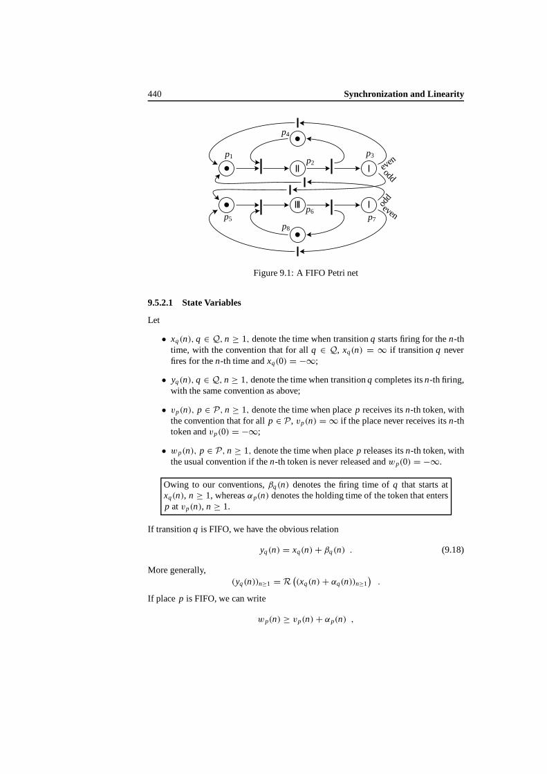
440 Synchronization and Linearity
even
odd
even
odd
p4
p2p3
p6p5 p7
p1
p8
Figure 9.1: A FIFO Petri net
9.5.2.1 State Variables
Let
• xq(n), q ∈ Q, n ≥ 1, denote thetime when transitionq startsfiring for then-thtime, with the convention that for allq ∈ Q, xq(n) = ∞ if transitionq neverfires for then-th time andxq(0) = −∞;
• yq(n), q ∈ Q, n ≥ 1, denote thetime when transitionq completes itsn-th firing,with the same convention as above;
• vp(n), p ∈ P, n ≥ 1, denote the time when placep receives itsn-th token, withthe convention that for all p ∈ P, vp(n) = ∞ if the place never receives itsn-thtoken andvp(0) = −∞;
• wp(n), p ∈ P, n ≥ 1, denote the time when placep releases itsn-th token, withthe usualconvention if then-th token is never released andwp(0) = −∞.
Owing to our conventions,βq(n) denotes the firing time ofq that starts atxq(n), n ≥ 1, whereasαp(n) denotes the holding time of the token that entersp at vp(n), n ≥ 1.
If transitionq is FIFO, we have the obvious relation
yq(n) = xq(n)+ βq(n) . (9.18)
More generally,(yq(n))n≥1 = R
((xq(n)+ αq(n))n≥1
).
If placep is FIFO, we can write
wp(n) ≥ vp(n)+ αp(n) ,

9.5. Evolution Equations of General Timed Petri Nets 441
since the token that entersp at time vp(n) stays therefor at leastαp(n) time units.More generally,
(wp(n))n≥1 ≥ R((vp(n)+ αp(n))n≥1
).
9.5.2.2 Initial Conditions
It is assumed that the origin of time and the initial marking have been fixed in such away that the variablesvp(n) andwp(n) satisfy the bounds
vp(n)
{= z p(n) ≤ 0 for n = 1, . . . , Mp, if Mp ≥ 1 ;
≥ 0, for n > Mp ,
andwp(n) ≥ 0 for n ≥ 1. These conventions are natural: they mean that tokens thatarrived in placep prior to the initial time and which leftp before that initial time arenot considered to belong to the initial marking. Similarly, tokens that arrived inp ‘ator after’ the initial time do not belong to the initial marking.
9.5.2.3 Upstream Equations Associated with Transitions
We first look at the relationships induced by a transitionq dueto the places precedingq. We first consider the case withoutstructural consumption conflicts, namely for everyplacep precedingq, the set of transitions that follow p is reduced toq.
No Structural Consumption Conflicts For all p ∈ π(q), one token leavesp at timewp(n). Sinceq is the only transition that can consume the tokens ofp, this correspondsto the starting of then-th firing of q. Hence,
xq(n) = max∀p∈π(q)
wp(n) .
In the FIFOcase, then-th token of placep to become available for enablingq must bethen-th to enterp, so that
xq(n) = maxp∈π(q)
(vp(n)+ αp(n)) .
More generally,xq(n) = max
p∈π(q)Up(n) ,
where(Up(n))n≥1 = R
((vp(n)+ αp(n))n≥1
).
General Case Without further specifications on how the conflict is resolved, we canonly state the following inequalities: in the FIFO case,
xq(n) ≥ maxp∈π(q)
(vp(n)+ αp(n)) , (9.19)
and more generallyxq(n) ≥ max
p∈π(q)Up(n) .
These inequalities are not very satisfactory, and we will return to this point later on.

442 Synchronization and Linearity
9.5.2.4 Downstream Equations Associated with Transitions
We now lookat the relationships induced by a transitionq dueto the places followingq. We first consider the case without structural supply conflicts, namely, for every placep following q, theset of transitionsthat precedep is reduced toq (that is, p is onlyfed by thisq).
No Structural Supply Conflicts If no other transition than q can feed the placesfollowing q, the token entering placep ∈ σ(q) with rank(Mp + n) has been producedby then-th firingof transitionq; therefore,
yq(n) = vp(Mp + n) , ∀p ∈ σ(q) .
In the FIFO case, this leads to the relation
xq(n)+ βq(n) = vp(Mp + n) , ∀p ∈ σ(q) ,
whereas in the general case
R((xq(k) + βq(k))k≥1
)n= vp(Mp + n) , ∀p ∈ σ(q) .
General Case Without further specifications, we can only state the following in-equalities: in the FIFO case,
xq(n)+ βq(n) ≥ vp(Mp + n) , ∀p ∈ σ(q) ,
whereas, in the general case,
R((xq(k) + βq(k))k≥1
)n≥ vp(Mp + n) , ∀p ∈ σ(q) .
9.5.2.5 Upstream Equations Associated with Places
We now focus on the upstream relationships induced by placep. Considerthe se-quences{yq(n)}n≥1, for all q ∈ π(p). With each of them, associate a point process onthe real line, where the points are located atyq(n). Wecan look at the arrival processinto p asthe superimposition of these|π(p)| point processes.
With all q ∈ π(p), we associate an integeriq ∈ N representing a number ofcomplete firings ofq. If transition q has completed exactlyiq firings for allq ∈ π(p),thenplacep has received exactly
∑q∈π(p) iq tokens. The set of vectors(i) = (iq )q∈π(p)
such that then-th token hasentered placep is hence
Apn =
i ∈ N|π(p)|
∣∣∣∣∣∣
∑
q∈π(p)
iq = n
.
The last token producedby the transition firings specified by somei ∈ Apn entersp
at time maxq∈π(p) yq(iq ), whereyq(0) = −∞ by convention. Sincen tokens havereachedp once all the firings specified byi have been completed, one obtains
vp(n + Mp) ≤ infi∈Ap
n
maxq∈π(p)
yq(iq ) . (9.20)
9.5. Evolution Equations of General Timed Petri Nets 443
But vp(n + Mp) should be equal to someyt0(n0) since at least one collection of eventsputsn tokens in placep (unlessAp
n is empty andvp(n + Mp) = ∞). Hence equalitymusthold true in (9.20). We then obtain the following final relation:
vp(n + Mp) = inf{i∈N|π(p)| |∑q∈π(p) iq=n} maxq∈π(p)
yq(iq ) , (9.21)
whereyq(0) = −∞ by convention.
9.5.2.6 Downstream Equations Associated with Places
We now concentrate on the downstream relationships induced by a placep. It is inthis type of equations that the structural consumption conflicts associated with generalPetri nets become apparent.
Consider the sequences{xq(n)}n≥1, for all q ∈ σ(p). With all q ∈ σ(p), weassociate an integeriq ∈ N representing some number of firing initiations ofq. If qhas started exactlyiq firings for allq ∈ σ(p), then exactly
∑q∈σ (p) iq tokens have been
withdrawn fromp. The set of vectorsi = (iq )q∈σ (p) such that then-th token has leftplacep is hence
Bpn =
i ∈ N|σ (p)|
∣∣∣∣∣∣
∑
q∈σ (p)
iq = n
.
For anyi in this set, the last token to leavep leavesat time maxq∈σ (p) xq(iq ). Hence
wp(n) ≤ infi∈B p
n
maxq∈σ (p)
xq(iq ) .
Using a similar reasoning as previously, we obtain the final relation
wp(n) = inf{i∈N|σ (p)||∑q∈σ (p) iq=n} maxq∈σ (p)
xq(iq ) . (9.22)
Relations (9.21) and (9.22) exhibit nothing but a superficial symmetry. Indeed,while (9.21) allows one to construct the sequence{vp(n)} from the knowledge of whathappens upstream ofp and earlier, this is not true at all for (9.22) which only providessome sort ofbackward property stating that the knowledge of what will happen follow-ing p in the future allows one to reconstruct what happens inp now. The reason forthis is that the way the conflict is solved is not yet sufficiently precise. We show nowone natural way of solving conflicts, whichwe will call switching. Several other waysare conceivable likecompetition, whichwe will also outline.
9.5.2.7 Switching
Within thissetting,each place that has several transitionsdownstream receives a switch-ing sequence{ρp(n)} with values inσ(p)N. In the sameway as then-th token to enterplace p receives a holding timeαp(n), it also receives a route to which it must beswitched. This information is given byρp(n), whichspecifies which transition it mustbe routed to. In other words, only those tokens such thatρp(n) = q should be taken

444 Synchronization and Linearity
into account byq ∈ σ(p). By doing so, one completely specifies the behavior of thesystem. For instance, in the FIFO case, one obtains the inequality
xq(n) ≥ wp(ηp,q(n)) , ∀p ∈ π(q) ,
where theswitching function ηp,q is defined by
ηp,q(0) = 0, ηp,q(n) = inf
{m ≥ 1
∣∣∣∣∣
m∑
k=1
1{ρp(k) = q} ≥ n
}, n ≥ 1 . (9.23)
Whenever the behavior of the places upstream ofq is specified,one can go further andobtain the desiredforward equation, as we will see in the next section.
Example 9.17 In our example (see Figure 9.1), the switchings are deterministic. Theyare chosen as follows:
ρ3(2n) = 1 , ρ3(2n + 1) = 5 , ρ7(2n) = 5 , ρ7(2n + 1) = 1 , ∀n ∈ N .
9.5.2.8 Competition
The places followingp compete forthe tokens of p on a First Come First Served(FCFS) basis: within this interpretation, the tokens that have been served in placepcan be seen as building up somequeue of tokens. Once a transition q following p isenabled except for the condition depending onp, it puts in a request for one token insomeFCFSqueue of requests. This request is served (and the corresponding transitionenabled) as soon as it is at the head of the request line and there is one token in thetoken queue.
9.5.3 Evolution Equations for Switching
In this subsection it is assumed that all places receive some switching. For places witha single downstream transition, this sequence is trivial in the sense that it always routestokens to this transition.
Theorem 9.18 Under the foregoing assumptions, the state variables vp(n), p ∈ P, n ≥1, of a FIFO Petri net satisfy the (nonlinear) recurrence equations
vp(n + Mp) =∧
{i∈N|π(p)|
∣∣∣∣∣∑
q∈π(p)iq=n
}
⊕
{q∈π(p),t∈π(q)}vt (ηt,q(iq ))αt (ηt,q(iq))βq (iq ) ,
(9.24)
for n ≥ 1, with the initial condition vp(n) = z p(n) for 1≤ n ≤ Mp, if Mp ≥ 1.

9.5. Evolution Equations of General Timed Petri Nets 445
Proof In addition to the variablesvp(n), we will make use of the auxiliary variablesxq(n), q ∈ Q, n ≥ 1. Owing to the switching assumptions, Inequality (9.19) can bereplaced by the relation
xq(n) =⊕
p∈π(q)
∧{
jp≥1
∣∣∣∣∣
jp∑k=1
1{ρp(k)=q}=n
}vp( jp)αp( jp) , n ≥ 1 ,
or, equivalently,
xq(n) =⊕
p∈π(q)vp(ηp,q(n))αp(ηp,q(n)) , n ≥ 1 , (9.25)
where we used theswitching functionηp,q defined in (9.23), and the FIFO assumption,which implies that the mappingi �→ vp(i)αp (i) is nondecreasing.
Similarly, using (9.18) in (9.21) yields
vp(n + Mp) =∧
{i∈N|π(p)| |∑q∈π(p) iq=n }
⊕
q∈π(p)
xq(iq )βq (iq ) , n ≥ 1 . (9.26)
Equation (9.24) follows immediately from (9.25) and (9.26).
Remark 9.19 In the case when the Petri net is not FIFO, Equations (9.25) and (9.26)have to bereplaced by
xq(n) =⊕
p∈π(q)
(R(vp(m)αp(m))m≥1
)(ηp,q (n))
, n ≥ 1 ,
and
vp(n + Mp) =∧
{i∈N|π(p)| |∑q∈π(p) iq=n }
⊕
q∈π(p)
(R(xq(m)βq (m))m≥1
)(iq )
, n ≥ 1 ,
respectively.
Remark 9.20 In (9.24), wecan get ridof the firing timesβq(n) by changing theholding timesαp(ηp,q(n)), ∀p ∈ π(q), into αp(ηp,q(n))βq (n). Thus we obtain anequivalent net withβq(n) = 0 andαp(n) > 0, q ∈ Q, p ∈ P, n ≥ 1, where theequivalence means that the entrancetimesare the same inboth systems.

446 Synchronization and Linearity
Example 9.21 In our example, we obtain
v1(n + 1) =∧
n3+n7=n
(1v3(2n3)⊕ 1v7(2n7 + 1)) , v1(1) = 0 ,
v2(n) = v1(n)⊕ v4(n) ,
v3(n) = 2v2(n) ,
v4(n + 1) = 2v2(n) , v4(1) = 0 ,
v5(n + 1) =∧
n3+n7=n
(1v3(2n3 + 1)⊕ 1v7(2n7)) , v5(1) = 0 ,
v6(n) = v5(n)⊕ v8(n) ,
v7(n) = 3v6(n) ,
v8(n + 1) = 3v6(n) , v8(1) = 0 .
9.5.4 Integration of the Recursive Equations
We assumethat the Petri net is FIFO. We use Remark 9.20 to assume (without loss ofgenerality) that βq(n) = 0, q ∈ Q, n ≥ 1. Finally, we assume thatthe switching isgiven as well as the holding times in the places and that in every circuit of the Petri netthere is a placep with 0 < αp(n) <∞, n ≥ 1.
In what follows we will use weighted trees where the weights are associated withthe nodes. We call theweight of a directed path the sum of the weights of all its nodesbut its source. A nodeN1 is said to bedeeper thana nodeN2 if we can find a directedpath fromN2 to N1. Finally, thedepth of a tree is the length of its longest directed path.
Definition 9.22 (Evolution tree) Let (p, n) ∈ P × N. An evolution tree A associatedwith (p, n) is a tree with root (p, n) defined recursively as follows.
• If n ≤ Mp, then A is reduced to a single node (p, n) with weight αp(n)+ z p(n).
• If n > Mp, choose one i ∈ N|π(p)| satisfying
∑t∈π(p) iq = n − Mp. Then A
is the tree with root (p, n) and with |π(π(p))| subtrees being evolution treesassociated with the nodes (q, ηq,t(iq )), t ∈ π(p), q ∈ π(q). The root (p, n) isgiven a weight αp(n).
The set of all theevolution trees of the pair(p, n) will be denotedE(p, n).In Equation (9.24), we can replace the variablesvt (ηt,q(n)) by using Equation (9.24)
once more. We obtain
vp(n + Mp) =∧
{i∈N|π(p)|
∣∣∣∣∣∑
q∈π(p)iq=n
}
⊕
{q∈π(p),t∈π(q)}
∧{
j∈N|π(t)|∣∣∣∣∣∑
s∈π(t)js=ηt ,q(it )−Mt
}
⊕
{s∈π(t),r∈π(s)}vr (ηr,s ( js))αr (ηr,s ( js))αt (ηt,q(it )) .

9.6. Min-Max Systems 447
If we use the distributivity of⊕ with respect to∧ (see(4.95)), this equality becomes:
vp(n + Mp) =∧
i∈Ij∈Jtq
⊕
q∈π(p)t∈π(q)s∈π(q)r∈π(s)
vr (ηrs ( j tqs ))αr (ηrs ( j tq
s ))αt (ηtq(iq )) ,
where
Idef=
i ∈ N|π(p)|
∣∣∣∣∣∣
∑
q∈π(p)
iq = n
, J tq def=
j tq ∈ N|π(t)|
∣∣∣∣∣∣
∑
s∈π(t)j tqs = ηtq(iq )− Mt
.
This equation represents the first step in the ‘integration’ of the recurrence equations.Indeed, we obtain a tree of depth 2 from the root(p, n + Mp). If we continue todevelop this equation,weobtain trees with increasing depths. We stop when each pathends with a leaf, namely, when it terminates with a node(q,m) with m ≤ Mq . Weeventually obtain the integration of Equation (9.24):
vp(n) = infA∈E(p,n)
C(A) , n ≥ Mp , with C(A) = supT∈T (A)
(w(T )) .
Thequantity C(A) is the weight of treeA, T (A) is the set of all thedirected paths fromthe root to any leaf of the treeA, andw(T ) is the weight of the directed pathT (i.e. thesum of the weights of all its nodes except its root).
Remark 9.23 The setE(p, n) might contain infinite trees, thusE(p, n) is not con-structible and this transformation of the recursive equations does not obviously givethe ‘constructiveness’ character of these equations. However, it is useful for prelimi-nary results. The reader is referred to [7]where this issue is furtheranalyzed.
9.6 Min-Max Systems
In this section we will be concerned with systems of which the evolution is determinedby three rather than two different operations, namely addition, maximization and min-imization. Because these operations occur simultaneously, a different notation for maxand min is necessary:⊕ is reserved for max, and∧ will denote min. The most generalsystem to be considered is of the form
x(k + 1) = A1 ⊗ x(k) ⊕ B1⊗ y(k) ⊕ C1 ⊗ v(k) ⊕ D1⊗w(k) , (9.27)
y(k + 1) = A2 , x(k) ∧ B2, y(k) ∧ C2, v(k) ∧ D2, w(k) , (9.28)
v(k) = A3 ⊗ x(k) ⊕ B3⊗ y(k) ⊕ C3 ⊗ v(k) ⊕ D3⊗w(k) , (9.29)
w(k) = A4 , x(k) ∧ B4, y(k) ∧ C4, v(k) ∧ D4, w(k) . (9.30)
The notation, here refers to the multiplication of two matrices (or a matrix and avector) in which the∧-operation is used instead of⊗ (see§6.6.1 and§9.2.4). Theexpressionsa ⊗ b and a , b are identical if at least eithera or b is a scalar. The

448 Synchronization and Linearity
operation⊕ has the neutral elementε whereas∧ has the neutral element�. Thefollowingconvention, in accordance with (5.7) and (5.8), is made:
�⊗ ε = ε , �, ε = � .
In analogy with conventional system theory, system (9.27)–(9.30) is called adescriptorsystem. It is assumed that the vectorsx(k), y(k), v(k) andw(k) are respectivelyn-,m-,p-, andq-dimensional. The matricesAl , Bl , Cl andDl , l = 1, . . . , 4, have appropriatedimensions. The elements of the matrices with an odd index are either finite orε andthe elements of the matrices with an even index are either finite or�.
Equations (9.29) and (9.30) are implicit equations inv(k) andw(k), respectively.It is assumed that the precedence graphG(E), whereE is the matrix
E =(
C3 D3
C4 D4
),
contains neither circuits nor loops. For later reference this condition is called ConditionC1:
Condition C1 The graphG(E) contains neither circuits nor loops.
Because of this condition, a finite number of repeated substitutions of the whole right-hand side of (9.29) and (9.30) into these same equations leads to, respectively,
v(k) = C∗3 ⊗ (A3 ⊗ x(k) ⊕ B3⊗ y(k) ⊕ D3⊗ w(k)) ,
w(k) = D∗′4 , (A4 , x(k) ∧ B4, y(k) ∧ C4, v(k)) ,
whereC∗3 = e⊕ C3⊕ C2
3 ⊕ · · · , D∗′4 = e ∧ D4 ∧ D2
4 ∧ · · · .
In these equations, the matrix product (which is used in the power computation ofmatrices) must be understood as being⊗, respectively,, when used in conjunctionwith ⊕, respectively∧. Similarly, the symbole denotesthe identity matrix inRmax,respectivelyRmin. Condition C1 is sufficient, but not necessary, forC∗3 andD∗′
4 to existin the expressions above.
Now the equations inv(k) andw(k) can be solved ina suitable order, and thesolutions can be expressed in terms ofx(k) and y(k). These solutions are writtensymbolically as
v(k) = f1(x(k), y(k)) , w(k) = f2(x(k), y(k)) .
If these equations are substituted into (9.27) and (9.28), then the new expressions forx(k + 1) andy(k + 1) will show a finite nesting of max- and min-operations.
For later reference, Equations (9.27)–(9.30), defining a mapping fromRn+m+p+q
to itself, will symbolically be denotedM. Similarly, the mapping of the correspondingnested equations is denotedM (M mapsRn+m to itself). Hence,
(x(k + 1) y(k + 1) v(k) w(k)
)′ = M((
x(k) y(k) v(k) w(k))′)
,(
x(k + 1) y(k + 1))′ = M
((x(k) y(k)
)′).
(9.31)

9.6. Min-Max Systems 449
9.6.1 General Timed Petri Nets and Descriptor Systems
Consider the network depicted in Figure 9.2. Each of the three nodes performs activi-
τ1
q1q3 q2
τ2τ3
Figure 9.2: A network
ties. The loops around these nodes, with time durationsτ1, τ2 andτ3, refer to processingor recycling times of one activity at the respective nodes. All other time durations areassumed to bezero. Nodeq1 delivers products to nodesq2 and q3 simultaneously.Nodeq3 startsprocessing on the first incoming product. To start an activity,eachnodemust have delivered its product(s) of the previous activity to its destination node(s). Ifthe destination node isq2, its buffer, indicated by a rectangle in the figure, can storeone incomingitem (whileq2 works at thepresent activity). Hence,if this buffer is full,nodeq1 cannot yet deliver a product and must wait until this buffer becomes empty.Similarly, there is a buffer just before nodeq3 which can contain two incoming itemsmaximally. If each buffer contains one token initially, one may be tempted to modelthe succession of firing times as follows:
x1(k + 1)= max(x1(k) + τ1, x2(k), x3(k)) ,
x2(k + 1)= max(x1(k) + τ1, x2(k) + τ2, x3(k)) ,
x3(k + 1)= max(min(x1(k) + τ1, x2(k) + τ2), x3(k) + τ3) ,
(9.32)
where the quantities xi (k), k = 1, 2, . . . , are the successive firing times of nodeqi .This model can be rewritten in the form (9.27)–(9.30) by addingw(k) = min(x1(k), x2(k))to (9.32) and by replacing the appropriate part in the last of the equations of (9.32) byw(k). Indeed, nodeq3 will process the firstarriving k-th product, of eitherq1 or q2,first. The last arriving product atq3, however, is not processed at all according to(9.32). It apparently leaves the system in some mysterious way. There is a discrepancybetween the problem statement and its model (9.32). In order to model the processingof the last arriving product also, one can introduce a fictive nodeq4, which isactuallynodeq3, and which takes care of the last arriving of the two products coming fromq1
andq2. If this fictive node has firing timesx4(k), then the new model becomes
x1(k + 1)= max(x1(k) + τ1, x2(k), x4(k)) ,
x2(k + 1)= max(x1(k) + τ1, x2(k) + τ2, x4(k)) ,
x3(k + 1)= max(min(x1(k) + τ1, x2(k) + τ2), x4(k) + τ3) ,
x4(k + 1)= max(max(x1(k) + τ1, x2(k) + τ2), x3(k + 1)+ τ3)
= max(x1(k) + τ1, x2(k) + τ2, x4(k) + 2τ3,
min(x1(k) + τ1 + τ3, x2(k) + τ2+ τ3)) .
(9.33)
Model (9.33) assumes that the buffer just beforeq3 must be emptied before a newcycle(k → k + 1) can be started. Note thatx3 does not appear on the right-hand side

450 Synchronization and Linearity
anymore and therefore the equation forx3(k + 1) can bedisregarded. It is obvious thatthis model can be rewritten in the form (9.27)–(9.30) also. Though model (9.33) doesnot throw away half-finished products, nodeq3 still might not always take the productwhich arrives first. Nodeq3 and its imagenodeq4 process the batch of the two arrivingk-th products (fromq1 andq2) according to first arrival. If the(k + 1)-st product ofq1,say, arrive before thek-th product ofq2, it has towait until this last k-th product hasarrived.
Yet another remark with respect to (9.33) must be made. According to (9.33),nodesq1 andq2 can start another cycle only afterq4 has startedits current activity.However, the performance ofthe network can be increased ifx4(k) in either the first orthe second equation of (9.33) is replaced byx3(k), depending on whetherx1(k)+ τ1 <
x2(k) + τ2 or not. Such a conditional dependence can neither be expressed in terms oftheoperations min, max and+, nor can it be shown graphically by means of a Petrinet as introduced in this book. This dependence can be expressed in Petri nets in whichso-called inhibitor arcs are allowed. The reader is referred to [1] about such arcs.
One canenlarge the batch size from which nodeq3 takes its productsaccording tothe FIFO priority rule. If, for instance, one introduces two fictive nodes, one forq1
andone forq2, and another pair of two fictive nodes, one node forq3 andone forq4,thenone can construct a model which has a batch size of four. The original productsnumberedk andk+1 coming from q1 and the original products numberedk andk+ 1coming from q2 are processed byq3, or oneof its images, according to FIFO. Thenext batch will then consist of the four original products numberedk + 2 andk + 3comingfrom bothq1 or its image andq2 or its image. The corresponding model willnot be written down explicitly; its (eight) scalar equations become rather unwieldyexpressions with nested forms of the operations max and min.
9.6.2 Existence of Periodic Behavior
In the following definition, the symbolM andM are those of (9.31).
Definition 9.24 A scalar λ, ε ≤ λ ≤ �, is called an eigenvalue of the mapping M, re-spectively M, if a vector
(x ′ y′ v′ w′
)′, respectively
(x ′ y′
)′, exists, where
either x or y has at least one finite element, such that
(λ⊗ x ′ λ, y′ v′ w′
)′ =M((
x ′ y′ v′ w′)′)
,
respectively, (λ⊗ x ′ λ, y′
)′ =M((
x ′ y′)′)
.
Such a vector is called an eigenvector of M, respectively M.
It will be clear that, provided Condition C1 holds, see§9.6, an eigenvalue ofM isalso an eigenvalue ofM and vice versa. A motivation to studyeigenvectors is that thesystemhas a very regular behavior if the initial condition coincides with an eigenvector.In fact, the firing times of the(k + 1)-st activities take place exactlyλ time units laterthan the firing times of thek-th activities. Conditions will be given under which theeigenvalue and a corresponding eigenvector exist.
9.6. Min-Max Systems 451
System(9.27)–(9.30) canbewritten as(
x(k + 1)v(k)
)=(
A1 C1
A3 C3
)⊗(
x(k)v(k)
)⊕(
B1 D1
B3 D3
)⊗(
y(k)w(k)
),
(y(k + 1)w(k)
)=(
B2 D2
B4 D4
),(
x(k)v(k)
)∧(
A2 C2
A4 C4
),(
x(k)v(k)
),
the two ‘autonomous’ equations of which are(
x(k + 1)v(k)
)=(
A1 C1
A3 C3
)⊗(
x(k)v(k)
), (9.34)
(y(k + 1)w(k)
)=(
B2 D2
B4 D4
),(
x(k)w(k)
). (9.35)
These two sets of autonomous equations can be considered as two subsystems of(9.27)–(9.30), connected by means of the matrices
(B1 D1
B3 D3
),
(A2 C2
A4 C4
). (9.36)
Condition C2 The first matrix in (9.36) is not identically� and the second one is notidenticallyε.
This amounts to saying that the two connections are actual.If Condition C1 is satisfied, thenv(k) can be solved from (9.34) and subsequently
besubstituted into the right-hand side of (9.34):
x(k + 1) = (A1 ⊕ C1 ⊗ C∗3 ⊗ A3)⊗ x(k) . (9.37)
Similarly, we obtain
y(k + 1) = (B2 ∧ D2, D∗′4 , B4), y(k) . (9.38)
Condition C3 The transition matrices of (9.37) and (9.38) are irreducible.
If Conditions C1 and C3 hold, then the matrices which governthe evolution of the sys-tems in (9.37) and (9.38) have unique eigenvalues, denotedλmax andλmin, respectively.The existence and uniqueness of these eigenvalues is a direct consequence of the theoryof Chapter 3. Now the following theorem, proved in [102], holds.
Theorem 9.25 Assume Conditions C1, C2 and C3 are fulfilled. The operator M hasan eigenvalue λ and a corresponding eigenvector
(x ′ y′
)′all of which components
are finite, i.e.
λ⊗(
xy
)=M((
xy
)), (9.39)
if and only if λmax ≤ λmin. Under these conditions, λ is unique and satisfies λmax ≤λ ≤ λmin.

452 Synchronization and Linearity
The condition that the components of the eigenvector must all be finite is essential forthe statement of this theorem to hold. As a counterexample, consider
x(k + 1) = 2x(k) ⊕ 3y(k) , y(k + 1) = 4x(k) ∧ 5y(k) .
The unique eigenvalue which falls within the scope of the above theorem isλ = 3.5with corresponding eigenvector
(0.5 1
)′. However,λ = λmax= 2 is also an eigen-
value with eigenvector(
e ε)′
. Similarly, λ = λmin = 5 is an eigenvalue with
eigenvector( � e
)′.
In Chapter 3 we saw that, within the max-plus algebra setting, the evolution ofa linear system, such as (9.37), converges in a finite number of steps to a periodicbehavior, the period being related to the length(s) of the critical circuit(s). Such aproperty has not (yet) been shown for systems within the min-max algebra setting,though simulations do point in this direction. Procedure 1, to be presented in the nextsubsection, is based on this observation.
9.6.3 Numerical Procedures for the Eigenvalue
Three numerical procedures for the calculation of the eigenvalue and correspondingeigenvector of M will be discussed briefly by means of examples. Of course, theseprocedures can also be applied to systems inRmax only.
Procedure 1 Consider (9.27) and (9.28) with
A1 =
ε 1 ε
ε e 12 1 ε
, B1 =
3 3 ε
3 ε ε
ε ε 1
, A2 =
� � 3� 3 �� 3 �
, B2 =
� 4 36 � �� 9 6
,
andC3 = C4 = (ε), B3 = B4 = (�). The evolution of this system will be studied bystarting with an arbitrary initial vector. If
(x(0)′ y(0)′
)′ = ( 1 2 3 4 5 6)′
,then (
x ′(0) y′(0)) = (
1 2 3 4 5 6)
,(x ′(1) y′(1)
) = (8 7 7 6 5 5
),
...(x ′(12) y′(12)
) = (38 37 37 37 37 37
),(
x ′(13) y′(13)) = (
40 40 40 40 40 40)
,(x ′(14) y′(14)
) = (43 43 42 43 43 43
),(
x ′(15) y′(15)) = (
46 46 45 45 46 45)
,(x ′(16) y′(16)
) = (49 48 48 48 49 49
),(
x ′(17) y′(17)) = (
52 51 51 51 51 51)
. . . .
This evolution is continued untilx(k) becomes linearly dependent on one of the pre-vious states
(x ′(l) y′(l)
)′, l = 1, . . . , k − 1. For this example, this occurs for
k = 17:(
x ′(17) y′(17))′ = 14⊗ ( x ′(12) y′(12)
)′. It is now claimed that
λ = 14/(17− 12) = 14/5 and that(∑16
j=12
(x ′( j ) y′( j )
)′)/5 is theeigenvector.
Note that in this expression for the eigenvector, the conventional operations addition

9.6. Min-Max Systems 453
and division occur. These are nonlinear operations within the min-max algebra! Forthe example, the eigenvector thus becomes
1
5
(216 214 212 213 215 213
)′.
It canbeverified by means of substitution that the quantities thus obtained are indeedthe eigenvalue and eigenvector. No general proof exists of the fact that this methodindeed yields the correct answers, however. If the same method is used for systems inthe max-plus algebra only, it is known that it does not always give the correct results. Insituations where it does not, a slightly more complicated algorithm exists which doesgive the correct results (see [28]).
Procedure 2 Consider (9.27)–(9.30) with sizesn = 2,m = 0, p = 0, q = 1. Thematrices concerned are given by
A1 =(
2 ε
2 3
), D1 =
(ee
), A4 =
(5 3), D4 = (�) .
If the exponential approach of§9.2 is applied to the definition of the eigenvalue givenin Definition 9.24, we obtain
zλ+x1 = z2+x1 + zw1 , (9.40)
zλ+x2 = z2+x1 + z3+x2 + zw1 , (9.41)
z−w1 = z−5−x1 + z−3−x2 . (9.42)
The quantities zx1 andzx2 can be solved from (9.40) and (9.41), and expressed inzw1.These solutions can be substituted into (9.42), which yields
z−w1 = z−w1z−5(zλ − z2)+ z−w1 z3 zλ − z3
z2(zλ − z2)−1 + 1.
Dividing this expression byz−w1 and after some rearranging, we obtain
z2λ+3+ z2λ−5+ z−1+ z8 = z0 + z2 + 2zλ−3+ zλ+6 + zλ+5 . (9.43)
The essence of this arrangement is that all the exponential terms have been moved tothat side of the equality symbol in such a way that only positive coefficients remain.Equation (9.43) must be valid asz →∞. Henceλ must satisfy
max(2λ+ 3, 2λ− 5,−1, 8) = max(0, 2, λ− 3, λ+ 6, λ+ 5) .
This equation is mosteasily solved graphically. The result isλ = 3 and thus theeigenvalue has been found.
This method is only suitable whenn,m, p and q are small. Essential is that anexplicit equation inzλ must beobtained.
Procedure 3 This procedure, which always works for systems which satisfy the con-ditions of Theorem 9.25, will be described by means of an algorithm. For an efficient

454 Synchronization and Linearity
way of explanation, (9.39) is rewritten asλ ⊗ a = M(a), wherea ∈ Rn+m . The
vector functionM has componentsMi , i = 1, . . . , n + m. If the eigenvector isa, thenMi (a) − ai must be equal toλ for all i. We will say that the accuracyη,whereη is a given arbitrary positive number, is achieved if we find ana suchthatmaxi(Mi (a)− ai
)−mini(Mi (a)− ai
)< η. We then usethe following algorithm.
1. Choose an arbitrarya ∈ Rn+m with all components finite.
2. Calculateci =Mi (a)−ai , i = 1, . . . , n+m. Definec = mini ci , c = maxi ci .
3. If c − c < η, then stop.
4. Construct disjoint subsetsϒi , i = 1, 2, 3, of ϒ def= {1, . . . , n + m} suchthat
• ϒ = ϒ1 ∪ ϒ2 ∪ ϒ3 ,
• j ∈ ϒ1 ⇔ c j < c + η/2 ,
• j ∈ ϒ2 ⇔ η/2≤ c j − c < η ,
• j ∈ ϒ3 ⇔ c j ≥ c + η .
5. Changea j into a j − η/2 for all j ∈ ϒ1. Do not change the othera-components.
6. Go to step 2.
This algorithm always ends in a finite number of steps. Ifk denotes the iteration indexof the algorithm, then thisk will, as an argument, specify the quantities related to thek-th iteration of the algorithm, and
{ci (k + 1) ≥ ci (k) for i ∈ ϒ1(k) ,
ci (k + 1) ≤ ci (k) for i ∈ ϒ2(k) ∪ ϒ3(k) .
Thereforec(k) is a nonincreasing function ofk and similarly c(k) is nondecreasing.At each iteration of the algorithm some elements ofϒ1 may have moved toϒ2 or viceversa. Someelements ofϒ3 may have moved toϒ2, butnot vice versa. Ask increases,ϒ1 andϒ2 will ultimately catch allci .
By means of the following example, it will be shown how the algorithm works:
a1(k + 1) = max(a1(k) + 1, a2(k) + 2, a3(k)) ,
a2(k + 1) = max(a1(k) + 2, a2(k), a3(k) + 1) ,
a3(k + 1) = min(a1(k) + 2, a2(k) + 4, a3(k) + 3) .
We takeη = 0.2 and start with a(0) = ( 1 2 3)′
. Application of the algorithm

9.6. Min-Max Systems 455
yields the following results:
a(0) =
123
, c(0) =
320
, a(1) =
12
2.9
, c(1) =
3
1.90.1
, . . . ,
a(9) =
12
2.1
, c(9) =
3
1.10.9
, a(10) =
122
, c(10) =
311
,
a(11) =
1
1.91.9
, c(11) =
2.91.11.1
, . . . , a(20) =
111
, c(20) =
222
.
For this example, even the exact results are obtained: the eigenvector isa(20) =(1 1 1
)′and the eigenvalueis 2.
9.6.4 Stochastic Min-Max Systems
We are given the system described by (9.27)–(9.30). In contrast to the previous subsec-tions, it is now assumed that the matrices in these formulæ are event-dependent;Al (k),Bl (k), etc. The reasonof this dependence is that (some of) the entries of these ma-trices will be assumed stochastic. For eachk, the stochastic entries are assumed to bemutually independent and moreover, it is assumed that there is no correlation for differ-entk-values. The underlying probability distributions are assumed to be finite, i.e. theentries can only assume a finite number of values. For the calculation of the averagethroughput, the same technique as used in Chapter 8 for max-plus algebra systems willbe used. As an example, consider
x1(k + 1) = max(x1(k) + τ1(k), x2(k), x3(k)) ,
x2(k + 1) = max(x1(k) + τ1(k), x2(k) + τ2(k), x3(k)) ,
x3(k + 1) = max(min(x1(k) + τ1(k), x2(k) + τ2(k)), x3(k) + 1) ,
(9.44)
which resembles (9.32). The stochastic quantitiesτi (k) are supposed to be indepen-dent of each other (i.e. for alli and allk). Assume thatτi (k) = 0 or τi (k) = 2, bothwith probability 0.5. Starting from an ‘arbitrary’x0-vector, sayx0 =
(0 0 0
)′,
we will set up thereachability tree of all possible states of (9.44). Fromx0, four newstates can be reached in one step in principle, since there are four possibilities for thecombination (τ1(0), τ2(0)). Actually, one of these states,
(2 2 2
)′, is a transla-
tion of x0 and hence is not considered to be a new state. For this example, it turnsout that the reachability tree consists of ten states which will be denotedn1, . . . , n10.Here n1 =
(0 0 0
)′. If for instance τ1(0) = τ2(0) = 0, then we get to state
n2 =(
0 0 1)′
. The ten states, together with their immediate successors, aregiven in Table 9.3. It is not difficult to show that, from any initial condition, thestatexk will converge in a finite number of steps to the Markov chain consisting ofthe given 10 nodes. Since the probabilities with which the different(τ1(k), τ2(k)) oc-cur are known, thetransition probabilities of a Markov chain in which the ten statesni

456 Synchronization and Linearity
Table 9.3: Reachable states
Initial τ1 = 0 τ1 = 0 τ1 = 2 τ1 = 2state τ2 = 0 τ2 = 2 τ2 = 0 τ2 = 2
n1 =(
0 0 0)′
n2 e n3 e n4 1 n1 2n2 =(
0 0 1)′
n2 1 n5 1 n1 2 n1 2n3 =(
0 2 1)′
n1 2 n6 2 n1 2 n6 2n4 =(
1 1 0)′
n1 1 n6 1 n7 1 n1 3n5 =(
0 1 1)′
n2 1 n3 1 n1 2 n8 2n6 =(
0 2 0)′
n4 1 n9 1 n1 2 n6 2n7 =(
2 2 0)′
n1 2 n6 2 n7 2 n1 4n8 =(
0 1 0)′
n1 1 n6 1 n4 1 n8 2n9 =(
1 3 0)′
n7 1 n10 1 n1 3 n6 3n10=
(2 4 0
)′n7 2 n10 2 n1 4 n6 4
are the nodes can be calculated. Subsequently, the stationary behavior of this Markovchain can be calculated. Once this stationarydistribution is known, it is not difficult tocalculate
limk→∞
E(xi (k + 1)− xi (k)) , (9.45)
which turns out to be independent of the subscripti. This method, together with itsproperties, has been described more extensively in Chapter 8 for only max-plus sys-tems. As long as the reachability-tree consists of a finite number of states, the methodworks equally well for min-max systems. For the example treated, it turns out that theexpression in (9.45) equals 1.376 time units. This quantity can be considered as theaverage cycletime of system (9.44).
9.7 About Cycle Times in General Petri Nets
In this section we are interested in finding how fast each transition can initiate firingin a periodically operated Petri net (not necessarily an event graph). Connections withChapter 2 will be made. It will not be assumed here that each transition fires as soonasit is enabled. The order and timing of the initiation of firings of enabled transitionsmust be chosen in such a way (if at all possible) that a periodic behavior is possible.Duringeach period, each transition must fire at least once. The thus smallest possibleperiod τ is called the cycle time and it is defined as the time to complete a firingsequence leading back to the initial marking. Therefore we will confine ourselves toconsistentPetri nets, i.e.
∃x > 0 , G′x = 0 ,
whereG was defined in§ 2.4.1. Later on in this section, we will narrow down theconsistent Petri nets to event graphs.

9.7. About Cycle Times in General Petri Nets 457
It is assumed that the holding and firing times are constant in time. Suppose thereis a firing time of at leastβi time units associated with transitionqi , i = 1, . . . , n.This means that whenqi is enabled and it initiates a firing, it takesβi time units beforethe firing is completed. Hence one token is reserved in each placep j ∈ π(qi) forat leastβi time units before the transition completes its firing. The ‘resource-timemultiplication’ + j is definedas (thenumber of tokens in placep j) × (the length oftime that these tokens remain in that place). Apopular interpretation is: if a tokenrepresents a potential buyer who has to wait, then+ j is proportional to the amount ofcoffee you will offer to all these buyers. In matrix form,+ = (G in)′Dx , where them-dimensional vector+ has an entry per place and whereD is the diagonal matrixwith the elementsβi on the diagonal and 0’s elsewhere (in conventional algebra). Herewe only considered the reserved tokens (reserved for the duration of the firing time).Now suppose that there are on average(µa) j tokens in placep j during one period(this average is with respect to clock time). Then the corresponding+ is given by thevectorµaτ (popular again: the amount of coffee which you will need during one cyclefor all waiting clients). Since this latter+ wascalculated for both the reserved and notreserved tokens, the following inequality holds:
µaτ ≥ (G in)′Dx . (9.46)
Sinceµa is the averageof a finite number of markingsµ, and sinceµ′y, with y satis-fying Gy = 0, does not depend on the particularµ (see§2.4.1), we obtain
y′µ0τ = y′µaτ ≥ y′(G in)′Dx
(whereµ0 is the initial marking or any other one), providedy ≥ 0. Hence
τ ≥ maxy
y′(G in)′Dx
y′µ0, subject to Gy = 0 , y ≥ 0 , y = 0 . (9.47)
It is tacitly assumed that the denominator of (9.47) is strictly greater than zero. In fact,it is not difficult to derive an upper bound forτ and hence the right-hand side of (9.47)must befinite.
An upper bound forτ is given by 2βmax∑
i xi , whereβmax is an upper bound forthe holding and firing times. If a transition starts firing, then any other transition, if it isenabled at all, will be enabled within 2βmax units oftime, the factor 2 coming from thefiring time of the first transition and from the holding time between the two transitions.Hence such a transition can initiate firing within 2βmax time units of the initiation offiring of the first transition. The total number of firings in a circuit is
∑xi . Thus the
upper bound has been obtained.For event graphs the analysis related to the lower bound onτ can be made more
explicit. Take those indices of they-vector which correspond to the indices of thetransitions of an arbitrary elementary circuit of the event graph equal to 1 and theother indices equal to 0. It can be shown that they-vector thus constructed satisfiesGy = 0, y ≥ 0, y = 0. If this y is used in (9.47) one obtains
τ ≥ maxk
∑
i∈ζk
βi
/µ0(ζk )
, (9.48)
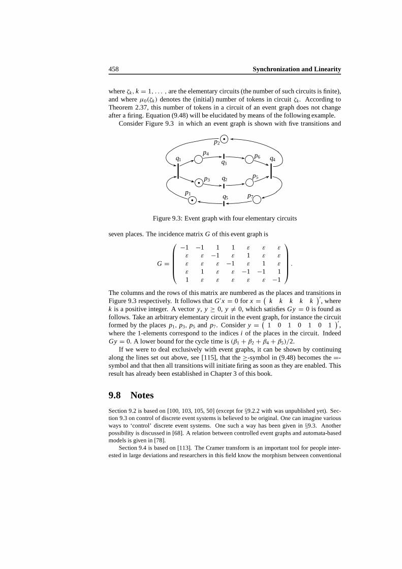
458 Synchronization and Linearity
whereζk, k = 1, . . . , are the elementary circuits (thenumber of such circuits is finite),and whereµ0(ζk) denotesthe (initial) number of tokens in circuitζk. According toTheorem 2.37, this number of tokens in a circuit of an event graph does not changeafter a firing. Equation (9.48) will be elucidated by means of the following example.
Consider Figure 9.3 in which an event graph is shown with five transitions and
p1
p2
p3
p4
p5
p6
p7
q1
q2
q3q4
q5
Figure 9.3: Event graph with four elementary circuits
seven places. The incidence matrixG of this event graph is
G =
−1 −1 1 1 ε ε ε
ε ε −1 ε 1 ε ε
ε ε ε −1 ε 1 ε
ε 1 ε ε −1 −1 11 ε ε ε ε ε −1
.
The columns and the rows of this matrix are numbered as the places and transitions inFigure 9.3 respectively. It follows thatG′x = 0 for x = ( k k k k k
)′, where
k is a positive integer. A vectory, y ≥ 0, y = 0, which satisfiesGy = 0 is found asfollows. Take an arbitrary elementary circuit in the event graph, for instance the circuitformed by the placesp1, p3, p5 and p7. Considery = ( 1 0 1 0 1 0 1
)′,
where the 1-elements correspond to the indicesi of the places in the circuit. IndeedGy = 0. A lower bound for the cycle time is(β1 + β2 + β4 + β5)/2.
If we were to deal exclusively with event graphs, it can be shown by continuingalong the lines set out above, see [115], that the≥-symbol in (9.48) becomes the=-symbol and that then all transitions will initiate firing as soon as they are enabled. Thisresult has already been established in Chapter 3 of this book.
9.8 Notes
Section 9.2 is based on [100, 103, 105, 50] (except for§9.2.2 with was unpublished yet). Sec-tion 9.3 on control of discrete event systems is believed to be original. One can imagine variousways to ‘control’ discrete event systems. One such a way has been given in§9.3. Anotherpossibility is discussed in [68]. A relation between controlled event graphs and automata-basedmodels is given in [78].
Section 9.4 is based on [113]. The Cramer transform is an important tool for people inter-ested in large deviations and researchers in this field know the morphism between conventional

9.8. Notes 459
algebra andmin-plusalgebra. But in general they are more interested in the probability side thanin the optimization one. Moreover, they are notmuch concerned with the algebraic point of view[3], [60], [125]. Bellman and Karush [17] were aware of the interest of the Fenchel transform(which they call max transform). Maslov has also clearly understood the analogy between prob-ability and dynamic programming and has developed a theory of idempotent integration [88].The analogue of some jump processes can be found in [55].
The law of large numbers, thecentral limit theorem, the Brownian decision process, thediffusion decision process and the min-plus invariance principle do not seem to have been writtendown explicitly before. Some work on the min-plus analogue of stochastic integrals, and moregenerally on the analogy between probability anddynamic programming, has been done byBellalouna under the supervision of M. Viot [16]. Some comments by P.L. Lions and R. Azencotton this morphism have been included in this section.
The first attempt to derive equations for general timed Petri nets can be traced back to [39].However, the approach proposed in that paper did not lead to explicit equations, owing to theproblem of consumption conflicts. The setting that is summarized in§9.5 is that of [7]. Theevolution equations established in this section can be shown to be ‘constructive’ whenever thePetri net is live, and a computational scheme can be obtained that allows one to determine thefiring times of the transitions iteratively (see [7]). Section 9.6 is based on [98] and [102].
Section 9.7 is based on [96]. As explained, the results of this section can be narrowed downto event graphs (see [115]), so asto get back the results which have been derived in a differentway in Chapter 3.

460 Synchronization and Linearity
Bibliography
[1] M. Ajmone Marsan, G. Balbo, and G. Conte.Performance Models of Multipro-cessor Systems. The MIT Press, Cambridge, Mass., USA, 1986.
[2] H. Attouch and R.J.B. Wets. Isometries of the Legendre-Fenchel transform.Transactions of the American Mathematical Society, 296:33–60, 1986.
[3] R. Azencott, Y. Guivarc’h, and R.F. Gundy. InEcole d’ete de Saint Flour 8.Springer-Verlag, Berlin, 1978.
[4] F. Baccelli, N. Bambos, and J. Walrand. Flow analysis of stochastic markedgraphs. InProceedings of the 28-th Conference on Decision and Control. IEEE,1989.
[5] F. Baccelli and P. Br´emaud.Palm Probabilities and Stationary Queues. Num-ber 41 in Lecture Notes in Statistics. Springer-Verlag, Berlin, 1987.
[6] F. Baccelli and P. Br´emaud. Elements of Queueing Theory. Applications ofMathematics. Springer-Verlag, Berlin, 1992.
[7] F. Baccelli, G. Cohen, and B. Gaujal. Recursive equations and basic propertiesof timed Petri nets.Journal of Discrete Event Dynamic Systems, 1-4:415–439,1992.
[8] F. Baccelli and T. Konstantopoulos. Estimates of cycle times in stochastic Petrinets. In I. Karatzas, editor,Proceedings of Workshop on Stochatic Analysis,Rutgers University, 1991. Springer-Verlag, Berlin.
[9] F. Baccelli and Z. Liu. On the executions of parallel programs on multiprocessorsystems—a queueing theory approach. Journal of the ACM, 37(2):373–414,1990.
[10] F. Baccelli and Z. Liu. Comparison properties of stochastic decision freePetri nets. Technical Report 1433, INRIA, Sophia-Antipolis, 06565 Valbonne,France,1991. To appear inIEEE Transactions on Automatic Control.
[11] F. Baccelli and Z. Liu. On a class of stochastic evolution equations.The Annalsof Probability, 20-1:350–374, 1992.
[12] F. Baccelli and A.M. Makowski. Queueing models for systems with synchro-nization constraints.Proceedings of the IEEE, 77:138–161, 1989. Special Issueon Dynamics of Discrete Event Systems.
461

462 Synchronization and Linearity
[13] Francois Baccelli. Ergodic theory of stochastic Petri networks.The Annals ofProbability, 20-1:375–396, 1992.
[14] Jean Le Bail, Hassane Alla, and Ren´e David. Hybrid Petri nets. InProceedingsof the 1-st European Control Conference, pages1472–1477, Grenoble, France,1991. Hermes, Paris.
[15] R. Barlow and F. Proschan.Statistical Theory of Reliability and Life Testing.Holt, Rinehart and Winston, 1975.
[16] F. Bellalouna.Processus de decision min-markoviens. PhD thesis, University ofParis-Dauphine, 1992. To appear.
[17] R. Bellman and W. Karush. Mathematical programming and the maximumtransform.SIAM Journal of Applied Mathematics, 10, 1962.
[18] Dimitri P. Bertsekas.Dynamic Programming. Prentice-Hall, Englewood Cliffs,N.J., 1987.
[19] J.D. Biggins. The first and last birth problem for a multitype age-dependentbranching process.Advances in Applied Probability, 8:446–459, 1976.
[20] P. Billingsley. Ergodic Theory and Information. John Wiley and Sons, NewYork, 1965.
[21] P.Billingsley.Convergence of Probability Measures. John Wiley and Sons, NewYork, 1968.
[22] G. Birkhoff. Lattice Theory. Amer. Math. Soc. Coll. Pub., Providence, 1967(3rd Ed.).
[23] T.S. Blyth. Matrices over ordered algebraic structures.Journal of London Math-ematical Society, 39:427–432, 1964.
[24] T.S. Blyth and M.F. Janowitz.Residuation Theory. Pergamon Press, Oxford,1972.
[25] Dieter Bochmann and Christian Posthoff.Binaere dynamische Systeme.Akademie-Verlag, Berlin, 1981.
[26] A. Borovkov. Asymptotic Methods in Queueing Theory. John Wiley and Sons,New York, 1984.
[27] J.G. Braker. Max-algebra modelling and analysis of time-table dependent net-works. InProceedings of the 1-st European Control Conference, pages1831–1836, Grenoble, France, 1991. Herm`es, Paris.
[28] J.G. Braker and G.J. Olsder. The power algorithm in max-algebra.Linear Alge-bra and its Applications, 182:67–89, 1993.

Bibliography 463
[29] W. Brauer, W. Reising, and G. Rozenberg, editors.Petri Nets: Applications andRelationships to Other Models of Concurrency, volume 255 ofLecture notes inComputer Science. Springer-Verlag, Berlin, 1987.
[30] W. Brauer, W. Reising, and G. Rozenberg, editors.Petri Nets: Central Mod-els and Their Properties, volume 254 ofLecture notes in Computer Science.Springer-Verlag, Berlin, 1987.
[31] Y. Brenier. Un algorithme rapide pour le calcul des transform´ees de Legendre-Fenchel discretes. Comptes Rendus a l’Academie des Sciences, 308:587–589,1989.
[32] Roger W. Brockett.Finite Dimensional Linear Systems. John Wiley and Sons,New York, 1970.
[33] R. A. Brualdi and H. J. Ryser.Combinatorial Matrix Theory. Cambridge Uni-versity Press, Cambridge, 1991.
[34] Z.-Q. Cao, K.H. Kim, and F.W. Roush.Incline Algebra and Applications. EllisHorwood Limited, Chichester, 1984.
[35] P. Caspi and N. Halbwachs. A functional model for describing and reasoningabout time behaviour of computing systems.Acta Informatica, 23:595–627,1986.
[36] P. Chretienne. Les Reseaux de Petri Temporises. These d’etat, University ofParis 6, Paris, 1983.
[37] G. Cohen, D. Dubois, J.P. Quadrat, and M. Viot. Analyse du comportementperiodique de syst`emesde production par la th´eorie des dio¨ıdes. Technical Re-port 191, INRIA, Rocquencourt, 78153 Le Chesnay, France, February 1983.
[38] G. Cohen, D. Dubois, J.P. Quadrat, and M. Viot. A linear system-theoretic viewof discrete event processes. InProceedings of the 22-nd Conference on Decisionand Control. IEEE,1983.
[39] G. Cohen, D. Dubois, J.P. Quadrat, and M. Viot. A linear system-theoretic viewof discrete event processes and its use for performance evaluation in manufac-turing. IEEE Transactions on Automatic Control, AC-30:210–220, 1985.
[40] G. Cohen, S. Gaubert, R. Nikoukhah, and J.P. Quadrat. Convex analysis andspectral analysis oftimed event graphs. InProceedings of the 28-th Conferenceon Decision and Control. IEEE,1989.
[41] G. Cohen, P. Moller, J.P. Quadrat, and M. Viot. Linear system theory for discreteevent systems. InProceedings of the 23-rd Conference on Decision and Control.IEEE,1984.
[42] G. Cohen, P. Moller, J.P.Quadrat,and M. Viot. Une theorielineaire des systemesa evenements discrets. Technical Report 362, INRIA, Rocquencourt, 78153 LeChesnay, France, January 1985.

464 Synchronization and Linearity
[43] G. Cohen, P. Moller, J.P. Quadrat, and M. Viot. Dating and counting events indiscrete event systems. InProceedings of the 25-th Conference on Decision andControl. IEEE,1986.
[44] Guy Cohen, Pierre Moller, Jean-Pierre Quadrat, and Michel Viot. Algebraictools for the performance evaluation of discrete event systems.Proceedingsof the IEEE, 77:39–58, 1989. Special Issue on Dynamics of Discrete EventSystems.
[45] J. Cohen, H. Kesten, and C. Newman. Random matrices and their applications.In Proceedings of a Summer Research Conference. AMS, June 1984.
[46] J.W. Cohen.The Single Server Queue. North-Holland, Amsterdam, 1969.
[47] F. Commoner, A. W. Holt, S. Even, and A. Pnuelly. Marked directed graphs.Computer and System Science, 5:511–523, 1971.
[48] J. Cook and B. Derrida. Directed polymers in a random medium: 1/d expansionand then-tree approximation.Journal of Physics, Series A: Mathematical andGeneral, 23:1523–1553, 1990.
[49] R.A. Cuninghame-Green.Minimax Algebra. Number 166 in Lecture Notes inEconomics and Mathematical Systems. Springer-Verlag, Berlin, 1979.
[50] R.A. Cuninghame-Green. Algebraic realization of discrete dynamical systems.In Proceedings of the 1991 IFAC Workshop on Discrete Event System Theoryand Applications in Manufacturing and Social Phenomena, pages11–15, Bei-ji ng, China, 1991. International Academic Publishers.
[51] R.A. Cuninghame-Green and P.F.J. Meijer. An algebra for piecewise-linear min-imax problems.Discrete Applied Mathematics, 2:267–294, 1980.
[52] Y. Dallery, Z. Liu, and D. Towsley. Equivalence, reversibility and symmetryproperties in assembly/disassembly networks. Technical Report 1267, INRIA,Rocquencourt, 78153 Le Chesnay, France, 1990.
[53] R. David and H. Alla. Continuous Petri nets. InProceedings of the 8th EuropeanWorkshop on Applications and Theory of Petri Nets, Saragossa, Spain, pages275–294, 1987.
[54] R.E. de Vries.On the asymptotic behavior of discrete event systems. PhD thesis,Delf t University of Technology, 1992.
[55] P. Del Moral, T. Thuillet, G. Rigal, and G. Salut. Optimal versus random pro-cesses: thenon-linear case. Technical report, LAAS, Toulouse, France, 1990.
[56] B. Derrida. Mean field theory of directed polymers in a random medium andbeyond.Physica Scripta, T38:6–12, 1990.
[57] P. Dubreil and M.L. Dubreil-Jacotin.Lecons d’Algebre Moderne. Dunod, Paris,France,1964.

Bibliography 465
[58] W. Fenchel. On the conjugate convex functions.Canadian Journal of Mathe-matics, 1:73–77, 1949.
[59] Forney, Jr. and G. David. The Viterbi algorithm. Proceedings of the IEEE,61:268–278, 1973.
[60] M.I. Freidlin and A.D. Wentzell.Random Perturbations of Dynamical Systems.Springer-Verlag, Berlin, 1979.
[61] F.R. Gantmacher.The Theory of Matrices. Chelsea Publishing Company, Eng-land, 1959.
[62] Stephane Gaubert.Theorie Lineaire des Systemes dans les Dioıdes. These,Ecole des Mines de Paris, Paris, 1992.
[63] P.W. Glynn. A gsmp formalism for discrete event systems.Proceedings of theIEEE, 77, 1989. Special Issue on Dynamics of Discrete Event Systems.
[64] M. Gondran and M. Minoux. Valeurs et vecteurs propres dans les dio¨ıdesetleur interpretation en th´eorie des graphes.Bulletin de la Direction des Etudes etRecherches, Serie C (Mathematiques, Informatique), (2):25–41, 1977. E.D.F.,Clamart, France.
[65] M. Gondran and M. Minoux. L’ind´ependancelineaire dans les dioıdes.Bulletinde la Direction des Etudes et Recherches, Serie C (Mathematiques, Informa-tique), (1):67–90, 1978. E.D.F., Clamart, France.
[66] M. Gondran and M. Minoux. Linear algebra in dioids: a survey of recent results.Annals of Discrete Mathematics., 19:147–164, 1984.
[67] M. Gondran and M. Minoux.Graphs and Algorithms. John Wiley and Sons,New York, 1984.
[68] Hans-Michael Hanisch. Dynamik von koordinierungssteuerungen in diskon-tinuierlichen verfahrentechnischen systemen.Automatisierungstechnik at,38:399–405, 1990.
[69] S. Helbig. Optimization problems on extremal algebras: Necessary and suf-ficient conditions for optimal points. In B. Borowski and F. Deutsch, editors,Parametric Optimization and Approximation, Lecture Notes in Control and In-formation Sciences, pages 166–184. Birkh¨auser-Verlag, Basel, 1985.
[70] Y.C. Ho and X.R. Cao. Perturbation Analysis of Discrete Event Dynamic Sys-tems. Kluwer Academic Publishers, 1991.
[71] J.L. Joly. Une famille de topologies sur l’ensemble des fonctions convexes pourlesquelles la polarit´e est bicontinue. Journal de Mathematiques Pures et Ap-pliquees, 52:421–441, 1973.
[72] Thomas Kailath.Linear systems. Prentice-Hall, Englewood Cliffs, N.J., 1980.

466 Synchronization and Linearity
[73] Richard M. Karp. A characterization of the minimum cycle mean in a digraph.Discrete Mathematics, 23:309–311, 1978.
[74] J.L. Kemeny and J.L. Snell.Finite Markov chains. Springer-Verlag, Berlin,1960, reprint 1976.
[75] J.F.C. Kingman. Subadditive ergodic theory.The annals of Probability, 1:883–909, 1973.
[76] J.F.C. Kingman. Subadditive processes. In P.-L. Hennequin, editor,Ecole d’etede probabilite de Saint-Flour, volume 539 ofLecture Notes in Mathematics,pages 165–223. Springer-Verlag, Berlin, 1976.
[77] Leonard Kleinrock.Queueing Systems. John Wiley & Sons, New York, 1976.
[78] Bruce H. Krogh, Jan Magott, and Lawrence E. Holloway. On the complexity offorbidden state problems for controlled marked graphs. InProceedings of the30-th Conference on Decision and Control, pages85–91. IEEE,1991.
[79] S.Y. Kung.VLSI Array Processors. Prentice-Hall, Englewood Cliffs, N.J., 1988.
[80] J. Kuntzmann.Theorie des Reseaux et Graphes. Dunod, Paris, France, 1972.
[81] Huibert Kwakernaak and Raphael Sivan.Linear Optimal Control Systems.Wiley-Interscience, New York, 1972.
[82] Stephane Lafortune and Hyuck Yoo. Some results on Petri net languages.IEEETransactions on Automatic Control, AC-35:482–485, 1990.
[83] S. Lavenberg. Maximum departure rate of certain open queueing networks hav-ing finite capacity constraints.RAIRO serie bleue, 12(4), 1978. Dunod, Paris.
[84] Charles E. Leiserson and James B. Saxe. Optimizing synchronous systems.Journal of VLSI and Computer Systems, 1:41–67, 1983.
[85] Rudolf Lidl and Gunther Pilz. Abstract Applied Algebra. Springer-Verlag,Berlin, 1984.
[86] P.L. Lions.Generalized Solutions of Hamilton-Jacobi Equation. Pitman, 1982.
[87] R. M. Loynes. The stability of queues with nonindependent inter-arrival andservicetimes. Proceedings of Cambridge Philosophical Society, 58:497–520,1962.
[88] V. Maslov. Methodes operatorielles. Editi ons MIR, Moscow, 1987. Frenchtranslation.
[89] L.E. Meester and J.G. Shanthikumar. Concavity of the throughput of tandemqueueing systems with finite storage space.Advances in Applied Probability,22:764–767, 1990.
[90] S.G. Mikhlin. Integral Equations. Pergamon Press, Oxford, 1957.

Bibliography 467
[91] Henryk Minc. Nonnegative Matrices. John Wiley and Sons, New York, 1988.
[92] Debasis Mitra and Isi Mitrani. Analysis for a novel discipline for cell coordina-tion in production lines, 1. Technical report, AT&T Bell Laboratories, MurrayHill, New Jersey 07974, USA, June 1988.
[93] Pierre Moller.Theorie Algebrique des Systemes a Evenements Discrets. These,Ecole des Mines de Paris, Paris, 1988.
[94] Michael K. Mollow. Performance analysis using stochastic Petri nets.IEEETransactions on Computers, C-31:913–917, 1982.
[95] T. Murata. Circuit theoretic analysis and synthesis of marked graphs.IEEETransactions on Circuits and Systems, CAS-24:400–405, 1977.
[96] Tadao Murata. Petri nets: Properties, analysis and applications.Proceedings ofthe IEEE, 77:541–580, 1989.
[97] Geert Jan Olsder. Applications of the theory of stochastic discrete-event systemsto array processors and scheduling in public transportation. InProceedings ofthe 28-th Conference on Decision and Control. IEEE,1989.
[98] Geert Jan Olsder. Eigenvalues of dynamic max-min systems.Journal on Dis-crete Event Dynamic Systems, 1:177–207, 1991.
[99] Geert Jan Olsder. Synchronized continuous flow systems. In S. Balemi, P. Kozakand R. Smedinga, editors,Discrete Event Systems: Modelling and Control,pages 113–124, Birkh¨auser, Basel, 1993.
[100] G.J. Olsder. On the characteristic equation and minimal realizations for discreteevent systems. In A. Bensoussan and J.L. Lions, editors,Analysis and Optimiza-tion of Systems, pages189–201. Springer-Verlag, Berlin, 1986.
[101] G.J. Olsder. Performance analysis of data-driven networks. In John McCanny,John McWhirter, and Earl Swartzlander Jr., editors,Systolic Array Processors,pages 33–41. Prentice-Hall, Englewood Cliffs, N.J., 1989.
[102] G.J. Olsder. Descriptor systems in min-max algebra. InProceedings of the1-st European Control Conference, pages1825–1830, Grenoble, France, 1991.Hermes, Paris.
[103] G.J. Olsder and R.E. de Vries. On an analogy of minimal realizations in con-ventional and discrete event dynamic systems. In P.Varaiya and A.B. Kurzhan-ski, editors, Discrete Event Systems: Models and Applications, volume 103 ofLecture Notes in Control and Information Sciences, pages149–161. Springer-Verlag, Berlin, 1988.
[104] G.J. Olsder, J.A.C. Resing, R.E. de Vries, M.S. Keane, and G. Hooghiemstra.Discrete event systems with stochastic processing times.IEEE Transactions onAutomatic Control, AC-35:299–302, 1990.
468 Synchronization and Linearity
[105] G.J. Olsder and C. Roos. Cramer and Cayley-Hamilton in the max-algebra.Linear Algebra and its Applications, 101:87–108, 1988.
[106] V.I. Oseledec¸. A multiplicative ergodic theorem. Lyapounov characteristic num-bers for dynamical systems.Transactions of Moscow Mathematical Society,19:197–231, 1968.
[107] E.P. Patsidou and J.C. Kantor. Application of minimax algebra to the study ofmultipurpose batch plants.Computers and Chemical Engineering, 15-1:35–46,1991.
[108] James L. Peterson.Petri Net Theory and the Modeling of Systems. Prentice-Hall,Englewood Cliffs, N.J., 1981.
[109] Max Plus. L’algebre(max,+) et sasymetrisation ou l’algebre des ´equilibres.Comptes Rendus a l’Academie des Sciences, 311:443–448, 1990.
[110] Max Plus. Linear systems in(max,+) algebra. In Proceedings of the 29-thConference on Decision and Control. IEEE,1990.
[111] Max Plus. A linear system theory for systems subject to synchronization andsaturation constraints. InProceedings of the 1-st European Control Conference,pages 1022–1033, Grenoble, France, 1991. Herm`es, Paris.
[112] Max Plus. Second order theory of min-linear systems and its application todiscrete event systems. InProceedings of the 30-th Conference on Decision andControl. IEEE,1991.
[113] J.P. Quadrat. Th´eoremesasymptotiques en programmation dynamique.ComptesRendus a l’Academie des Sciences, 311:745–748, 1990.
[114] P.J. Ramadge and W.M. Wonham. Supervisory control of a class of discreteevent processes. SIAM Journal of Control and Optimization, 25(1):206–230,Jan 1987.
[115] C.V. Ramamoorthy and Gary S. Ho. Performance evaluation of asynchronousconcurrent systems using Petri nets.IEEE Transactions on Software Engineer-ing, 6:440–449, 1980.
[116] Kurt J. Reinschke. Multivariable Control, a Graph-Theoretic Approach.Akademie-Verlag, Berlin, 1988.
[117] J.A.C. Resing, R.E. de Vries, M.S. Keane, G. Hooghiemstra, and G.J. Olsder.Asymptotic behaviour of random discrete event systems.Stochastic Processesand Their Applications, 36:195–216, 1990.
[118] C. Reutenauer and H. Straubing. Inversion of matrices over commutative semir-ing. Journal of Algebra, 88:350–360, 1984.
[119] R.T. Rockafellar.Convex Analysis. Princeton University Press, Princeton, N.J.,1970.
Bibliography 469
[120] D.E. Rutherford. Inverses of Boolean matrices.Proceedings of the GlasgowMathematical Association, 6:49–53, 1963.
[121] A.N. Shiryayev.Probability. Springer-Verlag, Berlin, 1984.
[122] E.D. Sontag.Mathematical Control Theory. Springer-Verlag, Berlin, 1990.
[123] D. Stoyan.Comparison Methods for Queues and Other Stochastic Models. JohnWiley and Sons, New York, 1984. English translation (D.J. Daley editor).
[124] H. Straubing. A combinatorial proof of the Cayley-Hamilton theorem.DiscreteMathematics, 43:273–279, 1983.
[125] S.R.S. Varadhan. InLarge Deviations and Applications, number 46 in CBMS-NSF Regional Conference Series in Applied Mathematics. SIAM, Philadelphia,Penn., USA, 1984.
[126] Edouard Wagneur. Moduloids and pseudomodules: 1. dimension theory.Dis-crete Mathematics, 98:57–73, 1991.
[127] L. Wang, C. Liu, and X. Xu. Some results on eigensystems of deterministicdiscrete event systems. Technical report, North-East University of Technology,Shenyang, China, 1990.
[128] J.H. Wedderburn. Boolean linear associative algebra.Annals of Mathematics,35:185–194, 1934.
[129] Doron Zeilberger. A combinatorial approach to matrix algebra.Discrete Math-ematics, 56:61–72, 1985.
[130] U. Zimmermann. Linear Combinatorial Optimization in Ordered AlgebraicStructures. North-Holland, Amsterdam, 1981.

470 Synchronization and Linearity

Notation
deg degree
dom dominant
epi epigraph
gcd greatest common divisor
hypo hypograph
lcm least common multiple
supp support
val valuation
2S collection of subsets ofS (including∅ andS itself)
N natural numbers
Z relative integer numbers
R real numbers
B the Boolean dioid
R R ∪ {−∞} ∪ {+∞} (similar definitions forN, Z, etc.)
Rmax dioid {R,max,+} (similar definitions forRmin, Zmax, etc.)
S symmetrizeddioid of Rmax
S⊕ see Equation (3.15)
S� see Equation (3.15)
S• see Equation (3.15)
S∨
S∨ = S
⊕ ∪ S�
S∨� S
∨� = S
∨ \ {ε}〈· , ·〉 scalar or duality product
⊕ addition in a dioid (pronounced ‘oplus’)
⊗ multiplication in a dioid (pronounced ‘otimes’)
, in the context ofRmax, (A , B)i j = infk(
Aik + Bkj)
∧ (greatest) lower bound in a lattice or dioid (pronounced ‘wedge’)
∨ (least) upper bound in a lattice or dioid (pronounced ‘vee’)
� minus sign in a symmetrized dioid (pronounced ‘ominus’)
◦− x �→ x ◦− a is the dual residual of y �→ y ⊕ a◦/ x �→ x◦/a (pronounced ‘x (right) divided bya’) is the residual ofy �→
y ⊗ a (in Rmax, this isx − a)
471

472 Synchronization and Linearity
··
xa is a two-dimensional displaynotation forx◦/a
◦\ x �→ a ◦\x (pronounced ‘a (left) dividingx ’) is the residual ofy �→ a⊗ y··
xa is a two-dimensional displaynotation fora ◦\x
∇ balance (see Definition 3.63)
∅ empty set
ε zero elementin a dioid
ε zero elementin the dater dioid (see (5.9))
� top (largest) element in a lattice or a (complete) dioid
e identity element in a dioid
e identity element in the dater dioid (see (5.9)) (also, integrator)
u best approximation from above of a signalu (u = eu)
x• x• = x � x (pronounced ‘x bullet’)
c first order derivative of functionc
c second order derivative of functionc
γ shift operator in the event domain (formallyγ x(k) = x(k − 1))
δ shift operator in the time domain (formallyδx(t) = x(t − 1))
θ shift operator on(�,F,P)
Ta translation bya
La left multiplication bya
Ra rightmultiplication by a
�g shift (by g)
"d gain (byd)
�a flow limiter (by a)
#w local integrator (over a window of widthw)
�∫
if f is a mapping fromR into Rmax, �∫ b
sa
f (s) = supa≤s≤b f (s)
| · | if P is a set,|P| is the cardinality ofP; if x ∈ S, |x | is the absolute value(see§3.4.1.1); if A is a matrix,|A| is its determinant
| · |l |ρ|l is the length of pathρ (total number of arcs)
| · |w |ρ|w is the weight of pathρ (total holding time)
| · |t |ρ|t is the totalnumber of tokens along pathρ
| · |⊕ see Equation (7.23)
| · |∧ see Equation (7.24)
≤st stochastic ordering
≤cx convex ordering
≤icx increasing convex ordering
[←, x ] closed lower set generated byx
[x,→] closed upper set generated byx

Notation 473
D�
� D�
� = {x | �(x) = x}D
�� D
�� = {x | �(x) ≤ x}
D�� D
�� = {x | �(x) ≥ x}
�∗ if � is a mapping,�∗ = e ⊕ � ⊕ �2 ⊕ · · · wheree is the identitymapping and, e.g.�2 = �◦�
�∗ if � is a mapping,�∗ = e ∧� ∧�2 ∧ · · ·�� (pronounced ‘pi sharp’) residual of mapping�
�� (pronounced ‘pi flat’) dual residual of mapping�
F evaluation homomorphism
Fe Fenchel transform
G (directed) graph
E set of arcs of a directed graph
V set of nodes of a directed graph
G(A) precedence graph associated with matrixA
NA number of m.s.c.s.’s ofG(A)
Gc(A) critical graph associated with matrixA
Vc set of nodes ofGc(A)
NcA number of m.s.c.s.’s ofGc(A)
S(A, y) saturation graph associated with matrixA and vectory
c(G) cyclicity of graphGπ π(i) is the set of immediate predecessors of nodei
σ σ(i) is the set of immediate successors of nodei
π+ π+(i) is the set of all predecessors of nodei (not includingi itself)
π∗ π∗(i) is the set of all predecessors of nodei (includingi itself)
σ+ σ+(i) is the set of all successors of nodei (not includingi itself)
σ ∗ σ ∗(i) is the set of all successors of nodei (includingi itself)
[i] m.s.c.s. containing nodei; more generally, equivalence class ofi for agiven equivalence relation
[< i] see Notation 2.3
[≤ i] see Notation 2.3
Ai j entry in rowi and column j of matrix A
x(i) see Notation 2.5
A(i)( j) see Notation 2.5
A· j column j of matrix A
A′ transpose of matrixA
A∗ if A is a square matrix,A∗ = e⊕ A⊕ A2 ⊕ · · ·A+ if A is a square matrix,A+ = AA∗ = A ⊕ A2 ⊕ · · ·

474 Synchronization and Linearity
cofi j (A) cofactor of matrixA associated with entry(i, j )
A� transpose of the matrix of cofactors ofA
P in a Petri net, set of places
Q in a Petri net, set of transitions
I in a Petri net, set of input transitions
µ vector such thatµi equals the number of tokens in placei in the initialmarking of aPetri net
α vector such thatαi is the holding time of placei of a (timed) Petri net
β vector such thatβi is the firing time of transitioni of a (timed) Petri net
wi( j ) lag times of thej -th initial token in placepi
v j (k) see Equation (2.16)
z j (k) see Definition 2.61
H algebra of impulse responses
S algebra of shift-invariant impulse responses
S algebra of nondecreasing shift-invariant impulse responses
Scx subset of convexelements ofSScv subset of concave elements ofSCcx dioid of closed convex functions fromRmax into Rmax
Dn×n dioid of n × n matrices with entries inDD% dioid closure ofDD� rational closure ofD
D[α] dioid of formal polynomials inα with coefficients inDP(D) dioid of polynomial functions overDD[[α]] dioid of formal power series inα with coefficients inDD(α) rational closure ofD ∪ α
D{α} algebraic closure ofD ∪ α
D{{α}} topological closure ofD ∪ α
Maxin[[γ, δ]] (pronounced ‘min max gamma delta’) the quotient ofB[[γ, δ]] by the
equivalence relationx ≡ y ⇔ γ ∗(δ−1)∗x = γ ∗(δ−1)∗ y
(�,F,P) probability space
F σ -algebra in a probability space
P probability
E mathematical expectation
MW see Equation (9.16)
1A indicator function of subset (or event)AQm,σ (x) quadratic form such thatQm,σ (m) = 0 andQm,σ (x) = σ−1
N (m, σ) Gaussian law with meanm and standard deviationσ

Index
⊕-morphism, 157⊕-supermorphism, 168⊗-morphism, 157∧-morphism, 227∧-submorphism, 168
absolute value, 130absorption law, 164activity, 4activity time, 4acyclicity, 36addition, 3, 7, 41
cancellative, 155idempotency of, 102symmetry of, 102
adjoint state, 249affine equation, 105
canonical form, 106, 108affine function, 105aggregation, 91algebra of convex functions, 280algebra of pairs, 130algebra of systems, 273algebraic equation, 127algebraic structure, 46, 102, 153
isomorphic, 9amplification, 273and-convergence, 56and-divergence, 56antisymmetry, 134antitone, 246aperiodicity, 45, 323approximation, 191, 225
best, 184arc, 35
dummy, 40ARMA equation, 219ARMA model, 422array processor
systolic, 20wavefront, 20
ascendant, 36assembly, 95associatedrandom variables, 389association, 388, 389
of random variables, 413associativity
of addition, 41, 154of multiplication, 41, 154
asymptotic behavior, 143automata theory, xiiiautomaton, 60autonomous, 56autonomous equation, 81axiomatics, 154
backward equation, 249backward process, 311, 332, 350balance, 129
linear,131, 135balance operator, 130balance relation, 130balanced element, 130bar, 54best approximation, 184
from above, 225from below, 225
bijection, 50binary system, 98binomial formula, 102Birkhoff’s ergodic theorem, 309Black plot, 268block diagram, 242blocking
after service, 343manufacturing, 358
Boole algebra, 156, 164Boolean matrix, 197
475

476 Synchronization and Linearity
Boolean variable, 45Borel-Cantelli lemma, 398Borovkov’s theorem, 360, 369bottom element, 159branching process, 395Brownian measure, 435Brownian motion, 429Brownian process, 434buffer, 18, 21buffersize, 19
calculusrational, 203
cancellative, 102, 155canonical basis, 276canonical form
maximum, 121minimum, 121
capacity, 89of network, 44
causality, 254Cayley-Hamilton theorem, 48, 52, 135,
419central limit theorem, 433chain,36, 158characteristic equation, 48, 51characteristic polynomial, 48Chernoff’s theorem, 392choice, 57circle, 54circuit, 10, 36
critical, 143elementary, 36empty, 37grey, 93
circuit of maximum weight, 195circuit representation, 49clock
absolute,221global, 20
closed convexfunction, 280closure
algebraic, 287dioid, 203, 286linear, 133polynomial, 286
rational, 203, 286series, 287topological, 287transitive, 36
communication time,4, 62commutative variables,197commutativity
of addition, 41, 154of multiplication, 49
competition, 60, 444composition
of graphs, 41of matrices, 41
composition operator, 307concave mapping, 120concavity
with respect to initial marking, 380,386
concavivied polynomial, 121concurrency, xiconflict, 57congruence, 154, 157continuity, 168continuous fluid system, 25control, 427controllability
structural, 300controller representation, 207, 260convex mapping, 120convexset,119convexity
stochastic, 413convolution, 198coordinate transformation, 220corner, 122
multiplicity, 122nonzero, 122pole, 124root, 124zero, 122, 124
correlation, 295correlation principle, 297cost function, 429counter, 5, 216, 244, 375
dynamic equation, 248counter description, 25, 67, 217

Index 477
counter realization, 260coupling, 315, 342, 360Cramer formula, 134Cramer system, 135Cramer transform, 432Cramer-Legendre transform, 390, 393customer, 18cycle mean, 46
maximum, 47, 111cycle time,29, 324, 384
bounds, 389, 390computation of, 373lower bound, 373upper bound, 373
cyclicity, 150asymptotic, 150
dater, 72, 215, 223, 271, 375backward equation, 251coding of, 230γ -transform, 224greatest, 226least, 226
dater description, 25, 217dater realization, 259De Morgan laws, 166deadlock, 60, 257, 260, 299decision, 57decomposition, 125, 131DEDS,see discrete event dynamic sys-
temdegree, 117, 198, 235delay operator, 207δ-transform, 216descendant, 36description
two-dimensional, 207descriptor system, 448destination, 36determinant, 134
negative, 135positive, 135
difference equation, 3first order, 8higher order, 8
diffusion process, 429, 436
digraph, 36acyclic, 36weighted, 46
dioid, 154Archimedian, 163commutative, 155complete,162distributive, 165, 166entire, 155matrix, 194quotient of, 221
dioid of systems, 273dioid structure, 222diophantine equation, 148disassembly, 95discrete event dynamic system, xidistance
shortest, 9distributivity, 41, 154division, 103, 179domain, 49dominant, 420dynamic programming, 11, 15, 32, 429dynamics, 71
earliest epoch, 4edge, 35eigenfunction, 261eigenpair, 370
random, 310, 335, 352eigenspace, 145
random, 370eigenvalue, 28
maximum, 112numerical procedure, 452Perron-Frobenius, 394random, 315
eigenvector, 28generalized, 28random, 315
enabled transition, 55enabling of transition, 63entrance time, 69, 76epigraph, 119, 245ε-input, 239equation

478 Synchronization and Linearity
affine, 203bilinear, 22canonical form, 127degenerated, 128homogeneous, 190implicit, 12
equivalence classminimum representative, 228
equivalence relation, 37ergodic process
Kingman’s theorem, 322ergodic sequence, 88
stationary, 307ergodic shift, 308ergodic theorem, 369
multiplicative, 317Erlangdistribution function, 383Euclidean division, 125evaluation homomorphism, 118, 262,
264, 281event, 215
renovating, 361, 369type of, 215
eventdomain, 207description, 215
event graph, 59equivalent, 79FIFO, 70live, 61safe, 62stable, 366stochastic, 87, 305timed, 62two-dimensional description, 215
eventnumbering, 70evolution tree, 446executiontime, 20expectation
mathematical, 307exponential, 419extremal algebra, 211extremal point, 120
facetbalanced, 138
factorization, 122, 139
feedback, 17, 273feedback connection, 30feedback stabilization, 294, 300Fenchel algorithm
fast, 432Fenchel transform, 119, 280FIFO, 69filter, 167finite capacity, 18, 89firing, 55
completion of, 72index, 63sequence, 58serialized, 63time, 62, 374
first in first out, 69first-order theorem, 305, 317, 319fixed-point, 184fixed-point equation, 184flow
cumulated,26flow limitation, 26flow limiter, 275flow-shop, 15fork, 328fork-join network, 327formal polynomial, 116formal polynomials
set of, 117formal power series, 197Fourier transform, 280frequency response, 261fundamental theorem, 123furnace, 96
gain, 273, 274amplification, 261, 268
γ -transform, 30, 218Gaussian elimination, 204general Petri net, 437
cycletime, 456generalized semi-Markov process, xiiigraph, 35
bipartite, 37concatenated, 42connected, 36

Index 479
critical, 143cyclicity of, 143directed, 35PERT, 382precedence, 39reduced, 37, 38saturation, 143strongly connected, 37transition, 39weighted, 38
graph theory, 4Green function, 429Green kernel, 435group, 101group structure, 156growth rate, 317
Hamilton-Jacobi-Bellman, 434Hamiltonian system, 253Hankel matrix, 424Hasse diagram, 158Hausdorff topology, 432head monomial, 117heat equation, 435higher order statistics, 341Hilbert space, 119HJB, see Hamilton-Jacobi-Bellmanholding time, 62, 63, 217, 374homomorphism, 157hypograph, 119
i.i.d., see independent and identicallydistributed
ideal, 167idempotency, 44, 155idempotent algebra, 107idempotent integration, 459identity, 274identity element, 12, 41, 155, 194identity matrix, 107
transition graph, 43idle, 91impulse, 218impulse response, 240, 276–286
nondecreasing, 279periodic behavior, 290
shift-invariant, 278incline algebra, 211independent and identically distributed,
317indicator function, 309inf-convolution, 27inf-semilattice
complete,160infinite series, 31infinite sum, 162information, 230, 238
cone of, 264inhibitor arc, 98initial condition, 69, 75
canonical, 95compatible, 76weakly compatible, 69, 84
initialization, 95canonical, 93
injectioncanonical, 191
inner dimension, 206input, 6, 30, 272input channel, 4input sequence
weakly compatible, 84input-output behavior, 90integral equation, 411integration, 27integrator, 275inter-input time, 321interarrival time, 341internal representation
reduction, 243inverseoperator
left, 196inversion, 249invertible element, 131involution, 432irreducibility, 44
calculation of, 45isomorphism, 157isotone, 160
Jensen’s inequality, 412join, 328

480 Synchronization and Linearity
join queue, 364
kanban, 98Karp’s theorem, 47Kingman’s theorem, 322, 329, 369Kolmogorov equation, 435
l.s.c.,see lower-semicontinuitylag time,69, 241, 341
initial, 314language
computer science, xiiiLaplace transform, 269, 280lattice, 160
complete,160distributive, 160inf-semilattice, 160sup-semilattice, 160
lattice theory, 158lattice-ordered group, 166Laurent series,197Lavenberg’s theorem, 341law of largenumbers, 433left division, 179left multiplication, 178length, 36
of transition graph, 43linear dependency, 425linear function, 105linear system theory, 271Little’s formula, 388local integrator, 275log-concave function, 382loop, 36, 58loop shaping, 301low-pass effect, 268lower bound, 159, 164lower set,167
closed, 167lower-semicontinuity, 162, 168, 272Lyapunov exponent
maximal,321, 370Lyapunov exponents, 317
m.s.c.s.,see subgraph, maximal stronglyconnected
majorant, 159manufacturing system, 15mapping
closure, 177continuous, 167dual closure, 177greatest dual closure, 185isotone, 160, 167least closure, 185residuated, 172
marked graph, 59marking, 54
concavity, 380destination, 58initial, 54, 374reachable, 57
Markov chain, 14, 400Markov parameter, 424matrix, 38
adjacency, 40correlation, 295diagonizable, 28identity, 10, 12, 30incidence, 40, 58inverse, 13invertibility, 212positive, 353sojourn-time, 294transfer, 30transition, 18
matrix dioid, 194max transform, 459max-plus algebra, 19, 28, 32, 102
symmetrization, 129maximal element, 159maximal strongly connected, 37maximization, 3, 7maximum element, 159maximum representative, 140, 171, 194,
225, 234mean weight, 46memory, 21MIMO system, 254min operation, 103minimal polynomial equation, 53minimal realization, 292, 424, 425

Index 481
minimal representation, 292minimax algebra, 211minimization, 9minimum element, 159minimum representative,171, 225, 227,
235minmaxγ δ, 232minmax system, 447minorant, 159minus sign, 130mixing, 68modeling power, 55, 88moduloid, 106monomial, 117, 198monotonicity
properties, 375stochastic, 375, 380with respect to initialmarking, 376with respect to timing sequence,
375with respect to topology, 378
multi-arc, 55multigraph, 35, 88multiplication, 3, 7, 41
cancellative, 155
negative element, 130net,see Petri netnetwork, 4
autonomous, 56data driven, 20
neutral element, 7node, 4, 35
blocked, 21downstream, 36final, 36initial, 36input-, 36internal, 6output-, 36upstream, 36
noise, 14nonautonomous equation, 83nondeterminism, 57number of tokens, 115numerical function, 198, 261
observabilitystructural, 300
observable, 67observation, 14observer representation, 207, 260optimal control, 249or-convergence, 56or-divergence, 56order
lexicographic, 171partial, 158total, 158, 162
order relation, 158, 160ordered set, 158ordering
convex, 374increasing and convex, 374stochastic, 374
origin, 36Oseledec
¸’s theorem, 370
outer dimension, 206output, 6, 30, 272output channel, 4
pallet, 15Palminversion formula, 369Palm probability, 369parallel composition, 41, 273parallel computation, 20parallel connection, 30partial permutation, 49
weight of, 50partially ordered set, 38path, 36
critical, 11, 382elementary, 36shortest, 9
path algebra, 211performance, 20performance evaluation, 28, 62periodic behavior, 93, 450periodicity, 29, 254, 255permanent, 420permutation, 49Perron-Frobenius, 101

482 Synchronization and Linearity
PERT graphstochastic, 382
PERT-exponential distribution function,382, 383
perturbation analysis, xiiiPetri net, 53, 54
bounded, 60conservative, 60consistent, 60, 456continuous, 98deadlocked, 60decision free, 59equivalence of, 66, 89general timed, 437live, 60safe, 60strictly conservative, 60synchronous, 60timing of, 63weakly consistent, 60
phase shift, 261, 268pixel, 238place, 53
downstream, 54FIFO, 70grey, 93input, 54output, 54stable, 366upstream, 54
planning, 9pointwise ergodic theorem, 309polynomial, 198
formal, 116polynomial equation, 127
degree of, 127polynomial function, 116, 117
canonical form, 121closed, 140
polynomial matrix, 201polynomial system, 287Pontryagin’s minimum principle, 253positive element, 130positivily homogeneous, 262post-condition, 54power series, 224
division, 201formal, 216subtraction, 201
pre-condition, 54predecessor, 36principal filter, 167principal ideal, 167probability calculus, 429probability law, 307probability space, 307
canonical, 309producer-consumer system, 307product, 41product carrier, 15production, 15production time, 5projector
spectral, 146proper function, 280
quadratic form, 430quantization, 67queue
fork-join network of, 327G/G/1/∞, 307
queuing system, 18quotient, 157
railway system, 22random variable, 88ratio equation, 330, 348
stationary solution, 331ratio of daters, 305ratio process, 330rational closure, 203rational element, 208rational function, 124
decomposition, 126proper, 126
rational system, 286rationality, 255reachability, 305, 356
by coupling, 356direct, 355
reachability graph, 57reachability tree, 57

Index 483
reachable condition, 95realizability, 255realization
finite dimensional, 253minimal, 254
realization theory, 423recycling, 63, 92reduction of balance, 132representation
internal, 250minimal, 206rational, 205
reservoir, 26residual, 172
dual, 174, 245residuation, 171, 249
dual, 173residuation theory, 216resource, 54, 90response
finite, 257Riccati equation, 253right division, 179rightmultiplication, 178ring, 155rival, 57root, 127, 140routing, 23
scalar function, 116scheduling, 11second-order theorem, 305, 317, 329,
335, 348second-order theory, 294semifield, 41, 101
commutative, 101idempotent, 101
semigrouplattice-ordered, 211
semiring, 210absorbing, 210idempotent, 210
sequencedominating, 374
seriescomposition, 41, 42, 273seriesconnection, 30
seriesexpansion, 13server, 18servicetime, 341set
partially ordered, 38shift, 274
ergodic, 308shift operator, 207, 307
backward, 224, 231, 308forward, 224
shortest pathmatrix, 10signal, 261, 271signature, 49, 134signature∗, 49signed element, 131signed vector, 133simple elements
decomposition in, 126simultaneity, 93sink, 36SISO system, 240skeleton, 121slope, 290
asymptotic, 298Sobolev space, 435sojourn time, 294solution, 110
extremal, 191greatest, 189least, 189particular, 190
source, 36source subgraph, 324spectral projector, 146spectral theory, 111stability, 268
internal, 298stability condition, 312, 315, 343stabilization
feedback, 300standard form
of evolution equation, 82of system, 67
state, 3state space
extended, 82

484 Synchronization and Linearity
reduced, 80state space realization, 90state variable,72, 375stationary regime
computation of, 373finitenessof, 312reachability, 305
stochastic concavity, 380stochastic event graph
stationary regime, 305storage, 92subdifferential, 267subdioid, 156
least, 203subdistributivity, 164subgradient, 267subgraph, 36
maximal strongly connected, 37subsolution, 110, 172
greatest, 110, 172substitution
repeated, 12subsystem, 30subtraction, 179successor, 36sum, 41sup-convolution, 27, 222sup-semilattice
complete,160super-eigenpair
right, 352superdistributivity, 165supersolution, 172
least, 173support, 40, 78, 117, 198
full, 118switching, 443switching function, 444symmetrizedalgebra, 130synchronization, xi, 59, 93system
causal, 277continuous-time, 25discreteevent, 25linear, 133max-plus linear, 272
representation of, 32shift-invariant, 278stochastic, 24unstable, 19
system oflinearequations, 108systolic system, 98
tail monomial, 117target time, 13Tarski’s fixed-point theorem, 186text recognition, 14θ-invariant, 309θ-shift, 307θ-stationarity, 308threshold effect, 268throughput, 29, 301, 324, 384time domain,207time domain representation, 32time-domain description, 215timed event graph, 62timing
constant, 63variable, 63
timing sequence, 374token, 54
distribution, 57overtaking, 64reserved, 62
top element, 158, 163absorbing, 163
trace, 46track, 22traffic, 22trajectory
nondecreasing, 154nonmonotonic, 154
transfer function, 238eigenfunction, 264numerical, 281rational, 205
transfer matrix, 30transient,255, 261transition, 53
competing, 57enabled, 55FIFO, 70

Index 485
firing of, 55fork-type, 56inlet, 95input, 83join-type, 56outlet, 95recycled, 72sink, 56source, 56
transitiveclosure, 36translation, 178transportation time, 4, 62transposition, 134traveling time, 4tree, 45Turing machine, 98two-dimensional
description, 221domain, 221domain description, 215, 230
u.s.c.,see upper-semicontinuityunit matrix,see matrix, identityupper bound, 159upper set, 167
closed, 167upper triangular block, 44upper-semicontinuity, 168utilization factor, 19
valuation, 117, 198, 235value function, 429variational problem, 436vertex, 35Viterbi algorithm, 14,15, 32
weak convergence, 410weaksubstitution, 132weak transitivity, 132weight, 38, 55weight of a path, 42
z-domain, 30z-transform, 30zero divisor, 102, 155zero element,12, 41, 42, 155
absorbing, 41, 102, 155zero matrix, 107, 194
transition graph, 43zero system,274