Synchronization of Pulse-Coupled Biological Oscillators

Renato E. Mirollo; Steven H. Strogatz

SIAM Journal on Applied Mathematics, Vol. 50, No. 6. (Dec., 1990), pp. 1645-1662.

Stable URL:

http://links.jstor.org/sici?sici=0036-1399%28199012%2950%3A6%3C1645%3ASOPBO%3E2.0.CO%3B2-2

SIAM Journal on Applied Mathematics is currently published by Society for Industrial and Applied Mathematics.

Your use of the JSTOR archive indicates your acceptance of JSTOR's Terms and Conditions of Use, available athttp://www.jstor.org/about/terms.html. JSTOR's Terms and Conditions of Use provides, in part, that unless you have obtainedprior permission, you may not download an entire issue of a journal or multiple copies of articles, and you may use content inthe JSTOR archive only for your personal, non-commercial use.

Please contact the publisher regarding any further use of this work. Publisher contact information may be obtained athttp://www.jstor.org/journals/siam.html.

Each copy of any part of a JSTOR transmission must contain the same copyright notice that appears on the screen or printedpage of such transmission.

JSTOR is an independent not-for-profit organization dedicated to and preserving a digital archive of scholarly journals. Formore information regarding JSTOR, please contact support@jstor.org.

http://www.jstor.orgFri Mar 30 17:43:09 2007

010 SlAM J. APPL. MATH. Q 1990 Society for Industrial and Applied Mathematics Vol. 50, No. 6, pp. 1645-1662, December 1990

SYNCHRONIZATION OF PULSE-COUPLED BIOLOGICAL OSCILLATORS*

RENATO E. MIROLLOt AND STEVEN H. STROGATZ!:

Abstract. A simple model for synchronous firing of biological oscillators based on Peskin's model of the cardiac pacemaker [Mathematical aspects of heartphysiology, Courant Institute of Mathematical Sciences, New York University, New York, 1975, pp. 268-2781 is studied. The model consists of a population of identical integrate-and-fire oscillators. The coupling between oscillators is pulsatile: when a given oscillator fires, it pulls the others up by a fixed amount, or brings them to the firing threshold, whichever is less.

The main result is that for almost all initial conditions, the population evolves to a state in which all the oscillators are firing synchronously. The relationship between the model and real communities of biological oscillators is discussed; examples include populations of synchronously flashing fireflies, crickets that chirp in unison, electrically synchronous pacemaker cells, and groups of women whose menstrual cycles become mutually synchronized.

Key words. synchronization, biological oscillators, pacemaker, integrate-and-fire

AMS(M0S) subject classifications. 92A09, 34C15, 58F40

1. Introduction. Fireflies provide one of the most spectacular examples of syn- chronization in nature [5], [6], [15], [20], [40], [48]. At night in certain parts of southeast Asia, thousands of male fireflies congregate in trees and flash in synchrony. Recalling displays he had seen in Thailand, Smith [40] wrote: "Imagine a tree thirty-five to forty feet high. . . ,apparently with a firefly on every leaf and all the fireflies flashing in perfect unison at the rate of about three times in two seconds, the tree being in complete darkness between flashes.. . . Imagine a tenth of a mile of river front with an unbroken line of [mangrove] trees with fireflies on every leaf flashing in synchronism, the insects on the trees at the ends of the line acting in perfect unison with those between. Then, if one's imagination is sufficiently vivid, he may form some conception of this amazing spectacle."

Mutual synchronization occurs in many other populations of biological oscillators. Examples include the pacemaker cells of the heart [23], [31], [34], [44]; networks of neurons in the circadian pacemaker [9], [33], [47]-[49] and hippocampus [45]; the insulin-secreting cells of the pancreas [38], [39]; crickets that chirp in unison [46]; and groups of women whose menstrual periods become mutually synchronized [3], [30], 1351. For further information and examples, see [47]-[49].

The mathematical analysis of mutual synchronization is a challenging problem. It is difficult enough to analyze the dynamics of a single nonlinear oscillator, let alone a whole population of them. The seminal work in this area is due to Winfree [47]. He simplified the problem by assuming that the oscillators are strongly attracted to their limit cycles, so that amplitude variations can be neglected and only phase variations need to be considered. Winfree discovered that mutual synchronization is a cooperative phenomenon, a temporal analogue of the phase transitions encountered in statistical physics. This discovery has led to a great deal of research on mutual synchronization, especially by physicists interested in the nonlinear dynamics of many-body systems (see [8], [lo], [29], [36], [37], [41]-[43] and references therein).

* Received by the editors August 3, 1989; accepted for publication (in revised form) December 15, 1989. i Department of Mathematics, Boston College, Chestnut Hill, Massachusetts 02167. The research of

this author was supported in part by National Science Foundation grant DMS-8906423. $ Department of Mathematics, Massachusetts Institute of Technology, Cambridge, Massachusetts 02139.

The research of this author was supported in part by National Science Foundation grant DMS-8916267.

1646 R. E. MIROLLO AND S. H.STROGATZ

In most of the previous theoretical work on mutual synchronization, it has been assumed that the interactions between oscillators are smooth. Much less work has been done for the case where the interactions are episodic and pulselike. This case is of special importance for biological oscillators, which often communicate by firing sudden impulses (see [13], [19], [33], [48, pp. 118-1201). For example, in the case of fireflies, the only interaction occurs when one firefly sees the flash of another, and responds by shifting its rhythm accordingly [5], [20].

This paper concerns the emergence of synchrony in a population of pulse-coupled oscillators. Our work was inspired by Peskin's model for self-synchronization of the cardiac pacemaker [34]. He modeled the pacemaker as a network of N "integrate-and-fire" oscillators [2], [4], [17], [18], [24], [25], each characterized by a voltagelike state variable xi, subject to the dynamics

When xi = 1, the ith oscillator "fires" and xi jumps back to zero. The oscillators are assumed to interact by a simple form of pulse coupling: when a given oscillator fires, it pulls all the other oscillators up by an amount E, or pulls them up to firing, whichever is less. That is,

(1.2) xi(t)= l=+xj(t+)=min (1, xj(t) + E ) V j # Z.

Peskin [34] conjectured that "(1) For arbitrary initial conditions, the system approaches a state in which all the oscillators are firing synchronously. (2) This remains true even when the oscillators are not quite identical." He proved conjecture (1) for the special case of N =2 oscillators, under the further assumptions of small coupling strength E and small dissipation y.

In this paper we study a more general version of Peskin's model and analyze it for all N. Instead of the differential equation (1.1), we assume only that the oscillators rise toward threshold with a time-course which is monotonic and concave down. We do, however, retain two of Peskin's most important assumptions: the oscillators have identical dynamics, and each is coupled to all the others. Our main result is that, for all N and for almost all initial conditions, the system eventually becomes synchronized. A corollary is that Peskin's conjecture (1) is true for all N and for all E, y > 0. Our methods are elementary and involve little more than considerations of monotonicity, concavity, etc.

In § 2 we describe our model and analyze it for the case of two oscillators. Section 3 extends the analysis to an arbitrary number of oscillators. In § 4 we relate our work to previous research and discuss some possible applications and open problems.

2. Two oscillators. 2.1. Model. First we generalize the integrate-and-fire dynamics (1.1). As before,

each oscillator is characterized by a state variable x which is assumed to increase monotonically toward a threshold at x = 1. When x reaches the threshold, the oscillator fires and x jumps back instantly to zero, after which the cycle repeats.

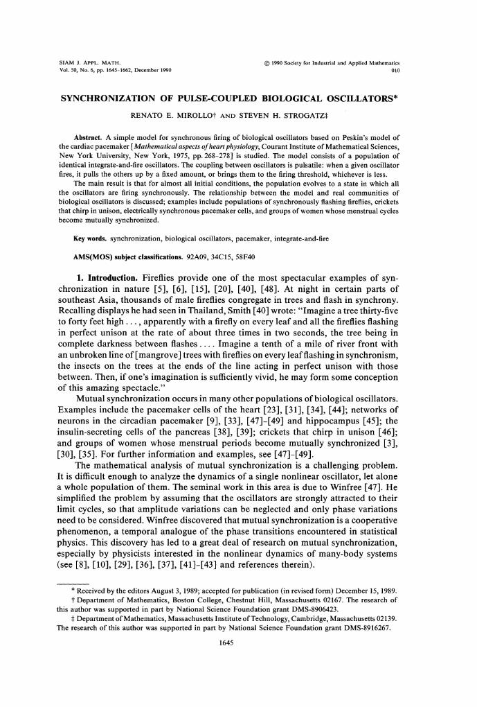
The new feature is that, instead of (1.1), we assume only that x evolves according to x =f ( 4 ) , where f : [0,1] + [0,1] is smooth, monotonic increasing, and concave down, i.e., f '>0 and f "<0. Here 4 E [0, 11 is a phase variable such that (i) d4/dt = 1/ T, where T is the cycle period, (ii) 4 =0 when the oscillator is at its lowest state x =0, and (iii) 4 = 1 at the end of the cycle when the oscillator reaches the threshold x = 1. Therefore f satisfies f(0) =0, f (1) = 1. Figure 1 shows the graph of a typical J:

SYNCHRONIZATION OF BIOLOGICAL OSCILLATORS

FIG. 1. Graph of the function J The timecourse of the integrate-and-fire oscillation is given by x =f ( 4 ) , where x is the state and @ is a phase variable proportional to time.

Let g denote the inverse function f-' (which exists since f is monotonic). Note that g maps states to their corresponding phases: g(x) = 4. Because of the hypotheses on J; the function g is increasing and concave up: g '> 0 and g"> 0. The endpoint conditions on g are g(0) =0, g(1) = 1.

Example. For Peskin's model (1.1), we find

where C = 1- e-". The intrinsic period T = y-' In [S,,/(S, - y)]. Now consider two oscillators governed by J; and assume that they interact by the

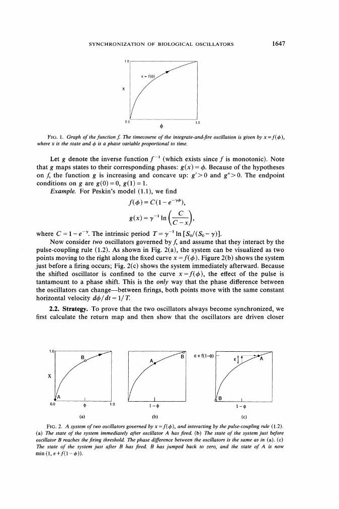
pulse-coupling rule (1.2). As shown in Fig. 2(a), the system can be visualized as two points moving to the right along the fixed curve x =f (4) . Figure 2(b) shows the system just before a firing occurs; Fig. 2(c) shows the system immediately afterward. Because the shifted oscillator is confined to the curve x =f ( 4 ) , the effect of the pulse is tantamount to a phase shift. This is the only way that the phase difference between the oscillators can change-between firings, both points move with the same constant horizontal velocity d 4 l d t = 1/ T.

2.2. Strategy. To prove that the two oscillators always become synchronized, we first calculate the return map and then show that the oscillators are driven closer

FIG. 2. A system of two oscillators governed by x =f ( @ ) , and interacting by the pulse-coupling rule (1.2). ( a ) The state of the system immediately after oscillator A has jired. ( b ) The state of the system just before oscillator B reaches the firing threshold. The phase diflerence between the oscillators is the same as in (a ) . ( c ) The state of the system just after B has jired. B has jumped back to zero, and the state of A is now min (1, E + f ( 1 - 4 ) ) .

1648 R. E. MIROLLO AND S. H. STROGATZ

together each time the map is iterated. Perfect synchrony is locked in when the oscillators have gotten so close together that the firing of one brings the other to threshold. They remain synchronized thereafter because their dynamics are identical.

2.3. Return map and firing map. The return map is defined as follows. Call the two oscillators A and B, and let us strobe the system at the instant after A has fired (Fig. 2(a)). Because A has just fired, its phase is zero. Let 4 denote the phase of B. The return map R ( 4 ) is defined to be the phase of B immediately after the next firing of A.

To calculate the return map, observe that after a time 1 - 4, oscillator B reaches threshold (Fig. 2(b)). During this time, A moves from zero to an x-value given by x, =f(1- 4 ) . An instant later, B fires and xA jumps to E +f(1- 4 ) or 1, whichever is less (Fig. 2(c)). If x, = 1, we are done-the oscillators have synchronized. Hence assume that xA = E +f(1- +f(1- 4 ) ) , 4 ) <1. The corresponding phase of A is g ( ~ where g =f -'as above.

We define the $ring map h by

Thus, after one firing, the system has moved from an initial state (4,, 4,) = (0, 4 ) to a current state (4A, 4,) = (h(4) , 0). In other words, the system is in essentially the same state as when we started-but with 4 replaced by h (4 ) and the oscillators interchanged. Therefore to obtain the return map R ( 4 ) , we follow the system ahead for one more iteration of h:

A caveat about the domains of h and R: In the calculation leading to (2.1), we assumed that F +f(1- 4 ) < 1. (Otherwise synchronization occurs after the next firing.) This assumption is satisfied for E E [O, 1) and 4 E (6, I), where 6 is defined by

Thus the domain of the map h, strictly speaking, is the subinterval (6, 1). Similarly, the domain of R is the subinterval (6, h-'(6)). This interval is nonempty because 6 < h-'(6) for E < 1, as is easily checked.

2.4. Dynamics. We will now show that there is a unique fixed point for R, and that this fixed point is a repeller.

LEMMA2.1. h ' (4) < -1 and R ' (4) > 1, for all 4. ProoJ: It suffices to show that h r (4 ) < -1, for all 4, since R ' (4) = hr(h(4))h ' (4) .

From (2.1), we obtain h t (4 ) = - g ' ( ~+f(1- 4))f '(1 - 4 ) . Since f and g are inverses, the chain rule implies f '(1- 4 ) = [gr( f(1- 4))]-'. Hence

Let u =f(1- 4 ) . Then (2.3) is of the form

By hypothesis, g"> 0 and E >0, so gr(& + u) > gr(u), for all u. This is where the concavity hypothesis on g is used. Finally, the hypothesis that gr(u) >0 for all u implies that h' <-1, as claimed. 0

SYNCHRONIZATION OF BIOLOGICAL OSCILLATORS 1649

PROPOSITION2.2. There exists a uniquejxed point for R in (6, h-'(a)), and it is a repeller.

ProoJ: To prove existence, it suffices to find a fixed point for h, because (2.2) implies that any fixed point for h is a fixed point for R. The fixed point equation for h is

It is easy to check that

and from Lemma 2.1 we have F r ( 4 ) = 1-h t ( 4 )>2 > 0. Hence h has a unique fixed point 4".

Since R(4") = 4" and R t ( 4 ) > 1 by Lemma 2.1, we have

Hence the fixed point for R is unique, and is a repeller. O The result (2.7) shows that R has simple dynamics-from any initial phase (other

than the fixed point), the system is driven monotonically toward 4 =0 or 4 = 1. In other words, the system is always driven to synchrony.

2.5. Solvable example. By making a convenient choice for the function f ( 4 ) , we can gain further insight into the dynamics of synchronization. The special case con- sidered here illustrates a number of qualitative phenomena that occur more generally.

Our criterion for choosing f is that the firing map h and the return map R should be as simple as possible. From Lemma 2.1, we know that h r (4 ) < -1. Suppose we insist that

where A > 1 is independent of 4. Then h and R would reduce to affine maps:

Now we seek the function f such that (2.8) is satisfied. Equation (2.4) dictates the appropriate choice of f-its inverse function g must satisfy the functional equation

Equation (2.1 1) has solutions of the form

where a and b are parameters and

(Note that (2.11) has more general solutions than (2.12), e.g., gr(u) =P(u ) ebu, where P(u) is any periodic function with period E. However (2.12) is sufficient for our purposes.)

1650 R. E. MIROLLO AND S. H. STROGATZ

After integrating (2.12) and imposing the endpoint conditions g(0 ) =0 and g(1 ) =

1, we find

The function f = g p l is given by

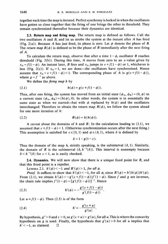
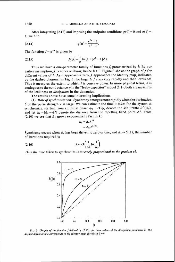
Thus we have a one-parameter family of functions J; parametrized by b. By our earlier assumption, f is concave down; hence b >0. Figure 3 shows the graph off for different values of b. As b approaches zero, f approaches the identity map, indicated by the dashed diagonal in Fig. 3; for large b, f rises very rapidly and then levels off. Thus b measures the extent to which f is concave down. In more physical terms, b is analogous to the conductance y in the "leaky capacitor" model (1.1); both are measures of the leakiness or dissipation in the dynamics.

The results above have some interesting implications. (1) Rate of synchronization. Synchrony emerges more rapidly when the dissipation

b or the pulse strength E is large. We can estimate the time it takes for the system to synchronize, starting from an initial phase 40.Let 4, denote the kth iterate ~ , ( 4 , ) , and let A, =14,- 4*I denote the distance from the repelling fixed point 4*.From (2.10) we see that A, grows exponentially fast in k :

A, = aohZk = A, e 2 E b k .

Synchrony occurs when 4, has been driven to zero or one, and A, -O ( 1 ) ; the number of iterations required is

Thus the time taken to synchronize is inversely proportional to the product ~ b .

0.0 0.2 0.4 0.6 0.8 1.O

0 F I G . 3. Graphs of the function f dejned by (2.15), for three values of the dissipation parameter b. The

dashed diagonal line corresponds to the identity map, for which b =0.

1651 SYNCHRONIZATION OF BIOLOGICAL OSCILLATORS

A similar result was found by Peskin [34]. He used Taylor series expansions to approximate the return map for the model (1.1) in the limit of small s and y. He showed that the rate of convergence to synchrony depends on the product s y (to lowest order in E and y), and concluded that synchrony is a "cooperative effect between the coupling and the dissipation; convergence disappears when either the coupling or the dissipation is removed." Our result shows that this product dependence holds even if s and b are not small.

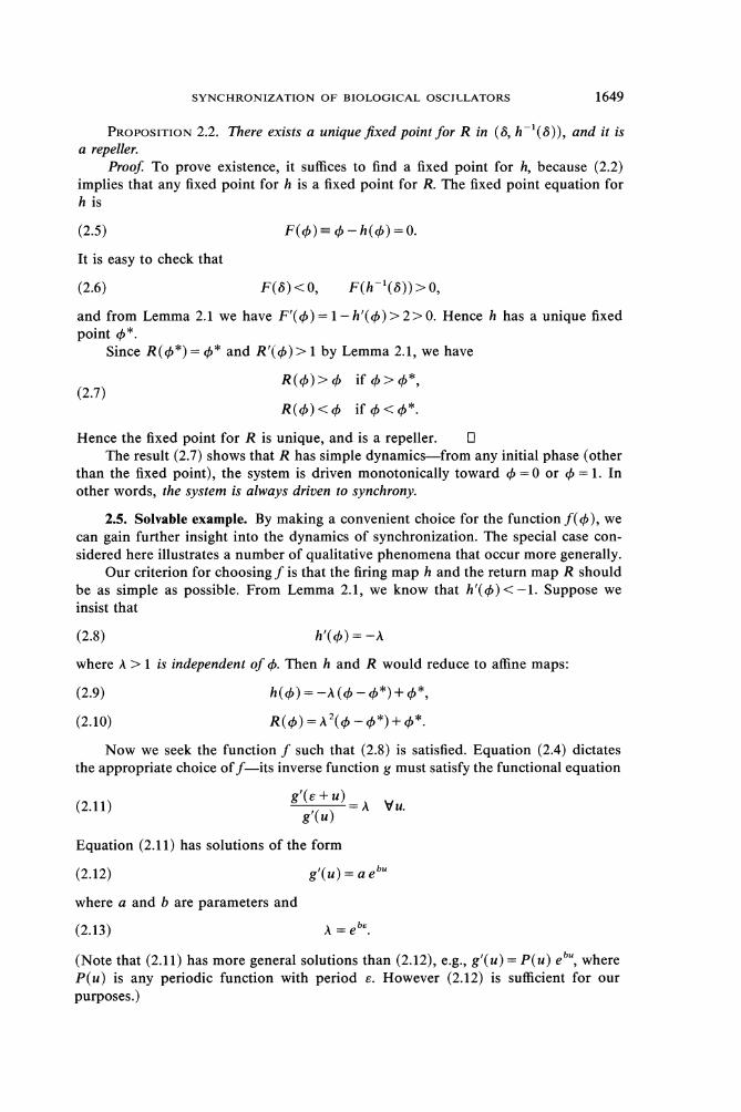
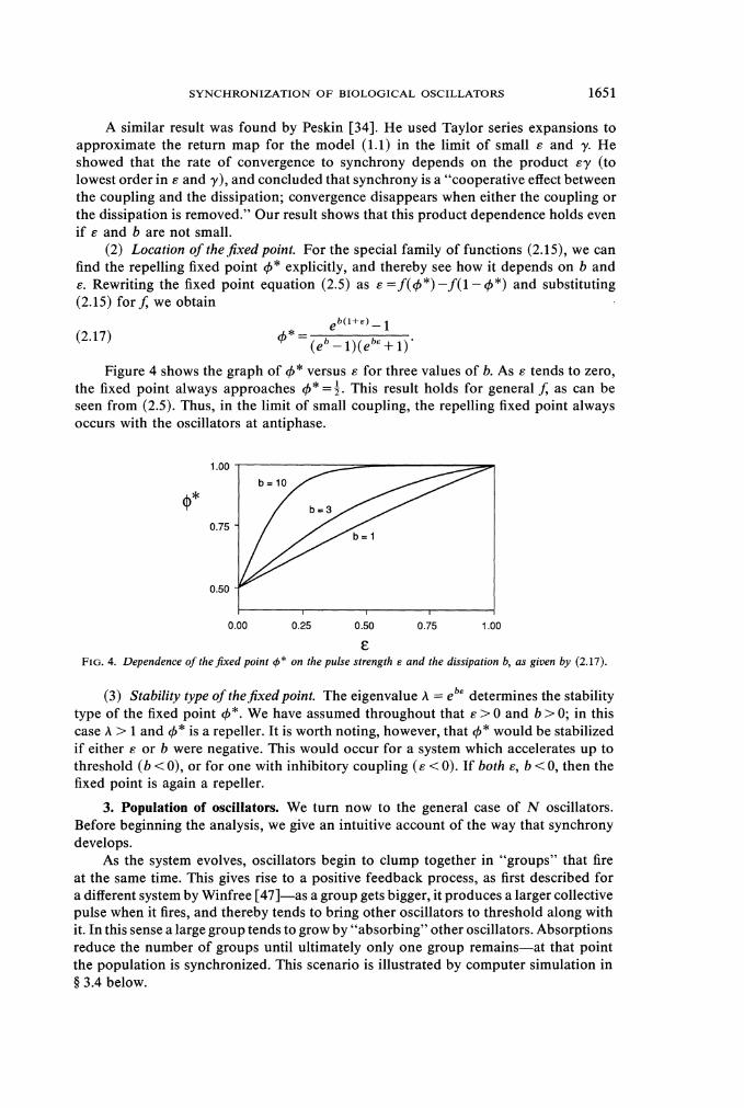
(2) Location of thejixedpoint. For the special family of functions (2.15), we can find the repelling fixed point 4" explicitly, and thereby see how it depends on b and s. Rewriting the fixed point equation (2.5) as s =f (4" ) -f (1- 4") and substituting (2.15) for J; we obtain

Figure 4 shows the graph of 4" versus s for three values of b. As s tends to zero, the fixed point always approaches 4" =$.This result holds for general J; as can be seen from (2.5). Thus, in the limit of small coupling, the repelling fixed point always occurs with the oscillators at antiphase.

0.00 0.25 0.50 0.75 1.OO

E F I G . 4 . Dependence of t h e j x e d point +* on the pulse strength E and the dissipation b, a s given by (2 .17) .

(3) Stability type of thejixedpoint. The eigenvalue A = ebEdetermines the stability type of the fixed point 4". We have assumed throughout that s>0 and b >0; in this case A > 1 and 4" is a repeller. It is worth noting, however, that 4" would be stabilized if either s or b were negative. This would occur for a system which accelerates up to threshold (b <0), or for one with inhibitory coupling ( s <0). If both s, b <0, then the fixed point is again a repeller.

3. Population of oscillators. We turn now to the general case of N oscillators. Before beginning the analysis, we give an intuitive account of the way that synchrony develops.

As the system evolves, oscillators begin to clump together in "groups" that fire at the same time. This gives rise to a positive feedback process, as first described for a different system by Winfree [47]-as a group gets bigger, it produces a larger collective pulse when it fires, and thereby tends to bring other oscillators to threshold along with it. In this sense a large group tends to grow by "absorbing" other oscillators. Absorptions reduce the number of groups until ultimately only one group remains-at that point the population is synchronized. This scenario is illustrated by computer simulation in § 3.4 below.

1652 R. E. MIROLLO AND S. H. STROGATZ

Our proof of synchrony has two parts. The first part (Theorem 3.1) shows that for almost all initial conditions, an absorption occurs in finite time. The hypotheses of Theorem 3.1 are general in the sense that they allow the groups to fire with different strengths, corresponding to the different numbers in each group. After an absorption occurs, there are N - 1 groups (or perhaps a smaller number if several oscillators were absorbed at the same time).

The second part of the proof (Theorem 3.2) rules out the possibility that there might exist sets of initial conditions of positive measure which, after a certain number of absorptions, live forever without experiencing the final absorptions to synchrony. Taken together, Theorems 3.1 and 3.2 show that almost all initial conditions lead to eventual synchrony.

In § 3.1, we define the state space. The dynamics are discussed in § 3.2, using the analogue of the firing map h discussed above. After defining the notion of "absorptions" more precisely in § 3.3, we present simulations in § 3.4 which illustrate the way that synchrony evolves. We state and prove the two parts of our main theorem in § 3.5. The argument appears somewhat technical, but is based on simple ideas involving the volume-expansion properties of the return map. An exactly solvable example is presen- ted in § 3.6.

3.1. State space. As before, we study the dynamics of the system by "strobing" it right after one of the oscillators has fired and returned to zero. The state of the system is characterized by the phases 4 , , . . . ,4, of the remaining n = N - 1 oscillators. Thus the possible states are given by the set

where we have indexed the oscillators in ascending order. The oscillators are currently labeled 0, 1,2, . . ,n, with the convention that 4, =0.

Because the oscillators are assumed to have identical dynamics and the coupling is all to all, the flow has a special property-it preserves the cyclic ordering of the oscillators. The order cannot change between firings, because the oscillators have identical frequencies, and the monotonicity of the function f ensures that the order is maintained after each firing. Hence the oscillators fire in reverse order to their current index: the oscillator currently labeled n is the next to fire, then n - 1, and so on. After oscillator n fires, we relabel it to zero, and relabel oscillator j to j + 1, for all j <n.

This simple indexing scheme would fail if the oscillators had different frequencies; then one oscillator could "pass" another, and the dynamics would be more difficult to analyze. The case of nonidentical frequencies is relevant to real biological oscillators and is discussed briefly in § 4.

3.2. Firing map. Let 4 = ( 4 , , . . ,4,) be the vector of phases immediately after a firing. As in § 2, we would like to find the firing map h, i.e., the map that transforms

to the vector of phases right after the next firing. To calculate h, note that the next firing occurs after a time 1 - 4,. During this

time, oscillator i has drifted to a phase 4i+ 1-4,, where i =0, 1,2, . . . ,n - 1. Thus the phases right before firing are given by the affine map a:Rn+Rn, defined by

After the firing occurs, the new phases are given by the map T :Rn+R", where

SYNCHRONIZATION OF BIOLOGICAL OSCILLATORS

Together the map

(3.4) h ( 4 ) = ~ ( 4 4 ) )

describes the new phases of the oscillators after one firing. Note that we have implicitly relabeled the oscillators, so the image vector h ( 4 )

represents the phases of the oscillators formerly labeled O,1,2, . . ,n - 1. That is, the original oscillator 0 has become 1, oscillator 2 has become 3, . . ,and oscillator n has become oscillator 0.

3.3. Absorptions. The set S is invariant under the affine map u, but not under the map T, because f ( a n ) + E 2 1 is possible. When this happens, it means that the firing of oscillator n has also brought oscillator n - 1 to threshold along with it. Thereafter the two oscillators act as one, because their dynamics are identical and they are coupled in the same way to all the.other oscillators. We call such an event an absorption.

Absorptions complicate matters in two ways: (1) Because of absorptions, the domain of h is not all of S. The domain is actually

the set

or, equivalently,

If 4 E S-S,, an absorption will occur after one firing of strength E.

(2) Absorptions create groups of oscillators that fire in unison with a combined pulse strength proportional to the number in the group. Equivalently, we can think of a group as a single oscillator with an enhanced pulse strength. Thus we now must allow for the possibility of different pulse strengths in the population. However this turns out to be easily handled-as will be seen in § 3.5, the proof of synchrony does not require identical pulse strengths; it requires only that the pulse strengths be nonnegative and not all zero.

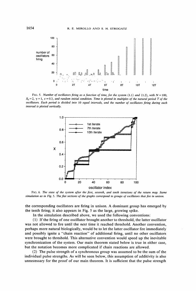
3.4. Numerical results. To illustrate the emergence of synchronization, we now present the results of a computer simulation of N = 100 oscillators. The system was started from a random initial condition: the states xi, i = 1, . . . ,N, were chosen independently from a uniform distribution on [0, 11, and then reindexed so that the xi were in ascending order. (This reindexing involves no loss of generality since each oscillator is coupled to all the others.) The subsequent evolution of the xi was governed by (1.1) and (1.2), with S0=2, y = 1, and E =0.3.

Figure 5 plots the number of oscillators firing as a function of time. At first there is little coherence among the oscillators, and the system organizes itself rather slowly. Then synchrony builds up in an accelerating fashion, as expected by the positive feedback argument given earlier. By t =9T the system is perfectly synchronized.

The slow initial buildup of synchrony is reminiscent of the observation [6] that among southeast Asian fireflies, synchronous flashing "builds up relatively slowly at dusk in the display trees, where each male is being stimulated by the light from many sources." In the present system as well, each oscillator receives many conflicting pulses during the incoherent initial stage.

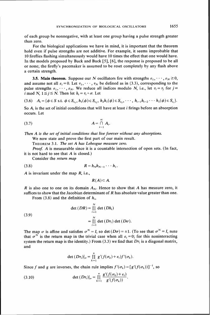
Figure 6 shows the evolution of the system in state space. The system was strobed immediately after each firing of oscillator i = 1. After the first firing, some shallow parts appear in the curve of xi versus i, corresponding to oscillators in nearly the same state. By the seventh firing, these parts have become completely flat-this means that

R. E. MIROLLO AND S. H. STROGATZ

80 -

number of oscillators 60 -firing

40 -

time

FIG. 5. Number of oscillatorsfiring as a function of time, for the system (1.1) and (1.2), with N = 100, So=2, y = 1, E =0.3, and random initial condition. Time is plotted in multiples of the natural period T of the oscillators. Each period is divided into 10 equal intervals, and the number of oscillators Jiring during each interval is plotted vertically.

4-- 10th iterate

X

0 20 40 60 80 100

oscillator index FIG. 6 . The state of the system after the Jirst, seventh, and tenth iterations of the return map. Same

simulation as in Fig. 5. The flat sections of the graphs correspond to groups of oscillators that fire in unison.

the corresponding oscillators are firing in unison. A dominant group has emerged by the tenth firing; it also appears in Fig. 5 as the large, growing spike.

In the simulation described above, we used the following conventions: (1) If the firing of one oscillator brought another to threshold, the latter oscillator

was not allowed to fire until the next time it reached threshold. Another convention, perhaps more natural biologically, would be to let the latter oscillator fire immediately and possibly ignite a "chain reaction" of additional firing, until no other oscillators were brought to threshold. This alternative convention would speed up the inevitable synchronization of the system. Our main theorem stated below is true in either case, but the notation becomes more complicated if chain reactions are allowed.

(2) The pulse strength of a synchronous group was assumed to be the sum of the individual pulse strengths. As will be seen below, this assumption of additivity is also unnecessary for the proof of our main theorem. It is sufficient that the pulse strength

1655 SYNCHRONIZATION OF BIOLOGICAL OSCILLATORS

of each group be nonnegative, with at least one group having a pulse strength greater than zero.

For the biological applications we have in mind, it is important that the theorem hold even if pulse strengths are not additive. For example, it seems improbable that 10 fireflies flashing simultaneously would have 10 times the effect that one would have. In the models proposed by Buck and Buck [5], [6], the response is proposed to be all or none; the firefly's pacemaker is assumed to be reset completely by any flash above a certain strength.

3.5. Main theorem. Suppose our N oscillators fire with strengths E, , ,E, 2 0, and assume not all si=0. Let T,, . . . ,T, be defined as in (3.3), corresponding to the pulse strengths E, , . ,EN. We reduce all indices modulo N, i.e., let = 7;. for j = i mod N,15j 5 N. Then let hi = .ri o a . Let

So Ai is the set of initial conditions that will have at least i firings before an absorption occurs. Let

Then A is the set of initial conditions that live forever without any absorptions. We now state and prove the first part of our main result. THEOREM3.1. The set A has Lebesgue measure zero. ProoJ: A is measurable since it is a countable intersection of open sets. (In fact,

it is not hard to see that A is closed.) Consider the return map

A is invariant under the map R, i.e.,

R is also one to one on its domain AN. Hence to show that A has measure zero, it suffices to show that the Jacobian determinant of R has absolute value greater than one.

From (3.8) and the definition of hi,

N

det (DR) = det (Dhi) i = l

(3.9) N

= n det ( D T ~ ) det (Da ) . i = l

The map a is affine and satisfies u N =I, SO det ( D a ) = +1. (To see that u N =I, note that aNis the return map in the trivial case when all si=0; for this noninteracting system the return map is the identity.) From (3.3) we find that D.ri is a diagonal matrix, and

Since f and g are inverses, the chain rule implies f '(uk)= rgl(f (ak))]-', so

det ( D T ~ ) ~ , n gl(f(ak)+ &i)=

k = l gf(f(uk))

1656 R. E. MIROLLO AND S. H. STROGATZ

By hypothesis, g"> 0 and g'> 0 so the right-hand side of (3.10) is greater than or equal to one, with equality if and only if ci = 0. Hence det (Dri) > 1, unless si=0. But by assumption E~ Z 0 for at least one i. Hence ldet (DR)I > 1. 0

We turn now to the second half of the proof of synchrony. The argument concerns the set of initial conditions which, after a certain number of absorptions, live forever without reaching ultimate synchrony. We will show that this set has measure zero.

Before defining this set more precisely, we first discuss the absorption process. For now, fix the pulse strength E to ease the notation. Suppose 4 = (4 , , . . ,4,) E S,, where S, denotes the state space (3.1), previously called S. (The dependence on n now becomes significant.) Let a ( 4 ) = ( a , , . . . ,a,). As above, let h denote the firing map corresponding to pulse strength E:

Absorption occurs if at least one of the coordinates aj satisfies f (uj)+ E 2 1, or equivalently, aj2 g(1- E) . Since the aj increase with j, there will be an index k such that aj2 g(1- E ) if and only if j> k. Of course, k = n means no absorption occurs, and k =0 means perfect synchrony is achieved. When k < n, we say "4 gets absorbed by h to Sk." In this case we define the image of 4 to be the point

Note that according to this definition the oscillators that get absorbed do not fire. This convention agrees with that used in the simulation shown in Figs. 5 and 6.

As above, we need to allow for the possibility of different pulse strengths. Assume that the ith oscillator (or synchronous group of oscillators) fires with strength ci and let hi denote the corresponding firing map (3.11) with E replaced by E ~ .

Now we discuss the dynamics under iteration of the firing maps. Assume that a point 4 E S, gets absorbed by h, to Sk. This means that the oscillators corresponding to E ~ , . . . ,E , - ~ + ,E ~ , have been absorbed by the oscillator corresponding to E , . These oscillators now form a synchronous group whose combined pulse strength is E, + . . . + E, -~+ , . After this absorption event, the iteration proceeds on Sk, with E sequence

Now we have a similar process on Skto iterate. We continue until we reach synchrony (k =0) or get stuck forever at some stage with k >0.

DEFINITION. Let B be the set of initial conditions in S, which, upon iteration of the maps hi with E sequence E, ,E ~ ,. . . ,E,+,, never achieve synchrony.

THEOREM3.2. The set B has Lebesgue measure zero. ProoJ: By induction on n. The case n = 1 follows from the results of § 2. Assume

the theorem is true for all E sequences E , , . . ,ck on Sk, where k <n. Let B,, denote the set of 4 E B such that 4 survives the applications of h,, . . . ,h,-, ,and then gets absorbed by h, to Sk.Hence

Let p denote Lebesgue measure. We already know that p (A) =0 from Theorem 3.1. Hence it suffices to show that ,u(B,,~) =0 for each (r, k).

First we consider the case where r = 1. Then Bl,k consists of points which get absorbed by h, to Sk. Furthermore, these points must be absorbed into a set C in Sk of measure zero since, by induction, for any problem on Sk, the set of points which do not achieve synchrony has measure zero.

SYNCHRONIZATION OF BIOLOGICAL OSCILLATORS 1657

Let 4 E Bl,k and let C be any set of measure zero in Sk.Write 4 = ( 4 , , . . . , 4 , ) and a ( 4 ) = ( a , , . . . ,a,). Then 4 is absorbed to

(g(f(c+l)SE1),' ' ' E C.,g ( f ( ( + k ) + ~ l ) )

Hence ( a , , . ,a,) E T;'C, where we use the notation T, for the map on Sknow. Since T, is a diffeomorphism, ,u(T;'c) =0. This means that the projection of the set CTB,,~ to Sk has This is possible only if p ( ~ B , , ~ ) = 0 . a is also ameasure zero. Since diffeomorphism, p (B1,k)=0.

Now suppose r > 1. Consider any Br,k. We have

hr-lhr-2 ' ' ' hlBr,k Bl,k.

Each hi is a diffeomorphism on its domain. Hence P(B, ,~) =0, for all k, r > 1. O

3.6. Solvable example. As in § 2, we can obtain further insight (and sharper results) if we assume that f belongs to the one-parameter family of functions (2.15). Then the return map R becomes very simple-it is given by an affine map whose linear part is a multiple of the identity, as we will now show.

In general, R is given by

where .ri :R" +Rn is defined by (3.3) with E replaced by E ~ :

Now suppose that g and f are given by (2.14) and (2.15). Then

g( f ( a k ) + si)= ebElak+constant,

and so

.ri=A i l +constant,

where

(3.12)

Hence R reduces to

(3.13) R = (A, . . . AN)I+constant,

because a commutes with I, and aN= I. Remarks. (1) For this example, R is an expansion map:

As before, we are assuming that b >0, E~2 0, for all i, and E~ f 0 for some i. An open question is whether R is always an expansion map, given the original,

more general hypotheses on the function J: Furthermore, Theorem 3.1 can be strengthened: the set A is (at most) a single

repellingjxed point. This follows from the observations that A is an invariant set and R is an expansion.

(2) To gain some intuition about the repelling fixed point, suppose that all the pulse strengths .si are very small, so that T~ is close to the identity map. Then the repelling fixed point 4" is close to the fixed point of a , namely,

1658 R. E. MIROLLO AND S. H. STROGATZ

In other words, the oscillators are evenly spaced in phase. This generalizes the earlier result that for N =2 and small E, the repelling fixed point occurs with the oscillators at antiphase.

4. Discussion. We have studied the emergence of synchrony in a system of integrate-and-fire oscillators with pulse coupling. The system generalizes Peskin's model [34] of the cardiac pacemaker by allowing more general dynamics than (1.1); we assume only that each oscillator rises toward threshold with a time-course which is monotonic and concave down. Our main result is that for all N and for almost all initial conditions, the system eventually becomes synchronized.

The analysis reveals the importance of the concavity assumption (related to the "leaky" dynamics of the oscillators) and the sign of the pulse coupling (the interactions are "excitatory"). Like Peskin 1341 we have found that synchrony is a cooperative effect between dissipation and coupling-it does not occur unless both are present.

In retrospect it may seem obvious that synchrony would always emerge in our model. We have made some strong assumptions-the oscillators are identical and they are coupled "all to all." On the other hand, we might well have imagined that the system could remain in a state of perpetual disorganization, or perhaps split into two subpopulations which fire alternately. Perpetual disorganization would actually occur if the oscillators were to follow a linear time-course, rather than one which is concave down-then the return map would be the identity and the system would never syn- chronize.

In any case, the behavior of oscillator populations can be counterintuitive. Winfree [48] has described some surprising phenomena in a "firefly machine" made of 71 electrically-coupled neon oscillators with a narrow distribution of natural frequencies. Such oscillators are akin to those considered here, being based on a voltage which accumulates to a threshold and then discharges abruptly. Winfree found that when the oscillators were coupled equally to one another through a common resistor, the system never synchronized, no matter how strong the coupling!

4.1. Relation to previous work. 4.1.1. Oscillator populations. To put our work in context with previous research

on oscillator populations, it is helpful to distinguish among three different levels of synchronization: synchrony, phase locking, and frequency locking. In this paper we use the term "synchrony" in the strongest possible sense: "synchrony" means "firing in unison." Synchrony is possible in our model because the oscillators are identical. True synchrony never occurs in real populations because there is always some distribu- tion of natural frequencies, which is then reflected in the distribution of firing times- typically the faster oscillators fire earlier. Nevertheless, some experimental examples provide a good approximation to synchrony, in the sense that the spread in firing times is small compared to the period of the oscillation. For example, this is the case for the firing of heart pacemaker cells [23], [31], [34], synchronous flashing of fireflies [5], [6], [20], chorusing of crickets [46], and menstrual synchrony among women [30].

"Phase locking" is a weaker form of synchronization in which the oscillators do not necessarily fire at the same time. The phase difference between any two oscillators is constant, but generally nonzero. Phase locking arises in studies of oscillator popula- tions with randomly distributed natural frequencies [8], [lo], [ l l ] , [29], [36], [37], [42], [43], [47], as well as in wave propagation in the Belousov-Zhabotinsky reagent [16], [28], [48], [50], [51] and in central pattern generators [7], [26], [27].

"Frequency locking" means that the oscillators run at the same average frequency, but not necessarily with a fixed phase relationship. If the coupling is too weak to

1659 SYNCHRONIZATION OF BIOLOGICAL OSCILLATORS

enforce phase locking, a system which is spatially extended may break up into distinct plateaus [12], [16], [48] or clusters [36], [37], [42], [43] of frequency-locked oscillators.

4.1.2. Integrate-and-fire models. The oscillators in our model obey "integrate-and- fire" dynamics. This is a reasonable assumption for biological oscillators, which often exhibit relaxation oscillations based on the buildup and sudden discharge of a mem- brane voltage or other activity variable [17], [18]. Most previous studies of integrate- and-fire oscillators have emphasized the dynamics of a single oscillator in response to periodic forcing, with special attention to bifurcations, mode locking, and chaos [2], [4], [24], [17]. Our concern is with interacting populations of integrate-and-fire oscil- lators, for which much work remains to be done.

4.1.3. Pulse coupling. The pulse coupling (1.2) is a simplification of biological reality. It produces only phase advances; a resetting pulse always causes an oscillator to fire earlier than normal. The experimentally measured phase-response curves for the flashing of fireflies, the firing of cardiac pacemaker cells, and the chirping of crickets all have more structure than (1.2) suggests (see [48, p. 1191). Other authors have studied models which incorporate more of the biological details of pulse coupling (see, for example, the heart models of Honerkamp [21] and Ikeda, Yoshizawa, and Sato [22] which include absolute and relative refractory periods, or the firefly models of Buck and Buck [5], [6] which include time delay between stimulus and response).

A surprising feature of pulse coupling has recently been discovered by Ermentrout and Kopell [13]. They found that in many different models of neural oscillators, excessively strong pulse coupling can cause cessation of rhythmicity-"oscillator deathH-and they also discuss the averaging strategies that real neural oscillators apparently use to avoid such a fate. Note however that there is no oscillator death in the simple model studied here, thanks to (unrealistic) discontinuities in the dynamics.

4.1.4. Synchronous fireflies. The model considered here is similar to a model of firefly synchronization proposed by Buck [5]. In the common American firefly Photinus pyralis, it appears that resetting occurs exclusively through phase advances. Buck postulates that when a firefly of this species receives a light pulse near the end of its cycle, its flash-control pacemaker is immediately reset to threshold, as in our model. However, in contrast to our model, pulses received during the earlier part of the cycle are assumed to have little or no effect.

Buck [5] also assumes a linear increase of excitation toward threshold, in contrast to the concave-down timecourse in the present model. He points out that Photinus pyralis is "not usually observed to synchronizeu-this is exactly what our model would predict if the rise to threshold were actually linear! (Synchrony would also fail if the timecourse were concave-up.)

A more likely explanation for the lack of synchrony in this species is that the coupling strength is too small to overcome the variability in flashing rate. This explana- tion is supported by the observation [5] that Photinus pyralis has a comparatively irregular flashing rhythm; for an individual male, the cycle-to-cycle variability (standard deviationlmean period) is =1/20, compared to =1/200 for males of the Thai species Pteroptyx malaccae.

Finally, the simple model discussed here does not account for those species of fireflies which exhibit phase delays in response to a light flash [5], [20].

4.2. Directions for future research. 4.2.1. Spatial structure. In its present form the model has no spatial structure;

each oscillator is a neighbor of all the others. How would the dynamics be affected if one replaced the all-to-all coupling with more local interactions, e.g., between nearest

1660 R. E. MIROLLO AND S. H. STROGATZ

neighbors on a ring, chain, d-dimensional lattice, or more general graph [I], [19], [32]? Would the system still always end up firing in unison, or would more complex modes of organization become possible?

By analogy with other large systems of oscillators, we expect that systems with reduced connectivity should have less tendency to become synchronized [a], [36], [42], [43]. (A similar rule of thumb is well known in equilibrium statistical mechanics: a ring of Ising spins cannot exhibit long-range order, but higher-dimensional lattices can.) Thus a ring of oscillators is a leading candidate for a system which might yield other behavior besides global synchrony. But we have not observed any such behavior in preliminary numerical studies-even a ring always synchronizes.

We therefore suspect that our system would end up firing in unison for almost all initial conditions, no matter how the oscillators were interconnected (as long as the interconnections form a connected graph). If correct, this would distinguish our pulse-coupled system from diffusively coupled systems of identical oscillators, which often support locally stable rotating waves [ I l l , [14], [48].

In any case, it will be more difficult to analyze our system if the coupling is not all to all, because we can no longer speak of "absorptions." Recall that in the all-to-all case, a synchronous subset of oscillators remains synchronous forever. This is not the case with any other topology-a synchronous group can now be disrupted by pulses impinging on the boundary of the group.

4.2.2. Nonidentical oscillators. Another restrictive assumption is that the oscil- lators are identical; then synchrony occurs even with arbitrarily small coupling. It would be more realistic to let the oscillators have a random distribution of intrinsic frequencies. Most of the work on mutual entrainment of smoothly coupled oscillators deals with this case [8], [lo], [ l l ] , [29], [31], [36], [37], [42], [43], [47], [48], but almost nothing is known for the case of pulse coupling.

One property of the present model can be anticipated: in a synchronous population the fastest oscillator would set the pace. This idea often crops up in popular discussions of synchronization, and is widely accepted in cardiology, but it is known to be wrong for certain populations of oscillators [6], [9], [23], [26], [31], [48]; nevertheless it is true for the present model. To see this, imagine that all the oscillators have just fired and are now at x =0. Then the first oscillator to reach threshold is the fastest one. Given our assumption that the population remains synchronous, all the other oscillators have to be pulled up to threshold at the same time. Thus the frequency of the population is that of the fastest oscillator.

A periodic solution of this form would be possible if the pulse strength were large enough to pull the slowest oscillator up to threshold. Even a weaker pulse might suffice if it could set off a "chain reaction" of firing by other oscillators.

Of course, such a synchronous solution might not be stable, and even if it were, there might be other locally stable solutions. For instance, could a synchronous state coexist with arrhythmia? Such bistability might have relevance for certain rhythm disturbances of the cardiac pacemaker.

REFERENCES

[I ] J. C. ALEXANDER, Patterns at primary Hopf bifurcations of a plexus of identical oscillators, SIAM J . Appl. Math., 46 (1986), pp. 199-221.

[2] P. ALSTRC~M, AND M. T. LEVINSEN,Nonchaotic transition from quasiperiodicity B. CHRISTIANSEN, to complete phase locking, Phys. Rev. Lett., 61 (1988), pp. 1679-1682.

[3] Anonymous, Olfactory synchrony of menstrual cycles, Science News, 112 (1977), p. 5.

1661 SYNCHRONIZATION OF BIOLOGICAL OSCILLATORS

J. BELAIR,Periodic pulsatile stimulation o fa nonlinear oscillator, J. Math. Biol., 24 (1986), pp. 217-232. J. BUCK,Synchronous rhythmicflashing offireflies 11, Quart. Rev. Biol., 63 (1988), pp. 265-289. J. BUCKAND E. BUCK, Synchronous fireflies, Scientific American, 234 (1976), pp. 74-85.

[7] A. H. COHEN, P. J. HOLMES, AND R. H. RAND, The nature ofthe coupling between segmental oscillators of the lamprey spinal cord for locomotion: a mathematical model, J. Math. Biol., 13 (1982), pp. 345-369.

[8] H. DAIDO, Lower critical dimension for poptrlations of oscillators with randomly distributedfrequencies: A renormalization-group analysis, Phys. Rev. Lett., 61 (1988), pp. 231-234.

[9] J. T. ENRIGHT, Temporal precision in circadian systems: a reliable neuronal clock from unreliable components?, Science, 209 (1980), pp. 1542-1545.

[lo] G. B. ERMENTROUT, Synchronization in a pool of mutually coupled oscillators with randomfrequencies, J. Math. Biol., 22 (1985), pp. 1-9.

[ I l l -, The behavior of rings of coupled oscillators, J. Math. Biol., 23 (1985), pp. 55-74. [12] G. B. ERMENTROUT A N D N. KOPELL, Frequency plateaus in a chain of weakly coupled oscillators. I,

SIAM J. Math. Anal., 15 (1984), pp. 215-237. [I31 -, Oscillator death in systems of coupled neural oscillators, SIAM J . Appl. Math., 50 (1990), pp.

125-146. [14] G. B. ERMENTROUT A N D J. RINZEL, Waves in a simple, excitable or oscillatory, reaction-diffusion

model, J. Math. Biol., 11 (1981), pp. 269-294. [I51 -, Beyond a pacemaker's entrainment limit: phase walk-through, Amer. J . Physiol., 246 (1984),

pp. R102-R106. [16] G. B. ERMENTROUT AND W. C. TROY, Phaselocking in a reaction-diffusion system with a linear frequency

gradient, SIAM J. Appl. Math., 46 (1986), pp. 359-367. [17] L. GLASSAND M. C. MACKEY, A simple model forphase locking of biological oscillators, J . Math. Biol.,

7 (1979), pp. 339-352. 1181 -, From Clocks to Chaos: The Rhythms o f l i fe , Princeton University Press, Princeton, NJ, 1988. [19] J. GRASMAN AND M. J. W. JANSEN, Mutually synchronized relaxation oscillators as prototypes of

oscillating systems in biology, J. Math. Biol., 7 (1979), pp. 171-197. [20] F. E. HANSON, Comparative studies ofjirefly pacemakers, Fed. Proc., 37 (1978), pp. 2158-2164. [21] J. HONERKAMP, The heart asa system ofcouplednonlinearoscillators,J. Math. Biol., 18 (1983), pp. 69-88. [22] N. IKEDA, S. YOSHIZAWA, AND T. SATO, Difference equation model of ventricular parasystole as an

interaction between cardiac pacemakers based on the phase response curve, J. Theoret. Biol., 103 (1983), pp. 439-465.

[23] J. JALIFE, Mutual entrainment and electrical coupling as mechanisms for synchronous jiring of rabbit sinoatrial pacemaker cells, J . Physiol., 356 (1984), pp. 221-243.

[24] J. P. KEENER, F. C. HOPPENSTEADT, AND J. RINZEL, Integrate-and-jire models of nerve membrane response to oscillatory input, SIAM J. Appl. Math., 41 (1981), pp. 503-517.

[25] B. W. KNIGHT,Dynamics ofencoding in apopulation of neurons, J . Gen. Physiol., 59 (1972), pp. 734-766. [26] N. KOPELL, Toward a theory of modelling central pattern generators, in Neural Control of Rhythmic

Movement in Vertebrates, A. H. Cohen, S. Rossignol, and S. Grillner, eds., John Wiley, New York, 1988, pp. 369-413.

[27] N. KOPELLAND G. B. ERMENTROUT, Symmetry andphaselocking in chains of weakly coupled oscillators, Comm. Pure Appl. Math., 39 (1986), pp. 623-660.

[28] N. KOPELL AND L. N. HOWARD, Plane wave solutions to reaction-d~ffusion equations, Stud. Appl. Math., 52 (1973), pp. 291-328.

[29] Y. KURAMOTO AND I. NISHIKAWA,Statistical macrodynamics of large dynamical systems. Case o f a phase transition in oscillator communities, J. Statist. Phys., 49 (1987), pp. 569-605.

1301 M. K. MCCLINTOCK, Menstrual synchrony and suppression, Nature, 229 (1971), pp. 244-245. [31] D. C. MICHAELS, E. P. MATYAS, AND J. JALIFE, Mechanisms of sinoatrialpacemaker synchronization:

a new hypothesis, Circulation Res., 61 (1987), pp. 704-714. [32] H. G. OTHMER, Synchronization, phase-locking and otherphenomena in coupled cells, in Temporal Order,

L. Rensing and N. I. Jaeger, eds., Springer-Verlag, Heidelberg, 1985, pp. 130-143. [33] T. PAVLIDIS, Biological Oscillators: Their Mathematical Analysis, Academic Press, New York, 1973. [34] C. S. PESKIN, Mathematical Aspects of Heart Physiology, Courant Institute of Mathematical Sciences,

New York University, New York, 1975, pp. 268-278. [35] M. J. RUSSELL, G. M. SWITZ, AND K. THOMPSON,Olfactory influences on the human menstrual cycle,

Pharmacol. Biochem. Behav., 13 (1980), pp. 737-738. 1361 H. SAKAGUCHI, S. SHINOMOTO, AND Y. KURAMOTO, Local and global sew-entrainments in oscillator

lattices, Progr. Theoret. Phys., 77 (1987), pp. 1005-1010. [371 -, Mutual entrainment in oscillator lattices with nonvariational type interaction, Progr. Theoret.

Phys., 79 (1988), pp. 1069-1079.

1662 R. E. MIROLLO AND S. H. STROGATZ

[38] A. SHERMAN AND J. RINZEL,Collective properties of insulin secreting cells, preprint. [39] A. SHERMAN, J. RINZEL,AND J. KEIZER,Emergence of organized bursting in clusters of pancreatic

beta-cells by channel sharing, Biophys. J. , 54 (1988), pp. 411-425. [40] H. M. SMITH, Synchronousflashing offireflies, Science, 82 (1935), p. 151. [41] S. H. STROGATZ,C. M. MARCUS, R. M. WESTERVELT, AND R. E. MIROLLO,Collective dynamics of

coupled oscillators with random pinning, Phys. D, 36 (1989), pp. 23-50. [42] S. H. STROGATZAND R. E. MIROLLO,Phase-locking and critical phenomena in lattices of coupled

nonlinear oscillators with random intrinsic frequencies, Phys. D, 31 (1988), pp. 143-168. [431 -, Collective synchronisation in lattices of nonlinear oscillators with randomness, J. Phys. A, 21

(1988), pp. L699-L705. [44] V. TORRE, A theory of synchronization oftwo heartpacemaker cells, J. Theoret. Biol., 61 (1976), pp. 55-71. [45] R. D. TRAUB,R. MILES,AND R. K. S. WONG, Model of the origin of rhythmic population oscillations

in the hippocampal slice, Science, 243 (1989), pp. 1319-1325. [46] T. J. WALKER,Acoustic synchrony: two mechanisms in the snowy tree cricket, Science, 166 (1969),

pp. 891-894. [47] A. T. WINFREE, Biological rhythms and the behavior of populations of coupled oscillators, J . Theoret.

Biol., 16 (1967), pp. 15-42. [481 -, The Geometry of Biological Time, Springer-Verlag, New York, 1980. [491 -, The Timing of Biological Clocks, Scientific American Press, New York, 1987. [SO] -, When Time Breaks Down: The Three-Dimensional Dynamics of Electrochemical Waves and

Cardiac Arrhythmias, Princeton University Press, Princeton, NJ, 1987. [51] A. T. WINFREE AND S. H. STROGATZ,Organizing centersfor three-dimensional chemical waves, Nature,

311 (1984), pp. 611-615.