synchrophasor applications for grid dynamic models …€¦ · · 2013-10-30for grid dynamic...
TRANSCRIPT

E n e r g y R e s e a r c h a n d D e v e l o p m e n t D i v i s i o n F I N A L P R O J E C T R E P O R T
SYNCHROPHASOR APPLICATIONS FOR GRID DYNAMIC MODELS AND THE MONITORING OF SYSTEM PARAMETERS
Appendices
JUNE 2009 CE C-500-2013-125-AP
Prepared for: California Energy Commission Prepared by: Lawrence Berkeley National Laboratory

PREPARED BY:
Primary Author(s): Joseph Eto Manu Parashar Nancy Lewis
Lawrence Berkeley National Laboratory Berkeley, CA
Contract Number: 500-02-004
Prepared for:
California Energy Commission
Jamie Patterson Contract Manager
Fernando Pina Office Manager Energy Systems Research Office
Laurie ten Hope Deputy Director ENERGY RESEARCH AND DEVELOPMENT DIVISION
Robert P. Oglesby Executive Director
DISCLAIMER
This report was prepared as the result of work sponsored by the California Energy Commission. It does not necessarily represent the views of the Energy Commission, its employees or the State of California. The Energy Commission, the State of California, its employees, contractors and subcontractors make no warranty, express or implied, and assume no legal liability for the information in this report; nor does any party represent that the uses of this information will not infringe upon privately owned rights. This report has not been approved or disapproved by the California Energy Commission nor has the California Energy Commission passed upon the accuracy or adequacy of the information in this report.

ACKNOWLEDGEMENTS
CERTS performers are grateful for the technical direction provided by The Public Interest Energy Research (PIER) Transmission Research Program (TRP) and Energy Commission PIER staff Jamie Patterson.
Task 2.0 was led by Manu Parashar, Electric Power Group (EPG), with assistance from research performers Jim Dyer, Simon Mo, Peng Xiao, Jose Coroas, EPG; Ken Martin, Bonneville Power Administration (BPA), Dan Trudnowski, Montana Tech, and Ian Dobson, University of Wisconsin. California Independent System Operator (California ISO) advisors for Task 2.0 were Dave Hawkins, Jim Hiebert, Brian O’Hearn, Greg Tillitson, Paul Bleuss, and Nan Liu.
Task 3.0 was led by Manu Parashar, EPG, with assistance from research performers Abhijeet Agarwal, and Jim Dyer, EPG; Ian Dobson, University of Wisconsin, Yuri Makarov and Ning Zhou, Pacific Northwest National Laboratory (PNNL). California ISO advisors for Task 3.0 were Soumen Ghosh, Matthew Varghese, Patrick Truong, Dinesh Salem-Natarajan, Yi Zhang and Robert Sparks.
i

PREFACE
The California Energy Commission Energy Research and Development Division supports public interest energy research and development that will help improve the quality of life in California by bringing environmentally safe, affordable, and reliable energy services and products to the marketplace.
The Energy Research and Development Division conducts public interest research, development, and demonstration (RD&D) projects to benefit California.
The Energy Research and Development Division strives to conduct the most promising public interest energy research by partnering with RD&D entities, including individuals, businesses, utilities, and public or private research institutions.
Energy Research and Development Division funding efforts are focused on the following RD&D program areas:
• Buildings End-Use Energy Efficiency
• Energy Innovations Small Grants
• Energy-Related Environmental Research
• Energy Systems Integration
• Environmentally Preferred Advanced Generation
• Industrial/Agricultural/Water End-Use Energy Efficiency
• Renewable Energy Technologies
• Transportation
Synchrophasor Applications for Grid Dynamic Models and the Monitoring of System Parameters is the final report for the Real Time System Operations project (contract number 500-03-024 MR041 conducted by the Consortium for Electric Reliability Technology Solutions (CERTS). The information from this project contributes to Energy Research and Development Division’s Energy Systems Integration Program
For more information about the Energy Research and Development Division, please visit the Energy Commission’s website at www.energy.ca.gov/research/ or contact the Energy Commission at 916-327-1551.
ii

ABSTRACT
The Synchrophasor Applications for Grid Dynamic Models and the Monitoring of System Parameters project focused on two parallel technical tasks: (1) Real-Time Applications of Phasors for Monitoring, Alarming and Control; and (2) a Real-Time Voltage Security Assessment Prototype Tool. The overall goal of the phasor applications project was to accelerate adoption and foster greater use of new, more accurate, time-synchronized phasor measurements by conducting research and prototyping applications on the California Independent System Operator’s phasor platform that provide previously unavailable information on the dynamic stability of the grid. The California Independent System Operator’s phasor platform is called the Real-Time Dynamics Monitoring System. Feasibility assessment studies were conducted on potential applications of this technology for small-signal stability monitoring, validating/improving existing stability nomograms, conducting frequency response analysis, and obtaining real-time sensitivity information on key metrics to assess grid stress. A nomogram is a graphical calculating device that consists of a two-dimensional diagram designed to allow the approximate graphical computation of a function. Based on study findings, prototype applications for real-time visualization and alarming, small-signal stability monitoring, measurement-based sensitivity analysis and frequency response assessment were developed, factory- and field-tested at the California Independent System Operator and at Bonneville Power Administration. The goal of the real-time voltage security assessment project was to provide the California Independent System Operator with a prototype voltage security assessment tool that runs in real time within their new reliability and congestion management system. The project team conducted a technical assessment of appropriate algorithms and developed a prototype incorporating state-of-the-art algorithms into a framework suitable for an operations environment. A functional specification was prepared that the California Independent System Operator used to procure a production-quality tool became part of a suite of advanced computational tools used for reliability and congestion management.
Key Words: Electricity grid, reliability, real-time operator tools, time synchronized phasor measurements, voltage security.
Please use the following citation for this report:
Eto, Joseph H., Manu Parashar, Nancy Jo Lewis. Consortium for Electric Reliability Technology Solutions (CERTS). 2009. Synchrophasor Applications for Grid Dynamic Models and the Monitoring of System Parameters. California Energy Commission, PIER Transmission Research Program. CEC-500-2013-125-AP.
iii

TABLE OF CONTENTS
Acknowledgements ................................................................................................................................... i
PREFACE ................................................................................................................................................... ii
ABSTRACT .............................................................................................................................................. iii
TABLE OF CONTENTS ......................................................................................................................... iv
APPENDIX A: Phasor Feasibility Assessment and Research Results Report ........................... A-1
APPENDIX B: Real-Time Voltage Security Assessment Report on Algorithms and Framework
.................................................................................................................................................................. B-1
APPENDIX C: Real-Time Voltage Security Assessment Algorithm's Simulation and Validation
Results ..................................................................................................................................................... C-1
APPENDIX D: Real-Time Voltage Security Assessment Summary Report ....................................
................................................................................................................................................................. D-1
APPENDIX E: Real-Time Voltage Security Assessment Functional Specifications for
Commercial Grade Application ......................................................................................................... E-1
iv

A‐1
APPENDIX A: Phasor Feasibility Assessment and Research Results Report

Arnold Schwarzenegger
Governor
REAL TIME SYSTEM OPERATION2006 – 2007
APPE
NDIX
A
Phasor Technology Applications Feasibility Assessment and
Research Results Report
Prepared For: California Energy Commission Public Interest Energy Research Program
Prepared By: Lawrence Berkeley National Laboratory
Month Year CEC-500-2008-XXX-APA


Prepared By: Lawrence Berkeley National Laboratory Joseph H. Eto, Principal Investigator Manu Parashar and Wei Zhou, Electric Power Group Dan Trudnowski, Montana Tech Yuri Makarov, Pacific Northwest National Laboratory Ian Dobson, University of Wisconsin Berkeley, CA 94720 Commission Contract No. 500-02-004 Commission Work Authorization No: MR-041 Prepared For: Public Interest Energy Research (PIER) California Energy Commission
Jamie Patterson Contract Manager Mike Gravely Program Area Lead ENERGY SYSTEMS INTEGRATION Mike Gravely Office Manager ENERGY SYSTEMS RESEARCH
Martha Krebs, Ph.D. PIER Director Thom Kelly, Ph.D. Deputy Director ENERGY RESEARCH & DEVELOPMENT DIVISION
Melissa Jones Executive Director
DISCLAIMER
This report was prepared as the result of work sponsored by the California Energy Commission. It does not necessarily represent the views of the Energy Commission, its employees or the State of California. The Energy Commission, the State of California, its employees, contractors and subcontractors make no warrant, express or implied, and assume no legal liability for the information in this report; nor does any party represent that the uses of this information will not infringe upon privately owned rights. This report has not been approved or disapproved by the California Energy Commission nor has the California Energy Commission passed upon the accuracy or adequacy of the information in this report.


FEASIBILITY ASSESSMENT AND RESEARCH RESULTS REPORT
Prepared For
California Independent System Operator (CA ISO)
Prepared By
Consortium for Electric Reliability Technology Solutions (CERTS)
Funded By
California Public Interest Energy Research Transmission Research Program
Date: Revised June 20, 2008
Consortium for Electric Reliability Technology Solutions
Phasor
Technology
Applications

The work described in this report was coordinated by the Consortium for Electric Reliability Technology Solutions with funding provided by the California Energy Commission, Public Interest Energy Research Program, through the University of California/California Institute of Energy Efficiency under Contract No. 500‐02‐004, MR‐041.
PREPARED FOR:
California Independent System Operator
PREPARED BY:
Electric Power Group
Manu Parashar, Ph.D. ‐ Principal Investigator
Wei Zhou ‐ Investigator
Montana Tech
Dan Trudnowski, Ph.D. ‐ Consultant
Pacific Northwest National Laboratory
Yuri Makarov, Ph.D. ‐ Principal Consultant
University of Wisconsin, Madison
Ian Dobson, Ph.D. ‐ Consultant
DATE: Revised June 20, 2008

i
Acknowledgements
Special thanks to California ISO staff Mr. Jim Hiebert, Mr. Brian O’Hearn, Mr. Brian Murry, Mr. Paul Bleuss, Mr. Greg Tillitson, Mr. Eric Whitley and Mr. Nan Liu for their consultations to the project and support for the RTDMS system.
Mr. Dave Hawkins (California ISO) for his expertise, comprehensive support, and advices.
Dr. Yuri V. Makarov (PNNL) and Prof. Ian Dobson, (University of Wisconsin‐Madison) for their role in suggesting methodologies on applying phasor technology to stability nomogram, literature review, participation in the brainstorm meetings, expertise and essential advices.
Prof. Dan Trudnowski (Montana Tech), for providing the algorithms for monitoring oscillatory modes under ambient system conditions and his support in the prototype development.
Mr William Mittelstadt, Mr Ken Martin (BPA), Dr John Hauer, Dr Henry Huang, Dr Ning Zhou (PNNL), Prof. John Pierre (University of Wyoming) for sharing their expertise and advise on the mode meter algorithm evaluation.
Mr. Jim Cole (California Institute for Energy Efficiency) for initiating and support of this project, and participants of the TAC meeting for their thoughtful suggestions.
Mr. Joseph Eto (Lawrence Berkeley National Lab) for his support.
Parashar, Manu, Wei Zhou, Dan Trudnowski, Yuri Marakov, Ian Dobson. Consortium for Electric Reliability Technology Solutions (CERTS). 2008. Phasor Technology Applications Feasibility Assessment and Research Results Report. California Energy Commission, PIER Transmission Research Program. CEC‐500‐2008‐XXX.

ii
Preface
The Public Interest Energy Research (PIER) Program supports public interest energy research and development that will help improve the quality of life in California by bringing environmentally safe, affordable, and reliable energy services and products to the marketplace.
The PIER Program, managed by the California Energy Commission (Energy Commission), conducts public interest research, development, and demonstration (RD&D) projects to benefit California.
The PIER Program strives to conduct the most promising public interest energy research by partnering with RD&D entities, including individuals, businesses, utilities, and public or private research institutions.
PIER funding efforts are focused on the following RD&D program areas:
• Buildings End‐Use Energy Efficiency
• Energy Innovations Small Grants
• Energy‐Related Environmental Research
• Energy Systems Integration
• Environmentally Preferred Advanced Generation
• Industrial/Agricultural/Water End‐Use Energy Efficiency
• Renewable Energy Technologies
• Transportation
Real Time System Operations (RTSO) 2006 ‐ 2007 is the final report for the Real Time System Operations project (contract number 500‐03‐024 MR041 conducted by the Consortium for Electric Reliability Technology Solutions (CERTS). The information from this project contributes to PIER’s Transmission Research Program.
For more information about the PIER Program, please visit the Energy Commission’s website at www.energy.ca.gov/pier or contact the Energy Commission at 916‐654‐5164.

iii
Table of Contents
1. OBJECTIVE ........................................................................ Error! Bookmark not defined. 2. INTRODUCTION ................................................................................................................. 7 3. METHODOLOGIES FOR USING PHASORS FOR STABILITY NOMOGRAMS ...... 13
3.1. Improving Existing Nomograms using Real‐Time Phasor Measurements .. 13 3.2. Use of PMUs for Reduced Dynamic Equivalents and Transient Stability Assessment
.............................................................................................................................. 16 3.3. New Concept of Wide Area Nomograms .......................................................... 17 3.4. Use of PMUs for Wide‐Area Voltage Security Assessment ............................ 24 3.5. Augmenting Existing Nomograms using Small‐Signal Stability Assessment25
4. ALGORITHMS FOR MONITORING SMALL‐SIGNAL STABILITY WITH PHASOR MEASUREMENTS ....................................................................................................... 27
4.1. Algorithms to Estimate the System Modes Using Synchronized Phasor Data28 4.2. Mode Selection ....................................................................................................... 30 4.3. Algorithm Tuning ................................................................................................. 31 4.4. Implementation of Small‐Signal Stability Monitoring Prototype Tool.......... 35
5. MEASUREMENT BASED SENSITIVITIES AND VOLTAGE STABILITY MONITORING ......................................................................................................................................... 41
5.1. Measurement based Sensitivities ........................................................................ 41 5.2. Voltage Stability Loading Margins ..................................................................... 43 5.3. Predicting Voltage Stability with Phasor Measurements ................................ 48 5.4. Implementation of Measurement bases Sensitivity Prototype Tool .............. 48
6. FREQUENCY RESPONSE MONITORING ..................................................................... 51 7. GRAPH THEORY BASED PATTERN RECOGNITION ............................................... 55 8. RTDMS SYSTEM ARCHITECTURE ................................................................................ 57 9. CONCLUSION .................................................................................................................... 59

iv
LIST OF FIGURES
Figure 1: Detecting potential “holes” in the nomograms ..................................................... 13
Figure 2: Detecting excessive “conservatism” in the nomograms ...................................... 14
Figure 3: Use of additional PMUs to monitor existing nomograms in real‐time .............. 16
Figure 4: MW Flow and Angle Difference tracking across COI – (a) the net MW flows remained unchanged (b) the transmission outage was captured by angle difference. .............. 18
Figure 5: Western interconnection transmission paths ......................................................... 20
Figure 6: Conceptual view of simple angle difference and advanced angle nomograms21
Figure 7: A cutset of stability boundary in rectangular coordinates of nodal voltages ... 22
Figure 8: Correlation between MW flows across critical flowgates and angle difference pairs ............................................................................................................................................... 23
Figure 9: PMU Measurement based phase angle trends in angle‐angle space .................. 24
Figure 10: Voltage stability boundary developed in angle‐angle space.............................. 25
Figure 11: Signal flow diagram. ............................................................................................... 27
Figure 12: Mode estimates for WECC data ............................................................................ 32
Figure 13: Long‐term Intertie mode trends (frequency & damping) with varying COI flows ............................................................................................................................................... 33
Figure 14: Long‐term Intertie mode spectral trends with varying COI flows ................... 34
Figure 15: Small‐Signal Stability Monitoring Display .......................................................... 35
Figure 16: Sample Mode Tracking Plot .................................................................................... 36
Figure 17: Sample Waterfall Plot .............................................................................................. 37
Figure 18: Block Diagram for the Small‐Signal Stability Monitoring Tool. ....................... 38
Figure 19: Improved Mode Tracking Plot with Bootstrapping Ellipse ............................... 39
Figure 20: Sample Spectral Analysis Display. ......................................................................... 40
Figure 21: P‐V curves and voltage sensitivities at different loading levels across COI ‐ (a) voltage sensitivity ~ 1kV/100MW under light loading conditions (b) voltage sensitivity ~ 3kV/100MW under increased loading conditions. ......................................................... 42
Figure 22: Estimating sensitivities using (a) Least Squares Regression (b) Orthogonal Regression. ........................................................................................................................... 43

v
Figure 23: Flow Chart for voltage stability assessment based on phasor measurements.44
Figure 24: Voltage stability analysis model for a multiple‐infeed load center using phasor measurements. ..................................................................................................................... 45
Figure 25: Estimating voltage stability margins with phasor measurements: (a) P‐V curve predicted by the multiple‐feed load center model; (b) phase measurement data used in the model parameter estimation. ............................................................................................. 47
Figure 26: Voltage Sensitivity Monitoring Display ................................................................ 49
Figure 27: Frequency response captured by the phasor measurement network due to the Colstrip unit outage – (a) the interconnection frequency response to the outage (b) the ringdown observed in the MW flows from the Colstrip bus. ....................................... 52
Figure 28: Real Time Dynamics Monitoring System Architecture. ..................................... 58

vi

7
1.0 INTRODUCTION Phasor technology is one of the key technologies on the horizon that holds great promise towards improving grid reliability, relieving transmission congestion, and addressing some of today’s operational challenges within the electric industry. This technology complements existing SCADA systems by providing the high sub‐second resolution and global visibility to address the new emerging need for wide area grid monitoring, while continuing to use existing SCADA infrastructure for local monitoring and control.
Recent advances in the field of phasor technologies offer new possibilities in providing the industry with tools and applications to address the blackout recommendations and to tackle reliability management and operational challenges faced by system operators and reliability coordinators. The utilization of real‐time phasor measurements in the fields of visualization, monitoring, protection, and control is expected to revolutionize the way in which the power grid of the future can identify and manage reliability threats and will respond to contingencies.
Phasor measurement data provide precise real‐time direct monitoring capability of the power system dynamics (beyond the static view currently available via SCADA) at a very high rate. They also have the capability of accurately estimating and dynamically tracking various system parameters that provide a quantitative assessment of the health of system under the current operating condition and the prevalent contingency. In particular, synchronized phasor measurements provide an accurate sequence of snap‐shots of the power system behavior at a very high rate (30 samples per second) along with precise timing information. The timing information is essential for real‐time continuous estimation of system parameters that classify the power system. A precise estimate of the load, generator and/or network parameters consequently provide the most accurate assessment of the system limits of the current operating system. This time series data along with real‐time system parameter estimates based on the data can be utilized to improve stability nomogram monitoring, small signal stability monitoring, voltage stability monitoring and system frequency response assessment. A main advantage of such methodologies is that they can measure actual system states and performance and do not rely on offline studies for its assessment, nor do they rely on comprehensive system models, which can be outdated or/and inaccurate.
1.1. Objective A California PIER funded multi‐year project plan aimed at developing Real‐Time Applications of Phasors for Monitoring, Alarming and Control is currently in place. One of the tasks within this plan is to research and evaluate the feasibility of using phasors for (1) improving stability nomograms as a first step towards wide area control, (2) monitoring small‐signal stability, (3) measuring key sensitivities related to voltage stability or dynamic stability, (4) assessing interconnection frequency response. (4) and applying graph theory concepts for pattern recognition.
The objective of the feasibility assessment study was to propose several approaches for using these time synchronized, high resolution PMU (Phasor Measurement Unit) measurements and

8
possibly other EMS/SCADA data for better assessment of the system operating conditions with respect to their stability limits. Some initial results and research prototypes that were developed as under this project are also discussed. These prototypes have been developed on the Real Time Dynamics Monitoring System (RTDMS™) which is the CERTS platform conducting phasor research.
1.2. Nomogram Validation The existing nomograms are built in the course of off‐line power flow, voltage, transient and post‐transient stability simulations for a “worst case” scenario. The “worst case scenario” may include
• The most limiting contingency conditions,
• Combinations of the critical (most influential) parameters,
• Most influential fault locations (for transient stability studies),
• Critical load demand conditions, and
• Generation dispatches.
The necessity of providing robustness to the nomograms is implied by the “worst case” approach. Thus the nomograms are designed to define secure operating conditions for all real‐life operating situations, even if these situations deviate from the conditions simulated by the operations engineers when they develop the nomograms.
One more reason that makes the existing nomograms even more conservative is the necessity to select two or three most influential (critical) parameters to describe the nomograms in a way that addresses a variety of real‐life situations resulting from errors accumulated by system parameters that are not included in the nomogram.
The nomograms are usually represented graphically on a plane of two critical parameters using piecewise linear approximation of the nomograms’ boundaries. The boundaries usually have a composite nature describing different types of operating limits such as thermal constraints, voltage and transient stability limits, and “cascading constraints”. If the third critical parameter is involved, the nomogram is represented as a family of limiting curves represented by the so‐called “diagonal axis”. Each of the curves along the “diagonal axis” corresponds to a certain value of the third critical parameters.
The pre‐calculated nomograms are used in the scheduling process, operations planning, and real‐time dispatch. With the implementation of the new California ISO market design, these nomograms will be incorporated as additional constraints limiting the Security Constrained Unit Commitment (SCUC) and Security Constrained Economic Dispatch (SCED) procedures.
™ Built upon GRID-3P Platform, U.S. Patent 7,233,843. Electric Power Group. All rights reserved.

9
Therefore, the limits specified by the nomograms contribute to the costs associated with congestion and will influence the forward and real‐time market prices in California.
The need for a more dynamically adjustable nomogram is well understood at the California ISO, and several ideas have been generated around the potential use of manually or automatically adjusted nomograms. This approach could potentially decrease the existing congestion cost in California which are estimated at up to $500 million a year. The idea of using the PMU data to improve and adjust the existing nomograms was also proposed by the California ISO.
In general terms, the proposed concept deals with the tradeoff between the pre‐calculated fixed operating limits that are based on extensive computations (which tend to be more conservative due to the uncertainty about the applications) and the limits calculated in real time and adjusted to the current system conditions (which must be computationally less expensive, but based on better knowledge of current conditions). By shifting the focus from some of the pre‐calculated operating constraints to real‐time calculations, it is possible to build more flexible nomograms.
Specifically, the use of real‐time measurements provided by PMUs and the results of real‐time stability assessment applications can complement the existing nomograms by making the pre‐calculated nomograms less conservative. These measurements can also provide data to select critical nomogram parameters for visualization based on real‐time information and determine new areas and situations where additional nomograms may be required.
At the same time, there are several limiting factors that need to be considered while addressing these tasks:
• The nomograms reflect various contingency and system conditions. The real‐time measurements reflect just the current system state/contingency, and therefore are not indicative of potential stability problems that might happen for the same load and generation pattern under different contingency conditions or under heavier loading conditions
• Although PMUs can track the dynamics of certain grid variables in real time, there are only a limited in number of PMUs distributed over a wide area. Since PMUs do not provide full observability of the system state – additional data from the state estimation and SCADA may be required
• The number and location of the existing PMUs may not be adequate to the task of monitoring of local stability limits such as those induced by voltage stability problems
Nevertheless, phasor measurements do provide wide area observability of system swing or oscillatory dynamics where the state estimator performance is too slow, and certain approaches that exploit these attributes can be suggested for nomogram validation purposes.

10
1.3. Small-Signal Stability Monitoring Low frequency electrical modes exist in the system that are of interest because they characterize the stability of the power system and limit the power flow across regions. While there is a danger that such modes can lead to instability in the power system following a sizable contingency in the system, there is also the risk of these modes becoming unstable (i.e., negatively damped) due to gradual changes in the system. The ability to continuously track the damping associated with these low frequency modes in real time and under normal conditions would therefore be a valuable tool for operators and power system engineers.
Recently there have been efforts to identify these low frequency modes under normal operating conditions. The concept is that there is broadband ambient noise present in the power system mainly due to random load variations in the system. The random variations act as a constant low‐level excitation to the electromechanical dynamics in the power system and are observed in the power‐flows through, or phase angle differences across, a transmission line. Assuming that the variations are truly random over the frequency range of interest (the oscillations typically lie between 0.1 to 2Hz), the spectral content of power‐flows across tie‐lines obtained from phasor measurements can be used to estimate the inter‐area modal frequencies and damping. Operators would be alarmed if the damping of these modes falls below predetermined thresholds (e.g. 3% or 5%).
1.4. Voltage Stability and Measurement Based Sensitivity Computations Sensitivity information, such as voltage sensitivities at critical buses to increased loading, have traditionally been computed by power system analysis tools that require complete modeling information. With the precise time synchronization and the diversity in the measurement sets from PMUs (i.e. voltage and current phasors, frequency, MW/MVAR flows), it is possible to correlate changes in one of these monitored metrics to another in real‐time and, therefore, directly measure and quantify such dependencies.
While voltages at key buses and their respective voltage sensitivities to additional loading are important indicators of voltage stability, for a complete voltage security assessment it is also essential to monitor and track the loading margins to the point‐of‐collapse and also account for contingencies. Fortunately, phasor measurements at a load bus or from a key interface also contain enough information to estimate the voltage stability margin and define a Voltage Stability Index for it. It is a well‐known fact that for a simplistic two‐bus system with a constant power load (i.e., a constant source behind an impedance and a load), the maximum loadability condition occurs when the voltage drop across the source impedance is equal to the voltage across the load. Hence, the idea is to use the phasor measurements at the bus to dynamically track in real‐time the two‐bus equivalent of the system (a.k.a. Thevenin equivalent). As these Thevenin parameters are being tracked dynamically, they reflect any changes that may occur in the power system operating conditions and consequently provide the most accurate assessment of loadability estimates.
11
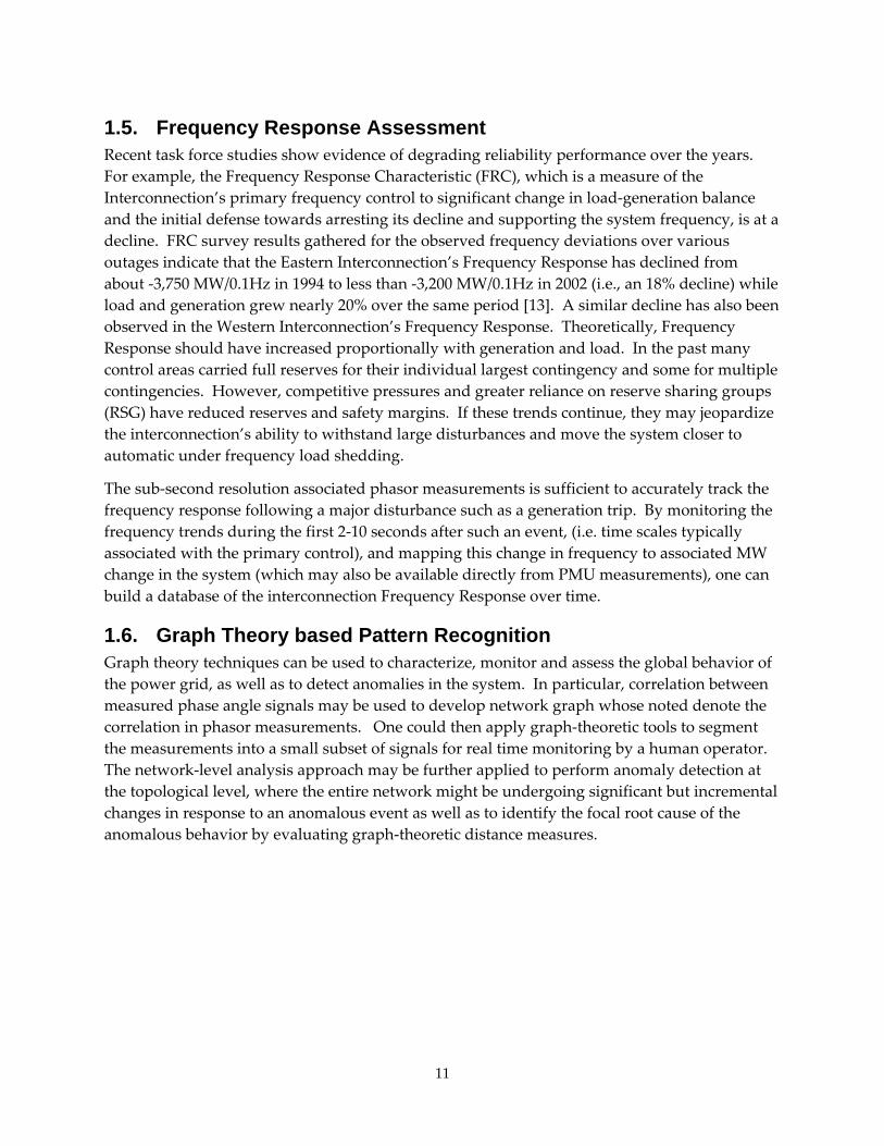
1.5. Frequency Response Assessment Recent task force studies show evidence of degrading reliability performance over the years. For example, the Frequency Response Characteristic (FRC), which is a measure of the Interconnection’s primary frequency control to significant change in load‐generation balance and the initial defense towards arresting its decline and supporting the system frequency, is at a decline. FRC survey results gathered for the observed frequency deviations over various outages indicate that the Eastern Interconnection’s Frequency Response has declined from about ‐3,750 MW/0.1Hz in 1994 to less than ‐3,200 MW/0.1Hz in 2002 (i.e., an 18% decline) while load and generation grew nearly 20% over the same period [13]. A similar decline has also been observed in the Western Interconnection’s Frequency Response. Theoretically, Frequency Response should have increased proportionally with generation and load. In the past many control areas carried full reserves for their individual largest contingency and some for multiple contingencies. However, competitive pressures and greater reliance on reserve sharing groups (RSG) have reduced reserves and safety margins. If these trends continue, they may jeopardize the interconnection’s ability to withstand large disturbances and move the system closer to automatic under frequency load shedding.
The sub‐second resolution associated phasor measurements is sufficient to accurately track the frequency response following a major disturbance such as a generation trip. By monitoring the frequency trends during the first 2‐10 seconds after such an event, (i.e. time scales typically associated with the primary control), and mapping this change in frequency to associated MW change in the system (which may also be available directly from PMU measurements), one can build a database of the interconnection Frequency Response over time.
1.6. Graph Theory based Pattern Recognition Graph theory techniques can be used to characterize, monitor and assess the global behavior of the power grid, as well as to detect anomalies in the system. In particular, correlation between measured phase angle signals may be used to develop network graph whose noted denote the correlation in phasor measurements. One could then apply graph‐theoretic tools to segment the measurements into a small subset of signals for real time monitoring by a human operator. The network‐level analysis approach may be further applied to perform anomaly detection at the topological level, where the entire network might be undergoing significant but incremental changes in response to an anomalous event as well as to identify the focal root cause of the anomalous behavior by evaluating graph‐theoretic distance measures.

12
13
2.0 METHODOLOGIES FOR USING PHASORS FOR STABILITY NOMOGRAMS
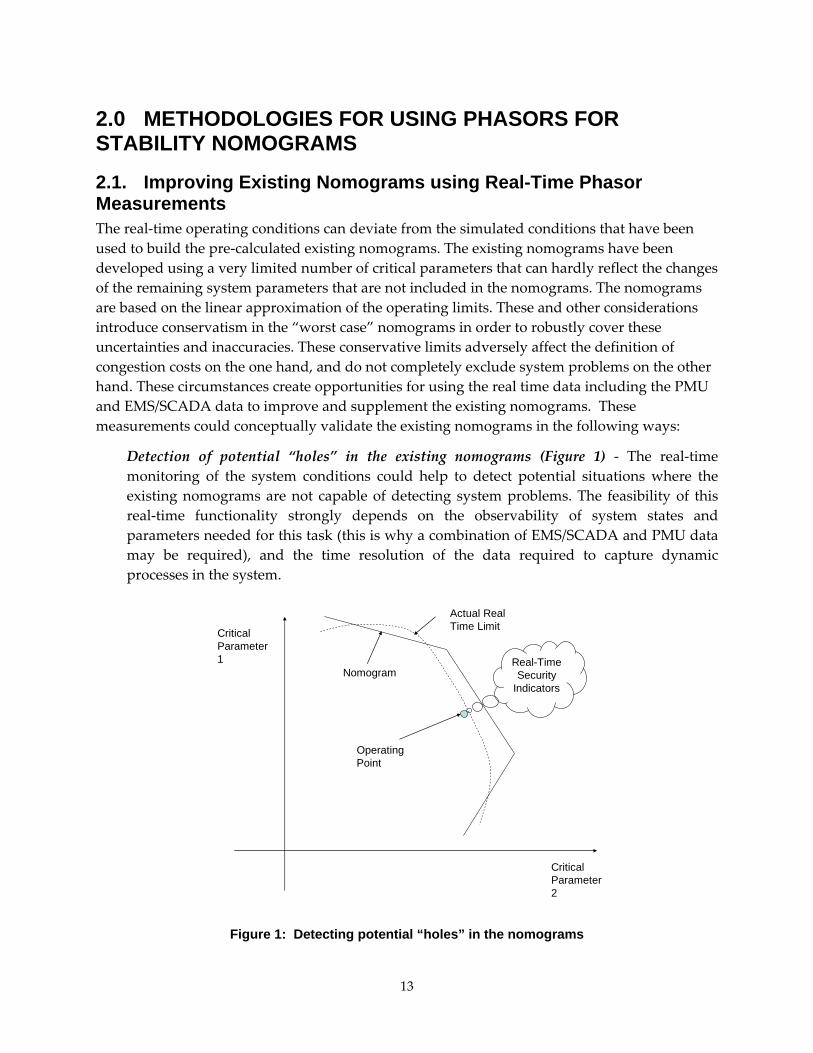
2.1. Improving Existing Nomograms using Real-Time Phasor Measurements The real‐time operating conditions can deviate from the simulated conditions that have been used to build the pre‐calculated existing nomograms. The existing nomograms have been developed using a very limited number of critical parameters that can hardly reflect the changes of the remaining system parameters that are not included in the nomograms. The nomograms are based on the linear approximation of the operating limits. These and other considerations introduce conservatism in the “worst case” nomograms in order to robustly cover these uncertainties and inaccuracies. These conservative limits adversely affect the definition of congestion costs on the one hand, and do not completely exclude system problems on the other hand. These circumstances create opportunities for using the real time data including the PMU and EMS/SCADA data to improve and supplement the existing nomograms. These measurements could conceptually validate the existing nomograms in the following ways:
Detection of potential “holes” in the existing nomograms (Figure 1) ‐ The real‐time monitoring of the system conditions could help to detect potential situations where the existing nomograms are not capable of detecting system problems. The feasibility of this real‐time functionality strongly depends on the observability of system states and parameters needed for this task (this is why a combination of EMS/SCADA and PMU data may be required), and the time resolution of the data required to capture dynamic processes in the system.
CriticalParameter1
CriticalParameter2
Nomogram
Actual RealTime Limit
OperatingPoint
Real-TimeSecurity
Indicators
Figure 1: Detecting potential “holes” in the nomograms

14
Detection of excessive “conservatism” in the existing nomograms ‐ This feature can help to detect potential situations where the existing nomograms are excessively limiting. The elements of this approach can be described as follows (see Figure 2):
CriticalParameter1
CriticalParameter2
Nomogram
Actual RealTime Limit
OperatingPoint
PotentialNomogramBottleneck
Figure 2: Detecting excessive “conservatism” in the nomograms
The essential elements of the proposed approach can be described as follows:
• At the current operating point, monitor the system security indicators2 using the PMU, SCADA, and State Estimation data. These indicators can be thermal limits, voltage limits, or other stability indices.
• Monitor the relative position of the current operating point against the “walls” of the relevant nomogram.
• Generate signals to the real‐time dispatchers whenever (i) the real‐time security indices indicate approaching limiting conditions – i.e. potential “hole” in the nomogram (ii) the operating point reaches the nomogram walls – i.e. potential conservatism in the nomogram.
• Memorize the snapshot whenever the security indicators signal the problem before a vicinity of the nomogram boundary is reached. This information can be used offline to “repair” the pre‐calculated nomogram.
2 Under the current CEC-CAISO Project Plan, the various new stability metrics that are planned for research and development under the “Monitoring” and “Small-Signal Stability” tasks could be used as stability indicators here.

15
Note: It is important to use this information with caution, because the current operating condition can be very different in comparison to the “worst case” condition implied by the nomogram. The nomogram “repair” should be only authorized when sufficient statistical data has been gathered to indicate the need for this change. The measurement data needs to be augmented with contingency computations based on this data in order to be applicable to updating nomogram walls that account for n‐1 security under contingencies.
For local limit assessment purposes, additional PMU units could be recommended to be installed in certain critical locations to provide full observability of the known problem regions so that all the critical and most influential set of parameters and states can be evaluated in real time with very high resolution. In existing systems, the information on possible violations becomes available to the grid operator with resolution from several seconds (within the SCADA/EMS cycle) to several minutes (as a result of the State Estimation cycle). Even if the nomogram monitoring feature is available to the real‐time dispatchers at all, the existing systems may have delays that may be critical in some emergency conditions. Sudden unanticipated changes (for instance, the ones that may be precursors of an approaching blackout) and other rapid dynamic processes are hard to capture on time frames based on the SCADA or EMS information. Short‐term parameter trends, which could lead to instabilities, and which are so important for predicting violations and real‐time decision making, are almost impossible to identify in the existing systems.
The use of PMUs to monitor existing nomograms would help to provide a tighter real‐time monitoring of the operational limits. The sub second information from the problem area would increase the situational awareness of the real‐time dispatch personnel and allow for more time for timely manual and automatic remedial actions in the future (Figure 3).

16
~
PMU1
PMU2
PDC
Problem Area
Detecting Violations in Real Time
Emergency Control
Short Term Trend
Preventive Control
Detecting Changes &Dynamic Processes
Situation Awareness
Figure 3: Use of additional PMUs to monitor existing nomograms in real-time
2.2. Use of PMUs for Reduced Dynamic Equivalents and Transient Stability Assessment Although phasor measurements cannot describe the complete system dynamics they seem to be well suited to identifying reduced dynamic equivalents. Here, a reduced dynamic model designed to capture some aspect of the system dynamics is assumed and the phasor measurements are used to estimate the current parameters of the reduced dynamic model in real time.
For example, the simplest dynamical equivalent is the swing equation for a single machine infinite bus system. With phasor angle measurements from a pair of critical points across the grid, the dynamics of the difference of the two angles can be used to fit the swing equation parameters such as synchronizing and damping torque. This swing equation would capture an aspect of the dynamics between the two areas in which the measurements were taken. Measurements could also be used to identify more elaborate multi‐machine dynamic equivalents that would better capture aspects of the western area dynamics. One approach would be to combine together phasor angle measurements in one area to obtain a combined phasor angle measurement representing a lumped node in the reduced dynamic mode representing that area.

17
These reduced dynamic equivalents may be used in both in transient stability and small‐signal oscillatory stability studies. For transient stability, the method relies on identifying a group of machines that separate from the other machines given a particular contingency. The machine groups are assumed to swing together. Consider phasor measurements from two groups ‐ one inside the separating group of machines and one outside the separating group. These two groups of phasor measurements could be used to identify the parameters of the single machine equivalent in the pre‐fault system. The change between the fault‐on and pre‐fault systems could be determined by offline simulation. The same change applied to the measurement based prefault system can be used to obtain an estimate of the fault‐on system trajectory. Such a transient stability assessment could be usefully applied to studied patterns of transient stability that cause known separations and to the binding transient stability limits. For oscillatory stability, such reduced dynamic models may capture the low frequency oscillatory modes. An advantage of such a model‐based approach is that it may be used to quickly obtain corrective measures to suppress oscillations or increase their damping.
Note: The use of the reduced dynamic equivalent is limited by the extent to which a simpler reduced dynamical model can usefully approximate the entire dynamics. However, in general, the assumption of a dynamic model allows for fewer measurements than in a static model because dynamic observer methods become feasible.
2.3. New Concept of Wide Area Nomograms Although the existing set of PMU measurements do not provide complete system observability, they could nevertheless provide wide‐area visibility and one could conceptualize a completely new type of Wide‐Area Nomograms for monitoring. The proposed concept relies on the hypothesis that for these wide‐area nomograms, nodal voltage angles (or magnitudes) may provide a more convenient coordinate system for measuring certain stability margins when compared with nodal power injections that are traditionally used for this purpose. In this case the phasor measurements would be ideal candidates for monitoring system conditions with respect to these wide‐area nomograms. A frequently proposed simple form of the wide‐area nomograms consists of inequalities applied to the voltage angle differences measured at different locations within the Interconnection – see Figure 4.
max , , 1, 2,3,...,i j ij i j nδ δ δ− ≤ = (1)
It is intuitively clear that large angle differences indicate more stress posed on the system, and that there are certain limits of this stress that make the system unstable or push it beyond the admissible operating limits such as thermal or voltage magnitude limits. At the same time, conditions applied to the angle differences are quite primitive and do not provide an acceptable accuracy of approximation of the power flow stability boundary, especially due to the nonlinear shape of this boundary.

18
The most convincing argument for using angles for the nomogram coordinates instead of the more traditional power flows (e.g. interface flows, total generation, total load, etc) is that angles are a more direct measure of transient stability, and therefore better coordinate system for observing transient stability. In particular, the implications of any topology changes, such as line outages, are directly observable in the angle measurement which may otherwise be absent in the MW flows – the angle difference across the interface increases when a line opens while the net MW flows through a corridor may remain unchanged (i.e. the excess power is rerouted through the other parallel lines). For this very reason, while the boundaries of conventional nomograms need to be adjusted to reflect topology changes, the boundaries of nomograms in the new angle coordinate system may be more static and consequently prove to be a more appropriate for monitoring and assessing proximity to instability.
The above mentioned scenario is illustrated by actual event that occurred on June 18th 2006, when a Malin‐Round Mountain transmission line outage occurred which redirected the net power flow through the other two lines (Malin‐Round Mountain 2 & Captain Jack‐Olinda) that collectively define the California Oregon Interface (COI) path. The net COI flows, however, remained unchanged.
` (a) (b)
Figure 4: MW Flow and Angle Difference tracking across COI – (a) the net MW flows remained unchanged (b) the transmission outage was captured by angle difference.
Note: Net MW flow across COI before event = (1207 + 1190 + 1235) = 3632 MW
Net MW flow across COI after event = (0 + 2123 + 1583) = 3706 MW
The above figures illustrate how net COI power flow did not change after the line trip, but, the phase angle difference across COI changed by 3.88 degrees indicating greater stress.
20 S d
M li R d Mt
Captain Jack – Olinda
M li R d Mt
20 S d
John Day ‐Malin
Malin ‐ Vincent
Lugo ‐ Vincent
~ 3.88 Degrees

19
Additionally, the fact that angle differences at other regions did not change seems to suggest that monitoring these angle difference changes can also be used to indicate the location of the event).
A better approximation of the wide‐area nomograms could be achieved by applying more precise approximating conditions representing linear combinations of the voltage angles determined at different locations within the Interconnection. A hypothetical wide area nomogram for three angles (shown in Figure 4) could be described by the following set of inequalities:
max11 1 12 2 12 2 1
max21 1 22 2 22 2 2
max1 1 2 2 2 2
...
m m m m
ρ δ ρ δ ρ δ δ
ρ δ ρ δ ρ δ δ
ρ δ ρ δ ρ δ δ
⎧ + + ≤⎪
+ + ≤⎪⎨⎪⎪ + + ≤⎩
(2)
Figure 5 shows a conceptual view of the simple angle difference nomogram (a) and advanced angle nomogram (b). The angle difference nomogram is basically a set of straight lines corresponding to different levels of δ3. The advanced angle diagram gives a set of broken straight lines that can be adjusted to provide a better accuracy of the stability boundary approximation. It is clear that the advanced angle nomogram can follow the actual nonlinear shape of the stability boundary much more closely and consequently provides much better accuracy than the simple angle difference nomogram. The advanced angle approach, solely based on the angle differences, is more related to the static angle stability and active power “loadability” of the Interconnection.

20
Figure 5: Western interconnection transmission paths
δ1
δ 3
δ 2

21
Actual Stability Boundaryat δ3 = 90 º
Actual Stability Boundaryat δ 3 = 90 º
δ1 δ1
δ2 δ2
Approximationsat different δ3
δ3 = 90 º
Approximationsat different δ3
δ3 = 90 º
(a) (b)
Figure 6: Conceptual view of simple angle difference and advanced angle nomograms
An even more accurate approximation can be achieved by the use of Cartesian coordinates instead of the polar coordinates, and by the use of m linear combinations of active and reactive components of the nodal voltages measured at different locations 1… n in the system describing the proposed wide‐area nomograms:
' " ' " ' "1 1 1 1 2 2 2 2 ... , 1,...,i i i i in n in n iV V V V V V i mα β α β α β γ+ + + + + + ≤ = (3)
Numerical experiments with the use of Cartesian coordinates on the test example in Figure 6 show that the stability boundary has a “more linear” shape and consequently is more accurate in its approximation.

22
Figure 7: A cutset of stability boundary in rectangular coordinates of nodal voltages (New England test system)3
Hence, a new concept of measuring the stability margin by distances calculated in the space of nodal voltages can be suggested.
While angles may be more conducive to monitoring stability, MW flows are still the true controllable variables in the power system. Hence, understanding the relationship between angle differences across a critical interface and MW flows through it is still important. Figure 8 show the net MW imports into California through the California‐Oregon Intertie (COI) over a 24 hour period under normal system conditions. Also shown is the angle difference between John Day (a substation up north in Oregon) and Vincent (a substation down south in southern California). The close correlation between these two trends suggest (1) using well chosen angle difference pairs to monitor stability does capture the conventional information present from monitoring the MW path flows while having the added advantage of also reflecting topology changes as mentioned earlier; (2) the relationship between flows and angle differences can easily be ascertained from similar trends ‐ e.g. Figure 8 trends suggest a 15 degree angle change for 1,000 MW increase in COI flows.
3 Y.V. Makarov, V. A. Maslennikov, and D. J. Hill, “Calculation of Oscillatory Stability Margins in the Space of Power System Controlled Parameters”, Proc. International Symposium on Electric Power Engineering Stockholm Power Tech: Power Systems, Stockholm, Sweden, 18‐22 June 1995, pp. 416‐422.
Actual Stability
Approximated Stability
Stability

23
Figure 8: Correlation between MW flows across critical flowgates and angle difference pairs
To better understand the behavior of these nodal voltage angles, these measurements were gathered over several hours by PMUs from different geographic locations within the Western Electricity Reliability Council (WECC) phasor network was used to generate the plots in Figure 9 (a) and (b). Using one of the three nodal voltage angles as the reference, the relative angles at the other two locations was plotted in angle‐angle space. In these plots, each set of hourly data is represented by a different color as indicated by the legend. The fact that these trends fall along a narrow and almost linear corridor in this angle‐angle space indicates that the behavior of these relative angles is highly correlated with each other. The directionality of this corridor on the other hand is representative of the interdependence of the interaction. For example, if angle differences are indicators of static stress across the grid, then the orientation of the trends in (a) suggests an increase in the stress across one interface implies an increase in the stress across the other interface. However, the trend orientation in (b) suggests the contrary ‐ an increase in the stress across one interface causes the relief of the stress across the second interface. This strong correlated behavior also suggests that limited observability with a few PMUs at key locations may be adequate to capture the system dynamics from a global prospective.

24
(a) (b)
Figure 9: PMU Measurement based phase angle trends in angle-angle space
2.4. Use of PMUs for Wide-Area Voltage Security Assessment A California PIER funded parallel effort by Consortium for Electricity Reliability Technology Solutions (CERTS) is currently underway in developing a Voltage Security Application (VSA) that runs in real time and provides real time dispatchers with real time reliability metrics related to voltage stability limits. The VSA application under development will be linked to the CAISO EMS system model and data. It will be used to develop and approximate voltage security regions (a type of multi‐dimensional nomograms) using linear approximations or hyperplanes, calculate voltage stability indices. In addition, VSA will identify and display abnormal low voltages, weak elements and places in the system most vulnerable to voltage and voltage stability related problems. This application will also perform contingency analysis and provide the system operators with contingency rankings based on voltage problems for the purposes of system monitoring and selecting preventive and emergency corrective actions.
The VSA platform described above can easily be expanded to study wide‐area voltage stability problems by selecting global stressing directions and developing the corresponding security regions. The algorithms being developed in the VSA application provide voltage magnitude and angle information, as well as their corresponding sensitivities and participation factors in voltage collapse. Hence, while the proposed VSA framework uses data from the CAISO state estimator and assumes full observability, this same VSA framework could also be used to develop wide‐area nomograms whose coordinates would be nodal voltage magnitudes and angles, and the PMU measurements could directly be used to monitor the system conditions with respect to these new nomograms for a wide‐area security assessment ( Figure 10).

25
Figure 10: Voltage stability boundary developed in angle-angle space
2.5. Augmenting Existing Nomograms using Small-Signal Stability Assessment Although small signal stability models and analysis tools are not widely used in the Western Interconnection, there is a growing interest to better understand small‐signal stability limits and possibly build associated nomograms for the WECC system. This is based on the observation that some types of potential instabilities could manifest themselves ahead of time through growing oscillations observed in the system. For example, it has been noticed that insufficient frequency response in California could lead to changes of the power flow patterns in post‐transient conditions and may lead to additional limits of the Operating Transfer Capability (OTC) on the Oregon‐California interties. The nature of these limitations is related to growing oscillations. The low frequency oscillations observed in the system are consequently of interest because they characterize the stability of the power system and limit the power flow across regions. While there is a danger that such modes can lead to instability in the power system following a sizable event in the system, there is also the risk of these modes becoming negatively damped or unstable due to gradual changes in the system. The ability to continuously track these modes and assess their stability would therefore be a valuable tool for power system engineers. Fortunately, the high resolution and wide‐area visibility that PMUs offer are well suited to observe these modes and assess the damping associated with these low frequency modes in real‐time.

26
Small‐signal stability software can be an essential addition to the real‐time monitoring capabilities offered by PMU measurements. State estimation results coupled with small signal stability models can help to identify the origin of poorly damped oscillations. The identification of oscillatory parameters such as magnitude, damping and frequency are needed before one can select measures to increase the stability margin.
The PMU snapshot data recording can be activated by poorly damped oscillations registered by PMUs and identified by the Small‐Signal Stability Monitoring applications. Parameters of these oscillations such as frequency, magnitude, and damping can be identified using special algorithms. Subsequent offline analysis using small‐signal and transient stability models will reveal how close these models are to reality. The use of offline models will help to better understand the origin and nature of these oscillations. Questions such as what changes in the system cause oscillations and the identification of a small set of descriptive variables that capture the phenomena are also some of the central issues related to the existing modal analysis tools.
Research work could be conducted to investigate the validity of such an approach. The objective of this study could be to screen the WECC system for locations where the Operating Transfer Capability (OTC) is limited by oscillatory problems. Then the typical frequencies could be determined. The next step is to find the places where these oscillations are better observable, and associate these locations with PMU placement. Oscillation‐related OTC limits could be compared with the existing nomograms, or may indicate the necessity of building additional nomograms. After such a set of verification and validation procedures, the results of the PMU‐based modal analysis could be used to detect potential violations in real time. Finally this will lead to the improvement of the pre‐calculated nomogram limits based on real‐time PMU data by observing the differences between the pre‐calculated OTC and the real transfers at which the oscillations start to grow.

27
3.0 ALGORITHMS FOR MONITORING SMALL-SIGNAL STABILITY WITH PHASOR MEASUREMENTS The underlying assumption enabling swing‐mode estimation is that the power system is primarily driven by random processes when operating in an ambient condition. An ambient condition is one where there is no significant disturbance occurring within the system. The primary driving function to the power system is the random variations of the loads. It has been shown that under such an assumption, the resulting power‐system signals will be colored by the system dynamics. This coloring allows one to estimate the swing‐mode frequencies and damping terms.
Consider the signal flow diagram in Figure 11 representing the excitation of a power system from random load variations. v(t) is a vector of random components added to each load; each element independent of the other. The output yi(t) is the ith measured signal at time t, and μi(t) is measurement noise located at the transducer. In general, μi(t) is a relatively small effect when quality instrumentation is employed; therefore, its effect is often negligible. Theory tells us that because v(t) is random, each yi(t) will also be random. But, yi(t) is colored by the dynamics of the system.
PowerSystem
random loadvariations v(t)
measurementnoise μk(t)
+
+ output yk(t){
Figure 11: Signal flow diagram.
Assuming a linear system mode, the output yi from Figure 11 can be written in auto‐regressive moving‐average (ARMA) form as
( ) ( ) ( ) ( )∑ ∑ ∑= = =
+⎟⎟⎠
⎞⎜⎜⎝
⎛−+−=
n
j
p
lk
m
jliljiji kTjTkTvbjTkTyakTy
il
1 1 0
μ , i = 1, 2, …, no (4)
where no is the number of output signals measured, T is the sample period, k is the discrete‐time integer, n is the order of the system, p is the order of vector v, and mil is the MA order of the ith output for the lth input. The autocorrelation of yi is defined to be
( ) ( ) ( ){ }qTkTykTyEqr iii −= (5)
where { }•E is the expectation operator. Over a finite number of data points, the autocorrelation is approximated by

28
( ) ( )∑+=
−≅N
qki qTkTykTy
Nqr
1
1)( (6)
where N is the total number of data points. Using the same analysis in [1], it can be shown that the autocorrelation satisfies
∑=
−−=n
jiji jqraqr
1)()( , q > m (7)
where m = max(mil). Another useful relationship involving the autocorrelation is
{ } ( ) ( ){ }ωωω *)()( iiiii YYEqrFS == (8)
{ })()( 1 ωiii SFqr −= (9)
where { }•F is the Fourier transform operator, ( )ωiY is the Fourier transform of yi(t) at
frequency ω, and ( )ω*iY is the conjugate of ( )ωiY . Sii is termed the power spectral density (also
referred to as the autospectrum) of yi. Effectively, it represents the energy in a signal as a function of frequency. If one knows the Auto‐Regressive (AR) aj coefficients in (4), then the system poles (or modes) can be calculated from the following equations.
( )nnn
j azazrootsz +++= − ...11 , j = 1, 2, …, n (10)
( )Tz
s jj
ln= (11)
3.1. Algorithms to Estimate the System Modes Using Synchronized Phasor Data Estimating a power system’s electromechanical modal frequency and damping properties using ambient time‐synchronized signals is achieved by using parametric system identification methods. Three estimation algorithms to solve the AR coefficients and thus the system modes have been well studied for application purposes and they are:
• Modified extended Yule Walker (YW),
• Modified extended Yule Walker with spectral analysis (YWS), and
• Sub‐space system identification (N4SID).
(1) Modified Extended Yule Walker (YW) The original Yule Walker algorithm is used to estimate the AR parameters and thus the system poles. The extended modified Yule Walker (YW) algorithm is a modified version of the original Yule Walker algorithm with extension to multiple signals for the analysis of

29
ambient power system data, namely, frequency data, voltage angle data, and etc. The algorithm starts by expanding (7) into matrix form as
⎥⎥⎥⎥
⎦
⎤
⎢⎢⎢⎢
⎣
⎡
+
++
−=
⎥⎥⎥⎥
⎦
⎤
⎢⎢⎢⎢
⎣
⎡
⎥⎥⎥⎥
⎦
⎤
⎢⎢⎢⎢
⎣
⎡
−+−+−+
+−++−−
)(
)2()1(
)()2()1(
)2()()1()1()1()(
2
1
Mmr
mrmr
a
aa
nMmrMmrMmr
nmrmrmrnmrmrmr
i
i
i
niii
iii
iii
MM
L
MOMM
L
L
(12a)
or
ii raR −= (12b)
For each output, (12) can be concatenated into one matrix problem as
⎥⎥⎥⎥⎥
⎦
⎤
⎢⎢⎢⎢⎢
⎣
⎡
−=
⎥⎥⎥⎥⎥
⎦
⎤
⎢⎢⎢⎢⎢
⎣
⎡
oo nn r
rr
a
R
RR
MM
2
1
2
1
(13)
The steps for solving the YW algorithm involve
• Estimating autocorrelation terms using (6),
• Constructing autocorrelation matrix equations (13),
• Solving the equations (13) for the AR coefficients,
• Solving the coefficients equation (10) for the discrete‐time modes, and
• Converting the discrete‐time modes to the continuous‐time modes using (11).
(2) Modified Extended Yule Walker with Spectral Analysis (YWS) The modified extended Yule Walker with Spectral analysis (YWS) follows the same procedure as the YW method to estimate the system modes, i.e., that the system modes are solved from AR coefficients which in turns are solved from the system autocorrelation matrix equations. However, the YWS algorithm estimates the system autocorrelation terms from its spectrum (9), while the YW algorithm estimates the system autocorrelation terms directly from data samples (6).
(3) Sub‐Space System Identification (N4SID) The third algorithm considered for mode estimation is the time‐domain subspace state‐space system identification algorithm known as N4SID. The reader is referred to [2] and [3]. Application of the N4SID algorithm to ambient power system data is described in [4]. The algorithm used for this report is implemented in the Matlab function “n4sid” available with the system identification toolbox. Because of the complexity and length of the
30
algorithm, it is not repeated here. Similar to the YW and YWS algorithm, the N4SID algorithm provides an estimate of the system’s characteristic equation parameters.
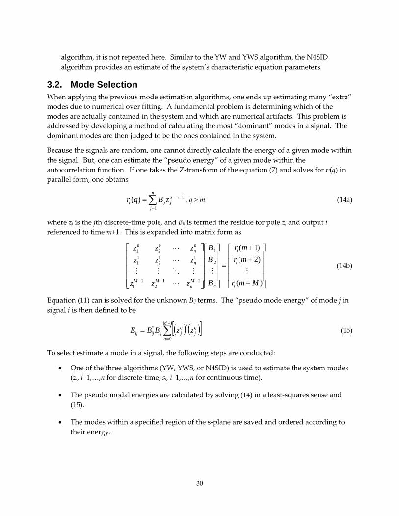
3.2. Mode Selection When applying the previous mode estimation algorithms, one ends up estimating many “extra” modes due to numerical over fitting. A fundamental problem is determining which of the modes are actually contained in the system and which are numerical artifacts. This problem is addressed by developing a method of calculating the most “dominant” modes in a signal. The dominant modes are then judged to be the ones contained in the system.
Because the signals are random, one cannot directly calculate the energy of a given mode within the signal. But, one can estimate the “pseudo energy” of a given mode within the autocorrelation function. If one takes the Z‐transform of the equation (7) and solves for ri(q) in parallel form, one obtains
∑=
−−=n
j
mqjiji zBqr
1
1)( , q > m (14a)
where zj is the jth discrete‐time pole, and Bij is termed the residue for pole zj and output i referenced to time m+1. This is expanded into matrix form as
⎥⎥⎥⎥
⎦
⎤
⎢⎢⎢⎢
⎣
⎡
+
++
=
⎥⎥⎥⎥
⎦
⎤
⎢⎢⎢⎢
⎣
⎡
⎥⎥⎥⎥⎥
⎦
⎤
⎢⎢⎢⎢⎢
⎣
⎡
−−− )(
)2()1(
2
1
112
11
112
11
002
01
Mmr
mrmr
B
BB
zzz
zzzzzz
i
i
i
in
i
i
Mn
MM
n
n
MM
L
MOMM
L
L
(14b)
Equation (11) can is solved for the unknown Bij terms. The “pseudo mode energy” of mode j in signal i is then defined to be
( ) ( )[ ]∑−
=
=1
0
**M
q
qj
qjijijij zzBBE (15)
To select estimate a mode in a signal, the following steps are conducted:
• One of the three algorithms (YW, YWS, or N4SID) is used to estimate the system modes (zi, i=1,…,n for discrete‐time; si, i=1,…,n for continuous time).
• The pseudo modal energies are calculated by solving (14) in a least‐squares sense and (15).
• The modes within a specified region of the s‐plane are saved and ordered according to their energy.

31
3.3. Algorithm Tuning To use each of the algorithms, several analysis parameters must be selected. This includes all the parameters in equations (4) through (15).
− N = number of data points used for analysis (required for all algorithms). Note that Ttotal = T*N.
− T = sample period for collecting data (required for all algorithms). − no = number of signals to analyze (required for all algorithms). − n = model order (required for all algorithms). − m = MA order (required for YW, YWS, and mode selection algorithms). − MAR = number of samples of the autocorrelation function used to solve for the AR
parameters. This equal to M in equation (9a). Required for the YW and YWS algorithms. − Nfft = number of samples used for the pwelch function in YWS. − MRES = number of samples of the autocorrelation function used to solve for the residue
parameters. This equal to M in equation (10b). Required for the all three algorithms. Extensive research on how to select these parameters has been done [5]. The research includes testing and evaluating the algorithms by Monte‐Carlo simulations on a test system as well as analysis of WECC PMU data. The recommended analysis parameters from the research are:
T = 0.2 sec.
Ttotal = 5 minutes or greater
no = 1 to 4 signals
n = 25, m = 10 for YW and YWS.
n = 20, m = 5 for N4SID.
MAR = MRES = 10 sec.
The above algorithms were applied to western system data. Approximately 2 hours of ambient data was collected from several PMUs within the WECC system on March 7, 2006. Extensive spectrum analysis was conducted on the data to determine the modal content. Analysis of the data indicated that frequency error estimated from finite‐difference of the voltage angles provided quality data.
Table 1 summarizes the results from the spectral analysis. As typical of the WECC system with Alberta connected, the system is dominated by the 0.265‐Hz “Intertie” mode and the 0.385‐Hz “Alberta” mode. Several higher‐frequency weaker inter‐area modes are also described in
Table 1.
The first step in the modal analysis is to select the appropriate signals. The goal is to select signals with high observability (i.e., large peaks in the power spectrum) of the “Intertie” and “Alberta” modes and low observability of the other modes. This is most easily done by

32
subtracting two signals that oscillate out of phase from each other at the frequencies of interest. Scanning
Table 1, one sees that the following signals are excellent choices for estimating the two modes of interest:
• (Grand Coulee Handford) – (Big Creek 3 230kV)
• (John Day) – (Vincent 230kV)
The 10 min. analysis window was applied to just over two hours of ambient data by sliding it in 5 min. steps. This results in 25 total mode‐meter analyses. For each case, the two modes with the largest pseudo‐energy terms in the region of the s‐plane bound by 0.2 Hz, 0.5 Hz, and 20% damping were estimated with a mode‐meter algorithm. The s‐domain plots of the results are shown in Figure 12. The two dominant “Intertie” and “Alberta” modes are observable within this data set and shown on the plots. All three algorithms are able to identify these modes with consistent results and comparable performance. Additionally, while the modal frequencies are relatively constant over the entire duration of the data set, there appears to be much greater variability in the % damping (i.e. 5% ‐ 20% damping) over time. Additionally, a longer term (24 hours) behavior of the “Intertie” mode (frequency & damping) and corresponding California‐Oregon Intertie (COI) loading conditions for different is shown in Figure 13. This plot shows a great deal of variability in the % damping over the 24 hour period.
Figure 12: Mode estimates for WECC data

33
Figure 13: Long-term Intertie mode trends (frequency & damping) with varying COI flows
Furthermore, in addition to the modes estimation algorithms discussed above, it is also desirable to understand the observability of a mode at a particular monitoring location. Such information will be helpful in identifying appropriate points for control actions towards mitigating poor damping situations. Waterfall plots, which are series of power‐spectrum snapshots of a monitored signal over time, are important for such investigation. The waterfall plot for the COI flows over the latter half of 24 hour period is shown in Figure 14, where the power‐spectral density within the frequency range of interest (y‐axis) and its recent trends over time (x‐axis) are illustrated. The magnitude of the power spectra shown along the z‐axis (color‐coded) truly indicates the power inherent in the selected signal and is interpreted as the square of the rms of the magnitude of the components in the signal along the frequency axis. Note that the variability observed in the % damping at 0.25 Hz (Figure 13) is also visible in the power‐spectral density at the same 0.25 Hz – i.e. as this mode’s damping changes over time, the spectral peak at this modal frequency becomes more/less prominent. Such modal variability over longer term time scales (minutes and hours) needs further investigation.

34
Figure 14: Long-term Intertie mode spectral trends with varying COI flows

35
3.4. Implementation of Small-Signal Stability Monitoring Prototype Tool During 2006, a Small‐Signal Stability Monitoring application that utilizes the above mentioned algorithms to monitor and track the low frequency modes prevalent within the power system in real time and under ambient system conditions, was developed. The application underwent field trial at both the CA ISO and BPA, prior to being migrated onto production hardware and installed in the CA ISO control center in June 2007. A sample operator display from this tool is shown in Figure 15.
Figure 15: Small-Signal Stability Monitoring Display
Some of the visualization capabilities that are available within the Small‐Stability Monitoring tool include:
• Color‐coded ‘speedometer’ type gauges that provide information on damping ratios and damping frequencies of the observable modes in the system. The sub‐areas within each gauge are color coded to represent different ranges of damping ratios – i.e., a 5%‐20% damping ratio shown in green indicating a safe operating region; a 3%‐5% damping ratio in yellow indicating an alert condition; and less than 3% damping ratio shown in red representing an alarm situation. The positions of the needles swing back and forth in real time to indicate the current damping ratios of the system modes.
36
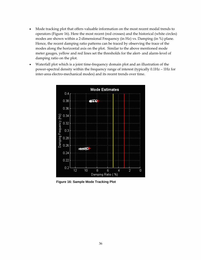
• Mode tracking plot that offers valuable information on the most recent modal trends to operators (Figure 16). Here the most recent (red crosses) and the historical (white circles) modes are shown within a 2‐dimensional Frequency (in Hz) vs. Damping (in %) plane. Hence, the recent damping ratio patterns can be traced by observing the trace of the modes along the horizontal axis on the plot. Similar to the above mentioned mode meter gauges, yellow and red lines set the thresholds for the alert‐ and alarm‐level of damping ratio on the plot.
• Waterfall plot which is a joint time‐frequency domain plot and an illustration of the power‐spectral density within the frequency range of interest (typically 0.1Hz – 1Hz for inter‐area electro‐mechanical modes) and its recent trends over time.
Figure 16: Sample Mode Tracking Plot

37
Figure 17: Sample Waterfall Plot
It is important to mention that appropriate pre‐processing of the data prior to running the algorithms is critical to performance the tool and the accuracy of the modal estimates. Data pre‐processing stage includes removing outlier and missing data, detrending, normalization, anti‐aliasing filtering and down sampling, etc. Additionally, to help focus on the interested range of frequency of the modes (i.e., the range of wide‐area oscillations), proper post‐processing is also desired. Post‐processing includes setting the maximum number of modes for display, setting the maximum associated damping ratio, setting the energy threshold for the modes, and setting proper frequency range. These pre‐ and post‐processing stages have been incorporated into the mode the prototype and are end‐user configurable (Figure 18).

38
Figure 18: Block Diagram for the Small-Signal Stability Monitoring Tool.
In late 2007/early 2008, the Small Signal Stability tool’s algorithms, visuals and feature set were further enhanced based on additional research and end user feedback. Some of the improvements included:
• Improved mode estimation algorithms and graphics to quantify the uncertainty associated with the mode estimates. Here, a newly developed ‘bootstrapping’ method was embedded into the tool that compute the uncertainty region or error bounds (a.k.a. confidence intervals) associated with each estimate and is illustrated as an ellipse on the same 2‐D frequency vs. damping ratio plane representing the uncertainties in both the modal damping and frequency (Figure 19). A smaller ellipse would therefore signify greater confidence in the modal estimate while a large ellipse would indicate greater uncertainty.

39
Figure 19: Improved Mode Tracking Plot with Bootstrapping Ellipse
• Capability to archive modal frequency and damping estimates for long term trending analysis thereby facilitating the ability to perform long‐term correlation analysis between modal performance and other key metrics (e.g., loading on key corridors).
• Ability to rewind, playback and recreate existing Small‐Signal Stability monitoring displays using historical data in memory.
• Ability to load single or multiple phasor disturbance files and perform small‐signal stability type of forensics to assess the stability of the power system prior to and after the event through various analysis techniques (e.g. spectral analysis, modal analysis). For example, the tool’s spectral analysis display, shown in Figure 20, lets the user to analyze the spectral content of chosen signals using three primary calculations (1) Power Spectral Density (PSD) or Auto‐Spectrum to identify sharp peaks indicative of strong oscillatory activity observable in the signal; (2) Coherency: to identify a signal’s correlation or participation in a particular mode; (3) Cross Spectral Density (CSD) or Cross‐Spectrum: to identify the relative phase information associated with a particular mode (i.e. mode shape information). Note: The PSD and CSD are calculated using Welch’s periodogram averaging technique – the algorithm parameter settings (e.g. time window, percent overlap, FFT window length) may be changed through a user friendly GUI.

40
Figure 20: Sample Spectral Analysis Display.

41
4.0 MEASUREMENT BASED SENSITIVITIES AND VOLTAGE STABILITY MONITORING
4.1. Measurement based Sensitivities It is well understood that with additional loading on the power system, there is degradation in the voltages across the system. This relationship is typically represented by the P‐V or Q‐V curves. Furthermore, the gradient at any point along such a curve provides the voltage sensitivity at that bus with respect to the loading conditions. The traditional method for obtaining this information is dependent on the system model, especially the load model, which is built by history data.
Phasor measurements offer the ability to obtain this very same information directly from the real time measurement without requiring any modeling information. In particular, PMU devices installed at a substation measure the voltage phasors (both magnitudes & angles) at a bus and the MW and MVAR flows on the monitored lines. With the precise time‐synchronized alignment and the high sub‐second resolution of these measurements, it is possible to trace out portions of the P‐V or Q‐V curves for a monitored critical load bus or corridor in real time. Additionally, there is enough loading variation within the system to estimate the local gradient of such curves which map changes in one variable (MW or MVARs) to changes in the other (voltages) – i.e., the current voltage sensitivities at that location/interface.
For illustration purposes, Figure 21 traces the P‐V curves, and tracks the voltage sensitivities at the Malin 500 kV bus over time under different COI loading conditions. The sensitivities are computed using linear regression on the most recent data set collected over a 10 minute window. The results exemplify how the voltage sensitivity increases with increased loading as the system operating point moves further down along the P‐V curve and closer to the voltage collapse point and can be used to anticipate low voltage problems. Additionally, is also possible to quickly detect discrete changes in the system such as control actions (e.g. insertion of cap banks), which cause these curves to shift outward (or inward).
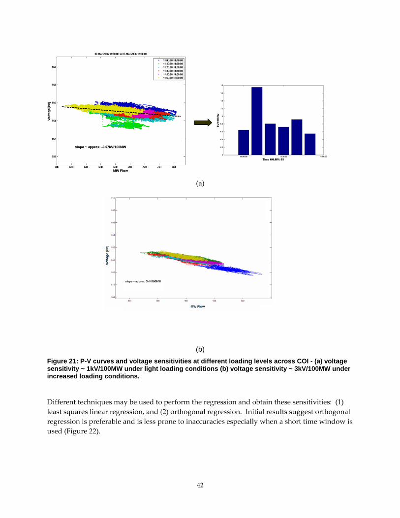
42
(a)
(b)
(b) Figure 21: P-V curves and voltage sensitivities at different loading levels across COI - (a) voltage sensitivity ~ 1kV/100MW under light loading conditions (b) voltage sensitivity ~ 3kV/100MW under increased loading conditions.
Different techniques may be used to perform the regression and obtain these sensitivities: (1) least squares linear regression, and (2) orthogonal regression. Initial results suggest orthogonal regression is preferable and is less prone to inaccuracies especially when a short time window is used (Figure 22).

43
(a) (b) Figure 22: Estimating sensitivities using (a) Least Squares Regression (b) Orthogonal Regression.
4.2. Voltage Stability Loading Margins A literature review on the utilization phasor measurements to monitor voltage stability margins has shown that such measurements at load bus or across a key interface can also be used to estimate the maximum loading margins at the bus and define a Voltage Stability Index (VSI) for the bus/interface [8‐11]. It is a well‐known fact that for a two‐bus system with a constant power load (i.e., a constant source behind an impedance and a load), the maximum loadability condition occurs when the voltage drop across the source impedance is equal to the voltage across the load. Hence, the idea is to use the phasor measurements at the bus to dynamically track in real‐time the two‐bus equivalent of the system. In particular, given the voltage and current phasor measurements at the bus (‘V ’ and ‘ I ’), it is possible to estimate the parameters of the Thevenin equivalent system (‘ thE ’ and ‘ thZ ’) from a sliding window of discrete samples using a recursive least squares scheme (RLS). The maximum loadability condition corresponds to the case when ‘ V2E th = ’ and the Voltage Stability Index can be defined as:
th
app
ZZ
VVVSI =Δ
= (16)
where ‘ VΔ ’ is the voltage drop across the Thevenin equivalent impedance and ‘ appZ ’ is the
apparent load impedance (i.e., ‘ IV ’). This indicator reaches unity at the maximum loadability
point. Furthermore, since the Thevenin parameters are being tracked dynamically, they reflect any changes that may occur in the power system operating conditions and consequently provide the most accurate assessment of loadability estimates.

44
The very same methodology can also be used to compute Voltage Stability Index for the power transfer across a tie‐line. By assuming a directional flow across the line, the line is replaced by a fictitious sink and source at the sending and receiving ends of the line respectively, that draw the same power as the tie‐line flows. One can now replace the system with its Thevenin equivalent and compute the VSI for the tie‐line flows as well.
Finally, if we assume that ‘Zth’ isn’t changing significantly, we can also compute a Power Margin (PM) from the two‐bus equivalent as:
( )th
2ththth
Z4IZES −=Δ (17)
Again, operators may be alarmed if these indices fall below predetermined thresholds (e.g. 5% of the current load/flow).
Figure 23: Flow Chart for voltage stability assessment based on phasor measurements.
More recently, a new voltage stability analysis model has been proposed for a multiple‐infeed load center where both sides of the interconnection to the load are assumed to be able to provide voltage support [21]. In this model, Thevenin equivalents are estimated at both sides of
At: 1) Key Load Buses
2) Key Transfer Corridors
Calculate in Real Time Thevenin Equivalent
Parameters for Remaining System
Predict Power Margin for Bus/Corridor
Compute ‘Voltage Stability Index’ (VSI) for Bus/Corridor
Measure in Real Time Phasor Voltage and Current
(V and I ) Compute Apparent Impedance ( I/VZ = )

45
the bus (Figure 24). In order to represent correctly the loads, the equivalent resistances cannot be ignored anymore.
Figure 24: Voltage stability analysis model for a multiple-infeed load center using phasor measurements.
To compute the equivalent parameters of the new model, the following least squares optimization problem needs to be solved (at least three measurements are required). Besides, the accuracy of the estimation highly depends on the sampling rate: it must be chosen so that data points are not too close to each other.
.....
.....)cos()sin()sin(
)cos()sin()sin()cos()sin()sin(
)cos()sin()sin(
,,,,,,,min
iriirr
iirirr
iriris
iirirr
rrrrssss IXIRrEVIXIRrE
IXIRsEVIXIRrE
RXERXEi
i
i
iiφφδ
φφδφφδ
φφδ
δδ ++−++
++−++
(18)
where: iii
iii
VQIVPI/)sin(
/)cos(−=
=φφ
The first advantage of such a model is that it provides a better representation of the real power system. Indeed, the fact that voltage support may come from both sides of the bus is now taken into account. The second important feature of this model is that it estimates the voltage stability margin of the system without having to make some hypothesis on the load model. Overall, it is
P, Q
I/φº
El/δlº
V/0º
XlXs RlRsEs/δsº

46
its simplicity that makes this model very easy to use for real time stability estimation of a transmission path.
In order to see whether this model gives accurate results, the multiple‐infeed model is tested at load center within the CA ISO. The following table presents the values of the computed equivalent Thevenin parameters:
Es Rs Xs El Rl Xl
1.066 0.067 0.034 0.989 0.01 0.041
From these results, the P‐V curves can be plotted (Figure 25). This method seems to give a good estimation of the voltage stability margin. However, it should be pointed out that the model was tested in an unstressed situation. Additional studies under stressed conditions are needed to further validate the approach.

47
0 0.5 1 1.5 2 2.5 3
0
0.2
0.4
0.6
0.8
1
P (pu)
V (p
u)
P-V curvePMU data
0.9 0.92 0.94 0.96 0.98 1 1.02 1.04 1.06 1.08 1.10.98
0.985
0.99
0.995
1
1.005
1.01
1.015
1.02
P (pu)
V (p
u)
P-V curvePMU data
Figure 25: Estimating voltage stability margins with phasor measurements: (a) P-V curve predicted by the multiple-feed load center model; (b) phase measurement data used in the model parameter estimation.
A limitation of the above approaches is that the initial margin estimates and stability indices incur abrupt jumps when discrete events such as generator limits are reached. However, given that system voltage collapse typically occurs at slower timescales, if these algorithms are used in a real‐time environment where the estimates are updating periodically at frequent intervals, then such an application should be able to provide adequate early warning to the operator in spite of the above mentioned limitation.

48
4.3. Predicting Voltage Stability with Phasor Measurements The synchronized voltage measurements also serve as a time series that can be used to develop an adaptive Auto‐Regressive (AR) predictive model to project the voltage trends a short interval into the future [12] (Note: A similar AR model was proposed for the small‐signal stability monitoring algorithms). This approach is especially useful to ascertain the outcome of a sudden disturbance injected into the system due to a fault or an outage. An AR model is ideal for expressing a signal as a mixture of exponentially decreasing and damped sinusoidal components (i.e., ‘ )tsin(Ae t β+ωα ’ where ‘A’, ‘α’, ‘ω’ and ‘β’ are the strength, damping, frequency and phase respectively). Hence, given ‘N’ measurement samples over a predefined time window, the objective is to fit them to a ‘p’ order Auto‐Regressive model (AR‐p) given by:
t
p
1iitit aXX +φ= ∑
=− (19)
where ‘Xt’ are the measurements, ‘φi’ are the model parameters (also called prediction coefficients) and ‘at’ is the white noise in the measurements. The Voltage Stability Index mentioned above can then be applied to the predicted trace for a fast stability assessment soon after the transient has been launched.
4.4. Implementation of Measurement bases Sensitivity Prototype Tool In late 2007, the phasor visualization tool was augmented with two new displays for measurement based Angle Sensitivity and Voltage Sensitivity. This has facilitate better understanding of Voltage‐(Real/Reactive) Power and Phase Angle‐Real Power relationships for key corridors and at critical generation and load buses where PMUs have been installed. The associated sensitivities (in kV/100MVAR or º/100MW) are also important stability indicators with respect to voltage and transient stability, and provide real time visual alarming to operators when these sensitivities exceed acceptable thresholds.
Figure 26 is a sample operator display for monitoring measurement based sensitivities. Here, the two signal pairs (e.g., voltage at a bus and loading at bus/flows across a corridor) for which the sensitivity is to be monitored and tracked are encircled by an ellipse, which is colored as per the sensitivity alarming threshold limits. Hence, multiple groups within the geographic display are illustrative of the various signal pairs for which the sensitivity is being computed in real time. For the one selected pair (highlighted in the display), the smaller panel on the top right provides the sensitivity trends color‐coded to represent normal, alert or alarm levels. The corresponding P‐V curve(s) is also shown in the bottom right with the most recent data points shown in red. In Figure 26, notice how the curve moves outward over time due to changing system conditions. The ability to track these curves and sensitivities in real time purely from system measurements, and therefore presenting the actual situation, is valuable information for the operator.

49
Figure 26: Voltage Sensitivity Monitoring Display

50

51
5.0 FREQUENCY RESPONSE MONITORING A control area’s contribution to frequency support is measured by the natural frequency response of its generators and load to frequency variations. It characterizes the typical frequency excursion (within the seconds timeframe) following a loss of a large generator on an Interconnection which is associated with primary control and is comprised of the following two components [13]:
− Natural arrest in frequency decline due to “load rejection” or reduced power consumption of frequency dependent loads (e.g. motors).
− The governing action of generating units responding to the declining frequency in the 3‐10 seconds timeframe in an attempt to partially recover the frequency before secondary frequency regulation or Automatic Generation Control (AGC) units bring the frequency back to 60Hz or pre‐event levels within 2‐10 minutes (i.e., AGC time constants).
Traditionally, the frequency response characteristic (‘β’), expressed in MW/0.1Hz and a measure of frequency control stiffness, is calculated using 1‐minute CPS data (one‐minute averages of ACE and “frequency deviation from scheduled”) using the following equation [16]:
Freq. Responseinterconnection = Biasinterconnection‐(ΔACEnet/Δfreq) (20)
where
Biasinterconnection = the interconnection frequency bias
ACEnet = the aggregate of the ACE for all the control areas in the interconnection
ΔACEnet = the net ACE change between two consecutive minutes
Δfreq = the frequency change between tow consecutive minutes
A larger value for ‘β’, expressed in MW/0.1Hz, indicates a stiffer frequency control allowing less drop following the loss of generation [14].
Although the above mentioned approach has shown merit [16], time skews between the different measurements can introduce inaccuracies and spurious results. Furthermore, given that the timescales associated with frequency response and primary control are in seconds, utilizing 1‐minute data for such analysis will have its obvious limitation. The time synchronization and the higher sub‐second resolution of phasor measurements overcome these restrictions and are more apt in observing frequency response following generator trips and deducing frequency response characteristics.
As an example, Figure 27 shows the frequency response captured by the WECC phasor network. These observations are consistent with following excerpt from the CA ISO event log:
“01/15/2006 ‐ 00:24 System frequency deviated from 59.995Hz to 59.947Hz and recovered to 59.961Hz by governor action when NWE Colstrip Unit 1 relayed while carrying 240 MW. System frequency returned to pre‐disturbance level at 00:29.”

52
A straightforward calculation on this dataset shows the frequency response coefficient to be:
β = ΔP/Δf = 240/(59.991‐59.961)= 800MW/0.1Hz (21)
(a)
(b)
Figure 27: Frequency response captured by the phasor measurement network due to the Colstrip unit outage – (a) the interconnection frequency response to the outage (b) the ringdown observed in the MW flows from the Colstrip bus.
Previous data has shown that the frequency response can vary significantly from one generation outage to another. With frequency response characteristic being an important element for reliable grid operations, developing a historical database of such events and correlating ‘β’ by peak/offpeak conditions, time of day, weekday/weekend, etc towards building

53
a better understanding of such trends is a worthwhile effort. Furthermore this process can be automated within the phasor system application:
• Identify generator trip events using a rate‐of‐change trigger (a 20mHz/second rate‐of‐change within a 1‐second window that is persistent for 2 or more seconds is proven to work well for this purpose).
• Approximate the interconnection frequency as a spatial average of geographically dispersed group of reliable PMU measurements that have been predefined.
• Calculate the relative frequency change (Δf) between the pre‐event interconnection frequency and its value 10‐20 seconds into the event – i.e. the timeframe associated with primary control to partially recover and stabilize the frequency.
• Inspect real powerflows out of all monitored generation stations to identify MW loss (ΔP) associated with the outage – (Note: in the case that the generation station is not monitored, this may have to be manually entered after the fact through a user interface).
• Calculate and record the frequency response characteristic (ΔP/Δf).

54

55
6.0 GRAPH THEORY BASED PATTERN RECOGNITION Graph theory techniques can be used to characterize, monitor and assess the global behavior of the power grid. Specifically, the correlation between any two voltage angles is a measure of the electrical connectivity amongst those points: a higher correlation coefficient implies that those two points are directly (or indirectly) electrically connected having lower net intermediate impedance between then than if the correction coefficient were of a higher value.
If, at each instance in time, one were to create a graph G={V,E}, whose nodes {V} correspond to each PMU in the system and whose edges {E} between nodes denote correlation in phasor measurements. For example, the edge eij between nodes Vi and Vj is given by E(xi(t) xj(t)) where xi(t) is the phasor time series at node Vj, and E() denotes expectation. Assuming an ergodic process during a measurement time window T and letting the vector Xi be denoted by Xi = [xi(1), ..., xi(T)], we get:
eij = XiT Xi, (22)
Once graph G(t) is formed by this process at time t, one could then perform network level processing on this graph to elicit some user‐specified information. For example, the first step could be to segment this graph into a number of strongly connected segments, each of which is weakly connected to other segments. Several methods are available for doing this; one of which is to adapt a powerful set of techniques known as spectral clustering. These methods require the evaluation of a few smallest eigenvalues and eigenvectors of the adjacency matrix A(t) of graph G(t) (Note: A(t)ij = eij). For a power network with thousands of nodes, this method will be computationally efficient enough for real time computation.
Segmenting the graph into spectral components should prove to be a valuable way of determining the main modes of the entire network without having to monitor individual PMUs . Within each segment one could compute the average signal or the typical signal (eithera mean, median or an actual signal from a node in that segment) and this information would represent the generic steady‐state or dynamic behavior for that segment.
The goal of this process is to obtain a small set of signals, one from each segment, which are sufficient to be monitored by a human operator for the purpose of real time systems monitoring. In contrast to some existing methods for obtaining a small number of monitorable signals (e.g. Principal Component Analysis), this proposed method relies on graph‐theoretic analysis which considers the entire power network and its topology at each time point. The segments obtained by this method will be indicative of the extant network architecture at that time instant. Therefore the monitorable signals using this method is liable to be sensitive not only to absolute or relative signal change at each individual PMU in isolation, but also sensitive to the nature of their interaction with each other.

56
This method is a more efficient way of summarizing the entire phasor dataset, because it relies on a small number of strongly connected components within the network. During the summarizing process, one can ensure that no relevant data signal goes unreported. This contrasts with the PCA based methods, which monitor a pre‐fixed small number of principal components and are insensitive to anomalous data, which appear merely as outliers to be rejected.
The network‐level analysis approach can further be developed to perform anomaly detection at the topological level, where the entire network might be undergoing significant but incremental changes in response to an anomalous event as well as to identify the focal root cause of the anomalous behavior by evaluating graph‐theoretic distance measures and other graph‐theoretic tools. In particular, from the correlation of time‐series data over several nodes, it is also possible to create a causality network, which is similar to the network describe earlier, but has directed edges with direction denoting causality. This kind of work has been successfully pioneered in the field of functional medical imaging. From such a causal network, the identification of the root cause or location becomes simply to look for the most highly connected node with outwardly‐directed edges. As a bonus, the causal network allows for even more advanced diagnostics: one can detect not only the root cause, but also see the pattern of propagation of the anomaly across the network. It might be possible to identify risky nodes in the network after each event, and recommend corrective measures.

57
7.0 RTDMS SYSTEM ARCHITECTURE The RTDMS platform for conducting phasor research and applications prototyping adheres to a Client/Server architecture where the RTDMS Data Management Server distributes the information to the RTDMS Client monitoring applications at multiple locations over LAN connection. The overall RTDMS system architecture is shown in Figure 28, and each of its different components are briefly described below.
At the CAISO, the Phasor Data Concentrator (PDC) receives multiple PDC data streams from each of the utility PDCs, packages those data streams together, and broadcasts the assembled data packet as a UDP stream in PDC Stream format. The PDCStream/C37.118 Data Interface has been designed to connect directly with the PDC output over a LAN, and to read in real‐time the complete phasor data stream, and calculate various scaled and derived values (such as MW and MVAR). The Data Quality Filter component provides the capability to remove erroneous data and perform noise filtering to improve data quality. Any configuration changes, such as setting filtering options, entering PMU/Signal longitudes and latitudes, defining alarming and event archiving attributes, etc, are performed through RTDMS Data Management Server GUI.
The parsed phasor data received from the CAISO PDC and derived quantities are stored into a Real‐Time Buffer in memory. This real‐time data cache is intended to provide high performance data write/read capability for further processing or visualization. Additionally, the data will also be stored in a SQL Database for long‐term trending and reporting purposes.
The Alarm/Event Processor component is designed as a Windows Service that retrieves data from the Real‐Time Cache and processes this information using the set of alarming criteria. The results of the Alarm Processor and Trig Logic are saved back into the Real‐Time Buffer for real‐time alarming within the RTDMS Client applications, the SQL Server for offline alarm report generation, as well as logged into a text file for easy access within the Server. Alarming and event detection parameters are centrally configured at the RTDMS Server through the Server GUI.
Like the Alarm/Event Processor, the Small‐Signal Stability Module is also an independent component that interfaces with the Real Time Buffer for data retrieval and results save‐back. The Small‐Signal Stability Module pre‐processes the data, performs the mode estimation functions, and post‐processes the answers. These results are saved back into the Real Time Buffer for real‐time monitoring and alarming within the RTDMS Client applications, as well as the RTDMS Database for long‐term trending. A Mode Definition GUI shall be provided on the server to centrally configure the modal estimation parameters and attributes.
The RTDMS Client applications (i.e. Visualization and Event Alarms, Small‐Signal Stability Monitoring, Event Analyzer, etc) are stand‐alone applications that can access the RTDMS Server through DCOM over a LAN connection for data retrieval from the Real‐Time Cache and, its display in real‐time, process this data into meaningful information, and display it using geographic and graphic displays. The Report Generator capability, however, retrieves data from the long‐term archive (SQL database). The RTDMS displays enable the user to monitor and

58
track meaningful performance metrics with respect to predefined thresholds and will be alarmed whenever these thresholds are violated.
Figure 28: Real Time Dynamics Monitoring System Architecture.

59
8.0 CONCLUSION This study explores various methodologies of applying phasor technology for improving stability nomograms, monitoring small‐signal stability, measuring key sensitivities related to voltage stability or dynamic stability, assessing interconnection frequency response, and applying graph theory concepts for pattern recognition. Many of the ideas proposed here, such as the small‐signal stability, measurement based sensitivities, etc, have already been implemented on the RTDMS phasor research platform and tested at CA ISO and BPA, while others are planned for development under a follow‐on contract. The development and testing of such prototypes on the RTDMS with California ISO and BPA system operators has accelerated the adoption and use of time‐synchronized phasor measurements for real‐time applications in the Western Interconnection. As the network has grown and matured and RTDMS applications expanded, CA ISO has invested in upgrading the hardware infrastructure to support the system. The phasor real‐time applications which initially ran on PCs/Workstation class machines in an isolated research environment have now migrated to production standards on the CAISO secure corporate network and supported by CAISO IT. The system is also operating reliably ‐ over 90% of the devices reporting, 99% data availability, and no system down time. An indication of the improved reliability is that RTDMS is now at the Reliability Coordinator (RC) Desk in the Folsom Control Room and is an integral part of the real time operations decision making process. The system now offers a rich set of features for wide‐area monitoring as well as analytics. This wide‐area, common view will allow operators to evaluate stability margins across critical transmission paths, detect potential system instability in real time, and, in the future, take manual or initiate automatic actions to mitigate or dampen these potential problems. It will also enable California ISO, California and WECC utilities to explore closely related issues, such as determining the optimal location of additional phasor measurements, and to gain the experience with the technology required to develop these advanced real‐time control applications.

60

61
9.0 References 1. Stoica, P., and R. Moses, Introduction to Spectral Analysis, Englewood Cliffs, NJ: Prentice
Hall, 1997, pp. 103‐106.
2. Pierre, J., D. Trudnowski, and M. Donnelly, “Initial Results in Electromechanical Mode Identification from Ambient Data,” IEEE Transactions on Power Systems, vol. 12, no. 3, Aug. 1997, pp. 1245‐1251.
3. Anderson, M., N. Zhou, J. Pierre, and R. Wies, “Bootstrap‐Based Confidence Interval Estimates for Electromechanical Modes from Multiple Output Analysis of Measured Ambient Data,” IEEE Transactions on Power Systems, vol. 20, no. 2, May 2005, pp. 943‐950.
4. Van Overschee, P., B. De Moor, Subspace Identification: Theory, Implementation, Application, Dordrecht: Kluwer Academic publishers, 1996.
5. Ljung, L., System Identification: Theory for the User, 2nd Ed., Prentice Hall, 1999.
6. Zhou, N. and J. Pierre, “Electromechanical Mode Estimation of Power Systems from Injected Probing Signals Using a Subspace Method,” Proceedings of North American Power Symposium (NAPS), August 2004.
7. D. J. Trudnowski, J. R. Smith, T. A. Short, and D. A. Pierre, ʺAn Application of Prony Methods in PSS Design for Multimachine Systems,ʺ IEEE Transactions on Power Systems, vol. 6, no. 2, pp. 118‐126, Feb. 1991.
8. K. Vu, M.M. Begovic, D. Novosel, M.M. Saha, “Use of Local Measurements to Estimate Voltage‐Stability Margin”, IEEE Transactions on Power Systems, Vol. 14, No. 3, Aug. 1999, pp. 1029‐1035.
9. D.E. Julian, R.P. Schulz, K.T. Vu, W.H. Quaintance, N.H. Bhatt, D. Novosel, “Quantifying Proximity to Voltage Collapse Using the Voltage Instability Predictor (VIP)”, 2000 IEEE Power Engineering Society Summer Meeting, Vol. 2, 16‐20 Jul. 2000, pp. 931‐936.
10. W.H. Quaintance, K. Uhlen, D.E. Julian, J.O. Gjerde, K.T. Vu, L.K. Vormedal, “Raising Energy Transfer in Corridors Constrained by Voltage Instability ‐ Statnett Case”, 2000 IEEE Power Engineering Society Summer Meeting, Vol. 4, 16‐20 Jul. 2000, pp. 2021‐2026.
11. B. Milosevic, M. Begovic, “Voltage‐Stability Protection and Control Using a Wide‐Area Network of Phasor Measurements”, IEEE Transactions on Power Systems, Vol. 18, No. 1, Feb. 2003, pp. 121‐127.
12. C. Xu, J. Liang, Z. Yun, L. Zhang, “The Small‐Disturbance Voltage Stability Analysis through Adaptive AR Model Based on PMU,” IEEE/PES Transmission and Distribution Conference & Exhibition, Dalian, China, 2005.

62
13. NERC Frequency Task Force of the NERC Resources Subcommmittee, “Frequency Response Standard Whitepaper ‐ Draft”, October 2003.
14. R.P. Schulz, “Modeling of Governing Response in the Eastern Interconnection”, Proc. 1999 Winter Meeting IEEE Power Engineering Society, pp. 561‐566.
15. J. Ingleson & M. Nagle, “Decline of Eastern Interconnection Frequency Response,” presented at 1999 Fault & Disturbance Conference, Georgia Tech, May 3‐4, 1999.
16. NERC Training Resources Working Group, “NERC Training Document – Understand and Calculate Frequency Response,” February 20, 2003.
17. A. G. Phadke, ʺSynchronized phasor measurements in power systemsʺ, IEEE Computer Applications in Power, Vol. 6, Issue 2, pp. 10‐15, April 1993.
18. J. Shi and J. Malik, “Normalized Cuts and Image Segmentation”, IEEE Transactions on Pattern Analysis and Machine Intelligence, Vol. 22, No. 8, August 2000.
19. R. Myers, R. C. Wilson, and E. R. Hancock, “Bayesian Graph Edit distance” IEEE Transactions on Pattern Analysis and Machine Intelligence, Vol. 22, No. 6, June 2000.
20. Y. Chen, G. Rangarajan, J. Feng, M. Ding, 2004 “Analyzing multiple nonlinear time series with extended Granger causality”. Physics Letters A 324, 26‐35.
21. M. Parniani, J.H. Chow, L. Vanfretti, B. Bhargava, and A. Salazar, :Voltage Stability Analysis of a Multiple‐Infeed Load Center Using Phasor Measurement Data, 2006 IEEE/PES Power Systems Conference and Exposition (IEEE Cat No. 06EX1305C), p 7 pp. 1299‐1305, Nov. 2006.

63
PSD (L,S, N) Ref. = GC50 PSD (L,S, N) Ref. = GC50 PSD (L,S, N) Ref. = AULT PSD (L,S, N) Ref. = DV01 PSD (L,S, N) Ref. = SYLM0.265 Hz 0.265 Hz 0.385 Hz 0.385 Hz 0.400 Hz 0.400 Hz 0.60 Hz 0.60 Hz 0.616 Hz 0.616 Hz
BUS NAME Cxy, angle Cxy, angle Cxy, angle Cxy, angle Sharp peak Cxy, angleGC50.VA.Grand Coulee Hanford Voltage L Reference L Reference N N NJDAY.VA.John Day Bus Voltage L 1.0, 0 deg. L 1.0, 0 deg. N N NMALN.VA.Malin N.Bus Voltage L 1.0, 0 deg. L 1.0, 0 deg. N N NCOLS.VA.Colstrip Bus Voltage L 0.95, 0 deg. L 0.90, 0 deg. N N NSYLM.VA.Sylmar Bus Voltage L 0.90, 180 deg. L 0.90, 180 deg. N N L ReferenceMPLV.VA.Maple Valley Bus Voltage L 1.0, 0 deg. L 1.0, 0 deg. N N NSUML.VA.Summer Lake 500 kV Voltage-N L 1.0, 0 deg. L 1.0, 0 deg. N N NMCN5.VA.McNary 500 kV Voltage-S L 1.0, 0 deg. L 1.0, 0 deg. N N NAULT.VA.Ault 345 kV Voltage (Craig) N N L Reference N NBEAR.VA.Bears Ears 345 kV Bus Voltage (B N N L 1.0, 0 deg. N NSHIP.VA.Shiprock 345 kV Voltage (San Juan S 0.6, 180 deg. N L 0.75, 0 deg. N L 0.1VN01.VA.Vincent 230 kV Voltage L 0.90, 180 deg. L 0.90, 180 deg. N N L 0.75, 0 deg.DV01.VA.Devers 500 KV Bus Voltage L 0.90, 180 deg. L 0.90, 180 deg. N L Reference NMDW5.VA.MIDWAY Bus Voltage L 0.95, 0 deg. L 0.9, 0 deg. N L 0.75, 180 deg. S 0.75, 180 deg.ML50.VA.ML500 Bus Voltage L 0.97, 0 deg. L 0.95, 0 deg. N L 0.75, 180 deg. S 0.75, 180 deg.PTSB.VA.PITSBG Bus Voltage L 0.97, 0 deg. L 0.95, 0 deg. N L 0.75, 180 deg. S 0.75, 180 deg.NOTES:1. PSD content (L = large, S = small, N = none).2. The 0.265-Hz mode is the N-S intertie mode.3. The 0.385-Hz mode has a similar shape as the 0.265-Hz mode. It is likey the Alberta mode; we have no measurements from Alberta to verify this.4. The 0.616-Hz sharp peak is likely an aliasing artifact due to the DC converters.5. The 0.60-Hz mode is likely a southern California vs. the middle of California. Much of the spectral information is "masked" by the 0.616-Hz aliasing peak.6. The 0.65-Hz mode is likely the BC Hydro vs. the northern US.
Table 1: Spectral content of WECC data


B‐1
APPENDIX B: Real-Time Voltage Security Assessment Report on Algorithms and Framework

Arnold Schwarzenegger
Governor
REAL TIME SYSTEM OPERATION2006 – 2007
APPE
NDIX
B
Real-Time Voltage Security Assessment Report on Algorithms and Framework
Prepared For: California Energy Commission Public Interest Energy Research Program
Prepared By: Lawrence Berkeley National Laboratory
Month Year CEC-500-2008-XXX-APB


Prepared By: Lawrence Berkeley National Laboratory Joseph H. Eto, Principal Investigator Manu Parashar and Abhijeet Agarwal, Electric Power Group Yuri Makarov, Pacific Northwest National Laboratory Ian Dobson, University of Wisconsin, Madison Berkeley, CA 94720 Commission Contract No. 500-02-004 Commission Work Authorization No: MR-041
Prepared For:Public Interest Energy Research (PIER) California Energy Commission
Jamie Patterson Contract Manager Mike Gravely Program Area Lead ENERGY SYSTEMS INTEGRATION Mike Gravely Office Manager ENERGY SYSTEMS RESEARCH
Martha Krebs, Ph.D. PIER Director
Thom Kelly, Ph.D. Deputy Director ENERGY RESEARCH & DEVELOPMENT DIVISION
Melissa Jones Executive Director
DISCLAIMER
This report was prepared as the result of work sponsored by the California Energy Commission. It does not necessarily represent the views of the Energy Commission, its employees or the State of California. The Energy Commission, the State of California, its employees, contractors and subcontractors make no warrant, express or implied, and assume no legal liability for the information in this report; nor does any party represent that the uses of this information will not infringe upon privately owned rights. This report has not been approved or disapproved by the California Energy Commission nor has the California Energy Commission passed upon the accuracy or adequacy of the information in this report.

Real Time Voltage Security Assessment (RTVSA) Algorithms & Framework Document
RTVSA REPORT
ON
ALGORITHMS & FRAMEWORK
Prepared For California Independent System Operator (CA ISO)
Prepared By Consortium for Electric Reliability Technology Solutions (CERTS)
Funded By: California Public Interest Energy Research
Transmission Research Program
Revised June 9, 2008
Consortium for Electric Reliability Technology Solutions
Real-Time
Voltage Security Assessment
(RTVSA)

Real Time Voltage Security Assessment (RTVSA) Algorithms & Framework Document
The work described in this report was coordinated by the Consortium for Electric Reliability Technology Solutions with funding provided by the California Energy Commission, Public Interest Energy Research Program, through the University of California/California Institute of Energy Efficiency under Work for Others Contract No. 500-02-004, MR-041. PREPARED FOR: California Independent System Operator PREPARED BY: Electric Power Group Manu Parashar, Ph.D. - Principal Investigator Abhijeet Agarwal - Investigator Pacific Northwest National Laboratory Yuri Makarov, Ph.D. - Principal Consultant University of Wisconsin, Madison Ian Dobson, Ph.D. - Consultant DATE: Revised June 2008

Real Time Voltage Security Assessment (RTVSA) Algorithms & Framework Document
ii
Acknowledgements
Special thanks to California ISO staff Dr. Soumen Ghosh, Dr. Matthew Varghese, Mr. Dinesh Salem Natarajan, Mr. Patrick Truong, Mr. Steve Gillespie, Mr. Bill Ellard, Mr. Catalin Micsa, Mr. Paul Bleuss and Mr. David Le for their consultations to the project. Mr. Dave Hawkins (California ISO) for his expertise, comprehensive support, and advices. Dr. Yuri V. Makarov and Dr. Ning Zhou (PNNL), for their role in suggesting the framework of the project, developing and selecting the methodology, participation in the brainstorm meetings, organizing face-to-face interviews and other contacts with the leading experts, advices, troubleshooting, literature review, and report writing. Prof. Ian Dobson, (University of Wisconsin-Madison), for his role in suggesting and developing the methodology, participation in the brainstorm meetings and interviews, expertise and essential advices. Dr. S. L. Greene (Price Waterhouse Coopers) for his help with the PSERC software. Mr. Jim Cole (California Institute for Energy Efficiency) for sponsorship and support of this project, and participants of the TAC meeting for their thoughtful suggestions. Mr. Joseph Eto (Lawrence Berkeley National Lab) for his support. Participants of the CERTS surveys for their expertise and advice:
Prof. M. Anantha Pai (University of California – Berkeley) Mr. Raymond L. Vice (Southern Company Services, Inc.) Dr. Savu Savulescu (Energy Concepts International Corp.) Dr. Michael Y. Vaiman and Mrs. Marianna Vaiman (V&R Energy Systems Research) Dr. Alex M. Kontorovich (Israel) Dr. Anatoliy Meklin (Pacific Gas and Electric) Prof. Marija D. Ilic (Carnegie Mellon University) Prof. Enrico De Tuglie (Politecnico di Bari, Italy) Prof. Gerald T. Heydt (Arizona State University) Mr. William Mittelstadt (Bonneville Power Administration) Prof. Yixin Yu (Tianjin University, China) Mr. Carson W. Taylor (Bonneville Power Administration) Prof. H.-D. Chiang (Cornell University) Dr. Navin Bhatt (American Electric Power)
Participants of the face-to-face interviews for their evaluation of the project and advice:
Prof. Ian Dobson (University of Wisconsin – Madison) Prof. Vijay Vittal (Arizona State University) Prof. Venkataramana Ajjarapu (Iowa State University) Dr. Zhao Yang Dong (University of Queensland, Australia) Dr. Anatoliy Meklin (Pacific Gas and Electric) Dr. Vitaliy Faybisovich (South California Edison) Dr. Michael Vaiman and Dr. Marianna Vaiman (V&R Energy Systems Research)

Real Time Voltage Security Assessment (RTVSA) Algorithms & Framework Document
iii
TABLE OF CONTENTS
1. INTRODUCTION AND BACKGROUND ......................................................................... 1
2. EXISTING VSA METHODS ............................................................................................... 2 2.1. STRESSING ALGORITHMS IN A SPECIFIED LOADING DIRECTION ........................................ 3 2.2. STRESSING ALGORITHMS IN THE MOST CRITICAL DIRECTION ........................................... 5 2.3. APPROXIMATION TECHNIQUES FOR SECURITY REGIONS ................................................... 6 2.4. OTHER TECHNIQUES.......................................................................................................... 7
3. OVERVIEW OF EXISTING TOOLS ................................................................................. 8 3.1. OFF REAL TIME TOOLS ..................................................................................................... 8 3.2. REAL TIME TOOLS ............................................................................................................ 8 3.3. SOME LIMITATIONS OF EXISTING TOOLS ........................................................................... 9
4. SURVEY SUMMARY AND RECOMMENDATIONS ................................................... 10 4.1. SURVEY OVERVIEW ........................................................................................................ 10 4.2. SUMMARY OF RESPONSES ............................................................................................... 10 4.3. CONCLUSIONS ................................................................................................................. 11 4.4. RECOMMENDATIONS ....................................................................................................... 11
5. CERTS REAL-TIME VOLTAGE SECURITY ASSESSMENT ALGORITHMS ....... 12 5.1. RTVSA (REAL-TIME VOLTAGE SECURITY ASSESSMENT) FRAMEWORK ........................ 14 5.2. ALGORITHMS OVERVIEW ................................................................................................ 16 5.3. CONTINUATION METHOD ................................................................................................ 19
5.3.1. Predictor & Corrector Equations and Algorithms ................................................. 20 5.3.2. Criteria to Determine Proximity to PoC ................................................................. 21
5.4. DIRECT METHODS TO CALCULATE THE EXACT BIFURCATION POINT .............................. 22 5.5. HYPERPLANES AT THE POINT OF COLLAPSE .................................................................... 22 5.6. STABILITY BOUNDARY ORBITING PROCEDURE ............................................................... 25
5.6.1. Finding the Left Eigenvector .................................................................................. 26 5.6.2. Changing the stress direction ................................................................................. 26 5.6.3. Predictor step of the orbiting direct method ........................................................... 27 5.6.4. Step Selection Procedure ........................................................................................ 28 5.6.5. Corrector step of the orbiting direct method .......................................................... 29
5.6.6. Calculating [ ]LxJx
t )(∂∂ .......................................................................................... 29
5.7. “SLICED BREAD” APPROACH .......................................................................................... 31 5.7.1. “Sliced Bread” Procedure in Descriptor Space ..................................................... 31 5.7.2. The Algorithm in the Descriptor Space .................................................................. 32 5.8.1. Procedure for Determining the Minimum Set of Hyperplanes ............................... 33
5.9. DESCRIPTOR SPACE FORMULATION ..................................................................................... 35 5.10. SPECIAL FEATURES OF THE RTVSA APPLICATION ............................................................ 37
6. APPENDIX A: HESSIAN METRIX OF POWER FLOW EQUATION .......................... 39
7. REFERENCES ........................................................................................................................ 58

Real Time Voltage Security Assessment (RTVSA) Algorithms & Framework Document
iv
LIST OF FIGURES
Figure 1: Multi Year Development Roadmap for CA ISO Voltage Security Assessment (VSA)
Project ................................................................................................................................. 13 Figure 2: Conceptual view of Voltage Security Region .............................................................. 15 Figure 3: RTVSA Algorithms Flowchart ...................................................................................... 18 Figure 4: Predictor and Corrector Steps ..................................................................................... 20 Figure 5: Left eigenvector of J(x) ............................................................................................... 22 Figure 6: Tangent and approximating hyperplanes ................................................................... 24 Figure 7: Transition from Parameter Continuation to Orbiting .................................................... 25 Figure 8: "Sliced bread" algorithm for the closed boundary ........................................................ 31 Figure 9: "Slice bread" algorithm for the open boundary ............................................................ 32 Figure 10: Tangent and approximating hyperplanes .................................................................. 34

Real Time Voltage Security Assessment (RTVSA) Algorithms & Framework Document
12/2/07 REV 6/92008 ii

Real Time Voltage Security Assessment (RTVSA) Algorithms & Framework Document
1 12/2/07 REV 6/92008
1. Introduction and Background Over the past 40 years, more than 30 major blackouts worldwide were related to voltage instability and collapse. Among them, at least 13 voltage-related blackouts happened in the United States, including two major blackouts in the Western Interconnection in 1996 and a wide-scale blackout in the Eastern Interconnection in 2003. Several times, the blackout investigation teams indicated the need for on-line power flow and stability tools and indicators for voltage performance system-wide in a real-time. These recommendations are not yet completely met by the majority of US power system control centers. The gap between the core power system voltage and reliability assessment needs and the actual availability and use of the voltage security analysis tools was a motivation to come forward with this project. The project aims to develop state-of-the-art methodologies, prototypes and technical specifications for the Real-Time Voltage Security Assessment (RTVSA) tools. These specifications can be later used by selected Vendors to develop industrial-grade applications for California Independent System Operator (CA ISO), other California Control Area Operators, and utilities in California. Currently CA ISO’s real time operations do not have a real-time dispatcher’s Voltage Security Assessment tool and corresponding wide-area visuals to effectively manage the voltage and VAR resources on the transmission system and to identify the following: Voltage security margin calculation
Worst-case contingencies leading to voltage collapse
Abnormal reductions of nodal voltages
Contingency ranks according to a severity index for system problems
System conditions with insufficient stability margin
Weakest elements within the grid
Controls to increase the available stability margin and avoid instability
The objectives of this report are to present a comprehensive survey of algorithms available worldwide for the purpose of performing voltage security assessment, make recommendations on the most appropriate techniques, and describe a framework along with the algorithms that have been included in the prototype RTVSA tool. The California Energy Commission (CEC), with input from CA ISO, requested an initiative to explore better avenues to optimize utilization of the existing transmission. As the first step to achieve this objective, Consortium for Electric Reliability Technology Solutions (CERTS)/Electric Power Group (EPG) formulated a survey to reach out to experts in this field for comments, information, suggestions, and recommendations. The choice of the PSERC (Power Systems Engineering Research Center) engine as a basis for building the VSA prototype was motivated by the results of the survey (described in Section 4). The algorithmic details can be found in Section 5.

Real Time Voltage Security Assessment (RTVSA) Algorithms & Framework Document
2 12/2/07 REV 6/92008
2. Existing VSA Methods Voltage instability and voltage collapse are complicated phenomena that depend on the interactions of multiple system components and power flow parameters including generators, excitation control and over excitation protection, voltage regulators, reactive power sources, components of the transmission and distribution system, such as switching capacitors, under load tap changers, static VAR compensators reaching reactive power limits and loads, such as induction motors, thermostats, manual activities that respond to the decaying voltage and attempt to restore the load to its original demand in spite of decaying voltage and other static and dynamic load characteristics. It is necessary to distinguish large-disturbance voltage stability, vulnerability to cascading events, and small disturbance voltage stability.
Large-disturbance voltage stability deals with the system ability to maintain voltages after such disturbances as generation trips, load loss, and system faults. It is analyzed by modeling long-term system dynamics. Large-disturbance voltage stability is analyzed by solving a set of nonlinear differential or algebraic equations (time domain simulations or numerical solution) [1], [33]. The system is considered voltage stable if its post-transient voltage magnitudes remain limited by certain pre-established reliability limits (5-10% depending on the severity of disturbance).
Cascading voltage collapse can be caused by a sequence of power system changes, as for example, when groups of induction motors stall in succession or when a series of generator reactive power limits are reached in succession. For cascading events, the NERC (North America Electric Reliability Council) and WECC (Western Electricity Coordination Council) reliability criteria require the grid planners to evaluate their risk and consequences [27]. There are just a few techniques developed to assist in understanding or simulating cascading collapses - see [42] for example. The main approach seems to be working out the sequence of events of each individual cascading outage with assistance from simulations. The more advanced time domain simulations can reproduce cascading outages. [31]
Small-disturbance stability is concerned with the ability of the system to control voltages following small perturbations or gradual change of parameters such as system load. This type of steady state stability is analyzed by linearizing nonlinear differential equations at a given operating point [1]. Because of the fact that linear differential equations can be solved analytically, there is no need to solve them numerically. There are many methods to check stability of the linearized system without solving it, that is, by analyzing the matrix of its coefficients J (small-signal stability matrix or system Jacobian matrix1). The most commonly used approach here involves computing the so-called eigenanalysis of matrix J [1]. The system is asymptotically stable (has positive damping) if all eigenvalues have negative real parts (are located on the left hand side of the complex plane). It is unstable otherwise (has negative damping). Eigenvalues λ are solutions of the characteristic equation det(J – λI) = 0, where I is the identity matrix. Alternatively, the eigenvalue problem can be rewritten as follows: (J – λI)R =0 or (Jt – λI)L =0, where nonzero vectors R and L are the right and left eigenvectors, and t is the symbol of matrix transposition.
The WECC Voltage Stability criterion mandates P-V and V-Q studies as the main approaches to analyze voltage stability margins [24].
P-V plots represent the load vs. the voltage of a selected bus. The load is defined as the bus load or the total load in an area or the system. P-V curves are calculated using the power flow solutions by step-by-step increasing the loads. The “nose point” of the curve corresponds to the maximum power which can be delivered to the load. The bus voltage at this point is the critical voltage. If the voltage of one particular bus approaches the nose point faster compared to the other buses, it is assumed that the system voltage stability margin is limited by this bus.
V-Q plots represent the bus voltage vs. reactive power of the same bus. To obtain the curve, a particular bus is assumed to be a voltage controlled bus. A series of power flow simulations are performed for
1 The Jacobian matrix of a set of n equations in n variables is an n × n matrix of partial derivatives whose entries are the derivatives of each equation with respect to each variable.

Real Time Voltage Security Assessment (RTVSA) Algorithms & Framework Document
3 12/2/07 REV 6/92008
various values of the bus voltage and the corresponding needed reactive injection. The V-Q curves are obtained by plotting the reactive power injection versus the voltage.
V-Q sensitivity analysis is conducted by linearizing the power flow problem and assuming that the active power injections are constant. The linearized system is reduced by eliminating voltage angle increments, and the resulting expression links voltage increments with the reactive power increments. The diagonal elements of the inverse reduced Jacobian matrix are sensitivities of the nodal voltages with respect to reactive power injections at the same buses. Large sensitivity indicated reduced stability margin. Negative sensitivity indicates instability.
Q-V modal analysis is based on the analysis of eigenvalues of the reduced Jacobian matrix. The magnitude of the eigenvalues gives the relative measure of the proximity to instability. When the system reaches instability, the modal analysis is helpful in identifying the voltage instability areas and elements which participate in each instability mode (eigenvalue).
Bus participation factors determine the buses associated with each stability mode. The size of bus participation factor indicates the effectiveness of remedial actions in stabilizing the corresponding mode. Branch participation factors (calculated for each mode) indicate which branches consume the most reactive power in response to an incremental change in reactive load. Generator participation factors indicate which generators supply the most reactive power in response to an incremental change in reactive power loading.
There is a huge interest and variety of methods for the voltage stability/security analysis. Universities, R&D organizations, individual developers and some vendors propose dozens of different promising methods and their modifications. At the same time, the industry has accepted just a few of these approaches as standard methods (i.e., the most traditional approaches such as P-V and V-Q simulations, and transient stability time-domain simulations), leaving the rest of the variety as purely experimental or supplementary tools. The degree of interest to the new VSA tools in the industry vary from one place to another, in some instances it is minimal. This is an unfortunate fact having in mind the importance of the voltage stability/security problem, the existing danger of massive voltage collapses in the U.S. power grids, and the lack of applications such as real-time tools actually used by the industry. One of the objectives pursued by this report is to analyze existing methods, and suggest some of them as state-of-the-art real-time VSA technologies for implementing them at the California ISO, other control areas, and utilities.
The first paper related to voltage instability apparently appeared in 1968 [32], [40]. Since then, numerous approaches for voltage stability assessment have been suggested. In this section, we will outline the techniques using the static voltage stability models with the emphasis on the saddle node bifurcations.
2.1. Stressing Algorithms in a Specified Loading Direction Step-by-step loading: Traditional power flow calculation methods, such as Newton-Raphson method, are not capable of determining the voltage stability boundary point directly and accurately. They diverge before the point of collapse is reached. The idea of the step-by-step loading is to exploit the quadratic convergence of the Newton-Raphson method in the vicinity of a solution. The procedure starts from a balanced power flow by incrementing the nodal power injections in a specified stress direction using some initial step size. If the Newton-Raphson method converges, the increment is repeated. In case of divergence, the step is divided by two, and by doing so, the next solution point is brought closer to the solution already found along the loading direction. The procedure stops when the step size becomes smaller than some specified accuracy. This method allows the use of detailed power system model including an accurate modeling of equipment limits (such as generator capability limits, switching capacitor limits, transformer tap changer limits, and others) and discrete controls (such as transformer and switching capacitor steps). Computational divergence is not the best criterion to determine the point of collapse since it can be caused by different reasons. [46-48][64].
Step-by-step loading with the analysis of a static small-signal stability criterion: In this method, instead or in addition to the power flow divergence criterion, the determinant (or an eigenvalue with the maximum

Real Time Voltage Security Assessment (RTVSA) Algorithms & Framework Document
4 12/2/07 REV 6/92008
real part, or the maximum singular value [65], or the distance between closely located power flow solutions [66]) of the small signal stability matrix J is calculated at each loading step. The moment when the determinant of J changes its sign is considered as the saddle node bifurcation point. This approach also helps to determine the small-signal stability boundary points corresponding to the saddle node or Hopf bifurcations if these points are met before the power flow feasibility boundary is reached [46].
Permanent or continuous loading: This technique uses the Matveev’s method for solving the power flow problem [49]. It has been shown that the Matveev’s numerical method always converges to a solution or to a point where the power flow Jacobian matrix is singular. The permanent loading (or continuous loading) algorithm [50] exploits that characteristic of the method. In this approach, the loading parameter is set large enough to make sure that the power flow problem does not have a solution (the point is outside of the power flow feasibility boundary in the parameter space). Beginning from the operating point, Matveev’s method starts to iterate producing the sequence of points. Approaching the boundary, the step size becomes smaller and smaller. Finally, when the step size becomes small enough and the process is stopped in the vicinity of the power flow feasibility boundary. Due to linearization, the final point is not exactly the point, where the stress vector intersects the power flow feasibility boundary. To eliminate this deviation, a modification of the permanent loading procedure is proposed [51], [52]. In this modification, the permanent loading steps play a role of a “predictor”. If the iterative process deviates too much from the loading direction, a “corrector” step is performed. Alternatively the permanent loading process is continued to the point of singularity, and only then the “corrector” step is implemented. This approach is one of the most commonly recognized and frequently used techniques in the industry.
Parameter continuation predictor-corrector methods are the most reliable power flow methods capable of reaching the point of collapse on the power flow feasibility boundary. The addition of new variables, called continuation parameters, determines the position of an operating point along some power system stress direction in the parameter space. The predictor step consists of an incremental movement of the power flow point along the state space trajectory, based on the linearization of the model. The corrector step, which follows each predictor step, consists in the elimination of the linearization error by balancing the power flow equations to some close point on the nonlinear trajectory.
Direct methods for finding the PoC in a given direction combine a parametric description of the system stress, based on the specified loading vector in the parameter space and a scalar parameter describing a position of an operating point along the loading trajectory and the power flow singularity condition expressed with the help of the Jacobian matrix multiplied by a nonzero right or the left eigenvector that nullifies the Jacobian matrix at the collapse point. Unlike the power flow problem, this reformulated problem does not become singular at the point of collapse and can produce the bifurcation point very accurately. In principle, the direct method allows finding the bifurcation points without implementing a loading procedure. There is however, a problem of finding the initial guesses of the state variables and the eigenvector that may be resolved by initial loading the system along the stress direction. By doing so, the initial guess of state variables can be obtained. To evaluate the initial guess for the eigenvector, the Lanczos or inverse iteration2 methods can be applied to calculate the eigenvector corresponding to the minimum real eigenvalue [58]-[63].
Optimization methods are based on maximization of a scalar parameter describing the position of an operating point along the loading trajectory subject to the power flow balance constraints. The maximum point achieved by the approach corresponds to the point of collapse met on the selected stress trajectory. The solution of this constrained optimization problem is determined by the Karush-Khun-Tucker conditions3 that produce a set of equations similar to the ones used in the direct method in its variant employing the left eigenvector; Lagrangian multipliers4 of this problem actually is the left eigenvector 2 Recommended algorithms for computing eigenvector and eigenvectors of the Jacobian matrix. A description of the inverse
iteration method is also given in Section 5.5. For more information and references see Eric W. Weisstein. "Lanczos Algorithm." From MathWorld-A Wolfram Web Resourcehttp://mathworld.wolfram.com/LanczosAlgorithm.html
3 The Karush-Khun-Tucker conditions define properties of a constraint optimization problem solution that can be used to find the optimal point without performing an optimization procedure – see Eric W. Weisstein. "Kuhn-Tucker Theorem." From MathWorld-- A Wolfram Web Resource. http://mathworld.wolfram.com/Kuhn-TuckerTheorem.html 4 Lagrangian multipliers are variables that help to present a constraint optimization problem an unconstraint optimization problem
under certain conditions – see Eric W. Weisstein. "Lagrange Multiplier." From MathWorld--A Wolfram Web Resource. http://mathworld.wolfram.com/LagrangeMultiplier.html

Real Time Voltage Security Assessment (RTVSA) Algorithms & Framework Document
5 12/2/07 REV 6/92008
nullifying the power flow Jacobian matrix at the point of collapse. The collapse point can be found directly by solving the set of equations, which is very similar to the direct method, or by applying an optimization method such as the interior point method5 or an alternative AEMPFAST optimization6 procedure that is proven to be able to get very close to the point of collapse of concern [56], [67], [68].
Approaches analyzed in this section assume that the system stress directions are known and reflect some typical load and generation patterns. In the market-driven systems, the generator dispatches are based on their energy bids and transmission congestion, and they may be very different from one dispatch interval to another. Therefore several system stress directions may need to be separately or jointly considered.
2.2. Stressing Algorithms in the Most Critical Direction Methods for finding the PoC (Point-of-Collapse) in the most critical direction employ the same ideas as the direct methods. The difference is that the stress direction in the parameter space is not fixed, and an additional condition requiring that the system stress vector will be a perpendicular vector with respect to the power flow feasibility boundary at the point of collapse is applied. This direction is called the critical direction determining the shortest distance to instability. The critical direction coincides with the direction of the left eigenvector nullifying the power flow Jacobian at the closest point of collapse [59], [70]-[73], [1].
By applying this approach, one can evaluate the worst case stress direction and the corresponding critical voltage stability margin for a given operating point in the parameter space. This is, of course, very useful additional information for the VSA purposes. At the same time, there are some potential problems with this technique that need to be addressed in practical calculations:
• The critical loading direction might be unrealistic or unlikely.
• Due to the nonlinear shape of the power flow feasibility boundary, besides the critical directions, some sub-critical system stresses with a comparable voltage stability margin might be observed [74]. In this situation, the critical loading direction does not provide a sufficient characterization of the voltage stability margin.
• The sub-critical stress directions correspond to the local minima of the distance to instability metric. By applying the method, it is hard to tell whether the result corresponds to the global or local minimum, what the other directions are and how many of them exist.
Parameter continuation methods for exploring power flow feasibility boundary. The robust predictor-corrector procedure can be successfully applied to explore the entire structure of the power flow feasibility boundary. Points on the solution boundary are described in the same way it is done in the direct method: using the power flow equations together with an equation which forces the power flow Jacobian to be singular. Contours describing the boundary are obtained by freeing two parameters of the system and following these contours [83]. High-order methods to follow the power flow feasibility boundary. The Newton-Raphson method is based on linearization of the power flow equations at each iteration. The high order method is a generalization of the Newton-Raphson method involving nonlinear terms of the Taylor series expansion [84]. It can be also considered as a parameter continuation technique. The method provides reliable solution of nonlinear algebraic problems up to points of singularity; convergence to a singular point if it occurs on the way of the iterative process; almost straight line motion of the iterative process in the space of power flow mismatches; and retention of zero mismatches. Once an initial point on the power flow feasibility boundary is found, further exploring of the boundary can be done by changing the stress vector in the
5 The interior point method is a linear or nonlinear programming method that achieves optimization by going through the middle of
the solid defined by the problem rather than around its surface - see Eric W. Weisstein, "Interior Point Method." From MathWorld--A Wolfram Web Resource. http://mathworld.wolfram.com/InteriorPointMethod.html
6 The AEMPFAST algorithm is a trade secret of the Optimal Technologies, Inc. The AEMPFAST software was extensively tested and evaluated by the California ISO. More information on the AEMPFAST can be found in [69].

Real Time Voltage Security Assessment (RTVSA) Algorithms & Framework Document
6 12/2/07 REV 6/92008
direction of interest and applying the direct method for exploring the boundary. Since the singularity equation J*R is equal to zero at the initial point, the high order method keeps it near zero during the iteration process; this means that the solution point is automatically kept on the power flow feasibility boundary [85]. The advantages of the analyzed techniques are that they do not require repeating the loading process and calculating multiple interior points of the voltage security region many times to reveal parts of the power flow feasibility boundary.
2.3. Approximation Techniques for Security Regions Hyperplane and quadratic approximations of the security region: One of the important problems that power system analysts and operators face when they use the concept of the power system security region is the problem of description of the security region’s boundary. The simple tabular description is not adequate to the purposes of visualization and practical use by system operators and in the automated VSA systems. There is a need of an analytical description and/or approximation of the boundary. The analytical description usually means the use of linear or nonlinear inequalities applied to a certain number of critical parameters such as power flows, load levels, voltage magnitudes, etc.; if all inequalities are satisfied, the analyzed operating point is considered to be inside the security region; if any of the inequalities is violated, the point is considered to be outside the security region. The approximation means a sort of interpolation between the boundary points obtained by any of the methods considered in this section. It can be used as a part of the analytical boundary description (for the automated VSA systems), or separately for the purposes of visualization. The simplest approximation uses linear inequalities. The first known use of the approximation ideas was apparently related to the operating nomograms – see [78] for more details. The operating nomograms are usually represented visually as piecewise linear contours on a plane of two critical parameters. If three critical parameters are involved, the nomogram is represented by a number of contour lines; each of them corresponds to a certain value of the third parameter. It becomes difficult to visualize a nomogram for four or more critical parameters. The natural extension of the linearized stability nomograms for three or more critical parameters is based on the use of hyperplanes - the planes that are defined in the multidimensional parameter space as approximations of the stability boundary. These efforts are described in [80] (voltage stability boundary approximation), [82], [87], [88] (transient/dynamic stability boundary approximation), and other works. In Russia, in a number of emergency control algorithms, a nonlinear approximation was successfully used to provide an analytical description of the stability boundary [89]. These approaches employ quadratic inequalities. The inequalities are applied to the nodal power injections, cutset power flows, and other parameters. The coefficients of these inequalities are pre-calculated offline based on multiple time domain or steady-state stability simulations. The hyperplane and quadratic approximations have a number of significant advantages:
• They allow to quickly analyze the stability margin in real time
• Due to their formal mathematical nature, they allow to simultaneously consider thermal, voltage stability, transient stability and other constraints within the same framework.
ANN-based techniques [20], [78], [87], [90]-[98]: The idea behind the techniques based on the artificial neural networks is to select a set of critical parameters such as power flows, loads, and generator limits, and then train an ANN on a set of simulation data to estimate the security margin. The ANN model de facto provides an approximation of the stability boundary. The advantages of the ANN models include their ability to accommodate nonlinearities and they are very fast while performing in real time. At the same time, there are difficulties associated with building the training datasets and ANN training. Pattern recognition methods establish a relationship between some selected parameters and the location of the system operating point with respect to the stability boundary [14,15]. Initially, training sets of stable and unstable operating points are generated, and a space reduction process is applied to reduce the dimensionality of the system model. Then the classifier functions (decision rules) are determined using

Real Time Voltage Security Assessment (RTVSA) Algorithms & Framework Document
7 12/2/07 REV 6/92008
the training set. This function is engaged in real time to determine the stability margin of a given contingency [20], [99], [100]. QuickStab algorithm is an alternative method to quickly and approximately evaluate the voltage stability margin in a given loading direction. The idea of this technology was originally developed by Paul Dimo. It includes the voltage stability practical criterion dQ/dV < 0 and Dimo’s network nodal equivalents (so called Zero Power Balance Networks or REI7 equivalents). Dimo’s finding is that under certain modeling assumptions the practical stability margin can be expressed as a straightforward formula applied to the nodal equivalents [101], [102].
2.4. Other Techniques Delta-plane method [113] is a new robust method for finding the power system load flow feasibility boundary on the plane defined by any three vectors of dependent variables (nodal voltages), called the Delta-plane. The method exploits some quadratic and linear properties of the load flow equations (X-ray theorem, [114]) and the power flow Jacobian written in rectangular coordinates. An advantage of the method is that it does not require an iterative solution of nonlinear equations (except the eigenvalue problem). Besides benefits of direct calculation of the power flow feasibility boundary points and visualization, the method is a useful tool for topological studies of power system multi-solution structures and stability regions. A disadvantage is that although the method works accurately in the state space, a mapping of its results into the parameter space is not a straightforward and accurate operation.
Hypercomplex power flow extensions allow reformulating the power problem so that the Jacobian matrix of the reformulated problem becomes non-singular along the power flow feasibility boundary so that the boundary can be explored using conventional numerical methods. A technique developed in Russia8 uses a combination of the complex and complex conjugate power flow equations along with the assumption that the complex and complex conjugate values of nodal voltages are independent variables. A similar technique developed in Ukraine assumes that the active and reactive components of the nodal voltages are complex numbers.
There is a progression from one-directional methods estimating the voltage stability margin in a specified direction to multi-directional methods evaluating the distances to instability, and further from the multi-directional methods to the methods exploring the entire voltage security region in the parameter space. In the market-driven systems, where the generation dispatches vary, the interactions between the various stresses can be accounted for by sensitivity methods or multi-directional and voltage security region techniques. The use of power flow existence criterion bears a potential danger of overestimating the actual voltage security margin in situations where the saddle node bifurcation, Hopf bifurcation, or transient stability conditions are violated before the power flow equations become inconsistent. Due to this consideration, the state-of-the-art methodology should be based on more precise voltage stability criteria.
7 REI – Radial Equivalent Independent 8 By A. M. Kantorovich

Real Time Voltage Security Assessment (RTVSA) Algorithms & Framework Document
8 12/2/07 REV 6/92008
3. Overview of Existing Tools P-V and V-Q simulation capabilities are provided by almost all industrial-grade VSA tools including ABB-VSA, PSS/TPLAN (Siemens), VSAT (Powertech), VSTAB (EPRI) and other applications as described in this section. An overview of voltage security assessment is provided below.
3.1. Off Real Time Tools ABB Voltage Security Assessment (ABB-VSA): This application computes the voltage collapse P-V curves and critical operating MW limit for increasing loading condition both for the real time network condition as well as for worse contingencies9. In addition to the prediction of this critical point, ABB-VSA determines the set of weakest load flow buses in the system that exhibit the worst voltage drops, thus contributing to voltage collapse. PSS/E Version 30 (Siemens) includes an additional fully automated feature that allows user to determine real power transfer or load level limit using P-V analysis or determine reactive margin with V-Q analysis. For the automatic contingency analysis, the TPLAN non-divergent power flow is used. For the automatic P-V and V-Q analyses, the IPLAN language10 script is used. For the post-contingency P-V and V-Q analyses, the Inertia/Governor Load Flow algorithm is used. In this algorithm, the speed governor action is modeled, as well as all automatic actions controlling voltages and frequency in the zero to three minute time frame. VSAT (Powertech Labs, Inc.): The Powertech voltage security software provides the following capabilities: contingency analysis based on voltage security margin; transfer limits calculation between a source and a sink and between any 3 sources/sinks, voltage level, reactive power, and thermal limits; P-V and V-Q analyses; modal analysis, and remedial actions. Powertech has also developed a near real time application of the DSA Tools described below. VSTAB, Version 5.2 (EPRI): VSTAB uses power flow based steady-state techniques for stability analysis. VSTAB automates contingency analysis and conducts P-V and V-Q simulations. VSTAB also performs a modal analysis by calculating smallest eigenvalues. NEPLAN – Voltage Stability (BCP Busarello+Cott+Partner Inc., Switzerland): NEPLAN software implements V-Q analysis, P-V analysis, V-Q sensitivity analysis and modal analysis functionalities. NEPLAN – Voltage Stability helps to identify weak buses, areas, and branches, voltage sensitivity and voltage stability indices. The tool also allows selecting measures to increase voltage stability margin. WPSTAB (National Technical University of Athens, Greece) is designed for the purpose of a long-term voltage stability and contingency evaluation. WPSTAB uses the Quasi Steady State approach based upon the time-scale decomposition of power system dynamics and a simplified representation of short-term dynamics, when focusing on long term phenomena. This program is used for the in-depth voltage stability analysis in the European Union OMASES project.
3.2. Real Time Tools ABB’s PSGuard: PSGUARD is a phasor measurement based platform that extends the basic functionality of Wide Area Measurement Systems to include real-time voltage stability assessment capability across key transmission corridors solely based on local measurements. It does this by estimating the amount of
9 R. Masiello, “Utilities Must Leverage Existing Resources and Upgrade Technology to Avoid Future Blackouts”, Electric Energy
T&D Magazine, pp. 44-47. May/June 2004. 10 The IPLAN language is used to control the host PSS/E program.

Real Time Voltage Security Assessment (RTVSA) Algorithms & Framework Document
9 12/2/07 REV 6/92008
additional active power that can be transported on a transmission line or corridor without jeopardizing voltage stability. Online application of DSA Tools (Powertech Labs, Inc., Canada): It conducts near-real-time security assessment based on the state estimator output. The DSA package runs voltage, transient, and small-signal analyses. The tool identifies violations, transient voltage and frequency dips, critical contingencies, and required remedial actions. Simplified analytical techniques are not used. The Powertech software can be integrated with the Energy Management System (EMS). EPRI CAR Project: The Community Activity Room (CAR) describes the static security region calculated using a full AC power flow model or a linearized DC power flow model. The CAR uses the MW power injections at each bus as the independent variables and expresses the line flows through these variables. This eliminates the intermediate step of computing bus voltages and angles as would normally be required to solve a load flow. With the direct equations relating line flows to bus injections, it is then possible to express the line flow inequality constraints as functions of bus injections. The Community Activity Room’s boundary is defined to be the intersection of all sets of constraints for the normal system topology and for all single branch contingency conditions. The CAR boundaries can be described using either deterministic or probabilistic approaches. The Community Activity Room can be used for online monitoring. QuickStab (Energy Consulting International, Inc.): QuickStab provides a quick evaluation of the maximum loadability for a user-specified security margin. It also helps to identify generators and inertias that may cause instability. QuickStab has been integrated with EMS/SCADA systems as a real time tool. ASTRE (University of Liège): The ASTRE software solves the base case, stresses the system in a pre-contingency situation, to simulate energy transactions, and filters out harmless contingencies. Security limits are determined through binary search organized in different ways. Beside security limit calculation, analysis and diagnosis facilities are provided.
3.3. Some Limitations of Existing Tools Many existing tools use the power flow existence criterion to compute the boundary. This has the
dangerous potential to overestimate the actual voltage security margin in situations where the saddle node bifurcation, Hopf bifurcation, or transient stability conditions are violated before the power flow equations become divergent.
• The limitations of P-V/Q-V plots that represent the load versus the voltage of a selected bus become apparent when voltage collapses are not concentrated in a few buses. Some voltage collapses are regional or involve the entire system. P-V curves are calculated using the power flow solutions by step-by-step increasing the loads. The “nose point” of the curve corresponds to the maximum power which can be delivered to the load. The bus voltage at this point is the critical voltage. If the voltage of one particular bus approaches the nose point faster compared to the other buses, it is assumed that the system voltage stability margin is limited by this bus. This information does not capture the extent to which all the variables participate in the voltage collapse.

Real Time Voltage Security Assessment (RTVSA) Algorithms & Framework Document
10 12/2/07 REV 6/92008
4. Survey Summary and Recommendations
4.1. Survey Overview CERTS/EPG formulated a survey to reach out to the experts in the field of voltage security for comments, information, suggestions, and recommendations related to the VSA project. The surveys were sent to fifty one experts in universities and in the power industry. Sixteen reviewers responded and their responses are summarized in Table 1. Eight of these respondents are from the power industry and eight are from academia. Four proposals for commercial software were received from Bigwood, V&R, NETSSS, and ECI.
Table 1: Analysis of Survey Trends
ISSUE RESPONSES / COMMENTS CONCLUSION
Voltage Security Assessment (VSA) (Hyperplanes for security regions)
- Online hyperplane possible - Not as unproven as interior point methods. - Ideally suited for phenomena that is local.
Hyperplanes well suited for VSA
Methodology for computing hyperplanes
- Loading & Generation Direction needed. - Stress path until voltage collapses. - At collapse, determine local boundary.
Use left eigenvector approach
Direct versus Time-domain methods
- Time domain iterative methods are proven and robust, capable of handling intermediate discrete actions/events. Example: Generator limits being reached Direct methods rely on simplistic models
Direct Method could be used for fine-tuning the security boundaries after an iterative set of continuation power flows
Weak elements identification - Voltage collapses are concentrated in certain regions in the sense that the voltage falls more in those regions. There is no single element that collapses. That is, voltage collapses occurs system wide with varying participation from all the system buses.
The participation is computed from the right eigenvector of the Jacobian evaluated at voltage collapse corresponding to the zero eigenvalue.
4.2. Summary of Responses The consensus opinion was that the hyperplane approach to defining security regions was ideally suited for voltage instability assessment. Voltage instability is more of a local area/region phenomenon. Several participants in the survey felt that full blown time domain classifiers should augment the algorithms that utilize Direct Methods. An engineer from a utility in Northern California said that it was not clear how switching conditions could be revealed without “time domain” simulations. A utility from the South shared its experience that it was unable to develop suitable production metrics because of the integration of both continuous (load growth) and non–continuous (contingency) factors into a single metric. The computational methods to be used in VSA could be grouped into 2 broad classes – the Iterative Approach using Continuation Power Flows and the Direct Method. The Direct Method does not provide information on any discontinuous events when the stress parameter is increased. These discontinuous events occur when a thermal, voltage or reactive limit is reached.

Real Time Voltage Security Assessment (RTVSA) Algorithms & Framework Document
11 12/2/07 REV 6/92008
4.3. Conclusions The majority of responses favor the use of the hyperplane approach in determining Voltage Security Assessment. Also, the majority of respondents do not see hyperplanes suitable for determining Dynamic Voltage Assessment at this time. Small Signal Stability Analysis is considered to be a good first step for Wide Area Stability Monitoring and assessment using phasor measurements.
4.4. Recommendations The primary recommendation for such a tool is to use the hyperplane approach in computing security regions for Voltage Security Assessment. Others are: The computational engine for CA ISO’s VSA is recommended to be the Continuation Power Flow.
This tool has been tested and proven by several researchers in commercial and non-commercial software.
An alternate recommendation is a hybrid approach, where a Direct Method could be used for fine-
tuning the security boundaries after an iterative set of continuation power flows.

Real Time Voltage Security Assessment (RTVSA) Algorithms & Framework Document
12 12/2/07 REV 6/92008
5. CERTS Real-Time Voltage Security Assessment Algorithms The overall proposed roadmap and framework for the project was based on the literature review and survey results, and formulated through discussions with CA ISO and with active participation of CERTS consultants Dr. Yuri Makarov and Prof. Ian Dobson over conference calls and meetings in Pasadena (August 25-26, 2005) and in Madison (September 9, 2005).

Real Time Voltage Security Assessment (RTVSA) Algorithms & Framework Document
13 12/2/07 REV 6/92008
Input Data Requirements
AlgorithmsResearch
PrototypeDevelopment
And Test
CA ISOProduction
QualityVSA
FunctionalSpecification
Survey recommended algorithms:(1) Continuation Power Flow
(2) Hyper planes(3) Bus participation factorsin voltage collapse to identifymost affected points/regions
(4) Compute sensitivities with respect to voltage set points &
generator VAR limits
Validate survey recommended algorithms using Humboldt
and San Diego areas
Utilization of CA ISO PTI CasesUtilization of CA ISO GE Planning
Model Cases
(1) VSA survey & framework based on input from academia and utilities(2) Contingency analysis
capabilities(3) Prototype functional
specification
(2) Use of direct methods(3) Implement Boundary orbiting
technique
Demonstrate VSA for Southern California (or other) Region
Research & evaluate utilization of
CA ISO CIM data
Contract #500 - 99- -013: BOA 20
Contract #500-02-004: MR-036 Current Contract #500-02-004
Phase 2: RTGM 2005 Phase 3: RTSO 2006-07-Phase 1: TO 21
MR-041
(1) Enhancements to Continuation Power Flow
Figure 1: Multi Year Development Roadmap for CA ISO Voltage Security Assessment (VSA) Project

Real Time Voltage Security Assessment (RTVSA) Algorithms & Framework Document
14 12/2/07 REV 6/92008
The roadmap consists of three task tracks focusing on different aspects of the project including data requirements, algorithms research, and prototype development & testing. The multiple phases are a systematic progression starting with initial research, algorithm development and proof-of-concept simulations, and data integration and project expansion. The project time span was two years (2005-2006) with the potential expansion for the future years. The overall framework and the algorithmic building blocks (such as the Continuation Powerflow, Hyperplane Approximations, Direct Methods, etc) and their technical details are described in the sections to follow.
5.1. RTVSA (Real-Time Voltage Security Assessment) Framework
Based on CA ISO’s analysis, the most promising method for determining the available voltage stability margin in real time is based on piece-wise linear approximation of the voltage collapse boundary in coordinates of independent power system parameters. The approximating conditions are calculated off-line as a set of inequalities specific for each analyzed contingency:
11 1 1 11 1 1 1
21 1 2 21 1 2 2
1 1 1 1
... ....... ....
...... ....
n nn n
n nn n
mn n mn n mm m
a P a P b Q b Q ca P a P b Q b Q c
a P a P b Q b Q c
⎧⎪⎪⎨⎪⎪⎩
+ + + + ≤+ + + + ≤
+ + + + ≤
(1)
The number of constraints m and the number of parameters P and Q included in each constraint are expected to be limited. Each face of the region approximates a part of the nonlinear region’s boundary. The advantages to the proposed approach are: • Fast and Convenient assessment: Having constraints (1) pre-calculated offline for each analyzed
contingency, it is very easy to quickly determine in real time:
o Whether the operating point is inside or outside the security region (by making sure that all approximating inequalities are satisfied)
o Which constraints are violated (by identifying violated inequalities), and
o What the most limiting constraints are (by calculating the distance from the current operating point to the approximating planes – see below).

Real Time Voltage Security Assessment (RTVSA) Algorithms & Framework Document
15 12/2/07 REV 6/92008
Voltage Security
Q1
P 1
Q 2
DA
B
Figure 2: Conceptual view of Voltage Security Region
• Easy-to-Calculate Security Margin: The distance d from the current operating point A to the nearest
constraint face B determines the MVA security margin11:
0 0 0 01 1 1 1
2 2 2 21 1
... ...
... ...i in n i in n i
i
i in i in
a P a P b Q b Q cd
a a b b
+ + + + + −=
+ + + + +
Where the current operating point 0 0 0 0
1 1,..., , ,...,n nA P P Q Q⎡ ⎤= ⎣ ⎦
The percent margin for each constraint i can be obtained based on a pre-established minimum admissible “MVA distance to instability” d*:
% 100%min *
100%
i
i
dd d
⎧ ⎫×⎪ ⎪= ⎨ ⎬⎪ ⎪⎩ ⎭
The resulting stability margin corresponds to the minimum distance, i.e. the distance to the closest constraint face:
%
( )min ii
D d=
• Online computation of Parameter Sensitivities: The normalized coefficients of the set of hyperplane equations denoted by (1) are sensitivities that can be interpreted in several ways. These coefficients can be calculated trivially by the following mathematical expressions:
11 We assume that the region is convex.

Real Time Voltage Security Assessment (RTVSA) Algorithms & Framework Document
16 12/2/07 REV 6/92008
0 2 2 2 21 1
0 2 2 2 21 1
... ...
, 1,...,... ...
i j
j i in i in
i j
j i in i in
aDP a a b b
bD j nQ a a b b
∂=
∂ + + + + +
∂= =
∂ + + + + +
where D is critical vector D AB→ →
= - see Figure 2. The different representations of these coefficients include: 1) The locations in the network where the most sensitive controls are needed
2) The left eigenvector nullifying the power flow Jacobian matrix at the point of collapse
3) This eigenvector has an identical representation to Lagrangian multipliers12 at PoC
5.2. Algorithms Overview
The important concepts that are used in the algorithm are stress direction (procedure), descriptor variables, state space, and parameter space. The stress direction (procedure) specifies how the system parameters change from their base case values as a function of a scalar amount of stress. For example, generation and load participation factors can define a stress direction and the amount of generation can give a scalar amount of stress and these together can specify the changes in the bus power injections that is, any system state along the stress direction can be associated with certain value of a stress parameter such as the percent of the total load increase in an area. Each specific direction and value of the stress parameter uniquely defines the system state. This implies certain fixed patterns for varying the system generation and loads (for example, load participation factors, sequence of generator dispatch, and others – detailed examples can be found in this report). Stress directions can include some local system stresses addressing a particular voltage stability problem area, and global stresses such as the total load growth and the corresponding generation redispatch in the system. Descriptor variables reflect the most influential or understandable combinations of parameters (or derivative parameters) that influence the voltage stability margin. Examples are the total area load, power flows in certain system paths, total generation, and others (the system operating nomograms’ coordinates are good examples of descriptor parameters). In the simplest case, descriptor parameters can include some primary system parameters such as nodal voltages and nodal power injections. Descriptor variables help to adequately address global and local voltage stability margins without involving thousands of primary parameters. Certain subsets of descriptor variables can correspond to some local voltage stability problem areas. The state space includes all system nodal voltage magnitudes and voltage phase angles. The (independent) parameter space includes all nodal power injections (for P-Q buses) and real power injections and voltage magnitudes (for P-V buses). The voltage stability boundary can be comprehensively (and uniquely) described in the parameter space (and the state space), but in this case the description would involve thousands of variables. Descriptor 12 This representation is well suited to imply a ‘Locational price’ for an ancillary service such as the distance to voltage collapse
specified in terms of dollars. Lagrangian multipliers specify the sensitivity of the constraints so that a constrained optimization problem becomes an unconstrained optimization problem – see Eric W. Weisstein. "Lagrange Multiplier" from MathWorld - A Wolfram Web Resource. http://mathworld.wolfram.com/LagrangeMultiplier.html

Real Time Voltage Security Assessment (RTVSA) Algorithms & Framework Document
17 12/2/07 REV 6/92008
parameters help to reduce the dimensionality of the problem by considering the most influential combinations of parameters (or derivative parameters). The descriptor parameter space includes all descriptor parameters. Since the points in the descriptor parameter space can be mapped into the points of the parameter and state spaces in many different ways (because of the limited number of descriptor parameters space dimensions), certain fixed system stress procedures should be introduced to make this mapping adequate and unique. The developed RTVSA algorithm operates in the parameter space or descriptor space as described in Section 5.9. The developed RTVSA algorithms consist of the following steps (which has been illustrated in a flowchart under Figure 3):
1. Initial system stressing procedure for a given stress direction to reach a vicinity of the Point of Collapse (PoC) in this direction. This step is implemented using the Parameter Continuation Method described in Section 5.3. The Continuation Method is one of the most reliable power flow computation methods; it allows approaching the PoC and obtaining the initial estimates of system state variables needed for the subsequent steps. The selected form of the continuation methods includes predictor and corrector steps.
2. The direct method – see Section 5.4 – is used then to refine the PoC location along the initial
stress direction (the continuation method would require multiple iterations to find the PoC with the required accuracy). At least one of the power flow Jacobian matrix eigenvalues must be very close to zero at the PoC.
3. The inverse iteration method or Arnoldi algorithm is applied to find the left eigenvector
corresponding to the zero eigenvalue at PoC – see Section 5.5. The left eigenvectors are used to build the set of approximating hyperplanes.
4. The stability orbiting procedure is then applied to trace the voltage stability boundary
along a selected slice. This procedure is a combination of a predictor-corrector method and the transposed direct method. Details are given in Section 5.6.
5. In case of divergence, the algorithm is repeated starting from Step 1 for a new stress direction
predicted at the last iteration of the orbiting procedure. Divergence may be caused, for example, by singularities of the stability boundary shape along the slice.
6. For a given voltage stability problem area and the corresponding descriptor parameters, the
“sliced bread procedure” is applied to explore the voltage stability boundary and build the set of approximating hyperplanes – see Section 5.7.
7. The approach to build the minimum set of hyperplanes based on the desired accuracy of the
approximation is given in Section 5.8.
8. The algorithm described above is implemented in the descriptor space as described in Section 5.9.

Real Time Voltage Security Assessment (RTVSA) Algorithms & Framework Document
18 12/2/07 REV 6/92008
Parameter Continuation Method (Predictor – Corrector)Including Voltage/Var
Limit Check
Direct Method
Boundary Orbiting Method
With Voltage/Var Limit Check
Convergence of Solution?
Tracing of Boundary
Complete?
Slice Bread Procedure
Output Data
- Converged Load Flow Solution - Single Stressing Direction and associated RASs- Descriptor Variables- Contingencies
Output Data
- Point of Collapse Solution- Left Eigenvector- Right Eigenvector- Load Margin- Weak Elements- Corrective Actions- Sensitivities
Input- Security Region Parameters (Ei & Ej)
NO
YES
YES
NO
2-D Security Region in Injection Space
Input
Input
di
dj
dk
PoC1
PoC2
PoC3
PoC4
PoC5
PoC6
PoC7
First “slice”,at dk = dk max
dk = dk min
A
B
C
D
Mapping of Nomogram (Injection � Descriptor
Space)
PV Curve Showing a Load Voltage (Indicates Point of Collapse Solution)
2-D Security Region for two Load Buses(Shown in Parameter Space)
3-D Security Region(Slice Bread Procedure)
- Descriptor Parameters
Reach Vicinity of Point of Collapse
- 2-D Nomogram
Note: The above procedure involves contingency analysis and screening and a security region is formed for the most binding contingency
Figure 3: RTVSA Algorithms Flowchart

Real Time Voltage Security Assessment (RTVSA) Algorithms & Framework Document
19 12/2/07 REV 6/92008
The developed RTVSA algorithm performs voltage security assessment calculations under both offline and real-time modes. The offline calculations produce an approximated voltage stability region (a 2-D, 3-D, or a higher dimensional nomogram) bases on multi-directional stressing situation presenting the interaction and tradeoffs between different stressing directions. The pre-calculated voltage stability region is an inner intersection of stability regions for the set of user-specified contingencies. The offline calculations should be conducted periodically (ideally, several times a day) to update the approximated voltage security region and to reflect the most recent changes in the system. The real-time calculations are conducted in real time (after each converged State Estimation cycle) to determine the current or future position of the system operating point against the walls of the approximated voltage stability region, and to calculate such essential security information as the available stability margin (distance to instability), the most limiting contingency, the most dangerous system stress directions, weak elements causing potential instability, and the recommended preventive and enhancement controls that help to increase the margin in an efficient way. Note: The offline calculations can also be conducted in real time if a few stressing directions representative of the actual system loading, given by the real time dispatch schedule, planned outages, and load forecast, and/or predetermined stresses are to be considered separately. In such a scenario, the available security margins, distance to instability, the most limiting contingency, weak elements causing potential instability, and the recommended preventive and enhancement controls that help to increase the margin in an efficient way can be obtained in real-time using the algorithms proposed in this document.
5.3. Continuation Method
The CERTS-RTVSA (Real Time Voltage Security Assessment) algorithm is based on methods that were originally used in the NSF-PSERC algorithm found at http://www.pserc.cornell.edu/tcc/. The algorithm is a variation of the predictor-corrector type of the continuation power flow. In the generic continuation power flow framework, Ф(z) is n+1 dimensional and represents the power flow equations augmented by a parameter Δλ that is free to change, Δx is the n dimensional change in the state vector, Δλ is 1 dimensional and Δz is n+1 dimensional.
],[ λΔΔ=Δ xz T
0=Δ∂Φ∂
+Δ∂Φ∂ λ
λx
x
where λ∂Φ∂
represents the stress vector
In the nomenclature used here, the ‘Parameters’ are defined as injections such as real power iP and
reactive power iQ inputs, and the `States’ are defined as voltage magnitudes V and angles δ (Note: The ‘Descriptive’ variables that classify the security regions could either be a linear combination of Parameters or States, or Cut Set Power Flows). The system Φ above is under-determined and the Tangent Vector zΔ is non-unique, unless one further constrains one of its elements. In the Ajjarapu-Christy [55] algorithm, the variable that moves the fastest in the previous iteration is constrained. If λΔ is always constrained, then the reduced Tangent Vector can be defined as

Real Time Voltage Security Assessment (RTVSA) Algorithms & Framework Document
20 12/2/07 REV 6/92008
λλ ∂Φ∂
∂Φ∂−=
ΔΔ
−
xx
1
Note that λ∂Φ∂ is the vector of “participation factors” of the set of buses forming the Sink. In other
words, if the change in Net System Load represented by λΔ moves by 1 MW, then λ∂Φ∂ denotes the distribution of the 1 MW across the buses constituting the Sink. Additionally, the sinks and source have distinctly different roles in the computations used to apply stress. The sinks are considered parameters of the model while the sources are variables. Stress is applied by incrementing the stress sinks and then solving the power flow problem to determine the variables. The proposed CERTS-RTVSA algorithm uses a variation of the above method which is described below.
5.3.1. Predictor & Corrector Equations and Algorithms
Predictor Equation:
00
1 1t ti i
zzzz
e z e
∂Φ⎡ ⎤⎢ ⎥ ⎡ ⎤∂Φ⎧ ∂Δ = ⎢ ⎥⎪ ⎢ ⎥⇔ −−− − − Δ = − − −∂⎨ ⎢ ⎥ ⎢ ⎥
⎪ ⎢ ⎥Δ = ⎢ ⎥⎩ ⎣ ⎦⎢ ⎥⎣ ⎦
where tie is a zero string with only ith element equal to 1.
Corrector Equation:
Use Newton Raphson to solve 0)( =Φ z
0=Δ iz
X(α)
z-z0
Predictor
Corrector
z0sΔz
(z-z0)tΔz=s(ΔztΔz)
z
Figure 4: Predictor and Corrector Steps
The main steps in the CERTS-RTVSA predictor algorithm are:
1. Solve the predictor equation and normalize the length of the composite predictor vector zΔ by
division by tz zΔ Δ

Real Time Voltage Security Assessment (RTVSA) Algorithms & Framework Document
21 12/2/07 REV 6/92008
2. Select the step size length s based on the maximum values maxδΔ and maxVΔ and the current value of the step multiplierγ .
Select s so that { } maxmaxs V VγΔ = Δ , while { } maxmaxs δ γ δΔ ≤ Δ ,
or { } maxmaxs δ γ δΔ = Δ , while { } maxmaxs V VγΔ ≤ Δ ,
whatever is achieved first. Note that in both the predictor† and the corrector‡ equation the ith index corresponds to the state that first reaches the maximum.
3. Scale the predictor vector zΔ by s so that *z s zΔ = Δ
4. Use *zΔ for solving the corrector equation
5. If the power flow for the corrector equation does not converge
a. Halve the step multiplier γ
b. Do not update z
c. Go to Step 2
6. If power flow for the corrector equation does converge
a. Halve the step multiplier if (γ is greater than minγ & Δλ changes sign). Go to Step 2
b. Update z and Go to Step 1
7. Criteria for stopping
a. Stop if γ is less than minγ in Step 5
b. Stop if Δλ changes sign & γ is less than minγ in Step 6
The maximum value of the step size is a criterion for limiting the deviation in states between each iteration. It is specified separately in per unit (pu) voltage and electrical degrees, maxδΔ and maxVΔ and has been selected as 0.08 radians (5 deg) and 0.05 pu based on engineering experience and experiments. Additionally, the initial step multiplier γ will be halved in the algorithm depending on
1. Whether the power flow is non-convergent 2. Whether γ is greater than the specified minimum multiplier minγ
5.3.2. Criteria to Determine Proximity to PoC
1. Small Elements on the Diagonal of the Triangularized Power Flow Jacobian Matrix
2. Power Flow Jacobian Matrix Condition Number
3. Minimum Singular Value
Some of the disadvantages of the above criteria are that these do not capture the sudden changes of power flow equations due to discrete events such as capacitor switching of handling reactive power constraints on generators. It misses the PoC points where the power flow become inconsistent without a singularity of the power flow Jacobian matrix due to discrete events mentioned above. In addition (2) & (3) are also computationally expensive. Some of the problems outlined here that relate to difficulties in determining the exact PoC are alleviated by the Direct Method, described next.

Real Time Voltage Security Assessment (RTVSA) Algorithms & Framework Document
22 12/2/07 REV 6/92008
5.4. Direct Methods to Calculate the Exact Bifurcation Point The exact location of the PoC can be calculated by solving the following system:
( ) 0( ) 0
1t
F x DJ x RR R
β⎧ + =⎪ =⎨⎪ =⎩
where ( )J x is the power flow Jacobian matrix and R is the right eigenvector corresponding to the zero eigenvalue of ( )J x . The loading direction D is exactly the same as the one used in the predictor-corrector procedure. To solve the above set of equations, it is important to select good initial guesses for unknown parameters x, β, and R. For x and β, use the values produced by the predictor-corrector method nearby the PoC. For R, a good initial guess would be the normalized increment of state variables xΔ nearby the bifurcation point. An example is the difference between two successive iterations close to PoC, as given below.
10
1
, PoCi ii
i i
x xR xx x
−
−
−≈ →
−
This recommendation is based on the fact that the trajectory of the state variables tends to the right eigenvector R in a small neighborhood of the PoC.
5.5. Hyperplanes at the Point of Collapse To determine the approximating hyperplane, the left eigenvector L is needed. This vector is an orthogonal vector with respect to the power flow feasibility boundary at the PoC in Figure 5. In order to calculate the left eigenvector, an inverse iteration technique is recommended13.
Figure 5: Left eigenvector of J(x)
13 The RTVSA code was implemented using Arnoldi algorithm

Real Time Voltage Security Assessment (RTVSA) Algorithms & Framework Document
23 12/2/07 REV 6/92008
The algorithm behind the inverse iteration method is as follows. Consider the linear system: 1 1( )t
PoC i i iJ x x E L Lλ − −⎡ ⎤→ − ⋅ ⋅ =⎣ ⎦%
where ( )PoCJ x x→ is the power flow Jacobian matrix calculated near the PoC; 1iλ − is an estimate of an
eigenvalue; E is the identity matrix, and 1iL − and iL% are successive estimates of the left eigenvalue. It is
recommended to normalize vector iL% at each iteration as follows:
ii
i
LLL
=%
%
The eigenvalue estimate iλ can be improved by applying the following correction:
11
1i i
i iL Lλ λ −
−
= +⋅%
In the vicinity of the PoC, the initial guess of λ should be selected as zero, 0 0λ = . The inverse iteration method usually demonstrates quick convergence. The exception is the case with closely located eigenvalues. Bad selection of the left eigenvector may slow down the iteration process. The recommended initial choice is 0L D= (loading direction). The tangent hyperplane p = F(x) can be easily found by applying the following formula: [ ] 0 ( )tL p PoC p F x⋅ − = → = Note that:
The approximating hyperplane is a tangent plane with respect to the load flow feasibility boundary if it is smooth at the PoC.
If the load flow feasibility boundary if it is convex, the entire tangent hyperplane lies outside the boundary. This prevents the direct use of the tangent hyperplane as the approximating hyperplane because of the overestimation of the actual margin – see Figure 6. Instead, a more conservative approximation by secant hyperplanes is suggested.
L is a perpendicular vector with respect to the hyperplane.
The hyperplane is actually a (n – 1) subspace of the n-dimensional space F(x). The following section describes the procedure to obtain an approximation of the power flow feasibility region by secant approximating hyperplane. It is assumed that the procedure is performed in the space of k parameters (nodal injections or descriptive parameters in the sequel) p = {p1, p2… pk}, and that the process is organized for a pair of parameters pi and pj that are varied while the rest are kept constant.

Real Time Voltage Security Assessment (RTVSA) Algorithms & Framework Document
24 12/2/07 REV 6/92008
Figure 6: Tangent and approximating hyperplanes
Effectively, this means that the power flow feasibility boundary is cut by a plane, and that we consider one cut set (“slice”) at a time to build the entire approximation. The following in the hyperplane building procedure:
1. Suppose we determined the first point of collapse PoC1, the normalized left eigenvector L1, ,11 =L and the corresponding tangent hyperplane 0)( 11 =−⋅ PoCpLt - see Figure 6.
2. The approximating hyperplane is obtained by parallel shifting the tangent hyperplane along vector L1 by the distance (d + m), there d and m is the user specified distances. Distance d regulates the accuracy of approximation and the number of required hyperplanes, distance m introduces an additional security margin. The approximating hyperplane equation becomes
1 1( )tL p PoC d m⋅ − = + 3. Now we start moving along the intersection boundary and the cut set plane (pi,pj). As it will be
described below, this motion can be implemented as another type of the parameter continuation procedure, where the intermediate points of collapse are available.
4. For each intermediate PoC, we will check the distance r to the tangent hyperplane determined at PoC1. We are looking for a point PoC2 where this distance is slightly les or equal to the user specified distance d:
1 2 1
1
( )r ,
t
t
L PoC PoCd r d
L
⋅ −= ≤ ≈
5. Continue moving in the same direction checking the distance r from the tangent hyperplane to the PoC2. We ate looking for the PoC3 where
3 3 2
3
( )r ,
t
t
L PoC PoCd r d
L
⋅ −= ≤ ≈
6. Calculate the new approximating hyperplane
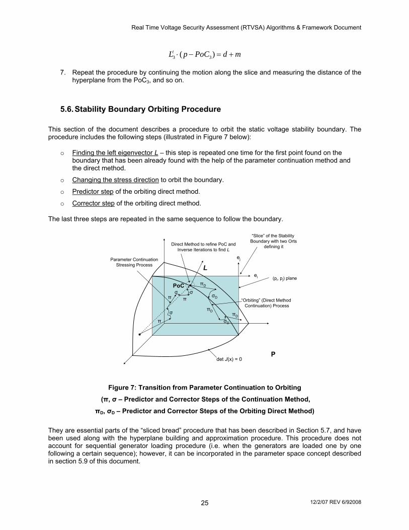
Real Time Voltage Security Assessment (RTVSA) Algorithms & Framework Document
25 12/2/07 REV 6/92008
3 3( )tL p PoC d m⋅ − = +
7. Repeat the procedure by continuing the motion along the slice and measuring the distance of the hyperplane from the PoC3, and so on.
5.6. Stability Boundary Orbiting Procedure This section of the document describes a procedure to orbit the static voltage stability boundary. The procedure includes the following steps (illustrated in Figure 7 below):
o Finding the left eigenvector L – this step is repeated one time for the first point found on the boundary that has been already found with the help of the parameter continuation method and the direct method.
o Changing the stress direction to orbit the boundary.
o Predictor step of the orbiting direct method.
o Corrector step of the orbiting direct method.
The last three steps are repeated in the same sequence to follow the boundary.
L
det J(x) = 0P
PoC
σ
π
ππσ σ
πD
σD
σD
πDπD
Parameter ContinuationStressing Process
“Orbiting” (Direct MethodContinuation) Process
Direct Method to refine PoC andInverse Iterations to find L
ej
ei
“Slice” of the Stability Boundary with two Orts
defining it
(pi, pj) plane
Figure 7: Transition from Parameter Continuation to Orbiting
(π, σ – Predictor and Corrector Steps of the Continuation Method,
πD, σD – Predictor and Corrector Steps of the Orbiting Direct Method)
They are essential parts of the “sliced bread” procedure that has been described in Section 5.7, and have been used along with the hyperplane building and approximation procedure. This procedure does not account for sequential generator loading procedure (i.e. when the generators are loaded one by one following a certain sequence); however, it can be incorporated in the parameter space concept described in section 5.9 of this document.

Real Time Voltage Security Assessment (RTVSA) Algorithms & Framework Document
26 12/2/07 REV 6/92008
5.6.1. Finding the Left Eigenvector
In order to calculate the left eigenvector, it is recommended to use the inverse iteration technique as described in section 5.5. The transposed direct method is suggested as an alternative approach. Transposed Direct Method
The Transposed Direct Method can be applied as an alternative of the inverse iteration method. It consists of solving the system (1) using the Newton-Raphson method. Transposed Direct Method Equations [2*nbus+1+nPV +2*nbus+1+nPV+1]:
'1 2
"2
( )
( , ) 0 - Active Power Balance [nbus]( , ) 0 - Reactive Power Balance [nbus]
0 - Reference Bus Equation [1]0 - PV Bus Equations [nPV]
( ) 0 - Singularity Con
D trans D
D D
PV D
RB
PVt
F x
P V P TQ V Q T
VJ x L
θ β βθ βθ
− =
− + =+ + =
Δ =Δ =
= dition [2*nbus+1+nPV]1 - Nonzero condition For the Left Eigenvector [1]tL L
⎧⎪⎪⎪⎪⎨⎪⎪⎪
=⎪⎩
(1)
Transposed Direct Method Variables xD [2*nbus+1+nPV +2*nbus+1+nPV+1]:
1
PV
2
- Voltage Phase Angles [nbus]V - Voltage Magnitudes [nbus]
- Source Factors (Distributed Slack Bus Factors) [1]Q - PV Bus Reactive Power Injections [nPV]
- Sink Factor (Stress Factor) [1]- Left EiL
θ
β
βgenvector [2*nbus+1+nPV]
(2)
Equation set (1) is very similar to the Direct Method equations set except that the last two equations in (1) are written for the left eigenvector L instead of the right eigenvector R.
The recommended initial choice of L is again
⎥⎥⎥⎥⎥
⎦
⎤
⎢⎢⎢⎢⎢
⎣
⎡
=
00
"
'
0D
D
TT
L (stress direction).
5.6.2. Changing the stress direction
We will use equation
⎪⎩
⎪⎨
⎧
=⋅=⋅
=⋅+⋅+=Φ
10)(
0)()(
LLLxJ
eexFz
t
tji ηγ
(3)

Real Time Voltage Security Assessment (RTVSA) Algorithms & Framework Document
27 12/2/07 REV 6/92008
Where
'1 2
"2
( )
( , ) 0 - Active Power Balance [nbus]( , ) 0 - Reactive Power Balance [nbus]
0 - Reference Bus Equation [1]0 - PV Bus Equations [nPV]
D D
PV D
RB
PV
F x
P V P TQ V Q T
V
θ β βθ βθ
=
⎧ − + =⎪ + + =⎪⎨Δ =⎪⎪Δ =⎩
(4)
ie and je are unit vectors spanning the “slice” plane ( , )i jp p - see Figure 7, and ],,,[ ηγLxz = .
In (4), parameter β2 is fixed, and two additional unknown parameters γ and η are added. By varying γ and η, one can explore the entire plane ( , )i jp p .
5.6.3. Predictor step of the orbiting direct method
Set (3) has one unknown more than the number of equations. It can be used to organize the prediction-correction process. The predictor equation becomes:
⎥⎥⎥⎥
⎦
⎤
⎢⎢⎢⎢
⎣
⎡
−
⋅+⋅+
−=
⎥⎥⎥⎥
⎦
⎤
⎢⎢⎢⎢
⎣
⎡
ΔΔΔΔ
⋅
⎥⎥⎥⎥⎥⎥⎥
⎦
⎤
⎢⎢⎢⎢⎢⎢⎢
⎣
⎡
−−−−−−−−−−−−−−
∂∂
StepLL
LxJeexF
Lx
E
L
xJLxJx
eexJ
t
tji
tr
t
tt
ji
1)(
)(
000
00)(])([
0)(ηγ
ηγ
(5)
where rE is the extended unit vector, and Step is the step size. Note that rE contains 2*nbus+1+nPV +2*nbus+1+nPV+2 elements.
' ",D DT T – fixed and equal to the initial loading direction;
β2 – fixed and equal to the value achieved by applying the direct method procedure;
x – variable, initially set equal to the values achieved by applying the direct method procedure;
L – variable, initially set equal to the vector obtained by the inverse iterations procedure or by the transposed direct method; and
γ, η – variables.
Equation (5) needs to be carried out only once for each predictor step.

Real Time Voltage Security Assessment (RTVSA) Algorithms & Framework Document
28 12/2/07 REV 6/92008
5.6.4. Step Selection Procedure
To force the procedure around the boundary, one of the last two elements in rE (corresponding to either ei or ej) must be fixed, and the remaining elements must be zeros. Algorithm:
1. Find a unit vector that belongs to the “slice” ( , )i je e and is orthogonal to L. This can be done by solving the following system
( )( ) ( )2 2
0
1
ti jL e eγ η
γ η
⋅ ⋅ + ⋅ =
+ = (6a)
To solve (6a), let us express η from the first equation in (6a), t
it
j
L eL e
η γ ⋅= − ⋅
⋅, and substitute it
into the second equation, ( ) ( )2
2 21
ti
tj
L eL e
γ γ⎛ ⎞⋅
+ =⎜ ⎟⎜ ⎟⋅⎝ ⎠. Therefore, (6a) has the following solution:
21
1t
it
j
ti
tj
L eL e
L eL e
γ σ
η γ
= ⋅⎛ ⎞⋅
+ ⎜ ⎟⎜ ⎟⋅⎝ ⎠
⋅= − ⋅
⋅
(6b)
where 1σ = ± . Unit vector i je eμ γ η= ⋅ + ⋅ gives a locally optimal orbiting direction of the
steady state stability boundary within the “slice” ( , )i je e .
2. At the initial orbiting point PoC0 (Figure 7), assume 1σ = + and go to the next step. At the subsequent steps, do the following.
o Assume 1σ = + .
o Find vector i je eμ γ η= ⋅ + ⋅ for γ and η determined using (6b).
o Find vector i je eξ γ η= Δ ⋅ + Δ ⋅ using γΔ and ηΔ determined at a previous predictor-corrector step.
o Check the cosine of the angle θ between vectors ξ and μ, costμ ξθ
μ ξ⋅
=⋅
.
o If cosθ is negative, reverse signs of γ and η (i.e. assume that 1σ = − ).
3. Set the last two elements in rE equal to γ and η . Set initial guesses Stepγ γΔ = ⋅ and
Stepη ηΔ = ⋅ .

Real Time Voltage Security Assessment (RTVSA) Algorithms & Framework Document
29 12/2/07 REV 6/92008
The idea behind this step is as follows. The last equation in (5) is ( ) ( )r rE i E j Stepγ η⋅Δ + ⋅Δ = ,
where ( )rE i and ( )rE j are the last two elements in rE . Since they are equal to γ and η , we
have Stepγ γ η η⋅Δ + ⋅Δ = . This condition will keep γΔ and ηΔ close to the locally optimal
orbiting direction i je eμ γ η= ⋅ + ⋅ as possible, and help to keep the step size closer to the one selected by the User (Step). Parameter Step must be always positive.
5.6.5. Corrector step of the orbiting direct method
The correction equation looks exactly as (5) with Step substituted by zero:
⎥⎥⎥⎥
⎦
⎤
⎢⎢⎢⎢
⎣
⎡
−
⋅+⋅+
−=
⎥⎥⎥⎥
⎦
⎤
⎢⎢⎢⎢
⎣
⎡
ΔΔΔΔ
⋅
⎥⎥⎥⎥⎥⎥⎥
⎦
⎤
⎢⎢⎢⎢⎢⎢⎢
⎣
⎡
−−−−−−−−−−−−−−
∂∂
01
)()(
000
00)(])([
0)(
LLLxJ
eexFLx
E
L
xJLxJx
eexJ
t
tji
tr
t
tt
jiηγ
ηγ
(7)
Equation (7) needs to be repeated until a convergence solution is obtained for each corrector step. Vector Er should be the same as determined in the predictor step. Note that after each predictor-corrector step, we get a point of the power flow feasibility boundary and the left eigenvector - that is all what is needed for the hyperplane approximation (section 5.5) and the “slice bread” procedure described in the next section. The corrector step of the orbiting direct method may not converge for various reasons, for example, singularities of the stability boundary shape along the slice. In this case, the VSA algorithms are repeated starting from the Continuation Method (section 5.3) for a new stress direction predicted at the last iteration of the orbiting procedure.
5.6.6. Calculating [ ]LxJx
t )(∂∂
Calculating the matrix [ ]LxJx
t )(∂∂
can be done using the Hessian matrices (described in Appendix A) -
second derivatives of the mismatch function F(x). This is what is recommended for the vendor’s implementation. To minimize the programming effort to build the prototype tool, approximate expressions can be applied as described below. However, they are more complicated and require more computational effort. Function F(x) can be represented as its Taylor series:

Real Time Voltage Security Assessment (RTVSA) Algorithms & Framework Document
30 12/2/07 REV 6/92008
2 3
2 3
1 1( ) ( ) ( ) ( , ) ( , , ) ...2 61 1( ) ( ) ( ) ( , ) ( , , ) ...2 6
F x R F x J x R W R R W R R R
F x R F x J x R W R R W R R R
ϑ ϑ ϑ ϑ ϑ ϑ ϑ
ϑ ϑ ϑ ϑ ϑ ϑ ϑ
+ = + + + +
− = − + − + (8)
Where 2 ( , )W R Rϑ ϑ and 3 ( , , )W R R Rϑ ϑ ϑ are the second- and third-order terms of the expansion. It is
obvious that 2 2( , ) ( , )W R R W R Rϑ ϑ ϑ ϑ= − − , 22 2( , ) ( , )W R R W R Rϑ ϑ ϑ= ,
3 3( , , ) ( , , )W R R R W R R Rϑ ϑ ϑ ϑ ϑ ϑ= − − − − , and that 33 3( , , ) ( , , )W R R R W R R Rϑ ϑ ϑ ϑ= .
By subtracting equations in (8),
3
3( ) ( ) 2 ( ) ( , , ) ...3
F x R F x R J x R W R R Rϑϑ ϑ ϑ+ − − = + + (9)
and
[ ]2
31( ) ( ) ( ) ( , , ) ...
2 6J x R F x R F x R W R R Rϑϑ ϑ
ϑ= + − − − + (10)
Finally, by differentiating (10), one can get
[ ] [ ] 21( ) ( ) ( ) ( )2
J x R J x R J x R ox
ϑ ϑ ϑϑ
∂= + − − +
∂ (11)
By substituting R by ek, where ek is a unit vector,
[ ] [ ] 0,)()(21)( →−−+=⋅
∂∂
kkkk eexJexJexJx
ϑϑϑϑ
(12)
Now,
[ ] { }
{ } [ ]{ }
[ ]{ } [ ]{ }
[ ]LxJx
e
LxJex
xJLex
exJLx
exJLx
exJx
LeexJexJL
ttk
ttk
tttk
kt
kt
kt
kkkt
⋅∂∂
=
⋅⋅∂∂
=⋅⋅∂∂
=
⋅⋅∂∂
=⋅⋅∂∂
=
⋅∂∂
=→−−+
)(
)()(
)()(
)(0,)()(21 )15(
ϑϑϑϑ
(13)
Row vector [ ]LxJx
e ttk ⋅∂∂ )( is the k-th row of the matrix [ ]LxJ
xt ⋅
∂∂ )( . Therefore, to calculate
[ ]LxJx
t ⋅∂∂ )( , one need to apply (13) to get each its row k.

Real Time Voltage Security Assessment (RTVSA) Algorithms & Framework Document
31 12/2/07 REV 6/92008
5.7. “Sliced Bread” Approach
The proposed “sliced bread” approach helps to explore the entire power flow feasibility boundary in the descriptor space and approximate it by a reasonable number of hyperplanes.
5.7.1. “Sliced Bread” Procedure in Descriptor Space
The “slice” is a cut set of the boundary obtained by varying a pair of descriptor parameters di and dj while the rest of the parameters remain constant. The released parameters form a cut set plane. These parameters may be limited by some limits:
min max
min max
i i i
j j j
d d d
d d d
≤ ≤
≤ ≤ (1)
Also, within the slice, the power flow feasibility boundary could be closed (Figure 8) or open (Figure 9). Each slice is traced and approximated using the algorithm described above. The possible criteria to stop tracing the slice is are as follow:
• Acceptable distance D between the last approximating hyperplane and the first PoC in the “slice”; for instance, in Figure 8, this condition is
di
dj
dk
PoC1
PoC2
PoC3
PoC4
PoC5
PoC6
PoC7
First “slice”,at dk = dk max
dk = dk min
A
B
C
D
Figure 8: "Sliced bread" algorithm for the closed boundary
A – First “slice” is finished due to the “round trip” condition A-B – Transition from the first to the second “slice”
C – Second “slice” is finished due to acceptable distance between the tangent hyperplane calculated at C and PoC6
D – No more slices because pk reaches pkmin
5 5 1
5
( ),
tL PoC PoCr D r D
L
⋅ −= ≤ ≈
where L is the left eigenvector, and/or

Real Time Voltage Security Assessment (RTVSA) Algorithms & Framework Document
32 12/2/07 REV 6/92008
• The “round trip” condition based on the analysis of the projections of the left eigenvectors L on the cut set plane. These projections form certain angles with the coordinate axes, for instance, with ip :
arccost
ii
L eL
ϕ⎛ ⎞⋅
= ⎜ ⎟⎜ ⎟⎝ ⎠
(2)
E.g., for Figure 8, this angle changes from its initial value about – 90° to its next value – 50°, then to + 40°, and so on. When this angle makes a full circle so that it passes again – 90°, this can be used as a criterion to stop tracing this particular slice.
• Cases when one of the descriptor parameters reaches its maximum or minimum value (points A and B in Figure 9).
The first slice can be selected at the maximum value of the fixed parameters, for instance, for maxk kd d= in Figure 8 and Figure 9. When the “slice” is finished, the procedure goes to the next slide. For this purpose, one of the fixed parameters is temporarily released (e.g., dk in Figure 8 and Figure 9), while one of the free parameters is temporarily fixed (e.g., dj). The transition is implemented with the help of the same procedure that was used to approximate the “slice”. The transition process ends when all fixed parameters reach their minimum values.
di
dj
dk
PoC4
PoC1
PoC5
PoC3
PoC2PoC6
A
B
C
First “slice” atdk=dk max
dk=dk min
dj max
dj min
Figure 9: "Slice bread" algorithm for the open boundary
A – First “slice” is finished because dj = djmax B – Second “slice” is finished because dj = djmin
C – Procedure stops because dk = dkmin
5.7.2. The Algorithm in the Descriptor Space
1. Calculate the base case point in X , P and D, that is x0, p0 and d0.
2. Specify an initial stress direction in D, Δd0 using inverse mapping Δp0 = Tdir = Vector-1(Δd0).
3. Specify the first slice (di, dj) in D.
4. Map the slice into P, (pi, pj) = (ei, ej) = Plane-1 (di, dj)

Real Time Voltage Security Assessment (RTVSA) Algorithms & Framework Document
33 12/2/07 REV 6/92008
5. Perform the parameter continuation method and direct method to determine PoC0 in X and P. Find the left eigenvector L0 and hyperplane H0.
6. Map PoC0, L0 and H0 back into D : PoC0D = Point(PoC0P), L0D = Vector(L0P), and H0D = Plane(H0P).
7. Initiate the Boundary Orbiting Procedure step along the slice (ei, ej) in P.
8. If the BOM step diverges, repeat the parameter continuation method and direct method to determine PoC1 in X and P. Find the left eigenvector L1 and hyperplane H1. Go to 10.
9. Otherwise, determine PoC1 in X and P as a result of the BOM step. Find the left eigenvector L1 and hyperplane H1.
10. Map PoC1 , L1 and H1 back into D , PoC1D = Point(PoC1P) , L1D = Vector(L1P), and H1D = Plane(H1P).
11. Check the slice stop tracing criteria as described in Section 5.7.1. Go to the next slice in D and start from Step 1.
12. Otherwise map the (di, dj) into P again at the new point, (pi, pj) = (ei, ej) = Plane-1 (di, dj).
5.8. Minimum Set of Hyperplanes
The objective of obtaining the minimum set of hyperplanes is to test the performance and accuracy of the proposed VSA technology, which includes the following steps:
• Selection of critical loading directions for a selected problem area • Performance of the predictor-corrector loading procedure • Calculation of the points of collapse and tangent hyperplanes • Calculation of the approximating hyperplanes (secant hyperplanes) • Evaluate the accuracy of approximation using the proposed approach and accuracy metric • Decide on whether the proposed selection of loading directions is adequate to the study areas
5.8.1. Procedure for Determining the Minimum Set of Hyperplanes
The following steps describe the procedure to determine the minimum set of hyperplanes:
1. Perform the predictor-corrector procedure for each selected loading direction – Sections 5.3. 2. Determine the Points of Collapse (PoC) - Section 5.4. 3. Apply inverse iterations method to calculate the left eigenvector L at the PoC – Section 5.5. 4. Calculate the tangent and secant hyperplanes – Section 5.5. To determine the required margin
(d+m), use 5, 10, 15, and 20% (j=1, 2…, 4) (configurable) of the maximum loading in the most limited direction. As a result, get four sets of secant hyperplanes for each direction, corresponding to the different margin (d+m) – Figure 10 (taken from section 5.5).
The tangent hyperplane equation is:
( ) 0ti iL p PoC⋅ − =
The secant approximating hyperplane equation is:
( )( )ti i j
L p PoC d m⋅ − = +

Real Time Voltage Security Assessment (RTVSA) Algorithms & Framework Document
34 12/2/07 REV 6/92008
Figure 10: Tangent and approximating hyperplanes
5. Select 10-20 additional loading directions for each area and perform the step-by step loading
procedure for the original and additional loading vectors. Evaluate the PoCk for each direction k assuming that this is the point of divergence.
6. For each evaluated PoCk, calculate the distance to each of the approximating hyperplanes at different margins (d+m)j using the following formula:
ji
ikti
ijk mdL
PoCPoCLr )(
)(+−
−⋅=
7. Summarize these experimental results for each area in the following table:
Hyperplane Loading Vector 1 Loading Vector 2 … Loading Vector k 1 5%
10% 15% 20%
2 5% 10% 15% 20%
… 5% 10% 15% 20%
i 5% 10% 15% 20%
Distances from PoC to Hyperplanes
8. Analyze the angles between the loading vectors Dk and the left eigenvectors Lk. These angles can be calculated as follows:
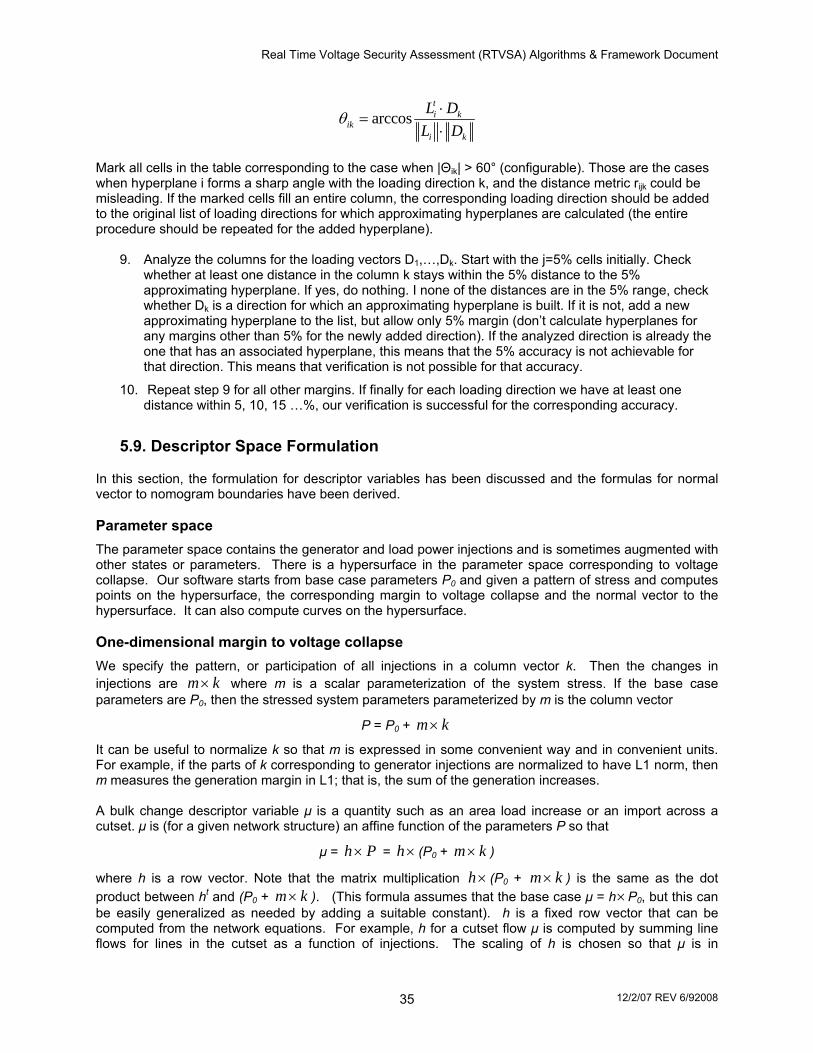
Real Time Voltage Security Assessment (RTVSA) Algorithms & Framework Document
35 12/2/07 REV 6/92008
arccosti k
iki k
L DL D
θ ⋅=
⋅
Mark all cells in the table corresponding to the case when |Θik| > 60° (configurable). Those are the cases when hyperplane i forms a sharp angle with the loading direction k, and the distance metric rijk could be misleading. If the marked cells fill an entire column, the corresponding loading direction should be added to the original list of loading directions for which approximating hyperplanes are calculated (the entire procedure should be repeated for the added hyperplane).
9. Analyze the columns for the loading vectors D1,…,Dk. Start with the j=5% cells initially. Check whether at least one distance in the column k stays within the 5% distance to the 5% approximating hyperplane. If yes, do nothing. I none of the distances are in the 5% range, check whether Dk is a direction for which an approximating hyperplane is built. If it is not, add a new approximating hyperplane to the list, but allow only 5% margin (don’t calculate hyperplanes for any margins other than 5% for the newly added direction). If the analyzed direction is already the one that has an associated hyperplane, this means that the 5% accuracy is not achievable for that direction. This means that verification is not possible for that accuracy.
10. Repeat step 9 for all other margins. If finally for each loading direction we have at least one distance within 5, 10, 15 …%, our verification is successful for the corresponding accuracy.
5.9. Descriptor Space Formulation
In this section, the formulation for descriptor variables has been discussed and the formulas for normal vector to nomogram boundaries have been derived. Parameter space The parameter space contains the generator and load power injections and is sometimes augmented with other states or parameters. There is a hypersurface in the parameter space corresponding to voltage collapse. Our software starts from base case parameters P0 and given a pattern of stress and computes points on the hypersurface, the corresponding margin to voltage collapse and the normal vector to the hypersurface. It can also compute curves on the hypersurface. One-dimensional margin to voltage collapse We specify the pattern, or participation of all injections in a column vector k. Then the changes in injections are km× where m is a scalar parameterization of the system stress. If the base case parameters are P0, then the stressed system parameters parameterized by m is the column vector
P = P0 + km×
It can be useful to normalize k so that m is expressed in some convenient way and in convenient units. For example, if the parts of k corresponding to generator injections are normalized to have L1 norm, then m measures the generation margin in L1; that is, the sum of the generation increases. A bulk change descriptor variable μ is a quantity such as an area load increase or an import across a cutset. μ is (for a given network structure) an affine function of the parameters P so that
μ = Ph× = ×h (P0 + km× )
where h is a row vector. Note that the matrix multiplication ×h (P0 + km× ) is the same as the dot product between ht and (P0 + km× ). (This formula assumes that the base case μ = h×P0, but this can be easily generalized as needed by adding a suitable constant). h is a fixed row vector that can be computed from the network equations. For example, h for a cutset flow μ is computed by summing line flows for lines in the cutset as a function of injections. The scaling of h is chosen so that μ is in

Real Time Voltage Security Assessment (RTVSA) Algorithms & Framework Document
36 12/2/07 REV 6/92008
convenient units such as MW of import through the cutset or MW of load. At the voltage collapse, we get:
μ* = h (P0 + m*×k) If we now assume a fixed stress direction or injection participation k, then m is also a function of μ:
khPh
m××−
= 0μ
Specifying μ and k now defines the system stress m and k. That is, the system stress can be specified by the amount of a bulk change of injections μ and also assuming the pattern, or participation of all injections in the column vector k. In summary, we can formulate the one-dimensional margin to voltage collapse as follows: We make the assumption of the participation factors k. Then we can specify an amount of stress by descriptor μ and the margin to voltage collapse can be specified by the descriptor margin μ* = h (P0 + m*×k). Two-dimensional voltage collapse nomogram Here we define two bulk change descriptor variables μ and η so the descriptor variables are the column vector d = (μ,η)T (superscript T indicates matrix transpose)14. Now h is a vector function given by the 2 × (number of parameters) matrix h = (h1
T, h2T)T so that
d = (μ,η)T = h×P = h (P0 + m×k)
The nomogram curve is given by (μ*, η*)T = h (P0 + m*×k) as k varies (note that m* is a function of k). We assume that the nomogram curve is given (locally) by:
g(d) = g((μ,η)T) = 0
If we now assume two fixed stress directions or injection participations k1 and k2, so that
P = P0 + m1×k1 + m2×k2,
then
d = (μ,η)T = h (P0 + m1×k1 + m2×k2) = d0 + M (m1, m2)T
where M is the 2 x 2 matrix
M = [h×k1, h×k2]
Then (m1, m2)T and P are also affine functions of (μ,η)T:
(m1, m2)T = 1−M ((μ,η)T - h×P0) P = P0 + (k1, k2) × (m1, m2)T
= P0 + (k1, k2) × 1−M × (d - d0)
Specifying (μ,η)T and k1 and k2 now defines the system stress in terms of injections P. That is, the system stress can be specified by the amount of a bulk change of injections (μ,η)T and also assuming the patterns, or participations of all injections in the column vectors k1 and k2. 14 For example, for the San Diego region, we could have (μ,η)T = (path 45/CFE import, SDG&E import)T or (μ,η)T = (SDG&E generation, SDG&E load)T

Real Time Voltage Security Assessment (RTVSA) Algorithms & Framework Document
37 12/2/07 REV 6/92008
In summary, we can formulate a two-dimensional margin to voltage collapse as follows: We make the assumption of the participation factor vectors k1 and k2. Then we can specify an amount of stress by descriptor vector d = (μ,η)T. The voltage collapse boundary can be specified by the curve g(d) = 0 in the nomogram. It is important to note the dependence of the nomogram curve on the choice of k1 and k2. Relation between parameter space and nomogram normals The descriptor parameters d considered here are affine functions of the parameter space parameters P given by
d = d0 + h ×P
where h is a matrix. As explained above, the nomogram curve is given by an equation
g(d) = 0
The nomogram curve has normal vector given by the row vector Dg. Dg has two components. The nomogram curve immediately induces a corresponding hypersurface in the parameter space defined by the equation
g(d0 + h×P) = 0
Differentiating g(d0 + h×P) with respect to P gives the normal vector to the parameter space hypersurface
hyperspace normal = Dg×h
This formula expresses the parameter space normal in terms of the nomogram curve normal and the transformation matrix h. Now we express the nomogram curve normal in terms of the parameter space normal. Assume as above a choice of k1 and k2 so that
P = P0 + (k1, k2) × 1−M × (d - d0)
Let the parameter space hypersurface be given by an equation
f(P)=0
The hypersurface has normal vector given by the row vector Df. Then the nomogram curve is given by
f(P0 + (k1, k2) × 1−M × (d - d0)) = 0
Differentiating the left hand side with respect to d gives the normal vector to the nomogram curve
nomogram normal = Df × (k1, k2) × 1−M
This formula expresses the nomogram normal in terms of the parameter space normal and a linear transformation.
5.10. Special Features of the RTVSA Application
The RTVSA application is based on an extensive analysis of the existing VSA approaches, by surveying the leading power system experts’ opinion worldwide, and also with feedback from industrial advisors. The mismatch between the core power system reliability needs and the availability of the VSA tools was a motivation to design the following special features into the RTVSA application. The underlying concepts are applicable to the simple one-dimensional approach or the more complex
multi-directional stressing to explore the entire voltage security region in the parameter space or in full P-Q injection space.

Real Time Voltage Security Assessment (RTVSA) Algorithms & Framework Document
38 12/2/07 REV 6/92008
The RTVSA tool has the ability of analyzing the effects of multiple transfers. There are no restrictions in distributing the source and sink over a large number of buses in geographically distant locations in the system. A non-local treatment of congestion15 is crucial because conservatism causes costly curtailment of profitable power transfers and a suboptimal use of the transmission system.
The RTVSA algorithm16 in Phase 2 uses the parameter continuation method, which is one of the most
reliable power flow methods capable of reaching the point of collapse on the power flow feasibility boundary. New variables called the continuation parameters are added and represents a position of a power flow operating point along some power system stress direction in the parameter space. The predictor step consists in an incremental moving of the power flow operating point along the state space trajectory, based on the linearization of the problem. The corrector step, that follows each predictor step, consists in elimination of the linearization error by balancing the power flow equations to some close point on the nonlinear trajectory.
The RTVSA algorithm in Phase 3 use Direct methods for finding the PoC, which combines the
parametric description of the system stress and the power flow singularity condition expressed with the help of the Jacobian matrix multiplied by a nonzero right or the left eigenvector that nullifies the Jacobian matrix at the collapse point. In principle, the Direct Method avoids implementing a loading procedure. There may be problems of finding the initial guesses of the state variables and the eigenvector that may be resolved by initial loading the system along the stress direction. By doing so, the initial guess of variables can be obtained. Many inaccuracies of the step-by-step loading methods that do not exactly converge to the PoC will be avoided by implementing the Direct Method. There are savings in computational expenses because of the absence of iterations even though the Direct Method solves a problem almost double in dimension to the step-by-step loading methods.
The RTVSA algorithm determines the “right eigenvector” and the “left eigenvector” at the PoC. The
weak elements are based on the right eigenvector and provide the extent to which variables participate in voltage collapse. This determines weak areas and also whether the collapse is an angle collapse. Large sensitivities of the margin to PoC indicate controllable parameters. These are represented by the left eigenvector and can be quantified for suitable corrective action by ranking the increase in margin with respect to a unit MW or MVAR in generator response.
Sensitivity computations relate changes in data to changes in transfer capability. The uncertainty in
the transfer capability due to uncertainty in the data was quantified in Phase 4 of the RTVSA algorithm. These computations revealed which data is significant in the transfer calculations.
15 Congestion can be quantified more precisely as the combined effect of multiple power transfers exceeding the transfer capability
of the transmission system. 16 The RTVSA algorithm falls into the class of non-divergent power flow methods that manipulate the step size of the Newton- Raphson method. If the power flow mismatches indicate divergence, the step size is reduced until convergence occurs or the step becomes very small. A very small step size is considered to be an indicator of the point of collapse.

39 12/2/07 REV 6/92008
6. Appendix A: Hessian Metrix of Power Flow Equation Ning Zhou, PNNL, Richland, WA 99352
10/06/2006~10/16/2006
I. SCALAR VERSION OF SECOND DERIVATIVES OF POWER INJECTIONS ................................................................................................................................... 39 II VECTORIZED JACOBIAN .......................................................................................................................................................................................................................... 43 III VECTORIZED HESSIAN ............................................................................................................................................................................................................................ 44 IV. DERIVATIVE OF TRANSPOSED JACOBIAN MULTIPLIED BY LEFT EIGENVECTOR ............................................................................................................ 49 V. NOTATION AND MATRIX IDENTITY: ................................................................................................................................................................................................... 56 REFERENCE ...................................................................................................................................................................................................................................................... 57 This document describes procedures of calculating the Hessian Matrix of Power flow equations. It also discusses the vectorization procedure,
which may improve the implement efficiency using Matlab. The calculation procedure of the [ ]LxJx
t ⋅∂∂ )( is also derived.
I. Scalar Version of Second Derivatives of Power InjectionS This section gives the identities for calculating the elements of Jacobian and Hessian matrix of power injection. Note that all the elements are in the scalar format. Thus, it may not be efficient to implement the algorithm using Matlab. Note: a) Matlab is not very efficient to implement ‘for’ loop. b) The notation used is similar to the notation used in [1] . c) The power injection and first derivative equations are extracted from [1].
• Real Power Injection
( )∑=
+=nbus
jijijijijjii BGVVP
1sincos θθ
First derivative w.r.t θi. (with fixed i)
( )∑=
−−−=∂∂ nbus
jiiiijijijijji
i
i BVBGVVP1
2cossin θθθ
Second derivative wrt θi
( )∑=
++−=∂∂
∂ nbus
jiiiijijijijji
ii
i GVBGVVP1
22
sincos θθθθ
Second derivative wrt θj (for j<>i)
( )ijijijijjiji
i BGVVP θθθθ
sincos2
+=∂∂
∂
Second derivative wrt Vi
( )∑=
−−−=∂∂
∂ nbus
jiiiijijijijj
ii
i BVBGVV
P1
2
cossin θθθ

40 12/2/07 REV 6/92008
Second derivative wrt Vj (for j<>i)
( )ijijijijiji
i BGVV
P θθθ
cossin2
−−=∂∂
∂
First derivative w.r.t θj (for j<>i, with fixed i and j. ).
( )ijijijijjij
i BGVVP θθθ
cossin −=∂∂
Second derivative wrt θi
( )ijijijijjiij
i BGVVP θθθθ
sincos2
+=∂∂
∂
Second derivative wrt θj
( )ijijijijjijj
i BGVVP θθθθ
sincos2
+−=∂∂
∂
Second derivative wrt θk (for k<>i, k<>j)
02
=∂∂
∂
kj
iPθθ
Second derivative wrt Vi
( )ijijijijjij
i BGVV
P θθθ
cossin2
−=∂∂
∂
Second derivative wrt Vj
( )ijijijijijj
i BGVV
P θθθ
cossin2
−=∂∂
∂
Second derivative wrt Vk ((for k<>i, k<>j)
02
=∂∂
∂
kj
i
VP
θ
First derivative w.r.t Vi. (with fixed i)
( )∑=
++=∂∂ nbus
jiiiijijijijj
i
i GVBGVVP
1sincos θθ
Second derivative wrt θi
( )∑=
−−⋅−=∂∂
∂ nbus
jiiiijijijijj
ii
i BVBGVV
P1
2
cossin θθθ
Second derivative wrt θj (for j<>i)
( )ijijijijjji
i BGVV
P θθθ
cossin2
−=∂∂
∂
Second derivative wrt Vi
iiii
i GVV
P 22
=∂∂
∂
Second derivative wrt Vj (for j<>i)
ijijijijji
i BGVV
P θθ sincos2
+=∂∂
∂
First derivative w.r.t Vj. (with fixed i and j, for j<>i)
( )ijijijijij
i BGVVP θθ sincos +⋅=
∂∂
Second derivative wrt θi
( )ijijijijiij
i BGVV
P θθθ
cossin2
−⋅−=∂∂
∂
Second derivative wrt θj
( )ijijijijijj
i BGVV
P θθθ
cossin2
−⋅=∂∂
∂
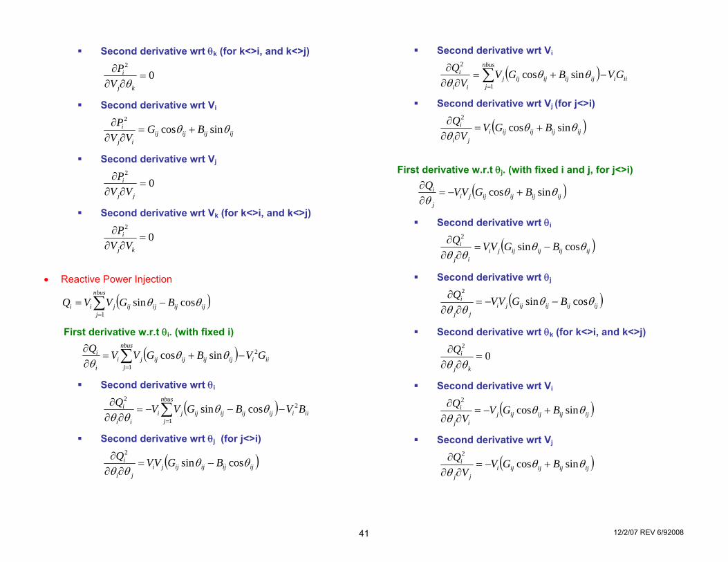
41 12/2/07 REV 6/92008
Second derivative wrt θk (for k<>i, and k<>j)
02
=∂∂
∂
kj
i
VPθ
Second derivative wrt Vi
ijijijijij
i BGVV
P θθ sincos2
+=∂∂
∂
Second derivative wrt Vj
02
=∂∂
∂
jj
i
VVP
Second derivative wrt Vk (for k<>i, and k<>j)
02
=∂∂
∂
kj
i
VVP
• Reactive Power Injection
( )∑=
−=nbus
jijijijijjii BGVVQ
1cossin θθ
First derivative w.r.t θi. (with fixed i)
( )∑=
−+=∂∂ nbus
jiiiijijijijji
i
i GVBGVVQ1
2sincos θθθ
Second derivative wrt θi
( )∑=
−−−=∂∂
∂ nbus
jiiiijijijijji
ii
i BVBGVVQ1
22
cossin θθθθ
Second derivative wrt θj (for j<>i)
( )ijijijijjiji
i BGVVQ θθθθ
cossin2
−=∂∂
∂
Second derivative wrt Vi
( )∑=
−+=∂∂
∂ nbus
jiiiijijijijj
ii
i GVBGVV
Q1
2
sincos θθθ
Second derivative wrt Vj (for j<>i)
( )ijijijijiji
i BGVV
Q θθθ
sincos2
+=∂∂
∂
First derivative w.r.t θj. (with fixed i and j, for j<>i)
( )ijijijijjij
i BGVVQ θθθ
sincos +−=∂∂
Second derivative wrt θi
( )ijijijijjiij
i BGVVQ θθθθ
cossin2
−=∂∂
∂
Second derivative wrt θj
( )ijijijijjijj
i BGVVQ θθθθ
cossin2
−−=∂∂
∂
Second derivative wrt θk (for k<>i, and k<>j)
02
=∂∂
∂
kj
iQθθ
Second derivative wrt Vi
( )ijijijijjij
i BGVV
Q θθθ
sincos2
+−=∂∂
∂
Second derivative wrt Vj
( )ijijijijijj
i BGVV
Q θθθ
sincos2
+−=∂∂
∂

42 12/2/07 REV 6/92008
Second derivative wrt Vk (for k<>i, and k<>j)
02
=∂∂
∂
kj
i
VQ
θ
First derivative w.r.t Vi. (with fixed i)
( ) iii
nbus
jijijijijj
i
i BVBGVVQ
−−=∂∂ ∑
=1cossin θθ
Second derivative wrt θi
( ) iii
nbus
jijijijijj
ii
i GVBGVVQ
−+=∂∂
∂ ∑=1
2
sincos θθθ
Second derivative wrt θj (for j<>i)
( )ijijijijjji
i BGVV
Q θθθ
sincos2
+−=∂∂
∂
Second derivative wrt Vi
iiii
i BVV
Q 22
−=∂∂
∂
Second derivative wrt Vj (for j<>i)
ijijijijji
i BGVV
Q θθ cossin2
−=∂∂
∂
First derivative w.r.t Vj. (with fixed i and j, for j<>i)
( )ijijijijij
i BGVVQ θθ cossin −=∂∂
Second derivative wrt θi
( )ijijijijiij
i BGVV
Q θθθ
sincos2
+=∂∂
∂
Second derivative wrt θj
( )ijijijijijj
i BGVV
Q θθθ
sincos2
+−=∂∂
∂
Second derivative wrt θk (for k<>i and k<>j)
02
=∂∂
∂
kj
i
VQθ
Second derivative wrt Vi
ijijijijij
i BGVV
Q θθ cossin2
−=∂∂
∂
Second derivative wrt Vj
02
=∂∂
∂
jj
i
VVQ
Second derivative wrt Vk (for k<>i and k<>j)
02
=∂∂
∂
kj
i
VVQ

43 12/2/07 REV 6/92008
II Vectorized JacobianThis section gives the vectorized Jacobian matrix. The method has been cross-validated through the comparison with the Matlab codes in [2]. Prof. DeMarco’s contributions are credited in the Matlab codes. Note that the vectorized Jacobian can be implemented efficiently using Matlab.
⎥⎦
⎤⎢⎣
⎡⋅⎥
⎦
⎤⎢⎣
⎡⋅⋅⎥
⎦
⎤⎢⎣
⎡⋅⎥
⎦
⎤⎢⎣
⎡=
⋅⋅=
⋅=
−
−
2
1
2
1
2
1
2
1
)(
)()(
)()(
VV
ee
Yconje
eV
V
VYconjVdiag
IconjVdiagS
j
j
j
j
θ
θ
θ
θ
rr
rr
(2.1)
2.1) Vectorized Jacobian wrt V
{ }
[ ]
⎥⎦
⎤⎢⎣
⎡⋅⋅+⎥
⎦
⎤⎢⎣
⎡⋅⋅=
⎥⎥⎥
⎦
⎤
⎢⎢⎢
⎣
⎡
⋅⋅+⎥⎥⎥
⎦
⎤
⎢⎢⎢
⎣
⎡
⋅⋅=
∂∂⋅+
∂∂⋅=
⋅∂∂
=∂∂
−
−
VVdiagVYconjdiag
VVconjdiagYconjVdiag
e
eVYconjdiag
e
eYconjVdiag
VVIconjdiag
VIconjVdiag
IconjVdiagVV
S
nbusnbus j
j
j
j
rv
rr
Or
Or
rr
rr
rr
)]([)()()(
)]([)()(
)()()(
)()(
11
θ
θ
θ
θ (2.2)
⎟⎠⎞
⎜⎝⎛∂∂
=∂∂
⎟⎠⎞
⎜⎝⎛∂∂
=∂∂
VSimag
VQ
VSreal
VP
(2.3)
2.2) Vectorized Jacobian wrt θ

44 12/2/07 REV 6/92008
{ }
[ ]
( ) ( )VjdiagVYconjdiagVjconjdiagYconjVdiag
ejV
ejVVYconjdiag
ejV
ejVYconjVdiag
VIconjdiagIconjVdiag
IconjVdiagS
nbusnbus jnbus
j
jnbus
j
rvrr
Or
Or
rr
rr
rr
⋅⋅⋅+⋅⋅⋅=
⎥⎥⎥
⎦
⎤
⎢⎢⎢
⎣
⎡
⋅⋅+⎥⎥⎥
⎦
⎤
⎢⎢⎢
⎣
⎡
−
−⋅⋅=
∂∂⋅+
∂∂⋅=
⋅∂∂
=∂∂
−
−
)]([)()()(
)]([)()(
)()()(
)()(
1111
θ
θ
θ
θ
θθ
θθ
(2.4)
⎟⎠⎞
⎜⎝⎛∂∂
=∂∂
⎟⎠⎞
⎜⎝⎛∂∂
=∂∂
θθθθSimagQSrealP
(2.5)
III Vectorized Hessian
Suppose that NNRxJ ×∈)( is the “full Jacobian” matrix. Then, the Hessian matrix can be expressed as ( )[ ] NNRxJvecx
×∈∂∂ 2
)( . The vectorized
Hessian matrix can be implemented more efficiently using Matlab than the scalar version.
3.1) ⎟⎟⎠
⎞⎜⎜⎝
⎛∂∂
∂∂
i
Sθθ
⎥⎥⎥
⎦
⎤
⎢⎢⎢
⎣
⎡
⋅⋅+⎥⎥⎥
⎦
⎤
⎢⎢⎢
⎣
⎡
−⋅⋅=∂∂
+∂∂
=∂∂
−
−
−
−−Δ
)(
)1(
)(
)1(21
0
0)]([
0
0)()(
inbus
ji
i
inbus
ji
i
iii
ii ejVVYconjdiagejVYconjVdiagSSS θθ
θθθvr
(3.1.1)
[ ]
[ ]⎪⎭
⎪⎬
⎫
⎪⎩
⎪⎨
⎧
⎥⎥⎥
⎦
⎤
⎢⎢⎢
⎣
⎡
−⋅⋅+⎥⎥⎥
⎦
⎤
⎢⎢⎢
⎣
⎡−⋅⋅=
⎥⎥⎥
⎦
⎤
⎢⎢⎢
⎣
⎡
⋅⎪⎭
⎪⎬
⎫
⎪⎩
⎪⎨
⎧
⎥⎥⎥
⎦
⎤
⎢⎢⎢
⎣
⎡
−⋅+⎥⎥⎥
⎦
⎤
⎢⎢⎢
⎣
⎡−⋅⋅=⎟⎟
⎠
⎞⎜⎜⎝
⎛∂∂
∂∂
−
−−
−
−
−−
−
)(
)1(
1
)(
)1(1
0
0)()(
0
0)()(
0
0)(
0
0)()(
1
in
ji
ij
i
jnbus
j
in
ji
ij
ii
ii
nbus
ii
ejVYconjVjdiagdiageVYconjVdiag
ejV
ejVejVYconjdiageVYconjVdiagS
θθ
θ
θ
θθ
θθ
rr
Or
(3.1.2)

45 12/2/07 REV 6/92008
[ ] [ ])()(0
0
0
0)(
)(0
0
0
0)]([
)(
)1(
)(
)1(
1
)(
)1(2
1
VjconjdiagYconjejVdiageVVYconjdiagdiag
ejV
ejVYconjejVdiageVVYconjdiagS
inbus
ji
i
inbus
ji
i
jnbus
j
inbus
ji
ij
ii
ii
nbus
ii
rv
Ov
⋅⋅⎪⎭
⎪⎬
⎫
⎪⎩
⎪⎨
⎧
⎥⎥⎥
⎦
⎤
⎢⎢⎢
⎣
⎡
+⎪⎭
⎪⎬
⎫
⎪⎩
⎪⎨
⎧
⎥⎥⎥
⎦
⎤
⎢⎢⎢
⎣
⎡
−⋅⋅=
⎥⎥⎥
⎦
⎤
⎢⎢⎢
⎣
⎡
−
−⋅⋅
⎪⎭
⎪⎬
⎫
⎪⎩
⎪⎨
⎧
⎥⎥⎥
⎦
⎤
⎢⎢⎢
⎣
⎡
+⎥⎥⎥
⎦
⎤
⎢⎢⎢
⎣
⎡−⋅⋅=⎟⎟
⎠
⎞⎜⎜⎝
⎛∂∂
∂∂
−
−
−
−
−
−
−
−
θθ
θ
θ
θθ
θθ
(3.1.3)
Thus,
[ ]
[ ] [ ])()(0
0
0
0)(
0
0)()(
0
0)()(
)(
)1(
)(
)1(
)(
)1(
VconjdiagYconjeVdiageVVYconjdiagdiag
eVYconjVdiagdiageVYconjVdiagS
inbus
ji
i
inbus
ji
i
in
ji
ij
ii
ii
ii
rv
rr
⋅⋅⎪⎭
⎪⎬
⎫
⎪⎩
⎪⎨
⎧
⎥⎥⎥
⎦
⎤
⎢⎢⎢
⎣
⎡
+⎪⎭
⎪⎬
⎫
⎪⎩
⎪⎨
⎧
⎥⎥⎥
⎦
⎤
⎢⎢⎢
⎣
⎡
−⋅⋅+
⎪⎭
⎪⎬
⎫
⎪⎩
⎪⎨
⎧
⎥⎥⎥
⎦
⎤
⎢⎢⎢
⎣
⎡
⋅⋅+⎥⎥⎥
⎦
⎤
⎢⎢⎢
⎣
⎡−⋅⋅=⎟⎟
⎠
⎞⎜⎜⎝
⎛∂∂
∂∂
−
−
−
−
−
−−
−
θθ
θθ
θθ
(3.1.4)
3.2) ⎟⎟⎠
⎞⎜⎜⎝
⎛∂∂
∂∂
i
SV θ
⎥⎥⎥
⎦
⎤
⎢⎢⎢
⎣
⎡
⋅⋅+⎥⎥⎥
⎦
⎤
⎢⎢⎢
⎣
⎡
−⋅⋅=∂∂
+∂∂
=∂∂
−
−
−
−−Δ
)(
)1(
)(
)1(21
0
0)]([
0
0)()(
inbus
ji
i
inbus
ji
i
iii
ii ejVVYconjdiagejVYconjVdiagSSS θθ
θθθvr
(3.2.1)
⎪⎭
⎪⎬
⎫
⎪⎩
⎪⎨
⎧
⎥⎥⎥
⎦
⎤
⎢⎢⎢
⎣
⎡
−⋅⋅⎥⎥⎥
⎦
⎤
⎢⎢⎢
⎣
⎡
+⎥⎥⎥
⎦
⎤
⎢⎢⎢
⎣
⎡−⋅⋅=
⎥⎥⎥
⎦
⎤
⎢⎢⎢
⎣
⎡
⋅⎪⎭
⎪⎬
⎫
⎪⎩
⎪⎨
⎧
⎥⎥⎥
⎦
⎤
⎢⎢⎢
⎣
⎡
−⋅+⎥⎥⎥
⎦
⎤
⎢⎢⎢
⎣
⎡−⋅⋅=⎟⎟
⎠
⎞⎜⎜⎝
⎛∂∂
∂∂
−
−−
−
−
−−
−
−
−
)(
)1(
)(
)1(1
0
0)(
0
0)()(
0
0)(
0
0)()(
1
1
1
1
inbus
ji
i
j
j
j
j
j
inbus
ji
ij
i
i
nbus
i
nbus
ii
ejVYconje
ediagjeYconjVdiag
e
eejVYconjdiagjeYconjVdiagS
V
θ
θ
θ
θ
θ
θ
θθ
θ
Or
Or
(3.2.2)
Type I Type II
Type II Type III

46 12/2/07 REV 6/92008
⎥⎥⎥
⎦
⎤
⎢⎢⎢
⎣
⎡
⋅⎪⎭
⎪⎬
⎫
⎪⎩
⎪⎨
⎧
⎥⎥⎥
⎦
⎤
⎢⎢⎢
⎣
⎡
+⎥⎥⎥
⎦
⎤
⎢⎢⎢
⎣
⎡⋅⋅=⎟⎟
⎠
⎞⎜⎜⎝
⎛∂∂
∂∂
−
−
−
−
nbus
ii
j
j
inbus
ji
ij
i e
eYconjejVdiagjeVYconjdiagS
V θ
θ
θθ
θO
v1
)(0
0
0
0)]([
)(
)1(2 (3.2.3)
⎥⎥⎥
⎦
⎤
⎢⎢⎢
⎣
⎡
⋅⎪⎭
⎪⎬
⎫
⎪⎩
⎪⎨
⎧
⎥⎥⎥
⎦
⎤
⎢⎢⎢
⎣
⎡
+⎥⎥⎥
⎦
⎤
⎢⎢⎢
⎣
⎡⋅⋅+
⎪⎭
⎪⎬
⎫
⎪⎩
⎪⎨
⎧
⎥⎥⎥
⎦
⎤
⎢⎢⎢
⎣
⎡
−⋅⋅⎥⎥⎥
⎦
⎤
⎢⎢⎢
⎣
⎡
+⎥⎥⎥
⎦
⎤
⎢⎢⎢
⎣
⎡−⋅⋅=
⎟⎟⎠
⎞⎜⎜⎝
⎛∂∂
∂∂
+⎟⎟⎠
⎞⎜⎜⎝
⎛∂∂
∂∂
=⎟⎟⎠
⎞⎜⎜⎝
⎛∂∂
∂∂
−
−
−
−
−
−−
−
nbus
ii
i
nbus
i
j
j
inbus
ji
ij
inbus
ji
i
j
j
j
iii
e
eYconjejVdiagjeVYconjdiag
ejVYconje
ediagjeYconjVdiag
SV
SV
SV
θ
θ
θθ
θ
θ
θ
θ
θθθ
Ov
Or
1
1
)(0
0
0
0)]([
0
0)(
0
0)()(
)(
)1(
)(
)1(
21
(3.2.4)
3.3) ⎟⎟⎠
⎞⎜⎜⎝
⎛∂∂
∂∂
iVS
θ
⎥⎥⎥
⎦
⎤
⎢⎢⎢
⎣
⎡
⋅⎪⎭
⎪⎬
⎫
⎪⎩
⎪⎨
⎧
⎥⎥⎥
⎦
⎤
⎢⎢⎢
⎣
⎡
⋅+⎥⎥⎥
⎦
⎤
⎢⎢⎢
⎣
⎡
⋅⋅⎥⎥⎥
⎦
⎤
⎢⎢⎢
⎣
⎡
=∂∂
+∂∂
=∂∂
−
−
−
−
−
−−Δ
)1(
)1(1
)(
)1(121
0
0)(
0
0)(
11
i
ji
jnbus
j
inbus
ji
jnbus
j
iii
i
nbus
i
nbus
eeV
eVYconjdiageYconj
eV
eV
VS
VS
VS θ
θ
θ
θ
θ
θ
MO (3.3.1)
Type I Type II
Type I Type III

47 12/2/07 REV 6/92008
⎪⎭
⎪⎬
⎫
⎪⎩
⎪⎨
⎧
⎥⎥⎥
⎦
⎤
⎢⎢⎢
⎣
⎡
⋅⋅⋅+⎥⎥⎥
⎦
⎤
⎢⎢⎢
⎣
⎡−⋅⋅=
⋅⋅⎪⎭
⎪⎬
⎫
⎪⎩
⎪⎨
⎧
⎥⎥⎥
⎦
⎤
⎢⎢⎢
⎣
⎡
⋅+⎥⎥⎥
⎦
⎤
⎢⎢⎢
⎣
⎡−⋅⋅=
⎥⎥⎥
⎦
⎤
⎢⎢⎢
⎣
⎡
⋅⎪⎭
⎪⎬
⎫
⎪⎩
⎪⎨
⎧
⎥⎥⎥
⎦
⎤
⎢⎢⎢
⎣
⎡
⋅+⎥⎥⎥
⎦
⎤
⎢⎢⎢
⎣
⎡−⋅⋅
⎥⎥⎥
⎦
⎤
⎢⎢⎢
⎣
⎡
=⎟⎟⎠
⎞⎜⎜⎝
⎛∂∂
∂∂
−
−−
−
−
−−
−
−
−−
−
)(
)1(
)(
)1(
1
)(
)1(11
0
0)()(
0
0)()(
)(0
0)(
0
0)()(
0
0)(
0
0)(
11
inbus
ji
j
inbus
ji
j
jnbus
j
inbus
ji
j
jnbus
j
i
ii
ii
nbus
ii
nbus
eYconjVdiagjdiagjeYconjVdiag
VdiagjeYconjdiagjeYconjVdiag
ejV
ejVeYconjdiagjeYconj
eV
eV
VS
θθ
θθ
θ
θ
θθ
θ
θ
θ
rr
rr
OO
(3.3.2)
[ ] [ ])(0
0
0
0)(
)()(0
0
0
0)(
)1(
)1(
1
)1(
)1(12
11
VdiagjYconjediagjeVYconjdiagdiag
eV
eVdiagjYconjediagje
eV
eVYconjdiag
VS
i
ji
j
jnbus
j
i
ji
j
jnbus
j
i
ii
nbus
ii
nbus
vr
MM
⋅⋅⋅⎪⎭
⎪⎬
⎫
⎪⎩
⎪⎨
⎧
⎥⎥⎥
⎦
⎤
⎢⎢⎢
⎣
⎡
+⎪⎭
⎪⎬
⎫
⎪⎩
⎪⎨
⎧
⎥⎥⎥
⎦
⎤
⎢⎢⎢
⎣
⎡⋅⋅=
⎪⎭
⎪⎬
⎫
⎪⎩
⎪⎨
⎧
⎥⎥⎥
⎦
⎤
⎢⎢⎢
⎣
⎡
⋅−⋅⋅⎪⎭
⎪⎬
⎫
⎪⎩
⎪⎨
⎧
⎥⎥⎥
⎦
⎤
⎢⎢⎢
⎣
⎡
+⎥⎥⎥
⎦
⎤
⎢⎢⎢
⎣
⎡⋅
⎪⎭
⎪⎬
⎫
⎪⎩
⎪⎨
⎧
⎥⎥⎥
⎦
⎤
⎢⎢⎢
⎣
⎡
⋅=⎟⎟⎠
⎞⎜⎜⎝
⎛∂∂
∂∂
−
−
−
−
−
−
−
−
θθ
θ
θ
θθ
θ
θ
θ
(3.3.3)
[ ] [ ])(0
0
0
0)(
0
0)()(
0
0)()(
)1(
)1(
)(
)1(
21
VdiagjYconjediagjeVYconjdiagdiag
eYconjVdiagjdiagjeYconjVdiag
VS
VS
VS
i
ji
j
inbus
ji
j
iii
ii
ii
vr
rr
⋅⋅⋅⎪⎭
⎪⎬
⎫
⎪⎩
⎪⎨
⎧
⎥⎥⎥
⎦
⎤
⎢⎢⎢
⎣
⎡
+⎪⎭
⎪⎬
⎫
⎪⎩
⎪⎨
⎧
⎥⎥⎥
⎦
⎤
⎢⎢⎢
⎣
⎡⋅⋅+
⎪⎭
⎪⎬
⎫
⎪⎩
⎪⎨
⎧
⎥⎥⎥
⎦
⎤
⎢⎢⎢
⎣
⎡
⋅⋅⋅+⎥⎥⎥
⎦
⎤
⎢⎢⎢
⎣
⎡−⋅⋅=
⎟⎟⎠
⎞⎜⎜⎝
⎛∂∂
∂∂
+⎟⎟⎠
⎞⎜⎜⎝
⎛∂∂
∂∂
=⎟⎟⎠
⎞⎜⎜⎝
⎛∂∂
∂∂
−
−
−
−−
−
Δ
θθ
θθ
θθθ
(3.3.4)
Type III
Type II Type I
Type II

48 12/2/07 REV 6/92008
3.4) ⎟⎟⎠
⎞⎜⎜⎝
⎛∂∂
∂∂
iVS
V
⎥⎥⎥
⎦
⎤
⎢⎢⎢
⎣
⎡
⋅⋅+⎥⎥⎥
⎦
⎤
⎢⎢⎢
⎣
⎡
⋅⋅=∂∂
+∂∂
=∂∂
−
−
−
−−Δ
)1(
)1(
)(
)1(21
0
0)]([
0
0)()(
i
ji
inbus
ji
iii
ii eVYconjdiageYconjVdiagVS
VS
VS θθ
rr (3.4.1)
⎪⎭
⎪⎬
⎫
⎪⎩
⎪⎨
⎧
⎥⎥⎥
⎦
⎤
⎢⎢⎢
⎣
⎡
⋅⋅⎥⎥⎥
⎦
⎤
⎢⎢⎢
⎣
⎡
=
⎥⎥⎥
⎦
⎤
⎢⎢⎢
⎣
⎡
⋅⎪⎭
⎪⎬
⎫
⎪⎩
⎪⎨
⎧
⎥⎥⎥
⎦
⎤
⎢⎢⎢
⎣
⎡
⋅=
⎟⎟⎠
⎞⎜⎜⎝
⎛∂∂
∂∂
−
−−
−
−−
)(
)1(
1
1
0
0)(
0
0)(
1
1
inbus
ji
j
j
j
j
inbus
ji
i
i
nbus
nbus
i
eYconje
ediag
e
eeYconjdiag
VS
V
θ
θ
θ
θ
θ
θ
O
Or
r
(3.4.2)
⎥⎥⎥
⎦
⎤
⎢⎢⎢
⎣
⎡
⋅⋅⎥⎥⎥
⎦
⎤
⎢⎢⎢
⎣
⎡
=⎟⎟⎠
⎞⎜⎜⎝
⎛∂∂
∂∂
−
−
−
−
nbus
i
j
j
inbus
ji
i e
eYconjediag
VS
V θ
θ
θ O
1
)(0
0
)(
)1(2 (3.4.3)
Thus,
⎥⎥⎥
⎦
⎤
⎢⎢⎢
⎣
⎡
⋅⋅⎥⎥⎥
⎦
⎤
⎢⎢⎢
⎣
⎡
+⎪⎭
⎪⎬
⎫
⎪⎩
⎪⎨
⎧
⎥⎥⎥
⎦
⎤
⎢⎢⎢
⎣
⎡
⋅⋅⎥⎥⎥
⎦
⎤
⎢⎢⎢
⎣
⎡
=
⎟⎟⎠
⎞⎜⎜⎝
⎛∂∂
∂∂
+⎟⎟⎠
⎞⎜⎜⎝
⎛∂∂
∂∂
=⎟⎟⎠
⎞⎜⎜⎝
⎛∂∂
∂∂
−
−
−
−
−
−−
Δ
nbus
ii
nbus j
j
inbus
ji
inbus
ji
j
j
iii
e
eYconjediageYconj
e
ediag
VS
VVS
VVS
V
θ
θ
θθ
θ
θ
OO
11
)(0
0
0
0)(
)(
)1(
)(
)1(
21
(3.4.4)
Type III Type II

49 12/2/07 REV 6/92008
IV. Derivative of Transposed Jacobian Multiplied by Left EigenVector
To implement the transposed direct method, we need to calculate [ ]LxJx
t ⋅∂∂ )( as described in [3]. An approximate expression for calculating
[ ]LxJx
t ⋅∂∂ )( is described in [3]. This section describes a procedure using the Hessian Matrix, which is an accurate expression. Also, the
implementing efficiency using Matlab is also considered. 4.1) Basic formula
[ ] [ ] ( )[ ]
[ ]
[ ]
[ ]⎥⎥⎥⎥⎥⎥⎥⎥
⎦
⎤
⎢⎢⎢⎢⎢⎢⎢⎢
⎣
⎡
∂∂
∂∂
∂∂
∂∂
∂∂
∂∂
=
⎥⎥⎥⎥⎥⎥⎥
⎦
⎤
⎢⎢⎢⎢⎢⎢⎢
⎣
⎡
∂∂
∂∂∂∂
=∂∂
⊗=⋅∂∂
=⋅∂∂
)]([
)]([
)]([
)(
)(
)(
)()()()(2
1
*
2*
1*
xFxx
L
xFxx
L
xFxx
L
xJx
L
xJx
L
xJx
L
xJvecx
LIxJLx
LxJx
N
t
t
t
Nt
t
t
tp
tt
MM
[ ]
⎥⎥⎥⎥⎥⎥⎥⎥⎥⎥⎥⎥⎥⎥⎥
⎦
⎤
⎢⎢⎢⎢⎢⎢⎢⎢⎢⎢⎢⎢⎢⎢⎢
⎣
⎡
∂Δ∂∂Δ∂∂∂∂∂∂∂∂∂
⋅ΔΔ
1
1
1
2
1
1
1
2
1
1
12121
2121
θ
θθθ
θ
θ
θ
βθθ
θ
PV
RB
PV
VQQPP
V
Q
Q
P
PQVV
LLLLLLPVRB
(4.1)
Notation: )(xF is defined in (1.3) of [4] N=2*nbus+1+npv

50 12/2/07 REV 6/92008
11 ];;;[ ×∈= N
pv RQVx βθ
1×∈ NRL is the left eigen-vector of the Jacobian matrix. NNRxJ ×∈)( is the “full Jacobian” matrix Vec(*) operator vectorizes a matrix by stacking its columns. For example,
⎥⎥⎥⎥
⎦
⎤
⎢⎢⎢⎢
⎣
⎡
=⎟⎟⎠
⎞⎜⎜⎝
⎛⎥⎦
⎤⎢⎣
⎡
4231
4321
vec
( )[ ] NNRxJvecx
×∈∂∂ 2
)( is the Hessian matrix.
Kronecker product:
⎥⎥⎥⎥
⎦
⎤
⎢⎢⎢⎢
⎣
⎡
=⊗Δ
BABABA
BABABABABABA
BA
mnmm
n
n
L
MOMM
L
L
21
22221
11211
4.2) To improve coding efficiency Combined with (4.1), the matrix multiplications described in [section III: Vectorized Hessian] can be implement more efficiently considering their structure features. There are three types of structure: 4.2.1) Type I Definition:
[ ]⎥⎥⎥
⎦
⎤
⎢⎢⎢
⎣
⎡⋅⇒
⎥⎥⎥
⎦
⎤
⎢⎢⎢
⎣
⎡−⋅⋅ −
0
0
0
0)()( i
ji kAeVYconjVdiag iθ
r (4.2)
Left eigen-vector multiplication:

51 12/2/07 REV 6/92008
[ ] [ ][ ] [ ]0)()(0
0000
0
00
0
***
*i
tQii
tpi
ii
iitQ
tP
i
it
Q
P ALkimagALkrealAkimagAkreal
LL
kAimag
kAreal
LL
+=⎥⎦
⎤⎢⎣
⎡⋅=
⎥⎥⎥⎥⎥⎥⎥⎥
⎦
⎤
⎢⎢⎢⎢⎢⎢⎢⎢
⎣
⎡
⎟⎟⎟
⎠
⎞
⎜⎜⎜
⎝
⎛
⎥⎥⎥
⎦
⎤
⎢⎢⎢
⎣
⎡⋅
⎟⎟⎟
⎠
⎞
⎜⎜⎜
⎝
⎛
⎥⎥⎥
⎦
⎤
⎢⎢⎢
⎣
⎡⋅
⋅⎥⎦
⎤⎢⎣
⎡ (4.3)
, where iA* stands for the ith column of A matrix . Matrix format
Let: ⎥⎥⎥
⎦
⎤
⎢⎢⎢
⎣
⎡⋅=
Δ
n
i
kk
kAB
1
( )( )
[ ] [ ]( )[ ]( )
[ ]{ })()()()()()( ****1*11*1
**1*1
**1*1
1
1
ntQnn
tpni
tQii
tpi
tQ
tp
nnii
nniitQ
tP
n
i
n
it
Q
P
t
Q
P
ALkimagALkrealALkimagALkrealALkimagALkrealdiag
AkAkAkimagAkAkAkreal
LLdiag
kk
kAimag
kk
kAreal
LL
diag
BimagBreal
LL
diag
+++=
⎭⎬⎫
⎩⎨⎧
⎥⎦
⎤⎢⎣
⎡⋅=
⎪⎪⎪⎪
⎭
⎪⎪⎪⎪
⎬
⎫
⎪⎪⎪⎪
⎩
⎪⎪⎪⎪
⎨
⎧
⎥⎥⎥⎥⎥⎥⎥⎥
⎦
⎤
⎢⎢⎢⎢⎢⎢⎢⎢
⎣
⎡
⎟⎟⎟
⎠
⎞
⎜⎜⎜
⎝
⎛
⎥⎥⎥
⎦
⎤
⎢⎢⎢
⎣
⎡⋅
⎟⎟⎟
⎠
⎞
⎜⎜⎜
⎝
⎛
⎥⎥⎥
⎦
⎤
⎢⎢⎢
⎣
⎡⋅
⋅⎥⎦
⎤⎢⎣
⎡=
⎪⎭
⎪⎬⎫
⎪⎩
⎪⎨⎧
⎥⎦
⎤⎢⎣
⎡⋅⎥
⎦
⎤⎢⎣
⎡
(4.4) Notice that each row of (4.4) is same as (4.3). Thus (4.4) can be used to calculate the (4.3) in matrix format 4.2.2) Type II Definition:

52 12/2/07 REV 6/92008
⎪⎭
⎪⎬
⎫
⎪⎩
⎪⎨
⎧
⎥⎥⎥
⎦
⎤
⎢⎢⎢
⎣
⎡⋅⇒
⎪⎭
⎪⎬
⎫
⎪⎩
⎪⎨
⎧
⎥⎥⎥
⎦
⎤
⎢⎢⎢
⎣
⎡
−⋅⋅
−
−−
0
0
0
0)()(
)(
)1(
i
in
ji
i
kAdiagejVYconjVjdiagdiag iθr
(4.5)
Left eigen-vector multiplication:
[ ] { }{ }
{ } { })()(
)()(
0
0
0
0
**
*
*
iitQii
tP
ii
iitQ
tP
i
i
t
Q
P
AkimagdiagLAkrealdiagL
AkimagdiagAkrealdiag
LL
kAdiagimag
kAdiagreal
LL
+=
⎥⎦
⎤⎢⎣
⎡⋅=
⎥⎥⎥⎥⎥⎥⎥⎥⎥
⎦
⎤
⎢⎢⎢⎢⎢⎢⎢⎢⎢
⎣
⎡
⎟⎟⎟⎟
⎠
⎞
⎜⎜⎜⎜
⎝
⎛
⎪⎭
⎪⎬
⎫
⎪⎩
⎪⎨
⎧
⎥⎥⎥
⎦
⎤
⎢⎢⎢
⎣
⎡⋅
⎟⎟⎟⎟
⎠
⎞
⎜⎜⎜⎜
⎝
⎛
⎪⎭
⎪⎬
⎫
⎪⎩
⎪⎨
⎧
⎥⎥⎥
⎦
⎤
⎢⎢⎢
⎣
⎡⋅
⋅⎥⎦
⎤⎢⎣
⎡
(4.6) , where iA* stands for the ith column of A matrix .
Matrix format
⎥⎥⎥
⎦
⎤
⎢⎢⎢
⎣
⎡⋅=
Δ
n
i
kk
kAB
1

53 12/2/07 REV 6/92008
( ) ( )[ ]
[ ][ ]( )
[ ]( )
( ) ( ) ( ) ( ) ( ) ( )[ ]( ) ( ) ( ) ( ) ( ) ( )[ ]( ) ( )( ) ( )( ) ( )
( ) ( )( ) ( )( ) ( )⎥
⎥⎥
⎦
⎤
⎢⎢⎢
⎣
⎡
⋅+⋅⋅+⋅⋅+⋅
=
⎥⎥⎥
⎦
⎤
⎢⎢⎢
⎣
⎡
⋅+⋅⋅+⋅⋅+⋅
=
⋅+⋅⋅+⋅⋅+⋅=
⋅+⋅⋅+⋅⋅+⋅=
⎪⎭
⎪⎬
⎫
⎪⎩
⎪⎨
⎧
⎥⎥⎥
⎦
⎤
⎢⎢⎢
⎣
⎡⋅=
⎪⎪⎪⎪
⎭
⎪⎪⎪⎪
⎬
⎫
⎪⎪⎪⎪
⎩
⎪⎪⎪⎪
⎨
⎧
⎥⎥⎥⎥⎥⎥⎥⎥⎥
⎦
⎤
⎢⎢⎢⎢⎢⎢⎢⎢⎢
⎣
⎡
⎟⎟⎟
⎠
⎞
⎜⎜⎜
⎝
⎛
⎥⎥⎥
⎦
⎤
⎢⎢⎢
⎣
⎡⋅
⎟⎟⎟
⎠
⎞
⎜⎜⎜
⎝
⎛
⎥⎥⎥
⎦
⎤
⎢⎢⎢
⎣
⎡⋅
⋅⎥⎦
⎤⎢⎣
⎡=
⎥⎦
⎤⎢⎣
⎡⋅
⎥⎥⎥⎥
⎦
⎤
⎢⎢⎢⎢
⎣
⎡
⎟⎟⎟
⎠
⎞
⎜⎜⎜
⎝
⎛
⎥⎥⎥
⎦
⎤
⎢⎢⎢
⎣
⎡⋅
⎟⎟⎟
⎠
⎞
⎜⎜⎜
⎝
⎛
⎥⎥⎥
⎦
⎤
⎢⎢⎢
⎣
⎡⋅=
⎥⎦
⎤⎢⎣
⎡⋅
)()()()()()(
)()()()()()(
)()()()()()(
)()()()()()(
)()()()(
)()(
)()(
**
**
1*11*1
**
**
1*11*1
****1*11*1
****1*11*1
**1*1
**1*1
1
1
11
nntQnn
tP
iitQii
tP
tQ
tP
nntQnn
tP
iitQii
tP
tQ
tP
tQnnPnnQiiPiiQP
tnQnnPniQiiPiQP
t
nnii
nnii
QP
t
n
i
n
i
t
Q
P
Q
P
t
n
i
t
n
i
Q
Ptt
AkdiagimagLAkdiagrealLAkdiagimagLAkdiagrealLAkdiagimagLAkdiagrealL
AkdiagLimagAkdiagLrealAkdiagLimagAkdiagLrealAkdiagLimagAkdiagLreal
LAkdiagimagLAkdiagrealLAkdiagimagLAkdiagrealLAkdiagimagLAkdiagreal
ALdiagkimagALdiagkrealALdiagkimagALdiagkrealALdiagkimagALdiagkreal
AkAkAkimag
AkAkAkrealLdiagLdiag
kk
kAimag
kk
kAreal
LdiagLdiag
LdiagLdiag
kk
kAimag
kk
kAreal
LdiagLdiag
BimagBreal
(4.7) Notice that each row of (4.7) is same as (4.6). Thus (4.7) can be used to calculate the (4.6) in matrix format. 4.2.2) Type III Definition:

54 12/2/07 REV 6/92008
[ ] AkVjconjdiagYconjejVdiag i
inbus
ji
ii
⎥⎥⎥
⎦
⎤
⎢⎢⎢
⎣
⎡⇒⋅⋅
⎪⎭
⎪⎬
⎫
⎪⎩
⎪⎨
⎧
⎥⎥⎥
⎦
⎤
⎢⎢⎢
⎣
⎡
−
−
0
0)()(
0
0
)(
)1( rθ (4.8)
Left eigen-vector multiplication:
[ ] )()(
0
00
0
0
00
0
**
*
*
iiiQiiiP
ii
ii
tQ
tP
i
it
Q
P AkimagLAkrealL
Akimag
Akreal
LL
Akimag
Akreal
LL
⋅+⋅=
⎥⎥⎥⎥⎥⎥⎥⎥
⎦
⎤
⎢⎢⎢⎢⎢⎢⎢⎢
⎣
⎡
⎟⎟⎟
⎠
⎞
⎜⎜⎜
⎝
⎛
⎥⎥⎥
⎦
⎤
⎢⎢⎢
⎣
⎡
⎟⎟⎟
⎠
⎞
⎜⎜⎜
⎝
⎛
⎥⎥⎥
⎦
⎤
⎢⎢⎢
⎣
⎡
=
⎥⎥⎥⎥⎥⎥⎥⎥
⎦
⎤
⎢⎢⎢⎢⎢⎢⎢⎢
⎣
⎡
⎟⎟⎟
⎠
⎞
⎜⎜⎜
⎝
⎛
⎥⎥⎥
⎦
⎤
⎢⎢⎢
⎣
⎡
⎟⎟⎟
⎠
⎞
⎜⎜⎜
⎝
⎛
⎥⎥⎥
⎦
⎤
⎢⎢⎢
⎣
⎡
⋅⎥⎦
⎤⎢⎣
⎡ (4.9)
, where *iA stands for the ith row of A matrix . Matrix format
Let: Ak
kk
B
n
i ⋅⎥⎥⎥
⎦
⎤
⎢⎢⎢
⎣
⎡=Δ 1

55 12/2/07 REV 6/92008
( )
( )
[ ]
( ) ( )( ) ( )( ) ( )⎥
⎥⎥
⎦
⎤
⎢⎢⎢
⎣
⎡
⋅+⋅⋅+⋅⋅+⋅
=
⎟⎟⎟
⎠
⎞
⎜⎜⎜
⎝
⎛⋅+
⎟⎟⎟
⎠
⎞
⎜⎜⎜
⎝
⎛⋅=
⎥⎥⎥⎥⎥⎥⎥⎥⎥
⎦
⎤
⎢⎢⎢⎢⎢⎢⎢⎢⎢
⎣
⎡
⎟⎟⎟
⎠
⎞
⎜⎜⎜
⎝
⎛
⎟⎟⎟
⎠
⎞
⎜⎜⎜
⎝
⎛
⋅=
⎥⎥⎥⎥⎥⎥⎥⎥⎥
⎦
⎤
⎢⎢⎢⎢⎢⎢⎢⎢⎢
⎣
⎡
⎟⎟⎟
⎠
⎞
⎜⎜⎜
⎝
⎛⋅
⎥⎥⎥
⎦
⎤
⎢⎢⎢
⎣
⎡
⎟⎟⎟
⎠
⎞
⎜⎜⎜
⎝
⎛⋅
⎥⎥⎥
⎦
⎤
⎢⎢⎢
⎣
⎡
⋅⎥⎦
⎤⎢⎣
⎡=
⎥⎥⎥
⎦
⎤
⎢⎢⎢
⎣
⎡⋅⎥
⎦
⎤⎢⎣
⎡
**
**
*11*11
*
*
*11
*
*
*11
*
*
*11
*
*
*11
1
1
11
)()(
)()()()(
)()(
nnQnnP
iiQiiP
QP
nn
iiQ
nn
iiP
nn
ii
nn
ii
QP
n
i
n
i
t
Q
P
t
Q
P
AkimagLAkrealLAkimagLAkrealLAkimagLAkrealL
AkAkAk
imagLdiagAkAkAk
realLdiag
AkAkAk
imag
AkAkAk
real
LdiagLdiag
Ak
kk
imag
Ak
kk
real
LdiagLdiag
Bimag
Breal
LdiagLdiag
nn
ii (4.10)
Notice that each row of (4.10) is same as (4.9). Thus (4.10) can be used to calculate the (4.9) in matrix format.

56 12/2/07 REV 6/92008
V. Notation and Matrix Identity: 5.1) Notation:
jiij θθθ −=
ijijij jBGY += (2.4)
⎥⎥⎥
⎦
⎤
⎢⎢⎢
⎣
⎡
=
⎥⎥⎥
⎦
⎤
⎢⎢⎢
⎣
⎡
=
nbus
nbus
jnbus
j
jnbus
j
eV
eVV
eV
eVVdiag
θ
θ
θ
θ
Mr
Or
1
1
1
1
)(
5.2) Basic Identity:
)()(
)()(
VYconjVdiag
IconjVdiagSrr
rr
⋅⋅=
⋅= or
VVYconjdiag
VIconjdiagSrr
rr
⋅⋅=
⋅=
))((
)())((
fgdiaggfdiag ⋅=⋅ )()(
xxfA
xxAf
∂∂
=∂
∂ )()(
{ }{ }fgdiagdiag
gfdiagdiaggdiagfdiag
⋅=⋅=
⋅
)()(
)()(

57 12/2/07 REV 6/92008
[ ]{ } [ ]{ }
[ ] { } [ ] { })()()()(
)()()()(
xfx
xgdiagxgx
xfdiag
xfxgdiagx
xgxfdiagx
∂∂
⋅+∂∂
⋅=
⋅∂∂
=⋅∂∂
⎥⎦
⎤⎢⎣
⎡⋅⎥
⎦
⎤⎢⎣
⎡=⎥
⎦
⎤⎢⎣
⎡⋅⎥
⎦
⎤⎢⎣
⎡=
⎥⎦
⎤⎢⎣
⎡⋅⎥
⎦
⎤⎢⎣
⎡=⎥
⎦
⎤⎢⎣
⎡⋅⎥
⎦
⎤⎢⎣
⎡=
−
−
2
1
2
1
2
1
2
1
2
1
2
1
2
1
2
1)(
θ
θ
θ
θ
θ
θ
θ
θ
j
j
j
j
j
j
j
j
ee
VV
VV
ee
V
VV
ee
ee
VV
Vdiag
r
r
Reference
[1] Ali Abur, Power System State Estimation Theory and implementation, Marcel Dekker, Inc, 2004 [2] PSERC’s matlab code of Predictor-Corrector Algorithm. [3] Yuri Makarov, Stability Boundary Orbiting Procedure, Sept. 2006. [4] Yuri Makarov, Understanding of Transition from PSERC Predictor-Corrector Algorithm to Direct Method, July 28, 2006

58 12/2/07 REV 6/9
7. REFERENCES [1] P. Kundur, Power System Stability and Control, New York: McGraw‐Hill, 1994.
[2] S. Lindahl, “Case studies of recent blackouts”, CRIS International Workshop on Power System Blackouts ~ Causes, Analyses, and Countermeasures, Lund, Sweden, May 3, 2004.
[3] Final Report on the August 14, 2003 Blackout in the United States and Canada: Causes and Recommendations, U.S. – Canada Power System Outage Task Force, April 5, 2004. Available onlinhttp://www.nerc.com/~filez/blackout.html
[4] G. Doorman, G. Kjǿlle, K. Uhlen, E. S. Huse, and N. Flatabǿ, “Vulnerability of the Nordic Power System”, Report to the Nordic Council of Ministers, SINTEF Energy Research, May 2004. Availablonline at http://sparky.harvard.edu/hepg/Papers/Doorman.vul.nordic.system.0504.pdf
[5] A. Kurita and T. Sakurai, “The Power System Failure on July 23, 1987 in Tokyo”, in Proceedings of 27th Conference on Decision and Control, December 1988.
[6] G.C. Bullock, “Cascading Voltage Collapse in West Tennessee, August 22, 1987”, Georgia Institute Technology 44th Annual Protective Relaying Conference, May 2‐‐4 1990.
[7] “The Electric Power Outages in the Western United States, July 2‐3, 1996”, DOE Report to the President, August 2, 1996. Available online at ftp://www.nerc.com/pub/sys/all_updl/docs/pubs/doerept.pdf
[8] “Western Systems Coordinating Council Disturbance Report for the Power System Outage that Occurred on the Western Interconnection on August 10, 1996”, October 18, 1996. Available online ftp://www.nerc.com/pub/sys/all_updl/docs/pubs/AUG10FIN.pdf
[9] “California ISO System Disturbance Report: December 8, 1998 ‐ San Francisco Area”. Available onlat http://www.caiso.com/docs/1999/03/31/1999033116341717931.pdf
[10] N. Dizdarevic, M. Majstrovic, S. Cudjic Coko, N. Mandic, and J. Bonovic, “Causes, Analyses and Countermeasures with Respect to Blackout in Croatia on January 12, 2003”, CRIS International Workshop on Power System Blackouts ~ Causes, Analyses, and Countermeasures, Lund, Sweden,May 3, 2004.
[11] “Technical Analysis of the August 14, 2003, Blackout: What Happened, Why, and What Did We Learn?”, Report to the NERC Board of Trustees by the NERC Steering Group, July 13, 2004. Availaonline at ftp://www.nerc.com/pub/sys/all_updl/docs/blackout/ NERC_Final_Blackout_Report_07_13_04.pdf
[12] “Power failure in Eastern Denmark and Southern Sweden on 23 September 2003”, Final report on course of events, Ekraft System, November 4, 2003. Available online at http://www.elkraft‐system
[13] “The Black‐Out In Southern Sweden and Eastern Denmark”, 23 September, 2003, Preliminary RepPM 2003‐10‐02, Svenska Kraftnät. Available at http://www.svk.se/upload/3195/Disturbance_Sweden_DenmarkSept23.pdf
[14] “Interim Report of the Investigation Committee on the 28 September 2003 Blackout in Italy”, PressRelease, Union for the Coordination of Transmission of Electricity UCTE, Brussels, Belgium, Octob3, 2003. Available online at http://www.energie‐schweiz.ch/imperia/md/content/medienmitteilungen/mm06‐122003/82.pdf

59 12/2/07 REV 6/92008
[15] “Black‐Out: The Events Of 28 September 2003”, Press Release, Gestore Rete Transmissione Nazionale, Italy, October 1, 2003. Available online at http://www.grtn.it/eng/documentinewsstatiche/blackout28set03.pdf
[16] C, Vournas, “Technical Summary on the Athens and Southern Greece Blackout of July 12, 2004”. Available online at http://www.pserc.org/Greece_Outage_Summary.pdf
[17] Отчет по расследованию аварии в ЕЭС России, происшедшей 25.05.2005. Председатель комиссии по расследованию аварии В.К.Паули, 18 июня 2005г. [Report on failure inquiry in UES of Russia that took place at May 25,2005 – in Russian]. Available online at: http://www.mosenergo.ru/download/r410_account.zip.
[18] “Voltage Stability of Power Systems: Concepts, Analytical Tools, and Industry Experience”, IEEE Special Publication90TH0358‐2‐PWR, 1990.
[19] “Modeling of Voltage Collapse Including Dynamic Phenomena”, CIGRE Task Force 38‐02‐10, 1993.
[20] P. W. Sauer, K. Tomsovic, J. Dagle, S. Widergren, T. Nguyen, and L. Schienbein, “Integrated Security Analysis”, Final Report, CERTS, July 2004. Available online at http://certs.lbl.gov/CERTS_P_RealTime.html
[21] “Memorandum on the Development and the Reasons of the East Coast US Blackout on August 14, 2003”, Department of Relay Protection and Automatics, SO‐CDA, September 10, 2003 – in Russian.
[22] S. Vakhterov, “It Was Possible to Avoid the Blackout”, Power Market, No. 1, 2004. – In Russian.
[23] Y. V. Makarov, V. I. Reshetov, V. A. Stroev, and N. I. Voropai, “Blackout Prevention in the United States, Europe and Russia”, Proceedings of the IEEE ‐ Special Issue on Power Technology & Policy “Forty years after the 1965 Blackout”, Vol. 93, No. 11, November 2005, pp. 1942‐1955 (Invited paper).
[24] “Voltage Stability Criteria, Undervoltage Load Shedding Strategy, and Reactive Power Reserve Monitoring Methodology”, Final Report, Reactive Power Reserve Work Group, Western Electricity Coordinating Council, May 1998. Available online at http://www.wecc.biz/modules.php?op=modload&name=Downloads&file=index&req=getit&lid=1038
[25] T. Van Cutsem and R. Mailhot, “Validation of a Fast Voltage Stability Analysis Method on the Hydro‐Quebec System”, IEEE Transactions on Power Systems, Vol. 12, No. 1, pp. 282‐292, February 1997.
[26] B. Gao, G. K. Morrison, and P. Kundur, ʺVoltage Stability Evaluation Using Modal Analysisʺ, IEEE Trans. on Power Systems, Vol. 7, No. 4, November 1992, pp. 1529‐1542.
[27] “Reliability Criteria”, Western Electricity Coordinating Council, April 2005. Available online at http://www.wecc.biz/modules.php?op=modload&name=Downloads&file=index&req=getit&lid=1029
[28] C. W. Taylor, Power System Voltage Stability. New York: McGraw‐Hill, 1994.
[29] T.J.E Miller, Editor, Reactive Power Control in Electric Systems. New York: John Wiley & Sons, 1982
[30] H. K Clark, “More attention to reactive [power] and voltage will present opportunities to improve grid reliability”, DOE Blackout forum, December 22, 2003. Available online at http://www.electricity.doe.gov/govforums/view_thread2.cfm?post_id=186.
[31] T. Van Cutsem, I. Dobson (Editor), C. DeMarco, D. Hill, I. Hiskens, T. Overbye, M. Venkatasubramanian, C. Vournas, Basic Theoretical Concepts, Chapter 2, IEEE Voltage Stability Work Group Report, April 1998. Available online at http://eceserv0.ece.wisc.edu/~dobson/WG/.

60 12/2/07 REV 6/92008
[32] B.M. Weedy and B.R. Cox, “Voltage stability of radial power linksʹʹ, Proc. IEEE, Vol.115, pp. 528‐536, April 1968.
[33] P. M. Anderson and A. A. Fouad. Power System Control and Stability, IEEE Press, New York 1994.
[34] A. M. Lyapunov, The General Problem of the Stability of Motion, London, Washington DC, Tayor & Francis, 1992.
[35] R. Seydel, From Equilibrium to Chaos: Practical Bifurcation and Stability Analysis, Springer‐Verlag, New York, 1994.
[36] S. Strogatz, Nonlinear Dynamics and Chaos: with Applications in Physics, Biology, Chemistry, and Engineering, Addison‐Wesley, Reading MA, 1994.
[37] Thompson, J.M.T., Stewart, H.B., Nonlinear Dynamics and Chaos: Geometrical Methods for Engineers and Scientists, John Wiley, New York, 1986.
[38] E.H. Abed, P.P. Varaiya, “Nonlinear Oscillations in Power Systems”, International Journal of Electric Energy and Power Systems, vol. 6, no. 1, January 1984, pp. 37‐43.
[39] C.‐W. Tan, M. Varghese, P. Varaiya, F.F. Wu, “Bifurcation, Chaos, and Voltage Collapse in Power Systems”, Proceedings of the IEEE, Special issue on nonlinear phenomena in power systems, November 1995, vol. 83, no. 11, pp. 1484‐1539.
[40] V. Ajjarapu and B. Lee, “Bibliography on Voltage stability”, Available online at http://www.ee.iastate.edu/~venkatar/Biblio/biblio.html#Group5.
[41] V. A. Venikov, V. A. Stroev, V. I. Idelchick, and V. I. Tarasov, “Estimation of electric power system steady‐state stability in load flow calculationʹʹ, IEEE Trans. on Power Apparatus and Systems, Vol. PAS‐94, pp.1034 ‐ 1041, May/June 1975.
[42] R. C. Hardiman, M. Kumbale, and Y. V. Makarov, “An Advanced Tool for Analyzing Multiple Cascading Failures”, Proceedings of the 8th International Conference on Probabilistic Methods Applied to Power Systems, Iowa State University, Ames, Iowa, September 12‐16, 2004.
[43] I. Dobson, “The Irrelevance of Load Dynamics for the Loading Margin to Voltage Collapse and its Sensitivities”, in L. H. Fink, Editor, Bulk power system voltage phenomena III, voltage stability, security & control, Proceedings of the ECC/NSF workshop, Davos, Switzerland, August 1994.
[44] C.A. Canizares, Conditions for saddle‐node bifurcations in AC/DC power systems, Electrical Energy & Power Systems, Vol. 17, No. 1, pp. 61‐68, 1995.
[45] Y. V. Makarov, D. H. Popovic, and D.J. Hill, “Stabilization of Transient Processes in Power Systems by an Eigenvalue Shift Approach”, IEEE Transactions on Power Systems, Vol. 13, Issue 2, May 1998, pp. 382 – 388.
[46] Yu. E. Gurevich, L.E. Libova, and A.A. Okin, “Design of Stability and Emergency Control Automatic Devices in Power Systems”, Energoatomizdat, Moscow, 1990 – in Russian.
[47] R. R. Austria, X. Y. Chao, N. P. Reppen, and D. E. Welsh, “Integrated Approach to Transfer Limit Calculations”, IEEE Computer Applications in Power, January 1995, pp. 48‐52.
[48] B. Gao, G.K. Morison and P. Kundur, ʺTowards the Development of a Systematic Approach for Voltage Stability Assessment of Large‐Scale Power Systemsʺ, IEEE Transactions on Power Systems, Vol. PWRS‐11, No. 3, August 1996, pp. 1314‐1324.

61 12/2/07 REV 6/92008
[49] V.A. Matveev, ʺA Method of Numeric Solution of Sets of Nonlinear Equationsʺ, Zhurnal Vychislitelnoi Matematiki I Matematicheskoi Fiziki, Vol. 4, No. 6, pp. 983‐994, 1964 ‐ in Russian.
[50] V.I. Tarasov, ʺImplementation of a Permanent Loading Procedure to Definition of Load Flows on a Limit of Aperiodic Steady‐State Stability”, Voprosy primeneniya matematicheskih metodov pri upravlenii regimami i razvitiem elektricheskih sistem, Irkutsk, pp. 50‐56, 1975 – in Russian.
[51] A.M. Kontorovich, Y.V. Makarov and A. A. Tarakanov, ʺImprovements of a Permanent Loading Technique to Compute Load Flows on Stability Marginʺ, Trudy LPI, No. 380, pp. 37‐41, 1982 ‐ in Russian.
[52] A. M. Kontorovich and Y. V. Makarov, “A permanent loading technique for fast analysis of power system stability limit load flows”, USSR National Scientific and Technical Conference “Problems of Stability and Reliability of the USSR Power System”, Dushanbe, 1989 – In Russian.
[53] P. Kessel and H. Glavitsch, “Estimating the voltage stability of a power system”, IEEE Transactions on Power Delivery, Vol.PWRD‐1, No. 3, July 1986, pp. 346‐354.
[54] G. B. Price, “A generalized circle diagram approach for global analysis of transmission system performance”, IEEE Trans. Power Apparatus and Systems, Vol. PAS‐103, No. 10, pp. 2881–2890, October 1984, pp. 2881‐2890.
[55] V. Ajjarapu and C. Christy, ʺThe Continuation Power Flow : A Tool to Study Steady State Voltage Stability,ʺ IEEE Transactions on Power Systems, Vol. 7, No. 1, February 1992, pp. 416‐423.
[56] T. Van Cutsem, C. Vournas, “Voltage Stability of Electric Power Systems”, Kluwer Academic Publishers (Power Electronics and Power Systems Series), Boston, 1998
[57] A. Bihain, G. Burt, F. Casamatta, T. Koronides, R. Lopez, S. Massucco, D. Ruiz‐Vega, and C. Vournas, “Advanced Perspectives and Implementation of Dynamic Security Assessment in the Open Market Environment”, CIGRE 2002, France, August 2002.
[58] J. Jarjis and F.D. Galiana, “Quantitative Analysis of Steady State Stability in Power Networksʹʹ, IEEE Trans. On Power Apparatus and Systems, Vol. PAS‐100, No. 1, January 1981, pp. 318‐326.
[59] A.M. Kontorovich, A.V. Kryukov, Y.V. Makarov, et al, Methods of stability indices computations for complicated power systems, Publishing House of the Irkutsk University, Irkutsk, 1988 (in Russian).
[60] C.A. Cañizares and F.L. Alvarado, “Computational Experience with the Point of Collapse Method on Very Large AC/DC Systemsʹʹ, Proceedings: Bulk Power System Voltage Phenomena ‐ Voltage Stability And Security, ECC/NSF Workshop, Deep Creek Lake, MD, August 1991; published by ECC Inc., Fairfax, Virginia.
[61] T. Van Custem, “A method to compute reactive power margins with respect to voltage collapseʹʹ, IEEE Trans. on Power Systems} Vol. 6, No. 1, February 1991, pp. 145‐156.
[62] C. A. Cañizares, , F. L. Alvarado, C. L. DeMarco, I. Dobson, W. F. Long, “Point of Collapse Methods Applied to AC/DC Power Systems”, IEEE Transactions on Power Systems, Vol. 7, Issue 2, May 1992, pp. 673 – 683.
[63] I. Dobson, “Observations on the Geometry of Saddle Node Bifurcation and Voltage Collapse in Electrical Power Systems”, IEEE Transactions on Circuits and Systems I: Fundamental Theory and Applications, Vol. 39, Issue 3, March 1992, pp. 240 – 243.

62 12/2/07 REV 6/92008
[64] P. W. Sauer and B. C. Lesieutre, “Power System Load Modeling”, J. H. Chow, P. V. Kokotovic and R. J. Thomas, (Editors), Systems and Control Theory for Power Systems, Springer‐Verlag 1995, pp. 283‐313.
[65] P. A. Löf, T. Smed, G. Andersson, and D. J. Hill, “Fast Calculation of a Voltage Stability Index,” IEEE Trans. Power Systems, vol. 7, no. 1, pp. 54–64, February 1992.
[66] Y. Tamura, H. Mori, and S. Iwamoto, “Relationship Between Voltage Instability and Multiple Load Flow Solutions in Electric Power Systems,”, IEEE Trans. on Power Apparatus and Systems, Vol.PAS‐102, pp.1115 ‐‐1123, May 1983.
[67] C.J. Parker, I.F. Morrison, and D. Sutanto, “Application of an Optimization Method for Determining the Reactive Margin From Voltage Collapse in Reactive Power Planning,” IEEE Trans. Power Systems, Vol. 11, No. 3, August 1996, pp. 1473–1481.
[68] G.D. Irisarri, X. Wang, J. Tong, and S. Mokhtari, “Maximum Loadability of Power Systems Using Interior Point Non‐linear Optimization Method,ʺ IEEE Trans. Power Systems, Vol. 12, No. 1, February 1997, pp. 162‐172.
[69] “Operations Review of June 14, 2000 PG&E Bay Area System Events Using AEMPFAST ® Software”, Consultant Report P500‐03‐085F, Prepared by CERTS for the California Energy Commission, October 2003.
[70] I. Dobson and L. Lu, “Computing an Optimal Direction in Control Space to Avoid Saddle Node Bifurcation and Voltage Collapse in Electric Power Systemsʹʹ, IEEE Trans. on Automatic Control, Vol. 37, No. 10, October 1992, pp. 1616‐1620.
[71] I. Dobson, L. Lu and Y. Hu, “A Direct Method for Computing a Closest Saddle Node Bifurcation in the Load Power Parameter Space of an Electric Power Systemʹʹ, IEEE International Symposium on Circuits and Systems, Singapore, June 1991, pp. 3019‐3022.
[72] I. Dobson and L. Lu, ‘New Methods for Computing a Closest Saddle Node Bifurcations and Worst Case Load Power Margin for Voltage Collapseʹʹ, IEEE Trans. on Power Systems, Vol. 8, No. 3, August 1993, pp. 905‐913.
[73] F. Alvarado, I. Dobson and Y. Hu, “Computation of Closest Bifurcations in Power Systemsʹʹ, IEEE Trans. on Power Systems, Vol. 9, No. 2, May 1994, pp. 918‐928.
[74] Y.V. Makarov, Q. Wu, D.J. Hill, D.H. Popovic and Z.Y. Dong, ʺCoordinated Steady‐State Voltage Stability Assessment and Controlʺ, Proc. International Conference on Advances in Power System Control, Operation and Management APSCOMʹ97, Wanchai, Hong Kong, November 11‐14, 1997.
[75] J. Kanetkar and S. Ranade, “Compact Representation of Power System Security ‐ A Review,” Proceedings of the North American Power Symposium, Reno, Nevada, 1992, pp. 312‐321.
[76] F. D. Galiana, “Power Flow Feasibility and the Voltage Collapse Problem”, Proceedings of 23rd CDC, Las Vegas, NV, December 1984, pp. 485‐487.
[77] P. Kessel and H. Glavitsch, “Estimating the Voltage Stability Regions of a Power System,” IEEE Transactions Power Delivery, Vol. PWRD‐1, July 1986, pp. 346‐354.
[78] J. D. McCalley, S. Wang, R. T. Treinen, and A. D. Papalexopoulos, “Security Boundary Visualization for Systems Operation”, IEEE Transactions on Power Systems, Vol. 12, No. 2, May 1997, pp. 940‐947.
[79] G. Zhou and J. D. McCalley, “Composite Security Boundary Visualization”, IEEE Transactions on Power Systems, Vol. 14, No. 2, May 1999, pp. 725‐731.

63 12/2/07 REV 6/92008
[80] J. Su, Y. Yu, H. Jia, P. Li, N. He, Z. Tang, and H. Fu, “Visualization of Voltage Stability Region of Bulk Power System”, Proceedings of International Conference on Power System Technology PowerCon 2002, Vol. 3, 2002, pp. 1665‐1668.
[81] M. A. Pai, “Power System Stability”, Amsterdam, The Netherlands: North Holland, 1981.
[82] Y. Zeng and Y. Yu, “A Practical Direct Method for Determining Dynamic Security Regions of Electrical Power Systems”, Proceedings of the International Conference on Power System Technology PowerCon 2002, Vol. 2, 2002, pp. 1270‐1274.
[83] I. A. Hiskens and R. J. Davy, “Exploring the Power Flow Solution Space Boundary”, IEEE Transactions on Power Systems, Vol. 16, No. 3, August 2001.
[84] Y.V. Makarov, V.A. Maslennikov, and D.J. Hill, “Calculation of Oscillatory Stability Margins in the Space of Power System Controlled Parametersʹʹ, Proc. of the International Symposium on Electric Power Engineering Stockholm Power Tech, Vol. Power Systems, Stockholm, Sweden, June 1995, pp. 416‐422.
[85] Y. V. Makarov and I. A. Hiskens, “A continuation method approach to finding the closest saddle node bifurcation pointʹʹ, Proceedings of the NSF/ECC Workshop on Bulk Power System Voltage Phenomena III, Davos, Switzerland, August 1994. Published by ECC Inc., Fairfax, Virginia.
[86] K. Huang and H. Yee, “Improved Tangent Hyperplane Method for Transient Stability Studies”, Proceedings of the International Conference on Advances in Power System Control APSCOM‐91, Vol. 1, 5‐8 November, 1991, pp. 363 – 366.
[87] M. Djukanovic, D. J. Sobajic, and Y.‐H. Pao, “Learning Tangent Hypersurfaces for Fast Assessment of Transient Stability, Proceedings of the Second International Forum on Applications of Neural Networks to Power Systems ANNPS ʹ93, 19‐22 April 1993, pp. 124 – 129.
[88] Y. Yu, Y. Zeng, C. Huang, S. T. Lee, and P. Zhang, “A Practical Direct Method for Determining Dynamic Security Regions of Electrical Power Systems by Power Perturbation Analysis”, International Conference on Electrical Engineering ICEE2004, July 4‐8, 2004, Sapporo, Japan.
[89] S. A. Sovalov and V. A. Semenov, Emergency Control in Power Systems, Energoatomizdat, Moscow, 1988 – in Russian.
[90] M. A. El‐Sharkawi, R. J. Marks, M. E. Aggoune, D. C. Park, M. J. Damborg, and L. E. Atlas, “Dynamic Security Assessment of Power Systems Using Back Error Propagation Artificial Neuron Networks,” Proceedings of the 2nd Symposium on Expert System Applications to Power Systems, Seattle, WA, July 1989.
[91] R. Kumar, A. Ipahchi, V. Brandwajan, M. A. El‐Sharkawi, and G. Cauley, “Neuron Networks for Dynamic Security Assessment of Large Scale Power Systems: Requirements Overview,” Proceedings of 1st International Forum on Applications of Neuron Networks to Power Systems, Seattle, WA, July 1991, pp. 65‐71.
[92] A.A. EI‐Keib and X. Ma, “Application of Artificial Neural Networks in Voltage Stability Assessment,” IEEE Transactions on Power System, Vol. 10, No.4, Nov. 1995, pp. 1890‐1896.
[93] S. Chauhan and M.P. Dava, “Kohonen Neural Network Classifier for Voltage Collapse Margin Estimation,” Electric Machines and Power Systems, Vol. 25, No. 6, July 1997, pp. 607‐619.

64 12/2/07 REV 6/92008
[94] Y. Mansour, A. Y. Chang, J. Tamby, E. Vaahedi, B. R. Corns, and M. A. El‐Sharkawi, “Large Scale Dynamic Security Screening and Ranking Using Neuron Networks,” IEEE Transactions on Power Systems, Vol. 12, No. 2, May 1997, pp. 954‐960.
[95] H B Wan and Y H Song, “Hybrid Supervised and Unsupervised Neural Network Approach to Voltage Stability Analysis”, Electric Power System Research, Vol. 47, No. 2, 1998, pp.115‐122.
[96] V. R. Dinavahi and S. C. Srivastava, “ANN Based Voltage Stability Margin Prediction”, IEEE Power Engineering Society Summer Meeting 2001, Vol. 2, 15‐19 July 2001, pp. 1275‐1280.
[97] A. Sittithumwat and K. Tomsovic, “Dynamic Security Margin Estimation Using Artificial Neural Networks”, IEEE Power Engineering Society Summer Meeting 2002, Vol. 3, 2002, pp. 1322‐ 1327.
[98] M. M. Salamaa, E. M. Saieda, M. M. Abou‐Elsaada, and E. F. Gharianyb, “Estimating the Voltage Collapse Proximity Indicator Using Artificial Neural Network”, Energy Conversion and Management, Vol. 42, No. 1, January 2001, pp. 69‐79.
[99] H. Hakim, “Application of Pattern Recognition in Transient Security Assessment,” Journal of Electrical Machines and Power Systems, Vol. 20, 1992, pp. 1‐15.
[100] L. Wehenkel, Automatic Learning Techniques in Power Systems, Kluwer Academic Publishers, MA, 1998.
[101] C. Aldea and S. C. Savulescu, “Evaluation of the Stability Reserve of Transelectrica’s Transmission System by Using Quickstab Professional”, WEC Regional Energy Forum – FOREN 2004, Neptun, 13‐17 June 2004.
[102] P. Dimo, “L’Analyse Nodale des Réseaux D’Énergie”, Eyrolles, 1971.
[103] T. Van Cutsem, C. Vournas, “Voltage Stability of Electric Power Systems”, Kluwer Academic Publishers (Power Electronics and Power Systems Series), Boston, 1998.
[104] T. Van Cutsem and R. Mailhot, “Validation of a Fast Voltage Stability Analysis Method on the Hydro‐Quebec System”, IEEE Transactions on Power Systems, Vol. 12, No. 1, February 1997.
[105] F. Paganini, B.C. Lesieutre, “Generic Properties, One‐Parameter Deformations, and The BCU Method”, IEEE Transactions On Circuits And Systems I: Fundamental Theory And Applications”, Vol. 46, No. 6, pp. 760‐763, June 1999.
[106] H.‐D. Chiang, C.‐C. Chu, and G. Cauley, “Direct Stability Analysis of Electric Power Systems Using Energy Functions: Theory, Applications, and Perspective”, Proceedings of the IEEE, 13, 1995, pp. 1497‐1529.
[107] H.‐D, Chiang, C.‐S. Wang, and H. Li, “Development of BCU classifiers for on‐line dynamic contingency screening of electric power systems”, IEEE Transactions on Power Systems, 14, 1999, pp. 660‐666.
[108] Y. V. Makarov, Z.‐Y. Dong, and D. J. Hill, “A General Method for Small Signal Stability Analysis”, IEEE Transactions on Power Systems, Vol. 13, Issue 3, August 1998, pp. 979 – 985.
[109] Z.‐Y. Dong, Y.V. Makarov, and D.J. Hill, “Genetic Algorithms in Power System Small Signal Stability Analysis”, Fourth International Conference on Advances in Power System Control, Operation and Management APSCOM‐97, Vol. 1, November 11‐14, 1997, pp. 342 ‐ 347 (Conference Publication No. 450).

65 12/2/07 REV 6/92008
[110] A.A. Fouad and V. Vittal, Power System Transient Stability Analysis Using the Transient Energy Function Method, Prentice Hall, 1991.
[111] I. Dobson, “Computing a Closest Bifurcation Instability in Multidimensional Parameter Spaceʹʹ, Journal of Nonlinear Science, Vol. 3, 1993, pp. 307‐327.
[112] Y.V. Makarov, V. A. Maslennikov, and D. J. Hill, “Calculation of Oscillatory Stability Margins in the Space of Power System Controlled Parameters”, Proc. International Symposium on Electric Power Engineering Stockholm Power Tech: Power Systems, Stockholm, Sweden, 18‐22 June, 1995, pp. 416‐422.
[113] Y. V. Makarov, D. J. Hill, and Z.‐Y. Dong, “Computation of Bifurcation Boundaries for Power Systems: A New Δ‐Plane Method”, IEEE Transactions on Circuits and Systems I: Fundamental Theory and Applications, Vol. 47, Issue 4, April 2000, pp. 536 – 544.
[114] Y.V. Makarov, D. J. Hill, and I. A. Hiskens, “Properties of Quadratic Equations and Their Application to Power System Analysis”, Electrical Power and Energy Systems, 22 (2000), pp. 313‐323.
[115] M. Fulczyk and M. Sobierajski, “Probabilistic assessment of power system voltage stability margin using P‐Q curve”, Proc. 8th International Conference on Probabilistic Methods Applied to Power Systems PSCE’2004, Iowa State University, Ames, Iowa, September 2004.
[116] “Voltage Stability/Security Assessment and On‐Line Control”, EPRI technical report TR‐101931‐V1‐4, Vol. 1‐4, 1993.
[117] “Voltage Stability Analysis Program (VSTAB)”, Version 2.1, User’s Manual, EPRI Research ProjectRP30400‐01, August 1992.
[118] Xiaokang Xu, M. W. Gustafson, B.P Lam, J. D. Mountford., and S. L. Johnson, “Assessment of Voltage Stability and Real and Reactive Margins Using Advanced Analytical Tools”, Proceedings of International Conference on Power System Technology PowerCon 2002, Vol. 4, 2002, pp. 2047 – 2051.
[119] “VSAT – Voltage Security Assessment Tool”, Available online: http://www.dsapowertools.com/downloads/VSAT_Brochure.pdf.
[120] “PowerWorld Simulator – PVQV”, Available online: http://www.powerworld.com/products/pvqv.asp.
[121] S. Lockwood, R. Navarro, E. Bajrektarevic, P. Burke, S. Kang, P. Ferron, V. Kotecha, S. Kolluri, M. Nagle, S. Lee, P. Zhang, S. K. Agarwal, M. Papic, J. Useldinger, P. C. Patro, L. Arnold, D. Osborn, L. Fan, L. Hopkins, Member, M. Y. Vaiman, and M. M. Vaiman, “Utility Experience Computing Physical and Operational Margins: Part I – Basic Concept and Evaluation”, 2004 IEEE PES Power Systems Conference & Exposition, New York, NY, October 10 ‐ 13, 2004.
[122] S. Lockwood, R. Navarro, E. Bajrektarevic, P. Burke, S. Kang, P. Ferron, V. Kotecha, S. Kolluri, M. Nagle, S. Lee, P. Zhang, S. K. Agarwal, M. Papic, J. Useldinger, P. C. Patro, L. Arnold, D. Osborn, L. Fan, L. Hopkins, Member, M. Y. Vaiman, and M. M. Vaiman, “Utility Experience Computing Physical and Operational Margins: Part II – Application to Power System Studies”, 2004 IEEE PES Power Systems Conference & Exposition, New York, NY, October 10 ‐ 13, 2004.
[123] “BOR‐Transient Stability: Dynamic Security Region”, Available online: http://www.vrenergy.com/docs/bor‐ts.pdf

66 12/2/07 REV 6/92008
[124] M. Papic, M. Y. Vaiman, and M. M. Vaiman, “Determining a Secure Region of Operation for Idaho Power Company”, IEEE Power Engineering Society General Meeting, June 12‐16, 2005, pp. 2720 – 2725.
[125] “NEPLAN Electricity ‐ Voltage Stability”, Available online: http://www.neplan.ch/sites/en/neplan_elec_calcmod_voltage_stability.asp.
[126] “CYMVSTAB, Voltage Stability”, Available online: http://www.cyme.com/software/cymvstab/.
[127] C.D. Vournas, “Interruptible Load as a Competitor to Local Generation for Preserving Voltage Security”, Available online: http://www.transmission.bpa.gov/orgs/opi/power_stability/DirLdContVournas.pdf.
[128] “On‐Line Application of DSATools”, Available online: http://www.dsapowertools.com/html/prod_application.php
[129] ʺPOM ‐ Real Time (POM‐RT)”, Available online: http://www.vrenergy.com/pom‐rt.htm.
[130] E. Hnyilicza, S. T. Y. Lee, F. C. Scbweppe, “Steady‐State Security Regions: Set‐Theoretic Approach,” Proceedings of the IEEE PICA Conference, pp. 347‐355,1975.
[131] S. T. Lee, “Community activity room as a new tool for transmission operation and planning under a competitive power market”, IEEE Bologna Power Tech Conference Proceedings, Vol. 4, 23‐26 June, 2003.
[132] “QuickStab at a Glance”, Available online: http://www.eciqs.com/QuickStab_at_a_Glance.htm.
[133] T. Van Cutsem, F. Capitanescu, C. Moors, D. Lefebvre, V. Sermanson, “An Advanced Tool for Preventive Voltage Security Assessment”, Proc. 7th Symposium of Specialists in Electric Operational and Expansion Planning (SEPOPE), Curitiba (Brazil), May 2000.
[134] D. Ernst, D. Ruiz‐Vega, M. Pavella, P. Hirsch, D. Sobajic, “A Unified Approach to Transient Stability Contingency Filtering, Ranking and Assessment”, IEEE Transactions of Power Systems, Vol. 16, No. 3, August 2001.
[135] A. Bihain, G. Burt, F. Casamatta, T. Koronides, R. Lopez, S. Massucco, D. Ruiz‐Vega, and C. Vournas, “Advanced Perspectives and Implementation of Dynamic Security Assessment in the Open Market Environment”, CIGRE 2002, France, August 2002.
[136] T. Van Cutsem, F. Capitanescu, C. Moors, D. Lefebvre, V. Sermanson, “An Advanced Tool for Preventive Voltage Security Assessment”, Proc. 7th Symposium of Specialists in Electric Operational and Expansion Planning (SEPOPE), Curitiba (Brazil), May 2000.
[137] “Local Capacity Technical Analysis”, Overview of Study Report and Preliminary Results, California ISO, June 23, 2005. Available online: http://www.caiso.com/docs/2005/06/24/2005062408465116859.pdf
[138] L. Tobias, “Local Capacity Technical Analysis for Year 2006”, Overview of Preliminary Results, California ISO Stakeholder Meeting, June 29, 2005. Available online: http://www.caiso.com/docs/2005/06/28/2005062816522619093.pdf
[139] “Common Information Model (CIM): CIM 10 Version”, EPRI, Palo Alto, CA: 2001, 1001976. Available online: http://www.epriweb.com/public/000000000001001976.pdf

67 12/2/07 REV 6/92008
[140] S. Greene, I. Dobson, and F. L. Alvarado, “Sensitivity of the Loading Margin to Voltage Collapse with Respect to Arbitrary Parameters”, IEEE Transactions on Power Systems, Vol. 12, Issue 1, February 1997, pp. 262 ‐ 272
[141] S. Greene, I. Dobson, and F. L. Alvarado, “Sensitivity of Transfer Capability Margins with a Fast Formula”, IEEE Transactions on Power Systems, Vol. 17, Issue 1, February 2002, pp. 34 – 40
[142] H. Wan; J. D. McCalley, V. Vittal, “Risk Based Voltage Security Assessment”, IEEE Transactions on Power Systems, Vol. 15, Issue 4, Nov 2000, pp. 1247 – 1254.
[143] S. Iwamoto and Y. Tamura, “A Load Flow Calculation Method for Ill‐conditioned Power Systems”, Proceedings of the IEEE PES Summer Meeting, Vancouver, British Columbia, Canada, July 1979.
[144] S. Iwamoto and Y. Tamura, “A Load Flow Calculation Method for Ill‐conditioned Power Systems”, IEEE Trans on Power Apparatus and Systems, 1981, Vol. PAS‐100(4), pp. 1736–1743.
[145] Y. V. Makarov and Z. Y. Dong , “Eigenvalues and Eigenfunctions” , Vol. 6: Computational Science and Engineering, Encyclopedia of Electrical and Electronics Engineering, edited by Professor John G. Webster, John Wiley & Sons, 1999, pp. 208‐220, invited.
[146] J. H. Wilkinson, The Algebraic Eigenvalue Problem, New York: Oxford University Press, 1965.
[147] A. S. Deif, Advanced Matrix Theory for Scientists and Engineers, 2nd Edition, Abacus Press, Gordon and Breach Science Publishers, Switzerland, 1991.
[148] P.‐A. Löf, G. Andersson, and D. J. Hill, ʺVoltage Dependent Reactive Power Limits for Voltage Stability Studies,ʺ IEEE Trans. Power Systems, Vol. 10, pp. 220‐228, February 1995.
[149] P.‐A. Löf, T. Smed, G. Andersson, and D. J. Hill, ʺFast Calculation of a Voltage Stability Index,ʺ IEEE Trans. Power Systems, Vol. 7, pp. 54‐64, February 1992.
[150] Energy Consulting International website, Available: http://www.scscc‐us.com/

C‐1
APPENDIX C: Real-Time Voltage Security Assessment Algorithm's Simulation and Validation Results

Arnold Schwarzenegger
Governor
REAL TIME SYSTEM OPERATION2006 – 2007
APPE
NDIX
C
Real-Time Voltage Security Assessment Algorithm's Simulation and Validation Results
Prepared For: California Energy Commission Public Interest Energy Research Program
Prepared By: Lawrence Berkeley National Laboratory
Month Year CEC-500-2008-XXX-APC


Prepared By: Lawrence Berkeley National Laboratory Joseph H. Eto, Principal Investigator Manu Parashar and Abhijeet Agarwal, Electric Power Group Berkeley, CA 94720 Commission Contract No. 500-02-004 Commission Work Authorization No: MR-041
Prepared For:Public Interest Energy Research (PIER) California Energy Commission
Jamie Patterson Contract Manager Mike Gravely Program Area Lead ENERGY SYSTEMS INTEGRATION Mike Gravely Office Manager ENERGY SYSTEMS RESEARCH
Martha Krebs, Ph.D. PIER Director
Thom Kelly, Ph.D. Deputy Director ENERGY RESEARCH & DEVELOPMENT DIVISION
Melissa Jones Executive Director
DISCLAIMER
This report was prepared as the result of work sponsored by the California Energy Commission. It does not necessarily represent the views of the Energy Commission, its employees or the State of California. The Energy Commission, the State of California, its employees, contractors and subcontractors make no warrant, express or implied, and assume no legal liability for the information in this report; nor does any party represent that the uses of this information will not infringe upon privately owned rights. This report has not been approved or disapproved by the California Energy Commission nor has the California Energy Commission passed upon the accuracy or adequacy of the information in this report.

Real-Time Voltage Security Assessment Tool (RTVSA)
ALGORITHM’S SIMULATION &
VALIDATION RESULTS
Prepared For: California Independent System Operator (CA ISO)
Prepared by: Consortium for Electric Reliability Technology Solutions (CERTS)
Funded By: California Public Interest Energy Research
Transmission Research Program
Date: January 15, 2008
Consortium for Electric Reliability Technology Solutions
Real-Time
Voltage Security Assessment
(RTVSA)

Real-Time Voltage Security Assessment Tool (RTVSA)
31/12/07 i
The work described in this report was coordinated by the Consortium for Electric Reliability Technology Solutions with funding provided by the California Energy Commission, Public Interest Energy Research Program, through the University of California/California Institute of Energy Efficiency under Work for Others Contract No. 500-02-004, MR-041. PREPARED FOR: California Independent System Operator PREPARED BY: Manu Parashar, Ph.D. - Principal Investigator Abhijeet Agarwal – Investigator Electric Power Group, LLC SPECIAL THANKS TO: The Contributors of the Various Algorithms Mentioned in this Document: Dr. Yuri Makarov, PNNL – Principal Consultant Dr. Ian Dobson, University of Wisconsin - Consultant Dr. Ning Zhou, PNNL - Consultant DATE: January 15, 2008
Real-Time Voltage Security Assessment (RTVSA)
31/12/07 ii
CONTENTS
1. INTRODUCTION .................................................................................................. 1 2. DESCRIPTION OF THE SYSTEM ........................................................................... 3
2.1 GENERATORS IN STUDY REGION .................................................................................................................... 3 2.2 LOADS IN THE STUDY REGION ........................................................................................................................ 4 2.3 SLACK BUS MODEL .......................................................................................................................................... 5
3. ALGORITHM RESULTS ......................................................................................... 6 3.1 PARAMETER CONTINUATION METHOD ............................................................................................................ 6 3.2 DIRECT METHOD .............................................................................................................................................. 9 3.3 BOUNDARY ORBITING METHOD .................................................................................................................... 10 3.4 MARGIN SENSITIVITIES ................................................................................................................................. 13 3.5 COLLAPSE PARTICIPATION FACTORS & VOLTAGE SENSITIVITIES .............................................................. 14
4. CONCLUSION .................................................................................................... 16

Real-Time Voltage Security Assessment (RTVSA)
31/12/07 iii
LIST OF FIGURES
Figure 1 - PV Curve for a Load Bus ............................................................................. 7 Figure 2 - Load at Mission vs. Load at Santiago ............................................................ 7 Figure 3 - Comparison of Apparent Power Solutions (at PoC) between RTVSA and GE PSLF . 8 Figure 4 - Comparison of Absolute Voltage Solutions (at PoC) between RTVSA and GE PSLF 8 Figure 5 - PoC Calculation by Predictor-Corrector Algorithm ........................................... 9 Figure 6 - Direct Method's Accelerated PoC Calculation ................................................ 10 Figure 7 - Security Region by Boundary Orbiting Method ............................................. 11 Figure 8 - Security Region for Two Loads (For Eigenvalues with Same Signs) .................. 11 Figure 9 - Testing the Precision of Boundary Orbiting Method ....................................... 12 Figure 10 - Switching of PV to PQ Buses and Vice-Versa .............................................. 12 Figure 11 - Lagrangian Multipliers for SDGE cases ...................................................... 13 Figure 12 - RTVSA Output: Hyperplane slices at Carlton Hills and Mission ....................... 14 Figure 13 - RTVSA Output: PoC in MW for Carlton Hills and Mission ............................... 14 Figure 14 - Top Eight Voltage Sensitivities for Stressing Pattern I ................................. 15 Figure 15 - Top Eight Angle Sensitivities for Stressing Pattern I .................................... 15

Real-Time Voltage Security Assessment (RTVSA)
31/12/07 iv
LIST OF TABLES
Table 1: Generators in Study Area .............................................................................. 3 Table 2: Loads in Study Area ..................................................................................... 5 Table 3: Percentage Difference between RTVSA and GE PSLF Calculations ........................ 9 Table 4: Patterns of SINK PF (Participation Factors) .................................................... 13 Table 5: Generator PF at the 3 Units of South Bay (SB) for all Vectors ........................... 13

Real-Time Voltage Security Assessment Tool (RTVSA)
31/12/07 1
1. INTRODUCTION
The Real-Time Voltage Security Assessment (RTVSA) project is designed to be part of the suite of advanced computational tools for congestion management that is slated for practical applications in California within the next couple of years. Modern voltage assessment methods include the development of such advanced functions as identification of weak elements, automatic selection of remedial actions and automatic development of composite operating nomograms and security regions. With all the research advancements in the area of Voltage Security Assessment over the past few decades, the feasibility of deploying production-grade VSA tools that run in real time and integrate with existing EMS/SCADA systems utilizing results from the state estimator, are increasingly becoming a reality. Some advanced contemporary real-time applications already promote the idea of using the security regions with the composite boundaries limited by stability, thermal, and voltage constraints. At the same time, the majority of these tools are still based on the static system power flow models and implement such traditional approaches as sink-source system stressing approach, P-V and V-Q analyses, V-Q sensitivity and modal analysis. Unfortunately, many of the most promising methods suggested in the literature have not been implemented yet in the industrial environment, including the state-of-the-art direct method to finding the exact Point of Collapse. Currently there exists no real-time monitoring tool for voltage security assessment. The problems of voltage security will be exacerbated by the effects of multi-transfers through the network. These sets of simultaneous transfers are manifest because of the buying and selling of electric power across the boundaries of control areas. Moreover the point of production and the point of delivery may be in geographically distant locations. The RTVSA application is based on an extensive analysis of the existing VSA methodologies, by surveying the leading power system experts’ opinion worldwide, and also with feedback from industrial advisors. Through this process, a state-of-the-art combination of approaches and computational engines was identified and selected for implementation in this project. The suggested approach is based on the following principles and algorithms:
- Use the concepts of local voltage problem areas and descriptive variables influencing the voltage stability problem in each area. Utilize information about the known voltage problem areas and develop formal screening procedures to periodically discover new potential problem areas and their description parameters.
- Use the descriptive variable space to determine the sequence of stress directions to
approximate and visualize the boundary. The stress directions are based on pre-determined generation dispatches and load scaling patterns..
- Use hyperplanes to approximate the voltage stability boundary.
- To calculate the approximating hyperplanes, apply a combination of the parameter
continuation techniques and direct methods as suggested in this report. Introduce a sufficient additional security margin to account for inaccuracies of approximation and uncertainties of the power flow parameters.
- Compute the control actions most effective in maintaining a sufficient security
margin.

Real-Time Voltage Security Assessment (RTVSA)
31/12/07 2
- Produce a list of abnormal reductions in nodal voltages and highlight the elements and regions most affected by potential voltage problems. The list of most congested corridors in the system will be ranked by the worst-case contingencies leading to voltage collapse.
The initial framework of this project was originally formulated by California ISO. The key elements of the suggested approach which are the use of parameter continuation, direct methods, and the hyperplane approximation of the voltage stability boundary were approved by a panel of leading experts in the area in the course of a survey conducted by Electric Power Group, LLC (EPG) in 2005. These concepts were also verified in the course of face-to-face personal meetings with well-known university professors, industry experts, software developers and included email discussions and telephone exchanges. CERTS industrial advisors approved these developments during various CEC Technical Advisory Committee (TAC) meetings conducted in the past years. In 2005, the project development team successfully implemented the parameter continuation predictor-corrector methods. Necessary improvements were identified and developed. The PSERC parameter continuation program and MATLAB programming language were used in the project. During 2006-07, research work included the implementation of Direct Methods to quickly and accurately determine the exact Point of Collapse (PoC), Boundary Orbiting techniques to trace the security boundary, the investigation of descriptive variables, and the validation of techniques for analyzing margin sensitivities. The above mentioned techniques have been tested using a ~6000 bus state estimator model covering the entire Western Interconnection and for the Southern California problem areas suggested by California ISO. These results are presented within this report.

Real-Time Voltage Security Assessment (RTVSA)
31/12/07 3
2. DESCRIPTION OF THE SYSTEM
The selection of the critical parameters influencing the voltage stability margin and stress directions was conducted based on engineering judgment. The stress directions were defined using the sink-source and balanced loading principles. This means that the generators and the loads participating in each stress scenario are identified, as well as their individual participation factors; the participation factors are balanced so that the total of MW/MVAR increments and decrements is equal to zero. This allows avoiding re-dispatching of the remaining generation. Based on the California ISO recommendation, two study areas were selected for verifying the prototype VSA algorithms: the Humboldt and San Diego problem areas. The San Diego region within Southern California suffers from voltage stability issues, and hence, forms a good test case. CA ISO provided the EPG team with the 5940 bus (1188 generators) State Estimator generated load flow solution on October 23, 2007 that spans the entire Western Interconnection and includes all buses/lines at or above the 115 kV level. Only elements below the 115kV level and external to the CAISO have been equivalenced. Within the CAISO jurisdiction, some of the lower voltage levels are also covered. Hence, this case precisely models the southern California region which is being studied.
2.1 Generators in Study Region
CA ISO identified the generators (Table 1) comprised in the region which have been used as the sources in the stressing scenarios:
Generating Units Max Capacity (MW)
South Bay 1 152 South Bay 2 156 South Bay 3 183 South Bay 4 232 Encina 1 106.3 Encina 2 110.3 Encina 3 110.3 Encina 4 306 Encina 5 345.6 Palomar 1X1 180.6 Palomar 2X1 180.6 Huntington Beach 1 226 Huntington Beach 2 226 Huntington Beach 3 225 Huntington Beach 4 227 Alamitos 1 175 Alamitos 2 176 Alamitos 3 322 Alamitos 4 320 Alamitos 5 482 Alamitos 6 481
Table 1: Generators in Study Area

Real-Time Voltage Security Assessment (RTVSA)
31/12/07 4
The generation stressing process adopted by the VSA tool involves all the generators, mentioned in table 1 above, with the participation factors calculated based on their maximum generation capacity:
)()(
max
max
TotalPgenGenPgen
GenofFactorionParticipat kk =
This participation factor for generators are dynamic, as they change once a generator reaches its maximum generation limit and is left out of the equation.
2.2 Loads in the Study Region
CA ISO also identified the loads (Table 2) comprised in the San Diego region which have been used as the sinks in the stressing scenarios:
Load Bus ID Base Load, Loadk (MW)
Moorpark 1 717 Riohondo 1 714 ValleySC 1 ValleySC 2
1 2
704 704
Santiago 1 699 Chino 1 Chino 2
12 3
440.93 220.07
Los Coches 1 Los Coches 2
31 32
25.266 25.266
Mission 1 Mission 2 Mission 3 Mission 4
30 31 32 33
23.391 23.391 23.391 23.391
Scripps 1 Scripps 2 Scripps 3
30 31 32
21.244 21.244 21.244
Old Town 1 Old Town 2 Old Town 3
30 31 32
21.109 21.109 21.109
Escondido 1 Escondido 2 Escondido 3
30 31 32
20.028 20.028 20.028
Telegraph Canyon 1 Telegraph Canyon 2
41 42
19.755 19.755
Capstrno 1 Capstrno 2
40 41
22.946 22.946
Miramar 1 Miramar 2 Miramar 3
30 31 32
21.231 21.231 21.231
Granite 1 Granite 2 Granite 3 Granite 4
30 31 32 33
21.001 21.001 21.001 21.001

Real-Time Voltage Security Assessment (RTVSA)
31/12/07 5
Mesa Rim 1 Mesa Rim 2 Mesa Rim 3
31 32 33
19.838 19.838 19.838
Spring Valley 1 Spring Valley 2
30 31
19.743 19.743
Rose Canyon 1 Rose Canyon 2
30 32
18.739 18.739
Prctrvly 1 Prctrvly 2
41 42
18.565 18.565
Oceanside 31 17.992 Del Mar 32 16.04 La Jolla 1 La Jolla 2
30 31
12.962 12.962
Encnitas 1 Encnitas 2 Encnitas 3
20 31 32
12.234 12.234 12.234
Loveland 1 7.155 Cabrillo 1 Cabrillo 2
30 31
6.433 6.433
Table 2: Loads in Study Area
The participation factors for the loads are calculated using their base case Loadk (in MWs), whereas the load power factor is maintained constant:
VectorStresstheofLoadTotalLoadBase
LoadofFactorionParticipat kk =
2.3 Slack Bus Model
The distributed slack bus model includes all buses in the system except the ones that participate in the stress vector. This model reacts to the active power mismatch that is caused by the stressing procedure and generation contingencies. The participation factors on the distributed slack buses are calculated proportionally to the Pgenmax of generators. This will approximately simulate the post transient governor power flow. There are a total of 775 generators in the system; hence, the slack buses consist of all the generators other than those switched off and the ones listed under Table 1 above.

Real-Time Voltage Security Assessment (RTVSA)
31/12/07 6
3. ALGORITHM RESULTS
The platform that was selected for implementing the RTVSA application includes the PSERC Continuation Power Flow program and MATLAB programming language. Major modifications have been made to the PSERC program to meet the objectives of the VSA project most efficiently. The developed RTVSA algorithms consist of the following steps:
1. Initial system stressing procedure for a given stress direction to reach a vicinity of the Point of Collapse (PoC) in this direction. This step is implemented using the Parameter Continuation Method. This method is one of the most reliable power flow computation methods; it allows approaching the PoC and obtaining the initial estimates of system state variables needed for the subsequent steps. The selected form of the continuation methods includes predictor and corrector steps.
2. The direct method is used then to refine the PoC location along the initial stress
direction (the continuation method would require multiple iterations to find the PoC with the required accuracy). At least one of the power flow Jacobian matrix eigenvalues must be very close to zero at the PoC.
3. The inverse iteration method or Arnoldi algorithm is applied to find the left
eigenvector corresponding to the zero eigenvalue at PoC.
4. The boundary orbiting procedure is then applied to trace the voltage stability boundary along a selected slice. This procedure is a combination of a predictor-corrector method and the transposed direct method. This code features a voltage/reactive power limit violation check that allows the generator buses to conveniently switch from a generator to a load bus and vice-versa, thus resulting in a significantly smooth and precise nomogram.
5. In case of divergence, the algorithm is repeated starting from Step 1 for a new
stress direction predicted at the last iteration of the orbiting procedure. Divergence may be caused, for example, by singularities of the stability boundary shape along the slice.
3.1 Parameter Continuation Method
Parameter continuation predictor-corrector method was chosen as the preferred method capable of reaching the vicinity of point of collapse on the power flow feasibility boundary. The addition of new variables called continuation parameters determines the position of an operating point along some power system stress direction in the parameter space. The predictor step consists of an incremental movement of the power flow point along the state space trajectory, based on the linearization of the model. The corrector step, which follows each predictor step, consists in the elimination of the linearization error by balancing the power flow equations to some close point on the nonlinear trajectory. The figure below shows the PV curve (real load vs. voltage magnitude plot) for a load bus that was part of the load stress vector in the RTVSA algorithm. The crosses are the predictor-corrector solution points as the algorithm traces the curve to reach the vicinity of the voltage instability point denoted by a star.

Real-Time Voltage Security Assessment (RTVSA)
31/12/07 7
Figure 1 - PV Curve for a Load Bus
Similarly, the parameter continuation method can also be illustrated for a 2D stressing scenario for two loads in the San Diego region as shown below:
Figure 2 - Load at Mission vs. Load at Santiago
In order to verify the results of the parameter continuation algorithm, the GE PSLF simulation engine was modified to incorporate the RTVSA stress vectors as well as the participation factor calculations, among other minor changes. The source and the sink
Inflection Point

Real-Time Voltage Security Assessment (RTVSA)
31/12/07 8
vectors were stressed1 to reach the point of voltage instability. The result of this comparative study revealed that the Point of Collapse solutions obtained from GE PSLF were indeed very close to that of the RTVSA algorithm as shown in Figures 3, 4 and the comparison chart in Table 3 below:
Figure 3 - Comparison of Apparent Power Solutions (at PoC) between RTVSA and GE PSLF
Figure 4 - Comparison of Absolute Voltage Solutions (at PoC) between RTVSA and GE PSLF
1 GE PSLF uses Brute-Force method to determine the Point of Collapse solution

Real-Time Voltage Security Assessment (RTVSA)
31/12/07 9
Loads % Difference in Power
% Difference in Voltage
Miraloma 0.04% 0.09%Vestal -2.19% 0.22%Mission 0.02% 0.19%Telegraph Canyon -0.01% 0.30%PRCTRVLY 0.02% 0.33%
Table 3: Percentage Difference between RTVSA and GE PSLF Calculations
3.2 Direct Method
Direct methods for finding the Point of Collapse in a given direction combine a parametric description of the system stress, based on the specified loading vector in the parameter space and a scalar parameter describing a position of an operating point along the loading trajectory and the power flow singularity condition expressed with the help of the Jacobian matrix multiplied by a nonzero right or the left eigenvector that nullifies the Jacobian matrix at the collapse point. Unlike the power flow problem, this reformulated problem does not become singular at the point of collapse and can produce the bifurcation point very accurately. In principle, the direct method allows finding the bifurcation points without implementing a loading procedure. There is, however, a problem of finding the initial guesses of the state variables and the eigenvector that may be resolved by initially loading the system along the stress direction. By doing so, the initial guess of state variables can be obtained. To evaluate the initial guess for the eigenvector, the inverse iteration method has been recommended to calculate the eigenvector corresponding to the minimum real eigenvalue. The RTVSA code, however, utilizes Arnoldi’s algorithm in Matlab software, also known as ‘eigs’ function, for simulation purposes. The accuracy and advantage of the Direct Method algorithm has be shown with the help of the two plots below, wherein the Direct Method algorithm (Figure 6) is capable of determining the solution point (Point of Collapse) in one step, compared to 18 iterations taken by the Predictor-Corrector algorithm (figure 5).
Figure 5 - PoC Calculation by Predictor-Corrector Algorithm

Real-Time Voltage Security Assessment (RTVSA)
31/12/07 10
Figure 6 - Direct Method's Accelerated PoC Calculation
3.3 Boundary Orbiting Method
After reaching the Point of Collapse (PoC) solution point using a combination of the Continuation Parameter and Direct Method for a specified stress direction, the challenge is to orbit a static voltage stability boundary without repeating the time-consuming Continuation Parameter method along a selected slice. This problem is effectively solved by using the Boundary Orbiting Method algorithm instead, in order to change the stress direction and thus, trace the security region. The Boundary Orbiting Method (BOM) may face divergence, for instance due to singularities at boundary edges, and hence, the continuation parameter method is repeated for a new stress direction predicted at the last iteration of the orbiting procedure. An example of a voltage security region for two loads in injection space has been shown below in Figure 7. The slope of the boundary is determined by the sign of the eigenvalue corresponding to the load element in the left eigenvector. The positive slope illustrated in Figure 7 is due to the opposite signs of the eigenvalues of the two loads. Similarly, eigenvalues of the same sign results in a negative slope as shown in Figure 8.

Real-Time Voltage Security Assessment (RTVSA)
31/12/07 11
Figure 7 - Security Region by Boundary Orbiting Method
Figure 8 - Security Region for Two Loads (For Eigenvalues with Same Signs)
X = Continuation Power Flow Solution from Base Case
= BOM Solutions x = Continuation Method Under BOM Divergence

Real-Time Voltage Security Assessment (RTVSA)
31/12/07 12
To test the accuracy of the boundary points obtained by the orbiting procedure, the Continuation Parameter method, along with the Direct Method, was simulated for certain stress directions. A typical test result, as shown in Figure 9 below, reveals the precision of the Boundary Orbiting Method.
Figure 9 - Testing the Precision of Boundary Orbiting Method
The original PSERC Predictor Corrector algorithm was designed to switch generator to load buses (i.e., PV to PQ buses) due to the nature of the one-dimensional stressing process. However, the RTVSA proposed two-dimensional security region calls for a more complex two way switching of the buses from type PV to PQ and back to a PV bus as and when required. Hence, the RTVSA tool was modified to accommodate the required algorithm for conveniently switching the buses, thus generating a precise and smooth security region as shown below:
Number of PV Buses
Figure 10 - Switching of PV to PQ Buses and Vice-Versa
o = BOM Solutions x = Continuation Power Flow Solutions

Real-Time Voltage Security Assessment (RTVSA)
31/12/07 13
3.4 Margin Sensitivities
The following input data is used as a simple example to examine the RTVSA tool. The stress parameters are sinks internal to Sand Diego region. The sources have been constrained to be the set of three generating units at South Bay. This corresponds to a scenario with no import from SONGS or Encina or from units West of the River or from Mexico. The sinks are loads at Carlton Hills (CHILLS) and Mission (MSSN). The sources are generator shifts at South Bay (SB).
Pattern Color CHILLS MSSN Code I green 0.99 0.01 1 0 II red 0.20 0.80 1 1 III blue 0.01 0.99 0 1 Table 4: Patterns of SINK PF (Participation Factors)2
SB
4519 SB
4520 SB
4524 0.30 0.35 0.35
Table 5: Generator PF at the 3 Units of South Bay (SB) for all Vectors The Lagrangian Multipliers3 at the PoC can also be interpreted as the left eigenvector at the PoC. Figure 11 shows the comparisons of Lagrangian Multipliers for the three stressing patterns. For example, Pattern II for CHILLS has a multiplier of 0.8, which means that reducing the load at CHILLS by 1 MW would increase the Margin to PoC by 0.8 MW. A bus with a very high Lagrangian Multiplier would signal congestion. Buses with very low Multipliers indicate locations at which power injections have almost no effect on the margin Margin to PoC that are a large electrical metric away from the point of collapse. Indicators, such as the statistics of multipliers that are above a certain threshold, can be used for distinguishing the “non-locality” of the collapse phenomenon.
Figure 11 - Lagrangian Multipliers for SDGE cases Figure 12 can be considered a geometric validation of the result. The intercepts on the y axis (Mission or MSSN) are smaller for patterns II and III because of the larger Lagrangian multipliers for Mission. Likewise, the intercept on the x axis (Carton Hills or CHILLS) is large for patterns II and III because of the small Lagrange multipliers at Carlton Hills. Stressing
2 The load at Carlton Hills is approximately four times smaller than the load at Mission. 3 The coefficients of the hyperplane consist of elements of the left eigenvector which can be interpreted as the Lagrangian multipliers corresponding to the parametric sensitivity of the hyperplane. The hyperplanes can be visualized as the constraints in a traditional optimization problem. The intercept on the descriptive variable axis is inversely proportional to the Lagrangian multiplier associated with the descriptive variable.
00.20.40.60.8
11.2
I II III
CHILLS MISSION

Real-Time Voltage Security Assessment (RTVSA)
31/12/07 14
Pattern I has the opposite arrangement - a large Lagrangian multiplier for Carlton Hills and a small multiplier for Mission.
Figure 12 - RTVSA Output: Hyperplane slices at Carlton Hills and Mission
The high values of PoC in the CHILLS-MSSN case in Figure 12 are because the example was meant to illustrate the effects of electrical limits on the transmission of power from the source buses to a set of distributed sink buses. The effects of thermal limits have been temporarily neglected. The sources are also assumed to have an unlimited supply of reactive power. Both of these relaxations show the electrical capacity of the corridors of power flows from South Bay to CHILLS and MSSN. This capacity is far greater than when thermal and power injection limits are enforced.
Figure 13 - RTVSA Output: PoC in MW for Carlton Hills and Mission
3.5 Collapse Participation Factors & Voltage Sensitivities
The participation is computed from the right eigenvector of the Jacobian evaluated at voltage collapse corresponding to the zero eigenvalue. The right eigenvector provides information on the extent to which variables participate during a voltage collapse condition. This determines weak areas and whether the collapse is an angle collapse. (Specifying to the operator which buses participate most in the voltage collapse is useful, but it should also be noted that the buses with the biggest falls in voltage in the collapse may not be the
0
500
1000
1500
2000
2500
I II III
CHILLS MISSION

Real-Time Voltage Security Assessment (RTVSA)
31/12/07 15
same as the most effective buses to inject reactive power. The most effective buses to inject reactive power are given by the left eigenvector or Lagrangian multipliers). Additionally, a byproduct of the continuation method is the availability of the tangent vector at each operating point before reaching the PoC which provides information about the degradation in voltage or angle profiles due to an incremental increase in loading (i.e., Voltage or Angle Sensitivities), assuming that the continuation is parameterized by the margin. In other words, if the Margin to PoC increases (decreases) by 100 MW, then the Voltage Sensitivities will indicate the extent to which the voltages will deteriorate (recover) and are expressed in terms of kV/(100 MW of the Margin to PoC. However, at the PoC, this trangent vector can also be used to approximate the right eigen-vector and therefore provides information on the Collapse Participation Factors. Figure 14 shows these for Stressing Pattern I.
00.5
11.5
22.5
33.5
44.5
5
KV/100 MW
Buses
CHILLS 4263
CHILLS 4265
LCOCHS 4393
CCRITA 4262
SANTEE 4512
LCOCHS 4392
ALPINE 4236
LVLAND 4399
Figure 14 - Top Eight Voltage Sensitivities for Stressing Pattern I
Similar to Voltage Sensitivities one can examine the top ranked Angle Sensitivities. See below for Stress Pattern I.
0
0.5
1
1.5
2
2.5
3
3.5
Deg/100 MW
Buses
CHILLS 4263
CHILLS 4265
CCRITA 4262
LCOCHS 4393
KEARNY 4355
ELCAJN 4299
BULVRD 4255
BULVRD 4253
Figure 15 - Top Eight Angle Sensitivities for Stressing Pattern I

Real-Time Voltage Security Assessment (RTVSA)
31/12/07 16
4. CONCLUSION
The RTVSA application is based on an extensive analysis of the existing VSA approaches, by surveying the leading power system experts’ opinion worldwide, and also with feedback from industrial advisors. The mismatch between the core power system reliability needs and the availability of the VSA tools was a motivation to design the RTVSA prototype. The robustness of the Parameter Continuation technique combines with the accuracy of the Direct Method and Boundary Orbiting Method makes the RTVSA prototype a preferred choice for an advanced VSA application. The underlying concepts are applicable to the simple one-dimensional approach or the more complex multi-directional stressing to explore the entire voltage security region in the parameter space or in full P-Q injection space. The RTVSA algorithms are complex enough to handle system stress/relief by allowing the generator buses to switch to load buses and vice-versa. Possible follow-on research to the current work could include enhancing the proven and tested methodologies to achieve (1) better approximation; (2) select the number and position of hyperplanes based on desired accuracy; (3) “sliced bread procedure” to systematically trace the security boundary in multi-dimensional space; and (4) compute transmission reliability margins for voltage collapse from margin sensitivities. Other good additions to the conducted research would be to evaluate non-iterative voltage stability analysis techniques for tracing the voltage stability boundary as well as researching methodologies to screen the power system to detect places vulnerable to voltage collapse and help select descriptor parameters.

D‐1
APPENDIX D: Real-Time Voltage Security Assessment Summary Report

Arnold Schwarzenegger
Governor
REAL TIME SYSTEM OPERATION2006 – 2007
APPE
NDIX
D
Real-Time Voltage Security Assessment Summary Report
Prepared For: California Energy Commission Public Interest Energy Research Program
Prepared By: Lawrence Berkeley National Laboratory
Month Year CEC-500-2008-XXX-APD


Prepared By: Lawrence Berkeley National Laboratory Joseph H. Eto, Principal Investigator Berkeley, CA 94720 Manu Parashar and Wei Zhou, Electric Power Group Dan Trudnowski, Montana Tech Yuri Makarov, Pacific Northwest National Laboratory Ian Dobson, University of Wisconsin, Madison Commission Contract No. 500-02-004 Commission Work Authorization No: MR-041 Prepared For: Public Interest Energy Research (PIER) California Energy Commission
Jamie Patterson Contract Manager Mike Gravely Program Area Lead ENERGY SYSTEMS INTEGRATION Mike Gravely Office Manager ENERGY SYSTEMS RESEARCH
Martha Krebs, Ph.D. PIER Director Thom Kelly, Ph.D. Deputy Director ENERGY RESEARCH & DEVELOPMENT DIVISION
Melissa Jones Executive Director
DISCLAIMER
This report was prepared as the result of work sponsored by the California Energy Commission. It does not necessarily represent the views of the Energy Commission, its employees or the State of California. The Energy Commission, the State of California, its employees, contractors and subcontractors make no warrant, express or implied, and assume no legal liability for the information in this report; nor does any party represent that the uses of this information will not infringe upon privately owned rights. This report has not been approved or disapproved by the California Energy Commission nor has the California Energy Commission passed upon the accuracy or adequacy of the information in this report.


SUMMARY REPORT
Prepared For:
California Independent System Operator (CA ISO)
Prepared by:
Consortium for Electric Reliability Technology Solutions (CERTS)
Funded By:
California Public Interest Energy Research Transmission Research Program
Revised June 26, 2008
Consortium for Electric Reliability Technology Solutions
Real-Time Voltage Security
Assessment (RTVSA)

i
Acknowledgement
This activity was lead by Manu Parashar, Electric Power Group (EPG), with assistance from research performers Abhijeet Agarwal, EPG and Yuri Makarov, Pacific Northwest National Laboratory and Ian Dobson, University of Wisconsin.
Citation
Parashar, Manu, etal. Consortium for Electric Reliability Technology Solutions (CERTS). 2008. Real‐Time Voltage Security Assessment Summary Report. California Energy Commission, PIER Transmission Research Program. CEC‐500‐2008‐XXX.

ii
Preface The Public Interest Energy Research (PIER) Program supports public interest energy research and development that will help improve the quality of life in California by bringing environmentally safe, affordable, and reliable energy services and products to the marketplace.
The PIER Program, managed by the California Energy Commission (Energy Commission), conducts public interest research, development, and demonstration (RD&D) projects to benefit California.
The PIER Program strives to conduct the most promising public interest energy research by partnering with RD&D entities, including individuals, businesses, utilities, and public or private research institutions.
PIER funding efforts are focused on the following RD&D program areas:
• Buildings End‐Use Energy Efficiency
• Energy Innovations Small Grants
• Energy‐Related Environmental Research
• Energy Systems Integration
• Environmentally Preferred Advanced Generation
• Industrial/Agricultural/Water End‐Use Energy Efficiency
• Renewable Energy Technologies
• Transportation
Real Time System Operations (RTSO) 2006 ‐ 2007 is the final report for the Real Time System Operations project (contract number 500‐03‐024 MR041 conducted by the Consortium for Electric Reliability Technology Solutions (CERTS). The information from this project contributes to PIER’s Transmission Research Program.
For more information about the PIER Program, please visit the Energy Commission’s website at www.energy.ca.gov/pier or contact the Energy Commission at 916‐654‐5164.

iii

iv
Table of Contents
Preface ................................................................................................................................................ ii 1.0 Introduction .......................................................................................................................... 1 2.0 Voltage Security Assessment (VSA) Surveys .................................................................. 3
2.1. Expert Recommendations ............................................................................................. 3 2.2. Industry Best Practices .................................................................................................. 6
3.0 CERTS RTVSA Framework and Algorithms ................................................................... 9 3.1. Real‐Time Voltage Security Assessment Framework ............................................... 9 3.2. CERTS RTVSA Algorithm Overview .......................................................................... 11 3.3. Some Special Features of the RTVSA Application .................................................... 15 3.4. Algorithm Simulation and Validation Results ........................................................... 17 3.5. Direct Method ................................................................................................................. 20 3.6. Boundary Orbiting Method .......................................................................................... 21
4.0 CERTS RTVSA Functional Specification .......................................................................... 25 4.1. On‐Line RTVSA Functional Overview........................................................................ 25 4.2. System Architecture ....................................................................................................... 28 4.3. Visualization and User Interaction .............................................................................. 31
5.0 Conclusion ............................................................................................................................ 33 Appendices
Appendix A, Survey 1 Results Table
Appendix B, Survey 2 Results Table
Appendix C, RTVSA Functional Specification Summary Table

v

vi
List of Figures
Figure 1: Multi Year Development Roadmap for California ISO Voltage Security Assessment (VSA) Project ....................................................................................................................................... 5
Figure 2: Conceptual view of Voltage Security Region ..................................................................... 10
Figure 3: RTVSA Algorithms Flowchart ............................................................................................... 14
Figure 4: PV Curve for a Load Bus ........................................................................................................ 18
Figure 5: Load at Mission vs. Load at Santiago ................................................................................... 19
Figure 6: Comparison of Power Solutions (at PoC) between RTVSA & GE PSLF .......................... 20
Figure 7: Comparison of Voltage Solutions (at PoC) between RTVSA & GE PSLF ....................... 20
Figure 8: PoC Calculation by Predictor‐Corrector Algorithm ........................................................... 21
Figure 9: Direct Methodʹs Accelerated PoC Calculation .................................................................... 21
Figure 10: Security Region by Boundary Orbiting Method ............................................................... 22
Figure 11: Security Region for Two Loads (For Eigenvalues with Same Signs) ............................. 23
Figure 12: Testing the Precision of Boundary Orbiting Method ....................................................... 24
Figure 13: Switching of PV to PQ Buses and Vice‐Versa .................................................................... 24
Figure 14: RTVSA System Architecture ................................................................................................ 29
List of Tables
Table 1: Survey 1 – University & Industry Recommendations on VSA Project ................................ 3
Table 2: Survey 2 – Evaluation of Existing RTVSA Tools & Industry’s Best Practices .................... 8
Table 3: Percentage Difference between RTVSA and GE PSLF Calculations .................................. 20
Table 4: Summary of RTVSA Capabilities ............................................................................................ 27

vii
1.0 Introduction Over the past 40 years, more than 30 major blackouts worldwide were related to voltage instability and collapse. Among them, at least 13 voltage‐related blackouts happened in the United States, including two major blackouts in the Western Interconnection in 1996 and a wide‐scale blackout in the Eastern Interconnection in 2003. Several times, the blackout investigation teams indicated the need for on‐line power flow and stability tools and indicators for voltage performance system‐wide in a real‐time. These recommendations are not yet completely met by the majority of U.S. power system control centers. The gap between the core power system voltage and reliability assessment needs and the actual availability and use of the voltage security analysis tools was a motivation to come forward with this project. The project’s aim was to develop state‐of‐the‐art methodologies, prototypes, and technical specifications for the Real‐Time Voltage Security Assessment (RTVSA) tools. These specifications can be later used by selected vendors to develop industrial‐grade applications for California ISO, other California Control Area Operators, and utilities in California.
An extensive analysis of existing VSA approaches was conducted. This included research by Consortium for Electric Reliability Technology Solutions (CERTS), surveys from the leading experts’ opinion worldwide, feedback from industrial advisors, and brainstorm meetings with the projects’ industry and academia consultants. A state‐of‐the‐art combination of approaches and computational engines was identified and selected for implementation in this project. Subsequently, a multi‐year project roadmap was developed which has guided the CERTS research on evaluating and demonstrating the recommended approaches on the California ISO test cases.
The initial framework of this project was originally formulated in close consultation with the California ISO. The key elements of the suggested approach which are the use of parameter continuation, direct methods, and the hyperplane approximation of the voltage stability boundary were approved by a panel of leading experts in the area in the course of a survey conducted by Electric Power Group, LLC (EPG) at the project’s onset in 2005. These concepts were also verified in the course of face‐to‐face personal meetings with well‐known university professors, industry experts, software developers, and included email discussions and telephone exchanges. CERTS industrial advisors approved these developments during various CEC Technical Advisory Committee (TAC) meetings conducted in the past years.
In 2005, the project development team successfully implemented the parameter continuation predictor‐corrector methods. Necessary improvements were identified and developed. The Power Systems Engineering Research Center (PSERC) parameter continuation program and MATLAB programming language were used in the project. During 2006‐07, research work included the implementation of Direct Methods to quickly and accurately determine the exact Point of Collapse (PoC), Boundary Orbiting techniques to trace the security boundary, the investigation of descriptive variables, and the validation of techniques for analyzing margin sensitivities. These techniques were tested using a ~6000 bus state estimator model covering the entire Western Interconnection and, for the Southern California problem, areas suggested by California ISO, and results were reported.

2
At the completion of the project, a functional specification document was developed which describes the design, functional and visualization requirements for a Real‐Time Voltage Security Assessment (RTVSA) tool, as well as California ISO’s preferences on certain implementation and visualization techniques.

3
2.0 Voltage Security Assessment (VSA) Surveys
2.1. Expert Recommendations CERTS/EPG formulated a survey to reach out to the experts in the field of voltage security for comments, information, suggestions, and recommendations related to the VSA project. The surveys were sent to fifty‐one experts in universities and in the power industry. Sixteen reviewers responded and their responses are summarized in Table 1. Eight of these respondents are from the power industry and eight are from academia. Four proposals for commercial software were also received from Bigwood, V&R, NETSSS, and ECI.
ISSUE RESPONSES / COMMENTS CONCLUSION
Voltage Security Assessment (VSA) (Hyperplanes for security regions)
‐ Online hyperplane possible ‐ Not as unproven as interior point methods. ‐ Ideally suited for phenomena that is local.
Hyperplanes well suited for VSA
Methodology for computing hyperplanes
‐ Loading & Generation Direction needed. ‐ Stress path until voltage collapses. ‐ At collapse, determine local boundary.
Use left eigenvector approach
Direct versus Time‐domain methods
‐ Time domain iterative methods are proven and robust, capable of handling intermediate discrete actions/events. Example: Generator limits being reached Direct methods rely on simplistic models
Direct Method could be used for fine‐tuning the security boundaries after an iterative set of continuation power flows
Weak elements identification
‐ Voltage collapses are concentrated in certain regions in the sense that the voltage falls more in those regions. There is no single element that collapses. That is, voltage collapses occurs system wide with varying participation from all the system buses.
The participation is computed from the right eigenvector of the Jacobian evaluated at voltage collapse corresponding to the zero eigenvalue.
Table 1: Survey 1 – University & Industry Recommendations on VSA Project

4
The consensus opinion was that the hyperplane approach to defining security regions was ideally suited for voltage instability assessment. Voltage instability is more of a local area/region phenomenon. Several participants in the survey felt that full blown time domain classifiers should augment the algorithms that utilize Direct Methods. An engineer from a utility in Northern California said that it was not clear how switching conditions could be revealed without “time domain” simulations. A utility from the South shared its experience that it was unable to develop suitable production metrics because of the integration of both continuous (load growth) and non–continuous (contingency) factors into a single metric. The computational methods to be used in VSA could be grouped into two broad classes – the Iterative Approach using Continuation Power Flows and the Direct Method. The Direct Method does not provide information on any discontinuous events when the stress parameter is increased. These discontinuous events occur when a thermal, voltage or reactive limit is reached.
The majority of responses favor the use of the hyperplane approach in determining Voltage Security Assessment. Also, the majority of respondents did not see hyperplanes suitable for determining Dynamic Voltage Assessment at this time. Small Signal Stability Analysis was considered to be a good first step for Wide Area Stability Monitoring and assessment using phasor measurements.
In summary, the primary recommendation for Real Time Voltage Security Assessment tool is to use the hyperplane approach in computing the corresponding security regions. Others are:
The computational engine for California ISO’s VSA is recommended to be the Continuation Power Flow. This tool has been tested and proven by several researchers in commercial and non‐commercial software.
An alternate recommendation is a hybrid approach, where a Direct Method could be used for fine‐tuning the security boundaries after an iterative set of continuation power flows.
These recommendations were incorporated into the overall proposed roadmap and project plan for the project (Figure 1), which was formulated through discussions with California ISO and through active participation of CERTS performers Dr. Yuri Makarov and Prof. Ian Dobson over conference calls and in meetings.

Input Data Requirements
AlgorithmsResearch
PrototypeDevelopment
And Test
CA ISOProduction
QualityVSA
FunctionalSpecification
Survey recommended algorithms:(1) Continuation Power Flow
(2) Hyper planes(3) Bus participation factorsin voltage collapse to identifymost affected points/regions
(4) Compute sensitivities with respect to voltage set points &
generator VAR limits
Validate survey recommended algorithms using Humboldt
and San Diego areas
Utilization of CA ISO PTI CasesUtilization of CA ISO GE Planning
Model Cases
(1) VSA survey & framework based on input from academia and utilities(2) Contingency analysis
capabilities(3) Prototype functional
specification
(2) Use of direct methods(3) Implement Boundary orbiting
technique
Demonstrate VSA for Southern California (or other) Region
Research & evaluate utilization of
CA ISO CIM data
Contract #500 - 99- -013: BOA 20
Contract #500-02-004: MR-036 Current Contract #500-02-004
Phase 2: RTGM 2005 Phase 3: RTSO 2006-07-Phase 1: TO 21
MR-041
(1) Enhancements to Continuation Power Flow
Figure 1: Multi Year Development Roadmap for California ISO Voltage Security Assessment (VSA) Project

6
2.2. Industry Best Practices During the course of the project, a second survey was conducted among the vendors and utilities – the focus here was to evaluate existing power system voltage security tools and to identify the industry’s best practices with the following goals:
• Survey interfaces and protocols that are currently used to import/export/exchange data, such as OPC or CIM/XML, in a power system simulation software, and thus, choose the one most appropriate for Real Time Voltage Security Assessment (RTVSA).
• Review available visualization capabilities within existing applications; identify the best available solutions and gaps between what is available and RTVSA vision.
• Assess processing capabilities of available applications, and recommend improvements for the RTVSA tool.
Several vendors and utilities responded to the survey request, providing valuable information about their tool’s interoperability, processing and visualization capabilities. Subsequently, the CERTS team followed up telephonically with the participants in order to better understand their system. The following conclusions have been drawn based on the information provided by utilities and vendors through the RTVSA survey. The detailed survey responses are provided in Appendix B.

7
Interfacing Capabilities
→ Tool type The tools are essentially standalone applications; however, they are ‘transformed’ into an EMS/SCADA (or on‐line) application by automatically triggering the tool for each valid SE solution.
→ Data integration For real‐time data, flat text files are predominantly in use that are either copied to shared folder or transferred via FTP. Service‐Oriented Architecture (SOA) and Enterprise Message Bus technologies are being developed by users.
Historical data are stored either in historians or in shared folders. Some tools (such as V&R’s POM) back up input data for offline studies, such as trend analysis or post‐mortem analysis.
→ Data source State Estimator
→ External data input & output formats
Flat text files (e.g., pss/e, pslf) are favored by most utilities and vendors. CIM/XML input is optional only for V&R’s POM and Powertech’s VSAT applications.
→ Input data model Both node/breaker and bus/branch is common
Comment: Typically, a topology processor, which is internal to tools, converts a node/breaker model to bus/branch for power flow calculations. Hence, a node/breaker model is redundant unless it proves visually useful to operators and dispatchers.
Processing Capabilities
→ Simulations ‐ Bigwood’s VSA&E and V&R’s POM can perform all simulations (mentioned in the survey) in real time
‐ ECI’s QuickStab perform all the simulations, though most of them run manually
‐ Bigwood’s VSA&E, V&R’s POM, and Powertech’s VSAT are the only ones to display operating nomograms

8
→ Maximum number of buses supported
Sufficiently large
→ PF simulation speed Less than a second for the majority (although this may vary depending on the number of buses, contingencies, processor speed, etc.)
→ Recommendations (for a real‐time tool)
Monitoring thermal overloads, voltage deviation, voltage stability and dynamic security (including the one based on phasor measurement data)
Visualization Capabilities
→ Common display formats ‐ Tabular (contingency list, corrective actions, voltage profiles, weak elements)
‐ Graphical (bar charts for voltages, Mvar reserves, etc. , PV plots, bubble plots)
‐ Geographical (voltage contours, interface flows, one‐line diagrams)
→ Most useful visualization capabilities
‐ Operating nomograms for various system parameters (such as generators, loads & import/export limits)
‐ Limiting contingencies
‐ Security margins
‐ Transfer limits bar charts
‐ Graphical Interface flows
‐ PV plots
‐ SCADA trending charts
‐ Alarming capability
→ Vendors have stated that their VSA application is being used by both real‐time operators and dispatchers
Table 2: Survey 2 – Evaluation of Existing RTVSA Tools & Industry’s Best Practices

9
3.0 CERTS RTVSA Framework and Algorithms The RTVSA application is based on an extensive analysis of the existing VSA approaches, by surveying the leading power system experts’ opinion worldwide, and also with feedback from industrial advisors, to address many of the limitations of existing tools such as:
Many existing tools use the power flow existence criterion to compute the boundary. This has the dangerous potential to overestimate the actual voltage security margin in situations where the saddle node bifurcation, Hopf bifurcation, or transient stability conditions are violated before the power flow equations become divergent.
The limitations of P‐V/Q‐V plots that represent the load versus the voltage of a selected bus become apparent when voltage collapses are not concentrated in a few buses. Some voltage collapses are regional or involve the entire system. P‐V curves are calculated using the power flow solutions by step‐by‐step increasing the loads. The “nose point” of the curve corresponds to the maximum power which can be delivered to the load. The bus voltage at this point is the critical voltage. If the voltage of one particular bus approaches the nose point faster compared to the other buses, it is assumed that the system voltage stability margin is limited by this bus. This information does not capture the extent to which all the variables participate in the voltage collapse.
Many of the existing voltage security applications are run in an offline analysis mode. The additional constraint that the voltage security assessment be performed in real time imposes new speed/performance requirements that can only be met through a combination of the state‐of‐the‐art algorithms embedded within an innovative framework.
The mismatch between the core power system reliability needs and the availability of the VSA tools was a motivation to design the following special features into the RTVSA application.
3.1. Real-Time Voltage Security Assessment Framework The most promising method for determining the available voltage stability margin in real time is based on piece‐wise linear approximation of the voltage collapse boundary in coordinates of independent power system parameters (i.e. Hyperplanes). The approximating conditions are calculated off‐line as a set of inequalities specific for each analyzed contingency:
11 1 1 11 1 1 1
21 1 2 21 1 2 2
1 1 1 1
... ....... ....
...... ....
n nn n
n nn n
mn n mn n mm m
a P a P b Q b Q ca P a P b Q b Q c
a P a P b Q b Q c
⎧⎪⎪⎨⎪⎪⎩
+ + + + ≤+ + + + ≤
+ + + + ≤
(1)
The number of constraints m and the number of parameters P and Q included in each constraint are expected to be limited. Each face of the region approximates a part of the nonlinear region’s boundary. The advantages to the proposed approach are:

10
• Fast and Convenient assessment: Having constraints (1) pre‐calculated offline for each analyzed contingency, it is very easy to quickly determine in real time:
o Whether the operating point is inside or outside the security region (by making sure that all approximating inequalities are satisfied)
o Which constraints are violated (by identifying violated inequalities), and
o What the most limiting constraints are (by calculating the distance from the current operating point to the approximating planes – see below).
Voltage Security
Q1
P 1
Q 2
DA
B
Figure 2: Conceptual view of Voltage Security Region • Easy‐to‐Calculate Security Margin: The distance d from the current operating point A to the
nearest constraint face B determines the MVA security margin1: 0 0 0 0
1 1 1 1
2 2 2 21 1
... ...
... ...i in n i in n i
i
i in i in
a P a P b Q b Q cd
a a b b
+ + + + + −=
+ + + + +
Where the current operating point 0 0 0 01 1,..., , ,...,n nA P P Q Q⎡ ⎤= ⎣ ⎦
The percent margin for each constraint i can be obtained based on a pre‐established minimum admissible “MVA distance to instability” d*:
1 We assume that the region is convex.
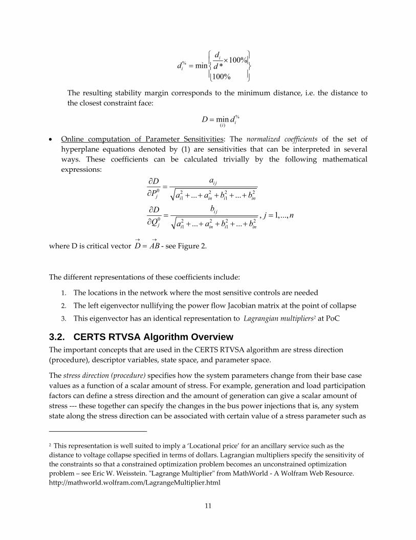
11
% 100%min *
100%
i
i
dd d
⎧ ⎫×⎪ ⎪= ⎨ ⎬⎪ ⎪⎩ ⎭
The resulting stability margin corresponds to the minimum distance, i.e. the distance to the closest constraint face:
%
( )min ii
D d=
• Online computation of Parameter Sensitivities: The normalized coefficients of the set of hyperplane equations denoted by (1) are sensitivities that can be interpreted in several ways. These coefficients can be calculated trivially by the following mathematical expressions:
0 2 2 2 21 1
0 2 2 2 21 1
... ...
, 1,...,... ...
i j
j i in i in
i j
j i in i in
aDP a a b b
bD j nQ a a b b
∂=
∂ + + + + +
∂= =
∂ + + + + +
where D is critical vector D AB→ →
= ‐ see Figure 2.
The different representations of these coefficients include:
1. The locations in the network where the most sensitive controls are needed
2. The left eigenvector nullifying the power flow Jacobian matrix at the point of collapse
3. This eigenvector has an identical representation to Lagrangian multipliers2 at PoC
3.2. CERTS RTVSA Algorithm Overview The important concepts that are used in the CERTS RTVSA algorithm are stress direction (procedure), descriptor variables, state space, and parameter space.
The stress direction (procedure) specifies how the system parameters change from their base case values as a function of a scalar amount of stress. For example, generation and load participation factors can define a stress direction and the amount of generation can give a scalar amount of stress ‐‐‐ these together can specify the changes in the bus power injections that is, any system state along the stress direction can be associated with certain value of a stress parameter such as
2 This representation is well suited to imply a ‘Locational price’ for an ancillary service such as the distance to voltage collapse specified in terms of dollars. Lagrangian multipliers specify the sensitivity of the constraints so that a constrained optimization problem becomes an unconstrained optimization problem – see Eric W. Weisstein. ʺLagrange Multiplierʺ from MathWorld ‐ A Wolfram Web Resource. http://mathworld.wolfram.com/LagrangeMultiplier.html

12
the percent of the total load increase in an area. Each specific direction and value of the stress parameter uniquely defines the system state. This implies certain fixed patterns for varying the system generation and loads (for example, load participation factors, sequence of generator dispatch, and others – detailed examples can be found in this report). Stress directions can include some local system stresses addressing a particular voltage stability problem area, and global stresses such as the total load growth and the corresponding generation redispatch in the system.
Descriptor variables reflect the most influential or understandable combinations of parameters (or derivative parameters) that influence the voltage stability margin. Examples are the total area load, power flows in certain system paths, total generation, and others (the system operating nomograms’ coordinates are good examples of descriptor parameters). In the simplest case, descriptor parameters can include some primary system parameters such as nodal voltages and nodal power injections. Descriptor variables help to adequately address global and local voltage stability margins without involving thousands of primary parameters. Certain subsets of descriptor variables can correspond to some local voltage stability problem areas.
The state space includes all system nodal voltage magnitudes and voltage phase angles.
The (independent) parameter space includes all nodal power injections (for P‐Q buses) and real power injections and voltage magnitudes (for P‐V buses).
The voltage stability boundary can be comprehensively (and uniquely) described in the parameter space (and the state space), but in this case the description would involve thousands of variables. Descriptor parameters help to reduce the dimensionality of the problem by considering the most influential combinations of parameters (or derivative parameters).
The descriptor parameter space includes all descriptor parameters. Since the points in the descriptor parameter space can be mapped into the points of the parameter and state spaces in many different ways (because of the limited number of descriptor parameters space dimensions), certain fixed system stress procedures should be introduced to make this mapping adequate and unique.
The developed RTVSA algorithms consist of the following steps (which has been illustrated in a flowchart under Figure 3):
1. Initial system stressing procedure for a given stress direction to reach a vicinity of the Point of Collapse (PoC) in this direction. This step is implemented using the Parameter Continuation Method. The Continuation Method is one of the most reliable power flow computation methods; it allows approaching the PoC and obtaining the initial estimates of system state variables needed for the subsequent steps. The selected form of the continuation methods includes predictor and corrector steps.
2. The direct method is used then to refine the PoC location along the initial stress direction (the continuation method would require multiple iterations to find the PoC with the required accuracy). At least one of the power flow Jacobian matrix eigenvalues must be very close to zero at the PoC.

13
3. The inverse iteration method or Arnoldi algorithm is applied to find the left eigenvector corresponding to the zero eigenvalue at PoC. The left eigenvectors are used to build the set of approximating hyperplanes.
4. The stability orbiting procedure is then applied to trace the voltage stability boundary along a selected slice. This procedure is a combination of a predictor‐corrector method and the transposed direct method.
5. In case of divergence, the algorithm is repeated starting from Step 1 for a new stress direction predicted at the last iteration of the orbiting procedure. Divergence may be caused, for example, by singularities of the stability boundary shape along the slice.
6. For a given voltage stability problem area and the corresponding descriptor parameters, the “sliced bread procedure” is applied to explore the voltage stability boundary and build the set of approximating hyperplanes.

14
Parameter Continuation Method (Predictor – Corrector)Including Voltage/Var
Limit Check
Direct Method
Boundary Orbiting Method
With Voltage/Var Limit Check
Convergence of Solution?
Tracing of Boundary
Complete?
Slice Bread Procedure
Output Data
- Converged Load Flow Solution - Single Stressing Direction and associated RASs- Descriptor Variables- Contingencies
Output Data
- Point of Collapse Solution- Left Eigenvector- Right Eigenvector- Load Margin- Weak Elements- Corrective Actions- Sensitivities
Input- Security Region Parameters (Ei & Ej)
NO
YES
YES
NO
2-D Security Region in Injection Space
Input
Input
di
dj
dk
PoC1
PoC2
PoC3
PoC4
PoC5
PoC6
PoC7
First “slice”,at dk = dk max
dk = dk min
A
B
C
D
Mapping of Nomogram (Injection � Descriptor
Space)
PV Curve Showing a Load Voltage (Indicates Point of Collapse Solution)
2-D Security Region for two Load Buses(Shown in Parameter Space)
3-D Security Region(Slice Bread Procedure)
- Descriptor Parameters
Reach Vicinity of Point of Collapse
- 2-D Nomogram
Note: The above procedure involves contingency analysis and screening and a security region is formed for the most binding contingency
Figure 3: RTVSA Algorithms Flowchart

15
The developed RTVSA algorithm performs voltage security assessment calculations under both offline and real‐time modes.
The offline calculations produce an approximated voltage stability region (a 2‐D, 3‐D, or a higher dimensional nomogram) bases on multi‐directional stressing situation presenting the interaction and tradeoffs between different stressing directions. The pre‐calculated voltage stability region is an inner intersection of stability regions for the set of user‐specified contingencies. The offline calculations should be conducted periodically (ideally, several times a day) to update the approximated voltage security region and to reflect the most recent changes in the system.
The real‐time calculations are conducted in real time (after each converged State Estimation cycle) to determine the current or future position of the system operating point against the walls of the approximated voltage stability region, and to calculate such essential security information as the available stability margin (distance to instability), the most limiting contingency, the most dangerous system stress directions, weak elements causing potential instability, and the recommended preventive and enhancement controls that help to increase the margin in an efficient way.
Note: The offline calculations can also be conducted in real time if a few stressing directions representative of the actual system loading, given by the real time dispatch schedule, planned outages, and load forecast, and/or predetermined stresses are to be considered separately. In such a scenario, the available security margins, distance to instability, the most limiting contingency, weak elements causing potential instability, and the recommended preventive and enhancement controls that help to increase the margin in an efficient way can be obtained in real‐time using the algorithms proposed in this document.
3.3. Some Special Features of the RTVSA Application The underlying concepts are applicable to the simple one‐dimensional approach or the more complex multi‐directional stressing to explore the entire voltage security region in the parameter space or in full P‐Q injection space.
The RTVSA tool has the ability of analyzing the effects of multiple transfers. There are no restrictions in distributing the source and sink over a large number of buses in geographically distant locations in the system. A non‐local treatment of congestion3 is crucial because conservatism causes costly curtailment of profitable power transfers and a suboptimal use of the transmission system.
The RTVSA algorithm4 in the initial stages uses the parameter continuation method, which is one of the most reliable power flow methods capable of reaching the point of collapse on the
3 Congestion can be quantified more precisely as the combined effect of multiple power transfers exceeding the transfer capability of the transmission system.
4 The RTVSA algorithm falls into the class of non‐divergent power flow methods that manipulate the step size of the Newton‐

16
power flow feasibility boundary. New variables called the continuation parameters are added and represents a position of a power flow operating point along some power system stress direction in the parameter space. The predictor step consists in an incremental moving of the power flow operating point along the state space trajectory, based on the linearization of the problem. The corrector step, that follows each predictor step, consists in elimination of the linearization error by balancing the power flow equations to some close point on the nonlinear trajectory.
The RTVSA algorithm also uses Direct methods for finding the PoC quickly and accurately, which combines the parametric description of the system stress and the power flow singularity condition expressed with the help of the Jacobian matrix multiplied by a nonzero right or the left eigenvector that nullifies the Jacobian matrix at the collapse point. In principle, the Direct Method avoids implementing a loading procedure. There may be problems of finding the initial guesses of the state variables and the eigenvector that may be resolved by initial loading the system along the stress direction. By doing so, the initial guess of variables can be obtained. Many inaccuracies of the step‐by‐step loading methods that do not exactly converge to the PoC will be avoided by implementing the Direct Method. There are savings in computational expenses because of the absence of iterations even though the Direct Method solves a problem almost double in dimension to the step‐by‐step loading methods.
The RTVSA algorithm determines the “right eigenvector” and the “left eigenvector” at the PoC. The weak elements are based on the right eigenvector and provide the extent to which variables participate in voltage collapse. This determines weak areas and also whether the collapse is an angle collapse. Large sensitivities of the margin to PoC indicate controllable parameters. These are represented by the left eigenvector and can be quantified for suitable corrective action by ranking the increase in margin with respect to a unit MW or MVAR in generator response.
Sensitivity computations relate changes in data to changes in transfer capability. The uncertainty in the transfer capability due to uncertainty in the data can be quantified to reveal which data is significant in the transfer calculations.
Raphson method. If the power flow mismatches indicate divergence, the step size is reduced until convergence occurs or the step becomes very small. A very small step size is considered to be an indicator of the point of collapse.

17
3.4. Algorithm Simulation and Validation Results The selection of the critical parameters influencing the voltage stability margin and stress directions was conducted based on engineering judgment. The stress directions were defined using the sink‐source and balanced loading principles. This means that the generators and the loads participating in each stress scenario are identified, as well as their individual participation factors; the participation factors are balanced so that the total of MW/MVAR increments and decrements is equal to zero. This allows avoiding re‐dispatching of the remaining generation. Based on the California ISO recommendation, two study areas were selected for verifying the prototype VSA algorithms: the Humboldt and San Diego problem areas.
The San Diego region within Southern California suffers from voltage stability issues, and hence, forms a good test case. California ISO provided the CERTS team with the 5940 bus (1188 generators) State Estimator generated load flow solution on October 23, 2006 that spans the entire Western Interconnection and includes all buses/lines at or above the 115 kV level. Only elements below the 115 kV level and external to the California ISO have been equivalenced. Within the California ISO jurisdiction, some of the lower voltage levels are also covered. Hence, this case precisely models the southern California region being studied.
The generation stressing process adopted by the VSA tool involves generators with the participation factors calculated based on their maximum generation capacity:
)()(
max
max
TotalPgenGenPgen
GenofFactorionParticipat kk =
This participation factor for generators are dynamic, as they change once a generator reaches its maximum generation limit and is left out of the equation. The participation factors for the loads are calculated using their base case Loadk (in MWs), whereas the load power factor is maintained constant:
VectorStresstheofLoadTotalLoadBase
LoadofFactorionParticipat kk =
The distributed slack bus model includes all buses in the system except the ones that participate in the stress vector. This model reacts to the active power mismatch that is caused by the stressing procedure and generation contingencies. The participation factors on the distributed slack buses are calculated proportionally to the Pgenmax of generators.
Parameter continuation predictor‐corrector method was chosen as the preferred method capable of reaching the vicinity of point of collapse on the power flow feasibility boundary. The addition of new variables called continuation parameters determines the position of an operating point along some power system stress direction in the parameter space. The predictor step consists of an incremental movement of the power flow point along the state space trajectory, based on the linearization of the model. The corrector step, which follows each predictor step, consists in the elimination of the linearization error by balancing the power flow equations to some close point on the nonlinear trajectory.

18
Figure 4 below shows the PV curve (real load vs. voltage magnitude plot) for a load bus that was part of the load stress vector in the RTVSA algorithm. The crosses are the predictor‐corrector solution points as the algorithm traces the curve to reach the vicinity of the voltage instability point denoted by a star.
Figure 4: PV Curve for a Load Bus Similarly, the parameter continuation method can also be illustrated for a 2D stressing scenario for two loads in the San Diego region as shown in Figure 5 below:
Inflection Point

19
Figure 5: Load at Mission vs. Load at Santiago In order to verify the results of the parameter continuation algorithm, the GE PSLF simulation engine was modified to incorporate the RTVSA stress vectors as well as the participation factor calculations, among other minor changes. The source and the sink vectors were stressed5 to reach the point of voltage instability. The result of this comparative study revealed that the Point of Collapse solutions obtained from GE PSLF were indeed very close to that of the RTVSA algorithm as shown in Figure 6, Figure 7 and the comparison chart in Table 3 below:
5 GE PSLF uses Brute‐Force method to determine the Point of Collapse solution

20
Figure 6: Comparison of Power Solutions (at PoC) between RTVSA & GE PSLF
Figure 7: Comparison of Voltage Solutions (at PoC) between RTVSA & GE PSLF
Loads % Difference in Power
% Difference in Voltage
Miraloma 0.04% 0.09%Vestal -2.19% 0.22%Mission 0.02% 0.19%Telegraph Canyon -0.01% 0.30%PRCTRVLY 0.02% 0.33%
Table 3: Percentage Difference between RTVSA and GE PSLF Calculations
3.5. Direct Method Direct methods for finding the Point of Collapse in a given direction combine a parametric description of the system stress, based on the specified loading vector in the parameter space and a scalar parameter describing a position of an operating point along the loading trajectory and the power flow singularity condition expressed with the help of the Jacobian matrix multiplied by a nonzero right or the left eigenvector that nullifies the Jacobian matrix at the collapse point. Unlike the power flow problem, this reformulated problem does not become singular at the point of collapse and can produce the bifurcation point very accurately.
In principle, the direct method allows finding the bifurcation points without implementing a loading procedure. There is, however, a problem of finding the initial guesses of the state variables and the eigenvector that may be resolved by initially loading the system along the stress direction. By doing so, the initial guess of state variables can be obtained. To evaluate the initial guess for the eigenvector, the inverse iteration method has been recommended to

21
calculate the eigenvector corresponding to the minimum real eigenvalue. The RTVSA code, however, utilizes Arnoldi’s algorithm in Matlab software, also known as ‘eigs’ function, for simulation purposes.
The accuracy and advantage of the Direct Method algorithm has be shown with the help of the two plots below, wherein the Direct Method algorithm (Figure 9) is capable of determining the solution point (Point of Collapse) in one step, compared to 18 iterations taken by the Predictor‐Corrector algorithm (Figure 8).
Figure 8: PoC Calculation by Predictor-Corrector Algorithm
Figure 9: Direct Method's Accelerated PoC Calculation
3.6. Boundary Orbiting Method After reaching the Point of Collapse (PoC) solution point using a combination of the Continuation Parameter and Direct Method for a specified stress direction, the challenge is to orbit a static voltage stability boundary without repeating the time‐consuming Continuation
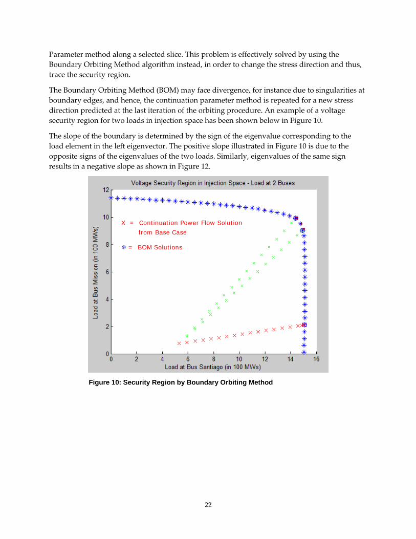
22
Parameter method along a selected slice. This problem is effectively solved by using the Boundary Orbiting Method algorithm instead, in order to change the stress direction and thus, trace the security region.
The Boundary Orbiting Method (BOM) may face divergence, for instance due to singularities at boundary edges, and hence, the continuation parameter method is repeated for a new stress direction predicted at the last iteration of the orbiting procedure. An example of a voltage security region for two loads in injection space has been shown below in Figure 10.
The slope of the boundary is determined by the sign of the eigenvalue corresponding to the load element in the left eigenvector. The positive slope illustrated in Figure 10 is due to the opposite signs of the eigenvalues of the two loads. Similarly, eigenvalues of the same sign results in a negative slope as shown in Figure 12.
Figure 10: Security Region by Boundary Orbiting Method
X = Continuation Power Flow Solution
from Base Case
= BOM Solutions

23
Figure 11: Security Region for Two Loads (For Eigenvalues with Same Signs)
To test the accuracy of the boundary points obtained by the orbiting procedure, the Continuation Parameter method, along with the Direct Method, was simulated for certain stress directions. A typical test result, as shown in Figure 13 below, reveals the precision of the Boundary Orbiting Method.

24
Figure 12: Testing the Precision of Boundary Orbiting Method
The original PSERC Predictor Corrector algorithm was designed to switch generator to load buses (i.e., PV to PQ buses) due to the nature of the one‐dimensional stressing process. However, the RTVSA proposed two‐dimensional security region calls for a more complex two way switching of the buses from type PV to PQ and back to a PV bus as and when required. Hence, the RTVSA tool was modified to accommodate the required algorithm for conveniently switching the buses, thus generating a precise and smooth security region as shown below:
Number of PV Buses
Figure 13: Switching of PV to PQ Buses and Vice-Versa
o = BOM Solutions
x = Continuation Power Flow Solutions

25
4.0 CERTS RTVSA Functional Specification A functional specification document was developed for the Real‐Time Voltage Security Assessment (RTVSA) tool that shall monitor voltage stability margin in real time, and will help the real time operators to manage this margin by controlling VAR resources, generation dispatch, and other resources on the transmission system. The application is expected to seamlessly integrate with the California ISO’s real‐time network analysis sequence (EMS) and run automatically after each successful state estimation process at every 5 minute intervals or on demand. The tool will help to identify the following:
1. Available voltage security margin
2. The most dangerous stresses in the system leading to voltage collapse
3. Worst‐case contingencies resulting in voltage collapse and/or contingencies with insufficient voltage stability margin
4. Contingency ranking according to a severity index for voltage stability related system problems
5. Weakest elements within the grid and the regions most affected by potential voltage problems
6. Controls to increase the available stability margin and avoid instability
7. Information about voltage problems at the look‐ahead operating conditions and for the worst‐case contingencies (contingencies with large severity ranks) that may appear in the future
8. A real‐time dispatcher’s situational awareness‐type wide area graphic and geographic displays.
This section summaries the key technical and functional requirements for the California ISO RTVSA tool.
4.1. On-Line RTVSA Functional Overview The RTVSA application will be integrated with California ISO’s real‐time network analysis sequence and run automatically after each successful state estimation process at every 5 minute intervals or on demand. The application will use data from the California ISO state estimation fed in every 5 minutes. The State Estimator (SE) solution, present in a Dynamic CIM/XML format, and the Detailed Network Model, present in a Static CIM/XML format, are outputs of California ISO’s ABB Ranger Energy Management System (EMS); whereas the RTVSA Supplementary Files are predefined set of flat files obtained from an external source. The above mentioned three files are required by the tool to perform a thorough voltage security assessment.

26
The RTVSA tool shall feature two dominant modes of operation:
1) Real‐Time Modes ‐ Real‐time operations mode
Real‐time look‐ahead mode
Under the ‘Real Time Operations Mode’, the RTVSA tool would perform a real time assessment utilizing the most current state estimator snapshot. On the other hand, the ‘Real Time Look‐Ahead Mode’ would be useful in performing a 2‐hour “look‐ahead” predictive assessment by applying planned outage information available within the EMS and load forecast over the next 2 hours to the current state estimator snapshot.
2) Study Mode ‐ Study mode offers off‐line analysis capabilities on either the real‐time data or on modified version of real‐time solved cases.
The two available modes described above serve different purposes for two separate user environments:
Real‐time modes for Operator Display Console users Study modes for Stand‐Alone Console users The associated functionality offered within these two modes of operation is summarized in Table 4.

27
Real Time Modes Study
Modes Real Time Look‐Ahead
Unidirectional Stressing
− contingency screening & ranking × × ×
− real time alarming ×
− voltage profiles × × ×
− MW/MVAR reserves × × ×
− single line diagrams × × ×
− Loading margins × × ×
− margin sensitivities to reactive support × × ×
− ranking of corrective controls × × ×
− identification of weak elements × × ×
Multidirectional Stressing
− 2‐D, 3‐D or N‐D Security Regions (Nomograms) developed Offline
×
− real time assessment of operating point including contingency ranking, margins
× × ×
− real time ranking of controls to steer away from the boundary
× × ×
Table 4: Summary of RTVSA Capabilities
The RTVSA processor will simultaneously operate between the two given modes, i.e. the real‐time performance of the RTVSA tool will not be compromised upon simulation of one or many study cases at any given instance. To meet the computing needs of RTVSA, this tool shall be deployed across a cluster of high performance distributed computing, supporting a scalable Server‐Client architecture. The RTVSA Central Server will be responsible for the data management, algorithmic computation, automation, and handling of remote client requests.

28
4.2. System Architecture The overall functionality of the RTVSA application can be subdivided into three interdependent modules, which are:
1. 1) Input Subsystems:
2. 2) Central Server:
3. 3) User Interfaces:
Figure 14 of the proposed system architecture illustrates the affiliations among the various modules, as well as the constitutive functionalities of each of the consoles.
There are three sources of data input subsystems (California ISO EMS, Data Input Module, and Flat Files Storage) to the Central Server vis‐à‐vis the RTVSA tool. Depending on the tool’s mode of operation, data can be acquired from any of the sources.

29
Figure 14: RTVSA System Architecture

30
As is shown in Figure 14, the California ISO’s ABB‐Ranger EMS generates Dynamic CIM/XML files at 5‐minute intervals. This file in combination with the Static CIM (which contains network topology information) provides all the necessary data required to run a power flow. The Data Input Module primarily accounts for combining and managing the various files required by the RTVSA tool to perform power flow calculations and voltage security analysis during a real‐time sequence. The RTVSA Supplementary Files are user predefined set of data that are essential while performing a complete voltage security assessment with the previously mentioned functionalities. These include Contingency List, Stressing Directions & Descriptor Variables, and Special Protection Schemes/Remedial Action Schemes.
The following are the data requirements for the RTVSA tool based on the operating modes:
Real‐Time Modes:
Data Source: California ISO EMS 1. Valid State Estimator Solution
2. Detailed Network Model
3. System Component Status Information
4. Available Power System Controls and their Priorities
5. Limits (Voltage, Thermal, MVAR)
6. Generator Model
7. Distributed Slack Bus Information
8. Low Voltage Load Models
9. HVDC Models & Control Schemes
Data Source: Data Input Module 10. Contingency List
11. Stressing Directions & Descriptor Variables
12. Special Protection Schemes/Remedial Action Schemes
Study Modes:
Data Source: Flat Files Storage 1. Real‐time solved case
2. Modified real‐time solved case
3. RTVSA Supplementary Files
The minimum requirement for the data that is required to correctly describe the system equipments are Bus data with breaker information and status, transmission line data, transformers and tap control data, Generator data, Load data, Fixed Shunt data, Controllable shunt and static VAR devices (SVD) data, and HVDC controls data.
The Central Server houses the RTVSA application that performs simulations pertaining to voltage security assessment, processes network topology models as required by the system, a

31
Central Manager that streamlines the various processes, and a storage system for RTVSA application’s study cases. The sub‐modules that collectively define the functionality of the Central Server include Server Manager, Topology Processor, Flat Files Storage, and Simulation Engine
The Simulation Engine sub‐module is the backbone of the system architecture. This unit is responsible for receiving data from the Server Manager, performing the various simulations, and sending the solution sets to the relevant users. It may run both in the real‐time and study modes, simultaneously, while operating on a distributed computing platform.
The User Interface of the RTVSA application can be categorized under two domains of operation: 1) Operator Display Console for Real‐time mode, which receives solution snapshots from the Central Server every time the RTVSA application runs on a set of real‐time data. 2) The Stand‐Alone Console caters to users of the RTVSA application under the study mode described earlier.
4.3. Visualization and User Interaction The goal of the RTVSA application is to provide the real‐time and study mode users with visualization capabilities that will assist them in making decisions. These capabilities can be classified under two broad domains: (1) Situational Awareness, and (2) Voltage Security Assessment.
Situational awareness type of displays present to the viewers simplified wide‐area real time metrics, detection, alarming, trace, and trend visualization solutions. Accompanying the real‐time displays would be scenarios under the worst case contingency. These include Voltage profiles at various buses, real and reactive power reserves across the system, Interface/line flows across key transmission corridors/voltage levels, and one‐line diagrams.
Voltage Security Assessment displays demonstrate results of the Voltage Security Assessment tool under the look‐ahead scenario with respect to key stressing direction(s). Such scenarios may be based on current operating conditions or under the worst case contingency. These illustrate voltage security conditions and metrics that help users study voltage stability and take decisions to prevent adverse situations. These capabilities include Real and reactive loading margins, Contingency ranking based on severity index (voltage margin, loading margin, etc.), Operating nomograms, Distance to instability, Weak elements information, and Corrective actions (preventive control, enhancement control)
The RTVSA visuals are displayed to both user interfaces: real‐time user interface located in California ISO’s Operator Consoles, and study‐mode interface located in Stand‐Alone Consoles. Since the simulation results obtained under each of the modes are case dependant (study or real‐time case), the visual displays and techniques are different for the two users.
The Operator Console users view real‐time results of RTVSA simulations under Current system scenario (base case) and System conditions under the worst case contingency. Display capabilities and features required for the Operator Console users to include Wide area geographic view of the current system conditions with the capability to zoom‐in on a desired

32
local area, effective displays of priority based corrective controls information with rankings based on their effectiveness for each simulated stressing direction(s), and the capability to modify and customize display settings.
Study mode users shall interact with the system through a GUI in order to select the desired study case, make necessary modification to the same, and run simulations with preferred execution parameters (Supplementary Files) and controls. They would be able to study the reliability of the system with the help of various displays as well as by comparing multiple study cases. Display capabilities required for the stand‐alone console users to include the ability to conveniently modify network topology, displays that indicate the available RTVSA execution control parameters and their current values, Emphasis on ‘Voltage Security Assessment’ type of displays, Capability to compare cases against each other, and Capability to plot simulation parameters and variables as a function of time.

33
5.0 Conclusion The Real Time Voltage Security Assessment project was designed to be part of the suite of advanced computational tools for congestion management that is slated for practical applications in California in the next few years. The prototype application that was developed under this project is based on an extensive analysis of the existing VSA approaches, by surveying the leading power system experts’ opinion worldwide, and also with feedback from industrial advisors. The mismatch between the core power system reliability needs and the availability of the VSA tools was a motivation to design the RTVSA prototype.
The robustness of the Parameter Continuation technique combines with the accuracy of the Direct Method and Boundary Orbiting Method makes the RTVSA prototype a preferred choice for an advanced VSA application.
The underlying concepts are applicable to the simple one‐dimensional approach or the more complex multi‐directional stressing to explore the entire voltage security region in the parameter space or in full P‐Q injection space. The RTVSA algorithms are complex enough to handle system stress/relief by allowing the generator buses to switch to load buses and vice‐versa.
The functional specification document prepared for the California ISO lays out the technical and functional requirements for a state‐of‐art Voltage Security Assessment tool that is designed to run in real time and is targeted towards real time operators to help them manage their reactive margin by controlling VAR resources, generation dispatch, and other resources on the transmission system. In particular, it allows operators to monitor system voltage conditions and provides real time reliability information related to reactive margin, abnormal nodal voltages, weak elements, contingency rankings, and recommended corrective actions. These functional specifications were used by the California ISO to select a vendor and to implement a commercial grade application to be in fully operation at the California ISO by summer 2008.

34
APPENDIX A – SURVEY 1 RESULTS TABLE
Reviewer VSA using Hyperplane Methods
[1] Recommends hyperplane approach for VSA. Furthermore suggests online hyperplane computation if loading directions and generating unit dispatch vectors are known a priori. Needs only up to 10 load flow runs with to compute “weak” elements.
[2] Adopted similar direct methods for contingency ranking and also in hybrid system aimed to give a measure of angle as well as voltage stability. These experiences demonstrate the applicability of the proposed methodologies.
Practical security boundary must account for grid topology changes (implying online security assessment).
[3] More information needed about the hyperplane approach to VSA.
[4] Has real potential – and it is not as unproven as some other concepts like interior point optimization.
[5] Seems to be ideally suited for voltage instability where the phenomena is more localized and ideally suited for decision based on measurements
Not convinced that Practical Dynamic Security Region direct method has any particular computational advantage over other methods
[6] Experience has shown that secure operating space calculations done off line rarely match exact real time conditions, which may well be away from design conditions, implying online security assessment or adequate safety margins.
[7] Least squares approximation of hyper planes with load flow simulations is prone to error enhancement for bad state estimator measurements.
[8] Proposes New Electricity Transmission Software Solutions (NETSS) for voltage optimization, and the economic assessment of voltage support measurements (known as pilot points).
It is important to determine the right locations to measure. Results depend on voltage dispatch strategies, loading conditions and system‐specific equipment status.
Reviewer General comments on Tools and Methodologies Discussed in the Survey
[9] Advises to use equations like J’(X) F(X) =0 to search for the closest points of the steady‐state stability boundary. He also warns that the thermal constraints are often more limiting than stability constraints.
[10] Methods not yet been utilized by grid operators. Emphasizes mode meter and system stiffness. Refers to WACS paper by Carson Taylor.

35
[11] Suggested the advantages of the following V&R products:
For off‐line computations the exact boundary of dynamic security region (security nomogram) is automatically constructed using V&R’s Boundary of Operating Region (BOR) software.
For on‐line computations, sensitivity‐based n‐dimensional boundary of operating region can be computed using BOR. The approximated boundary may be computed using Direct methods.
[12] Visualization of voltage stability region in cut‐set space has been implemented and a visualization system of dynamic security region in injection space to guarantee transient stability is in development for Henan Power System of CHINA
It might be used in monitoring, assessment and optimization of security. “Up to now almost all research results of mine are about the dynamic security region in power injection space and the voltage stability region in cut‐set power space. I think it might be used not only in security monitoring and control, but also in probabilistic security assessment.”
[13] Submitted a Proceeding of IEEE paper on WACS accepted for publication in May 2005. This paper co‐authored by Taylor describes an online demonstration of a new response based wide area control system with discontinuous actions for power system stabilization.
[14] Submitted a product overview of Energy Concepts International software “QuickStab”.
[15] Submitted a company overview and product list of Bigwood systems. This included information that showed partnerships with ABB to install BCU‐DSA at the EMS of three power companies. BCU method is the only method used in EPRI Direct 4.0 and BCU method has been implemented by Siemens, at the Northern Power Company.
[16] Provided areas of concern in the implementation of wide area monitoring such as: Validity of the system model to capture the phenomena of interest. Accuracy of angle measurements by PMUs. Accuracy of angle differences from PMUs of different vendors. Determining acceptable vs. unacceptable levels of angular separations among various pairs of PMU

36
APPENDIX B – SURVEY 2 RESULTS TABLE

37

38

39

40
APPENDIX C – RTVSA FUNCTIONAL SPECIFICATION SUMMARY TABLE
I Input Data Specifications
A Valid state estimation solution snapshots available every 5 minutes in dynamic CIM format.
B Detailed network model with node‐breaker details in the static CIM format.
C Contingency list containing all N‐1 and some user‐specified N‐2 contingencies with the associated RASs
D Stressing directions including generator dispatch sequence and load patterns, and associated RASs.
II Modes of Operation
A ‘Real time operations mode’ presenting real time voltage stability analysis using the current state estimator snapshot.
B ‘Real time look‐ahead mode’ providing predictive voltage stability analysis using a priori knowledge of planned outages and load forecast.
C ‘Study mode’ offering offline ‘what‐if’ capabilities on the real time study cases.
III Functional Capabilities
A Contingency analysis and ranking based on voltage violations or loading margins for each stressing directions.
B Voltage profiles, powerflow patterns, real/reactive reserves and loading margins to PoC under base case and most binding contingency.
C Margin sensitivities to reactive support for each stressing direction.
D Suggest and rank Enhancement Controls to increase reactive load margins and Preventive Remedial Controls to retract to a secure region.
E Identify weak elements and their voltage sensitivities to reactive load margins.
F Construct 2‐D, 3‐D or N‐D security regions (nomograms) offline for a set of pre‐defined stressing directions and descriptor variables.
G Evaluate current state estimator snapshot within N‐dimensional security regions.

41
H Real‐time alarming on voltage violations and low real/reactive load margins.
IV System Architecture & User Environments
A Central‐server/multi‐client architecture
B Simulation engine performing the various simulations and analysis.
C Topology processor to convert the node/breaker to bus/branch for analysis and vise‐versa for presenting simulation results.
D Flat file storage housing the most current real time solved cases and modified study cases.
E Real time information presented within Operator Display consoles.
F Study mode capabilities within stand‐alone user consoles.
G User interface to enable/disable automated controls, and modify simulation parameters, supplementary files (e.g. Stressing directions, contingency list, RASs).
V Visualization Capabilities
A Voltage profiles, real & reactive reserves at key stations, and power flows at the higher voltage levels within wide within wide area geographic displays.
B Real and reactive loading margins as bar graphs.
C One‐line diagrams within Operator Displays.

E‐1
APPENDIX E: Real-Time Voltage Security Assessment Functional Specifications for Commercial Grade Application

Arnold Schwarzenegger
Governor
REAL TIME SYSTEM OPERATION2006 – 2007
APPE
NDIX
E
Real-Time Voltage Security Assessment Functional Specifications for
Commercial Grade Application
Prepared For: California Energy Commission Public Interest Energy Research Program
Prepared By: Lawrence Berkeley National Laboratory
Month Year CEC-500-2008-XXX-APE


Prepared By: Lawrence Berkeley National Laboratory Joseph H. Eto, Principal Investigator Berkeley, CA 94720 Manu Parashar and Abhijeet Agarwal, Electric Power Group Yuri Makarov, Pacific Northwest National Laboratory Ian Dobson, University of Wisconsin, Madison Commission Contract No. 500-02-004 Commission Work Authorization No: MR-041
Prepared For:Public Interest Energy Research (PIER) California Energy Commission
Jamie Patterson Contract Manager Mike Gravely Program Area Lead ENERGY SYSTEMS INTEGRATION Mike Gravely Office Manager ENERGY SYSTEMS RESEARCH
Martha Krebs, Ph.D. PIER Director
Thom Kelly, Ph.D. Deputy Director ENERGY RESEARCH & DEVELOPMENT DIVISION
Melissa Jones Executive Director
DISCLAIMER
This report was prepared as the result of work sponsored by the California Energy Commission. It does not necessarily represent the views of the Energy Commission, its employees or the State of California. The Energy Commission, the State of California, its employees, contractors and subcontractors make no warrant, express or implied, and assume no legal liability for the information in this report; nor does any party represent that the uses of this information will not infringe upon privately owned rights. This report has not been approved or disapproved by the California Energy Commission nor has the California Energy Commission passed upon the accuracy or adequacy of the information in this report.


FUNCTIONAL SPECIFICATIONS For Commercial Grade Application
Prepared For: California Independent System Operator (CA ISO)
Prepared by: Consortium for Electric Reliability Technology Solutions (CERTS)
Funded By: California Public Interest Energy Research
Transmission Research Program
Date: April 09, 2007
Consortium for Electric Reliability Technology Solutions

The work described in this report was coordinated by the Consortium for Electric Reliability Technology Solutions with funding provided by the California Energy Commission, Public Interest Energy Research Program, through the University of California/California Institute of Energy Efficiency under Work for Others Contract No. 500-02-004, MR-041. PREPARED FOR: California Independent System Operator PREPARED BY: Electric Power Group Manu Parashar, Ph.D. - Principal Investigator Abhijeet Agarwal - Investigator Pacific Northwest National Laboratory Yuri Makarov, Ph.D. - Principal Consultant University of Wisconsin, Madison Ian Dobson, Ph.D. - Consultant DATE: April 2007

EXECUTIVE SUMMARY
Voltage stability is the ability of a power system to maintain acceptable voltages at all
buses in the system under normal operating conditions and after being subjected to a disturbance. A system enters a state of voltage instability when a disturbance, increase in load demand, or change in system condition cause a progressive and uncontrollable decline in voltage. The main factor causing voltage instability is the inability of the power system to meet the demand for reactive power. Voltage collapse is the process or sequence of events accompanying voltage instability which leads to a low unacceptable voltage profile in a significant part of the system. Objectives
Develop functional specifications for a Real-Time Voltage Security Assessment (RTVSA) tool that monitors voltage stability margin in real time, and help the real time dispatchers to manage this margin by controlling VAR resources, generation dispatch, and other resources on the transmission system. This application is expected to seamlessly integrate with the CA ISO’s real-time network analysis sequence (EMS) and run automatically after each successful state estimation process at every 5 minute intervals or on demand. The tool will help to identify the following:
1. Available voltage security margin 2. The most dangerous stresses in the system leading to voltage collapse 3. Worst-case contingencies resulting in voltage collapse and/or contingencies with
insufficient voltage stability margin 4. Contingency ranking according to a severity index for voltage stability related system
problems 5. Weakest elements within the grid and the regions most affected by potential voltage
problems 6. Controls to increase the available stability margin and avoid instability 7. Information about voltage problems at the look-ahead operating conditions and for
the worst-case contingencies (contingencies with large severity ranks) that may appear in the future
8. A real-time dispatcher’s situational awareness-type wide area graphic and geographic displays.
Approach
An extensive analysis of existing VSA approaches was conducted. This included research by Consortium for Electric Reliability Technology Solutions (CERTS), surveys from the leading experts’ opinion worldwide, feedback from industrial advisors and brainstorm meetings with the projects’ industry and academia consultants. A state-of-the-art combination of approaches and computational engines was identified and selected for implementation in this project. Subsequently, a multi-year project roadmap was developed which has guided the CERTS research on evaluating and demonstrating the recommended approaches on the CA ISO test cases.
This document describes the design, functional and visualization requirements for a Real-Time Voltage Security Assessment (RTVSA) tool, as well as CA ISO’s preferences on certain implementation and visualization techniques.

CONTENTS
1. INTRODUCTION .................................................................................................. 1
1.1 BACKGROUND .................................................................................................... 1
2. ON-LINE RTVSA FUNCTIONAL OVERVIEW .......................................................... 3
2.1 MODES OF OPERATION .......................................................................................... 3 2.2 RTVSA CAPABILITIES ........................................................................................... 4 2.3 SYSTEM HARDWARE PERFORMANCE REQUIREMENTS ......................................................... 6
3. SYSTEM ARCHITECTURE ..................................................................................... 7
3.1 INPUT SUBSYSTEMS ............................................................................................. 9 3.1.1 CA ISO EMS .............................................................................................. 9 3.1.2 Data Input Module ..................................................................................... 9 3.1.3 Flat Files Storage ....................................................................................... 9
3.2 DATA REQUIREMENTS ......................................................................................... 10 3.2.1 Data Description ...................................................................................... 10 3.2.2 Modeling Details ...................................................................................... 12
3.3 INPUT SUBSYSTEMS INTERFACE REQUIREMENTS ........................................................... 13 3.4 CENTRAL SERVER .............................................................................................. 14
3.4.1 Server Manager ....................................................................................... 14 3.4.2 Topology Processor .................................................................................. 15 3.4.3 Flat Files Storage ..................................................................................... 15 3.4.4 Simulation Engine .................................................................................... 15
3.5 USER INTERFACES ............................................................................................. 17 3.5.1 Operator Display Console .......................................................................... 17 3.5.2 Stand-Alone Console ................................................................................ 18
4. VISUALIZATION & USER INTERACTION ........................................................... 19
4.1 RECOMMENDED VISUALIZATION TECHNIQUES .............................................................. 19 4.2 USER INTERACTION ............................................................................................ 20
5. SUMMARY TABLE .............................................................................................. 22

LIST OF FIGURES
Figure 1 - RTVSA System Architecture ........................................................................ 8 Figure 2 - Input Subsystems Interface ...................................................................... 13

LIST OF TABLES
Table 1 - Summary of RTVSA capabilities .................................................................... 6 Table 2 - RTVSA Summary Table .............................................................................. 22

ACKNOWLEDGEMENTS
Special thanks to California ISO staff Dr. Soumen Ghosh, Dr. Matthew Varghese, Mr. Dinesh Salem Natarajan, Mr. Patrick Truong, Mr. Steve Gillespie, Mr. Bill Ellard, Mr. Catalin Micsa, and Mr. David Le for their consultations to the project. The project team also appreciates contributions from Mr. Paul Bleuss, Mr. Robert Sparks, Mr. Ruhua You, Mr. Ray Camacho, Mr. J Sprouse, Mr. Y Zhang, Mr. Sirajul Chowdhury, Mr. Eric Whitley, and Dr. Enamul Haq. Mr. Dave Hawkins (California ISO) for his expertise, comprehensive support, and advice.
Dr. Yuri V. Makarov and Dr. Ning Zhou (PNNL), for their role in suggesting the framework of the project, developing and selecting the methodology, participation in the brainstorm meetings, organizing face-to-face interviews and other contacts with the leading experts, advice, troubleshooting, literature review, and report writing.
Prof. Ian Dobson, (University of Wisconsin-Madison), for his role in suggesting and developing the methodology, participation in the brainstorm meetings and interviews, expertise and essential advice. Dr. S. L. Greene (Price Waterhouse Coopers) for his help with the PSERC software.
Mr. Jim Cole (California Institute for Energy Efficiency) for sponsorship and support of this project, and participants of the TAC meeting for their thoughtful suggestions. Mr. Joseph Eto (Lawrence Berkeley National Lab) for his support. Participants of the CERTS surveys for their expertise and advice:
Prof. M. Anantha Pai (University of California – Berkeley) Mr. Raymond L. Vice (Southern Company Services, Inc.) Dr. Savu Savulescu (Energy Concepts International Corp.) Dr. Michael Y. Vaiman and Mrs. Marianna Vaiman (V&R Energy Systems Research) Dr. Alex M. Kontorovich (Israel) Dr. Anatoliy Meklin (Pacific Gas and Electric) Prof. Marija D. Ilic (Carnegie Mellon University) Prof. Enrico De Tuglie (Politecnico di Bari, Italy) Prof. Gerald T. Heydt (Arizona State University) Mr. William Mittelstadt (Bonneville Power Administration) Prof. Yixin Yu (Tianjin University, China) Mr. Carson W. Taylor (Bonneville Power Administration) Prof. H.-D. Chiang (Cornell University) Dr. Navin Bhatt (American Electric Power) Kalle Chan (American Electric Power) Mani Subramanian (ABB) Vidya Vankayala (British Columbia Transmission Company) Xiaochuan Luo (New England ISO) Dede Subakti (Midwest ISO) Jianzhong Tong (PJM) Hamid Hamadani (Powertech Labs Inc.) Marianna Vaiman (V&R Energy)

Participants of the face-to-face interviews for their evaluation of the project and advice: Prof. Ian Dobson (University of Wisconsin – Madison) Prof. Vijay Vittal (Arizona State University) Prof. Venkataramana Ajjarapu (Iowa State University) Dr. Zhao Yang Dong (University of Queensland, Australia) Dr. Anatoliy Meklin (Pacific Gas and Electric) Dr. Vitaliy Faybisovich (South California Edison) Dr. Michael Vaiman and Dr. Marianna Vaiman (V&R Energy Systems Research)
1
1. INTRODUCTION
California Independent System Operator’s (CA ISO) intends to implement a Real-Time
Voltage Security Assessment (RTVSA) tool as a part of the suite of advanced computational tools for monitoring and preventing system problems and congestion management in the California ISO Control Area. Modern voltage assessment methods include such advanced functions as identification of real/reactive loading margins under different stressing conditions and associated weak elements, advice on selection of remedial actions and automatic development of operating nomograms and security regions. Real-time production-grade Voltage Security Assessment tools are becoming increasingly available nowadays. These tools are integrated with EMS/SCADA systems and use results from the state estimator.
1.1 Background A system enters a state of voltage instability when a disturbance, increase in load
demand, or change in system condition causes a progressive and uncontrollable decline in voltage. The main factor causing voltage instability is the inability of the power system to meet the demand for reactive power. Voltage stability is the ability of a power system to maintain acceptable voltages at all buses in the system under normal operating conditions and after being subjected to a disturbance. Voltage stability margin is the distance to instability determined for a selected loading or stress direction in parameter space.
It is known that voltage magnitudes alone are poor indicators of voltage stability or
security. Voltages can be near normal with generators, synchronous condensers, and Static VAR compensators (SVCs) near current limiting levels, thus resulting in a possible voltage collapse. However, as a security problem distinct from voltage collapse, it is also desirable that the system voltage magnitudes remain within limits, and some of the control actions to maintain voltage magnitudes may also be of benefit in avoiding voltage instability. Sufficient reactive power reserves at generators and SVCs contribute strongly to maintaining voltage stability, but do not measure the ability of the transmission system to transmit reactive power. Both voltage magnitudes and reactive load margins are useful indicators; however, the voltage stability margin is the more accurate and complete metric for the proximity to voltage collapse.
CA ISO system operators need to know how to more effectively manage the grid and its reactive resources, including coordination with other organizations (interconnected system operators, load-serving entities, and generators), within today’s changed operational environment, particularly during periods of system stress. Today, generation operated by independent power producers as well as generation operated by utilities are not responding to system-operator-directed voltage-VAR requirements as reliably as they did prior to restructuring. This condition, which is compounded by the continued, large volumes of long distance energy transactions in the Western Electricity Coordination Council (WECC), is creating very unusual and dangerous voltage patterns that could jeopardize the reliability of both the CA ISO’s grid and the Western Interconnection. Inadequate, region-wide coordination of VAR reserves was a contributor the 1996 west coast blackouts, leading WECC to adopt stricter voltage-VAR requirements.
The California Energy Commission has been sponsoring the ongoing research to review, and assess the state-of-art in voltage security assessment that is geared towards a real time environment. This work has been conducted by the Electric Power Group and Pacific Northwest National Laboratory (CERTS members) with an active participation of the leading

2
University professors (through PSERC). At the onset of the project, a questionnaire had been distributed among 60 leading specialists worldwide in order to collect a collective and incorporate their feedback and ideas on the state-of-the art approaches and technologies in the area. Based on the responses and feedback from this expert community, a multi-year project roadmap was developed which has guided the CERTS research on evaluating and demonstrating the recommended approaches on the CA ISO test cases. Leading utilities have also been interviewed in parallel on their implementation of a similar voltage security assessment tool within their operations or planning environment.

3
2. ON-LINE RTVSA FUNCTIONAL OVERVIEW
The RTVSA application will be integrated with CA ISO’s real-time network analysis sequence and run automatically after each successful state estimation process at every 5 minute intervals or on demand. The application will use data from the CA ISO state estimation fed in every 5 minutes. The State Estimator (SE) solution, present in a Dynamic CIM/XML format, and the Detailed Network Model, present in a Static CIM/XML format, are outputs of California ISO’s ABB Ranger Energy Management System (EMS); whereas the RTVSA Supplementary Files are predefined set of flat files obtained from an external source. The above mentioned three files are required by the tool to perform a thorough voltage security assessment.
2.1 Modes of Operation The RTVSA tool shall feature two dominant modes of operation: 1) Real-Time Modes - Real-time operations mode - Real-time look-ahead mode
Under the ‘Real Time Operations Mode’, the RTVSA tool would perform a real time
assessment utilizing the most current state estimator snapshot. On the other hand, the ‘Real Time Look-Ahead Mode’ would be useful in performing a 2-hour “look-ahead” predictive assessment by applying planned outage information available within the EMS and load forecast over the next 2 hours to the current state estimator snapshot.
In general context, the real-time mode will provide the system operators up-to-date
information on the security status of the system with respect to voltage stability, including real time contingency analysis to ensure security of the system in the event of occurrence of any of critical contingencies, and compute key indices such as real or reactive loading margins under different stressing scenarios that quantify the degree of stability or instability for each case. The application will also suggest appropriate controls to the operator for increasing these margins.
The real-time case results are automatically stored into a centrally located rolling Flat File archive for future retrieval. The size of this rolling buffer of RTVSA solved cases must be configurable and shall be determined by CA ISO depending on the storage space requirements. 2) Study Mode - Study mode offers off-line analysis capabilities on either the real-time data or on modified version of real-time solved cases.
Under the study mode, the users of the stand-alone console would have the option and convenience to run the RTVSA simulation engine on a “study case”. Such study cases are: (1) real time RTVSA solved cases archived overtime within the Flat Files Storage (under Central Server), (2) modified versions of the above mentioned real-time solved cases to study hypothetical scenarios. For instance, a study mode user may extract a previously archived RTVSA solved case from the Flat Files Storage, remove one or more transmission lines, manually specify stressing directions, resolve using the RTVSA simulation capabilities and perform a complete voltage security assessment, and export this as a new “study case” to the central server if so desired.
The RTVSA tool should restrict users from overwriting a real-time solved case. Any
modifications made to these cases must be stored as a new study case. Although multiple

4
users would be allowed to simultaneously access the same file, the RTVSA tool should prevent everyone, except the first user of the case, from imposing changes to the same. This ‘locking’ feature of the tool would help in preventing certain possibly conflicts. However, all the users should have the option to perform simulations as well as to save the case (under a different name) in order to make the desired changes.
The two available modes described above serve different purposes for two separate user environments:
Real-time modes for Operator Display Console users Study modes for Stand-Alone Console users
The associated functionality offered within these two modes of operation are described in details in the next section and summarized in Table 1.
2.2 RTVSA Capabilities
The RTVSA application shall offer the following categories of functional capabilities: Real Time Voltage Stability Analysis under Unidirectional Stressing 1) Contingency screening and ranking with respect to voltage limit violations or loading
margins associated with known stressing direction – The application should perform such contingency analysis under all N-1 conditions and some user defined N-2 conditions within each 5 minute real time cycle. A directional stressing, representative of the actual system loading conditions based on the real time dispatch schedule and load forecast, will be used for this analysis and the most binding contingency shall be identified.
2) Wide area monitoring capabilities offering real time situational awareness to the
operators on key indicators that are closely associated with voltage security – These include voltage profiles at select buses, real or reactive reserves at key generators both under base case and the most binding contingency within geographic visualization. It also includes animated power flow visuals at the higher voltage levels (e.g. 500 kV, 230 kV, and 138 kV). The application will also have the capability of sending real time alarms to the end-users on voltage violations and insufficient real or reactive loading margins.
3) Real time voltage stability analysis with known stressing direction – The application shall
present the loading margins (real or reactive) to the point of collapse under the base case and the most binding contingency, allowing for an additional 2.5% and 5% (user configurable) safety margins for N-1 and N-2 contingencies, respectively. (Note to CA ISO: Voltage margins between base case and Point of Collapse (POC) solution may be an optional voltage stability metric).
4) Quantify the efficacy of reactive power support at the most effective buses in terms of
their sensitivities (Note to CA ISO: These sensitivities translate to a linear constraint and is representative of the voltage stability limit associated with the unidirectional stressing which can be incorporated into Security Constrained Unit Commitment (SCUC) and Security Constrained Economic Dispatch (SCED) applications in the future).
5) Rank available corrective controls based on their effectiveness – These actions may
include enhancement controls that optimally increase the loading margin with respect to

5
the stressing direction, or remedial controls in the situation that a contingency may lead the system state into an insecure region.
6) Identify the weak elements within the system associated with the one-dimensional
stressing – These are buses/regions with the grid that experience severe degradation in their voltage profile at the voltage collapse caused by the additional stressing. The proportions by which the voltage magnitudes will fall at these buses shall be presented.
Comprehensive Voltage Security Assessment under Multi-Directional Stressing
This is generalization of the above mentioned capabilities to a multi-directional stressing situation presenting the interaction and tradeoffs between different stressing directions, and the associated interpretation of the safe-operating region as a 2-D or 3-D (or higher dimensional) nomogram. The application shall: 1) Develop and update voltage security regions offline on demand based on a set of pre-
defined stressing directions – The boundaries of these regions shall be expressed as piece-wise linear approximations (i.e., hyperplanes) in coordinates of key descriptive parameters (such as MW transfers, total MW generation, total MW loading, etc) associated with the stressing directions. As with the unidirectional stressing case, these security region boundaries too shall be representative of the most binding contingency in the various stressing directions (Note to CA ISO: These hyperplanes are representative of the voltage stability limits associated with various stressing scenarios which can ultimately be embedded into SCUC and SCED applications).
2) Real time voltage security assessment with respect to the multidirectional stressing –
The voltage stability margins between the most current base case operating condition and the security region boundaries shall be evaluated within each 5 minute real time cycle.
3) Suggest appropriate controls to enhance margin to the boundary – While the current
operating point is within the security region, the application should also suggest appropriate control actions to optimally steer away from the closest boundary.

6
Real Time Modes Study
Modes Real Time Look-Ahead Unidirectional Stressing
− contingency screening & ranking × × × − real time alarming × − voltage profiles × × × − MW/MVAR reserves × × × − single line diagrams × × × − Loading margins × × × − margin sensitivities to reactive support × × × − ranking of corrective controls × × × − identification of weak elements × × ×
Multidirectional Stressing − 2-D, 3-D or N-D Security Regions (Nomograms) developed Offline
×
− real time assessment of operating point including contingency ranking, margins
× × ×
− real time ranking of controls to steer away from the boundary
× × ×
Table 1 - Summary of RTVSA capabilities (Note to CA ISO: The above mentioned unidirectional and multidirectional stressing analysis could be implemented through a ‘staged approach’ whereby the more straightforward unidirectional capabilities could be requested from the vendor over the short-term and successfully demonstrated at the CA ISO, and this capability could by enhanced at a follow-on stage and transformed to handle the broader multidirectional stressing for a more comprehensive security assessment.
2.3 System Hardware Performance Requirements The RTVSA processor will simultaneously operate between the two given modes, i.e. the
real-time performance of the RTVSA tool will not be compromised upon simulation of one or many study cases at any given instance.
To meet the computing needs of RTVSA, this tool shall be deployed across a cluster of
high performance distributed computing, supporting a scalable Server-Client architecture. The RTVSA Central Server will be responsible for the data management, algorithmic computation, automation, and handling of remote client requests.
At any given time, the CA ISO anticipates that there will be XX real-time and YY off
study mode users of the application. Under these conditions, the vendor will be asked to recommend appropriate hardware requirements to ensure that the CPU usage at the RTVSA Central Server not exceed 50% over any extended periods of time.

7
3. SYSTEM ARCHITECTURE
The overall functionality of the RTVSA application can be subdivided into three
interdependent modules, which are:
1) Input Subsystems
- CA ISO EMS
- Data Input Module
- Flat Files Storage
2) Central Server
- Server Manager
- Topology Processor
- Flat Files Storage
- Simulation Engine
3) User Interfaces
- Operator Display Console (Real-Time Mode Interface)
- Stand-Alone Console (Study Mode Interface)
The following figure of the proposed system architecture illustrates the affiliations
among the various modules, as well as the constitutive functionalities of each of the consoles.

8
Figure 1 - RTVSA System Architecture

9
3.1 Input Subsystems
There are three sources of data input to the Central Server vis-à-vis the RTVSA tool: 1) CA ISO EMS 2) Data Input Module 3) Flat Files Storage Depending on the tool’s mode of operation, data can be acquired from any of the above mentioned sources.
3.1.1 CA ISO EMS
California ISO’s ABB-Ranger EMS generates Dynamic CIM/XML files at 5-minute intervals. This file in combination with the Static CIM (which contains network topology information) provides all the necessary data required to run a power flow. These files are available to the Data Input Module for purposes of combining them with the RTVSA Supplementary Files. The SE solution is passed on at a frequency set by the RTVSA Central Server. The Detailed Network Model file is not required frequently unless the network topology undergoes modifications.
(Note to CA ISO: The CA ISO EMS also houses a historian which stores the dispatcher’s load flow saved cases for 7 days (subject to expansion). This database may be used for fetching files under the study mode, for purposes such as trending and post-disturbance assessment. Since both the Static and Dynamic CIM files are stored, the RTVSA tool should be equipped to match the timestamp on both the files during the retrieval process).
3.1.2 Data Input Module The Data Input Module primarily accounts for combining and managing the various files
required by the RTVSA tool to perform power flow calculations and voltage security analysis during a real-time sequence. With the help of a Data Manager, the Static and Dynamic CIM files, as well as the RTVSA Supplementary Files are combined into a single file to be transferred to the Server Manager within the Central Server module. This manager shall check for any missing or poorly transmitted data and take necessary actions.
The RTVSA Supplementary Files are user predefined set of data that are essential while performing a complete voltage security assessment with the previously mentioned functionalities. These include:
Contingency List Stressing Directions & Descriptor Variables Special Protection Schemes/Remedial Action Schemes
These files are fetched for each real-time simulation sequence, and a copy of these files is stored in Flat Files Storage since they are needed during offline studies. The tool shall offer a convenient way (e.g. GUI) to edit the above mentioned supplementary files.
3.1.3 Flat Files Storage Please refer to page 15 for details.

10
3.2 Data Requirements
The following are the data requirements for the RTVSA tool based on the operating modes: Real-Time Modes: Data Source: CA ISO EMS
1. Valid State Estimator Solution 2. Detailed Network Model 3. System Component Status Information 4. Available Power System Controls and their Priorities 5. Limits (Voltage, Thermal, MVAR) 6. Generator Model 7. Distributed Slack Bus Information 8. Low Voltage Load Models 9. HVDC Models & Control Schemes
Data Source: Data Input Module
10. Contingency List 11. Stressing Directions & Descriptor Variables 12. Special Protection Schemes/Remedial Action Schemes
The RTVSA tool running in real-time modes would require all the above mentioned data
to be present in the Central Server. Study Modes: Data Source: Flat Files Storage
1) Real-time solved case 2) Modified real-time solved case 3) RTVSA Supplementary Files
While running the RTVSA tool under a study mode, the user has the option to choose
between the two study cases – real-time solved case or the modified solved case. RTVSA Supplementary Files would also be required here for a complete voltage security assessment with the previously mentioned functionalities.
3.2.1 Data Description
The following are details on the required list of data: 1. Valid SE solution Contains Nodal voltage magnitudes and phase angles, and is the solved load flow solution obtained from the EMS that guarantees convergence. 2. Detailed Network Model Contains information in a volume sufficient for detailed power flow simulations, under the CA ISO standards, i.e., branch information (connectivity data, line impedance), breaker status, etc 3. System Component Status Information Includes the current status of generators, transmission circuits, transformers, switching devices, and other system components

11
4. Available Power System Controls and their priorities1 The available controls and their priorities must be provided to support the control advisory function of the RTVSA application. Examples are:
- Tap Changers - Static VAR Compensator (SVC) - Fixed and Controllable Shunt - Generator Redispatch, etc.
5. Limits (Voltage, Thermal, MVar, Others)2 Consists of operational limits of system facilities/components that are to be specified in appropriate units, e.g. transformer limits in MVA, line limits in Amps, etc 6. Generator Model Required information for generator modeling, such as: - MVA ratings - Qmax, Qmin values - Leading and lagging power factor 7. Distributed Slack Bus Information Required for governor power flow simulations 8. Low Voltage Load Models These models (static characteristics) should cover the low voltage load behavior and voltage collapse situations. Any load model switching for low voltage cases should be clearly described by the vendor. 9. HVDC Models & Control Schemes1 Note: Vendors are requested to provide details on HVDC modeling and control schemes their RTVSA tool would feature. 10. Contingency List Consists of:
- All (N-1) and some (N-2) contingencies, or - User specified contingency list - Any Remedial Action Schemes (RASs) associated with these contingencies
11. Stressing Directions & Descriptor Variables Contains:
- Generator dispatch sequence & pattern (Should be capable of factoring in CA ISO’s Unit Commitment Operating Procedures) - Load stress pattern (Should feature the capability to assign participation factors to loads on an individual, area or zonal basis)
Descriptor variables are parameters that influence the voltage stability margin in certain
parts of the system (voltage stability problem areas). Examples of descriptor variables are: total area load, power flows in certain transmission paths, total area generation, and so on. The operating engineers’ should be able to define/modify these variables for the known voltage problem areas in the course of offline studies.
1 The study mode users should have the capability to turn off the power system controls for simulation purposes. 2 The study mode users should be able to turn off the operational limits for study purposes.

12
12. Special Protection Schemes/Remedial Action Schemes
During the system stressing process (mentioned in ‘Data Description #11’ above) and contingency analysis, it is required for the RTVSA tool to automatically trigger Remedial Action Schemes (RAS) or Special Protection Schemes (SPS) to provide realistic voltage stability margins.
3.2.2 Modeling Details
Accurate modeling of voltage stability conditions and parameters that influence them is a must for the RTVSA application. This includes the following requirements: (1) Voltage stability conditions simulated using full power flow Jacobian singularity
conditions.
(2) The algorithms used must converge accurately to the power system equilibrium in all cases in which that equilibrium exists, including cases at and nearly at voltage collapse.
(3) Low voltage/voltage stability load models including the models reflecting the OLTC action (e.g., constant active and reactive power for the OLTC regulation range), static characteristics representing load behavior outside the regulation range of the OLTC, and static characteristics approximately reflecting load behavior at the low voltage conditions
(4) Special Protection Schemes (SPS), Under-Voltage Protection schemes, and Remedial actions schemes (including remote RAS)
(5) Consistent treatment of the discrete event sequences, for example, the switching sequence of capacitors (non-uniqueness of these sequences for a given stressing path is not acceptable)
(6) Distributed slack bus/post-transient power flow (governor) model
(7) Generation dispatch options reflecting California ISO models and practices (e.g. generators maximum and minimum active power output, reliability must-run units, emission-induced constraints, etc)
(8) Multi-area power flow
(9) Adequate modeling of the reduced (equivalent) parts of the system, especially, voltage and governor responses of the reduced part of the system.
The RTVSA tool should be capable of handling CIM/XML file format at both the input and output ends. The minimum requirement for the data that is required to correctly describe the system equipments have been briefly mentioned here. 1. Bus data
- Consisting of all bus types: swing/slack, PQ, PV, HVDC - Representation with breaker information and status
2. Transmission line data
- Consisting of: out-of-service, in-service, bypassed, and HVDC lines - Representation with lossy model
3. Transformers and tap control data
- Model types: 2 & 3 winding transformers - Control types: Fixed impedance with no control, voltage, MW, and MVAR control

13
4. Generator data - Generator remote regulation - Reactive power limits as Qmin/Qmax
5. Load data
- Static model as described under Modeling Details (3) above 6. Fixed Shunt data 7. Controllable shunt and static VAR devices (SVD) data
- SVD control types: locked, stepwise control, continuous control, stepwise control with deadband, on/off control with deadband - Models any controllable capacitive/inductive devices, such as:
o Static VAR compensators (SVC) o Mechanically Switched Capacitors (MSC) o Synchronous Condensers
8. HVDC controls
- The vendor is requested to provide details on the control modes featured by their tool. Note: The vendor is asked to provide model parameterization details for their tool, as well as any additional modeling details beyond the above mentioned set of minimum requirements.
3.3 Input Subsystems Interface Requirements As described above, the RTVSA processor may operate, though simultaneously, under
the two mentioned modes. The files required under each of the modes have also been described in details. The question that yet remains to be answered is how should data be transferred from one module to another? Specifically:
Data flow along Interface 1 (refer to Figure 2 below)
Data Manager
CA ISO ABB-Ranger
EMS
Flat File StorageStudy ModeReal-Time
Mode
RTVSA Processor
Interface 1
Figure 2 - Input Subsystems Interface
The approach that will be used to transfer data along Interface 1 should result in the seamless integration of the RTVSA tool with CA ISO’s EMS, thus minimizing time lag and enabling the tool to run in “real-time”. Industry standard technologies such as, messaging queue, web services, COM/DCOM, etc shall be used for this data transfer. Vendors are requested to suggest feasible options for this data exchange between RTVSA and CA ISO’s ABB-Ranger EMS. Implementation details will be worked out in close consultation between CA ISO IT/Network Applications experts and the chosen vendor.

14
Note: The vendor is requested to recommend supported interface options in their responses.
3.4 Central Server The Central Server houses the RTVSA application that performs simulations pertaining
to voltage security assessment, processes network topology models as required by the system, a Central Manager that streamlines the various processes, and a storage system for RTVSA application’s study cases.
This module is capable of simultaneously handling both real-time and study mode data processing based on the State Estimator solutions and study cases, respectively. The real-time data set solution outputs are displayed to the real-time mode interface users, whereas the study case results are demonstrated to the study mode interface users. Both these results are also stored in Flat Files Storage for trending purposes, post-disturbance analysis and future retrieval. The Central Server allows customization to server settings such as alarms, threshold levels, and simulation frequency. The sub-modules that collectively define the functionality of the Central Server include:
1) Server Manager
2) Topology Processor
3) Flat Files Storage
4) Simulation Engine
The tasks of each of the sub-modules will now be discussed in details.
3.4.1 Server Manager This sub-module is responsible for the following four tasks: 1) Automation Scheduler – automates the process of retrieving the real-time data at regular intervals (every 5 minutes for instance); these files are the SE snapshot, RTVSA Supplementary Files and the Detailed Network Model (when needed). 2) Processes Manager – manages the various sub-modules contained within the Central Server (i.e. topology processor, simulation engine, and flat files storage) under both the real-time and study mode environments. It procures either real-time data or study cases, performs the relevant topology processing with the help of the Topology Processor, executes the voltage security assessment application via the Simulation Engine, and stores the solutions (depending on server settings) in Flat Files Storage. These solution files are also sent to the relevant users upon certain processing of its network topology. 3) Status and Logging Manager – is responsible for displaying the current server status relevant to users, such as the details of the data set the Simulation Engine is currently working upon, time at which the process started, and the number of contingencies it has already simulated to name a few. It also maintains solution logs, and time & name stamps for every solved/modified case. This helps in identifying appropriate solved cases while retrieving them from the storage module. 4) Client Request Manager – identifies and pursues requests that originate from the Stand-Alone Console. These requests can be in the form of:

15
Retrieval of study cases from Flat Files Storage
Modification request to RTVSA Supplementary Files present in the storage
Submission of study cases for simulations
The Client Request Manager should restrict users from overwriting a real-time solved case. Although the Manager may allow multiple users to simultaneously access the same file, it should prevent everyone, except the first user of the case, from imposing changes to the same. This ‘locking’ feature prevents from overwriting of study cases or causing system deadlocks and bottlenecks. However, all the users should have the option to perform simulations as well as to save the case (under a different name) in order to make the desired changes.
3.4.2 Topology Processor The topology processor sub-module, as the name suggests, deals in either converting
node/breaker model to bus/branch format and vice-versa or validating network modifications submitted by Stand-Alone Console users. For instance, it checks for and eliminates any islands (or hanging buses) that have been created due to the removal of transmission line(s) in study cases submitted by users.
The Detailed Network model, which the Server Manager receives as a real-time data in
node/breaker model format, is converted to bus/branch format as required by power flow algorithms. Additionally, the Simulation Engine solutions are mapped back to the node/breaker model for one-line diagram displays to users.
3.4.3 Flat Files Storage The storage space provided in the Central Server stores the following information:
Real-time solved cases - solution outputs from Simulation Engine for each real-time data set
Modified real-time solved cases - modifications to real-time solved cases submitted by users and/or the simulation solutions thereto
Original or modified versions of RTVSA Supplementary Files
Every modified case has a name tag that identifies the user responsible for making the change(s). While a user is working upon a study case, the system (specifically the Client Request Manager) prevents another user from using the same case for modification purposes.
3.4.4 Simulation Engine The Simulation Engine sub-module is the backbone of the system architecture. This unit
is responsible for receiving data from the Server Manager, performing the various simulations, and sending the solution sets to the relevant users. It may run both in the real-time and study modes, simultaneously, while operating on a distributed computing platform.
All the data that is delivered to the Central Server is rendered to the Engine for
simulation purposes. Moreover, the Detailed Network Model file (received from the EMS in a Node/Breaker format) is converted into a Bus/Branch model (by the Topology Processor) as required by power flow algorithms.
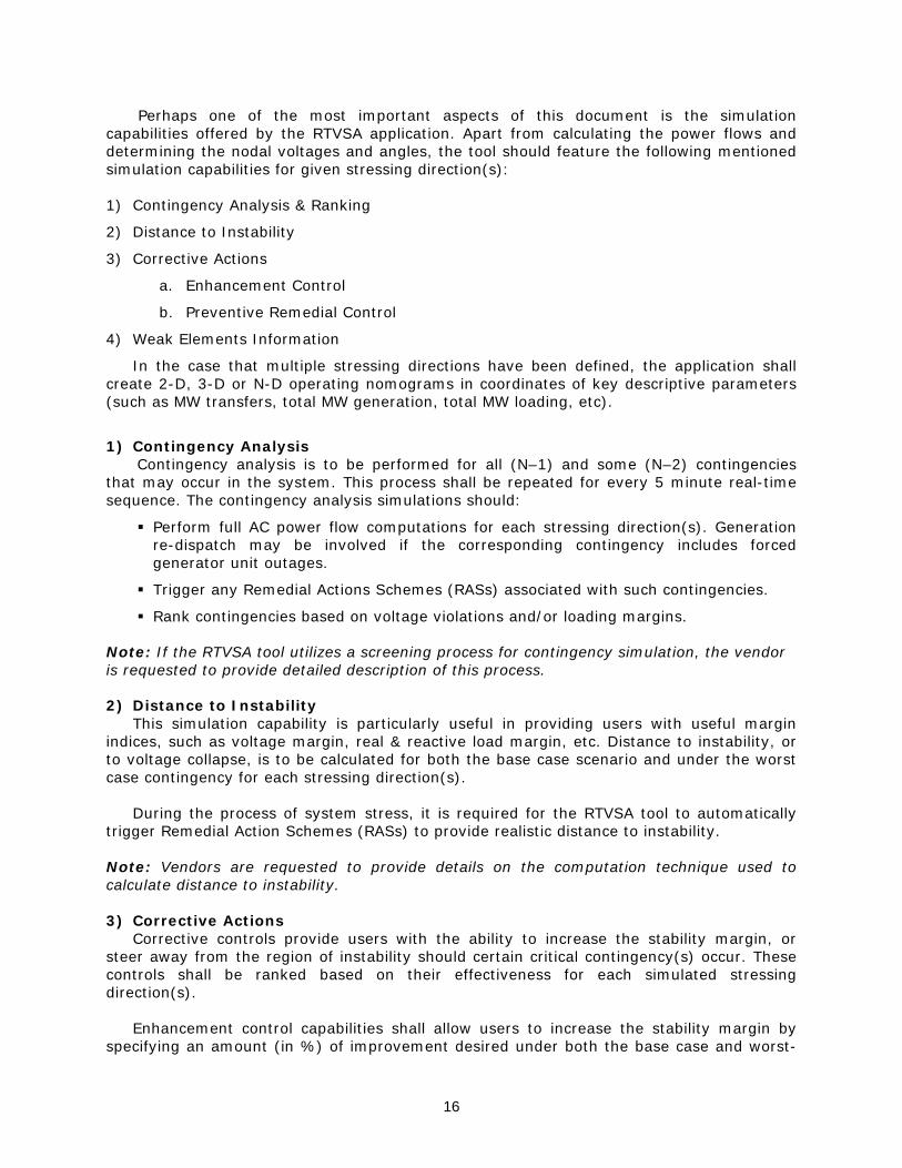
16
Perhaps one of the most important aspects of this document is the simulation capabilities offered by the RTVSA application. Apart from calculating the power flows and determining the nodal voltages and angles, the tool should feature the following mentioned simulation capabilities for given stressing direction(s): 1) Contingency Analysis & Ranking
2) Distance to Instability
3) Corrective Actions
a. Enhancement Control
b. Preventive Remedial Control
4) Weak Elements Information
In the case that multiple stressing directions have been defined, the application shall create 2-D, 3-D or N-D operating nomograms in coordinates of key descriptive parameters (such as MW transfers, total MW generation, total MW loading, etc).
1) Contingency Analysis
Contingency analysis is to be performed for all (N–1) and some (N–2) contingencies that may occur in the system. This process shall be repeated for every 5 minute real-time sequence. The contingency analysis simulations should:
Perform full AC power flow computations for each stressing direction(s). Generation re-dispatch may be involved if the corresponding contingency includes forced generator unit outages.
Trigger any Remedial Actions Schemes (RASs) associated with such contingencies.
Rank contingencies based on voltage violations and/or loading margins.
Note: If the RTVSA tool utilizes a screening process for contingency simulation, the vendor is requested to provide detailed description of this process.
2) Distance to Instability This simulation capability is particularly useful in providing users with useful margin
indices, such as voltage margin, real & reactive load margin, etc. Distance to instability, or to voltage collapse, is to be calculated for both the base case scenario and under the worst case contingency for each stressing direction(s).
During the process of system stress, it is required for the RTVSA tool to automatically
trigger Remedial Action Schemes (RASs) to provide realistic distance to instability. Note: Vendors are requested to provide details on the computation technique used to calculate distance to instability. 3) Corrective Actions
Corrective controls provide users with the ability to increase the stability margin, or steer away from the region of instability should certain critical contingency(s) occur. These controls shall be ranked based on their effectiveness for each simulated stressing direction(s).
Enhancement control capabilities shall allow users to increase the stability margin by
specifying an amount (in %) of improvement desired under both the base case and worst-
17
case contingency. This capability includes controlling of the phase shifters, ULTCs, static VAR devices, controllable shunts, etc for improving the current system state.
Preventive remedial controls provide the ability for users to secure the system from
critical (or insecure) contingencies by suggesting priority-based control actions to improve margin indices. For instance, if the current base case scenario indicates sufficient load margin, whereas the occurrence of a certain contingency(s) places the system in the insecure operating region, the tool would determine ‘preventive’ controls to retract into a safe operating region. 4) Weak Elements Information
This simulation capability shall provide voltage sensitivity information with respect to stressing direction(s). This may be at various buses/regions that experience severe degradation in their voltage profile under additional stressing representative of voltage collapse patterns. 5) Operating Nomograms
The boundaries of the 2-D, 3-D or N-D operating nomograms shall be expressed as piece-wise linear approximations (i.e., hyperplanes) in coordinates of key descriptive parameters (such as MW transfers, total MW generation, total MW loading, etc.) associated with the stressing directions.
3.5 User Interfaces The users of the RTVSA application can be categorized under two domains of operation: 1) Real-time mode users or users of the Operator Display Console 2) Study mode users or users of the Stand-Alone Console
3.5.1 Operator Display Console
Operator Display Console receives solution snapshots from the Central Server every time the RTVSA application runs on a set of real-time data. The users of this console, called real-time mode users, view results to RTVSA tool’s simulations (consisting of the ones mentioned in Section 3.4.4) in the two mentioned modes, namely: real-time operations mode and real-time look-ahead mode. The Real-Time Mode Interface facilitates exchange of unidirectional data from the Server Manager located within the Central Server. It receives only the real-time solutions data for display purposes, and restricts users from interacting with the Central Server. The interaction capabilities of these users are limited to the post processing of solution data. These include customization of display settings, such as, assigning a value (say 5%) to the reactive load margin on top of the most binding contingency – a criteria mandated by Western Electric Coordinating Council (WECC). A Configuration Graphical User Interface (GUI) allows users to switch between the various display options, as well as update and modify the current display methodology. The users have the capability to look at the system from a bird’s eye view (wide-area visualization), and subsequently zoom into the area of interest (local area view and/or one-line diagrams).

18
3.5.2 Stand-Alone Console
The Stand-Alone Console caters to users of the RTVSA application under the study mode described earlier. The users have the option to choose from any of the following two study cases: 1) RTVSA tool’s real-time solved case 2) User modified real-time solved case
After selecting the appropriate case, the user may modify solution parameters and network topology, and with the help of certain required Supplementary Files, perform simulations to study hypothetical scenarios. The Study Mode Interface sub-module is responsible for exchanging data to and from the Central Server. The Client Request Manager, which is a part of the Server Manager, manages various requests originating from the Stand-Alone Console users. The users shall have the capability to request files from the Flat Files Storage (i.e., study cases) to conduct studies. The Simulation Engine performs the desired calculations and returns the results to the Server Manager. Subsequently, the Server Manager [optionally] saves results in Flat Files Storage (along with the appropriate time and name stamps), as well as passes on the solutions to the Study Mode Interface for display purposes.
The study-mode console is to be equipped with an effective and user-friendly graphic user interface with point and click features, and pull-down menus. Modern graphics shall be used for the quick assessment of complex situations.
The study-mode RTVSA environment must be easy to understand and manipulate. The
following is the summary of the features that shall be available to users: 1. Ability to request study cases and save modification and simulation results thereto. 2. Ability to adjust certain system parameters and to compute the sensitivity of the results to changes in parameters: this may apply to selection of fewer or more contingencies, together with the ability to construct system scenarios for study purposes. 3. Capability to perform ‘what-if’ and post-disturbance analysis on desired case(s) 4. Ability to visualize simulation results through appropriate graphical means. The capability to plot simulation parameters and variables as a function of time (trend analysis) is also desirable. 5. Ability to compare simulation results obtained from multiple cases.

19
4. VISUALIZATION & USER INTERACTION
The goal of the RTVSA application is to provide the real-time and study mode users with
visualization capabilities that will assist them in making decisions. These capabilities can be classified under two broad domains: (1) Situational Awareness, and (2) Voltage Security Assessment. Situational Awareness
Situational awareness type of displays present to the viewers simplified wide-area real time metrics, detection, alarming, trace, and trend visualization solutions. Accompanying the real-time displays would be scenarios under the worst case contingency. These include, but are not limited to:
Voltage profiles at various buses
Real and reactive power reserves across the system
Interface/line flows across key transmission corridors/voltage levels
One-line diagrams
Voltage Security Assessment The display capabilities under this category demonstrate results of the Voltage Security
Assessment tool under the look-ahead scenario with respect to key stressing direction(s). Such scenarios may be based on current operating conditions or under the worst case contingency. These illustrate voltage security conditions and metrics that help users study voltage stability and take decisions to prevent adverse situations. These capabilities include, but are not limited to:
Real and reactive loading margins
o Margin at base case to point of collapse (POC)
o Margin under worst case contingency base case to POC
Contingency ranking based on severity index (voltage margin, loading margin, etc.)
Operating nomograms
Distance to instability
Weak elements information
Corrective actions (preventive control, enhancement control)
4.1 Recommended Visualization Techniques
Based on discussions held with CA ISO operators and operating engineers/planners, the following are some of the preferred visualization techniques mentioned: “Situational Awareness” type wide area geographic color-coded contour plots displaying information for both the base case and under the worst-case contingency about:
o Nodal voltages
o Real & Reactive reserves

20
o Interface/line flows with respect to flow limits
The color coding legend on contour plots shall accommodate different ‘normal’ operating ranges for the different substations. For example, a particular 500 kV bus at a substation may normally operate at 525 kV and this should be appropriately indicated by the ‘normal’ color used within the legend.
For each of the operating modes, the users would like to be able to view the loading margins as bar graphs under the base case and the most binding contingency.
Additionally, for the real time modes, and under the most binding contingency, the line flows should also be shown within a geographic display at least at the higher voltage levels. The more detailed flows under these situations should be visible on one-line diagrams within CA ISO’s Operator Display Consoles.
The ability to filter and view information by regional buses and by voltage levels
The tools should support alarming capabilities when voltage profiles and/or margins drop below pre-defined operating limits. These limits should be configurable.
4.2 User Interaction
The RTVSA visuals are displayed to both user interfaces: real-time user interface located in CA ISO’s Operator Consoles, and study-mode interface located in Stand-Alone Consoles. Since the simulation results obtained under each of the modes are case dependant (study or real-time case), the visual displays and techniques are different for the two users.
The Operator Console users view real-time results of RTVSA simulations under four system scenarios:
(1) Current system scenario (base case)
(2) System conditions under the worst case contingency
(3) 2 hour look-ahead condition under base case
(4) 2 hour look-ahead conditions under the worst case contingency
Although presenting multiple plots may sound intimidating to users, a clever layout of the visuals may reduce the involved complexities. For instance, the “current mode” tab would display plots (1) & (2), and by simply clicking on the “look-ahead” tab, the displays would switch to plots (3) & (4) – thereby replacing the old values with new one while keeping the display pattern (or technique) unchanged.
Here are some of the display capabilities and features required for the Operator Console users: Wide area geographic view of the current system conditions with the capability to zoom-
in on a desired local area
‘Situational Awareness’ and ‘Voltage Security Assessment’ type displays for the above mentioned four system scenarios
Effective displays of priority based corrective controls information with rankings based on their effectiveness for each simulated stressing direction(s).
The capability to modify and customize display settings

21
Study mode users shall interact with the system through a GUI in order to select the
desired study case, make necessary modification to the same, and run simulations with preferred execution parameters (Supplementary Files) and controls. They would be able to study the reliability of the system with the help of various displays as well as by comparing multiple study cases. The following are some of the display capabilities required for the stand-alone console users: The ability to conveniently modify network topology through means such as one-line diagrams, tabular displays, etc. The same applies for the various user-defined RTVSA supplementary files.
Displays that indicate the available RTVSA execution control parameters and their current values.
Emphasis on ‘Voltage Security Assessment’ type of displays.
Capability to compare cases against each other through appropriate graphical means which focus on the key parameters associated with various comparisons (e.g. indices, margins, sensitivities and trends). For example, it would be desirable to be able to assess the sensitivity of results to any parameter of a component via clicking on that component in the GUI.
Capability to plot simulation parameters and variables as a function of time.

22
5. SUMMARY TABLE
The RTVSA feature set and functional capabilities are summarized in the table below: I Input Data Specifications A Valid state estimation solution snapshots available every 5 minutes in dynamic CIM
format. B Detailed network model with node-breaker details in the static CIM format. C Contingency list containing all N-1 and some user-specified N-2 contingencies with the
associated RASs D Stressing directions including generator dispatch sequence and load patterns, and
associated RASs.
II Modes of Operation A ‘Real time operations mode’ presenting real time voltage stability analysis using the
current state estimator snapshot. B ‘Real time look-ahead mode’ providing predictive voltage stability analysis using a
priori knowledge of planned outages and load forecast. C ‘Study mode’ offering offline ‘what-if’ capabilities on the real time study cases.
III Functional Capabilities A Contingency analysis and ranking based on voltage violations or loading margins for
each stressing directions. B Voltage profiles, powerflow patterns, real/reactive reserves and loading margins to
PoC under base case and most binding contingency. C Margin sensitivities to reactive support for each stressing direction. D Suggest and rank Enhancement Controls to increase reactive load margins and
Preventive Remedial Controls to retract to a secure region. E Identify weak elements and their voltage sensitivities to reactive load margins. F Construct 2-D, 3-D or N-D security regions (nomograms) offline for a set of pre-
defined stressing directions and descriptor variables. G Evaluate current state estimator snapshot within N-dimensional security regions. H Real-time alarming on voltage violations and low real/reactive load margins.
IV System Architecture & User Environments A Central-server/multi-client architecture B Simulation engine performing the various simulations and analysis. C Topology processor to convert the node/breaker to bus/branch for analysis and vise-
versa for presenting simulation results. D Flat file storage housing the most current real time solved cases and modified study
cases. E Real time information presented within Operator Display consoles. F Study mode capabilities within stand-alone user consoles. G User interface to enable/disable automated controls, and modify simulation
parameters, supplementary files (e.g. Stressing directions, contingency list, RASs).
V Visualization Capabilities A Voltage profiles, real & reactive reserves at key stations, and power flows at the higher
voltage levels within wide within wide area geographic displays. B Real and reactive loading margins as bar graphs. C One-line diagrams within Operator Displays.
Table 2 - RTVSA Summary Table