synopses for massive data: samples, histograms, wavelets...
TRANSCRIPT
Foundations and TrendsR© inDatabasesVol. 4, Nos. 1–3 (2011) 1–294c© 2012 G. Cormode, M. Garofalakis, P. J. Haasand C. JermaineDOI: 10.1561/1900000004
Synopses for Massive Data: Samples,Histograms, Wavelets, Sketches
By Graham Cormode, Minos Garofalakis,Peter J. Haas and Chris Jermaine
Contents
1 Introduction 2
1.1 The Need for Synopses 31.2 Survey Overview 51.3 Outline 6
2 Sampling 11
2.1 Introduction 112.2 Some Simple Examples 122.3 Advantages and Drawbacks of Sampling 172.4 Mathematical Essentials of Sampling 212.5 Different Flavors of Sampling 322.6 Sampling and Database Queries 382.7 Obtaining Samples from Databases 562.8 Online Aggregation Via Sampling 65
3 Histograms 69
3.1 Introduction 713.2 One-Dimensional Histograms: Overview 793.3 Estimation Schemes 853.4 Bucketing Schemes 95
3.5 Multi-Dimensional Histograms 1123.6 Approximate Processing of General Queries 1273.7 Additional Topics 135
4 Wavelets 144
4.1 Introduction 1444.2 One-Dimensional Wavelets and
Wavelet Synopses: Overview 1454.3 Wavelet Synopses for Non-L2 Error Metrics 1554.4 Multi-Dimensional Wavelets 1714.5 Approximate Processing of General Queries 1814.6 Additional Topics 185
5 Sketches 201
5.1 Introduction 2015.2 Notation and Terminology 2035.3 Frequency Based Sketches 2105.4 Sketches for Distinct Value Queries 2405.5 Other Topics in Sketching 257
6 Conclusions and Future Research Directions 263
6.1 Comparison Across Different Methods 2636.2 Approximate Query Processing in Systems 2676.3 Challenges and Future Directions for Synopses 269
Acknowledgments 275
References 276
Foundations and TrendsR© inDatabasesVol. 4, Nos. 1–3 (2011) 1–294c© 2012 G. Cormode, M. Garofalakis, P. J. Haasand C. JermaineDOI: 10.1561/1900000004
Synopses for Massive Data: Samples,Histograms, Wavelets, Sketches
Graham Cormode1, Minos Garofalakis2,Peter J. Haas3, and Chris Jermaine4
1 AT&T Labs — Research, 180 Park Avenue, Florham Park, NJ 07932,USA, [email protected]
2 Technical University of Crete, University Campus — Kounoupidiana,Chania, 73100, Greece, [email protected]
3 IBM Almaden Research Center, 650 Harry Road, San Jose, CA95120-6099, USA, [email protected]
4 Rice University, 6100 Main Street, Houston, TX 77005, USA,[email protected]
Abstract
Methods for Approximate Query Processing (AQP) are essential fordealing with massive data. They are often the only means of provid-ing interactive response times when exploring massive datasets, and arealso needed to handle high speed data streams. These methods proceedby computing a lossy, compact synopsis of the data, and then execut-ing the query of interest against the synopsis rather than the entiredataset. We describe basic principles and recent developments in AQP.We focus on four key synopses: random samples, histograms, wavelets,and sketches. We consider issues such as accuracy, space and time effi-ciency, optimality, practicality, range of applicability, error bounds onquery answers, and incremental maintenance. We also discuss the trade-offs between the different synopsis types.
1Introduction
A synopsis of a massive dataset captures vital properties of the originaldata while typically occupying much less space. For example, supposethat our data consists of a large numeric time series. A simple summaryallows us to compute the statistical variance of this series: we maintainthe sum of all the values, the sum of the squares of the values, andthe number of observations. Then the average is given by the ratio ofthe sum to the count, and the variance is ratio of the sum of squaresto the count, less the square of the average. An important property ofthis synopsis is that we can build it efficiently. Indeed, we can find thethree summary values in a single pass through the data.
However, we may need to know more about the data than merely itsvariance: how many different values have been seen? How many timeshas the series exceeded a given threshold? What was the behavior ina given time period? To answer such queries, our three-value summarydoes not suffice, and synopses appropriate to each type of query areneeded. In general, these synopses will not be as simple or easy to com-pute as the synopsis for variance. Indeed, for many of these questions,there is no synopsis that can provide the exact answer, as is the casefor variance. The reason is that for some classes of queries, the query
2

1.1 The Need for Synopses 3
answers collectively describe the data in full, and so any synopsis wouldeffectively have to store the entire dataset.
To overcome this problem, we must relax our requirements. In manycases, the key objective is not obtaining the exact answer to a query,but rather receiving an accurate estimate of the answer. For example,in many settings, receiving an answer that is within 0.1% of the trueresult is adequate for our needs; it might suffice to know that the trueanswer is roughly $5 million without knowing that the exact answer is$5,001,482.76. Thus we can tolerate approximation, and there are manysynopses that provide approximate answers. This small relaxation canmake a big difference. Although for some queries it is impossible toprovide a small synopsis that provides exact answers, there are manysynopses that provide a very accurate approximation for these querieswhile using very little space.
1.1 The Need for Synopses
The use of synopses is essential for managing the massive data thatarises in modern information management scenarios. When handlinglarge datasets, from gigabytes to petabytes in size, it is often impracticalto operate on them in full. Instead, it is much more convenient to build asynopsis, and then use this synopsis to analyze the data. This approachcaptures a variety of use-cases:
• A search engine collects logs of every search made, amount-ing to billions of queries every day. It would be too slow, andenergy-intensive, to look for trends and patterns on the fulldata. Instead, it is preferable to use a synopsis that is guar-anteed to preserve most of the as-yet undiscovered patternsin the data.
• A team of analysts for a retail chain would like to study theimpact of different promotions and pricing strategies on salesof different items. It is not cost-effective to give each analystthe resources needed to study the national sales data in full,but by working with synopses of the data, each analyst canperform their explorations on their own laptops.
4 Introduction
• A large cellphone provider wants to track the health ofits network by studying statistics of calls made in differentregions, on hardware from different manufacturers, under dif-ferent levels of contention, and so on. The volume of infor-mation is too large to retain in a database, but instead theprovider can build a synopsis of the data as it is observedlive, and then use the synopsis off-line for further analysis.
These examples expose a variety of settings. The full data may residein a traditional data warehouse, where it is indexed and accessible, butis too costly to work on in full. In other cases, the data is stored as flat-files in a distributed file system; or it may never be stored in full, butbe accessible only as it is observed in a streaming fashion. Sometimessynopsis construction is a one-time process, and sometimes we needto update the synopsis as the base data is modified or as accuracyrequirements change. In all cases though, being able to construct a highquality synopsis enables much faster and more scalable data analysis.
From the 1990s through today, there has been an increasing demandfor systems to query more and more data at ever faster speeds. Enter-prise data requirements have been estimated [173] to grow at 60% peryear through at least 2011, reaching 1,800 exabytes. On the other hand,users — weaned on Internet browsers, sophisticated analytics and sim-ulation software with advanced GUIs, and computer games — havecome to expect real-time or near-real-time answers to their queries.Indeed, it has been increasingly realized that extracting knowledgefrom data is usually an interactive process, with a user issuing a query,seeing the result, and using the result to formulate the next query,in an iterative fashion. Of course, parallel processing techniques canalso help address these problems, but may not suffice on their own.Many queries, for example, are not embarrassingly parallel. More-over, methods based purely on parallelism can be expensive. Indeed,under evolving models for cloud computing, specifically “platform as aservice” fee models, users will pay costs that directly reflect the com-puting resources that they use. In this setting, use of ApproximateQuery Processing (AQP) techniques can lead to significant cost savings.Similarly, recent work [15] has pointed out that approximate processing
1.2 Survey Overview 5
techniques can lead to energy savings and greener computing. ThusAQP techniques are essential for providing, in a cost-effective manner,interactive response times for exploratory queries over massive data.
Exacerbating the pressures on data management systems is theincreasing need to query streaming data, such as real time financialdata or sensor feeds. Here the flood of high speed data can easily over-whelm the often limited CPU and memory capacities of a stream pro-cessor unless AQP methods are used. Moreover, for purposes of networkmonitoring and many other applications, approximate answers sufficewhen trying to detect general patterns in the data, such as a denial-of-service attack. AQP techniques are thus well suited to streaming andnetwork applications.
1.2 Survey Overview
In this survey, we describe basic principles and recent developments inbuilding approximate synopses (i.e., lossy, compressed representations)of massive data. Such synopses enable AQP, in which the user’s queryis executed against the synopsis instead of the original data. We focuson the four main families of synopses: random samples, histograms,wavelets, and sketches.
A random sample comprises a “representative” subset of the datavalues of interest, obtained via a stochastic mechanism. Samples canbe quick to obtain, and can be used to approximately answer a widerange of queries.
A histogram summarizes a dataset by grouping the data values intosubsets, or “buckets,” and then, for each bucket, computing a small setof summary statistics that can be used to approximately reconstruct thedata in the bucket. Histograms have been extensively studied and havebeen incorporated into the query optimizers of virtually all commercialrelational DBMSs.
Wavelet-based synopses were originally developed in the contextof image and signal processing. The dataset is viewed as a set ofM elements in a vector — that is, as a function defined on the set0,1,2, . . . ,M − 1 — and the wavelet transform of this function isfound as a weighted sum of wavelet “basis functions.” The weights,
6 Introduction
or coefficients, can then be “thresholded,” for example, by eliminatingcoefficients that are close to zero in magnitude. The remaining smallset of coefficients serves as the synopsis. Wavelets are good at capturingfeatures of the dataset at various scales.
Sketch summaries are particularly well suited to streaming data.Linear sketches, for example, view a numerical dataset as a vector ormatrix, and multiply the data by a fixed matrix. Such sketches are mas-sively parallelizable. They can accommodate streams of transactions inwhich data is both inserted and removed. Sketches have also been usedsuccessfully to estimate the answer to COUNT DISTINCT queries, anotoriously hard problem.
Many questions arise when evaluating or using synopses.
• What is the class of queries that can be approximatelyanswered?
• What is the approximation accuracy for a synopsis of a givensize?
• What are the space and time requirements for constructinga synopsis of a given size, as well as the time required toapproximately answer the query?
• How should one choose synopsis parameters such as the num-ber of histogram buckets or the wavelet thresholding value?Is there an optimal, that is, most accurate, synopsis of a givensize?
• When using a synopsis to approximately answer a query, isit possible to obtain error bounds on the approximate queryanswer?
• Can the synopsis be incrementally maintained in an efficientmanner?
• Which type of synopsis is best for a given problem?
We explore these issues in subsequent chapters.
1.3 Outline
It is possible to read the discussion of each type of synopsis in isolation,to understand a particular summarization approach. We have tried touse common notation and terminology across all chapters, in order to
1.3 Outline 7
facilitate comparison of the different synopses. In more detail, the topicscovered by the different chapters are given below.
1.3.1 Sampling
Random samples are perhaps the most fundamental synopses for AQP,and the most widely implemented. The simplicity of the idea — exe-cuting the desired query against a small representative subset of thedata — belies centuries of research across many fields, with decadesof effort in the database community alone. Many different methods ofextracting and maintaining samples of data have been proposed, alongwith multiple ways to build an estimator for a given query. This chap-ter introduces the mathematical foundations for sampling, in termsof accuracy and precision, and discusses the key sampling schemes:Bernoulli sampling, stratified sampling, and simple random samplingwith and without replacement.
For simple queries, such as basic SUM and AVERAGE queries, it isstraightforward to build unbiased estimators from samples. The moregeneral case — an arbitrary SQL query with nested subqueries — ismore daunting, but can sometimes be solved quite naturally in a pro-cedural way.
For small tables, drawing a sample can be done straightforwardly.For larger relations, which may not fit conveniently in memory, or maynot even be stored on disk in full, more advanced techniques are neededto make the sampling process scalable. For disk-resident data, sam-pling methods that operate at the granularity of a block rather than atuple may be preferred. Existing indices can also be leveraged to helpthe sampling. For large streams of data, considerable effort has beenput into maintaining a uniform sample as new items arrive or exist-ing items are deleted. Finally, “online aggregation” algorithms enhanceinteractive exploration of massive datasets by exploiting the fact thatan imprecise sampling-based estimate of a query result can be incre-mentally improved simply by collecting more samples.
1.3.2 Histograms
The histogram is a fundamental object for summarizing the frequencydistribution of an attribute or combination of attributes. The most
8 Introduction
basic histograms are based on a fixed division of the domain(equi-width), or using quantiles (equi-depth), and simply keep statisticson the number of items from the input which fall in each such bucket.But many more complex methods have been designed, which aim toprovide the most accurate summary possible within a limited spacebudget. Schemes differ in how the buckets are chosen, what statisticsare stored, how estimates are extracted, and what classes of query aresupported. They are quantified based on the space and time require-ments used to build them, and the resulting accuracy guarantees thatthey provide.
The one-dimensional case is at the heart of histogram construction,since higher dimensions are typically handled via extensions of one-dimensional ideas. Beyond equi-width and equi-depth, end biased andhigh biased, maxdiff and other generalizations have been proposed. Fora variety of approximation-error metrics, dynamic programming (DP)methods can be used to find histograms — notably the “v-optimalhistograms” — that minimize the error, subject to an upper bound onthe allowable histogram size. Approximate methods can be used whenthe quadratic cost of DP is not practical. Many other constructions,both optimal and heuristic, are described, such as lattice histograms,STHoles, and maxdiff histograms. The extension of these methodsto higher dimensions adds complexity. Even the two-dimensional casepresents challenges in how to define the space of possible bucketings.The cost of these methods also rises exponentially with the dimen-sionality of the data, inspiring new approaches that combine sets oflow-dimensional histograms with high-level statistical models.
Histograms most naturally answer range–sum queries — for exam-ple, “compute total sales between July and September for adults fromage 25 through 40” — and their variations. They can also be used toapproximate more general classes of queries, such as aggregations overjoins. Various negative theoretical and empirical results indicate thatone should not expect histograms to give accurate answers to arbitraryqueries. Nevertheless, due to their conceptual simplicity, histograms canbe effectively used for a broad variety of estimation tasks, including set-valued queries, real-valued data, and aggregate queries over predicatesmore complex than simple ranges.
1.3 Outline 9
1.3.3 Wavelets
The wavelet synopsis is conceptually close to the histogram summary.The central difference is that, whereas histograms primarily producebuckets that are subsets of the original data-attribute domain, wave-let representations transform the data and seek to represent the mostsignificant features in a wavelet (i.e., “frequency”) domain, and cancapture combinations of high and low frequency information. The mostwidely discussed wavelet transformation is the Haar-wavelet transform(HWT), which can, in general, be constructed in time linear in thesize of the underlying data array. Picking the B largest HWT coeffi-cients results in a synopsis that provides the optimal L2 (sum-squared)error for the reconstructed data. Extending from one-dimensional tomulti-dimensional data, as with histograms, provides more definitionalchallenges. There are multiple plausible choices here, as well as algo-rithmic challenges in efficiently building the wavelet decomposition.
The core AQP task for wavelet summaries is to estimate the answerto range sums. More general SPJ (select, project, join) queries can alsobe directly applied on relation summaries, to generate a summary ofthe resulting relation. This is made possible through an appropriately-defined AQP algebra that operates entirely in the domain of waveletcoefficients.
Recent research into wavelet representations has focused on errorguarantees beyond L2. These include L1 (sum of errors) or L∞(maximum error), as well as relative-error versions of these measures.A fundamental choice here is whether to restrict the possible coef-ficient values to those arising under the basic wavelet transform, orto allow other (unrestricted) coefficient values, specifically chosen toreduce the target error metric. The construction of such (restricted orunrestricted) wavelet synopses optimized for non-L2 error metrics is achallenging problem.
1.3.4 Sketches
Sketch techniques have undergone extensive development over thepast few years. They are especially appropriate for streaming data,in which large quantities of data flow by and the sketch summary must
10 Introduction
continually be updated quickly and compactly. Sketches, as presentedhere, are designed so that the update caused by each new piece of datais largely independent of the current state of the summary. This designchoice makes them faster to process, and also easy to parallelize.
“Frequency based sketches” are concerned with summarizing theobserved frequency distribution of a dataset. From these sketches, accu-rate estimations of individual frequencies can be extracted. This leadsto algorithms for finding approximate “heavy hitters” — items thataccount for a large fraction of the frequency mass — and quantilessuch as the median and its generalizations. The same sketches can alsobe used to estimate the sizes of (equi)joins between relations, self-joinsizes, and range queries. Such sketch summaries can be used as prim-itives within more complex mining operations, and to extract waveletand histogram representations of streaming data.
A different style of sketch construction leads to sketches for“distinct-value” queries that count the number of distinct values ina given multiset. As mentioned above, using a sample to estimate theanswer to a COUNT DISTINCT query may give highly inaccurateresults. In contract, sketching methods that make a pass over the entiredataset can provide guaranteed accuracy. Once built, these sketchesestimate not only the cardinality of a given attribute or combinationof attributes, but also the cardinality of various operations performedon them, such as set operations (union and difference), and selectionsbased on arbitrary predicates.
In the final chapter, we compare the different synopsis methods.We also discuss the use of AQP within research systems, and discusschallenges and future directions.
In our discussion, we often use terminology and examples thatarise in classical database systems, such as SQL queries over relationaldatabases. These artifacts partially reflect the original context of theresults that we survey, and provide a convenient vocabulary for the var-ious data and access models that are relevant to AQP. We emphasizethat the techniques discussed here can be applied much more generally.Indeed, one of the key motivations behind this survey is the hope thatthese techniques — and their extensions — will become a fundamentalcomponent of tomorrow’s information management systems.
2Sampling
2.1 Introduction
The use of random samples as synopses for AQP has an almost 30 yearhistory in the database research literature, with the earliest major-venue database sampling paper being published in 1984 [251]. Thisarguably makes sampling the longest studied method for AQP. Sam-pling as a research topic in probability theory and statistics has aneven longer history. Laplace and others famously used sampling to esti-mate the population of the French empire in the 18th century [28]. Thestudy of survey sampling — sampling from a finite population suchas a database — blossomed and matured as a sub-field of statisticsin the first half of the 20th century, due most notably to the pioneer-ing work of Jerzy Neyman. See Hansen’s 1987 retrospective on surveysampling [159] for an interesting historical perspective on the field ofsurvey sampling from a statistical point of view.
With such a long history, the breadth and variety of the sampling-based estimation methodologies that are applicable to AQP are stag-gering. Given the variety of the work, this chapter will not attemptto cover and summarize most or even a majority fraction of the work
11
12 Sampling
from the research literature in depth. Rather, the goal of the chap-ter is to serve as a tutorial on the application of sampling to AQP inan information-management environment; references to papers in theresearch literature will be given as appropriate.
The basic topics covered by the chapter, in order, are as follows:
(1) A basic definition and simple examples of sampling for AQP.(2) A treatment of the advantages and disadvantages of AQP
using sampling.(3) An introduction to the basic probability and statistics con-
cepts that underlie data sampling, including example deriva-tions of bias and variance, as well as a catalog of the differenttypes of sampling schemes that are applicable to AQP.
(4) A discussion of how sampling can be applied to estimate theanswer to most of the common SQL query constructs.
(5) A discussion of how random samples can actually be drawnfrom large datasets that are stored on disk, and how samplingin this context differs from traditional survey sampling.
(6) A short discussion of online estimation via sampling.
2.2 Some Simple Examples
The basic idea behind sampling is quite simple. Given a dataset —which we sometimes call a “population” — and a query with anunknown (possibly multi-attribute) numerical result that we wish toestimate, a small number of elements are first selected at random fromthe dataset. Then a few statistics are computed over the sample, suchas the sample mean and variance. Finally, these statistics are used toestimate the value of the query result and provide bounds on the accu-racy of the estimate.
For an example of the process, imagine that we wish to answer thequery
SELECT SUM (R.a)
FROM R
and that dataset R comprises the ten different R.a values
〈3,4,5,6,9,10,12,13,15,19〉.
2.2 Some Simple Examples 13
A sample of this data of size n = 5 can be obtained by simulating therolling of a ten-sided die five times using an appropriate pseudorandomnumber generator (PRNG). A PRNG is an algorithm which takes aninput a seed — that is, a string of bits — and then performs a number ofnumerical operations on the seed to obtain a new, seemingly randombit string that has no obvious statistical correlation with the inputstring. By div-ing or mod-ing the output string, a number with theappropriate range can be obtained — in our case, from 1 to 10. See[118] for a discussion of pseudorandom number generation.
In our example sampling process, rolling the number j on the ithtrial implies that the ith item chosen at random from the population isthe jth item in the population. This straightforward sampling scheme isknown as simple random sampling with replacement (SRSWR) becausethe same element may be sampled multiple times, so conceptually, anelement is returned to the population for possible re-selection wheneverit is selected. Say that we roll the die five times and obtain the followingsequence of numbers:
〈6,3,5,3,9〉Then the associated sample of R.a values is:
〈10,5,9,5,15〉Using the resulting sample, it is then quite easy to estimate the
answer to the SUM query. We compute the sum of the sample values,which is 44, and then scale up this sum by a factor of 2, to compensatefor the fact that we have only seen roughly 5/10 = 1/2 of the valuesin the population. (We say “roughly” because we are sampling withreplacement.)
There is another, very useful way to derive the foregoing estimator.Denote by ti the value of the ith item in the population and by Xi
the random variable that represents the number of times that this ithitem appears in the sample. For instance, X6 = 1 and X3 = 2 in ourexample since the sixth item (t6 = 10) appears once and the third item(t3 = 5) appears twice. The expected value of Xi is defined as E[Xi] =∑5
j=0 j × Pr[Xi = j], and has the following interpretation: if we drewmany samples of size 5 and recorded the frequency of item i in each
14 Sampling
sample, then, with probability 1, the average of these item-i frequencieswould approach the number E[Xi] as the number of samples increased.That is, E[Xi] represents the value of Xi we expect to see “on average.”Now consider the estimator
Y =N∑
i=1
XitiE[Xi]
=∑
i∈ sample
XitiE[Xi]
, (2.1)
where N = 10 is the population size and “sample” denotes the set ofdistinct items appearing in the sample (the set comprising items 6, 3, 5,and 9 in our example). The second equality holds because Xi = 0 forany item i that does not appear in the sample, so that such an itemdoes not contribute to the sum. Because E[X + Y ] = E[X] + E[Y ] andE[cX] = cE[X] for any random variablesX, Y , and constant c, we have
E[Y ] = E
[N∑
i=1
XitiE[Xi]
]=
N∑i=1
E
[XitiE[Xi]
]=
N∑i=1
E[Xi]tiE[Xi]
=N∑
i=1
ti.
Observe that the rightmost term is the true query answer Q, and so theestimator Y is unbiased in that E[Y ] = Q. That is, Y is equal to the truequery result on average, which is a desirable property of a sampling-based estimator. The estimator Y is an example of a Horvitz-Thompson(HT) estimator (see Sarndal, Section 2.8 [268]; the HT estimator wasfirst described in a 1952 paper [170]). To see that Y corresponds to thefirst “scale-up” estimator that we described, note that at each samplingstep, the ith item is included with probability p = 1/10. Since thereare n = 5 sampling steps, it is intuitive1 that the expected number oftimes that item i appears in the sample is E[Xi] = np = 5/10 = 1/2.Since E[Xi] is the same for each item i, we can see that Y is computedby simply multiplying the sum
∑Ni=1Xiti by 1/E[Xi] = 2. As discussed
previously, this latter sum is simply the sum over all of the sampleitems, so that Y indeed corresponds to the scale-up estimator.
For many sampling schemes, such as simple random sampling with-out replacement (SRSWR), an item can appear at most once in a sam-ple (Xi = 0 or 1). In this case E[Xi] = 1 × Pr[Xi = 1] = pi, where pi
1 Technically, Xi has a binomial distribution, so that Pr[Xi = j] =(n
j
)pj(1 − p)n−j , and a
standard calculation shows that E[Xi] = np.
2.2 Some Simple Examples 15
is the probability that item i is included in the sample. Thus, an HTestimator of a sum is typically expressed as the sum of the item valuesin the sample, each divided by the item’s probability of inclusion:
Y =∑
i∈sample
tipi. (2.2)
Sums of functions of item values, such as∑N
i=1 t2i can be estimated in
an analogous manner, for example, Y =∑
i∈sample t2i /pi. An unbiased
sampling-based estimator of the average value in the data is Y/N , thatis, we divide the HT estimator for the sum by the number of itemsin the data. As discussed in the sequel, other quantities of interestcan be expressed as functions of one or more sums, and hence canbe estimated (in an approximately unbiased manner) as correspond-ing functions of HT estimators of the sums. Thus the HT samplingand estimation framework is quite general in that, for many samplingschemes, many estimators for sum-related queries can be representedas an HT estimator or a variant of an HT estimator.
Error bounds (usually probabilistic in nature) for our SUM-queryestimator Y defined in (2.1) can be obtained in many ways; seeSection 2.4.2 for an in-depth discussion. One classical approach to errorbounds is via the Central Limit Theorem (CLT) [95]. First we computethe sample variance of the sampled item values 〈10,5,9,5,15〉, which is
14((10 − 8.8)2 + (5 − 8.8)2 + (9 − 8.8)2
+(5 − 8.8)2 + (15 − 8.8)2) = 17.2,
since the average of the five sampled item values is 8.8. (We divide byn − 1 = 4 rather than n = 5 to compensate for sampling bias.) Thisserves as an estimate for the variance of the population. Accordingto the CLT, when N and n are reasonably large the quantity Y/N
(which estimates the population mean) will be approximately nor-mally distributed with a variance of (approximately) 17.2/5, whichimplies that Y itself is approximately normally distributed, with avariance of 17.2 × (100/5) = 344, where 5 is the size of the sam-ple and 100 is the square of the size of the dataset. This is onlyan approximation of the variance of Y because 17.2 is only an
16 Sampling
approximation of the population variance. Furthermore, slightly morethan 95% of the mass of the normal distribution is within two standarddeviations of the mean of the distribution (where the “standard devia-tion” is the square root of the variance). Then, since
√344 = 18.55,
there is (approximately) a 95% chance that our estimate is within±37.10 of the correct answer. This range can be used to providean end user with some idea of the accuracy of the sampling-basedestimate.
As another example of an HT estimator, this time for a slightlymore complicated query, suppose that we wish to estimate the sumR.a + 4 × S.b over a cross product of two datasets R and S. We canfirst independently sample 10% of the tuples from R and 10% of thesamples S, and then take a cross product of the two samples, therebyobtaining a random sample U of all of the items in R × S. The prob-ability that a given element (r,s) ∈ R × S is included in the sampleU is simply 10% × 10% = 1%, which is the joint probability that r issampled from R and s is sampled from S. The HT estimator of thequery result is then Y = (1/0.01)
∑(r,s)∈U (r.a + 4 × s.b). That is, we
simply compute the summation over the sample and then scale up theresult by a factor of 100 to compensate for the sampling.2
The above examples illustrate perhaps the simplest applications ofrandom sampling to AQP; more complex examples are given in thesequel. Unless specified otherwise, we will focus on the use of sam-pling for approximate answering of aggregation queries, that is, queriesin which relational operations are applied to a set of base relationsto produce an intermediate relation, and then the tuples of this rela-tion are fed into a function — such as SUM, AVERAGE, and so on —that computes a number (or small set of numbers) that comprisethe final query result. Sampling may also be applied to a query thatreturns a set of tuples; the goal here is to produce a representativesample of these tuples. Such samples are useful for purposes of audit-ing, exploratory data analysis, statistical quality control, and privacyenforcement [242].
2 Note that the samples obtained by this process are not, in fact independent samples fromthe cross product, which introduces some complications in the analysis of the accuracy ofthe estimator Y . See Section 2.6.1 for more details.
2.3 Advantages and Drawbacks of Sampling 17
2.3 Advantages and Drawbacks of Sampling
Now that we have illustrated the use of sampling with a simple example,we will next discuss various scenarios in which sampling is, or is not,useful. Advantages of sampling include:
(1) Simplicity. Conceptually, it is very simple to understand theidea of drawing items at random from a dataset, then scalingup the result of a query over the sample to guess the resultof applying the query to the whole dataset.
(2) Pervasiveness. Sampling is widely supported by database sys-tems, and support for sampling is part of the current SQLstandard (SQL-2008).
(3) Extensive theory. Almost 100 years of prior research in surveysampling can be applied directly to sampling massive data.Classic results such as the CLT can be used to assess theerror of estimates obtained via sampling, to determine howmany samples to obtain to achieve a desired accuracy, and todevelop special-purpose sampling strategies that obtain highaccuracy for difficult queries.
(4) Immediacy. Sampling is unique in that it need not rely ona pre-constructed model that has been built offline, beforequery processing has begun. Since (by definition) a samplecontains a small subset of the data — perhaps only a fewhundred tuples — it can often be constructed after a queryhas been issued, without incurring a delay that is long enoughto be perceptible to an end-user.
(5) Adaptivity. Unlike “one-and-done” approximation methodsthat rely on a pre-constructed model, sampling permitsonline approximation: if a small sample does not provideenough accuracy for a specific query, then more tuples canbe sampled to provide for more accuracy while the user waits,in an online fashion. In contrast, if a data structure such asan AMS sketch [7] does not provide enough accuracy, theuser has no option for incrementally improving the synopsis.
(6) Flexibility. A “sample” is a very general-purpose data struc-ture and as such, the same sample can be used to answer
18 Sampling
a wide variety of arbitrary queries. The generality resultsfrom the fact that sampling commutes with common queryoperations such as selection, projection, and grouping. In thecontext of aggregation queries, sampling also commutes, inan appropriate sense, with the cross product and join opera-tions; see Section 2.6.1. That is, it is often possible to replacethe input relations to an aggregation query by samples fromthose relations and use the query result to obtain well-behaved estimators of the true query result. (“Well behaved”estimators are computable from the information at hand,are unbiased or approximately unbiased, improve in accuracyas the sample size is increased, and come with assessmentsof estimator accuracy.) This is true no matter what formthe underlying boolean selection or join predicate takes —equi-joins, greater-than predicates, not-equal-to-predicates,arbitrary and complicated CNF expressions — all commutewith sampling and so all work seamlessly with sampling. Itis also true whether the underlying attributes are numericalor categorical.
(7) Insensitivity to dimension. The accuracy of sampling-basedestimates is usually independent of the number of attributesin the data. That is, unlike other methods such as wave-lets and histograms, there are no combinatorial difficultiesinduced by the “dimensionality” of the data.
(8) Ease of implementation. Because sampling commutes withmany of the common query operations, it is possible to usea database engine itself to evaluate a query over a sample.That is, a database query can be sped up by first samplingthe database, then feeding the sample into the databaseengine where the original query is run without modifica-tion, and then adjusting the final answer — for example,by scaling it upwards — to take the sampling into account.This means that sampling can be used as an approximationmethod in a database environment with very little modifi-cation to the source code of the database system. This isprecisely the idea, for example, behind the AQUA project

2.3 Advantages and Drawbacks of Sampling 19
which proposed storing a sample of a database inside anotherdatabase instance, and using the same database engine toprocess incoming queries using the sample [3].
However, sampling has its own particular drawbacks as well. Mostnotably:
(1) Because sampling relies on having a reasonable chance ofselecting some of the data objects that are relevant foranswering a query, sampling can be unsuitable for approx-imating the answer to queries that depend only upon a fewtuples from the dataset (that is, those queries that are highlyselective). For example, if only ten tuples out of one millioncontribute to a query answer, then a 1% sample of the datais unlikely to select any of them, and the resulting estimatecan be poor. This is one reason why, despite all of sampling’sbenefits, statistical synopses such as histograms are far morewidely used as tools for selectivity estimation in commercialdatabase systems.
(2) The fact that samples are generally used for AQP by simplyapplying an incoming query to the sample is sometimes seenas a drawback, and not as a benefit. Evaluating a query overa large, 5% sample of a database may take 5% of the timethat it takes to evaluate the query over the entire dataset.A 20× speedup may be significant, but other, more compactsynopses such as histograms can provide much faster esti-mates. This is another reason that sampling is not widelyused for selectivity estimation — it is widely thought thatproviding an estimate via a sample is much more expensivethan estimation via other methods.
(3) Sampling is generally sensitive to skew and to outliers.Reconsider our example from the previous section. If ourdataset instead contained the ten items:
〈3,4,5,6,9,10,12,13,15,1099〉Then any estimate for the final sum will be quite inaccurate.Indeed, a sample that happens to miss 1099 will radically
20 Sampling
underestimate the final sum, and a (p × 100)% sample thathappens to hit 1099 will overestimate the sum by approxi-mately a factor of 1/p.
(4) There are important classes of aggregation queries for whichthe basic HT setup of Section 2.2 breaks down, in which casesampling-based estimation usually becomes very challenging.One way that an HT estimator can run into trouble is whenthe inclusion probability pi of an item into the sample — seeEquation (2.2) — depends on the (unknown) distributionof values in the data population. In this case, the inclusionprobabilities are unknown at estimation time so the HT for-mula cannot be used directly. (More generally, the quantitiesE[Xi] as in Equation (2.1) may be unknown.) For example,consider the problem of evaluating the sum of R.a over rela-tion R, subject to the constraint that we wish to only considerthose tuples whose R.b value does not appear anywhere inattribute S.c from relation S. This is effectively a NOT IN
query of the form:
SELECT SUM (R.a)
FROM R
WHERE R.b NOT IN (SELECT S.c FROM S)
Suppose that one independently samples both R and S (say,without replacement) and then attempts to estimate thequery result using an HT estimator in a manner similarto the final example in Section 2.2. The probability that agiven tuple r is included in U — the sample set of itemsfrom R whose R.a values are to be summed — depends onwhether r fails to find a match in the sample from S, andthis latter probability depends on the frequency distributionof attribute S.c, which is unknown. Thus it is difficult tocharacterize the sample set U . Indeed, some r from R canactually appear in the result if one samples R and S first andthen runs the query over the samples, even when r does notappear in the true result set — simply because r has no matein the sample from S does not mean that it has no mate in all
2.4 Mathematical Essentials of Sampling 21
of S. Thus, it is hard to use sampling to estimate the answerto this query. NOT IN queries are not the only example of this.Others that are difficult are those having the SQL DISTINCT
keyword (in other words, duplicate removal), as well as thosewith the IN or EXISTS keywords, those containing antijoinsand outer joins, and most queries with set-based (as opposedto bag-based) semantics. Another way that the HT approachcan fail is when the aggregate of interest cannot be expressedin terms of sums or functions of sums. MAX and MIN queriesare typical examples. Sections 2.6.2 and 2.6.3 contain somecurrent research results related to these hard sampling andestimation problems.
2.4 Mathematical Essentials of Sampling
2.4.1 A Mathematical Model For Sampling
Before covering specific work relevant to sampling for AQP, it is instruc-tive to describe some of the basic statistical principles underlying sam-pling, introduce the reader to some of the common terminologies, anddemonstrate how those principles might apply to the simple samplingexample from the previous section. Virtually all of the ideas in thedatabase literature and in the statistics literature are derived directlyfrom the basic ideas introduced here.
As described previously, a sample is a set of data elements selectedvia some random process. The sampling process can be modeled statis-tically as follows. As in Section 2.2, denote by tj the jth item or tuple inthe dataset and by Xj the random variable that controls the number ofcopies of the item that are included in the sample. Intuitively, we view arandom variable as a mathematical object that encapsulates the idea of“random chance.” It can be thought of as a non-deterministic machine,where “pressing a button” on the machine causes a random value tobe produced; this is known as a “trial” over the variable. In our case,a trial over Xj produces a non-negative integer value xj . The behaviorof the various Xjs defines the behavior of the underlying sampling pro-cess. If xj is zero, then tj is not sampled. Otherwise, tj is sampled xj
times. By changing the sampling process (with replacement, without
22 Sampling
replacement, biased, unbiased, etc.) we change the statistical propertiesof the various Xjs, and change the statistical properties of the samplingprocess. For example, if so-called “Bernoulli” sampling is desired (seeSection 2.5.3), then we use a PRNG to simulate flipping a biased coinonce for each and every data item. The item is included in the sampleif the coin comes up heads; otherwise, it is not. In this case, each Xj
takes the value one if the coin comes up heads, and takes the value zerootherwise.
Given the various Xjs that control the sampling process, the nextthing that is needed to apply sampling to the problem of AQP is anestimator that can be used to guess the answer to the query. An esti-mator Y can be thought of as nothing more than a function F that hasbeen parameterized on all of the data elements and all of the randomvariables that control the sampling process:
Y = F (〈(t1,X1),(t2,X2), . . . ,(tn,Xn)〉)In general, F will satisfy the constraint that:
F (〈. . . ,(tj−1,Xj−1),(tj ,0),(tj+1,Xj+1), . . .〉)= F (〈. . . ,(tj−1,Xj−1),(tj+1,Xj+1), . . .〉)
In other words, F cannot “look at” the tuple tj if the associated xj = 0.However, this restriction is not absolute; some sampling-based estima-tors described in the database literature make use of summary statisticsover the dataset, such as the pre-computed average value of each tupleattribute [193]. In this case, F may have access to statistics that con-sider every tj in the dataset.
Since applying a function such as F to a set of random variablesresults in a new random variable, Y is itself a random variable. Per-forming a trial over this random variable (i.e., performing the samplingprocess to obtain each xj and then applying F to the result) gives usan actual estimate for the answer to the query. It is this estimate thatis returned to the user. Often, the estimate contains a single numericalvalue. However, in the general case it may contain a vector of values;for example, Y may be defined so that it estimates the result of a GROUP
BY query.
2.4 Mathematical Essentials of Sampling 23
2.4.2 Bias and Variance: Quantifying Accuracy
In general, the utility or accuracy of Y is quantified by determining Y sbias and variance. The bias of Y is defined as:
bias(Y ) = E[Y ] − Qwhere E[Y ] is the expected value of Y and Q is the actual query result.This determines how far away, on average, Y will be from Q. Thevariance of Y is:
σ2(Y ) = E[(Y − E[Y ])2] = E[Y 2] − E2[Y ]
which measures the spread of Y around its average value. High spread isbad, since it means that the estimator has a great degree of variabilityand often falls far from its expected value. If Y has low bias and lowvariance, then Y is (usually) a high-quality estimator.
It is instructive to make these concepts a little more concrete byconsidering the application of these principles to an actual samplingprocess and estimator. Consider the case of SRSWR, as described inSection 2.2. Without loss of generality and for simplicity of notation,here and in most of our discussion of sampling we use the notation tjto denote the jth tuple in the dataset and we assume that tj is a realnumber. While this may seem restrictive, it is really not. tj can in factbe the result of any mathematical or logical expression over actual dataitems. For example, consider the query:
SELECT SUM(r.extendedprice * (1.0 - r.tax))
FROM R as r
WHERE r.suppkey = 1234
In this case, we can set tj to be r.extendedprice * (1.0 - r.tax)
if r.suppkey = 1234 where r is the jth tuple in R; otherwise, ifr.suppkey <> 1234 then tj is set to zero.
Since we assume that tj encapsulates any underlying selection pred-icate as well as the function to be aggregated, the answer to a single-relation SUM query can always be written as:
Q =∑
j
tj
24 Sampling
Now imagine that we have a particular dataset instance where〈t1, t2, . . . , t10〉 take the values 〈3,4, . . . ,19〉, as in our example fromSection 2.2. For our dataset of size 10 and a sample of size 5, we canformalize the estimator from Section 2.2 as:
Y = F (〈(t1,X1), . . . ,(t10,X10)〉) =105
10∑j=1
tjXj
As discussed in Section 2.2, each Xj is a binomially-distributed randomvariable with parameters p = 1/10 and n = 5 under SRSWR.3 ThusE[Xj ] = np = 1/2 and hence E[Y ] = Q, so that Y is unbiased. Finally,note that the five samples are mutually statistically independent.
We now consider the variance of this particular estimator. In thiscase, since E[Y ] = Q, we have E2[Y ] = Q2. However, in order to com-pute the variance, it is also necessary to know E[Y 2]. This can bederived via algebraic manipulation:
E[Y 2] = E
2
∑j
tjXj
2 = E
4
∑i
∑j
titjXiXj
= E
4
∑i
t2iX2i + 8
∑i<j
titjXiXj
= 4∑
i
(t2iE[X2
i ])
+ 8∑i<j
titjE[XiXj ]
This leaves us with two summations. In the first summation, the termE[X2
i ] must be evaluated. This is simply the second moment of the bino-mial distribution, and according to any standard textbook on discretedistributions, this value is np + n(n − 1)p2 = 1
2 + 15 = 7
10 . ComputingE[XiXj ] is more non-standard due to the constraint that the variousXj ’s must sum to n, but in this case its value can be evaluated as
3 Note that while each Xj is binomial, it must be the case that∑
j Xj is 5, since n = 5samples are taken overall. Thus, the various Xjs are marginally binomial, but not inde-pendent. This correlation does not affect E[Y ], but must be taken into account whencomputing E[Y 2], as we discuss subsequently.
2.4 Mathematical Essentials of Sampling 25
n(n − 1)p2 = 15 .4 Plugging this into the above equation, we have:
E[Y 2] =145
∑i
t2i +85
∑i<j
titj
And so the variance of Y , denoted as σ2(Y ), is:
σ2(Y ) =145
∑i
t2i +85
∑i<j
titj − Q2
Plugging in the actual values for our dataset, we have:
σ2(Y ) =145× 1166 +
85× 4025 − 9216 = 488.8
The observant reader may note that 488.8 differs considerably fromthe value 17.2 × 100
5 = 344 that was computed via the CLT in the priorsection. The reason for this is that 488.8 is the actual variance of ourestimator Y ; there are no approximations here. The value 344 fromthe prior section was obtained by using the sample itself to estimatethe variance of the underlying population (since, in practice, the truepopulation variance of 488.8 would be unknown to the user).
More generally, for a HT estimator Y as in Equation (2.1), based ona sample of size N , let πi = E[Xi] and πij = E[XiXj ] for 1 ≤ i, j ≤ N .Using the fact that E[Y ] =
∑i ti (because Y is unbiased), algebraic
4 The intuition behind the formula E[XiXj ] = n(n − 1)p2 is as follows. We can view Xi
(and Xj) as the number of heads over a sequence of n coin flips; a “heads” on the kthflip in the sequence associated with Xi means that the kth tuple sampled was ti. LetXi,k be a random variable controlling the output of the kth flip, so that Xi =
∑k Xi,k.
Then E[XiXj ] = E[∑
k1,k2 Xi,k1Xj,k2]. Since we can push the expectation into the sum,we have E[XiXj ] =
∑k1,k2 E[Xi,k1Xj,k2]. Thus, we need only consider how to evaluate
E[Xi,k1Xj,k2]. If k1 = k2, then Xi,k1Xj,k2 is always zero; that is, if the two coin flips areboth the kth flip in the sequence, then they can never both come up heads — this wouldimply that the kth sample selected both ti and tj , which is not possible. If, on the otherhand, the two coin flips are not both the same flip in the sequence, the probability thatboth are heads is p2, since the two flips are independent. In this case, E[Xi,k1Xj,k2] = p2.Summing over all n2 pairs of coin flips that contribute to E[XiXj ], we have E[XiXj ] =n2p2 − np2, which is n(n − 1)p2.
26 Sampling
manipulations as before show that
σ2(Y ) = E[Y 2] − E2[Y ] = E
(∑
i
Xitiπi
)2 −
(∑i
ti
)2
= E
∑
i
∑j
Xitiπi
Xjtjπj
−∑
i
∑j
titj (2.3)
=∑
i
∑j
πijtitjπiπj
−∑
i
∑j
titj =∑
i
∑j
(πij
πiπj− 1
)titj .
In practice, we need to estimate σ2(Y ) from the sample at hand.Observe that σ2(Y ) is expressed as a sum (over the cross-product ofthe dataset with itself), so that we can use the HT trick yet again toderive an unbiased estimator of σ2(Y ):
σ2(Y ) =∑
i
∑j
XiXj
πij
(πij
πiπj− 1
)titj
=∑
i,j∈sample
XiXj
πij
(πij
πiπj− 1
)titj . (2.4)
Plugging the values for our dataset into these formulas yields the sameanswers as before: σ2(Y ) = 488.8 and σ2(Y ) = 344. The variance for-mulas, however, also hold for other sampling schemes besides SRSWR.If the sampling scheme is such that an item can appear at most oncein the sample — so that the HT estimator has the form given in Equa-tion (2.2) — then πi = pi and πij = pij , where pi is the probability thatdata item i is included in the sample and pij is the probability thatitems i and j are both included in the sample. Moreover, E[X2
i ] = E[Xi]since Xi = 0 or 1, so that the above formulas takes on the special forms
σ2(Y ) =∑
i
(1pi− 1
)t2i + 2
∑i<j
(pij
pipj− 1
)titj
and
σ2(Y ) =∑
i∈sample
1pi
(1pi− 1
)t2i + 2
∑i,j∈sample
i<j
1pij
(pij
pipj− 1
)titj .
2.4 Mathematical Essentials of Sampling 27
The key point here is that, whereas E[Y ] only depends on the individ-ual inclusion probabilities pi, the variance of Y depends on the jointinclusion probabilities pij , which can be challenging to calculate. Thisadditional complexity explains why the variance of an estimator can bemuch harder to estimate than the expected value. It also explains whytwo different sampling schemes can have the same marginal inclusionprobabilities and hence can both lead to unbiased HT estimators, butthe variance properties of the estimators can differ dramatically if thejoint inclusion probabilities differ.
2.4.3 From Bias and Variance To Accuracy Guarantees
Although bias and variance are important statistics that are very usefulfor describing the error of a sampling-based estimate, most users arelikely to be more comfortable with probabilistic confidence bounds (seeSarndal et al., Section 2.11 [268]). A confidence bound is a probabilisticguarantee of the form:
“There is a p × 100% chance that the true answer to the query is withinthe range l to h.”
Central Limit Theorem. There are many ways to provide for confi-dence bounds. The most common method is to assume that the erroron an unbiased, sampling-based estimator Y is normally distributed.That is, we assume that Y can be modeled as:
Y ≈ Q + N (0,σ2(Y ))
In this equation, N = N (0,σ2(Y )) is a normally-distributed randomvariable with mean zero and a variance of σ2(Y ). Then, if we choosenumbers lo and hi so that:
p =∫ hi
lofN (x)dx
where fN is the probability density function of N , we know that thereis a p × 100% chance that lo ≤ Q − Y ≤ hi. (Here we use the fact thatQ − Y = −N has the same distribution as N because the normal dis-tribution is symmetric about the origin.) By algebraic manipulation, it
28 Sampling
then holds that if l = Y + lo and h = Y + hi — here l and h are ran-dom variables — there is a p × 100% chance that the random interval[l,h] contains Q. For example, since∫ 1.98σ(Y )
−1.98σ(Y )fN (x)dx = 0.95,
if we assume normality of the error, then for unbiased Y we are jus-tified in saying that there is around a 95% chance that Q is withinY − 2σ(Y ) to Y + 2σ(Y ), which is perhaps the most commonly-usedconfidence bound. Such a confidence bound is often inverted to arriveat the equivalent statement that “Y estimates Q to within ±2σ(Y )with 95% probability.” By approximating σ2(Y ) with a sample-basedestimate σ2(Y ) as in Sections 2.2 and 2.4.2, and then taking the squareroot to get an estimate σ(Y ) of σ(Y ), we can roughly assess the accu-racy of Y at estimation time (and potentially increase the number ofsamples if the accuracy is not deemed sufficient).
Although there is never any guarantee that the error of Y is nor-mally distributed, the statistical justification for assuming normalityis typically the CLT, which states that as the number of independentsamples taken from a distribution approaches infinity, the observeddifference between the mean of the distribution and the mean of thesamples looks increasingly like a sample from a normally-distributedrandom variable. In the authors’ own experience, for most of the esti-mators one would encounter in a data analysis environment, normalityis a safe assumption. This seems to be true even when the samples arecorrelated (as they will be if sampling without replacement is used),and when the number of samples is not very, very large. The robustnessof the normality assumption stems from statistical theory — see, forexample, [22, 158] — which asserts that variants of the CLT hold ingreat generality, that is, under various weakenings of both the inde-pendence and identical-distribution assumptions. In our experience,normality is especially safe if the specified p does not exceed 95%;deviations from normality tend to be most pronounced in the tails ofthe error distribution. In Section 2.2, we used exactly the CLT boundto assert that the answer to our example query was 88 ± 37.10 withroughly 95% certainty.
2.4 Mathematical Essentials of Sampling 29
Chebyshev Bounds. However, normality is never guaranteed. Theauthors have generally found that statisticians are more accepting ofdistributional assumptions than are computer scientists, who tend tobe more conservative. If one eschews distributional assumptions, thendistribution-free bounds can be used instead. These are looser, butmore comforting. One common bound is due to Chebyshev’s inequality,which implies that for an unbiased estimator Y ,
Pr[|Y − Q| ≥ p− 12σ(Y )] ≤ p
Thus, according to Chebyshev’s inequality, there is a p × 100%chance that Q is between Y − p− 1
2σ(Y ) and Y + p− 12σ(Y ). While
such bounds are comforting, they are often much looser than CLT-based bounds. Had we applied Chebyshev bounds to our examplefrom Section 2.2, we would have obtained a confidence interval of88 ± 117.32.
Hoeffding Bounds. Other distribution-free bounds are Hoeffdingbounds [169] and Chernoff bounds [157]. Whereas bounds based onChebyshev’s inequality assume that the variance of the underlying dis-tribution is known, Hoeffding bounds are applicable when Y = 1
n
∑iXi,
where the value of Xi ranges from lowi to hii. In this case,
Pr[|Y − E[Y ]| ≥ d] ≤ 2exp(− 2d2n2∑
i(hii − lowi)2
)
Hoeffding bounds could apply to our example from Section 2.2 asfollows. Recall that we sampled values 〈10,5,9,5,15〉 which we can mul-tiply by 1
p to obtain the sequence 〈100,50,90,50,150〉; the mean of thissequence is an unbiased estimate for Q. If we assume that 50 and 150represent reasonable low and high bounds on the possible numbers wecould obtain via this process, we can approximate
∑i(hii − lowi)2 by
n(150 − 50)2 = 50,000. We then solve the equation
0.05 = 2exp(− 2d2n2
50,000
)
for d, giving d = 192.06; this implies that 88 ± 192.06 is a 95% confi-dence interval for the query answer. Note that while this interval is quitewide, it would have been even wider had we used the correct low and
30 Sampling
high values from the dataset, which are often unknown at query time.The excessive width of Hoeffding bounds is their main drawback; inaddition to being distribution-free, their main benefit is the fact thata variance estimate was not required. Obtaining a variance estimatecan be quite challenging for some sampling problems, and Hoeffdingbounds are attractive in such circumstances.
Chernoff Bounds. Chernoff bounds are closely related to Hoeffdingbounds, but apply to bounding Y = 1
n
∑iXi when each Xi can only
take the value zero or one. Thus, they are not used as often as theother bounds for direct construction of confidence bounds for sampling-based estimators, but they do appear as important tools for construct-ing accuracy proofs for various dataset approximation methodologies,sampling-based and otherwise.
Biased Vs. Unbiased Estimates. The preceding discussion hasassumed throughout that Y is unbiased. In practice, not all good esti-mators are unbiased. Biased estimators are sometimes more accuratethan unbiased estimators, and often easier to construct. For example,consider the problem of estimating the size of the join of a relationwith itself, using a sample of the relation. An example of such a queryis obtained via a slight modification of the SQL we have been using asa running example:
SELECT COUNT (*)
FROM R as r1, R as r2
WHERE r1.a BETWEEN r2.a - 3 AND r2.a + 3
Imagine that we draw a size n = 5 with-replacement sample of R, thenuse the sample as a proxy for R. We join the sample with itself, andscale the result by 1
n2p2 = 4. If we had used two independent samplesof R rather than a single one, we would obtain an unbiased estimatefor Q via this process (see Section 2.6.1). But joining the sample withitself produces bias. To show this, we begin with the expectation of theresulting estimator Y :
E[Y ] = E
4
∑j,k
I(tj .a BETWEEN tk.a − 3 AND tk.a + 3)XjXk
2.4 Mathematical Essentials of Sampling 31
where I is the indicator function returning 1 if the boolean argumentevaluates to true and 0 otherwise. We can simplify this as follows, usingI(tj .a, tk.a) as shorthand for I(tj .a BETWEEN tk.a − 3 AND tk.a + 3):
E[Y ] = E
4
∑j
∑k
I(tj .a, tk.a)
= E
4
∑j
I(tj .a, tj .a)X2j + 4 × 2
∑j<k
I(tj .a, tk.a)XjXk
= 4∑
j
I(tj .a, tj .a)E[X2j ] + 4 × 2
∑j<k
I(tj .a, tk.a)E[XjXk]
From Section 2.4.2, we know that E[X2j ] = 7
10 , and E[XjXk] = 15 . Thus
we have:
E[Y ] =145
∑j
I(tj .a, tj .a) +85
∑j<k
I(tj .a, tk.a)
Since Q =∑
j I(tj .a, tj .a) + 2∑
j<k I(tj .a, tk.a), Q = E[Y ] and Y isbiased. Intuitively, the bias here results from the fact that this estimatorover-emphasizes the importance of tuples that join with themselves.
If (as in this case) Y is biased, there are three obvious tactics to use.One is to ignore the bias. Many estimators exhibit bias that diminisheslinearly (or faster) with increasing sample size. The term asymptoticallyunbiased is often used for such estimators. If the bias is significant, asecond tactic is to estimate the bias as well as the query result, correctfor the bias, and thus obtain an unbiased estimator. However, this cansometimes result in an estimator whose standard error — defined as(bias2(Y ) + σ2(Y ))1/2 — is actually greater than the original biasedestimator. A third tactic is to simply accept the bias, then compute,estimate, or bound the bias to obtain an estimate for the standard errorof the estimator. One can then use either CLT-based or Hoeffding-basedconfidence bounds, replacing σ(Y ) in the relevant formulas with thestandard error.
Unfortunately, the standard deviation cannot be replaced by thestandard error with impunity, because as the bias increases, the actualand user-specified coverage rates for the confidence bounds tend to
32 Sampling
diverge. A rule-of-thumb is that for p ≤ 0.95, then it is generally safeto replace the standard deviation with the standard error as long as theratio of bias(Y ) to σ(Y ) does not exceed 0.5; see Sarndal et al. [268],page 165.
2.5 Different Flavors of Sampling
In this section, we catalog the various sampling schemes applicable ina data analysis environment. For each scheme, we give a high-leveldescription of the scheme, and also describe the standard unbiasedestimator used along with the sampling process to provide an unbi-ased estimate for the query answer Q in the case of a single-relationSUM query. Many of the results follow directly from our results for HTestimators. The focus here is on the high-level statistical aspects ofthe various schemes; actual implementation details are deferred untilSection 2.7.
2.5.1 Simple Random Sampling With Replacement
This is the classic form of random sampling, and is precisely theform of sampling used in the example estimation procedure detailedin Section 2.4.2. Logically, to draw a sample of size n from a relation R
of size |R|, the following two steps are undertaken, n times:
(1) Produce a random number r from 1 to |R|, inclusive.(2) Obtain the rth item from the dataset and add it to the
sample.
For SRSWR, the standard estimator for a single-relation SUM queryis a simple generalization of the estimator from Section 2.4.2:
Y =|R|n
∑j
Xjtj
Under SRSWR, it is possible to view the sampling process as perform-ing a sequence of trials over tuple-valued random variables, where eachtrial produces a sampled tuple. Under this view, the random variablesare independent, and identically distributed (since each sampled tuple
2.5 Different Flavors of Sampling 33
is drawn from the discrete distribution of all possible tuples). That is,the random variables controlling the sampling are “i.i.d.” and the clas-sical CLT will apply to any estimator that sums the sampled values, orthat sums some function of the sampled values. In the case of the SUM
query estimate given above, the variance of this estimator is simply
σ2(Y ) =|R|2σ2(R)
n
and the CLT applies. In this expression, σ2(R) is the variance of the tjsin the underlying relation. As discussed above, in practice σ2(R) mustbe estimated, and the variance of the sampled data items is substitutedfor the variance of the actual relation.
SRSWR as a sampling method has several advantages. First, muchof the statistical analysis is simpler for this kind of sampling becauseSRSWR is the only type of sampling where a sample of n tuples canbe viewed as a sequence of trials over n “i.i.d.” random variables. Sincemuch of classical statistics — for example, the classical version of theCLT — applies most straightforwardly to such a case, analysis is typi-cally easier.
A drawback of SRSWR is that for most estimation problems,without-replacement sampling has lower variance than with-replacement sampling for a fixed sampling size (see the next subsec-tion below). This is especially the case as the sampling fraction growslarge — greater than 5% or 10%. Indeed, most fixed-size, without-replacement estimators will have zero variance when the sample sizen = |R|, which is not the case under SRSWR.
2.5.2 Simple Random Sampling Without Replacement
In SRSWoR, the sampling process is constrained so that it cannot drawthe same data item more than once. Logically, to draw a sample of sizen from relation |R|, the following two steps are undertaken, until nsamples have been obtained:
(1) Produce a random number r from 1 to |R|, inclusive.(2) If the rth item from the data has not been previously added
to the sample, then obtain this item and add it to the sample.

34 Sampling
For SRSWoR, the standard HT estimator for a single-relation SUM
query is identical to the case of SRSWR:
Y =|R|n
∑j
Xjtj
However, the variance changes slightly, and becomes:
σ2(Y ) =|R|(|R| − n)σ2(R)
n
It should be clear from the above formula that SRSWoR generallyprovides for lower-variance estimates than SRSWR, due to the quantityn being subtracted from |R| in the variance’s numerator. The intuitionbehind the reduced variance is that SRSWoR controls the number oftimes that item j is in the sample (it is always zero or one), whereasSRSWR allows item j to (possibly) be sampled numerous times, andhence sees fewer of R’s tuples for a given sample size.
2.5.3 Bernoulli and Poisson Sampling
Bernoulli sampling (and its generalization, known as Poisson sampling)is quite a bit different from both SRSWR and SRSWoR. In Poissonsampling, a (possibly separate and unique) inclusion probability pj isassociated with each tuple in the dataset. In Bernoulli sampling, eachpj must be the same. Given all of the pjs, each Xj is an independentBernoulli (0/1) random variable where Pr[Xj = 1] = pj . Since (unlikeboth SRSWR and SRSWoR) all of the various Xjs are independent,Pr[XiXj = 1] = E[XiXj ] = pipj . Thus, drawing a sample using Poissonsampling is equivalent to flipping |R| independent coins in sequence; a“heads” on the jth coin flip implies the that jth tuple from the datasetis included in the sample.
Specifically, to draw a Poisson sample from a dataset, the followingtwo steps are undertaken for each data item. For the jth tuple:
(1) Generate a random number r from 0 to 1.(2) If r is less than pj , include the tuple in the sample.
Note that the sample size is random. Using Equation (2.2) and theresults in Section 2.4.2, we see that, under Poisson sampling, the HT
2.5 Different Flavors of Sampling 35
estimator Y for a single-relation SUM query has the simple form:
Y =∑
i∈sample
tipi
and, moreover,
σ2(Y ) =∑
i
(1pi− 1
)t2i
and
σ2(Y ) =∑
i∈sample
1pi
(1pi− 1
)t2i .
Since the form of this variance is quite different than for SRSWRand SRSWoR, it can be challenging to directly compare Poisson sam-pling with the other two options. In practice, Poisson sampling caneither be marginally worse than the other options or perhaps far better,depending upon whether the Poisson sample has been appropriatelybiased. Since Poisson sampling results in a variable-sized sample, itwill generally have relatively higher variance compared to the othertwo options for a comparably-sized sample if the sampling process isnot biased towards particular tuples; that is, if pi = pj for every i, j pair.
However, one big advantage of Poisson sampling is that by care-fully tailoring the pjs so that the process is more likely to select moreimportant data items, variance can be greatly reduced, sometimes bya very significant amount. This is often called biased sampling. A care-fully biased sample can more than compensate for any increase in vari-ance due to a variable sample size. In particular, it should be clear byexamining the above variance formula that by making pj large for thoseitems with a correspondingly large tj while at the same time keeping thesample size small by making pj small for those items with a correspond-ingly small tj , a relatively low-variance estimator can be produced.
2.5.4 Stratified Sampling
The strength of Poisson sampling is that it is quite easy to biasthe sample to the more important data objects by simply tweaking
36 Sampling
the various pis. SRSWR can be biased in a similar fashion by amend-ing the sampling process so that, rather than giving each data objectidentical selection probabilities, the process used to obtain each tupleis biased. Specifically, choose pjs between 0 and 1 so that
∑j pj = 1.
Then to draw a sample of size n from relation |R|, the following threesteps are undertaken, n times:
(1) Generate a random number r between 0 and 1.(2) Find j such that
∑i<j pi ≤ r ≤
∑i≤j pi.
(3) Obtain the jth item from the dataset and add it to thesample.
Then, at each sampling step,
Pr[jth item selected] = Pr
∑
i<j
pi ≤ r ≤∑i≤j
pi
=
∑i≤j
pi −∑i<j
pi = pj .
Unfortunately, it is not so easy to bias SRSWoR in a similar fashion.Imagine that we attempt to apply a similar scheme to SRSWoR. Whena tuple is obtained using SRSWoR, by definition it is not possible toobtain the same tuple a second time. This means that after addingthe jth tuple to the sample during SRSWoR, all of the other ps mustbe updated. Given that the jth tuple has been sampled, the proba-bility of sampling ti for i = j should be larger for the next samplingstep. The difficulty here is that each p becomes a random variable thatchanges depending what is observed during the sampling process. As aresult, attempting to characterize the sampling process statistically isexceedingly difficult at best.
Due to this difficulty, a different strategy, called stratification, isused to bias SRSWoR. In stratified sampling, all of the tuples inthe dataset are first grouped into m different subclasses or strata. Toobtain a sample of size n, SRSWoR is performed separately on eachstrata; the number of samples obtained from the ith strata is ni, where∑m
i=1ni = n. To estimate the answer to a single-relation SUM query,the total aggregate value of each individual stratum is estimated; byadding up the estimates, an estimate for the sum over the entire datasetis obtained. Formally, let Ri denote the ith stratum. Then the HT
2.5 Different Flavors of Sampling 37
estimator is defined by setting
Yi =|Ri|ni
∑tj∈Ri
Xjtj
and
Y =m∑
i=1
Yi.
Since the various sampling processes are independent, the variance ofY is nothing more than the sum of the individual variances:
σ2(Y ) =m∑
i=1
σ2(Yi)
Furthermore, since each strata is sampled using SRSWoR, it is easy tocalculate σ2(Yi) accordingly.
One of the most classic results in survey sampling theory is theso-called Neyman allocation, based upon the pioneering work of JerzyNeyman [240]. The Neyman allocation prescribes a set of ni values tominimize σ2(Y ). Specifically, to optimize ni, choose each ni so that:
ni =n|Ri|σ2(Yi)∑mj=1 |Rj |σ2(Yj)
In practice, a small pilot sample can be used to estimate the σ2(Yj)sand hence the optimal allocation.
If the dataset can be broken into strata, stratified sampling canprovide for dramatic variance reduction compared to SRSWoR. Thereare two ways in which stratification can reduce variance. First, thesimple process of breaking R into strata provides a natural avenue forvariance reduction because one can create strata that are internallyhomogeneous, even in a dataset that is quite heterogeneous. For exam-ple, imagine a dataset containing two “clusters” of values; one set ofvalues that are close to 10, and another set that are close to 100. Mixingthem together results in a population with relatively high variance —with an even number of 10s and 100s, σ2(R) will be 2025. Thus, anestimate obtained via SRSWoR may be relatively inaccurate for smallsample size. However, by stratifying into one set of values that are

38 Sampling
close to 10 and one set that is close to 100, it may be that σ2(R1) andσ2(R2) are both quite small — if R1 is composed entirely of 10s and R2
is composed entirely of 100s, then σ2(R1) = σ2(R2) = 0.Second, even if it is not possible to produce strata that are all inter-
nally homogeneous, the Neyman allocation naturally targets (biases)more resources to those strata that are more likely to add to estima-tion error, thereby reducing variance in a fashion that is analogous tooptimizing the various pjs in Bernoulli sampling. The only case wherethe Neyman allocation cannot help is when all of the internal stratavariances are identical.
Several notable incarnations of stratified sampling have appearedbefore in the database literature. As early as 1992, Haas andSwami [156] proposed the use of stratification for increasing theaccuracy of join size estimation via random sampling. A more recentexample of stratification in the database literature is the paper ofChaudhuri et al. [47] (an extended version of this paper appearedsubsequently [48]). The key idea of this work is to use query workloadinformation to partition the data into various stratum in such away as to maximize the accuracy of queries that are answered usingthe resulting stratification. As another example, Babcock et al. [13]propose a stratification scheme where strata are constructed so as toensure that, for any particular GROUP BY query, one or more strata canbe targeted that will potentially contribute many tuples to the query.
2.6 Sampling and Database Queries
Thus far, we have focused mostly on sampling for a simple SUM queryover a single relation. While this is clearly a useful application of sam-pling, not all database queries are single-relation queries. In this section,we consider the problem of sampling for other queries familiar from thedatabase world.
We begin with a discussion of the “easy” case: aggregation queriesthat contain a mix of relational selections, projections, cross products(joins), and grouping operations, followed by the final aggregation oper-ation. These operations are “easy” because for the most part, all ofthem commute with sampling in the sense that the sampling operation
2.6 Sampling and Database Queries 39
can be pushed past the operations, deep down into a query plan. Inother words, it is possible to first sample one or more relations, andthen apply various combinations of these operations to obtain a wellbehaved estimator (often an HT estimator or variant thereof) of thefinal query result.
The “hard” case includes queries where the HT approach breaksdown, as discussed in Section 2.3. This includes queries involvingduplicate removal, antijoins, and outer joins. These operations do notcommute with sampling. For example, sampling a relation and thenapplying duplicate removal to the sample breaks the HT approachbecause tuple inclusion probabilities depend on the numbers ofduplicates in the database — in other words, the data distribution —and hence are unknown at estimation time. For these hard queries,much more advanced estimation procedures are needed.
Finally, we conclude the section by considering sampling for otheraggregates such as AVERAGE and VARIANCE.
2.6.1 The Easy Case: Relational Operators that Commutewith Sampling
For any query plan that contains only selection, projection, cross prod-uct (join), and grouping, making use of a sampling to estimate the finalresult is easy: sample each underlying relation first, then use any appli-cable query plan to evaluate the desired query over the samples. Thefinal step is to appropriately scale up the query result(s) to compensatefor the sampling. In the setting of the cross-product operation, we havealready seen this approach in action in the final example of Section 2.2.More generally, if the sampling fraction for the ith of m relations ispi, then by using any applicable query plan to evaluate the query overthe samples and scaling the aggregate result by
∏ni=1 pi, one can obtain
an unbiased estimate for the answer to multi-relation SUM query usingthe HT approach. Historically, this particular estimator has appearedmany times in the database literature for estimating the size of joins[152, 153, 171, 172, 271]. Perhaps the most well-known application isthe so-called “ripple join” estimator of Haas and Hellerstein, whichseems to be the first time that the estimator was considered for usebeyond COUNT [147].
40 Sampling
In more detail, consider an arbitrary select/project/join/groupingquery of the form:
SELECT AGG(f(r1 • r2 • . . . • rm))FROM R1 AS r1 , R2 AS r2 , . . .
WHERE g(r1 • r2 • · · · • rm)GROUP BY h(r1 • r2 • · · · • rm)
Here “•” denotes tuple concatenation, and f , g, and h are arbitraryfunctions which take concatenations of tuples from the base relationsas input. Let tj1,j2,...,jm be the result of concatenating the j1th tuplefrom R1, the j2th tuple from R2, and so on, to form one candidateinput tuple to the AGG operation. Then, following standard databasesemantics, the following is the final set of values that are input into theaggregate function AGG for the group having identifier gid:
Ans = f(tj1,j2,...,jm) where g(tj1,j2,...,jm)
= true and h(tj1,j2,...,jm) = gid
Using our definition from Section 2.4, a sample of this result set is amathematical object taking the form:
(Xj1,j2,...,jmf(tj1,j2,...,jm) where g(tj1,j2,...,jm)
= true and h(tj1,j2,...,jm) = gid
In this expression, as in the case of single-relation sampling, the variousXj1,j2,...,jms control the number of copies of tuples from Ans that appearin the sample.5
Clearly, one way to obtain such a sample is to first materializethe set Ans, and then apply a sampling scheme such as SRSWoR orSRSWR directly to Ans. This would define the various Xj1,j2,...,jmsdirectly according to the sampling scheme that is used. However, if wefirst apply a scheme such as SRSWoR or SRSWR to each base relation,
5 To keep the notation reasonable, in the remainder of this chapter we will generally usetj1,j2,...,jm to denote the complex expression “f(tj1,j2,...,jm ) where g(tj1,j2,...,jm ) = trueand h(tj1,j2,...,jm ) = gid and zero otherwise”. Any time an arithmetic operation such as +or × is applied to a tuple tj1,j2,...,jm , the reader can assume that this is shorthand forapplying the operation to the result of applying f , g, and h to the tuple.
2.6 Sampling and Database Queries 41
and then answer the query over the resulting samples, we still obtaina set that is precisely of this form, though with different Xj1,j2,...,jmsin general. More precisely, if the underlying sampling scheme appliedto base relation i defines a random variable X(i)
j which specifies howmany copies of the jth tuple from relation i are included in the samplefrom this relation, then it is the case that
Xj1,j2,...,jm =m∏
i=1
X(i)ji.
This expression follows immediately from basic query semantics; for asimple select/project/join/grouping query, if one includes n copies of atuple t in a relation, then n copies will appear in the query output forevery tuple that depends upon t.
Given this mathematical definition for Xj1,j2,...,jm , it is quite simpleto define an HT estimator that is unbiased for SUM queries and works byfirst sampling the underlying relations, then applying the query to thesamples, and then scaling up the result. For example, imagine that weperform Bernoulli sampling on each underlying relation, and that theprobability of including any given tuple in the result set is p. Becausethe sampling of each relation is independent, we have
E[Xj1,j2,...,jm ] =m∏
i=1
E[X(i)ji
] = pm
Thus, an unbiased HT estimator for the answer to a SUM query over agroup with identifier gid is simply
Y =∑j1
∑j2
· · ·∑jm
Xj1,j2,...,jmtj1,j2,...,jm
pm=
1pm
∑j1,...,jm∈sample
tj1,j2,...,jm .
In the general case, it is possible to use this tactic to create an unbiasedestimator when applying almost any sampling scheme to the underlyingrelations. As long as the various samplings are independent, it willalways be the case that
E[Xj1,j2,...,jm ] =m∏
i=1
E[X(i)ji
].

42 Sampling
Thus, the desired HT estimator is obtained by multiplying eachtj1,j2,...,jm in the final sample by 1/
∏mi=1E[X(i)
ji].
We have not discussed (and will not discuss) how to compute andestimate the variance of an estimator such as Y . Conceptually it isnot too difficult to generalize Equations (2.3) and (2.4) to the generalsetting considered here, but the derivations can be quite tedious anderror prone. As in all variance computations, one must compute theexpected value of products of pairs of the variables that control thesampling process: Xi1,i2,...,im × Xj1,j2,...,jm . In contrast to computingthe expected value of Xj1,j2,...,jm =
∏mi=1X
(i)ji
— which is quite sim-ple because the input relations are sampled independently — com-puting the expected value of Xi1,i2,...,im × Xj1,j2,...,jm is more involvedbecause both Xi1,i2,...,im and Xj1,j2,...,jm have constituent parts thatrefer to tuples sampled from the same input relations. Specifically,E[X(k)
ikX
(k)jk
] = E[X(k)ik
]E[X(k)jk
] in general, because these random vari-ables refer to tuples that are both sampled from the kth relation; clearlyX
(k)ik
and X(k)jk
are not independent when ik = jk, since both randomvariables then refer to the same tuple. Even when ik = jk, the randomvariables X(k)
ikand X(k)
jkwill be statistically dependent under any fixed-
size sampling scheme, since∑
jX(k)j = nk, where nk is the fixed number
of tuples sampled from the kth relation. Thus potentially tricky corre-lations arise, and the possible cases must be considered carefully. Werefer the interested reader to several research papers which include therelevant derivations [146, 189].
This section has explained some of the basic concepts behind sam-pling for general, multi-relation join queries. Given the vast scope forexploring both the theory and practice of sampling for such queries,many details have been left out. Thus, we encourage the interestedreader to look more carefully at this topic. The best place to start iswith the Haas-Hellerstein ripple join paper [147]. We close this subsec-tion by trying to address a few of the more important details, at leastat a high level.
Sampling and Joining: Do They Really Commute? We note thatseveral papers in the database literature — see, for example, [50, 243] —explicitly or implicitly claim that sampling cannot be pushed down past
2.6 Sampling and Database Queries 43
a join a query plan, and that the only way to sample from the result ofa join of R and S is to sample from R and then fully join that samplewith all of the tuples in S (or vice versa). On the surface, this seems toconflict with much of what has been presented in this section, so someclarification is in order.
For a sampling scheme S over a population U and a subset A ⊆ U ,denote by PS (A;U) the probability that scheme S will output A as asample. Then two sampling schemes S1 and S2 over U are said to beequivalent if PS1(A;U) = PS2(A;U) for all A ⊆ U . For certain samplingschemes, such as Bernoulli sampling, and certain database operations,such as selection, the sampling scheme in which selection precedes sam-pling is equivalent, in the above sense, to the scheme in which selectionfollows sampling. In general, however, sampling relations R and S andthen joining the samples is not equivalent to joining R and S and thensampling from the join. For example, suppose that in scheme S1 wetake a 10% Bernoulli sample from each of R and S and join the samples.In scheme S2, we take a 1% Bernoulli sample from the join of R and S.It is true that the sample-inclusion probability for a tuple r • s is 1%for both schemes. However, suppose that r joins with both tuples s
and t from S. Under S1, the probability that both r • s and r • t arein the sample is
Pr[r, s, and t are sampled] = 0.1 × 0.1 × 0.1 = 0.001,
whereas under S2, the probability is
Pr[r • s and r • t are sampled] = 0.01 × 0.01 = 0.0001,
and the schemes are not equivalent. Indeed, as discussed before, S1
introduces statistical dependencies between the sampled elements ofthe join. So in this sense, the sampling and join operations do notcommute.
However, when estimating the result of an aggregation query —such as a SUM query — over a join, we do not care that sampling doesnot commute with join in the foregoing sense. We can still push sam-pling below the join in the query plan, as long as we compute our HTestimator properly, that is, as long as we scale up properly. Of course,the scale-up procedure for schemes such as S1 and S2 may differ, since

44 Sampling
the Xi,j random variables may have different distributions, but in bothcases we can compute an HT estimator. So in this sense, sampling andjoin do commute. Note that, in our example, both schemes actually usethe same HT estimator Y , since the individual item-inclusion probabili-ties are the same. The variance σ2(Y ), however, differs sharply betweenthe schemes, because — as we demonstrated — the joint inclusion prob-abilities differ.
Sampling and then Joining: Accuracy Concerns. That beingsaid, there are some valid concerns associated with pushing samplesthrough more complex query plans. The most significant concern relatesto the potentially high variance of estimators that result from samplingand then joining. Sampling and then joining differs from sampling overa single-relation query in that for the case of a single-relation query,the sampling fraction is relatively unimportant; even a few hundredsamples from a billion-tuple relation can result in an estimate havinghigh accuracy if the values that are being aggregated themselves havelow variance. This is not the case when sampling multiple relations andthen joining. This process is far more sensitive to the sampling fractionand may need much larger sample sizes than sampling when for theresult of a single-relation query.
Consider the case of a two-relation join of R1 and R2, as illustratedin Figure 2.1. This figure depicts the two-dimensional grid that resultsfrom computing the cross product of the two input relations, where thetuples from one relation create the x-axis of the grid, and the tuplesfrom the second relation create the y-axis of the grid. The tuples fromthe cross product that actually contribute to the answer to the queryare the black cells in the grid. The difficulty of sampling for the answerto this query is that if the relations are sampled first and then thesamples are joined, a black cell is present in the resulting sample onlyif both of its constituent tuples from R1 and R2 were present in thesample. In this particular example, since each tuple in R1 joins withexactly one tuple in R2, we have a foreign-key join and there are 11tuples in the answer set. If three samples are taken from both R1 andfrom R2 and then joined, then the expected number of answer tuplesfound is 3
11 × 37 × 11 = 9
7 , or slightly more than one out of the eleven
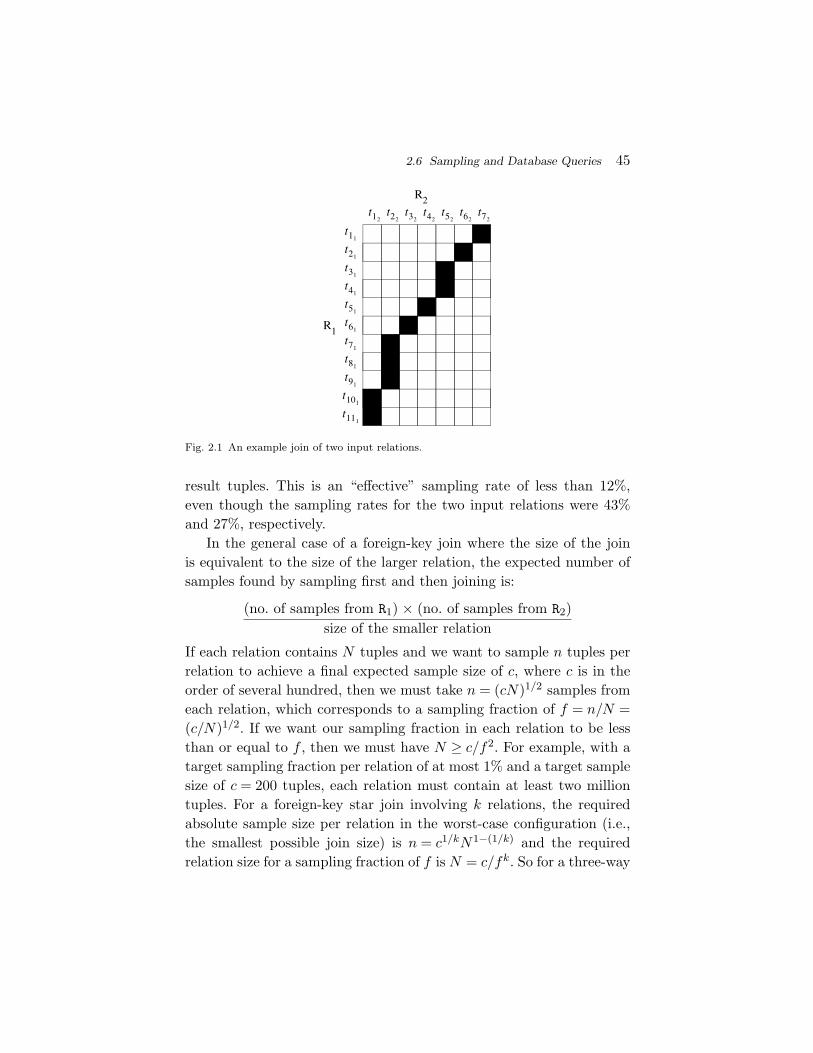
2.6 Sampling and Database Queries 45
R1
R2
t11
t21
t31
t41
t51
t61
t71
t81
t91
t101
t111
t12t22
t32t42
t52t62
t72
Fig. 2.1 An example join of two input relations.
result tuples. This is an “effective” sampling rate of less than 12%,even though the sampling rates for the two input relations were 43%and 27%, respectively.
In the general case of a foreign-key join where the size of the joinis equivalent to the size of the larger relation, the expected number ofsamples found by sampling first and then joining is:
(no. of samples from R1) × (no. of samples from R2)size of the smaller relation
If each relation contains N tuples and we want to sample n tuples perrelation to achieve a final expected sample size of c, where c is in theorder of several hundred, then we must take n = (cN)1/2 samples fromeach relation, which corresponds to a sampling fraction of f = n/N =(c/N)1/2. If we want our sampling fraction in each relation to be lessthan or equal to f , then we must have N ≥ c/f2. For example, with atarget sampling fraction per relation of at most 1% and a target samplesize of c = 200 tuples, each relation must contain at least two milliontuples. For a foreign-key star join involving k relations, the requiredabsolute sample size per relation in the worst-case configuration (i.e.,the smallest possible join size) is n = c1/kN1−(1/k) and the requiredrelation size for a sampling fraction of f is N = c/fk. So for a three-way
46 Sampling
join, each relation must have at least 200 million tuples. So clearlythe sample-then-join approach breaks down for foreign-key joins if therelations are not very large or if many relations are involved in the join.(See [154] for a detailed discussion of the effectiveness of sample-then-join in the setting of join selectivity estimation.) In any case, unlikethe single-relation scenario, the required absolute sample sizes are quitelarge, and grow with the size of the input relations.
This particular drawback of multi-relation sampling is widely recog-nized. One key idea in the database literature aimed at getting aroundthis problem is Archarya et al.’s proposal for using join synopses [4].Since most database queries make use of foreign key joins, Archaryaet al. propose the idea of (logically) pre-joining the database relationsacross those foreign keys, then drawing a sample of the resulting rela-tion. This sample (called a join synopsis) is maintained for use in AQP.Any multi-relation query which employs a subset of the pre-computed,foreign key joins in the join synopsis can then be re-written as a sin-gle relation query over the synopsis, thereby avoiding the inaccuracyincurred via the sampling of multiple relations. The drawback of thismethod is that it only handles those joins that are built into the joinsynopsis.
Another proposal for dealing with such hard cases is thestratification-based scheme called bifocal sampling proposed byGanguly et al. [103]. For each possible join key, this method first par-titions each relation into two subsets: those tuples with dense keys(appearing many times in the relation), and those with sparse keys(only appearing a few times). Samples are obtained from both sets.When joining two relations, the total aggregate value obtained by join-ing only those tuples with dense keys is estimated using the standardsample-then-join estimation procedure described in this section. Theintuition is that this is the “easy case,” where sampling followed by ajoin works quite well. Then the total aggregate value involving tupleswith sparse keys is estimated with the help of an index. That is, fora sampled tuple from R, the precise set of matching tuples from S islocated using an index, which effectively reduces the sampling pro-cess to single-relation sampling from R. The index is used becausesparse keys can be problematic when sampling and then joining: if an
2.6 Sampling and Database Queries 47
important key value which joins with many tuples from the other rela-tion is not included in the sample, then a severe underestimate is likely.In this way, the very hard case for sampling and then joining is avoided.
2.6.2 The Hard Case: Rel Ops that Do Not Commute
The reason that sampling “commutes” with the operations of selection,projection, joins, and grouping is that for such queries, whether onesamples first and then runs a query plan, or whether runs a queryplan and then samples, one can always derive an appropriate randomvariable of the form Xj1,j2,...,jm that controls the number of copies oftj1,j2,...,jm in the answer set. Furthermore, the statistical properties ofXj1,j2,...,jm depend only upon the sampling process, and not upon theactual data in the database. Thus, quantities such as the expected valueof Xj1,j2,...,jm are easily derived and HT estimators can be computed.
As discussed previously, this approach fails for certain types ofqueries. Consider the following antijoin example, which is similar tothe NOT IN example of Section 2.3:
SELECT SUM(EMP.SALARY)
FROM EMP WHERE NOT EXISTS (
SELECT * FROM SALES
WHERE EMP.ID = SALES.ID)
The problem here is that if one first samples EMP and SALES and thenruns the query, the statistical properties of the random variable Xi,which controls whether or not the ith tuple from EMP contributes tothe final sum, actually depend upon the data itself. If there are manytuples in SALES that match up with the ith tuple in EMP, then thistuple is more likely to be discounted via a match with some memberof the sample of SALES and Xi is more likely to be zero. If there arefew tuples in SALES that match up with the ith tuple in EMP, then Xi
is more likely to be non-zero.Thus, if one samples first and then runs the query, it is difficult
to characterize the random process that governs which tuples appearin the resulting “sample.” The end result is that for all practical pur-poses, the antijoin operation does not commute with sampling. Otheroperations, such as outer joins, duplicate removal, and semijoin are
48 Sampling
all closely related to antijoin — for example, the antijoin generalizesthe duplicate removal operation — and hence they share many of thedifficulties experienced when sampling for the result of an antijoin.
Although these operations do not commute with sampling, the situ-ation is not hopeless; sampling-based estimation for aggregation queriesis still possible. One cannot, however, simply apply these operationsto samples of the underlying relations and then scale up the finalanswer in a simple manner. More sophisticated estimation techniquesare required. We summarize some of the significant results from thedatabase literature below.
Sampling and Duplicate Removal. The most widely-studied ofthese “difficult” operations is the SQL DISTINCT operator (i.e., dupli-cate removal) over a single relation, in conjunction with the COUNT
aggregate. This is the so-called “COUNT-DISTINCT problem.” TheCOUNT-DISTINCT problem has received so much attention for a num-ber of reasons. First, a good solution to the COUNT-DISTINCT problemwould be of great utility in cost-based query optimization. It can beexpensive to compute the exact number of distinct values for a columnin a relation, and yet this quantity is of key importance when esti-mating the size of a join — hence, estimating the number of distinctvalues using a small sample is desirable. Second, when using samplingto estimate the answer to a GROUP BY query, it is always possible thatone or more groups may exist in the data, and yet no samples fromthe group have yet been obtained. Thus, an estimate for the number ofdistinct values for the grouping attribute/s would give a user an idea ofhow many such unseen groups still exist. Finally, in a ROLAP setting,estimating the size of a datacube — that is, the number of nonemptycells — for purposes of storage allocation often amounts to estimatingthe number of distinct combinations of dimension attributes present inthe underlying dataset.
Perhaps the earliest paper in the database literature to consider thisproblem is due to Hou et al. [171], where they suggest using Goodman’sestimator, which first appeared in the statistical literature in 1949 (seeSection 3.4 of Hou et al. for more details). The most widely-referenced
2.6 Sampling and Database Queries 49
paper in the database literature to consider this problem is due to Haaset al. [151]. In an extension of this paper, Haas and Stokes [155] combboth the statistical literature and the database literature and come upwith eight different estimators (including Goodman’s estimator), whichthey show can all be viewed as “generalized jackknife” estimators, andderive error formulas for such estimators. They then empirically testthe estimators on 47 different real datasets. They observe that for lowskew cases — that is, where the duplication factors for various distinctvalues do not differ widely — an “unsmoothed second-order jackknife”or a “stabilized” version of this estimator works best (see Shao [272]for an introduction to the jackknife). For high skew cases, an estimatorfrom the statistical literature (Schlosser’s estimator) works best. Theauthors therefore propose a hybrid estimator that combines the threeestimators. To use this estimator, the squared coefficient of variation ofthe distinct-value duplication factors is first estimated from the sample,and then one of the three estimators is selected accordingly.
Charikar et al. [44] note that there is a spectrum of instances forthe COUNT-DISTINCT problem; at one extreme there are those probleminstances with little or no skew (e.g., there is just one distinct value thatencompasses the entire dataset), and at the other there are those prob-lem instances with a tremendous amount of skew (there is one distinctvalue that encompasses most of the dataset, and a large number of val-ues with one tuple each). The problem is that with a small sample, noestimator can handle both cases well. Thus, an estimator must alwaysdo a poor job on one or the other, which sets a theoretical bound on theaccuracy of any COUNT-DISTINCT estimator. They go on to propose aquite simple estimator that meets this theoretical bound. This is calledthe “Guaranteed-Error Estimator.” They also propose a version of theGuaranteed-Error Estimator that is analogous to Haas et al.’s hybridestimator, with the additional goal of providing for a smooth transitionfrom the low-skew to high-skew case. Experiments show that this new,adaptive estimator works well in practice, though we have found thatthe relative performance of the various estimators is rather sensitiveto the accuracy criterion used. Overall, sampling-based estimation ofCOUNT-DISTINCT queries remains a very challenging problem.
50 Sampling
SUM Aggregates over Antijoins and Semijoins. Very few papershave tried to attempt sampling-based estimates for these more generalqueries. Jermaine et al. [190] consider the problem of sampling for two-relation, NOT IN queries (such as the EMP and SALES example givenabove), and characterize the bias of the estimator which samples thetwo input relations first, then joins the samples. They suggest thatone way to handle such queries in practice is to use an approach thatsamples the two input relations, then selects a few of the tuples fromthe outer relation (EMP in our example). For those tuples, exact countsof the number of matches in the inner relation are computed. Thisinformation is used to unbias the resulting estimate.
One problem with this approach is that it requires the use of anindex on the inner relation. In subsequent work, Joshi and Jermaine[195] consider estimation procedures for antijoins that do not requireany such index. An unbiased estimator is developed, which unfortu-nately has high variance. The authors therefore consider the applicationof a “superpopulation method” to the problem (see Sarndal, Section13.6 [268]) which first learns a generative model for the data, and thendevelops a biased estimator that happens to work well on datasets thatare generated using the learned model.
In the (somewhat biased!) opinion of the author of this chapter,sampling-based estimates for the answer to queries containing antijoins,semijoins, and other difficult operations is an under-studied prob-lem, and there are still many limitations in the state-of-the-art. Chiefamong those is that existing work is limited to antijoins or semijoins oftwo relations, and not to more complex query plans that contain otheroperations such as additional joins in the inner or outer query. Thus,we hope that more research attention will be paid to this problem.
2.6.3 Beyond SUM Aggregates
The final topic that we discuss with respect to SQL queries over sam-ples is the problem of estimating the answer to aggregate functionsother than SUM (and COUNT, which is nothing more than the aggregateSUM(1)). Our discussion largely follows Haas [144], who provides anin-depth discussion of estimating (and giving confidence bounds for)
2.6 Sampling and Database Queries 51
the AVERAGE, STD DEV and VARIANCE aggregate functions over multi-relation queries.
We begin by considering those aggregate functions that can bewritten as arithmetic functions of multiple SUM queries. These includeAVERAGE, STD DEV and VARIANCE.
Average. We first consider AVERAGE queries of the form:
SELECT AVERAGE(f(r1 • r2 • · · · • rm))FROM R1 AS r1 , R2 AS r2 , . . .
WHERE g(r1 • r2 • · · · • rm)
This can be written as the ratio of two individual SUM results. Thenumerator is:
SELECT SUM(f(r1 • r2 • · · · • rm))FROM R1 AS r1 , R2 AS r2 , . . .
WHERE g(r1 • r2 • · · · • rm)
And the denominator is:
SELECT SUM(1)
FROM R1 AS r1 , R2 AS r2 , . . .
WHERE g(r1 • r2 • · · · • rm)
Given this relationship, one obvious tactic is to estimate these twoquantities at the same time, using the same samples, to obtain two esti-mators which we call YSUM and YCOUNT. By dividing these two estimators,we obtain an estimator for the final AVERAGE. Fortunately, “ratio esti-mators” of this sort over samples result in an (approximately) unbiasedestimate for the final query result, and so YAVERAGE = YSUM/YCOUNT is gen-erally a high quality estimate for the actual query result. Not only is thisestimator approximately unbiased, but in practice it also has very lowvariance; typically much lower than the variance of either the numer-ator or the denominator. The reason is that since the two estimatesuse the same samples, they are highly correlated. If the numeratoroverestimates (or underestimates) the SUM, the denominator will alsooverestimate (or underestimate) the COUNT, and the resulting estimatemay still be high quality.
Although it is intuitively clear that the estimator YAVERAGE has lowvariance, actually computing this variance is challenging. The problem
52 Sampling
is the division operation in the estimator’s definition. Since the vari-ance of any estimator Y is E[Y 2] − E2[Y ], the variance of our AVERAGEestimator is written as
E
[Y 2SUM
Y 2COUNT
]− E2
[YSUMYCOUNT
].
The difficulty here is that YSUM and YCOUNT are themselves sums overmany different, correlated Xj1,j2,...,jm random variables, and so eachof the two terms in the variance is a ratio of two correlated, com-plex sums. One might obtain a reasonable estimator for E2[ YSUM
YCOUNT] by
squaring YSUMYCOUNT
, but dealing with E[ Y 2SUM
Y 2COUNT
] is particularly nasty, since itrequires computing the expected value of a ratio of two complicatedsquares.
Fortunately, there are some tools at our disposal for handling thisdifficult computation. The standard way that this is handled in statis-tics is via use of the so-called delta method, also known as Taylor lin-earization; see Sarndal [268, Section 5.5]. In our example, the techniqueuses a first-order Taylor series to remove the ratios from the variancecomputation. Specifically, write the AVERAGE estimator as
YAVERAGE = g(YSUM,YCOUNT) =YSUMYCOUNT
.
To apply the delta method, expand the function g(x,y) = x/y in a first-order Taylor series around the true query results QSUM and QCOUNT toobtain the approximation YAVERAGE ≈ YAVERAGE, where
YAVERAGE = g(QSUM,QCOUNT) +∂g
∂x(QSUM,QCOUNT) × (YSUM − QSUM)
+∂g
∂y(QSUM,QCOUNT) × (YCOUNT − QCOUNT)
=QSUM
QCOUNT+
1QCOUNT
(YSUM − QSUM) − QSUM
Q2COUNT
(YCOUNT − QCOUNT).
The justification is that for a sufficiently large sample size, YSUM andYCOUNT will be close to QSUM and QCOUNT, so that the Taylor serieswill be a good approximation. We then approximate the varianceof YAVERAGE by the variance of YAVERAGE. Computing the variance ofa linear function of random variables is relatively easy, using the
2.6 Sampling and Database Queries 53
fact that σ2(aX + c) = a2σ2(X) and σ2(X + Y ) = σ2(X) + σ2(X) +2Cov(X,Y ) for any random variables X, Y and constants a, c, where“Cov” denotes covariance. We obtain
σ2(YAVERAGE) =1
Q2COUNT
σ2(YSUM) +Q2
SUM
Q4COUNT
σ2(YCOUNT)
−2QSUM
Q3COUNT
Cov(YSUM,YCOUNT). (2.5)
We can compute the variances of YSUM and YCOUNT (somewhat tediously)as discussed in Section 2.6.1; the covariance computation is similar.When estimating σ2(YAVERAGE) from a sample, we replace the unknownconstants QSUM and QCOUNT in equation (2.5) by their estimates YSUM andYCOUNT.
Variance. VARIANCE is a trickier extension of AVERAGE, since the vari-ance of a set of values is the average squared value in the set, minusthe square of the average value in the set. To develop an estimator forthis quantity, we consider the following SUM query:
SELECT SUM(f2(r1 • r2 • · · · • rm))FROM R1 AS r1 , R2 AS r2 , . . .
WHERE g(r1 • r2 • · · · • rm)
We then define an estimator YSUM2 that is appropriate for this query.Given YCOUNT, YSUM, and YSUM2 , the following is a reasonable estimatorfor the query result:
YSUM2
YCOUNT− Y 2
SUM
Y 2COUNT
Note that this estimator may have some bias, because while the termYSUM2YCOUNT
is (nearly) unbiased for the average squared value of all tj1,j2,...,jm
in the data, and while YSUMYCOUNT
is (nearly) unbiased for the averagetj1,j2,...,jm in the data, squaring YSUM
YCOUNTdoes not necessarily result in
an unbiased estimate for the square of the average tj1,j2,...,jm . In fact,squaring an estimator generally results in an estimator with at leastsome upward bias; thus, in the authors’ experience the resulting, over-all estimator can underestimate the variance. However, as the samplingfraction increases, the bias shrinks and the resulting estimator is very
54 Sampling
reasonable. Just as in the case of AVERAGE, an estimate for the vari-ance of this estimator can be obtained via application of the Taylorlinearization method.
Standard Deviation. An estimator for the STD DEV aggregate isobtained by simply taking the square root of the estimator for AVERAGE.While this may induce some additional bias, it is also a reasonablechoice. Again, an estimate for the variance of the estimator can beobtained via the Taylor linearization method.
Median. Though MEDIAN is not one of the standard SQL aggregatefunctions (because it cannot always be evaluated in a single passthrough the dataset) it is quite common in practice, and it is alsoamenable to sampling. The obvious estimator is applied by simplyobtaining the median value of the items that have been sampled fromthe dataset. A procedure for estimating the variance of this estimator ismore involved; we point the reader to Sarndal et al. [268], Section 5.11for details of the variance computation in the case of a single relation.
Min and Max. Sampling for the MIN and MAX aggregate functions froma finite population is an exceedingly difficult task. The problem is thata dataset can define an arbitrary distribution, and without any prior orworkload knowledge it is virtually impossible to use a sample to guessthe largest (or smallest) value without inspecting every data item. Forexample, imagine that a relation contains the following values:
〈1,1,2,4,5,7,8,1010〉
Now, imagine a second relation that contains the following values:
〈1,1,1,7,12,19,36,45〉.
It should be clear that without domain knowledge, any estimator forthe MAX aggregate function which generally works well on a relationthat resembles the first instance will not work well on a relation thatresembles the second. The problem is that if an estimator works well onthe first type of dataset by scaling up some statistic that is computedover the sampled data items, it will (likely) radically overestimate theMAX value for the second type. By the same token, an estimator tailored
2.6 Sampling and Database Queries 55
for the second type of dataset would radically underestimate on thoseof the first type.
Given its difficulty, the problem has not been studied extensivelyin the database literature. The relevant statistical literature focusesmostly on estimation procedures for parametric distributions [212]. Theonly paper in the database literature which proposes using samplingfor aggregates of this form employs a so-called “Bayesian” estimator[241] that does, in fact, employ prior information to make the problemmore reasonable [293]. The basic idea is to first (offline) learn whatthe distribution of values in common queries tends to look like. Thiscan be done by looking at a historical query workload. For example,we might first construct a statistical model that says that one halfof the time, the set of tuples queried looks like the first relation; theother half of the time, the set of tuples queries looks like the second.Then, when a query is issued and a sample is obtained, the original,offline model is updated to take into account the new samples that havebeen obtained (this is a classic example of the Bayesian approach).This additional information can be used to construct a relatively high-quality estimator. For example, if, after taking five samples we obtain〈1,1,7,32,45〉, we might more accurately guess that we are in the secondregime, and so taking the largest value in the sample (45) will providea reasonable estimate for the query answer. If we determine that weare in the first regime, then we might estimate the MAX as being muchlarger than the largest sampled item.
Top-k. A top-k query computes the k most frequent values in a datasetR, along with their frequencies. The challenge is that simply taking thetop-k values in a random sample of size n and scaling the correspond-ing frequencies upward by a factor of |R|/n overestimates the truefrequencies of the top-k values, even though such a scale-up procedureunbiasedly estimates the frequency of any individual, specified valuein the data. This difficulty stems from the fact that the expectation ofthe maximum of a set of random variables (the frequency estimators) isgreater than the maximum of their expectations (the true frequencies).Cohen et al. [55] provide sampling and estimation procedures for thisproblem.

56 Sampling
2.7 Obtaining Samples from Databases
Thus far, we have focused exclusively on how one might make useof random samples from a dataset. We now consider the question ofhow one might obtain random samples from a dataset that is stored,for example, by a database management system on a modern harddisk. Specific topics include: tuple-based versus block-based sampling,sampling in a single pass from a relation, sampling from an index, andsingle-pass sampling in such a way as to take into account deletions.
2.7.1 Block-Based versus Tuple-Based Sampling
At the present time, most (large) datasets are stored on hard disks,and this situation will continue for at least the next few years. Thisfact is of fundamental importance in sampling, because hard disks aremechanical devices. To obtain a random tuple from the dataset (e.g.,when implementing SRSWoR), the disk head must physically be movedto the track containing the desired data, and the disk must spin untilthe desired tuple falls under the disk head before it can be transferredto the CPU. Because the moving parts in a hard disk are subject tothe laws of Newtonian physics, it is difficult to accelerate the disk headfast enough to cut the cross-disk “seek” time down under a few mil-liseconds. Furthermore, due to the huge forces involved in spinninga disk quickly, a full revolution of the disk will always require a fewmore milliseconds. This means that the process of obtaining an itemfrom a randomly-selected location on disk takes around three to fivemilliseconds, even for the fastest disks. Such considerations can oftenmake random sampling from a disk a very expensive proposition — at5 milliseconds per sample, this is only 200 samples per disk, per second.
One way around this problem is to obtain an entire block of datatuples at one time, as opposed to a single tuple. Datasets are naturallyorganized into blocks (or pages) that are atomic in the sense that ifone tuple from a page is read into main memory, then all of the tuplesare read into memory. The reason for such an organization is thatthe additional cost to read hundreds or thousands of tuples that areco-located with a given tuple is small or even negligible due to thedensity with which bits are written on the surface of the disk. In many
2.7 Obtaining Samples from Databases 57
applications, it is hard to justify wasting this data. In the remainder ofthis section, we refer to the tactic of obtaining an entire page or blockof tuples from a randomly selected location on disk (as opposed to asingle tuple) as block-based or block-level random sampling.
Obviously, block-based random sampling radically increases the rateat which data can be randomly sampled from disk. However, the Xj
random variables governing how many copies of each tuple are selectedvia block-based random sampling do not retain their statistical proper-ties vis-a-vis tuple-based sampling, and quite strange correlations canbe induced. For example, imagine that tuples are generally clusteredon disk via their insertion time into the dataset. This makes it morelikely that block-based sampling will select groups of tuples that wereinserted into the dataset at roughly the same time, which may alterthe statistical properties of any subsequent estimators.
Fortunately, this issue can be dealt with. Imagine that rather thanviewing a relation R as a pool of |R| tuples that may be sampled, therelation is viewed as a pool of |R|b blocks that might be sampled, andthe sampling process is used to select those blocks at random, ratherthan tuples. For example, to implement SRSWoR in order to obtain nblocks, we might run the following two steps, until n blocks have beenobtained:
(1) Produce a random number r from 1 to |R|b, inclusive.(2) If the rth block from the dataset has not been previously
added to the sample, then obtain this block and add it tothe sample.
Given such a sampling process, most of the estimators discussed thus far(most notably, the standard selection/projection/join/grouping estima-tor from Section 2.6.1) can be applied with only a slight modification.This is done as follows. Rather than letting tj1,j2,...,jm refer to the valueobtained after applying functions f , g, and h to the result of concate-nating tuple j1 from the first relation with tuple j2 from the secondrelation and so on (see Section 2.6.1), tj1,j2,...,jm instead refers to thetotal aggregate value obtained by applying f , g, and h to the crossproduct of all of the tuples in the j1th block from the first relation,the j2th block from the second relation, and so on. Specifically, let B(i)
j
58 Sampling
refer to the set of tuples in the jth block from the ith relation and letf ′(t) = f(t) if g(t) = true and h(t) = gid; otherwise, f ′(t) = 0. Then let
tj1,j2,...,jm =∑
t1∈B(1)j1
∑t2∈B
(2)j2
· · ·∑
tm∈B(m)jm
f ′(t1 • t2 • · · · • tm).
Also redefine Xj1,j2,...,jm to be the random variable that controlswhether the sample contains block j1 from relation 1, block j2 fromrelation 2, and so on. Given these redefinitions of tj1,j2,...,jm andXj1,j2,...,jm in terms of blocks rather than tuples, our prior discussionabout sampling for SUM, COUNT, AVERAGE, VARIANCE, and STD DEV overjoins and grouping formally applies without modification. Crucially,the analysis of variance and unbiasedness still holds without modifi-cation, and all of the estimation and variance computations formulashold as written (but with the new block-level interpretation). Perhapsthis result is not surprising, since we have merely redefined the blockas the atomic sampling unit.
The resulting estimator will usually be more accurate than if onlyone tuple is used from each sampled block. Furthermore, if the tuplesin each block are truly uncorrelated, then the extra accuracy gainedby using all of the data in a block or page can be very significant.A block or page may have hundreds or thousands of tuples. Since vari-ance generally decreases linearly with sample size in the case wheresamples are uncorrelated, using all of the tuples in a block can result ina thousand-fold decrease in variance for the same number of disk-headmovements.
We note, however, that block-based sampling is not always the pre-ferred retrieval method. We refer the interested reader to Haas andKonig, who carefully consider the issue [149]. For example, as theauthors point out, it may be that one is worried not just about thenumber of random seeks, but also about the CPU cost of processingall of the tuples in a block, which can sometimes be expensive. In thiscase, tuple-based sampling may be the better choice, or a hybrid schemethat samples blocks and tuples may be preferred. Also, the foregoingtrick — of simply redefining the estimation process so that it uses sam-pled blocks rather than sampled tuples — is only applicable when theunderlying computation makes use of summations over tuples that can
2.7 Obtaining Samples from Databases 59
be redefined as summations over blocks. For example, the computationunderlying a COUNT-DISTINCT query does not use such summations. Forsuch queries, the question of block-based versus tuple-based sampling ismuch more complicated. See Haas et al. [150] for a partial discussion ofhow to apply block-based sampling to the COUNT-DISTINCT problem.In general, current COUNT-DISTINCT estimators based on block-levelsampling schemes tend to be extremely variable; more work on thisproblem is needed. Finally, see Chaudhuri et al. [49] for other applica-tions of block-based sampling.
2.7.2 Sampling via a Full Scan
Compared to either block-based or tuple-based sampling, the fastestway to get data off of a disk is always via a sequential scan: first, thedisk head is moved to the beginning of the data file, and then data areread in sequence from start to finish. A sequential scan will typicallyread tuples from disk ten times as fast as a block-based algorithm, andpossibly tens of thousands as times as fast as a tuple-based algorithm.
The goal is to read all of the tuples in a file from start to finishsuch that, for any n ≥ 1, a size n random sample of the file is availableafter n tuples have been read. The problem, of course, is that the firstn tuples in a data file are likely not anything close to a random sampleof the tuples in the file. This situation is easily remedied if the datain the file have been randomly shuffled before the scan is started. Thisidea was pioneered by Hellerstein et al. [164] in their paper on “onlineaggregation.” To perform the required random shuffling, it is easiestto attach a random bit string to each tuple in the dataset. Then, anefficient, external sort (such as a two-phase, multi-way merge sort) isused to order the data so that they are sorted in ascending order of thisbit string. After the sort, the first n tuples in the file are equivalent to ntuples selected via SRSWoR. Another approach is to use spare computeresources to perform the required re-ordering in the background, so thatas new data are added, the random order is still maintained [260].
2.7.3 Sampling From Indexes
One of the difficulties associated with implementing tuple-based sam-pling is ensuring that tuples are selected with the correct probability.
60 Sampling
This can be non-trivial because each disk page may have a differentnumber of tuples on it. If one first selects a page at random, thenselects a random tuple from within the page, tuples on pages that havefewer tuples are more likely to be sampled. This can result in bias.
One way to overcome this problem is using an available indexingstructure to guide the sampling process. The pioneering work in thisarea is due to Olken and Rotem. In one paper, they consider howto use the structure of a hashed file to implement sampling so thateach tuple is selected with the appropriate probability [246]. In thatpaper, a number of accept/reject-based sampling algorithms are pro-posed. “Accept/reject” methods first locate a tuple at random, thencompute the probability of locating the tuple, and then decide ran-domly whether to accept or reject the random tuple. If the tuple has alarge probability of being located, then it is rejected with high proba-bility to compensate for the higher probability of being located.
In another paper, Olken and Rotem consider accept/reject algo-rithms for sampling from B+-Trees [244]. One problem with suchaccept/reject algorithms is that if things go poorly, many, many tuplesmay need to be located before any tuple is accepted for inclusion inthe sample. Antoshenkov [9] follows up Olken and Rotem’s B+-Treealgorithms and attempts to address the problem with accept/rejectsampling in this context by proposing the use of a “pseudo-ranked”B+-Tree. If a B+-Tree contains “rank” information (that is, each nodein the tree contains statistics on how many tuples are contained in eachof its subtrees) then sampling is quite easy, and an accept/reject algo-rithm is not needed. Specifically, a random number r from 1 to |R| isgenerated, and the rank information is used to locate the rth tuple inthe tree. But (as Antoshenkov points out) maintaining the rank infor-mation is costly when the tree is updated, because it requires updatesto all of the nodes from root to leaf at each and every insertion intothe tree. Thus, Antoshenkov proposes pseudo-ranked B+-Trees, whereonly bounding information on the number of tuples in each subtree isstored. If this bound is reasonably tight, then the vast majority of therejections can be avoided.
We close this subsection by noting that one very desirable charac-teristic of algorithms for sampling from B+-Trees is that they can be
2.7 Obtaining Samples from Databases 61
used for sampling directly from the result of a relational selection pred-icate, without having to sample the entire relation and then filter thesamples to obtain a sample of a desired size. For example, a databasemay store data corresponding to many years of retail sales, but a userquery might focus on only two days’ worth of data. If the tuple times-tamps are indexed by a B+-Tree, it is possible to use the structureof the tree to sample directly from those two days. Any branches ofthe tree falling outside of the desired range are treated as having zerotuples, and the accept/reject or ranked sampling algorithm is modifiedaccordingly.
2.7.4 Sampling From Tuple Streams
Most of the methods discussed thus far for drawing a sample from adataset have assumed that the dataset is fully materialized and thegoal is to draw a single tuple at random. A larger sample is drawn viarepeated invocations of the sampling algorithm. This is not always thecase. It may be that the data are treated as a “stream,” where the goalis to maintain a sample of all of the data that have been encounteredthus far, or to maintain data structures that allow a sample to beproduced once the last tuple from the stream as been encountered.Such a stream-based scenario is relevant when the data flow throughthe system at high speed without ever being stored on disk [74]. Itis also relevant when one wishes to draw a sample of non-trivial sizefrom a data file, so it is better to draw the sample in batch in a single,sequential pass rather than via a large number of random accesses.
In this subsection, we give only the briefest overview of stream-basedsampling algorithms. For a more detailed treatment, we refer the inter-ested reader to Haas’ chapter, “Data-Stream Sampling: Basic Tech-niques and Results,” in Garofalakis et al.’s book on data stream pro-cessing [106], as well as to the recent PhD dissertation of Gemulla [112].
Certain stream-based sampling algorithms are trivial. For example,Bernoulli (or Poisson) sampling over a stream in one pass is easy. Sup-pose that the inclusion probability for the jth tuple is pj . As this tuplepasses by, we need only simulate a coin-flip where the probability ofseeing “heads” is pj . If a heads is obtained, the tuple is added to the

62 Sampling
sample. Otherwise, the sample is ignored. Rather than simulating indi-vidual coin flips, we can speed up the algorithm by simulating thegaps between subsequent acceptances: at each acceptance, the algo-rithm simulates the gap until the next acceptance — which can bedone quite easily — and then essentially “goes to sleep” until the nextaccepted tuple arrives.
Perhaps the most classic stream-based sampling algorithm is theSRSWoR algorithm for a data stream of unknown size, which is knownas the reservoir algorithm. The basic idea was proposed at least onceor twice in the early 1960s; see, for example, Fan et al. [94] and their“method 4.” It was then refined and made popular in the computer sci-ence research literature by Vitter [283]. The underlying concept is quitesimple, and many variations are possible, each with its own performancecharacteristics. The algorithm starts by selecting the first n tuples fromthe input stream and putting them into an array called the “reservoir.”These tuples are trivially a size-n “random sample” of the tuples seenso far. Subsequently, when the ith tuple in the stream arrives (i > n),the tuple is accepted into the reservoir with probability n/i, replacinga randomly chosen reservoir element; with probability 1 − (n/i), theith tuple is ignored. It can be shown that, at any time during process-ing, the contents of the reservoir form a uniform, size-n random sampleof all tuples seen so far. (A sampling scheme is uniform if any twopopulation subsets of the same size are equally likely to be output bythe scheme; samples produced by a uniform sampling scheme are alsocalled “uniform.”) Vitter shows how the algorithm can be speeded upby simulating the gap between acceptances, as described for Bernoullisampling; in the current setting however, simulating the gap is far fromtrivial, and accept/reject techniques are needed.
Several variations of the reservoir algorithm have appeared in thedatabase literature. Brown and Haas [27] consider use of the reservoiralgorithm for sampling in parallel from multiple streams. Several papers[113, 191] consider the case when the sample to be maintained is toolarge to keep in memory, and must be stored on disk.
Another widely-known stream-based sampling algorithm from thedatabase literature is the algorithm for producing concise samples andits close cousin, the algorithm for producing counting samples [124].
2.7 Obtaining Samples from Databases 63
Both of these algorithms attempt to produce a bounded-size, com-pressed representation of a uniform sample, where not only is eachsampled tuple included in the representation, but information on thenumber of repetitions in the stream is also represented. In the extremecase where only a few values ever appear in the stream, these samplingalgorithms may not even need to sample at all, and the entire streamcan be summarized via a set of (tuple, count) pairs.
A unique problem when sampling from a data stream in a dynamicenvironment is that the data stream may also contain deletions of exist-ing data, as well as insertions of new data. This is especially relevant ifthe goal is to maintain a sampling-based synopsis of a large dataset inan online fashion by only monitoring the insert/delete stream, so thatat any instant, one always has access to a sample of the current versionof the underlying dataset without having to look at any of the basedata.
Gemulla et al. [115, 117] have provided a state-of-the-art algorithmfor maintaining a bounded-size SRSWoR from a data stream in a singlepass while allowing both insertions and deletions. Bounded-size samplesare desirable because they reduce the complexity of memory manage-ment and allow control of the computational costs for algorithms thatuse the samples. The authors propose a “random pairing” (RP) algo-rithm, assuming that the data size is relatively stable. The idea is to“compensate” for prior deletions by pairing each inserted tuple withan “uncompensated” prior deletion. In more detail, when a deletionis encountered, the RP algorithm removes the tuple from the reser-voir, if it is present. If the deleted tuple is present, a counter c1 isincremented; if it is not, c2 is incremented. If both counters equal 0just before a new insertion is encountered, the insertion is processedaccording to the classical reservoir algorithm. Otherwise, the insertionis randomly “paired” either with a “bad” prior deletion that resultedin a tuple being removed from the reservoir or with a “good” deletionthat did not affect the reservoir; the respective pairing probabilities arec1/(c1 + c2) and c2/(c1 + c2). If the new insertion is paired with a baddeletion, it is added to the reservoir, so that the reservoir size increases,and c1 is decremented by 1. If the new insertion is paired with a gooddeletion, it is not added to the reservoir and c2 is decremented by 1.
64 Sampling
In a later paper [116], the authors consider the problem of maintaininga Bernoulli sample over a multiset in the presence of insertions anddeletions.
A problem that has plagued the literature in this area is that somestreaming algorithms which attempt to bound the sample size (includ-ing some of the foregoing algorithms) introduce subtle departures fromthe asserted uniformity of the samples. The problems usually arise fromattempts to combine Bernoulli sampling — which has unbounded sam-ple size — with a bounding step that involves ideas such as periodicallypurging the Bernoulli sample or switching over to reservoir samplingwhen the sample sizes hits an upper bound. Nonuniformity for the con-cise/counting samples previously mentioned and for a scheme called“Bernoulli sampling with purging” is demonstrated in [27] and [112,Section 3.5.1B], respectively. The “hybrid Bernoulli” (HB) scheme in[27] and a “random pairing with resizing” (RPR) algorithm given in[115, 117] (designed to extend the RP algorithm to handle datasetsthat grow over time), also can be shown to suffer from this drawback.
One general approach for handling this problem is to settle forprobabilistic bounds on the sample size that are exceeded with verysmall probability. Alternatively, the nonuniformity problem for the HBscheme can be eliminated for an insertion-only stream by suitably ran-domizing the time at which a switchover to reservoir sampling starts.Gemulla [112, Section 4.2] shows that the RPR scheme can also berepaired. The basic idea when enlarging a sample from size n to size n′
(> n) is to initially convert the sample to one that is statistically equiv-alent to a sample produced by an RP scheme with maximum samplesize n′ and d uncompensated deletions. (Here d is a parameter of theresizing algorithm.) This conversion requires access to the base data,but the author shows that any resizing algorithm must involve suchaccess. After the initial conversion, the RP algorithm is run until thenumber of uncompensated deletions drops to 0, which implies that thesample size is equal to n′. The parameter d can be chosen to optimizethe trade-off between the cost of accessing the base data and the costof waiting for new stream elements to arrive.
The discussion so far has focused on uniform samples, but it isoften desirable to obtain a sample from a stream in a biased way.
2.8 Online Aggregation Via Sampling 65
For example, Babcock et al. [14] consider how to maintain a sampleof the k most recent tuples from the stream. This involves expiringdata that were included in the sample but are not in the k most recenttuples. Aggarwal [5] considers how to decay the inclusion probabilityof each tuple as new tuples arrive in the stream, so that with highprobability, only the most recent tuples are included in the sample. Inthis work, the “recency” of a tuple t is defined in terms of the numberof tuples that have appeared since t passed by on the stream. Gemullaand Lehner [114] consider the obvious question of how to maintain asample when the “recency” of t is defined in terms of the time that haspassed since t first appeared on the stream. This is challenging, sincethe rate at which tuples appear over time can change. If t arrives ata time when many tuples have recently arrived, but then (over time)fewer and fewer tuples show up, t will have its inclusion probability riseover time. This means that it is not acceptable to simply throw out allof the tuples that are not immediately included in the sample, and soit is not possible to guarantee a particular sample size using boundedspace. In response to this, the authors develop a sampling scheme thatworks using bounded space, and does provide a lower bound on theexpected sample size. Other interesting schemes for biased samplinghave been proposed in the setting of network monitoring and relatedproblems; see [54] and references therein.
2.7.5 Materialized Sample Views
Finally, we mention the problem of trying to maintain a materializedsample view in the presence of updates to the dataset. Just as a mate-rialized view is a pre-computed query result for some important query,a materialized sample view is a materialized sample from the queryresult for some important query. Perhaps the best sources for infor-mation on this problem are Olken’s PhD thesis [242] and Olken andRotem’s paper on the subject [245].
2.8 Online Aggregation Via Sampling
We close the chapter on sampling with a brief discussion of online aggre-gation. One of the key advantages of sampling is that it is additive: if
66 Sampling
one obtains a small sample, then adds some data to it, one obtainsa larger (and presumably more accurate) synopsis of the base data.This means that if a user is not happy with the accuracy incurredvia a sampling-based estimate, then more data can be added to thesample via an incremental procedure, and the estimate can be com-puted once again. Indeed, the process of adding more data and thenre-estimating the query answer can be repeated again and again untilthe desired accuracy has been obtained; this process is known as onlineaggregation. The ability to support online aggregation is quite uniqueto sampling. The assumption which generally underlies online aggre-gation is that data are randomly shuffled on disk, so that an efficientrelation scan can obtain random samples of larger and larger size. Incontrast, other AQP methods such as wavelets, sketches, etc., are “oneand done” methods — if the estimate obtained is not accurate enough,then the user has no recourse except to create a larger synopsis, usuallyat great expense.
The idea of online aggregation was first proposed by Hellersteinet al. in their 1997 paper [164]. The goal was to provide quick inter-active access to large datasets, allowing the user to determine on thefly whether the current query results were “sufficiently” accurate; if so,then the query could be terminated, thereby letting the user get onto their next interactive query. In their original paper, they consideredsingle-relation queries with (possibly) a GROUP BY thrown in. One ofthe key technical innovations of the original online aggregation paper(originally suggested by M.R. Stonebraker) is the idea of “index strid-ing,” where the convergence of the different groups to the true queryanswer is controlled by using an index to sample from the differentgroups at different rates. This is in contrast to the obvious way of han-dling a GROUP BY query: drawing a single sample without regard to thegrouping operation, and then applying a series of different estimatorsto the sample, with one estimator for each group — a group’s estimatorassigns zero values to all of those tuples that do not belong to its group.
Later, Haas and Hellerstein extended their idea to multi-relationqueries [146, 147], and they proposed the idea of a ripple join. In aripple join of two relations R and S, a group of random tuples are first
2.8 Online Aggregation Via Sampling 67
read from R, then a group of random tuples are read from S. Thesetuples are joined, and an estimate is produced. Then another groupof tuples are read from R; all of the tuples read thus far from R arejoined with all of the tuples read thus far from S, and another estimateis produced. Next, another group of tuples are read from S; all tuplesread thus far from S are joined with all tuples read thus far from R,and another estimate is produced. This process is repeated until allof the tuples from R and S have been joined. The sampling rates aredynamically adjusted to that sampling effort is biased toward the inputrelation with the most variable data. The basic idea of a ripple joinwas later extended so that the ripple join was applicable in a paralleldatabase environment [218].
One big problem with the ripple join is that it is not scalable — itonly works if the results become sufficiently accurate quickly, so thatthe query can be aborted very early on. The whole algorithm relies onobtaining a few more tuples from an input relation, and then beingable to efficiently join those tuples with all of the tuples obtained thusfar from the other input relation. In practice, this means storing eachrelation in a hash table, and probing the hash table for matches whennew tuples are read into memory. Unfortunately, this does not work ifthe tuples read thus far from both relations can not be stored in suchan in-memory hash table due to the amount of data. In such a case,the ripple join must go to disk to find matches for new tuples, which isan exceedingly expensive proposition.
In response to this issue, Jermaine et al. propose a system for onlineaggregation called DBO that uses a whose sequence of ripple joins intandem with a full query evaluation plan [188]. Every time that mainmemory fills with tuples, another ripple join estimate is produced andused to increase the accuracy of the current estimate for the queryresult. Then, all of those tuples are sorted and written back to diskas part of a sort-merge join. As new data are read, main memoryagain fills and another ripple join estimate is produced. Again, this esti-mate is incorporated into the current estimate for the ultimate queryresult. Those tuples are again sorted and written back to disk. This isrepeated until all of the input relations have been broken into sorted
68 Sampling
runs. Furthermore, the sort-merge joins make use of a randomized sortorder, so that the merge phase of each sort-merge join outputs tuples inrandom order. Thus, those tuples can be used as input for ripple joinshigher up in the query plan. In this way, it is possible to obtain tighterand tighter estimates via additional ripple joins throughout query pro-cessing, up until the time that the final answer is produced.
3Histograms
The histogram is a venerable and well studied dataset synopsis, usedin a wide variety of modern computer systems. In the database setting,histograms have been an integral component of query optimizers sinceat least the mid-1990s [43, p. 662], and are often used by the infor-mation management and statistical communities for purposes of datavisualization. So far, histograms have not been used extensively forapproximate query processing in commercial systems, but have greatpotential for this purpose. As a consequence, histogram-based approx-imation techniques have been extensively studied by the databaseresearch community; the AQUA system for approximate query pro-cessing developed at Bell Laboratories [125] is a notable example ofa research prototype. A renewed surge of interest in histogram tech-niques has been driven by the networking community, who need small-space synopses to summarize patterns in packet traffic, in order toreduce congestion, detect denial-of-service attacks, and so forth. Thisnew generation of histograms must contend with stringent space andtime requirements, as well as the ever shifting statistical characteristicsof streaming data.
69
70 Histograms
As discussed in the review paper of Ioannidis [179], use of histogramsand bar charts for data summarization and visualization goes backto the 18th century, and the term “histogram” itself was coined bystatistician Karl Pearson in the 1890s. Histograms have been studiedin the database literature for over 25 years, starting with the paper ofPiatetsky-Shapiro and Connell [251]. Not surprisingly then, the statis-tical and database literature on histograms is enormous. As with otherapproximation techniques, we do not attempt to give an exhaustivesurvey. Rather, we focus on distinguishing those aspects of histogramsthat are pertinent to AQP; key themes of our development are theadoption of a model-free point of view and the generalization of thenotion of a histogram far beyond its classical origins. Our emphasisthroughout is on those results and techniques that appear to have thegreatest potential for practical use.
In the remainder of this chapter, we first introduce the key issuespertinent to histograms via a discussion of several simple, classicalhistograms, and delineate some important differences between thestatistical and database viewpoints. We then focus on the use ofone-dimensional (1D) histograms for approximate query answering,especially for “range-sum” queries, for example, queries that specifythe number of data items having values in a specified range. Althoughmulti-dimensional histograms and general queries are of primaryimportance in our setting, a careful discussion of 1D-histograms isworthwhile because of their relative simplicity, well-developed theory,and historical importance. Moreover, techniques developed for 1D-histograms often appear as components of more elaborate algorithmsfor multi-dimensional histograms. We then discuss multi-dimensionalhistograms and approximate answering of general queries. It will beapparent from our discussion that 1D-histograms for range sums havereceived a disproportionate share of attention in the literature; perhapsby highlighting the relative paucity of results on multidimensionalhistograms and general queries, we will inspire further research onthese challenging but important topics. We conclude the chapterby discussing histograms over streaming data, as well as specializedtechniques for real-valued data.
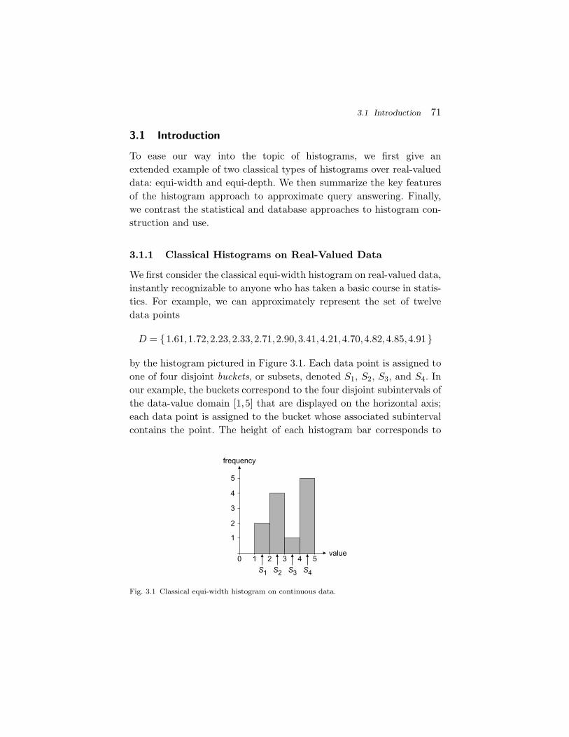
3.1 Introduction 71
3.1 Introduction
To ease our way into the topic of histograms, we first give anextended example of two classical types of histograms over real-valueddata: equi-width and equi-depth. We then summarize the key featuresof the histogram approach to approximate query answering. Finally,we contrast the statistical and database approaches to histogram con-struction and use.
3.1.1 Classical Histograms on Real-Valued Data
We first consider the classical equi-width histogram on real-valued data,instantly recognizable to anyone who has taken a basic course in statis-tics. For example, we can approximately represent the set of twelvedata points
D = 1.61,1.72,2.23,2.33,2.71,2.90,3.41,4.21,4.70,4.82,4.85,4.91
by the histogram pictured in Figure 3.1. Each data point is assigned toone of four disjoint buckets, or subsets, denoted S1, S2, S3, and S4. Inour example, the buckets correspond to the four disjoint subintervals ofthe data-value domain [1,5] that are displayed on the horizontal axis;each data point is assigned to the bucket whose associated subintervalcontains the point. The height of each histogram bar corresponds to
0 1
1
2
2
3
3
4
4
5
5value
frequency
S1 S2 S3 S4
Fig. 3.1 Classical equi-width histogram on continuous data.

72 Histograms
the number of points that fall in the associated bucket, that is, to thefrequency for the bucket.
This histogram is specified by the lower boundary of the leftmostbucket (1.0), the bucket width (1.0), and the four frequency countsfor the four buckets (2, 4, 1, 5). Although, in this example, the datahas merely been reduced from twelve numbers to six numbers, it isclear that the degree of compression can be much higher, for example,a similar histogram representing 106 points having values between 1and 5 would still be represented by six numbers. Clearly, the histogramis a lossy representation of the data.
If the bucket boundaries are specified a priori (and hence are knownto bracket the data values), then the histogram can be constructed dur-ing a single pass through the data, using four counters to compute thebucket frequencies. Thus the histogram requires O(1) time per item —or O(N) time in total — and O(B) space to construct, where N isthe number of data values and B is the number of buckets. Also notethat the histogram is easy to maintain in the presence of insertions anddeletions: simply determine the bucket associated with an insertion ordeletion transaction, and increment or decrement the correspondingcounter as appropriate.
Suppose that we are given the histogram in Figure 3.1 and wish toestimate the number of points N whose values lie between 1.1 and 4.5.This corresponds to a range-count query that can be expressed in SQLsyntax as
SELECT COUNT(*) FROM D WHERE D.val >= 1.1 AND D.val <= 4.5
Clearly, the contribution from the buckets S2 and S3 to the queryanswer are four points and one point, respectively, and these num-bers are exact. The computations for these buckets are easy since theyare completely contained within the query range [1.1,4.5]. The prob-lem is to estimate the contributions from the buckets S1 and S4, eachof which partially overlaps the query range. A standard approxima-tion is the continuous-value assumption, which simply assigns a countby multiplying the bucket frequency by the fraction of the bucketinterval that lies within the query range. In our example, the frac-tion of the S1 and S4 intervals that lie within the query range are
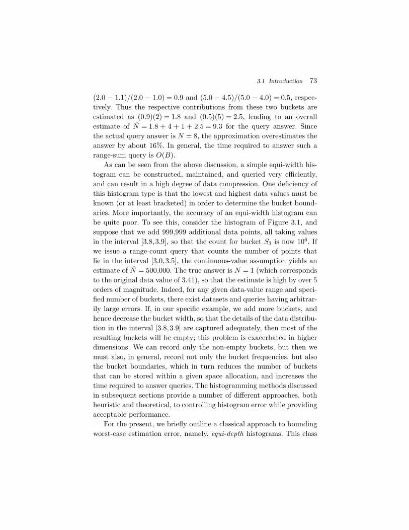
3.1 Introduction 73
(2.0 − 1.1)/(2.0 − 1.0) = 0.9 and (5.0 − 4.5)/(5.0 − 4.0) = 0.5, respec-tively. Thus the respective contributions from these two buckets areestimated as (0.9)(2) = 1.8 and (0.5)(5) = 2.5, leading to an overallestimate of N = 1.8 + 4 + 1 + 2.5 = 9.3 for the query answer. Sincethe actual query answer is N = 8, the approximation overestimates theanswer by about 16%. In general, the time required to answer such arange-sum query is O(B).
As can be seen from the above discussion, a simple equi-width his-togram can be constructed, maintained, and queried very efficiently,and can result in a high degree of data compression. One deficiency ofthis histogram type is that the lowest and highest data values must beknown (or at least bracketed) in order to determine the bucket bound-aries. More importantly, the accuracy of an equi-width histogram canbe quite poor. To see this, consider the histogram of Figure 3.1, andsuppose that we add 999,999 additional data points, all taking valuesin the interval [3.8,3.9], so that the count for bucket S3 is now 106. Ifwe issue a range-count query that counts the number of points thatlie in the interval [3.0,3.5], the continuous-value assumption yields anestimate of N = 500,000. The true answer is N = 1 (which correspondsto the original data value of 3.41), so that the estimate is high by over 5orders of magnitude. Indeed, for any given data-value range and speci-fied number of buckets, there exist datasets and queries having arbitrar-ily large errors. If, in our specific example, we add more buckets, andhence decrease the bucket width, so that the details of the data distribu-tion in the interval [3.8,3.9] are captured adequately, then most of theresulting buckets will be empty; this problem is exacerbated in higherdimensions. We can record only the non-empty buckets, but then wemust also, in general, record not only the bucket frequencies, but alsothe bucket boundaries, which in turn reduces the number of bucketsthat can be stored within a given space allocation, and increases thetime required to answer queries. The histogramming methods discussedin subsequent sections provide a number of different approaches, bothheuristic and theoretical, to controlling histogram error while providingacceptable performance.
For the present, we briefly outline a classical approach to boundingworst-case estimation error, namely, equi-depth histograms. This class
74 Histograms
0 1.6
1
2.3
2
3.4
3
4.8
4
5value
frequency
S1 S2 S3 S4
Fig. 3.2 Equi-depth histogram on continuous data.
of histograms — first proposed in the database literature by Piatetsky-Shapiro and Connell [251] — selects bucket boundaries so that eachbucket contains the same number of data points. Selecting bucketboundaries for N data points and B buckets is essentially equivalentto computing the (N/B)-quantiles of the dataset. Figure 3.2 displaysa 4-bucket equi-depth histogram for the dataset D given above. (Notethat the equi-depth representation is not unique in general.) For sucha histogram, one must store the lower boundaries of each bucket, theupper boundary of the rightmost bucket, and the total number of datapoints. Using the equi-depth histogram together with the continuous-value assumption, the estimated answer to the previous range-countquery on [1.1,4.5] is N = 3 + 3 + ((4.5 − 3.4)/(4.8 − 3.4))3 = 8.4, andthe overestimation error is now only about 5%. More importantly, weknow that the estimated answer to any range-count query can be offby at most ±6, since at most two buckets can partially overlap thequery range, and each bucket can erroneously include or exclude atmost 3 points. More generally, for a B bucket equi-depth histogramand any query that selects at least 100s% of the data points, the errorin the query answer is at most ±(200/(sB))%. Thus we can control theworst-case error for a large class of queries and datasets.
We pay a price, however, for the increased control: to construct thehistogram, one either has to sort the data or use a quantile-computationalgorithm. The former approach is expensive for large datasets,requiring Ω(N) space — typically unacceptable in practice — for an
3.1 Introduction 75
in-memory sort of a dataset containing N points, and otherwise requir-ing multiple passes over the data for an external sort. Specialized algo-rithms for directly computing quantiles are similarly expensive. Indeed,Munro and Paterson [233] have shown that, for any such algorithm,at least Ω(N) memory is required to compute a specified quantile ina single pass. The memory requirement can be reduced to O(N1/p)at the expense of requiring p passes through the data, which is alsotypically unacceptable. One must therefore resort to approximate com-putation of quantiles. Greenwald and Khanna [131], for example, givean algorithm that computes an ε-approximate quantile, that is, an ele-ment whose rank r′ is within ±εN of the nominal rank r. The spacerequirement of this algorithm is O(ε−1 log(εN)). Various versions of thequantile-digest algorithm [68, 167] can also be used in this setting. See[296] for a recent literature review.
3.1.2 Key Issues for Histograms
We see from the foregoing discussion that a histogram is obtained bypartitioning the dataset into buckets (i.e., subsets) and, for each bucket,storing summary statistics about the data values in the bucket. Infor-mation about the buckets themselves, such as bucket boundaries, isalso stored. At query time, the summary and bucket information isused to (approximately) reconstruct the data in the bucket in orderto approximately answer the query. Important aspects of a histograminclude:
• Bucketing scheme As discussed in the sequel, buckets neednot be disjoint in general, and may even be recursive, in orderto better capture the structure of the data. Data items canbe assigned to buckets based on local considerations such assimilarity of values or value frequencies, or on broader criteriasuch as “global optimality” of the histogram with respect toa workload or specified class of queries.
• Statistics stored per bucket In our examples so far, the onlyinformation stored for a bucket is the number of points inthe bucket, together with information about bucket bound-aries. The choice of which information to store is usually
76 Histograms
determined by the method used to approximate the datavalues in the bucket. As discussed previously, there is a trade-off between the amount of information stored per bucket andthe number of buckets that can be maintained.
• Intra-bucket approximation scheme The only scheme dis-cussed so far has been the continuous-value assumption forfrequency counts, but many other approaches are possible.The approximation scheme also depends on the class ofqueries that the histogram is being used to answer.
• Class of queries answered Historically, much of the focushas been on answering range-count queries of the type dis-cussed above, as well as point-count queries (or simply pointqueries) for discrete data, such as
SELECT COUNT(*) FROM D WHERE D.color = ’red’
Such queries correspond to “selectivity estimation” queriesthat are used extensively in database query optimizers. Morerecently, there has been increasing interest in approximateanswers to online analytical processing (OLAP) queries andgeneral SQL queries.
• Efficiency Here efficiency refers to the space and timerequirements for constructing the histogram, as well as thecost of using the histogram to approximately answer a query.The space requirements, in particular, can determine whetheror not use of a given histogram is practically feasible — forsome histograms the space needed for construction exceedsthe size of the data itself. The construction costs depend onhow the data is accessed; we distinguish between “datacube”and “relational” access models for discrete data, as definedin Section 3.2.2.
• Accuracy The goal is usually to give the most accurateanswers possible, given a constraint on the allowable size(in bytes) of the histogram. Many different notions of accu-racy have been proposed, and much research has gone intoproducing histograms that are “optimal” in the sense ofhaving the smallest approximation error subject to a size
3.1 Introduction 77
constraint. Especially in the case of 1D-histograms and inthe context of selectivity estimation for query optimization,many of the different histogram types discussed in the sequelhave similar (and practically acceptable) accuracies, providedthat the histograms are allocated “sufficient” storage space;for example, the experiments in [286] indicate that, for 1D-histograms, the marginal benefits of increasing the bucketcount diminish sharply beyond about 20 buckets. The dif-ferences are more marked for multi-dimensional histograms,and even 1D-histograms might only be allocated a smallamount of memory if many histograms are being maintainedin parallel; see, for example, the discussion of a “synop-sis warehouse” architecture in [19, 27]. Also, the precisionrequirements might be higher for general approximate queryanswering than for the special case of selectivity estimation inthe context of query optimization (where many other sourcescontribute to the uncertainty of a query-plan cost estimate).Because approximate query-answering systems are not yet inwide use, there is a paucity of practical guidance on accuracyrequirements.
• Error estimates This issue is closely related to, but differ-ent from, the issue of histogram accuracy. Since histogramsyield approximate query answers, it is highly desirable to pro-vide the user with tight error bounds for the specific queryof interest. Some histogram construction methods provide aguarantee on the overall “average” error over a set of queries,which does not yield a useful error estimate for an individualquery, or on the maximum error over a class of queries, whichusually provides a query-specific error estimate that is tooloose. Similarly, some methods guarantee that the histogramis optimal (or ε-close to optimal) for a class of queries, butagain this does not yield individual error estimates.
• Incremental maintenance Especially when summarizinghigh-speed data streams, it is often important to efficientlyupdate a histogram in the presence of insertions to anddeletions from the dataset.
78 Histograms
3.1.3 Statistical versus Database Viewpoint
In the statistics literature, histograms originally were used simply tosummarize and visually represent data. More recently, however, his-tograms have often been viewed as nonparametric density estima-tors [270]. That is, the dataset is modeled as a collection of independentand identically distributed (i.i.d.) samples from an unknown probabilitydensity function f , and the histogram is a piecewise-constant approx-imation of f . (The estimation problem is “nonparametric” in that fis not assumed to lie in any particular parametric family of distribu-tions such as the normal, exponential, or gamma families.) A typicalproblem in this setting is to choose bucket widths in a one-dimensionalequi-width histogram to minimize the mean integrated squared error,defined as
MISE = E
[∫[f(x) − f(x)]2 dx]
],
where E is the expectation operator and f is the piecewise-constanthistogram approximation to the density function. (Note that f , beingcomputed from random samples from f , is viewed as a random func-tion, and hence the expectation operation appears in the definitionof MISE.) If, for example, the number of data points N is large, fis twice differentiable, and the first derivative f ′ is square integrable,then the MISE is minimized by choosing the bucket width equal tocN−1/3, where the constant c = c(f) depends on the specific form of f .Scott [270] describes various data-based bounds and approximationsto the unknown constant c(f). In general, there are better, smootherapproximants to f , including frequency polygons, averaged shifted his-tograms, and kernel density estimators.
In contrast, the database literature almost always takes a model-free point of view, considering the data that is present in the databaseas the only data of interest.1 The goal is simply to obtain a low-errorcompressed representation of the dataset. As discussed in Section 3.7.2,however, direct application of statistical histogramming techniques to
1 We assume throughout that data values are known with certainty; see Cormode et al. [62]for a discussion of histograms over uncertain data.
3.2 One-Dimensional Histograms: Overview 79
real-valued data sometimes leads to good estimation accuracy, even inthe absence of a rigorous statistical model.
Another key difference between the two points of view is that thevast majority of enterprise database applications center on discretedata, that is, discrete numerical data or categorical data. Without lossof generality, we can take the domain of a discrete attribute to be aset of integers of the form U = 1,2, . . . ,M . We often use intervalnotation and denote this set by [1,M ]; this is convenient since bucketsare often defined via disjoint segments of [1,M ], analogous to the par-titioning of the real line as in Figure 3.1. For discrete numerical data orordered categorical data, there is usually a natural mapping of the dis-crete values to the integers, for example, day-month-year data can beexpressed in terms of the number of days elapsed since a fixed referencedate. In principal, we can also map unordered categorical data to inte-gers, since the queries of interest in this setting are point queries so thatthe mapping can be arbitrary. Maintaining histograms on unorderedcategorical data is problematic, however, because an index is needed tomap each categorical value to a histogram bucket; the space and query-time requirements for such a mapping index are typically unacceptablein practice. We henceforth reserve the term “discrete data” for datawhose domain has a natural mapping to the integers. Note that real-valued data can also be mapped to the integers by discretizing, but,as discussed in Section 3.7.2, methods that are especially tailored toreal-valued data tend to have superior performance. Conversely, tech-niques developed for real-valued data can have inferior performance inthe discrete setting.
3.2 One-Dimensional Histograms: Overview
In the next few sections we study 1D-histograms in the setting of AQP.Except for Section 3.7.2, we focus on discrete data.
3.2.1 Basic Notation and Terminology for 1D-Histograms
As discussed above, we can think of a multiset D of discrete dataas having domain U = [1,M ], and we denote by f(i) the number ofpoints in D having value i ∈ U , that is, the frequency of value i. The
80 Histograms
queries considered so far have focused on computing counts, that is,sums of frequencies, over regions of the domain of data values. In orderto encompass not only multisets of discrete data, but also a range ofimportant applications including selectivity estimation, time series pro-cessing, and OLAP queries, we generalize this setup as follows. Let g bea nonnegative function defined on U , and consider the problem of esti-mating quantities such as α =
∑i∈Q g(i), where Q ⊆ U is the query
region. When g = f and Q is of the form Q = l, l + 1, l + 2, . . . ,uor Q = i, this goal corresponds to approximating the answers to arange-count or a point-count query, respectively. For general functionsg, this goal corresponds to approximating the answers to range-sum andpoint-sum queries. For example, g(i) might be the total sales revenuefor a company on day i, and we might be interested in approximatelyanswering the range-sum query
SELECT SUM(SALES) FROM D WHERE D.day >= 7 AND D.day < 14
The assumption that g is nonnegative slightly simplifies the mathe-matics, and entails no loss of generality, because a dataset containingnegative g values can always be shifted by subtracting the smallestsuch value from each data element. In Section 3.6, we discuss the useof histograms for estimating the answers to more general types of SQLqueries.
Our discussion initially focuses on bucketing schemes that partitionthe domain [1,M ] into exhaustive, mutually disjoint segments. We firstdiscuss methods for estimating the answer to query result, given afixed set of buckets. We then consider the problem of determining ahigh quality set of bucket boundaries, and also discuss more complex,hierarchical bucketing schemes.
3.2.2 Data Access Models
To help focus attention on practical histogram schemes, we need toidentify histograms whose construction and usage costs are acceptablefor various applications. When analyzing the cost of a specific algo-rithm for constructing a histogram on discrete data, we first need tospecify the format in which the data is available; the data access model
3.2 One-Dimensional Histograms: Overview 81
strongly influences the cost of histogram construction. In this sectionwe discuss data access models and in the following section we discusshistogram costs. We assume throughout a centralized, sequential pro-cessing model. Recent work — see, for example, Kempe et al. [206] —has focused on the computation of histograms in novel processingenvironments such as distributed peer-to-peer networks, but this topicis beyond the scope of our discussion.
We focus on two primary data access models: the “datacube”and “relational” models. In the datacube model, the data is accessedas described previously, namely, as a list of values in the formg(1),g(2), . . . ,g(M). This scenario corresponds, for example, to thecase where each i is the index of a cell in a (one-dimensional) dat-acube and g(i) is the “measure value” in the cell, as in the previoussales-revenue example. The assumption here is that the number ofcells M is so large that the datacube will not fit in memory, and ahistogram synopsis is needed to quickly answer OLAP queries. Inthe important special case where g equals the frequency function f ,the datacube model assumes that the exact frequency distributionhas been tabulated for the data, but that there are so many distinctdata values that this distribution needs to be summarized. Thedatacube model also encompasses the discrete time-series model,where g(1),g(2), . . . ,g(M) are viewed as time-ordered observations.We emphasize that, despite our classical-sounding terminology, thesemodels are relatively abstract, and hence apply in settings that gobeyond traditional database management systems.
In contrast, the relational model assumes that the data is availablesimply as a list of length N of the form (j1,v1),(j2,v2), . . . ,(jN ,vN ),where each jn is an element of [1,M ] and vn is a value associatedwith jn. The data can be viewed as a sequence of “tuples” from atwo-column relational table. The value g(i) is obtained by applyingan aggregation operation such as SUM or AVERAGE to the elementsin the set Ai = vn : jn = i. For example, (in,vn) might represent atransaction in which vn dollars worth of merchandise was sold on day in,so that, using the SUM aggregate, g(i) represents the total revenue onday i. In relational-database terms, the tuples are grouped by the firstattribute and then aggregated. Figure 3.3 contrasts the relational and
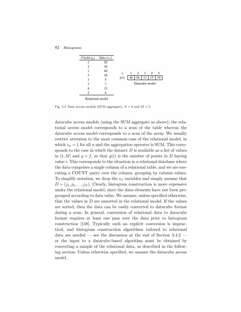
82 Histograms
CityId (jn) Sales (vn)2 202 301 405 103 53 74 152 6
Relational model
i: 1 2 3 4 5g(i): 40 56 12 15 10
Datacube model
Fig. 3.3 Data access models (SUM aggregate), N = 8 and M = 5.
datacube access models (using the SUM aggregate as above); the rela-tional access model corresponds to a scan of the table whereas thedatacube access model corresponds to a scan of the array. We usuallyrestrict attention to the most common case of the relational model, inwhich vn = 1 for all n and the aggregation operator is SUM. This corre-sponds to the case in which the dataset D is available as a list of valuesin [1,M ] and g = f , so that g(i) is the number of points in D havingvalue i. This corresponds to the situation in a relational database wherethe data comprises a single column of a relational table, and we are exe-cuting a COUNT query over the column, grouping by column values.To simplify notation, we drop the vn variables and simply assume thatD = (j1, j2, . . . , jN ). Clearly, histogram construction is more expensiveunder the relational model, since the data elements have not been pre-grouped according to data value. We assume, unless specified otherwise,that the values in D are unsorted in the relational model. If the valuesare sorted, then the data can be easily converted to datacube formatduring a scan. In general, conversion of relational data to datacubeformat requires at least one pass over the data prior to histogramconstruction [138]. Typically such an explicit conversion is imprac-tical, and histogram construction algorithms tailored to relationaldata are needed — see the discussion at the end of Section 3.4.2 —or the input to a datacube-based algorithm must be obtained byconverting a sample of the relational data, as described in the follow-ing section. Unless otherwise specified, we assume the datacube accessmodel.
3.2 One-Dimensional Histograms: Overview 83
3.2.3 Histogram Cost Considerations
What are “reasonable” costs for constructing and using a histogram?For at least some applications and data sizes, the user is able to toleratea complete pass through the data, or perhaps even two passes, forhistogram construction, provided that the per-item processing cost issmall. This is especially true for the datacube access model, and lessso for the relational data access model. When the amount of data ismassive, an increasingly important scenario, then even a single passthrough the data might be prohibitively expensive.
In this latter case, a common approach is to build a histogram froma small uniform sample of the data [234, 251, 257]. As discussed byPoosala et al. [257], for example, Kolmogorov’s Theorem implies thatthe sampling error can be controlled simultaneously for all possiblerange queries by taking a sufficiently large sample. Donjerkovicand Ramakrishnan [90] point out that the sample size needs to beinflated to deal with the information loss incurred by compressing thesample into a histogram; for example, for an equi-depth histogramwith B buckets, the authors use Kolmogorov’s Theorem to obtainthe rule-of-thumb formula s ≈ 100B2 for the required sample size s,under the assumption that the sampling error should be an order ofmagnitude smaller than the histogram error. On the other hand, whenusing “maxdiff” and related histograms for query optimization — seeSection 3.4.1 — Poosala et al. found experimentally that a samplesize of 2000 was more than sufficient for 1D-histogram construction.Chaudhuri et al. [51] consider a more sophisticated approach tocollecting a sample on which to build an equi-depth histogram. Fortuple-level sampling schemes, they use Chernoff bounds to computethe sample size necessary to bound either a maximum-error metric or astronger “symmetric difference” error metric. For page-level samplingschemes — which are far more I/O efficient than tuple-level schemesbut incur dependencies between tuples stored on the same disk page —the authors propose an adaptive sampling method. At each stepof the sampling process, the adaptive method uses cross-validationto estimate the sampling error in the equi-depth histogram that iscomputed from the disk pages sampled so far. If the error exceeds thetarget, the sampling process continues; otherwise, sampling stops.

84 Histograms
Although the foregoing sampling approaches are currently used incommercial systems such as DB2 and Microsoft SQL Server, they raisethe question of whether the sample could instead be used directlyfor approximate query answering. Moreover, any potential histogram-related error bounds for an individual query must be inflated to reflectthe additional error due to sampling, and the resulting overall errorbounds will then be probabilistic in nature. In addition, any optimal-ity assertions about a histogram — see, for example, the algorithms inSection 3.4.2 — will then be compromised.
Even when a complete pass through the data is acceptable, manypublished algorithms have an unacceptably large Ω(M) or Ω(N) spacerequirement (under the datacube or relational access model, respec-tively) for constructing the histogram. One possibility for dealing withthis situation is to use a sample, as discussed above. For example, anearly histogram implementation in DB2 piggybacked a reservoir-samplecomputation [283] on top of a complete database scan by the RUN-STATS statistics-collection utility, and then computed a “compressedhistogram” (see Section 3.4.1) from the sample. Indeed, any synopsiscomputed from a full scan can be used in this manner, provided that thehistogram can be computed directly from the synopsis without havingto first generate the complete (approximated) dataset. For example,Gilbert et al. [127] use sketches to limit the space needed to constructa histogram; see Section 3.7.1. Again, this approach raises the questionas to whether the underlying synopsis could instead be used directlyfor query answering. A related strategy is to first take a sample, whichis used to determine the histogram buckets, and then compute thebucket statistics via a complete data scan. Under this strategy, thereis no sampling error for the bucket statistics, since they are computedexactly. The buckets themselves may be chosen suboptimally, however,and hence any optimality guarantees are weakened (but not as muchas when bucket statistics are also estimated). An alternative strategyis to use a disk-based algorithm to compute the histogram. There hasbeen very little research in this area; one exception is literature ondisk-based algorithms for computing quantiles (as needed, e.g., to com-pute an equi-depth histogram); see [143]. Of course, use of a disk-based
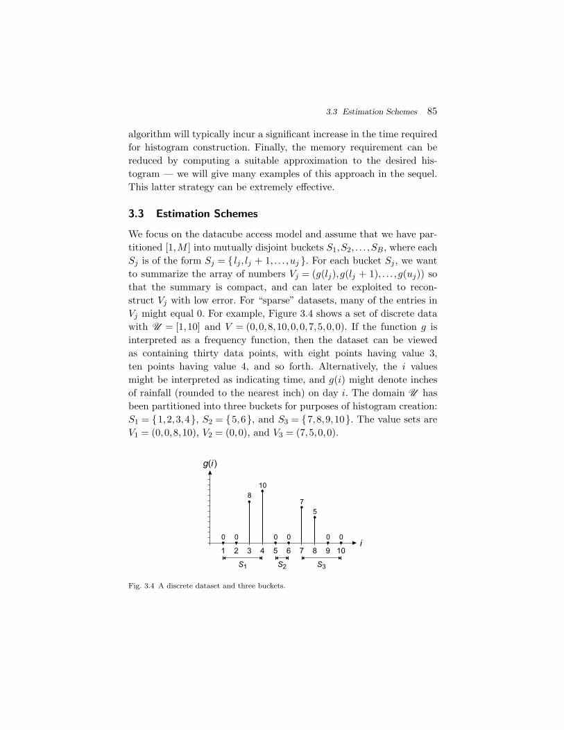
3.3 Estimation Schemes 85
algorithm will typically incur a significant increase in the time requiredfor histogram construction. Finally, the memory requirement can bereduced by computing a suitable approximation to the desired his-togram — we will give many examples of this approach in the sequel.This latter strategy can be extremely effective.
3.3 Estimation Schemes
We focus on the datacube access model and assume that we have par-titioned [1,M ] into mutually disjoint buckets S1,S2, . . . ,SB, where eachSj is of the form Sj = lj , lj + 1, . . . ,uj . For each bucket Sj , we wantto summarize the array of numbers Vj = (g(lj),g(lj + 1), . . . ,g(uj)) sothat the summary is compact, and can later be exploited to recon-struct Vj with low error. For “sparse” datasets, many of the entries inVj might equal 0. For example, Figure 3.4 shows a set of discrete datawith U = [1,10] and V = (0,0,8,10,0,0,7,5,0,0). If the function g isinterpreted as a frequency function, then the dataset can be viewedas containing thirty data points, with eight points having value 3,ten points having value 4, and so forth. Alternatively, the i valuesmight be interpreted as indicating time, and g(i) might denote inchesof rainfall (rounded to the nearest inch) on day i. The domain U hasbeen partitioned into three buckets for purposes of histogram creation:S1 = 1,2,3,4, S2 = 5,6, and S3 = 7,8,9,10. The value sets areV1 = (0,0,8,10), V2 = (0,0), and V3 = (7,5,0,0).
0 0
810
7
S1 S2 S3
i
g(i )
00 0 0
5
1 2 4 5 6 7 8 9 103
Fig. 3.4 A discrete dataset and three buckets.
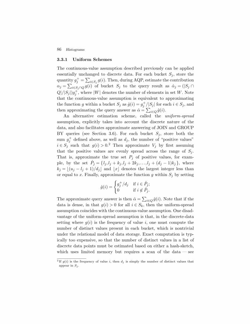
86 Histograms
3.3.1 Uniform Schemes
The continuous-value assumption described previously can be appliedessentially unchanged to discrete data. For each bucket Sj , store thequantity g+
j =∑
i∈Sjg(i). Then, during AQP, estimate the contribution
αj =∑
i∈Sj∩Q g(i) of bucket Sj to the query result as αj = (|Sj ∩Q|/|Sj |)g+
j , where |W | denotes the number of elements in set W . Notethat the continuous-value assumption is equivalent to approximatingthe function g within a bucket Sj as g(i) = g+
j /|Sj | for each i ∈ Sj , andthen approximating the query answer as α =
∑i∈Q g(i).
An alternative estimation scheme, called the uniform-spreadassumption, explicitly takes into account the discrete nature of thedata, and also facilitates approximate answering of JOIN and GROUPBY queries (see Section 3.6). For each bucket Sj , store both thesum g+
j defined above, as well as dj , the number of “positive values”i ∈ Sj such that g(i) > 0.2 Then approximate Vj by first assumingthat the positive values are evenly spread across the range of Sj .That is, approximate the true set Pj of positive values, for exam-ple, by the set Pj = lj , lj + kj , lj + 2kj , . . . , lj + (dj − 1)kj , wherekj = (uj − lj + 1)/dj and x denotes the largest integer less thanor equal to x. Finally, approximate the function g within Sj by setting
g(i) =
g+j /dj if i ∈ Pj ;
0 if i ∈ Pj .
The approximate query answer is then α =∑
i∈Q g(i). Note that if thedata is dense, in that g(i) > 0 for all i ∈ Sk, then the uniform-spreadassumption coincides with the continuous-value assumption. One disad-vantage of the uniform-spread assumption is that, in the discrete-datasetting where g(i) is the frequency of value i, one must compute thenumber of distinct values present in each bucket, which is nontrivialunder the relational model of data storage. Exact computation is typ-ically too expensive, so that the number of distinct values in a list ofdiscrete data points must be estimated based on either a hash-sketch,which uses limited memory but requires a scan of the data — see
2 If g(i) is the frequency of value i, then dj is simply the number of distinct values thatappear in Sj .

3.3 Estimation Schemes 87
Section 5.4 — or on a sample of the data points in a bucket — see[44, 155, 257] and Section 2.6.2. Such estimation can noticeably increasethe time and space requirements for histogram construction, and thesampling-based approach, in particular, can yield inaccurate estimateseven at reasonable sample sizes.
Figure 3.5 displays histograms for the dataset in Figure 3.4 based onthe continuous-value and uniform-spread assumptions. For the range-sum query with Q = 3,4,5,6,7, for which the exact result is α = 25,the two schemes yield respective estimates of α = 12 and α = 15,respectively. Although the uniform-spread assumption outperforms thecontinuous-value assumption in this example, a fairly comprehensiveset of experiments conducted by Wang and Sevcik [288] indicate that,in general, the opposite result holds true for OLAP queries (both one-dimensional and multi-dimensional) over discrete data.
0 0
S1 S2 S3
i
g(i )
3 3 3 34.5 4.5 4.5 4.5
1 2 4 5 6 7 8 9 103
^
(a) Continuous-value assumption
0 0
S1 S2 S3
i
g(i )
0 0
99
6 6
0 0
1 2 4 5 6 7 8 9 103
^
(b) Uniform-spread assumption
Fig. 3.5 Histograms using uniform estimation schemes.
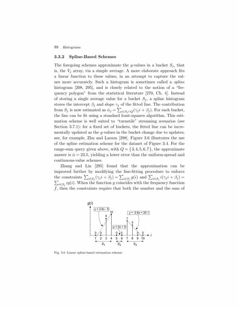
88 Histograms
3.3.2 Spline-Based Schemes
The foregoing schemes approximate the g-values in a bucket Sj , thatis, the Vj array, via a simple average. A more elaborate approach fitsa linear function to these values, in an attempt to capture the val-ues more accurately. Such a histogram is sometimes called a splinehistogram [208, 295], and is closely related to the notion of a “fre-quency polygon” from the statistical literature [270, Ch. 4]. Insteadof storing a single average value for a bucket Sj , a spline histogramstores the intercept βj and slope γj of the fitted line. The contributionfrom Sj is now estimated as αj =
∑i∈Sj∩Q(γji + βj). For each bucket,
the line can be fit using a standard least-squares algorithm. This esti-mation scheme is well suited to “turnstile” streaming scenarios (seeSection 3.7.1): for a fixed set of buckets, the fitted line can be incre-mentally updated as the g-values in the bucket change due to updates;see, for example, Zhu and Larson [298]. Figure 3.6 illustrates the useof the spline estimation scheme for the dataset of Figure 3.4. For therange-sum query given above, with Q = 3,4,5,6,7, the approximateanswer is α = 23.5, yielding a lower error than the uniform-spread andcontinuous-value schemes.
Zhang and Lin [295] found that the approximation can beimproved further by modifying the line-fitting procedure to enforcethe constraints
∑i∈Sj
(γji + βj) =∑
i∈Sjg(i) and
∑i∈Sj
i(γji + βj) =∑i∈Sj
ig(i). When the function g coincides with the frequency functionf , then the constraints require that both the number and the sum of
810
7
S1 S2 S3
i
g(i)
00 0 0
5
1 2 4 5 6 7 8 9 103
0 0
y = 0x + 0
y = 3.8x - 5y = -2.6x + 25.1
Fig. 3.6 Linear spline-based estimation scheme.
3.3 Estimation Schemes 89
the data points in Sk must match their true values. (The method in[295] actually assumes that the number dj of distinct values in Sj isknown, and initially applies a uniform-spread assumption. Thus thesums appearing on the left side of the above constraints are actuallyover the set Pj rather than Sj , where Pj is defined as in Section 3.3.1.)
This approach can, in principle, be extended by using polynomialrather than linear functions to model the data points. It is not clearwhether such additional complication is worth the effort, however, sincethen more coefficients must be stored for each bucket, to the detrimentof the number of buckets that can be maintained. Also, the fittingprocess becomes ever more expensive. Even in the case of linear splines,other techniques, such as the 4LT method discussed below, seem to havesuperior performance in general.
3.3.3 Four-Level Trees
Buccafurri et al. [37] have provided an extremely effective estimationscheme that involves storing, for each bucket Sj , the usual bucket totalg+j , together with an additional integer that encodes a description of the
data distribution in the bucket. This description can be represented asa four-level tree (4LT) that hierarchically represents partial sums of theg function. The experiments in [37] show that the increase in accuracyof the 4LT representation far outweighs any accuracy loss caused by thedecrease in the number of buckets that will fit into allocated memory.The technique has been developed for functions g whose domain is asubset of the integers, but the ideas can potentially be extended toother g functions.
We illustrate the method using an example taken from [37], whereintegers are assumed to comprise 32 bits. Consider a fixed bucket Sk
consisting of 16 values, specifically,
Vk = (7,5,18,0,6,10,0,6,0,6,9,5,13,0,8,7).
When Vk is divided into j (≥1) equally sized segments, denote by σi/j
the sum of the values in the ith such segment, so that σ1/1 = 100 is thesum of all of the values, σ2/4 = 6 + 10 + 0 + 6 = 22 is the sum of thevalues in the second quarter of Vk, and so forth. The 4LT for this
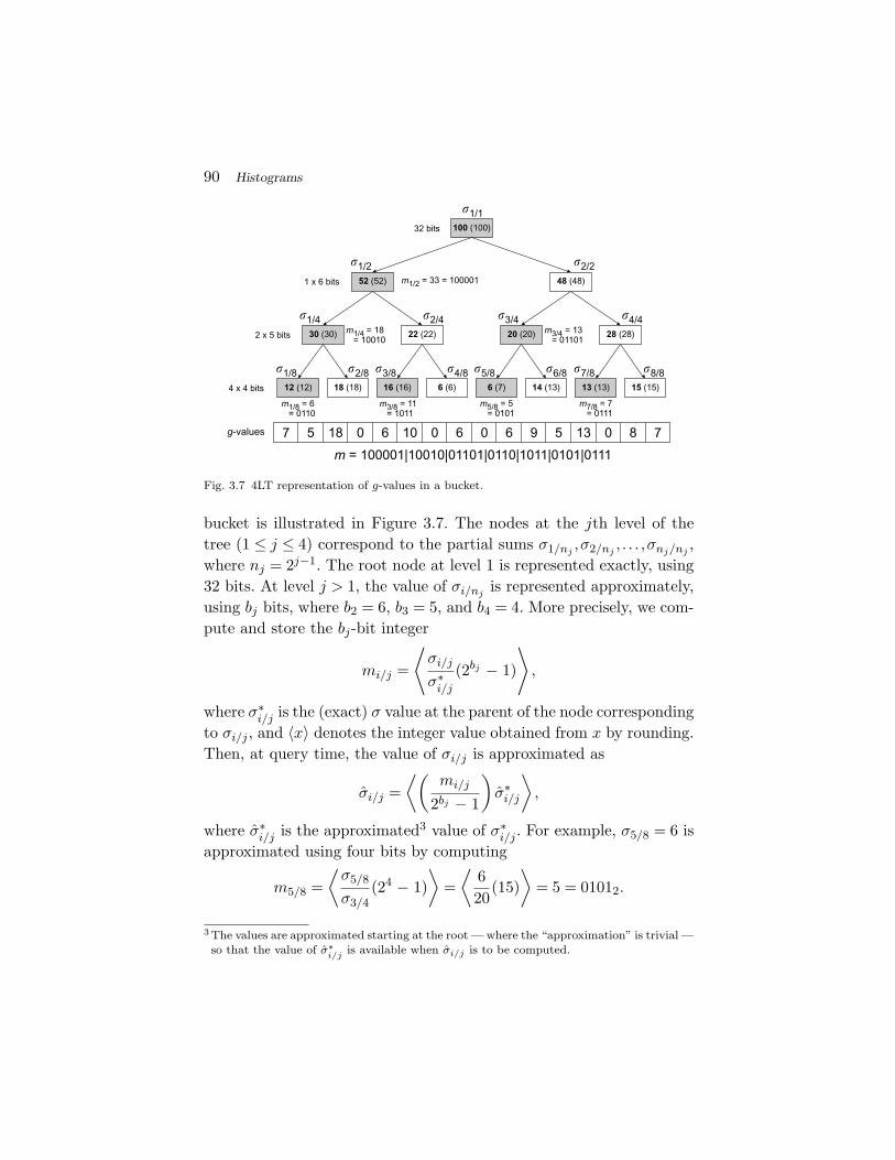
90 Histograms
1/1
1/8 2/8 3/8 4/8 5/8 6/8 7/8 8/8
4/43/42/4
2/2
1/4
1/2
100 (100)
52 (52) 48 (48)
30 (30) 22 (22) 20 (20) 28 (28)
12 (12) 18 (18) 16 (16) 6 (6) 6 (7) 14 (13) 13 (13) 15 (15)
32 bits
1 x 6 bits
2 x 5 bits
4 x 4 bits
7 5 18 0 6 10 0 6 0 6 9 5 13 0 8 7g-values
m1/2 = 33 = 100001
m1/4 = 18= 10010
m1/8 = 6= 0110
m3/8 = 11= 1011
m5/8 = 5= 0101
m7/8 = 7= 0111
m3/4 = 13= 01101
m = 100001|10010|01101|0110|1011|0101|0111
Fig. 3.7 4LT representation of g-values in a bucket.
bucket is illustrated in Figure 3.7. The nodes at the jth level of thetree (1 ≤ j ≤ 4) correspond to the partial sums σ1/nj
,σ2/nj, . . . ,σnj/nj
,where nj = 2j−1. The root node at level 1 is represented exactly, using32 bits. At level j > 1, the value of σi/nj
is represented approximately,using bj bits, where b2 = 6, b3 = 5, and b4 = 4. More precisely, we com-pute and store the bj-bit integer
mi/j =
⟨σi/j
σ∗i/j
(2bj − 1)
⟩,
where σ∗i/j is the (exact) σ value at the parent of the node corresponding
to σi/j , and 〈x〉 denotes the integer value obtained from x by rounding.Then, at query time, the value of σi/j is approximated as
σi/j =⟨(
mi/j
2bj − 1
)σ∗
i/j
⟩,
where σ∗i/j is the approximated3 value of σ∗
i/j . For example, σ5/8 = 6 isapproximated using four bits by computing
m5/8 =⟨σ5/8
σ3/4(24 − 1)
⟩=⟨
620
(15)⟩
= 5 = 01012.
3 The values are approximated starting at the root — where the “approximation” is trivial —so that the value of σ∗
i/jis available when σi/j is to be computed.

3.3 Estimation Schemes 91
Then σ5/8 is approximated4 as
σ5/8 =⟨(m5/8
15
)σ3/4
⟩= 〈(5/15)(20)〉 = 7.
In the figure, the approximated value of each σi/j is shown in paren-theses.
The final 32-bit integer that is stored with the bucket is obtainedby concatenating the mi/j values corresponding to the shaded nodes inthe figure. The mi/j values for the non-shaded nodes do not need tobe stored, because the corresponding σi/j values can be approximateddirectly by subtracting the approximated σ value for the node’s siblingfrom the approximated σ value for the node’s parent. For example, weapproximate σ6/8 as σ6/8 = σ3/4 − σ5/8 = 20 − 7 = 13. To actually esti-mate the contribution of the bucket to a range-sum query, we simplyadd up the σ values that cover the elements contained in Q; we tryto use the σ values at the highest levels of the tree, since these havethe greatest accuracy. If necessary, the continuous-value assumption isused to estimate g-values at a finer granularity than is provided by theleaf nodes of the 4LT. For example, if the query region Q overlaps thefirst thirteen values in the bucket, then we estimate the bucket’s con-tribution as σ1/2 + σ3/4 + 0.5σ7/8 = 52 + 20 + (0.5)(13) = 78.5, wherethe first two terms estimate (exactly, as it happens) the contributionsof the first eight plus the next four g-values, and the last term estimatesthe thirteenth g-value using the continuous-value assumption. The trueanswer is 85, so the error in the estimate is approximately 8%.
3.3.4 Heterogeneous Estimation Schemes
Ioannidis [178] notes that histogram accuracy can be improved byallowing different estimation schemes in different buckets. Althoughsuch histograms are relatively expensive to compute, they may beappropriate when high accuracy is needed and storage space for thehistogram is limited.
4 This example may seem somewhat artificial, because we can already represent the integerσ5/8 = 6 using only four bits; identifying such “simple” cases, however, would require atleast one more bit, and would complicate the algorithm further.
92 Histograms
Wang and Sevcik [288] developed a specific approach along theselines, defining a “hierarchical model-fitting” (HMF) histogram thatuses one of the continuous-value, uniform-spread, or 4LT schemes for agiven bucket, depending on which scheme best approximates the datain the bucket. The criterion used to compare schemes is inspired bythe “minimum description length” principle from statistics [264], whichattempts to balance model complexity and accuracy in a principledmanner. As discussed in [288], a scheme M2 for a bucket is preferredover a scheme M1 if k2 ≤ k1 and D(p‖q2) < D(p‖q1), where kl is thenumber of “parameters” of Ml, that is, the number of summary statis-tics that scheme Ml requires to be stored for the bucket, and D(p‖ql)is a “relative entropy” measure of the distance between the true andestimated g-values in the bucket. In more detail, the g-values (assumednonnegative) in bucket Sj can be normalized to a probability mass func-tion p by dividing each value g(i) by the bucket sum g+
j . The approxi-mated g-values under scheme Ml can similarly be normalized to a prob-ability mass function ql. The relative-entropy distance of ql from p maythen be defined as D(p‖ql) =
∑i∈Sj
p(i) log(p(i)/ql(i)). (The authorsactually use a slightly different, more complex definition that moreeffectively measures the distance between the two probability massfunctions when the data in a bucket is sparse.) If D(p‖q2) < D(p‖q1)but k2 > k1, then M2 is preferred to M1 if the benefit/cost ratio
ρ =D(p‖q1) − D(p‖q2)
k2 − k1
is sufficiently large, that is, if the decrease in distance per additionalparameter is large enough.
Buccafurri et al. [32] also propose the use of different estimationmethods in different buckets, in the context of a histogram having arecursive bucket structure (see Section 3.4.3). They also use a greedyalgorithm to determine the overall design of the histogram.
Recently, Kanne and Moerkotte [197] have proposed a heteroge-neous estimation scheme that uses several new types of buckets. Thesimplest buckets store the number of distinct values and, instead of thetraditional average bucket frequency, the “q-middle” frequency. Thislatter frequency is defined for bucket S as
√(mini∈S g(i))(maxi∈S g(i)).
3.3 Estimation Schemes 93
In addition, a bucket might also store the average frequency and thefrequencies of the values that define the bucket boundaries. The idea isto approximate each frequency in the bucket by the q-middle frequencyfor point queries or range queries with relatively short ranges, and bythe average frequency for range queries with longer ranges, using athreshold on range length to determine which estimation scheme touse. Several other bucket types tailored to range queries are also pro-posed, as well as a bucket type that stores exact frequencies in a com-pressed form. The goal is to control the “q-error” of the histogram; seeSection 3.4.2 for definitions.
3.3.5 A Probabilistic Scheme
Buccafurri et al. [33] follow an approach that is quite different fromthe foregoing methods, using a probability model over datasets. Sup-pose that the total sum s of the g-values in the dataset and the totalnumber d of positive g-values are known. Fix a range-sum query Q andconsider the class of histograms such that the summary data storedin each bucket comprises the average of the g-values in the bucket,together with the number of positive g-values in the bucket. Denote byG the finite set of all nonnegative functions defined on U such that thesum of the g-values is s and exactly d of the g-values are positive. For agiven histogram H, denote by GH the subset of functions in G that are“compatible” with H; that is, g ∈ GH if and only if the partitioning ofg according to the buckets of H yields summary statistics that coincideexactly with those in H. The maximum-entropy-style method in [33]imposes a probability distribution over GH in which each of its elementsis equally likely. This distribution then induces a probability distribu-tion over the answer to Q. The authors provide closed-form formulasfor the mean and variance of this latter distribution — the mean is theestimated query answer and the variance is taken as a measure of theprecision of the answer.
Importantly, this approach can gracefully incorporate additionalknowledge about the data by restricting the set G appropriately. Theauthors focus on knowledge that comprises either a lower bound onthe number of positive g-values lying within the query range or a lower
94 Histograms
bound on the number of g-values in the range that are equal to 0. Undermany bucketing schemes, the leftmost and the rightmost g-values in abucket are forced to be non-zero, and this knowledge can lead to moreprecise query-answer estimates than are obtained under, for example,the continuous-value or uniform spread assumptions.
3.3.6 Error Estimates for Individual Queries
The bucketing schemes in Section 3.4.2 below provide, as a byproduct,an estimate of the aggregate error of the entire histogram, for example,the maximum error for a point query, or the average L2 error over allpoint queries, or even a workload-weighted average error. In a similarspirit, Donjerkovic and Ramakrishnan [90] provide a sampling-basedscheme for assessing the worst-case estimation error for range queriesin an equi-depth histogram. None of these estimates, however, givethe user precise feedback about the estimation error for the particularquery that is being evaluated. An estimate such as the maximum errorover any point query is likely to be very conservative with respect to aspecific query. The probabilistic method of the previous section returnsa “precision number” in the form of a variance, but this number ismore an indicator of the degree of potential error than a metric of thetrue error of the approximate answer relative to exact answer that iscomputed over the actual g-values that comprise the dataset.
To address the precision issue, one simple scheme — c.f. Poosalaet al. [255] — stores the maximum and minimum g-value in a bucket,along with the usual summary statistic(s), such as the average g-value.Then a rough precision estimate can be returned to the user. For exam-ple, consider a range-sum query α that is approximately answeredusing a given histogram, where we summarize each bucket by itsaverage g-value. Suppose that all but one bucket is contained withinthe query range. Also suppose that, for the partially covered bucketSj , values g(i),g(i + 1), . . . ,g(i + n − 1) lie within the query range.Then, since the contributions to the query answer from the completelycovered buckets are exact, we know that α − L ≤ α ≤ α + U , whereL = n(gavg
j − gminj ) and U = n(gmax
j − gavgj ). If the histogram is effec-
tive at minimizing the variability of g-values in a bucket, then gmaxj
3.4 Bucketing Schemes 95
and gminj will be close to gavg
j , and the bounds will be useful. Jagadishet al. [185] suggest a similar idea, and Read et al. [262] elaborate onthe approach in the setting of more complex histograms. Of course, theadditional information inflates the per-bucket memory requirements,so that a histogram that incorporates the foregoing scheme will havefewer buckets, and hence less accuracy. This trade-off seems worthwhile,however, in order to provide users with feedback on the quality of theirapproximated query-answers.
3.4 Bucketing Schemes
The scheme used to assign data points to buckets for purposes of sum-marization is crucially important to achieving good approximate queryanswers. In this section, we describe a range of bucketing schemesfor 1D-histograms, ranging from heuristic to provably optimal. Wefocus, as usual, on general range-sum queries under the datacube accessmodel, that is, estimating quantities of the form α =
∑i∈Q g(i), where
Q ⊆ U = [1,M ] for some M ≥ 1; Section 3.7.2 describes techniquesespecially suitable for real-valued data.
As seen from the discussion in Section 3.3, the crux of histogram-based estimation is to approximate the g-values in a bucket with a fewsummary numbers, such as an average or the slope and intercept of aline. As shown in early work by Ioannidis and Christodoulakis [177, 181](in the context of using histograms to estimate join sizes for categoricaldata), it follows that good (and sometimes optimal) approximationsare often obtained by grouping together elements of U having similarg-values. For example, a serial histogram first sorts the elements ofU by g-value to obtain an ordered sequence U ′ = (i1, i2, . . . , iM ) withg(i1) ≤ g(i2) ≤ ·· · ≤ g(iM ), and then assigns elements of U to bucketsby partitioning U ′ into disjoint segments. Arbitrary bucketing by g-values is impractical, however, because then an index is needed to mapi-values to buckets. We therefore restrict attention to bucketing schemesthat partition the domain [1,M ] into disjoint segments.
3.4.1 Heuristic Schemes
We first consider various heuristic schemes — specifically the equi-width,equi-depth, “compressed,” and “maxdiff” bucketing methods — that
96 Histograms
have been adopted in commercial database systems for use within thequery optimizer because of their relatively low construction costs. Thesemethods do not come with optimality guarantees: they typically performwell on average, occasionally providing a seriously inaccurate result forsome unlucky query.
3.4.1.1 Equi-Width Histograms
The equi-width histogram technique described in Section 3.1.1 can beapplied to discrete data as well as continuous data. The histogramcan be computed in a single pass with O(1) cost per data item and thespace complexity isO(B), under either the datacube or relational accessmodels. (Recall the definitions of these models from Section 3.2.2, aswell as the discussion on construction costs.)
3.4.1.2 Equi-Depth Histograms
The equi-depth bucketing scheme of Section 3.1.1 can also be appliedto discrete data. In the current setting, the goal is to have the sum ofg-values be the same for every bucket, that is,
∑i∈Sj
g(i) =∑
i∈Skg(i)
for all j and k. When defining the buckets, some minor technical com-plications can arise when certain data values are very frequent, so thatmultiple quantiles coincide; see [251] for details.
Under the datacube model, and assuming that the sum g+ =∑
i g(i)of g-values is known, the list of g-values is simply scanned once todetermine the bucket boundaries, requiring O(B) space in total; if g+
is unknown, then an additional scan of the data is required. Underthe relational model, computing the histogram corresponds to findingB − 1 equally-spaced quantiles. A naive algorithm scans the data intomemory (if possible), sorts it, and reads off the quantiles, incurring anO(N) space cost and an O(N logN) time cost. Alternatively, a disk-based sort can be used, but this requires multiple passes over the data.Typically these straightforward approaches are impractical, but can beapplied to a sample of the data. The disk-based quantile algorithmin [143] assumes that the dataset is stored in K disk-resident blocks,and assumes a fixed-size memory buffer for holding data. Using algo-rithms that employ an efficient median-finding algorithm, the authors
3.4 Bucketing Schemes 97
show how to compute an exact set of buckets with O(K logB) I/O costand O(K logB) CPU cost; these costs are still quite high. In practice,as discussed in Section 3.1.1, algorithms for computing approximatequantiles must be employed in order to achieve acceptable space andtime complexity. For example, the one-pass algorithm of Greenwaldand Khanna [131] has a worst-case time complexity O(Nε−1 log(εN))and a space complexity of O(ε−1 log(εN)). The recent algorithm ofZhang and Wang [296] requires more space, O(ε−1 log2(εN)), but lesstime, O(N log(ε−1 log(εN))).
3.4.1.3 Singleton-Bucket Histograms
An SB-histogram places elements of [1,M ] having extremely large orsmall g-values into singleton buckets, and reverts to a classical bucket-ing scheme to represent the remaining data. For example, an end-biasedhistogram [177, 181] places the B1 elements of [1,M ] having the largestg-values and the B2 elements having the smallest g-values in singletonbuckets, and uses a single bucket to represent the remaining values (viathe continuous-value assumption). When B2 = 0, such a histogram iscalled a high-biased histogram. A compressed histogram [257] is simi-lar to a high-biased histogram, except that an equi-depth histogram isused to represent the g-values for theM − B1 non-singleton elements of[1,M ]; in the usual implementation, the g-value for a singleton bucketmust exceed g+/B, where g+ =
∑i g(i) as before.
Under the datacube model, two passes through the data are needed,each with O(1) processing cost per item: one to identify the k largestg-values and compute the sum of the remaining g-values, and one tocompute the equi-depth histogram for the non-large g-values. The over-all space requirement for construction is O(B), as with the equi-depthhistogram.
Under the relational model, both quantiles and highly frequent val-ues must be computed. Computation of quantiles is the same as for anequi-depth histogram. The frequencies of the most frequent values usu-ally can be estimated with high precision from a simple uniform sample,as in [257]; Cohen et al. [55] give a more elaborate scheme for estimatingthe k highest frequency values, and Gemulla et al. [116] give a sampling
98 Histograms
algorithm that provides unbiased, low-variance estimates of both highand low frequencies, at the expense of storing “tracking counters” inthe sample. Note in this connection that the more skewed the frequencydistribution, the more important it is to estimate the frequent valuesand the easier this estimation problem becomes. One simple algorithm,proposed in [257], is to take a small sample and create a counter foreach distinct value in the sample. The exact frequencies of these dis-tinct values are then computed exactly based on a full scan of the data.The idea is that highly frequent values with appear in the sample withhigh probability. For example, if 106 data points have values distributedaccording to a Zipf(0.86) distribution (roughly an “80-20” law), thena 0.1% sample will contain the 10 most frequent values with proba-bility approximately 99.9%. Alternatively, more sophisticated full-scanlimited-memory algorithms can be used; see, for example, [46, 65], aswell as Section 5.3.4.1.
3.4.1.4 Maxdiff Histograms
A maxdiff histogram [257] with B buckets partitions the sequence[1,M ] by placing a bucket boundary between elements i and i + 1 ifthe difference |g(i + 1) − g(i)| is among the B − 1 largest such differ-ences. For the datacube model, only a single scan is needed, with O(1)processing cost per item, and the total space requirement is O(B). Forthe relational model, the data-values must be converted to the dat-acube format and then processed as above. Such a conversion requiresa complete sort of the data, which is usually unacceptable in practice.For this reason, the maxdiff histogram for relational data is typicallycomputed from a sample, as in [257].
3.4.1.5 Generalizing Bucketing Schemes
The foregoing bucketing schemes can be generalized by imposing ahomogeneity requirement not on the g-values within a bucket, buton other data properties. For example, when the data is sparse,so that many g-values are equal to 0 and the uniform-spreadestimation scheme is applicable, then similarity of g-values withina bucket is not the only criterion for a good bucketing scheme;

3.4 Bucketing Schemes 99
similar spacing between successive positive elements in a bucket isalso desirable. For i ∈ [1,M ] with g(i) > 0, define the spread of i ass(i) = minj ∈ [i + 1,M ] : g(j) > 0 − i, where we take s(i) = M − iif g(j) = 0 for j ∈ [i + 1,M ]. Similarly define the area of i as a(i) =g(i)s(i). We can then replace the function g in the definition of theabove bucketing scheme by the functions s or a [257]. That is, thebucketing schemes try to make the spreads or areas within each bucketas homogeneous as possible. The motivation behind the use of area isto balance the goals of equalizing g-values and equalizing spreads. Thecumulative function c(i) =
∑ij=1 g(i) has also been proposed. Adapt-
ing the terminology in [257], one can then talk about, for example, amaxdiff(g), maxdiff(s), maxdiff(c), or maxdiff(a) histograms, depend-ing on whether the function g, s, c, or a is used when determining thebuckets.5 (As usual, the area scheme reduces to the g-value schemeas the data becomes dense.) Virtually all other bucketing schemes canbe similarly generalized, and even unified in some cases. For example,we can view equi-width and equi-depth histograms as “equi-sum(s)”and “equi-sum(g)” histograms, where an equi-sum(h) histogram selectsbuckets so that the bucket sum h+
j =∑
i∈Sjh(i) is the same for each j.
Under the datacube model, the bucketing algorithms are virtuallyunchanged, except that a lookahead buffer of length 1 is required tocompute spreads. Under the relational model, the spreads must beestimated. Poosala et al. [257] found that computing spreads from adata sample yielded acceptable results; more sophisticated estimates ofspreads can be derived from estimates of the number of distinct valuesin a bucket; see the discussion of equi-depth histograms in Section 3.3.1.
The experiments in [257] indicate that, for moderately sparse data,the maxdiff(a) scheme yields the best accuracy, but the accuracy ofthe maxdiff(g), compressed(g), and compressed(a) schemes is almostas good. Because of their good balance of accuracy and practicality,versions of the maxdiff and compressed histograms are currently used inSQLServer and DB2 products; see [179, 182]. As noted in Giannella andSayrafi [120], however, the experimental results in the early literature
5 The original paper [257] considered the special case where g equals the frequency func-tion f , and referred to frequency, spread, and area as the possible “source parameters” fordetermining buckets.
100 Histograms
on heuristic bucketing schemes are far from definitive, and no heuristicscheme uniformly dominates the others.
3.4.2 Schemes with Optimality Guarantees
In light of the purely empirical performance studies for the foregoingheuristic schemes, and the limitations of these studies, the questionnaturally arises of whether there exist efficient algorithms for deter-mining a set of provably “optimal” or “near-optimal” histogram buck-ets that maximize estimation accuracy, subject to an upper bound onthe histogram size. To formulate the problem more precisely, one mustspecify the estimation scheme used for the buckets, the class of buck-eting schemes allowed, and the accuracy criterion. A large literaturehas grown up around this topic, which we briefly summarize in thissection. Unless specified otherwise, all of the algorithms assume thedatacube access model, so that the input g-values are given in theform g(1), . . . ,g(M). As discussed previously, all of these algorithmsassume at least one complete pass through the data; if sampling isnecessary, then the optimality statements will not hold in general,because the bucket boundaries will not be based on the complete data.Another running assumption is that the maximum g-value R is suchthat logR = O(logM), which is typically the case when g-values cor-respond to frequency counts. When the g-values are real, they areassumed to be of bounded precision, so that they can be rescaled tointegers and satisfy the above assumption.
3.4.2.1 A Basic Dynamic-Programming Approach
We first describe the basic DP method of Jagadish et al. [185], whichwas the first optimality result to appear in the database literature.6
This basic algorithm — which focuses on minimizing an L2-error met-ric — typifies a broad class of optimal-histogram algorithms and isperhaps the easiest to understand. As will be seen, the cost of the algo-rithm is often unacceptable in practice, so much subsequent work has
6 As pointed out by Karras and Mamoulis [202], the algorithm can be viewed as a specialcase of a curve-approximation scheme due to Bellman [18].
3.4 Bucketing Schemes 101
focused on improving the basic algorithm either by using approximateDP techniques or by focusing on more tractable error metrics suchas L∞.
The (somewhat limited) class of histograms considered determinesbuckets by decomposing the domain U = [1,M ] into disjoint seg-ments and estimating the g-values for the elements within a bucketusing the continuous-value assumption; that is, for each i ∈ [1,M ], thehistogram estimates g(i) as the average g-value for the bucket con-taining i. The accuracy metric for the histogram is the (squared)L2 distance between the vector of actual and estimated g-values:E(H) =
∑Mi=1(g(i) − gH(i))2, where gH(i) is the estimated g-value for
i ∈ [1,M ], based on the histogram H. Such a histogram is called av-optimal histogram in [182].
The DP approach exploits the fact that the error metric E(H)decomposes into the sum of errors for the individual buckets. Fixk ∈ [2,M ], j ∈ [1,M ], and i ∈ (1, j], and consider an arbitrary but fixedk-bucket histogram over [1, j] whose rightmost bucket is Sk = [i, j]. Bythe decomposability of the error metric, the L2 error Ek[1, i, j] of thishistogram can be expressed as Ek[1, i, j] = E0
k−1[1, i) + L2[i, j], whereE0
k−1[1, i) is the contribution to the L2 error from the first k − 1 buck-ets over [1, i) and L2[i, j] is the contribution from bucket Sk. Clearly,a better histogram is obtained by adjusting the first k − 1 bucketsto coincide with those of the optimal (k − 1)-bucket histogram over[1, i). Denote the error of this latter histogram by E∗
k−1[1, i), so thatthe improved version of the original k-bucket histogram has overallerror E∗
k−1[1, i) + L2[i, j]. This is the minimum possible error for ak-bucket histogram over [1, j] having rightmost bucket [i, j]. Thus thebest k-bucket histogram over [1, j] is obtained by choosing a histogramof this latter type, using the best possible value of i, that is, choosingi to minimize E∗
k−1[1, i) + L2[i, j]. The error E∗k [1, j] for this optimal
histogram thus satisfies the equation
E∗k [1, j] = min
i∈(1,j]E∗
k−1[1, i) + L2[i, j]. (3.1)
This is the Bellman optimality equation of DP, and we denote by I∗k,j
the value of i that minimizes the right side; that is, I∗k,j is the position
of the lower boundary of the rightmost bucket in an optimal k-bucket

102 Histograms
histogram on [1, j]. For convenience, also set T ∗k,j = E∗
k [1, j], so that T ∗k,j
is the L2 error of the optimal k-bucket histogram on [1, j].The DP algorithm proceeds by computing — via (3.1) — and stor-
ing T ∗k,j and I∗
k,j for k = 1,2, . . . ,B and j = 1,2, . . . ,M . Observe in thisconnection that the L2 errors can be computed efficiently by precom-puting the quantities R(1)
i =∑i
l=1 g(i) and R(2)i =
∑il=1 g
2(i) for eachi ∈ [1,M ]. Then the L2 error for a bucket with end points a and b iscomputed as follows, where m = b − a + 1:
L2[a,b] =b∑
i=a
g(i) − (1/m)
b∑j=a
g(j)
2
=b∑
i=a
g2(i) − (1/m)
b∑
j=a
g(j)
2
= (R(2)b − R(2)
a−1) − (1/m)(R(1)b − R(1)
a−1)2.
To start the computation, we set T ∗1,j = E∗
1 [1, j] = L2[1, j] for j ∈ [1,M ];we can set each I∗
1,j to an arbitrary value. After every T ∗i,j and I∗
i,j hasbeen computed, the lower bucket boundaries for the optimal B-buckethistogram are determined in order of decreasing position as
iB = I∗B,M ,
iB−1 = I∗B−1,iB−1,
iB−2 = I∗B−2,iB−1−1,
...
i2 = I∗2,i3−1,
i1 = 1.
The L2 error of the optimal histogram is simply T ∗B,M .
The time and space complexity for computing the R(1)i and R
(2)i
constants is O(M). Computation of each (I∗k,j ,T
∗k,j) pair requires
O(M) operations, corresponding to exploring all possible values of ifor the minimization in Bellman’s equation. There are O(MB) suchpairs, which also must be stored. Thus the overall time complexity
3.4 Bucketing Schemes 103
is O(M2B) — with multiple passes required over the data — andthe space complexity is O(MB). The algorithm can be extended toother accuracy metrics, but the time complexity for the general case isO(M3B); see [202], as well as Lin and Zhang [216]. (The latter papergives a DP algorithm for spline histograms under a uniform-workload-based error metric for range queries.) Guha [133] provides a generaltechnique for reducing the space complexity of synopsis constructionalgorithms, and shows how the technique can be specialized to reducethe space complexity of the foregoing algorithm from O(MB) to O(M).The basic idea is to use a divide-and-conquer strategy for placing bucketboundaries, where a dynamic program is used to find the dividing point;Guha shows that this program has smaller space complexity than theoriginal dynamic program, and an overall space reduction is achievedbecause the resulting set of subproblems can share the same workingspace.
A key strength of the DP approach is that it extends straightfor-wardly to a broad range of different error measures, for example,
• the L1 error, defined as E(H) =∑M
i=1 |g(i) − gH(i)|, whereeach gH(i) is the median of the g-values in the bucket con-taining i;• the χ2 error, defined as E(H) =
∑Mi=1(g(i) − gH(i))2/gH(i),
where gH(i) =√|Sj |−1
∑l∈Sj
g2(l) and Sj is the bucket con-taining i;• workload-weighted versions of the L2 and L1 error metrics;
and• the KL metric of Giannella and Sayrafi [120], defined asE(H) =
∑Bj=1 |Sj |Ej , where |Sj | is the length of bucket Sj
and
Ej = log |Sj | −∑i∈Sj
g(i)g+j
logg(i)g+j
,
with g+j , as before, the sum of the g-values in bucket Sj .
The approach can also handle other estimation schemes, such as g-valuesummaries comprising the geometric mean or the median of the valuesin a bucket, or the spline-based schemes as described in Section 3.3.2.
104 Histograms
The precise formulas for time and space complexity may change, how-ever, depending on the details of the error metrics and estimationschemes; see, for example, [138, Section 4].
Jagadish et al. [184], extend this approach to the problem of glob-ally optimizing a set of 1D histograms. Specifically, the problem is toallocate a total of B buckets among the histograms in order to min-imize a global error metric. This metric is a weighted sum of the L2
errors for the histograms in the set, where the weight of a histogramcorresponds to the probability that an incoming query will probe theattribute associated with the histogram; these probabilities are esti-mated from a query workload. The authors provide both a DP and agreedy algorithm.
3.4.2.2 Improved DP Algorithms
Even with the improvement of Guha [133], the performance of the basicalgorithm is likely to be unacceptable in practice. To address this issue,a number of algorithms have been developed to solve a relaxed versionof the optimality problem. Such algorithms produce a histogram whoseerror is at most (1 + ε) times the minimum possible error — whereε is specified by the user — and are sometimes called ε-approximatehistograms. The best results in this area are largely contained in recentwork by Guha et al. [138]. For example, under the L2 error metric,the authors provide a one-pass algorithm that produces a near-optimalhistogram while having a near-linear time complexity of O(M + Qτ)and a space complexity of O(Bτ + Q), where τ = min(Bε−1 logM,M)and Q = B(Bε−1 logτ + logM) logτ . For typical values of B and ε, itholds that τ M andQ Bτ logM . The algorithm is rather intricate,and the reader is referred to the original paper for details; the key ideais to follow the DP approach outlined above, but, for each k ∈ [2,B],to efficiently and dynamically approximate the quantity E∗
k−1[1, i) inBellman’s equation by a piecewise-constant function of i.
Guha et al. [138] show that their techniques extend to any errormetric E such that
• the error E[a,b] of a bucket with end points a and b onlydepends on a, b, and the g-values in the bucket;
3.4 Bucketing Schemes 105
• the overall histogram error is the sum of the bucket errors;• O(1) information can be maintained for each i value such thatE[a,b] can be computed efficiently, for example, the quanti-ties R(1)
i and R(2)i in the basic DP algorithm; and
• the error metric is “interval monotone” in that E[a,b] ≤E[a − 1, b] and E[a,b] ≤ E[a,b + 1].
This class of metrics includes those described in the previous section.Note, however, that, for example, the authors’ scheme for the L1
metric requires a preprocessing step having O(M logM) time andspace complexity, which may be practically infeasible. Other metricsamenable to the methods in [138] include certain relative-error met-rics [141] such as the L2 relative error metric
∑Mi=1(g(i) − gH(i))2/w2
i .Here wi = max(g(i), c) and gH(i) = γj with Sj being the bucket thatcontains i and γj being a constant chosen to minimize the con-tributions to the error from the g-values in Sj . Specifically, γj =Cj − B2
j − Aj , where Aj =∑
i∈Sj(1/wj), Bj =
∑i∈Sj
(g(i)/w(i)), andCj =
∑i∈Sj
(g2(i)/w(i)). Note that c is a sanity constant that preventsundue influence by very small g-values. The methods in [138] also applyto the L1 relative-error metric but, as with the simpler L1 absolute-errormetric mentioned in the previous subsection, the space complexity isunacceptably high.
3.4.2.3 Maximum-Error Metric
In general, the L∞ metric — that is, the maximum error met-ric — is more tractable than other metrics such as L1 and L2. Guhaet al. [141] provide an algorithm for computing a near-optimal his-togram under the L∞ relative-error metric. This metric is defined asmax1≤i≤M |g(i) − gH(i)|/|wi|, where, as before, wi = max(g(i), c) andgH(i) = γj with Sj being the bucket that contains i. As with the L2 rel-ative error metric, γj is chosen to minimize the error contribution frombucket Sj . In this case, the formula for γj is encapsulated in Table 3.1,which also gives the resulting error contribution from the bucket. (Theoverall histogram error is the maximum of the bucket errors.) In thetable, “min” and “max” refer to the minimum and maximum g-values
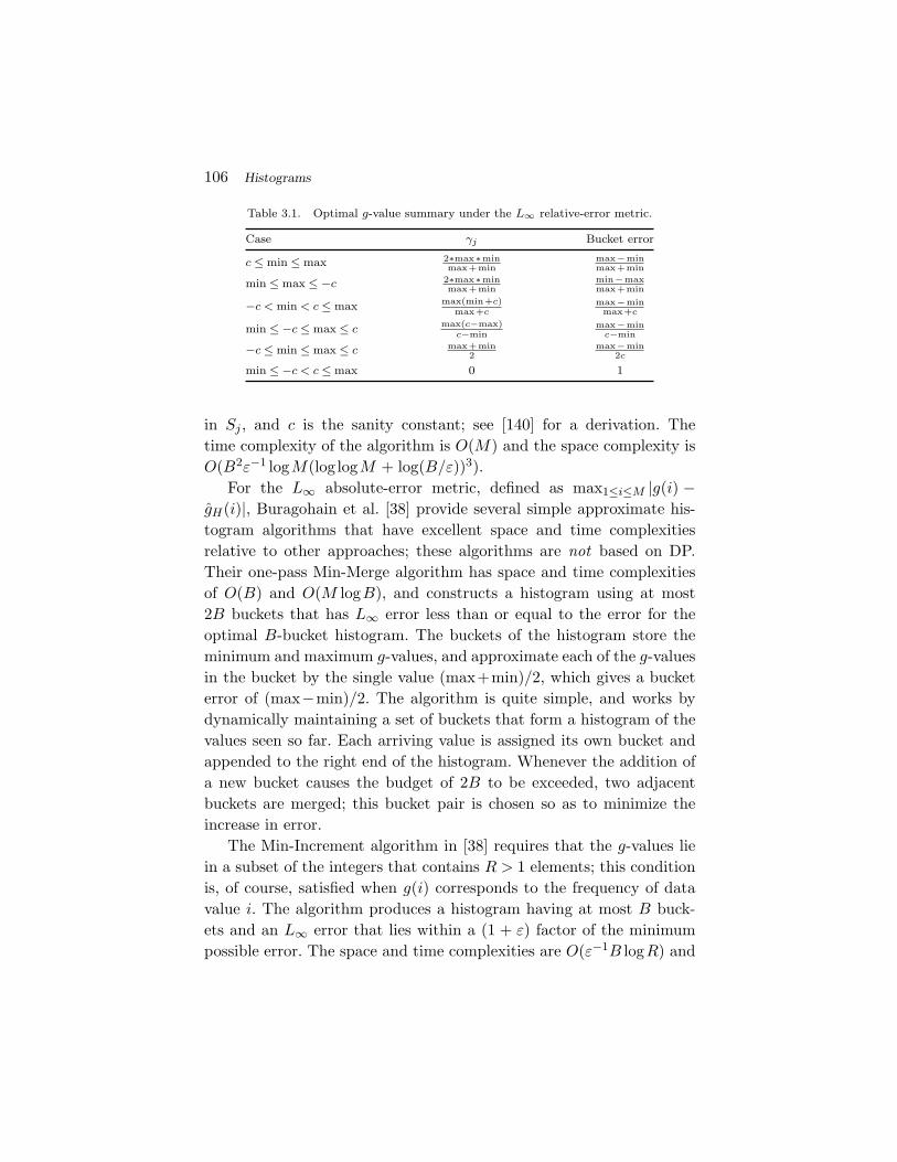
106 Histograms
Table 3.1. Optimal g-value summary under the L∞ relative-error metric.
Case γj Bucket error
c ≤ min ≤ max 2∗max∗minmax+min
max−minmax+min
min ≤ max ≤ −c 2∗max∗minmax+min
min−maxmax+min
−c < min < c ≤ max max(min+c)max+c
max−minmax+c
min ≤ −c ≤ max ≤ cmax(c−max)
c−minmax−min
c−min
−c ≤ min ≤ max ≤ c max+min2
max−min2c
min ≤ −c < c ≤ max 0 1
in Sj , and c is the sanity constant; see [140] for a derivation. Thetime complexity of the algorithm is O(M) and the space complexity isO(B2ε−1 logM(log logM + log(B/ε))3).
For the L∞ absolute-error metric, defined as max1≤i≤M |g(i) −gH(i)|, Buragohain et al. [38] provide several simple approximate his-togram algorithms that have excellent space and time complexitiesrelative to other approaches; these algorithms are not based on DP.Their one-pass Min-Merge algorithm has space and time complexitiesof O(B) and O(M logB), and constructs a histogram using at most2B buckets that has L∞ error less than or equal to the error for theoptimal B-bucket histogram. The buckets of the histogram store theminimum and maximum g-values, and approximate each of the g-valuesin the bucket by the single value (max+min)/2, which gives a bucketerror of (max−min)/2. The algorithm is quite simple, and works bydynamically maintaining a set of buckets that form a histogram of thevalues seen so far. Each arriving value is assigned its own bucket andappended to the right end of the histogram. Whenever the addition ofa new bucket causes the budget of 2B to be exceeded, two adjacentbuckets are merged; this bucket pair is chosen so as to minimize theincrease in error.
The Min-Increment algorithm in [38] requires that the g-values liein a subset of the integers that contains R > 1 elements; this conditionis, of course, satisfied when g(i) corresponds to the frequency of datavalue i. The algorithm produces a histogram having at most B buck-ets and an L∞ error that lies within a (1 + ε) factor of the minimumpossible error. The space and time complexities are O(ε−1B logR) and
3.4 Bucketing Schemes 107
O(ε−1M logR). The Min-Increment algorithm proceeds by solving the“dual” problem of finding the histogram with the minimal number ofbuckets whose error does not exceed a given bound. This dual prob-lem is solved for a range of exponentially increasing error values of theform ei = (1 + ε)i for i = 1,2, . . . , logR/ε, which lie in the range [1,R]of possible error values. The algorithm for solving the dual problem,called Greedy-Insert, is very simple. A list of buckets is maintained,with the rightmost bucket being “open” and the rest being “closed.”The algorithm starts with a single, open bucket. Arriving points areadded to the open bucket as long as the error does not exceed the spec-ified error bound e; if the bound is about to be exceeded, the bucketbecomes closed and the arriving g-value is placed in a new, open bucket.Observe that, because successive ei values are separated by a factor of(1 + ε), there exists an i∗ such that ei∗−1 ≤ eopt ≤ ei∗ ≤ (1 + ε)eopt,where eopt is the L∞ error of the optimal B-bucket histogram. Theminimum bucket histogram with bound ei∗ is the desired approximatehistogram, and the challenge is to identify i∗, since eopt is unknown.The Min-Increment algorithm simply maintains a set of histograms asin the Greedy-Insert algorithm, one for each ei value. Whenever thebucket count for such a histogram exceeds B, it is discarded; by theminimal-bucket property of Greedy-Insert, the error for such a his-togram is less than or equal to ei∗−1. After all of the g-values havebeen processed, the surviving histogram with the smallest ei value isthe desired approximate histogram. Buragohain et al. [38] extend theMin-Merge and Min-Increment algorithms to handle spline histogramsas in Section 3.3.2.
3.4.2.4 Range-Query Error Metric
All of the algorithms so far use an error metric that is orientedtoward minimizing “pointwise” errors in reconstructing the value ofeach g(i). If a histogram is primarily to be used in approximatelyanswering range queries, it makes sense to use an error metric thatreflects this fact. Guha et al. [139] provide an algorithm that attemptsto minimize error with respect to a workload W of hierarchicalrange queries. A range query Qij with i ≤ j asks for the range sum
108 Histograms
αij = g(i) + g(i + 1) + · · · + g(j). A set Q of hierarchical range queriessatisfies the property that, for each pair Qij ,Qkl ∈Q, either the ranges[i, j] and [j,k] are disjoint or one contains the other. A workload W com-prises a set Q of hierarchical range queries together with a probabilitydistribution P = pij over the queries in Q such that pij denotes theprobability that an incoming query Q will correspond to Qij ∈Q, thatis, will be a range query over [i, j]. Let αH
ij denote the estimate of αij
for a given histogram H, and denote by eHij = (αij − αHij )2 the corre-
sponding squared error. Next, let EH =∑
(i,j) eHij pij be the expected
(squared) error with respect to the workload when using histogram H.Finally, let H∗ be the histogram that minimizes the error and denoteby E∗ = EH∗ the minimal error. Guha et al. develop an efficient DPalgorithm that, for any ε ∈ (0,1), produces a histogram having O(B/ε)buckets and whose expected error with respect to W is the minimalB-bucket error E∗. The time complexity is O(M + B2ε−5M ε|Q|) andthe space complexity is O(Bε−3M2ε/3). The key idea is to restrict com-putation to a “sparse” system of intervals that covers the ranges in Q,increasing the number of histogram buckets in the process but reducingthe overall DP complexity. This method can be potentially extendedto other error metrics and estimation schemes.
The foregoing bucketing schemes assume the datacube access model.To handle the relational access model (with SUM aggregate) in a one-pass manner, one needs algorithms that can incrementally update ahistogram upon scanning a data item of the form (i,v) for some i ∈[1,M ], which has the interpretation “increment the current value of g(i)by v.” As usual, a key example has v ≡ 1, so that g is interpreted as thefrequency of data value i. Algorithms for handling this situation are aspecial case of algorithms for maintaining histograms over streamingdata, and are discussed in Section 3.7.1.
3.4.2.5 q-Error Metric
Recently, Kanne and Moerkotte [197] have forcefully argued forthe use of the q-error to evaluate the quality of a histogram,especially in the context of query optimization. If nonnegativeg-values g(1),g(2), . . . ,g(M) are approximated by histogram estimates
3.4 Bucketing Schemes 109
gH(1), gH(2), . . . , gH(M) then the q-error of the approximation isdefined as max1≤i≤M max(g(i)/gH(i), gH(i)/g(i)). A key motivation forthe use of q-error rests on recent results of Moerkotte et al. [230] thatdirectly relate q-errors of cardinality estimates to query-plan costs. Forexample, for a query consisting of multiple sort-merge joins or Gracehash joins, it can be shown that C(P ) ≤ q4C(P ), where C(P ) and C(P )are the query costs for optimal plans based on estimated and exact joincardinalities and q represents a worst-case q-error in the intermediatejoin-cardinality estimates. In [197], a DP-style algorithm is given forexact computation of a “q-optimal” histogram. Such a histogram hasminimal size, subject to an upper bound on the q-error. The class ofhistograms considered allows heterogeneous bucket types, as describedin Section 3.3.4. The exact algorithm is costly, and so a greedy heuris-tic is also provided. The experiments reported in [197] indicate that,for a wide range of datasets, it is possible to obtain a heterogeneoushistogram of reasonable size for which the q-error at most 2. Note thatspecial care must be taken to deal with the case g(i) = 0, since theq-error for such a value can be infinite.
3.4.3 Hierarchical Bucketing Schemes
The bucketing schemes discussed so far simply partition the range[1,M ] into disjoint segments. More elaborate schemes attempt to bettercapture the structure of the data by defining buckets in a hierarchicalmanner. The resulting data structures lie on the boundary betweenhistograms and synopses such as wavelets. We describe two such pro-posals below, n-level trees and lattice histograms. In the context ofmulti-dimensional histograms, Section 3.5.1 describes the hierarchicalSTHoles bucketing scheme of Bruno et al. [30].
3.4.3.1 n-Level Trees
The n-level tree (nLT) introduced in [35] is designed to answer hierar-chical range queries. In an exact nLT, sums over the data are storedas an n-level binary tree. The root node stores the sum of g(1)–g(M).The left child node stores (roughly) the sum of g(1)–g(M/2), and theright child stores the sum of g(M/2)–g(M). This scheme continues

110 Histograms
recursively, with the left child of a node storing the sum of g-valuesover the first half of the node’s range and the right child storing thesum over the right half. The storage requirement of the nLT is thenreduced by using the same tricks and approximations as in the 4LTmethod described in Section 3.3.3. Namely, only the sums for left-childnodes are stored, because the right-child sums can be reconstructedas a difference between the left-child sum and the parent-node sum.Moreover, the number of bits used to represent the sums decreases asthe node level increases. Specifically, the sum for the root node (level 0)is represented using 32 bits, the sum of the left-child node (level 1) isrepresented using k (< n) bits. From then on, the number of bits in therepresentation decreases by 1 as the level increases by 1. The nLT isused to answer a query in a manner similar to the hierarchical-range-query histogram of Guha et al. [139] described in Section 3.4.2. The ideais to attempt to cover the query range by one or more nodes that are ashigh up in the tree as possible. If, after such an attempted covering, aportion of the query range is not completely covered, then the sum overthis remaining portion is estimated using the continuous-value assump-tion. Experiments in [35] show that the accuracy of this approach canbe superior to maxdiff, v-optimal, and wavelet approaches.
The price for this improved accuracy is that, under the datacubeaccess model, the nLT requires O(M logM) time to construct andO(logM) time to answer a query. The nLT is relatively easy to update,requiring O(logM) time complexity to handle a change in g(i) for somespecified value of i.
3.4.3.2 Lattice Histograms
We conclude our discussion of 1D-histograms by describing recent workby Karras and Mamoulis [198, 200] on a synopsis called a lattice his-togram (LH), which is actually a hybrid of a histogram and a waveletsynopsis. The motivation for this work is to try and exploit both thetraditional histogram’s ability to flexibly and accurately capture locallysmooth data, yielding buckets containing similar data values, while alsoexploiting any underlying hierarchies of the data in order to capturenon-local interrelations, as is done effectively by hierarchical synopsis
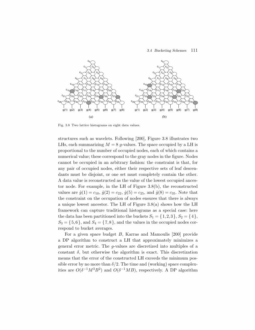
3.4 Bucketing Schemes 111
c0
c1 c2
c3 c4 c5
c6 c7 c8 c9
c11 c12 c13 c14
c15 c16 c17 c18 c19 c20
c21 c22 c23 c24 c25 c26 c27
c28
g(1) g(2) g(3) g(4) g(5) g(6) g(7) g(8)
c29 c30 c31 c32 c33 c34 c35
c10
g(1) g(2) g(3) g(4) g(5) g(6) g(7) g(8)
c0
c1 c2
c3 c4 c5
c6 c7 c8 c9
c11 c12 c13 c14
c15 c16 c17 c18 c19 c20
c21 c22 c23 c24 c25 c26 c27
c28 c29 c30 c31 c32 c33 c34 c35
c10
(a) (b)
Fig. 3.8 Two lattice histograms on eight data values.
structures such as wavelets. Following [200], Figure 3.8 illustrates twoLHs, each summarizing M = 8 g-values. The space occupied by a LH isproportional to the number of occupied nodes, each of which contains anumerical value; these correspond to the gray nodes in the figure. Nodescannot be occupied in an arbitrary fashion: the constraint is that, forany pair of occupied nodes, either their respective sets of leaf descen-dants must be disjoint, or one set must completely contain the other.A data value is reconstructed as the value of the lowest occupied ances-tor node. For example, in the LH of Figure 3.8(b), the reconstructedvalues are g(1) = c10, g(2) = c22, g(5) = c25, and g(8) = c35. Note thatthe constraint on the occupation of nodes ensures that there is alwaysa unique lowest ancestor. The LH of Figure 3.8(a) shows how the LHframework can capture traditional histograms as a special case: herethe data has been partitioned into the buckets S1 = 1,2,3, S2 = 4,S3 = 5,6, and S4 = 7,8, and the values in the occupied nodes cor-respond to bucket averages.
For a given space budget B, Karras and Mamoulis [200] providea DP algorithm to construct a LH that approximately minimizes ageneral error metric. The g-values are discretized into multiples of aconstant δ, but otherwise the algorithm is exact. This discretizationmeans that the error of the constructed LH exceeds the minimum pos-sible error by no more than δ/2. The time and (working) space complex-ities are O(δ−1M3B2) and O(δ−1MB), respectively. A DP algorithm
112 Histograms
specialized to the L∞ maximum-error metric reduces these require-ments to O(δ−1M3) and O(δ−1M), but clearly the time and spacecosts are impractical. To address this problem, the authors recommenda divide-and-conquer procedure in which the g-values are first par-titioned using a “primary” synopsis such as an ordinary histogram,and then a set of LHs are constructed, one per bucket. In follow-onwork that focuses on the class of weighted L∞ metrics (which includemaximum-relative-error metrics), Karras [198] provides an algorithmfor constructing a LH that exactly minimizes the error metric of inter-est, along with a much less expensive greedy algorithm that is shownempirically to produce LH’s that are close to optimal. The idea is todevelop exact and greedy algorithms that minimize the LH size subjectto a given error bound, and then solve the original space-bounded prob-lem by combining the error-bounded algorithms with binary search.The time and space complexities for the exact algorithm are O(M4) andO(M3), and the corresponding complexities for the greedy algorithmare O(M + B2) and O(M). The space complexity even of the greedyalgorithm may still be impractical but again the divide-and-conquerprocedure can potentially be applied. An interesting line of researchwould try and further improve efficiency by incorporating approximateDP ideas along the lines of Guha et al. [138].
3.5 Multi-Dimensional Histograms
The foregoing discussion has focused primarily on histograms for asingle attribute. In practice, however, the paramount need is to cap-ture multidimensional distributions, that is, the statistical relationshipsbetween different attributes. In query optimization, for example, failureto capture dependencies is the key cause of poor selectivity estimatesand consequent selection of bad query plans.
Given a bucketing scheme, most of the estimation schemes describedfor 1D-histograms generalize in a straightforward manner. The majorfocus of our discussion is therefore on bucketing schemes. As dis-cussed below, multi-dimensional histograms present much greater tech-nical challenges than 1D-histograms, because there are many moredegrees of freedom for choosing bucket boundaries, and the potentialfor an exponential explosion in time and memory costs is great.
3.5 Multi-Dimensional Histograms 113
Moreover, data tends to be sparser in higher dimensions, making effi-cient proximity-based compression difficult. The problem of providingaccurate multi-dimensional histograms at reasonable cost is an ongoingresearch area, and the following results are provisional at best.
As before, we focus on the problem of estimating quantities suchas α =
∑i∈Q g(i), but now i = (i1, i2, . . . , id) for some dimension d > 1,
and the query region Q — as well as each histogram bucket Sj — is asubset of U = [1,M1] × [1,M2] × ·· · × [1,Md]; typically, bothQ and Sj
are hyperrectangles. Thus the total number of g-values in the dataset isM = M1M2 · · ·Md; for example, M = md if M1 = M2 = · · · = Md = m.(Typically, however, many of these g-values are equal to 0.) Unlessspecified otherwise, we assume the datacube access model throughout.Indeed, none of the techniques below can directly handle the relationalaccess model, except for equi-width histograms, which, as discussedin Section 3.5.1, are impractical. Thus techniques such as sampling orsketching might need to be used; c.f. Section 3.2.3. Muralikrishna andDeWitt [234], for example, found that sampling worked well with theirmulti-dimensional histogramming method — see Section 3.5.1 — forup to three dimensions.
3.5.1 Bucketing Schemes
We first discuss why the bucketing problem is extremely challenging,and then review a range of bucketing strategies that have been pro-posed in the literature. Even the most successful of these schemes donot perform well when the dimensionality of the data is high. For high-dimensional data, the most promising practical approach maintains acollection of low-dimensional histograms, of the type discussed in thissection, and combines estimates from the different histograms into anoverall approximate query answer. Section 3.5.2 describes this multi-histogram approach. In connection with this strategy, some potentiallyuseful bucketing schemes for low-dimensional histograms include theheuristic algorithm of Wang and Sevcik [287] and the approximate algo-rithms for optimal 2D-histograms in Muthukrishnan et al. [237]; theyeach require a minimal number of passes over the data to construct.Both of these algorithms, and others, are discussed in the sequel.

114 Histograms
3.5.1.1 Challenges
To appreciate the fundamental difficulties of the bucketing problem fora d-dimensional histogram, first observe that the number of bucketsin a d-dimensional equi-width histogram grows exponentially in d; formany real-world datasets, the vast majority of the cells will be empty,and a waste of storage. Moreover, to achieve good accuracy in a regionof the data domain where the data values are highly nonuniform, thecell widths for this region, and hence for the entire histogram, willneed to be small, further amplifying the memory-consumption prob-lem. Conversely, for a given (small) memory bound, the accuracy of anequi-width histogram will typically be unacceptable, unless the data isuniform.
Combatting the above accuracy problem typically incurs large spaceand/or time costs for constructing the histogram. Indeed, under thedatacube access model, any construction algorithm that requires a com-plete pass over the input data — an O(M) time requirement in ourprevious notation — will be restricted to small values of d, becauseM grows exponentially in d. Many of the bucketing schemes proposedin the literature, though yielding much better accuracy than the equi-width approach, require multiple passes over the data, which severelylimits their practicality. The VI histogram technique of Wang andSevcik [287], described below, partially addresses this issue.
Theoretical results confirm the difficulty of the d-dimensional buck-eting problem. Recall from Section 3.4.2 that an exact v-optimal1D-histogram can be constructed in polynomial time, specifically,O(M2B) under the datacube access model. In contrast, Muthukrishnanet al. [237] show that, even when d = 2, this problem is NP-hard, as area broad class of related histogram-construction problems. Even com-puting an ε-approximate equi-depth histogram with a specified numberB of buckets in each dimension is challenging [207]. As a consequence,most of the bucketing schemes studied so far have been heuristic.
A related issue is that the number of buckets intersected by a queryis likely to increase as the number of dimensions increases. This poten-tially slows down the process of efficiently answering a query. Carefullydesigned data structures are needed to ameliorate this problem.
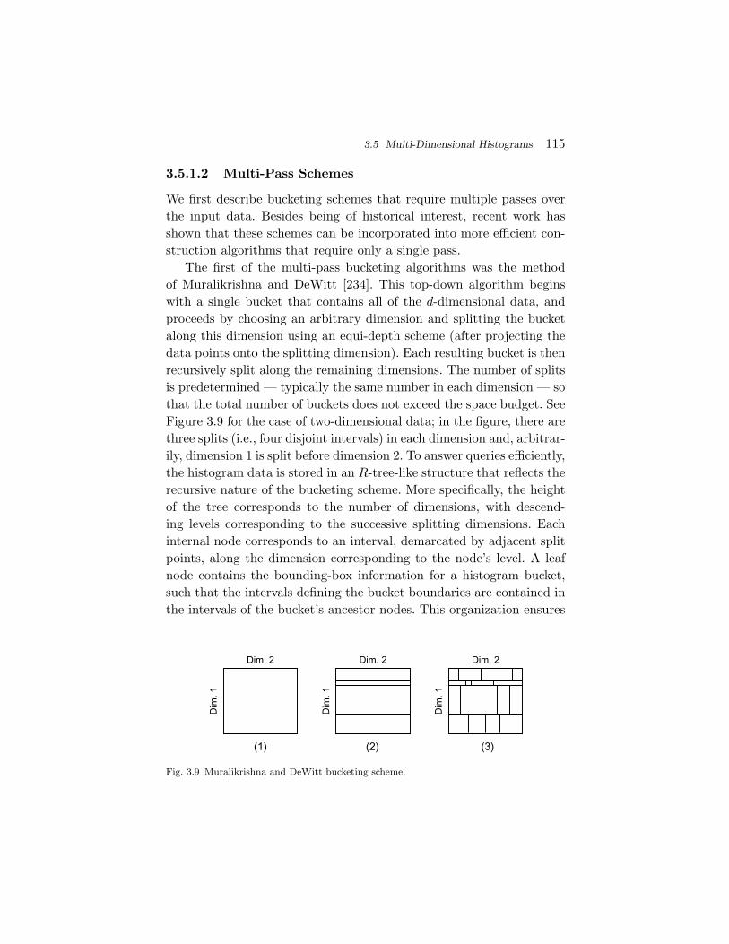
3.5 Multi-Dimensional Histograms 115
3.5.1.2 Multi-Pass Schemes
We first describe bucketing schemes that require multiple passes overthe input data. Besides being of historical interest, recent work hasshown that these schemes can be incorporated into more efficient con-struction algorithms that require only a single pass.
The first of the multi-pass bucketing algorithms was the methodof Muralikrishna and DeWitt [234]. This top-down algorithm beginswith a single bucket that contains all of the d-dimensional data, andproceeds by choosing an arbitrary dimension and splitting the bucketalong this dimension using an equi-depth scheme (after projecting thedata points onto the splitting dimension). Each resulting bucket is thenrecursively split along the remaining dimensions. The number of splitsis predetermined — typically the same number in each dimension — sothat the total number of buckets does not exceed the space budget. SeeFigure 3.9 for the case of two-dimensional data; in the figure, there arethree splits (i.e., four disjoint intervals) in each dimension and, arbitrar-ily, dimension 1 is split before dimension 2. To answer queries efficiently,the histogram data is stored in an R-tree-like structure that reflects therecursive nature of the bucketing scheme. More specifically, the heightof the tree corresponds to the number of dimensions, with descend-ing levels corresponding to the successive splitting dimensions. Eachinternal node corresponds to an interval, demarcated by adjacent splitpoints, along the dimension corresponding to the node’s level. A leafnode contains the bounding-box information for a histogram bucket,such that the intervals defining the bucket boundaries are contained inthe intervals of the bucket’s ancestor nodes. This organization ensures
Dim
. 1
Dim. 2
Dim
. 1
Dim. 2
Dim
. 1
Dim. 2
(1) (2) (3)
Fig. 3.9 Muralikrishna and DeWitt bucketing scheme.
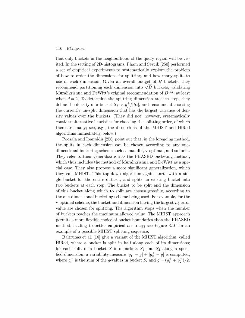
116 Histograms
that only buckets in the neighborhood of the query region will be vis-ited. In the setting of 2D-histograms, Pham and Sevcik [250] performeda set of empirical experiments to systematically explore the problemof how to order the dimensions for splitting, and how many splits touse in each dimension. Given an overall budget of B buckets, theyrecommend partitioning each dimension into
√B buckets, validating
Muralikrishna and DeWitt’s original recommendation of B1/d, at leastwhen d = 2. To determine the splitting dimension at each step, theydefine the density of a bucket Sj as g+
j /|Sj |, and recommend choosingthe currently un-split dimension that has the largest variance of den-sity values over the buckets. (They did not, however, systematicallyconsider alternative heuristics for choosing the splitting order, of whichthere are many; see, e.g., the discussions of the MHIST and HiRedalgorithms immediately below.)
Poosala and Ioannidis [256] point out that, in the foregoing method,the splits in each dimension can be chosen according to any one-dimensional bucketing scheme such as maxdiff, v-optimal, and so forth.They refer to their generalization as the PHASED bucketing method,which thus includes the method of Muralikrishna and DeWitt as a spe-cial case. They also propose a more significant generalization, whichthey call MHIST. This top-down algorithm again starts with a sin-gle bucket for the entire dataset, and splits an existing bucket intotwo buckets at each step. The bucket to be split and the dimensionof this bucket along which to split are chosen greedily, according tothe one-dimensional bucketing scheme being used. For example, for thev-optimal scheme, the bucket and dimension having the largest L2 errorvalue are chosen for splitting. The algorithm stops when the numberof buckets reaches the maximum allowed value. The MHIST approachpermits a more flexible choice of bucket boundaries than the PHASEDmethod, leading to better empirical accuracy; see Figure 3.10 for anexample of a possible MHIST splitting sequence.
Baltrunas et al. [16] give a variant of the MHIST algorithm, calledHiRed, where a bucket is split in half along each of its dimensions;for each split of a bucket S into buckets S1 and S2 along a speci-fied dimension, a variability measure |g+
1 − g| + |g+2 − g| is computed,
where g+i is the sum of the g-values in bucket Si and g = (g+
1 + g+2 )/2.
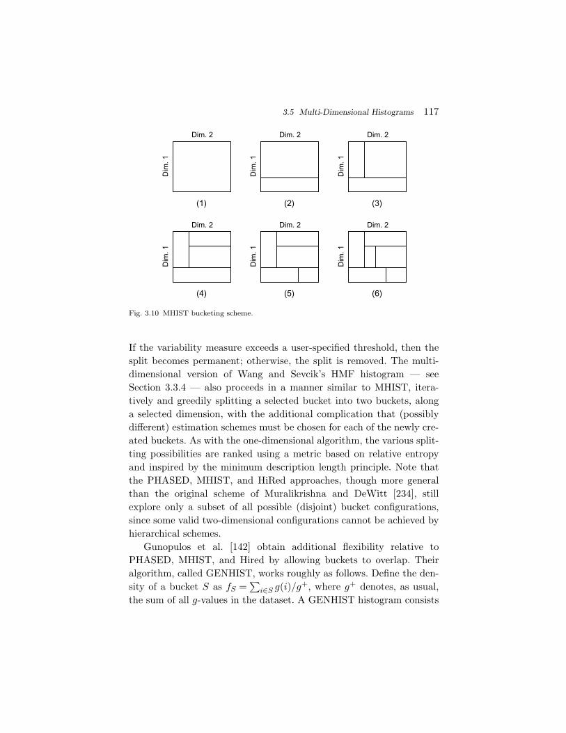
3.5 Multi-Dimensional Histograms 117
Dim
. 1
Dim
. 1
Dim. 2 Dim. 2
Dim
. 1
Dim. 2
(1) (2) (3)
Dim
. 1
Dim
. 1
Dim. 2 Dim. 2
Dim
. 1
Dim. 2
(4) (5) (6)
Fig. 3.10 MHIST bucketing scheme.
If the variability measure exceeds a user-specified threshold, then thesplit becomes permanent; otherwise, the split is removed. The multi-dimensional version of Wang and Sevcik’s HMF histogram — seeSection 3.3.4 — also proceeds in a manner similar to MHIST, itera-tively and greedily splitting a selected bucket into two buckets, alonga selected dimension, with the additional complication that (possiblydifferent) estimation schemes must be chosen for each of the newly cre-ated buckets. As with the one-dimensional algorithm, the various split-ting possibilities are ranked using a metric based on relative entropyand inspired by the minimum description length principle. Note thatthe PHASED, MHIST, and HiRed approaches, though more generalthan the original scheme of Muralikrishna and DeWitt [234], stillexplore only a subset of all possible (disjoint) bucket configurations,since some valid two-dimensional configurations cannot be achieved byhierarchical schemes.
Gunopulos et al. [142] obtain additional flexibility relative toPHASED, MHIST, and Hired by allowing buckets to overlap. Theiralgorithm, called GENHIST, works roughly as follows. Define the den-sity of a bucket S as fS =
∑i∈S g(i)/g
+, where g+ denotes, as usual,the sum of all g-values in the dataset. A GENHIST histogram consists
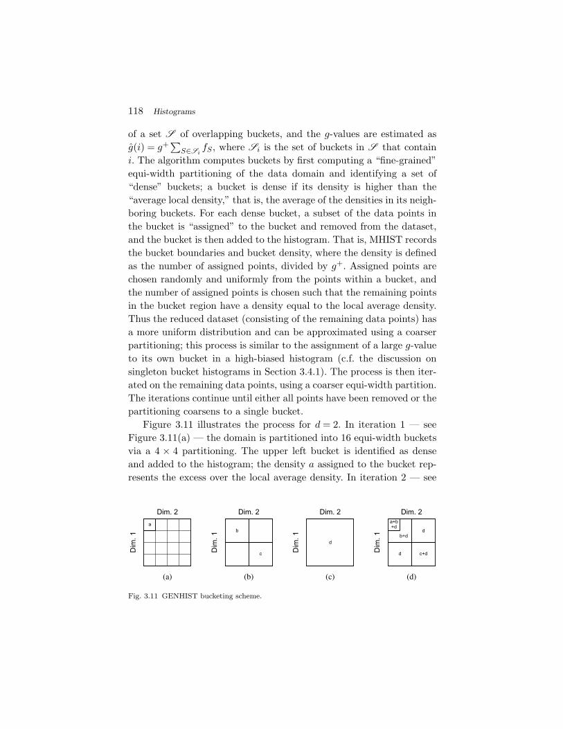
118 Histograms
of a set S of overlapping buckets, and the g-values are estimated asg(i) = g+∑
S∈SifS , where Si is the set of buckets in S that contain
i. The algorithm computes buckets by first computing a “fine-grained”equi-width partitioning of the data domain and identifying a set of“dense” buckets; a bucket is dense if its density is higher than the“average local density,” that is, the average of the densities in its neigh-boring buckets. For each dense bucket, a subset of the data points inthe bucket is “assigned” to the bucket and removed from the dataset,and the bucket is then added to the histogram. That is, MHIST recordsthe bucket boundaries and bucket density, where the density is definedas the number of assigned points, divided by g+. Assigned points arechosen randomly and uniformly from the points within a bucket, andthe number of assigned points is chosen such that the remaining pointsin the bucket region have a density equal to the local average density.Thus the reduced dataset (consisting of the remaining data points) hasa more uniform distribution and can be approximated using a coarserpartitioning; this process is similar to the assignment of a large g-valueto its own bucket in a high-biased histogram (c.f. the discussion onsingleton bucket histograms in Section 3.4.1). The process is then iter-ated on the remaining data points, using a coarser equi-width partition.The iterations continue until either all points have been removed or thepartitioning coarsens to a single bucket.
Figure 3.11 illustrates the process for d = 2. In iteration 1 — seeFigure 3.11(a) — the domain is partitioned into 16 equi-width bucketsvia a 4 × 4 partitioning. The upper left bucket is identified as denseand added to the histogram; the density a assigned to the bucket rep-resents the excess over the local average density. In iteration 2 — see
Dim
. 1
Dim. 2
(a)
a
Dim
. 1
Dim. 2
(b)
b
c Dim
. 1
Dim. 2
(c)
d
Dim
. 1
Dim. 2
(d)
a+b+d
b+d
c+d
d
d
Fig. 3.11 GENHIST bucketing scheme.
3.5 Multi-Dimensional Histograms 119
Figure 3.11(b) — the domain is partitioned into 4 equi-width buckets,and the upper left and lower right buckets are each identified as denseand added to the histogram, with respective densities b and c. In iter-ation 3 — see Figure 3.11(c) — the partitioning has coarsened to asingle bucket, which is added to the histogram. In this case the densityd of the bucket is computed as the sum of the g-values remaining in thedataset, divided by the sum g+ of the entire original set of g-values. Thefinal density approximation for a given region is computed as the sumof the densities of the buckets that contain the region, as illustrated inFigure 3.11(d). Note that the bucket having density b overlaps (in factcompletely contains) the bucket having density a; in general, arbitraryoverlaps are possible.
Although the GENHIST method provides very accurate query-result estimates, the costs for constructing and using the histogramare quite high, as are the space requirements for computing and stor-ing the histogram. For example, the complexity of the initial densitycomputations is exponential in the dimension of the data. Experimentsby Baltrunas et al. [16] indicate that, given a space budget, the simpleHiRed histogram can dominate GENHIST in speed and accuracy, atleast on some datasets.
A related bucketing scheme is the STHoles method of Brunoet al. [30], which we discuss for the case in which g(i) correspondsto the frequency of a value i. In this scheme, high-density regions arecompletely, not partially, removed, in a recursive fashion. Thus bucketscan have “holes,” which are themselves buckets that can have holes, andso forth; see Figure 3.12. Unlike the other bucketing schemes discussedso far, the method for creating buckets (“drilling holes”) and assigningsummary values to buckets rests not upon a scan of the data, but ratheron observing query feedback, that is, the actual numbers of tuples thatsatisfy selection queries issued by users. Srivastava et al. [275] improveupon the original STHoles scheme by updating the bucket summaryvalues using a maximum entropy approach that ensures consistency ofthe bucket counts with respect to the feedback observations. Recently,Kaushik et al. [205] have extended the maximum entropy approach tohandle feedback information that includes information about distinct-value counts. He et al. [163] predict the future query workload, based

120 Histograms
Dim.2
Dim
. 1
b0b1
b2
b3
b0
b2
b3
b1
Fig. 3.12 STHoles bucketing scheme.
on past queries, and create a “proactive” STHoles histogram from thisworkload, which is then merged with the ordinary “reactive” STHoleshistogram when the future time arrives. Luo et al. [219] provide meth-ods for scheduling queries so as to maximize the rate at which anSTHoles histogram converges to an accurate representation of the data,and also introduce an interpolation method that leads to improvedaccuracy for regions in a bucket that are “close” to holes. The vari-ous STHoles construction techniques are somewhat tangential to oursetting, in which queries are answered approximately, and not exactly.However, one could envision a scenario where the system switches backand forth between a training regime — in which queries are processedexactly and the feedback is used to build or refine histograms — and anapproximate-processing regime. The system would switch to the train-ing regime whenever the error in the approximate answers exceeds aspecified threshold.
In general, there is a trade-off between the flexibility of a bucketingscheme and the amount of data that needs to be stored in order tospecify the buckets. The more information that needs to be stored perbucket, the fewer buckets that can be maintained. Fuchs et al. [99]give a scheme for compressing the bucket information in STHoles, andshow that use of this technique can reduce the relative error by upto 40%. The compression technique is to quantize the each coordinateof a bucket relative to the corresponding coordinate of the smallestenclosing bucket.
3.5 Multi-Dimensional Histograms 121
3.5.1.3 Single-Pass Schemes
As discussed previously, the multi-dimensional equi-width histogramcan be constructed in a single pass (or at most two passes if the rangeof data values is unknown), but this histogram performs extremelypoorly as the dimension d increases. Wang and Sevcik [287] proposethe VI (values and intervals) histogram, a high-biased histogram thatcan be constructed in a single pass through the data.7 The algorithmhas the important advantage that it need only scan the positive g-values, leading to significant reductions in time complexity when onlypositive g-values in a dataset are explicitly stored. The idea is to placeany g-value larger than g+/20 into its own bucket; the threshold ischosen to limit the possible number of such buckets (to 20) and is basedon empirical studies. The remaining values are stored in a relativelycoarse memory-resident equi-width histogram (with about 20 buckets ineach dimension), which is then compressed into a PHASED histogram.The VI histogram comprises the PHASED histogram together with thesingleton buckets. The experiments in [287] indicate that this techniquehas the potential to strike a good balance between histogram accuracyand practicality.
In related work, Pham and Sevcik [250] study the problem of deter-mining the number of singleton buckets to maintain in a more sys-tematic fashion. They focus on thresholds of the form g+/(αB), wherethe parameter α determines the priority placed on singleton buckets.Poosala et al. [257] used this type of threshold (with α = 1) for theoriginal maxdiff histogram. Pham and Sevcik found empirically thatthe optimal choice of α is highly sensitive to the particular bucketingscheme used, with, for example, a value of α ≈ 3 being roughly optimalfor PHASED histograms with equi-depth partitioning.
3.5.1.4 Optimal Histograms
Results on optimal and near-optimal multidimensional histogramsare quite sparse, and indeed are found primarily in a paper by
7 Actually, the algorithm requires that g+ be known (or well approximated) a priori, andso might require two passes rather than one, as with the multi-dimensional equi-widthhistogram.
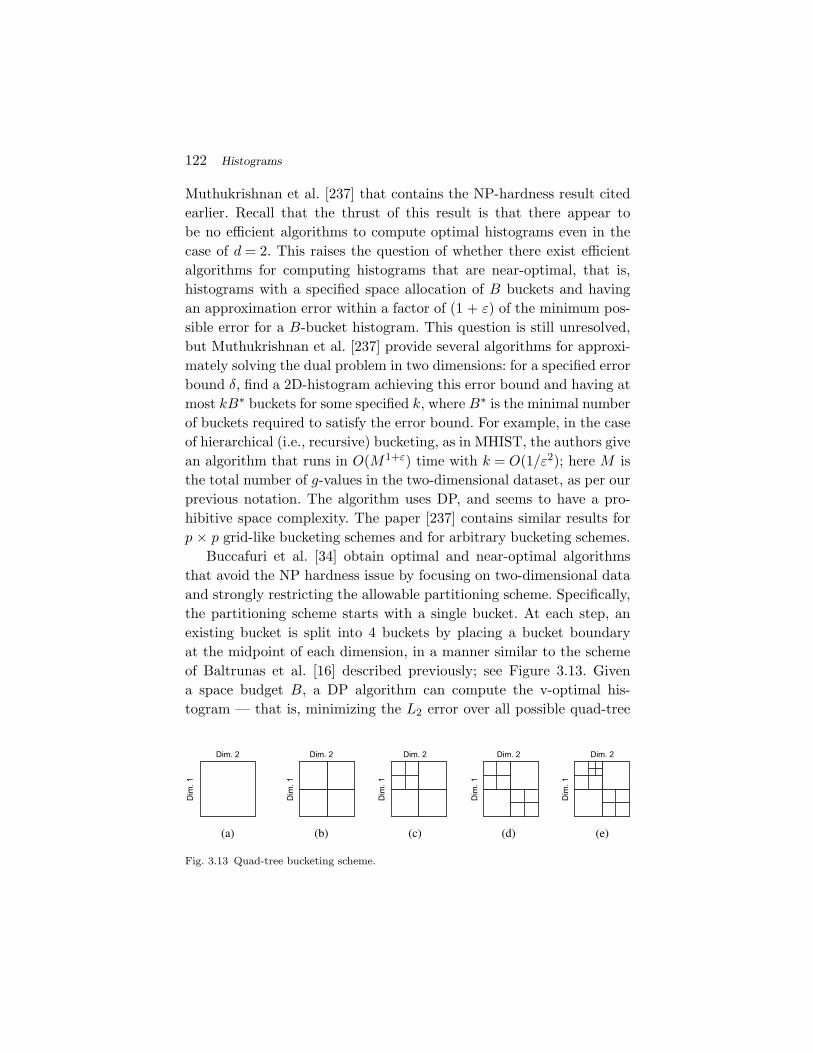
122 Histograms
Muthukrishnan et al. [237] that contains the NP-hardness result citedearlier. Recall that the thrust of this result is that there appear tobe no efficient algorithms to compute optimal histograms even in thecase of d = 2. This raises the question of whether there exist efficientalgorithms for computing histograms that are near-optimal, that is,histograms with a specified space allocation of B buckets and havingan approximation error within a factor of (1 + ε) of the minimum pos-sible error for a B-bucket histogram. This question is still unresolved,but Muthukrishnan et al. [237] provide several algorithms for approxi-mately solving the dual problem in two dimensions: for a specified errorbound δ, find a 2D-histogram achieving this error bound and having atmost kB∗ buckets for some specified k, where B∗ is the minimal numberof buckets required to satisfy the error bound. For example, in the caseof hierarchical (i.e., recursive) bucketing, as in MHIST, the authors givean algorithm that runs in O(M1+ε) time with k = O(1/ε2); here M isthe total number of g-values in the two-dimensional dataset, as per ourprevious notation. The algorithm uses DP, and seems to have a pro-hibitive space complexity. The paper [237] contains similar results forp × p grid-like bucketing schemes and for arbitrary bucketing schemes.
Buccafuri et al. [34] obtain optimal and near-optimal algorithmsthat avoid the NP hardness issue by focusing on two-dimensional dataand strongly restricting the allowable partitioning scheme. Specifically,the partitioning scheme starts with a single bucket. At each step, anexisting bucket is split into 4 buckets by placing a bucket boundaryat the midpoint of each dimension, in a manner similar to the schemeof Baltrunas et al. [16] described previously; see Figure 3.13. Givena space budget B, a DP algorithm can compute the v-optimal his-togram — that is, minimizing the L2 error over all possible quad-tree
(b) (c)
Dim
. 1
Dim
. 1
Dim. 2 Dim. 2 Dim. 2 Dim. 2 Dim. 2
Dim
. 1
Dim
. 1
Dim
. 1
(a) (d) (e)
Fig. 3.13 Quad-tree bucketing scheme.
3.5 Multi-Dimensional Histograms 123
partitionings — in time O(BM logM). This complexity is still imprac-tical, and so the authors provide a greedy algorithm having O(B logB)time complexity; the idea is to greedily choose a bucket to split, specif-ically, the bucket having the maximum L2 error. The greedy algorithmcan further be improved using the two-dimensional generalization ofthe techniques described in Section 3.3.3, namely, storing a subset ofbucket sums explicitly and using these to derive sums for non-storedbuckets, and using an analog of the 4LT to better estimate values withineach bucket.
We conclude this section by briefly discussing connections to multi-dimensional indexes. We have seen that, for the PHASED-type his-togram of Muralikrishna and DeWitt, the histogram is stored ina data structure that looks similar to an R-tree, except that theleaf nodes, instead of holding pointers to data items, contain countvalues. This close relationship between histograms and indices hasbeen pointed out by several authors; see, for example, the survey byIoannidis [179]. Indeed, Read et al. [262] propose augmenting exist-ing B+-tree indices to hold summary statistics for use in aggregationqueries, and Aoki [10] proposes analogous modifications of the Gener-alized Search Tree (GiST) in the context of selectivity estimation. Theoverall hope is to leverage the highly effective technology that has beendeveloped for indexing multi-dimensional data.
3.5.2 Collections of Histograms
Even the best of the foregoing bucketing methods has difficulty deal-ing with data of very high dimension. One possibility for dealing withthis problem is to approximate the full datacube via a collection ofhistograms, where each histogram is constructed over a small subsetof the total set of dimensions. A graphical statistical model capturesthe global correlation structure of the data and is used to combineresults from the different histograms into an overall approximation.We describe a couple of such methods below.
To simplify the exposition, we focus on point-count queries andassume that the g function coincides with the frequency function f .Thus our data is a multi-dimensional array of frequencies with entries
124 Histograms
of the form f(v1,v2, . . . ,vd), where 1 ≤ vk ≤Mk for k ∈ [1,d]. That is,f(v1,v2, . . . ,vd) is the number of data points x = (x1,x2, . . . ,xd) withxi = vi for i ∈ [1,d]. We denote by N the total number of points andby h the relative frequency function: N =
∑v1,v2,...,vd
f(v1,v2, . . . ,vd)and h(v1,v2, . . . ,vd) = f(v1,v2, . . . ,vd)/N . We denote marginal relativefrequencies over a collection of dimensions A ⊆ 1,2, . . . ,d using sub-scripts; for example, h2,4(u,w) =
∑v1,v3,v5,...,vd
h(v1,u,v3,w,v5, . . . ,vd).Conditional relative frequencies are defined analogously to conditionalprobabilities, for example, h2|3(u | v) = h2,3(u,v)/h3(v). Thus if W
is the collection of points whose third dimension has value v, thenh2|3(u | v) is the fraction of points in W having second dimension equalto u. Two dimensions i and j are independent if hi,j(u,v) = hi(u)hj(v)for all i ∈ [1,Mi] and j ∈ [1,Mj ]. This notion corresponds to the usualnotion of statistical independence if we select a pointX at random fromthe dataset; the quantity hi(u) is then the probability that Xi = u, thequantity hi,j(u,v) is the probability that Xi = u and Xj = v, and soforth. Dimensions i and k are conditionally independent, given dimen-sion j, if hi,k|j(u,w | v) = hi|j(u | v)hk|j(w | v) for all u,v,w.
3.5.2.1 Decompositions Based on Graphical Models
Deshpande et al. [83] capture the correlation structure of the datadimensions by means of a “decomposable interaction model.” Such amodel can be represented graphically as a Markov network, that is,an undirected graph in which the nodes represent dimensions and anedge represents a direct correlation between the dimensions that itconnects. Two dimensions i and k that are separated by a dimension jare conditionally independent, given dimension j. The Markov net-work serves to define a collection of (possibly non-disjoint) groups ofdimensions, which correspond to the cliques (maximal completely con-nected subgraphs) of the network. A joint histogram is maintained foreach clique, and desired joint distributions are computed by combin-ing marginal relative frequencies for the various histograms accordingto rules that are determined by the interaction model. In one simplescenario, for example, the cliques correspond to disjoint groups of cor-related dimensions, and dimensions in different cliques are considered
3.5 Multi-Dimensional Histograms 125
to be independent. Thus, if a dataset contains dimensions i, j, k,and l, and there are two cliques [i, j] and [k, l], then we estimatehi,l(t,w) as hi,l(t,w) = hi,j
i (t)hk,ll (w), where hi,j is the approximate
relative frequency function for dimensions i and j, based on the 2D-histogram over these dimensions, hi,j
i is the approximate marginal rel-ative frequency function for dimension i that is computed from hi,j ,and similarly for dimensions k and l. More generally, the model candeal with conditional independence relationships, for example, in whichdimensions i and k are independent, given the value of a third dimen-sion j. For this example, the cliques would be [i, j] and [j,k], and weestimate hi,j,k(u,v,w) as hi,j,k(u,v,w) = hi,j(u,v)hj,k(v,w)/hj,k
j (v) or,equivalently, hi,j,k(u,v,w) = hi,j(u,v)hj,k(v,w)/hi,j
j (v). To limit com-putational complexity, cliques are constrained to contain at mostthree or four dimensions. The interaction model is fitted using aheuristic “forward selection” search process, in which full indepen-dence is assumed initially — so that there is exactly one singletonclique per dimension — and cliques are built up incrementally basedon improvements in the approximation, as measured by decreasesin Kullback-Liebler distance between h and h. For a given pro-posed interaction model, the number of buckets per histogram isallocated using a greedy algorithm, and bucket boundaries withineach histogram are also selected in a greedy fashion. The resultingoverall candidate model is then scored. Lim et al. [214] have devel-oped a feedback-based variant of the foregoing algorithm, which theycall SASH.
Getoor et al. [119] explore an approach somewhat similar to theone above, but based on a Bayesian network representation. Here thenetwork is represented as a directed acyclic graph, and a given dimen-sion is independent of its non-descendants, given its parents. In thisframework, the relative frequency distribution is represented via a setof conditional univariate probability distributions, where the distribu-tion of a given dimension is conditioned on the values of its parents.As in [83], the statistical graphical model is fitted to the data usinga heuristic search through possible correlation structures. For a givencandidate structure, the needed conditional probabilities are simplyestimated via sample frequencies when the number of frequency values
126 Histograms
is not too large; otherwise, bucketing techniques analogous to those in[83] must be used.
Both of the foregoing techniques can be modified to use moresophisticated types of histograms of the type discussed previously, butthe construction costs will increase accordingly. In general, the con-struction costs for these algorithms are fairly heavy, but can poten-tially be alleviated using, for example, sampling techniques. In anycase, the decomposition of the entire joint distribution into a familyof related distributions seems necessary in order to summarize high-dimensional data using histograms, so this line of research deservesfurther exploration.
3.5.2.2 Approximating a Hierarchical Datacube
In a somewhat different setting, Poosala and Ganti [254] considerthe problem of identifying an optimal configuration of histograms —MHIST histograms in particular — that approximate the differentsubcubes of a hierarchical datacube. A hierarchical datacube in d dimen-sions comprises a collection of 2d − 1 subcubes, where a subcube corre-sponding to the dimensions in the set D ′ ⊆ D = 1,2, . . . ,d is obtainedby aggregating over the dimensions in D\D ′. Thus a given subcube cor-responding to a set D ′ of dimensions can be approximated directly bya |D ′|-dimensional histogram, or may be approximated indirectly byfirst approximating a subcube with dimension set D ′′ ⊃ D ′, and thenaggregating over the dimensions in D ′′\D ′. The problem is to identify acollection of subcube histograms that occupy minimal space, subject toan upper bound on the allowable maximum approximation error over allsubcubes. To approximately answer a given OLAP query once a solu-tion has been obtained, all approximated subcubes whose dimensionscover the query dimensions are considered, and the subcube havingminimum average relative approximation error — as computed dur-ing histogram creation — is used. (This technique contrasts with theother techniques in this section, in which multiple partial histogramsare combined together, via assumptions of independence or conditionalindependence, to approximately answer a query.) The authors showthat a solution to the minimum weighted set cover problem (MWSC)
3.6 Approximate Processing of General Queries 127
yields a set of histograms that satisfy the error bound and whose spacerequirement is within a constant factor of the space required for theoptimal configuration. A standard greedy algorithm for solving MWSCis employed to compute the near-optimal histogram configuration.
3.6 Approximate Processing of General Queries
The discussion so far has concentrated on the use of histograms forapproximate answering of range-sum queries, which are central toOLAP applications. As we have seen, there has been an enormousamount of research in this area. A smaller but perhaps even moreimportant line of work has attempted to extend histogram methodol-ogy to the more general setting of SQL queries that involve multi-tableoperations such as joins. Work in this area has focused on the estima-tion of COUNT queries over the result of a select-project-join (SPJ)query over a set of tables (typically in the context of selectivity esti-mation for query optimization), as well as approximating the results ofset-valued queries. In this section, we describe the key results in thisarea, which still poses a tremendous challenge to histogram technology.
3.6.1 Aggregation Queries Over Joins
In this section, we consider the problem of approximating the answer toa simple COUNT(*) query over a table that is itself obtained via a joinoperation over a set of base tables. (In the query optimization setting,this task corresponds to estimating the size of a multi-table join.) Aspointed out by Dobra [86], this framework extends straightforwardlyto queries of the form:
SELECT AGG(h1(A1)*h2(A2)*· · ·*hk(Ak))
FROM
R1,R2, . . . ,Rk
WHERE . . .
where each hi is a real-valued function on a set Ai of attributes fromRi, the WHERE clause contains local and join predicates, and AGG is anaggregation function such as SUM, COUNT, AVG, or STDDEV. As discussedbelow, there have been a number of theoretical results that characterize

128 Histograms
the difficulty of this problem, that compare the relative effectiveness ofhistograms and other types of synopses, and that provide some guid-ance in configuring a histogram to answer such queries.
3.6.1.1 A Negative Result
The database community first contributed to the theory of histogramsvia the work of Ioannidis and Christodoulakis [180]. The study in[180] focuses on a setting in which all joins are equality joins, butneed not be key to foreign-key joins. Exactly one column in each tableserves as the join column for all joins in which the table participates(“t-clique” joins). Individual single-bucket histograms are maintainedon the join columns, using the continuous-values estimation schemewithin the bucket. The analysis in [180] shows that the estimation errorgrows exponentially as the number of joins increases, indicating thatthis approach, in general, will work poorly, unless each histogram isexceedingly accurate or the estimation problem (data and or query)has special properties that can be exploited (see below).
3.6.1.2 Refinements: Relative Effectiveness of Histograms
Dobra [86], refines the above theoretical results by identifying somespecial conditions under which accurate results can be obtained, andcompares histograms to samples and sketches in several scenarios. Tohighlight the main ideas, we focus on the case of size estimation for asimple two-table equality join, where, for each table R and S, a single-bucket uniform histogram is maintained on the join column. Supposethat the join column values have domain U = [1,M ], and, for i ∈ U ,denote by ri and si the frequency of the ith join value in R and S. Thehistogram-based estimate of the join size is simply Mrs, where r is theaverage of r1, r2, . . . , rM , and similarly for s. Clearly, this estimate willbe accurate if ri ≈ r and si ≈ s for all i ∈ U , but such a uniformity con-dition is usually violated in practice. A more general condition allowsboth the ris and the sis to be heterogeneous, but requires that there beno “systematic relationship” between ri and si as i varies. Conceptu-ally, one can envision specifying the ris and the sis, but then randomlypermuting the sis to break any relationship, that is, to replace each
3.6 Approximate Processing of General Queries 129
si by sσ(i), where σ is a random permutation of the elements of U .This model is called the random-shuffling assumption, and it can beshown that, under this probabilistic model, the histogram estimate isunbiased for the true join size, and is close to the true join size withhigh probability.8
Dobra extends this result to multi-bucket histograms which are“aligned,” in the sense that the R-histogram and S-histogram use thesame set of buckets. He then shows that, under the random shufflingassumption, aligned histograms are much more accurate, on average,than samples and sketches. On the other hand, when the random-shuffling assumption does not hold, aligned histogram estimates arepoor, on average, unless the histogram sizes are close to the columnsizes. In particular, for estimating the size of a self join, aligned his-tograms are shown to perform fundamentally worse, on average, thansamples or sketches. As pointed out in [86], however, non-aligned his-tograms, such as high-biased histograms, may do substantially betterthan aligned histograms, so no general conclusions can be drawn inthis case. The foregoing results are theoretical in that they cannot beapplied a priori to choose between synopses for a specific query work-load and set of tables.
Kaushik et al. [204] provide a number of fundamental theoreticalresults pertaining to the relative effectiveness of histogram synopsesfor estimating the size of general SPJ queries. These results analyzethe space complexity of histograms and other types of synopses. Undera general estimation model that includes both deterministic and prob-abilistic estimation methods, they establish the following results in aprecise, information-theoretic sense:
• Under the usual absolute, ratio, and relative error metrics,and with no assumptions on the data distribution, efficientestimation is impossible for any synopsis, in that it is impos-sible to simultaneously guarantee “small” errors (constant orpolylogarithmic in the data size) and a small synopsis size,even for single-column equality selection queries on a singletable; c.f. the informal example in Section 3.1.1.
8 The unbiasedness result was originally proved by Ioannidis [177], but for a differentpurpose.
130 Histograms
• Under a looser “threshold” error criterion, which only triesto estimate whether the result size is smaller or largerthan a specified threshold, efficient estimation is possible forsingle-column selections as above but not for range selectionqueries.
• For single-table selections, histograms are the most space-efficient type of synopsis; the resulting errors, although“large” in the above sense, are typically acceptable in prac-tice, validating the observed efficacy of histograms in thissetting.
• For specific, skewed, data distributions and a given spacebudget, the worst case error guarantees can be substantiallyimproved, again supporting practical experience.
• The space complexity for handling COUNT queries overarbitrary joins is substantially higher that the space com-plexity for single-table queries; this result complements andstrengthens the results in [180].
• The above negative result does not hold for the special caseof key-foreign key joins, and an effective technique for han-dling such queries is to use as a synopsis a small sample fromthe precomputed join, in an extension of the “join synopsis”technique of Acharya et al. [3]. Kaushik et al. [204] show thattheir proposed synopsis has near-optimal space complexity.
A histogram-oriented analogue to the above synopsis of Kaushiket al. is the notion of Statistics on Intermediate Tables (SITs) intro-duced for use in the query optimizer for the SQL Server product byBruno and Chaudhuri [29]; In DB2 for LUW [52], SITs are called“statistical views.” The idea is to create histograms, rather thansamples, on intermediate query results. The major challenges of thisapproach (and to that of Kaushik et al.) are: (a) determining for whichof the many sub-expressions of an SQL workload the system shouldcollect SITs, and (b) ensuring that the system can effectively exploitthe SITs. Standard view-matching algorithms can potentially be usedto handle challenge (b); challenge (a) has not received attention in thegeneral setting of approximate query answering.
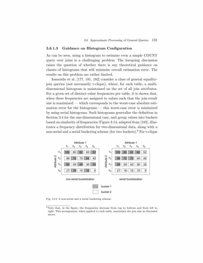
3.6 Approximate Processing of General Queries 131
3.6.1.3 Guidance on Histogram Configuration
As can be seen, using a histogram to estimate even a simple COUNTquery over joins is a challenging problem. The foregoing discussionraises the question of whether there is any theoretical guidance onclasses of histograms that will minimize overall estimation error. Theresults on this problem are rather limited.
Ioannidis et al. [177, 181, 182] consider a class of general equality-join queries (not necessarily t-clique), where, for each table, a multi-dimensional histogram is maintained on the set of all join attributes.For a given set of distinct-value frequencies per table, it is shown that,when these frequencies are assigned to values such that the join-resultsize is maximized — which corresponds to the worst-case absolute esti-mation error for the histograms — this worst-case error is minimizedby using serial histograms. Such histograms generalize the definition inSection 3.4 for the one-dimensional case, and group values into bucketsbased on similarity of frequencies; Figure 3.14, adapted from [182], illus-trates a frequency distribution for two-dimensional data, along with anon-serial and a serial bucketing scheme (for two buckets).9 For t-clique
100
96
60
27
85
72
59
18
82
70
40
15
60
54
36
10
52
40
35
5
Attribute 1
Attr
ibut
e 2
v1
v1
v2
v2
v3
v3
v4 v5
v4
100
96
60
27
85
72
59
18
82
70
40
15
60
54
36
10
52
40
35
5
Attribute 1
Attr
ibut
e 2
v1
v1
v2
v2
v3
v3
v4 v5
v4
non-serial bucketization serial bucketization
bucket 1
bucket 2
Fig. 3.14 A non-serial and a serial bucketing scheme.
9 Note that, in the figure, the frequencies decrease from top to bottom and from left toright. This arrangement, when applied to each table, maximizes the join size as discussedabove.
132 Histograms
queries with a large number of joins, estimation error is minimized usinghigh-biased histograms — in which, as discussed in Section 3.4.1, thevalues with the highest frequencies are assigned to singleton bucketsand the remaining values are assigned to a common bucket.
Some results on choosing the optimal serial histogram for a givenjoin attribute are presented in [177, 181]. These results only apply tothe worst-case-error scenario described above, and depend on both thespecific query of interest and the precise contents of all of the tables;thus the optimal histograms are sensitive to changes in the data. It isshown in [182] that, using a v-optimality criterion, optimal histogramscan be determined separately for each table, and independent of a par-ticular query. Specifically, it suffices to determine a histogram for ajoin attribute A on a table R that is optimal with respect to the joinof R to itself. This optimal histogram will be a serial histogram ingeneral, which can be extremely expensive to construct and use. Con-sequently, based on empirical evidence, the authors recommend theuse of end-biased histograms. Of course, practically speaking, any ofthe histograms discussed previously can be considered, once optimalityguarantees are no longer being provided.
3.6.2 Set-Valued Queries
Ioannidis and Poosala [183] initiated the study of how to use histogramtechniques to approximate the answers to set-valued queries over dis-crete data. They assume that a multi-dimensional bucketing schemehas been specified for each table in the database (Section 3.5.1), anduse the multi-dimensional version of the uniform-spread assumption(Section 3.3.1) to approximate the data values. That is, given that abucket — that is, a hyper-rectangle in d-dimensional space — con-tains mi distinct values in the ith dimension (1 ≤ i ≤ d), the set of(multivariate) distinct values present in the bucket is approximatedas a set of m1m2 · · ·md distinct values, uniformly spread out over thebucket. The frequency for each of these distinct value is the averagefrequency for the bucket, that is, the total number of data points inthe bucket divided by the quantity m1m2 · · ·md. See Figure 3.15 for anexample in two dimensions, involving an 8 × 8 bucket; in the figure,

3.6 Approximate Processing of General Queries 133
0
4
2
6
8
9 8
7 8
13
original data distribution
Attribute1
Attr
ibut
e 2
Attr
ibut
e 2
Attribute1
0
4
2
6
0 2 4 6 8 0 2 4 6 8
8
3333
3 3
3
3
333
3 33
approximate data distribution
Fig. 3.15 Uniform-spread assumption in two dimensions.
black dots correspond to distinct data values, with the correspond-ing frequency displayed next to the value. Thus the original data in thebucket comprises 45 tuples having five distinct tuple values (1,3), (2,3),(4,5), (5,5), and (6,1), with respective frequencies 9, 8, 7, 8, and 13;here there are m1 = 5 distinct values (1, 2, 4, 5, and 6) in dimension 1and m2 = 3 values (1, 3, and 5) in dimension 2. The approximateddata comprises m1m2 = 5 × 3 = 15 distinct tuple values, each with fre-quency 45/15 = 3 and spaced evenly throughout the bucket.
The authors perform AQP by, in effect, applying the query Q ofinterest to the approximate tables R1, R2, . . . , Rk corresponding to thehistogram synopses H1,H2, . . . ,Hk of the original tables R1,R2, . . . ,Rk,thereby producing an output table S that approximates the trueresult table S. To achieve acceptable performance, the system actu-ally proceeds by storing each histogram Hi in relational form andtransforming Q into an equivalent query Q′ that is applied directlyover H1,H2, . . . ,Hk to produce a result histogram H ′, which is thenexpanded to the (approximate) result relation S. The query Q′ is gen-erated so as to ensure that H ′ is indeed a synopsis of S.
To illustrate the process, consider a table R having a single attributeA and let H be a histogram synopsis of R. Assume that H is stored as arelation H with schema H(lo, hi, dv, avg, sp). Each row of H rep-resents a histogram bucket, having bucket boundaries lo and hi, andcontaining dv distinct values. The columns avg and sp represent theaverage frequency and spread of the values in the bucket, and are used
134 Histograms
to approximate the data distribution in the bucket (using the uniform-spread assumption as previously described). All 1D-histograms in thesystem share this schema. Consider the selection query Q: SELECT A
FROM R WHERE A = c. We rewrite this query to a new query Q′ over H:
SELECT c, c, 1, avg, 0
FROM H
WHERE (c >= lo) AND (c <= hi) AND (MOD(c-lo,sp) == 0)
If the selection is nonempty, then this query creates an output his-togram H′ having exactly one singleton bucket containing the value c,that is, a bucket for which the lower and upper boundaries both equal c,the number of distinct values is exactly 1, and the average spread is triv-ially 0. To create this output bucket, the query finds the bucket in H thatpotentially contains the value c (via the first two clauses of the WHERE
expression). Next, the query checks whether c is a multiple of the spread(via the final clause of the WHERE expression); under the uniform-spreadassumption, such multiples, and only such multiples, have positive fre-quency, namely avg, and this avg value is returned as the frequency ofc in the singleton output bucket. A (slightly tricky) SQL query can thenbe applied to transform H ′ into an approximate result relation S con-sisting of avg rows, each equal to c. Observe that, with this approach,we never have to expand H into an approximate relation — which canbe as large as the original relation R — thereby reducing processingcosts. These techniques extend to multi-dimensional histograms andother relational operators besides selection.
In related work, Poosala et al. [255] observe that the foregoing tech-nique can also be applied to aggregation queries over relational expres-sions. The idea is to first proceed as above in computing an outputhistogram H ′ which is a synopsis of an approximation to the relationalexpression. Then, instead of expanding H ′ into an approximate outputrelation as above, we simply apply the original aggregation operatorto H ′ — after rewriting it appropriately — to produce an approxi-mate answer to the original aggregation query. For example, considera histogram H ′ as above for a table S that approximates a single-column table S of sales data, where S is computed via join queries overmultiple base tables and S is created by executing analogous queries
3.7 Additional Topics 135
over histogram synopses of the base tables. If the original aggregationquery is SELECT SUM(SALES) FROM S, then the answer to this querycan be approximated as the answer to the query
SELECT SUM(avg*(dv*lo+0.5*dv*(dv-1)*sp))
FROM H’
This query, in effect, computes the answer to the query SELECT
SUM(SALES) FROM S. Observe that, for a given bucket of the his-togram H ′, the transaction amounts that occur with positive frequencyare lo, lo+sp, lo+2*sp, . . ., lo+(dv-1)sp under the uniform-spreadassumption; these numbers sum to dv*lo+0.5*dv*(dv-1)*sp. Becauseeach of these values occurs with frequency avg, the total contribution tothe sum of sales from the bucket is avg*(dv*lo+0.5*dv*(dv-1)*sp).The above query simply sums up the contributions from the differentbuckets.
3.7 Additional Topics
We conclude this chapter with a discussion of histograms over stream-ing data, as well as techniques targeted specifically toward real-valueddata.
3.7.1 Histograms Over Streaming Data
As mentioned at the end of Section 3.4.2, histograms over streamingdata are needed to handle the relational data access scenario. Suchhistograms are becoming ever more important in their own right, dueto the increasing importance of streaming data, such as the data fromsensor and IP networks. In this section, we describe algorithms formaintaining histograms over streaming data. We first discuss meth-ods for one-dimensional data, and then briefly describe extensions tomultidimensional data.
We consider turnstile and sliding-window streaming-data models.The turnstile model was described at the end of Section 3.4.2: eachnew transaction is of the form “increment the current value of g(i)by v.” When v is constrained to be a positive integer, one obtainsthe cash-register model as a special case. Sliding-window models are
136 Histograms
described later in the section. We note that the term “streaming data”is sometimes used to describe the scenario where a histogram construc-tion algorithm takes a single pass over a finite set of N items and useso(N) memory — and often O(1) memory in practice — to constructthe histogram. We would maintain that this level of performance isrequisite for an algorithm to be practically useful, and do not reservethe term “streaming data” for this scenario.
Early work by Donjerkovic et al. [89] proposed a histogram mainte-nance algorithm that supports the cash-register model. Their approach,however, does not control the approximation error over time.
Gilbert et al. [127] provide a histogram maintenance algorithm thatsupports the full turnstile model. The algorithm maintains a sketchbased on distance-preserving random projections — see Section 5 —and in turn uses the sketch to maintain an accurate wavelet representa-tion of the data — see Section 4. On demand, the algorithm recovers,with high probability, a near-optimal histogram; that is, the error isoptimal within a factor of (1 + ε), with respect to an L1 or L2 errormetric. The algorithm, which is rather complicated, has space com-plexity that is polynomial in τ = Bε−1 logM , and requires O(τ) timeto process each transaction. Muthukrishnan et al. [239] extend theseresults to a workload-dependent L2 metric, that is, a metric of the form∑M
i=1wi(g(i) − g(i))2, where w = (w1,w2, . . . ,wM ) represents a weightor probability distribution over possible point queries. Results are givenfor both the datacube and turnstile models, and for cases where theworkload vector w is provided either in compressed form (e.g., usingthe Ziv-Lempel encoding) or in uncompressed form.
Qiao et al. [258] provide a heuristic adaptive scheme for histogrammaintenance (no error guarantees) that splits and merges buckets to tryand ensure narrower buckets in regions that are near the boundaries ofrange queries or values that are queried more frequently. An exponentialsmoothing approach is used to summarize a changing workload.
The problem of dynamically maintaining an (approximate) equi-depth histogram under the turnstile model is equivalent to the prob-lem of dynamically maintaining (approximate) quantiles under thismodel. Sketches have been successfully employed for this problem; seeSection 5.3.4.3.
3.7 Additional Topics 137
A related approach, also applicable to the turnstile model, maintainsa random sample of data values, called a backing sample, and constructsan approximate histogram from the sample. Gibbons et al. [126] pro-pose such a scheme for maintaining an approximate equi-depth or com-pressed histogram; we focus here on the simpler equi-depth case. Thealgorithm takes an initial sample and then computes a correspondinginitial equi-depth histogram. As records are inserted and deleted intothe database, the algorithm maintains the backing sample and incre-ments or decrements the bucket counts, as appropriate. Recall that,ideally, the bucket counts for an equi-depth histogram with B bucketsshould all be equal to |R|/B, where |R| is the number of records in thedatabase; if the count for a bucket becomes very large or very small rel-ative to the other bucket counts, then the algorithm recomputes the his-togram from scratch, using the current backing sample. The algorithmactually tries to reduce the number of such recomputations by splittingand merging adjacent buckets to even out the counts. The method formaintaining a backing sample handles database insertions by using astandard reservoir sampling algorithm, and handles deletions by remov-ing the tuple from the reservoir, if present. Whenever a tuple is removedfrom the reservoir, the method decreases the reservoir size by 1; whenthe reservoir size reaches a specified lower threshold, the method recom-putes the sample from scratch. Gemulla et al. [116, 117] give improvedalgorithms for maintaining a backing sample, which can be used inconjunction with the foregoing histogram maintenance algorithm.
Buragohain et al. [38] show that their Min-Increment algorithm —see the discussion of maximum-error metrics in Section 3.4.2 — canbe extended to a sliding-window model. In this model, the goal isto maintain, after a total of n g-values have been observed, a his-togram of the most recent w of these n values, that is, of the valuesg(n − w + 1),g(n − w + 2), . . . ,g(n). We assume here that each g(i)value belongs to some finite subset of the integers that contains R ele-ments. Such an algorithm must take only one pass over the data, havelow per-item processing cost, and have a o(w) space complexity. Theextended version of Min-Increment is the first such algorithm havingoptimality guarantees. Specifically, the L∞ error is within a (1 + ε)factor of the optimal error for a B-bucket histogram, while using at

138 Histograms
most B + 1 buckets; the memory requirement is O(ε−1B logR), whichis indeed o(w), and a processing time of O(ε−1B logR) per arriving dataitem. The algorithm is similar to the original Min-Increment algorithmin that it maintains a set of histograms as in the Greedy-Insert algo-rithm, one for each error bound ei as defined previously. The differenceis that a histogram bucket is eliminated if and only if either (1) all ofthe data points in the bucket fall outside the window or (2) the numberof buckets exceeds B + 1, in which case the oldest bucket is deleted.Observe that the number of buckets may exceed B; it might be hopedthat, by increasing the number of buckets by some factor β, the L∞error bound could be reduced to match that of the optimal B-buckethistogram, thereby eliminating the (1 + ε) approximation factor. Theauthors prove, however, that this is impossible. Using a DP approach,Guha et al. [138] provide a sliding-window algorithm called AHIST-L-∆that maintains a data structure of size O(w + B2ε−1) with O(1) pro-cessing cost per arriving data item; an ε-approximate histogram can beproduced on demand for a time complexity of O(B3 log2w + τB2ε−1),where τ = min(Bε−1 logw,w). Although the space requirements areheavy relative to the method of Buragohain et al., there is no restrictionto L∞ error.
Buccafurri and Lax [36] provide a variant of the n-level tree —see Section 3.4.3 — suitable for approximately answering range-sumqueries over a sliding window. The key difference from the originalnLT is that a running range sum for the r most recent g-values ismaintained in a buffer, where r = w/2n−1 with w = the window sizeand n = the number of levels in the tree. When the buffer fills up,the sum is added to the tree by overwriting the oldest leaf node andpropagating the update to all of the nodes on the path connecting theleaf to the root. In this way, the per-item update cost, as well as thetime to approximately answer a range-sum query, is O(logw).
The above sliding-window model might more precisely be called a“datacube” sliding-window model, since it is closely related to the dat-acube model of data access (Section 3.2.2). Note that the g(i) valuesare partitioned according to time, that is, according to the i values.A sliding-window setting that corresponds to the relational model of

3.7 Additional Topics 139
data access assumes a sequence of values d1 = (j1,v1),d2 = (j2,v2), . . .as in Section 3.2.2 — so that each jn is an element of [1,M ] — togetherwith a specified partition of [1,M ] into B buckets. Thus data items areassigned to buckets based on the jn values, which do not correspond,in general, to the arrival order of the items. Suppose that each g(i)is obtained applying the SUM aggregate to the set Ai = vn : jn = i.This special case can be viewed as a modified turnstile model in which,at the arrival of data item di, the value g(ji) is incremented by vi, andthe value of g(jm) is decremented by vm; here the index m = i − wcorresponds to the data item that is dropping out of the window.10
Now further assume that each vi is an integer lying in the range [1,R]for some R ≥ 1. Then the sliding-window problem is to maintain ahistogram having the specified set of buckets, where the g-values arecomputed from the last w data items dn−w+1,dn−w+2, . . . ,dn . Asusual, the most important special case occurs when each vi equal 1,so that g(i) is the number of the last w data items having value i.Datar et al. [77] provide a data structure called an “exponential his-togram” that can be used to maintain, for each bucket, the sum ofthe g-values to within a factor of 1 + ε, thereby approximating thetrue histogram over the sliding window (where we use the continuous-value assumption within each bucket). The total space requirement isO(Bε−1 logw(logR + logw)), and the worst-case per-item processingtime is O(logw + logR).
We now consider multi-dimensional data. Several of the foregoingmethods for maintaining 1D-histograms under the general turnstilemodel can be extended to the multi-dimensional case. In particular,the backing-sample approach of Gibbons et al. can be adapted for usewith the multi-dimensional equi-depth histogram of Muralikrishna andDewitt.
Moreover, Thaper et al. [278] have extended the sketch-based tech-nique of Gilbert et al. [127] to a multi-dimensional setting; see alsoSection 5.3.5.1. Recall that this algorithm maintains a sketch of the datastream based on random projections, and then produces a near-optimal
10 Note that turnstile algorithms cannot be applied to this problem, since the value vm isnot available when di arrives.

140 Histograms
histogram on demand. For the multidimensional algorithm, the timeto produce a histogram having error at most (1 + ε) times the mini-mum possible error is roughly O(M log(MB/ε2)). Muthukrishnan andStrauss [238] improve on this result using advanced techniques basedon tensor products of Haar wavelets.
3.7.2 Techniques for Real-Valued Data
The discussion so far has focused on discrete data. Some experimen-tal evidence in Blohsfeld et al. [23] and Korn et al. [209] indicatesthat, for COUNT queries on real-valued data, superior performancemight be obtained by using (and extending) classical statistical meth-ods, which were originally developed under the assumption that thedata are i.i.d. samples from a continuous probability density function(see Section 3.1.3). These methods are also potentially desirable for thecase of discrete data in which the domain size M is large and the mul-tiplicity of each distinct value in the dataset is close to 1. We looselydescribe such data also as “real-valued.”
The basic tool used is kernel density (KD) estimation [85, 162, 270,273, 285], which has been extensively studied in the statistical litera-ture. We briefly describe this approach below, and the discuss its appli-cation in the database setting, first to one-dimensional data and thento multi-dimensional data.
One motivation behind KD methods that the bucket values — andhence the estimates — of a classical equi-width histogram can be verysensitive to the placement of the bucket boundaries. This suggests thatmultiple histograms be obtained from a “base” equi-width histogram bysystematically shifting the histogram (i.e., uniformly shifting the bucketboundaries) by various amounts. Approximate COUNT values are thenobtained by averaging the results from these histograms. Letting thenumber of shifted histograms increase to infinity, we obtain a specialcase of a KD estimator having a “rectangular kernel.”
The general form of a one-dimensional KD estimator based on datavalues x1,x2, . . . ,xn is
fh(u) =1nh
n∑i=1
K
(u − xi
h
),
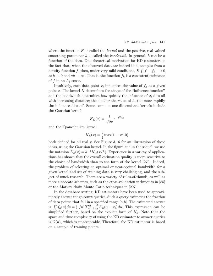
3.7 Additional Topics 141
where the function K is called the kernel and the positive, real-valuedsmoothing parameter h is called the bandwidth. In general, h can be afunction of the data. One theoretical motivation for KD estimators isthe fact that, when the observed data are indeed i.i.d. samples from adensity function f , then, under very mild conditions, E[
∫ |f − fh|]→ 0as h→ 0 and nh→∞. That is, the function fh is a consistent estimatorof f in an L1 sense.
Intuitively, each data point xi influences the value of fh at a givenpoint x. The kernel K determines the shape of the “influence function”and the bandwidth determines how quickly the influence of xi dies offwith increasing distance; the smaller the value of h, the more rapidlythe influence dies off. Some common one-dimensional kernels includethe Gaussian kernel
KG(x) =1√2πe−x2/2
and the Epanechnikov kernel
KE(x) =34
max(1 − x2,0)
both defined for all real x. See Figure 3.16 for an illustration of theseideas, using the Gaussian kernel. In the figure and in the sequel, we usethe notation Kh(x) = h−1KG(x/h). Experience in a variety of applica-tions has shown that the overall estimation quality is more sensitive tothe choice of bandwidth than to the form of the kernel [270]. Indeed,the problem of selecting an optimal or near-optimal bandwidth for agiven kernel and set of training data is very challenging, and the sub-ject of much research. There are a variety of rules-of-thumb, as well asmore elaborate schemes, such as the cross-validation techniques in [85]or the Markov chain Monte Carlo techniques in [297].
In the database setting, KD estimators have been used to approxi-mately answer range-count queries. Such a query estimates the fractionof data points that fall in a specified range [a,b]. The estimated answeris∫ ba fh(u)du = (1/n)
∑ni=1
∫ ba Kh(u − xi)du. This expression can be
simplified further, based on the explicit form of Kh. Note that thespace and time complexity of using the KD estimator to answer queriesis O(n), which is unacceptable. Therefore, the KD estimator is basedon a sample of training points.
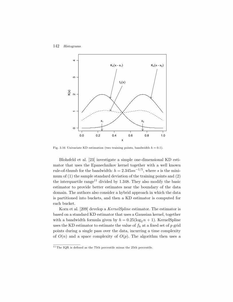
142 Histograms
0.0 0.2 0.4 0.6 0.8 1.0
01
23
4
x
K(x
)
fh(x)
x1 x2
Kh(x − x1) Kh(x − x2)
Fig. 3.16 Univariate KD estimation (two training points, bandwidth h = 0.1).
Blohsfeld et al. [23] investigate a simple one-dimensional KD esti-mator that uses the Epanechnikov kernel together with a well knownrule-of-thumb for the bandwidth: h = 2.345sn−1/5, where s is the mini-mum of (1) the sample standard deviation of the training points and (2)the interquartile range11 divided by 1.348. They also modify the basicestimator to provide better estimates near the boundary of the datadomain. The authors also consider a hybrid approach in which the datais partitioned into buckets, and then a KD estimator is computed foreach bucket.
Korn et al. [209] develop a KernelSpline estimator. The estimator isbased on a standard KD estimator that uses a Gaussian kernel, togetherwith a bandwidth formula given by h = 0.25(log2n + 1). KernelSplineuses the KD estimator to estimate the value of fh at a fixed set of p gridpoints during a single pass over the data, incurring a time complexityof O(n) and a space complexity of O(p). The algorithm then uses a
11 The IQR is defined as the 75th percentile minus the 25th percentile.
3.7 Additional Topics 143
cubic-spline interpolation scheme to estimate fh(x) for arbitrary valuesof x, thus approximating the range-query result
∫ ba fh(u)du by a simple
polynomial expression.The experiments in [23, 209] both show that the KD based methods
provide better accuracy than maxdiff histograms for real-valued data,reducing the error of some estimates by almost a factor of 6. Thus thereis an argument for using specialized techniques when dealing with real-valued data.
The foregoing KD techniques for one-dimensional data can beextended to multidimensional data; this fact was explicitly recognizedin the database setting in [142]. The general form of a D-dimensionalestimator is
fh(u) =1
nh1h2 · · ·hD
n∑i=1
K
(u1 − xi1
h1,u2 − xi2
h2, . . . ,
ud − xiD
hD
),
where now h = (h1,h2, . . . ,hD) and xi = (xi1,xi2, . . . ,xiD). For example,K might be a multivariate Gaussian density or a product of one-dimensional kernels. To simplify computations, the above model is oftenspecialized to an axis-aligned, product-form estimator:
fh(u) =1
nh1h2 · · ·hD
×n∑
i=1
K1
(u1 − xi1
h1
)K2
(u2 − xi2
h2
), . . . ,Kd
(ud − xiD
hD
),
where each Ki is a one-dimensional KD estimator. This form is used in[142], with each Ki equal to the Epanechnikov kernel. Only one passthrough the data (or a sample of the data) is needed to construct a KDestimator, and so there is a significant cost advantage. The downside,indicated by experiments in [142], is an increase in relative error relativeto techniques such as GENHIST (up to 250% in some experiments).

4Wavelets
4.1 Introduction
Wavelets are a useful mathematical tool for hierarchically decomposingdatasets in ways that are both efficient and theoretically sound. Broadlyspeaking, the wavelet transform of a dataset consists of a coarse over-all approximation together with detail coefficients that influence thedataset at various scales. The wavelet transform has a long history ofsuccessful applications in signal and image processing [186, 221, 276].More recently, several studies have demonstrated the effectiveness ofthe wavelet transform as a basic tool for AQP over massive relationaltables and continuous data streams. Briefly, the idea is to apply thewavelet transform to the input relation to obtain a compact data syn-opsis that comprises a select small collection of wavelet coefficients.The excellent energy compaction and de-correlation properties of thewavelet transform allow for concise and effective approximate repre-sentations that exploit the structure of the data. Furthermore, wavelettransforms are generally simple linear transformations, thus allowingfor efficient synopsis-construction algorithms.
Compared to sampling and histograms, wavelets are a relativenewcomer to the field of AQP, and they have not yet been adopted for
144
4.2 One-Dimensional Wavelets and Wavelet Synopses: Overview 145
use in commercial database systems. Still, the area of wavelet-basedapproximation has seen intense interest from database and algorithmsresearchers in the last few years, and several novel tools and techniqueswith potential for practical use have been developed. In the remainderof this chapter, we first introduce the key concepts of the wavelet trans-form and wavelet-based data synopses, focusing on the one-dimensionalHaar wavelet decomposition. Our initial discussion concentrates on theconstruction and properties of wavelet synopses optimized for L2 (i.e.,sum-squared) error metrics. We then proceed to cover more recentresults on the challenging problem of optimizing wavelet synopses fornon-L2 error measures. As in the case of histograms, perhaps due tothe inherent limitations of the infamous “curse of dimensionality,” thevast majority of algorithmic and theoretical work on wavelet synopseshas concentrated on the one-dimensional case. Later in the chapter, wediscuss multi-dimensional wavelets and techniques for efficient AQPover wavelet synopses. Finally, we conclude the chapter by discussingwavelets over streaming data, techniques that optimize synopsis stor-age (e.g., for multi-measure data or better compression), and “hybrid”synopses that combine ideas from both wavelets and histograms.
Following the bulk of the database literature on wavelets, our dis-cussion in this chapter focuses primarily on the Haar Wavelet Trans-form (HWT). Conceptually, Haar is probably the simplest wavelet basis(based on recursive pairwise averaging and differencing), and the result-ing wavelets are easy to compute and have been found to perform wellin practice for a wide variety of applications ranging from image editingand querying to OLAP and streaming-data approximations. Further-more, many of the ideas and techniques developed for Haar waveletsnaturally carry over to more sophisticated wavelet bases.
4.2 One-Dimensional Wavelets andWavelet Synopses: Overview
We start by defining one-dimensional Haar wavelets and exploring someof their key properties as a data-reduction tool. We then describe asimple, one-pass algorithm for building wavelet synopses optimized forL2-error, as well as the use of such synopses for range-query estimation.
146 Wavelets
Finally, we draw some parallels between wavelets and histograms asdata-reduction mechanisms.
4.2.1 Haar Wavelets: Definitions and Key Properties
Suppose we are given the one-dimensional data vector A containing theM = 8 data values A = [2,2,0,2,3,5,4,4]. The HWT of A can be com-puted as follows. We first average the values together pairwise to geta new “lower-resolution” representation of the data with the followingaverage values [2,1,4,4]. In other words, the average of the first twovalues (i.e., 2 and 2) is 2, that of the next two values (i.e., 0 and 2) is 1,and so on. Obviously, some information has been lost in this averagingprocess. To be able to restore the original values of the data (treated asa data array or vector), we need to store some detail coefficients, thatcapture the missing information. In Haar wavelets, these detail coeffi-cients are simply the differences of the (second of the) averaged valuesfrom the computed pairwise average. Thus, in our simple example,for the first pair of averaged values, the detail coefficient is 0 since2 − 2 = 0, for the second we again need to store −1 since 1 − 2 = −1.Note that no information has been lost in this process — it is fairlysimple to reconstruct the eight values of the original data array fromthe lower-resolution array containing the four averages and the fourdetail coefficients. Recursively applying the above pairwise averagingand differencing process on the lower-resolution array containing theaverages, we get the following full decomposition:
Resolution Averages Detail Coefficients
3 [2, 2, 0, 2, 3, 5, 4, 4] —2 [2, 1, 4, 4] [0,−1,−1,0]1 [3/2, 4] [1/2, 0]0 [11/4] [−5/4]
The wavelet transform (also known as the wavelet decomposition)of A is the single coefficient representing the overall average of the
4.2 One-Dimensional Wavelets and Wavelet Synopses: Overview 147
data values followed by the detail coefficients in the order of increasingresolution. Thus, the one-dimensional HWT of A is given by WA =[11/4, −5/4, 1/2, 0, 0, −1, −1, 0]. Each entry in WA is called a waveletcoefficient. The main advantage of using WA instead of the originaldata vector A is that for vectors containing similar values most of thedetail coefficients tend to have very small values. Thus, eliminatingsuch small coefficients from the wavelet transform (i.e., treating themas zeros) introduces only small errors when reconstructing the originaldata, resulting in a very effective form of lossy data compression.
Note that, intuitively, wavelet coefficients carry different weightswith respect to their importance in rebuilding the original data val-ues. For example, the overall average is obviously more important thanany detail coefficient since it affects the reconstruction of all entriesin the data. In order to equalize the importance of all wavelet coeffi-cients, we need to normalize the final entries of WA appropriately. Acommon normalization scheme is to scale each wavelet coefficient by√M/2l = 2(logM−l)/2, where M is the number of input data values and
l denotes the level of resolution at which the coefficient appears (withl = 0 corresponding to the “coarsest” resolution level). Thus, the nor-
malized ith HWT coefficient, c∗i , is simply c∗i = ci
√M
2level(ci). (As we
discuss later, this normalization scheme ensures the orthonormality ofthe underlying Haar wavelet basis.)
The Haar-Tree Representation. A helpful tool for exploring andunderstanding the multi-resolution nature and key properties of theHWT is the Haar-tree structure [224]. The Haar tree is a hierarchicalstructure built based on the wavelet transform process (even thoughit is primarily used as a conceptual tool, a Haar tree can be eas-ily constructed in linear O(M) time). Figure 4.1 depicts the Haartree for our simple example data vector A. Each internal node ci(i = 0, . . . ,7) is associated with a wavelet coefficient value, and eachleaf A[i] (i = 0, . . . ,7) is associated with a value in the original dataarray; in both cases, the index i denotes the positions in the (data orwavelet transform) array. For example, c0 corresponds to the overallaverage of A. Note that the values associated with the Haar tree nodescj are the unnormalized coefficient values; the resolution levels l for

148 Wavelets
0
c5
A[2] A[3]
−1
3 5
c6 −1
A[4] A[5]
4 4
c7
A[6] A[7]
0
c0 11/4
2 2 2
c4
A[0] A[1]
0
l = 3
l = 2
l = 1 c3 01/2c2
c1 −5/4
l = 0
Fig. 4.1 Haar-tree structure for our example data array A (M = 8).
the coefficients (corresponding to levels in the tree) are also depicted.(We use the terms “node,” “coefficient,” and “node/coefficient value”interchangeably in what follows.)
Given a Haar tree T and an internal node t of T , t = c0,leftleaves(t) (rightleaves(t)) denotes the set of leaf (i.e., data)nodes in the subtree rooted at t’s left (resp., right) child; furthermore,we let leaves(t) = rightleaves(t) ∪ leftleaves(t), that is, the set ofall leaf nodes in t’s subtree. Also, given any (internal or leaf) node u,path(u) is the set of all (internal) nodes in T that are proper ancestorsof u (i.e., the nodes on the path from u to the root of T , including theroot but not u) with non-zero coefficients. A key property of the HWTis that the reconstruction of any data value A[i] depends only on thevalues of coefficients on path(A[i]); more specifically, we have
A[i] =∑
cj∈path(A[i])
signi,j · cj , (4.1)
where signi,j = +1 if A[i] ∈ leftleaves(cj) or j = 0, and signi,j = −1otherwise. Thus, reconstructing any data value involves summing atmost logM + 1 coefficients. For example, in Figure 4.1, A[4] = c0 −c1 + c6 = 11
4 − (−54)+ (−1) = 3.
The support of a coefficient ci (denoted support(ci)) is defined asthe region of (contiguous) data values that ci is used to reconstruct (i.e.,the range of data/leaf nodes in the subtree rooted at ci); the support ofa coefficient ci is uniquely identified by its coordinate i. Note that the
4.2 One-Dimensional Wavelets and Wavelet Synopses: Overview 149
supports of all coefficients at resolution level l of the HWT are exactlythe 2l (disjoint) dyadic ranges of size M/2l = 2logM−l over the domainU = [0,M − 1], defined as
Rl,k = [k · 2logM−l, . . . ,(k + 1) · 2logM−l − 1] for k = 0, . . . ,2l − 1,
for each resolution level l = 0, . . . , logM . 1 Furthermore, the supportsof the Haar wavelet coefficients are naturally nested across levels: Givenany pair of (distinct) coefficients ci and cj , their support sets are eithercompletely disjoint (i.e., support(ci) ∩ support(cj) = ∅) or one is com-pletely contained within the other (i.e., support(ci) ⊂ support(cj) orsupport(cj) ⊂ support(ci)).
The Haar Wavelet Basis for RM . The mathematical foundation of
the HWT relies on vector inner-product computations over the vectorspace R
M using the Haar wavelet basis. In general, a wavelet basisφiM−1
i=0 for RM is a basis where each vector is constructed by dilating
a single function, referred to as the mother wavelet φ. The Haar motherwavelet is defined as:
φH(t) =
1 if 0 ≤ t < 1/2−1 if 1/2 ≤ t < 10 otherwise.
The Haar wavelet basis for RM is composed of the vectors
φl,k[i] =
√2l
M· φH
(i − k · 2logM−l
2logM−l
)=
√2l
M· φH
(i · 2l − kM
M
),
(4.2)
where i ∈ [0,M − 1], l = 0, . . . , logM − 1 and k = 0, . . . ,2l − 1, plustheir orthonormal complement vector ψM = 1√
M1M . (Here 1M denotes
theM -vector whose entries are all equal to 1.) Note that the φl,k vectorsare essentially dilated and translated versions of the mother waveletfunction φH over the corresponding Rl,k dyadic support intervals.To simplify notation, we denote the Haar wavelet basis of R
M as
1 To simplify the exposition in this chapter, we assume that the domain U is indexedstarting from 0 and that the domain size M is a power of 2 (e.g., by padding the arraywith zero entries).
150 Wavelets
the collection of vectors φi : i = 0, . . . ,M − 1, where φ0 = ψM andφi = φl,k with l = log i and k = i − 2log i for i = 0, . . . ,M − 1. It isthen not difficult to see that each of the (normalized) coefficients c∗ii = 0, . . . ,M − 1 in the HWT of A can be expressed as the inner prod-uct of A with the corresponding Haar basis vector φi; more formally,
c∗i = 〈A,φi〉 =M−1∑j=0
A[j] · φi[j].
It can be shown that the above Haar vector basis φii=0,...,M−1 isan orthonormal basis of R
M ; that is, for any pair of vectors φk,φl inthe basis, 〈φk,φl〉 = 1 if k = l and 0 otherwise. The original data arrayA ∈ R
M can then be expressed in the Haar wavelet basis as a linearcombination of the Haar basis vectors using the corresponding HWTcoefficients: A =
∑M−1i=0 c∗iφi. Haar wavelets are also an example of a
wavelet system with compact support; that is, for any basis vector φk
there exists a closed interval I = [a,b] such that φk[x] = 0 for any x ∈ I.Interestingly, Haar wavelets (discovered in 1910) were the only knownwavelets of compact support until the discovery of the Daubechieswavelet families in 1988 [78].
4.2.2 Wavelet-based Data Reduction: Minimizing L2 Error
Given a limited amount of storage for approximating a large data arrayA, our goal is to build a sparse representation of A in the Haar waveletbasis. Such a sparse representation (also known as wavelet synopsis)of A is constrained to use a number of basis elements that is muchsmaller than the size M of the target data array; of course, the data-reduction benefits of sparsity are counteracted by a loss in the fidelityof the representation and its ability to accurately capture the data.More specifically, a wavelet synopsis of a data array A retains a certainnumber BM of the coefficients in the wavelet transform of A as ahighly-compressed approximate representation of the original data (theremaining coefficients are implicitly set to 0).
A key step here is a coefficient thresholding process in order to deter-mine the “best” subset of B coefficients to retain, so that some overall
4.2 One-Dimensional Wavelets and Wavelet Synopses: Overview 151
error measure in the approximation is minimized. The thresholdingmethod of choice for most early work on wavelet-based data reductionand approximation [41, 42, 224, 225, 284] is conventional coefficientthresholding that greedily retains the B largest HWT coefficients inabsolute normalized value. Let A denote the approximate data arrayreconstructed by using a subset B of only BM Haar coefficients ina wavelet synopsis of the original data array A. By the orthonormalityof the Haar wavelet basis, the HWT preserves the Euclidean length orL2-norm of any vector (Parseval’s Theorem) [221, 276]; then, for theerror vector A − A, we have
‖A − A‖2 =
√√√√M−1∑i=0
(A[i] − A[i])2 =√∑
c∗i ∈B
(c∗i )2. (4.3)
Thus, the conventional thresholding method of retaining the B largestcoefficients in absolute normalized value is in fact provably optimal withrespect to minimizing the overall L2-norm (or, sum-squared) error inthe data approximation for the given amount of space B. Despite itssimplicity, L2-error thresholding may not always be the best choicefor AQP systems — we discuss wavelet thresholding schemes for othererror metrics later in this chapter.
Similar to histogram-based summaries, the construction of waveletsynopses can take place during an offline statistics-collection process,whose goal is to create concise statistical approximations for thevalue distributions of either individual attributes or combinations ofattributes in the relations of a DBMS [3, 107, 178]. (Statistics col-lection is usually an off-line process, carried out during night-time orother system-idling periods.) Once created, such statistical summariesare typically stored as part of the DBMS-catalog information. Morespecifically, a wavelet synopsis comprising B wavelet coefficients canbe stored as a collection of B pairs (ij , cij ) : j = 1, . . . ,B, where ijand cij denote the index and value (respectively) of the jth retainedsynopsis coefficient. Wavelet-synopsis information in the DBMS catalogcan then be exploited for several different purposes, including result-size estimation for cost-based query optimization and AQP.
152 Wavelets
4.2.3 Efficient Wavelet Decomposition
As in the case of histograms, we consider two primary data-access mod-els: In the datacube model, the data is accessed as described previously,that is, in the form of an M -component data array A. Here, i denotesthe cell index in a (one-dimensional) datacube and A[i] is the corre-sponding “measure value.” In contrast, the relational model assumesthat the data is available simply as an (unordered) unaggregated listof N (index, value) pairs (i1,v1),(i2,v2), . . . ,(iN ,vN ), where each ik isan index value in U = [0,M − 1] and vk is an associated value. Theith entry A[i] of the data array then corresponds to the aggregate ofthe vk values appearing with index i in a relational representation.For instance, in the important special case of a frequency distributionarray A, we have vk = 1 for all k, and A[i] is the total frequency f(i) ofvalue i in the relational list. Recall that conversion of relational datato the datacube format requires at least one pass over the data, andcan be impractical, especially in the case of sparse, multi-dimensionaldata (considered later in this chapter). Unless otherwise specified, weassume the datacube model in the ensuing discussion.
One of the key benefits of wavelets is that they generally representa linear transformation of a data array, and, thus, they are simple andefficient to compute (typically, requiring a single pass over the array).In the case of a one-dimensional data array A, there is an easy one-passalgorithm based on the Haar-tree structure (Figure 4.1) for computing asynopsis comprising the B largest (normalized) Haar coefficients [130].(Our discussion in this section focuses on L2 coefficient threshold-ing.) The algorithm steps through the array entries A[i] (for i = 0, . . .,M − 1) maintaining the following two sets of (partial) coefficients:
(1) The B highest HWT coefficient values for the portion of Aseen thus far; and,
(2) The current logM + 1 straddling partial HWT coefficients,one for each level of the Haar tree. At level l, the kth detailcoefficient straddles a given data element A[i] if and only if ibelongs to the coefficient’s dyadic support region, that is, ifand only if i ∈ [k · 2logM−l, (k + 1) · 2logM−l − 1]. (Note thatthere is at most one such coefficient per level.)
4.2 One-Dimensional Wavelets and Wavelet Synopses: Overview 153
When processing A[i], the value for each of the affected straddlingcoefficients is updated. Following these updates, some coefficients mayno longer be straddling (i.e., their computation is now complete).In that case, the value of these newly-completed coefficients is comparedagainst the current set of B highest coefficients, and only the B largestcoefficient values in the combined set are retained. Also, for levels wherea straddling coefficient has been completed, a new straddling coefficientis initiated (with an initial value of 0). Thus, using a max-heap for main-taining the top B HWT coefficients, we can compute a B-term wave-let synopsis in a single pass over a one-dimensional data array usingO(B + logM) space and O(logM) processing time per data item [130].
4.2.4 Range-Aggregate Query Estimation
Often, concise data synopses are used as a tool for enabling effective(compile-time) estimates of the result sizes of relational operators forthe purpose of cost-based query optimization. (Accurate estimates ofsuch result sizes play a critical role in choosing an effective physicalexecution plan for an input SQL query.) Probably the most fundamen-tal such estimation task is estimating the selectivity of (i.e., the num-ber of data tuples satisfying) a range-predicate selection like l ≤ X ≤ h.Assuming our input data arrayA holds the (one-dimensional) frequencydistribution for the target relational attribute X, this estimation task isequivalent to estimating the result of the range-COUNT query A(l : h) =∑h
i=lA[i]. Based on the rule for data-value reconstruction using Haarwavelets, it is not difficult to see that an internal node cj contributesto the range-COUNT A(l : h) only if cj ∈ path(A[l]) ∪ path(A[h]). Morespecifically, A(l : h) =
∑cj∈path(A[l])∪path(A[h])xj , where
xj =(h − l + 1) · cj , if j = 0(|leftleaves(cj , l : h)| − |rightleaves(cj , l :h)|) ·cj , otherwise.
where leftleaves(cj , l:h)=leftleaves(cj) ∩ A[l],A[l + 1], . . . ,A[h](i.e., the intersection of leftleaves(cj) with the summation range) andrightleaves(cj , l : h) is defined similarly [284]. (Note that coefficientswhose subtree is completely contained within the summation rangehave a net contribution of zero, and can be safely ignored.) For instance,
154 Wavelets
in the example array of Figure 4.1, A(2 : 6) = 5c0 + (2 − 3)c1 − 2c2 =5 × 11
4 − (−54) − 1 = 14. In other words, given a B-coefficient synop-
sis of the d array, computing A(l : h) (for any boundaries l, h) onlyinvolves retained coefficients in path(A[l])∪ path(A[h]) and, thus, canbe estimated by summing only minB, 2logM + 1 synopsis coeffi-cients [284].
4.2.5 The Connection between Histograms and Wavelets
At this point, it is interesting to consider the key similarities anddifferences between wavelets and histograms as data-reduction tools.Clearly, both wavelets and histograms rely on partitioning the underly-ing data domain into continuous ranges (i.e., sub-intervals of [0,M − 1])and using a piecewise-constant approximation for each data range.2
A B-bucket histogram defines exactly B piecewise-constant ranges; incontrast, a B-coefficient Haar wavelet synopsis can define anywherebetween B and 3B + 1 such ranges. To see this, note that each Haarbasis function is a piecewise-constant function of 4 pieces (3 intervalboundaries). Thus, a B-coefficient Haar wavelet synopsis can equiva-lently be seen as a histogram of up to 3B + 1 buckets. This observationseems to suggest that, for a given space budget, Haar wavelets are betterthan histograms in accurately modeling datasets with a larger numberof discontinuities [202]. It is also important to note, however, that whilehistogram ranges can form any arbitrary partitioning of [0,M − 1], thewavelet ranges are (by definition) constrained to a subset of the collec-tion of dyadic ranges Rl,k over [0,M − 1].
In the other direction, any piecewise-constant function fI over anarbitrary interval I ⊆ [0,M − 1] can be expressed in the Haar wave-let basis as fI =
∑j〈fI ,φj〉φj , and there are only 2logM + 1 basis
functions φj for which the corresponding coefficient (inner product)is non-zero — these are exactly the coefficients whose support inter-sects an endpoint of I. Thus, a Haar wavelet representation cansimulate a histogram over [0,M − 1] with at most a 2logM + 1 =O(logM) blowup in space (i.e., number of required terms). This alsonaturally implies that an L2-error optimal Haar wavelet synopsis
2 In this discussion we focus on basic histograms as in Section 3.3.1.
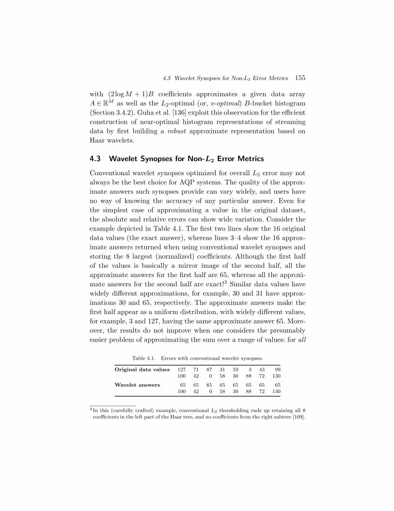
4.3 Wavelet Synopses for Non-L2 Error Metrics 155
with (2logM + 1)B coefficients approximates a given data arrayA ∈ R
M as well as the L2-optimal (or, v-optimal) B-bucket histogram(Section 3.4.2). Guha et al. [136] exploit this observation for the efficientconstruction of near-optimal histogram representations of streamingdata by first building a robust approximate representation based onHaar wavelets.
4.3 Wavelet Synopses for Non-L2 Error Metrics
Conventional wavelet synopses optimized for overall L2 error may notalways be the best choice for AQP systems. The quality of the approx-imate answers such synopses provide can vary widely, and users haveno way of knowing the accuracy of any particular answer. Even forthe simplest case of approximating a value in the original dataset,the absolute and relative errors can show wide variation. Consider theexample depicted in Table 4.1. The first two lines show the 16 originaldata values (the exact answer), whereas lines 3–4 show the 16 approx-imate answers returned when using conventional wavelet synopses andstoring the 8 largest (normalized) coefficients. Although the first halfof the values is basically a mirror image of the second half, all theapproximate answers for the first half are 65, whereas all the approxi-mate answers for the second half are exact!3 Similar data values havewidely different approximations, for example, 30 and 31 have approx-imations 30 and 65, respectively. The approximate answers make thefirst half appear as a uniform distribution, with widely different values,for example, 3 and 127, having the same approximate answer 65. More-over, the results do not improve when one considers the presumablyeasier problem of approximating the sum over a range of values: for all
Table 4.1. Errors with conventional wavelet synopses.
Original data values 127 71 87 31 59 3 43 99100 42 0 58 30 88 72 130
Wavelet answers 65 65 65 65 65 65 65 65100 42 0 58 30 88 72 130
3 In this (carefully crafted) example, conventional L2 thresholding ends up retaining all 8coefficients in the left part of the Haar tree, and no coefficients from the right subtree [109].
156 Wavelets
possible ranges within the first half involving x = 2 to 7 of the values,the approximate answer will be 65 · x, while the actual answers varywidely. For example, for both the range A[0] to A[2] and the range A[3]to A[5], the approximate answer is 195, while the actual answer is 285and 93, respectively. On the other hand, exact answers are provided forall possible ranges within the second half.
The simple example above illustrates that conventional wavelet syn-opses suffer from several important problems, including the introduc-tion of severe bias in the data reconstruction and wide variance inthe quality of the data approximation, as well as the lack of non-trivial guarantees for individual approximate answers. To address theseshortcomings, recent work has proposed novel thresholding schemesfor building wavelet synopses that try to minimize different, non-L2 approximation-error metrics that might be better suited for vari-ous AQP scenarios. For instance, to provide error guarantees in theapproximation of individual data values, a wavelet synopsis could beconstructed to minimize error metrics such as the maximum abso-lute error or the maximum relative error (with an appropriate sanitybound s) in the data reconstruction;4 that is, minimize maxiabsErrior maxirelErri, where
absErri = |A[i] − A[i]| and relErri =|A[i] − A[i]|
max|A[i]|,s .
Another important class of error metrics is the Lp-norm error
‖A − A‖p =
(∑i
|A[i] − A[i]|p) 1
p
in the data reconstruction (for any p ≥ 0), as well as the (more general)weighted Lp-norm error
‖A − A‖p,w =
(∑i
wi · |A[i] − A[i]|p) 1
p
,
4 The role of the sanity bound is to ensure that relative-error numbers are not undulydominated by small data values [156, 284].

4.3 Wavelet Synopses for Non-L2 Error Metrics 157
where a weight vector w = (w0,w2, . . . ,wM−1) is used to associate dif-ferent “significance” to the errors for different values in the underlyingdata domain [111]. Such weights are an important tool for capturing theimportance of individual data values, for example, based on the non-uniformities of the observed query workload (see also Section 4.3.3).Note that maximum-error metrics correspond to L∞-norm error (i.e.,p =∞), whereas relative-error metrics are special cases of weightedLp-norm error (with wi = 1/max|A[i]|,s).
Wavelet thresholding algorithms for optimizing such non-L2 errormetrics can be classified into two broad categories. Most early work onthe problem (e.g., [108, 109, 111]) focused solely on the case of restrictedwavelets, where the algorithm selects values retained for the synopsisfrom the standard HWT coefficient values (i.e., computed by standardpairwise averaging and differencing). However, as observed by Guhaand Harb [134], such a restriction makes little sense when optimizingfor non-L2 error, and can, in fact, lead to sub-optimal synopses. Theirwork considers unrestricted Haar wavelets, where the values retainedin the synopsis are specifically chosen to optimize a general (weighted)Lp-norm error metric. In what follows, we survey these two relatedlines of research. We also discuss the concurrent efforts of Matiasand Urieli [222, 223] on building workload-optimal wavelet synopsesthrough the design of appropriate weighted Haar wavelet bases thatallow for optimal greedy thresholding based on Parseval’s theorem.
4.3.1 Restricted Haar Wavelets for Non-L2 Error
We start with a brief description of early work on probabilistic thresh-olding schemes that implicitly try to optimize for maximum errorthrough the minimization of appropriate probabilistic metrics. We thendiscuss techniques for deterministic wavelet thresholding that selectHWT values to directly optimize various (non-L2) error metrics.
4.3.1.1 Probabilistic Wavelet Synopses
The problems and biases of conventional, greedy wavelet thresh-olding were first observed by Garofalakis and Gibbons [108, 109].Their work introduces probabilistic wavelet synopses that rely on
158 Wavelets
probabilistic thresholding algorithms based on ideas from randomizedrounding [232]: The key idea is to deterministically retain the mostimportant coefficients while randomly rounding the other coefficientseither up to a larger value (called a rounding value) or down to zero.The probability of rounding up versus down is selected so that theexpected value of the rounded coefficient equals the original coefficient.By carefully selecting the rounding values (through appropriate opti-mization procedures), the thresholding algorithm ensures that (1) theexpected total number of coefficients in the synopsis is B, and (2) adesired maximum-error metric (e.g., maximum relative error) in thereconstruction of the data is minimized [109].
More specifically, each non-zero coefficient ci in the wavelet trans-form of the data array A is associated with a random variable Ci
such that (1) Ci takes the value zero (i.e., ci is discarded from thesynopsis) with some (possibly zero) probability, and (2) E[Ci] = ci.The probabilistic wavelet synopsis for A, comprises the values for thoserandom variables Ci with non-zero values.5 The general form of theserandom variables is determined using a randomized rounding scheme,with a rounding value, λi, for each non-zero ci such that Ci ∈ 0,λi,0 < ci
λi≤ 1, and
Ci =
λi with probability
ciλi
0 with probability 1 − ciλi
Thus, the thresholding scheme essentially “rounds” each non-zero wave-let coefficient ci independently to either λi or zero by flipping a biasedcoin with success probability ci
λi. For this rounding process, the expected
value of each rounded coefficient is E[Ci] = λi · ciλi
+ 0 · (1 − ciλi
) = ci(i.e., the actual coefficient value), and its variance is simply Var(Ci) =E[C2
i ] − (E[Ci])2 = λ2i · ci
λi− c2i = (λi − ci) · ci. (For the special case
where a coefficient is deterministically retained, λi = ci, and indeedVar(Ci) = 0.) Let A[i] (A(l : h)) denote the estimator for the datavalue A[i] (resp., the range sum/count A(l : h)), as calculated based onthe coefficient values retained in a probabilistic wavelet synopsis. By
5 Note that the values stored in the synopsis can be different from those of the correspondingHWT coefficients. Still, we chose to classify this as a “restricted” approach since it insistson maintaining the values of individual HWT coefficients on expectation.
4.3 Wavelet Synopses for Non-L2 Error Metrics 159
the linearity of point and range-sum reconstruction (Section 4.2) andlinearity of expectation, it is not difficult to prove that these estimatorsare unbiased; that is, E[A[i]] = A[i] and E[A(l : h)] = A(l : h) [109].
The above development holds for any choice of rounding valuesλi, as long as 0 < ci
λi≤ 1. The choice of the λis is crucial, how-
ever, because it determines the variances of probabilistic estimatorsas well as the expected number of coefficients retained. Indeed, thekey to providing “good” error guarantees for individual data valuesand range sums lies in selecting the λis to ensure small variances fordata-value reconstruction while not exceeding the prescribed spacelimit for the synopsis. (Note that, essentially, the retention proba-bilities ci
λican be seen as the amount of fractional storage assigned
to individual coefficients ci.) Based on these observations, [108, 109]propose novel thresholding algorithms based on DP formulations overthe Haar-tree structure that explicitly minimize appropriate probabilis-tic metrics (such as the maximum normalized standard error or themaximum normalized bias) in the randomized synopsis construction;these formulations are then combined with a quantization of the poten-tial fractional-storage allotments to give polynomial-time combinatorialtechniques [109]. More specifically, employing a quantization that allo-cates fractional storage to coefficients at multiples of 1/q (where q > 1is an integer input parameter), the DP algorithms of [109] construct aB-coefficient probabilistic wavelet synopsis in time O(Mq2B log(qB)).Since this complexity can be problematic, especially for large synopsissizes B, Deligiannakis et al. [79] propose an approximation scheme that,given a desired approximation factor ε, builds aB-coefficient probabilis-tic wavelet synopsis in O(Mq logqminlogM logR/ε,Bq) (where R isroughly proportional to the maximum absolute Haar-coefficient valuein the decomposition), while guaranteeing that the quality of the finalsolution is within a factor of (1 + ε) of that obtained by the (exact)techniques of [109] for the same problem instance.
4.3.1.2 Deterministic Thresholding Techniques
The probabilistic synopses of [108, 109] try to probabilisticallycontrol data-value reconstruction error through the optimization ofappropriate probabilistic measures (like normalized standard error or

160 Wavelets
bias [108, 109]). Such schemes can suffer from important shortcomings,including the potential pitfalls of randomized techniques (e.g., a “bad”sequence of coin flips resulting in a poor synopsis), and the ad-hocnature of the space-quantization requirement of [108, 109] whose impacton the quality of the final solution is not entirely clear. Furthermore,the synopsis space bound is only preserved on expectation, and theestimated variance in the space usage can be large [134].
To address these issues, Garofalakis and Kumar [110, 111] design amore direct, deterministic solution that explicitly minimizes the errormetric of interest. Their DP-based, deterministic thresholding algo-rithms for building coefficient synopses provably optimize the maxi-mum relative error or absolute error in the data-value reconstruction(the key metrics considered in [109]). Furthermore, their algorithmictechniques are directly applicable to a much broader class of distributiveapproximation-error metrics (which includes, for instance, weighted Lp-norm error) [111]. We now briefly overview some of the key ideas of theirsolution.
Given a target error metric err ∈ relErr, absErr, the goal is to effi-ciently select the B Haar coefficients that minimize maxi∈1,...,M erri,where erri is the reconstruction error for A[i]. The challenge here isthat, since each coefficient contributes with different signs to each halfof its support range, these error metrics do not have a simple mono-tonic structure along the Haar-tree structure. To formulate a valid DPrecurrence for maximum error metrics, the key idea is to condition theoptimal error value for an error subtree not only on the root node cj ofthe subtree and the amount B of synopsis storage allotted, but also onthe error that “enters” that subtree through the coefficient selectionsmade on the path from the root to node cj (excluding cj itself), i.e.,coefficient selections on path(cj). The basic observation here is that,since the depth of the Haar tree is O(logM), we can afford to tabu-late all such possible selections while keeping the running-time of thealgorithm in the low-polynomial range [110, 111].
More formally, let B denote the total space budget for the syn-opsis, and let Tj be the subtree of the Haar-tree rooted at nodecj , with coeff(Tj) (data(Tj)) denoting the set of coefficient (respec-tively, data) values in Tj . Finally, let E[j,b,S] denote the optimal
4.3 Wavelet Synopses for Non-L2 Error Metrics 161
(i.e., minimum) value of the maximum error (relative or absolute)among all data values in Tj assuming a synopsis space budget of bcoefficients for the Tj subtree, and that a subset S ⊆ path(cj) (of sizeat most minB − b, logM + 1) of proper ancestors of cj have beenselected for the synopsis; that is, assuming a relative-error metric (i.e.,err = relErr),
E[j,b,S] = minSj⊆coeff(Tj),|Sj |≤b
max
A[i]∈data(Tj)relErri
,
where
relErri =|A[i] −∑
ck∈path(A[i])∩(Sj∪S) signi,k · ck|max|A[i]|,s .
(The case for absolute error (i.e., err = absErr) is defined similarly.)The E[j,b,S] entries can be efficiently computed through a DP recur-rence [111] (discussed below); clearly, E[0,B,φ] gives the desired opti-mal error value at the root node of the Haar tree (the correspondingerror-optimal wavelet synopsis can then be built by simply re-tracingthe choices of the DP computation using standard techniques).
The base case for the DP recurrence occurs for data (i.e., leaf) nodesin the Haar tree; that is, for cj = A[j −M ] with j ≥M (see Figure 4.1).In this case, E[j,b,S] is not defined for b > 0, whereas for b = 0 and foreach subset S ⊆ path(A[j −M ]) (of size ≤ minB, logM + 1)
E[j,0,S] =|A[j −M ] −∑
ck∈S signj−M,k · ck|r
,
where r = max|A[j −M ]|,s for err = relErr, and r = 1 for err =absErr.
In the case of an internal Haar-tree node cj with j < M , the DPalgorithm has two distinct choices when computing E[j,b,S], namelyeither drop coefficient cj or keep it in the final synopsis. If cj is droppedfrom the synopsis, then it is easy to see that the maximum error fromcj ’s two child subtrees (i.e., c2j and c2j+1) will be propagated upward;thus, the minimum possible maximum error E[j,b,S] for Tj in this caseis simply
Edrop[j,b,S] = min0≤b′≤b
maxE[2j,b′,S],E[2j + 1, b − b′,S]
. (4.4)
162 Wavelets
If, on the other hand, cj is kept in the synopsis (assuming, of course,b ≥ 1), the least possible error E[j,b,S] for Tj is computed as
Ekeep[j,b,S] = min0≤b′≤b−1
maxE[2j,b′,S ∪ cj],
E[2j + 1, b − b′ − 1,S ∪ cj]. (4.5)
(Note that the right-hand side of the recurrence is well-defined in bothcases.) The final value for E[j,b,S] is defined as the minimum of thetwo possible choices for coefficient cj (Equations (4.4) and (4.5) above);that is,
E[j,b,S] = minEdrop[j,b,S],Ekeep[j,b,S].The above recurrence can be translated to a DP algorithm in a straight-forward manner; furthermore, both the time and (total) space complex-ity of the algorithm can be shown to be O(M2) [111, 132]. (Assumingthat unnecessary parts of the DP matrix can be paged out, the working-space requirement of the algorithm is only O(MminB, logM) [111].)Guha [133] proposes a space-efficient implementation of this dynamicprogram that requires only O(B logM) space while slightly increasingthe time complexity to O(M2 logB). The key technical idea is to avoidtabulating the solutions to all Haar-subtree problems and repeatedlysolve the same subproblems in a top-down fashion in order to determinethe optimal synopsis (essentially, trading time for space).
Interestingly, the above algorithmic solutions have general applica-bility for a natural, wide class of distributive error metrics [111]. Briefly,an error metric f() is distributive if and only if for any collection ofdisjoint domain ranges R1, . . . , Rk,
f(∪ki=1Ri) = g(f(R1), . . . ,f(Rk)),
where g() is some combining function for the errors over individualregions. In addition to maximum absolute/relative error metrics, theclass of distributive error functions also naturally encompasses severalother important error metrics, including (the pth power of) Lp-normand weighted Lp-norm error [111].
Heuristics and Related Approaches. The quadratic O(M2) timeand space complexity of the optimal DP thresholding algorithm of

4.3 Wavelet Synopses for Non-L2 Error Metrics 163
[110, 111] can be problematic for large datasets. To overcome suchpotential limitations, Karras and Mamoulis [201] propose a greedyheuristic solution for maximum-error thresholding that guaranteesnear-linear complexity. We now briefly review the main ideas of theirthresholding scheme.
Let serri = A[i] − A[i] denote the signed accumulated error in thesynopsis for a data node A[i] after some coefficient deletions. For acoefficient node ck not yet discarded from the synopsis, the maximumpotential absolute error MAk that ck can effect on the synopsis is
MAk = maxA[i]∈leaves(ck)
|serri − signi,k · ck|.
The greedy algorithm for maximum absolute error discards, at eachstep, the coefficient in the running synopsis with the maximum valueof MAk [201]. The key observation here is that the maintenance of MAk
for any coefficient ck can be performed efficiently, without accessingall data nodes in leaves(ck). More specifically, since the removal ofa coefficient ck impacts equally the signed errors in its left or rightsubtrees, the maximum and minimum signed errors in the left (right)subtree of ck are decreased (increased) by exactly ck. And, clearly, themaximum absolute error incurred by the removal of ck must occurat one of these four positions of error extrema: Letting maxl
k, minlk
(maxrk, min
rk) denote the maximum and minimum signed errors in the
left (right) subtree of ck, we can compute MAk as follows:
MAk = max|max lk − ck|, |min l
k − ck|, |max rk + ck|, |minr
k + ck|.
Thus, by maintaining these four quantities maxlk, min
lk, max
rk, and
minrk at each coefficient node, the greedy algorithm can compute MAk
in constant time using the above formula. To determine the next coef-ficient to discard, all coefficients are placed in a min-heap structureH based on their MA values, and the coefficient ck at the root of theheap is removed. After the removal of ck the min/max error informa-tion for all descendant and ancestor coefficients of ck in the Haar treemust be updated. The total number of such updates can be shownto be O(M logM) and each such update can require an O(logM)re-positioning in the heap — this gives an overall time complexity of
164 Wavelets
O(M log2M) while the space complexity is O(M) (constant informa-tion for each coefficient node) [201].
For maximum relative error minimization, the greedy heuristic of[201] discards, at each step, the coefficient with the minimum maximumpotential relative error:
MRk = maxA[i]∈leaves(ck)
|serri − signi,k · ck|max|A[i]|,s
.
In this case, however, the effect of removing a coefficient ck is differentfor each data value in leaves(ck); thus, the algorithm maintains thevalues affected for each ck in an augmented max-heapHk based on theirpotential relative error values, so that the value causing the maximumpotential error can be accessed in constant time. These per-coefficientheaps raise the time/space costs by a factor O(logM), raising the over-all time and space complexity of the greedy algorithm to O(M log3M)and O(M logM), respectively [201].
Also motivated by the quadratic time complexity of the optimal DPin [110, 111], Muthukrishnan [235] considers the special case of weightedL2-error metrics where the weight vector w = (w0,w2, . . . ,wM−1) isk-flat, that is it comprises kM piecewise constant partitions (or,equivalently, w is represented as a k-bucket histogram over [0,M − 1]).The key technical observation here is that the optimization problem foreach piecewise constant (in terms of weight) portion of the Haar treecan be solved greedily through a local application of Parseval’s theorem.This implies that the expensive optimal dynamic program needs to beexecuted only over the portion of the Haar tree up to internal nodesthat correspond to dyadic ranges contained within piecewise constantportions of w; essentially, such piecewise constant tree nodes are treatedas leaves in the DP. Thus, for such k-flat weight vectors, the weightedL2 optimization problem can be solved in time O(MB2k logM) [235].
4.3.2 Unrestricted Haar Wavelets for Non-L2 Error
In its most general form, wavelet synopsis construction is a sparse wave-let representation problem where, given a wavelet basis φiM−1
i=0 for RM
and an input data vector (or, signal) A ∈ RM , the goal is to construct
an approximate representation A as a linear combination of at most B

4.3 Wavelet Synopses for Non-L2 Error Metrics 165
basis vectors so as to minimize some normed distance between A andA.6 The sparse B-term representation A belongs to the non-linear space∑M−1
i=0 ziφi :zi ∈ R,‖Z‖0 ≤ B, where the L0 norm ‖Z‖0 denotes thenumber of non-zero coefficients in the vector Z = (z0,z1, . . . ,zM−1). (Weuse AZ to denote the approximate representation for a specific coeffi-cient vector Z.) For the case of L2 error, by Parseval’s theorem, theL2 norm of A − A is preserved in the wavelet space; thus, generalizingEquation (4.3), we have
‖A − AZ‖22 =∑
i
A[i] −
∑j
zjφi[j]
2
=∑
i
(〈A,φi〉 − zi)2.
It is clear that the optimal solution under the L2 error measure is toretain the largest B inner products 〈A,φi〉 which are exactly the largest(normalized) coefficients c∗i in the HWT expansion of A. Thus, thegreedy thresholding approach of Section 4.2.2 is optimal for L2-errorminimization even in this generalized setting. For other error norms,however, restricting the zis to the set of computed HWT coefficientsof A can result in suboptimal solutions. As a simple example, considerthe data vector A = [1,4,5,6] whose HWT gives [4,−1.5,−1.5,−0.5].Assuming B = 1, the optimal solution for maximum absolute (or, L∞)error is Z∗ = [3.5,0,0,0], whereas the best solution restricted to thecomputed HWT coefficients is [4,0,0,0]; furthermore, the example canbe generalized to any B and larger error gaps by simply scaling andrepeating the values in A with alternating signs [134].
A first step in solving the generalized (unrestricted) sparse Haarwavelet representation problem is demonstrating the existence of abounded set R from which coefficient values in Z can be chosen whileensuring a solution that is close to the optimal unrestricted solution(where zis range over all reals). Guha and Harb [134] prove that, forLp-error minimization, the maximum (un-normalized) coefficient valuein the optimal solution Z∗ satisfies maxi|z∗
i | ≤ 2M1/pαmax, whereαmax = maxi|A[i]| (i.e., the maximum absolute value in the input
6 This is an instance of the general non-linear approximation problem in approximationtheory [84].
166 Wavelets
data).7 Furthermore, they demonstrate that, by rounding the coeffi-cient values in the optimal solution Z∗ to the nearest multiple of someδ > 0 (obtaining a “rounded” solution Zδ) introduces bounded additiveerror in the target Lp norm; more specifically,
‖A − AZδ‖p ≤ ‖A − AZ∗‖p + δM1/p minB, logM. (4.6)
Thus, the above additive error over the optimal solution can be guar-anteed while restricting the search for coefficient values over a set ofsize [134]:
|R| = 2 · maxi|z∗i |
δ≤ 4M1/pαmax
δ. (4.7)
The search for the optimal sparse wavelet representation is con-ducted using a dynamic program that is very similar to the DP for-mulation for the restricted case [110, 111], with two key differences:First, the search at a given Haar-tree node j also ranges over all pos-sible value selections at node j (i.e., over all values in R); and, second,the optimal error at a Haar-tree node j is conditioned on the sumof values of ancestors of j (which can also be restricted to R) [134].Letting E[j,b,V ] denote the minimum Lp error for subtree Tj usingexactly b coefficients and assuming that the ancestors of node j add up(with the proper signs) to value V in the final solution. Then, similarto the restricted case, we can compute E[j,b,V ] = minEdrop[j,b,V ],Ekeep[j,b,V ], where
Edrop[j,b,V ] = minb′∈[0,b]
E[2j,b′,V ],E[2j + 1, b − b′,V ]
Ekeep[j,b,V ] = minb′∈[0,b−1],r∈R
E[2j,b′,V +r],E[2j+1, b − b′ − 1,V −r]represent the choice of dropping or keeping the basis functionat node j. Note that, in the case that j is kept, the searchalso ranges over all possible coefficient values in R. The runningtime of this DP is O(|R|2MB), while its working-space require-ment is O(|R|B log(M/B)). (In the case of maximum (L∞) error,binary search over R can be used, reducing the running timecomplexity to O(|R|2M log2B).) Combined with Equations (4.6)–(4.7),
7 Following [134], we focus on the un-normalized Haar basis in order to simplify the state-ment of the results.
4.3 Wavelet Synopses for Non-L2 Error Metrics 167
this implies that the unrestricted Lp-optimal Haar wavelet syn-opsis can be approximated to within an additive error of εαmax
(where αmax = maxi|A[i]|) in time O( 1ε2M
1+4/pB(minB, logM)2)and space O(1
εM2/pBminB, logM log(M/B)) [134].
The approach also extends to weighted Lp error and relative errornorms; however, the time and space complexities become dependent onthe value of the minimum weight coefficient miniwi and the minimumnormalizing factor maxminiA[i],s, respectively [134]. It is alsointeresting to note that removing the restriction of choosing Haar coef-ficient values enables the streaming computation of the (near-optimal)sparse wavelet representation in one pass over the entries of A — seeSection 4.6.1.
In more recent theoretical work, Guha and Harb [135, 160] demon-strate how one can extend the DP ideas described above to obtain atrue (1 + ε) approximation scheme for unrestricted sparse Haar waveletrepresentations under Lp error that runs in time O( 1
ε2M1+2/pB log3M)
and uses O(1εM
1/pB log3M) space. (As earlier, the running time for thecase of maximum error (p =∞) can be reduced by a factor of B/ log2B
by using binary search.) Their work also examines the gap between therestricted and unrestricted versions of the wavelet approximation prob-lem, proving that a restricted solution which greedily retains at most Bwavelet coefficients is a O(M1/p logM) approximation to the optimalunrestricted solution for all Lp norms; in fact, this result holds for anywavelet family of compact support [135].
Optimizing Maximum Error through the Dual Problem. Forthe special case of (weighted) maximum (L∞) error metrics, Karraset al. [203] propose an alternative approach to constructing near-optimal unrestricted Haar synopses based on the dual problem offinding error-bounded Haar summaries: Given an upper bound E onthe error, find a space-optimal synopsis that guarantees maximumerror ≤ E .8 A key observation here is that there exists a natural DPformulation for this dual problem that avoids the two-dimensional tab-ulation over all possible incoming values v and space allotments b for
8 Some preliminary ideas on using the dual formulation for the restricted problem are alsosketched in the short article by Muthukrishnan [235].
168 Wavelets
every Haar tree node — this essentially eliminates the dependence ofrunning time and space on the synopsis size B, which can result insignificant efficiency gains [203].
More specifically, let S[j,v] denote the minimum number of non-zero coefficients that need to be retained in subtree Tj assuming anincoming value V (from the ancestor nodes of node j), in order toensure a maximum error bound of E ; then, S[j,V ] can be recursivelycomputed through the following DP recurrence:
S[j,V ] = minr∈Rj,V
S[2j,V + r] + S[2j + 1,V − r] + (r = 0),
where (r = 0)denotes theboolean indicatorvariable that is 1 iff r = 0,andRj,V is the set of possible values for node j given an incoming value V .By quantizing the potential values into multiples of a small resolutionstep δ (as earlier), the size of the set of possible values at each node canbe shown to be |Rj,V | = O(E
δ ); this, in turn, implies a DP algorithm forconstructing the error-bounded Haar synopsis in O((E
δ )2M logM) timeusingO(E
δ logM) space [203]. This error-bounded algorithm can be usedas a subroutine in a solution to the original space-bounded maximum-error synopsis construction problem that uses binary search over a rangedefined by lower/upper bounds on the optimal maximum error for a B-coefficient synopsis until the “right” error value is discovered. Comparedto the time requirements of the error-bounded solution, this binary searchincreases the running time of the space-bounded procedure by a factorof O(logE ∗), where E ∗ denotes the optimal (minimum) maximum-errorvalue for aB-coefficient synopsis [203].
Pang et al. [247] also address the (dual) error-bounded version ofthe unrestricted maximum-error wavelet representation problem, andpropose fast, linear-time (i.e., O(M)) approximation algorithms thathave a logM approximation guarantee (i.e., the space for the resultingsynopsis is at most logM times the size of the optimal synopsis for thegiven maximum-error bound E ). Their key technical observation is thatunrestricted coefficient values in the synopsis can be viewed as simpleshift transformations on the ranges of values in Haar subtrees. The ideais then to employ such shift transformations in a bottom-up mannerover the Haar-tree structure in a manner that ensures that the errorranges in the underlying subtrees satisfy the given error bound E . Their
4.3 Wavelet Synopses for Non-L2 Error Metrics 169
most sophisticated strategy (termed S-Shift) computes only ranges ofshift values in the bottom-up pass, and then uses a top-down pass toperform “late-binding” of shift coefficients in a smart way that tries tofurther reduce the size of the synopsis [247].
4.3.3 Weighted Haar Wavelets for Workload-based Error
Weighted error metrics, such as the weighted L2 error√∑iwi(A[i] − A[i])2, generalize standard error norms making it
possible to model the distribution of the query workload. The ideahere is that the weight vector w = (w0,w1, . . . ,wM−1) with wi ∈ [0,1]and
∑iwi = 1 captures the distribution of individual point queries,
with wi being the probability of occurrence for a query on A[i]. Thus,the wi weights represent the “significance” of individual data pointsin the query workload, and minimizing the weighted error norm isessentially equivalent to minimizing the expected query-answeringerror.
Matias and Urieli [222, 223] have proposed a methodology fordesigning wavelet synopses that specifically targets such weighted(workload-based) error metrics. Their solution relies on exploiting theweight vector w to define appropriate weighted inner-product andnorm operators, and design a corresponding orthonormal weighted Haarwavelet basis for R
M ; then, by Parseval’s theorem, the largest coeffi-cients in this weighted basis are guaranteed to minimize the correspond-ing weighted error metric.
Consider the weighted L2 error norm ‖A − A‖2,w =√∑iwi(A[i] − A[i])2. Based on the workload vector w, define a
weighted inner product
〈a,b〉w = M
M−1∑i=0
wi · a[i]b[i].
Note that this is a generalization of the standard inner product (whichassumes wi = 1/M for all i), that also satisfies all the mathematicalconditions for an inner-product operator [223]. Furthermore, it is easyto verify that the corresponding weighted-inner-product norm is exactly√
〈a,a〉w =√M · ‖a‖2,w,
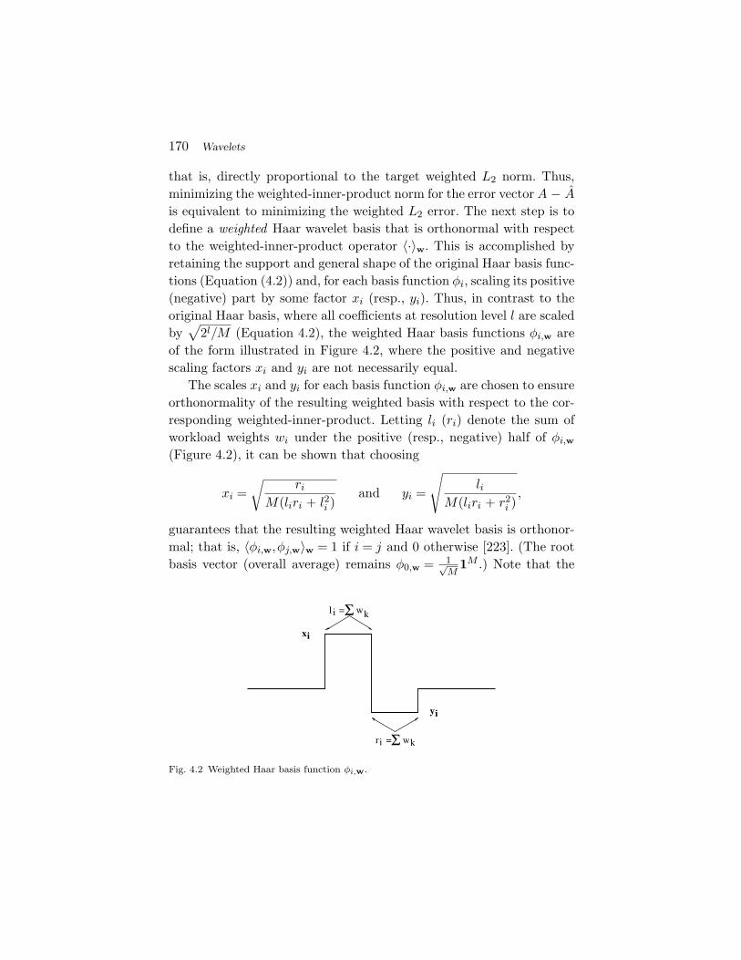
170 Wavelets
that is, directly proportional to the target weighted L2 norm. Thus,minimizing the weighted-inner-product norm for the error vector A − Ais equivalent to minimizing the weighted L2 error. The next step is todefine a weighted Haar wavelet basis that is orthonormal with respectto the weighted-inner-product operator 〈·〉w. This is accomplished byretaining the support and general shape of the original Haar basis func-tions (Equation (4.2)) and, for each basis function φi, scaling its positive(negative) part by some factor xi (resp., yi). Thus, in contrast to theoriginal Haar basis, where all coefficients at resolution level l are scaledby
√2l/M (Equation 4.2), the weighted Haar basis functions φi,w are
of the form illustrated in Figure 4.2, where the positive and negativescaling factors xi and yi are not necessarily equal.
The scales xi and yi for each basis function φi,w are chosen to ensureorthonormality of the resulting weighted basis with respect to the cor-responding weighted-inner-product. Letting li (ri) denote the sum ofworkload weights wi under the positive (resp., negative) half of φi,w
(Figure 4.2), it can be shown that choosing
xi =√
riM(liri + l2i )
and yi =
√li
M(liri + r2i ),
guarantees that the resulting weighted Haar wavelet basis is orthonor-mal; that is, 〈φi,w,φj,w〉w = 1 if i = j and 0 otherwise [223]. (The rootbasis vector (overall average) remains φ0,w = 1√
M1M .) Note that the
r =
Σ wkl =
xi
yi
i Σ wk
i
Fig. 4.2 Weighted Haar basis function φi,w.
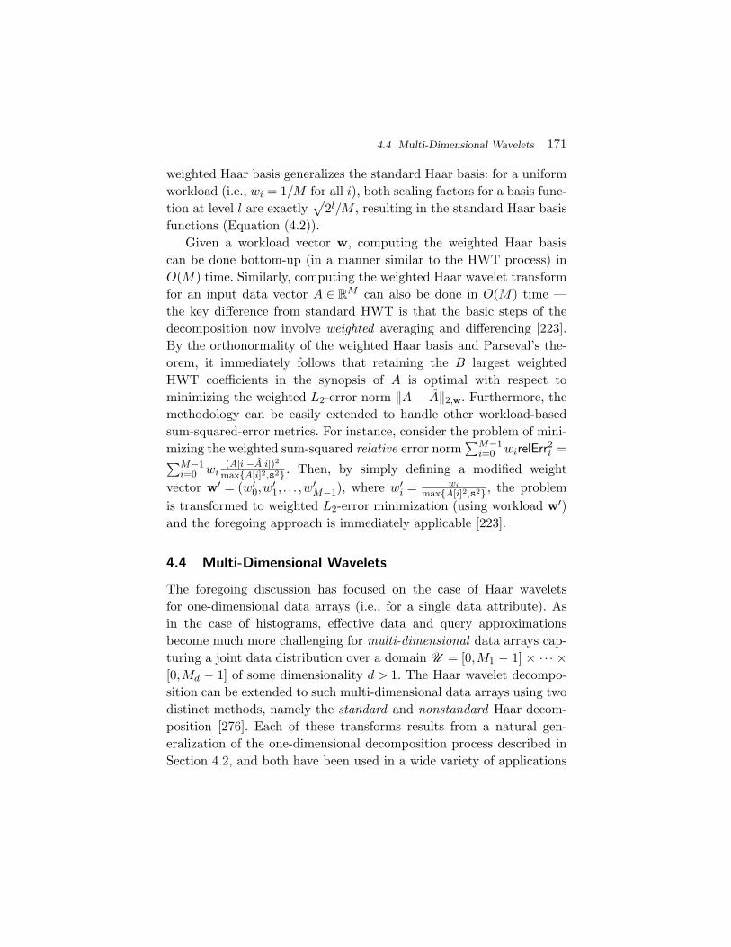
4.4 Multi-Dimensional Wavelets 171
weighted Haar basis generalizes the standard Haar basis: for a uniformworkload (i.e., wi = 1/M for all i), both scaling factors for a basis func-tion at level l are exactly
√2l/M , resulting in the standard Haar basis
functions (Equation (4.2)).Given a workload vector w, computing the weighted Haar basis
can be done bottom-up (in a manner similar to the HWT process) inO(M) time. Similarly, computing the weighted Haar wavelet transformfor an input data vector A ∈ R
M can also be done in O(M) time —the key difference from standard HWT is that the basic steps of thedecomposition now involve weighted averaging and differencing [223].By the orthonormality of the weighted Haar basis and Parseval’s the-orem, it immediately follows that retaining the B largest weightedHWT coefficients in the synopsis of A is optimal with respect tominimizing the weighted L2-error norm ‖A − A‖2,w. Furthermore, themethodology can be easily extended to handle other workload-basedsum-squared-error metrics. For instance, consider the problem of mini-mizing the weighted sum-squared relative error norm
∑M−1i=0 wirelErr2i =∑M−1
i=0 wi(A[i]−A[i])2
maxA[i]2,s2 . Then, by simply defining a modified weightvector w′ = (w′
0,w′1, . . . ,w
′M−1), where w′
i = wimaxA[i]2,s2 , the problem
is transformed to weighted L2-error minimization (using workload w′)and the foregoing approach is immediately applicable [223].
4.4 Multi-Dimensional Wavelets
The foregoing discussion has focused on the case of Haar waveletsfor one-dimensional data arrays (i.e., for a single data attribute). Asin the case of histograms, effective data and query approximationsbecome much more challenging for multi-dimensional data arrays cap-turing a joint data distribution over a domain U = [0,M1 − 1] × ·· · ×[0,Md − 1] of some dimensionality d > 1. The Haar wavelet decompo-sition can be extended to such multi-dimensional data arrays using twodistinct methods, namely the standard and nonstandard Haar decom-position [276]. Each of these transforms results from a natural gen-eralization of the one-dimensional decomposition process described inSection 4.2, and both have been used in a wide variety of applications
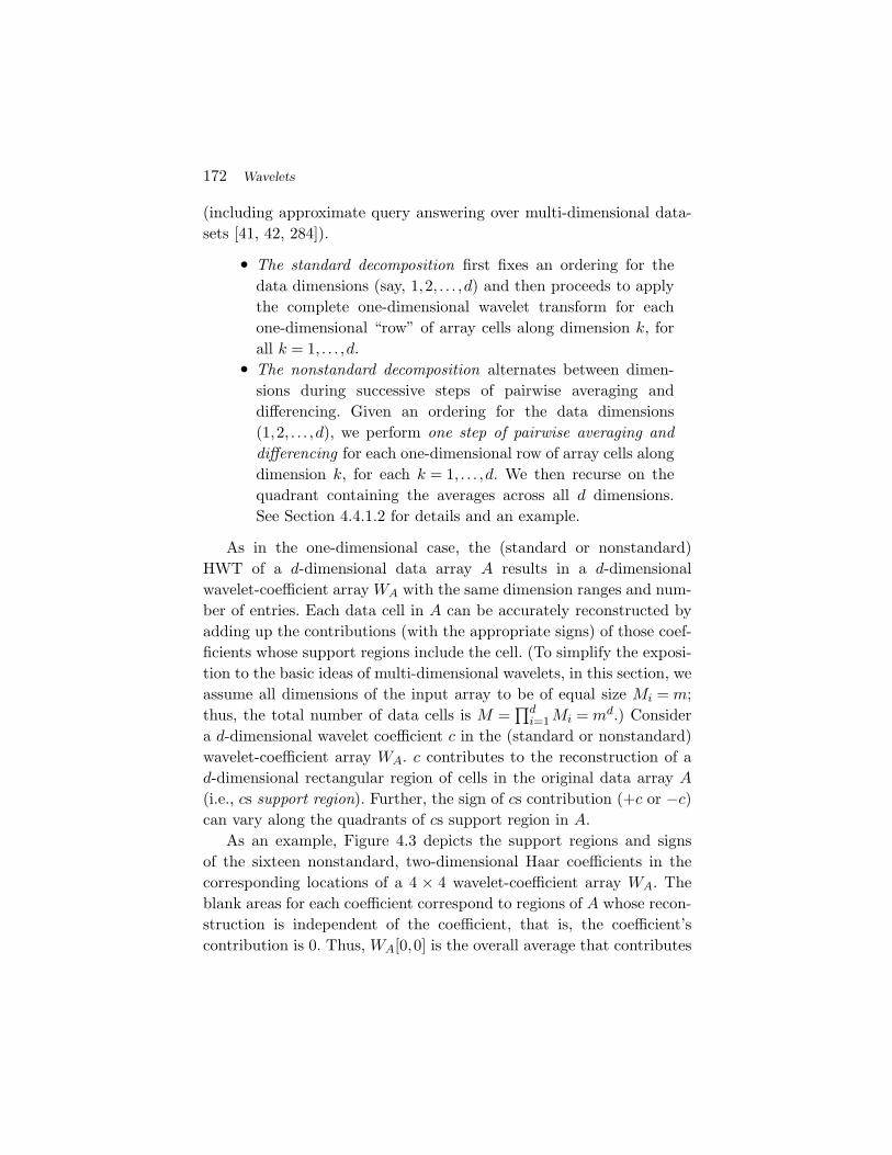
172 Wavelets
(including approximate query answering over multi-dimensional data-sets [41, 42, 284]).
• The standard decomposition first fixes an ordering for thedata dimensions (say, 1,2, . . . ,d) and then proceeds to applythe complete one-dimensional wavelet transform for eachone-dimensional “row” of array cells along dimension k, forall k = 1, . . . ,d.
• The nonstandard decomposition alternates between dimen-sions during successive steps of pairwise averaging anddifferencing. Given an ordering for the data dimensions(1,2, . . . ,d), we perform one step of pairwise averaging anddifferencing for each one-dimensional row of array cells alongdimension k, for each k = 1, . . . ,d. We then recurse on thequadrant containing the averages across all d dimensions.See Section 4.4.1.2 for details and an example.
As in the one-dimensional case, the (standard or nonstandard)HWT of a d-dimensional data array A results in a d-dimensionalwavelet-coefficient array WA with the same dimension ranges and num-ber of entries. Each data cell in A can be accurately reconstructed byadding up the contributions (with the appropriate signs) of those coef-ficients whose support regions include the cell. (To simplify the exposi-tion to the basic ideas of multi-dimensional wavelets, in this section, weassume all dimensions of the input array to be of equal size Mi = m;thus, the total number of data cells is M =
∏di=1Mi = md.) Consider
a d-dimensional wavelet coefficient c in the (standard or nonstandard)wavelet-coefficient array WA. c contributes to the reconstruction of ad-dimensional rectangular region of cells in the original data array A
(i.e., cs support region). Further, the sign of cs contribution (+c or −c)can vary along the quadrants of cs support region in A.
As an example, Figure 4.3 depicts the support regions and signsof the sixteen nonstandard, two-dimensional Haar coefficients in thecorresponding locations of a 4 × 4 wavelet-coefficient array WA. Theblank areas for each coefficient correspond to regions of A whose recon-struction is independent of the coefficient, that is, the coefficient’scontribution is 0. Thus, WA[0,0] is the overall average that contributes
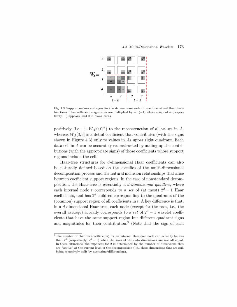
4.4 Multi-Dimensional Wavelets 173
_
+
+_
+_
+_+ _+_
+_
+__+
+__+
+_
+__+
+__+
+_
+ _+_ +_
W =A
+0
1
2
3
0 1 2 3l l= 0 = 1
k
Fig. 4.3 Support regions and signs for the sixteen nonstandard two-dimensional Haar basisfunctions. The coefficient magnitudes are multiplied by +1 (−1) where a sign of + (respec-tively, −) appears, and 0 in blank areas.
positively (i.e., “+WA[0,0]”) to the reconstruction of all values in A,whereas WA[3,3] is a detail coefficient that contributes (with the signsshown in Figure 4.3) only to values in As upper right quadrant. Eachdata cell in A can be accurately reconstructed by adding up the contri-butions (with the appropriate signs) of those coefficients whose supportregions include the cell.
Haar-tree structures for d-dimensional Haar coefficients can alsobe naturally defined based on the specifics of the multi-dimensionaldecomposition process and the natural inclusion relationships that arisebetween coefficient support regions. In the case of nonstandard decom-position, the Haar-tree is essentially a d-dimensional quadtree, whereeach internal node t corresponds to a set of (at most) 2d − 1 Haarcoefficients, and has 2d children corresponding to the quadrants of the(common) support region of all coefficients in t. A key difference is that,in a d-dimensional Haar tree, each node (except for the root, i.e., theoverall average) actually corresponds to a set of 2d − 1 wavelet coeffi-cients that have the same support region but different quadrant signsand magnitudes for their contribution.9 (Note that the sign of each
9 The number of children (coefficients) for an internal Haar-tree node can actually be lessthan 2d (respectively, 2d − 1) when the sizes of the data dimensions are not all equal.In these situations, the exponent for 2 is determined by the number of dimensions thatare “active” at the current level of the decomposition (i.e., those dimensions that are stillbeing recursively split by averaging/differencing).
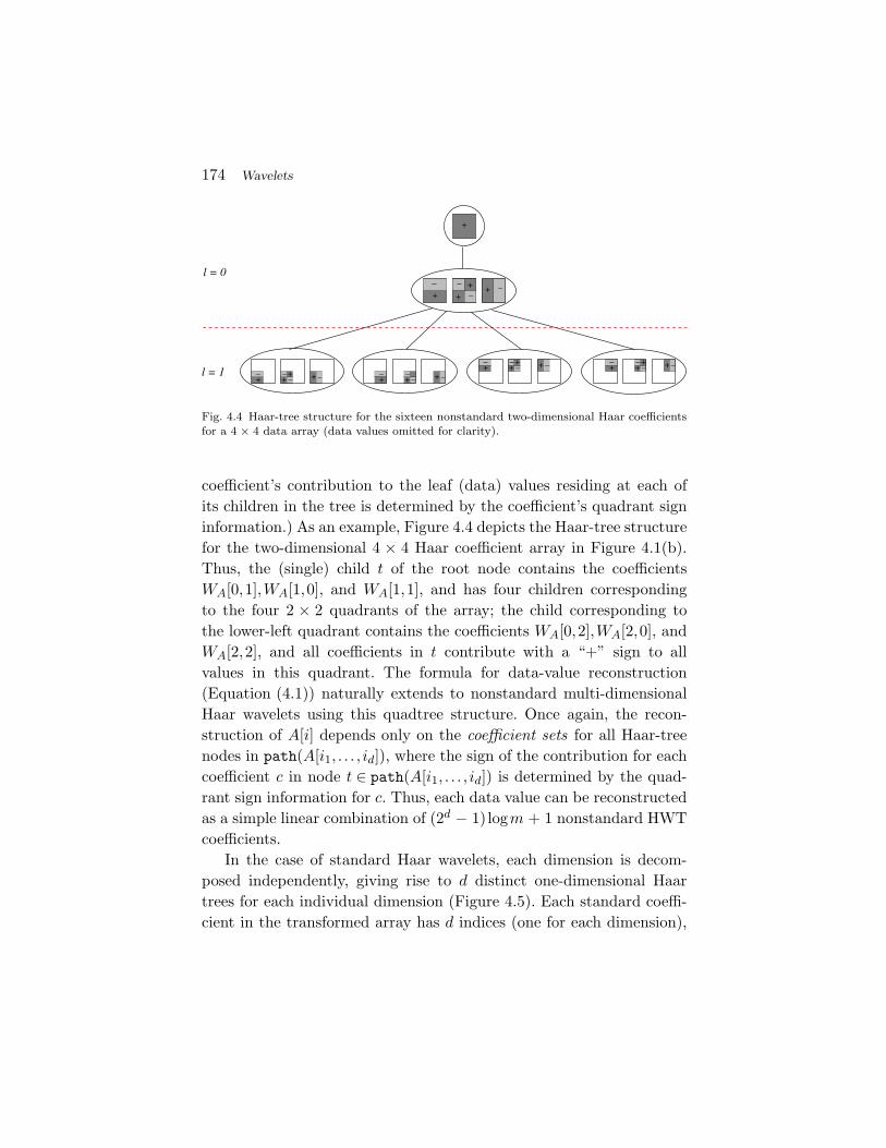
174 Wavelets
+_
+__+ +_
+_
+__+ +_
+_
+ __+ +
+_
+
+
l = 0
_+ __
+_l = 1
__
++
+
_+ _
Fig. 4.4 Haar-tree structure for the sixteen nonstandard two-dimensional Haar coefficientsfor a 4 × 4 data array (data values omitted for clarity).
coefficient’s contribution to the leaf (data) values residing at each ofits children in the tree is determined by the coefficient’s quadrant signinformation.) As an example, Figure 4.4 depicts the Haar-tree structurefor the two-dimensional 4 × 4 Haar coefficient array in Figure 4.1(b).Thus, the (single) child t of the root node contains the coefficientsWA[0,1],WA[1,0], and WA[1,1], and has four children correspondingto the four 2 × 2 quadrants of the array; the child corresponding tothe lower-left quadrant contains the coefficients WA[0,2],WA[2,0], andWA[2,2], and all coefficients in t contribute with a “+” sign to allvalues in this quadrant. The formula for data-value reconstruction(Equation (4.1)) naturally extends to nonstandard multi-dimensionalHaar wavelets using this quadtree structure. Once again, the recon-struction of A[i] depends only on the coefficient sets for all Haar-treenodes in path(A[i1, . . . , id]), where the sign of the contribution for eachcoefficient c in node t ∈ path(A[i1, . . . , id]) is determined by the quad-rant sign information for c. Thus, each data value can be reconstructedas a simple linear combination of (2d − 1) logm + 1 nonstandard HWTcoefficients.
In the case of standard Haar wavelets, each dimension is decom-posed independently, giving rise to d distinct one-dimensional Haartrees for each individual dimension (Figure 4.5). Each standard coeffi-cient in the transformed array has d indices (one for each dimension),
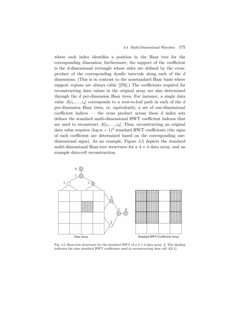
4.4 Multi-Dimensional Wavelets 175
where each index identifies a position in the Haar tree for thecorresponding dimension; furthermore, the support of the coefficientis the d-dimensional rectangle whose sides are defined by the cross-product of the corresponding dyadic intervals along each of the d
dimensions. (This is in contrast to the nonstandard Haar basis wheresupport regions are always cubic [276].) The coefficients required forreconstructing data values in the original array are also determinedthrough the d per-dimension Haar trees. For instance, a single datavalue A[i1, . . . , id] corresponds to a root-to-leaf path in each of the dper-dimension Haar trees, or, equivalently, a set of one-dimensionalcoefficient indices — the cross product across these d index setsdefines the standard multi-dimensional HWT coefficient indexes thatare used to reconstruct A[i1, . . . , id]. Thus, reconstructing an originaldata value requires (logm + 1)d standard HWT coefficients (the signsof each coefficient are determined based on the corresponding one-dimensional signs). As an example, Figure 4.5 depicts the standardmulti-dimensional Haar-tree structures for a 4 × 4 data array, and anexample data-cell reconstruction.
1
0
32
3
2
1 0
Data Array Standard HWT Coefficient Array
Fig. 4.5 Haar-tree structures for the standard HWT of a 4 × 4 data array A. The shadingindicates the nine standard HWT coefficients used in reconstructing data cell A[2,1].
176 Wavelets
4.4.1 Multi-Dimensional Wavelet DecompositionAlgorithms
The complexity in designing efficient Haar-wavelet decompositionalgorithms for a multi-attribute relational table R comes from thefact that such algorithms cannot afford to build the multi-dimensionaljoint-frequency array AR (i.e., the datacube representation) of R. Theproblem here is that the number of cells M in this datacube array AR
grows exponentially in the dimensionality d, and is typically orders ofmagnitude larger than the number of tuples in R. Thus, computation-and I/O-efficient decomposition algorithms for multi-dimensional datahave to work off the relational “set-of-tuples” representation of R. Suchefficient decomposition algorithms have been proposed for both formsof the multi-dimensional HWT.
4.4.1.1 Standard HWT Decomposition
Recall that, in the standard decomposition, the complete one-dimensional HWT is applied to each one-dimensional “row” of cellsalong dimension k, for all k = 1, . . . ,d. For instance, in the two-dimensional case, the one-dimensional HWT is first applied to eachrow of the data; then, we treat the transformed rows as data and applyanother pass of the one-dimensional HWT to each column.
Vitter and Wang [284] propose I/O-efficient algorithms for thestandard multi-dimensional HWT of a (ROLAP) relation R, which isassumed to be in dimension order 〈d,d − 1, . . . ,1〉; that is, the indicesof the tuple entries change most rapidly along the rightmost dimen-sion 1, next most rapidly along dimension 2, and so on. In the multi-dimensional data space, the entries for which the values in the k-prefixof the dimensions d, . . . ,d − k + 1 are fixed form a (d − k)-dimensionalhyperplane denoted as 〈d − k, . . . ,1〉. The key idea in the decomposi-tion algorithms of [284] is to break the standard HWT computationinto hyperplanes (in the chosen dimension order), such that the com-plete decomposition for each hyperplane can be carried out entirelyin-memory. Assuming a memory of size S and a disk-block size b, theirfirst algorithm partitions the dimensions into groups (i.e., hyperplanes〈i + j, . . . , i + 1, i〉 such that the product of the group’s dimension sizes
4.4 Multi-Dimensional Wavelets 177
satisfies Mi × ·· · ×Mi+j ≤ S − 2b (reserving two block-sized buffersfor I/O). Assuming g such groups, the algorithm performs g passesover the data, processing the groups in reverse order (i.e., in increasingorder of the start index i), one per pass. In the (g − m + 1)-st pass,each hyperplane in the mth dimension group is read in, one by one,and processed (performing an in-memory standard HWT); then, theresults are written out to disk for the next pass. After each pass, theoutput produced on disk needs to be transposed in order to regroupthe cells according to the dimension order required by the next pass;this transposition step can be performed in a logarithmic number ofdistribution passes over the data.
The second algorithm of [284], exploits intelligent buffering andknowledge of the dimension sizes to avoid explicit transposition stepsbetween passes. The key idea is to employ a double output buffer foreach cell of the hyperplane to appropriately re-order the output ofeach pass; in this manner, the transposition is essentially achieved “forfree” as a result of the buffering mechanism. (Of course, the size of thehyperplanes for each pass must be smaller to account for all the out-put buffers needed — more specifically, the product of the dimensionsizes in a hyperplane now has to be ≤ S/(2b + 1).) Letting M =
∏iMi
denote the number of cells in the data array, the I/O complexity ofboth algorithms in [284] can be shown to be O( |R|
S logS/bMb ) — that is,
they both require O(logS/bMb ) passes over the tuples in R [284].
4.4.1.2 Nonstandard HWT Decomposition
Abstractly, the nonstandard Haar decomposition alternates betweendimensions during successive steps of pairwise averaging anddifferencing: given an ordering for the data dimensions (1,2, . . . ,d), itperforms one step of pairwise averaging and differencing for each one-dimensional row of array cells along dimension k, for each k = 1, . . . ,d.(The results of earlier averaging and differencing steps are treatedas data values for larger values of k.) This process is then repeatedrecursively only on the quadrant containing averages across all dimen-sions. One way of conceptualizing this procedure is to think of a2 × 2 × ·· · × 2(= 2d) hyper-box being shifted across the data array,
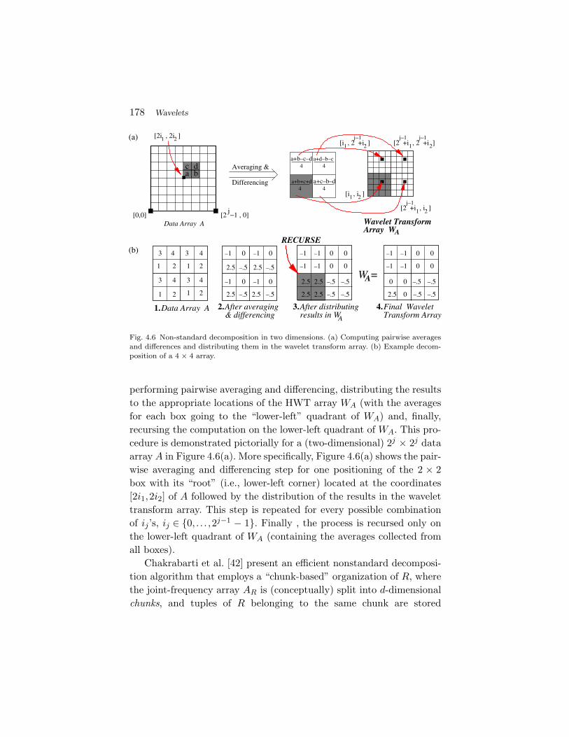
178 Wavelets
j
1 2
[2i , 2i ]1 2
Averaging &
Differencing
3
1 2
4
1 2
3 4
3
21
43
1
4
2
Data Array A1.
Wavelet Transform Array WA
2.5
2.5
0
2.5
0
2.5
0 0
–1 –1
–1 –1
–.5 –.5
–.5–.5
After averaging& differencing
2.
2.5
0
2.5
2.5 2.5
00
0–1 –1
–1 –1
–.5 –.5
–.5 –.5
After distributingresults in W
3.A
RECURSE
Final WaveletTransform Array
4.
(a)
a+d–b–c4 4
4
a+b–c–d
a+c–b–d
[0,0]
dca b
[i , 2 +i ]j–1
21
a+b+c+d4
Data Array A
(b)
2.5
0
00
0–1 –1
–1 –1
–.5–.5
–.5 –.5
0 0
0
W =A
[2 −1 , 0]
[2 +i , 2 +i ]1 2
[2 +i , i ]1 2
j–1
j–1 j–1
[i , i ]
Fig. 4.6 Non-standard decomposition in two dimensions. (a) Computing pairwise averagesand differences and distributing them in the wavelet transform array. (b) Example decom-position of a 4 × 4 array.
performing pairwise averaging and differencing, distributing the resultsto the appropriate locations of the HWT array WA (with the averagesfor each box going to the “lower-left” quadrant of WA) and, finally,recursing the computation on the lower-left quadrant of WA. This pro-cedure is demonstrated pictorially for a (two-dimensional) 2j × 2j dataarray A in Figure 4.6(a). More specifically, Figure 4.6(a) shows the pair-wise averaging and differencing step for one positioning of the 2 × 2box with its “root” (i.e., lower-left corner) located at the coordinates[2i1,2i2] of A followed by the distribution of the results in the wavelettransform array. This step is repeated for every possible combinationof ij ’s, ij ∈ 0, . . . ,2j−1 − 1. Finally , the process is recursed only onthe lower-left quadrant of WA (containing the averages collected fromall boxes).
Chakrabarti et al. [42] present an efficient nonstandard decomposi-tion algorithm that employs a “chunk-based” organization of R, wherethe joint-frequency array AR is (conceptually) split into d-dimensionalchunks, and tuples of R belonging to the same chunk are stored
4.4 Multi-Dimensional Wavelets 179
contiguously on disk. (If R is not chunked, then an extra sortingstep is required.) Their algorithm assumes that each chunk can fit inmemory, and uses the nonstandard methodology described in Figure 4.6to compute and distribute coefficients in the HWT array in a recursive,“depth-first” fashion. The key observation here is that the decompo-sition of the d-dimensional array AR can be computed by recursivelycomputing the full decomposition for each of the 2d quadrants of AR
and then performing pairwise averaging and differencing on the com-puted 2d quadrant averages. Thus, the entire computation for decom-posing a chunk can be performed when the chunk is loaded from diskfor the first time (hence no chunk is read twice). Lower resolution coef-ficients are computed by first accumulating, in main memory, averagesfrom the 2d quadrants (generated from the previous level of resolution)followed by pairwise averaging and differencing, thus requiring no extraI/O. The end result is a fairly simple recursive algorithm for efficientlycomputing the nonstandard HWT [42]. Assuming a relation R alreadystored in chunks, the algorithm of [42] only needs one pass over thetuples of R; if R is not already chunked, then an extra sorting step isneeded, thus resulting in an I/O complexity that matches that of thestandard HWT algorithms in [284].
4.4.2 Multi-Dimensional HWT Coefficient Thresholding
L2 Error Thresholding. Modulo a simple normalization step, boththe standard and nonstandard multi-dimensional HWT bases retainthe orthonormality property. Thus, as in the one-dimensional case,Parseval’s theorem guarantees that retaining the B largest multi-dimensional HWT coefficients in absolute normalized value is theoptimal strategy for minimizing the overall L2 error in the data approx-imation [221, 276].
A potential issue with the multi-dimensional HWT is that, due tothe repeated averaging and differencing of neighboring cells, the den-sity of the data (i.e., number of non-zero cells) continuously increases(by a factor as high as O(logM)) during each pass of the decomposi-tion process. Thus, the decomposition algorithms have to process moreand more entries during successive passes, even though a large portion

180 Wavelets
of the entries can be very small in magnitude. To avoid this problem,Vitter and Wang [284] propose an adaptive thresholding scheme thatdiscards intermediate coefficient values in each pass via an on-line learn-ing process. (A similar technique is also used in [42].) The key idea is todynamically maintain a cutoff value based on on-line statistics on thedistribution of intermediate coefficient values maintained during eachpass. Coefficients smaller than the cutoff are discarded on the fly. Thecutoff value is adjusted periodically as the statistics on the observedcoefficient values shifts. Despite its heuristic nature, this adaptive tech-nique works quite well in practice [42, 284].
Non-L2 Error Thresholding. There are very few known results onthe problem of effectively thresholding multi-dimensional Haar wave-lets for non-L2 error metrics. The basic DP approaches for restrictedand unrestricted wavelet synopses (Sections 4.3.1.2 and 4.3.2) can benaturally extended to the case of multi-dimensional data (based on theappropriate multi-dimensional Haar-tree structures, e.g., Figure 4.4).However, the time and space complexity of the dynamic programincrease explosively with data dimensionality rendering the approachinapplicable even for relatively small dimensionalities (e.g., 2–5). Forthe restricted case, Garofalakis and Kumar [111] introduce efficientapproximation schemes based on approximate dynamic programs thatexplore a much smaller number of options than the optimal DP formu-lation, while offering tunable ε-approximation guarantees for the finaltarget maximum-error metric.
4.4.3 Multi-Dimensional Range-Aggregate QueryEstimation
For range-count aggregates, the observations and techniques discussedin the case of one-dimensional data (Section 4.2.4) can be naturallyextended to the multi-dimensional case. In the case of the d-dimensionalstandard HWT (where the Haar “tree” structure can conceptuallybe thought of as the cross-product of the d one-dimensional Haartrees), a coefficient with value v at location (i1, i2, . . . , id) contributes tothe range-COUNT query A(l1 : h1, . . . , ld′ : hd′) only if id′+1 = · · · = id = 0,
4.5 Approximate Processing of General Queries 181
and its contribution is given by the formula [284]:
v ·d′∏
j=1
(|leftleavesj(ij , lj :hj)|−|rightleavesj(ij , lj :hj)|) ×d∏
j=d′+1
Mj ,
where |leftleavesj(ij , lj : hj)| denotes the size of the intersection ofthe leaf set in the left child subtree of coefficient ij (along dimen-sion j) and the corresponding one-dimensional query range [lj ,hj ] (with|rightleavesj(ij , lj : hj)| defined similarly). Using this fact, it can beshown that, given a synopsis comprising B standard HWT coefficientsof A, the range-COUNT A(l1 : h1, . . . , ld′ : hd′) can be estimated in timeO(minB,∏d′
i=1Mi) [284]. Similar bounds and estimation algorithmscan also be given for the case of the nonstandard decomposition, byexploiting the regular quadtree structure of the nonstandard Haar tree(Figure 4.4).
4.5 Approximate Processing of General Queries
We now turn our attention to techniques for fast approximate pro-cessing of full-fledged SQL queries using wavelet synopses of data(thought of as relations). Going beyond simple range aggregations,Chakrabarti et al. [42] propose an AQP algebra (which includes allconventional aggregate and non-aggregate SQL operators, such asselect, project, join, sum, and average) that operates directly overthe wavelet synopses of relations, while guaranteeing the correct rela-tional operator semantics. Query processing algorithms for these oper-ators work entirely in the wavelet-coefficient domain — that is, theirinput(s) and output are sets of wavelet coefficients (rather than rela-tional tables). This allows for extremely fast response times, since theapproximate query execution engine can do the bulk of its processingover compact wavelet synopses, essentially postponing the (expensive)expansion/ rendering step into relational tuples until the end-result ofthe query (Figure 4.7).
In the AQP framework of [42], a HWT coefficient is representedby a triple W = 〈R,S,v〉, where: (1) W.R is the d-dimensional supporthyper-rectangle of W (represented by low and high boundary valuesalong each dimension); (2) W.S stores the coefficient sign information

182 Wavelets
T1 T2 Tk, , . . . ,
T1 T2 Tk, , . . . ,
WS
. . .
W
Wavelet-CoefficientSynopses
Wavelet CoefficientsResult Set of
ApproximateRelations
Result Approximate Relation
)
)
)
)
SW render(
op( )
render(
render(
op(
S
, , . . . ,W W W1T 2T kT
, , . . . ,W W W
W
1T 2T kT
1T
kT
Fig. 4.7 Processing relational query operators efficiently in the wavelet-coefficient domain(i.e., the “down-then-right” execution path) [42].
for different regions of W.R, which can be captured by a 2-bit signvector (storing the sign value (+/−) for the low/high end of the coef-ficient range) plus the value where the sign changes, for each of theD dimensions; and, (3) W.v is the (scalar) magnitude of the coeffi-cient. Based on this coefficient representation, the semantics of basicrelational operators can be defined in a natural manner.
Selection, Projection, and Join. Consider a selection opera-tor over a wavelet synopsis (i.e., set of HWT coefficients) WT ,selectpred(WT ), where pred represents a generic conjunctive pred-icate on a subset of k ≤ d data attributes. This select operatoreffectively filters out the portions of the wavelet coefficients in thesynopsis WT that do not overlap with the k-dimensional selectionrange, and thus do not contribute to cells in the selected hyper-rectangle [42]. Similarly, the projection operator projectXi1 ,...,Xik
(WT )(where Xi1 , . . . ,Xik denote the k ≤ d projection attributes) effectivelyprojects out the remaining d − k dimensions for each coefficient supporthyper-rectangle and adjusts the coefficient’s magnitude by an appro-priate multiplicative constant (to aggregate the contributions of arraycells that are “projected out”) [42].
The most interesting operator in this approximate, wavelet-based relational algebra is probably the join, with the general formjoinpred(WT1 ,WT2), where T1 and T2 are (approximate) relations ofdimensionality d1 and d2, respectively, and pred is a conjunctive k-aryequi-join predicate of the form (X1
1 = X21 ) ∧ . . . ∧ (X1
k = X2k), where
4.5 Approximate Processing of General Queries 183
Xij (j = 1, . . . ,di) denotes the jth attribute of Ti (i = 1,2). (Assuming,
without loss of generality, that the join attributes are the first k ≤mind1,d2 attributes of each joining relation.) Note that the result ofthe join operation is a set of (d1 + d2 − k)-dimensional wavelet coef-ficients; that is, the join operation returns coefficients of (possibly)different dimensionality than any of its inputs.
To understand the join processing algorithm of [42], consider themulti-dimensional joint-frequency arrays AT1 and AT2 correspondingto the join operator’s input arguments. Let (i11, . . . , i
1d1
) and (i21, . . . , i2d2
)denote the coordinates of two cells belonging to AT1 and AT2 , respec-tively. If the indexes of the two cells match on the join dimensions,that is, i11 = i21, . . . , i
1k = i2k, then the cell in the join result array with
coordinates (i11, . . . , i1d1, i2k+1, . . . , i
2d2
) is populated with the product ofthe count values contained in the two joined cells. Since the cell countsfor ATi are derived by appropriately summing the contributions of theHWT coefficients in WTi and a numeric product can always be dis-tributed over summation, the join operator can be processed entirelyin the wavelet-coefficient domain by considering all pairs of coefficientsfrom WT1 and WT2 . Briefly, for any two coefficients from WT1 andWT2 that overlap in the join dimensions, and, therefore, contributeto joining data cells, define an output coefficient with magnitudeequal to the product of the two joining coefficients and a supporthyper-rectangle with ranges that are (a) equal to the overlap of thetwo coefficients for the k (common) join dimensions, and (b) equal tothe original coefficient ranges along any of the d1 + d2 − 2k remainingdimensions [42]. The sign information for an output coefficient alongany of the k join dimensions is derived by appropriately multiplyingthe sign-vectors of the joining coefficients along that dimension, takingcare to ensure that only signs along the overlapping portion aretaken into account. (The sign information along non-join dimensionsremains unchanged.) An example of this process in two dimensions(d1 = d2 = 2, k = 1) is depicted in Figure 4.8.
Aggregation. Most conventional aggregation operators, likecount, sum, and avg, can also be naturally processed over the
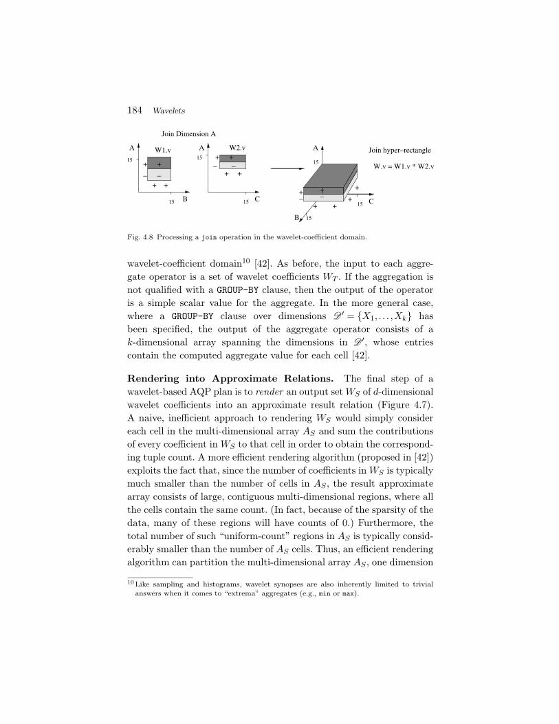
184 Wavelets
C
+
−+ +
+
−−−
+ +
−++
−
Join hyper–rectangle
W.v = W1.v * W2.v
W2.vW1.v
+ +
15 15
1515
15
15
15
+
++ +
CB
AA
Join Dimension A
A
B
Fig. 4.8 Processing a join operation in the wavelet-coefficient domain.
wavelet-coefficient domain10 [42]. As before, the input to each aggre-gate operator is a set of wavelet coefficients WT . If the aggregation isnot qualified with a GROUP-BY clause, then the output of the operatoris a simple scalar value for the aggregate. In the more general case,where a GROUP-BY clause over dimensions D ′ = X1, . . . ,Xk hasbeen specified, the output of the aggregate operator consists of ak-dimensional array spanning the dimensions in D ′, whose entriescontain the computed aggregate value for each cell [42].
Rendering into Approximate Relations. The final step of awavelet-based AQP plan is to render an output setWS of d-dimensionalwavelet coefficients into an approximate result relation (Figure 4.7).A naive, inefficient approach to rendering WS would simply considereach cell in the multi-dimensional array AS and sum the contributionsof every coefficient in WS to that cell in order to obtain the correspond-ing tuple count. A more efficient rendering algorithm (proposed in [42])exploits the fact that, since the number of coefficients in WS is typicallymuch smaller than the number of cells in AS , the result approximatearray consists of large, contiguous multi-dimensional regions, where allthe cells contain the same count. (In fact, because of the sparsity of thedata, many of these regions will have counts of 0.) Furthermore, thetotal number of such “uniform-count” regions in AS is typically consid-erably smaller than the number of AS cells. Thus, an efficient renderingalgorithm can partition the multi-dimensional array AS , one dimension
10 Like sampling and histograms, wavelet synopses are also inherently limited to trivialanswers when it comes to “extrema” aggregates (e.g., min or max).
4.6 Additional Topics 185
at a time, into such uniform-count data regions and output the (single)count value corresponding to each such region (the same for all enclosedcells). In order to partition AS into uniform-count ranges along dimen-sion i, the only points that should be considered are those where thecell counts along i could potentially change. These are precisely thepoints where a new coefficient’s support hyper-rectangle starts or ends,or the sign of the coefficient’s contribution changes (along dimension i).The process can be carried out efficiently using a priority queue for thecoefficients in WS [42].
4.6 Additional Topics
We conclude this chapter with a discussion of wavelet-based synopsesover streaming data, techniques to optimize coefficient storage (e.g.,for handling multi-measure datasets or compressing the synopsis), and“hybrid” methods combining features of both wavelets and histograms.
4.6.1 Wavelets over Streaming Data
When dealing with streaming data, the goal is to continuously tracka compact synopsis of B wavelet coefficient values for a dynamic datavector A that is rendered as a continuous stream of updates. Algorithmsfor this problem should satisfy the key small space/time requirementsfor streaming algorithms; more formally, streaming wavelet algorithmsshould (ideally) guarantee (1) sublinear space usage (for storing a syn-opsis of the stream), (2) sublinear per-item update time (to maintainthe synopsis), and (3) sublinear query time (to produce a, possiblyapproximate, wavelet summary), where “sublinear” typically meanspolylogarithmic in the (large) domain size M . The streaming waveletsummary construction problem has been examined under two distinctdata streaming models.
4.6.1.1 Wavelets in the Ordered Aggregate Model
The bulk of the results on wavelets over streaming data assumes thelimited ordered aggregate (or, time-series) model. Here, the entriesof the input data vector A are rendered over time in the increasing
186 Wavelets
(or, decreasing) order of the index domain values; this means, forinstance, that A[0] (or, the set of all updates to A[0]) is seen first,followed by A[1], then A[2], and so on. Thus, the synopsis construc-tion algorithm works with the datacube access model but is essentiallyallowed only one pass over the A[i] entries and memory that is sig-nificantly smaller than the size M of the data (typically in the orderof B or polylog(M)). Note that the algorithm for L2-optimal waveletsynopses described in Section 4.2.3 is in fact such a streaming algo-rithm for time-series data that uses O(B + logM) space and O(logM)processing time per item [130].
For non-L2 error, Karras and Mamoulis [201] describe heuristicextensions of their greedy maximum absolute/relative error algorithms(for the restricted version of the problem) that operate in a single passover the A[i] data entries employing only O(B) memory. Their stream-ing methods work by discarding a pair of coefficients for each arrivingpair of data entries: As in the static case, the pair is selected greed-ily (based on minimizing the maximum potential error), but with thescope now limited to the already-built part of the Haar tree. Throughthe use of appropriate data structures and auxiliary information, thetime complexity of the algorithm is also shown to be O(B) per streamelement [201].
For the unrestricted case, Guha and Harb [134] observe that thecomputation of their approximate DP algorithm (Section 4.3.2) cannaturally be performed in a streaming fashion over the entries of A,using the general paradigm of “stream-and-merge” in a manner sim-ilar to the L2 streaming algorithm in Section 4.2.3. The key obser-vation is that, in order to compute the error array E[i, ·, ·] at aninternal node i, the algorithm only requires knowledge of the errorarrays in is two child nodes, E[2i, ·, ·] and E[2i + 1, ·, ·]. For instance,in Figure 4.1, when A[0] arrives, the algorithm computes the errorarray associated with that leaf node, say EA[0]. When A[1] arrives,the error array EA[1] is computed, and immediately combined withEA[0] to compute the error array E[4, ·, ·] for node c4, after whichboth EA[0] and EA[1] are discarded. Proceeding in this manner, itis easy to see that, at any point in time, there is at most oneerror array stored at each level of the underlying Haar tree. This
4.6 Additional Topics 187
implies a streaming DP algorithm that employs the same space as theoffline algorithm described in Section 4.3.2; for instance, the stream-ing algorithm guarantees an approximation of the unrestricted Lp-optimal Haar wavelet synopsis to within an additive error of εαmax
(where αmax = maxi|A[i]|) in time O( 1ε2M
1+4/pB(minB, logM)2)and space O(1
εM2/pBminB, logM log(M/B)) (which is sublinear for
p > 2) [134]. Analogous results hold for weighted and relative Lp error,as well as maximum (L∞) error [134].
It is interesting to note that the unrestricted optimization of coef-ficient values actually enables the above streaming DP computation:Error arrays can be computed at each internal node i based on theestimated range R of incoming values and value selections at the node(Section 4.3.2), and this can be done independently of coefficient valuesat ancestors of i (which are required in the optimal restricted dynamicprogram of [111]). Using this observation, Guha and Harb [134] alsosuggest a simpler, faster variant of their unrestricted DP algorithmthat offers a guaranteed additive-error approximation of the optimalrestricted solution in the aggregate streaming model: The key idea isto only consider at each internal node i the better of rounding up orrounding down the coefficient value ci to the nearest multiples of therounding step δ (rather than considering the entire range R). Thissimplification improves the running time by a factor of |R|, while guar-anteeing an additive error of εαmax over the optimal restricted waveletsynopsis [134].
4.6.1.2 Wavelets in the General Turnstile Model
As discussed in Section 3, the general turnstile streaming model allowsupdates to the data vector A to appear in arbitrary order in the stream;at any time point, the value of a vector entry is simply the aggre-gate of all updates for that entry seen so far. That is, each streamingupdate is a pair of the form (i,±v), denoting a net change of ±v in theA[i] entry; that is, the effect of the update is to set A[i]← A[i] ± v.(The model naturally generalizes to multi-dimensional data: for d datadimensions, each update ((i1, . . . , id),±v) effects a net change of ±v onentry A[i1, . . . , id].) The problem of maintaining an accurate wavelet
188 Wavelets
summary becomes significantly more complex when moving to thismuch more general streaming model. For instance, Gilbert et al. [130]prove a strong lower bound on the space requirements of the problem —their result essentially shows that, for arbitrary data vectors renderedin the turnstile streaming model, nearly all of the data must be storedto recover the exact top-B HWT coefficients.
In early work on incremental wavelet maintenance, Matiaset al. [225] consider the problem of maintaining the top-B HWT coeffi-cients (i.e., an L2-optimized Haar wavelet synopsis) in the presence ofsuch turnstile updates to the data. They observe that, given an update(i,∆(i)) to entry A[i], the value of a coefficient cj ∈ path(A[i]) in thesynopsis can be updated in constant time using the simple formula
cj,new =
cj,old + ∆(i)
2logM−l(j) if A[i] ∈ leftleaves(cj)
cj,old − ∆(i)2logM−l(j) if A[i] ∈ rightleaves(cj)
,
where l(j) denotes the level of resolution of coefficient cj . Still, a keyproblem is how to detect that a new coefficient becomes significantand needs to enter the top-B synopsis (due to a shift in the underlyingdata distribution), and what value should be assigned to this new coef-ficient given that it was not monitored as part of the previous top-Bcollection. Matias et al. [225] propose a solution based on a proba-bilistic counting technique [232]: Given an update to A[i] that affectscoefficient cj (i.e., cj ∈ path(A[i])), a coin is flipped with a probabil-ity p(j) of heads. If the coin flip gives heads, then coefficient cj is setto a value v(j), and it replaces the smallest coefficient in the currenttop-B synopsis. Intuitively, the idea is to set the parameters p(j) andv(j) so that 1/p(j) corresponds to the (expected) number of updatesneeded at leaf A[i] to bring the magnitude of coefficient cj from itsinitial value of zero to |v(j)|. Based on the earlier formula, this givesp(j) = 1/(|v(j)| · 2logM−l(j)). The value of parameter v(j) depends onboth the current synopsis and the position of the update; more specif-ically, the magnitude |v(j)| is heuristically determined as a constantmultiple of the minimum coefficient magnitude in the synopsis, whilethe sign of the coefficient is a + (−) if the update occurs in its left (resp.,right) subtree [225]. This probabilistic counting heuristic extends natu-rally to multi-dimensional wavelets and seems to perform adequately in
4.6 Additional Topics 189
practice [225]; however, it cannot provide any guarantees on the qualityof the maintained synopsis.
More recent solutions for maintaining an L2-optimized wavelet syn-opsis over turnstile data streams rely on randomized schemes thatreturn only an approximate synopsis comprising (at most) B Haarcoefficients that is provably near-optimal (in terms of the underlying L2
error) assuming that the data vector satisfies the “small-B property”(i.e., most of its energy is concentrated in a small number of HWT coef-ficients) — this assumption is typically satisfied for most real-life datadistributions [130]. One of the key ideas is to maintain a randomizedAMS sketch [7], a broadly applicable stream synopsis structure compris-ing randomized linear projections of the streaming data vector A. TheAMS sketch and its applications are examined in detail in Section 5;here, we just briefly outline some of its main properties in the contextof dynamic wavelet maintenance. An atomic AMS sketch of A is sim-ply the inner product 〈A,ξ〉 = ∑
iA[i]ξ(i), where ξ denotes a randomvector of four-wise independent ±1-valued random variates. Such vari-ates can be easily generated on-line through standard pseudo-randomhash functions ξ() using only O(logM) space (for seeding) [7, 130]. Tomaintain this inner product over the stream of updates to A, initializea running counter X to 0 and set X ← X ± vξ(i) whenever the update(i,±v) is seen in the input stream. An AMS sketch of A comprisesseveral independent atomic AMS sketches (i.e., randomized counters),each with a different random hash function ξ().
It can be shown that, for any two M -vectors (say, A andB), if we let Z denote the O(log(1/δ))-wise median of O(1/ε2)-wise means of independent copies of the atomic AMS sketchproduct (
∑iA[i]ξj(i))(
∑iB[i]ξj(i)), then, |Z − 〈A,B〉| ≤ ε‖A‖2‖B‖2
with probability ≥ 1 − δ [6, 7]. In other words, using (lower-dimensional) AMS sketches comprising only O( log(1/δ)
ε2 ) (typically, M) atomic counters we can approximate the vector inner product〈A,B〉 to within ±ε‖A‖2‖B‖2 (hence, implying an ε-relative error esti-mate for the squared L2 norm ‖A‖22).
The above property, in conjunction with the fact that Haarcoefficients of A are inner products of A with a fixed set of wavelet-basis vectors, forms the key to developing efficient, approximate wavelet
190 Wavelets
maintenance algorithms in the turnstile model. Gilbert et al. [130] pro-pose a solution (termed “GKMS” in the remainder of our discussion)that focuses primarily on the one-dimensional case. GKMS maintainsan AMS sketch for the streaming data vector A. To produce the approx-imate L2-optimized B-term representation, GKMS employs the con-structed sketch of A to estimate the inner product of A with all wave-let basis vectors, essentially performing an exhaustive search over thespace of all wavelet coefficients to identify important ones. More for-mally, assuming that there is a B-coefficient approximate representa-tion of the signal with energy at least η‖A‖22 (“small B property”), theGKMS algorithm uses a maintained AMS sketch to exhaustively esti-mate each Haar coefficient and selects up to B of the largest coefficients(excluding those whose square is less than ηε‖A‖22/B, where ε < 1 isthe desired accuracy guarantee). GKMS also uses techniques basedon range-summable random variables constructed using Reed-Mullercodes to reduce or amortize the cost of this exhaustive search by allow-ing the sketches of basis vectors (with potentially large supports) tobe computed more quickly. Summarizing, the key result of [130] statesthat, assuming there exists a B-term representation with energy atleast η‖A‖22, then, with probability at least 1 − δ, the GKMS algorithmfinds a representation of at most B coefficients that captures at least(1 − ε)η of the signal energy ‖A‖22, using O(log2M log(M/δ)B2/(ηε)2)space and per-item processing time.
A potential problem lies in the query time requirements of theGKMS algorithm: even with the Reed-Muller code optimizations, theoverall query time for discovering the top coefficients remains superlin-ear in M (i.e., at least Ω( 1
ε2M logM)), violating our third requirementon streaming schemes. This also renders direct extensions of GKMS tomultiple dimensions infeasible since it implies an exponential explosionin query cost (requiring at least O(M) = O(md) time to cycle throughall coefficients in d dimensions). In addition, the update cost of theGKMS algorithm is linear in the size of the sketch since the wholedata structure must be “touched” for each update. This is problem-atic for high-speed data streams and/or even moderate sized sketchsynopses.
4.6 Additional Topics 191
To address these issues, Cormode et al. [64] propose a novel solu-tion that relies on two key technical ideas. First, they work entirely inthe wavelet domain: instead of sketching the original data entries, theiralgorithms sketch the wavelet-coefficient vector WA as updates arrive.This avoids any need for complex range-summable hash functions (i.e.,Reed-Muller codes). Second, they employ hash-based grouping in con-junction with efficient binary-search-like techniques to enable very fastupdates as well as identification of important coefficients in polyloga-rithmic time.
• Sketching in the Wavelet Domain. The idea here is that it ispossible to efficiently produce sketch synopses of the streamdirectly in the wavelet domain; that is, the impact of eachstreaming update can be translated on the relevant waveletcoefficients [64]. By the linearity properties of the HWT andthe earlier description, an update to the data entries corre-sponds to only polylogarithmically many coefficients in thewavelet domain. Thus, on receiving an update to A, it can bedirectly converted to O(polylog(M)) updates to the waveletcoefficients, and an approximate (sketch) representation ofthe wavelet coefficient vector WA can be maintained.
• Time-Efficient Updates and Large-Coefficient Searches.Sketching in the wavelet domain means that, at query time,an approximate representation of the wavelet-coefficient vec-tor WA is available, and can be employed to identify allthose coefficients that are “large,” relative to the total energyof the data ‖WA‖22 = ‖A‖22. While AMS sketches can pro-vide such estimates (a point query is just a special case ofan inner product), querying remains much too slow takingat least Ω( 1
ε2M) time to find which of the M coefficientsare the B largest. Instead, the schemes in [64] rely on adivide-and-conquer or binary-search-like approach for find-ing the large coefficients. This requires the ability to effi-ciently estimate sums-of-squares for groups of coefficients,corresponding to dyadic subranges of the domain [0,M − 1].
192 Wavelets
Low-energy regions can then be disregarded, recursing onlyon high-energy groups — this guarantees no false negatives,as a group that contains a high-energy coefficient will alsohave high energy as a whole.
The key to the solution of [64] is a hash-based probabilistic synopsisdata structure, termed Group-Count Sketch (GCS), that can estimatethe energy of fixed groups of elements from a vector W of size M underthe turnstile streaming model. This translates to several streaming L2-norm estimation problems (one per group). A simple solution would beto keep an AMS sketch of each group separately; however, there can bemany (e.g., linear in M) groups, implying space requirements that areO(M). Streaming updates should also be processed as quickly as possi-ble. The GCS synopsis requires small, sublinear space and takes sublin-ear time to process each stream update item; more importantly, a GCScan provide a high-probability estimate of the energy of a group withinadditive error ε‖W‖22 in sublinear time. The GCS synopsis first parti-tions items of w into their group using an id() function (which, in thecase of Haar coefficients, is trivial since it corresponds to fixed dyadicranges over [0,M − 1]), and then randomly maps groups to bucketsusing a hash function h(). Within each bucket, a second stage of hash-ing of items to sub-buckets is applied (using another hash function f()),where each contains an atomic AMS sketch counter in order to estimatethe L2 norm of the elements in the bucket.11 As with most randomizedestimation schemes, a GCS synopsis comprises t independent instan-tiations of this basic randomized structure, each with independentlychosen hash function pairs (h(),f()) and ξ families for the AMS esti-mator; during maintenance, a streaming update (x,u) is used to updateeach of the t AMS counters corresponding to element x. (A pictorialrepresentation of the GCS synopsis is shown in Figure 4.9.) To estimatethe energy of a group g, for each independent instantiation m = 1, . . . , tof the bucketing structure, the squared values of all the AMS counters inthe sub-buckets corresponding to bucket hm(g) are summed, and thenthe median of these t values is returned as the estimate. Summarizing,
11 Note that this second-level bucket structure essentially results in a “fast AMS” sketch(Section 5.3.3.1) that is used for L2 estimation.
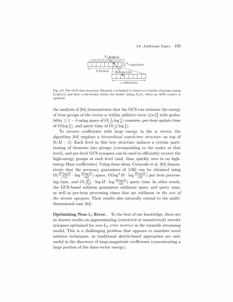
4.6 Additional Topics 193
b buckets
c subbuckets
x h(id(x))
t repetitions
f(x) +u (x)ξ
Fig. 4.9 The GCS data structure: Element x is hashed (t times) to a bucket of groups (usingh(id(x))) and then a sub-bucket within the bucket (using f(x)), where an AMS counter isupdated.
the analysis of [64] demonstrates that the GCS can estimate the energyof item groups of the vector w within additive error ε‖w‖22 with proba-bility ≥ 1 − δ using space of O( 1
ε3 log 1δ ) counters, per-item update time
of O(log 1δ ), and query time of O( 1
ε2 log 1δ ).
To recover coefficients with large energy in the w vector, thealgorithm [64] employs a hierarchical search-tree structure on top of[0,M − 1]: Each level in this tree structure induces a certain parti-tioning of elements into groups (corresponding to the nodes at thatlevel), and per-level GCS synopses can be used to efficiently recover thehigh-energy groups at each level (and, thus, quickly zero in on high-energy Haar coefficients). Using these ideas, Cormode et al. [64] demon-strate that the accuracy guarantees of [130] can be obtained usingO(B3 logM
ε3η3 · log B logMεηδ ) space, O(log2M · log B logM
εηδ ) per item process-
ing time, and O( B3
ε3η3 · logM · log B logMεηδ ) query time. In other words,
the GCS-based solution guarantees sublinear space and query time,as well as per-item processing times that are sublinear in the size ofthe stream synopsis. Their results also naturally extend to the multi-dimensional case [64].
Optimizing Non-L2 Error. To the best of our knowledge, there areno known results on approximating (restricted or unrestricted) waveletsynopses optimized for non-L2 error metrics in the turnstile streamingmodel. This is a challenging problem that appears to mandate novelsolution techniques, as traditional sketch-based approaches are onlyuseful in the discovery of large-magnitude coefficients (concentrating alarge portion of the data-vector energy).

194 Wavelets
4.6.2 Optimizing Coefficient Storage: Extended andHierarchically-Compressed Wavelet Synopses
Extended Wavelets. Massive complex tabular datasets with multiplemeasures (multiple numeric entries for each table cell) arise naturally inseveral application domains, including OLAP environments and time-series analysis/correlation systems. As an example, a corporate salesdatabase may tabulate, for each available product, (1) the number ofitems sold, (2) revenue and profit numbers for the product, and (3) costsassociated with the product, such as shipping and storage costs.Similarly, real-life applications that monitor continuous time-series typ-ically have to deal with several readings (measures) that evolve overtime; for example, a network-traffic monitoring system takes readingson each time-tick from a number of distinct elements, such as routersand switches, in the underlying network and typically several measuresof interest need to be monitored (e.g., input/output traffic numbers foreach router or switch interface) even for a fixed network element.
Traditionally, two obvious strategies, termed Individual and Com-bined, have been employed when adapting wavelet-based methods oversuch multi-measure datasets [276]. The Individual algorithm performsthe wavelet decomposition on each of the individual measures, andstores the important coefficients for each measure separately. On theother hand, the Combined algorithm performs a joint wavelet decom-position on the multi-measure dataset by treating all the measures asa vector of values and, at the end, determines a subset of vectors ofcoefficient values to retain in the synopsis (e.g., based on the L2 normof the coefficient vectors). As an example, Table 4.2 depicts the set ofcombined HWT coefficients for a dataset with µ = 2 measures, wherethe values for the first measure (i.e., first vector row) are identical tothose in our first example array in Section 4.2.1, while the values forthe second measure (i.e., second row) are [4,6,3,5,2,8,3,3].
Such “obvious” Individual and Combined approaches can lead topoor synopsis-storage utilization and suboptimal solutions even in verysimple cases [80]. Due to the nature of the wavelet decomposition andthe possible correlations across different measures, there are many sce-narios in which multiple — but not necessarily all — wavelet coefficients
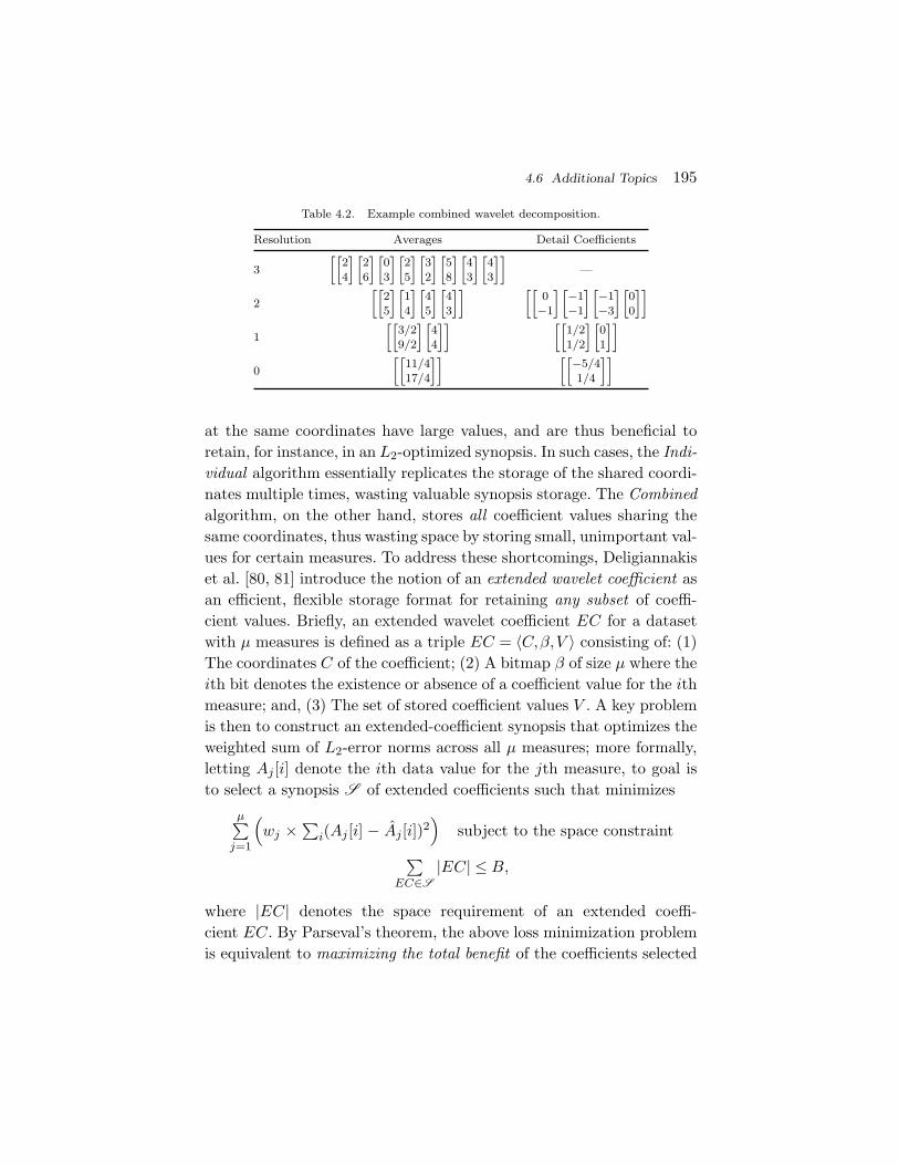
4.6 Additional Topics 195
Table 4.2. Example combined wavelet decomposition.
Resolution Averages Detail Coefficients
3[[
24
][26
][03
][25
][32
][58
][43
][43
]]—
2[[
25
][14
][45
][43
]] [[0
−1
][−1−1
][−1−3
][00
]]
1[[
3/29/2
][44
]] [[1/21/2
][01
]]
0[[
11/417/4
]] [[−5/41/4
]]
at the same coordinates have large values, and are thus beneficial toretain, for instance, in an L2-optimized synopsis. In such cases, the Indi-vidual algorithm essentially replicates the storage of the shared coordi-nates multiple times, wasting valuable synopsis storage. The Combinedalgorithm, on the other hand, stores all coefficient values sharing thesame coordinates, thus wasting space by storing small, unimportant val-ues for certain measures. To address these shortcomings, Deligiannakiset al. [80, 81] introduce the notion of an extended wavelet coefficient asan efficient, flexible storage format for retaining any subset of coeffi-cient values. Briefly, an extended wavelet coefficient EC for a datasetwith µ measures is defined as a triple EC = 〈C,β,V 〉 consisting of: (1)The coordinates C of the coefficient; (2) A bitmap β of size µ where theith bit denotes the existence or absence of a coefficient value for the ithmeasure; and, (3) The set of stored coefficient values V . A key problemis then to construct an extended-coefficient synopsis that optimizes theweighted sum of L2-error norms across all µ measures; more formally,letting Aj [i] denote the ith data value for the jth measure, to goal isto select a synopsis S of extended coefficients such that minimizes
µ∑j=1
(wj ×
∑i(Aj [i] − Aj [i])2
)subject to the space constraint
∑EC∈S
|EC| ≤ B,
where |EC| denotes the space requirement of an extended coeffi-cient EC. By Parseval’s theorem, the above loss minimization problemis equivalent to maximizing the total benefit of the coefficients selected
196 Wavelets
in the synopsis S , where the benefit of the (normalized) ith coeffi-cient for the jth measure c∗ji is exactly its weighted squared magnitudewj(c∗ji)
2 [80, 81]; that is, maximize
∑EC=〈C,β,V 〉∈S
( ∑j,β(j)=1
wj × (c∗ji)2
)under the constraint
∑EC∈S
|EC| ≤ B.
Deligiannakis et al. [80, 81] design an optimal DP algorithm forsolving the above extended wavelet synopsis construction problem giventhe full sequence of combined wavelet coefficients for a multi-measuredataset. A key complication here arises from the storage dependenciesacross measures due to the fact that the storage penalty for an extendedcoefficient’s “header” (i.e., the (coordinates, bitmap) information) isshared across all chosen coefficient values. Thus, their solution relies ontwo mutually-recursive DP recurrences that are tabulated in parallel tocompute an optimal solution using O(MµB) time and space. They alsopropose a simpler, faster greedy algorithm that selects coefficient valuesfor the synopsis based on their benefit-to-space ratio, and requires onlyO(Mµ2 log(Mµ)) time and O(Mµ) space; furthermore, they prove thattheir greedy solution is a min2,1 + 1
BMAX−1
approximation for the
extended-coefficient benefit-maximization problem, where MAX is themaximum space requirement for an extended coefficient (i.e., storingall µ values) [80]. Finally, they discuss the extension of earlier resultson non-L2 error minimization for single-measure data [109, 111] to themulti-measure setting using the idea of Partial-Order DP over the µmeasure dimensions, as well as more efficient greedy heuristics for theproblem [80].
In follow-up work, Guha et al. [137] make the crucial observationthat the DP solution only needs to decide the number p ∈ [0,µ] of val-ues to store for each combined coefficient, since the p values that rankhighest in terms of weighted benefit wj(c∗ji)
2 always give the highestbenefit among all p-subsets. This allows for a simpler and more effi-cient optimal DP solution that runs in O(Mµ(logµ + logB) + µ2B2)time and O(µB + B2) space. Furthermore, they propose an efficientO(Mµ(logµ + logB)) greedy strategy (also based on the coefficient
4.6 Additional Topics 197
values’ benefit-to-space ratio) that guarantees a benefit that is no lessthan that of the optimal solution while using only slightly more space(B + MAX instead of B) [137].
Hierarchically-Compressed Wavelet Synopses. One of the keyideas of extended wavelets is that the storage of coordinates for relatedcoefficient values can be effectively shared in order to improve the qual-ity of wavelet synopses for complex, multi-measure data. Sacharidiset al. [266] observe that similar ideas can also be exploited acrosshierarchically-related coefficients to effectively compress conventional,single-measure wavelet synopses. In a nutshell, the idea is to storeentire paths of wavelet coefficients using only the coordinates of thebottom-most coefficient cbot on the path, along with the set of coef-ficient values (ancestors of cbot) and a small bitmap indicating thenumber of nodes on the stored path. A Hierarchically-CompressedWavelet Synopsis (HCWS) then comprises a set of such hierarchically-compressed (HC) coefficients whose total storage requirements do notexceed a given space budget B. As an example, Figure 4.10 depictstwo hierarchically-compressed coefficients over the Haar tree of a16-entry data array — the corresponding triples of (bottom-most coor-dinates, bitmap, values) are (11,11110,−11,−5,−5.5,15.5,20) and(15,110,−18,−9,−4.5) (where the last 0 entry in the bitmap acts asa stop bit).
By avoiding the explicit storage of coefficient coordinates, a HCWScan allow more coefficient values to be stored for the given space budget,thus resulting in potentially significant gains in accuracy. This is espe-cially the case for datasets with multiple spikes and discontinuitieswhere the Haar-wavelet differencing process across averages of neigh-boring regions can give multiple hierarchically-nested coefficients withlarge values [266]. For the example in Figure 4.10, assuming a coor-dinate and a coefficient value each require 32 bits, the two HC coef-ficients store 8 coefficient values requiring a total of 328 bits, whichwould only allow storing only 5 coefficient values in the traditionalscheme — the difference in the respective L2 errors is also significant(over 60%). Sacharidis et al. [266] formulate and solve the problem ofconstructing an L2-optimal HCWS for a given space budget B. They
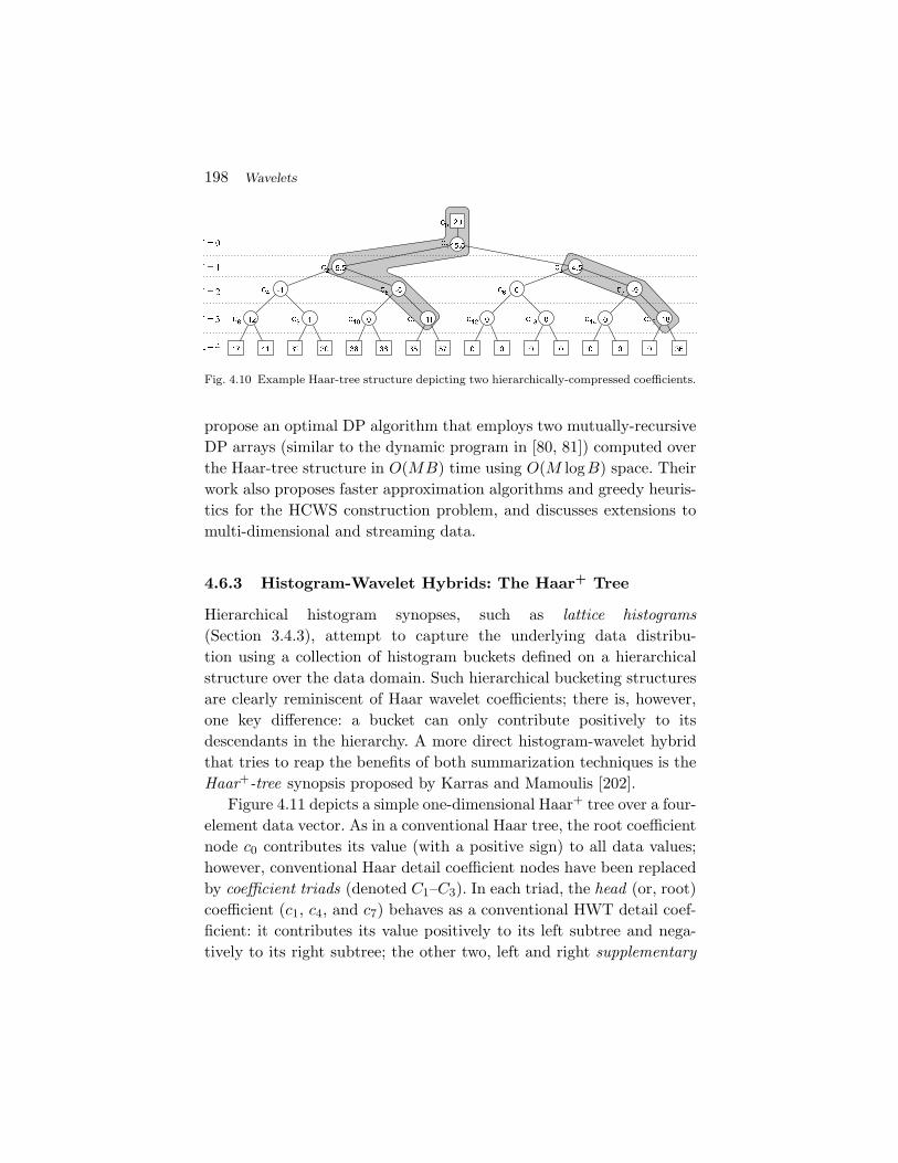
198 Wavelets
Fig. 4.10 Example Haar-tree structure depicting two hierarchically-compressed coefficients.
propose an optimal DP algorithm that employs two mutually-recursiveDP arrays (similar to the dynamic program in [80, 81]) computed overthe Haar-tree structure in O(MB) time using O(M logB) space. Theirwork also proposes faster approximation algorithms and greedy heuris-tics for the HCWS construction problem, and discusses extensions tomulti-dimensional and streaming data.
4.6.3 Histogram-Wavelet Hybrids: The Haar+ Tree
Hierarchical histogram synopses, such as lattice histograms(Section 3.4.3), attempt to capture the underlying data distribu-tion using a collection of histogram buckets defined on a hierarchicalstructure over the data domain. Such hierarchical bucketing structuresare clearly reminiscent of Haar wavelet coefficients; there is, however,one key difference: a bucket can only contribute positively to itsdescendants in the hierarchy. A more direct histogram-wavelet hybridthat tries to reap the benefits of both summarization techniques is theHaar+-tree synopsis proposed by Karras and Mamoulis [202].
Figure 4.11 depicts a simple one-dimensional Haar+ tree over a four-element data vector. As in a conventional Haar tree, the root coefficientnode c0 contributes its value (with a positive sign) to all data values;however, conventional Haar detail coefficient nodes have been replacedby coefficient triads (denoted C1–C3). In each triad, the head (or, root)coefficient (c1, c4, and c7) behaves as a conventional HWT detail coef-ficient: it contributes its value positively to its left subtree and nega-tively to its right subtree; the other two, left and right supplementary
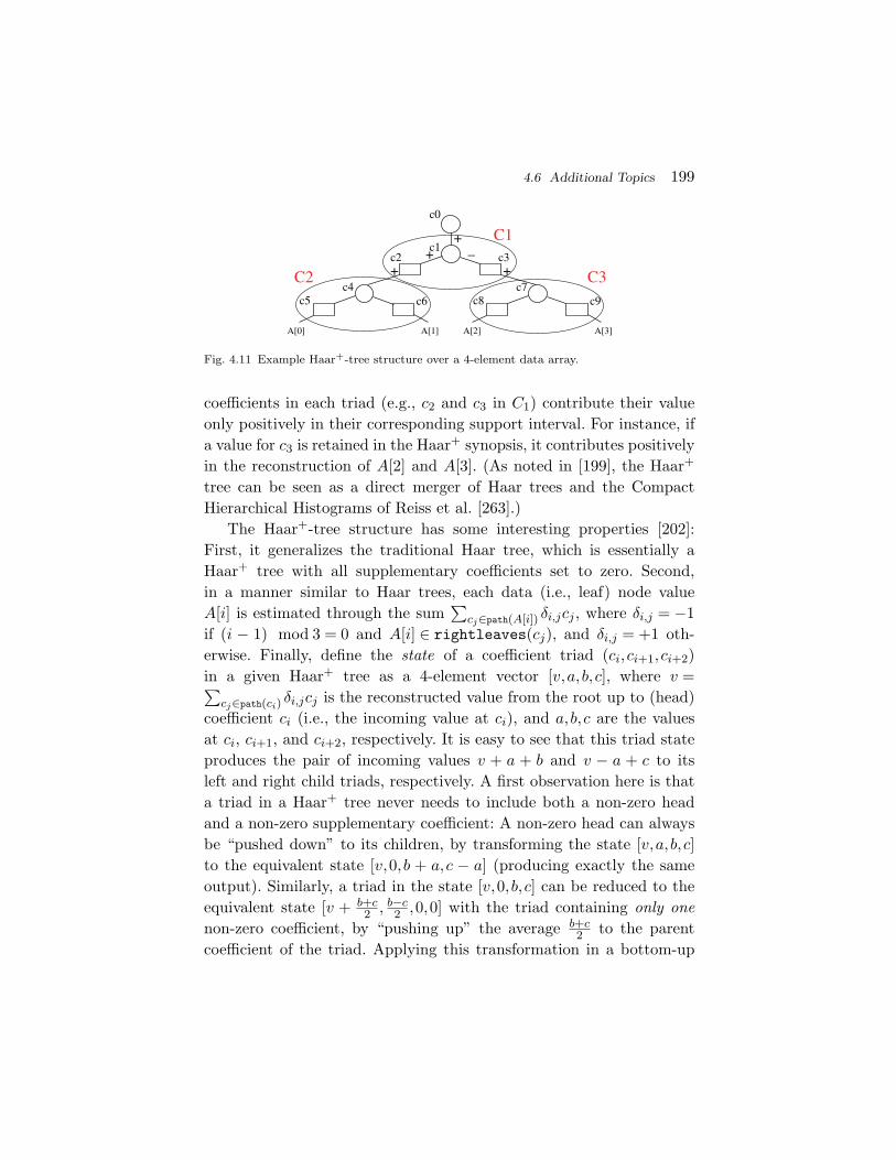
4.6 Additional Topics 199
A[2]
c5 c6c7
c9
A[0] A[1] A[3]
c8
c2 c3
c0
c1
c4
C1
C3C2
++
+–
+
Fig. 4.11 Example Haar+-tree structure over a 4-element data array.
coefficients in each triad (e.g., c2 and c3 in C1) contribute their valueonly positively in their corresponding support interval. For instance, ifa value for c3 is retained in the Haar+ synopsis, it contributes positivelyin the reconstruction of A[2] and A[3]. (As noted in [199], the Haar+
tree can be seen as a direct merger of Haar trees and the CompactHierarchical Histograms of Reiss et al. [263].)
The Haar+-tree structure has some interesting properties [202]:First, it generalizes the traditional Haar tree, which is essentially aHaar+ tree with all supplementary coefficients set to zero. Second,in a manner similar to Haar trees, each data (i.e., leaf) node valueA[i] is estimated through the sum
∑cj∈path(A[i]) δi,jcj , where δi,j = −1
if (i − 1) mod 3 = 0 and A[i] ∈ rightleaves(cj), and δi,j = +1 oth-erwise. Finally, define the state of a coefficient triad (ci, ci+1, ci+2)in a given Haar+ tree as a 4-element vector [v,a,b,c], where v =∑
cj∈path(ci) δi,jcj is the reconstructed value from the root up to (head)coefficient ci (i.e., the incoming value at ci), and a,b,c are the valuesat ci, ci+1, and ci+2, respectively. It is easy to see that this triad stateproduces the pair of incoming values v + a + b and v − a + c to itsleft and right child triads, respectively. A first observation here is thata triad in a Haar+ tree never needs to include both a non-zero headand a non-zero supplementary coefficient: A non-zero head can alwaysbe “pushed down” to its children, by transforming the state [v,a,b,c]to the equivalent state [v,0, b + a,c − a] (producing exactly the sameoutput). Similarly, a triad in the state [v,0, b,c] can be reduced to theequivalent state [v + b+c
2 , b−c2 ,0,0] with the triad containing only one
non-zero coefficient, by “pushing up” the average b+c2 to the parent
coefficient of the triad. Applying this transformation in a bottom-up
200 Wavelets
fashion over the Haar+-tree structure, allows the transformation of anyHaar+ tree H into an equivalent Haar+ tree H ′ (producing exactly thesame data values), such that H ′ is at least as sparse as H (i.e., containsthe same or smaller number of non-zero coefficients) and every triadin H ′ contains at most one non-zero coefficient [202].
The above analysis simplifies the search for error-optimal B-termHaar+-tree representations, since it implies that the search only needsto consider at most one non-zero coefficient in each triad of the optimalsolution. Letting E[i, b,v] denote the minimum error value at coefficienttriad Ci with an incoming value of v and space b allocated to the subtreerooted at Ci, Karras and Mamoulis [202] present a generalization of theunrestricted DP thresholding algorithm in Section 4.3.2 that can con-struct error-optimal Haar+-tree synopses for a wide class of distribu-tive error metrics (that include the various Lp-norm errors). A keyresult of [202] is an analysis of the Haar+-tree structure that allowsthe effective delimitation of the search space for possible incoming andcoefficient values to a range of values bounded by a small constantmultiple of ∆ = maxiA[i] − miniA[i] (i.e., the range of underlyingdata values). Using an analysis similar to that of Section 4.3.2, theHaar+-tree DP algorithm is shown to run in time O((∆
δ )2MB), whereδ is small quantization parameter that controls additive approximationerror [202]. Extensions of Haar+-tree synopses to multiple dimensions,as well as maximum-error optimization techniques based on the dual(space-bounded) problem are discussed in [199].
5Sketches
5.1 Introduction
Of all the methods for generating data synopses presented in thisvolume, sketches have the shortest history, and consequently have hadthe least direct impact on real systems thus far. Nevertheless, theirflexibility and power suggests that they will surely become a fixture inthe next generation of tools and systems for working with large data.Certainly, they have already had significant impact within various spe-cialized domains that process large quantities of structured data, inparticular those that involve the streaming processing of data.
The notion of streaming has been popularized within recent yearsto capture situations where there is one chance to view the input, as it“streams” past the observer. For example, in processing financial datastreams (streams of stock quotes and orders), many such transactionsare witnessed every second, and a system must process these as theyare seen, in real time, in order to facilitate real time data analysisand decision making. Another example that is closer to the motivatingapplications discussed so far is the sequence of updates to a traditionaldatabase — insertions and deletions to a given relation — which alsoconstitute a stream to be processed. Streaming algorithms typically
201
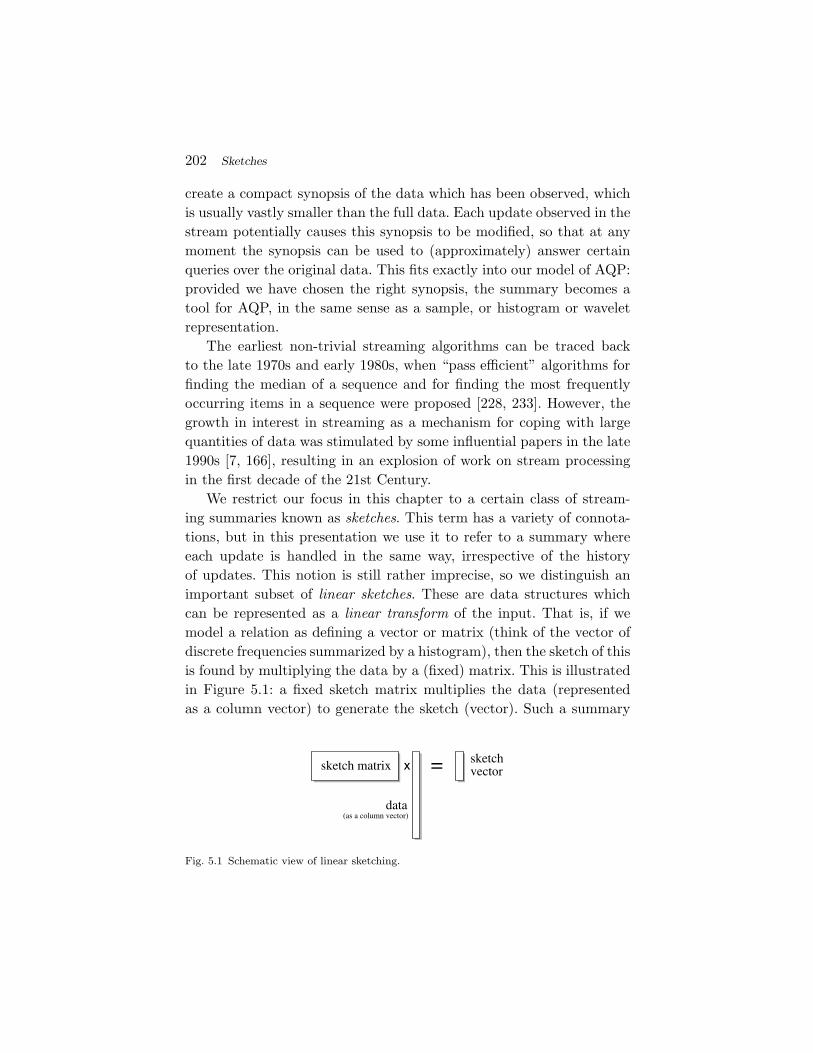
202 Sketches
create a compact synopsis of the data which has been observed, whichis usually vastly smaller than the full data. Each update observed in thestream potentially causes this synopsis to be modified, so that at anymoment the synopsis can be used to (approximately) answer certainqueries over the original data. This fits exactly into our model of AQP:provided we have chosen the right synopsis, the summary becomes atool for AQP, in the same sense as a sample, or histogram or waveletrepresentation.
The earliest non-trivial streaming algorithms can be traced backto the late 1970s and early 1980s, when “pass efficient” algorithms forfinding the median of a sequence and for finding the most frequentlyoccurring items in a sequence were proposed [228, 233]. However, thegrowth in interest in streaming as a mechanism for coping with largequantities of data was stimulated by some influential papers in the late1990s [7, 166], resulting in an explosion of work on stream processingin the first decade of the 21st Century.
We restrict our focus in this chapter to a certain class of stream-ing summaries known as sketches. This term has a variety of connota-tions, but in this presentation we use it to refer to a summary whereeach update is handled in the same way, irrespective of the historyof updates. This notion is still rather imprecise, so we distinguish animportant subset of linear sketches. These are data structures whichcan be represented as a linear transform of the input. That is, if wemodel a relation as defining a vector or matrix (think of the vector ofdiscrete frequencies summarized by a histogram), then the sketch of thisis found by multiplying the data by a (fixed) matrix. This is illustratedin Figure 5.1: a fixed sketch matrix multiplies the data (representedas a column vector) to generate the sketch (vector). Such a summary
x = vectorsketch
data(as a column vector)
sketch matrix
Fig. 5.1 Schematic view of linear sketching.
5.2 Notation and Terminology 203
is therefore very flexible: a single update to the underlying data (aninsertion or deletion of a row in the relational data example) has theeffect of modifying a single entry in the data vector. In turn, the sketchis modified by adding to the sketch the result of applying the matrix tothis change alone. This meets our requirement that an update has thesame impact irrespective of any previous updates. Another property oflinear sketches is that the sketch of the union of two relations can befound as the (vector) sum of their corresponding sketches.
Any given sketch is defined for a particular set of queries. Queriesare answered by applying some (technique specific) procedure to a givensketch. In what follows we will see a variety of different sketches. Forsome sketches, there are several different query procedures that can beused to address different query types, or give different guarantees forthe same query type.
We comment that the idea of sketches, and in particular the lineartransform view is not so very different from the summaries we have seenso far. Many histogram representations with fixed bucket boundariescan be thought of as linear transforms of the input. The Haar WaveletTransform is also a linear transform1. However, for compactness andefficiency of computation, it is not common to explicitly materializethe (potentially very large) matrix which represents the sketch trans-form. Instead, all useful sketch algorithms perform a transform whichis defined implicitly by a much smaller amount of information, oftenvia appropriate randomly chosen hash functions. This is analogous tothe way that a histogram transform is defined implicitly by its bucketboundaries, and the HWT is defined implicitly by the process of aver-aging and differencing.
5.2 Notation and Terminology
As in the preceding sections, we primarily focus on discrete data.We think of the data as defining a multiset D over a domain U =1,2, . . . ,M so that f(i) denotes the number of points in D having a
1 A key conceptual difference between the use of HWT and sketches is that the HWT islossless, and so requires additional processing to produce a more compact summary viathresholding, whereas the sketching process typically provides data reduction directly.
204 Sketches
value i ∈ U . These f(i) values therefore represent a set of frequencies,and can also be thought of as defining a vector f of dimensionM = |U |.In fact, many of the sketches we will describe here also apply to themore general case where each f(i) can take on arbitrary real values,and even negative values. We say that f is “strict” when it can onlytake on non-negative values, and talk of the “general case” when thisrestriction is dropped.
The sketches we consider, which were primarily proposed in thecontext of streams of data, can be created from a stream of updates:think of the contents of D being presented to the algorithm in someorder. Following Muthukrishnan [236], a stream updates is referredto as a “time-series” if the updates arrive in sorted order of i;“cash-register” if they arrive in some arbitrary order; and “turnstile”if items which have previously been observed can subsequently beenremoved. “Cash-register” is intended to conjure the image of a collec-tion of unsorted items being rung up by a cashier in a supermarket,whereas “turnstile” hints at a venue where people may enter or leave.Streams of updates in the time-series or cash-register models necessar-ily generate data in the strict case, whereas the turnstile model canprovide strict or general frequency vectors, depending on the exactsituation being modeled.
These models are related to the datacube and relational modelsdiscussed already: the cash-register and turnstile models, and whetherthey generate strict or general distributions, can all be thought of asspecial cases of the relational model. Meanwhile, the time-series modelis similar to the datacube model. Most of the emphasis in the designof streaming algorithms is on the cash-register and turnstile models.For more details on models of streaming computations, and on algo-rithms for streaming data generally, see some of the surveys on thetopic [12, 105, 236].
Modeling a relation being updated with insert or delete operations,the number of rows with particular attribute values gives a strict turnstilemodel. But if the goal is to summarize the distribution of the sum of a par-ticular attribute, groupedbya secondattribute, then thegeneral turnstilemodel may be generated. In both cases, sketch algorithms are designed tocorrectly reflect the impact of each update on the summary.
5.2 Notation and Terminology 205
5.2.1 Simple Examples: Count, Sum, Average,Variance, Min and Max
Within this framework, perhaps the simplest example of a linear sketchcomputes the cardinality of a multiset D: this value N is simply trackedexactly, and incremented or decremented with each insertion into D ordeletion from D respectively. The sum of all values within a numericattribute can also be sketched trivially by maintaining the exact sumand updating it accordingly. These fit our definition of being a (trivial)linear transformation of the input data. The average is found by divid-ing the sum by the count. Here, in addition to the maintenance ofthe sketch, it was also necessary to define an operation to extract thedesired query answer from the sketch (the division operation). The sam-ple variance of a frequency vector can also be computed in a sketch-ing fashion, by tracking the appropriate sums and sums of squaredvalues.
Considering the case of tracking the maximum value over a streamof values highlights the restriction that linear sketches must obey.There is a trivial streaming algorithm to find the maximum value of asequence — just remember the largest one seen so far. This is a sketch,in the sense that every value is treated the same way, and the sketchmaintenance process keeps the greatest of these. However, it is clearlynot a linear sketch. Note that any linear sketch algorithm implicitlyworks in the turnstile model. But there can be no efficient stream-ing algorithm to find the maximum in a turnstile stream (where thereare insertions and deletions to the dataset D): the best thing to do isto retain f in its entirety, and report the greatest value i for whichf(i) > 0.
5.2.2 Fingerprinting as sketching
As a more involved example, we describe a method to fingerprint adataset D using the language of sketching. A fingerprint is a compactsummary of a multiset so that if two multisets are equal, then theirfingerprints are also equal; and if two fingerprints are equal then thecorresponding multisets are also equal with high probability (where theprobability is over the random choices made in defining the fingerprint
206 Sketches
function). Given a frequency vector f , one fingerprint scheme computesa fingerprint as
h(f) =M∑i=1
f(i)αi mod p,
where p is a prime number sufficiently bigger than M , and α is a valuechosen randomly at the start. We observe that h(f) is a linear sketch,since it is a linear function of f . It can easily be computed in the cashregister model, since each update to f(i) requires adding an appropriatevalue to h(f) based on computing αi and multiplying this by the changein f(i) modulo p.
The analysis of this procedure relies on the fact that a polynomial ofdegree d can have at most d roots (where it evaluates to zero). Testingwhether two multisets D and D′ are equal, based on the fingerprintsof their corresponding frequency vectors, h(f) and h(f ′), is equivalentto testing the identity h(f) − h(f ′) = 0. Based on the definition of h,if the two multisets are identical then the fingerprints will be identical.But if they are different and the test still passes, the fingerprint willgive the wrong answer. Treating h() as a polynomial in α, h(f) − h(f ′)has degree no more than M : so there can only be M values of α forwhich h(f) − h(f ′) = 0. Therefore, if p is chosen to be at least M/δ,the probability (based on choosing a random α) of making a mistakeis at most δ, for a parameter δ. This requires the arithmetic operationsto be done using O(logM + log1/δ) bits of precision, which is feasiblefor most reasonable values of M and δ.
Such fingerprints have been used in streaming for a variety of pur-poses. For example, Yi et al. [294] employ fingerprints within a systemto verify outsourced computations over streams.
5.2.3 Comparing Sketching with Sampling
These simple examples seem straightforward, but they serve to high-light the difference between the models of data access assumed by thesketching process. We have already seen that a small sample of the datacan only estimate the average value in a dataset, whereas this “sketch”can find it exactly. But this is due in part to a fundamental differencein assumptions about how the data is observed: the sample “sees” only
5.2 Notation and Terminology 207
those items which were selected to be in the sample whereas the sketch“sees” the entire input, but is restricted to retain only a small summaryof it. Therefore, to build a sketch, we must either be able to performa single linear scan of the input data (in no particular order), or to“snoop” on the entire stream of transactions which collectively buildup the input. Note that many sketches were originally designed for com-putations in situations where the input is never collected together inone place (as in the financial data example), but exists only implicitlyas defined by the stream of transactions.
Another way to understand the difference in power between themodels of sampling and streaming is to observe that it is possible todesign algorithms to draw a sample from a stream (see Section 2.7.4),but that there are queries that can be approximated well by sketchesthat are provably impossible to compute from a sample. In particular,we will see a number of sketches to approximate the number of distinctitems in a relation (Section 5.4), whereas no sampling scheme can givesuch a guarantee (Section 2.6.2). Similarly, we saw that fingerprintingcan accurately determine whether two relations are identical, whereasunless every entry of two relations is sampled, it is possible that the twodiffer in the unsampled locations. Since the streaming model can simu-late sampling, but sampling cannot simulate streaming, the streamingmodel is strictly more powerful in the context of taking a single passthrough the data.
5.2.4 Properties of Sketches
Having seen these simple examples, we now formalize the main prop-erties of a sketching algorithm.
• Queries Supported. Each sketch is defined to support acertain set of queries. Unlike samples, we cannot simply exe-cute the query on the sketch. Instead, we need to perform a(possibly query specific) procedure on the sketch to obtainthe (approximate) answer to a particular query.
• Sketch Size. In the above examples, the sketch is constantsize. However, in the examples below, the sketch has oneor more parameters which determine the size of the sketch.A common case is where parameters ε and δ are chosen by
208 Sketches
the user to determine the accuracy (approximation error) andprobability of exceeding the accuracy bounds, respectively.
• Update Speed. When the sketch transform is very dense(i.e. the implicit matrix which multiplies the input has veryfew zero entries), each update affects all entries in the sketch,and so takes time linear in the sketch size. But typically thesketch transform can be made very sparse, and consequentlythe time per update may be much less than updating everyentry in the sketch.
• Query Time. As noted, each sketch algorithm has its ownprocedure for using the sketch to approximately answerqueries. The time to do this also varies from sketch to sketch:in some cases it is linear (or even superlinear) in the size ofthe sketch, whereas in other cases it can be much less.
• Sketch Initialization. By requiring the sketch to be a lineartransformation of the input, sketch initialization is typicallytrivial: the sketch is initialized to the all-zeros vector, sincethe empty input is (implicitly) also a zero vector. However, ifthe sketch transform is defined in terms of hash functions, itmay be necessary to initialize these hash functions by draw-ing them from an appropriate family.
5.2.5 Sketching Sets with Bloom Filters
As a more complex example, we briefly discuss the popular BloomFilter as an example of a sketch. A Bloom filter, named for its inventor[24], is a compact way to represent a subset S of a domain U . Itconsists of a binary string B of length m <M initialized to all zeros,and k hash functions h1 . . .hk, which each independently map elementsof U to 1,2, . . .m. For each element i in the set S, the sketch setsB[hj(i)] = 1 for all 1 ≤ j ≤ k. This is shown in Figure 5.2: an item i ismapped by k = 3 hash functions to a filter of size m = 12, and theseentries are set to 1. Hence each update takes O(k) time to process.
After processing the input, it is possible to test whether any given iis present in the set: if there is some j for which B[hj(i)] = 0, then theitem is not present, otherwise it is concluded that i is in S. From this
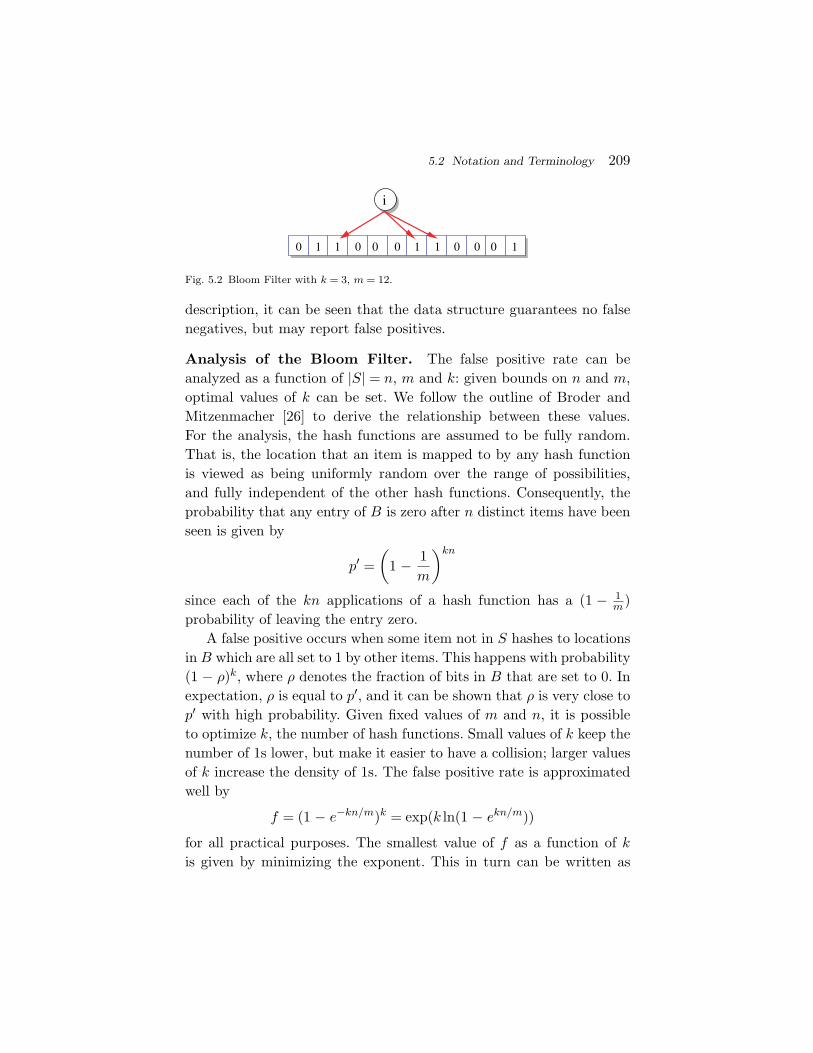
5.2 Notation and Terminology 209
00 00 1 1 11 1 000
i
Fig. 5.2 Bloom Filter with k = 3, m = 12.
description, it can be seen that the data structure guarantees no falsenegatives, but may report false positives.
Analysis of the Bloom Filter. The false positive rate can beanalyzed as a function of |S| = n, m and k: given bounds on n and m,optimal values of k can be set. We follow the outline of Broder andMitzenmacher [26] to derive the relationship between these values.For the analysis, the hash functions are assumed to be fully random.That is, the location that an item is mapped to by any hash functionis viewed as being uniformly random over the range of possibilities,and fully independent of the other hash functions. Consequently, theprobability that any entry of B is zero after n distinct items have beenseen is given by
p′ =(
1 − 1m
)kn
since each of the kn applications of a hash function has a (1 − 1m)
probability of leaving the entry zero.A false positive occurs when some item not in S hashes to locations
in B which are all set to 1 by other items. This happens with probability(1 − ρ)k, where ρ denotes the fraction of bits in B that are set to 0. Inexpectation, ρ is equal to p′, and it can be shown that ρ is very close top′ with high probability. Given fixed values of m and n, it is possibleto optimize k, the number of hash functions. Small values of k keep thenumber of 1s lower, but make it easier to have a collision; larger valuesof k increase the density of 1s. The false positive rate is approximatedwell by
f = (1 − e−kn/m)k = exp(k ln(1 − ekn/m))
for all practical purposes. The smallest value of f as a function of kis given by minimizing the exponent. This in turn can be written as
210 Sketches
−mn ln(p) ln(1 − p), for p = e−kn/m, and so by symmetry, the smallest
value occurs for p = 12 . Rearranging gives k = (m/n) ln2.
This has the effect of setting the occupancy of the filter to be 0.5,that is, half the bits are expected to be 0, and half 1. This causesthe false positive rate to be f = (1/2)k = (0.6185)m/n. To make thisprobability at most a small constant, it is necessary to make m > n.Indeed, setting m = cn gives the false positive probability at 0.6185c:choosing c = 9.6, for example, makes this probability less than 1%.
Bloom Filter viewed as a sketch. In this form, we consider theBloom filter to be a sketch, but it does not meet our stricter condi-tions for being considered as a linear sketch. In particular, the datastructure is not a linear transform of the input: setting a bit to 1 isnot a linear operation. We can modify the data structure to make itlinear, at the expense of increasing the space required. Instead of abitmap, the Bloom filter is now represented by an array of counters.When adding an item, we increase the corresponding counters by 1, thatis, B[hj(i)]← B[hj(i)] + 1. Now the transform is linear, and so it canprocess arbitrary streams of update transactions (including removalsof items). The number of entries needed in the array remains the same,but now the entries are counters rather than bits.
One limitation when trying to use the Bloom Filter to describetruly large datasets is that the space needed is proportional to n, thenumber of items in the set S being represented. Within many AQPscenarios, this much space may not be practical, so instead we look formore compact sketches. These smaller space sketches will naturally beless powerful than the Bloom filter: when using a data structure that issublinear in size (i.e., o(n)) we should not expect to accurately answerall set-membership queries, even allowing for false positives and falsenegatives.
5.3 Frequency Based Sketches
In this Section, we present a selection of sketches which solve a varietyof problems related to estimating functions of the frequencies, f(i). Ourpresentation deliberately does not follow the chronological development
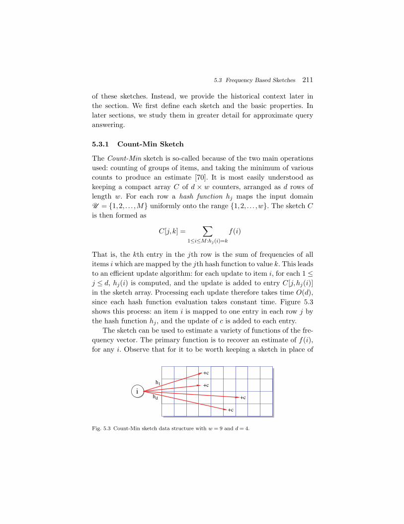
5.3 Frequency Based Sketches 211
of these sketches. Instead, we provide the historical context later inthe section. We first define each sketch and the basic properties. Inlater sections, we study them in greater detail for approximate queryanswering.
5.3.1 Count-Min Sketch
The Count-Min sketch is so-called because of the two main operationsused: counting of groups of items, and taking the minimum of variouscounts to produce an estimate [70]. It is most easily understood askeeping a compact array C of d × w counters, arranged as d rows oflength w. For each row a hash function hj maps the input domainU = 1,2, . . . ,M uniformly onto the range 1,2, . . . ,w. The sketch Cis then formed as
C[j,k] =∑
1≤i≤M :hj(i)=k
f(i)
That is, the kth entry in the jth row is the sum of frequencies of allitems i which are mapped by the jth hash function to value k. This leadsto an efficient update algorithm: for each update to item i, for each 1 ≤j ≤ d, hj(i) is computed, and the update is added to entry C[j,hj(i)]in the sketch array. Processing each update therefore takes time O(d),since each hash function evaluation takes constant time. Figure 5.3shows this process: an item i is mapped to one entry in each row j bythe hash function hj , and the update of c is added to each entry.
The sketch can be used to estimate a variety of functions of the fre-quency vector. The primary function is to recover an estimate of f(i),for any i. Observe that for it to be worth keeping a sketch in place of
+c
+c
+c
hd
+ci
h1
Fig. 5.3 Count-Min sketch data structure with w = 9 and d = 4.
212 Sketches
simply storing f exactly, it must be that wd is much smaller than M ,and so the sketch will necessarily only approximate any f(i). Theestimation can be understood as follows: in the first row, it is thecase that C[1,h1(i)] includes the current value of f(i). However, sincewM , there will be many collisions under the hash function h1, sothat C[1,h1(i)] also contains the sum of all f(i′) for i′ that collides withi under h1. Still, if the sum of such f(i′)s is not too large, then this willnot be so far from f(i).
In the strict case, all these f(i′)s are non-negative, and so C[1,h1(i)]will be an overestimate for f(i). The same is true for all the otherrows: for each j, C[j,hj(i)] gives an overestimate of f(i), based on adifferent set of colliding items. Now, if the hash functions are chosen atrandom, the items will be distributed uniformly over the row. So theexpected amount of “noise” colliding with i in any given row is just∑
1≤i′≤M,i′ =i f(i′)/w, a 1/w fraction of the total count. Moreover, bythe Markov inequality [229, 232], there is at least a 50% chance thatthe noise is less than twice this much. Here, the probabilities arise dueto the random choice of the hash functions. If each row’s estimate off(i) is an overestimate, then the smallest of these will be the closest tof(i). By the independence of the hash functions, it is now very unlikelythat this estimate has error more than 2
∑1≤i′≤M f(i′)/w: this only
happens if every row estimate is “bad,” which happens with probabilityat most 2−d.
Rewriting this, if we pick w = 2/ε and d = log1/δ, then our esti-mate of f(i) has error at most εN with probability at least 1 − δ.Here, we write N =
∑1≤i′≤M f(i′) as the sum of all frequencies —
equivalently, the number of rows in the defining relation if we aretracking the cardinality of attribute values. The estimate is simplyf(i) = mind
j=1C[j,hj(i)]. Producing the estimate is quite similar to theupdate procedure: the sketch is probed in one entry in each row (as inFigure 5.3). So the query time is the same as the update time, O(d).
5.3.1.1 Perspectives on the Count-Min sketch
At its core, the Count-Min sketch is quite simple: just arrange the inputitems into groups, and compute the net frequency of the group. As such,
5.3 Frequency Based Sketches 213
we can think of it as a histogram with a twist: first, randomly permutethe domain, then create an equi-width histogram with w buckets onthis new domain. This is repeated for d random permutations. Queryanswering to estimate a single f(i) is to find all the histogram bucketsthe item i is present in, and take the smallest of these. Viewed fromanother angle, the sketch can also be viewed as a small space, countingversion of a Bloom filter [26, 57].
In this presentation, we omit detailed discussion of some of the tech-nical issues surrounding the summary. For example, for the analysis, thehash functions are required to be drawn from a family of pairwise inde-pendent functions. However this turns out to be quite a weak condition:such functions are very simple to construct, and can be evaluated veryquickly indeed [39, 280]. The estimator described is technically biased,in the statistical sense: it never underestimates but may overestimate,and so is not correct in expectation. However, it is straightforward tomodify the estimator to be unbiased, by subtracting an appropriatequantity from the estimate. Heuristically, we can estimate the countof some “dummy” items such as f(M + 1) whose “true count” shouldbe zero to estimate the error in the estimation [192]. We discuss thevariant estimators in more detail in Section 5.3.5.3.
Lastly, the same sketch can also be used when the stream is general,and so can contain some items with negative frequencies. In this case,the sketch can be built in the same way, but now it is not correct totake the smallest row estimate as the overall estimate: this could befar from the true value if, for example, all the f(i) values are negative.Instead, one can take the median of the row estimates, and apply thefollowing general “Chernoff bounds argument”.
Chernoff Bounds Argument. Suppose there are multiple indepen-dent copies of an estimator, each of which is a “good” estimate of adesired quantity with at least a constant probability (although it’s notpossible to tell whether or not an estimate is good just by looking at it).The goal is to combine these to make an estimate which is “good” withhigh probability. A standard technique is to take the median of enoughestimates to reduce the error. Although it is not possible to determinewhich estimates are good or bad, sorting the estimates by value will
214 Sketches
place all the “good” estimates together in the middle, with “bad” esti-mates above and below (too low or too high). Then the only way thatthe median estimate can be bad is if more than half of the estimatesare bad, which is unlikely. In fact, the probability of returning a badestimate is now exponentially small in the number of estimates.
The proof makes use of a Chernoff bound. Assume that eachestimate is good with probability at least 7/8. The outcome of eachestimate is an independent random event, so in expectation only 1/8 ofthe estimates are bad. So the final result is only bad if the number ofbad events exceeds its expectation by a factor of 4. Set the numberof estimates to be 4ln1/δ for some desired small probability δ. TheChernoff bound (slightly simplified) in this situation states that if X isthe sum of independent Poisson trials, then for 0 < ρ ≤ 4,
Pr[X > (1 + ρ)E[X]] < exp(−E[X]ρ2/4).
See [232] for a derivation of this bound. Since each estimate is indeedan independent Poisson trial, then this setting is modeled with ρ = 3and E[X] = 1
2 ln1/δ. Hence,
Pr[X > 2log1/δ] < exp(−9/8ln1/δ) < δ
This implies that the taken the median of O(log1/δ) estimates reducesthe probability of finding a bad final estimate to δ.
5.3.2 Count Sketch
The Count-Sketch [45] is similar to the Count-Min sketch, in that it canprovide an estimate for the value of any individual frequency. The maindifference is the nature of the accuracy guarantee provided for the esti-mate. Indeed, we can present the Count Sketch by using exactly thesame sketch building procedure as the Count-Min sketch, so that theonly difference is in the estimation procedure.
Now, given the Count-Min sketch data structure built on the stream,the row estimate of f(i) for row j is computed based on two buckets:hj(i), the bucket which contains f(i), and also
h′j(i) =
hj(i) − 1 if hj(i) mod 2 = 0
hj(i) + 1 if hj(i) mod 2 = 1

5.3 Frequency Based Sketches 215
which is an adjacent bucket.2 So if hj(i) = 3 then h′j(i) = 4, while
if hj(i) = 6 then h′j(i) = 5. The row estimate is then C[j,hj(i)] −
C[j,h′j(i)]. Here, we assume that w, the length of each row in the sketch,
is even.The intuition for this estimate comes from considering all the
“noise” items which collide with i: the distribution of such items inthe hj(i)th entry of row j should look about the same as the distri-bution in the h′
j(i)th entry, and so in expectation, these will cancelout, leaving only f(i). More strongly, one can formally prove that thisestimator is unbiased. Of course, the estimator still has variance, andso does not guarantee the correct answer. But this variance can beanalyzed, and written in terms of the sum of squares of the items,F2 =
∑Mi=1 f(i)2. It can be shown that the variance of the estimator is
bounded by O(F2/w). As a result, there is constant probability thateach row estimate is within
√F2/w of f(i). Now by taking the median
of the d row estimates, the probability of the final estimate being out-side these bounds shrinks to 2−O(d). Rewriting, if the parameters arepicked as d = O(log1/δ) and w = O(1/ε2), the sketch guarantees to findan estimate of f(i) so that the error is at most ε
√F2 with probability
at least 1 − δ.In fact, this sketch can be compacted further. Observe that when-
ever a row estimate is produced, it is found as either C[j,2k − 1] −C[j,2k] or C[j,2k] − C[j,2k − 1] for some (integer) k. So rather thanmaintaining C[j,2k − 1] and C[j,2k] separately, it suffices to keep thisdifference in a single counter. This can be seen by maintaining separatehash functions gj which map all items in U = 1,2, . . . ,M uniformlyonto −1,+1. Now the sketch is defined via
C[j,k] =∑
1≤i≤M :hj(i)=k
gj(i)f(i).
This meets the requirements for a linear sketch, since it is a linearfunction of the f vector. It can also be computed in time O(d): foreach update to item i, for each 1 ≤ j ≤ d, hj(i) is computed, and theupdate multiplied by gj(i) is added to entry C[j,hj(i)] in the sketch
2 Equivalently, this can also be written as h′j(i) = hj(i) + (hj(i) mod 2) − (hj(i) + 1
mod 2).
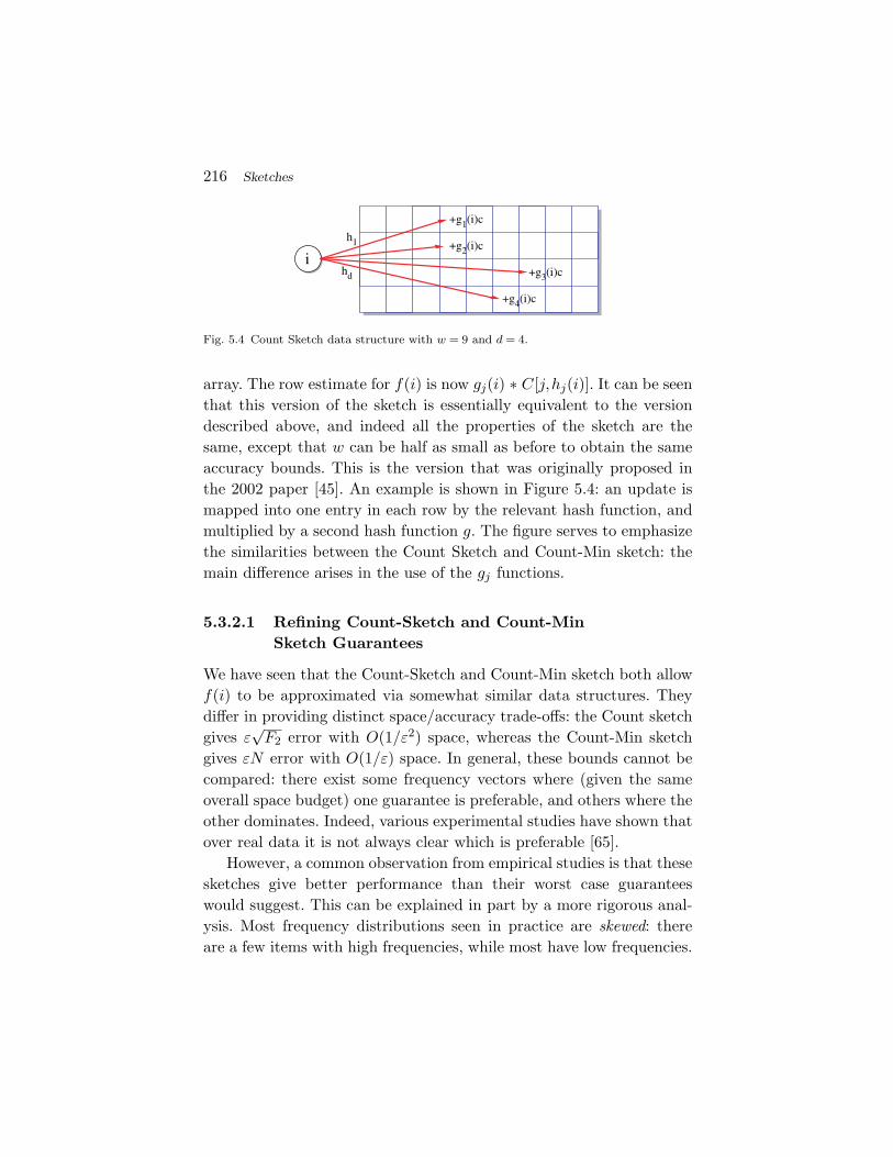
216 Sketches
hd
i
+g1(i)c
+g3(i)c
+g2(i)c
+g4(i)c
h1
Fig. 5.4 Count Sketch data structure with w = 9 and d = 4.
array. The row estimate for f(i) is now gj(i) ∗ C[j,hj(i)]. It can be seenthat this version of the sketch is essentially equivalent to the versiondescribed above, and indeed all the properties of the sketch are thesame, except that w can be half as small as before to obtain the sameaccuracy bounds. This is the version that was originally proposed inthe 2002 paper [45]. An example is shown in Figure 5.4: an update ismapped into one entry in each row by the relevant hash function, andmultiplied by a second hash function g. The figure serves to emphasizethe similarities between the Count Sketch and Count-Min sketch: themain difference arises in the use of the gj functions.
5.3.2.1 Refining Count-Sketch and Count-MinSketch Guarantees
We have seen that the Count-Sketch and Count-Min sketch both allowf(i) to be approximated via somewhat similar data structures. Theydiffer in providing distinct space/accuracy trade-offs: the Count sketchgives ε
√F2 error with O(1/ε2) space, whereas the Count-Min sketch
gives εN error with O(1/ε) space. In general, these bounds cannot becompared: there exist some frequency vectors where (given the sameoverall space budget) one guarantee is preferable, and others where theother dominates. Indeed, various experimental studies have shown thatover real data it is not always clear which is preferable [65].
However, a common observation from empirical studies is that thesesketches give better performance than their worst case guaranteeswould suggest. This can be explained in part by a more rigorous anal-ysis. Most frequency distributions seen in practice are skewed: thereare a few items with high frequencies, while most have low frequencies.
5.3 Frequency Based Sketches 217
This phenomenon is known by several names, such as Pareto, Zipfian,and long tailed distributions. For both Count Sketch and Count-Minsketch, a skewed distribution helps estimation: when estimating a fre-quency f(i), it is somewhat unlikely that any of the few high frequencyitems will collide with i under hj — certainly it is very unlikely thatany will collide with i in a majority of rows. So it is possible to sep-arate out some number k of the most frequent items, and separatelyanalyze the probability that i collides with them. The probability thatthese items affect the estimation of f(i) can then be bounded by δ.This leaves only a “tail” of lower frequency items, which still collidewith i with uniform probability, but the net effect of this is lower sincethere is less “mass” in the tail. Formally, let fi denote the ith largestfrequency in f , and let
Fres(k)1 =
M∑i=k+1
fi and Fres(k)2 =
M∑i=k+1
f2i
denote the sum and the sum of squares of all but the k largest fre-quencies. As a result, we can bound the error in the sketch estimates
in terms of F res(k)1 /w and
√F
res(k)2 /w for the Count-Min and Count
sketch respectively, where k = O(w) [45, 71].
5.3.3 The AMS Sketch
The AMS sketch was first presented in the work of Alon, Matias andSzegedy [7]. It was proposed to solve a different problem, to estimatethe value of F2 of the frequency vector, the sum of the squares of the fre-quencies. Although this is straightforward if each frequency is presentedin turn, it becomes more complex when the frequencies are presentedimplicitly, such as when the frequency of an item is the number of timesit occurs within a long, unordered, stream of items. Estimating F2 mayseem like a somewhat obscure goal in the context of AQP. However,it has a surprising number of applications. Most directly, F2 equatesto the self-join size of the relation whose frequency distribution on thejoin attribute is f (for an equi-join). The AMS sketch turns out to behighly flexible, and is at the heart of estimation techniques for a varietyof other problems which are all of direct relevance to AQP.
218 Sketches
5.3.3.1 AMS Sketch for Estimating F2
We again revert to the sketch data structure of the Count-Min sketchas the basis of the AMS sketch, to emphasize the relatedness of all thesesketch techniques. Now each row is used in its entirety to make a rowestimate of F2 as
w/2∑k=1
(C[j,2k − 1] − C[j,2k])2.
Expanding out this expression in terms of f(i)s, it is clear that theresulting expression includes
∑Mi=1 f(i)2 = F2. However, there are also
a lot of cross terms of the form ±2f(i)f(i′) for i = i′ such that eitherhj(i) = hj(i′) or |hj(i) − hj(i′)| = 1. That is, we have errors due to crossterms of frequencies of items placed in the same location or adjacentlocations by hj . Perhaps surprisingly, the expected contribution of thesecross terms is zero. There are three cases to consider for each i and i′
pair: (a) they are placed in the same entry of the sketch, in which casethey contribute 2f(i)f(i′) to the estimate; (b) one is placed in the 2kthentry and the other in the 2k − 1th, in which case they contribute−2f(i)f(i′) to the estimate; or (c) they are not placed in adjacententries and so contribute 0 to the estimate. Due to the uniformity of hj ,cases (a) and (b) are equally likely, so in expectation (over the choiceof hj) the expected contribution to the error is zero.
Of course, in any given instance there are some i, i′ pairs whichcontribute to the error in the estimate. However, this can be boundedby studying the variance of the estimator. This is largely an exercise inalgebra and applying some inequalities (see [7, 281] for some details).The result is that the variance of the row estimator can be boundedin terms of O(F 2
2 /w). Consequently, using the Chebyshev inequality[232], the error is at most F2/
√w with constant probability. Taking the
median of the d rows reduces the probability of giving a bad estimateto 2−O(d), by the Chernoff bounds argument outlined above.
As in the Count-Sketch case, this sketch can be “compacted” byobserving that it is possible to directly maintain C[j,2k − 1] − C[j,2k]in a single entry, by introducing a second hash function gj which mapsU uniformly onto −1,+1. Technically, a slightly stronger guarantee
5.3 Frequency Based Sketches 219
is needed on gj : because the analysis studies the variance of the rowestimator, which is based on the expectation of the square of the esti-mate, the analysis involves looking at products of the frequencies of fouritems and their corresponding gj values. To bound this requires gj toappear independent when considering sets of four items together: thisadds the requirement that gj be four-wise independent. This conditionis slightly more stringent than the pairwise independence needed of hj .
Practical Considerations for Hashing. Although the terminol-ogy of pairwise and four-wise independent hash functions may beunfamiliar, they should not be thought of as exotic or expensive. Afamily of pairwise independent hash functions is given by the functionsh(x) = ax + b mod p for constants a and b chosen uniformly between0 and p − 1, where p is a prime. Over the random choice of a and b,the probability that two items collide under the hash function is 1/p.Similarly, a family of four-wise independent hash functions is given byh(x) = ax3 + bx2 + cx + d mod p for a,b,c,d chosen uniformly from[p] with p prime. As such, these hash functions can be computed veryquickly, faster even than more familiar (cryptographic) hash functionssuch as MD5 or SHA-1. For scenarios which require very high through-put, Thorup has studied how to make very efficient implementations ofsuch hash functions, based on optimizations for particular values of p,and partial precomputations [280, 281].
Consequently, this sketch can be very fast to compute: each updaterequires only d entries in the sketch to be visited, and a constant amountof hashing work done to apply the update to each visited entry. Thedepth d is set as O(log1/δ), and in practice this is of the order of 10–30,although empirically d can be set as low as 3 or 4 without any obviousproblem [65].
AMS sketch with Averaging versus Hashing. In fact, theoriginal description of the AMS sketch gave an algorithm that wasconsiderably slower: the original AMS sketch was essentially equivalentto the sketch we have described with w = 1 and d = O(ε−2 log1/δ).Then the mean of O(ε−2) entries of the sketch was taken, to reducethe variance, and the final estimator found as the median of O(log1/δ)

220 Sketches
such independent estimates. We refer to this as the “averaging ver-sion” of the AMS sketch. This estimator has the same space cost asthe version we present here, which was the main objective of [7]. Thefaster version, based on the “hashing trick” is sometimes referred to as“fast AMS” to distinguish it from the original sketch, since each updateis dramatically faster.
Historical Notes. Historically, the AMS Sketch [7] was the first tobe proposed as such in the literature, in 1996. The “Random SubsetSums” technique can be shown to be equivalent to the AMS sketchfor estimating single frequencies [129]. The Count-Sketch idea was pre-sented first in 2002. Crucially, this seems to be the first work where itwas shown that hashing items to w buckets could be used instead oftaking the mean of w repetitions of a single estimator, and that thisobtains the same accuracy. Drawing on this, the Count-Min sketch wasthe first to obtain a guarantee in O(1/ε) space, albeit for an F1 insteadof F2 guarantee [70]. Applying the “hashing trick” to the AMS sketchto make it very fast to update seems to have been discovered in parallelby several people. Thorup and Zhang were among the first to publishthis idea [281], and an extension to inner-products appeared in [63].
5.3.4 Approximate Query Processing with FrequencyBased Sketches
Now that we have seen the definitions and basic properties of theCount-Min Sketch, Count-Sketch and AMS Sketch, we go on to seehow they can be applied to approximate the results of various aggre-gation queries.
5.3.4.1 Point Queries and Heavy Hitters
Via Count-Min and Count Sketch, we have two mechanisms to approx-imate the frequency of any given item i. One has accuracy propor-tional to εN , the other proportional to ε
√F2. To apply either of these,
we need to have in mind some particular item i which is of interest.A more common situation arises when we have no detailed a prioriknowledge of the frequency distribution, and we wish to find which
5.3 Frequency Based Sketches 221
are the most significant items. Typically, those most significant itemsare those which have high frequencies — the so-called “heavy hitters.”More formally, we define the set of heavy hitters as those items whosefrequency exceeds a φ fraction of the total frequency, for some chosen0 < φ < 1.
The naive way to discover the heavy hitters within a relation isto exhaustively query each possible i in turn. The accuracy guaranteesindicate that the sketch should correctly recover those items with f(i) >εN or f(i) > ε
√F2. But this procedure can be costly, or impractical,
when the domain size M is large — consider searching a space indexedby a 32 or 64 bit integer. The number of queries is so high that theremay be false positives unless d is chosen to be sufficiently large to ensurethat the overall false positive probability is driven low enough.
In the cash-register streaming model, where the frequencies onlyincrease, a simple solution is to combine update with search. Note thatan item can only become a heavy hitter in this model following anarrival of that item. So the current set of heavy hitters can be tracked ina data structure separate to the sketch, such as a heap or list sorted bythe estimated frequency [45]. When the frequency of an item increases,at the same time the sketch can be queried to obtain the current esti-mated frequency. If the item exceeds the current threshold for being aheavy hitter, it can be added to the data structure. At any time, thecurrent set of (approximate) heavy hitters can be found by probing thisdata structure.
We can compare this to results from sampling: standard samplingresults argue that to find the heavy hitters with εN accuracy, a sampleof size O(1/ε2) items is needed. So the benefits of the Count-Min sketchare clear: the space required is quadratically smaller to give the sameguarantee (O(1/ε) compared toO(1/ε2)). However, the benefits becomemore clear in the turnstile case when, if there is significant numbersof deletions in the data, causing the set of Heavy Hitters to changeconsiderably over time. In such cases it is not possible to draw a largesample from the input stream.
Heavy Hitters over Strict Distributions. When the data arrivesin the turnstile model, decreases in the frequency of one item can cause
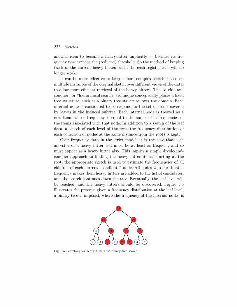
222 Sketches
another item to become a heavy-hitter implicitly — because its fre-quency now exceeds the (reduced) threshold. So the method of keepingtrack of the current heavy hitters as in the cash-register case will nolonger work.
It can be more effective to keep a more complex sketch, based onmultiple instances of the original sketch over different views of the data,to allow more efficient retrieval of the heavy hitters. The “divide andconquer” or “hierarchical search” technique conceptually places a fixedtree structure, such as a binary tree structure, over the domain. Eachinternal node is considered to correspond to the set of items coveredby leaves in the induced subtree. Each internal node is treated as anew item, whose frequency is equal to the sum of the frequencies ofthe items associated with that node. In addition to a sketch of the leafdata, a sketch of each level of the tree (the frequency distribution ofeach collection of nodes at the same distance from the root) is kept.
Over frequency data in the strict model, it is the case that eachancestor of a heavy hitter leaf must be at least as frequent, and somust appear as a heavy hitter also. This implies a simple divide-and-conquer approach to finding the heavy hitter items: starting at theroot, the appropriate sketch is used to estimate the frequencies of allchildren of each current “candidate” node. All nodes whose estimatedfrequency makes them heavy hitters are added to the list of candidates,and the search continues down the tree. Eventually, the leaf level willbe reached, and the heavy hitters should be discovered. Figure 5.5illustrates the process: given a frequency distribution at the leaf level,a binary tree is imposed, where the frequency of the internal nodes is
20
3 8 34671
135
14
9
34
7
2
Fig. 5.5 Searching for heavy hitters via binary-tree search.
5.3 Frequency Based Sketches 223
the sum of the leaf frequencies in the subtree. Nodes which are heavy(in this example, whose frequency exceeds 6) are shaded. All unshadednodes can be ignored in the search for the heavy hitters.
Using a tree structure with a constant fan-out at each node, thereareO(logM) levels to traverse. Defining a heavy hitter as an item whosecount exceeds φN for some fraction φ, there are at most 1/φ possible(true) heavy hitters at each level. So the amount of work to discover theheavy hitters at the leaves is bounded by O(logM/φ) queries, assumingnot too many false positives along the way. This analysis works directlyfor the Count-Min sketch. However, it does not quite work for findingthe heavy hitters based on Count-Sketch and an F2 threshold, since theF2 of higher levels can be much higher than at the leaf level.
Nevertheless, it seems to be an effective procedure in practice.A detailed comparison of different methods for finding heavy hittersis performed in [65]. There, it is observed that there is no clear “best”sketch for this problem: both approaches have similar accuracy, giventhe same space. As such, it seems that the Count-Min approach mightbe slightly preferred, due to its faster update time: the Count-Minsketch processed about 2 million updates per second in speed trials,compared to 1 million updates per second for the Count Sketch. Thisis primarily since Count-Min requires only one hash function evaluationper row, to the Count Sketch’s two.3
Heavy Hitters over General Distributions. For general distri-butions which include negative frequencies, this procedure is not guar-anteed to work: consider two items, one with a large positive frequencyand the other with a large negative frequency of similar magnitude.If these fall under the same node in the tree, their frequencies effec-tively cancel each other, and the search procedure may mistakenly failto discover them. General distributions can arise for a variety of reasons,for example in searching for items which have significantly different fre-quencies in two different relations, so it is of interest to overcome thisproblem. Henzinger posed this question in the context of identifyingwhich terms were experiencing significant change in their popularity
3 To address this, it would be possible to use a single hash function, where the last bitdetermines gj and the preceding bits determine hj .
224 Sketches
within an Internet search engine [165]. Consequently, this problem issometimes also referred to as the “heavy changers” problem.
In this context, various “group testing” sketches have been pro-posed. They can be thought of as turning the above idea inside out:instead of using sketches inside a hierarchical search structure, thegroup testing places the hierarchical search structure inside the sketch.That is, it builds a sketch as usual, but for each entry in the sketch keepsO(logM) additional information based, for instance, on the binaryexpansion of the item identifiers. The idea is that the width of thesketch, w, is chosen so that in expectation at most one of the heavyhitters will land in each entry, and the sum of (absolute) frequenciesfrom all other items in the same entry is small in comparison to the fre-quency of the heavy hitter. Then, the additional information is in theform of a series of “tests” designed to allow the identity of the heavyhitter item to be recovered. For example, one test may keep the sum offrequencies of all items (within the given entry) whose item identifieris odd, and another keeps the sum of all those whose identifier is even.By comparing these two sums it is possible to determine whether theheavy hitter item identifier is odd or even, or if more than one heavyhitter is present, based on whether one or both counts are heavy. Byrepeating this with a test for each bit position (so O(logM) in total),it is possible to recover enough information about the item to correctlyidentify it. The net result is that it is possible to identify heavy hittersover general streams with respect to N or F2 [69]. Other work in thisarea has considered trading off more space and greater search times forhigher throughput [269]. Recent work has experimented with the hier-archical approach for finding heavy hitters over general distributions,and shown that on realistic data, it is still possible to recover mostheavy hitters in this way [31].
5.3.4.2 Join Size Estimation
Given two frequency distributions over the same domain, f and f ′,their inner product is defined as
f · f ′ =M∑i=1
f(i) ∗ f ′(i)
5.3 Frequency Based Sketches 225
This has a natural interpretation, as the size of the equi-join betweenrelations where f denotes the frequency distribution of the joinattribute in the first, and f ′ denote the corresponding distribution inthe second. In SQL, this is
SELECT COUNT(*) FROM D, D’
WHERE D.id = D’.id
The inner product also has a number of other fundamental inter-pretations that we shall discuss below. For example, it also can be usedwhen each record has an additional “measure” value, and the queryis to compute the sum of products of measure values of joining tuples(e.g., finding the total amount of sales given by number of sales of eachitem multiplied by price of each item). It is also possible to encode thesum of those f(i)s, where i meets a certain predicate as an inner prod-uct where f ′(i) = 1 if and only if i meets the predicate, and 0 otherwise.This is discussed in more detail below.
Using the AMS Sketch to estimate inner products. GivenAMS sketches of f and f ′, C and C ′ respectively, that have been con-structed with the same parameters (that is, the same choices of w,d,hj ,and gj), the estimate of the inner product is given by
w∑k=1
C[j,k] ∗ C ′[j,k].
That is, the row estimate is the inner product of the rows.The bounds on the error follow for similar reasons to the F2 case
(indeed, the F2 case can be thought of as a special case where f = f ′).Expanding out the sum shows that the estimate gives f · f ′, with addi-tional cross-terms due to collisions of items under hj . The expectationof these cross terms in f(i)f ′(i′) is zero over the choice of the hash func-tions, as the function gj is equally likely to add as to subtract any giventerm. The variance of the row estimate is bounded via the expectationof the square of the estimate, which depends on O(F2(f)F2(f ′)/w).Thus each row estimate is accurate with constant probability, which isamplified by taking the median of d row estimates.
226 Sketches
Comparing this guarantee to that for F2 estimation, we note thatthe error is bounded in terms of the product
√F2(f)F2(f ′). In general,√
F2(f)F2(f ′) can be much larger than f · f ′, such as when each off and f ′ is large but f · f ′ can still be small or even zero. However,this is unavoidable: lower bounds show that no sketch (more strongly,no small data structure) can guarantee to estimate f · f ′ with errorproportional to f · f ′ unless the space used is at least M [210].
In fact, we can see this inner product estimation as a generalizationof the previous methods. Set f ′(i) = 1 and f ′(i′) = 0 for all i′ = i. Thenf · f ′ = f(i), so computing the estimate of f · f ′ should approximatethe single frequency f(i) with error proportional to
√F2(f)F2(f ′)/w =√
F2(f)/w. In retrospect this is not surprising: when we consider build-ing the sketch of the constructed frequency distribution f ′ and makingthe estimate, the resulting procedure is identical to the procedure ofestimating f(i) via the Count-Sketch approach. Using the AMS sketchto estimate inner-products was first proposed in [6]; the “fast” versionwas described in [63].
Using the Count-Min sketch to estimate inner products. TheCount-Min sketch can be used in a similar way to estimate f · f ′. Infact, the row estimate is formed the same way as the AMS estimate,as the inner product of sketch rows:
w∑k=1
C[j,k] ∗ C ′[j,k].
Expanding this sum based on the definition of the sketch results inexactly f · f ′, along with additional error terms of the form f(i)f ′(i′)from items i and i′ which happen to be hashed to the same entry byhj . The expectation of these terms is not too large, which is proved bya similar argument to that used to analyze the error in making pointestimates of f(i). We expect about a 1/w fraction of all such termsto occur over the whole summation. So with constant probability, thetotal error in a row estimate is NN ′/w (where N =
∑Mi=1 f(i) and
N ′ =∑M
i=1 f′(i)). Repeating and taking the minimum of d estimates
makes the probability of a large error exponentially small in d.
5.3 Frequency Based Sketches 227
Applying this result to f = f ′ shows that Count-Min sketch canestimate f · f = F2 with error N2/w. In general, this will be muchlarger than the corresponding AMS estimate with the same w, unlessthe distribution is skewed. For sufficiently skewed distribution, a morecareful analysis (separating out the k largest frequencies) gives tighterbounds for the accuracy of F2 estimation [71]. Setting f ′ to pick outa single frequency f(i) has the same bounds as the point-estimationcase. This is to be expected, since the resulting procedure is identicalto the point estimation protocol.
Comparing AMS and Count-Min sketches for join size esti-mation. The analysis shows the worst case performance of the twosketch methods can be bounded in terms of N or F2. To get a betterunderstanding of their true performance, Dobra and Rusu performeda detailed study of sketch algorithms [88]. They gave a careful statis-tical analysis of the properties of sketches, and considered a varietyof different methods to extract estimates from sketches. From theirempirical evaluation of many sketch variations for the purpose of join-size estimation across a variety of datasets, they arrive at the followingconclusions:
• The errors from the hashing and averaging variations of theAMS sketches are comparable for low-skew (near-uniform)data, but are dramatically lower for the hashing version (themain version presented in this chapter) when the skew ishigh.
• The Count-Min sketch does not perform well when the datahas low-skew, due to the impact of collisions with many itemson the estimation. But it has the best overall performancewhen the data is skewed, since the errors in the estimationare relatively much lower.
• The sketches can be implemented to be very efficient: eachupdate to the sketch in their experiments took between 50and 400 nanoseconds, translating to a processing rate of mil-lions of updates per second.
228 Sketches
As a result, the general message seems to be that the (fast) AMSversion of the sketches are to be preferred for this kind of estimation,since they exhibit fast updates and accurate estimations across thebroadest range of data types.
5.3.4.3 Range Queries and Quantiles
Another common type of query is a range-count, for example
SELECT COUNT(*) FROM D
WHERE D.val > = l AND D.val < = h
for a range l . . .h. Note that these are the exactly the same as the range-count and range-sum queries considered over histogram representations(defined in Section 3.1.1).
A direct solution to this query is to pose an appropriate inner-product query. Given a range, it is possible to construct a frequencydistribution f ′ so that f ′(i) = 1 if l ≤ i ≤ h, and 0 otherwise. Thenf · f ′ gives the desired range-count. However, when applying the AMSapproach to this, the error scales proportional to
√F2(f)F2(f ′). So
here the error grows proportional to the square root of the length of therange. Using the Count-Min sketch approach, the error is proportionaltoN(h − l + 1), that is it grows proportional to the length of the range,clearly a problem for even moderately sized ranges. Indeed, this is thesame error behavior that would result from estimating each frequencyin the range in turn, and summing the estimates.
Range Queries via Dyadic Ranges. The hierarchical approach,outlined in Section 5.3.4.1, can be applied here. A standard techniquewhich appears in many places within streaming algorithms is to repre-sent any range canonically as a logarithmic number of so-called dyadicranges. A dyadic range is a range whose length power of two, andwhich ends at a multiple of its own length (the same concept is used inthe Haar Wavelet Transform, see Section 4.2.1). That is, it can be writ-ten as [j2a + 1 . . .(j + 1)2a]. Examples of dyadic ranges include [1 . . .8],[13 . . .16], [5 . . .6] and [27 . . .27]. Any arbitrary range can be canoni-cally partitioned into dyadic ranges with a simple procedure: find the
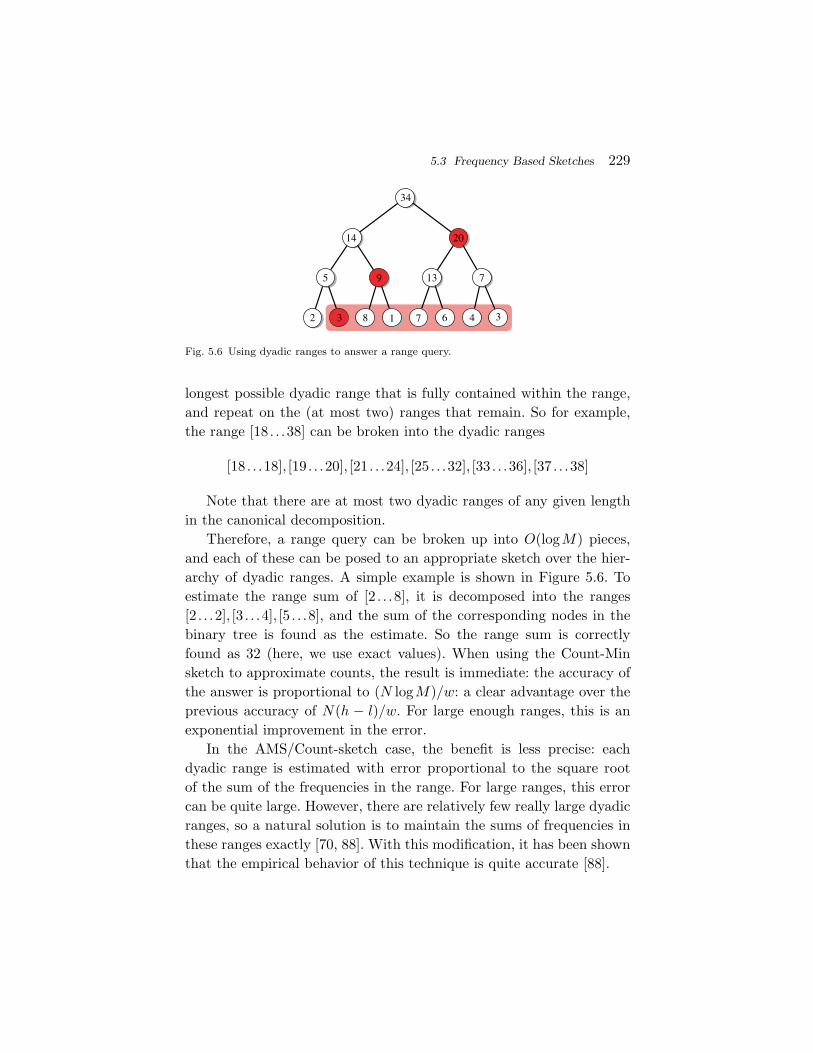
5.3 Frequency Based Sketches 229
20
3 8 34671
135
14
9
34
7
2
Fig. 5.6 Using dyadic ranges to answer a range query.
longest possible dyadic range that is fully contained within the range,and repeat on the (at most two) ranges that remain. So for example,the range [18 . . .38] can be broken into the dyadic ranges
[18 . . .18], [19 . . .20], [21 . . .24], [25 . . .32], [33 . . .36], [37 . . .38]
Note that there are at most two dyadic ranges of any given lengthin the canonical decomposition.
Therefore, a range query can be broken up into O(logM) pieces,and each of these can be posed to an appropriate sketch over the hier-archy of dyadic ranges. A simple example is shown in Figure 5.6. Toestimate the range sum of [2 . . .8], it is decomposed into the ranges[2 . . .2], [3 . . .4], [5 . . .8], and the sum of the corresponding nodes in thebinary tree is found as the estimate. So the range sum is correctlyfound as 32 (here, we use exact values). When using the Count-Minsketch to approximate counts, the result is immediate: the accuracy ofthe answer is proportional to (N logM)/w: a clear advantage over theprevious accuracy of N(h − l)/w. For large enough ranges, this is anexponential improvement in the error.
In the AMS/Count-sketch case, the benefit is less precise: eachdyadic range is estimated with error proportional to the square rootof the sum of the frequencies in the range. For large ranges, this errorcan be quite large. However, there are relatively few really large dyadicranges, so a natural solution is to maintain the sums of frequencies inthese ranges exactly [70, 88]. With this modification, it has been shownthat the empirical behavior of this technique is quite accurate [88].
230 Sketches
Quantiles via Range Queries. The quantiles of a frequencydistribution on an ordered domain divide the total “mass” of the dis-tribution into equal parts. More formally, the φ quantile q of a distribu-tion is defined by q = minn :
∑ni=1 ≥ φN. The most commonly used
quantile is the median, which corresponds to the φ = 0.5 point. Otherquantiles describe the shape of the distribution, and the likelihood thatitems will be seen in the “tails” of the distribution. They are also com-monly used within database systems for approximate query answering,and within simple equidepth histograms (Section 3.1.1).
There has been great interest in finding the quantiles of distributionsdefined by streams — see the work of Greenwald and Khanna, andreferences therein [131]. Gilbert et al. were the first to use sketchesto track the quantiles of streams in the turnstile model [129]. Theirsolution is to observe that finding a quantile is the dual problem toa range query: we are searching for a point q so that the range queryon [1 . . . q] gives φN . Since the result of this range query is monotonein q, we can perform a binary search for q. Each queried range canbe answered using the above techniques for approximately answeringrange queries via sketches, and in total O(logM) queries will be neededto find a q which is (approximately) the φ-quantile.
Note here that the error guarantee means that we will guarantee tofind a “near” quantile. That is, the q which is found is not necessarilyan item which was present in the input — recall, in Section 5.2.5 weobserved that whenever we store a data structure that is smaller thanthe size of the input, there is not room to recall which items wereor were not present in the original data. Instead, we guarantee thatthe range query [1 . . . q] is approximately φN , where the quality of theapproximation will depend on the size of the sketch used. Typically,the accuracy is proportional to εN , so when ε φ, the returned pointwill close to the desired quantile. It also means that extreme quantiles(like the 0.001 or the 0.999 quantile) will not be found very accurately.The most extreme quantiles are the maximum and minimum values inthe dataset, and we have already noted that such values are not wellsuited for linear sketches to find.
5.3 Frequency Based Sketches 231
5.3.4.4 Sketches for Measuring Differences
A difference query is used to measure the difference between two fre-quency distributions. The Euclidean difference treats the frequency dis-tributions as vectors, and measures the Euclidean distance betweenthem. That is, given two frequency distributions, it computes
√F2(f − f ′) =
√√√√ M∑i=1
(f(i) − f ′(i))2
Note that this is quite similar in form to an F2 calculation, except thatthis is being applied to the difference of two frequency distributions.However, we can think of this as applying to an implicit frequencydistribution, where the frequency of i is given by (f(i) − f ′(i)). Thiscan be negative, if f ′(i) > f(i). Here, the flexibility of sketches whichcan process general streams comes to the fore: it does not matter thatthere are negative frequencies. Further, it is not necessary to directlygenerate the difference distribution. Instead, given a sketch of f as Cand a sketch of f ′ as C ′, it is possible to generate the sketch of (f − f ′)as the array subtraction (C − C ′). This is correct, due to the linearityproperties of sketches. Therefore, from the two sketches an approxi-mation of
√F2(f − f ′) can be immediately computed. The accuracy
of this approximation varies with√F2(f − f ′)/
√w. This is a power-
ful guarantee: even if F2(f − f ′) is very small compared to F2(f) andF2(f ′), the sketch approach will give a very accurate approximation ofthe difference.
More generally, arbitrary arithmetic over sketches is possible: theF2 of sums and differences of frequency distributions can be foundby performing the corresponding operations on the sketch repre-sentations. Given a large collection of frequency distributions, theEuclidean distance between any pair can be approximated using onlythe sketches, allowing them to be clustered or otherwise compared. Themathematically inclined can view this as an efficient realization of theJohnson–Lindenstrauss Lemma [194].
232 Sketches
5.3.5 Advanced Uses of Sketches
In this section, we discuss how the sketches already seen can be appliedto higher dimensional data, more complex types of join size estimation,and alternate estimation techniques.
5.3.5.1 Higher Dimensional Data
Sketches can naturally summarize higher dimensional data. Givena multidimensional frequency distribution such as f(i1, i2, i3), it isstraightforward for most of the sketches to summarize this: we justhash on the index (i1, i2, i3) where needed. This lets us compute, forexample, point queries, join size queries and distinct counts over the dis-tributions. But these queries are not really fundamentally different formulti-dimensional data compared to single dimensional data. Indeed,all these results can be seen by considering applying some linearizationto injectively map the multidimensional indices to a single dimension,and solving the one-dimensional problem on the resulting data.
Things are more challenging when we move to range queries. Nowthe query is specified by a product of ranges in each dimension, whichspecifies a hyper-rectangle. With care, the dyadic range decompositiontechnique can be lifted to multiple dimensions. In a single dimension,we argued that any range could be decomposed into O(logM) dyadicranges. Analogously, any dimensional range over 1, . . . ,M can bedecomposed into O(logM) dyadic hyper-rectangles: rectangles formedas the product of dyadic ranges. Figure 5.7 shows the decompositionsof a small two dimensional rectangle of dimensions 4 by 4. Each of thenine subfigures shows a different combination of dyadic ranges on thex and y axes.
Applying this approach, we quickly run into a “curse of dimension-ality” problem: there are logM different types of hyper-rectangle tokeep track of, so the space required (along with the time to processeach update and each query) increases by at least this factor. So forrange queries using Count-Min sketches, for example, the space cost tooffer εN accuracy grows in proportion to (logM)2/ε.4 For more than
4 This exponent is 2, because we need to store (logM/) sketches, and each sketch needsto be created with parameter w proportional to (logM)/ε so that the overall accuracy ofthe range query is εN .

5.3 Frequency Based Sketches 233
Fig. 5.7 Dyadic decomposition of a 4 by 4 rectangle.
2 or 3, this cost can be sufficiently large to be impractical. Meanwhile,a sample of O(1/ε2) items from the distribution is enough to estimatethe selectivity of the range with accuracy ε, and hence the size of therange sum with accuracy εN , irrespective of the dimensionality. There-fore, if it is possible to maintain a sample, this will often be preferablefor higher dimensional data.
Alternatively, we can make independence assumptions, as discussedin the histogram case (Section 3.5.2): if we believe that there are no cor-relations between the dimensions, we can keep a sketch of each dimen-sion independently, and estimate the selectivity over the range as theproduct of the estimated selectivities. However, this does not seem rep-resentative of real data, where we expect to see many correlated dimen-sions. A compromise is to decompose the dimensions into pairs whichare believed to be most correlated, and sketch the pairwise distributionof such pairs. Then the product of selectivities on each correlated paircan estimate the overall selectivity, and hence the range sum.
The work of Thaper et al. [278] uses multidimensional sketchesto derive approximate histogram representations. Given a proposed
234 Sketches
bucketing (set of hyper-rectangles and weights), it computes the errorby measuring the difference between a sketch of the data and a sketchof the histogram. The algorithm can then search over bucketings tofind the best (according to the approximations from sketching). Vari-ous methods are applied to speed up the search. Considering rectanglesin a particular order means that sketches can be computed incremen-tally; [278] also suggests the heuristic of only considering buckets thatare dyadic hyper rectangles. Empirical study shows that the methodfinds reasonable histograms, but the time cost of the search increasesdramatically as the domain size increases, even on two-dimensionaldata.
5.3.5.2 More Complex Join Size Estimation
Multi-way join size estimation. Dobra et al. propose a techniqueto extend the join-size estimation results to multiple join conditions[87]. The method applies to joins of r relations, where the join conditionis of the form
WHERE R1.A1 = R2.A1 AND R2.A2 = R3.A2 AND ...
The main idea is to take the averaging-based version of the AMS sketch(where all items are placed into every sketch entry). A sketch is built foreach relation, where each update is multiplied by r independent hashfunctions that map onto −1,+1. Each hash function corresponds toa join condition, and has the property that if a pair of tuples joinunder that condition then they both hash to the same value (this is ageneralization of the technique used in the sketches for approximatingthe size of a single join). Otherwise, there is no correlation betweentheir hash values. A single estimate is computed by taking the productof the same entry in each sketch. Putting this all together, it followsthat sets of r tuples which match on all the join conditions get theirfrequencies multiplied by 1, whereas all other sets of tuples contributezero in expectation. Provided the join graph is acyclic, the variance ofthe estimation grows as 2a
∏rj=1F2(Rj), where a is the number of join
attributes, and F2(Rj) denotes the F2 (self-join size) of relation Rj .This gives good results for small numbers of joins.
5.3 Frequency Based Sketches 235
A disadvantage of the technique is that is uses the slower averag-ing version of the AMS sketch: each update affects each entry of eachsketch. To apply this using the hashing trick, we need to ensure thatevery pair of matching tuples get hashed into the same entry. Thisseems difficult for general join conditions, but is achievable in a multi-way join over the same attribute, i.e. a condition of the form
WHERE R1.A = R2.A AND R2.A = R3.A AND R3.A = R4.A
Now the sketch is formed by hashing each tuple into a sketch basedon its A value, and multiplying by up to two other hash functionsthat map to −1,+1 to detect when the tuple from Rj has joiningneighbors from Rj−1 and Rj+1.
Note that such sketches are valuable for estimating join sizes withadditional selection conditions on the join attribute: we have a joinbetween R1 and R2 on A, and R3 encodes an additional predicate on Awhich can be specified at query time. This in turn captures a variety ofother settings: estimating the inner product between a pair of ranges,for example.
Non-equi joins. Most uses of sketches have focused on equi-joins andtheir direct variations. There has been surprisingly little study of usingsketch-like techniques for non-equi joins. Certain natural variations canbe transformed into equi-joins with some care. For example, a joincondition of the form
WHERE R1.A < = R2.B
can be incorporated by modifying the data which is sketched. Here, thefrequency distribution of R1 is sketched as usual, but for R2, we set f(i)to count the total number of rows where attribute B is greater than orequal to i. The inner product of the two frequency distributions is nowequal to the size of join. This approach has the disadvantage that it isslow to process the input data: each update to R2 requires significanteffort to propagate the change to the sketch. An alternate approachmay be to use dyadic ranges to speed up the updates: the join can bebroken into joins of attribute values whose difference is a power of two.
236 Sketches
There has been more effort in using sketches for spatial joins. Thisrefers to cases where the data is considered to represent points in a ddimensional space. A variety of queries exist here, such as (a) the spa-tial join of two sets of (hyper) rectangles, where two (hyper)rectanglesare considered to join if they overlap; and (b) the distance join oftwo sets of points, where two points join if they are within distancer of each other. Das et al. [76] use sketches to answer these kindsof queries. They assume a discretized domain, where the underlyingd dimensional frequency distribution encodes the number of points(if any) at each coordinate location. In one dimension, it is pos-sible to count how many intervals from one set intersect intervalsfrom the second set. The key insight is to view an interval intersec-tion as the endpoint of one interval being present within the otherinterval (and vice-versa). This can then be captured using an equi-join between the endpoint distribution of one set of intervals andthe range of points covered by intervals from the other set. There-fore, sketches can be applied to approximate the size of the spatialjoin. A little care is needed to avoid double counting, and to han-dle some boundary cases, such as when two intervals share a commonendpoint.
This one dimensional case extends to higher dimensions in a fairlynatural way. The main challenge is handling the growth in the numberof boundary cases to consider. This can be reduced by either assum-ing that each coordinate of a (hyper)rectangle is unique, or by forcingthis to be the case by tripling the range of each coordinate to encodewhether an object starts, ends, or continues through that coordinatevalue. This approach directly allows spatial joins to be solved. Distancejoins of point sets can be addressed by observing that replacing eachpoint in one of the sets with an appropriate object of radius r and thencomputing the spatial join yields the desired result.
5.3.5.3 Alternate Estimation Methods and Sketches
There has been much research into getting the best possible accuracyfrom sketches, based on variations on how they are updated and howthe estimates are extracted from the sketch data structure.
5.3 Frequency Based Sketches 237
Domain Partitioning. Dobra et al. propose reducing the varianceof sketch estimators for join size by partitioning the domain into p
pieces, and keeping (averaging) AMS sketches over each partition [87].The resulting variance of the estimator is the sum of the products of theself-join sizes of the partitioned relations, which can be smaller than theproduct of the self-join sizes of the full relations divided by p. With apriori knowledge of the frequency distributions, optimal partitions canbe chosen. However, it seems that gains of equal or greater accuracyarise from using the fast AMS sketch (based on the hashing trick) [88].The hashing approach can be seen as a random sketch partitioning,where the partition is defined implicitly by a hash function. Since noprior knowledge of the frequency distribution is needed here, it seemsgenerally preferable.
Skimmed Sketches. The skimmed sketch technique [102] observesthat much of the error in join size estimation using sketches arisesfrom collisions with high frequencies. Instead, Ganguly et al. propose“skimming” off the high frequency items from each relation by extract-ing the (approximate) heavy hitters, so each relation is broken intoa “low” and a “high” relation. The join can now be broken into fourpieces, each of which can be estimated from either the estimated heavyhitters, or from sketches after the contributions of the sketches havebeen subtracted off. These four pieces can be thought of as (a) high-high (product of frequencies of items which are heavy hitters in bothrelations) (b) low-low (inner product estimation from the skimmedsketches) and (c) high-low and low-high (product of heavy hitter itemswith corresponding items from the other sketch). This is shown to bean improvement over the original scheme based on averaging multi-ple estimates together (Section 5.3.3.1). However, it is unclear whetherthere is a significant gain over the hashing version of AMS sketcheswhere the hashing randomly separates the heavy hitters with highprobability.
Conservative Update. The conservative update method can beapplied on Count-Min sketches (and also on Bloom Filters with coun-ters) when the data is presented in the cash-register model. It tries
238 Sketches
to minimize overestimation by increasing the counters by the smallestamount possible given the information available. However, in doing soit breaks the property that the summary is a linear transform of theinput. Consider an update to item i in a Count-Min sketch. The updatefunction maps i to a set of entries in the sketch. The current estimatef(i) is given by the least of these: this has to increase by at least theamount of the update u to maintain the accuracy guarantee. But ifother entries are larger than f(i) + u, then they do not need to beincreased to ensure that the estimate is correct. So the conservativeupdate rule is to set
C[j,hj(i)]← max(f(i) + u,C[j,hj(i)])
for each row j. The same technique can be applied to Bloom Filters thatuse counters [57], and was first proposed by Estan and Varghese [93].
Least Squares Estimation. The approach of taking the minimumvalue as the estimate from Count-Min sketch is appealing for its sim-plicity. But it is also open to criticism: it does not take full account ofall the information available to the estimator. Lee et al. studied usinga least-squares method to recover estimated frequencies of a subset ofitems from a Count-Min sketch [213]. That is, using the fact that thesketch is a linear transform of the input, write the sketch as a multi-plication between a version of the sketch matrix and a vector of thefrequencies of the items of interest. To avoid generating too large aproblem to solve, all items that are not of interest are modeled as asmall number of extra variables which add “noise” to the sketch entries.This linear system can be solved by applying the matrix (pseudo)inverseof the sketch matrix, and the result minimizes the difference betweenthe sketch of the reconstructed data and the sketch of the original data.This should be no worse than the simple min-estimator, and could bemuch better. Experiments in [213] indicate that this approach reduceserror, but as more items are recovered, the time cost to solve the equa-tions grows rapidly.
Several other methods have been considered for squeezing moreaccuracy out of simple sketch data structures. Lu et al. use Mes-sage Passing, which also tries to find a distribution of counts which
5.3 Frequency Based Sketches 239
is consistent with the values recorded in the sketch of the observeddata [217]. Jin et al. empirically measure the accuracy of an instance ofa Count-Min sketch [192]. They estimate the frequency of some itemswhich are known to have zero count, say M + 1,M + 2 . . . etc. Theaverage of these estimates is used as τ , the expected error, and allestimated counts are reduced by τ . Likewise, Deng and Rafiei proposechanging the row estimate of f(i) to the value of the entry containing i,less the average value of the other entries in the same row, and analyzethe variance of the resulting estimate [82]. A similar notion was usedby Thorup and Zhang within their “new” estimator for F2, which isshown to give guaranteed accuracy [281].
Skipping and Sampling. Over truly massive data, and extremelyhigh update speeds, even the “fast” sketches Count Min, Count Sketchand (fast) AMS can fail to scale. A natural idea is that if there is somuch data, it surely can’t be necessary to observe it all to capture themain shape of the frequency distribution. Instead, we can “skip over”some fraction of the input. Bhattacharyya et al. [20] study the ideaof skipping over items for heavy hitter and self-join size queries. Todetermine when to sketch and when to skip, they keep track of thevolume of data that has been skipped, and only skip when the neteffect of the skipped data (whatever the value happens to be) on theestimation cannot be too large.
Rusu and Dobra [265] study sketching over a Bernoulli sample of thedata. They analyze the accuracy, and show how much of the variancearises from the sketching, how much from the sampling, and how muchfrom the interaction of the two. As the sampling rate decreases, thesampling has a proportionately greater impact on the overall accuracy.Their experimental study shows that while sampling does decrease theoverall accuracy, estimates of join and self-join size can still be quitegood when only sketching a tenth or a hundredth of the input data.Note that none of these methods will extend to distinct value queries:as discussed in Section 2.6.2, it is known that no sampling method canguarantee to give good results for all possible inputs. Hence, applyingsketching on top of sampling can be no better than the underlyingsampling method.
240 Sketches
Hardware Implementations. In addition to the various softwareimplementations discussed so far [88, 65], there has been work on build-ing hardware implementations of sketch methods to further increasetheir scalability. These can take advantage of the fact that, due tolinearity, sketches can be easily parallelized, and even within a singleupdate, there is significant parallelism across the d repetitions. Severalteams have studied effective parallel implementations of the Count-Min sketch. Lai and Byrd [211] describe a performance on a SIMDarchitecture which can achieve high throughput with low energy usage.Thomas et al. [279] implement the Count-Min sketch on the Cell pro-cessor (multi-core) architecture, and analyze choices in the schedulingand load-balancing issues that arise.
Lower Bounds. All of the variations try different methods toimprove the accuracy or speed of the sketching, with varied results. It isnatural to ask, can any procedure asymptotically improve the accuracy,for a given amount of space? In general, the answer is no: for many ofthe queries studied, there are lower bounds proved which show that thespace used by the sketches are essentially optimal in their dependenceon ε or M . However, typically these lower bounds are proved by consid-ering various “worst case” frequency distributions. Often the frequencydistributions seen in reality are far from worst-case, and often can bewell modeled by standard statistical distributions (such as Zipfian orPareto distributions). Here, it is possible to see better space/accuracytrade-offs. Several prior works have analyzed sketches under distribu-tional assumptions and quantified these trade-offs [45, 71].
5.4 Sketches for Distinct Value Queries
Problems relating to estimating the number of distinct items presentin a sequence have been heavily studied in the last two decades. Thecentral problem is equivalent to finding the cardinality of an attributein a relation. The simple SQL fragment
SELECT COUNT (DISTINCT A)
FROM R
5.4 Sketches for Distinct Value Queries 241
is sufficiently difficult to approximate in small space that dozens ifnot hundreds of research papers have tackled the problems and vari-ations. More generally, we are interested in approximating the resultsof set valued queries: queries which perform a variety of set operations(intersection, union, difference) and then ask for the cardinality of theresulting set. We will see that the key to answering such queries is tofirst answer the simpler COUNT DISTINCT queries.
5.4.1 Linear Space Solutions
We first present solutions which use space linear in the size of theattribute cardinality. For cash-register streams, a natural solution is touse a compact set representation such as a Bloom filter. For each itemin the stream, the procedure then tests whether it is already present inthe Bloom filter. If the item is not present in the filter, then it is insertedinto the filter, and the current count of distinct items is increased. Bythe one-sided error nature of the Bloom filter, the resulting count neveroverestimates the true count, but may underestimate due to collisions.To ensure a small constant rate of under-counting, it is necessary to setthe size of the Bloom filter to be proportional to the cardinality beingestimated. Due to the compactness of the Bloom filter bit vector, thisrequires less space than storing the full representation of the set, butonly by constant factors.
The linear counting method due to Whang et al. [289] takes a relatedapproach. The method can be understood as keeping a Bloom filterwith a single hash function (k = 1). The number of distinct items isestimated based on the fraction of bits in the filter which remain as 0.If this fraction is z, then the number of distinct items is estimated asm ln1/z (where m is the number of bits in the filter). Again, for this toyield an accurate estimation, them is required to be proportional to (anupper bound on) the number of distinct items. Based on some numericalanalysis, this constant of proportionality is shown to be relatively low:to get low error, it is sufficient to have m be a factor of (roughly) 10times smaller than the true cardinality of the relation.
Both linear counting and Bloom filters can be modified to allow dele-tions, by using the trick of replacing bits with counters: each deletion
242 Sketches
removes the effect of a prior insertion, and the estimators are modifiedaccordingly. However, this extension potentially blows up the spacefurther, since single bits are replaced with, say, 32 bit integers.
Both these approaches have the limitation that some a priori knowl-edge of the cardinality being estimated is needed. That is, to use thempractically, it is necessary to know how large to make their filters. If thefilter size is underestimated, then the filter will saturate (be almostentirely full of 1s), and the estimation will be useless. On the otherhand, if the filter is mostly empty then the estimate will be very accu-rate, but the unused space will be wasted. Subsequent methods do notrequire any prior knowledge of the cardinality, and adjust to widelyvarying cardinalities.
5.4.2 Flajolet–Martin Sketches
The Flajolet–Martin sketch is probably the earliest, and perhaps thebest known method for approximating the distinct count in smallspace [97]. It is also based on a bitmap B, but items are mappednon-uniformly to entries. The size of the bitmap is chosen to be loga-rithmic in the largest possible cardinality being estimated, so a muchweaker upper bound is needed, and typically 32 or 64 bits will sufficefor one instance of the bitmap. A hash function h is associated withthe bitmap, so that half the items are mapped to 1, a quarter to 2, andso on. That is,
Pr[h(i) = j] = 2−j ,
where the probability is taken over the random choice of the hash func-tion. Such a hash function is easy to generate from a function that mapsuniformly onto a range: given a uniform hash function h′, we set h(i) tobe the number of trailing zeros in the binary representation of h′(i) plusone. So if h′(i) = 3, we set h(i) = 1, while if h′(i) = 24, we set h(i) = 4.
The sketch is updated in the same way as a Bloom filter: eachupdate is hashed by h, and we set B[h(i)] to 1. A simple example isshown in Figure 5.8: an item i is hashed to location 4. There is alreadya 1 in this location, so the sketch does not change. After seeing n
distinct items, the low entries in the bitmap are expected to be setto 1, but it is unlikely that any very high entries will be set to 1. More

5.4 Sketches for Distinct Value Queries 243
00 01 1 01 1
i
Fig. 5.8 FM sketch data structure.
precisely, the expected number of items which are hashed to jth entryis (approximately) n/2j . Locations which expect to receive more than1 item are very likely to be set to 1, while locations which expect toreceive a number of items that is less than 1 are more likely to remainas 0. The transition occurs around where n/2j = 1, that is, around thelog2nth entry. So it is unlikely that entries above logn are set, whilemost entries below logn should be set to 1. Around logn it is expectedthat there will be a mixture of zeros and ones. A variety of differentestimators are possible, such as the position of the leftmost zero in thearray, or the position of the rightmost one (indexing the array from thefirst entry as the leftmost).
Flajolet and Martin advocated using the position of the leftmostzero [97]. Intuitively this is more robust, since it represents the com-pound event that all n items were not hashed there, whereas a singleitem can affect the position of the rightmost one. To build an estimator,they take k repetitions of the process with different hash functions, andfind the mean position of the leftmost zero across these repetitions as r.The estimated value is given by n = 1.2928 · 2r: here, 1.2928 is a scalingconstant derived from the analysis assuming that the hash functionsare perfectly random. The variance of this estimator grows with 1/
√k,
so by taking O(1/ε2 log1/δ) repetitions, the resulting estimation n iswithin εn of the true value n with probability at least 1 − δ.
Alon et al. analyze the effect of using the two raised to the powerof the position of the rightmost one as the estimator, when using hashfunctions with only pairwise independence [7]. Under this restrictedsetting, they show that the probability of overestimating by a factor ofc > 2 or underestimating by a factor of c′ < 1/2 is at most 1/c + 1/c′.In other words, the method gives a constant factor approximation withconstant probability using only logarithmic space. In fact, the spaceneeded is only O(logn), since we only need to record the index of the
244 Sketches
rightmost one, rather than the full bitmap. Durand and Flajolet referto this method as “log-log counting”, and analyze it further assumingfully independent hash functions. They provide an unbiased estimatorbased on an appropriate scaling constant [92]. Taking k repetitions hasapproximately twice the variance of k instances of the original Flajolet–Martin estimator, but each repetition requires much less space to store.
The downside of these approaches as described is that they are slowto process: O(k) hash functions have to be evaluated for each update.Recognizing this, Flajolet and Martin proposed using “stochastic aver-aging,” where now the items are first hashed to one of k FM sketches,which is then updated in the usual way. Here, each update requiresonly a constant amount of hashing, and so is much faster to update.The stochastic averaging can be viewed as an analogue of the “hashingtrick” in Section 5.3. It is can also be seen as a generalization of thelinear hashing described in Section 5.4.1: an FM sketch is kept in eachentry of a Bloom filter instead of just a single bit.
5.4.2.1 Linear version of FM Sketch
The methods based on the Flajolet Martin sketch and its variantsassume a cash-register model of the stream. But over transactionstreams in the turnstile model, it is necessary to also process deletionsof items. The natural solution is to replace the bits in the sketch withcounters which are incremented for each inserted item that touches theentry, and decremented for each deleted item [97]. At any instant, wecan extract a corresponding bitmap by setting each non-zero counter to1, which is exactly the bitmap that would have been obtained by pro-cessing just those items which have non-zero counts. It therefore followsimmediately that this linear sketch correctly processes deletions.
In the general case, there may be items with negative frequencies.It is less obvious how to interpret a COUNT DISTINCT query oversuch frequency distributions. However, these distributions can ariseimplicitly: it has been argued that it is useful to compute the numberof items in two different distributions which have different frequencies.By subtracting the two frequency distributions as f − f ′, the num-ber of items with different frequencies corresponds to the number of
5.4 Sketches for Distinct Value Queries 245
items in f − f ′ that have non-zero frequency. This measure has beendubbed “the Hamming norm” or L0, as a limiting case of Lp
p norms [61].Approximating this quantity requires a different solution: the sum offrequencies of all items which hash to the same entry may be zero, eventhough not all of the frequencies are zero. Instead of a counter then, wecan use a fingerprint of the items mapping to the entry (Section 5.2.2):with high probability, this will identify whether or not the frequencyvector of items mapping to an entry is the zero vector.
5.4.3 Distinct Sampling
The idea of distinct sampling (also known as adaptive sampling) is tocombine the decreasing probabilities from FM sketches with a sam-pling technique. Flajolet [96] attributes the invention of the techniqueto Wegman in the mid 1980s. A similar technique was subsequently pro-posed by Gibbons and Tirthapura [122], which was shown to requireonly limited independence hash functions. Extensions to other applica-tion domains were subsequently presented in [121].
The method is quite simple: the algorithm maintains a set of at mostk items from the input (and possibly some additional information, suchas their multiplicity). During the execution of the algorithm, a integervariable l records the current “level” of the sampling. Each item in theinput is hashed using a function h which obeys
Pr[h(i) = j] = 2−j ,
that is, the same conditions as the FM sampling variants. The item isincluded in the sample if the hash value is at least the current level, sothat h(i) ≥ l (hence we may say that the level of some item is l, or talkabout the items that are at some particular level). Initially, l = 1 andso all distinct items are sampled.
When the sample is full (i.e., it contains more than k distinct items),the level is increased by 1. The sample is then pruned: all items in thesample whose hash value is less than the current value of l are rejected.Note that when l increases by 1, the effective sampling rate halves,and so we expect the sample to decrease in size to approximately k/2.At any moment, the current number of distinct items in the whole

246 Sketches
Level 1:
Level 2:
Level 4:
3, 6, 7, 8, 10, 14, 18, 19, 20
Level 3:
3, 8, 10, 14, 20
3, 10, 14
14
Fig. 5.9 Distinct sampling with k = 3.
sequence so far can be estimated as s2l, where s denotes the currentnumber of items in the sample. In the extreme case when k = 1, we cansee this as being similar to a single instance of log-log counting method.However, because typically k > 1, the accuracy should be better sinceit is less sensitive to a single item with a very high hash level.
Figure 5.9 shows a small example of distinct sampling for k = 3.Level 1 indicates the full set of distinct items that are present in thedata, but this exceeds the capacity of the sample. At level 2, five ofthe nine items in the original input hash to a level greater than one.There are exactly three items that hash to level 3 or above, so thealgorithm would currently be running at level l = 3. However, as soonas a new item arrives with h(i) ≥ 3, the capacity of the sample wouldbe exceeded, and the algorithm would advance to l = 4. Based on theinformation in the figure, items “3” and “10” would be dropped whenthis happens.
Analysis shows that the process for estimating F0 has similar vari-ance behavior to the preceding methods. Assuming perfect hash func-tions, the variance grows with 1/
√k [96]. With weaker assumptions
on the strength of the hash functions, Gibbons and Tirthapura provea similar results: that setting k = O(1/ε2) is sufficient to estimate thetrue cardinality with relative error ε with constant probability. TakingO(log1/δ) parallel repetitions with different hash functions, and takingthe median estimate in the usual way will reduce the failure probabil-ity to δ. The proof requires showing that the process stops at the rightlevel, and that the number of items seen at the final level is close tothe expected number.
5.4.3.1 Distinct Sampling With Deletions
Extending these ideas to handle deletions in the stream is less straight-forward than for the FM sketch methods. It is certainly possible to
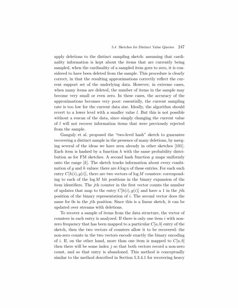
5.4 Sketches for Distinct Value Queries 247
apply deletions to the distinct sampling sketch: assuming that cardi-nality information is kept about the items that are currently beingsampled, when the cardinality of a sampled item goes to zero, it is con-sidered to have been deleted from the sample. This procedure is clearlycorrect, in that the resulting approximations correctly reflect the cur-rent support set of the underlying data. However, in extreme cases,when many items are deleted, the number of items in the sample maybecome very small or even zero. In these cases, the accuracy of theapproximations becomes very poor: essentially, the current samplingrate is too low for the current data size. Ideally, the algorithm shouldrevert to a lower level with a smaller value l. But this is not possiblewithout a rescan of the data, since simply changing the current valueof l will not recover information items that were previously rejectedfrom the sample.
Ganguly et al. proposed the “two-level hash” sketch to guaranteerecovering a distinct sample in the presence of many deletions, by merg-ing several of the ideas we have seen already in other sketches [101].Each item is hashed by a function h with the same probability distri-bution as for FM sketches. A second hash function g maps uniformlyonto the range [k]. The sketch tracks information about every combi-nation of g and h values: there are k logn of these entries. For each suchentry C[h(i),g(i)], there are two vectors of logM counters: correspond-ing to each of the logM bit positions in the binary expansion of theitem identifiers. The jth counter in the first vector counts the numberof updates that map to the entry C[h(i),g(i)] and have a 1 in the jthposition of the binary representation of i. The second vector does thesame for 0s in the jth position. Since this is a linear sketch, it can beupdated over streams with deletions.
To recover a sample of items from the data structure, the vector ofcounters in each entry is analyzed. If there is only one item i with non-zero frequency that has been mapped to a particular C[a,b] entry of thesketch, then the two vectors of counters allow it to be recovered: thenon-zero counts in the two vectors encode exactly the binary encodingof i. If, on the other hand, more than one item is mapped to C[a,b]then there will be some index j so that both vectors record a non-zerocount, and so that entry is abandoned. This method is conceptuallysimilar to the method described in Section 5.3.4.1 for recovering heavy
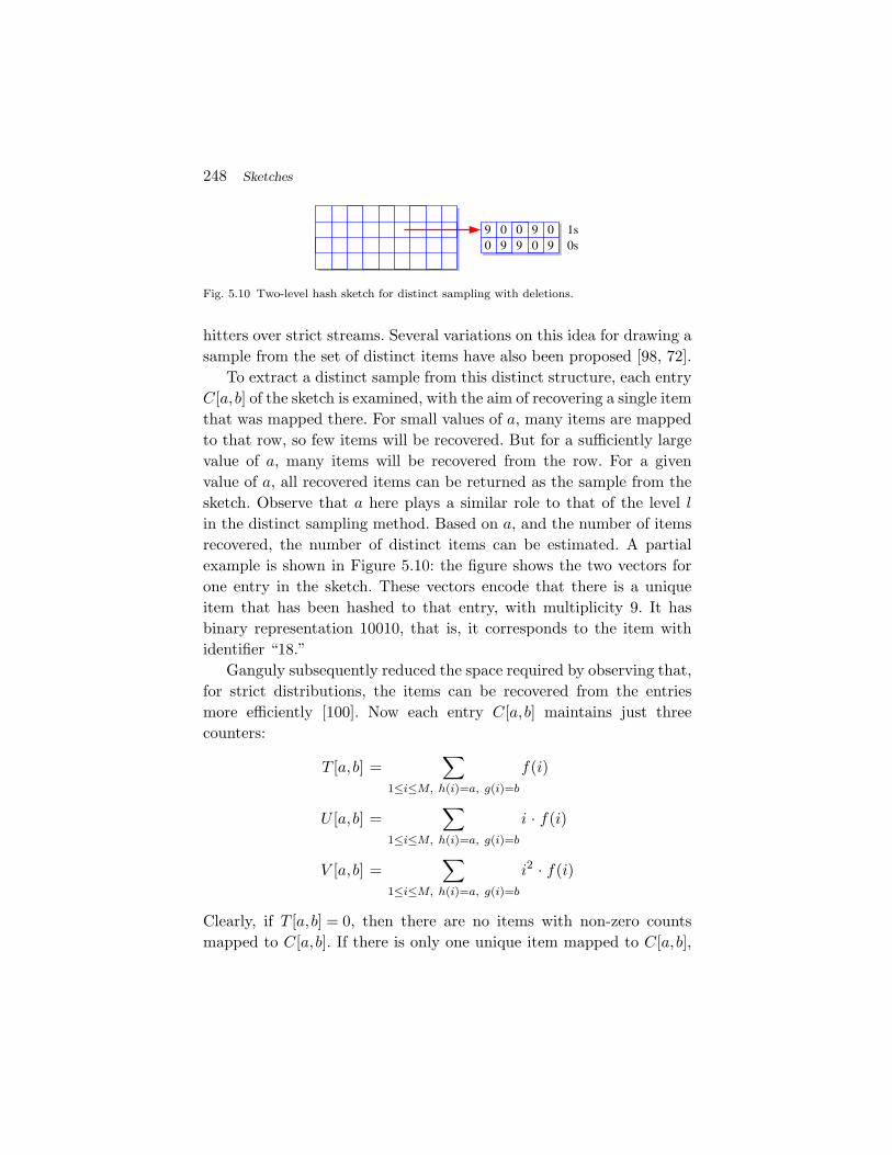
248 Sketches
1s0s
9 0909
0009 9
Fig. 5.10 Two-level hash sketch for distinct sampling with deletions.
hitters over strict streams. Several variations on this idea for drawing asample from the set of distinct items have also been proposed [98, 72].
To extract a distinct sample from this distinct structure, each entryC[a,b] of the sketch is examined, with the aim of recovering a single itemthat was mapped there. For small values of a, many items are mappedto that row, so few items will be recovered. But for a sufficiently largevalue of a, many items will be recovered from the row. For a givenvalue of a, all recovered items can be returned as the sample from thesketch. Observe that a here plays a similar role to that of the level lin the distinct sampling method. Based on a, and the number of itemsrecovered, the number of distinct items can be estimated. A partialexample is shown in Figure 5.10: the figure shows the two vectors forone entry in the sketch. These vectors encode that there is a uniqueitem that has been hashed to that entry, with multiplicity 9. It hasbinary representation 10010, that is, it corresponds to the item withidentifier “18.”
Ganguly subsequently reduced the space required by observing that,for strict distributions, the items can be recovered from the entriesmore efficiently [100]. Now each entry C[a,b] maintains just threecounters:
T [a,b] =∑
1≤i≤M, h(i)=a, g(i)=b
f(i)
U [a,b] =∑
1≤i≤M, h(i)=a, g(i)=b
i · f(i)
V [a,b] =∑
1≤i≤M, h(i)=a, g(i)=b
i2 · f(i)
Clearly, if T [a,b] = 0, then there are no items with non-zero countsmapped to C[a,b]. If there is only one unique item mapped to C[a,b],
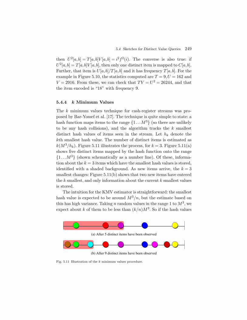
5.4 Sketches for Distinct Value Queries 249
then U2[a,b] = T [a,b]V [a,b] = i2f2(i). The converse is also true: ifU2[a,b] = T [a,b]V [a,b], then only one distinct item is mapped to C[a,b].Further, that item is U [a,b]/T [a,b] and it has frequency T [a,b]. For theexample in Figure 5.10, the statistics computed are T = 9,U = 162 andV = 2916. From these, we can check that TV = U2 = 26244, and thatthe item encoded is “18” with frequency 9.
5.4.4 k Minimum Values
The k minimum values technique for cash-register streams was pro-posed by Bar-Yossef et al. [17]. The technique is quite simple to state: ahash function maps items to the range 1 . . .M3 (so there are unlikelyto be any hash collisions), and the algorithm tracks the k smallestdistinct hash values of items seen in the stream. Let hk denote thekth smallest hash value. The number of distinct items is estimated ask(M3/hk). Figure 5.11 illustrates the process, for k = 3. Figure 5.11(a)shows five distinct items mapped by the hash function onto the range1 . . .M3 (shown schematically as a number line). Of these, informa-tion about the k = 3 items which have the smallest hash values is stored,identified with a shaded background. As new items arrive, the k = 3smallest changes: Figure 5.11(b) shows that two new items have enteredthe k smallest, and only information about the current k smallest valuesis stored.
The intuition for the KMV estimator is straightforward: the smallesthash value is expected to be around M3/n, but the estimate based onthis has high variance. Taking n random values in the range 1 toM3, weexpect about k of them to be less than (k/n)M3. So if the hash values
(a) After 5 distinct items have been observed
(b) After 9 distinct items have been observed
Fig. 5.11 Illustration of the k minimum values procedure.
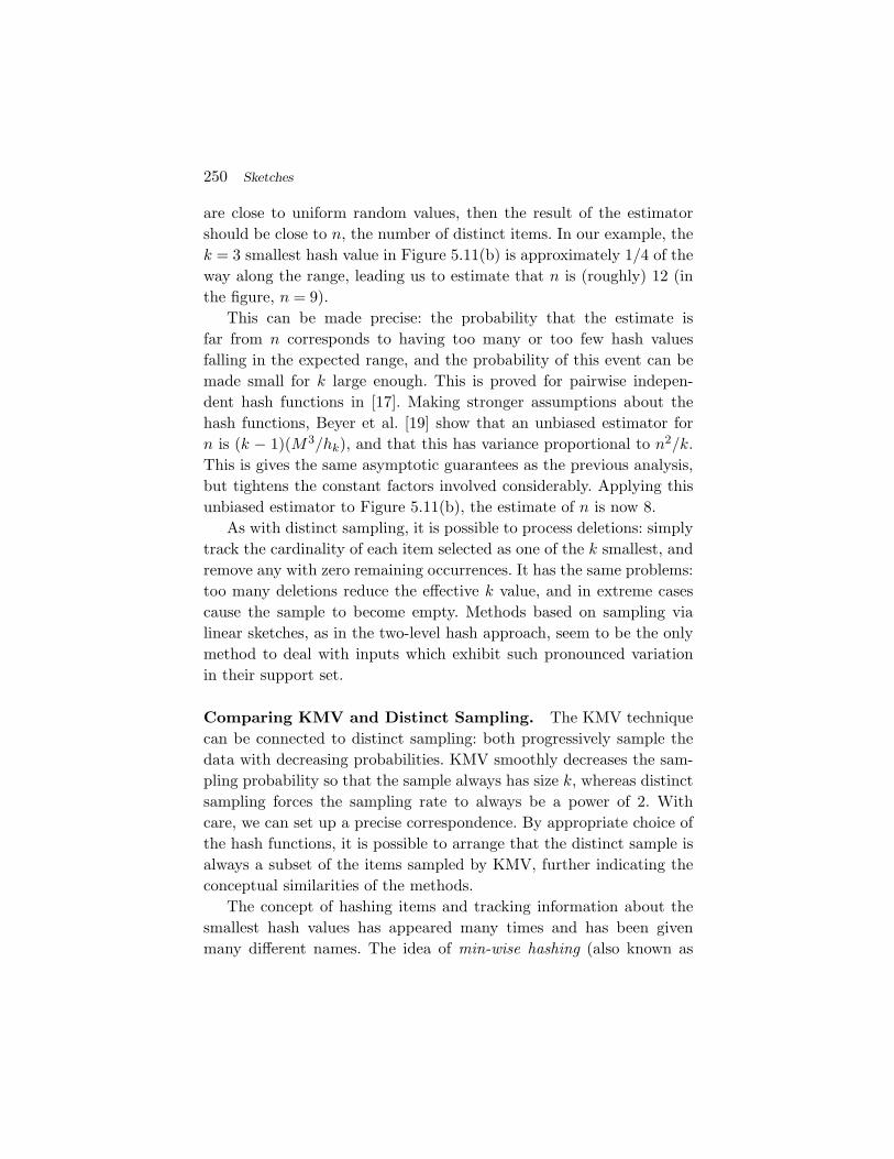
250 Sketches
are close to uniform random values, then the result of the estimatorshould be close to n, the number of distinct items. In our example, thek = 3 smallest hash value in Figure 5.11(b) is approximately 1/4 of theway along the range, leading us to estimate that n is (roughly) 12 (inthe figure, n = 9).
This can be made precise: the probability that the estimate isfar from n corresponds to having too many or too few hash valuesfalling in the expected range, and the probability of this event can bemade small for k large enough. This is proved for pairwise indepen-dent hash functions in [17]. Making stronger assumptions about thehash functions, Beyer et al. [19] show that an unbiased estimator forn is (k − 1)(M3/hk), and that this has variance proportional to n2/k.This is gives the same asymptotic guarantees as the previous analysis,but tightens the constant factors involved considerably. Applying thisunbiased estimator to Figure 5.11(b), the estimate of n is now 8.
As with distinct sampling, it is possible to process deletions: simplytrack the cardinality of each item selected as one of the k smallest, andremove any with zero remaining occurrences. It has the same problems:too many deletions reduce the effective k value, and in extreme casescause the sample to become empty. Methods based on sampling vialinear sketches, as in the two-level hash approach, seem to be the onlymethod to deal with inputs which exhibit such pronounced variationin their support set.
Comparing KMV and Distinct Sampling. The KMV techniquecan be connected to distinct sampling: both progressively sample thedata with decreasing probabilities. KMV smoothly decreases the sam-pling probability so that the sample always has size k, whereas distinctsampling forces the sampling rate to always be a power of 2. Withcare, we can set up a precise correspondence. By appropriate choice ofthe hash functions, it is possible to arrange that the distinct sample isalways a subset of the items sampled by KMV, further indicating theconceptual similarities of the methods.
The concept of hashing items and tracking information about thesmallest hash values has appeared many times and has been givenmany different names. The idea of min-wise hashing (also known as
5.4 Sketches for Distinct Value Queries 251
min-wise independent permutations) is quite similar [25]. There, focushas been on designing compact families of hash functions which havethe desired properties without needing to make strong independenceassumptions. Estimators based on min-wise hashing typically keep k
independent hash functions and take the item with least hash value ineach repetition. They therefore take more time to process each updatecompared to tracking the k minimum values from a single hash func-tion. Cohen and Kaplan’s work on bottom-k sketches generalizes KMVideas to cases when items have weights which are combined with thehash values to determine which items should be retained in the sketch[56]. Beyer et al. [19] have also identified connections between esti-mators for KMV and for priority sampling (which does not considerduplicate elimination) [91].
5.4.5 Approximate Query Processing on SetValued Queries
As remarked above, the data structures which provide us with estimatesfor count distinct queries can also be extended to a variety of other“distinct” queries.
5.4.5.1 Union and Sum Queries
The FM sketch variants are mainly limited to estimating the simplecount-distinct queries initially discussed. However, they (in commonwith all the methods discussed for count distinct estimation) naturallyallow the size of unions to be approximated with the same accuracy.That is, given some arbitrary collection of sets, each of which is sketchedusing the same hash function(s), it is possible to accurately approximatethe cardinality of the union of certain sets. For FM sketches, it sufficesto simply build a new FM sketch where each entry is the bitwise-or ofall the corresponding entries in the sketches of the sets in the union,and apply the estimation procedure to this new sketch. This followsbecause the resulting sketch is exactly that which would have beenobtained had the union of the sets been sketched directly.
Similar results apply for KMV and distinct sampling methods: inthose cases, the procedure just takes the items sampled in the union
252 Sketches
of the sketches as the input to a new sketch (with the same hashfunction), and extracts the estimate from the resulting sketch. Thecorrectness of the resulting sketch follows immediately by observingthat no other items from the input could be present in the sketch ofthe union.
It is also possible to use these sketches to approximate various kindsof “distinct sum” queries. Here, the stream may contain multiple valuesof f(i), and the aim is to compute the sum of the max of each value fora given i. This can be accomplished by replacing each f(i) in the streamwith new items (i,1),(i,2), . . .(i,f(i)). The number of distinct items inthe new stream gives exactly the distinct sum. However, when the f(i)scan be very large, it is quite time consuming to generate and sketch somany new items. Instead, various methods have been suggested to morerapidly compute the results, either via simulating the effect of addingf(i) items quickly [60], or by designing “range efficient” algorithms forcount distinct [249].
5.4.5.2 Distinct Prefix Queries
FM sketches and Distinct samples also allow a limited kind of COUNTDISTINCT with selection queries to be answered accurately over cash-register streams. We refer to these as Distinct Prefix queries: the queryis to approximate the number of distinct items seen whose identifier isless than a certain value. For FM sketches, instead of keeping a single bitin the jth sketch entry, the sketch instead records the smallest identifierof any item that has been hashed to B[j]. Then, given a query value q,the estimation procedure extracts a bitmap from the sketch, by settingthe jth bit to 1 if B[j] < q, and 0 otherwise. The result is exactly theFM sketch that would have been obtained if only those items less than qhad been inserted.
Likewise, for distinct sampling, rather than advancing the levelwhenever the sample becomes full, the sketch instead keeps samplesfor all levels l. At each level l, it retains the k smallest identifiers whichhash to that level or above. Then, given the query q, the estimate isformed by finding the first level l where there are some items greaterthan q, and estimating the answer as r2l, where r is the number of items
5.4 Sketches for Distinct Value Queries 253
at level l that are less than q. Again, it is possible to argue that werecover exactly the information that would have been seen had only theitems less than q arrived. Figure 5.9 shows what would happen whenapplying this for a sample of size 3: the items in the shaded region ateach level would be retained.
These variations are quite natural, and were originally proposed toaddress estimating the number of distinct items seen within a recenttime window [77, 123], which can be interpreted exactly as a DistinctPrefix Query. Note that the results here are quite strong: the approx-imate answers are within relative error of the true answer, since it ispossible to argue that there is enough information to build the synopsisof the selected data.
5.4.5.3 Predicates on Items
The Distinct Prefix can be thought of as applying a predicate to itemsand asking for the number of distinct items satisfying the predicate.More generally, we might want to know how many distinct items passany given predicate at query time. Since KMV and Distinct Samplingboth provide a sample of the distinct items, it is natural to apply thepredicate to the sample, and build an estimate: take the fraction ofitems in the sample which pass the predicate, ρ, and multiply this bythe estimate of the total number of distinct items n. It can be arguedthat this a good estimator for the true answer [121].
However, the error in this estimator is proportional not to the trueanswer, but rather to the accuracy with which n is estimated. Thisshould not be surprising: the same behavior follows for approximatingthe selectivity of a predicate via sampling without the DISTINCT key-word (see Section 2.4.3). For example, if a predicate is highly selective,then it is unlikely that many items passing the predicate happenedto be placed in the sample, and so we do not have a good handle onthe exact selectivity. More precisely, if the sample size is k, then thevariance of the estimator of ρ, the true fraction of items, behaves likeρ/k. So to get a selectivity estimate which is within relative error of ε,the size of the samples k needs to be O(ε−2ρ−1). This technique forestimating the selectivity of predicates has been applied in a variety of
254 Sketches
situations: Frahling et al. use it to estimate quantities over geometricstreams such as the weight of the minimum spanning tree [98].
5.4.5.4 Set Operations
Many queries are based on estimating the cardinality of the results ofperforming operations on a collection of sets. We have already seenthat set unions can be easily answered by sketch data structures forcount distinct. We now show how methods which draw a sample, suchas KMV and distinct sampling, can use the samples from different setsto approximate more complex set-based queries.
Consider first estimating the size of the intersection between twosets. Given sketches that draw k samples uniformly over each relationRA and RB, then these can be combined to find a sample from theunion. However, it is not correct to just take the union of the samples:this would not be a uniform sample if one relation were much largerthan the other. Instead, the correct thing to do is to take the samplescorresponding to the k distinct smallest hash values. This is a uniformsample over the union RA ∪ RB.
We can now view estimating the intersection size as a special caseof estimating the selectivity of a predicate: the predicate selects thoseitems which are present in both RA and RB. Although there is notenough information to evaluate this predicate over arbitrary sets, thereis enough to evaluate it over the sample that has been built: just counthow many items in the union sample are present in the samples of bothrelations. The fraction of matching items, ρ is an unbiased estimatorfor the true fraction, that is,
E[ρ] =|RA ∩ RB||RA ∪ RB| .
So multiplying the estimate for |RA ∪ RB|, the size of the union, givesa good estimator for the intersection size.
The accuracy of this estimator for intersection depends primarilyon the size of the union. This is because, if the intersection is verysmall, it is unlikely that the procedure would sample items from theintersection unless the samples of both relations are large. It is morelikely that it would sample many items from the union of the relations
5.4 Sketches for Distinct Value Queries 255
outside the intersection. The variance of the selectivity estimation canbe shown to scale with |RA ∩ RB|/(|RA ∪ RB|
√k).
The same concept extends to arbitrary set expressions over relationsRA,RB,RC . . .. Again, the estimation procedure takes items with the ksmallest hash values from the union of all the sketches of the relations,and then evaluates the selectivity of the set expression on this sampleas ρ. This can also be viewed as a more complex predicate which can beevaluated exactly on the sampled items. With this view, the variance ofthe estimator can be analyzed in a similar way to before. This techniqueis implicit in the work of Ganguly et al. [101], and is generalized andmade explicit in the work of Beyer et al. [19].
The same idea works for estimating the cardinality of multiset oper-ations such as multiset difference. Here, it is necessary to include thecounts of items in the samples. Operations on the samples are appliedin the natural way: union operations take the sum of counts of sam-pled items, while multiset differences make appropriate subtractionsof counts. The fraction of matching items in the samples is found bycounting those that have non-zero counts after applying the appropri-ate computations on the sample [19].
Certain set operations can also be evaluated using Flajolet–Martinsketch variants. This follows by using certain identities. For example,for sets A and B,
|A ∩ B| = |A| + |B| − |A ∪ B|.
Therefore, since Flajolet–Martin sketches can be combined to approxi-mate the size of the union of sets, the estimates can also yield approx-imations of the intersection size. However, the (absolute) error hereis proportional to |A ∪ B|/√k, which is greater than the error of theestimators derived based on KMV and distinct sampling.
5.4.5.5 Comparison between sketches for DistinctValue Estimation
Analytically, all the estimators proposed for distinct value estimationhave broadly the same performance: as a function of a size parame-ter k, their variance is proportional to 1/
√k. Consequently, they can
256 Sketches
all provide ε relative error using space O(1/ε2 log1/δ). The exact spacerequired is a function of the exact constants in the variance (which areunderstood very well for most methods), and on exactly what infor-mation needs to be retained by the sketch (bitmaps, hash values, orsampled items).
Still, to fully understand which methods are preferable for par-ticular tasks, empirical evaluation is necessary. A recent study byMetwally et al. performed a thorough comparison of algorithms forthe core problem of distinct count estimation [226]. They gave eachmethod the same amount of space for a sketch, and compared theaccuracy and time cost on a networking dataset. Their experimentsshows that methods using bitmaps could be the most accurate —perhaps unsurprising, since it is possible to squeeze in more informa-tion into bitmaps, compared to retaining item identifiers. Indeed, theprovocative conclusion of their study is that one of the earliest, meth-ods, Linear Counting (Section 5.4.1), is preferable to the more com-plex methods that have come since. This is due in part to its speedand accuracy on the data in question, for which approximate cardi-nalities are known in advance. However, in the wider context of AQP,it could be argued that the extra flexibility that arises from having asample of (hashed) items to answer broader classes of queries is moredesirable.
Distinct sampling and KMV methods show an order of magni-tude worse accuracy than bitmap based methods in the experimentsin [226]: this is perhaps to be expected, since the (hashed) item identi-fiers are also at least tens of bits in size. The processing times reportedfor all methods are comparable: approximately a million updates persecond.
However, the conclusion is not the same for queries more complexthan simple distinct counting. Beyer et al. performed experiments com-paring the KMV approach to a version of log-log counting for set oper-ation estimation [19]. They allocated space equivalent to k = 8192 forthe KMV estimator. Across a variety of queries, the KMV approachobtained accuracy of around 2%–3% average relative error, whereasthe log-log method incurred around two to three time as much error

5.5 Other Topics in Sketching 257
in the same space. Beyer et al. also observe that the choice of hashfunctions can empirically affect the quality of estimators, which mayexplain their differing behavior seen across experimental studies.
5.4.6 Lower Bounds
Ultimately, all the methods for count-distinct estimation take O(1/ε2)space to give ε relative accuracy (where O notation hides logarithmicdependency on other factors like m). In fact, this dependency has beenshown to be tight, in that no method can have a lower dependency on ε.Indyk and Woodruff demonstrated this by analyzing the complexity ofan abstract problem called “Gap-Hamming” [175]. They showed thatapproximating Count-Distinct with sufficient accuracy can solve Gap-Hamming, and that Gap-Hamming has a high complexity, implying thelower bound. Subsequently, Jayram et al. considerably simplified thehardness proof for Gap-Hamming [187].
5.5 Other Topics in Sketching
In this section, we briefly survey some perspectives on sketch-basedmethods for AQP.
5.5.1 Sketches for Building Other Summaries
One demonstration of the flexibility of sketch-based methods is the factthat there has been considerable work on using sketches to build dif-ferent types of summary. In fact, for all the other major summariesin AQP — samples, histograms, and wavelets — there are methodsto extract such a summary from sketch information. This can be use-ful when users are familiar with the semantics of such summaries, orhave well-established methods for visualizing and processing such sum-maries.
Sketches for Sampling. The methods discussed in Sections 5.4.3and 5.4.4 produce samples from the set of distinct items in a relation ina sketch-like manner. Further, the two-level hash structure described inSection 5.4.3.1 gives a linear sketch structure to achieve this. However,
258 Sketches
there are fewer results for using sketches to sample from the raw fre-quency distribution, e.g. to include item i in the sample with probabilityf(i)/N . Only recently have their been schemes to implement so-calledLp sampling, which aim to draw i with probability f(i)/
∑i |f(i)|p
[196, 231]. These methods guarantee always drawing a sample of sizeO(k) over turnstile streams, but the sampling probabilities only approx-imate the desired distribution within a (1 ± ε) factor.
Sketches for Histograms. Gilbert et al. [127] used sketches to buildhistogram representations of data. The sketch needed is similar to othersketch constructions, but augmented to allow range sums to be com-puted rapidly. This is needed when trying to compute the impact ofpicking a particular bucket to be part of the histogram. Based on adynamic programming method for constructing the histogram, the finalresult guarantees an approximation to the optimal histogram undera given error metric (L1 or L2 error). Thaper et al. used sketchesto find histograms of multi-dimensional data, based on a greedysearch [278].
Sketches for Wavelets. There has been much interest in buildingsketches to recover wavelet representations. Gilbert et al. [128] intro-duce the problem. They observe that the problem can be solved exactlywhen the data is presented in the timeseries model (i.e., sorted andaggregated), since there are only O(logN) coefficients that “straddle”any index in the data, which can be tracked to find the largest coef-ficients. They also show that, in the cash-register model, any waveletcoefficient can be found via appropriate range sum computations, andproposed using sketches to estimate the largest coefficients. It was sub-sequently suggested that it may be more efficient to compute the wave-let transform “on the fly”: since the HWT is a linear transform, it ispossible to build a sketch of the coefficients, without materializing thecoefficient vector explicitly [64]. The problem is then reduced to findingthe heavy hitters under the F2 measure, that is, to find all items whosefrequency exceeds φF2 for some fraction φ. This is solved by a variantof the AMS sketch with multiple levels of hashing and grouping. Moredetails on this technique are provided in Section 4.6.1.
5.5 Other Topics in Sketching 259
5.5.2 Other Sketch Methods
The ideas within sketches have been used to build sketches for differentqueries. Many common ideas are present: use of limited-independencehash functions, hierarchical decompositions of ranges and so on. Someadditional ideas are also commonly used: picking random values fromappropriate distributions, combining multiple sketch methods together,and use of PRNGs to minimize the space needed. We briefly surveysome of these, and see how they are connected to the methods we havediscussed already.
5.5.2.1 Sketches for Lp norms and Entropy
The F2 estimation problem is a special case of a more general classof functions over sketches, the Lp norms. For a general distribution offrequencies, the Lp norm is defined as
Lp =
(M∑i=1
|f(i)|p)1/p
.
The AMS sketch therefore accurately approximates the L2 norm.Within the streaming community, there is considerable interest in beingable to provide accurate approximations of other Lp norms. As p < 1approaches 0, the norm approaches the “Hamming norm,” that is, thenumber of non-zero entries in the vector. Computations based on suchnorms (e.g., clustering) vary whether the emphasis is on the magnitudeor the number of differences between vectors. Estimating Lp norms forp = 1 ± δ for small values of δ has also been instrumental in some meth-ods for estimating entropy [161].
A general technique for 0 < p ≤ 2 is based on sketches that use stabledistributions. Each entry in the sketch is formed as the inner productof the frequency distribution with a vector of entries each drawn ran-domly from a stable distribution. A stable distribution is a statisticaldistribution that has a stability parameter α. They have the propertythat sums of multiples of stable distributions are also distributed asa stable distribution — this can be viewed as a generalization of theCentral Limit Theorem, and indeed the normal distribution is stablewith parameter α = 2 [299].

260 Sketches
By fixing the stability parameter of all distributions to be α = p,the resulting sketch entry is distributed as a stable distribution scaledby Lp. Taking the median of all the sketch entries was shown by Indykto be an accurate approximation of Lp [174]. To make this a smallspace approximation, the entries of the sketch matrix are not stored.Instead, they are generated on demand using a pseudo-random numbergenerator so that the entry is the same every time it is accessed. Suchsketches have been used in a variety of settings, such as for approxi-mately clustering large data under Lp distance [66].
There has also been a lot of work on approximating Lp for p > 2.Here, strong lower bounds indicate that the size of the sketch needed isat least Ω(M1−2/p) [292]. Various solutions have been proposed whichachieve this space cost (up to logarithmic factors) [21, 176]. The HSS(for Hierarchical Sampling from Sketches) is based on randomly select-ing subsets of items via hash functions, and then extracting the heavyhitters from these subsets of items using Count Sketches. The infor-mation about the approximate frequencies of the recovered items isthen combined to form an estimate of the overall Lp norm of the fullfrequency distribution. Owing to the lower bounds, the resulting datastructure can be very large.
The ideas within the HSS sketch have also been applied to approxi-mate the empirical entropy of the frequency distribution. That is, toestimate
H =M∑i=1
f(i)N
log(N
f(i)
)
However, tighter error bounds result from using methods based on sam-pling and tracking information about the sampled elements [40], or byvia interpolating estimates from sketches for Lp norms [8, 161].
5.5.2.2 Combinations of Sketches
We have previously discussed several examples of combining differ-ent types of sketches: take, for example, the use of fingerprints withinFlajolet–Martin sketches to track count-distinct over general frequencydistributions (Section 5.4.2.1). For linear sketches in particular, it is
5.5 Other Topics in Sketching 261
often possible to combine multiple sketches via nesting to answer morecomplex queries.
A particular example arises when we wish to make sketches “dupli-cate resilient.” The “distinct heavy hitters” problem arises when theinput consists of a sequence of tuples (i, j), and the frequency of i in themultiset input D is now defined as d(i) = |j : (i, j) ∈ D|, the numberof distinct js that i occurs with. This models a variety of problems,particularly ones which occur in networking settings [282]. One solu-tion combines the Count-Min Sketch with Flajolet–Martin sketches:instead of keeping a counter of the items mapped there, each entry ofthe Count-Min sketch can keep the Flajolet–Martin sketch summaryof the items [59]. This sketch allows the estimation of d(i) for a given iby applying the Count-Min estimation procedure to the estimates fromeach Flajolet–Martin sketch in the data structure. A careful analysis isneeded to study the space-accuracy tradeoff of the resulting “CM-FMsketch”.
Several other combinations of sketches have been studied. Ingeneral, it is not possible to form arbitrary combinations of sketches:instead, a more cautious approach is needed, with the new estimatorsrequiring new analysis on a case-by-case basis.
5.5.2.3 Deterministic Sketches
Most of the sketches we have seen so far involve randomization. Apartfrom trivial sketches (for sum, count, average etc.), the accuracy guar-antees hold only with some probability over the random choice of hashfunctions. It is natural to ask whether the more complex queries trulyrequire randomization to approximate. It turns out that this is notalways the case: there exist sketches for certain queries which do notrequire randomness. However, they require substantially more spaceand time to create than their randomized equivalents, so they may beprimarily of academic interest.
The CR-Precis data structure as analyzed by Ganguly andMajumder [104] (first suggested by Gasieniec and Muthukrishnan [236])is similar to the Count-Min sketch, but determines which items to counttogether in each entry based on residues modulo prime numbers. The
262 Sketches
accuracy guarantees for point queries are shown based on the Chi-nese Remainder theorem, hence the CR in the name. The sketch keepsd = O(1/ε logM) rows, but the rows are of different lengths. The jthrow corresponds to the jth prime number that is greater than k (k is aparameter of the data structure), pj . The th entry in the jth row con-tains the sum of all frequencies of items whose identifier is mod pj .That is, the entries of the sketch C are given by
C[j,] =∑
1≤i≤M, i mod pj=
f(i).
Due to the choice of parameters of the sketch, no pair of items i and i′
can collide in every row (by the Chinese Remainder theorem). In fact,any pair can collide in at most logkM rows. Point queries can beanswered as in the Count-Min case, by extracting the count of everyentry where i is placed, and taking the minimum of these. Using thebound on collisions, the error in the estimate is at most N(logkM)/d.Choosing d to be large enough makes this error as small as desired.To guarantee εN error, the total space needed grows proportional to1/ε2 — in comparison to the 1/ε growth of the (randomized) Count-Min sketch. Given this deterministic bound for point queries, deter-ministic results for heavy hitters, range-queries and quantiles all fol-low using the same reductions as in Section 5.3.4. However, for otherqueries, no deterministic sketch is possible: it is known that randomnessis required to estimate the number of distinct items and to estimate F2
in small space [7, 166].

6Conclusions and Future Research Directions
In this final chapter, we conclude our survey by looking more broadlyacross synopses for massive data. We draw comparisons across the fourclasses of synopses surveyed, and summarize the strengths and weak-nesses of existing approaches. We also discuss the role of AQP viasynopses in existing and future systems. Lastly, we look to the futureand discuss the prospects for broader adoption of AQP ideas, as wellas new research directions.
6.1 Comparison Across Different Methods
So far, we have primarily considered each type of synopsis in isolation.We now recap the methods, and identify their strengths and weaknessesfor different aspects of AQP problems.
Sampling Pros and Cons. The chief strength of sampling-basedapproximation methods is that they are very flexible with regard to thequeries that can be answered: they offer the generic solution of simplyevaluating the query over sampled data, instead of over the full orig-inal data. Sampling also adapts very naturally to higher dimensionaldata (since the sample itself is essentially “dimension agnostic”). This
263
264 Conclusions and Future Research Directions
flexibility makes sample synopses ideal for general-purpose querying,when the set of queries is not fully known in advance. The accuracyof a sampling-based estimate of a query answer will be highly depen-dent on the query being evaluated, but such estimates usually comewith query-specific error bounds, thereby permitting assessment of theaccuracy. This powerful feature of sampling — as well as the ability toimprove estimation accuracy on the fly by simply increasing the numberof samples — ties in well with the notion of online aggregation, wherethe error bounds narrow in real time as more and more samples areobtained. Note that samples are the only one of the synopses discussedhere that can easily be incrementally adjusted to improve estimationaccuracy.
Sampling is well-suited for detecting “broad patterns” within thedata, that is, features that are likely to be present in any subsetof the data. It is much less suited to problems when the object ofinterest is a rare event (a “needle in a haystack”). Sampling doespoorly on applications such as fraud or anomaly detection, wherethe unusual activity is unlikely to be included in any sample. Forthe same underlying reasons, sampling gives lower accuracy when thedata is highly variable. It can do badly at estimating distinct counts,because values with a small number of duplicates are easily missed whensampling.
Sampling becomes more complex when the data is subject to manyinsertions and deletions, requiring more complex incremental samplemaintenance techniques to ensure that the stored data remains a uni-form sample of the underlying data. Lastly, a more pragmatic weak-ness of sampling is that interpreting the guarantees from sampling canrequire a degree of statistical knowledge and experience. It may there-fore be inappropriate to present the raw guarantees from a samplingestimate to a statistically unsophisticated user.
Histograms Pros and Cons. A main advantage of histograms isthat they are relatively simple to interpret, which makes it easierfor system builders to construct and interrogate histograms. In par-ticular, the simplicity of dividing up domains into ranges and keep-ing basic statistics like counts has led to the relative popularity of

6.1 Comparison Across Different Methods 265
histograms within query optimizers and within packages for businessintelligence, data analysis, and data visualization. The large amount ofresearch dedicated to histograms has shown how they can be used fora variety of estimation purposes — although further work is needed toidentify the full range of applicability. For various classes of queries,such as point and range queries, the theory supporting these querieshas been quite well-developed, so that there are strong notions ofoptimality. Advanced types of histogram are also sufficiently power-ful to very accurately capture the structure of a data-value frequencydistribution.
As with most summary structures other than samples, histogramsdo not adapt well to higher dimensional data. In theory, to give gooderror bounds their size must scale exponentially with the numberof dimensions. This problem occurs in practice not only for simplebucket constructions, which track buckets that are the cross-productof one-dimensional divisions, but also for more complex hierarchicalconstructions.
Also, as with synopses other than samples, there has been muchmore work devoted to quantifying the average or maximum error over abroad class of queries than in providing error estimates that are specificto the query posed by the user. Providing such feedback is crucial whenmaking decisions based on approximate answers to queries.
Building accurate histograms requires deciding which bucket bound-aries to adopt, and computing statistics about each bucket. Naively,this requires at least two passes over the data. This approach does notadapt well when the data is dynamic and shifting. Techniques basedon sketches can help in this case, but the overhead is quite high: thespace for the sketches to construct the histograms is much larger thanthe size of the histograms themselves. It is often unclear in such sce-narios whether direct use of the sketch would be simpler and moreefficient.
Lastly, many histogram techniques have several parameters whichhave to be set a priori, such as the number of buckets, statistics tokeep within each bucket, and other parameters that determine whento split or merge buckets. Setting these parameters can be off-putting,and wrong choices can lead to summaries with poor performance.
266 Conclusions and Future Research Directions
Wavelets Pros and Cons. Wavelets share with histograms thenotion of storing simple statistics (primarily counts) of collections ofitems from the input domain. Whereas histograms excel at capturingthe local structure of contiguous data values, wavelets are particularlywell suited to capturing non-local structures.
The linearity of the basic Haar transform makes them moreamenable than histograms to maintenance under dynamic data,although it is still non-trivial to maintain wavelet coefficients underarbitrary update patterns.
As with histograms, extending wavelets to higher dimensions bringsseveral challenges. There are multiple definitions of how to construct amulti-dimensional wavelet, and in practice it seems that a large numberof coefficients must be retained to guarantee accurate reconstruction ofthe data distribution. Also, as with histograms, techniques for providingquery-specific error estimates are not well developed.
Sketches Pros and Cons. Sketches were first proposed in the con-text of high speed streams of data, and consequently the most refinedimplementations of sketches are very efficient to process updates to thedata. The algorithms themselves are of necessity quite simple, to enablehigh throughput implementations; the complexity is mostly mathemat-ical in nature, and lies in the analysis of estimation accuracy. Sketchingalgorithms rely on hash functions with certain mathematical propertiesto give their guarantees, but these hash functions are relatively simpleand fast in practice, with reference implementations widely available.
The main limitation of sketching techniques — especially in contrastto the general-purpose sampling paradigm — is that each sketch tendsto be focused on answering a single type of query. A reasonable range ofquery types can be answered via sketching, but the techniques do notseem to extend well to more complex queries which combine multiplesub-queries. Ongoing research aims to broaden the set of queries thatcan be answered by sketching, but general purpose techniques that areclosed for a large class seem out of reach. An additional drawback isthat sketches have a number of parameters that affect their accuracyand probability of failure, and these parameters may be unintuitive insome cases.
6.2 Approximate Query Processing in Systems 267
6.2 Approximate Query Processing in Systems
Several research prototype systems have placed synopses front andcenter, and have typically focused on sampling-based methods. Theseinclude Aqua (for Approximate Query Answering system), developedat Bell Labs in the 1990s [2, 3]; CONTROL (Continuous Output andNavigation Technology with Refinement On-Line), a project at UCBerkeley in the 1990s focusing on the use of sampling to providea user with online, continually-refining answers to queries of varioustypes [11, 168, 259]; and DBO (DataBase Online), which aimed toachieve performance similar to traditional DBMS systems while refin-ing an approximate answer with probabilistic error bounds.
With respect to real-world systems, acceptance of synopses has beenslow at best, but there have been a few successes. The notion of AQPwould doubtless have been anathema to the developers of the earliestcommercial database systems in the 1960s and 1970s. The initial focusof such systems was transaction processing, and approximations to acustomer’s bank balance or a store’s inventory level are unacceptable.Several key developments and trends since that time, however, havemade AQP an essential component of under-the-hood query processingtechnology, and are paving the way for wider acceptance of approximateanswering of user queries.
Perhaps the earliest use of approximation technology in databasemanagement systems (DBMSs) resulted from the development ofrelational DBMSs, starting in the mid 1970s. The cost-based queryoptimizers in these systems needed to quickly evaluate the size of vari-ous intermediate query results, in order to cost competing query plans.These result sizes, called “cardinalities,” could be viewed as the answersto a set of SQL COUNT queries. Importantly, cardinalities need tobe determined only to a degree of accuracy sufficient for query-plancomparison. As a result, quick approximation techniques based on his-tograms, sampling, and distinct-count sketching rapidly found theirway into query optimizers, and remain an important application ofsynopses. Initial estimation schemes were rather crude, and usuallyassumed that the frequency distribution was uniform, so that any twodistinct values had the same frequency. However, over time, systems
268 Conclusions and Future Research Directions
began to employ histograms and distinct-count sketches to approxi-mate the distribution of values within an attribute of a relation moreprecisely, leading to better cost estimates in the presence of highly non-uniform attribute-value distributions. More recently, optimizers havebegun to use sampling to reduce the I/O and CPU costs of computingoptimizer statistics. Current systems supplement these techniques withsummaries that are very specific to the queries being computed, suchas actual measurements of the sizes of partial query results; these lattertechniques are most effective when the data does not change too rapidly.See [148] for a recent discussion of statistics and query optimizers.
With respect to approximate answers for user queries, samplinghas clearly made the greatest inroads into commercial systems. Indeed,the latest version of the SQL standard, which has been implementedin virtually all current commercial relational database systems, allowsspecification of sampling queries. For example, the query
SELECT SUM SALES / 0.02
FROM transactions AS t TABLESAMPLE BERNOULLI(2)
WHERE t.product = ‘widget‘
GROUP BY t.city;
estimates the total sales of widgets in each city represented in thetransactions table by means of a 2% Bernoulli sample of the rowsof the table.
With the development of data mining technology in the early 1990s,enterprises became increasingly aware that their large stores of oper-ational data were an untapped source of valuable information forstrategic planning and decision support. The emphasis in this settingwas often discovery of interesting patterns in large amounts of data,a problem ideally suited to AQP techniques. Sampling-based methodswere commonly used for this purpose. For example, a large retailermight generate a column of pseudo-random numbers, sort the data onthis column, and then run a query of interest on the first 1% of the rowsof the sorted table to get a quick, rough estimate of the exact queryanswer obtained by processing all of the records. Similarly, as largescientific datasets were increasingly stored on DBMSs, the need forquick pattern discovery further motivated interest in AQP, especially
6.3 Challenges and Future Directions for Synopses 269
sampling. Though flexible and fast, sampling procedures could notalways handle certain types of queries well, such as COUNT DISTINCTqueries and highly selective join queries. For this reason, much researchwas devoted to alternative schemes that take a complete pass throughthe data, but have small memory requirements.
One objection to bringing synopses fully into commercial data man-agement systems is that this would require a major re-architectingof the existing system. However, this is no barrier for new systemsdesigned to handle new data scenarios. One particular example thathas arisen since the start of the 21st century is in Data Stream Man-agement Systems (DSMS). These systems are designed to handle datawhich arrives online as a stream, such as network data or financialtransactions. Such data can arrive in large quantities and at high speed,which motivates the adoption of approximate methods to answer com-plex aggregate queries, in addition to exact methods for simpler orhighly selective queries.
Systems such as Gigascope (a network diagnosis and debugging toolused at AT&T [74]) and StreamInsight (from Microsoft [227]) allowUser Defined Aggregate Functions (UDAFs) and User Defined Opera-tors (UDOPs) to be called by queries. UDAFs and UDOPs are specifiedin the form of source code, which is then compiled into queries. In thiscontext, there has been much effort to build libraries of implementa-tions of synopses, such as sketch and sampling methods [67]. Thesesystems demonstrate that there is a concrete need for AQP in situ-ations when exact query processing is not scalable, and approximateanswers are acceptable.
6.3 Challenges and Future Directions for Synopses
Given that, outside of sampling, historical applications of synopses havebeen either behind the scenes or in niche/prototype systems, it is rea-sonable to ask what are the prospects for broader usage of the syn-opses described in this survey. Can we expect to see greater use ofapproximate answers in information management, or will they remaina minority interest to the majority goal of providing exact answers? Weconclude by examining some of the obstacles to adoption of synopses
270 Conclusions and Future Research Directions
for AQP. These obstacles can also be viewed as a spur to innovation,both in educating information-system designers and users, and in over-coming the limitations of current AQP technology.
6.3.1 Understanding Approximation
A key challenge is how to present results to the end user. Userspose a query knowing that there exists an exact answer; they maystruggle to understand an answer which may be presented as a confi-dence interval. Somehow, the transition from an “exact” answer (overdata which almost certainly contains minor errors and omissions) toan “approximate” one introduces more uncertainty than the typi-cal user is currently able to accept. Part of the challenge here is ineducation and presentation: how to educate users to accept uncer-tainty in their query results, and how to present these uncertain-ties as palatably and intuitively as possible. The stochastic-simulationcommunity has recently discussed issues related to presentation ofuncertain results [290]. The idea is to describe uncertainty at a levelthat matches a user’s sophistication, without being misleading at anypoint; such research may also be helpful in the AQP setting. Simi-larly, research in human-computer interaction and collaborative dataanalysis could be useful in communicating uncertainty in a visual man-ner, as well as making users more comfortable with approximate queryanswers.
In some sense, users are already comfortable with approximations;they just fail to completely realize this. For example, opinion polls arewidely used, though there is always a statistical margin of error (usu-ally described either with mentioning this error at all or using roughlanguage such as “correct to within an accuracy of ± three percent-age points.”) Weather forecasts are in their nature approximate, anddriving directions, which apparently promise the shortest route, morecommonly compute merely a “shortish” route, to make the computa-tion more scalable. Search engines that say “there are about 10 millionanswers” are approximating wildly. In all of these cases, people can livewith the uncertainty; the challenge is to make them aware of what theyare already doing.
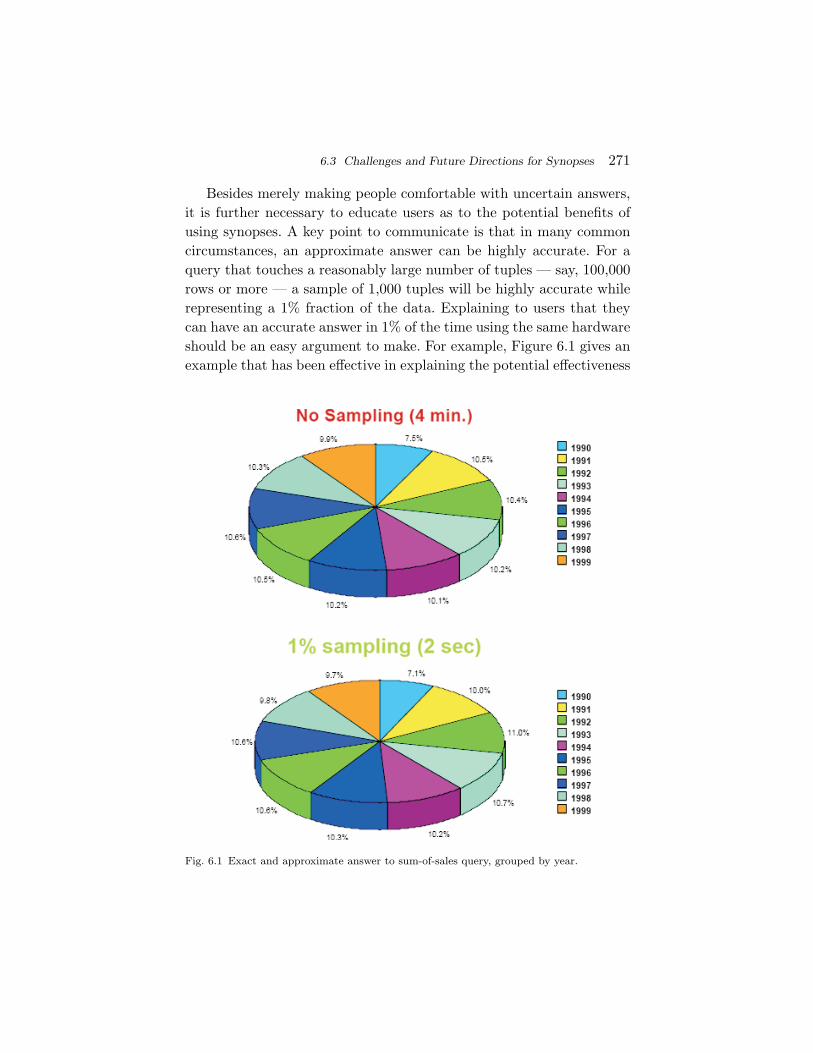
6.3 Challenges and Future Directions for Synopses 271
Besides merely making people comfortable with uncertain answers,it is further necessary to educate users as to the potential benefits ofusing synopses. A key point to communicate is that in many commoncircumstances, an approximate answer can be highly accurate. For aquery that touches a reasonably large number of tuples — say, 100,000rows or more — a sample of 1,000 tuples will be highly accurate whilerepresenting a 1% fraction of the data. Explaining to users that theycan have an accurate answer in 1% of the time using the same hardwareshould be an easy argument to make. For example, Figure 6.1 gives anexample that has been effective in explaining the potential effectiveness
Fig. 6.1 Exact and approximate answer to sum-of-sales query, grouped by year.
272 Conclusions and Future Research Directions
of AQP; the figure has been adapted from an article on database sam-pling written for business users of DB2 [145]. Visual comparison ofthe two pie charts (and their corresponding computation times) showshow the approximate result still manages to effectively convey the “bigpicture” at a fraction of the computational cost.
6.3.2 Parallelism
The alternative to approximation is to continue building bigger sys-tems. Popular architecture paradigms are trending towards increasedparallelism and distributed processing (as per the MapReduce/Hadoopmodel) which still fixes exact solutions as the default goal. Still, it haslong been observed that data volumes are growing at faster rates thancomputing power [291], and this trend continues. This suggests thatapproximation is increasingly a necessary tool to adopt in order tofacilitate interactive querying. There has been some initial work oncombining approximate processing techniques with MapReduce archi-tectures [58, 248], and this seems to be a promising direction for futureresearch.
Moreover, as mentioned in the introduction, the advent of Cloudcomputing and green computing will likely result in users become moresensitive to the dollar and energy costs of executing a given query.(Given the rising cost of energy, these latter costs might often serve as aproxy for dollar costs.) In this setting, synopses provide an increasinglyimportant tool for letting a user obtain useful results at a lower cost.Thus an ongoing technical challenge is to extend synopsis techniquesto work in a parallel and distributed setting; some work along theselines has already been described, and new methods are being activelydeveloped; see, for example, Cormode et al. [73].
6.3.3 Incorporation into Commercial Systems
Objections to using synopses include the fact that full integrationinto existing data management systems may require significant re-architecting, possibly negating the investment of many hundreds ifnot thousands of person-years of effort to build the current sys-tems. In recent years, however, there has been a revolution in DBMS
6.3 Challenges and Future Directions for Synopses 273
architecture, driven by cloud computing [1], multicore processors [261],and scientific data applications [277]. There is a unique opportunity,therefore, to build AQP techniques into such systems from the out-set. This comprehensive integration could focus not only on deliveryof approximate answers to end users, but also incorporation of syn-opses into the processing engine. Hence, though it may be difficult tobuild new AQP techniques into existing commercial query optimizers,such synopses might be useful for new query optimization tasks such asload balancing in MapReduce systems. As discussed previously, newerapplications such as network monitoring, sensor systems — that is, set-tings in which stringent CPU and memory constraints are prevalent —are relatively accepting to the use of synopses. Finally, another pathfor incorporating AQP techniques into emerging systems is throughthe development of analytical libraries, such as in the ongoing MADlibproject [220].
6.3.4 Uncertain Data
This article has focused on approximate answers to queries that are exe-cuted over exact, deterministic data and hence have an exact answer(though perhaps unknown and expensive to compute). In recent years,however, there has been a surge of activity related to query processingover uncertain data [75, 267]. This uptick in interest corresponds to anincreasing awareness that most data is not, in fact, exact — uncertaintyarises in numerous ways, including information extraction from text,data integration, noisy sensor readings, and deliberate anonymizationto preserve privacy. These developments have two important implica-tions for AQP.
First, acknowledging that one’s data is uncertain leads naturally to ageneral willingness to accept an quick approximate query answers. Thatis, it does not make much sense to spend enormous effort computingan exact answer if the data itself does not justify such high precision.There has been increasing, fruitful interaction between the traditionalstochastic analysis, stochastic optimization, and statistics communitieson one hand, and the database community on the other. This con-vergence has been accelerated by the embrace of advanced statistical
274 Conclusions and Future Research Directions
methods by the search community. As a consequence, it is plausible thatthe general database user community will feel increasingly comfortablewith non-exact data processing and AQP in particular.
Second, a new technical challenge arises. What should synopses looklike in the context of a probabilistic database? What is the interplaybetween data uncertainty and query approximation? There has beenalmost no research on this topic to date.
6.3.5 Other Technical Challenges
As can be seen from our survey, many technical challenges remain. Per-haps the chief of these, at least for the non-sampling based synopses,is to accurately represent high dimensional distributions. A promis-ing future direction is to describe the broad dependencies via high-level statistical models, such as Bayesian and Markov networks, andthen describe low-dimensional correlations via the synopses we havedescribed.
Another challenge is to extend synopses to other kinds of data. Forexample, researchers have been exploring concise graph-based synopsesfor XML data [215, 252, 253]. This work has also inspired a purelygraph-based approach to approximating relational data [274].
Besides improving on the synopses themselves, an important chal-lenge is to find higher-level methods of working with synopses. Thegoal here is to allow complex query plans to be translated to operateentirely in the AQP domain rather than on the exact data.
A related problem is to gain a better theoretical understanding ofthe applicability, accuracy, and performance of synopses. For example,can one prove that a given class of synopses is complete and consis-tent (in some appropriate sense) for a given class of queries? Can theinformation-theoretic perspective in [204] be extended to other syn-opses and query classes? It is also possible that approximation theoryin its full force [53] might provide additional theoretical insights.

Acknowledgments
The work of Minos Garofalakis was partially supported by the Euro-pean Commission under FP7-FET Open (Future and Emerging Tech-nologies) ICT-2009.8.0 grant no. 255957 (LIFT).
275
References
[1] A. Abouzeid, K. Bajda-Pawlikowski, D. J. Abadi, A. Rasin, and A. Silber-schatz, “HadoopDB: An architectural hybrid of MapReduce and DBMS tech-nologies for analytical workloads,” PVLDB, vol. 2, no. 1, pp. 922–933, 2009.
[2] S. Acharya, P. B. Gibbons, and V. Poosala, “Aqua: A fast decision supportsystem using approximate query answers,” in International Conference onVery Large Data Bases, 1999.
[3] S. Acharya, P. B. Gibbons, V. Poosala, and S. Ramaswamy, “The Aquaapproximate query answering system,” in ACM SIGMOD International Con-ference on Management of Data, 1999.
[4] S. Acharya, P. B. Gibbons, V. Poosala, and S. Ramaswamy, “Join synopses forapproximate query answering,” in Proceedings of the ACM SIGMOD Inter-national Conference on Management of Data, pp. 275–286, New York, NY,USA, 1999.
[5] C. C. Aggarwal, “On biased reservoir sampling in the presence of streamevolution,” in Proceedings of the International Conference on Very Large DataBases, pp. 607–618, 2006.
[6] N. Alon, P. Gibbons, Y. Matias, and M. Szegedy, “Tracking join and self-joinsizes in limited storage,” in ACM Principles of Database Systems, 1999.
[7] N. Alon, Y. Matias, and M. Szegedy, “The space complexity of approximatingthe frequency moments,” in ACM Symposium on Theory of Computing, 1996.
[8] A. Andoni, R. Krauthgamer, and K. Onak, “Streaming algorithms fromprecision sampling,” CoRR, p. abs/1011.1263, 2010.
[9] G. Antoshenkov, “Random sampling from pseudo-ranked B+ trees,” inProceedings of the International Conference on Very Large Data Bases,pp. 375–382, 1992.
276
References 277
[10] P. M. Aoki, “Algorithms for index-assisted selectivity estimation,” in Proceed-ings of the International Conference on Data Engineering, p. 258, 1999.
[11] R. Avnur, J. M. Hellerstein, B. Lo, C. Olston, B. Raman, V. Raman, T. Roth,and K. Wylie, “CONTROL: Continuous output and navigation technologywith refinement on-line,” in Proceedings of the ACM SIGMOD InternationalConference on Management of Data, pp. 567–569, 1998.
[12] B. Babcock, S. Babu, M. Datar, R. Motwani, and J. Widom, “Models andissues in data stream systems,” in ACM Principles of Database Systems, 2002.
[13] B. Babcock, S. Chaudhuri, and G. Das, “Dynamic sample selection for approx-imate query processing,” in Proceedings of the ACM SIGMOD InternationalConference on Management of Data, pp. 539–550, New York, NY, USA, 2003.
[14] B. Babcock, M. Datar, and R. Motwani, “Sampling from a moving windowover streaming data,” in SODA, pp. 633–634, 2002.
[15] W. Baek and T. Chilimbi, “Green: A framework for supporting energy-conscious programming using controlled approximation,” in Proceedings ofPLDI, pp. 198–209, 2010.
[16] L. Baltrunas, A. Mazeika, and M. H. Bohlen, “Multi-dimensional histogramswith tight bounds for the error,” in Proceedings of IDEAS, pp. 105–112, 2006.
[17] Z. Bar-Yossef, T. Jayram, R. Kumar, D. Sivakumar, and L. Trevisian, “Count-ing distinct elements in a data stream,” in Proceedings of RANDOM 2002,2002.
[18] R. Bellman, “On the approximation of curves by line segments using dynamicprogramming,” Communications of ACM, vol. 4, no. 6, p. 284, 1961.
[19] K. S. Beyer, P. J. Haas, B. Reinwald, Y. Sismanis, and R. Gemulla, “Onsynopses for distinct-value estimation under multiset operations,” in ACMSIGMOD International Conference on Management of Data, 2007.
[20] S. Bhattacharrya, A. Madeira, S. Muthukrishnan, and T. Ye, “How to scalablyskip past streams,” in Scalable Stream Processing Systems (SSPS) Workshopwith ICDE 2007, 2007.
[21] L. Bhuvanagiri, S. Ganguly, D. Kesh, and C. Saha, “Simpler algorithm forestimating frequency moments of data streams,” in ACM-SIAM Symposiumon Discrete Algorithms, 2006.
[22] P. Billingsley, Probability and Measure. Wiley, third ed., 1999.[23] B. Blohsfeld, D. Korus, and B. Seeger, “A comparison of selectivity estimators
for range queries on metric attributes,” in Proceedings of the ACM SIGMODInternational Conference on Management of Data, pp. 239–250, 1999.
[24] B. Bloom, “Space/time trade-offs in hash coding with allowable errors,” Com-munications of the ACM, vol. 13, no. 7, pp. 422–426, July 1970.
[25] A. Broder, M. Charikar, A. Frieze, and M. Mitzenmacher, “Min-wise indepen-dent permutations,” in ACM Symposium on Theory of Computing, 1998.
[26] A. Z. Broder and M. Mitzenmacher, “Network applications of bloom filters:A survey,” Internet Mathematics, vol. 1, no. 4, 2003.
[27] P. G. Brown and P. J. Haas, “Techniques for warehousing of sample data,”in Proceedings of the International Conference on Data Engineering, p. 6,Washington, DC, USA, 2006.
278 References
[28] B. Bru, “The estimates of Laplace. an example: Research concerning the pop-ulation of a large empire, 1785–1812,” in Journal de la Societe de statistiquede Paris, vol. 129, pp. 6–45, 1988.
[29] N. Bruno and S. Chaudhuri, “Exploiting statistics on query expressions foroptimization,” in Proceedings of the ACM SIGMOD International Conferenceon Management of Data, pp. 263–274, 2002.
[30] N. Bruno, S. Chaudhuri, and L. Gravano, “STHoles: A multidimensionalworkload-aware histogram,” in Proceedings of the ACM SIGMOD Inter-national Conference on Management of Data, pp. 211–222, 2001.
[31] T. Bu, J. Cao, A. Chen, and P. P. C. Lee, “A fast and compact method forunveiling significant patterns in high speed networks,” in IEEE INFOCOMM,2007.
[32] F. Buccafurri, F. Furfaro, G. Lax, and D. Sacca, “Binary-tree histograms withtree indices,” in Proceedings of Database and Expert Systems Applications,pp. 861–870, 2002.
[33] F. Buccafurri, F. Furfaro, and D. Sacca, “Estimating range queries usingaggregate data with integrity constraints: A probabilistic approach,” in Pro-ceedings of the International Conference on Database Theory, pp. 390–404,2001.
[34] F. Buccafurri, F. Furfaro, D. Sacca, and C. Sirangelo, “A quad-tree basedmultiresolution approach for two-dimensional summary data,” in Proceedingsof the International Conference on Scientific and Statistical Database Man-agement, pp. 127–137, 2003.
[35] F. Buccafurri and G. Lax, “Fast range query estimation by n-level tree his-tograms,” Data Knowledge in Engineering, vol. 51, no. 2, pp. 257–275, 2004.
[36] F. Buccafurri and G. Lax, “Reducing data stream sliding windows by cyclictree-like histograms,” in PKDD, pp. 75–86, 2004.
[37] F. Buccafurri, G. Lax, D. Sacca, L. Pontieri, and D. Rosaci, “Enhanc-ing histograms by tree-like bucket indices,” VLDB Journal, vol. 17, no. 5,pp. 1041–1061, 2008.
[38] C. Buragohain, N. Shrivastava, and S. Suri, “Space efficient streaming algo-rithms for the maximum error histogram,” in Proceedings of the InternationalConference on Data Engineering, pp. 1026–1035, 2007.
[39] J. L. Carter and M. N. Wegman, “Universal classes of hash functions,” Journalof Computer and System Sciences, vol. 18, no. 2, pp. 143–154, 1979.
[40] A. Chakrabarti, G. Cormode, and A. McGregor, “A near-optimal algorithm forcomputing the entropy of a stream,” in ACM-SIAM Symposium on DiscreteAlgorithms, 2007.
[41] K. Chakrabarti, M. Garofalakis, R. Rastogi, and K. Shim, “Approximatequery processing using wavelets,” in Proceedings of the International Con-ference on Very Large Data Bases, pp. 111–122, Cairo, Egypt, September2000.
[42] K. Chakrabarti, M. N. Garofalakis, R. Rastogi, and K. Shim, “Approxi-mate query processing using wavelets,” The VLDB Journal, vol. 10, no. 2–3,pp. 199–223, September 2001. (Best of VLDB’2000 Special Issue).
[43] D. Chamberlin, A Complete Guide to DB2 Universal Database. MorganKaufmann, 1998.

References 279
[44] M. Charikar, S. Chaudhuri, R. Motwani, and V. R. Narasayya, “Towardsestimation error guarantees for distinct values,” in Proceedings of ACMSIGMOD-SIGACT-SIGART Symposium on Principles of Database Systems,pp. 268–279, 2000.
[45] M. Charikar, K. Chen, and M. Farach-Colton, “Finding frequent items in datastreams,” in International Colloquium on Automata, Languages and Program-ming, 2002.
[46] M. Charikar, K. Chen, and M. Farach-Colton, “Finding frequent items in datastreams,” Theoretical Computer Science, vol. 312, no. 1, pp. 3–15, 2004.
[47] S. Chaudhuri, G. Das, and V. R. Narasayya, “A robust, optimization-basedapproach for approximate answering of aggregate queries,” in Proceedingsof the ACM SIGMOD International Conference on Management of Data,pp. 295–306, 2001.
[48] S. Chaudhuri, G. Das, and V. R. Narasayya, “Optimized stratified samplingfor approximate query processing,” ACM Transactions on Database Systems,vol. 32, no. 2, p. 9, 2007.
[49] S. Chaudhuri, G. Das, and U. Srivastava, “Effective use of block-level samplingin statistics estimation,” in Proceedings of the ACM SIGMOD InternationalConference on Management of Data, pp. 287–298, 2004.
[50] S. Chaudhuri, R. Motwani, and V. Narasayya, “On random sampling overjoins,” SIGMOD Record, vol. 28, no. 2, pp. 263–274, 1999.
[51] S. Chaudhuri, R. Motwani, and V. R. Narasayya, “Random sampling forhistogram construction: How much is enough?,” in Proceedings of the ACMSIGMOD International Conference on Management of Data, pp. 436–447,1998.
[52] K. K. Chen, “Influence query optimization with optimization profiles and sta-tistical views in DB2 9: Optimal query performance in DB2 9 for Linux, UNIX,and Windows,” Available at www.ibm.com/developerworks/db2/library/techarticle/dm-0612chen, 2006.
[53] W. Cheney and W. Light, A Course in Approximation Theory. Brooks/Cole,Pacific Grove, CA, 2000.
[54] E. Cohen, G. Cormode, and N. G. Duffield, “Structure-aware sampling ondata streams,” in SIGMETRICS, pp. 197–208, 2011.
[55] E. Cohen, N. Grossaug, and H. Kaplan, “Processing top-k queries fromsamples,” in Proceedings of CoNext, p. 7, 2006.
[56] E. Cohen and H. Kaplan, “Summarizing data using bottom-k sketches,” inACM Conference on Principles of Distributed Computing (PODC), 2007.
[57] S. Cohen and Y. Matias, “Spectral bloom filters,” in ACM SIGMOD Inter-national Conference on Management of Data, 2003.
[58] T. Condie, N. Conway, P. Alvaro, J. Hellerstein, K. Elmeleegy, and R. Sears,“MapReduce online,” in NSDI, 2010.
[59] J. Considine, M. Hadjieleftheriou, F. Li, J. W. Byers, and G. Kollios, “Robustapproximate aggregation in sensor data management systems,” ACM Trans-actions on Database Systems, vol. 34, no. 1, April 2009.
[60] J. Considine, F. Li, G. Kollios, and J. Byers, “Approximate aggregationtechniques for sensor databases,” in IEEE International Conference on DataEngineering, 2004.
280 References
[61] G. Cormode, M. Datar, P. Indyk, and S. Muthukrishnan, “Comparing datastreams using Hamming norms,” in International Conference on Very LargeData Bases, 2002.
[62] G. Cormode, A. Deligiannakis, M. N. Garofalakis, and A. McGregor, “Proba-bilistic histograms for probabilistic data,” PVLDB, vol. 2, no. 1, pp. 526–537,2009.
[63] G. Cormode and M. Garofalakis, “Sketching streams through the net: Dis-tributed approximate query tracking,” in International Conference on VeryLarge Data Bases, 2005.
[64] G. Cormode, M. Garofalakis, and D. Sacharidis, “Fast approximate wave-let tracking on streams,” in Proceedings of the International Conference onExtending Database Technology, Munich, Germany, March 2006.
[65] G. Cormode and M. Hadjieleftheriou, “Finding frequent items in datastreams,” in International Conference on Very Large Data Bases, 2008.
[66] G. Cormode, P. Indyk, N. Koudas, and S. Muthukrishnan, “Fast mining oftabular data via approximate distance computations,” in IEEE InternationalConference on Data Engineering, 2002.
[67] G. Cormode, F. Korn, S. Muthukrishnan, T. Johnson, O. Spatscheck, andD. Srivastava, “Holistic UDAFs at streaming speeds,” in ACM SIGMODInternational Conference on Management of Data, pp. 35–46, 2004.
[68] G. Cormode, F. Korn, S. M. Muthukrishnan, and D. Srivastava, “Space- andtime-efficient deterministic algorithms for biased quantiles over data streams,”in Proceedings of ACM Principles of Database Systems, pp. 263–272, 2006.
[69] G. Cormode and S. Muthukrishnan, “What’s new: Finding significant differ-ences in network data streams,” in Proceedings of IEEE Infocom, 2004.
[70] G. Cormode and S. Muthukrishnan, “An improved data stream summary:The count-min sketch and its applications,” Journal of Algorithms, vol. 55,no. 1, pp. 58–75, 2005.
[71] G. Cormode and S. Muthukrishnan, “Summarizing and mining skewed datastreams,” in SIAM Conference on Data Mining, 2005.
[72] G. Cormode, S. Muthukrishnan, and I. Rozenbaum, “Summarizing and min-ing inverse distributions on data streams via dynamic inverse sampling,” inInternational Conference on Very Large Data Bases, 2005.
[73] G. Cormode, S. Muthukrishnan, K. Yi, and Q. Zhang, “Optimal sampling fromdistributed streams,” in Proceedings of ACM Principles of Database Systems,pp. 77–86, 2010.
[74] C. Cranor, T. Johnson, O. Spatscheck, and V. Shkapenyuk, “Gigascope: Astream database for network applications,” in ACM SIGMOD InternationalConference on Management of Data, 2003.
[75] N. N. Dalvi, C. Re, and D. Suciu, “Probabilistic databases: Diamonds in thedirt,” Communications of the ACM, vol. 52, no. 7, pp. 86–94, 2009.
[76] A. Das, J. Gehrke, and M. Riedewald, “Approximation techniques for spatialdata,” in ACM SIGMOD International Conference on Management of Data,2004.
[77] M. Datar, A. Gionis, P. Indyk, and R. Motwani, “Maintaining stream statisticsover sliding windows,” in ACM-SIAM Symposium on Discrete Algorithms,2002.
References 281
[78] I. Daubechies, Ten Lectures on Wavelets. Philadelphia, PA: Society for Indus-trial and Applied Mathematics (SIAM), 1992.
[79] A. Deligiannakis, M. Garofalakis, and N. Roussopoulos, “An approxima-tion scheme for probabilistic wavelet synopses,” in Proceedings of theInternational Conference on Scientific and Statistical Database Management,Santa Barbara, California, June 2005.
[80] A. Deligiannakis, M. Garofalakis, and N. Roussopoulos, “Extended waveletsfor multiple measures,” ACM Transactions on Database Systems, vol. 32, no. 2,June 2007.
[81] A. Deligiannakis and N. Roussopoulos, “Extended wavelets for multiple mea-sures,” in Proceedings of the ACM SIGMOD International Conference onManagement of Data, San Diego, California, June 2003.
[82] F. Deng and D. Rafiei, “New estimation algorithms for streaming data: Count-min can do more,” http://www.cs.ualberta.ca/˜fandeng/paper/cmm.pdf,2007.
[83] A. Deshpande, M. N. Garofalakis, and R. Rastogi, “Independence is good:Dependency-based histogram synopses for high-dimensional data,” in Pro-ceedings of the ACM SIGMOD International Conference on Management ofData, pp. 199–210, 2001.
[84] R. A. DeVore, “Nonlinear approximation,” Acta Numerica, vol. 7, pp. 51–150,1998.
[85] L. Devroye and G. Lugosi, Combinatorial Methods in Density Estimation.Springer, 2001.
[86] A. Dobra, “Histograms revisited: When are histograms the best approxima-tion method for aggregates over joins?,” in Proceedings of ACM Principles ofDatabase Systems, pp. 228–237, 2005.
[87] A. Dobra, M. Garofalakis, J. E. Gehrke, and R. Rastogi, “Processing com-plex aggregate queries over data streams,” in ACM SIGMOD InternationalConference on Management of Data, 2002.
[88] A. Dobra and F. Rusu, “Statistical analysis of sketch estimators,” ACM Trans-actions on Database Systems, vol. 33, no. 3, 2008.
[89] D. Donjerkovic, Y. E. Ioannidis, and R. Ramakrishnan, “Dynamic histograms:Capturing evolving data sets,” in Proceedings of the International Conferenceon Data Engineering, p. 86, 2000.
[90] D. Donjerkovic and R. Ramakrishnan, “Probabilistic optimization of top Nqueries,” in Proceedings of the International Conference on Very Large DataBases, pp. 411–422, 1999.
[91] N. Duffield, C. Lund, and M. Thorup, “Estimating flow distributions fromsampled flow statistics,” in ACM SIGCOMM, 2003.
[92] M. Durand and P. Flajolet, “Loglog counting of large cardinalities,” inEuropean Symposium on Algorithms (ESA), 2003.
[93] C. Estan and G. Varghese, “New directions in traffic measurement andaccounting,” in ACM SIGCOMM, 2002.
[94] C. T. Fan, M. E. Muller, and I. Rezucha, “Development of sampling plans byusing sequential (item by item) selection techniques and digital computers,”Journal of the American Statistical Association, pp. 387–402, 1962.
282 References
[95] G. Fishman, Monte Carlo: Concepts, Algorithms and Applications. Springer,1996.
[96] P. Flajolet, “On adaptive sampling,” Computing, vol. 43, no. 4, 1990.[97] P. Flajolet and G. N. Martin, “Probabilistic counting algorithms for database
applications,” Journal of Computer and System Sciences, vol. 31, pp. 182–209,1985.
[98] G. Frahling, P. Indyk, and C. Sohler, “Sampling in dynamic datastreams and applications,” in Symposium on Computational Geometry, June2005.
[99] D. Fuchs, Z. He, and B. S. Lee, “Compressed histograms with arbitrary bucketlayouts for selectivity estimation,” Information on Science, vol. 177, no. 3,pp. 680–702, 2007.
[100] S. Ganguly, “Counting distinct items over update streams,” Theoretical Com-puter Science, vol. 378, no. 3, pp. 211–222, 2007.
[101] S. Ganguly, M. Garofalakis, and R. Rastogi, “Processing set expressions overcontinuous update streams,” in ACM SIGMOD International Conference onManagement of Data, 2003.
[102] S. Ganguly, M. Garofalakis, and R. Rastogi, “Processing data-stream joinaggregates using skimmed sketches,” in International Conference on ExtendingDatabase Technology, 2004.
[103] S. Ganguly, P. B. Gibbons, Y. Matias, and A. Silberschatz, “Bifocal sam-pling for skew-resistant join size estimation,” SIGMOD Record, vol. 25, no. 2,pp. 271–281, 1996.
[104] S. Ganguly and A. Majumder, “CR-precis: A deterministic summary structurefor update data streams,” in ESCAPE, 2007.
[105] M. Garofalakis, J. Gehrke, and R. Rastogi, “Querying and mining datastreams: You only get one look,” in ACM SIGMOD International Conferenceon Management of Data, 2002.
[106] M. Garofalakis, J. Gehrke, and R. Rastogi, eds., Data Stream Management:Processing High-Speed Data Streams. Springer, 2011.
[107] M. Garofalakis and P. B. Gibbons, “Approximate query processing: Tamingthe terabytes,” Tutorial in International Conference on Very Large DataBases, Roma, Italy, September 2001.
[108] M. Garofalakis and P. B. Gibbons, “Wavelet synopses with error guarantees,”in Proceedings of the ACM SIGMOD International Conference on Manage-ment of Data, pp. 476–487, Madison, Wisconsin, June 2002.
[109] M. Garofalakis and P. B. Gibbons, “Probabilistic wavelet synopses,” ACMTransactions on Database Systems, vol. 29, no. 1, March 2004. (SIGMOD/PODS’2002 Special Issue).
[110] M. Garofalakis and A. Kumar, “Deterministic wavelet thresholding formaximum-error metrics,” in Proceedings of the ACM SIGACT-SIGMOD-SIGART Symposium on Principles of Database Systems, Paris, France, June2004.
[111] M. Garofalakis and A. Kumar, “Wavelet synopses for general error metrics,”ACM Transactions on Database Systems, vol. 30, no. 4, December 2005.(SIGMOD/PODS’2004 Special Issue).
References 283
[112] R. Gemulla, “Sampling algorithms for evolving datasets,” PhD Thesis, Tech-nische Universitat Dresden, Available at http://nbn-resolving.de/urn:nbn:de:bsz:14-ds-1224861856184-11644, 2009.
[113] R. Gemulla and W. Lehner, “Deferred maintenance of disk-based randomsamples,” in Proceedings of International Conference on Extending DatabaseTechnology, Lecture Notes in Computer Science, pp. 423–441, 2006.
[114] R. Gemulla and W. Lehner, “Sampling time-based sliding windows in boundedspace,” in SIGMOD Conference, pp. 379–392, 2008.
[115] R. Gemulla, W. Lehner, and P. J. Haas, “A dip in the reservoir: Maintainingsample synopses of evolving datasets,” in Proceedings of the InternationalConference on Very Large Data Bases, pp. 595–606, 2006.
[116] R. Gemulla, W. Lehner, and P. J. Haas, “Maintaining Bernoulli samples overevolving multisets,” in Proceedings of ACM Principles of Database Systems,pp. 93–102, 2007.
[117] R. Gemulla, W. Lehner, and P. J. Haas, “Maintaining bounded-size samplesynopses of evolving datasets,” VLDB Journal, vol. 17, no. 2, pp. 173–202,2008.
[118] J. E. Gentle, Random Number Generation and Monte Carlo Methods.Springer, second ed., 2003.
[119] L. Getoor, B. Taskar, and D. Koller, “Selectivity estimation using probabilisticmodels,” in Proceedings of the ACM SIGMOD International Conference onManagement of Data, pp. 461–472, 2001.
[120] C. Giannella and B. Sayrafi, “An information theoretic histogram for singledimensional selectivity estimation,” in Proceedings of ACM Conference onApplications on Computing, pp. 676–677, 2005.
[121] P. Gibbons, “Distinct sampling for highly-accurate answers to distinct valuesqueries and event reports,” in International Conference on Very Large DataBases, 2001.
[122] P. Gibbons and S. Tirthapura, “Estimating simple functions on the union ofdata streams,” in ACM Symposium on Parallel Algorithms and Architectures(SPAA), 2001.
[123] P. Gibbons and S. Tirthapura, “Distributed streams algorithms for slid-ing windows,” in ACM Symposium on Parallel Algorithms and Architectures(SPAA), 2002.
[124] P. B. Gibbons and Y. Matias, “New sampling-based summary statistics forimproving approximate query answers,” in Proceedings of the ACM SIGMODInternational Conference on Management of Data, pp. 331–342, New York,NY, USA, 1998.
[125] P. B. Gibbons, Y. Matias, and V. Poosala, “Aqua project white paper,” Tech-nical report, Bell Laboratories, Murray Hill, NJ, 1997.
[126] P. B. Gibbons, Y. Matias, and V. Poosala, “Fast incremental maintenance ofapproximate histograms,” ACM Transactions on Database Systems, vol. 27,no. 3, pp. 261–298, 2002.
[127] A. Gilbert, S. Guha, P. Indyk, Y. Kotidis, S. Muthukrishnan, and M. Strauss,“Fast, small-space algorithms for approximate histogram maintenance,” inACM Symposium on Theory of Computing, 2002.
284 References
[128] A. Gilbert, Y. Kotidis, S. Muthukrishnan, and M. Strauss, “Surfing wave-lets on streams: One-pass summaries for approximate aggregate queries,” inInternational Conference on Very Large Data Bases, 2001.
[129] A. C. Gilbert, Y. Kotidis, S. Muthukrishnan, and M. Strauss, “How to sum-marize the universe: Dynamic maintenance of quantiles,” in InternationalConference on Very Large Data Bases, 2002.
[130] A. C. Gilbert, Y. Kotidis, S. Muthukrishnan, and M. J. Strauss, “One-passwavelet decomposition of data streams,” IEEE Transactions on Knowledgeand Data Engineering, vol. 15, no. 3, pp. 541–554, May 2003.
[131] M. Greenwald and S. Khanna, “Space-efficient online computation of quantilesummaries,” in ACM SIGMOD International Conference on Management ofData, 2001.
[132] S. Guha, “A note on wavelet optimization,” (Manuscript available from: http://www.cis.upenn.edu/˜sudipto/note.html.), September 2004.
[133] S. Guha, “On the space-time of optimal, approximate and streaming algo-rithms for synopsis construction problems,” VLDB Journal, vol. 17, no. 6,pp. 1509–1535, 2008.
[134] S. Guha and B. Harb, “Wavelet synopsis for data streams: Minimizingnon-euclidean error,” in Proceedings of the ACM SIGKDD InternationalConference on Knowledge Discovery and Data Mining, Chicago, Illinois,August 2005.
[135] S. Guha and B. Harb, “Approximation algorithms for wavelet transform cod-ing of data streams,” in Proceedings of the Annual ACM-SIAM Symposiumon Discrete Algorithms, Miami, Florida, January 2006.
[136] S. Guha, P. Indyk, S. Muthukrishnan, and M. J. Strauss, “Histogramming datastreams with fast per-item processing,” in Proceedings of the InternationalColloquium on Automata, Languages, and Programming, Malaga, Spain, July2002.
[137] S. Guha, C. Kim, and K. Shim, “XWAVE: Optimal and approximate extendedwavelets for streaming data,” in Proceedings of the International Conferenceon Very Large Data Bases, Toronto, Canada, September 2004.
[138] S. Guha, N. Koudas, and K. Shim, “Approximation and streaming algo-rithms for histogram construction problems,” ACM Transactions on DatabaseSystems, vol. 31, no. 1, pp. 396–438, 2006.
[139] S. Guha, N. Koudas, and D. Srivastava, “Fast algorithms for hierarchicalrange histogram construction,” in Proceedings of ACM Principles of DatabaseSystems, pp. 180–187, 2002.
[140] S. Guha and K. Shim, “A note on linear time algorithms for maximum errorhistograms,” IEEE Transactions on Knowledge Data Engineering, vol. 19,no. 7, pp. 993–997, 2007.
[141] S. Guha, K. Shim, and J. Woo, “REHIST: Relative error histogram construc-tion algorithms,” in Proceedings of the International Conference on Very LargeData Bases, pp. 300–311, 2004.
[142] D. Gunopulos, G. Kollios, V. J. Tsotras, and C. Domeniconi, “Approximatingmulti-dimensional aggregate range queries over real attributes,” in Proceed-ings of the ACM SIGMOD International Conference on Management of Data,pp. 463–474, 2000.

References 285
[143] A. P. Gurajada and J. Srivastava, “Equidepth partitioning of a data setbased on finding its medians,” in Proceedings of Applications of Computing,pp. 92–101, 1991.
[144] P. J. Haas, “Large-sample and deterministic confidence intervals for onlineaggregation,” in Proceedings of International Conference on Scientific andStatistical Database Management, pp. 51–63, 1997.
[145] P. J. Haas, “The need for speed: Speeding up DB2 UDB using sampling,”IDUG Solutions Journal, vol. 10, no. 2, pp. 32–34, 2003.
[146] P. J. Haas and J. M. Hellerstein, “Join algorithms for online aggregation,”IBM Research Report RJ 10126, 1998.
[147] P. J. Haas and J. M. Hellerstein, “Ripple joins for online aggregation,” inProceedings of the ACM SIGMOD International Conference on Managementof Data, pp. 287–298, 1999.
[148] P. J. Haas, I. F. Ilyas, G. M. Lohman, and V. Markl, “Discovering andexploiting statistical properties for query optimization in relational databases:A survey,” Statistical Analysis and Data Mining, vol. 1, no. 4, pp. 223–250,2009.
[149] P. J. Haas and C. Konig, “A bi-level bernoulli scheme for database sampling,”in Proceedings of the ACM SIGMOD International Conference on Manage-ment of Data, pp. 275–286, 2004.
[150] P. J. Haas, Y. Liu, and L. Stokes, “An estimator of the number of speciesfrom quadrat sampling,” Biometrics, vol. 62, pp. 135–141, 2006.
[151] P. J. Haas, J. F. Naughton, S. Seshadri, and L. Stokes, “Sampling-basedestimation of the number of distinct values of an attribute,” in Proceedings ofthe International Conference on Very Large Data Bases, pp. 311–322, 1995.
[152] P. J. Haas, J. F. Naughton, S. Seshadri, and A. N. Swami, “Fixed-precisionestimation of join selectivity,” in Proceedings of ACM Principles of DatabaseSystems, pp. 190–201, 1993.
[153] P. J. Haas, J. F. Naughton, S. Seshadri, and A. N. Swami, “Selectivity andcost estimation for joins based on random sampling,” Journal of Computerand Systems Science, vol. 52, no. 3, pp. 550–569, 1996.
[154] P. J. Haas, J. F. Naughton, and A. N. Swami, “On the relative cost of samplingfor join selectivity estimation,” in Proceedings of ACM Principles of DatabaseSystems, pp. 14–24, 1994.
[155] P. J. Haas and L. Stokes, “Estimating the number of classes in a finite popula-tion,” Journal of American Statistical Association, vol. 93, no. 444, pp. 1475–1487, 1998.
[156] P. J. Haas and A. N. Swami, “Sequential sampling procedures for query sizeestimation,” in Proceedings of the ACM SIGMOD International Conferenceon Management of Data, pp. 341–350, New York, NY, USA, 1992.
[157] T. Hagerup and C. Rub, “A guided tour of chernoff bounds,” Information onProcessing Letters, vol. 33, no. 6, pp. 305–308, 1990.
[158] P. Hall and C. Heyde, Martingale Limit Theory and Its Application. AcademicPress, 1980.
[159] M. Hansen, “Some history and reminiscences on survey sampling,” in Statis-tical Science, vol. 2, pp. 180–190, 1987.
286 References
[160] B. Harb, “Algorithms for linear and nonlinear approximation of large data,”PhD Thesis, University of Pennsylvania, 2007.
[161] N. J. A. Harvey, J. Nelson, and K. Onak, “Sketching and streaming entropy viaapproximation theory,” in Proceedings of the IEEE Conference on Foundationsof Computer Science, 2008.
[162] T. Hastie, R. Tibshirani, and J. Friedman, The Elements of Statistical Learn-ing: Data Mining, Inferences, and Prediction. Springer, 2001.
[163] Z. He, B. S. Lee, and X. S. Wang, “Proactive and reactive multi-dimensionalhistogram maintenance for selectivity estimation,” Journal of Systems andSoftware, vol. 81, no. 3, pp. 414–430, 2008.
[164] J. M. Hellerstein, P. J. Haas, and H. J. Wang, “Online aggregation,” in Pro-ceedings of the ACM SIGMOD International Conference on Management ofData, pp. 171–182, 1997.
[165] M. Henzinger, “Algorithmic challenges in search engines,” Internet Mathemat-ics, vol. 1, no. 1, pp. 115–126, 2003.
[166] M. Henzinger, P. Raghavan, and S. Rajagopalan, “Computing on datastreams,” Technical Report SRC 1998-011, DEC Systems Research Centre,1998.
[167] J. Hershberger, N. Shrivastava, S. Suri, and C. D. Toth, “Adaptive spatialpartitioning for multidimensional data streams,” in Proceedings of ISAAC,pp. 522–533, 2004.
[168] C. Hidber, “Online association rule mining,” in Proceedings of the ACM SIG-MOD International Conference on Management of Data, pp. 145–156, 1999.
[169] W. Hoeffding, “Probability inequalities for sums of bounded randomvariables,” Journal of the American Statistical Association, vol. 58, no. 301,p. 1330, 1963.
[170] D. G. Horvitz and D. J. Thompson, “A generalization of sampling withoutreplacement from a finite universe,” Journal of the American Statistical Asso-ciation, vol. 47, pp. 663–695, 1952.
[171] W.-C. Hou, G. Ozsoyoglu, and B. K. Taneja, “Statistical estimators forrelational algebra expressions,” in Proceedings of ACM SIGACT-SIGMOD-SIGART Symposium on Principles of Database Systems, pp. 276–287, 1988.
[172] W.-C. Hou, G. Ozsoyoglu, and B. K. Taneja, “Processing aggregate relationalqueries with hard time constraints,” in Proceedings of the ACM SIGMODInternational Conference on Management of Data, pp. 68–77, 1989.
[173] IDC, “The diverse and exploding digital universe,” IDC White Paper, March2008.
[174] P. Indyk, “Stable distributions, pseudorandom generators, embeddings anddata stream computation,” in IEEE Conference on Foundations of ComputerScience, 2000.
[175] P. Indyk and D. Woodruff, “Tight lower bounds for the distinct elementsproblem,” in IEEE Conference on Foundations of Computer Science, 2003.
[176] P. Indyk and D. P. Woodruff, “Optimal approximations of the frequencymoments of data streams,” in ACM Symposium on Theory of Computing,2005.
[177] Y. E. Ioannidis, “Universality of serial histograms,” in Proceedings of the Inter-national Conference on Very Large Data Bases, pp. 256–267, 1993.
References 287
[178] Y. E. Ioannidis, “Approximations in database systems,” in Proceedings of theInternational Conference on Database Theory, pp. 16–30, 2003.
[179] Y. E. Ioannidis, “The history of histograms (abridged),” in Proceedings of theInternational Conference on Very Large Data Bases, pp. 19–30, 2003.
[180] Y. E. Ioannidis and S. Christodoulakis, “On the propagation of errors in thesize of join results,” in Proceedings of the ACM SIGMOD International Con-ference on Management of Data, pp. 268–277, 1991.
[181] Y. E. Ioannidis and S. Christodoulakis, “Optimal histograms for limitingworst-case error propagation in the size of join results,” ACM Transactionson Database Systems, vol. 18, no. 4, 1993.
[182] Y. E. Ioannidis and V. Poosala, “Balancing histogram optimality and practi-cality for query result size estimation,” in Proceedings of the ACM SIGMODInternational Conference on Management of Data, pp. 233–244, 1995.
[183] Y. E. Ioannidis and V. Poosala, “Histogram-based approximation of set-valuedquery-answers,” in Proceedings of the International Conference on Very LargeData Bases, pp. 174–185, 1999.
[184] H. V. Jagadish, H. Jin, B. C. Ooi, and K.-L. Tan, “Global optimization ofhistograms,” in Proceedings of the ACM SIGMOD International Conferenceon Management of Data, pp. 223–234, 2001.
[185] H. V. Jagadish, N. Koudas, S. Muthukrishnan, V. Poosala, K. C. Sevcik, andT. Suel, “Optimal histograms with quality guarantees,” in Proceedings of theInternational Conference on Very Large Data Bases, pp. 275–286, 1998.
[186] B. Jawerth and W. Sweldens, “An overview of wavelet based multiresolutionanalyses,” SIAM Review, vol. 36, no. 3, pp. 377–412, 1994.
[187] T. S. Jayram, R. Kumar, and D. Sivakumar, “The one-way communicationcomplexity of gap hamming distance,” http://www.madalgo.au.dk/img/SumSchoo2007_Lecture_20slides/Bibliography/p14_Jayram_07_Manusc_ghd.pdf, 2007.
[188] C. Jermaine, S. Arumugam, A. Pol, and A. Dobra, “Scalable approximatequery processing with the DBO engine,” in ACM SIGMOD International Con-ference on Management of Data, 2007.
[189] C. Jermaine, A. Dobra, S. Arumugam, S. Joshi, and A. Pol, “The sort-merge-shrink join,” ACM Transactions on Database Systems, vol. 31, no. 4,pp. 1382–1416, 2006.
[190] C. Jermaine, A. Dobra, A. Pol, and S. Joshi, “Online estimation for subset-based sql queries,” in Proceedings of the International Conference on VeryLarge Data Bases, pp. 745–756, 2005.
[191] C. Jermaine, A. Pol, and S. Arumugam, “Online maintenance of very largerandom samples,” in Proceedings of the ACM SIGMOD International Confer-ence on Management of Data, pp. 299–310, 2004.
[192] C. Jin, W. Qian, C. Sha, J. X. Yu, and A. Zhou, “Dynamically maintainingfrequent items over a data stream,” in Proceedings of the ACM Conference onInformation and Knowledge Management, 2003.
[193] R. Jin, L. Glimcher, C. Jermaine, and G. Agrawal, “New sampling-basedestimators for OLAP queries,” in Proceedings of the International Conferenceon Data Engineering, p. 18, Washington, DC, USA, 2006.
288 References
[194] W. Johnson and J. Lindenstrauss, “Extensions of Lipshitz mapping intoHilbert space,” Contemporary Mathematics, vol. 26, pp. 189–206, 1984.
[195] S. Joshi and C. Jermaine, “Sampling-based estimators for subset-basedqueries,” VLDB Journal, Accepted for Publication, 2008.
[196] H. Jowhari, M. Saglam, and G. Tardos, “Tight bounds for lp samplers, findingduplicates in streams, and related problems,” in ACM Principles of DatabaseSystems, 2011.
[197] C.-C. Kanne and G. Moerkotte, “Histograms reloaded: The merits of bucketdiversity,” in Proceedings of the ACM SIGMOD International Conference onManagement of Data, pp. 663–674, 2010.
[198] P. Karras, “Optimality and scalability in lattice histogram construction,”PVLDB, vol. 2, no. 1, pp. 670–681, 2009.
[199] P. Karras and N. Mamoulis, “Hierarchical synopses with optimal error guar-antees,” ACM Transactions on Database Systems, vol. 33, no. 3, August 2008.
[200] P. Karras and N. Mamoulis, “Lattice histograms: A resilient synopsis struc-ture,” in Proceedings of the International Conference on Data Engineering,pp. 247–256, 2008.
[201] P. Karras and N. Manoulis, “One-pass wavelet synopses for maximum-errormetrics,” in Proceedings of the International Conference on Very Large DataBases, Trondheim, Norway, September 2005.
[202] P. Karras and N. Manoulis, “The Haar+ tree: A refined synopsis data struc-ture,” in Proceedings of the International Conference on Data Engineering,Istanbul, Turkey, April 2007.
[203] P. Karras, D. Sacharidis, and N. Manoulis, “Exploiting duality in summa-rization with deterministic guarantees,” in Proceedings of the ACM SIGKDDInternational Conference on Knowledge Discovery and Data Mining, San Jose,California, August 2007.
[204] R. Kaushik, J. F. Naughton, R. Ramakrishnan, and V. T. Chakaravarthy,“Synopses for query optimization: A space-complexity perspective,” ACMTransactions on Database Systems, vol. 30, no. 4, pp. 1102–1127, 2005.
[205] R. Kaushik and D. Suciu, “Consistent histograms in the presence of distinctvalue counts,” PVLDB, vol. 2, no. 1, pp. 850–861, 2009.
[206] D. Kempe, A. Dobra, and J. Gehrke, “Gossip-based computation of aggre-gate information,” in Proceedings of the IEEE Conference on Foundations ofComputer Science, pp. 482–491, 2003.
[207] S. Khanna, S. Muthukrishnan, and S. Skiena, “Efficient array partitioning,”in Proceedings of the International Colloquium on Automata, Languages andProgramming, pp. 616–626, 1997.
[208] A. C. Konig and G. Weikum, “Combining histograms and parametric curvefitting for feedback-driven query result-size estimation,” in Proceedings of theInternational Conference on Very Large Data Bases, pp. 423–434, 1999.
[209] F. Korn, T. Johnson, and H. V. Jagadish, “Range selectivity estimation forcontinuous attributes,” in Proceedings of the International Conference on Sci-entific and Statistical Database Management, pp. 244–253, 1999.
[210] E. Kushilevitz and N. Nisan, Communication Complexity. Cambridge Univer-sity Press, 1997.

References 289
[211] Y.-K. Lai and G. T. Byrd, “High-throughput sketch update on a low-powerstream processor,” in Proceedings of the ACM/IEEE Symposium on Architec-ture for Networking and Communications Systems, 2006.
[212] M. R. Leadbetter, G. Lindgren, and H. Rootzen, Extremes and Related Prop-erties of Random Sequences and Processes: Springer Series in Statistics.Springer, 1983.
[213] G. M. Lee, H. Liu, Y. Yoon, and Y. Zhang, “Improving sketch reconstruc-tion accuracy using linear least squares method,” in Internet MeasurementConference (IMC), 2005.
[214] L. Lim, M. Wang, and J. S. Vitter, “SASH: A self-adaptive histogram set fordynamically changing workloads,” in Proceedings of the International Confer-ence on Very Large Data Bases, pp. 369–380, 2003.
[215] L. Lim, M. Wang, and J. S. Vitter, “CXHist: An on-line classification-basedhistogram for XML string selectivity estimation,” in Proceedings of the Inter-national Conference on Very Large Data Bases, pp. 1187–1198, 2005.
[216] X. Lin and Q. Zhang, “Error minimization for approximate computation ofrange aggregate,” in Proceedings of the International Conference on DatabaseSystems for Advanced Applications, pp. 165–172, 2003.
[217] Y. Lu, A. Montanari, B. Prabhakar, S. Dharmapurikar, and A. Kabbani,“Counter braids: A novel counter architecture for per-flow measurement,” inSIGMETRICS, 2008.
[218] G. Luo, C. J. Ellmann, P. J. Haas, and J. F. Naughton, “A scalable hashripple join algorithm,” in Proceedings of the ACM SIGMOD InternationalConference on Management of Data, pp. 252–262, New York, NY, USA, 2002.
[219] J. Luo, X. Zhou, Y. Zhang, H. T. Shen, and J. Li, “Selectivity estimationby batch-query based histogram and parametric method,” in Proceedings ofAustralasian Database Conference on ADC2007, pp. 93–102, 2007.
[220] MADlib library for scalable analytics, http://madlib.net.[221] S. Mallat, A Wavelet Tour of Signal Processing. Academic Press, Second ed.,
1999.[222] Y. Matias and D. Urieli, “Optimal workload-based weighted wavelet
synopses,” in Proceedings of the International Conference on Database Theory,Edinburgh, Scotland, January 2005.
[223] Y. Matias and D. Urieli, “Optimal workload-based weighted waveletsynopses,” Theoretical Computer Science, vol. 371, no. 3, pp. 227–246, 2007.
[224] Y. Matias, J. S. Vitter, and M. Wang, “Wavelet-based histograms for selectiv-ity estimation,” in Proceedings of the ACM SIGMOD International Conferenceon Management of Data, pp. 448–459, Seattle, Washington, June 1998.
[225] Y. Matias, J. S. Vitter, and M. Wang, “Dynamic maintenance of wavelet-based histograms,” in Proceedings of the International Conference on VeryLarge Data Bases, Cairo, Egypt, September 2000.
[226] A. Metwally, D. Agrawal, and A. E. Abbadi, “Why go logarithmic if we can golinear? Towards effective distinct counting of search traffic,” in InternationalConference on Extending Database Technology, 2008.
[227] Microsoft. Microsoft StreamInsight. http://msdn.microsoft.com/en-us/library/ee362541.aspx, 2008.
290 References
[228] J. Misra and D. Gries, “Finding repeated elements,” Science of ComputerProgramming, vol. 2, pp. 143–152, 1982.
[229] M. Mitzenmacher and E. Upfal, Probability and Computing: Randomized Algo-rithms and Probabilistic Analysis. CUP, 2005.
[230] G. Moerkotte, T. Neumann, and G. Steidl, “Preventing bad plans by bound-ing the impact of cardinality estimation errors,” PVLDB, vol. 2, no. 1,pp. 982–993, 2009.
[231] M. Monemizadeh and D. P. Woodruff, “1-pass relative-error lp-sampling withapplications,” in ACM-SIAM Symposium on Discrete Algorithms, 2010.
[232] R. Motwani and P. Raghavan, Randomized Algorithms. Cambridge UniversityPress, 1995.
[233] J. I. Munro and M. S. Paterson, “Selection and sorting with limited storage,”Theoretical Computer Science, vol. 12, pp. 315–323, 1980.
[234] M. Muralikrishna and D. J. DeWitt, “Equi-depth histograms for estimatingselectivity factors for multi-dimensional queries,” in Proceedings of the ACMSIGMOD International Conference on Management of Data, pp. 28–36, 1988.
[235] S. Muthukrishnan, “Subquadratic algorithms for workload-aware Haar waveletsynopses,” in Proceedings of the International Conference on Founda-tions of Software Technology and Theoretical Computer Science (FSTTCS),Hyderabad, India, December 2005.
[236] S. Muthukrishnan, “Data streams: Algorithms and applications,” Foundationsand Trends in Theoretical Computer Science, vol. 1, no. 2, pp. 117–236,2005.
[237] S. Muthukrishnan, V. Poosala, and T. Suel, “On rectangular partitionings intwo dimensions: Algorithms, complexity, and applications,” in Proceedings ofthe International Conference on Database Theory, pp. 236–256, 1999.
[238] S. Muthukrishnan and M. Strauss, “Maintenance of multidimensional his-tograms,” in Proceedings of the International Conference on FoundationsSoftware Technical and Theoretical Computer Science (FSTTCS), vol. 2914of Lecture Notes in Computer Science, pp. 352–362, Springer, 2003.
[239] S. Muthukrishnan, M. Strauss, and X. Zheng, “Workload-optimal histogramson streams,” in Proceedings of ESA, pp. 734–745, 2005.
[240] J. Neyman, “On the two different aspects of the representative method: Themethod of stratified sampling and the method of purposive selection,” Journalof the Royal Statistical Society, vol. 97, pp. 558–625, 1934.
[241] A. O’Hagan and J. J. Forster, Bayesian Inference. Volume 2B of Kendall’sAdvanced Theory of Statistics. Arnold, second ed., 2004.
[242] F. Olken, “Random sampling from databases,” Technical Report LBL-32883,Lawrence Berekeley National Laboratory, 1993.
[243] F. Olken and D. Rotem, “Simple random sampling from relational databases,”in Proceedings of the International Conference on Very Large Data Bases,pp. 160–169, 1986.
[244] F. Olken and D. Rotem, “Random sampling from B+ trees,” in Proceedingsof the International Conference on Very Large Data Bases, pp. 269–277, 1989.
[245] F. Olken and D. Rotem, “Maintenance of materialized views of samplingqueries,” in Proceedings of the International Conference on Data Engineer-ing, pp. 632–641, 1992.
References 291
[246] F. Olken, D. Rotem, and P. Xu, “Random sampling from hash files,” SIGMODRecord, vol. 19, no. 2, pp. 375–386, 1990.
[247] C. Pang, Q. Zhang, D. Hansen, and A. Maeder, “Unrestricted wavelet synopsesunder maximum error bound,” in Proceedings of the International Conferenceon Extending Database Technology, Saint Petersburg, Russia, March 2009.
[248] N. Pansare, V. Borkar, C. Jermaine, and T. Condie, “Online aggregation forlarge MapReduce jobs,” PVLDB, vol. 5, 2011. (To appear).
[249] A. Pavan and S. Tirthapura, “Range-efficient counting of distinct elementsin a massive data stream,” SIAM Journal on Computing, vol. 37, no. 2,pp. 359–379, 2007.
[250] H. T. A. Pham and K. C. Sevcik, “Structure choices for two-dimensionalhistogram construction,” in Proceedings of CASCON, pp. 13–27, 2004.
[251] G. Piatetsky-Shapiro and C. Connell, “Accurate estimation of the number oftuples satisfying a condition,” in Proceedings of the ACM SIGMOD Interna-tional Conference on Management of Data, pp. 256–276, 1984.
[252] N. Polyzotis and M. N. Garofalakis, “XCluster synopses for structured XMLcontent,” in Proceedings of the International Conference on Data Engineering,p. 63, 2006.
[253] N. Polyzotis and M. N. Garofalakis, “XSKETCH synopses for XMLdata graphs,” ACM Transactions on Database Systems, vol. 31, no. 3,pp. 1014–1063, 2006.
[254] V. Poosala and V. Ganti, “Fast approximate answers to aggregate queries ona data cube,” in Proceedings of the International Conference on Scientific andStatistical Database Management, pp. 24–33, 1999.
[255] V. Poosala, V. Ganti, and Y. E. Ioannidis, “Approximate query answeringusing histograms,” IEEE Data Engineering Bulletins, vol. 22, no. 4, pp. 5–14,1999.
[256] V. Poosala and Y. E. Ioannidis, “Selectivity estimation without the attributevalue independence assumption,” in Proceedings of the International Confer-ence on Very Large Data Bases, pp. 486–495, 1997.
[257] V. Poosala, Y. E. Ioannidis, P. J. Haas, and E. J. Shekita, “Improved his-tograms for selectivity estimation of range predicates,” in Proceedings of theACM SIGMOD International Conference on Management of Data, pp. 294–305, 1996.
[258] L. Qiao, D. Agrawal, and A. E. Abbadi, “RHist: Adaptive summarizationover continuous data streams,” in Proceedings of the ACM Conference onInformation and Knowledge Management, pp. 469–476, 2002.
[259] V. Raman and J. M. Hellerstein, “Potter’s Wheel: An interactive data cleaningsystem,” in Proceedings of the International Conference on Very Large DataBases, pp. 381–390, 2001.
[260] V. Raman, B. Raman, and J. M. Hellerstein, “Online dynamic reordering,”VLDB Journal, vol. 9, no. 3, pp. 247–260, 2000.
[261] V. Raman, G. Swart, L. Qiao, F. Reiss, V. Dialani, D. Kossmann, I. Narang,and R. Sidle, “Constant-time query processing,” in Proceedings of the Inter-national Conference on Data Engineering, pp. 60–69, 2008.
[262] R. L. Read, D. S. Fussell, and A. Silberschatz, “Computing bounds onaggregate operations over uncertain sets using histograms,” in Proceedings of

292 References
Post-ILPS ’94 Workshop on Uncertainty in Databases and Deductive Systems,pp. 107–117, 1994.
[263] F. Reiss, M. N. Garofalakis, and J. M. Hellerstein, “Compact histogramsfor hierarchical identifiers,” in Proceedings of the International Conferenceon Very Large Data Bases, pp. 870–881, 2006.
[264] J. Rissanen, “Stochastic complexity and modeling,” Annals of Statistics,vol. 14, no. 3, pp. 1080–1100, 1986.
[265] F. Rusu and A. Dobra, “Sketches for size of join estimation,” ACM Transac-tions on Database Systems, vol. 33, no. 3, 2008.
[266] D. Sacharidis, A. Deligiannakis, and T. Sellis, “Hierarchically-compressedwavelet synopses,” The VLDB Journal, vol. 18, no. 1, pp. 203–231, January2009.
[267] A. D. Sarma, O. Benjelloun, A. Y. Halevy, S. U. Nabar, and J. Widom, “Rep-resenting uncertain data: Models, properties, and algorithms,” VLDB Journal,vol. 18, no. 5, pp. 989–1019, 2009.
[268] C.-E. Sarndal, B. Swennson, and J. Wretman, Model-Assisted SurveySampling. Springer, second ed., 1992.
[269] R. T. Schweller, Z. Li, Y. Chen, Y. Gao, A. Gupta, Y. Zhang, P. A. Dinda,M.-Y. Kao, and G. Memik, “Reversible sketches: Enabling monitoring andanalysis over high-speed data streams,” IEEE Transactions on Networks,vol. 15, no. 5, 2007.
[270] D. W. Scott, Multivariate Density Estimation: Theory Practice, and Visual-ization. Wiley, 1992.
[271] S. Seshadri, “Probabilistic methods in query processing,” PhD Thesis,University of Wisconsin at Madison, Madison, WI, USA, 1992.
[272] J. Shao and D. Tu, The Jackknife and Bootstrap. Springer Series in Statistics,1995.
[273] B. W. Silverman, Density Estimation for Statistics and Data Analysis.Chapman and Hall, 1986.
[274] J. Spiegel and N. Polyzotis, “TuG synopses for approximate query answering,”ACM Transactions on Database Systems, vol. 34, no. 1, 2009.
[275] U. Srivastava, P. J. Haas, V. Markl, and N. Megiddo, “ISOMER: Consistenthistogram construction using query feedback,” in Proceedings of the Interna-tional Conference on Data Engineering, 2006.
[276] E. J. Stollnitz, T. D. DeRose, and D. H. Salesin, Wavelets for ComputerGraphics — Theory and Applications. San Francisco, CA: Morgan KaufmannPublishers, 1996.
[277] M. Stonebraker, J. Becla, D. J. DeWitt, K.-T. Lim, D. Maier, O. Ratzes-berger, and S. B. Zdonik, “Requirements for science data bases and scidb,” inProceedings of CIDR, 2009.
[278] N. Thaper, P. Indyk, S. Guha, and N. Koudas, “Dynamic multidimensionalhistograms,” in ACM SIGMOD International Conference on Management ofData, 2002.
[279] D. Thomas, R. Bordawekar, C. C. Aggarwal, and P. S. Yu, “On efficient queryprocessing of stream counts on the cell processor,” in IEEE InternationalConference on Data Engineering, 2009.

References 293
[280] M. Thorup, “Even strongly universal hashing is pretty fast,” in ACM-SIAMSymposium on Discrete Algorithms, 2000.
[281] M. Thorup and Y. Zhang, “Tabulation based 4-universal hashing with appli-cations to second moment estimation,” in ACM-SIAM Symposium on DiscreteAlgorithms, 2004.
[282] S. Venkataraman, D. X. Song, P. B. Gibbons, and A. Blum, “New streamingalgorithms for fast detection of superspreaders,” in Network and DistributedSystem Security Symposium NDSS, 2005.
[283] J. S. Vitter, “Random sampling with a reservoir,” ACM Transactions onMathematical Software, vol. 11, no. 1, pp. 37–57, 1985.
[284] J. S. Vitter and M. Wang, “Approximate computation of multidimen-sional aggregates of sparse data using wavelets,” in Proceedings of the ACMSIGMOD International Conference on Management of Data, Philadelphia,Pennsylvania, May 1999.
[285] M. P. Wand and M. C. Jones, Kernel Smoothing. Chapman and Hall, 1995.[286] H. Wang and K. C. Sevcik, “Utilizing histogram information,” in Proceedings
of CASCON, p. 16, 2001.[287] H. Wang and K. C. Sevcik, “A multi-dimensional histogram for selectivity esti-
mation and fast approximate query answering,” in Proceedings of CASCON,pp. 328–342, 2003.
[288] H. Wang and K. C. Sevcik, “Histograms based on the minimum descriptionlength principle,” VLDB Journal, vol. 17, no. 3, 2008.
[289] K. Y. Whang, B. T. Vander-Zanden, and H. M. Taylor, “A linear-time proba-bilistic counting algorithm for database applications,” ACM Transactions onDatabase Systems, vol. 15, no. 2, p. 208, 1990.
[290] J. R. Wieland and B. L. Nelson, “How simulation languages should reportresults: A modest proposal,” in Proceedings of Winter Simulation Conference,pp. 709–715, 2009.
[291] R. Winter and K. Auerbach, “The big time: 1998 winter VLDB survey,”Database Programming and Design, August 1998.
[292] D. Woodruff, “Optimal space lower bounds for all frequency moments,” inACM-SIAM Symposium on Discrete Algorithms, 2004.
[293] M. Wu and C. Jermaine, “A bayesian method for guessing the extreme valuesin a data set,” in Proceedings of the International Conference on Very LargeData Bases, pp. 471–482, 2007.
[294] K. Yi, F. Li, M. Hadjieleftheriou, G. Kollios, and D. Srivastava, “Random-ized synopses for query assurance on data streams,” in IEEE InternationalConference on Data Engineering, 2008.
[295] Q. Zhang and X. Lin, “On linear-spline based histograms,” in Proceed-ings of the International Conference on Web-Age Information Management,pp. 354–366, 2002.
[296] Q. Zhang and W. Wang, “A fast algorithm for approximate quantiles in highspeed data streams,” in Proceedings of the International Conference on Sci-entific and Statistical Database Management, p. 29, 2007.
[297] X. Zhang, M. L. King, and R. J. Hyndman, “Bandwidth selection for multi-variate kernel density estimation using MCMC,” in Econometric Society 2004Australasian Meetings, 2004.
294 References
[298] Q. Zhu and P.-A. Larson, “Building regression cost models for multidatabasesystems,” in Proceedings of the International Conference on Parallel andDistributed Information Systems, pp. 220–231, 1996.
[299] V. M. Zolotarev, One Dimensional Stable Distributions, volume 65 ofTranslations of Mathematical Monographs. American Mathematical Society,1983.