synthesis of azeotropic batch distillation separation...
TRANSCRIPT

Synthesis of Azeotropic Batch Distillation
Separation Systems
A DISSERTATION SUBMITTED TO THE GRADUATE SCHOOL
IN PARTIAL FULFILLMENT OF THE REQUIREMENTS
for the degree
DOCTOR OF PHILOSOPHY
in
CHEMICAL ENGINEERING
by
Boyd T. Safrit
Department of Chemical Engineering
Carnegie Mellon University
5000 Forbes Avenue
Pittsburgh, PA 15213
May 3, 1996

Abstract
Batch distillation has received renewed interest as the market for small volume,
high value, specialty chemicals has increased. While batch distillation is more flexible
than continuous distillation because the same equipment can be used for several products
and operating conditions, batch distillation can be less flexible when azeotropes are
present in the mixture to be separated. Azeotropes can form batch distillation regions
where the types of feasible separations can be more limited than in continuous distillation.
New types of batch column configurations, such as the middle vessel column, can
help in the separation of azeotropic mixtures. We show how insights developed for
continuous distillation can identify the feasible products and possible column profiles for
such a column. We compare extractive distillation using the middle vessel column and a
batch rectifying column. While both can often theoretically recover 100% of the pure
components from a binary azeotropic mixture, the middle vessel has the benefits of a finite
size still pot which is made possible by “steering” the still composition versus time. We
also investigate the operation of the extractive middle vessel column by looking at the
sensitivity of a profit function to some of the operational parameters.
In order to separate azeotropic mixtures in general, a sequence of batch columns
must normally be used. A tool for finding the basic, continuous and batch distillation
regions for any mixture is developed in order to synthesize such sequences. This tool,
given an initial still composition, can determine the possible products at total reflux and
reboil and infinite number of trays for a variety of batch column configurations. We then
show how to use such a tool in the synthesis of all possible batch column sequences.

Acknowledgments
The majority of the work done in this thesis was carried out using the ASCEND
system, which is an object-oriented equation based modeling environment. I have to first
thank Kirk Abbott and Ben Allan for the years of work they put in recoding ASCEND into
C and adding a much more flexible user interface. I could have never obtained the results I
did without this version of ASCEND or their help in other areas of this thesis.
I also have to thank Bob Huss for all of the conversations we had over the last
couple of years that ranged from his research, my research, basic distillation design and
synthesis to about any other area one can imagine. I miss being able to turn around in my
chair and asking Bob to fix my mistakes!
Many thanks also go out to Urmila Diwekar and Oliver Wahnschafft for the
collaboration on much of my work and the extra help here and there that was so important.
A very special thanks goes to my advisor, Art Westerberg, who has guided myself
and my research over the past 5 years. His famous quote that I love, “I have my Ph.D., you
get yours,” says much about Art, his advising philosophy, and the way I feel about my
work. He was always there for guidance and the occasional “divine intervention” but the
extra confidence and pride gained in doing one’s own work is what I believe Art means in
his quote.
And finally, I have to thank my family and all of the many friends I have found
here in Pittsburgh for all of their support and encouragement. My life and thesis would
have been considerably less tolerable without you.

Table of Contents
i
Table of Contents
Chapter 1 1Introduction and Overview
1.1: Introduction 11.2: Overview of Chapter 2 31.3: Overview of Chapter 3 41.4: Overview of Chapter 4 51.5: Overview of Chapter 5 51.6: Overview of Chapter 6 6
Chapter 2 7Extending Continuous Conventional and Extractive Distillation
Feasibility Insights to Batch DistillationAbstract 72.1: Introduction 92.2: Basic Concepts 12
2.2.1: Batch Column Product Sequences and Still Paths 122.2.2: Feasible Product and Possible Column Profile Regions 152.2.3: Extractive Distillation Feasibility and Operation 16
2.3: Insights into Batch Distillation 202.3.1: Feasible Product and Possible Column Profile Regions 202.3.2: Steering the Middle Vessel Still Composition 242.3.3: Batch Extractive Distillation 26
2.4: Simulation Results 292.5: Conclusions and Future Work 352.6: Nomenclature 362.7: Acknowledgments 36References 37
Chapter 3 39Improved Operational Policies for Batch Extractive Distillation Columns
Abstract 393.1: Introduction 413.2: Basic Concepts 45
3.2.1: Feasible Products for Batch Distillation 453.2.2: Batch Extractive Distillation Feasibility and Operation 463.2.3: Flexibility of the Middle Vessel Column 49
3.3: Operation of Middle Vessel Column 513.4: Simulation Results 53
3.4.1: Nonazeotropic Mixtures 533.4.2: Azeotropic Mixtures 55
3.5: Conclusions and Future Work 633.6: Nomenclature 643.7: Acknowledgments 65

Table of Contents
ii
References 66
Chapter 4 68Algorithm for Generating the Distillation Regions for Azeotropic
Multicomponent MixturesAbstract 684.1: Introduction 704.2: Background 73
4.2.1: Basic Distillation 734.2.2: Batch Distillation 75
4.3: Algorithm for Finding Distillation Boundaries and Regions 794.3.1: Use of Stability and Temperature Information 804.3.2: Basic Distillation Boundaries for 3-Component Systems 814.3.3: Basic Distillation Boundaries for 4-Component Systems 864.3.4: Basic Distillation Boundaries for n-Component Systems 894.3.5: Finding the Continuous Distillation Boundaries 914.3.6: Finding the Batch Distillation Boundaries 914.3.7: Basic Distillation Regions 954.3.8: Continuous Distillation Regions 954.3.9: Batch Distillation Regions 96
4.4: Example of 4-Component System 974.5: Algorithm Validation 1094.6: Impact of Curved Boundaries 1104.7: Conclusions 1114.8: Nomenclature 1134.9: Acknowledgments 113References 114
Chapter 5 116Synthesis of Azeotropic Batch Distillation
Separation SystemsAbstract 1165.1: Introduction 1185.2: Background 119
5.2.1: Nonazeotropic Systems 1195.2.2: Azeotropic Systems 120
5.3: Determination of Batch Distillation Regions 1215.3.1: Distillation Region Representation 1215.3.2: Product Determination 1235.3.3: Effect of Recycling 127
5.4: Column Sequence Network 1325.4.1: State-Task Representation 1325.4.2: Algorithm for Generating Network 134
5.5: Example 1365.6: Impact of Synthesis Assumptions 150
5.6.1: Straight Line Distillation Boundaries 1505.6.2: Total Reflux/Reboil and Infinite Number of Trays 151

Table of Contents
iii
5.7: Conclusions 1525.8: Nomenclature 1535.9: Acknowledgments 153References 154
Chapter 6 156Conclusions and Future Directions
6.1: Conclusions 1566.2: Future Directions 158
Nomenclature 159References 161

List of Figures
iv
List of Figures
2.1 Middle Vessel Column with Extractive Section 10
2.2 Batch Rectifier (a) and Stripper (b) 11
2.3 Product Sequence and Still Path for Rectifier at Infinite Reflux and Trays 14
2.4 ∆ Pinch Point Curves for Acetone/Methanol/Water 19
2.5 Infeasible Middle Vessel Column Specification 20
2.6 Feasible Product Regions for Batch Rectifier and Stripper 22
2.7 Products from Extractive Middle Vessel Column 31
2.8 Still Paths for Extractive Batch Columns 33
2.9 Still Pot Holdups in Extractive Batch Columns 34
3.1 Middle Vessel Column with Extractive Section 42
3.2 ∆ Pinch Point Curves for Acetone/Methanol/Water 48
3.3 Extractive Middle Vessel Column Operation 53
3.4 Still Path for Batch-Dist Optimization 55
3.5 Profit vs. Time for Main Operational Step for Case 1 56
3.6 Final Profit vs. Entrainer Flow Rate 57
3.7 Final Profit vs. Switching Time T1 58
3.8 Profit vs. Time for Main Operational Step for Case 2 59
3.9 Final Profit vs. LB for Entrainer Flow Rate 60
3.10 Comparison of Bottom Flow Rate Policies 62
4.1 Basic vs. Continuous Distillation Regions 71
4.2 Acetone/Methanol/Chloroform Example, Bernot et al. (1990) 74
4.3 System Not Uniquely Defined by Temperature 80
4.4 Example of Saddle Separatrix 84
4.5 Inverse of System 421-m from Doherty and Caldarola (1985) 85
4.6 Finding Basic Distillation Boundaries for 5 Components 90
4.7 Example of Type 2 System 93

List of Figures
v
4.8 Acetone/Benzene/Chloroform/Methanol Example 98
4.9 MaxRS and MinRS of 4-Component Example 105
4.10 Basic and Batch Boundaries for 4-Component Example 108
4.11 Impact of Curved Continuous Distillation Boundaries 111
5.1 Using Vectors to Represent Batch Distillation Regions 123
5.2 Possible MVC Residues 125
5.3 Effect of Recycle on Changing Distillation Regions 128
5.4 Effect of Curved Boundaries on Recycling 129
5.5 Kinked Straight Line Boundaries 131
5.6 Acetone/Chloroform/Methanol Residue Curve Map 136
5.7 Key for Column Network Diagrams 138
5.8 Column Network for S1 140
5.9 Rectifier Branch of S1 (S1R) Network 141
5.10 Stripper Branch of S1 (S1S) Network 142
5.11 MVC Branch of S1 (S1MVC) Network 143
5.12 EMVC Branch of S1 (S1EMVC) Network 143
5.13 Column Network for S2 145
5.14 Rectifier Branch of S2 (S2R) Network 146
5.15 Stripper Branch of S2 (S2S) Network 147
5.16 MVC Branch of S2 (S2MVC) Network 148
5.17 EMVC Branch of S2 (S2EMVC) Network 148
5.18 Comparison of Recoveries of Chloroform 149
5.19 Impact of Curved Boundaries of Batch Column Sequencing 151

List of Tables
vi
List of Tables
2.1 Wilson Interaction Parameters 29
2.2 Column Parameters 29
3.1 Comparison for Batch-Dist Optimization 54
3.2 Input Cost and Revenue Values 56
4.1 Acetone/Benzene/Chloroform/Methanol Example Input 97
5.1 Infinite Dilution K Values 127
5.2 Properties of the Distillation Tasks 133
5.3 Acetone/Benzene/Chloroform/Methanol Example Input 137
5.4 Infinite Dilution K values for Example Problem 137

1
Chapter 1
Introduction and Overview
1.1 IntroductionDistillation is one of the oldest unit operations that is still in use today. The early
distillation processes were batch oriented, but continuous distillation processes soon took
over as the demand for products made batch distillation a less desirable choice. However,
there has been a renewed interest in batch distillation as the market for small volume, high
value, specialty chemicals has increased. Batch distillation is very well suited to these
kinds of products. Much of the research done in distillation has been in the area of
continuous processes. While there is still much to be learned about continuous distillation,
there is an even larger void in the knowledge of batch distillation. This is why there has
been such an increase in the number of publications investigating batch distillation
synthesis, modeling, simulation, design, control, and optimization.
1.1: Introduction
2
Batch distillation is normally thought to be more flexible than continuous
distillation because batch distillation can handle multiple products and operating
conditions, and the design requirement for batch distillation is less than that for
continuous distillation. However, the presence of azeotropes in the mixture to be separated
can make batch distillation less flexible. Azeotropes can form continuous and batch
distillation regions which limit the types of feasible separations. Depending on the feed to
the distillation process, the desired products may be unreachable due to the distillation
boundaries and resulting distillation regions formed by the azeotropes. Batch distillation
regions are normally more numerous than the continuous regions for the same mixture and
the separation of the mixture into its pure components can be much more difficult than in
continuous distillation.
Our goal is to separate a mixture into its pure components using batch distillation.
In order to make these separations, we investigated new types of batch column
configurations and determined the types of feasible products and possible column profiles
for several types of batch column configurations. As mentioned above, separation by
batch distillation can be complicated further by batch distillation boundaries and regions.
A tool for finding the basic distillation regions was developed where a basic distillation
region was defined as a set of residue curves each having a common unstable and stable
node pair. We then found the continuous and batch distillation regions using the basic
distillation regions from which feasible batch distillation products were determined. This
tool can find the distillation regions for any mixture and requires minimal input.
The presence of azeotropes in the multicomponent mixtures also requires that

1.2: Overview of Chapter 2
3
sequences of columns be used in separating the mixture into its pure components. Several
column configurations can be used in the proposed sequence, and it is necessary that we
know what are the batch distillation regions and feasible products for each of these
column configurations. Using the distillation region finding tool, we have shown that it is
possible to synthesize all possible sequences of batch distillation columns using several
different column configurations operating under the conditions of total reflux/reboil and
infinite number of trays.
Chapters 2-5 are completed papers that have been or will be published
individually. Each chapter has its own abstract, nomenclature, and a complete list of
nomenclature and references is included at the end. We will first present a brief overview
of each chapter.
1.2 Overview of Chapter 2In the first paper which was published inIndustrial and Engineering Chemistry
Research(1995, 34, p. 3257-3264), we present a relatively new type of batch column
configuration called a middle vessel column. This column is very similar to a continuous
column in that simultaneous top and bottoms products are taken. In place of a feed tray,
the middle vessel column has a normal tray with a very large holdup. This tray acts like a
still pot for the column.
We begin by presenting some basic concepts governing continuous and batch
distillation. In particular, we look at some of the work by Van Dongen and Doherty (1985)
and Bernot et al. (1990, 1991) which used residue curves in analyzing batch distillation
processes and Wahnschafft et al. (1992, 1993) which developed insights into finding the

1.3: Overview of Chapter 3
4
feasible product regions, possible column profiles, and extractive distillation for
continuous systems. We then take these insights and extend them to batch distillation for
batch rectifier, stripper, and middle vessel columns. We also show how one can “steer” the
middle vessel still composition versus time. We can use still path steering to increase the
flexibility of the middle vessel column.
Finally, we investigate extractive batch distillation using the batch rectifier and
middle vessel columns. We show that it is theoretically possible to recover 100% of a
binary azeotropic mixture in its pure components using both types of column
configurations with the batch rectifier requiring an infinite size still pot. Simulation studies
confirm this investigation.
1.3 Overview of Chapter 3We begin by looking at our work from the previous chapter. In particular we are
interested in how one would realistically operate a middle vessel column with and without
an extraction agent. We propose that the still path steering algorithm presented in the
previous chapter is a good approximation to the best bottoms flow rate policy and present
some evidence to this proposal. We realize that there are many adjustable parameters for
the extractive middle vessel column such as reflux and reboil ratio policies, entrainer and
bottoms flow rate policies, vapor boil up policies and product fraction switching times and
that this type of batch operation should be solved as an optimal control problem. We look
at the sensitivity of the final profit, defined as the revenue from the sale of the pure
products minus the utility costs divided by the total batch processing time, to several of
these optimization variables. Finally, we investigate a type of bottoms flow rate policy
different than the still path steering algorithm and show that, while the new policy does

1.4: Overview of Chapter 4
5
increase the final profit somewhat, the normal still path steering algorithm is a good first
guess.
1.4 Overview of Chapter 4We begin this chapter by reviewing the literature on finding continuous and batch
distillation boundaries and regions. We point out some deficiencies in some of this work
and present our algorithm for finding the basic distillation boundaries. We first find
maximum and minimum separating surfaces that separate the composition space into
subregions, each having it own unstable and stable node. These separating surfaces define
the basic distillation boundaries. We build all constituent 3-component systems, then all
constituent 4-component systems, and so forth. In this manner, we can find the basic
distillation boundaries for any mixture.
Using algorithms published by Bernot et al. (1991), we show how to find the batch
distillation boundaries and the resulting batch distillation regions. We implemented our
algorithms and developed a distillation region finding tool which we validated on several
4-component systems and all topologically possible 3-component systems
1.5 Overview of Chapter 5In the last paper, we discuss how one would begin to synthesize sequences of batch
distillation columns with the purpose of separating an azeotropic mixture into its pure
components. Using batch column configurations that were investigated in the previous
chapters, we integrated the distillation region finding tool with a batch column sequence
synthesis tool that generated all possible batch column configurations under the
assumption of total reflux/reboil and infinite number of trays. Using a state-task network

1.6: Overview of Chapter 6
6
where the states were mixtures to be separated and the tasks were different types of batch
columns that could operate on the states, we were able to represent the network of all
possible batch column sequences with no indication of what the best sequence would be.
1.6 Overview of Chapter 6We present final conclusions for all of the work presented in the previous chapters.
Directions for improvements and future work are highlighted.

7
Chapter 2
Extending Continuous Conventional andExtractive Distillation Feasibility Insightsto Batch Distillation
Abstract
Researchers have begun to study a batch column with simultaneous top and
bottom products, sometimes called a middle vessel column. The column is similar to a
continuous column in that it has both a rectifying and a stripping section. However,
instead of a feed tray, the middle vessel column has a tray with a large holdup that acts like
the still pot. Using ternary diagrams, we show that one can identify the feasible products
and possible column profile regions for the batch rectifier, the stripper, and the middle
vessel columns using methods developed for continuous distillation. Using insights

2: Abstract
8
developed for continuous distillation, we also compare extractive distillation using the
batch rectifier and middle vessel column and show that these columns can theoretically
recover all of the pure distillate product from an azeotropic feed. However, the batch
rectifier requires a still pot of infinite size. It is possible to “steer” the still pot composition
in the middle vessel column by adjusting column parameters such as the product and
extractive agent flow rates. Theoretically, it thus becomes possible to recover all of the
distillate product without the need for an infinite still pot.

2.1: Introduction
9
2.1 IntroductionWith the renewed interest in batch distillation, some interesting work has appeared in the
literature discussing novel types of batch distillation columns. One such column, usually
called the middle vessel column, is very similar to a continuous distillation column in that
there is a rectifying section above the feed tray and a stripping section below the feed tray.
In the case of the middle vessel column shown in Figure 2.1 (disregard the extractive
section for the moment), the feed tray can be thought of as a tray with a very large holdup,
similar to the still pot in normal batch distillation. This type of batch column configuration
was originally proposed by Devyatikh and Churbanov (1976). Meski and Morari (1993)
and Devidyan et al. (1994) showed that for a 3-component constant relative volativity
system (depending on, for example, reflux and reboil ratio, ratio of boilup rates in both
column sections, and number of trays), the middle vessel column can accomplish quite
different separations. In particular, one can remove the light component as a distillate
product, the heavy component as a bottoms product, while enriching the intermediate
component in the middle vessel. At the end of the distillation operation, only the
intermediate component would be left in the middle vessel, thereby separating a three
component mixture into its pure components with only one column. Meski et al. also
showed that the middle vessel column could process the same mixture twice as fast as a
typical batch column. However, their results were obtained for constant relative volativity
mixtures. Hasebe et al. (1992) also studied the middle vessel column. They compared the
separation of a 3-component, constant relative volativity system using a batch rectifier and
stripper, shown in Figure 2.2, and the middle vessel column. They optimized the operation
of these columns using as an objective function the amount of product recovered per

2.1: Introduction
10
Figure 2.1: Middle Vessel Column with Extractive Section
E,xe
D,xd
B,xb
H,xs
ExtractiveSection
StrippingSection
RectifyingSection
NUpperTray=Nupper
NLowerTray=0
NLowerTray=Nlower
NLowerTray=1
NUpperTray=NEntrainer
NUpperTray=1

2.1: Introduction
11
Figure 2.2: Batch Rectifier (a) and Stripper (b)
processing time and showed that the middle vessel column performed better than the
rectifier in almost all cases.
For azeotropic mixtures, the work done by Van Dongen and Doherty (1985) and
by Bernot et al. (1990, 1991) identified the product sequences for azeotropic mixtures in
batch rectifiers (strippers) at infinite reflux (reboil) and infinite number of trays. Using
only residue curve maps, they could predict the order of the distillate (bottoms) products.
However, it is possible that one will remove a number of the products as azeotropes or at
near azeotropic compositions. These products have to be processed in some further steps,
D,xd
H, xs B, xb
H, xs
(a) (b)

2.2: Basic Concepts
12
recycled, or disposed of.
The problem of azeotropic products in continuous distillation has been studied
quite extensively. One technique widely used in breaking azeotropes is that of extractive
distillation, in which one feeds a heavy component, called an entrainer, close to the top of
the column. This component changes the relative volativities of the azeotrope-forming
species and pulls some of the components down the column that normally show up in the
distillate. Wahnschafft and Westerberg (1993) carried out a graphical analysis using
residue curve maps where they show why extractive distillation is possible for an
appropriate entrainer. They also identified the limits of the extractive distillation.
There has been limited work in the literature regarding azeotropic batch extractive
distillation. Koehler et al. (1995) discussed industrial applications of batch azeotropic and
extractive distillation. Yatim et al. (1993) simulated a batch extractive distillation column
using a batch rectifier. They compared their simulations to experimental data that was
collected and got favorable results. They were able to recover approximately 82% of their
main distillate product in relatively pure form. However, no work has been published
using the middle vessel column for extractive distillation.
2.2 Basic Concepts2.2.1 Batch Column Product Sequences and Still Paths
A distillation region is a region of still compositions that give the same product
sequence when distilled using batch distillation (Ewell and Welch, 1945). Using residue
curve maps, Van Dongen and Doherty (1985) and Bernot et al. (1990) identified these
distillation regions and predicted the product sequences for azeotropic mixtures using a
batch rectifier at infinite reflux and infinite number of trays. In identifying these products,

2.2: Basic Concepts
13
they were also able to predict how the still composition changed versus time, sometimes
called the still path. For their pseudo-steady state model of a batch rectifier, they used an
overall component material balance
(2.1)
wherexs andxd are the still and distillate mole fractions andξ is a dimensionless measure
of time.xs andxd must lie on a line that is tangent to the instantaneous change of the still
composition. The instantaneous change in still composition will be in a direction opposite
that of the direction pointing toxd from xs. Also, the column profile must follow the
residue curve due to the assumption of quasi steady state operation at infinite reflux, where
they have approximated the distillation curves with the residue curves in their analysis.
Their quasi steady state analysis neglects holdup effects and is thus, in principle, valid
only for zero holdup on all trays. However, this simplified analysis has the advantage of
providing insights into the most important phenomenon, the effect of the VLE on the
feasible separations.
In determining the product sequence, Bernot et al. pointed out that the first product
obtained is the local minimum temperature or unstable node of the distillation region
where the still composition currently resided. This product, whether one of the pure
components or an azeotrope, is obtained in pure form because of the assumption of infinite
number of trays. The column will continue to produce this product, with the still
composition moving in a direction opposite that of the product, until the still path
intersects a distillation region boundary or an edge of the composition space. At this point
the product will normally switch to the next lowest temperature node. Figure 2.3 shows an
ξd
dxs xs xd–=

2.2: Basic Concepts
14
Figure 2.3: Product Sequence and Still Path for Rectifier at Infinite Reflux and Trays
example of the product sequence and a still path for a batch rectifier. The figure shows the
two different distillation regions. The column profile will follow the residue curve through
the still composition (total reflux curve) until it runs into the acetone/methanol azeotrope,
which is the lowest temperature node in this particular distillation region, and hence the
first distillate product. The still path moves directly away from the azeotropic product,
required by Equation 2.1, until one has depleted all of the acetone from the system. The
Acetone
WaterMethanol
Azeotrope
100.0oC64.7oC
56.5oC
55.5oC20.0% MethanolUnstable Node
Stable Node
S
First DistillateCut
Second
Cut Distillate
Still Path
Distillation RegionBoundary
Distillation Regions
Total Reflux Curve

2.2: Basic Concepts
15
column profile will now lie along the methanol/water binary edge, with methanol being
the next distillate product. The still path will move away from the product, toward the
water vertex. The batch rectifier will continue to produce methanol as a distillate, until one
has depleted all of the methanol from the system, at which point only water will remain in
the column. While the example in Figure 2.3 is straightforward, the still paths and product
sequences for other systems can be quite complex, as pointed out by Bernot et al. (1990,
1991).
2.2.2 Feasible Product and Possible Column Profile RegionsSeveral researchers have worked on identifying the feasible product regions for
continuous distillation. Wahnschafft et al. (1992) were able to predict these regions for a
specified feed composition using a graphical analysis of the residue curve map of the
system. While residue curves closely approximate composition profiles for the total reflux
situation, the curves can also be used to derive the limits for operation at any finite reflux
ratio. At finite reflux ratios, the occurrence of one or more pinch points limits the feasible
separations. Wahnschafft et al. showed how pinch point curves can be used to assess the
feasible separations. A pinch point curve is the collection of tangent points on several
residue curves, whose tangent lines point back through the product or feed. For the
product pinch point curves, these points correspond to pinch points in the column where a
vapor and liquid stream that pass each other are in equilibrium, requiring an infinite
number of trays to carry out the specified separation at the current reflux ratio. The reflux
ratio must be increased in order to bypass the pinch point. See work by Wahnschafft et al.
(1992) for more details. They also were able to identify the regions of possible column
profiles for both column sections, given product specifications. These regions of profiles

2.2: Basic Concepts
16
contain all profiles that were attainable when a product was specified. Each column profile
region is bounded by the total reflux curve (approximated here as the residue curve that
passes through the product composition) and the product pinch point curve. So, for
example, when the distillate composition is specified, it is possible to map out all of the
rectifying profiles that contain the specified distillate product. For a continuous column,
there is a distillate and bottoms product resulting in distillate and bottoms product pinch
point curves. If the rectifying and stripping column profile regions intersect in at least one
point, then a tray by tray calculation can be performed from one specified product to the
other resulting in a feasible column specification. If these regions do not intersect, then
there exists no tray by tray calculation between the specified products and the column is
not feasible. Also, the feed composition does not necessarily need to lie in any of the
possible column profile regions for the column to be feasible. But the feed composition
must lie on a mass balance line between the distillate and bottoms compositions due to the
overall mass balance constraint.
2.2.3 Extractive Distillation Feasibility and OperationAn extension of conventional continuous distillation, extractive distillation can be
analyzed using many methods developed for conventional distillation. In a continuous or
middle vessel extractive column, there are three tray sections: rectifying, extractive, and
stripping, shown in Figure 2.1 for the middle vessel column. The rectifying section is
responsible for separating the intended distillate product from the entrainer, while the
extractive section breaks the azeotrope. Wahnschafft and Westerberg (1993) carried out a
graphical analysis for continuous extractive distillation containing a 3-component
mixture. As pointed out earlier, if the rectifying and stripping profile regions do not

2.2: Basic Concepts
17
intersect, then the column is infeasible. Wahnschafft and Westerberg showed that, with the
appropriate entrainer, the extractive section can “join” a rectifying profile region with a
stripping region that do not intersect. Without the extractive section, the separation would
be infeasible.
Wahnschafft and Westerberg showed that there are areas in the residue curve map
in which the extractive section will carry out the required separation and areas in which
the section will not work as required. Figure 2.4 shows an example of these regions for the
acetone/methanol/water system, with the shading denoting areas where the extractive
section will not work. If any of the compositions in the extractive section lie within these
shaded regions, the column will not produce the intended distillate product, acetone in this
case. The∆ pinch point curves mark the boundaries of these areas. The∆ point is the
difference point for the geometric construction of tray by tray composition profiles in the
extractive section. An overall mass balance for tray j in the extractive section produces the
following equations:
(2.2)
(2.3)
(2.4)
where Vj and Lj are vapor and liquid flow rates from tray j and E and D are the entrainer
and distillate flow rates.∆=D-E (or E-D) and is located on a line connecting E and D but
outside of the composition triangle. The higher the ratio of E to D, the closer∆ is to E and
Vj 1–E+ D L j+=
Vj 1–L j– ∆… D E>( )=
L j V– j 1–∆… E D>( )=

2.2: Basic Concepts
18
vice versa. The composition of∆, which again can lie outside of the composition space,
can be found by:
(2.5)
For example, we have a∆ point and some arbitrary extractive tray composition,
Lk, shown in Figure 2.4, and we take an equilibrium step to produce Vk, the vapor coming
up from this tray. Then, given Equation 2.4, the liquid coming down from the tray above
this, Lk+1, must lie on a line between the Vk and∆. We can repeat this analysis for tray
k+1 and see that, as we move up the column toward the acetone/water binary edge, the
temperatures associated with each tray decrease, resulting in a feasible extractive section.
The∆ pinch point curves are generated by finding the tangent points on all of the residue
curves that lie on a line through∆, as shown in Figure 2.4. Again, these curves mark the
boundaries of the infeasible extractive regions.
In using extractive distillation, we can “connect” a stripping profile section with a
rectifying profile that did not intersect before using the extractive section, resulting in a
feasible column specification. Figure 2.5 shows an infeasible column specification
because the rectifying and stripping profile regions do not intersect. These regions were
calculated using the analyses shown in Section 2.2.2. The extractive section will step from
the stripping profile region to the rectifying profile region, creating a path of tray by tray
calculations from the specified bottoms to distillate products. There is a minimum E flow
rate in which the infeasible extractive regions would occupy the entire residue curve map,
resulting in no feasible space for the extractive section. In Figure 2.4 for instance, the
minimum E would correspond to the case where the two infeasible extractive regions
x∆i Dxd
iExe
i–
D E–------------------------ i, 1…NC 1–= =

2.2: Basic Concepts
19
intersected at a single point or line. Increasing E would open up a space between the two
regions, in which an extractive section could pass through.
Figure 2.4: ∆ Pinch Point Curves for Acetone/Methanol/Water
Acetone
Water
Methanol
Azeotrope
100.0oC
64.7oC
56.5oC
55.5oC20.0% MethanolUnstable Node
Stable Node
∆ Pinch PointCurves
Infeasible Regionfor Extractive Section
DDDE
∆
Lk
Lk+1
Vk+1
Lk+2
Vk
S
E
D

2.3: Insights into Batch Distillation
20
Figure 2.5: Infeasible Middle Vessel Column Specification
2.3 Insights into Batch Distillation2.3.1 Feasible Product and Possible Column Profile Regions
The analysis presented in Section 2.2.2 for feasible product and column profile
regions in continuous columns can be extended to batch distillation. One of the key
differences is that the still and product compositions change with time, so the basic
feasibility analysis covers only an instance in time. Also, the still composition, S, is a tray
composition (when holdup effects are ignored) and must lie on the column profiles from
each product just like any other tray composition. In continuous distillation, the feed
D
S
Possible Rectifying Profiles
B
Possible Stripping ProfilesProduct PinchPoint Curves
Acetone
WaterMethanol
Azeotrope
100.0oC64.7oC
56.5oC
55.5oC20.0% MethanolUnstable Node
Stable Node

2.3: Insights into Batch Distillation
21
composition (which in general is not the same as the feed tray composition) does not have
to lie on the same column profiles as the products. For the batch rectifier, there is only one
product, the distillate. Shown in Figure 2.6, the feasible product region is bounded by two
curves: the total reflux curve through the specified still composition S and the tangent to
the residue curve through S. The total reflux curve gives all distillate compositions that are
possible at infinite reflux and varying number of trays. As the number of trays is increased,
the distillate composition moves up the total reflux curve until, at infinite number of trays,
the distillate composition is exactly the local minimum temperature node (pentane in
Figure 2.6). The other boundary is determined at an infinite number of trays and varying
reflux ratios, resulting in the existence of pinch points in the column. All of the points on
this boundary give a distillate composition whose product pinch point curve will pass
through S. Since S must lie on the same column profiles as each of the distillate
compositions, S must also lie on the distillate pinch point curves. This defines the case of
infinite number of trays and minimum reflux ratio for each distillate composition located
on the tangent to the total reflux curve through S. The shaded region for the batch rectifier
in Figure 2.6 shows all of the possible distillate products for the specified still
composition, at various combinations of reflux and number of trays.
For the batch stripper column, the feasible product region is found in a manner
similar to that for the batch rectifier column. The region is bounded by the total reboil
curve through S, giving the possible bottoms compositions at infinite reboil, and the
tangent to the total reboil curve through S. This latter boundary gives the bottoms
compositions whose product pinch curves will pass through S. Figure 2.6 also shows the
shaded region of possible bottoms products for the specified still composition.

2.3: Insights into Batch Distillation
22
Figure 2.6: Feasible Product Regions for Batch Rectifier and Stripper
The feasible product regions for the middle vessel column can be found in the
same way as for the batch rectifier and stripper. The middle vessel column is basically a
batch rectifier on top of a batch stripper, with only the still pot in common. The same
arguments made above concerning the feasible products for the rectifier and stripper apply
for the rectifying and stripping sections of the middle vessel column. Note that while in
continuous distillation the distillate, feed, and bottoms compositions must all lie on the
Pentane
HeptaneHexane98.4oC68.7oC
36.1oC
Stable Node
Unstable Node
S
Rectifier
Stripper
Total Reflux CurveThrough S
DB
DD
Tangent Line to ResidueCurve Through S

2.3: Insights into Batch Distillation
23
same mass balance line, these compositions do not have to lie on a mass balance line due
to the dynamic behavior of the column. So in Figure 2.6, we could have pentane as our
distillate product and heptane as our bottoms product with the specified still composition
S, which would be impossible in continuous distillation. If the products do lie on a straight
line through S and remain there and if the distillate and bottoms flow rates are the same,
the still composition will not change resulting in a constant composition column operating
at minimum reflux and reboil ratio. Thus we see that the middle vessel column offers a lot
of flexibility for operation, with the feasible products region being the combination of the
products possible for batch rectifiers and strippers. For the current still composition S
shown in Figure 2.6, the middle vessel column products could be anywhere in the
respective two shaded regions.
Using the pseudo-steady state model (zero holdup on all trays except the still), the
regions of possible column profiles for the batch distillation are found exactly as for
continuous distillation in Section 2.2.2. For each specified product, the region of possible
profiles is bounded by the total reflux curve through that product and the product’s pinch
point curve (see Wahnschafft et al., 1992). Figure 2.5 shows these regions for a specified
distillate and bottoms product. These profiles will again only apply at the current product
compositions, so if the products change, the regions of profiles will change. These profile
regions contained all profiles that would contain the product in question at all
combinations of the reflux or reboil ratio and number of trays.
As also seen for continuous distillation, the rectifying and stripping profile regions
must intersect in at least one point for a column specification to be feasible. However, for
2.3: Insights into Batch Distillation
24
batch distillation, there is one more necessary condition for the column specification to be
feasible. S is a tray composition and thus must lie on the column profile from D and from
B. If heat is added or removed from the middle vessel, the rectifying and stripping profiles
will not be continuous, but they must meet at S. S must, therefore, be contained in the
intersection of the two column sections so that a path of tray by tray calculations from B to
S then to D can be performed. An example of an infeasible middle vessel column
specification can be found in Figure 2.5. Here, the distillate and bottoms products have
been specified as D and B with still composition S. Also shown are the regions of possible
column profiles for each product. Each region is bounded again by the total reflux curve
through its product and that product’s pinch point curve. S in Figure 2.5 is contained in the
region of possible column profiles for B, so the bottom section of the column is feasible.
However, S is not included within the region of possible column profiles for D, and the
two regions of profiles do not even intersect in at least one point. It is not possible to
perform a tray by tray calculation from S to D, hence the distillate specification is
infeasible.
2.3.2 Steering the Middle Vessel Still CompositionAs mentioned earlier, it is possible to separate a 3-component mixture into its pure
components using a middle vessel column. By removing the lightest component overhead
and the heaviest component at the bottom, the intermediate component will remain in the
still. For this specific operation, column parameters (e.g. product withdrawal rates) must
be chosen in such a manner that the still composition does accumulate in the intermediate
component. As the still path for the batch rectifier is a function of the distillate and still
compositions, the still path for the middle vessel still path is a function of the distillate,

2.3: Insights into Batch Distillation
25
bottoms, and still compositions. From the overall component mass balance,
(2.6)
we see that the direction of the still path is in a direction opposite to that of the combined
directions ofxs to xd andxs to xb, due to the removal of the distillate and bottoms
products, respectively. How these directions are combined is determined by the magnitude
of D and B, based on vector addition. So, depending on the magnitude of the product flow
rates, it is possible to “steer” the still composition in a variety of directions. For example,
Figure 2.6 shows the residue curve map of pentane/hexane/heptane. In a middle vessel
column with infinite reflux and reboil ratios and infinite number of trays, pentane will be
the distillate product, while heptane will be the bottoms product. The directions DD and
DB show the directions the respective product withdrawals force the still composition to
move. At B = 0, the still path will move directly away from pentane until it hits the
hexane/heptane binary edge, at which time hexane will become the distillate product. And
at D = 0, the still path will move directly away from heptane until the still path hits the
pentane/hexane binary edge with hexane becoming the new bottoms product. Between
these two limiting cases, D and B can be set so that the region of possible directions is
anywhere between DD and DB.
The direction of the still path can also be determined by combining the distillate
and bottoms product into a “net product”, again depending on the magnitudes of the
product flow rates. In Figure 2.6, if the net product is the point where the dotted line
passing from hexane through S intersects the pentane/heptane binary edge, the
instantaneous change of the still path would be in a direction directly opposite this, i.e.,
tdd Hxs
Dxd Bxb+ –=

2.3: Insights into Batch Distillation
26
exactly toward the hexane vertex. If the still path is directed toward the hexane vertex
during the entire distillation operation, only hexane will remain in the column at the end of
the distillation, thereby separating a 3-component mixture using only one column.
The ability to steer the still composition in this way shows the flexibility of the
middle vessel column. In the extreme, by setting B = 0, the column can act like a batch
rectifier, and vice versa for a batch stripper, which may be appropriate for certain
situations. This flexibility makes the middle vessel column an excellent choice for
equipping a batch separation system.
2.3.3 Batch Extractive DistillationWhile continuous distillation will have a constant∆ (difference) point, normal
batch distillation has a constantly changing∆ point due to changing still and product
compositions and flow rates. Thus it is possible for the batch extractive column to work
for a period of time but then cease to produce the desired products because the still
composition has intersected the∆ pinch point curves. Yatim et al. (1993) simulated a batch
extractive distillation using a rectifier and also compared the results to experimental data
they collected. They mention that they were able to recover approximately 82% of the
distillate (acetone) from an azeotropic mixture with methanol, using water as an entrainer.
The distillate that was obtained was approximately 96% acetone.
We now want to explore their results using the pinch curve analysis for the batch
extractive rectifier. In Figure 2.4, their∆ point would lie along the acetone/water binary
edge (the distillate product was mostly acetone and water and the entrainer was pure
water) but outside the composition triangle. S marks the initial still composition they used.

2.3: Insights into Batch Distillation
27
As mentioned earlier, the still path for a batch rectifier is a function of the distillate and
still compositions. Since now there is an entrainer feed, the still path is also a function of
the entrainer composition and flow rate. The direction of the still path will be a
combination of the distillate withdrawal driving the still composition directly away from
the distillate composition, acetone in this case (DD in Figure 2.4), and the entrainer
pulling the still composition toward the water vertex (DE in Figure 2.4) as water is
continually added to the system. Since the entrainer addition is normally several times
greater than the distillate withdrawal,∆ will lie close to the water vertex and the direction
of the still path is more toward the water vertex. Yatim et al. were able to draw off a nearly
constant composition distillate product for the main operational step. Whether or not the
magnitude of the distillate flow rate was constant could not be determined from their
paper. The∆ point and∆ pinch point curves will only be constant if their entrainer and
distillate flow rates and compositions were constant. If we were to assume that these flow
rates were constant, their still path would eventually intersect the∆ pinch point curve from
the methanol vertex to the acetone/water binary edge. At this point, the extractive section
would no longer be able to maintain the acetone/methanol separation, and methanol would
come over in the distillate product. This could be one explanation of their limited acetone
recovery of 82%. To increase the recovery of acetone during the main separation step the
intersection of the still path and∆ pinch point curve could be postponed and even avoided
in the rectifier by increasing the entrainer to distillate flow rate ratio, which will move the
∆ point closer to the water vertex and the∆ pinch point curve toward the methanol/water
binary edge. At an infinite entrainer to distillate flow rate ratio, the ∆ point will become the
entrainer composition, and the∆ pinch point curve will lie exactly on the methanol/water

2.3: Insights into Batch Distillation
28
binary edge. In this case, it is theoretically possible to recover all of the distillate product
because there are no infeasible extractive regions. However, increasing the entrainer flow
rate will also increase the size of the still pot that is required because the entrainer, water
in this case, accumulates in the still pot. Thus a 100% distillate recovery would require an
infinite size still pot.
We can use the middle vessel column to overcome the problem of the still pot size
limitation. Using a middle vessel column for extractive distillation, the still path is now a
function of the distillate, bottoms, still, and entrainer compositions. The still path direction
will be a combination of the distillate and bottoms withdrawal, driving the still away from
the respective products, while entrainer addition pulls the still composition toward the
entrainer vertex. The entrainer can be removed at the bottom and recycled. If the entrainer
addition and bottoms withdrawal are exactly the same, the net still path will move directly
away from the distillate product, eventually intersecting a∆ pinch point curve or edge of
the composition space. However, if we use the still pot steering ideas described earlier, the
addition and removal of entrainer could be adjusted so that the still path never intersects
the∆ pinch point curves. A 100% recovery of the distillate product is theoretically
possible in a 3-component mixture when the still path is steered toward the intermediate
component and away from the infeasible extractive regions. In reality, however, a 100%
recovery will usually not be feasible due to requirements of high number of trays, long
processing times, and high reflux. However, the ability to steer around these∆ pinch point
curves can be very helpful in increasing the distillate product recoveries. Also, because the
entrainer is continually removed from the column, the still pot will not accumulate
entrainer. The smaller still pot still may well make batch extractive distillation a more

2.4: Simulation Results
29
economically attractive option.
2.4 Simulation ResultsWe simulated both the batch rectifier and middle vessel columns using water as the
entrainer for the azeotropic mixture of acetone and methanol. Both models ignored holdup
effects (except in the still), i.e., we assumed a pseudo-steady state on all of the trays except
for the still. We used the Wilson correlation in modeling the thermodynamics of the
system with the Wilson parameters shown in Table 2.1. We integrated the columns using
ASCEND (Piela et al., 1993), an equation-based modeling system, and the integrator
LSODE (Hindmarsh, 1983). Table 2.2 shows the column parameters used for the
simulations, while Figure 2.1 shows how we numbered the column trays.
We performed the distillation operation for the middle vessel column in three
steps: a period of entrainer (water) addition with no bottoms removal but with distillate
Table 2.1: Wilson Interaction Parameters
λ(row,column) Acetone Methanol Water
Acetone 1.0 0.65675 0.16924
Methanol 0.77204 1.0 0.43045
Water 0.40640 0.94934 1.0
Table 2.2: Column Parameters
ColumnType
NUpper NLower NEntrainerInitial
Holdup
Initial StillComposition
Acetone / Methanol
StillBoilupRate
MiddleVessel
18 10 12 300 mol 50% / 50% 5.5 mol/s
Rectifier 18 - 12 300 mol 50% / 50% 5.5 mol/s

2.4: Simulation Results
30
(acetone) removal, a period of normal distillate and bottoms (water) removal with the
bottoms recycled back as the entrainer, and a period with no entrainer addition and a
distillate product consisting mainly of the intermediate component (methanol). The first
step was necessary in order for the bottoms to become enriched in water so that it could be
recycled back as fresh entrainer. The third step was necessary to make the final still
composition meet a methanol purity specification. While all three operational steps were
important in the separation of the azeotropic mixture, only the second operational step will
be analyzed further.
At the beginning, the still contains 150 mol each of acetone and methanol. We
carried out the first operational step mentioned previously for approximately 10 s,
compared to 180 s for the second operational step. Figure 2.7 shows the product
compositions versus time for the middle vessel extractive column during the main
operational step, i.e., the second step. The distillate was about 96% acetone as seen in
Yatim et al. (1993) and the bottoms was about 99.8% water, which we recycled back as the
entrainer. The reflux and reboil ratios were calculated in order to maintain these distillate
and bottoms purities. We obtained the still product, methanol, at the end of the distillation
because we recovered 99.5% of the acetone as the distillate product and we removed all of
the water as the bottoms product. Thus the third operation was not necessary for this
particular example. This simulation demonstrates that we could separate a three
component mixture using only one middle vessel column. Steering the still pot
composition made this possible by avoiding the infeasible extractive section regions of the

2.4: Simulation Results
31
Figure 2.7: Products from Extractive Middle Vessel Column
composition space and by continually enriching the still composition in the intermediate
component, methanol. In order to properly steer the still, the following constraint was
added to the model:
(2.7)
whereD, S, B, and E denote the distillate, still, bottom, and entrainer compositions and
0.0 40.0 80.0 120.0 160.0 200.0Time (s)
0.0
0.1
0.2
0.3
0.4
0.5
0.6
0.7
0.8
0.9
1.0
Mol
e F
ract
ion
Distillate Product - AcetoneStill Product - MethanolBottoms Product - Water
Dxd acetone( )
xs acetone( )---------------------------------------
B E–( ) xe water( )
xs water( )--------------------------------------------------=

2.4: Simulation Results
32
flow rates. Equation 2.7 determines the bottoms flow rate so that the still path is directed
toward the methanol vertex, away from the infeasible extractive regions. This equation
assumes there is a negligible amount of water in the distillate, and a negligible amount of
acetone in the bottoms and entrainer and that the entrainer and bottoms compositions are
the same. It should be noted that, while we separated the three components into relatively
pure components, we observed large reflux and reboil ratios and diminishing distillate
flow rates resulting in long processing times. Thus, eventually we must perform an
optimization to decide how far to drive the distillate recovery.
Figure 2.8 shows the still path from the simulation of the middle vessel column.
The∆ pinch point curves are very similar to those calculated in Figure 2.4. We steered the
still path continually at the methanol vertex which, coincidentally, kept the still path out of
the infeasible extractive regions. In this particular example, steering the still path away
from the infeasible extractive regions was not difficult due to the shape of these regions
and the high E to D ratio. Also, the calculated bottoms flow rate was always greater than
the entrainer flow rate. If these two flow rates were identical, the still composition would
have moved directly away from the acetone vertex toward the methanol/water binary
edge. But we had a net entrainer removal, allowing the still path to proceed toward the
methanol vertex. The still path steering algorithm (Equation 2.7) we used was rather
simple, and we could have used a much more complicated algorithm in the case where the
infeasible extractive regions were more curved or occupied more of the composition
space. Also shown is the still path for the batch extractive rectifier that was simulated. The
conditions and column parameters used for the simulation of the batch rectifier were
identical to those for the extractive and rectifying sections of the middle vessel column.

2.4: Simulation Results
33
Figure 2.8: Still Paths for Extractive Batch Columns
Note that the still path for the rectifier did reach the methanol/water binary edge. The
reason was that the distillate flow rate had to be continually decreased in order to meet the
distillate product specification, increasing the E to D ratio. This moved the∆ point closer
to the entrainer vertex which in turn shifts the lower∆ pinch point curve toward the
methanol/water binary edge. The∆ pinch point curve will coincide with the methanol/
water binary edge in the limit of the∆ point being exactly the entrainer composition (an
Acetone
WaterMethanol
Azeotrope
100.0oC64.7oC
56.5oC
55.5oC20.0% MethanolUnstable Node
Stable Node
Middle Vessel ColumnBatch Rectifier
Initial Still Composition

2.4: Simulation Results
34
infinite E/D ratio). While the rectifier was able to remain in the feasible extractive region,
it would have become infeasible if D were kept constant, keeping the∆ pinch point curves
constant. Also, the final still composition for the rectifier was not pure methanol as seen in
the middle vessel column. Figure 2.9 shows the still holdup versus time for the middle
vessel column and the batch rectifier. The holdup for the middle vessel column decreases
continually until it reaches approximately 150 mol, the initial amount of methanol in the
column. However, the holdup for the rectifier increases during the entire operation, ending
at an amount almost 13 times that of the middle vessel column due to the continued
addition and no removal of water from the column. The contents of the rectifier’s still will
have to be processed in order to remove the methanol from the water.
Figure 2.9: Still Pot Holdups in Extractive Batch Columns
Time (s)0.0 40.0 80.0 120.0 160.0 200.0
0.0
200.0
400.0
600.0
800.0
1000.0
1200.0
1400.0
1600.0
1800.0
2000.0
Mol
es
Middle Vessel ColumnBatch Rectifier

2.5: Conclusions and Future Work
35
2.5 Conclusions and Future WorkIn this paper, we used graphical techniques developed for continuous distillation to
examine the potential of using nonconventional batch distillation column configurations to
separate azeotropic mixtures. In particular, we used the work of Wahnschafft et al. (1992)
to find the regions of instantaneous feasible products for the batch rectifier and stripper
and middle vessel columns. From this we showed that the still in the middle vessel column
can be steered in many directions by appropriate choices of various column parameters,
normally the product withdrawal rates. We were also able to show the regions of possible
column profiles for the specified distillate and bottoms products and that the still
composition must lie in the intersection of these regions for the middle vessel column to
be feasible.
We also extended the work done for continuous extractive columns by
Wahnschafft et al. (1993) to include the batch rectifier and the middle vessel column. We
were able to show graphically one explanation for the limited recovery of the distillate
product seen in the work of Yatim et al. (1993). We suggest it may be due to the column’s
extractive section becoming infeasible during the column operation. However, the
capability of steering the middle vessel column’s still composition enabled the theoretical
100% recovery of the distillate product without an infinite size still pot, as seen in the
batch rectifier. We steered the still composition around the∆ pinch point curves which
limited the distillate recovery. Simulations of the middle vessel column and batch rectifier
showed that a near 100% recovery is possible in both columns, but steering the middle
vessel column’s still path enabled the mixture to be separated into its pure components
with a much smaller required still pot size.

2.6: Nomenclature
36
While the steering of the still path in the middle extractive vessel column does
determine the optimal entrainer withdrawal to addition ratio, the flexibility of the middle
vessel column allows for many other column parameters to be optimized. Further work is
needed to investigate the sensitivity of parameters such as reflux and reboil ratios, number
of trays, and product withdrawal rates, as well as the optimization of operation of this
column.
2.6 NomenclatureB = Bottoms product flow rateD = Distillate product flow rateDB = Still path direction due to bottoms product removalDD = Still path direction due to distillate product removalDE = Still path direction due to entrainer addition∆ = Delta pointE = Entrainer flow rateλ(i,j) = Wilson interaction parameter,λijLj = Liquid flow rate from tray jNEntrainer = Entrainer feed locationNLower = Number of trays in lower section of columnNUpper = Number of trays in upper section of columnS = Still or middle vessel compositionVj = Vapor flow rate from tray jxb = Bottom product compositionxd = Distillate product compositionx∆ = ∆ point compositionxe = Entrainer compositionxs = Still composition
2.7 AcknowledgmentsThis work has been supported by Eastman Chemicals and the Engineering Design
Research Center, a NSF Engineering Research Center, under Grant No. EEC-8943164.

2: References
37
References
Bernot C., M. F. Doherty, and M. F. Malone. Patterns of Composition Change inMulticomponent Batch Distillation.Chem. Eng. Sci.1990, 45, 1207-1221.
Bernot C., M. F. Doherty, and M. F. Malone. Feasibility and Separation Sequencing inMulticomponent Batch Distillation.Chem. Eng. Sci. 1991, 46, 1311-1326.
Devidyan A. G., V. N. Kira, G. A. Meski, and M. Morari. Batch Distillation in a Columnwith a Middle Vessel.Chem. Eng. Sci. 1994, 49 (18), 3033-3051.
Devyatikh G. G. and M. F. Churbanov.Methods of High Purification.Znanie, 1976.
Ewell R. H. and L. M. Welch. Rectification in Ternary Systems Containing BinaryAzeotropes. Ind. Eng. Chem. Res. 1945, 37 (12), 1224-1231.
Hasebe S., B. B. Abdul Aziz, I. Hashimoto, and T. Watanabe. Optimal Design andOperation of Complex Batch Distillation Column.Proc. IFAC Workshop, London,1992.
Hindmarsh A. C. ODEPACK: A Systematized Collection of ODE Solvers.ScientificComputing. 1983, 55-64.
Koehler J., H. Haverkamp, and N. Schadler. Zur diskontinuierlichen Rektifikationazeotroper Gemische mit Hilfsstoffeinsatz. Submitted toChemie-Ingenieur-Technik. 1995.
Meski G. A. and M. Morari. Batch Distillation in a Column with a Middle Vessel.Presented at AIChE Annual Meeting, St. Louis.1993, paper 152a.
Piela P., R. McKelvey, and A. W. Westerberg. An Introduction to the ASCEND ModelingSystem: Its Language and Interactive Environment.J. Management InformationSystems. 1993, 9, 91-121.
Van Dongen D. B., and M. F. Doherty. On the Dynamics of Distillation Processes - VI.Batch Distillation.Chemical Engineering Science, 1985,40, 2087-2093.
Wahnschafft O. M., J. W. Koehler, E. Blass, and A. W. Westerberg. The ProductComposition Regions of Single Feed Azeotropic Distillation Columns. Ind. Eng.Chem. Res. 1992, 31, 2345-2362.
Wahnschafft O. M. and A. W. Westerberg. The Product Composition Regions ofAzeotropic Distillation Columns. 2. Separability in Two-Feed Columns andEntrainer Selection. Ind. Eng. Chem. Res.1993, 32, 1108-1120.
Yatim H., P. Moszkowicz, M. Otterbein, and P. Lang. Dynamic Simulation of a Batch

2: References
38
Extractive Distillation Process. European Symposium on Computer Aided ProcessDesign-2.1993, S57-S63.

39
Chapter 3
Improved Operational Policies for BatchExtractive Distillation Columns
Abstract
We and others (Hasebe et al., 1994, Meski et al., 1993, Devidyan et al., 1994) have
previously developed insights into batch distillation when using a “middle vessel” batch
column. We extended earlier work on reachable product regions for continuous columns
to this and other batch column configurations. Our work also examined the use of a
continuously flowing extractive agent to facilitate the separation of azeotropic mixtures.
A middle vessel batch column has both an enriching and stripping section and thus
both a distillate and bottoms product. In many ways it is just like a traditional continuous
column, but we feed it by charging a middle tray having a very large holdup (a pot or still)

3: Abstract
40
with the initial feed. Our work compared running this column with running a batch
rectifier for an azeotropic mixture when using an extractive agent. We showed that both
are often able in theory to recover all of the distillate component in relatively pure form,
with the middle vessel accomplishing this by “steering” the still pot composition against
time through the choice of reflux, reboil, entrainer and product rates. The middle vessel
also requires a much smaller pot as we can continually remove and recycle the extractive
agent.
In this work we show the sensitivity of the separation’s profit to the entrainer flow
rate, the operation’s switching times between fractions, as well as the bottom flow rate
policy for an extractive middle vessel batch column. We illustrate with an example
problem.

3.1: Introduction
41
3.1 IntroductionRecently, a novel type of batch distillation column has shown up in the literature.
This column, called a complex batch column or middle vessel column, can be seen in
Figure 3.1 (disregard the extractive section for the moment). It is a combination of the
conventional batch column or rectifier and the inverted batch column or stripper column.
The middle vessel column acts similarly to a continuous column in that distillate and
bottoms products are taken simultaneously, with the middle vessel’s still being a tray with
a very large holdup.
Meski et al. (1993), Devidyan et al. (1994), and Hasebe et al. (1994) have studied
the middle vessel column using 3-component, constant relative volativity systems. They
found that the middle vessel column can accomplish quite different separations depending
on reflux and reboil ratios, boilup rates in both column sections, and number of trays.
Hasebe et al. (1994) also pointed out that the middle vessel column almost always
performed better than the rectifier when they optimized the operation of these columns
using as the objective function the total amount of product recovered divided by the total
processing time.
For multifraction operation, there has been much work done for the batch rectifier
but little or no work done for the middle vessel column. For example, Chiotti et al. (1989)
optimized the design and operation of a batch rectifier. They used successive binary
separations with an objective function being the sum of annualized investment, operating,
and inventory costs. Sundaram and Evans (1993) optimized the separation of a
multicomponent constant relative volativity mixture using various reflux ratio policies.
Their objective function was profit per mol feed. Nonconstant reflux ratio policies

3.1: Introduction
42
Figure 3.1: Middle Vessel Column with Extractive Section
produced an objective function that was at least 20% greater than that of using a constant
reflux for each fraction. Farhat et al. (1990) maximized (or minimized) a set of product (or
waste) fractions that met some set of product specifications. They assumed either a
E,xe
D,xd
B,xb
H,xs
ExtractiveSection
StrippingSection
RectifyingSection

3.1: Introduction
43
constant, linear, or exponential reflux policy for each fraction. The start and termination
times for each fraction and reflux were the calculated optimization variables. They found
that the linear and exponential reflux policies offered 5 to 10% more distillate product than
the constant reflux policy.
For the batch separation of azeotropic mixtures, there exist distillation regions
whose boundaries cannot be crossed, as also seen in conventional distillation. In batch
distillation however, there may also exist additional boundaries that do not occur in
continuous distillation. Using residue curve maps, Bernot et al. (1990) identified these
distillation regions and boundaries. Using the methods that they developed, Bernot et al.
predicted the product sequences for azeotropic mixtures using a batch rectifier at infinite
reflux and infinite number of trays. In identifying these products, they also identified the
change of the still composition versus time, sometimes called the still path, which was
also shown on the residue curve maps. They also pointed out that the still composition will
move in a direction away from the current product, until the still composition hits a
distillation boundary or an edge of the composition space.
To facilitate the actual separation of azeotropes, extractive distillation is often
used. In extractive distillation, normally a heavy component, called an entrainer, is fed
close to the top of the column. This component changes the relative volativities of the
azeotropic species and pulls some of the components down the column that normally
show up in the distillate. The literature for extractive batch distillation is very scarce.
Koehler (1995) discussed industrial applications of batch azeotropic and extractive
distillation. Also, Yatim et al. (1993) simulated a batch extractive distillation column

3.1: Introduction
44
using a batch rectifier. They considered the azeotropic system of acetone/ methanol, while
using water as the extractive agent. They recovered approximately 82% of the acetone in a
relatively pure form. Safrit et al. (1995a) identified the feasible product regions for
extractive distillation by extending insights developed for continuous distillation by
Wahnschafft et al. (1993). Safrit et al. offered one explanation of the limited distillate
recovery seen by Yatim et al. They found the regions of infeasible extractive distillation
and point out that Yatim et al. may have gone into these regions (or very close to them).
Safrit et al. showed that it is possible to recover 100% of the distillate product using a
batch rectifier and middle vessel column. However, the rectifier required a still of infinite
size, while the middle vessel did not have this limitation. One can steer the still
composition of the middle vessel column towards the intermediate component, affecting a
three component azeotropic separation in one column with no waste. High reflux and
reboil ratios were encountered, however, demanding that an optimization of the column’s
parameters as well as the operation be carried out. Lang et al. (1995) extended the work of
Yatim et al. (1993) by investigating different operational policies for batch extractive
distillation using a batch rectifier. They implemented different policies for the reflux ratio
and entrainer flow rate and compared the recoveries of these policies.
The optimization of a separation like the one above will require the solution of an
optimal control problem, where the column parameters are optimized simultaneously with
the optimization of the entire operation. The operation will more than likely be a
multifraction operation in which the fraction switching times will become important
variables in the solution of the optimal control problem. The choice of objective function
will also be an important part of the optimization.

3.2: Basic Concepts
45
3.2 Basic Concepts3.2.1 Feasible Products for Batch Distillation
One important issue in continuous and batch distillation is determining the feasible
products for a specified feed. While much work has been done in this area in continuous
distillation, batch distillation has seen little attention. Diwekar et al. (1989) and Wu et al.
(1989) looked at the determination of the maximum and minimum reflux ratio, minimum
number of trays, and the reachable products for these bounds when a set of product
specifications is made for a batch rectifier.
Wahnschafft et al. (1992) investigated the feasible product and possible column
profiles for continuous distillation. They were able to predict the regions of feasible
products for a specified feed composition using a graphical analysis of the residue curve
map of the system. Pinch point curves were an important part of their analysis. A pinch
point curve is the collection of tangent points on several residue curves, whose tangent
lines point back through the product or feed composition. For the product pinch point
curves, these points correspond to pinch points in the column where a vapor and liquid
stream that pass each other are in equilibrium, requiring an infinite number of trays (or
increased reflux ratio) to carry out the specified separation.
For batch distillation, Safrit et al. (1995a) extended the analysis above to batch
distillation. But since the products and the “feed” are continually changing in batch
distillation, the feasible product and possible column profile analyses apply only at the
current instance in time. Also, the still composition, S, behaves just as any other tray
composition, when holdup effects are ignored. So S had to lie on the column profiles
(rectifying profiles for a rectifier or rectifying and stripping profiles for the middle vessel).

3.2: Basic Concepts
46
This was unlike the feed composition in continuous distillation which need not lie on this
tray by tray profile. Safrit et al. showed that the regions of feasible distillate products were
bounded by two curves: the total reflux curve and the line that was tangent to the total
reflux curve at S. At total reflux, the rectifying column profile coincided with the total
reflux curve, with the distillate depending on the number of trays. The other boundary
consists of the collection of distillate compositions whose product pinch point curves go
through S. This boundary defined the case of an infinite number of trays and varying
reflux ratio, resulting in the existence of a pinch point in the column. The possible
stripping profiles for the middle vessel column were found in the same way as the
rectifying profiles above, except that the reboil ratio and number of trays below the still
were considered.
The regions of possible rectifying and stripping profiles were also found. With
some product specifications having been made, these regions were bounded by the residue
curve through the products (approximation of the total reflux curve) and the product pinch
point curves. These regions applied only at the current product compositions for the
middle vessel column. If the products changed, then the regions of profiles changed. For
the product specifications to be feasible in continuous distillation, the regions of profiles
must have intersected in at least one point. This condition applied to the middle vessel
column as well. However, there was a further condition for the product specifications to be
feasible in the middle vessel column. The still composition must lie in this intersection in
order for the still composition to lie on both the rectifying and stripping column profiles.
3.2.2 Batch Extractive Distillation Feasibility and OperationSafrit et al. (1995a) showed that the graphical analysis for continuous extractive

3.2: Basic Concepts
47
distillation for 3-component mixtures also applied to batch distillation at the current
instance in time. As pointed out earlier, if the rectifying and stripping profile regions did
not intersect, then the column was infeasible. Extractive distillation “added” another tray
section or profile region that created a path of tray by tray calculations between the
previously infeasible product specifications. The extractive column, shown in Figure 3.1,
has three tray sections: rectifying, extractive and stripping. The purpose of the extractive
agent that is fed at the top of the extractive section is to break the azeotrope that would
normally be the distillate product. Wahnschafft et al. showed that the feasibility of the
extractive section could be determined from∆ pinch point curves where the∆ point was
the difference point for the geometric construction of the tray by tray profiles in the
extractive section and was a function of the distillate and entrainer streams. The higher the
ratio of E to D, the closer∆ was to E and vice versa. In the case of E=0, the∆ point
corresponded to D, and the column would have been an ordinary continuous column.
These∆ pinch point curves marked the boundaries of the feasible extractive sections.
Figure 3.2 shows such curves and regions for the acetone/methanol/water system. The
shaded regions denote infeasible extractive section regions. If any of the extractive section
tray compositions lie within these regions, the extractive section will not perform as
required.
Safrit et al. used the above analysis in examining the results of Yatim et al. (1993),
in which they obtained a limited recovery of the distillate, acetone in this case, when using
water as an extractive agent for the acetone/methanol azeotropic mixture. Safrit et al.
postulated that the still composition moved into an infeasible extractive region, thereby
making the separation infeasible. They further showed that it was theoretically possible to

3.2: Basic Concepts
48
recover 100% of the distillate product using a rectifier and a middle vessel column. The
rectifier required an infinite size still pot because water was continually added to the
system but never removed. Using still path steering for a middle vessel configuration, they
were able to recover 99.5% of the distillate product in finite time without the need for an
infinite still because water was taken out of the bottom of the column and recycled back as
entrainer.
Figure 3.2: ∆ Pinch Point Curves for Acetone/Methanol/Water
Acetone
Water
Methanol
Azeotrope
100.0oC
64.7oC
56.5oC
55.5oC20.0% MethanolUnstable Node
Stable Node
∆ Pinch PointCurves
Infeasible Regionfor Extractive Section
∆
E
D
D
E
SB
P is resultant vector formovement of pot composition
P
(see discussion)

3.2: Basic Concepts
49
In reality, however, a 100% recovery would usually still not be feasible due to
requirements of high number of trays, long processing times, and high utility costs.
Somewhere during the middle vessel operation, the point of diminishing returns will
occur. This stopping time is another variable that needs to be determined from the
optimization of the middle vessel operation.
3.2.3 Flexibility of the Middle Vessel ColumnParameters such as reflux and reboil ratio, vapor boilup rates in the top and bottom
sections, and distillate and bottom withdrawal rates are all variables that can be specified
or calculated in different combinations such that many types of separations are possible. In
particular, the product withdrawal rates greatly affect the type of separation that is carried
out. Safrit et al. (1995a) found that the middle vessel column was capable of separating a
three component mixture into its pure components using only one column. But the product
withdrawal rates were chosen in an appropriate manner so that the still holdup became
pure in the intermediate component. From the overall column component material
balance, Safrit et al. showed that:
(3.1)
whereD, B, andE represent the distillate, bottoms, and entrainer compositions and flow
rates andxs andH characterize the still. The direction of the still path was in a direction
opposite to that of the combined directions ofxs to xd andxs to xb andxe to xs. How these
directions were combined was determined by the magnitude ofD, B andE, based on
vector addition. These “vectors” can be seen in Figure 3.2. If we withdraw distillate
product, the pot composition P moves directly away from D; if we add entrainer, we draw
tdd Hxs
Dxd Bxb+ – Exe+=

3.2: Basic Concepts
50
the pot composition toward E; and, if we remove entrainer as the bottom product, we
move the pot composition directly away from E. So, depending on the magnitude of the
product flow rates and entrainer flow rate, it was possible to “steer” the still composition
in a variety of directions. If we add no entrainer (vector towards E is of zero length) for
instance, the direction of the still path could be determined by combining the distillate and
bottoms product into a “net product”. Bernot et al. (1990) had pointed out that the
instantaneous change in the still composition was in a direction directly away from the
product, the net product in this case. As shown by Safrit et al., the distillate and bottom
withdrawal rates could be chosen so that the direction of the still path was continuously
aimed at the intermediate component. Eventually, the still composition arrived at the pure
intermediate component, separating the mixture into its three pure components using only
one column.
As mentioned above, the middle vessel column has many degrees of freedom from
which many types of separations can be carried out. With so many combinations of these
degrees of freedom from which to choose, it is necessary to optimize the column
parameters. Knowing the type of separation that one wants to carry out still leaves many
decisions to be made. In particular, if column parameters such as reflux and reboil ratios
are allowed to vary during the column’s operation, the optimization now becomes an
optimal control problem. If more than one fraction is to be taken, column parameters such
as reflux and reboil ratio, and product withdrawal rates in all fractions can greatly affect
the entire operation of the column during the collection of its product and waste fractions.
Obviously, the choice of an objective function will also influence the final conditions of
the column and its operation. With aspects of the entire operation (i.e. utility costs, product

3.3: Operation of Middle Vessel Column
51
value, time constraints) being emphasized differently in different objective functions,
many interesting solutions can be encountered.
3.3 Operation of Middle Vessel ColumnAs mentioned earlier, Safrit et al. (1995a) found that it was possible to recover
nearly 100% of the distillate product when separating acetone and methanol using water
as an extractive agent, also called the entrainer. They observed high reflux and reboil
ratios towards the end of the operation. They had 2 operational steps: (1) initial still
charged with 150 mols each of acetone and methanol, infinite reboil ratio, entrainer
addition, and distillate (acetone) product removal, followed by (2) distillate and bottoms
(water) product removal with entrainer (water) addition. While the mixture was separated
into its pure components in finite time, there must exist a time where continuing the
operation is not economically sensible. To properly optimize the operation of this column,
a suitable objective function must be formulated. A general objective function could be
profit per time, taking into account revenues realized from the sale of the column products
and costs due to utility consumption, capital investment, inventory costs, and waste
disposal. For the limiting case of only maximizing the product revenues and neglecting
the related costs, the optimal operation would be very similar to the case shown by Safrit
et al. The still path steering that took place may not have been an optimal way of running
the column, but it must have been close as we can theoretically obtain a 100% recovery of
all pure components. In addition, reflux and reboil ratio policies will come out of the
solution to the optimal control problem.
However, we must include some of the costs relating to the operation of this
column to obtain realistic results. In this work, we will consider product revenues along

3.3: Operation of Middle Vessel Column
52
with the utility and waste costs. The objective function now has the form
max J = (product revenue - utility costs - waste costs) / total operation time (3.2)
with column parameters such as reflux and reboil ratios, vapor boilup rates, product and
entrainer flow rates, operating times, etc. being the optimized variables. But what are the
wastes and their associated costs? For the acetone/methanol system using water as an
entrainer, the first distillate product will be acetone. Water will be taken out as a bottoms
product. This water could then be purified in some later step, disposed of as waste, or, in
the case of this work, produced sufficiently pure so it can be recycled back as entrainer. If
the operation is cut short before the still reaches some specification on methanol (i.e. >
99%), then we have to take a waste cut in order to purify the methanol in the still. Using
the results of Bernot et al. (1990), the distillate for this waste cut will be at or close to the
local minimum temperature node, the acetone/methanol azeotrope because we are no
longer feeding in an extractive agent. The bottoms composition will still be some water/
methanol mixture. Figure 3.3 shows a schematic of this operation.
The operation has been broken into 2 periods (neglecting the initial infinite reboil
period) with the first period producing our distillate product and the second period taking a
waste cut in order to enrich the still in methanol. However, our waste cut will be the
acetone/methanol azeotrope or very close to it. Since this mixture contains practically only
the initial raw materials, we can recycle this product back to the next batch of mixture to
be processed. Therefore, there is no waste cost associated with this cut, or any other cut
for that matter. This also eliminates the need to include the raw material costs in the
objective function because we are selling everything we process.

3.4: Simulation Results
53
Figure 3.3: Extractive Middle Vessel Column Operation
3.4 Simulation Results3.4.1 Nonazeotropic Mixtures
The software package Batch-Dist (Diwekar et al., 1991) was modified in order to
model the middle vessel with a side feed stream. We looked at several different cases of
reflux and reboil ratio policies (either constant or varying linearly or exponentially with
time) and calculated the fraction switching times, as was done in Farhat et al. (1990), for
each of the different policies. Initially, our optimization variables were the reflux and
reboil ratio policies, bottom vapor boilup rate, and the switching time, T1 from Figure 3.3,
with T2 being a fixed quantity. Constraints on the average product purities (distillate, still,
bottoms) for every fraction could be added into the problem, as well as bounds on the
optimization variables. Our objective function was similar to Farhat et al. where we were
maximizing the sum of the amounts of a set of the products. The utility and waste costs
t = 0 t = T1 t = T2
Acetone Azeotrope
Water
Turn OffWater
Water
Methanol

3.4: Simulation Results
54
were neglected initially. Each product could be assigned a weighting factor, which is a
positive number for the products (product value) and negative for the waste cuts (waste
disposal cost). The form of the objective function was
(3.3)
where NP is the number of products,βi is the value of product i, and Pi is the amount of
product i produced. We optimized example 2 found in Farhat et al. for the middle vessel
column. The convexity properties of this model were not known, so any optimized
solution may only have been a local optimum.
Table 3.1 shows the comparison of our optimization with the middle vessel column
and that of Farhat et al. using a rectifier. While a direct comparison is not possible due to
different total number of trays for the two cases, the optimization showed again that the
middle vessel column was capable of separating a three component mixture in only one
fraction with no waste. Safrit et al. (1995a) accomplished this by adding an equality
constraint into their model that continuously forced the still composition towards the
intermediate component. However, Figure 3.4 shows the still path for our optimization
(exponential reflux and reboil ratio polices), where we see that the still path is
Table 3.1: Comparison for Batch-Dist Optimization
TraysAbove Still
TraysBelowStill
Numberof
Fractions
% Recovery ofProducts
Const/Linear/Exp
TotalProcessing
Time
Batch-Dist 5 5 1 100/100/100 1.5 hr
Farhat et al. (1990) 5 0 3 86.14/95.34/NR 2.3 hr
max βiPii 1=
NP
∑

3.4: Simulation Results
55
continuously aimed at the intermediate composition without the need of the extra equality
constraint. The optimal way in which to run this type of separation using the middle vessel
column is with the still path aimed directly at the intermediate component throughout the
operation. If utility costs were included into the objective function, we would probably see
that the optimum would become a two fraction operation similar to that presented in
Section 3.3.
Figure 3.4: Still Path for Batch-Dist Optimization
3.4.2 Azeotropic MixturesThe Wilson correlation was also implemented for the modeling of the
thermodynamics of the system. However, the optimizer and simulation software had
difficulties due to the azeotropic behavior of the system. We then used ASCEND (Piela et.
al, 1993), an equation based modeling system, and LSODE (Hindmarsh, 1983) to solve
the dynamic column models. But we did not have the optimization capabilities that were
Distillate Product
S
Intermediate Bottoms Product
Unstable Node
Stable NodeProduct

3.4: Simulation Results
56
built into the Batch-Dist software. The reflux and reboil ratio policies were then calculated
to meet the distillate (xacetone = 0.96) and bottoms (xwater = 0.997) product specifications.
The ending time, T2, was chosen as the time when the methanol composition in the still
met its specification (xmethanol = 0.99). Case studies were done, varying the switching
time, T1, and the entrainer flow rate, E. For the input data for case 1 in Table 3.2, Figure
3.5 shows how the accumulated costs and revenues change versus time in the main
Figure 3.5: Profit vs. Time for Main Operational Step for Case 1
operational step (acetone recovery), with a maximum accumulated profit of the form in
Equation 3.4 at topt1= 111s.
Table 3.2: Input Cost and Revenue Values
Case Cacetone Cmethanol Csteam CCW
1 $1 / mol $0.3 / mol $0.0025 / lbm $0.006 / gal
2 $2 / mol $0.9 / mol $0.006 / lbm $0.006 / gal
0.0 20 40 60 80 100120140160180200Time (s)
-100.0
-70.0
-40.0
-10.0
20.0
50.0
80.0
110.0
140.0
170.0
200.0
Acc
umul
ated
Val
ue (
$)
topt1
CostRevenueProfit

3.4: Simulation Results
57
profit = (Cacetone*Pacetone+ Cmethanol*Pmethanol) -(CsteamAsteam + CCW*A CW) (3.4)
We looked at the sensitivity of the objective, defined as the final profit in Equation
3.5,to changes in several of the column and operational parameters. The objective function
will be sensitive to many parameters such as the reflux and reboil policies, entrainer and
bottoms flow rate policies, vapor boilup ratios, fraction switching time, and the operation
ending time (T2). From Figure 3.6 we can see the sensitivity of the final profit to the
max final profit = {(Cacetone*Pacetone+ Cmethanol*Pmethanol) -
(CsteamAsteam + CCW*A CW)} / T2 (3.5)
entrainer flow rate, E, which is held constant in the main operational step. The final profit
had a maximum around E = 6 mol/s. The values of T1 for all of the simulations were set to
Figure 3.6: Final Profit vs. Entrainer Flow Rate
0.0 3.0 6.0 9.0 12.0 15.0
Entrainer flow rate (mol/s)
0.0
0.1
0.2
0.3
0.4
0.5
0.6
0.7
0.8
0.9
1.0
Fin
al P
rofit
($/
s)
Case 1Case 2

3.4: Simulation Results
58
be the time where the accumulated profit was maximized in the main operational step. At
low values of E, the separation between acetone and methanol became much more
difficult, resulting in higher condenser duties. At high values of E where the separation
was easier, the added water increased the internal column liquid flow rates, thereby
increasing the duty that was required in the still and reboiler. Obviously, the entrainer flow
rate will have an optimal policy, similar to what would be calculated for the reflux and
reboil ratios, when the entire separation is solved as an optimal control problem.
The final profit also depended on T1, because the second operational step had an
impact on the revenue (methanol product) and cost (utilities). Figure 3.7 shows the final
profit versus several different choices of T1 with the entrainer flow rate being the one
Figure 3.7: Final Profit vs. Switching Time T1
found above to maximize the final profit, E = 6 mol/s. We did not implement the stopping
criterion for the second operational step exactly so there is some noise in the data in Figure
75 85 95 105 115 125 135 145 155Switching Time T1 (s)
0.3
0.4
0.5
0.6
0.7
0.8
0.9
Fin
al P
rofit
($/
s)
Case 1Case 2

3.4: Simulation Results
59
3.7. Nonetheless, there is an obvious maximum in the final profit around T1=112s, which
comes close to topt1. Since the solution to this problem was so sensitive to product values
and utility costs, we cannot make the general statement that the best value for T1 will be
the value found for topt1. Using T1=112s and E = 6 mol/s, we recovered 82.0% of the
acetone and 92.3% of the methanol that was originally charged in the column. We carried
out similar simulations of the input data for case 2 in Table 3.2. Figure 3.8 shows the
accumulated profit for case 2 with topt1 = 121s at an entrainer flow rate = 7 mol/s. The
Figure 3.8: Profit vs. Time for Main Operational Step for Case 2
sensitivity of the entrainer flow rate for case 2 was determined as in case 1 and is seen in
Figure 3.6. The behavior was quite similar to that seen in case 1. The entrainer flow rate
maximized the final profit around 7 mol/s. Because the products were worth more, the
profit at the optimum entrainer flow rate was higher. We also looked at the sensitivity of
the final profit to changes in T1. Figure 3.7 shows this analysis for case 2. Again, the
0 20 40 60 80 100 120 140 160 180 200Time (s)
-200.0
-100.0
0.0
100.0
200.0
300.0
400.0
500.0
600.0
700.0
800.0
Acc
umul
ated
Val
ue (
$)
CostRevenueProfit
topt1

3.4: Simulation Results
60
apparent optimum T1 = 120s was very near the value of topt1. Using T1=121s and E = 7
mol/s, we recovered 88.5% of the acetone and 94.9% of the methanol that was originally
charged in the column. The increased product values of case 2 forced the main operational
step of case 2 to recovery more of the acetone, which in turn made recovering the
methanol easier and more profitable.
As mentioned, the optimal entrainer flow rate will actually be an optimal policy
when the problem is solved as an optimal control problem. To illustrate this, we assumed a
linear entrainer flow rate policy that was a function of time which had the form
flow rate (entrainer) = LA (mol/s) + LB (mol/s^2) * time (s) (3.6)
Figure 3.9 shows the sensitivity of the final profit to the parameter LB for several fixed
values of LA. There was a maximum in the final profit for each set of data. For LA = 6.0
Figure 3.9: Final Profit vs. LB for Entrainer Flow Rate
-0.06-0.04-0.02 0.00 0.02 0.04 0.06LB (mol/s^2)
0.550
0.575
0.600
0.625
0.650
0.675
0.700
0.725
0.750
0.775
0.800
Fin
al P
rofit
($/
s)
LA = 7.0 (mol/s)LA = 10.0 (mol/s)
LA = 6.0 (mol/s)LA = 4.0 (mol/s)

3.4: Simulation Results
61
mol/s, we can see that the maximum final profit occurred when we had an almost constant
entrainer flow rate throughout the main operational step while for LA = 10 mol/s the
maximum final profit occurred at a negative value for LB. In this case, we were feeding
too much entrainer in the beginning of the operational step which increased the still and
reboiler duties. The negative value for LB continuously decreased the entrainer flow rate
from 10.0 mol/s until it reached a value of ~6.1 mol/s at the switching time of 130s. One
interesting characteristic of Figure 3.9 is the minimum in the final profit exhibited by most
of the data sets. These minima mainly occur in the region of negative LA parameters. At
first, one would think that if we continually decrease the entrainer flow rate, the reflux
ratio would have to increase due to the increased difficulty of separation. This would in
turn raise the condenser duty. While this situation is happening, the duty in the still is
normally dominated by the large flow rate of entrainer down the column and its large heat
of vaporization. There is a point in the operation when the duty is no longer dominated by
the entrainer flow rate and the still duty actually decreases, resulting in the rise of the final
profit vs. LB curves on the left of Figure 3.9.
One other question that remains is how good of a first approximation of the best
bottoms product removal policy is the still path steering algorithm. To illustrate this, we
removed the still path steer constraint and added a constraint that equated the bottoms and
entrainer flow rates for a duration of the main operational step after which we switched
back to the normal still steering algorithm. By equating the bottoms and entrainer flow
rates, we created another type of still path steering algorithm. Many such algorithms could
have been implemented, and this one was for illustrative purposes only. A comparison of
the normal still path steering algorithm and the mixed algorithm can be seen in Figure

3.4: Simulation Results
62
3.10. For these examples, LA = 6.0 mol/s and LB = 0.2 mol/s^2. The mixed algorithm gave
a final profit = 0.800644 $/s where the normal still path steering algorithm gave a final
Figure 3.10: Comparison of Bottom Flow Rate Policies
profit = 0.779609 $/s. In the mixed algorithm, we are not taking out as much entrainer in
the bottoms which decreases the necessary reboiler duty. For the assumed utility costs for
this example, the condenser duty was dominated by the still and reboiler duties. So while
the condenser duty was increased because we were approaching the∆ pinch point path,
the amount of bottoms product was less than in the normal still path steering algorithm
resulting in a lower reboiler duty. This could be a possible explanation of the increased
final profit. While the bottoms withdrawal rate will also have some optimal policy that can
do better than the normal still path steering algorithm, this algorithm is a good first
approximation. Also shown on Figure 3.10 is the∆ pinch point path. Each point on this
Normal Still Path SteeringMixed Algorithm∆ Pinch Point Trajectory
Acetone56.5oC
WaterMethanol
Azeotrope
100.0oC64.7oC
55.5oC20.0% MethanolUnstable Node
Stable Node
Sinitial

3.5: Conclusions and Future Work
63
trajectory is the intersection of the line connecting the current still composition and the∆
point with the current∆ pinch point curve. The∆ pinch point paths for each of the two
cases shown in Figure 3.10 were, for all intensive purposes, the same. The two different
bottoms flow rate policies, at least for the input parameters used, did have an affect on the
final profit, but had little effect on the∆ pinch point paths. The∆ pinch point curves are a
function of the distillate and entrainer streams. The steering algorithm has a small effect
on these streams so the∆ pinch point paths will not change very much. We plotted these
paths in Figure 3.10 to show the distance the still path and∆ pinch point paths were from
each other as this distance is a measure of the difficulty of the extractive separation.
3.5 Conclusions and Future WorkUsing previous work by Safrit et al. (1995a) in the analysis of extractive batch
distillation using a middle vessel column, we looked at the operation and optimization of
such a column in separating a three component azeotropic mixture into its pure
components. While it is possible to recover nearly all of the distillate product, simulations
showed that the entire operation should be done in two steps: distillate and bottoms
recovery with entrainer addition, and a waste cut to purify the intermediate component in
the still with no entrainer addition. For our example of separating acetone/methanol using
water as an entrainer, there were no waste cuts because the distillate product in the second
step was the acetone/methanol azeotrope which was recycled back to the next batch of
mixture to be separated.
We also looked at the sensitivities of the final profit to various column operation
parameters, in particular the entrainer flow rate policy, bottoms flow rate policy, and the
switching time between operational steps. We showed that these variables do have a large

3.6: Nomenclature
64
effect on the final solution and should be solved for as the reflux and reboil ratio policies
would be solved in an optimal control problem. While the optimal policies for the
entrainer and bottoms flow rates were not obvious, the value of the switching time, T1,
that maximized the final profit for the simulations run was very near to the value of the
time in which the accumulated profit was maximized in the main operational step
(distillate recovery step), topt1. The problem solution was very sensitive to assumed
product value and operational costs, and it was not possible to make the general statement
that the best T1 was the value of topt1. We also found that the still path steering algorithm
provides a good first approximation to the bottoms flow rate policy for certain types of
objective functions.
As we have shown, the operation of the extractive middle vessel column is very
sensitive to variables such as reflux/reboil ratios, entrainer and bottoms flow rates, and
fraction switching times. This design of this column and its operation need to be
optimized simultaneously as an optimal design/control problem where the optimization
will be limited by the characteristics such as the form of objective function, product values
and utility costs, and the particular components that are to be separated.
3.6 Nomenclatureβi = Weighting factor for product iB = Bottoms product flow rateD = Distillate product flow rateDB = Still path direction due to bottoms product removalDD = Still path direction due to distillate product removalDE = Still path direction due to entrainer addition∆ = Delta pointE = Entrainer flow rateλ(i,j) = Wilson interaction parameter,λijH = Still HoldupLA = Constant parameter in flow rate policy equation
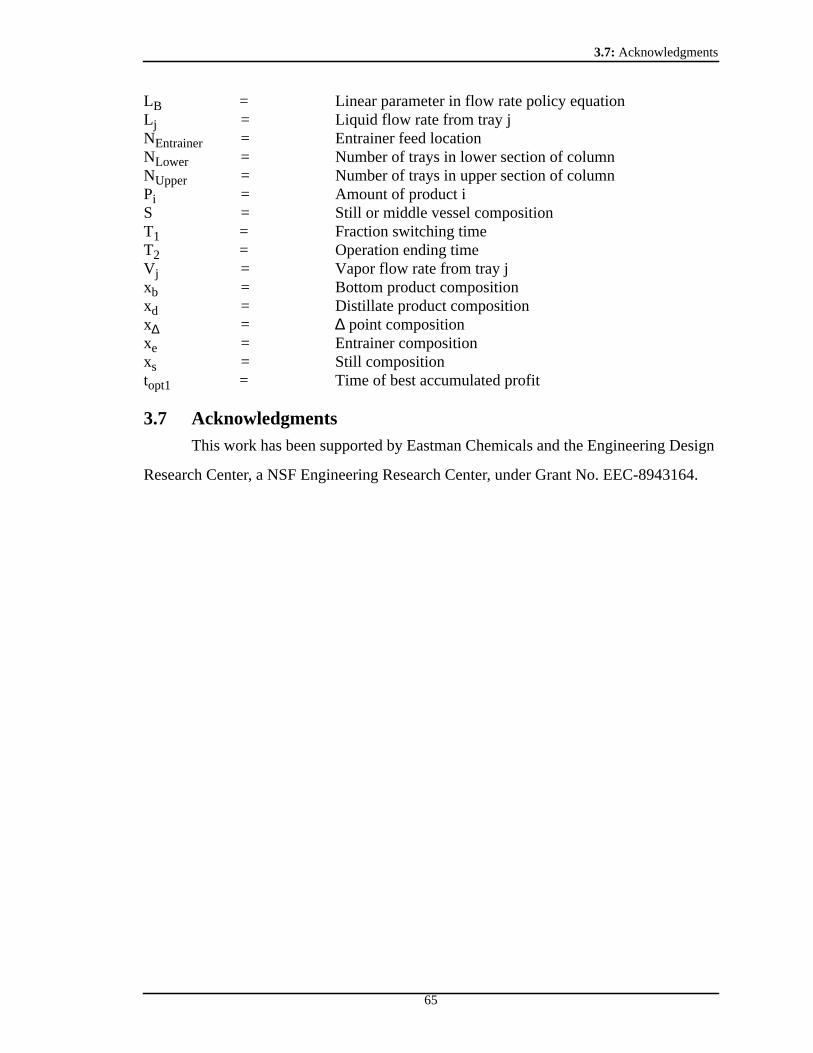
3.7: Acknowledgments
65
LB = Linear parameter in flow rate policy equationLj = Liquid flow rate from tray jNEntrainer = Entrainer feed locationNLower = Number of trays in lower section of columnNUpper = Number of trays in upper section of columnPi = Amount of product iS = Still or middle vessel compositionT1 = Fraction switching timeT2 = Operation ending timeVj = Vapor flow rate from tray jxb = Bottom product compositionxd = Distillate product compositionx∆ = ∆ point compositionxe = Entrainer compositionxs = Still compositiontopt1 = Time of best accumulated profit
3.7 AcknowledgmentsThis work has been supported by Eastman Chemicals and the Engineering Design
Research Center, a NSF Engineering Research Center, under Grant No. EEC-8943164.

3: References
66
References
Bernot C., M. F. Doherty, and M. F. Malone,1990. “Patterns of Composition Change inMulticomponent Batch Distillation.”Chem. Eng. Sci., 45, 1207-1221.
Chiotti O. J., and O. A. Iribarren,1989. “An Optimization Module for Batch Distillationwith Intermediate Cuts.”Comput. in Industry, 13, 169-180.
Devidyan A. G., V. N. Kira, G. A. Meski, and M. Morari,1994. Batch Distillation in aColumn with a Middle Vessel.Chem. Eng. Sci., 49 (18), 3033-3051.
Diwekar U. M., K. P. Madhavan, R. E. Swaney,1989. "Optimization of MulticomponentBatch Distillation Columns."Industrial Engineering and ChemistryResearch,28,p. 1011-1017.
Diwekar U. M., and K. P. Madhavan,1991. “Batch-Dist: A comprehensive Package forSimulation, Design, Optimization and Optimal Control of Multicomponent,Multifraction Batch Distillation Column.” Comput. Chem. Eng., 12, 833-842.
Chiotti O. J., and O. A. Iribarren,1989. “An Optimization Module for Batch Distillationwith Intermediate Cuts.”Comput. in Industry, 13, 169-180.
Farhat S., M. Czernicki, L. Pibouleau, and S. Domenech,1990. “Optimization ofMultiple-Fraction Batch Distillation by Nonlinear Programming.”AICHEJournal, 36, 1349-1360.
Hasebe S., B. B. Abdul Aziz, I. Hashimoto, and T. Watanabe,1994. “Optimal Design andOperation of Complex Batch Distillation Column.” in press.
Hindmarsh A. C,1983. “ODEPACK: A Systematized Collection of ODE Solvers.”Scientific Computing, 55-64.
Koehler J., H. Haverkamp, and N. Schadler,1995. “Zur diskontinuierlichen Rektifikationazeotroper Gemische mit Hilfsstoffeinsatz.” Submitted toChemie-Ingenieur-Technik.
Lang P., Lelkes Z., P. Moszkowicz, M. Otterbein, and H. Yatim,1995. “DifferentOperational Policies for the Batch Extractive Distillation.” Computers chem.Engng., 19,S645-S650.
Meski G. A. and M. Morari,1993. “Batch Distillation in a Column with a Middle Vessel.”Presented at AIChE Annual Meeting, St. Louis, paper 152a.
Piela P., R. McKelvey, and A. W. Westerberg,1993. “An Introduction to the ASCENDModeling System: Its Language and Interactive Environment.”J. ManagementInformation Systems, 9, 91-121.

3: References
67
Safrit B. T., A. W. Westerberg, U. M. Diwekar, O. M. Wahnschafft,1995a. “ExtendingContinous Conventional and Extractive Distillation Feasibility Insights to BatchDistillation.” Ind. Eng. Chem. Res., 34, 3257-3264.
Sundaram S., and L. B. Evans,1993. "Synthesis of Separations by Batch Distillation."Industrial Engineering and Chemical Research, 32, p. 500-510.
Wahnschafft O. M., J. W. Koehler, E. Blass, and A. W. Westerberg,1992. “The ProductComposition Regions of Single Feed Azeotropic Distillation Columns.” Ind. Eng.Chem. Res., 31, 2345-2362.
Wahnschafft O. M. and A. W. Westerberg,1993. “The Product Composition Regions ofAzeotropic Distillation Columns. 2. Separability in Two-Feed Columns andEntrainer Selection.” Ind. Eng. Chem. Res., 32, 1108-1120.
Wu W., and T. Chiou,1989. “Determination of Feasible Reflux Ratios and MinimumNumber of Plates Required in Multicomponent Batch Distillation.”IndustrialEngineering and Chemical Research, 28, p. 1862-1867.
Yatim H., P. Moszkowicz, M. Otterbein, and P. Lang,1993. “Dynamic Simulation of aBatch Extractive Distillation Process.” European Symposium on Computer AidedProcess Design-2,S57-S63.

68
Chapter 4
Algorithm for Generating the DistillationRegions for Azeotropic MulticomponentMixtures
Abstract
The azeotropic behavior of a mixture can limit the feasible separations that are
possible by both continuous and batch distillation. The azeotropes can create continuous
and batch distillation boundaries and regions, and knowledge of these boundaries and
regions is very important during the synthesis and design of distillation based separation
systems. Infeasible designs can be screened out early in the design process, saving
valuable time and resources.
We propose an algorithm to find the basic distillation regions from which all of the

4: Abstract
69
continuous and batch distillation regions for a n-component system can be found, given all
the azeotropes, their boiling point temperatures, and their node/saddle characteristics. A
basic distillation region is a set of residue curves which all share the same unstable and
stable node pair. Within each basic region, continuous and batch distillation regions can be
determined. The continuous and batch regions give information about the types of feasible
products one can obtain using either continuous or batch distillation. This algorithm can
be applied to continuous columns and batch rectifiers, strippers, and middle vessel
columns. The algorithm determines the boundaries and regions for all k-component
systems before solving the (k+1)-component systems. In this manner, we will show how
to find the distillation boundaries and regions for any n-component system.

4.1: Introduction
70
4.1 IntroductionThe separation of mixtures using distillation processes can be complicated by the
presence of azeotropic behavior. Azeotropes can show up as the products of these
distillations, possibly making the desired pure product impossible to produce. In this case,
methods such as extractive distillation, changing the column’s operational pressure,
changing the column’s feed composition, or switching to nondistillation based separation
methods must be used to break the azeotrope. Azeotropes can also create distillation
boundaries which form distillation regions in which the types of feasible separations are
limited. It is important that one knows what these distillation boundaries and regions are
for a particular mixture when one is designing a separation system for this mixture.
Without the knowledge of these boundaries and regions, infeasible separation systems
could be generated wasting valuable time and resources. A tool for finding the distillation
boundaries and regions would be very important and helpful during the synthesis and
design phase of azeotropic distillation systems.
We will define a basic distillation region as a set of distillation trajectories or
residue curves that start at a particular local minimum temperature node (unstable node)
and terminate at a particular local maximum temperature node (stable node). These nodes
can be either azeotropes or pure components.The unstable node is the limiting distillate
product meaning this node will be the distillate product for a column at total reflux and
having an infinite number of trays. The stable node will be the limiting bottoms product.
When sets of residue curves share an unstable or stable node but not both, a surface or
boundary will separate these sets of residue curves. This surface is a basic distillation
boundary. Except in the case of very curved basic distillation boundaries, the feed to the

4.1: Introduction
71
continuous distillation column determines in which basic distillation region the separation
will lie. Also it is difficult to cross such boundaries without using methods like extractive
distillation. Many researchers in the past have called such a distillation region a
continuous region but we will show later that a continuous distillation region should
represent something else.
Basic distillation regions can be broken up into continuous distillation regions and
batch distillation regions where the regions tell us something about the types of feasible
products one can obtain while operating in a particular distillation region. A continuous
distillation region is very similar to a basic distillation region with a couple of exceptions.
Figure 4.1 shows an example of a system with one basic distillation region as there is only
Figure 4.1: Basic vs. Continuous Distillation Regions
one unstable and one stable node. For this case we have a straight line boundary A-BC
that splits the basic region into two continuous regions. Using the reachable product
concepts of Wahnschafft et al. (1992), we can readily show that no column profile can
A
C200.0oC
100.0oC
Stable Node
Unstable Node
B150.0oCSaddle
BC140.0oCSaddle
ContinuousBoundary

4.1: Introduction
72
cross this straight A-BC boundary. Thus a continuous column could have profiles and
products in either the continuous region (A, B, BC) or in the continuous region (A, C, BC)
but not in both. As mentioned, many researchers have defined as continuous region what
we have termed a basic region. However using our definition of a continuous region, we
will see that a basic region is a building block for both continuous and batch regions. As
we are about to note continuous regions are now defined similarly to batch regions as they
describe the types of feasible products located within each region.
Ewell and Welch (1945) defined a batch distillation region as a region of
compositions all of which produce the same product sequence upon rectification using a
traditional batch column. The initial still composition determines in which batch
distillation region one is operating, and the desired product cannot be obtained if it does
not belong to the product sequence defined by the current batch distillation region. The
batch distillation regions are subsets of the basic regions for a particular mixture and can
be different for different types of batch column configurations. In Figure 4.1, there are two
batch distillation regions: (A, B, BC) and (A, C, BC). The regions give information about
the product sequences that can be obtained in each batch distillation region.
We shall first review the existing literature on basic and batch distillation regions
where researchers have attempted to generate these regions using a variety of methods.
We then present our algorithm for determining the basic, continuous, and batch distillation
regions. In this algorithm, we show how to determine the distillation boundaries and
regions for 3-component systems. We determine the distillation boundaries and regions
for 4-component systems by calculating the distillation boundaries of all the individual 3-

4.2: Background
73
component systems first. We generate surfaces in the 4-component space that separate the
composition space into subregions, each containing one unstable node and one stable
node. These surfaces are very similar to the 3-component systems, and we determine the
distillation regions for these surfaces in the same manner as for 3-component systems.
Using this approach, we show how it is possible to find the distillation regions for any n-
component system when using a continuous distillation column or a batch rectifier,
stripper, or middle vessel column. While we believe this algorithm to be quite general, as
with all previous approaches of which we are aware, we have no proof the algorithm will
work for all possible topologies. Thus for now one should validate the results. We show
how we have done this validation with several examples.
4.2 Background4.2.1 Basic Distillation
As stated earlier, a basic distillation region is defined as a set of residue curves that
start at a particular unstable node and terminate at a particular stable node. Most
researchers call such a region a continuous region, but we will define it as a basic region.
Figure 4.2 shows a 3-component example where there are four sets of residue curves
starting at either the unstable node CM or AM and ending at either the stable node M or
AC. These sets of residue curves are separated by basic distillation boundaries. The
boundaries that terminate at a stable node are stable separatrices, while the boundaries that
start at an unstable node are unstable separatrices. These boundaries separate the
composition space into basic distillation regions. Our goal is to find these boundaries by
enumerating all of the distillation regions for a particular mixture.
Most of the work done in finding basic distillation regions has come out of the
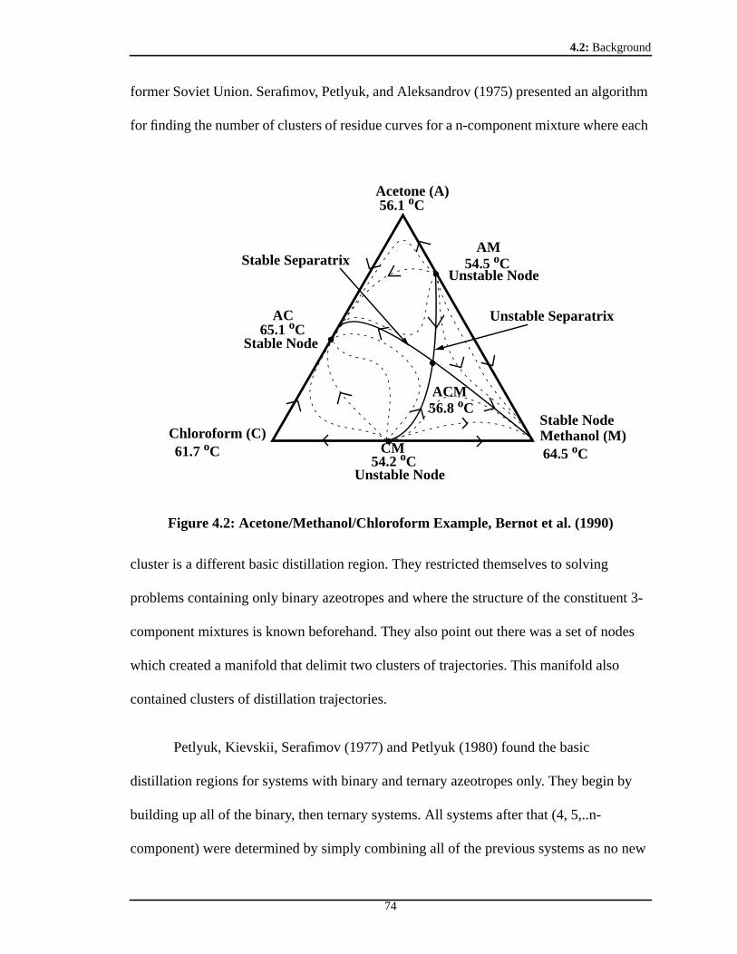
4.2: Background
74
former Soviet Union. Serafimov, Petlyuk, and Aleksandrov (1975) presented an algorithm
for finding the number of clusters of residue curves for a n-component mixture where each
Figure 4.2: Acetone/Methanol/Chloroform Example, Bernot et al. (1990)
cluster is a different basic distillation region. They restricted themselves to solving
problems containing only binary azeotropes and where the structure of the constituent 3-
component mixtures is known beforehand. They also point out there was a set of nodes
which created a manifold that delimit two clusters of trajectories. This manifold also
contained clusters of distillation trajectories.
Petlyuk, Kievskii, Serafimov (1977) and Petlyuk (1980) found the basic
distillation regions for systems with binary and ternary azeotropes only. They begin by
building up all of the binary, then ternary systems. All systems after that (4, 5,..n-
component) were determined by simply combining all of the previous systems as no new
Acetone (A)
Methanol (M)Chloroform (C)
56.1oC
64.5oC61.7oC
65.1oC
54.5oC
56.8oC
54.2oC
Stable Separatrix
Unstable Separatrix
Stable Node
Stable Node
Unstable Node
Unstable Node
AC
CM
ACM
AM

4.2: Background
75
azeotropes were added to the systems. They generated all possible systems using different
permutations of the possible connections between all of the nodes of the current system.
They searched the tree of these possible systems using a depth first search and applied a
feasibility test to each system. This test consisted of a list of rules and heuristics based on
the assumption that the systems had no higher dimensional azeotropes than a ternary
azeotrope. Similar to Serafimov, Petlyuk, and Aleksandrov (1975), these researchers
recognized that manifolds separating distillation regions existed and that any binary and
ternary azeotropes must lie on these manifolds.
Baburina, Platonov, and Slin’ko (1988) generated and classified the possible 3-
component systems. They were able to analyze each system for feasibility using a
bifurcation analysis and several conditions relating to the conjugacy of the critical points
belonging to each basic distillation region. While they did not extend their analysis to
more than 3-component systems, they mention in closing that their algorithm opens up the
possibility of analyzing higher dimensional systems.
Serafimov (1987) presented a literature review on the thermodynamic topological
analysis of azeotropic separation systems. Other than the previously mentioned work
above, Doherty and Caldarola (1985) and Doherty (1985) presented a method for
generating 3-component systems using a topological relationship between the nodes of the
system and a set of rules and heuristics for determining the basic distillation boundaries.
Matsuyama (1975) also enumerated all of the possible 3-component systems.
4.2.2 Batch DistillationIn batch distillation, the initial still composition defines in which batch distillation

4.2: Background
76
region one is currently operating. The rectification of this still composition will produce a
sequence of products, starting with the local minimum temperature node or the unstable
node. The products after the unstable node consist of a set of saddle nodes and possibly a
stable node in order of increasing boiling temperatures. Each batch distillation region,
therefore, is made up of a set of compositions that will produce the same product sequence
when they are separated (Ewell and Welch, 1945).
The work that has been done in identifying batch distillation regions is somewhat
limited. Malenko (1970a, b, c) did some interesting work in a series of papers where he
first pointed out that the change in still composition versus time (still path) proceeds in a
direction directly opposite that of the current distillate product during ideal fractionation
(using a traditional batch rectifying column). He then stated that the still path will proceed
in this direction until it hits a face of the composition space or a distillation boundary. He
could then analyze a lower dimensional system since the face of the composition space
where the current distillate product lies could not be reached again. He introduced the
concept of a maximum temperature surface (MTS) which is a separator of distillation lines
(residue curves). The MTS separated the composition space into subregions each having
its own unstable node. The number of MTS’s for a n-component system was one less than
the number of unstable nodes that are present in that n-component space, and the
dimension of the MTS is n-1 (for a 4-component system, the MTS was a planar surface of
dimension 3). The nodes that make up the MTS are nodes which have more than one ridge
line passing through them or, more simply put, belong to more than one set of residue
curves as seen in continuous distillation. Starting with 3-component systems whose
structures (batch distillation boundaries) were known, Malenko identified the MTS’s for

4.2: Background
77
each of the 3-component systems. These MTS’s then made up the MTS manifold for the
4-component system. The 4-component MTS acted like another face of the 4-component
space and batch distillation boundaries were added to this manifold because Malenko
pointed out that the distillation lines or the still path could not cross the MTS. Using these
techniques, Malenko was able to decompose a n-component system down to n-1, n-2, etc.
using the methods of MTS analysis until only 3-dimensional systems remained. The
structure of these 3-dimensional systems was known a priori or calculated by hand. His
work was for the batch rectifier column only.
Van Dongen and Doherty (1985) and Bernot, Doherty, and Malone (1990, 1991)
did some very interesting work in finding the still and product paths and batch distillation
regions for batch rectifying and stripping columns for 3 and 4-component systems. They
developed the following heuristic for identifying the batch distillation regions for 3-
component systems: “First the composition triangle is divided into regions each
containing one unstable node. In each of these regions the other batch distillation
boundaries are found by joining the unstable node to all the saddles and nodes of its
region.” They used the stable separatrices to divide the composition space. This algorithm
applied to the batch rectifier. A similar algorithm joining each stable node to all of the
saddles and nodes of its region was developed for a batch stripper. The boundaries that
divided the composition triangle into subregions each containing one unstable node are
the MTS’s seen in Malenko’s work. They also point out that the regions for a batch
rectifier and stripper differ slightly when the boundaries are curved. Several 4-component
examples were shown, but there was only one unstable or stable node in each example
making the batch distillation regions easier to find.

4.2: Background
78
Recently, Ahmad and Barton (1995a, b) have presented an algorithm for finding
the batch distillation regions. They began by testing the algorithm for finding the batch
distillation boundaries of Bernot, Doherty, and Malone (1991) on all possible ternary
systems and pointed out that there were a few systems in which the algorithm failed to
give the correct batch distillation regions. They assumed for their work that these types of
systems would not occur. They defined a stable separating boundary as any edge of the
composition simplex or any stable separatrix. Also defined was the concept of primary
boundaries which consist of all of the 3-component batch distillation boundaries. Using
these concepts, they defined their algorithm for finding the batch distillation region
boundaries for a n-component mixture as:
• Find batch distillation region boundaries for all 3-component systems using thealgorithm of Bernot, Doherty, and Malone (1991). These boundaries are the primaryboundaries.
• Find the stable separating boundaries (stable separatrices) for all 4-componentsystems and add any primary boundaries not introduced earlier.
• Repeat above step for all 5-component systems, 6-component systems, etc.
They then go on to prove three main points:
• A batch distillation region consists of k vertices where k is the number ofcomponents for the current system and that the dimension of this region is k-1 (e.g.for k=3, the region will be a plane and for k=4, the region will be a 3-dimensionalvolume).
• The edges that make up the region are primary boundaries.• All pairs of the k vertices that form this region must be connected by primary
boundaries and there must be a path of increasing temperature between all vertices.
Some of the proofs for these statements were contained in these two papers, while the
remaining proofs were referenced in a paper in preparation (Ahmad, Zhang, and Barton,
1995). They also enumerated the batch distillation regions by finding all paths between
vertices that started at an unstable node and, while traversing on primary boundaries of
increasing temperature, visited k-1 vertices (k was the number of components in the

4.3: Algorithm for Finding Distillation Boundaries and Regions
79
current system). One other interesting result from their work was the idea of using vectors
that originated at some reference point and passed through the vertices of the batch
distillation regions to represent the regions. In this manner, one could quickly calculate to
which batch distillation region a particular composition belonged. They looked at 3, 4 and
8-component examples. But these examples contained either one unstable and/or one
stable node making the batch distillation regions easier to find. If there is only one
unstable node, the batch distillation boundaries are generated by simply connecting the
unstable node to every other node in the composition space.
4.3 Algorithm for Finding Distillation Boundaries and RegionsAs shown above, there has been a significant amount of work done in finding the
distillation regions for basic and batch distillation processes. Most of these algorithms
suffer from many of the same problems: they only use the temperature information about
nodes in the calculation of these regions, they fail to solve difficult 4-component and
higher systems, and the algorithms are difficult to understand and implement. While some
of the ideas of the algorithm we will present here come from the work reviewed above, we
will show that a simple, general algorithm exists for finding the basic, continuous, and
batch distillation regions. Assuming straight distillation boundaries, we will show how to
find the basic and continuous distillation boundaries. We next present the algorithms for
finding the batch distillation boundaries after which we will generate the basic, continuous
and batch distillation regions. We will find the batch boundaries and regions for a batch
rectifier, stripper, and middle vessel column. However, we will first show why the stability
information AND the temperature information about the system nodes are both necessary
in correctly determining the distillation boundaries and regions.

4.3: Algorithm for Finding Distillation Boundaries and Regions
80
4.3.1 Use of Stability and Temperature InformationAs pointed out earlier, most of the algorithms created for the determination of the
distillation boundaries and regions of a particular system use only the boiling points of the
nodes of the system. Figure 4.3 shows an example of a system in which the temperature
information about the system does not uniquely define the system. In both cases (I and II),
the temperature information about the nodes is identical, but the stability information is
different resulting in different distillation boundaries and regions. The stability
information of a system consists of determining whether a node (pure component or
azeotrope) is an unstable node, stable node, or a saddle. We show in Section 4.3.3 how to
determine these stabilities for a particular system. Algorithms must use the stability and
temperature information in order to correctly determine the distillation boundaries and
regions for the particular system.
Figure 4.3: System Not Uniquely Defined by Temperature
A
C200.0oC
100.0oC
Stable Node
Unstable Node
B150.0oCSaddle
BC140.0oCSaddle
AB160.0oC
Stable Node
A
C200.0oC
100.0oC
Stable Node
Unstable Node
B150.0oCSaddle
BC140.0oC
Unstable Node
AB160.0oCSaddle
III

4.3: Algorithm for Finding Distillation Boundaries and Regions
81
4.3.2 Basic Distillation Boundaries for 3-Component SystemsWe have seen the notion of separating planes or manifolds dividing the
composition space into subregions, each containing one unstable node, in the work of
several previous researchers, but not all of these researchers have grasped the true nature
and importance of this separating manifold. Malenko (1970b) was the first researcher to
really understand that not only does this manifold act like another face of the composition
space, but that distillation boundaries exist on this manifold. He called this manifold a
maximum temperature surface (MTS) as he thought this surface was a ridge in the
contours of temperature profiles on a composition diagram. Van Dongen and Doherty
(1984) proved that these ridges did not correspond to temperature ridges. However, some
kind of separating surface does exist. Figure 4.2 shows an example of acetone/methanol/
chloroform. Malenko would have identified the MTS as the surface (line) AC-ACM-M.
This surface, which we will call a maximum residue surface (MaxRS), is a separating
manifold that separates a composition space into subregions each containing its own
unstable node (UN). Each residue curve will follow a path of increasing temperature,
converging towards and terminating on the MaxRS. In this example, we create two
subregions: one with AM as its unstable node (UN) and one with CM as its UN. The
MaxRS separates out two sets of residue curves each having its own UN. The MaxRS also
corresponds to the stable separatrix for this system, as used earlier as a separating surface
in several of the other works we examined.
If we look at the behavior of the MaxRS, we again see that the MaxRS is a
boundary between two UNs. Each of these UNs must be able to “see” each node on this
surface meaning that a residue curve from the UN to each node on the MaxRS must exist

4.3: Algorithm for Finding Distillation Boundaries and Regions
82
as all residue curves terminate on the MaxRS. If the UN could not see all of the nodes on
the MaxRS, then there must be some other separating surface, and we have not found the
correct MaxRS. The nodes that make up the MaxRS are actually the nodes that the various
UNs have in common when we traverse the various connections between nodes while
increasing in temperature. For example, in Figure 4.2, all of the nodes that the UNs can
reach only using the binary connections are: UNL(CM)=(C, AC, M) and UNL(AM)=(A,
AC, M) where A is the acetone node, C is chloroform, and M is methanol. To complete
these lists, we add the ternary azeotrope to both, getting the unstable node lists
UNL(CM)=(C, AC, M, ACM) and UNL(AM)=(A, AC, M, ACM). We have to include the
ternary azeotrope because every node on the composition simplex must be able to “see”
the ternary azeotrope when the ternary azeotrope is a saddle. No basic distillation
boundary can separate a node from the ternary saddle azeotrope. If we find the nodes that
appearin at least two of these lists, we get the intersection list INT(CM, AM)=(AC, M,
ACM). Three nodes are in common to both of the UNs and must make up the MaxRS. We
add the connections ACM-AC and ACM-M to the system. Basically we connect each
stable node (SN) in the intersection list to every node in the list that is not a SN unless a
ternary saddle azeotrope exists, in which case we connect each SN to the ternary saddle
azeotrope. This method correctly finds the stable separatrix and the MaxRS for the 3-
component system.
If we look at Figure 4.2, we see that there is also a manifold that separates the
composition space into subregions, each having its own SN. We will call this a minimum
residue surface or MinRS. If we use the same kind of analysis as above for the UNs but
now follow the directions of decreasing temperature from the SNs, we find the nodes of

4.3: Algorithm for Finding Distillation Boundaries and Regions
83
the MinRS to be: SNL(AC)=(A, AM, C, CM, ACM), SNL(M)=(AM, CM, ACM), and
INT(AC, M)=(AM, CM, ACM). We add the connections AM-ACM and CM-ACM to the
system. The MinRS forms the unstable separatrix of the system. So the MaxRS and
MinRS divide the composition space into four sets of residue curves, each having its own
UN and SN pair. These two manifolds determine the basic distillation regions for this
example. We could also invert all of the temperatures and stability of the nodes (unstable
to stable and stable to unstable) in Figure 4.2 and apply the above analysis. We would find
that the “inverted” system’s MaxRS and MinRS were the original system’s MinRS and
MaxRS, respectively, and would find the same basic distillation boundaries as in the
original system. These two separating surfaces are composition spaces of dimension k-2,
where k is the number of components (a line in this case of k=3), as seen in the literature
mentioned previously.
However, we cannot rely on equating the stable separatrix to the MaxRS and
equating the unstable separatrix to the MinRS as done in some of the other work. Figure
4.4 shows an example where we have two UNs and three SNs. There must be a MaxRS in
this system separating out the two UNs. The stable separatrix is ABC-A. But there is a
separatrix, ABC-BC, which we will call a saddle separatrix because it does not conform to
the definitions of unstable or stable separatrices. This saddle separatrix connects two
saddle nodes and is part of the MaxRS as it is part of the surface that separates the region
into subregions, each having one unstable node. If we were looking for only the stable
separatrices to make up the MaxRS, the segment ABC-BC would not be included, and the
composition space would not be divided into regions, each having its own UN.

4.3: Algorithm for Finding Distillation Boundaries and Regions
84
Figure 4.4: Example of Saddle Separatrix
For this example, if we find the common nodes for all of the UNs and find their
intersection list we get: UNL(AB)=(A, B, ABC), UNL(AC)=(A, C, ABC), and INT(AB,
AC)=(A, ABC). The only connection we can add to the system is ABC-A, or the stable
separatrix. However, when we find the MinRS for this example, we get: SNL(A)=(AB,
AC, ABC), SNL(B)=(AB, BC, ABC), SNL(C)=AC, BC, ABC). Noting that the
intersection list contains any node in at least two of these lists we get INT(A, B, C)=(AB,
AC, ABC, BC). So the connections we are able to add are AB-ABC, AC-ABC, and ABC-
BC as the ternary saddle azeotrope must be connected to everything in the intersection list.
By using the MaxRS and MinRS together, we are able to determine the basic distillation
boundaries for 3-component systems. We can further add that any basic distillation
boundaries for a 3-component system must lie on either the MaxRS or MinRS because we
A
C90.0oC
100.0oC
Stable Node
Stable Node
B80.0oC
Stable NodeBC
70.0oCSaddle
AC50.0oC
Unstable NodeAB
60.0oCUnstable Node
ABC65.0oCSaddle
Saddle Separatrix
Stable Separatrix

4.3: Algorithm for Finding Distillation Boundaries and Regions
85
cannot block any node not on one of these surfaces from these surfaces. All residue curves
from nodes not on one of these surfaces must either increase in temperature to the MaxRS
or decrease in temperature to the MinRS.
As pointed out by Ahmad and Barton (1995a), the method of Bernot, Doherty, and
Malone (1991) to find the batch distillation regions failed on two types of the 87 feasible
3-component systems that were enumerated by Doherty and Caldarola (1985). These two
types consisted of a type (1) in which the ternary azeotrope is a SN connected only to a
binary saddle and a type (2) where the UN is a pure component and the SN is one of this
component’s binary azeotropes. In type 1, the stable separatrix did not divide the
composition space into regions each having its own UN. This behavior is not only a
problem in finding batch regions but also in finding basic distillation boundaries. Figure
4.5 shows an example of type 1 which is the inverse of system 421-m from Doherty and
Figure 4.5: Inverse of System 421-m from Doherty and Caldarola (1985)
A
C50.0oC
90.0oC
Unstable Node
Saddle
B70.0oCSaddle BC
80.0oCSaddle
AC150.0oC
Stable Node
AB60.0oCSaddle
ABC100.0oC
Stable Node Unstable Separatrix
Stable Separatrix
S1
S2

4.3: Algorithm for Finding Distillation Boundaries and Regions
86
Caldarola (1985). In order to capture this stable separatrix connection, the following
“preprocessing” step is made to our current algorithm:
• If a k dimensional azeotrope exists (where k is the total number of components in thecurrent system) and this azeotrope is an UN (SN) and there is only one SN (UN),then any path of decreasing (increasing) temperature from a stable (unstable) nodethat ends in a saddle must be supplemented by the connection of the azeotrope to thissaddle. This step must be done before finding the common node and intersectionlists.
For the example in Figure 4.5, we would recognize that there is a k dimensional
(azeotrope involving all k=3 components) azeotrope and it is an SN and there is only one
UN, C. The path of increasing temperature C-BC ends in a saddle. So we must add the
connection BC-ABC before we do any further analysis of the system. Applying the rest of
the algorithm gives for the MinRS: SNL(AC)=(A, AB, C), SNL(ABC)=(BC, B, AB, C),
and INT(AC, ABC)=(AB, C). We add the connection C-AB to the system, giving the
correct structure. Every residue curve must end (start) at a SN (UN) and, if we have a
residue curve that ends at a saddle while traversing in decreasing (increasing) temperature,
the residue curve must terminate at the azeotrope involving all components of the
particular system. This azeotrope must be a SN (UN). This additional preprocessing step
correctly finds the basic distillation boundaries for all of the type 1 systems referred to
above. The type 1 and 2 systems will be investigated further when we discuss finding the
batch distillation boundaries.
4.3.3 Basic Distillation Boundaries for 4-Component SystemsAs shown in Malenko (1970b, c) and Ahmad and Barton (1995a, b), the edges of
the 4-component separating manifold or MaxRS (which is a plane) is made up of the 3-
component MaxRS’s (which are lines). The 4-component MaxRS acts like another face of
the 4-component simplex, which are 3-component systems. The MaxRS separates the

4.3: Algorithm for Finding Distillation Boundaries and Regions
87
original 4-component space into separate 4-component spaces, each having its own UN.
Similarly, the MinRS acts like another face of the composition space by separating the
original 4-component space into subspaces each having its own SN. These two surfaces or
manifolds (MaxRS and MinRS) can be found in the same manner as for 3-component
systems: by finding the UNL and SNL and INT lists but only using existing connections
that are basic distillation boundaries. They also have the same characteristics of their 3-
component system counterparts meaning that any new connections (basic boundaries) that
are to be added to the system must be between nodes on the MaxRS or MinRS (except for
the case of an unstable or stable 4-component azeotrope in which case we apply the
preprocessing step as before). So once we have found the MaxRS and MinRS, we can
treat them as 3-component systems since they really act like faces of the 4-component
mixture. But what are the stabilities of the nodes on each of these individual faces when
we are treating these faces as 3-component systems? Fidkowski, Malone, and Doherty
(1993) showed that by looking at the eigenvalues ofJ calculated at the pure component
and azeotropic compositions (x=liquid and y=vapor) of a particular mixture such that
(4.1)
(4.2)
with (4.3)
where (4.4)
one could determine the stabilities of the nodes (pure components and azeotropes) of the
ξddx x y– x 1 K–( ) ξ is dimensionless time,= =
J δij yij–[ ] δij is the Kronecker delta,=
xii 1=
n
∑ 1=
yij xj∂∂yi=

4.3: Algorithm for Finding Distillation Boundaries and Regions
88
current system. For an n-component system, there will be n-1 eigenvalues. If all of the
eigenvalues are positive, the node is an UN (all eigenvectors or residue curves move in
time away from the UN); if all are negative, the node is a SN (all eigenvectors or residue
curves collapse onto the SN); and if positive and negative, the node is a saddle (some
eigenvectors move away and some collapse onto the saddle). For example in Figure 4.2,
each node has two eigenvalues, resulting in two eigenvectors) associated with it. Node
CM for instance has an eigenvector growing away from it along the chloroform/methanol
binary edge. It also has an eigenvector growing away from it that points to the interior of
the composition space. Since all eigenvectors grow away from the node CM, this node is
an UN. Node M (methanol) also has two eigenvectors associated with it: one collapsing
onto the node along the acetone/methanol binary edge and one collapsing onto the node
along the chloroform/methanol binary edge. Since all eigenvectors are collapsing onto the
node M, this node is a SN. And for the node ACM, there are two eigenvectors associated
with it: one collapsing onto the node from the nodes AM or CM and one growing away
from the node towards the nodes AC or M. The node ACM is a saddle node because it has
eigenvectors that collapse and grow away from it.
If we are looking at the nodes on the MaxRS for a 4-component system, we know
that these nodes must have at least one negative eigenvalue as residue curves collapse onto
the MaxRS from the other nodes in the 4-component space not on the MaxRS (all residue
curves terminate on the MaxRS). The remaining two eigenvalues must describe the
stability of the MaxRS nodes with respect to each other. In this way we can treat the
MaxRS as a 3-component system with the proper stability information. The same
argument applies for the MinRS except that we can account for one positive eigenvalue

4.3: Algorithm for Finding Distillation Boundaries and Regions
89
from the other nodes not on the MinRS because all residue curves begin on the MinRS.
The other two eigenvalues describe the stability of the MinRS nodes with respect to each
other.
To find the basic distillation boundaries for the 4-component system (after having
determined all of the basic distillation boundaries for the constituent 3-component
systems), we apply the following algorithm:
• k=4.• Apply the preprocessing step if necessary.• Find UNL(unstable nodes) and the intersection list INT(unstable nodes), creating the
MaxRS.• Update the stabilities of the MaxRS nodes using the algorithm described above.• Solve this new system as a 3-component system using the algorithm defined earlier.• Find SNL(stable nodes) and the intersection list INT(stable nodes), creating the
MinRS.• Update the stabilities of the MinRS nodes using the algorithm described above.• Solve this new system as a 3-component system using the algorithm defined earlier.
In this manner, we can determine all of the additional basic distillation boundaries for all
of the constituent 4-component systems.
4.3.4 Basic Distillation Boundaries for n-Component SystemsAs shown above, finding the basic distillation boundaries for a 4-component
system breaks down to solving all of the constituent 3-component systems, finding the
MaxRS and MinRS for the 4-component system, and then solving the MaxRS and MinRS
as 3-component systems. This same scheme can be used to solve 5-component systems,
creating a solution tree shown in Figure 4.6. One can easily see that to find the basic
distillation boundaries for any n-component system, we need only recursively apply the
algorithm for 3-component systems. By finding the basic distillation boundaries for all
constituent ternary, then quaternary, etc. systems, we can find these boundaries for any n-
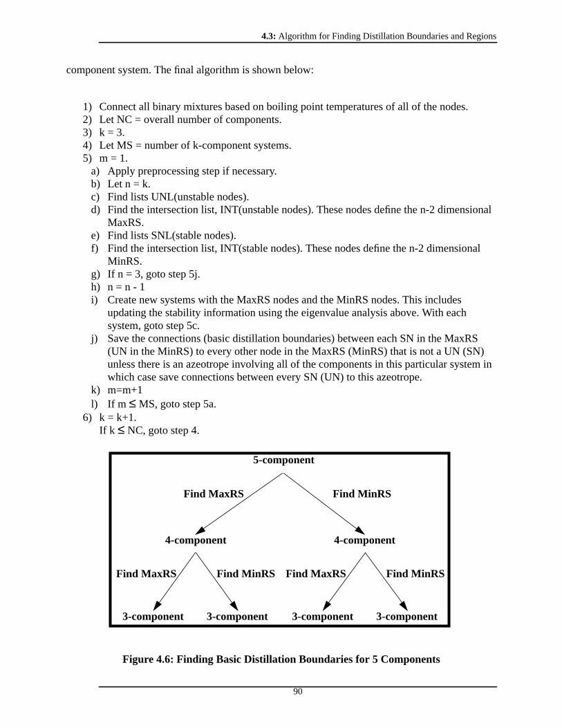
4.3: Algorithm for Finding Distillation Boundaries and Regions
90
component system. The final algorithm is shown below:
1) Connect all binary mixtures based on boiling point temperatures of all of the nodes.2) Let NC = overall number of components.3) k = 3.4) Let MS = number of k-component systems.5) m = 1.
a) Apply preprocessing step if necessary.b) Let n = k.c) Find lists UNL(unstable nodes).d) Find the intersection list, INT(unstable nodes). These nodes define the n-2 dimensional
MaxRS.e) Find lists SNL(stable nodes).f) Find the intersection list, INT(stable nodes). These nodes define the n-2 dimensional
MinRS.g) If n = 3, goto step 5j.h) n = n - 1i) Create new systems with the MaxRS nodes and the MinRS nodes. This includes
updating the stability information using the eigenvalue analysis above. With eachsystem, goto step 5c.
j) Save the connections (basic distillation boundaries) between each SN in the MaxRS(UN in the MinRS) to every other node in the MaxRS (MinRS) that is not a UN (SN)unless there is an azeotrope involving all of the components in this particular system inwhich case save connections between every SN (UN) to this azeotrope.
k) m=m+1l) If m ≤ MS, goto step 5a.
6) k = k+1.If k ≤ NC, goto step 4.
Figure 4.6: Finding Basic Distillation Boundaries for 5 Components
5-component
4-component
3-component
Find MaxRS Find MinRS
4-component
3-component
Find MaxRS Find MinRS
3-component 3-component
Find MaxRS Find MinRS

4.3: Algorithm for Finding Distillation Boundaries and Regions
91
4.3.5 Finding the Continuous Distillation BoundariesAs mentioned earlier, basic and continuous distillation regions are very similar.
Figure 4.1 shows an example system with one basic distillation region and two continuous
regions. The boundary A-BC can not be crossed by a continuous column profile so this
boundary is a continuous boundary. In order to find all of the additional continuous
boundaries (those in addition to the basic boundaries) we simply have to connect the UN
to the SN for each basic distillation region. These connections will form continuous
distillation regions whose nodes more accurately describe the types of feasible products
that one could obtain using continuous distillation.
4.3.6 Finding the Batch Distillation BoundariesNow that we can find all of the basic distillation boundaries creating sets of residue
curves each having their own UN and SN pair, we can place the batch distillation
boundaries within each of these regions. The algorithm for placing the batch distillation
boundaries of Bernot, Doherty, and Malone (1991) for a batch rectifier was shown by
Ahmad and Barton (1995a) to work on almost all 3-component systems. The algorithm
did not work on two types of systems. Type 1, shown in Figure 4.5, has a stable separatrix
that does not completely divide the composition space into regions each having one UN
because there is only one UN. If we were to rectify a initial still composition of S1 as
shown in Figure 4.5, the still path would move directly away from the UN (C vertex) until
it intersects the stable separatrix. When the current still composition exactly lies on this
stable separatrix, the still composition will follow the stable separatrix up to the stable
ternary azeotrope as pointed out by Bernot, Doherty, and Malone (1990). The distillate
will be the intersection of a line tangent to the stable separatrix at the current still
composition and the B-C binary edge. If we assume that the stable separatrix is a straight

4.3: Algorithm for Finding Distillation Boundaries and Regions
92
line, the distillate composition will be the BC saddle azeotrope. However, if the boundary
were curved, the distillate composition would vary along the B-C binary edge depending
on the curvature of the separatrix. So in assuming straight distillation boundaries, the
distillate product will now become the BC azeotrope with the still path following the
stable separatrix until only the ternary azeotrope is left in the column (Malone, 1996).
However, rectification of an initial still composition S2 will produce the product sequence:
C, AB, then B. When the algorithm of Bernot, Doherty, and Malone (1991) for finding the
batch distillation boundaries for a batch rectifier is applied to this system, we will create
the batch boundaries C-B and C-ABC resulting in three batch distillation regions: (C, AB,
B), (C, BC, ABC), and (C, B, BC). However, how can we connect the nodes C to B when
there is a binary azeotrope between B and C? There has to be a batch boundary B-C
creating two batch distillation regions: (C, AB, B) where the product sequence C-AB-B
can be taken (as seen for the initial still composition S2) and (C, B, BC) which is a batch
region of zero area where no products can be taken. In this case, two of the batch regions,
(C, AB, B) and (C, BC, ABC), appear to occupy some of the same composition space.
Further, what about the type 2 systems? Figure 4.7 shows an example of this kind
of system. This example has only one UN and one SN creating only one basic distillation
region (and no basic distillation boundaries). If we were to place several initial still
compositions within this composition space and separate them using a batch rectifier at
total reflux and infinite number of trays, we would obtain B as our first distillate product in
all cases. The change in still composition or still path will move in a direction directly
opposite this distillate product until it hits an edge of the composition space or a basic
boundary. In this case, the still path continues until it intersects the A-C binary edge, at

4.3: Algorithm for Finding Distillation Boundaries and Regions
93
which point the distillate product will switch to A. We will produce A until no more A
Figure 4.7: Example of Type 2 System
remains in the column leaving only C left in the column. It is impossible to produce BC as
a distillate product. This example is very similar to the example shown in Figure 4.5 of the
type 1 system because we have two batch distillation regions one of which has zero area,
created by adding the batch boundary B-C to the system.
If we do the same experiment on the system in Figure 4.7 using an inverted batch
column or batch stripper, our first bottoms product will always be BC. If the initial still
composition lies to the right of the batch stripper boundary shown in Figure 4.7, the still
path will intersect the A-C binary edge, producing C then A. But if the initial still
composition lies to the left of the batch boundary, the still path will intersect the A-B
A
C70.0oC
60.0oC
Saddle
Saddle
B50.0oC
Unstable NodeBC
100.0oCStable Node
Batch Distillation Boundaryfor Batch Stripper Only

4.3: Algorithm for Finding Distillation Boundaries and Regions
94
binary edge, producing A then B. So there are two batch distillation regions, defined by
the boundary A-BC, when we use the batch stripper column. With the assumption of
straight distillation boundaries, the distillation boundaries for the batch rectifier and
stripper are not identical, which violates behavior suggested by several researchers.
Bernot, Doherty, and Malone (1991) also reported an algorithm for determining the batch
distillation boundaries for the batch stripper column. This algorithm connected the SN in
each continuous region to every other node in this region. Using this algorithm, we find
the correct batch distillation boundaries for the batch stripper for the example in Figure
4.7. If we were to invert all of the temperatures and stabilities of the nodes in this example,
we would find that the behavior of the rectifier and stripper has now been switched. The
batch boundaries and regions for the original rectifier are the boundaries and regions for
the “inverted system” stripper and vice versa. As long as we apply the correct algorithm
for the particular batch column configuration, we can correctly identify the batch
distillation boundaries.
The top and bottom section of the MVC act just like a rectifier and stripper. So the
batch distillation boundaries defining the distillate product sequence are the rectifier’s
boundaries and the batch distillation boundaries defining the bottoms product sequence
are the stripper’s boundaries. The batch boundaries for the MVC are the batch boundaries
that are in common to both the rectifier and stripper. As seen in the batch rectifier and
stripper, the still path for the MVC cannot cross the batch boundaries that are also basic
boundaries.
We must apply the algorithm for finding the batch boundaries to each system that
4.3: Algorithm for Finding Distillation Boundaries and Regions
95
we generate: all constituent 3-component systems and their corresponding MaxRS’s and
MinRS’s, all constituent 4-component systems and their corresponding MaxRS’s and
MinRS’s, etc. The batch distillation boundaries will, therefore, consist of all of the basic
boundaries we found previously and the additional boundaries we found using the above
algorithm. Again, we are assuming straight line boundaries.
4.3.7 Basic Distillation RegionsTo enumerate the basic distillation regions, we must find all sets of residue curves.
Starting at each UN, we find all nodes that we can reach along basic distillation
boundaries and the edges of the composition space while increasing in temperature. If we
collect all nodes that lie on a path to a particular SN, these nodes along with the UN and
SN define the nodes that make up one basic distillation region. We do this analysis for
each UN and SN pair, enumerating all of the basic distillation regions.
4.3.8 Continuous Distillation RegionsThe continuous distillation regions are very similar to the basic regions. If no UN
to SN connections (continuous boundaries) have been made between nodes within a basic
region, the continuous and basic regions are the same. However if some continuous
boundaries were added, the basic region will be split into several continuous regions. We
can find the nodes that make up the continuous regions by combining the nodes on similar
paths of either increasing or decreasing temperature while traversing on basic and
continuous boundaries and edges of the composition space only. Two paths are similar if
one of the paths contains all of the nodes of the other path. The resulting continuous
region will consist of an UN, a series of saddle nodes, and a SN.

4.3: Algorithm for Finding Distillation Boundaries and Regions
96
4.3.9 Batch Distillation RegionsAs pointed out by Malenko (1970b, c) and Bernot, Doherty, and Malone (1990)
and proved by Ahmad and Barton (1995a), the number of vertices that make up a batch
distillation region for a batch rectifier is k where k is the number of components in the
current system. The vertices that make up these regions includes one UN, a series of
saddle nodes, and possibly a SN, and all pairs of these nodes must be connected (Ahmad
and Barton, 1995a). As we saw in the examples of type 1 and type 2 systems, a batch
boundary may be possible between two pure components that have a binary azeotrope
between them. This boundary separated the binary azeotrope out of the batch region
because the azeotrope was never a product. The boundary also connected the final pair of
nodes that made up the batch distillation region, creating a set of k=3 nodes in which all
pairs of nodes are connected. However, we saw earlier that for the example in Figure 4.5,
it appears that two batch regions overlap. Any composition in the batch region (C, BC,
ABC) will result in the product sequence C-BC-ABC and any composition not in that
region but in the region (C, AB, B) will result in the product sequence C-AB-B. If a
particular composition appears to lie in more than one batch region, it must actually lie in
the batch region which contains the SN as the still path will intersect the stable separatrix
containing this SN. So in the case of Figure 4.5, S1 will lie in the region (C, BC, ABC).
For the batch stripping column, we use the same algorithm, except now we start at
all of the SNs and follow paths of decreasing temperature. As seen for batch boundaries,
the batch regions for the MVC are a combination of the rectifier and stripper columns. If
the rectifier and stripper regions are the same, then the regions for the MVC are the same
as the rectifier and stripper. If they are different, then the rectifying section of the MVC

4.4: Example of 4-Component System
97
will be constrained to the rectifier batch region and the stripping section of the MVC will
be constrained to the stripper batch region.
4.4 Example of 4-Component SystemWe will now apply the algorithm to the 4-component example of acetone/benzene/
chloroform/methanol. After finding the basic distillation boundaries and regions, we will
investigate the continuous and batch distillation boundaries and regions for the batch
rectifier. Table 1 shows the input to the algorithm (not shown is the eigenvalue information
about each constituent 3-component system) using UNIFAC to model the
thermodynamics of the system:
First, we will find the basic distillation boundaries for all of the constituent 3-component
systems. Figure 4.8 shows all of these systems. After creating all of the binary systems, we
Table 4.1: Acetone/Benzene/Chloroform/Methanol Example Input
Node %A %B %C %M Tb (C) Stabilitynum +
eigenvaluesnum -
eigenvalues
A 100.0 0 0 0 56.07 S 2 1
B 0 100.0 0 0 80.14 SN 0 3
C 0 0 100.0 0 60.62 S 2 1
M 0 0 0 100.0 64.48 SN 0 3
AM 68.34 0 0 31.66 53.46 UN 3 0
AC 38.38 0 61.62 0 64.06 S 1 2
CM 0 0 65.78 34.22 53.50 UN 3 0
BM 0 39.96 0 60.04 56.53 S 1 2
ACM 25.82 0 28.72 45.46 55.93 S 1 2
ABCM 17.11 9.500 25.94 47.45 55.79 S 2 1

4.4: Example of 4-Component System
98
Figure 4.8: Acetone/Benzene/Chloroform/Methanol Example
must apply our algorithm to each 3-component system. For each system, we apply the
preprocessing step and then find the common UN and SN node lists and their intersection
lists (the MaxRS and MinRS). In finding these lists, we traverse only on connections
A
BC
56.07oC
80.14oC60.62oC
64.06oCAC
A
MC
56.07oC
64.48oC60.62oC
64.06oC
53.46oC
55.93oC
53.05oC
AC
CM
ACM
AM
A
BM
56.07oC
80.14oC64.48oC
53.46oCAM
56.53oCBM
C
BM
60.62oC
80.14oC64.48oC
53.05oCCM
56.53oCBM
I II
III IV
Basic and Batch Boundaries
Additional Batch Boundaries
4.4: Example of 4-Component System
99
between nodes that are preexisting basic distillation boundaries. For these 3-component
systems, these links are the binary edges or connections from the preprocessing step. To
these we add any ternary azeotropes which are saddles. Below we show these steps for all
of the 3-component systems:
System INo processing step because there is no ternary azeotrope
UNL(A)=(B, AC)UNL(C)=(B, AC)MaxRS=INT(A, C)=(B, AC)Connect each SN to every other non-SN node in the intersection list:AC-B
SNL(B)=(A, C)MinRS=INT(B)=empty setNo new connections
System IIThere is no preprocessing step because the ternary azeotrope is a saddle
UNL(AM)=(M, A, AC, ACM)UNL(CM)=(M, C, AC, ACM)MaxRS=INT(AM, CM)=(M, AC, ACM)Connect each SN to the ternary azeotrope: ACM-M, ACM-AC
SNL(M)=(AM, CM, ACM)SNL(AC)=(A, AM, C, CM, ACM)MinRS=INT(M, AC)=(AM, CM, ACM)Connect each UN to the ternary azeotrope: AM-ACM, CM-ACM
System IIIThere is no preprocessing step because there is no ternary azeotrope
UNL(AM)=(M, A, B)MaxRS=INT(AM)=empty setNo new connections
SNL(M)=(AM, BM)SNL(B)=(BM, A, AM)MinRS=INT(M, B)=(AM, BM)Connect each UN to every other non-UN in the intersection list: AM-

4.4: Example of 4-Component System
100
BM
System IVThere is not preprocessing step because there is no ternary azeotrope
UNL(CM)=M, C,MaxRS=INT(CM)=empty setThere are no new connections
SNL(M)=(CM, BM)SNL(B)=(BM, C, CM)MinRS=INT(M, B)=(CM, BM)Connect each UN to every other non-UN: CM-BM
Figure 4.8 shows the connections (basic distillation boundaries) found in the above
analysis using dotted lines (ignore the dashed lines at present). To find the basic
distillation regions, we follow all paths along basic distillation boundaries from each UN
to every SN that can be reached, shown below for each of the 3-component systems:
System IA - B
- AC - BC - B
- AC - B
System IIAM - M
- ACM- M- ACM- AC- A - AC
CM - M- ACM- M- ACM- AC- C - AC
System IIIAM - M
- BM - M- BM - B- A - B
System IVCM - M

4.4: Example of 4-Component System
101
- BM - M- BM - B- C - B
We collect all nodes in paths with a common starting node (UN) and ending node (SN)
and find that our basic distillation regions are:
System I(A, AC, B)(C, AC, B)
System II(AM, ACM, A, AC)(AM, ACM, M)(CM, ACM, C, AC)(CM, ACM, M)
System III(AM, BM, M)(AM, BM, A, B)
System IV(CM, BM, M)(CM, BM, C, B)
We can now find the continuous distillation regions for the 3-component systems. First we
combine nodes on similar paths of increasing temperature. For example, system III in
Figure 4.8 has two basic distillation regions. There are five paths of increasing
temperature: AM-M, AM-BM-M, AM-B, AM-BM-B, and AM-A-B. We combine similar
paths (one path contains all nodes of the other path) and get the following lists: AM-BM-
M, AM-BM-B, AM-A-B. These three lists define the three continuous distillation regions
that make up this particular system. Applying this algorithm to all of the 3-component
systems, we obtain the following continuous distillation regions:
System I(A, AC, B)(C, AC, B)

4.4: Example of 4-Component System
102
System II(AM, A, AC)(AM, ACM, AC)(AM, ACM, M)(CM, ACM, AC)(CM, ACM, M)(CM, C, AC)
System III(AM, A, B)(AM, BM, B)(AM, BM, M)
System IV(CM, BM, M)(CM, BM, B)(CM, CM B)
In order to find the remaining batch distillation boundaries for the 3-component
systems, we connect each UN in the basic distillation regions found above to every other
node in the basic region. These additional batch boundaries are shown in Figure 4.8 with
dashed lines. The additional boundaries are for the batch rectifier. For the batch stripper,
we connect each SN in each of the basic regions to every other node in that region. The
batch distillation regions for the rectifier are found by finding the paths of increasing
temperature containing three nodes while traversing on all batch distillation boundaries
(basic and additional batch boundaries). The paths below are all of the paths obtained
when looking for batch distillation boundaries containing three nodes:
System IA - AC - BC - AC - B
System IIAM - A - AC
- ACM- AC- ACM- M
CM - ACM- AC- ACM- M

4.4: Example of 4-Component System
103
- C - AC
System IIIAM - A - B
- BM - B- BM - M
System IVCM - BM - M
- BM - B- C - B
All pairs of nodes in the above lists are connected so the lists represent all of the 3-
component batch distillation regions. In this particular example, the batch and continuous
distillation regions are the same. Neither continuous or batch distillation is particularly
more flexible than the other.
Now that we have determined the distillation boundaries and regions for all of the
constituent 3-component regions, we must now investigate all of the 4-component
systems, in this case the sole system of acetone/benzene/chloroform/methanol. First we
find the 4-component MaxRS and find the distillation boundaries for the MaxRS using the
3-component algorithm just described. The same procedure is repeated for the 4-
component MinRS:
4-Component SystemNo preprocessing step because quaternary azeotrope is a saddle.
UNL(CM)=(CM, M, ACM, AC, B, C, BM, ABCM)UNL(AM)=(AM, A, B, ACM, AC, M, BM, ABCM)MaxRS=INT(CM, AM)=(B, M, AC, ACM, BM, ABCM)
SNL(M)=(M, ACM, AM, CM, BM, ABCM)SNL(B)=(A, C, AC, BM, CM, AM, ACM, ABCM)MinRS=INT(M, B)=(AM, CM, ACM, BM, ABCM)
Figure 4.9 shows the 3-component systems that the MaxRS and MinRS create. These

4.4: Example of 4-Component System
104
systems are now treated like any other 3-component system:
MaxRSUpdate the stabilities of the MaxRS nodes by subtracting one negativeeigenvalue from each node giving the following node stabilities:
Unstable Nodes: ABCMStable Nodes: B, MSaddles: AC, ACM, BM
Preprocessing step creates connections: ABCM-ACM, ABCM-BM
UNL(ABCM)=(ABCM, BM, AC, ACM, B, M)MaxRS=INT(ABCM)=empty setNo new connections
SNL(M)=(M, ACM, BM, ABCM)SNL(B)=(B, BM, AC, ACM, ABCM)MinRS=INT(M, B)=(ACM, BM, AMCB)Connect each UN to the quaternary azeotrope: BM-ABCM, ACM-ABCM
MinRSUpdate the stabilities of the MinRS nodes by subtracting one positiveeigenvalue from each node giving the following node stabilities:
Unstable Nodes: AM, CMStable Nodes: BM, ACMSaddles: ABCM
No preprocessing step since quaternary azeotrope is a saddle
UNL(AM)=(AM, BM, ACM, ABCM)UNL(CM)=(ACM, BM, ABCM)MaxRS=INT(AM, CM)=(BM, ACM, ABCM)Connect each SN to the quaternary azeotrope: BM-ABCM, ACM-ABCM
SNL(ACM)=(AM, CM, ABCM)SNL(BM)=(AM, CM, ABCM)MinRS=INT(ACM, BM)=(AM, CM, ABCM)Connect each UN to the quaternary azeotrope: AM-ABCM, CM-ABCM
With this final step, we have found all of the basic distillation boundaries for the 4-
component example. The 4-component basic distillation regions are found by following

4.4: Example of 4-Component System
105
the basic distillation boundaries and edges of the 4-component system of increasing
temperature from each UN to the SNs. We collect the nodes which lie in paths having a
common UN and SN, giving for this example the following:
Basic Distillation Regions(AM, A, AC, BM, ACM, ABCM, B)(AM, ACM, BM, ABCM, M)(CM, ACM, BM, ABCM, M)(CM, C, AC, BM, ACM, ABCM, B)
Figure 4.9: MaxRS and MinRS of 4-Component Example
The continuous distillation regions are found by combining the similar paths of
increasing temperature for each basic distillation region. For the basic region (AM, A, AC,
BM, ACM, ABCM, B), we can trace out the following paths of increasing temperature:
M
B80.14oC
64.48oC
Stable Node
Stable Node
AC64.06oCSaddle
ACM55.93oCSaddle
AM
CM53.50oC
53.46oC
Unstable Node
Unstable Node
BM56.53oC
Stable Node
ACM55.93oC
Stable Node
MinRSMaxRS
BM56.53oCSaddle
ABCM55.79oC
Unstable Node
ABCM55.79oCSaddle
Basic and Batch Boundaries
Additional Batch Boundaries

4.4: Example of 4-Component System
106
Paths of increasing temperatureAM - A - B
- A - AC - B- ABCM- ACM - AC - B
- BM - B- ACM - AC - B- BM - B
We merge the third and forth lists into a single list since the lists use the same connection
(AM-ABCM). Now we must combine the similar lists. Clearly, we can combine the first
and second list since the second list contains all of the first list’s nodes. In a similar
manner we can combine fifth and sixth list into the “merged” third list as the third list has
all of the nodes contained in the fifth and sixth list. We now have two lists, (AM, A, AC,
B) and (AM, ABCM, ACM, BM, AC, B), which define the continuous distillation regions
for this particular basic distillation region. If we apply this algorithm to the other three
basic distillation regions, we find that all of the continuous distillation regions are:
Continuous Distillation Regions(AM, A, AC, B)(AM, ABCM, ACM, BM, AC, B)(AM, ABCM, ACM, BM, M)(CM, A, AC, B)(CM, ABCM, ACM, BM, AC, B)(CM, ABCM, ACM, BM, M)
To find the additional batch distillation boundaries for the batch rectifier, we
connect the UN for each basic region (all of the 3-component systems, MaxRS, MinRS,
and the 4-component system) to every other node in the particular system. The batch
boundaries for the 3-component systems, MaxRS, and the MinRS are shown in Figures
4.8 and 4.9. All of the additional batch boundaries added to the example are:
Additional Batch Distillation BoundariesAM - BAM - AC

4.4: Example of 4-Component System
107
CM - ACCM - BABCM-BABCM-MABCM-AC
The batch distillation regions are found by finding all paths of increasing temperature
connecting n=4 nodes (n is the number of components) where all pairs of the nodes must
be connected. When we apply this algorithm to the example, we obtain the following
batch distillation regions:
Batch Distillation Regions(AM, A, AC, B)(AM, ABCM, BM, B)(AM, ABCM, BM, M)(AM, ABCM, ACM, AC)(AM, ABCM, ACM, M)(AM, ABCM, AC, B)(CM, C, AC, B)(CM, ABCM, BM, B)(CM, ABCM, BM, M)(CM, ABCM, ACM, AC)(CM, ABCM, ACM, M)(CM, ABCM, AC, B)
We have found all of the basic, continuous, and batch distillation boundaries and
resulting regions for this 4-component example. Figure 4.10 shows the acetone/benzene/
chloroform/methanol composition space with the basic and batch distillation boundaries
found above. Also shown with shaded surfaces are the MaxRS and MinRS. One can easily
see that the MaxRS separates out the composition space into regions each having its own
UN and that the MinRS does the same thing for SNs. These two manifolds create the four
basic distillation regions from which the six continuous and twelve batch distillation
regions are formed. The batch distillation boundaries and regions are those that result
when using a batch rectifier in the separation of this 4-component system. In order to

4.4: Example of 4-Component System
108
Figure 4.10: Basic and Batch Boundaries for 4-Component Example
accommodate the batch stripper or MVC, we simply have to use the algorithm explained
in Section 4.3.6 for the batch stripper or MVC.
M
C
B
A
AM
AC
ABCM
BM
CMACM
Stable Node
Unstable NodeUnstable Node
Stable Node
BatchBasicand Batch
BoundariesSurfacesMaxRS
MinRS
4.5: Algorithm Validation
109
As mentioned previously, the algorithm is easily extendable to 5 or more
component systems by simply breaking down each n-component system into (n-1)-
component systems, then into (n-2)-component systems, and so forth. In this manner, we
can determine the distillation boundaries and regions for any mixture.
4.5 Algorithm ValidationWe implemented the algorithm for finding the basic, continuous and batch
distillation boundaries and regions. The input to this code requires information such as
that shown in Table 4.1. Examples of azeotrope finding tools presented by Fidkowski,
Malone, and Doherty (1993) and Westerberg and Wahnschafft (1996) are perfect for
obtaining this information. The only input that is required then are the components that
make up the mixture. The azeotrope finding tool calculates the compositions,
temperatures, and stability information for each of the pure component and azeotropic
nodes for the system in question.
We first tested the algorithms and code by finding the basic and batch boundaries
and regions for each of the 87 3-component systems enumerated by Doherty and
Caldarola (1985). We correctly identified these boundaries and regions for all systems,
including the type 1 and 2 systems that were identified earlier. We further tested the code
against several example problems, including the 4-component example shown in Section
4.4 where we obtained the same distillation regions and boundaries as shown there. We
also used the examples shown in Malenko (1970b) in testing the code. In both cases, the
distillation regions and boundaries we found match those found by Malenko. Malenko’s
results compared very favorably with experimental work done using the same systems.

4.6: Impact of Curved Boundaries
110
To determine if the correct basic distillation regions were being found for a
particular system, many different starting compositions were selected in order to cover the
entire composition space. With each of these starting compositions, we found the UN and
SN for the region containing this composition by simulating a total reflux/reboil and
infinite number of trays situation. The compositions with a common UN and SN pair
defined a basic distillation region. For the 4-component example shown in Section 4.4, we
confirmed using these simulations that there were four basic distillation regions having the
same UN/SN pairs as predicted.
We confirmed the batch distillation regions in a manner very similar to that for the
basic regions. Using MultibatchDS which was a commercial version of Batch-Dist
(Diwekar and Madhavan, 1991), we selected initial still compositions for the batch
rectifier that would cover the composition space. We simulated the batch rectifier at high
reflux and number of trays in order to find the product sequence associated with the region
containing the initial still composition. We collected similar product sequences which
defined the batch distillation regions. The twelve batch regions found for the 4-component
example in Section 4.4 were confirmed using this technique.
4.6 Impact of Curved BoundariesAs pointed out, we used the assumption of straight line distillation boundaries in
the analysis and generation of the distillation boundaries and regions of a particular
mixture. There are several implications of this assumption. In Figure 4.1, we pointed out
that there was a continuous boundary A-BC which created two continuous distillation
regions as no column profile could cross this boundary. Figure 4.11 shows an example
where such a boundary must be curved as a column profile could certainly cross the

4.7: Conclusions
111
straight line boundary A-BC. The distillate product, feed, and bottoms product lie on a
mass balance line and also line on the same residue curve which is an approximation of
total reflux. Also as pointed out by Bernot et al. (1990, 1991) the still and product paths
for batch distillation will follow the stable or unstable separatrices depending on the batch
column configuration. Curved batch boundaries can cause the product composition to
exhibit a varying composition in time as the still or product follows the curved
separatrices. So the product sequence one obtains may be slightly different (different
product sequences) than we would predict using straight line batch distillation boundaries.
Figure 4.11: Impact of Curved Continuous Distillation Boundaries
4.7 ConclusionsThe ability to find the distillation boundaries and regions of a particular mixture is
very important in the synthesis and design phase of distillation-based separations systems
because infeasible flowsheets can be screened out early. We first defined a basic
distillation region as a region of residue curves with a common UN and SN pair. While
A
C200.0oC
100.0oC
Stable Node
Unstable Node
B150.0oCSaddle
BC140.0oCSaddle
Feed
Dist
Bot

4.7: Conclusions
112
many researchers call such a region a continuous region, we showed that a more
appropriate definition of a continuous distillation region exists. We proposed an algorithm
for finding the basic, continuous, and batch distillation boundaries and regions, where the
basic boundaries and regions were necessary in finding the continuous and batch
boundaries and regions. This algorithm found the basic boundaries first, using notions of
maximum and minimum residue surfaces that separated the composition space into
subregions each having its own unstable and stable node, respectively. The basic regions
were found by finding clusters of residue curves sharing the same unstable and stable node
pair. For each of these basic regions, we showed how to find the continuous boundaries
and regions and also how to apply algorithms published by other researchers in finding the
batch distillation boundaries and regions. In particular, we were able to apply these
algorithms to several systems on which the algorithms were thought to fail. We showed
how to extend our algorithm to 4, 5, and n-component systems. We assumed straight line
distillation boundaries for these algorithms. This assumption needs to be removed so a
more reasonable prediction of the distillation regions can be obtained.
We implemented these algorithms and tested and validated the resulting code on
several example problems, including all possible 3-component systems. The code required
only the components in question and an azeotrope finding tool to find the compositions,
temperatures, and stability information of all of the pure component and azeotropic nodes.
While this algorithm worked on the examples and is believed to be general and robust,
strange topologies such as type 1 and 2 shown earlier may have different behaviors than
that predicted by these algorithms. No formal proof of this algorithm exists at this time.

4.8: Nomenclature
113
4.8 NomenclatureUN = unstable nodeSN = stable nodeUNL(unstable node) = common UN list which are the nodes reached by
increasing temperature from unstable nodeSNL(stable node) = common SN list which are the nodes reached by
decreasing temperature from stable nodeINT(list_nodes) = intersection list which are the nodes appearing in a least
two of the UNL or SNL of the list_nodes
4.9 AcknowledgmentsThis work has been supported by Eastman Chemicals and the Engineering Design
Research Center, a NSF Engineering Research Center, under Grant No. EEC-8943164.
The authors also wish to thank Urmila Diwekar for the use of her code MultibatchDS that
uses the IVC-SEP thermodynamic software from Denmark.

4: References
114
References
Ahmad B. S., and P. I. Barton,1995a. “Solvent Recovery Targeting for PollutionPrevention in Pharmaceutical and Specialty Chemical Manufacturing.”AIChESymposium Series.90, p. 59 - 73.
Ahmad B. S., and P. I. Barton,1995b. “Synthesis of Batch Processes with IntegratedSolvent Recovery and Recycling.” Presented the AIChE Annual Meeting, MiamiBeach, FL.
Ahmad B. S., Y. Zhang, and P. I. Barton,1995. “Pollution Prevention in Pharmaceuticaland Specialty Chemical Manufacturing: The Theory of HomogeneousMulticomponent Azeotropic Batch Distillation.” In Preparation.
Baburina L. V., V. M. Platonov, and M. G. Slin’ko,1988. “Classification of Vapor-LiquidPhase Diagrams for Homoazeotropic Systems.”Theor. Found. Chem. Eng. 22, p.390-396.
Bernot C., M. F. Doherty, and M. F. Malone,1990. “Patterns of Composition Change inMulticomponent Batch Distillation.”Chemical Engineering Science, 45, p. 1207-1221.
Bernot C., M. F. Doherty, and M. F. Malone,1991. “Feasibility and SeparationSequencing in Multicomponent Batch Distillation.”Chemical EngineeringScience, 46, p. 1311-1326
Diwekar U. M., and K. P. Madhavan,1991. “Batch-Dist: A Comprehensive Package forSimulation, Design, Optimization and Optimal Control Of Multicomponent,Multifraction Batch Distillation Columns.”Computers and Chemical Engineering,12, p. 833-842.
Doherty M. F.,1985. “The Presynthesis Problem for Homogeneous AzeotropicDistillations has a Unique Explicit Solution.” Chem. Eng. Sci. 40, p. 1885-1889.
Doherty M. F. and G. A. Caldarola,1985. “Design and Synthesis of HomogeneousAzeotropic Distillations. 3. The Sequencing of Columns for Azeotropic andExtractive Distillations.”Ind. Eng. Chem. Fundam. 24, p. 474-485.
Ewell R. H., and L. M. Welch,1945. “Rectification in Ternary Systems ContainingBinary Azeotropes.”Ind. Eng. Chem., 37, p. 1224-1231.
Fidkowski Z. T., M. F. Doherty, and M. F. Malone,1993. “Computing Azeotropes inMulticomponent Mixtures.”Computers chem. Engng, 17, p. 1141-1155
Malenko Y. I.,1970a. “Physicochemical Analysis of Fractional Distillation Diagrams. I.Theoretical Basis of Method”Russian Journal of Physical Chemistry, 44, p. 824-

4: References
115
826.
Malenko Y. I.,1970b. “Physicochemical Analysis of Fractional Distillation Diagrams. II.Quaternary Systems”Russian Journal of Physical Chemistry, 44, p. 916-919.
Malenko Y. I.,1970c. “Physicochemical Analysis of Fractional Distillation Diagrams. III.Multicomponent (n-Component) Systems”Russian Journal of PhysicalChemistry, 44, p. 920-922.
Malone M. F.,1996. Personal Correspondence.
Matsuyama H.,1975. “Synthesis of Azeotropic Distillation Systems.” Presented at theJAPAN-US Joint Seminar, Kyoto, Japan.
Petlyuk F. B.,1979. “Structure of Concentration Space and Synthesis of Schemes forSeparating Azeotropic Mixtures.”Theor. Found. Chem. Eng. 13, p. 683-689.
Petlyuk F. B., V. Y. Kienskii, and L. A. Serafimov, 1977. “Method for the Isolation of theRegions of the Rectification of Polyazeotropic Mixtures using an ElectronicComputer.”Theor. Found. Chem. Eng. 11, p. 1-7.
Serafimov L. A.,1987. “Thermodynamic Topological Analysis and the Separation ofMulticomponent Polyazeotropic Mixtures.”Theor. Found. Chem. Eng. 21, p.44-54.
Serafimov L. A., F. B. Petlyuk, and I. B. Aleksandrov,1974. “The Number of TrajectoryClusters Representing Continuous Rectification of Azeotropic MulticomponentMixtures.” Theor. Found. Chem. Eng. 8, p.847-850.
Van Dongen D. B., and M. F. Doherty,1984. “On the Dynamics of Distillation Processes- V. The Topology of the Boiling Temperature Surface and its Relation toAzeotropic Distillation.”Chemical Engineering Science, 39, p. 883-892.
Van Dongen D. B., and M. F. Doherty,1985. “On the Dynamics of Distillation Processes- VI. Batch Distillation.”Chemical Engineering Science, 40, p. 2087-2093.
Wahnschafft O. M.; J. W. Koehler; E. Blass; and A. W. Westerberg,1992. “The ProductComposition Regions of Single Feed Azeotropic Distillation Columns.” Ind. Eng.Chem. Res., 31, 2345-2362.
Westerberg A.W., and O. Wahnschafft,1996. “Synthesis of Distillation-Based SeparationProcesses.” To appear inAdvances in Chemical Engineering, Academic Press,23.

116
Chapter 5
Synthesis of Azeotropic Batch DistillationSeparation Systems
Abstract
The sequencing of batch distillation systems, in particular batch distillation
columns, can be complicated by the existence of azeotropes in the mixture. These
azeotropes can form batch distillation regions where, depending on the initial feed to the
batch column, the types of feasible products and separations are limited. It is very
important that these distillation regions are known while attempting to synthesize
sequences of batch columns so infeasible designs can be eliminated early on in the design
phase. The distillation regions also give information regarding the feasible products that
can be obtained when the mixture is separated using a variety of batch column

5: Abstract
117
configurations.
We will show how a tool for finding the batch distillation regions of a particular
mixture can be used in the synthesis of batch distillation column sequences. These
sequences are determined by the initial feed composition to the separation network. The
network of all possible sequences will be generated using state-task networks when batch
rectifying, stripping, middle vessel, and extractive middle vessel columns are allowed. We
do not determine which sequence is the best as the best sequence will depend the
particular application to which one is applying the algorithms. We show an example
problem for illustration of this technique.

5.1: Introduction
118
5.1 IntroductionThe presence of azeotropes in a mixture can create distillation regions where the
types of feasible separations are limited. The knowledge of these regions is very important
when one is designing a distillation separation system because desired products may not
be obtainable. The products of batch distillation in particular can be seriously limited by
the distillation region in which one is operating. A sequence of several columns may be
necessary in order to separate a mixture into its pure components, and several different
types of columns may also have to be used. There may be many different feasible
sequences where each sequence may have different benefits and drawbacks. It is important
that all possible feasible sequences are generated and analyzed early in the design phase so
the best possible design can be chosen.
Using a synthesis tool for finding the batch distillation regions for a particular
mixture (Safrit and Westerberg, 1996), we will synthesize all possible feasible batch
column sequences. The network of these sequences will be represented using a state-task
network where the states are mixtures and the tasks are different types of distillations
applied to the states. Using the assumption of total reflux/reboil and infinite number of
trays, we will show how batch distillation regions and their associated products can be
represented as a system of vectors (Ahmad and Barton, 1995). We will then use the region
finding tool in conjunction with this vector representation in determining the feasible
products for a particular state (mixture) when different tasks (distillation column types)
are applied to these states. The network of these state-task networks will then be
generated, and an example illustrating this technique will be presented. We do not offer
any indication as to which sequence is the best as this will depend on the particular

5.2: Background
119
application. We will first review some of the existing literature on sequencing batch
columns.
5.2 Background5.2.1 Nonazeotropic Systems
The literature in the area of sequencing batch distillation columns for
nonazeotropic systems is limited. While much work has been done in optimizing the
product and waste cuts of a mixture for a particular kind of batch distillation column, very
few researchers have investigated sequences of batch columns. There is one possible
explanation of this. Because the systems are nonazeotropic, product cuts can be made to
consist of a pure component as there are no azeotropes that could limit the types of
feasible separations by forming batch distillation regions. One could separate a mixture
into its pure components by simply taking enough product cuts using any type of batch
column configuration. The need for sequencing columns is not as important and necessary
as we will see it is for azeotropic systems. However, the production of waste cuts and the
methods of recycling and disposing of them could make one particular kind of column
more desirable than another kind of column. A particular sequence of columns may be
more advantageous over another sequence when factors such as waste disposal, trace
impurities, and recycle costs are factored into the problem.
Chiotti and Iribarren (1989) presented work on the optimization of a two batch
column sequence used for separating a 3-component mixture. Using a simplified model
for binary separations, they optimized the reflux/reboil ratio and cut locations. The global
objective function was the sum of investment. They allowed the recycling of intermediate
(waste) cuts to the next batch. The two column sequences generated consisted of either a

5.2: Background
120
rectifier followed by another rectifier, rectifier then a stripper, stripper then another
stripper, and a stripper then a rectifier.
Sundaram and Evans (1993) generated the network of alternative sequences using
a batch rectifier and optimized the best sequence based on waste disposal, operating,
revenue, and energy costs. Using a shortcut method for a batch rectifier, they produced
optimized values for the overhead product sequences, cut location, and reflux ratio policy
where the reflux ratio was discretized by breaking each cut into subcuts. They mention
that allowing multiple types of columns would result in a MINLP that is much more
difficult to solve.
Both of these works assume a preexisting column design. In the synthesis and
early design phase, this kind of information may not be available. In fact, these
assumptions should not be made in the synthesis phase as these assumptions may remove
feasible and desirable designs from consideration.
5.2.2 Azeotropic SystemsThe need for sequencing batch columns is very important when the mixtures to be
separated include azeotropes. Batch distillation can produce azeotropic products which
must be recycled to other batches, disposed of in some manner, or processed in an
alternative manner such as extractive distillation. Different batch column configurations
can create quite different sequences because of the existence of azeotropes and the
resulting batch distillation regions. A distillation region is a region of still compositions
that give the same product sequence when distilled using batch distillation (Ewell and
Welch, 1945). Recent work by Ahmad et al. (1995a, b) and Safrit and Westerberg (1996)

5.3: Determination of Batch Distillation Regions
121
have shown that finding the batch distillation regions for an n-component system is
possible.
Bernot et al. (1991) used residue curve maps in creating azeotropic batch column
sequences for 3 and 4-component systems. They allowed both batch rectifiers and
strippers in their analysis. Using the assumption of total reflux/reboil ratio and infinite
number of trays, they were able to synthesize several feasible sequences quickly using
only the residue curve maps of the particular system. Any azeotropes that were produced
were either broken using a specific entrainer, recycled back to the next batch, or recycled
back to the reactor in the flowsheet.
Ahmad and Barton (1995a, b) have investigated finding the batch distillation
regions for an n-component system and used this kind of tool in sequencing batch
columns. They integrated the reaction and separation steps of a particular process and
optimized a particular sequence of reactors and batch rectifiers (at total reflux ratio and
infinite number of trays) that would minimize the amount of waste produced by the
process. They developed a MILP formulation relating the feasible products for each batch
distillation region with the equations describing the reaction kinetics and flowsheet
characteristics. This optimization found the best composition and amount of solvents fed
to the reactors and the best recycling options for the column products.
5.3 Determination of Batch Distillation Regions5.3.1 Distillation Region Representation
Using the algorithms found in Safrit and Westerberg (1996), we can find all of the
batch distillation regions of a particular system. These regions are made up of NC nodes
(pure component and azeotrope) where NC is the number of components in the system.

5.3: Determination of Batch Distillation Regions
122
But once we have found these batch regions, how do we represent them and determine
which region a particular mixture lies within? Ahmad and Barton (1995a) presented a very
elegant way of representing the batch regions. Using vectors from the origin to each node
in a batch region, they prove that any composition in that batch region can be described as
(5.1)
(5.2)
wheres is the composition in question,ni is the composition of node i in the batch region,
andαi are the relative amounts of each batch region node that make up the composition in
question. Figure 5.1 shows an example of this kind of representation. For this example,
n1=(1, 0, 0),n2=(0, 1, 0),n3=(0, 0, 1),n4=(0.5, 0, 0.5), ands=(0.1, 0.45, 0.45). Notice that
s is the composition of the mixture in question. There are two batch regions in this
example: AC-A-B and AC-C-B. If we were to solve forα in the linear system
(5.3)
we would find thatα=(0.45, 0.35, 0.2). If we assumed that S lies in the other region and
were to solve forα in the linear system
(5.4)
we would find thatα = (-0.35, 0.45, 0.9). From Equation 5.2, we know that the multipliers
have to be positive so we have determined that S does not lie in the region AC-A-B but in
the region AC-C-B. We also know that S is made up of 45% of pure B, 35% of pure C and
s αinii 1=
NC
∑=
0 αi 1≥ ≥
n2 n3 n4α s=
n1 n2 n4α s=

5.3: Determination of Batch Distillation Regions
123
20% of the binary azeotrope AC. This analysis assumes straight line distillation
boundaries, and the remainder of the work presented on the area of column sequencing
will include this assumption.
Figure 5.1: Using Vectors to Represent Batch Distillation Regions
5.3.2 Product DeterminationAs seen in the Section 5.3.1, we can determine the amount of each node that makes
up a composition in a particular batch distillation region by looking at the vector of
multipliersα. These multipliers can also tell us about the products one can expect to get
out of a certain type of batch column configuration. We will look at four types of batch
column configurations: the batch rectifier, stripper, middle vessel column (MVC), and
extractive MVC. The batch regions for the rectifier and stripper can be found using the
tool developed by Safrit and Westerberg (1996). These regions are not necessarily the
same for these two column configurations. The multipliers tell us the actual amount of
each node (product) that we would obtain by operating the batch column at total reflux/
C
B
A
50% AAC
50% C
S
n3
n2
n1
n4s

5.3: Determination of Batch Distillation Regions
124
reboil and infinite number of trays and taking NC-1 product cuts. The last product will be
whatever is left in the column or the column residue. We do not have to take any waste
cuts between the product cuts due to the assumption of total reflux/reboil and infinite
number of trays.
Safrit et al. (1995) looked at identifying the feasible products for the MVC and
showed that the top and bottoms products did not have to lie on the same material balance
line as the feed as seen in continuous distillation. They also showed that, at total reflux/
reboil and infinite number of trays, a MVC will produce the unstable node (UN) as a
distillate product and will produce the stable node (SN) as a bottoms product. It was
possible to produce a pure distillate and bottoms product simultaneously in some cases.
One could also “steer” the still path in time by manipulating the product flow rates which
can produce the saddle node in the 3-component system as the still product. The rectifying
and stripping sections of the MVC are decoupled and act the same as a rectifier and
stripper. So it is necessary to find the batch distillation regions for the rectifier and stripper
when we want to analyze the MVC. These two sets of regions will be found using the
same still (middle vessel) composition. Once we have found these regions, the distillate
product for the MVC will be the UN for the computed batch rectifier distillation region
and the bottoms product will be the SN of the computed batch stripper distillation region.
The batch distillation boundaries for the MVC will consist of any batch boundaries that
are common to both the rectifier and stripper. As previously mentioned, it is possible to
steer the still path to a particular node. The top and bottom products can be taken in
different ratios, resulting in several different possible MVC residues. There are two
limiting cases for the MVC residue: a rectifier taking all of the UN as a top product

5.3: Determination of Batch Distillation Regions
125
followed by a stripper taking all of the remaining SN as a bottoms product and a stripper
taking all of the SN as a bottoms product followed by a rectifier taking all of the remaining
UN as a top product. In between these two cases, the residue of the MVC will depend on
the ratio of the top and bottoms products that are being taken. For example, Figure 5.2
shows a particular basic distillation region enlarged. For the initial still composition S, a
rectifier would produce a top product of the UN AB resulting in a residue of R1 followed
Figure 5.2: Possible MVC Residues
by a stripper would produce a bottoms product of the SN A resulting in a residue of S1.
This is one of the limiting MVC residues. The other limiting residue is found by putting S
in a stripper resulting in a residue of S2 followed by a rectifier resulting in the limiting
MVC residue of R2. From Figure 5.2, we can see that the MVC residue must lie on the
plane defined by the top and bottoms products (AB and A) and the still composition (S).
One way in which to find the possible MVC residues is to find all rectifier residues starting
with the still compositionS and letting the still composition vary fromS to S2 along the
line S-S2. The possible MVC residues will consist of the all of the rectifier residues found
A
BC
AC
BC
AB
UNSN
UN
SN
ABC
SN
A
AC
ABUN
ABC
SN
S
S2
R1
MVC 1
S1
R2
S

5.3: Determination of Batch Distillation Regions
126
above. For the example in Figure 5.2, we would find that the compositions found while
sweeping the still composition would be all compositions on the basic boundary ABC-
AC. For the synthesis algorithm presented here (using the assumptions of total reflux/
reboil and infinite number of trays), we will pick possible MVC residue compositions that
are the average of each of the two nodes that make up an edge which is included in the
possible MVC residues found above. The point MVC1 on Figure 5.2 show such points for
this example. There may be more than one possible MVC residue when the basic
distillation region within which one is operating is made up of four or more nodes. Two of
the nodes are taken up as products (UN and SN) and two more nodes are required to create
multiple MVC residues.
Safrit et al. (1995a and b) investigated using a MVC as an extractive batch column
by continuously feeding in an entrainer agent in the rectifying section of the MVC. They
found that for certain binary azeotropic systems that the addition of an entrainer agent
permitted the 100% recovery of all three pure components. In particular, they looked at a
system with a minimum boiling binary azeotrope. They recovered one of the azeotrope
forming components as a pure distillate product, recovered the entrainer agent as a pure
bottoms product and recycled that back as entrainer agent, and steered the still
composition so it would accumulate in the other azeotrope forming component. Using the
extractive MVC, they were able to split certain binary azeotropes and recover practically
100% of all components in pure form. In order to pick a good entrainer agent, we could
use the method of Wahnschafft and Westerberg (1993) where they looked that the infinite
dilution K values (Ki = yi / xi) of the components in question. For example, Table 5.1
shows an example of the infinite dilution K values for acetone and methanol in water

5.3: Determination of Batch Distillation Regions
127
using the Wilson correlations to calculate the vapor-liquid equilibrium. The ratio of
Kacetone / Kmethanol = 4.60 means that in excess amounts of water, acetone is much more
volatile than methanol and the methanol gets pulled down the column, thereby breaking
the acetone-methanol binary azeotrope. Water is a good entrainer agent in this case. This
feasibility test provides a quick and simple method of testing whether or not certain
components can be used as entrainer agents for a certain mixture.
5.3.3 Effect of RecyclingRecycling of waste cuts or pure components has been frequently used in order to
increase the level of separation that is possible for a particular mixture. In the case of
curved distillation boundaries, mixing of previously separated material can even eliminate
a column from the distillation column sequence (Wahnschafft et al., 1992). We have
assumed straight line boundaries and total reflux/reboil and infinite number of trays,
however. Looking at Equations 5.1 and 5.2, we see that mixing in a pure component or
azeotrope corresponding to a node that already makes up the current batch distillation
region will only alter the relative amounts of the region nodes in the mixture. The mixture
will stay in the same region. Recycling in this situation does not afford any additional
benefits. If the recycled mixture does not lie in the current batch region, we may be able to
carry out some additional separation tasks. Figure 5.3 shows an example with three batch
regions: AC-AB-A, AC-AB-B, and AC-B-C. The current mixture composition S lies in
the batch region AC-AB-A. Mixing any of the nodes AC, AB, or A into S will not move
Table 5.1: Infinite Dilution K Values
in / K∞ of: acetone methanol water
water 39.35 8.56 1.00

5.3: Determination of Batch Distillation Regions
128
Figure 5.3: Effect of Recycle on Changing Distillation Regions
the mixture into another region. However if we mix any of the nodes B or C into S, we can
possibly move into another batch region resulting in a different product sequence. For
example, if we were to mix C into S, the resulting composition, R, will lie somewhere
along the dotted line in Figure 5.3. Where R lies on this line depends on the relative
amounts of the mixtures C and S,γ = amount C/ amount S, that are mixed together. As can
be seen, we can move S into the other two batch regions by careful selection ofγ. In order
to explore all possible sequence alternatives, a search of all possible values ofγ must be
carried out so all reachable batch regions are investigated. However, we need to produce at
least the amount of C that we recycle for the separation process to be feasible, as we shall
now investigate.
Figure 5.4 shows another example with an associated continuous distillation
configuration producing all three pure components. We have represented the distillation
boundary AC-B as three different possibilities: concave (1), straight (2), and convex (3).
While this configuration seems feasible for any of the three boundaries, closer
C
BA
50% AAC
AB
50% C
50% A50% B
SR (γ = 0)
R (γ = ∞)

5.3: Determination of Batch Distillation Regions
129
Figure 5.4: Effect of Curved Boundaries on Recycling
examination reveals that only option 3 is feasible.We know that the relative amounts of A
and C remain unchanged along the line AC-B. The same can be said for the line D2-B.
C
B
AC
E
F
A
B
C C
C
AC azeotrope
F
E
P3P2
P1
A
P
D3
D2
D1
D
M3
M2
M1
Distillation Line
Mixing Line
M
P3
P1

5.3: Determination of Batch Distillation Regions
130
Using these facts, we can derive the following relationship
(5.5)
where the lengths of these lines correspond to the amounts of the endpoints of the lines
according to the lever rule. For example, the length of C-M2 gives an indication of the
amount of P2 in relation to the amount of C recycled, which is determined by the length of
M2-P2. For the case of the straight line boundary, the amount of C that is recycled is the
exact same amount as the amount that can be recovered in the last column according to
Equation 5.5. C is never removed from the system and will accumulate in time so this
option is infeasible. For the convex boundary (3), we can derive a similar relationship to
Equation 5.5 showing that
(5.6)
However, P3 is the actual product composition for the bottoms product of the first column.
The length of M3-P3 represents the amount of C that is mixed. Because the length of M3-
P3 is less than the length of M3-P3, the amount of C that is recovered in the last column is
more than the amount that is recycled. Because of the convex boundary, the configuration
with recycling is now feasible.
A similar argument can be made for the concave boundary except that length of
M1-P1 is greater than the length of M1-P1 meaning that the amount of C that is recycled is
greater than the amount that is recovered in the last column. This option is infeasible
because the distillation configuration does not produce enough C for the recycling task.
C M 2–
M 2 P2–--------------------
C D2–
D2 AC–----------------------=
C M 3–
M 3 P3–--------------------
C D3–
D3 AC–----------------------=

5.3: Determination of Batch Distillation Regions
131
From the above examples, we can see that without curved boundaries, recycling
cannot increase the level of separation in a particular separation network. One exception
of this observation is shown in Figure 5.5. The distillation boundaries are straight, but,
Figure 5.5: Kinked Straight Line Boundaries
with the presence of the ternary azeotrope, the boundary AC-BC is kinked or effectively
curved. If the AC-BC boundary were the straight dashed line shown in Figure 5.5, the
pointP could represent the top product of the first column. The nodes AC, BC, and C form
C
B
AC
A
D
M
Distillation Line
Mixing Line
BC
ABC
AB
F
D
C C
C
AC azeotrope
E
P BC
M
B
E
P
FP

5.4: Column Sequence Network
132
a triangle on whichP lies. The lengths of AC-P and BC-P represent the relative amounts
of the products BC and AC and the length of M-P represents the amount of C that is
recycled. Using the procedure outlined in Section 5.3.1, we know that the amount of C
that can be recovered is exactly the same amount that we have recycled. Since the
boundary AC-BC is kinked, the true top product composition of the first column is P. The
relative amounts of the products AC and BC are the same as before but less C must be
recycled to get to the same mix point M. The amount of C that is recovered in the last
column, represented by the length of AC-D, is the same no matter how the boundary AC-
BC is represented. As long as the top product of the first column, point P, lies above the
dashed line AC-BC, the kinked boundaries allow us to derive a feasible configuration by
recycling C.
As we have seen, recycling can increase the separation capabilities if the
distillation column configuration can produce the required amount of recycled agent.
Curved distillation boundaries are necessary in order for the configurations to be feasible
so we will not include recycling in any further analysis as we have assumed straight line
boundaries, and we do not account for kinks caused by the placing of multicomponent
azeotropes.
5.4 Column Sequence Network5.4.1 State-Task Representation
In order to build the network of all feasible batch column sequences, we must first
find some way in which to represent the mixtures that need to be separated and the types
of possible distillations that can be used. This kind of system is easily represented using a
state-task network (STN) where the states are the mixtures that need to be separated and

5.4: Column Sequence Network
133
the tasks are the different types of batch column configurations that transform the states
into other states. This representation was also used by Kondili et al. (1993) for the
scheduling of batch processes and Sargent (1994) for the synthesis of simple and complex
continuous distillation systems. A state (mixture) has a set of properties associated with it:
a composition vector and the amount of the state. The tasks which can operate on the state
consist of rectifier, stripper, MVC, and extractive MVC tasks. Each of these tasks
transform the state into a new state and can also create others. The transformed state is the
residue mixture after the product(s) is removed from the original state, and the created
state(s) is the product generated by the distillation task. Only single fraction operations are
considered as a multi-fraction operation can be represented as a series of single fraction
operations. Table 5.2 summarizes the properties of the various tasks. The tasks will
operate on the states in a manner that depends not only on the type of task but also the
conditions of the state. Using the methods shown in Sections 5.3.1 and 5.3.2, we will
determine within which batch region the mixture (state) lies. Every distillation
configuration (task) that will be used on this mixture depends on the batch region as the
particular distillation task may be infeasible for the mixture in question. For example, a
Table 5.2: Properties of the Distillation Tasks
TaskResidue State
LocationProduct State
Location
rectifier reboiler top
stripper condenser bottom
MVC middle vessel top,bottom
extractive MVC middle vessel top,bottom

5.4: Column Sequence Network
134
pure component or azeotrope could not be separated using a batch rectifier or stripper. The
products from the distillation task will now become new states which will have all of the
distillation tasks applied to them. The residue of the distillation task is also a new state
which will have the distillation tasks applied also. In this manner, we can begin to build
the network of column sequences and develop an algorithm for the synthesis of batch
column sequences.
5.4.2 Algorithm for Generating NetworkWe begin to synthesize the batch column sequences by applying all of the
distillation tasks to the initial mixture. With each application we create new states. To each
of these which are not final products or azeotropes, we apply all the tasks, creating even
more new states. We identify if a state already exists in the tree we are creating. If it does,
we merge the just created state with the previously created state that is the same,
converting the tree into a network. Thus we recursively apply this procedure. It continues
until no tasks can be applied to any states. At this point, the entire network of batch
column sequences has been built and interesting sequences can be extracted for further
examination, optimization, etc. Each distillation task is outlined below as well as an
overall task, Expand Task, which is the combination of all the possible distillation tasks:
Rectifier• If state S is a pure component or azeotrope, task is infeasible and return.• Find batch rectifier distillation region using S.• Top product is the UN of this batch region.• Create a new state TP with the top product.• Calculate transformed state TS (reboiler residue) by removing TP from S.
Stripper• If state S is a pure component or azeotrope, task is infeasible and return.• Find batch stripper distillation region using S.• Bottom product is the SN of this batch region.

5.4: Column Sequence Network
135
• Create a new state BP with the bottom product.• Calculate transformed state TS (condenser residue) by removing BP from S.
MVC• If state S is a pure component or azeotrope, task is infeasible and return.• Find batch rectifier distillation region using S.• Top product is the UN of this batch region.• Create a new state TP with the top product.• Find batch stripper distillation region using S.• Bottom product is the SN of this batch region.• Create a new state BP with the bottom product.• Calculate transformed states TS (multiple middle vessel residues) according to
Section 5.3.2.• Create a new state with TS if amount>0.
Extractive MVC• If state S is a pure component, task is infeasible and return.• Update S by adding in entrainer agent.• Find batch rectifier distillation region using S.• Top product is the UN of this batch region.• Check infinite dilution K values of the top product forming components in the
entrainer agent.• If no components have a ratio of K values>1.5, task is infeasible and return.• Create a new state TP with the pure components with K values>1.5 times all other K
values of components not in the top product.• Find batch stripper distillation region using S.• Bottom product is the SN of this batch region.• Create a new state BP with the bottom product.• Calculate transformed state TS (middle vessel residue) by removing TP and BP from
S.• Create a new state with TS if amount>0.
Expand Task• Apply Rectifier Task to current state.• Apply Expand Task to rectifier task’s TS.• Apply Expand Task to rectifier task’s TP.• Apply Stripper Task to current state.• Apply Expand Task to stripper task’s TS.• Apply Expand Task to stripper task’s BP.• Apply MVC Task to current state.• Apply Expand Task to all of MVC task’s TSs.• Apply Expand Task to MVC task’s TP.• Apply Expand Task to MVC task’s BP.• Apply Extractive MVC Task to current state.• Apply Expand Task to Extractive MVC task’s TS.• Apply Expand Task to Extractive MVC task’s TP.

5.5: Example
136
• Apply Expand Task to Extractive MVC task’s BP.
The algorithm starts by applying Expand Task to the initial state (initial batch mixture).
Expand Task is recursively called on all new states until no new states can be created. The
network has now been created.
5.5 ExampleWe will now illustrate the algorithm for building the network of batch column
sequences by working through an example. The algorithm previously mentioned for
building the batch column network was implemented and attached to the distillation
region finding tool of Safrit and Westerberg (1996). Figure 5.6 shows the system acetone/
chloroform/methanol. As can be seen, there are many azeotropes and six batch rectifier
distillation regions. The regions are the same for the batch stripper. For this example, we
will be using ethylene glycol (EG) as an entrainer agent. Table 5.3 shows input necessary
for the region finding tool, and Table 5.4 shows the infinite dilution
Figure 5.6: Acetone/Chloroform/Methanol Residue Curve Map
A
MC
56.07oC
64.48oC60.62oC
64.06oC
53.46oC
55.93oC
53.05oC
AC
CM
ACM
AM
Basic and Batch BoundariesAdditional Batch Boundaries
UNSN
UN
SN
1
4
6
5
2
3

5.5: Example
137
K values for this system. We will assume that the ratio of the K values for extraction has to
be greater than 1.5 for the extraction in question to be feasible. The factor of 1.5 is chosen
here for illustrative purposes only, and the actual value chosen will depend on the
economics of the extractive distillation. From Table 5.4, we can see that EG can break
apart the acetone-methanol binary azeotrope (41.10/25.60=1.61 > 1.5) and the
chloroform-methanol binary azeotrope (46.90/25.60=1.83 > 1.5) but not the acetone-
chloroform binary azeotrope (46.90/41.10=1.14 < 1.5). EG will also separate acetone and
Table 5.3: Acetone/Benzene/Chloroform/Methanol Example Input
Node %A %C %M %EG Tb (C) Stabilitynum +
eigenvaluesnum -
eigenvalues
A 100.0 0 0 0 56.07 S 2 1
C 0 100.0 0 0 60.62 S 1 2
M 0 0 100.0 0 64.48 S 1 2
EG 0 0 0 100.0 197.38 SN 0 3
AM 68.34 0 31.66 0 53.46 UN 3 0
AC 38.38 61.62 0 0 64.06 S 1 2
CM 0 65.78 34.22 0 53.50 UN 3 0
ACM 25.82 28.72 45.46 0 55.93 S 2 1
Table 5.4: Infinite Dilution K values for Example Problem
in / K∞ of: acetone chloroform methanol EG
acetone 1.00 0.45 1.76 0.010
chloroform 0.60 1.00 5.50 0.140
methanol 3.37 2.97 1.00 0.003
EG 41.10 46.90 25.60 1.00

5.5: Example
138
chloroform from methanol when we are trying to break the ternary azeotrope ((41.10 and
46.90)/25.60 > 1.5). The region finding tool produced the following batch distillation
regions (for the rectifier and stripper):
Batch Distillation Regions(AM, A, AC, EG)(AM, ACM, AC, EG)(AM, ACM, M, EG)(CM, C, AC, EG)(CM, ACM, AC, EG)(CM, ACM, M, EG)
There are no batch regions in which we can obtain more than one pure component product
(other then EG) using non-extractive columns.
After we generated the batch distillation boundaries and the resulting batch regions
for the four batch column configurations, we built the column network by picking a
composition for the acetone/chloroform/methanol mixture to be separated. We first picked
a composition S1 in batch region 4 in Figure 5.6 such that S1(acetone, chloroform,
methanol) = (0.3, 0.1, 0.6). Using the key in Figure 5.7, the resulting batch column
Figure 5.7: Key for Column Network Diagrams
0.00000.00001.00000.0000100.00
R
0.25000.25000.25000.2500100.00
Rectifier Task
Stripper Task
Middle Vessel Column Task
Extractive Middle Vessel Column Task
Pure Product State (fraction A, C, M, EG, amount)
Waste or Recycle State (fraction A, C, M, EG, amount)
Branch to R Substructure

5.5: Example
139
network is shown in Figure 5.8. The rectifier, stripper, MVC, and extractive MVC
branches of the network are shown in Figures 5.9, 5.10, 5.11, and 5.12. The amount of EG
added to each extractive MVC was set to be the same amount of the original state sent to
this task for illustrative purposes only. The actual amount of EG required would need to be
determined in more detailed studies. Repeated tasks were shown with more than one
arrow coming into the task.
Several interesting conclusions can be made about Example S1. First, every
sequence required at least one extractive MVC to recover at least two of the pure
components. Chloroform could not be recovered in pure form as the only product
containing chloroform was the acetone-chloroform binary azeotrope. This product can not
be recycled back into the process unless it is used as makeup solvent. If the chloroform
was the result of a reaction for instance, we could not recycle this product back as
chloroform would eventually build up in the system. We could also dispose of the product
as waste. Other solutions include changing entrainer agents to one that can break the
acetone-chloroform azeotrope or having a set of entrainer agents from which we could
pick a feasible entrainer agent.

5.5: Example
140
Figure 5.8: Column Network for S1
0.68340.00000.31660.000030.743
0.12980.14440.72580.000069.257
0.25820.28720.45460.000034.819
0.00000.00001.00000.000034.438
0.68340.00000.31660.000030.743
0.30000.10000.60000.0000100.00
0.75000.25000.00000.000040.000
0.00000.00001.00000.000060.000
0.00000.00000.00001.0000100.00
1.00000.00000.00000.000021.010
0.00000.00001.00000.00009.7332
0.00000.00000.00001.000030.743
S1
S1R
0.00000.00001.00000.000034.438
0.45760.15250.38990.000065.562
S1S
S1MVC
S1EMVC

5.5: Example
141
Figure 5.9: Rectifier Branch of S1 (S1R) Network
0.25820.28720.45460.000034.819
0.00000.00001.00000.000034.438
0.25820.28720.45460.000034.189
0.00000.00001.00000.000034.438
0.12980.14440.72580.000069.257
0.47340.52660.00000.000018.990
0.00000.00001.00000.000050.267
0.00000.00000.00001.000069.257
0.47340.52660.00000.000018.990
0.00000.00001.00000.000015.829
0.00000.00000.00001.000034.819
1.00000.00000.00000.00002.7618
0.38380.61620.00000.000016.228
1.00000.00000.00000.00002.7618
0.38380.61620.00000.000016.228
S1R

5.5: Example
142
Figure 5.10: Stripper Branch of S1 (S1S) Network
0.25820.28720.45460.000034.819
0.68340.00000.31660.000030.743
0.68340.00000.31660.000030.743
0.25820.28720.45460.000034.819
0.45760.15250.38990.000065.562
0.75000.25000.00000.000040.000
0.00000.00001.00000.000025.562
0.00000.00000.00001.000065.562
0.47340.52660.00000.000018.990
0.00000.00001.00000.000015.829
0.00000.00000.00001.000034.819
1.00000.00000.00000.00002.7618
0.38380.61620.00000.000016.228
1.00000.00000.00000.00002.7618
0.38380.61620.00000.000016.228
S1S
1.00000.00000.00000.000021.010
0.00000.00001.00000.00009.7332
0.00000.00000.00001.000030.743
0.38300.61620.00000.000016.228
1.00000.00000.00000.000023.772
0.38300.61620.00000.000016.228
1.00000.00000.00000.000023.772
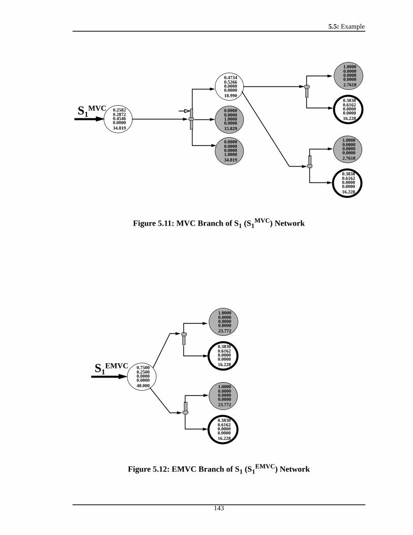
5.5: Example
143
Figure 5.11: MVC Branch of S1 (S1MVC ) Network
Figure 5.12: EMVC Branch of S1 (S1EMVC ) Network
0.25820.28720.45460.000034.819
0.47340.52660.00000.000018.990
0.00000.00001.00000.000015.829
0.00000.00000.00001.000034.819
S1MVC
0.38380.61620.00000.000016.228
1.00000.00000.00000.00002.7618
0.38380.61620.00000.000016.228
1.00000.00000.00000.00002.7618
0.38300.61620.00000.000016.228
1.00000.00000.00000.000023.772
0.75000.25000.00000.000040.000
S1EMVC
0.38300.61620.00000.000016.228
1.00000.00000.00000.000023.772

5.5: Example
144
Another initial composition was chosen such that S2(acetone, chloroform,
methanol) = (0.1, 0.3, 0.6). This composition was located within batch region 3 in Figure
5.6. The resulting batch column network is shown in Figure 5.13. The rectifier, stripper,
MVC, and extractive MVC branches of the network for S2 are shown in Figures 5.14,
5.15, 5.16, and 5.17. The network for S1 and S2 were very similar with one main
difference. The chloroform-methanol binary azeotrope was the UN for the latter example
meaning that we could take this as a product and separate the chloroform and methanol
using an extractive MVC. So a portion of the chloroform could be removed from the
mixture as a pure product with the remainder showing up again as waste product
consisting of the acetone-chloroform binary azeotrope. But it may be much more feasible
to recycle the waste product back into the process as the chloroform will not build up in
the system as seen for Example S1. There were actually two different recoveries of
chloroform possible for Example S2. If we took a chloroform-methanol product anywhere
in the sequence, we recovered 62.92% of the chloroform and all of the other components
as pure products. If we do not take a chloroform-methanol product anywhere in the
sequence, the best recovery of chloroform is 46.48%. Figure 5.18 shows example
sequences of each of these two kinds of chloroform recoveries.
The initial composition for the two examples drastically affected the possible pure
products that were obtainable. While the two networks were very similar, only S2 was
capable of producing any pure chloroform. For the example of acetone/chloroform/
methanol, another entrainer agent could be chosen such that the acetone-chloroform
binary azeotrope could be separated resulting in a 100% recovery of all pure components.

5.5: Example
145
Figure 5.13: Column Network for S2
0.00000.65780.34220.000028.697
0.14020.15600.70380.000071.303
0.25820.28720.45460.000038.730
0.00000.00001.00000.000032.573
0.00000.65780.34220.000028.697
0.10000.30000.60000.0000100.00
0.25000.75000.00000.000040.000
0.00000.00001.00000.000060.000
0.00000.00000.00001.0000100.00
0.00001.00000.00000.000018.877
0.00000.00001.00000.00009.8201
0.00000.00000.00001.000028.697
S2
S2R
0.00000.00001.00000.000032.573
0.14830.44490.40680.000067.427
S2S
S2MVC
S2EMVC

5.5: Example
146
Figure 5.14: Rectifier Branch of S2 (S2R) Network
0.25820.28720.45460.000038.730
0.00000.00001.00000.000032.573
0.25820.28720.45460.000038.730
0.00000.00001.00000.000032.573
0.14020.15600.70380.000071.303
0.47340.52660.00000.000021.123
0.00000.00001.00000.000050.180
0.00000.00000.00001.000071.303
0.47340.52660.00000.000021.123
0.00000.00001.00000.000017.607
0.00000.00000.00001.000038.730
1.00000.00000.00000.00003.0719
0.38380.61620.00000.000018.051
S2R
1.00000.00000.00000.00003.0719
0.38380.61620.00000.000018.051

5.5: Example
147
Figure 5.15: Stripper Branch of S2 (S2S) Network
0.25820.28720.45460.000038.730
0.00000.65780.34220.000028.697
0.14830.44490.40680.000067.427
0.25000.75000.00000.000040.000
0.00000.00001.00000.000027.427
0.00000.00000.00001.000067.427
0.00001.00000.00000.000018.877
0.00000.00001.00000.00009.8200
0.00000.00000.00001.000028.697
1.00000.00000.00000.00003.0719
0.38380.61620.00000.000018.051
S2S
0.47340.52660.00000.000021.123
0.00000.00001.00000.000017.607
0.00000.00000.00001.000038.730
0.38300.61620.00000.000026.055
0.00001.00000.00000.000013.945
0.25820.28720.45460.000038.730
0.00000.65780.34220.000028.697
1.00000.00000.00000.00003.0719
0.38380.61620.00000.000018.051
0.38300.61620.00000.000026.055
0.00001.00000.00000.000013.945

5.5: Example
148
Figure 5.16: MVC Branch of S2 (S2MVC ) Network
Figure 5.17: EMVC Branch of S2 (S2EMVC ) Network
0.25820.28720.45460.000038.730
0.47340.52660.00000.000021.123
0.00000.00001.00000.000017.607
0.00000.00000.00001.000038.730
S2MVC
0.38380.61620.00000.000018.051
1.00000.00000.00000.00003.072
0.38380.61620.00000.000018.051
1.00000.00000.00000.00003.072
0.38300.61620.00000.000026.055
0.00001.00000.00000.000013.945
0.25000.75000.00000.000040.000
S2EMVC
0.38300.61620.00000.000026.055
0.00001.00000.00000.000013.945

5.5: Example
149
Figure 5.18: Comparison of Recoveries of Chloroform
Another interesting observation is that all instances of the MVC only have one
possible residue. We showed in Section 5.3.2 that the MVC can have multiple possible
residues. The basic distillation regions that Examples S1 and S2 occupy consist of three
nodes. When all of the top product (UN) and bottoms product (SN) are removed, the only
0.00000.65780.34220.000028.697
0.14020.15600.70380.000071.303
0.10000.30000.60000.0000100.00
S2
0.47340.52660.00000.000021.123
0.00000.00001.00000.000050.180
0.00000.00000.00001.000071.303
1.00000.00000.00000.00003.0719
0.38380.61620.00000.000018.051
0.00001.00000.00000.000018.877
0.00000.00001.00000.00009.8201
0.00000.00000.00001.000028.697
0.25000.75000.00000.000040.000
0.00000.00001.00000.000060.000
0.00000.00000.00001.0000100.00
0.38300.61620.00000.000026.055
0.00001.00000.00000.000013.945
30 mol C
18.877 mol C
13.945 mol C(46.48% recovery)
(62.92% recovery)

5.6: Impact of Synthesis Assumptions
150
possible MVC residue is the other node in the region. Multiple MVC residues can
possibly occur when the basic distillation region is made up of four or more nodes
5.6 Impact of Synthesis Assumptions5.6.1 Straight Line Distillation Boundaries
As pointed out by Safrit and Westerberg (1996), there are several implications of
assuming straight line distillation boundaries mainly dealing with the predicted batch
products. The assumption does not affect the distillation region finding tool to any great
degree, but it seriously affects the column sequencing algorithm presented here. The
amount of a product in a particular mixture can be quite different when we allow the
boundaries to be curved instead of straight. Boundary curvature may also allow a
sequence to move into another batch region by using different batch column
configurations in series. For example, in Figure 5.19 we could take the initial still
composition S and take out a distillate product D1 using a batch rectifier. We will continue
to take D1 as the distillate product with the still path moving directly away from D1 until
the still path intersects the distillation boundary AC-B. If we assume straight line
boundaries, this intersection would be X while the intersection would be R1 if we were
using the actual curved boundary. We were able to remove more of the D1 product when
we used the curved boundary. Now let us take the residue of the batch rectifier and feed it
to a batch stripper. Using straight line boundaries, our bottoms product would be B2 and
the residue would be the AC binary azeotrope. However, if we had used the curved
boundary, our bottoms product would still have been B2, but the residue would be R2
which is in a different batch region than the initial still composition. The residue R2 would
then be feed to a batch rectifier producing C as a distillate product and AC as the residue.

5.6: Impact of Synthesis Assumptions
151
The amount of the AC residue product would be small as the majority of A would have
already been taken out in the first column. The azeotrope can then be recycled. Recycling
can also benefit from curved boundaries as we showed in Section 5.3.3. As we have
shown, straight line boundaries can limit and remove the types of feasible sequences we
can generate.
Figure 5.19: Impact of Curved Boundaries of Batch Column Sequencing
5.6.2 Total Reflux/Reboil and Infinite Number of TraysThe assumptions of total reflux/reboil and infinite number of trays affect the purity
of product that can be obtained. Using these assumptions, the distillate or bottoms
products using nonextractive batch columns will be the unstable or stable node
respectively. If we were to relax these assumptions, the products now would be close to
their original states but slightly less pure depending on how much we have relaxed the
assumptions. Also, the switching between product cuts will not be instantaneous. So waste
or slop cuts will have to be taken between product cuts in order to meet any purity
specifications. These slop cuts must be processed further either as disposed waste or as a
recycled product. And as seen in other works such as Wahnschafft et al. (1992), some very
A C56.07oC 60.62oC64.06oC
80.14oC
AC
B
S
D1
R1
B2
R2
X

5.7: Conclusions
152
curved boundaries can be crossed at finite reflux resulting in further feasible separations.
5.7 ConclusionsAzeotropic mixtures can severely limit the feasible products one can obtain using
batch distillation. These azeotropes can create batch distillation regions where the region
is defined by the product sequence associated with the particular distillation region. A
sequence of several batch columns consisting of different types of batch column
configurations may be necessary in order to separate out the mixture into its pure
components. There may also exist many of these feasible sequences, each having its own
benefits and drawbacks. All of these sequences must be analyzed during the synthesis and
early design phase so the best separation system is chosen for further design and analysis.
We have showed how to use a tool for finding batch distillation regions in
generating the network of all possible batch column sequences. Under the assumptions of
total reflux/reboil, infinite number of trays, and straight line distillation boundaries, this
tool was capable of finding the distillation regions for four different batch column
configurations: rectifier, stripper, middle vessel column, and extractive middle vessel
column. We found that the initial mixture composition could seriously affect the types of
pure component products we could obtain and that different entrainer agents were
necessary in order to recover all of pure components.
The assumptions of total reflux/reboil, infinite number of trays, and straight line
distillation boundaries need to be removed from the problem so the effects of recycling
and remixing can be further explored. It may be possible that these assumptions remove
feasible and even optimal designs from consideration as the network is sure to grow when

5.8: Nomenclature
153
these assumptions are removed from the problem.
5.8 NomenclatureNC = number of componentsNN = number of nodes (pure component and azeotropic)MVC = middle vessel columnxi = liquid mole fractionyi = vapor mole fractionK = yi / xiUN = unstable nodeSN = stable nodeni = i-th batch region vector (i=1..NN)s = composition vectorαi = i-th batch region vector multiplier (i=1..NN)
5.9 AcknowledgmentsThis work has been supported by Eastman Chemicals and the Engineering Design
Research Center, a NSF Engineering Research Center, under Grant No. EEC-8943164.

5: References
154
References
Ahmad B. S., and P. I. Barton,1995a. “Solvent Recovery Targeting for PollutionPrevention in Pharmaceutical and Specialty Chemical Manufacturing.”AIChESymposium Series.90, p. 59 - 73.
Ahmad B. S., and P. I. Barton,1995b. “Synthesis of Batch Processes with IntegratedSolvent Recovery and Recycling.” Presented the AIChE Annual Meeting, MiamiBeach, FL.
Ahmad B. S., Y. Zhang, and P. I. Barton,1995. “Pollution Prevention in Pharmaceuticaland Specialty Chemical Manufacturing: The Theory of HomogeneousMulticomponent Azeotropic Batch Distillation.” In Preparation.
Bernot C., M. F. Doherty, and M. F. Malone,1991. “Feasibility and SeparationSequencing in Multicomponent Batch Distillation.”Chemical EngineeringScience, 46, p. 1311-1326
Chiotti O. J., and O. A. Iribarren, 1989. “An Optimization Module for Batch Distillationwith Intermediate Cuts.”Computers in Industry, 13, p. 169-180.
Ewell R. H. and L. M. Welch,1945. “Rectification in Ternary Systems Containing BinaryAzeotropes.” Ind. Eng. Chem. Res.37 (12), p. 1224-1231.
Kondili E., C. C. Pantelides, and R. W. H. Sargent,1993. “A General Algorithm for Short-term Scheduling of Batch Operations-I: MILP Formulation.”Computers andChem. Engng., 17(2), p. 211-227.
Safrit B. T., A. W. Westerberg, U. M. Diwekar, O. M. Wahnschafft,1995a. “ExtendingContinuous Conventional and Extractive Distillation Feasibility Insights to BatchDistillation.” Ind. Eng. Chem. Res., 34, p. 3257-3264.
Safrit B. T., A. W. Westerberg, U. M. Diwekar, O. M. Wahnschafft,1995b. “ImprovedOperational Polices for Batch Extractive Distillation Columns.” Tech ReportEDRC 06-200-95, Engineering Design and Research Center, Carnegie MellonUniversity.
Safrit B. T., A. W. Westerberg,1996. “Algorithm for Generating the Distillation Regionsfor Azeotropic Multicomponent Mixtures.” To be submitted toInd. Eng. Chem.Res.
Sargent R. W. H.,1994. “A Functional Approach to Process Synthesis and its Applicationto Distillation Systems.” Centre for Process Systems Engineering, ImperialCollege of Science, Technology and Medicine.
Sundaram S., and L. B. Evans,1993. “Synthesis of Separations by Batch Distillation.”

5: References
155
Industrial Engineering and Chemical Research, 32, p. 500-510.
Wahnschafft O. M.; J. W. Koehler; E. Blass; and A. W. Westerberg,1992. “The ProductComposition Regions of Single Feed Azeotropic Distillation Columns.” Ind. Eng.Chem. Res., 31, 2345-2362.
Wahnschafft O. M. and A. W. Westerberg,1993. “The Product Composition Regions ofAzeotropic Distillation Columns. 2. Separability in Two-Feed Columns andEntrainer Selection.” Ind. Eng. Chem. Res., 32, 1108-112

156
Chapter 6
Conclusions and Future Directions
6.1 ConclusionsIn order to synthesize sequences of batch distillation columns, we first explored a
relatively new type of batch column configuration called a middle vessel column. Using
insights developed for continuous distillation, we were able to map out the feasible
product regions for the batch rectifier, stripper, and middle vessel column given the
current still composition. We were also able to identify the regions of possible column
profiles given product specifications and were able to determine if the product
specifications were feasible. In the case of an infeasible product specification, we again
used insights developed for extractive continuous distillation and found that extractive
batch distillation can make some infeasible product specifications feasible. We also
showed how one can “steer” the still composition versus time and separate out all pure

6.1: Conclusions
157
components from a 3-component mixture. Using this still path steering, we were able
theoretically to recover 100% of the pure components from a binary mixture using the
extractive middle vessel column. Comparisons to the extractive batch rectifier showed that
the rectifier required an infinite size still pot but the middle vessel column did not.
We then further investigated the operation of the extractive middle vessel column.
There were many adjustable parameters for the extractive middle vessel column such as
the reflux/reboil ratio policies, entrainer and bottoms flow rate policies, vapor boilup rate
policies, and fraction switching times that affected the operation of this kind of column.
Simulation studies showed that the final profit of the operation was indeed sensitive to
these optimization variables. A different bottoms flow rate policy than the still path
steering algorithm was simulated and found to slightly improve the final profit. However,
we showed that the normal still path steering algorithm was a good first guess for the
bottoms flow rate policy.
A tool for finding the continuous and batch distillation boundaries and regions for
any mixture was then developed. Using maximum and minimum separating surfaces, we
divided the composition space into subregions each having its own unstable and stable
nodes. These subregions were the basic distillation regions from which we showed how to
determine the continuous and batch boundaries and regions. The tool was validated by
correctly finding the distillation regions for all topologically possible 3-component
systems and several different 4-component systems. We then used this tool in synthesizing
sequences of batch columns. Several different batch column configurations were used and
all were operated at total reflux/reboil and infinite number of trays except for the

6.2: Future Directions
158
extractive middle vessel column. Using state-task networks, we were able to represent the
network of all possible batch column sequences for a particular initial composition.
6.2 Future DirectionsThe extractive middle vessel column, with it many adjustable parameters, needs to
be investigated further. The entire three fraction operation (start-up, main distillate
recovery, and waste cut step) needs to be solved as an optimal control problem with
variables such as reflux/reboil ratio policies, entrainer and bottoms flow rate polices, and
fraction switching times as the optimized variables. Only in solving this problem as an
optimal control can the best values for these variables be found.
The assumptions of straight line boundaries and total reflux/reboil and infinite
number of trays need to be removed from the batch region finding and column sequencing
tools. Once these assumptions are removed, we can begin to explore recycling as a means
of extending the types of feasible separation sequences. The number of feasible batch
column sequences will surely increase as well. The distillation region finding tool is also
sufficiently small enough that it could be placed into other software or optimization
routines with the purpose of proper initialization and screening of proposed designs,
finding potential products, screening of possible entrainers for a particular mixture, or
optimizing process solvents and conditions for increased separation capabilities.

Nomenclature
159
Nomenclature
αi = i-th batch region vector multiplier (i=1..NN)βi = Weighting factor for product iB = Bottoms product flow rateD = Distillate product flow rateDB = Still path direction due to bottoms product removalDD = Still path direction due to distillate product removalDE = Still path direction due to entrainer addition∆ = Delta pointE = Entrainer flow rateλ(i,j) = Wilson interaction parameter,λijH = Still HoldupINT(list_nodes) = intersection list which are the nodes appearing in a least two
of the UNL or SNL of the list_nodesKi = relative volatitivy = yi / xiLA = Constant parameter in flow rate policy equationLB = Linear parameter in flow rate policy equationLj = Liquid flow rate from tray jMVC = middle vessel columnni = i-th batch region vector (i=1..NN)NEntrainer = Entrainer feed locationNLower = Number of trays in lower section of columnNUpper = Number of trays in upper section of columnNC = number of componentsNN = number of nodes (pure component and azeotropic)Pi = Amount of product is = composition vectorS = Still or middle vessel compositionSN = stable nodeSNL(stable node) = common SN list which are the nodes reached by decreasing
temperature from stable nodeT1 = Fraction switching timeT2 = Operation ending timetopt1 = Time of best accumulated profitUN = unstable nodeUNL(unstable node) = common UN list which are the nodes reached by increasing
temperature from unstable nodeVj = Vapor flow rate from tray jxb = Bottom product compositionxd = Distillate product compositionx∆ = ∆ point compositionxe = Entrainer composition
Nomenclature
160
xi = liquid mole fractionxs = Still compositionyi = vapor mole fraction

References
161
References
Ahmad B. S., and P. I. Barton,1995a. “Solvent Recovery Targeting for PollutionPrevention in Pharmaceutical and Specialty Chemical Manufacturing.”AIChESymposium Series.90, p. 59 - 73.
Ahmad B. S., and P. I. Barton,1995b. “Synthesis of Batch Processes with IntegratedSolvent Recovery and Recycling.” Presented the AIChE Annual Meeting, MiamiBeach, FL.
Ahmad B. S., Y. Zhang, and P. I. Barton,1995. “Pollution Prevention in Pharmaceuticaland Specialty Chemical Manufacturing: The Theory of HomogeneousMulticomponent Azeotropic Batch Distillation.” In Preparation.
Baburina L. V., V. M. Platonov, and M. G. Slin’ko,1988. “Classification of Vapor-LiquidPhase Diagrams for Homoazeotropic Systems.”Theor. Found. Chem. Eng. 22, p.390-396.
Bernot C., M. F. Doherty, and M. F. Malone,1990. “Patterns of Composition Change inMulticomponent Batch Distillation.”Chemical Engineering Science, 45, p. 1207-1221.
Bernot C., M. F. Doherty, and M. F. Malone,1991. “Feasibility and SeparationSequencing in Multicomponent Batch Distillation.”Chemical EngineeringScience, 46, p. 1311-1326
Chiotti O. J., and O. A. Iribarren,1989. “An Optimization Module for Batch Distillationwith Intermediate Cuts.”Comput. in Industry, 13, 169-180.
Devidyan A. G., V. N. Kira, G. A. Meski, and M. Morari,1994. Batch Distillation in aColumn with a Middle Vessel.Chem. Eng. Sci., 49 (18), 3033-3051.
Devyatikh G. G. and M. F. Churbanov.Methods of High Purification.Znanie, 1976.
Devidyan A. G., V. N. Kira, G. A. Meski, and M. Morari,1994. Batch Distillation in aColumn with a Middle Vessel.Chem. Eng. Sci., 49 (18), 3033-3051.
Diwekar U. M., K. P. Madhavan, R. E. Swaney,1989. "Optimization of MulticomponentBatch Distillation Columns."Industrial Engineering and ChemistryResearch,28,p. 1011-1017.
Diwekar U. M., and K. P. Madhavan,1991. “Batch-Dist: A comprehensive Package forSimulation, Design, Optimization and Optimal Control of Multicomponent,Multifraction Batch Distillation Column.” Comput. Chem. Eng., 12, 833-842.
Doherty M. F.,1985. “The Presynthesis Problem for Homogeneous Azeotropic

References
162
Distillations has a Unique Explicit Solution.” Chem. Eng. Sci. 40, p. 1885-1889.
Doherty M. F. and G. A. Caldarola,1985. “Design and Synthesis of HomogeneousAzeotropic Distillations. 3. The Sequencing of Columns for Azeotropic andExtractive Distillations.”Ind. Eng. Chem. Fundam. 24, p. 474-485.
Ewell R. H. and L. M. Welch. Rectification in Ternary Systems Containing BinaryAzeotropes. Ind. Eng. Chem. Res. 1945, 37 (12), 1224-1231.
Farhat S., M. Czernicki, L. Pibouleau, and S. Domenech,1990. “Optimization ofMultiple-Fraction Batch Distillation by Nonlinear Programming.”AICHEJournal, 36, 1349-1360.
Fidkowski Z. T., M. F. Doherty, and M. F. Malone,1993. “Computing Azeotropes inMulticomponent Mixtures.”Computers chem. Engng, 17, p. 1141-1155
Hasebe S.; B. B. Abdul Aziz; I. Hashimoto; and T. Watanabe. Optimal Design andOperation of Complex Batch Distillation Column.Proc. IFAC Workshop, London,1992.
Hindmarsh A. C. ODEPACK: A Systematized Collection of ODE Solvers.ScientificComputing. 1983, 55-64.
Kondili E., C. C. Pantelides, and R. W. H. Sargent,1993. “A General Algorithm for Short-term Scheduling of Batch Operations-I: MILP Formulation.”Computers andChem. Engng., 17(2), p. 211-227.
Koehler J., H. Haverkamp, and N. Schadler,1995. “Zur diskontinuierlichen Rektifikationazeotroper Gemische mit Hilfsstoffeinsatz.” Submitted toChemie-Ingenieur-Technik.
Lang P., Lelkes Z., P. Moszkowicz, M. Otterbein, and H. Yatim,1995. “DifferentOperational Policies for the Batch Extractive Distillation.” Computers chem.Engng., 19,S645-S650.
Malenko Y. I.,1970a. “Physicochemical Analysis of Fractional Distillation Diagrams. I.Theoretical Basis of Method”Russian Journal of Physical Chemistry, 44, p. 824-826.
Malenko Y. I.,1970b. “Physicochemical Analysis of Fractional Distillation Diagrams. II.Quaternary Systems”Russian Journal of Physical Chemistry, 44, p. 916-919.
Malenko Y. I.,1970c. “Physicochemical Analysis of Fractional Distillation Diagrams. III.Multicomponent (n-Component) Systems”Russian Journal of PhysicalChemistry, 44, p. 920-922.

References
163
Malone M. F.,1996. Personal Correspondence.
Matsuyama H.,1975. “Synthesis of Azeotropic Distillation Systems.” Presented at theJAPAN-US Joint Seminar, Kyoto, Japan.
Meski G. A. and M. Morari,1993. “Batch Distillation in a Column with a Middle Vessel.”Presented at AIChE Annual Meeting, St. Louis, paper 152a.
Petlyuk F. B.,1979. “Structure of Concentration Space and Synthesis of Schemes forSeparating Azeotropic Mixtures.”Theor. Found. Chem. Eng. 13, p. 683-689.
Petlyuk F. B., V. Y. Kienskii, and L. A. Serafimov, 1977. “Method for the Isolation of theRegions of the Rectification of Polyazeotropic Mixtures using an ElectronicComputer.”Theor. Found. Chem. Eng. 11, p. 1-7.
Piela P., R. McKelvey, and A. W. Westerberg,1993. “An Introduction to the ASCENDModeling System: Its Language and Interactive Environment.”J. ManagementInformation Systems, 9, 91-121.
Safrit B. T., A. W. Westerberg, U. M. Diwekar, O. M. Wahnschafft,1995a. “ExtendingContinous Conventional and Extractive Distillation Feasibility Insights to BatchDistillation.” Ind. Eng. Chem. Res., 34, 3257-3264.
Safrit B. T., A. W. Westerberg, U. M. Diwekar, O. M. Wahnschafft,1995b. “ImprovedOperational Polices for Batch Extractive Distillation Columns.” Tech ReportEDRC 06-200-95, Engineering Design and Research Center, Carnegie MellonUniversity.
Safrit B. T., A. W. Westerberg,1996. “Algorithm for Generating the Distillation Regionsfor Azeotropic Multicomponent Mixtures.” To be submitted toInd. Eng. Chem.Res.
Sargent R. W. H.,1994. “A Functional Approach to Process Synthesis and its Applicationto Distillation Systems.” Centre for Process Systems Engineering, ImperialCollege of Science, Technology and Medicine.
Serafimov L. A.,1987. “Thermodynamic Topological Analysis and the Separation ofMulticomponent Polyazeotropic Mixtures.”Theor. Found. Chem. Eng. 21, p.44-54.
Serafimov L. A., F. B. Petlyuk, and I. B. Aleksandrov,1974. “The Number of TrajectoryClusters Representing Continuous Rectification of Azeotropic MulticomponentMixtures.” Theor. Found. Chem. Eng. 8, p.847-850.
Sundaram S., and L. B. Evans,1993. “Synthesis of Separations by Batch Distillation.”Industrial Engineering and Chemical Research, 32, p. 500-510.

References
164
Van Dongen D. B., and M. F. Doherty,1984. “On the Dynamics of Distillation Processes- V. The Topology of the Boiling Temperature Surface and its Relation toAzeotropic Distillation.”Chemical Engineering Science, 39, p. 883-892.
Van Dongen D. B., and M. F. Doherty,1985. “On the Dynamics of Distillation Processes- VI. Batch Distillation.”Chemical Engineering Science, 40, p. 2087-2093.
Wahnschafft O. M., J. W. Koehler, E. Blass, and A. W. Westerberg,1992. “The ProductComposition Regions of Single Feed Azeotropic Distillation Columns.” Ind. Eng.Chem. Res., 31, 2345-2362.
Wahnschafft O. M. and A. W. Westerberg,1993. “The Product Composition Regions ofAzeotropic Distillation Columns. 2. Separability in Two-Feed Columns andEntrainer Selection.” Ind. Eng. Chem. Res., 32, 1108-1120.
Westerberg A.W., and O. Wahnschafft,1996. “Synthesis of Distillation-Based SeparationProcesses.” To appear inAdvances in Chemical Engineering, Academic Press,23.
Wu W., and T. Chiou,1989. "Determination of Feasible Reflux Ratios and MinimumNumber of Plates Required in Multicomponent Batch Distillation."IndustrialEngineering and Chemical Research, 28, p. 1862-1867.
Yatim H.; P. Moszkowicz; M. Otterbein; and P. Lang. Dynamic Simulation of a BatchExtractive Distillation Process. European Symposium on Computer Aided ProcessDesign-2.1993, S57-S63.