synthesis of service life prediction for bridges in texas ... · 1. report no. fhwa/tx-19/0-6938-1...

TECHNICAL REPORT

Sponsored by the Texas Department of Transportation

TECHNICAL REPORT 0-6938-1

TxDOT PROJECT NUMBER 0-6938

Synthesis of Service Life Prediction for Bridges in Texas: Final Report

Lu Gao Yi-Lung Mo Shalaka Dhonde Daisy Saldarriaga Lingguang Song Ahmed Senouci August 2017; Published March 2019

University of Houston College of Technology Department of Construction Management

1. Report No.FHWA/TX-19/0-6938-1

2. Government Accession No. 3. Recipient's Catalog No.

4. Title and SubtitleSynthesis of Service Life Prediction for Bridges in Texas: Final Report

5. Report DateSeptember 2017; Published March2019

6. Performing Organization Code7. Author(s)

Lu Gao, Yi-Lung Mo, Shalaka Dhonde, Daisy Saldarriaga, LingguangSong, Ahmed Senouci

8. Performing Organization Report No.0-6938-1

9. Performing Organization Name and Address 10. Work Unit No. (TRAIS)University of Houston4800 Calhoun RoadHouston, TX 77204-4003

11. Contract or Grant No.0-6938

12. Sponsoring Agency Name and AddressTexas Department of TransportationResearch and TechnologyImplementation OfficeP. O. Box 5080Austin, Texas 78763-5080

13. Type of Report and Period CoveredTechnical ReportSept 1, 2016 – Sept 30 2017

14. Sponsoring Agency Code

15. Supplementary NotesProject performed in cooperation with the Texas Department of Transportation and the Federal Highway Administration.

16. AbstractIn procurement requirements for design-build project contracts for bridge structures, the Texas Department ofTransportation (TxDOT) may implement a 100-year service life requirement. However, there are no indicated measuresor any technical recommendations that provide directions to satisfy the given requirement of service life. In addition,TxDOT and consultants use TxDOT recommendations for durability to improve performance during service life ofdesign-bid-build and design-build projects but no quantitative methods or codified guidance is available to validate howthe enhanced service life requirements are met. Further, the state of Texas has large number of existing old bridge thusthe evaluation of the remaining service life of these bridges is a very important economic issue for TxDOT. Thereplacement of all these bridges is not possible since the available financial resources are limited. Therefore, it is veryessential to prioritize the repair works based on the estimated remaining service life. As a result, this research study hasbeen conducted to obtain information about state-of-the-art and state-of practice of bridge service life prediction. Theresearch team gathered and analyzed the relevant information on various topics related to service life prediction whichcan be utilized as guidelines while dealing with the determination of service life of old as well as new bridges.

The extensive literature survey conducted by the research team provides valuable information for TxDOT which can be helpful for service life prediction of bridges in the state of Texas. By utilizing the collected information under the scope of the project, the following benefits can be achieved: 1) This project would provide guidance on managing available funds efficiently for the required repair activities using the data on condition of the bridges. 2). The review of the available information obtained from different sources would provide better understanding of various deterioration models used for predicting service life, inspection checks and methods, maintenance practices and rehabilitation or replacement requirements for bridges, and would enhance the knowledge on achieving and extending the service life of bridges in Texas. 3). The output from this research project would be beneficial for maintaining the existing bridges in a good condition, improving their service life to make them economically efficient and determining strategies to achieve design service life for newly constructed bridges.

17. Key WordService Life Prediction, Bridge, Mechanistic Model,Empirical Model, Corrosion Control

18. Distribution StatementNo restrictions. This document is available to the publicthrough the National Technical Information Service,Springfield, Virginia 22161; www.ntis.gov.

19. Security Classif. (of this report)Unclassified

20. Security Classif. (of this page)Unclassified

21. No. of Pages174

22. Price

Synthesis of Service Life Prediction for Bridges in Texas: Final Report

by

Lu Gao, Yi-Lung Mo, Shalaka Dhonde, Daisy Saldarriaga, Lingguang Song, Ahmed Senouci

Research Project 0-6938

Department of Construction Management

Department of Civil Engineering University of Houston (UH)

Performed in Cooperation with the

Texas Department of Transportation and the Federal Highway Administration

August 31, 2017

iii

Disclaimer

This research was performed in cooperation with the Texas Department of Transportation and the U.S. Department of Transportation, Federal Highway Administration. The contents of this report reflect the views of the authors, who are responsible for the facts and accuracy of the data presented herein. The contents do not necessarily reflect the official view or policies of the FHWA or TxDOT. This report does not constitute a standard, specification, or regulation, nor is it intended for construction, bidding, or permit purposes. Trade names were used solely for information and not product endorsement.

iv

Table of Contents

Chapter 1. Introduction ............................................................................................................... 1

Chapter 2. Durability Related Tests for Concrete Bridge ........................................................ 2

2.1 Concrete Condition ........................................................................................................... 4

2.1.1 Surface Defects (e.g., Crack, Delamination, Spalling) .............................................. 4

2.1.2 Concrete Resistivity and Permeability ....................................................................... 9

2.1.3 Concrete Cover and Rebar Distribution ................................................................... 13

2.1.4 Concrete Strength..................................................................................................... 13

2.1.5 Sulfate Resistance Test ............................................................................................ 16

2.1.6 Alkali-Silica Reaction Tests .................................................................................... 16

2.2 Rebar Corrosion Condition ............................................................................................. 17

2.2.1 Corrosion Potential .................................................................................................. 17

2.2.2 Corrosion Rate ......................................................................................................... 17

2.2.3 Chloride Related Test .............................................................................................. 18

2.2.4 Carbonation Depth Measurement Test .................................................................... 20

2.3 Case Studies .................................................................................................................... 21

2.3.1 NCHRP Project 558 (Sohanghpurwala, 2006) ........................................................ 21

2.3.2 VDOT (Williamson et al., 2007) ............................................................................. 22

Chapter 3. Durability Related Tests for Steel Bridge .............................................................. 24

3.1 Fatigue ............................................................................................................................. 24

3.1.1 Acoustic Emission (AE) .......................................................................................... 24

3.1.2 Smart Paint ............................................................................................................... 24

3.1.3 Penetrant Test (Dye Penetrant) ................................................................................ 24

3.1.4 Magnetic Particle ..................................................................................................... 24

3.2 Corrosion ......................................................................................................................... 25

3.2.1 Corrosion Sensors .................................................................................................... 25

3.2.2 Robotic Inspection ................................................................................................... 25

3.2.3 Radiology Neutron Method (Thermal Neutron Radiography) ................................ 25

3.2.4 Optical Holography .................................................................................................. 26

3.3 Other Defects................................................................................................................... 26

3.3.1 Radiographic Testing ............................................................................................... 26

3.3.2 Ultrasonic Testing (UT) ........................................................................................... 27

3.3.3 Eddy Current ............................................................................................................ 27

v

Chapter 4. Empirical Models for Predicting Bridge Service Life .......................................... 28

4.1 Factors Affecting the Deterioration and Service Life of Concrete Bridges .................... 28

4.2 Factors Affecting the Deterioration and Service Life of Steel Bridges .......................... 28

4.3 Service Life Prediction Models ....................................................................................... 28

4.4 Bridge Condition Data .................................................................................................... 29

4.5 Models From Previous Studies ....................................................................................... 29

4.5.1 Linear/Non-linear Regression Models ..................................................................... 29

4.5.2 Time Series Models ................................................................................................. 33

4.5.3 Panel Data Models/Dynamic Panel Models ............................................................ 33

4.5.4 Discrete Choice Models ........................................................................................... 34

4.5.5 Duration Models or Survival Models or Reliability Models ................................... 34

4.5.6 Weibull Survival Models ......................................................................................... 37

4.5.7 Markov Models ........................................................................................................ 37

4.5.8 Markov Chain Based Models................................................................................... 37

4.5.9 Semi-Markov Models .............................................................................................. 41

4.5.10 Stochastic Gamma Process Deterioration Models ................................................. 41

4.5.11 Artificial Intelligence Models ................................................................................ 42

4.6 Case Study Using Texas Bridge Data ............................................................................. 44

4.6.1 Data .......................................................................................................................... 44

4.6.2 Variables .................................................................................................................. 44

4.6.3 Models...................................................................................................................... 44

4.7 Review of Bridge Infrastructure Maintenance Planning Models .................................... 47

4.7.1 Markov Chain Based Linear Programming (LP) ..................................................... 48

4.7.2 Integer Programming (IP) ........................................................................................ 51

4.7.3 Reliability Model ..................................................................................................... 52

Chapter 5. Mechanistic Models for Predicting Bridge Service Life ...................................... 53

5.1 Chloride-Induced Corrosion for Concrete Bridge ........................................................... 53

5.1.1 Deterioration Process ............................................................................................... 53

5.1.2 Service Life Estimation............................................................................................ 55

5.2 Carbonation-Induced Corrosion for Concrete Bridge ..................................................... 66


5.2.2 Carbonation Service Life Prediction ........................................................................ 68

5.3 Sulfate Attack Deterioration for Concrete Bridge........................................................... 71


5.3.2 Sulfate Attack Service Life Prediction .................................................................... 71

vi

5.4 Freeze-Thaw Deterioration for Concrete Bridge ............................................................ 72


5.4.2 Service Life Prediction ............................................................................................ 73

5.4.3 Commercial Software .............................................................................................. 74

5.5 Alkali Silica Reaction Deterioration for Concrete Bridge .............................................. 74


5.5.2 Service Life Prediction ............................................................................................ 75

5.6 Fatigue Life Prediction for Steel Bridge ......................................................................... 76

5.6.1 Fatigue Life Prediction ............................................................................................ 76

Chapter 6. Corrosion Control Methods .................................................................................... 80

6.1 Impacts of Corrosion Control Methods on Bridge Service Life ..................................... 81

6.2 Mechanical Barrier Methods ........................................................................................... 82

6.2.1 Protective Coatings .................................................................................................. 82

6.2.2 Corrosion-Resistant Reinforcement ......................................................................... 82

6.2.3 Corrosion-Resistant Materials ................................................................................. 84

6.2.4 High-performance Concrete..................................................................................... 85

6.3 Electrochemical Methods ................................................................................................ 87

6.3.1 Cathodic Protection .................................................................................................. 87

6.3.2 Electrochemical Chloride Extraction ....................................................................... 87

6.3.3 Corrosion Inhibitors ................................................................................................. 87

6.4 Corrosion Control for Existing Concrete Bridges ........................................................... 88

6.4.1 Membranes and sealers ............................................................................................ 89

6.4.2 Low-slump Concrete (dense concrete) .................................................................... 90

6.4.3 Latex-modified Concrete ......................................................................................... 90

6.4.4 Silica Fume Concrete ............................................................................................... 90

6.5 Corrosion Protection for Steel Bridges (Construction and Industrial, 2005) .................. 90

6.5.1 Paint Coatings .......................................................................................................... 90

6.5.2 Metallic Coatings ..................................................................................................... 91

6.5.3 Weathering Steel ...................................................................................................... 92

6.6 Selection of Corrosion Control Alternatives ................................................................... 93

Chapter 7. Service Life Prediction Models for Bridges Older than 75 Years ....................... 94

7.1 Service Life Prediction of SK Bridge in Japan (Emoto et al., 2014) .............................. 94

7.2 Service Life Prediction of Bridge in Canada (Morales and Bauer, 2006) ...................... 96

7.3 Service Life Prediction of Bridges in Indiana (Barde et al., 2009) ................................. 97

7.3.1 Development of the Service Life Model for Corrosion due to Chloride Ingress ..... 97

vii

7.3.2 Development of the Service Life Model for Deterioration due to Freeze-Thaw ..... 99

7.3.3 Development of Model for Shrinkage of Concrete ................................................ 101

7.4 Service Life Prediction for Bridges in Nebraska (Hatami and Morcous, 2011) ........... 102

7.4.1 Deterministic Deterioration Models for Nebraska Bridges (Hatami and Morcous, 2011) .................................................................................................................. 103

7.4.2 Stochastic Deterioration Models for Nebraska Bridges......................................... 106

7.5 Service Life Prediction of Old RC Bridge in Taiwan (Huang et al. 2011) ................... 107

7.6 Service Life Prediction for Bridges in Virginia, Florida, New Jersey, Minnesota, and New York (Balakumaran, 2012) ......................................................................... 108

7.6.1 Virginia Pilot Bridge .............................................................................................. 109

7.6.2 Florida Pilot Bridge................................................................................................ 109

7.6.3 New Jersey Bridge ................................................................................................. 109

7.6.4 Minnesota Pilot Bridge .......................................................................................... 110

7.7 Service Life of Bridges in Canada and Taiwan (Ranjith et al., 2016) .......................... 111

7.7.1 Service Life Prediction of a Vachon Bridge Barrier Wall ..................................... 111

7.7.2 Service Life Prediction of Tzyh-Chyang Bridge Taiwan ...................................... 112

7.7.3 Service Life Prediction of Dah-Duh Bridge in Taiwan ......................................... 112

Chapter 8. Service Life Prediction for Newly Constructed Bridge under Design-build Contracts .............................................................................................................................. 114

8.1 Fib Bulletin 34: Model Code for Service Life Design .................................................. 114

8.1.1 Design service life tSL ............................................................................................ 115

8.1.2 Experimental Tests for Quantification of Parameters ............................................ 115

8.2 Case Studies .................................................................................................................. 118

8.2.1 The New NY Tappan Zee Bridge and the Ohio River Bridge (Bergman, 2016) .. 118

8.2.2 Tappan Zee Bridge ................................................................................................. 119

8.2.3 Gateway Bridge ..................................................................................................... 120

8.2.4 Ohio River Bridge .................................................................................................. 123

8.2.5 FDOT’s Surface Resistivity Test (Presuel-Moreno et al., 2013) ........................... 124

8.2.6 MoDOT’s Surface Resistivity Test (Hudson, 2015).............................................. 124

Chapter 9. Determining Remaining Service Life When a Bridge Is Returned to Its Owner ................................................................................................................................... 126

9.1 Introduction ................................................................................................................... 126

9.2 Case Studies .................................................................................................................. 126

9.2.1 I-595 Corridor Roadway Improvements Project (Fort Lauderdale, Florida) ......... 127

9.2.2 US 181 Harbor Bridge Project (Corpus Christi, Texas) ........................................ 130

9.2.3 Regina Bypass Project (Saskatchewan, Canada) ................................................... 132

viii

9.2.4 Northeast Stoney Trail, (Alberta, Canada) ............................................................ 134

9.2.5 North Commuter Parkway and Traffic Bridge Project (Saskatchewan, Canada， 2015) .................................................................................................................. 135

9.2.6 Portsmouth Bypass Project (Scioto, Ohio) ............................................................ 136

9.2.7 Aberdeen Western Peripheral Route (Aberdeenshire, Scotland) ........................... 141

9.2.8 The Presidio Parkway (San Francisco, California) ................................................ 142

References .................................................................................................................................. 145

Appendix A. Most Commonly Adopted Bridge Service Life Estimation Models ............... 157

ix

List of Figures

Figure 1. Physical Principle of IE (Gucunski et al., 2013) ............................................................. 5

Figure 2. Bridge Deck Survey Using MIRA Ultrasonic System. B-scans (top) and Equipment and Data Collection (bottom) (Gucunski et al., 2013) ............................................. 6

Figure 3. Principle of Impulse Response Testing (Gucunski et al., 2013) ..................................... 8

Figure 4. Evaluation of a Layer Modulus by SASW (USW) Method (Gucunski et al., 2013) ............................................................................................................................................ 8

Figure 5. Principle of Passive Infrared Thermography (Gucunski et al., 2013) ............................. 9

Figure 6. Electrical Resistivity Principle (Gucunski et al., 2013) ................................................ 10

Figure 7. Schematic illustration of concrete resistivity measurement by two-plate method (Presuel-Moreno et al., 2013) ................................................................................................... 11

Figure 8. Schematic diagram of typical concrete failure mechanism during probe penetration (Helal et al., 2015b) ................................................................................................ 14

Figure 9. Schematic diagram of typical pull-out resistance methods (Helal et al., 2015b) .......... 14

Figure 10. Schematic diagram of pull-off resistance NDT method (Helal et al., 2015b) ............. 15

Figure 11. Maturity test apparatus with thermocouple (Helal et al., 2015b) ................................ 16

Figure 12. HCP Principle (Gucunski et al., 2013) ........................................................................ 17

Figure 13. GPM Principle (Gucunski et al., 2013) ....................................................................... 18

Figure 14. Schematic illustrations of bulk diffusion test (Presuel-Moreno et al., 2013) .............. 19

Figure 15. Schematic illustrations of RCM test setup (Presuel-Moreno et al., 2013) .................. 20

Figure 16. Chain Drag................................................................................................................... 21

Figure 17. Continuity Test ............................................................................................................ 22

Figure 18. Corrosion Rate Test ..................................................................................................... 22

Figure 19. General principle of radiography (Balasko and Svab, 1996) ...................................... 26

Figure 20. Confusion Matrix of Naïve Bayes Classification Model ............................................ 46

Figure 21. Confusion Matrix of Decision Tree Classification Model .......................................... 47

Figure 22. Confusion Matrix of Logistic Regression ................................................................... 47

Figure 23. Chloride Corrosion Deterioration Process for a Concrete Element (Hu et al., 2013) .......................................................................................................................................... 53

Figure 24. Schematic diagram of reinforcing steel corrosion in concrete as an electrochemical process. (Zhao et al., 2011) ............................................................................. 54

Figure 25. Schematic diagram of corrosion cracking processes (Liu, 1996)................................ 59

Figure 26. Expansive pressure on surrounding concrete due to formation of rust products (Liu, 1996) ................................................................................................................................. 60

x

Figure 27. Input parameters .......................................................................................................... 60

Figure 28. Effect of corrosion on the diameter and cross-section of reinforcing steel bars, with diameters of 10mm and 20mm (Andrade et al., 1990) ..................................................... 61

Figure 29. Corrosion of steel in concrete as a function of pH (INC., 2005) ................................. 67

Figure 30. Frequency of freeze-thaw exposure typically encountered in different areas of the United States (PCA, 2002) .................................................................................................. 73

Figure 31. Example of data from a representative fatigue test (Fasl, 2013) ................................. 76

Figure 32. Impressed current cathodic protection......................................................................... 87

Figure 33. Flowchart of remaining life prediction (Emoto et al., 2014) ...................................... 96

Figure 34. Probability of cracking for different shrinkage values of three different concrete mixtures (Barde et al., 2009) .................................................................................... 102

Figure 35. Original deck deterioration curve for state bridges (Hatami and Morcous, 2011) ........................................................................................................................................ 104

Figure 36. Deterioration curves of state bridge decks with different ADT- year 2009 (Hatami and Morcous, 2011) .................................................................................................. 104

Figure 37. Deterioration curves of state bridge decks with different ADTT - year 2009 (Hatami and Morcous, 2011) .................................................................................................. 105

Figure 38. Deterioration curves of steel and prestressed concrete superstructure - years 1998 to 2010 (Hatami and Morcous, 2011) ............................................................................ 105

Figure 39. Deterioration model of substructure - years 1998 to 2010 (Hatami and Morcous, 2011) ....................................................................................................................... 106

Figure 40. Deterioration curves of concrete bridge decks at different environments (Hatami and Morcous, 2011) .................................................................................................. 107

Figure 41. Deterioration curves of concrete bridge decks with ECR and BR (Hatami and Morcous, 2011) ....................................................................................................................... 107

Figure 42. Bridge Remaining Service Life Estimation (Huang et al., 2011) ............................. 108

Figure 43. Diffusion Curve for Virginia Pilot Bridge (Balakumaran, 2012) .............................. 109

Figure 44. Diffusion Curve for New Jersey Pilot Bridge (Balakumaran, 2012) ........................ 110

Figure 45. Diffusion Curve of Minnesota Pilot Bridge (Balakumaran, 2012) ........................... 110

Figure 46. Test Cells (NT Build 492, 2017) ............................................................................... 118

Figure 47. Tappan Zee Bridge Concept Design (LaViolette, 2014) ........................................... 119

Figure 48. Gateway Upgrade Project (Gateway Upgrade Project, 2017) ................................... 120

Figure 49. Ohio River Bridge (Ohio Bridge Project Overview, 2017) ....................................... 123

Figure 50. I-595 Corridor Roadway Improvements (I-595, 2017) ............................................. 127

Figure 51. Concept Design of the New Harbor Bridge (TxDOT, 2015) .................................... 130

Figure 52. Regina Bypass Freeway Project (Regina, 2017) ....................................................... 132

xi

Figure 53. Northeast Stoney Trail (Flatiron, 2017) .................................................................... 134

Figure 54. Traffic Bridge Proposed Concept Design (City of Saskatoon, 2017) ....................... 135

Figure 55. Portsmouth Bypass Project (Portsmouth Gateway Group, 2017) ............................. 137

Figure 56. The Route Map of Aberdeen Western Peripheral Route ........................................... 141

Figure 57. Presidio Parkway Map (Wikibooks, 2017) ............................................................... 143

xii

List of Tables

Table 1. Overall Value and Ranking of NDT Technologies (Gucunski et al., 2013) ..................... 3

Table 2. Service life estimation parameters to measure and NDT tests and accuracy ................... 4

Table 3. Correlation between surface resistivity and chloride ion permeability (Presuel-Moreno et al., 2013) .................................................................................................................. 11

Table 4. Relationship between non-steady-state migration coefficients and resistance to chloride penetration (Presuel-Moreno et al., 2013) .................................................................. 20

Table 5. Deterioration of Bridge Components (Bolukbasi et al., 2004) ....................................... 31

Table 6. Confusion Matrix ............................................................................................................ 45

Table 7. Performance Comparison of Classification Models ....................................................... 46

Table 8. Notation .......................................................................................................................... 49

Table 9. A and B Values ............................................................................................................... 63

Table 10. Corrosion Rates and Remaining Service Life (Clear, 1989) ........................................ 64

Table 11. Chloride Threshold Levels ............................................................................................ 64

Table 12. Typical permeability values (IAEA, 2002) ................................................................... 69

Table 13. Values of β (IAEA, 2002) ............................................................................................. 69

Table 14. Summary of corrosion control methods and their impact on bridge service life .......... 82

Table 15. Optimal treatment for various level of corrosion .......................................................... 93

Table 16. Extension in service life for different corrosion control treatments (Sohanghpurwala, 2006) ........................................................................................................... 93

Table 17. Mean values of input parameters (Ranjith et al., 2016) .............................................. 111

Table 18. Remaining service life of RC bridge barrier wall, Vachon Bridge (Ranjith et al., 2016) ........................................................................................................................................ 111


Table 20. Remaining service life of Tzyh-Chyang Bridge, Taiwan. (Ranjith et al., 2016) ........ 112


Table 22. Remaining service life of Dah-duh Bridge, Taiwan (Ranjith et al., 2016) ................. 113

Table 23. Indicative Values for the Design Service Life tSL (Schiessl, 2006) ............................ 115

Table 24. Design-Build-Operate Bridge Projects ....................................................................... 126

Table 25. Handback Requirements (FDOT, 2008) ..................................................................... 129

Table 26. New Harbor Bridge Residual Life at Handback (Years) (TxDOT, 2014) .................. 131

Table 27. Handback Requirements (SaskBuilds, 2015) ............................................................. 133

Table 28. Handback Requirements (City of Saskatoon, 2015) ................................................... 136

xiii

Table 29. Residual Life Requirements ........................................................................................ 139

Table 30. Residual Life of Elements of Structures ..................................................................... 142

Table 31. Handback Requirements (West Coast Infrastructure Exchange, 2016) ..................... 144

1

Introduction The state of Texas has over 50,000 bridges, of which a large number are existing old bridges. The evaluation of the remaining service life of these bridges is a very important economic issue for the Texas Department of Transportation (TxDOT). Therefore, it is necessary to prioritize the repair works based on the estimated remaining service life. The research team has conducted a thorough review of the state-of-the-art and state-of-practice of bridge service life prediction models and the results are summarized in this report. The purpose of this report is to provide TxDOT with a comprehensive summary of prediction model to estimate service life of bridges. Chapter 2 and 3 contain information regarding the durability tests for concrete and steel bridges respectively. Chapter 4 presents empirical models for predicting bridge service life, including a total of 20 models used by other states and countries. A preliminary machine learning modeling of NBI data collected in Texas is also presented in Chapter 4. Chapter 5 presents mechanistic models for predicting bridge service life, including corrosion, carbonation, sulfate attack, freeze-thaw, alkali silica reaction, and fatigue. Corrosion control methods are presented in Chapter 6 and include mechanical barrier and electrochemical methods, as well as a review of alternative materials resistant to corrosion. Chapter 7 contains a review of 12 reports regarding service life prediction models for old bridges. Chapter 8 presents service life prediction for newly constructed bridge under design-build contracts. Chapter 9 presents a review of remaining service life verification at handoff.

2

Durability Related Tests for Concrete Bridge In the United States, the most common Non-Destructive Tests (NDT) includes Acoustic Emission, Electrical Resistivity Method, Delamination Detection Machinery, Ground Penetrating Radar, Electromagnetic Methods, Impact-Echo Testing, Infrared Thermography, Ultrasonic Pulse Echo Testing, Magnetic Method, Neutron Probe, Nuclear Method, Pachometer, Smart Concrete and Rebound and Penetration. Gucunski et al. (2013) graded the performance of each NDT technology for four deterioration types: delamination, corrosion, cracking and concrete deterioration. The final grade values obtained for each NDT method for all deterioration types are showed in the following table. The authors concluded that even though some technologies showed potential for detecting and assessing each deterioration type, no single technology can potentially evaluate all deterioration types. Three technologies were identified as having a good potential for corrosion detection (half-cell potential, electrical resistivity, and galvanostatic pulse measurement) and six technologies were identified as having a good potential for delamination detection (impact echo, ultrasonic pulse echo, impulse response, chain dragging and hammer sounding, ground penetrating radar and infrared thermography).

3

Table 1. Overall Value and Ranking of NDT Technologies (Gucunski et al., 2013)

4

The following table shows the accuracies of the measured parameters in the service-life estimation of reinforced concrete bridges. These accuracies were collected from different sources in the existing literature (Barnes and Zheng, 2008; Hasan and Yazdani, 2016; Gudimettla and Crawford, 2015; Helal et al., 2015a; IAEA, 2002; Lo and Lee, 2002; Her & Lin, 2014).

Table 2. Service life estimation parameters to measure and NDT tests and accuracy

2.1 Concrete Condition 2.1.1 Surface Defects (e.g., Crack, Delamination, Spalling)

2.1.1.1 Impact-Echo Testing

The impact echo (IE) method is a seismic or stress wave–based method used in the detection of defects in concrete, especially delamination (Sansalone and Carino, 1989). The main purpose of impact echo testing is to detect and characterize wave reflectors or “resonators” in a concrete bridge deck. This is achieved by striking the surface of the tested object and measuring the response at a nearby location. The following figure shows the application of the impact echo testing technology to a bridge deck.

5

Figure 1. Physical Principle of IE (Gucunski et al., 2013) Applications:

• Characterization of surface-opening cracks (vertical cracks in bridge decks). • Detection of ducts, voids in ducts, and rebars. • Material characterization.

Limitations:

• In case of a deck with asphalt concrete overlay, detection of delamination is possible only when the asphalt concrete temperature is sufficiently low so that the material is not highly viscous, or when the overlay is intimately bonded to the deck.

• It is necessary to conduct data collection on a very dense test grid to define the boundary conditions for delaminated areas accurately.

2.1.1.2 Ground Penetrating Radar (GPR)

Ground Penetrating Radar is one of the rapid NDT methods which uses electromagnetic (EM) waves to locate objects buried inside the structure and produce contour maps of subsurface features such as steel reinforcement, wire mesh, etc. In this type of NDT method, GPR antenna transmits high EM waves into bridge deck and then a portion of energy is reflected back to the surface from reflector present inside. This energy is further received by antenna. GPR uses electromagnetic waves to locate objects buried inside the structure and to produce contour maps of subsurface features (steel reinforcements, wire meshes, or other interfaces inside the structures). Applications:

• Condition assessment of bridge decks and tunnel linings • Pavement profiling • Mine detection • Archaeological and geophysical investigations • Borehole inspection and building inspection

6

• Evaluation of the deck thickness • Measurement of the concrete cover and rebar configuration • Characterization of delamination potential • Characterization of concrete deterioration • Description of concrete as a corrosive environment • Estimation of concrete properties

Limitations:

• Inability to directly image and detect delamination of bridge deck unless they are epoxy impregnated or filled with water

• Negatively affected by cold conditions • Unable to provide any information regarding mechanical properties of concrete • Cannot provide information about presence of corrosion, corrosion rates or rebar section

loss 2.1.1.3 Ultrasonic Pulse Echo (UPE)

UPE uses ultrasonic (acoustic) stress waves to detect objects, interfaces, and anomalies. These waves are generated by exciting a piezoelectric material with a short-burst, high amplitude pulse that has very high voltage and current. This test concentrates on measuring transit time of ultrasonic waves that are passing through material and reflected to the surface of tested medium. Based on transit time, this technology can be used to indirectly detect internal flaws such as cracking voids, delamination, etc. A UPE test concentrates on measuring the transit time of ultrasonic waves traveling through a material and being reflected to the surface of the tested medium. Based on the transit time or velocity, this technique can also be used to indirectly detect the presence of internal flaws. An ultrasonic wave is generated by a piezoelectric element. As the wave interfaces with a defect, a small part of the emitted energy is reflected back to the surface.

Figure 2. Bridge Deck Survey Using MIRA Ultrasonic System. B-scans (top) and Equipment and Data Collection (bottom) (Gucunski et al., 2013)

7

Applications: • Condition assessment for evaluating probable material damage from Aggregate Silica

Reaction (ASR), freeze–thaw, and other deterioration processes. • Used in material quality control and quality assurance of concrete and hot-mix asphalt, to

evaluate material modulus and strength. • Measurement of the depth of vertical (surface) cracks in bridge decks or other elements.

Limitations:

• Unable to provide reliable modulus values on deteriorated sections of a concrete deck, such as de-bonded or delaminated sections.

• Plays only a supplemental role in deterioration detection, and experience is required for understanding and interpreting test results.

• The USW modulus evaluation becomes more complicated for layered systems, such as decks with asphalt concrete overlays, where the moduli of two or more layers differ significantly.

2.1.1.4 Infrared Thermography Technology

The infrared thermography technology is used before applying hammer sounding tests to detect possible subsurface deterioration including delamination or spall of concrete through the monitoring of temperature variations on a concrete surface using a high-end infrared camera. In the process of crack detection using High Resolution Digital Imaging, the sections of concrete bridge elements are photographed using motion-controlled digital camera. These digital images are then analyzed by image processing to determine structure’s current condition including crack size, location, and distribution. Applications include:

• To detect voids and delamination in concrete. • To detect delamination and de-bonding in pavements, voids in shallow tendon ducts (small

concrete cover), cracks in concrete, and asphalt concrete segregation for quality control.

Limitations: • Does not provide information about the depth of the flaw. • Deep flaws are also difficult to detect. • Affected by surface anomalies and boundary conditions.

2.1.1.5 Impulse Response

The impulse response method is a dynamic response method that evaluates the dynamic characteristics of a structural element to a given impulse. The typical frequency range of interest in impulse response testing is 0 to 1 kHz. The basic operation of an impulse response test is to apply an impact with an instrumented hammer on the surface of the tested element and to measure the dynamic response at a nearby location using a geophone or accelerometer (Clausen and Knudsen, 2012).

8

Figure 3. Principle of Impulse Response Testing (Gucunski et al., 2013)

2.1.1.6 Ultrasonic Surface Waves (USW)

The ultrasonic surface waves (USW) method is a branch of the spectral analysis of surface waves (SASW) method used to evaluate material properties (elastic moduli) in the near surface zone. The SASW uses the phenomenon of surface wave dispersion (i.e., velocity of propagation as a function of frequency and wavelength, in layered systems to obtain the information about layer thickness and elastic moduli). The USW and SASW tests are the same, but the frequency range of interest is limited to a narrow high-frequency range in which the surface wave penetration depth does not exceed the thickness of the tested object. The surface wave velocity can be precisely related to concrete modulus in bridge decks, using either the measured or assumed mass density, or Poisson ratio of the material. A USW test consists of recording the response of the deck, at two receiver locations, to an impact on the surface of the deck, as illustrated in the following figure.

Figure 4. Evaluation of a Layer Modulus by SASW (USW) Method (Gucunski et al., 2013) 2.1.1.7 Infrared Thermography

To detect subsurface defects, IR thermography keeps track of electromagnetic wave surface radiations related to temperature variations in the infrared wavelength.

9

Figure 5. Principle of Passive Infrared Thermography (Gucunski et al., 2013)

2.1.1.8 Chain Dragging and Hammer Sounding

Chain dragging and hammer sounding are the most common inspection methods used by state DOTs and other bridge owners for the detection of delaminations in concrete bridge decks. The objective of dragging a chain along the deck or hitting it with a hammer is to detect regions where the sound changes from a clear ringing sound (sound deck) to a somewhat muted and hollow sound (delaminated deck). Chain dragging is a relatively fast method for determining the approximate location of a delamination. The speed of chain dragging varies with the level of deterioration in the deck. Hammer sounding is much slower and is used to accurately define the boundaries of a delamination. It is also a more appropriate method for the evaluation of smaller areas (Gucunski et al. , 2013). 2.1.1.9 Acoustic Emission

The phenomenon of acoustic sound generation in structures under stress is called Acoustic Emission (AE). Acoustic emission works by detecting how acoustic waves in materials propagate due to the presence of structural flaws. Under an applied load, a stress acts on the material and produces local plastic deformation. This stress produces an elastic wave that travels outward from the source, moving through the body until it arrives at sensors attached to the surface of the structure. An AE test covers a large area with one test and it can also be used for continuous monitoring (Rehman et al., 2016). 2.1.2 Concrete Resistivity and Permeability 2.1.2.1 Electrical Resistivity

The electrical resistivity (ER) technique is used to find moisture in the concrete which can be linked to the presence of cracks. The presence and amount of water and chlorides in concrete are important parameters in assessing its corrosion state or describing its corrosive environment. Damaged and cracked areas, resulting from increased porosity, are preferential paths for fluid and ion flow. The higher the ER of the concrete is, the lower the current passing between anodic and cathodic areas of the reinforcement will be (Gucunski et al., 2013).

10

Figure 6. Electrical Resistivity Principle (Gucunski et al., 2013)

The electrical resistivity (ρ) or conductivity (σ) of concrete indicates the resistance of concrete against the flow of electrical current. The determination of electrical resistivity of concrete has become an established non-destructive measurement technique in the assessment of the durability of concrete structures. Electrical resistivity of concrete is affected by a number of factors such as pore structure (continuity and tortuosity), pore solution composition, moisture content, and temperature. Pore structure of concrete varies with water to cementitious material (w/cm) ratio, degree of hydration, and use of mineral admixtures such as blast furnace slag, fly ash and silica fume. Concrete pore solution contains K+, Na+, Ca2+, SO4 2-, and OH–. Chloride ion may also appear due to the deicing salt or seawater. The use of mineral admixture could change the composition and concentration of ions in pore solution. However, it has been found that changes in pore structure exerted a greater influence on the measured resistivity than changes in pore solution composition and concentration. Degree of hydration affects resistivity as further hydration reduces the concrete porosity. When concrete resistivity is measured, the electrical current is mainly due to the ion mobility, ion-ion, and ion solid interactions. Moisture content plays an important role in concrete resistivity as electrical current in the concrete is carried by the pore water. Electrical resistivity increases with decreasing moisture content. Temperature change was found to have a significant effect on electrical resistivity of concrete, and usually, an increase in temperature leads to decrease in resistivity. Temperature affects resistivity by changing the ion mobility, ion-ion, and ion-solid interactions, as well as the ion concentration in pore solution. Various techniques have been developed to measure the resistivity of concrete. Two-electrode method and four-electrode method are the most used methods. Resistivity can be measured by the following formula

𝜌𝜌 = 𝑅𝑅𝐴𝐴𝐿𝐿

(1)

where 𝑅𝑅 is the resistance of a prismatic or cylinder specimen; 𝐴𝐴 is the area of the cross-section, and L is the length of the specimen, as shown in the following figure.

11

Figure 7. Schematic illustration of concrete resistivity measurement by two-plate method

(Presuel-Moreno et al., 2013) 2.1.2.1.1 Correlation between Concrete Resistivity and Diffusivity

During the chloride diffusion process, diffusivity is the controlling parameter which determines the time it takes for chloride ions to diffuse into concrete and reach the critical chloride threshold for corrosion limitation. However, most test methods, such as the Rapid Chloride Migration (RCM) test, Rapid Chloride Permeability Test (RCPT) or Bulk Diffusion (BD) method, are either expensive or time-consuming for determining the concrete permeability properties, which limits their use as a routine quality control tool. Recently, electrical resistivity of concrete has been applied as an indirect method to evaluate concrete chloride permeability. The Florida Department of Transportation (FDOT) performed experiments to study the correlation between resistivity and Rapid Chloride Permeability results (Kessler et al. , 2005). In this investigation, resistivity was measured using the Wenner method. This research reported a good correlation between RCP test and resistivity results for specimens that were wet cured in a controlled environment or cured in lime water. Based on this correlation, FDOT developed a surface resistivity method (FDOT FM5-578 and then an AASHTO test method TP-95) to characterize concrete permeability and proposed a relationship between resistivity and chloride permeability.

Table 3. Correlation between surface resistivity and chloride ion permeability (Presuel-Moreno et al., 2013)

12

Besides investigations carried out on laboratory specimens, research has also been performed on field results to correlate electrical resistivity and apparent diffusivity coefficients (Dca). As Dca is usually obtained after a long period of exposure ranging from months to years and even longer, the aging effect needs to be considered as concrete diffusivity changes with time. 2.1.2.1.2 Correlation between Concrete Resistivity and Corrosion Rates

During the crack initiation stage, rebar is depassivated and corrosion has initiated. In this stage, the most important parameter is corrosion rate which determines how fast the reinforced concrete structure is deteriorating. The propagation stage of concrete structures could be significantly increased by reducing the corrosion rate. Once corrosion is initiated by chloride ions, corrosion rate is dependent on numerous parameters such as relative humidity (RH), oxygen availability, ratio of anodic/cathodic area, concrete resistivity and so on. When concrete is under water or concrete cover is thick, corrosion rate of steel in concrete is usually considered to be under cathodic control, that is, corrosion rate is dependent on the availability of O2. When concrete is under aerated condition, such as the splash zone, the O2 flux into concrete is usually enough to support the anodic current. In this condition, cathodic control no longer exists and the factor limiting the corrosion rate is the flow of ionic current through concrete, that is, the electrical resistivity of concrete. Resistive control describes the relationship between corrosion rate and electrical resistivity of concrete (or mortar), which has been studied by various investigations. The correlation between the corrosion rate of depassivated steel and concrete resistivity has been reported in various research works (Alonso et al. , 1988; Bertolini and Polder, 1997; Andrade and Alonso, 1996). Most of these investigations found a linear relationship between corrosion rate and concrete conductivity. An empirical equation describing relation between corrosion rate and resistivity was proposed by Andrade and Alonso (2004):

𝐼𝐼𝑐𝑐𝑐𝑐𝑐𝑐𝑐𝑐 = 3 × 103

𝜌𝜌 (2)

With 𝐼𝐼𝑐𝑐𝑐𝑐𝑐𝑐𝑐𝑐 in 𝜇𝜇𝐴𝐴/𝑐𝑐𝑚𝑚2 and 𝜌𝜌 (electrical resistivity) in Ω ∙ 𝑐𝑐𝑚𝑚. 2.1.2.2 Permeation Test Method

The permeability of aggressive substances into concrete is the main cause for concrete deterioration. Permeability represents the governing property for estimating the durability of concrete structures. Permeation tests are non-destructive testing methods that measure the near-surface transport properties of concrete. The three categories of measuring concrete permeability are:

• hydraulic permeability which is the movement of water through concrete; • gas permeability which is the movement of air through concrete; • chloride-ion permeability which involves the movement of electric charge.

13

The measuring of chloride penetrability is the most commonly used non-destructive method that provides an indication of concrete permeability through established correlations. The standard guideline on the application and interpretation of chloride penetrability is ASTM C 1202: Standard Test Method for Electrical Indication of Concrete’s Ability to Resist. The test involves coring a standard sized cylinder from the in-situ concrete. The sample is then trimmed, sealed with an epoxy coating from two sides, saturated in water and then placed in a split testing device filled with a sodium chloride solution with an applied voltage potential ( Concrete Institute of Australia, 2008). The charge passing through the concrete is then measured where:

• A value of between 100 and 1000 Coulombs represents low permeability • A value greater than 4000 Coulombs represents high permeability

2.1.3 Concrete Cover and Rebar Distribution

2.1.3.1 Pachometer

Also, known as a cover meter, a pachometer is used to detect the presence of ferromagnetic materials (e.g. steel or iron) embedded in concrete. Primarily, a pachometer measures the depth of concrete cover to the reinforcing steel. It operates by generating a magnetic field and measuring the interaction between the field and the metal. The intensity of the response is a function of the location and size of the embedded material. A pachometer is very useful for determining if a section of a road deck has inadequate concrete cover due to erosion on the surface (Ryan et al. , 2006).

2.1.4 Concrete Strength

2.1.4.1 Rebound and Penetration

In use since the 1950s, this method is very simple and easy to use. A standardized hammer strikes the surface of the concrete, and the amount of rebound is measured. The amount of rebound is related to the strength of the concrete that was struck. However, because of the high variability of concrete mixes, there is no absolute scale for concrete strength based on the measured rebound. Thus, this method can only be used to determine relative concrete strength throughout a concrete bridge (Ryan et al. , 2006). 2.1.4.2 Penetration Resistance Method

Penetration resistance methods are invasive NDT procedures that explore the strength properties of concrete using previously established correlations. These methods involve driving probes into concrete samples using a uniform force. Measuring the probe’s depth of penetration provides an indication of concrete compressive strength by referring to correlations. Due to the insignificant effect of the penetration resistance methods on the structural integrity of the probed sample, the tests are considered to be non-destructive despite the disturbance of the concrete during penetration. The most commonly used penetration resistance method is the Windsor probe system. The system consists of a powder-actuated gun, which drives hardened allow-steel probes into concrete samples while measuring penetration distance via a depth gauge. The penetration of the Windsor probe creates dynamic stresses that lead to the crushing and fracturing of the near-surface concrete (Helal et al. , 2015b).

14

Figure 8. Schematic diagram of typical concrete failure mechanism during probe

penetration (Helal et al., 2015b) 2.1.4.3 Pull-out Resistance Methods

Pull-out resistance methods measure the force required to extract standard embedded inserts from the concrete surface. Using established correlations, force required to remove the inserts provides an estimate of concrete strength properties. The two types of inserts, cast-in, and fixed-in-place, define the two types of pull-out methods. Cast-in tests require an insert to be positioned within the fresh concrete prior to its placement. Fixed-in-place tests require less foresight and involve positioning an insert into a drilled hole within hardened concrete. Pull-out resistance methods are non-destructive yet invasive methods which are commonly used to estimate compressive strength properties of concrete. The most commonly used pull-out test method is the LOK test developed in 1962 by Kierkegarrd-Hansen. The test requires an insert embedment of 25mm to insure sufficient testing of concrete with coarse aggregates. The force required to remove the insert is referred to as the “lok-strength”, which in other pull-out resistance methods is referred to as the pull-out force (Helal et al., 2015b).

Figure 9. Schematic diagram of typical pull-out resistance methods (Helal et al., 2015b)

2.1.4.4 Pull-off Resistance Method

The pull-off test is an in-situ strength assessment of concrete which measure the tensile force required to pull a disc bonded to the concrete surface with an epoxy or polyester resin. The pull-off force provides an indication of the tensile and compressive strength of concrete by means of

15

established empirical correlation charts. The most commonly used pull-off test is the 007 Bond Test. The test consists of a hand operated lever, bond discs, an adjustable alignment plate, and force gauges. The disc is bonded to the concrete surface by a high strength adhesive and is attached to the hand operated lever by a screw. After leveling the adjustable alignment plate, tension force is applied by the lever and measured by the force gauge. The pull-off tensile strength is calculated by dividing the tensile force at failure by the disc area and is used to determine the compressive strength of concrete by using previously established empirical correlations. The main advantage of pull-off test methods is that they are simples, quick and could be used to test a wide range of construction settings. A significant limitation is the curing time required for the adhesive, which is generally around 24 hours. Another limitation relates to the human error in surface preparation which may cause the adhesive to fail (Helal et al., 2015b).

Figure 10. Schematic diagram of pull-off resistance NDT method (Helal et al., 2015b)

2.1.4.5 Maturity Test Method

The maturity method is a NDT technique for determining strength gain of concrete based on the measured temperature history during curing. The maturity function is presented to quantify the effects of time and temperature. The resulting maturity factor is then used to determine the strength of concrete based on established correlations. The maturity method has various applications in concrete construction such as formwork removal and post-tensioning. Temperature versus time is recorded using thermocouples inserted into fresh concrete. The measured time history could be used to compute a maturity index which provides a reliable estimate of early age concrete strength as a function of time. The standard guideline on the testing and interpretation of the maturity method is ASTM C 1074-11: Standard Practice for Estimating Concrete Strength by Maturity Method. The factors that lead to variability in testing are aggregate properties, cement properties, water-cement ratio and curing temperature (Concrete Institute of Australia, 2008). Before attempting to estimate in-situ strength of concrete, laboratory testing on concrete samples of similar characteristics must be performed to develop the correct maturity function while minimizing the effect of the aforementioned factors. Temperature probe locations must be carefully selected to measure a representative temperature of the entire concrete section (Helal et al., 2015b).

16

Figure 11. Maturity test apparatus with thermocouple (Helal et al., 2015b)

2.1.5 Sulfate Resistance Test

According to ASTM C 150, Type II cement contains less than 8% C3A, and Type V cement contains less than 5%. Additionally, the use of Type MS (moderate sulfate resistant) cement and Type HS (high sulfate resistant) cement can provide sulfate resistance. Tests to examine sulfate resistance include petrographic examination of sulfate-exposed specimens over time and ASTM C 1157. ASTM C 1157 utilizes a physical test (ASTM C 1012) for sulfate resistance by evaluating expansion of mortar prisms made with the cement and requiring them to have expansion below a certain limit without specifying the cement composition limits (Ferraris et al., 2006). 2.1.6 Alkali-Silica Reaction Tests

There are various methods to identify ASR distress. To determine that ASR is the cause of damage, the presence of ASR gel must be verified. Petrographic examination (ASTM C 856 or AASHTO T 299) is the most positive method for identifying ASR distress in concrete. Silica gel appears as a darkened area in the aggregate particle or around its edges. Another method to detect ASR gel in concrete is the uranyl-acetate treatment procedure. The concrete surface is sprayed with a solution of uranyl acetate, rinsed with water, examined under ultraviolet light and ASR gel appear as bright yellow or green areas (Natesaiyer et al., 1992). Another method for detecting gel in concrete structures is the Los Alamos staining method, which is used in the field as well as the laboratory. In this method, the substance is applied to a fresh concrete surface and viewed for yellow staining, which indicates gel containing potassium. A second substance called rhodamine B, is applied to the rinsed surface and allowed to react, and then the surface is rinsed with water. The rhodamine B stain produces a dark pink stain in the area of the yellow stain. The stain corresponds to calcium-rich ASR gel. It is important to note that presence of gel identified by both the uranyl-acetate treatment and the Los Alamos staining method does not necessarily mean that destructive ASR has occurred. To confirm the diagnostic, additional tests are necessary. Additionally, the ultrasonic surface waves test could be used for evaluating probable material damage from alkali-silica reaction.

17

2.2 Rebar Corrosion Condition 2.2.1 Corrosion Potential

2.2.1.1 Half-Cell Potential

The half-cell potential (HCP) measurement is an electrochemical technique to evaluate active corrosion in reinforced steel and prestressed concrete structures. The method can be used at any time during the life of a concrete structure and in any climate, as long as the temperature is higher than 2◦C (Gucunski et al. , 2013). This method can measure the potential difference between a standard portable half-cell, normally a copper/copper sulphate standard reference electrode placed on the surface of the concrete with the steel reinforcement underneath. The reference electrode is connected to the positive end of the voltmeter and the steel reinforcement to the negative. As a result, the test shows the probability of corrosion activity taking place at the point where the measurement of potentials is taken from a half-cell, typically a copper-copper sulphate half-cell. An electrical contact is established with the exposed steel and the half-cell is moved across the surface of concrete for measuring the potentials.

Figure 12. HCP Principle (Gucunski et al., 2013)

2.2.2 Corrosion Rate

2.2.2.1 Linear Polarization Resistance (LPR)

Linear polarization resistance (LPR) is a non- destructive testing technique used in steel corrosion rate measurement. There is a direct relationship between the measured corrosion current and the mass of steel consumed by Faraday’s law. Corrosion current can be derived indirectly throughout the following expression:

𝑖𝑖𝑐𝑐𝑐𝑐𝑐𝑐𝑐𝑐 = 𝐵𝐵/𝑅𝑅𝑝𝑝 (3) where, icorr = the change in current (mA/ft2); B = a constant relating to the electrochemical characteristics of steel in concrete;

18

Rp = the polarization resistance expressed as Rp = (change in potential)/ (applied current).

2.2.2.2 Galvanostatic Pulse Measurement (GPM)

Galvanostatic pulse measurement (GPM) is an electrochemical NDT method used for rapid assessment of rebar corrosion, based on the polarization of rebars using a small current pulse.

Figure 13. GPM Principle (Gucunski et al., 2013)

2.2.3 Chloride Related Test

For bridge deck evaluation, measurements and samples are to be taken from the critical failure zone of the bridge deck and equally distributed throughout the length of the deck in non-damaged areas. Critical failure zone is typically the right traffic lane wheel path areas. Damage is defined as spalled, delaminated, and patch areas (asphalt or concrete). Thus, a damage condition survey is to be performed before cover depth measurements and chloride sampling (Williamson et al., 2007). Due to the high alkalinity (pH >12.5) of the concrete pore solution, a passive oxide film is formed on the rebar surface. This passive layer initially protects the rebar from corrosion (Presuel-Moreno et al., 2013). However, the presence of chloride ions could destroy the passive layer even at high alkalinity once it exceeds a certain concentration threshold (CT). Once CT is exceeded, corrosion initiates and then propagates. Chloride diffusivity into concrete is usually considered the most important parameter that determines the service life of reinforced concrete structures. Time to corrosion initiation is strongly related to the chloride ion permeability of concrete. The corrosion propagation period is the time from corrosion initiation to the end service of structures, which is controlled by the corrosion rate. Transport of chloride ions into concrete involves complex physical and chemical processes. Diffusion is the main mechanism to transport chlorides into water-saturated concrete from the concrete surface to the rebar surface. The corrosion rate is usually mainly controlled by the electrical resistivity of concrete once corrosion has initiated.

19

Various test procedures have been developed to evaluate the chloride penetration resistance of concrete. These tests are classified into three categories: 1) diffusion tests including AASHTO T259 (salt ponding test), NT BUILD 433 (bulk diffusion test) and other natural long-term full- immersion tests; 2) migration tests, including ASTM C1202 (rapid chloride permeability test) and NT Build 492 (chloride migration test); 3) indirect tests, such as electrical resistivity measurement. Duration of the test methods ranges from minutes (resistivity method) to several years (diffusion test) (Presuel-Moreno et al., 2013). 2.2.3.1 Bulk Diffusion Test (ASTM C1556)

Bulk diffusion test, designated as NT Build 433 or ASTM C1556, is a test method used to determine the apparent chloride diffusion coefficient of concrete (Build, 1995; ASTM, 2003). In this method, chloride ions penetrate into concrete only through diffusion, as shown in the following figure. The exposure time for this test is at least 35 days for low quality concrete and 90 days for high quality concrete. Longer exposure times up to 1 to 3 years are also used.

Figure 14. Schematic illustrations of bulk diffusion test (Presuel-Moreno et al., 2013) 2.2.3.2 Rapid Chloride Migration Test

Rapid Chloride Migration (RCM) test is designed according to NT Build 492 (Build, 1999). A potential ranging from 10V-60V is used to accelerate the penetration of chlorides and the test period ranges from 6 to 96 hours. The duration and applied voltage depends on the quality of concrete. The averaged chloride penetration depth is obtained by splitting the specimen and spraying 0.1N AgNO3 as a color indicator at the cross section. Non-steady-state migration coefficient (Dnssm) can be obtained with the following equation:

𝐷𝐷𝑛𝑛𝑛𝑛𝑛𝑛𝑛𝑛 = 0.0239(273 + 𝑇𝑇)𝐿𝐿

(𝑈𝑈 − 2)𝑡𝑡�𝑥𝑥𝑑𝑑 − 0.0238�

(273 + 𝑇𝑇)𝐿𝐿𝑥𝑥𝑑𝑑𝑈𝑈 − 2

� (4)

where, 𝐷𝐷𝑛𝑛𝑛𝑛𝑛𝑛𝑚𝑚 = non-steady-state migration coefficient, 1012𝑚𝑚2/𝑛𝑛; 𝑈𝑈 = absolute value of the applied voltage, 𝑉𝑉; 𝑇𝑇 = average value of the initial and final temperatures in the anolyte solution, oC; 𝐿𝐿 = thickness of the specimen, mm; 𝑥𝑥𝑑𝑑 = average value of the penetration depths, mm; 𝑡𝑡 = test duration, hour.

20

Figure 15. Schematic illustrations of RCM test setup (Presuel-Moreno et al., 2013)

Based on results from RCM test, the resistance to chloride penetration can be assessed by the relationship shown in the following table.

Table 4. Relationship between non-steady-state migration coefficients and resistance to chloride penetration (Presuel-Moreno et al., 2013)

𝑫𝑫𝒏𝒏𝒏𝒏𝒏𝒏𝒏𝒏 (𝟏𝟏𝟏𝟏𝟏𝟏𝟏𝟏𝒏𝒏𝟏𝟏/𝒏𝒏) Resistance to chloride penetration > 15 Low 10-15 Moderate 5-10 High 2.5-5 Very high < 2.5 Extremely high

2.2.3.3 Neutron Probe for Detection of Chlorides

Also known as Prompt Gamma Neutron Activation (PGNA), this NDT method determines the composition of light elements (Ca, Si, Fe, Cl, S, Al) in concrete. The amounts of these elements present in concrete provide an assessment of the concrete’s general structural condition. A given section of concrete is irradiated with neutrons by a portable californium neutron source. When irradiated, each element produces a characteristic gamma ray which is detected and counted by a highly pure germanium detector (Lee et al., 2014). 2.2.4 Carbonation Depth Measurement Test

To physically measure the extent of carbonation on concrete, a freshly exposed surface of the concrete is sprayed with a 1% phenolphthalein solution. The indicator solution turs pink when pH is above 8.6, and where the solution remains colorless the pH of the concrete is below 8.6, suggesting carbonation. The 1% phenolphthalein solution is made by dissolving 1g of phenolphthalein in 90cc of ethanol. The solution is then made up to 100cc by adding distilled

21

water. On freshly extracted cores the core is sprayed with phenolphthalein solution, the depth of the uncolored layer from the external surface is measured to the nearest mm at 4 or 8 positions, and the average taken. In drilled holes, the dust is first removed from the hole and again the depth of the uncolored layer measured at 4 or 8 positions and the average taken. If the concrete still retains its alkaline characteristics the color of the concrete will change to purple. If carbonation has taken place the pH will have changed to 7 and there will be no color change (IAEA, 2002). 2.3 Case Studies 2.3.1 NCHRP Project 558 (Sohanghpurwala, 2006)

NCHRP Report 558 (Sohanghpurwala, 2006) developed field evaluation procedures for bridge superstructure members. The evaluation consists of the following steps.

1. Grid stationing. In this step, the structure is usually marked by a grid with space of 2 feet or 5 feet. The distance can be measured by tools such as a land wheel.

2. Visual survey. The visual survey should be conducted according to the ACI 201.1 R-92 “Guide for Making a Condition Survey of Concrete in Service”.

3. Delamination survey. In this step, the delamination survey is recommended to be carried out based on ASTM D-4580-86 “Standard Practice for Measuring Delaminations in Concrete Bridge Decks by Sounding”. The survey can be done by using a hammer, chain, or chain drag.

Figure 16. Chain Drag

4. Cover depth measurements. A minimum of 30 measurements per span is required to

measure the cover depths. 5 out of the 30 measurements need to be done by excavating cores. The rest measurements can be obtained from covermeter.

5. Continuity testing. Prior to conducting corrosion potential and corrosion rate testing, electrical continuity of the reinforcing bar must be confirmed. Continuity between locations can be measured by a multimeter and low resistance copper wire.

22

Figure 17. Continuity Test

6. Chloride ion distribution core sampling. The cores need to be extracted based on ASTM

C42/C42M-99 “Standard Test Method for Obtaining and Testing Drilled Cores and Sawed Beams of Concrete”.

7. Corrosion potential survey. The corrosion potential survey should be carried out based on ASTM C-876 “Standard Test Method for Half-Cell Potentials of Uncoated Reinforcing Steel in Concrete”.

8. Corrosion rate measurement. Corrosion rates can be measured using linear polarization device, which measures the corrosion current density (CCD) of the reinforcing steel at a test location.

Figure 18. Corrosion Rate Test

9. Concrete resistivity test. Resistivity can be measured by two type of tests four-point and single point tests (Balakumaran, 2012).

2.3.2 VDOT (Williamson et al., 2007)

Virginia DOT (Williamson et al. , 2007) developed service life estimates of concrete bridge decks and costs for maintaining concrete bridge decks for 100 years. With respect to service life estimates, a probability based chloride corrosion service life model was used to estimate the service life of bridge decks built under different concrete and cover depth specifications between 1969 and 1971 and 1987 and 1991. In addition, the influence of using alternative reinforcing steel as a secondary corrosion protection method was also evaluated. Life cycle costs were estimated for maintaining bridge decks for 100 years considering the present age of the deck.

23

The research surveyed 37 bridge decks. The distribution of bridge deck types was as follows: 10 bare steel with w/c = 0.47, 16 with w/c = 0.45 and 11 with w/cm = 0.45. The authors stated that bridge deck rehabilitation decisions are based on the deterioration of the worst-span lane of the deck. The right-hand lane normally receives more traffic and therefore deteriorates at a faster rate. For that reason, and due to safety and traffic control issues, only the right-hand lanes were surveyed. The deck survey included a visual survey, non-destructive testing, and the collection of 15 - 4 in concrete cores per deck. The following data were gathered for each bridge deck during the visual survey:

• The length and width of the right traffic lane were measured. • Patched areas within the right-hand lane were measured and recorded.

The following non-destructive tests were conducted during the field survey:

• Cover depth determinations for the top mat of reinforcing steel. 40-80 measurements were taken per span at 4-foot intervals in the wheel paths using a Profometer 3 cover depth meter. If the span length did not allow for 40 measurements to be taken at 4-foot intervals the interval was reduced to 2 feet.

• The right-hand lane was sounded using the chain drag method to determine delaminated areas.

The concrete cores were taken within the wheel paths on the deck as that is the critical deterioration area. Three of the cores were taken for petrographic analysis purposes and did not contain reinforcing steel. Of the remaining 12, all contained reinforcing steel and 3 were taken directly over cracks in the deck. After the cores were removed the water on the surface resulting from the coring process was allowed to evaporate. The cores were then wrapped in two layers of 4-mil polyethylene and one layer of aluminum foil. The cores were then wrapped in a protective layer of duct tape to preserve the in-place moisture content of the concrete samples until they could be analyzed in the lab. The following tests were conducted in the laboratory on the cores taken from the bridge decks:

• Chloride concentrations were determined in accordance to ASTM C 1152-97 at the following seven depths for each concrete core sample: 0.5 in, 0.75 in, 1.0 in, 1.25 in, 1.5 in, at the depth of the reinforcement, and below the reinforcement.

• Chloride titration data for diffusion constant (Dca) and surface concentration (C0), cover depth measurements, and the deck damage survey was used to estimate service lives.

24

Durability Related Tests for Steel Bridge 3.1 Fatigue 3.1.1 Acoustic Emission (AE)

AE is also used to inspect steel structures and operates on the same principles as described in the concrete structures section. As steel deforms under stress, it produces energy in the form of elastic waves. Damage in the steel will correspond to detectable fluctuations in the elastic wave, which are picked up by sensors attached to the surface of steel members (Nair and Cai, 2010). AE is particularly effective at detecting fatigue in steel members and is commonly used to inspect fracture critical sections of a bridge. 3.1.2 Smart Paint

Smart paint uses microencapsulated dyes that outline fatigue cracks as the crack forms and propagates. The paint contains a small resin layer which conducts electricity, and electrodes are attached to measure the depth and size of a crack. This promising method could enable engineers to monitor vibrations throughout the lifetime of a structure, allowing for very accurate predictions of when fatigue will become a problem (Lee et al. , 2014). 3.1.3 Penetrant Test (Dye Penetrant)

The penetrant test is used to detect surface flaws in steel members. Based on the principle of capillary action, the surface tension of the dye allows it to penetrate into small openings in steel. These capillary forces are very strong and can act against the force of gravity, which is particularly useful when inspecting steel members which are suspended (Hellier, 2001). A penetrant test requires no specialized equipment and can be performed rapidly. Various substances can be used and may be applied in many ways, from simple application with aerosol spray cans to more sophisticated means, such as dipping in large tanks on an automatic basis. More sophisticated methods require tanks, spraying, and drying equipment. A quantitative analysis, dye penetrant testing is simple to do and is a good way to detect surface-breaking cracks in nonferrous metals. It’s suitable for automatic testing, but with the same limitations that apply to automatic defect recognition in magnetic particle inspection. Disadvantages of dye penetrant testing method are: it restricted to surface-breaking defects only and it is less sensitive than some other methods and uses a considerable number of consumables. 3.1.4 Magnetic Particle

The magnetic particle method is used to detect surface or near surface defects. The steel member to be inspected is placed under a magnetic field and a fine powdered ferrous material is sprayed or blown onto the member. The concentration of the ferrous particles indicates the presence of a crack of flaw. For this method to work, the magnetic field must be aligned perpendicular to an expected discontinuity, requiring that the inspector have some idea of where the crack is located beforehand (Lee et al. , 2014). Basically, magnetic crack detection equipment takes two forms. First, for test pieces that are part of a large structure, or for pipes and heavy castings, for example, that cannot be moved easily, the equipment takes the form of just a power pack to generate a high current. For factory applications on smaller, more manageable test pieces, bench-type equipment with a power

25

pack, an indicating ink system that recirculates the fluid, and facilities to grip the workpiece and apply the current flow or magnetic flux flow in a methodical, controlled manner is preferred. The advantage of magnetic particle inspection is that it is generally is simple to operate and apply. This testing is quantitative, and it can be automated, apart from viewing. However, modern developments in automatic defect recognition can be used in parts with simple geometries, such as billets and bars. In this case, a special camera captures the defect indication image and processes it for further display and action. This type of nondestructive testing is restricted to ferromagnetic materials, as well as to surface or near-surface flaws. Magnetic particle inspection is not fail-safe; lack of indication can mean that no defects exist, or that the process wasn’t carried out properly. 3.2 Corrosion 3.2.1 Corrosion Sensors

This method evaluates direct measurements of the electrical resistance of steel members to detect the extent and rate of corrosion in the member. A continuous monitoring tool, corrosion sensors provide a direct measurement of metal loss (Reading and Denzine, 1996). 3.2.2 Robotic Inspection

Designed to eliminate the need for human inspectors, robotic inspection is essentially an automated inspector who does not require rest or pay. A specially designed car holds the robot in a specially designed multi-linkage system, and allows it to move freely underneath a bridge. The robot is equipped with a variety of cameras and sensors that allow it to locate cracks or other flaws, without putting a human inspector in danger (Oh et al. , 2009). 3.2.3 Radiology Neutron Method (Thermal Neutron Radiography)

Neutron radiography utilizes transmission of radiation to obtain information on the structure and/or inner processes of a given object. The basic principle of NR is very simple. The object under examination is placed in the path of the incident radiation, and the transmitted radiation is detected by a two-dimensional imaging system. The NR arrangement consists of a neutron source, a pin-hole type collimator which forms the beam, and a detecting system which registers the transmitted image of the investigated object. The most important characteristic technical parameter of an NR facility is the collimation ratio 𝐿𝐿/𝐷𝐷, where L is the distance between the incident aperture of the collimator and the imaging plane, 𝐷𝐷 is the diameter of the aperture. This important parameter describes the beam collimation and will limit the obtainable spatial resolution by the inherent blurring independently from the properties of the imaging system. This unsharpness 𝑈𝑈𝑏𝑏𝑏𝑏𝑏𝑏𝑚𝑚 can be related to the distance between the object and the detector plane l2 and the 𝐿𝐿/𝐷𝐷 ratio (Balasko´ and Sva´b, 1996):

𝑈𝑈𝑏𝑏𝑏𝑏𝑏𝑏𝑛𝑛 = 𝑙𝑙𝑛𝑛𝐿𝐿𝐷𝐷�

(5)

26

Figure 19. General principle of radiography (Balasko and Svab, 1996)

3.2.4 Optical Holography

Optical Holographic techniques can be used for nondestructive testing of materials (HNDT). Non-optical Holography techniques include Acoustical, Microwave, X-Ray and Electron beam Holography. HNDT essentially measures deformations on the surface of the object. However, there is sufficient sensitivity to detect sub-surface and internal defects in metallic and composite specimens. In HNDT techniques, the test sample is interferometrically compared with the sample after it has been stressed (loaded). A flaw can be detected if by stressing the object it creates an anomalous deformation of the surface around the flaw. Optical holography is an imaging method, which records the amplitude and phase of light reflected from an object as an interferometric pattern on film. It thus allows reconstruction of the full 3-D image of the object. In HNDT, the test sample is interferometrically compared in two different stressed states. Stressing can be mechanical, thermal, vibration, etc. The resulting interference pattern contours the deformation undergone by the specimen in between the two recordings. Surface, as well as sub-surface defects, show distortions in the otherwise uniform pattern. Also, the characteristics of the component, such as vibration modes, mechanical properties, residual stress, etc. can be identified through holographic inspection. 3.3 Other Defects 3.3.1 Radiographic Testing

Using either gamma or x-rays, this testing method is used to detect cracks, voids, separations, and inclusions in a steel member. When high energy radio waves pass through a metal object, they are absorbed differently by flaws. To capture the location of flaws, photographic film is placed on the opposite side of the member from which the radio waves are being emitted. The photographic film creates a permanent record of defects with a 1:1 ratio to the actual geometry of the member (Hellier, 2001). Various radiographic and photographic accessories are necessary, including radiation monitors, film markers, image quality indicators, and darkroom equipment. Radiographic film and processing chemicals also are required. In radiographic testing, information is presented pictorially. A permanent record is provided, which can be viewed at a time and place distant from the test. Radiography is not suitable for several types of testing situations. For example,

27

radiography is inappropriate for surface defects and automation, unless the system incorporates fluoroscopy with an image intensifier or other electronic aids. Radiography generally can’t cope with thick sections, and the testing itself can pose a possible health hazard. Film processing and viewing facilities are necessary, as is an exposure compound. With this method, the beam needs to be directed accurately for 2-D defects. Also, radiographic testing does not indicate the depth of a defect below the surface. 3.3.2 Ultrasonic Testing (UT)

In addition to concrete structures, UT can be used to inspect steel members and operates on the same principle as described previously. It is primarily used to detect cracks, loss of cross section, and measure the thickness of steel members. Additionally, UT can be used to measure real time strain of a steel member, particularly useful when trying to evaluate structural response due to dynamic loads such as road traffic (Fuchs et al. , 1998). 3.3.3 Eddy Current

Eddy currents are created through a process called electromagnetic induction. An alternating electric current is applied to a small coil which creates a fluctuating magnetic field. When this field comes in contact with a conducting material, such as a steel member, eddy currents are induced in the material. When structural flaws are present the eddy currents are disrupted (Hellier, 2001). Most eddy current electronics have a phase display that allows the operator to identify defect conditions. Some units can inspect a product simultaneously at two or more different test frequencies. These units allow specific, unwanted effects to be electronically canceled to give improved defect detection. Most automated systems are for components with simple geometries. Eddy current testing is suitable for automation and can determine a range of conditions of the conducting material, such as defects, composition, hardness, conductivity, and permeability. Information can be provided in simple terms, often go or no-go. Phase display electronic units can be used to obtain greater product information. Compact, portable testing units are available, and this type of testing does not require consumables, except for probes, which sometimes can be repaired. This technique is flexible because of the many probes and test frequencies that can be used for different applications. A disadvantage of eddy current is that many parameters can affect the responses. This means that the signal from a desired material characteristic (for example, a crack) may be masked by an unwanted parameter, such as hardness change. Careful probe and electronics selection is necessary in some applications. Also, tests generally are restricted to surface-breaking conditions and slightly subsurface flaws.

28

Empirical Models for Predicting Bridge Service Life 4.1 Factors Affecting the Deterioration and Service Life of Concrete Bridges For concrete bridges, the factors affecting life expectancy include climatic conditions (freeze index and cumulative precipitation), geometric (including span length and number of spans), age, construction technique, wearing surface type, bond strength of overlay with bridge deck, highway functional class, repair history, deck distressed area, traffic volume, wheel locations, and accumulated truck loads (Ford et al. , 2012). The deterioration of concrete bridges are also linked to corrosion, fatigue, temperature, and/or collision causing changes in strength and stiffness (Lin, 1995). Primarily, concrete deterioration is caused by corrosion of reinforcement steel, which is determined by the chloride concentration, diffusion coefficient, average depth of bar cover, size and spacing of reinforcement, concrete type, type of curing, amount of air entrainment, carbonation, and water-to-cement ratio (Sohanghpurwala, 2006). 4.2 Factors Affecting the Deterioration and Service Life of Steel Bridges In the case of steel bridges, deterioration and life expectancy have been analyzed on factors including bridge age, volume of truck traffic, truck size distributions, truck axle configuration and weight, cumulative precipitation, freeze index, road classification, type of wearing surface, degradation of individual component, fatigue durability, span length, and high temperatures (Rodriguez et al., 2005). 4.3 Service Life Prediction Models Both empirical and mechanistic models have been applied in the literature of bridge life expectancy estimation. Some literature focused on the life of the entire bridge while other literature focused on bridge component longevity. While empirical modeling techniques relies on historical bridge condition data (mostly via visual inspection), mechanistic deterioration models focus on damage mechanisms (such as corrosion, fatigue, overstress) of the bridge through field or laboratory tests. For these reasons, empirical models are usually used at network-level, and mechanistic models are applied for project-level analysis. In this report, empirical service life estimation models will be briefly discussed. However, the focus of this report is on the mechanistic deterioration models. Various researchers have considered deterioration of highway bridges and tried to track change over time for various types of bridge and service conditions (i.e., type of roadway) by using National Bridge Inventory (NBI) condition numbers or a similar state-specific index (Azizinamini et al., 2014). In the literature, the following empirical models have been used for bridge service life prediction. Each type of model is discussed in the following sections.

• Linear/nonlinear regression models • Times series models • Panel model/dynamic panel model • Discrete choice models • Duration/Survival/Reliability models

29

• Markov chain based models • Machine learning models

4.4 Bridge Condition Data The 1968 Federal-Aid Highway Act required that bridge data are regularly collected. Examples of bridge database include FHWA’s NBI database and the Long-Term Bridge Performance (LTBP) program. The NBI database contains inspection data from all 50 states and Puerto Rico. This data has been available since 1992. Inspections are typically conducted biannually, pending special exemptions. Various performance measures exist in the NBI database that can be used in life determination, including Sufficiency Rating, Inventory Rating, Structural Evaluation, Deck Geometry, Bridge Posting, Scour Critical Bridges, Deck, Substructure, or Superstructure (Recording, 1995). The following are the condition definitions of the three NBI data items of deck, superstructure, and substructure (Ford et al. , 2012).

0. FAILED CONDITION - out of service - beyond corrective action. 1. “IMMINENT” FAILURE CONDITION - major deterioration or section loss present in

critical structural components or obvious vertical or horizontal movement affecting structure stability. Bridge is closed to traffic, but corrective action may put back in light service.

2. CRITICAL CONDITION - advanced deterioration of primary structural elements. Fatigue cracks in steel or shear cracks in concrete may be present or scour may have removed

1. substructure support. Unless closely monitored, it may be necessary to close the bridge until corrective action is taken.

2. SERIOUS CONDITION - loss of section, deterioration, spalling, or scour have seriously affected primary structural components. Local failures are possible. Fatigue cracks in steel or shear cracks in concrete may be present.

3. POOR CONDITION - advanced section loss, deterioration, spalling or scour. 4. FAIR CONDITION - all primary structural elements are sound but may have minor section

loss, cracking, spalling or scour. 5. SATISFACTORY CONDITION - structural elements show some minor deterioration. 6. GOOD CONDITION - some minor problems. 7. VERY GOOD CONDITION - no problems noted. 8. EXCELLENT CONDITION.

Another standard of bridge condition inspection is the ”AASHTO Guide for Commonly recognized (CoRe) Structural Elements” (Thompson and Shepard, 2000), which was created in 1992 as a basis for states to describe bridge element condition at an appropriate level of detail for maintenance management (AASHTO, 2010). 4.5 Models From Previous Studies 4.5.1 Linear/Non-linear Regression Models

Linear and non-linear regression models are the most commonly applied technique by agencies for infrastructure asset performance modeling, due to their ease of application and interpretation. For example, a linear regression model can be expressed as

𝑦𝑦𝑖𝑖 = 𝑥𝑥𝑖𝑖′𝛽𝛽 + 𝜀𝜀𝑖𝑖, 𝑖𝑖 = 1, . . . ,𝑁𝑁 (6)

30

where 𝑦𝑦𝑖𝑖 represents the condition of the 𝑖𝑖 th bridge and 𝑥𝑥𝑖𝑖 represent the variables of traffic, material, environment and other factors. Such models can be applied to (1) predict a continuous performance measure as a function of age and other variables or (2) directly predict service life as a function of the explanatory variables. Linear regression models can be extended to various model subtypes by changing the error term assumptions (e.g., ordinary, indirect, generalized, two-stage and three- stage least squares, instrumental variables, limited and full information maximum likelihood, and seemingly unrelated regression).

4.5.1.1 Bolukbasi et al. (2004)

Historic NBI rating data for 2,601 bridges from Illinois was used to define regression equations relating the condition rating of the deck, superstructure, and substructure to the bridge age. Bridges with sudden rating increase were not included in the study. The regression equations propose the rating and a corresponding service life if no maintenance is performed. Equations are provided for nine bridge categories, and each category has equations to estimate the rating for the deck, superstructure, and substructure. Third degree polynomial equations were developed using regression analysis in the following form:

𝑌𝑌𝑖𝑖(𝑇𝑇) = 𝐶𝐶0 + 𝐶𝐶1 × 𝑇𝑇 + 𝐶𝐶2 × 𝑇𝑇2 + 𝐶𝐶3 × 𝑇𝑇3 (7) Where 𝑌𝑌𝑖𝑖(𝑇𝑇) is the condition rating of the ith element at a given age T , and C0, C1, C2 and C3 are constants. The following table summarizes the deterioration equations and sums of squares of residuals of each group of bridges for different components.

31

Table 5. Deterioration of Bridge Components (Bolukbasi et al., 2004)

According to Bolukbasi et al. (2004), the end of service life of a bridge is typically defined as when a rating of 3 is obtained, and thus maintenance would be required to continue the use of the structure. 4.5.1.2 Agrawal and Kawaguchi (2009)

Agrawal and Kawaguchi (2009) developed regression equations relating condition rating to age for common bridge components in the state of New York. The result of Agrawal and Kawaguchi’s work was a computer program based on summarized Pontis data that calculates the deterioration rates of bridge components. The program uses a cascade algorithm to classify bridges based on different factors. These factors, which are shown below, were used to create a class of bridges with similar characteristics.

• Element design type • New York State Department of Transportation (NYSDOT) Region • Bridge ownership • Superstructure design type • Superstructure material type • AADT • Salt usage • Snow accumulation

32

• Climate groups • Functional class • Feature under

Within a specific component, multiple equations may be provided for different materials or types of components. As an example, for deck curb, four equations were provided, where 𝑇𝑇 is the time in years: Granite/ Granite/Stone: CR = 7 − 0.0605424T+0.0001089T2 – 1.0 ×10-7T3 (8) Steel Plate: CR = 7-0.0577393T − 0.0001956T2 – 1.7×10-6T3 (9) Timber: CR = 7-0.0584921T − 0.0003144T2-2.4×10-6T3 (10) Concrete: CR = 7 − 0.0507576T − 0.0002625T 2 − 1.9 × 10−6T 3 (11)

The ratings in the state of New York goes from 1 to 7, where 7 indicates perfect condition, 5 indicates minor deterioration but still functioning as designed, 3 indicates serious deterioration or not functioning as designed, and 1 indicates a failed condition. Ratings 2, 4, and 6 are used to assign a middle ground between the odd numbered ratings. If the failure state is defined as a condition rating 3 and the component no longer functioning as designed, then the service life of each component can be estimated (Board, 2015). 4.5.1.3 Stukhart et al. (1991)

Stukhart et al. (1991) presented numerous equations predicting the condition rating for bridge decks, superstructures, and substructures to the Texas Department of Transportation (TxDOT). The majority of the equations either use NBI data for Texas bridges or the opinion of expert engineers. Part of the equations were determined using regression analysis by the Transportation Systems Center and is a function of age and ADT. Additional equations developed using the NBI data for Texas bridges, related age and ADT to condition ratings. Linear, piecewise linear, and nonlinear equations were proposed. Further, more equations were developed based on expert opinion considering the worst case scenario, the most likely scenario, and the best-case scenario. The nonlinear equations are terminated at the minimum value, and beyond this point, the condition rating would appear to increase, which is not possible without maintenance. As only bridges without maintenance, repair, or rehabilitation were used in the analysis, the rating should not increase with increasing age. Piecewise linear equations were determined for different functional classifications for the deck, superstructure, and substructure condition ratings. The coefficients B0, B1, B2, and B3 used in the piecewise linear equations are presented in the following table. The condition rating CR is described by three linear equations that are applicable during certain times (t) of the bridge life:

CR = �𝐵𝐵0 + 𝐵𝐵1𝑡𝑡, 𝑖𝑖𝑖𝑖 𝑡𝑡 ≤ 𝑡𝑡1

𝐵𝐵0 + 𝐵𝐵1𝑡𝑡1 + 𝐵𝐵2 (𝑡𝑡 − 𝑡𝑡1), 𝑖𝑖𝑖𝑖 𝑡𝑡1 < 𝑡𝑡 < 𝑡𝑡2𝐵𝐵0 + 𝐵𝐵1𝑡𝑡1 + 𝐵𝐵2 (𝑡𝑡2 − 𝑡𝑡1) + 𝐵𝐵3 (𝑡𝑡 − 𝑡𝑡2), 𝑖𝑖𝑖𝑖 𝑡𝑡 > 𝑡𝑡2

(12)

The authors defined t1 and t2 as 25 and 45 years, respectively. A nonlinear regression analysis was performed to determine the parameters for the best-fit exponential decay curve. Parameters were determined for bridge decks and superstructures based on functional classification using the multiyear data set. The best-fit parameters and equations were used to estimate the service life of

33

bridge decks and superstructures. The basic equation used to estimate the service life is shown in the following equation.

𝐶𝐶𝑅𝑅 = 𝛽𝛽1𝑏𝑏𝑡𝑡/𝛽𝛽2 (13) The estimated service life is approximately equal to the absolute value of 𝛽𝛽2 for this set of data. Looking at the values of 𝛽𝛽2, the only reasonable values are for decks of prestressed concrete bridge on the state and farm-to-market highway systems. Finally, more equations were developed based on a survey of Texas bridge engineers’ opinions. They were asked to provide estimates of the worst-case, the most likely, and the best-case expected remaining service life based on expert opinion. The predicted remaining service life was based on a given condition rating: 9 for new, 7 for good, 5 for fair, and 3 for poor condition. From these responses, an estimated condition rating deterioration rate was determined. As it is usual with opinion based surveys, there was significant variation in the responses. 4.5.2 Time Series Models

Time series models is used to predict future condition values based on previously observed conditions. The general representation of an autoregressive model, well known as AR(p), is

𝑦𝑦𝑡𝑡 = 𝛼𝛼0 + 𝛼𝛼1𝑦𝑦𝑡𝑡−1 + 𝛼𝛼2𝑦𝑦𝑡𝑡−2 + ⋯+ 𝛼𝛼𝑝𝑝𝑦𝑦𝑡𝑡−𝑝𝑝 + 𝜀𝜀𝑡𝑡 (14) in which yt represents the condition of a bridge at time period t, yt−p represents the condition of the bridge at time period t − p. α are the coefficients to be estimated, and εt is the error term. 4.5.3 Panel Data Models/Dynamic Panel Models

Panel data contain observations of multiple individuals, N, obtained over multiple time periods, T, where N>>T . Panel data model has been applied to bridge deterioration modeling (e.g., Madanat et al., 1997; Bulusu and Sinha, 1997). A panel model has the form

𝑦𝑦𝑖𝑖𝑡𝑡 = 𝛼𝛼 + 𝑥𝑥𝑖𝑖𝑡𝑡′ 𝛽𝛽 + 𝑢𝑢𝑖𝑖𝑡𝑡,𝑖𝑖 = 1, … . ,𝑁𝑁; 𝑡𝑡 = 1, … ,𝑇𝑇 (15) where i is the individual dimension and t is the time dimension. Different assumptions can be made on the precise structure of this general model, including the fixed effects model and the random effects model. The fixed effects model’s error term is assumed to be

uit = ui + vit (16) in which vit is a normal distributed random error term. ui is the unobserved individual-specific, time-invariant effects, which is assumed to be correlated with the other explanatory variables. random effects model assumes ui is a random variable uncorrelated with the explanatory variables, and ui ∼ 𝑁𝑁 (0,𝜎𝜎2). Typical estimation methods for panel data model include first difference (FD) estimator and within-group (WG) estimator. Unlike panel data models, dynamic panel data models include lagged levels of the dependent variable as regressors.

𝑦𝑦𝑖𝑖𝑡𝑡 = 𝛼𝛼 + 𝑥𝑥𝑖𝑖,𝑡𝑡−1 + 𝑥𝑥𝑖𝑖𝑡𝑡′ 𝛽𝛽 + 𝑢𝑢𝑖𝑖𝑡𝑡,𝑖𝑖 = 1, …𝑁𝑁; 𝑡𝑡 = 1, … ,𝑇𝑇 (17) Since lags of the dependent variable are correlated with the lagged error terms, traditional estimators such as FD and WG estimators are inconsistent, because the lagged dependent variables

34

are correlated with the error terms. Instrumental variables of deeper lagged need to be used to get consistent estimators. 4.5.4 Discrete Choice Models

Discrete choice models are usually used to estimate discrete condition indicators (e.g., NBI condition ratings) (Zhang and Gao, 2016). Discrete choice models can be expressed mathematically using utility functions. Let Uni be the utility that the nth bridge (or bridge component) being in condition state i. The behavior of the bridge is utility-maximizing: the nth bridge chooses the condition state that provides the highest utility. The condition state of the nth bridge is designated by a set of binary variables yni for each condition state:

𝑦𝑦𝑛𝑛𝑖𝑖 = �1 𝑖𝑖𝑖𝑖 𝑈𝑈𝑛𝑛𝑖𝑖 > 𝑈𝑈𝑛𝑛𝑛𝑛 , 𝑗𝑗 ≠ 𝑖𝑖

0, 𝑐𝑐𝑡𝑡ℎ𝑏𝑏𝑐𝑐𝑒𝑒𝑖𝑖𝑛𝑛𝑏𝑏 (18)

The utilities, U, are further defined as functions of explanatory variables in a linear form,

𝑈𝑈𝑛𝑛𝑖𝑖 = 𝛽𝛽𝑥𝑥𝑛𝑛𝑖𝑖 + 𝜀𝜀𝑛𝑛𝑖𝑖 (19) where xni is a vector of observed, explanatory variables relating to condition state i. β is a corresponding vector of coefficients of the observed variables, and εni captures the impact of all unobserved factors that affect the choice. The probability of being in different condition states is then

P (yni = 1) = P (Uni > Unj, j ≠ i) (20) Different distribution assumptions of εni lead to different forms of discrete choice models, including Binary Logit, Binary Probit, Multinomial Logit, Conditional Logit, Multinomial Probit, Nested Logit, Generalized Extreme Value Models, Mixed Logit, and Exploded Logit. 4.5.5 Duration Models or Survival Models or Reliability Models

Duration models, sometimes statistical analysis is data censoring. Usually, the failure time is unknown for some of the bridge facilities labeled as reliability models or survival models, is a probabilistic approach for predicting the likelihood of a continuous dependent variable passing beyond or “surviving” at any given unit of time (Ng and Moses, 1996; Klatter and Van Noortwijk, 2003; Van Noortwijk and Klatter, 2004; Hearn and Xi, 2007; Agrawal and Kawaguchi, 2009). The specific feature that distinguishes survival analysis from classical. The only information available is that the bridge has survived up to a certain time and the bridge is no longer followed up afterwards. This type of censoring is called right censoring. For right-censored data, the actual information of the ith bridge structure, i=1,...,n, is contained in the pair (ti, di), where ti is the failure time, and di is the censoring indicator, taking the value one if the event has been observed (failed), otherwise di takes value zero (censored). Then the censoring indicator can be expressed as

𝑑𝑑𝑖𝑖 = �1 𝑖𝑖𝑖𝑖 𝑡𝑡𝑖𝑖 ≤ 𝑐𝑐𝑖𝑖0 𝑖𝑖𝑖𝑖 𝑡𝑡𝑖𝑖 > 𝑐𝑐𝑖𝑖

(21)

where, 𝑐𝑐𝑖𝑖 is the censoring time. For a random time to failure, 𝑇𝑇, the probability density function of T is defined as f (t) and the cumulative distribution function as 𝐹𝐹(𝑇𝑇) = 𝑃𝑃(𝑇𝑇 ≤ 𝑡𝑡). Two other

35

functions that are useful in this context are the survival function S(t) = P (T > t) = 1 − F (t), and the hazard function h(t) = f (t)/S(t), which can be interpreted as the instantaneous rate of failure given survival up until time t. The assumptions about the hazard function form lead to different reliability models (e.g., Weibull, lognormal). The hazard function is usually defined a function of different the explanatory variables representing the traffic and environmental factors. 4.5.5.1 Ng and Moses (1996)

A bridge deterioration model is an essential component of a computerized bridge management system (BMS). Existing BMSs use Markov chain theory to model the deterioration process as a decay of condition ratings over time. An alternative approach based on time-dependent reliability theory is proposed by the authors. The new approach is in principle a generalization of the Markov chain models. Rather than addressing the stochastic nature of condition rating, the proposed approach seeks to model the random time using survival analysis. The ratings are random variables. Therefore, the probability of these ratings may reach or exceed a certain threshold value within the time interval [0,t]. The authors define the reliability function S(t) as the probability of survival of a system within the time [0,t]. In other words, it is the probability that the time to failure exceeds the time, t (Ng and Moses, 1996):

S(t) = P [T > t], t ≥ 0 (22)

where T is a non-negative random variable representing the time to failure and is commonly known as the failure time or lifetime. The threshold value for failure was specified at the condition rating of 3. The reliability function S(t) expresses the reliability of a new bridge at any point in time. For an in-service bridge, the authors used an equivalent function known as hazard function, h(t). The hazard function specifies the instantaneous rate of failure at time 𝑡𝑡 given that the individual survives up until time t. Therefore,

h(t) = f (t)/S(t) (23) where 𝑖𝑖(𝑡𝑡) is the probability density function of 𝑇𝑇. Given the distribution of 𝑇𝑇 in any of these forms, information about the remaining life and future bridge performance can be determined. 4.5.5.2 Klatter and Van Noortwijk (2003)

A methodology for a probabilistic life-cycle cost approach to bridge management was applied to the concrete highway bridges in the Netherlands. The Dutch national road network contains over 3,000 highway bridges, most of which are 30 years old or more. The annual maintenance cost of these bridges is a substantial part of the total maintenance cost. The question arises of when to carry out bridge replacements. A fundamental solution is to take a life-cycle cost approach with costs of maintenance and replacement and service lifetime as key elements. Maintenance strategies were drawn up for groups of similar elements, such as concrete elements, preserved steel, extension joints, and bearings. The structures were categorized into generic types, each with its own maintenance characteristics. For each structure, the maintenance cost was estimated on the basis of the life-cycle cost analyses of the underlying elements. After aggregation over the entire stock, this process eventually led to the maintenance cost on a network level. To calculate the life-cycle cost, lifetime distributions for concrete bridges were determined, and the expected cost of replacing the bridge stock was computed. The uncertainty in the lifetime of a bridge can best be

36

represented with a Weibull distribution, which can be fit on the basis of aggregating the lifetimes of demolished bridges (complete observations) and the ages of current bridges (right censored observations). Using renewal theory, the future expected cost of replacing the bridge stock can then be determined while taking into account current bridge ages and the corresponding uncertainties in future replacement times. The proposed methodology has been used to estimate the cost of replacing the Dutch stock of concrete bridges as a function of time (Klatter and Van Noortwijk, 2003). 4.5.5.3 Noortwijk and Klatter (2004)

This authors proposed a new method to determine lifetime distributions for concrete bridges and to compute the expected cost of maintaining and replacing a bridge stock. The uncertainty in the lifetime of a bridge can be represented with a Weibull distribution. It is recommended to fit this Weibull distribution on the basis of aggregating the lifetimes of demolished bridges (complete observations) and the ages of current bridges (right-censored observations). Using renewal theory, the future expected cost of replacing the bridge stock can then be determined while taking account of the current bridge ages and the corresponding uncertainties in the future replacement times. The same approach has been applied to the maintenance times of bridge elements. The proposed method is used to estimate the expected cost of maintaining and replacing the Dutch stock of concrete viaducts and bridges as a function of time (Van Noortwijk and Klatter, 2004). 4.5.5.4 Hearn and Xi (2007)

This study examines costs and performance of four types of reinforced concrete bridge decks currently in service on Colorado DOT (CDOT) highway bridges. These four types allow a comparison between bare decks and decks with waterproofing membranes, and between decks with uncoated steel reinforcement and decks with epoxy-coated steel reinforcement. Histories of deck condition ratings are used to estimate deck service life and to generate population models of service life. Decks with waterproofing membrane have longer service life than bare decks. Condition data indicate longer service life for decks with uncoated reinforcing steel, but this outcome may be due to the limited extent of condition data for decks having epoxy-coated reinforcement. Costs for bridge decks are evaluated as initial costs, present values, and annualized costs. By all present value and annualized cost measures, decks with waterproofing membrane are least expensive. This outcome is not sensitive to the value of the discount factor (Hearn and Xi, 2007). Service life is taken as the time required, in years, for a new bridge deck to reach NBI condition rating 5. Individual estimates of deck service life are used to compute discrete, cumulative probability of reaching condition rating five.

𝐷𝐷(𝑥𝑥𝑖𝑖) = 𝑛𝑛𝑖𝑖𝑁𝑁

(24) Where N is the total number of decks in a population, 𝑥𝑥𝑖𝑖 is a sorted list of service life values running from least time to greatest time, ni are index values (1, 2, 3, ..., N ) corresponding to the service life values xi, and D(xi) are discrete fractional values of probability. The error between discrete probability values and the population models is computed as:

Err = Σ(D(xi) − F (xi))2 (25)

37

Error is evaluated at every data point, and summed for overall error between discrete data and each population model. 4.5.6 Weibull Survival Models

Weibull survival models are used to model the probability of failure. These models are useful for any change in state and can be applied based on age and utilize actual scatter in duration data for a particular state considering the duration as a random variable. These are more reliable for calculating deterioration rates.

𝑆𝑆𝑖𝑖(𝑡𝑡) = 𝑏𝑏−� 𝑡𝑡𝜂𝜂𝑖𝑖

�𝛽𝛽𝑖𝑖

, 𝑡𝑡 > 0,𝛽𝛽𝑖𝑖 > 0, 𝜂𝜂𝑖𝑖 > 0 (26)

where βi, ηi = pair of shape and scale parameters. 4.5.7 Markov Models

Markov Models describe probability of transition between discrete states for fixed time. They can estimate how likely a structure is to degrade a particular amount over a given period of time. In these models, the next condition depends only on the current condition of the structure and does not relate to the historical condition of a bridge or structure. The deterioration progress is divided into discrete states which are derived from periodical inspection information. 4.5.8 Markov Chain Based Models

Markovian chain theory is one of the most widely used methods in bridge deterioration modeling (Jiang and Sinha, 1989; Estes and Frangopol, 2001; Ertekin et al. , 2008b). In this approach, the condition of a bridge is first discretized into n states in terms of its condition index. Hence, bridge condition can be represented by a condition state probability vector:

Xt = [X1t, . . . , Xnt]’ (27) where: Xt = condition state probability vector of a bridge at year t; Xnt= probability that a bridge stays in state i at year t; i = 1, ..., n; where the increase of i corresponds to a worse condition state and ∑ 𝑋𝑋𝑖𝑖𝑡𝑡 = 1𝑛𝑛

𝑖𝑖 The deterioration process of a bridge can be expressed by the change of the elements of the condition state probability vectors. A Transition Probability Matrix (TPM) is used to represent this change. A typical TPM for bridge deterioration can be expressed as:

Pt= �𝑃𝑃11𝑡𝑡 𝑃𝑃12𝑡𝑡 ⋯ 𝑃𝑃1𝑛𝑛𝑡𝑡⋮ ⋱ ⋮0 0 ⋯ 1

� (28)

where: 𝑃𝑃𝑡𝑡 = Transition Probability Matrix (TPM) of year t;

38

𝑃𝑃𝑖𝑖𝑛𝑛𝑡𝑡 = probability that the condition will deteriorate from state 𝑖𝑖 to state 𝑗𝑗 in year 𝑡𝑡, when 𝑖𝑖 < 𝑗𝑗 ; or the probability that the condition will stay in the same state in year 𝑡𝑡 when 𝑖𝑖 = 𝑗𝑗. In the Markovian assumption, the future condition states of a bridge depend only on its current condition state, and that states experienced before it have no impact on its future condition. To calculate the future condition state probability, only the present condition state probability vector and the TPM are needed. Because a bridge cannot improve to a better condition state by itself, the elements Pijt are replaced by 0 for i > j. Furthermore, the value of 1 in the last row of the TPM corresponding to state n indicates that the bridge condition cannot deteriorate further. From all the above, the deterioration process of bridge condition without the intervention of maintenance can be expressed as:

𝑋𝑋𝑡𝑡+1 = 𝑋𝑋𝑡𝑡𝑃𝑃𝑡𝑡 (29) An advanced integrated method using state-/time-based model to build a reliable transition probability for prediction long-term performance of bridge elements has been studied (Bu et al., 2012). 4.5.8.1 Jiang and Sinha (1989)

Jiang and Sinha (1989) discussed the results of regression analysis and Markov chain analysis to estimate the average rating of a group of bridges. They considered Interstate and non-Interstate bridges, steel and concrete bridges. At the beginning the authors considered traffic volume and geographic location, but later did not consider them as separate categories because they did not seem to influence the regression analysis. A relatively small sample was used in the regression analysis. Thus, the results may have been influenced by the limited amount of data available and used. The results of the regression analysis were coefficients for a third-order polynomial describing the NBI condition rating as a function of bridge age. Coefficients were determined for the different bridge types and the deck, superstructure, and substructure. The constant term in the prediction equation is always 9, which represents that the bridge component was in perfect condition when new. The end of service life is assumed to occur when the condition rating reaches a value of 3. The authors developed the following polynomial model for a concrete bridge superstructure:

CS(t) = 9.0 − 0.28877329t + 0.0093685t2 − 0.00008877t3 (30) where CS(t) is the condition rating of the bridge at time t, where t is the age of the bridge in years. 4.5.8.2 Zhang et al. (2003)

This paper presents the results of a study using Louisiana’s National Bridge Inventory (NBI) to determine matrices of the deterioration of bridge components (elements) that can be used in Pontis software. These matrices are for a simplified three-element bridge preservation model the authors developed for the Louisiana Department of Transportation and Development. The results indicate that the deterioration of bridge components does not correlate well with the age of bridges and that the Markov transition probability is a good tool for predicting bridge deterioration. When using state NBI data to generate Markov matrices of bridge components’ deterioration, the resulting probabilities will be affected by the average bridge age in the database and the time intervals

39

depending upon which NBI data are initially analyzed. This fact should be considered in the use of these deterioration matrices for predicting future bridge deterioration (Zhang et al. , 2003). An element deterioration matrix is of the form:

(31)

where dij is the probability with which a bridge component (element) deteriorates from a rating 𝑖𝑖 to a rating 𝑗𝑗 on a 𝑡𝑡-year interval. The deterioration matrix 𝐷𝐷𝑡𝑡 was developed in this study from the transition probability matrix:

(32)

This is an empirical formula which is based upon the consideration that historically, Louisiana had no bridge preservation program in place, and most actions on bridges were done through the federal bridge replacement program or by local maintenance crews. In most cases, bridges were replaced when they were in very poor condition (NBI rating 3 or 4). 4.5.8.3 Hallberg (2005)

Lifetime Engineering (or Life Cycle Engineering) is a technical approach for meeting the current objective of sustainable development. The approach is aimed to turn today’s reactive and short-term design, management, and maintenance planning towards an optimized and long-term technical approach. The life cycle based management and maintenance planning approach include condition assessment, predictive modeling of performance changes, maintenance, repair and refurbishment planning and decisions. The Life Cycle Management System (LMS) is a predictive and generic life cycle based management system aimed to support all types of decision making and planning of optimal maintenance, repair, and refurbishment activities of any constructed works. The system takes into account some aspects in sustainable and conscious development such as human requirements, life cycle economy, life cycle ecology and cultural requirements. The LMS is a system by which the complete system or parts thereof, works in co-operation or as a complement to existing business support systems. The system is module based where each module represents a subprocess within the maintenance management process. The scope of this thesis is focused on development and adaptation of the predictive characteristic of LMS towards a

40

presumptive user. The objective is to develop and adapt a Service Life Performance Analysis module applicable for condition based Facility Management System in general and for condition based Bridge Management System in particular. Emphasis is placed on development and adaptation of a conditional probability based Service Life Performance Analysis model in which degradation models and Markov chains play a decisive role. The thesis deals also with development and adaptation of environmental exposure data recording and processing, with special emphasis on quantitative environmental classification to provide a simplified method of Service Life Performance Analysis (Hallberg, 2005). The input data for the model consisted in inspection, material, and environmental data. The authors assumed that a known degradation function is denoted by Y(n), then,

E(X(n, P )) ∼= Y (n) (33) where n is the time, P is the transition matrix. The elements, 𝑝𝑝𝑖𝑖𝑛𝑛 , in the transition matrix P are determined numerically by an iterative process such as the sum of the differences between the known degradation function Y (n), and the Markov chain function E(X(n, P )) is minimized.

min ∑ |𝑌𝑌(𝑛𝑛) − 𝐸𝐸�𝑋𝑋(𝑛𝑛,𝑃𝑃)�|𝑁𝑁𝑛𝑛=1 (34)

where N is the time period. 4.5.8.4 Ertekin et al. (2008)

Bridge Life Cycle Cost Analysis (BLCCA) has received a great deal of attention, especially in the last decade. Currently, there is no consensus on the required level of detail in performing a BLCCA concerning the number of elements that should be studied to attain a certain level of accuracy. However, some analysts, as mentioned in NCHRP-483 report, suggest that considering three elements (substructure, deck, and superstructure) yields an adequately detailed description of most highway bridges. The majority of previous studies, however, focused more on developing algorithms for one individual element of the bridge or the bridge itself as one element, rather than all the components as a system. Such a system approach would make the empirical results more realistic. Thus, this paper’s main objective is to develop a comprehensive BLCCA methodology using real data available in the National Bridge Inventory. Here, this inventory is primarily used for modeling the deterioration behavior of the bridge. The methodology predicts the agency and user costs using Genetic Algorithm for cost optimization, and Markov-Chain approach for deterioration modeling. Monte-Carlo Simulation is used for dealing with uncertainties. The BLCCA algorithm developed by the authors can be a valuable tool for allocating limited public resources efficiently and maintaining all parts of the bridges functioning at acceptable levels. To validate the effectiveness of the suggested algorithm, results from a hypothetical case study are presented, which verify that the proposed methodology can be successfully applied to steel and concrete superstructure bridges that constitute the majority of bridges (Ertekin et al. , 2008a). Initial condition state of the bridge is called CSi. As a bridge deteriorates, the condition state for the bridge will change. This final state of the bridge is called CSf . The probability that the condition state of a bridge will change from CSi to CSj for a given time interval is given by Tij . Considering there are 10 unique condition states, the transition probability matrix T will be a 10 x 10 matrix. The whole transition matrix T can be represented by a vector P which contains the diagonal of the matrix.

P = [P11 P22 P33 P44 P55 P66 P77 P88 P99 P1010] (35)

41

Final condition state probability distribution CSf for a bridge part with an initial condition state probability distribution CSi after N number of transitions can be shown as:

CSf = CSiT N (36) 4.5.9 Semi-Markov Models

These models come under a class of stochastic process which moves from one state to another with successive states visited forming a Markov chain. Semi-Markov models make use of random holding time rather than fixed regular intervals. Random holding time helps to incorporate ‘time factor’ into the model. Probabilistic distribution function is employed to predict future condition state of bridge elements. The model assumes that transition probability depends on time spent in initial condition state which gives more realistic results. 4.5.10 Stochastic Gamma Process Deterioration Models

In this type of model, increments are independent, non-negative random variables such as loss of steel section due to corrosion. The variables have gamma distribution with a time dependent shape function and same scale parameters. These models are also suitable for modelling gradual damage which monotonically accumulates over time such as corrosion, wear, erosion, creep of materials, etc.

𝑖𝑖(𝑡𝑡) =𝛽𝛽𝜆𝜆(𝑡𝑡)

Γ�𝜆𝜆(𝑡𝑡)�𝑥𝑥𝜆𝜆(𝑡𝑡)−1𝑏𝑏−𝛽𝛽𝛽𝛽 (37)

where, t = the time interval (or age); x(t) = random variable denoting the cumulative amount of deterioration; Γ(λ(t)) = Gamma function. 4.5.10.1 Nebraska (Hatami and Morcous, 2011)

Hatami and Morcous (2011) presented in a report the results of a project for the Nebraska Department of Roads in which they developed deterioration models for Nebraska bridges. The models used NBI condition ratings for bridge decks, superstructures, and substructures based on data from 1998 to 2010. The authors used only data for state bridges in the analysis because they believed that inspections done by state inspectors have stricter requirements. These models were defined using deterministic and stochastic approaches. The following factors were considered in the development of the deterioration models:

• Structure type • Deck type • Wearing surface • Deck protection • Average daily traffic (ADT) • Average daily truck traffic (ADTT) • Location

42

The authors develop several equations for the deterioration model. For example, they used the following equations in which deterioration is related to ADTT:

AADT < 100 : R = 10.189 − 0.233T + 0.0092T 2 − 0.0002T 3 100 < ADT T < 500 : R = 10.754 − 0.342T + 0.0127T 2 − 0.0002T 3

ADT T > 500 : R = 10.372 − 0.2311T + 0.0039T 2 − 0.00004T 3 (38)

4.5.11 Artificial Intelligence Models

Artificial intelligence (AI) models or machine learning models make use of computer techniques that aim to automate intelligent behaviors. Artificial intelligence models consist of expert systems, artificial neural networks (ANN) and case-based reasoning (CBR). ANN models are non-linear, adaptive models which predict conditions based on what it has learnt from past data. The most common learning technique is a non-linear form of three-stage least squares regression, where instruments are estimated to predict future events. ANN models are based on a Bayesian network approach which updates estimates by applying weighted averages based on previous estimates. The weights are based on the number of observations. These models can be better used for smaller databases; however, the ability to adapt makes these models particularly useful in applications where adjustment of predictions due to new data, such as inputs from a monitoring system, can be made in real-time. 4.5.11.1 Sobanjo (1997)

Sobanjo (1997) used a multi-layer perceptron model (MPL) to predict condition ratings of bridge superstructures using the age of the bridge parameter as the only input. The network was able to identify 79% of the ratings correctly by testing a set of 38 ratings. 4.5.11.2 Cattan et el. (1997)

Cattan and Mohammadi (1997) developed a neural network approach to predict the condition rating of railway bridges in the metropolitan area of Chicago. The output of the ANN model was the overall condition of the bridge on a rating scale of 1 to 5. The input vector contained physical characteristics of the bridge. The input parameters used were bridge height, bridge length, number of tracks, number of spans, span length, span built, substructure built, deck built, span condition, substructure condition, and deck condition. Many combinations of input parameters were tested and as a result performing network was able to precisely identify 73% of the ratings with testing data that was not previously seen. 4.5.11.3 Li and Burguen˜ o (2010)

Li and Burgueno (2010) used ANN to predict the rating of certain bridge elements. They compared different ANN methods on predicting bridge abutment condition ratings in the state of Michigan. The ANN models were responsible for predicting the discrete National Bridge Inventory (NBI) abutment rating based on physical and operational bridge parameters. The models compared were the MLP, radial basis function (RBF), support vector machine (SVM), supervised self-organizing map (SSOM), fuzzy neural network (FNN), and the ensemble neural network (ENN). Based on predictions from the MLP model, lifetime deterioration curves were created. The results were acceptable, 56% of the time the rating was predicted correctly, identifying the rating within ± 1 of

43

the true rating 87% of the time, and successfully identifying a damaged abutment 65% of the time. A damaged abutment is assumed to happen when the condition rating reaches a value of 4 or lower. 4.5.11.4 Morcous (2002)

Morcous (2002) compared an ANN model and a case-based reasoning (CBR) model to predict concrete bridge deck condition ratings. The physical and operational parameters of the bridges were taken from the Quebec Ministry of Transportation database. As a result, 33% of the predicted ratings fell within a tolerance of ±0.1 of the original rating, and 100% fell within ±1.0 of the original rating. The rating scale ranges from 1 to 6. 4.5.11.5 Lee et al. (2008)

Lee et al. (2008) developed ANNs to generate past condition ratings and used them to predict future NBI deck ratings. The networks predicted the condition ratings based on non-bridge parameters related to climate, traffic, and population changes. The networks were allowed to make non-discrete rating predictions, but the NBI rating scale was used as the condition rating. The model predicted 79% of the historical data within ±10% of the actual ratings. Using these generated ratings, future condition rating predictions were made based only on past condition ratings, and the average error was 3%. 4.5.11.6 Melhem and Cheng (2003)

The authors demonstrated that it is feasible to use either the k-nearest-neighbor instance-based learning (IBL) technique or the inductive learning (IL) technique for engineering applications in classification and prediction problems such as estimating the remaining service life of bridge decks. It is shown that IBL is more efficient than IL: The best achieved percentages of correctly classified instances are 50% as generated by k-nearest-neighbor IBL and 41.8% when generated by the C4.5/IL learning algorithm. From a machine learning (ML) standpoint both these values are considered low, but this is attributed to the fact that the deterioration model used to compute the remaining service life turned out to be inadequate. It is based on a methodology developed under the Strategic Highway Research Program (SHRP) for life-cost analysis of concrete bridges relative to reinforcement corrosion. Actual bridge deck surveys were obtained from the Kansas Department of Transportation that include the type of attributes needed for the SHRP methodology. The experimentation with the ML algorithms reported in this paper also describes the experience of facing an imperfect model, or with incomplete data or missing attributes. The input to a ML program that learns to diagnose bridge failures may consist of descriptions of bridge structure, traffic pattern, and historical performance data. The output may be a knowledge structure that can concisely explain the reasons for previous failures, or predict when another bridge component can be expected to fail or may need to be replaced. (Melhem and Cheng, 2003). 4.5.11.7 Narasinghe et al. (2006)

This paper presents a methodology for predicting reliability based remaining service lives and estimation of serviceability conditions for masonry arch bridges using Artificial Neural Networks (ANNs). In this ANNs analysis, training was processed by Back-Propagation (BP) Algorithm with

44

corresponding parameters. The critical failure mode of the masonry arch bridge is based on axle loads. The parameters for Back-Propagation are mean values (Mµ) and standard deviations (Mσ) of proposed safety margin of the masonry arch bridge. Those parameters were used to predict the serviceability condition of the masonry arch bridges. Finally, the remaining service life of the masonry arch bridge was determined using a target failure probability, while assuming that the current rate of loading magnitude and frequency are constant for future prediction. Proposed methodology is illustrated with a case study bridge selected in the national road network of Sri Lanka (Narasinghe et al. , 2006). 4.6 Case Study Using Texas Bridge Data 4.6.1 Data

Raw inventory data (1994 ~ 2016) retrieved from the TxDOT NBI database was used to develop the condition prediction model. Data from the year 2000 was missing. In order to exclude repair or reconstruction effects on the modeling, data records where condition improved between consecutive years were removed from the database. In total, 289,529 data points were used in the estimation. 4.6.2 Variables

Several sets of prediction variables were applied to develop prediction models. The 9 input variables are (the numbers represent their index in the NBI database):

• 2 District • 3 County • 27 Yr Built • 29 AADT • 31 Design Load • 34 Skew • 43 1 Mn Span Ty • 49 Str Lgth • 52 Deck Width • Lagged 67 Str Eval

While 27 Yr Built 29 AADT, 49 Str Lgth, 52 Deck Width, and Lagged 67 Str Eval are continuous variables, the rests are treated as categorical variables. The variable 27 Yr Built is converted to age of the bridge (as in 2016). The variable “67 Str Eval” was designated as the response variable. 4.6.3 Models

The following models were tested using the sklearn machine learning package1. 1 http://scikit-learn.org/

45

Classification models: • Naïve Bayes • Logistic regression • Decision Tree Classifier

Regression models:

• Linear regression • Ridge regression • Lasso regression • Decision tree regressor

The models were evaluated by splitting the dataset into training (75%) and testing (25%) parts. For classification models, we used precision rate, recall rate, F1 score, accuracy, and confusion matrix to evaluate different models. For regression models, we used r2 score to evaluate different models. Confusion matrix is a table that reports the number of false positives, false negatives, true positives, and true negatives.

Table 6. Confusion Matrix Predicted Value Positive Negative

True Value Positive True Positive (TP) False Negative (FN) Negative False Positive

(FP) True Negative

(TN) Precision rate (P) is the ratio of the number of records which was determined correctly as positive by classifier to the total number of records which was classified as positive.

𝑃𝑃 =𝑇𝑇𝑃𝑃

𝑇𝑇𝑃𝑃 + 𝐹𝐹𝑃𝑃 (39)

Recall rate (R) is defined as the ratio of the number of records, which was determined correctly as positive by classifier, to the total number of records which was positive.

𝑅𝑅 =𝑇𝑇𝑃𝑃

𝑇𝑇𝑃𝑃 + 𝐹𝐹𝑁𝑁 (40)

Accuracy (A) is defined as the ratio of the number of records that were determined correctly by classifier to the total number of records.

𝐴𝐴 =𝑇𝑇𝑃𝑃 + 𝑇𝑇𝑁𝑁

𝑇𝑇𝑃𝑃 + 𝐹𝐹𝑃𝑃 + 𝐹𝐹𝑁𝑁 + 𝑇𝑇𝑁𝑁 (41)

F1 score is defined as the harmonic mean of precision and recall.

𝐹𝐹1 = 2𝑃𝑃 × 𝑅𝑅𝑃𝑃 + 𝑅𝑅

(42)

46

r2 score indicates the proportion of the variance in the dependent variable that is predictable from the independent variables.

𝑐𝑐2 = 1 −∑ (𝑦𝑦𝑖𝑖 − 𝑦𝑦�𝑖𝑖)2𝑛𝑛𝑖𝑖=1∑ (𝑦𝑦𝑖𝑖 − 𝑦𝑦�)2𝑛𝑛𝑖𝑖=1

(43)

where, 𝑦𝑦𝑖𝑖 = The true value of dependent variable of the 𝑖𝑖th data point; 𝑦𝑦�𝑖𝑖 = The predicted value of the dependent variable of the 𝑖𝑖th data point; 𝑦𝑦� = The average value of the dependent variable; 𝑛𝑛 = The number of data points. The performance of these models are presented below. The best classification model is Decision Tree Classification. The best regression model is Ridge Regression.

Table 7. Performance Comparison of Classification Models Accuracy Precision Recall R2 Score Naïve Bayes 0.076 0.450 0.080 - Decision Tree Classification

0.950 0.950 0.950 -

Logistic Regression 0.685 0.570 0.690 - Linear Regression - - - 0.925 Lasso Regression - - - 0.898 Decision Tree Regression

- - - 0.878

Ridge Regression - - - 0.925

Figure 20. Confusion Matrix of Naïve Bayes Classification Model

47

Figure 21. Confusion Matrix of Decision Tree Classification Model

Figure 22. Confusion Matrix of Logistic Regression

4.7 Review of Bridge Infrastructure Maintenance Planning Models Bridge maintenance planning models try to find the optimal balance between costs and benefits of maintenance treatments and the most appropriate time to execute maintenance. Parameters considered in the planning include the cost of failure, the cost of preventive maintenance and the cost of rehabilitation and reconstruction. The foundation of any maintenance planning model relies on the underlying deterioration process and failure behavior of the structure. Maintenance planning optimization is one of the most critical issues in bridge management since the failure of a bridge during actual operation can be a costly and dangerous event.

48

Numerous efforts have been made to develop optimization models as maintenance strategy decision-making aids. In the rest of this section, some popular maintenance planning models are discussed.

4.7.1 Markov Chain Based Linear Programming (LP)

The Markov Chain based linear programming model is a discrete-time setting model. It is usually used for network-level bridge maintenance planning problem. In the LP model, facilities with similar deterioration patterns are grouped together. The solution of this model determines the percentage of a group’s maintenance strategy instead of the strategy for each facility (Wu et al. 2009; Gao et al. 2010). The mathematical expression of the LP model can be explained as follows. Consider a bridge network as a set 𝒮𝒮 = {1,2, … , 𝑆𝑆} of different groups of facilities with homogeneous properties. ℐ ={1,2, … , 𝐼𝐼} is defined as a set of state space with elements representing the facility condition state. Each element of this set represents a specific condition state. In each time period, a decision should be made to determine the proportion of system that should receive maintenance treatment and the type of treatment that should be applied. A set of basic maintenance treatments is defined as ℳ ={1,2, … ,𝑀𝑀}, where the 𝑀𝑀th treatment is set to be the most effective and also expensive. The planning time horizon is represented by the discrete set of time periods 𝒯𝒯 = {1,2, … ,𝑇𝑇}. Linear programming can be efficiently solved by the simplex algorithm. The simplex algorithm solves Linear Programming problems by constructing a feasible solution at a vertex of the polytope and then walking along a path on the edges of the polytope to vertices with non-decreasing values of the objective function until an optimum is reached. In general, the simplex algorithm is very efficient and can be guaranteed to find the global optimum if certain precautions against cycling are taken. Multiple optimal solutions are also possible in Linear programming problems. The sets, parameters and variables used in the LP model are presented as follows.

49

Table 8. Notation Sets S set of facility groups and { }1,2,..., S=S

I set of facility condition states and { }1,2,..., I=I with I represents the worst condition state

M set of maintenance treatments and { }1,2,..., M=M with the thM treatment being the most effective and expensive

T set of planning periods { }1,2,...,T=T

Parameters

tB available budget at time period t

smtC unit cost of applying the m th treatment to the s th facility group at time period t

sL number of the s th facility group

sijmP

deterioration transition probability from condition state i to state j when the m th

treatment is applied to the s th facility group. sijmP satisfies the constraint of

( )1, , , ,sijmj

P s i j m∈

= ∈ ∈ ∈∑I

S I M

1siX proportion of the s th facility group in condition state i at the beginning of the first time period, which is known to the decision maker before the maintenance planning

*X minimum requirement on the proportion of facilities in the first condition state ( )P t condition state probability vector of a facility at time period t

D transition probability matrix

ijd

probability that the facility will deteriorate from state i to state j in one time period, if

i j< and ( ),i j ∈I ; probability that the facility will stay in the same state in one time

period, if i j= and ( ),i j ∈I

Variables

simtX proportion of the s th facility group in condition state i that receives the m th treatment at time period t

sitX proportion of the s th type facility in condition state i at time period t

smtM proportion of the s facility group that receives the m th treatment at time period t

4.7.1.1 Deterioration Modeling in Markov Chain Maintenance Planning Models

The concept of bridge condition is developed to quantitatively relate the condition of a facility to its ability to serve its users. Bridge condition is often represented by discrete ratings or states. Using discrete ratings instead of continuous indicators simplifies the computational complexity of the maintenance decision-making process, as details are not necessary at this level of management. The basic idea of the discrete-time, state-based model is introduced as follows. Facility condition at different years is represented by a condition state probability vector:

1( ) [ ( ), ( )]TIP t p t p t= (44)

50

The deterioration process of a facility can be expressed by the change of the elements in the condition state probability vectors ( )P t . A transition probability matrix D can be used to calculate this change.

11 12 1

22 20

0 0 1

I

I

d d dd d

D

=

(45)

Because a facility cannot improve to a better condition state by itself, the elements ijd is replaced by 0 for i j> . Furthermore, the value of 1 in the last row of D corresponding to state I indicates that the condition cannot deteriorate further. From all the above, the future condition can be predicted as:

( ) ( )1P t D P t+ = × (46) where, ( )1P t + represents the condition state probability vector at time 1t + ;

4.7.1.2 Markov Chain Based Maintenance Planning Models

Consider a bridge network as a set S of facilities. Condition { }1,2,..., I=I is defined as a set of state space with elements representing the facility condition in which 1 represents the best condition state and I the worst. A set of basic maintenance treatments is defined as

{ }1,2,..., M=M , where the M th maintenance treatment is set to be most effective and expensive.

The planning time horizon is represented by the discrete set of time periods { }1,2,...,T=T . During each time period, the conditions of the facilities deteriorate due to usage, aging, and environment. The maintenance treatment applied at time period t will affect the condition at time period 1t + . Using the discrete-time, state-based deterioration model, the infrastructure maintenance planning problem with deterministic budgets is formulated in the following equations.

1 11 1 1 1 1 1

1 1max1

T S M S I M

s s mt i m s simTt s m s i ms

s

L X P L XL T = = = = = =

∈

+ +

∑∑∑ ∑∑∑∑S

(47)

1 11

s.t. , ,M

sim sim

X X s i=

= ∀ ∈ ∈∑ S I (48)

, 11 1 1

, , , 2,...,M M I

sjmt sijm sim tm m i

X P X s j t T−= = =

= ∀ ∈ ∈ =∑ ∑∑ S I (49)

1 1 1,

S I M

smt simt s ts i m

C X L B t= = =

≤ ∀ ∈∑∑∑ T (50)

0 1, , , ,simtX s i m t≤ ≤ ∀ ∈ ∈ ∈ ∈S I M T (51)

51

The objective of the planning problem is to maximize the proportion of all facilities in the best condition state over the planning horizon. The first term inside the parenthesis represents the proportion from time period 1 to time period T . The second term in the parenthesis represents the proportion at time period 1+T , because a facility's condition at time period 1+T is fully determined by its condition and applied maintenance treatments at time period T . The second constraint represents the initial condition of each facility group at the beginning of the planning horizon. The third constraint represents the deterioration process of the facilities between two consecutive time periods. The fourth constraint ensures that the annual expenditure of maintenance activities does not exceed the budget. Once the decision variables simtX of above equations are obtained, the condition of each facility group can be calculated as:

1, , ,

M

sit simtm

X X s i t=

= ∀ ∈ ∈ ∈∑ S I T (52)

The maintenance decision is then calculated as:

1, , ,

I

smt simti

M X s m t=

= ∀ ∈ ∈ ∈∑ S M T

(53)

4.7.2 Integer Programming (IP)

The IP model is another discrete-time setting approach to solving multiple facilities maintenance planning problem with budget constraints. The advantage of IP over LP is that its solution will assign maintenance treatments directly to individual facilities. However, it is usually applied to small-scale systems because the computational burden of combinatorics. Wang et al. (2003) developed a multi-objective IP model for network-level transportation infrastructure maintenance planning. The authors used the branch and bound algorithm to solve the proposed model. However, due to the combinatory nature of the IP approach, the computational burden of network-level maintenance planning problem increases exponentially as the number of facilities under consideration increases. Therefore, some researchers tend to use approximation techniques when dealing with large-scale infrastructure maintenance planning. The mathematical formulation of the IP approach can be explained as follows. Let 𝒯𝒯 = {1,2, … ,𝑇𝑇} represent the set of planning horizon. 𝒜𝒜 is defined as a set with 𝑁𝑁 elements representing facilities in the system. A set of basic maintenance treatments is defined as ℳ = {1,2, … ,𝑀𝑀}, where the 𝑀𝑀th treatment is set to be the most effective and expensive. Given the initial condition of facility 𝑏𝑏, 𝑛𝑛𝑏𝑏0, and the deterioration function 𝑖𝑖(∙), the IP formulation is:

max�� 𝑛𝑛𝑏𝑏𝑡𝑡𝑏𝑏∈𝒜𝒜𝑡𝑡∈𝒯𝒯

(54)

s. t. � � 𝑐𝑐𝑏𝑏𝑛𝑛𝑡𝑡𝑢𝑢𝑏𝑏𝑛𝑛𝑡𝑡𝑛𝑛∈ℳ𝑏𝑏∈𝒜𝒜

≤ 𝐵𝐵𝑡𝑡,∀𝑡𝑡 ∈ (55)

𝑛𝑛𝑏𝑏𝑡𝑡 = 𝑖𝑖(𝑛𝑛𝑏𝑏𝑡𝑡−1) + � 𝑢𝑢𝑏𝑏𝑛𝑛𝑡𝑡𝑏𝑏𝑛𝑛𝑛𝑛∈ℳ

, ∀𝑏𝑏 ∈ 𝒜𝒜, 𝑡𝑡 ∈ 𝒯𝒯 (56)

� 𝑢𝑢𝑏𝑏𝑡𝑡𝑛𝑛𝑛𝑛∈ℳ

≤ 1, ∀𝑏𝑏 ∈ 𝒜𝒜, 𝑡𝑡 ∈ 𝒯𝒯 (57)

𝑢𝑢𝑏𝑏𝑡𝑡𝑛𝑛 ∈ {0,1},∀𝑏𝑏 ∈ 𝒜𝒜, 𝑡𝑡 ∈ 𝒯𝒯,𝑚𝑚 ∈ ℳ (58) 𝑛𝑛𝑏𝑏𝑡𝑡 > 0,∀𝑏𝑏 ∈ 𝒜𝒜, 𝑡𝑡 ∈ 𝒯𝒯 (59)

52

where, 𝑐𝑐𝑏𝑏𝑛𝑛𝑡𝑡 = maintenance cost of applying the 𝑚𝑚th treatment to facility 𝑏𝑏 at year 𝑡𝑡; 𝐵𝐵𝑡𝑡 = budget at year t; 𝑢𝑢𝑏𝑏𝑛𝑛𝑡𝑡 = binary variable, equals to 1 if the 𝑚𝑚th treatment is applied to facility 𝑏𝑏 and equals to 0 otherwise; 𝑛𝑛𝑏𝑏𝑡𝑡 = condition of facility 𝑏𝑏 at year t; 𝑖𝑖(∙) = deterioration function; 𝑏𝑏𝑛𝑛 = maintenance effectiveness of the 𝑚𝑚th treatment.

The objective function is to maximize the average annual condition of all facilities. The second constraint states that the annual expenditure cannot exceed the available budget. The third constraint represents the deterioration process of the infrastructure facility. The fourth constraint states that only one treatment can be applied to the same facility each year. The fifth and sixth constraints define the decision variables of the IP model. 4.7.3 Reliability Model

Reliability model is one of the continuous-time setting models. It is usually used to model maintenance plan for infrastructure facilities whose failures can be clearly defined (e.g., bridge). For a single facility, there are different reliability models that can be used, including age replacement models, minimal repair models, and inspection/maintenance models. Age replacement models deal with optimal replacement policies, which are based on age dependent operating costs. Minimal repair models focus on repairing a failed unit rather than replacing it. They usually combine a periodic replacement policy with a minimal repair activity upon a unit failure. Finally, inspection/maintenance models are concerned with maintenance policies in which the current state of a system is not known but is available through an inspection. For multi-facility systems, reliability maintenance models aim at optimal maintenance policies for a system consisting of several units of facilities, which may or may not depend on each other. Multi-facility reliability maintenance models include block or group maintenance models, inventory models and opportunistic models. One example of the reliability model application is to develop an optimal replacement policy that will minimize the sum of operating and replacement costs per unit time. The replacement policy is to perform replacements at time intervals of length 𝑡𝑡𝑐𝑐. The objective is to determine the optimal interval between replacements to minimize the total cost of operation and replacement per unit time. The total cost per unit time, for replacement at time 𝑡𝑡𝑐𝑐, can be expressed as

𝐶𝐶(𝑡𝑡𝑐𝑐) = 𝑐𝑐(𝑡𝑡) + 𝐶𝐶𝑐𝑐 = 1𝑡𝑡𝑟𝑟�∫ 𝑐𝑐(𝑡𝑡)𝑑𝑑𝑡𝑡𝑡𝑡𝑟𝑟0 + 𝐶𝐶𝑐𝑐� (60)

where,

𝑐𝑐(𝑡𝑡) = operating cost per unit time at time 𝑡𝑡 after replacement; 𝐶𝐶𝑐𝑐 = cost of a replacement.

53

Mechanistic Models for Predicting Bridge Service Life

5.1 Chloride-Induced Corrosion for Concrete Bridge 5.1.1 Deterioration Process

Reinforced concrete structures when exposed to chloride ions cause premature corrosion of steel reinforcement. The intrusion of chloride ions, present in deicing salts and seawater, come in contact with reinforced concrete can cause steel corrosion if oxygen and moisture are also available to sustain the reaction. Chlorides dissolved in water can pass through concrete to reach the rebar through cracks. Chloride-containing admixtures can also be one of the causes of corrosion. The risk of corrosion increases as the chloride content of concrete increases. When the chloride content at the surface of the steel exceeds a certain limit i.e. threshold value, corrosion will occur if water and oxygen are also available. Federal Highway Administration (FHWA) studies have found that a threshold limit of 0.20% total (acid-soluble) chloride by weight of cement could induce corrosion of reinforcing steel in bridge decks (Clear, 1974). The following figure shows a typical chloride corrosion deterioration process, which consists of diffusion, rust accumulation, and cracking propagation process.

Figure 23. Chloride Corrosion Deterioration Process for a Concrete Element (Hu et al.,

2013) 5.1.1.1 Analytical Models

Corrosion is an electrochemical process which involve the flow of electrons and ions. At active sites on the bar, called anodes, iron atoms lose electrons and move into the surrounding concrete as ferrous ions. This process is called half-cell oxidation reaction or the anodic reaction. The electrons remain in the bar and flow to sites called cathodes, where they combine with water and oxygen in the concrete. The reaction at the cathode is called a reduction reaction. Anodic reaction is expressed as per following:

2Fe → 2Fe2 + 4e− (61)

54

Cathodic reaction is expressed as per following: 2H2O + O2 + 4e− → 4OH− (62)

To maintain electrical neutrality, the ferrous ions migrate through the concrete pore water to these cathodic sites where they combine to form iron hydroxides, or rust:

2Fe2+ + 4OH− → 2Fe(OH)2 (63) This initial precipitated hydroxide tends to react further with oxygen to form higher oxides. They increase in volume as the reaction products react further with dissolved oxygen leads to internal stress within the concrete that may be sufficient to cause cracking and spalling of the concrete cover. The electrochemical process of corrosion can be demonstrated by referring to the following figure.

Figure 24. Schematic diagram of reinforcing steel corrosion in concrete as an

electrochemical process. (Zhao et al., 2011) 5.1.1.2 Exposure to Chloride Ions

Chloride-induced corrosion is caused by the presence of chlorides in the environment. Chloride ions are common in nature and it is possible to find them in the mix ingredients of concrete. They also may be intentionally added as a component of accelerating admixtures. However, chloride ions sources which cause the most problems are deicing salts (usually calcium chloride) and sea water. Moreover, groundwater may be contaminated with chloride ions coming from runoff water for example from bridges or pavements treated with deicing salts (Clifton, 1991). Steel embedded in concrete develops a passive oxide layer that is highly protective and grows at a very slow rate. As long as the steel remains in good alkaline concrete, the passive layer will prevent corrosion initiation on the surface of the steel. Generally, the chloride ion concentration at some depth just below the surface is often referred to as the surface concentration of chloride ions. It is this concentration of chloride ions that with time diffuses into the concrete element. Previous studies on bridge decks indicated that the chloride concentration in the first 0.25 inch of concrete from the surface is very dependent on exposure conditions (Sohanghpurwala, 2006). The accumulation of chloride ions occurs at about the depth of 0.5 inches because of the exposure of the surface of the concrete to moisture. Rain, snow, and water from other sources that flow over the bridge deck can wash away the chloride ions from the first 0.25 inch of concrete. However, the accumulation occurring a little deeper in the concrete is not affected by such exposure.

55

5.1.2 Service Life Estimation

In the literature, service life prediction for corrosion-induced damages is usually modeled in the following three stages:

1. Time to corrosion initiation t1 - the time for chloride ions to penetrate the concrete surface and onto the passive film surrounding the reinforcement;

2. Time from initiation to cracking t2 - the time when corrosion products form and cracking, spalling, or sufficient structural damage occurs;

3. Time from corrosion damage propagating to a limit state t3. The reinforced concrete bridge service life T (regarding corrosion) is determined as the sum of these two periods.

𝑇𝑇 = 𝑡𝑡1 + 𝑡𝑡2 + 𝑡𝑡3 (64) 5.1.2.1 Time to Corrosion Initiation (𝒕𝒕𝟏𝟏)

5.1.2.1.1 Fick’s 2nd Law

The time of the corrosion initiation is determined by Fick’s 2nd law with corrosion assumed to initiate at the rebar surface when the chloride content reaches a threshold level. Previous studies have showed that chloride diffusion into concrete can be modeled by the error function solution to Fick’s second law of diffusion (Hu et al. , 2013).

𝜕𝜕𝐶𝐶𝜕𝜕𝑡𝑡

= 𝐷𝐷𝑐𝑐𝑏𝑏𝜕𝜕2𝐶𝐶𝜕𝜕𝑥𝑥2

(65)

where, Dca = the apparent diffusion coefficient; C = chloride concentration; x = depth from surface. The error function solution to the above equation is

𝐶𝐶(𝑥𝑥, 𝑡𝑡) = 𝐶𝐶0 �1 − erf � 𝛽𝛽2�𝐷𝐷𝑐𝑐𝑐𝑐𝑡𝑡

�� (66)

where, C (x; t) = chloride concentration at depth x at time t; C0 = surface chloride concentration; Dca = the apparent diffusion coefficient; t = diffusion time; x = depth from surface; and erf = statistical error function and erf(x) = 2

√𝛽𝛽∫ 𝑏𝑏−𝑡𝑡2𝑑𝑑𝑡𝑡𝛽𝛽0

The time to corrosion initiation t1 can be estimated using the following equation:

𝑡𝑡1 = 𝑐𝑐 ∙ �𝑏𝑏𝑐𝑐𝑖𝑖−1 �1 − 𝐶𝐶𝑡𝑡ℎ

𝐶𝐶𝑐𝑐��−2

4𝐷𝐷𝑐𝑐𝑏𝑏 (67)

56

where, 𝑡𝑡1 = the time to corrosion initiation; c = the depth of concrete cover; Cth = the threshold level of chloride concentration. 5.1.2.1.2 Bazant (1979)

Bazant (1979) developed a model to estimate the time when the critical Cl- concentration at steel surface will be reached.

𝑡𝑡1 = 𝑐𝑐

12𝐷𝐷𝑐𝑐⎝

⎛ 𝑐𝑐

1 −�𝐶𝐶𝑡𝑡ℎ𝐶𝐶0 ⎠

⎞

2

(68)

where, t1 = the time to corrosion initiation; c = the depth of concrete cover; Cth = the threshold level of chloride concentration; C0 = surface chloride concentration. 5.1.2.2 Time from Initiation to Cracking (𝒕𝒕𝟏𝟏)

5.1.2.2.1 Bazant (1979)

In 1979, Bazant proposed a numerical model for corrosion of reinforcement to assess the time to corrosion which may cause splitting of concrete cover. The damage observed due to corrosion considers the volume of expansion because of the arrangement of hydrated rust over the remaining rebar center. The accumulated rust is expansive in nature and its volume is about four times the volume of guardian steel. The rust is responsible for exerting outward radial pressure on concrete in the surroundings. The radial pressure gives rise to solid (cover concrete) splits.

𝑡𝑡2 = 𝑞𝑞𝑐𝑐𝑐𝑐𝑐𝑐 𝐷𝐷∆𝐷𝐷𝑝𝑝𝑗𝑗𝑐𝑐

(69)

where, 𝑞𝑞𝑐𝑐𝑐𝑐𝑐𝑐 = Combined density factor for steel and rust-3600 kg/m3. 𝐷𝐷 = Diameter of rebar (mm). ∆𝐷𝐷 = Increase in diameter of rebar due to rust formation (cm). p = Perimeter of bar (mm). 𝑗𝑗𝑐𝑐 = Instantaneous corrosion rate of rust (g/m2-s). Instantaneous corrosion rate of rust can be calculated as follows:

𝑗𝑗𝑐𝑐 = 𝑊𝑊𝐹𝐹𝑖𝑖𝑐𝑐𝑐𝑐𝑐𝑐𝑐𝑐 (70)

Where, W = Equivalent weight of steel = 27.925.

57

F = Faraday’s constant = 96,847C. 𝑖𝑖𝑐𝑐𝑐𝑐𝑐𝑐𝑐𝑐 = Corrosion current density (μA/cm2). Critical time, 𝑡𝑡𝑐𝑐𝑐𝑐 , is defined as the time at which corrosion would produce cracks throughout the cover and is expressed as follows:

𝑡𝑡𝑐𝑐𝑐𝑐 = 𝑡𝑡1 + 𝑡𝑡2 (71) where, 𝑡𝑡𝑐𝑐𝑐𝑐𝑐𝑐 = steady-state corrosion period. 5.1.2.2.2 Morinaga (1989)

Morinaga (1989) suggested model for measuring the amount of corrosion of steel in cement while expansion of rust on the rebar causes breaking of concrete. Corrosion rate is an important parameter which contributes in determining the time to cracking of the concrete. The time from start of corrosion to cover cracking is a component of the factors such as corrosion rate, solid clear cover, and steel bar distance across.

𝑄𝑄𝑐𝑐𝑐𝑐 = 0.602𝐷𝐷 �1 + 2𝐶𝐶𝑣𝑣𝐷𝐷�0.85

(72)

where, 𝑄𝑄𝑐𝑐𝑐𝑐 = Amount of corrosion when concrete cracks (×10-4 g/cm2); 𝐶𝐶𝑣𝑣 = Concrete cover thickness (mm); D = Diameter of rebar (mm). 𝑡𝑡2 can be obtained as follows:

𝑡𝑡2 =𝑄𝑄𝑐𝑐𝑐𝑐𝑗𝑗𝑐𝑐

(73)

where, 𝑗𝑗𝑐𝑐 = Instantaneous corrosion rate of rust (g/m2-s). 5.1.2.2.3 Wang and Zhao (1993)

The research by Wang and Zhao (1993) focusses on the thickness of the corrosion product and compares to the time term when the surface concrete cracks. An expression has been established an expression to focus the proportion of thickness of corrosion product to the penetration depth of the rebar H and further comparing to the crack in spread concrete.

∆𝐻𝐻

= 0.33 �𝐷𝐷𝐶𝐶𝑣𝑣�0.565

𝑖𝑖𝑐𝑐𝑐𝑐1.436 (74)

where, D = Diameter of reinforcing bar (mm); 𝐶𝐶𝑣𝑣 = Cover thickness (mm); 𝑖𝑖𝑐𝑐𝑐𝑐 = Cube strength of concrete (kN/cm2);

58

∆ = Thickness of corrosion product (cm); H = Cracks in concrete cover. Using thickness of corrosion product, cracks in cover concrete can be determined. In addition, determining ‘H’ can help to obtain the time required for longitudinal cracking of cover concrete and it can be expressed as follows:

𝑡𝑡2 = 𝐻𝐻𝜌𝜌𝑐𝑐

(75)

where, 𝜌𝜌𝑐𝑐 = penetration rate of rebar due to corrosion. Penetration rate of rebar can be calculated as follows:

𝜌𝜌𝑐𝑐 = 𝑊𝑊𝐹𝐹𝜌𝜌𝑛𝑛𝑡𝑡

𝑖𝑖𝑐𝑐𝑐𝑐𝑐𝑐𝑐𝑐 (76)

where, 𝑊𝑊 = Equivalent weight of steel = 270925; 𝐹𝐹 = Faraday’s constant = 96,847C; 𝑖𝑖𝑐𝑐𝑐𝑐𝑐𝑐𝑐𝑐 = Corrosion current density (μA/cm2); 𝜌𝜌𝑛𝑛𝑡𝑡 = Density of steel (kg/m3). 5.1.2.2.4 Liu and Weyers (1998)

Liu and Weyers (1998) proposed a method to estimate the critical amount of rust required to produce a crack and the time required to generate that volume of rust. In this method, the corrosion cracking process of a thick-wall concrete cylinder is assumed to follow three steps as shown in the following figure.

1. Free expansion. As the corrosion takes place on the surface of rebar, the porous area will be filled with the corrosion products. This stage represents the period when the total amount of corrosion products WT is less than the amount of corrosion products required to fill the porous area around the interface WP .

2. Stress initiation. When WT exceeds WP , the formation of corrosion products starts to

generate expansive pressure on the concrete. The pressure increases with the increase of corrosion.

3. Cracking. This stage represents the period when the corrosion products WT exceeds the

critical amount of corrosion products Wcrit, which is the amount of corrosion products needed to create cracking of the cover concrete.

59

Figure 25. Schematic diagram of corrosion cracking processes (Liu, 1996)

The critical amount of rust required to produce a crack can be calculated by solving the following equation.

𝑊𝑊𝑐𝑐𝑐𝑐𝑖𝑖𝑡𝑡 = 𝜌𝜌𝑐𝑐𝑐𝑐𝑛𝑛𝑡𝑡 �𝜋𝜋𝐷𝐷(𝑑𝑑𝑛𝑛 + 𝑑𝑑0) + 𝑊𝑊𝑠𝑠𝑡𝑡𝜌𝜌𝑠𝑠𝑡𝑡� (77)

Where, Wcrit = critical volume of corrosion product required to induce a crack; ρrust = density of rust (226lb/ft3 in (Liu and Weyers, 1998)); d0 = thickness of the pore band around the steel-concrete interface (4.9 mils in (Liu and Weyers,1998)); ρst = density of steel; D = diameter of the steel; Wst = the amount of steel corroded, equals to αWcrit; α = the ratio between molecular weight of steel and molecular weight of corrosion products (0.523 for Fe(OH)3 and 0.622 for Fe(OH)2); ds = the thickness of corrosion products to generate pressure equivalent to the concrete tensile strain. Liu and Weyers (1998) showed that ds can be expressed by the following equation.

𝑑𝑑𝑛𝑛 =𝑐𝑐𝑖𝑖𝑡𝑡𝐸𝐸𝑏𝑏𝑒𝑒

�𝑏𝑏2 + 𝑏𝑏2

𝑏𝑏2 − 𝑏𝑏2+ 𝜐𝜐𝑐𝑐� (78)

where, c = depth of concrete cover; D = diameter of rebar;

60

Wst = amount of steel corroded; 𝑏𝑏 = inner radius of the thick-walled cylinder, 𝑏𝑏 = (𝐷𝐷 + 2𝑑𝑑0)/2; 𝑏𝑏= outer radius of the thick-walled cylinder, b = c + (D + 2d0) / 2; Eef = effective elastic modulus of concrete; ft = tensile strength of concrete; vc = Poisson’s ratio for concrete.

Figure 26. Expansive pressure on surrounding concrete due to formation of rust products

(Liu, 1996)

Figure 27. Input parameters Based on the previous equation, the time to cracking, t2, can be estimated by

𝑡𝑡2 = 𝑊𝑊𝑐𝑐𝑟𝑟𝑖𝑖𝑡𝑡2

2𝑘𝑘𝑝𝑝 (79)

where kp is the rate of rust production

kp = 0.098(1/α)πDicorr (80) in which icorr is the annual mean corrosion rate (mA/ft2) and D is the steel diameter (mm). Various techniques (e.g., linear polarization resistance (LPR) and AC impedance) are available to estimate the corrosion rate of steel in concrete. To measure the existing steel corrosion status, methods such as half-cell potential can be used. In Stewart et al. (Stewart and Rosowsky, 1998), the mean current density (icorr) is taken as 1 µA/cm2. However, the authors also noted that the maximum current

61

density for uncracked concrete in an aggressive environment may be several orders of magnitude higher than this, and may increase further if the concrete cover is cracked. 5.1.2.3 Time for Corrosion Damage Propagating to a Limit State (𝒕𝒕𝟑𝟑)

5.1.2.3.1 Reduction in Reinforcement Section (Andrade et al. , 1990)

The measurement of corrosion currents of steel reinforcement in concrete have been used in estimating the remaining service life of reinforced concrete in which corrosion is the main deterioration mechanism. The polarization resistance technique was used to measure corrosion currents. Andrade et al. (1990) used measurements of corrosion current to estimate the remaining service life. The model considers reduction in reinforcement section as the major consequence of corrosion, instead of cracking or spalling of the concrete as seen in other models.

Figure 28. Effect of corrosion on the diameter and cross-section of reinforcing steel bars, with diameters of 10mm and 20mm (Andrade et al., 1990)

The corrosion current was converted to reductions in the diameter of reinforcing steel by the relationship:

θ(t) = θi − 0.023icorrt (81) Where, θ(t) = rebar diameter at time t (mm); θi = initial diameter of the rebar (mm); icorr= corrosion rate (µA/cm2); t = time after the beginning of the propagation period (years); 0.023 = conversion factor of µA/cm2 into mm/year.

62

The service life predictions were estimated by modeling the effects of reduction in cross-section of the reinforcement on load capacity of the concrete. 5.1.2.3.2 Percentage of Damaged Area (Williamson et al., 2007)

Williamson et al. (2007) used a deterioration level of 12% as the End of Functional Service Life (EFSL) for a bridge deck which is most commonly rehabilitated at the 12% damage level. The authors developed the following estimation model based on surveyed data of 7 bridge decks in Virginia.

𝑡𝑡3 = 8.61 �√%𝐷𝐷𝑏𝑏𝑡𝑡𝑏𝑏𝑐𝑐𝑖𝑖𝑐𝑐𝑐𝑐𝑏𝑏𝑡𝑡𝑖𝑖𝑐𝑐𝑛𝑛 + 1.38 − 1.45� − 3.34 (82) where % Deterioration is the specified damage level (e.g., 12%). It takes around 16 years for the damaged area propagate from 2% to 12%. 5.1.2.3.3 Percentage of Damaged Area (Hu et al. , 2013)

Hu et al. (2013) used Monte Carlo simulation to estimate the cracking area of bridge decks in Michigan. The authors divided the whole deck into many cells with each cell containing only one rebar. Initial conditions such as chloride concentration, concrete strength, and diffusion coefficient are assumed to follow normal distributions among different cells. Simulations were conducted to estimate the time 25% of the deck area has been damaged by corrosion-induced cracks. 5.1.2.3.4 Crack Width (Hu et al. , 2013)

A crack width of 0.3 mm (0.013 in) is frequently recommended as the maximum limit. Rahim et al. (2006) reported that some European countries set 0.2 mm as the limit crack width for service life. A crack width limit state of 0.01 in (0.3 mm) was selected because it has been suggested that crack widths of less than 0.01 in (0.3 mm) have little to no effect on the ingress of chlorides into the concrete (Atimay and Ferguson, 1974). Williamson et al. (2007) estimated that the total crack propagation time (until 0.3 mm) in Virginia is around 6 years. Hu et al. (2013) used the following equation to calculate the crack width at the surface of the concrete.

ws = 0.1916∆As + 0.164 (83) where, ws = the surface crack width; ∆As = D − D(t), the average loss of rebar cross-section; D(t) =diameter of rebar at time t, and D(t) = time variant area of rebar;

𝐷𝐷(𝑡𝑡) = � 𝐷𝐷, 𝑡𝑡 ≤ 𝑡𝑡1

𝐷𝐷 − 2𝜆𝜆(𝑡𝑡 − 𝑡𝑡1), 𝑡𝑡1 < 𝑡𝑡 ≤ 𝑡𝑡1 + 𝐷𝐷/2𝜆𝜆 0, 𝑡𝑡 ≥ 𝑡𝑡1 + 𝐷𝐷/2𝜆𝜆

where,

63

D = initial diameter of bar; λ = corrosion rate and λ ≈ 0.0116Ricorr

R = a factor that includes the effect of highly localised pitting normally associated with chloride contamination and R = 4 ∼ 6; t = elapsed time; and t1 = corrosion initiation time. 5.1.2.3.5 Crack Width (Vu et al., 2005)

Vu et al., (2005) proposed another empirical equation to calculate the time to excessive cracking for reinforced concrete structures.

𝑡𝑡3 = 𝑡𝑡1 + 𝑘𝑘𝑅𝑅 × 0.0114𝑖𝑖𝑐𝑐𝑐𝑐𝑐𝑐𝑐𝑐 �𝐴𝐴 �𝑐𝑐𝑒𝑒𝑐𝑐�𝐵𝐵� (84)

where, t3 = Time to excessive cracking for reinforced concrete structures (years); t1 = Time to crack initiation; kR = Rate of loading correction factor; icorr = Corrosion current density (µA/cm2); A, B = Constants based upon the crack width limit state selected (i.e. 0.3 mm (0.012 in), 0.5 mm (0.02 in), and 1.0 mm (0.039 in)); c = cover depth (mm); wc = water to cement ratio.

𝑘𝑘𝑅𝑅 = 0.95 [𝑏𝑏𝑥𝑥𝑝𝑝 �−0.3𝑖𝑖𝑐𝑐𝑐𝑐𝑐𝑐𝑐𝑐(exp)

𝑖𝑖𝑐𝑐𝑐𝑐𝑐𝑐𝑐𝑐(𝑐𝑐𝑏𝑏𝑏𝑏𝑟𝑟)� −

𝑖𝑖𝑐𝑐𝑐𝑐𝑐𝑐𝑐𝑐(exp)

2500𝑖𝑖𝑐𝑐𝑐𝑐𝑐𝑐𝑐𝑐(real))+ 0.3] (85)

where, icorr(exp) = The applied corrosion rate used during the experiment (µA/cm2); icorr(real) = The corrosion rate observed in the structure being analyzed.

Table 9. A and B Values Limit crack width A B

0.3 mm 65 0.45 0.5 mm 225 0.29 1.0 mm 700 0.23

5.1.2.4 Remaining Life Prediction

5.1.2.4.1 Widyawati et al. (2014)

The remaining life prediction for a reinforced concrete bridge in the case of section loss due to steel corrosion can be expressed as the number of expected years life as if the section loss is left uncorrected. In other words, the remaining life R can be expressed using the life expectancy (T) and the period of service (t).

R = T – t (86)

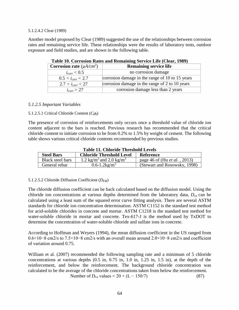
64

5.1.2.4.2 Clear (1989)

Another model proposed by Clear (1989) suggested the use of the relationships between corrosion rates and remaining service life. These relationships were the results of laboratory tests, outdoor exposure and field studies, and are shown in the following table.

Table 10. Corrosion Rates and Remaining Service Life (Clear, 1989) Corrosion rate (µA/cm2) Remaining service life

icorr < 0.5 no corrosion damage 0.5 < icorr < 2.7 corrosion damage in the range of 10 to 15 years 2.7 < icorr < 27 corrosion damage in the range of 2 to 10 years

icorr > 27 corrosion damage less than 2 years

5.1.2.5 Important Variables

5.1.2.5.1 Critical Chloride Content (Cth)

The presence of corrosion of reinforcements only occurs once a threshold value of chloride ion content adjacent to the bars is reached. Previous research has recommended that the critical chloride content to initiate corrosion to be from 0.2% to 1.5% by weight of cement. The following table shows various critical chloride contents recommended by previous studies.

Table 11. Chloride Threshold Levels Steel Bars Chloride Threshold Level Reference Black steel bars 1.2 kg/m3 and 2.0 kg/m3 page 46 of (Hu et al. , 2013) General rebar 0.6-1.2kg/m3 (Stewart and Rosowsky, 1998)

5.1.2.5.2 Chloride Diffusion Coefficient (Dca)

The chloride diffusion coefficient can be back calculated based on the diffusion model. Using the chloride ion concentrations at various depths determined from the laboratory data, Dca can be calculated using a least sum of the squared error curve fitting analysis. There are several ASTM standards for chloride ion concentration determination. ASTM C1152 is the standard test method for acid-soluble chlorides in concrete and mortar. ASTM C1218 is the standard test method for water-soluble chloride in mortar and concrete. Tex-617-J is the method used by TxDOT to determine the concentration of water-soluble chloride and sulfate ions in concrete. According to Hoffman and Weyers (1994), the mean diffusion coefficient in the US ranged from 0.6×10−8 cm2/s to 7.5×10−8 cm2/s with an overall mean around 2.0×10−8 cm2/s and coefficient of variation around 0.75. William et al. (2007) recommended the following sampling rate and a minimum of 5 chloride concentrations at various depths (0.5 in, 0.75 in, 1.0 in, 1.25 in, 1.5 in), at the depth of the reinforcement, and below the reinforcement. The background chloride concentration was calculated to be the average of the chloride concentrations taken from below the reinforcement.

Number of Dca values = 20 + (L − 150/7) (87)

65

where, L = length of the bridge deck in feet. 5.1.2.5.3 Surface Chloride Concentrations (C0)

It was suggested by previous studies (e.g., Williamson et al., 2007) that the chloride concentration profiles for bridge deck cores reach a maximum at a depth of approximately 0.5 inch after 5 to 10 years of exposure to deicing salts, due to the propensity for chlorides to be washed out of the surface of the deck resulting in lower concentrations at the surface than at a depth just below the surface. Thus, it is suggested to use the chloride concentration at a depth of 0.5 inches (or 0.25 to 0.75 in) as the C0. The mean surface chloride content in the US varied from 1.2kg/m3 to 8.2kg/m3. The mean and coefficient of variation of surface chloride content is 3.5kg/m3 and 0.5, respectively (Hoffman and Weyers, 1994). The chloride concentration in concrete (𝐶𝐶0 and C(x, t)) can be determined through analysis of concrete samples, which can be collected on-site at different depths up to and beyond the depth of the reinforcing steel using a hammer drill. The chloride ion content of concrete is usually measured in a laboratory using wet chemical analysis (Sohanghpurwala, 2006).

5.1.2.5.4 Depth of Cover

The location of a reinforcement bar and its depth of cover (c) can be obtained by using a pachometer or a covermeter. These devices measure variations in magnetic flux caused by the presence of reinforcement bars to locate their presence and depth (Sohanghpurwala, 2006). Another method consists in drilling small holes into the concrete to measure the depth from surface. This method can be more accurate, but it also introduces defects into the structure. The number of cover depth measurements are to be determined as (Williamson et al., 2007).

Number of cover depths = 40 + (L − 20/3) (88) where, L = length of the bridge deck in feet. 5.1.2.6 Commercial Software

• STADIUM (SIMCO) is powerful software developed to predict the service life of a

concrete structure. It can take into account the effect of concrete and reinforcement type, exposure condition, repair history and can evaluate the performance of a concrete structure by estimating the transport of chloride ions based on experimentally obtained (or user provided) parameters. It uses advanced models to estimate the transfer of chloride ions, which can account for the interaction of multiple ions (Nernst-Planck equation), water movement, and temperature (Hu et al. , 2013).

• Life-365 is a program used to predict the service life of concrete structures. The service life is assumed to be the sum of the initiation period of corrosion process and the propagation period. The initiation period is estimated by solving Fick’s second law using the finite difference method while assuming the diffusion coefficient of concrete to be a

66

function of both time and temperature. The propagation period is assumed to be constant (6 or 20 yrs.) (Hu et al. , 2013).

5.2 Carbonation-Induced Corrosion for Concrete Bridge 5.2.1 Deterioration Process

Carbonation occurs when carbon dioxide from the air penetrates into concrete and reacts with hydroxides, such as calcium hydroxide, to form carbonates. In the reaction with calcium hydroxide, calcium carbonate is formed. Carbonation is generally a slow process and involves a physiochemical reaction between atmospheric carbon dioxide and the calcium hydroxide generated in cement hydration. The production of calcium carbonate reduces the pH level of the concrete:

Ca(OH)2 + CO2 → CaCO3 + H2O (89) Corrosion of steel due to carbonation usually occurs particularly in an urban area which has a high level of carbon dioxide, emitted from vehicles and industrial factories. Carbonation can be defined as the chemical reaction between carbon dioxide present in the air and cement hydration products such as mainly calcium hydroxide and the CSH gel phase, which results in the formation of calcium carbonate. Thus, the risk of carbonation is more severe in urban or/and industrial area. Carbonation of concrete itself does not do harm in view of the performance of the structure, adversely a marginal enhancement of the compressive strength was observed. However, when carbonation reaches the depth of the steel, the high alkalinity of the concrete pore solution is neutralized, and hydration products are dissolved then to lower the buffering capacity of hydrations against a pH fall. At this moment, the passivation layer on the steel surface, which otherwise would protect the steel embedment from a corrosive environment, is destroyed, and steel is directly exposed to oxygen and water, eventually to corrode (Ann et al. , 2010). In high-quality concrete, it has been estimated that carbonation will proceed at a rate up to 1.0 mm (0.04in) per year. Commonly, the time needed to carbonate 20mm of high-quality concrete is estimated to be of the order of tens of years, and the penetration rate of carbon dioxide falls quickly below a mm/year soon after construction (Page and Treadaway, 1982; Locke, 1983). The amount of carbonation is affected by a high water-cement ratio, low cement content, short curing period, low strength, and highly permeable or porous paste. These factors are responsible for increasing carbonation level in concrete. Carbonation is highly dependent on the relative humidity of the concrete. The highest rates of carbonation occur when the relative humidity is maintained between 50% and 75%. Below 25% relative humidity, the degree of carbonation that takes place is considered insignificant. Above 75% relative humidity, moisture in the pores restricts CO2 penetration (Institute, 1992). Carbonation induced corrosion often occurs on areas of structures that are exposed to rainfall, shaded from sunlight, and have a low concrete cover over the reinforcing steel. Carbonation of concrete can reduce its alkalinity sufficiently to depassivate the steel and initiate corrosion. Carbonation involves the reaction of gaseous carbon dioxide with calcium hydroxide of concrete to form calcium carbonate. If fully carbonated, the pH of the concrete is reduced to around 9 at which pH steel is susceptible to corrosion. Also, if the depth of carbonation extends to the

67

reinforcing steel, then the chloride ion threshold concentration can be significantly reduced. The rate and extent of carbonation depend on the environmental relative humidity, reaching a maximum at 50% relative humidity. Diffusion of gaseous carbon dioxide takes place several orders of magnitude more rapidly through air than through water. If the pores of concrete are saturated with water, the amount of carbonation occurring will be negligible (Clifton, 1991). Most damage to concrete bridges occurs due to rebar corrosion. Fresh concrete around the steel embedded creates a corrosion resistant barrier because of the high alkalinity (pH > 13) within the concrete. However, over time the presence of chlorides, carbonation, acid attack or combination of all these reduces pH of concrete. At this point, the natural corrosion barrier is lost and the reinforcement steel starts to corrode (INC., 2005). The following figure shows the influence of pH on steel corrosion occurrence.

Figure 29. Corrosion of steel in concrete as a function of pH (INC., 2005)

The potential for rebar corrosion in bridges can be predicted in advance by measuring concrete pH and chloride content at the first rebar level. Once the concrete pH reaches level 11 or the water-soluble chloride content in the cement reaches 300ppm, corrosion will occur. The most common method for measuring the pH of concrete is the extraction of pore solution. However, this method is a time consuming and destructive process. Researchers have worked continuously to develop non-destructive methods using embedded sensors with the purpose of measuring concrete pH based on real-time monitoring. The different sensors that have been developed can be categorized into different types such as ion-sensitive-field-effect transistor (iSFET), fiber optic, hydrogel film and solid-state pH sensors (Behnood et al. , 2016).

68

5.2.2 Carbonation Service Life Prediction

5.2.2.1 Hookham (1990)

A carbonation model proposed by Hookham (1990), was used to predict the service life of an ore dock constructed in 1909. The model has the following formulation:

tc = L/Rc (90) where, tc = time to full cover carbonation L = remaining uncarbonated cover Rc = rate of carbonation The prediction of remaining service life was modeled using the relationship:

t2 = kc ∗ ke ∗ L2 + ka ∗ L (91) where, t2 = service life in years; L = thickness of concrete cover; kc = quality coefficient of the concrete; ke = coefficient of environment; ka = coefficient of active corrosion. 5.2.2.2 Clifton (1991)

Another approach for predicting the remaining service life when carbonation is the main deterioration process, is to use the square root of time principle, which is given by the following equation:

x = [2Dc (c1 − c2)t]1/2 (92) where, x = the carbonation depth (mm); Dc = the diffusion coefficient for CO2 of concrete of a given composition and moisture condition; c1 − c2 = the concentration difference of CO2 between air and the carbonation front, and t = time. 5.2.2.3 IAEA (2002)

The time required for carbonation can be estimated knowing the concrete grade and using the following equation:

t = (d/k)2 (93) where, t = the time for carbonation; d = the concrete cover; k = the permeability. Typical permeability values are shown in the following table.

69

Table 12. Typical permeability values (IAEA, 2002) Concrete Grade Permeability 15 17 20 10 25 6 30 5 35 4 40 3.5

Another formula used to estimate the depth of carbonation, utilizes the age of the structure, the water-cement ratio and a constant, which varies depending on the surface coating on the concrete.

𝐶𝐶 = √𝑦𝑦𝑅𝑅(4.6𝛽𝛽−1.76)√7.2

(94) where, y = age of structure in years; x = water-to-cement ratio; C = carbonation depth; R = a constant (R = αβ). R varies depending on the surface coating on the concrete (β) and whether the concrete has been in external or internal service (α). α is 1.7 for indoor concrete and 1.0 for outdoor concrete. β values are shown in the following table.

Table 13. Values of β (IAEA, 2002) Finished Condition Indoor Outdoor No Layer 1.7 1.0 Plaster 0.79 Mortar + plaster 0.41 Mortar 0.29 0.28 Mortar + paint 0.15 Tiles 0.21 0.07 Paint 0.57 0.8

5.2.2.4 Papadakis (2005)

For constant values of parameters and one dimension geometry, the progress of carbonation depth, xc (m), with time t (s), is given by the following equation (Papadakis, 2005).

𝑥𝑥𝑐𝑐 = � 2𝐷𝐷𝑒𝑒,𝐶𝐶𝐶𝐶2�𝐶𝐶𝐶𝐶2100�𝑡𝑡

0.33𝐶𝐶𝐶𝐶+0.214𝐶𝐶𝐶𝐶𝐶𝐶 (95)

where, CO2 = CO2 content in the ambient air at concrete surface (varies between 0.03%-0.15%);

70

De,CO2 = effective diffusivity of CO2 in carbonated concrete (𝑚𝑚/𝑛𝑛2); CSH = calcium silicate hydrate content in concrete volume (kg/m3); CH = calcium hydroxide content in concrete volume (kg/m3). In an ambient relative humidity, RH (%), the diffusivity is given by the following empirical equation (Papadakis, 1999).

𝐷𝐷𝑏𝑏,𝐶𝐶𝐶𝐶2 = 6.1 × 10−6 �𝜀𝜀𝑐𝑐 − 𝜀𝜀𝑏𝑏𝑖𝑖𝑐𝑐

1 − 𝐴𝐴𝑑𝑑𝐴𝐴

− 𝜀𝜀𝑏𝑏𝑖𝑖𝑐𝑐�

3

�1 −𝑅𝑅𝐻𝐻100

�2.2

(96)

where, εair = volume fraction of entrapped air per concrete volume (m3/m3) εc = porosity of carbonated concrete dA = aggregate density (kg/m3) A = aggregate-content in concrete volume (kg/m3). The equations presented are valid for Portland and blended cements (Papadakis, 2005). The critical time, tcr,carb (s), required for carbonation to reach the reinforcement placed at a distance c (concrete cover, m) from the outer surface, can be estimated with the following equation:

𝑡𝑡𝑐𝑐𝑐𝑐,𝑐𝑐𝑏𝑏𝑐𝑐𝑏𝑏 =(0.33𝐶𝐶𝐻𝐻 + 0.214𝐶𝐶𝑆𝑆𝐻𝐻)𝑐𝑐2

2𝐷𝐷𝑏𝑏,𝐶𝐶𝐶𝐶2 �𝐶𝐶𝐶𝐶2100�

(97)

As a general conclusion from various works, the propagation period depends strongly on relative humidity. According to Morinaga (1989), for a typical environmental temperature of 20oC and a relative humidity between 55% and 95%, the rate of corrosion, qc (10−4𝑔𝑔/cm2/year), of the rebar in concrete can be estimated with the following formula:

qc = 65(RH/100) – 35 (98) The critical amount of corrosion that causes cracking of the concrete cover, for typical concrete strength and a reinforcing bar of 10mm diameter, can be estimated by (Morinaga, 1989):

Qcr = 6(1 + 0.2c)0.85 (99) where, Qcr = 10-4 g/cm2; c = concrete cover (mm). As a result, the propagation period in years can be estimated by the ratio Qcr/qc:

tpr,carb = [6(1 + 0.2c)0.85] / [65(RH/100) − 35] (100) Finally, the service lifetime, Zcarb (in years), as regards the carbonation-induced corrosion of the concrete reinforcement, is the total sum of the two periods (tcr,carb has to be converted in years dividing by 31,557,600s/year):

71

Zcarb = tcr,carb + tpr,carb (101) 5.3 Sulfate Attack Deterioration for Concrete Bridge 5.3.1 Deterioration Process

Sulfates are present in most cements, some aggregates, soils, groundwater, sea water, industrial wastes and acid rain. Sulfates can attack concrete by reacting with hydrated components in the cement. These reactions can induce enough pressure to break the concrete and result in loss of strength and also accelerates the corrosion of the reinforcement. Environmental conditions have a significant influence on sulfate attack: the attack is greater in concrete subject to wet-dry cycles. Sulfates can accumulate at the concrete surface of a structure when water evaporates. This situation leads sulfates to increase in concentration becoming a potential for causing deterioration in concrete. If the concrete structure is continuously immersed in water containing sulfates, a softening process takes place as the sulfates ingress into the concrete. The effect area is behind the sulfate-moving interface and its depth is proportional to the depth of the interface. As a result, of the softening process the mechanical properties of the concrete are reduced. Assuming that the concrete is continuously immersed in the sulfate water, the process is likely to be controlled by diffusion (Clifton, 1991). Moreover, porous concrete is susceptible to weathering caused by salt crystallization. For example, sodium sulfate and sodium carbonate are salts known to cause weathering of concrete. As a result of surface evaporation, salt solutions can migrate to the surface by capillary action and the solution phase becomes supersaturated and salt crystallization occurs. Occasionally this crystallization produce pressures big enough to cause cracks and scaling in concrete (Mehta, 2000). Sulfate attack is commonly seen in arid areas of the United States like the Northern Great Plains and parts of the Western. Sulfates are also present in seawater but are not as severe as an exposure of sulfates in groundwater. Sulfate attack can be external or internal. The external attack is the most common type of attack and is caused by penetration of sulfates in solution for example in groundwater. The internal attack is due to the presence of a soluble source in the concrete at the time of mixing. 5.3.2 Sulfate Attack Service Life Prediction

5.3.2.1 Atkinson and Hearne (1989)

The service life model for sulfate attack of concrete is based on a model developed by Atkinson and Hearne (1989). The model is based on following assumptions:

• Sulfate ions from the environment penetrate the concrete by diffusion • Sulfate ions react expansively with aluminates in the concrete, and • Cracking and delamination of concrete surfaces result from the expansive reactions.

The model considered diffusion as the main mode of sulfate ion transport into the concrete. The basic equation developed by Atkinson and Hearne is (Lee et al. , 2013):

𝑅𝑅 = 𝑋𝑋𝑛𝑛𝑝𝑝𝑏𝑏𝑟𝑟𝑟𝑟𝑡𝑡𝑛𝑛𝑝𝑝𝑏𝑏𝑟𝑟𝑟𝑟

=𝐸𝐸𝐵𝐵2𝑐𝑐0𝐶𝐶𝐸𝐸𝐷𝐷𝑖𝑖𝛼𝛼𝛼𝛼(1 − 𝜐𝜐)

(102)

where,

72

C0 = concentration of sulfate in solution (mol/m3) CE = concentration of reacted sulfate as ettringite (mol/m3) Di = diffusion coefficient of sulfate ions in concrete (m2/s) E = elastic modulus (20GPa) R = degradation rate of concrete by sulfate ions (mm/sec) α = roughness factor of the area occurring degradation (assumed 1.0) B = stress of 1 mol sulfate to react in 1m3 (1.8x10-6 m3/mol) γ = energy required to destroy concrete surface (10J/m2) v = Poisson’s ratio (0.2) The basic assumption of the model is that damaging expansion and cracking is due to the formation of expansive ettringite within the concrete. This leads to failure when the tension caused by the growing ettringite crystals exceeds the concrete strength and a layer Xspall thick spalls from the concrete surface. When cracking and delamination of concrete surface occur, a new surface is exposed to a concentration of sulfate ions similar to the groundwater sulfate concentration, rather than the smaller concentration from diffusion. The model predicts that the sulfate attack rate will be mainly controlled by the concentration of sulfate ions and aluminates, diffusion and reaction rates and the fracture energy of concrete (Clifton, 1991). 5.4 Freeze-Thaw Deterioration for Concrete Bridge 5.4.1 Deterioration Process

Abrupt changes in temperature are one of the most destructive factors affecting concrete. These changes can cause cycles of freezing and thawing. Freezing temperatures can cause water to frozen and expand around 9%. Water contained in concrete also freezes and produces pressure in the pores and capillaries of the concrete. If such pressure is higher than the tensile strength of concrete it will cause a rupture in the structure. Concrete does not have to be completely saturated with water for damage to occur, for most concretes the critical level of saturation is approximately 85%. The accumulative effect of consecutive freeze-thaw cycles can eventually cause significant damage to concrete like cracking, scaling, and crumbling. The following figure shows the frequency of freeze-thaw exposure of different regions of the United States. It is notable that in the majority of Texas’ territory it is rare to find freeze-thaw cycles and in the north part of the state it is occasional to have exposure to freeze-thaw cycles.

73

Figure 30. Frequency of freeze-thaw exposure typically encountered in different areas of

the United States (PCA, 2002) 5.4.2 Service Life Prediction

5.4.2.1 Chen and Qiao (2015)

A service life prediction model is based on the previous experimental studies from Li et al., and Russel et al (Jinyu et al. , 1999) (Russell, 1943). According to the authors, an equivalent coefficient (CEquivalent) for the number of freeze/thaw (F/T) cycles in the indoor laboratory (Nindoor) is approximately to be 6.5 in their study. They assumed that the annual F/T cycles (NAnnual) in some severe environments are 200, thus, the service life T (in years) can be calculated as:

T = (CEquivalentNIndoor )/NAnnual (103) It is important to consider that the equivalent coefficient for the number of laboratory F/T cycles with respect to the field F/T cycles varies depending on the region and its environment condition. Moreover, several important factors should be noted for this service life prediction model for concrete subject to cyclic F/T degradation as far as the equivalent coefficient is concerned.

• Critical level of saturation plays a significant role in affecting the F/T concrete resistance. • Air entrainment is an important factor that will affect the F/T deterioration. • Permeability of concrete may considerably impact the F/T durability of concrete.

The accuracy of the predicted service life depends on the accuracy of the equivalent coefficient for the number of F/T cycles calculated in the laboratory where the critical saturation level, air entrainment and permeability of the studied concrete are required (Chen and Qiao, 2015). 5.4.2.2 Shuman et al. (1989)

Another empirical model described by Shuman et al. (1989), frost durability is modeled by relating the decrease in the dynamic modulus of elasticity of concrete to the percentage of entrained air, water cement ratio and number of F/T cycles using ASTM C666. According to the experimental results, changes in dynamic modulus were assumed linear when the number of F/T cycles was over 50. The amount of annual degradation, Rft, based on the fraction of strength loss, is given by:

74

𝑅𝑅𝑒𝑒𝑡𝑡 = (𝑁𝑁/𝑇𝑇𝑐𝑐)[0.05/𝜃𝜃12 − 0.21𝑇𝑇𝑐𝑐] (104)

where, N = number of F/T cycles; Tc = amount of experimental time required to reach a 50% decrease in dynamic modulus of elasticity; θ = water content of the concrete; Tr = unsaturated pore content of the concrete. Finally, it was recognized that ASTM C 666 usually significantly overestimates the field damage caused by frost attack. In conclusion, this model will likely considerably underestimate the service life of concretes exposed to freeze thaw cycles. 5.4.3 Commercial Software

CONLIFE can be used to predict the service life of concrete structures due to sulfate attack and freeze-thaw effects. It assumes that sorption is the primary transport mechanism in concrete. A test method for sorptivity is proposed (Hu et al. , 2013). 5.5 Alkali Silica Reaction Deterioration for Concrete Bridge 5.5.1 Deterioration Process

Normally aggregates in concrete are chemically inert. However, some aggregates react with the alkali hydroxides in it causing expansion and cracking over time. There are two types of alkali aggregate reactions: alkali-silica reaction (ASR) and alkali-carbonate reaction (ACR). The most common type is the ASR, which is of more concern than ACR because aggregates containing reactive silica materials are more common. Cases of ACR are very rare and restricted to a few isolated regions (FHWA). In the Alkali-Silica Reaction, the aggregates composed of certain forms of silica can react with alkali hydroxide in concrete to form a gel that grows as it takes water from the surrounding cement paste or the environment. As the gel grows, it could produce enough pressure to cause concrete damage, as represented by the following equations: Alkalis + ReactiveSilica → GelReactionProduct GelReactionProduct + Moisture → Expansion For alkali-silica reaction to occur, three essential components must be present:

• Reactive forms of silica in the aggregate • High-alkali pore solution • Sufficient moisture

The use of reactive aggregates in concrete is one of the conditions for ASR to happen. These aggregates tend to breakdown under exposure to highly alkaline pore solution in concrete and consequently react with the alkali-hydroxides (sodium and potassium) to form the ASR gel.

75

Another condition is the high-alkali-content pore solution. Alkali hydroxides in solution will react readily with reactive forms of silica in aggregate. As the aggregate reactivity increases, gel reaction products can be formed with lesser concentrations of alkali. That is why the use of low-alkali cements alone may not be sufficient to control ASR with highly reactive aggregates. The potential for the alkali-silica reaction increases as the alkalinity of the pore solution increases. If the alkali concentration is big enough, the alkali hydroxides break stronger silicon bonds found in less reactive aggregates to form the gel. This is the reason why some non-reactive aggregates occasionally show ASR. The other condition for the alkali-silica reaction to occur is sufficient moisture. It has been found that concrete with highly reactive aggregates and high-alkali cements have shown little or no expansion in certain very dry environments (FHWA). Similarly, differences in moisture in various parts of the same concrete structure have resulted in very different outcome. The parts of the structure that were exposed to a constant moisture have shown significant damage due to ASR, whereas the parts of the structure that remained dried showed little or no damage. Consequently, the exposure conditions and the presence of moisture in the concrete structure represent a key role in the alkali-silica reaction. The most common indicators of alkali-silica reaction are map cracking, closed joints, and concrete surfaces spalling. Usually, the cracks appear in areas with constant moisture, therefore, to avoid the alkali-silica reaction it is recommended to keep concrete structures as dry as possible. Moreover, the reaction can be virtually stopped if the internal relative humidity of the concrete is kept below 80% (FHWA), but it is complicated for this condition to reach and maintain. Potentially reactive aggregates are present all over the country. However, ASR damage to concrete is not common because of measures taken to control it. Moreover, not all ASR gel reaction products experience excessive and destructive swelling. 5.5.2 Service Life Prediction

There is not much literature on the service-life of concrete experiencing alkali-aggregates reactivity. Delaware Department of Transportation (DelDOT) developed a method for determining the rating of ASR with the purpose to generate an approximate ASR reaction rate to predict concrete pavement life. The method of ASR rating was developed using an ASR test that allowed to track the progression of the ASR with time. The time frame for the process was set to twenty years. The ASR rating is composed of six ratings from 0 to 6, none, low, average, moderate, heavy and severe respectively. The ASR rating data from DelDOT was plotted against time, and the ASR reaction rate was determined from the curve. Since DelDOT does not check regularly the state of pavements, it is limited to a single data point, the core being tested for ASR. For this reason, the authors decided that ASR reaction rate is a straight line and the two points for drawing the line would be the time the core is tested, t, and the time the pavement is initially rated 0. The following equation was developed (Attoh-Okine and Atique, .

ASRReactionRate = ASRrating#/(tt − t0) (105) where, tt = date cored (all time is years); t0 = date pavement placed; ASR Rating 3 = rating of core at tt.

When the ASR reaction rate is estimated, it is possible to use it to obtain an approximate prediction for the remaining service life using the following equation.

76

Years Remaining = (5.0 − ASRrating#)/ASRreactionrate (106) 5.6 Fatigue Life Prediction for Steel Bridge 5.6.1 Fatigue Life Prediction

Fatigue is the process of cumulative damage of a material subjected to cyclic loading resulting in microscopic cumulative damage until a crack appears. There are two prevalent methods for characterizing the fatigue resistance of a structure component. The resistance can be determined experimentally following a stress-based approach (S-N curves) or numerically from a fracture-mechanics model. 5.6.1.1 Stress-Based Approach

The classical experimental method to characterize fatigue resistance is to test a given detail in tension at a constant-amplitude stress range and count the number of cycles to failure. Nominally identical details are tested at different constant-amplitude stress ranges until failure. The stress range, Sr, is defined as the difference between the highest and lowest values in a stress history. After testing the detail at various stress ranges, the data can be plotted on a graph of number of cycles to failure (Nf ) for various cyclic stress ranges (Sr). The data are typically plotted on a log-log plot. It was determined empirically that stress range and type of detail are the primary variables affecting fatigue resistance. It is important to note that the stress range is typically the nominal stress range. The flow of stresses at discontinuities and/or welds creates locations of stress concentrations that lead to higher magnitudes than calculated from engineering mechanics (bending stress, axial stress, etc.). Because the stress concentrations vary with the detail, the nominal stress (stress calculated away from the discontinuities and/or welds) is typically used to characterize the S-N curves.

Figure 31. Example of data from a representative fatigue test (Fasl, 2013)

By considering a single type of detail, the fatigue resistance can be described by

𝑁𝑁𝑒𝑒 = 𝐶𝐶 × 𝑆𝑆𝑐𝑐𝐵𝐵 (107) where, Nf = number of cycles until failure at Sr; C = empirical constant for specific detail from fatigue data (ksiB ); Sr = nominal constant-amplitude stress range (ksi);

77

B = slope of the S-N curve. The constants B and C are determined empirically from the fatigue data. To determine the fatigue resistance, regression techniques are used to define the line that goes through the mean of the data. For most metals, the slope of the S-N curve (B) will vary between -2 to -4 (-3 used by most specifications). The code value is determined by moving the mean failure line approximately two standard deviations to the left (or down). The code value in the AASHTO Load and Resistance Factor Design (LRFD) Bridge Design Specifications typically corresponds to a 95% confidence interval of a 95% probability of survival (probability of failure of approximately 5%). There is a stress range at which the detail is assumed to have an infinite fatigue life for a given constant-amplitude stress range. This horizontal line corresponds to the constant-amplitude fatigue limit (CAFL). The determination of the CAFL historically corresponded to two million cycles, at which point the specimen would be declared a “run-out” test. The two-million cycle limit was based upon equipment limitations during the period of testing (1970s- 1980s). With modern testing facilities, specimens can be and are often tested to much higher cycle counts (Fasl, 2013). The equation currently used in the AASHTO LRFD Specifications is shown below.

𝑁𝑁𝑒𝑒 = ASr3

(108)

where, Nf = number of cycles until failure at Sr; A = fatigue constant for detail category (ksi3); Sr = constant-amplitude stress range (ksi). The AASHTO LRFD Specifications provide examples of typical types of details that fit into each of the eight fatigue categories. For instance, Category A corresponds to the fatigue resistance of the base metal (i.e. flat plate with no weld attachments) and Category B corresponds to continuous longitudinal fillet welds. Because the CAFL are high and the fatigue constants are so large, these types of details never control the fatigue resistance of a bridge. Instead, the design of details with discontinuities or attachments with fillet or groove welds parallel and perpendicular to the applied stress are more likely to be controlled by fatigue considerations. In those situations, the fatigue category varies between C and E’. If the effective stress range is less than the constant-amplitude fatigue limit (CAFL), fatigue failure can occur if the maximum stress range is greater than the CAFL. However, if the maximum stress range is less than the CAFL, fatigue failure will not occur. A straight-line extension of the S-N curves can be used for effective stress ranges less than the CAFL. 5.6.1.1.1 Miner’s Rule

The S-N curve uses a constant-amplitude stress range. However, real structures are subjected to varying-amplitude stress ranges. A cumulative damage theory is needed to relate the varying-amplitude cycles to the constant-amplitude fatigue data. Miner’s rule is the most commonly-used

78

cumulative damage theory because it is simple and agrees well with historic fatigue data. The rule follows a linear-damage hypothesis and is expressed by the following equations.

𝐷𝐷𝑛𝑛 =𝑛𝑛𝑛𝑛𝑁𝑁𝑒𝑒 ,

𝐷𝐷 = �𝐷𝐷𝑛𝑛

𝑘𝑘

𝑛𝑛=1

(109)

where, Dj = contribution of cycles nj to Miner’s damage accumulation index; D = Minor’s damage accumulation index; nj = number of cycles measured at Sr,j ; k = number of different stress ranges; Nf,j = number of cycles until failure at Sr,j . The damage from a spectrum of stress ranges equals the damage from a single, effective stress range as shown in the equation below.

𝑆𝑆𝑐𝑐𝑏𝑏 = ��𝑛𝑛𝑛𝑛𝑁𝑁𝑛𝑛

𝑘𝑘

𝑛𝑛=1

𝑆𝑆𝑐𝑐,𝑛𝑛3 �

1/3

(110)

where, Sre = effective stress range (ksi); Nm = total number of cycles measured. 5.6.1.1.2 Cycle-Counting

When field measurements are utilized, a cycle-counting method is needed to transform the stress history into a histogram of stress amplitudes. Four types of counting methods for fatigue analysis are included in ASTM E1049 (ASTM, 1999): (1) level-crossing counting, (2) peak counting, (3) simple-range counting, and (4) rain flow counting or related methods. 5.6.1.1.3 AASHTO Manual for Bridge Evaluation (2011)

In 2011, AASHTO released the second edition of the Manual for Bridge Evaluation (AASHTO, 2011) for evaluating fatigue in steel bridges. The following equation can be used to estimate the remaining fatigue life.

𝑌𝑌 =𝑅𝑅𝑅𝑅 × 𝐴𝐴

365 × 𝑛𝑛 × (𝐴𝐴𝐴𝐴𝐷𝐷𝑇𝑇)𝐶𝐶𝑆𝑆 × (𝑅𝑅𝑛𝑛 × 𝑆𝑆𝑐𝑐)3− 𝑏𝑏 (111)

where, Y = fatigue life in years; RR = resistance factor; A = detail constants (ksi3);

79

n = stress cycles per truck passage; AADTSL = average number of trucks per day in a single lane averaged over the entire fatigue life; Sr = stress range (ksi); RS = partial load factor.

80

Corrosion Control Methods In the United States, the highway system is a complex phenomenon which plays an important role as a part of economics. As per the study, the annual cost of corrosion to all bridges (including steel bridges) is 8.29 billion dollars which also includes an indirect cost incurred by bridge closures (Harichandran et al. , 2010). Because of the severity of the problem, researchers have developed the corrosion protection methods. To slow chloride’s ingress into concrete structures, different technologies and methods have been used. These corrosion control methods can be categorized by the mechanism by which they provide protection: mechanical or electrochemical methods. The mechanical barrier methods control the transportation of chemicals like chloride ions, oxygen, and moisture to spots where corrosion reactions are occurring or may occur. The electrochemical methods interfere with the chemical or electrical part of the corrosion process allowing it to control its progression. Corrosion control methods include low-permeability concretes, corrosion inhibitors, polymer overlays, deck sealers, increased concrete cover depth, electrochemical extraction, and cathodic protection. Each of these methods has its own advantages and disadvantages (Sohanghpurwala, 2006). Freyermuth (2009) lists the following options for achieving an extended service life of concrete bridges:

• Use of high-performance concrete to decrease permeability; • Use of prestressing to reduce or control cracking; • Use of jointless bridges, or bridge segments, and integral bridges; • Use of integral deck overlays on precast concrete segmental bridges in aggressive

environments; and • Selective use of stainless steel reinforcing.

A research by National Bureau of Science (now National Institute of Standards and Technology) and the Federal Highway Administration (FHWA) on epoxy coated reinforcement (ECR) showed that the performance of ECR is very well in salt-contaminated concrete and provides protection to minimize premature deterioration of concrete due to expansive corrosion. On the other hand, field investigations showed that even though ECR has a better performance than traditional bare steel reinforcement, the bridges which have been constructed using ECR are showing indications of surface damage and repairs are required to avoid progress of damage. Adoption of stainless steel or stainless steel-clad reinforcement is one of the ways of corrosion protective measures. Stainless steel is different from the regular black steel. A passive film of chromium oxide on stainless steel helps to prevent further surface corrosion. In addition, it blocks the spread of the corrosion into the internal structure. The corrosive threshold for stainless steel in concrete is about 10 times higher than that of traditional black steel. Based on the results of field investigations, it is found that bridge decks using stainless-reinforcement had no corrosion- induced cracks after 9 years of service. This is the reason which proves stainless steel an attractive material to reduce corrosion in highway and bridge infrastructure. The cost of stainless steel is a major concern for owners. An increase in the initial cost is 5.5 to 15.6 percent while using stainless steel in a bridge deck, and is therefore typically considered to protect critical and hard-to-repair

81

structures. Epoxy-coated reinforcing bars is one of the most widely used for preventing corrosion of reinforcement. The corrosion is controlled in the epoxy coating due to following factors:

• Resistance Inhibition: It provides electrical resistance to limit transfer of current between anodic and cathodic sites;

• Oxygen Deprivation: Excludes oxygen thus hindering the cathodic reaction; • Inhibition or aestivation: Introduces material into the interfacial environment to stimulate

the development of passive or inhibitive surface films; ECR is cost-effective in the long run even though its cost is higher than regular black steel. In practice, the corrosion of ECR does occur. When the adhesion between the epoxy coating and the reinforcement is lost, the surface of the steel will be exposed to the environment causing corrosion. Water absorption properties of the coating can cause the de-bonding of the coating. Damage to the coating during manufacture, fabrication, transportation, or construction also contribute in corrosion introduction. Small regions of steel exposed to the surrounding environment can corrode. These problems can be reduced by proper design of the coating and proper handling during the transportation and construction process but cannot be eliminated. The effectiveness of the ECR is influenced by various factors including the existence of concrete cracks, the thickness of concrete cover, the type of steel for the bottom reinforcement, and the type of the coating. Cathodic protection is another method to control or reduce corrosion of reinforcing bars present in concrete. In the case of cathodic protection, an auxiliary anode provides an external current to the protected metal. Thus, corrosion is reduced or stopped. Two methods are used to supply external current. In one of the methods, the protected metal is connected to a more active sacrificial metal like zinc. In the second method, an external current source is applied. This method is effective in reducing the corrosion of steel in concrete though it has many drawbacks. The use of external power requires to be charged and replaced regularly. The wiring and connections also induce additional cost. If an active metal is used, the cost of obtaining and replacing the sacrificed metal can also be high. 6.1 Impacts of Corrosion Control Methods on Bridge Service Life The following table presents a summary of different methods to address corrosion in concrete and steel elements of a bridge. Some of these corrosion control strategies have significant impact on extending bridge service life. For example, the use of low permeability concrete could delay the time to reach the chloride threshold up to 50 years. Moreover, latex modified concrete, silica fume concrete, and fly ash concrete used in a repair overlay could extend the service life of a bridge deck between 22 to 26 years. Electrochemical methods like cathodic protection, corrosion inhibitor, and electrochemical extraction could extend bridge service life from 5 to 25 years (Sohanghpurwala, 2006). The use of protection methods for steel bridges (Paint coating, metallic coating, weathering steel) could lead to a service life extension from 30 to 120 years.

82

Table 14. Summary of corrosion control methods and their impact on bridge service life Method Impact on service life

Epoxy coated reinforcement At best marginal (e.g., 5 years) (Williamson, 2007) Galvanized steel The chloride threshold values for galvanized steel are estimated to be 2.5 times

greater than carbon steel (Yeomans, 2004). Stainless steel Chloride threshold values for stainless steel have been reported to be at least

10.4 times greater than carbon steel (Clemeña, 2003). MMFX-2 steel The reported range of initiation values is 3.5 – 9.2 times that of carbon steel

(Clemeña, 2003; Trejo, 2002). Nonmetallic reinforcement Fiber-reinforced plastic bars: bridge deck mean service life is between 65–90

years (Frosch et al., 2014) High performance concrete Time required for the chloride to reach threshold value will be 49 years for

moderate exposure to chlorides, and 27 years for severe exposure to chlorides (Mohsen et al., 2010)

Cathodic protection Service life can be extended 5 to >25 years (Sohanghpurwala, 2006) Corrosion inhibitor Service life can be extended 4 to 6 years (Sohanghpurwala, 2006) Electrochemical extraction Service life can be extended 10 to 20 years (Sohanghpurwala, 2006) Penetrating sealers Service life can be extended 5 to 7 years (Sohanghpurwala, 2006) Low slump concrete Low-permeability concrete where chloride ions diffuse at a slower rate.

Service life of repair overlay is 22 to 26 years (Weyers et al., 1993) Latex modified concrete Low-permeability concrete where chloride ions diffuse at a slower rate.

Service life of repair overlay is 22 to 26 years (Weyers et al., 1993) Silica fume concrete The service life of a repair overlay is estimated to be 22 to 26 years (Weyers

et al., 1993) Fly ash concrete Incorporation of fly ash into concrete alone is useful to decrease the level of

corrosion by delaying the corrosion process (Montes-Garcia, 2015) Paint coating Three-coat systems with a zinc-rich primer can have a service life of 30 years

before a major touch-up is required (Kline, 2008) Metallic coating properly applied metallized coatings (zinc, 85%Zinc/15%Aluminum, and

Aluminum) of at least 6 mils thickness provide 30 years of protection in most bridge exposure environments (FHWA, 1997)

Weathering steel Bridges fabricated from unpainted weathering steel can achieve a 120 year design life with only nominal maintenance (Corus, 2005)

6.2 Mechanical Barrier Methods 6.2.1 Protective Coatings

Protective coatings can be used to protect metals exposed to a corrosive environment. In simplest terms, they are pigments or fillers embedded in a variety of binders. Protective coatings can employ one or more protective mechanisms. These include providing a barrier between the protected metal and the surrounding corrosive environment, sacrificial corrosion protection and corrosion inhibitors e.g. barrier coatings, galvanizing technique, metalizing, etc. Barrier methods are often used in conjunction with other corrosion protection methods, such as epoxy-coated steel or other alternative reinforcement. Barriers are provided in the form of concrete overlays, waterproof membranes, and concrete sealers. 6.2.2 Corrosion-Resistant Reinforcement

Corrosion-resistant reinforcement is a measure to eliminate the risk of reinforcement corrosion, even in the most corrosive chloride-containing environments. Adopting corrosion-resistant steel

83

reinforcement (CRSR) is the simplest solution because this not only solves the corrosion problem in a foolproof manner but also leaves the site activities nearly unchanged. This is particularly advantageous because serious changes to site operations introduce difficulties and uncertainties. Using non-metallic reinforcement may solve the corrosion problem, but most such reinforcement cannot be adjusted onsite. Some may be brittle (for example, carbon fiber bars) and sensitive to impacts from a vibrator, walking on the reinforcement should usually be avoided, and all of these types of reinforcement are light and should be anchored to the formwork to keep them from floating. Normal reinforcement (also termed mild steel, black steel, or carbon steel reinforcement) is efficiently protected from corrosion when cast into a good quality, alkaline, and chloride-free concrete. This is the well-known, unique benefit of using reinforced concrete in building and construction. Only when carbonation reaches the level of the reinforcement or, more seriously, when chlorides in sufficient quantity reach the surface of the reinforcement will the passivating effect be eliminated and corrosion may start. Particularly serious are the situations in which the initial concrete has been polluted with chlorides from the aggregates, the mixing water, or chloride-based accelerators. Recent years’ developments within the area of noncorrodible or corrosion-protected reinforcement for concrete structures are opening promising new doors in the fight against reinforcement corrosion. The following products that have different degrees of resistance against corrosion are available:

• Stainless-steel reinforcement • Epoxy-coated reinforcement • Hot-dip galvanized reinforcement (zinc coating) (This application is limited but may be a

fully viable protection in concrete exposed to carbonation. In general, zinc coating is not considered adequate, or cost-effective, for structures exposed to chlorides)

• Non-metallic reinforcing bars, such as reinforcing bars from glass fibers, aramid fibers, or carbon fibers. (The non-metallic reinforcing bars will probably, for many more years, only have limited applicability due to the major differences needed when constructing onsite. They may have a potential within the precasting industry.)

Alternative reinforcing steels considered were galvanized steel, MMFX-2, and stainless steel. MMFX steel has considerably high corrosion resistance due to patented and proprietary steel microstructure formed during its production (Thomas 1996). This unique characteristic helps to minimize the formation of micro galvanic cells in the steel structure, hence minimizing corrosion initiation. Therefore, MMFX’s steels are highly corrosion resistant and are equal or better than existing steels in their mechanical properties such as yield strength, energy absorption, toughness, brittleness, ductility, weldability, hardness, and formability. There are two types of steels, Dual Phase Steel and Microcomposite Steel (Xi et al., 2004). Dual Phase Steel is characterized as a microcomposite ferritic / martensitic low carbon steel that has been rolled and quenched in a controlled manner. This steel exhibits superior corrosion resistance in reinforced concrete applications and superior mechanical properties compared to existing rebar (i.e., A615). Microcomposite Steel is defined as steel that exhibits similar microstructure characteristics without ferrite. It is different from the Dual Phase Steel in terms of material composition and does not require quenching to produce the prerequisite microstructure for its corrosion resistance and mechanical properties.

84

The following state DOTs have ongoing projects using the new steel: • Florida: FRP composites and MMFX steel for deck slab; • Iowa: MMFX steel for deck slab; • Kentucky: clad stainless steel and MMFX steel for deck slab; • South Dakota: MMFX steel for decks and pavements

However, a 2007 Virginia project (Williamson et al. , 2007) recommended that newly constructed bridge decks be built under current specifications with bare steel reinforcement. The decision to use bare steel reinforcement over available alternative reinforcements was made upon the determination that the service lives of bridge decks constructed under current cover depth and low permeable concrete specifications are expected to exceed 100 years regardless of reinforcement type. Therefore, reinforcement type should be selected on a first-cost basis. Bare steel being the least costly alternative would typically be the reinforcement of choice. However, alternative reinforcements such as stainless steel, stainless steel clad, or MMFX-2 may be used in place of bare steel as a secondary corrosion protection method for extreme chloride exposures or where a redundant corrosion protection system is required by FHWA. 6.2.2.1 Epoxy-Coated Reinforcement

Epoxy-coated reinforcement (ECR) employs fusion bonded epoxy coatings as a barrier coating. Epoxy coated rebar, also referred to as green rebar, is used in concrete subjected to corrosive conditions. These may include exposure to deicing salts or marine environments. Epoxy coated rebar or corrosion-resistant rebar is used instead of conventional reinforcing bars to strengthen the concrete and protect against corrosion. The epoxy coating is applied in a factory to the steel prior to shipping to ensure corrosion resistance. Epoxy-coated steel reinforcing bars (rebar) may be used in any concrete subjected to corrosive conditions. It was reported that epoxy coated reinforcing steel corrosion protection performance is at best marginal, providing about 5 years’ additional corrosion resistance in field structures (Weyers et al., 2006). 6.2.2.2 Nonmetallic Reinforcement

CFRP and GFRP as rebars are one of the solutions for the problem of corrosion. The strength of FRP bars is up to 6-10 times of black steel and weight is up to one fifth of the steel. Though, the use of these rebars can be limited due to high cost. Fiber reinforced plastic (FRP) reinforcement can provide corrosion-free service. FRP bars have had problems with an aging process known as creep, but that can be avoided with attention to loading. The fiber production technology is improving so this is an area that deserves consideration in future construction projects. 6.2.3 Corrosion-Resistant Materials

If extended maintenance free service life is desired, it is important to incorporate corrosion resistant materials. Structural steel elements can be fabricated from corrosion-resistant materials. Weathering steels are special alloys that develop a corrosion-resistant patina, or rust. Stainless steel can also be incorporated in bridges. Usually, stainless steels would be too expensive to use as beams. However, they can find use in other critical components that will be exposed to corrosive environments. Aluminum is actually a reactive metal. It forms an oxide layer that generally is quite

85

stable and protects the underlying reactive metal. Aluminum is also an amphoteric metal, which means that it can be attacked if exposed to either acidic or alkaline conditions. Pozzolans and other supplementary cementing materials (SCM) including fly ash (FA), ultrafine fly ash (UFFA), Metakaolin (MK), silica fume (SF), and ground granulated blast-furnace slag (GGBS) have been used as partial replacement of cement to improve the durability of reinforced concrete structures. The long-term concrete permeability has been found to be significantly reduced by using pozzolanic and SCM admixtures. However, it has been found that concrete which contains some of these pozzolans, and SCM, such as GGBS and Class F FA has slower reaction rates compared with ordinary Portland cement concrete (OPC), which is reflected by both lower strength and lower chloride resistance properties at early age (e.g. 28 days). The quality control tests, such as compressive test and diffusivity test, are usually carried out at 28 days, which is not long enough for concrete with slow reacting pozzolans to achieve passing values. High performance concretes (HPC) with Class F FA or slag as the only pozzolans or SCM present usually shows slow hydration. As time passes the hydration of concrete with these pozzolans reduce the pore size and pore connectivity (in the order of a few months to a few years). Resistivity measurement can be used to monitor the concrete hydration (Presuel-Moreno et al. , 2013). 6.2.4 High-performance Concrete

The continuous demand for increased strength and improved durability of concrete structures has led to the development of HPC. This development has had three main objectives in mind:

• Protect the reinforcement against corrosion, in particular, provide protection against ingress of chlorides by creating dense impermeable concrete in the cover zone with low penetrability of aggressive ions, such as chlorides, sulfates, and carbon dioxide;

• Resist deterioration of the concrete when exposed to the aggressiveness of the environment, such as sulfates, seawater, and other chemical attacks, as well as resist freezing and thawing attack; and

• Provide adequately high strength to fulfill the structural requirements. HPC for normal types of structures will usually have a relatively high cementitious binder content (blended cements), a low water-cement ratio (in the range of 0.35 to 0.40), and a high content of water-reducing admixture and high-range water-reducing admixture. Such concrete can be conveniently used for bridges, marine works, offshore structures, high-rise buildings, and more, where the strength requirements usually remain within the range of 50 MPa to 80 MPa (7.3 ksi to ksi) (Rostam, 2008). One drawback has been that these more-refined concretes become more sensitive in the actual handling during execution. The increased sensitivity of HPC compared with normal concrete relates to the mixing, transporting, placing, compacting, and curing processes. HPC requires an experienced and competent workforce and high-quality workmanship to achieve the potential benefits, but this is not always available on site. HPC on the better end of the strength scale can be difficult to place and compact, and the risk of honeycombs, particularly in the cover is, however, necessary to have these potential problems in mind when designing structures based on the application of HPC and to take the competence of the local workforce into account when making the selections. One new issue has evolved during the past few years that may influence the broad, but not always successful, application of HPC. This is related to the increased availability and competitiveness of non-corrodible reinforcement bars to avoid reinforcement corrosion in

86

heavily chloride-containing environments. Stainless-steel reinforcement is currently the most convincing solution for the reinforcement corrosion problems.

Also, the quality and efficiency of compaction are extremely dependent on the person handling the vibrator. Hence, the better the concrete, from a durability point of view, the greater the risk of having inferior or bad execution lead to reduced quality in the final structure. This fact is seldom respected onsite. This inconsistency is due to the dominating influence of the execution process on the final performance of the structure. To varying degrees, these concretes differ from the long-term known types of structural concrete through the following:

• The dosing and mixing become more complicated and sensitive, even with respect to timing and sequence of adding the different ingredients.

• The placing requires special methods and routines because such mixtures can be rather cohesive and sticky.

• Compaction is more demanding because the vibration should be more intensive and requires more vibration energy.

• The denseness of the concrete, when correctly placed and compacted, minimizes bleeding, and the available water is so limited that protection against evaporation should be introduced promptly following leveling and troweling of horizontal surfaces exposed to drying in order to avoid plastic shrinkage cracking. Normal curing compounds are usually not sufficiently effective.

• The high content of cementitious material will most often generate more heat than normal concrete, thus increasing the risk of thermal cracking. However, this depends on the cementitious material used in the individual cases, where, for example, slag cement has a reduced risk of thermal cracking due to a slow rate of hydration.

• The autogenous, or chemical, shrinkage is more pronounced due to the low water-cement ratio, and this sets much stronger demands on controlling the temperature differences in hardening concrete if thermal cracking is to be avoided. The generally accepted limiting temperature differences may have to be halved, and in extreme cases reduced to one-third, for HPC to avoid unacceptable thermal cracking.

• HPC requires air entrainment to be frost resistant according to the generally adopted (rather severe) freezing and thawing tests. However, such mixtures with high contents of high range water-reducing admixture are usually difficult to air entrain, and the air may easily disappear during the compaction due to the increased vibration energy needed. Hence, HPC may be more sensitive to freezing and thawing, in other words, less frost resistant than normal types of structural concrete.

The sensitive elements of HPC are not necessarily valid for all types and uses of such concretes. It is, however, necessary to have these potential problems in mind when designing structures based on the application of HPC and to take the competence of the local workforce into account when making the selections. One new issue has evolved during the past few years that may influence the broad, but not always successful, application of HPC. This is related to the increased availability and competitiveness of non-corrodible reinforcement bars to avoid reinforcement corrosion in heavily chloride-containing environments. Stainless-steel reinforcement is currently the most convincing solution for the reinforcement corrosion problems.

87

6.3 Electrochemical Methods 6.3.1 Cathodic Protection

A cathodic protection system for reinforced concrete consists of reinforcement to be protected, an anode, a power source, concrete surrounding the steel, a monitoring system, and cabling to carry the system power and monitoring signals. Each cathodic protection system contains two types of anodes. “Anode conductor”, acts as a contact point and a power supply line for the secondary anode. “Anode” is the material that distributes the current over the surface of the structure. Cathodic protection works by using current to shift the potential of the reinforcing steel in the negative direction. If the potential is shifted far enough so that all of the steel reinforcement becomes cathodic, corrosion will be stopped. The following figure shows the impressed current cathodic protection.

Figure 32. Impressed current cathodic protection

6.3.2 Electrochemical Chloride Extraction

Electrochemical chloride removal is the process of removing chloride ions from contaminated concrete by electrochemical means. Electrochemical chloride extraction is similar to cathodic protection. The reinforcement is connected to the negative pole of a DC power source, while a temporary external anode, placed within an electrolyte covering the concrete surface, is connected to the positive pole. Current is run through the reinforcement to the anode, creating an electrical field in which chloride ions are pulled away from the reinforcement and towards the electrolyte where they are absorbed for removal. 6.3.3 Corrosion Inhibitors

Corrosion inhibitors are defined as chemical substances that are added to concrete in small concentrations to reduce the level of corrosion or completely stop corrosion. The corrosion inhibiting admixtures are classified as per following:

1. Anodic Inhibitors: Anodic inhibitors work as passivators on the rebar. They form protective films on anodic surfaces or by absorption on the metal. Chromates, nitrites, molybdates, alkali phosphates, silicates, and carbonate are examples of anodic inhibitors. Some anodic inhibitors such as nitrites are supposed to be applied in large doses as insufficient quantity of inhibitors will not be able to treat all of the anodic sites and pitting corrosion may occur

88

due to the high cathode to anode ratio (Fadayomi, 1997). The most widely used anodic inhibitor in the U.S. is calcium nitrate. The dosage of calcium nitrites is decided based on the expected chloride content during structure’s service life. Actual dosages range from two to six gallons per cubic yard. Nitrite is one of the components in an acceleration admixture. The application of nitrite will help to reduce the setting time of fresh concrete mix. Retarders are generally used to balance the setting time, especially when large dosages of calcium nitrites are used.

2. Cathodic Inhibitors: Cathodic inhibitors are defined as the inhibitors which work by

forming an insoluble protective film on alkaline cathodic surfaces through the production of an insoluble compound at high pH levels. The reaction between cathode and oxygen is prevented by the protective film. Zinc, salts of antimony, magnesium, manganese, and nickel are examples of cathodic inhibitors. These inhibitors are generally less effective as compared to the anodic inhibitors.

3. Organic Inhibitors: In the case of this type of inhibitor, the corrosion at the anodes and

cathodes are simultaneously inhibited. Organic inhibitors include amines, ester, and sulfonates. These inhibitors form a protective barrier (monomolecular film) between the rebar and the chloride ions that prevents the reaction between the iron and chloride ions. While using these inhibitors, estimation of chloride loading for the structure is not required because of their way of functioning (form protective barrier without competing reaction with chloride ions). The dosage is one gallon per cubic yard, which should be added during batching. The organic inhibitors function well in cracked concrete in laboratory tests. The protective barrier formed keeps working even though chloride ions penetrate directly to rebar through cracks.

4. Field study of corrosion inhibitors in other states: The FHWA investigated the

effectiveness of corrosion inhibiting admixtures in outdoor exposure of reinforced concrete slabs (Virmani et al, 1983). The evaluation of reinforcement was done by measuring the macrocell corrosion current, half-cell potential, driving voltage, concrete electrical resistivity, and visual inspection. The conclusion of the study states that calcium nitrite is effective in reducing the corrosion rate in black steel bar at chloride-to-nitrite ratios of 1.79 or less.

6.4 Corrosion Control for Existing Concrete Bridges For the rehabilitation of existing concrete bridge structures that are damaged by corrosion of steel bars due to chloride ingress or carbonation, there are many ways to fix the problem with certain levels. The rehabilitation methods can be classified as conventional and unconventional rehabilitation methods based on the nature of the repair procedures. In conventional rehabilitation methods, barrier is provided on the surface of damaged concrete to protect the concrete from further ingress of chloride ions, moisture, and oxygen. The available rehabilitation methods (Sprinkel et al. 1993; Whiting et al. 1999; Zollinger et al. 2001) can be grouped as a removal of distressed concrete and without concrete removal. In the first type, portions of concrete section need to be removed (Vorster et al. 1992) and replaced with some types of patching material such as low slump concrete, latex modified concrete, or silica fume concrete. Sealers can be applied on the surface of the new concrete. This type of repair method for corrosion damage is adopted for

89

considerable amounts of concrete which have cracked or spalled and repairs are necessary for safety and continued operations. In the second category, concrete removal is skipped since overlay membranes and sealers are applied on the surface of the concrete. This type of repair method for corrosion damage should be used on structures subjected to harsh environments as an initial treatment or when the structure has been exposed for a considerable time to the environment, but no significant distress has occurred. 6.4.1 Membranes and sealers

Membranes and sealers are helpful in preventing further ingress of chloride ions. Urethanes, neoprenes, and epoxies are some of the examples of the membranes. They are usually applied in multiple layers and can bridge cracks in concrete. Some of these products are solvent-based which may not prove suitable for some areas. Most of the given sealers are not suitable for sites where abrasion occurs. Also, the effectiveness of these methods decreases over time. Hence, they need to be reapplied after a certain period. The length of the period varies and depends on the performance of the membranes.

The following are some membranes and sealers used in research and repair projects:

1. Linseed oil 2. A two-component, marine-grade epoxy coating utilizing an epichlorohydrin/bisphenol 3. A base resin and polyaliphatic amine curing agent 4. A solution of an alkyltrialkoxy silane (ATS) in isopropanol 5. A solution of an oligomeric alkyl-alkoxy siloxane (AAS) in a blend of naphtha and

diacetone. From experience, some highway departments have had difficulties with membrane debonding and stripping. These problems normally need the removal and replacement of the membrane in ten years or less, depending on both the volume of traffic as well as the environment. Some membranes can also deteriorate after about 15 years of service life due to the presence of traffic stresses and aging. One of the causes of debonding includes the water that is trapped on top of the membrane. Freezing and thawing, along with pressure from traffic load, weaken the bottom part of the asphalt overlay and the bond between the asphalt overlay and membrane (Khossrow and Hawkins, 1998). In recent years, application of penetration sealants has been a trend on bridge decks for corrosion protection. Attanayaka et al. (2002) evaluated the extent of durability obtained by the use of penetrating sealants on concrete bridge decks. The ouput of the study was that penetrating sealants are an effective means of protecting concrete bridge decks. The use of high molecular weight methacrylate is recommended based on its extensive applications in the field. Silane and siloxane penetrating sealers can be used on new decks. High molecular weight methacrylate (HMWM) in conjunction with silane sealers can be used on cracked decks. If the maximum crack width is less than 0.002-inches, silane sealers are adequate to seal the deck. When the crack width is between 0.002- and 0.08-inches, silane and HMWM sealers can be applied provided an adequate drying period is maintained between silane and HMWM applications.

90

6.4.2 Low-slump Concrete (dense concrete)

Low-slump concrete which is also known as dense concrete is produced by using a high content of cement (typically 800 pounds per cubic yard) and low water-cement ratio (below 0.35). In order to make it workable, HRWR is usually added. This type of concrete could provide low permeability of concrete such that the concrete is well consolidated. On the other hand, its performance is not as good as latex modified concrete or silica fume concrete. The reason behind this is the limited workability, which may make it difficult to place and consolidate. The advantage of this method over the others is its low cost. 6.4.3 Latex-modified Concrete

A latex-modified concrete is formed by adding liquid styrene-butadiene latex into a conventional concrete mix. In general, the latex-modified concrete mix contains 658 pounds of cement per cubic yard, 15 percent of latex solid by weight of cement, and a water cement ratio of 0.35. The latex modifies the pore structures of concrete resulting into a low permeability concrete. The disadvantage of this method is that there are some cracking problems that are involved in the process. One of the methods suggests to add micro-fibers to change the crack pattern from several large cracks to many microcracks. 6.4.4 Silica Fume Concrete

In a concrete mix, silica fume reacts with calcium hydroxide (CH) in hydrated Portland cement paste to form calcium-silicate-hydrates (C-S-H), which assists to reduce the concrete permeability to a considerable level. The typical silica fume concrete mix contains about 658 pounds of cement per cubic yard, 8 to 10 percent of silica fume by weight of cement, and a water to cementitious ratio of less than 0.40. HRWR is usually added to reach 6 to 8 inches of slump. CDOT used this type of concrete for deck overlay. The mix is called Class SF. Cracking due to plastic shrinkage is the problem associated with this type of concrete. Good casting and curing procedures could reduce this problem. 6.5 Corrosion Protection for Steel Bridges (Construction and Industrial, 2005) 6.5.1 Paint Coatings

Paint systems for steel bridges have been introduced as a response to technological advancements giving an improved performance which also complies with industrial environmental legislation. The previous system of 5 and 6 coats have been replaced with 3 and 4 coat alternatives with increasing individual film thickness. The examples include epoxy and polyester glass flake coatings which are designed in order to provide high build thickness with one or two coat applications. Also, single coat high build elastomeric urethane coatings (to d.f.t. of 1000 micrometer) which have been used on several new bridges in Scotland since 1988. Modern specifications consist of sequential coating application of paints or paints applied over metal coatings forming a coating system called as ‘duplex’. This protective paint systems usually consist of primer, undercoat(s) and finish coats. Each layer in this system has a specific function associated with it. The different types are applied in a sequence of primer followed by intermediate/build coats, and finally, the finish or top coat is provided.

91

1. Primers: The primer is applied directly onto the cleaned steel surface. The purpose of the

primer is to make the surface wet and to provide good adhesion for the next applied coats. In the case of primers for steel surfaces, these are also usually required to provide corrosion inhibition.

2. Intermediate (undercoats) coats: Intermediate or undercoats ‘build’ the total film thickness of the system. The thicker coating indicates the longer life. Undercoats are designed to enhance the overall protection. When they are highly pigmented, they help to decrease permeability to oxygen and water. The incorporation of laminar pigments, such as micaceous iron oxide (MIO), reduces or delays moisture penetration in humid atmospheres and improves tensile strength. Modern specifications include inert pigments such as glass flakes to act as laminar pigments. Undercoats must remain compatible with finishing coats when there are unavoidable delays in applying them.

3. Finishes: The required appearance and surface resistance of the system is provided by the finishes. Based on the conditions of exposure, it should provide the first line of defense against weather and sunlight, open exposure, and condensation (as on the undersides of bridges).

4. The paint system: The compatibility between the various superimposed coats is very important in the painting system. All of them maybe of the same or different generic type, but all paints must be obtained from the same dealer and applied in accordance with their recommendations.

6.5.2 Metallic Coatings

Thermal (metal) spraying and hot-dip galvanizing are the most commonly used methods of applying metallic coatings to structural steel. The choice of coating metal and its thickness decide if the corrosion protection is affordable or not using metallic coatings. The method of application is not considered as a matter of any issue.

1. Thermal spray coatings: Zinc or aluminum can be used in thermal spray coatings. The metal in the form of wire or powder is fed through a special spray gun containing a heat source which can be either an oxygas flame or an electric arc. Molten globules of the metal are blown by a compressed air jet onto the steel surface. Alloying does not occur and the produced coating consists of overlapping platelets of metal, and is porous. The adhesion of sprayed metal coatings to steel surfaces is considered mechanical in nature. Therefore, its necessary to apply the coating to a clean roughened surface and blast cleaning with a coarse grit abrasive is normally specified. The sealing of pores is done by applying a thin organic coating which penetrates into the surface. The specified coating thicknesses vary between 100-200 (microns) for aluminium, and 100-150 microns for zinc. Thermal spray coatings can be applied in the shops as well as in site, there is no limitation on the size of the workpiece, and the steel surface remains cool, so there are no distortion problems.

2. Hot-dip galvanizing: Hot-dip galvanizing can be described as a process that involves immersion of the steel component to be coated in a bath of molten zinc after pickling and fluxing and then withdrawing it. The immersed surfaces are provided with a uniform coat of zinc alloy and zinc layers that form an integral bond with the substrate. Once the zinc solidifies, it usually assumes a crystalline metallic lustre, referred to as spangling. The

92

thickness of the galvanized coating is characterized by factors such as the size and thickness of the workpiece, the steel surface preparation, and the chemical composition of the steel. Thick steel parts and steels which have been abrasive blast cleaned tend to produce relatively thick coatings. As hot-dip galvanizing is a dipping process, there is a certain limitation on the size of components that can be galvanized. However, ‘double-dipping’ can often be used when the length or width of the workpiece exceeds the size of the bath. For many applications, hot-dip galvanizing is used without further protection. To provide extra durability, paint coatings are applied. The combination of metal and paint coatings are called as a ’duplex’ coating. When galvanized coatings are subjected to paints, special surface preparation treatments should be used to ensure good adhesion. These include light blast cleaning to roughen the surface and provide a mechanical key, the application of special etch primers or ’T’ wash, which is an acidified solution designed to react with the surface and provide a visual indication of effectiveness.

3. Bolts, nuts, and washers: The exposed surfaces of bolted fasteners need protection to at least the same level as the primary members of steelwork. The crevices associated with these fasteners are particularly vulnerable. Short term protection of the fastener can be obtained by the specification of an electroplated or sherardized coating, but the full coating system should be applied after assembly. Hot-dip galvanized fasteners should be overpainted after assembly. The Highways Agency Specification for Highway Works (SHW) requires stripe coats to be applied to all fasteners, including washers.

6.5.3 Weathering Steel

Weathering steels are defined as high strength low alloy steels, which give an enhanced resistance to rusting under normal atmospheric conditions compared to that ordinary carbon manganese steels. The most commonly used grade for bridges in the UK is S355J2W+N. Due to the presence of moisture and air, the alloying elements in weathering steel tend to produce a rust layer adhering to the base metal. This rust ‘patina’ develops under conditions of alternate wetting and drying to produce a protective barrier, which hinders further access of oxygen and moisture. The given corrosion rate is much lower as compared to that for conventional structural steels. Benefits: Painting is not required for weathering steel bridges. Periodic inspection and cleaning should be the only maintenance required to ensure the satisfactory performance of the bridge. Hence, weathering steel bridges are ideal where access is difficult or dangerous, and where future disruption needs to be minimized. Cost savings from the elimination of the protective paint system outweigh the additional material costs. The initial costs of weathering steel bridges are approximately 5 percent lower than conventional painted steel alternatives. Also, weathering steel bridges require minimal future maintenance which greatly reduces the direct costs of the maintenance operations as well as the indirect costs of traffic delays or rail possessions. Limitations on use: Weathering steel bridges are suitable for use in most locations. However, under certain environmental conditions, the performance of weathering steel will not be satisfactory thus should be avoided. These conditions include: Highly marine environments (coastal regions). (b)Continuously wet or damp conditions. (c) Certain highly industrial environments.

93

The use of de-icing salt on roads both over and under weathering steel bridges may cause problems in extreme cases. Such extreme cases include leaking expansion joints where salt laden run-off can flow directly over the steel, and salt spray from roads under wide bridges with minimum headroom where ‘tunnellike’ conditions are created. 6.6 Selection of Corrosion Control Alternatives According to “NCHRP report 558” Manual on Service Life of Corrosion-Damaged Reinforced Concrete Bridge Superstructure Elements”, the procedure for selecting a corrosion control or mitigation treatment includes the following steps.

1. Observe corrosion indications during routine bridge inspection. 2. Perform preliminary corrosion condition evaluation. 3. Calculate the remaining service life. 4. If the remaining service life is greater than 20 years, no action is needed. If the remaining

service life is between 10 and 20 years, schedule repair and rehabilitation. 5. Perform in-depth corrosion condition evaluation within 2 years prior to construction.

6.Select a corrosion control treatment to extend the service life. The following table shows the optimal protection for a particular corrosion level (Sohanghpurwala, 2006). The corrosion level is defined as a measure of the average distribution of the chloride ions with respect to the threshold. While 0 represents a condition in which the chloride concentration at all locations at the steel depth is equal to the threshold, 10 represents the condition in which the chloride concentration at all locations at the steel depth is close to 0.

Table 15. Optimal treatment for various level of corrosion Corrosion Severity Level Optimal Treatment

9-10 Do Nothing 7-10 Sealers 5-10 Membranes 4-10 Overlays & Overlays + Membranes 2-10 Corrosion Inhibitors <10 Cathodic Protection, Electrochemical Extraction

The following table shows the service life extensions that have been reported in the literature for various corrosion control treatments.

Table 16. Extension in service life for different corrosion control treatments (Sohanghpurwala, 2006)

Corrosion Control Treatments Service Life (years) Patching 4 to 10

Repair of Epoxy-Coated >3 Corrosion Inhibitor 4 to 6

Overlay 10 to 20 Penetrating Sealers 5 to 7 Cathodic Protection 5 to >25

Electrochemical Extraction 10 -20

94

Service Life Prediction Models for Bridges Older than 75 Years The state of Texas has a large number of existing old bridges and the evaluation their remaining service life is very important to the Texas Department of Transportation (TxDOT) for prioritizing the repair, rehabilitation or replacement works. The research team has conducted a thorough review of the bridge service life prediction models implemented in various states other than Texas as well as in other countries. The purpose of this chapter is to provide TxDOT with a comprehensive summary of state of-the-art on service life prediction for the existing old bridges. This chapter contains a summary of 12 case studies related to the service life prediction of old bridges from other states and countries. 7.1 Service Life Prediction of SK Bridge in Japan (Emoto et al., 2014) This paper describes a method of the remaining life prediction of an aged RC-T girder bridge based on the concrete core test results. In this study, data obtained from collected concrete core specimens were examined by chloride ion and carbonation tests. As a result, carbonation is more dominant than the chloride ion on the deterioration process although the bridge is located within 1 km upstream from the mouth of the river pouring into the Seto Inland Sea. The carbonation rate coefficient and the apparent diffusion coefficient of chloride ions were determined, and the remaining life prediction where the main factor of deterioration is carbonation has been found from the concrete core test results. This study aimed to evaluate the deterioration process of collected concrete cores extracted from an aged bridge (approximately 70 years old in service) that is being demolished. The investigation was conducted by extracting the collected concrete cores from an aged bridge (called SK Bridge). The SK Bridge had been constructed on the main route of the National Highway No. 2. Carbonation is considered to be the main deterioration factor because of the heavy traffic volume. There is also concern about the possibility of chloride attack because the SK Bridge is located within 1 km upstream from the mouth of the river pouring into the Seto Inland Sea. The investigation was conducted by extracting the collected concrete cores from an aged bridge (called SK Bridge). The SK Bridge has a total length of 168 m, a width of 11 m, and an eightspan cantilever hinged T-girder’s bridge completed in 1942. After about 70 years of service, the demolition of the bridge began in 2013. This study mainly aimed to evaluate the deterioration factor of the collected concrete cores extracted from the SK Bridge and to develop a method for predicting the remaining life of the bridge in the case where the deterioration factor is caused mainly by chloride ions and carbonation. Based on visual inspection, the rebars have been found to be corroded. The thickness of the concrete cover is approximately 40 mm. The collected concrete cores of the C-series were analyzed for chloride ion content. The collected concrete cores at depths between 0 and 105 mm in depth direction were divided into seven pieces (at 15 mm intervals) and, thus, prepared for the analyses of the chloride ion content. The measurement was conducted in accordance with JIS A 1154: 2003 “Methods of Test for Chloride Ion Content in Hardened Concrete,” and the specimens were examined down to the depth at which the initial chloride ion content could be determined.

95

On the basis of the analysis results obtained previously, the apparent diffusion coefficient of chloride ion was calculated from the following equation:

𝐶𝐶(𝑥𝑥, 𝑡𝑡) = 𝐶𝐶0 �1 − 𝑏𝑏𝑐𝑐𝑖𝑖 �𝑥𝑥

2�𝐷𝐷𝑏𝑏𝑝𝑝𝑡𝑡�� + 𝐶𝐶𝑖𝑖(𝑥𝑥, 0) (112)

where C(x,t) is the chloride ion content in depth x at time t, C0 is the chloride ion content at the concrete surface, Dap is the apparent diffusion coefficient of the chloride ions, and Ci(x, 0) is the initial chloride ion content in concrete. The collected concrete cores of the M-series were analyzed for carbonation depth. The carbonation test is most commonly carried out by spraying 1% phenolphthalein solution on freshly exposed surfaces of concrete girders or on concrete cores. The carbonation depth was assessed using 1% phenolphthalein solution, the indicator that appears pink (or purple) in contact with alkaline concrete. Colored area detected as an alkaline area, is defined as the healthy concrete area (un-carbonated). The colorless area is defined as the carbonation area. On the basis of the Standard Specification Design of JSCE, the critical chloride ion content for steel corrosion is assigned by 1.2 kg/m3. The average value of the carbonation depth in the main girder is 49 mm, which is greater than the thickness of the concrete cover. This means that the requirement of the remaining (uncarbonated) concrete cover (10 mm), which is an indicator of the degree of influence of carbonation, was considerably exceeded. In nearly half of the concrete cores investigated, the maximum value of carbonation depth was reaching 60 mm or greater, which is considerably greater than the concrete cover.

From these results, it was concluded that the deterioration of the SK Bridge was caused mainly by carbonation in view of the fact that the chloride ion contents at the reinforcement locations had not reached the critical chloride ion content for steel corrosion and that the carbonation depth was considerably greater than the thickness of the concrete cover. The following figure shows the flowchart of the remaining life prediction method in the cases where deterioration is caused by chloride attack and where it is caused by carbonation.

96

Figure 33. Flowchart of remaining life prediction (Emoto et al., 2014)

7.2 Service Life Prediction of Bridge in Canada (Morales and Bauer, 2006) In a Canadian research report (Morales and Bauer, 2006), fatigue evaluation procedures for old steel bridges are listed as the following three steps:

• Calculate the variable-amplitude stress spectrum caused by the actual loading. • Relate this variable-amplitude stress spectrum to an equivalent constant-amplitude stress

by some cumulative approach. • Compare the resulting applied stress parameter with a fatigue strength curve in order to get

the fatigue life or show that the applied stress is below an allowable stress value. The authors also stated that fatigue behavior and remaining life assessment is uncertain still today. It is difficult to evaluate the exact number of load cycles and the effects of truck volume and weight increases. Truck traffic history is often unknown, original drawings and specifications are not available, and maintenance history, truck superposition, lateral distribution and future traffic are parameters difficult to establish accurately. Assessment is even harder when the bridge has been repaired or reinforced. The authors used the following equation for estimating remaining service life:

𝑌𝑌𝑒𝑒 =𝑖𝑖𝑓𝑓 × 106

𝑇𝑇𝑏𝑏𝐶𝐶(𝑅𝑅𝑛𝑛𝑆𝑆𝑐𝑐)3− 𝑏𝑏 (113)

where,

97

f = Remaining life factor; K = Constant for detail category as per AASHTO; Ta = Daily truck traffic in shoulder lane; C = Cycles per truck passage; Sr = Nominal stress range produced by truck load in ksi; Rs = Reliability factor; a = Age of bridge in years. 7.3 Service Life Prediction of Bridges in Indiana (Barde et al., 2009) Indiana Department of Transportation (INDOT) conducted a study to relate material properties with the exposure conditions that are dominant in the state of Indiana to estimate the performance of existing old concrete bridge decks. Three major distress behaviors namely chloride ingress, freezing and thawing, and shrinkage cracking were considered under investigation to develop the relationship between measured properties and predicted the performance of the concrete structure. The prediction models of service life were developed using a combination of material properties and exposure conditions and implemented for the old bridge decks present in the state of Indiana.

7.3.1 Development of the Service Life Model for Corrosion due to Chloride Ingress

The research study introduced a four-step model to estimate the service life of old bridges deck in Indiana based on the corrosion due to chloride ingress. It is described as follows:

1. Measurement of chloride ingress in concrete using Rapid Chloride Permeability Test (RCPT)

2. Transformation of the results of RCPT into diffusion coefficient (D) using the Nernst-Einstein equation

3. Development of relationship between the service life and the diffusion coefficient using Life 365TM

4. Relating back the service life to RCPT results As per suggested by FHWA, the RCPT (ASTM C 1202/ AASHTO T 277) was adopted to measure the chloride permeability of bridge decks in Indiana. For transforming the results of RCPT into diffusion coefficient, Nernst-Einstein Equation was used which can be expressed as follows:

𝐷𝐷𝑖𝑖 = 𝑅𝑅 𝑇𝑇 𝜎𝜎𝑖𝑖𝑍𝑍𝑖𝑖2 𝐹𝐹2 𝐶𝐶𝑖𝑖

(114)

Where, 𝐷𝐷i is the Diffusivity (cm2/s) of the species i, R is the universal gas constant expressed in j/mol-K, T is temperature in Kelvin (293 K), 𝑍𝑍𝑖𝑖 is the charge of the species i, and F is the Faraday’s constant (96500 coulombs/mo), 𝐶𝐶𝑖𝑖 is the concentration of species I in mol/cm3, 𝜎𝜎𝑖𝑖 is the partial conductivity of species i, expressed as S/cm. The above equation can further be presented as,

𝐷𝐷 = 𝑅𝑅𝑇𝑇𝐿𝐿(0.75)𝑍𝑍2𝐹𝐹2𝐶𝐶𝑖𝑖𝑉𝑉𝐴𝐴𝑡𝑡

𝑄𝑄𝑡𝑡 (115)

Where, L is the specimen length in mm, V is the voltage (V = 60 volts) applied to the specimen, A is the area of specimen, t is the time in seconds and 𝑄𝑄𝑡𝑡 is the total charged passed measured in Coulombs. To validate the diffusion coefficient obtained from the developed equation, diffusion coefficient obtained from Life365TM was compared with calculated diffusion coefficient.

98

The deterioration of concrete structures due to corrosion is observed mainly due to chloride ingress. The chloride ingress in concrete depends on various factors such as clear cover, diffusion coefficient, and surface concentration. Hence, it is essential to consider these parameters while studying corrosion due to chloride ingress. Life365TM is a software which allows to make changes in mixture proportions and eventually predicts the service life influenced by these factors. Thus, Life365TM was selected to assist in the assessment of these factors and to predict the service life of reinforced concrete structures subjected to chlorides. Diffusion coefficient (D), time to reach maximum surface concentration (𝑡𝑡𝑛𝑛𝑏𝑏𝛽𝛽), clear cover on reinforcement, surface concentration for chlorides (𝐶𝐶𝑛𝑛), corrosion initiation concentration or threshold concentration of chlorides (𝐶𝐶𝑡𝑡) were varied as an input in the software for evaluation and their influence on the predicted service life was studied. Generally, for calculating service life of old bridges, time for initiation of corrosion and propagation time are considered where propagation time is a function of the type of reinforcement and the protection provided to it (Kirkpatrick et al., 2002a; Thomas and Bentz, 2000). In the case of this research study, propagation time was considered as 20 years (as per suggested in Life365TM). Thus, the service life of bridge decks was calculated by adding the propagation time to time to corrosion initiation. 7.3.1.1 Development of Corrosion Model for Latex Modified Concrete (LMC) Bridge Deck

Service life, in this case, can be calculated by considering T1 and T2 where T1 stands for the time taken for chlorides to diffuse through the LMC to reach the interface and T2 stands for the time taken after chlorides reach interface to a time when chloride concentration at the reinforcement reaches threshold concentration. The service life can be calculated as follows:

Service Life = 𝑇𝑇1 + 𝑇𝑇2 + 𝑇𝑇𝑝𝑝 (116) where, 𝑇𝑇𝑝𝑝 is the propagation time approximated as 20 years.

7.3.1.2 Corrosion Model for Concrete without Any Replacement of Cement (m = 0.2)

The anticipated service life for a plain concrete can be calculated as follows: 𝑇𝑇𝑐𝑐𝑏𝑏𝑝𝑝𝑏𝑏𝑖𝑖𝑐𝑐 = 𝑡𝑡1 + 20 (117)

Where, 𝑇𝑇𝑐𝑐𝑏𝑏𝑝𝑝𝑏𝑏𝑖𝑖𝑐𝑐 is the service life and 𝑡𝑡1 is the time to corrosion initiation for bridge deck with plain concrete. Here, ‘m’ accounts for the effects of hydration process for Plain Portland cement. 7.3.1.3 Corrosion Model for Concrete with Cement Replaced by Fly ash or Slag (m>0.2)

In this case, 𝑇𝑇𝑐𝑐𝑏𝑏𝑝𝑝𝑏𝑏𝑖𝑖𝑐𝑐 is a function of m. The results of the given case are expressed in two stages. In the first stage, the service life for m=0.28 was calculated using the RCPT results. Further, for the mix design with m other than 0.28, 𝑇𝑇𝑐𝑐𝑏𝑏𝑝𝑝𝑏𝑏𝑖𝑖𝑐𝑐 obtained in the first step was multiplied with the multiplying factor. The anticipated service life for a given case of concrete can be calculated as follows: 𝑇𝑇𝑐𝑐𝑏𝑏𝑝𝑝𝑏𝑏𝑖𝑖𝑐𝑐 = 𝑡𝑡2 + 20 (118)

99

𝑆𝑆𝑏𝑏𝑐𝑐𝑆𝑆𝑖𝑖𝑐𝑐𝑏𝑏 𝑙𝑙𝑖𝑖𝑖𝑖𝑏𝑏 = 𝑀𝑀𝑢𝑢𝑙𝑙𝑡𝑡𝑖𝑖𝑝𝑝𝑙𝑙𝑖𝑖𝑐𝑐𝑏𝑏𝑡𝑡𝑖𝑖𝑐𝑐𝑛𝑛 𝑖𝑖𝑏𝑏𝑐𝑐𝑡𝑡𝑐𝑐𝑐𝑐 × 𝑇𝑇𝑐𝑐𝑏𝑏𝑝𝑝𝑏𝑏𝑖𝑖𝑐𝑐 𝑖𝑖𝑐𝑐𝑐𝑐 𝑚𝑚 = 0.28

where, 𝑡𝑡2 is the time to corrosion initiation for the given case. 7.3.1.4 Concrete with Cement Replaced with Silica Fume

In this case, the anticipated service life varies when percent silica fume replaced is changed. To find out the anticipated service life, two steps were considered. In the first step, the service life of concrete with 6 % silica fume replacement was calculated using the RCPT results. Further, for the mix design with different proportion of silica fume replacement, 𝑇𝑇𝑐𝑐𝑏𝑏𝑝𝑝𝑏𝑏𝑖𝑖𝑐𝑐 obtained for 6 % silica fume replacement was multiplied with the multiplying factor (MF). The anticipated service life for a given case of concrete can be calculated as follows: 𝑇𝑇𝑐𝑐𝑏𝑏𝑝𝑝𝑏𝑏𝑖𝑖𝑐𝑐 = 𝑡𝑡3 + 20 𝑆𝑆𝑏𝑏𝑐𝑐𝑆𝑆𝑖𝑖𝑐𝑐𝑏𝑏 𝑙𝑙𝑖𝑖𝑖𝑖𝑏𝑏 = 𝑀𝑀𝑢𝑢𝑙𝑙𝑡𝑡𝑖𝑖𝑝𝑝𝑙𝑙𝑖𝑖𝑐𝑐𝑏𝑏𝑡𝑡𝑖𝑖𝑐𝑐𝑛𝑛 𝑖𝑖𝑏𝑏𝑐𝑐𝑡𝑡𝑐𝑐𝑐𝑐 × 𝑇𝑇𝑐𝑐𝑏𝑏𝑝𝑝𝑏𝑏𝑖𝑖𝑐𝑐 𝑖𝑖𝑐𝑐𝑐𝑐 6% 𝑛𝑛𝑖𝑖𝑙𝑙𝑖𝑖𝑐𝑐𝑏𝑏𝑖𝑖𝑢𝑢𝑚𝑚𝑏𝑏 (119)

where, 𝑡𝑡3 is the time to corrosion initiation for the given case. 7.3.1.5 Concrete with Replacement of Cement by Fly Ash and Silica Fume

In this case, 𝑇𝑇𝑐𝑐𝑏𝑏𝑝𝑝𝑏𝑏𝑖𝑖𝑐𝑐 is a function of amount of cement replaced by silica fume and fly ash. An anticipated service life can be calculated as follows:

𝑇𝑇𝑐𝑐𝑏𝑏𝑝𝑝𝑏𝑏𝑖𝑖𝑐𝑐 = 𝑡𝑡4 + 20 (120) where, 𝑡𝑡4 is the time to corrosion initiation for the given case. 7.3.2 Development of the Service Life Model for Deterioration due to Freeze-Thaw

The service life of bridge decks can be described as the time required for the given structure to attain the pre-defined damage level. The damage level (D) is characterized by a loss of strength, degradation of stiffness, or permanent expansion. In the case of freeze-thaw deterioration, the damage (D) is can be explained by the relative reduction in dynamic modulus of elasticity (Fagerlund, 2004), as per given below:

𝐷𝐷 = ∆𝐸𝐸𝐸𝐸0

(121)

where, ∆E is the reduction of the dynamic modulus at the time of measurement and E0 is the initial dynamic modulus. The service life for old bridges can be expressed as a combination of two different terms as follows:

𝑆𝑆𝑏𝑏𝑐𝑐𝑆𝑆𝑖𝑖𝑐𝑐𝑏𝑏 𝐿𝐿𝑖𝑖𝑖𝑖𝑏𝑏 = 𝐿𝐿𝑖𝑖𝑖𝑖𝑏𝑏𝑖𝑖𝑛𝑛𝑖𝑖𝑡𝑡 + 𝐿𝐿𝑖𝑖𝑖𝑖𝑏𝑏𝑛𝑛𝑏𝑏𝑐𝑐 (122)

Where, 𝐿𝐿𝑖𝑖𝑖𝑖𝑏𝑏𝑖𝑖𝑛𝑛𝑖𝑖𝑡𝑡 is the time required to initiate the freeze thaw damage and 𝐿𝐿𝑖𝑖𝑖𝑖𝑏𝑏𝑛𝑛𝑏𝑏𝑐𝑐 is the time required for damage propagation. The research study includes development of the relationship for each of these two terms that are mentioned above.

100

7.3.2.1 Development of Model for 𝑳𝑳𝑳𝑳𝑳𝑳𝑳𝑳𝑳𝑳𝒏𝒏𝑳𝑳𝒕𝒕

The time required for damage initiation was calculated using a model developed under this section. Based on the research of Fagerlund (2004), it was noted that various parameters such as porosity, sorptivity, critical saturation of concrete and exposure conditions are associated with the calculation of the time for damage initiation. By considering all these parameters, the service life can be calculated using the following expression:

𝐿𝐿𝑖𝑖𝑖𝑖𝑏𝑏𝑖𝑖𝑛𝑛𝑖𝑖𝑡𝑡(𝑌𝑌𝑏𝑏𝑏𝑏𝑐𝑐𝑛𝑛) = � 𝑡𝑡𝑤𝑤𝑡𝑡𝑤𝑤−𝑛𝑛𝑖𝑖𝑐𝑐𝑛𝑛𝑝𝑝𝑡𝑡

� (123)

Where, 𝑡𝑡𝑤𝑤 is the time of uninterrupted water uptake, 𝑡𝑡𝑤𝑤−𝑛𝑛𝑖𝑖𝑐𝑐𝑘𝑘𝑝𝑝𝑡𝑡 (hours) is the annual cumulative duration of all wetting events that lasted more than nick point time which described as the time at which the sorptivity of concrete changes. 7.3.2.2 Development of Model for 𝑳𝑳𝑳𝑳𝑳𝑳𝑳𝑳𝒏𝒏𝑳𝑳𝒔𝒔

The time of damage propagation 𝐿𝐿𝑖𝑖𝑖𝑖𝑏𝑏𝑛𝑛𝑏𝑏𝑐𝑐 is the time between the initiation of damage and time when concrete reaches a specific pre-defined level of damage. During this period, concrete is subjected to alternate drying and wetting periods. The assumption states that the moisture level in concrete increases with each new freeze thaw cycle. The time of damage propagation can be expressed as follows:

𝐿𝐿𝑖𝑖𝑖𝑖𝑏𝑏𝑛𝑛𝑏𝑏𝑐𝑐 = �𝐷𝐷𝑛𝑛

𝐴𝐴 ∙ ∆𝑆𝑆� ∙

1𝑛𝑛

(124)

where, 𝐷𝐷𝑛𝑛 is the damage level, A is the fatigue limit giving the maximum possible damage, ∆𝑆𝑆 is increase in saturation per freeze thaw cycle, n is the number of freeze thaw cycles per year. By combining the expressions obtained for 𝐿𝐿𝑖𝑖𝑖𝑖𝑏𝑏𝑖𝑖𝑛𝑛𝑖𝑖𝑡𝑡 and 𝐿𝐿𝑖𝑖𝑖𝑖𝑏𝑏𝑛𝑛𝑏𝑏𝑐𝑐 , the service life can be represented as follows:

𝑆𝑆𝑏𝑏𝑐𝑐𝑆𝑆𝑖𝑖𝑐𝑐𝑏𝑏 𝐿𝐿𝑖𝑖𝑖𝑖𝑏𝑏 = ��𝑆𝑆𝐶𝐶𝐶𝐶− 𝑆𝑆𝑏𝑏

𝑒𝑒 �2

𝑡𝑡𝑤𝑤−𝑛𝑛𝑖𝑖𝑐𝑐𝑛𝑛𝑝𝑝𝑡𝑡� + � 𝐷𝐷𝑠𝑠

𝐴𝐴 ∙ ∆𝐶𝐶� ∙ 1

𝑛𝑛 (125)

Where, 𝑆𝑆𝐶𝐶𝑅𝑅 is the critical saturation, 𝑆𝑆𝑏𝑏 is the saturation of concrete up to nick point time and e is the constant obtained from the secondary sorptivity and volume of total voids.

The service life calculation for the concrete was carried out in two parts (𝐿𝐿𝑖𝑖𝑖𝑖𝑏𝑏𝑖𝑖𝑛𝑛𝑖𝑖𝑡𝑡 and 𝐿𝐿𝑖𝑖𝑖𝑖𝑏𝑏𝑛𝑛𝑏𝑏𝑐𝑐) as per explained above and the results obtained for each part were compared to experimental data separately. The results for 𝐿𝐿𝑖𝑖𝑖𝑖𝑏𝑏𝑖𝑖𝑛𝑛𝑖𝑖𝑡𝑡 were compared with the results of a software named “CONCLIFE” which is developed by NIST to predict service life of concrete subjected to freeze thaw deterioration. However, no published data was found for comparing the results obtained for 𝐿𝐿𝑖𝑖𝑖𝑖𝑏𝑏𝑛𝑛𝑏𝑏𝑐𝑐. Hence, it was compared with the results from ASTM C 666 which simulates a severe freeze thaw condition.

101

7.3.3 Development of Model for Shrinkage of Concrete

A four-step service life prediction model was studied under the research which relates shrinkage in concrete with a probability of cracking. The four steps in the model are as follows:

1. Measurement of concrete’s shrinkage (microstrain) (ASTM C 157) 2. Transformation of shrinkage results into a cracking potential θ 3. Relating cracking potential to the probability of cracking 4. Relating probability of cracking back to the shrinkage results

In order to predict the probability of cracking, cracking potential, 𝜃𝜃𝐶𝐶𝑅𝑅(𝑡𝑡), is incorporated which is defined as the ratio of residual stress (σ(t)) and tensile strength (𝑖𝑖𝑡𝑡′(t)), as shown below:

𝜃𝜃𝐶𝐶𝑅𝑅(𝑡𝑡) = 𝜎𝜎(𝑡𝑡)𝑒𝑒𝑡𝑡′(𝑡𝑡)

(126)

The potential for shrinkage cracking observed in concrete depends on various factors such as material stiffness, shrinkage rate, the magnitude of shrinkage, stress relaxation, and material toughness. The probability of cracking of concrete, (𝑝𝑝𝑒𝑒), can be expressed as follows:

𝑝𝑝𝑒𝑒 = 𝑝𝑝 �𝑙𝑙𝑛𝑛 �𝑅𝑅𝑄𝑄� < 0� = 𝑝𝑝�

(ln�𝐶𝐶𝑄𝑄�−𝜇𝜇ln�𝐶𝐶𝑄𝑄�

𝐶𝐶𝐷𝐷ln�𝐶𝐶𝑄𝑄�

< −𝜇𝜇

ln�𝐶𝐶𝑄𝑄�

𝐶𝐶𝐷𝐷ln�𝐶𝐶𝑄𝑄�

� = 𝑝𝑝(𝑍𝑍 < −𝛽𝛽) = ∅(−𝛽𝛽) (127)

where Q is the load, R is the material resistance, 𝜇𝜇ln�𝐶𝐶𝑄𝑄�

is the mean value of the natural logarithm

of R divided by Q and 𝑆𝑆𝐷𝐷𝑟𝑟𝑛𝑛�𝐶𝐶𝑄𝑄� corresponds to the standard deviation of the natural logarithm of

the R divided by Q, Z is the standard normal variable and ∅ denotes the cumulative density function, 𝛽𝛽 is the reliability index which can be expressed as follows:

𝛽𝛽 = 𝜇𝜇ln (𝑅𝑅𝑄𝑄)

𝑆𝑆𝐷𝐷ln (𝑅𝑅𝑄𝑄)

(128)

LRFD approach was implemented to relate the probability of cracking with the shrinkage in the system and the results of the investigation are as shown in the following figure.

102

Figure 34. Probability of cracking for different shrinkage values of three different concrete

mixtures (Barde et al., 2009) The above figure demonstrates the relationship between the probability of cracking and shrinkage for three different concrete mixtures. These three mixtures are classified as Base, Fast and Slow and they denote normal concrete, fast strength gaining concrete and slow strength gaining concrete, respectively. Slow strength gaining concrete has the lowest probability of cracking for the given magnitude of shrinkage. From the assessment of cracking probability, following grades of concrete are suggested (Barde et al., 2009):

• Grade 4 – for material experiencing less than 5% probability of cracking • Grade 3 – for material experiencing less than 20% probability of cracking • Grade 2 – for material experiencing less than 50% probability of cracking • Grade 1 – for material experiencing more than 50% probability of cracking

In addition to Degree of Restraint (DOR) = 100%, the simulations with DOR equal to 80% and 60% were also performed and it was observed that the probability of cracking gets affected by the degree of restraint where a lower degree of restrain relates to the lower probability of cracking. However, additional research is expected for quantifying the rate development of material properties and moisture gradients. 7.4 Service Life Prediction for Bridges in Nebraska (Hatami and Morcous,

2011) In 1999, Nebraska Bridge Management System (NBMS) was developed to help in optimizing budget allocation for the maintenance, rehabilitation, and replacement requirements of old highway bridges in Nebraska. To determine the life cycle cost, it is essential to predict the deterioration of bridges. The aim of the research conducted by Hatami and Morcous (2011) was to develop deterioration models for existing old Nebraska bridges utilizing the condition ratings of bridge components such as deck, superstructure, and substructure. This data was collected from the bridge inspections carried out during the period between 1998 to 2010. The factors such as

103

structure type, deck type, wearing surface, deck protection, ADT (Average Daily Traffic), ADTT (Average Daily Truck Traffic), and highway district related to old bridges under consideration were utilized while developing these models. The research also contributed towards developing Pontis deterioration models using the inventory and condition data easily available in the NBMS database. For the calculation of deterioration rates of bridge elements, two different categories are available which include deterministic approaches and stochastic approaches. Deterministic models involve mathematical or statistical formula stating relationship between the factors responsible for bridge deterioration and the measure of a bridge’s condition. The output of obtained for such model is in the form of deterministic values which represent the average predicted conditions. These models can be developed using straight-line extrapolation, regression, and curve-fitting methods. On the other hand, stochastic approaches are based on the Markov-chain theory where the performance level is specified as discrete states (Hatami and Morcous, 2011). The curve fitting techniques were adopted in the research study to develop deterioration models for deck, superstructure, and substructure of the bridge. 7.4.1 Deterministic Deterioration Models for Nebraska Bridges (Hatami and

Morcous, 2011)

7.4.1.1 Deck

The deterioration models for the deck of old bridges were developed by considering the impact of different parameters such as the type of wearing surface, average daily traffic (ADT), average daily truck traffic (ADTT), highway agency district, and type of deck protection. While developing the deterioration curves for decks, three cases including original deck, re-deck and overlays were considered under study. The following figure shows the deterioration curves developed for the original decks of state bridges which do not have year-reconstructed in the database. The data during a period between 1998 to 2010 were collected and duplicate data was eliminated. Dash line represents the national average deterioration rate which takes 8 years to drop from high to lower condition in bridge decks. It can be seen from the following figure that the original concrete decks have lower deterioration rate than national average. The deterioration formula for the original deck of state bridges can be expressed as follows:

Y = -0.0001X3 + 0.0093X2 - 0.2531X + 10.2915 (129)

where, X= age (years); Y= condition rating of deck.

104

Figure 35. Original deck deterioration curve for state bridges (Hatami and Morcous, 2011)

The traffic volume is another factor associated with the bridge deck which will affect the rate of deterioration of bridge decks. The research study has considered average daily traffic (ADT) and average daily truck traffic (ADTT) to study the impact of these parameters on deterioration curves.

The following figure shows the deterioration curves of state bridge decks with different levels of traffic at the year 2009. It can be inferred from the figure that decks subjected to lower traffic volumes have better condition than those subjected to higher traffic volume. Hence, the rate of deterioration will be comparatively higher for the bridge decks with higher traffic volume.

Figure 36. Deterioration curves of state bridge decks with different ADT- year 2009

(Hatami and Morcous, 2011)

Similarly, for ADTT, the deterioration curves of bridge decks with different levels of ADTT at the year 2009 can be seen in the following figure. It represents ADTT less than 100, more than 100 and less than 500, and more than 500. The figure shows that decks with lower ADTT have better condition than those with higher ADTT.

105

Figure 37. Deterioration curves of state bridge decks with different ADTT - year 2009

(Hatami and Morcous, 2011)

7.4.1.2 Superstructure

The bridge superstructure gets affected due to a harsh environment, high traffic volume, and aging resulting into deterioration. The superstructure is mainly made up steel, concrete or prestressed concrete, however, steel and prestressed concrete superstructures are considered to study deterioration. The deterioration curves are obtained for the year from 1998 to 2010 for steel and prestressed concrete by combining the data for superstructure are as shown in the following figure. It can be inferred from the figure that steel and prestressed concrete superstructure have similar deterioration rates from condition 9 to 7.

Figure 38. Deterioration curves of steel and prestressed concrete superstructure - years

1998 to 2010 (Hatami and Morcous, 2011)

7.4.1.3 Substructure

The deterioration curves are obtained for substructure by considering and combining all data from the year 1998 to 2010 available in the database. Deterioration curves for substructure are as shown in the following figure.

106

Figure 39. Deterioration model of substructure - years 1998 to 2010 (Hatami and Morcous,

2011) 7.4.2 Stochastic Deterioration Models for Nebraska Bridges

The Markov decision process (MDP) is one of the most commonly adopted stochastic deterioration models and it was implemented in Pontis which has an application of assisting transportation agencies in managing bridge inventories as well as making decisions about preservation and functional improvements for their structures (Hatami and Morcous, 2011). In the research study, the condition data of old Nebraska bridges were used to develop state-based stochastic deterioration models. Original concrete decks were taken into consideration for establishing these stochastic models. The transition probability matrices for concrete decks with low, moderate, and severe environments were obtained and used to develop the deterioration curves. The following figure demonstrates that the relationship between the average condition rating of concrete bridge decks and their age for a specific environmental category. It can be observed that there is no significant change in the deterioration of deck with respect to different environmental categories from condition 9 to 7. If the condition 5 is selected as the minimum acceptable deck condition, the predicted average service life of bridge decks in low, moderate, and severe environments are observed to be 72, 58, and 42 years, respectively. This considerable variation in the service life of bridge decks shows the noticeable impact of the environmental categories on the performance of bridge decks.

107

Figure 40. Deterioration curves of concrete bridge decks at different environments (Hatami

and Morcous, 2011) Furthermore, a transition probability matrices were also developed for bridge decks with Epoxy Coated Rebar (ECR) and Black Rebar (BR) to obtain corresponding deterioration curves. The following figure shows the deterioration curves for both the cases mentioned above.

Figure 41. Deterioration curves of concrete bridge decks with ECR and BR (Hatami and

Morcous, 2011) It can be seen from figure that the bridge decks with ECR have better performance as compared to those with BR. In the case of a condition rating higher than 5, it is seen that the expected service life of ECR bridge decks is about 2.5 to 3 times longer than BR bridge decks. In addition, if condition 5 is considered as the minimum acceptable deck condition, the predicted average service lives of bridge decks with ECR and BR are observed to be about 68 and 40 years, respectively. Thus, it can be inferred that the service life of bridge decks can vary accordingly with the selection of a deck protection. 7.5 Service Life Prediction of Old RC Bridge in Taiwan (Huang et al. 2011) In this report, the assessment procedure for the remaining service life of aged RC bridges is discussed in a case study for a bridge built in 1944. The evaluation of the durability status of a

108

concrete bridge follows the steps below. At every step, a score is assigned to each of the evaluation criterion. The weighted average score is considered as the evaluation result for the whole bridge.

1. Bridge environment evaluation (climatic conditions, truck volume, age of bridge); 2. Bridge component evaluation (bridge abutment, foundation, pier, bearing, major bearing

system of superstructure, deck, sidewalk bearing system, railing); 3. Concrete durability evaluation (resistivity, compression strength, spalling, delamination,

cover depth); 4. Rebar corrosion evaluation (corrosion potential, carbonation depth, chloride concentration,

corrosion rate); 5. Evaluation of individual component; 6. Evaluation of the whole bridge.

Based on the ratings from the evaluation procedures above, the following recommendations will be made:

• No action needed • Maintenance • Repair • Replacement

The remaining service life prediction for bridges is based on the evaluation of chloride and carbonation corrosion. The flow chart in the following figure shows the procedure of estimating the remaining service life for old bridges.

Figure 42. Bridge Remaining Service Life Estimation (Huang et al., 2011)

7.6 Service Life Prediction for Bridges in Virginia, Florida, New Jersey,

Minnesota, and New York (Balakumaran, 2012) Balakumaran (2012) performed deterioration modelling for chlorides using Fick’s Second Law of Diffusion on the five old bridge decks from the states including Virginia, Florida, New Jersey, and

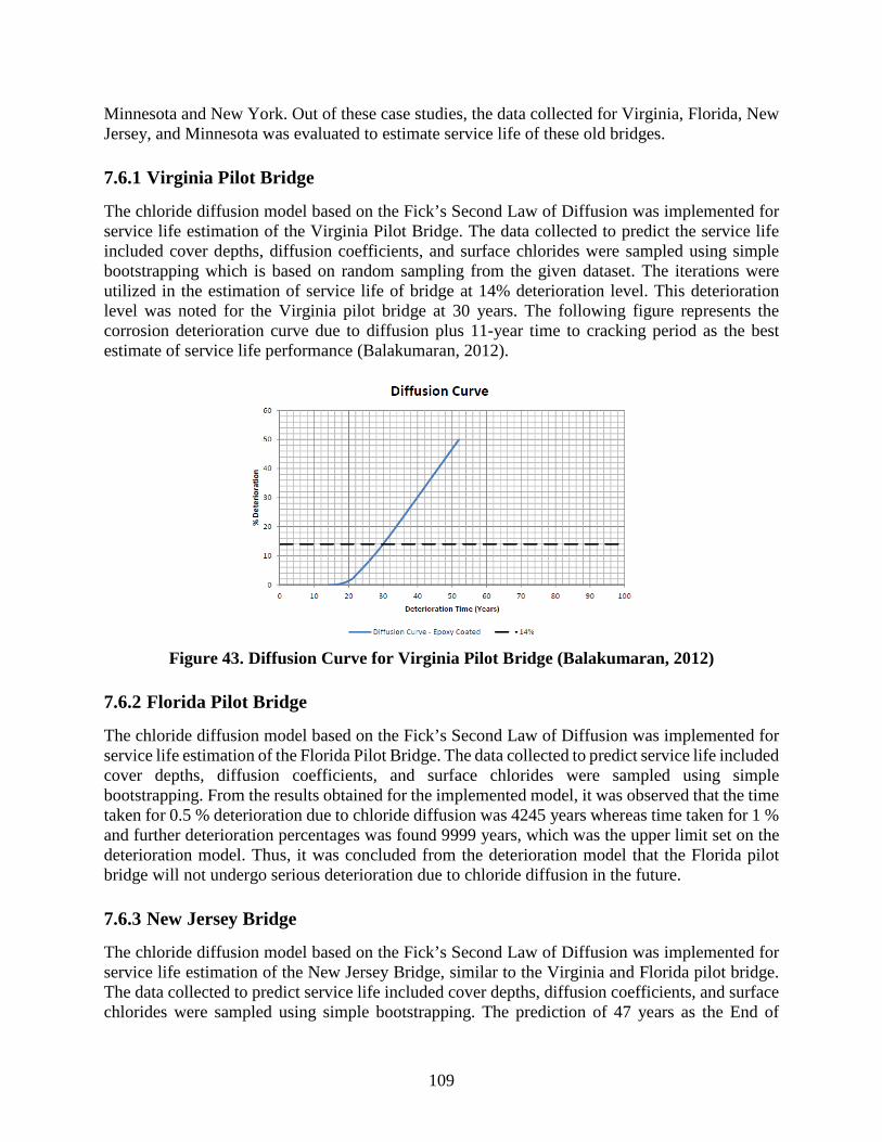
109

Minnesota and New York. Out of these case studies, the data collected for Virginia, Florida, New Jersey, and Minnesota was evaluated to estimate service life of these old bridges. 7.6.1 Virginia Pilot Bridge

The chloride diffusion model based on the Fick’s Second Law of Diffusion was implemented for service life estimation of the Virginia Pilot Bridge. The data collected to predict the service life included cover depths, diffusion coefficients, and surface chlorides were sampled using simple bootstrapping which is based on random sampling from the given dataset. The iterations were utilized in the estimation of service life of bridge at 14% deterioration level. This deterioration level was noted for the Virginia pilot bridge at 30 years. The following figure represents the corrosion deterioration curve due to diffusion plus 11-year time to cracking period as the best estimate of service life performance (Balakumaran, 2012).

Figure 43. Diffusion Curve for Virginia Pilot Bridge (Balakumaran, 2012)

7.6.2 Florida Pilot Bridge

The chloride diffusion model based on the Fick’s Second Law of Diffusion was implemented for service life estimation of the Florida Pilot Bridge. The data collected to predict service life included cover depths, diffusion coefficients, and surface chlorides were sampled using simple bootstrapping. From the results obtained for the implemented model, it was observed that the time taken for 0.5 % deterioration due to chloride diffusion was 4245 years whereas time taken for 1 % and further deterioration percentages was found 9999 years, which was the upper limit set on the deterioration model. Thus, it was concluded from the deterioration model that the Florida pilot bridge will not undergo serious deterioration due to chloride diffusion in the future. 7.6.3 New Jersey Bridge

The chloride diffusion model based on the Fick’s Second Law of Diffusion was implemented for service life estimation of the New Jersey Bridge, similar to the Virginia and Florida pilot bridge. The data collected to predict service life included cover depths, diffusion coefficients, and surface chlorides were sampled using simple bootstrapping. The prediction of 47 years as the End of

110

Functional Service Life (EFSL) was suggested to consider as the service life of the New Jersey pilot bridge, if the bridge deck was not overlaid. The following figure represents the corrosion deterioration curve for the New Jersey Bridge at 5% deterioration rate.

Figure 44. Diffusion Curve for New Jersey Pilot Bridge (Balakumaran, 2012) 7.6.4 Minnesota Pilot Bridge

The service life estimation of the Minnesota pilot bridge deck was run using the data which involved cover depth, surface chloride concentration and diffusion coefficient. The chloride initiation rates were utilized in the model. While calculating the deterioration rate for the given case, the presence of large number of cracks over the entire length of the bridge deck was ignored. The bridge deck was 26 years in service during the time of inspection. The diffusion curve for Minnesota pilot bridge is presented in the following figure.

Figure 45. Diffusion Curve of Minnesota Pilot Bridge (Balakumaran, 2012)

111

7.7 Service Life of Bridges in Canada and Taiwan (Ranjith et al., 2016) The corrosion of reinforcement is one of the serious durability issues while dealing with service life of concrete structures such as a bridge. This is more critical in case of when the rebar in the concrete is exposed to the marine or aggressive environment. Especially, in case of old bridges which are serving for a longer time, it is extremely essential to apply protection measures to avoid future damage of the bridges. Service life prediction considering the corrosion damage play an important role as visible structural damage due to reinforcement corrosion represents a late stage to take any preventive or protection measures. Ranjith et al. (2016) has taken into account well known corrosion models to predict the service life of old Reinforced Concrete (RC) structures in Canada and Taiwan. Ranjith et al. (2016) considered Bazant’s model, Morinaga’s model, Wang and Zhao’s model and IRC model to study the impact of cover thickness, corrosion rate, increase in diameter of the bar, perimeter of the bar, etc. The competence of the models in predicting the service life has been studied by comparing following case studies:

1. Vachon bridge, Laval, Canada (Case i) 2. Vachon bridge, Laval, Canada (Case ii) 3. Tzyh-chyang bridge, Taiwan (Case iii) 4. Dah-duh bridge, Taiwan (Case iv)

7.7.1 Service Life Prediction of a Vachon Bridge Barrier Wall

In 1996, the service of transportation of Quebec attempted the rehabilitation of the vachon span bridge, which is a noteworthy interstate scaffold in Laval Canada (Cusson et al., 2011). A part of the process consisted of remaking the extremely corroded solid boundary walls. The obstruction divider support comprised of bars of 15 mm diameter. On the mentioned location, studies were performed on obstruction divider which included estimations of rate of corrosion and corrosion potential and concrete electrical resistivity. Significant uncertainties and variabilities associated with main important parameters associated with service life prediction were taken into accounts The significant uncertainty and variability connected with the main parameters governing the service life of RC structures subjected to aggressive environments necessitated the utilization of mathematical models for a dependable expectation of their remaining service life. (Ranjith et al., 2016). The following tables gives the mean values of input parameters and the remaining service life of RC bridge barrier wall.

Table 17. Mean values of input parameters (Ranjith et al., 2016)

Table 18. Remaining service life of RC bridge barrier wall, Vachon Bridge (Ranjith et al.,

2016)

112

7.7.2 Service Life Prediction of Tzyh-Chyang Bridge Taiwan

The Tzyh-chyang bridge was completed in 1980 (Liang et al., 2009). This extension finds 34k + 558 of Taiwan-19 line and walks over the Jwo-shosi stream for associating the Chang hua and Yun-lin counties. This bridge is provided with 48 gaps, length of 2224 m, and width of 14.8 m (Ranjith et al., 2016). The following tables show the mean values of input parameters and remaining service life.


Table 20. Remaining service life of Tzyh-Chyang Bridge, Taiwan. (Ranjith et al., 2016)

7.7.3 Service Life Prediction of Dah-Duh Bridge in Taiwan

The Dah-duh bridge was completed in June 1969 (Liang et al., 2009). This bridge finds 181K + 435 of Taiwan1 line and walks over the Dah-duh stream for joining the Taichung and Chang-hua areas and Chang-hua counties. The total length of the bridge is 1000 m and width 30 m (Ranjith

113

et al., 2016). The following tables show the mean values of input parameters and remaining service life of the Dah-duh bridge.


Table 22. Remaining service life of Dah-duh Bridge, Taiwan (Ranjith et al., 2016)

114

Service Life Prediction for Newly Constructed Bridge under Design-build Contracts This chapter documents information regarding the quantitative criteria for bridge structure evaluation and for identifying deterioration models that assist in examining whether a design-build project meets design requirements. 8.1 Fib Bulletin 34: Model Code for Service Life Design The objective of the Model Code for Service Life Design is to identify agreed durability related models and to prepare the framework for standardization of performance based design approaches. The basic idea of service life design is to establish a design approach to avoid deterioration caused by environmental action comparable to load design. This approach follows four steps (Schiessl, 2006).

• The first step in the design approach is to quantify the deterioration mechanism with realistic models describing the process physically and/or chemically with sufficient accuracy (e.g. ingress of carbonation into the concrete depending on the environment and the relevant concrete quality parameters).

• The second step is the definition of limit states against the structure should be designed for.

Appropriate limit states would be o Depassivation of reinforcement caused by carbonation o Cracking due to reinforcement corrosion o Spalling of concrete cover due to reinforcement corrosion o Collapse due to loss of cross section of the reinforcement

• The third step is the calculation of the probability that the limit states defined above occur

(determination of the probability of occurrence).

• The fourth step is the definition of the type of limit state (SLS, ULS) of the limit states described in step 2. Normally depassivation will be classified as a SLS as there is no immediate consequence on structural safety if the reinforcement is depassivated. If cracking and spalling occurs in anchorage zones without sufficient transversal reinforcement, spalling may lead to collapse. In this case cracking and spalling need to be defined as ULS. In other cases, if cracking and spalling does not influence the load bearing capacity of the structural element, cracking and spalling may be defined as SLS.

The service life design approach has the following different levels. The full probabilistic approach (level 1) will be used only for exceptional structures. Based on the full probabilistic approach a partial safety factor approach comparable to load design is given. The partial safety factor approach (level 2) is a deterministic approach where the probabilistic nature of the problem (scatter of material resistance and environmental load) is taken into account by partial safety factors. The other two approaches are deemed to satisfy approach the avoidance of deterioration design approach.

115

8.1.1 Design service life tSL

Indicative values for the design service life tSL are given in the following table.

Table 23. Indicative Values for the Design Service Life tSL (Schiessl, 2006) Design service Examples 10 Temporary structures (structures or parts

of structures that can be dismantled with a view to being re-used should not be considered as temporary)

10-25 Replaceable structure parts, e.g., gantry girders, bearings

15-30 Agricultural and similar structures 50 Building structures and other common

structures 100 Monumental buildings structures, bridges,

and other civil engineering structures 8.1.2 Experimental Tests for Quantification of Parameters

This section briefly describes the test procedures for quantifying specific parameters associated with service life design approach presented for carbonation induced corrosion as well as chloride induced corrosion. 8.1.2.1 Carbonation Induced Corrosion (Uncracked Concrete)

8.1.2.1.1 Limit state equation for the depassivation of the reinforcement

A full probabilistic design approach for the modelling of carbonation induced corrosion of uncracked concrete has been developed based on the following equation.

𝑔𝑔�𝑏𝑏, 𝑥𝑥𝑐𝑐(𝑡𝑡)� = 𝑏𝑏 – 𝑥𝑥𝑐𝑐(𝑡𝑡) = 𝑏𝑏 − �2 ∙ 𝑘𝑘𝑏𝑏 ∙ 𝑘𝑘𝑐𝑐 ∙ �𝑘𝑘𝑡𝑡 ∙ 𝑅𝑅𝐴𝐴𝐶𝐶𝐶𝐶,0−1 + 𝜀𝜀𝑡𝑡� ∙ 𝐶𝐶𝑛𝑛 ∙ √𝑡𝑡 ∙ 𝑊𝑊(𝑡𝑡) (130)

where, a = concrete cover; xc(t) = carbonation depth at the time t; t = time; ke = environmental function; kc = execution transfer parameter; kt = regression parameter; 𝑅𝑅𝐴𝐴𝐶𝐶𝐶𝐶,0−1 = inverse effective carbonation resistance of concrete;

εt = error term; CS = CO2-concentration; W(t) = weather function.

116

8.1.2.1.2 Performance tests for the determination of 𝑹𝑹𝑨𝑨𝑨𝑨𝑨𝑨,𝟏𝟏−𝟏𝟏

Accelerated Carbonation (ACC) test method with the following procedure has been chosen as the reference test method.

• Production of concrete specimens with the following dimensions: height/width/length = 100/100/500 [mm].

• After removing of the formwork the specimens have to be stored in tap water with a

temperature of Tref = 20°C for overall seven days (reference curing).

• Subsequent to the water storage described above, the specimens are removed from the water and stored for 21 further days in a standardized laboratory climate (Tref 20°C, RHref = 65 %).

• At the age of 28 days (tref = 28 d) the specimens are placed in a carbonation chamber with

the standardised laboratory climate (Tref 20°C, RHref = 65 %). In the chamber the specimens are exposed to a CO2 concentration of CS = 2.0 vol.-% during 28 days.

• After removal the concrete specimens are split and the carbonation depth is measured at

the plane of rupture with an indicator solution consisting of 1.0g phenolphthalein per liter.

• By evaluation of the measured carbonation depth according to following equation, the mean value of the reference inverse effective carbonation resistance can be determined.

𝑅𝑅𝐴𝐴𝐶𝐶𝐶𝐶,0−1 = �𝛽𝛽𝑐𝑐

𝜏𝜏�2 (131)

where, 𝑅𝑅𝐴𝐴𝐶𝐶𝐶𝐶,0−1 = inverse effective carbonation resistance of concrete [(m²/s)/(kg/m³)]

τ = ‘time constant’ in [(s/kg/m³)0.5], for described test conditions: τ = 420 xc = measured carbonation depth in the compliance test [m] 8.1.2.2 Chloride Induced Corrosion – Uncracked Concrete

8.1.2.2.1 Limit state equation for the depassivation of the reinforcement

Full probabilistic design approach for the modelling of chloride induced corrosion in uncracked concrete has been developed based on the following equation.

𝐶𝐶𝑐𝑐𝑐𝑐𝑖𝑖𝑡𝑡 = 𝐶𝐶(𝑥𝑥 = 𝑏𝑏, 𝑡𝑡) = 𝐶𝐶0 + (𝐶𝐶𝐶𝐶,𝐴𝐴𝛽𝛽 − 𝐶𝐶0) ∙ �1 − 𝑏𝑏𝑐𝑐𝑖𝑖 𝑏𝑏−𝐴𝐴𝛽𝛽2∙�𝐷𝐷𝑐𝑐𝑝𝑝𝑝𝑝,𝐶𝐶∙𝑡𝑡

� (132)

where, Ccrit = critical chloride content; C(x,t) = content of chlorides in the concrete at a depth x and at time t; C0 = initial chloride content of the concrete; CS,Δx = chloride content at a depth Δx and a certain point of time t; X = depth with a corresponding content of chlorides C(x,t); a = concrete cover;

117

Δx = depth of the convection zone (concrete layer, up to which the process of chloride penetration differs from Fick’s 2nd law of diffusion); Dapp,C = apparent coefficient of chloride diffusion through concrete; 𝑡𝑡 = time; erf = error function; Also,

𝐷𝐷𝑏𝑏𝑝𝑝𝑝𝑝,𝑐𝑐 = 𝑘𝑘𝑏𝑏𝐷𝐷𝑅𝑅𝐶𝐶𝑅𝑅,0𝑘𝑘𝑡𝑡𝐴𝐴(𝑡𝑡) (133) where, ke = environmental transfer variable; be = regression variable; Tref = standard test temperature; Treal = temperature of the structural element or the ambient air; DRCM,0 = chloride migration coefficient; kt = transfer parameter; A(t) = subfunction considering the ‘ageing’. 8.1.2.2.2 Rapid Chloride Migration Method

The NT Build 492 test comes from the NordTest (Based in Finland) family of test methods and is not yet widely used in the United States. This is an alternative to ASTM C1202, and the result is a diffusion coefficient that can be used to assess the quality of concrete. This test is an electrical method, very similar to the rapid chloride (RCP) test. The sample for the test is cut from a 4‑inch

by 8‑inch cylinder. It does not have to be coated with epoxy, but it goes through 24‑hour conditioning similar to the RCP samples. During the exposure period, the sample is sandwiched between a sodium chloride solution and a sodium hydroxide solution. The test is run for a time and at a voltage determined by the sample’s initial current with an applied 30V. The time of exposure ranges from 24 to 96 hours. After the test is completed, the sample is split in half and a silver nitrate solution is sprayed on the fractured surface. White silver nitrate precipitate forms on the part of the face where chloride ions are present. The depth of chloride penetration is measured as the average of seven measurements across the width of the sample. Diffusion coefficient is calculated from values of chloride penetration, sample thickness, exposure time, voltage, and average sample temperature (NT Build 492, 2017).

118

Figure 46. Test Cells (NT Build 492, 2017)

8.2 Case Studies 8.2.1 The New NY Tappan Zee Bridge and the Ohio River Bridge (Bergman, 2016)

The International Federation for Structural Concrete (fib) Model Code for Service Life Design was implemented on the New NY (Tappan Zee) Bridge and the Ohio River Bridge — Downtown Crossing between Kentucky and Indiana. The approach is analogous to structural design for which durability-related loads and resistances are assessed and quantified probabilistically, considering element specific exposures and material properties (Bergman, 2016). Fib design (FIB, 2006) has recently been implemented in ISO 16204:2012 Service Life Design of Concrete Structures. The fib methodology provides a rational probability-based approach to service life design of concrete structures subject to corrosion, a major deterioration mechanism for bridges, tunnels, and marine structures. In this design methodology, durability loads include surface chloride concentrations and ambient temperature, and durability resistances include concrete cover and permeability. Based on the fib methodology, durability requirements can be quantified and measured to verify that the required materials and properties are achieved. The concrete permeability is represented by the concrete chloride migration coefficient, and is determined by the test NTBuild 492 Chloride Migration Coefficient from Non-Steady State Migration Experiments. In contrast to other concrete durability tests, the NTBuild 492 can be efficiently implemented as part of the construction quality control and assurance processes. Similar to concrete compressive strength tests, the NTBuild 492 is performed on standard concrete cylinders at 28 days after casting, and the test has a 24-hour duration. The test provides a direct measurement of the concrete resistance to chloride penetration and the measured value is used directly in service life calculations. This fib methodology goes beyond traditional “deemed-to-satisfy” rules and subjective durability requirements, providing a documented and validated probabilistic limit states design approach to service life. The contractor can demonstrate that service life requirements are met and the owner can be confident that their asset will not deteriorate prematurely. This approach benefits all parties involved on the project.

119

8.2.2 Tappan Zee Bridge

8.2.2.1 Project Description

The New NY (Tappan Zee) Bridge project is a $3.9 billion effort to replace the nearly 60-year old functionally obsolete Governor Malcolm Wilson Tappan Zee Bridge. The new crossing comprises twin parallel 4.98-km long structures with cable-stayed main spans. A design-build team designed the parallel replacement main span cable-stayed bridges. Construction of the bridges is currently ongoing and is scheduled for completion in 2018 by Tappan Zee Constructors, a design-build LLC composed of Fluor Enterprises, American Bridge Company, Granite Construction Northeast and Traylor Bros. The bridge is owned by the New York State Thruway Authority and represents their first design-build project.

Figure 47. Tappan Zee Bridge Concept Design (LaViolette, 2014)

8.2.2.2 Durability Design

In order to achieve the required service life, a probabilistic approach to the concrete durability design was used in this project. This approach provides reliability-based methods for explicitly determining the service life of the concrete elements. These new service life design tools were taken from the fib bulletin 34: Model Code for Service Life Design. The methodology was developed through the publicly funded DuraCrete research project and was validated by a consortium of universities and consulting firms to offer a reliability-based approach similar in principle to modern limit states design-based structural design codes (CSCE, 2014). The fib methodology provides a rational probability-based approach to service life design of concrete structures subject to corrosion, a major deterioration mechanism for bridges, tunnels and marine structures. This state-of-the-art durability design methodology has been implemented on the New NY (Tappan Zee) Bridge and the Ohio River Bridge — Downtown Crossing between Kentucky and Indiana. The approach is analogous to structural design for which durability-related loads and resistances are assessed and quantified probabilistically, considering element specific exposures and material properties. For a bridge subject to chloride-induced reinforcement corrosion, a durability load is the chloride exposure level, and corresponding durability resistances are the chloride migration coefficient of concrete and cover thickness. Using this approach, durability requirements can be quantified and measured to verify that the required materials and properties are achieved. Concrete compressive

120

strength is routinely measured as a means of verifying the structural performance. Based on the fib methodology, durability requirements can be quantified and measured to verify that the required materials and properties are achieved. Concrete compressive strength is measured as a means of verifying the structural performance; we can now do the same for the durability requirements. The concrete permeability is represented by the concrete chloride migration coefficient, and is determined by the test NTBuild 492 Chloride Migration Coefficient from Non-Steady State Migration Experiments. In contrast to other concrete durability tests, the NTBuild 492 can be efficiently implemented as part of the construction quality control and assurance processes. Similar to concrete compressive strength tests, the NTBuild 492 is performed on standard concrete cylinders at 28 days after casting and the test has a 24-hour duration. The test provides a direct measurement of the concrete resistance to chloride penetration and the measured value is used directly in service life calculations. 8.2.3 Gateway Bridge


The Second Gateway Bridge is being built next to the original bridge to duplicate the Gateway Arterial crossing of the Brisbane River. It is 1627m long with a main span of 260m. The three river spans are constructed by the cast in-situ balanced cantilever method with segments varying from 15m to 5m deep and the approach spans are typically 71m long and constructed by match cast segmental construction with epoxy joints. The new bridge is designed and is being built with a design life target of 300 years.

Figure 48. Gateway Upgrade Project (Gateway Upgrade Project, 2017)


The Second Gateway Bridge is a prestressed and reinforced concrete bridge that sits in a range of environmental exposure conditions. The durability of the concrete comprising the bridge elements is the major factor in achieving a long service life. The project scope and technical requirements (PSTR) for the bridge specified that the durability be applied diligently and continuously throughout the process of design, construction and throughout the maintenance period, and that the Second Gateway Bridge have a design life of 300 years, with some replaceable sub-items having design lives ranging from 20 years (wearing course) to 100 years (bearings). Design life

121

was defined as the period assumed in design for which the structure or structural element is required to perform its intended purpose without replacement or major structural repairs (Connal and Berndt, 2009). In addition to a 300 year design life dictated for the bridge structure, several other requirements were mandated from the PSTR. These were aimed at ensuring a minimum level of durability:

– Minimum 40 MPa concrete strength – Minimum 20% fly ash – Electrical connectivity of reinforcement in concrete piles, pile caps and piers for possible

future installation of cathodic protection, and – Mix requirements for concrete in potential acid sulphate soil

The design process for addressing durability in this project is summarized as follows: - Define the characteristics of the environment - Identify the potential deterioration mechanisms in that environment - Determine the likely rate of deterioration - Assess the material life - Define the required material performance - Take a probabilistic approach to the variability of the relevant parameters - Assess and define the need for further protection

In terms of chloride ingress, the greatest concern was for pile caps in the tidal/splash zone of the Brisbane River. The following describes the approach taken to predict chloride penetration. The same principal was used for other chloride-bearing exposure environments. Modelling of chloride ingress versus depth of cover was performed. It was assumed that all transport of chloride ions in concrete would occur by ionic diffusion. Such diffusion can be modelled using a solution to Fick’s Second Law of Diffusion as shown in the following equation (Gateway Upgrade Project, 2017).

𝑐𝑐𝛽𝛽,𝑡𝑡 = 𝑐𝑐𝑛𝑛 �1 − erf �𝑥𝑥

2√𝐷𝐷𝑡𝑡�� (134)

where, D = diffusion coefficient of chloride through concrete; 𝑐𝑐𝛽𝛽,𝑡𝑡= chloride concentration at depth x and time t; 𝑐𝑐𝑛𝑛 = surface chloride concentration; Erf = numerical error function; t = time (s). The changes in diffusion coefficient with time can be modelled according to the following equation as given in ACI Life 365:

𝐷𝐷𝑡𝑡 = 𝐷𝐷𝑡𝑡0 �𝑡𝑡0𝑡𝑡�𝑛𝑛

(135)

Where, 𝐷𝐷𝑡𝑡 = diffusion coefficient at time t; 𝐷𝐷𝑡𝑡0 = diffusion coefficient at time of testing 𝑡𝑡0;

122

𝑡𝑡0 = time at test; 𝑡𝑡 = time; 𝑚𝑚 = age factor depending on mix proportions. The above two equations can be combined to the following equation, which predicts chloride ingress versus time for a changing diffusion coefficient.

𝐶𝐶𝛽𝛽,𝑡𝑡 = 𝑐𝑐𝑛𝑛

⎣⎢⎢⎢⎡1 − erf

⎝

⎜⎛ 𝑥𝑥

2� 11 −𝑚𝑚𝐷𝐷 �𝑡𝑡0𝑡𝑡 �

𝑛𝑛�𝑡𝑡 − � 𝑡𝑡𝑡𝑡𝑛𝑛

�𝑛𝑛𝑡𝑡𝑛𝑛�

⎠

⎟⎞

⎦⎥⎥⎥⎤ (136)

where, 𝑡𝑡𝑛𝑛 = age at start of exposure. Use of the above equation to predict chloride diffusion over a prolonged period could potentially result in underestimation of chloride concentration at a given depth of cover (6). For a life of 100 years, the above equation still gives an acceptable prediction. The 300 year design life for the Second Gateway Bridge required consideration of how underestimation of chloride concentration due to assumed ongoing reduction of diffusion coefficient could be avoided. A time weighted average diffusion coefficient (DTWA) was calculated assuming reduction of the diffusion coefficient over the first 30 years according to the above equations, followed by a constant value thereafter. The time weighted diffusion coefficient was calculated according to the following equation:

𝐷𝐷𝑇𝑇𝑊𝑊𝐴𝐴 =∑ 𝐷𝐷𝑡𝑡𝑖𝑖𝑡𝑡𝑖𝑖𝑛𝑛𝑖𝑖=1∑ 𝑡𝑡𝑖𝑖𝑛𝑛𝑖𝑖=1

(137)

where, 𝐷𝐷𝑇𝑇𝑊𝑊𝐴𝐴 = time weighted average diffusion coefficient; 𝐷𝐷𝑡𝑡𝑖𝑖 = diffusion coefficient at time 𝑡𝑡𝑖𝑖. 8.2.3.2.1 Carbonation

Another potential risk, particularly for concrete exposed to atmospheric conditions, is carbonation. This was primarily of concern for the superstructure elements of the Second Gateway Bridge. The process of carbonation results in reduction of concrete pH. The passive iron oxide layer, which protects reinforcement from corrosion in concrete structures, is only maintained at higher pH levels. If the concrete becomes carbonated to the depth of reinforcement, the passive iron oxide layer is no longer stable and corrosion can occur in the presence of sufficient water and oxygen. The rate of carbonation of concrete is related to a combination of factors. These include CO2 concentration, moisture content of the concrete and diffusivity of hardened cement paste. The diffusivity in turn depends on mix design (cementitious content, presence and proportion of supplementary cementing materials, water/cementitious material ratio), extent of curing, pore size and distribution within the concrete, and connectivity of pores. The presence of cracks permits local ingress of CO2 and can result in carbonation and subsequent corrosion ahead of the main carbonation front in sound concrete. The risk of reinforcement corrosion initiation by the process

123

of carbonation can be reduced by using high quality concrete and sufficient depth of cover. The rate of carbonation in atmospheric environments is expressed typically expressed by the following equation.

𝐷𝐷𝑏𝑏𝑝𝑝𝑡𝑡ℎ 𝑐𝑐𝑖𝑖 𝐶𝐶𝑏𝑏𝑐𝑐𝑏𝑏𝑐𝑐𝑛𝑛𝑏𝑏𝑡𝑡𝑖𝑖𝑐𝑐𝑛𝑛 (𝑚𝑚𝑚𝑚) = 𝐶𝐶 ∙ 𝑡𝑡0.5 (138) Where, C = carbonation rate (mm/year0.5); t = time (years) 8.2.3.2.2 Other Durability Issues

In addition to reinforcement corrosion due to chloride ingress or carbonation, durability assessment for the Second Gateway Bridge considered other mechanisms of deterioration including sulphate attack, alkali-aggregate reaction and acid sulphate soils. The approach taken to ensure durability was to use high quality concrete with supplementary cementitious materials, appropriate cover, and, where necessary additional protection such as sacrificial steel casing. 8.2.4 Ohio River Bridge


Procured under a public private partnership contract (PPP), the main river spans of the $763 million Ohio River Bridges East End Crossing feature a 695.1m long three-span steel composite cablestayed bridge with a center span of 365.9m. The Ohio River Bridges East End Crossing project is currently in construction under a $763 million Public Private Partnership (P3) contract. The P3 contract was awarded by the Indiana Finance Authority (IFA), the project owner, to the consortium of WVB East End Partners – a consortium consisting of Walsh Investors, Bilfinger Project Investments and Vinci Concessions – with Walsh Construction Co. and Vinci as contractors and Jacobs as the Lead Designer. The project provides for a new river crossing approximately eight miles upstream (northeast) of the Louisville downtown area to complete an interstate loop around Louisville, KY by connecting the Gene Snyder Freeway (KY-841) with the Lee Hamilton Highway (IN-265).

Figure 49. Ohio River Bridge (Ohio Bridge Project Overview, 2017)

124


The overall approach followed to achieving the 100-year service life for the non-replaceable components and the required service lives in the replaceable components of the bridge is based on combining

1. A high-quality design including strategies to achieve high durability and eliminating non-durable details;

2. Highly durable materials; 3. Effective quality control; and 4. Inspection and maintenance.

The methodologies presented in fib Model Code 2010 and fib Model Code for Service Life Design are used as guidelines for verifying the required durability of the concrete components. As outlined in the fib Model Code, the limit states associated with durability are verified using one of the following approaches:

1. Full probabilistic approach (probabilistic safety format); 2. Semi-probabilistic approach (partial safety factor format); 3. Deemed-to-satisfy; and 4. Avoidance-of-deterioration.

Concrete components of the bridge are designed to achieve the specified service life with a target confidence level of 90 percent, which is a substantially higher standard than “expected” life, which is often applied for concrete durability and which reflects only a 50 percent confidence of achieving the target life. The requirements specified above and the detailed selection of materials including concrete mixes, design details and all other provisions and methods for achieving the specified service life are included in a very comprehensive Corrosion Protection Plan. 8.2.5 FDOT’s Surface Resistivity Test (Presuel-Moreno et al., 2013)

Over the last couple of decades, there has been an increasing interest in measuring the electrical resistivity (conductivity) on water-saturated concrete specimens to evaluate concrete durability. It has been found that electrical concrete resistivity correlates well with the concrete chloride diffusivity. The Florida Department of Transportation (FDOT) has replaced the rapid chloride permeability (RCP) test (ASTM C1202) with a surface resistivity (SR) test (Florida Method, FM5-578) using a four pin Wenner probe array. FDOT’s research found a good correlation between RCP test values and SR measurements for specimens that were wet cured in a controlled environment (or under full immersion) at room temperature (RT). Resistivity of concrete has also been correlated to corrosion rate of depassivated reinforcement (Presuel-Moreno et al. 2013). 8.2.6 MoDOT’s Surface Resistivity Test (Hudson, 2015)

DOTs are using surface resistivity testing for QA and acceptance of newly-placed concrete, verification of in-place properties, and evaluating corrosion potential (primarily on bridge decks) (Hudson, 2015).

125

MoDOT studied concrete mixtures to verify existing relationships between surface resistivity (SR), rapid chloride permeability (RCP), chloride ion diffusion, and the AASHTO penetrability classes. The research also performed a precision and bias evaluation to provide acceptable limits should SR be implemented for quality assurance and refine language in the AASHTO test standard. In the precision and bias determination concrete was produced from three field sites and tested at both UMKC and MoDOT labs. Field mixtures included a paving mixture, a bridge deck mixture, and a structural mixture. Eleven other mix designs were produced in the lab and evaluated for RCP correlation and included paving, bridge deck, structural, and repair mixtures per Missouri Department of Transportation requirements. Additional testing included surface resistivity testing on sealed samples and an existing bridge deck. Results showed excellent correlation between SR and RCP which matched existing relationships provided by AASHTO and other state DOTs. The structural mixture containing 50% Class F fly ash had the best performance with “very low” chloride ion penetrability at 90 days. A ternary paving mixture with 20% Class C fly ash and 30% slag replacement for cement also demonstrated low permeability as well as high compressive strength with an average value of over 9,000 psi at 90 days. The two repair mixtures showed moderate to low penetrability readings and high early strength consistent with their desired purpose. Tests were also performed on a series of slab samples to evaluate SR as a tool for evaluating sealer application. The presence of silane and lithium silicate were able to be detected by the SR test. As a value added to the laboratory research, field testing was attempted on a bridge deck with the goal of providing non-destructive insight to the steel condition in the field. Due to the condition of the bridge conclusions, could not be drawn other than making recommendations for future bridge deck evaluations. The extensive amount of surface resistivity testing on 14 concrete mixtures at ages from 3 hours to 90 days using multiple labs, equipment, operators, and curing conditions has verified RCP relationships and allowed refinement of a testing procedure for a MoDOT standard in the Engineering Policy Guide. Surface resistivity presents an opportunity to improve MoDOT concrete mixtures and specifications to increase durability without adding significant additional testing costs.

126

Determining Remaining Service Life When a Bridge Is Returned to Its Owner

9.1 Introduction Public-Private Partnership (PPP) projects can take a number of forms, but typically involves a “long-term contractual relationship between government agencies and private sector partners for the provision and operation of an infrastructure asset. The Federal Highway Administration has listed a number of variations of the typical PPP contract, such as:

• The Design-Build (DB) contract. The design-builder (private sector) is responsible for the design work and the construction of the project. Financing, maintenance, and operation are the owner’s responsibility (public sector).

• Build-Operate-Transfer (BOT) or Design-Build-Operate-Maintain (DBOM) or Design-Construct-Maintain (DCM). In these PPP variations the public sector finances the project and receives revenues from the private sector. The contractor is not only responsible for the design and construction of the facility, but also for its operations and maintenance.

• Design-Build-Finance-Operate (DBFO). In this variation, the private sector is responsible for financing the project in addition to designing, building, and operating the project. Fees paid by the users or the public sector in the form of “shadow tolls” or “pass-through” tolls are the major sources of revenue for the private sector. Ownership of the project remains with the public agency and the contractor must return (“handover”) the facilities to the public sector at the end of the contract period.

This technical memorandum documents several case studies regarding the scenarios when the operation and maintenance responsibility is transferred back to government owner from a private developer. 9.2 Case Studies Eight case studies are discussed in this section regarding the remaining service life requirements when a bridge is returned to the owner. The following table shows the name and concession periods of these bridge projects.

Table 24. Design-Build-Operate Bridge Projects Project Concession

Periods Location

I-595 Corridor Roadway Improvements Project

35 years Fort Lauderdale, Florida

US 181 Harbor Bridge Project 25 years Corpus Christi, Texas Regina Bypass Project 30 years Saskatchewan, Canada Northeast Stoney Trail 30 years Alberta, Canada North Commuter Parkway and Traffic Bridge Project

30 years Saskatchewan, Canada

Portsmouth Bypass Project 35 years Scioto, Ohio Aberdeen Western Peripheral Route 26 years Aberdeenshire, Scotland The Presidio Parkway Project 30 years San Francisco, California

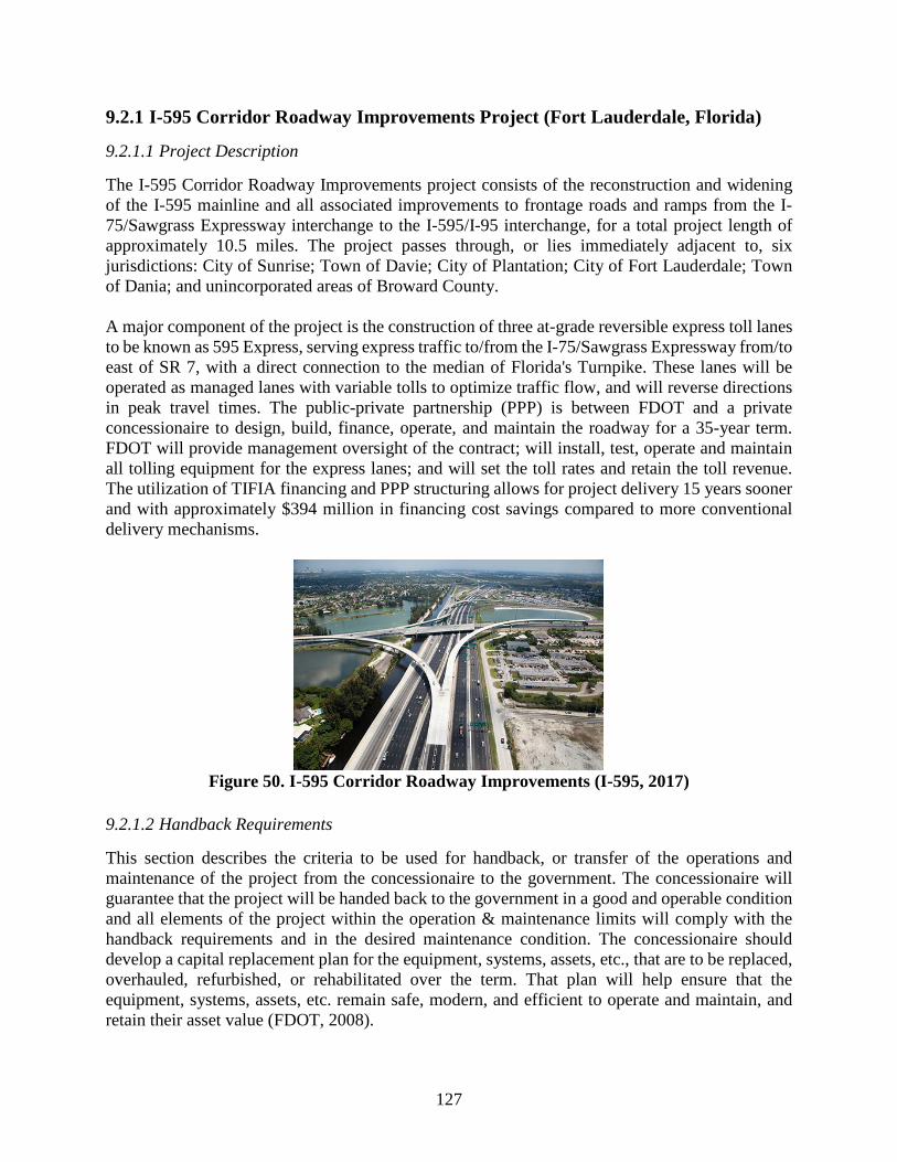
127

9.2.1 I-595 Corridor Roadway Improvements Project (Fort Lauderdale, Florida)


The I-595 Corridor Roadway Improvements project consists of the reconstruction and widening of the I-595 mainline and all associated improvements to frontage roads and ramps from the I-75/Sawgrass Expressway interchange to the I-595/I-95 interchange, for a total project length of approximately 10.5 miles. The project passes through, or lies immediately adjacent to, six jurisdictions: City of Sunrise; Town of Davie; City of Plantation; City of Fort Lauderdale; Town of Dania; and unincorporated areas of Broward County. A major component of the project is the construction of three at-grade reversible express toll lanes to be known as 595 Express, serving express traffic to/from the I-75/Sawgrass Expressway from/to east of SR 7, with a direct connection to the median of Florida's Turnpike. These lanes will be operated as managed lanes with variable tolls to optimize traffic flow, and will reverse directions in peak travel times. The public-private partnership (PPP) is between FDOT and a private concessionaire to design, build, finance, operate, and maintain the roadway for a 35-year term. FDOT will provide management oversight of the contract; will install, test, operate and maintain all tolling equipment for the express lanes; and will set the toll rates and retain the toll revenue. The utilization of TIFIA financing and PPP structuring allows for project delivery 15 years sooner and with approximately $394 million in financing cost savings compared to more conventional delivery mechanisms.

Figure 50. I-595 Corridor Roadway Improvements (I-595, 2017)

9.2.1.2 Handback Requirements

This section describes the criteria to be used for handback, or transfer of the operations and maintenance of the project from the concessionaire to the government. The concessionaire will guarantee that the project will be handed back to the government in a good and operable condition and all elements of the project within the operation & maintenance limits will comply with the handback requirements and in the desired maintenance condition. The concessionaire should develop a capital replacement plan for the equipment, systems, assets, etc., that are to be replaced, overhauled, refurbished, or rehabilitated over the term. That plan will help ensure that the equipment, systems, assets, etc. remain safe, modern, and efficient to operate and maintain, and retain their asset value (FDOT, 2008).

128

The concessionaire should prepare a Handback Evaluation Plan that will be used to determine the condition, performance and residual life of the project assets. The Handback Evaluation Plan should be submitted to the government at minimum of 60 months (5 years) prior to the expected end of the team. The Handback Evaluation Plan should identify the testing, evaluation, and calculation methods that are to be utilized during the condition assessment and the calculation of residual life of all project assets. The Handback Evaluation Plan should include all of the pertinent tests, inspections, processes and evaluations required to verify and demonstrate to the government that all equipment and systems function as intended and meet the life remaining requirements as specified in the following table.

129

Table 25. Handback Requirements (FDOT, 2008)

Asset Description Asset Sub System Description

Handback Evaluation Tasks Handback Evaluation Criteria Life Remaining at Handback (Years)

Bridge Within the O&M Limits (Operating Period)

Pending the results of the testing and inspection criteria, each Bridge under the responsibility of the Concessionaire should have an overall condition rating of six (6) or better. This condition rating is in accordance with the National Bridge Inspection Standards and procedure 850-010- 030 (Bridge and Other Structures Inspection and Reporting) or its successor.

If any Bridge Structure under the responsibility of the Concessionaire is found to have an overall condition rating less than six (6), the Concessionaire should be responsible for making any and all repairs necessary to improve the condition rating of the Bridge(s) to a six (6) or better. All repairs should be of a substantial and permanent nature.

N/A

130

9.2.2 US 181 Harbor Bridge Project (Corpus Christi, Texas)


The Texas Department of Transportation and Flatiron/Dragados entered into a comprehensive development agreement for the Harbor Bridge Replacement Project in Corpus Christi On September 28, 2015. The new Corpus Christi Harbor Bridge will allow larger ships to deliver their cargo to the Port of Corpus Christi. The current bridge was built in the late 1950s. Plans for a replacement bridge to improve safety have been in the works for more than a decade. The proposed $800m project includes construction of a new cable stayed bridge, demolition of the existing Harbor Bridge and the reconstruction of portions of US 181, I-37 and the Crosstown Expressway. In addition to designing and constructing the new bridge, the agreement also requires the developer to operate and maintain the facility for 25 years.

Figure 51. Concept Design of the New Harbor Bridge (TxDOT, 2015)


According to the project agreement, the developer should prepare a Handback Plan that contains the methodologies and activities to be undertaken or employed to meet the handback requirements at the end of the O&M Period. The Handback Plan should be presented in two parts:

(a) for the New Harbor Bridge and (b) for the Roadway Section.

The developer should submit the Handback Plan, including a Residual Life Methodology plan, to TxDOT for review and approval at least 60 months before the end of the O&M period. The Handback Plan should contain the evaluation and calculation criteria to be adopted for the calculation of the residual life at handback for all elements of the project. The scope of any Residual Life testing should be included, together with a list of all independent residual life testing organizations, proposed by developer. These organizations should be on TxDOT’s approved list at the time the testing is performed, as well as during the writing the Handback Plan, have third party quality certification, and be financially independent of developer and not be an affiliate of developer. The developer should make sure that the New Harbor Bridge and the Roadway Section to meet the residual life requirements at the termination date. Residual Life Requirements, defining the

131

number of years of residual life for each element at the end of the 25-year O&M period, are as follows:

Table 26. New Harbor Bridge Residual Life at Handback (Years) (TxDOT, 2014) Maintained Element Residual Life at

Handback (years) All Elements associated with foundations, towers, substructures, superstructure framing system, and deck including: Reinforced concrete Pre-stressed concrete Structural steel

50

External post tensioning cables 35 Deck wearing surface 15 Stay cables and stay cable components 50 Stay cable dampers 15 Sign and lighting structures 50 Corrosion protection (metalizing) for structural steel 10 Galvanizing of structural steel 10 Expansion joints including any replaceable components of such joints

5

Bearings 25 Inspection and access equipment not part of maintenance travelers

35

Internal access ladders and platforms 35 Pedestrian-Only Railings 35 Railing 35 Electrical and mechanical parts 5 Lightning Protection System 5 Navigational lighting 5

According to the agreement (TxDOT, 2014), the developer should perform a hands-on inspection of all parts of each structure for residual life estimation. More specifically, the developer should undertake non-destructive testing appropriate to the type of structure and component to include:

• measurement of settlement/geometry; • identification and measurement of de-lamination of concrete; • measurement of chloride and carbonation profiles from surface to reinforcement and/or

stressed tendon level; and • the in-situ strength testing of concrete elements.

The developer should include within inspection of steel structures testing necessary to determine the residual life of corrosion protection systems and, where necessary, the depth of corrosion and/or the measurement of remaining structural thickness for hidden and exposed parts. The developer should also test all lengths of welds for cracking at key areas of structural steelwork. The developer should also remove corrosion protection covers to stay cable anchorages and inspect the anchorages. The developer should identify for TxDOT approval the number and location of specific individual stay cable strands to be inspected with further inspections based on the results of these initial inspections. The developer should reinstate all corrosion protection systems to their original state following inspection.

132

The residual life methodology for structures should: • draw on historical asset maintenance and repair records, inspection and test histories for

each structure; • take account of the Authority and FHWA records of other structures with similar

characteristics; • include a load rating based on the original structural design calculations, the as-built

drawings and the current condition of the structure as a result of specified inspections; and • take account of any trends in asset deterioration to determine the rate of deterioration and

to predict the future condition of individual elements and the entire structure. 9.2.3 Regina Bypass Project (Saskatchewan, Canada)


The Regina Bypass is a four-lane twinned highway connector road linking two National Highway System routes in Regina, Saskatchewan. Highway 1 (the Trans-Canada Highway) and Highway 11 will be linked by this new route, forming a partial ring road around the city. The route will replace the city's existing Ring Road as the primary urban bypass route around the city. The contractor will design, build, finance, operate and maintain the project over a 30-year period.

Figure 52. Regina Bypass Freeway Project (Regina, 2017)


According to the project agreement (SaskBuilds, 2015), at the expiry date, the bypass infrastructure should meet the required performance levels. The residual service life (RSL) will be determined to have been achieved only if there is no projected need for rehabilitation in respect of the Bypass Infrastructure during the specified RSL period (for clarity, such rehabilitation excludes basic routine maintenance of any component of the Bypass Infrastructure which will be required during the anticipated RSL period). At the expiry date, the structures should be in adequate condition and function as designed with no loss of structural strength and should meet the Performance Measures. The developer should complete any required maintenance or rehabilitation prior to the expiry date to meet the required functionality state and condition prior to returning the structures to the government’s control and management. The developer should also perform annual condition inspection of all structures and report the findings within the most current annual report. The developer should also issue a structure inspection report for each structure, signed and sealed

133

by the Bridge Structural Engineer in accordance with the procedures shown in the Ontario Structure Inspection Manual (OSIM), and Saskatchewan OSIM Supplement Structures Inspection Guide Policy. At the expiry date, when the government assumes responsibility for the structures, it should meet or exceed the requirements defined in the following table.

Table 27. Handback Requirements (SaskBuilds, 2015) Asset Category Required Condition Bridge Elements - Girders, Piers, Foundations, and Abutments

- New - RSL should be the Minimum Required Design Life of the element less the age of the element at the Expiry Date.

- Existing - Minimum required RSL of 40 years. Bridge Deck - Asphalt - Minimum required RSL of 10 years. Bridge Deck - Water Proofing Membrane

Minimum required RSL of 10 years.

Bridge Deck – Concrete - New - RSL should be the Minimum Required Design Life of the bridge deck less the age of the bridge deck at the Expiry Date.

- Existing - Minimum required RSL of 40 years. - No areas with a material defect severity of medium, severe or very severe for

scaling, spalling and unfilled cracks. - No areas of alkali aggregate reactivity. - Copper Sulfate Electrode (CSE) test results showing a minimum of 90% with

readings less negative than –0.300 V. - Maximum total average chloride content of 0.020, by percent weight, at the

top mat of reinforcing or 100 mm depth, whichever is less. - No areas that are delaminated or debonded as determined by chain drag testing

or hammer sounding in accordance with ASTM D4580 Bridge Elements - Curbs, Barriers and Medians

- New - RSL should be the Minimum Required Design Life of the element less the age of the element at the Expiry Date.

- Existing - Minimum required RSL of 40 years. - CSE test results showing a minimum of 90% of readings less negative than -

0.300 V. - No areas that are delaminated as determined by chain drag testing or hammer

sounding in accordance with ASTM D4580. Bridge Joints - Minimum required RSL of seals at the Expiry Date should be 10 years.

- Minimum required RSL of steel components of the joint at the Expiry Date should be 25 years.

Bridge Bearings - New - RSL should be the Minimum Required Design Life of the bridge bearings less the age of the bridge bearings at the Expiry Date.

- Existing - Minimum required RSL of 10 years. - Minimum 50 µm galvanized or 70 µm metallized coating thickness

Bridge Railings and Piles - Minimum 50 µm galvanized coating thickness or 70 µm metallized thickness Major Retaining Walls - New - RSL should be the Minimum Required Design Life of the Major

Retaining Wall less the age of the Major Retaining Wall at the Expiry Date Major Culverts - New - RSL should be the Minimum Required Design Life of the Major

Culvert less the age of the Major Culvert at the Expiry Date. - Existing – Minimum required RSL of 10 years.

Major Sign Structures - New - RSL should be the Minimum Required Design Life of the Major Sign Structure less the age of the Major Sign Structure at the Expiry Date.

- Minimum 50 µm galvanized coating thickness or 70 µm metallized thickness. Notes: - CSE and chloride testing and chain drag testing should be carried out at 12 months prior to the Expiry Date. - CSE and chloride testing and chain drag testing should be carried out in accordance with the requirements of

ASTM C876, ASTM D4580, and the Minister of Highways and Infrastructure’s bridge inspection procedures. - Chloride content testing is performed in accordance with the “Standard Test Method for Chloride Content in

Concrete Using the Specific Ion Probe” and “The Method of Field Determination of Total Chloride Content”.

134

9.2.4 Northeast Stoney Trail, (Alberta, Canada)


The 13-mile Northeast Stoney Trail (NEST), is a northeast portion of a ring road around Calgary. The road extends from Deerfoot Trail, the main north-south route through Calgary, south to 17 Avenue SE. The project included 23 bridge structures and six interchanges, including one major interchange at Deerfoot Trail and one at the Trans-Canada Highway 1. According to the Alberta government, Deerfoot Trail is the heaviest traveled road in the entire Province of Alberta, with an estimated 30,000 to 40,000 vehicles expected to use the new ring road each day. Under the P3 financing model, the road was finished on time and on budget. The Public Private Partnership project for the Province of Alberta was developed by Bilfinger Berger BOT, and the project was designed and built by Stoney Trail Constructors, a joint venture led by Flatiron.

Figure 53. Northeast Stoney Trail (Flatiron, 2017)

9.2.4.2 HandBack Requirements

According to the agreement between the government and the contractor, at the end of the operating period, the bridge structures should be in adequate condition and function as designed with no loss of structural strength and should meet the handback performance requirements. The contractor should complete any required maintenance or rehabilitation prior to the end of the team to meet the required functionality state and handback condition prior to returning the bridge structures to the government’s control and management. For concrete bridge decks, the following requirements need to be met:

1. The decks should not have any physical defects or chemical deterioration. 2. Concrete bridge decks cast-to-grade should not have any cracks greater than 0.1 mm in

width and a linear measurement of 0.2 m of cracking per square metre of bridge deck area. 3. The underside of all concrete decks should be free of stains resulting from deterioration,

efflorescence and exudation. 4. Any cracking on the deck underside should be limited to a maximum width of 0.3 mm.

The government also carries out a number of inspections including concrete deck, copper sulphate electrode (“CSE”) or half-cell testing, chloride ion content testing, ultrasonic inspection of steel elements, scour survey, steel culvert barrel measurement, timber coring, concrete girder, paint

135

system and vertical clearance measurement. The following handback performance requirements for these inspections should be met: - CSE test results showing a minimum of 75% of readings less negative than –0.300 V. - Maximum total average chloride content of 0.025, by percent weight, at the top mat of

reinforcing or 100 mm depth, whichever is less. - The deck area should not be delaminated or debonded as determined by chain drag testing or

hammer sounding in accordance with ASTM D4580.

Moreover, all individual components of the bridge rated 4 or less under the government’s Bridge Inspection and Maintenance (BIM) System should be considered in non-conformance and the contractor should perform repairs to achieve a rating of 5 or higher. 9.2.5 North Commuter Parkway and Traffic Bridge Project (Saskatchewan,

Canada， 2015)


Saskatoon’s North Commuter Parkway and Traffic Bridge Replacement project are being funded through a public-private partnership (P3) with the federal government. Saskatchewan is contributing $50 million to the project, while the federal government is providing an additional investment of up to $66 million through the P3 Canada Fund. The 107-year-old traffic bridge will be replaced and a new bridge connecting roadways and crossing the city’s north end will be constructed. After completion, traffic congestion will be reduced and travel times will be shortened. The following figure shows the concept design the new bridge.

Figure 54. Traffic Bridge Proposed Concept Design (City of Saskatoon, 2017)


The project agreement states that at the expiry date, all structures should be in adequate condition and function as designed with no loss of structural strength, and should meet the performance requirements. The contractor should complete any required maintenance or rehabilitation prior to the expiry date to meet the required functionality state and condition prior to returning the bridge structures to the government. At the expiry date, when the government assumes responsibility for

136

the structures, these should meet or exceed the requirements defined in the following table (City of Saskatoon, 2015).

Table 28. Handback Requirements (City of Saskatoon, 2015) Asset Category Required Condition

All concrete elements except concrete wearing surfaces

- Minimum required RSL of 75 years. - Chloride concentration at 25mm below surface shall not exceed

0.01% Cl- by weight of concrete. - No delaminations or debonding present. - Carbonation front shall be within design parameters with a

minimum of 3 tests per class of concrete per exposure condition to be undertaken.

- Scaling shall not exceed 10 mm depth for elements with exposure condition F1 and 5 mm depth in all other conditions.

Concrete wearing surfaces - Minimum required RSL of 20 years. - Undertake a field survey of all concrete wearing surfaces at a

minimum of 1.5 m intervals to identify areas of abrasion. Bridge river piers - Minimum required RSL of 120 years.

- A field survey of all piers at 1 m intervals shall be undertaken to map abrasion at the waterline.

Bridge deck – asphalt - Minimum required RSL of 20 years. - No Fair or Poor condition states present. - Ravelling of bridge deck asphalt shall not exceed 20% of the deck

area. Bridge weathering steel (excluding Traffic Bridge main truss verticals and diagonals)

- Minimum required RSL of 100 years. - All elements in Excellent condition state with no performance

deficiencies.

Bridge weathering steel for Traffic Bridge main truss verticals and diagonals


deficiencies. Bridge coatings - Minimum required RSL of 25 years.

- All elements in Excellent condition state with no performance deficiencies.

Bridge expansion joint – glands


deficiencies. Bridge expansion joint – armouring and cover plates


deficiencies. - Perform a full leakage test to confirm all components are

operating as designed. Bridge bearings - Minimum required RSL of 50 years.

- All elements in Excellent condition state with no performance deficiencies.

Major Retaining Walls - Minimum required RSL of 50 years. Major Sign Structures - Minimum required RSL of 20 years.

9.2.6 Portsmouth Bypass Project (Scioto, Ohio)


The Portsmouth Bypass is a $634 million, 16-mile, four-lane, limited-access highway around the City of Portsmouth in Scioto County in South Central Ohio. The project will provide a largely

137

access controlled alternative to I-77 and I-75 for motorists making trips between southern Ohio and the Columbus region, saving over 70 miles on some trips. The project is being delivered as an availability payment design-build-finance-operate-maintain (DBFOM) concession. The term of the concession is expected to extend for 35 years. The project is the first availability payment P3 concession in Ohio. According to the project, public benefits include: correcting deficiencies in the existing system, improving regional mobility, enhancing the region’s competitive advantage for businesses, and decreasing crash rates. Designated as State Route 823, the project will improve regional mobility to provide travel time savings of up to 16 minutes per trip compared to the current route. Given the rural nature of the County, this project and subsequent development could also have a material impact on the County’s high unemployment rates. The State estimates the financial structure, including the TIFIA loan, accelerates delivery of the project and benefits by 8 years.

Figure 55. Portsmouth Bypass Project (Portsmouth Gateway Group, 2017)


According to the RFP, the developer should carry out the inspection and testing detailed in the Renewal Work Plan for assessing the condition of the critical structural elements against intended performance and predicting the time to maintenance and residual life. Unless the method of inspection is mutually agreed in the Handback Inspection Report the inspection method should be in accordance with the inspection manuals, guidance, and standards issued by the government that detail the means and methods for assessing the condition of national highway system assets including road pavement, Structures, cut slopes and embankments and other ancillary assets such as signs, fences, barriers and lighting stock, current at the time of inspection. The developer should prepare and submit a Residual Life Methodology to the government for Non‐Discretionary approval sixty (60) months before the end of the Maximum Term. The government will review and respond to the Residual Life Methodology within 45 Business Days (9 weeks). In reviewing and commenting on the methodology, the government should be allowed access to all of the developer’s records used in the preparation of the report. The government’s Non‐Discretionary approval of the Residual Life Methodology, including the scope and schedule of inspections, should be required before commencement of Residual Life inspections. The Residual Life Methodology should contain the evaluation and calculation criteria to be adopted for the calculation of the Residual Life of each Element at the end of the Maximum Term. It should

138

follow Good Industry Practice and procedures and also be in accordance with the government’s testing and forecasting methodologies in use at similar owned or operated assets. The scope of any Residual Life testing should be included, together with a list of all independent inspection and testing organizations proposed by the developer. These organizations should be financially independent of the developer. The government should be given the opportunity to witness any of the inspections and/or tests and should be provided with a minimum of 15 Business Days notice prior to the performance of any such tests. Specific requirements to be included in the Residual Life Methodology are set forth in the following table. These inspection and testing requirements are to be reviewed to ensure that they conform with Good Industry Practice at the end of the Maximum Term and reflect all technological advancements in the field of inspection, testing and residual life calculation.

139

Table 29. Residual Life Requirements Element Residual

Life at Handback

(yrs)

Inspection Requirements Residual Life Methodology (RLM) Requirement

Reinforced concrete 40 - Inspections of Structures shall be undertaken by independent testing organizations.

- Inspections shall follow the latest inspection guidelines (as they apply at the relevant date that the testing is undertaken) recognized by the Department.

- A close examination shall be made of all parts of each structure.

- Non‐destructive tests shall be undertaken appropriate to the type of Structure. These shall include the measurement of structural deflection under calibrated load, the measurement of chloride and carbonation profiles from surface to reinforcement and/or tendon level, half‐cell potential and the in‐situ strength testing of concrete elements.

- Testing of steel structures shall include the depth of corrosion and/or the measurement of remaining structural thickness for hidden and exposed parts.

- All lengths of weld shall be tested for cracking at key areas of structural steelwork.

RLM shall: - Draw on historical asset maintenance records,

inspection and test histories for each structure. - Take account of the Department and FHWA

records of other Structures on the network with similar characteristics.

- Include an assessment of load carrying capacity based on the original structural design calculations, the as built drawings, loading history and results of load deflection tests where appropriate.

- Take account of any trends in asset deterioration to determine the rate of deterioration and to predict the future condition of individual elements and the entire Structure.

- Take account of industry guidance relating to residual life estimation. The measured performance shall be compared with expected performance and trends in asset deterioration and maintenance to predict the future condition and maintenance requirements of main structural elements.

Pre‐stressed concrete 40 Structural steelwork 40 Weathering steel 40 Corrugated steel 40

Bridge Deck (Structural)

15 - Inspections shall be in accordance with the Durability Plan schedule.

- Inspections shall, at a minimum, the identification and measurement of delamination in Bridge decks by chain dragging or hammer sounding, the measurement of chloride and carbonation profiles from surface to reinforcement and/or tendon level, half‐cell potential and the in‐situ strength testing of concrete elements

As above

Railing 25 - Inspections of structures shall be undertaken by independent engineers, test facilities and specialists.

- For visual inspections and measurement, competence shall be based on experience and training.

- Draw on historical asset maintenance records, inspection and test histories for each Structure. Bearings 25

Overhead sign supports (structural Elements)

15

140

Element Residual Life at

Handback (yrs)

Inspection Requirements Residual Life Methodology (RLM) Requirement

Retaining walls (Including MSE Walls)

40 - For specialist inspections, competence shall be based on the possession of valid national or international certification by a recognized certification authority.

- Inspections shall follow the latest inspection guidelines (at the time of inspection) issued by the Department.

- A close visual inspection shall be made of all parts of each Structure including items such as hidden or limited access components such as cables, bearings and expansion joints.

- Take account of the Department and FHWA records of other Structures on the network with similar characteristics.

141

9.2.7 Aberdeen Western Peripheral Route (Aberdeenshire, Scotland)


The Aberdeen Western Peripheral Route (AWPR) is a major infrastructure development proposed to take place on the outskirts of Aberdeen, in Aberdeenshire, Scotland. First announced in January 2003, it was approved by ministers in late 2009. Construction began on 19 February 2015. For the most part, the new dual carriageway will have 2 lanes in each direction, with the exception of the section between North Kingswell Junction and Craibstone Junction, where 3 lanes will operate in each direction and the existing Trunk Road south of Charleston Junction, which will be widened to a three lane carriageway for a short section between Charleston and the next junction to the south of Findon. It is a Design, Build, Finance and Operate major highway in Scotland. The concession period is expected to be 26 years.

Figure 56. The Route Map of Aberdeen Western Peripheral Route


According to the Design, Build, Finance and Operation Agreement, not less than 57 months or more than 63 months before the expiry date the company should consult and comply with the reasonable requirements of the government to agree a procedure for the return of the assets in a condition that meets the handback requirements and should ensure that the transfer proceeds smoothly and with minimum disruption to the level of service provided to users. Where residual life of an element of the assets is specified, the residual life should be measured from the expiry date. The residual life of each element of the assets should as a minimum be the greater of either 5 years the value specified in the following table. The company should take all reasonable steps to demonstrate that the residual life of each element of the assets has been achieved.

142

Table 30. Residual Life of Elements of Structures Structural Element Residual Life (Years) Reinforced Concrete 30 Prestressed Concrete 30 Structural Steelwork 30

Weathering Steel 30 Corrugated steel buried Structures 30

Corrosion protection for structural steelwork 5 Deck waterproofing 5

Deck Joints: (a) Asphaltic Plug 5

(b) Elastomeric 5 (c) Elastomeric (in metal runners) 5

Vehicle/pedestrian parapets 15 Pedestrian parapets 15

Bearings: (a) Elastomeric 15

(b) Mechanical/Roller 15 (c) PTFE Coating 8

Sign/Signal Gantries 15 Reinforced Earth/Anchored Earth Structures 30

Crib walls 30 Soil nails 30

Ground Anchors 30 Catenary lighting systems 8

High mast lighting 8 CCTV poles 8

Traffic signal poles 8

9.2.8 The Presidio Parkway (San Francisco, California)


The Presidio Parkway project is also known as Doyle Drive Replacement project. Doyle Drive is a 1.6 mile segment of Route 101 in San Francisco that provides access to the Golden Gate Bridge from the south; it connects Marin and San Francisco counties and links the peninsula and North Bay Area counties. The Presidio Parkway project is divided into two phases. Phase I was delivered by the California Department of Transportation (Caltrans) through a traditional design-bid-build process. The Phase I construction began in late 2009 and was completed in April 2012. The Phase II of this project is delivered through a public-private partnership.

143

Figure 57. Presidio Parkway Map (Wikibooks, 2017)


Four years (48 months) prior to the expected end of the term, the developer shall prepare a Handback Renewal Work Plan that identifies the developer’s plan for repairing, replacing, renovating, and inspecting the assets such that the assets comply with the specified life remaining at the end of the Term. The Handback Renewal Work Plan shall be updated annually and include the results from the last Annual Handback Evaluation Report and the estimated cost and schedule of the remaining Handback Renewal Work. The developer shall coordinate all aspects of the Handback Renewal Work Plan with the Department. Following each of the inspections of the Project assets by the Department as described in the Handback Renewal Work Plan, and in any case on a yearly basis following the evaluation to be done by the developer accordingly to the Handback Evaluation Plan, the developer shall update the Handback Renewal Work Plan and submit it to the Department for approval until the plan is completed at the agreed upon Termination Date. This plan shall also include any areas that are under remedial work due to a contamination or fuel spill. The developer will retain all remediation responsibility (and liability) until such time that the developer has received, and submitted to the Department, acceptable documentation indicating that the developer has complied with all directives and fulfilled and completed their remediation obligations as directed by the governing municipal entity, whether it be a Federal, State, County or Local government.

144

Table 31. Handback Requirements (West Coast Infrastructure Exchange, 2016) Asset Description

Asset Sub System Description

Handback Evaluation Tasks

Handback Evaluation Criteria Life Remaining at Handback (Years)

Bridges Within the O&M Limits

- Final inspection of all structures shall be conducted in accordance with Maintenance Manual Volume II, Section 4 for the H Family within 180 calendar days before the end of the Term.

- Complete all tests in the Handback Renewal Work Plan to demonstrate the achievement of the required life remaining at the end of the Term.

- Overall condition rating of eighty (80) or better on the FHWA Standard Structure Sufficiency Rating scale for all Structures;

- Achievement of standards in the Handback Renewal Work Plan to demonstrate the achievement of the required life remaining at the end of the Term.

45 Years

145

References AASHTO. (2010). Bridge Element Inspection Manual. AASHTO, LRFR. 2011. The Manual For

Bridge Evaluation. AASHTO. (2015). Standard Method Electrical Indication of Concrete's Ability to Resist

Chloride Ion Penetration. AASHTO Designation: T 277. American Association of State Highway and Transportation Officials, Washington, DC.

Adams, Teresa M, Pincheira, Jose A, and Huang, Ying-Hua. 2002. Assessment and rehabilitation strategies/guidelines to maximize the service life of concrete structures. Tech. rept.

Agrawal, Anil Kumar, and Kawaguchi, Akira. (2009). Bridge element deterioration rates. Tech. rept. New York State Department of Transportation.

Alonso, Carmen, Andrade, C, and Gonzalez, JA. 1988. Relation between resistivity and corrosion rate of reinforcements in carbonated mortar made with several cement types. Cement and concrete research, 18(5), 687–698.

Andrade, C, and Alonso, C. 2004. Test methods for on-site corrosion rate measurement of steel reinforcement in concrete by means of the polarization resistance method. Materials and Structures, 37(9), 623–643.

Andrade, C, and Alonso, Cruz. 1996. Corrosion rate monitoring in the laboratory and on-site. Construction and Building Materials, 10(5), 315–328.

Andrade, Carmen, Alonso, M Cruz, and Gonzalez, Jose Antonio. 1990. An initial effort to use the corrosion rate measurements for estimating rebar durability. In: Corrosion rates of steel in concrete. ASTM International.

Ann, KY, Pack, S-W, Hwang, J-P, Song, H-W, and Kim, S-H. 2010. Service life prediction of a concrete bridge structure subjected to carbonation. Construction and Building Materials, 24(8), 1494–1501.

ASTM, C. (1997). 1202-97. Standard test method for electrical indication of concrete’s ability to resist chloride ion penetration. Annual book of ASTM standards, 4(2), 639-644.

ASTM, C. (2008). 157, Standard Test Method for Length Change of Hardened Hydraulic-Cement Mortar and Concrete. ASTM International: West Conshohocken, PA.

ASTM (2015). C666 / C666M-15. Standard Test Method for Resistance of Concrete to Rapid Freezing and Thawing, ASTM International, West Conshohocken, PA.

ASTM, C. (2003). 1556. Standard test method for determining the apparent chloride diffusion coefficient of cementitious mixtures by bulk diffusion. Annual book ASTM standards.

ASTM, E. (1999). 1049. Standard practices for cycle counting in fatigue analysis. Atimay, E, and Ferguson, PM. 1974. Early Chloride Corrosion of Reinforcing–A Test Report.

Materials Performance, 13(12), 18–21. Atkinson, Alan, and Hearne, John A. 1989. Mechanistic model for the durability of concrete

barriers exposed to sulphate-bearing groundwaters. MRS Online Proceedings Library Archive, 176.

146

Attoh-Okine, Nii, and Atique, Farzana. 2006. Service Life Assessment of Concrete with ASR and Possible Mitigation.

Azizinamini, Atorod, Power, Edward H, Myers, Glenn F, and Ozyildirim, H Celik. 2014. Bridges for Service Life Beyond 100 Years: Innovative Systems, Subsystems, and Components. Tech. rept.

Balakumaran, S. S. G. (2012). Corrosion Testing and Modeling of Chloride-Induced Corrosion Deterioration of Concrete Bridge Decks (Doctoral dissertation).

Balasko, M, and Svab, E. (1996). Dynamic neutron radiography instrumentation and applications in Central Europe. Nuclear Instruments and Methods in Physics Research Section A: Accelerators, Spectrometers, Detectors and Associated Equipment, 377(1), 140–143.

Barde, V., Radlinska, A., Cohen, M., and Weiss, W. J. (2009). Relating material properties to exposure conditions for predicting service life in concrete bridge decks in Indiana. Report No: FHWA/IN/JTRP-2007/27

Barnes, Reuben, and Zheng, Tony. 2008. Research on factors affecting concrete cover measurements. The e-Journal of Nondestructive Testing. Austra´lia.

Bazant, Z. P. (1979). Physical model for steel corrosion in concrete sea structures--theory. Journal of the Structural Division, 105(ASCE 14651 Proceeding).

Behnood, Ali, Van Tittelboom, Kim, and De Belie, Nele. 2016. Methods for measuring pH in concrete: A review. Construction and Building Materials, 105, 176–188.

Bentz, D. P., and Ehlen, M. A. (2002). CONCLIFE, User's manual. Bergman, Don. 2016. 100 year service life - integrating durability and structural design.

http://www.cowi-na.com/menu/news/all-news/100-year-service-life---integrating-durability-and-structural-design [Accessed: 2017-03-16].

Bertolini, Luca, and Polder, R. 1997. Concrete resistivity and reinforcement corrosion rate as a function of temperature and humidity of the environment. Netherlands Organisation for Applied Scientific Research.

Board, Transportation Research. 2015. Bridges for Service Life Beyond 100 Years: Service Limit State Design. SHRP 2 Report S2-R19B-RW-1. Tech. rept.

Bolukbasi, Melik, Mohammadi, Jamshid, and Arditi, David. 2004. Estimating the future condition of highway bridge components using national bridge inventory data. Practice Periodical on Structural Design and Construction, 9(1), 16–25.

Bu, Guoping, Lee, Jaeho, Guan, Hong, Blumenstein, Michael, and Loo, Yew-Chaye. 2012. Performance Prediction of Concrete Elements in Bridge Substructures using Integrated Deterioration Method. Pages 108–115 of: IABSE Congress Report, vol. 18. International Association for Bridge and Structural Engineering.

Buckland and Taylor, Integrating Durability and Structural Design, http://scope.cowi.com/sites/default/files/9194-CorpusChristi-ServiceLife%20v2.pdf (Accessed July 30, 2017).

Build, NordTest. 1999. Concrete, mortar and cement-based repair materials: chloride migration coefficient from non-steady-state migration experiments. Nordtest method, 492.

http://www.cowi-na.com/menu/news/all-news/100-year-service-life---integrating-durability-and-structural-design



http://scope.cowi.com/sites/default/files/9194-CorpusChristi-ServiceLife%20v2.pdf

http://scope.cowi.com/sites/default/files/9194-CorpusChristi-ServiceLife%20v2.pdf

147

Build, NT. 1995. 443. Concrete, hardened: accelerated chloride penetration. Nordtest method. Bulusu, Srinivas, and Sinha, Kumares. 1997. Comparison of methodologies to predict bridge

deterioration. Transportation Research Record: Journal of the Transportation Research Board, 34–42.

Canadian Society for Civil Engineering (CSCE) (2014) https://csce.ca/wp-content/uploads/2012/04/CIV_Fall2014.pdf (Accessed July 22, 2017).

Cattan, Jacques, and Mohammadi, Jamshid. 1997. Analysis of bridge condition rating data using neural networks. Computer-Aided Civil and Infrastructure Engineering, 12(6), 419–429.

Chen, Fangliang, and Qiao, Pizhong. 2015. Probabilistic damage modeling and service-life prediction of concrete under freeze–thaw action. Materials and Structures, 48(8), 2697–2711.

City of Saskatoon, (2015). North Commuter Parkway and Traffic Bridge Project Agreement, https://www.saskatoon.ca/sites/default/files/documents/city-clerk/reportspublications/ncptb_project_agreement_council_version_20141209.pdf (Accessed on July 22, 2017).

City of Saskatoon, https://www.saskatoon.ca/business-development/major- projects/current-projects/north-commuter-parkway-traffic-bridge-replacement- project (Accessed July 22, 2017).

Clausen, Jesper S, and Knudsen, Asger. 2012. Onsite measurements of concrete structures using impact-echo and impulse response. Emerging Technologies in Non-Destructive Testing V, 117– 122.

Clear, Kenneth C. 1974. Evaluation of Portland cement concrete for permanent bridge deck repair. Tech. rept.

Clear, Kenneth C. 1989. Measuring rate of corrosion of steel in field concrete structures. Transportation research record.

Clemeña, G. G. (2003). INTERIM REPORT INVESTIGATION OF THE RESISTANCE OF SEVERAL NEW METALLIC REINFORCING BARS TO CHLORIDE-INDUCED CORROSION IN CONCRETE. Report No. VTRC, 04-R7. Clifton, JF. 1991. Predicting the remaining service life of concrete. Tech. rept. National Inst. of

Standards and Technology (NML), Gaithersburg, MD (United States). Center for Atomic, Molecular and Optical Physics.

Concrete Institute of Australia. 2008. Non-destructive Testing of Concrete. Connal, J., and Berndt, M. (2009). Sustainable bridges: 300 year design life for Second Gateway

Bridge. In Austroads Bridge Conference, 7th, 2009, Auckland, New Zealand. Construction, Corus, and Industrial. (2005). Corrosion protection of steel bridges. Corus Construction & Industrial. (2005). Weathering steel bridges. Cusson, D., Lounis, Z., and Daigle, L. (2011). Durability monitoring for improved service life

predictions of concrete bridge decks in corrosive environments. Computer‐Aided Civil and Infrastructure Engineering, 26(7), 524-541.

https://csce.ca/wp-content/uploads/2012/04/CIV_Fall2014.pdf



https://www.saskatoon.ca/sites/default/files/documents/city-clerk/reports-publications/ncptb_project_agreement_council_version_20141209.pdf




https://www.saskatoon.ca/business-development/major-projects/current-projects/north-commuter-parkway-traffic-bridge-replacement-project




148

Emoto, Hisao, Takahashi, Jun, Widyawati, Ratna, and Miyamoto, Ayaho. 2014. Performance evaluation and remaining life prediction of an aged bridge by J-BMS. Procedia Engineering, 95, 65–74.

Ertekin, A Oguz, Nassif, Hani H, and Ozbay, Kaan. 2008a. An LCCA Algorithm for Bridges: A Comprehensive Approach. In: Proceedings of the 87 th annual meeting of the Transportation Research Board.

Ertekin, Ali Oguz, Nassif, Hani H, and Ozbay, Kaan. 2008b. Life-cycle cost analysis algorithm for bridges: comprehensive approach. In: Transportation Research Board 87th Annual Meeting.

Estes, Allen C, and Frangopol, Dan M. 2001. Bridge lifetime system reliability under multiple limit states. Journal of bridge engineering, 6(6), 523–528.

Fagerlund, G. (2004). A service life model for internal frost damage in concrete. Lund University. (Report TVBM; Vol. 3119)

Fasl, Jeremiah David. 2013. Estimating the remaining fatigue life of steel bridges using field measurements.

Florida Department of Transportation (FDOT) (2008). To Design, Build, Finance, Operate and Maintain The I-595 Corridor Roadway Improvements Project, http://595express.info/documents/ContractDocuments/I595_RFP_VII_DII_S5_Handback_final_for_exec.pdf (Accessed on July 20, 2017).

Ferraris, Chiara F, Stutzman, Paul E, and Snyder, Kenneth A. 2006. Sulfate resistance of concrete: a new approach. R&D Serial.

FHWA (1997) https://www.fhwa.dot.gov/publications/research/infrastructure/structures/bridge/metal.cfm

FIB, FIB. 2006. Model code for service life design. International federation for structural concrete (FIB). Switzerland, 110.

Flatiron, Northeast Stoney Trail, https://www.flatironcorp.com/project/northeast- stoney-trail/ (Accessed July 30, 2017)

Ford, Kevin, Arman, Mohammad, and Labi, Samuel. 2012. Estimating Life Expectancies of Highway Assets, Volume 2: Final Report. Vol. 2. Transportation Research Board.

Freyermuth, Cliff. 2009. Service life and sustainability of concrete bridges. Aspire, Fall, 12–15. Frosch, R. J., Labi, S., & Sim, C. (2014). Increasing Bridge Deck Service Life: Volume I-

Technical Evaluation. Fuchs, PA, Clark, AV, Lozev, MG, Halabe, U, Klinkhachorn, P, Petro, S, and GangaRao, H.

1998. Ultrasonic instrumentation for measuring applied stress on bridges. Journal of nondestructive evaluation, 17(3), 141–152.

Gao, L., Xie, C. and Zhang, Z. (2010), Network-Level Multi-Objective Optimal Maintenance and Rehabilitation Planning, CD Proceedings of the Transportation Research Board’s 89th Annual Meeting, Washington, D.C.

http://595express.info/documents/ContractDocuments/I-595_RFP_VII_DII_S5_Handback_final_for_exec.pdf

http://595express.info/documents/ContractDocuments/I-595_RFP_VII_DII_S5_Handback_final_for_exec.pdf

https://www.flatironcorp.com/project/northeast-stoney-trail/



149

Gateway Upgrade Project, Brisbane Queensland, http://www.boral.com.au/major-projects/gateway-bridge/index.html (Accessed July 22, 2017).

Goethals Bridge Replacement Project. Technical Due Diligence Report. (2013). https://emma.msrb.org/EP772201-EP598531-EP999920.pdf

Golden Ears Bridge, https://en.wikipedia.org/wiki/Golden_Ears_Bridge, (Accessed July 21, 2017).

Goodspeed, C. H., Vanikar, S., and Cook, R. (1996). High-performance concrete defined for highway structures. Concrete International, 18(2), 62-67.

Government of Alberta Ministry of Infrastructure (2008). NEST DBFO Agreement, http://www.transportation.alberta.ca/Content/docType353/Production/NWASch18.pdf (Accessed July 20, 2017).

Gucunski, Nenad, et al., 2013. Nondestructive testing to identify concrete bridge deck deterioration. Transportation Research Board.

Gudimettla, Jagan M, and Crawford, Gary L. 2015. Field Experience in using Resistivity Tests for Concrete. In: Transportation Research Board 94th Annual Meeting.

Guignier, F. and Madanat, S.M. (1999), Optimisation of infrastructure systems maintenance and improvement policies, Journal of Infrastructure Systems, 5(4). Hallberg, Daniel. 2005. Development and adaptation of a life cycle management system for

constructed work. Ph.D. thesis, KTH. Harichandran, Ronald S, Burgueno, Rigoberto, Zhang, Gang, and Garratt, Matthew. 2010. ECR

Bridge Decks: Damage Detection and Assessment of Remaining Service Life for Various Overlay Repair Options-Part II. Tech. rept.

Hasan, Md Istiaque, and Yazdani, Nur. 2016. An Experimental and Numerical Study on Embedded Rebar Diameter in Concrete Using Ground Penetrating Radar. Chinese Journal of Engineering, 2016.

Hatami, A., and Morcous, G. (2011). Developing deterioration models for Nebraska bridges (Report No. M302).

Hearn, George, and Xi, Yunping. 2007. Service life and cost comparisons for four types of CDOT bridge decks. Tech. rept. Colorado Department of Transportation, Research Branch.

Helal, J, Sofi, M, and Mendis, P. 2015a. Non-destructive testing of concrete: A review of methods. Electron. J. Struct. Engnr, 14, 97–105.

Helal, J, Sofi, M, and Mendis, P. 2015b. Non-Destructive Testing of Concrete: A Review of Methods.

Hellier, Charles. 2001. Handbook of nondestructive evaluation. Her, Shiuh-Chuan, and Lin, Sheng-Tung. 2014. Non-destructive evaluation of depth of surface

cracks using ultrasonic frequency analysis. Sensors, 14(9), 17146–17158. Hoffman, PC, and Weyers, RE. 1994. Predicting critical chloride levels in concrete bridge decks.

Structural safety and reliability, ICOSSAR, 93, 957–959.

http://www.boral.com.au/major-projects/gateway-bridge/index.html



https://emma.msrb.org/EP772201-EP598531-EP999920.pdf

https://en.wikipedia.org/wiki/Golden_Ears_Bridge

http://www.transportation.alberta.ca/Content/docType353/Production/NWASch18.pdf



150

Hookham, Charles J. 1990. Rehabilitation of Great Lakes Steel’s No. One Dock. Special Publication, 122, 385–400.

Hu, Nan, Haider, Syed W, and Burguen˜o, Rigoberto. 2013. Development and validation of deterioration models for concrete bridge decks, Phase 2: Mechanics-based degradation models. Rep. RC-1587B, 131.

Huang, Ran, Chang, Jiang-Jhy, Yeih, Wei-chung, Liang, Ming-Te, and Weng, Tsai-Lung. 2011. Evaluation for Material Durability and Residual Life Predication of RC Bridges Guide. http: //www.ihmt.gov.tw/periodical/pdf/B1015140.pdf [Accessed: 2017-03-16].

Hudson, Dirk Paul. 2015. Evaluation of Resistivity Meters for Concrete Quality Assurance, Project TR201414. Ph.D. thesis, Faculty of the University of Missouri-Kansas City in partial fulfillment of the requirements for the degree MASTER OF SCIENCE by DIRK PAUL HUDSON BS, University of Missouri-Kansas City.

IAEA. 2002. Guidebook on non-destructive testing of concrete structures. International Atomic Energy Agency.

Impressed Current Cathodic Protection. http://www.jpbroomfield.co.uk/pages/impressed-current-cathodic-protection.php (Accessed: 2016-12-27).

INC., GEMITE Products. 2005. Corrosion of Steel in Concrete due to Carbonation. Inc., Ground Penetrating Radar Systems. http://www.gp-radar.com/concrete.html.Accessed:

February 25, 2017. Institute, American Concrete. 1992. Guide to Durable Concrete. Instruments, Germann. http://germann.org/products-by-application. Accessed: February 25,

2017. Instruments, NDT James. http://www.ndtjames.com/Cor-Map-II-p/ c-cm-5000-cu.htm#specs.

Accessed: February 25, 2017. IRC special publication 60-2002: An approach document for assessment of remaining life of

concrete bridges. Iseki, H., and Houtman, R. (2010). Examination of Recent Developments in DBFO Public

Private Partnership Transportation Projects in North America. In Online Selected Proceeding of the 12th World Conference on Transportation Research.

I-595 Corridor Roadway Improvements, http://www.glfusa.com/project/i-595- corridor-roadway-improvements/#image-4 (Accessed July 22, 2017)

Jeong, Y., Kim, W., Lee, I., and Lee, J. (2016). Bridge service life estimation considering inspection reliability. KSCE Journal of Civil Engineering, 1-12.

Jiang, Yi, and Sinha, Kumares C. 1989. Bridge service life prediction model using the Markov chain. Transportation Research Record.

Jinyu, Li, Wenyu, Xu, Jianguo, Cao, Li, Lin, and Yushi, Guan. 1999. Stydy on the mechanism of concrete destruction under frost action [J]. Journal of Hydraulic Engineering, 1.

JSA - JIS A 1154. 2012. Methods of Test for Chloride Ion Content in Hardened Concrete.

http://www.ihmt.gov.tw/periodical/pdf/B1015140.pdf

http://www.ihmt.gov.tw/periodical/pdf/B1015140.pdf

http://www.jpbroomfield.co.uk/pages/impressed-current-cathodic-protection.php

http://www.jpbroomfield.co.uk/pages/impressed-current-cathodic-protection.php

http://www.gp-radar.com/concrete.html

http://germann.org/products-by-application

http://www.ndtjames.com/Cor-Map-II-p/c-cm-5000-cu.htm#specs

http://www.ndtjames.com/Cor-Map-II-p/c-cm-5000-cu.htm#specs

http://www.glfusa.com/project/i-595-corridor-roadway-improvements/#image-4



151

Kessler, Richard J, Powers, Rodney G, Paredes, Mario, Paredes, Mario, et al., 2005. Resistivity Measurements of Water Saturated Concrete as an Indicator of Permeability. In: CORROSION 2005. NACE International.

Kirkpatrick, T. J., Weyers, R. E., Anderson-Cook, C. M., and Sprinkel, M. M. (2002a). Probabilistic model for the chloride-induced corrosion service life of bridge decks. Cement and concrete research, 32(12), 1943-1960.

Klatter, HE, and Van Noortwijk, JM. 2003. Life-cycle cost approach to bridge management in the Netherlands. Pages 179–188 of: Proceedings of the 9th International Bridge Management Conference, April 28-30, 2003, Orlando, Florida, USA.

Kline, E.S. (2008). "Steel Bridge: Corrosion Protection for 100 Years," Journal of Protective Coatings and Linings, 22-31.

Labi, S., Frosch, R. J., Samdariya, A., & Qing, Y. (2014). Increasing bridge deck service life: Volume II—Economic evaluation (Joint Transportation Research Program Publication No. FHWA/IN/JTRP-2014/17). West Lafayette, IN: Purdue University. http://dx.doi.org/10.5703/1288284315517

LaViolette, M., Tappan Zee Hudson River Crossing (2014) http://www.structuremag.org/?p=7098 (Accessed July 30, 2017)

Lee, Hojae, Cho, Myung-Sug, Lee, Jong-Suk, and Kim, D. 2013. Prediction model of life span degradation under sulfate attack regarding diffusion rate by amount of sulfate ions in seawater. International Journal of Materials, Mechanics and Manufacturing, 1(3), 251–255.

Lee, Jaeho, Sanmugarasa, Kamalarasa, Blumenstein, Michael, and Loo, Yew-Chaye. 2008. Improving the reliability of a Bridge Management System (BMS) using an ANN-based Backward Prediction Model (BPM). Automation in Construction, 17(6), 758–772.

Lee, Sangwook, Kalos, Niko, et al., 2014. Non-destructive testing methods in the US for bridge inspection and maintenance. KSCE Journal of Civil Engineering, 18(5), 1322–1331.

Li, Zhe, and Burguen˜o, Rigoberto. 2010. Using soft computing to analyze inspection results for bridge evaluation and management. Journal of Bridge Engineering, 15(4), 430–438.

Liang, Ming-Te, Lin, Li-Hsien, and Liang, Chih-Hsin. (2002). Service life prediction of existing reinforced concrete bridges exposed to chloride environment. Journal of Infrastructure systems, 8(3), 76–85.

Liang, M. T., Huang, R., Feng, S. A., and Yeh, C. J. (2009). Service life prediction of pier for the existing reinforced concete bridges in chloride-laden environment. Journal of Marine Science and Technology, 17(4), 312-319.

Lin, Kai-Yung. 1995. Reliability-based minimum life cycle cost design of reinforced concrete girder bridges.

Liu, Youping. 1996. Modeling the time-to-corrosion cracking of the cover concrete in chloride contaminated reinforced concrete structures. Ph.D. thesis, Virginia Polytechnic Institute and State University.

http://www.structuremag.org/?p=7098

152

Liu, Youping, and Weyers, Richard E. 1998. Modeling the time-to-corrosion cracking in chloride contaminated reinforced concrete structures. Materials Journal, 95(6), 675–680.

Lo, Y, and Lee, HM. 2002. Curing effects on carbonation of concrete using a phenolphthalein indicator and Fourier-transform infrared spectroscopy. Building and Environment, 37(5), 507– 514.

Locke, CE. 1983. Mechanism of corrosion of steel in concrete. National Assoc. of Corrosion Engineers, 10.

MOLIT (2012b). “Guideline and Commentary of Safety Inspection and In-depth Safety Inspection for Structures-Bridge.” Ministry of Land, Infrastructure and Trasport, Seoul, Korea.

Madanat, Samer M, Karlaftis, Matthew G, and McCarthy, Patrick S. 1997. Probabilistic infrastructure deterioration models with panel data. Journal of infrastructure systems, 3(1), 4–9.

Mccarten, P. (2004). Applying a systems method for setting structure performance targets and measures for a long term concession. In AUSTROADS BRIDGE CONFERENCE, 5TH, 2004, HOBART, TASMANIA, AUSTRALIA (No. AP- G79/04).

Mehta, P Kumar. 2000. Sulfate attack on concrete separating myths from reality. Concrete International, 22(8), 57–61.

Melhem, Hani G, and Cheng, Yousheng. 2003. Prediction of remaining service life of bridge decks using machine learning. Journal of Computing in Civil Engineering, 17(1), 1–9.

Mohsen A. Issa and Atef Khalil. (2010). Diffusivity and permeability of high performance concrete for bridge decks.

Montes-Garcia, P., Jiménez-Quero, V., & López-Calvo, H. (2015). Assessment of high performance concrete containing fly ash and calcium nitrite based corrosion inhibitor as a mean to prevent the corrosion of reinforcing steel. In Journal of Physics: Conference Series (Vol. 582, No. 1, p. 012028). IOP Publishing.

Morales, Miguel, and Bauer, Dominique. 2006. Fatigue and remaining life assessment of steel bridges more than 50 years old. In: 7th International Conference on Short and Medium Span Bridges.

Morcous, G. 2002. Comparing the use of artificial neural networks and case-based reasoning in modeling bridge deterioration. In: Annual conf. of the Canadian society of civil engineering, Montreal.

Morinaga, S. 1989. Prediction of service lives of reinforced concrete buildings based on rate of corrosion of reinforcing steel. Special Report of the Institute of Technology, Skimiza Corporation, Japan.

Nair, Archana, and Cai, CS. 2010. Acoustic emission monitoring of bridges: Review and case studies. Engineering structures, 32(6), 1704–1714.

Narasinghe, SB, Karunananda, PAK, and Dissanayake, PBR. 2006. Service Life Prediction of Masonry Arch Bridges Using Artificial Neural Networks. In: HPC: Build Fast, Build to Last. The 2006 Concrete Bridge Conference.

153

Natesaiyer, K, Hover, KC, and Snyder, KA. 1992. Protected-Paste Volume of Air-Entrained Cement Paste. Part 1. Journal of Materials in Civil Engineering, 4(2), 166–184.

North Carolina Department of Transportation (NCDOT), Book 2, Technical Provisions. (2014). https://www.ncdot.gov/projects/I77ExpressLanes/download/ExecutedTechnicalR equirements.pdf

Ng, SK, and Moses, F. 1996. Prediction of bridge service life using time-dependent reliability analysis. Bridge management, 3, 26–32.

NT Build 492: Non-Steady State Chloride Migration (Diffiusion Coefficient), https://www.betonconsultingeng.com/services/concrete-testing/nt-build-492/ (Accessed July 30, 2017).

Oh, Je-Keun, Jang, Giho, Oh, Semin, Lee, Jeong Ho, Yi, Byung-Ju, Moon, Young Shik, Lee, Jong Seh, and Choi, Youngjin. 2009. Bridge inspection robot system with machine vision. Automation in Construction, 18(7), 929–941.

Ohio Department of Transportation (2014). Request for Proposal to Design-Build- Finance-Operate-Maintain of Portsmouth Bypass Project, https://www.dot.state.oh.us/Divisions/InnovativeDelivery/PortsmouthRFP/20140606_Portsmouth_ProjectScope.pdf (Accessed July 22, 2017).

Ohio Bridge Project Overview, http://kyinbridges.com/downtown-crossing/overview/ (Accessed July 22, 2017).

Page, CL, and Treadaway, KWJ. 1982. Aspects of the electrochemistry of steel in concrete. Papadakis, Vagelis G. 2000. Effect of supplementary cementing materials on concrete resistance

against carbonation and chloride ingress. Cement and concrete research, 30(2), 291–299. Papadakis, VG. 1999. Supplementary Cementing Materials in Concrete—Activity, Durability

and Planning. Danish Technological Institute Concrete Center. Papadakis, VG. 2005. Estimation of Concrete Service Life–The Theoretical Background. Patras

Science Park, Patras. Patterson, W. D. O. (1987). Road deterioration and maintenance effects: Models for planning

and management, Johns Hopkins University Press, Baltimore. Portland Cement Association (PCA). 2002. Types and Causes of Concrete Deterioration. Portsmouth Gateway Group, http://www.portsmouthjv.com/portsmouth-bypass/ (Accessed July

22, 2017). Presuel-Moreno, Francisco, Liu, Yanbo, Wu, Yu-You, and Arias, Wendy. 2013. Analysis and

Estimation of Service Life of Corrosion Prevention Materials Using Diffusion, Resistivity and Accelerated Curing for New Bridge Structures-Volume 2: Accelerated Curing of Concrete With High Volume Pozzolans (Resistivity, Diffusivity and Compressive Strength).

Rahim, Ashraf M, Jansen, Daniel C, and Abo-Shadi, Nagi A. 2006. Concrete bridge deck crack sealing: an overview of research. California Polytechnic State University, Civil and Environmental Engineering.

https://www.ncdot.gov/projects/I77ExpressLanes/download/ExecutedTechnicalRequirements.pdf

https://www.ncdot.gov/projects/I77ExpressLanes/download/ExecutedTechnicalRequirements.pdf

https://www.betonconsultingeng.com/services/concrete-testing/nt-build-492/

https://www.dot.state.oh.us/Divisions/InnovativeDelivery/PortsmouthRFP/20140606_Portsmouth_ProjectScope.pdf



http://kyinbridges.com/downtown-crossing/overview/

http://kyinbridges.com/downtown-crossing/overview/

http://www.portsmouthjv.com/portsmouth-bypass/

154

Ranjith, A., Rao, K. B., and Manjunath, K. (2016). Evaluating the effect of corrosion on service life prediction of RC structures–A parametric study. International Journal of Sustainable Built Environment, 5(2), 587-603.

Reading, MS, and Denzine, AF. 1996. A critical comparison of corrosion monitoring techniques used in industrial applications. Industrial Corrosion and Corrosion Control Technology, 511.

Recording, FHWA. 1995. coding guide for the structure inventory and appraisal of the nation’s bridges. Federal Highway Administration Report FHWA-PD-96-001.

Regina Bypass Freeway Project, http://www.roadtraffic- technology.com/projects/regina-bypass-freeway-project-saskatchewan-province/ (Accessed July 30, 2017)

Rehman, Sardar Kashif Ur, Ibrahim, Zainah, Memon, Shazim Ali, and Jameel, Mohammed. 2016. Nondestructive test methods for concrete bridges: A review. Construction and Building Materials, 107, 58–86.

Rodriguez, MM, Gkritza, K, Labi, S, and Sinha, KC. 2005. Factors affecting bridge deck deterioration in Indiana. In: Procs., 84th Annual Meeting of Transportation Research Board.

Rostam, Steen. 2008. International perspective: Extending the service lives of bridges. PCI journal, 53(1), 121–142.

Russell, Richard Joel. 1943. Freeze-and-thaw frequencies in the United States. Eos, Transactions American Geophysical Union, 24(1), 125–133.

Ryan, Thomas W, Hartle, RA, Mann, J Eric, and Danovich, LJ. 2006. Bridge inspector’s reference manual. FHWA NHI, 03–001.

Sansalone, Mary, and Carino, Nicholas J. 1989. Detecting delaminations in concrete slabs with and without overlays using the impact-echo method. Materials Journal, 86(2), 175–184.

SaskBuilds (2015). Regina Bypass Project Agreement. http://www.saskbuilds.ca/projects/ReginaBypass/Project%20Agreement/The%20Regina%20Bypass%20Project%20-%20Schedule%2015-3%20-%20500%20-%20Handback%20Requirements%20(Execution%20Version).pdf (Accessed July20, 2017).

Schiessl, P., and Task Group Model Code for Service Life Design of Concrete Structures International Federation for Structural Concrete. (2006). Model code for service life design. fib, CEB-FIP.

Shuman, R, Rogers, VC, and Shaw, RA. 1989. The barrier code for predicting long-term concrete performance. In: Waste processing, transportation, storage and disposal, technical programs and public education.

Siemes, A., Vrouwenvelder, A., and Van Den Beukel, A. (1985). Stochastic modeling of building materials performance in durability. In Problems in Service Life Prediction of Building and Construction Materials (pp. 253-263). Springer Netherlands.

http://www.roadtraffic-technology.com/projects/regina-bypass-freeway-project-saskatchewan-province/



http://www.saskbuilds.ca/projects/ReginaBypass/Project%20Agreement/The%20Regina%20Bypass%20Project%20-%20Schedule%2015-3%20-%20500%20-%20Handback%20Requirements%20(Execution%20Version).pdf





155

Smilowitz, K. and Madanat, S.M. (2000), “Optimal Inspection and Maintenance Policies for Infrastructure Networks”, Computer-Aided and Infrastructure Engineering, 15(1), pp. 5–13.

Sobanjo, JO. 1997. A neural network approach to modeling bridge deterioration. Pages 623–626 of: Computing in Civil Engineering. ASCE.

Sohanghpurwala, Ali Akbar. 2006. Manual on service life of corrosion-damaged reinforced concrete bridge superstructure elements. Transportation Research Board.

Stewart, Mark G, and Rosowsky, David V. 1998. Time-dependent reliability of deteriorating reinforced concrete bridge decks. Structural Safety, 20(1), 91–109.

Stukhart, G, JAMES, RW, Garcia-Diaz, A, Bligh, RP, Sobanjo, J, and McFarland, WF. 1991. STUDY FOR A COMPREHENSIVE BRIDGE MANAGEMENT SYSTEM FOR TEXAS. FINAL REPORT. REVISED JULY 1991. Tech. rept.

Thomas, M. D. A., and Bentz, E. C. (2000). Life-365 computer program for predicting the service life and life-cycle costs of reinforced concrete exposed to chlorides. American Concrete Institute, Committee, 365.

Thompson, P. D., Ford, K. M., Arman, M. H. R., Labi, S., Sinha, K. C., and Shirole, A. M. (2012b). Estimating life expectancies of highway assets, volume 2: Final report, NCHRP Report 713. Federal Highway Administration, U.S. Department of Transportation, Washington D.C., U.S.

Thompson, P., and Shepard, R. (2000). AASHTO Commonly-recognized bridge elements. In: Materials for National Workshop on Commonly Recognized Measures for Maintenance, Scottsdale, Arizona.

Trejo, D. (2002). Evaluation of the critical chloride threshold and corrosion rate for different steel reinforcement types. Texas A&M University.

TxDOT selects company to design and build new harbor bridge, (2015). http://www.kristv.com/story/28946043/txdot-selects-company-to-design-and-build-new-harbor-bridge (Accessed July 30, 2017).

TxDOT (2014) US 181 HARBOR BRIDGE PROJECT Comprehensive Development Agreement, https://ftp.dot.state.tx.us/pub/txdot-info/spd/cda/us181- harbor/executed/tp.pdf (Accessed July 22, 2017).

Van Noortwijk, JM, and Klatter, HE. 2004. The use of lifetime distributions in bridge maintenance and replacement modelling. Computers and Structures, 82(13), 1091–1099.

Vu, Kim, Stewart, Mark G, and Mullard, John. 2005. Corrosion-induced cracking: experimental data and predictive models. ACI structural journal, 102(5), 719.

Wang, X.M., Zhao, H.Y. (1993). The residual service life prediction of RC structures. In: Nagataki, S. (Ed.), Durability of Building Materials and Components, vol. 6. E and FN Spon, pp. 1107–1114.

Wang, F., Zhang, Z. and Machemehl, R.B. (2003), “Decision-Making Problem for Managing Pavement Maintenance and Rehabilitation Projects”, Transportation Research Record 1853, Transportation Research Board, Washington, D.C., pp. 21–28.

http://www.kristv.com/story/28946043/txdot-selects-company-to-design-and-build-new-harbor-bridge



https://ftp.dot.state.tx.us/pub/txdot-info/spd/cda/us181-harbor/executed/tp.pdf

https://ftp.dot.state.tx.us/pub/txdot-info/spd/cda/us181-harbor/executed/tp.pdf

156

West Coast Infrastructure Exchange (2016). Performance-Based Infrastructure (PBI) Transportation Project Case Studies, http://westcoastx.com/assets/documents/Transportation%20PBI%20Case%20Studies/WCX%20PBI%20Transportation%20Project%20Case%20Studies.pdf (Accessed July 22, 2017)

Weyers, R. E., Prowell, B. D., Sprinkel, M. M., & Vorster, M. (1993). Concrete bridge protection, repair, and rehabilitation relative to reinforcement corrosion: A methods application manual. Contract, 100, 103.

Weyers, Richard E, Sprinkel, Michael M, Brown, Michael C, et al., 2006. Summary report on the performance of epoxy-coated reinforcing steel in Virginia. Tech. rept. Virginia Center for Transportation Innovation and Research.

Widyawati, Ratna, Takahashi, Jun, Emoto, Hisao, and Miyamoto, Ayaho. 2014. Remaining life prediction of an aged bridge based on concrete core test. Procedia Engineering, 95, 88–99.

Wikibooks, Public-Private Partnership Policy Casebook/Presidio, https://en.wikibooks.org/wiki/PublicPrivate_Partnership_Policy_Casebook/Presidio (Accessed July 22, 2017).

Williamson, Gregory, Weyers, Richard E, Brown, Michael C, Sprinkel, Michael M, et al., 2007. Bridge Deck Service Life Prediction and Costs.

Xi, Yunping, Abu-Hejleh, Naser, Asiz, Andi, and Suwito, A. 2004. Performance evaluation of various corrosion protection systems of bridges in Colorado. Tech. rept. the Department.

Yeomans, S. (2004). Galvanized steel reinforcement in concrete. Elsevier. Zhang, Zhanmin, and Gao, Lu. 2016. A nested modelling approach to infrastructure performance

characterisation. International Journal of Pavement Engineering, 1–7. Zhang, ZHONGJIE, Sun, XIAODUAN, and Wang, XUYONG. 2003. Determination of bridge

deterioration matrices with state national bridge inventory data. Pages 207–218 of: 9th International Bridge Management Conference.

Zhao, Xuefeng, Gong, Peng, Qiao, Guofu, Lu, Jie, Lv, Xingjun, and Ou, Jinping. 2011. Brillouin corrosion expansion sensors for steel reinforced concrete structures using a fiber optic coil winding method. Sensors, 11(11), 10798–10819.

http://westcoastx.com/assets/documents/Transportation%20PBI%20Case%20Studies/WCX%20PBI%20Transportation%20Project%20Case%20Studies.pdf



https://en.wikibooks.org/wiki/Public-Private_Partnership_Policy_Casebook/Presidio

https://en.wikibooks.org/wiki/Public-Private_Partnership_Policy_Casebook/Presidio

157

Appendix A. Most Commonly Adopted Bridge Service Life Estimation Models The research team has conducted a thorough review of the state-of-the-art and state-of-practice of bridge service life prediction. Both empirical and mechanistic service life prediction models have been reviewed under the scope of the project. This appendix summarizes the most commonly-used service life estimation models in the literature. Details of these models can be found in the final report of this project.

A. 1 Service Life Estimation Model for Chloride-Induced Corrosion Reinforced concrete structures when exposed to chloride ions cause premature corrosion of steel reinforcement. The intrusion of chloride ions, present in deicing salts and seawater, come in contact with reinforced concrete can cause steel corrosion if oxygen and moisture are also available to sustain the reaction. Critical chloride content, chloride diffusion coefficient, surface chloride concentrations, and depth of cover are some of the critical variables that need to be taken into consideration while dealing with chloride induced corrosion. Service life prediction for corrosion-induced damages is usually modeled in the following two stages: 1. Time to corrosion initiation 𝑡𝑡1 - the time for chloride ions to penetrate the concrete surface and

onto the passive film surrounding the reinforcement; 2. Time for corrosion damage propagating to a limit state 𝑡𝑡2. The reinforced concrete bridge service life 𝑇𝑇 (regarding corrosion) is determined as the sum of these two periods.

𝑇𝑇 = 𝑡𝑡1 + 𝑡𝑡2 Time to corrosion initiation: 𝒕𝒕𝟏𝟏

The time to corrosion initiation 𝑡𝑡1 can be estimated using the following equation:

𝑡𝑡1 = 𝑐𝑐 ∙ �𝑏𝑏𝑐𝑐𝑖𝑖−1 �1 − 𝐶𝐶𝑡𝑡ℎ

𝐶𝐶𝑐𝑐��−2

4𝐷𝐷𝑐𝑐𝑏𝑏

where, 𝑡𝑡1 = the time to corrosion initiation; 𝑐𝑐 = the depth of concrete cover; 𝐶𝐶𝑡𝑡ℎ = the threshold level of chloride concentration; 𝐶𝐶0 = surface chloride concentration; 𝐷𝐷𝑐𝑐𝑏𝑏 = the apparent diffusion coefficient; 𝑏𝑏𝑐𝑐𝑖𝑖 = statistical error function. Damage propagating: 𝒕𝒕𝟏𝟏

The propagation period is usually assumed to be constant (6 or 20 years).

158

A.2 Service Life Prediction for Carbonation-Induced Corrosion For constant values of parameters and one dimension geometry, the progress of carbonation depth, 𝑥𝑥𝑐𝑐(𝑚𝑚), with time 𝑡𝑡(𝑛𝑛), can be evaluated using following equation.

𝑥𝑥𝑐𝑐 = � 2𝐷𝐷𝑏𝑏,𝐶𝐶𝐶𝐶2 �𝐶𝐶𝐶𝐶2100� 𝑡𝑡

0.33𝐶𝐶𝐻𝐻 + 0.214𝐶𝐶𝑆𝑆𝐻𝐻

The critical time, 𝑡𝑡𝑐𝑐𝑐𝑐,𝑐𝑐𝑏𝑏𝑐𝑐𝑏𝑏, required for carbonation to reach the reinforcement placed at a distance 𝑐𝑐 (concrete cover) from the outer surface, can be estimated with the following equation:

𝑡𝑡𝑐𝑐𝑐𝑐,𝑐𝑐𝑏𝑏𝑐𝑐𝑏𝑏 =(0.33𝐶𝐶𝐻𝐻 + 0.214𝐶𝐶𝑆𝑆𝐻𝐻)𝑐𝑐2

2𝐷𝐷𝑏𝑏,𝐶𝐶𝐶𝐶2 �𝐶𝐶𝐶𝐶2100�

𝐶𝐶𝐶𝐶2 = 𝐶𝐶𝐶𝐶2 content in the ambient air at concrete surface (varies between 0.03%-0.15%); 𝐷𝐷𝑏𝑏, 𝐶𝐶𝐶𝐶2 = effective diffusivity of 𝐶𝐶𝐶𝐶2 in carbonated concrete (𝑚𝑚/𝑛𝑛2); CSH = calcium silicate hydrate content in concrete volume (kg/m3); CH = calcium hydroxide content in concrete volume (kg/m3); 𝑐𝑐 = concrete cover.

A.3 Sulfate Attack Service Life Prediction The service life model for sulfate attack is based on following assumptions:

• Sulfate ions from the environment penetrate the concrete by diffusion • Sulfate ions react expansively with aluminates in the concrete, and • Cracking and delamination of concrete surfaces result from the expansive reactions.

The model considered diffusion as the main mode of sulfate ion transport into the concrete. The basic equation is

𝑅𝑅 = 𝑋𝑋𝑛𝑛𝑝𝑝𝑏𝑏𝑟𝑟𝑟𝑟𝑡𝑡𝑛𝑛𝑝𝑝𝑏𝑏𝑟𝑟𝑟𝑟

=𝐸𝐸𝐵𝐵2𝑐𝑐0𝐶𝐶𝐸𝐸𝐷𝐷𝑖𝑖𝛼𝛼𝛼𝛼(1 − 𝜐𝜐)

where, C0 = concentration of sulfate in solution (mol/m3); CE = concentration of reacted sulfate as ettringite (mol/m3); Di = diffusion coefficient of sulfate ions in concrete (m2/s) ; E = elastic modulus (20GPa); R = degradation rate of concrete by sulfate ions (mm/sec); α = roughness factor of the area occurring degradation (assumed 1.0); B = stress of 1 mol sulfate to react in 1m3 (1.8x10-6 m3/mol); γ = energy required to destroy concrete surface (10J/m2); v = Poisson’s ratio (0.2).

159

A.4 Network-Level Bridge Service Life Estimation Both empirical and mechanistic models have been applied in the literature of bridge life expectancy estimation. Some literature focused on the life of the entire bridge while other literature focused on bridge component longevity. While mechanistic deterioration models focus on damage mechanisms (such as corrosion, fatigue, overstress) of the bridge through field or laboratory tests, empirical modeling techniques relies on historical bridge condition data (mostly via visual inspection). For these reasons, empirical models are usually used at network-level, and mechanistic models are applied for project-level analysis. Various researchers have considered deterioration of highway bridges and tried to track change over time for various types of bridge and service conditions (i.e., type of roadway) by using National Bridge Inventory (NBI) condition numbers or a similar state-specific index. Markov Chain Based Models Markovian chain theory is one of the most widely used methods in bridge deterioration modeling. In this approach, the condition of a bridge is first discretized into n states in terms of its condition index. Hence, bridge condition can be represented by a condition state probability vector:

𝑋𝑋𝑡𝑡 = (𝑋𝑋1𝑡𝑡, … ,𝑋𝑋𝑛𝑛𝑡𝑡)′ where: 𝑋𝑋𝑡𝑡 = condition state probability vector of a bridge at year t; 𝑋𝑋𝑛𝑛𝑡𝑡 = probability that a bridge stays in state 𝑖𝑖 at year 𝑡𝑡; 𝑖𝑖 = 1, . . . ,𝑛𝑛; where the increase of 𝑖𝑖 corresponds to a worse condition state and ∑ 𝑋𝑋𝑖𝑖𝑡𝑡𝑛𝑛

𝑖𝑖 = 1. The deterioration process of a bridge can be expressed by the change of the elements of the condition state probability vectors. A Transition Probability Matrix (TPM) is used to represent this change. A typical TPM for bridge deterioration can be expressed as:

Pt= �𝑃𝑃11𝑡𝑡 𝑃𝑃12𝑡𝑡 ⋯ 𝑃𝑃1𝑛𝑛𝑡𝑡⋮ ⋱ ⋮0 0 ⋯ 1

�

where: 𝑃𝑃𝑡𝑡 = Transition Probability Matrix (TPM) of year 𝑡𝑡; 𝑃𝑃𝑖𝑖𝑛𝑛𝑡𝑡 = probability that the condition will deteriorate from state 𝑖𝑖 to state 𝑗𝑗 in year 𝑡𝑡, when 𝑖𝑖 < 𝑗𝑗 ; or the probability that the condition will stay in the same state in year 𝑡𝑡 when 𝑖𝑖 = 𝑗𝑗. In the Markovian assumption, the future condition states of a bridge depend only on its current condition state, and that states experienced before it have no impact on its future condition. To calculate the future condition state probability, only the present condition state probability vector and the TPM are needed. Because a bridge cannot improve to a better condition state by itself, the elements 𝑃𝑃𝑖𝑖𝑗𝑗𝑡𝑡 are replaced by 0 for 𝑖𝑖 > 𝑗𝑗. Furthermore, the value of 1 in the last row of the TPM corresponding to state n indicates that the bridge condition cannot deteriorate further. From all the above, the deterioration process of bridge condition without the intervention of maintenance can be expressed as:

𝑋𝑋𝑡𝑡+1 = 𝑋𝑋𝑡𝑡𝑃𝑃𝑡𝑡

160

Machine Learning Models Machine learning models are usually used to handle large amount of data and select the most important features for bridge condition prediction. The research team has tested a number of machine learning models on Texas NBI data and their performance are presented below. The best classification model is Decision Tree Classification. The best regression model is Ridge Regression.

Table A1. Performance Comparison of Classification Models Accuracy Precision Recall R2 Score Naïve Bayes 0.076 0.450 0.080 - Decision Tree Classification

0.950 0.950 0.950 -

Logistic Regression 0.685 0.570 0.690 - Linear Regression - - - 0.925 Lasso Regression - - - 0.898 Decision Tree Regression

- - - 0.878

Ridge Regression - - - 0.925