SYNTHESIS OF TxDOT STORM DRAIN DESIGN

by

David Thompson Associate Professor

Department of Civil Engineering Texas Tech University

Xing Fang

Associate Professor Department of Civil Engineering

Lamar University

and

Gharty-Chhetri Om Bahadur Research Assistant

Department of Civil Engineering Lamar University

Report 4553-1

Project Number 0-4553 Research Project Title: Synthesis of Storm Drain Design; Current Methodologies and Need for Alternatives to the Rational Method

Sponsored by the Texas Department of Transportation

October 2003

Center for Multidisciplinary Research in Transportation Department of Civil Engineering

Texas Tech University P.O. Box 41023

Lubbock, TX 79409-1023

ii

TABLE OF CONTENTS

Page No.

List of Tables…………………………………………………………………... v List of Figures………………………………………………………………….. vii

1. INTRODUCTION

1.1 Hydrologic Perspectives of Storm Drainage Systems…….…………… 1 1.2 Background and Scope of the Study…………………………………… 4

2. LITERATURE REVIEW

2.1 Rational Method for Storm Drain Design 2.1.1 Introduction……………………………………….…………… 6 2.1.2 Assumption of Rational Formula………………………………. 6 2.1.3 Rational Formula

2.1.3.1 Runoff Coefficient……………………………………... 7 2.1.3.2 Rainfall Intensity, Rainfall Duration and Time

of Concentration……………………………………. 7 2.1.4 Limitation of Rational Formula……………………………….. 11

2.2 Hydrograph Generation Methods 2.2.1 Hydrograph Development for Inlets…………………………… 12 2.2.2 Modified Rational Method…………………………………….. 13

2.3 Design of Stormwater System 2.3.1 Introduction……………………………………………………. 15 2.3.2 Design Frequency and Spread…………………………………. 16 2.3.3 Curbs and Gutters……………………………………………… 17 2.3.4 Flow in Gutters with Uniform Sections………………………... 18 2.3.5 Flow in Gutters with Composite Sections……………………... 19 2.3.6 Drainage Inlet Design

2.3.6.1 Interception Capacity and Efficiency on Continuous Grade Inlet………………………………… 21 2.3.6.2 Curb Opening Inlets…………………………………… 22 2.3.6.3 Grate Inlets……………………………………………... 24

2.4 Journal Publication on Storm Drainage System Design 2.4.1 Introduction…………………………………………………….. 29 2.4.2 Rational Method for Peak Flow Estimation……………………. 29 2.4.3 Street Stormwater Storage Capacity…………………………… 29

iii

2.4.4 Hydraulic Performance of Highway Storm Sewer Inlet………………….………………………………………… 30

2.4.5 Improvements in Curb Opening and Grate Inlet Efficiency……………………………………….…….……….. 30

2.4.6 Stormwater Flow on Curb TxDOT Type Concrete Roadway………………………………………….…………… 30

2.4.7 Design of Curb Opening Inlet Structure………………………. 31 2.4.8 Storm Sewer Design Sensitivity Analysis Using

ILSD-2 Model………………………………………………… 34 2.4.8.1 Effect of Time Distribution of Rainfall……………….. 35 2.4.8.2 Effect of Overland Flow Hydrograph

Generation Method…………………………………… 36 2.4.8.3 Effect of Technique for Routing Flow

Through Sewers………………………………………. 37

3. COMPUTER MODELS FOR STORMWATER SYSTEM DESIGN 3.1 Introduction…………………………………………………………… 40

3.2 WinStorm……………………………………………………………… 40 3.3 StormCAD…………………………………………………….………. 41 3.4 Hydraflow……………………………………………………………... 41 3.5 SWMM………………………………………………………………... 42 3.6 FHWA Stormwater System Model, HYDRA………………………… 43 3.7 MIDUSS………………………………………………………………. 43 3.8 HydroCAD…………………………………………………….……… 44

4. DRAINAGE SYSTEM FOR CASE STUDY 4.1 Introduction……………………………………………………………. 45 4.2 Hypothetical Drainage System for Case Study………………………... 45

5. RESULTS OF CASE STUDY

5.1 Introduction……………………………………………………………. 47 5.2 Case Study by Using WinStorm and StormCAD……………………… 47 5.3 Case Study by Using Hydraflow

5.3.1 Simulation Result With Analysis w/Design Option…………… 51 5.3.2 Simulation With Enhanced Modeling System Option………… 51

5.4 Conceptual Disconnect in Storm Drain Design……………………….. 53 5.5 Case Study by Using SPLIT Program…………………………………. 54

iv

5.6 Case Study by Using SWMM…………………………………………. 55 5.6.1 Results From Runoff Layer……………………………………. 55 5.6.2 Results From Runoff and Hydraulic Layer……………………. 57 5.6.3 Results From SCS Method in Runoff Layer…………………… 58 5.6.4 Comparison Between WinStorm and SWMM………………… 58

6. IMPLEMENTATION OF MODEL TESTING FOR HIGHWAY 77/83

6.1 Description of Study Site and TxDOT Design Policy…………………. 60 6.2 Simulation Results by Using StormCAD and WinStorm……………… 61

7. FEASIBILITY OF INLINE WATER QUALITY TREATMENT

7.1 Concepts of Inline Water Quality Treatment………………………….. 56 7.2 Flow Simulation in Larger Pipes by Using SWMM…………………… 71

8. SUMMARY AND CONCLUSIONS………………………………………… 77 REFERENCES……………………………………………………………………….. 81 APPENDIX A CALCULATION OF WINSTORM AND STORMCAD 5. Flow From Watershed to Inlet by Rational Method…………………………… 85 6. Carryover Flow Computation for Each Inlet………………………………….. 86 7. Carryover Flow From Inlet Upstream…………………………………………. 89 8. Flow Computation in Pipe…………………………………………………….. 92 APPENDIX B HYDRAFLOW SETUP………………………………………. 95

APPENDIX C SPLIT PROGRAM

C.1 Introduction to SPLIT Program……………………………………………….. 98 C.2 Modification of SPLIT Program………………………………………………. 99 C.3 Discussion on SPLIT Program Output……………………………………….... 99 APPENDIX D CASE STUDY USING SWMM

D.1 Setup of Storm Drainage Network…………………………………………….. 107 D.2 Precipitation Data……………………………………………………………… 107 D.3 Sub-catchment Data and Hydrograph Generation……………………………... 109 D.4 Simulation Control Data……………………………………………………….. 113

v

D.5 Inlet Input in Extran (Hydraulic) Layer………………………………………... 115 D.6 Simulation Result by Using Runoff Layer for Both Nodes and Pipes………… 117 D.7 Simulation Result by Using Runoff and Hydraulic Layers Without Inlet

Restriction……………………………………………………………………… 119 D.8 Simulation Result by Using Inlet Restriction D.8.1 Maximum Capacity of 3.0 cfs to Inlet Without Gutter………………… 124

D.8.2 Maximum Capacity of 3.0 cfs to Inlet With Gutter…………………… 126 D.8.3 Using Rating Curve With/Without Gutter Section……………………. 128

D.9 Simulation Using SCS Unit Hydrograph Method…………….……………….. 130

vi

List of Tables Chapter 2 Page No.

Table 2.1 Values of runoff coefficient for Rational Formula

(ASCE, 1992)……………………………………………………… 8 Table 2.2 Resistance Factor For Overland Flow…………………………………. 9 Table 2.3 Suggested Minimum Design Frequency and

Spread (Brown et. al, 1996)………………………………………... 16 Table 2.4 Manning’s n for Street and Gutter Pavement

Gutters (FHWA, HDS-3)…………………………………………... 18 Table 2.5 Recommended Pavement Cross Slopes………………………………... 19 Table 2.6 Types of Grates for which Design Procedures

are developed (Brown. et.al, 1996)………………………………… 26 Table 2.7 Values of Coefficient K in Equation (2.32)

(Fiuzat, et. al, 2000)………………………………………………... 32

Chapter 4 Page No.

Table 4.1 Configuration data for four catchments………………………………... 46 Table 4.2 Configuration data for grade inlets…………………………………….. 46 Table 4.3 Configuration data for underground conduits………………………….. 46 Chapter 5 Page No.

Table 5.1 Carryover calculation at inlets by StormCAD…………………………. 49 Table 5.2 Carryover calculation at inlets by WinStorm………………………….. 49 Table 5.3 Pipe flow calculation using StormCAD……………………………….. 50 Table 5.4 Flow calculation in pipes using WinStorm……………………………. 50

vii

Table 5.5 Calculated flow parameters at inlets by Hydraflow with Analysis

w/Design option…………………………………………………… 52 Table 5.6 Calculated flow parameters in “Lines” by Hydraflow with Analysis

w/Design option…………………………………………………… 52 Table 5.7 Calculated flow parameters in “Lines” by Hydraflow with EMS option…………………………………………………… 53 Table 5.8 Results from WinStorm and modified SPLIT program……………….. 54 Table 5.9 Peak flow (cfs) in the nodes and conduits simulated by using Rational

method and SCS method under Runoff layer……………………… 56 Table 5.10 Peak discharge in the pipes resulted from SWMM under different inlet

settings using Rational method……………………………………. 58 Table 5.11 Peak discharge in the pipes resulted from SWMM under

different inlet settings using SCS hydrology method……………… 59 Chapter 6 Page No.

Table 6.1 Characteristics of inlets tested by WinStorm and

StormCAD………………………………………………………… 63 Table 6.2 Simulated intercepted and bypassed flow from

WinStorm and StormCAD………………………………………… 63 Table 6.3 Pipe parameters and simulated pipe flow using

WinStorm and StormCAD………………………………………… 63 Table 6.4 Discharge obtained from WinStorm for different return

periods for pipes of U.S 77/83 Highway………………………….. 65

viii

List of Figures

Chapter 1 Page No.

Figure 1.1 The urban drainage system (from Proctor and Redfern, 1976)………………………………………………… 2

Figure 1.2 Combined urban drainage system (from

Metcalf and Eddy et al., 1971)…………………………………….. 3

Chapter 2 Page No.

Figure 2.1 Intensity-Duration-Frequency (IDF) curves…………………………… 11 Figure 2.2 (a) Hydrograph when duration of rainfall is greater than tc……………….. 14 Figure 2.2 (b) Hydrograph when duration of rainfall is equal to tc…………………… 14 Figure 2.2 (c) Hydrograph when duration of rainfall is less than tc…………………... 15 Figure 2.3 Typical gutter sections (Brown et. al, 2001)…………………………… 17 Figure 2.4 Types of storm drain inlets (Brown et. al, 2001)………………………. 21 Figure 2.5 Depressed curb opening inlet (Brown et. al, 2001)……………………. 23 Figure 2.6 Curb opening inlet with different throats

(Mays, 2001)……………………………………………………….. 25 Figure 2.7 Grate inlet frontal flow interception efficiency

(Brown et. al, 1996)………………………………………………... 28 Figure 2.8 Characteristics spread TA and TB corresponding

to inlet sizes LA and LB (after Fiuzat et.al, 2000)………………….. 33 Figure 2.9 Sewer district (Nouh, 1987)……………………………………………. 35 Figure 2.10 Effect of time distribution of rainfall on least-cost

sewer system design (Nouh, 1987)………………………………… 36 Figure 2.11 Effect of overland flow hydrograph generation method

on least-cost Sewer system design (Nouh, 1987)………………….. 37 Figure 2.12 Effect of technique for routing flow through sewers on

ix

least-cost sewer system design (Nouh, 1987)……………………… 39

Chapter 4 Page No.

Figure 4.1 Hypothetical storm drainage system for case study…………………… 45

Chapter 5 Page No. Figure 5.1 Color-coded simulation results using StormCAD…………………….. 48

Chapter 6 Page No. Figure 6.1 Topographic location of project site and U.S. 77/83

Expressway………………………………………………………… 61 Figure 6.2 Set up of trunk line A of U.S. 77/83 under StormCAD………………... 62

Chapter 7 Page No.

Figure 7.1 Typical Layout of city with Stormceptor installed (from

http://www.stormceptor.com/applications.php)…………………… 68 Figure 7.2 A typical Stormceptor (from

http://www.stormceptor.com/single_inline_unit.php)……………... 68 Figure 7.3a Available Stormwater treatment systems (CE News, 2003)………….. 69 Figure 7.3b Available Stormwater treatment systems (CE News, 2003)………….. 70 Figure 7.3c Available Stormwater treatment systems (CE News, 2003)…………… 71 Figure 7.4 Layout of dynamic section view before simulation……………………. ..72 Figure 7.5 Storage capacity available and the head developed

at time 8:25:20……………………………………………………... 73 Figure 7.6 Fluctuation of flow with time on pipe conduit L3

using SWMM………………………………………………………. ..74 Figure 7.7 SWMM output of time distributed flow in pipe conduit L4…………… ..74 Figure 7.8 SWMM output of time distributed flow in pipe conduit L2…………… ..75

x

Figure 7.9 Dynamic section view of flooding occurred in Node 3 due to a smaller pipe size……………………………………………….. ..76

Figure 7.10 Dynamic section view at the end of simulation due to

a smaller pipe size……………………………………………………… 76

Appendix A Page No. Figure A.1 Rainfall data input as table form in StormCAD……………………….. 85 Figure A.2 Watershed (catchment) setting and simulation results

for Inlet I-1…………………………………………………………. 86 Figure A.3 Inlet setting and simulation results for Inlet I-1………………………... 87 Figure A.4 Flow simulation results for Inlet I-1…………………………………… 88 Figure A.5 Watershed (catchment) setting and simulation results

for Inlet I-2…………………………………………………………. 89 Figure A.6 Inlet setting and simulation results for Inlet I-2………………………... 90 Figure A.7 Flow simulation results for Inlet I-2…………………………………… 91 Figure A.8 Pipe settings and flow simulation results in pipe P-1………………….. 92 Figure A.9 Pipe settings and flow simulation results in pipe P-2………………….. 93 Figure A.10 Rainfall data input using equations in StormCAD ……………………. 94

Appendix B Page No. Figure B.1 Network setup of the case study in Hydraflow………………………… 95 Figure B.2 Rainfall IDF Curve generated in Hydraflow…………………………... 96 Figure B.3 Design constraints and initial condition setup in

Hydraflow………………………………………………………….. . 97 Figure B.4 Calculation option dialog in Hydraflow……………………………….. 97

Appendix C Page No. Figure C.1 Simulated surface flow components at the inlet I-1

xi

(Node 1) by using modified SPLIT program………………………. 101 Figure C.2 Simulated subsurface flow components at the inlet

I-1 (Node 1) by using modified SPLIT program…………………... 102 Figure C.3 Simulated surface flow components at the inlet I-2

(Node 2) by using modified SPLIT program………………………. 103 Figure C.4 Simulated subsurface flow components at the inlet

I-2 (Node 2) by using modified SPLIT program…………………... 104 Figure C.5 Simulated surface flow components at the inlet I-3

(Node 3) by using modified SPLIT program………………………. 105 Figure C.6 Simulated surface flow components at the inlet I-2 (Node 2)

by using modified SPLIT program (Tc= 5 min.)…………………... 106

Appendix D Page No. Figure D.1 Network setup of case study in CAiCE SWMM………………………. 107 Figure D.2 Infiltration Dialog box in SWMM……………………………………... 108 Figure D.3 Input parameters for Horton Equation in SWMM……………………... 108 Figure D.4 Rainfall data as constant time interval for duration

of 10 minutes………………………………………………………. 109 Figure D.5 Sub-catchment input parameter dialog box……………………………. 110 Figure D.6a Different sub-catchment shapes to illustrate effect

of sub-catchment width (Huber, 1988.)…………….……………… 111 Figure D.6b Sub-catchment hydrographs for different shapes of

Figure D.6a (Huber, 1988)……….…………………………….…... 111 Figure D.6c Sub-catchment hydrographs developed by Kinematic

Wave Method with different basin widths…………………………. 112 Figure D.7 Unit hydrograph methods available in SWMM………………………... 113 Figure D.8a Runoff interface files selection dialog box…………………………….. 114 Figure D.8b Interface file selection dialog box in Extran mode…………………….. 114 Figure D.9 Node data input dialog box in Extran layer……………………………. 115

xii

Figure D.10a Rating curve for the curb inlet of L = 10 ft…………………………….. 116 Figure D.10b Graphical view of rating curve in Figure D.10a……………………….. 116 Figure D.11 Gutter section defined in case study to carry non

captured flow downstream…………………………………………. 117 Figure D.12 Hydrograph output of SWMM for Node N1…………………………... 118 Figure D.13 Time series plot of flows and velocity by SWMM

for conduit L1……………………………………………………… 118

Figure D.14 Time series flow output by SWMM for Node-N2……………………... 119 Figure D.15 Time series plot of flows and velocity by SWMM

for conduit L4……………………………………………………… 119

Figure D.16 SWMM output for Node-N2 solved in Runoff layer only (Tc = 10 minutes)……………………………………………... 120

Figure D.17 SWMM output for Node-N3 solved in Runoff layer only…………….. 121 Figure D.18 SWMM output for Node-N4 solved in Runoff layer only…………….. 121 Figure D.19 SWMM output for Node-N2 solved in Runoff layer only

(Tc = 5 minutes)……………………………………………………. 122 Figure D.20 Time series output of flow, velocity and elevation for

conduit L-1 resulted from Extran layer of SWMM………………... 123 Figure D.21 Time series output of flow, velocity and elevation for

conduit L-2 resulted from Extran layer of SWMM………………... 123 Figure D.22 Time series output of flow, velocity and elevation for

conduit L-3 resulted from Extran layer of SWMM………………... 124 Figure D.23a Time series output of flow, velocity and elevation for conduit L-1 resulted

from Extran layer of SWMM for a Maximum capacity of 3.0 cfs for inlet (Time step for simulation 5 seconds)………………………… 125

Figure D.23b Time series output of flow, velocity and elevation for conduit L-1 resulted

from Extran layer of SWMM for a Maximum capacity of 3.0 cfs for inlet (Time step for simulation 60 seconds)……………………….. 125

xiii

Figure D.24 Time series output of flow, velocity and elevation for conduit L2 resulted from Extran layer of SWMM for a maximum interception capacity of 3.0 cfs for inlet………….…………………………………………………. 126

Figure D.25 Variation in flow and elevation with respect to time in

the surface conduit Gutter 1………………………………………... 127 Figure D.26 Variation in flow and elevation with respect to time in the

surface conduit Gutter 2……………………………………………. 127 Figure D.27 Time series output of flow, velocity and elevation for

conduit L-1 resulted from Extran layer of SWMM using rating curve as inlet restriction………………………………. 128

Figure D.28 Time series output of flow, velocity and elevation for

conduit L-1 resulted from Extran layer of SWMM using rating curve as inlet restriction………………………………. 129

Figure D.29 Variation in flow and elevation with respect to time

in the surface conduit Gutter 1 using rating curve…………………. 129 Figure D.30 Variation in flow and elevation with respect to time

in the surface conduit Gutter 2 using rating curve…………………. 130 Figure D.31a Simulated hydrographs using SCS Method in

CAiCE SWMM…………………………………………………….. 131 Figure D.31b Simulated hydrograph using SCS Method in

XP SWMM………………………………………………………… 132 Figure D.32 Time series output from SWMM for conduit L-1……………………... 133 Figure D.33 Time series output from SWMM for conduit Gutter1…………………. 133 Figure D.34 Time series output from SWMM for conduit L-2……………………... 134 Figure D.35 Time series output from SWMM for conduit Gutter 2………………… 134 Figure D.36 Time series output from SWMM for conduit L-3……………………... 135 Figure D.37 Time series output from SWMM for conduit Gutter 3………………… 135 Figure D.38 Time series output from SWMM for conduit L-4……………………... 136

xiv

DISCLAIMER

The contents of this report reflect the views of the authors, who are responsible for the facts and accuracy of the data presented herein. The contents do not necessarily reflect the official view or policies of the Texas Department of Transportation (TxDOT). This report does not constitute a standard, specification, or regulation. The United States government and the State of Texas do not endorse products or manufacturers. Trade or manufacturer’s names appear herein solely because they are considered essential to the object of this report. The researcher in charge of this project was David Thompson.

There was no invention or discovery conceived or first actually reduced to practice in the course of or under this contract, including any art, method, process, machine, manufacture, design, or composition of matter, or any new useful improvement thereof, or any variety of plant, which is or may be patentable under the patent laws of the United States of America or any foreign country.

xv

ACKNOWLEDGEMENT

The authors would like to thank the project director, James J. Mercier, who has provided needed guidance and assistants. Special thanks go to the program coordinator, David Stolpa, and the project advisors, George (Rudy) Herrmann and Michael Stan, whose recommendations have been very helpful. Numerous other TxDOT personnel also took time to provide insights and information that assisted the project, and we sincerely appreciate their help. Finally, we wish to express our appreciation to TxDOT for its financial sponsorship of the project.

xvi

CHAPTER ONE

INTRODUCTION

1.1 Hydrological Perspectives of Storm Drainage Systems The study of flood prevention and mitigation is a focus in both hydrology and

hydraulics. The storm-induced flood is the most severe and frequent natural flood disaster in the world. A rainstorm may generate a large rate of surface runoff in the short period of time in response to high-intensity rainfall. The resulting runoff cannot be drained quickly and leads to water accumulation and flooding in streets, roads and residential areas. Storm drain systems are typically designed to carry flow from a rainfall event away from areas where it is unwanted (such as parking lots and roadways). Flooding occurs when either a heavy storm that exceeds the design criteria of the structure or inadequate capacity to drain flood flows exists. Thus stormwater drainage (storm sewers) design is an important part of civil engineering. Appropriate drainage design should maintain compatibility and minimize interference with existing drainage patterns; control flooding of property, structures and roadways for design flood events; and minimize potential environmental impacts in stormwater runoff. Stormwater collection systems must be designed to provide adequate surface drainage while at the same time meeting other stormwater management goals such as water quality, stream bank channel protection, habitat protection and groundwater recharge.

The development of the Rational formula and the Manning formula in the late 1880’s represents two major advances in modern hydrology. Gradually, hydrologists replaced empiricism with Rational analysis and observed data to solve practical hydrological problems. Green and Ampt (1911) developed a physically based model for infiltration; Sherman (1932) devised the unitgraph (unit hydrograph) method to transform effective rainfall to the direct runoff hydrograph; Horton developed infiltration theory (1933) and a description of drainage basin form (1945); and Gumbel (1941) proposed the extreme value law for hydrologic studies.

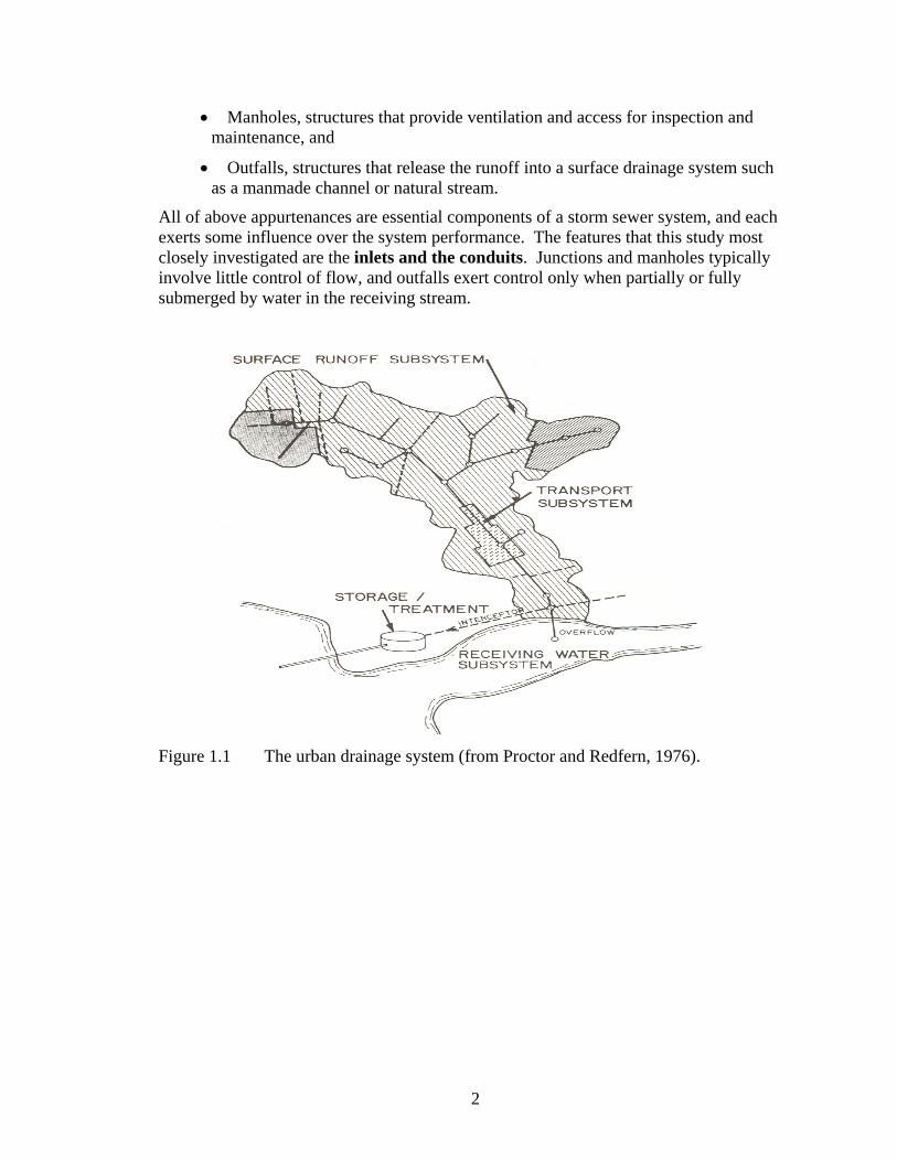
Storm sewers, in general, can be divided into two categories according to the functional classification as “separate system” that carries only the stormwater from the roadways and adjacent areas (Figure 1.1) and “combined sewers”, which carry waste water from residences, offices, industrial complexes, etc (Figure 1.2) during dry periods and which also convey stormwater during rainfall events. This study mainly focuses on the “separate system” or the stormwater drainage system. The principal or the major hydraulic components in stormwater drainage system include (Figures 1.1 and 1.2):

• Inlets, structures that pass runoff from the surface of the land into the closed conduit system,

• Conduits, structures that convey water received from the inlets from one location to another,

• Junctions, structures that connect adjacent conduits,

2

• Manholes, structures that provide ventilation and access for inspection and maintenance, and

• Outfalls, structures that release the runoff into a surface drainage system such as a manmade channel or natural stream.

All of above appurtenances are essential components of a storm sewer system, and each exerts some influence over the system performance. The features that this study most closely investigated are the inlets and the conduits. Junctions and manholes typically involve little control of flow, and outfalls exert control only when partially or fully submerged by water in the receiving stream.

Figure 1.1 The urban drainage system (from Proctor and Redfern, 1976).

3

Figure 1.2 Combined urban drainage system (from Metcalf and Eddy et al., 1971).

The design of stormwater drainage is generally accomplished by rainfall modeling, runoff modeling, followed by the design of conduits or pipes and appurtenances. Before designing or evaluating any stormwater drainage system, the engineer must first determine the acceptable level of risk of failure (in the hydrologic sense), which is expressed in the return interval, or the average length of time (in years, taken over a long period of time) between subsequent hydrologic failures. From the return interval, and from an analysis of the contributing watershed, storm duration and depth are determined, from which are computed the discharges that the system must convey.

Rainfall information can be obtained from a variety of sources, most likely intensity-duration-frequency relations or from rainfall atlases such as HYDRO-35 (Frederick et. al. 1977) or TP-40 (Hershfield, 1961). Once the hyetograph for a design has been developed, it is used to compute runoff rates to be used in the drainage system design. Currently, there are numerous hydrological methods available for computing peak flows, developing runoff hydrographs, and routing hydrographs. Some of them include Rational method, Modified Rational method, SCS/NRCS method, Clark method, Snyder method, Kinematic Wave method, EPA Runoff method, Nash method, and SBUH

4

(Santa Barbara Urban Hydrograph) Method. The choice and selection of method depends on geographic location, whether a hydrograph is required or only a peak discharge is needed, available data, and available resource.

Flow of water through a conduit is said to be closed conduit flow or open channel flow based on whether or not the surface of water is at atmospheric pressure. In closed conduit flow, the cross-sectional area of the flow is the same as that of the inside of the conduit and the hydraulic grade line is above the grade of the crown of the pipe. However, in open channel flow, the cross-sectional area of the flow, and hence other flow parameters such as the velocity, depend not only on the size and shape of the conduit, but also on the depth of flow. As a consequence, open channel flow is more difficult to treat from an analytical point of view than is pipe flow. Flow can be further classified as steady and unsteady flow depending on change of flow parameters (e.g., depth) with time. Although most collection system design is based on steady state flow hydraulics, flow in storm sewers is inherently unsteady because of the nature of precipitation and runoff transformation. A variety of methods exist for evaluating unsteady flow in conveyance systems, ranging from the most sophisticated numerical solutions of the Saint-Venant to simple approximation methods.

Today expenditure for urban drainage works and pollution control facilities are among the largest items in the budget of most municipalities, and represent a significant percentage of federal funding of public works. Widespread access to computers and the commencement of sampling have led to the development of urban runoff models that have been calibrated and validated by comparisons with measured data. The need for comprehensive approaches for the simulation of flow quantities and the limitations of the Rational method was recognized in the late 1950’s, with the development and application of these models, even though hydrograph methods had been introduced much earlier. The first uses of hydrologic models for urban flow simulation followed the development of the Road Research Laboratory Model (RRL) in the United Kingdom, and the Chicago Model in the U.S. (Watkins, 1962; Kiefer et al., 1970). Many models are used in the U.S., such as the EPA’s Storm Water Management Model (SWMM), the Water Resources Engineers (WRE) model, the University of Cincinnati model, Illinois Urban Drainage Area Simulator (ILLUDAS), and HYDROCOMP (Brandstetter, 1977).

Computer models are important to engineers because they can be used to execute engineering computations, either resulting in a savings of time and money, or by allowing more complex analyses or more alternatives to be examined for the same cost in resources. During the last 25 years there has been a proliferation of computer models that can be used for various aspects of the design of stormwater collection, storage and conveyance structures. Computer modeling became an integral part of hydrologic and hydraulic design and analysis in the early to mid 1970’s when several federal agencies began the development of software. Some private civil engineering software companies also developed good computer models. Many of these computer models were developed by adding more graphical user interface features to the existing governmental computer models.

1.2 Background and Scope of the Study

5

The Texas Department of Transportation (TxDOT) currently uses the Rational method for development of design peak flow rates for its highway storm drainage design. Watersheds for which it is used have drainage areas less than 200 acres. The Rational method is an "instantaneous" peak discharge method that is popular due to its simplicity. The Rational method assumes a linear relation between rainfall rate for the time of concentration of the watershed and peak instantaneous discharge. The drawback of the Rational method, however, is that the time distribution and accumulation of flow cannot be precisely accounted for through each node (inlet) and run (conduit) of the system. Instead, the accumulated effects of all contributing sub-basins and branches are assumed to be “lumped” into a single equivalent basin when designing or analyzing each successive node or run. Use of peak discharge values also limits the hydraulic design and analysis of the system to the assumption of simple steady-state flow conditions. While this may result in a simple design process, the inability to consider unsteady flow and the inherent storage available in these systems may result in the missed opportunity to develop more cost-effective designs. Simple steady-state flow assumptions may also be inadequate to address the complex hydraulics that could be associated with the need to include non-traditional hydraulic features, such as in-line water quality basins. Therefore, the proposed study is intended to be the first phase in evaluating TxDOT procedures for storm drain design, not only in terms of the adequacy of current TxDOT practice relative to new directions in the field, but also in anticipation of the need to evaluate more complex features that might be required by changes in water quality regulations.

The study is accomplished by completing two tasks: (1) a literature review to synthesize both the technical approach (Rational method versus other hydrological methods) and modeling efforts of drainage networks with various computer software packages, and (2) use of modeling tests on simple cases to examine storm drainage design. The study performed is summarized in this report as follows: Chapter Two provides not only a thorough literature review on Rational method, Modified Rational method, and inlet design, but also a review of recent journal papers dealing with storm drainage design. Computer software packages to analyze the stormwater system are presented in the Chapter Three. Chapter Four provides the basic setup of the case study. Results of the case study are summarized in the Chapter Five, which presents model results of the simple drainage system by using different software packages like WinStorm, StormCAD, Hdyraflow and SWMM. Detailed information on model setup and some intermediate results of the case study are presented separately in the Appendix A to Appendix D. This case study allowed the researchers to examine technical approaches implemented in these computer models, and developed useful results and conclusions on storm drainage design procedures. For example, most of the simple models for storm drainage design, for example, WinStorm and Hydraflow, exhibit a conceptual disconnect1 between the sizing of inlets and the design of the pipeline network. The study of unsteady processes from rainfall and runoff was examined by 1 The conceptual disconnect referred to here occurs the inlet design approach allows some of the incoming flow to bypass or carryover from one inlet to the next. This avoids the requirement of very long inlet lengths. However, in the conduit design procedure, all flow from the subwatershed is assumed to enter the system through the inlet. Therefore, one set of flows is used to design the inlets and a second, and greater, set of flows is used to design the conduit.

6

performing SWMM simulation on the simple system. Furthermore, part of the storm drainage system designed for U.S. Highway 77/83 was tested under different return periods and are presented in the Chapter Six, and this led us to conclude conservative design does exist in many TxDOT storm drainage systems. Feasibility of in-line water quality treatment by using extra capacity of over-designed conduits is also explored and discussed on the Chapter Seven. Chapter Eight addresses summary and conclusions of the study.

7

CHAPTER TWO LITERATURE REVIEW

2.1 Rational Method for Storm Drain Design

2.1.1 Introduction Early stormwater or catchment runoff estimation throughout the world was based

on designer’s experience and judgment. Current practice is that the watershed that is to be drained by a proposed storm sewer system will be generally divided into one or more sub-catchments or sub-watersheds that are of reasonable size and are approximately homogeneous in nature. These watersheds may include residential, commercial or industrial areas, but usually have larger proportions of pavement and the streets and roads which are the principal surface drainage conveyance, have short time of concentration, and have well-defined flow paths, typically through gutters, ditches and medians of streets and roads. Mr. Emil Kuichling, City Engineer of Rochester, New York, developed a method (Rational formula) based on his measurements on five sub-basins in Rochester, ranging in size from 25 to 357 acres (Kuichling, 1889). Based on his measurements, he concluded the following:

1. Runoff volume is proportional to imperviousness.

2. Maximum discharge occurs when the rainfall lasts long enough for the entire watershed area to contribute flow.

3. Peak discharge is proportional to intensity of rainfall.

4. Antecedent moisture levels are likely to have a significant effect on peak flow.

Now known as the Rational method, the technique developed by Kuichling is used extensively in the United States and has encountered little change since its original development.

2.1.2 Assumptions of Rational Method The following assumptions (Mays, 2001) are generally made when one applies

the Rational formula:

• The rainfall intensity is constant with respect to time.

• The rainfall intensity is constant with respect to space over the watershed drainage area.

• The frequency distributions of the event rainfall and the peak runoff rate differ in mean value but have the same variance (are parallel if plotted in probability space).

• The time of concentration of a basin is constant and is easily determined.

8

• Despite the natural temporal and special variability of abstractions from rainfall, the percentage of event rainfall that is converted to runoff can be estimated reliably.

• The runoff coefficient is invariant, regardless of season of the year or depth or intensity of rainfall.

2.1.3 Rational Formula The Rational method is the most frequently used urban hydrology method. It is

used to estimate the peak instantaneous discharge from the watershed, and it is assumed that the peak runoff rate is proportional to the peak intensity of rainfall multiplied by the contributing area. The constant of proportionality is called a “runoff coefficient”, always lesser than unity.

Mathematically Rational formula is represented as

AiCCQ rd= (2.1)

where, Q = maximum runoff rate (ft3/s in English units, m3/s in SI units),

Cr = the runoff coefficient (dimensionless),

Cd = dimensional correction factor (1.008 in English units, 1/360 = 0.00278 in SI units),

i = average rainfall intensity (inches/hour in English units, mm/hour in SI units),

A = contributing watershed area (acres in English units, hectares in SI units).

2.1.3.1 Runoff Coefficient The runoff coefficient Cr is the variable of the Rational method least susceptible

to precise determination and requires judgment and understanding on the part of the design engineer. While engineering judgment will always be required in the selection of runoff coefficients, typical coefficients represent the integrated effects of many drainage basin parameters. Recommended runoff coefficients for the Rational method are presented on Table 2.1.

Where watershed is not homogeneous but is characterized by dispersed areas that can be characterized by different runoff coefficients, a weighted runoff coefficient should be determined. The weighting is based on the area of each land use and is computed using the following equation:

∑

∑

=

== n

jj

n

jjj

w

A

ACC

1

1 (2.2)

where Aj is the area for land cover j,

9

Cj is the runoff coefficient for area j,

n is the number of distinct land covers within the watershed, and

Cw is the weighted runoff coefficient.

2.1.3.2 Rainfall Intensity, Rainfall Duration and Time of Concentration Historic rainfall data are compiled and analyzed to predict storm characteristics.

Based on previous statistical analysis, as the duration of rainfall increases, the average intensity of that rainfall tends to decrease. This means that a short burst of rainfall, while it might not result in a greater depth of rainfall, will, in general, have a greater intensity than a longer burst. Rainfall-runoff models typically require determination of the time of concentration or a similar timing parameter. In the Rational method, design rainfall intensity is a direct function of the time of concentration. Time of Concentration is defined as the length of time it takes for water to travel from the hydraulically most remote point in a basin, sub-watershed, or watershed to the outlet. There is no practical way of measuring the time of concentration (Mays, 2001). From elementary considerations of free-surface flow (that is. velocity of flow increases with increasing depth of flow), we know that for any given storm duration, greater rainfall depths will induce greater depths of flow in the drainage network, and travel times through the basin that will be less than those that will occur during smaller, more frequent rainfall events. Time of concentration is the sum of the flow time for overland or sheet flow, which occurs in headwater areas; the time for shallow concentrated flow (swales, natural channels), which occurs immediately downstream of overland flow; and the flow time for open channel or sewer flow, which tends to occur in the lower reaches of a tributary area (US Department of Agriculture, 1986). However, sometimes only one or two of these components exists. Therefore, in general, it can be said that estimation of time of concentration requires significant engineering judgment.

Table 2.1 Values of runoff coefficient for Rational Formula (ASCE, 1992).

Land Use C Land Use C

Business: Lawns:

Downtown areas 0.70 – 0.95 Sandy soil, flat, 2% 0.05 - 0.10

Neighborhood areas 0.50 - 0.70 Sandy soil, avg., 2-7% 0.10 - 0.15

Sandy soil, steep, 7% 0.15 - 0.20

Residential: Heavy soil, flat, 2% 0.13 - 0.17

Single-family areas 0.30 – 0.50 Heavy soil, avg., 2-7% 0.18 - 0.22

Multi units, detached 0.40 – 0.60 Heavy soil, steep, 7% 0.25 - 0.35

Multi units, attached 0.60 – 0.75

Suburban 0.25 - 0.40 Streets:

Asphalt 0.70 - 0.95

Industrial: Concrete 0.80 - 0.95

10

Light areas 0.50 – 0.80 Brick 0.70 - 0.85

Heavy areas 0.60 – 0.90

Unimproved areas 0.10 - 0.30

Parks, cemeteries 0.10 – 0.25 Drives and walks 0.75 - 0.85

Playgrounds 0.20 – 0.35 Roofs 0.75 - 0.95

Railroad yard areas 0.20 – 0.40

There are several different methods for estimating the time of concentration. Because available procedures are based on a wide variety of hydrologic and hydraulic conditions, the selection of a procedure or procedures for a given sub-basin should include comparison of the hydrologic-hydraulic characteristics of the sub-basin to the hydrologic-hydraulic characteristics of the sub-basins used to develop the time of concentration. Generally, the disparity between estimates of time of concentration by the various methods decreases as basin area decreases (Mays, 2001).

One commonly used method for estimation of time of concentration for overland flow, concentrated flow, and conduit flow respectively is discussed here. The overland flow is usually estimated using Kerby/Hathaway equation. The Kerby/Hathaway equation is an empirical relation developed by Kerby (1959) on the basis of published research on airport drainage done by Hathaway (1945).

467.0

0

00

67.0

⎥⎥⎦

⎤

⎢⎢⎣

⎡=

SLN

t (2.3)

where t0 = travel time of overland flow, minutes,

N = overland flow resistance factor, dimensionless,

L0 = length of the overland flow segment, feet, and

0S = slope of overland flow segment, feet vertical/feet horizontal.

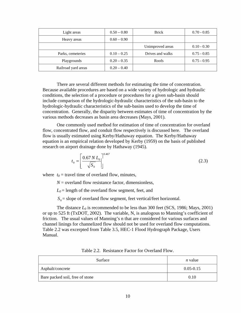
The distance L0 is recommended to be less than 300 feet (SCS, 1986; Mays, 2001) or up to 525 ft (TxDOT, 2002). The variable, N, is analogous to Manning’s coefficient of friction. The usual values of Manning’s n that are considered for various surfaces and channel linings for channelized flow should not be used for overland flow computations. Table 2.2 was excerpted from Table 3.5, HEC-1 Flood Hydrograph Package, Users Manual.

Table 2.2. Resistance Factor for Overland Flow.

Surface n value

Asphalt/concrete 0.05-0.15

Bare packed soil, free of stone 0.10

11

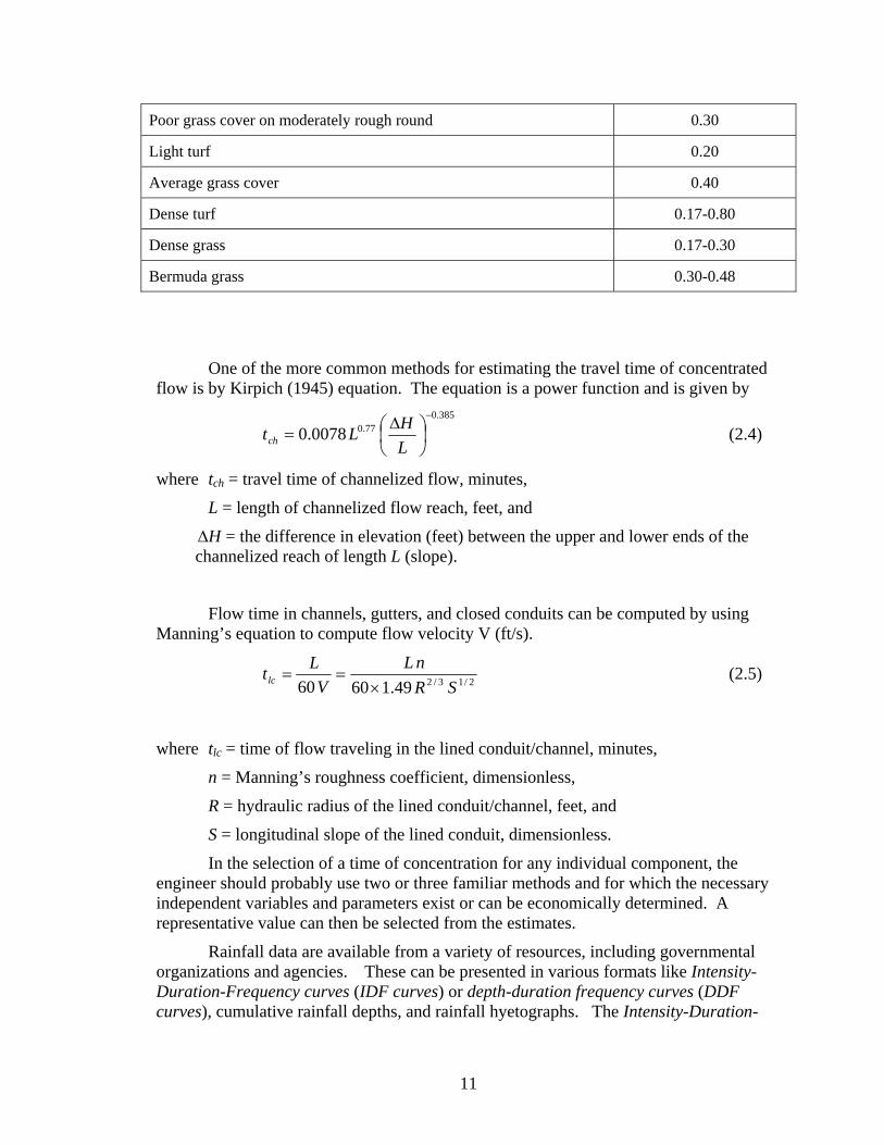
Poor grass cover on moderately rough round 0.30

Light turf 0.20

Average grass cover 0.40

Dense turf 0.17-0.80

Dense grass 0.17-0.30

Bermuda grass 0.30-0.48

One of the more common methods for estimating the travel time of concentrated flow is by Kirpich (1945) equation. The equation is a power function and is given by

385.0

77.00078.0−

⎟⎠⎞

⎜⎝⎛ Δ=

LHLtch (2.4)

where tch = travel time of channelized flow, minutes,

L = length of channelized flow reach, feet, and

HΔ = the difference in elevation (feet) between the upper and lower ends of the channelized reach of length L (slope).

Flow time in channels, gutters, and closed conduits can be computed by using Manning’s equation to compute flow velocity V (ft/s).

2/13/249.16060 SRnL

VLtlc ×

== (2.5)

where tlc = time of flow traveling in the lined conduit/channel, minutes,

n = Manning’s roughness coefficient, dimensionless,

R = hydraulic radius of the lined conduit/channel, feet, and

S = longitudinal slope of the lined conduit, dimensionless.

In the selection of a time of concentration for any individual component, the engineer should probably use two or three familiar methods and for which the necessary independent variables and parameters exist or can be economically determined. A representative value can then be selected from the estimates.

Rainfall data are available from a variety of resources, including governmental organizations and agencies. These can be presented in various formats like Intensity-Duration-Frequency curves (IDF curves) or depth-duration frequency curves (DDF curves), cumulative rainfall depths, and rainfall hyetographs. The Intensity-Duration-

12

Frequency curves (IDF curves) or depth-duration frequency curves (DDF curves) are plots of rainfall intensity (or depth) versus duration of event rainfall. Usually, there are several curves on a single graph, one for each of several different rainfall frequencies (return periods). These curves are hyperbolic or exponential decay type curves, which vary by geographical location (e.g. by county), and for many counties such relationships have been developed for the use of designers. The general shape of an Intensity-Duration-Frequency (IDF) curve is shown on Figure 2.1, and illustrates the average rainfall intensities corresponding to a particular storm recurrence interval for various storm durations.

Figure 2.1 Intensity-Duration-Frequency (IDF) curves.

Mathematically these curves can be represented in different forms as follows

nDbai

)( += (2.6)

nDb

nRPai)(

)(

+= (2.7)

32 )(ln)(ln)(ln DdDcDbai +++= (2.8)

where i is rainfall intensity, in/hr or mm/hr,

D is duration of rainfall in minutes,

13

RP is the Return Period (yr), and

The parameters, a, b ,c ,d, m, n define the shape and appropriate units, and are determined for curve fitting to IDF data. For example, TxDOT uses the Equation (2.6) to compute rainfall intensity for its hydrologic design, coefficients a, b, and n are available for each county in Texas and for return periods of 2-, 5-, 10-, 25-, 50-, and 100-years, respectively. This is also implemented in TxDOT’s design software WinStorm 3.0.

2.1.4 Limitation of Rational Method Though simple to use, the Rational method does have limitations. First is the

runoff coefficient. The runoff coefficient incorporates a large number of variables into a single index that ranges between 0 and 1. In addition, the parameter can take on a wide range of values even for the same land use characteristics. As a result, there appears to be an amount of subjectivity in selecting a runoff coefficient.

Secondly, the Rational method is simplistic in its accounting of runoff and loss processes, so must be limited to small, relatively homogenous and simple watersheds, usually less than 200 acres (80 ha.), which typically have times of concentration of less than 20 minutes (ASCE, 1992; Wanielista et al., 1997).

A final limitation of the Rational method is that it only provides a single value on the discharge hydrograph, the peak discharge. If the objective is to determine the size for an inlet or a pipe, then this single point on the discharge hydrograph is adequate. However, to design a detention basin one must have the direct runoff hydrograph, that is, a time history of the runoff. Therefore, the Rational method does not give any time-distributed information in any sense.

2.2 Hydrograph Generation Methods

2.2.1 Hydrograph Development for Inlets The Rational method only provides designer a peak discharge, not a hydrograph.

Use of the peak discharge limits the hydraulic design and analysis of storm drain systems to the assumption of steady-state flow conditions. In order to consider unsteady flow and inherent storage available in storm drain systems for cost effective design, hydrographs at inlets and inside pipes are required. A hydrograph is a time series of instantaneous discharge versus time at a particular location within a watershed. Hydrographic analysis is performed when flow routing is important, such as in the design of stormwater detention, water quality facility and pump stations. It can also be used to evaluate flow routing through large storm drainage systems to more precisely reflect flow peaking conditions in each segment of the system.

Most approaches to hydrograph estimation are based on the concept of the unit hydrograph, first introduced by Sherman (1932), which is a hydrograph produced by a unit depth of runoff distributed uniformly over a basin for defined period of time. The basic theory rests on the assumption that the runoff response of a drainage basin to an effective rainfall input is linear; that is, it may be described by a linear differential equation or the concepts of proportionality and superposition can be applied. Unit

14

hydrographs can be developed from rainfall and runoff data of a watershed, and can typically be applied to the same watershed for other rainfall events. For un-gaged basins, synthetic unit hydrographs can be developed from theoretical or empirical formulas relating hydrograph peak flow and time characteristics of the basin to watershed or rainfall characteristics, or can be transposed from nearby, hydrologically similar watersheds, for which exist rainfall-runoff data. However, the synthetic unitgraphs have certain limitation and the engineer or the hydrologist should apply them with caution to new areas. Extensive literature exists on various methods (e.g., Clark, Snyder, Nash, SCS.) to develop synthetic unit hydrographs. A brief discussion on two popular methods of generating synthetic hydrograph is given here.

Snyder’s Method: Snyder (1938) was the first to develop a synthetic unit hydrograph based on a study of watersheds in the Appalachian Highlands. It allows computation of lag time, time base, unit hydrograph duration, peak discharge, and hydrograph time widths at 50 and 75 percent of peak flow. By using these seven points, a sketch of the unit hydrograph is obtained and checked to see if it contains 1 unit of direct runoff.

Dimensionless SCS Unit Hydrograph: The method developed by Soil Conservation Service (SCS) is a dimensionless unit hydrograph developed by Victor Mockus (NRCS, 1972), derived from a large number of unit hydrographs ranging in size and geographic location. The hydrograph is represented as a simple triangle with rainfall duration, time of rise, time of fall and peak flow. This method requires only the determination of the time to peak and the peak discharge.

Methods for developing synthetic unit hydrographs discussed in hydrology textbooks are typically for relative large watersheds. For example, the relation of Snyder’s method is considered applicable to drainage areas ranging in size from 10 to 10,000 mile2. Some of the stormwater simulation models, for example, XP or Visual SWMM (which will be introduced later), also use Snyder’s method, SCS method, and other unit hydrograph methods to develop hydrographs from local catchments (few acres or more) for inlets of a storm drain system. Designer and engineers should pay attention while applying those methods. In the next section, modified Rational method is discussed in detail, which has been widely used for developing hydrograph for inlets.

2.2.2 Modified Rational Method The modified Rational method (MRM) is an extension of the traditional Rational

method. The MRM produces a runoff hydrographs, and hence the runoff volume while the original Rational method is meant to produce only the peak design discharge. The MRM, which has found widespread use in the engineering practice in recent years, is used to size detention/retention facilities for a specified recurrence interval and concurrent release rate.

The MRM is based on the same assumptions as the conventional Rational method. An important additional assumption is that the rainfall intensity averaging time used in the modified Rational method equals the storm duration (“Urban Surface Water Management” by Walesh, 1989). This assumption means that the rainfall, and the runoff

15

generated by that rainfall, occurring before or after the rainfall averaging period is not accounted for.

In the MRM, it is also assumed that an urban stormwater runoff hydrograph under the design storm can be approximated as being either triangular or trapezoidal in shape. The rising and the falling limbs follow a linear time-area relationship trend for the sub-basin, that is, their contributions are linear.

Three different possible types of hydrograph can be developed for the given sub-basin using the MRM. Hydrograph type is a function of the storm duration or the length of rainfall, d, with respect to the time of concentration, tc. The following three types are possible (“Urban Surface Water Management” by Walesh, 1989):

(a) If the storm duration (d) is greater than the watershed time of concentration (tc), the resulting hydrograph is a trapezoidal in shape with uniform maximum discharge as determined from the conventional Rational method AiCCQ rd= for the difference between tc and duration of storm. The linear rising and falling limbs each has duration of tc as shown in Figure 2.2(a).

(b) If the storm duration (d) is equal to time of concentration (tc), there is a rise to full contribution (peak), followed by a recession over tc back to zero. The resulting hydrograph is triangular in shape as shown in Figure 2.2 (b) with a peak discharge of AiCCQ rd= .

Time

Dis

char

ge

Figure 2.2(a) Hydrograph when duration of rainfall is greater than tc.

16

Time

Dis

char

ge

Figure 2.2(b) Hydrograph when duration of rainfall is equal to tc.

(c) If the storm duration (d) is less than the time of concentration (tc), then the resulting hydrograph is trapezoidal in shape with a maximum uniform discharge of ( )crdp tdAiCCQ /' = from the end of the storm (d) to the time of concentration tc. The linear rising and falling portions of the hydrograph each has a duration of d as show in Figure 2.2(c).

Thus, the MRM can obtain the time-distributed discharge, which is useful to predict downstream flooding or to determine the size of the detention basin. The designers should limit use of the MRM for sizing detention basins for watershed drainage areas not exceeding 20 to 30 acres (Mays, 2001).

17

Time

Dis

char

ge

Figure 2.2(c) Hydrograph when duration of rainfall is less than tc.

2.3 Design of Stormwater System (Inlets)

2.3.1 Introduction

When rain falls on a sloped pavement surface, it forms a thin layer of water that increases in thickness as it flows to the sides of the roadway. This accumulation of water can disrupt traffic flow, reduce vehicular skid resistance, increase potential for motorist hydroplaning, and contribute to pavement deterioration. The objective in highway drainage design is to minimize such problems by collecting runoff in gutters and intercepting runoff using stormwater inlets that direct flow to subsurface conveyance systems, culverts, or ditches. Proper design of drainage facilities is therefore essential to maintaining safe vehicular travel conditions and ensures that highway service levels will avoid disruption.

This section of the report provides the guidelines for evaluating roadway features and design criteria as they relate to gutter and inlet hydraulics and storm drain design. Procedures for performing gutter flow calculations are based on a modification of Manning's equation. For detailed discussion on inlet capacity calculations, the reader is referred to Federal Highway Administration guidance documents, including Hydraulic Engineering Circular (HEC) No. 12 and HEC No. 22. Storm drain design is based on the use of the Rational formula.

2.3.2 Design Frequency and Spread

Two of the major design variables considered in sizing and locating highway drainage structures are the frequency and the allowable spread of water on the pavement.

18

Spread and design frequency are interrelated, because the implication of allowable spread can be significantly different for storms of different recurrence intervals (Brown et al., 1996). Thus, the main objective is to collect runoff in the gutter and convey it to inlets in a way that provides safety for traffic during the design storm event at a reasonable cost. Selection of recurrence interval and spread for the design are dependent on the acceptable risks and the budgetary limitation for the drainage system. The factors to be considered in selecting design frequency and spread include highway classification, design speed, traffic volumes, rainfall intensity and the capital cost. Moreover, it is the responsibility of the designer to select a design frequency and spread that meets the needs of a particular project. Suggested minimum design frequencies and spread based highway classification and design speed are presented on Table 2.3.

Table 2.3. Suggested Minimum Design Frequency and Spread (Brown et al., 1996).

Road Classification Design Frequency Design Spread <70 km/hr (45 mph) 10-year Shoulder + 1 m (3 ft) >70 km/hr (45 mph) 10-year Shoulder High volume or divided

or bi-directional Sag point 50-year Shoulder + 1 m (3 ft)

<70 km/hr (45 mph) 10-year ½ Driving Lane >70 km/hr (45 mph) 10-year Shoulder Collector

Sag point 10-year ½ Driving Lane Low ADT (Average

Daily Traffic) 5-year ½ Driving Lane

High ADT 10-year ½ Driving Lane Local Street

Sag Point 10-year ½ Driving Lane

2.3.3 Curbs and Gutters A curb serves as the outside edge of pavements and performs multiple functions,

such as the following

• Act as a boundary between the roadway and the adjacent properties

• Provide pavement delineation

• Prevent erosion

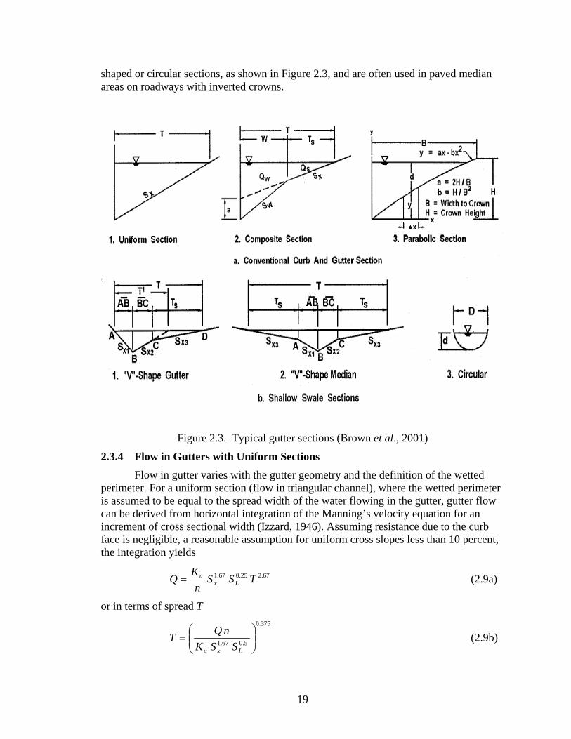
A gutter is a section of pavement adjacent to the curb that is designed to convey water to curb inlets during a runoff event. The gutter may include a portion or all of a traffic lane. Gutter cross slopes may be the same as that of the pavement or may be designed with a steeper cross slope, usually 80 mm per meter (1 inch per foot). Gutter sections can be categorized as conventional or shallow swale type, as shown in Figure 2.3. Conventional curb and gutter sections usually have a triangular shape with the curb forming the near-vertical leg of the triangle. Conventional gutters may have a straight cross slope, a composite cross slope where the gutter slope varies from the pavement cross slope or a parabolic section. Shallow swale gutters typically have V-

19

shaped or circular sections, as shown in Figure 2.3, and are often used in paved median areas on roadways with inverted crowns.

Figure 2.3. Typical gutter sections (Brown et al., 2001)

2.3.4 Flow in Gutters with Uniform Sections

Flow in gutter varies with the gutter geometry and the definition of the wetted perimeter. For a uniform section (flow in triangular channel), where the wetted perimeter is assumed to be equal to the spread width of the water flowing in the gutter, gutter flow can be derived from horizontal integration of the Manning’s velocity equation for an increment of cross sectional width (Izzard, 1946). Assuming resistance due to the curb face is negligible, a reasonable assumption for uniform cross slopes less than 10 percent, the integration yields

67.225.067.1 TSSn

KQ Lx

u= (2.9a)

or in terms of spread T 375.0

5.067.1 ⎟⎟⎠

⎞⎜⎜⎝

⎛=

Lxu SSKnQT (2.9b)

20

where

Ku = 0.376 (0.56 in English units),

n = Manning’s coefficient (Table 2.4),

Q = gutter flow rate m3/s (or cfs),

T = spread of water onto the pavement in m (or ft), or top width of flow,

Sx = gutter cross slope in m/m (or ft/ft), and

SL = longitudinal slope, or grade, of the highway in m/m (ft/ft).

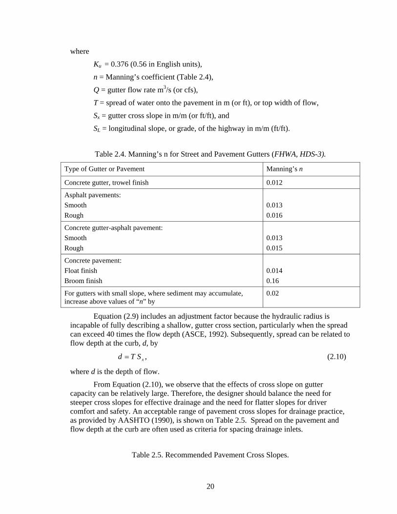
Table 2.4. Manning’s n for Street and Pavement Gutters (FHWA, HDS-3).

Type of Gutter or Pavement Manning’s n

Concrete gutter, trowel finish 0.012

Asphalt pavements: Smooth Rough

0.013 0.016

Concrete gutter-asphalt pavement: Smooth Rough

0.013 0.015

Concrete pavement: Float finish Broom finish

0.014 0.16

For gutters with small slope, where sediment may accumulate, increase above values of “n” by

0.02

Equation (2.9) includes an adjustment factor because the hydraulic radius is incapable of fully describing a shallow, gutter cross section, particularly when the spread can exceed 40 times the flow depth (ASCE, 1992). Subsequently, spread can be related to flow depth at the curb, d, by

,xSTd = (2.10)

where d is the depth of flow.

From Equation (2.10), we observe that the effects of cross slope on gutter capacity can be relatively large. Therefore, the designer should balance the need for steeper cross slopes for effective drainage and the need for flatter slopes for driver comfort and safety. An acceptable range of pavement cross slopes for drainage practice, as provided by AASHTO (1990), is shown on Table 2.5. Spread on the pavement and flow depth at the curb are often used as criteria for spacing drainage inlets.

Table 2.5. Recommended Pavement Cross Slopes.

21

Surface type Range of cross slope

High-type surface 2- Lanes 3 or more lanes, each direction

0.015-0.020 0.015 minimum; increase 0.005-0.010 per lane; 0.040 maximum.

Intermediate surface 0.015-0.030

Low-type surface 0.020-0.060

Shoulders Bituminous or concrete with curbs

0.020-0.060

2.3.5 Flow in Gutters with Composite sections Design computations for composite gutter sections require additional consideration of flow in the depressed section. The depression serves to capture more flow from the gutter and thus increasing gutter capacity and inlet efficiency. Thus, the total flow incorporating the depressed section flow is given by

sw QQQ += (2.11)

where

Q = total gutter flow rate in m3/s (or cfs),

Qw = flow rate in the depressed section of the gutter m3/s (or cfs), and

Qs = flow capacity of the gutter section above the depressed section m3/s (or cfs).

Qs can be evaluated using Equation (2.9) if T is taken as only the spread over the un-depressed portion of the gutter, Ts (Fig. 2.3). Equation (2.11) can be used in conjunction with the following expressions for computing flow in a composite cross section (Brown et al., 1996).

( ) ⎪⎪

⎭

⎪⎪

⎬

⎫

⎪⎪

⎩

⎪⎪

⎨

⎧

−⎥⎦

⎤⎢⎣

⎡−

+

+=

11/

/1

/1/1 67.20

WTSS

SSE

xw

xw (2.12)

and

( )01 EQ

Q s

−= (2.13)

where

E0 = ratio of flow in a chosen width to total gutter flow (Qw/Q), and

Sw = cross slope of the depressed portion of the gutter in m/m (or ft/ft), and Sw is expressed as

22

WaSS xw += , (2.14)

where a = depth of gutter depression in m (ft), and

W = width of the depressed section m (or ft) given in Fig. 2.3.

2.3.6 Drainage Inlet Design The primary purpose of the storm drain inlet is to intercept all or a portion of the

flow as flow accumulates in gutters and spread encroaches upon pre-specified design values, and to discharge it into an underground storm drainage conveyance system. The design characteristics of inlets eventually control the rate at which runoff is removed from the gutter and enters the storm drainage system. Subsequently, inadequate inlet capacity or poorly located inlets can cause hazardous flooding to the traffic or the property. Therefore, the responsibility of the designer is to determine the type, size, and spacing of inlets to intercept a sufficient portion of the design gutter flow, while preserving attention to cost. In addition, the designer should ensure that inlets do not project significantly above a pavement surface or pose as an obstacle to oncoming traffic.

Inlets commonly used in practice for the drainage of highway surfaces include (Figure 2.4)

1) Curb-opening inlets

2) Grate inlets

3) Slotted drain inlets

4) Combination inlets

Inlets can be further classified as being on a “continuous grade” or in “sump”. The term “continuous grade” refers to an inlet so located that the grade of the street (road) has a continuous slope past the inlet and therefore ponding does not occur at the inlet. The sump condition exists whenever water is restricted to the inlet area because the inlet is located at a low point. A sump condition also called as “inlets on sag”, can occur at a change in grade of the street (road) from positive to negative or at an intersection due to the crown slope of a cross street.

23

Figure 2.4. Types of storm drain inlets (Brown et al., 2001).

2.3.6.1 Interception Capacity and Efficiency on Continuous Grade Inlet Inlet capacity, Qi, is the amount of gutter flow intercepted by an inlet under a

given set of conditions, which is conveyed to the stormwater pipe. The efficiency of an inlet, E, is the percent of total runoff that the inlet will convey to the underground pipe for those conditions. The efficiency of an inlet depends on cross slope, longitudinal slope, total gutter flow, inlet geometry, and, to lesser extent, pavement roughness. Whereas interception capacity of all inlets increases with increasing gutter flow rates, efficiency generally decreases with increasing gutter flow (Brown, et al., 1996). Mathematically, efficiency E is defined by the following equation

QQ

E i= (2.15)

where

E = inlet efficiency,

Q = total gutter flow in m3/s (or cfs), and

24

Qi = intercepted capacity in m3/s (or cfs).

Any flow that is not intercepted by an inlet is termed carryover flow, or bypass flow and is defined as follows:

Qb = Q – Qi (2.16)

where

Qb = bypass flow in m3/s (or cfs),

Q = total gutter flow in m3/s (or cfs), and

Qi = interception capacity in m3/s (or cfs).

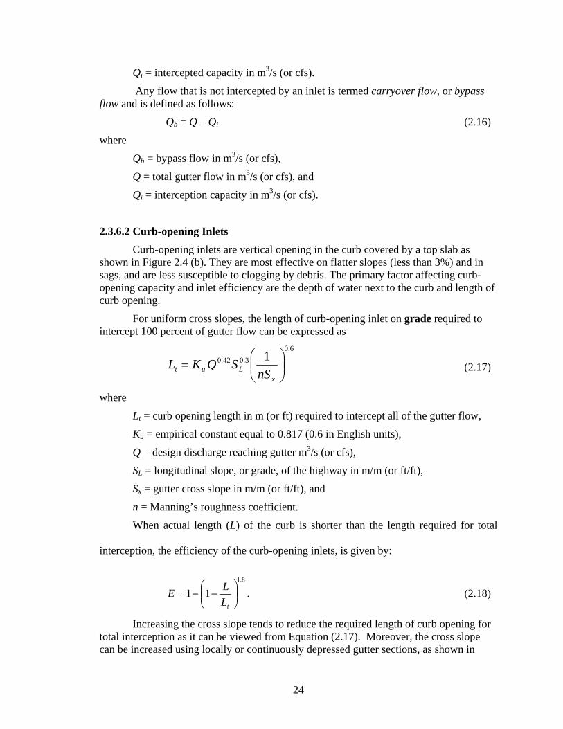
2.3.6.2 Curb-opening Inlets Curb-opening inlets are vertical opening in the curb covered by a top slab as

shown in Figure 2.4 (b). They are most effective on flatter slopes (less than 3%) and in sags, and are less susceptible to clogging by debris. The primary factor affecting curb-opening capacity and inlet efficiency are the depth of water next to the curb and length of curb opening.

For uniform cross slopes, the length of curb-opening inlet on grade required to intercept 100 percent of gutter flow can be expressed as

6.03.042.0 1

⎟⎟⎠

⎞⎜⎜⎝

⎛=

xLut nS

SQKL (2.17)

where

Lt = curb opening length in m (or ft) required to intercept all of the gutter flow,

Ku = empirical constant equal to 0.817 (0.6 in English units),

Q = design discharge reaching gutter m3/s (or cfs),

SL = longitudinal slope, or grade, of the highway in m/m (or ft/ft),

Sx = gutter cross slope in m/m (or ft/ft), and

n = Manning’s roughness coefficient.

When actual length (L) of the curb is shorter than the length required for total

interception, the efficiency of the curb-opening inlets, is given by:

8.1

11 ⎟⎟⎠

⎞⎜⎜⎝

⎛−−=

tLLE . (2.18)

Increasing the cross slope tends to reduce the required length of curb opening for total interception as it can be viewed from Equation (2.17). Moreover, the cross slope can be increased using locally or continuously depressed gutter sections, as shown in

25

Figure 2.5. Therefore, the length of inlet required for 100 percent interception can be computed by use of an equivalent cross slope, Se, in Equation (2.17) in place of Sx. The term Se can be determined by

0' ESSS wxe += , (2.19)

where

Eo = ratio of flow in the depressed section to total gutter flow determined by the gutter configuration upstream of the inlet, defined in Equation (2.12), and

'wS = cross slope of the depressed section measured form the cross slope of the

pavement, m/m (or ft/ft) and can be expressed as

WaSw =' (Figures. 2.3 and 2.5). (2.20)

Figure 2.5. Depressed curb opening inlet (Brown et al., 2001).

Thus, for curb-opening inlets with less than 100 percent interception, depressed sections can significantly increase the interception capacity and efficiency. Equation (2.18), for calculating efficiency, is applicable for both uniform and composite cross slopes.

Curb-opening inlets on Sump (Sag) can operate either as a weir or as an orifice. They act as a weirs for ponding depth at the curb less than or equal to the height of the curb opening (Brown et al., 1996). In this case, the equation for the interception capacity of a curb-opening inlet is given by

2/3dLCQ wi = (2.21)

where

Cw = weir discharge coefficient 1.60 (3.0 in English units),

L = length of the curb-opening in m (or ft), and

26

d = depth at curb measured form the normal cross slope in m (or ft).

For depressed curb-opening inlet (Fig. 2.5), the capacity is computed by

( ) 2/38.1 dWLCQ wi += , (2.22)

where

W = lateral width of depression in m (or ft), and

Cw = weir discharge coefficient 1.25 (2.3 in English units).

The application of Equation (2.22) is limited to depths at the curb less than or equal to the height of the opening plus the depth of depression. Curb-opening inlets operate as orifices at depths greater than approximately 1.4 times the opening height. The interception capacity for depressed or undepressed curb opening inlet operating as horizontal orifice throat, as shown in Figure 2.6 (a), is computed by the following equation

( ) 5.000 2 dgLhCQi = (2.23)

For other throat configurations as shown in Figure 2.6(b) and 2.6(c), this expression is generalized as

2/1

0 22 ⎥

⎦

⎤⎢⎣

⎡⎟⎠⎞

⎜⎝⎛ −=

hdgACQ igi , (2.24)

where

C0 = orifice discharge coefficient (0.67),

Ag = effective area of the curb opening, m2 (or ft2),

g = gravitational acceleration,

di = depth at lip of curb-opening, m (or ft),

h = height of curb-opening orifice, m (or ft), and

d0 = effective head on the center of the orifice throat, m (or ft).

2.3.6.3 Grate Inlets

Grate inlets consist of an opening in the gutter or ditch covered by one or more, flush-mounted grates placed parallel to the flow, as shown in Figure 2.4 (a). The main advantage of grate inlets is that they can be installed in the direct path of runoff. The highly susceptible of grate inlet to debris clogging is however, the principal disadvantage. Consideration should be given where the bicycle or pedestrian traffic occurs. The grates for which design procedures have been developed are listed in Table 2.6 (Brown et al., 1996).

27

Figure 2.6. Curb opening inlets with different throats (Mays, 2001).

When the velocity approaching the grate is less than the “splash-over’ velocity, the grate will intercept essentially all of the frontal flow and conversely, when the gutter flow velocity exceeds the “splash-over” velocity for the grate, only part of the flow will be intercepted (Brown et al., 1996). A part of the flow along the side of the grate will be intercepted, dependent on the cross slope of the pavement, the length of the grate, and flow velocity.

28

Table 2.6. Types of grates for which design procedures is developed (Brown et. al. 1996).

P-50 Parallel bar grate with bar spacing 48 mm (1-7/8 in) on center.

P-50x100 Parallel bar grate with bar spacing 48 mm (1-7/8 in) on center and 10 mm (3/8 in) diameter lateral rods spaced at 102 mm (4 in) on center

P-30 Parallel bar grate with 29 mm (1-1/8 in) on center bar spacing

Curved Vane Curved vane grate with 83 mm (3-1/4 in) longitudinal bar and 108 mm (4-1/4 in) transverse bar spacing on center

45°- 60 Tilt Bar45° tilt-bar grate with 57 mm (2-1/4 in) longitudinal bar and 102 mm (4 in) transverse bar spacing on center

45°- 85 Tilt Bar45° tilt-bar grate with 83 mm (3-1/4 in) longitudinal bar and 102 mm (4 in) transverse bar spacing on center

30°- 85 Tilt Bar30° tilt-bar grate with 83 mm (3-1/4 in) longitudinal bar and 102 mm (4 in) transverse bar spacing on center

Reticuline "Honeycomb" pattern of lateral bars and longitudinal bearing bars

The ratio of frontal flow to total gutter flow, E0, for uniform cross slope can be expressed by Equation (2.25):

,113/8

0 ⎟⎠⎞

⎜⎝⎛ −−==

TW

QQ

E w (2.25)

where

Q = total gutter flow, m3/s (or cfs),

Qw = flow in width W, m3/s (or cfs),

W = width of depressed gutter or grate, m (or ft), and

T = total spread, m (or ft).

Similarly, the ratio of side to gutter flow is expressed as:

,11 0EQ

QQQ ws −=⎟⎟

⎠

⎞⎜⎜⎝

⎛−= (2.26)

where

Qs = side flow, m3/s (cfs).

The ratio of intercepted flow to total frontal flow, or frontal flow efficiency, Rf, is expressed by:

( ),1 0VVKR ff −−= (2.27)

where

Kf = 0.0295 (0.09 in English units),

29

V = velocity of flow in gutter, m/s (or ft/s), and

V0 = gutter velocity where splash over first occurs, also called as splash-over velocity, m/s (or ft/s).

The frontal flow efficiency can be determined graphically using the curves in Figure 2.7, which accounts for grate length, bar configuration, and gutter velocity at which splash over occurs. The ratio of side flow intercepted to total side flow is expressed as:

,

.

.1

1

3.2

8.1

⎟⎟⎠

⎞⎜⎜⎝

⎛+

=

LSVK

R

x

ss (2.28)

where

Ks = 0.0828 (0.15 in English units), and

L = Length of gutter section, m (or ft).

The overall efficiency, E, of the grate can be evaluated as a function of the frontal and side flow efficiencies by using

).1( 00 ERERE sf −+= (2.29)

Combination inlets (Figure 2.4 (c)) and the slotted inlets (Figure 2.4 (d)) are less commonly used and are not discussed in detail here. The interested reader is suggested to refer Chapter 4 of FHWA HEC-22 Manual for detailed discussion.

30

Figure 2.7. Grate inlet frontal flow interception efficiency (Brown et al., 1996).

31

2.4 Journal Publications on Storm Drainage System Design

2.4.1 Introduction In the 1970s, one of the active water resources research areas was urban stormwater drainage. It evolved from concern of urban flood mitigation, primarily with respect to water quantity, to the concept of stormwater quality and quantity management. As a partial response to the need, the first international conference on urban storm drainage was held April 11-15, 1978, at the University of Southampton in England. The second and third international conferences on urban storm drainage were held at Urbana, Illinois, USA, on June 15-19, 1981, and in Göteberg, Sweden in June 1984. Dr. Yen (1981a, 1981b) developed two volumes of proceedings for the second conference: the first is “Urban Stormwater Hydraulics and Hydrology” containing 50 papers, and the second is “Urban Stormwater Quality, Management and Planning” containing 60 papers. Unfortunately, papers dealing with inlet design or inlet efficiencies are few. In the following sections, several papers from the literature are presented.

Although some studies were performed and reported in the literature, most of computer software packages for inlet design discussed in the Chapter Four and Five are basically automated versions of a method developed for use by hand, that is the classical Rational method to compute peak discharge and to size stormwater pipe system (Herrmann, 2002).

2.4.2 Rational Method for Peak Flow Rate Estimation The Rational method continues to be the most widely used approach for estimating T-year return frequency peak flow rates for small catchments of about one square mile or less in area (Hromadka et al., 1987). The balanced design storm (U.S. Army Crops of Engineers, 1990) unit hydrograph method is perhaps the second most widely used technique for estimating peak flow rates (and is the most widely used method for developing runoff hydrographs) but is generally considered to be more accurate than the Rational method. Hromadka and Whitley (1994, 1996) reported that both of these techniques for estimating peak flow rates are mathematically comparable. They concluded that the Rational method can be significantly improved by including an additional multiplicative constant that corresponds to the S-Hydrograph or unit hydrograph type (e.g., SCS, Mountain, Desert, Valley, etc.). They extended the Rational Equation to Qp = ε CIA for the developed valley in Orange County, California. The adjustment factor, ε, has a reported value of about 1.0 (mean of 0.98 with a range of 0.97 to 1.02), but for undeveloped portions of Orange County, it has a value of 0.86, ranging from 0.83 to 0.89. The similarity between these values may explain why the Rational method continues to be widely used even though other, more computationally sophisticated techniques, are readily available.

32

2.4.3 Street Stormwater Storage Capacity

The primary function of a street is to maintain the movement of traffic. Under the assumption that street drainage will be designed to collect stormwater as fast as possible, the street stormwater capacity has been defined as its hydraulic conveyance, estimated by Manning's formula. This practice has resulted in a prevailing experience that street intersections are often flooded. Guo (2000) presented an investigation on street hydraulic capacity. It was found that the street stormwater capacity at a sump is in fact dictated by the storage capacity rather than the conveyance capacity. A new design methodology was developed in Guo’s study to consider the street depression storage as a criterion when sizing a sump inlet. Design parameters required by this method include the local intensity-duration-frequency information, catchment area, runoff coefficient, street transverse slope, and the configuration of the sump area as a fraction of a circle (Guo, 2000).

2.4.4 Hydraulic Performance of Highway Storm Sewer Inlets

Laboratory experiments (Hotchkiss et al., 1991) were performed with highway stormwater curb inlets to 1) reduce the oblique standing wave that extends into the highway from the downstream side of the inlet and 2) determine the effect of highway resurfacing on inlet efficiency. The work was performed at the University of Nebraska Hydraulic Modeling Basin on a section of full-scale single lane highway with a longitudinal slope of three percent and a transverse slope of two percent. All measured flows were supercritical. Four alternatives to reduce the oblique standing wave were tested but produced only minimally better conditions. Careless highway resurfacing that covers inlet transitions drastically reduces inlet efficiency. Efficiency for this case can be predicted with previously developed equations and is less than one-half that achieved with standard design transitions (Hotchkiss et al., 1991).

2.4.5 Improvements in Curb-Opening and Grate Inlet Efficiency Draining stormwater quickly and efficiently from highways is an important part of every highway design. Laboratory experiments (Hotchkiss, 1994) were conducted to develop curb-opening and grate inlet efficiency curves for the Nebraska standard inlet (single and in series), the city of Lincoln canted inlet, a new grate inlet (single and in series), and an inlet affected by resurfacing. Experiments were performed for the on-grade inlets on a full-scale roadway surface that was treated with sand-imbedded paint to produce an average Manning's n of 0.016. The constant longitudinal and cross slopes were 3 and 2 percent, respectively. Supercritical flow prevailed over the flow range of 0.5 to 5 ft3/sec. Based on results from Hotchkiss (1994), the Nebraska standard inlet provides about 20 percent greater efficiency than the equivalent AASHTO-type inlet. Canted inlet performance was only marginally better than that of the Nebraska standard inlet. The new grate inlet performance was very similar to that of curb-opening inlets. Inlets in series increased efficiencies by almost 20 percent over the efficiencies of single inlets. Finally, roadway resurfacing that covers inlet transitions reduces efficiency by about 50 percent (Hotchkiss, 1994).

33

2.4.6 Stormwater Flow on a Curbed TxDOT Type Concrete Roadway In 1946, C.F. Izzard introduced the gutter flow equation derived via integration of

Manning’s velocity equation across a gutter section. Literature reviews (Ickert and Crosby, 2003) indicated that Izzard suggested increasing Manning’s n when using the integrated equation. Although the integrated equation is used extensively, the suggested increase in Manning’s n appears to not have been implemented. There is a discrepancy between the geometric equation (the product of Manning’s velocity equation and flow area) and the integrated equation that results in overestimation of a gutter’s flow capacity when using the integrated equation and traditional values of Manning’s n. With intent to improve driving conditions with more accurate gutter flow computation methods, the derived geometric and integrated equations are evaluated for three definitions of the wetted perimeter of a curbed section. Also, experimental data were evaluated to determine Manning’s n for a curbed TxDOT (Texas Department of Transportation) type concrete roadway at various longitudinal and transverse slopes.

2.4.7 Design of Curb Opening Inlet Structure

The South Carolina Department of Transportation (SCDOT) has experienced hydraulic and structural problems with two of its curb-opening structures, called Type 5 and Type 6, primarily used on city streets. Hydraulically, the structure has a tendency to be plugged by debris with the accompanying loss of capacity. Furthermore, the top slab of the structures frequently failed structurally under the load of vehicle wheels (usually large heavy trucks) that jumped the curb. Replacing broken slabs burdened SCDOT with substantial budget and personnel costs. A new structure was developed in 1989 at Clemson University. The study (Fiuzat et al., 2000) was conducted mainly to investigate the hydraulic efficiency of curb opening inlet structures adopted by the SCDOT. They discussed the design equations and methodology for the utilization of the new structure. The primary features of the structure they studied are listed below:

• Throat opening of 9.9 cm to avoid clogging

• Gutter depression of 5.1 cm from its normal level to allow for the large vertical opening. Further depression of the gutter would be unsafe for pedestrians and bicycles.

• Top slab of 20.3 cm thick (capable to withstand 10 tons of wheel load)

• The smallest structure is 122 cm (4 ft) along the road, and empties into a standard catch basin of size 122 cm x 122 cm.

The hydraulic efficiency E of the curb inlet structure is defined as QQE i /100= , and where Q is the flow rate on the road gutter, and Qi is the flow rate intercepted by the inlet. The parameters affecting the efficiency are roadway geometry (longitudinal and cross slope of road), flow properties (road/gutter flow rate, flow spread) and the inlet geometry (length, gutter depression, transition length, sharpness of the edge of curb opening). The effect of these factors was studied by Bowman (1988) and Soares (1991) and, based on

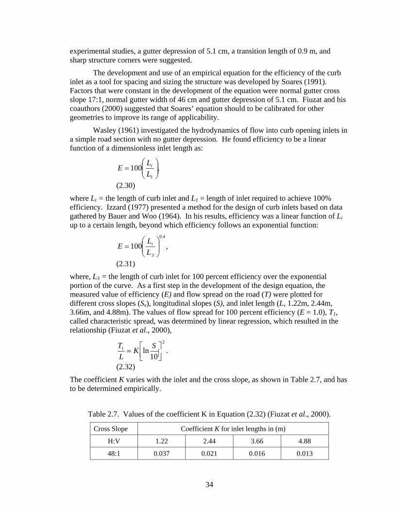
34

experimental studies, a gutter depression of 5.1 cm, a transition length of 0.9 m, and sharp structure corners were suggested.

The development and use of an empirical equation for the efficiency of the curb inlet as a tool for spacing and sizing the structure was developed by Soares (1991). Factors that were constant in the development of the equation were normal gutter cross slope 17:1, normal gutter width of 46 cm and gutter depression of 5.1 cm. Fiuzat and his coauthors (2000) suggested that Soares’ equation should to be calibrated for other geometries to improve its range of applicability.

Wasley (1961) investigated the hydrodynamics of flow into curb opening inlets in a simple road section with no gutter depression. He found efficiency to be a linear function of a dimensionless inlet length as:

,1001⎟⎟⎠

⎞⎜⎜⎝

⎛=

LL

E i

(2.30)

where Li = the length of curb inlet and L1 = length of inlet required to achieve 100% efficiency. Izzard (1977) presented a method for the design of curb inlets based on data gathered by Bauer and Woo (1964). In his results, efficiency was a linear function of Li up to a certain length, beyond which efficiency follows an exponential function:

,1004.0

3⎟⎟⎠

⎞⎜⎜⎝

⎛=

LL

E i

(2.31)

where, L3 = the length of curb inlet for 100 percent efficiency over the exponential portion of the curve. As a first step in the development of the design equation, the measured value of efficiency (E) and flow spread on the road (T) were plotted for different cross slopes (Sx), longitudinal slopes (S), and inlet length (L, 1.22m, 2.44m, 3.66m, and 4.88m). The values of flow spread for 100 percent efficiency (E = 1.0), T1, called characteristic spread, was determined by linear regression, which resulted in the relationship (Fiuzat et al., 2000),

2

1

10ln ⎥⎦

⎤⎢⎣⎡=

SKLT .

(2.32)

The coefficient K varies with the inlet and the cross slope, as shown in Table 2.7, and has to be determined empirically.

Table 2.7. Values of the coefficient K in Equation (2.32) (Fiuzat et al., 2000).

Cross Slope Coefficient K for inlet lengths in (m)

H:V 1.22 2.44 3.66 4.88

48:1 0.037 0.021 0.016 0.013

35

36:1 0.031 0.019 0.014 0.011

48:1 0.027 0.016 0.012 0.010

36:1 0.018 0.012 0.010 0.008

The efficiency E, in percent, is reported to be related with the dimensionless flow spread T1/T as follows:

1

8.01100 TforT

TTE ≥⎟⎠⎞

⎜⎝⎛= , and

(2.33)

1100 TforTE <= . (2.34)

A plot of calculated efficiencies using Equation (2.33) was compared with a plot of measured values, and there was reasonable agreement between the two approaches. As a final step, Equations (2.32) and (2.33) were combined to obtain:

8.02

10ln100

⎪⎭

⎪⎬⎫

⎪⎩

⎪⎨⎧

⎥⎥⎦

⎤

⎢⎢⎣

⎡⎟⎠⎞

⎜⎝⎛

⎟⎠⎞

⎜⎝⎛=

STKLE .

(2.35)

Equation (2.35) provides the efficiency of the curb inlet of length (L) for given values of flow spread (T, design spread), cross slope (Sx), and longitudinal slope (S).

Wasley (1961) and Izzard (1977) previously found that the efficiency of curb inlets as a function of the dimensionless inlet length (L/L1). The dimensionless spread T1/T was related to the dimensionless length L/L1 (Fiuzat et. al., 2000). In Figure 2.8, LB is a fraction of LA, and TA and TB are the characteristic spreads T1 of the respective inlets. The efficiency of the inlet LB, given the flow spread TA is given by Wasley (1961) as

A

BB L

LE = .

(2.36)

LA

LB

Flow

TB TA

Inlet

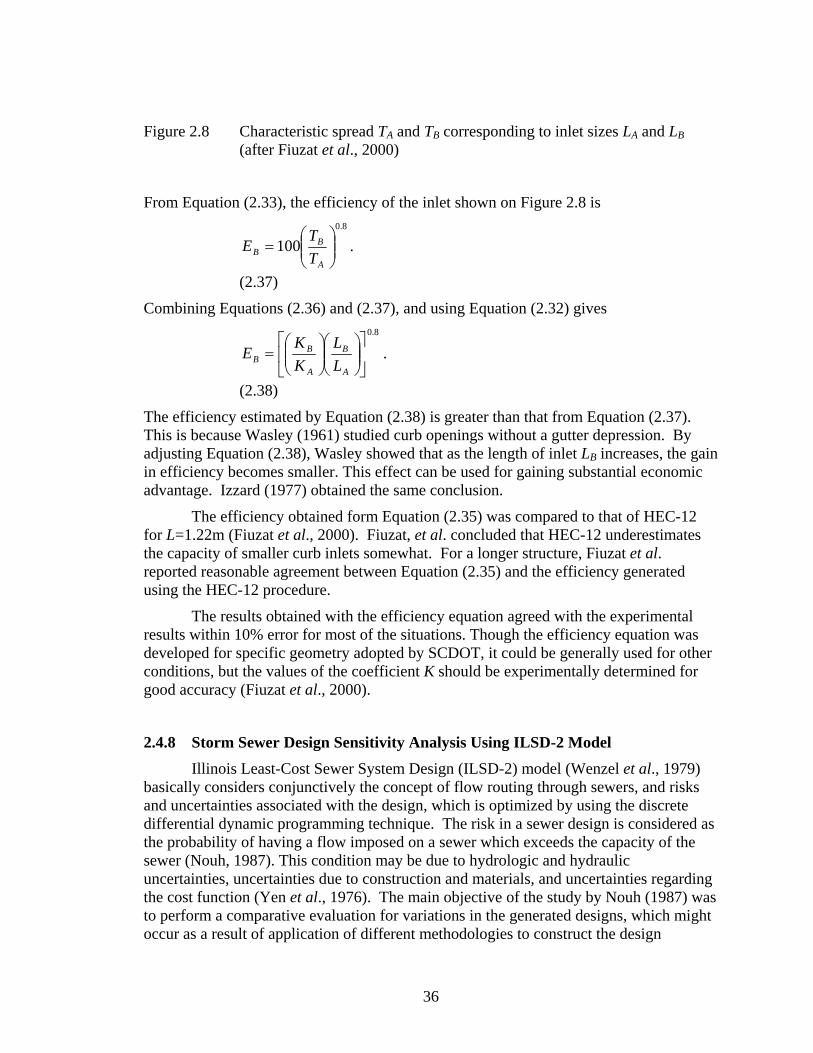
36

Figure 2.8 Characteristic spread TA and TB corresponding to inlet sizes LA and LB (after Fiuzat et al., 2000)

From Equation (2.33), the efficiency of the inlet shown on Figure 2.8 is

8.0

100 ⎟⎟⎠

⎞⎜⎜⎝

⎛=

A

BB T

TE .

(2.37)

Combining Equations (2.36) and (2.37), and using Equation (2.32) gives 8.0

⎥⎦

⎤⎢⎣

⎡⎟⎟⎠

⎞⎜⎜⎝

⎛⎟⎟⎠

⎞⎜⎜⎝

⎛=

A

B

A

BB L

LKK

E .

(2.38)

The efficiency estimated by Equation (2.38) is greater than that from Equation (2.37). This is because Wasley (1961) studied curb openings without a gutter depression. By adjusting Equation (2.38), Wasley showed that as the length of inlet LB increases, the gain in efficiency becomes smaller. This effect can be used for gaining substantial economic advantage. Izzard (1977) obtained the same conclusion.

The efficiency obtained form Equation (2.35) was compared to that of HEC-12 for L=1.22m (Fiuzat et al., 2000). Fiuzat, et al. concluded that HEC-12 underestimates the capacity of smaller curb inlets somewhat. For a longer structure, Fiuzat et al. reported reasonable agreement between Equation (2.35) and the efficiency generated using the HEC-12 procedure.

The results obtained with the efficiency equation agreed with the experimental results within 10% error for most of the situations. Though the efficiency equation was developed for specific geometry adopted by SCDOT, it could be generally used for other conditions, but the values of the coefficient K should be experimentally determined for good accuracy (Fiuzat et al., 2000).

2.4.8 Storm Sewer Design Sensitivity Analysis Using ILSD-2 Model

Illinois Least-Cost Sewer System Design (ILSD-2) model (Wenzel et al., 1979) basically considers conjunctively the concept of flow routing through sewers, and risks and uncertainties associated with the design, which is optimized by using the discrete differential dynamic programming technique. The risk in a sewer design is considered as the probability of having a flow imposed on a sewer which exceeds the capacity of the sewer (Nouh, 1987). This condition may be due to hydrologic and hydraulic uncertainties, uncertainties due to construction and materials, and uncertainties regarding the cost function (Yen et al., 1976). The main objective of the study by Nouh (1987) was to perform a comparative evaluation for variations in the generated designs, which might occur as a result of application of different methodologies to construct the design

37

hyetograph, to generate the overland flow hydrographs, and /or to route the flow through the sewers. Computer subroutines were developed for constructing ten different shapes of hyetographs, for generating overland flow hydrographs by three different methods, and for routing flow hydrographs by different techniques (Nouh, 1987).

Nouh (1987) applied ILSD-2 model to a simple case study, but produced some results that are useful for other complex systems. For the testing of the model, a district of east Riyadh City, Saudi Arabia was selected by Nouh (1987): watershed area = 1.278 x 106 square meters (315 acres) consisting of 18% industrial sites, 8% retail stores, 70% residential sections, and 4% grassy land. The area (Figure 2.9) was divided into 32 sub-catchments, ranging in size from 2x104 to 8.8x104 m2, and in imperviousness, from 45 to 80%. Time of concentration was about 20 minutes for normal antecedent conditions in the pervious area, the initial infiltration capacity, the constant infiltration and decay rate of infiltration selected were 76 mm/hr, 7.4 mm/hr and 0.0012/s, respectively, for Horton’s infiltration equation. The sewer system layout, manhole locations and data on the cost of the sewers are the inputs into the ILSD-2 model to generate the least-cost design.

Figure 2.9. Sewer district (Nouh, 1987)

2.4.8.1 Effect of Time Distribution of Rainfall

The hyetograph can have significant effect on the peak flow and the volume for the least-cost design of storm sewer systems. Ten different shapes of hyetograph, including the Uniform, Hershfield, Sifalda, SCS-6 hr, Keifer and Chu, Composite, Huff (1st quartile), Pilgrim and Cordery, Triangular, and Trapezoidal distributions were investigated by ILSD-2 model (Nouh, 1987). Infiltration losses corresponding to each shapes of hyetograph were determined using the mathematical model developed by Akan

38

and Yen (1981 and 1984). These losses were used to determine the aerially averaged infiltration parameters required for generation of overland flow hydrographs.

Each hyetograph was constructed for a 10-yr design rainfall and used together with the ILLUDAS model to generate the overland flow hydrographs to the inlets/manholes of the case study sewer system which was designed by the ILSD-2 Model. The risk of failure was evaluated for a 2-year service period. The baseline for comparison was the design developed for a uniform (constant rate) hyetograph. The expressed relative values for a particular design hyetograph reflect use of that hyetograph instead of the uniform hyetograph in the least cost design of the storm sewer system. From Figure 2.10, the shape of the design hyetograph resulted in the reduction in the total sewer cost (design and construction cost) and in an increase in the risk of failure. In general, the more the reduction in the total sewer cost, the greater the risk of failure. The greatest amount of cost reduction results from using the trapezoidal hyetograph, followed by the triangular, Pilgrim and Cordery, and Huff hyetographs.

39

Figure 2.10 Effect of time distribution of rainfall on least-cost sewer system design

(Nouh, 1987)

2.4.8.2 Effect of Overland Flow Hydrograph Generation Method Several methods were developed to generate overland flow hydrographs for the

purpose of designing urban facilities (Nouh, 1987). To investigate the value of using a more sophisticated hydrology and hydraulics method for runoff hydrograph generation on the least cost design of storm sewer system, three methods with differing degrees of accuracy were considered. These methods, ILLUDAS (Illinois Urban Drainage Area Simulator, Terstriep and Stall, 1974), UCUR (University Cincinnati Urban Runoff Model, Papadakis and Preul, 1972), and SWMM (Metcalf and Eddy, 1971), were used independently with each of the design hyetographs to generate overland flow hydrographs to the inlets of the sewer system designed using the ILSD-2 model. The

40

results from different methods were compared and expressed relative to those using the Rational method for peak flow estimation at the inlets of the system. Generally, the use of SWMM, followed by the UCUR and the ILLUDAS methods resulted in the least design cost and highest risk of failure. On the other hand, the use of the Rational method resulted in the greatest design cost and lowest risk. From Figure 2.11, the total sewer cost associated with the trapezoidal hyetograph together with the SWMM method was about 67 percent of the cost for the same system designed using the traditional Rational method. Such significant saving in the total sewer cost may encourage the use of methods, which are more accurate than the Rational method for the design of storm sewer system (Nouh, 1987).

Figure 2.11 Effect of overland flow hydrograph generation method on least-cost sewer

system design (Nouh, 1987)

41

2.4.8.3 Effect of Techniques for Routing Flow through Sewers

For hydraulic routing of hydrographs through storm sewers, the most common techniques are steady-uniform flow (traditional Rational method approach), the ILLUDAS, nonlinear kinematics wave, Muskingum–Cunge, and SWMM (unsteady and hydrodynamic methods). The routing method in a particular model represents the unsteady gravity flow in sewers. This part of sensitivity analysis was to give a comparative evaluation for the effect of using these techniques on the least cost design of storm sewer systems.

Based on results presented in Figure 2.12, if the routing mechanism better approximates the physics associated with flow movement, then the reduction in the design cost is increased along with the risk of hydraulic failure. This is true for all of the investigated hyetographs. The ILLUDAS technique is more accurate than the steady flow technique because it considers the effect of water storage in the sewers. After comparing all of the approaches, it is clear that SWMM is the most accurate among those used because it considers, at least partially, the backwater effects. Designs developed using SWMM cost 83 percent of those developed using the Rational method, but the risk of failure was 2.3 times greater than that of the system designed using the Rational method. These findings encourage use the flow routing techniques that better represent the physics of flow in the design of storm sewers (Nouh, 1987).

Nouh (1987) made the following conclusions: The hyetograph, which resulted the least total sewer cost, is trapezoidal. The more sophisticated the methods used for runoff generation and flow routing through the storm sewers, the lower the resulting total sewer cost of design, but the greater the risk of hydraulic failure. The SWMM method for overland flow hydrograph generation provides no significant improvements in the design over the UCUR method but it does over the ILLUDAS and the Rational methods. Thus, it is recommended for the design of storm sewer systems. The ILLUDAS method may be used for small sewer systems. However, it is not advisable to use the Rational method especially when the storm sewer system is large because it results in designs that are more costly than required. Finally, SWMM is recommended for large storm sewer systems, while the rest of the techniques, including the steady flow technique may be use for small storm sewer systems.

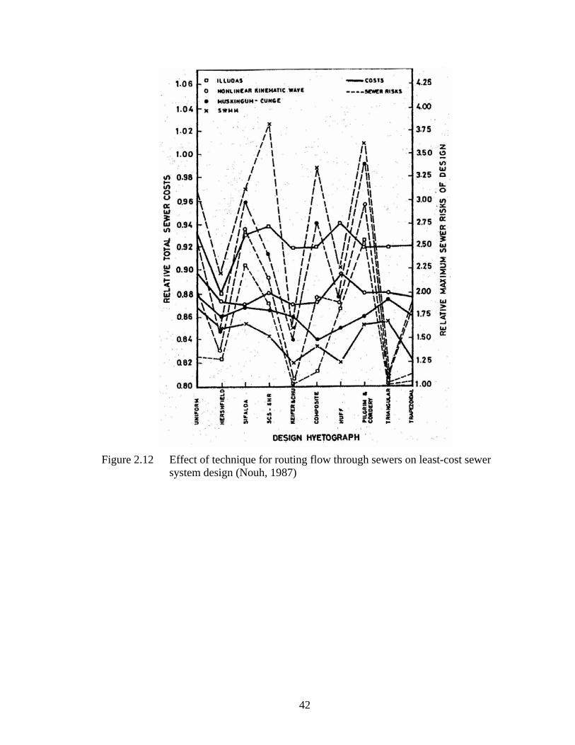
42

Figure 2.12 Effect of technique for routing flow through sewers on least-cost sewer

system design (Nouh, 1987)

43

CHAPTER THREE COMPUTER MODELS FOR STORMWATER SYSTEM

3.1 Introduction

Computer models are important tools for engineers because they can help engineers perform engineering task in a faster and better way. Numerous computer models exist for stormwater system analysis and design. Some of the commercial software packages that will be discussed in the following sections are listed below

1. WinStorm (storm drain analysis/design, TxDOT)

2. StormCAD (design and analysis of gravity flow pipe networks, Haestad Methods)

3. Hydraflow (hydrology and hydraulic analysis of storm sewer network, InteliSOLVE)

4. SWMM (urban runoff quantity and quality modeling, USEPA)

5. HYDRA (Storm Sewer Design Model, FHWA)

6. MIDUSS by Alan A. Smith Inc.

7. HydroCAD by Applied Microcomputer Systems

3.2 WinStorm WinStorm Version 3.0 (http://www.dot.state .tx.us/isd/software/software.htm),

developed by TxDOT, is public domain software and can be downloaded from TxDOT’s web site. It is used to model storm drainage systems using a drainage network comprised of three basic drainage components, namely drainage areas, node and links. The user describes the components of the system by proceeding through a series of dialog windows defining each portion of the drainage component, drainage area, nodes and links. WinStorm is capable of designing and analyzing a system simultaneously when sizes of features are specified. Additionally, two storms of different frequency can be run simultaneously in order to evaluate the performance of a system during different events, or design a system based on one event and analyze the design under a different event. The current or most recent version includes Graphical User Interface (GUI), which was an upgrade from WinStorm 2.0.

WinStorm computes the peak discharge associated with the drainage area and has the capability of designing/analyzing seven different types of storm drain inlets. It allows six conveyance elements to be used to connect the inlets, which includes pipes, box culverts, arch-pipes, elliptical pipes, semicircular pipes, and ditches. WinStorm can optionally compute the junction loss at the nodes and provides graphical visualization of the hydraulic grade line for a selected reach. SCS TR20 and the Rational method are the two runoff computational procedures involved in WinStorm.

Because WinStorm was particularly developed for the state of Texas, the user has the option of only choosing the county in the state of Texas for which the IDF curve is

44

developed and described as Equation (2.6). Pumps in the system are not supported in WinStorm. While multiple incoming links to a node is allowed, only one outgoing link from a node is supported. Diversion and loop within a system must be modeled as separate networks and the network must terminate at a single point (outfall).

3.3 StormCAD

StormCAD (version 5) is a computer program for the design and analysis of gravity-flow pipe networks. The program can be run either within the AutoCAD environment or in stand-alone mode using its own graphical interface. To use the program, a graphical representation of the pipe network, containing all information such as pipe data, inlet characteristics, watershed areas and rainfall information is constructed (WinStorm doesn’t has the capability to do that). Rainfall information is calculated using rainfall tables, Equations (2.6, 2.7, 2.8), or the National Weather Service’s HYDRO-35 data. It is one of the commercial software products of Haestad Method Inc., which can be purchased at the URL: http://www.haestad.com/software/ stmcstandalone/default.asp.

Network flows are computed in StormCAD using built-in numerical models, which use both the direct step and standard step gradually-varied flow method. Flow from inlets is calculated using the Rational method, and both intercepted flow and carryover flow are computed. Flow calculations are valid for both pressure pipe flow and varied open-channel flow situations, including hydraulic jumps, backwater, and drawn-down curves. Its capabilities include analyzing various storm sewer design scenarios and presenting the results both in report format and as a graphical plot. The entire network or a portion of the network can be designed based on a set of user-defined constraints. These design constraints include minimum/maximum velocity, slope and cover; choice of pipe invert and crown matching at structures; inlet efficiency; and gutter spread and depth. The invert elevations and diameters of pipes, as well as the size of a drainage inlet necessary to maintain a given spread (for inlets in sag) or capture efficiency (for inlets on grade) can be computed. Profiles of the network can be generated, which are useful for viewing the hydraulic grade line.

3.4 Hydraflow

Hydraflow is also a commercial computer program used for storm drain network design and analysis, and is developed by InteliSOLVE. Hydraflow can be purchased at the URL: http://www.intelisolve.com/stormsew.html. The current version of Hydraflow (version 2003) allows the user to design and analyze a storm sewer system consisting up to 250 pipelines and inlets. The data input is by spreadsheet. Conduits are specified one at a time, beginning at the downstream end. The lines (conduits) are automatically numbered in the order in which they are input.

Once the system data is input, Hydraflow offers four different ways to compute results: analysis with design, enhanced modeling system, full design, and capacity only. The method depends on the level of accuracy needed and whether the user is modeling an existing system or designing a new one. In either case, the results are the hydraulic grade

45

line, the full flow capacity of the system, flows at inlets including carryover, captured and bypassed flows, and total cost of the system.

Hydraflow allows specifying certain design constraints and initial conditions. It has the option of plotting or generating IDF curves from existing data, third degree polynomial equation, NWS Hydro-35 data, or from a NOAA (National Oceanic and Atmospheric Administration, Atlas 2 published by NWS in 1973). In addition, it also has the feature of interactive design where the user can make changes during the solution process. It displays the results in Summary, DOT style, Inlet, FL-DOT (Florida DOT) style, calculation and cost reports along with custom report.

3.5 SWMM

SWMM, developed by the U.S. Environmental Protection Agency (USEPA), is a comprehensive computer model for mathematical simulation of urban runoff quantity and quality in storm sewers, combined sewers (storm and sanitary), and natural drainage systems on the basis of rainfall (hyetograph) and other meteorological inputs and system characterization (catchment, conveyance, storage/treatment) (Huber and Dickinson, 1992). Both single-event and continuous-event (long-term) processes can be simulated by the SWMM. Rainfall, snowmelt, surface and sub-surface runoff, and flow routing can be simulated. The watershed is broken into a finite number of sub-catchments that can be readily described by their hydraulic and geometric properties. SWMM can be used for screening, planning, design, and operation purposes for stormwater management.

SWMM consists of three principal computational blocks and five service blocks. The computational blocks are Runoff, Transport, and Extran blocks. The service blocks include Combine, Statics, Rain, Temp and Graph. The runoff block produces hydrographs and pollutographs at inlet locations with an option of snowmelt simulation, and simulates flow in pipes by non-linear reservoir routing. The transport block routes the incoming hydrographs and pollutographs through the sewer system based on kinematic wave routing, and uses the first order decay, scour and deposition to generate dry-weather flow and quality. The Extran block is intended to solve the St. Venant equations (one-dimensional, unsteady partial differential equations describing conservation of mass and conservation of momentum). In the Extran bloc, dynamic wave simulation is used to route flows through an open or closed conduit stormwater system (Roesner et al., 1988).

A node in SWMM represents the junction of hydraulic elements (links) and acts as a location for input of flow and pollutants into the drainage system. A node can also represent a storage device such as a pond or lake, a point junction representing a point of change in channel or conduit geometry, a boundary condition in the model, a sewage treatment plant in the transport layer, or a watershed in runoff layer. Links represent the hydraulic elements for flow and constituent transport through the system (for example pipe, channel, pump, weir, orifices regulator, real-time control device, etc.). There are more than 30 different types of conduits included in SWMM.

Several companies have modified the original version of SWMM. Some of latest versions of SWMM include:

46

• PCSWMM 2002 (developed by Computational Hydraulic Inc.)

• Mike SWMM 2002 (developed by Danish Hydraulic Institute)

• Visual SWMM 2000 (developed by CAiCE Software Corporation)

• XP-SWMM 2000 (developed by XP software Pty. Ltd.)

3.6 FHWA Storm Sewer Design Mode, HYDRA HYDRA is a part of a package of integrated design computer programs called

HYDRAIN developed by the U.S. Federal Highway Administration. HYDRA is used as storm drain design model by federal and other engineers. Like all FHWA software packages, the model HYDRA is distributed under contract with the FHWA through McTrans Software Center at the Civil Engineering Department of the University of Florida at Gainesville. Commercial vendors have linked HYDRA to an integrated CADD/GIS system for interactive design.

The program’s primary use is in analyzing the adequacy of existing storm drains or designing new storm drains and inlets by the Rational method as described previously (Section 2.1) or by the modified Rational method (Section 2.2); the latter represents the hydrograph as a trapezoid having a volume equal to the calculated net rain.

In addition to the modified Rational method, commercial versions of HYDRA allow design by SCS methods or the Santa Barbara hydrograph method. HYDRA has an uncommon but useful feature of allowing the hydraulic grade lines to be checked through underground storm sewers. Backwater calculations determine the total system energy losses and hydraulic grade line elevation, allowing an indication of whether inlets, manholes, or junction boxes will overflow, which is implementation of steady state hydraulics. Another useful feature is that street and gutter flows that exceed the inlet capacity of the storm sewers are routed by HYDRA to the next downstream location and added to the hydrograph at that point.

3.7 MIDUSS Software MIDUSS is a stormwater modeling program intended for designers of stormwater

systems with emphasis on the detailed design of devices for centralized or on-site BMPs. The program is positioned midway between detailed design programs with no simulation capability and hydrological simulators with no design features. BMPs include wet and dry ponds and MIDUSS has many tools for the design of outflow controls for a variety of storage facilities including rooftop and parking lot storage. It includes an exfiltration trench design. One can design a drainage network consisting of an unlimited number of pipes, channels, ponds and diversion structures.

The hydrology in MIDUSS is versatile with many built-in models:

• 5 storm types,

• 3 infiltration models, and

• 4 overland flow methods plus a lag and route tool for modeling large catchments.

47

Another feature of MIDUSS is the ability to run in Automatic mode where a

previously created output file serves as the basis for the input database. This is when

testing a design under a more severe storm or completing a design in two or more

sessions.

The design options in MIDUSS include:

• Pipe sizing (in which hydraulic gradient is reported if the pipe is surcharged).

• Open channels of either a generalized trapezoidal shape or a more complex cross-section defined graphically and modified with up to 50 co-ordinate pairs.

• Hydrograph flood routing in part-full pipes or open channels.

• Detention ponds including a variety of tools for computing depth-discharge and depth-storage curves for a variety of outflow control devices and pond geometries.

• Ex-filtration trenches with multiple perforated and non-perforated pipes.

• Diversion structures for separation of hydrograph components (e.g. major and minor).

The above detailed design tools are available at all points in the development of the drainage network. MIDUSS is developed by Alan A. Smith Inc., a software development company established in 1978.

3.8 HydroCAD HydroCAD is a Computer Aided Design tool for use by civil engineers for

modeling stormwater runoff. It is based largely on the hydrology techniques developed by the Soil Conservation Service (SCS/NRCS), combined with other hydrology and hydraulics calculations. The general features include Rational method, SCS method, and SBUH (Santa Barbara Urban Hydrograph) as runoff hydrograph generation method, reach and pond routing plus built-in hydraulics, graphics, and on-screen routing diagram.

HydroCAD was developed by Applied Microcomputer Systems in 1986 and is being continuously updated. HydroCAD can be used for drainage projects ranging from small runoff studies to detention pond designs. The capabilities of HydroCAD also include

• Time of concentration calculation using sheet flow method, shallow concentrated flow, channel flow, curve number method,

• Rainfall management,

• Unit hydrographs method (SCS, custom unit hydrograph),

• Exporting and importing hydrographs, and

48

• Twelve types of pond outlet hydraulics and pond storage capabilities.

49

CHAPTER FOUR 2.1.1 Drainage System for Case Study

4.1 Introduction

In this chapter, a simple drainage system developed by Mr. George (Rudy) Herrmann is presented. This is a hypothetical system (Herrmann, 2002) and is to provide a test bed for the comparison of different design approaches implemented in the several computer software packages. In addition to model testing on hypothetical drainage system, a select subset of the software packages was tested on a real drainage system, and will be presented in the Chapter 6.

4.2 Hypothetical Drainage System for Case Study

A simple hypothetical drainage system (analogous model) was used to test the differences in results obtained from application of different computer software packages for storm drainage design. The model system comprises of four drainage areas, and is shown in Figure 4.1. The system consisted of four inlets (I-1 to I-4 in Figure 4.1) interconnected by underground conduits (P-1 to P-4 in Figure 4.1) and terminating with a free outlet (O-1 in Figure 4.1). For simplicity, the inlets were curb-opening inlet, because this type of inlet has fewer parameters. Rainfall intensity is one of input variables for applying the Rational method and is computed as a function of the time of concentration of the subwatershed. Rainfall intensity for Lubbock County (Texas) was used for the case study. The 2-year design storm was used to develop the basic design of the network, and it was analyzed using a 5-year design storm.

The catchments, inlet, and conduit configuration parameters used in the case study are given in Tables 4.1 to 4.3. Because abstractions in the Rational method are characterized by the runoff coefficient, C, no other forms of direct losses were incorporated into the model. For the simple model, the runoff coefficient was set to a value of 1.0 (implying an impervious area) for all catchments. Results and conclusions developed through the case study are independent of values of runoff coefficients used.

Figure 4.1. Hypothetical storm drainage system for case study.

I-1 I-2 I-3 I-4 O-1P-1 P-2 P-3 P-4

50

Table 4.1 Configuration data for four catchments.

Inlet ID C Value Area (acre) TC (minutes)

I-1 1.0 1.00 10

I-2 1.0 1.00 5

I-3 1.0 1.00 15

I-4 1.0 1.00 12

Table 4.2 Configuration data for grade inlets.

Slopes Gutter Inlet ID Inlet

type Inlet

Length (ft) Long. (%)

Trans. (%)

n Depression (ft)

Bypass to Inlet ID

I-1 Curb 10.00 0.10 2.50 0.014 0.04 I-2

I-2 Curb 10.00 0.10 2.50 0.014 0.04 I-3

I-3 Curb 10.00 0.10 2.50 0.014 0.04 I-4

I-4 Curb 10.00 0.10 2.50 0.014 0.04 O-1

Table 4.3 Configuration data for underground conduits.

Flow line elevation

Run U/S (ft)

D/S (ft)

2.1.1 Shape Span (ft)

Rise (ft)

Length (ft)

Slope (%)

n values

ID D/S

P-1 88.00 86.00 Box 2.00 2.00 600.00 0.33 0.013 I-2

P-2 86.00 83.00 Box 2.00 2.00 1000.00 0.30 0.013 I-3

P-3 81.00 80.50 Box 3.00 3.00 400.00 0.13 0.013 I-4

P-4 77.00 74.00 Box 3.00 3.00 300.00 1.00 0.013 O-1

51

CHAPTER FIVE RESULTS OF CASE STUDY

5.1 Introduction The results obtained for the case study from different software packages are

discussed in this chapter. Detailed calculation on the results and the basic setup required to operate the software packages are presented in the Appendix A to D. The results acquired from the software packages are presented in tabular format.

Typically in storm drain design, inlet flow quantity calculations are done separately from pipe system flows. In other words, most designers assume that all of the flows computed by the Rational Method (using maximum travel time as time of concentration) will enter the pipes, which is implemented in Hydraflow. WinStorm and StormCAD use the same methodology to handle the flow entering the pipe system even they have different methods to compute cumulative CA values before the Rational Method is applied. The following sections further explain results developed for the case study by using steady models: WinStorm, StormCAD and Hydraflow, and by using unsteady models: SPLIT program and SWMM. The steady models only compute peak discharge for the storm drain design, while the unsteady models develop hydrographs at inlets and route through the pipe system.

5.2 Case Study by Using WinStorm and StormCAD

The hypothetical drainage system presented in the Chapter Four was first tested by using WinStorm and StormCAD. The Appendix A gives detailed calculations on flows from watershed to inlet, carryover flow at inlet, carryover flow from upstream inlet, and pipe flow. Results of computations using StormCAD are graphically shown in Figure 5.1. For example, intercepted flow at the inlet I-1 (0.839 CA) is indicated in red. This flow directly enters the pipe P-1. Carryover CA from inlet I-1 (0.161 CA) plus local CA of inlet I-2 is indicated in green (total 1.161 CA). Intercepted flow from I-2 combined with pipe flow in P-1 is indicated by the yellow pipe, which is the flow in the pipe P-2. The same process is then repeated for remaining part of the system, as depicted in Figure 5.1 (tp is travel time in pipe).

Carryover calculation results for four inlets developed by StormCAD and WinStorm, respectively, are given in Tables 5.1 and 5.2. When StormCAD was used (Table 5.1), for example, total CA for the inlet I-3 is equal to carryover CA from the inlet I-2 (0.228, blue square in catchment 2 of Figure 5.1) plus local CA (1.0). Therefore StormCAD actually uses local rainfall intensity and carryover CA to recalculate carryover flow. WinStorm does calculate the carryover simply by using equation (2.16), and WinStorm directly adds carryover flow from upstream inlet and the local flow together (Table 5.2). Total flow to each inlet simulated using StormCAD and WinStorm are highlighted in both Tables 5.1 and 5.2, and the difference between simulated discharges is relative small (<0.2 cfs in the case study).

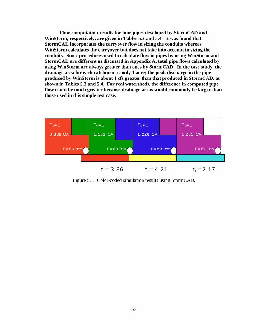
52

Flow computation results for four pipes developed by StormCAD and WinStorm, respectively, are given in Tables 5.3 and 5.4. It was found that StormCAD incorporates the carryover flow in sizing the conduits whereas WinStorm calculates the carryover but does not take into account in sizing the conduits. Since procedures used to calculate flow in pipes by using WinStorm and StormCAD are different as discussed in Appendix A, total pipe flows calculated by using WinStorm are always greater than ones by StormCAD. In the case study, the drainage area for each catchment is only 1 acre; the peak discharge in the pipe produced by WinStorm is about 1 cfs greater than that produced in StormCAD, as shown in Tables 5.3 and 5.4. For real watersheds, the difference in computed pipe flow could be much greater because drainage areas would commonly be larger than those used in this simple test case.

Figure 5.1. Color-coded simulation results using StormCAD.

Tc=10 0.839 CA

E=83.9%

Tc=10 1.161 CA

E=80.3%

Tc=15 1.228 CA

E=83.3%

Tc=12 1.205 CA

E=81.3%

tp=3.56 tp=4.21 tp=2.17

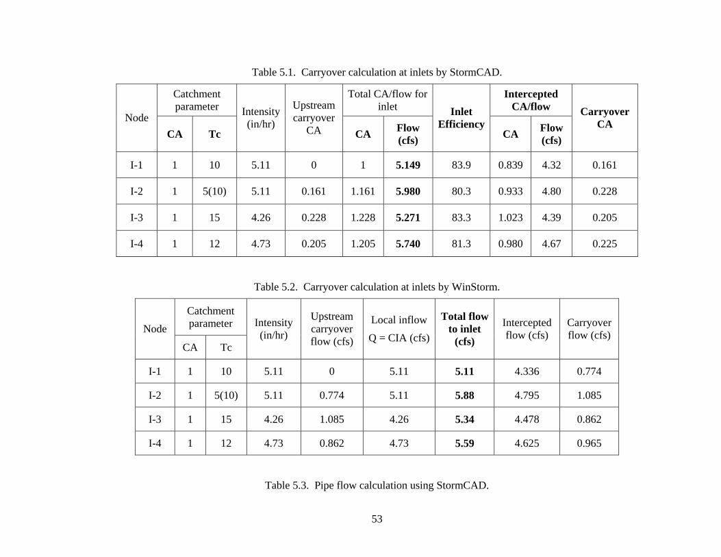
53

Table 5.1. Carryover calculation at inlets by StormCAD.

Catchment parameter

Total CA/flow for inlet

Intercepted CA/flow

Node CA Tc

Intensity (in/hr)

Upstream carryover

CA CA Flow (cfs)

Inlet Efficiency

CA Flow (cfs)

Carryover CA

I-1 1 10 5.11 0 1 5.149 83.9 0.839 4.32 0.161

I-2 1 5(10) 5.11 0.161 1.161 5.980 80.3 0.933 4.80 0.228

I-3 1 15 4.26 0.228 1.228 5.271 83.3 1.023 4.39 0.205

I-4 1 12 4.73 0.205 1.205 5.740 81.3 0.980 4.67 0.225

Table 5.2. Carryover calculation at inlets by WinStorm.

Catchment parameter Node

CA Tc

Intensity (in/hr)

Upstream carryover flow (cfs)

Local inflow

Q = CIA (cfs)

Total flow to inlet

(cfs)

Intercepted flow (cfs)

Carryover flow (cfs)

I-1 1 10 5.11 0 5.11 5.11 4.336 0.774

I-2 1 5(10) 5.11 0.774 5.11 5.88 4.795 1.085

I-3 1 15 4.26 1.085 4.26 5.34 4.478 0.862

I-4 1 12 4.73 0.862 4.73 5.59 4.625 0.965

Table 5.3. Pipe flow calculation using StormCAD.

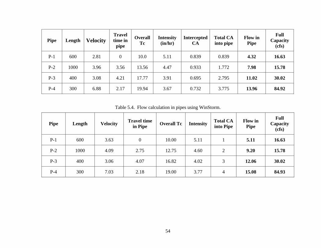
54

Pipe Length Velocity Travel time in

pipe

Overall Tc

Intensity (in/hr)

Intercepted CA

Total CA into pipe

Flow in Pipe

Full Capacity

(cfs)

P-1 600 2.81 0 10.0 5.11 0.839 0.839 4.32 16.63

P-2 1000 3.96 3.56 13.56 4.47 0.933 1.772 7.98 15.78

P-3 400 3.08 4.21 17.77 3.91 0.695 2.795 11.02 30.02

P-4 300 6.88 2.17 19.94 3.67 0.732 3.775 13.96 84.92

Table 5.4. Flow calculation in pipes using WinStorm.

Pipe Length Velocity Travel time in Pipe Overall Tc Intensity Total CA

into Pipe Flow in

Pipe

Full Capacity

(cfs)

P-1 600 3.63 0 10.00 5.11 1 5.11 16.63

P-2 1000 4.09 2.75 12.75 4.60 2 9.20 15.78

P-3 400 3.06 4.07 16.82 4.02 3 12.06 30.02

P-4 300 7.03 2.18 19.00 3.77 4 15.08 84.93

98

5.3 Case Study by Using Hydraflow

The input for Hydraflow for the case study is given in Appendix B. Hydraflow has four options for computing/generating results. For the case study the Return Period chosen was 5 year and the calculation options investigated were on two different options available namely “Analysis w/ Design” and “Enhanced Modeling System” to study the difference in the process of simulating results. The “Full Design” and “Capacity Only” options, which can be used to design the pipe size, are of less concern in the study. Furthermore, the calculations of the former two options are processed and their results are compared and tabulated separately.

5.3.1 Simulation with Analysis w/ Design Option Table 5.5 below gives the total flow from catchment; the captured and the bypassed flows resulted from Hydraflow for the inlet configuration while flow computation in the pipes is shown in Table 5.6. Calculation procedure used to develop results in Table 5.5 was based on FHWA guidelines as discussed in Chapter 2. The results obtained (Table 5.5) are similar to those of WinStorm outputs (Table 5.4) except the precision.

Under this calculation option, the time of concentration (18.80 minutes) for Line (pipe) L-2 in Table 5.6 is the summation of the upstream Tc (10 minutes) and the travel time in the conduit by assuming that pipe is flowing full and not considering pipe slope: 8.8 minutes = [(600ft)/{(4.53cfs)/(4ft2)}]/(60s/min), where 4 ft2 is the full-flow cross section area, and 4.53 cfs is intercepted flow. This travel time in pipe L-2 is much greater than the travel time (3.5 seconds) computed by using Manning’s equation, e.g., in WinStorm (Table 5.4) and StormCAD (Table 5.3). This treatment on computing travel time in pipes may not produce reliable results.

Rainfall intensity and then Total Runoff by the Rational method in Table 5.6 are calculated and based on the time of concentration calculated by the above method. While the total flow in Table 5.6 is simply the summation of captured flows from the inlets (Table 5.5) in the upstream direction (9.44cfs = 4.53cfs + 4.91cfs). The result so obtained for the total flow was due to using the option “Use inlet captured flows in system” under Flow Options of Design Codes (Fig. B.3), otherwise the total flow would be the same as the total runoff (system flows) as illustrated in Table 5.7.

5.3.2 Simulation With Enhanced Modeling System (EMS) Option This option is used when one has to analyze existing systems and where the hydraulic analysis is critical and maximum accuracy is of importance (Hydraflow, Storm Sewers 2003 User’s Guide). While solving the model with this option on, Hydraflow undergoes three system iterations to achieve a practical balance between accuracy and the time required to produce results. The model was solved without using the Flow Option “Use inlet captured flows in system” under Design Codes (Fig. B.3), therefore the total runoff is the same as the total flow (Table 5.7) for each pipe. The model resulted the same values of flow parameters for the catchment and the inlet as those developed in

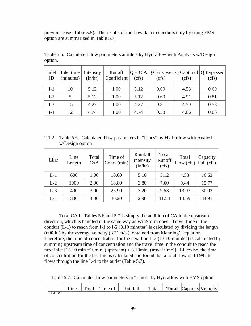
99

previous case (Table 5.5). The results of the flow data in conduits only by using EMS option are summarized in Table 5.7.

Table 5.5. Calculated flow parameters at inlets by Hydraflow with Analysis w/Design option.

Inlet ID

Inlet time (minutes)

Intensity (in/hr)

Runoff Coefficient

Q = CIA (cfs)

Q Carryover (cfs)

Q Captured (cfs)

Q Bypassed (cfs)

I-1 10 5.12 1.00 5.12 0.00 4.53 0.60 I-2 5 5.12 1.00 5.12 0.60 4.91 0.81 I-3 15 4.27 1.00 4.27 0.81 4.50 0.58 I-4 12 4.74 1.00 4.74 0.58 4.66 0.66

2.1.2 Table 5.6. Calculated flow parameters in “Lines” by Hydraflow with Analysis

w/Design option

Line Line Length

Total CxA

Time of Conc. (min)

Rainfall intensity (in/hr)

Total Runoff (cfs)

Total Flow (cfs)

Capacity Full (cfs)

L-1 600 1.00 10.00 5.10 5.12 4.53 16.63 L-2 1000 2.00 18.80 3.80 7.60 9.44 15.77 L-3 400 3.00 25.90 3.20 9.53 13.93 30.02 L-4 300 4.00 30.20 2.90 11.58 18.59 84.91

Total CA in Tables 5.6 and 5.7 is simply the addition of CA in the upstream

direction, which is handled in the same way as WinStorm does. Travel time in the conduit (L-1) to reach from I-1 to I-2 (3.10 minutes) is calculated by dividing the length (600 ft.) by the average velocity (3.21 ft/s.), obtained from Manning’s equation. Therefore, the time of concentration for the next line L-2 (13.10 minutes) is calculated by summing upstream time of concentration and the travel time in the conduit to reach the next inlet [13.10 min.=10min. (upstream) + 3.10min. (travel time)]. Likewise, the time of concentration for the last line is calculated and found that a total flow of 14.99 cfs flows through the line L-4 to the outlet (Table 5.7).

Table 5.7. Calculated flow parameters in “Lines” by Hydraflow with EMS option.

Line Line Total Time of Rainfall Total Total Capacity Velocity

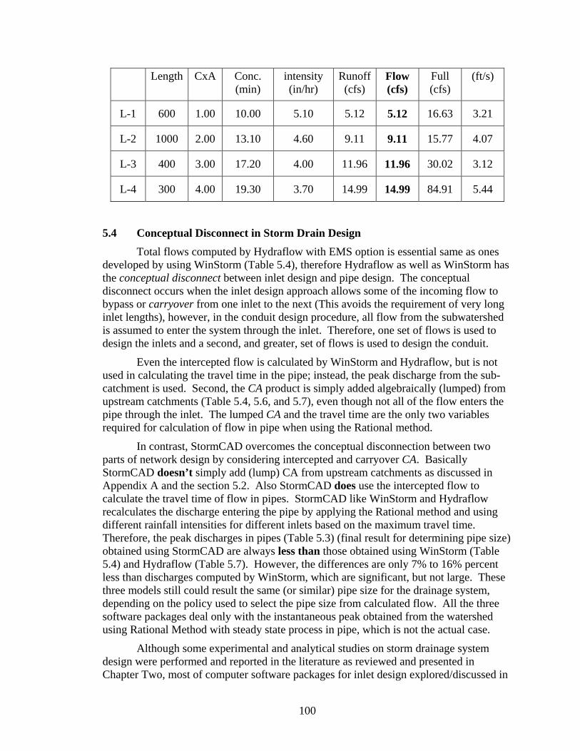
100

Length CxA Conc. (min)

intensity (in/hr)

Runoff (cfs)

Flow (cfs)

Full (cfs)

(ft/s)

L-1 600 1.00 10.00 5.10 5.12 5.12 16.63 3.21

L-2 1000 2.00 13.10 4.60 9.11 9.11 15.77 4.07

L-3 400 3.00 17.20 4.00 11.96 11.96 30.02 3.12

L-4 300 4.00 19.30 3.70 14.99 14.99 84.91 5.44

5.4 Conceptual Disconnect in Storm Drain Design Total flows computed by Hydraflow with EMS option is essential same as ones

developed by using WinStorm (Table 5.4), therefore Hydraflow as well as WinStorm has the conceptual disconnect between inlet design and pipe design. The conceptual disconnect occurs when the inlet design approach allows some of the incoming flow to bypass or carryover from one inlet to the next (This avoids the requirement of very long inlet lengths), however, in the conduit design procedure, all flow from the subwatershed is assumed to enter the system through the inlet. Therefore, one set of flows is used to design the inlets and a second, and greater, set of flows is used to design the conduit.

Even the intercepted flow is calculated by WinStorm and Hydraflow, but is not used in calculating the travel time in the pipe; instead, the peak discharge from the sub-catchment is used. Second, the CA product is simply added algebraically (lumped) from upstream catchments (Table 5.4, 5.6, and 5.7), even though not all of the flow enters the pipe through the inlet. The lumped CA and the travel time are the only two variables required for calculation of flow in pipe when using the Rational method.

In contrast, StormCAD overcomes the conceptual disconnection between two parts of network design by considering intercepted and carryover CA. Basically StormCAD doesn’t simply add (lump) CA from upstream catchments as discussed in Appendix A and the section 5.2. Also StormCAD does use the intercepted flow to calculate the travel time of flow in pipes. StormCAD like WinStorm and Hydraflow recalculates the discharge entering the pipe by applying the Rational method and using different rainfall intensities for different inlets based on the maximum travel time. Therefore, the peak discharges in pipes (Table 5.3) (final result for determining pipe size) obtained using StormCAD are always less than those obtained using WinStorm (Table 5.4) and Hydraflow (Table 5.7). However, the differences are only 7% to 16% percent less than discharges computed by WinStorm, which are significant, but not large. These three models still could result the same (or similar) pipe size for the drainage system, depending on the policy used to select the pipe size from calculated flow. All the three software packages deal only with the instantaneous peak obtained from the watershed using Rational Method with steady state process in pipe, which is not the actual case.

Although some experimental and analytical studies on storm drainage system design were performed and reported in the literature as reviewed and presented in Chapter Two, most of computer software packages for inlet design explored/discussed in

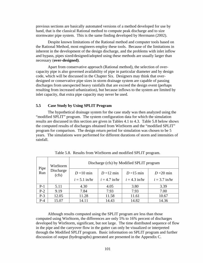
101

previous sections are basically automated versions of a method developed for use by hand, that is the classical Rational method to compute peak discharge and to size stormwater pipe system. This is the same finding developed by Herrmann (2002).

Despite known limitations of the Rational method and computer tools based on the Rational Method, most engineers employ these tools. Because of the limitations in inherent in the development of the design discharge, and the problems with inlet inflow and bypass, pipes sized/designed/adopted using these methods are usually larger than necessary (over-designed).

Apart from conservative approach (Rational method), the selection of over-capacity pipe is also governed availability of pipe in particular diameter and by design code, which will be discussed in the Chapter Six. Designers may think that over-designed or conservative pipe sizes in storm drainage system are capable of passing discharges from unexpected heavy rainfalls that are exceed the design event (perhaps resulting from increased urbanization), but because inflows to the system are limited by inlet capacity, that extra pipe capacity may never be used.

5.5 Case Study by Using SPLIT Program

The hypothetical drainage system for the case study was then analyzed using the “modified SPLIT” program. The system configuration data for which the simulation results are discussed in this section are given in Tables 4.1 to 4.3. Table 5.8 below shows the computed results of discharges obtained from WinStorm and the “modified SPLIT” program for comparison. The design return period for simulation was chosen to be 5 years. The simulations were performed for different durations of storm and intensities of rainfall.

Table 5.8. Results from WinStorm and modified SPLIT program.

Discharge (cfs) by Modified SPLIT program Pipe Run

WinStorm Discharge

(cfs) D =10 min

i = 5.1 in/hr

D =12 min

i = 4.7 in/hr

D =15 min

i = 4.3 in/hr

D =20 min

i = 3.7 in/hr

P-1 5.11 4.30 4.05 3.80 3.39 P-2 9.19 7.84 7.93 7.93 7.00 P-3 12.05 11.28 11.58 11.61 10.67 P-4 15.07 14.11 14.43 14.82 14.36

Although results computed using the SPLIT program are less than those computed using WinStorm, the differences are only 5% to 16% percent of discharges developed by WinStorm, significant, but not large. The time distributed sequence of flow in the pipe and the carryover flow in the gutter can only be visualized or interpreted through the Modified SPLIT program. Basic information on SPLIT program and further discussion of output (hydrographs) generated are presented in the Appendix C.

102

5.6 Case Study by Using SWMM The hypothetical drainage system was extensively analyzed using Visual and XP

SWMM. The background information on SWMM, model setup, and many intermediate results developed by SWMM are given in Appendix D. SWMM consists of three principal computational blocks (layers or modes): Runoff, Transport (Sanitary), and Extran (Hydraulic) blocks. There are two options in SWMM to connect conduits with four inlet nodes and the outfall node for the case study. If the conduits connecting nodes are created under the Runoff layer, non-linear reservoir approach is used to simulate runoff passing through conduits. If the conduits connecting nodes are created under the Hydraulic (Extran) layer, the St. Venant equations (one-dimensional, unsteady state continuity and momentum partial differential equations) for dynamic wave simulation (Roesner et al., 1988) on an open or closed conduit wastewater or stormwater system are solved to generate hydrographs.

5.6.1 Results From Runoff Layer

First, both inlets and pipes (links) were set up under runoff layer. SWMM simulates runoff hydrograph at inlets, and all flow collected/generated at inlets gets into underground pipe (no inlet restriction under Runoff layer) and routes through pipe by non-linear reservoir method. For all inlets except the most upstream one, routed hydrograph from upstream pipe combines with local inflow hydrograph generated through catchment modeling. Figure 5.2 shows hydrograph generated at the inlet N-1 and by using Rational formula for unit hydrograph method. Peak discharge is 4.6 cfs at 8:13AM (rainfall starts at 8:00AM and lasts 10 minutes with 5.11”/hr intensity, time of concentration is 10 minutes for catchment at the inlet N-1). Figure 5.3 shows hydrograph and flow velocity after pipe routing, and peak discharge is slight smaller (4.1 cfs) and at a later time (8:15AM). These are two examples of hydrograph for illustration only, and other simulated hydrographs by SWMM are presented in the Appendix D.

The peak discharges at all the nodes and the conduits obtained after solving the model in the SWMM Runoff layer using the Rational method and the SCS method as the hydrograph generation technique, respectively, are summarized in Table 5.9. A typical value of 484 for the shape factor, as determined by Soil Conservation Service for most watersheds, though actual value may range from 300 for flat swampy country to 600 for steep terrain, was utilized while simulating under SCS method. Because of the fact that Rational method is more conservative than SCS method, the peak flows simulated, in nodes and eventually in conduits, obtained from the Rational method are found to be greater than one obtained from the SCS method. Peak discharges in pipes are always less than one at corresponding nodes (Table 5.9) because they are peak values after non-linear reservoir routing in the pipes.

Table 5.9 Peak flow (cfs) in the nodes and conduits simulated by using Rational method and SCS method under Runoff layer.

103

Rational Method SCS Method Node Peak Discharge at

Node Peak Discharge in

Pipe Peak Discharge at

Node Peak Discharge in

Pipe

N-1 4.61 4.14 3.50 3.11

N-2 8.52 7.05 6.42 5.15

N-3 10.34 9.96 7.76 7.32

N-4 13.21 13.17 9.64 9.62

Figure 5.2. Hydrograph output of SWMM for Node N1.

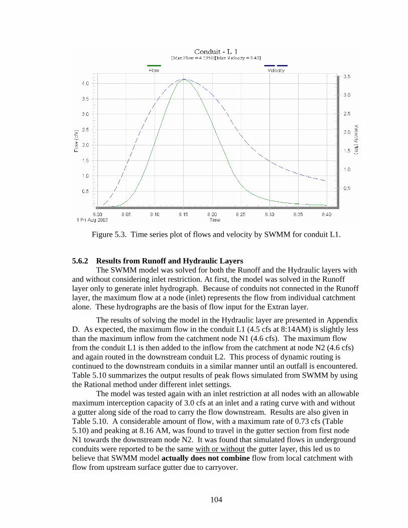
104

Figure 5.3. Time series plot of flows and velocity by SWMM for conduit L1.

5.6.2 Results from Runoff and Hydraulic Layers The SWMM model was solved for both the Runoff and the Hydraulic layers with and without considering inlet restriction. At first, the model was solved in the Runoff layer only to generate inlet hydrograph. Because of conduits not connected in the Runoff layer, the maximum flow at a node (inlet) represents the flow from individual catchment alone. These hydrographs are the basis of flow input for the Extran layer.

The results of solving the model in the Hydraulic layer are presented in Appendix D. As expected, the maximum flow in the conduit L1 (4.5 cfs at 8:14AM) is slightly less than the maximum inflow from the catchment node N1 (4.6 cfs). The maximum flow from the conduit L1 is then added to the inflow from the catchment at node N2 (4.6 cfs) and again routed in the downstream conduit L2. This process of dynamic routing is continued to the downstream conduits in a similar manner until an outfall is encountered. Table 5.10 summarizes the output results of peak flows simulated from SWMM by using the Rational method under different inlet settings.

The model was tested again with an inlet restriction at all nodes with an allowable maximum interception capacity of 3.0 cfs at an inlet and a rating curve with and without a gutter along side of the road to carry the flow downstream. Results are also given in Table 5.10. A considerable amount of flow, with a maximum rate of 0.73 cfs (Table 5.10) and peaking at 8.16 AM, was found to travel in the gutter section from first node N1 towards the downstream node N2. It was found that simulated flows in underground conduits were reported to be the same with or without the gutter layer, this led us to believe that SWMM model actually does not combine flow from local catchment with flow from upstream surface gutter due to carryover.

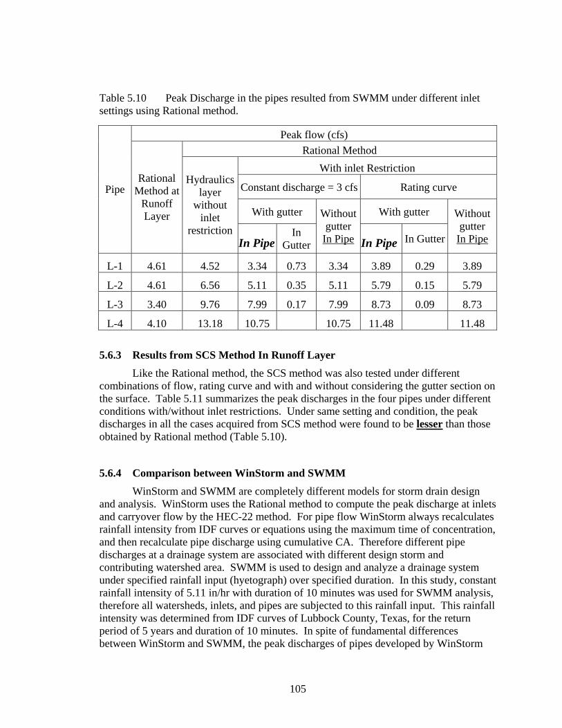
105

Table 5.10 Peak Discharge in the pipes resulted from SWMM under different inlet settings using Rational method.

Peak flow (cfs) Rational Method

With inlet Restriction

Constant discharge = 3 cfs Rating curve

With gutter With gutter

Pipe Rational

Method at Runoff Layer

Hydraulics layer

without inlet

restrictionIn Pipe

In Gutter

Without gutter

In Pipe In Pipe In Gutter

Without gutter

In Pipe

L-1 4.61 4.52 3.34 0.73 3.34 3.89 0.29 3.89

L-2 4.61 6.56 5.11 0.35 5.11 5.79 0.15 5.79

L-3 3.40 9.76 7.99 0.17 7.99 8.73 0.09 8.73

L-4 4.10 13.18 10.75 10.75 11.48 11.48

5.6.3 Results from SCS Method In Runoff Layer

Like the Rational method, the SCS method was also tested under different combinations of flow, rating curve and with and without considering the gutter section on the surface. Table 5.11 summarizes the peak discharges in the four pipes under different conditions with/without inlet restrictions. Under same setting and condition, the peak discharges in all the cases acquired from SCS method were found to be lesser than those obtained by Rational method (Table 5.10).

5.6.4 Comparison between WinStorm and SWMM WinStorm and SWMM are completely different models for storm drain design

and analysis. WinStorm uses the Rational method to compute the peak discharge at inlets and carryover flow by the HEC-22 method. For pipe flow WinStorm always recalculates rainfall intensity from IDF curves or equations using the maximum time of concentration, and then recalculate pipe discharge using cumulative CA. Therefore different pipe discharges at a drainage system are associated with different design storm and contributing watershed area. SWMM is used to design and analyze a drainage system under specified rainfall input (hyetograph) over specified duration. In this study, constant rainfall intensity of 5.11 in/hr with duration of 10 minutes was used for SWMM analysis, therefore all watersheds, inlets, and pipes are subjected to this rainfall input. This rainfall intensity was determined from IDF curves of Lubbock County, Texas, for the return period of 5 years and duration of 10 minutes. In spite of fundamental differences between WinStorm and SWMM, the peak discharges of pipes developed by WinStorm

106

(Table 5.4) and SWMM (Tables 5.10 and 5.11) are compared. The peak flows in the conduits produced by SWMM varied to some extent, depending on methods for hydrograph generation and flow routing in the pipe. Peak flows simulated in pipes using SWMM are smaller than those obtained by WinStorm (Table 5.4), the differences are up to 24% (Rational method in Table 5.10) to 41% (SCS method in Table 5.11) percent of discharges developed by WinStorm, significant, but not large. The differences between peak discharges developed using SWMM and WinStorm could be greater for actual application to design problems, instead of the simple rainfall settings and storm drain network tested here.

Table 5.11. Peak Discharge in the pipes resulted from SWMM under different inlet settings using SCS hydrology method.

Peak flow (cfs) SCS Method

With inlet Restriction Constant discharge = 3 cfs Rating curve

With gutter With gutter Pipe

SCS Method Runoff Layer

Hydraulics layer

without inlet

restriction In Pipe In Gutter

Without gutter

In Pipe In Pipe In Gutter

Without gutter

In Pipe

L-1 3.50 3.77 3.35 0.10 3.35 3.43 0.09 3.43

L-2 3.50 4.75 4.46 0.04 4.46 4.45 0.04 4.45

L-3 2.64 7.07 6.77 0.02 6.77 6.75 0.02 6.75

L-4 3.11 9.25 8.91 8.91 8.89 8.89

CHAPTER SIX

IMPLEMENTATION OF MODEL TESTING FOR HIGHWAY 77/83

6.1 Description of Study Site and TxDOT Design Policy

For comparison with the previous example, data were taken from an existing drainage system on the U.S. 77/83 expressway for comparison using WinStorm and StormCAD. Furthermore, some of the current stormwater sewer design policies and regulation that TxDOT are currently pursuing for highway stormwater design are also discussed.

Texas Department of Transportation (TxDOT) with the Federal Aid, proposed state highway improvement on U.S. 77/83 expressway. The expressway, located on the Pharr District (southern part of Texas) of Cameroon County, was only covered for a total

107

length of 3.086 miles as shown by dark line in the Figure 6.1. The main aim of the project was to upgrade the existing stormwater drainage system. The stormwater conveyance line was, for convenience, divided into 5 trunk lines A, B, C, D and E respectively, based on discharging outlet. Trunk line A is comprised of 34 junctions with 24 inlets, 8 manholes and an outlet while Trunk line B consisted of 31 junctions among which 20 were inlets, 10 manholes and an outfall, and Trunk line C, D and E took account of 33, 27, 14 junctions including the outlet, respectively. TxDOT Engineers utilized their in-house developed computer software called WinStorm for all of TxDOT drainage design and analysis projects, so did they for the U.S. 77/83 project too.

The process of computing a hydrograph begins with selection of a design storm, the first step of which is to select a design frequency. Often, the local approving authority (city, county, drainage district, etc.) will specify the level of design to be used for any particular type of structure. Likewise, TxDOT has its policy of using either 2 or 5 year, preferably 5 year, as the storm frequency for roadways of functional classification, while design frequency for interstate and limited access highways is 10 years. In order to alleviate or eliminate some common mistakes in storm drain design that result in operational problems, TxDOT also has certain regulation in selection of conveyance (pipe) sizes. The minimum sizes of conduit that TxDOT utilizes is 18 inches in order to facilitate cleaning and debris clearing, but occasionally designer may use 12 inches for short laterals form an inlet to a junction box with one joint or so (Herrmann, 2003). The standard sizes that TxDOT generally employ include 18, 21, 24, 30, 36, 42, 48, 54, 60 and 72 inches of diameter. Even pipes on 3-inch increment are available on market, however, TxDOT designers experienced that the bid prices for 3-inch increment pipes (e.g., 15, 21, 27, 33 inches) are always more than for the next even 6-inch increment pipes (e.g., 18, 24, 30, 36 inches) (Herrmann, 2003). The conduit of the storm drain system shall be placed at not less than the grade that maintains a minimum of 2 feet per second velocity with a maximum of 12 feet per second.

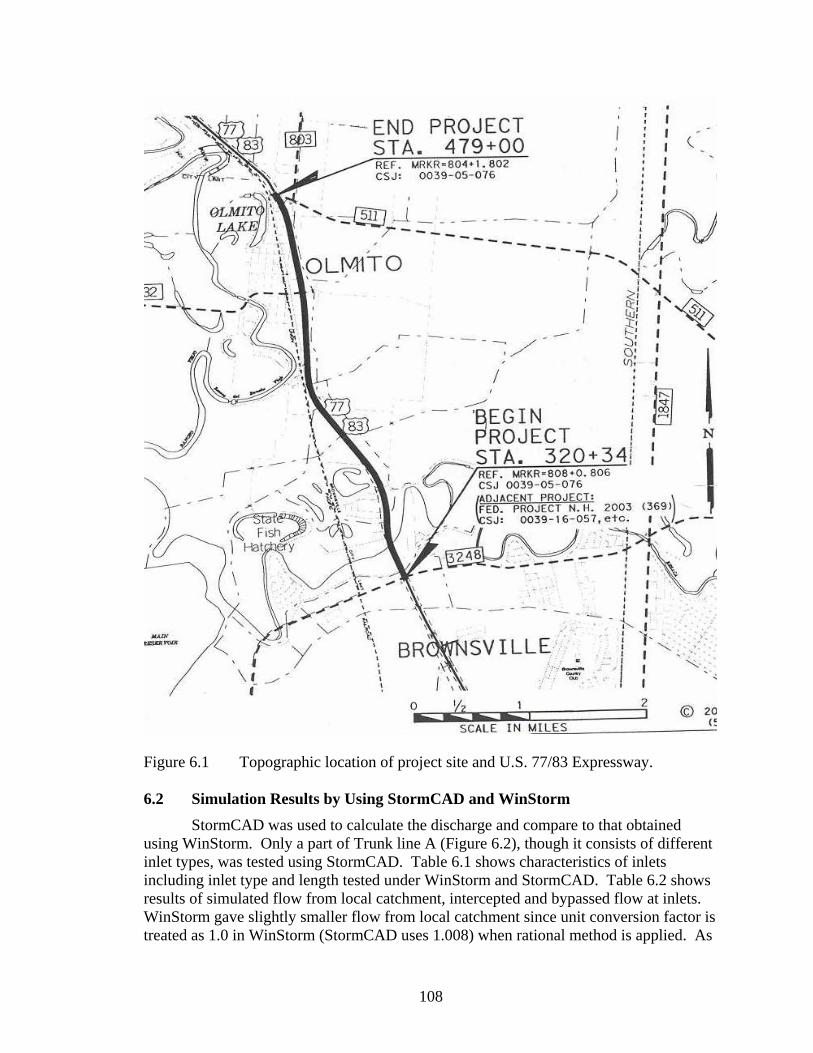
108

Figure 6.1 Topographic location of project site and U.S. 77/83 Expressway. 6.2 Simulation Results by Using StormCAD and WinStorm StormCAD was used to calculate the discharge and compare to that obtained using WinStorm. Only a part of Trunk line A (Figure 6.2), though it consists of different inlet types, was tested using StormCAD. Table 6.1 shows characteristics of inlets including inlet type and length tested under WinStorm and StormCAD. Table 6.2 shows results of simulated flow from local catchment, intercepted and bypassed flow at inlets. WinStorm gave slightly smaller flow from local catchment since unit conversion factor is treated as 1.0 in WinStorm (StormCAD uses 1.008) when rational method is applied. As

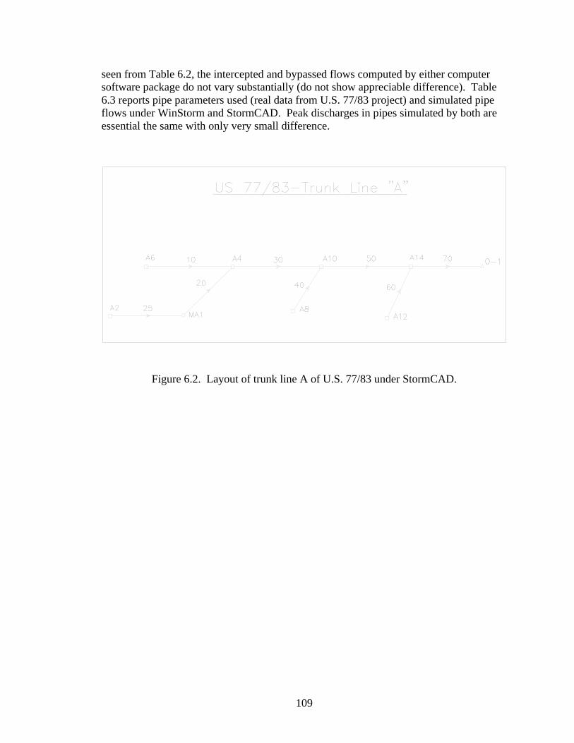
109

seen from Table 6.2, the intercepted and bypassed flows computed by either computer software package do not vary substantially (do not show appreciable difference). Table 6.3 reports pipe parameters used (real data from U.S. 77/83 project) and simulated pipe flows under WinStorm and StormCAD. Peak discharges in pipes simulated by both are essential the same with only very small difference.

Figure 6.2. Layout of trunk line A of U.S. 77/83 under StormCAD.

110

Table 6.1 Characteristics of inlets tested by WinStorm and StormCAD.

Inlet C A (Acre) Tc (min) Inlet type Inlet length (ft) A2 0.90 2.89 46.66 Grate on Sag 3.0 A4 0.42 2.12 18.25 Grate on Sag 3.0 A6 0.45 1.97 17.23 Curb on grade 20.0

A10 0.56 1.19 64.44 Grate on grade 7.0 A8 0.77 2.22 37.78 Curb on grade 15.0

A14 0.59 2.36 66.66 Grate on grade A12 0.74 2.31 44.05 Curb on grade 15.0

Table 6.2 Simulated intercepted and bypassed flow from WinStorm and StormCAD.

Runoff from catchment (cfs) Intercepted Bypassed Intercepted Bypassed Inlet WinStorm StormCAD WinStorm StormCAD

A2 8.64 8.71 8.639 0.00 8.71 0.00 A4 5.22 5.26 5.221 0.00 5.26 0.00 A6 5.51 5.55 5.507 0.00 5.55 0.00

A10 1.80 1.82 1.739 0.06 1.73 0.08 A8 6.51 6.56 6.507 0.00 6.56 0.00

A14 3.63 3.66 3.479 0.21 3.48 0.26 A12 5.89 5.94 5.889 0.00 5.94 0.00

Table 6.3 Pipe parameters and simulated pipe flow using WinStorm and StormCAD.

Flow in pipe Pipe

Pipe Length

(ft)

Upstream/ Downstream

Elevations

Diameter (ft)

Full Capacity

(cfs) WinStorm

(cfs) StormCAD

(cfs) 10 100 24.52/23.4 2.0 25.94 5.51 5.55 25 48 25.6/25.38 2.0 18.65 8.64 8.71 20 145 24.88/23.47 2.5 43.82 8.64 8.69 30 490 23.38/22.47 3.0 31.14 14.55 14.67 40 79 23.75/23.66 2.0 8.27 6.51 6.56 50 588 22.45/21.60 3.0 27.48 18.13 18.2 60 49 23.38/23.07 1.5 8.91 5.89 5.94 70 98 21.24/21.01 3.5 52.81 25.75 25.71

111

As noted in Table 6.3, full capacity available in the pipes is found to be much greater than simulated flows by WinStorm and StormCAD. Hence one can conclude that the conduits are over-designed for the specified return period, which was 5 year (TxDOT output was labeled as 10 year return period, but all flows reported were based on 5 year return period). Therefore, in order to analyze the optimum return period for the full capacity available, the storm drainage system for U.S. 77/83 was modeled several times for different return periods without changing any of its physical characteristics of the system. Table 6.4 below summarizes the discharge on pipe obtained from WinStorm by altering the return period for each case. Allowing a tolerance discharge of 5 cfs as compared with the full capacity of pipe (Qf), they are classified as over-designed (Q < Qf –5), under-designed (Q > Qf) and appropriately designed pipes (Qf –5 < Q < Qf). In the Table 6.4, the discharges shown in normal font indicate that pipes are appropriately designed, while the discharges in underlined and bold fonts indicate that pipes are under-designed and over-designed, for corresponding return period, respectively.

If U.S. 77/83 was designed for 5-year return period, 20 out of 32 pipes were over-designed. If U.S. 77/83 was designed for 10-year return period, 15 out of 32 pipes were still over-designed, while there were six pipes under-designed. One can also conclude from Table 6.4 that some of the pipes (nine pipes) were over-designed even up to return period of 100-year. Minimum pipe size used for U.S. 77/83 was 18 inches (1.5 ft) in order to facilitate cleaning and debris clearing. This modeling test clearly indicates that there are many pipes, designed by using WinStorm and TxDOT policy in selecting pipe size, may have large capacity present that will never be utilized. These extra capacities could be utilized for other purpose, e.g., in-line water quality treatment, which will be further discussed in the next section.

As noted from Table 6.4, pipe 70 is over designed up to a return period of 100 year while the inlet A14 linking the pipe 70 is under designed as it does not capture all flow reaching it (Table 6.2). Due to conservatism of Rational Method, which results over-designed pipes, it is recommended that TxDOT engineers should design inlet as big as possible or distribute inlets with a shorter distance to capture all incoming flow. There were two sag inlets (A2 and A4) analyzed (Table 6.1) both WinStorm and StormCAD always consider 100% incoming flow to be intercepted, which may not be true in the reality. Sag inlet design in conjunction to geometry design is needed be investigated further.

112

Table 6.4. Discharge obtained from WinStorm for different return periods for pipes of U.S 77/83 Highway.

Discharge (cfs) Run No.

Diameter (ft) 5 yrs 10 yrs 25 yrs 50 yrs 100 yrs

Full Capacity

(cfs) 10 2.0 5.51 6.46 7.30 7.96 8.55 25.94 20 2.5 8.64 10.17 11.68 13.05 14.07 43.82 30 3.0 14.55 17.14 19.69 22.02 23.73 31.14 40 2.0 6.51 7.65 8.76 9.73 10.49 8.27 50 3.0 18.13 21.38 24.69 27.85 30.04 27.48 60 1.5 5.89 6.93 7.95 8.87 9.56 8.91 70 3.5 25.75 30.40 35.14 39.66 42.79 52.81 80 3.5 26.14 30.86 35.68 40.27 43.46 30.53 90 3.5 26.47 31.25 36.15 40.83 44.08 50.58

100 3.5 26.85 31.72 36.70 41.47 44.78 46.72 110 1.5 3.51 4.14 4.78 5.39 5.81 7.26 120 3.5 32.24 38.09 44.10 49.84 53.82 42.20 130 1.5 3.95 4.65 5.34 5.96 6.42 10.80 140 3.5 34.62 40.93 47.41 53.65 57.99 41.55 150 1.5 4.16 4.89 5.61 6.25 6.74 22.15 160 3.5 37.42 44.24 51.25 58.03 62.75 177.48 170 1.5 0.35 0.41 0.46 0.50 0.53 9.13 180 3.5 37.52 44.36 51.38 58.18 62.91 40.98 190 1.5 2.94 3.44 3.86 4.17 4.46 5.69 200 3.5 38.34 45.33 52.53 59.50 64.35 59.92 210 3.5 40.84 48.29 55.97 63.42 68.57 52.98 220 1.5 2.38 2.79 3.13 3.37 3.61 4.76 230 2.0 3.15 3.70 4.15 4.48 4.80 57.53 240 3.5 41.43 48.99 56.81 64.42 69.70 52.39 250 1.5 5.77 6.76 7.62 8.28 8.88 6.02 260 1.5 8.31 9.75 11.05 12.09 12.99 17.43 270 3.5 46.97 55.55 64.43 73.15 79.19 55.00 280 1.5 4.77 5.61 6.40 7.07 7.61 5.58 290 3.5 49.60 58.69 68.08 77.38 83.81 71.76 300 3.5 49.60 58.69 68.08 77.38 83.81 49.81 25 2.0 8.64 10.17 11.68 13.05 14.07 18.65

205 1.5 6.00 7.04 7.97 8.72 9.37 7.18

113

CHAPTER SEVEN FEASIBILITY OF INLINE STORMWATER QUALITY

TREATMENT

7.1 Concepts of Inline Water Quality Treatment

Urban drainage systems are vital infrastructure assets, which protect our town and cities from flooding and the transmission of waterborne diseases. They are usually constructed as a network of buried pipelines that can be either “combined sewers system” or “separate system”. Initially the separate system used to transport the stormwater away from one area and directly disposed to the nearest river. It is now realized that the scheme, whilst removing a potential threat from one area, often simply passes large quantities of water forward so that it becomes someone else’s problem downstream. Uncontrolled, rapid urban runoff presents not only an increase in the risk of downstream flooding, but also has an adverse effect on river habitat due to changes in channel morphology through man’s actions in the name of flood defense. The modern drainage engineer is therefore faced with some interesting challenges in maintaining the levels of flood protection demanded by society without any cause of damages to the natural environment.

An urban stormwater Best Management Practice (BMP) is a “technique, measure or structural control that is used for a given set of conditions to manage the quantity and improve the quality of stormwater runoff in the most cost-effective manner”. BMP can generally be divided into structural and nonstructural categories. Structural BMPs are techniques that can be used to address flow control and pollution removal in stormwater runoff and include infiltration systems, detention systems, retention systems, filtration systems, and wetlands. Nonstructural BMPs on the other hand are practices designed to prevent pollutants from entering stormwater runoff or to reduce the volume of runoff that may include public education, minimizing pollutants disposal, good housekeeping etc.

In-line storage refers to the practices designed to use the unused volume temporarily available within the stormwater system to store stormwater runoff. While these practices can reduce storm peak flows, they are unable to improve water quality or protect downstream channels, as the intent will be to make the system self-cleaning to reduce maintaining requirements. Storage is achieved by placing devices in the storm drain system to restrict the rate of flow. Controls to restrict flow can either be fixed or adjustable. Fixed systems will probably be cheaper and require less maintenance as compared to that of adjustable systems. Hence, if storage is combined with an end-of-pipe treatment, the flow attenuation will help equalize the load to the treatment process and, hence, optimize the treatment plant.

An example of BMP is Stormceptor, an in-line treatment structure. A layout of typical urban area with Stormceptor installed is shown in Figure 7.1. A Stormceptor (Figure 7.2) is a pre-fabricated concrete structure designed for remove free oil (i.e., hydrocarbons) and suspended solids (i.e., sediment) from stormwater runoff. Two

114

working condition applies: one is the Normal operating conditions and the other is the By-pass operating condition. Under normal operating conditions (more than 90% of all storm events), stormwater flows into the upper chamber and is diverted by a u-shaped weir, into the separation-holding chamber (Figure 7.2). Right angle outlets direct flow around the circular walls of the chamber. Fine and coarse sediments settle to the floor of the chamber, while the petroleum products rise and become trapped beneath the fiberglass insert. During infrequent, high flow events (less than 10% of all storm events), peak stormwater flows pass over the diverting weir and continue into the downstream storm sewer system. This by-pass activity creates pressure equalization across the by-pass chamber, preventing scouring and re-suspension of previously trapped pollutants. Based on the loading condition, location and the operational condition they can be positioned in series, in the inlet junction and submerged condition respectively.

There are numerous stormwater treatment systems available today. Their mechanism or operational procedure that a particular treatment pursues, the various treatment processes that a system can undergo, the possible pollutants removed, vendor address are summarized in Figure 7.3a, 7.3b and 7.3c, obtained from CE News (ASCE, 2003). As discussed and concluded through model testing by using U.S. 77/83 data, there are many pipes having extra capacity which never will be utilized. Can these extra capacities be used for in-line water quality treatment? For example, pipes with extra capacity can function as a storage reservoir just before Stormceptor. SWMM will be used to study feasibility of large pipe as storage reservoir for in-line water quality treatment and to examine dynamics of flow in the reservoir in the next section.

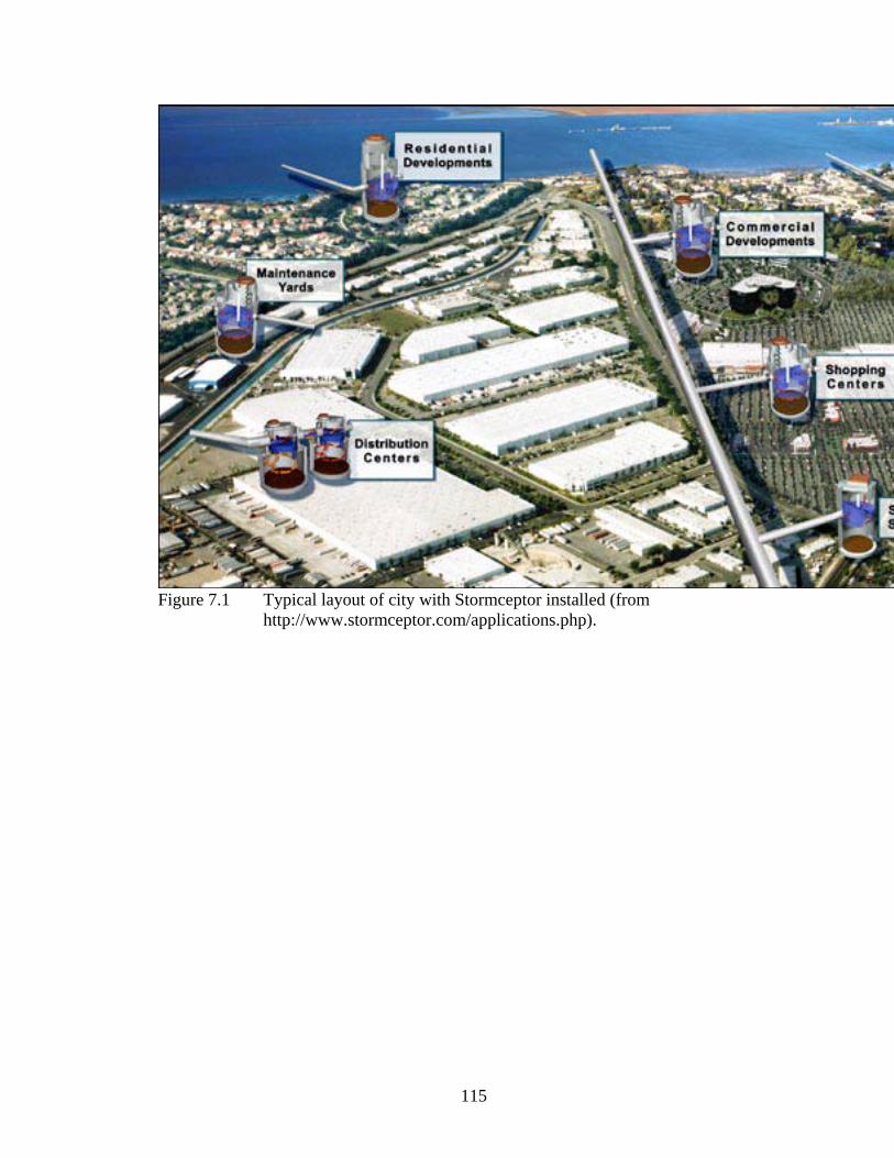
115

Figure 7.1 Typical layout of city with Stormceptor installed (from http://www.stormceptor.com/applications.php).

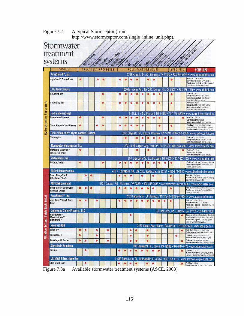
116

Figure 7.2 A typical Stormceptor (from http://www.stormceptor.com/single_inline_unit.php).

Figure 7.3a Available stormwater treatment systems (ASCE, 2003).

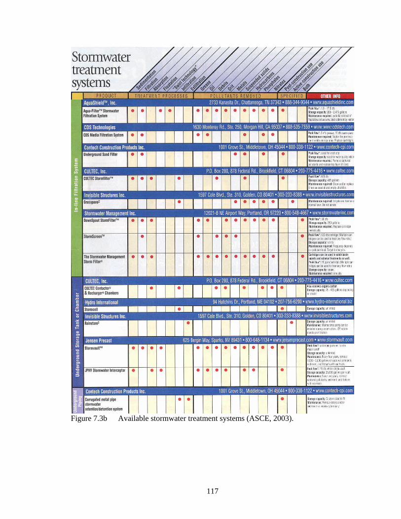
117

Figure 7.3b Available stormwater treatment systems (ASCE, 2003).

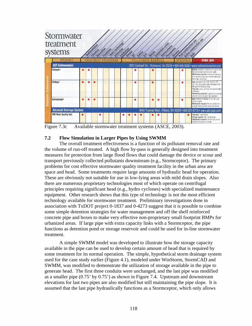
118

Figure 7.3c Available stormwater treatment systems (ASCE, 2003). 7.2 Flow Simulation in Larger Pipes by Using SWMM The overall treatment effectiveness is a function of its pollutant removal rate and the volume of run-off treated. A high flow by-pass is generally designed into treatment measures for protection from large flood flows that could damage the device or scour and transport previously collected pollutants downstream (e.g., Stormceptor). The primary problems for cost effective stormwater quality treatment facility in the urban area are space and head. Some treatments require large amounts of hydraulic head for operation. These are obviously not suitable for use in low-lying areas with mild drain slopes. Also there are numerous proprietary technologies most of which operate on centrifugal principles requiring significant head (e.g., hydro cyclones) with specialized maintenance equipment. Other research shows that this type of technology is not the most efficient technology available for stormwater treatment. Preliminary investigations done in association with TxDOT project 0-1837 and 0-4273 suggest that it is possible to combine some simple detention strategies for water management and off the shelf reinforced concrete pipe and boxes to make very effective non-proprietary small footprint BMPs for urbanized areas. If large pipe with extra capacity links with a Stormceptor, the pipe functions as detention pond or storage reservoir and could be used for in-line stormwater treatment.

A simple SWMM model was developed to illustrate how the storage capacity available in the pipe can be used to develop certain amount of head that is required by some treatment for its normal operation. The simple, hypothetical storm drainage system used for the case study earlier (Figure 4.1), modeled under WinStorm, StormCAD and SWMM, was modified to demonstrate the utilization of storage available in the pipe to generate head. The first three conduits were unchanged, and the last pipe was modified as a smaller pipe (0.75’ by 0.75’) as shown in Figure 7.4. Upstream and downstream elevations for last two pipes are also modified but still maintaining the pipe slope. It is assumed that the last pipe hydraulically functions as a Stormceptor, which only allows

119

limited flow pass through or say it is equivalent to the treatment facility hydraulically. The model with the same rainfall pattern was simulated using Runoff layer (SCS Method) and the Hydraulic layer under XP SWMM for a simulation period of 1 hour 30 minutes. Figure 7.5 shows the basic layout in dynamic profile view after solving the model in Hydraulic layer of SWMM. Figure 7.5 shows clearly the storage capacity and the head developed in the pipe at time 8:25:20 that can be used (needed) in the stormwater treatment facility as the rainfall was started as 8:00 for only ten minutes.

Figure 7.4 Layout of dynamic section view before simulation started.

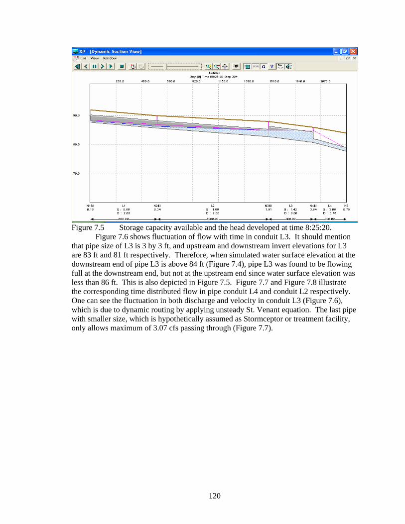
120

Figure 7.5 Storage capacity available and the head developed at time 8:25:20.

Figure 7.6 shows fluctuation of flow with time in conduit L3. It should mention that pipe size of L3 is 3 by 3 ft, and upstream and downstream invert elevations for L3 are 83 ft and 81 ft respectively. Therefore, when simulated water surface elevation at the downstream end of pipe L3 is above 84 ft (Figure 7.4), pipe L3 was found to be flowing full at the downstream end, but not at the upstream end since water surface elevation was less than 86 ft. This is also depicted in Figure 7.5. Figure 7.7 and Figure 7.8 illustrate the corresponding time distributed flow in pipe conduit L4 and conduit L2 respectively. One can see the fluctuation in both discharge and velocity in conduit L3 (Figure 7.6), which is due to dynamic routing by applying unsteady St. Venant equation. The last pipe with smaller size, which is hypothetically assumed as Stormceptor or treatment facility, only allows maximum of 3.07 cfs passing through (Figure 7.7).

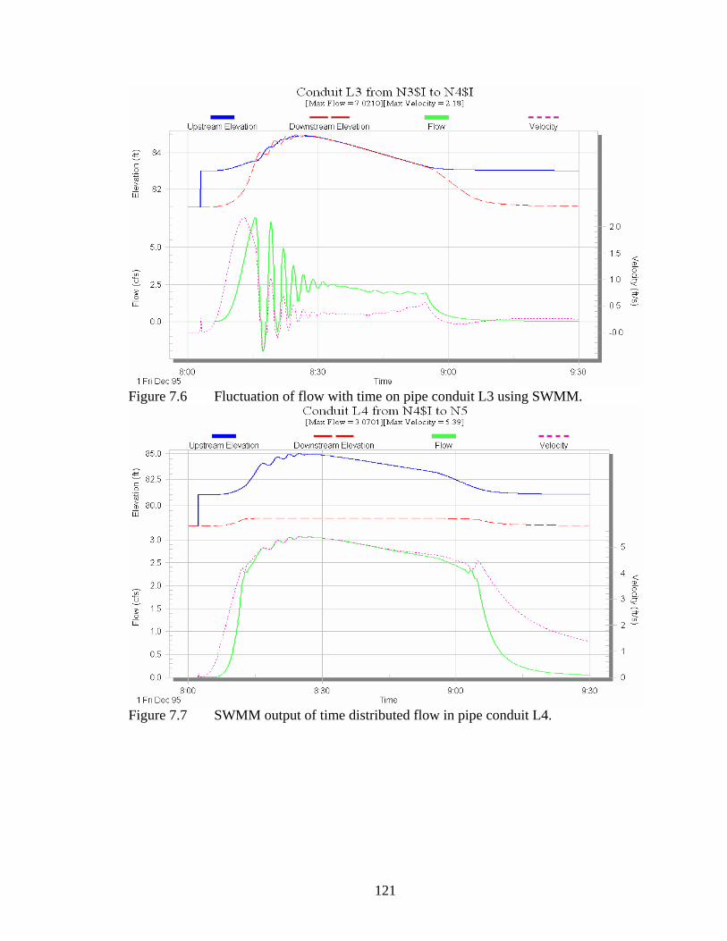
121

Figure 7.6 Fluctuation of flow with time on pipe conduit L3 using SWMM.

Figure 7.7 SWMM output of time distributed flow in pipe conduit L4.

122

Figure 7.8 SWMM output of time distributed flow in pipe conduit L2.

Moreover care should be taken in selecting flow capacity of the treatment facility so that there occur no flooding while generating the head needed. Figure 7.9 shows the case of flooding in the node and the conduit L3 by making the last pipe size further smaller (0.25 by 0.25 ft). This resulted maximum flow in L4 to be only 0.2 cfs. The maximum hydraulic grade line (purple color) shows flooding at the downstream end of conduit L3 on 8:31:50. Current hydraulic grade line is given as blue color. Figure 7.10 shows water surface elevations in pipes at the end of simulation (9:30). Even maximum flows through smaller pipe for both model testing may not real flow capacity for any Stormceptor or other treatment facility, SWMM simulation does give us idea that extra pipe capacity is feasible as storage reservoir to build necessary head for treatment facility, and size of treatment facility is also important in order to avoid street flooding and any further damage to public and private properties.

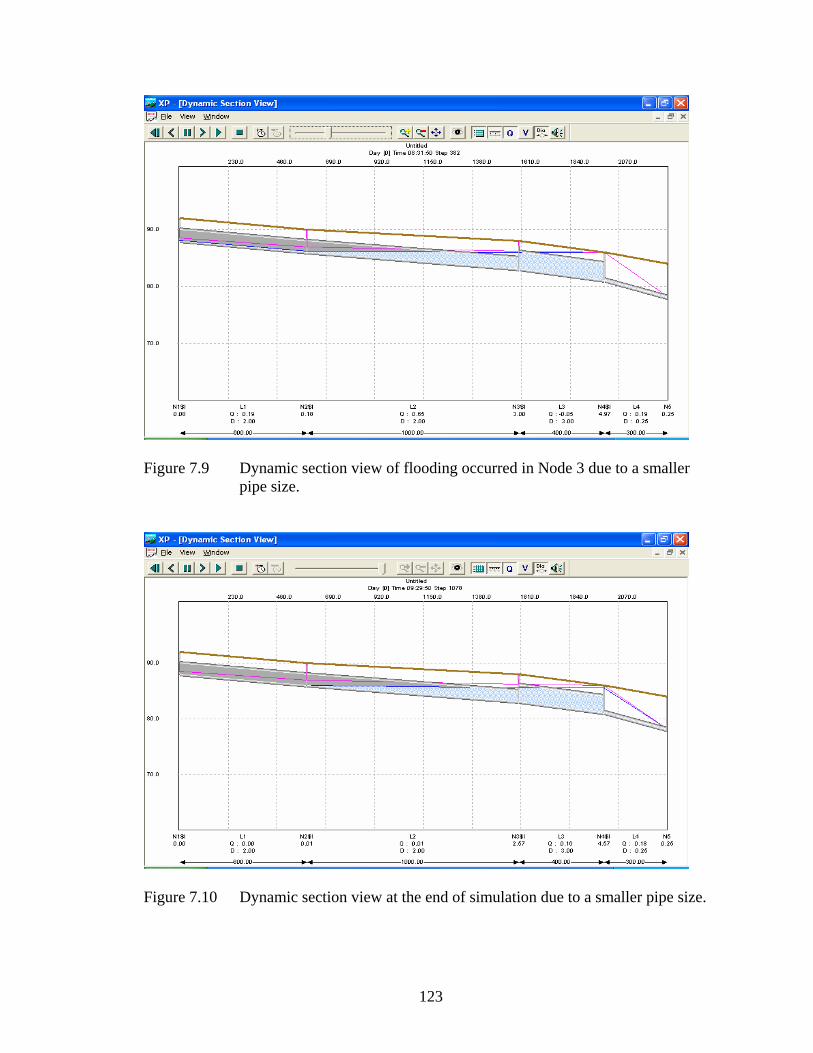
123

Figure 7.9 Dynamic section view of flooding occurred in Node 3 due to a smaller pipe size.

Figure 7.10 Dynamic section view at the end of simulation due to a smaller pipe size.

124

CHAPTER EIGHT SUMMARY AND CONCLUSION

Storm drain systems are typically designed with one purpose: to carry flow from a

rainfall event away from areas where it is unwanted (such as parking lots and roadways). Because of this primary functionality, most storm drainage systems are designed to adequately convey a peak flow rate, based on the characteristics of the watershed and the rainfall event. Design of storm drainage systems in most of the agencies is generally accomplished by application of the rational method. The rational method assumes a linear relation between rainfall rate for the time of concentration of the watershed and peak instantaneous discharge. Actually the process by which rainfall translates into runoff is a very complex and unsteady process affected/controlled by many variables. Rational method is probably adequate for design of simple culverts; the impact of hydraulic routing in more complex drainage networks calls this procedure into question. Storm drains are dendritic or "branched" hydraulic systems consisting of contributing sub basins and their respective inlets, laterals, junctions, trunklines, manholes, and outfalls. The hydraulics at any point throughout the system can change significantly. These changes can be due to both the variability of the hydrologic characteristics of the contributing sub basins and the associated hydraulic features of each branch or feature in the storm drain system. This study performed is intended to evaluate TxDOT procedures for storm drain design, not only in terms of the adequacy of current TxDOT practice relative to new directions in the field, but also in anticipation of the need to evaluate more complex features that might be required by changes in water quality regulations.

An in-depth literature review was performed to synthesize both the technical

approach (Rational method versus other hydrological methods) and modeling efforts of drainage networks with various computer software packages, which were summarized in Chapter Two. Rational Method for storm drainage design was reviewed, including basic assumptions, how to quantify runoff coefficient, rainfall intensity, time of concentration, and limitations of the method. Modified rational method was reviewed as one of the procedures used to develop runoff hydrographs for inlets. Many other methods are available to develop hydrographs for watersheds to account for unsteady processes from rainfall to runoff, they are not reviewed in detail (briefly discussed) in this study and are illustrated in many standard textbooks of hydrology. The design of inlets (especially curb inlet in grade and sag), flow in uniform and composite gutter, interception flow, inlet efficiency, concept of carry over flow and bypassed flow were reviewed in detail in Chapter Two. Moreover, several different computer models or software packages, which are often used for the storm drainage design, were also included in the literature review. Several journal papers were reviewed and summarized to explore recent developments in the field of storm drainage design.

As a simple testing case study, a hypothetical storm drainage system was

examined in detail, as reported in Chapter Four, using several software packages, including WinStorm, StormCAD, Hydraflow, the custom-developed SPLIT program, and SWMM. This hypothetical system, comprising four inlets, four conduits and one outfall, was initially developed and used by a TxDOT engineer, Mr. George (Rudy) Herrmann

125

during his graduate program. The first three models use only the Rational Method and the steady flow approach for the storm drainage analysis and design. The fourth model, the SPLIT program, considers a simple time distribution of surface and the sub-surface flow. The last model, Visual or XP SWMM, developed from the original EPA SWMM, not only has the option of estimating runoff hydrographs at inlets using different methods (for example, unit hydrograph, NRCS/SCS method, and kinematic wave) but also includes the complete unsteady hydraulic open channel pipe flow with a graphical interface. Results developed using these computer models were summarized, analyzed and compared. Model results were presented in graphical and tabular format. Furthermore, results obtained were also compared to manual calculations wherever applicable. Model testing was then implemented on a real world project, the storm drainage system for U.S. Highway 77/83 on the Pharr District (southern part of Texas) of Cameroon County. Model testing was conducted for different return periods. Finally, the concept and feasibility of in-line water quality treatment was discussed with the aid of SWMM simulation results.

Through literature review, reviewing the results of the case study and examining

the calculation procedures of various computer models (packages), the following conclusions were made:

(1). Some computer models, for example, WinStorm and Hydraflow, have a

conceptual disconnect between the inlet and pipe design process. Though the carryover flow is calculated in the inlet design process (typically based on FHWA HEC-22), it is ignored in the computation of flow in pipes.

First, the intercepted flow is not used in calculating the travel time in the pipe;

instead, the peak discharge from the sub-catchment is used. Second, the CA product is simply added algebraically (lumped) from upstream catchments, even though not all of the flow enters the pipe through the inlet. The lumped CA and the travel time are the only two variables required for calculation of flow in pipe when using the Rational method.

(2). In contrast, StormCAD overcomes the conceptual disconnection between two

parts of network design by considering intercepted and carryover CA. Therefore, the peak discharges in pipes (Table 5.3) (final result for determining pipe size) obtained using StormCAD are less than those obtained using WinStorm (Table 5.4) and Hydraflow (Table 5.7). However, the peak discharges are still in the same order of magnitude. Therefore, these three models could result the same (or similar) pipe size for the drainage system, depending on the policy used to select the pipe size from calculated flow. All the three software packages deal only with the instantaneous peak obtained from the watershed using Rational Method with steady state process in pipe, which is not the actual case.

(3). Despite known limitations of the Rational method and computer tools based

on the Rational Method, most engineers employ these tools. Because of the limitations in inherent in the development of the design discharge, and the problems with inlet inflow

126

and bypass, pipes sized/designed /adopted using these methods are usually larger than necessary (over-designed).

(4). Results from the SPLIT or the modified SPLIT program include simple time

distributed hydrographs of inlet from the watershed and in the pipes, while those from SWMM include inlet hydrographs and the complete dynamic solution of pipe flows. SWMM allows the user to examine unsteady flow process in a storm drainage system subjected to a specified rainfall event. The peak flows in the conduits produced by these two models varied to some extent, depending on methods for hydrograph generation and flow routing in the pipe. Peak flows simulated in pipes using SWMM (Table 5.10 and 5.11) and SPLIT (Table 5.8) are smaller than those obtained by WinStorm (Table 5.4), however the peak flows are still in the same order of magnitude. The differences between peak discharges developed using SWMM and WinStorm could be greater for actual application to design problems, instead of the simple rainfall settings and storm drain network tested here.

(5). Based on the literature review (especially, “Storm Sewer Design Sensitivity

Analysis Using ILSD-2 Model, Nouh 1987), use of the Rational method results in the highest construction cost and lowest failure risk (conservative), while the SWMM technique is the most accurate (by considering unsteady and hydrodynamic processes) among those studied, it produced cost and risk values of 0.83 and 2.30 times the steady flow values (Rational method). Overall designs developed using SWMM can result in less construction cost and greater risk of hydraulic failure in comparison to the other design approaches, if the agency is willing to reduce the amount of hidden conservatism in the resulting designs. Finally, SWMM is recommended for large drainage systems, while the rest of the techniques, including the steady flow technique may be used for small drainage systems.

(6). Two commercial versions of SWMM, namely CAiCE Visual SWMM and

XP-SWMM 2000, were tested in the study. Though both were developed from the EPA SWMM module, they produced somewhat different results. A simple case was presented in Figure 3.55a and Figure 3.55b. Therefore, a question arises about which product is more correct. Little research work of the nature represented by the current study is present in the professional literature.

(7). Numerous model applications to an actual system for a variety of return

periods were conducted. Some pipes were larger than required (over-designed) for return periods of up to 100 years. Apart from conservative approach (Rational method), the selection of over-capacity pipe is also governed availability of pipe in particular diameter and by design code. Designers may think that over-designed or conservative pipe sizes in storm drainage system are capable of passing discharges from unexpected heavy rainfalls that are exceed the design event (perhaps resulting from increased urbanization), but because inflows to the system are limited by inlet capacity, that extra pipe capacity may never be used. However, the unused volume (storage) available in the pipe can be possibly used for in-line treatment of storm discharges to improve the water quality with/ without flow control device (if head is required) as discussed in the Chapter Seven.

127

(8). If pipe capacity is sufficient to manage flows up to a return period of 100

years (Table 6.4), if the inlet does not capture the incoming flow (Table 6.2), the capacity is “wasted.” Therefore, it is recommended that TxDOT engineers modify the design guidelines either to include additional inlet capacity commensurate with pipeline capacity, or that pipeline capacity can be reduced. Furthermore, WinStorm and StormCAD assume that sag inlets intercept all incoming flow instantaneously, which may not be true. During heavy storms, sag inlets may be subjected to a long-standing pool of water, and none of the models is currently treating the dynamic nature of flow at sag inlets. Further investigation of the interaction of hydrographs and inlet capacity at sag inlets is suggested.

Overall, it is concluded that further research into development or application of

sophisticated modeling technology is not currently warranted for design and analysis of TxDOT drainage network designs. The SWMM model is useful for analyzing flow dynamics of in-line treatment of storm discharges. Furthermore, TxDOT engineers should realize the disconnect between inlet design and conduit design using current tools. In general, the result is that conduits are larger than required for the flows they actually convey under design conditions. Therefore, there is implicit in current design practice additional conservatism beyond that implied by the design criteria. This is important because of the expectation of the number of failures based on anecdotal observations. Finally, further research into sag inlet design is warranted.

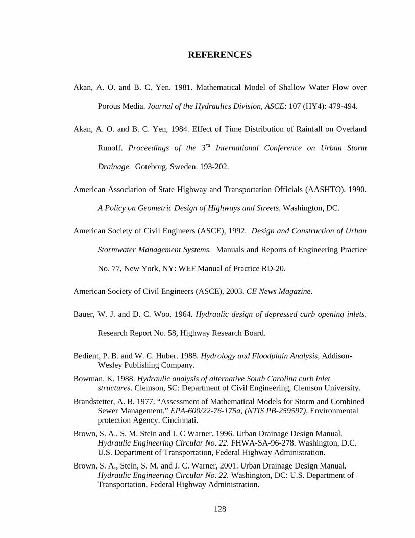
128

REFERENCES

Akan, A. O. and B. C. Yen. 1981. Mathematical Model of Shallow Water Flow over

Porous Media. Journal of the Hydraulics Division, ASCE: 107 (HY4): 479-494.

Akan, A. O. and B. C. Yen, 1984. Effect of Time Distribution of Rainfall on Overland

Runoff. Proceedings of the 3rd International Conference on Urban Storm

Drainage. Goteborg. Sweden. 193-202.

American Association of State Highway and Transportation Officials (AASHTO). 1990.

A Policy on Geometric Design of Highways and Streets, Washington, DC.

American Society of Civil Engineers (ASCE), 1992. Design and Construction of Urban

Stormwater Management Systems. Manuals and Reports of Engineering Practice

No. 77, New York, NY: WEF Manual of Practice RD-20.

American Society of Civil Engineers (ASCE), 2003. CE News Magazine.

Bauer, W. J. and D. C. Woo. 1964. Hydraulic design of depressed curb opening inlets.

Research Report No. 58, Highway Research Board.

Bedient, P. B. and W. C. Huber. 1988. Hydrology and Floodplain Analysis, Addison-Wesley Publishing Company.

Bowman, K. 1988. Hydraulic analysis of alternative South Carolina curb inlet structures. Clemson, SC: Department of Civil Engineering, Clemson University.

Brandstetter, A. B. 1977. “Assessment of Mathematical Models for Storm and Combined Sewer Management.” EPA-600/22-76-175a, (NTIS PB-259597), Environmental protection Agency. Cincinnati.

Brown, S. A., S. M. Stein and J. C Warner. 1996. Urban Drainage Design Manual. Hydraulic Engineering Circular No. 22. FHWA-SA-96-278. Washington, D.C. U.S. Department of Transportation, Federal Highway Administration.

Brown, S. A., Stein, S. M. and J. C. Warner, 2001. Urban Drainage Design Manual. Hydraulic Engineering Circular No. 22. Washington, DC: U.S. Department of Transportation, Federal Highway Administration.

129

Federal Highway Administration (FHWA), 1977. Design Charts for Open-Channel Flow.

Hydraulic Design Series No. 3. Washington DC: U.S. Department of

Transportation.

Federick, R.H., V.A. Myers, and E.P. Auciello. 1977. Five-to 60-Minutes Precipitation

Frequency for the Eastern and Central United States. NOAA Technical

Memorandum NWS HYDRO-35. Silver Spring, Maryland: National Weather

Service, Office of Hydrology.

Fiuzat A. A., C. E. Soares and B. L Sill. 2000. Design of Curb Opening Inlet Structure.

Iranian journal of science and technology 24 (1): 11-21.

Green, W.H. and G. A. Ampt. 1911. Studies on Soil Physics. J. Agric. Sci. 4:1. 1-24.

Gumbel, E. J. 1941. The Return Period of Flood Flows. Ann. Math. Stat. 12:2. 163-190.

Guo, J. C.Y. 2000. Street stormwater storage capacity. Water Environment Research 72: (5) 626-630.

Hathaway, G. A. 1945. Design of Drainage Facilities. Transactions of the American

Society of Civil Engineers vol. 110.

Herrmann, G. R. 2002. Individual studies on: Time Distributed Storm Sewer

Performance, Considering the Effect of Inlet Restriction.

Herrmann, G. R. 2003. Personal communication through e-mail.

Hershfield, D. M. 1961. Rainfall Frequency Atlas of the United States for Durations from 30 Minutes to 24 Hours and Return Period from 1 to 100 years. Technical Paper No. 40. Washington, D.C.: Weather Bureau, U.S. Dept. of Commerce.

Horton, R. E. 1933. The role of Infiltration in the Hydrologic Cycle. 14 Trans. Am.

Geophys. Union. 446-460.

Horton, R. E.1945. Erosional Development of Streams and Their Drainage Basins:

130

Hydrophysical Approach to Quantitative Morphology. 56 Bull. Geol. Soc. Am,

275-370.

Hotchkiss, R. H. and D. Bohac 1991. Efficiency of Highway Storm Water Inlets, Nebraska Department of Roads. Report RES1 (0099) p 440.

Hotchkiss, R. H., 1994. Improvements in curb-opening and grate inlet efficiency. Transportation Research Record (1471): 24-30.

Hromadka II, T.C. and R. J. Whitley. 1994. The Rational Method for Peak Flow Rate Estimation. Water Resources Bulletin 3 (6). American water Resources Association.

Hromadka II, T.V., r. H. McCuen, and C. C. Yen. 1987. Computational Hydrology in Flood control Design and Planning. Lighthouse Publications. Mission Viejo. California.

Huber, W.C. and R. E. Dickinson. 1988. Stormwater Management Model (SWMM)

User’s Manual, Version 4.0. U.S. Environmental Protection Agency. Program

Developed by Environmental Research Laboratory Office of Research and

Development.

Huber, W.C. and R. E Dickinson. 1992. Stormwater Management Model (SWMM)

User’s Manual, Version 4.0. U.S. Environmental Protection Agency. Program

Developed by Environmental Research Laboratory Office of Research and

Development.

Ickert, R. A. and C. E. Crosby. 2003. Storm Water Flow on a Curbed TxDOT Type

Concrete Roadway.

Izzard, C. F. 1946. Hydraulics of Runoff from Developed Surfaces, Proc. Highway

Research Board 26: 129-150, Washington, DC.

Izzard, C. F. 1964. Tentative results on capacity of curb opening inlets. Highway

Research Board. Research Report No. 11-13.

131

Izzard, C. F. 1977. Simplified method for design of curb opening inlets. Transportation

Research Record No. 631.

Kerby, W. S. 1959. Time of Concentration for Overland Flow. Civil Engineering 29(3).

Kiefer, C. J., J. P. Harrison and T. Hixson. 1970. Unpublished Preliminary Report.

Chicago Hydrograph Method.

Kirpich, Z. P. 1940. Time of Concentration of Small Agricultural Watersheds. Civil

Engineering 10(6).

Kuichling, E. 1889. The Relation between Rainfall and the Discharge in Sewers in Populous Districts. Trans. ASCE No 20.

Mays, L. M. 2001. Stormwater collection systems design handbook. McGraw-Hill

Companies, Inc.

McCuen, R. H. 1998. Hydrologic Analysis and Design. Second Edition, Prentice-Hall,

Inc. Upper Saddle River, NJ.

Metcalf and Eddy Inc. 1971. Storm Water Management Model, Final Report. U.S.

Environmental Protection Agency. Washington, D. C. Water Quality office.

Nouh, M. 1987. Storm Sewer Design Sensitivity Analysis using ILSD-2 Model. Journal

of Water Resources Planning and Management113 (1).

NRCS (National Resources Conservation Service). 1972. National Engineering

Handbook, Section 4, Hydrology. U.S. Department of Agriculture. Washington

DC.

Papadakis, C. N. and H. C. Preul. 1972. University of Cincinnati Urban Runoff Model.

Journal of the Hydraulics Division, ASCE 98 (HY10): 1789-1804.

132

Papadakis, C. N. and H. C. Preul. 1973. Testing of Methods of Determination of Urban

Runoff. Journal of the Hydraulics Division, ASCE 99 (HY10): 1319-1335.

Proctor and Redfern Ltd. and James F. MacLaren Ltd. 1976. Stormwater Management

Model Study, Vol. I, Final Report. Ministry of the Environment. Research Report

No. 47. Ontario, Canada: Environment Canada.

Roesner, L. A., J. A. Aldrich and R. E. Dickinson. 1988. Stormwater Management Model

User’s Manual, Version 4, Addendum I, EXTRAN. Environmental Protection

Agency. 203, Athens.

Sherman, L. K. 1932. Streamflow from Rainfall by the Unitgraph Method. Engineering

News Record 108: 501-505.

Soarres, C. E. 1991. Analysis of the efficiency of an alternative South Carolina storm

water drainage structure. Clemson: Department of Civil Engineering, Clemson

University.

Soares, C. E. and B. L. Sill. Winter, 2000. Design of curb opening inlet structure. Iranian Journal of Science & Technology 24 (1): 11-21.

Soil Conservation Service (SCS). 1986. Urban Hydrology for Small Watersheds.

Technical Release 55. Washington D.C.

Terstriep, M. L. and J. B. Stall. 1974. The Illinois Urban Drainage Area simulator –

ILLUDAS. Bulletin No. 58. Illinois State Water Survey, Urbana III.

TxDOT (Texas Department of Transportation). 2002. Hydraulic Design Manual.

U.S. Army Corps of Engineers. 1990. HEC-1, Flood Hydrograph Package. Hydraulic

Engineering Center.

U.S. Federal Highway Administration (USFHWA). 1999. User’s Manual for HYDRAIN

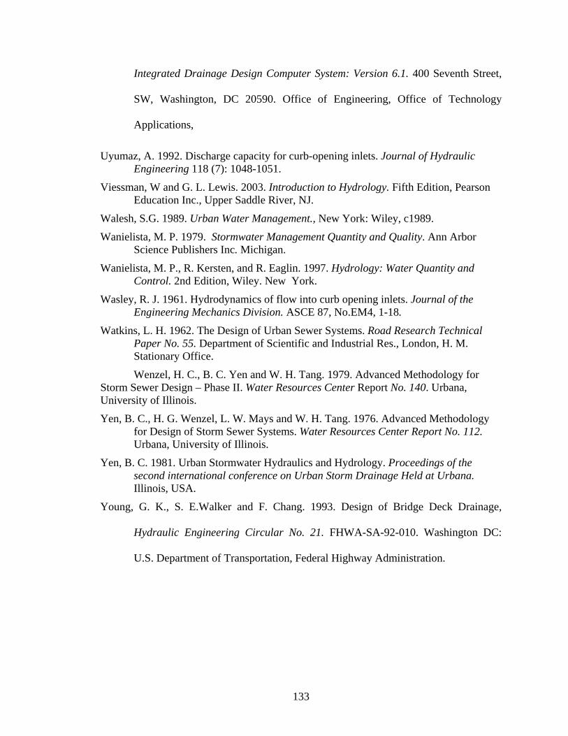
133

Integrated Drainage Design Computer System: Version 6.1. 400 Seventh Street,

SW, Washington, DC 20590. Office of Engineering, Office of Technology

Applications,

Uyumaz, A. 1992. Discharge capacity for curb-opening inlets. Journal of Hydraulic Engineering 118 (7): 1048-1051.

Viessman, W and G. L. Lewis. 2003. Introduction to Hydrology. Fifth Edition, Pearson Education Inc., Upper Saddle River, NJ.

Walesh, S.G. 1989. Urban Water Management., New York: Wiley, c1989.

Wanielista, M. P. 1979. Stormwater Management Quantity and Quality. Ann Arbor Science Publishers Inc. Michigan.

Wanielista, M. P., R. Kersten, and R. Eaglin. 1997. Hydrology: Water Quantity and Control. 2nd Edition, Wiley. New York.

Wasley, R. J. 1961. Hydrodynamics of flow into curb opening inlets. Journal of the Engineering Mechanics Division. ASCE 87, No.EM4, 1-18.

Watkins, L. H. 1962. The Design of Urban Sewer Systems. Road Research Technical Paper No. 55. Department of Scientific and Industrial Res., London, H. M. Stationary Office.

Wenzel, H. C., B. C. Yen and W. H. Tang. 1979. Advanced Methodology for Storm Sewer Design – Phase II. Water Resources Center Report No. 140. Urbana, University of Illinois.

Yen, B. C., H. G. Wenzel, L. W. Mays and W. H. Tang. 1976. Advanced Methodology for Design of Storm Sewer Systems. Water Resources Center Report No. 112. Urbana, University of Illinois.

Yen, B. C. 1981. Urban Stormwater Hydraulics and Hydrology. Proceedings of the second international conference on Urban Storm Drainage Held at Urbana. Illinois, USA.

Young, G. K., S. E.Walker and F. Chang. 1993. Design of Bridge Deck Drainage,

Hydraulic Engineering Circular No. 21. FHWA-SA-92-010. Washington DC:

U.S. Department of Transportation, Federal Highway Administration.

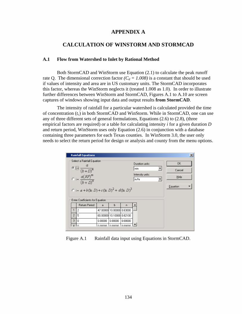
134

APPENDIX A

CALCULATION OF WINSTORM AND STORMCAD A.1 Flow from Watershed to Inlet by Rational Method

Both StormCAD and WinStorm use Equation (2.1) to calculate the peak runoff rate Q. The dimensional correction factor (Cd = 1.008) is a constant that should be used if values of intensity and area are in US customary units. The StormCAD incorporates this factor, whereas the WinStorm neglects it (treated 1.008 as 1.0). In order to illustrate further differences between WinStorm and StormCAD, Figures A.1 to A.10 are screen captures of windows showing input data and output results from StormCAD.

The intensity of rainfall for a particular watershed is calculated provided the time of concentration (tc) in both StormCAD and WinStorm. While in StormCAD, one can use any of three different sets of general formulations, Equations (2.6) to (2.8), (three empirical factors are required) or a table for calculating intensity i for a given duration D and return period, WinStorm uses only Equation (2.6) in conjunction with a database containing three parameters for each Texas counties. In WinStorm 3.0, the user only needs to select the return period for design or analysis and county from the menu options.

Figure A.1 Rainfall data input using Equations in StormCAD.

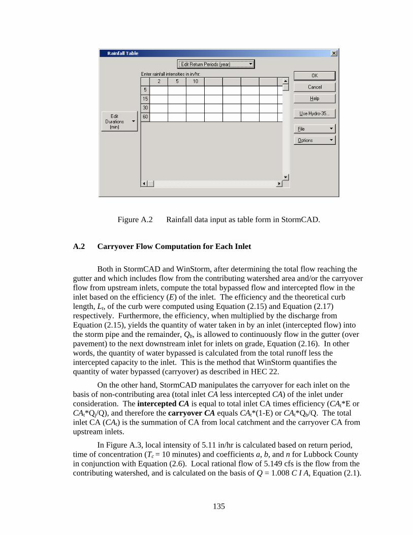
135

Figure A.2 Rainfall data input as table form in StormCAD.

A.2 Carryover Flow Computation for Each Inlet

Both in StormCAD and WinStorm, after determining the total flow reaching the gutter and which includes flow from the contributing watershed area and/or the carryover flow from upstream inlets, compute the total bypassed flow and intercepted flow in the inlet based on the efficiency (E) of the inlet. The efficiency and the theoretical curb length, Lt, of the curb were computed using Equation (2.15) and Equation (2.17) respectively. Furthermore, the efficiency, when multiplied by the discharge from Equation (2.15), yields the quantity of water taken in by an inlet (intercepted flow) into the storm pipe and the remainder, Qb, is allowed to continuously flow in the gutter (over pavement) to the next downstream inlet for inlets on grade, Equation (2.16). In other words, the quantity of water bypassed is calculated from the total runoff less the intercepted capacity to the inlet. This is the method that WinStorm quantifies the quantity of water bypassed (carryover) as described in HEC 22.

On the other hand, StormCAD manipulates the carryover for each inlet on the basis of non-contributing area (total inlet CA less intercepted CA) of the inlet under consideration. The intercepted CA is equal to total inlet CA times efficiency (CAt*E or CAt*Qj/Q), and therefore the carryover CA equals CAt*(1-E) or CAt*Qb/Q. The total inlet CA (CAt) is the summation of CA from local catchment and the carryover CA from upstream inlets.

In Figure A.3, local intensity of 5.11 in/hr is calculated based on return period, time of concentration (Tc = 10 minutes) and coefficients a, b, and n for Lubbock County in conjunction with Equation (2.6). Local rational flow of 5.149 cfs is the flow from the contributing watershed, and is calculated on the basis of Q = 1.008 C I A, Equation (2.1).

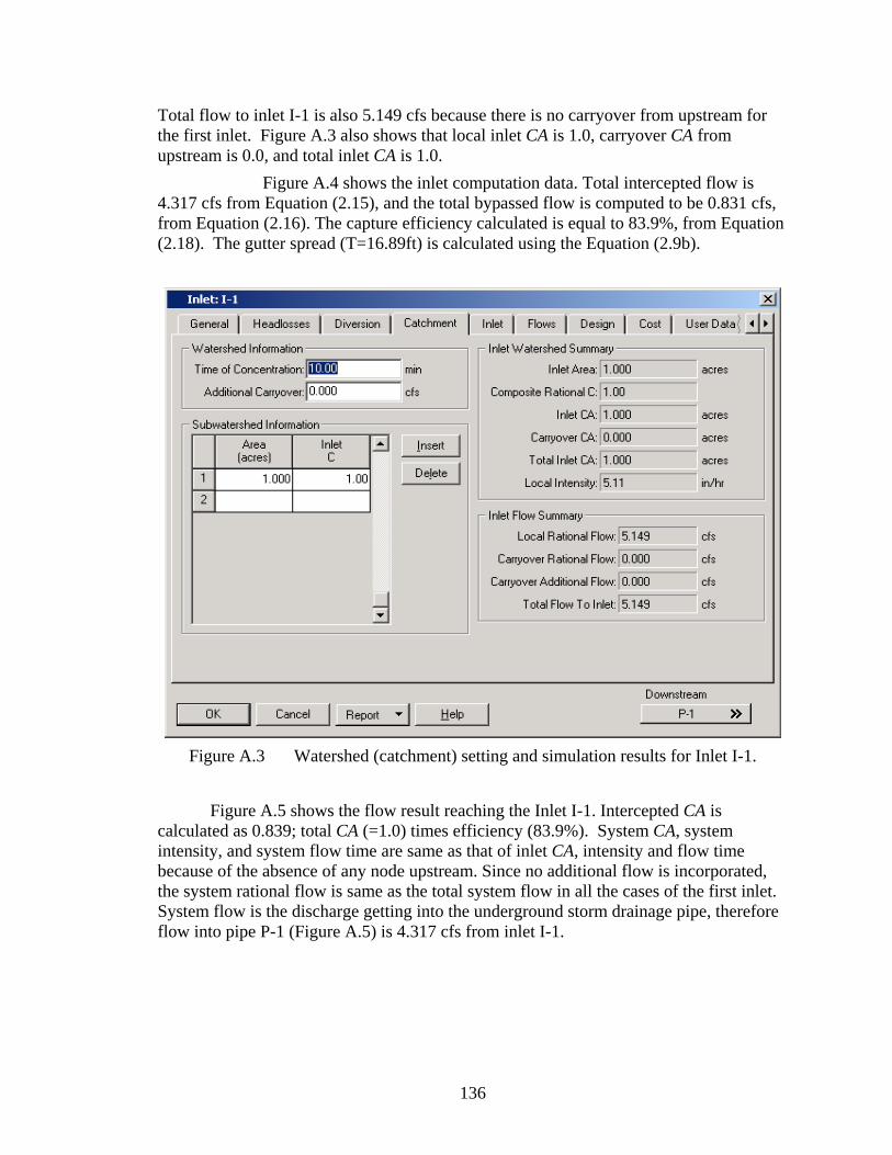
136

Total flow to inlet I-1 is also 5.149 cfs because there is no carryover from upstream for the first inlet. Figure A.3 also shows that local inlet CA is 1.0, carryover CA from upstream is 0.0, and total inlet CA is 1.0.

Figure A.4 shows the inlet computation data. Total intercepted flow is 4.317 cfs from Equation (2.15), and the total bypassed flow is computed to be 0.831 cfs, from Equation (2.16). The capture efficiency calculated is equal to 83.9%, from Equation (2.18). The gutter spread (T=16.89ft) is calculated using the Equation (2.9b).

Figure A.3 Watershed (catchment) setting and simulation results for Inlet I-1.

Figure A.5 shows the flow result reaching the Inlet I-1. Intercepted CA is

calculated as 0.839; total CA (=1.0) times efficiency (83.9%). System CA, system intensity, and system flow time are same as that of inlet CA, intensity and flow time because of the absence of any node upstream. Since no additional flow is incorporated, the system rational flow is same as the total system flow in all the cases of the first inlet. System flow is the discharge getting into the underground storm drainage pipe, therefore flow into pipe P-1 (Figure A.5) is 4.317 cfs from inlet I-1.

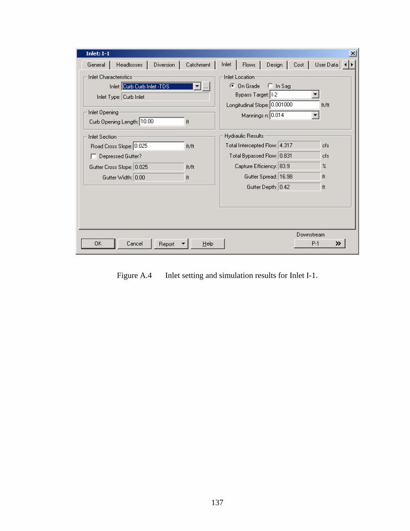
137

Figure A.4 Inlet setting and simulation results for Inlet I-1.

138

Figure A.5 Flow simulation results for Inlet I-1. Because not all water flowing in the gutter can enter the inlet (due to its

restriction), carryover flow has to be considered while designing. StormCAD incorporates the carryover flow in sizing the conduits whereas WinStorm calculates the carryover but does not take into account in sizing the conduits2. This important observation will be further explained in details through the following sections.

A.3 Carryover Flow From Inlet Upstream StormCAD calculates the carryover flow for each inlet (Qbup in Equation 3.1)

based on the non-contributing area of the upstream inlet (carryover CA) and the local intensity (ilocal) of the inlet under consideration rather than directly considering the quantity of flow bypassed (not using Qb given in equation 2.16).

Qbup = (Carryover CA)up x ilocal (3.1)

2 And it is important to notice that WinStorm is the principal design tool that TxDOT designers use for storm drain networks.

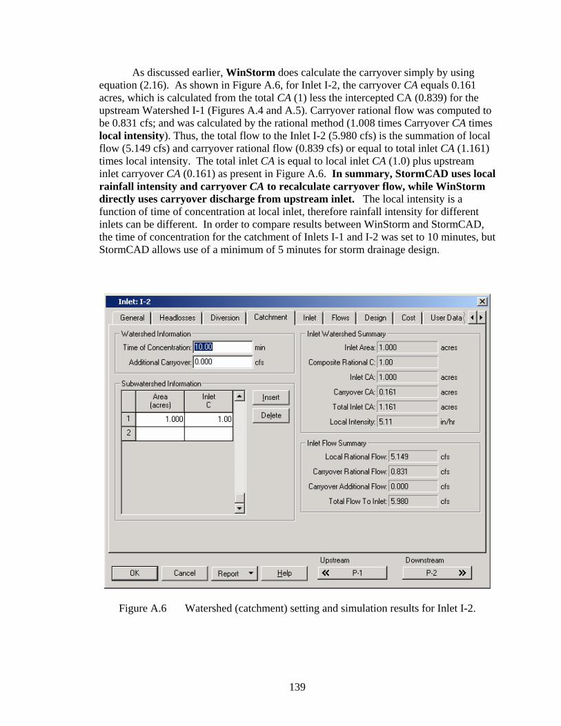
139

As discussed earlier, WinStorm does calculate the carryover simply by using equation (2.16). As shown in Figure A.6, for Inlet I-2, the carryover CA equals 0.161 acres, which is calculated from the total CA (1) less the intercepted CA (0.839) for the upstream Watershed I-1 (Figures A.4 and A.5). Carryover rational flow was computed to be 0.831 cfs; and was calculated by the rational method (1.008 times Carryover CA times local intensity). Thus, the total flow to the Inlet I-2 (5.980 cfs) is the summation of local flow (5.149 cfs) and carryover rational flow (0.839 cfs) or equal to total inlet CA (1.161) times local intensity. The total inlet CA is equal to local inlet CA (1.0) plus upstream inlet carryover CA (0.161) as present in Figure A.6. In summary, StormCAD uses local rainfall intensity and carryover CA to recalculate carryover flow, while WinStorm directly uses carryover discharge from upstream inlet. The local intensity is a function of time of concentration at local inlet, therefore rainfall intensity for different inlets can be different. In order to compare results between WinStorm and StormCAD, the time of concentration for the catchment of Inlets I-1 and I-2 was set to 10 minutes, but StormCAD allows use of a minimum of 5 minutes for storm drainage design.

Figure A.6 Watershed (catchment) setting and simulation results for Inlet I-2.

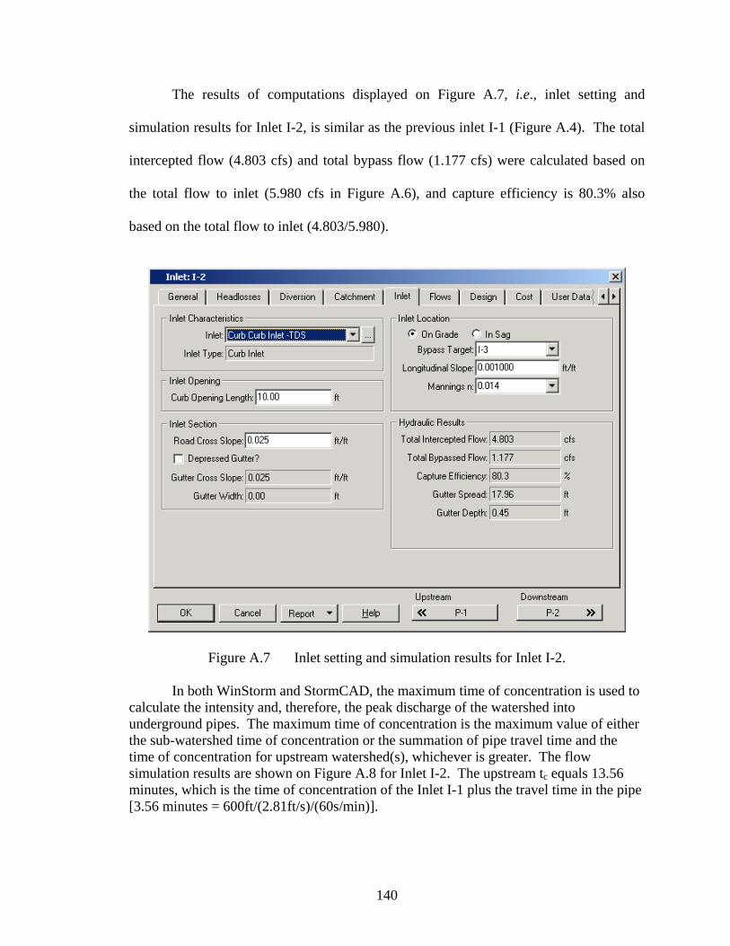
140

The results of computations displayed on Figure A.7, i.e., inlet setting and

simulation results for Inlet I-2, is similar as the previous inlet I-1 (Figure A.4). The total

intercepted flow (4.803 cfs) and total bypass flow (1.177 cfs) were calculated based on

the total flow to inlet (5.980 cfs in Figure A.6), and capture efficiency is 80.3% also

based on the total flow to inlet (4.803/5.980).

Figure A.7 Inlet setting and simulation results for Inlet I-2.

In both WinStorm and StormCAD, the maximum time of concentration is used to calculate the intensity and, therefore, the peak discharge of the watershed into underground pipes. The maximum time of concentration is the maximum value of either the sub-watershed time of concentration or the summation of pipe travel time and the time of concentration for upstream watershed(s), whichever is greater. The flow simulation results are shown on Figure A.8 for Inlet I-2. The upstream tc equals 13.56 minutes, which is the time of concentration of the Inlet I-1 plus the travel time in the pipe [3.56 minutes = 600ft/(2.81ft/s)/(60s/min)].

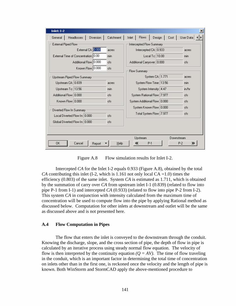
141

Figure A.8 Flow simulation results for Inlet I-2.

Intercepted CA for the Inlet I-2 equals 0.933 (Figure A.8), obtained by the total CA contributing this inlet (I-2, which is 1.161 not only local CA =1.0) times the efficiency (0.803) of the same inlet. System CA is estimated as 1.711, which is obtained by the summation of carry over CA from upstream inlet I-1 (0.839) (related to flow into pipe P-1 from I-1) and intercepted CA (0.933) (related to flow into pipe P-2 from I-2). This system CA in conjunction with intensity calculated from the maximum time of concentration will be used to compute flow into the pipe by applying Rational method as discussed below. Computation for other inlets at downstream and outlet will be the same as discussed above and is not presented here.

A.4 Flow Computation in Pipes

The flow that enters the inlet is conveyed to the downstream through the conduit. Knowing the discharge, slope, and the cross section of pipe, the depth of flow in pipe is calculated by an iterative process using steady normal flow equation. The velocity of flow is then interpreted by the continuity equation (Q = AV). The time of flow traveling in the conduit, which is an important factor in determining the total time of concentration on inlets other than in the first one, is reckoned once the velocity and the length of pipe is known. Both WinStorm and StormCAD apply the above-mentioned procedure to

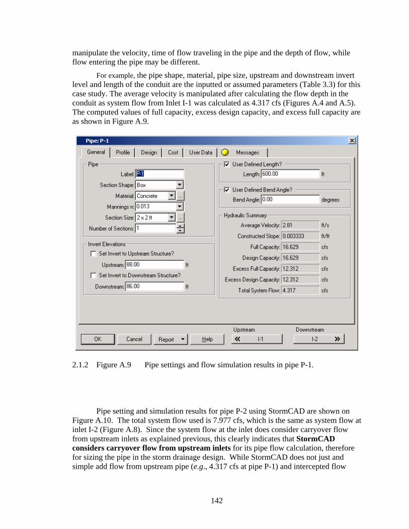
142

manipulate the velocity, time of flow traveling in the pipe and the depth of flow, while flow entering the pipe may be different.

For example, the pipe shape, material, pipe size, upstream and downstream invert level and length of the conduit are the inputted or assumed parameters (Table 3.3) for this case study. The average velocity is manipulated after calculating the flow depth in the conduit as system flow from Inlet I-1 was calculated as 4.317 cfs (Figures A.4 and A.5). The computed values of full capacity, excess design capacity, and excess full capacity are as shown in Figure A.9.

2.1.2 Figure A.9 Pipe settings and flow simulation results in pipe P-1.

Pipe setting and simulation results for pipe P-2 using StormCAD are shown on Figure A.10. The total system flow used is 7.977 cfs, which is the same as system flow at inlet I-2 (Figure A.8). Since the system flow at the inlet does consider carryover flow from upstream inlets as explained previous, this clearly indicates that StormCAD considers carryover flow from upstream inlets for its pipe flow calculation, therefore for sizing the pipe in the storm drainage design. While StormCAD does not just and simple add flow from upstream pipe (e.g., 4.317 cfs at pipe P-1) and intercepted flow

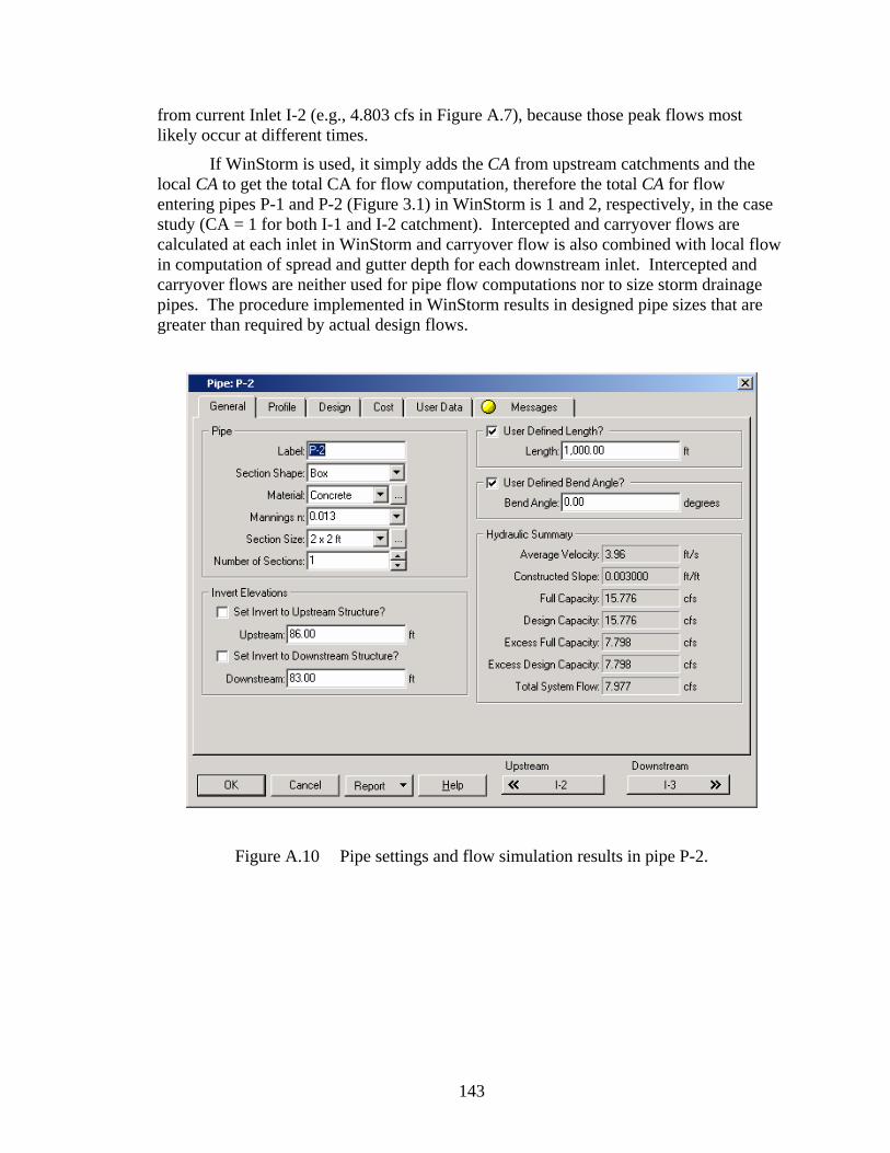
143

from current Inlet I-2 (e.g., 4.803 cfs in Figure A.7), because those peak flows most likely occur at different times.

If WinStorm is used, it simply adds the CA from upstream catchments and the local CA to get the total CA for flow computation, therefore the total CA for flow entering pipes P-1 and P-2 (Figure 3.1) in WinStorm is 1 and 2, respectively, in the case study (CA = 1 for both I-1 and I-2 catchment). Intercepted and carryover flows are calculated at each inlet in WinStorm and carryover flow is also combined with local flow in computation of spread and gutter depth for each downstream inlet. Intercepted and carryover flows are neither used for pipe flow computations nor to size storm drainage pipes. The procedure implemented in WinStorm results in designed pipe sizes that are greater than required by actual design flows.

Figure A.10 Pipe settings and flow simulation results in pipe P-2.

144

APPENDIX B

HYDRAFLOW SETUP The primary network setup of the case study in Hydraflow is shown in Figure B.1. The network in Hydraflow is basically made up of “Lines”. A line has a length of stormwater pipe with a junction at the upstream end. Junctions can be manholes, inlets, j-boxes (junction), or other structures where losses or gains of flow occur. The graphical part of the network of storm drainage system in Hydraflow is portrayed in the Plan view. It automatically numbers the lines in the order that they are input. However, the first line starts from the outfall or the most downstream end. Therefore, the first line that is input will be line number 1 and the second line input will be number 2, and so on. The remaining data for the links are completed by switching to the “Lines” view and filling the blanks needed. For example, the flow data and the physical data such as invert elevations, pipe sizes, etc. is filled in the spreadsheet display table provided. The junction data (inlet data) are completed by switching to “Inlet” view. The data in the “Inlet” view, for the study is acquired from the Table 4.1 and Table 4.2.

Figure B.1. Network setup of the case study in Hydraflow.

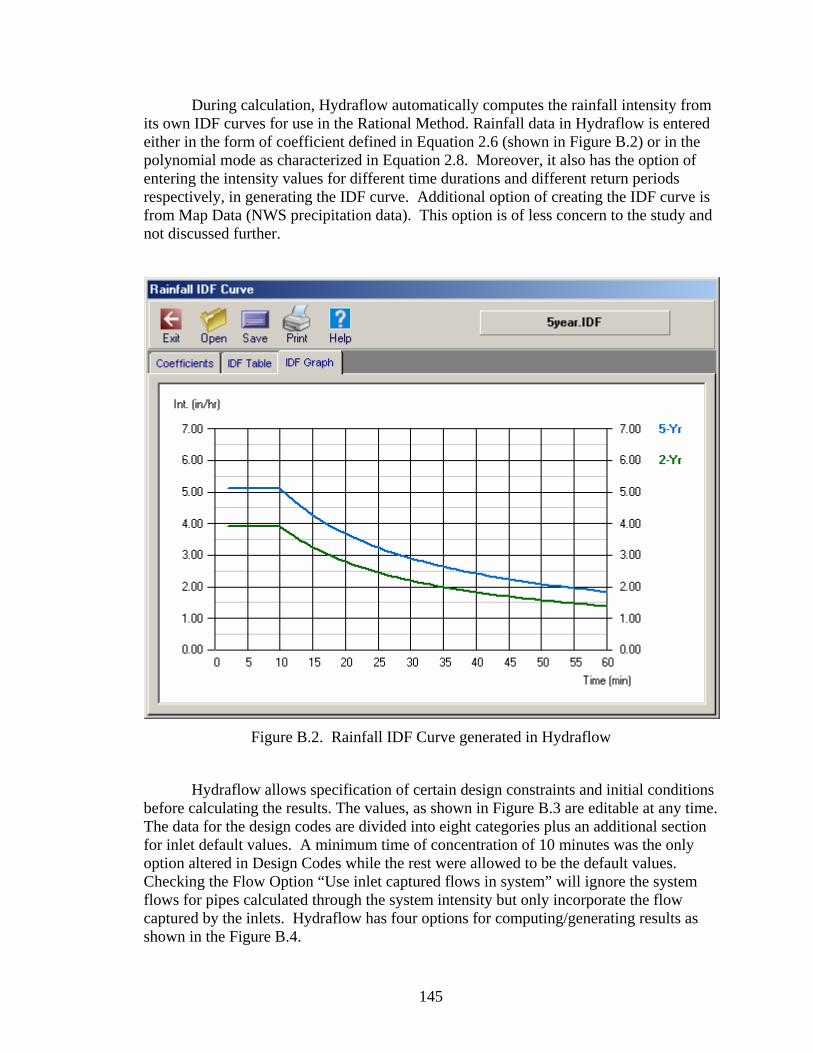
145

During calculation, Hydraflow automatically computes the rainfall intensity from its own IDF curves for use in the Rational Method. Rainfall data in Hydraflow is entered either in the form of coefficient defined in Equation 2.6 (shown in Figure B.2) or in the polynomial mode as characterized in Equation 2.8. Moreover, it also has the option of entering the intensity values for different time durations and different return periods respectively, in generating the IDF curve. Additional option of creating the IDF curve is from Map Data (NWS precipitation data). This option is of less concern to the study and not discussed further.

Figure B.2. Rainfall IDF Curve generated in Hydraflow

Hydraflow allows specification of certain design constraints and initial conditions before calculating the results. The values, as shown in Figure B.3 are editable at any time. The data for the design codes are divided into eight categories plus an additional section for inlet default values. A minimum time of concentration of 10 minutes was the only option altered in Design Codes while the rest were allowed to be the default values. Checking the Flow Option “Use inlet captured flows in system” will ignore the system flows for pipes calculated through the system intensity but only incorporate the flow captured by the inlets. Hydraflow has four options for computing/generating results as shown in the Figure B.4.

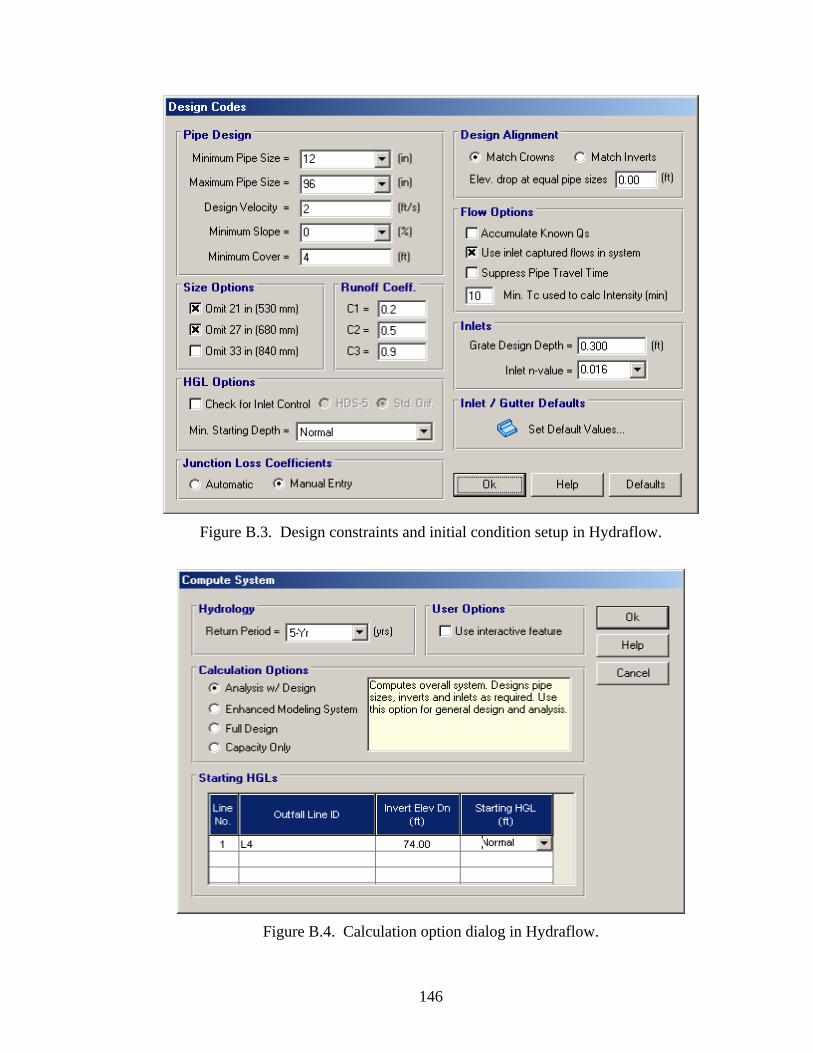
146

Figure B.3. Design constraints and initial condition setup in Hydraflow.

Figure B.4. Calculation option dialog in Hydraflow.

147

APPENDIX C SPLIT PROGRAM

C.1 Introduction to SPLIT Program

George R. Herrmann, P.E., executed a study titled “Time Distributed Storm Sewer Performance, Considering the Effect of Inlet Restriction.” In his report, he stated that “no extra security is gained in the system by the conservative design procedure, due to the limiting factor in the system, which is the restriction of the inlet. The performance of a storm sewer system can be only as good as the performance of its most restrictive component…” (Herrmann, 2002). The central premise of his report was based on three hypotheses, that are as follows:

1. The traditional method of sizing conduits is overly conservative, resulting in conduits that are overly large for their purpose,

2. The system cannot perform at a level any greater than its most restrictive features, which are the inlets, and

3. Hypothesis (1) is compounded by hypothesis (2), and therefore any excess capacity built into the system is valueless, as it can never come into use, because of the restriction of the inlets.

In order to verify the hypothesis and support his statement, he developed program coded in FORTRAN 77 called “SPLIT”. The SPLIT program considers the following conditions to exist:

• The actual area is multiplied by the runoff coefficient, giving an “effective area”,

• The area is essentially rectangular, such as a stretch of roadway, and that the rise and recession of contribution are both linear.

• If time of concentration tc for a watershed is less than the storm duration, there is a rise to full contribution, constant flow for the difference between tc and duration, then recession to zero over tc after cessation of rainfall.

• If tc is equal to the storm duration, there is a rise to full contribution, followed by a recession over tc back to zero.

• If tc is greater than the storm duration, there is a rise at the same rate of rise as above until cessation of rainfall, then a recession at the same rate to zero.

• Rainfall duration should be integer minutes.

SPLIT takes into account only the traditional rational method for analysis. It is a simple program to assess the hypotheses presented above and not intended as a design or analysis tool. The following items are not addressed in the analysis:

1. It was developed only for curb inlets without depression. No other types of inlets and gutter with depression can be tested or analyzed.

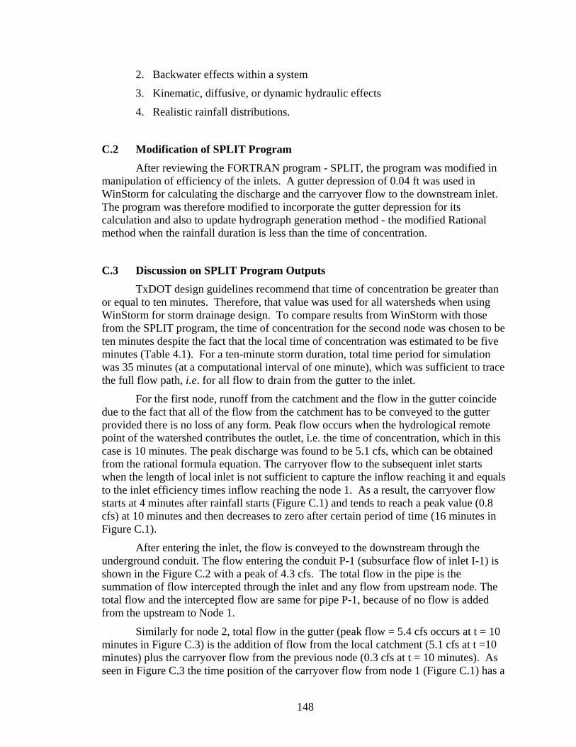
148

2. Backwater effects within a system

3. Kinematic, diffusive, or dynamic hydraulic effects

4. Realistic rainfall distributions.

C.2 Modification of SPLIT Program After reviewing the FORTRAN program - SPLIT, the program was modified in

manipulation of efficiency of the inlets. A gutter depression of 0.04 ft was used in WinStorm for calculating the discharge and the carryover flow to the downstream inlet. The program was therefore modified to incorporate the gutter depression for its calculation and also to update hydrograph generation method - the modified Rational method when the rainfall duration is less than the time of concentration.

C.3 Discussion on SPLIT Program Outputs

TxDOT design guidelines recommend that time of concentration be greater than or equal to ten minutes. Therefore, that value was used for all watersheds when using WinStorm for storm drainage design. To compare results from WinStorm with those from the SPLIT program, the time of concentration for the second node was chosen to be ten minutes despite the fact that the local time of concentration was estimated to be five minutes (Table 4.1). For a ten-minute storm duration, total time period for simulation was 35 minutes (at a computational interval of one minute), which was sufficient to trace the full flow path, i.e. for all flow to drain from the gutter to the inlet.

For the first node, runoff from the catchment and the flow in the gutter coincide due to the fact that all of the flow from the catchment has to be conveyed to the gutter provided there is no loss of any form. Peak flow occurs when the hydrological remote point of the watershed contributes the outlet, i.e. the time of concentration, which in this case is 10 minutes. The peak discharge was found to be 5.1 cfs, which can be obtained from the rational formula equation. The carryover flow to the subsequent inlet starts when the length of local inlet is not sufficient to capture the inflow reaching it and equals to the inlet efficiency times inflow reaching the node 1. As a result, the carryover flow starts at 4 minutes after rainfall starts (Figure C.1) and tends to reach a peak value (0.8 cfs) at 10 minutes and then decreases to zero after certain period of time (16 minutes in Figure C.1).

After entering the inlet, the flow is conveyed to the downstream through the underground conduit. The flow entering the conduit P-1 (subsurface flow of inlet I-1) is shown in the Figure C.2 with a peak of 4.3 cfs. The total flow in the pipe is the summation of flow intercepted through the inlet and any flow from upstream node. The total flow and the intercepted flow are same for pipe P-1, because of no flow is added from the upstream to Node 1.

Similarly for node 2, total flow in the gutter (peak flow = 5.4 cfs occurs at t = 10 minutes in Figure C.3) is the addition of flow from the local catchment (5.1 cfs at t =10 minutes) plus the carryover flow from the previous node (0.3 cfs at t = 10 minutes). As seen in Figure C.3 the time position of the carryover flow from node 1 (Figure C.1) has a

149

lag of 3 minutes in node 2, which is due to the gutter travel time (3 minutes). The carryover at node I-2 to the subsequent inlet (I-3) begins only after the efficiency of the inlet start falling below 100%, and has a peak of 0.9 cfs at t = 10 minutes with turning point of 0.5 cfs at t = 13 minutes (Figure C.3). The total subsurface flow for the inlet I-2 (flow in conduit P-2 shown in Figure C.4) is the summation of the flow reaching the node 2 from the upstream pipe (P-1) and the flow intercepted by the inlet I-2. The flow rate in the pipe P-2 reaches 7.4 cfs at t = 10 minutes, has a peak of 7.8 cfs at t = 13 minutes, and reduces to zero at t = 24 minutes. This hydrograph includes integrated effects from catchment runoff, intercepted flow and carryover flow of both inlets, and upstream pipe flow. This process of interception and carryover is continued (due to the inlet restriction) until the flow reaches the downstream outlet.

Figure C.5 gives the hydrograph at the inlet I-3, where rainfall duration (10 minutes) is shorter than the catchment time of concentration (15 minutes), by using modified SPLIT program. The response of flow from the catchment to the inlet tend to rise linearly from zero until the duration of storm (10 minutes) is reached and remains constant for a duration equal to time of concentration (15 minutes) and then descend back to zero at the same rate of increase. Therefore, the inlet is likely to receive runoff from the watershed for a total duration of 25 minutes (Figure C.5) even though the storm last for only 10 minutes. The peak discharge between 10 to 15 minutes is 3.4 cfs, which is only a portion of peak discharge computed by the rational method: 10/15 CIA = 10/15 x 5.1cfs = 3.4 cfs. Figure C.5 also shows other surface flow components at the inlet I-3.

Figure C.6 gives an example of the surface flow hydrograph at the inlet 2 if actual time of concentration of 5 minutes (Table 4.1) is used for catchment linking to the inlet. This results that the storm duration (10 minutes) is greater than the watershed time of concentration (tc). From Figure C.6, it is observed that though the time of concentration of the watershed is only 5 minutes, the peak discharge of 5.1 cfs (Rational method) starts at 5 minutes, remains constant until the end f storm, and then falls linearly to zero within 5 minutes (tc). this is a trapezoidal hydrograph based on modified rational method as discussed in details in the section 2.2.2 of Chapter two.

150

NODE 1 (surface flow)

0

1

2

3

4

5

6

0 5 10 15 20

Time (min)

Flow

(cfs

)Runoff from catchment Carryover flow from U/S Total flow in gutter carryover flow to D/S

Figure C.1. Simulated surface flow components at the inlet I-1 (node 1) by using modified SPLIT program.

151

NODE 1 (Subsurface flow)

0

1

2

3

4

5

6

0 5 10 15 20

Time (min)

Flow

(cfs

)

Intercepted flow Flow from U/S Node Total flow through Pipe 1

Figure C.2. Simulated subsurface flow components at the inlet I-1 (node 1) by using modified SPLIT program.

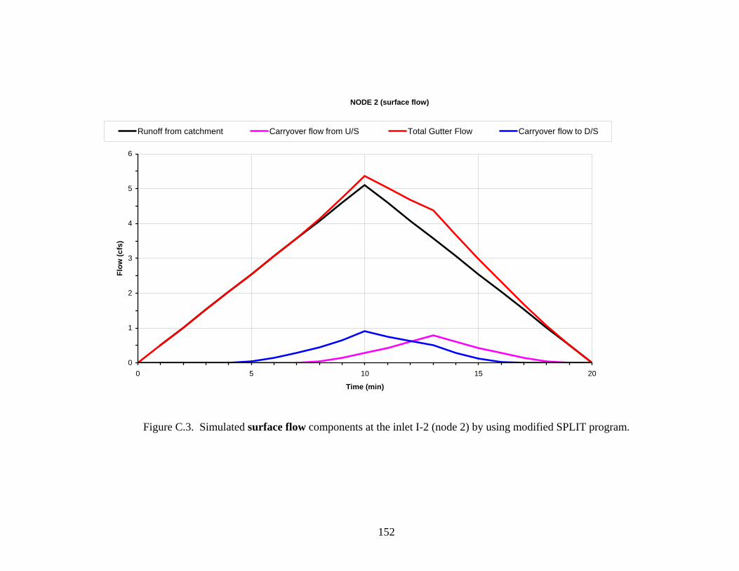
152

NODE 2 (surface flow)

0

1

2

3

4

5

6

0 5 10 15 20

Time (min)

Flow

(cfs

)Runoff from catchment Carryover flow from U/S Total Gutter Flow Carryover flow to D/S

Figure C.3. Simulated surface flow components at the inlet I-2 (node 2) by using modified SPLIT program.

153

NODE 2 (Sub surface flow)

0

1

2

3

4

5

6

7

8

9

0 5 10 15 20

Time (min)

Flow

(cfs

)

Intercepted flow Flow from U/S Node Total flow

Figure C.4 Simulated subsurface flow components at the inlet I-2 (node 2) by using

modified SPLIT program.

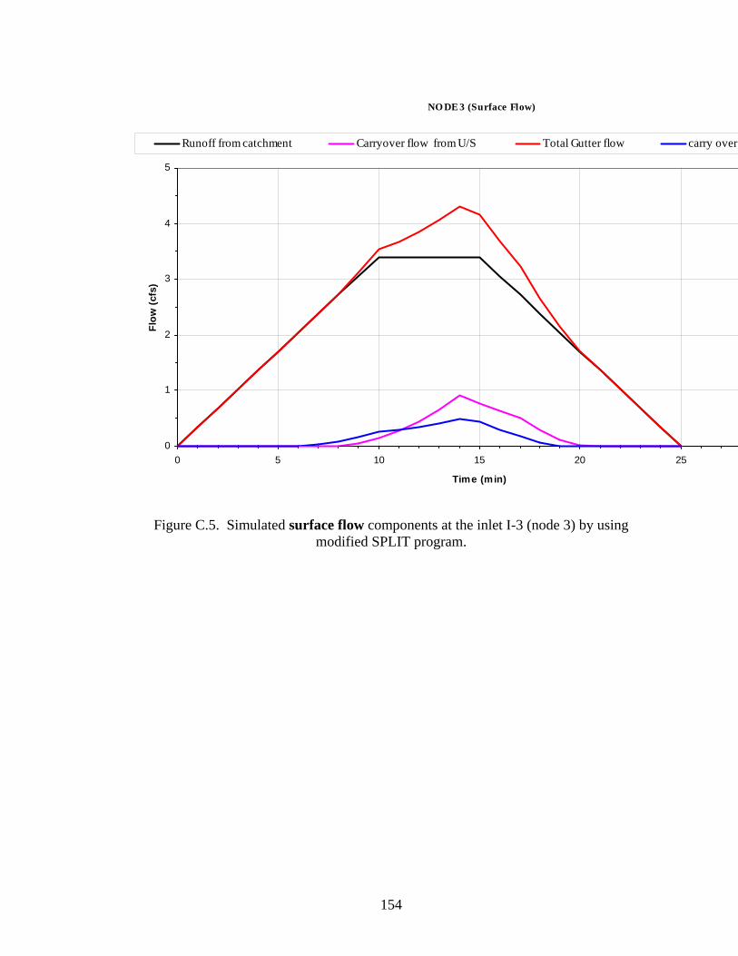
154

NO DE 3 (Surface Flow)

0

1

2

3

4

5

0 5 10 15 20 25

Time (min)

Flow

(cfs

)Runoff from catchment Carryover flow from U/S Total Gutter flow carry over

Figure C.5. Simulated surface flow components at the inlet I-3 (node 3) by using

modified SPLIT program.

155

NODE 2 (surface flow)

0

1

2

3

4

5

6

0 5 10 15

Time (min)

Flow

(cfs

)Runoff from catchment Carryover flow from U/S Total Gutter Flow Carryov

Figure C.6. Simulated surface flow components at the inlet I-2 (node 2) by using modified SPLIT program (Tc=5 min.).

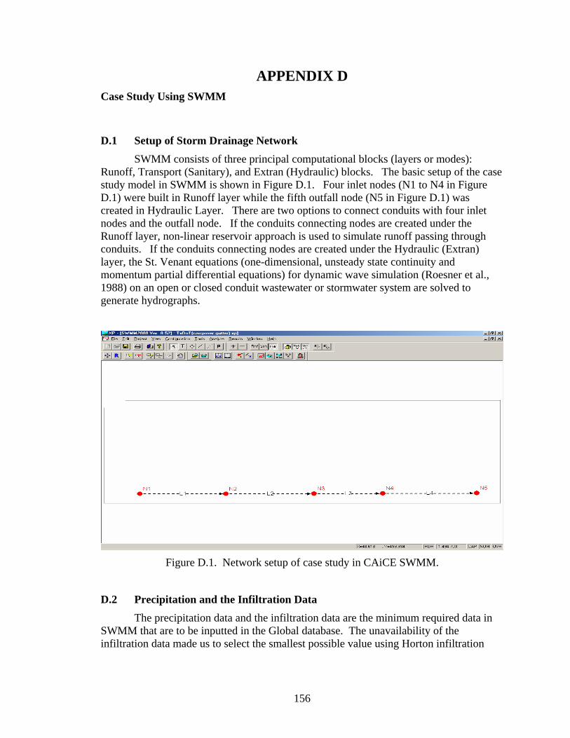
156

APPENDIX D Case Study Using SWMM

D.1 Setup of Storm Drainage Network SWMM consists of three principal computational blocks (layers or modes):

Runoff, Transport (Sanitary), and Extran (Hydraulic) blocks. The basic setup of the case study model in SWMM is shown in Figure D.1. Four inlet nodes (N1 to N4 in Figure D.1) were built in Runoff layer while the fifth outfall node (N5 in Figure D.1) was created in Hydraulic Layer. There are two options to connect conduits with four inlet nodes and the outfall node. If the conduits connecting nodes are created under the Runoff layer, non-linear reservoir approach is used to simulate runoff passing through conduits. If the conduits connecting nodes are created under the Hydraulic (Extran) layer, the St. Venant equations (one-dimensional, unsteady state continuity and momentum partial differential equations) for dynamic wave simulation (Roesner et al., 1988) on an open or closed conduit wastewater or stormwater system are solved to generate hydrographs.

Figure D.1. Network setup of case study in CAiCE SWMM.

D.2 Precipitation and the Infiltration Data

The precipitation data and the infiltration data are the minimum required data in SWMM that are to be inputted in the Global database. The unavailability of the infiltration data made us to select the smallest possible value using Horton infiltration

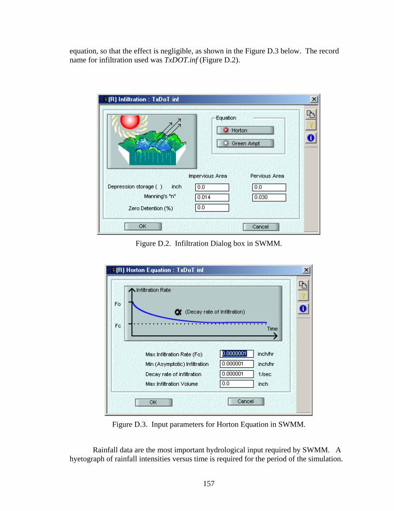
157

equation, so that the effect is negligible, as shown in the Figure D.3 below. The record name for infiltration used was TxDOT.inf (Figure D.2).

Figure D.2. Infiltration Dialog box in SWMM.

Figure D.3. Input parameters for Horton Equation in SWMM.

Rainfall data are the most important hydrological input required by SWMM. A hyetograph of rainfall intensities versus time is required for the period of the simulation.

158

For single event simulation, the data is usually entered for a gauge directly as a synthetic design storm. For continuous simulation, a historical rainfall sequence is normally used. Each sub-catchment in SWMM references a single rain gauge. The data for each rain gauge may be input manually or defined to come from an external interface file. It is allowable to use a combination of manually entered rain gauges and some to be read in from an external interface file. Current case study used constant time interval of 1 minute with intensity of 5.11 in/hr with duration of 10 minutes (TxDOT rainfall) as input for rainfall data (Figure D.4). This rainfall intensity was used for the case study under WinStorm and StormCAD and was based on IDF curve at Lubbock County, Texas. One should keep in mind that WinStorm and StormCAD always recalculate rainfall intensity based on time of concentration for each inlet and pipe before the Rational method is applied to compute the peak discharge, while SWMM applies given rainfall hyetograph to all inlets and pipes and to simulate their hydrological responses. SWMM does allow user to link different rainfall patterns to different catchments, which is not used in our case study.

Figure D.4. Rainfall data as constant time interval for duration of 10 minutes.

D.3 Sub-catchment Data and Hydrograph Generation SWMM has the capability of analyzing multiple sub-catchments for each inlet

and allow the user to input up to five sub-catchments for a single node as shown in the Figure D.5 when hydrograph generation technique used is original SWMM runoff non-linear reservoir method. Required data for each sub-catchment are area, percent impervious, width, and longitudinal slope. Sub-catchments are modeled as idealized rectangular areas with the slope of the catchment perpendicular to the width. In this case study, the catchment area is 1 acre square with width and length of 208 feet, and the slope

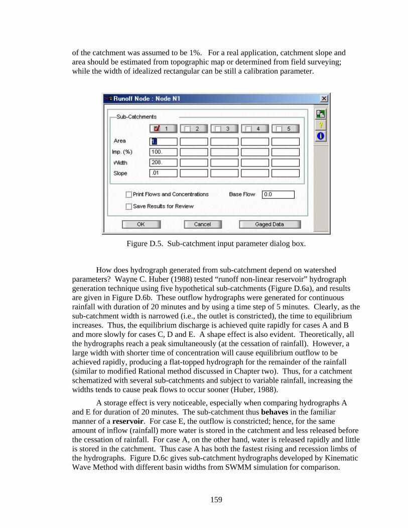
159

of the catchment was assumed to be 1%. For a real application, catchment slope and area should be estimated from topographic map or determined from field surveying; while the width of idealized rectangular can be still a calibration parameter.

Figure D.5. Sub-catchment input parameter dialog box.

How does hydrograph generated from sub-catchment depend on watershed parameters? Wayne C. Huber (1988) tested “runoff non-linear reservoir” hydrograph generation technique using five hypothetical sub-catchments (Figure D.6a), and results are given in Figure D.6b. These outflow hydrographs were generated for continuous rainfall with duration of 20 minutes and by using a time step of 5 minutes. Clearly, as the sub-catchment width is narrowed (i.e., the outlet is constricted), the time to equilibrium increases. Thus, the equilibrium discharge is achieved quite rapidly for cases A and B and more slowly for cases C, D and E. A shape effect is also evident. Theoretically, all the hydrographs reach a peak simultaneously (at the cessation of rainfall). However, a large width with shorter time of concentration will cause equilibrium outflow to be achieved rapidly, producing a flat-topped hydrograph for the remainder of the rainfall (similar to modified Rational method discussed in Chapter two). Thus, for a catchment schematized with several sub-catchments and subject to variable rainfall, increasing the widths tends to cause peak flows to occur sooner (Huber, 1988).

A storage effect is very noticeable, especially when comparing hydrographs A and E for duration of 20 minutes. The sub-catchment thus behaves in the familiar manner of a reservoir. For case E, the outflow is constricted; hence, for the same amount of inflow (rainfall) more water is stored in the catchment and less released before the cessation of rainfall. For case A, on the other hand, water is released rapidly and little is stored in the catchment. Thus case A has both the fastest rising and recession limbs of the hydrographs. Figure D.6c gives sub-catchment hydrographs developed by Kinematic Wave Method with different basin widths from SWMM simulation for comparison.

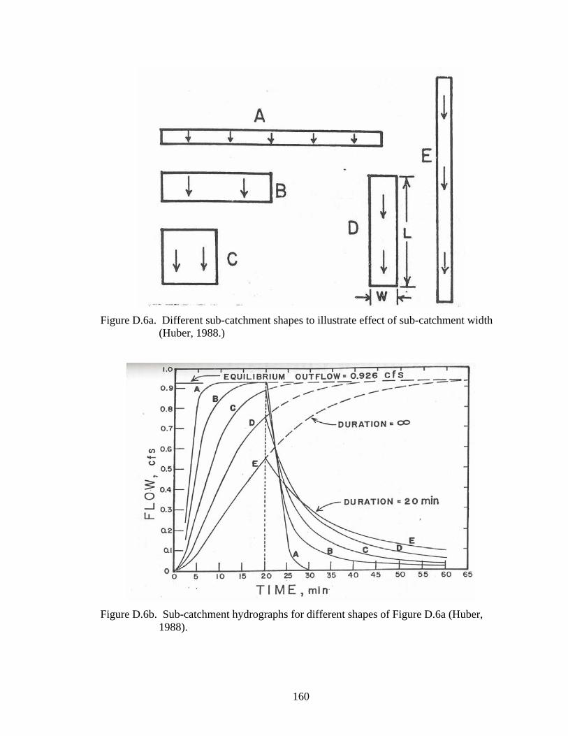
160

Figure D.6a. Different sub-catchment shapes to illustrate effect of sub-catchment width

(Huber, 1988.)

Figure D.6b. Sub-catchment hydrographs for different shapes of Figure D.6a (Huber,

1988).

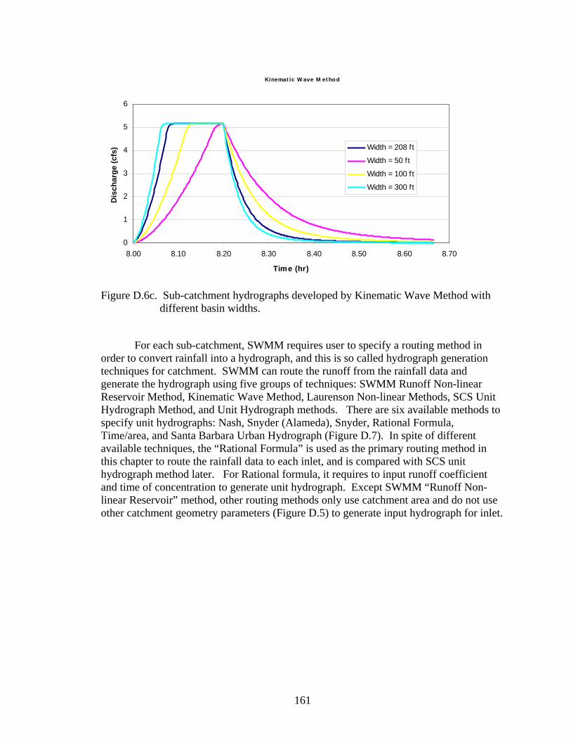
161

Kinemat ic W ave M et hod

0

1

2

3

4

5

6

8.00 8.10 8.20 8.30 8.40 8.50 8.60 8.70

Time (hr)

Dis

char

ge (c

fs) Width = 208 ft

Width = 50 ft

Width = 100 ft

Width = 300 ft

Figure D.6c. Sub-catchment hydrographs developed by Kinematic Wave Method with

different basin widths.

For each sub-catchment, SWMM requires user to specify a routing method in order to convert rainfall into a hydrograph, and this is so called hydrograph generation techniques for catchment. SWMM can route the runoff from the rainfall data and generate the hydrograph using five groups of techniques: SWMM Runoff Non-linear Reservoir Method, Kinematic Wave Method, Laurenson Non-linear Methods, SCS Unit Hydrograph Method, and Unit Hydrograph methods. There are six available methods to specify unit hydrographs: Nash, Snyder (Alameda), Snyder, Rational Formula, Time/area, and Santa Barbara Urban Hydrograph (Figure D.7). In spite of different available techniques, the “Rational Formula” is used as the primary routing method in this chapter to route the rainfall data to each inlet, and is compared with SCS unit hydrograph method later. For Rational formula, it requires to input runoff coefficient and time of concentration to generate unit hydrograph. Except SWMM “Runoff Non-linear Reservoir” method, other routing methods only use catchment area and do not use other catchment geometry parameters (Figure D.5) to generate input hydrograph for inlet.

162

Figure D.7. Unit hydrograph methods available in SWMM.

D.4 Simulation Control Data The runoff simulation is controlled by Runoff Job Control dialog box under

“Special” pull-down menu. Evaporation, Time control, and Print control are the three essential control data to be inputted while the rest are optional. A default value of 0.1 mm/inch is selected as the evaporation rate which otherwise it pops a warning message stating that the model during the simulation will use the default evaporation rate. Time series of simulated flow parameters at individual node and conduit will be printed in the OUT file if selected in the print control (default option). Finally, time control information consisting of starting and ending time of the simulation has to be entered in the time control dialog box. The runoff layer has three time steps: wet which is used when the precipitation is occurring, transition which is used when the watershed has surface storage but the precipitation has stopped, and dry which is used for the inter-event times of the simulation. The same date as in the rainfall starting date should be used for the runoff layer Job control.

After Job Control is set up appropriately, simulation results, i.e., runoff hydrograph at each inlet and pipe, are stored on binary interface files when “solve” button is clicked. Each of the SWMM layers, when are solved, can read and write certain types of interface files. The most common set up for stormwater system modeling uses rainfall interface files for runoff layer, runoff layer saves the flows (hydrograph) for all active nodes to an output SWMM interface files, and hydraulics layer reads the existing runoff layer interface file (i.e. hydrograph at each inlet) to perform dynamic routing in storm drainage pipes. The interface file name should have an extension .INT as convention. The Runoff module is also capable of creating and reading Rainfall interface files plus reading a Temperature interface file created by the utilities module. An interface file resulting from runoff layer is created for later use as an input in the Extran or Hydraulics layer (Figure D.8 a &b). Not only the interface file name must be the same, but also file location or directory, e.g. C:\CAiCE\samples\Final\” in Figure D.8a &b, must be specified the exact same, otherwise hydrographs generated in Runoff layer can not be passed into the Extran (Hydraulics) layer.

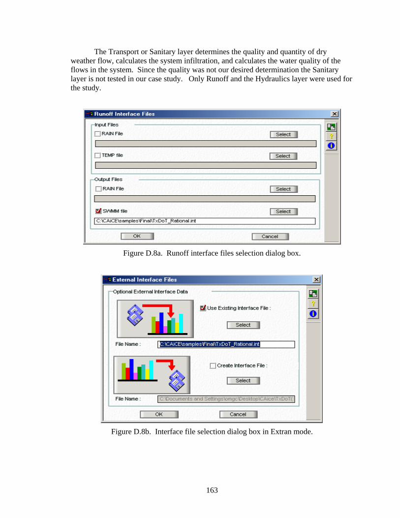
163

The Transport or Sanitary layer determines the quality and quantity of dry weather flow, calculates the system infiltration, and calculates the water quality of the flows in the system. Since the quality was not our desired determination the Sanitary layer is not tested in our case study. Only Runoff and the Hydraulics layer were used for the study.

Figure D.8a. Runoff interface files selection dialog box.

Figure D.8b. Interface file selection dialog box in Extran mode.

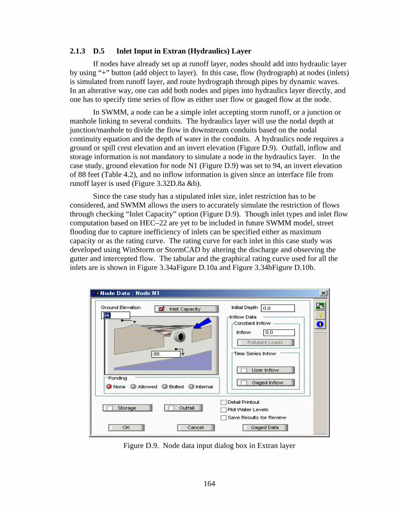
164

2.1.3 D.5 Inlet Input in Extran (Hydraulics) Layer

If nodes have already set up at runoff layer, nodes should add into hydraulic layer by using “+” button (add object to layer). In this case, flow (hydrograph) at nodes (inlets) is simulated from runoff layer, and route hydrograph through pipes by dynamic waves. In an alterative way, one can add both nodes and pipes into hydraulics layer directly, and one has to specify time series of flow as either user flow or gauged flow at the node.

In SWMM, a node can be a simple inlet accepting storm runoff, or a junction or manhole linking to several conduits. The hydraulics layer will use the nodal depth at junction/manhole to divide the flow in downstream conduits based on the nodal continuity equation and the depth of water in the conduits. A hydraulics node requires a ground or spill crest elevation and an invert elevation (Figure D.9). Outfall, inflow and storage information is not mandatory to simulate a node in the hydraulics layer. In the case study, ground elevation for node N1 (Figure D.9) was set to 94, an invert elevation of 88 feet (Table 4.2), and no inflow information is given since an interface file from runoff layer is used (Figure 3.32D.8a &b).

Since the case study has a stipulated inlet size, inlet restriction has to be considered, and SWMM allows the users to accurately simulate the restriction of flows through checking “Inlet Capacity” option (Figure D.9). Though inlet types and inlet flow computation based on HEC–22 are yet to be included in future SWMM model, street flooding due to capture inefficiency of inlets can be specified either as maximum capacity or as the rating curve. The rating curve for each inlet in this case study was developed using WinStorm or StormCAD by altering the discharge and observing the gutter and intercepted flow. The tabular and the graphical rating curve used for all the inlets are is shown in Figure 3.34aFigure D.10a and Figure 3.34bFigure D.10b.

Figure D.9. Node data input dialog box in Extran layer

165

Figure D.10a. Rating curve for the curb inlet of L = 10 ft.

FigureD.10b. Graphical view of rating curve in Figure D.10a.

Conduits or links are added connecting the nodes. The physical parameters of the conduits are shown in the Table4.3 for the case study. Moreover due to the inlet restriction, all the flow approaching the node (inlet) may or may not enter the underground pipe (link). Flow that doesn’t enter the inlet is carried over to the next subsequent inlet as an overland flow. By default, SWMM does not route the flow on the road surface, which keeps above the ground due to inlet restriction or spills out from a

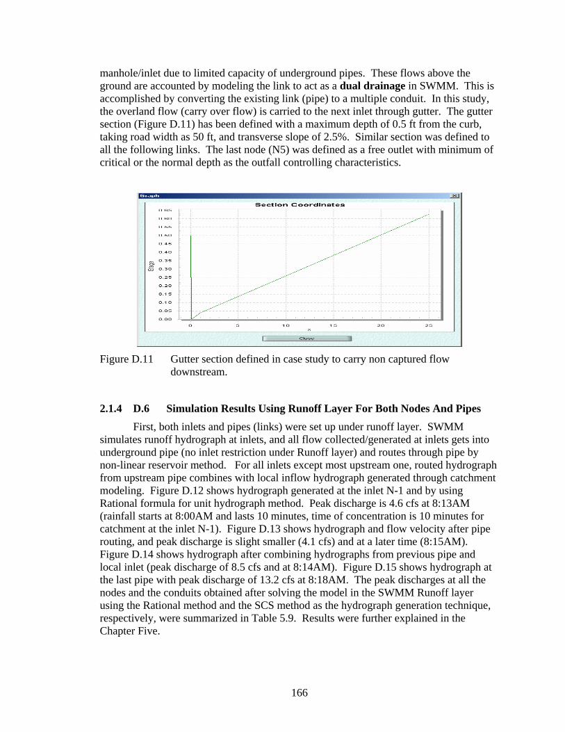
166

manhole/inlet due to limited capacity of underground pipes. These flows above the ground are accounted by modeling the link to act as a dual drainage in SWMM. This is accomplished by converting the existing link (pipe) to a multiple conduit. In this study, the overland flow (carry over flow) is carried to the next inlet through gutter. The gutter section (Figure D.11) has been defined with a maximum depth of 0.5 ft from the curb, taking road width as 50 ft, and transverse slope of 2.5%. Similar section was defined to all the following links. The last node (N5) was defined as a free outlet with minimum of critical or the normal depth as the outfall controlling characteristics.

Figure D.11 Gutter section defined in case study to carry non captured flow

downstream.

2.1.4 D.6 Simulation Results Using Runoff Layer For Both Nodes And Pipes First, both inlets and pipes (links) were set up under runoff layer. SWMM

simulates runoff hydrograph at inlets, and all flow collected/generated at inlets gets into underground pipe (no inlet restriction under Runoff layer) and routes through pipe by non-linear reservoir method. For all inlets except most upstream one, routed hydrograph from upstream pipe combines with local inflow hydrograph generated through catchment modeling. Figure D.12 shows hydrograph generated at the inlet N-1 and by using Rational formula for unit hydrograph method. Peak discharge is 4.6 cfs at 8:13AM (rainfall starts at 8:00AM and lasts 10 minutes, time of concentration is 10 minutes for catchment at the inlet N-1). Figure D.13 shows hydrograph and flow velocity after pipe routing, and peak discharge is slight smaller (4.1 cfs) and at a later time (8:15AM). Figure D.14 shows hydrograph after combining hydrographs from previous pipe and local inlet (peak discharge of 8.5 cfs and at 8:14AM). Figure D.15 shows hydrograph at the last pipe with peak discharge of 13.2 cfs at 8:18AM. The peak discharges at all the nodes and the conduits obtained after solving the model in the SWMM Runoff layer using the Rational method and the SCS method as the hydrograph generation technique, respectively, were summarized in Table 5.9. Results were further explained in the Chapter Five.

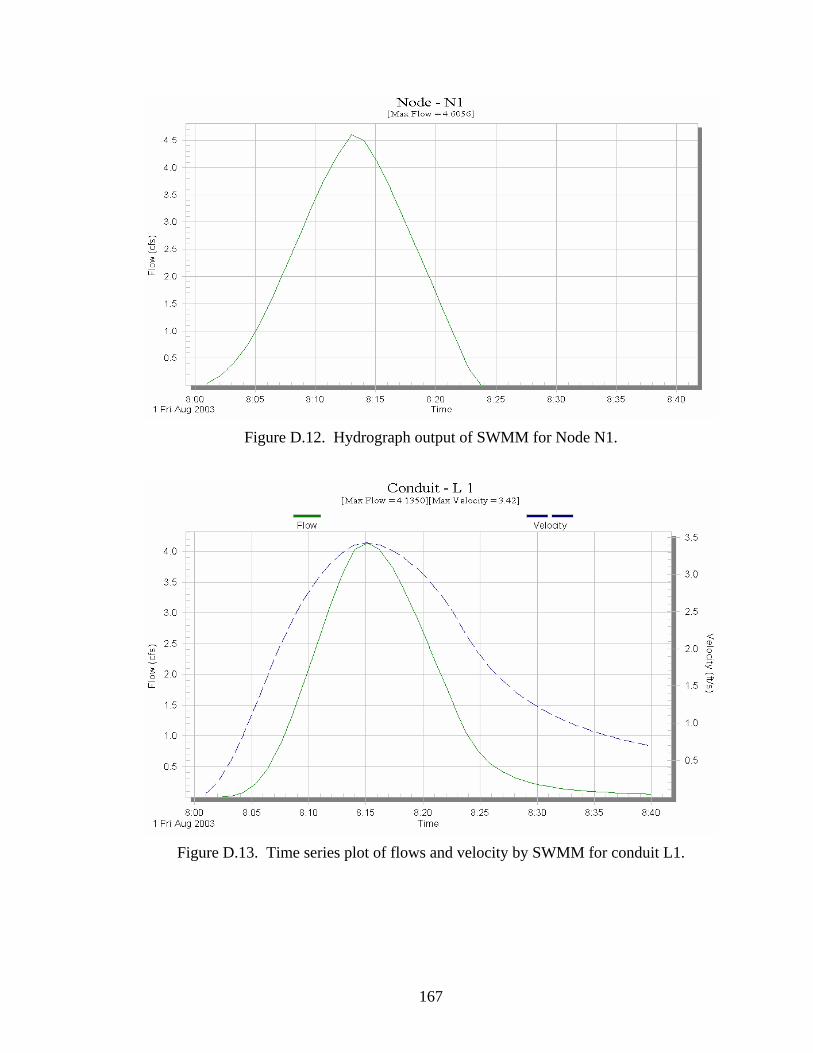
167

Figure D.12. Hydrograph output of SWMM for Node N1.

Figure D.13. Time series plot of flows and velocity by SWMM for conduit L1.

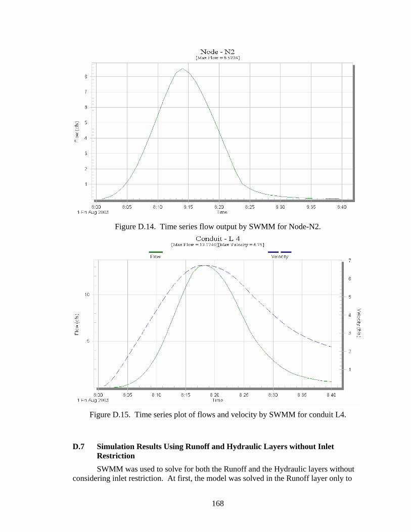
168

Figure D.14. Time series flow output by SWMM for Node-N2.

Figure D.15. Time series plot of flows and velocity by SWMM for conduit L4.

D.7 Simulation Results Using Runoff and Hydraulic Layers without Inlet

Restriction SWMM was used to solve for both the Runoff and the Hydraulic layers without

considering inlet restriction. At first, the model was solved in the Runoff layer only to

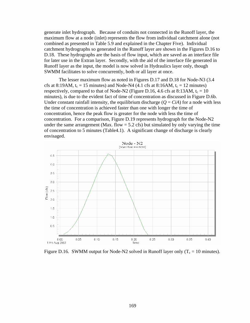
169

generate inlet hydrograph. Because of conduits not connected in the Runoff layer, the maximum flow at a node (inlet) represents the flow from individual catchment alone (not combined as presented in Table 5.9 and explained in the Chapter Five). Individual catchment hydrographs so generated in the Runoff layer are shown in the Figures D.16 to D.18. These hydrographs are the basis of flow input, which are saved as an interface file for later use in the Extran layer. Secondly, with the aid of the interface file generated in Runoff layer as the input, the model is now solved in Hydraulics layer only, though SWMM facilitates to solve concurrently, both or all layer at once.

The lesser maximum flow as noted in Figures D.17 and D.18 for Node-N3 (3.4 cfs at 8:19AM, tc = 15 minutes) and Node-N4 (4.1 cfs at 8:16AM, tc = 12 minutes) respectively, compared to that of Node-N2 (Figure D.16, 4.6 cfs at 8:13AM, tc = 10 minutes), is due to the evident fact of time of concentration as discussed in Figure D.6b. Under constant rainfall intensity, the equilibrium discharge (Q = CiA) for a node with less the time of concentration is achieved faster than one with longer the time of concentration, hence the peak flow is greater for the node with less the time of concentration. For a comparison, Figure D.19 represents hydrograph for the Node-N2 under the same arrangement (Max. flow = 5.2 cfs) but simulated by only varying the time of concentration to 5 minutes (Table4.1). A significant change of discharge is clearly envisaged.

Figure D.16. SWMM output for Node-N2 solved in Runoff layer only (Tc = 10 minutes).

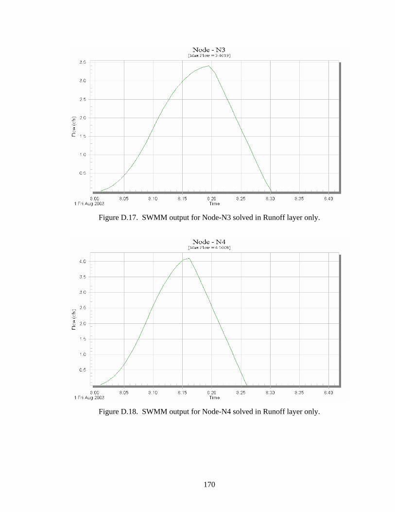
170

Figure D.17. SWMM output for Node-N3 solved in Runoff layer only.

Figure D.18. SWMM output for Node-N4 solved in Runoff layer only.

171

Figure D.19. SWMM output for Node-N2 solved in Runoff layer only (Tc = 5 minutes).

Hydraulic layer performs a dynamic routing of stormwater and/or sanitary flows

throughout the major storm drainage system to the points of outfall or to the receiving water system. It uses a link-node description of the sewer system which facilitates the discrete representation of the physical prototype and the mathematical solution of the gradually-varied unsteady flow (St. Venant) equation which forms the mathematical basis of the model. It receives hydrograph input(s) at locations by interface file, which is transferred from an upstream mode (e.g. the Runoff Block).

The result of solving the model in the Hydraulic layer is revealed in Figures D.20 to D.22. As expected, the maximum flow in the conduit L1 (4.5 cfs at 8:14AM) is slightly lesser than the maximum inflow from the catchment node N1 (4.6 cfs). The maximum flow from the conduit L1 is then added to the inflow from the catchment at node N2 (4.6 cfs) and again routed in the downstream conduit L2. The result after routing the combined flow is represented in Figure D.21, which shows a maximum flow of 6.6 cfs and maximum velocity of 3.84 ft/sec. This process of dynamic routing is continued to the downstream conduits (e.g., Figure D.22 for L3) in a similar manner until an outfall is encountered.

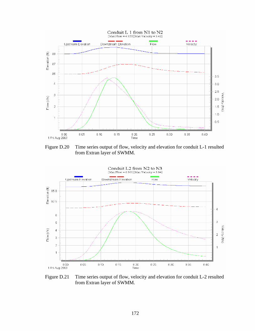
172

Figure D.20 Time series output of flow, velocity and elevation for conduit L-1 resulted

from Extran layer of SWMM.

Figure D.21 Time series output of flow, velocity and elevation for conduit L-2 resulted

from Extran layer of SWMM.

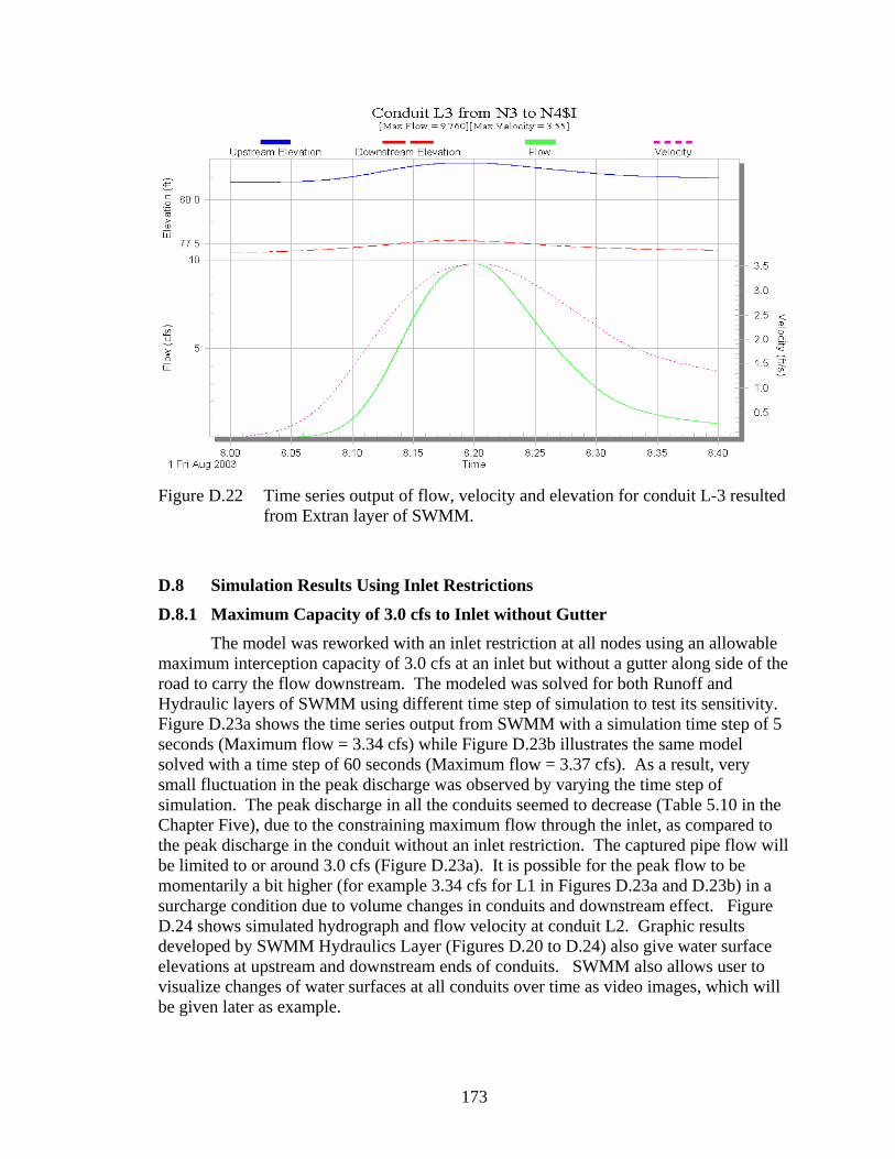
173

Figure D.22 Time series output of flow, velocity and elevation for conduit L-3 resulted

from Extran layer of SWMM.

D.8 Simulation Results Using Inlet Restrictions

D.8.1 Maximum Capacity of 3.0 cfs to Inlet without Gutter The model was reworked with an inlet restriction at all nodes using an allowable

maximum interception capacity of 3.0 cfs at an inlet but without a gutter along side of the road to carry the flow downstream. The modeled was solved for both Runoff and Hydraulic layers of SWMM using different time step of simulation to test its sensitivity. Figure D.23a shows the time series output from SWMM with a simulation time step of 5 seconds (Maximum flow = 3.34 cfs) while Figure D.23b illustrates the same model solved with a time step of 60 seconds (Maximum flow = 3.37 cfs). As a result, very small fluctuation in the peak discharge was observed by varying the time step of simulation. The peak discharge in all the conduits seemed to decrease (Table 5.10 in the Chapter Five), due to the constraining maximum flow through the inlet, as compared to the peak discharge in the conduit without an inlet restriction. The captured pipe flow will be limited to or around 3.0 cfs (Figure D.23a). It is possible for the peak flow to be momentarily a bit higher (for example 3.34 cfs for L1 in Figures D.23a and D.23b) in a surcharge condition due to volume changes in conduits and downstream effect. Figure D.24 shows simulated hydrograph and flow velocity at conduit L2. Graphic results developed by SWMM Hydraulics Layer (Figures D.20 to D.24) also give water surface elevations at upstream and downstream ends of conduits. SWMM also allows user to visualize changes of water surfaces at all conduits over time as video images, which will be given later as example.

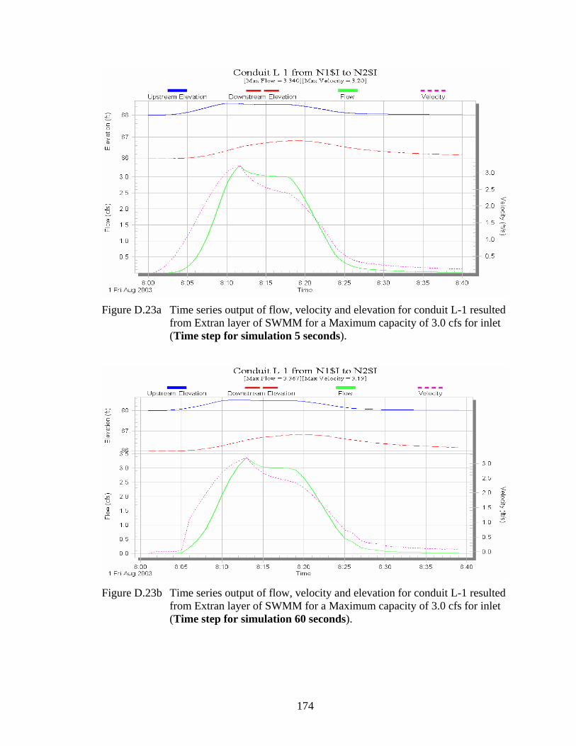
174

Figure D.23a Time series output of flow, velocity and elevation for conduit L-1 resulted

from Extran layer of SWMM for a Maximum capacity of 3.0 cfs for inlet (Time step for simulation 5 seconds).

Figure D.23b Time series output of flow, velocity and elevation for conduit L-1 resulted

from Extran layer of SWMM for a Maximum capacity of 3.0 cfs for inlet (Time step for simulation 60 seconds).

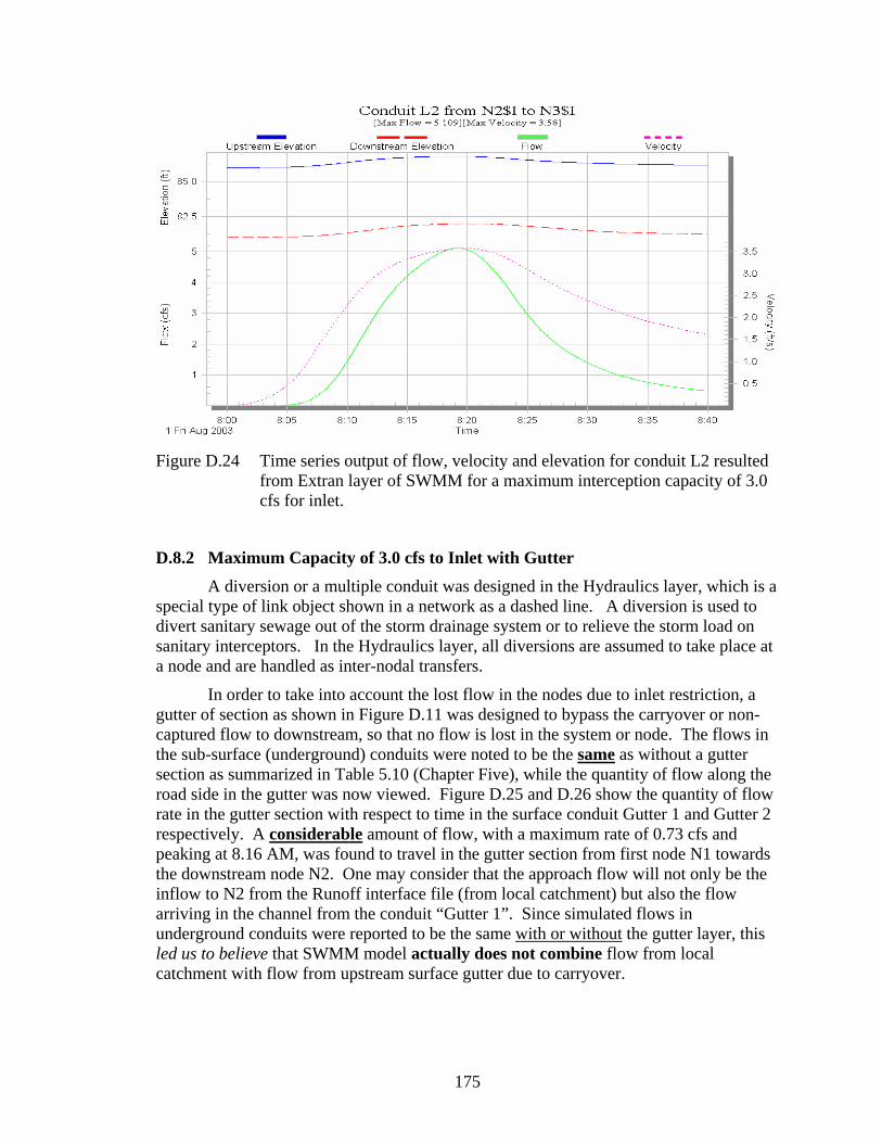
175

Figure D.24 Time series output of flow, velocity and elevation for conduit L2 resulted

from Extran layer of SWMM for a maximum interception capacity of 3.0 cfs for inlet.

D.8.2 Maximum Capacity of 3.0 cfs to Inlet with Gutter A diversion or a multiple conduit was designed in the Hydraulics layer, which is a

special type of link object shown in a network as a dashed line. A diversion is used to divert sanitary sewage out of the storm drainage system or to relieve the storm load on sanitary interceptors. In the Hydraulics layer, all diversions are assumed to take place at a node and are handled as inter-nodal transfers.

In order to take into account the lost flow in the nodes due to inlet restriction, a gutter of section as shown in Figure D.11 was designed to bypass the carryover or non-captured flow to downstream, so that no flow is lost in the system or node. The flows in the sub-surface (underground) conduits were noted to be the same as without a gutter section as summarized in Table 5.10 (Chapter Five), while the quantity of flow along the road side in the gutter was now viewed. Figure D.25 and D.26 show the quantity of flow rate in the gutter section with respect to time in the surface conduit Gutter 1 and Gutter 2 respectively. A considerable amount of flow, with a maximum rate of 0.73 cfs and peaking at 8.16 AM, was found to travel in the gutter section from first node N1 towards the downstream node N2. One may consider that the approach flow will not only be the inflow to N2 from the Runoff interface file (from local catchment) but also the flow arriving in the channel from the conduit “Gutter 1”. Since simulated flows in underground conduits were reported to be the same with or without the gutter layer, this led us to believe that SWMM model actually does not combine flow from local catchment with flow from upstream surface gutter due to carryover.

176

Figure D.25 Variation in flow and elevation with respect to time in the surface conduit

Gutter 1.

Figure D.26 Variation in flow and elevation with respect to time in the surface conduit

Gutter 2.

177

D.8.3 Using Rating Curve With/Without Gutter Section

The case study was investigated again using a rating curve as the restriction for the inlet. The rating curve (Figure D.10a & b) for each inlet in this study was developed using WinStorm or StormCAD, by altering the discharge and observing the gutter flow and intercepted flow. As discussed in the previous section, the conduits resulted the same flow amount either considering with or without the gutter section (Table 5.10 in the Chapter Five). The only difference being the flow is reflected graphically if gutter section is considered. As seen from Figure D.27 and D.28 and also in Table 5.10, the intercepted flow in the conduit using rating curve is greater than that of restricting the inlet with a maximum of 3.0 cfs (Figure D.23a and D.24). Moreover, the time to reach the peak flow is also shifted to a greater value of 8:14AM for L1 for this case (Figure D.27) than with the similar one previously dealt in section (8.12 AM for L1 in Figure D.23a).

A lesser amount of flow in gutter, 0.29 cfs in gutter 1 and 0.15 cfs for gutter 2 (Figure D.29 and D.30, Table 5.10) respectively, using the rating curve as compared to constant discharge of 3.0 cfs, was simulated, and is due to more interception capacity for the inlet with rating curve than one restricting to constant 3 cfs.

Figure D.27 Time series output of flow, velocity and elevation for conduit L-1 resulted

from Extran layer of SWMM using rating curve as inlet restriction.

178

Figure D.28 Time series output of flow, velocity and elevation for conduit L-1 resulted

from Extran layer of SWMM using rating curve as inlet restriction.

Figure D.29 Variation in flow and elevation with respect to time in the surface conduit

Gutter 1 using rating curve.

179

Figure D.30 Variation in flow and elevation with respect to time in the surface conduit

Gutter 2 using rating curve.

D.9 Simulation Using SCS Unit Hydrograph Method As an alternative to the Rational method of generating hydrograph by Runoff

layer, hydrographs may optionally be generated by the SCS method also. The difference between the two methods is that instead of specifying runoff coefficient in Rational method, pervious area curve number along with the shape factor or the peak rate factor is employed in the SCS method. The pervious area curve number CN is a dimensionless number depending on hydrologic soil group, cover type, treatment, hydrological condition, and antecedent moisture conditions. This number has a valid range from 0 to 100 with typical values from 60 to 90 and 98 for impervious surfaces. The pervious curve number in our case study was selected as 100, which is an ideal condition of impervious surface. The typical value for the shape factor K as suggested by Soil Conservation Service is 484 for a hydrograph where the volume under the rising side of the triangular unit hydrograph is equal to the volume under the rising limb of the curvilinear unit hydrograph. Actual values may vary from 300 in very flat swampy country to 600 in steep terrain. This shape factor depends not only on the size of the watershed but also on the geographic location.

The SCS method was tested on two different computer software packages of SWMM, i.e., CAiCE Visual SWMM and XP-SWMM, under the same rainfall pattern as in the case study. The hydrographs obtained as a result of solving in the Runoff layer for the first catchment by CAiCE SWMM and XP-SWMM are illustrated in Figures D.31a and D.31b for different shape factor K values, respectively. Comparing the Figures one can clearly envisage that the hydrograph (flow vs. time) generated by CAiCE SWMM and XP-SWMM are inconsistent, since the peak discharge computed by former (Q=3.5

180

cfs) is lesser than computed by the latter (Q=3.9 cfs). The catchment was tested for its sensitivity to the shape factor value (K=300, K=400, K=484, K=500 and K=600), while the other input parameters remained unchanged. It is observed that by increasing the value of shape factor the peak flow is increased while the time base of the hydrograph is reduced.

Like the Rational method, the SCS method was also tested under different combinations of flow, rating curve and with and without considering the gutter section on the surface. Table 5.11 given in the Chapter Five summarizes the peak discharges in the four pipes under different conditions of with/without inlet restrictions. Under same setting and condition, the peak discharges in all the cases acquired from SCS method were found to be less than those obtained by Rational method (Table5.10 in the Chapter Five).

Comparison of Simulated Hydrographs in CAiCE SWMM (SCS Method)

0.0

1.0

2.0

3.0

4.0

5.0

0 10 20 30 40

Time (min.)

Dis

char

ge (c

fs)

K=300

K=400

K=484

K=500

K = 600

Figure D.31a. Simulated hydrographs using SCS Method in CAiCE SWMM.

181

Comparison of Simulated Hydrographs in XP SWMM(SCS Method)

0.0

1.0

2.0

3.0

4.0

5.0

0 10 20 30 40

Time (min.)

Dis

hcar

ge (c

fs)

K = 300

K = 400

K = 484

K = 500

K = 600

FigureD.31b. Simulated hydrograph using SCS Method in XP SWMM.

The case study was tested again using SCS methodology at the Runoff layer for nodes, and multiple links (pipes) with gutter were set up at hydraulics layer. Inlets at hydraulics layer use rating curve (FigureD.10a &D.10b) for inlet capacity. A standard shape factor of 484 was utilized while simulating the model, as suggested by Soil Conservation Service for most watersheds. The first watershed contributes a peak flow of 3.5 cfs (Table5.11) to the node N-1, a part of which enters the node while the rest is carried over to the next inlet N-2 through the gutter. Figure D.32 shows the flow vs. time (hydrograph) in the conduit L-1 where the maximum flow reads 3.43 cfs at 8.13 AM, while Figure D.33 gives for the gutter flow (very small). Figure D.34 to D.38 show simulated hydrographs in pipes L-2 to L-4 and in their associated gutters.

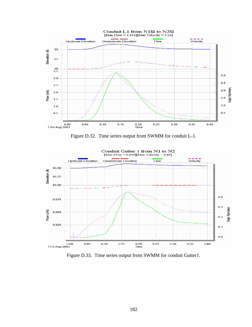
182

Figure D.32. Time series output from SWMM for conduit L-1.

Figure D.33. Time series output from SWMM for conduit Gutter1.

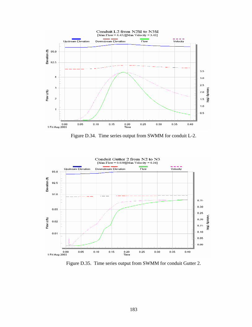
183

Figure D.34. Time series output from SWMM for conduit L-2.

Figure D.35. Time series output from SWMM for conduit Gutter 2.

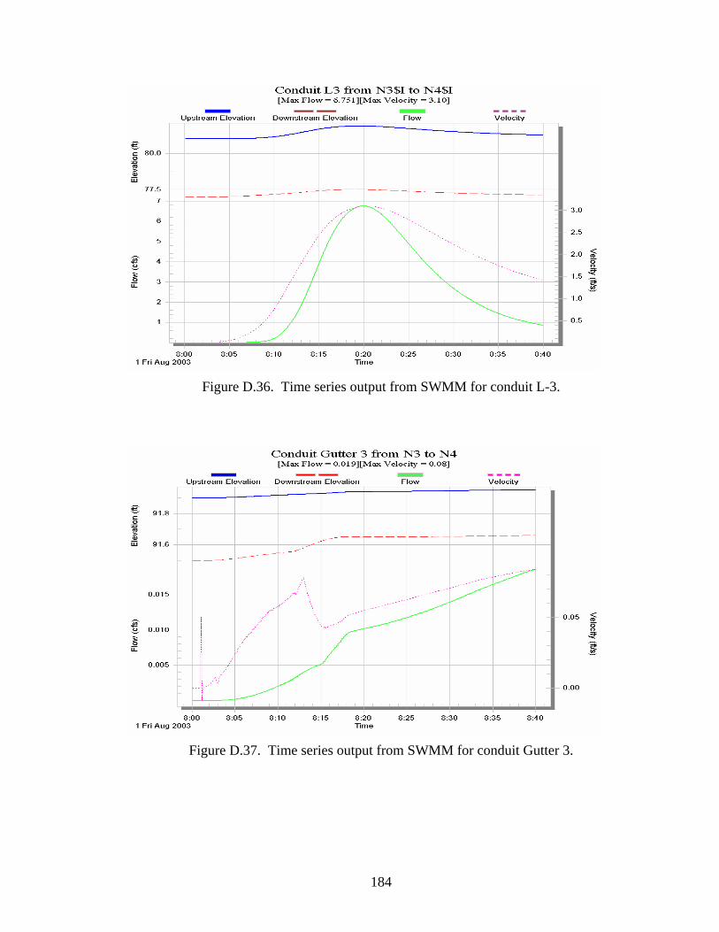
184

Figure D.36. Time series output from SWMM for conduit L-3.

Figure D.37. Time series output from SWMM for conduit Gutter 3.

185

Figure D.38. Time series output from SWMM for conduit L-4.