Synthetic Aperture Radar Imaging Using SpectralEstimation Techniques

Shivakumar RamakrishnanVincent Demarcus

Jerome Le NyNeal PatwariJoel Gussy

University of MichiganEECS 559 - Advanced Signal Processing

10 Apr 02

2

I. Introduction ...................................................................................................... 3II. Background: Spotlight Synthetic Aperture Radar............................................. 3

1. Range Compression..................................................................................... 5Mixing .............................................................................................................. 6Low-Pass Filtering ........................................................................................... 7Fourier Transforming ....................................................................................... 7

2. Cross-Range Resolution Problem................................................................ 73. Phase history and SAR data ........................................................................ 8

III. Spectral Estimation Techniques ................................................................... 91. FFT............................................................................................................. 102. Periodogram based Methods ..................................................................... 10

Windowed Periodogram................................................................................. 10Blackman-Tukey ............................................................................................ 11Welch Method................................................................................................ 11

3. Covariance-Based Methods ....................................................................... 12Capon Method ............................................................................................... 13Subspace Decomposition Methods................................................................ 13APES Method ................................................................................................ 14

IV. Quantitative Analysis of the Techniques on Simulated Data ...................... 151. Spatial Resolution ...................................................................................... 162. Noise Performance..................................................................................... 18

Mean Squared Error ...................................................................................... 19Signal to Noise Ratio ..................................................................................... 20

3. Quadratic Phase Error Performance .......................................................... 22V. Image Quality with Simulated Phase History Data......................................... 24

1. Simulated Images......................................................................................... 242. Effect of Quadratic Phase Errors on Image Quality ...................................... 263. Computational Complexity............................................................................ 28

VI. Image Quality with Actual Phase History Data ........................................... 281. Transitioning from Simulated to Real Data ................................................... 282. Final Images................................................................................................. 30

VII. Conclusion:................................................................................................. 32VIII. References................................................................................................. 34

3

I. Introduction

Synthetic Aperture Radar (SAR) imaging has had an impact in many disciplinesover the past few decades. The high quality images taken from satellites andaircraft, initially designed for military surveillance and target detection, have beenapplied to make advances in accurate mapping, geological exploration,environmental monitoring, and agriculture. Satellite and airborne SAR data hasbecome readily available in the past decade, and processing of the data hasbecome key. Traditional FFT-based methods to process signal and phase historydata into images are widely used, even though they suffer from poor resolution andhigh sidelobe artifacts. However, modern spectral estimation methods provide anattractive alternative that can improve resolution, help eliminate image speckleeffects, and increase the accuracy of interferometric height estimates. Thesemethods promise to improve the clarity and applicability of SAR imaging for manyapplications.

This project set out to explore various spectral estimation techniques that can beapplied to SAR imaging systems. In Section II, we show how SAR imagingsystems record data that has a Fourier Transform relationship with the image thatwe want to measure. In Section III, we show how to apply spectral estimationtechniques learned in class and in the literature [1-3] to two dimensions. InSection IV, we study the performance of SAR imaging methods in simulationsusing computer-generated SAR data. Then, in Section V, we evaluate theperformance of each method visually using simulated SAR images in the presenceof additive noise and phase errors. Finally, actual SAR data was used with ouralgorithms to judge the effect of the implemented algorithms on real SAR systems.

II. Background: Spotlight Synthetic Aperture Radar

The goal of the SAR imaging system is to produce an estimate of the amplitude ofthe reflectivity function g(x,y) of a scene. In this section, we show how illuminatingthe scene using radar produces phase history data that has a two-dimensionalFourier Transform relationship with g(x,y). The main goal of this project is to studythe power spectral estimation problem of converting the phase history to an image.However, it is important to gain a physical understanding of the measurementprocess that produces the phase history to justify the mathematical model usedand to be able to generate test data for our simulations.

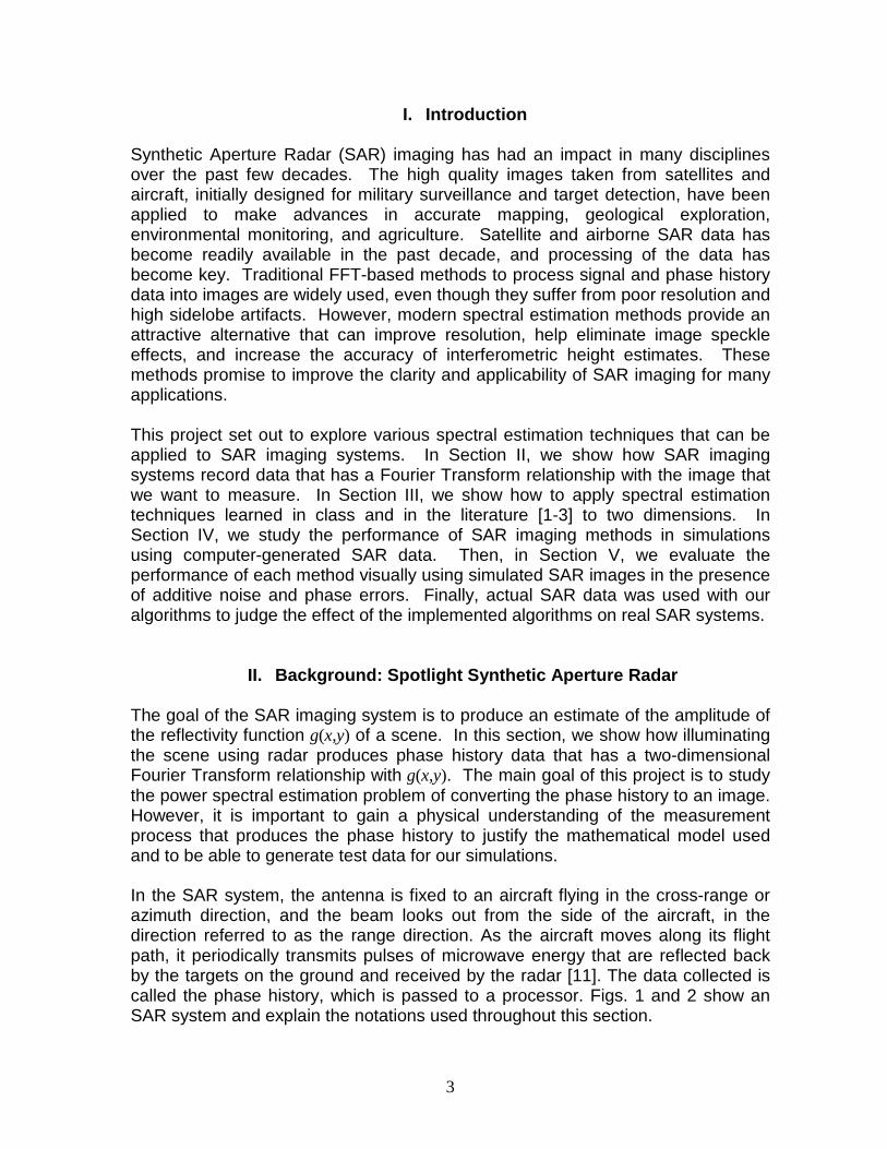
In the SAR system, the antenna is fixed to an aircraft flying in the cross-range orazimuth direction, and the beam looks out from the side of the aircraft, in thedirection referred to as the range direction. As the aircraft moves along its flightpath, it periodically transmits pulses of microwave energy that are reflected backby the targets on the ground and received by the radar [11]. The data collected iscalled the phase history, which is passed to a processor. Figs. 1 and 2 show anSAR system and explain the notations used throughout this section.

4

Figure 1. Spotlight mode synthetic aperture radar. The radar is steered continually duringthe flight. [11]

Figure 2. SAR principle. The data received in each pulse is the reflectivity integrated overa wave front y = y1. [11]

5

A SAR system launches spherical wave fronts, but because the radar platformtypically operates at standoff distances that are large compared to the scenediameter, these wave fronts are well approximated as planar. The receivermeasures the signals reflected by all targets lying along the same constant-rangecontour at the same time. Thus the measured signal is not simply the value of thecomplex reflectivity function at any one ground position (x,y). Instead, the receiverintegrates the reflectivity values from all targets that lie along the correspondingconstant ground range line y = y1. The SAR system resolves the ambiguity byusing information from the other times that the target is illuminated as the aircraftmoves along its flight path [11]. The longer the target is illuminated, the moreinformation we can get on the position.

Two different principal modes are used in SAR imaging:1. In the strip-map mode, the antenna is aimed orthogonal to the flight path

and keeps this orientation2. When better resolution for a smaller ground patch is desired, the spotlight

mode is preferred. In this mode, the illuminating radar beam is steeredcontinually as the aircraft moves, so that it illuminates the same patch overa longer period of time.

In this project, we restrict our analysis to the latter technique. Processing of thephase history generated in spotlight mode requires 2-D power spectral estimationmethods for image formation, which is the motivation for our project.

1. Range Compression

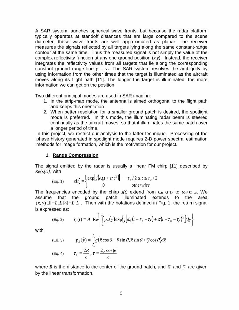
The signal emitted by the radar is usually a linear FM chirp [11] described byRe{s(t)}, with

(Eq. 1) ( ) ( )[ ] ≤≤−+

=otherwise

tttjts cc

0

2/2/exp 20 τταω

The frequencies encoded by the chirp s(t) extend from ω0−α τc to ω0+α τc. Weassume that the ground patch illuminated extends to the area

],[],[),( LLLLyx −×−∈ . Then with the notations defined in Fig. 1, the return signalis expressed as:

(Eq. 2) ( ) ( ) ( )[ ]{ }

−−+−−= ∫−

L

L

c ydytytjypAtr 2000expRe)( τταττωθ

with

(Eq. 3) ( )∫−

+−=L

L

xdyxyxgyp θθθθθ cossin,sincos)(_

(Eq. 4)c

y

c

R ψττ cos2,

20 ==

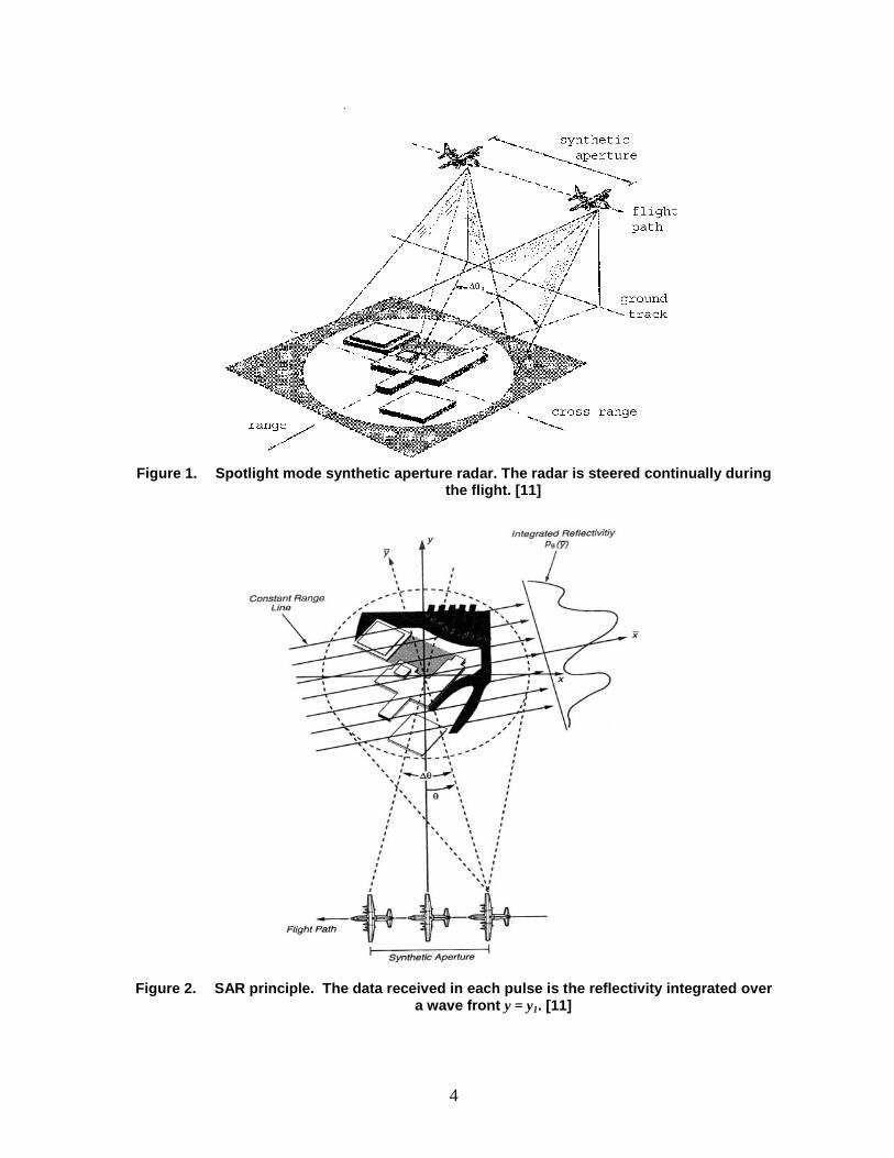
where R is the distance to the center of the ground patch, and x and y are givenby the linear transformation,

6

(Eq. 5) θθ sincos yxx +=(Eq. 6) θθ cossin yxy +−=

Note that we introduce the depression angle ψ, i.e. the angle that the incidentmicrowave makes with the ground, and c, the speed of light.

The first task is to remove the effect of the carrier from rc(t). We will then show thatthe collection of functions ( )ypθ obtained over an interval of viewing angles,

∆θ, contains sufficient information to reconstruct g(x,y).

The equation for rc(t) can be interpreted as the convolution of pθ and the signal s,with the output evaluated at t+τ0, where τ0 is the delay of the wavefront receivedform y=0 (the middle line of the illuminated ground patch). We define the patchpropagation time τp as the difference in two-way propagation delay between atarget at the near-edge and a target at the far-edge of the illuminated patch (τ0 =4Lcosψ/c). Then we can see that the equation for rc(t) is valid only for times that arein the common intersection of the return from near-edge and far-edge targets. Thisrestricts the processing window to the common time segment for which chirpreturns from all targets in the ground patch exist simultaneously:

(Eq. 7)2222 00cpcp t

τττττ

τ +−≤≤−+

In our case, we take τc >>τp, and then there is an attractive technique which can beused to deconvolve s(t) from rc(t), called deramp processing. This is accomplishedin three steps:

1) Mixing the returned signal with the delayed in-phase and quadratureversions of the transmitted FM chirp;

2) Low-pass filtering the mixer output; and3) Fourier transforming the low-passed signal.

We give the mathematical analysis of these steps in the following.

MixingThe mixing step requires that we know the round-trip propagation time τ0 to thecenter of the ground patch; this is determined by electronic navigation systems,and imperfections on this value makes it necessary to have additional post-processing techniques. The deramp mixing terms are given by:

(Eq. 8)))()(sin()(

))()(cos()(2

000

2000

τατωτατω−+−−=

−+−=

tttcand

tttc

Q

I

By multiplying rc(t) with the first signal, one can show that we obtain the followingexpression:

7

−+−ℜ+

−−+−+−−ℜ=

∫

∫

−

−

L

L

L

L

cI

ydtyyjypA

ydyttytjypA

tr

_

00

__2

_

_2

0

_2

00

_

0

__

))](2)(()([exp)(2

)]))(()(()2)(2([exp)(2

)(

ταωτατ

ττταττω

θ

θ

Low-Pass FilteringWe see that we can remove the first term in the previous expression with a low-pass filter. We do this to remove the part of the signal centered at frequency 2ω0and to extract the baseband signal. We proceed in a similar way with thequadrature component, to get the signals:

(Eq. 9) ( )( )[ ]{ }

−+−ℜ= ∫−

L

L

cI ydtyyjypA

tr 002 2)()(exp)(

2)( ταωτατθ

(Eq. 10) ( )( )[ ]{ }

−+−ℑ= ∫−

L

L

cQ ydtyyjypA

tr 002 2)()(exp)(

2)( ταωτατθ

(Eq. 11) ( )( )[ ]{ }

−+−=+= ∫−

L

L

cQcIc ydtyyjypA

tjrtrtr 002 2)()(exp)(

2)()()( ταωτατθ

Ignoring the quadratic phase term ατ2 (we could add this effect in a more precisestudy), we get at the output of the quadrature demodulator:

(Eq. 12) ( ) ( ) ( )( ) ydtc

yjyp

Atr

L

L

c ∫−

−+−= 00 2

cos2exp

2ταωψ

θ

Fourier TransformingWe can recognize in the last expression the Fourier transform of pθ over a certainrange of spatial frequencies. Plugging the interval on which the signal is processed(Eq. (7)), we conclude that the Fourier transform is determined over the interval ofspatial frequencies Y =(2/c) cosψ (ω0+2α(t-τ0)) given by (with τc>>τp):

(Eq. 13) )(cos2

)(cos2

00 cc cY

cατωψατωψ +≤≤−

And thus a final Fourier transformation (also called range compression) of rc(t)gives the estimate of )( ypθ .

2. Cross-Range Resolution Problem

Now that we have recovered xdyxyxgypL

L

)cossin,sincos()( θθθθθ +−= ∫−

for y in [-L, L] and θ describing an interval ∆θ, we still have to show that we canextract from it an estimate of the reflectivity function g(x,y). The Projection-Slice

8

theorem states that the 1D Fourier transform of any projection function pθ(u) isequal to the 2D Fourier transform G(X,Y) of the image to be reconstructed (i.e. thereflectivity function) evaluated along a line in the Fourier domain that lies at thesame angle θ measured from the X axis [11]. That is:

(Eq. 14)

∫ ∫

∫∞

∞−

∞

∞−

+−

∞

∞−

−

=

==

dxdyeyxgYXGwhere

UPdueupUUG

yYxXj

juU

)(),(),(

)()()sin,cos( θθθθ

Note that the finite limits –L and L can be used here because g is zero outside thecircle centered at the origin with radius L. This result is easily shown using arotational change of variable:

(Eq. 15)

−=

_

_cossin

sincos

y

x

y

x

θϑθθ

in the expression of G(U cosθ, U sinθ).

Therefore, we see that starting from the projection functions )( ypθ over a range of

θ, we can determine the values of the two-dimensional Fourier transform G(X,Y)along lines of the same orientation by taking the one-dimensional Fouriertransform of )( ypθ . If the projections span 180° of viewing directions, we can thenobtain the complete Fourier transform G(X,Y) of the reflectivity function in a circularregion. In practice, the projections are taken for a discrete set of angles θ andpositions y . Thus we can obtain a reconstructed image g(x,y) by simply taking thediscrete inverse Fourier transform of the data. However, as we have seen, thesedata are organized in a way that is compatible with a polar coordinate system, andin practice, we must first perform a polar to Cartesian coordinates interpolation inorder to use the FFT algorithm. A more precise description of this transformationcan be found in [11].

3. Phase history and SAR data

To conclude this section of the SAR imaging system, we sum up the results thatjustify the study that we will conduct in the following sections. In this report, we usethe phase history, that is, SAR data in its final form after the Cartesian to polarinterpolation. From the results of this section, we know that applying a 2D-FFT onthis phase history will furnish an estimate of the reflectivity function g(x,y). Thus,this complicated data acquisition process can be exploited very simply in thisproject.

9

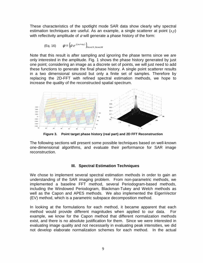
These characteristics of the spotlight mode SAR data show clearly why spectralestimation techniques are useful. As an example, a single scatterer at point (x,y)with reflectivity amplitude of α will generate a phase history of the form:

(Eq. 16) ( ) MmNnmynxje ≤≤≤≤

+= 0,0)(αφ

Note that this result is after sampling and ignoring the phase terms since we areonly interested in the amplitude. Fig. 1 shows the phase history generated by justone point; considering an image as a discrete set of points, we will just need to addthese functions to generate the final phase history. A single point scatterer resultsin a two dimensional sinusoid but only a finite set of samples. Therefore byreplacing the 2D-FFT with refined spectral estimation methods, we hope toincrease the quality of the reconstructed spatial spectrum.

Figure 3. Point target phase history (real part) and 2D FFT Reconstruction

The following sections will present some possible techniques based on well-knownone-dimensional algorithms, and evaluate their performance for SAR imagereconstruction.

III. Spectral Estimation Techniques

We chose to implement several spectral estimation methods in order to gain anunderstanding of the SAR imaging problem. From non-parametric methods, weimplemented a baseline FFT method, several Periodogram-based methods,including the Windowed Periodogram, Blackman-Tukey and Welch methods aswell as the Capon and APES methods. We also implemented the EigenVector(EV) method, which is a parametric subspace decomposition method.

In looking at the formulations for each method, it became apparent that eachmethod would provide different magnitudes when applied to our data. Forexample, we know for the Capon method that different normalization methodsexist, and there is no absolute justification for them. Since we were interested inevaluating image quality and not necessarily in evaluating peak intensities, we didnot develop elaborate normalization schemes for each method. In the actual

10

MATLAB implementations, we chose to simply normalize each method by its peaklevel and display on a dB scale.

In addition, we normalized the units of the results. Since the FFT is an estimate ofamplitude, while all other methods are estimates of power, there is a discrepancyin the results unless we normalize one or the other. Since we use the FFT as ourbaseline, we chose to take the square root of the output of all methods except forthe FFT. (We could have chosen to square the FFT and leave the others alone,but the choice was arbitrary). Since our images are displayed on a dB scale, thesquare root operation does affect the range, but doesn’t change the imageotherwise.

1. FFT

To establish an initial image, a 2-D FFT was applied to the phase history data. Asmentioned, this image was used as a baseline for comparing the results of thespectral estimation techniques described below. Note that in practice, the FFT andthe Windowed Periodogram are the most common methods used for generatingSAR images.

2. Periodogram based Methods

The first spectral estimation methods studied were the Periodogram basedmethods, namely, the Windowed Periodogram, Blackman-Tukey, and Welchmethods. These can be thought of as refined versions of the FFT and were simpleto implement.

Windowed PeriodogramThe windowed Periodogram was the first spectral estimation technique evaluated.A two-dimensional discrete space extension of the 1-D case described in [2] wasderived. The resulting formula was found to be:

(Eq. 17)

21

0

1

0

)(),(),(1

),(ˆ ∑∑−

=

−

=

+−=M

m

N

n

mnjyxp

yxemnymnvMN

ωωωωφ

where ),( mnv is a 2-D window function, and ),( mny is the two-dimensional phasehistory of size [NxM]. Here, ωx and ωy are frequencies that correspond to point (x,y)of the image. This formula was implemented in MATLAB using a 2-D FFT. Forthis implementation, the window size was chosen to be equal to the phase historysize. In this case, choosing a rectangular window function is equivalent to the 2-Dun-windowed Periodogram. Of the variety of window functions available for use inthe windowed Periodogram, a Taylor window was chosen. A Taylor window iscommonly used in SAR imaging because it provides strong sidelobe reductions

11

with minimal effect on resolution [6]. Additionally, the sidelobe reduction isselectable via the window parameters. For this evaluation, the peak sidelobe levelwas set to –35dB and the number of nearly constant level sidelobes adjacent tothe mainlobe was chosen as 5. These are typical SAR parameters. The Taylorwindow equations were obtained from [6]. The 2-D window was formed bycombination of the 1-D window functions in MATLAB.

Blackman-TukeyThe next method studied was the Blackman-Tukey method. This method seeks toimprove on the high statistical variance of the spectral estimator as described in[2]. The implementation of this method can be thought of as a locally weightedaverage of the Periodogram. The 2-D formulation was found to be (here * denotesa convolution)

(Eq. 18) ),(),(ˆ),(ˆyxyxpyxBT V ωωωωφωωφ ∗=

where ),( yxV ωω is the Fourier transform of the window function also referred to as

the spectral window. The convolution of this spectral window with thePeriodogram estimate results in a smoothing effect in the frequency domainimage. While this will theoretically reduce the variance, the resolution is degraded.Careful selection of the window function and its size are necessary to ensure goodresults. In this case, a Hamming window whose size was one half the final imagesize was chosen based on subjective assessment of the images. Using MATLAB,the actual application of the window was applied using a 2-D IFFT on thePeriodogram estimate, multiplying by the window function and then using a 2-DFFT to obtain the Blackman-Tukey estimate. The Periodogram estimate usedhere was the un-windowed type as described above.

Welch MethodThe final Periodogram based method implemented was the Welch method. Thismethod also seeks to trade resolution for variance through averaging. The 2-Ddiscrete space formulation was found to be:

(Eq. 19)

( ) ( ) ( ) ( )[ ] ( )∑∑ ∑ ∑= =

−

=

−

=

+−+−+−=Sy

d

Sx

c

M

m

N

n

mnjyx

SSxyyxw

yS xS

yx

xy

emKdnKcymnvNMSS 1 1

21

0

1

0

1,1,111

,ˆ ωωωωφ

In this case, the image is divided into overlapping blocks and averaged together.The terms

xSN andySM define the size of each block, and the terms xK and yK

define the amount of overlap. In this case, the 2-D window ),( mnv is chosen to bethe size of each block. The recommended value for xK and yK provides for 50%

12

overlap of each block and is given by is N/2 and M/2 respectively where N and Mare the total phase history size. This is what was used in this study. The xS and

yS terms define the total number of blocks and is given by the integer parts of

x

xs

x K

KNNS x

)( +−= and

y

ys

y K

KMMS y

)( +−= .

3. Covariance-Based Methods

The next spectral estimation methods studied centered on the autocovariancematrix. These methods include the Capon method, EigenVector (EV) method, andthe Amplitude and Phase Estimation (APES) method. To use these methods, thefirst task was to determine the autocovariance matrix.

In two dimensions, the estimation of the autocovariance matrix from the signalhistory data poses two problems. First, there is no consensus among researchersof which method has the best performance. Secondly, the resultingautocovariance matrix is much larger in this 2-D case than it was in the 1-D case.A 1-D signal length M would result in a correlation matrix size on the order of M. Asquare image with dimensions MxN would have a autocovariance matrix size theorder of (MN), and correspondingly memory requirements on the order of (MN)2.As we attempted to do operations on real phase data of dimensions 256x256, wewere limited by the memory available on our computers.

The simplest method used for autocovariance matrix estimation is the covariancemethod, or sub-aperture averaging [1]. In this method, a small sub-aperture Xi,j (amatrix of size Kx by Ky) is chosen from the signal history matrix starting at datapoint (i,j). Then a vector of length (Kx*Ky) is formed by 'raster scanning', ie.,stacking columns of Xi,j on top of each other to form a one-dimensional vector, xi,j.Then, the outer product of xi,j is taken, resulting in a autocovariance matrix Ri,j.This process is repeated for all possible (i,j) and all of the Ri,j are averagedtogether. This produces a 'unidirectional' subaperture estimate R.

The selection of Kx and Ky is up to the user - 40-50% of the data record lengths Mand N respectively are recommended by [1], while [7] insists only that Kx << M andKy << N to ensure a sufficient number of lagged products for statistical stability.

A variation of this method is forward-backward subaperture averaging. Thismethod helps average out the noise by using the fact that a 2-D sinusoid evolvesin one spatial direction in the same manner as the conjugate sinusoid evolves inthe opposite spatial direction [1]. Also, the forward-backward method gives amatrix that is better conditioned than just the forward sample covariance matrix.There are other methods that can be implemented in a computationally lessintensive manner - specifically, Toepliz-Block-Toepliz method [8]. However, toease implementation time, we used forward-backward subaperture averaging inthis report.

13

Capon MethodThe Capon method, also called the minimum variance method, is of keyimportance in high-resolution 2-D spectral estimation. It was originally proposedfor 2-D signals [9]. If we define the 2D Fourier vectors as

(Eq. 20) [ ] [ ] TMjjTMjjyx

yyXX eeeeW ωωωωωω )1()1( 11),( −−−−−− ⊗= …

(where ⊗ denotes the Kronecker product of the two vectors), the amplitude at eachpoint is given by:

(Eq. 21) ( ) ( ) ( )yxyxHyxw WRW ωωωω

ωωφ,,

1,ˆ

1−=

The Capon method is designed to pass a 2-D sinusoid at a given frequencywithout distortion while minimizing the variance of the noise of the resulting image[7]. Calculation of the above equation involves two computationally intensivetasks: inversion of the R matrix, and matrix multiplication by W(ωx ,ωy) vectors,which must be done for each image point.

Subspace Decomposition MethodsThe EigenVector (EV) and MUSIC methods are both parametric methods thatexploit the assumption that the phase history data is a sum of 2-D sinusoids in abackground of white noise. They are called subspace decomposition methods forpeak estimation because they separate the eigenvectors of the autocovariancematrix into those corresponding to signals and to clutter. In the EV method, theamplitude of the image at a point ( )yx ωω , is given by:

(Eq. 22) ( )( ) ( )yx

clutter

Hii

iyx

H

yxEV

WvvW ωωλ

ωωωωφ

,1

,

1,ˆ

=

∑

while in the MUSIC method, the image amplitude is given by:

(Eq. 23) ( )( ) ( )yx

clutter

Hiiyx

HyxMUSIC

WvvW ωωσωωωωφ

,,

1,ˆ

2

=

∑

Both methods attempt to bring the denominator to zero when a sinusoidal signalcorresponding to a point in the SAR image aligns with one of the signal subspaceeigenvectors. At that point, the result is a peak in the image estimate. Thus thesemethods do not accurately represent the scattering intensity at each point, but

14

rather show the 'pointiness' of the image. The MUSIC method is considered to bea poor performer in SAR applications [1]. Note that Eq. 22, the EV method usesthe inverse of the eigenvalues of the clutter subspace, while in Eq. 23, the MUSICmethod uses a constant. The MUSIC method is exploiting further the assumptionthat clutter is white noise. In practice, this assumption is not entirely true, and theEV method more accurately shows the features of the image. This is why we havechosen to implement the EV method, rather than MUSIC. However, we are notusing the EV method to identify particular point scatterers, as we would in a trueparametric estimation problem. Instead, we display the normalized amplitude ofEq. 22. As we will see in the results section, this will provide us with a visuallyappealing result.

Note that if all of the eigenvectors are included in the clutter subspace (modelorder = 0) the EV method becomes identical to the Capon method. Thus thedetermination of model order is critical to operation of the EV method. We mustdecide based on an eigenvalue of the R matrix whether its correspondingeigenvector corresponds to the clutter or to the signal subspace. The number ofeigenvectors chosen to be in the signal subspace is called the model order. Forour computer-generated SAR data from several point targets in white noise, theeigenvalues corresponding to the different subspaces differ by orders ofmagnitude. However, in real SAR images, there will be more of a continuum ofeigenvalues. One method is to select the model order such that a fixed fraction ofthe energy is attributed to the signal subspace [1]. Another method is to choose afixed number for the model order. In our simulations, the EV method model orderwas chosen to make sure that 98% of the signal energy is included in the signalsubspace.

APES MethodThe APES method is a matched filter bank method that assumes that the phasehistory data is a sum of 2-D sinusoids in noise. Empirically, the APES methodresults in wider spectral peaks than the Capon method, but more accurate spectralestimates for amplitude in SAR [3]. In the Capon method, although the spectralpeaks are narrower than the APES, the sidelobes are higher than that for theAPES. As a result, the estimate for the amplitude is expected to be less accuratefor the Capon method than for the APES method.

The SAR image is estimated using a form similar to the Capon method. Althoughit uses the forward-backward subaperture averaging autocovariance matrixestimate R̂ , the APES method uses it indirectly through another matrix Q , whichis another estimate of the covariance matrix. The matrix Q is given by:

(Eq. 24) ( ) ( ) ( ) ( ) ( )[ ]( )( )11

,,,,ˆ,+−+−

+−=

yx

yxH

yxyxH

yx

yx KNKM

ωωωωωωωωωω

ggggRQ

15

where ( ) ( )yxjiyx ωωωω ,, , WXg = and ( ) ( )yxjiyx ωωωω ,, , WXg = . The data matrix

ji ,X is the subaperture matrix as defined above and ji ,X is the same matrix flipped

upside down and left to right. The vector ( )yx ωω ,W is the Kx by Ky matrix given by:

(Eq. 25) ( ) ( )[ ] ( )[ ]TKjjTKjjyx

yx eeee ωωωωωω 11 ...1...1, −− ⊗=W

The constants M, N and Kx, Ky are the dimensions of the full data matrix and the2-D filter, respectively. The SAR image is then formed as follows:

(Eq. 26) ( ) ( )( )( ) ( ) ( )( ) ( ) ( )yxyxyx

H

yxyxyxH

yxyx KNKM ωωωωωω

ωωωωωωωωφ

,,,

,,,

11

1,ˆ

1

1

WQW

gQW−

−

+−+−=

Note that a matrix inversion, ( )yx ωω ,1−Q , must be calculated for each data point

(x,y) of the image. As a result of this requirement, the APES method requiresabout 1.5 times more computation than the Capon method [10].

IV. Quantitative Analysis of the Techniques on Simulated Data

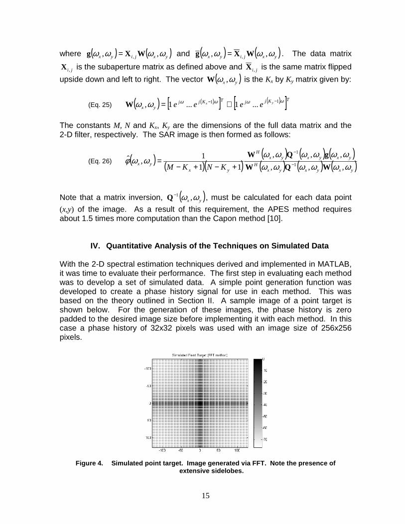
With the 2-D spectral estimation techniques derived and implemented in MATLAB,it was time to evaluate their performance. The first step in evaluating each methodwas to develop a set of simulated data. A simple point generation function wasdeveloped to create a phase history signal for use in each method. This wasbased on the theory outlined in Section II. A sample image of a point target isshown below. For the generation of these images, the phase history is zeropadded to the desired image size before implementing it with each method. In thiscase a phase history of 32x32 pixels was used with an image size of 256x256pixels.

Figure 4. Simulated point target. Image generated via FFT. Note the presence ofextensive sidelobes.

16

As we know from theory, a variety of spectral estimation methods try to trade offnoise variance and resolution. In 2-D, this tradeoff still remains, as the results ofour simulations show. In this section we determine the spatial resolution of eachmethod presented in Section III. Then, we add various levels of noise into thephase histories in order to judge the noise variance performance.

1. Spatial Resolution

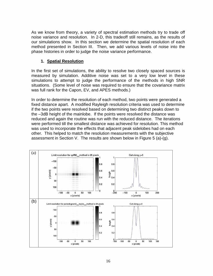
In the first set of simulations, the ability to resolve two closely spaced sources ismeasured by simulation. Additive noise was set to a very low level in thesesimulations to attempt to judge the performance of the methods in high SNRsituations. (Some level of noise was required to ensure that the covariance matrixwas full rank for the Capon, EV, and APES methods.)

In order to determine the resolution of each method, two points were generated afixed distance apart. A modified Rayleigh resolution criteria was used to determineif the two points were resolved based on determining two distinct peaks down tothe –3dB height of the mainlobe. If the points were resolved the distance wasreduced and again the routine was run with the reduced distance. The iterationswere performed till the smallest distance was achieved for resolution. This methodwas used to incorporate the effects that adjacent peak sidelobes had on eachother. This helped to match the resolution measurements with the subjectiveassessment in Section V. The results are shown below in Figure 5 (a)-(g).

(a)

(b)

17

(c)

(d)

(e)

(f)

18

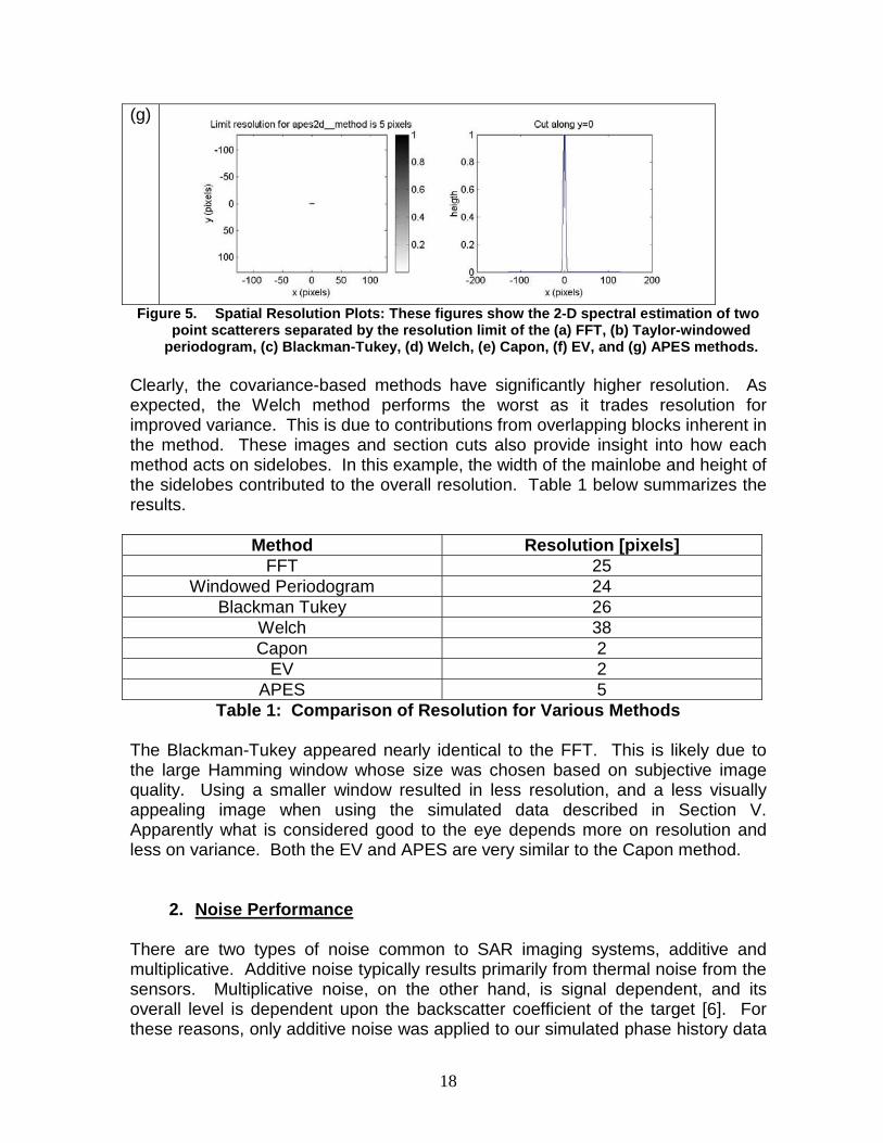
(g)

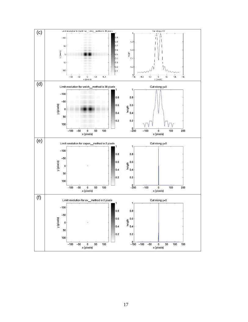
Figure 5. Spatial Resolution Plots: These figures show the 2-D spectral estimation of twopoint scatterers separated by the resolution limit of the (a) FFT, (b) Taylor-windowed

periodogram, (c) Blackman-Tukey, (d) Welch, (e) Capon, (f) EV, and (g) APES methods.

Clearly, the covariance-based methods have significantly higher resolution. Asexpected, the Welch method performs the worst as it trades resolution forimproved variance. This is due to contributions from overlapping blocks inherent inthe method. These images and section cuts also provide insight into how eachmethod acts on sidelobes. In this example, the width of the mainlobe and height ofthe sidelobes contributed to the overall resolution. Table 1 below summarizes theresults.

Method Resolution [pixels]FFT 25

Windowed Periodogram 24Blackman Tukey 26

Welch 38Capon 2

EV 2APES 5

Table 1: Comparison of Resolution for Various Methods

The Blackman-Tukey appeared nearly identical to the FFT. This is likely due tothe large Hamming window whose size was chosen based on subjective imagequality. Using a smaller window resulted in less resolution, and a less visuallyappealing image when using the simulated data described in Section V.Apparently what is considered good to the eye depends more on resolution andless on variance. Both the EV and APES are very similar to the Capon method.

2. Noise Performance

There are two types of noise common to SAR imaging systems, additive andmultiplicative. Additive noise typically results primarily from thermal noise from thesensors. Multiplicative noise, on the other hand, is signal dependent, and itsoverall level is dependent upon the backscatter coefficient of the target [6]. Forthese reasons, only additive noise was applied to our simulated phase history data

19

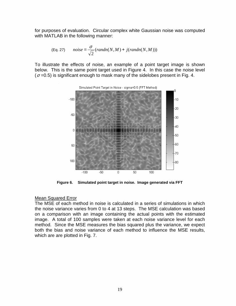
for purposes of evaluation. Circular complex white Gaussian noise was computedwith MATLAB in the following manner:

(Eq. 27) ))),((),((2

MNrandnjMNrandnnoise += σ

To illustrate the effects of noise, an example of a point target image is shownbelow. This is the same point target used in Figure 4. In this case the noise level(σ =0.5) is significant enough to mask many of the sidelobes present in Fig. 4.

Figure 6. Simulated point target in noise. Image generated via FFT

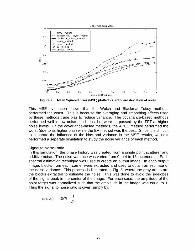
Mean Squared ErrorThe MSE of each method in noise is calculated in a series of simulations in whichthe noise variance varies from 0 to 4 at 13 steps. The MSE calculation was basedon a comparison with an image containing the actual points with the estimatedimage. A total of 100 samples were taken at each noise variance level for eachmethod. Since the MSE measures the bias squared plus the variance, we expectboth the bias and noise variance of each method to influence the MSE results,which are are plotted in Fig. 7.

20

Figure 7. Mean Squared Error (MSE) plotted vs. standard deviation of noise.

This MSE evaluation shows that the Welch and Blackman-Tukey methodsperformed the worst. This is because the averaging and smoothing effects usedby these methods trade bias to reduce variance. The covariance-based methodsperformed well in low noise conditions, but were surpassed by the FFT at highernoise levels. Of the covariance-based methods, the APES method performed theworst (due to its higher bias) while the EV method was the best. Since it is difficultto separate the influence of the bias and variance in the MSE results, we nextperformed a separate simulation to study the noise variance of each method.

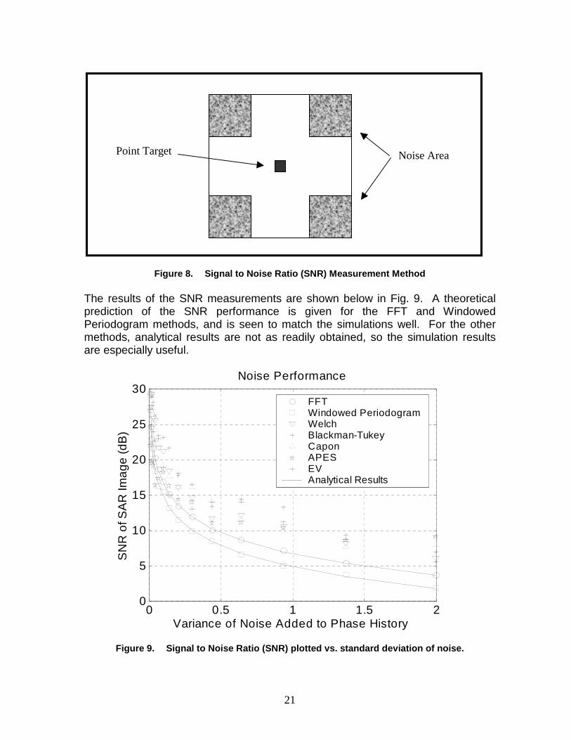
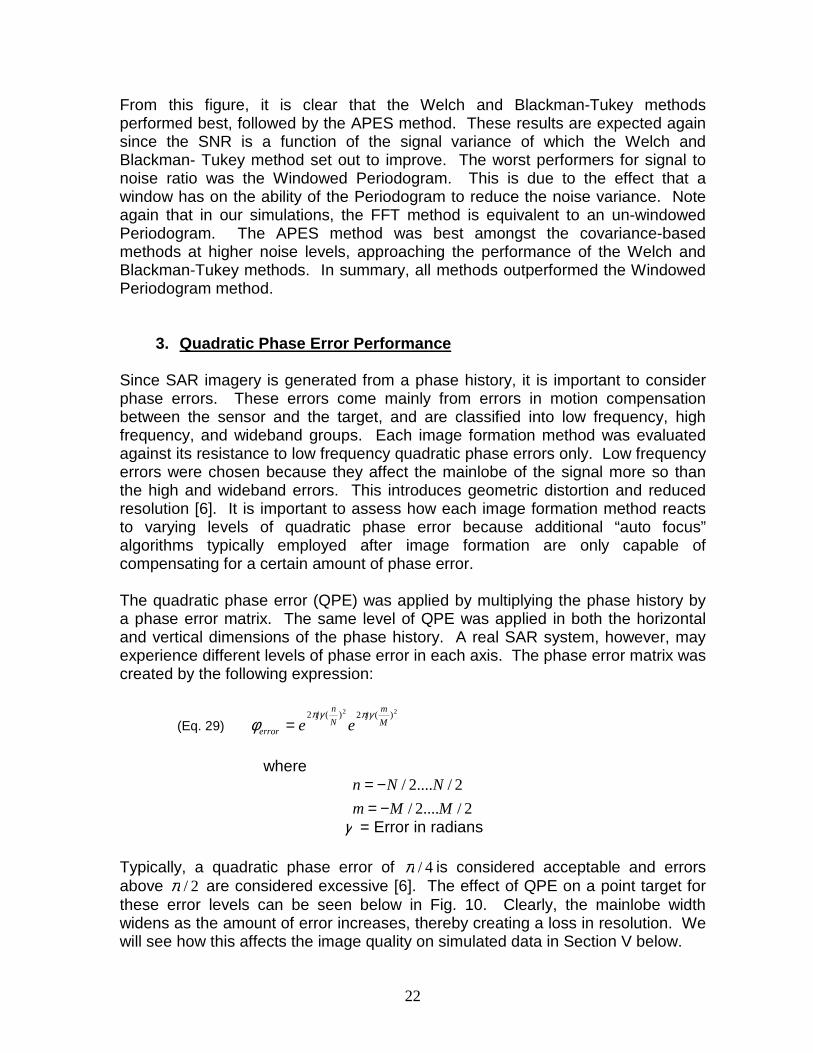
Signal to Noise RatioIn this simulation, the phase history was created from a single point scatterer andadditive noise. The noise variance was varied from 0 to 4 in 13 increments. Eachspectral estimation technique was used to create an output image. In each outputimage, blocks from each corner were extracted and used to obtain an estimate ofthe noise variance. This process is illustrated in Fig. 8, where the gray areas arethe blocks extracted to estimate the noise. This was done to avoid the sidelobesof the signal peak in the center of the image. For each case, the amplitude of thepoint target was normalized such that the amplitude in the image was equal to 1.Thus the signal to noise ratio is given simply by:

(Eq. 28)2ˆ

1

σ=SNR

21

Figure 8. Signal to Noise Ratio (SNR) Measurement Method

The results of the SNR measurements are shown below in Fig. 9. A theoreticalprediction of the SNR performance is given for the FFT and WindowedPeriodogram methods, and is seen to match the simulations well. For the othermethods, analytical results are not as readily obtained, so the simulation resultsare especially useful.

0 0.5 1 1.5 20

5

10

15

20

25

30

Variance of Noise Added to Phase History

SN

Ro

fSA

RIm

ag

e(d

B)

Noise Performance

FFTWindowed PeriodogramWelchBlackman-TukeyCaponAPESEVAnalytical Results

Figure 9. Signal to Noise Ratio (SNR) plotted vs. standard deviation of noise.

Noise AreaPoint TargetNoise Area

22

From this figure, it is clear that the Welch and Blackman-Tukey methodsperformed best, followed by the APES method. These results are expected againsince the SNR is a function of the signal variance of which the Welch andBlackman- Tukey method set out to improve. The worst performers for signal tonoise ratio was the Windowed Periodogram. This is due to the effect that awindow has on the ability of the Periodogram to reduce the noise variance. Noteagain that in our simulations, the FFT method is equivalent to an un-windowedPeriodogram. The APES method was best amongst the covariance-basedmethods at higher noise levels, approaching the performance of the Welch andBlackman-Tukey methods. In summary, all methods outperformed the WindowedPeriodogram method.

3. Quadratic Phase Error Performance

Since SAR imagery is generated from a phase history, it is important to considerphase errors. These errors come mainly from errors in motion compensationbetween the sensor and the target, and are classified into low frequency, highfrequency, and wideband groups. Each image formation method was evaluatedagainst its resistance to low frequency quadratic phase errors only. Low frequencyerrors were chosen because they affect the mainlobe of the signal more so thanthe high and wideband errors. This introduces geometric distortion and reducedresolution [6]. It is important to assess how each image formation method reactsto varying levels of quadratic phase error because additional “auto focus”algorithms typically employed after image formation are only capable ofcompensating for a certain amount of phase error.

The quadratic phase error (QPE) was applied by multiplying the phase history bya phase error matrix. The same level of QPE was applied in both the horizontaland vertical dimensions of the phase history. A real SAR system, however, mayexperience different levels of phase error in each axis. The phase error matrix wascreated by the following expression:

(Eq. 29)22 )(2)(2

M

mj

N

nj

error eeγπγπ

φ =

where

2/....2/

2/....2/

MMm

NNn

−=−=

γ = Error in radians

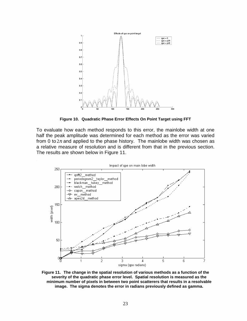
Typically, a quadratic phase error of 4/π is considered acceptable and errorsabove 2/π are considered excessive [6]. The effect of QPE on a point target forthese error levels can be seen below in Fig. 10. Clearly, the mainlobe widthwidens as the amount of error increases, thereby creating a loss in resolution. Wewill see how this affects the image quality on simulated data in Section V below.

23

Figure 10. Quadratic Phase Error Effects On Point Target using FFT

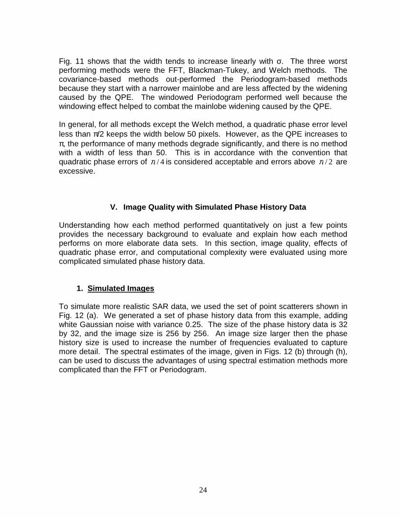
To evaluate how each method responds to this error, the mainlobe width at onehalf the peak amplitude was determined for each method as the error was variedfrom 0 to π2 and applied to the phase history. The mainlobe width was chosen asa relative measure of resolution and is different from that in the previous section.The results are shown below in Figure 11.

Figure 11. The change in the spatial resolution of various methods as a function of theseverity of the quadratic phase error level. Spatial resolution is measured as the

minimum number of pixels in between two point scatterers that results in a resolvableimage. The sigma denotes the error in radians previously defined as gamma.

24

Fig. 11 shows that the width tends to increase linearly with σ. The three worstperforming methods were the FFT, Blackman-Tukey, and Welch methods. Thecovariance-based methods out-performed the Periodogram-based methodsbecause they start with a narrower mainlobe and are less affected by the wideningcaused by the QPE. The windowed Periodogram performed well because thewindowing effect helped to combat the mainlobe widening caused by the QPE.

In general, for all methods except the Welch method, a quadratic phase error levelless than π/2 keeps the width below 50 pixels. However, as the QPE increases toπ, the performance of many methods degrade significantly, and there is no methodwith a width of less than 50. This is in accordance with the convention thatquadratic phase errors of 4/π is considered acceptable and errors above 2/π areexcessive.

V. Image Quality with Simulated Phase History Data

Understanding how each method performed quantitatively on just a few pointsprovides the necessary background to evaluate and explain how each methodperforms on more elaborate data sets. In this section, image quality, effects ofquadratic phase error, and computational complexity were evaluated using morecomplicated simulated phase history data.

1. Simulated Images

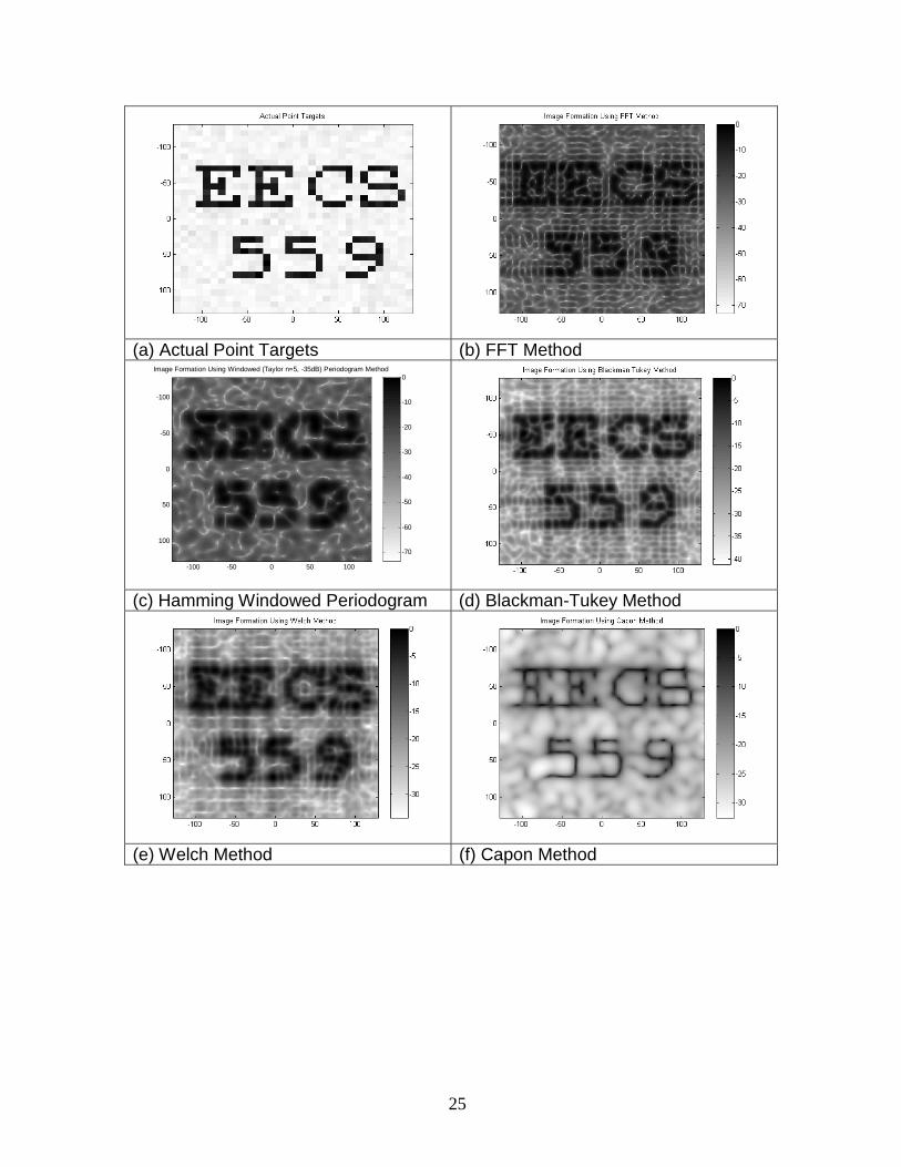
To simulate more realistic SAR data, we used the set of point scatterers shown inFig. 12 (a). We generated a set of phase history data from this example, addingwhite Gaussian noise with variance 0.25. The size of the phase history data is 32by 32, and the image size is 256 by 256. An image size larger then the phasehistory size is used to increase the number of frequencies evaluated to capturemore detail. The spectral estimates of the image, given in Figs. 12 (b) through (h),can be used to discuss the advantages of using spectral estimation methods morecomplicated than the FFT or Periodogram.

25

(a) Actual Point Targets (b) FFT Method

-70

-60

-50

-40

-30

-20

-10

0Image Formation Using Windowed (Taylor n=5, -35dB) Periodogram Method

-100 -50 0 50 100

-100

-50

0

50

100

(c) Hamming Windowed Periodogram (d) Blackman-Tukey Method

(e) Welch Method (f) Capon Method

26

-70

-60

-50

-40

-30

-20

-10

0Image Formation Using APES Method

-100 -50 0 50 100

-100

-50

0

50

100

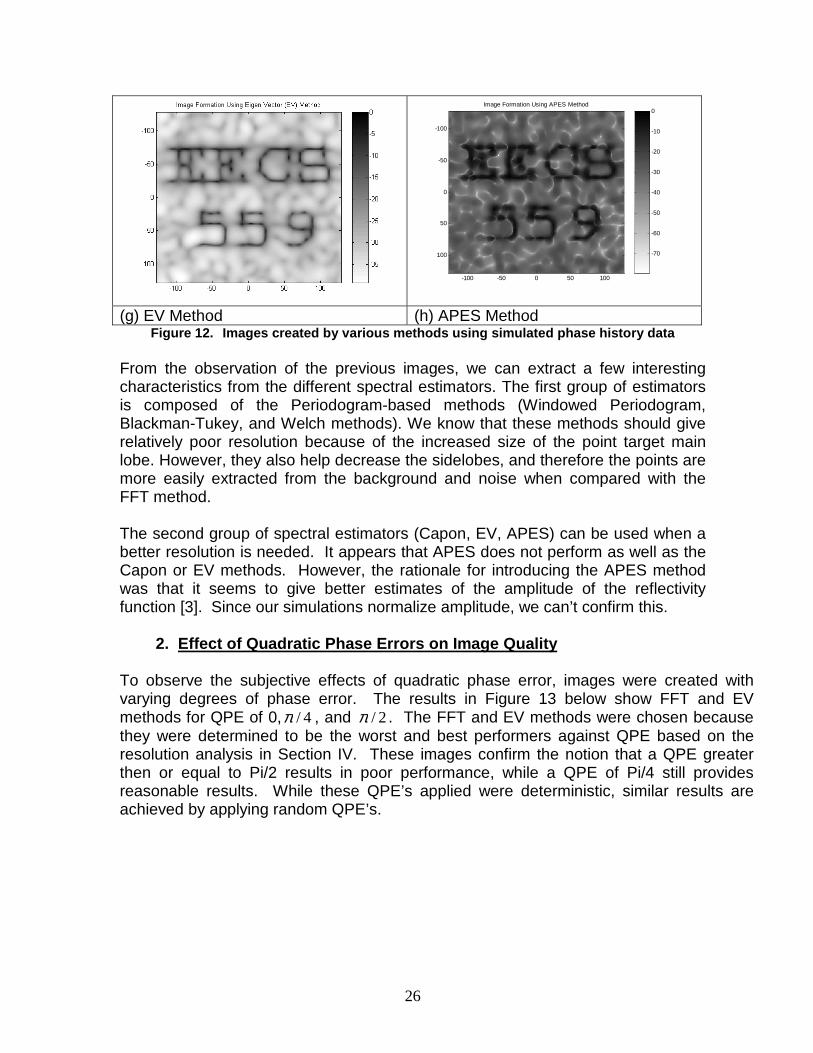
(g) EV Method (h) APES MethodFigure 12. Images created by various methods using simulated phase history data

From the observation of the previous images, we can extract a few interestingcharacteristics from the different spectral estimators. The first group of estimatorsis composed of the Periodogram-based methods (Windowed Periodogram,Blackman-Tukey, and Welch methods). We know that these methods should giverelatively poor resolution because of the increased size of the point target mainlobe. However, they also help decrease the sidelobes, and therefore the points aremore easily extracted from the background and noise when compared with theFFT method.

The second group of spectral estimators (Capon, EV, APES) can be used when abetter resolution is needed. It appears that APES does not perform as well as theCapon or EV methods. However, the rationale for introducing the APES methodwas that it seems to give better estimates of the amplitude of the reflectivityfunction [3]. Since our simulations normalize amplitude, we can’t confirm this.

2. Effect of Quadratic Phase Errors on Image Quality

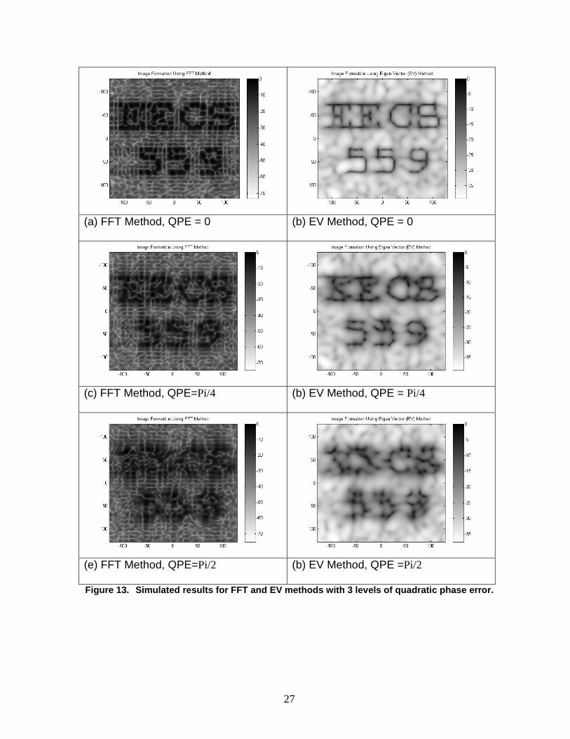
To observe the subjective effects of quadratic phase error, images were created withvarying degrees of phase error. The results in Figure 13 below show FFT and EVmethods for QPE of 0, 4/π , and 2/π . The FFT and EV methods were chosen becausethey were determined to be the worst and best performers against QPE based on theresolution analysis in Section IV. These images confirm the notion that a QPE greaterthen or equal to Pi/2 results in poor performance, while a QPE of Pi/4 still providesreasonable results. While these QPE’s applied were deterministic, similar results areachieved by applying random QPE’s.

27

(a) FFT Method, QPE = 0 (b) EV Method, QPE = 0

(c) FFT Method, QPE=Pi/4 (b) EV Method, QPE = Pi/4

(e) FFT Method, QPE=Pi/2 (b) EV Method, QPE =Pi/2

Figure 13. Simulated results for FFT and EV methods with 3 levels of quadratic phase error.

28

3. Computational Complexity

Although it was not an initial objective of this project, the computational complexityfor some of the methods became an issue during simulations. Using the simulateddata described above, the computation times for each method were determined inMATLAB. These are shown below in Table 2. These times were computed usinga Sun Workstation running Unix with 2048MB of memory.

Method Computation Time [sec]FFT 0.1236

Windowed Periodogram 0.2319Blackman Tukey 0.6223

Welch 17.5674Capon 617.4787

EV 617.7149APES 221.6561

Table 2: Comparison of Computation Times for Various Methods

Although the algorithms used were not optimized with respect to computation time,it is clear that the covariance-based methods require substantially more processingtime than the FFT and Periodogram-based methods. This issue becomes evenmore critical when larger phase histories and images need to be processed, or ifnear real-time processing is required. Theoretically, the covariance basedmethods are on the order of (KxxKy)

3 computations while the Periodogram basedmethods exploit the efficient FFT which is of the order of (NxM)log(NxM). TheAPES method, however, was implemented using a fast algorithm that provided athreefold increase in processing time. Similar algorithms may be possible for theCapon and EV methods. Ultimately, the covariance methods are limited by theinversion or eigen decomposition of the autocovariance matrix.

VI. Image Quality with Actual Phase History Data

We were fortunate in this project to be able to use actual SAR phase history datacollected by Veridian-ERIM International. This data was collected by the DataCollection System (DCS) air-to-ground X-band radar system mounted in a ConvairCV-580 aircraft. The image is of the area around the University of Michiganfootball stadium. In this section, we describe the processing of this data and relatesome issues that arise when using real phase history data. Then, our spectralestimators are applied to the data and the resulting images are shown.

1. Transitioning from Simulated to Real Data

Dealing with the much larger data set associated with actual SAR phase historydata presented significant computation challenges. With a phase history size of

29

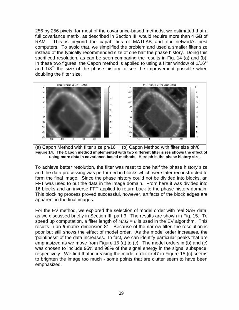
256 by 256 pixels, for most of the covariance-based methods, we estimated that afull covariance matrix, as described in Section III, would require more than 4 GB ofRAM. This is beyond the capabilities of MATLAB and our network’s bestcomputers. To avoid that, we simplified the problem and used a smaller filter sizeinstead of the typically recommended size of one half the phase history. Doing thissacrificed resolution, as can be seen comparing the results in Fig. 14 (a) and (b).In these two figures, the Capon method is applied to using a filter window of 1/16th

and 1/8th the size of the phase history to see the improvement possible whendoubling the filter size.

(a) Capon Method with filter size ph/16 (b) Capon Method with filter size ph/8Figure 14. The Capon method implemented with two different filter sizes shows the effect of

using more data in covariance-based methods. Here ph is the phase history size.

To achieve better resolution, the filter was reset to one half the phase history sizeand the data processing was performed in blocks which were later reconstructed toform the final image. Since the phase history could not be divided into blocks, anFFT was used to put the data in the image domain. From here it was divided into16 blocks and an inverse FFT applied to return back to the phase history domain.This blocking process proved successful, however, artifacts of the block edges areapparent in the final images.

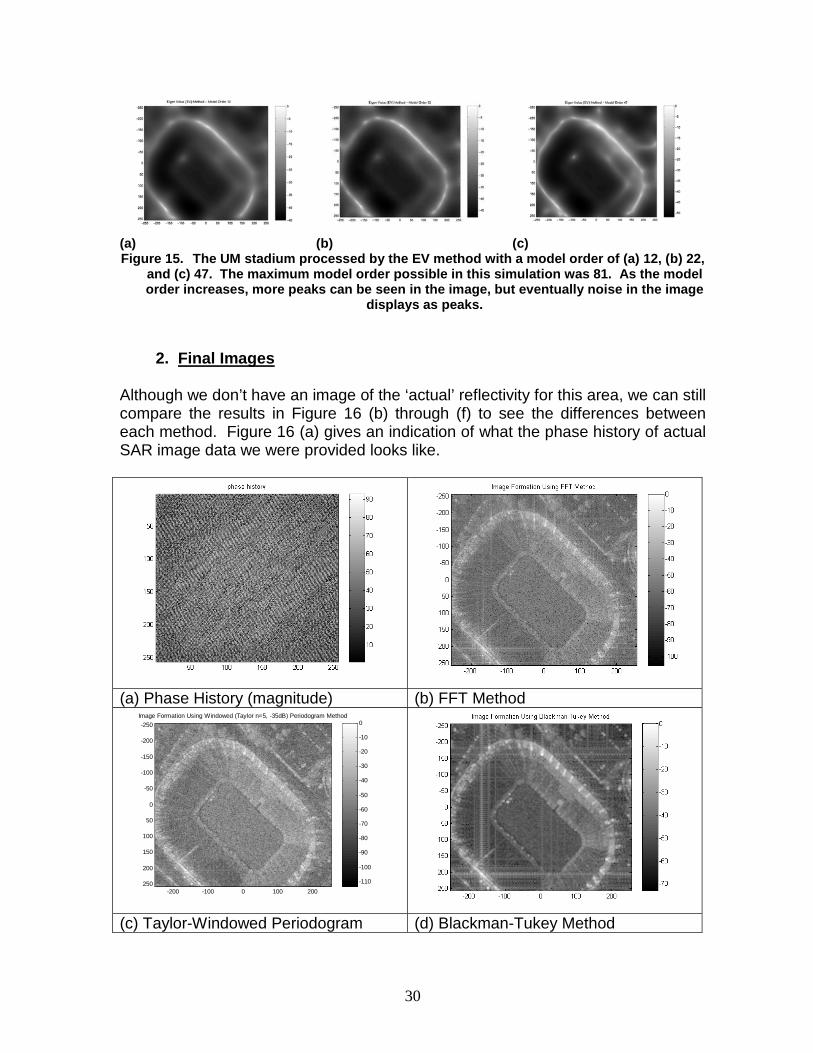
For the EV method, we explored the selection of model order with real SAR data,as we discussed briefly in Section III, part 3. The results are shown in Fig. 15. Tospeed up computation, a filter length of M/32 = 8 is used in the EV algorithm. Thisresults in an R matrix dimension 81. Because of the narrow filter, the resolution ispoor but still shows the effect of model order. As the model order increases, the'pointiness' of the data increases. In fact, we can identify particular peaks that areemphasized as we move from Figure 15 (a) to (c). The model orders in (b) and (c)was chosen to include 95% and 98% of the signal energy in the signal subspace,respectively. We find that increasing the model order to 47 in Figure 15 (c) seemsto brighten the image too much - some points that are clutter seem to have beenemphasized.

30

(a) (b) (c)Figure 15. The UM stadium processed by the EV method with a model order of (a) 12, (b) 22,

and (c) 47. The maximum model order possible in this simulation was 81. As the modelorder increases, more peaks can be seen in the image, but eventually noise in the image

displays as peaks.

2. Final Images

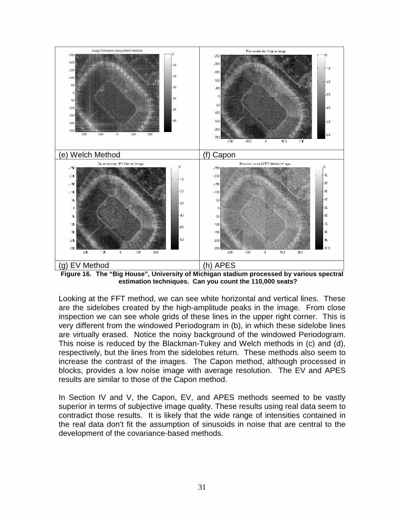
Although we don’t have an image of the ‘actual’ reflectivity for this area, we can stillcompare the results in Figure 16 (b) through (f) to see the differences betweeneach method. Figure 16 (a) gives an indication of what the phase history of actualSAR image data we were provided looks like.

(a) Phase History (magnitude) (b) FFT Method

-110

-100

-90

-80

-70

-60

-50

-40

-30

-20

-10

0Image Formation Using Windowed (Taylor n=5, -35dB) Periodogram Method

-200 -100 0 100 200

-250

-200

-150

-100

-50

0

50

100

150

200

250

(c) Taylor-Windowed Periodogram (d) Blackman-Tukey Method

31

-60

-50

-40

-30

-20

-10

0Image Formation Using Welch Method

-200 -100 0 100 200

-250

-200

-150

-100

-50

0

50

100

150

200

250

(e) Welch Method (f) Capon

(g) EV Method (h) APESFigure 16. The “Big House”, University of Michigan stadium processed by various spectral

estimation techniques. Can you count the 110,000 seats?

Looking at the FFT method, we can see white horizontal and vertical lines. Theseare the sidelobes created by the high-amplitude peaks in the image. From closeinspection we can see whole grids of these lines in the upper right corner. This isvery different from the windowed Periodogram in (b), in which these sidelobe linesare virtually erased. Notice the noisy background of the windowed Periodogram.This noise is reduced by the Blackman-Tukey and Welch methods in (c) and (d),respectively, but the lines from the sidelobes return. These methods also seem toincrease the contrast of the images. The Capon method, although processed inblocks, provides a low noise image with average resolution. The EV and APESresults are similar to those of the Capon method.

In Section IV and V, the Capon, EV, and APES methods seemed to be vastlysuperior in terms of subjective image quality. These results using real data seem tocontradict those results. It is likely that the wide range of intensities contained inthe real data don’t fit the assumption of sinusoids in noise that are central to thedevelopment of the covariance-based methods.

32

VII. Conclusion:

This project set out to explore various spectral estimation techniques that can beapplied to SAR imaging systems. As we had little background in SAR, extensiveresearch was conducted to understand the image formation process. This allowedus to accurately generate simulated data representative of the real SAR images towhich we could apply the spectral estimation techniques once they were derivedfor the 2-D case.

The techniques used were grouped together based on their similarities with thePeriodogram-based methods consisting of the Windowed Periodogram method,Blackman-Tukey method, and Welch method. Similarly, the remaining methods,Capon, EV, and APES were grouped together based on their extensive use of theautocovariance matrix. In the Periodogram based methods, the results show thatthe Welch and the Blackman-Tukey method do result in better noise performanceat the cost of increased bias. Additionally, there seemed to be a clear benefit inusing the Taylor window to reduce sidelobes. The covariance-based methodsprovided the best overall results on simulated data. This was based on resolution,MSE, and SNR criteria as well as subjective assessment of the simulated imagedata under various noise and phase error conditions. The subjective evaluation ofthe images revealed that resolution (or bias) has a larger effect on SAR imagequality than noise variance does.

Finally, applying the spectral estimation techniques to actual SAR data revealedsome surprises. The images created with the covariance-based methods didresult in images without sidelobes and with subjective image quality equal to thatof the Windowed Periodogram method, but they didn’t have as much of aresolution advantage as we would have expected. The covariance-based methodsalso come at the price of significantly increased computational complexity andmemory usage. While faster algorithms may be implemented, they are still limitedby the inversion or eigen decomposition of the covariance matrix. This issuebecame critical when large data sets of actual phase history data was used.

Which method is best? It depends on the application. Based on the real dataresults, it is hard to beat the Windowed Periodogram. It is apparent that thecovariance-based methods did not perform as well on actual data as they did onsimulated data. Perhaps this indicates a departure from the model of a sum ofsinusoids in noise. In particular, if the real scene is not just a set of pointscatterers that produce a linear combination of complex exponentials, then thecovariance-based methods will not perform as well as they did in the simulations[1].

Table 3 below summarizes our findings on the performance of various methods.Overall, these findings are inline with [1].

33

Method Advantages DisadvantagesFFT Fast, simple Large sidelobesWindowedPeriodogram

Fast, reducedsidelobes

Reduced resolution

Blackman Tukey Good noiseperformance

Large sidelobes

Welch Good noiseperformance

Poor Resolution

Capon High resolution High computational complexity,medium results w/ actual data

EV High resolution High computational complexity,medium results w/ actual data

APES High resolution, fasterthan Capon or EV

High computational complexity,medium results w/ actual data

Table 3: Summary of Characteristics of Each Method

Overall, this project provided great insight into issues associated with applyingtheoretical solutions to real engineering problems. This basic understanding willbe helpful in applying more advanced signal processing techniques in our futurecareers.

Lastly, the authors wish to thank Veridian-ERIM International for providing theactual SAR data for use in our analysis.

34

VIII. References

[1] DeGraaf, S. R. “SAR Imaging via Modern 2-D Spectral Estimation Methods”,IEEE Transactions on Image Processing, Vol. 7, No. 5, May 1998, pp. 729-761.

[2] Stoica P. and Moses R. Introduction to Spectral Analysis. Prentice Hall, UpperSaddle River, NJ, 1997.

[3] Li, J. and Stoica P. “An Adaptive Filtering Approach to Spectral Estimation andSAR Imaging”, IEEE Transactions on Signal Processing, Vol. 44, No. 6, June1996, pp. 1469-1484.

[4] Oliver, C. and Quegan, S. Understanding Synthetic Aperture Radar Images.Artech House, Boston, 1998.

[5] Munson, D.C., Jr. and Visentin, R.L. “A signal processing view of strip-mappingsynthetic aperture radar “, IEEE Transactions on Acoustics, Speech and SignalProcessing, Vol. 37, No. 12, Dec. 1989, pp. 2131 –2147.

[6] Carrara, W.G., Goodman, R.S., Majewski, R.M. “Spotlight Synthetic ApertureRadar-Signal Processing Algorithms “, Artech House, Norwood, MA, 1995.

[7] Kay, Stephen M. Modern Spectral Analysis. PTR Prentice Hall, Upper SaddleRiver, New Jersey, 1988.

[8] Jakobsson, A., Marple, L. Jr., and Stoica, P. “Computationally Efficient Two-Dimensional Capon Spectrum Analysis,” IEEE Transactions on Signal Processing,Vol. 48, No. 9, Sept 2000, pp. 2651-2661.

[9] Capon, J. “High Resolution Frequency-Wavenumber Spectrum Analysis”,Proceedings of the IEEE, Vol. 57, Aug. 1969, pp. 1408-1418.

[10] Liu, Z-S, Li, H, and Li, J. “Efficient Implementation of the Capon and APES forSpectral Estimation”, IEEE Transactions on Aerospace and Electronic Systems,Vol. 34, No. 4, Oct. 1998, pp. 1314-1319.

[11] Jakowatz, C., et al, “Spotlight-Mode Synthetic Aperature Radar: A SignalProcessing Approach”, Kluwer Academic Publishers, Boston, MA, 1996.