syrthes 4.2 user manual - edf 3/chercheurs/syrthes... · user manual for the syrthes code version...

SYRTHES 4.2

User Manual

I. Rupp, C. Peniguel

2014

EDF R&DMFEE

User Manual for the SYRTHES code Version 4.2 Version 1.0

AVERTISSEMENT / WARNING

L’acces a ce document, ainsi que son utilisation, sont strictement limites aux personnes ex-pressement habilitees par EDF.EDF ne pourra etre tenu responsable, au titre d’une action en responsabilite contractuelle, enresponsabilite delictuelle ou de tout autre action, de tout dommage direct ou indirect, ou dequelque nature qu’il soit, ou de tout prejudice, notamment, de nature financier ou commercial,resultant de l’utilisation d’une quelconque information contenue dans ce document.Les donnees et informations contenues dans ce document sont fournies ”en l’etat” sans aucunegarantie expresse ou tacite de quelque nature que ce soit.Toute modification, reproduction, extraction d’elements, reutilisation de tout ou partie de cedocument sans autorisation prealable ecrite d’EDF ainsi que toute diffusion externe a EDF dupresent document ou des informations qu’il contient est strictement interdite sous peine de sanc-tions.

——

The access to this document and its use are strictly limited to the persons expressly authorizedto do so by EDF.EDF shall not be deemed liable as a consequence of any action, for any direct or indirect damage,including, among others, commercial or financial loss arising from the use of any informationcontained in this document.This document and the information contained therein are provided ”as are” without any war-ranty of any kind, either expressed or implied.Any total or partial modification, reproduction, new use, distribution or extraction of elementsof this document or its content, without the express and prior written consent of EDF is strictlyforbidden. Failure to comply to the above provisions will expose to sanctions.

Accessibilite : EDF /143 c©EDF 2012

EDF R&DMFEE


Abstract

This document is the user manual of version 4 of the SYRTHES thermal code. It presents thescope of the code and the available diverse functions. The first chapters address the phenomenawhich can be modeled with syrthes.

syrthes includes a graphic interface which enables the user to become familiar with all theparameters necessary for the code. The different windows are described and the nature andmeaning of each parameter is detailed.

A methodology for the application of syrthes and its method of calculation are proposedherein.


EDF R&DMFEE


Executive Summary

This document is the user manual of the thermal code syrthes version 4.2.


EDF R&DMFEE


Contents

AVERTISSEMENT / WARNING . . . . . . . . . . . . . . . . . . . . . . . . . . . . . 2

Abstract . . . . . . . . . . . . . . . . . . . . . . . . . . . . . . . . . . . . . . . . . . . . 3

Executive Summary . . . . . . . . . . . . . . . . . . . . . . . . . . . . . . . . . . . . . 4

1 Introduction 11

2 Some information concerning this document 13

2.1 For whom is this manual written? . . . . . . . . . . . . . . . . . . . . . . . . . . . 13

2.2 Organization of the manual . . . . . . . . . . . . . . . . . . . . . . . . . . . . . . 13

2.3 How complete is this manual? . . . . . . . . . . . . . . . . . . . . . . . . . . . . . 14

3 Thermal conduction: functions and specificities 15

3.1 Thermal conduction . . . . . . . . . . . . . . . . . . . . . . . . . . . . . . . . . . 15

3.1.1 Simulated phenomena . . . . . . . . . . . . . . . . . . . . . . . . . . . . . 15

3.1.2 Geometrical aspects . . . . . . . . . . . . . . . . . . . . . . . . . . . . . . 16

3.1.2.1 Cartesian bidimensional simulations . . . . . . . . . . . . . . . . 16

3.1.2.2 Axisymmetrical bidimensional simulations . . . . . . . . . . . . 17

3.1.2.3 Tridimensional simulations . . . . . . . . . . . . . . . . . . . . . 17

3.1.2.4 List of the finite elements accepted by syrthes . . . . . . . . . 18

3.1.3 Materials handled . . . . . . . . . . . . . . . . . . . . . . . . . . . . . . . 18

3.1.3.1 Materials with isotropic behavior . . . . . . . . . . . . . . . . . . 19

3.1.3.2 Orthotropic Properties . . . . . . . . . . . . . . . . . . . . . . . 19

3.1.3.3 Anisotropic properties . . . . . . . . . . . . . . . . . . . . . . . . 20

3.1.4 Initial conditions . . . . . . . . . . . . . . . . . . . . . . . . . . . . . . . . 21

3.1.5 Boundary conditions . . . . . . . . . . . . . . . . . . . . . . . . . . . . . . 21

3.1.6 Volumetric source terms . . . . . . . . . . . . . . . . . . . . . . . . . . . . 24

3.1.7 Contact resistances . . . . . . . . . . . . . . . . . . . . . . . . . . . . . . . 24

4 Thermal radiation: function and specificities 27

4.1 Generalities . . . . . . . . . . . . . . . . . . . . . . . . . . . . . . . . . . . . . . . 27

4.2 The treatment of thermal radiation in syrthes . . . . . . . . . . . . . . . . . . . 28

4.3 Validation . . . . . . . . . . . . . . . . . . . . . . . . . . . . . . . . . . . . . . . . 28

4.4 Geometries . . . . . . . . . . . . . . . . . . . . . . . . . . . . . . . . . . . . . . . 28

4.5 Physical properties . . . . . . . . . . . . . . . . . . . . . . . . . . . . . . . . . . . 29

4.6 Boundary conditions . . . . . . . . . . . . . . . . . . . . . . . . . . . . . . . . . . 29

4.7 Solar radiation . . . . . . . . . . . . . . . . . . . . . . . . . . . . . . . . . . . . . 30

4.7.1 Calculation of solar radiation . . . . . . . . . . . . . . . . . . . . . . . . . 30

4.7.2 Shade . . . . . . . . . . . . . . . . . . . . . . . . . . . . . . . . . . . . . . 32

4.7.3 Horizon . . . . . . . . . . . . . . . . . . . . . . . . . . . . . . . . . . . . . 32

4.7.4 Example . . . . . . . . . . . . . . . . . . . . . . . . . . . . . . . . . . . . . 32


EDF R&DMFEE


5 Heat and mass transfer: function and specificities 35

5.1 Physical model . . . . . . . . . . . . . . . . . . . . . . . . . . . . . . . . . . . . . 35

5.1.1 Equation de conservation de la masse d’eau : . . . . . . . . . . . . . . . . 36

5.1.2 Equation de conservation de la masse d’air sec : . . . . . . . . . . . . . . . 36

5.1.3 Equation de conservation de la chaleur : . . . . . . . . . . . . . . . . . . . 36

5.2 List of symbols . . . . . . . . . . . . . . . . . . . . . . . . . . . . . . . . . . . . . 37

6 Coupling with a thermal hydraulic code 39

7 General Environment 41

7.1 Organization of the input data and the results . . . . . . . . . . . . . . . . . . . 42

7.1.1 Data files . . . . . . . . . . . . . . . . . . . . . . . . . . . . . . . . . . . . 43

7.1.2 Result files . . . . . . . . . . . . . . . . . . . . . . . . . . . . . . . . . . . 44

7.1.3 Storage/Memory file for view factors . . . . . . . . . . . . . . . . . . . . 45

7.1.4 Coupling syrthes with a thermal hydraulic code . . . . . . . . . . . . . . 45

7.2 Creating a mesh for syrthes . . . . . . . . . . . . . . . . . . . . . . . . . . . . . 45

7.3 Visualize syrthes results . . . . . . . . . . . . . . . . . . . . . . . . . . . . . . . 45

7.3.1 Conversion of syrthes results to Ensightformat . . . . . . . . . . . . . . 46

7.3.2 Conversion of results to med format . . . . . . . . . . . . . . . . . . . . . 46

8 Data files relative to SYRTHES 47

8.1 Geometric Files . . . . . . . . . . . . . . . . . . . . . . . . . . . . . . . . . . . . 47

8.1.1 Conduction mesh . . . . . . . . . . . . . . . . . . . . . . . . . . . . . . . . 47

8.1.2 Radiation mesh . . . . . . . . . . . . . . . . . . . . . . . . . . . . . . . . . 47

8.1.3 Formats of the mesh files . . . . . . . . . . . . . . . . . . . . . . . . . . . 48

8.2 Parameter files . . . . . . . . . . . . . . . . . . . . . . . . . . . . . . . . . . . . . 48

8.3 Standard weather data file . . . . . . . . . . . . . . . . . . . . . . . . . . . . . . . 48

8.3.1 Contents of the weather data file . . . . . . . . . . . . . . . . . . . . . . . 48

8.3.2 Example of use . . . . . . . . . . . . . . . . . . . . . . . . . . . . . . . . . 49

8.4 User data files . . . . . . . . . . . . . . . . . . . . . . . . . . . . . . . . . . . . . . 50

9 Interpreted functions 51

9.1 What can be defined with the interpreted functions? . . . . . . . . . . . . . . . . 51

9.2 How to define a function? . . . . . . . . . . . . . . . . . . . . . . . . . . . . . . . 52

9.3 Interpreted functions in syrthes . . . . . . . . . . . . . . . . . . . . . . . . . . . 52

10 Parameter file 53

10.1 Genaralities concerning the data file syrthes data.syd . . . . . . . . . . . . . . 53

10.2 Genaralities concerning the tables in the syrthes.gui interface . . . . . . . . . . 54

10.3 Home window . . . . . . . . . . . . . . . . . . . . . . . . . . . . . . . . . . . . . 57

10.4 Control of window . . . . . . . . . . . . . . . . . . . . . . . . . . . . . . . . . . . 58

10.4.1 Time management tab . . . . . . . . . . . . . . . . . . . . . . . . . . . 58

10.4.2 Solver information tab . . . . . . . . . . . . . . . . . . . . . . . . . . . 60

10.5 Window: File Names . . . . . . . . . . . . . . . . . . . . . . . . . . . . . . . . . 61

10.6 Parameters for conduction . . . . . . . . . . . . . . . . . . . . . . . . . . . . . . 64

10.6.1 Window: Initial conditions . . . . . . . . . . . . . . . . . . . . . . . . . 64

10.6.2 Window: Boundary conditions . . . . . . . . . . . . . . . . . . . . . . 64

10.6.2.1 Heat exchange tab . . . . . . . . . . . . . . . . . . . . . . . . 65

10.6.2.2 Flux tab . . . . . . . . . . . . . . . . . . . . . . . . . . . . . . . 66

10.6.2.3 Dirichlet tab . . . . . . . . . . . . . . . . . . . . . . . . . . . . 67


EDF R&DMFEE


10.6.2.4 Contact resistance tab . . . . . . . . . . . . . . . . . . . . . . 68

10.6.2.5 Infinite radiation tab . . . . . . . . . . . . . . . . . . . . . . . 69

10.6.3 Physical properties window . . . . . . . . . . . . . . . . . . . . . . . . 69

10.6.3.1 Isotropic tab . . . . . . . . . . . . . . . . . . . . . . . . . . . . 70

10.6.3.2 Orthotropic tab . . . . . . . . . . . . . . . . . . . . . . . . . . 70

10.6.3.3 Anisotropic tab . . . . . . . . . . . . . . . . . . . . . . . . . . 71

10.6.4 Volumetric conditions window . . . . . . . . . . . . . . . . . . . . . . . 73

10.6.5 Window: periodicity . . . . . . . . . . . . . . . . . . . . . . . . . . . . . 74

10.7 Management of code output: Output window . . . . . . . . . . . . . . . . . . . 76

10.7.1 Management of intermediary results . . . . . . . . . . . . . . . . . . . . . 76

10.7.2 Field of maximum temperatures . . . . . . . . . . . . . . . . . . . . . . . 77

10.7.3 Probes tab . . . . . . . . . . . . . . . . . . . . . . . . . . . . . . . . . . . 77

10.7.4 Surface balance tab and Volume balance tabs . . . . . . . . . . . . . 79

10.8 Parameters for radiation . . . . . . . . . . . . . . . . . . . . . . . . . . . . . . . 80

10.8.1 Window: Spectral parameters . . . . . . . . . . . . . . . . . . . . . . . 80

10.8.2 Window: View Factors . . . . . . . . . . . . . . . . . . . . . . . . . . . 81

10.8.3 Window: View Factors - symmetry and periodicity . . . . . . . . . 82

10.8.4 Window: Material Radiation Properties . . . . . . . . . . . . . . . . 84

10.8.5 Window: Boundary conditions . . . . . . . . . . . . . . . . . . . . . . 85

10.8.6 Window: Boundary conditions - imposed temperature . . . . . . . 86

10.8.7 Window: Boundary conditions - Imposed Flux . . . . . . . . . . . . 87

10.8.8 Window: Boundary conditions - Problem with aperture . . . . . . 88

10.9 Parameters for models of humidity . . . . . . . . . . . . . . . . . . . . . . . . . . 89

10.9.1 Control window . . . . . . . . . . . . . . . . . . . . . . . . . . . . . . . . 90

10.9.2 Window: Humidity - Inital conditions . . . . . . . . . . . . . . . . . . 92

10.9.3 Window: Humidity - Material properties . . . . . . . . . . . . . . . . 94

10.9.4 Window: Humidity - Coupled Boundary Conditions . . . . . . . . . 95

10.9.5 Window: Humidity - Volumetric source terms . . . . . . . . . . . . 96

10.10 Window: Conjugate Heat Transfer . . . . . . . . . . . . . . . . . . . . . . . . 98

11 Data for heat and mass transfers 101

11.1 Data in the file syrthes data.syd . . . . . . . . . . . . . . . . . . . . . . . . . . 101

11.1.1 General data . . . . . . . . . . . . . . . . . . . . . . . . . . . . . . . . . . 101

11.1.2 Manage the precision of the solvers . . . . . . . . . . . . . . . . . . . . . 101

11.1.3 Definition of materials . . . . . . . . . . . . . . . . . . . . . . . . . . . . . 101

11.1.4 Boundary conditions . . . . . . . . . . . . . . . . . . . . . . . . . . . . . . 101

11.2 Materials library . . . . . . . . . . . . . . . . . . . . . . . . . . . . . . . . . . . . 101

11.2.1 Data structure . . . . . . . . . . . . . . . . . . . . . . . . . . . . . . . . . 101

11.2.2 How are the properties of the materials defined? . . . . . . . . . . . . . . 102

11.2.3 How are the diverse functions used? . . . . . . . . . . . . . . . . . . . . . 103

11.2.4 How can a new material be defined? . . . . . . . . . . . . . . . . . . . . . 103

11.2.4.1 To create the new material . . . . . . . . . . . . . . . . . . . . . 103

11.2.4.2 To use the new material in syrthes run . . . . . . . . . . . . . 104

12 User functions 105

12.1 Description of the variables included in the user functions . . . . . . . . . . . . . 105

12.2 Functions of file user.c . . . . . . . . . . . . . . . . . . . . . . . . . . . . . . . . 107

12.2.1 Reading a specific data file: user read myfile() . . . . . . . . . . . . . . . 107

12.2.2 Writing additional variables in the result file: user add var in file() . . . . 107


EDF R&DMFEE


12.2.3 Definition of a specific transformation of periodicity: user transfo perio() 108

12.3 Functions of the file user cond.c . . . . . . . . . . . . . . . . . . . . . . . . . . . 108

12.3.1 Initialization of the temperature: user cini() . . . . . . . . . . . . . . . . . 108

12.3.2 Physical characteristics: user cphyso() . . . . . . . . . . . . . . . . . . . . 108

12.3.3 Boundary conditions: user limfso() . . . . . . . . . . . . . . . . . . . . . . 109

12.3.4 Volumetric source terms: user cfluvs() . . . . . . . . . . . . . . . . . . . . 109

12.3.5 Contact resistance: user resscon() . . . . . . . . . . . . . . . . . . . . . . 110

12.4 Functions for file user ray.c . . . . . . . . . . . . . . . . . . . . . . . . . . . . . 110

12.4.1 Function user ray() . . . . . . . . . . . . . . . . . . . . . . . . . . . . . . . 110

12.4.2 Function user solaire() . . . . . . . . . . . . . . . . . . . . . . . . . . . . . 111

12.4.3 Function user propincidence() . . . . . . . . . . . . . . . . . . . . . . . . . 111

12.5 Functions to assist with parallel computations . . . . . . . . . . . . . . . . . . . . 111

12.5.1 Calculation of a sum . . . . . . . . . . . . . . . . . . . . . . . . . . . . . . 111

12.5.2 Calculation of a minimum or a maximum of a variable . . . . . . . . . . . 111

13 Result files 113

13.1 Result files: additionnal . . . . . . . . . . . . . . . . . . . . . . . . . . . . . . . . 113

13.1.1 Contents of additional files . . . . . . . . . . . . . . . . . . . . . . . . . . 113

13.1.2 Principle . . . . . . . . . . . . . . . . . . . . . . . . . . . . . . . . . . . . 113

13.1.3 How to write variables in an additional file? . . . . . . . . . . . . . . . . . 114

14 Do a thermal calculation with syrthes 115

14.1 Introduction . . . . . . . . . . . . . . . . . . . . . . . . . . . . . . . . . . . . . . . 115

14.2 Preliminary phase: set a syrthes environment . . . . . . . . . . . . . . . . . . . 115

14.3 Running calculation with syrthes interface . . . . . . . . . . . . . . . . . . . . . 115

14.4 Run a manual calculation (without the syrthes.gui) . . . . . . . . . . . . . . . 118

14.4.1 Step 1: Create a new calculation case . . . . . . . . . . . . . . . . . . . . 118

14.4.2 Step 2: Create a mesh and convert it to syrthes format . . . . . . . . . 118

14.4.3 Step 3: Filling in the data file syrthes data.syd . . . . . . . . . . . . . . 119

14.4.4 Step 4 (optional): User functions . . . . . . . . . . . . . . . . . . . . . . . 119

14.4.5 Step 4: Create an executable program and run syrthes . . . . . . . . . . 120

14.4.6 Step 5: Visualize the results . . . . . . . . . . . . . . . . . . . . . . . . . . 122

14.5 Do a follow-up calculation . . . . . . . . . . . . . . . . . . . . . . . . . . . . . . . 122

14.6 Emergency stop of syrthes calculation . . . . . . . . . . . . . . . . . . . . . . . 122

14.7 Analysis of the results . . . . . . . . . . . . . . . . . . . . . . . . . . . . . . . . . 122

14.8 The generation of syrthes meshes . . . . . . . . . . . . . . . . . . . . . . . . . . 123

14.9 Calculating with a CFD code coupled to syrthes . . . . . . . . . . . . . . . . . 124

15 Conclusion 125

A syrthes FILE FORMATS 127

A.1 Description of the geometry file: file.syr . . . . . . . . . . . . . . . . . . . . . . 127

A.2 Result files: file.res . . . . . . . . . . . . . . . . . . . . . . . . . . . . . . . . . 129

A.3 Transient result file: file.rdt . . . . . . . . . . . . . . . . . . . . . . . . . . . . 130

A.4 Additional result file: file.add . . . . . . . . . . . . . . . . . . . . . . . . . . . . 131

A.5 Time record history probe results: file.his . . . . . . . . . . . . . . . . . . . . 131

A.6 Surfface or volume balance: file.flu . . . . . . . . . . . . . . . . . . . . . . . . 132

B syrthes keywords file: syrthes data.syd 133


EDF R&DMFEE


C Physical quantities and units of measurement 139

D Internet links 141


EDF R&DMFEE



EDF R&DMFEE


Chapter 1

Introduction

In numerous industrial processes, thermal phenomena play a preponderant role in the mechan-ical structure of materials.

In the case of thermal shocks, for example, when certain components are subjected to brusque orsignificant variations of temperature. The resulting differential expansions can cause mechanicalstress which provokes the appearance of fissures and cracks.

For a long time, the study of these phenomena and the optimization of procedures have reliedon experience and parametric trial studies. Independent of the often elevated cost, the experi-mental approach has only led to a limited number of locations where the quantitative values areaccessible (in fact, only where sensors can be placed).

With the advent of increasingly powerful computers, it is now more interesting to propose nu-meric tools which enable the simulation of phenomena having an impact on the different systemsof the industrial process. Indeed, a flexible tool, well-adapted to the understanding of the phe-nomena and to parametric studies is now available.

It is with this objective that the Syrthes code of thermal conduction and radiation has beendeveloped syrthes.

The manual includes the essential functions offered by syrthes for simulation as well as themethod to apply them.


EDF R&DMFEE



EDF R&DMFEE


Chapter 2

Some information concerning thisdocument

The purpose of this document is to render the syrthes 4 code of thermal solid and radiationeasier and more pleasant to use.

The different functions of the code as well as the input data are described.

Moreover, syrthes includes a particular function which enables it to be interfaced with a CFDcode for the simulation of industrial configurations where the fluid and solid interact thermally.syrthescan be coupled with the CFD Code Code Saturne [1].

2.1 For whom is this manual written?

The manual targets the occasional user with a good knowledge of pre- and post-processors havingbeen trained, even minimally, on the syrthes solid thermal code.

In cases of use when coupled with a thermal hydraulic code, it is assumed that the user also hasexcellent knowledge of the latter. Complete beginners are advised to have some training, evenif short, on how to best deal with thermal problems using this tool. If not, the user can startby following the tutorial and doing the case studies which are provided in the distribution.

2.2 Organization of the manual

This manual has been divided into diverse chapters having different objectives. The detailedtable of contents (at the beginning of the manual), the index, as well as the structure of thedocument are meant to facilitate the search and access of desired information. The recapitulativetables in the appendix can also contribute to either directly answer user questions or to indicatewhere a more detailed explanation can be found.

Chapter 3 is very general with the objective of presenting the full potential of syrthes andto evoke some general principles used by the code designers. Reading it can be useful for anyinexperienced user or by users with questions concerning the adequacy between the possibilitiesoffered by this version of the code and the problem they would like to treat. In addition, thesecond part of the chapter is important as it outlines certain conventions and methodologieswhich are used in syrthes.


EDF R&DMFEE


Chapter 7 describes the architecture of the software which can help the user organize the sim-ulation. In particular, this chapter outlines the different files and tools which are used both upand downstream of a calculation. It describes in detail the utility programs used to produce thefiles in the different post-processor formats.

Chapter 8 concerns data files used during a calculation. Chapter 10 is entirely devoted to theinput of the parameters for the calculation, this being a major step in the successful completionof a study. All the parameters and their impact on the calculation are explained in detail.

Chapter 12 concerns the user functions. Note that in numerous cases it is not necessary toemploy these functions, the use of keywords or of the function ”interpretee” being sufficient.Each of these functions is described in detail.

Chapter 14 offers a possible methodology to do a calculation. Users may thus find valuableinformation assembled in the chapter to develop the most appropriate working method of theirown.

Finally, the appendix includes the description of the formats of different Syrthes data and resultfiles as well as recapitulative tables which synthesize the input and give the user rapid access tothe information.

2.3 How complete is this manual?

The objective of this manual is to describe the use of syrthes, not to describe the numericalmethods used or to give all the elements necessary to the extension of syrthesfunctions.

When Syrthes calculations are coupled with a CFD code, it is assumed that the user has recourseto the appropriate manuals relative to the CFD code (for example [1]).

Those interested in an overview of the methods used in syrthes can consult, among others,[8]. This reference describes certain theoretical and numerical aspects used in version 1.0. Thefundamental equations and basic numerical methods remain applicable in the current version ofthe code.

Diverse configurations illustrating the code application domain can be found on the syrthescode web site [4] and in the validation manual [3].


EDF R&DMFEE


Chapter 3

Thermal conduction: functions andspecificities

The objective of this chapter is to give a precise idea of the potentialities of the syrthescodein the domain of thermal conduction.

To begin, the physical phenomena which have been taken into consideration will be discussedfollowed by the choices of modeling which have been made. Finally, the principle conventionsused in syrthes can be found in this chapter.

Thus, this chapter should be referred to:

• to verify if the problem to be treated is covered in the scope of application of this version

• to understand certain mechanisms affecting the modeling

• to become familiar with the convention that has been chosen

• to find information on the principles used and the functioning of the graphical user interface(GUI)

The objective of this chapter is not to explain how a function works and even less the under-lying theory, but to make apparent its existence. The elements and operations relative to theimplementation are addressed in the following chapters of this document.

3.1 Thermal conduction

The different capabilities of syrthes are described succinctly, highlighting the advantages anddisadvantages of each. Readers should be warned against the apparent complexity upon a firstreading. Indeed, it must be emphasized that in the majority of cases only one aspect or morelikely a small part of the possibilities offered will be concerned.

The different possibilities are classed in ascending order of difficulty and of probability of occur-rence.

3.1.1 Simulated phenomena

When different parts of a solid body have different temperatures, the heat spreads from the”hot” regions to the ”cold” ones. This transfer is essentially done in three different ways:


EDF R&DMFEE


• conduction (heat is transferred within the material itself)

• convection (heat is transferred by the displacement of one part of the body to other parts ofthe same body)

• radiation (heat is transferred at a distance by electromagnetic radiation)

Convection is taken into account by the CFD code. Conduction and radiation in a transparentenvironment are treated by the syrthescode. The study can be made by taking radiation intoconsideration in a semi-transparent environment if the CFD code includes such a possibility.

The application of a theorem can establish, for a solid, the following type of equation:

ρCp∂T

∂t= −div ~q +Φ

Where ρ is the volumetric mass and Cp is the specific heat of the material. The temperature Tis unknown. The left side of the equation constitutes the time dependence of the phenomenon,the right side characterizes the way in which the heat is propagated in a continuous environment(~q represents the heat flux), Φ is here a volumetric source term.

This equation is applicable to the phenomenon of heat transmission in an environment witha single behavior. At the domain boundary, several types of phenomena can be separately orsimultaneously present. For the modeling of phenomena, a panoply of boundary conditions isoffered to the user and is detailed in a paragraph at the end of this chapter.

This equation can take diverse forms depending on the approximations that the user is readyto make relative to the case. Cases where the geometric characteristics restrict the dimensionof the simulation to 2 (Cartesian or axisymmetrical) are particularly detailed.

3.1.2 Geometrical aspects

Fundamentally, space is three-dimensional. Occasionally, the phenomenon acts independentlyfollowing one direction in space. Very often, the validity of an approximation is directly relatedto the experience of the user. It is thus tempting to resolve the phenomenon in only thecorresponding sub-space, which greatly reduces the difficulty (and the cost) of the study.

From this perspective (and to avoid hampering the possibilities of interfacing with CFD codes),syrthes can also execute Cartesian 2-dimensional and axisymmetrical simulations.

3.1.2.1 Cartesian bidimensional simulations

Figure 3.1: Bidimensional approximation


EDF R&DMFEE


The equation is thus written in a 2-dimensional space (x, y), therefore the temperature, physicalproperty of the materials, boundary conditions and all relative elements to the simulation aredependent on only two spatial variables. The discretization of the equation (2-1) is done on afinite element 3-node triangular mesh (given by the user) generated, for example, by simail orIdeas-MS. Only right angles of the triangles can be used.

3.1.2.2 Axisymmetrical bidimensional simulations

Other cases exploit the fact that in certain problems revolution symmetry exists in one part.It is, for example, impossible to differentiate the behavior, geometry or solicitation of one slicefrom another. Thermal phenomenon is thus calculated in a plane whose thickness is assumed tobe null, the 3-dimensional aspect being integrated implicitly in the equation itself. There again,reducing the problem from 3-dimensional to 2-dimensional space leads to calculations that aresignificantly less complex yet as exact, providing of course, that the basic hypothesis is indeedvalid.

In syrthes either the Ox or Oy axis of axisymmetry can be chosen.

There again, the discretization depends on the same 3-node triangular elements.

Figure 3.2: Axisymmetric approximation

3.1.2.3 Tridimensional simulations

When the space of the resolution is compatible with the space of the phenomenon, no restric-tion or approximation is necessary. The discretization is done with the 4-node non-structuredtetrahedral mesh with planar faces. The tetrahedral mesh is generated by simail or Ideas-MSor any other software providing that the information relative to the geometry conforms to oneof the two formats or to the syrthes format (Cf. 13).


EDF R&DMFEE


3.1.2.4 List of the finite elements accepted by syrthes

Figure 3.3: Tetrahedrons used by syrthes in 3D

Figure 3.4: 2D Triangles used by syrthes in 2D or as radiation elements in 3D

Figure 3.5: Segments used by syrthes as radiation elements in 2D

3.1.3 Materials handled

All bodies transfer heat. Nevertheless, their conductive behavior can vary considerably fromone material to another. It is necessary, therefore, to differentiate the materials which impactthe problem. Sometimes, their behavior even becomes dependent in a continuous fashion on thespace, for example, in cases where their characteristics depend on local variables. Often, it is thelocal temperature which modifies the characteristics of the material. In this case, the equation(2-1) will become necessarily non-linear, but the variation of the characteristics defining the


EDF R&DMFEE


material is, most of the time, slow (in time). Thus, the characteristics corresponding to thelocal temperature of the preceding time step can be used.

Density, heat capacity, and conductivity are among the properties which define a conductiveenvironment. For example:

• ρ = rho(x, y, z, t, T, . . . )

• Cp = Cp(x, y, z, t, T, . . . )

• k = k(x, y, z, t, T, . . . )

These properties are defined simply by keywords if they are constant or if they are expressed asa function. In the most complex cases, a user function (cphyso.c)) is available to define for eachelement of the domain these different properties.

For modeling, the flux (a fundamentally continuous quantity) is linked to the local tempera-ture gradient by the intermediary of the conductivity (noted k). Depending on the material,this quantity is either a scalar or a matrix. The following paragraphs examine the differentpossibilities that can occur.

3.1.3.1 Materials with isotropic behavior

This case is most frequently encountered. It corresponds to a solid which, when subjected tocontact at one point, diffuses this heat isotropically in space (the isothermal heat contours formconcentric circles in 2 dimensions and spheres in 3 dimensions). This can be interpreted as aco-linearity of flux and temperature gradient. The expression of the flux is therefore expressedby the classic Fourier Law:

~q = −k−−→grad T

Thus, only one scalar value needs to be defined in each node of the mesh (and likewise, only onescalar value when the conductivity is identical throughout the domain). This choice is certainlythe most economical in terms of memory space and allows for the most complicated calculations.This choice represents the vast majority of applications.

3.1.3.2 Orthotropic Properties

Occasionally, heat in a body is not propagated isotropically, meaning that subsequent to contactwith one point in space, there will be one principal direction of heat transmission. This can bethe case in composite materials, or materials. When conductive properties of the material arealigned with the reference axes, material behavior is said to be orthotropic.


EDF R&DMFEE


Figure 3.6: Example of material with orthotropic behavior

Conductivity is then represented by a matrix such as the following:

K =

kxx 0 00 kyy 00 0 kzz

In this matrix, each coefficient (kxx for example) remains variable in time, space,. . . and candepend on all the accessible local parameters.

3.1.3.3 Anisotropic properties

The functions of the previous cases can be applied to anisotropic materials, meaning whendifferent conductive behaviors of a material cannot be aligned relative to the reference axeschosen for the calculation. The following figure presents a structure whose behavior can beanisotropic.

Figure 3.7: Example of material with anisotropic behavior


EDF R&DMFEE


The conductivity is thus represented by a matrix such as that below:

K =

kxx kxy kxzkyy kyz

kzz

Remark: As the matrix is symmetrical and positive, there is always a reference point in whichit can be expressed diagonally. This property is used to enter the data via the keywords when,as is often the case, the matrix of conductivity relative to the point of reference is known for thematerial in question. Nevertheless, the user function (user cond.c(user cphyso)) can programthe most general possible behavior. However, use of this model necessitates more significant ITresources in terms of memory and higher calculation costs, making the distinction between thedifferent behaviors interesting.

3.1.4 Initial conditions

The temperature of the solid must be set at an initial time t (which is generally taken as thepoint of origin). This distribution of the temperature can be continuous or discontinuous, butphysically, considering the regularizing nature of the diffusion operator, a continuous distributionappears rapidly.

Most often, the initial temperature is considered as constant throughout the domain. To facili-tate the introduction of this data, a keyword allows a constant value to be imposed on the entiredomain or on the defined sub-domains with the assistance of the numbers of the materials.

In the most complex cases, where the initial temperature can be defined with the aid of functions(on the domain or sub-domains), it is also possible to define them in the data file via theinterpreted/ interface functions (9).

As a last resort, if the treated case requires a very specific initial condition, the user functionuser cond.c (user initmp) designed for this purpose, can be used. Details concerning the useof keywords and the user function can be found in chapters 8 and 12.

3.1.5 Boundary conditions

In order to completely describe the problem and to resolve it numerically, different conditionsaffecting the domain boundaries must be defined. syrthes boundary conditions are quite classic.They are outlined in this paragraph. The boundary conditions can be of several types:

• Dirichlet(imposed temperature value)It is considered that at the boundary, the temperature is constant or variable relative totime and space but in a continuous manner. It is a condition relatively simple to introduceeven if it often constitutes an approximation. Indeed, from an experimental point of view(even in the laboratory) imposing temperature of a surface is extremely difficult.This condition is imposed on the boundary faces of the domain; the code automaticallytranscribes it internally on the corresponding nodes.


EDF R&DMFEE


The imposed temperature value can be set on all or part of the boundary. The correspond-ing can be identified by referencing them in the mesh generator. Similarly, if the Dirichletcondition can be expressed as a function, the function can also be input in the data file (9).If, however, the case is more complex, the user function user cond.c (user limfso), canbe used (see chapter 12 for instructions).

• fluxAnother very common boundary condition is imposed flux. The flux is imposed on theboundary faces.

Similar to Dirichlet conditions and depending on the complexity of the problem, either thekeyword file can be used to input a constant value or an interface function (”interpretee”)(see chapters 10 and 9). A user function can handle very complex cases. A detaileddescription of the use of the corresponding function user cond.c (user limfso).can befound in chapter 12.

• heat exchange coeffcientIn many physical cases, the flux is proportional to the temperature difference existing be-tween the temperature surface (noted T ) and the temperature of the surrounding mediumin which the solid is located (noted To). The flux can thus be expressed as the formh(T − To). The quantity h is generally called the heat exchange coefficient which is ex-pressed in W/mK. In the case of a forced flow, this parameter is generally related to thelocal velocity of the fluid, to its nature, as well as to the local fluid characteristics.

Following the same logic, depending on the complexity of the case to be treated, either thekeyword file or the GUI (see chapters 10 and 9) can be used to define the values, or a userfunction user cond.c (user limfso) (a description of which can be found in chapter 12.Note that two parameters are required on each face. The first is the temperature value ofthe external medium; the second parameter represents the heat exchange coefficient.

• infinite radiationHere, a boundary condition must not be confused with the calculation of the thermal ra-diation in a confined medium . On the domain boundary, only the heat exchange whichcorresponds to the loss (or gain) by radiation of the object relative to its exterior sur-rounding environment is calculated.

Both the emissivity of the material and the temperature of the environment can be defined.These parameters will be the constants or the interface functions ”interpretees” in the datafiles, or can be programmed in the user function user cond.c (user limfso).

• symmetryIn many studies, the domain of calculation can be advantageously reduced if it has sym-metries. The calculation can thus be done on 1/2, 1/4 or 1/8 (in three dimensions) of thedomain. For conduction, a condition of symmetry is equivalent to a adiabatic (zero flux)condition which does not require any particular parameters. It will not appear in the datafiles for conduction, but it is mandatory to specify it in cases of thermal radiation.


EDF R&DMFEE


• periodicityThe periodic boundary conditions can be applied between two faces having any orientation,the possible geometric transformation which enables them to be connected being anytranslation or rotation in space (or composed of rotations following the three directions inspace).

Figure 3.8 illustrates how to handle a problem on a reduced domain by employing periodicboundary conditions of rotation:

Figure 3.8: Periodicity of rotation

Note that it is possible to handle several directions of periodicity simultaneously (up to2 in 2D and 3 in 3D) enabling very large plates having a repetitive pattern to be treatedeasily and exactly.

Figure 3.9: Application having periodicity in 2 directions simultaneously


EDF R&DMFEE


In the example seen in figure 3.10, the reduced calculation domain of the periodic patternrequires taking into account two directions of periodicity:

Figure 3.10: Application of a periodic case in 2 simultaneous directions

3.1.6 Volumetric source terms

Sometimes, certain physical mechanisms lead to the appearance of heat within the solid itself.This is typically the case for metallic bodies submitted to electromagnetic phenomena. Theresulting Joule effect can be modeled by a volumetric flux.

With syrthes source terms (or volumetric flux) can be imposed on the elements in all or part ofthe domain. They can be variable in space and time. The simple case of a constant volumetricflux on a well-identified sub-domain can be handled with the GUI and/or the keyword file (seechapter 10). The same is true for cases where the flux can be defined in the form of an interpreted(9). For more complex situations, programming of the most complex variations can be donewith a user function user cond.c (user cfluvs).

3.1.7 Contact resistances

In some industrial mechanisms, often solid pieces belonging to a system are composed of differentmaterials. These materials are often glued or bolted together, and heat transfer occurs betweenthem. A more precise study of heat transfer shows that even if the two different materials appearoptically perfectly sealed, they are not sufficiently interlocked to be considered as forming onecontinuous medium. A small gap of air may create a discontinuous temperature field. However,the flux remains continuous.

This type of modeling is also used to simulate a defect in a solid or the behavior of a fissure. Thesolid cannot therefore be considered as continuous but, likewise, it is also impossible to considertotal independence between the two boundaries. Indeed, a continuous heat flux can breach thegap.

The notion of contact resistance between the two pieces is thus introduced. It is, in fact, a heatexchange condition between the two faces in contact where the external condition constitutesthe temperature of the face on the other side of the gap. Unlike boundary conditions previouslydescribed, temperatures of both faces remain unknown in the problem and are likely to vary ateach point at each time step.


EDF R&DMFEE


Figure 3.11: Contact resistance

The following relationships can be noted:{g (Ta − Tb) = ka grad Tg (Tb − Ta) = kb grad T

where Ta and Tb are unknowns in the equation.

Either the keywords file described in chapter 10 can be used to set the proper value of thecontact resistance or a function describing the variation of this resistance (9). For complexconfigurations, the user function user cond.c (user limfso). can be employed.

Warning: In practice, the determination of the coefficient g may prove to be delicate. Signifi-cant empirical observation is necessary as well as a quantification of the imbrications of the twomedia concerned requiring a certain know-how.


EDF R&DMFEE



EDF R&DMFEE


Chapter 4

Thermal radiation: function andspecificities

4.1 Generalities

All substances continually emit electromagnetic radiation over a wide frequency band. Thisradiation is, in fact, related to the internal energy of the body. The higher the internal energy, thehigher the electromagnetic agitation, which is accompanied by the emission of ultra-relativisticelementary particles. Inversely, the energy transmitted as electromagnetic radiation excites theelectrons in the medium, thereby increasing the systems internal energy.

This mode of heat transfer is quite different from that of convection or conduction. Indeed, thereis no need for a support medium1. Instead of a simple flux vector2 as in the case of conduction,the radiative flux corresponds to the total of radiation emitting from all directions in space. Thisleads to an integral formulation. When the three heat transfer modes (convection, conductionand radiation) are coupled together, the resolution of an integro-differential equation is oftenvery difficult.

In an enclosure, complex radiation heat exchanges are present when radiation leaves one cell toattain a position in space where it is partially reflected and emitted multiple times.

Fortunately, in numerous situations, approximations can simplify the problem while remainingrigorous. The choices as well as the restrictions of the radiation model in syrthes are presentedbelow:

• treatment is limited to heat radiation in a transparent medium, that is to say radiationexchanges from surface to surface

• the solid bodies are considered to be opaque

• the solid bodies have a diffused behavior

• the solid bodies have grey behavior (at least by band)

Further details on these concepts can be seen in reference [2].

1Energy emitted in the form of radiation propagates very well in a vacuum.2This leads to the notion of differential equation.


EDF R&DMFEE


4.2 The treatment of thermal radiation in syrthes

With different approximations, often justified in most cases, and a discretization of time andspace, the equation can be formulated in a matrix form.

1− ρ1F11 −ρ1F12 · · · −ρ1F1N

−ρ2F21 1− ρ2F22 · · ·...

......

. . ....

−ρNFN1 · · ·... 1− ρNFNN

J1J2.

JN

=

E1

E2

.EN

In the previous system of equations, Ei represents the emittance of face i and ρi designates thereflectivity (ρi = 1− εi, ε being the emissivity of face i).

The unknowns are the radiosity3 (noted as J in the previous system) in each of the N facescomposing the mesh of the radiation considered. In the previous equation, a purely geometricquantity 4 noted as Fij appears which can be physically interpreted as the proportion of energyleaving face i and attaining face j. Thus:

Fij =1

Si

∫x∈Si

∫y∈Sj

cosθ1 cosθ2πr2

V (x, y) dy dx

with Si the surface of the face i, x and y being two points belonging to the faces i and j. θ1and θ2 are the two angles between the normals of each face and the line of sight between thetwo points x and y. r is the distance between point x and y, V (x, y) is the function of visibilitybetween points x and y. This quadruple integral is often very difficult to calculate.

Once again, see reference [2] for further details on this point.

4.3 Validation

The treatment of thermal radiation in syrthes was validated on a certain number of configu-rations.

A first step was to validate precisely the calculation of the view factors, which constitute a keypoint in the treatment of radiation. Comparative tests were executed on certain configurationswhere analytical expressions for simple cases exist. Then more complex configurations, particu-larly cases with occluding faces, were studied, enabling the validation of shadows. In the secondphase, tests investigating the solver of the radiative system were done. Again, the solutionsproposed by syrthes were compared with analytical case-study solutions. In all cases studied,very satisfactory results were obtained with syrthes.

See reference [3] for further details on the validation.

4.4 Geometries

As with conduction, syrthes can handle radiation in Cartesian 2D, axisymmetrical 2D and inall 3D situations.

3The radiosity is the radiation flux which escapes from a cell.4This parameter is often called form factor or view factor.


EDF R&DMFEE


The treatment of axisymmetrical configurations has given way to specific developments whichhave enabled the reconstruction of a three-dimensional mesh for the calculation of view factors.A quick and efficient method is available which takes advantage of asymmetrical approximation.In certain applications, the domain of calculation can be advantageously reduced by taking sym-metries or periodic conditions into consideration. The radiation module can deal with multiplesymmetries (up to 2 in 2D, and 3 in 3D). However, the virtually reconstructed domain must beclosed. In particular, two symmetrical planes facing each other are not authorized because, inthat case, the domain would reproduce itself infinitely.

Figure 4.1: Symmetries for radiation

For periodicity, only periodicity of rotation is authorized (the only one leading to a closeddomain).The 360◦of the overall structure can only be divided by an integer. Thus 1/2, 1/3, 1/4, 1/5,. . . ofthe complete domain can be modeled.

Figure 4.2: Periodicity for radiation

4.5 Physical properties

syrthes can handle heat radiation for solid gray bodies by bands. Several spectral bands canthus be defined and the spectral emissivity can be given for each of them.Emissivity can also vary with space, temperature, etc. . .

4.6 Boundary conditions

For radiation, the natural condition is to be in contact with a solid surface for which conductiveheat transfer can be solved. However, certain configurations may necessitate the use of boundaryconditions specific to heat radiation. The most frequent case corresponds to situations wherethe grid used for radiation does not define a closed domain, for example in the presence of inletsand outlets.


EDF R&DMFEE


Figure 4.3: Specific boundary conditions for radiation

It is possible to set the following boundary conditions for radiation meshing:

• coupling with conductionThis is the condition that can handle the majority of faces.

• imposed temperatureThis is the condition which is generally used to close the calculation domain of radiation.

• imposed fluxIn cases of gray material per band, the flux must be provided for each spectral band.

4.7 Solar radiation

syrthes includes a function which can calculate heat transfer originating from solar radiation.Two approaches are proposed depending on the type of modeling desired:

• For conditions with constant sunlight it is possible to define the position of the sun (angleof sun rays relative to the calculation domain) and the value of solar flux.

• Direct and diffused sunlight flux can be provided by syrthes by the inclusion of a weatherfile. In this case, the file contains the flux received by a horizontal surface.

• syrthes can automatically calculate sunlight radiation relative to the geographic positionand to the day of the year and time. Sunlight radiation can, moreover, be compensatedby the presence of clouds.

4.7.1 Calculation of solar radiation

The total of solar radiation (Φ) is obtained by the sum of the direct radiation (ΦI ) plus thediffused radiation (Φd) which is expressed in the following manner:

Φ = ΦI +Φdfdf


EDF R&DMFEE


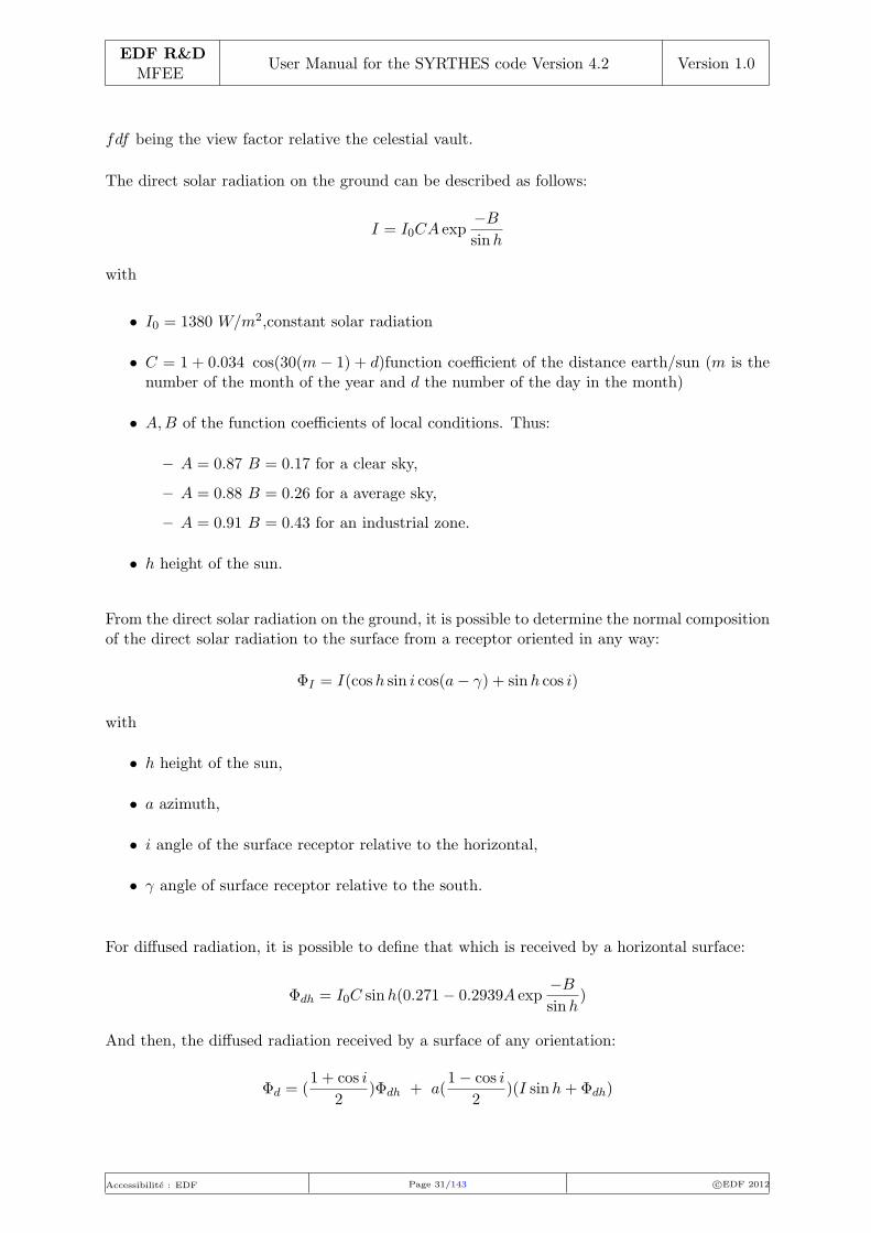
fdf being the view factor relative the celestial vault.

The direct solar radiation on the ground can be described as follows:

I = I0CA exp−B

sinh

with

• I0 = 1380 W/m2,constant solar radiation

• C = 1 + 0.034 cos(30(m− 1) + d)function coefficient of the distance earth/sun (m is thenumber of the month of the year and d the number of the day in the month)

• A,B of the function coefficients of local conditions. Thus:

– A = 0.87 B = 0.17 for a clear sky,

– A = 0.88 B = 0.26 for a average sky,

– A = 0.91 B = 0.43 for an industrial zone.

• h height of the sun.

From the direct solar radiation on the ground, it is possible to determine the normal compositionof the direct solar radiation to the surface from a receptor oriented in any way:

ΦI = I(cosh sin i cos(a− γ) + sinh cos i)

with

• h height of the sun,

• a azimuth,

• i angle of the surface receptor relative to the horizontal,

• γ angle of surface receptor relative to the south.

For diffused radiation, it is possible to define that which is received by a horizontal surface:

Φdh = I0C sinh(0.271− 0.2939A exp−B

sinh)

And then, the diffused radiation received by a surface of any orientation:

Φd = (1 + cos i

2)Φdh + a(

1− cos i

2)(I sinh+Φdh)


EDF R&DMFEE


4.7.2 Shade

In syrthes, solar radiation is calculated exactly relative to the geometry which is modeled. Inthe case, for example, of the modeling of a group of buildings, syrthes automatically calculatesthe shade of the buildings relative to one another and to the relative position of the sun.

In certain configurations, obstacles appear that may not need to be calculated thermally butwhich create partial and diffused shade for the zones of interest: vegetation, particularly trees,is a typical example.

In this case, syrthes includes an option to define the faces of radiation which do not interactwith the model of conduction but which generate shade by allowing only a part of the solarradiation to pass.

This model can be considered as a geometric homogenization to represent the zones illuminatedby the spectrum but by intermittence, in much the same way as when the sun rays pass throughleaves moving in the wind.

4.7.3 Horizon

When considering solar radiation, it is necessary to model a domain sufficiently large so that thecalculation of radiative fluxes are as realistic as possible. Indeed, taking once again the exampleof a group of buildings, it is necessary to model the surface of the ground around the zone ofinterest sufficiently so that the heat exchanges between the buildings and the earth are correctlyevaluated. In fact, a calculation domain that is too restricted will lead to fewer heat exchangeswith the ground resulting with a probable over- or under- evaluation of temperature.Thus, from a thermal point of view, the calculation of the temperature under the ground farfrom the buildings is not often interesting and would only serve to increase the size of the meshin the case of conduction.

To avoid this difficulty, syrthes includes ”horizon” faces. They only appear in the radiationmesh and are not coupled to the conduction mesh. They do not participate in the heat transferfrom face to face (thus the radiation calculation is not rendered more complex) but allow thedefinition of a ground temperature surrounding the domain and, thus, the calculation of radiationflux between the modeled surfaces and the ”distant ground”.

4.7.4 Example

Figure 4.4 illustrates a simplified example which was used for the modeling (in 2D) of twobuildings, the east facade of the tallest of which is covered with trees (presence of ”shade”cells). Also noteworthy is the extension of the radiation mesh by ”horizon” cells to calculate theradiative exchanges with the distant ground.


EDF R&DMFEE


Figure 4.4: Modeling of two buildings and a wall of trees


EDF R&DMFEE



EDF R&DMFEE


Chapter 5

Heat and mass transfer: functionand specificities

Most of the thermal courses describe the 3 thermal transfer modes that are the conduction, con-vection and radiation. But, there is an another transfer mode, often forgotten : the enthalpictransfer, connected to the transfers of mass. A fluid in movement transports its heat throughthe space. This phenomenon is neither conduction, nor the convection, nor radiation. It is thefourth phenomenon of thermal transfer.

In its most classical applications, the thermal analysis of buildings envelopes ignores totallythis phenomenon. The materials which constitute them are considered as purely conductiveand completely characterized by their thermal conductivity (even if we know that for many ofthem, radiation in semi-transparent media contributes widely to the thermal exchange). Atthe boundaries, on the interface between the components of envelope and the atmospheres, theexchanges are represented as a simple mixe of convection and linearized infrared radiation.Nevertheless, most of the materials which make up buildings’ envelopes are porous. The transfersof mass can thus occur there. Besides, the most insulating materials are also the most porous,thus potentially the most permeable. So, the maximum transfers of mass (high permeability)correspond to the minimum transfers of heat (low thermal conductivity). From then on, forthe extremely successful components from standard thermal point of view, those for whom theheat flux are the most low, it seems essential to examine more in detail the impact of themass transfers on the heat transfer. To reach there, it is necessary to handle the heat fluxquestion which allows to determine the main factors influencing the thermal performance ofthese components. At this stage, it is necessary to use numerical taking into account heat andmass transfers.

5.1 Physical model

We consider that the porous media is constituted by three phases :

• a solid phase, which is the skeleton of the material,

• a liquid phase constituted by pure water condensed in the pores of the material

• a gaseous phase which occupies the rest of the porous network.

syrthes supposes that the 3 phases are in equilibrium : they have the same temperature andthe 2 phases of water are in equilibrium.


EDF R&DMFEE


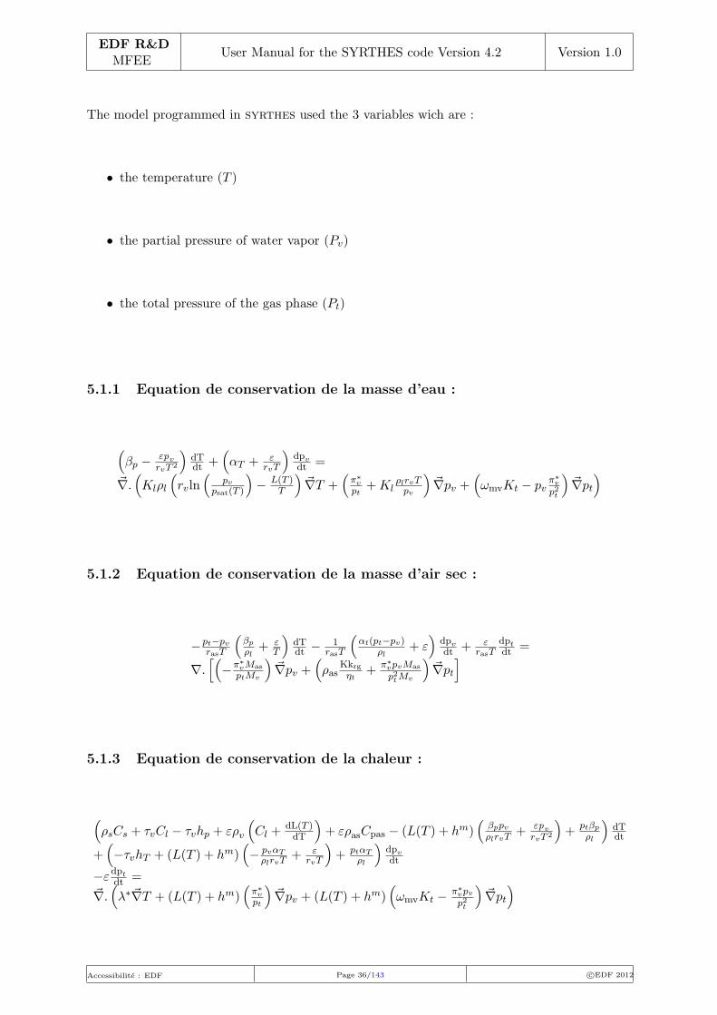
The model programmed in syrthes used the 3 variables wich are :

• the temperature (T )

• the partial pressure of water vapor (Pv)

• the total pressure of the gas phase (Pt)

5.1.1 Equation de conservation de la masse d’eau :

(βp − εpv

rvT 2

)dTdt +

(αT + ε

rvT

)dpvdt =

~∇.(Klρl

(rvln

(pv

psat(T )

)− L(T )

T

)~∇T +

(π∗vpt

+KlρlrvTpv

)~∇pv +

(ωmvKt − pv

π∗v

p2t

)~∇pt

)

5.1.2 Equation de conservation de la masse d’air sec :

−pt−pvrasT

(βp

ρl+ ε

T

)dTdt − 1

rasT

(αt(pt−pv)

ρl+ ε

)dpvdt + ε

rasTdptdt =

∇.[(

−π∗vMas

ptMv

)~∇pv +

(ρas

Kkrgηt

+ π∗vpvMas

p2tMv

)~∇pt

]

5.1.3 Equation de conservation de la chaleur :

(ρsCs + τvCl − τvhp + ερv

(Cl +

dL(T )dT

)+ ερasCpas − (L(T ) + hm)

(βppvρlrvT

+ εpvrvT 2

)+

ptβp

ρl

)dTdt

+(−τvhT + (L(T ) + hm)

(− pvαT

ρlrvT+ ε

rvT

)+ ptαT

ρl

)dpvdt

−εdptdt =

~∇.(λ∗~∇T + (L(T ) + hm)

(π∗vpt

)~∇pv + (L(T ) + hm)

(ωmvKt − π∗

vpvp2t

)~∇pt

)


EDF R&DMFEE


5.2 List of symbols

Symbole Signification Unite

ci Titre molaire du gaz i -

Cp Notation generique pour une chaleur massiquea pression constante J/kg.K

Cl Chaleur massique de l’eau liquide J/kg.K

Cpas, Cpv Chaleur massique a pression constante de l’air sec et de la vapeur d’eau J/kg.K

Cs Milieu poreux : Chaleur massique du materiau sec J/(kg.K)

D Notation generique pour une diffusivite m2/s

Dv Coefficient de diffusion de la vapeur d’eau dans l’air. kg/m.s

Das Coefficient de diffusion de l’air sec dans l’air. kg/m.s

e Notation generique pour une epaisseur m

f Facteur de resistance a la diffusion dans un milieu poreux. -

G Notation generique pour une enthalpie libre. J

g Notation generique pour une enthalpie libre massique. J/kg

~g Notation generique pour une densite de flux

~gc Densite de flux de chaleur dans le milieu poreux W/m2

~gv Densite de flux de vapeur dans le milieu poreux kg/(m2s)

~gas Densite de flux d’air sec dans le milieu poreux kg/(m2s)~Gv Densite de flux de vapeur dansl’air. kg/(m2s)~Gas Densite de flux d’air sec dansl’air. kg/(m2s)

H Notation generique pour une enthalpie J

h Notation generique pour une enthalpie massique J/kg

has, hv,hl Enthalpie massique de l’air sec,de la vapeur d’eau, de l’eau liquide J/kg

hm Chaleur de sorption de l’eau adsorbee J/kg

hT Derivee partielle de hm par rapport a pv J/kg.Pa

hP Derivee partielle de hm par rapport a T J/kg.K

has Coefficient d’echange d’air sec kg/m2.s

hc Coefficient d’echange de chaleur W/m2.K

hl Coefficient d’echange d’eau liquide kg/m2.s.Pa

hv Coefficient d’echange de vapeur kg/m2.s

ht Coefficient d’echange advectif du gaz kg/m2.s.Pa

HR Humidite relative (pv/psat) -

K Permeabilite intrinseque m2

Kt, Kl Permeabilite au gaz, a l’eau liquide s

krg, krl Permeabilite relative au gaz, a l’eau liquide -

L(T) Chaleur latente d’evaporation de l’eau J/kg

m Notation generique pour une masse kg

m Debit massique kg/s

mas Masse d’air sec kg

mv Masse de vapeur d’eau kg

ml Masse d’eau liquide kg

M Rapport entre la masse molaire de l’air sec et celle de la vapeur d’eau -

Mas Masse molaire de l’air sec kg/mol

Mv Masse molaire de l’eau kg/mol


EDF R&DMFEE


p Notation generique d’une pression (Notation generique d’un perimetre) Pa (m)

pas, pv Pression partielle d’air sec, de vapeur d’eau Pa

Pl Pression liquide Pa

psat Pression de vapeur saturante Pa

pt Pression totale de la phase gazeuse Pa

R Constante des gaz parfaits J/mol.K

rv Constante des gaz parfaits pour la vapeur d’eau (rv = R/Mv) J/kg.K

ras Constante des gaz parfaits pour l’air sec (ras = R/Mas) J/kg.K

S Notation generique pour une surface m2

T Notation generique pour une temperature K

t Notation generique pour le temps s

U Notation generique pourl’energie interne J

u Notation generique pour une energie interne massique J/m3

V Notation generique pour un volume m3

W Notation generique pour un travail. J

αT Pente de l’isotherme de sorption(αt =

(∂τv∂pv

)T

)kg/m3.Pa

βP Derivee partielle de l’isotherme de sorption par rapport a T kg/m3.K

ε Porosite -

λ Notation generique pour une conductivite thermique W/m.K

λ∗ Conductivite thermique du materiau humide W/m.K

Λ Chaleur totale de changement d’etat de l’eau.Λ = L(T ) + hm J/kg

π Permeabilite a la vapeur d’eau (formule ~gv = −π~∇pv) s

Π Notation generique pour une permeance (π/e) s/m

πair Permeabilite a la vapeur d’eau de l’air (formule ~gv = −πair~∇pv) s

πapp Permeabilite a la vapeur d’eau apparente (formule ~gv = −πapp~∇pv) s

π∗as Coefficient de diffusion de l’air sec (formule ~gas,diff = −π∗

as~∇(pas/pt) kg/(ms)

π∗v Coefficient de diffusion de la vapeur d’eau (formule ~gv,diff = −π∗

v~∇(pv/pt) kg/(ms)

µ Facteur de resistance a la vapeur d’eau ( µ∗ = π∗a

π∗v) -

ηl Viscosite dynamique de l’eau liquide Pa.s

ηt Viscosite dynamique de la phase gazeuse Pa.s

ωmi Titre massique du gaz i ( ρiρt) -

% Notation generique pour une masse volumique kg/m3

ρas Masse volumique partielle de l’air sec kg/m3

ρl Masse volumique de l’eau liquide kg/m3

ρs Masse volumique du materiau sec. kg/m3

ρv Masse volumique partielle de la vapeur d’eau kg/m3

ρt Masse volumique totale d’un gaz kg/m3

τv Taux d’humidite (masse d’eau par unite de volume de milieu poreux). kg/m3


EDF R&DMFEE


Chapter 6

Coupling with a thermal hydrauliccode

To understand multi-physical phenomena, syrthes can be used in association with a thermalhydraulic code. This will enable a better comprehension of the boundary conditions for the fluidor for the solid.

When doing a numerical simulation of a phenomenon, it is necessary to model and solve thephenomenon inside the concerned domain and also to take into consideration the boundaryconditions at the interface. Most of the time, boundary conditions of a solid are relativelyunknown or are very difficult to understand. Taking into account the fluid domain can, in manycases, eliminate this difficulty or, at least, reduce it significantly. For example, when a pipe isthermally insulated, imposing an adiabatic (zero flux) condition on the exterior surface is quiterigorous. On the contrary, if the material is thick or if a transient thermal evaluation is done,imposing an adiabatic condition at the fluid/solid interface could lead to a significant error.

Figure 6.1: Modeling of a thermally insulated pipe

Another example of an application is the modeling of thermal transients.

The thermal interaction between fluid and solid is fundamental in cases of thermal shocks, whichare very frequent in industrial processes (nuclear hydraulics for example). Consider the case ofa thermal shock (significant and rapid increase of the fluid temperature) in a piping system.


EDF R&DMFEE


The thermal inertia of the solid will lead to a gradual increase of temperature of the surface,and inversely a partial cooling of the fluid. After a certain length, the impact of the shock maybe spread over the pipe and be considerably reduced. At the end of the pipe, the thermal loadis significantly lower which can become compatible with safety requirements, unlike the veryconservative attitude concerning a surface without thermal inertia.

Figure 6.2: Reduction of a thermal shock due to thermal inertia

In certain cases, interest in simulating a fluid/solid thermal coupling is in gaining knowledgeabout the solid temperature field. Within this context, the simulation of thermal coupling withthe fluid provides better boundary conditions at the interface for the solid calculations.

This can be the case in the cooling process of a metallic object by water jets, air jets or by naturalconvection. A classic approach consists of approximating the effect of the fluid by heat exchangelaws. Unfortunately, imposing these coefficients may lead to significant errors of measurementwhere local parameters of the fluid temperature and the associated heat exchange coefficient aredifficult to determine.

Figure 6.3: Example: cooling of the internal baffle structure of a nuclear reactor

At the conclusion of the coupled calculations, the thermal results can be transferred to a mechan-ical code to determine the mechanical stresses originating from thermal phenomena. syrthescan give the results in MED format [5] [6] (via a specific utility program avalaible in thesyrthes package: syrthes4med30), which can then be read, for example, by the mechanicalcode Code Aster.


EDF R&DMFEE


Chapter 7

General Environment

This chapter gives an outline of syrthes architecture and the tools that accompany it.In the first paragraph, an overview is given. In the second paragraph, the organization of thekernel of the code is described as well as its input and output files.

Figure 7.1: Flow chart of the syrthes program


EDF R&DMFEE


Thermal radiation is presented as a syrthes module to differentiate the treatments of transferby conduction and by radiation (in a closed medium) during the use of the code. In this way, thegeneral functioning of the code is not overloaded. A unique keyword activates thermal radiationin a closed medium.

Once this is activated, complementary data must be provided. On the contrary, if the moduleis not activated, the keywords will simply not be read (note that it is not necessary to deletethe data file).

This approach is particularly flexible when evaluating the importance of radiation transfer ina given problem: a calculation restricted only to conduction is directly possible from the cal-culation ”conduction+radiation” simply by deactivating the radiation calculation in the datafile.

7.1 Organization of the input data and the results

The general structure of the functioning of syrthesis presented in figure 7.2.

The parts indicated on the table in dashed lines are indicative of the radiation module.

Figure 7.2: Flow chart of syrthes functioning

The organization of the files is presented in the form seen in figure 7.3.

The complete description of these files is found in chapters 8, 12 and in appendix 13.


EDF R&DMFEE


Figure 7.3: syrthes data and result files

7.1.1 Data files

The input files necessary for the syrthes code are the following:

• *.syr: a geometric file containing the non-structured mesh of the solid domain. This filecontains, among others, the list of elements, the coordinates of the nodes, the references forthe elements, etc. . . This file is in syrthesformat. Paragraph ?? examines possible toolsto generate such a file. In calculations with radiation, a second geometric file is necessaryto describe the radiating surface.

• syrthes data.syd: a file with diverse keywords (for the choice of options), the cal-culation parameters, the numerical criteria associated with the resolution, the physicalconditions and the boundary conditions. Even if the name of this file is traditionallysyrthes data.syd, it is not imposed and can be changed as necessary.

• User source files (user.c,user cond.c,user ray.c, user hmt.c) which are optional butuseful to define complex conditions. Chapter 12 describes these functions.


EDF R&DMFEE


7.1.2 Result files

syrthes generates a certain number of result files relative to the options chosen for the sim-ulation. All the names of the file results have the same prefix and are distinguished by theirextension:

• .res: result file containing the principle variables of the calculation in each node of themesh. It is the temperature for a calculation of conduction/radiation. If the model of heatand mass transfer is activated, they are the temperature, the vapor pressure and the totalpressure.

• .rdt: transient: similar to the previous result file but containing the results in severaltime steps defined by the user.

• .his: history file: for tracking the evolution of the temperature over time (and also thevapor pressure and the total pressure) on a limited number of points defined by the user(probes).

• .mnx: minimum and maximum file: at each time step, syrthes calculates the mini-mum and maximum of a certain number of variables. These values are saved in columnsin the file.

• .flu: heat balance file: if the user requests it in the data file, it is possible to calculatethe surfacic heat balance and/or the volumetric heat balance at each time step. The valuesare displayed in the listing file but also in this file which can later be used to trace curves.

• .add: additional file: This file is optional. It enables the user to save certain variables orparameters in the file which can then be visualized in the post-processor. The structure ofthis file is identical to that of a traditional result file. Parameters calculated on the meshnodes as well as parameters calculated on the elements can be saved here.

Thermal radiation in the calculations does not generate results in themselves because they areinterpreted by the modification of the temperature field in the solid. It is thus the traditionalsyrthes result files which handle the coupling of conduction + radiation phenomena.

Nevertheless, it is interesting to have access to certain parameters directly linked to radiation.Thus, it is possible to request the code to generate certain results directly on the radiation mesh.

As for solids, three files are available:

• rad.res: a result file which contains the temperature and the radiation flux per band

• rad.rdt: a chronological file which contains the temperature and the radiation flux perband but in diverse time steps

Remark: in radiation, the discretization used is type P0; meaning that the parameters are con-stant per cell.


EDF R&DMFEE


7.1.3 Storage/Memory file for view factors

This file (mesh.fdf) is only used in calculations for the coupling of conduction + radiation. Itis not directly exploitable by the user but stores information very expensive to calculate. Inthe initial phase, it is necessary to calculate the geometric parameters quantities which are theview factors, generally considered as being costly with a large number of mesh cells. The totalnumber of view factors is n(n− 1)/2 if n is the number of independent cells.

syrthes includes an option to save the parameters in the file which avoids the recalculationof the parameters for subsequent calculations. Indeed, these parameters are purely geometricaland remain constant if the geometry does not change.

7.1.4 Coupling syrthes with a thermal hydraulic code

In the case of coupling syrthes with a CFD code, the file organization remains unchanged. Thefiles relative to the fluid code are simply added to the syrthes directory. A specific script willsimultaneously launch both the fluid and solid applications using MPI [7] (see chapter 6).

7.2 Creating a mesh for syrthes

As for any industrial calculations, the large volume of data for the calculation absolutely neces-sitates the use of eficient pre- and post- processors.

The mesh of finite elements of the solid domain can be done with any mesh generator: thestructures of the data issued from the mesher must be compatible with those accepted bysyrthes.

Currently, syrthes includes a conversion tool convert2syrthes4 which automatically recog-nizes files formatted in gambit, gmsh, Ideas-MS, Salome, simail. convert2syrthes4: con-version of a mesh file to syrthes format convert2syrthes4 -m geo.xxx [-r geo.syr]

. geo.xxx: name of mesh file (.neu, .msh, .unv, .med, .des)

. geo.syr: name of mesh file converted to syrthes format (if the name is not provided, it willautomatically be named geo.syr).

The use of all other mesh generators is possible on the condition that they are compatible withthe syrthes format (see the format of files in Appendix A).

7.3 Visualize syrthes results

Whatever the option retained, syrthes always provides a result file containing the value oftemperature at each mesh node.

Utility programs transform these results into syrthes format in a data base compatible withdiverse post-processors.

The format of syrthes result files are given in Appendix A.


EDF R&DMFEE


7.3.1 Conversion of syrthes results to Ensightformat

syrthes4ensight: transformation of a syrthes file to an Ensight data base formatted en-quotecase.

use: syrthes4ensight -m geo.syr -r resu1.res -o fich ensight

. geo.syr: name of syrthesgeometric file,

. resu1.res: name of syrthesresult file. This file can be either the result file (.res) containingonly one time step or the transient file (.rdt) which will treat n time steps.

. fich ensight: name of the file in Ensightformat

Note that this file format can then be read by Ensight and paraview paraview.

7.3.2 Conversion of results to med format

syrthes4med30: transformation of a syrthes file to a med data base med [9].Use: syrthes4tomed30 -m geo.syr -r resu1.res -o fichier.med

. geo.syr: name of syrthes geometric file

. resu1.res: name of syrthes result file

. fichier.med: name of file containing the mesh and results in med format


EDF R&DMFEE


Chapter 8

Data files relative to SYRTHES

To do a calculation, syrthes requires at least a parameter file, where the case and the numericalchoices can be precisely defined, and a geometric file for the description of the calculation domain.

8.1 Geometric Files

8.1.1 Conduction mesh

This file is mandatory. This file contains the mesh of the solid domain as well as diverse referencesapplied on the nodes, the boundary edges in 2D or faces in 3D of the mesh.

The solid mesh being unstructured, syrthes requires necessary information: a table of nodecoordinates, the connectivity of the volumetric mesh and the connectivity of the boundary mesh.

The mesh must be composed exclusively of the following:

• 3-node triangles in two dimensions (triangles with straight sides), and 2-node edges for theboundary

• 4-node tetrahedrons in three dimensions (tetrahedrons with planar surfaces), and 3-nodetriangle for the boundary

8.1.2 Radiation mesh

When the thermal radiation calculation is activated, a second mesh must be provided to syrthes whichis also unstructured.

syrthes requires necessary information: a table of node coordinates and the connectivity of themesh with references of the elements.

The surfacic mesh is composed exclusively of the following:

• 2-node segments in two dimensions

• 3-node triangles in three dimensions

Note that the conduction and radiation meshes are totally independent and that it is absolutelynot necessary that they are coincident (conformal) (but they can be as well).


EDF R&DMFEE


8.1.3 Formats of the mesh files

syrthes 4 only authorizes one type of mesh: the syrthes format. This format is described theappendix.

To obtain a mesh in this format, syrthes includes a file conversion tool.

This utility convert2syrthes accepts the input from the following formats:

• simail mesh generator files (extension .des),

• Ideas-MS mesh generator files (extension .unv),

• Salome mesh generator files in med format (extension .med),

• gmsh mesh generator files (extension .msh),

• gambit mesh generator files (extension .neu),

The identification of the file format is made by the extension which is given to the name of thegeometric file. This extension is thus imposed and mandatory.

8.2 Parameter files

This file contains all the user parameters to do a calculation. The following chapter is entirelydevoted to it. It is generally named syrthes data.syd.

8.3 Standard weather data file

For calculations in which meteorological conditions must be input, it is possible to providesyrthes with a complementary weather file.

The name of this file is provided by the syrthes parameter filesyrthes data.syd.FICHIER METEO=If the name of the file is provided, it will be automatically read when thecalculation starts running and the information read can be used in the user functions of thefilesuser.c, user cond.c, user hmt.c and user ray.c.

8.3.1 Contents of the weather data file

In this file, the data is provided in columns. The first line is particular: it indicates the numberof columns in the file.The weather file is read line by line, regardless of the number of columns.Generally, each line corresponds to an instant and on the same line different variables of thisinstant are found.

Below is an example of a weather file:

3

0 20 5.1

300 22 5.5


EDF R&DMFEE


600 24 5.3

900 23 6.2

1200 21 5.8

In this example, the first line indicates that each line is composed of three variables. After that,on each line is given: the time in seconds, the exterior temperature and the wind velocity.

After having read the file, the data are stored in the meteo structure of the Meteo type. Thenumber of lines in the chart is stored in the variable meteo.nelem.

The following table summarizes the content of the weather file and provides the variables inwhich information is stored in syrthes.

This data can then be used in the different user functions.

8.3.2 Example of use

An example of the use of data provided in a weather data file is described below (on the basis ofthe example presented above). This represents only a fraction of the user function user limfso

available in the file user cond.c.

For this example, a condition for heat exchange on the boundary of the domain is imposed. Theheat exchange coefficient is set at 10 W/(m2K), the exterior temperature is provided by theweather file.

In the data file syrthes data.syd, a heat exchange condition is imposed on the boundary ofreference 1:

CLIM_T_PROG= COEF_ECH 1

The function user limfso of the file user.c is programmed in the following way:

/* Heat Exchange Condition */

/* ----------------------- */

if (mescoeffech)

{

/* Searching the time step */

if (tempss <= meteo.var[0][0])

num=0;

else if (tempss >= meteo.var[0][meteo.nelem-1])

num=meteo.nelem-1;

else

{

num=1;

while (tempss>meteo.var[0][num]) num++;

num--;

}


EDF R&DMFEE


/* For each node of each heat exchange boundary element */

for (j=0;j<echang.ndmat;j++)

for (i=0;i<echang.nelem;i++)

{

nr=maillnodeus.nrefe[echang.numf[i]]; /* boundary element reference */

if (nr==1){ /* if the reference is 1 */

echang.val1[j][i]=meteo.var[1][num]; /* Temperature found in the file */

echang.val2[j][i]=10; /* Heat exchange coefficient */

}

}

}

8.4 User data files

Certain calculations can necessitate the use of particular data originating, for example, frommeasurements or from calculations done in other disciplines having an impact on the thermalmodeling.

In this case, syrthes includes a pre-programmed function to read data from a file provided bythe user regardless of the format. The user function can be modified according to the file content.

The file will be read by the function user read myfile of the file user.c.

The read data will be stored in the structure myfile. The following fields are also included inthis structure:

• myfile.actif: activation of the reading of a personal file

• myfile.nbvar: number of variables to read

• myfile.nelem: number of values per variable

• myfile.var[myfile.nbvar][myfile.nelem]: values of the variables

After having input the number of variables and the number of values per variable to read insection 1 of the function, the reading of the file is then programmed in section 3 in the fileformat.


EDF R&DMFEE


Chapter 9

Interpreted functions

As seen in previous chapters, syrthes can handle variable physical characteristics (boundaryconditions, physical properties,. . . ). In a great number of cases the variations of these parame-ters are expressed in the form of functions dependent on space, time and temperature.

To facilitate the definition of these variation functions and to limit the programming of the userfunctions to very specific and complex configurations, syrthes defines these functions directlyin the data file syrthes.data.syd.

9.1 What can be defined with the interpreted functions?

syrthes accepts interpreted functions for the following parameters:

• Initial conditions of temperature, vapor pressure and total pressure

– keyword CINI T FCT=

– keyword CINI PV FCT=

– keyword CINI PT FCT=

• Temperature boundary conditions

– Heat exchange condition (value of the exterior temperature and of the heat exchangecoefficient)keyword CLIM T FCT=

– Dirichlet Condition (value of the imposed temperature)keyword CLIM T FCT=

– Flux Condition (value of the surface flux)keyword CLIM T FCT=

• Physical properties

– for isotropic materialskeyword CPHY MAT ISO FCT=


EDF R&DMFEE


– for orthotropic materialskeyword CPHY MAT ORTHO 2D FCT=

keyword CPHY MAT ORTHO 3D FCT=

– for anisotropic materialskeyword CPHY MAT ANISO 2D FCT=

keyword CPHY MAT ANISO 3D FCT=

• Volumetric flux on temperature, vapor pressure and total pressurekeyword CVOL T FCT=

keyword CVOL PV FCT=

keyword CVOL PT FCT=

9.2 How to define a function?

A function is an expression which can use all the mathematical symbols and functions knownin programming language C. It cannot include the space character which is considered as adelimiter. The variables which can be present in the expression are the following (upper andlower cases must be respected!):

• tt: physical time (in seconds)

• T: temperature (in degrees C)

• x,y,z (z is only allowable in 3 dimensions): the coordinates of the node or of the center ofa cell (in meters)

Example: definition of properties of an isotropic material where the volumetric mass and theheat capacity are constant but where the conductivity is defined by an interpreted function.

CPHY_MAT_ISO_FCT= 7700 460. 0.07223+0.005211*tt-1.197e-5*tt*tt 24 23 26

9.3 Interpreted functions in syrthes

Once the functions have been defined in the user data file syrthes.data, a specific pre-processor(ppfonc syrthes) interprets and generates the corresponding C functions.

Generally, this phase is hidden to the user because it is integrated in the script/command torun syrthes. The command for manual use of the pre-processor is provided:

ppfonc_syrthes syrthes_data.syd

Once the code has finished being executed, the file (util fct.c)is made available which will betaken into account at the moment of the execution of the code.


EDF R&DMFEE


Chapter 10

Parameter file

Generally, the syrthes parameter file is named syrthes data.syd, which is not imposed and canbe changed whenever desired. However, for convience and clarity, this appellation will be usedin this document.

This file is made up of keywords with default values which must be input.

10.1 Genaralities concerning the data file syrthes data.syd

This file is input through the user interface syrthes.gui.

By following the different interface rubrics, the input data are defined. All data are stored inthe file syrthes data.syd which will be read by syrthes.

The syrthes data.syd file is a text file composed of keywords. Even if it is generally auto-matically filled by the syrthes.gui interface, it is nevertheless possible to input in it by usinga simple ”text editor”. This is interesting in particular cases, for example, parametric calcula-tions which may require a large number of calculations by modifiying only some of the inputparameters. The sequence of the calculations can managed automatically by running the usersown script.

For this reason, the description of input data via the user interface is described in this chapter,but by specifying the corresponding keyword in the file syrthes data.syd.

Below are all the notations useful for the functioning of the syrthes data.syd file:

• The order of keywords is random,

• The keywords, nevertheless, are grouped by theme and generally preserve the proposedorder to maintain a certain logic in the file,

• syrthes then reads the file sequentially: if a keyword appears several times it is the lastvalue read which will be used for the calculation,

• For a given keyword, all the parameters must be provided on the same line,

• All lines starting with the character ”/” are comments,

• Keywords that are not used can be deleted from the file


EDF R&DMFEE


• Keywords relative to radiation (ie. keywords in the paragraph Data for Radiation ”DON-NEES POUR LE RAYONNEMENT” are not read unless the keyword ”PRISE EN COMPTEDU RAYONNEMENT CONFINE=” was previously positioned to ”oui”),

• Keywords relative to humidity transfer (ie. key words in the paragraph ”DONNEESCOMPLEMENTAIRES POUR LES TRANSFERTS COUPLES” Complementary data forcoupled transfers are not read unless the keyword ”MODELISATION DES TRANSFERTSD HUMIDITE=” was previously positioned to ”oui”.

• Most of the parameters have default values.

Once placed in the directory corresponding to the case being studied, syrthes graphic interfacewill be launched by typing:

syrthes.gui

10.2 Genaralities concerning the tables in the syrthes.gui in-terface

For the functioning of syrthes several types of variables must be read. It is possible to distin-guish a part of the parameters by simply defining a value. It is possible, for example, to cite thedefinition of the value of the time step: syrthes accepts a real value which will define the latter.

But there are also more complex data such as the initial conditions, boundary conditions andphysical conditions. Input data in the code, a list of conditions must be provided. In these cases,syrthes.gui will propose a definition of the values in a table. Figure 10.1 shows an example ofsuch.

Figure 10.1: syrthes.gui - Window: Example of a table

The definition of initial conditions will now be considered.


EDF R&DMFEE


The mesh was planned in consequence and contains different zones where the elements havedifferent references.

Three types of conditions are possible:

• Constant: the value of the condition is constant, it is a real value. In this case, the valueof the condition, and the list of references of the elements of the mesh where it is applied,must be provided and a comment can be added if desired.

• Function: the value of the condition can be expressed in the form of an interface function”interpretee” and can be written relative to the variables t (time), T (temperature), x,y, z (spatial coordinates). In this case, it is necessary to provide the function which isexpressed by using exclusively the variables cited t, T , x, y, z (respect the upper and lowercases) and the list of references of elements of the mesh where it is applied. A commentcan be added if necessary.

• Program: the value of the condition is complex (interpolation in a file for example) andit will be directly programmed in the user source files. The references of elements of themesh where it is applied must be provided, and a comment can be added if desired.

Figure shows an example:

Figure 10.2: syrthes.gui - Window: Example where different types of conditions are used

Non-utilization of certain conditions

By default, all the conditions defined are active and will be taken into consideration in the cal-culation. This is reflected in the window where the beginning of each line is checked (presenceof an X).


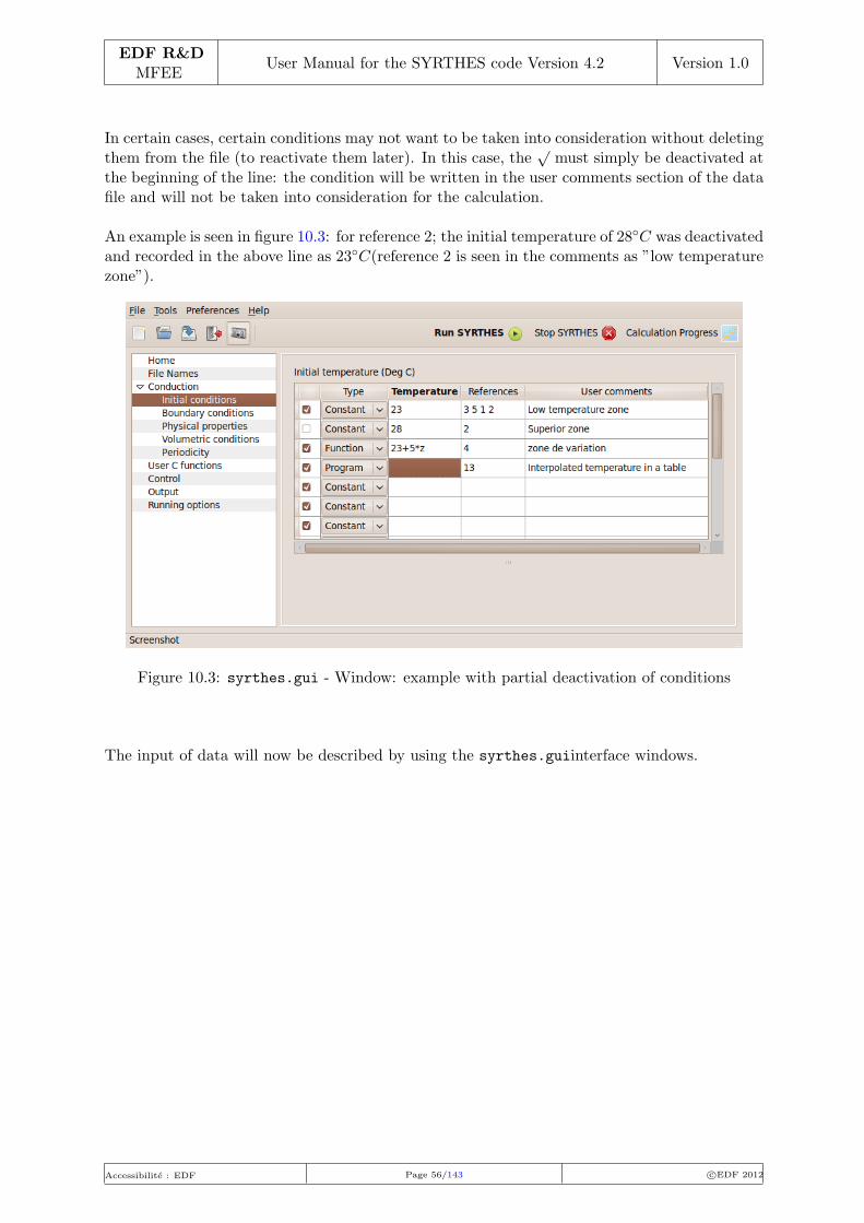
EDF R&DMFEE


In certain cases, certain conditions may not want to be taken into consideration without deletingthem from the file (to reactivate them later). In this case, the

√must simply be deactivated at

the beginning of the line: the condition will be written in the user comments section of the datafile and will not be taken into consideration for the calculation.

An example is seen in figure 10.3: for reference 2; the initial temperature of 28◦C was deactivatedand recorded in the above line as 23◦C(reference 2 is seen in the comments as ”low temperaturezone”).

Figure 10.3: syrthes.gui - Window: example with partial deactivation of conditions

The input of data will now be described by using the syrthes.guiinterface windows.


EDF R&DMFEE


10.3 Home window

The home window appears at the startup of the interface:

Figure 10.4: syrthes.gui - Window: Home

The following data must be provided:

B Case title

Description It is possible to entitle the study here.Keyword titre etude=Value String of charactersDefault —

B User description of the case

Description It is possible to add a comment for the description of the study hereKeyword non-applicableValue —Default —

B Dimension of the problem

Description Definition of the dimension of the study which can be in 3 dimensions(3D), 2 dimensions

Keyword dimension du probleme=Value 2d cart or 2d axi ox or 2d axi oy or 3dDefault 3d

Finally, it is possible to activate the different physical models in syrthes:


EDF R&DMFEE


B Thermal radiation

Description Activation of the thermal radiation modelKeyword prise en compte du rayonnement confine=Value oui or nonDefault non

B Humidity

Description Activation of of transfers coupled with mass and temperature. Twomodels are available: models with 2 equations (temperature and vaporpressure) and models with 3 equations (temperature, vapor pressure andtotal pressure)

Keyword modelisation des transferts d humidite=Value 0, 2 or 3Default 0

10.4 Control of window

The adjustment of the parameters for the calculation pilot can be done in this window.

It has two tabs. The first (Time managment) is for the management of time, and the second(Solver information) is to control iterative solver parameters.

10.4.1 Time management tab

In general it is the management of time that is dealt with here.

syrthes is, above all, based on an unsteady algorithm. A convergence of the usteady algorithmis used for research in a steady state.

In numerous cases, the calculation is not made in only one run. A first calculation is done,the results are analyzed and a new calculation is launched taking as the initial parameters theresults from the first calculation. It is a sequence of calculations.

In other cases, a system usually in a steady state which is suddenly subjected to a transientmight need to be studied. In this case, the steady state will be calculated first before the startingof the transient. In this case, a sequence of calculations will be executed but it will be equallypossible to ”reset” the physical time to start the transient to t = 0 for example.

B Restart calculation

Description A sequence of calculations, it is necessary to later provide the result fileof the first calculation as the input data.

Keyword suite de calcul=Value oui or nonDefault non


EDF R&DMFEE


B Setting a new restart time

Description In the case of a sequence of calculations, it is possible to redefine thephysical start time (adjustment for example)

Keyword suite: nouveau temps initial=Value If real < 0: no modification, time restart is done according to time

indicated on the next fileValue If real > 0: the physical time is reset to this valueDefault -1

Management of time and of time steps.

The number of time steps is indicated in a global way on the totality of the calculation. Thus,if 150 time steps have been done during the first calculation and that 200 more are neededduring subsequent calculations, the number of time steps to indicate will be 350. In this way,the chronology of calculations can be conserved and the management of the sequence will beeasier.

Three time steps options are possible:

• constant: the same time step will be used throughout the calculation, only one valueneeds to be provided to the code.

• automatic: the time step is calculated automatically by the syrthes function of thegradient of the temperature. In this case, an initial time step needs to be input and themaximum of temperature variation authorized between two successive time steps. Finally,a maximum value of the time step is requested in order to set it when the convergence isattained.

• by blocks: several constant time steps can be defined during the calculation. For example,the first ten time steps are of 1.5s, the next 30 time steps are of 0.5s, and the 100 subsequenttime steps are at 1s.

B Global number of time steps

Description Number of time steps at which the code will stopKeyword nombre de pas de temps solides=Value integer > 0Default —

B Time step: ConstantB Time step (in seconds)

Description Choice of one constant time stepKeyword pas de temps solide=Value real > 0Default —


EDF R&DMFEE


B Time step: Automatic

Description Choice of one automatic time step, based on the temperature gradientKeyword pas de temps solide=Solid time stepValue —Keyword pas de temps automatique=Value gradient T max (real > 0), max time step (real > 0)Default — —

B Time step: By blocks

Description Choice of a constant time step per blockKeyword pas de temps multiples=Value Iteration value (whole > 0), max time step (real > 0)Default — —

10.4.2 Solver information tab

The equation of heat in a solid is resolved with an iterative method of a preconditioned conju-gated gradient type.

The precision of the resolution can be adjusted. A compromise between the desired precisionand the calculation time necessary to resolve it is found with two values designed for this effect.

It is necessary, here, to point out a technical point: the stop test of the iterative method em-ployed is based on three criteria:

• the maximum number of iterations given,

• a criterion of absolute convergence (‖Ax− b‖ < εabs),

• a criterion of relative convergence (‖Ax−b‖‖‖xn‖ < εrel)where xn is the result of the resolution

to the preceding time step.xs.

The algorithm stops:

• when the number of maximum iterations is attained,

• when the two criteria of convergence are respected.

In this way, the solver can be completed piloted:

• to request a very exact precision: by imposing a very strict criterion of absolute convergenceand a sufficiently large number of iterations,

• to request a less precise and/or to limit the numberof iterations.

When the resolution of the coupled transfers is activated, similar criteria are used for the vaporpressure and total pressure variables.


EDF R&DMFEE


B Solver precision

Description Precision requested to the iterative solver of the linear system for theresolution of conduction

Keyword nombre iterations solveur temperature=Value integer > 0Default 100

Keyword nombre iterations solveur pression de vapeur=Value integer > 0Default 100

Keyword nombre iterations solveur pression totale=Value integer > 0Default 100

B Maximum number of iterations

Description maximum number of iterations authorized for the iterative solver of thelinear system for the resolution of conduction

Keyword precision pour le solveur temperature=Value real > 0Default 10−5

Keyword precision pour le solveur pression de vapeur=Value real > 0Default 10−5

Keyword precision pour le solveur pression totale=Value real > 0Default 10−5

10.5 Window: File Names

This window provides the names of the syrthes data and result files. The first frame is dedicatedto the data files.

• Conduction mesh: It is necessary to input at least the name of the mesh for theresolution of the conduction. Note that if the mesh file is not in syrthesformat, thesyrthes.gui interface will automatically use the converter of format1 to have a mesh filein syrthesformat1.

• Radiation mesh: In the case where the thermal radiation is activated in the principlewindow, the name of the radiation mesh must also be input.

• Restart File: In the case of sequential calculations, it is necessary to input the name ofthe results file from which the new calculation can be launched. Only the prefix must begiven.

17.2


EDF R&DMFEE


• Weather data: Optionally, a weather data file can be input including values that can beused in the boundary conditions for example.

Figure 10.5: syrthes.gui - Window: File Names

The second frame is dedicated to the Results Names files.

• Results names prefix: the prefixes of the result files are defined here. All the generalfiles per code will take this prefix and can then be distinguished by the extensions.

Warning: if an existing prefix name is input, the former results will be deletedby the new calculation.


EDF R&DMFEE


B Conduction mesh

Description Name of the conduction meshKeyword maillage conduction=Value String of characters without spacesDefault —

B Radiation mesh

Description Name of the radiation mesh fileKeyword maillage rayonnement=Value String of characters without spacesDefault —

B Restart file

Description Name of the file for sequencial calculationsKeyword prefixe du resultat precedent pour suite de calcul=Value String of characters without spacesDefault —

B Weather data

Description Name of weather data fileKeyword fichier meteo=Value String of characters without spacesDefault —

B Results names prefix

Description Prefixe that will be used for all the results filesKeyword prefixe des fichiers resultats=Value String of characters without spacesDefault —


EDF R&DMFEE


10.6 Parameters for conduction

10.6.1 Window: Initial conditions

Definition of the initial conditions: The initial temperature of all the nodes of the mesh mustbe input.

If, and only if, the initialization is identical in the entire domaine (either a uniform temperature,the same function throughout, or an initial condition programmed for the entire domain), thelist of references of the elements concerned can be reduced to ”-1” meaning ”all the elements”.

Figure 10.6: syrthes.gui - Window Conduction - Initial conditions

B Initial conditions

Description Initial temperature in ◦CKeyword cini t= temperature referencesValue RealDefault T = 20

Keyword cini t fct= temperature referencesValue fonction T(x,y,z,t,T)Default T = 20

Keyword cini t prog= referencesValue user.c(user cini) to programDefault T = 20

10.6.2 Window: Boundary conditions

Definition of the boundary conditions: This window includes 5 tabs which define the boundaryconditions according to their type.


EDF R&DMFEE


For each boundary condition, the list of references of the boundary faces concerned by thiscondition is provided.

Remark 1: all boundary faces for which no boundary condition is specified will automatically beconsidered as adiabatic (zero flux).

Remark 2: for the resolution of the conduction in syrthes an adiabatic (zero flux) conditionof (or of symmetry) is not required to be explicitly imposed. This part of the domain boundaryshould simply be left without a boundary condition.

10.6.2.1 Heat exchange tab

Heat exchange boundary condition: An exterior temperature (in ◦C) and a heat exchangecoefficient (W/m2/◦C) must be input.

Figure 10.7: syrthes.gui - Window: Boundary conditions - Heat Exchange

B Boundary conditions - Exchange

Description Boundary condition of Heat ExchangeKeyword clim t= coef ech T h referencesValue Real, RealDefault T=20, h=0

Keyword clim t fct= coef ech T h referencesValue 2 functions T (x, y, z, t, T ) et h(x, y, z, t, T )Default T=20, h=0

Keyword clim t prog= coef ech ReferencesValue user.c(user limfso) to programDefault T=20, h=0


EDF R&DMFEE


10.6.2.2 Flux tab

Flux boundary condition: The flux in W/m2 must be input.

Figure 10.8: syrthes.gui - Window: Boundary conditions - Flux

B Boundary conditions - Flux

Description Boundary condition of type FluxKeyword clim t= flux Flux referencesValue RealDefault ϕ = 0

Keyword clim t fct= flux Flux referencesValue function varphi(x, y, z, t, T )Default ϕ = 0

Keyword clim t prog= flux referencesValue user.c(user limfso) to programDefault ϕ = 0


EDF R&DMFEE


10.6.2.3 Dirichlet tab

Dirichlet boundary condition: An imposed temperature in ◦Cmust be input here.

Figure 10.9: syrthes.gui - Window: Boundary conditions - Dirichlet

B Boundary conditions - Dirichlet

Description Boundary condition of type imposed temperatureKeyword clim t= dirichlet temperature referencesValue RealDefault T = 0

Keyword clim t fct= dirichlet T (x, y, z, t, T ) ReferencesValue functionDefault T = 0

Keyword Clim t prog= dirichlet referencesValue user.c(user limfso) to programDefault T = 0


EDF R&DMFEE


10.6.2.4 Contact resistance tab

Contact resistance boundary condition: The value of the contact resistance must be input herein W/m2/◦C and the references of the two groups of faces between which the contact resistancewill be applied. Note that in the data file syrthes.data the two reference groups are separatedby ”-1”.

Figure 10.10: syrthes.gui - Window: Boundary conditions - Contact resistance

B Boundary conditions - Contact resistance

Description Boundary condition of type imposed temperatureKeyword clim t= res contact g ref groupe 1 -1 ref groupe 2Value RealDefault g=0

Keyword clim t fct= res contact g(x, y, z, t, T ) Resistance ref groupe 1 -1ref groupe 2

Value fonction g(x, y, z, t, T )Default g=0

Keyword clim t prog= res contact ref groupe 1 -1 ref groupe 2Value user.c(user limfso) to programDefault g=0


EDF R&DMFEE


10.6.2.5 Infinite radiation tab

Infinite radiation boundary condition: The value of the emissivity of the surface and the infinitetemperature (◦C) must be input here.

Figure 10.11: syrthes.gui - Window: Boundary conditions - Infinite radiation

B Boundary conditions - Infinite radiation

Description Boundary condition of type Infinite radiationKeyword clim t= ray infini ε T∞ ReferencesValue Real∈ [0, 1],realDefault ε = 0, T=20

Keyword clim t fct= ray infini ε T∞ ReferencesValue 2 function f(x, y, z, t, T )Default ε = 0, T=20

Keyword clim t prog= ray infini referencesValue user.c(user limfso) to programDefault ε = 0, T=20

10.6.3 Physical properties window

Definition of the physical properties of materials:

This window includes three tabs which define isotropic, orthotropic and anisotropic materialswithin the same domain of calculation.

If, and only if, the domain is only composed of one single material, the list of references of theelements concerned can be reduced to ”-1”. If not, for each material, the list of references ofelements concerned by this condition will be provided.


EDF R&DMFEE


10.6.3.1 Isotropic tab

Definition of materials with isotropic behavior: the thermal conductivity will thus be defined bya scalar (possibly variable in time and space) on the elements.

Figure 10.12: syrthes.gui - Window: Physical properties - Isotropic

Isotropic solids are defined by:

. the volumetric mass ρ (kg/m3)

. the heat capacity Cp (J/kgK)

. the thermal conductivity k (W/mK)

B Physical properties - Isotropic - Type=Constant

Description Isotropic materials with properties defined by a constantKeyword cphy mat iso= ρ Cp k referencesValue 3 real > 0Default 7700 460 25

B Physical properties - Isotropic - Type=Function

Description Isotropic materials with properties defined by a functionKeyword cphy mat iso fct= ρ Cp k referencesValue 3 functions f(x, y, z, t, T )Default 7700 460 25

B Physical properties - Isotropic - Type=Program

Description Isotropic materials with programmed propertiesKeyword cphy mat iso prog= referencesValue —Default 7700 460 25

10.6.3.2 Orthotropic tab

Definition of materials with orthotropic behavior: the thermal conductivity will thus be de-fined by a diagonal matrix (the terms of which can vary in time and space) on the elements.Orthotropic solids are defined by:


EDF R&DMFEE


Figure 10.13: syrthes.gui - Window Physical properties - Orthotropic

Orthotropic solids are defined by:

. volumetric mass ρ (kg/m3)

. heat capacity Cp (J/kg K)

. thermal conductivity (W/mK) It is necessary to give 2 or 3 values (respectively in 2D and3D): The conductivity following the direction x, y and possibly z.

B Physical properties - Orthotropic - Type=Constant

Description Orthotropic materials with properties defined by a constantKeyword 2D cphy mat ortho 2d= ρ Cp kx ky referencesKeyword 3D cphy mat ortho 3d= ρ Cp kx ky kz referencesValue 4 or 5 real > 0Default rho = 7700 Cp = 460 kx = 25 ky = 25 kz = 25

B Physical properties - Orthotropic - Type=Function

Description Orthotropic materials with properties defined by a functionKeyword 2D cphy mat ortho 2d fct= ρ Cp kx ky referencesKeyword 3D cphy mat ortho 3d fct= ρ Cp kx ky kz referencesValue 4 or 5 functions f(x, y, z, t, T )Default rho = 7700 Cp = 460 kx = 25 ky = 25 kz = 25

B Physical properties - Orthotropic - Type=Program

Description Orthotropic materials with programmed propertiesKeyword 2D cphy mat ortho 2d prog= referencesKeyword 3D cphy mat ortho 3d prog= referencesValue —Default 7700 460 25

10.6.3.3 Anisotropic tab

Definition of materials with anisotropic behavior: the thermal conductivity will thus be definedby a symmetrical matrix 3× 3 in 3 dimensions or 2× 2 in 2 dimensions (the terms of which canvary in time and space) on the elements of the mesh.


EDF R&DMFEE


Figure 10.14: syrthes.gui - Window Physical properties - Anisotropic

Anisotropic solids are defined by:

. volumetric mass ρ (kg/m3)

. specific heat Cp (J/kg K)

. thermal conductivity: in 2 dimensions conductivity is defined following the axes x and y ofthe local point of reference of the solid then the angle of rotation around axis z. In 3dimensions, the conductivity follows the axes x, y and z of the local point of reference ofthe solid.

The conductivity is difined by the point of reference, then the componements of the three axesof the local point of reference in the global reference point.

Figure 10.15 illustrates an example of the definition of anisotropic conductivity in the case ofa disk. The ellipsoides indicate the type of heat propogation relative to the definition of theconductivity. In both cases, the conductivity is 25 W/mK in the first direction and 5 W/mKin the second.

If the studied reference is aligned with the point of reference in the first case (figure on the left),a 45◦angle, in contrast, would be indicated around z in the second case.

Figure 10.15: Anisotropic conductivity in 2 dimensions


EDF R&DMFEE


B Physical properties - Anisotropic - Type=Constant

Description Anisotropic c materials with properties defined by a constantKeyword 2D cphy mat aniso 2d= ρ Cp kx ky θ referencesKeyword 3D cphy mat aniso 3d= ρ Cp kx ky kz ux uy uz vx vy vz wx wy wz

referencesValue 4 or 5 real > 0Default rho = 7700 Cp = 460 kx = 25 ky = 25 kz = 25

ux = 1 uy = 0 uz = 0 vx = 0 vy = 1 vz = 0 wx = 0 wy = 0 wz = 1

B Physical properties - Anisotropic - Type=Function

Description Anisotropic materials with properties defined by a functionKeyword 2D cphy mat aniso 2d fct= ρ Cp kx ky referencesKeyword 3D cphy mat aniso 3d fct= ρ Cp kx ky kz referencesValue 4 or 5 fonctions f(x, y, z, t, T ) , 1 angle or3 vecteursDefault ux = 1 uy = 0 uz = 0 vx = 0 vy = 1 vz = 0 wx = 0 wy = 0 wz = 1

rho = 7700 Cp = 460 kx = 25 ky = 25 kz = 25

B Physical properties - Anisotropic - Type=Program

Description Anisotropic materials with programmed propertiesKeyword 2D cphy mat aniso 2d prog= referencesKeyword 3D cphy mat aniso 3d prog= referencesValue —Default 7700 460 25

10.6.4 Volumetric conditions window

Definition of Source Terms in W/m3:If, and only if, the source term is identical throughout the entire domain (either a constantvalue for all the elements, a source term defined by the same function throughout, or a sourceterm programmed for the entire domain), the list of references of the elements concerned can bereduced to ”-1”, meaning ”all the elements”.

Figure 10.16: syrthes.gui - Window Volumetric conditions


EDF R&DMFEE


B Volumetric conditions - Type=Constant

Description Definition of a constant Source TermKeyword cvol t Φ referencesValue realDefault Φ = 0

B Volumetric conditions - Type=Function

Description Definition of a Source Term by an interface function: fonction interpreteeKeyword cvol t fct Φ referencesValue fonction f(x, y, z, t, T )Default Φ = 0

Description Definition of a programmed Source TermKeyword cvol t prog Φ referencesValue —Default Φ = 0

10.6.5 Window: periodicity

Paragraph 3.1.5 has details concerning the treatment of periodicity.

It is possible to define periodicity of translation and rotation. It is also possible to define morethan one periodicity. In 2 dimensions up to 2 periodicities of translation of can be defined.In 3 dimensions, it is possible to have up to 3 periodicities of translation or one periodicity oftranslation + one periodicity of rotation.

• translationIn this case, the translation of the vector (Vx, Vy, Vz) must be input enabling the passagefrom boundary 1 to boundary 2; then the list of references for boundary 1, followed by thelist of references for boundary 2. In the case where the data file syrthes.data is filleddirectly, note that the two lists must be separated by a ”-1”.

Either of the two boundaries can be named ”boundary 1” or ”boundary 2” for the definitionof the periodic frontiers. The denomination is not imposed and it is the definition of thetranslation vactor which must be coherent with the choice that was made. Thus, in thebelow example, it is the right boundary that was chosen to be named ”boundary 1”, thetranslation vector will consequently be negative. It is during the definition of the list ofreferences the nodes belonging to boundary 1 and boundary must be implicitly defined.


EDF R&DMFEE


Figure 10.17: syrthes.gui - Window: Periodicity-Periodicity of translation

Figure 10.18: Definition of a translation

• 2-dimensional rotationIn this case, it is manadatory that the rotation is around a colinear z axis. Information toinput: the coordinates of the center of the rotation (Px and Py) and the angle in degrees(the angle is considered positive in the trigonometric sense).

- the coordinates of the center of the rotation (Px and Py)

- the angle in degrees (the angle is considered positive in the trigonometric sense)

- the references of the faces which describe boundary 1, then the references of the faceswhich describe boundary 2

• 3-dimensional rotationIn this case, the following information must be input:

- an invariant point of P

- an A vector defining the axis in rotation

- the angle of the rotation around this axis

- the references of the faces which describe boundary 1, then which describe boundary 2


EDF R&DMFEE


Figure 10.19: syrthes.gui - Window: Periodicity - Periodicity of rotation

B Periodicity of rotation

Description Declaration of a periodicity of rotationKeyword 2D clim= periodicite 2d r Px Py θ ref groupe1 -1 ref groupe2Keyword 2D clim= periodicite 3d r Px Py Pz Ax Ay Az θ ref groupe1 -1

ref groupe2Value 3 or 7 realDefault 2D Px = 0 Py = 0 θ = 0Default 3D Px = 0 Py = 0 Pz = 0 Ax = 1 Ay = 0 Az = 0 θ = 0

B Periodicity of translation

Description Declaration of a periodicity of translationKeyword 2D clim= periodicite 2d t Vx Vy ref groupe1 -1 ref groupe2Keyword 2D clim= periodicite 3d t Vx Vy Vz ref groupe1 -1 ref groupe2Value 2 or 3 realDefault 2D Px = 0 Py = 0 θ = 0Default 3D Px = 0 Py = 0 Pz = 0 Ax = 1 Ay = 0 Az = 0 θ = 0

To summarize, make sure that the geometric transformation enables the first group of referencesto be transformed into the second group.

10.7 Management of code output: Output window

10.7.1 Management of intermediary results

At the end of the calculation, syrthes provides a result file containing the values of the cal-culated variables (temperature and others) in each node of the mesh. In the case of the studyof a transient or simply to evaluate the convergence of stable-state calculations, access to theentire temperature field (and other variables in the case of coupled transfers) may be requiredat different moments of the transient.

This option will thus activate the recording of the intermediary results in the ”transient” file


EDF R&DMFEE


(.rdt). The frequency of the recording of these intermediary results can be done in threedifferent ways:

• by setting an iteration frequency: a whole n must be defined and the recording will beexecuted every n time steps,

• by setting a frequency in seconds: a real dt must be defined and the recording will beexecuted every dt seconds

• by setting a list of instants (in seconds) for which recorded results are needed. If an instantrequested does not correspond to a time step, the field is interpolated between instantsn > 1 and n.

BDescriptionKeyword PAS DES SORTIES CHRONO SOLIDE ITERATIONS= nValue integer > 0 or -1Default -1

BDescriptionKeyword PAS DES SORTIES CHRONO SOLIDE SECONDES= dtValue real > 0Default —

BDescriptionKeyword INSTANTS SORTIES CHRONO SOLIDE SECONDES= t1 t2 t3

. . .Value List of real > 0 and ascending coordinatesDefault —

10.7.2 Field of maximum temperatures

During a calculation, the maximum temperature attained in each node of the mesh may berequired. The field obtained here is not, therefore, physical but representative of the maximumtemperature which was attained during the transient for each of the nodes.

It is possible, then, to verify that a criterion of maximum temperature was never passed duringthe transient.

B Maximum temperature field

Description Maximum temperature fieldsKeyword Ecriture du champ de temperatures maximales dans le

fichier de resultatsValue oui or nonDefault non

10.7.3 Probes tab

In the case of large meshes, it is sometimes difficult (for reasons of disk space) to save numer-ous successive time steps. Consequently, it is particularly interesting to be able to follow theevolution of the temperature in a limited number of points: on the one hand, it can be possible


EDF R&DMFEE


to observe the temperature variations (and other variables in the case of coupled transfers) instrategic points of the domain and, on the other hand, to facilitate the appreciation of the con-vergence of the calculations.

These points can, for example, correspond to ”numerical probes” to follow the evolution of eachtime step.

A probe is defined by its coordinates. If this does not correspond to a node of the mesh, thevalues of the variables will be interpolated to the coordinates of the probe.

The values of the probes are saved in the ”history” (.his) file. The format of the file is discussedin Appendix A.

The frequency of the backup of the values of the probes is defined in seconds. If the value ofthe frequency is inferior to the value of the time step, syrthes will make a record at each timestep. There is no time interpolation.

Figure 10.20: syrthes.gui - Window Output, Probes tab

BDescription Frequency of outputKeyword hist= freq frequencyValue real(frequency in seconds)Default 1

B Definition by coordinates

Description Definition of the probe coordinatesKeyword hist= coord x y zValue 2D 2 realValue 3D 3 realDefault —


EDF R&DMFEE


10.7.4 Surface balance tab and Volume balance tabs

syrthes can provide balance results, either on the cell boundaries (surface balance results) oron the volumetric elements (volumetric balance results).

In both cases, the list of the references must be input and syrthes will provide in return thefluxes on all of the cells or elements concerned by these references. It is possible to define severalgroups of references for results of portions of boundaries or domains.

The results are provided in the listing in Watt.

Figure 10.21: syrthes.gui - Window: Output, Surface balance tab

Figure 10.22: syrthes.gui - Window: Output, Volume balance tab


EDF R&DMFEE


B Surface balance

DescriptionKeyword bilan flux surfaciques= referencesValue —Default —

B Volume balance

DescriptionKeyword bilan flux volumiques= referencesValue —Default —

10.8 Parameters for radiation

The window only appears if the confined radiation option is activated on the Home interfacewindow.

10.8.1 Window: Spectral parameters

This window corresponds to the definition of wavelength intervals of each of the spectral bandswhich will be used during a radiation calculation if at least one of the materials has gray perband radiation behavior. All of the spectral bands are defined in this table. Note that in thistable, the bands are joined and ordered, encompassing the entire range of the spectrum. Bydefault, the number of spectral bands possible is 100, which is already quite considerable andis never reached in usual configurations. Numerically, by default the shortest wavelength isconsidered to be 10e−10m and the longest around 10m. In the majority of configurations, grayradiation (only one band) corresponds to the entire spectrum, meaning section of wavelength[10e−10m, 10m].

Figure 10.23: syrthes.gui - Window: Definition of spectral bands


EDF R&DMFEE


B Definition of radiation spectral band

Description number and maximum, minimum limits of the bandKeyword rayt= bande lbd1 lbd2Value integer real > 0. rAel> 0.Default 1 10e−10 10.

10.8.2 Window: View Factors

This window corresponds to the data necessary for the calculation of view factors. The approachadopted by Syrthes for the treatment of confined radiation is based on the radiosity. This isdone through the calculation of a purely geometric quantity, the view factors. The view factorbetween two cells corresponds to the fraction of the hemispheric flux leaving the first cell andarriving at the second. From a numercal point of view, this corresponds to a complex calculationof quadruple integral for each independent couple of cells considered. The number of these viewfactors is thus potentially considerable because it depends on square of the number of cells.

For this reason, the view factors are proposed to be stored. It is the object of the first keywordwhich has two possible choices:

Figure 10.24: syrthes.gui - Window: View Factor

B View Factor Management

Description Choice between calculation or readingKeyword LECTURE DES FACTEURS DE FORME SUR FICHIER=Value OUI or NONDefault NON

The table in this window corresponds to the definition of the internal points which can identifythe hollow cavities within which radiation from surface to surface will be applied. It is indeedimpossible from only one or several known surfaces to know where the exterieur and interior


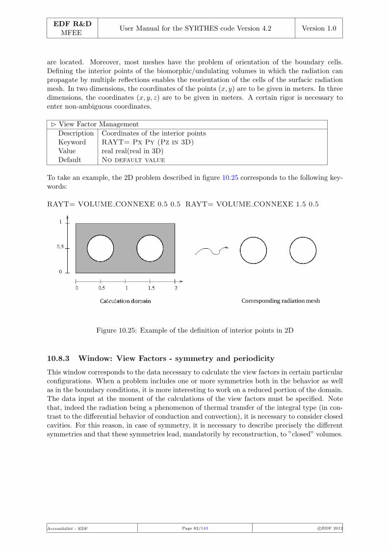
EDF R&DMFEE


are located. Moreover, most meshes have the problem of orientation of the boundary cells.Defining the interior points of the biomorphic/undulating volumes in which the radiation canpropagate by multiple reflections enables the reorientation of the cells of the surfacic radiationmesh. In two dimensions, the coordinates of the points (x, y) are to be given in meters. In threedimensions, the coordinates (x, y, z) are to be given in meters. A certain rigor is necessary toenter non-ambiguous coordinates.

B View Factor Management

Description Coordinates of the interior pointsKeyword RAYT= Px Py (Pz in 3D)Value real real(real in 3D)Default No default value

To take an example, the 2D problem described in figure 10.25 corresponds to the following key-words:

RAYT= VOLUME CONNEXE 0.5 0.5 RAYT= VOLUME CONNEXE 1.5 0.5

Figure 10.25: Example of the definition of interior points in 2D

10.8.3 Window: View Factors - symmetry and periodicity

This window corresponds to the data necessary to calculate the view factors in certain particularconfigurations. When a problem includes one or more symmetries both in the behavior as wellas in the boundary conditions, it is more interesting to work on a reduced portion of the domain.The data input at the moment of the calculations of the view factors must be specified. Notethat, indeed the radiation being a phenomenon of thermal transfer of the integral type (in con-trast to the differential behavior of conduction and convection), it is necessary to consider closedcavities. For this reason, in case of symmetry, it is necessary to describe precisely the differentsymmetries and that these symmetries lead, mandatorily by reconstruction, to ”closed” volumes.


EDF R&DMFEE


Figure 10.26 shows an acceptable situation on the left (by specifying 2 symmetries), whereasthe modeling on the right (corresponding to a canal infinitely long which will be troncated) isnot acceptable.

Figure 10.26: Example of acceptable and unacceptable configurations

The corresponding window is the following:

Figure 10.27: syrthes.gui - Window: Definitions of periodicity and symmetry planesfor radiation

The maximum number of symmetries in 2D is 2, and in 3D is 3. The real coefficients definingthe symmetry planes must be input.

B Symmetry in 2D

Description Coefficients of the symmetry plane ax+by+c=0 in 2DKeyword RAYT= SYMETRIE 2D a b cValue real real realDefault no default value


EDF R&DMFEE


B Symmetry in 3D

Description Coefficients of the symmetry plane ax+by+cz+d=0 in 2DKeyword RAYT= SYMETRIE 3D a b c dValue real real real realDefault No default value

For the periodicity, the requirements for the closing of the space are the same. The periodicity in2D and in 3D is input differently. In 2D, simply an invariant point and an angle of rotation areinput. The indicated angle must equal 360◦when multiplied by a whole number. The maximumnumber of periodicity is 1 in 2D. The input data in 3D are: an invariant point, a directionvector corresponding to the norm normale of the plane considered, and the angle of rotationexpressed in degrees. The indicated angle must equal 360◦when multiplied by a whole number.The maximum number of periodicity in 3D is 2.

B Periodicity in 2D

Description Coefficients of periodicityKeyword RAYT= PERIODICITE 3D Ix Iy Iz Vx Vy Vz teta (in degree)Value real real real real real real realDefault no default value

10.8.4 Window: Material Radiation Properties

This window corresponds to the specification of the radiative properties of materials. In thisversion of SYRTHES, radiation is not considered to be semi-transparent, which necessitates thatthe emmisivity ε is provided for each material (per spectral band 9λ) if several bands have beendefined). Spectral reflectivity is automatically deducted from the emissivity by the formula:

ρλ = 1− ελ

Figure 10.28: syrthes.gui - Window: Definition of material radiation properties


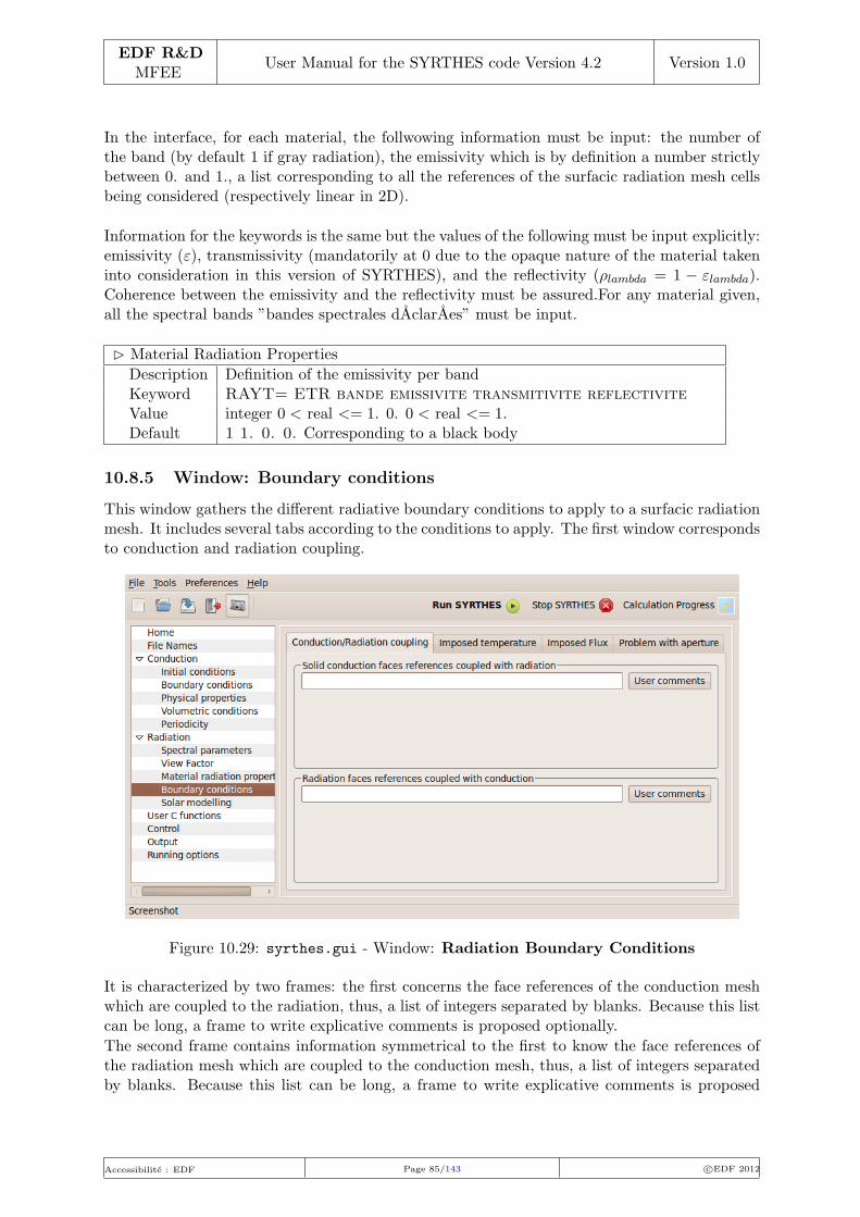
EDF R&DMFEE


In the interface, for each material, the follwowing information must be input: the number ofthe band (by default 1 if gray radiation), the emissivity which is by definition a number strictlybetween 0. and 1., a list corresponding to all the references of the surfacic radiation mesh cellsbeing considered (respectively linear in 2D).

Information for the keywords is the same but the values of the following must be input explicitly:emissivity (ε), transmissivity (mandatorily at 0 due to the opaque nature of the material takeninto consideration in this version of SYRTHES), and the reflectivity (ρlambda = 1 − εlambda).Coherence between the emissivity and the reflectivity must be assured.For any material given,all the spectral bands ”bandes spectrales dAclarAes” must be input.

B Material Radiation Properties

Description Definition of the emissivity per bandKeyword RAYT= ETR bande emissivite transmitivite reflectiviteValue integer 0 < real <= 1. 0. 0 < real <= 1.Default 1 1. 0. 0. Corresponding to a black body

10.8.5 Window: Boundary conditions

This window gathers the different radiative boundary conditions to apply to a surfacic radiationmesh. It includes several tabs according to the conditions to apply. The first window correspondsto conduction and radiation coupling.

Figure 10.29: syrthes.gui - Window: Radiation Boundary Conditions

It is characterized by two frames: the first concerns the face references of the conduction meshwhich are coupled to the radiation, thus, a list of integers separated by blanks. Because this listcan be long, a frame to write explicative comments is proposed optionally.

The second frame contains information symmetrical to the first to know the face references ofthe radiation mesh which are coupled to the conduction mesh, thus, a list of integers separatedby blanks. Because this list can be long, a frame to write explicative comments is proposed


EDF R&DMFEE


optionally.

The corresponding keywords are the following:

B Conduction/Radiation Coupling

Description Definition of the face references of conduction coupled to radiationKeyword CLIM= COUPLAGE RAYONNEMENT ref1 ref2 ...Value liste d’integersDefault no default value

B Radiation/Conduction Coupling

Description Definition of the faces references of radiaton coupled to conductionKeyword CLIM RAYT= COUPLAGE CONDUCTION ref1 ref2 ...Value list of integersDefault No default value

10.8.6 Window: Boundary conditions - imposed temperature

In certain cases, it is necessary to impose a temperature directly on the faces of the radiationmesh. This can help to avoid the meshing of the adjacent solid or when it has an unknown form.This can also correspond to configurations where the solid wall is non-existant (the door of anopen over) but for which the considered radiative space must be absolutely closed.

Figure 10.30: syrthes.gui - Window: Imposed radition temperature

The input data are the temperature (in ◦C), the face references of the radiation mesh on whichis applied the imposed temperature. Warning: these faces cannot be coupled with conduction.


EDF R&DMFEE


B Imposed radiation temperature

Description Definition of the radiative faces at imposed temperature and valueKeyword CLIM RAYT= COUPLAGE CONDUCTION T (in ◦C) refValeur real > 273.15 list of integersDefaut no default value

10.8.7 Window: Boundary conditions - Imposed Flux

This window corresponds to the flux directly imposed on the cells of the radiation. This func-tionality is used for example, to specify an adiabatic condition, meaning that the flux exchangeis zero (without having necessarily to mesh a solid wall). In the case where the flux is not zero,the situation can become complex relative to the data specifications when several spectral bandsare considered, limiting this option to specialists. Indeed, the proportion of the radiative fluximposed for each of the spectral bands considered must be input. The keywords to input arethus: the number of the spectral band, the flux per band, the list of references of the surfacicradiation mesh. In the case of a gray configuration (which represents the vast majority of cases),only one band is present per cell, and thus only the flux needs to be imposed.

Figure 10.31: syrthes.gui - Window: Radiative Imposed Flux


B Radiation Imposed Flux

Description Definition of the radiative faces at imposed flux and values (and possiblyby per band)

Keyword CLIM RAYT= FLUX IMPOSE PAR BANDE bande Flux (inW/m2) ref

Value integer 0 < real list of integersDefault no default value


EDF R&DMFEE


10.8.8 Window: Boundary conditions - Problem with aperture

This is a very specific window and must only be used advisedly. In certain configurations, theradiation mesh does not correspond to a closed space. This is typical of an oven door which,when it is open to the exterior, enables the interior of the oven to ”see” or to be influenced bythe external conditions. This window can, thus, be used to specify that the radiative problem isopen and to indicate the temperature of an equivalent black body corresponding to the radiativeambiance of the exterior environment.

Once this option is selected, the internal code cannot activate certain procedures to ensureenergy savings. Thus, it is recommended in such situations to mesh the aperture with theassistance of fictive surface cells resulting in a radiation mesh closing the volume and to imposea temperature on these same radiation cells. This solution is the most flexible (several differenttemperatures can be imposed as well as a different emissivity from that of the black body.

Figure 10.32: syrthes.gui - Window: Specification of a problem with aperture


B Radiation problem with aperture

Description Definition of a problem with aperture)Keyword DOMAINE DE RAYONNEMENT CONFINE OUVERT SUR L

EXTERIEUR=Value NON or OUIDefault NON

If the first keyword is activated, the keyword that can indicate the temperature of an equivalentblack body representative of the exterior environment must be specified.


EDF R&DMFEE


B Temperature of an equivalent exterior black body

Description Temperature of the exterior black body (in degrees)Keyword RAYT= TEMPERATURE INFINI T extValue real > 273.15Default 20

10.9 Parameters for models of humidity

This window appears only if the humidity option is activated in the Home interface window.Activating this function will eliminate the possibility to acces a purely thermal modeling. Thehumidity models being very complex and the characteristics of the physical evolutions of thematerials being relatively laborious to define, only a limited list of material is proposed via inter-face, rendering impossible the graphic input of the characteristics of the materials themselves.For this reason, despite the complexity of the underlying physical models, the graphic interfaceof the programmed humidity models in Syrthes appears concise and simple. Expanding thelist of available materials over time is possible but demands advanced programming. For thisreason, during the conception of syrthes such evolutions had been reserved to the specialistsof the domain in collaboration with the designers of the code.

Note that two large selections of humidity models are possible: The first corresponds to a modelwith two equations where the temperature and vapor pressure are resolved. This choice willimpact certain interface windows and the models programmed in syrthes .

Figure 10.33: syrthes.gui - Window: Humidity option with 2 equations activated


EDF R&DMFEE


The window in figure 10.34 corresponds to a choice of a model that is more complete wheretemperature, vapor pressure and the total pressure will be programmed. Once again, certaindata relative to these three equations must be input.

Figure 10.34: syrthes.gui - Window: Humidity option with 3 equations model activated

For the keywords file, this choice can be seen as the following form:

B Humidity

Description Activation of transfers coupled with mass and temperature. Two modelsare available: model with 2 equations (temperature and vapor pressure)and model with 3 equations (temperature, vapor pressure, and totalpressure)

Keyword modelisation des transferts d humidite=Valeur 0, 2 or 3Defaut 0

10.9.1 Control window

This window corresponds to the extension of the control window of a thermal calculation alone.The part concerning the time steps is unchanged, the notion of an automatic time step beingmanaged uniquely by evolutions of temperature. This choice was made because managing thetime step through a combination of physical critera based on the three variables can be too con-straining. Moreover, the temperature evolutions often being the most rapid, it is better duringthe transient to be associated to the temperature.


EDF R&DMFEE


The resolution of the variables pv and pv require that information be input into the solvers.For this reason, the window in figure 10.35 is proposed:

Figure 10.35: syrthes.gui - Window: Control window for the humidity solver

Information relative to the total pressure is presented, depending on the option of a model witheither two or three equations. The requested precision as well as the maximum number of iter-ations are found for each of the variables. These two parameters have a direct influence on theCPU time of the calculation. Imposing criteria which are too lax often leads to a divergenceof the system with a behavior which is sometimes particularly non linear. This is especiallytrue for the pv and pt variables, the number of iterations changes after the first simulationsdepending on the convergence of the interative systems.

For the keywords file, this information can be seen as the following form:

B Solver precision

Description Precision requested for the interative solver of the linear system for theresolution of conduction

Keyword nombre iterations solveur temperature=Value integer > 0Default 100

Keyword nombre iterations solveur pression de vapeur=Value integer > 0Default 100

Keyword nombre iterations solveur pression totale=Value integer > 0Default 100


EDF R&DMFEE


B Maximum number of iterations

Description Maximum number of interations authorized for the interative solver ofthe linear system for the resolution of conduction

Keyword precision pour le solveur temperature=Value real> 0Default 10−6

Keyword precision pour le solveur pression de vapeur=Value real> 0Default 10−15

Keyword precision pour le solveur pression totale=Value real> 0Default 10−14

10.9.2 Window: Humidity - Inital conditions

This window corresponds to temperature, vapor pressure pv and optionally to the quantity ptwhen the humidity model with three equations is activated. For each variable of the system, thedifferent values must be input. The first column shows the type of boundary conditions whichcan be adopted for the values:

• Constant

• Function

• Program

The second column is for the variable on which this initial condition will be applied. The thirdcolumn corresponds to the list of references of the elements on which this initial condition willbe applied. Note that the values are imposed on the elements for ergonomic reasons but arethen assigned to the nodes of the mesh in a continuous field. At the interface of two adjacentdomains, the last condition encountered will delete the first. In the configuration where the usersub program user hmt.c has been selected, the initial conditions are imposed on the nodes ofthe finite element mesh.


EDF R&DMFEE


Figure 10.36: syrthes.gui - Window: Initial conditions in the humidity model

B Initial humidity conditions

Description Initial condition in t (in ◦C)Keyword cini t= Temperature referencesValue realDefault T = 20

Keyword cini t fct= Temperature referencesValue fonction (x,y,z,t,T)Default T = 20

Keyword cini t prog= referencesValue user.c (user hmt cini) to program


Description Initial condition of vapor pressure pv (in Pa)Keyword cini pv= Pression de vapeur referencesValue realDefault Pv = 2800

Keyword cini pv fct= Pression de vapeur referencesValue function(x,y,z,t,T)Default Pv = 2800

Keyword cini pv prog= referencesValue user hmt.c( user hmt cini) to program


EDF R&DMFEE



Description Initial condition of vapor pressure pt (en Pa)Keyword cini pt= Pression totale referencesValue realDefault Pv = 101300

Keyword cini pt fct= Pression de vapeur referencesValue function (x,y,z,t,T)Default Pv = 101300

Keyword cini pt prog= referencesValue user hmt.c (user hmt cini) to program

Note that by default, a temperature of 20◦Cis proposed, a coherent vapor pressure (in particularinferior to the saturated vapor pressure) and a total pressure corresponding to the ambientpressure (1 bar=101300Pa).

10.9.3 Window: Humidity - Material properties

In this window it is possible to specify where the different materials in the domain are found. Alist of materials for which the behavior is sometimes complex is linked to the Syrthes materialslibrary and the references of the mesh.

Figure 10.37: syrthes.gui - Window: Designation of materials in the humidity model

This choice was made because the input of material characteristics is often complex and becausein practice the simulations often use the same materials. This also avoids calculations withmaterial properties which vary from one configuration to another.

At regular intervals, this list can be enriched by syrthes developers in collaboration with thespecialists of the domain or the laboratories which do experiental measurements on materials.For the keywords file, the synthax is thus the following:


EDF R&DMFEE


B Humidity - Material properties

Description Initial condition of vapor pressure pt (in Pa)Keyword hmt mat= chaine references

The keyword string can have for example the values in the following list:

• MAT BETON

• MAT BOIS PIN

• MAT PSE NORMAL

• MAT LAINE VERRE

• MAT BOIS AGGLO

• MAT POLYURETHANE

• etc...

As an example, if the domains characterized by the elements with references 2, 4 and 32 are ofciment and that the domain with the elements having the reference 8 corredspond to fiberglass,the imput in the keywords file would be:

HMT MAT= MAT BETON 2 4 32HMT MAT= MAT LAINE VERRE 8

10.9.4 Window: Humidity - Coupled Boundary Conditions

This window corresponds to the boundary conditions of the humidity models. In contrast tothe boundary conditions of the temperature models, the only conditions are heat exchanges(because of its physical characteristic when specifying the coupled boundary conditions).

This table thus includes the heat exchange boundary conditions for temperature, vapor pressureand optionally the total pressure if the model with three equations is activated. Another datacan be found that is not currently used in the syrthes code (it will be used in future versions)having a heat exchange coefficient of water in its liquid state. Its value (even if it appears in theinterace) is not interpreted or set at 0.


EDF R&DMFEE


Figure 10.38: syrthes.gui - Window: Boundary conditions of the humidity models

The corresponding keywords appear as the following:

B Humidity Boundary Conditions

Description Constant coupled boundary conditions in T Pv and PtKeyword clim hmt= hhh t ext ht ext pv ext hpv ext pt ext hpt extValue real real real real real real referencesDefault No value (corresponding to an adiabatic and watertight wall)

Description Constant coupled boundary conditions in function T Pv and PtKeyword clim hmt fct= t ext ht ext pv ext hpv ext PT ext hpt ext

references

Value Each function can depend on the variables (x,y,z,t,T,Pv,Pt)

Description Coupled boundary conditions as a sub-programKeyword clim hmt prog= referencesValue user hmt.c (user hmt limfso) to program

10.9.5 Window: Humidity - Volumetric source terms

This graphic window corresponds to the possibility for each of the variables to introduce sourceterms. For the temerature equation, this can correspond to the possibility of adding a Jouleeffect or an exothermic or endothermic chemical reaction.

The source terms are imposed on the elements of each domain. For the other two variables,the subadjacent physical meaning signification physique sous-jacente is not as easy. They wereprogrammed for generalization and can enable the modeling of the most macroscopic effects.


EDF R&DMFEE


Figure 10.39 shows the corresponding graphic interface window:

Figure 10.39: syrthes.gui - Window: Humidity model for source terms

This is the same methodology as for the imposed initial conditions: one choice for the type ofboundary conditions (constant, function, sub-program), the variable on which the condition isapplied, the imposed value, and the references of the elements on which the condition is applied.Note, in coherence with the other windows, that the activation of the sub-program option willdeactivate the possibility to input values or functions, the objective being to avoid ambiguityconcerning the placement of where the conditions must be input. The corresponding keywordsappear as the following:

B Humidity - Volumetric term sources in T

Description Impose a volumetric term for T in humidityKeyword cvol t= source (W/m3) referencesValue real referencesDefault No value (or 0 source term)

Description Impose a volumetric term for T as a functionKeyword cvol t fct= fonction source(x,y,z,t,T,Pv,Pt) referencesDescription Impose a volumetric term for T as a sub-functionValue user hmt.c (user hmt cfluvs) to program

B Humidity - Volumetric term sources in Pv

Description Impose a volumetric term for Pv in humidityKeyword cvol pv= source (Pa/m3) referencesValue real referencesDefault No value (or 0 source term)

Description Impose a volumetric term for Pv as a functionKeyword cvol pv fct= fonction source(x,y,z,t,T,Pv,Pt) referencesDescription Impose a volumetric term for Pv as a sub-functionValue user hmt.c (user hmt cfluvs) to program


EDF R&DMFEE


B Humidity - Volumetric term sources in Pt

Description Impose a volumetric term for Pt in humidityKeyword cvol pt= source (Pa/m3) referencesValue real referencesDefault No value (or 0 source term)

Description Impose a volumetric term for Pt as a functionKeyword cvol pt fct= fonction source(x,y,z,t,T,Pv,Pt) referencesDescription Impose a volumetric term for Pt as a sub-functionValue user hmt.c (user hmt cfluvs) to program

10.10 Window: Conjugate Heat Transfer

The coupling of syrthes with one (or several) CFD code/s with the corresponding meshes isdone through the references. In the case of coupling with the Code Saturne or neptune, it ispossible to execute the following couplings:

• surfacic: the thermal coupling of the fluid and solid domains is done through the contactsurfaces:

Figure 10.40: Example of a surfacic coupling application

B Conjugate Heat Transfer

Description Surface couplingKeyword CLIM= COUPLAGE SURF FLUIDE nom cas CFD referencesValue Name of CFD case (ie from repertoire)Default


EDF R&DMFEE


• volumetric: the domain fluid generally presents encumbered zones where the solid is ho-mogenized and is represented in the fluid by loss of charge. Inversely, multiple fluid flowsare not explicitely meshed in the solid and are also homogenized. Only the ”effect” on thefluid is taken into consideration on the solid.A typical example of this configuration is the case of a solid carried by a great number offluid canals (exchanger)

Figure 10.41: Example of a volumetric coupling application

B Conjugate Heat Transfer

Description Surface couplingKeyword CLIM= COUPLAGE VOL FLUIDE nom cas CFD referencesValue Name of CFD case (ie from repertoire)Default


EDF R&DMFEE



EDF R&DMFEE


Chapter 11

Data for heat and mass transfers

11.1 Data in the file syrthes data.syd

11.1.1 General data

• Activation of the model of coupled heat transfer (= 2 for the model with 2 equations, =3for the model with 3 equations). In the current version, only the model with 3 equationsis available.

11.1.2 Manage the precision of the solvers

The precision of the solver can be defined independently for each of the variables. The advisedvalues are:

• 10−5 for the temperature,

• 10−6 for the vapor pressure,

• 10−14 for the total pressure.

11.1.3 Definition of materials

The properties of materials are defined on the elements. The different materials present in thedomain are defined by the colors of the elements.The different materials are identified by their names which were defined in the include filehmt libmat.h.

11.1.4 Boundary conditions

Only the heat exchange conditions are available. For each variable, the heat exchange coefficientand the value of the exterior variable is set.The boundary conditions are imposed on the boundary faces.

11.2 Materials library

11.2.1 Data structure

• Humid: This structure contains the model used for the resolution (model with 2 or 3equations) and a table which indicates the number of the material of each element of themesh.


EDF R&DMFEE


– model = 2 or 3

– mat[maillnodes.nelem]: material number of the element

• ConstPhyhmt: This structure defines the constant physical properties of the fluid and theair of the materials

– rhol: Volumetric mass of the liquid

– rhot: Volumetric mass of the air

– R: Constant of the ideal gas

– xmv: Molecular mass of the vapor

– xmas: Molecular mass of the dry air

– Rv: Vapor constant per unit mass

– Ras: Dry air constant per unit mass

– Cpv: Vapor specific heat capacity at constant pressure

– Cpas: Dry air specific heat capacity at constant pressure

– Cpl: Water specific heat capacity at constant pressure

• ConstMateriaux: this structure defines the physical constants of each material

– rhos: Volumetric density of dry material

– cs: Heat capacity of dry material

– eps0: Porosity of the dry material

– xk: Intrinsic permeability

– xknv: Knudsen permeability

– taumax: Maximum rate of volumetric humidity

For each material the values are defined in the function fmat cont xxx

11.2.2 How are the properties of the materials defined?

The properties of the materials are defined in functions located in the materials librarylib material syrthes edf.

All the functions defining the properties of a material ”my material” are defined in the functionhmt lib mon materiau.c and in the corresponding include file hmt lib mon materiau.h.

The following functions are defined for each material:

• fmat const my material: definition of the constants of the material

• fmat ftauv my material: calculation of the volumetric humidity rate

• fmat falpha my material: slope of the sorption isotherm

• fmat fkrg my material: relative permeability of gas

• fmat fkrl my material: relative permeability of liquid


EDF R&DMFEE


• fmat fklambt my material: relative conductivity of humid material

• fmat fpiv my material: diffusion coefficient of the vapor in the material

• fmat fhm my material: complementary latent heat

• fmat fdhmtauv my material: ∂hm∂τv

• fmat fbetap my material:

• fmat fdhp my material:

• fmat fdht my material:

11.2.3 How are the diverse functions used?

In a loop on the elements, the following are included:

• material of the current element: nmat = humid.mat[i],

• the structure constmateriaux[nmat] contains all the constants of the material nmat

• a function can be called directly with: fmat nom[nmat](parametres)

Example: fmat ftauv[nmat](constphyhmt,constmateriaux[nmat],pve[i],psat,t)

11.2.4 How can a new material be defined?

This section discribes how it is possible to add a new material in the material library.As the source code of syrthes is avalaible, you can add directly your new material in theoriginal code source. But generally creation of a local new library is prefered : original versionis preserved and laws and functions of the new material can be tested before being inserted inthe standard version.

11.2.4.1 To create the new material

1. To create a standard study case using syrthes.gui (or syrthes4 create case command).

2. To go into the case directory.To prepare the addition of a new material, use the command : syrthes4 create mylibmat.Now, you have 2 additionnal directories : mylibmat src and mylibmat include, the localMakefile has been modified and, if you hadn’t the user hmt.c file in your case it has beenalso copied.

3. To go into the directory mylibmat include.To create the new material :

(a) To use the example of two existing files describing a material, to copy them to a newname.For example :cp syr hmt lib beton.c syr hmt lib xxx.c

cp syr hmt lib beton.h syr hmt lib xxx.h

(b) In these two files (syr hmt lib xxx.c and syr hmt lib xxx.h) to update the names of thefunctions with the name of the new material (for example, replace fmat fbetap beton

with fmat fbetap xxx). To program all of the functions for the new material.


EDF R&DMFEE


(c) To update the file syr hmt libmat.c: add a line#include "syr hmt libmat xxx.c

(d) To update the file syr hmt libmat.h

• To update the total number of defined materials (add 1): #define NB MAT 7

• To attribute a number to a new material: #define MAT XXX 6

• To add at the end of the list liste mat[NB MAT] ] a name for this new material(explicit name without spaces). It is this name that will be used in the data filesyrthes.data to identify the materials present in the case in progress.

• To add the file include: #include "syr hmt libmat xxx.h

• For each of the functions, to add the name of the function corresponding to thenew material to the existing list.

4. To add the new material to the material list in the graphical user interface, to edit thefile syr syr hmt material.txt and simply add the name of your new material (put the samename as you has used in the file syr syr hmt libmat.h).

Warning :

1. Don’t modified the directory mylibmat src

2. File user hmt.c must be in your study case

New material will be taken into account automatically when running syrthes (when usingsyrthes.gui “Run SYRTHES” button or using the command line syrthes.py.

11.2.4.2 To use the new material in syrthes run

In the syrthes data file, the new material can be used as the other material. The key wordslineHMT MAT= MAT XXX 2 5 3 will set the new material on elements referenced 2, 5 or 3.

With syrthes.gui, to active the advanced mode (“Tools/Advanced mode”), then to choose“Advanced Mode” in the list on the left. Put


EDF R&DMFEE


Chapter 12

User functions

In order to make the use of syrthes easier, it is possible to define a certain number of conditions(physical, boundary) directly in the data files:

• If the conditions are defined by constants, no programming is necessary and the conditionscan be modified without compiling or editing the links

• If the conditions can be described by functions, it is also possible to define them in thedata file. If they are modified during a calculation, they must be reinterpreted by thepre-processor to be integrated into the executable program.

But there are some cases where the conditions cannot be expressed so simply. For example,conditions which necessitate the reading of data in a specific file.

In all of such complex cases, it is necessary to be able to directly program the user functions.

The user functions are regrouped in 4 files:

user.c: general user functions,

user cond.c: user functions for conduction,

user ray.c: user functions for radiation,

user hmt.c: user functions for coupled heat and mass transfers.

The user functions are reviewed in the following paragraphs. For each of them, their specificitiesare detailed.

12.1 Description of the variables included in the user functions

• The characteristics of the mesh are contained in the maillnodes:

– maillnodes.ndim: dimension of the case in study (2 or 3)

– maillnodes.nelem: number of elements of the mesh

– maillnodes.npoin: number of nodes of the mesh


EDF R&DMFEE


– maillnodes.coords[j][i]: coordinate j (j=0 for x, j=1 for y, j=2 for z) of the nodei(i ∈ [0,maillnodes.npoin[)

– maillnodes.nodes[j][i]: node j of element i (j ∈ [0, 3] for a tetrahedron in 3dimensions and j ∈ [0, 2] for a triangle in 2 dimensions 2), (i ∈ [0,maillnodes.nelem[)

– maillnodes.nrefe[i]: reference of element i (i ∈ [0,maillnodes.nelem[)

• The variables of the calculations are calculated at each node

– t[i]: temperature of node i (i ∈ [0,maillnodes.npoin[)

– pv[i]: vapor pressure of node i (i ∈ [0,maillnodes.npoin[)

– pt[i]: total pressure of node i (i ∈ [0,maillnodes.npoin[)

• The physical properties are defined in each element

– physol.rho[i]: density of element i (i ∈ [0, physol.nelem[ note that physol.nelem =maillnodes.nelem)

– physol.cp[i]]: heat capacity of element i (i ∈ [0, physol.nelem[ note that physol.nelem =maillnodes.nelem)

• The isotropic conductivity is defined for the list of elements having a conductivity of thistype. Thus:

– physol.kiso.k[i]: the isotropic thermal conductivity of element i with i ∈ [0, physol.kiso.nelem[

• The orthotropic conductivity is defined for the list of elements which have a conductivityof this type. Thus:

– physol.kortho.k11[i]: the thermal conductivity of element i in direction x withi ∈ [0, physol.kortho.nelem[

– physol.kortho.k22[i]: the thermal conductivity of element i in direction y withi ∈ [0, physol.kortho.nelem[

– physol.kortho.k33[i]: the thermal conductivity of element i in direction z withi ∈ [0, physol.kortho.nelem[ (in 3 dimensions only)

• The anisotropic conductivity is defined for the list of elements having a conductivity ofthis type. Thus:

– physol.kaniso.k11[i]: the conductivity of element i in the direction of x withi ∈ [0, physol.kaniso.nelem[

– physol.kaniso.k22[i]: the conductivity of element i in the direction of y withi ∈ [0, physol.kaniso.nelem[

– physol.kaniso.k12[i]: the conductivity of element i in the direction of xy withi ∈ [0, physol.kaniso.nelem[

– physol.kaniso.k33[i]: the conductivity of element i in the direction of z withi ∈ [0, physol.kaniso.nelem[ (in 3 dimensions only)


EDF R&DMFEE


– physol.kaniso.k13[i]: ]: the conductivity of element i in the direction of xz withi ∈ [0, physol.kaniso.nelem[ (in 3 dimensions only)

– physol.kaniso.k23[i]: the conductivity of element i in the direction of yz withi ∈ [0, physol.kaniso.nelem[ (in 3 dimensions only)

• Flux boundary condition

– flux.val1[j][i]: flux (W/m2) at node j of element i (j ∈ [0, 3] for 3 dimensionaltetrahedrons and j ∈ [0, 2] for 2 dimensional triangles), i ∈ [0, f lux.nelem[ i is thusthe local number of the ith boundary face with flux

• Heat exchange boundary condition

– echang.val1[j][i]: temperature

– echang.val2[j][i]: exchange coefficient

12.2 Functions of file user.c

The functions presented in this file are general and can be used regardless of the type of calcu-lation.

12.2.1 Reading a specific data file: user read myfile()

This function enables additional data to be read in a file of any format. The parameters are thefollowing:

. struct Myfile *myfile: of all information contained in the file.

12.2.2 Writing additional variables in the result file: user add var in file()

This function enables the calculations of specific fields and to record them in the result file.These fields can thus be post-treated in the same way as the principle variables: temperatureand possibly vapor pressure and total pressure. Adimensionalization of certain variables is anexample of one of the applications. The parameters are the following:

. struct Maillage maillnodes: the mesh,

. struct Cvol *fluxvol: the volumetric source terms,

. struct Variable variable: all the variables of the calculation (T, Pv, Pt),

. struct Prophy physol: the physical properties.


EDF R&DMFEE


12.2.3 Definition of a specific transformation of periodicity: user transfo perio()

In the case of periodicity, this function enables the definition of a complex transformation toshift from boundary 1 to boundary 2. The parameters are the following:

. ndim: dimension of the study (2 or 3),

. x, y, z: coordinates of a node of boundary 1

. xt, yt, zt: coordinates of the node transposed to boundary 2 (result of the function)

12.3 Functions of the file user cond.c

The functions in this file enable the programming of the parameters relative to the resolutionof a conductive problem.

12.3.1 Initialization of the temperature: user cini()

An initial temperature can be given to the solid in the function. It can be variable in space.

The parameters are the following:

. struct Maillage maillnodes: the mesh,

. t[maillnodes.npoin]: temperature at each solid node (result of the function),

. struct PasDeTemps *pasdetemps: all the information relative to time management,

. struct Meteo meteo: data concerning the weather when necessary,

. struct Myfile myfile: personal file when necessary.

12.3.2 Physical characteristics: user cphyso()

This function enables the definition of the laws of variation of the physical properties of materialsin the calculations of conduction or conduction/radiation.It is not used for coupled heat and mass transfers.

. tempss: physical current time (seconds),

. t[maillnodes.npoin]: temperature at each solid node,

. struct Maillage maillnodes: mesh,

. struct Prophy physol: physical properties to input (result of the function),




The variable characteristics are the following:


EDF R&DMFEE


• density physol.rho[i] (kg/m3)

• heat capacity physol.cp[i] (J/kgK)

• thermal conductivity physol.k[i] (W/mK) for materials with isotropic behavior, physol.k11[i],physol.k22[i], physol.k33[i] for materials with orthotropic behavior, or physol.k11[i],physol.k22[i], physol.k33[i],physol.k12[i], physol.k13[i], physol.k23[i] formaterials with anisotropic behavior.

12.3.3 Boundary conditions: user limfso()

The laws of complex variation of the boundary conditions can be defined in this function forcalculations of conduction or conduction/radiation.It is not used for coupled heat and mass transfers.The boundary conditions are imposed on the boundary faces of the elements.

. tempss: physical current time (seconds)


. struct Maillage maillnodeus: boundary mesh,

. t[maillnodes.npoin]: temperature at each solid node

. struct Clim diric: Dirichlet condition (imposed temperature) (result of the function),

. struct Clim flux: Flux condition (result of the function),

. struct Clim echang: Heat exchange condition (result of the function),

. struct Clim rayinf: Infinite radiation condition (result of the function),




The user part is divided in 4 sections, each dealing with a specific boundary condition. If, inthe physical case under study, one of the condition types is not necessary, lines relative to thecondition are simply left as comments.

12.3.4 Volumetric source terms: user cfluvs()

The laws of complex variation for volumetric flux can be defined in this function for calculationsof conduction or conduction/radiation.

It is not used for coupled mass and temperature transfers.

The boundary conditions are imposed on the boundary faces of the elements.

. tempss: physical current time (seconds),



EDF R&DMFEE


. t[maillnodes.npoin]: temperature at each solid node,

. struct Cvol fluxvol: volumetric source term (result of the function),




12.3.5 Contact resistance: user resscon()

The laws of complex variation for contact resistances can be defined in this function.

. tempss: physical current time (seconds)


. struct Maillage maillnodeus: boundary mesh,

. t[maillnodes.npoin]: the temperature at each solid node,

. tcor[maillnodes.npoin]: the temperature of the node face to face,

. struct Contact rescon: resistance de contact (result of the function),


. struct SDparall sdparall: for the management of parallel computations.

12.4 Functions for file user ray.c

The programming of parameters relative to the resolution of a study concerning radiation isdealt with in this file.

12.4.1 Function user ray()

As seen in preceding chapters, the physical properties and boundary conditions for radiation aregenerally provided in the interface and are indicated in the data file syrthes.data.

Nevertheless, in certain complex cases, it is sometimes necessary to vary the coefficients relativeto the particular law or to the tabulations. In this case, it is possible to program individual lawsof variations directly.

The following can be defined in this function:

• The radiative properties of the material (emissivity),

• The temperature of the radiation of the faces with ”imposed temperature”

• The radiation flux of the faces with ”imposed flux”


EDF R&DMFEE


12.4.2 Function user solaire()

Personalized calculations for direct and diffused solar fluxes can be defined in this function whenthe solar radiation option is activated.

12.4.3 Function user propincidence()

Complex radiation properties of materials relative to the angle of incidence can be defined inthis function.

12.5 Functions to assist with parallel computations

In certain cases, it is necessary to have personalized programs, especially in particular post-treatment cases.

For sequential calculations, it is easy to access the values of a variable in the entire domain ofcalculation. But when simultaneous calculations are required, each processor can only ”see” aportion of the total domain. Thus, it is necessary to use specific functions for the managementof interfaces between the different processors.

To facilitate this, several functions are proposed which can be called in a general way so thatthe execution can then be made sequentially or simultaneously.

The family of currently available functions is the following:

• Calculation of a sum,

• Calculation of a minimum or a maximum.

12.5.1 Calculation of a sum

Example: On the current processor, the number nloc has been calculated which represents thenumber of nodes whose temperature exceeds a defined criteria. The number of nodes in thesame situation for the entire domain is thereafter needed. The function somme int parall canbe used to solve this question under the form:

n glob=somme int parall(n loc)

where nglob contains the sum of nloc snloc of all the processors.

Note: For serial calculations, the result will simply be nglob = nloc.

This function has been created to be used with ”double” or ”integer” variable types:

• int = somme int parall(int)

• double = somme double parall(double)

12.5.2 Calculation of a minimum or a maximum of a variable

The calculation of a minimum or a maximum of a field is done in two steps:

• Step 1: calculation of min/max on the local processor


EDF R&DMFEE


• Step 2: calculation of min/max on all the processors

The first step is usual: the table containing the variable is scanned to search for the min and max.The second step is then done automatically by the functions min xx parall/maxw xx parall.Depending on the type of variable to calculate and on the operation to be done, one of thefollowing functions is used:

• int = min int parall(int)

• int = max int parall(int)

• double = min double parall(double)

• double = max double parall(double)

Exemple: if Vmax loc is the maximum on the local processor, the maximum of all the processorswill be determined by: Vmax glob = max double parall(Vmax loc)

Note: If the calculation is run in serial, Vmax glob = Vmax loc will be obtained.


EDF R&DMFEE


Chapter 13

Result files

The number of result files generated by syrthes depends on the options selected. From thename of the prefix assigned in the data file (for example: resu1), all the result files with specificextensions will be created, as seen as follows:

• resu1.res result file: field of different variables at the end of the calculation,

• resu1.rdt: transient result file, field of different variables at different time steps,

• resu1.his: history file for results at probes,

• resu1.mnx: min/max result file

• resu1.add: additional result file

13.1 Result files: additionnal

13.1.1 Contents of additional files

syrthes offers the possibility of writing the fields of complementary results. The file (name.add)which will be generated by syrthes is in the same format as the standard result file (name.res).Thus, it is possible to visualize it with the same post-processor.

The additional result files can contain:

• node fields,

• element fields,

• node fields and element fields.

13.1.2 Principle

At any time, a complementary variable can be calculated from the data available in the code.This variable is stored in a table which can be used by calling up the recorded function of thisvariable in the additional file.

The writing frequency of the additional results is identical to the writing frequency of thehistorical output.


EDF R&DMFEE


13.1.3 How to write variables in an additional file?

The variable can be written in the additional file at any place in the code. To visualize thevariable on the mesh, the variable must be calculated on all of the nodes or elements of themesh.

For a variable on the nodes there are thus: maillnodes.npoin values, and for a value on theelements there are thus maillnodes.nelem values.

1. In the source of the code, the variable is calculated and stored in a work table (for example:trav proportional to the number of nodes or elements, depending on the nature of thenew variable)

2. Call the functions:if (ecraddfile) add var in file(int nb val,double *trav,char* name,int type);with;

• if (ecraddfile): test if it is the moment to record the variable in the file

• nb val: number of values to write,

• trav: variable,

• name: name of the variable (string of 12 characters maximum without spaces),

• type: =2 for a variable on the elements; =3 for a variable on the nodes,

3. Examples: to write the new files ”MY VAR” stored in table:if (ecraddfile) add var in file(maillnodes.npoin,trav1,"MY VAR’’,3); if (ecraddfile)add var in file(maillnodes.nelem,trav2,"MY VAR’’,2);

Note that the writing frequency for the additional variables is the same as for the main variables(temperature, Pv, Pt). Thus, the output option for transient result field must be selected in theGUI (or by the appropriate keyword in the syrthes data.syd file).


EDF R&DMFEE


Chapter 14

Do a thermal calculation withsyrthes

14.1 Introduction

The different phases of a calculation are the following:

• analysis of the physical problem, choice of the calculation domain, of the physical models,

• generation of the mesh of the solid domain, setting of the references to identify the differentmaterials, boundary conditions, physical conditions, etc. . .If necessary, calculation of heat transfer, generation of the radiation mesh.

• update of the data file syrthes.data for conduction and, if necessary, for radiation,

• update, if necessary, the user functions,

• creation of the execution program and run the calculation,

• and if everything goes well, analysis of the results.

14.2 Preliminary phase: set a syrthes environment

For smooth operation, syrthes uses a certain number of environment variables which are setin the user environment via the file syrthes.profile.

Before using the code, it is thus necessary to ”source” this file:> . /..../syrthes4.x.y-z/arch/NOM ARCH/bin/syrthes.profile

Note: this command can be input directly in the user environment files (.profile or .bashrc)so that it is automatically executed upon login.

14.3 Running calculation with syrthes interface

From the work directory the following command is given:> syrthes.gui


EDF R&DMFEE


The following window will appear on the screen:

Figure 14.1: syrthes.gui- Window: Creation of a new case

It is necessary to ”create a new case” by inputting the name of the case. The interface will thencreate a new directory which will contain the basic files to run a calculation.

The main window of the interface appears on the screen:

Figure 14.2: syrthes.gui- Window: syrthes user interface

Different menus will drop down in the left side of the window to input the different parametersnecessary for the calculation.Generally, the different rubrics are perused in order finishing by”Running options”.


EDF R&DMFEE


Once all of the input data have been defined, the code can be run by clicking ”Run SYRTHES”.

Figure 14.3: syrthes.gui- Window: ”Running options” run the calculation

During the calculation, the progress can be visualized as well as the evolution of the differentvariables through the probes defined previously in the ”Output” window.

Figure 14.4: syrthes.gui- Window: Progress of a syrthes calculation

Note that a calculation can be run from all the interface windows which include the ”RunSYRTHES” button on the tool bar.


EDF R&DMFEE


Figure 14.5: syrthes.gui- Window: Run the calculation from the tool bar

The calculation can be stopped at any time by clicking ”Stop SYRTHES”. In this case, syrtheswill finish the current time step and store the results.

Figure 14.6: syrthes.gui- Window: Interruption of a calculation

14.4 Run a manual calculation (without the syrthes.gui)

14.4.1 Step 1: Create a new calculation case

A utility is available to automatically create a ”calculation case”, meaning that a directorycontaining a copy of all the files which will eventually be used for the calculation. Thus, apre-filled data file can be included where only the values of certain parameters will be modified.

syrthes4_create_case my_cas

14.4.2 Step 2: Create a mesh and convert it to syrthes format

The syrthes meshes are composed of 3-node 2-dimensional triangles or 4-node 3-dimensionaltetrahedrons.


EDF R&DMFEE


In the case where the radiative transfers are also resolved, a second mesh must be provided: itis composed of 2-node 2-dimensional segments or of 3-node 3-dimensional triangles.

The format of the mesh is determind by the file name extension. The formats currently takeninto consideration are the following:

• gmsh (.msh)

• med (.med)

• simail (.des)

• gambit (.neu)

• Ideas-MS (.unv)

• syrthes (.syr)

When the mesh is finished it must be converted into the syrthes format with the assistance ofthe tool convert2syrthes4.

The parameters of this utility are the following:

> convert2syrthes4 -m source -o destination.syr

or

> convert2syrthes4 -m source

In the second case, the default file destination will be source.syr.

Note: When using the graphic interface to define the calculation parameters, the conversion ofthe format is done automatically if the mesh file chosen is not already in the syrthesformat.

14.4.3 Step 3: Filling in the data file syrthes data.syd

Once in the my case directory, the data file for syrthes must be created. This file is generallynamed syrthes data.syd.It is created with the assistance of the syrthesuser interface which is run with the command:> syrthes.gui

Note that an example of pre-filled data files can be found in the directory with all of the knownkeywords available in the code.

14.4.4 Step 4 (optional): User functions

In complex cases, where the physical conditions of the calculation can be defined neither by con-stants nor by interpreted functions (which are defined simply via the interface in the parameterfile), it is possible to program the laws of variation of these parameters directly into the codevia the user functions.

Examples of user source files can be found in the usr directory. If needed, the necessary file/scan be copied into the current directory and can be programmed in accordance with the caseunder study.


EDF R&DMFEE


The 4 files are respectively dedicated to the following functions: general (user.c), conductivetransfers (user cond.c), radiative transfers (user ray.c), and heat and mass transfer (user hmt.c).

• user.c: general functions

. user read myfile(): reading of a specific data file,

. user add var in file(): input of additional variables in the result files,

. user transfo perio(): definition of a specific periodic transformation.

• user cond.c: functions for conduction transfers

. user cini(): initial conditions

. user cphyso(): physical conditions,

. user limfso(): boundary conditions ,

. user cfluvs(): volumetric source terms,

. user rescon() or user rescon parall(): contact resistances

. user transfo perio(): definition of a particular transformation for periodicity condi-tions

. user read myfile(): reading of a specific data file

• user ray(): functions dedicated to radiative transfers

. user ray(): material parameters (emissivity, radiation boundary conditions (imposedtemperature or flux)

. user solaire(): definition of solar flux

. user propincidence(): calculation of the radiation physical properties relative to theangle of incidence

• user hmt(): functions for coupled mass and temperature transfers

. user hmt affectmat(): designation of the material on the mesh

. user hmt cini(): definition of the initial conditions

. user hmt limfso(): boudary conditions for the temperature, vapor pressure and totalpressure

. user hmt cfluvs(): definition of volumetric source terms

. user hmt rescon(): definition of contact resistances

14.4.5 Step 4: Create an executable program and run syrthes

In the case of the use of the user interface, the running options of the calculation can be definedin the ”Running options” window and the calculation can be directly run by clicking ”RunSYRTHES”.

The calculation can also be run via the following syrthes.py script:

> syrthes.py -n NB_PROC -d FILE [-r NB_PROC_RAY] [-l FILE] [-v POSTPROC]


EDF R&DMFEE


The parameters for this command are the following:

-n NB PROCDefines the number of processors to use for the conduction calculation-n 1: the calculation is done sequentially

-d FILEDefines the name of the data file for syrthes (generally syrthes data.syd)

-r NB PROC RAYDefines the number of processors to use for the radiation calculation.In cases with a radiation calculation, it is possible to resolve the radiative problem on anumber of processors different from the one used for conduction so that parallel calcula-tions can be done relative to the size of the conduction and radiation problem. The -roption is only used if the number of processors is different for conduction and radiation. Ifit is not defined, the number of processors for radiation will be equal to that of conduction.

NB PROC RAY ≤ NB PROCis mandatory

Option default: NB PROC RAY = NB PROC.

-l FILERedirects the standard output (the calculation log) in the file FILE.

-v POSTPROCThe conversion of the syrthes result file into a readable format by another post-processoris done in this option. Two formats are currently available: Ensight (POSTPROC=ensight)and med (POSTPROC=med). Thus, at the end of the calculation, both the SYRTHESfiles and the files in the requested format are obtained. Optional default: there is noconversion of syrthes result files to the format of a post-processor.

Examples of a calculation run:

• Sequential execution, output comments on the screen

> syrthes.py -n 1 -d syrthes.data

• Sequential execution, output comments written in the ”listing1” file and conversion of theresults respectively to Ensight and med formats

> syrthes.py -n 1 -d syrthes_data.syd -l listing1 -v ensight

> syrthes.py -n 1 -d syrthes_data.syd -l listing1 -v med

• Parallel execution on 2 processors, output comments written in the ”listing1” files

> syrthes.py -n 2 -d syrthes_data.syd -l listing1

• Execution on 10 processors for conduction and on 4 for radiation, output comments writtenin the ”listing1” files

> syrthes.py -n 10 -r 4 -d syrthes_data.syd -l listing1


EDF R&DMFEE


14.4.6 Step 5: Visualize the results

When the calculation is finished, syrthes generates result files in its own format. If the con-version was requested at the time of the running of the code, the files will be ready to visualizein the selected post-processor.

If not, tools are available to do the conversions to either the Ensight or medformats:

> syrthes4med30 -m maillage.syr -r resu.res -o post.med

> syrthes4ensight -m maillage.syr -r resu.res -o post

The result file (containing the fields from the last time step calculated), like the transient file(containing the fields from several moments/instants) can be converted:

> syrthes4med30 -m maillage.syr -r resu.res -o fin.med

> syrthes4med30 -m maillage.syr -r resu.rdt -o chrono.med

The history files present the values of the probes in columns and can be visualized with anydata plotting program (Gnuplot, Xmgrace, Excel . . . ).

14.5 Do a follow-up calculation

If the calculation is not finished (convergence is not attained or transient to follow), it is possibleto proceed to the next calculation. The new number of time steps to be done must be definedand the preceding result file (.res) will be provided to syrthes. The calculation will use thisfield as its initial field and will continue until the new stop criterion.

14.6 Emergency stop of syrthes calculation

In certain circumstances, it is necessary to stop a calculation in progress prematurely (conver-gence state attained for example).

When using the syrthes graphic interface, it is sufficient to click on ”stop” at the top left of thewindow (cf. figure 14.6). If not, it is possible to manually stop the execution code by creatingin the syrthes execution directory an empty file named syrthes.stop: the code will stop atthe end of the running time step and backup the result files of this time step.

When not using the syrthes graphic interface, use the following command to prompt an emer-gency stop:

touch syrthes.stop

Don’t forget to remove the syrthes.stop file before running again syrthes !

14.7 Analysis of the results

The data reduction of a calculation always starts with the analysis of the listing file.

From the very first trial of a new case, information provided by the initialization phase mustbe examined: for example, the order of magnitude of the number of nodes, of elements, of facessubmitted under this or that boundary condition, etc . . .


EDF R&DMFEE


These first verifications have several objectives:

• To verify the data: has a condition been omitted, do the references and type of conditionsagree, are the values of the boundary conditions exact?

• To ensure the correlation between what was desired and what the code actually inter-preted

• To ensure that the initializations proceeded normally and that everything seems coherent

The calculation procedureAt each time step, it is possible to have information on the convergence of the solver. Whensearching for a steady state, the number of iterations necessary for the solver to attain a givenconvergence tends to decrease with each time step: the calculation proceeds normally.

The convergence of the solverIf difficulties of convergence appear (high number of iterations, mediocre precision attained), itis generally possible to improve the conditioning of the system by adopting a smaller time step.

In cases of transient-state calculations, it is important to obtain a good convergence from thesolver at each time step. If the precision attained by the solver is still not good enough (around10−4 for example), it might be necessary to increase the number of iterations of the solver or tochoose a smaller time step. This is even more important when the calculation includes explicitconditions such as surfacic flux or volumetric source terms.

Evaluating the convergenceIn all numerical calculations, the evaluation of the convergence is often delicate and worrisome.Indeed, there is no absolute criterion that can confirm that a calculation is converged. Itis necessary, therefore, to use a certain number of ”indicators” which can help evaluate theconvergence. To cite a few:

• The behavior of the iterative solver (reduction of the number of iterations necessary toobtain very accurate precision)

• The definition of probes at several ”strategic” points in the domain: an examination ofthis chronology can reveal curves with asymptotic tendencies

• The analysis of results in the post-processor: the examination of the temperature profilesat diverse time steps shows the evolution of the temperature over time

• The experience of the user. . .

14.8 The generation of syrthes meshes

The solid domain is discretized by a non-structured mesh. It is currently possible to use themeshes issued from the mesh generators simail, Ideas-MS, gambit, Salome, gmsh.

During the generation phase, it is necessary to bear in mind the following:

• Certain sensitive zones where the physical phenomena are important must be meshed morefinely


EDF R&DMFEE


• The regularity of the elements facilitates the convergence of the calculation. Elementswith angles greater than 90◦ should be particularly avoided and a ”reasonable” distortionshould be conserved for each element.

• The physical characteristics of the case must be anticipated at the moment of the concep-tion of the mesh by placing for example, judiciously, the references on the boundary facesin view of the boundary conditions that will be imposed.

• In the same way, the element references must be anticipated relative to the differentmaterials. It is always possible to input more references than are strictly necessary: onematerial can have several different references to identify particular zones.

• The references must be positive integers. A face or an element whose reference is 0 (zero)is considered as not having a reference.

14.9 Calculating with a CFD code coupled to syrthes

syrthes was conceived so that the calculation methodology is identical regardless of whetherthe calculation is for a solid alone or for a calculation of a fluid/solid coupling.

Regardless of the application, the syrthes initialization should always be done within theframework of only simple conduction/radiation calculations. Even if the final objective is todo a fluid/solid calculation, this investment will pay off fully as the method for the calculationremains unchanged. Indeed, in a simplified manner, the fluid will only be treated as a particularboundary condition of the solid domain.

syrthes and the CFD code are completely independent so that it is possible to completely”uncouple” problems associated with fluids and solids: they can be analyzed separately andit is possible (and even advised) to start by establishing the two calculations (fluid and solid)separately before trying to couple them. Once all the conditions for each of the two domainshave been input and verified (with a small number of time steps), the coupling can be quicklyput in place.

Similarly, if a numerical problem appears, the uncoupling of the two codes is immediate, facili-tating the identification or localization of the source of the problem. Is the problem purely fluid,purely solid or rather linked to the transfer of data between the fluid and solid domains?


EDF R&DMFEE


Chapter 15

Conclusion

Today, syrthes enables the scientific community to treat complex problems by handling simul-taneously the phenomena of conduction, radiation and, when coupled with a thermal hydrauliccode, convection.

As more and more phenomena are integrated into the simulation, more and more precise resultscan be expected. However, the calculations become more delicate to manage as it is necessaryto understand very different physical phenomena evolving on time scales which are, themselves,very different.

This document presents the elements indispensible for running the syrthes code. The mostcomplex models (thermal radiation and mass transfers) have been uncoupled so as not to penalizethe users during the running of the code for conduction calculations alone.

Although the current version can already treat complex cases, the syrthes functions will evolverelative to the needs of the users. For this, users can contact the user support service at thefollowing e-mail address: [email protected].


EDF R&DMFEE



EDF R&DMFEE


Appendix A

syrthes FILE FORMATS

A detailed description of the syrthesfile formats is presented here.

In this chapter, the character strings appearing in the files will be detailed. The spaces will bereplaced by dots (·) in order to count or identify them more easily.

A.1 Description of the geometry file: file.syr

The geometrical files for conduction and radiation files are data bases containing respectivelythe meshes of the solid domain and the radiative surfaces. They are in SYRTHES file format.They contain successively a list of nodes (with coordinates and references), a list of elements(with their corresponding nodes) and a list of boundary elements.The geometrical file begins with the following type of header:

• lines 1 to 3: comments (the line contains the number of the file version)

• line 4: c··dimension·=%2i

• line 5: c··dimension ·of elts·=%2i

• line 6: c··number ·of ·noeuds·=···%10i

• line 7: c··number ··of ·elements·=··%10i

• line 8: c··number ··of ·boundary ·elements ·=··%10i

• line 9: c··number ··of ·nodes ·per ·element·=·%3i

This is followed by the rubric of node coordinates.

• line 1: c

• line 2: c$·rubrique·=·nodes

• line 3: c

• lines 4 to 3+number of nodes:

num, numref,x,y,z


EDF R&DMFEE


. num: number of the node

. numref: reference number of the node

. x y z: coordinates of the node. Note: there are always 3 coordinates (in 2dimensions , the third coordinate is set at zero)

The corresponding format is the following: %10i%4i %14.7e %14.7e %14.7e

Rubric containing the connectivity.

• line 1: c

• line 2: c$·rubrique·=·elements

• line 3: c

• lines 4 to 3+number of elements:

num, numref, list of nodes

. num: number of the element

. numref: reference number of the element

. liste of nodes: list of nodes belonging to the element

- format for tetrahedrons: %10i%4i%10i%10i%10i%10i- format for triangles: %10i%4i%10i%10i%10i

Rubric for the connectivity of the boundary mesh.

• line 1: c

• line 2: c$·rubrique·=·boundary ·elements

• line 3: c

• lines 4 to 3+nombre of boundary elements:

num, numref, list of nodes

. num: number of the element

. numref: reference number of the element

. list of nodes: list of nodes belonging to the element

- format for triangles: %10i%4i%10i%10i%10i- format for segments: %10i%4i%10i%10i

Example of a geometric file:

C*V4.2*******************************************C

C FICHIER GEOMETRIQUE SYRTHES C

C************************************************C

C DIMENSION = 2

C DIMENSION DES ELTS = 2

C NOMBRE DE NOEUDS = 1632

C NOMBRE D’ELEMENTS = 2904


EDF R&DMFEE


C NOMBRE D’ELEMENTS DE BORD = 360

C NOMBRE DE NOEUDS PAR ELEMENT = 3

C************************************************C

C

C$ RUBRIQUE = NOEUDS

C

1 0 1.0000001E-02 -1.2600000E+00 0.0000000E+00

2 2 1.6210891E-02 -1.2600000E+00 0.0000000E+00

3 3 2.2919025E-02 -1.2600000E+00 0.0000000E+00

...

1631 11 -6.2373497E-02 -1.6934443E+00 0.0000000E+00

1632 11 -3.1358525E-02 -1.6983566E+00 0.0000000E+00

C

C$ RUBRIQUE = ELEMENTS

C

1 1 464 459 457

2 1 464 457 443

3 1 463 455 461

...

2903 4 1439 1440 1455

2904 4 1455 1440 1456

C

C$ RUBRIQUE = ELEMENTS DE BORD

C

1 12 1457 1577

2 12 1577 1578

3 12 1578 1579

...

359 11 1455 1454

360 11 1456 1455

A.2 Result files: file.res

The final result files constitute, at minimum, the temperature field at the mesh nodes. In certaincases, they can be completed by other variables such as vapor pressure or total pressure. Theyare provided in the result file file.res.

The file is composed of a heading followed by tables of the values of each variable in all of thenodes or elements of the domain.

• line 1: comments

• line 2: title of calculation


• line 4: ndpt, temps, dt

. ndpt: number of the current time step

. temps: current physical time (seconds)

. dt: value of the time step of the calculation (seconds)

Format: ***NTSYR= %12d··***TEMPS=·%25.17e····***DT= %25.17e


Then for each result variable, the following group appears:

• ligne 1: nom variable, type, nombre de valeurs


EDF R&DMFEE


. nom variable: name of the variable

. type: 3 if the variable is situated on the nodes of the mesh, =2 if it is on the elements

. nombre de valeurs: number of values of the variable to read

Format: ***VAR=·%12s·***TYPE=·%1d··***NB=·%12d

• llines thereafter: the values of the variables with the format:%16.9e ·%16.9e ·%16.9e ·%16.9e ·%16.9e·%16.9e

A portion of a result file is presented below:

***SYRTHES V4.2**************************************************************************************

***test

*****************************************************************************************************

***NTSYR= 200 ***TEMPS= 2.00000000000000000e+03 ***DT= 1.00000000000000000e+01

*****************************************************************************************************

***VAR= TEMPERATURE ***TYPE= 3 ***NB= 1632

6.831441621e+01 6.432582907e+01 6.141672959e+01 5.914107062e+01 5.731541770e+01 5.582278873e+01

5.458769860e+01 5.360385316e+01 5.285596152e+01 5.234869685e+01 5.210827404e+01 5.211661097e+01

5.211090628e+01 5.210260576e+01 5.210201619e+01 5.210129368e+01 5.209428516e+01 5.209615136e+01

...

Example of a result file containing several variables:

***SYRTHES V4.2**************************************************************************************

***3rond2d

*****************************************************************************************************

***NTSYR= 20 ***TEMPS= 2.00000000000000000e+03 ***DT= 1.00000000000000000e+02

*****************************************************************************************************

***VAR= T_RAYT ***TYPE= 2 ***NB= 240

3.334941692e+01 3.336039388e+01 3.336235707e+01 3.336378464e+01 3.334543983e+01 3.334455717e+01

3.334816760e+01 3.334080425e+01 3.335122335e+01 3.336330610e+01 3.335612920e+01 3.336189721e+01

3.334442619e+01 3.336157198e+01 3.335899521e+01 3.333605267e+01 3.334725889e+01 3.335815803e+01

...

2.014586463e+01 2.014532492e+01 2.014451528e+01 2.010664813e+01 2.010819385e+01 2.010989737e+01

2.011203369e+01 2.011454749e+01 2.011732019e+01 2.011997618e+01 2.012224452e+01 2.012426189e+01

2.012646412e+01 2.012931101e+01 2.013276455e+01 2.013633879e+01 2.013968336e+01 2.014266663e+01

***VAR= FLUX_RAYT_0 ***TYPE= 2 ***NB= 240

2.708572064e+01 2.295235281e+01 1.886771293e+01 1.854430627e+01 2.897069267e+01 3.010793899e+01

2.819272821e+01 3.042816076e+01 2.592430422e+01 1.932451244e+01 2.459923549e+01 1.982890576e+01

2.959205919e+01 2.155202148e+01 1.902344504e+01 3.253932734e+01 2.949392474e+01 2.114157281e+01

...

-1.391292096e+01 -1.415382152e+01 -1.485118622e+01 -1.533997472e+01 -1.547424191e+01 -1.549937847e+01

-1.536760020e+01 -1.574304674e+01 -1.658142281e+01 -1.721341010e+01 -1.770233205e+01 -1.845574101e+01

A.3 Transient result file: file.rdt

This file has exactly the same structure as the final result file. Thus, a transient-state file is asequence/collection/series of n result files at different moments.

Each time step is composed of a heading followed by a table of variables.

***SYRTHES V4.2**************************************************************************************

***3rond2d

*****************************************************************************************************

***NTSYR= 3 ***TEMPS= 3.00000000000000000e+02 ***DT= 1.00000000000000000e+02

*****************************************************************************************************


3.324105218e+01 3.017225325e+01 2.796251301e+01 2.626939269e+01 2.495094400e+01 2.391359628e+01

2.309401245e+01 2.247691786e+01 2.203925954e+01 2.177092351e+01 2.167852479e+01 2.168633947e+01


EDF R&DMFEE


2.168499125e+01 2.168170661e+01 2.168296751e+01 2.168376981e+01 2.168047768e+01 2.168241924e+01

...

2.000057807e+01 2.000061200e+01 2.000063578e+01 2.000064621e+01 2.000173891e+01 2.000178319e+01

2.000170335e+01 2.000145612e+01 2.000112158e+01 2.000082052e+01 2.000061129e+01 2.000052194e+01

2.000056352e+01 2.000066393e+01 2.000072968e+01 2.000077085e+01 2.000080119e+01 2.000081342e+01

***SYRTHES V4.2**************************************************************************************

***3rond2d

*****************************************************************************************************

***NTSYR= 6 ***TEMPS= 6.00000000000000000e+02 ***DT= 1.00000000000000000e+02

*****************************************************************************************************


3.511913396e+01 3.238455849e+01 3.039483673e+01 2.884447380e+01 2.760831568e+01 2.660665068e+01

2.578849324e+01 2.514980564e+01 2.468052818e+01 2.438396762e+01 2.427825146e+01 2.428703137e+01

2.428548891e+01 2.428174557e+01 2.428312361e+01 2.428398721e+01 2.428024169e+01 2.428243654e+01

...

2.001092025e+01 2.000959903e+01 2.000784694e+01 2.000619816e+01 2.000498141e+01 2.000439638e+01

2.000449059e+01 2.000492626e+01 2.000527600e+01 2.000552773e+01 2.000571147e+01 2.000578183e+01

A.4 Additional result file: file.add

This file is only used if specific output has been defined. This is the case when particular prop-erties need to be calculated on all of the nodes. It has a structure identical to that of the resultfile (.res) and can be post-treated in the same manner.

It contains as many variables as has been defined.

A.5 Time record history probe results: file.his

In this file, the results are presented in columns which can then be exploited with any dataplotting program.

The information that is presented on each line depends on the type of calculation.

• 3-dimensional thermal calculation:time, T, x, y, z, node number, node reference, element number

• C2-dimensional thermal calculation:time, T, x, y, z, node number, node reference, element number

• 3-dimensional thermal calculation with model of mass transfer with 3 equations: time, T,Pv, Pt, x, y, z, node number, node reference, element number

The information concerning the location of the probe is always present. It is input in differentways depending on the type of probe:

• node reference: only provided if the probe has been selected by reference color (if not, thevalue is set to zero).

• node number: only provided if the probe has been defined by the number of the node (ifnot, the value is set to zero).

• element number: standard when the probe has been defined by its coordinates. Thus it isknown in which element it is located.


EDF R&DMFEE


1.000000000e+02 9.926858975e-01 0.000000000e+00 0.000000000e+00 0.000000000e+00 0 0 186703

1.000000000e+02 5.000000000e+01 -4.000000000e-01 -2.000000000e-01 -1.000000000e-01 0 0 72596

1.000000000e+02 5.000000000e+01 4.000000000e-01 2.000000000e-01 1.000000000e-01 0 0 18220

1.000000000e+02 1.174418736e+00 -2.683000000e-01 -8.690000000e-03 -9.090000000e-03 0 0 166272

1.000000000e+02 1.170485122e+00 -8.511000000e-03 -8.690000000e-03 -9.090000000e-03 0 0 88507

2.000000000e+02 6.287605434e+00 0.000000000e+00 0.000000000e+00 0.000000000e+00 0 0 186703

2.000000000e+02 5.000000000e+01 -4.000000000e-01 -2.000000000e-01 -1.000000000e-01 0 0 72596

2.000000000e+02 5.000000000e+01 4.000000000e-01 2.000000000e-01 1.000000000e-01 0 0 18220

2.000000000e+02 7.194522600e+00 -2.683000000e-01 -8.690000000e-03 -9.090000000e-03 0 0 166272

2.000000000e+02 6.635236144e+00 -8.511000000e-03 -8.690000000e-03 -9.090000000e-03 0 0 88507

3.000000000e+02 1.274094847e+01 0.000000000e+00 0.000000000e+00 0.000000000e+00 0 0 186703

3.000000000e+02 5.000000000e+01 -4.000000000e-01 -2.000000000e-01 -1.000000000e-01 0 0 72596

3.000000000e+02 5.000000000e+01 4.000000000e-01 2.000000000e-01 1.000000000e-01 0 0 18220

3.000000000e+02 1.462179880e+01 -2.683000000e-01 -8.690000000e-03 -9.090000000e-03 0 0 166272

3.000000000e+02 1.310238010e+01 -8.511000000e-03 -8.690000000e-03 -9.090000000e-03 0 0 88507

4.000000000e+02 1.883960243e+01 0.000000000e+00 0.000000000e+00 0.000000000e+00 0 0 186703

4.000000000e+02 5.000000000e+01 -4.000000000e-01 -2.000000000e-01 -1.000000000e-01 0 0 72596

4.000000000e+02 5.000000000e+01 4.000000000e-01 2.000000000e-01 1.000000000e-01 0 0 18220

4.000000000e+02 2.151773042e+01 -2.683000000e-01 -8.690000000e-03 -9.090000000e-03 0 0 166272

4.000000000e+02 1.917194365e+01 -8.511000000e-03 -8.690000000e-03 -9.090000000e-03 0 0 88507

...

A.6 Surfface or volume balance: file.flu

It is possible to request syrthes to calculate surface or volume balance at each time step. Theseresults (surfacic or volumetric) are calculated at each time step and are indicated in the listingfiles, but that are also stored in this file to be exploited by a data plotting program.

For surfacic results, the following is seen on the line:

• Balance #: the number of the surfacic results,

• Lim Cond= (W: the power coming from the boundary conditions across the surface,

• Radiative=(W): the power coming from the heat exchanges across the surface,

• Convection= (W): the power coming from the heat exchanges with the fluid in cases whenthe calculation is coupled with a CFD code.

For volumetric results, the following is seen on the line:

• Balance #: the number of the volumetric results

• Volume Flux= (W): the power in the defined volume

An example of a file with one calculation of a surfacic flux result and one calculation of a volu-metric flux result is presented below:

SURF Time= 1.00000000e+02 Balance 1 * Lim_Cond= 0.00000e+00 Radiative= 0.00000e+00 Convection= 0.00000e+00

VOL Time= 1.00000000e+02 Balance 1 * Volume_Flux= 0.00000e+00

SURF Time= 2.00000000e+02 Balance 1 * Lim_Cond= -1.59993e-08 Radiative= 0.00000e+00 Convection= 0.00000e+00









EDF R&DMFEE


Appendix B

syrthes keywords file:syrthes data.syd

This paragraph provides the keywords accepted by syrthes.

/*********************************************************************

/*********************************************************************

/ FILE NAMES

/*********************************************************************

/*********************************************************************

MAILLAGE CONDUCTION= Mesh/sol.syr

MAILLAGE RAYONNEMENT=

/

FICHIER METEO=

/

PREFIXE DES FICHIERS RESULTATS= resu1

/

PREFIXE DU RESULTAT PRECEDENT POUR SUITE DE CALCUL= resus1

/

/*********************************************************************

/*********************************************************************

/ GENERAL DATA

/*********************************************************************

/*********************************************************************

TITRE ETUDE= mon_cas

/

/ (2D_CART ou 2D_AXI_OX ou 2D_AXI_OY ou 3D)

DIMENSION DU PROBLEME= 3D

SUNITE DE CALCUL= NO

/SUITE: NOUVEAU TEMPS INITIAL= 0

/

/Radiation

/------------

PRISE EN COMPTE DU RAYONNEMENT CONFINE= NON

/

/Coupled transferts (0, 2 or 3)

/------------------------------

MODELISATION DES TRANSFERTS D HUMIDITE= 0

/

/Time step

/---------------

PAS DE TEMPS SOLIDE= 10.

/PAS DE TEMPS AUTOMATIQUE= 1 10000.

/PAS DE TEMPS MULTIPLES= 100 1.

/PAS DE TEMPS MULTIPLES= 200 10.


EDF R&DMFEE


NOMBRE DE PAS DE TEMPS SOLIDES= 1

/

/

/Output

/--------

PAS DES SORTIES CHRONO SOLIDE ITERATIONS= -1

/PAS DES SORTIES CHRONO SOLIDE SECONDES= 1.2

/INSTANTS SORTIES CHRONO SOLIDE SECONDES= 1.2 5.2 9.3

/

CHAMP DE TEMPERATURES MAXIMALES= NON

/

/

/Numerical choice

/-----------------

NOMBRE ITERATIONS SOLVEUR TEMPERATURE= 100

PRECISION POUR LE SOLVEUR TEMPERATURE= 1.E-5

/

/NOMBRE ITERATIONS SOLVEUR PRESSION VAPEUR= 100

/PRECISION POUR LE SOLVEUR PRESSION VAPEUR= 1.E-6

/

/NOMBRE ITERATIONS SOLVEUR PRESSION TOTALE= 100

/PRECISION POUR LE SOLVEUR PRESSION TOTALE= 1.E-14

/

/

/*********************************************************************

/*********************************************************************

/ CONDUCTION

/*********************************************************************

/*********************************************************************

/***************************************************************

/ the variables which can be used in the functions

/are the following:

/

/ tt --> current physical time/s

/ x y (z) --> coordinates of the center of gravity of the element

/ T --> temperature of the element

/ PV --> vapor pressure of the element

/ PT --> total pressure of the element

/

/***************************************************************

/

/ -------------------------------

/ Input of initial conditions

/ -------------------------------

/ keyword value list of references

CINI_T= 20. -1

/CINI_T_FCT= 20.+T/2. -1

/

/

/ --------------------------------------

/ Definition of the boundary conditions

/ --------------------------------------

/

/

/ keyword type value list of references

/

/.................................................................

/ for a calculation of conduction/radiation without coupled transfers

/


EDF R&DMFEE


/CLIM_T= COEF_ECH 25. 5. 1 2

/CLIM_T_FCT= COEF_ECH 2*T+12 1000+0.1*X 2 4 23

/CLIM_T_PROG= COEF_ECH 5 6

/

/CLIM_T= DIRICHLET 0. 3

/CLIM_T_FCT= DIRICHLET 3*X-2 3

/CLIM_T_PROG= DIRICHLET 3

/

/CLIM_T= FLUX 1000. 4 5 6

/CLIM_T_FCT= FLUX 3*X-2 4 5 6

/CLIM_T_PROG= FLUX 4 5 6

/

/CLIM_T= RES_CONTACT 50. 7 4 -1 12

/CLIM_T_FCT= RES_CONTACT 3*X-2. 8 -1 23 34

/CLIM_T_PROG= RES_CONTACT 8 -1 3

/

/CLIM_T= RAY_INFINI 0.3 20. 8 9

/CLIM_T_FCT= RAY_INFINI 3*X-2. 0.1*X 8 9

/CLIM_T_PROG= RAY_INFINI 8 9

/

/.................................................................

/ in all cases:

/

/

/

/

/CLIM= PERIODICITE_2D T 1. 0. 5 -1 2 3

/CLIM= PERIODICITE_3D T 1. 0. 0. 5 -1 2 3

/

/CLIM= PERIODICITE_2D R 0. 0. 90 5 -1 1 2

/CLIM= PERIODICITE_3D R 0. 0. 0. 1. 0. 0. 90 5 -1 1 2

/

/CLIM= COUPLAGE_RAYONNEMENT 1 2

/

/

/CLIM= COUPLAGE_SURF_FLUIDE nom_saturne 1 2

/

/CLIM= COUPLAGE_VOL_FLUIDE nom_saturne 3

/

/

/

/ -------------------------------------

/ Definition of volumetric conditions

/ -------------------------------------

/CVOL_T= 1000000. 12

/CVOL_T_FCT= 23000*T/X 13

/CVOL_T_PROG= 13

/

/CVOL_PV= 2300. 12

/CVOL_PV_FCT= 230*PV/X 13

/CVOL_PV_PROG= 13

/

/CVOL_PT= 1000000. 12

/CVOL_PT_FCT= 23*PT/X 13

/CVOL_PT_PROG= 13

/

/ ----------------------------------------------------------

/ Definition physical conditions (SYRTHES conduction)

/ ----------------------------------------------------------


EDF R&DMFEE


/ keyword type value List of references

/

/

/CPHY_MAT_ISO= rho cp k ref

/

/CPHY_MAT_ORTHO_2D= rho cp kx ky ref

/CPHY_MAT_ORTHO_3D= rho cp kx ky kz ref

/

/CPHY_MAT_ANISO_2D= rho cp kx ky alpha ref

/CPHY_MAT_ANISO_3D= rho cp kx ky kz axe1(3 reals) axe2(3 reals) axe3(3 reals) ref

/

/--------------

/

/CPHY_MAT_ISO_FCT= rho cp k ref

/

/CPHY_MAT_ORTHO_2D_FCT= rho cp kx ky ref

/CPHY_MAT_ORTHO_3D_FCT= rho cp kx ky kz ref

/

/CPHY_MAT_ANISO_2D_FCT= rho cp kx ky alpha ref

/CPHY_MAT_ANISO_3D_FCT= rho cp kx ky kz axe1(3 reals) axe2(3 reals) axe3(3 reals) ref

/

/--------------

/

/CPHY_MAT_ISO_PROG= ref

/

/CPHY_MAT_ORTHO_2D_PROG= ref

/CPHY_MAT_ORTHO_3D_PROG= ref

/

/CPHY_MAT_ANISO_2D_PROG= ref

/CPHY_MAT_ANISO_3D_PROG= ref

/

/

/CPHY= K_ANISOTROPE_2D Kxy A ref

/CPHY= K_ANISOTROPE_2D 25. 5. 45 -1

/

/CPHY= K_ANISOTROPE_3D Kxyz axe1 axe2 axe3 ref

/CPHY= K_ANISOTROPE_3D 25. 25. 5. 1. 0. 0. 0. 1. 0. 0. 0. 1. -1

/

/

/ -----------

/ History

/ -----------

/HIST= FREQ_SECONDS 100.

/HIST= FREQ_ITER 10

/HIST= FREQ_LIST_TIMES 100.2 140.6 170.3

/

/Probe for fine mesh

/HIST= NOEUDS 93 96 125 128

/HIST= NOEUDS

/

/HIST= COORD 0. 0. 0. 1. 1. 2. (en 2d)

/HIST= COORD 0. 0. 0. 0. 1. 0. 1. 2. 1. (en 3d)

/

/ -----------

/ Results

/ -----------

/BILAN FLUX SURFACIQUES= 12 4

/BILAN FLUX VOLUMIQUES= 2 6 7

/*********************************************************************

/*********************************************************************


EDF R&DMFEE


/ DATA FOR RADIATION

/*********************************************************************

/*********************************************************************

NOMBRE DE BANDES SPECTRALES POUR LE RAYONNEMENT= 1

DOMAINE DE RAYONNEMENT CONFINE OUVERT SUR L EXTERIEUR= NON

/

/ Output

/ -------

ECRITURES OPTIONNELLES RAYONNEMENT= NON

/

/ Management of correspondants and view factors

/------------------------------------------------

NOMBRE DE REDECOUPAGES POUR CALCUL DES FACTEURS DE FORME= 0

LECTURE DES FACTEURS DE FORME SUR FICHIER= NON

/

/ -----------------------------------------

/ Input of radiation conditions

/ -----------------------------------------

/

/ RAYT= VOLUME_CONNEXE Px Py Pz

RAYT= VOLUME_CONNEXE 20. 1. 0.0

/

/

/RAYT= SYMETRIE_2D ax + by + c = 0

/RAYT= SYMETRIE_3D ax + by + cz + d = 0

/RAYT= PERIODICITE_2D Ix Iy teta

/RAYT= PERIODICITE_3D Ix Iy Iz Vx Vy Vz teta

/

/ bande lbd1 lbd2

RAYT= BANDES_SPECTRALES 1 1.e-10 10.

/

RAYT= TEMPERATURE_INFINI 20

/

/ bande emissi transm reflect ref

RAYT= ETR 1 0.9 0. 0.1 -1

/

/ ------------------------------------------

/ Radiation boundary conditions

/ ------------------------------------------

/

/CLIM_RAYT= COUPLAGE_CONDUCTION 1 3 4

/

/CLIM_RAYT= TEMPERATURE_IMPOSEE temp (degre C) ref

/CLIM_RAYT= TEMPERATURE_IMPOSEE 30. 3

/

/CLIM_RAYT= FLUX_IMPOSE_PAR_BANDE bande flux (w/m2) ref

/

/*********************************************************************

/*********************************************************************

/ COMPLEMENTARY DATA FOR THE COUPLED TRANSFERS

/*********************************************************************

/*********************************************************************

/ ------------------------

/ Definition of the materials

/ ------------------------

/HMT_MAT= BETON 2 4 32

/

/ ---------------------------------

/ Initial conditions on PV and PT


EDF R&DMFEE


/ ---------------------------------

/ keyword value list of references

/

/CINI_PV= 2800. 1

/CINI_PV_FCT= 2800.+x 1

/

/CINI_PT= 101300. 1

/CINI_PT_FCT= 101300.+x 1

/

/ -----------------------------------

/ Boundary conditions on PV and PT

/ -----------------------------------

/

/CLIM_HMT= HHH T_ext ht_ext PVext hpv_ext PT_ext hpt_ext References

/CLIM_HMT= HHH 20. 2. 2600. 4. 101300. 3. 3 4 23 1

/CLIM_HMT_FCT= HHH 20*x 2*T 2600. 4. 101300. 3. 3 4 23 1

/CLIM_HMT_PROG= HHH 3 4 23 1

/

/CLIM_HMT= RES_CONTACT 20. 30. 50. 7

/CLIM_HMT_FCT= RES_CONTACT 20*x 30*pv 50*pt 7

/CLIM_HMT_PROG= RES_CONTACT 7


EDF R&DMFEE


Appendix C

Physical quantities and units ofmeasurement

Quantity Unit Meaning

T ◦C Temperatureρ kg/m3 DensityCp J/kgK Heat Capacityk W/mK Thermal conductivityϕ W/m2 Surfacic fluxΦ W/m3 Volumetric fluxh W/m2K Heat exchange coefficientg W/m2K Contact resistanceαi degree Angles~q W/m2 Flux vectorρi Reflectivityεi EmissivityFij View factorSi m2 Surface (radiation)


EDF R&DMFEE



EDF R&DMFEE


Appendix D

Internet links

• syrthes :

http://rd.edf.com/syrthes

• Code Saturne :

http://www.code-saturne.org

• Salome :

http://www.salome-platform.org


EDF R&DMFEE



EDF R&DMFEE


Bibliography

[1] Code Saturne User Guide. http://www.code-saturne.org.

[2] Rupp I, Peniguel C. SYRTHES - Conduction et rayonnement thermique - Manuel theoriquede la version 3.3. Rapport EDF R&D HI-83/01/039/A.

[3] Rupp I, Peniguel C. SYRTHES 4.0 - Thermal Conduction and Radiation - Validation Man-ual. http://rd.edf.com/syrthes.

[4] SYRTHES Open Source Thermal code EDF http://rd.edf.com/syrthes.

[5] Salome The Open Source Integration Platform for Numerical Simulation http://www.salomeplatform.org.

[6] MEDModule Documentation http://docs.salome platform.org/salome 6 4 0/MED index.html.

[7] MPI The Message Passing Interface Standard http://www.mcs.anl.gov/research/projects/mpi/index.htm.

[8] Peniguel C, Rupp I. Couplage Thermique Fluide-Solide - Version 1.0 - Resolution desequations de la chaleur au sein d’un solide en elements finis (Theorie - Methodes Numeriques- Validation). Rapport EDF/DER HE-41/93/015/A.

[9] Berthou J.Y., Lefebvre V. Guide de reference de la bibliotheque d’echanges de donnees MEDV2.0. Rapport EDF/DRD HI-76/2000/003/A.


syrthes 4.2 user manual - edf 3/chercheurs/syrthes... · user manual for the syrthes code version...

Documents