system architecture evaluation using modular performance analysis

Int J Softw Tools Technol TransferDOI 10.1007/s10009-006-0019-5

SPE C IA L SE C TION ON QUA NTITATIVE ANALYS IS OF REAL-TIME EMBEDDED SYSTEMS

System architecture evaluation using modular performanceanalysis: a case study

Ernesto Wandeler · Lothar Thiele ·Marcel Verhoef · Paul Lieverse

© Springer-Verlag 2006

Abstract Performance analysis plays an increasinglyimportant role in the design of embedded real-time sys-tems. Time-to-market pressure in this domain is highwhile the available implementation technology is oftenpushed to its limit to minimize cost. This requires anal-ysis of performance as early as possible in the life cycle.Simulation-based techniques are often not sufficientlyproductive. We present an alternative, analytical, ap-proach based on Real-Time Calculus. Modular perfor-mance analysis is presented through a case study inwhich several candidate architectures are evaluated fora distributed in-car radio navigation system. The anal-ysis is efficient due to the high abstraction level of the

This work has been carried out as part of the boderc projectunder the responsibility of the Embedded Systems Institute.

E. Wandeler (B) · L. ThieleETH Zürich, Information Technology and ElectricalEngineering Department, Computer Engineeringand Networks Laboratory (TIK), Gloriastrasse 35,8092 Zürich, Switzerlande-mail: [email protected]

L. Thielee-mail: [email protected]

M. H. G. VerhoefChess Information Technology B.V., Nieuwe Gracht 13,2011 NB, Haarlem, The Netherlands

M. H. G. VerhoefRadboud University Nijmegen, Institute for Computingand Information Sciences, Nijmegen, The Netherlandse-mail: [email protected]

P. LieverseSiemens VDO Trading B.V., Luchthavenweg 48, 5657 EB,Eindhoven, The Netherlandse-mail: [email protected]

model, which makes the technique suitable for earlydesign exploration.

1 Introduction

Today’s embedded systems industry is mainlycharacterized by the extremely high time-to-market pr-essure. In particular, in the areas of consumer and mass-market electronics, such as mobile telephones, productlife cycles are measured in weeks and months rather thanyears. This tremendous pressure has caused a shift in theway these embedded systems are designed. Recently,industrial focus was mainly on improving the efficiencyof the design process and raising the quality of the engi-neered product. Introduction of advanced tools for bothhardware and software design, the adoption of UML,and the implementation of quality improvement pro-grams to reach higher levels of the capability maturitymodel (CMM) are just a few examples of these efforts.

Industry has now realized that these investments areinsufficient to become and stay competitive becausethe gains achieved still do not meet the required time-to-market targets. The main problem is that productdevelopment times often exceed the technology inno-vation cycle. At the time the product is ready, it may beoutdated altogether or it may be able to be produced atlower cost using some other technology that has justbecome available. Both scenarios are equally under-mining for the business case of the product. Therefore,industrial focus is shifting from improving the systemimplementation phase towards improving the systemdesign phase. The capability to assess new ideas quickly,either inspired by novel technology or by changed marketconditions, is essential. This evaluation process shall belight-weight, fast, and reliable such that new products

E. Wandeler et al.

will meet customer requirements can be produced fasterand at minimum cost.

The main question to solve in the early stages of thedesign is whether or not a particular distribution of func-tionality over a proposed system decomposition (theso-called system architecture) will meet the overallrequirements. This is a hard problem because, paradox-ically, there are still many unknowns that might havegreat impact on the system performance. Design spaceexploration and system level performance analysis areproposed as solutions to this problem and several tech-niques have been developed to implement these con-cepts. Note that performance analysis is not necessarilyrestricted to the timing aspects of the system, althoughit will be the main focus of this paper.

For example, SystemC [7] is such a system-leveldesign technique. It consists of a modeling language (aC++ class library), a simulation-based kernel, and a ver-ification library. These components are used to buildand exercise executable models at the system level. Thedevelopment process is improved mainly by raising thelevel of abstraction from traditional VHDL or Verilog-based hardware design and by providing a platform forhardware/software co-design. Hence, it takes less timeto construct a model and analyze its fitness for purpose.

While this is already a big step forward, it still hassome major drawbacks, as is the case with other simula-tion-based techniques as well, for example Matlab/Sim-ulink. First of all, constructing a simulation model is, ingeneral, not a trivial task. Quite some effort is needed tocompose a model especially if it needs to cover a widerange of architectural derivatives. Furthermore, thesemodels need to be sufficiently detailed to be of valueto support the major design decisions; often this hasrepercussions on the amount of time needed to exe-cute the models and analyze the simulation results. Ofcourse, libraries of building blocks can be developedto construct new simulation models more efficiently.But the initial cost of creating these building blocksremains and this investment is only worthwhile if thelibrary is actually used sufficiently often. Application ofsimulation-based techniques is therefore often postponed to later stages of the design process becausethey are considered too expensive due to these longlead times.

This paper proposes an approach to the problem ofperformance analysis in the very early phases of thesystem life cycle that does not have the disadvantagesdescribed above. As mentioned before, one of the keyproblems is that simulation based techniques require adetailed description of the actual computation that isperformed. Our approach is to characterize functional-ity merely by describing incoming and outgoing event

rates, message sizes, and execution times. Similarly,capacity of computing and communication resourcescan be described. Real-Time Calculus [17] is then usedto compute hard upper and lower bounds of the sys-tem performance. This calculation can be done very effi-ciently, because the model is at a much higher level ofabstraction than a typical simulation-based model.

First, we introduce modular performance analysis(MPA) with Real-Time Calculus. This technique is thenapplied to a case study of a distributed in-car radionavigation system. The case study is described usingsequence diagrams which we annotate to feed the analy-sis method with data. Then, several architectural deriva-tives are proposed and the analysis results are discussed.Finally, we draw some conclusions from the case studyand suggest directions for future research.

Related work. Two recent publications give an extensiveoverview of various performance evaluation methodol-ogies that are currently available. Gries [6] lists method-ologies from the area of system-on-chip design, wherethe focus is on evaluating the performance of combinedhardware–software systems. However, the techniquesused in this domain are often more focused on hard-ware than on software.

Balsamo et al. [2] compares methodologies that arecoming from the area of software engineering. There, thefocus is on evaluating the performance of software archi-tectures on a given hardware platform. The design oroptimization of the hardware is typically not considered.

The case study presented in this paper is based on theReal-Time Calculus presented in [3], which is also men-tioned in the overview of Gries [6]. While the Real-TimeCalculus has until now mainly been applied for data-dominated systems, such as network processors, we haveapplied it to a more control-oriented and software-inten-sive system. Real-Time Calculus is based on the well-known Network Calculus [10] which is in turn based onmax-plus algebra [1]. Note that max-plus algebra hasbeen applied to a wide variety of problems, includingscheduling and performance analysis of dynamic dis-crete event systems, see http://www.maxplus.org. Themethod proposed in this paper uses a notation thatis close to current engineering practice, while main-taining the sound mathematical basis provided by theReal-Time Calculus.

Some of the techniques used in this paper are in-spired by other software-oriented performance analysismethodologies mentioned in [2]. For example, softwareperformance evaluation (SPE [16]), also annotatessequence diagrams with information on resource utili-zation. However, the analysis is done differently: prob-abilistic queuing networks are used as the underlying

System architecture evaluation using modular performance analysis

System Model

ArchitectureApplication

Formalspecification

Inputtraces

Analysis

Analysis results

Datasheets

Measure-ments

Formalspecification

ComponentsimulationModel of Computation and

Communication Resources(Service Curves)

Model of Environment(Arrival Curves)

Model of Application Tasks & HW/SW Components(Abstract Components)

Abstract PerformanceModel

MappingScheduling

UML sequencediagrams

UML/SysMLdiagrams

tasks graphs

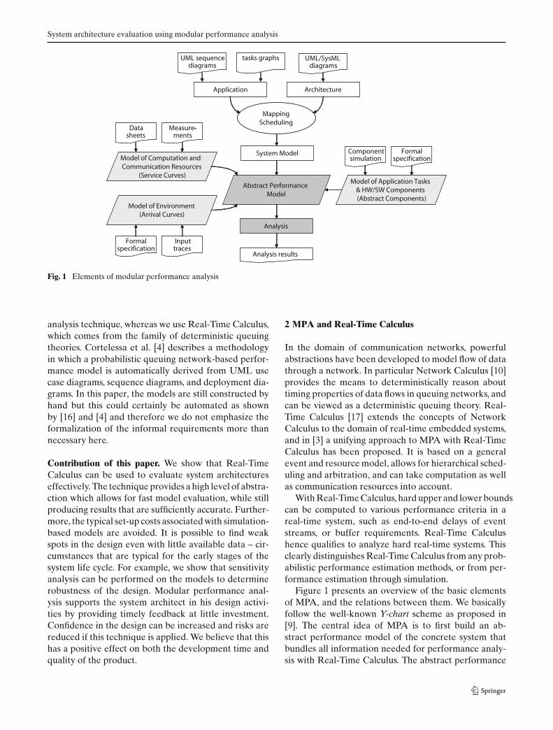
Fig. 1 Elements of modular performance analysis

analysis technique, whereas we use Real-Time Calculus,which comes from the family of deterministic queuingtheories. Cortelessa et al. [4] describes a methodologyin which a probabilistic queuing network-based perfor-mance model is automatically derived from UML usecase diagrams, sequence diagrams, and deployment dia-grams. In this paper, the models are still constructed byhand but this could certainly be automated as shownby [16] and [4] and therefore we do not emphasize theformalization of the informal requirements more thannecessary here.

Contribution of this paper. We show that Real-TimeCalculus can be used to evaluate system architectureseffectively. The technique provides a high level of abstra-ction which allows for fast model evaluation, while stillproducing results that are sufficiently accurate. Further-more, the typical set-up costs associated with simulation-based models are avoided. It is possible to find weakspots in the design even with little available data – cir-cumstances that are typical for the early stages of thesystem life cycle. For example, we show that sensitivityanalysis can be performed on the models to determinerobustness of the design. Modular performance anal-ysis supports the system architect in his design activi-ties by providing timely feedback at little investment.Confidence in the design can be increased and risks arereduced if this technique is applied. We believe that thishas a positive effect on both the development time andquality of the product.

2 MPA and Real-Time Calculus

In the domain of communication networks, powerfulabstractions have been developed to model flow of datathrough a network. In particular Network Calculus [10]provides the means to deterministically reason abouttiming properties of data flows in queuing networks, andcan be viewed as a deterministic queuing theory. Real-Time Calculus [17] extends the concepts of NetworkCalculus to the domain of real-time embedded systems,and in [3] a unifying approach to MPA with Real-TimeCalculus has been proposed. It is based on a generalevent and resource model, allows for hierarchical sched-uling and arbitration, and can take computation as wellas communication resources into account.

With Real-Time Calculus, hard upper and lower boundscan be computed to various performance criteria in areal-time system, such as end-to-end delays of eventstreams, or buffer requirements. Real-Time Calculushence qualifies to analyze hard real-time systems. Thisclearly distinguishes Real-Time Calculus from any prob-abilistic performance estimation methods, or from per-formance estimation through simulation.

Figure 1 presents an overview of the basic elementsof MPA, and the relations between them. We basicallyfollow the well-known Y-chart scheme as proposed in[9]. The central idea of MPA is to first build an ab-stract performance model of the concrete system thatbundles all information needed for performance analy-sis with Real-Time Calculus. The abstract performance

E. Wandeler et al.

model unifies essential information about the environ-ment, about the available computation and communica-tion resources, about the application tasks (or dedicatedHW/SW components), as well as about the system archi-tecture itself.

The environment models describe how a system isbeing used by the environment: how often will systemfunctions be called, how much data is provided as inputto the system, and how much data is generated by thesystem back to its environment. Environment modelscan be derived from formal behavior specifications orfor example from measured input traces. We will showhow UML sequence diagrams can be used to formalizethese aspects.

The resource models provide information about theproperties of the computing and communication re-sources that are available within a system, such as pro-cessor speed and communication bus bandwidth. Thisinformation is typically found in data sheets or bench-marks, or can be obtained from measurements on exist-ing systems.

The application task (or dedicated HW/SW compo-nent) models provide information about the processingsemantics that is used to execute the various applicationtasks or to run the dedicated HW/SW components.

Finally, the system model captures information aboutthe applications and the available hardware architec-ture, and it also defines the mapping of tasks to com-putation or communication resources of the hardwarearchitecture and specifies the scheduling and arbitrationschemes used on these resources. In Sect. 3, we will elab-orate in more detail on how to specify this informationusing UML and other methods, and we will show how toconstruct abstract performance models using this infor-mation. We will present the model of the environmentin Sect. 2.1 and the model of computation and commu-nication resources in Sect. 2.2. The model of applicationtasks and dedicated HW/SW components and construc-tion of the abstract performance model is presented inSect. 2.3 and 2.4. Finally, we explore the analysis of theabstract performance models in Sect. 2.5.

2.1 Arrival curves: a general event stream model

A trace of an event stream can conveniently be de-scribed by means of a cumulative function R(t), definedas the number of events seen on the event stream inthe time interval [0, t). While any R always describesone concrete trace of an event stream, a tuple α(�) =[αu(�), αl(�)

]of upper and lower arrival curves [5] pro-

vides an abstract event stream model, representing allpossible traces of an event stream.

For this, the upper arrival curve αu(�) provides anupper bound on the number of events that are seen onthe event stream in any time interval of length �, andanalogously, the lower arrival curve αl(�) provides alower bound on the number of events in a time inter-val �. In other words, in any time interval of length �

there will always arrive at least αl(�) and at most αu(�)

events on an event stream that is modeled by α(�).Arrival curves were first introduced in [5], and are

defined as follows:

Definition 1 (arrival curves) Let R(t) denote the num-ber of events that arrive on an event stream in the timeinterval [0, t). Then, R, αu and αl are related to eachother by the following inequality

αl(t − s) ≤ R(t) − R(s) ≤ αu(t − s), ∀s < t (1)

with αl(0) = αu(0) = 0. ��Arrival curves substantially generalize the classical

representation of standard event arrival patterns such assporadic, periodic, periodic with jitter, or others.Besides being able to represent any event stream withknown deterministic timing behavior that is obtainedfrom a system specification, it is also possible to deter-mine arrival curves corresponding to any finite lengthevent stream trace, obtained for example from observa-tion or simulation. For this, a sliding window approachcan be used.

Example 1 In literature, standard event arrival patternsare often specified by a parameter triple (p, j, d), wherep denotes the period, j the jitter, and d the minimuminter-arrival distance of events in the modeled stream.Event streams that are specified using these parameterscan directly be modeled by the following arrival curves:

αl(�) =⌊

� − jp

⌋(2)

αu(�) = min

{⌈� + j

p

⌉,⌈

�

d

⌉}(3)

2

4

6

8

10

# ev

ents

αu

αl

p

j

d

p

pj

Fig. 2 Arrival curves from (p, j, d)


In Fig. 2, the relation between these parameters andthe corresponding arrival curves is graphically depicted.Note that in this particular example the jitter is muchgreater than the period which is typical for a so-calledevent streams with bursts. This also explains the steepascend at the beginning of the upper arrival curve.

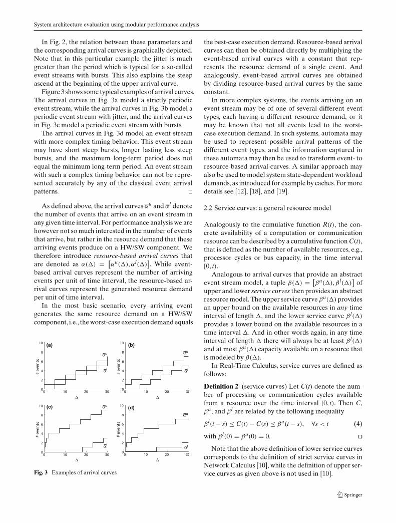
Figure 3 shows some typical examples of arrival curves.The arrival curves in Fig. 3a model a strictly periodicevent stream, while the arrival curves in Fig. 3b model aperiodic event stream with jitter, and the arrival curvesin Fig. 3c model a periodic event stream with bursts.

The arrival curves in Fig. 3d model an event streamwith more complex timing behavior. This event streammay have short steep bursts, longer lasting less steepbursts, and the maximum long-term period does notequal the minimum long-term period. An event streamwith such a complex timing behavior can not be repre-sented accurately by any of the classical event arrivalpatterns. ��

As defined above, the arrival curves αu and αl denotethe number of events that arrive on an event stream inany given time interval. For performance analysis we arehowever not so much interested in the number of eventsthat arrive, but rather in the resource demand that thesearriving events produce on a HW/SW component. Wetherefore introduce resource-based arrival curves thatare denoted as α(�) = [

αu(�), αl(�)]. While event-

based arrival curves represent the number of arrivingevents per unit of time interval, the resource-based ar-rival curves represent the generated resource demandper unit of time interval.

In the most basic scenario, every arriving eventgenerates the same resource demand on a HW/SWcomponent, i.e., the worst-case execution demand equals

0 10 20 300

2

4

6

8

10

∆

# ev

ents

αu

αl

0 10 20 300

2

4

6

8

10

∆

# ev

ents

αu

αl

0 10 20 300

2

4

6

8

10

∆

# ev

ents

αu

αl

0 10 20 300

2

4

6

8

10

∆

# ev

ents

αu

αl

(a)

(d)(c)

(b)

Fig. 3 Examples of arrival curves

the best-case execution demand. Resource-based arrivalcurves can then be obtained directly by multiplying theevent-based arrival curves with a constant that rep-resents the resource demand of a single event. Andanalogously, event-based arrival curves are obtainedby dividing resource-based arrival curves by the sameconstant.

In more complex systems, the events arriving on anevent stream may be of one of several different eventtypes, each having a different resource demand, or itmay be known that not all events lead to the worst-case execution demand. In such systems, automata maybe used to represent possible arrival patterns of thedifferent event types, and the information captured inthese automata may then be used to transform event- toresource-based arrival curves. A similar approach mayalso be used to model system state-dependent workloaddemands, as introduced for example by caches. For moredetails see [12], [18], and [19].

2.2 Service curves: a general resource model

Analogously to the cumulative function R(t), the con-crete availability of a computation or communicationresource can be described by a cumulative function C(t),that is defined as the number of available resources, e.g.,processor cycles or bus capacity, in the time interval[0, t).

Analogous to arrival curves that provide an abstractevent stream model, a tuple β(�) = [

βu(�), β l(�)]

ofupper and lower service curves then provides an abstractresource model. The upper service curve βu(�) providesan upper bound on the available resources in any timeinterval of length �, and the lower service curve β l(�)

provides a lower bound on the available resources in atime interval �. And in other words again, in any timeinterval of length � there will always be at least β l(�)

and at most βu(�) capacity available on a resource thatis modeled by β(�).

In Real-Time Calculus, service curves are defined asfollows:

Definition 2 (service curves) Let C(t) denote the num-ber of processing or communication cycles availablefrom a resource over the time interval [0, t). Then C,βu, and β l are related by the following inequality

β l(t − s) ≤ C(t) − C(s) ≤ βu(t − s), ∀s < t (4)

with β l(0) = βu(0) = 0. ��Note that the above definition of lower service curves

corresponds to the definition of strict service curves inNetwork Calculus [10], while the definition of upper ser-vice curves as given above is not used in [10].

E. Wandeler et al.

The service curves of a resource can be determinedusing data sheets, using analytically derived properties,or by measurement. For example, in the simplest caseof an unloaded processor, whose capacity we measurein available processing cycles per time unit, both theupper and the lower resource curves are equal and arerepresented by straight lines βu(�) = β l(�) = f · �,where f equals the processor speed, i.e., the number ofavailable processing cycles per time unit. With servicecurves, we may also model communication resources,where the service curves are bounded by the minimumand maximum number of transmittable bits in a giventime interval.

Example 2 Figure 4 shows some examples of servicecurves that model the resource availability on proces-sors or communication channels. The service curves inFig. 4a model a resource with full availability, while theservice curves in Figure 4(b) model a bounded delayresource. The service curves in Fig. 4c model the re-source availability of one slot on a time division multipleaccess (TDMA) resource, and finally the service curvesin Fig. 4d model a periodic resource as defined in [15]. ��

2.3 From components to abstract components

In a real-time system, an incoming event stream is typi-cally processed on a sequence of HW/SW components,that we will interpret as tasks on a task chain that areexecuted on possibly different hardware resources.

Figure 5 shows such a component. A trace of an eventstream, described by R(t), enters the component and isprocessed using a hardware resource whose availabilityis described by C(t). After being processed, the eventsare emitted on the output of the component, resulting

0 10 20 300

5

10

15

∆

# cy

cles

βu

βl

(c)

0 10 20 300

5

10

15

∆

# cy

cles

βu

βl

(a)

0 10 20 300

5

10

15

∆

# cy

cles

βu

βl

(b)

0 10 20 300

5

10

15

∆

# cy

cles

βu

βl

(d)

Fig. 4 Examples of service curves

0

2

4

6

8

t

0

2

4

6

8

t 0

2

4

6

8

t

0

2

4

6

8

t

C’(t)

C(t)

R’(t)R(t)

T

Fig. 5 A concrete component, processing an event stream on aresource

in an outgoing event stream trace, described by R′(t),and the remaining resources that were not consumed toprocess the event trace R(t) are made available to othercomponents and are described by an outgoing resourceavailability C′(t).

The relations between R(t), C(t), R′(t), and C′(t) de-pend on the processing semantics of the component. Theoutgoing event stream R′(t) will typically not equal theincoming event stream R(t), as it may, for example, ex-hibit more (or less) jitter. Analogously, C′(t) will differfrom C(t).

For modular performance analysis with Real-TimeCalculus, we model such a HW/SW component as anabstract component as shown in Fig. 6. Here, an abstractevent stream α(�) enters the abstract component and isprocessed using an abstract resource β(�). The outputis then again an abstract event stream α′(�), and theremaining resources are expressed again as an abstractresource β ′(�).

0

2

4

6

8

∆

FP0

2

4

6

8

∆ 0

2

4

6

8

∆

0

2

4

6

8

∆ β'(∆ )

β(∆ )

α'(∆ )α(∆)

FP

Fig. 6 An abstract component, processing an abstract eventstream on an abstract resource


Internally, such an abstract component is specifiedby a set of functions that relate the incoming arrival andservice curves to the outgoing arrival and service curves:

α′ = fα(α, β) (5)

β ′ = fβ(α, β) (6)

For a given abstract component, these relations fα andfβ depend on the processing semantics of the modeledconcrete component, and must be determined such thatα′(�) correctly models the event stream with event traceR′(t) and that β ′(�) correctly models the resource avail-ability C′(t).

As an example of an abstract component, consider aconcrete component that is triggered by the events ofan incoming event stream. A fully preemptable task isinstantiated at every event arrival to process the incom-ing event, and active tasks are processed in a greedyfashion in FIFO order, while being restricted by theavailability of resources. Such a component can be mod-eled as an abstract component with following internalrelations1 [3]:

α′uFP = min

{(αu ⊗ βu) � β l, βu

}(7)

α′lFP = min

{(αl � βu

)⊗ β l, β l

}(8)

β ′uFP =

(βu − αl

)� 0 (9)

β ′lFP =

(β l − αu

)⊗ 0 (10)

Components with the above described processing seman-tics are very common in the area of real-time embeddedsystems, and we will refer to them as a fixed priority (FP)components.

To model a component with different processingsemantics, one has to determine the appropriate inter-nal relations fα and fβ to obtain a corresponding abstractcomponent.

2.4 Abstract system performance models

At this point, we know how to model event streams,computation and communication resources, as well assingle HW/SW components (tasks). But in order to ana-lyze performance criteria of a system, we need to buildan abstract model of the complete system architecture.We will call such a model the abstract performance modelof a system.

To obtain the abstract performance model of a sys-tem, we first need to abstractly model all event streamsthat trigger the system, all computation and commu-nication resources that are available to the system, as

1 See the Sect. 6 for a definition of ⊗, �, ⊗, and �.

well as all components (tasks) in the system, using thecorresponding abstract representations, as described inthe preceding sections. Then, by correctly interconnect-ing all arrival and service inputs and outputs of all theseabstract models, we obtain the abstract performancemodel of the system. An example of an abstractperformance model is depicted in Fig. 14.

The arrival inputs and outputs in the abstract perfor-mance model are interconnected to reflect the flow ofdata in the system horizontally, while the interconnec-tions of service inputs and outputs model the resourcesharing policies in the system vertically.

To elaborate on the service interconnections, supposethat several components of a system are allocated tothe same resource. In the concrete system, these com-ponents share this resource according to a schedulingpolicy. In the abstract performance model, this sched-uling policy on a resource can then be modeled by theway the abstract resources β are distributed among thedifferent abstract components.

For example, consider preemptive fixed priority sched-uling: an abstract component A with the highest prioritymay use all available resources of a CPU, whereas anabstract component B with the second highest priorityonly gets the resources that were not consumed by A.This resource sharing policy is modeled in the abstractperformance model by using the service curves β ′

A thatexit the abstract FP component A as input to the abstractFP component B.

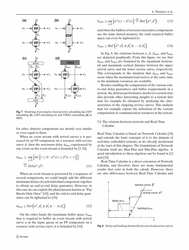
For some other scheduling policies, such as GPS (gen-eralized processor sharing) or TDMA (time divisionmultiple access), the available resources must be dis-tributed differently, while for some scheduling policies,such as EDF (earliest deadline first) or non-preemptivescheduling, different abstract components, with tailoredinternal relations, must be used. Some examples of howto model different scheduling policies are depicted inFig. 7.

2.5 Analysis

After interconnecting all abstract models of a system tothe system’s abstract performance model as described inthe previous section, this abstract performance modelcaptures all the information that builds the basis forperformance analysis with Real-Time Calculus. Variousperformance criteria, such as end-to-end delay guaran-tees or buffer requirements can be computed analyt-ically in this abstract performance model. The exactanalysis methods may thereby slightly vary for differ-ent abstract components but remains deterministic atall times. Following, we present the performance anal-ysis methods for FP components. The analysis methods

E. Wandeler et al.

βs1

α'AFP

FP

share

sum

βs2

β's2 β's1

β'

β

α'B

αA

αB

β

α'AFP

FP

β'B

α'B

αA

αB

β'A

β

α'A

EDF

β'

α'B

αA

αB

FP

βslot1

TDMA

FP

βslot2

α'A

α'B

αA

αB

β'slot2β'slot1

(a) (b)

(c) (d)

Fig. 7 Modeling of preemptive fixed priority scheduling (a), EDFscheduling (b), GPS scheduling (c) and TDMA scheduling (d) inMPA

for other abstract components are mostly very similaror even equal to these.

When an event stream with arrival curves α is pro-cessed by an FP component on a resource with servicecurve β, then the maximum delay dmax experienced byany event on the event stream is bounded by [3,10]:

dmax ≤ supλ≥0

{inf

{τ ≥ 0 : αu(λ) ≤ β l(λ + τ)

}}

def= Del(αu, β l) (11)

When an event stream is processed by a sequence ofseveral components, we could simply add the differentmaximum delays of each individual component togetherto obtain an end-to-end delay guarantee. However, inthis case we can exploit the phenomenon known as “PayBursts Only Once” [10], and the end-to-end delay guar-antee can be tightened to [10]:

dmax ≤ Del(αu, β l

1 ⊗ β l2 ⊗ · · · ⊗ β l

n

)(12)

On the other hand, the maximum buffer space bmaxthat is required to buffer an event stream with arrivalcurve α in the input queue of an FP component on aresource with service curve β is bounded by [10]:

bmax ≤ supλ≥0

{αu(λ) − β l(λ)

}def= Buf

(αu, β l

)(13)

and when the buffers of several consecutive componentsuse the same shared memory, the total required bufferspace can even be tightened to:

bmax ≤ Buf(αu, β l

1 ⊗ β l2 ⊗ . . . ⊗ β l

n

)(14)

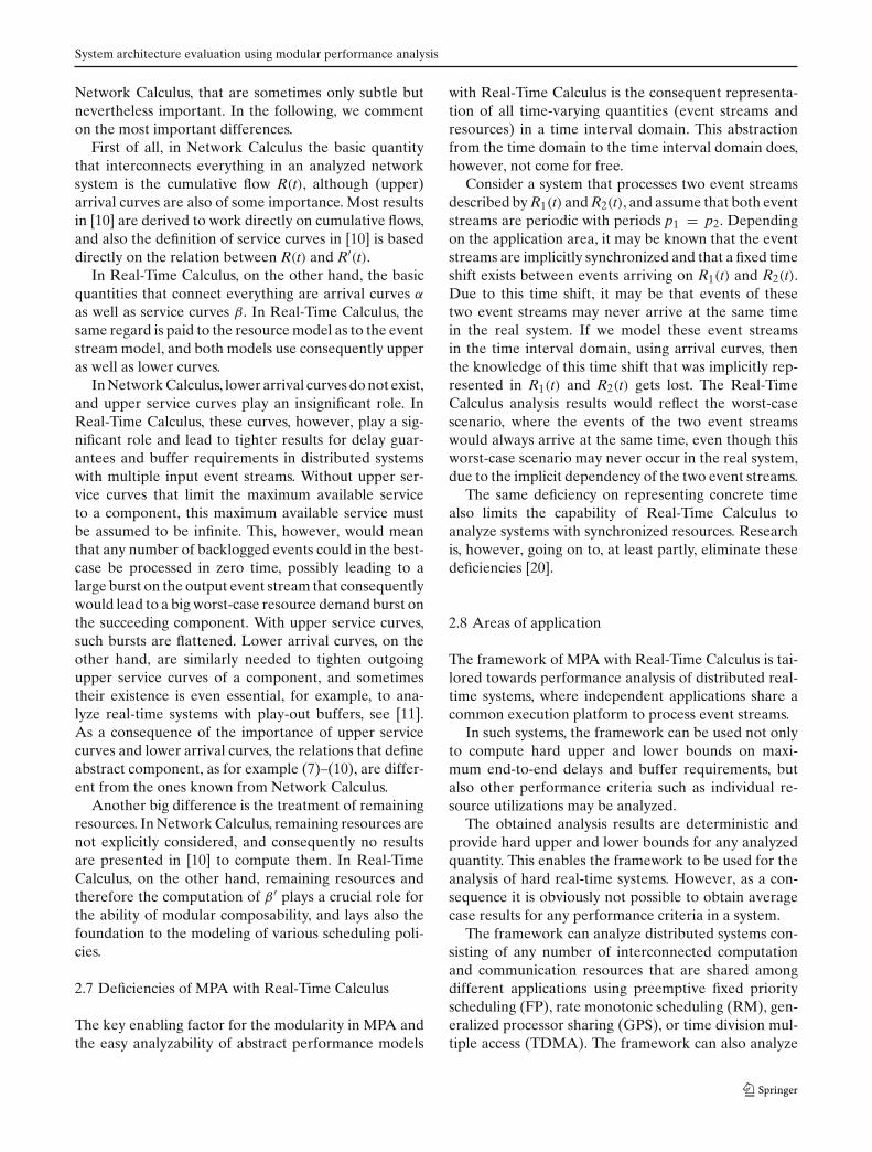
In Fig. 8, the relations between α, β, dmax, and bmaxare depicted graphically. From this figure, we see thatdmax and bmax are bounded by the maximum horizon-tal and maximum vertical distance between the upperarrival curve and the lower service curve, respectively.This corresponds to the intuition that dmax and bmaxoccur when the maximum load arrives at the same timeas the minimum resources are available.

Besides enabling the computation of the various end-to-end delay guarantees and buffer requirements in asystem, the abstract performance model of a system mayalso provide other interesting insights to a system thatmay for example be obtained by analyzing the char-acteristics of the outgoing service curves. This analysismay for example expose the utilization of the variouscomputation or communication resources in the system.

2.6 The relation between network and Real-TimeCalculus

Real-Time Calculus is based on Network Calculus [10]and extends the basic concepts of it to the domain ofreal-time embedded systems, as we already mentionedat the start of this chapter. The foundations of NetworkCalculus itself are Max-Plus and Min-Plus algebra. Agood introduction to these algebras can be found in [1]and [10].

Real-Time Calculus is a direct extension of NetworkCalculus, and therefore there are many fundamentalresults that exist in both the calculi. However, thereare also differences between Real-Time Calculus and

∆

β

αu

l

delay dmax

backlog bmax

service curve

arrival curve

Fig. 8 Delay and backlog obtained from arrival and service curves


Network Calculus, that are sometimes only subtle butnevertheless important. In the following, we commenton the most important differences.

First of all, in Network Calculus the basic quantitythat interconnects everything in an analyzed networksystem is the cumulative flow R(t), although (upper)arrival curves are also of some importance. Most resultsin [10] are derived to work directly on cumulative flows,and also the definition of service curves in [10] is baseddirectly on the relation between R(t) and R′(t).

In Real-Time Calculus, on the other hand, the basicquantities that connect everything are arrival curves α

as well as service curves β. In Real-Time Calculus, thesame regard is paid to the resource model as to the eventstream model, and both models use consequently upperas well as lower curves.

In Network Calculus, lower arrival curves do not exist,and upper service curves play an insignificant role. InReal-Time Calculus, these curves, however, play a sig-nificant role and lead to tighter results for delay guar-antees and buffer requirements in distributed systemswith multiple input event streams. Without upper ser-vice curves that limit the maximum available serviceto a component, this maximum available service mustbe assumed to be infinite. This, however, would meanthat any number of backlogged events could in the best-case be processed in zero time, possibly leading to alarge burst on the output event stream that consequentlywould lead to a big worst-case resource demand burst onthe succeeding component. With upper service curves,such bursts are flattened. Lower arrival curves, on theother hand, are similarly needed to tighten outgoingupper service curves of a component, and sometimestheir existence is even essential, for example, to ana-lyze real-time systems with play-out buffers, see [11].As a consequence of the importance of upper servicecurves and lower arrival curves, the relations that defineabstract component, as for example (7)–(10), are differ-ent from the ones known from Network Calculus.

Another big difference is the treatment of remainingresources. In Network Calculus, remaining resources arenot explicitly considered, and consequently no resultsare presented in [10] to compute them. In Real-TimeCalculus, on the other hand, remaining resources andtherefore the computation of β ′ plays a crucial role forthe ability of modular composability, and lays also thefoundation to the modeling of various scheduling poli-cies.

2.7 Deficiencies of MPA with Real-Time Calculus

The key enabling factor for the modularity in MPA andthe easy analyzability of abstract performance models

with Real-Time Calculus is the consequent representa-tion of all time-varying quantities (event streams andresources) in a time interval domain. This abstractionfrom the time domain to the time interval domain does,however, not come for free.

Consider a system that processes two event streamsdescribed by R1(t) and R2(t), and assume that both eventstreams are periodic with periods p1 = p2. Dependingon the application area, it may be known that the eventstreams are implicitly synchronized and that a fixed timeshift exists between events arriving on R1(t) and R2(t).Due to this time shift, it may be that events of thesetwo event streams may never arrive at the same timein the real system. If we model these event streamsin the time interval domain, using arrival curves, thenthe knowledge of this time shift that was implicitly rep-resented in R1(t) and R2(t) gets lost. The Real-TimeCalculus analysis results would reflect the worst-casescenario, where the events of the two event streamswould always arrive at the same time, even though thisworst-case scenario may never occur in the real system,due to the implicit dependency of the two event streams.

The same deficiency on representing concrete timealso limits the capability of Real-Time Calculus toanalyze systems with synchronized resources. Researchis, however, going on to, at least partly, eliminate thesedeficiencies [20].

2.8 Areas of application

The framework of MPA with Real-Time Calculus is tai-lored towards performance analysis of distributed real-time systems, where independent applications share acommon execution platform to process event streams.

In such systems, the framework can be used not onlyto compute hard upper and lower bounds on maxi-mum end-to-end delays and buffer requirements, butalso other performance criteria such as individual re-source utilizations may be analyzed.

The obtained analysis results are deterministic andprovide hard upper and lower bounds for any analyzedquantity. This enables the framework to be used for theanalysis of hard real-time systems. However, as a con-sequence it is obviously not possible to obtain averagecase results for any performance criteria in a system.

The framework can analyze distributed systems con-sisting of any number of interconnected computationand communication resources that are shared amongdifferent applications using preemptive fixed priorityscheduling (FP), rate monotonic scheduling (RM), gen-eralized processor sharing (GPS), or time division mul-tiple access (TDMA). The framework can also analyze

E. Wandeler et al.

resources that are shared with any hierarchical compo-sition of these scheduling policies.

Research is currently going on to analyze systems withshapers, as well as resources that are shared using earli-est deadline first scheduling (EDF) and non-preemptivescheduling policies.

So far, the framework was only used to analyze sys-tems without cyclic dependencies. For systems with cyclicdependencies, it is, however, possible to perform a fixed-point analysis. While this area still requires further re-search, first promising results are already available [14].

In the framework, tasks are specified only by theirexecution demand. This sometimes limits the level ofdetail that can be modeled and analyzed, especiallywhen it comes to including functional properties of a sys-tem. The framework may, however, be used to analyzesystems with deterministic execution demand variabilityas introduced for example by deterministic caches, datadependencies or different occurring event types.

3 Case study: distributed in-car radio navigation system

The case study presented in this section is inspired by asystem architecture definition study for a distributed in-car radio navigation system. Such a system typically exe-cutes a number of concurrent applications that share acommon platform. Nevertheless, each application mighthave hard individual performance requirements thatneed to be met by the platform. During the system defi-nition phase, several candidate platform architecturesmight be proposed by the engineers and the systemarchitect needs to evaluate each one. Typical questionsthat need to be answered are: (1) does this platformmeet the performance requirements of all applications(2) how robust is the platform with respect to changesin application or architecture parameters and (3) can Ireplace components in the architecture by cheaper (butless powerful) components to save cost but still meet theperformance criteria of all applications? We present theapplications and the architecture candidates in Sect. 3.We briefly show how these are modeled and how a MPAmodel is composed. In Sect. 4 we will show how typicaldesign questions, as the ones mentioned before, can beanalyzed using Real-Time Calculus.

An overview of the system is presented in Fig. 9, it iscomposed of three main clusters of functionality:

– The man–machine interface (MMI) which takes careof all interaction with the user, such as handling keyinputs and graphical display output.

NAV RAD

MMI

MAP DB

Fig. 9 High-level overview of a distributed radio navigationsystem

– The navigation functionality (NAV) which is respon-sible for destination entry, route planning, and turn-by-turn route guidance giving the driver both audibleand visual advices. The navigation functionality re-lies on the availability of a map database, typicallystored on a CD or DVD, and positioning informa-tion, e.g., speed and GPS. The latter is not shownhere.

– The radio functionality (RAD) which is responsiblefor basic tuner and volume control as well as han-dling of traffic information services such as RDS/TMC (radio data system/traffic message channel).RDS/TMC is broadcast along with the audio signalof radio channels.

The key question that is investigated in this paperis how to distribute the functionality over the availableresources, such that we meet our global timing require-ments. To achieve this goal, the following steps weretaken:

1. identify key usage scenarios and system functions2. quantify event rates, message sizes, and execution

times3. identify resources and their communication struc-

ture4. quantify resource and communication capacities5. compose a MPA model, calculate, and evaluate


A general description of a new product is typicallymade during the initial phase of an industrial productcreation process. For example, an Operational ConceptDescription from the IEEE 12207 system life cycle stan-dard [8] may be produced. Such a document does notonly list functional and non-functional requirements,boundary conditions and other restrictions for the design,it should also contain high-level use-cases. These use-cases are the starting point for the design of the systemarchitecture. The use-cases and associated sequence dia-grams are analyzed and annotated in such a way thatthey are useful for MPA analysis. This is step 1 and2 of the recipe described above. Although there is noprinciple limit to the amount of scenarios that can beanalyzed, it is not uncommon to first concentrate onthose scenarios that are expected to have the highestimpact on the set of requirements to be met. It is thesystem architect who makes this decision, often basedon previous experience. The order of magnitude of thenumbers shown in the sequence diagrams in this paper isrealistic. During the design, the system architect tries toimprove the accuracy of the numbers by using for exam-ple better estimation techniques on details of the design,such as worst-case execution time analysis (WCET) orby performing measurements on existing and compara-ble systems. In our case study, we have selected threedistinctive scenarios:

1. “Change volume” – The user turns the rotary buttonand expects instantaneous audible feedback fromthe system. Furthermore, the visual feedback (thevolume setting on the screen) should be timely andsynchronized with the audible feedback. This seem-ingly trivial use-case is actually quite complex be-cause many components are affected. Changingvolume might involve commanding a digital signalprocessor (DSP) and an amplifier in such a way thatthe quality of the audio signal is maintained whilechanging the volume. This scenario is shown in detailin Fig. 10. Note that three operations are identi-fied, HandleKeyPress, AdjustVolume, and Update-Screen. Execution times, event rates, and messagesizes are estimated and annotated in the sequencediagram together with the principle timing require-ments applicable to this scenario.

2. “Address look-up” – Destination entry is supportedby a smart “typewriter” style interface. By turninga knob the user can move from letter to letter; bypressing it the user will select the currently high-lighted letter. The map database is searched for eachletter that is selected and only those letters in the on-screen alphabet are enabled that are potential next

letters in the list. This scenario is shown in detail inFig. 11. Note that the DatabaseLookup operationis expensive compared to the other operations andthat the size of the output value of the operation is16 times larger than the input message.

3. “TMC message handling” – Digital traffic informa-tion is very important for in-car radio navigationsystems. It enables features such as automatic re-planning of the planned route in case a traffic jamoccurs ahead. It is also increasingly important toenhance road safety by warning the driver, for exam-ple when a ghost driver is spotted on the plannedroute. RDS TMC is such a digital traffic informationservice. TMC messages are broadcast by radio sta-tions together with stereo audio sound. RDS TMCmessages are encoded: only problem location iden-tifiers and message types are transmitted. The mapdatabase is accessed to translate these identifiersand to construct human readable text. The TMCmessage handling scenario is shown in Fig. 12.

The scenarios sketched above have an interestingproperty: they can occur in parallel. RDS TMC messagesmust be processed while the user changes the volume orenters a destination. However, “Change Volume” and“Address Look-up” cannot occur at the same time be-cause they share a common resource; the rotary buttonis used for both. The architecture shown in Fig. 9 sug-gests to assign the three clusters of functionality eachto its own processing unit. The computation resourcesare interconnected by a single communication bus. Doesthis architecture meet our requirements and is it the bestarchitecture for our applications?

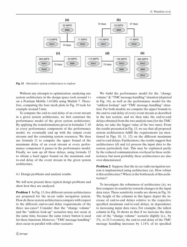
Figure 13 shows that there are many more potentialarchitectures that might be applicable. Note that thecapacity of the resource units and communication infra-structure is quantified, completing steps 3 and 4 of ourapproach. Again, the order of magnitude of the num-bers shown in the diagram is correct – they are takenfrom the data sheets of several commercially availableautomotive CPUs. Observe that architecture (b) canonly be evaluated if we introduce an additional oper-ation on the MMI resource that transfers the data fromone communication link to another, in the case that NAVwants to communicate to RAD or vice versa.

Sufficient information is now available to constructthe MPA models for each architecture. The model forarchitecture (a) is shown in Fig. 14. Note that the re-sources occur as column headings in the model.Observe that all outgoing horizontal arrows from theperformance components NAV, RAD, and MMI, repre-senting their respective output message flows, connectto an input of a BUS performance component, which

E. Wandeler et al.

: User : MMI : Radio

keyPress()

SetVolume()

HandleKeyPress( )

AdjustVolume( )

NoticeAudibleChange( )

UpdateScreen( )

32 eventsper second(at most)

4 bytes32x second

GetVolume()

NoticeVisualChange( )

4 bytes32x second

Vol

K2V

(K

eypr

ess

to V

isua

l) de

lay

< 2

00 m

sec

and

Vol

A2V

(A

udib

le to

Vis

ual)

dela

y <

50

mse

c

Execution time estimatesHandleKeyPress() 1E5 instructionsAdjustVolume() 1E5 instructionsUpdateScreen() 5E5 instructions

Fig. 10 Annotated sequence diagram for “change volume”

encodes the notion of the shared communication medium.In the case of architecture (b), two BUS resources(columns) would exist in the model instead of one.

The scenarios, that were defined by the sequence dia-grams, are depicted as the rows of the model. Eachrow starts with a load scenario symbol, which is con-nected to the input of a performance component. Theflow of the sequence diagrams can be followed, in hor-izontal direction, in the MPA model. Take for exam-ple the “change volume” scenario from Fig. 10. Eventsarrive at the MMI where HandleKeyPress is executedand the result is forwarded, via the communication bus,to RAD. AdjustVolume is executed and the result is sentback to MMI via the same communication bus. Finally,UpdateScreen is executed and the scenario is completed.The load scenario data, α is extracted from the annota-tions in the sequence diagram. The resource model data,β, is extracted from the informal deployment diagramsshown in Fig. 13.

As described in Sect. 2.4, the order of the rows inthe MPA model determines the priority. In this case, the“change volume” scenario is assigned a higher prioritythan “Handle TMC”. The system architect decides the

initial priority setting again based on experience. Thisdoes not hinder the evaluation in any way, since the pri-orities are easily changed by rearranging the vertical or-der of the scenarios. A MPA model must be constructedfor each proposed architecture. This is normally a sim-ple tasks because it is merely reconnecting event flowsin the horizontal direction.

4 System analysis

In this section, we will look at some typical design prob-lems that occur during the early phases of a systemdesign cycle, and we will address them using the approachto MPA presented in Sect. 2.

For a correct interpretation of the results in thissection, we need to remember that in order to be appli-cable for the analysis of hard real-time systems, themodular performance analysis presented in Sect. 2 isdesigned to compute hard upper and lower bounds forall system characteristics. While these upper and lowerbounds are always hard, they are in general not tight(exact). So the analysis performed is conservative and


: User : MMI : Navigation

AddressLookup()

keyPress()

NavResult()

DatabaseLookup( )

UpdateScreen( )


once per second

Add

r de

lay

< 2

00 m

sec

message size 4 bytesonce second

message size64 bytes

HandleKeyPress( )

Execution time estimatesHandleKeyPress() 1E5 instructionsDatabaseLookup() 5E6 instructionsUpdateScreen() 5E5 instructions

Fig. 11 Annotated Sequence Diagram for “Address Look-up”

: RadioStation : Radio : Navigation : MMI : User

Receive()

Receive()

HandleTMC()

UpdateScreen( )


300 messagesper 15 minutes32 bytes eachuniform distribution

300 messagesper 15 minutes64 bytes each

30 messagesper 15 minutes64 bytes each

TM

C d

elay

< 1

sec

for

urge

nt T

MC

mes

sage

s

HandleTMC( )

DecodeTMC( )

Execution time estimatesHandleTMC() 1E6 instructionsDecodeTMC() 5E6 instructionsUpdateScreen() 5E5 instructions

Fig. 12 Annotated sequence diagram for “TMC message handling”

the computed maximum delays in this section aretherefore hard upper bounds to the real maximum de-lays in the real system.

Due to this conservative approach, it may be thatwe reject a system architecture that would fulfill all

system requirements in reality, but for which our analysiscannot guarantee the fulfillment of all system require-ments. The other way around, we can guarantee that anysystem architecture accepted by our analysis fulfills allsystem requirements in reality.

E. Wandeler et al.

22 MIPS

11 MIPS113 MIPS

72 kbps

MMI

NAV RAD

(a)

22 MIPS

11 MIPS113 MIPS

72 kbps

MMI

NAV RAD

(b)57 kbps

22 MIPS260 MIPS

72 kbpsNAV

RAD

130 MIPS113 MIPS

72 kbpsNAV RADMMI

MMI

(c) (d)

260 MIPS

RAD

MMI

NAV

(e)

Fig. 13 Alternative system architectures to explore

Without any attempts to optimization, analyzing onesystem architecture in the design space took around 1 son a Pentium Mobile 1.6 GHz using Matlab 7. There-fore, computing the four mesh plots in Fig. 19 took forexample around 5 min.

To compute the end-to-end delay of an event streamin a given system architecture, we first construct theperformance model of the given system architecture.By applying the transformations given in formulas 7–10at every performance component of the performancemodel, we eventually end up with the output eventstreams and the remaining system resources. We thenuse formula 11 to compute the upper bound of themaximum delay of an event stream at every perfor-mance component it passes in the performance model.Finally, we sum up all these delays, using formula 12to obtain a hard upper bound on the maximum end-to-end delay of the event stream in the given systemarchitecture.

4.1 Design problems and analysis results

We will now present three typical design problems andshow how they are analyzed.

Problem 1 In Fig. 13, five different system architecturesare proposed for the in-car radio navigation system.How do these system architectures compare with respectto the different end-to-end delay requirements of thethree use-cases? Consider that the “change volume”and the “address look-up” scenarios may not occur atthe same time, because the same rotary button is usedfor these functions. However, “TMC message handling”does occur in parallel with either scenario.

We build the performance model for the “changevolume” & “TMC message handling” situation (depictedin Fig. 14), as well as the performance model for the“address lookup” and “TMC message handling” situa-tion. For both models, we compute the upper bounds tothe end-to-end delay of every event stream as describedin the last section, and we then take the end-to-enddelays obtained from the two analysis runs (for the TMCdelay, we take the bigger value of the two runs). Fromthe results presented in Fig. 15, we see that all proposedsystem architectures fulfill the requirements (as men-tioned in Figs. 10, 11, 12) on the different maximumend-to-end delays. Furthermore, the results suggest thatarchitectures (d) and (e) process the input data to thesystem particularly fast. This may be explained partlyby the reduced communication overhead in these archi-tectures, but most probably, these architectures are alsoover-dimensioned.

Problem 2 Suppose that the in-car radio navigation sys-tem is implemented using architecture (a). How robustis this architecture? Where is the bottleneck of this archi-tecture?

To investigate the robustness of architecture (a), wefirst compute its sensitivity towards changes in the inputdata rates. These sensitivity results are shown in Fig. 16.The height of the columns in this figure depict the in-crease of end-to-end delays relative to the respectivespecified maximum end-to-end delays, in dependenceto increasing input data rates. For example, the tallestcolumn in Fig. 16 shows us that if we increase the datarate of the “change volume” scenario slightly (i.e., by3%, to 33.3 events/s), the end-to-end delay of the TMCmessage handling increases by 1.14% of its specified


Fig. 14 MPA model forsystem architecture (a) ofFig. 13

CPU1 BUS CPU3CPU2

Change Volume

Receive TMC

MMI NAV RAD

α

α

β ββ β

Fig. 15 Maximumend-to-end delays for eachsystem architecture

0

10

20

30

40

50

0

10

20

30

0

20

40

60

80

0

150

300

450

Vol K2V Delay [ms] Vol A2V Delay [ms]

TMC Delay [ms]Addr Delay [ms]

A EDCB EDCBA

A EDCB EDCBA

maximum end-to-end delay (i.e., 1.14% of 1,000 ms or11.4 ms).

From the results shown in Fig. 16, we see that archi-tecture (a) is very sensitive towards increasing the in-put data rate of the “change volume” scenario, whileincreasing the input data rate of the “address look-up”and the “TMC message handling” scenarios do not re-ally affect the response times. And in fact, further anal-ysis reveals that in order to still guarantee all systemrequirements, we must not increase the input data rateof the “change volume” scenario by more than 7%, whilewe could increase the input data rate of the other twoscenarios by a factor of more than 20.

After investigating the system sensitivity towardschanges in the input data rates, we investigate thesystem sensitivity towards changes in the resource capac-ities. These sensitivity results are shown in Fig. 17. The

height of the columns in this figure depicts the increaseof end-to-end delays relative to the respective specifiedmaximum end-to-end delays, in dependence to decreas-ing resource capacities. For example, from the tallestcolumn in Fig. 17 we know that if we decrease capac-ity of the MMI processor by 1% (i.e., to 21.78 MIPS),the end-to-end delay of the TMC message handling in-creases by 3.22% of its specified maximum end-to-enddelay (i.e., 3.22% of 1,000 or 32.2 ms).

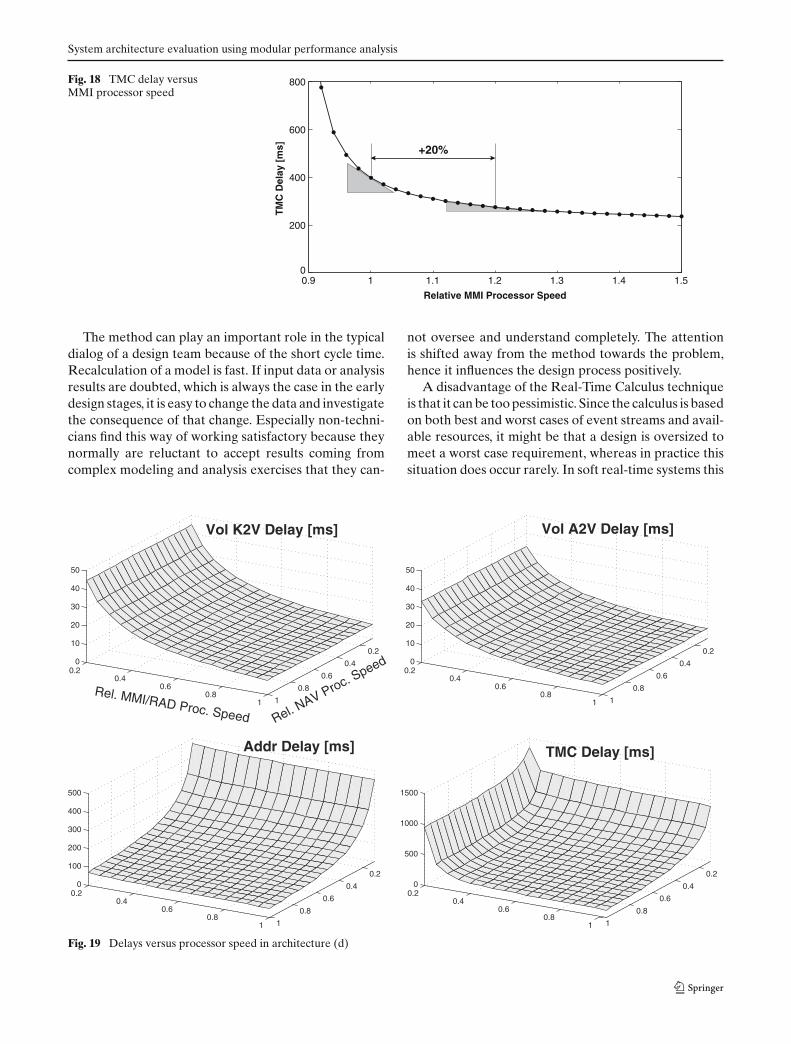
From the results shown in Fig. 17, we see that archi-tecture (a) is most sensitive towards the capacity of theMMI processor. This suggests that the MMI processoris a potential bottleneck of architecture (a). To inves-tigate this further, we compute the end-to-end delay ofthe TMC message handling for different MMI processorcapacities. The results of these computations are shownin Fig. 18.

E. Wandeler et al.

0

0.2

0.4

0.6

0.8

1

1.2

Change Vol.

Vol K2V

Vol A2V

Addr

TMC

[%]

Addr. Lookup Receive TMC

Fig. 16 Sensitivity towards changes in the input data rates

0

0.5

1

1.5

2

2.5

3

3.5

NAV RADIO MMI BUS

Vol K2V

Vol A2V

Addr

TMC

[%]

Fig. 17 Sensitivity towards changes in the resource capacities

From Fig. 18, we see that indeed at its given operationpoint, the end-to-end delay of the TMC message han-dling in architecture (a) is very sensitive towards changesof the MMI processor capacity. And the analysis revealsthat with a decrease of the MMI processor capacity to89% of its initial capacity, we cannot guarantee finiteresponse times anymore.

To sum up, the above analysis results suggest thatincreasing the capacity of the MMI processor wouldmake architecture (a) more robust. To support this state-ment, we individually increase the capacity of each re-source by 20%, and we then analyze how much we canincrease the input data rate of the “change volume” sce-nario while still fulfilling the requirements. Remember,with the initial resource capacities, we can increase the

data rate of the “change volume” scenario by 7% andthe data rate of the other two scenarios by a factor ofmore than 20 while still guaranteeing all requirements.From this analysis, we learn that increasing the resourcecapacities of the RAD processor, the NAV processor,and the BUS does not allow to increase the input daterate of the “change volume” scenario more than withthe initial capacities, while increasing the MMI proces-sor capacity allows us to increase the data rate of the“change volume” scenario by 60%.

Problem 3 Suppose system architecture (d) is chosenfor further investigation. The results of Problem 1 indi-cate that architecture (d) is probably over-dimensioned.So how should the two processors in this system archi-tecture be dimensioned, to obtain an economic systemthat still fulfills the end-to-end delay requirements of allscenarios?

We compute the upper bound to the end-to-end delayof every event stream in architecture (d) for differentprocessor capacities. The results are shown in Fig. 19.

In the plots in Fig. 19, the NAV processor capacityis varied in steps of 5% from 100% down to 10% ofits initial capacity. At the same time, the MMI/RADprocessor capacity is varied in steps of 5% from 100%down to 20% of its initial capacity.

As we see from the plots, the delays of the “changevolume” scenario are not much affected by changesof the NAV processor capacity and the delay of the“address look-up” scenario is not much affected bychanges of the MMI/RAD processor capacity. On theother hand, the delay of the “TMC message handlingscenario” is affected by the changes of both proces-sor capacities. From the results, we learn that we coulddecrease both the NAV processor capacity as well asthe MMI/RAD processor capacity down to 25% of theirinitial capacity (i.e., 29 and 33 MIPS, respectively), whilestill guaranteeing the fulfillment of all system require-ments.

5 Conclusions and future work

Real-Time Calculus was originally intended for stream-based applications. We have shown in this case study thatit is also well-suited for modeling control-oriented anddistributed software-intensive systems. Creating MPAmodels is a relatively simple task that requires littleeffort. The models presented in this paper were com-posed manually and analyzed within the same workingday. Quantifying the event rates and resource capaci-ties actually took up more time than building the modelbecause this information is seldom readily available.


Fig. 18 TMC delay versusMMI processor speed

0.9 1 1.1 1.2 1.3 1.4 1.50

200

400

600

800

Relative MMI Processor Speed

TM

C D

elay

[m

s] +20%

The method can play an important role in the typicaldialog of a design team because of the short cycle time.Recalculation of a model is fast. If input data or analysisresults are doubted, which is always the case in the earlydesign stages, it is easy to change the data and investigatethe consequence of that change. Especially non-techni-cians find this way of working satisfactory because theynormally are reluctant to accept results coming fromcomplex modeling and analysis exercises that they can-

0.2

0.4

0.6

0.8

1

0.20.4

0.60.8

1

0

100

200

300

400

500

Addr Delay [ms]

0.2

0.4

0.6

0.8

1

0.20.4

0.60.8

1

0

500

1000

1500

TMC Delay [ms]

0.2

0.4

0.6

0.8

1

0.20.4

0.60.8

1

0

10

20

30

40

50

Rel. MMI/RAD Proc. Speed Rel. NAV Proc. Speed

Vol K2V Delay [ms]

0.2

0.4

0.6

0.8

1

0.20.4

0.60.8

1

0

10

20

30

40

50

Vol A2V Delay [ms]

Fig. 19 Delays versus processor speed in architecture (d)

not oversee and understand completely. The attentionis shifted away from the method towards the problem,hence it influences the design process positively.

A disadvantage of the Real-Time Calculus techniqueis that it can be too pessimistic. Since the calculus is basedon both best and worst cases of event streams and avail-able resources, it might be that a design is oversized tomeet a worst case requirement, whereas in practice thissituation does occur rarely. In soft real-time systems this

E. Wandeler et al.

might entail a design which is too expensive. The currentapproach to counter this phenomenon is to increase thelevel of detail in the model, while still preserving thesimplicity of the approach. The future research goal isthat a few critical parts of a system may be modeled indetail, while other less critical parts may be modeledon a higher level of abstraction. With this approach, themodel of system parts that seem to be critical may evenbe refined during the analysis process.

Modular performance analysis is a composable tech-nique. Abstract performance components can actuallyconsist of other MPA models. This approach has notbeen explored in this paper, neither have we investi-gated its impact on the analysis speed.

Future work. A Java implementation of the Real-TimeCalculus, using Matlab as the user interface, is currentlyunder development. These tools are inspired by a proto-type implementation that was made earlier usingMathematica. Our aim is to compare MPA to other per-formance analysis techniques based on the case studypresented in this paper. Comparison would include (butis not restricted to) classical scheduling analysis tech-niques, timed automata, Markovian, and traditionalsimulation. Furthermore, we plan to evaluate larger casestudies, in particular, to investigate the scalability ofMPA. Integration with UML tools, in particular, throughthe profile for schedulability, performance, and time[13] is needed to make MPA tool support acceptableto industry. The complete MPA model of the case studypresented here can be found at http://www.mpa.ethz.ch.

Acknowledgments The authors wish to thank Erik Gaal, Evertvan de Waal, Jozef Hooman, Jan Broenink, Lou Somers, FritsVaandrager and the anonymous reviewers for providing feedbackand comments to the paper. Furthermore, we would like to thankSiemens VDO Automotive, in particular Roland van Venrooy, fortheir support. This project is partly supported by the NetherlandsMinistry of Economic Affairs under the Senter TS program. Partof the presented work is funded by the Swiss National ScienceFoundation (SNF) under the Analytic Performance Estimation ofEmbedded Computer Systems project 200021-103580/1, and byARTIST2.

Appendix: Min-Plus and Max-Plus Calculi

Both min-plus and max-plus calculi define a specialalgebra (the min-plus dioid and max-plus dioid, respec-tively). Traditionally, we are used to work with thealgebraic structure (R, +, ×), i.e., with the set of realsendowed with the operations of addition and multipli-cation that possess a number of properties such as asso-ciativity, commutativity, distributivity, etc.

In difference to this, min-plus calculus works with analgebraic structure (R ∪ ∞, ∨, +). Here, the operationof addition becomes the computation of the infimum(or the minimum), and the operation of multiplicationbecomes the addition. Most axioms known from con-ventional algebra still apply to this algebraic structure.And in max-plus calculus, the infimum and minimumare simply replaced by supremum and maximum.

In Real-Time Calculus, we often need to computeconvolutions and deconvolutions defined in min-plusand max-plus calculi. These operations are defined asfollows [10]:

The min-plus convolution ⊗ and the min-plus decon-volution � of two functions f and g are defined as:

(f ⊗ g)(�) = inf0≤λ≤�

{f (� − λ) + g(λ)} (15)

(f � g)(�) = supλ≥0

{f (� + λ) − g(λ)} (16)

The max-plus convolution ⊗ and the max-plus decon-volution � of two functions f and g are defined as:(f ⊗ g

)(�) = sup

0≤λ≤�

{f (� − λ) + g(λ)} (17)

(f � g

)(�) = inf

λ≥0{f (� + λ) − g(λ)} (18)

For more information on min-plus and max-plus cal-culi see [10] and [1].

References

1. Bacelli, F., Cohen, G., Olsder, G.J., Quadrat, J.P.: Synchroni-zation and Linearity: An Algebra for Discrete Event Systems.Wiley Series in Probability and Mathematical Statistics. JohnWiley & Sons Ltd, New York (1992)

2. Balsamo, S., Di Marco, A., Inverardi, P.: Model-based perfor-mance prediction in software development: A survey. IEEETrans Softw Eng 30(5), 295–310 (2004)

3. Chakraborty, S., Künzli, S., Thiele, L.: A general frameworkfor analysing system properties in platform-based embeddedsystem designs. In: Proceedings of 6th Design, Automationand Test in Europe (DATE), Munich, Germany, pp. 190–195(2003)

4. Cortellessa, V., Mirandola, R.: Deriving a queueing networkbased performance model from UML diagrams. In: Proceed-ings of 2nd International Workshop on Software and Perfor-mance (WOSP), Ottawa, Ontario, Canada, pp. 58–70 (2000)

5. Cruz, R.L.: A calculus for network delay. IEEE Trans Infor-mation Theory 37(1), 114–141 (1991)

6. Gries, M.: Methods for evaluating and covering the designspace during early design development. Tech. Rep. UCB/ERLM03/32, Electronics Research Lab, University of California atBerkeley (2003)

7. Grotker, T., Liao, S., Martin, G., Swan, S.: System Design withSystemC. Kluwer, Dordrecht (2002)

8. IEEE/EIA: ISO/IEC 12207:1995 Standard for InformationTechnology – Software life cycle processes. The Institute ofElectrical and Electronics Engineers, Inc. (1998)


9. Kienhuis, B., Deprettere, E., Vissers, K., van der Wolf, P.:An approach for quantitative analysis of application-specificdataflow architectures. In: ASAP ’97: Proceedings of theIEEE International Conference on Application-SpecificSystems, Architectures and Processors, IEEE ComputerSociety, Washington, DC, USA, p. 338 (1997)

10. Le Boudec, J.Y., Thiran, P.: Network Calculus - A Theory ofDeterministic Queuing Systems for the Internet. No. 2050 inLecture Notes in Computer Science (LNCS). Springer, BerlinHeidelberg New York (2001)

11. Maxiaguine, A., Chakraborty, S., Künzli, S., Thiele, L.: Eval-uating schedulers for multimedia processing on buffer-con-strained soc platforms. IEEE Design Test 21(5), 368–377(2004)

12. Maxiaguine, A., Künzli, S., Thiele, L.: Workload character-ization model for tasks with variable execution demand. In:Proceedings of 7th Design, Automation and Test in Europe(DATE) (2004)

13. Object Management Group: UML Profile for Schedula-bility, Performance and Time Specification (2004). URLhttp://www.uml.org/. Version 1.1, ptc/04-02-01

14. Schioler, H., Larsen, K.G., Jessen, J., Dalsgaard, J.: Cync - amethod for real time analysis of systems with cyclic data flows.In: Proceedings of the 13th International Conference on Real-Time Systems, Automation and Test in Europe (RTS). Paris,France (2005)

15. Shin, I., Lee, I.: Periodic resource model for composi-tional real-time guarantees. In: Proceedings of the Real-TimeSystems Symposium (RTSS), IEEE Press, pp. 2–13 (2003)

16. Smith, C.U., Williams, L.G.: Computer Performance Eval-uation: Modeling Techniques and Tools, chap. Perfor-mance Engineering Evaluation of Object-Oriented Systemswith SPE*ED™. No. 1245 in Lecture Notes in ComputerScience (LNCS). Springer, Berlin Heidelberg New York(1997)

17. Thiele, L., Chakraborty, S., Naedele, M.: Real-Time Calcu-lus for scheduling hard real-time systems. In: Proceedingsof IEEE International Symposium on Circuits and Systems(ISCAS), vol. 4, pp. 101–104 (2000)

18. Wandeler, E., Maxiaguine, A., Thiele, L.: Quantitative charac-terization of event streams in analysis of hard real-time appli-cations. In: 10th IEEE Real-Time and Embedded Technologyand Applications Symposium (RTAS) (2004)

19. Wandeler, E., Thiele, L.: Abstracting functionality for modu-lar performance analysis of hard real-time systems. In: AsiaSouth Pacific Design Automation Conference (ASP-DAC)(2005)

20. Wandeler, E., Thiele, L.: Characterizing workload correla-tions in multi processor hard real-time systems. In: 11th IEEEReal-Time and Embedded Technology and Applications Sym-posium (RTAS), IEEE, San Francisco, USA, pp. 46–55(2005)

system architecture evaluation using modular performance analysis

Documents