system identi cation of post stall aerodynamics for uav...

System Identification of Post Stall Aerodynamics for

UAV Perching

Warren Hoburg ∗ and Russ Tedrake †

MIT Computer Science and Artificial Intelligence Lab, Cambridge, MA, 02139, USA

For a UAV to perch on a wire, aircraft control systems which operate far outside typicaloperating envelopes must be developed. The relevant transient aerodynamics at high angleof attack are not addressed today by control-accessible aerodynamic models. In this work,we present a set of physically-inspired basis functions which have enabled system identifica-tion of a nonlinear aerodynamics model along perching trajectories. Data is collected usinga motion capture system which, critically, allows free-flight data from real system trajec-tories to be gathered. When simulated forward, the identified model accurately predictsthe observed perching trajectories, making it an indispensable tool for designing feedbackcontrollers that stabilize perching trajectories.

Nomenclature

x state vector = [x z θ φ x z θ φ]T

x, z position of CG in world coordinatesθ pitch angleφ elevator angleα wing angle of attackV total velocitys subset of basis function indices(le + lh) distance from CG to elevator, mn number of basis functions in modelu servo commandˆx predicted x acceleration (world coords), m/sβxi linear contribution of basis function i to ˆxpQ state-wise weighting for simulation error

Subscripti Variable numberp plane coordinatesel elevator

I. Introduction

Birds routinely execute maneuvers that take them far outside the operating bounds of today’s aircraftcontrol systems. Designing a UAV that perches like a bird represents a formidable task in control systemdesign and aerodynamics modeling. In order to strike a perch with small horizontal and vertical velocities,a fixed-wing UAV glider must exploit pressure drag at high angles of attack to quickly decelerate whilemaintaining enough lift or upward momentum to stay aloft. The resulting trajectories are characterized bynonlinear and transient aerodynamics, and a lack of control-accessible first-principles models makes this anatural setting for identifying models using data from the real system. We propose that by choosing a set∗Research Staff, AIAA Student Member.†Associate Professor, Department of Electrical Engineering and Computer Science, AIAA Member.

1 of 9

American Institute of Aeronautics and Astronautics

of physically-inspired nonlinear basis functions, we can identify a stable aerodynamics model which, whensimulated, accurately predicts the trajectories followed by the real plane. Such a model is immediately usefulfor stabilizing trajectories using linear-time-varying (LTV) control, or other nonlinear control approaches.The choice of a small set of physically-inspired basis functions (as opposed to radial basis functions orbarycentric interpolators) makes the model more likely to generalize for data outside the training set.

II. Relation to Previous Work

Cory and Tedrake have demonstrated successful perching of a small foam glider in a motion captureenvironment. In,1 the plane was controlled using a feedback policy optimized on a coarse grid over state-space. The dynamics model was identified on the real plane, using a linear combination of barycentricinterpolator basis functions to predict lift, drag, and moment coefficients as functions of angle of attackand elevator angle. It was also found that flat plate theory (equation 1 below) was a good first-orderapproximation to the idenitified lift and drag coefficient model.

CL = 2 sin(α) cos(α) (1)

CD = 2 sin2(α) (2)

The current work essentially builds on the idea that instead of learning a model comprised of basisfunctions spaced on a grid, physically inspired basis functions can form the core model which is more likelyto generalize to data outside the training set.

III. Experimental Setup

The current work uses the same setup as is described in detail in.1 During a perching trajectory, wecontrol the elevator deflection φ by setting a servo command u in a 50 Hz control loop. The plane is launchedfrom a custom crossbow launcher at approximately 6 m/s into a Vicon MX motion capture environment,which uses reflective markers on the plane to track position and orientation at 120 Hz. This controlledenvironment, which provides sub-mm position data, has proven to be an effective setup for efficient systemidentification. We argue that collecting free-flight data on the real system is critical if an accurate dynamicsmodel is to be learned from data. This is for three reasons: 1) much faster transients are possible, 2)acceleration-dependent terms are excited, and 3) lack of stag, mount, or wall interference.

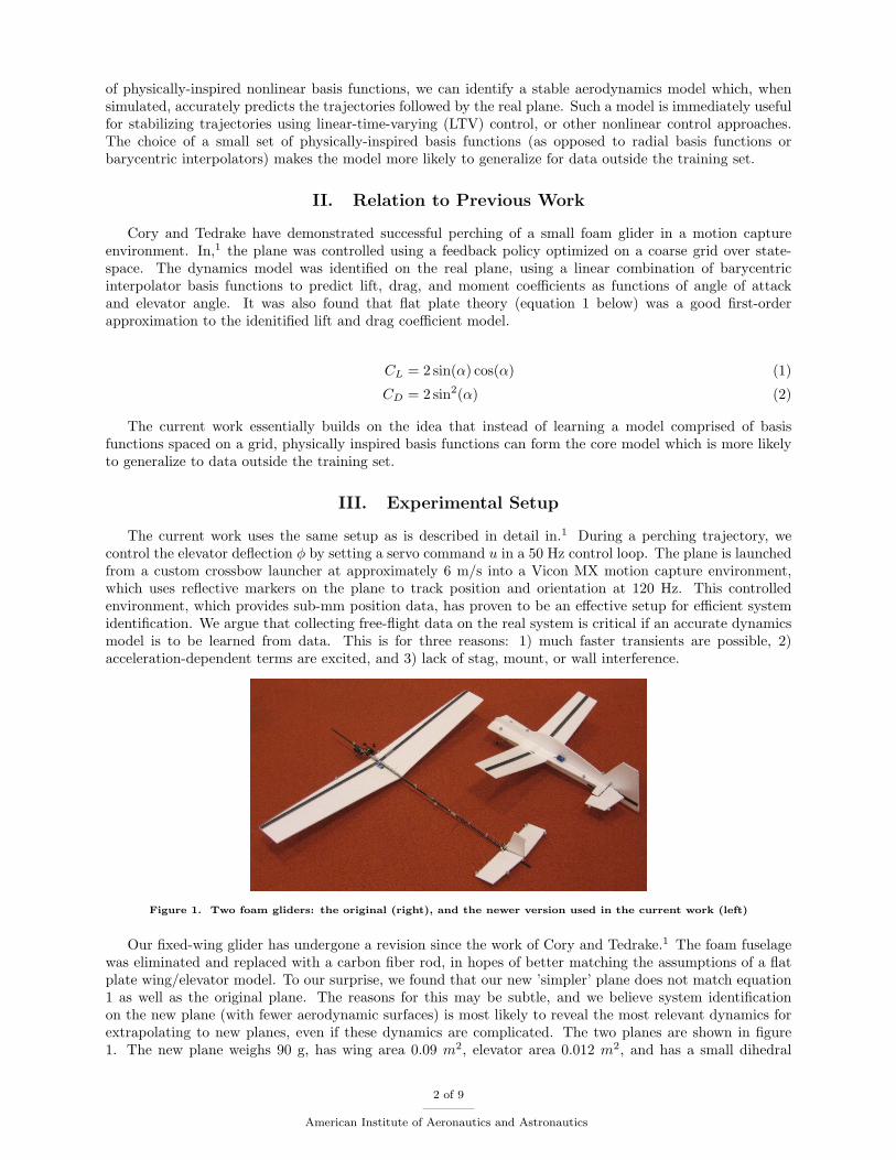
Figure 1. Two foam gliders: the original (right), and the newer version used in the current work (left)

Our fixed-wing glider has undergone a revision since the work of Cory and Tedrake.1 The foam fuselagewas eliminated and replaced with a carbon fiber rod, in hopes of better matching the assumptions of a flatplate wing/elevator model. To our surprise, we found that our new ’simpler’ plane does not match equation1 as well as the original plane. The reasons for this may be subtle, and we believe system identificationon the new plane (with fewer aerodynamic surfaces) is most likely to reveal the most relevant dynamics forextrapolating to new planes, even if these dynamics are complicated. The two planes are shown in figure1. The new plane weighs 90 g, has wing area 0.09 m2, elevator area 0.012 m2, and has a small dihedral

2 of 9


angle and vertical stabilizer to provide passive roll and yaw stability, thus constraining our problem to 2Dlongitudinal (pitch) dynamics.

IV. System Identification

We seek to identify a model for the aerodynamics along an observed perching trajectory. To do so, wegather data by repeatedly firing the plane and executing a hand-tuned open-loop control tape which getsthe plane near the perch (on average, with some standard deviation). After preprocessing the data fromour motion capture system, we simply use least squares to fit a quasi-steady model for acceleration in planecoordinates as a function of current state, x. We fit accelerations instead of forces since added-mass effectstend to make the mapping from force to acceleration more complicated than linear in mass and inertia. Themodel for accelerations is a linear combination of physically-inspired basis functions we specify (in appendixA). Since we have a general feel for what sorts of terms to place in our basis functions, but don’t know theexact aerodynamics, we specify approximately 50 possible basis functions, and then choose the ones thatpredict real data with the smallest residual. We aim to keep the number of basis functions in the modelsmall (about 2-3 for each acceleration predicted) in order to minimize overfitting, which tends to make themodel inaccurate in simulation.

IV.A. Preprocessing

We begin by filtering raw position and orientation data acausally with a 3rd order low-pass Butterworth filter.We then differentiate twice using a finite difference stencil to get instantaneous velocity and acceleration data,and finish the conversion from 3D to 2D data using the filtered data. Next, we do a coordinate transformto express the observed inertial accelerations in plane coordinates (normal and tangential to the wing), andremove gravity (since we want to predict accelerations due to aerodynamic forces only): xp

zp

θ

=

cos(θ) sin(θ) 0− sin(θ) cos(θ) 0

0 0 1

x

z + g

θ

(3)

The choice of coordinates normal and tangential to the wing, as opposed to normal and tangential tovelocity (lift and drag) is a break from standard aerodynamic practice, and is sensible because our wing isliterally a flat plate, as opposed to an airfoil. We find that the aerodynamics normal and tangential to thewing are more ’decoupled’ than the lift and drag aerodynamics.

(x, z)

le

g

lh

..

θ

−φ

α

[x, z]

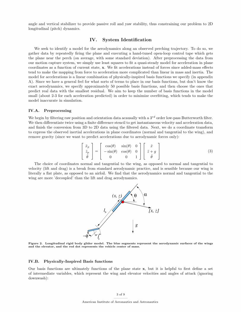
Figure 2. Longitudinal rigid body glider model. The blue segments represent the aerodynamic surfaces of the wingsand the elevator, and the red dot represents the vehicle center of mass.

IV.B. Physically-Inspired Basis functions

Our basis functions are ultimately functions of the plane state x, but it is helpful to first define a setof intermediate variables, which represent the wing and elevator velocities and angles of attack (ignoringdownwash):

3 of 9


xel = x+ (le + lh)θ sin(θ) zel = z − (le + lh)θ cos(θ) (4)

V =√x2 + z2 Vel =

√x2el + z2

el (5)

α = θ − atan2(z, x) αel = θ + φ− atan2(zel, xel) (6)

From here we define a number of physically-inspired functions of the above variables. The full list of ourbasis functions is in appendix A.

IV.C. Least-Squares Fit

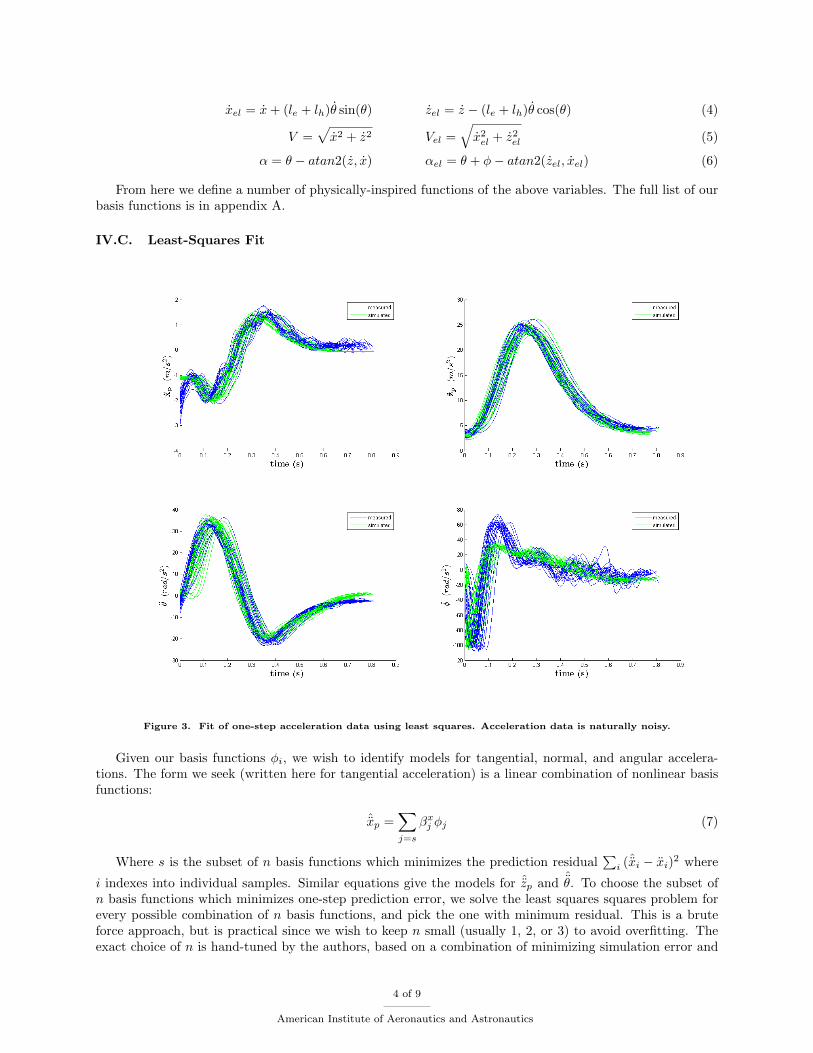
Figure 3. Fit of one-step acceleration data using least squares. Acceleration data is naturally noisy.

Given our basis functions φi, we wish to identify models for tangential, normal, and angular accelera-tions. The form we seek (written here for tangential acceleration) is a linear combination of nonlinear basisfunctions:

ˆxp =∑j=s

βxj φj (7)

Where s is the subset of n basis functions which minimizes the prediction residual∑i (ˆxi − xi)2 where

i indexes into individual samples. Similar equations give the models for ˆzp and ˆθ. To choose the subset of

n basis functions which minimizes one-step prediction error, we solve the least squares squares problem forevery possible combination of n basis functions, and pick the one with minimum residual. This is a bruteforce approach, but is practical since we wish to keep n small (usually 1, 2, or 3) to avoid overfitting. Theexact choice of n is hand-tuned by the authors, based on a combination of minimizing simulation error and

4 of 9


minimizing overfitting. Increasing n by one always decreases one-step residual, but may increase simulationerror by making the model less stable. Overfitting creates quickly changing gradients in the model, whichare undesirable if the model is later to be linearized for control purposes.

The specific model we have identified for our current glider is:

ˆxp = βx6φ6 + βx24φ24 = βx6V3 cos(α) + βx24V

2el sin(αel) sin(φ) (8)

ˆzp = βz1φ1 + βz6φ6 + βz9φ9 = βz1V2 sin(α) + βz6V

2 cos3(α) + βz9V θ cos(α) (9)ˆθ = βθ29φ29 + βθ30φ30 = βθ29V

2 sinα cosα+ βθ30V2el sin(αel) cos(αel) cos(φ) (10)

To convert these plane frame accelerations back to world coordinates, we simply invert equation 3.

IV.D. Elevator Model

We also identify a second-order linear model for the elevator angle φ based on the lagged control inputu(t − τ), where τ represents the delay associated with sensing and processing (approximately 28 ms). Toidentify the elevator models, we again use a least squares approach to identify the βφi in:[

φ

φ

]=

[0 1βφ1 βφ2

] [φ

φ

]+

[0βφ3

]u(t− τ) (11)

IV.E. Results: Prediction in Simulation

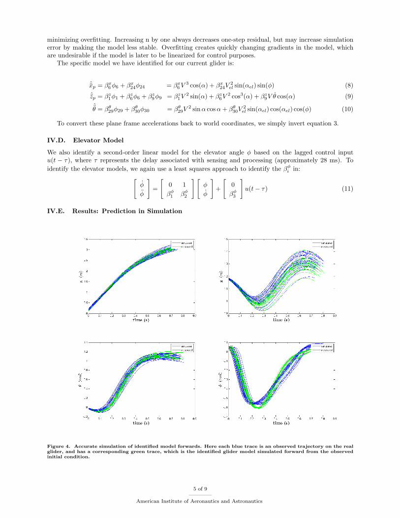
Figure 4. Accurate simulation of identified model forwards. Here each blue trace is an observed trajectory on the realglider, and has a corresponding green trace, which is the identified glider model simulated forward from the observedinitial condition.

5 of 9


To evaluate our identified model, we attempt to use it to simulate forward from the same initial conditionas the observed data, running the same open loop control tape. We pick as our initial condition a point inthe trajectory where the elevator has begun to deflect, which removes transients associated with the planeleaving our launching mechanism. As shown in figure 4 the simulated and observed trajectories match closely,with a maximum error (over all trajectories) of 13 cm in x, 12 cm in z, 6.6 degrees in θ, and 5.6 degrees in φ,and with a mean error of 2 cm in x, 2 cm in z, 1.5 degrees in θ, and 1.5 degrees in φ. This implies that themodel is stable, and therefore useful for control tasks such as LTV stabilization of the observed trajectory.

V. Model Refinement through Gradient Descent

While the model predicts the observed data well, we can do better through optimization of the rightcost function. Above, we used a simple least squares approach to minimize the one-step prediction error∑i (ˆxi − xi)2. However, ultimately we would like our model to minimize long term simulation errors, and

we cannot expect minimizing one-step prediction error to correspond to minimizing simulation error. Wedefine the simulation error as the (squared) error between observed and simulated trajectories which startat the same initial condition: ∫ T

0

(xsim − xmeas)TQ(xsim − xmeas)dt (12)

Where Q is a weighting on errors in each state variable - usually unity for x, z, and θ, and zero elsewhere.Starting from the least squares solution, we can tweak our model parameters (using gradient descent) to bringthis simulation error to a local minimum. To do so, we must calculate the gradients of the simulation errorcost function (equation 12) with respect to changes in the parameters of our model, βi. This is accomplishedusing well-known methods, such as back-propagation through time (BPTT) or Real-Time Recurrent Learning(RTRL).2

Figure 5. Reduction of model simulation error using gradient descent. The parameters are initialized to the leastsquares solution, and then tweaked using gradient descent to bring simulation error to a local minimum.

6 of 9


Using gradient descent to bring the simulated trajectory in closer agreement with a single observedtrajectory (as shown in figure 5) is especially useful when attempting to stabilize a trajectory using feedback.Whether we choose to stabilize the observed or the simulated trajectory, discrepancies between the modeledand observed dynamics show up as disturbances, and minimizing them is critical for performance.

VI. Future Work: LTV Stabilization

Ultimately, the authors’ modeling work is motivated by a desire to stabilize feasible perching trajectoriesusing feedback. The feedback control we envision requires an accurate dynamics model (such as the onewe have presented), and will enable perching from perturbed initial conditions and with disturbances suchas gusts. One control approach which may be well suited to this problem is Linear Time Varying (LTV)stabilization of one or many desired trajectories.4 This is work in progress, but initial simulation resultssuggest LTV control using our identified model successfully reduces the final distance from the perch, whenstarting from a randomly perturbed initial condition.

Figure 6. Stabilization of perching trajectory using LTV control. The glider dynamics were simulated forward fromrandom initial conditions using 1) an open loop control tape (red dots), and 2) LTV control (green dots). Green dotsare more tightly packed around the perch than red dots, showing that the LTV controller is working. Ongoing LTVresearch is essentially focused on clumping the green dots closer to the perch.

VII. Conclusions

We have presented a simple set of physically-inspired basis functions which have enabled us to identifya compact model for the aerodynamics of a glider following a specific perching trajectory. The model isidentified from free-flight data in a motion capture environment, which ensures that we have observed all therelevant (transient) system dynamics. Starting with a least squares fit that minimizes one-step predictionerror, the model is fine-tuned using gradient descent to minimize the simulation error over the entire perchingtrajectory. Initial results indicate that LTV control (trajectory stabilization) successfully brings the gliderclose to the perch from perturbed initial conditions.

7 of 9


Acknowledgments

The authors thank labmates Rick Cory, John Roberts, and Joseph Moore for their help with the experi-ments. This research was supported by the a Microsoft Research New Faculty Fellowship and by the MITLincoln Laboratory Advanced Concepts Committee.

References

1Cory, R. and Tedrake, R., “Experiments in Fixed-Wing UAV Perching,” Proceedings of the AIAA Guidance, Navigation,and Control Conference, AIAA, 2008.

2Williams, R. J. and Zipser, D., “A Learning Algorithm for Continually Running Fully Recurrent Neural Networks,”Neural Computation, Vol. 1, 1989, pp. 270–280.

3Williams, D., Collins, J., Quach, V., Kerstens, W., Buntain, S., Colonius, T., Tadmor, G., and Rowley, C., “Low ReynoldsNumber Wing Response to an Oscillating Freestream with and without Feed Forward Control,” slides from talk at AIAA ASMOrlando 2009, 2009.

4Roberts, J. W., Cory, R., and Tedrake, R., “On the Controllability of Fixed-Wing Perching,” Accepted in the Proceedingsof the American Controls Conference (ACC), 2009.

5Anderson, A., Pesavento, U., and Wang, Z. J., “Unsteady aerodynamics of fluttering and tumbling plates,” J. FluidMech., Vol. 541, 2005, pp. 65–90.

6Tedrake, R., Jackowski, Z., Cory, R., Roberts, J. W., and Hoburg, W., “Learning to Fly like a Bird,” Under review ,2009.

7Wickenheiser, A. M. and Garcia, E., “Optimization of Perching Maneuvers Through Vehicle Morphing,” Journal ofGuidance, Control, and Dynamics, Vol. 31, No. 4, July-August 2008, pp. 815–824.

8Hoburg, W., Roberts, J. W., Moore, J., and Tedrake, R., “The Perching Number: A Dimensionless Analysis of Post-stallManeuvering in Birds and Planes,” Working Draft , 2009.

9Tedrake, R., “LQR-Trees: Feedback motion planning on sparse randomized trees,” Under review , 2009.10Langelaan, J. W. and Bramesfeld, G., “Gust Energy Extraction for Mini- and Micro- Uninhabited Aerial Vehicles,”

Proceedings of the 46th Aerosciences Conference, 2008, p. 15.11Andreas Schtte, G. E. and Raichle, A., “Numerical Simulation of Maneuvering Aircraft by Aerodynamic, Flight Mechanics

and Structural Mechanics Coupling,” Journal of Aircraft , Vol. 46, Jan/Feb 2009, pp. 53–64.

8 of 9


A. Full List of Basis Functions

φ1 = V 2 sin(α)

φ2 = V 2 cos(α)

φ3 = V 2 sin(α) cos2(α)

φ4 = V 2 sin2(α) cos(α)

φ5 = V 2 sin3(α)

φ6 = V 2 cos3(α)

φ7 = V θ

φ8 = V θ sin(α)

φ9 = V θ cos(α)

φ10 = θ2

φ11 = θ

φ12 = sin(φ)

φ13 = V 2 sin(φ)

φ14 = V θ sin(φ)

φ15 = V φ sin(φ)

φ16 = V (θ + φ) sin(φ)

φ17 = V θ cos(φ)

φ18 = V (θ + φ) sin(φ) cos(φ)

φ19 = sin(αφ)

φ20 = V 2el sin(αel)

φ21 = Velθ sin(αel)

φ22 = Velφ

φ23 = V 2el sin(αel) cos(φ)

φ24 = V 2el sin(αel) sin(φ)

φ25 = Velφ sin(αel)

φ26 = Velφ cos(αel)

φ27 = V 2el sin(αel) cos(αel)

φ28 = V θ sin(α) cos(α)

φ29 = V 2 sin(α) cos(α)

φ30 = V 2el sin(αel) cos(αel) cos(φ)

φ31 = V 2el sin(αel) cos(αel) sin(φ)

φ32 = θ|θ|

φ33 = V θ|θ|

φ34 = θ|θ| sin(α) cos(α)

φ35 = θ|θ| sin(α)

φ36 = θ|θ| cos(α)

φ37 = θ2 sin(α) cos(α)

φ38 = Vel(θ + φ)

φ39 = Vel(θ + φ) sin(αel)

φ40 = Vel(θ + φ) cos(αel)

φ41 = Vel(θ + φ) sin(αel) cos(αel)

9 of 9


system identi cation of post stall aerodynamics for uav...

Documents