systematic and liquidity risk in subprime-mortgage backed

Systematic and Liquidity Risk in Subprime-MortgageBacked Securities�

Mardi Dungey+ Gerald P. Dwyer# and Thomas Flavin&+University of Tasmania, CFAP, University of Cambridge and CAMA

#Federal Reserve Bank of Atlanta, University of Carlos III, Madrid and CAMA&National University of Ireland, Maynooth

August 2011

Abstract

The misevaluation of risk in securitized �nancial products is central to understand-ing the Financial Crisis of 2007-2008. This paper characterizes the evolution of factorsa¤ecting collateralized debt obligations (CDOs) based on subprime mortgages. A keyfeature of subprime-mortgage backed indices is that they are distinct in their vintageof issuance. Using a latent factor framework that incorporates this vintage e¤ect, weshow the increasing importance of a common factor on more senior tranches during thecrisis. We examine this common factor and its relationship with spreads. We estimatethe e¤ects on the common factor of the �nancial crisis.

JEL Classi�cation: G12, G01, C32

Keywords: asset backed securities, subprime mortgages, �nancial crisis, factor mod-els, Kalman �lter

�We are grateful for comments from Paul Koch, Belén Nieto, Ellis Tallman, participants at a FinancialManagement Association conference, a Federal Reserve "Day Ahead" conference on Financial Markets, anINFINITI conference, and a Western Economic Association conference as well as participants in seminars atAustralian National University, the Central Bank of Brazil, the University of Tasmania and West VirginiaUniversity. We thank Christian Gilles, Paul Kupiec and Charles Smithson for important assistance inunderstanding the ABX index of CDO prices. Dungey acknowledges support from ARC Discovery GrantDP0664024. Dwyer thanks the Spanish Ministry of Education and Culture for support of project SEJ2007-67448/ECON and ECO2010-17158. Any errors are our responsibility. The views expressed here are ours andnot necessarily those of the Federal Reserve Bank of Atlanta or the Federal Reserve System. Author contactdetails: Dungey: [email protected], Dwyer: [email protected], Flavin: thomas.�[email protected].

1 Introduction

Securities based on subprime mortgages played a central role in the Financial Crisis of 2007-

2008. The shortcomings of models for pricing these securities became apparent when real

estate prices started to fall and mortgages became delinquent. Di¢ culties valuing these

securities led to widespread problems trading them, (Dwyer and Tkac, 2011).

The period leading up to the crisis was one of dramatic growth in asset backed securities

and structured �nancial products. These products were tranched and rated and acquired

by investors across the world. Chiesa (2008) shows that pooled and tranched securities

can generate optimal risk transfer, although one rationale for the issuance of pooled and

tranched securities is an informational advantage about underlying asset quality enjoyed

by informed sellers (DeMarzo, 2005). Increased demand for structured securities led to an

expansion in the range of underlying assets (Benmelech and Dlugosz, 2009) and the creation

of structured securities based on subprime mortgages increased dramatically. Mian and Su�

(2009) provide evidence that an increased demand for these products a¤ected the market for

subprime mortgages by resulting in less stringent lending criteria and contributing to their

subsequent growth.

The spread of this crisis from a relatively small sector of the �nancial system across

markets and international borders resulted in widespread �nancial distress.1 Among other

e¤ects, banks in much of the world su¤ered substantial losses followed by serious retrench-

ment and restructuring. The turbulence and ensuing lack of con�dence spread to other asset

markets and the real economy. Brunnermeier (2009), Dwyer and Tkac (2009) and others

document the evolution and spread of the crisis and the role of subprime-mortgage backed

securities in it.

The misperception and misevaluation of risk in structured �nancial products is central

to many explanations of the �nancial crisis. This may have arisen partly due to the fail-

ure of some market participants to di¤erentiate between the risk of AAA-rated tranches of

Collateralized Debt Obligations (CDOs) and AAA-rated corporate bonds (Brennan, Hein

and Poon, 2009). In addition to possible mispricing, the valuation of CDO tranches is par-

ticularly problematic in the event of widespread defaults (Smithson, 2009), a feature not

apparent before defaults increased in 2007. Valuation models have four key inputs: default

1Dwyer and Tkac (2009) estimate that subprime mortgages are no more than one percent of global bondvalues, stock values and bank deposits.

1

rates, prepayment risk, recovery rates and default correlations. Problems estimating the last

two were important during the �nancial crisis. Default correlations inevitably are based on

historical data and were underestimated based on a period of increasing house prices and

economic expansion. As default correlations increase, the probability of observing large-scale

defaults also increases, causing the prices of senior CDO tranches to fall. Estimates of re-

covery rates also were a¤ected. Consequently, the risk priced in the di¤erent CDO tranches

was underestimated. Coval, Jubek and Sta¤ord (2009) analyze the risk inherent in the secu-

ritization process and in particular how risk migrates to higher-rated tranches in the event

of increasing importance of a large common shock such as falling house prices.

A better understanding of the factors underlying price changes in these subprime-mortgage

backed assets is important for understanding their role in the crisis. We characterize the

driving forces behind the decreases in these securities� prices. In earlier work, Longsta¤

and Rajan (2008) show that a theoretical pricing model for CDOs can be represented as

a three factor model, with common, credit rating and idiosyncratic shocks. An empirical

application using tranches of corporate credit default swap indices (CDX) from 2003 to 2005

suggests that idiosyncratic default risk accounts for around 65 percent of the risk premium,

while common risk accounts for only 8 percent of that premium. Extending the time period,

Bhansali, Gingrich and Longsta¤ (2008) show a substantial increase in common-event risk

in 2007 and 2008.

An additional but potentially key feature of subprime-mortgage backed indices is variation

in the quality of the underlying loans and collateral over time. Demyanyk and Van Hemert�s

(2011) analysis of subprime loans indicates a gradual and persistent deterioration of loan

quality from 2001 to 2007. To re�ect this deterioration, we extend Longsta¤ and Rajan�s

(2008) model to include a fourth factor, a vintage factor. This vintage factor re�ects risks

associated with the dates the securities were created. The model is applied to asset tranches

of mortgage backed securities using the Markit ABX.HE indices for three vintages over the

period January 2006 to December 2009. An innovation of this paper is the exploitation

of the unbalanced panel structure of the data to identify the vintage, credit, common and

idiosyncratic e¤ects. This allows us to assess the contribution of all factors to the asset prices

and returns. We specify the model in state-space form and estimate it with a Kalman �lter.

The ABX.HE data have been examined in several studies of the �nancial crisis. Fender

and Scheicher (2009) use two vintages to track the crisis and �nd that increased liquidity risk

2

and decreasing risk appetite were important factors in the price decreases of the higher-rated

tranches. Our paper di¤ers in many respects; we extract risk factors di¤erently and focus on

the level rather than the change of the common factor. Longsta¤(2010) uses the ABX indices

to test for contagion from the subprime-asset backed market to other parts of the �nancial

system. He �nds strong evidence of contagion and liquidity risk with revisions to risk premia

identi�ed as the most likely transmission channel. Longsta¤ also �nds that ABX returns

lead stock market returns and bond yield changes by up to three weeks, suggesting that

signi�cant information was uncovered in this market that led to subsequent price changes in

other markets. Gorton (2009) �nds that declines in the ABX indices and the repo market

were highly correlated due to some combination of counterparty risk and lack of liquidity.

Our results summarize the behavior of subprime-mortgage backed securities in terms of

four factors. In 2006, all factors have a discernible role in asset returns. The common factor

becomes more important when the �nancial turmoil begins and has a larger e¤ect on AAA

tranches than in the pre-crisis period. We examine the common factor�s relationship with

observable factors including real estate prices, the VIX index and interest rate spreads which

re�ect the �nancial crisis. We �nd that liquidity and counterparty risk, as represented by the

spread between the London Interbank Borrowing Rate (LIBOR) and the Overnight Index

Swap (OIS) rate, is su¢ cient to characterize the relationship between the common factor

and the �nancial crisis as re�ected in interest rate spreads. We do a counterfactual analysis

of the evolution of the common factor if the LIBOR-OIS spread had remained at pre-crisis

levels throughout. We estimate that the common factor is 20 percent lower at the end of

2009 than it would have been if LIBOR-OIS had not been elevated during the �nancial crisis.

Likewise we estimate that the actual value of the REIT index is about 40 percent lower and

VIX some 50 percent higher than in the simulated model with a stable interest rate spread.

The decreases in the common factor, decreases in the REIT index and increases of VIX are

the estimated e¤ects of the elevated values of LIBOR-OIS during the crisis, not e¤ects of

lower housing prices.2

The paper is structured as follows. Section 2 describes the ABX data and highlights its

unique features which are re�ected in the econometric model presented in Section 3. The

estimates of the factors are discussed in Section 4. Section 5 relates the common factor to

observable short-term �xed-income spreads. Section 6 concludes.

2A REIT index is included with the common factor in a cointegrating vector in order to re�ect thestochastic trend in housing prices.

3

2 Tracking the market for subprime mortgages

The price decreases in asset backed securities during the �nancial di¢ culties of 2007 to 2009

were dramatic. They represent declines in the values of the underlying assets but probably

also reassessments of the risks and liquidity of such assets. We analyze the risk factors

inherent in these tranched pools by examining the relatively new indices of CDOs used as

the basis for credit default swaps related to subprime-mortgage backed securities. These

indices, entitled ABX.HE, were introduced in January 2006 by Markit and are widely used

by market participants to track the market for subprime mortgages and to bet on it.

Figure 1 shows the evolution of the indices from January 2006 to December 31, 2009.

Each issue is subdivided into �ve tranches, varying from AAA to BBB-, where the ratings are

the lower of those issued by Moody�s and S&P. The index values are derived from underlying

credit default swaps with the insurance coupon �xed for the life of trading. The coupon is

set so the index trades at par �100 �at inception unless such a coupon exceeds 500 basis

points, in which case the coupon is set at 500 basis points.

Each vintage of the index is based on twenty mortgage backed CDO deals created within

the previous six months. For example, the ABX.HE 06-1 index is constructed from deals

created in the second half of 2005. The issuers are the largest originators.3 Strict require-

ments must be met to qualify for inclusion in the index. For example, the value of each deal

must be at least $500 million and each tranche must have an average life between four and

six years, and the AAA tranche must have a weighted average life of more than �ve years.

Furthermore, no security originator can have more than four deals included.

New indices were created every six months from January 2006 to July 2007. No indices

have been created since then because there are too few new CDOs meeting the eligibility

requirements.4 New indices every six months with similar underlying securities might have

created an index that could be spliced together as is done sometimes with on-the-run bonds

and futures prices. Each vintage represents quite di¤erent risks though. At least part of

the explanation for these vintage e¤ects is an increase in the riskiness of the underlying

mortgages (Demyanyk and Van Hemert, 2011). This increase in risk is re�ected in increased

coupon rates for insurance on the ABX indices from 2006 to 2007. Figure 1 shows substantial

3Licensed dealers in the ABX.HE indices included ABN AMRO, Bank of America, Barclays Capital,Bear Stearns, BNP Paribas, Calyon, Citigroup, Credit Suisse, Deutsche Bank, Goldman Sachs, JPMorgan,Lehman Brothers, Merrill Lynch, Morgan Stanley, RBS Greenwich, UBS and Wachovia.

4As of this writing in 2011, there has been very little securitization since 2008.

4

heterogeneity in the index values across vintages from 2006 to the end of 2009 with later

values declining more, which is consistent with the mortgages being riskier. These consid-

erations suggest that successive rolls of the ABX are not suitable for splicing to create a

continuous series, as Longsta¤ and Rajan (2008) do for CDX data. Instead, each new index

is best viewed as a unique vintage with the risk of the underlying pool of assets di¤erent

between vintages.

Our initial analysis extracts a common factor from the behavior of daily ABX returns.

These �returns�on the ABX are the di¤erences in the logarithms of the indices. Descriptive

statistics for each tranche of each vintage are given in Table 1. The data set is unbalanced;

all vintages exist at the end of the period but the vintages are created over time. Within

each vintage, the standard deviation of returns is lowest for the AAA security. The �rst

vintage has returns with the lowest volatility and there is some evidence of higher standard

deviations of returns for later vintages. The distributions are negatively skewed with the

exception of the AAA tranche of the �nal vintage. All assets display excess kurtosis. This

is greatest for the �rst vintage, possibly re�ecting the sustained low-variance period at the

start of the period.

Tables 2 and 3 present correlations of the returns across credit ratings for given vintages

and across vintages for given credit ratings. The correlations of the AAA tranches with

other tranches decrease monotonically as ratings decline. The correlations across vintages

are highest for the AAA tranches but this is not particularly surprising because they bear

less idiosyncratic risk than lower-rated tranches.

3 Modelling framework for ABX data

Financial market returns are frequently modelled with latent factor models, for example by

Diebold and Nerlove (1989) and Dungey and Martin (2007). In this paper, we include four

factors re�ecting vintage e¤ects in addition to the common, credit rating and idiosyncratic

factors present in Longsta¤and Rajan (2008). The explicit di¤erences in ratings and vintages

and the unbalanced nature of the data allow us to identify these four factors from the data

rather than applying factor labels ex post. The model is

yi;j;t = �i;jwt + �i;jvi;t + 'i;jkj;t + �i;jfi;j;t: (1)

5

where yi;j;t is the demeaned return on the ABX index of vintage i and credit rating j at time

t. The vintage is the date of issuance of the security. The factors represent a common shock

a¤ecting all assets, wt; a vintage shock unique to all assets of a particular index date, vi;t; a

ratings shock unique to assets of a speci�c rating across all vintages, kj;t; and idiosyncratic

shocks, fi;j;t:

To capture serial correlation in the data, the common, ratings and vintage factors follow

AR(1) processes. As in previous research on factor models (Dungey, Pagan and Martin,

2000), we do not estimate persistence in the idiosyncratic shocks. The additional features of

the model can be written

wt = �wwt�1 + �w;t (2)

vi;t = �v;ivi;t�1 + �v;i;t (3)

kj;t = �k;jkj;t�1 + �k;j;t (4)

fi;j;t = �i;j;t (5)

E��w;t

�= 0;E

��w;t�w;s

�= �2w: (6)

E��z;t�= 0; E

��z;t�z;s

�= �2z for t = s for z = (v; i); (k; j); (i; j) (7)

E��z;t�z;s

�= 0 for t 6= s for z = (v; i); (k; j); (i; j) (8)

E��z;t; �a;t

�= 0 for a; z = (v; i); (k; j); (i; j) and a 6= z (9)

where equations (6) to (9) indicate that the shocks to each factor are independent with

constant variances. There are no other restrictions on the variance-covariance matrix of the

returns. The conditional variances of the returns vary over time and we account for this

feature of the data. Our state space model is already heavily parameterized and it is imprac-

tical to include ARCH estimation directly into the estimation of the factor model. Instead,

we pre-�lter the returns by estimating an IGARCH(1,1) model and use the standardized

returns in the factor model.5 If we let yi;j;t represent these standardized returns and ri;j;t

represent the raw (unstandardized) returns, then

ri;j;t = ai;j + hi;j;tyi;j;t (10)

h2i;j;t = 1;i;j(ri;j;t�1 � ai;j)2 +�1� 1;i;j

�h2i;j;t�1:

5Pre�ltering the data may result in ine¢ ciency in the second stage of estimation. The consistency ofthe estimates is una¤ected by two-stage estimation if the estimators are orthogonal, which seems a strongassumption in our application. We do not focus on statistical signi�cance of parameters and our analysis ofthe factors uses estimates of the factors with the �ltering reversed.

6

Table 4 presents the parameter estimates of the IGARCH models estimated by Quasi

Maximum Likelihood for all credit ratings and vintages (Lumsdaine, 1996). Table 5 presents

summary statistics for the adjusted returns and Figure 2 shows the adjusted returns. The

graphs suggest that the IGARCH model has stabilized the variances relative to the variances

in the original series.

The factor model can be rewritten in state-space form as

Yt = Z�t + S"t (11)

�t+1 = ��t +Rut (12)

where Yt is the vector of the returns in each asset, E["t] = 0; E["t"0t] = H;E[ut] = 0; and

E[utu0t] = Q. The evolving latent factors are contained in the vector �t and the idiosyncratic

factors, fi;j;t are contained in the vector "t.

To reduce the dimensionality of the estimation problem and keep it tractable, our em-

pirical estimation is based on a system of nine asset returns selected to span the range of

ratings and vintages. We examine AAA, AA and BBB- rated securities from the January

2006, January 2007 and July 2007 vintages. The AAA and AA tranches have the largest

share of the value of underlying subprime-mortgage bonds, and the BBB- tranche is included

because it is the lowest rated tranche. We include the January 2006 and July 2007 vintages

because they are the �rst and last issuances available. We prefer the January 2007 vintage to

the July 2006 vintage mainly because the January 2007 vintage is based on later mortgages.

These mortgages may have been less carefully vetted when created and may be a¤ected more

by the decline in housing prices and mortgages subsequently becoming upside down.

7

The following de�nitions of Z and �t show the form of the restrictions in the model,

Z =

26666666666664

�1;AAA �1;AAA 0 0 '1;AAA 0 0�1;AA �1;AA 0 0 0 '1;AA 0�1;BBB �1;BBB 0 0 0 0 '1;BBB�2;AAA 0 �2;AAA 0 '2;AAA 0 0�2;AA 0 �2;AA 0 0 '2;AA 0�2;BBB 0 �2;BBB 0 0 0 '2;BBB�3;AAA 0 0 �3;AAA '3;AAA 0 0�3;AA 0 0 �3;AA 0 '3;AA 0�3;BBB 0 0 �3;BBB 0 0 '3;BBB

37777777777775(13)

�t =

2666666664

wtv1;tv2;tv3;tkAAA;tkAA;tkBBB;t

3777777775. (14)

De�ning � as a 7� 7 diagonal matrix of autoregressive parameters, � = [�w �v;i �k;j] for alli; j; St as a 9�9matrix with parameters �i;j on the main diagonal; andR as the appropriatelysized identity matrix where the factor variances are standardized to unity, we can estimate

the parameters by the standard Kalman �lter procedure.6 Its prediction equations are given

by

at+1 = �atjt (15)

Ptjt+1 = �Ptjt�0 + SQS 0 (16)

where Ptjt+1 is the prediction vector. The updating equations are

atjt = at + PtZ0F�1t vt (17)

Ptjt = Pt � PtZ 0F�1t ZP 0t (18)

where

vt = Yt � Z�t (19)

Ft = ZPtZ0 + Z: (20)

6Starting values are taken as the consistent estimates of the parameters of the factor model in equation(1) obtained from unconditional moments using GMM.

8

Furthermore, we accommodate the unbalanced nature of our data by constructing a dummy

matrix, Dt, as follows

Dt =

26666666666664

1 1 0 0 1 0 01 1 0 0 0 1 01 1 0 0 0 0 1d1t 0 d1t 0 d1t 0 0d1t 0 d1t 0 0 d1t 0d1t 0 d1t 0 0 0 d1td2t 0 0 d2t d2t 0 0d2t 0 0 d2t 0 d2t 0d2t 0 0 d2t 0 0 d2t

37777777777775(21)

where d1t takes the value of 1 from the initiation of the 07-1 vintage onwards and 0 otherwise

and d2t is similarly de�ned with respect to the vintage 07-2. The Kalman �lter equations are

then modi�ed by replacing Z with Z �Dt wherever it appears in the �lter with the operator

� indicating element-by-element multiplication.

4 Results

A preliminary yet informative way to analyze the results is to perform an unconditional

variance decomposition using equation (1) which implies

Var(yi;j) = �2i;j Var(w) + �

2i;j Var(vi) + '

2i;j Var(kj) + �

2i;j Var(fi;j) (22)

so that, for example, the contribution of the vintage factor to variance in asset yi;j is expressed

as�2i;j Var(vi)

�2i;j Var(w) + �2i;j Var(vi) + '

2i;j Var(kj) + �

2i;j Var(fi;j)

and similarly for other contributing factors.

Table 6 presents the unconditional variance decomposition for the full period of each vin-

tage and for selected subperiods.7 For the full period, the common factor is most important

for the AAA and AA ratings for all vintages. Variability of the BBB- tranches is less closely

related to the common factor and more closely related to the rating factor. The vintage fac-

tors are relatively unimportant for all assets. The ratings factors, on the other hand, a¤ect

all of the vintages and credit ratings, although they are less important for the AA tranches

of the January and July 2007 vintages. The importance of idiosyncratic factors di¤ers across

7The parameter values themselves are estimated consistently, but are not very informative by themselves.The parameter values are available from the authors upon request.

9

vintages and across ratings. In particular, they exert a stronger in�uence on later vintages

and we also observe an upward drift in terms of ratings over time. This likely re�ects the

losses and consequent collapse in prices for the lower-rated tranches of the later vintages,

which decimated the protection for the higher-rated tranches. As a result of the large losses,

idiosyncratic losses on mortgages migrate up to the AA and even the AAA tranches.

Table 6 also presents the unconditional variance decompositions for subperiods. In the

non-crisis period of 2006, the variances of the AAA and AA tranches are dominated by

the common factor and the credit rating factors. The idiosyncratic factor is easily the most

important factor for the BBB- tranche and is quite unimportant for the higher-rated tranches.

This is consistent with the role of the BBB- tranche as the absorber of the relatively small

idiosyncratic losses. The common shock accounts for about half the variance of the AAA and

AA tranches. This contrasts with Longsta¤and Rajan�s (2008) �nding that a common factor

is relatively unimportant in non-crisis periods. The �rst half of 2007 does not look markedly

di¤erent for these securities. There are however di¤erences in the relative importance of

the factors for the January 2007 vintage. The AAA securities look little di¤erent, but the

idiosyncratic factor becomes quite a bit more important for the AA securities, roughly the

same as for the BBB- tranche of the January 2006 vintage.

In the crisis from July 2007 to the end of 2008, the relative contributions of the factors

change markedly. The common factor is most important for the AAA-rated tranches of

all vintages. For the BBB- tranches, idiosyncratic factors remain prominent although the

common factor exerts more in�uence and the ratings factors assume most importance. Idio-

syncratic factors remain most important for the BBB- tranche in the January 2006 vintage,

though, as well as for the AA tranches of the January and July 2007 vintages. Vintage

factors, never especially important, all but disappear.

In 2009, there is little evidence of any return to pre-crisis factor contributions. The

variance decompositions are hard to distinguish from those of the crisis period. This analysis

reveals substantial time variation in the relative factor contributions to ABX returns.

Figure 3 shows daily variance decompositions for each vintage and credit rating. Each

page contains a panel of graphs, with columns 1 to 3 representing AAA, AA and BBB- rated

assets respectively. The �rst row in each panel presents the observed asset return volatility,

and the following rows present the contributions of each factor to that volatility. Note that

the common factor, shown in the second row, tends to be more important for the higher-rated

10

tranches and the idiosyncratic factor tends to be more important for lower-rated assets. It is

important to note that this is the variance decomposition for the standardized returns, not

the raw returns. We discuss each of the factors in turn before delving more deeply into the

relationship between the common factor with observables.

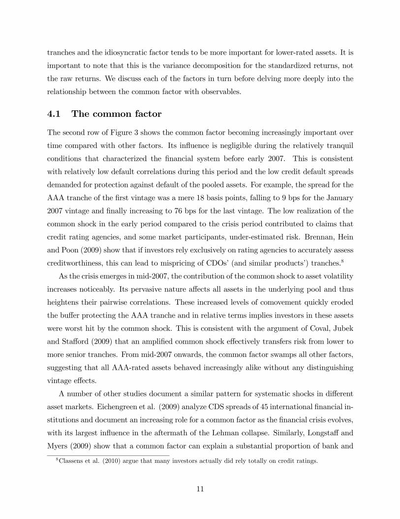
4.1 The common factor

The second row of Figure 3 shows the common factor becoming increasingly important over

time compared with other factors. Its in�uence is negligible during the relatively tranquil

conditions that characterized the �nancial system before early 2007. This is consistent

with relatively low default correlations during this period and the low credit default spreads

demanded for protection against default of the pooled assets. For example, the spread for the

AAA tranche of the �rst vintage was a mere 18 basis points, falling to 9 bps for the January

2007 vintage and �nally increasing to 76 bps for the last vintage. The low realization of the

common shock in the early period compared to the crisis period contributed to claims that

credit rating agencies, and some market participants, under-estimated risk. Brennan, Hein

and Poon (2009) show that if investors rely exclusively on rating agencies to accurately assess

creditworthiness, this can lead to mispricing of CDOs�(and similar products�) tranches.8

As the crisis emerges in mid-2007, the contribution of the common shock to asset volatility

increases noticeably. Its pervasive nature a¤ects all assets in the underlying pool and thus

heightens their pairwise correlations. These increased levels of comovement quickly eroded

the bu¤er protecting the AAA tranche and in relative terms implies investors in these assets

were worst hit by the common shock. This is consistent with the argument of Coval, Jubek

and Sta¤ord (2009) that an ampli�ed common shock e¤ectively transfers risk from lower to

more senior tranches. From mid-2007 onwards, the common factor swamps all other factors,

suggesting that all AAA-rated assets behaved increasingly alike without any distinguishing

vintage e¤ects.

A number of other studies document a similar pattern for systematic shocks in di¤erent

asset markets. Eichengreen et al. (2009) analyze CDS spreads of 45 international �nancial in-

stitutions and document an increasing role for a common factor as the �nancial crisis evolves,

with its largest in�uence in the aftermath of the Lehman collapse. Similarly, Longsta¤ and

Myers (2009) show that a common factor can explain a substantial proportion of bank and

8Classens et al. (2010) argue that many investors actually did rely totally on credit ratings.

11

CDO equity return variation.

4.2 Ratings and vintage factors

Both the rating and vintage factors exert a time-varying in�uence on asset return variability.

At various times, the speci�c rating and vintage helped to di¤erentiate between assets. For

the earliest vintage, 06-1, ratings matter and this factor accounts for a non-trivial amount

of asset return variability. For later vintages, ratings matter little for the two most senior

tranches but continue to be an important determinant of returns for the equity tranche. In

relative terms the contribution of the vintage factor is the smallest of all factors. However,

in early 2007 as ABS markets become unsettled, the vintage factor has a pronounced e¤ect.

This suggests that market participants began to distinguish between ABX indices on the

basis of the underlying asset quality. For all tranches the largest impact of the vintage factor

occurs for the July 2007 issuance. The deals underlying this issue were struck in the �rst

half of 2007, when US house price declines were already evident (previous issues were based

on rising and then peak house prices).

The rating and vintage factors play an important role in distinguishing assets during

non-crisis periods. However, during crisis, their in�uence is swamped by the common and

idiosyncratic components.

4.3 The idiosyncratic factor

Just as the common factor exerts its greatest in�uence on the most senior claim, idiosyncratic

shocks have their greatest e¤ect at the other end of the rating spectrum. In the earliest

vintage, idiosyncratic risk almost exclusively a¤ects the BBB- tranche and were of little

concern to holders of more senior claims because the lower-rated tranches absorbed these

risks. In later vintages, there is a greater role for idiosyncratic shocks as mezzanine tranches

also exhibit some vulnerability to them, most likely due to the inadequacy of the equity

tranches to protect them. Interestingly, idiosyncratic shocks fall in importance for BBB-

rated assets, which may be due to overwhelming in�uence of the common shock or may also

re�ect a lack of trades when the value of the BBB- tranche �attened out near zero.9

The behavior of the idiosyncratic shock is consistent with the arguments outlined earlier.

9The buyer of insurance in the CDS on the CDO makes an initial payment to the insurance seller equalto the the di¤erence between 100 and and the index value. When the index is near zero, this becomes asubstantial unsecured loan.

12

In normal market conditions, when assets in the underlying pool exhibited relatively low

correlation, idiosyncratic risk resulted in a few random subprime mortgage defaults whose

e¤ects were absorbed by the equity tranche or other lower-rated tranches. The onset of the

crisis in July 2007 led to this risk source being swamped by the common shock, limiting its

impact on asset return volatility.

5 What drives the common factor?

Initially, we recover the level of the common factor. The logarithm of the value of the

underlying asset, pi;j;t, for vintage i, credit rating j, in period t, from the adjusted return,

yi;j;t; accounting for GARCH is

pi;j;t = a+ hi;j;tyi;j;t + pi;j;t�1 (23)

by the de�nition of the return and the equation for conditional heteroskedasticity (10).The

relationship between this index value and the factors can be seen by substituting for yi;j;t to

write

pi;j;t = a+ hi;j;t��i;jwt + �i;jvi;t + 'i;jkj;t + �i;jfi;j;t

�+ pi;j;t�1: (24)

The contribution of the factors to the value of the assets can then be written as

pi;j;t = a+ �i;jhi;j;twt + �i;jhi;j;tvi;t + 'i;jhi;j;tkj;t + �i;jhi;j;tfi;j;t + pi;j;t�1 (25)

where �i;jhi;j;twt is the contribution of the common factor to the value of the asset with

vintage i and rating j in period t. Note that the common factor including heteroskedasticity

is di¤erent for each tranche and vintage because di¤erent conditional standard deviations

translate the adjusted returns into raw returns.

Section 4 showed that the common factor plays a major part in changes to the values

of the most senior tranches of subprime-mortgage backed assets. We focus the rest of our

analysis on the drivers of the common factor. We use the AAA tranche of the 06-1 vintage to

construct the level of the common factor hi;j;twt because it represents the highest valued CDO

tranche for the longest period.10 Figure 4 shows the integrated common factor with its level

10For example, Hu (2007) reports that for CDOs issued in 2006, AAA-rated assets accounted for 85% ofdollar value and 36% of the number of tranches, while the �gures for Baa and lower rated assets were 3.7%and 24% respectively. Many deals had more than one AAA tranche. The ABX index is based on the mostsubordinate AAA tranche.

13

set to unity at the start of the series.11 The evolution of the common factor can be usefully

compared to that of the AAA tranche of the ABX index for January 2006, both of which

are shown in Figure 4 for convenience. Consistent with the common factor�s substantial

importance in the evolution of the AAA tranches, the common factor re�ects many of the

characteristics of the AAA tranche.

Observable economic variables potentially related to the deterioration of the ABX are

real estate prices, general �nancial market volatility and liquidity and counterparty risk. We

use the logarithm of a daily price index for the U.S. real estate trusts (REITs) represented

by the Dow Jones Equity All REIT Index to re�ect news about housing prices; and the

logarithm of the VIX index as a measure of general �nancial market volatility.

Liquidity and counterparty default risk are measured by three one-month interest rate

spreads: the spread between the London Interbank Borrowing Rate (LIBOR) and the

overnight index swap rate (OIS), LIBOR-OIS; the spread between LIBOR and the U.S.

Treasury Bill rate, the TED spread; and the spread between the commercial paper rate and

the U.S. Treasury Bill rate, CPR-TB.

LIBOR-OIS can be viewed as re�ecting counterparty risk from the standpoint of a lender

to another institution. Borrowers who believe the market is overstating their risk may also

view this spread as re�ecting liquidity. The TED spread is another common measure of

liquidity and counterparty risk and would be partly redundant with the inclusion of LIBOR-

OIS. The spread between OIS and the Treasury Bill rate (OIS-TB), which excludes the part

of the TED spread already represented by LIBOR-OIS, provides a straightforward means of

examining the informativeness of one spread relative to the other. OIS-TB is the clearest

indicator of liquidity issues because the OIS rate is the rate for almost fully collateralized

private transactions and the Treasury Bill rate is a nominal risk free rate. We also include the

spread between the commercial paper rate on AA-rated asset-backed commercial paper and

the U.S. Treasury bill rate, which can be interpreted as re�ecting �ights to quality during

the crisis due to concerns about the value of the underlying assets.

Figure 5 shows the observable factors. The �gures clearly show evidence of episodes with

increasing and then decreasing spreads, most evidently for the CPR-TB spread but also for

the spread of LIBOR over OIS.

11The contribution of the common factor to the measured return on the ABX is the common factor timesits coe¢ cient of 0.83. The contribution of the level of the factor to the level of ABX though depends onan unobserved initializing constant for the level of the common factor which cannot be recovered from �rstdi¤erence alone.

14

Unit root tests indicate one unit root in each of the common factor, REIT and VIX. This

unexpected outcome for the VIX is consistent with the results reported by Zhang, Sanning

and Sha¤er (2010) for options prices. Johansen cointegration tests, reported in Table 7, are

consistent with one cointegrating vector between the common factor and the logarithms of

the Dow-Jones REIT index and VIX.

Table 8 presents a 3-variable Vector Error Correction Mechanism (VECM) for the com-

mon factor, the logarithm of the REIT index and the logarithm of VIX. All equations in-

clude two lags of all variables.12 One month interest-rate spreads for LIBOR-OIS, OIS-TB,

and CPR-TB are included as exogenous variables. The errors are speci�ed as a diagonal

GARCH(1,1) , estimated using a diagonal Vech structure. The zero restrictions on errors

across variables reduces the number of parameters estimated.13

Table 9 presents tests to restrict this set of equations by deleting spreads. The results

clearly indicate that LIBOR-OIS is very informative for these variables. The results also

clearly indicate that the CPR-TB is not informative and can be dropped at little cost. The

OIS-TB spread is somewhat informative, with a p-value of 10.3 percent for dropping it from

the equations with both other spreads but a p-value of only 20.5 percent when the commercial

paper rate spread is not included in the equations. Overall, the results are consistent with

the informativeness of the spread of LIBOR - OIS but not the other spreads. Table 10

presents the estimated three-equation VECM with LIBOR-OIS as the only spread. While

t-ratios might suggest that LIBOR-OIS is not uniformly important, likelihood ratio tests

indicate that each of the variables re�ects movements in LIBOR-OIS.14

The estimates in Table 10 can be used as the basis for comparing actual events with

events estimated without the behavior of LIBOR-OIS re�ecting the �nancial crisis. The

no-�nancial-turmoil behavior of LIBOR-OIS from its behavior prior to the �nancial crisis.

It is relatively simple to date the �nancial crisis in terms of LIBOR-OIS. It spiked from 9.65

12The choice of lag length is based on F-tests and Akaike Information Criterion values, reported in Table9, which support the reduction from 3 to 2 lags but not further. We also examined evidence for a VECMwhere spreads are treated as exogenous. For LIBOR less OIS in a four-equation system, the p-value is 13.4percent. For LIBOR less OIS in a �ve-equation system, the p-value is 13.7 percent. These systems involvemany parameters, so these results are at best indicative. Attempts to estimate a six-variable system withthe AA asset-backed commercial paper rate were not successful.13Bauwens, Laurent and Rombouts (2006) and Silvennoinen and Teräsvirta (2008) review multivariate

GARCH models.14The p-values for deleting the current and two lagged values of LIBOR-OIS are 0.01 percent, 4.30 percent,

and 0.02 percent for the common factor, the logarithm of the REIT index and for the logarithm of VIXequations respectively.

15

basis points on August 8, 2007 to 38.18 basis points on August 9. This spike is extraordinary

and not a random date. On August 9, 2007, BNP Paribus suspended redemptions in three

funds holding securities based on subprime mortgages. Later that day, the European Central

Bank and the Federal Reserve dramatically increased repurchase agreements with banks to

provide additional reserves to banks. From the inception of the ABX indices on January 19,

2006 to August 8, 2007, the mean LIBOR-OIS spread is 6.32 basis points with a standard

deviation of 1.38 basis points. The maximum spread is 11.95 basis points. For the rest of

our time period, the mean spread is 64.38 basis points with a standard deviation of 58.88

basis points; the maximum spread is 337.75 basis points on October 10, 2008. As Figure

5 shows, the LIBOR-OIS spread decreased from these extraordinary values. From June 1,

2009 to the end of 2009, the mean spread is 9.87 basis points with a standard deviation of

1.16 basis points, with a maximum of 12.95 basis points in these seven months. Even this

slightly elevated level of LIBOR-OIS may well be a re�ection of the �nancial crisis.

While there always is variation in LIBOR-OIS, we simplify our simulation by setting

LIBOR-OIS to its average value before the �nancial crisis and impose that value for the

crisis period. We then simulate the behaviour of the common factor, REIT and VIX using

the same innovations to those three variables as derived from the estimates in Table 10. If

LIBOR-OIS were exactly the same as its historical values, the actual values of the common

factor, the REIT index and VIX would occur. The simulation is �dynamic�in the sense that

values of the common factor, the REIT index and VIX persist into subsequent periods, so

that deviations of simulated from actual values persist. The estimated VECM, of course,

will predict adjustment of the three variables in the cointegrating vector back to the stable

long-run relationship. This need not mean adjustment of the levels of the variables back to

their values before the �nancial crisis.

Figure 6 shows the actual and simulated values of the common factor, the REIT index

and VIX. By the end of 2009, all of the variables still show e¤ects of the �nancial crisis as

re�ected in LIBOR-OIS. None of the variables has returned to values similar to their values

before the �nancial crisis. The percentage deviations between the actual values of the series

�the common factor, the REIT stock price index and VIX �are shown in Figure 7. The

deviations are substantial. At the end of 2009, the simulation shows that the common factor

would have been 20 percent higher if the LIBOR-OIS had stayed close to its value before

the �nancial crisis. Similarly, the REIT index is slightly more than 40 percent lower than

16

it would have been under the simulation. In contrast the VIX is over 50 percent higher as

a result of the LIBOR-OIS experiences than in the simulation where LIBOR-OIS remained

around its pre-crisis values.

Even if LIBOR-OIS returns to pre-crisis values, the cointegrated values of the common

factor, the REIT index and VIX need not return to their pre-crisis values even though they

will return to the cointegrated relationship. The estimated cointegrating vector suggests

that it will take a long time for the variables to return to equilibrium and that the shocks

to LIBOR-OIS re�ected in the common factor are likely to have permanently changed this

factor in the wake of the crisis.

6 Conclusion

We characterize the behavior of the ABX indices of subprime-mortgage backed assets during

the Financial Crisis of 2007 and 2008. In the process, we gain a better understanding of the

sources of the decline of this market, in particular the falls due to liquidity and counterparty

risk. We apply a latent factor model to an unbalanced panel of returns by credit rating

and vintage to obtain a measure of the common movement. The unbalanced nature of

the data lends itself to identi�cation of four factors from the returns: a common factor, a

vintage factor relating to the issuance dates of the securities, a credit rating factor and an

idiosyncratic factor.

All factors exert a time-varying in�uence on the volatility of asset returns. The factor

common to all tranches and vintages shows the most important change in variation over

time. The common factor�s in�uence on the highly rated tranches increases with the �nancial

crisis, although not dramatically. This is consistent with market participants underpricing,

and credit agencies underestimating, the coming �nancial di¢ culties. This of course is easier

to see now than before the crisis. Given the structure of CDOs, the most senior tranches are

quite vulnerable to the miscalculation of common risk. The increasing magnitude of common

undiversi�able shocks changes the return behavior of AAA tranches dramatically as the crisis

unfolds. As a result, the demarcation between tranches becomes blurred as assets within

the underlying pool becoming increasingly correlated. Consequently, it is the common shock

that is most closely associated with the main damage to the values of CDOs. As suggested

by Coval, Jubek and Sta¤ord (2009), the securitization process led to more vulnerability to

common risk that had been unimportant during the low volatility environment before 2007

17

but came to the fore with a vengeance during the subsequent downturn. At the other end of

the spectrum, the role of idiosyncratic shocks in determining asset returns is predominantly

associated with the lowest rated tranche, but even this is largely overwhelmed by the common

factor after July 2007. Similarly, in the earlier tranquil market conditions, both the ratings

and vintage factors are important for some tranches but again their in�uence is dwarfed by

the common factor during the �nancial crisis.

To estimate the e¤ects of counterparty risk and liquidity di¢ culties in �nancial markets,

we delve deeper into the origins of the common factor. We relate the common factor to

observable variables commonly mentioned as being crucial in the initiation and transmission

of the crisis, capturing the real estate downturn, general �nancial market volatility, market

liquidity decreases and increasing counterparty risk. The common factor, the REIT index

and VIX are cointegrated and related to the LIBOR-OIS spread. The LIBOR-OIS spread

played a critical role. Because the spread was elevated during the crisis, at the end of 2009,

the common factor was 20 percent lower, the REIT index was 40 percent lower and the

VIX was 50 higher than without the disruptions re�ected in LIBOR-OIS. This of course

does not imply that setting LIBOR-OIS to pre-crisis values would have reduced the e¤ect

on the other variables. Fixing a price cannot help. On the other hand, our results indicate

that macroprudential supervision is an even more di¢ cult task than commonly thought. A

�nancial crisis has nontrivial e¤ects that continue well after it is over.

References[1] Bauwens, L., S. Laurent and J.V.K. Rombouts. 2006. Multivariate GARCH models: A

survey. Journal of Applied Econometrics 21, 79-109.

[2] Benmelech, E., and J. Dlugosz. 2009. The alchemy of CDO credit ratings. Journal ofMonetary Economics 56 (5), 617-634.

[3] Bhansali, V., R. Gingrich and F. Longsta¤. 2008. Systemic credit risk: What is themarket telling us? Financial Analysts Journal 64 (4), 16-24.

[4] Brennan, M.J., J. Hein and S. Poon. 2009. Tranching and Rating. European FinancialManagement 15 (5), 891-922.

[5] Brunnermeier, M.K. 2009. Deciphering the 2007-08 Liquidity and Credit Crunch. Jour-nal of Economic Perspectives 23 (1), 77-100.

[6] Chiesa, G. 2008. Optimal credit risk transfer, monitored �nance, and banks. Journal ofFinancial Intermediation 17, 464-477.

18

[7] Classens, S., G. Dell�Ariccia, D. Igan and L. Laeven. 2010. Lessons and policy impli-cations from the global �nancial crisis. International Monetary Fund working paper,WP/10/44.

[8] Coval, J., J. Jubek, and E. Sta¤ord. 2009. The Economics of Structured Finance. Journalof Economic Perspectives 23 (1), 3-25.

[9] DeMarzo, P. 2005. The pooling and tranching of securities: A model of informed inter-mediation. Review of Financial Studies, 18, 1-35.

[10] Demyanyk, Y., and O. Van Hemert. 2011. Understanding the subprime mortgage crisis.Review of Financial Studies, 24 (6), 1848-1880.

[11] Diebold F.X., and M. Nerlove. 1989. The dynamics of exchange rate volatility: a mul-tivariate latent-factor ARCH model. Journal of Applied Econometrics 4: 1�22.

[12] Dungey, M., and V.L. Martin. 2007. Unravelling �nancial market linkages during crises.Journal of Applied Econometrics 22 (1), 89-119.

[13] Dungey, M., A. Pagan and V. L. Martin. 2000. AMultivariate Latent Factor Decomposi-tion of International Bond Yield Spreads. Journal of Applied Econometrics 15, 697-715.

[14] Dwyer, G.P., and P. Tkac. 2009. The Financial Crisis of 2008 in Fixed Income Markets.Journal of International Money and Finance 28 (8), 1293-1316.

[15] Dwyer, G.P., and P. Tkac. 2011. The Financial Crisis of 2008 and Subprime Securities.Financial Contagion: The Viral Threat to the Wealth of Nations, edited by Robert W.Kolb, pp. 229-36. New York: John Wiley & Sons, Inc.

[16] Eichengreen, B., A. Mody, M. Nedeljkovic and L. Sarno. 2009. How the subprime cri-sis went global: Evidence from bank credit default swap spreads. National Bureau ofEconomic Research working paper no. 14904.

[17] Fender, I., and M. Scheicher. 2009. The pricing of subprime mortgage risk in goodtimes and bad: Evidence from the ABX.HE indices. Applied Financial Economics 19,1925-1945.

[18] Gorton, G. 2009. Information, liquidity and the (ongoing) panic of 2007. AmericanEconomic Review 99:2, 567-72.

[19] Hu, J. 2007. Assessing the credit risk of CDOs backed by structured �-nance securities: Rating analysts� challenges and solutions. Available at SSRN:http://ssrn.com/abstract=1011184

[20] Longsta¤, F. A. 2010. The subprime mortgage credit crisis and contagion in �nancialmarkets. Journal of Financial Economics 97, 436-50.

[21] Longsta¤, F. A., and A. Rajan. 2008. An Empirical Analysis of the Pricing of Collater-alized Debt Obligations. Journal of Finance 63 (2), 529-563.

19

[22] Longsta¤, F. A. and B. Myers. 2009. Valuing toxic assets: An analysis of CDO equity.National Bureau of Economic Research working paper no. 14871.

[23] Lumsdaine, R. L. 1996. Consistency and Asymptotic Normality of the Quasi-MaximumLikelihood Estimator in IGARCH(1,1) and Covariance Stationary GARCH(1,1) Models.Econometrica 64 (3), 575-96.

[24] Mian, A., and A. Su�. 2009. The consequences of mortgage credit expansion: Evidencefrom the 2007 mortgage default crisis. Quarterly Journal of Economics 124 (4), 1449 -1496.

[25] Silvennoinen, A., and T. Teräsvirta. 2008. Multivariate GARCH models. In Handbookof Financial Time Series, edited by T. G. Anderson et al. Berlin: Springer-Verlag.

[26] Smithson, C. 2009. Valuing �Hard-to-Value�Assets and Liabilities: Notes on ValuingStructured Credit Products. Journal of Applied Finance 2 (1&2), 1-12.

[27] Zhang, J., L. W. Sanning and S. Sha¤er. 2010. Market E¢ ciency Test in the VIXFutures Market. CAMA working paper no. 8/2010.

20

Appendix: Details on Data SeriesThe data series used in this paper are described below:ABX Data, all from Bloomberg:

� ABX.HE-A 06-1: 0.54% Coupon Closing Price, RED ID: 0A08AFAA7

� ABX.HE-A 07-1: 0.64% Coupon Closing Price, RED ID: 0A08AFAC0

� ABX.HE-A 07-2: 3.69% Coupon Closing Price, RED ID: 0A08AFAD8

� ABX.HE-AAA 06-1: 0.18% Coupon Closing Price, RED ID:0A08AHAA1

� ABX.HE-AAA 07-1: 0.09% Coupon Closing Price, RED ID:0A08AHAC6

� ABX.HE-AAA 07-2: 0.76% Coupon Closing Price, RED ID:0A08AHAD4

� ABX.HE-BBB 06-1: 1.54% Coupon Closing Price, RED ID:0A08AIAB6

� ABX.HE-BBB 07-1: 2.24% Coupon Closing Price, RED ID: 0A08AIAC4

� ABX.HE-BBB 07-2: 5.00% Coupon Closing Price, RED ID: 0A08AIAD2

Other series:

� US Real estate sector price index - Datastream code: DJAREIT

� VIX: CBOE Market volatility index �from Merrill Lynch and the Wall Street Journal.

� Interest rates: 1-month LIBOR; Overnight Index Swap (OIS) rate; 1-month Treasurybill rate; and 1-month Treasury bill rate. LIBOR and OIS rates are from Bloomberg.The Treasury bill rate and AA asset-backed 1-month commercial paper rate are fromthe Board of Governors of the Federal Reserve.

21

Table 1Summary Statistics for Asset Returns by Vintage

Rating Mean Standard Minimum Maximum Skewness Excess NumberDeviation Kurtosis of observations

Vintage 06-1AAA -0.0002 0.0091 -0.082 0.076 -0.842 18.900 990AA -0.0011 0.0191 -0.140 0.143 -0.180 13.518 990A -0.0022 0.0213 -0.132 0.105 -0.421 7.575 990BBB -0.0031 0.0218 -0.206 0.107 -2.905 22.872 990BBB- -0.0031 0.0201 -0.187 0.112 -1.822 14.126 990



Vintage 07-2AAA -0.0017 0.0227 -0.104 0.139 0.057 6.093 613AA -0.0049 0.0278 -0.140 0.148 -0.888 5.843 613A -0.0047 0.0260 -0.142 0.091 -0.623 3.517 613BBB -0.0046 0.0247 -0.199 0.086 -1.217 8.121 613BBB- -0.0044 0.0248 -0.156 0.090 -0.871 4.906 613

This table presents summary statistics for all vintages and all ratings of theABX index for all dates from inception to December 31, 1999. The left-skewnessand excess kurtosis of the returns for vall vintages and ratings is evident.

Table 2Correlations of Returns across Credit Ratings within Vintages

Rating AAA AA A BBB BBB- AAA AA A BBB BBB-Vintage 06-1 Vintage 06-2

AAA 1 1AA .833 1 .599 1A .492 .594 1 .396 .638 1BBB .381 .415 .649 1 .220 .435 .581 1BBB- .395 .428 .595 .837 1 .190 .402 .509 .740 1

Vintage 07-1 Vintage 07-2AAA 1 1AA .571 1 .605 1A .300 .550 1 .399 .646 1BBB .257 .412 .527 1 .287 .507 .481 1BBB- .284 .398 .464 .827 1 .242 .455 .458 .841 1

The correlations include all vintages and ratings available. The data for eachvintage uses all available data available for computing the correlations acrosscredit ratings.

Table 3Correlations of Returns across Vintages within credit ratingsVintage 06-1 06-2 07-1 07-2 06-1 06-2 07-1 07-2

AAA credit rating AA credit rating06-1 1 106-2 .869 1 .604 107-1 .815 .888 1 .506 .711 107-2 .812 .865 .932 1 .503 .675 .785 1

A credit rating BBB credit rating06-1 1 106-2 .631 1 .514 107-1 .480 .584 1 .461 .601 107-2 .549 .586 .561 1 .477 .497 .481 1

BBB- credit rating06-1 106-2 .508 107-1 .523 .565 107-2 .432 .418 .471 1

This table shows the simple correlations of returns for all available vintagesand ratings for the ABX indices. The tables uses the maximum number ofobservations possible to compute each correlation. For example, the correlationof the AAA tranches of the January 2006 vintage and the July 2006 vintage usesall observations for which data are available for both vintages. Similarly, thecorrelation of the AAA tranches of the January 2006 vintage and the January2007 vintage uses all observations for which data are are available for bothvintages.

Table 4Estimates of IGARCH Models

Estimated Parameter RatingAAA AA A BBB BBB-

Vintage 06-1Constant -0.00004 0.00003 0.00015 -0.00154 0.00010Standard error of constant 0.00001 0.00004 0.00006 0.00052 0.00020IGARCH term ( 1) 0.1829 0.1746 0.1835 0.1873 0.0988Standard error of 1 0.0333 0.0311 0.0180 0.0455 0.0143

Vintage 06-2Constant -0.00042 0.00005 0.00002 -0.00190 0.00037Standard error of constant 0.00064 0.00008 0.00006 0.00067 0.00118IGARCH term ( 1) 0.1438 0.1993 0.2000 0.1908 0.1029Standard error of 1 0.0565 0.0423 0.0200 0.0406 0.0235

Vintage 07-1Constant 0.00019 0.00018 -0.00080 -0.00280 -0.00240Standard error of constant 0.00012 0.00017 0.00064 0.00097 0.00086IGARCH term ( 1) 0.1294 0.1650 0.1584 0.1472 0.1280Standard error of 1 0.0178 0.0330 0.0286 0.0646 0.0356

Vintage 07-2Constant 0.00077 -0.00090 -0.00218 -0.00299 0.00196Standard error of constant 0.00100 0.00186 0.00149 0.00105 0.00063IGARCH term ( 1) 0.1044 0.0943 0.1370 0.1249 0.1528Standard error of 1 0.0288 0.0879 0.0344 0.2062 0.0392

The parameters are estimates of the IGARCH equations for the returns ri;j;t

ri;j;t = a+ hi;j;tyi;j;t

h2i;j;t = 1r2i;j;t�1 + (1� 1)h2i;j;t�1

where hi;j;t is the conditional standard deviation of ri;j;t and yi;j;t is theinnovation in the return with zero mean and unit standard deviation. The tablepresents estimate parameters for all vintages and ratings.

Table 5Summary Statistics for Standardized Asset Returns by Vintage.

Rating Mean Standard Minimum Maximum Skewness Excess NumberDeviation Kurtosis of observations

Vintage 06-1AAA -0.0876 1.3641 -17.798 8.473 -3.154 36.585 990AA -0.1067 1.2440 -8.002 8.614 -0.390 8.506 990A -0.1400 1.1693 -5.923 8.292 0.157 7.038 990BBB -0.1622 1.1564 -7.056 12.827 0.628 21.347 990BBB- -0.1763 1.1378 -7.586 8.337 -0.342 8.594 990



Vintage 07-2AAA -0.0699 1.1123 -7.825 4.898 -1.015 7.171 613AA -0.1178 1.1359 -5.960 8.358 0.071 8.795 613A -0.1693 1.1197 -5.268 6.843 -0.010 4.147 613BBB -0.1958 1.1379 -6.832 6.508 -1.024 8.218 613BBB- -0.1807 1.1287 -7.404 6.462 -0.535 7.060 613

This tables shows summary statistics for the returns standardized for theIGARCH in the raw returns. There still is skewness and excess krutosis, al-though generally quite a bit less than in the raw returns.

Table 6Average Contribution of Factors to Variance in Returns for Subperiods

FactornVintage and rating January 2006 January 2007 July 2007AAA AA BBB- AAA AA BBB- AAA AA BBB-

Start of each vintage to December 2009Common .49 .62 .24 .58 .32 .29 .55 .47 .32Vintage .05 .02 .01 .00 .00 .00 .00 .00 .00Credit rating .43 .35 .39 .40 .11 .52 .33 .15 .63Idiosyncratic .03 .01 .37 .03 .57 .19 .38 .38 .05

January 2006 to December 2006Common .43 .50 .21Vintage .08 .03 .00Credit rating .45 .46 .29Idiosyncratic .03 .01 .50

January 2007 to June 2007Common .37 .50 .18 .47 .30 .24Vintage .13 .09 .00 .00 .00 .00Credit rating .46 .40 .41 .50 .22 .57Idiosyncratic .04 .01 .41 .03 .48 .19

July 2007 to December 2008Common .53 .71 .26 .59 .32 .30 .55 .46 .33Vintage .02 .01 .00 .00 .00 .00 .00 .00 .00Credit rating .42 .28 .43 .38 .08 .51 .33 .14 .62Idiosyncratic .03 .00 .32 .03 .60 .19 .12 .41 .05

January 2009 to December 2009Common .57 .70 .27 .62 .34 .30 .58 .48 .32Vintage .02 .01 .00 .00 .00 .00 .00 .00 .00Credit rating .39 .29 .45 .35 .10 .53 .31 .16 .64Idiosyncratic .02 .00 .28 .02 .56 .17 .11 .36 .04

The �rst panel of the table shows the variance decompositions for each of thevintages from the inception of each vintage until the end of 2009. The secondpanel shows the variance decompositions for a period clearly before the �nancialcrisis, 2006. The second panel shows the variance decomposition for the �rsthalf of 2007, when there were developments foreshadowing the �nancial crisisthat started in August 2007. The third panel shows the variance decompositionfor the period most evidently one of �nancial crisis and the fourth panel showsdevelopments in 2009.

Table 7

Cointegration Tests and Cointegrating Vector

Cointegration rank tests

Number of cointegrating vectors Eigenvalue Trace statistic p-value Maximum eigenvalue statistic p-value

None 0.0423 57.768 <10�4 41.927 <10�4

At most 1 0.0132 15.841 0.1819 12.934 0.1381

At most 2 0.0030 2.9071 0.5982 2.907 0.5982

Cointegration vector

Level of

Variable Comon factor REIT index VIX Constant

Coe¢ cient 1 -0.5138 0.1386 1.5652

Standard error 0.0651 0.0477 0.4767

The p-values are based on MacKinnon, Haug and Michelis (1999). The trace test and maximum eigenvalue test lead

to the same conclusion: one cointegrating vector among the three variables.

1

Table 8

Estimates of Error Correction Mechanisms

Variable(lag) Change in the logarithm of Change in the logarithm of Change in the logarithm of

the common factor the REIT index VIX

Coe¢ cient Standard p-value Coe¢ cient Standard p-value Coe¢ cient Standard p-value

Deviation Deviation Deviation

Constant 0.608�10�4 0.168�10�4 0.0003 0.0017 0.0007 0.0261 -0.0023 0.0028 0.4170

Cointegrating vector(1) 0.692�10�4 0.544�10�4 0.2040 0.0129 0.0077 0.0917 -0.0719 0.0247 0.0036

LIBOR-OIS(1) -0.0018 0.0004 <10�4 0.0201 0.0126 0.1101 0.1013 0.0373 0.0066

LIBOR-OIS(2) 0.0009 0.0004 0.0164 -0.0316 0.0131 0.0156 -0.0909 0.0390 0.0198

OIS-TB(1) -0.0007 0.0003 0.0280 0.0008 0.0072 0.9177 0.0325 0.0232 0.1611

OIS-TB(2) 0.0006 0.0003 0.0624 -0.0007 0.0073 0.3374 -0.0288 0.0258 0.2655

CPR-TB(1) 0.0007 0.0003 0.0317 0.0018 0.0057 0.7479 0.0034 0.0121 0.7797

CPR-TB(2) -0.0006 0.0003 0.0734 0.0044 0.0057 0.4371 -0.0070 0.0148 0.6355

dlfw(1) 0.3000 0.0357 <10�4 0.2057 0.1430 0.1502 -0.1009 0.3491 0.7726

dlfw(2) -0.0178 0.0380 0.6400 -0.3146 0.1135 0.0056 0.0102 0.3453 0.9758

dlreit(1) 0.0003 0.0005 0.5474 -0.1467 0.0374 0.0001 -0.0461 0.0870 0.5957

dlreit(2) 0.0002 0.0004 0.6484 -0.0250 0.0383 0.5147 -0.0456 0.0830 0.5829

dlvix(1) 0.269�10�4 0.800�10�4 0.7371 -0.0206 0.0084 0.0139 -0.1422 0.0400 0.0004

dlvix(2) 0.154�10�5 0.559�10�4 0.9780 -0.0071 0.0090 0.4267 -0.0752 0.0398 0.0585

Diagonal VECH estimates of IGARCH(1,1) processes

Constant Term Squared-innovation Term Conditional-Variance Term

Row 1 0.160�10�09 -0.108�10�7 0.338�10�7 0.7329 0.0499 0.0408 0.6431 0.8920 0.9011

Row 2 0.295�10�5 -0.640�10�5 0.0996 0.0613 0.8960 0.9279

Row 3 0.193�10�3 0.0684 0.8904

Log likelihood of system 8778.14

1

Table 8 description

This table shows estimates of the vector error correction mechanism with two lags of all variables. It also shows estimates of the GARCH(1,1)

parameters estimated for each of the three equations. The variable dlfw is the change in the logarithm of the common factor for the AAA

tranche of the January 2006 vintage, dlreit is the change in the logarithm of the REIT index, and dlvix is the change in the logarithm of VIX. All

interest rate spreads are based on interest rates with one month to maturity. LIBOR-OIS is the spread of LIBOR over OIS. OIS-TB is the spread

of OIS over the Treasury bill rate. CPR-TB is the spread of the commercial paper rate on AA-rated asset-backed commercial paper over the

Treasury bill rate.

2

Table 9Likelihood Ratio Tests of Restrictions on Error Correction Mechanism

Test Test Statistic Degrees of Freedom p-valueLag length

2 lags to 1 lag 32.118 18 0.02133 lags to 2 lags 11.906 18 0.8520

Conditional on other spreads in equationsDrop Libor-OIS 40.292 6 0.3461Drop Libor-TB 10.568 6 0.1027Drop CPR-TB 6.735 6 0.3461

Conditional on CPR-TB not in equationsDrop Libor-OIS 34.776 6 <10�4

Drop Libor-TB 8.478 6 0.2051Conditional on CPR-TB and OIS-TB not in equations

Drop Libor-OIS 37.318 12 0.0002Current Libor-OIS helps to predict all three variables

3-variable system 14.876 3 0.0019

In addition to the 3 underlying variables in the cointegrating vector error-correction mechanism �the common factor, the reit stock price index and VIX�the variables included are Libor minus the overnight index swap (OIS) rate,Libor minus the Treasury Bill rate (which can be represented by OIS minusthe Treasury Bill rate if Libor-OIS is included in the equations) and the AAcommercial paper rate minus the Treasury Bill rate. The tests for lag lengthare based on estimates of the VECM with lagged values of the three spreads.The Akaike Information Criterion values are -17.9322, -17.9386 and -17.9241 forlag lengths of three, two and one, leading to a choice of the same lag length asF-ratios. The last test examines whether current values of Libor-OIS includedin each of the three equations in the 3-variable ECM help to predict the threevariables.

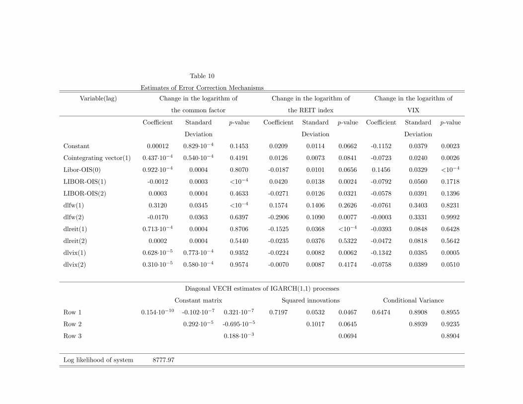
Table 10

Estimates of Error Correction Mechanisms

Variable(lag) Change in the logarithm of Change in the logarithm of Change in the logarithm of

the common factor the REIT index VIX

Coe¢ cient Standard p-value Coe¢ cient Standard p-value Coe¢ cient Standard p-value

Deviation Deviation Deviation

Constant 0.00012 0.829�10�4 0.1453 0.0209 0.0114 0.0662 -0.1152 0.0379 0.0023

Cointegrating vector(1) 0.437�10�4 0.540�10�4 0.4191 0.0126 0.0073 0.0841 -0.0723 0.0240 0.0026

Libor-OIS(0) 0.922�10�4 0.0004 0.8070 -0.0187 0.0101 0.0656 0.1456 0.0329 <10�4

LIBOR-OIS(1) -0.0012 0.0003 <10�4 0.0420 0.0138 0.0024 -0.0792 0.0560 0.1718

LIBOR-OIS(2) 0.0003 0.0004 0.4633 -0.0271 0.0126 0.0321 -0.0578 0.0391 0.1396

dlfw(1) 0.3120 0.0345 <10�4 0.1574 0.1406 0.2626 -0.0761 0.3403 0.8231

dlfw(2) -0.0170 0.0363 0.6397 -0.2906 0.1090 0.0077 -0.0003 0.3331 0.9992

dlreit(1) 0.713�10�4 0.0004 0.8706 -0.1525 0.0368 <10�4 -0.0393 0.0848 0.6428

dlreit(2) 0.0002 0.0004 0.5440 -0.0235 0.0376 0.5322 -0.0472 0.0818 0.5642

dlvix(1) 0.628�10�5 0.773�10�4 0.9352 -0.0224 0.0082 0.0062 -0.1342 0.0385 0.0005

dlvix(2) 0.310�10�5 0.580�10�4 0.9574 -0.0070 0.0087 0.4174 -0.0758 0.0389 0.0510

Diagonal VECH estimates of IGARCH(1,1) processes

Constant matrix Squared innovations Conditional Variance

Row 1 0.154�10�10 -0.102�10�7 0.321�10�7 0.7197 0.0532 0.0467 0.6474 0.8908 0.8955

Row 2 0.292�10�5 -0.695�10�5 0.1017 0.0645 0.8939 0.9235

Row 3 0.188�10�3 0.0694 0.8904

Log likelihood of system 8777.97

1

Table 10 description

This table shows estimates of the vector error correction mechanism with the current value and two lags of LIBOR minus OIS and two lags

of the other variables. It also shows estimates of the GARCH(1,1) parameters estimated for each of the three equations. The de�nitions of

variables are provided in the note to Table 8.

2

Figure 1 ABX Indices by Vintage

This figure shows the levels of the Markit ABX indices of Collateralized Debt Obligations based on subprime mortgages. The data are from Haver Analytics. The vintages are January 2006 (06‐1), July 2006 (06‐2), January 2007 (07‐1) and July 2007 (07‐2). No indices have been created subsequently. The premium is set on the indices to have an initial value of 100 based on a survey of market participants, unless that premium is over 500 basis points in which case the premium is 500 basis points. The initial trading values were less than 100 for lower rated tranches in the January 2007 vintage and for the July 2007 vintages.

-

20.0

40.0

60.0

80.0

100.0

1/2006 1/2008 1/2010

06-1 vintage

-

20.0

40.0

60.0

80.0

100.0

1/2006 1/2008 1/2010

06-2 Vintage

-

20.0

40.0

60.0

80.0

100.0

1/2006 1/2008 1/2010

07-1 VintageAAAAAABBBBBB-

-

20.0

40.0

60.0

80.0

100.0

1/2006 1/2008 1/2010

07-2 Vintage

These are the returns adjusted for IGARCH(1,1) based on the estimates in Table 4. The “06‐1” vintage is the January 2006; the “07‐1” vintage is the January vintage; the “07‐2” vintage is the July 2007 vintage. The seemingly near‐zero variances are periods of relatively low volatility.

‐20

‐10

0

10

1/2006 1/2008 1/20

AAA 06‐1

‐10

‐5

0

5

10

1/2006 1/2008 1/20

AA 06‐1

‐10

‐5

0

5

10

1/2006 1/2008 1/20

BBB‐ 06‐1

‐10

‐5

0

5

10

1/2006 1/2008 1/20

AAA 07‐1

‐10

‐5

0

5

10

1/2006 1/2008 1/20

AA 07‐1

‐10

‐5

0

5

10

1/2006 1/2008 1/20

BBB‐ 07‐1

‐10

‐5

0

5

10

1/2006 1/2008 1/20

AAA 07‐2

‐10

‐5

0

5

10

1/2006 1/2008 1/20

AA 07‐2

‐10

‐5

0

5

10

1/2006 1/2008 1/20

BBB‐ 07‐2

Figure 2Returns Adjusted for IGARCH

Figure 3 Variance Decomposition January 2006 Vintage

02468101214161820

Jan‐06 Jul‐06 Jan‐07 Jul‐07 Jan‐08 Jul‐08 Jan‐09 Jul‐09

standardized return

0

1

2

3

4

5


common

0

2

4

6

8

10

12

14

16


vintage

0

1

2

3

4

5

6


ratings

0

1

2

3

4


idiosyncratic

02468101214161820


standardized return

0

1

2

3

4

5


common

0

2

4

6

8

10

12

14

16


vintage

0

1

2

3

4

5

6


ratings

02468101214161820


standardized return

0

1

2

3

4

5


common

0

2

4

6

8

10

12

14

16


vintage

0

1

2

3

4

5

6

Jan‐06 Jul‐06 Jan‐07 Jul‐07 Jan‐08 Jul‐08

ratings

0

1

2

3

4

Jan‐06 Jul‐06 Jan‐07 Jul‐07 Jan‐08 Jul‐08

idiosyncratic

0

1

2

3

4


idiosyncratic

January 2007 Vintage

0

2

4

6

8

10


standardized return

0

1

2

3

4

5

6


common

0.0

0.5

1.0

1.5

2.0


vintage

0

1

2

3

4

5

6


ratings

0

1

2

3

4

5

6

7


idiosyncratic

0

2

4

6

8

10


standardized return

0

1

2

3

4

5

6


common

0.0

0.5

1.0

1.5

2.0


vintagex10‐20

0

1

2

3

4

5

6


ratings

0

2

4

6

8

10


standardized return

0

1

2

3

4

5

6


common

0.0

0.5

1.0

1.5

2.0


vintagex10‐20

0

1

2

3

4

5

6


ratings

0

1

2

3

4

5

6


idiosyncratic

0

1

2

3

4

5

6

7


idiosyncratic

July 2007 Vintage

0

2

4

6

8

10


standardized return

0

1

2

3

4

5


common

0.0

0.5

1.0

1.5

2.0


vintagex10‐18

0

2

4

6

8


ratings

0

1

2

3

4

5


idiosyncratic

0

2

4

6

8

10


standardized return

0

1

2

3

4

5


common

0.0

0.5

1.0

1.5

2.0


vintagex10‐18x10‐18

0

2

4

6

8


ratings

0

2

4

6

8

10


standardized return

0

1

2

3

4

5


common

0.0

0.5

1.0

1.5

2.0


vintagex10‐18

0

2

4

6

8


ratings

0

1

2

3

4

5


idiosyncratic

0

1

2

3

4

5


idiosyncratic

This figure shows the daily variance decomposition for each vintage and credit rating within each vintage. The first row of each panel shows squared standardized returns. The following rows in the panel show the contributions by the common factor, the corresponding vintage factor, the corresponding ratings factor and the idiosyncratic factor. The vertical scales of the graphs differ vertically but not horizontally. The vertical scales differ too much to use the same scale for all graphs. Comparisons across credit ratings within a vintage are simpler with the same scale for all three credit ratings.

Figure 4 The Integrated Common Factor

The left panel shows the integrated common factor for the January 2006 AAA vintage with the initial value normalized to 1. This value reflects the conditionally heteroskedastic behavior of the common factor derived from the conditional heteroskedasticity in the original returns. The right panel shows the actual value of the AAA tranche of the January 2006 vintage of the ABX index. Many common features appear in both figures.

0.00

0.20

0.40

0.60

0.80

1.00

1.20

1/2006 1/2007 1/2008 1/2009

Integrated Common FactorAAA Tranche of 2006‐1 Vintage

-

20.0

40.0

60.0

80.0

100.0

1/2006 1/2007 1/2008 1/2009

ABX Index ValueAAA Tranche of 2006‐1 vintage

Figure 5 Observable Variables

This figure shows the values of the variables other than the ABX index which are included in the analysis of the variables’ relationships. The figures suggest that the Dow‐Jones Equity All REIT index and VIX have slow moving components, possibly unit roots, while the spreads do not. By the end of 2009, the spreads return to values similar to those before the crisis, although the behavior is not identical.

4.0

4.5

5.0

5.5

6.0

1/2006 1/2007 1/2008 1/2009

Logarithm of Dow Jones Composite All REIT Index

2.0

2.5

3.0

3.5

4.0

4.5

5.0

1/2006 1/2007 1/2008 1/2009

Logarithm of VIX

-

100

200

300

400

1/2006 1/2007 1/2008 1/2009

Libor minus OIS rate1 month

0

100

200

300

400

500

1/2006 1/2007 1/2008 1/2009

Libor minus Treasury Bill Rate1 month

0

100

200

300

400

500

600

1/2006 1/2007 1/2008 1/2009

AA Asset‐backed Commercial Paper Rate less Treasury Bill Rate, 1 month

Figure 6 Actual and Simulated Values

Of the Common Factor, REIT Index and VIX

This figure shows the actual values of the integrated logarithm of the common factor, the logarithm of the Dow‐Jones Equity All REIT index and the logarithm of VIX. These actual values are shown on each graph with the simulated value from the estimated vector error correction mechanism in Table 10. The simulated values are from a dynamic simulation with LIBOR less OIS held to its mean value from January 19, 2006 to December 31, 2009.

0.0

0.2

0.4

0.6

0.8

1.0

1.2

1/2006 1/2007 1/2008 1/2009

ActualSimulated

4.0

4.5

5.0

5.5

6.0

1/2006 1/2007 1/2008 1/2009

ActualSimulated

2.0

2.5

3.0

3.5

4.0

4.5

5.0

1/2006 1/2007 1/2008 1/2009

ActualSimulated

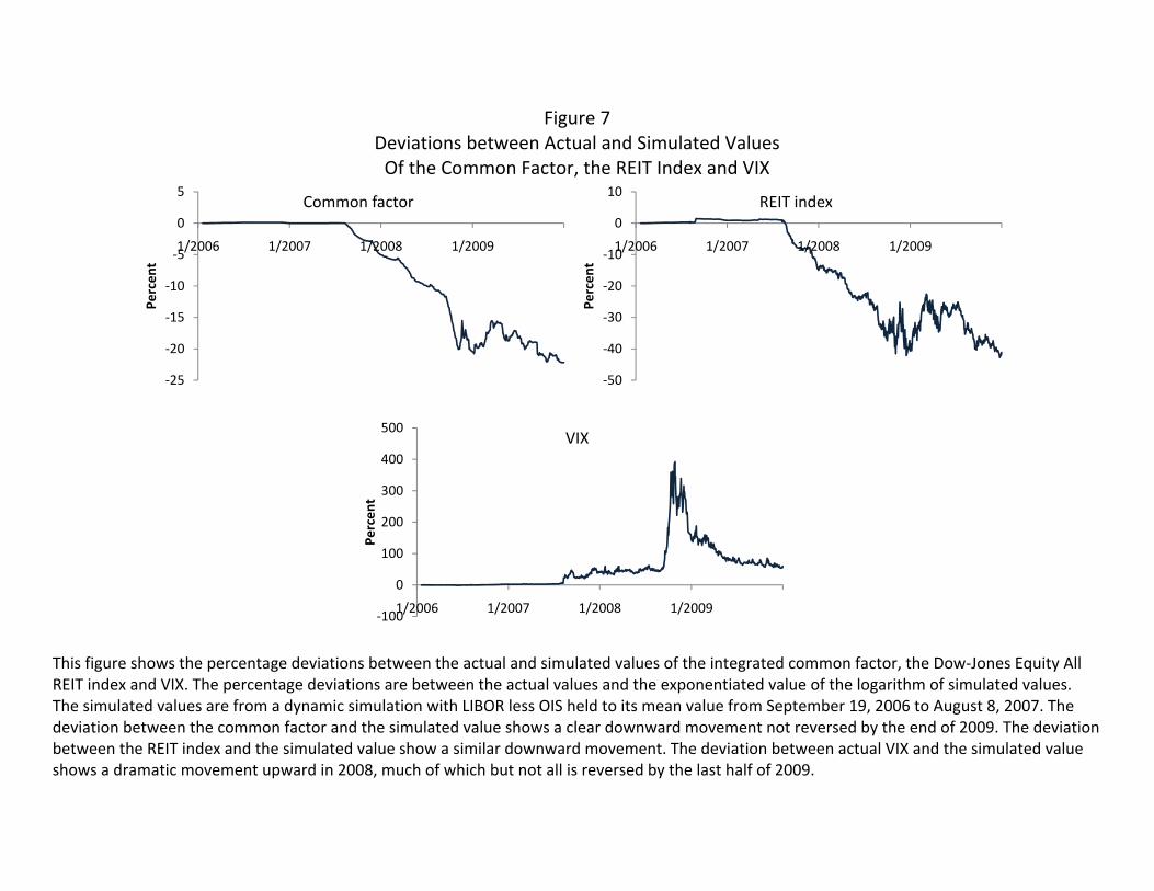
Figure 7 Deviations between Actual and Simulated Values Of the Common Factor, the REIT Index and VIX

This figure shows the percentage deviations between the actual and simulated values of the integrated common factor, the Dow‐Jones Equity All REIT index and VIX. The percentage deviations are between the actual values and the exponentiated value of the logarithm of simulated values. The simulated values are from a dynamic simulation with LIBOR less OIS held to its mean value from September 19, 2006 to August 8, 2007. The deviation between the common factor and the simulated value shows a clear downward movement not reversed by the end of 2009. The deviation between the REIT index and the simulated value show a similar downward movement. The deviation between actual VIX and the simulated value shows a dramatic movement upward in 2008, much of which but not all is reversed by the last half of 2009.

‐25

‐20

‐15

‐10

‐5

0

5

1/2006 1/2007 1/2008 1/2009

Percen

t

Common factor

‐50

‐40

‐30

‐20

‐10

0

10

1/2006 1/2007 1/2008 1/2009

Percen

t

REIT index

‐100

0

100

200

300

400

500

1/2006 1/2007 1/2008 1/2009

Percen

t

VIX

systematic and liquidity risk in subprime-mortgage backed

Documents