systematic component of monetary policy in open economy svar's: a new agnostic identification...

Barcelona Graduate School of Economics

Master Thesis

Systematic Component of MonetayPolicy in Open Economy SVAR’s:

A New Agnostic IdentificationProcedure

Authors:

Adrian Ifrim

Onundur Pall Ragnarsson

Supervisor:

Prof. Luca Gambetti

A thesis submitted in fulfilment of the requirements

for the degree of MSc. in Macroeconomic Policy and Financial Markets

in the

July 2015

http://www.university.com

BARCELONA GRADUATE SCHOOL OF ECONOMICS

Abstract

MSc. in Macroeconomic Policy and Financial Markets

Systematic Component of Monetay Policy in Open Economy SVAR’s:

A New Agnostic Identification Procedure

by Adrian Ifrim and Onundur Pall Ragnarsson

We propose a new identification method in open economy models by restricting both

the systematic component of monetary policy and the IRFs to a monetary policy shock,

at the same time remaining agnostic with respect to the effects of monetary policy

shocks on output and open economy variables. We estimate the model for the U.S/U.K

economies and find that a U.S monetary shock has a significant and permanent effect

on output. Quantitatively a 0.4% annual increase in the interest rates causes output to

contract by 1.2%. This contradicts the findings of Uhlig (2005) and Scholl and Uhlig

(2008). We compute the long-run multipliers implied by the monetary policy reaction

function and compare our identification with to the ones proposed by Uhlig (2005),

Scholl and Uhlig (2008) and Arias et al. (2015). We argue that neither of the above

schemes identify correctly the monetary policy shock since the latter overestimates the

effects of the shock and the former implies a counterfactual behavior of monetary policy.

We also find that the delayed overshooting puzzle is a robust feature of the data no

matter what identification is chosen.

University Web Site URL Here (include http://)

Contents

Abstract i

Contents ii

List of Figures iii

List of Tables iv

Introduction 1

1 Literature Review 3

2 Econometric Methodology 9

2.1 The Model . . . . . . . . . . . . . . . . . . . . . . . . . . . . . . . . . . . 9

2.2 Identification Strategy . . . . . . . . . . . . . . . . . . . . . . . . . . . . . 12

2.3 Estimation . . . . . . . . . . . . . . . . . . . . . . . . . . . . . . . . . . . 15

3 Results 17

Conclusions 25

A Median and Closest to Median IRFs 26

Bibliography 28

ii

List of Figures

3.1 IRFs from a monetary policy shock: Identification 1 . . . . . . . . . . . . 18

3.2 Monetary policy shock implied by Identification 1 . . . . . . . . . . . . . . 18

3.3 Distribution of long-run multipliers under Identification 1 . . . . . . . . . 19

3.4 FEVD for the close to median model:Identification 1 . . . . . . . . . . . . 20

3.5 IRF from a monetary policy shock: Identification 2 . . . . . . . . . . . . . 21

3.6 FEVD of the monetary policy shock: Identification 2 . . . . . . . . . . . . 22

3.7 Distribution of the long-run multipliers under Identification 2 . . . . . . . 23

3.8 IRF from a monetary policy shock: Identification 3 . . . . . . . . . . . . . 24

A.1 Median and Closest to Median IRFs under Identification 1 . . . . . . . . . 26



iii

List of Tables

3.1 Long-run multipliers for the closest to median IRF . . . . . . . . . . . . . 19

3.2 Empirical probabilities of the multipliers under Identification 1. . . . . . 20

3.3 Empirical probabilities of the multipliers under Identification 2. . . . . . . 22

iv

Introduction

This paper is meant to contribute on two fronts. First, it includes a new ap-

proach to the identification of monetary policy shocks in structural vector autoregres-

sions (SVARs). This part relies heavily on the method developed by Arias et al. (2014).

That method is an improvement upon the agnostic identification procedure originally

presented by Uhlig (2005). Second, the aim is to contribute to the particular strain

of empirical research initiated by the Dornbusch model. This literature focuses on the

effects of monetary policy on currency exchange rates and has yielded some puzzling

results. Most notably, the so-called delayed overshooting puzzle. The Dornbusch model

and the empirical puzzles are described in more detail in Chapter 1.

Scholl and Uhlig (2008) study the effects of monetary policy in an open economy

SVAR using the Uhlig (2005) methodology. They find substantial evidence of delayed

overshooting. Furthermore, their results suggest that this puzzle is not simply a man-

ifestation of wrongly identified monetary policy shocks. The motivation for our study

comes from the fact that Arias et al. (2014) present a new algorithm to draw from the

correct posterior uniform distribution on the set of orthogonal matrices conditional on

the zero restrictions. Uhlig (2005) originally applied his method to study the real effects

of U.S. monetary policy. He found that contractionary monetary policy shocks have no

clear effect on real GDP, thus providing empirical support for money neutrality. How-

ever, using the improved methodology, Arias et al. (2015) recover the real effects, simply

by drawing from the correct posterior distribution. This beckons the question: Do the

impulse responses of currency exchange rates to contractionary monetary policy shocks

still display a delayed overshooting of the long-run appreciated value if the improved

methodology of Arias et al. (2014) is applied? Or will the puzzle disappear?

We identify monetary policy shocks by imposing sign and zero restrictions on the

monetary policy reaction function and sign restrictions on the impulse response func-

tions. We do not restrict the responses of output and open-economy variables and thus

remain agnostic with respect to the effects on these variables. We find that monetary

policy shocks have a significant and permanent effect on the level of output and that

the exchange rate manifests a delayed overshooting under our baseline identification.

1

List of Tables 2

The remainder of this paper is organized as follows. In section 2 we review the

literature of empirical research following Dornbusch’s model. In section 3 the SVAR

model and the identification technique are laid out. Results are reported in section 4.

Section 5 concludes.

Chapter 1

Literature Review

In his seminal paper, Dornbusch (1976) sets out to explain a tendency of exchange

rates to overshoot on impact their long term depreciation, following expansionary shocks

to monetary policy. To this end, he develops a rational expectations model. The model

assumptions include a liquidity effect of monetary policy shocks, uncovered interest rate

parity (UIP) and long-run purchasing power parity (PPP). Assuming sticky prices but

flexible exchange rates and asset prices, initial overshooting of the exchange rate is

derived as an outcome. In the model, overshooting is shown to hinge on the behavior

of real output. If real output is fixed, the exchange rate initially overshoots its long-run

depreciation in response to an expansionary shock. On the other hand, if real output is

responsive to aggregate demand, the exchange rate may no longer overshoot, although

it still depreciates in the long-run.

Empirical studies in the early and mid 1990s failed to provide support for the

Dornbusch model. Instead, they indicated that the peak overshooting does not occur

contemporaneously to a contractionary monetary policy shock. Rather, there is gradual

appreciation, followed by gradual depreciation. The peak appreciation is delayed by one

to three years, before the exchange rate converges on its long term appreciated value.

This has become known as the ‘delayed overshooting puzzle’. This also implies a ‘forward

discount puzzle’. It is characterized by persistent increases in the forward discount

premium conditional on contractionary domestic monetary policy shocks. The premium

is the gain due to the policy shock, from borrowing foreign currency for k periods at the

time of the policy shock, exchanging it for US dollars, investing it at the US rate, and

exchanging it back to the foreign currency at horizon k. It therefore incorporates both

the compounded interest rate differential over the k periods following the policy shock,

and the (foreseen) movement in nominal exchange rates between horizons 0 and k. It

represents a failure of the UIP condition. It has been debated whether the two puzzles

are only twin appearances, or if they can arise independently of one another.

3

Chapter 1. Literature review 4

Eichenbaum and Evans (1993) use three different methods to identify U.S. mone-

tary policy shocks in a VAR. First, they identify monetary policy shocks as innovations

to the ratio of non-borrowed reserves to total reserves (NBRX). Second, they identify

such shocks as orthogonalized shocks to the federal funds rate. Lastly they identify the

shocks using the Romer and Romer (1989) framework. They find that expansionary

shocks to monetary policy lead to sharp, persistent depreciations in U.S. nominal and

real exchange rates, and can account for more than 20% of the exchange rate variance.

Furthermore they find the maximal depreciation to occur up to more than two years

after impact. Clarida and Galı (1994) attempt to explain real exchange rate fluctu-

ations in the post-Bretton Woods era, using nominal shocks to supply, demand and

money. They use a Cholesky decomposition identification in structural VARs for the

US-German, Japanese, British and Canadian bilateral cases. Following Blanchard and

Quah (1989), they also apply a long run zero restriction on the response of output to

aggregate demand shocks. For the US-Germany and US-Japan regressions the results fit

the Dornbusch model relatively well. There is an initial real depreciation of the dollar

(3.8% for Germany, 3.5% for Japan). The real exchange rate effects of a nominal shock

die out after 16 to 20 quarters for Germany, and 12 to 16 quarters for Japan. The nom-

inal exchange rate overshoots substantially. In the long run the dollar depreciates (by

1.7% against the DM, 1.2% against the yen), while initially the nominal exchange rate

depreciates (by more than 4% against the DM, by more than 3.5% against the yen).

However the results depart from the Dornbusch model in that the nominal exchange

rate keeps depreciating for some time following the shock (4 quarters for Germany, 2

quarters for Japan). For Britain and Canada the results are qualitatively similar.

The authors also perform forecast error variance decomposition, and find that nominal

shocks explain a substantial part of the variance in the USD to DM and USD to yen

real exchange rates. 41% and 35% respectively. They find less such evidence for the

real exchange rates against Canada and the UK. Grilli and Roubini (1996) focus on

‘liquidity models’ where money has real effects without an assumption of sticky prices

or wages. They present the results of a recursively identified 7-variable VAR where

they use the differential between short- and long-term interest rates instead of just the

short-term rate, for France, Germany, Japan, Canada, Italy and the U.K. In each case

the U.S. is used as the foreign country. In four of these countries (not the U.K. and

Italy), delayed overshooting appears. The maximal appreciation occurs several months

after the contractionary shock. The authors note the limitations to their analysis. The

recursive structure of the identification restrictions is unrealistic. It requires that the

exchange rate be put after the domestic interest rate in the VAR ordering. This implies

that monetary policy does not contemporaneously respond to shocks to the exchange

rate. Also their approach only solves the price puzzle partially.


Kim and Roubini (2000) develop an identified VAR approach for open economy

models and apply this approach to the same G-7 countries as Grilli and Roubini (1996).

The structural identification implies that the model is composed of several blocks. The

first two equations describe the money market equilibrium. The next two describe the

domestic goods market equilibrium (output and price determination equations). The

fifth and sixth equations represent the exogenous shocks coming from the world econ-

omy, the U.S. interest rate and the oil price shocks. The last equation describes the

exchange rate market. The impact effect of the monetary contraction on the exchange

rate is a significant appreciation, with the exception of France. In almost all cases, after

the initial impact appreciation, the exchange rate starts to depreciate quite quickly. Al-

though the depreciation does not start right after the impact, the authors do not observe

the same delay in the overshooting as previous research did.

Cushman and Zha (1997) argue that delayed overshooting arises, in empirical

studies of small open economies, as a result of an inappropriate identification of monetary

policy for such economies. The recursive Cholesky decomposition approach is plausible

for the US because its economy is large and relatively closed. It implies that policy does

not respond to contemporaneous changes in the exchange rate. The monetary authority

in a small open economy is, however, likely to respond quickly to the exchange rate

as well as to both home and foreign interest rates. The authors therefore propose to

explicitly model the features of small open economies in structural VARs. Using data

for Canada and the U.S. for the period 1974-1993 they model Canada as the small open

economy and use the U.S. as a proxy for the rest of the world. In the identification

the foreign policy maker is restricted from reacting to Canadian variables, by a block

exogeneity restriction. The foreign block is kept in its reduced form with normalization

in lower-triangular form. No other restrictions on the coefficients of lagged variables

are imposed. The specification assumes that the Bank of Canada can react to the ex-

change rate, interest rates in both countries, money stock M1 and commodity prices

in US contemporaneously, but not to output, CPI or trade flows contemporaneously.

With this identification no exchange or interest rate puzzle arises. The exchange rate

response resembles Dornbusch-type initial overshooting. UIP deviations are found to be

very small, significantly different from zero for only four months (not consecutive) over

the whole 4 year horizon. The authors view this as confirmation of the UIP condition.

Kim and Roubini (2000) are critical of the recursive identification method, when

there is reason to believe that monetary policy responds to exchange rate movements

contemporaneously. They find little evidence of a forward discount puzzle and delayed

overshooting.

Kim (2005) examines the international transmission of U.S. monetary policy.

The foreign world is represented by the non-US G7 economies. The author uses both

the recursive Cholesky decomposition approach and the non-recursive one suggested by


Blanchard and Watson (1986), Bernanke (1986) and Sims (1986). With models includ-

ing the trade balance, exports, imports, the nominal exchange rate and the terms of

trade. The nominal exchange rate is the effective rate against a basket of currencies of

17 industrial countries. When allowing for contemporaneous effects of monetary policy

shocks and identifying them as shocks to the Federal Funds Rate, he finds an impulse

response of the nominal exchange rate compatible with initial overshooting. Identifying

the shocks as innovations to NBRX however, he finds delayed overshooting, with the

maximal response occurring after close to two years.

Kalyvitis and Michaelides (2001) examine the effects of U.S. monetary policy on

the exchange rate using the Bernanke and Mihov (1998) indicator of monetary policy

(B-M indicator). It nests many VAR-based indicators and takes into account changes in

FOMC operating procedures and policy targets. They modify the original specifications

by Eichenbaum and Evans (1993) to include relative output and relative prices. Relative

output captures the relative business cycle position of the US and the foreign country,

and helps determine short-run exchange rate movements. Relative prices capture long-

run exchange rate adjustment based on PPP. They use data for all observations available

for the B-M indicator, 1975:1 to 1996:12 and run a five variable SVAR for the Germany,

Japan, Italy, France and UK bilateral cases. They find evidence of initial overshooting.

There is a significant appreciation of the USD for around 3 months for all currencies.

The appreciation is instantaneous and not delayed. The only country that shows a dif-

ferent impulse response is Britain. Even though delayed overshooting does not arise in

this setup, UIP is still found to be violated.

Faust and Rogers (2003) criticize the preceding literature for using implausible

identifying restrictions, such as restricting policy from responding contemporaneously

to the financial variables. Policy makers have access to real time data on them. The

authors ask whether delayed overshooting is special to recursive formulations with du-

bious restrictions, or if it also holds for other plausible formulations. They run a VAR

comparable to that of Eichenbaum and Evans (1993). The data ranges from 1974:1

to 1997:12. Six lags and a constant are included, and the system is estimated for the

US-UK and US-Germany bilateral cases. The shock to NBRX is interpreted as the

monetary policy shock. All implausible restrictions against contemporaneous effects are

then dropped, and the effects of monetary policy shocks checked across all identifications

consistent with the restrictions left standing. This follows a method developed by Faust

(1998). They find that delayed overshooting is sensitive to dubious assumptions. It is

possible to identify ’reasonable’ monetary policy shocks that have a nearly contempo-

raneous maximal exchange rate response to monetary policy. This is compatible with

initial overshooting. However they also find the possibility of overshooting delay of up

to three years.


Also, every possible identification of monetary policy shocks, when dubious restrictions

are dropped, is found to yield large UIP deviations, mostly between 30 and 90 basis

points. The authors are unable to reject the existence of large and variable UIP devi-

ations, but find no evidence for the existence of plausible money shocks that produce

small deviations. The forward discount puzzle is therefore found not to be simply a twin

appearance of delayed overshooting.

The authors also run a 14 variable VAR for the same time period, including more foreign

variables. The results from that regression are similar with regard to overshooting and

the forward discount puzzle. It however suggests that monetary policy accounts for a

smaller portion of exchange rate volatility than previously thought. In the 7 variable

model at horizon 48, about 10-50%. In the 14 variable model however, monetary policy

is estimated to account for merely 2-6% in the US-UK case, and 2-13% for the US-

Germany case. Upper bound estimates are around 30% for both cases.

Kim (2005) sees delayed overshooting not as a puzzle, but a plausible outcome for

small open economies. His explanation rests on the foreign exchange policy reaction to

monetary policy. In response to a contractionary monetary policy shock, the exchange

rate appreciates, but the foreign exchange policy mitigates the appreciation initially as

’leaning against the wind’ intervention, so that the impact appreciation becomes weak.

When the effect of the foreign exchange policy on the exchange rate is short-lived but

the effect of monetary policy is more prolonged, the exchange rate may further appre-

ciate as the effect of the foreign exchange policy disappears, and the maximum effect

is only found in delay. The author runs a structural VAR for Canada, with the U.S.

representing the foreign sector. Data ranges from 1975:1 to 2002:2. He includes for-

eign exchange reserves of the Bank of Canada, a Canadian money aggregate, short-term

interest rates, CPI and industrial production. Also the exchange rate (CAD price of

one USD) and the US Federal Funds Rate. The Bank of Canada is assumed not to

react contemporaneously to output and prices, and not to the federal funds rate at all.

The Federal funds rate is only seen as a concern for the Bank of Canada because of its

effect on the exchange rate, which the bank is allowed to react to contemporaneously.

In the monetary policy it reacts possibly to the monetary aggregate and exchange rate.

Contemporaneous interactions of the two policies are allowed for. The results show typ-

ical delayed overshooting, with maximal appreciation after 20 months. The effect stays

significant for almost 4 years. However, the author also estimates impulse responses to

such a shock to foreign exchange policy and finds that it leads to a sharp depreciation in

the exchange rate. That effect however is relatively short lived and dies out after about

10 months. Subtracting the impulse response of the exchange rate to foreign exchange

policy from the impulse response to monetary policy, yields an overall outcome roughly

consistent with initial overshooting of the Dornbusch type.

Scholl and Uhlig (2008) find delayed overshooting in a Bayesian VAR of the same


type as Eichenbaum and Evans (1993). They apply an agnostic identification method

following Uhlig (2005). Domestic contractionary monetary policy shocks are assumed to

lead to increases in neither domestic price level nor the ratio of non-borrowed reserves

to total reserves for 12 months. Also, they are assumed not to decrease domestic short

term interest rates for 12 months. The impulse response of exchange rates is not re-

stricted. Thus, in their own view, the authors remain agnostic about it. Sizeable and

robust evidence of a delayed overshooting puzzle is found for all bilateral exchange rates

(USD-GBP, USD-DM and USD-JPY) and to a lesser extent the same for the exchange

rate of USD to a basket of currencies of the G7 economies. The maximal appreciation of

both nominal and real exchange rates, in response to a contractionary shock, is realized

after 1 to 2 years. In this case a forward discount puzzle also appears.

To check whether the forward discount puzzle appears even when delayed over-

shooting is restricted away, the identification of monetary policy shocks is restricted

even further. The impulse response of the domestic vs. foreign (3 month) interest rate

differential is restricted to be positive following a contractionary shock. Also, exchange

rates are restricted to appreciate on impact and then depreciate monotonically to the

long-term value. A sizeable and persistent forward discount premium occurs. The evi-

dence is strongest in the USD-DM case, where the premium is significant over the whole

5 year horizon of the impulse response. In the other cases of USD-GBP, USD-JPY

and USD-G7 the forward premium is less pronounced but still significant at the 1 year

horizon. This means that the UIP condition is violated even when delayed overshooting

does not occur. The authors interpret this as an indication that the delayed overshooting

puzzle is not simply a manifestation of wrongly identified monetary policy shocks. Fore-

cast error variance decomposition indicates that US monetary policy shocks account for

roughly 10% of the movements of all the bilateral nominal exchange rates. For the G7

currency basket, the shocks are found to account for about 20% of the movements. This

is consistent with Kim and Roubini (2000) and Faust and Rogers (2003). It however

contrast Clarida and Galı (1994) and Eichenbaum and Evans (1993).

Chapter 2

Econometric Methodology

This section is organzed in three parts. First we present the methodology introduced by

Arias, Rubio-Ramırez, and Waggoner (2014) (ARRW henceforth). Secondly, we describe

the identification procedure of the monetary policy shock. The last section presents the

estimation strategy and the dataset.

2.1 The Model

Consider the following reduced form VAR(p):

yt = c+

p∑l=1

Blyt−l + ut for 1 ≤ t ≤ T (2.1)

where yt is a n × 1 vector of variables, Bl are n × n matrices of coeffecients to be

estimated, and ut is a n× 1 vector of residuals with covariance matrix Σ. The model in

2.1 can be rewritten in a more compact form as

yt = B+xt + ut for 1 ≤ t ≤ T (2.2)

where B+ = (B1 . . . Bp c) and x′t = (y

′t−1 . . . yt−p 1). The dimensions of B+ and xt are

n × (np + 1) and (np + 1) × 1. Letting P denote the lower Cholesky factor of Σ, by

premultiplying equation 2.2 by P−1 and taking the transpose we arrive at the structural

representation of the VAR model:

yt′A0 = x

′tA+ + ε

′t for 1 ≤ t ≤ T (2.3)

9

Chapter 2. Eonometric Methodology 10

where A0 = (P−1)′

, A+ = B′+(P−1)

′and ε

′t = u

′t(P−1)

′. Notice that E[εtε

′t] = I. The

matrices (A0, A+) are the structural parameters while B+ and Σ are the reduced-form

parameters. Defining Q as any orthonormal matrix of dimension n × n, the structural

parameters (A0, A+) and (A0Q,A+Q) are observationally equivalent in the sense that

they produce the same reduced form VAR representation.

Proof. yt′A0Q = x

′tA+Q+ ε

′t. The reduced form parameters are:

B = A+QQ′A−10 = B

′+A0A

−10 = B

′+ where we have used the fact that QQ

′= In.

Σr = E[(A−10 )′Qεtε

′tQ′A−10 ] = (A−10 )

′A−10 = PP

′= Σ QED

Since the identification strategy involves sign and zero restrictions on A0 and on the

impulse-response functions we next define the IRF and the methodology used for iden-

tification. Given the structural parameteres (A0, A+) the IRF of the i′th variable to the

j′th structural shock at horizon h is given be the element from row i, column j of the

matrix

Lh(A0, A+) = [F h]nn(A−10 )′

= [F h]nnP (2.4)

where

F =

B1 . . . Bp−1 Bp

In . . . 0 0...

. . ....

...

0 . . . In 0

and [ ]nn is an operator that selects the n×n upper left block. From 2.4 it can be easily

seen that Lh(A0Q,A+Q) = [F h]nnPQ = Lh(A0, A+)Q. Assuming we want to impose

restrictions on A0 and on IRF at several horizons, define the n(k + 2)× n matrix

f(A0, A+) =

A0

L0(A0, A+)...

Lk(A0, A+),

where k represents the horizon. Sign and zero resrictions can be implemented with the

matrices Sj , Zj for 1 ≤ j ≤ n which have the same number of columns as rows in

f(A0, A+). The j index represents the shock and each row of Sj , Zj will have exactly


one nonzero element. Since (A0, A+) and (A0Q,A+Q) are observationally equivalent,

the structural parameters will satisfy the zero and sign restrictions if

Zjf(A0, A+)Qej = 0

Sjf(A0, A+)Qej > 0,

where ej represents the j′th column in the identity matrix In.

For convenience we reproduce here the main results from the ARRW methodology. The

idea is to draw an orthonormal matrix Q which satisfies the zero restrictions and then

to check if the sign restrictions are also satisfied. Theorem 4 in ARRW reformulates

the Gram-Schmidt recursive algorithm such that the resulting orthonormal matrix Q

will satisfy the zero restrictions. The resulting structural parameters (A0Q,A+Q) will

then represent a draw from the correct posterior distribution conditional on the zero

restrictions, given a specific prior density. We now formalize the above argument. Define

Rj(A0, A+) =

[Zjf(A0, A+)

Q′j−1

]

where Qj−1 = [q1 . . . qj−1] and qj = Qej .

Theorem 2.1. For 1 ≤ j ≤ n, let Zj represent the zero restrictions ordered so that

zj ≤ n− j where zj is the number of restriction associated to shock j (zj = rank(Zj)).

Let (A0, A+) be any value of the structural parameteres. The orthonormal matrix Q is

obtained as follows:

1. Let j = 1.

2. Find a matrix Nj−1 whose columns form an orthonormal basis for the null space

of Rj(A0, A+).

3. draw xj from a standard normal distribution on Rn.

4. qj = Nj−1(N′j−1xj/ ‖ N

′j−1xj ‖).

5. If j = n stop; otherwise let j = j + 1 and move to step 2.

Algorithm for sign and zero restrictions

1. Draw (B′+,Σ) from the posterior distribution of the reduced form parameters.


2. Use Theorem 2.1 to draw an orthonormal matrix Q such that the structural pa-

rameters ((P−1)′Q,B

′+(P−1)

′Q) satisfy the zero restrictions. Theorem 5 in ARRW

states that if π is the prior density for the reduced-form parameters then the struc-

tural parameters ((P−1)′Q,B

′+(P−1)

′Q) are a draw from the posterior with respect

to the prior π(A0, A+) = π(B′+,Σ)2

−n(n+1)2 |det(Σ)|

2n+np+22 , conditional on the zero

restrictions.

3. If there are only sign restrictions replace step 2 with this algorithm. Let X be a

n × n random matrix with each element having a standard normal distribution.

Compute matrix Q from the QR decomposition: 1 X = QR.

4. Keep the draw if Sjf(P−1)′, B′+(P−1)

′)qj > 0, where qj represents the j′th column

of Q.

5. Return to Step 1 until the required number of draws from the posterior distribution

conditional on the sign and zero restrictions has been obtained.

2.2 Identification Strategy

The first choice to consider is the selection of variables. Following the literature on open-

economy SVAR we adopt the Eichenbaum and Evans (1993) specification. In particular

we use data for industrial production, yt; prices, pt, foreign industrial production, y∗t ;,

federal funds rate, it; foreign interbank rate, i∗t ; real exchange rate, rert; and the ratio of

non-borrowed reserves to total reserves, nbrxt. Christiano and Eichenbaum (1991) found

that the ratio of non-borrowed reserves to total reserves is closely related to monetary

policy choices, which represents an advantage of this specification. In this paper we use

an agnostic identifcation procedure, in the sense that we do not impose any restrictions

to the responses of open-economy variables and output. Most of the literature focuses on

identifying monetary policy shocks by restricting the responses of inflation, interest rates

and monetary aggregates to such shocks. Uhlig (2005), Scholl and Uhlig (2008) restrict

the responses of interest rates, prices and reserves to a monetary policy shock. Arias

et al. (2015) argue that this identification scheme implies a counterfactual systematic

component of monetary policy and suggests placing restrictions directly on the monetary

policy reaction function. We adopt both views and argue that identification of monetary

policy shocks implies restricting both the systematic component of monetary policy and

the responses of interest rates, reserves and prices. Identifying monetary policy shocks by

imposing only restrictions on the systematic component result in long-run multipliers of

prices and output which are hard to reconcile with monetary theory. Our identification

1the diagonal elements of matrix R have been normalized to be positive


is consistent with Taylor-type rules and implies that the federal funds rate responds

only to output and prices and the response is positive. In addition, we also restrict the

responses of prices, reserves and interest rates.

Identification 1.

1. The federal funds rate is the monetary policy instrument and it reacts contempo-

raneously only to output and prices. The response coefficients of output and prices

are non-negative.

2. For k periods the responses of prices and reserves are non-positive while the re-

sponse of interest rates is non-negative.

Our identification entails imposing sign and zero restrictions on the matrix of structural

parameters A0 and on the impulse response functions. Without loss of generality we

label the first equation in the SVAR model as the monetary policy equation. The first

equation of the SVAR model given by 2.3 is

yt′a0,1 = x

′tal,1 + ε1t for 1 ≤ t ≤ T (2.5)

where al,1 denotes the first column in the matrix Al and ε1t denotes the first element of

εt. Taking into account that we focus on the contemporaneous reaction of the monetary

policy instrument, we can abstract from the lags and write equation 2.5 as2

it = φyyt + φy∗y∗t + φppt + φnbrxnbrxt + φrerrert + φi∗i

∗t + a−10,71ε1t (2.6)

where φy = −a−10,71a0,11, φy∗ = −a−10,71a0,21, φp = −a−10,71a0,31, φnbrx = −a−10,71a0,41, φrer =

−a−10,71a0,51, φi∗ = −a−10,71a0,61 and al,ij represents the element on column j, row i from

matrix Al. Part 1 of our identification implies φy > 0 , φp > 0, φy∗ = 0, φnbrx = 0,

φrer = 0 and φi∗ = 0. The monetary policy reaction function becomes:

it = φyyt + φppt + a−10,71ε1t with φy > 0 and φy > 0. (2.7)

For the second part of the identification strategy we use an horizon of 12 periods, as in

Scholl and Uhlig (2008). Using the methodology described in the first section of this

chapter, the above restrictions can be implemented using the following matrices:

2the ordering of the variables is (yt, y∗t , pt, nbrxt, rert, i

∗t , it)


f(A0, A+) =

A0

L0(A0, A+)

L1(A0, A+)...

L10(A0, A+)

L11(A0, A+)

, Z1 =

0 1 0 0 0 0 . . . 0

0 0 0 1 0 0 . . . 0

0 0 0 0 1 0 . . . 0

0 0 0 0 0 1 . . . 0

, S1 =

S01

Snbrx1

Sp1

Si1

where

S01 =

−1 0 0 0 0 0 0

0 0 −1 0 0 0 0 O3,84

0 0 0 0 0 0 1

represents the block corresponding to sign restrictions on matrix A0 and Oi,j a block

containing 0 elements of dimension i× j. The rest of the (12×91) blocks, Snbrx1 , Sp

1 and

Si1 correspond to the sign restrictions associated to non-borrowed reserves, prices and

interest rates and each row of each block will contain exactly one nonzero element: -1

for pt and nbrxt and 1 for it. The dimension of Z1 is 4× 91.

Our identification strategy imposes restrictions only on the contemporaneous coefficients

of the monetary policy rule given by 2.7 while it abstracts from the lags of the other

variables included in our model. In practice, the coefficients of lagged prices and output

could be negative which is not consistent with a monetary policy reaction function guided

by the Taylor principle. We check the consistency of our identification by computing

the long-run multipliers of prices and output. Considering the lags of prices and output,

equation 2.7 becomes:

(1−a−10,71

p∑i=1

ai,71Li)it = (a−10,71(

p∑i=1

ai,11Li−a0,11))yt+(a−10,71(

p∑i=1

ai,31Li−a0,31))pt (2.8)

where p denotes the lag length and L is the lag operator. The long-run multipliers are

the partial derivatives of the steady state solution, yt = y∗, pt = p∗, it = i∗:

Φy =∂i∗

∂y∗=

(a−10,71(∑p

i=1 ai,11 − a0,11))1− a−10,71(

∑pi=1 ai,71)

(2.9)

Φp =∂i∗

∂p∗=

(a−10,71(∑p

i=1 ai,31 − a0,31))1− a−10,71(

∑pi=1 ai,71)

(2.10)


We compare our baseline identification with the ones proposed by Scholl and Uhlig

(2008) and Arias et al. (2015). Identification 2 implies only restricting the coefficients of

the monetary policy rule while Identification 3 ipmplies restricting the impulse responses

of the monetary policy shock.

Identification 2. The federal funds rate is the monetary policy instrument and it reacts

contemporaneously only to output and prices. The response coefficients of output and

prices are non-negative.

The matrices f(A0, A+), Z1 and S1 now take the following form:

f(A0, A+) =[A0

], Z1 =

0 1 0 0 0 0 0

0 0 0 1 0 0 0

0 0 0 0 1 0 0

0 0 0 0 0 1 0

, S1 =

−1 0 0 0 0 0 0

0 0 −1 0 0 0 0

0 0 0 0 0 0 1

.

Identification 3. For 12 periods, the responses of prices and reserves are non-positive

while the response of interest rates is non-negative.

Under this identification there are no zero restriction and we have to define only matrices

f(A0, A+) and S1:

f(A0, A+) =

L0(A0, A+)

L1(A0, A+)...

L10(A0, A+)

L11(A0, A+)

, S1 =

Snbrx1

Sp1

Si1

where each of the subblocks of the matrix S1 are of dimension (12× 84).

2.3 Estimation

We estimate equation 2.1 with 6 lags using Bayesian techniques using a Normal-Wishart

prior as in Uhlig (2005). Thus the prior is uninformative and the posterior will be cen-

tered around the OLS estimator. We use 1000 draws of the reduced-form parameters

(B+,Σ) from the Normal-Wishart posterior and of the orthonormal matrix Q. Our

dataset includes monthly variables for U.S and U.K and is obtained from the St. Louis

Fed Database. Our dataset spans from 1978M1 to 2007M11 and includes: U.S industrial

production (INDPRO), U.S consumer price index (CPIAUCSL),U.S non-borrowed re-

serves (BOGNOBOR), U.S total reserves (TRARR), federal funds rate (FEDFUNDS),


nominal exchange rate U.S/U.K (EXUSUK), U.K industrial production (GBRPROIND-

MISMEI), U.K consumer price index (GBRCPIALLMINMEI), U.K interbank interest

rate (IRSTCI01GBM156N). Except for interest rates, all the other variables are season-

ally adjusted and are in 100log. For ploting we use 68% confidence intervals and the

closest to median IRF. Following Fry and Pagan (2007), we use the closest to median

IRF instead of the median for 2 reasons. First, the median as a way of summarizing the

data could be misleading since it is a mixture of structural parameters from different

models. Secondly, this permits us to retrieve the shock that generated the closest to

median IRF since the latter is generated by a single model. Since we are interested in

only one shock, define Θt as a n × t matrix containing the IRF of the monetary pol-

icy shock up to horizon t. Let Θmed and Θstd represent the median impulse responses

and the standard deviation of the impulse responses across the 1000 draws. Define the

standardized impulses response function as:

Θt = (Θt −Θmed)�Θstd (2.11)

where � denotes the Hadamard matrix division (elementwise). The closest to median

IRF is defined as the one that minimizes vec(Θt)′vec(Θt) where vec is the vectorization

operator.

Chapter 3

Results

In this chapter we present the impulse response functions to a monetary policy shock

corresponding to our baseline identification. We also report the shock that generated the

closest to median IRFs and the forecast error decomposition. We compare our results

to two related identification schemes: Arias et al. (2015) and Scholl and Uhlig (2008).

The former uses only part 1 of our identification while the latter part 2 with different

specifications of the model. We argue that the identification of the monetary policy

shock is accomplished only by merging the two schemes which represents our baseline

model. To support our methodology, we then compute the distribution of the long-run

multipliers of prices and output implied by our identification strategy and the one of

Arias et al. (2015). Figure 3.1 presents the impulse response functions corresponding to

Identification 1. The liquidity puzzle and the price puzzle were avoided by construction.

The latter will be relaxed later. The shock corresponds to a 0.4% annualized increase

in the federal funds rate. The U.K interbank market seems to respond rather fast to

the U.S monetary policy shock, with the increase in interest rates becoming significant

3 months after the shock. The real exchange rate decreases on impact and continues

to appreciate for another 6 months after which it starts depreciating. The response

is significant for 25 months after the shock. There is clearly a delayed overshooting

in the exchange rate, in contrast with the theory developed by Dornbusch and in line

with the results reported by Scholl and Uhlig (2008). The response of U.S output is

not significant on impact and for the next year following the monetary policy shock

confirming the fact the effects of monetary policy shocks are transmitted with lags to

the real economy. The decrease builds up over time reaching its lowest point after two

and a half year after the shock. Monetary policy responds by lowering interest rates

in line with the systematic component implied by the model but the response is not

enough to counteract the decrease in output. Overall the effects of a monetary policy

tightening have a long-lived and significant effect on the level of output. Quantitatively,

17

Chapter 3. Results 18

a 0.4% annualized increase in the interest rates decreases output by 1.2%, 5 years after

the shock.

10 20 30 40 50 60

−0.15

−0.1

−0.05

0

0.05

U.S Output

10 20 30 40 50 60

−0.06

−0.04

−0.02

0

0.02

0.04

0.06

0.08

U.K Output

10 20 30 40 50 60

−0.12

−0.1

−0.08

−0.06

−0.04

−0.02

U.S CPI

10 20 30 40 50 60−0.25

−0.2

−0.15

−0.1

−0.05

0

Non−borrowed/Total reserves

10 20 30 40 50 60

−0.4

−0.3

−0.2

−0.1

0

Real Exchange rate U.K/U.S

10 20 30 40 50 60

−0.05

0

0.05

0.1

0.15

0.2

U.K interbank rate

10 20 30 40 50 60

0

0.1

0.2

0.3

0.4

0.5

Fed Funds

Note: the vertical bars denote the horizon up to which the sign restrictions were imposed

Figure 3.1: IRFs to a monetary policy shock: Identification 1

The monetary policy shocks implied by the closest to median IRF is plotted in figure 3.2.

It can be seen that the volatility of the shock decreasesed from 1984 onwards. It appears

that monetary policy stability has also contributed to the great moderation period.

Jul78 Mar80 Nov81 Jul83 Mar85 Nov86 Jul88 Mar90 Nov91 Jul93 Mar95 Nov96 Jul98 Mar00 Nov01 Jul03 Mar05 Nov06

−2

−1.5

−1

−0.5

0

0.5

1

Figure 3.2: Monetary policy shock implied by Identification 1


As argued in Chapter 2 the lagged coefficients of inflation and output could turn to

be negative in the Taylor type rule equation. This would not be consistent with the

Taylor rule principle and would represent a counterfactual behavior of monetary policy

for the U.S economy. We check the consistency of our identification with the Taylor rule

principle by computing the long-run price and output multipliers given by equations 2.9

and 2.10.

Φy Φp

Multiplier 2.27 6.46

Table 3.1: Long-run multipliers for the closest to median IRF

Table 3.1 presents these long-run multipliers associated to the closest to median IRF.

Notice that while both multipliers are larger than 0, the central bank responds three

times more aggresively to price fluctuations than to output fluctuations. Furthermore the

price multiplier is larger than 1 which is in line with the Taylor rule principle. Figure 3.3

displays the distributions of the long-run multipliers accros all the 1000 models (draws).

0 5 10 15 20 25 30 35

0.02

0.04

0.06

0.08

0.1

0.12

Inflation Long−Run Multipliers: Φp

0 1 2 3 4 5

0.05

0.1

0.15

0.2

0.25

0.3

0.35

0.4

0.45

0.5

0.55

Output Long−Run Multipliers: Φy

Figure 3.3: Distribution of long-run multipliers under Identification 1

Both distribution have their mass above 0, implying that the Taylor principle is satisfied

across almost all models, not just for the closest to median one. Table 3.2 presents the

empirical probabilities of the multipliers taking specific values.


i P (Φi > 0) P (Φi > 1) P (Φi > 5) P (Φi > 10) P (Φi > 20) P (Φi > 50)

Φp 1 0.9960 0.7650 0.2650 0.0390 0

Φy 1 0.5820 0 0 0 0

Table 3.2: Empirical probabilities of the multipliers under Identification 1.

The first row contains the probabilities of the inflation multipliers taking values larger

than 0, 1, 10, 20 and 50. The implied long-run multipliers of inflation are greater than

0 for all models and larger than 1 for 99.6% of the models. The probability of having a

large multiplier, bigger than 20 is only 4%. This is encouraging since our identification

yields promising results not only for the close to median model but across all models.

As regards the probabilities of the output multipliers, all the models imply values larger

than 0 and smaller than 5. Figure 3.4 presents the variance explained by the monetary

policy shock. As expected, the monetary policy shock explains a large portion of the

variation in the federal funds rate. Monetary policy appears to be effective in stabilizing

inflation with nearly 20-30% of the variability in this variable accounted for by this

shock, following the first months after the impact. The exchange rate volatility is also

partly explained by the monetary shock. However it seems that there are other factors

more important that determine the exchange rate dynamics. The explanatory power for

variations in output increases over time reaching 18% after 5 years.

10 20 30 40 50 600

5

10

15

20U.S Output

10 20 30 40 50 600

0.5

1

1.5

2U.K Output

10 20 30 40 50 600

5

10

15

20

25

30U.S CPI

10 20 30 40 50 600

2

4

6

8Non−borrowed/Total reserves

10 20 30 40 50 600

2

4

6

8

10

12

14Real Exchange rate U.K/U.S

10 20 30 40 50 600

2

4

6

8

10U.K interbank rate

10 20 30 40 50 600

10

20

30

40

50

60Fed Funds

Figure 3.4: FEVD for the closest to median model under Identification 1


We now turn to the two alternative identification shemes proposed by Uhlig (2005),

Scholl and Uhlig (2008) and Arias et al. (2015).

Monetary Policy Shocks under Identification 2

Figure 3.5 presents the impulse response implied by this identification (baseline identi-

fication in Arias et al. (2015)). The response of output and interest rates closely follows

the one reported in their paper. Nevertheless, it is hard to believe that this identifi-

cation captures only the effects of a monetary policy shock. First, under this scheme

an increase in the annualized interest rate of 0.2% causes output to fall by 1-1.2%. We

believe that this overestimates the true effect of a monetary policy shock on output

and that the decrease in output captures other factors than the monetary policy shock.

Secondly, the response of the federal funds rate is not significant at any horizon. It is

hard to justify a contractionary monetary policy shock that does not affect significantly

interest rates, on impact or over time.

10 20 30 40 50 60

−0.25

−0.2

−0.15

−0.1

−0.05

0

U.S Output

10 20 30 40 50 60

−0.04

−0.02

0

0.02

0.04

0.06

0.08

U.K Output

10 20 30 40 50 60−0.12

−0.1

−0.08

−0.06

−0.04

−0.02

0

U.S CPI

10 20 30 40 50 60

−0.2

−0.15

−0.1

−0.05

0

0.05

0.1


10 20 30 40 50 60−0.4

−0.3

−0.2

−0.1

0

0.1


10 20 30 40 50 60

−0.05

0

0.05

0.1

0.15U.K interbank rate

10 20 30 40 50 60

−0.2

−0.1

0

0.1

0.2

0.3

0.4

Fed Funds

Figure 3.5: IRF from a monetary policy shock: Identification 2

Figure 3.6 plots the explanatory power associated to the monetary policy shock under

Identification 2. The monetary policy shock explains 13% on impact and 2% after 1

year of the variation in interest rate. It is widely accepted that during the time period

covered in our sample, the Federal Reserve has used almost continously the federal funds


rate as a monetary policy instrument 1. Thus a shock that explains only 13% on impact

and 2% in the long-run from the variations in the federal funds rate cannot be correctly

labeled as a monetary policy shock.

10 20 30 40 50 600

5

10

15

20

25U.S Output

10 20 30 40 50 600

0.5

1

1.5

2U.K Output

10 20 30 40 50 600

10

20

30

40

50U.S CPI

10 20 30 40 50 600

0.5

1

1.5

2

2.5Non−borrowed/Total reserves

10 20 30 40 50 600

0.5

1

1.5

2Real Exchange rate U.K/U.S

10 20 30 40 50 600

0.5

1

1.5

2

2.5

3

3.5U.K interbank rate

10 20 30 40 50 600

2

4

6

8

10

12

14Fed Funds

Figure 3.6: FEVD of the monetary policy shock: Identification 2

In line with our previous analysis, we compute the empirical distributions of the long-

run multipliers implied by Identification 2. The results are plotted in figure 3.7. Both

distributions have their mass above 0. The values of the long-run multipliers implied

by the closest to median model are very similar to those under Identification 1: 6.2

for inflation and 2.1 for output. What is important to note is the support of these

distributions. Table 3.3 presents the probabilities that these multipliers take values

greater than some thresholds.

i P (Φi > 0) P (Φi > 1) P (Φi > 20) P (Φi > 50) P (Φi > 100) P (Φi > 150) P (Φi > 200)

Φp 0.995 0.943 0.226 0.101 0.059 0.038 0.029

Φy 0.994 0.860 0.073 0.033 0.014 0.009 0.006

Table 3.3: Empirical probabilities of the multipliers under Identification 2.

The distributions of the long-run multipliers have fatter tails than the ones under Iden-

tification 1. The probability of drawing a negative multiplier for inflation or output is

1See Bernake and Blinder (1992), Sims and Zha (2006)


around 0.5%. What is more suspect is that the probability of having a large multi-

plier is very high. Table 3.3 shows that the probability of having an inflation multiplier

larger than 50 or 100 is 10% and 6% respectively. It is not clear for us how a value

of 100 for the inflation multiplier can be interepreted or justified. We believe that this

identification captures something else besides the monetary policy shock and that the

systematic component of monetary policy is not entirely separated from other factors

affecting interest rates. Under Identification 1 both of the above probabilities are 0.

−16000−14000−12000−10000 −8000 −6000 −4000 −2000 0 2000 40000

1

2

3

4

5

6

7

8x 10

−4 Inflation Long−Run Multipliers: Φp

−4000 −3500 −3000 −2500 −2000 −1500 −1000 −500 0 500 10000

0.02

0.04

0.06

0.08

0.1

0.12

0.14

0.16

0.18

Output Long−Run Multipliers: Φy

Figure 3.7: Distribution of the long-run multipliers under Identification 2

.

Monetary Policy Shocks under Identification 3

The impulse response functions to a monetary policy shock under Identification 3 are

presented in figure 3.8. The shock corresponds to 0.25 percentage points increase in

the annualized interest rate. This identification corresponds to the one used in Scholl

and Uhlig (2008) but implemented using the new methodology proposed by Arias et al.

(2015) which draws the coefficients from the correct posterior distribution. There is one

notable difference in the results from the two methodologies. In Scholl and Uhlig (2008),

the response of output to a monetary policy shock is not significant at any horizon of the

impulse response functions. This result supports the view that a contractionary mone-

tary policy cannot significantly influence the real economy. Figure 3.8 tells a different


story. Using the same identification scheme but with the refined methodology, the effect

of a contractionary monetary policy shock on output is positive and significant over

the first 7 months following the shock. Under this identification scheme contractionary

monetary policy shocks do not operate with lags but instead have a contemporaneously

significant positive effect on the level of output. This result cannot capture the true

effects of a monetary policy tightening. It is hard if not impossible to justify that an

increase in the interest rates causes output to increase in the short-term. Moreover, this

identification is very similar to the one used by Uhlig (2005) but with sign restricions

imposed at different horizons. Arias et al. (2015) showed that the identification used by

the latter implies a counterfactual bahavior of the monetary policy for the United States

and thus does not correctly identify monetary policy shocks.

10 20 30 40 50 60

0

0.1

0.2

0.3

0.4

Fed Funds

10 20 30 40 50 60

−0.25

−0.2

−0.15

−0.1

−0.05

0

0.05

U.K Output

10 20 30 40 50 60

−0.1

−0.08

−0.06

−0.04

−0.02

U.S CPI

10 20 30 40 50 60

−0.35

−0.3

−0.25

−0.2

−0.15

−0.1

−0.05

0Non−borrowed/Total reserves

10 20 30 40 50 60

−0.7

−0.6

−0.5

−0.4

−0.3

−0.2

−0.1

0

0.1


10 20 30 40 50 60−0.3

−0.2

−0.1

0

0.1

U.K interbank rate

10 20 30 40 50 60

−0.1

−0.05

0

0.05

0.1

0.15

U.S Output

Figure 3.8: IRF from a monetary policy shock: Identification 3

Conclusions

We propose a new agnostic identification scheme for monetary policy shocks in open

economy SVARs restricting both the systematic component of monetary policy and the

impulse response functions. We also analyse two related identification methods proposed

by Arias et al. (2015) and Uhlig (2005), Scholl and Uhlig (2008). The former restricts

only the systematic component of the monetary policy reaction function. We find that

this identification yields very large values for the long-run multipliers of inflation and

output that are hard to interpret or reconcile with empirical evidence. Furthermore,

we argue that under this identification scheme monetary policy effects on output are

overestimated and that this procedure does not fully indentify monetary policy shocks.

The latter implies counterfactual behavior of the U.S monetary policy; the impulse re-

sponse functions under this identification showed that a contractionary monetary policy

shock has a positive and significant effect on output during the first 7 months following

the shock. We use the refined methodology proposed by Arias et al. (2014) and impose

zero and sign restrictions on the systematic component of the monetary policy and sign

restrictions on the responses of interest rate, inflation and reserves. Thus we remain

agnostic about the response of output and open-economy variables. We find that an

annual increase of 0.4-0.5 percentage points in the federal funds rate causes output to

contract by 1.2% in the long run. Under our identification monetary policy affects the

real economy with lags and the effect on output is significant and permanent in the long-

run. The delayed overshooting puzzle is present under all three identification methods

and it appears to be robust regardless the identification choosen. Under our baseline

identification the delay is around 5-6 months, in line with the findings of Scholl and

Uhlig (2008).

25

Appendix A

Median and Closest to Median

IRFs

10 20 30 40 50 60−0.14

−0.12

−0.1

−0.08

−0.06

−0.04

−0.02

0

U.S Output

MedCloseMed

10 20 30 40 50 60−0.05

0

0.05

U.K Output

MedCloseMed

10 20 30 40 50 60

−0.1

−0.09

−0.08

−0.07

−0.06

−0.05

−0.04

−0.03

U.S CPI

MedCloseMed

10 20 30 40 50 60

−0.18

−0.16

−0.14

−0.12

−0.1

−0.08

−0.06

−0.04

−0.02


MedCloseMed

10 20 30 40 50 60

−0.4

−0.35

−0.3

−0.25

−0.2

−0.15

−0.1

−0.05


MedCloseMed

10 20 30 40 50 60

0

0.05

0.1

U.K interbank rate

MedCloseMed

10 20 30 40 50 600

0.1

0.2

0.3

0.4

Fed Funds

MedCloseMed

Figure A.1: Median and Closest to Median IRFs under Identification 1

26

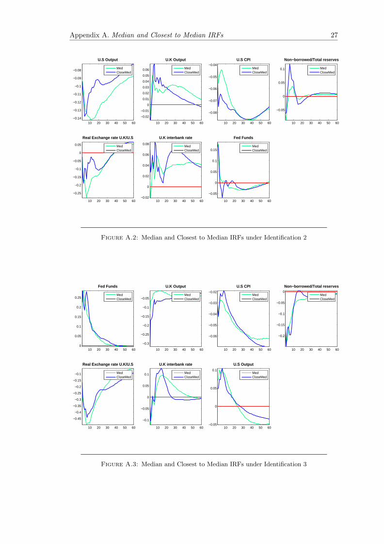
Appendix A. Median and Closest to Median IRFs 27

10 20 30 40 50 60−0.14

−0.13

−0.12

−0.11

−0.1

−0.09

−0.08

U.S Output

MedCloseMed

10 20 30 40 50 60

−0.02

−0.01

0

0.01

0.02

0.03

0.04

0.05

0.06

U.K Output

MedCloseMed

10 20 30 40 50 60

−0.08

−0.07

−0.06

−0.05

−0.04

U.S CPI

MedCloseMed

10 20 30 40 50 60

−0.05

0

0.05

0.1


MedCloseMed

10 20 30 40 50 60

−0.25

−0.2

−0.15

−0.1

−0.05

0

0.05


MedCloseMed

10 20 30 40 50 60−0.02

0

0.02

0.04

0.06

0.08

U.K interbank rate

MedCloseMed

10 20 30 40 50 60

−0.05

0

0.05

0.1

0.15

Fed Funds

MedCloseMed


10 20 30 40 50 600

0.05

0.1

0.15

0.2

0.25

Fed Funds

MedCloseMed

10 20 30 40 50 60

−0.3

−0.25

−0.2

−0.15

−0.1

−0.05

U.K Output

MedCloseMed

10 20 30 40 50 60

−0.06

−0.05

−0.04

−0.03

−0.02

U.S CPI

MedCloseMed

10 20 30 40 50 60

−0.2

−0.15

−0.1

−0.05

0


MedCloseMed

10 20 30 40 50 60

−0.45

−0.4

−0.35

−0.3

−0.25

−0.2

−0.15

−0.1


MedCloseMed

10 20 30 40 50 60

−0.1

−0.05

0

0.05

0.1

U.K interbank rate

MedCloseMed

10 20 30 40 50 60−0.05

0

0.05

0.1

U.S Output

MedCloseMed


Bibliography

H. Uhlig. What are the effects of monetary policy on output? results from an agnostic

identification procedure. Journal of Monetary Economics, 52:381–419, May 2005.

A. Scholl and H. Uhlig. New evidence on the puzzles: Results from agnostic identification

on monetary policy and exchange rates. Journal of International Economics, 76:1–13,

February 2008.

J.E. Arias, D. Caldara, and J.F. Rubio-Ramırez. The systematic component of mon-

etary policy in svars: An agnostic identification procedure. International Finance

Discussion Papers. Board of Governors of the Federal Reserve System, (1131), March

2015.

J. E. Arias, J. F. Rubio-Ramırez, and D. F. Waggoner. Inference based on svars identified

with sign and zero restrictions: Theory and applications. Board of Governors of the

Federal Reserve System International Finance Discussion Papers, (1110), April 2014.

R. Dornbusch. Expectations and exchange rate dynamics. Journal of Political Economy,

84(6):1161–1176, December 1976.

M. Eichenbaum and C. Evans. Some empirical evidence on the effects of monetary policy

shocks on exchange rates. NBER Working Paper Series, (4271), February 1993.

C. D. Romer and D. H. Romer. Does monetary policy matter? a new test in the spirit

of friedman and schwarz. NBER Macroeconomics Annual, 4:121–184, May 1989.

R. Clarida and J. Galı. Sources of real exchange rate fluctuations: How important

are nominal shocks? NBER Working Paper Series. National Bureau of Economic

Research, (4658), February 1994.

O. J. Blanchard and D. Quah. The dynamic effects of aggregate demand and supply

disturbances. The American Economic Review, 79(4):655–673, September 1989.

V. Grilli and N. Roubini. Liquidity models in open economies: Theory and empirical

evidence. European Economic Review, 40:847–859, 1996.

28

References 29

S. Kim and N. Roubini. Exchange rate anomalies in the industrial countries: A solution

with a structural var approach. Journal of Monetary Economics, 45:561–586, June

2000.

D. O. Cushman and T. Zha. Identifying monetary policy in a small open economy under

flexible exchange rates. Journal of Monetary Economics, 39:433–448, 1997.

S. Kim. Monetary policy, foreign exchange policy, and delayed overshooting. Journal of

Money, Credit and Banking, 37(4):775–782, August 2005.

O. J. Blanchard and M. Watson. Are All Business Cycles Alike? 1986.

B. S. Bernanke. Alternative explanations of the money-income correlation. NBER

Working Paper Series, (1842), February 1986.

C. A. Sims. Are forecasting models usable for policy analysis? Federal Reserve Bank of

Minneapolis Quarterly Review, 10(1):2–16, Winter 1986.

S. Kalyvitis and A. G. Michaelides. New evidence on the effects of us monetary policy

on exchange rates. Economic Letters, 71(2):255–263, April 2001.

B. S. Bernanke and I. Mihov. Measuring monetary policy. The Quarterly Journal of

Economics, 113(3):869–902, August 1998.

J. Faust and J. H. Rogers. Monetary policy’s role in exchange rate behavior. Journal of

Monetary Economics, 50:1403–1424, August 2003.

J. Faust. The robustness of identified var conclusions about money. Board of Governors

of the Federal Reserve System International Finance Discussion Papers, (610), April

1998.

L. J. Christiano and M. Eichenbaum. Identification and the liquidity effect of a monetary

policy shock. NBER Working Paper Series, (3920), November 1991.

R. Fry and A. Pagan. Some issues in using sign restrictions for identifying structural

vars. NCER Working Paper Series, (14):1–19, April 2007.

B. S. Bernake and A. S. Blinder. The federal funds rate and the channels of monetary

transmission. American Economic Review, (82), 1992.

C. A. Sims and T. Zha. Were there regime switches in u.s. monetary policy? American

Economic Review, (96), 2006.

systematic component of monetary policy in open economy svar's: a new agnostic identification...

Economy & Finance

identication strategy

macroeconomic policy

new identication method

median irfs

s monetary shock

median model

open economy svars

open economy models