OFFICE OFFINANCIAL RESEARCHU.S. DEPARTMENT OF THE TREASURY

Office of Financial Research Working Paper #0005 February 7, 2013

Systematic Scenario Selection

Mark D. Flood1

George G. Korenko2

1 Office of Financial Research, mark.flood@treasury.gov 2 Edgeworth Economics, gkorenko@edgewortheconomics.com

The Office of Financial Research (OFR) Working Paper Series allows staff and their co‐authors to disseminate preliminary research findings in a format intended to generate discussion and critical comments. Papers in the OFR Working Paper Series are works in progress and subject to revision. Views and opinions expressed are those of the authors and do not necessarily represent official OFR or Treasury positions or policy. Comments are welcome as are suggestions for improvements, and should be directed to the authors. OFR Working Papers may be quoted without additional permission.

www.treasury.gov/ofr

Systematic Scenario Selection Stress testing and the nature of uncertainty

Mark D. Flood† George G. Korenko‡

February 7, 2013

ALL COMMENTS ARE VERY WELCOME

† Senior Policy Advisor, Office of Financial Research (OFR): mark.flood@treasury.gov. ‡ Senior Vice President, Edgeworth Economics: gkorenko@edgewortheconomics.com. We gratefully acknowledge helpful comments from Dennis Bams, Bertrand Candelon, Greg Feldberg, Paul Glasserman, Alan Genz, Bryan Goudie, Art Hogan, Benjamin Kay, Alexander McNeil, Jonathan Sokobin, Peyton Young, and conference and seminar participants at the Federal Housing Finance Agency, a Nov. 2008 Washington DC GARP chapter meeting, the 2009 European Banking Symposium at the U. of Maastricht, the 2009 meeting of the Eastern Finance Association, a 2009 Loyola U. conference on Risk Management and Corporate Governance, the 2010 meeting of the Financial Management Association, the 2010 Winter Simulation Conference, and a 2012 research workshop at the Office of Financial Research. Any remaining errors pertain to the authors alone. Views and opinions expressed are those of the authors and do not necessarily represent official positions or policy of the Office of Financial Research, the U.S. Treasury, or Edgeworth Economics.

DCMI summary Title=" Systematic Scenario Selection: Stress testing and the nature of uncertainty" Creator="Mark D. Flood" Creator="George G. Korenko" Date="2013-02-01" Language=en

2

Systematic Scenario Selection Stress testing and the nature of uncertainty

Abstract We present a technique for selecting multidimensional shock scenarios for use in financial stress testing. The methodology systematically enforces internal consistency among the shock dimensions by sampling points of arbitrary severity from a plausible joint probability distribution. The approach involves a grid search of sparse, well distributed, stress-test scenarios, which we regard as a middle ground between traditional stress testing and reverse stress testing. Choosing scenarios in this way reduces the danger of “blind spots” in stress testing. We suggest extensions to address the issues of non-monotonic loss functions and univariate shocks. We provide tested and commented source code in Matlab®.

Keywords: risk management, stress testing, maximum portfolio loss, elliptical distribution, value at risk, Knightian uncertainty

Contents

1. Introduction a. Risk-modeling considerations

i. Scenario types ii. Risk factors

iii. Distributional assumptions iv. Loss definition

b. Elliptical distributions 2. The Algorithm

a. Mapping an arbitrary ellipsoid to the unit spheroid b. Assigning a scenario mesh over the unit spheroid

i. A binary hypercube mesh ii. Higher-order meshes

c. Inverting the mapping 3. Practical Extensions

a. Non-monotonic loss functions b. Univariate shocks

4. Conclusions 5. References 6. Appendix A: Source code

a. Hyperellipsoid class b. Supporting functions

7. Appendix B: Alternate algorithm for mapping an ellipse to the unit spheroid

3

1. Introduction

This paper presents an efficient and systematic methodology for selecting multiple well

distributed stress scenarios (or shocks) in the context of elliptically distributed multivariate risk

factors. The recent crisis is a chastening reminder of the potential for large, rare shocks in

financial markets. Because these events are typically difficult to observe in practice, they tend to

defy the traditional statistical tools of risk management, such as value at risk or extreme value

theory. In that context, stress testing is an increasingly important tool for understanding portfolio

risk exposures. It is standard practice within financial institutions (CGFS, 2005), and is also

codified in regulation and international standards, starting with the Basel market risk amendment

(BCBS, 1996), and exemplified more recently by the Federal Reserve’s 2009 Supervisory

Capital Assessment Program (SCAP) and ongoing Comprehensive Capital Analysis and Review

(CCAR).1 An important part of a stress testing implementation is the selection of the particular

scenarios to consider. Recent practice has focused on two objectives to guide scenario selection,

which stand to some degree in natural tension: that they should be severe but plausible.2

Because it can be applied without reference to precise event probabilities, stress testing is

1 For a general survey of stress testing, see Alfaro and Drehmann (2009), Borio, Drehmann, and Tsatsaronis (2012),

Čihák (2007), Drehmann (2009) or Quagliarello (2009). Regarding the use of stress testing in the Basel accord, see BCBS (2006, esp., ¶718). On the SCAP and CCAR, see FRB (2009) and FRB (2012). Other prominent regulatory stress testing programs include the International Monetary Fund’s (IMF) Financial Sector Assessment Programs (FSAP) (see Blaschke, Jones, Majnoni, and Martinez Peria, 2001; or IMF, 2011); and the European Banking Authority’s (EBA) EU-Wide Stress Tests (see EBA, 2011). 2 The notion of “severe yet plausible” scenarios is widely discussed (see, for example, Alfaro and Drehmann, 2009, Breuer, et al., 2009, or Sorge, 2004, p. 3), but never unambiguously defined. Roughly, “severity” indicates sufficiently impactful to reveal fragilities or vulnerabilities in the portfolio or system; “plausibility” indicates sufficiently realistic to justify managerial attention or remediation.

4

well suited to cases of Knightian uncertainty.3 At least two important forces can give rise to

Knightian uncertainty in the context of financial risk management. First, the statistical

distribution of crucial risk factors may simply be unknown. For example, the long-term default

and prepayment risk of various innovative mortgage securities in the early 2000s was largely a

matter of conjecture and extrapolation, because these products had never experienced the

contraction phase of a business cycle. Even if their statistical behavior is generally well

understood, behavior in the tails may be clouded by a dearth of extreme observations.4 In

addition, statistical regime shifts can invalidate historical data, often abruptly and without

warning. Rowe (2006) provides the example of the 1997 Asian currency crisis. The events of

September 2008, while painful in all other respects, have been instructive to stress testers in that

they illustrate the possibility and potential impact of an extreme scenario in the most

sophisticated and developed financial markets. Finally, the loss function itself may be unknown;

this may not be true for an individual portfolio manager, but regulators frequently face varying

degrees of opacity about institutions’ portfolios.

In traditional stress testing, the tester (for example, the regulator) chooses one or more

shocks, and calculations reveal the response – for example, mark-to-model losses – of the

institution or portfolio. Note that the scenarios are posited ex ante, typically without detailed

knowledge of the portfolio loss function. Careful choice of scenarios is important. Analyzing

each scenario is typically expensive, both computationally and organizationally, so that a

parsimonious scenario budget must be imposed. Moreover, an incautious choice of scenarios can

lead to disputes over plausibility or reliability. Both outlandishly as well as insignificantly

3 Knight (1921) dichotomizes situations of imperfect information into “risk,” where the probability law is known, and “uncertainty,” where it is not known. Knightian uncertainty is sometimes called “epistemic uncertainty.” 4 Glasserman, Kang and Kang (2012) propose a data envelopment technique to make efficient use of a limited number of tail observations.

5

stressful scenarios may be problematic, albeit in different ways. An alternative is reverse stress

testing, which asks some variant of the inverse question: what is the most likely event that could

create a response exceeding a given threshold, such as losses in excess of available capital.

Reverse stress testing obviates disputes over plausibility by choosing the scenario most likely to

provoke the relevant outcome.

There have been a number of recent theoretical papers on alternative approaches to stress

testing, including Breuer (2007, 2008), Glasserman, Kang and Kang (2012), Breuer, Jandačka,

Rheinberger and Summer (2009), Studer (1999), Pritsker (2011), and Breuer and Csiszár (2010).

Any stress testing implementation must address two broad issues in an environment of limited

information: (a) What is the nature of the forces or factors imposing stress on the system or

portfolio?; and (b) What is system’s response to those stresses?5 Both of these are challenging

problems that would benefit from careful analysis. However, there is as yet no unified theory of

stress testing: it is still a practical technique, and must be engineered to address the requirements

of each particular problem at hand.6 The methodology we outline below is tailored to several

practical objectives and constraints:

(1) For simplicity, we focus on tests for market risks. Much of what we describe should

generalize readily to credit and other risks, but we leave those topics for future

research.

(2) We assume that the risk factors can be reasonably well described by an elliptical

5 We refer to the system response problem as understanding the portfolio “loss function.” Borio, Drehmann, and Tsatsaronis (2012, p. 2) break this step down further into three components: (a) identifying the assets and liabilities that create the risk exposures; (b) defining the particular outcome, such as portfolio losses, ex-post capital, or institutional failure to be measured; and (c) understanding the mathematical model for mapping from shocks to measured outcomes. 6 “It is critical to design stress tests properly, tailoring them to the specific purpose,” Borio, Drehmann, and Tsatsaronis (2012, p. 1). Friedman, Huang and Huang (2010) underscore this point by demonstrating how knowledge of the “severity function” (we call this the “loss function” below) can be exploited via hill climbing to identify more efficiently the especially stressful scenarios within the plausible set. In our context, we presume that the loss function is not directly observable to the stress tester.

6

distribution. When this assumption is apt, the internal consistency of shocks across

the individual component risk factors can be achieved by restricting attention to the

likely comovements as defined by the elliptical distribution. This internal consistency

is an important precondition for plausibility. For example, in the spirit of Stock and

Watson (2002), we have been experimenting in other work with estimating a system

of market risk factors such as interest rates, credit spreads and volatility surfaces,

forecasting their joint distribution with the goal of finding internally consistent

simultaneous shocks to a wide range of market factors. After pre-filtering the series

with a vector autoregression, principal components analysis (PCA), and GARCH, the

joint distribution of the residual series is indeed approximately elliptically

distributed.7

(3) We consider a situation, confronted in many regulatory stress tests, in which the loss

function is not directly observable, in part because the portfolio composition cannot

be precisely observed without intensive effort. For example, an opaque portfolio may

conceal surprising contingent losses, such as embedded “short put” positions, that

might be discovered through a systematic search that reveals potential losses for a

wide range of market scenarios.

(4) Tailoring the stress scenarios to known features of particular portfolios may be

discouraged, because this would “unfairly” disadvantage individual firms in the

context of a “bottom-up” test applied to many firms simultaneously, such as the

SCAP or CCAR. 7 As another simple example, it is well known that a variation in a detailed interest-rate term structure can be well represented by three orthogonal principal components, corresponding roughly to the short rate, the long rate, and the curvature (see Alexander, 2008, chapter II). By construction, then, orthogonal shocks chosen in this space of latent factors correspond to shocks that are internally consistent in the space of interest rates. In other words, imposing this structure excludes the possibility of a broad class of implausible (internally inconsistent) shocks such as a large jump up in the 30-day rate simultaneous with a sharp drop in the 60-day rate.

7

(5) A corollary of the imperfect knowledge of portfolio composition is that the set of

relevant stressors – the appropriate dimensions of the state space from which to

choose scenarios – may also be unclear, encouraging the “casting of a wide net” for

many possible factors. The factor space may be large, providing another motivation

for PCA as a technique to reduce the number of factor dimensions to consider.

The methodology we propose involves a grid search of sparse, well distributed, stress-test

scenarios, which we regard as a middle ground between traditional stress testing and reverse

stress testing. Because the optimal trade-off between parsimony and accuracy depends

significantly on the practical details of a given implementation, such as the number and type of

institutions being examined or the nature of risks under consideration, we offer a methodology

that works well for small scenario sets while also scaling well to larger samples.8 By “well

distributed” we mean that the stress scenarios are approximately evenly distributed in the

outcome space. We believe it to be especially useful in the context of Knightian uncertainty

about the portfolio risk exposures, which can arise in a number of important practical contexts.

For example, in its recent SCAP program, the Federal Reserve tested multiple financial

institutions simultaneously. For comparability, all institutions faced identical scenarios in these

tests; for fairness, the scenarios were chosen before examining the individual banks’ portfolios.

This intentional information gap, justified by the desire to treat firms equitably, creates

significant, unavoidable Knightian uncertainty for policymakers, even in the absence of

adversarial behavior such as intentional concealment of significant loss exposures.9 Scenario

8 The heart of the trade-off is that computational cost and accuracy of response are typically both increasing in the number of scenarios. Thus, there is no guarantee that a sufficiently accurate scenario set will also be adequately parsimonious. Addressing this question requires detailed understanding of the implementation context, and is therefore beyond our scope here. 9 It is well known that investment managers can manipulate standard performance metrics by embedding “short puts” or other contingent negative exposures to boost the portfolio average; see Lo (2001), Foster and Young (2010), and Goetzmann, Ingersoll, Spiegel, and Welch (2007). On the other hand, Friedman, Huang and Huang (2010) point

8

selection typically occurs once in these exercises, so there is limited or no opportunity for an

iterative search of the scenario space in these exercises. Similar issues face others evaluating

financial portfolios at “arm’s length” or with otherwise restricted access to the intimate details of

portfolio composition and risk exposures: for example, external auditors, third-party risk model

validators, and due-diligence evaluators of investment advisors or fund of funds managers.

1.a. Risk-modeling considerations

The choice of shocks is one of the key elements in any stress test. An important criterion

in selecting stress scenarios is the “severe but plausible” standard advanced by the Bank for

International Settlements (BIS), among others (see note 2 above). Because plausibility is seldom

explicitly defined, it can become a contentious issue, especially if the stress tests could lead to

regulatory interventions or other binding constraints on behavior. Such ambiguity – along with

the resulting “plausibility wars” – is inherent to all forecasting.

Some of the most important stress scenarios, such as the 2008 market collapse, were

systemic events involving liquidity and deleveraging spirals, behavioral feedback effects, and

other structural breaks and non-linearities that are inherently difficult to predict and therefore

easy to dismiss as ex ante implausible. Indeed, Borio, Drehmann and Tsatsaronis (2012)

emphasize the “paradox of financial instability,” that the system appeared strongest precisely

when it was most vulnerable. In the counterfactual world of the typical stress test, a

macroeconomic shock occurs, and we observe the subsequent impact on financial portfolios;

awkwardly, the recent financial crisis preceded the macroeconomic reaction.

out correctly that stress testers with deeper knowledge of the portfolio composition can be more effective. This underscores the point made by Borio, Drehmann and Tsatsaronis (2012) that the appropriate stress testing methodology depends on the details of the specific implementation context; there is no universally optimal approach.

9

We work explicitly with probability contours from multivariate elliptical distributions.

While this does not eliminate the inherent subjectivity of the plausible, for all the reasons just

highlighted, it nonetheless provides a benchmark to guide discussions of plausibility. In this

regard, the 2008 market event provided a well documented historical example of the statistical

behavior of risk factors in a major financial crisis. We encourage the use of the shocks that

mimic the post-2008 volatility regime alongside shocks corresponding to more tranquil episodes.

If performed systematically, a multi-scenario sampling exercise can be useful in

discovering “short puts” and other contingent exposures that could result in fatal losses.10 Such

contingencies need not be the result of intentional concealment; for example, hedged portfolios

can leave non-monotonic basis risk, which can then be magnified via leverage. Nonetheless,

when embedded in a complex portfolio, contingent exposures will often lurk beyond the view of

regulators and investors. Moreover, unlike value-at-risk (VaR), stress testing can facilitate an

attribution analysis from an identified loss outcome to the details of the underlying stress

scenario. If multiple stress scenarios are tested – as we propose here – then a diverse sample of

such attributions can be assembled to provide a more complete picture of the loss exposures.

This has advantages over the typical approach to reverse stress testing, which only reports the

single worst scenario found. Contingent losses can also have a systemic aspect if they are

correlated across firms. Widely shared contingent exposures can lead to crowded trades – with

concomitant fire sales and negative feedback loops – if the shared contingency moves into the

money for all participants simultaneously and markets cannot accommodate a large, rapid order

flow. Applying systematic sampling of portfolio exposures to the cross-section of firms may

10 Agarwal and Naik (2004) document the prevalence of contingent exposures in hedge fund portfolios, for example. Lo (2001) provides an overview of a number of related issues. Goetzmann, Ingersoll, Spiegel and Welch (2007) demonstrate how embedded contingencies can distort standard performance measures, potentially misleading outsiders without direct knowledge of the portfolio.

10

help expose such shared contingencies. In sum, certain stress-testing implementations call for

the application of multiple multi-dimensional shocks to multiple firms (perhaps repeatedly over

time).

1.a.i. Scenario types

In practice financial risk managers typically stress-test their portfolios using either

historical replication scenarios or hypothetical risk-factor changes.11 Historical scenarios are

based on extreme events in the past, such as the 1987 stock market crash, and are prima facie

plausible. While this provides information on the sensitivity of the portfolio to market shocks, it

restricts attention to prior stress episodes. The same prima facie plausibility makes it likely that

portfolio managers will be defended against a recurrence. Hypothetical scenarios, in contrast, are

not constrained to replicate specific past incidents, and can therefore span a greater set of

possibilities. The Basel Committee has proposed that stress scenarios should be plausible, “most

adverse,” and that they should help to identify risk-mitigation possibilities.12 In particular,

reverse stress tests are usually hypothetical: BIS (2006, ¶718(Lxxxiii)) suggests that, “a bank

should also develop its own stress tests which it identifies as most adverse based on the

characteristics of its portfolio.” A drawback to hypothetical scenarios is that they depend on the

quality of the inputs and methods used to generate them, and are therefore potentially biased by

11 BIS (2009, p. 5) highlights the distinction between historical and hypothetical shocks. Breuer and Krenn (1999, §3 and §4) discuss the issues in additional detail. Regarding historical scenarios, see Crouhy, Galai, and Mark (2001), section 6.3 (pp. 232-241), on “Stress Testing and Scenario Analysis.” BIS (2006, ¶718(Lxxxii)) recommends testing against, “past periods of significant disturbance.” ECB (2006, p. 150) further distinguishes between historical, hypothetical, probabilistic, and reverse-engineered scenarios. Our methodology falls in the probabilistic category, meaning it is based on the probability distribution of the risk factors. See Jones, Hilbers, and Slack (2004) for a discussion of the traditional approach to hypothetical scenario construction. For additional regulatory analyses, see BIS (2005a), Haldane (2009), and the Senior Supervisors Group (2008). Our method is similar to the “stress envelope” approach, described by Crouhy, Galai, and Mark (2001, pp. 233-236), in that we propose shocking multiple exogenous risk factors simultaneously. It is not “systematic sampling” in the sense of Glasserman (2004, pp. 208-209). 12 Breuer, et al (2009, p. 205-206) interpret these criteria as “plausible,” “severe,” and “suggestive of risk-reducing action.” ECB (2006, p. 150) asserts that scenarios should be “plausible, extreme and of systemic relevance.”

11

the idiosyncratic views of the analysts making the selection.

To avoid these limitations, we select hypothetical scenarios systematically, via a grid

search. A systematic approach faces challenges of its own. For example, Breuer (2008)

demonstrates that defining “plausibility” in terms of a probability threshold induces an artifact of

“dimensional dependence,” whereby the addition of (even irrelevant) risk dimensions increases

the maximum loss. To avoid this, he suggests standardizing on the Mahalanobis radius (as in our

equation (6) below) instead of the raw threshold probability level.

1.a.ii. Risk factors

Scenario-based methodologies select from a universe of possible outcomes for a set of

exogenous risk factors. Following Studer (1999), Breuer (2007, 2008), Breuer, et al (2009), and

others, we select scenarios for risk factors that obey a multivariate elliptical distribution. Given

such a point set, analysts evaluate the properties of the portfolio (for example, position

valuations, credit losses, risk-factor sensitivities) as functions of each scenario. Our approach is

relevant, for example, for the significant practical case of a regulator, internal or external auditor,

clearinghouse, or model validator who must assess portfolio risk without direct and ongoing

access to full portfolio information. Given an outsider’s perspective, it is important to be

agnostic ex-ante about the risk exposures within the portfolio.

One advantage of a factor-based approach is that the stochastic characteristics of

exogenous risk factors are typically easier to analyze than the characteristics of the positions or

portfolios themselves, due to the non-linear nature of many financial instruments, including those

with contingent payoffs or embedded option clauses. Significantly, the loss function for many

instruments is not only non-linear, but non-monotonic, implying that extremes in the risk-factor

space need not correspond to extreme losses (see Section 3.a below). In many cases, the need for

formal risk analysis increases with the amount of non-linearity structured into a position, since

12

users are less likely to have well developed intuitions for the behavior of more complex

exposures. While position-level non-linearities may smooth out in the aggregation to a highly

diversified portfolio, this is not necessarily the case.

We start with an elliptical shell, which might be interpreted as the isoprobability

threshold for extreme events defined by simultaneous outcomes for the risk factors that occur at

a specified probability quantile, α. Breuer (2008) interprets it more generally, as the elliptical

shell of the relevant Mahalanobis radius. Although this question of interpretation may be

relevant for the ultimate application, it does not affect the mechanics of the algorithm presented

here. Given an elliptical shell, we map it to a unit spheroid, and project a collection of lattices

(or mesh) onto the surface of the spherical shell.

1.a.iii. Distributional assumptions

The literature on mesh generation is large (Bern and Plassmann, 2000). For example,

traditional (quasi-)Monte Carlo methods are based on point sets that sample the unit cube in d

dimensions, but plausible domains for variables of interest are much more usually elliptical or

spherical. Since the cube contains points that the enclosed sphere does not, this approach leads

to excessive rejection regions in the corners of the cube. This becomes more problematic as the

dimensionality d increases. Pistovčák and Breuer (2004, p. 385) state,

“So far, there is no algorithm known which generates low-discrepancy sequences in an n-dimensional ellipsoid. Though it is possible to generate points in a cuboid which encloses the ellipsoid, this is practical only if n is low.”

We propose to remedy this situation (noting that there is a substantial literature on techniques for

uniform packing of points on the sphere; see footnote 17 below). We present a lattice algorithm

for selecting well distributed points on the surface of an arbitrary d-dimensional ellipsoid. The

algorithm satisfies three practical requirements:

1) It guarantees that all the “corners” (i.e., the orthants defined by the axes of the

13

isoprobability ellipsoid) of the space will be reached by at least one scenario. This ensures that the method has reasonable coverage of the state space even for small samples.13

2) It spaces scenarios approximately evenly throughout the ellipsoid. (Precisely evenly distributed points can be computationally very costly to find.14)

3) It has computational complexity of order O(N), independent of d, where N is the number of scenarios. This ensures that the method scales efficiently to larger samples if needed.

Regarding requirement (1), Studer (1997, p. 71) notes that capturing scenarios in the corners is

useful in estimating the “mixed” cross-product terms in a quadratic expansion of the loss

function. Requirements (2) and (3) are interrelated, as the approximation allowed by

requirement (2) makes possible the attainment of linear complexity in (3). The methodology

exploits certain fundamental properties of multivariate elliptical distributions, and its immediate

applicability is limited to that family. We also present a natural extension to the algorithm to

generate a point set distributed throughout the interior of the d-dimensional ellipsoid.

The family of multivariate elliptical distributions includes some of those most commonly

used in financial and statistical analysis, including the multivariate normal (including normal

variance mixtures), Student’s t (with the multivariate Cauchy as a special case), and logistic.

The elliptical family also includes some more exotic examples, such as the symmetric

multivariate normal inverse Gaussian (NIG) and the symmetric multivariate generalized

hyperbolic distributions (Bingham and Kiesel, 2002). Moreover, multivariate elliptical

distributions play a canonical role in modern theoretical and empirical finance, including the

standard capital asset pricing model of jointly normal excess returns on equities, and multifactor

Gaussian affine-yield models of the term structure of interest rates (see Campbell, Lo, and

MacKinlay (1997), chapters 5 and 11). While elliptical distributions impose a significant

13 For ellipsoids defined by rotation, such as an ordinary sphere, some or all of the axes may be undefined. In such cases, the axes might be chosen arbitrarily or by other criteria. 14 For example, Bendito, Carmona, Encinas and Gesto (2008) find that iterative solutions for certain versions of the problem can be on the order of O(N15), where N is the number of points. See Sun and Chen (2008, p. 191) for a definition of uniformity of a point set on the sphere.

14

symmetry restriction – specifically, all univariate marginal distributions must be symmetric –

they can be significantly easier to use for practical risk modeling in situations where this

symmetry constraint is plausible. In many cases, the symmetry restriction has proven to be

reasonably consistent with the underlying data processes.

1.a.iv. Loss definition

The practice of stress testing has been formalized in a number of recent papers. The

maximum loss measure of Studer (1997, 1999) captures the notion of stress testing as a search for

those combinations of risk-factor outcomes that would generate unacceptably large (for example,

default- or failure-inducing) portfolio losses. The maximum loss metric is weakly coherent, and

generalizes readily to a concept of “dangerous regions” in the factor space that would produce

losses in excess of some critical threshold of acceptable portfolio risk. Heretofore, practical

implementations of the maximum loss measure have been limited by either restrictive

assumptions on the shape of the loss function, as in Studer (1997, §3.4.1), or computationally

costly iterative approximation algorithms such as Studer (1997), or Pistovčák and Breuer (2004).

We follow McNeil, Frey, and Embrechts (2005, §2.1) in defining a portfolio value, Vt, as

a function of time and a vector of exogenous risk factors, ut d: Vt ≡ f(t, ut), and losses, Lt, as

the negative of changes in value:

Lt+1(ut, wt+1) ≡ –[Vt+1 – Vt] = –[f(t+1, ut+1) – f(t, ut)] = f(t, ut) – f(t+1, ut+wt+1) , (1)

where the innovation in the risk factors, wt+1, is a random variable, conditional on the

information available at time t, denoted Ft. Given the loss function, define the conditional loss

distribution via its cumulative distribution function:

FLt+1|Ft(wt+1, L*) ≡ P[Lt+1(ut, wt+1) ≤ L* | Ft] , (2)

where ut Ft, and L* is an arbitrary loss threshold. Randomness enters the model only

15

through the innovation to the exogenous risk factors, wt+1, due to the conditioning on Ft.

In this context, stress scenarios can be seen as a form of quasi-Monte Carlo integration of

the loss function, Lt+1(u, w).15 From this perspective, we are interested in finding the large-loss

“hot spots” on Lt+1(u, w). Studer (1997, 1999) and Breuer (2007) pose this as the problem of

searching for the maximum loss portfolio within a so-called “trust region,” Wp d, of the

factor space:

Lmax|Wp(ut, wt+1) ≡ max wWpL (ut, w), (3)

In other words, the maximum loss, Lmax, is the largest loss for any scenario within the plausible

subset, Wp. This maximum loss measure is weakly coherent.16 Studer (1997, p. 76) extends

the analysis beyond an individual maximal loss scenario, to consider “dangerous regions”

exceeding a specified loss threshold. A desirable characteristic of quasi-Monte Carlo integration

is that, typically, in the limit as N→∞, the integral converges to the true function, Lt+1(u, w) as

long as the loss function is continuous.17 A second desirable characteristic of quasi-Monte Carlo

15 Scenario-based approaches, including the method described here, are less sophisticated than many Monte Carlo techniques, such as importance sampling, control variates, or conditional Monte Carlo, which exploit special features of the problem at hand to obtain greater efficiency in estimation. Many Monte Carlo techniques are intended to price securities, and therefore benefit from a high degree of precision. Similarly, adaptive sampling methodologies, which allow feedback from testing early scenarios to help guide stratification of later samples, also use special features of the problem domain and are more complex than our approach. See Boyle, Broadie, and Glasserman (1997), Glasserman (2004), and Lemieux (2009) for an overview of Monte Carlo techniques in finance. Thompson and Seber (1996) discuss adaptive sampling. In essence, adaptive sampling is a form of importance sampling, in which the “important” regions are not determined theoretically, for example, by likelihood ratios, but via information learned from analysis of a first-stage sample. In this context, our sampling approach might be useful as a first-stage grid search to seed a multi-stage adaptive sample. Because the typical goal in assessing portfolio risk is to identify the extrema of the loss function, as described below, second-stage and later adaptive samples might be determined by some form of hill-climbing algorithm. 16 See Studer (1997), pp. 23-24. Weak coherence is defined by Artzner, et al (1999). Studer’s approach is applied in a series of papers, including Breuer and Krenn (1999), Breuer (2007, 2008), and Breuer and Csiszár (2010). Studer’s loss function is defined relative to the expected outcome at a forecast horizon, T, rather than the base case, ut; thus: LT = –[f(T, ut+wT) – f(t, ut+E(wT))]. This has the convenient property of pre-centering the loss distribution, so that equation (10) below is superfluous. This pre-centering does not otherwise affect most of the analysis that follows below. Note that the two definitions converge if wt follows a random walk. 17 See Niederreiter (1992) for details. For the special case of a quadratic loss function, Studer (1997) is able to derive a number of useful results, including a search algorithm that applies a series of local quadratic approximations to

16

integration is that low-discrepancy point sets constrain the integration error in finite samples.

1.b. Elliptical distributions

Consider a general multivariate elliptical distribution for the risk factors,

W ~ Ed(μ, Σ), (4)

where W d, and where μ d is the location (i.e., mean) vector, and Σ dd is the

dispersion matrix.18 Given a particular elliptical distribution, Ed(μ, Σ), the plausible subset, Wp

described above might naturally be specified as the region in d bounded by an isoquant of the

distribution at some appropriate confidence level, such as the 99th percentile ellipsoidal shell.

For example, the multivariate Student’s t distribution, W ~ td(ν, μ, Σ), is elliptical with

covariance matrix cov(W) = (ν/(ν–2))Σ, defined only if ν > 2. A d-dimensional elliptical

distribution is related to an underlying k-dimensional spherical distribution, S ~ Sk, via an affine

transformation, W μ + AS, where the symbol “” indicates equality in distribution. In general,

the matrix A dk is related to the dispersion matrix as: AAT = Σ. For simplicity, we restrict

attention to the common special case in which Σ is positive definite, d = k, and A is the dd

lower-triangular Cholesky factorization of the dispersion matrix, also written as A = Σ½.

Alternatively, W μ + RAS0, where S0 is uniformly distributed on the k-dimensional unit

spheroid, R is a radial random variable (the “generating variate”) independent of S0, and A = Σ½.

The quadratic form:

Q(W, μ, Σ–1) ≡ (W–μ)TΣ–1(W–μ), (5) find the unique maximum loss for a more general (i.e., non-quadratic) loss function. In the present paper, we do not focus directly on the shape of the loss function. 18 The presentation of elliptical distributions here parallels McNeil, Frey, and Embrechts (2005), §3.3.2, pp. 93ff, who elaborate the issues in much greater detail. The implication of equation (4) is that the distribution, Ed(μ, Σ) defines a set of concentric elliptical shells of the form given by equation (6); the probability density is the same at any point on such an elliptical shell. See also Fang, Kotz, and Ng (1990). The multivariate t distribution is particularly useful in risk-management applications. In addition to generalizing the multivariate normal distribution as a special case ( ), the t distribution also exhibits fat tails and tail dependence, both of which frequently occur in empirical data sets describing financial markets.

17

defines the isoprobability contours of an elliptical distribution.19 In other words, a set of points,

ε(μ, Σ–1, c) ≡ w d : Q(w, μ, Σ–1) = c (6)

for some constant c (the Mahalanobis radius), defines an ellipsoid, ε(μ, Σ–1, c) d, of equal

probability density. One of these ellipsoids, ε(μ, Σ–1, cα), will correspond to the extreme-event

probability threshold of interest, α. For example, in a VaR application, a threshold of α = 0.99

(indicating that a probability mass of (1 – α) = 0.01 lies outside the ellipsoid) might be

appropriate. It is useful to note that μ, Σ–1, and cα determine the location (i.e., center), shape, and

size, respectively, of the ellipsoid. The eigenvectors of Σ–1 fall along the principal axes of the e

ellipsoid (assuming the axes have been identified), while the lengths of the principal axes are

proportional to the inverse square root of the eigenvalues of Σ–1. The variable cα is the constant

of proportionality that establishes the absolute length of the principal axes. (See the class:

hyperellipsoid in Appendix A.)

The relationship between the probability threshold, α, and the size, cα, of the

corresponding ellipsoidal contour depends on the specific elliptical distribution under

consideration, via the formula:

(W–μ)TΣ–1(W–μ) R2 ↔ α = P[(W–μ)TΣ–1(W–μ) ≤ cα] = P[R2 ≤ cα] (7)

where P[•] indicates probability, and R is the generating variate described above.20 Recall the

19 This quadratic form is the square of the Mahalanobis distance, DM(W), from W to the center, μ, with respect to Σ:

DM(W) = [(W–μ)TΣ–1(W–μ)]½ .

See, for example, Frahm (2004) or Liu and Rubin (1995). The Mahalanobis distance is a generalization of ordinary Euclidean distance (the special case, Σ = Id) that essentially normalizes by the size of the ellipsoid in the direction of W. This normalization adjusts for covariance, and also renders the Mahalanobis distance scale-invariant. It is convenient below to parameterize the ellipsoid via the inverse of the dispersion matrix, Σ–1, rather than Σ directly. This is a cosmetic detail that simplifies the software implementation without constraining the results. 20 See McNeil, Frey, and Embrechts (2005, §3.3.3), Fang, Kotz, and Ng (1990, §2.5), and Frahm (2004, §1.1, especially his Example 1 (pp. 4-5) and Example 4 (pp. 6-7)) for further discussion. Frahm (2004), Bingham, Kiesel and Schmidt (2003), Tyler (1987), and Liu and Rubin (1995) offer some strategies for estimating the parameters, μ and Σ, of an elliptical distribution. Huffer and Park (2007) suggest a general test for elliptical symmetry.

18

artifact of “dimensional dependence” described by Breuer (2008), and his recommendation to

standardize a stress-testing regime on plausible Mahalanobis radii rather than specific probability

thresholds. While this avoids dimensional dependence if the number of factors is varied, now we

must choose a value for cα rather than α. To find the size parameter, cα, when W has a

multivariate normal distribution, we start with the fact that R2 ~ χd2 , so that:

α = P[R2 ≤ cα] = χd2 (cα) → cα = [χd

2 ]

–1(α) , (8)

where χd2 (•) is the chi-square cumulative distribution function (c.d.f.), and [χd

2 ]

–1(•) is the chi-

square inverse c.d.f. Similarly, if W has a d-dimensional t distribution, then R2/d ~ Fd,υ, the F

distribution with d and υ (numerator and denominator, respectively) degrees of freedom,

implying P[(1/d)R2 ≤ κα] = Fd,υ (κα) for an arbitrary measurement threshold κα [0, ). Now

choose κα ≡ (1/d)cα, so that

Fd,υ (κα) = P[(1/d)R2 ≤ κα] = P[R2 ≤ cα] = α = Fd,υ (cα/d) → cα = d [Fd,υ]–1

(α) , (9)

where [Fd,υ]–1

(•) is the inverse of the c.d.f. for the Fd,υ distribution. (See the functions:

sizeparam_normal_distn and sizeparam_t_distn in Appendix A.)

2. The Algorithm

The core of our methodology takes as given an estimated ellipsoid, ε(μ, Σ–1, cα), and

seeks a sample of points on its surface. These points will be our sample of stress events (or

shock scenarios), chosen to form a regularly spaced grid or mesh on the ellipsoid. The

identification of scenario points proceeds in seven discrete steps, numbered as follows:

3. Translation (mean adjustment) 2. Rotation of the eigenvectors to the coordinate axes 1. Stretching to a unit spheroid 0. Assigning a uniform shock scenario mesh

19

–1. Invert step 1: Stretching back to an ellipsoid –2. Invert step 2: Rotation –3. Invert step 3: Translation

This numbering scheme emphasizes that each negatively numbered step simply reverses the

effect of the corresponding positively numbered step.

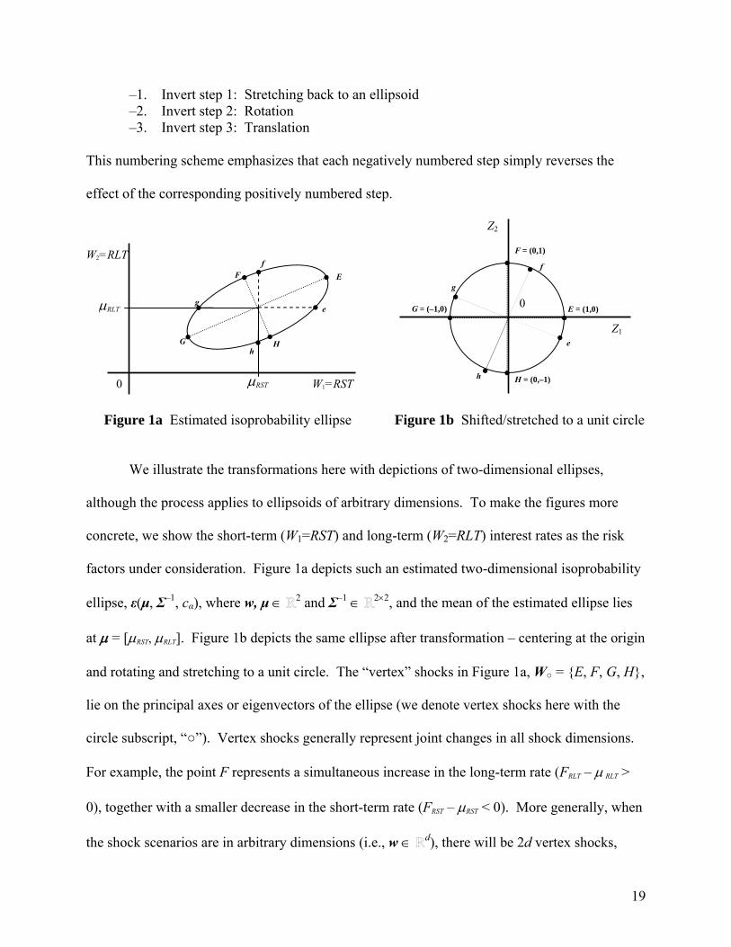
Figure 1a Estimated isoprobability ellipse Figure 1b Shifted/stretched to a unit circle

We illustrate the transformations here with depictions of two-dimensional ellipses,

although the process applies to ellipsoids of arbitrary dimensions. To make the figures more

concrete, we show the short-term (W1=RST) and long-term (W2=RLT) interest rates as the risk

factors under consideration. Figure 1a depicts such an estimated two-dimensional isoprobability

ellipse, ε(μ, Σ–1, cα), where w, μ 2 and Σ–1 22, and the mean of the estimated ellipse lies

at = [RST, RLT]. Figure 1b depicts the same ellipse after transformation – centering at the origin

and rotating and stretching to a unit circle. The “vertex” shocks in Figure 1a, W = E, F, G, H,

lie on the principal axes or eigenvectors of the ellipse (we denote vertex shocks here with the

circle subscript, “”). Vertex shocks generally represent joint changes in all shock dimensions.

For example, the point F represents a simultaneous increase in the long-term rate (FRLT – RLT >

0), together with a smaller decrease in the short-term rate (FRST – RST < 0). More generally, when

the shock scenarios are in arbitrary dimensions (i.e., w d), there will be 2d vertex shocks,

RST

H

F E

G

e

f

g

h

RLT

0 W1=RST

W2=RLT

H = (0,–1)

F = (0,1)

E = (1,0) G = (–1,0)

e

f

g

h

0

Z1

Z2

20

namely “up” and “down” along each axis or eigenvector.

2.a. Mapping an arbitrary ellipsoid to the unit spheroid

The first step (i.e., Step 3) in our algorithm translates (i.e., shifts or mean-adjusts) the

ellipsoid to be centered at the origin, via an affine transformation, Tw:x: w d → x d.

Specifically, we translate x = w – . In general, assuming a column vector, d, a matrix W

dn, and a column of ones, 1n n:

X = W – [1nT] (10)

shifts all of the points in W simultaneously. The shape and orientation of the ellipse do not

change during translation, so there is no adjustment to the inverse dispersion matrix, Σ–1. (See

the functions: translate and center_at_origin in Appendix A.)

The next two steps (Step 2 and Step 1): (a) rotate the ellipsoid so that the principal axes

fall along the coordinate axes, and (b) stretch it to a unit spheroid, ε(0d, Id, 1).21 We combine

these steps into a single transformation, Tx:z: x d → z d. The original (i.e., translated)

ellipsoid is the set of points:

ε(0d, Σ–1, cα) = x d : xTΣ–1x = cα. (11)

Substitute the eigenvalue decomposition,

Σ–1 = ΓΛΓ T, (12)

for the inverse dispersion matrix in this definition, where Γ is a matrix of orthogonal unit

eigenvectors, as columns:

Γ = [γ1, …, γd] , (13)

21 We begin with a “short form” of the derivation. A longer explication that better matches the software implementation appears in Appendix B. This first formulation of the transformation was suggested by Alexander McNeil in private correspondence.

21

and Λ is a diagonal matrix of the corresponding eigenvalues, Λ = diag(λ1, …, λd). Because the

dispersion matrix, Σ, is assumed to be positive definite, its inverse is also positive definite, and

therefore Σ–1 has positive eigenvalues.22 Thus, we may split the eigenvalue matrix into the

product of square roots, to rewrite equation (11) as:

ε(0d, Σ–1, cα) = x d : xTΓΛ½Λ½Γ Tx = cα = x d : xTΓΛ½cα

–1Λ½Γ Tx = 1. (14)

Now write z = (cα–½Λ½Γ T) x, and observe that this defines an invertible linear transformation:

z = (cα–½Λ½Γ T) x = Tx:z x (15)

Substituting, the original ellipsoid can then be written:

ε(0d, Σ–1, cα) = x = Tx:z

–1z : z d, zTz = 1. (16)

From this, we conclude that Tx:z–1 maps the unit spheroid, ε(0d, Id, 1) = z d : zTz = 1, into

the ellipsoid, and that Tx:z maps the original ellipsoid to the unit spheroid.

2.b. Assigning a scenario mesh over the unit spheroid

Given the unit spheroid in d, we now turn our attention to the central problem of

distributing systematically on its surface a regularly spaced mesh of N points (denoted by the

hash subscript, “#”). This can be seen as a special case of the N-points best-packing problem,

which has a long history in mathematics.23

22 Because the unit eigenvectors in this case are orthogonal, we may apply the equality, Γ–1 = ΓT, which is a property of any orthogonal matrix. Thus, we may calculate the diagonalization instead as ΓΛΓ–1, if that is more convenient. In any case, the calculations necessary for the eigenvalue decomposition are implemented as part of most matrix algebra packages, for example, the Matlab® eig() or Scilab spec() function. 23 See, for example, Hardin and Saff (2004), Dragnev (2002), and Saff and Kuijlaars (1997) for an introduction to the best-packing literature. The best-packing problem has applications in virology, organic chemistry (“buckyball” large carbon molecules), electrostatics, signal processing, fluid dynamics, and, of course, the design of soccer balls. A general solution involves a highly non-linear optimization with non-linear constraints, and is notoriously difficult (see Smale (1998), Problem #7). Most approaches involve so-called “elliptic Fekete points,” which minimize the aggregate log potential among the points. For example, Thomson’s problem minimizes the aggregate Coulomb potential according to an inverse-square law (for example, mutually repelling electrons on a metal sphere). More generally, one can minimize the aggregate Riesz s-potential with exponent s > 0. The special case when s = is known as Tammes’s problem or the “hard-spheres problem.” In practice, approximate solutions are typically determined by computationally complex iterative algorithms; in a pair of papers, Bendito, Carmona, Encinas, Gesto

22

2.b.i. A binary hypercube mesh

We propose a simple binary mesh algorithm that has linear computational complexity,

O(N), and generates scenario points, Z# = z#1, …, z#N, that span all d dimensions, stand in clear

relation to the vertices of the underlying ellipsoid, and are exactly evenly spaced (in the sense

that the distance between any point and its closest neighbor is the same for all points).24 The

binary mesh has some desirable properties. First, the algorithm is minimal in the sense that it

generates a single scenario for each of the 2d orthants of the d-dimensional state space, and so

achieves the minimum number of scenarios required to reach every “corner” of the space – i.e.,

into every orthant defined by the principal axes of the ellipsoid. Note that the mesh size is

exponential in the number of state dimensions. Second, each of the 2d corner points in the binary

mesh involves all of the individual principal components of the distribution moving

simultaneously by an equal magnitude relative to their individual variances. In practical

applications, these “equally weighted” shocks – and the related vertex shocks, included in the

ternary mesh discussed below – are likely to have special interpretative significance. Finally,

since subsequent analysis of each scenario is likely to be computationally expensive, a minimal

mesh economizes on computational resources.

The algorithm proceeds in two phases. The first phase amounts to finding the corners of

a d-dimensional hypercube enclosing the unit spheroid. More formally, let Ξd d denote the

smallest hypercube enclosing the d-dimensional unit spheroid (i.e., a hypercube centered at the

origin, with sides of length 2), and let ZΞ dN denote a matrix of points on the surface of Ξd.

& Sánchez (2008) and Bendito, Carmona, Encinas & Gesto (2008) find solutions to various constrained variants of the Fekete problem with computational complexity ranging from O(N2.8) to O(N15). 24 Bern and Plassmann (2000) and Glasserman (2004) provide a useful overview of mesh-generation and lattice algorithms.

23

In the case of a binary mesh, the columns of ZΞ are merely the distinct corner points of Ξd. The

first step assigns a value of either +1 or –1 to each element in a d-dimensional vector, and

considers all possible combinations of such assignments. For example, for a standard 3-

dimensional sphere, the first phase generates a set of N = 2d = 23 = 8 points:

1

1

1

1

1

1

111

111

111

111

111

111

ΞZ , (17)

which are the corners of a minimal cube enclosing the sphere. The corner points of Ξd span the

scenario state space and are also clearly related to the vertex points, which are the points of

tangency between the unit spheroid and Ξd.

In the second step, for each corner point (i.e., each column of ZΞ), we scale the

coordinates to find a matching vector of unit length, so that the latter points lie on the surface of

the unit spheroid. This simply requires division by the length of each vector:

2/1

1

2##

d

jiji zz . (18)

In the special case of the minimal binary mesh, | z#ij | = 1 for each “corner” point, so the problem

reduces to division by i#z = d ½ :

Z# = d– ½ZΞ. (19)

Note that the scaling in equation (19) applies only to the special case of a minimal binary mesh.

2.b.ii. Higher-order meshes

If additional scenarios are needed, the mesh can be extended in an obvious fashion by

generating a regular Cartesian mesh (i.e., a square lattice) of the required fineness on each two-

dimensional face of the enclosing hypercube. Define the fineness, φ, of the mesh as the number

of “regularly” (in a sense to be defined below) spaced points to iterate along each dimension of

24

each two-dimensional face of Ξd.25 For example, the binary mesh (φ=2) jumps from corner to

corner (+1 and –1) of each face, while a ternary mesh (φ=3) iterates over three values (+1, 0, and

–1) in each dimension. Using C dj to indicate the number of combinations of d dimensions

chosen j at a time, the general formula for the number of surface points generated in this way is

given by:

d

b

bbddbd

d CN3

22 , for φ ≥ 2, d ≥ 3. (20)

This represents the count of all the points on the full φd grid, minus those that do not lie on an

exterior two-dimensional face. Thus, in three dimensions, there are 33–20(3!/3!)(3-2)3 = 26

points in a ternary mesh, which includes the binary corners, plus the midpoint of each edge and

face of the minimal enclosing cube, but excluding the origin itself. In practice, the origin might

be included in the sample as a base-case scenario. The scenario count can also be written as the

sum of three terms, the cardinalities of the sets of: (a) binary corner points; (b) non-corner

exterior edge points; and (c) non-edge exterior face points:26

25 We define a mesh of fineness φ = 1, or “unary mesh,” as point set consisting of the center of each two-dimensional face. Beyond the binary case, such Cartesian meshes still have linear computational complexity in the number of scenarios, O(N), although N itself will grow rapidly as the fineness of the Cartesian mesh increases, via the curse of dimensionality. It is easily verified that the number of scenarios grows rapidly as φ and d increase. As Studer (1997, pp. 14-15) notes, dimensionality under a standard Basel methodology can be quite large. The number of two-dimensional faces on the hypercube is an exponentially increasing function of d. Specifically, the number of pairwise combinations of dimensions is Cd

2 = ½(d(d–1)), and the number of parallel two-dimensional faces for each pair of dimensions is 2d–2, for an overall total number of faces given by [½(d(d–1))2d–2] for d ≥ 2. As a result, with φ=10 and d=6, for example, there are already 201,280 scenarios in the overall mesh. If subsequent scenario processing is computationally costly, then there is a strong incentive not to use too fine a mesh. 26 The three-dimensional case (d=3) is deceptively simple, and consists essentially of subtracting a (φ–2)3 cubical grid of points from an enclosing φ3 cubical grid. In higher dimensions, the calculation gets more complicated. To prove the equivalence between equations (20) and (21), note that (21) can be rewritten as:

2

0

22b

bbddbdCN ,

which merges easily with the summation term in (20). In other words, it is sufficient to show that:

d

b

bbddbd

d C0

22 ,

25

N = [2d] + [d 2d–1](φ – 2) + [d (d – 1)2d–3](φ – 2)2, φ ≥ 2, d ≥ 3. (21)

The factors in square brackets in (21) are the counts of corners, edges, and faces, respectively

(see Coxeter (1973), Eq. 7-25, p. 122), and the factor involving (φ – 2) is the number of non-

boundary points per edge or face. Again, the simple scaling defined for the corner points in

equation (19) does not apply in general for the points of a higher-order mesh.27

For mesh finenesses beyond ternary (i.e., for φ ≥ 3), scenario clustering becomes a

concern. That is, if scenarios are evenly spaced on Ξd for φ ≥ 3, they will show a tendency to

cluster once mapped back to the unit spheroid. If we denote the radius of the spheroid as r, equal

to the half-length of a side of the enclosing hypercube, then the (d–1)-dimensional “surface,” c,

and d-dimensional “volume,” vc, of the hypercube are given by, respectively:

c(d, r) = 2d(2r)d–1 and vc(d, r) = (2r)d . (22)

In contrast, the surface and volume, s and vs, of the corresponding spheroid are given by:

)2(

2),(

12

d

rrd

dd

s

and )21(

),(2

d

rrd

dd

s

(23)

where Γ(•) is the standard gamma function.28 The amount of hypercube surface condensed onto

the spheroid surface by our mapping grows rapidly as d increases. Noting that it is an increasing

positive function, independent of r, define the cube/sphere surface (or volume) contraction ratio:

which is true by the Binomial Theorem. Equation (21) also works (trivially) for d=1 and d=2. 27 For large point sets, a Cartesian mesh has the familiar advantages of low-discrepancy sequences: it is efficient (i.e., requires relatively few scenarios) in the sense that the mesh is nowhere dense on Ξd for φ < ∞, but representative (i.e., covers the full surface) in the sense that it is dense in the limit as φ → ∞. Other low-discrepancy sequences are also possible – for example, Sobol’ or Halton sequences (see Niederreiter, 1992) – but the Cartesian mesh has advantages in tractability. 28 For details, see Coxeter (1973), Eqs. 7-31 and 7-32, and Table I(iii), and the surrounding discussion. Leopardi (2007) and Hamkins (1996) survey some useful results regarding the unit sphere in d. Note that the “volume” of a spheroid in d is equivalent (via homeomorphism) to the “surface” of a (d+1)-dimensional spheroid in d+1.

26

2

)21()2(

)(

)(

)(

)()(

d

d

s

c

s

c d

dv

dv

d

ddg

, (24)

For example, g(3) ≈ 1.91, but doubling the dimensionality to d = 6 implies a six-fold increase in

the ratio: g(6) ≈ 12.38. It is not obvious how this contraction is distributed on the sphere.

Figure 2a Mesh (φ=30), no adjustment Figure 2b Mesh (φ=30), with adjustment

Because the possibility of clustering, we make a compensating adjustment to the mesh

points assigned to the enclosing hypercube. Our adjustment is based on the spherical distance, θ,

between two points, za and zb in d (see Leopardi (2007), p. 12):

ba

ba1ba cos),(

zz

zzzz

T

. (25)

This represents the angle in radians between the vectors, and is unchanged when we map the pair

of points on the hypercube surface to their projections on the spheroid. We propose to equalize

this spherical distance between consecutive points in the mesh. Specifically, let ζij Z#

denote the subset of scenario points confined to a single two-dimensional face of the hypercube.

For each such two-dimensional face, we generate a mesh of φ rows and φ columns, indexed

i=1,…,φ and j=1,…,φ respectively, and then adjust the points so that the spherical distance is the

27

same for any pair of consecutive points, ζij and ζi,j+1, in row i (or ζij and ζi+1, j in column j).

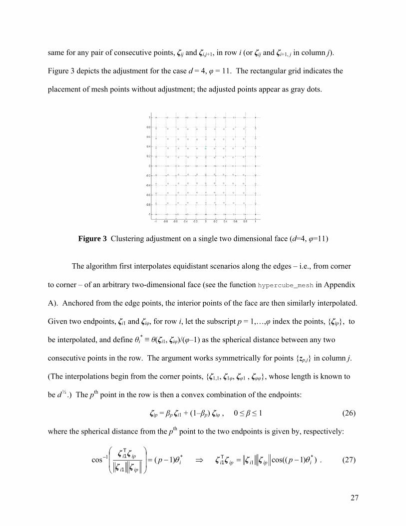
Figure 3 depicts the adjustment for the case d = 4, φ = 11. The rectangular grid indicates the

placement of mesh points without adjustment; the adjusted points appear as gray dots.

Figure 3 Clustering adjustment on a single two dimensional face (d=4, φ=11)

The algorithm first interpolates equidistant scenarios along the edges – i.e., from corner

to corner – of an arbitrary two-dimensional face (see the function hypercube_mesh in Appendix

A). Anchored from the edge points, the interior points of the face are then similarly interpolated.

Given two endpoints, ζi1 and ζiφ, for row i, let the subscript p = 1,…,φ index the points, ζip, to

be interpolated, and define θi* ≡ θ(ζi1, ζiφ)/(φ–1) as the spherical distance between any two

consecutive points in the row. The argument works symmetrically for points zp,j in column j.

(The interpolations begin from the corner points, ζ1,1, ζ1φ, ζφ1 , ζφφ, whose length is known to

be d ½ .) The pth point in the row is then a convex combination of the endpoints:

ζip = βp ζi1 + (1–βp) ζiφ , 0 ≤ β ≤ 1 (26)

where the spherical distance from the pth point to the two endpoints is given by, respectively:

))1cos(()1(cos *1

*1iipiipii

ipi

ipi pp

ζζζζ

ζζ

ζζ TT

11

1 . (27)

28

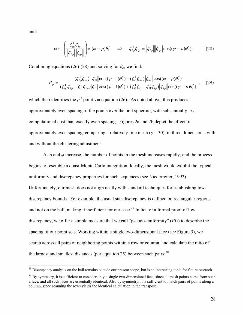
and:

))cos(()(cos **1iipiipii

ipi

ipi pp

ζζζζ

ζζ

ζζ TT

. (28)

Combining equations (26)-(28) and solving for βp, we find:

))cos(()())1cos(()(

))cos(()())1cos(((*

111*

11

*1

*1

iiiiiiiiiiii

iiiiiiiip

pp

pp

ζζζζζζζζζζ

ζζζζζζTTTT

TT ) , (29)

which then identifies the pth point via equation (26). As noted above, this produces

approximately even spacing of the points over the unit spheroid, with substantially less

computational cost than exactly even spacing. Figures 2a and 2b depict the effect of

approximately even spacing, comparing a relatively fine mesh (φ = 30), in three dimensions, with

and without the clustering adjustment.

As d and φ increase, the number of points in the mesh increases rapidly, and the process

begins to resemble a quasi-Monte Carlo integration. Ideally, the mesh would exhibit the typical

uniformity and discrepancy properties for such sequences (see Niederreiter, 1992).

Unfortunately, our mesh does not align neatly with standard techniques for establishing low-

discrepancy bounds. For example, the usual star-discrepancy is defined on rectangular regions

and not on the ball, making it inefficient for our case.29 In lieu of a formal proof of low

discrepancy, we offer a simple measure that we call “pseudo-uniformity” (PU) to describe the

spacing of our point sets. Working within a single two-dimensional face (see Figure 3), we

search across all pairs of neighboring points within a row or column, and calculate the ratio of

the largest and smallest distances (per equation 25) between such pairs:30

29 Discrepancy analysis on the ball remains outside our present scope, but is an interesting topic for future research. 30 By symmetry, it is sufficient to consider only a single two-dimensional face, since all mesh points come from such a face, and all such faces are essentially identical. Also by symmetry, it is sufficient to match pairs of points along a column, since scanning the rows yields the identical calculation in the transpose.

29

),(min

),(max),(

11,...,1,,...,1

11,...,1,,...,1

ijij

ji

ijijjidPU

. (30)

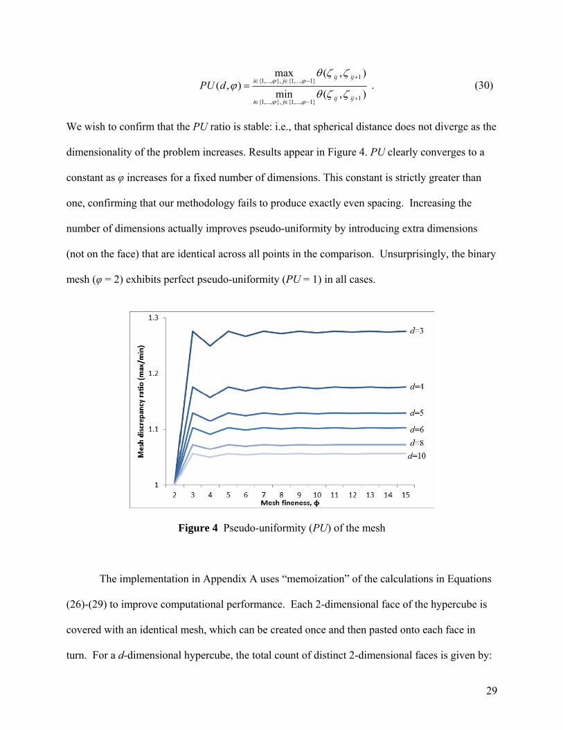
We wish to confirm that the PU ratio is stable: i.e., that spherical distance does not diverge as the

dimensionality of the problem increases. Results appear in Figure 4. PU clearly converges to a

constant as φ increases for a fixed number of dimensions. This constant is strictly greater than

one, confirming that our methodology fails to produce exactly even spacing. Increasing the

number of dimensions actually improves pseudo-uniformity by introducing extra dimensions

(not on the face) that are identical across all points in the comparison. Unsurprisingly, the binary

mesh (φ = 2) exhibits perfect pseudo-uniformity (PU = 1) in all cases.

Figure 4 Pseudo-uniformity (PU) of the mesh

The implementation in Appendix A uses “memoization” of the calculations in Equations

(26)-(29) to improve computational performance. Each 2-dimensional face of the hypercube is

covered with an identical mesh, which can be created once and then pasted onto each face in

turn. For a d-dimensional hypercube, the total count of distinct 2-dimensional faces is given by:

30

)!2(!2

!2)( 2

d

ddFaces d . (31)

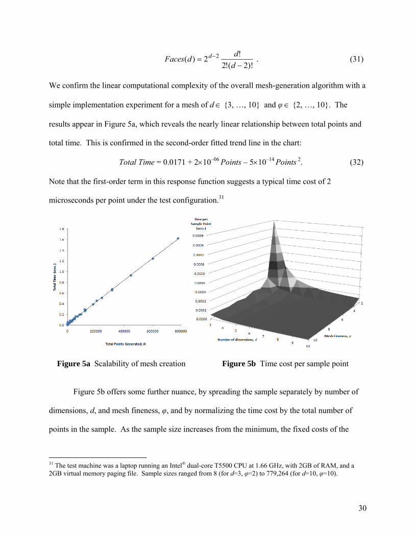
We confirm the linear computational complexity of the overall mesh-generation algorithm with a

simple implementation experiment for a mesh of d 3, …, 10 and φ 2, …, 10. The

results appear in Figure 5a, which reveals the nearly linear relationship between total points and

total time. This is confirmed in the second-order fitted trend line in the chart:

Total Time = 0.0171 + 210–06 Points – 510–14 Points 2. (32)

Note that the first-order term in this response function suggests a typical time cost of 2

microseconds per point under the test configuration.31

Figure 5a Scalability of mesh creation Figure 5b Time cost per sample point

Figure 5b offers some further nuance, by spreading the sample separately by number of

dimensions, d, and mesh fineness, φ, and by normalizing the time cost by the total number of

points in the sample. As the sample size increases from the minimum, the fixed costs of the

31 The test machine was a laptop running an Intel® dual-core T5500 CPU at 1.66 GHz, with 2GB of RAM, and a 2GB virtual memory paging file. Sample sizes ranged from 8 (for d=3, φ=2) to 779,264 (for d=10, φ=10).

31

generation process are quickly averaged away, and the cost per point converges toward a stable

value. The time per point for the largest sample (d=10, φ=10) is 2.0812 10–06 seconds, which is

consistent with the first-order slope coefficient in equation (31).

2.c. Inverting the mapping

Given a mesh of scenario points, Z#, the next step is to invert Step 1, stretching the unit

spheroid back to the original shape of the ellipsoid and keeping track of the mesh as we perform

the transformation. Using the definitions established in Step 1, this inversion is straightforward.

Since Ty:z = cα–½Λ½ is the transformation that produced the unit spheroid (see equation (15)), its

inverse will precisely undo that stretching:

Y# = [Ty:z–1]Ty:zY# = [Ty:z

–1]Z# = [cα½Λ–½]Z#.

(33)

Step –2 inverts Step 2, rotating the unit ellipsoid back to its original orientation, keeping

track of the mesh of scenario points as we apply the inverse of Tx:y = Γ–1:

X# = [Tx:y–1]Tx:y X# = [Tx:y

–1]Y# = [Γ]Y#. (34)

The final step is to reverse the mean-adjustment of Step 3, above, by adding the mean

back into each of our scenario points:

W# = X# + [1NT] , (35)

the columns of which are a set of systematically chosen scenario points in the original coordinate

space. Recursively substituting equations (32) and (33) into equation (34), we have a closed-

form expression for the scenario set in the original coordinate space, stated as a function W#(•) of

the mesh, Z#, generated on the unit spheroid:

W#(Z#) = [cα½ΓΛ–½] Z# + [1N

T] . (36)

Stating W#(•) as a function of Z# emphasizes the separation between the transformation function

32

and the generation of the underlying mesh. Indeed, Z could be any set of points on the unit

spheroid, not necessarily generated via a Cartesian mesh. For example, large scenario sets

generated via computationally costly best-packing techniques might be calculated in advance and

cached, to be transformed via equation (35) as the elliptical parameters are estimated.

3. Practical Extensions

In this section we offer two simple extensions to the basic framework presented above to

address situations of particular interest in financial risk management applications.

3.a. Non-monotonic loss functions

Financial valuations frequently increase or decrease monotonically with underlying

fundamental factors. For example, the value of U.S. Treasury bills, a short-term discount

instrument, always falls when short-term interest rates rise. Just as commonly, however, the loss

function that relates financial valuations to fundamental factors is non-monotonic.32 Indeed, the

relationship between position valuations and underlying factors can easily grow complicated

when diverse portfolios, structured securities, derivatives, or hedging instruments are involved.

For example, hedged portfolios typically leave a residual (and non-monotonic) basis risk, which

is then frequently magnified via leverage to create economically significant exposures.

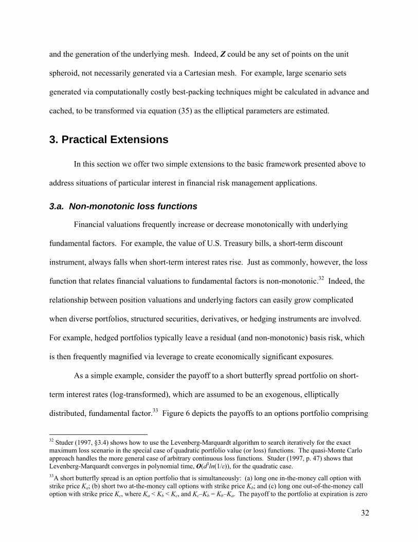
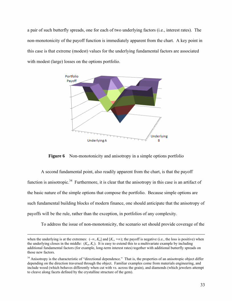
As a simple example, consider the payoff to a short butterfly spread portfolio on short-

term interest rates (log-transformed), which are assumed to be an exogenous, elliptically

distributed, fundamental factor.33 Figure 6 depicts the payoffs to an options portfolio comprising

32 Studer (1997, §3.4) shows how to use the Levenberg-Marquardt algorithm to search iteratively for the exact maximum loss scenario in the special case of quadratic portfolio value (or loss) functions. The quasi-Monte Carlo approach handles the more general case of arbitrary continuous loss functions. Studer (1997, p. 47) shows that Levenberg-Marquardt converges in polynomial time, O(d3ln(1/ε)), for the quadratic case. 33A short butterfly spread is an option portfolio that is simultaneously: (a) long one in-the-money call option with strike price Ka; (b) short two at-the-money call options with strike price Kb; and (c) long one out-of-the-money call option with strike price Kc, where Ka < Kb < Kc, and Kc–Kb = Kb–Ka. The payoff to the portfolio at expiration is zero

33

a pair of such butterfly spreads, one for each of two underlying factors (i.e., interest rates). The

non-monotonicity of the payoff function is immediately apparent from the chart. A key point in

this case is that extreme (modest) values for the underlying fundamental factors are associated

with modest (large) losses on the options portfolio.

Figure 6 Non-monotonicity and anisotropy in a simple options portfolio

A second fundamental point, also readily apparent from the chart, is that the payoff

function is anisotropic.34 Furthermore, it is clear that the anisotropy in this case is an artifact of

the basic nature of the simple options that compose the portfolio. Because simple options are

such fundamental building blocks of modern finance, one should anticipate that the anisotropy of

payoffs will be the rule, rather than the exception, in portfolios of any complexity.

To address the issue of non-monotonicity, the scenario set should provide coverage of the

when the underlying is at the extremes: (–, Ka] and [Kc, +); the payoff is negative (i.e., the loss is positive) when the underlying closes in the middle: (Ka, Kc). It is easy to extend this to a multivariate example by including additional fundamental factors (for example, long-term interest rates) together with additional butterfly spreads on those new factors. 34 Anisotropy is the characteristic of “directional dependence.” That is, the properties of an anisotropic object differ depending on the direction traversed through the object. Familiar examples come from materials engineering, and include wood (which behaves differently when cut with vs. across the grain), and diamonds (which jewelers attempt to cleave along facets defined by the crystalline structure of the gem).

34

interior of the spheroid, and not focus solely on a mesh defined on an extreme shell (for example,

for cα, with α = 99.9%). One simple possibility would be to nest collection of elliptical

isoprobability shells, differing only in the probability threshold, α. Unfortunately, this would not

deal efficiently with the problem of anisotropy, because the points on each shell would be

radially collinear with points on the other concentric shells. We propose instead a radial

adjustment of the points in a given spheroid mesh, Z#. In effect, the scenario points would be

systematically plunged to varying depths into the interior of the ball. Given a mesh, Z# dN,

of N scenario points, multiply each column of the mesh by a different radial factor, Ri [0, 1],

i1, …, N. Collecting the radial factors into a diagonal matrix, R = diag(R1, …, RN) NN,

we can write this contracted mesh, Z dN, as:

Z = Z#R. (37)

One obvious choice of radial factors is a one-dimensional low-discrepancy sequence,

such as a van der Corput sequence. The low-discrepancy property allows for even distribution of

the contraction factors. In addition, the van der Corput sequence is well understood (see

Glasserman (2004, ch. 5), and Niederreiter (1992, ch. 3)). Note that an approximately uniform

distribution of contraction factors, Ri, will create a clustering of points toward the center of the

spheroid, since the volume of a spheroid follows a simple d th-order power-law. With this in

mind, a more uniform distribution of points within the spheroid is achieved by “volume-

adjusting” the equally spaced van der Corput points via element-wise exponentiation of the

vector of radial factors:

Z = Z#Rd, where Rd ≡ diag(R1

1/d, …, RN1/d) . (38)

Of course, the contractions in Rd will tend toward unity as d grows large in high-dimensional

applications. In these situations, it may be preferable to apply contraction only to a subset of the

35

factor dimensions.

3.b. Univariate shocks

This section presents a straightforward extension of the algorithm to identify univariate

shocks. We consider two varieties of univariate shocks: “conditional” and “unconditional.”

Unconditional univariate shocks are determined by marginalizing out each dimension of the joint

distribution, and then identifying the two-tailed critical points on the univariate marginal

distribution corresponding to the extreme-event probability threshold, α. Conditional univariate

shocks are located where lines extending from the center of the ellipsoid in directions parallel to

the coordinate axes (i.e., the individual shock dimensions) intersect the isoprobability ellipsoid.

We first consider unconditional (i.e., marginal) shocks, which are the natural

interpretation in many applications. We use a permutation matrix to extract the marginal. For

elliptically distributed random vectors, W ~ Ed(μ, Σ), the univariate marginal distributions are

also elliptical, Wi ~ E1(μi, σi2), with a distribution of the same “kind” as the underlying joint

distribution.35 For example, a multivariate normal distribution has normal margins, and a

multivariate t distribution has t margins with the same degrees of freedom parameter. More

generally, any affine transformation of an elliptical random vector is also elliptical. Thus, if W

μ + AS is elliptical, with S k a spherical random vector and A dk, then its affine

transformation, V = b + BW with V,b m and B md, is an m-dimensional elliptical random

vector (m < d) of the same type as W. To extract a marginal, choose b = 0m (i.e., a vector of

zeros) and B = P, a matrix of 0s and 1s, with PPT = Im. P is a “permutation and deletion” matrix,

35 More formally, the joint and marginal distributions will share the same characteristic generator, ψ*(u), which is related to the more familiar characteristic function for the distribution, ψ(t) = (eitTX). Note that the characteristic generator is a function of a scalar variable, u, while the characteristic function is a function of a d-dimensional parameter, t. For elliptical distributions, the characteristic generator and characteristic function are related via: ψ(t) = (eitTX) = eitTμψ*(tTΣt). For example, for the multivariate normal distribution, the characteristic generator takes the form ψ*(u) = e–u/2, while for the multivariate t distribution the form of ψ*(u) is considerably more complicated. See Fang, Kotz, and Ng (1990, §2.1 and §3.3.6), and McNeil, Frey, and Embrechts (2005, §3.3) for further details.

36

which extracts the desired marginal elements, Pμ and PΣPT, of the location vector and dispersion

matrix, Σ = AAT. For example, with m = 2:

1

0

0

1

0

1

0

0

0

1

0

0

1

0

0

1and

0

0

1

0

0

1

2

1

3

2

1T PPPμ

, (39)

P is an affine transformation, so the marginal distribution, V ~ Em(Pμ, PΣPT), is elliptical of the

same type as W (See Frahm (2004), p. 13). The univariate marginal is simply a special case with

m = 1. In summary, given a specific functional form for the distribution, determining the

unconditional (marginal) univariate shock scenarios is straightforward.

On the other hand, conditional univariate shocks (denoted by the perpendicular subscript,

“”) lie on the same ellipsoid that defines the multivariate shocks. For each conditional

univariate shock scenario, the most natural conditioning restriction is to assume no change in the

other d–1 dimensions, providing an estimate of the ceteris paribus sensitivity to the individual

shock dimensions. The upshot is a set of 2d univariate scenarios, up and down in each

dimension, that lie on the surface of the chosen isoprobability ellipsoid. For example, consider

the conditional univariate shocks, W = e, f, g, h, located on line segments extending from the

center of the ellipse in Figure 1, above. The point f in Figure 1 represents an upward shock to the

long-term interest rate (fRLT – RLT > 0), conditional on no change to the short-term interest rate

(fRST – RST = 0). In general, we can represent the set of conditional univariate shocks, W, as a

d2d matrix, W = [w1, …, w2d], each column of which represents a single shock scenario, wi

d, i 1, …, 2d.

To facilitate the analysis, we manipulate the conditional shocks after Step 3, mean-

adjustment of the ellipsoid. Let xi [0, …, 0, xi, 0, …, 0]T denote a conditional univariate shock

vector on the mean-adjusted ellipsoid (i.e., xi is a vector with shock value xi in the ith dimension,

37

and zeroes elsewhere), and let ωii denote the ith diagonal element of the matrix Σ–1. The shocks

are solutions to the quadratic form, cα = xiTΣ–1 xi, or, substituting:

cα = [0, …, 0, xi, 0, …, 0]TΣ–1[0, …, 0, xi, 0, …, 0] = xi2ωii. (40)

Rearranging, we can solve for the pairs of shocks of opposite sign: xi = ±(cα/ωii)½. More

explicitly, for i1, …, d let:

xi↑ = +(cα/ωii)

½, (41)

and,

xi↓ = –(cα/ωii)

½. (42)

Denote the corresponding vectors as xi↑ and xi

↓. For example, the (mean-adjusted) matrix of

points [e, f, g, h] (as columns) from Figure 1 above, would be relabeled as [x1↑, x2

↑, x2↓, x1

↓]

respectively. Slightly more generally, let Ω define the diagonal matrix, Ω ≡ diag(ω11, …,ωdd),

and write the d2d matrix of univariate shocks, X d2d, as the adjoin of the dd up and down

shock matrices, ±cα½Ω–½:

X = cα

½[ Ω–½ | –Ω–½ ] (43)

(See the function: univariate_shocks in Appendix A.)

These 2d conditional univariate shocks, X d2d, can augment the set of N mesh-based

scenarios, X# dN, described in Step 0 above. Thus, let X# d(N+ 2d) denote the adjoin:

X# = [ X# | X ] = [ X# | cα½Ω–½ | –cα

½Ω–½ ]. (44)

This is essentially a notational convenience that allows us to manipulate all of the shock

scenarios at once. Carrying this forward, we get the adjoin-modified versions of equation (34):

W# = X# + [1(N+ 2d)T] . (45)

and equation (35):

W#(Z#) = cα½[ ΓΛ–½Z# | Ω

–½ | –Ω–½ ] + [1(N+ 2d)T] . (46)

38

4. Conclusions We have developed a quasi-Monte-Carlo algorithm for systematic generation of shock scenarios

from an arbitrary multivariate elliptical distribution. The algorithm selects a systematic mesh of

arbitrary fineness that approximately evenly covers an isoprobability ellipsoid in d dimensions.

Choosing scenarios systematically reduces the danger of “blind spots” in a stress test. The

methodology is particularly well suited to elliptically distributed market risk factors, where the

elliptical distribution provides “plausibility guidance” for generating internally consistent

scenarios. The methodology is intended for an implementation context – commonly encountered

in regulatory stress tests – where the loss function is unobservable and scenarios cannot be tested

sequentially or otherwise tailored to known features of particular portfolios. A corollary of the

imperfect knowledge of the portfolio is that the set of relevant stress factors composing the

scenarios may also be unclear, encouraging the casting of a wide net for possible factors. The

algorithm has linear computational complexity, which distinguishes it from computationally

costly point-packing routines that generate precisely evenly distributed points. We suggest

extensions to address the issues of non-monotonic loss functions and univariate shocks. We also

provide tested and commented source code in Appendix A.

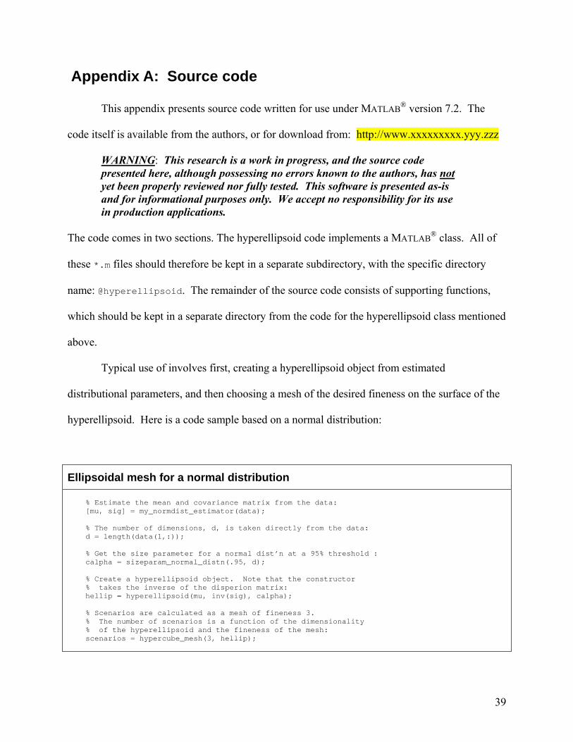
39

Appendix A: Source code

This appendix presents source code written for use under MATLAB® version 7.2. The

code itself is available from the authors, or for download from: http://www.xxxxxxxxx.yyy.zzz

WARNING: This research is a work in progress, and the source code presented here, although possessing no errors known to the authors, has not yet been properly reviewed nor fully tested. This software is presented as-is and for informational purposes only. We accept no responsibility for its use in production applications.

The code comes in two sections. The hyperellipsoid code implements a MATLAB

® class. All of

these *.m files should therefore be kept in a separate subdirectory, with the specific directory

name: @hyperellipsoid. The remainder of the source code consists of supporting functions,

which should be kept in a separate directory from the code for the hyperellipsoid class mentioned

above.

Typical use of involves first, creating a hyperellipsoid object from estimated

distributional parameters, and then choosing a mesh of the desired fineness on the surface of the

hyperellipsoid. Here is a code sample based on a normal distribution:

Ellipsoidal mesh for a normal distribution % Estimate the mean and covariance matrix from the data: [mu, sig] = my_normdist_estimator(data); % The number of dimensions, d, is taken directly from the data: d = length(data(1,:)); % Get the size parameter for a normal dist’n at a 95% threshold : calpha = sizeparam_normal_distn(.95, d); % Create a hyperellipsoid object. Note that the constructor % takes the inverse of the disperion matrix: hellip = hyperellipsoid(mu, inv(sig), calpha); % Scenarios are calculated as a mesh of fineness 3. % The number of scenarios is a function of the dimensionality % of the hyperellipsoid and the fineness of the mesh: scenarios = hypercube_mesh(3, hellip);

40

Here is another code sample based on a multivariate t distribution:

Ellipsoidal mesh for a t distribution % Estimate the mean, covariance, and d.o.f. from the data: [mu, sig, nu] = my_tdist_estimator(data); % The number of dimensions, d, is taken from the data: d = length(data(1,:)); % Get the size parameter for a normal dist’n at a 95% threshold : calpha = sizeparam_t_distn(.95, d, nu); % Create a hyperellipsoid object; note the use of the inverse of sig: hellip = hyperellipsoid(mu, inv(sig), calpha); % Scenarios are calculated as a mesh of fineness 3. scenarios = hypercube_mesh(3, hellip);

41

Appendix B: Alternate algorithm for mapping an ellipse to the unit spheroid

In the interest of enhanced unit-testing, modularity, and source-code re-use, the algorithm

implement in Appendix A is structured differently from the exposition provided in section 2.a

above. Thus, we re-derive here the transformation, Tx:z, in a form that more closely matches the

software implementation.

We begin by identifying d linearly independent points (denoted by the four-pointed star

subscript, “”) for which we know the coordinates under both the “input” and “output”

coordinate systems. An input point is some xi d for which the matching output point z

i =

Tx:z xi is known. For the dd input and output matrices X

and Z

, we have:

Z

= Tx:z X (47)

implying:

Tx:z = Z X

–1. (48)

For input points, choose the d positive vertices, X

dd, which lie on the eigenvectors of the

inverse dispersion matrix, Σ–1. (See the functions: make_ellipsoid_from_vertices and

vertices in Appendix A.) For a non-degenerate ellipsoid, these eigenvectors are linearly

independent, ensuring that we can diagonalize Σ–1 via the spectral decomposition, Σ–1 = ΓΛΓ T,

where Γ and Λ are as defined in section 2.a above. The distance from the origin of the ith such

vertex (i.e., the half-length of the corresponding principal axis) is:

li (cα/λi)½. (49)

Using this fact to define a diagonal matrix of principal axis half-lengths,

L diag(l1, …, ld) = diag[(cα/λ1)½., …, (cα/λd)

½] = cα½Λ–½. (50)

we can write the input points, X

, in terms of the eigenvector matrix, and the principal-axis half-

42

lengths, li:

X

= [l1γ1, …, ldγd] = ΓL = Γ(cα½Λ–½) (51)

For the matching “output” points, Z

we choose the vertices of the unit simplex in d, given by

the columns of the identity matrix, Id, so that:

Z

= Id = Tx:z (Γcα½Λ–½) = Tx:z X. (52)

implying the transformation:

Tx:z = (Tx:z

–1) –1 = (Γcα½Λ–½) –1 = cα

–½Λ½Γ –1 (53)

which decomposes neatly into separate transformations for rotation,

Tx:y = Γ –1, (54)

and stretching,

Ty:z = cα

–½Λ½. (55)

(See the functions: linear_transform and rotate_to_coordaxes in Appendix A.)

43

References

Agarwal, Vikas, and Narayan Y. Naik. “Risks and Portfolio Decisions Involving Hedge Funds,” Review of Financial Studies 17, no. 1 (2004): 63-98.

Ahmad, Rizwan, Yuanmu Deng, Deepti S. Vikram, Bradley Clymer, Parthasarathy Srinivasan, Jay Zweier, and Periannan Kuppusamy. “Quasi Monte Carlo-based isotropic distribution of gradient directions for improved reconstruction quality of 3D EPR imaging.” Journal of Magnetic Resonance 184, no. 2 (2007): 236-45.

Alexander, Carol, Market Risk Analysis II: Practical Financial Econometrics, Wiley. 2008.

Alfaro, Rodrigo, and Mathias Drehmann. “Macro Stress Tests and Crises: What Can We Learn?” BIS Quarterly Review (December 2009): 29–41.

Artzner, Philippe, Freddy Delbaen, Jean-Marc Eber, and David Heath. “Coherent Measures of Risk.” Mathematical Finance 9, (1999): 203-228.

Committee on the Global Financial System (CGFS). Stress testing at major financial institutions: survey results and practice. Bank for International Settlements. Basel: CGFS, 2005.

Basel Committee on Banking Supervision (BCBS). Amendment to the capital accord to incorporate market risks, Technical Report 24, Bank for International Settlements. Basel: BCBS, 1996.

Basel Committee on Banking Supervision (BCBS). International Convergence of Capital Measurement and Capital Standards: A Revised Framework, Comprehensive Version. Bank for International Settlements. Basel: BCBS, 2006.

Basel Committee on Banking Supervision (BCBS). Principles for sound stress testing practices and supervision. Bank for International Settlements. Basel: BCBS, 2009.

Bendito, Enrique, Angeles Carmona, Andres M. Encinas and J. M. Gesto, A. Gomez, Jose C. Mourino, and M. T. Sánchez. “Computational Cost of the Fekete Problem I: The Forces Method on the 2-Sphere.” Working Paper, 2008.

Bendito, Enrique, Angeles Carmona, Andres M. Encinas and J.M. Gesto. “Computational Cost of the Fekete Problem II: On Smale’s 7th Problem.” Working Paper, 2008.

Bern, Marshall, and Paul Plassmann. “Mesh Generation,” in: J. Sack and J. Urrutia, eds. Elsevier Science. Handbook of Computational Geometry, (2000): 291-332.

Bingham, Nick, and Rudiger Kiesel. “Semi-parametric modelling in finance: theoretical foundations,” Quantitative Finance 2, no. 4 (2002): 241-250.

Bingham, Nick, Rudiger Kiesel, and Rafael Schmidt. “A semi-parametric approach to risk management.” Quantitative Finance 3, no. 6 (2003): 426-441.

Blaschke, Winfrid, Matthew T. Jones, Giovanni Majnoni, and Soledad Martinez Peria “Stress Testing of Financial Systems: An Overview of Issues, Methodologies, and FSAP Experiences.” Working Paper 01/88, International Monetary Fund, 2001.

Board of Governors of the Federal Reserve (FRB). The Supervisory Capital Assessment Program: Overview of Results. Technical Report. May 2009.

44

Board of Governors of the Federal Reserve (FRB). Comprehensive Capital Analysis and Review 2012: Methodology and Results for Stress Scenario Projections. Technical Report, March 2012.

Borio, Claudio, and Mathias Drehmann. “Towards an operational framework for financial stability: ‘Fuzzy’ measurement and its consequences.” In: Banco Central de Chile (ed.), Financial stability, monetary policy and central banking, (2011).

Borio, Claudio, Mathias Drehmann, and Kostas Tsatsaronis. “Stress Testing Macro Stress Testing: Does It Live up to Expectations?” BIS Working Papers no. 369, Basel: Bank for International Settlements, January 2012.

Boyle, Phelim, Mark Broadie, and Paul Glasserman. “Monte Carlo methods for security pricing.” Journal of Economic Dynamics and Control 21, no. 8-9 (1997): 1267-1321.

Breuer, Thomas. “Overcoming Dimensional Dependence of Worst Case Scenarios and Maximum Loss.” Journal of Risk 11, (2008): 79-92.

Breuer, Thomas. “A Short Guide to Managing Risk in Worst Case Scenario.” Working Paper, University of Applied Sciences, Vorarlberg, 2007.

Breuer, Thomas, and Imre Csiszár. “If Worse Comes to Worst: Systematic Stress Testing in General Risk Models.” Working Paper, University of Applied Sciences, Vorarlberg, 2010.

Breuer, Thomas, Jandačka, M.; Rheinberger, K. & Summer, M. “How to Find Plausible, Severe and Useful Stress Scenarios.” International Journal of Central Banking 5, (2009): 205-224.

Breuer, Thomas, and Gerald. Krenn. “Guidelines on Market Risk, Volume 5: Stress Testing.” Oesterreichische Nationalbank, 1999.

Campbell, John, Andrew Lo, and A. Craig MacKinlay. The Econometrics of Financial Markets, Princeton University Press. 1997.

Čihák, Martin. “Introduction to Applied Stress Testing.” Working Paper No. 07/59, International Monetary Fund, 2007.

Claessens, Stijn, and Kristin Forbes. “International Financial Contagion: The Theory, Evidence and Policy Implications.” Working Paper, MIT, November 2004.

Committee on the Global Financial System. “Stress testing at major financial institutions: survey results and practice.” CGFS Publication 24, Bank for International Settlements, Basel: CGFS, January 2005.

Coxeter, Harold Scott M. Regular Polytopes, Dover Publications. 1973.

Crouhy, Michael, Dan Galai, and Robert Mark. Risk Management, McGraw-Hill. 2001.

Dragnev, Peter. “The Science of Spherical Arrangements - Fullerenes, Electrons, and Soccer Ball Designs,” presentation slides, Sigma Xi Brown Bag talk, IPFW, December 2002. http://users.ipfw.edu/dragnevp/Sigma_Xi1.ppt, downloaded January 11, 2008.

Drehmann, Mathias. “Macroeconomic stress testing banks: A survey of methodologies,” in M. Quagliariello, ed. Stress testing the banking system: Methodologies and applications, (2009): 37-67.

45

European Banking Authority (EBA). “2011 EU-Wide Stress Test Aggregate Report.” Technical report, London: EBA, July 2011.

European Central Bank (ECB). “Country-Level Macro Stress-Testing Practices.” Financial Stability Review, (2006): 147-154.

Fang, Kai-Tai, Samuel Kotz, and Kai Wang Ng. Symmetric Multivariate and Related Distributions, Monographs on Statistics and Applied Probability, 36. Chapman and Hall. 1990.

Foster, Dean, and H. Peyton Young. “Gaming Performance Fees by Portfolio Managers.” Quarterly Journal of Economics 125, no. 4 (2010): 1435-1458.

Frahm, Gabriel. “Generalized Elliptical Distributions: Theory and Applications.” Ph.D. thesis, Wirtschafts- und Sozialwissenschaftliche Fakultät der Universität zu Köln (Cologne), 2004.

Friedman, Craig, Jinggang Huang, and Yuchang Huang. “Finding Stress Scenarios the Get the Job Done, with a Credit Risk Application.” Working Paper, Standard & Poor’s, December 2010.

Genz, Alan, and Frank Bretz. “Methods for the Computation of Multivariate t-Probabilities.” Journal of Computational and Graphical Statistics 11, no. 4 (2002): 950-971.

Glasserman, Paul. Monte Carlo Methods in Financial Engineering, Springer Verlag, New York. 2004.

Goetzmann, William, Jonathan Ingersoll, Matthew Spiegel, and Ivo Welch. “Portfolio Performance Manipulation and Manipulation-proof Performance Measures.” Review of Financial Studies 20, no. 5 (2007): 1503-1546.

Haldane, Andrew. “Why Banks Failed the Stress Test: The basis for a speech given at the Marcus-Evans Conference on Stress-Testing, 9-10 February 2009.” Manuscript, Bank of England, 2009.

Hamkins, John. “Design and Analysis of Spherical Codes.” Ph. D. thesis, University of Illinois, Dept. of Electrical Engineering, 1996.

Hardin, Doug, and E. B. Saff. “Discretizing Manifolds via Minimum Energy Points.” Notices of the American Mathematical Society 15, no. 10 (2004): 1186-1194.

Huffer, Fred, and Cheolyong Park. “A test for elliptical symmetry.” Journal of Multivariate Analysis 98, no. 2 (2007): 256-281.

International Monetary Fund (IMF). Financial Sector Assessment Program Update: United Kingdom, Stress Testing the Banking Sector. Technical Note. 2011.

Jones, Matthew, Paul Hilbers, and Graham Slack. “Stress Testing Financial Systems: What to Do When the Governor Calls.” Working Paper No. 04/127, International Monetary Fund, 2004.

Knight, Frank. Risk, Uncertainty and Profit, Houghton-Mifflin. 1921.

Leopardi, Paul. “Distributing points on the sphere: Partitions, separation, quadrature and energy.” Ph.D. thesis, University of New South Wales, Dept. of Applied Mathematics, 2007.

46

Lemieux, Christiane. Monte Carlo and Quasi-Monte Carlo Sampling, Springer. 2009.

Liu, Chuanhai, and Donald B. Rubin. “ML Estimation of the t Distribution Using EM and Its Extensions, ECM and ECME.” Statistica Sinica 5, (1995): 19-39.

Lo, Andrew. “Risk Management for Hedge Funds: Introduction and Overview.” Financial Analysts Journal 57, no. 6 (2001): 16-33.

McKay, David. Information Theory, Inference, and Learning Algorithms, Cambridge University Press. 2003.

McNeil, Alexander, Rudigar Frey, and Paul Embrechts. Quantitative Risk Management, Princeton University Press. 2005.

Niederreiter, Harold. Random Number Generation and Quasi-Monte Carlo Methods, Number 63 in CBMS–NSF Regional Conference Series in Applied Mathematics, Society for Industrial and Applied Mathematics (SIAM), Philadelphia. 1992.

Pistovčák, F., and Thomas Breuer. “Using Quasi-Monte Carlo Scenarios in Risk Management.” in: H. Niederreiter, ed. Monte Carlo and Quasi-Monte Carlo Methods 2002, (2004): 379-392.

Pritsker, Matt. “Enhanced Stress Testing and Financial Stability.” Working paper, Federal Reserve Bank of Boston, May 2005.

Rowe, David. “Building pessimised scenarios.” Risk Magazine, January (2006): 90.

Quagliarello, Mario. “Macroeconomic stress-testing: definitions and main components.” in M. Quagliariello, ed. Stress testing the banking system: Methodologies and applications, Cambridge University Press, (2009): 18-36.

Saff, E., and Arno Kuijlaars. “Distributing Many Points on a Sphere.” Mathematical Intelligencer 19, no. 1 (1997): 5-11.

Senior Supervisors Group, 2008, Observations on Risk Management Practices during the Recent Market Turbulence, 2008. http://www.newyorkfed.org/newsevents/news/ banking/2008/SSG_Risk_Mgt_doc_final.pdf, downloaded September 18, 2008.

Smale, Steve. “Mathematical Problems for the Next Century.” Mathematical Intelligencer 20, no. 2 (1998): 7-15.

Sorge, Macro. “Stress-testing financial systems: an overview of current methodologies.” Working Paper No. 165, Bank for International Settlements, 2004.

Stock, James, and Mark Watson. “Forecasting Using Principal Components from a Large Number of Predictors.” Journal of the American Statistical Association, 97, no. 460 (2002): 1167-1179.

Strang, Gilbert. Linear Algebra and Its Applications, Academic Press. 1980.

Strang, Gilbert. “Linear Transformations and Their Matrices,” MIT Open Courseware, Linear Algebra, Spring 2005. http://mfile.akamai.com/7870/rm/mitstorage.download.akamai.c om/7870/18/18.06/videolectures/strang-1806-lec30-24nov1999-220k.rm, downloaded 16 August 2007.

Studer, Gerold. “Maximum Loss for Measurement of Market Risk,” Ph.D. thesis, Swiss Federal Institute of Technology, Zurich (ETH Zürich), Dept. of Mathematics, 1997.

47

Studer, Gerold. “Market Risk Computation for Nonlinear Portfolios.” Journal of Risk 1, no. 4 (1999): 33-53.

Sun, Xingping, and Zhenzhong Chen. “Spherical basis functions and uniform distribution of points on spheres.” Journal of Approximation Theory 151, no. 2 (2008): 186-207.

Tyler, David. “A Distribution-Free M-Estimator of Multivariate Scatter.” Annals of Statistics 15, no. 1 (1987): 234-251.