SYSTEMATICS AND GLACIAL POPULATION HISTORY OF THE

ALTERNIFOLIUM GROUP OF THE FLOWERING PLANT GENUS

CHRYSOSPLENIUM (SAXIFRAGACEAE)

BY

Nicholas Levsen

Submitted to the graduate degree program in Ecology and Evolutionary Biology and the Graduate Faculty of the University of Kansas in partial fulfillment of the

requirements for the degree of Doctor of Philosophy

________________________

Chairperson

Committee Members * _______________________*

_______________________*

_______________________*

_______________________*

Date Defended:________________

i

The Dissertation Committee for Nicholas Levsen certifies that this is the approved

version of the following dissertation:

SYSTEMATICS AND GLACIAL POPULATION HISTORY OF THE

ALTERNIFOLIUM GROUP OF THE FLOWERING PLANT GENUS

CHRYSOSPLENIUM (SAXIFRAGACEAE)

Committee:

________________________________ Chairperson*

________________________________

________________________________

________________________________

________________________________

Date Approved:_______________________

ii

TABLE OF CONTENTS: List of Tables iii List of Figures v Acknowledgements vii Abstract vii Chapter One: INTRODUCTION 1 Chapter Two: CHRYSOSPLENIUM 17 PHYLOGENY Chapter Three: CHRYSOSPLENIUM 31 IOWENSE ISSR STUDY Chapter Four: CHRYSOSPLENIUM 57 TETRANDRUM ISSR STUDY Chapter Five: COMPARATIVE 89 STUDY OF GENE STATISTIC ESTIMATION METHODS List of References 123 Appendix LIST OF SPECIMENS 152

iii

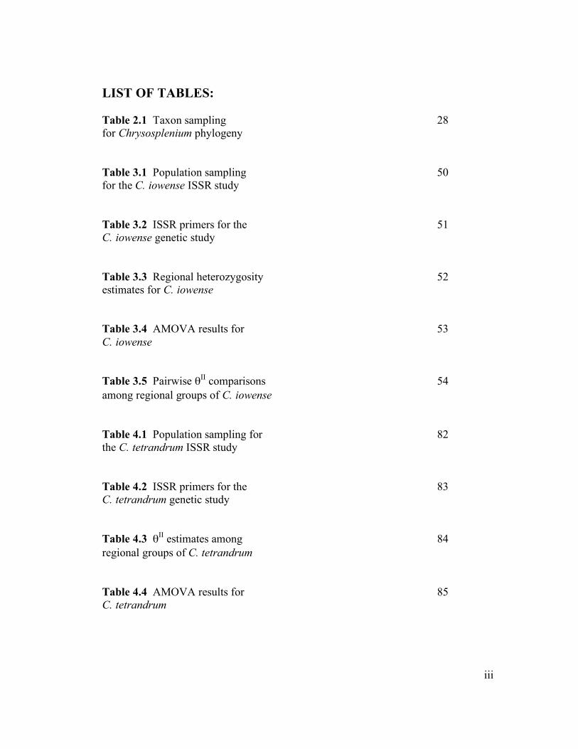
LIST OF TABLES: Table 2.1 Taxon sampling 28 for Chrysosplenium phylogeny Table 3.1 Population sampling 50 for the C. iowense ISSR study Table 3.2 ISSR primers for the 51 C. iowense genetic study Table 3.3 Regional heterozygosity 52 estimates for C. iowense Table 3.4 AMOVA results for 53 C. iowense Table 3.5 Pairwise θII comparisons 54 among regional groups of C. iowense Table 4.1 Population sampling for 82 the C. tetrandrum ISSR study Table 4.2 ISSR primers for the 83 C. tetrandrum genetic study Table 4.3 θII estimates among 84 regional groups of C. tetrandrum Table 4.4 AMOVA results for 85 C. tetrandrum

iv

Table 5.1 Summary of gene 113 statistic estimate comparisons Table 5.2 Taxon sampling for 114 Tolpis in method comparison study

v

LIST OF FIGURES:

Figure 2.1 Phylogenetic reconstruction 29 of Chrysosplenium

Figure 2.2 Principal Components Analysis 30 of morphological data from C. iowense, C. tetrandrum, and C. rosendahllii

Figure 3.1 Distribution map for 55 C. iowense

Figure 3.2 Principal Coordinates Analysis 56 of ISSR data from C. iowense

Figure 4.1 Distribution map for 86 C. tetrandrum

Figure 4.2 Principal Coordinates Analysis 87 of ISSR data from C. tetrandrum

Figure 4.3 Principal Components Analysis 88 of morphological data mixed (C. tetrandrum-C. rosendahlii and C. tetrandrum-C. iowense) populations

Figure 5.1 Comparison of FST estimates 115 produced from Tolpis ISSR and allozyme datasets

Figure 5.2 Simulated data show 116 differences in FST estimates between Bayesian and standard methods

vi

Figure 5.3 Simulated data show 117 differences in FST estimates between Bayesian and standard methods

Figure 5.4 Comparison of FIS 118 estimates produced from Tolpis ISSR and allozyme datasets

Figure 5.5 Simulated data show 119 effects of sample size on Bayesian estimates of inbreeding

Figure 5.6 Comparison of HS 120 estimates produced from Tolpis ISSR and allozyme datasets

Figure 5.7 Comparison of HiS 121 estimates produced from Tolpis ISSR and allozyme datasets

Figure 5.8 Comparison of HT 122 estimates produced from Tolpis ISSR and allozyme datasets

vii

ACKNOWLEDGEMENTS:

I would like to acknowledge the following people, as contributors to this work and to

my general education. I thank M. Mort, D. Crawford, C. Freeman, J. Roberts, and C.

Haufler for serving on my graduate committee and guiding my progress throughout

my graduate study. I thank J. Archibald and C. Randle for invaluable service as

mentors and friends, as well as for having made significant contributions to my own

technical knowledge and capability. I thank a number of people who have assisted in

field collection of plant material, including: B. Bennett, K. Davis, J. Foote, C. Henry,

H. Hernandez, J. Jorgenson, D. Murray, S. C. Parker, C. Roland, W. Schorg, T.

Skjonsberg, and L. Tyrrell. I thank the institutions that have provided funding for this

research, including: National Science Foundation (DDIG DEB-0710371), University

of Kansas Graduate School, University of Kansas Natural History Museum and

Biodiversity Research Center, University of Kansas Department of Ecology and

Evolutionary Biology, and Sigma Xi. Finally, I would like to thank my family (Dad,

Mom, Cathy, Katie, Bryan, and Erin) for the support and entertainment.

viii

ABSTRACT:

The flowering plant genus Chrysosplenium comprises approximately 57 species of

herbaceous perennials. These species are mainly distributed in the Northern

Hemisphere where they occur in moist habitats. Though the center of diversity, and

presumed location of origin, for the genus is east temperate Asia, more recently

radiating taxa have invaded the arctic of North America and Europe. There are six

species of Chrysosplenium in North America and four of them (i.e., C. iowense, C.

tetrandrum, C. wrightii, and C. rosendahlii) belong to the section Alternifolia.

Termed the Alternifolium group, this collection of species presents an excellent

opportunity to study the evolution of variation in arctic and alpine environments.

Similar to many arctic taxa, these species display very little morphologic or genetic

variation, but they exhibit diversity in chromosome number, breeding system,

geographic distribution, and ecology. Though the Alternifolium group has been the

subject of numerous taxonomic studies, no thorough investigation of its evolutionary

history has been conducted. This study used a combination of genetic and phenotypic

data (e.g., DNA sequence, Inter-Simple Sequence Repeat, morphology) to determine

the patterns of variation present within the Alternifolium group and then used these

patterns to infer historical processes that might have contributed to them. Through

the course of the study, however, it also became necessary to investigate the

applicability of genetic estimates derived from different molecular markers and

statistical methods. Appropriate comparisons among genetic estimates are critical to

accurately interpret results and generate new predictions.

1

CHAPTER ONE:

INTRODUCTION

From the time of its inception, the field of evolutionary biology has ascribed special

importance to the study of so-called “natural laboratories”, particularly as they are

manifest in the environments of oceanic islands (Darwin, 1859; Wallace, 1881;

MacArthur & Wilson, 1967). This focus is predicated on the existence of a suite of

common insular characteristics (e.g., discreteness and isolation, small size, ecological

diversity, and dynamic geologic history), which simultaneously render a biological

system unique while also capable of providing insight into the formulation of

complex and broadly applied evolutionary theory (MacArthur & Wilson, 1967;

Emerson, 2002). It is largely this capability, conjoined with an undoubted affinity of

biologists for the exotic and generally equatorial, that explains why so many of the

venerable works of evolutionary biology concern the diversification of island lineages

(e.g., finches, Darwin, 1859; Anolis lizards, Losos et al., 1998; Hawaiian

silverswords, Baldwin et al., 1991). However, islands or island-like features are not

restricted to the world’s oceans, but exist even within the continental expanse in the

form of caves, gallery forests, tide pools, and arctic and alpine tundra (MacArthur &

Wilson, 1967). The Arctic, in particular, presents an intriguing opportunity for

evolutionary research, as the region exhibits many of the attributes that make oceanic

islands amenable to such investigations, while maintaining a markedly distinct

taxonomic, climatic, and geological character (Yurtsev, 1994). Certainly, the history

2

of the arctic biota is a global history amplified, as its patterns of variation bear, with

unmatched fidelity, the marks of upheaval inflicted by a geological and climatic

revolution that even the founders of evolutionary thought considered to be of rare

importance (Darwin, 1859; Wallace, 1881). Today, the arctic biota comprises a

patchwork of individual lineages, each having evolved through the forceful coaction

of historical, stochastic (e.g., genetic drift), and deterministic (e.g., natural selection)

processes (Weider & Hobæk, 2000). It is in regard to the interplay of these processes

that the role of the arctic as a “natural laboratory” is most powerfully applied, as it

offers a prospective understanding of the individual and collective influence of

evolutionary mechanisms operating therein (U.S. Polar Research Board, 1998;

Weider & Hobæk, 2000). However, despite all prospects, the arctic biota remains

relatively unknown with regard to the nature of both evolutionary pattern and process

(Murray, 1987; Steltzer et al., 2008). The following studies represent an effort to

delineate patterns of genetic and morphologic variation within a group of closely

related arctic and boreal plant species, as well as determine the behavior of molecular

and analytical methods that might best be applied in the pursuit of such delineation.

Perhaps, with the future proliferation of similar studies, biologists might more

extensively exploit the impressive research potential of the arctic biota.

The Arctic and its flora

The Arctic

3

Any discussion of evolution in the arctic flora must begin with a definition of that

region, especially considering with what difficulty a precise and universally accepted

circumscription has faced in the past. The Arctic is a region vast in both size (~2 300

000 sq. mi.) and complexity, however, delimitation of its boundaries is often made in

the most simplistic terms (Polunin, 1951; Downes, 1965). The common biological

definition of the Arctic, which is by no means wholly uninformative, assigns to it all

the treeless area beyond the climatic timberline (Billings & Mooney, 1968; Murray,

1987). Though this definition is operational and has been employed throughout most

studies of arctic plants, more detailed descriptions have been proposed (e.g., Polunin,

1951; Elvebakk et al., 1999). The more contemporary of these definitions (i.e.,

Elvebakk et al., 1999) equates the Arctic to the Arctic Bioclimatic Zone, which is

characterized by both arctic tundra vegetation and an arctic climate. In contrast,

Polunin’s (1951) description

…I have come to accept as truly arctic only certain areas of land, fresh water,

and adjacent sea. These are in general those that lie north of whichever of the

following is situated farthest north in each sector of the northern hemisphere:

(1) a line 80 km. (50 miles) north of the northern limit of coniferous forest or

at least more or less continuous taiga, i.e. terrain with sparsely scattered

trees; (2) north of the present-day northern limit of at least

microphanerophytic growth (i.e., of trees 2-8 m. in height but excluding

straggling bushes in unusually favourable situations), the northern extremities

of tongues or outliers separated by not more than fifteen degrees of longitude

2

being united across; or (3) north of the northern Nordenskiöld line, which is

determined by the formula V =9 – 0.1K, where V is the mean of the warmest

month and K is the mean of the coldest month, both in degrees Centigrade.

places less emphasis on plant community composition. Both authors, however,

provide a more nuanced view of arctic boundaries than is traditionally available,

offering an important basis for the consideration of ecological variation within the

Arctic.

A popular depiction of the Arctic is that of an area that is uniformly cold and

desertic (Polunin, 1951). While true that the Arctic is primarily a peripheral

environment with very little biologically usable heat and low levels of precipitation

(additional attributes include: short growing season, strong wind, long photoperiod,

low light intensity, and low nitrogen supply), such generalizations cannot fully or

accurately represent this ecologically complex region (Billings & Mooney, 1968;

Savile, 1972; Murray, 1987). In fact, efforts to reflect even large-scale differences in

arctic ecology have produced up to five subdivisions of this biome (Elvebakk et al.,

1999). Though these subdivisions are primarily defined by plant community

composition, their differentiation is ultimately the result of variation in physiographic

conditions, which influence species’ distributions (Hansell et al., 1998). This

variation is spatially and temporally structured with factors such as periglacial (e.g.

formation of ice mounds and frost blisters) and thermokarst (e.g., formation of thaw

lakes and sinkholes) processes effecting changes in local and regional topography,

2

temperature, moisture, etc. (Murray, 1987; Trenhaile, 2004). Recognition of arctic

habitat diversity is a critical component for understanding adaptive evolution and

phytogeography in arctic plant species.

The arctic flora

An arctic plant species is typically and simply defined as one that has the main part of

its range in the Arctic (Polunin, 1951). However, what distinguishes these species

from all but their alpine relatives is the ability to metabolize, grow, and reproduce at

low temperatures (Billings & Mooney, 1968). Few vascular plants have this

capability, and its rarity is signified by the relatively small size (~1500 species) of the

Arctic Flora (Murray, 1995). In contrast, the much smaller Cape Floristic Region

(~88 000 sq. km.) is home to over 9000 species (Cowling & Heijnis, 2001; Goldblatt

& Manning, 2002). Modest as it is, consideration of the Arctic as a floristic region,

by some (Yurtsev, 1994) emphasizes the unique taxonomic, ecological, and genetic

qualities of the flora.

As previously alluded to, the arctic flora displays an unusual taxonomic structure

that has been artfully described by one author (Savile, 1972) as “a depauperate

miscellany”. Indeed, the arctic flora consists of relatively few endemic genera and in

most cases, a small number of arctic species per genus or family are observed

(Yurtsev, 1994). Though there are a number of endemic arctic species (> 10% of all

3

arctic species), many more can be described as having arctic-alpine or largely boreal

distributions (Bliss, 1971). Consideration of the taxonomic distribution of arctic

species within prominent arctic genera, such as Carex or Saxifraga, suggests that the

flora was formed by repeated invasions from multiple geographic origins, rather than

any in situ radiation of taxa (Savile, 1972).

The perceived lack of diversity in the arctic flora is, perhaps, its most well known

feature (Willig et al., 2003; Grundt et al., 2006). This condition has long been

attributed to aspects of arctic plant biology and environmental history (Steltzer et al.,

2008). Specifically, substantial range reductions, experienced during periods of

Pleistocene glaciation, are thought to have reduced variation in arctic species, while

self-pollination and clonality, modes of reproduction believed common in the arctic,

combine with severe selection regimes to maintain variation at low levels (Billings &

Mooney, 1968; Murray, 1987; Hewitt 1996; Pamilo & Savolainen, 1999; Abbott et al.

2000). The issue with this entire perception is that is it is based on a number of

questionable assumptions regarding the arctic flora and its history. Of these

assumptions, the following refutations or critiques may be offered: it is well

established that glacial action was also capable of increasing levels of intra- and inter-

specific variation (Abbott et al., 2000; Alsos et al., 2005; Marr et al., 2008); the

prominence of inbreeding and asexuality in arctic plants has never been broadly or

intensively tested and is beginning to prove less frequent than thought (Murray, 1987;

Gabrielsen & Brochmann, 1998; Steltzer et al., 2008); and, the arctic is a complex

4

environment for which it would be ill-informed to envision a uniform direction and

strength of selection (Murray 1987; Hansell et al., 1998). However, beyond the

problems with its theoretical underpinnings, the view that the arctic flora is wholly

depauperate has been repeatedly contradicted by empirical study. This includes

demonstrations of high polyploid frequency (Packer, 1969; Brochmann et al. 2004),

high genetic diversity (Bauert, 1996; Gabrielsen & Brochmann, 1998; Abbott &

Brochmann, 2003), and prolific cryptic species formation in arctic taxa (Grundt et al.,

2006). The continued discovery of novel variation within and among arctic plant

species not only revises our view of this flora but also offers biologists intriguing new

insights into its evolutionary history.

The history of the Arctic and evolution of the arctic flora

If glacial epochs in temperate lands and mild climates near the poles have, as now

believed by men of eminence, occurred several times over the past history of the

earth, the effects of such great and repeated changes, both on the migration,

modification, and extinction of species, must have been of overwhelming

importanceof more importance, perhaps, than even the geological changes of sea

and land. (Wallace, 1881)

The glacial periods and their climatic consequences have apparently played the most

prominent part in the development of present arctic and boreal biota, and unless

these features are studied in parallel to the variation and present area of different

5

species the problems of their origin and evolution will remain unsolved. (Hultén,

1937).

The importance of the climatic and geologic history of the Arctic cannot be

understated with regard to the evolution of the arctic flora. For, it is surely a biota

that was forged in the freezing crucible of a rapidly changing planet. The history of

the modern Arctic begins in the middle Miocene (~15 mya); prior to this, northern

polar-regions supported a vast, continuous boreal forest that extended across the

Bering Land Bridge to cover both North America and Asia (Bliss, 1971; Savile, 1972;

Murray, 1995). However, at that time a global cooling trend, which continued into

the Pleistocene, was re-established and thermophilic taxa began to recede from high

latitude environments (Tiffney & Manchester, 2001). Contemporaneous orogenic

processes, which gave rise to the North American Cordillera, the Alps, and other

mountain ranges, provided routes of migration for alpine plant species to move into

the newly transformed arctic environments (Savile, 1972; Murray, 1995). These

alpine migrants, along with a few cold-tolerant boreal species, formed the precursors

of the arctic flora and established the first tundra-dominated plant communities

(Savile, 1972). Though, the circumpolar tundra belt did not exist until the late

Pliocene (~3 mya; Bliss, 1971; Murray, 1995).

The Pleistocene (1.8 – 0.01 mya) was a formative event in the history of global

plant diversity. Significant changes in climate throughout this period resulted in the

large-scale redistribution of species and strongly influenced evolutionary process

6

(Hewitt 1996). Climate change was experienced most severely at the polar-regions,

where species redistribution was additionally compelled by the movements of

massive continental ice sheets (Pielou, 1991). Four major glacial stages mark the

Pleistocene, each followed by a warmer inter-glacial period. The most recent of these

glacial stages, referred to in North America as the Wisconsin, reached its maximum

approximately 18 000 years ago (Pielou, 1991). At that time, ice covered much of

what are now Canada and the northern portion of the United States, and plant

populations were forced to persist in ice-free areas, mostly located beyond the glacial

margins (Dahl, 1946; Abbott & Brochmann, 2003). These ice-free areas are more

commonly known as glacial refugia and can be classified into two types: open and

closed (Lindroth, 1969). The open refugium was located south of the continental ice

sheets and included the large ‘southern’ North American refugium described by

Darwin (1859). This area harbored huge numbers of species and served as a major

source for the recolonization of previously glaciated landscapes. Closed refugia were

located within the margins of the continental glaciers and were either completely or

partially surrounded by ice (Lindroth, 1969). These included the areas referred to as

‘Nunataks’ (Blytt, 1876), or mountain top refugia, and coastal refugia (Hultén, 1937;

Dahl, 1946; Heusser, 1960). Perhaps the most important example of a closed

refugium is Beringia (Hultén, 1937), the region that includes modern day Alaska,

much of the Yukon Territory, and northeastern Asia. Beringia is known to have

remained ice-free throughout the Pleistocene and to have harbored a great number of

arctic and boreal plant species (Colinvaux, 1967; Hopkins, 1967; Abbott &

7

Brochmann, 2003). The exchange of arctic species between Asia and North America

through this region was an important factor in the development of the arctic flora

(Murray 1987). Additional examples of North American closed refugia include

southwestern Kodiak Island (Karlstrom, 1969), the Driftless Area (Baker et al., 1980;

Pusateri et al., 1993), and ‘Nunatak’ refugia in the southern Canadian Rockies

(Packer & Vitt, 1974; Loehr et al., 2005; Marr et al., 2008). In the past it was often

difficult or impossible to identify the specific refugia that harbored a given species

(Abbott & Brochmann, 2003). Today, hypotheses concerning the location of refugia

and their putative roles in post-glacial recolonization are tested using patterns of

genetic variation. These studies serve to reinforce the understanding of the

Pleistocene as a period fundamental to the evolution of arctic plants.

Taxon

Saxifragales

Saxifragales is a distinctive angiosperm order, consisting of approximately 2470

species (Jian et al., 2008). It is confidently placed within the Eudicot clade, though

its relationship to other Eudicot lineages is largely unresolved (Soltis et al., 2005).

The latest circumscription of the order (The Angiosperm Phylogeny Group II, 2003)

ascribes to it 12 families (Altingiaceae, Cercidiphyllaceae, Crassulaceae,

Daphniphyllaceae, Grossulariaceae, Haloragaceae, Hamamelidaceae, Iteaceae,

8

Paeoniaceae, Peridiscaceae, Pterostemonaceae, and Saxifragaceae), and though this

composition has been described as surprising, it is well supported by molecular

phylogenetic analyses (Chase et al., 1993; Soltis et al., 1997a, 1998, 2000; Soltis &

Soltis, 1997; Hoot et al., 1999). Despite the success at broad circumscription and

extensive genetic sampling efforts, relationships within the Saxifragales remain

difficult to ascertain (Jian et al., 2008). This condition is primarily attributed to the

ancient (100-120 mya) but rapid radiation of the order, which may also account for its

impressive level of morphological diversity (Magallón et al., 1999; Soltis et al., 2005;

Jian et al., 2008). Only two groups, commonly resolved as sister taxa, are

consistently supported by molecular phylogenetic analyses; the Saxifragaceae alliance

(i.e. Saxifragaceae sensu stricto, Grossulariaceae, Iteaceae, and Pterostemon) and the

Crassulaceae + Haloragaceae alliance (Fishbein & Soltis, 2004; Soltis et al., 2005;

Jian et al., 2008). Phylogenetic analyses conducted within the last year using nearly

51 000 bp of DNA sequence data failed to improve resolution within the Saxifragales

(Jian et al., 2008).

Saxifragaceae sensu stricto includes approximately 30 genera of herbaceous

perennials (Soltis et al., 2001). The narrow circumscription of the family, supported

by phylogenetic analyses (Chase et al., 1993; Morgan & Soltis, 1993; Soltis & Soltis,

1997) and phenotypic characters (e.g., iridioid chemistry, embryology, and serology),

follows the taxonomic treatments of Takhtajan (1987) and Thorne (1992). The

largest genera include Saxifraga (300 spp.), Chrysosplenium (~57 spp.), and

9

Heuchera (~50 spp.; Judd et al., 2002). This is primarily a northern hemisphere

family; centers of diversity include western North America as well as alpine regions

of Europe and Asia (Soltis et al., 2001). The recent and rapid radiation of the family

appears to have resulted in a high degree of morphological similarity among the

genera, which, in turn, has led to difficulty in resolving evolutionary relationships

(Judd et al., 2002). The nature of these origins has also been implicated in the

widespread hybridization known from some Saxifragaceous genera, which may also

complicate phylogenetic investigation (Soltis et al., 2001). Analyses of DNA

sequence data (cpDNA: matK, rbcL, trnL-trnF, and psbA-trnH; rDNA: ITS and 26S)

have helped greatly in understanding many of the relationships within the family,

especially those at the deeper-level (Soltis et al., 2001).

The genus Chrysosplenium L. comprises ~ 57 herbaceous perennial species,

which are native to moist habitats (Hara, 1957). The genus is a member of the well-

supported Heucheroid clade (Soltis et al., 2001) and has typically been placed as

sister to Peltoboykinia (Johnson & Soltis, 1994, 1995; Soltis et al., 1993, 1996, 2001).

Chrysosplenium is distinguished from other Saxifragaceae by their tetramerous,

apetalous flowers (pentamery is the inferred ancestral state for the family; Ronse

Decraene et al., 1998), flavonoid chemistry (Collins et al., 1975; Bohm et al., 1977;

Bohm & Wilkins, 1978), and DNA sequence characters (Nakazawa et al., 1997;

Soltis et al., 2001). In addition, members of Chrysosplenium utilize a rare (also found

in Mitella as well as other genera outside of Saxifragaceae) seed dispersal mechanism

10

that is effected when raindrops strike the dehisced fruit (‘splash cup’) containing the

seed and ejects the seeds up to a meter from the parent plant (Savile, 1953; Nakanishi,

2002). The genus is broadly distributed throughout arctic, alpine, and boreal

environments of the northern hemisphere; two Chilean endemics represent the only

species to occur in the Southern Hemisphere (Hara, 1957). Hara (1957) suggested

that the region of origin for the genus was South America, but evidence from

molecular phylogenetic analyses (Soltis et al., 2001), as well as consideration of rust

parasite evolution (Savile, 1975) point to eastern temperate Asia. The genus has been

subdivided into two sections (i.e., Alternifolia and Oppositifolia; Franchet, 1890)

based on phyllotaxis. Monophyly of the sections is supported by DNA sequence data

(Nakazawa et al., 1997; Soltis et al., 2001) and flavonoid chemistry (Bohm & Collins,

1979). The first large-scale molecular phylogenetic investigation of the genus was

conducted by Nakazawa et al. (1997) and used the cpDNA regions matK and rbcL to

determine relationships among the 16 Japanese species. That study supported the

monophyly of the genus as its sections. More recently, Soltis et al. (2001) employed

cpDNA matK sequence data for an expanded data set comprising 29 members of the

genus. That study resolved a number of deeper-level relationships and provided a

framework for testing a number of theories regarding character evolution and

biogeography. Despite these positive attributes, the utility of the Soltis et al. (2001)

phylogeny is limited, especially with regard to species-level relationships, by

incomplete taxon sampling and low resolution. This is particularly true of the North

American, alternate-leaved species, forming what will hereafter be referred to as the

11

Alternifolium group, for which their relationships among each other as well as to the

rest of the genus were left largely unresolved.

The Alternifolium group comprises four species (C. wrightii Franch. & Savigny,

C. iowense Rydb., C. tetrandrum (Lund ex Malmgr.) Th. Fr., and C. rosendahlii

Packer) that occur in arctic, alpine, and boreal environments in North America, as

well as in Europe and Asia (Packer, 1963). With the exception of C. wrightii, the

group exhibits very little morphological diversity and members are similar in

appearance to the Old World species, C. alternifolium. This condition has resulted in

some taxonomic controversy, each member of the Alternifolium group having been

included in C. alternifolium by some authors at the ranks of subspecies and variety,

resulting in great fluctuations in the range of the latter (Rose, 1897; Gray, 1950;

Packer, 1963). Despite the close morphological similarity, the group displays

considerable variation in chromosome number (C. iowense, 2n = c. 120; C.

tetrandrum, 2n = 24; C. wrightii, 2n = 24; C. rosendahlii, 2n = 96) and geographic

distribution (Packer, 1963). There also appears to be some variation in breeding

system; C. iowense exhibits a mixed mating system and C. tetrandrum is an obligate

selfer (Warming, 1909; Packer, 1963; Weber, 1979). Though their North American

ranges vary greatly in size and location, each has clearly been influenced by

Pleistocene glaciation, as evidenced by a number of distributional disjunctions

(Packer, 1963). The most striking of these disjunctions are exhibited by C.

tetrandrum and C. iowense. A few populations of Chrysosplenium tetrandrum occur

12

in the Rocky Mountains of Colorado, Montana, and Idaho, isolated from the species’

main circumpolar distribution (Packer, 1963; Weber, 2003). Chrysosplenium iowense

is primarily distributed in the southern Canadian boreal forest, however, isolated

populations persist in the Driftless Area of northeastern Iowa and southeastern

Minnesota, where they are strongly associated with ice caves (Weber, 1979). Though

this group presents great potential for comparative investigations into ice age

influences on patterns of intra-specific genetic variation, only one previous molecular

study has been conducted on any species of the Alternifolium group and that was

quite limited in both its scope and results (Schwartz, 1985).

Molecular and analytical methods

Heritable variation is an integral component of Darwinian evolution and assessing

levels of this variation is, quite naturally, critical to evolutionary study (Darwin,

1859; Wright, 1931). Despite Darwin’s early recognition of their importance, such

assessments only became possible, almost half a century after the publication of The

Origin of Species (Darwin, 1859), with the rediscovery of Mendelian genetics

(Wright, 1931). For the next 60 years, genetic variation was estimated via analyses of

phenotypic trait differences in populations. However, this method was not readily

informative for genetic investigation, as accurate results required the following

conditions:

13

(1) Phenotypic differences caused by allelic substitution at single loci must be

detectable in single individuals. (2) Allelic substitutions at one locus must be

distinguishable from substitutions at other loci. (3) A substantial portion of

(ideally, all) allelic substitutions must be distinguishable from each other. (4)

Loci studied must be an unbiased sample of the genome with respect to

physiological effects and degree of variation. (Hubby & Lewontin, 1966).

The situation was greatly improved with the advent of enzyme electrophoresis and the

birth of molecular genetics (Hunter & Markert, 1957; Harris, 1966; Hubby &

Lewontin, 1966; Lewontin & Hubby, 1966; Stebbins, 1989). By visualizing protein

variation, for the first time researchers were able to assess directly allele frequencies

at a given locus. The continued development of molecular approaches has produced

various DNA-based methods, each with certain advantages and disadvantages.

Today, a major division of these methods concerns the information content of the data

(i.e., dominant versus codominant) that each type of approach produces. The

differences require important analytical considerations and at present it is not well

understood how analogous estimates of gene-statistics derived from each of these

method types might compare (Nybom & Bartish, 2000). This is problematic, as it is

often desirable to apply knowledge gained in one study to the interpretation of results

in another. Without a proper comparative context, vast reserves of information

regarding genetic patterns and evolutionary process may become useless.

Codominant markers

14

The use of codominant molecular markers (i.e., marker that allows discrimination of

heterozygotes) began with the development of enzyme electrophoresis in the 1960s

(Lewontin and Hubby, 1966; Hubby & Lewontin, 1966). Since that time, allozyme

variation has been studied in a number of plant species and the method is still applied,

in some circumstances to great effect (e.g., Crawford et al., 2005; Crawford et al.,

2006; Grundmann et al., 2007). The nature of their appeal is that enzyme studies are

relatively inexpensive and allow a direct estimation of allele frequencies in

populations (Clegg, 1989). The latter point is critical, as a direct observation allows

more accurate calculation of genetic statistics (e.g., FST, FIS, GST, HS, HT; Wright,

1943; Nei, 1973) and thus, a more informed consideration of evolutionary process.

Recently, a DNA-based codominant marker, known as a microsatellite, has become

popular (Powell et al., 1996; Varshney et al., 2005). This marker is able to overcome

some of the traditional shortfalls of allozymes, including lack of variation and

sampling bias, which were largely attributable to the inherent methodological

requirements of allozyme loci (i.e., coding regions; Clegg, 1989; Hamrick & Godt,

1989; Wendel & Weeden, 1989). Codominant markers remain the preferred choice

for most analyses of genetic variation due to the availability of analytical options. As

microsatellites become easier to develop, they are beginning to displace the subject of

the next section, the dominant marker.

Dominant markers

15

Arbitrarily amplified DNA (AAD) methods (e.g., AFLP, inter-simple sequence

repeat, randomly amplified polymorphic DNA), to which they are sometimes

referred, are hyper-variable PCR-based methods that produce dominant data (i.e.,

type of data that does not allow discrimination of heterozygote from dominant

homozygote; Wolfe & Liston, 1998). These data are produced in the form of band

presences or absences, which represent the presence or absence of a single ‘dominant

allele’ at an anonymously amplified ‘locus’ (Nybom & Bartish, 2000). Because these

methods are generally incapable of determining ‘allele’ number at each ‘locus’, one

cannot determine whether a band phenotype represents a heterozygote or a dominant

homozygote (Nybom & Bartish, 2000). Advantages of these methods include: the

capability to produce large data sets, low expense for development and use, and

significant levels of variation (Huang & Sun, 2000; Archibald et al., 2006). However,

because allele frequencies cannot be directly determined from dominant data,

analytical approaches have proven challenging (Meudt & Clarke, 2007). In recent

years, probabilistic statistical approaches have been developed to infer allele

frequencies from these data sets based on band frequencies (Zhivotovsky, 1999;

Holsinger et al., 2002; Vekemans, 2002). From these inferences it becomes possible

to calculate analogues of the traditional genetic statistics used for codominant

markers (Holsinger et al., 2002). Given their ability to overcome some of the

disadvantages of dominant data, these methods have become widely used. However,

we do not yet understand how statistical estimates derived from different marker

16

and/or analytical types differ. Once such an understanding can be reached, we can

reduce the limitations on the application of knowledge, utilizing the full collection of

the past.

17

CHAPTER TWO:

PHYLOGENY OF CHRYSOSPLENIUM (SAXIFRAGACEAE) BASED ON NUCLEAR AND CHLOROPLAST DNA SEQUENCE DATA

Abstract

Chrysosplenium is a genus of approximately 57 perennial herbaceous species. These

species are distributed primarily in arctic, alpine, and boreal environments throughout

the Northern Hemisphere. Members of the genus are readily distinguished from other

Saxifragaceae by their tetramerous, apetalous flowers, however morphological and

genetic variation within the genus is low and many species relationships remain

unresolved. The alternate-leaved species that occur in North America (C. iowense, C.

tetrandrum, C. wrightii, and C. rosendahlii) represent one group within

Chrysosplenium that is relatively unknown phylogenetically, though it exhibits

striking patterns of variation in chromosome number and biogeographic distribution.

Parsimony and likelihood analyses of a combined data set of chloroplast and nuclear

DNA sequences provide the first intensive investigation of relationships within the

group and place it, with strong support, as sister to C. japonicum. Most relationships

within the group were poorly supported or unresolved. A multivariate statistical

approach to analyzing data from five morphological characters is able to distinguish

clearly among the three species for which taxonomic identification can be difficult.

18

Introduction

The genus Chrysosplenium L. (Saxifragaceae) comprises approximately 57 species of

herbaceous perennials that are native to moist habitats (Hara, 1957). These species

are distinguished from other Saxifragaceae by their tetramerous, apetalous flowers

(pentamery is considered ancestral in the Saxifragaceae; Ronse Decraene et al., 1998)

and their flavonoid chemistry (Bohm & Collins, 1979). Representatives of the genus

are found in arctic, alpine, and boreal environments throughout the Northern

Hemisphere. Only two species, C. valdivicum Hook. and C. macranthum Hook.,

occur in the Southern Hemisphere, and these are native to extreme southern Chile

(Hara, 1957). Hara (1957) suggested that the Chilean range represented the

geographic origin for the genus, however, species diversity, patterns of rust-parasite

evolution, and phylogeny-based biogeographic analyses strongly support east

temperate Asia in this role (Savile, 1975; Soltis et al., 2001).

Aside from leaf arrangement, which was used by Franchet (1890) to subdivide

the genus into two sections (Alternifolia and Oppositifolia), the high level of

morphological similarity within Chrysosplenium has made determining relationships

among taxa difficult. Nakazawa et al. (1997) were the first to employ a DNA

sequencing approach to a phylogenetic study within Chrysosplenium. Using the

chloroplast genes rbcL and matK, they were able to confirm the monophyly of

Chrysosplenium as well as begin to determine relationships among Japanese members

19

of the genus. That study was followed by a genus-wide phylogeny produced by

Soltis et al. (2001). Again using matK, the study included 29 species, sampled from

across the generic distribution. Soltis et al. (2001) also showed strong support for the

monophyly of Chrysosplenium as well as for section Oppositifolia. Though the Soltis

et al. (2001) phylogenetic analysis was successful in resolving deeper-level

relationships within the genus and testing theories of character evolution and

biogeography, its utility is limited by incomplete taxon sampling and low resolution.

This is especially the case for the North American alternate-leave species of the

genus, which form what I will refer to as the Alternifolium group.

The Alternifolium group consists of four species (i.e., C. wrightii Franch. &

Savigny, C. iowense Rydb., C. tetrandrum (Lund ex Malmgr.) Th. Fr., and C.

rosendahlii Packer) that occur in arctic, alpine, and boreal environments in North

America as well as in Europe and Asia (Packer, 1963). Aside from C. wrightii, the

species are morphologically very similar to each other as well as to C. alternifolium,

an Old World species (Packer, 1963). The lack of distinguishing morphological

characters, despite impressive variation in chromosome number, has caused multiple

revisions to the taxonomic status of each of these species, particularly with respect to

C. alternifolium (Gray, 1950; Packer, 1963). Stamen number is the primary

morphological character for differentiating among the Alternifolium group species,

and while seed size and flower shape measurements provide some information,

variation in these traits results in overlapping value ranges (Packer, 1963). Soltis et

20

al. (2001) only sampled two species, C. iowense and C. tetrandrum, from the

Alternifolium group, for which a sister-species relationship was only very weakly

supported. Considering the relative attention that has been paid to this group of

species in the taxonomic literature (e.g., Rose, 1897; Simmons, 1906; 1913; Hara,

1957; Hultén, 1960; Packer, 1963) it would be of interest to apply a molecular

phylogenetic approach to test hypotheses of relationships within the Alternifolium

group, as well as between it and the rest of the genus. We used DNA sequence data

from four gene regions (one rDNA, three cpDNA) to address the following questions:

(1) does the addition of the nuclear ribosomal region increase support for tip groups

within the genus; (2) what is the position of the Alternifolium group within

Chrysosplenium; and (3) what are the species-level relationships within the

Alternifolium group. In addition, we use a multivariate statistical approach (i.e.,

Principal Components Analysis) of quantitative taxonomic characters to determine if

a combined analysis of these data might better differentiate C. iowense, C.

tetrandrum, and C. rosendahlii.

Materials and methods

Phylogenetic taxon sampling

We sampled 34 individual accessions (Table 2.1) representing 21 ingroup taxa and 3

outgroup taxa. With a main goal of understanding relationships among members of

21

the Alternifolium group, sampling was concentrated on those species (i.e., C.

iowense, C. tetrandrum, C. wrightii, and C. rosendahlii) and each is represented by

three or four individuals. Plant material was obtained from natural populations or

herbarium specimens. The non-Alternifolium group samples (except Mitella spp.) are

the same as those used in Nakazawa et al. (1997) and Soltis et al. (2001). Sequences

for the matK gene were obtained from GenBank (AB003044-AB003060).

DNA extraction and sequencing

Total DNA was extracted either using DNeasy Plant Mini Kits (Qiagen, Valenci, CA)

or a CTAB protocol (see Nakazawa et al., 1997; Soltis et al., 2001). Two chloroplast

loci (trnL-F spacer and rpL16) and nuclear ribosomal ITS (including 5.8s) were PCR

amplified. PCR primers used for the trnL-F spacer were “C” and “F” (Taberlet et al.,

1991), for rpL16 they were F71 and REx2 (Shaw et al., 2005), and were NNC-18S10

and C26A for ITS (Wen & Zimmer, 1996). PCR reactions included 1X Biomix

(Midwest Scientific, St. Louis, Missouri) and 0.64 µM forward and reverse primer.

In ITS amplifications, 0.5% dimethylsulfoxide was included to reduce secondary

structure. PCR amplifications were carried out under the following conditions: 2 min

at 95°C; 30 cycles of 45 s at 95°C, 45 s at 48° C, and 4 min at 72°C; and a final

extension of 10 min at 72°C. PCR products were purified and sequenced by

Macrogen Inc. (Seoul, Korea). The internal primers, ITS-1 and ITS-4 (White et al.,

1990), were used for sequencing of ITS.

22

Phylogenetic analyses

DNA sequence alignment was accomplished by eye using Se-Al version 1.0

(Rambaut, 1996); insertion/deletion events were subsequently scored using the

complex gap coding option in the program SEQSTATE (Müller, 2005). Parsimony

analyses were conducted in PAUP* (Swofford, 1998) with all characters equally

weighted. Analyses were first performed on individual combined DNA sequence and

gap character data sets. Comparison of the resulting topologies revealed no instances

of well-supported topological differences. All data were combined into a single data

matrix for subsequent analyses. Initial searches were conducted using 1000 replicates

of RANDOM taxon addition and NNI branch swapping. Each set of shortest trees

from these initial searches was used for subsequent analyses employing TBR branch

swapping. Relative support for the recovered clades was assessed using jackknife

analyses with 1,000 replicates, 37% deletion, TBR branch swapping and the “emulate

Jac” command.

MODELTEST 3.6 (Posada & Crandall, 1998) was used to determine the appropriate

model for the DNA sequence data set. Maximum liklihood (ML) analyses were

performed using GARLI 0.942 (available at

http://www.bio.utexas.edu/faculty/antisense/garli/Garli.html) employing the model

23

determined by MODELTEST. To determine node support, we did 100 bootstrap

replicates in GARLI.

Morphometric sampling and analyses

Population sampling was conducted across the western North American ranges of C.

tetrandrum, C. iowense, and C. rosendahlii, but primarily in regions where species

ranges occur in close proximity or are overlapping (e.g., northern Alaska, western

Alberta). The total number of sampled individuals included in the morphometric

study was 294 (C. tetrandrum = 243, C. iowense = 31, and C. rosendahlii = 20). Six

quantitative traits were measured on each sampled individual: seed length, seed

width, sepal length, sepal width, hypanthium length, and hypanthium width. The

presence or absence of leaf and sepal maculation was also assessed as a binary

character. Floral measurements were taken from one of the central flowers in the

inflorescence. Length and width measurements of each sepal and hypanthium

measured were combined to produce ratio characters, which were used to perform a

Principal components analyses (PCA; PC-ORD; McCune & Mefford, 1999) .

Individuals with missing measurement values were excluded from those analyses.

Results

24

The combined ITS-cpDNA data set included 3656 nucleotide characters and 134

insertion/deletion characters. Of the 3790 total characters, 500 were parsimony

informative. Parsimony analyses recovered six minimum length trees of 1594 steps

(CI = 0.6953, RI = 0.8318; Fig. 2.1).

Our analyses support the monophyly of Chrysosplenium (100% jackknife; 100%

likelihood bootstrap) as well as that of section Alternifolia (94% jackknife; 96%

likelihood bootstrap). In both analyses, a clade including two opposite-leaved species

(i.e., C. pseudofauriei H. Lev. and C. grayanum Maxim.) is placed as sister to the

alternate-leaved clade, making section Oppositifolia paraphyletic. Relationships

among the rest of the opposite leaved species were generally well supported. Among

the alternate-leaved species, a strongly supported (92% jackknife; 80% likelihood

bootstrap) clade was recovered including all accessions of the Alternifolium group as

well as individuals of C. alternifolium. With the exception of one strongly supported

group (99% jackknife; 93% likelihood bootstrap) that includes all accessions of C.

iowense and one weakly (63% likelihood bootstrap) supported group including C.

wrightii and C. tetandrum, most relationships within this clade are unresolved or

poorly supported. The only difference between the likelihood and parsimony

topologies involved the placement of the Chilean species C. valdivicum. This taxon

was placed as sister to the album-rhabdospermum-pilosum clade in the likelihood

analysis and alternatively, sister to the nesting clade of album-rhabdospermum-

25

pilosum. However, neither of these placements is well supported (51% jackknife and

bootstrap).

Morphology

Relationships among sampled individuals in the PCA are shown in Fig. 2.2. The

results of the analysis show three clearly differentiated clusters of individuals

corresponding to pre-identified species groups. The first two axes account for

70.513% of the variance in the data set. The eigenvector output shows that

differentiation along the first axis is largely determined by seed length and seed

width, while differentiation in the second axis is determined by sepal shape and

maculation presence/absence.

Discussion

Phylogenetic relationships

The results of our phylogenetic analyses are largely congruent with previous efforts

by Nakazawa et al. (1997) and Soltis et al. (2001) but do differ rather conspicuously

with regard to the monophyly of section Oppositifolia. This difference may be a

result of taxon sampling or the use of the nuclear ribosomal gene ITS. One benefit to

using multiple data partitions in phylogenetic analysis is the ability to identify inter-

26

specific gene flow events. Though there is no direct biological evidence to suggest

that our topology is the result of chloroplast capture or hybridization, these processes

are known to be common in some genera of the Saxifragaceae (Soltis et al., 2001).

The likelihood and parsimony topologies were mostly congruent, and both

analyses showed higher levels of relative support for tip groups than those reported in

the Soltis et al. (2001) phylogeny. Both analyses supported a monophyletic section

Alternifolia, though this taxon was not broadly sampled in these analyses. The

Alternifolium group was recovered as paraphyletic in the parsimony analyses with

regard to C. alternifolium. This is not surprising given the morphological similarity

of these elements (Packer, 1963). The strong support for a C. iowense clade, which is

sister to the rest of the Alternifolium group and C. alternifolium, provides evidence

for its status as a distinct species (Hara, 1957; Packer, 1963). A sister group

relationship between C. tetrandrum and C. wrightii is intriguing as these are the only

diploid species in the clade and they share overlapping ranges (Packer, 1963).

Chrysosplenium wrightii is the most morphologically distinct species of the

Alternifolium group, and it grows at elevations above 1200 m. in Alaska and Siberia.

Chrysosplenium tetrandrum is circumpolar and occurs along wet stream margins and

bogs. Further phylogenetic studies to demonstrate more conclusively the relationship

between these two species would provide an evolutionary context for studies of

adaptive evolution in the arctic.

27

Morphology

With the exception of C. wrightii, members of the Alternifolium group display little

morphological diversity and species identification often relies on accurate

assessments of stamen number. Additional taxonomic characters have been proposed

(e.g., hypanthium shape, seed length; Packer, 1963); however, because of variation in

trait values, these do not provide diagnostic tests of identity. Our morphometric

analysis used five taxonomic characters (hypanthium shape, sepal shape, seed length,

seed width, and presence/absence of maculation) of limited utility. The results of this

analysis show that these three species can be effectively differentiated from one

another using a combination of quantitative and qualitative traits.

The lack of morphological and genetic differentiation among the North American

alternate leaved species may reflect a recent radiation of the genus into the arctic.

Nonetheless, the variation that is exhibited in this group (e.g., ecological, cytological)

warrants continued study with the goal of providing a phylogenetic basis for studies

of arctic and boreal diversification.

28

Table 2.1 Species of Chrysosplenium included in the combined phylogenetic analyses.

29

Figure 2.1 A strict consensus of 6 most parsimonious trees on the left and a Maximum Likelihood tree on the right. Numbers above branches on the strict consensus tree are jackknife support values ≥ 50% and numbers above branches on ML tree are bootstrap values above ≥ 50%. Taxa in black font are members of the Alternifolium group.

30

Figure 2.2 Results from a Principal Components Analysis. The two axes shown are those accounting for greatest variance. The gray diamond represents C. tetrandrum individuals, the open circles are C. iowense, and the dark squares are C. rosendahlii.

31

CHAPTER THREE: DETERMINING PATTERNS OF GENETIC DIVERSITY AND POST-GLACIAL RECOLONIZATION OF WESTERN CANADA IN THE IOWA GOLDEN SAXIFRAGE, CHRYSOSPLENIUM IOWENSE (SAXIFRAGACEAE), USING INTER-SIMPLE SEQUENCE REPEATS (ISSR)

Abstract

Chrysosplenium iowense Rydb. (Saxifragaceae) is a southern Canadian boreal forest

species with a small number of disjunct populations occurring in the Driftless Area of

northeastern Iowa and southeastern Minnesota. This disjunction is attributed to the

actions of glacial movement and climate change during the Pleistocene. Populations

within each of these distributions may have been isolated for 115 000 years or more

and though levels of genetic divergence between these regions may be significant,

there is no morphological or cytological variation associated with this geographic

break. We employed inter simple sequence repeat (ISSR) markers to determine

patterns of genetic diversity within 12 populations (6 Canadian; 6 Iowan) of C.

iowense and elucidate the routes of post-glacial recolonization for the species.

Despite finding relatively high levels of genetic divergence (θII = 0.383, θII = 0.299)

between Driftless Area and Canadian populations, there is no conclusive evidence of

a speciation event within C, iowense. Analyses show moderate levels of genetic

diversity within the species (HT = 0.188), the majority of which is partitioned among

individuals within populations (68.18%), which were similar across the northern (HT

32

= 0.234, HT = 0.28) and southern (HT = 0.189) ranges. Finally, the patterns of genetic

diversity within C. iowense suggest that the Canadian range was established by

migrants originating in now extinct refugial populations that existed outside the

Driftless Area.

Introduction

Throughout the Quaternary Period, global climate changes along with cycles of

glacial advance and retreat repeatedly altered the physical distribution of plant species

(Abbott et al., 2000). For many high latitude plant taxa, the recency and magnitude

of these redistributions have had important effects on their current genetic structure

(Hewitt, 1996; Hewitt, 2004). In some cases, range fragmentation and subsequent

isolation of populations introduced high levels of genetic drift, producing strong

genetic differentiation without, necessarily, a correlated change in phenotype (Lande,

1980; Hewitt, 2001; Petit et al., 2003). At its most pronounced, this process may

have led to the prolific formation of cryptic species in the arctic and sub-arctic

(Grundt et al., 2006). However, few groups of arctic or sub-arctic plants have been

investigated to corroborate this finding. We have applied a hyper-variable molecular

genetic approach to determine whether a Pleistocene-age range disjunction in the

boreal species Chrysosplenium iowense Rydb. (Saxifragaceae) has resulted in a level

of genetic divergence between isolated ranges that is indicative of a speciation event.

33

Chrysosplenium iowense is a perennial herb native to the boreal forests of North

America (Packer, 1963). Though it is primarily distributed in southwest and central

Canada, the species is also found in small isolated populations throughout the

Driftless Area of Iowa and Minnesota (Packer, 1963; Weber, 1979). This “northern”

range disjunction is shared by other boreal and arctic plant species (e.g., Mertensia

paniculata, Ribes hudsonianum, Carex media) and is likely the product of climatic

and glacial dynamics operating in the late Pleistocene (Pusateri et al., 1993). Though

no identified morphological or cytological differences distinguish populations from

the two ranges of C. iowense (Packer, 1963), prolonged isolation may be presumed to

have resulted in strong genetic differentiation.

The Driftless Area of the midwestern United States comprises adjacent regions of

Iowa, Minnesota, Wisconsin, and Illinois (Hartley, 1966). The name refers to the

region’s lack of Wisconsin age (115-15 kya) glacial drift, strong evidence that it

remained ice-free during the most recent glaciation (Hartley, 1966). In Iowa and

Minnesota, the limits of the Driftless Area are coincident with those of the Paleozoic

Plateau, a regionally unique physiographic feature characterized by a rugged, bedrock

controlled landscape highly dissected by deeply entrenched streams (Hartley, 1966).

Differential weathering of bedrock has resulted in the widespread development of

karst features (e.g., caves, sinkholes) throughout the Driftless Area, providing a

diversity of microhabitats for numerous exotic plant species (Hedges, 1972; Pusateri

et al., 1993). Prominent among these features, north-facing algific talus slopes are

34

perforated with “ice caves” and “cold air vents” that maintain the summer

temperature of nearby soil at close to 15°C (Hedges, 1972; Weber, 1979). The

temperature requirements for successful sexual reproduction in C. iowense mean that

Driftless Area populations of this species occur only within close proximity of these

slopes (Weber, 1979). Because of this physiologically imposed range restriction,

Driftless Area C. iowense constitutes only about 15 small populations and is thus,

listed as threatened in Iowa and endangered in Minnesota (Weber, 1979; The

PLANTS Database, 2007). The limited southern range of C. iowense is in contrast

with its more extensive northern range (Fig. 3.1), in which populations are patchily

distributed among wet stream margins and bog habitats of the Canadian boreal forest

(Packer, 1963).

Aside from simply geographic distance, additional causes of restricted gene flow

among populations of C. iowense may be aspects of the species’ reproductive

biology. Though C. iowense exhibits a mixed mating system, the putative insect

pollinators are collembolans with presumably small (e.g., < 10cm/day; Weber, 1979;

Bengtsson et al., 1994) dispersal distances. Seeds are dispersed via a splash cup

mechanism (Savile, 1953; Nakanishi, 2002) and the maximum, experimentally

determined dispersal distance is 45cm (Weber, 1979). Despite potentially larger

secondary dispersal distances achieved through water transport in streams and rivers,

the majority of gene flow in C. iowense appears to operate on a relatively small

spatial scale.

35

To date, there has been only limited investigation into the genetic structure of C.

iowense. Using eight isozyme loci, Schwartz (1985) was unable to show any

variation within or among five Driftless Area populations. This result is probably less

a reflection of a complete lack of genetic variation within the species and more a

demonstration of the need for more variable molecular markers to detect existing

polymorphism (Clegg, 1989; Coates & Byrne, 2005). No genetic study has been

conducted that has included Canadian populations and thus, there is no information as

to the relationships among populations of the two ranges or relative levels of genetic

diversity within each range. The lack of information regarding these points is

significant when we consider the goal of conserving populations of C. iowense in

Iowa and Minnesota.

To determine patterns of genetic diversity within C. iowense, across the species’

distribution, we employed analyses of hypervariable, PCR-based inter-simple

sequence repeat (ISSR) markers (Huang & Sun, 2000). We use these data to address

the following questions: (1.) what is the level of genetic divergence between

Canadian and Driftless Area populations of C. iowense; (2.) do patterns of genetic

diversity differ between the different ranges of this species; (3.) what is the route(s) of

post-glacial recolonization for Canadian populations of C. iowense?

Materials and methods

36

Population sampling

Twelve populations of C. iowense were sampled for this study, including six from the

Driftless Area of northeastern Iowa, four from central Alberta, and two from western

Manitoba (Fig. 3.1; Table 3.1). Sample sizes varied between 10 and 20 individuals

per population, depending on total population size. From each sampled individual,

leaf material was removed and stored in silica gel. To avoid obtaining multiple

samples from a single genet, which for C. iowense form discernible clumps typically

< 1 m in diameter (Weber, 1979), a minimum spacing requirement of 0.5 m between

sampled clumps was used.

DNA extraction and ISSR survey

Eight individuals per population (96 total) were randomly selected for ISSR

genotyping. DNA was extracted using DNeasy Plant Mini Kits (Qiagen, Valencia,

CA). Methods for DNA amplification, as well as PCR product electrophoresis,

visualization and sizing of products, and scoring are discussed in detail by Archibald

et al. (2006). All PCR reactions were a total of 25µL, including 0.5µL DNA, 50µM

dye-labeled primer (D4, WellRED, Proligo, St. Louis, MO), 25mM MgCl2, and 2x

Bullseye (0.05 units/µL Bullseye Taq polymerase, 150mM Tris-HCl pH 8.5, 40mM

(NH4)2SO4, 1.5mM MgCl2, 0.2% Tween 20, 0.4mM dNTP’s, and stabilizer; MIDSCI,

37

St. Louis, MO). The four primers (Table 3.2) chosen for this study demonstrated

utility during screening. Each PCR run involved 5 min at 94°C; 40 cycles of 45 s at

94°C, 45 s at 49-60°C, and 90 s at 72°C; 10 min at 72°C.

ISSR electrophoresis and analysis was performed on a CEQ 8000 Genetic

Analysis System (Beckman Coulter, Fullerton, CA), using the Fragment Analysis

Module. Fluorescently labeled primers allowed detection by the automated sequencer

and fragment sizes were estimated using a custom 1000 bp size standard (MapMarker

1000, BioVentures, Murfeesboro, TN); bands of a given size were considered to

represent a single locus. Fragment analysis was conducted using the manufacturer’s

software (Beckman Coulter, Fullerton, CA). Analysis parameters were set to default

for minimum acceptable peak height and relative height. Each reaction was analyzed

in two separate runs and only those bands that appeared in both were included in the

final data set.

Data analysis

Numbers of polymorphic loci and private bands for populations and regional groups

were determined with the program FAMD v1.108 (Schlüter & Harris, 2006). HICKORY

v1.1 (Holsinger & Lewis, 2003) analyses produced estimates of expected

heterozygosity, HS (average panmictic heterozygosity) and HT (total panmictic

heterozygosity), analogous to those described by Nei (1973). The Bayesian

38

hierarchical model employed by HICKORY is useful for the analysis of dominant data,

which do not allow a direct determination of allele frequency or heterozygosity.

Statistical differences among heterozygosity estimates are determined by comparing

Bayesian credible intervals. Significance is assigned when neither 95% credible

interval includes the other estimate’s mean value.

A distance matrix, derived from the Dice similarity coefficient, was computed in

FAMD. Dice’s (1945) coefficient is appropriate for dominant genetic data because it

excludes “shared-absence” characters, which are less likely to be homologous than

“shared-presences” (Archibald et al., 2006). Dice is calculated as

Sij =2n

11

2n11+ n

01+ n

10

where n11 is the number of shared bands between individuals and n01/n10 are the

number of mismatches between individuals. The distance transformation is expressed

as D = 1 – S.

Analyses of molecular variance (AMOVA) were performed, using ARLEQUIN

v3.1 (Excoffier, 2005), to determine the apportionment of genetic variation within C.

iowense. These include one three-level AMOVA and three two-level AMOVAs, one

39

for each geographic region. The significance of observed variance components was

determined with 5000 permutations.

A Mantel test was performed in ALLELES IN SPACE v1.0 (Miller, 2005) to

determine the level of association between genetic and geographic distance in the data

set. The analysis used a Dice distance matrix of individuals and geographic

distances, which were calculated from latitude/longitude coordinates of sample

locations and then log transformed. Significance was assessed by 5000 permutations.

To determine the genetic affinities of the 96 individuals involved in this study, a

principal coordinates analysis (PCoA), based on the Dice distance matrix, was

performed in FAMD. Levels of genetic differentiation among populations and regional

groups were determined by calculating θII, a Bayesian analogue of Wright’s (1951)

FST (Holsinger, 2002). Unlike the AMOVA-based measures of differentiation

produced in ARLEQUIN, which are derived from a matrix of squared Euclidean

distances among haplotypes generated from ‘multi-locus’ band phenotypes

(Excoffier, 2005), θII is estimated from the variance in inferred allele frequencies at

each sampled locus (Holsinger & Lewis, 2003). The Bayesian hierarchical model

implemented in HICKORY v1.1 (Holsinger & Lewis, 2003) permits θII to be estimated

from dominant ISSR data without the need to invoke assumptions regarding the level

of inbreeding in populations (Holsinger, 2002). The HICKORY analyses were

conducted under the ƒ-free model, following the authors’ (Holsinger & Lewis, 2003)

40

suggestion for dominant marker data sets. MCMC sampling parameters were set to

default values: burn-in (50,000), sampling (250,000), and thinning (50). Two runs

were performed for each analysis to ensure convergence of the MCMC sampling

algorithm. Statistical comparisons of θII estimates were performed using the posterior

comparisons option in HICKORY. This method approximates the posterior distribution

of θIIA - θII

B (i.e., the difference between estimates of θII derived from data sets A and

B) from a sample of θIIAi - θII

Bi (i.e., the difference between paired random samples

from the posterior distribution of θII for each data set; Holsinger & Lewis, 2003;

Holsinger & Wallace, 2004). If the 95% credible interval of this distribution includes

zero, then the estimates cannot be considered statistically different (Holsinger &

Lewis, 2003).

Results

Four ISSR primers produced 1195 scorable loci of which 1165 (97.5%) were

polymorphic across all samples. The distribution of polymorphic loci (pl) and private

bands (pb) for individual populations and groups is summarized in Table 3.1. When

the data set is partitioned based on geography, the Driftless Area has the highest

number of both polymorphic loci (936) and private bands (179). The Canadian

regions have comparably smaller counts: Alberta, 857 pl and 84 pb, and Manitoba,

553 pl and 33 pb. The number of polymorphic loci and private bands for individual

populations range from 411 to 595 (mean 501 ± 61.5) and 2 to 18 (mean 8.33 ± 4.75),

41

respectively. There is no statistical evidence to suggest significant differences among

these values.

The program HICKORY produced estimates of expected heterozygosity, among

these the species-wide estimate for the total expected heterozygosity, HT = 0.188

(Table 3.3). Additional analyses revealed significant differences among

heterozygosity estimates for geographic regions. Comparisons of Bayesian 95%

credible intervals showed statistically higher values of heterozygosity in Manitoba

(HS = 0.276; HT = 0.28) as compared to Alberta (HS = 0.219; HT = 0.234) and the

Driftless Area (HS = 0.18; HT = 0.189), which were different from each other.

A three-level AMOVA (Table 3.4), with all 12 populations grouped into three

geographic regions, found the majority (68.18%) of genetic variation partitioned

among individuals within populations. Differences among regions accounted for

26.89% of the total variation, while differences among populations within regions

accounted for 4.93%. Three two-level AMOVAs were performed to determine the

apportionment of genetic variation within each geographic region. In the Driftless

Area, 92.68% of the genetic variation was partitioned among individuals within

populations and 7.32% was found among populations. These percentages were

comparable to the results found for the Alberta and Manitoba regions.

42

The Mantel test, performed in ALLELES IN SPACE, was significant (r = 0.55, p <

0.0001) for a correlation between Dice and geographic distance in the data set. A

PCoA (Fig. 3.2), based on Dice distances among all 96 individuals, produced three

discrete clusters of individuals, which were grouped based on geographic affinities.

The three primary axes explained 30%, 7.15%, and 5.85% of the total genetic

variance.

Bayesian estimates of genetic differentiation within and among each of the three

geographic regions are summarized in Table 3.5. Posterior comparisons of θII show

statistical differences among values. The greatest level of inter-regional genetic

differentiation (θII = 0.383) occurs between the Driftless Area and Manitoba, while

measures of differentiation between Alberta and Manitoba (θII = 0.259) and the

Driftless Area and Alberta (θII = 0.299) are statistically indistinguishable. Within

region θII estimates suggest low levels of differentiation. Values for the Driftless

Area (θII = 0.063) and Alberta (θII = 0.086) are not statistically different, while the

estimate for Manitoba (θII = 0.028) is smaller.

Discussion

Automated ISSRs present a number of benefits to the study of closely related

lineages, which include increasing the number of scorable loci per primer, while also

improving the accuracy of locus size estimation and homology assessment (see

43

Archibald et al., 2006). These benefits serve to produce larger, more accurate

datasets than manual ISSR or enzyme studies, with a greater ability to resolve

relationships among groups, populations, or even individuals (Crawford & Mort,

2004). In this investigation, an automated ISSR approach produced many

polymorphic loci, discounting Schwartz’s (1985) earlier inferences about C. iowense

biology, which were based on an invariant enzyme dataset.

Patterns of genetic diversity

A cessation or reduction in gene flow among population subdivisions is expected

to increase differentiation at selectively neutral loci through the enhanced action of

genetic drift (Epperson, 2003). Under most circumstances (see Ibrahim, 1996), the

prolonged isolation of subdivisions will produce relatively high levels of genetic

structure, while decreasing population-level gene diversity (Epperson, 2003). This

pattern of genetic variation is predicted for many high latitude plant taxa, which

experienced numerous instances of range fragmentation and/or restriction throughout

the Pleistocene and whose current populations are mutually isolated by factors of

distance, breeding system, etc. (Hewitt 1996; Hewitt, 2001; Petit et al., 2003). For

some, the extent of genetic differentiation, absent concomitant phenotypic change,

has led to the formation of new cryptic species, a process that may be particularly

common in the arctic and greatly enhance our view of biodiversity in that region

(Grundt et al., 2006). One goal of this study is to determine the levels of divergence

44

among populations of C. iowense and evaluate whether those levels are suggestive of

a speciation event.

Chrysosplenium iowense, a high latitude species with a significant distributional

disjunction and a limited dispersal capability, exhibits a pattern of differentiation

expected among geographically disparate ranges. Namely, that genetic distance

among individuals is strongly associated with the geographic distance between them

(see results of Mantel Test), suggestive of a scenario of “isolation by distance” (IBD;

Wright, 1943; Epperson, 2003). A PCoA (Fig. 3.2) grouped individuals into three

units, which correspond to geographic regions (i.e., Driftless Area, Alberta,

Manitoba). According to the results of the PCoA and θII estimation (Table 3.5), the

greatest level of genetic divergence among these units occurred between the Driftless

Area and the Canadian regions. When we compare the θII values among these

regions, only the estimate of divergence between the Driftless Area and Manitoba (θII

= 0.383) exceeds the average ΦST value (0.35 ± 0.18) for intra-specific ISSR studies

reported by Nybom (2004). However, both the Driftless Area/Manitoba and Driftless

Area/Alberta (θII = 0.299) divergence estimates show significantly higher values than

that resulting from a comparison between C. iowense and its sister species, C.

tetrandrum (θII = 0.238; 95% credible interval, 0.201 – 0.281). In their study of

cryptic speciation in arctic Draba, Grundt et al. (2006) describe a correlation between

genetic distance and the accumulation of hybrid sterility factors, which leads to

speciation. While our results show relatively high levels of genetic divergence

45

among the ranges of C. iowense, they are not high enough to clearly indicate a

speciation event and lack the conclusive evidence of reproduction isolation that could

be provided by a biosystematic study such as was applied to Draba.

In addition to the development of genetic structure, aspects of life history,

breeding system, and spatial distribution can affect the levels of genetic diversity

within a species or population (Hamrick & Godt, 1989; Nybom & Bartish, 2000).

Considering the physical (e.g., size, location) and ecological (e.g., available

pollinators, length of growing season, forest community, etc.) differences between the

two ranges of C. iowense, we compared their respective levels of gene diversity to

determine any dissimilarity. The results show that the patterns of genetic diversity do

differ across the species, but not substantially. The largest differences were observed

for levels of panmictic heterozygosity (HS and HT; Table 3.3), which were highest for

the Manitoba region and lowest for the Driftless Area. Due, likely to complex glacial

population histories, it is difficult to unambiguously place the Driftless Area and

Manitoba regional groups of C. iowense in categories of geographic range (e.g.,

widespread or narrow distribution) based on heterozygosity values. However, levels

of heterozygosity for the Alberta region are consistent with other ISSR-based values

for widespread species (Sica et al., 2005; Al et al., 2007). A three-level AMOVA

(Table 3.4) found that the majority (68.18%) of genetic variability in C. iowense is

accounted for by differences among individuals within populations. This result,

which was confirmed by two-level AMOVAs conducted within each geographic

46

region, is generally reflective of outcrossing species (Chung, 2004) and confirms

earlier reports of this breeding system for C. iowense (Weber, 1979). Though the

Driftless Area had the largest number of private bands, when combined, the Canadian

regions slightly exceed this value (Table 3.1). This comparably similar level of

genetic variation may be attributable to C. iowense’s status in the Driftless Area as a

putative glacial relict (Schwartz, 1985; Abbott et al., 2000; Petit et al., 2003).

Historical biogeography

The current distribution of C. iowense is most readily attributable to

environmental forces operating during the last glaciation (115-15 kya), specifically

the advance and retreat of continental glaciers (Hewitt, 1996; Abbott et al., 2000). As

the glaciers scoured much of northern North America, most plant and animal species

migrated south and persisted in a large southern refugium (Darwin, 1859; Abbott &

Brochmann, 2003). Boreal and arctic plants like C. iowense would have persisted

relatively close to the glacial front in large swaths of tundra and boreal forest

(Pusateri, 1993; Petit et al., 2001). When the glaciers receded, these species migrated

north and recolonized previously ice-covered habitat (Hewitt, 2001). However, due

to a lack of palynological and fossil evidence, we are often unsure of the origin of

these colonists or the routes of their recolonization (Abbott et al., 2000). In these

cases, it is necessary to test historical biogeographic scenarios using analyses of

patterns of genetic diversity (Abbott et al., 2000). Three potential scenarios of post-

47

glacial recolonization for C. iowense include: (1.) a long distance dispersal event

either from the Driftless Area to Canada or vice versa; (2.) a gradual northern

migration of populations from the Driftless Area back to Canada; (3.) the

establishment of Canadian populations by colonists from an alternate source.

Reid’s paradox states that for many trees and herbs, the observed mean dispersal

distance of a species cannot explain the extent of its current distribution (Reid, 1899).

This principle certainly applies to C. iowense and may be solved by invoking the

occasion of a rare long distance dispersal event. However, these events often leave

the signature of a genetic bottleneck, including a loss of genetic diversity, the extent

of which depends on the length and severity (i.e., reduction in population) of the

bottleneck (Hewitt, 1996; Ibrahim et al., 1996). This is not the pattern observed for

C. iowense. Instead, levels of genetic diversity are moderate for all regions and even

comparatively high in Manitoba.

The second scenario describes a gradual “stepping-stone” dispersal of

populations from the Driftless Area to the area of the current Canadian distribution.

Under this scenario, effective population sizes would remain moderately large and the

ancestors of current Driftless Area and Canadian populations would have been

exchanging genes until quite recently (9 – 10kya; Pusateri, 1993). Again, this pattern

is not entirely supported by the genetic evidence. The level of divergence and

respective amounts of accumulated private bands between these distributions is

suggestive of a longer period of isolation than that allowed under this scenario.

48

While the southern refugium was the primary region for glacial survival of

species, there is evidence of the existence of other, smaller refuges within the glacial

margins (Stehlik, 2003). Nunataks (Blytt, 1876), as these refugia are known, are

proposed to have existed within the Canadian Rocky Mountains, near the current

distribution of Alberta populations of C. iowense and may have served as a center of

recolonization for the species (Packer & Vitt, 1974). Current Canadian populations

may also have been established by migrants from relict populations existing in the

southern refugium, isolated from those that established the Drifltess Area distribution.

Though this hypothesis is extremely difficult to demonstrate with confidence, given

the current nonexistence of these alternative populations, our genetic data is most

supportive of this scenario. The level of divergence between the two distributions, as

well as the relative levels of genetic diversity within each suggests that Canadian

populations were established by migrants, separate from the ancestors of current

Driftless Area populations.

Conservation

In both Iowa and Minnesota, C. iowense is restricted to the Driftless Area where

it occurs in approximately 15 populations and is legally protected from extirpation

(Weber, 1979; The PLANTS Database, 2007). The species is not known from any

other locality within the United States. An extensive study of the species’ biology of

Driftless Area C. iowense was produced by Weber (1979) and reported that the

49

southern distribution of this species was not limited by “its functioning biology”, but

rather the small amount of available habitat. From this we may conclude that the

restricted condition of its Driftless Area range has probably existed for thousands of

years, since the retreat of the Wisconsin glaciers. However, the rarity of this species

in Iowa and Minnesota combined with its environmental sensitivity and the prospect

of imminent climate change should warrant concern for its long-term viability. This

case is strengthened by the potential that prolonged isolation has rendered this

southern element a new cryptic species, truly endemic to the Driftless Area. Our

study is the first informative genetic survey of C. iowense and provides some of the

first (see Chung, 2004) estimates of patterns of genetic diversity for northern species

occurring in the Driftless Area. Though the observed levels of genetic divergence

between the Driftless Area and Canadian populations cannot substantively determine

whether the relict populations represent a novel species, they do indicate that Driftless

Area C. iowense is a unique genetic element within the species. Clearly, further study

of morphology, cytology, biosystematics, and genetics are required to understand the

taxonomic status and future viability of C. iowense.

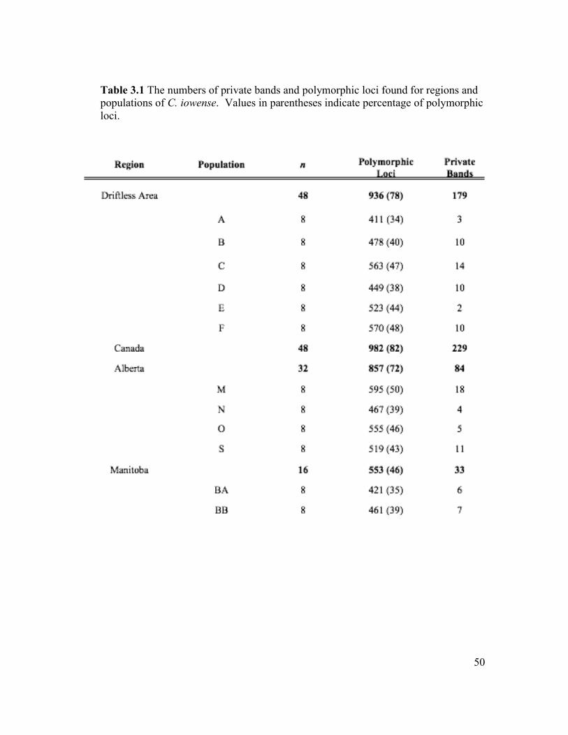
50

Table 3.1 The numbers of private bands and polymorphic loci found for regions and populations of C. iowense. Values in parentheses indicate percentage of polymorphic loci.

51

Table 3.2 Four dye-labeled ISSR primers used to genotype C. iowense.

52

Table 3.3 Estimates of average panmictic heterozygosity (HS) and total pooled heterozygosity (HT) for regional groups of C. iowense. Values in parentheses show the lower and upper bounds of a 95% Bayesian credible interval. Asterisks indicate values that are statistically different from others within the same column.

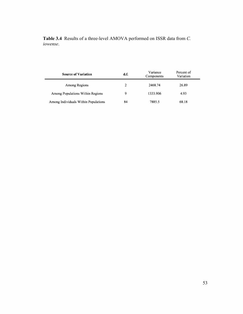
53

Table 3.4 Results of a three-level AMOVA performed on ISSR data from C. iowense.

54

Table 3.5 Pairwise θII comparisons among geographic regions of C. iowense. Values in parentheses show the lower and upper bounds of a 95% Bayesian credible interval. Asterisks indicate a value that is statistically different.

55

Figure 3.1 Map shows the species distribution of C. iowense, as well as sampling locations for the 12 populations analyzed in this study. The location of the Driftless Area is indicated in gray in the inset map.

N E W

S

56

Figure 3.2 Results of principal coordinates analysis (PCoA). The first three axes are represented in two 2-dimensional graphs. Individuals are coded by shape and color according to geographic origin (light gray triangle = Manitoba, dark gray square = Alberta, black circle = Driftless Area).

57

CHAPTER FOUR: THE GENETIC STRUCTURE AND GLACIAL HISTORY OF CHRYSOSPLENIUM TETRANDRUM, DETERMINED WITH INTER-SIMPLE SEQUENCE REPEATS

Abstract

The herbaceous perennial Chrysosplenium tetrandrum (Lund ex Malmgr.) Th. Fr.

(Saxifragaceae) is a self-pollinating, circumpolar species with a broad latitudinal

distribution and significant North American range disjunction. The southernmost

populations are isolated in the Colorado and Montana Rocky Mountains, distantly

separated from elements of the main range, which is largely coincident with known

glacial refugia (e.g., Beringia and Canadian Arctic Archipelago) as well as recently

deglaciated areas. We employed analyses of inter-simple sequence repeats (ISSRs)

and morphology to determine patterns of variation within the western North

American range of C. tetrandrum and test hypotheses of glacial population history

and reproductive strategy. We found very low levels (θII = 0.085) of range-wide

genetic differentiation and genetic diversity (HS = 0.077, HT = 0.084), which are

consistent with findings in other arctic species and attributed to recent population

establishment and clonality. Low levels of genetic differentiation within the Alaska

range (θII = 0.072), which might signify a recent bottleneck or range expansion into

the region. Both the Colorado and Alaska regions showed strong differentiation

between themselves and other geographic groups, suggesting long-term isolation.

The findings generally demonstrate a complex glacial history for the species.

58

Introduction

Factors that influence patterns of genetic variation within plant species are myriad.

They include contemporary as well as historical attributes of an organisms’ biology

(e.g., life history, physiology) and environment (e.g., physiography), which serve to

shape networks of gene flow within and among populations and determine the local

effects of genetic drift and natural selection (Stebbins, 1950; Silvertown, 2001). To

date, studies have revealed the genetic structure of hundreds of plant species, while

extensive reviews have detailed the specific roles of physical and biological attributes

in determining that structure (e.g., Hamrick et al., 1979; Loveless & Hamrick, 1984;

Hamrick & Godt 1989; Nybom & Bartish, 2000; Nybom, 2004). Despite the wealth

of genetic data available for many plant species, there still exist taxa for which, the

patterns of genetic variation and their causes remain largely unknown. Notable

among these groups is the arctic flora, which is thought to be lacking in biodiversity

at all levels but has been largely unexamined (Murray, 1987; Steltzer et al., 2008).

Throughout the late Tertiary and Quaternary periods, polar and sub-polar regions

of the world experienced substantial alterations to their physical environment. Cycles

of global climate change together with repeated periods of glacial advance and retreat

redistributed species across the landscape and established harsh new ecological

regimes at high latitude (Ewing & Donn, 1956; Billings & Mooney, 1968; Pielou,

1991). These events are believed to have had significant effects on the genetic

59

structure of arctic and boreal plant species (Hewitt, 1996; Hewitt, 2004). The actions

of glacial expansion, particularly regarding the extirpation of populations and the

reduction of species’ ranges, are credited with establishing a general state of low

intra-specific genetic diversity within the arctic flora (Pamilo & Savolainen, 1999).

The maintenance of this condition is largely attributed to the assumed frequency of

self-pollination in many arctic species, but may also stem from the influence of

powerful selective forces operating in stressful polar environments (Billings and

Mooney, 1968; Bliss, 1971). It is important to note, however, that these hypothesized

patterns of variation have not been widely confirmed (Murray, 1987; Steltzer et al.,

2008). To date, only a few arctic species (e.g., Saxifraga oppositifolia L. and Dryas

integrifolia Vahl.) have been the subject of intensive genetic study and, for these,

levels of genetic variation are often higher than traditional assumptions suggest

(Tremblay & Schoen, 1999; Abbott et al., 2000). Such findings have emphasized

additional aspects of arctic plant biology and glacial history, including the persistence

of populations in glacial refugia and higher-than-expected levels of outcrossing,

which contribute to the generation or maintenance of intra-specific genetic variation

(Hewitt, 1996; Gabrielsen & Brochmann, 1998; Hewitt, 2000; Abbott & Brochmann,

2003). Discordance between expected and observed results serves to underscore the

difficulty in establishing generalized theory to explain or predict patterns of variation

in a complex flora. An improved understanding of the evolution of the arctic flora

will require a consideration of this complexity, certainly as it relates to species’

glacial history, ecology, breeding system, and phylogenetic affinity. In the present

60

study, we investigate patterns of variation within the western North American range

of the arctic species Chrysosplenium tetrandrum (Lund ex Malmgr.) Th. Fr.

(Saxifragaceae) to elucidate further, arctic plant diversity.

Chrysosplenium tetrandrum is a widespread, circumpolar species with a complex

glacial and pre-glacial history (Fig. 4.1; Packer, 1963). The species range reaches as

far north as Murchisonfjord, North-East Land, Spitsbergen Archipelago (80° 3’ N;

Aiken et al., 1999) and is largely continuous throughout the arctic, but at its southern

extent, high elevation populations in Colorado remain strongly disjunct from the

central distribution (Packer, 1963). Weber (2003) suggested that these disjunct

elements may be late Tertiary-age relicts of a once prominent Oroboreal flora. These

populations, he contended, survived the Pleistocene glaciations in situ, persisting in

isolated Nunatak (i.e., high mountain) refugia (Blytt, 1876; Weber, 2003). Additional

ice-free regions existed in North America during the Pleistocene glaciations,

including the area to the south of the major ice-sheets (Darwin, 1859), Beringia (i.e.,

Alaska, Yukon Territory, and parts of Siberia; Hultén, 1937), coastal areas of western

British Columbia and southeastern Alaska (Heusser, 1960), and the Canadian Arctic

Archipelago (Hultén, 1937). The current distribution of C. tetrandrum (Fig. 4.1)

includes portions of each of these regions and it is possible that all of them played a

role in the glacial survival of the species. The long-term isolation and range

reduction associated with glaciation and refugial survival would have had significant

effects on patterns of genetic variation within species such as C. tetrandrum.

61

While glacial history has an important effect on levels of intra-specific genetic

diversity, so too do contemporary patterns of gene flow within species. However, at

present, these patterns are completely unknown within C. tetrandrum. The mode of

reproduction and breeding system of the species, which represent important

determinants in these patterns, are not confirmed, but preliminary evidence suggests

that C. tetrandrum is obligately self-pollinating and capable of vegetative

reproduction via stoloniferous growth (Warming, 1909; Packer, 1963; Weber, 1979).

These characteristics, combined with a short dispersal distance (< 0.5 m; Weber,

1979; Nakanishi, 2002), implies that intra-specific gene flow in C. tetrandrum is quite

localized and significantly limited.

As with many arctic plants species, the morphology of C. tetrandrum is highly

reduced and largely uniform across its range (Savile, 1972; Billings, 1987). Though

knowledge of the cause of taxonomically significant morphological variation in C.

tetrandrum is desirable, the relationship between genetic and morphological variation

in the species is unclear. Phenotypic plasticity is viewed as an important contributor

to phenotypic variation in arctic species and may account for the relatively high

degree of variation observed in traits of C. tetrandrum (Savile, 1972; Stenström et al.,

2002).

62

Instances of inter-specific gene flow can also have important consequences for

the evolution of a species. Such exchanges can produce novel genetic variation and

ultimately result in rapid speciation (Rieseberg, 1997; Rieseberg & Willis, 2007). In

the arctic, hybridization is thought to be quite common and consequently, important

to the evolution of the flora (Brochmann et al., 2004). In the case of C. tetrandrum,

the species is sympatric with a closely related species at two separate points in its

North American range (arctic coast, C. rosendahlii Packer; Alberta, C. iowense

Rydb.; Table 4.1). Within the sympatric zones, species have been found growing in

close proximity and exhibiting approximately identical phenology (Packer, 1963).

Despite this, there exists no evidence of hybridization between these taxa in either

region (Packer, 1963). A lack of gene flow may be attributable to biological barriers,

such as self-pollination and differences in chromosome number among species (i.e.,

C. tetrandrum 2n = 24, C. iowense 2n = c. 120, C. rosendahlii 2n = 96; Packer, 1963).

While hybridization between C. tetrandrum and either C. iowense or C. rosendahlli

appears unlikely, the prospect has not been thoroughly investigated. Both the

frequency of hybridization in other members of Saxifragaceae (e.g., Heuchera L.,

Mitella L.; Soltis et al., 2001) and the moderate levels of outcrossing described in C.

iowense suggest the possibility of even limited inter-specific gene flow.

The goal of this study was to determine patterns of genetic diversity within the

western North American range of C. tetrandrum. To achieve this, we employed inter-

simple sequence repeat (ISSR) markers (Huang & Sun, 2000) and used these data to

63

address the following questions: (1) what do contemporary levels of genetic diversity

indicate about patterns of gene flow within western North American C. tetrandrum;

(2) what is the level of genetic divergence between the Colorado and Montana

distribution of C. tetrandrum and its main Canadian and Alaskan distribution; (3) are

patterns of morphological variation correlated with those of genetic variation; and (4)

is there evidence of inter-specific gene flow between C. tetrandrum and C. iowense

and/or C. rosendahlii?

Materials and methods

Population sampling

Forty populations of C. tetrandrum were sampled from across the species’ western

North American range (Fig. 4.1; Table 4.1). These include two Alaskan populations

from which C. rosendahlii individuals were also collected and one Albertan

population from which C. iowense individuals were also collected (mixed populations

were not included in species-wide analyses). Whole flowering shoots were collected

from between 3 and 20 individuals per population, depending on total population size.

To avoid obtaining multiple samples from a single genet, a minimum spacing

requirement of 1 m between sampled clumps was used. The shoots were pressed and

stored in coin envelopes. Leaf material was removed from each shoot and dried in

64

silica gel for DNA extraction. For ten random individuals, duplicate DNA collections

were made to determine the reproducibility of the ISSR analyses (Bonin et al., 2004).

DNA extraction and ISSR survey

Between 3 and 16 individuals per population (402 total) were randomly selected

(when possible) for ISSR genotyping. DNA was extracted using DNeasy Plant Mini

Kits (Qiagen, Valencia, CA). Methods for DNA amplification, as well as PCR

product electrophoresis, visualization and sizing of products, and scoring are

discussed in detail by Archibald et al. (2006). All PCR reactions were a total of

25µL, including 0.5µL DNA, 50µM dye-labeled primer (D4, WellRED, Proligo, St.

Louis, MO), 25mM MgCl2, and 2x Bullseye (0.05 units/µL Bullseye Taq polymerase,

150mM Tris-HCl pH 8.5, 40mM (NH4)2SO4, 1.5mM MgCl2, 0.2% Tween 20, 0.4mM

dNTP’s, and stabilizer; MIDSCI, St. Louis, MO). The four primers (Table 4.2)

chosen for this study demonstrated utility during screening. Each PCR run involved 5

min at 94°C; 40 cycles of 45 s at 94°C, 45 s at 49-60°C, and 90 s at 72°C; 10 min at

72°C. ISSR electrophoresis and analysis was performed on a CEQ 8000 Genetic

Analysis System (Beckman Coulter, Fullerton, CA), using the Fragment Analysis

Module. Fluorescently labeled primers allowed detection by the automated sequencer

and fragment sizes were estimated using a custom 1000 bp size standard (MapMarker

1000, BioVentures, Murfeesboro, TN); bands of a given size were considered to

represent a single ‘locus’. Fragment analysis was conducted using the manufacturer’s

65

software (Beckman Coulter, Fullerton, CA). Analysis parameters were set to default

for minimum acceptable peak height and relative height.

Morphological measurement

Six quantitative traits were measured on each sampled individual: seed length, seed

width, sepal length, sepal width, hypanthium length, and hypanthium width. The

presence or absence of leaf and sepal maculation was also assessed as a binary

character. Floral measurements were taken from one of the central flowers in the

inflorescence. Length and width measurements of each sepal and hypanthium

measured were combined to produce ratio characters, which were used for

morphometric analyses. Individuals with missing measurement values were excluded

from those analyses.

Data analysis

The ISSR band profiles for duplicate samples were compared, and those loci that

exhibited a high frequency (≥ 40%) of mismatch across duplicate comparisons were

removed from the dataset. ISSR reproducibility was assessed, using the edited

dataset, as one minus the average frequency of mismatch for all duplicate

comparisons (Bonin et al., 2004).

66

We calculated the percentage of polymorphic loci (FAMD v1.108; Schlüter and

Harris 2006) and the number of private bands (i.e., a band that is present only in a

specific group and occurs in ≥ 4 individuals within that group) for each population

and regional group. To determine levels of genetic diversity within and among

populations, estimates of Nei’s (1973) average panmictic heterozygosity (HS) and

total panmictic heterozygosity (HT) were calculated using a Bayesian hierarchical

model (HICKORY v1.1; Holsinger & Lewis, 2003). Morphological diversity within

populations was measured by calculating average pair-wise morphometric (i.e.,

squared Euclidean distance) distances (APD) among individuals (PC-ORD; McCune &

Mefford, 1999). Levels of statistical significance among estimates of HS and HT were

determined by comparing 95% Bayesian credible intervals. Significance is assigned

when neither 95% credible interval includes the other estimate’s mean value.

Significant differences among APD estimates were determined with a permutation

analysis of variance (ANOVA; PERMDISP2; Anderson, 2004). A nonparametric

permutation approach was necessary given the non-independence of pair-wise

distance values.

Distance matrices were calculated for both the ISSR (FAMD v1.108; Schlüter &

Harris, 2006) and morphological (PC-ORD; McCune & Mefford, 1999) datasets. The

ISSR distance matrix was computed using the Dice similarity coefficient (Dice,

1945), which is desirable for use with dominant genetic data like ISSRs because it

excludes ‘shared absence’ characters (Archibald et al., 2006). Dice is calculated as

67

Sij =2n

11

2n11+ n

01+ n

10

where n11 is the number of shared bands between individuals and n01/n10 are the

number of mismatches between individuals. The distance transformation is expressed

as D = 1 – S. The morphological distance matrix is based on the squared Euclidean

distance measure, which was calculated from five morphological traits (i.e., seed

length, seed width, sepal length/width, hypanthium length/width, and

presence/absence maculation). A matrix of geographic distances (kilometers) among

sampled populations was also calculated (GEOGRAPHIC DISTANCE MATRIX GENERATOR

v1.2.2; Ersts, 2008).

Three Mantel tests were conducted to identify correlations between distance

matrices. The first test, ISSR distance versus geographic distance, was computed

using the software program ALLELES IN SPACE v1.0 (Miller, 2005), while the other

two, morphological distance versus geographic distance and morphological distance

versus ISSR distance, were computed using the program zt (Bonnet & Van de Peer,

2002). In each test, statistical significance was assessed by 10 000 permutations.

To analyze relationships among individuals, we performed a principal

coordinates analysis (PCoA; FAMD v1.108; Schlüter & Harris, 2006) using the Dice

distance matrix.

68

Levels of genetic differentiation among populations and regional groups were

estimated by calculating θII (HICKORY v1.1; Holsinger & Lewis, 2003), a Bayesian

analogue of Wright’s (1951) FST. The Bayesian approach is popular for producing

estimates of genetic differentiation from dominant data sets. This is because the

method permits θII to be estimated from the variance in inferred allele frequencies,

which cannot be directly observed from dominant data, without the need to invoke

assumptions regarding the level of inbreeding in populations (Holsinger et al. 2002).

HICKORY v1.1 (Holsinger & Lewis, 2003) analyses were conducted under the ƒ-free

model, following the authors’ (Holsinger & Lewis, 2003) suggestion for dominant

marker data sets. MCMC sampling parameters were set to default values: burn-in (50

000), sampling (250 000), and thinning (50). Two runs were performed for each

analysis to ensure convergence of the MCMC sampling algorithm. Statistical

comparisons of θII estimates were performed using the posterior comparisons option

in HICKORY. This method approximates the posterior distribution of θIIA - θII

B (i.e.,

the difference between estimates of θII derived from data sets A and B) from a sample

of θIIAi - θII

Bi (i.e., the difference between paired random samples from the posterior

distribution of θII for each data set; Holsinger & Lewis, 2003; Holsinger & Wallace,

2004). If the 95% credible interval of this distribution includes zero, then the

estimates cannot be considered statistically different (Holsinger & Lewis, 2003).

A locus-by-locus analysis of molecular variance (AMOVA) was performed

(ARLEQUIN v3.1; Excoffier et al., 2005) to determine the apportionment of genetic

69

variation within C. tetrandrum. Unlike the standard AMOVA computed in

ARLEQUIN, the locus-by-locus AMOVA treats each marker in a multi-locus genotype

as unlinked (Excoffier et al., 2005). Significance of observed variance components

was determined with 5000 permutations.

Analysis of mixed populations

To investigate the possibility of inter-specific gene flow between C. tetrandrum and

either C. iowense or C. rosendahlii, we constructed new, smaller genetic and

morphological data sets for each case. For C. tetrandrum - C. iowense, the data sets

consisted of five populations, including: two of C. tetrandrum (i.e., BD and CM), two

Alberta populations of C. iowense and one mixed population (i.e., BC; Table 4.1).

For C. tetrandrum – C. rosendahlii, the data sets consisted of six populations,

including: two of C. tetrandrum (i.e., BX and CE), two Northern Alaskan populations

of C. rosendahlii, and two mixed populations (i.e., BZ and CC; Table 4.1). Principal

components analyses (PCA) were performed (PC-ORD; McCune & Mefford, 1999) on

the two morphological data sets to identify intermediate phenotypes. Locus-by-locus

AMOVAs (ARLEQUIN v3.1; Excoffier et al., 2005) were performed on each of the

genetic data sets to identify loci that exhibit high (≥ 0.5) levels of differentiation, φST,

between species. These, highly differentiated loci, composed new genetic data sets

that were analyzed in NEWHYBRIDS v1.1 (Anderson, 2003), which implements a

Bayesian approach to testing hypotheses of hybrid ancestry. The program computes

70

the posterior probability that individuals belong to different hybrid categories: pure C.

tetrandrum, pure C. iowense or C. rosendahlii, F1, F2, backcross with C. tetrandrum,

and backcross with C. iowense or C. rosendahlii. Two replicate runs of each analysis

were performed to ensure consistency among results.

Results

Genetic and morphological variation

ISSR analyses produced 701 loci, of which, 659 (94%) were polymorphic across all

samples. Repeatability of ISSR markers was 95%. Table 4.1 summarizes the

distribution of private bands (PB) and polymorphic loci (PL) among populations and

regions. The percentage of polymorphic bands varied among populations (range, 10 -

50%; mean, 24% ± 11) and regions (range, 29 – 76%; mean, 55% ± 18). The most

polymorphic region was Alaska/Yukon (76%) followed closely by Washington

(70%). Private bands (PB) were found in only two populations, population H (five

bands) and population U (one band), and three regions, Washington (eight), British

Columbia (three), and Alaska/Yukon (nine).

Range-wide estimates of average panmictic heterozygosity and total panmictic

heterozygosity were 0.077 (± 0.004) and 0.084 (± 0.005), respectively.

Heterozygosity estimates were statistically invariant across populations, but did differ

71

among regions, with values for Alaska/Yukon (HS = 0.085; HT = 0.092) significantly

lower than those of other groups (Table 4.1). The average pair-wise distance (APD)

measure, which indicates levels of morphological variation within groups, was found

to be statistically invariant among populations and regions (Table 4.1).

Three Mantel tests produced the following estimates of association between sets

of distance matrices: ISSR versus geographic (r = 0.015, P = 0.238), morphological

versus geographic (r = -0.104, P = 0.086), and ISSR versus morphological (r = -

0.013, P = 0.433). In all three tests, we found no significant correlation between

matrices.

The first three plotted axes of the PCoA (Fig. 4.2) accounted for 18.43% of the

total variation at the molecular level. The analysis did not indicate clear genetic

structure within C. tetrandrum. This finding is consistent with the range-wide

Bayesian estimate of genetic differentiation (θII = 0.085 ± 0.004). Pair-wise estimates

of genetic differentiation within and among regions are summarized in Table 4.3.

The highest intra-regional θII values were found in Alberta (0.173) and Colorado

(0.214). Inter-regional FST values were highest in comparisons made to

Alaska/Yukon, Colorado, and Montana.

A locus-by-locus AMOVA (Table 4.4) reported that the greatest percentage of

genetic variation (84.59%) in the data set was accounted for by differences among

72

individuals within populations. In contrast, very little variation was accounted for by

differences among populations (11.9%) or regions (3.52%).

Inter-specific gene flow

Principal components analyses

In the case of each species-to-species comparison, a PCA (Fig. 4.3) of morphological

data clearly grouped all individuals into one of two species groups and did not

indicate any individuals with intermediate phenotypes that might suggest mixed

ancestry.

Genetic analyses

To identify genetic evidence of gene flow between C. tetrandrum and C. iowense, a

reduced ISSR data set was constructed and consisted of 33 loci, which were found to

be highly differentiated (φST ≥ 0.5) between species. Genetic analyses placed 38 out

of 50 individuals into pure species categories with a posterior probability greater than

0.8. One individual, belonging to the mixed population and indicated in Fig. 4.3 by

an arrow, was placed with high posterior probability (0.933) in the C. tetrandrum

backcross category.

73

The data set for the C. tetrandrum-C. rosendahlii comparison consisted of six

highly differentiated loci. Nineteen of seventy-two individuals were placed within a

pure species category with a posterior probability above 0.8 and no individuals were

placed within a hybrid category with a probability higher than 0.3.

Discussion

Genetic diversity and breeding system in C. tetrandrum

Reproductive strategy is one of the most important factors to influence patterns of

genetic diversity within plant species (Loveless & Hamrick, 1984; Nybom & Bartish,

2000). Components of reproductive strategy (e.g., mode of reproduction and

breeding system) dictate a fundamental level of gene flow within and among

populations, which can then be modified by additional aspects of a species’ biology

and ecology (Hamrick & Godt, 1989). Asexual modes of reproduction eliminate

chromosomal recombination and gene flow among individuals, though multiclonal

populations are often as genetically diverse as their sexual counterparts (Ellstrand &

Roose, 1987; Hamrick & Godt, 1989; Coates & Byrne, 2005). Alternatively, sexual

reproduction allows for recombination and gene flow, though the rates of these

processes are determined by breeding system. Predominant outcrossing systems,

characterized by gene flow among unrelated individuals, are associated with high

levels of intra-populational diversity. Predominant self-pollinating systems result in

74

reduced rates of recombination and lower levels of diversity within populations (Jain,

1976; Hamrick & Loveless, 1984).

Chrysosplenium tetrandrum has been described (Warming,1909) as a purely

selfing species. The results of this study are mixed in their support for this assertion.

Analyses of ISSR markers yielded very low range-wide estimates of expected

heterozygosity (HS = 0.077, HT = 0.084) and similarly low values for individual

populations and regions (Table 1). These results are consistent with an autogamous

C. tetrandrum. Alternatively, low range-wide estimates of genetic differentiation (θII

= 0.085) contradict this hypothesis. Predominant selfing species lack gene flow

among individuals and populations, leading to high levels of genetic differentiation,

which were not observed in this study (Hamrick & Godt, 1989). We consider two

factors to be central to reconciling this contradiction; the first is the importance of

asexual reproduction suggested for C. tetrandrum and the second is the recent (8 -10

kya) establishment of many populations in the western range of this species as a result

of glacial dynamics. Balloux et al. (2003) demonstrated that, by effectively fixing

heterozygotes, asexual reproduction in diploid species increases gene diversity at

individual loci and decreases population differentiation. The authors also suggested

that with predominant asexual reproduction there is an expected decrease in

genotypic diversity (e.g., HS, HT), as we see with our results (Balloux et al., 2003).

However, despite its explanatory ability, we cannot conclusively identify asexuality

as a main cause of the observed genetic patterns given that evidence of its effect (e.g.,

75

heterozygote excess at single loci) is not available to investigations using dominant

molecular markers (Balloux et al., 2003). Short evolutionary history can also explain

low levels of species-wide differentiation at high latitudes (Odasz & Savolainen,

1996; Max et al., 1999; Pamilo & Savolainen, 1999). For many high latitude

populations, the period since glacial retreat may have been too short for many

population processes to have reached equilibrium (Varvio et al., 1986; Pamilo &

Savolainen, 1999). With the presumed frequency of clonality in arctic plants, both of

these processes may be operating interactively to reduce levels of genetic

differentiation within some high latitude species.

Genetic structure

As previously mentioned, the overall measure of genetic differentiation was low (θII =

0.085), particularly when compared to the φST value (0.35 ± 0.18) reported by Nybom

(2004) as an average for intra-specific ISSR studies. However, our result is

comparable to the average species-wide FST estimate from other high latitude species

(0.036; Hamrick & Godt, 1989). The θII estimates are consistent with the results of

an AMOVA (Table 4.4) and a PCoA (Fig. 4.3), which report that most of the

variation in the data set is accounted for by differences among individuals within

populations. There is no statistical support (see results of ISSR v geographic distance

Mantel test) for the hypothesis that levels of genetic differentiation were the result of

isolation-by-distance (Wright, 1943). Again, we attribute this pattern largely to

76

recent population establishment and, perhaps also, the fixation of ancestral allele

frequencies by of asexual reproduction.

Glacial refugia and post-glacial migration

The Pleistocene history of glaciation in northwestern North America is complex

(Heusser, 1960). Over a period of two million years this region experienced four

major glacial stages (i.e., Nebraskan, Kansan, Illinoian, Wisconsin), the most recent

of which, Wisconsin, reached its maximum extent about 18 kya (Trenhaile, 2004).

Throughout each of these stages large ice-sheets covered much of northern North

America (Pielou, 1991). The arctic, boreal, and north temperate plant species that

occur in high latitude environments today are descendants of ancestors that survived

these glaciations in ice-free areas, known as glacial refugia (Pielou, 1991). Two of

the largest and most important refugia in western North America were the Southern

refugium (Darwin, 1859), which consisted of the entire region south of the Laurentide

and Cordilleran glaciers, and Beringia (Hultén, 1937), which includes large tracts of

what is today Alaska and the Yukon Territory. Additional, smaller refugia existed

along the coasts of British Columbia and southern Alaska, as well as possibly in the

southern Canadian Rocky Mountains (Heusser, 1960; Loehr et al., 2005). The use of

molecular data to determine the role of these North American refugia has become

commonplace (e.g., Tremblay & Schoen, 1999; Eidesen et al., 2007; Marr et al.,

2008) and this accumulating information provides the basis for further formulation of

77

genetic predictions given specific historical scenarios. In the following, we discuss

the putative roles (i.e., glacial refuge or area of recolonization) of sampled geographic

regions as determined by patterns of genetic variation.

Alaska/Yukon

Alaska and the Yukon Territory form the western portion of the Beringia refugium

(Hultén, 1937). Paleontological and molecular evidence (Hopkins, 1967; Abbott et

al., 2000; Abbott & Brochmann, 2003) confirm both the existence of arctic plant

species in the area throughout the Wisconsin glaciation (115-15 kya) and the region’s

role as a center for post-glacial recolonization. Thus, we expected Alaska/Yukon

populations of C. tetrandrum to exhibit comparatively high levels of genetic diversity

(Table 4.1) and differentiation among populations (Table 4.3), reflecting long-term

persistence and large population sizes (Hewitt, 2004). The results, however, show

very low levels of genetic diversity (Table 4.1) and differentiation within the region

(Table 4.3), patterns that are more consistent with scenarios of rapid range expansion

or recent bottleneck events, or both (Ibrahim et al., 1995; Hewitt, 1996). Given then,

a scenario of recent range expansion, it is difficult to determine if contemporary

Alaska/Yukon populations are derived from Beringian ancestors or non-Beringian

migrants that moved into Alaska following glacial retreat. If the former is correct, the

high levels of genetic differentiation between this region and others, evidenced by θII

estimates and private band numbers, strongly suggest that those resident Beringian

78

populations did not serve as important sources of post-glacial recolonization for this

species.

Washington

Sampled Washington populations occur at the northern edge of the southern refugium

and perhaps also served as a source of post-glacial recolonization (Heusser, 1960;

Soltis et al., 1996). While genetic diversity estimates (Table 4.1) provide

inconclusive evidence of a refugial history for this region, low levels of genetic

differentiation between these populations and the Canadian ranges suggest recent

connections or the presence of recurrent gene flow (Cruzan & Templeton, 2000).

British Columbia and Alberta

Most of British Columbia and Alberta were completely glaciated as late as 10 kya

(Heusser, 1960; Trenhaile, 2004) and the contemporary C. tetrandrum range in these

regions is expected to have been established during a period of post-glacial

recolonization. Generally, low levels of genetic diversity and differentiation would

characterize a scenario of recent range expansion, however, if populations in these

areas are derived from separate refugia they may exhibit comparatively high levels of

differentiation (Hewitt, 1996; Marr et al., 2008). In fact, the results are consistent

with both explanations. British Columbia populations maintain low levels of genetic

79

diversity and differentiation, while Albertan populations show much higher levels of

intra-regional divergence. The relatively low levels of differentiation between

Alberta and both British Columbia and Washington suggest that either of the latter

regions served as one source of migrants during the recolonization process. The other

putative refugial source is not known, though it may be the unglaciated portion of the

southern Canadian Rockies that occurred between the Laurentide and Cordilleran

glaciers (Packer & Vitt, 1974; Loehr et al., 2005).

Colorado and Montana

According to Weber (2003), Colorado and possibly Montana populations of C.

tetrandrum may be oroboreal relicts from the late Tertiary (2-3 mya). This suggests a

considerable period of isolation for these populations and would require high levels of

differentiation from the main distribution (Hewitt, 1996). While the levels of

divergence are higher than most in the data set, they do not demonstrate conclusively

a long period of isolation, certainly no more in some cases than that experienced by

the Alaskan populations. The high levels of differentiation and genetic diversity are

consistent with long-term persistence in this region (Hewitt, 2004; Abbott et al.,

2000).

Morphological variation

80

In predominant self-pollinating species, recombination rates are decreased and the

persistence of linkage disequilibrium is increased (Jain, 1976; Flint-Garcia et al.,

2003). Thus, compared to predominant outcrossing species, self-pollinators are

expected to exhibit stronger associations between neutral genetic and morphological

variation (Price et al., 1984). However, we find that ISSR variation is not correlated

with morphological variation in C. tetrandrum. This non-association may be

attributed to the independent segregation of genetic and quantitative trait loci, perhaps

due to some sexual reproduction in populations, or the highly plastic nature of

measured morphological traits.

Mixed populations

The North American range of C. tetrandrum becomes sympatric with those of its

sister species, C. iowense (in western Alberta) and C. rosendahlii (on arctic coast).

Packer (1963) posited that habitat differences between these species were not

substantial and that, while they had not yet been found, there was no reason that

mixed populations could not occur. In this study, we identified mixed populations

between C. tetrandrum and C. iowense and C. tetrandrum and C. rosendahlii.

However, despite the spatial proximity of these conspecific individuals, there exist

some compelling barriers to inter-specific gene flow. These barriers include different

chromosome numbers for each species and predominantly selfing mode of

reproduction (Warming, 1909; Packer, 1963). We found no evidence of

81

morphological intermediates in any of the mixed populations that might suggest

hybrid ancestry. Likewise, genetic analyses were largely unable to exhibit evidence

of gene flow. One individual in the C. tetrandrum-C. iowense mixed population was

identified with high confidence as a backcross. This result is not compelling evidence

of widespread gene flow, but should promote further investigation of these mixed

populations, especially with regard to chromosome numbers.

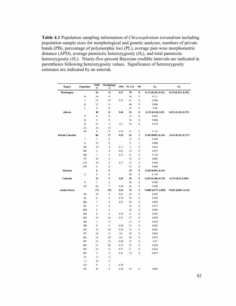
82

Table 4.1 Population sampling information of Chrysosplenium tetrandrum including population sample sizes for morphological and genetic analyses, numbers of private bands (PB), percentage of polymorphic loci (PL), average pair-wise morphometric distance (APD), average panmictic heterozygosity (HS), and total panmictic heterozygosity (HT). Ninety-five percent Bayesian credible intervals are indicated in parentheses following heterozygosity values. Significance of heterozygosity estimates are indicated by an asterisk.

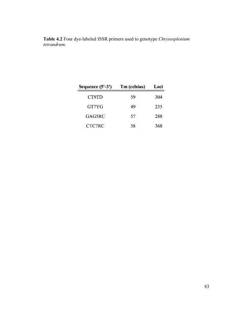
83

Table 4.2 Four dye-labeled ISSR primers used to genotype Chrysosplenium tetrandrum.

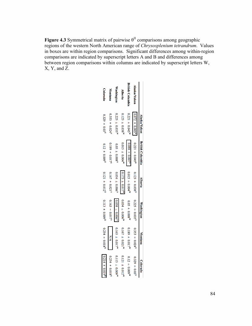
84

Figure 4.3 Symmetrical matrix of pairwise θII comparisons among geographic regions of the western North American range of Chrysosplenium tetrandrum. Values in boxes are within region comparisons. Significant differences among within-region comparisons are indicated by superscript letters A and B and differences among between region comparisons within columns are indicated by superscript letters W, X, Y, and Z.

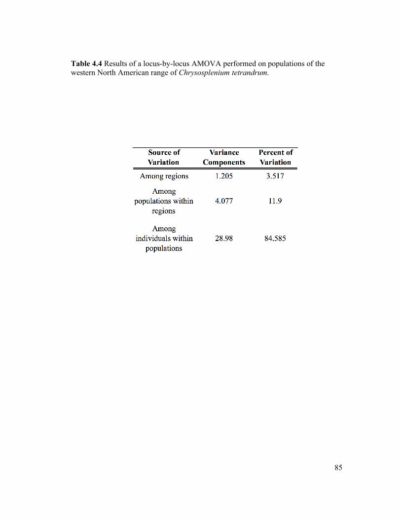
85

Table 4.4 Results of a locus-by-locus AMOVA performed on populations of the western North American range of Chrysosplenium tetrandrum.

86

Figure 4.1 Map shows the species distribution of Chrysosplenium tetrandrum, as well as sampling locations for 40 populations analyzed in this study.

N E W

S

87

Figure 4.2 Principal coordinates analysis (PCoA) of ISSR profiles. The first three axes are represented in two 2-dimensional graphs. Chrysosplenium tetrandrum individuals are coded by shape and color according to geographic origin.

88

Figure 4.3 Principal components analyses (PCA) of morphological data. The result on the left is from analysis between Chrysosplenium tetrandrum and C. rosendahlii and the result on the right is from a C. tetrandrum and C. iowense comparison. The arrow indicates the individual, which was recovered with high probability as a C. tetrandrum backcross.

89

CHAPTER FIVE:

NEI’S TO BAYES’: COMPARING COMPUTATIONAL METHODS AND GENETIC MARKERS FOR ESTIMATING PATTERNS OF GENETIC VARIATION IN TOLPIS (ASTERACEAE)

Abstract

Accurate determination of patterns of genetic variation provides a powerful

inferential tool for studies of evolution and conservation. For more than 30 years,

enzyme electrophoresis was the preferred method for elucidating these patterns. As a

result, evolutionary geneticists have acquired considerable understanding of the

relationship between patterns of allozyme variation and aspects of evolutionary

process. Myriad molecular markers and statistical analyses have since emerged,

enabling improved estimates of patterns of genetic diversity. With these advances,

there is a need to evaluate results obtained with different markers and analytical

methods. We present a comparative study of gene statistic estimates (FST, GST, FIS,

HS, and HT) calculated from an ISSR and an allozyme data set derived from the same

populations using both standard and Bayesian statistical approaches. Significant

differences were found between estimates, owing to the effects of marker and

analysis type. Most notably, FST estimates for codominant data differ between

Bayesian and standard approaches. Levels of statistical significance are greatly

affected by methodology and, in some cases are not associated with similar levels of

90

biological significance. Our results suggest that caution should be used in equating or

comparing results obtained using different markers and/or methods of analysis.

Introduction

The patterns of genetic variation within and among populations are of interest to

diverse fields in plant biology including population genetics, systematics, and

conservation. For the past four decades, following the demonstration of the utility of

enzyme electrophoresis (Harris, 1966; Hubby & Lewontin, 1966; Lewontin & Hubby,

1966), there has been an ever-increasing use of various types of molecular markers to

assess genetic variation. The basic rationale for molecular markers replacing earlier

approaches such as quantitative characters as a means of assessing genetic variation is

the more direct equation between genotype and phenotype obtained with molecular

methods (Lewontin & Hubby, 1966; Schulman, 2007). However, as the science has

progressed, considerations of improved efficiency and sensitivity have promoted the

development of new molecular markers, many of which present significant analytical

challenges to accurately assessing genetic variation (Sunnucks, 2000). Although

ongoing developments in statistical analyses offer the potential to overcome these

challenges, there is still a general inability to knowledgeably compare analogous

estimates derived from different marker classes and/or statistical methods (Bonin et

al., 2007).

91

For more than four decades, allozyme markers have been an invaluable tool for

studies of evolutionary genetics, providing plant biologists with a straightforward,

low cost means of estimating levels of intra-specific genetic variation (Cruzan, 1998).

Allozymes produce codominant data, which permit direct observation of allele

frequencies at allozyme loci and can be used rather simply to calculate various gene

statistics (Hubby & Lewontin, 1966; Lewontin & Hubby, 1966; Hamrick, 1989;

Weeden & Wendel, 1989). In addition, because of the highly conserved nature of

allozyme loci in flowering plants (Gottlieb, 1982) homologous loci can be compared

between closely related species. Practical advantages of allozymes include the

relative procedural simplicity and low cost of the method (Clegg, 1989). Because of

the large database that has accrued for allozymes, their estimated patterns of variation

can be compared among plants with different ecological and life history traits (e.g.,

Hamrick & Godt, 1989). One of the major criticisms of allozyme data concerns the

level of genome sampling; allozyme variation can only be determined for protein-

coding genes (many of the assays are for enzymes of glycolysis and the citric acid

cycle) of which, in plants, there is a rather small (~ 40) potential pool of useful

candidates (Clegg, 1989; Wendel & Weeden, 1989). This number is further reduced

for within-species studies where often only about 50% of the loci are polymorphic

(Hamrick & Godt, 1989). In addition, variation at each of these loci may only be

detected if it affects the electrophoretic mobility of the enzyme with the standard

conditions employed (Lewontin & Hubby, 1966; Clegg, 1989). As much as 20% of

the base substitutions may go undetected (Coates & Byrne, 2005). Allozyme

92

variation is often absent in groups of recently radiated taxa for which allozymes

frequently provide limited and/or imprecise estimates of population genetic structure

(e.g., Schwartz, 1985; Crawford et al., 1987).

In contrast to allozymes, arbitrarily amplified DNA (AAD) methods (e.g., AFLP,

inter-simple sequence repeat, and random amplified polymorphic DNA) are able to

produce large data sets, especially when loci are visualized using polyacrylamide

gels. These loci presumably represent neutral, rapidly evolving regions from across

the genome (Clegg, 1989; Huang & Sun, 2000; Krauss, 2000; Archibald et al., 2006).

Very small amounts of plant material are needed for these markers, making them

ideal for use with rare species. Utilizing PCR, AAD methods amplify a specific

region of DNA or ‘allele’, which is visualized on an electrophoretic gel as a band

presence or absence. Because band presence can indicate either the dominant

homozygote or heterozygote, genotype and allele frequencies cannot be directly

determined and estimation of gene statistics can be problematic (Meudt & Clarke,

2007). This represents a significant disadvantage compared to allozymes. However,

the increased level of variation often seen with AAD markers and the increased ease

of obtaining the required amount of plant material has led to these markers being

preferred over allozymes in many studies; particularly in cases where genetic

variation within and among populations and/or species is low (Crawford et al., 1994;

Crawford et al., 2001).

93

Although codominant markers like allozymes are preferred for most genetic

studies, especially those that calculate statistics requiring knowledge of allele

frequencies, recently developed analytical techniques have allowed researchers to

take greater advantage of the benefits of dominant markers (Krauss, 2000; Bonin et

al., 2007). The traditional approach to estimating levels of population structure with

allele frequency data has typically involved the use of F-statistics (i.e., FIT, FIS, FST).

These were originally defined by Wright (1943; 1951) and based on correlations

between uniting gametes at different hierarchical levels, total population (T) and

population subdivision (S). Nei (1973; 1977), seeking to expand the use of Wright’s

F-statistics beyond a single locus two allele system, redefined them as functions of

partitioned gene diversity and calculated levels of inbreeding (FIS and FIT) and

genetic differentiation (GST) using measures of observed (HO) and expected (HS and

HT) heterozygosity. Nei’s (1973) coefficient of gene differentiation, GST, is a multi-

locus, multi-allele equivalent of Wright’s FST.

Though F-statistics have been used extensively with codominant data, the

methodological requirement of allele frequency estimates has made their application

to dominant data problematic. Bayesian statistical analysis is an approach that is

increasingly applied to evolutionary genetic studies because it ostensibly offers

investigators the ability to overcome some of the analytical shortfalls of dominant

data sets (Zhivotovsky, 1999; Holsinger et al., 2002). One of the more prominent

implementations of Bayesian statistics to the analysis of dominant data is the method

94

described by Holsinger et al. (2002). The method is based on a Bayesian hierarchical

model and directly estimates an FST analogue (θB) from dominant or codominant data,

while incorporating the effect of uncertainty in inbreeding (FIS) on this estimate

(Holsinger et al., 2002). Holsinger et al. (2002) has demonstrated that this method

produces reliable estimates of FST (although see Bonin et al., 2007) and allele

frequencies without the assumption of a known inbreeding coefficient, which is

required by other approaches (Lynch & Milligan, 1994; Zhivotovsky, 1999). By

using the Bayesian estimate of mean allele frequency to calculate expected panmictic

heterozygosities (HS and HT), the method is also able to produce an estimate of Nei’s

GST, known as GSTB. Under this framework, θB corresponds to a random-effects

model of population sampling, which produces estimates from all potentially sampled

populations and presumably reduces sampling error (Weir, 1996, p. 162; Holsinger,

1999). Alternatively, the GST B estimate corresponds to a fixed-effects model and is

derived from all actually sampled populations (Weir, 1996, p. 162; Holsinger, 1999).

Unlike standard implementations of the random-effects model (i.e., Weir and

Cockerham, 1984), the Bayesian method is able to use it without a specified model of

population divergence (Holsinger, 1999).

Despite their respective limitations, both allozyme and dominant data offer

viable, low cost alternatives to more resource intensive methods (e.g., microsatellites;

Schulman, 2007; Agarwal et al., 2008). At present, the greatly increased use of

dominant markers over allozymes and the aforementioned large database available for

95

allozymes provides the potential to compare results from the two types of markers

and relate them to many traits of plant ecology and life history. However, the

relationships among analogous gene statistics derived from different marker classes

and statistical methods are not well known. A better understanding of the

comparability of gene statistic estimates derived from different methods will allow a

more complete synthesis of the knowledge accumulated throughout more than 40

years of molecular genetic research. The opportunity for researchers to employ the

full body of this knowledge will benefit a broad range of studies across the fields of

plant genetics, systematics, and conservation, placing in a larger biological context

the results of newer methods of data production and analysis.

For insight into the relationships among gene statistic estimates, comparisons of

these estimates should be conducted across a broad range of biological conditions

(i.e., patterns of genetic variation) and include empirical data for both codominant

and dominant markers from the same populations. The purpose of this study was to

respond to this need for comparative data among different commonly used markers

and methods of analysis. We present a comparison of analogous estimates of FST,

GST, FIS, and expected heterozygosity derived from dominant (inter-simple sequence

repeat, ISSR) and codominant (allozyme) data sets for the angiosperm genus Tolpis

(Asteraceae) using the Holsinger et al. (2002) Bayesian method, as well as standard

approaches to codominant and dominant data. Tolpis represents a recent radiation for

which both dominant and codominant data have been used to assess genetic

96

relationships among taxa, as well as other aspects of species biology (Crawford et al.,

2006; Archibald et al., 2006). By comparing specific estimates (Table 5.1), our goal

was to determine patterns of relationships among analogous gene statistics and

provide additional information as to the operation of Bayesian analysis when applied

to individual empirical studies.

Materials and methods

Data

Tolpis (Asteraceae) is a Macaronesian and Mediterranean angiosperm genus, of

which the majority of species represent a recent radiation within the Canary Island

archipelago (Park et al., 2001; Crawford et al., 2006). From this Canarian radiation,

we sampled 15 populations across five species (Table 5.2), constituting the bulk of

the so-called T. laciniata-T. lagopoda complex (Archibald et al., 2006; Crawford et

al., 2006). This complex comprises a high level of morphological and ecological

variation, though all species share a perennial habit and are highly self-incompatible

(Crawford et al., 2008). Tolpis laciniata and T. lagopoda, in particular, form large

outcrossing populations (Crawford et al., 2006).

Individuals from each of the 15 populations sampled were genotyped at 10

polymorphic allozyme loci (GPI-2, PGM-1, TPI-1, TPI-2, PGD-1, PGD-2, GDH,

97

AAT-2, AAT-3, MDH-3) and at 1510 polymorphic ISSR loci. Protocols for enzyme

electrophoresis and ISSR amplification and scoring are described in Crawford et al.

(2006) and Archibald et al. (2006), respectively. Population sample sizes varied

between marker classes. The allozyme data set averaged 17 individuals per

population (range, 6-29), while the ISSR data set averaged almost eight individuals

per population (range, 3-14). All 10 allozyme loci had three or more alleles (seven

maximum) at a locus.

Analyses

Allozyme data were analyzed using both the Bayesian approach implemented in the

program HICKORY v1.1 (Holsinger & Lewis, 2003) and the standard methods

described by Nei and Chesser (1983), which were manually calculated. HICKORY

estimates the Bayesian analogue of Weir and Cockerham’s (1984) FST and Wright’s

FIS (1951), designated in the program as θII and ƒ, respectively (Holsinger, 1999;

Holsinger et al., 2002; Holsinger & Lewis 2003). It also provides estimates of Nei’s

(1973) average expected panmictic heterozygosity (HS), total expected panmictic

heterozygosity (HT), and coefficient of gene differentiation (GST), denoted by GSTB.

Bayesian analyses of the codominant allozyme data set in HICKORY were performed

with default parameter settings (burn-in = 50 000, sampling = 250 000, thinning = 50)

under the full model analysis, which provides estimates of both θII and ƒ. Nei and

Chesser’s (1983) methods produce unbiased estimates of GST, FIS, HS, and HT. The

98

GST statistic is a multi-locus, multi-allele estimate of Wright’s FST (Nei, 1973) and is

often (as in the cases of Hall et al., 1994; Yeh et al., 1997) designated as the latter for

ease of discussion. For this reason, we too refer to this estimate as FST. However,

considering its statistical affinity we compared it to both θII and GSTB.

The ISSR data set was analyzed using HICKORY, under both the ƒ-free and full

model options and with ARLEQUIN v3.1 (Excoffier et al., 2005). Under HICKORY’s

full model, estimates of ƒ influence those of θII and vice versa (Holsinger et al.,

2002). Because estimates of ƒ have been shown to be unreliable when calculated

from dominant data sets, especially with small population sample sizes, Holsinger

and Lewis (2003) suggest that under these conditions the ƒ-free model, which

removes the constraints of ƒ on θII estimation, may be more appropriate. Both of

these analyses were performed under the default parameter settings described above.

Two replicate runs of each HICKORY analysis, for both marker classes, were produced

to ensure convergence of the Markov chain Monte Carlo (MCMC) sampler.

In ARLEQUIN, a locus-by-locus analysis of molecular variance (AMOVA)

produced locus-specific estimates of φST, which is an FST analogue based on pair-wise

squared Euclidean distances (Excoffier et al., 1992; Excoffier et al., 2005). The

average of these individual values was calculated to produce the multi-locus estimate

reported in the results. The AMOVA is a commonly used method for producing

estimates of genetic differentiation from dominant data.

99

Statistical comparisons among estimates were conducted using 95% Bayesian

credible intervals and confidence intervals for individual estimates. In HICKORY, the

production of a sample log file during analysis allowed a statistical comparison of θII

and ƒ estimates (described in Holsinger & Wallace, 2004) using the posterior

comparison option. Pairwise comparisons involving non-Bayesian estimates required

the calculation of a 95% confidence interval (Zar, 1999), which could be compared to

a similar Bayesian credible interval. Estimates were considered statistically different

if each confidence/credible interval did not overlap the other estimate’s mean value.

The following comparisons (summarized in Table 5.1) were considered for

statistical analysis and discussion: i. comparison between Bayesian and standard

analyses of an allozyme data set; ii. comparison between models of Bayesian analysis

applied to an ISSR data set; iii. comparison between Bayesian and AMOVA

estimates applied to an ISSR data set; iv. comparison between ISSR and allozyme

estimates produced by Bayesian analyses.

Sample size differences

Population sample size is an important factor in gene statistic estimation and

differential sampling of a given population or set of subpopulations may yield

disparate estimates of genetic structure (Bonin et al., 2007). In this study, differences

100

in population sample sizes between marker classes could potentially account for

differences in estimates of population parameters between those classes. To

determine if, and in what way, the differences in sample size between the ISSR and

allozyme data sets have influenced estimates of genetic differentiation in this study,

the following analyses were conducted: 1.) populations with ISSR sample sizes of

three individuals (i.e., 17 and 1869; Table 5.2) were removed from the allozyme and

ISSR data sets and FST and/or θII were recalculated for both; 2.) population sample

sizes in the allozyme data set were reduced, randomly, to equal the corresponding

sample sizes in the ISSR data set, then FST and θII estimates were recalculated.

Data simulation and analysis

Two data simulation studies were conducted to address aspects of Bayesian gene

statistic estimation that surfaced in the results of our analyses of the empirical data

sets. Simulation study 1 was designed to investigate divergent allozyme FST

estimates for standard and Bayesian methods, while simulation study 2 addressed the

effects of sample size on accurate ƒ estimation with dominant data.

Simulation study 1

The program EASYPOP v1.7 (Balloux, 2001), a forward-time simulator employing an

individual based model of evolution, was used to produce 110 codominant data sets.

101

Evolution was simulated at 15 multiallelic loci (i.e., with five alleles each) for four

populations of 100 diploid individuals each and 20 individuals per population were

randomly subsampled for analysis. There was no migration, mutation, or selfing, and

mating was random. Simulation durations (i.e., number of generations) were varied

to produce different final FST values. Each of the data sets was analyzed using a

standard approach in the program POPGENE v1.32 (Yeh and Boyle, 1997; Yeh et al.,

1997) and the Bayesian full model from HICKORY. The differences between the

FST/GST estimates produced by these methods were plotted against the simulated FST.

Simulation study 2

Using the program EASYPOP v1.7 (Balloux, 2001), we simulated five data sets at each

of five FST value ranges (0.01-0.1, 0.275-0.325, 0.4-0.45, 0.55-0.6, 0.8-0.85) for four

different sample sizes (20, 50, 100, and 200 individuals). Data sets consisted of 10

populations of 500 individuals each. Each population was randomly subsampled to

produce the sample sizes listed above. Individuals’ genotypes comprised 100

biallelic loci, which were converted to dominant data. Simulated FIS values ranged

between 0.13 and 0.15. Evolution input parameters for simulations included: no

migration, no mutation, and a 0.25 selfing value. Simulated data sets were analyzed

in HICKORY under the full model.

Results

102

FST and GST

Our estimates of FST differed according to analytical method (Fig. 5.1). The standard

method (AS; see Table 5.1 for designation of methods) estimate for allozymes (0.388

± 0.22) exceeded all three of the Bayesian θII values, including that produced (0.172 ±

0.017) for the same allozyme data set (AB). Different model analyses of ISSR data in

HICKORY produced significantly different results for θII (IB, 0.165 ± 0.003; IBf, 0.147

± 0.007), though neither could be distinguished statistically from the AB estimate.

The AMOVA-based φST estimate (IS, 0.137 ± 0.151) was statistically different from

the IB estimate, but not from that of IBf.

Only one of the listed methods (IBf) produced statistically overlapping estimates

of GST and FST, and comparisons among GST estimates gave slightly different results

than those with FST (Fig. 5.1). Most notable among these results, the GSTB estimate

for AB (0.258 ± 0.018) was not found to be different from the AS estimate reported

above. The IBf (0.138 ± 0.008) and IB (0.157 ± 0.003) methods produced

significantly different estimates of GSTB and each differed from the AB estimate.

The effect of sample size differences between data sets was investigated by

altering, either through the removal of whole populations or individuals within

populations, the sample design of the full data analysis and recalculating FST and θII

103

values. The removal of populations 17 and 1869, each with an ISSR sample size of

three, produced estimates for AS, AB, and IBf that were not significantly different from

the corresponding values in the full data analysis. Reducing population sample sizes

in the allozyme data set did not significantly change the AS FST estimate (0.439), but

did lower the AB θII estimate (0.129) as compared to the full data analysis.

In simulation study 1, we found a strong positive linear relationship (Fig. 5.2)

between the difference in FST estimates and the simulated FST. We observe the same

positive relationship for Bayesian GSTB estimates (Fig. 5.3), though the increase in the

difference between estimates over the span of FST values is of a much smaller

magnitude.

FIS

Mean estimates of inbreeding based on allozymes (AS, 0.317 ± 0.339; AB, 0.28 ±

0.037) are not statistically distinguishable (Fig. 5.4). The ISSR-based Bayesian

estimate (IB, 0.999 ± 0.0009) produced by the full model analysis is extremely high

and is not corroborated by any other biological data.

From simulation study 2, we report the average difference between ƒ and the

simulated FIS for each FST value and sample size (Fig. 5.5). We found that increasing

sample size up to 200 individuals per population had little effect on the accuracy of ƒ

104

estimation. While changing FST values did affect the relationship of simulated and

estimated FIS values, it, likewise, did not result in a change in the accuracy of the

Bayesian ƒ estimate.

Expected heterozygosity

Average expected panmictic heterozygosity (HS) estimates differ between model runs

(IB, 0.173 ± 0.0008; IBf, 0.147 ± 0.007) conducted on ISSR data (Fig. 5.6). Both of

these values also differ from the AB estimate (0.228 ± 0.007). The large degree of

error surrounding the AS estimate (0.194 ± 0.175) does not allow it to be

distinguished from the other estimates, despite, in some cases, large differences in

mean value. This is also the issue when considering individual population HiS

estimates (Fig. 5.7), where the AS estimate is almost never statistically different from

the AB value, except in the case of populations 6 and 1883. Comparisons made

among HICKORY-based heterozygosity estimates for individual populations show

consistently that there are differences between model runs and data sets. The

Bayesian total pooled expected heterozygosity (HT) estimates differed between

models and data sets (IB, 0.2047 ± 0.001; IBf, 0.1707 ± 0.009; AB, 0.307 ± 0.008; Fig.

5.8). While the AS estimate of HT (0.316 ± 0.229) is most similar to that of the AB

method, it cannot be distinguished from any of the three Bayesian HT estimates.

Discussion

105

The increasing use of recently developed molecular genetic markers and their

concomitant statistical analyses necessitates an improved understanding of the

comparability of genetic estimates across various methodological approaches. Such

an understanding is especially important given the wealth of genetic and life history

information that is restricted to interpretations of allozyme data sets, now that

allozymes are being increasingly supplanted by AAD and other markers. However,

despite a number of comparative reviews of molecular markers (e.g., Nybom &

Bartish, 2000; Nybom, 2004; Coates & Byrne, 2005), there are few (e.g., Virk et al.,

2000) that conduct exhaustive comparisons of alternative marker data sets produced

from identical populations and under similar analytical conditions. Even more rare

are studies in which both different markers and different methods of analysis have

been compared (Holsinger & Wallace, 2004). In order to contribute to the overall

understanding of relationships among analogous gene statistic estimates, we

conducted a narrowly focused, comparative study of a set of gene statistics calculated

in three different analytical environments from empirically derived dominant and

codominant data. The study shows that estimates differ between analytical method

and marker type, though not always in the manner suggested by the literature.

Consider first the confidence with which estimates of population differentiation

obtained by different markers and analyses can be compared. The apportionment of

genetic diversity within and among populations is one of the most important measures

106

for biologists because it is broadly informative. For example, it is often employed in

conservation strategies aimed at preserving maximum genetic diversity in a species,

specifically as an aid to identifying genetically distinct (e.g., highly differentiated)

elements within a species. Estimates of genetic differentiation among populations

based on allozymes are available for a multitude of taxa, and the level and pattern of

differentiation are often associated with a variety of life history attributes, especially

breeding system (Hamrick & Godt, 1989). However, the lack of variation at

allozyme loci, particularly in rare species, may preclude calculations of genetic

differentiation. In these cases it would be advantageous to determine whether

estimates of differentiation from AADs are comparable to estimates from allozymes

for species with similar life history and ecological attributes.

FST and GST

The FST statistic estimates the level of population differentiation based on the degree

of fixation of alleles among populations, and is subject to the effects of selection,

drift, and mutation. The influence of these processes is an important consideration in

comparing statistical estimates produced by different molecular markers. The

expected differences in the detectable rate of mutation and level of selective control

operating at allozyme and AAD loci may contribute to divergence in FST estimates

between these marker classes. In fact, under a broad range of conditions, mutation

rate appears to be the prime factor in determining the degree of genetic differentiation

107

among populations, with higher mutation rates corresponding to lower FST values

(Hedrick, 1999; Fu et al., 2003; Holsinger & Wallace, 2004). Despite the presumably

higher mutation rates in AAD markers than in allozyme markers, we did not find that

the ISSR data set produced a comparably lower θII estimate than the allozymes (Fig.

5.1). Although not consistent with the expected result, this finding does not appear to

be uncommon in genetic studies employing both allozymes and AAD markers and

may reflect the influence of other evolutionary processes (e.g., natural selection or

genetic drift; Zeng et al., 2003; Volis et al., 2005).

However, when we consider estimates of GSTB, we find that the amount of

genetic differentiation in the ISSR data set is significantly lower than it is in the

allozyme data set (Fig. 1). A similar relationship is revealed when comparing the AS

estimate to the IBf or IB θII estimates, and both of these findings reflect the expected

pattern of genetic differentiation under the assumption that a differential mutation rate

between marker types is a strong determining force. In addition, the non-significant

difference between allozyme and ISSR θII estimates, which contradicts the expected

result, seems to be more a product of the Bayesian method employed, than an

indication of biological reality. This explanation is supported by the results of our

simulated data study, which demonstrate that as “true” FST values become larger in a

codominant data set HICKORY will underestimate levels of genetic differentiation to an

increasingly greater degree (Figs. 5.2 and 5.3). We are unsure of the reason for the

underestimation by θII, but suggest that it may be caused by the random-effects

108

sampling model implemented in HICKORY. Random-effects estimates of θII are

calculated from Bayesian estimates of allele frequency in all potentially sampled

populations (Holsinger, 1999). In a standard analysis of variance approach, the

random-effect model is expected to produce smaller test statistics relative to the

fixed-effect model by increasing mean square values (Weir, 1996, p. 162). This

expectation is supported by the findings of simulated data study 1, which generally

produced larger estimates of GSTB (i.e., fixed-effect estimate) when compared to θII

(Figs. 5.2 and 5.3).

Statistically significant differences observed between full and ƒ-free model

ISSR-based estimates of θII and GSTB may be due to the confounding effects of

erroneous ƒ estimates under the full model (Holsinger & Lewis, 2003). However,

despite statistical significance the respective mean estimates of these models do not

differ substantially. In fact, the statistically significant finding is almost definitely

due to the large number of ISSR loci used in these analyses, illustrating the

occasional discordance between statistical and biological significance (Hedrick,

1999).

Our manipulation of population and individual sampling produced only slight,

and mostly nonsignificant, changes in FST estimates for both allozymes and ISSRs,

and in no circumstance did it change relationships among estimates. Given this, we

conclude that differences in sample size between data sets seem to have played little

109

role in producing the divergent estimates of FST in allozymes and ISSRs that were

observed.

While our results for the Tolpis data sets cannot be viewed as generally

applicable guidelines for estimating population differentiation, several comments are

warranted. The most significant finding is the difference between Bayesian and

standard estimates of FST for codominant markers. While the underlying statistical

affinities of these procedures do differ, it appears more likely that the influence of

some component(s) of the HICKORY implementation (e.g., the random-effects

sampling design) is primarily responsible for the significant differentiation between

these estimates. Alternatively, the close approximation of the Bayesian GSTB estimate

to the standard FST (Fig. 5.3), both of which are based on the unbiased GST statistic of

Nei and Chesser’s (1983), suggests that these are much more comparable values.

Thus we caution against comparing allozyme-based FST values estimated from a

standard method to those from the Bayesian procedure implemented in HICKORY.

With regard to estimates of population differentiation (θII and GSTB) from ISSR

markers, significantly different, but very similar values were obtained with the full

and ƒ-free models. Given the possible confounding effects of erroneous ƒ estimates

under the full model (Holsinger & Lewis, 2003), in view of our results, we

recommend using the ƒ-free model. Or, if both models are used and substantially

different results are obtained, more confidence should be placed in results from the ƒ-

free model. Comparison of population differentiation estimates between codominant

110

and dominant markers is not straightforward because of the aforementioned issues

with both the methods and markers. However, given that our simulation study

suggests that, with codominant data, GSTB is a better approximation of Nei and

Chesser’s (1983) unbiased FST than is θII, it may be more meaningful to use this

statistic for comparison with dominant data as well. Finally, considering our results

as well as those of a more extensive review conducted by Bonin et al. (2007), we find

that the AMOVA-based φST estimate, a commonly used approach for dominant data,

is generally quite similar to the θII value estimated under the ƒ-free model of

HICKORY. Nevertheless, we believe it is prudent, given the limited investigation into

the comparability of these statistics and the ease of formatting for their respective

analyses, for one to calculate both estimates for dominant data sets and compare only

like statistics.

FIS

Our results for inbreeding are quite clear in demonstrating that the co-dominant

allozyme markers, whether using standard or Bayesian analyses, are to be preferred

over AAD markers. These results are not surprising as Holsinger and Lewis (2003)

cautioned that dominant data might not be appropriate for estimating ƒ, at least under

the tested Bayesian framework. Though Holsinger and Lewis (2003) did suggest that

a large sample size might overcome these issues, our own simulations show no

evidence of this. Even at sample sizes of 200 individuals per population, we found

111

significant differences between estimated ƒ and the expected (i.e., simulated) value

(Fig. 5.5). This result suggests that estimating ƒ in HICKORY with dominant data is

largely uninformative.

Expected heterozygosity

Although the large confidence intervals for heterozygosity estimates of HS and HT

using standard analyses of allozymes result in no statistical difference between them

and all other analyses, a few comments can be proffered about the results. The

Bayesian estimates for allozymes are substantially higher than those for ISSR

markers. Nybom and Bartish (2000) and Coates and Byrne (2005) reviewed

estimates of diversity from allozyme and AAD (mostly RAPD) markers. Because

data in those reviews are from standard analyses of both types of markers and there is

variation in the method used to produce their estimates, such as whether to include

monomorphic loci (excluded in our study), they are of limited value for our purposes.

However, with these caveats in mind, higher diversity estimates with AAD markers

appear to be more common than those with allozymes. By contrast, our results

suggest higher estimates for allozymes. Neither published data nor results of the

present study provide compelling reasons for predicting a priori the relative levels of

diversity estimates provided by the two markers. Additional studies are needed

before a more definitive assessment can be made.

112

Biological vs. statistical significance

Earlier in the discussion we alluded to the difference between statistical and

biological significance (Hedrick, 1999), and several additional comments are in order

because the significance issue is important to the interpretation of our analyses. In

particular, the relatively small number of loci sampled in the standard allozyme

approach resulted in a large degree of error in estimation and made it difficult to find

this estimate significantly different from those of other methods, though, in

comparison, its mean value was often quite divergent. In contrast, significant

differences in estimation between the two Bayesian models (full and ƒ-free) with

ISSRs were common, despite very similar mean estimates. These findings can be

attributed to two effects, that of the large number of ISSR loci analyzed and the

statistical sampling procedure of the Bayesian method, which also greatly decreased

error for the analysis of the 10-locus allozyme data set. Certainly, the differences

presented between θII and FST, given the large error surrounding the mean, may be

interpreted as more substantial than those between the two Bayesian models,

especially considering that the former influences interpretations of method

comparisons much more meaningfully than the latter.

113

Table 5.1 The five combinations of molecular marker and statistical method considered in this study are shown along with their respective abbreviations. The far right column lists the four methodological comparisons described in this study of gene statistic estimates from the genus Tolpis.

114

Table 5.2 Population sampling information detailing Tolpis taxonomic affinities, sample size for the respective markers, and geographic origin within the Canarian Archipelago.

115

Figure 5.1 Mean values for FST among Tolpis populations, including θII and φST, (diamond) and GST

B (square) estimates across five analysis categories (AS, AB, IBf, IB, and IS). Bars indicate 95% credible/confidence interval. The table in the upper right shows comparisons among statistically different (indicated with an X) estimates of genetic differentiation produced by the different methods.

116

Figure 5.2 Correlation between the difference in standard and Bayesian estimates of FST and the simulated FST.

117

Figure 5.3 Correlation between the difference in standard FST and Bayesian GST estimates and the simulated FST.

118

Figure 5.4 Mean values for FIS and ƒ estimates for Tolpis populations across three analysis categories (no estimate produced in ƒ-free Bayesian model; AS, AB, and IB). Bars indicate 95% credible/confidence interval.

119

Figure 5.5 Average difference between ƒ estimation and simulated FIS for data sets at four sample sizes (20, 50, 100, and 200 individuals per population). Bars show the negative or positive aspect of the 95% confidence interval. Intervals that do not intersect the zero line (broken) indicate statistically significant differences between the estimated and simulated FIS.

120

Figure 5.6 Mean values for HS estimates for Tolpis populations across four analysis categories (AS, AB, IBf, and IB). Bars indicate 95% credible/confidence interval.

121

Figure 5.7 Mean values for within population expected panmictic heterozygosity (HiS) estimates for Tolpis populations across four analysis categories (AS = diamond; AB = square; IBf = circle; IB = triangle). Shared colors indicate a lack of significance among estimates. Standard allozyme (AS) estimates did not differ statistically from any of the other three estimates in any population other than 6 and 1883.

122

Figure 5.8 Mean values for HT estimates for Tolpis populations across four analysis categories (AS, AB, IBf, and IB). Bars indicate 95% credible/confidence interval.

123

LIST OF REFERENCES:

Abbott, R., & Brochmann, C. (2003). History and evolution of the arctic flora: in the

footsteps of Eric Hultén. Molecular Ecology , 12, 299-313.

Abbott, R., & Comes, H. (2004). Evolution in the Arctic: a phylogeographic analysis

of the circumarctic plant, Saxifraga oppositifolia (Purple saxifrage). New Phytologist

, 161, 211-224.

Abbott, R., Chapman, H., Crawford, R., & Forbes, D. (1995). Molecular diversity and

derivations of populations of Silene acaulis and Saxifraga oppositifolia from the high

Arctic and more southerly latitudes. Molecular Ecology , 4, 199-207.

Abbott, R., Smith, L., Milne, R., Crawford, R., Wolff, K., & Balfour, J. (2000).

Molecular analysis of plant migration and refugia in the arctic. Science , 289, 1343-

1346.

Agarwal, M., Shrivastava, N., & Padh, H. (2008). Advances in molecular marker

techniques and their applications in plant sciences. Plant Cell Reports , 27, 617-631.

Al, C.-X., Zhang, L.-S., Wei, H.-R., Jin, S.-N., Yuan, K.-J., & Liu, Q.-Z. (2007).

Study on the genetic diversity of natural chestnut of Shandong by ISSR. Chinese

Journal of Biotechnology , 23, 628-633.

124

Alsos, I., Engelskjon, T., Gielly, L., Taberlet, P., & Brochmann, C. (2005). Impact of

ice ages on circumpolar molecular diversity: insights from an ecological key species. .

Molecular Ecology , 14, 2739-2753.

Anderson, E., & Thompson, E. (2002). A model-based method for identifying species

hybrids using multilocus genetic data. Genetics , 160, 1217-1229.

Anderson, L., Hu, F., Nelson, D., Petit, R., & Paige, K. (2006). Ice-age endurance:

DNA evidence of a white spruce refugium in Alaska. Proceedings of the National

Academy of Sciences of the United States of America , 103, 12447-12450.

Anderson, M. (2004). PERMDISP: a FORTRAN computer program for

permutational analysis of multivariate dispersions (for any two-factor ANOVA

design) using permutation tests. New Zealand: Department of Statistics, University of

Aukland.

Archibald, J., Crawford, D., Santos-Guerra, A., & Mort, M. (2006). The utility of

automated analysis of inter-simple sequence repeat (ISSR) loci for resolving

relationships in the Canary Island species of Tolpis (Asteraceae). American Journal of

Botany , 93, 1154-1162.

Baker, R., Van Zant, K., & Dulian, J. (1980). Three late glacial pollen and plant

macrofossil assemblages from Iowa. Palynology , 4, 197-203.

Baldwin, B., Kyhos, D., Dvorak, J., & Carr, G. (1991). Chloroplast DNA evidence

for a North American origin of the Hawaiian silversword alliance (Asteraceae).

125

Proceedings of the National Academy of Sciences of the United States of America ,

88, 1840-1843.

Balloux, F. (2001). EASYPOP (Version 1.7): A computer program for population

genetics simulation. The Journal of Heredity , 92, 301-302.

Balloux, F., & Lugon-Moulin, N. (2002). The estimation of population differentiation

with microsatellite markers. Molecular Ecology , 11, 155-165.

Balloux, F., Lehmann, L., & de Meeus, T. (2003). The population genetics of clonal

and partially clonal diploids. Genetics , 164, 1635-1644.

Bauert, M., Kaelin, M., Baltisberger, M., & Edwards, P. (1998). No genetic variation

detected within isolated relict populations of Saxifraga cernua in the Alps uisng

RAPD markers. Molecular Ecology , 7, 1519-1527.

Bell, K., & Bliss, L. (1980). Plant reproduction in a high arctic environment. Arctic

and Alpine Research , 12, 1-10.

Bengtsson, G., Hedlund, K., & Rundgren, S. (1994). Food- and density-dependent

dispersal: evidence from a soil Collembolan. The Journal of Animal Ecology , 63,

513-520.

Berg, L., & Lascoux, M. (2000). Neutral genetic differentiation in an island model

with cyclical parthenogenesis. Journal of Evolutionary Biology , 13, 488-494.

126

Billings, W. (1987). Constraints to plant growth, reproduction, and establishment in

Arctic environments. Arctic and Alpine Research , 19, 357-365.

Billings, W., & Mooney, H. (1968). The ecology of arctic and alpine plants.

Biological Reviews of the Cambridge Philosophical Society , 43, 481-529.

Bliss, L. (1971). Arctic and alpine plant life cycles. Annual Review of Ecology and

Systematics , 2, 405-438.

Bliss, L., Courtin, G., Pattie, D. R., & Whitfield, D. W. (1973). Arctic tundra

ecosystems. Annual Review of Ecology and Systematics , 4, 359-399.

Blytt, A. (1876). Essay on the immigration of the Norwegian Flora during alternating

rainy and dry periods. Christiana: Cammermeyer.

Bocher, T. (1951). Distributions of plants in the circumpolar area in relation to

ecological and historical factors. The Journal of Ecology , 39, 376-395.

Bohm, B., & Wilkins, C. (1978). Chemosystematic studies in the Saxifragaceae s.l.,

8. The flavanoids of Elmmera racemosa (Watson) Rydberg. Brittonia , 30, 327-333.

Bohm, B., & Collins, F. (1979). Flavonoids of some species of Chrysosplenium.

Biochemical Systematics and Ecology , 7, 195-201.

Bohm, B., Collins, F., & Bose, R. (1977). Flavonoids of Chrysosplenium tetrandrum.

Phytochemistry , 16, 1205-1209.

127

Bonin, A., Bellemain, E., Eidesen, P., Pompanon, F., Brochmann, C., & Taberlet, P.

(2004). How to track and assess genotyping errors in population genetics studies.

Molecular Ecology , 13, 3261-3273.

Bonin, A., Ehrich, D., & Manel, S. (2007). Statistical analysis of amplified fragment

length polymorphism data: a toolbox for molecular ecologists and evolutionists.

Molecular Ecology , 16, 3737-3758.

Bonnet, E., & Van de Peer, Y. (2002). zt - a software tool for simple and partial

Mantel tests. Journal of Statistical Software , 7, 1-12.

Brochmann, C., Brysting, A., Alsos, I., Borgen, L., Grundt, H., Scheen, A., et al.

(2004). Polyploidy in arctic plants. Biological Journal of the Linnean Society , 82,

521-536.

Brubaker, L., Anderson, P., Edwards, M., & Lozhkin, A. (2005). Beringia as a glacial

refugium for boreal trees and shrubs: new perspectives from mapped pollen data.

Journal of Biogeography , 32, 833-848.

Brunsfeld, S., & Sullivan, J. (2005). A multi-compartmented glacial refugium in the

northern Rocky Mountains: evidence from the phylogeography of Cardamine

constancei (Brassicaceae). Conservation Genetics , 6, 895-904.

Chase, M., Soltis, D., Olmstead, R., Morgan, D., Les, D., Mishler, B., et al. (1993).

Phylogenetics of seed plants: an analysis of nucleotide sequences from the plastid

gene rbcL. Annals of the Missouri Botanical Garden , 80, 528-580.

128

Chung, M., Gelembiuk, G., & Givnish, T. (2004). Population genetics and

phylogeography of endangered Oxytropis campestris var. chartacea. Molecular

Ecology , 13, 3657-3673.

Clegg, M. (1989). Molecular diversity in plant populations. In A. Brown, M. Clegg,

A. Kahler, & B. Weir, Plant populations genetics: breeding and genetic resources.

Sunderland, MA: Sinauer.

Coates, D., & Byrne, M. (2005). Genetic variation in plant populations: assessing

cause and pattern. In R. Henry, Plant diversity and evolution: genotypic and

phenotypic variation in higher plants. Cambridge, MA: CABI Publishing.

Colinvaux, P. (1967). Quaternary vegetational history of arctic Alaska. . In D.

Hopkins, The Bering Land Bridge. Stanford: The Stanford University Press.

Comes, H., & Kadereit, W. (1998). The effect of Quaternary climatic changes on

plant distributions and evolution. Trends in Plant Sciences , 3, 432-438.

Cowling, R., & Heijnis, C. (2001). The identification of broad habitat units as

biodiversity entities for systematic conservation planning in the Cape Floristic

Region. South African Journal of Botany , 67, 15-38.

Crandall, K., & Templeton, A. (1993). Empirical tests of some predictions from

coalescent theory with applications to intraspecific phylogeny reconstruction.

Genetics , 134, 959-969.

129

Crawford, D., & Mort, M. (2004). Single-locus molecular markers for inferring

relationships at lower taxonomic levels: observations and comments. Taxon , 53, 631-

635.

Crawford, D., Archibald, J., Santos-Guerra, A., & Mort, M. (2006). Allozyme

diversity within and divergence among species of Tolpis (Asteraceae-Lactuceae) in

the Canary Islands: systematic, evolutionary, and biogeographical implications.

American Journal of Botany , 93, 656-664.

Crawford, D., Archibald, J., Stoermer, D., Mort, M., Kelly, J., & Santos-Guerra, A.

(2008). A test of Baker's law: breeding systems and the radiation of Tolpis

(Asteraceae) in the Canary Islands. International Journal of Plant Sciences , 169,

782-791.

Crawford, D., Stuessy, T., Cosner, M., Haines, D., Wiens, D., & Penailillo, P. (1994).

Lactoris fernandeziana (Lactoridaceae) on the Juan Fernández Islands: allozyme

uniformity and field observations. Conservation Biology , 8, 277-280.

Crawford, D., Stuessy, TF, & Silva, M. (1987). Allozyme divergence and the

evolution of Dendroseris (Compositae: Lactuceae) on the Juan Fernández Islands.

Systematic Botany , 12, 435-443.

Crawford, D., Tago-Nakazawa, M., Stuessy, T., Anderson, G., Bernardello, G., Ruiz,

E., et al. (2001). Intersimple sequence repeat (ISSR) variation in Lactoris

130

fernandeziana (Lactoridaceae), a rare endemic of the Juan Fernández Archipelago,

Chile. . Plant Species Biology , 16, 185-192.

Cruzan, M. (1998). Genetic markers in plant evolutionary ecology. Ecology , 79, 400-

412.

Cruzan, M., & Templeton, A. (2000). Paleoecology and coalescence:

phylogeographic analysis of hypotheses from the fossil record. Trends in Ecology and

Evolution , 15, 491-496.

Dahl, E. (1946). On different types of unglaciated areas during the Ice Ages and their

significance to phytogeography. New Phytologist , 45, 225-242.

Darwin, C. (1859). The origin of species. London: John Murray.

Dice, L. (1945). Measures of the amount of ecological association between species.

Journal of Ecology , 26, 297-302.

Downes, J. (1965). Adaptations of insects in the arctic. Annual Review of Entomology

, 10, 257-274.

Eidesen, P., Carlsen, T., Molau, U., & Brochmann, C. (2007). Repeatedly out of

Beringia: Cassiope tetragona embraces the Arctic. Journal of Biogeography , 34,

1559-1574.

Ellstrand, N., & Elam, D. (n.d.). Population genetic consequences of small population

size: implications for plant conservation. Annual Review of Ecology and Systematics .

131

Elvebakk, A., Elven, R., & Razzhivin, V. (1999). Delimitation, zonal and sectorial

subdivision of the Arctic for the Panarctic Flora Project. In I. Nordal, & V. Razzhivin,

The species concept in the High Arctic-A Panarctic Flora Initiative. Olso: The

Norwegian Academy of Science and Letters.

Emerson, B. (2002). Evolution on oceanic islands: molecular phylogenetic

approaches to understanding pattern and process. Molecular Ecology , 11 (6), 951-

966.

Epperson, B. (2003). Geographical genetics. Princeton, NJ: Princeton University

Press.

Ersts, P. (2008). Geographic Distance Matrix Generator (version 1.2.2). (C. f.

American Museum of Natural History, Producer) Retrieved 2008, from

http://biodiversityinformatics.amnh.org/open_source/gdmg

Ewens, W. (1982). On the concept of the effective population size. Theoretical

Population Biology , 21, 373-378.

Excoffier, L., Laval, L., & Schneider, S. (2005). Arlequin ver. 3.0: an integrated

software package for population genetics data analysis. Evolutionary Bioinformatics

Online , 1, 47-50.

Excoffier, L., Smouse, P., & Quattro, J. (1992). Analysis of molecular variance

inferred from metric distances among DNA haplotypes:application to human

mitochondrial DNA restriction data. Genetics , 131, 479-491.

132

Gray, A. (1950). Gray's Manual of Botany. Revised by Fernald, M. New York: van

Nostrand Co.

Fernald, M. (1925). Persistence of plants in unglaciated areas of boreal America.

Memoirs of the American Academy of Arts and Sciences , 15, 238-342.

Fishbein, M., & Soltis, D. (2004). Further resolution of the rapid radiation of

Saxifragales (Angiosperms, eudicots) supported by mixed-model Bayesian analysis.

Systematic Botany , 29, 883-891.

Fishbein, M., Hibsch-Jetter, C., Soltis, D., & Hufford, L. (2001). Phylogeny of

Saxifragales (angiosperms: eudicots): analysis of rapid, ancient radiation. Systematic

Biology , 50, 817-847.

Franchet, A. Monographie du genere Chrysosplenium Tournfort. Nouvelles Archives

du Muséum d'histoire naturelle publiées par les professeurs-administrateurs de cet

établissement. Troisiéme Série., (Paris) iii. 2, 87-114.

Fu, R., Gelfand, A., & Holsinger, K. (2003). Exact moment calculations for genetic

models with migration, mutations, and drift. Theoretical Population Biology , 63,

231-243.

Gabrielsen, T., & Brochmann, C. (1998). Sex after all: high levels of diversity

detected in the arctic clonal plant Saxifraga cernua using RAPD markers. Molecular

Ecology , 7, 1701-1708.

133

Goldblatt, P., & Manning, J. (2002). Plant diversity of the Cape Region of southern

Africa. Annals of the Missouri Botanical Garden , 89, 281-302.

Gottlieb, L. (1982). Conservation and duplication of isozymes in plants. Science ,

216, 373-380.

Grundmann, M., Ansell, S., Russel, S., Koch, M., & Vogel, J. (2007). Genetic

structure of the widespread and common Mediteranean bryophyte Pleurochaete

squarrosa (Brid.) Lindb. (Pottiaceae) - evidence from nuclear and plastidic DNA

sequence variation and allozymes. Molecular Ecology , 16, 709-722.

Grundt, H., Kjølner, S., Borgen, L., Reiseberg, L., & Brochmann, L. (2006). High

biological species diversity in the arctic flora. Proceedings of the National Academy

of the United States of America , 103, 972-975.

Hall, P., Orrell, L., & Bawa, K. (1994). Genetic diversity and mating system in a

tropical tree, Carapa guianensis (Meliaceae). American Journal of Botany , 81, 1104-

1111.

Hamrick, J. (1989). Isozymes and the analysis of genetic structure in plant

populations. In D. Soltis, & P. Soltis, Isozymes in Plant Biology. Portland, Oregon:

Dioscorides Press.

Hamrick, J., & Godt, M. (1989). Allozyme diversity in plant species. In A. Brown, M.

Clegg, A. Kahler, & B. Weir, Plant population genetics: breeding and genetic

resources. Sunderland, MA: Sinauer.

134

Hansell, R., Malcolm, J., Welch, H., Jefferies, R., & Scott, P. (1998). Atmospheric

change and biodiversity in the Arctic. Environmental Monitoring and Assessment ,

49, 303-325.

Hara, H. (1957). Synopsis of the genus Chrysosplenium L. Journal of the Faculty of

Science University of Tokyo Section III Botany , 7, 1-90.

Harris, H. (1966). Enzyme polymorphisms in man. Proceedings of the Royal Society

of London Series B, Biological Sciences , 164, 298-310.

Hartley, T. (1966). The flora of the "Driftless Area". The University of Iowa studies in

natural history , 21, 87-127.

Hedges, T. (1972). Expanded joints and other periglacial phenomena along the

Niagara Escarpment. . Biuletyn Peryglacjalny , 21, 87-127.

Hedrick, P. (1999). Perspective: highly variable loci and their implications in

evolution and conservation. Evolution , 53, 313-318.

Heusser, C. (1960). Late-Pleistocene environments of North Pacific North America.

New York: American Geographical Society.

Hewitt, G. (2004). Genetic consequences of climatic oscillations in the Quaternary.

Philosophical Transactions of the Royal Society , 359, 183-195.

Hewitt, G. (1996). Some genetic consequences of ice ages, and their role in

divergence and speciation. Biological Journal of the Linnean Society , 58, 247-276.

135

Hewitt, G. (2001). Speciation, hybrid zones and phylogeography - or seeing genes in

space and time. Molecular Ecology , 10, 537-549.

Holsinger, K. (1999). Analysis of genetic diversity in geographically structured

populations: a Bayesian perspective. Hereditas , 130, 245-255.

Holsinger, K., & Lewis, P. (2003). Retrieved from Hickory v0.8:

http://darwin.eeb.uconn.edu/hickory/hickory.html

Holsinger, K., & Wallace, L. (2004). Bayesian approaches for the analysis of

population genetic structure: an example from Platanthera leucophaea

(Orchidaceae). Molecular Ecology , 13, 887-894.

Holsinger, K., Lewis, P., & Dey, D. (2002). A Bayesian approach to inferring

population structure from dominant markers. Molecular Ecology , 13, 887-894.

Hoot, S., Magallon, S., & Crane, P. (1999). Phylogeny of basal eudicots based on

three molecular data sets: atpB, rbcL, and 18S nuclear ribosomal DNA sequences.

Annals of the Missouri Botanical Garden , 86, 1-32.

Hopkins, D. (1967). The Bering Land Bridge. Stanford, CA: Stanford University

Press.

Huang, J., & Sun, M. (2000). Genetic diversity and relationships of sweetpotato and

its wild relatives in Ipomoea series Batatas (Convolvulaceae) as revealed by inter-

simple sequence repeat (ISSR) and restriction analysis of chloroplast DNA.

Theoretical and Applied Genetics , 100, 1050-1060.

136

Hubby, J., & Lewontin, R. (1966). A molecular approach to the study of genic

heterozygosity in natural populations. I. The number of alleles at different loci in

Drosophila pseudoobscura. Genetics , 54, 577-594.

Hulten, E. (1937). Outline of the history of Arctic and Boreal Biota during the

Quaternary period. New York: Lehre J Cramer.

Hunter, R., & Markert, C. (1957). Histochemical demonstration of enzymes separated

by zone electrophoresis in starch gels. Science , 125, 1294-1295.

Ibrahim, K., Nicholas, R., & Hewitt, G. (1996). Spatial patterns of genetic variation

generated by different forms of dispersal during range expansion. Heredity , 77, 282-

291.

Jain, S. (1976). The evolution of inbreeding in plants. Annual Review of Ecology and

Systematics , 7, 469-495.

Jian, S., Soltis, P., Gitzendanner, M., Moore, M., Li, R., Hendry, T., et al. (2008).

Resolving an ancient, rapdi radiation in Saxifragales. Systematic Biology , 57, 38-57.

Johnson, L., & Soltis, D. (1994). matK DNA sequences and phylogenetic

reconstruction in Saxifragaceae s. str. Systematic Botany , 19, 143-156.

Johnson, L., & Soltis, D. (1994). matK DNA sequences and phylogenetic

reconstruction in Saxifragaceae s. str. Systematic Botany , 19, 143-156.

137

Judd, W., Campbell, C., Kellogg, E., Stevens, P., & Donoghue, M. Plant Systematics:

a phylogenetic approach. Sunderland, MA: Sinauer .

Karlstrom, T., & Ball, G. (1969). The Kodiak Island Refugium: its geology, flora,

fauna and history. Toronto: The Ryerson Press.

Krauss, S. (2000). Accurate gene diversity estimates from amplified fragment length

polymorphism (AFLP) markers. Molecular Ecology , 9, 1241-1245.

Lande, R. (1980). Genetic variation and phenotypic evolution during allopatric

speciation. The American Naturalist , 116, 463-479.

Leberg, P. (1992). Effects of population bottlenecks on genetic diversity as measured

by allozyme electrophoresis. Evolution , 46, 477-494.

Lewontin, R., & Hubby, J. (1966). A molecular approach to the study of genic

heterozygosity in natural populations. II. Amount of variation and degree of

heterozygosity in natural populations of Drosophila pseudoobscura. Genetics , 54,

595-609.

Lindroth, C. (1969). The biological importance of Pleistocene refugia. In T.

Karlstrom, & G. Ball, The Kodiak Island Refugium: its geology, flora, fauna and

history. Toronto: The Ryerson Press.

Linhart, Y., & Grant, M. (1996). Evolutionary significance of local genetic

differentiation in plants. Annual Review of Ecology and Systematics , 27, 237-277.

138

Loehr, J., Worley, K., Grapputo, A., Carey, J., Veitch, A., & Coltman, D. (2005).

Evidence for cryptic glacial refugia from North American mountain sheep

mitochondrial DNA. Journal of Evolutionary Biology , 19, 419-430.

Losos, J., Jackman, T., Larson, A., de Queiroz, K., & Rodriguez-Schettino, L. (1998).

Contingency and determinism in replicated adaptive radiations of island lizards.

Science , 279, 2115-2118.

Loveless, M., & Hamrick, J. (1984). Ecological determinants of genetic structure in

plant populations. Annual Review of Ecology and Systematics , 15, 65-95.

Lynch, M., & Milligan, B. (1994). Analysis of population genetic structure with

RAPD markers. Molecular Ecology , 3, 91-99.

MacArthur RH, W. E. (1967). The theory of island bigeography . Princeton, NJ:

Princeton University Press.

Magallon, S., Crane, P., & Herendeen, P. (1999). Phylogenetic pattern, diversity and

diversification of eudicots. Annals of the Missouri Botanical Garden , 86, 297-372.

Marr, K., Allen, G., & Hebda, R. (2008). Refugia in the Cordilleran ice sheet of

western North America: chloroplast DNA diversity in the Arctic-alpine plant Oxyria

digyna. Journal of Biogeography , 35, 1323-1334.

Max, K., Mouchaty, S., & Schwaegerle, K. (1999). Allozyme and morphological

variation in two subspecies of Dryas octopetala (Rosaceae) in Alaska. American

Journal of Botany , 86, 1637-1644.

139

McCune, B., & Mefford, M. (1999). PC-ORD. Multivariate analysis of ecological

data. Gleneden Beach, Oregon: MjM Software Design.

Meudt, H., & Clarke, A. (2007). Almost forgotten or latest practice? AFLP

applications, analyses and advances. Trends in Plant Science , 12, 106-117.

Meusel, H., Jaeger, E., & Weinert, E. (1965). Vergleichende chorologie der

zentraleuropaeischen flora. Jena: Bd 9. Fischer.

Miller, M. (2005). Alleles In Space (AIS): computer software for the joint analysis of

interindividual spatial and genetic information. Journal of Heredity , 96, 722-724.

Morgan, D., & Soltis, D. (1993). Phylogenetic relationships among members of

Saxifragaceae s.l. based on rbcL sequence data. Annals of the Missouri Botanical

Garden , 80, 631-660.

Müller, K. (2005). SeqState: primer design and sequence statistics for phylogenetic

DNA datasets. Application note. Applied Bioinformatics , 4, 65-69.

Murray, D. (1987). Breeding systems in the vascular flora of Arctic North America.

In K. Urbanska, Differentiation Patterns in Higher Plants. New York: Academic

Press.

Murray, D. (1995). Causes of arctic plant diversity: origin and evolution. In F. Chapin

III, & C. Korner, Arctic and Alpine Biodiversity: Patterns, Causes and Ecosystem

Consequences. Heidelberg: Springer.

140

Nakanishi, H. (2002). Splash seed dispersal by raindrops. Ecological Research , 17,

663-671.

Nakazawa, M., Wakabayashi, M., Ono, M., & Murata, J. (1997). Molecular

phylogenetic analysis of Chrysosplenium (Saxifragaceae) in Japan. Journal of Plant

Research , 110, 265-274.

Nei, M. (1973). Analysis of gene diversity in subdivided populations. Proceedings of

the National Academy of Sciences of the United States of America , 70, 3321-3323.

Nei, M. (1973). Analysis of gene diversity in subdivided populations. Proceedings of

the National Academy of Sciences of the United States of America , 70, 3321-3323.

Nei, M. (1977). F-statistics and analysis of gene diversity in subdivided populations.

Annals of Human Genetics , 41, 225-233.

Nei, M., & Chesser, R. (1983). Estimation of fixation indices and gene diversities.

Annals of Human Genetics , 47, 253-259.

Nybom, H. (2004). Comparison of different nuclear DNA markers for estimating

intraspecific genetic diversity in plants. Molecular Ecology , 13, 1143-1155.

Nybom, H., & Bartish, I. (2000). Effects of life history traits and sampling strategies

on genetic diversity estimates obtained with RAPD markers in plants. Perspectives in

Plant Ecology, Evolution and Systematics , 3, 93-114.

141

Odasz, A., & Savolainen, O. (1996). Genetic variation in populations of the Arctic

perennial Pedicularis dasyantha (Scrophulariaceae) on Svalbard, Norway. American

Journal of Botany , 83, 1379-1385.

Packer, J. (1963). The taxonomy of some North American species of Chrysosplenium

L., Section Alternifolia Franchet. Canadian Journal of Botany , 41, 85-103.

Packer, J., & Vitt, D. (1974). Mountain Park: a plant refugium in the Canadian Rocky

Mountains. Canadian Journal of Botany , 52, 1393-1409.

Pamilo, P., & Savolainen, O. (1999). Post-glacial colonization, drift, local selection

and conservation value of populations: a northern perspective. Hereditas , 130, 229-

238.

Park, S.-J., Korompal, E., Francisco-Ortega, J., Santos-Guerra, A., & Jansen, R.

(2001). Phylogenetic relationships of Tolpis (Asteraceae: Lactuceae) based on ndhF

sequence data. Plant Systematics and Evolution , 226, 23-33.

Petit, R., Aguinagalde, I., de Beaulieu, J.-L., Bittkau, C., Brewer, S., Cheddadi, R., et

al. (2003). Glacial refugia: hotspots but not melting pots of genetic diversity. Science

, 300, 1563-1565.

Petit, R., Bialozyt, R., Brewer, S., Cheddadi, R., & Comps, B. (2001). From spatial

patterns of genetic diversity to postglacial migration processes in forest trees. In J.

Silvertown, & J. Antonovics, Integrating ecology and evolution in a spatial context:

142

14th special symposium of the British Ecological Society. Cambridge: Cambridge

University Press.

Pielou, E. (1991). After the ice age: the return of life to glaciated North America.

Chicago: The University of Chicago Press.

Polunin, N. (1951). The real Arctic: suggestions for its delimitation, subdivision, and

characterization. The Journal of Ecology , 39, 308-315.

Posada, D., & Crandall, K. (1998). MODELTEST: testing the model of DNA

substitution. Bioinformatics , 14, 817-818.

Powell, W., MMachray, G., & Provan, J. (1996). Polymorphism revealed by simple

sequence repeats. Trends in Plant Science , 1, 215-222.

Pusateri, W., Roosa, D., & Farrar, D. (1993). Habitat and distribution of plants special

to Iowa's Driftless Area. Journal of Iowa Academy of Science , 100, 29-53.

Rambaut, A. (1996). Se-Al, sequence alignment program v1. d1. Oxford: University

of Oxford.

Reid, C. (1899). The Origin of the British Flora. London: Dulau.

Rieseberg, L., & Willis, J. (2007). Plant speciation. Science , 317, 910-914.

Ronse Decraene, L., Roels, P., Smets, E., & Backlund, A. (1998). The floral

development and floral anatomy of Chrysosplenium alternifolium, an unusual

member of the Saxifragaceae. Journal of Plant Research , 111, 573-580.

143

Rose, J. (1897). Preliminary revision of the North American species of

Chrysosplenium. Botanical Gazette , 23, 274-277.

Savile, D. (1972). Arctic adaptations in plants. Monograph No. 6 , 1-81.

Savile, D. (1975). Evolution and biogeography of Saxifragaceae with guidance from

their rust parasites. Annals of the Missouri Botanical Garden , 62, 354-361.

Savile, D. (1953). Splash-cup dispersal mechanism in Chrysosplenium and Mitella.

Science , 117, 250-251.

Shaw, J., Lickey, E., Beck, J., Farmer, S., Liu, W., Miller, J., et al. (2005). The

tortoise and the hare II: relative utility of 21 noncoding chloroplast DNA sequences

for phylogenetic analysis. American Journal of Botany , 92, 142-166.

Schlüter, P., & Harris, S. (2006). Analysis of multilocus fingerprinting data sets

containing missing data. Molecular Ecology Notes , 6, 569-572.

Schulman, A. (2007). Molecular markers to assess genetic diversity. Euphytica , 158,

313-321.

Schwartz, O. (1985). Lack of protein polymorphism in the endemic relict

Chrysosplenium iowense (Saxifragaceae). Canadian Journal of Botany , 63, 2031-

2034.

144

Sica, M., Gamba, G., Montieri, S., Gaudio, L., & Aceto, S. (2005). ISSR markers

show differentiation among Italian populations of Asparagus acutifolius L. BMC

Genetics , 6.

Silvertown, J. (2001). Plants stand still, but their genes dont't: non-trivial

consequences of the obvious. In J. Silvertown, & J. Antonovics, Integrating Ecology

and Evolution in a Spatial Context. (pp. 3-20). London: Blackwell Science.

Slatkin, M. (1987). Gene flow and the geographic structure of natural populations.

Science , 236, 787-792.

Soltis, D., & Soltis, P. (1997). Phylogenetic relationships among Saxifragaceae sensu

lato: a comparison of topologies based on 18S and rbcL sequences. American Journal

of Botany , 84, 504-522.

Soltis, D., Gitzendanner, M., Strenge, D., & Soltis, P. (1997). Chloroplast DNA

intraspecific phylogeography of plants for the Pacific Northwest. Plant Systematics

and Evolution , 206, 353-373.

Soltis, D., Hibsch-Jetter, C., Soltis, P., Chase, M., & Farris, J. (1997a). Molecular

phylogenetic relationships among angiosperms: an overview based on rbcL and 18S

rDNA sequences. In K. Watsuki, & P. Raven, Evolution and diversification of land

plants. Tokyo: Springer.

145

Soltis, D., Kuzoff, R., Conti, E., Gornall, R., & Ferguson, K. (1996). matK and rbcL

gene sequence data indicate that Saxifraga (Saxifragaceae) is polyphyletic. American

Journal of Botany , 83, 371-382.

Soltis, D., Kuzoff, R., Mort, M., Zanis, M., Fishbein, M., Hufford, L., et al. (2001).

Elucidating deep-level phylogenetic relationships in Saxifragaceae using sequences

for six chloroplastic and nuclear DNA regions. Annals of the Missouri Botanical

Garden , 88, 669-693.

Soltis, D., Soltis, P., Chase, M., Mort, M., Albach, D., Zanis, M., et al. (2000).

Angiosperm phylogeny inferred from a combined data set of 18S rDNA, rbcL and

atpB sequences. Botanical Journal of the Linnean Society , 133, 381-461.

Soltis, D., Soltis, P., Endress, P., & Chase, M. (2005). Phylogeny and evolution of

angiosperms. Sunderland, MA: Sinauer Associates.

Soltis, D., Soltis, P., Mort, M., Chase, M., Savolainen, V., Hoot, S., et al. (1998).

Inferring complex phylogenies using parsimony: an empirical approach using three

large DNA data sets for angiosperms. Systematic Biology , 47, 32-42.

Soltis, D., Tago-Nakazawa, M., Xiang, Q.-Y., Kawano, S., Murata, J., Wakabayashi,

M., et al. (2001). Phylogenetic relationships and evolution in Chrysosplenium

(Saxifragaceae) based on matK sequence data. American Journal of Botany , 88, 883-

893.

146

Stebbins, G. (1950). Variation and Evolution in Plants. New York: Columbia

University PRess.

Stehlik, I. (2003). Resistance or emigration? Response of alpine plants to the ice ages.

Taxon , 52, 499-510.

Steltzer, H., Hufbauer, R., Welker, J., Casalis, M., Sullivan, P., & Chimner, R.

(2008). Frequent sexual reproduction and high intraspecific variation in Salix arctica:

Implications for a terrestrial feedback to climate change in the High Arctic. Journal of

Geophysical Research , 113, G03S10.

Stenstrom, A., Jonsdottir, I., & Augner, M. (2002). Genetic and environmental effects

on morphology in clonal sedges in the Eurasian arctic. American Journal of Botany ,

89, 1410-1421.

Sunnucks, P. (2000). Efficient genetic markers for population biology. Trends in

Ecology and Evolution , 15, 199-203.

Swofford, D. (1998). PAUP*: phylogenetic analysis using parsimony (* and other

methods), version 4.0. Sunderland, MA: Sinauer .

Takhtajan, A. (1987). System of Magnoliophyta. Leningrad: Academy of Sciences.

The Angiosperm Phylogeny Group. (2003). An update of the Angiosperm Phylogeny

Group classification for the orders and families of flowering plants: APG II.

Botanical Journal of the Linnean Society , 141, 399-436.

147

Thorne, R. (1992). An updated phylogenetic classification of the flowering plants.

Aliso , 13, 365-389.

Tiffney, B., & Manchester, S. (2001). The use of geological and paleontological

evidence in evaluating plant phylogeographic hypotheses in the Northern Hemisphere

Tertiary. International Journal of Plant Science , 162, S3-S17.

Tremblay, N., & Schoen, D. (1999). Molecular phylogeography of Dryas integrifolia:

glacial refugia and past recolonization. Molecular Ecology , 8, 1187-1198.

Trenhaile, A. (2004). Geomorphology: a Canadian perspective. (Second Edition ed.).

New York: Oxford University Press.

USDA, NRCS. (2007). Retrieved August 2007, 13, from The PLANTS Database:

http://plants.usda.gov

US Polar Research Board. (1998). Future Directions for the National Science

Foundation's Arctic Natural Sciences Program. Commission on Geosciences,

Environment, and Resources . National Research Council.

Varshney, R., Graner, A., & Sorrells, M. (2005). Genic microsatellite markers in

plants: features and applications. Trends in Biotechnology , 23, 48-55.

Varvio, S.-L., Chakraborty, R., & Nei, M. (1986). Genetic variation in subdivided

populations and conservation genetics. Heredity , 57, 189-198.

148

Vekemans, X. (2002). AFLP-SURV version 1.0. (Laboratoire de Genetique et

Ecologie Vegetale, Universite Libre de Bruxelles) Retrieved from

hyyp://ulb.be/sciences/lagev/aflp-surv.html

Virk, P., Zhu, J., Newbury, H., Bryan, G., Jackson, M., & Ford-Lloyd, B. (2000).

Effectiveness of different classes of molecular markers for classifying and revealing

variation in rice (Oryza sativa) germplasm. Euphytica , 112, 275-284.

Volis, S., Yakubov, B., Shulgina, I., Ward, D., & Mendlinger, S. (2005).

Distinguishing adaptive from nonadaptive genetic differentiation: comparison of QST

and FST at two spatial scales. Heredity , 95, 466-475.

Walker, D., Raynolds, M., Daniels, F., Einarsson, E., Elvebakk, A., Gould, W., et al.

(2005). The circumpolar Arctic vegetation map. Journal of Vegetation Science , 16,

267-282.

Wallace, A. (1881). Island life. New York: Harper & Bros.

Warming, E. (1909). Saxifragaceae. Morphology and biology. Meddelelser om

Gronland , 7, 169-236.

Watterson, G. (1984). Allele frequencies after a bottleneck. Theoretical population

Biology , 26, 387-407.

Weber, R. (1979). Species biology of Chrysosplenium iowense. Masters Thesis .

University of Northern Iowa.

149

Weber, W. (2003). The Middle Asian Element in the Southern Rocky Mountain Flora

of the western United States: a critical biogeographical review. Journal of

Biogeography , 30, 649-685.

Weeden, N., & Wendel, J. (1989). Genetics of plant isozymes. In D. Soltis, & P.

Soltis, Isozymes in Plant Biology. Portland, Oregon: Dioscorides Press.

Weider, L., & Hobaek, A. (2000). Phylogeography and arctic biodiversity: a review.

Annales Zoologici Fennici , 37, 217-231.

Weir, B. (1996). Genetic Data Analysis II. Sunderland, MA: Sinauer Associates.

Weir, B., & Cockerham, C. (1984). Estimating F-statistics for the analysis of

population structure. Evolution , 38, 1358-1370.

Wendel, J., & Weeden, N. (1989). Visualization and interpretation of plant isozymes.

In D. Solits, & P. Soltis, Isozymes in Plant Biology. Portland, Oregon: Dioscorides

Press.

White, T., Bruns, T., Lee, S., & Taylor, J. (1990). Amplification and direct

sequencing of fungal ribosomal RNA genes for phylogenetics. In D. Gelfand, J.

Sminsky, & T. White, PCR protocols: a guide to methods and applications. San

Diego: Academic Press.

Whitlock, M., & Barton, N. (1997). The effective size of a subdivided population.

Genetics , 146, 2427-2441.

150

Widmer, A., & Lexer, C. (2001). Glacial refugia: sanctuaries for allelic richness, but

not for gene diversity. Trends in Ecology and Evolution , 18, 267-268.

Willig, M., Kaufman, D., & Stevens, R. (2003). Latitudinal gradients of biodiversity:

pattern process, scale, and synthesis. Annual Review of Ecology, Evolution and

Systematics , 34, 273-309.

Wolfe, A., & Liston, A. (1998). Contributions of PCR-based methods to plant

systematics and evolutionary biology. In D. Soltis, P. Soltis, & J. Doyle, Plant

Molecular Systematics II. Boston: Kluwer Academic Publishers.

Wright, S. (1931). Evolution in Mendelian populations. Genetics , 16, 97-159.

Wright, S. (1943). Isolation by distance. Genetics , 28, 114-138.

Wright, S. (1951). The genetical structure of populations. Annals of Eugenics , 15,

323-354.

Wright, S. (1965). The interpretation of population structure by F-statistics with

special regard to systems of mating. Evolution , 19, 395-420.

Yeh, F., & Boyle, T. (1997). Population genetic analysis of co-dominant and

dominant markers and quantitative traits. Belgian Journal of Botany , 129, 157.

Yeh, F., Yang, R., & Boyle, T. (1997). POPGENE version 1.32.

Yurtsev, B. (1994). Floristic division of the Arctic. Journal of Vegetation Science , 5,

765-776.

151

Zar, J. (1999). Biological Statistics. Upper Saddle River, NJ: Prentice Hall.

Zeng, J., Zou, Y., Bai, J., & Zheng, H. (2003). RAPD analysis of genetic variation in

natural populations of Betula alnoides from Guanxi, China. Euphytica , 134, 33-41.

Zhivotovsky, L. (1999). Estimating population structure in diploids with multilocus

dominant DNA markers. Molecular Ecology , 8, 907-913.

152

APPENDIX: SPECIMEN LIST

Taxon, Herbarium, Accession #, Collection #, Location * represented in morphological data sets † represented in molecular data sets

Chrysosplenium alternifolium, UTRECHT, U 0248432, Iltis 15, Russia

Chrysosplenium alternifolium, UTRECHT, U 0248388, Russia

Chrysosplenium alternifolium, UTRECHT, U 0248398, Scotland

Chrysosplenium alternifolium, UTRECHT, U 0248431, Mennega 145, Greece

Chrysosplenium alternifolium, UTRECHT, U 0248423, Mennega 85, Belgium

Chrysosplenium alternifolium, UTRECHT, U 0248397, Burg H, Belgium

Chrysosplenium alternifolium, UTRECHT, U 0248430, Hekking 3545, Belgium

Chrysosplenium alternifolium, UTRECHT, U 0248390, Belgium

Chrysosplenium alternifolium, UTRECHT, U 0248399, 185, Yugoslavia

Chrysosplenium alternifolium, UTRECHT, U 0248412, 68-1959, Yugoslavia

Chrysosplenium alternifolium, UTRECHT, U 0248387, Lampinen 11494, Finland

Chrysosplenium alternifolium, UTRECHT, U 0248405, Moldavia

Chrysosplenium alternifolium, UTRECHT, U 0248429, Rentrop 70-1082, Norway

Chrysosplenium alternifolium, UTRECHT, U 0248416, 101, Luxemburg

Chrysosplenium alternifolium, UTRECHT, U 0248419, 43, France

Chrysosplenium alternifolium, UTRECHT, U 0248420, 185, Italy

Chrysosplenium alternifolium, UTRECHT, U 0248409, Bulgaria

Chrysosplenium alternifolium, UTRECHT, U 0248410, Czech Republic

Chrysosplenium alternifolium, UTRECHT, U 0248425, Groet 27, Duitsland

153

Chrysosplenium alternifolium, UTRECHT, U 0248402, Western Europe

Chrysosplenium alternifolium, UTRECHT, U 0248401, Florschuetz, Duitsland

Chrysosplenium alternifolium, UTRECHT, U 0248415, Willems 414, Germany

Chrysosplenium alternifolium, UTRECHT, U 0248392, Western Europe

Chrysosplenium alternifolium, UTRECHT, U 0248391, Kooper, Western Europe

Chrysosplenium alternifolium, UTRECHT, U 0248389, Western Europe

Chrysosplenium alternifolium, UTRECHT, U 0248386, Germany

Chrysosplenium alternifolium, UTRECHT, U 0248433, Western Europe

Chrysosplenium alternifolium, UTRECHT, U 0248385, Western Europe

Chrysosplenium alternifolium, UTRECHT, U 0248417, 168, Germany

Chrysosplenium alternifolium, UTRECHT, U 0248427, 67-586, Austria

Chrysosplenium alternifolium, UTRECHT, U 0248428, 67-619, Austria

Chrysosplenium alternifolium, UTRECHT, U 0248426, Kramer 1130, Austria

Chrysosplenium alternifolium, UTRECHT, U 0248396, Nigg., Western Europe

Chrysosplenium alternifolium, UTRECHT, U 0248404, Kramer 4133, Austria

Chrysosplenium alternifolium, UTRECHT, U 0248403, 65-1383, Switzerland

Chrysosplenium alternifolium, UTRECHT, U 0248400, Kramer 1330, Austria

Chrysosplenium alternifolium, UTRECHT, U 0248435, 8084, Western Europe

Chrysosplenium alternifolium, UTRECHT, U 0248422, Kramer 7313, Switzerland

Chrysosplenium alternifolium, UTRECHT, U 0248418, 289, Switzerland

Chrysosplenium alternifolium, UTRECHT, U 0248421, 65-1352, Switzerland

Chrysosplenium alternifolium, UTRECHT, U 0248411, Kramer 3, Switzerland

154

Chrysosplenium alternifolium, UTRECHT, U 0248394, Switzerland

Chrysosplenium alternifolium, UTRECHT, U 0248393, Western Europe

Chrysosplenium alternifolium, UTRECHT, U 0248395, Swart, Western Europe

Chrysosplenium alternifolium, UTRECHT, U 0248408, Switzerland

Chrysosplenium alternifolium, UTRECHT, U 0248407, Palkowa, Poland

Chrysosplenium alternifolium, UTRECHT, U 0248424, Frey, Poland

Chrysosplenium alternifolium, UTRECHT, U 0248406, Frey, Poland

Chrysosplenium alternifolium, UTRECHT, U 0248444, Groet 26, Netherlands

Chrysosplenium alternifolium, UTRECHT, U 0248443, Willemsen, Netherlands

Chrysosplenium alternifolium, UTRECHT, U 0248442, Jonker, Netherlands

Chrysosplenium alternifolium, UTRECHT, U 0248441, de Viries, Netherlands

Chrysosplenium alternifolium, UTRECHT, U 0248440, Arnolds 1279, Netherlands

Chrysosplenium alternifolium, UTRECHT, U 0248439, Jonker, Netherlands

Chrysosplenium alternifolium, UTRECHT, U 0248438, Rubers, Netherlands

Chrysosplenium alternifolium, UTRECHT, U 0248445, Oudemans 403, Netherlands

Chrysosplenium alternifolium, UTRECHT, U 0248446, van Steenis, Western Europe

Chrysosplenium alternifolium, UTRECHT, U 0248413, van Royen 623, Netherlands

Chrysosplenium alternifolium, UTRECHT, U 0248448, Dijkstra 3119, Netherlands

Chrysosplenium alternifolium, UTRECHT, U 0248437, Wttewaal, Netherlands

Chrysosplenium alternifolium, UTRECHT, U 0248436, Mennega 8124, Western

Europe

Chrysosplenium alternifolium, UTRECHT, U 0248434, 71-114, Western Europe

155

Chrysosplenium alternifolium, UTRECHT, U 0248447, Gadella, Netherlands

Chrysosplenium alternifolium, LEIDEN, 951,239-305, Jacobs, Western Europe

Chrysosplenium alternifolium, LEIDEN, 908,234-1437, Western Europe

Chrysosplenium alternifolium, LEIDEN, 908,234-1438, Baenitz, Western Europe

Chrysosplenium alternifolium, LEIDEN, 908,234-1431, Meissner, Western Europe

Chrysosplenium alternifolium, LEIDEN, 908,234-1432, Western Europe

Chrysosplenium alternifolium, LEIDEN, 908,234-1422, Western Europe

Chrysosplenium alternifolium, LEIDEN, 910,130-351, Suringar, Switzerland

Chrysosplenium alternifolium, LEIDEN, 910,130-369, Germany

Chrysosplenium alternifolium, LEIDEN, 910,130-356, Suringar, Switzerland

Chrysosplenium alternifolium, LEIDEN, 984,166-325, Western Europe

Chrysosplenium alternifolium, LEIDEN, 933, 54 72, Western Europe

Chrysosplenium alternifolium, LEIDEN, 908,234-1364, Western Europe

Chrysosplenium alternifolium, LEIDEN, 908,234-1436, Western Europe

Chrysosplenium alternifolium, LEIDEN, 972,050-271, Mennema 1747, Duitsland

Chrysosplenium alternifolium, LEIDEN, 972,050-270, Mennema 1748, Duitsland

Chrysosplenium alternifolium, LEIDEN, 908,234-1363, Western Europe

Chrysosplenium alternifolium, LEIDEN, 984. 7 924, Renaud-nooy, Duitsland

Chrysosplenium alternifolium, LEIDEN, 5955, Rh lep, Western Europe

Chrysosplenium alternifolium, LEIDEN, 908,234-597, Western Europe

Chrysosplenium alternifolium, LEIDEN, 937 19 223, Germany

Chrysosplenium alternifolium, LEIDEN, 10017, Groeplep, Western Europe

156

Chrysosplenium alternifolium, LEIDEN, 936,184 194, Western Europe

Chrysosplenium alternifolium, LEIDEN, 944,280-122, Bayer, Western Europe

Chrysosplenium alternifolium, LEIDEN, 987,251-785, 11281, Germany

Chrysosplenium alternifolium, LEIDEN, 936,160-122, Weber, Germany

Chrysosplenium alternifolium, LEIDEN, 949,180-150, Western Europe

Chrysosplenium alternifolium, LEIDEN, 951,255-965, de Wit 4533, Western Europe

Chrysosplenium alternifolium, LEIDEN, 951,256-320, Western Europe

Chrysosplenium alternifolium, LEIDEN, 466107, Timmermans, Germany

Chrysosplenium alternifolium, LEIDEN, 908,234-1440, Hartsen, Western Europe

Chrysosplenium alternifolium, LEIDEN, 957. 72 922, Germany

Chrysosplenium alternifolium, LEIDEN, 954,354-119, Summerhayes 2344, England

Chrysosplenium alternifolium, LEIDEN, 956,245-480, Sandwith, England

Chrysosplenium alternifolium, LEIDEN, 972,090-400, Sprague, England

Chrysosplenium alternifolium, LEIDEN, 297008, Sandwith, England

Chrysosplenium alternifolium, LEIDEN, 297007, Sandwith, England

Chrysosplenium alternifolium, LEIDEN, 511408, Anoniem, Poland

Chrysosplenium alternifolium, LEIDEN, 224005, Frey, Poland

Chrysosplenium alternifolium, LEIDEN, 937,217-305, Pawlowska, Poland

Chrysosplenium alternifolium, LEIDEN, 979,280-530, Gugnacka, Poland

Chrysosplenium alternifolium, LEIDEN, 979,284-528, Nikolov, Bulgaria

Chrysosplenium alternifolium, LEIDEN, 908,234-1428, Pristan, Germany

Chrysosplenium alternifolium, LEIDEN, 983,209-720, Russia

157

Chrysosplenium alternifolium, LEIDEN, 224027, Madalski, Russia

Chrysosplenium alternifolium, LEIDEN, 979,290-079, Dadakova, Czech Republic

Chrysosplenium alternifolium, LEIDEN, 191202, Olaru, Romania

Chrysosplenium alternifolium, LEIDEN, 909,234-1429, Western Europe

Chrysosplenium alternifolium, LEIDEN, 984. 86 645, , France

Chrysosplenium alternifolium, LEIDEN, 957. 72 217, Pucktler, Germany

Chrysosplenium alternifolium, LEIDEN, 159, Nooteboom, France

Chrysosplenium alternifolium, LEIDEN, 908,234-1435, France

Chrysosplenium alternifolium, LEIDEN, 964,41-611, Jansoncius, France

Chrysosplenium alternifolium, LEIDEN, 964,41-612, Louis, France

Chrysosplenium alternifolium, LEIDEN, 908,235-311, France

Chrysosplenium alternifolium, LEIDEN, 908,275-689, Gerard, France

Chrysosplenium alternifolium, LEIDEN, 908,280-494, Western Europe

Chrysosplenium alternifolium, LEIDEN, 908,280-60, France

Chrysosplenium alternifolium, LEIDEN, 908,238-60, France

Chrysosplenium alternifolium, LEIDEN, 908,234-1433, Western Europe

Chrysosplenium alternifolium, LEIDEN, 953,5-919, Koster 3820, France

Chrysosplenium alternifolium, LEIDEN, 50401, Verbiest 835, Luxemburg

Chrysosplenium alternifolium, LEIDEN, 965,350-348, Luxemburg

Chrysosplenium alternifolium, LEIDEN, 92891, Balgooy 1162, Luxemburg

Chrysosplenium alternifolium, LEIDEN, 959,115-536, Luxemburg

Chrysosplenium alternifolium, LEIDEN, 953,5-933, Koster 3819, Luxemburg

158

Chrysosplenium alternifolium, LEIDEN, 951,98-646, Hiusman, Belgium

Chrysosplenium alternifolium, LEIDEN, 979,280-700, Van der Veken 9611, Belgium

Chrysosplenium alternifolium, LEIDEN, 12327, Belgium

Chrysosplenium alternifolium, LEIDEN, 466108, Timmermans, Switzerland

Chrysosplenium alternifolium, LEIDEN, Wieffering 6302, Switzerland

Chrysosplenium alternifolium, LEIDEN, Wieffering 6208, Switzerland

Chrysosplenium alternifolium, LEIDEN, Wieffering 6126, Switzerland

Chrysosplenium alternifolium, LEIDEN, 15873, Mennema 553, Switzerland

Chrysosplenium alternifolium, LEIDEN, 211015, Van der Land, Switzerland

Chrysosplenium alternifolium, LEIDEN, 952,304-501, Gattiker-Horgen, Switzerland

Chrysosplenium alternifolium, LEIDEN, Groep I00I7, Switzerland

Chrysosplenium alternifolium, LEIDEN, 953,5-932, Koster 3822, Switzerland

Chrysosplenium alternifolium, LEIDEN, 953,346-532, van Royen 1723, Switzerland

Chrysosplenium alternifolium, LEIDEN, 954,183-968, Western Europe

Chrysosplenium alternifolium, LEIDEN, 952,100-420, Becking, Switzerland

Chrysosplenium alternifolium, LEIDEN, 959,288-250, Switzerland

Chrysosplenium alternifolium, LEIDEN, 959,169-063, Barkman 1952, Switzerland

Chrysosplenium alternifolium, LEIDEN, Zw.69, Switzerland

Chrysosplenium alternifolium, LEIDEN, 947,143-826, Switzerland

Chrysosplenium alternifolium, LEIDEN, 953,5-924, Koster 3821, Switzerland

Chrysosplenium alternifolium, LEIDEN, Austria

Chrysosplenium alternifolium, LEIDEN, Austria

159

Chrysosplenium alternifolium, LEIDEN, Groep 10097, Western Europe

Chrysosplenium alternifolium, LEIDEN, H.N. 5608, Austria

Chrysosplenium alternifolium, LEIDEN, 953,132-251, Barkman 3562, Austria

Chrysosplenium alternifolium, LEIDEN, 936,184-42, Austria

Chrysosplenium alternifolium, LEIDEN, 466106, Timmermans, Austria

Chrysosplenium alternifolium, LEIDEN, 958,137-778, Stam, Austria

Chrysosplenium alternifolium, LEIDEN, 958,137-771, Stam, Austria

Chrysosplenium alternifolium, LEIDEN, 955,141-228, Stam, Austria

Chrysosplenium alternifolium, LEIDEN, 908,234-1424, Austria

Chrysosplenium alternifolium, LEIDEN, 959,115-582, D.D., Austria

Chrysosplenium alternifolium, LEIDEN, 950,124-70, Alm 1048, Sweden

Chrysosplenium alternifolium, LEIDEN, 959,351-934, Sweden

Chrysosplenium alternifolium, LEIDEN, 948,146-243, Sweden

Chrysosplenium alternifolium, LEIDEN, 18, Sweden

Chrysosplenium alternifolium, LEIDEN, 512845, Huttunen, Finland

Chrysosplenium alternifolium, LEIDEN, 224007, Jokela, Finland

Chrysosplenium alternifolium, LEIDEN, 224014, Larjomaa, Finland

Chrysosplenium alternifolium, LEIDEN, 908, 235-408

Chrysosplenium alternifolium, LEIDEN, 908,234-1426, Western Europe

Chrysosplenium alternifolium, LEIDEN, 204243, Denmark

Chrysosplenium alternifolium, LEIDEN, 956,062-710, Italy

Chrysosplenium alternifolium, LEIDEN, 908,234-1427, Italy

160

Chrysosplenium alternifolium, LEIDEN, 150291, Schabel, Western Europe

Chrysosplenium alternifolium, LEIDEN, 908,234-1368, Western Europe

Chrysosplenium alternifolium, LEIDEN, 959,115-580, D.D., Western Europe

Chrysosplenium alternifolium, LEIDEN, 926,236-74, Western Europe

Chrysosplenium alternifolium, LEIDEN, 908,234-1425, Western Europe

Chrysosplenium alternifolium, LEIDEN, 104183, Western Europe

Chrysosplenium alternifolium, LEIDEN, Groep 19616, Western Europe

Chrysosplenium alternifolium, LEIDEN, 947,143-888, Western Europe

Chrysosplenium alternifolium, LEIDEN, 947,143-889, Western Europe

Chrysosplenium alternifolium, LEIDEN, 947,143-890, Western Europe

Chrysosplenium alternifolium, LEIDEN, 908,234-1430, Western Europe

Chrysosplenium alternifolium, LEIDEN, 948,115-7, van Steenis, Western Europe

Chrysosplenium alternifolium, ALA, V079760, Elias 7715, Russia

Chrysosplenium alternifolium, ALA, V94624, Murray 634, Russia

Chrysosplenium alternifolium, ALA, V90907, Petrovsky 77-19P, Russia

Chrysosplenium alternifolium, ALA, V115127, Russia

Chrysosplenium alternifolium, ALA, V083300, Petrovsky, Russia

Chrysosplenium alternifolium, ALA, V90906, Petrovsy 77-104P, Russia †

Chrysosplenium alternifolium ssp. Arctomontanum, ALA, V88610, Petrovsky, Russia

Chrysosplenium alternifolium ssp. sibiricum, ALA, V154523, Solstad 04/1026,

Russia †

161

Chrysosplenium alternifolium ssp. Sibiricum, ALA, V154470, Solstad 04/0343,

Russia

Chrysosplenium alternifolium ssp. Sibiricum, ALA, V129008, Kharkevick, Russia

Chrysosplenium iowense, KANU, Levsen NL061704-29, Iowa *†

Chrysosplenium iowense, KANU, Levsen NL061704-06, Iowa *†

Chrysosplenium iowense, KANU, Levsen NL061704-59, Iowa *†

Chrysosplenium iowense, KANU, Levsen NL061704-13, Iowa *†

Chrysosplenium iowense, KANU, Levsen NL061904-83, Iowa *†

Chrysosplenium iowense, KANU, Levsen NL061704-19, Iowa *†

Chrysosplenium iowense, KANU, Levsen NL061704-07, Iowa *†

Chrysosplenium iowense, KANU, Levsen NL061704-76, Iowa *†

Chrysosplenium iowense, KANU, Levsen NL061704-24, Iowa *†

Chrysosplenium iowense, KANU, Levsen NL062506-457, Canada *†

Chrysosplenium iowense, KANU, Levsen NL062506-471, Canada *†

Chrysosplenium iowense, KANU, Levsen NL063005-347, Canada *†

Chrysosplenium iowense, KANU, Levsen NL062906-489, Canada *†

Chrysosplenium iowense, LEIDEN, 168590, Thorne 12450, Iowa

Chrysosplenium oppositifolium, UTRECHT, U 0248414, van Groyen 623,

Netherlands

Chrysosplenium oppositifolium, LEIDEN, 959,228-759, Switzerland

Chrysosplenium rosendahlii, ALA, V129262, Eriksen, Canada

Chrysosplenium rosendahlii, ALA, V95055, Edlund 12619, Canada

162

Chrysosplenium rosendahlii, ALA, V105136, Murray 3182, Alaska

Chrysosplenium rosendahlii, ALA, V105214, Murray 4588, Alaska

Chrysosplenium rosendahlii, ALA, 75102, Murray 4525, Alaska

Chrysosplenium rosendahlii, ALA, V105111, Murray 3511, Alaska

Chrysosplenium rosendahlii, KANU, Foote NL0705-379, Canada *†

Chrysosplenium rosendahlii, KANU, Foote NL0705-383, Canada *

Chrysosplenium rosendahlii, KANU, Foote NL0705-386, Canada *

Chrysosplenium rosendahlii, KANU, Levsen NL080306-824 Alaska *†

Chrysosplenium tetrandrum, KANU, Levsen NL062105-167, Washington *†

Chrysosplenium tetrandrum, KANU, Levsen NL062105-180, Washington *†

Chrysosplenium tetrandrum, KANU, Levsen NL062205-216, Washington *†

Chrysosplenium tetrandrum, KANU, Levsen NL062205-198, Washington *†

Chrysosplenium tetrandrum, KANU, Levsen NL062205-232, Washington *†

Chrysosplenium tetrandrum, KANU, Levsen NL062405-245, Canada *†

Chrysosplenium tetrandrum, KANU, Levsen NL062405-258, Canada *†

Chrysosplenium tetrandrum, KANU, Levsen NL062705-276, Canada *†

Chrysosplenium tetrandrum, KANU, Levsen NL062805-296, Canada *†

Chrysosplenium tetrandrum, KANU, Levsen NL062805-314, Canada *†

Chrysosplenium tetrandrum, KANU, Levsen NL062905-331, Canada *†

Chrysosplenium tetrandrum, KANU, Levsen NL070305-396, Montana *†

Chrysosplenium tetrandrum, KANU, Levsen NL070305-407, Montana *†

Chrysosplenium tetrandrum, KANU, Levsen NL062906-499, Canada *†

163

Chrysosplenium tetrandrum, KANU, Levsen NL070106-512, Canada *†

Chrysosplenium tetrandrum, KANU, Levsen NL070406-514, Canada *†

Chrysosplenium tetrandrum, KANU, Levsen NL070606-519, Canada *†

Chrysosplenium tetrandrum, KANU, Levsen NL070606-530, Canada *†

Chrysosplenium tetrandrum, KANU, Levsen NL070906-544, Canada *†

Chrysosplenium tetrandrum, KANU, Levsen NL071506-568, Alaska *†

Chrysosplenium tetrandrum, KANU, Levsen NL071506-578, Alaska *†

Chrysosplenium tetrandrum, KANU, Levsen NL071606-590, Alaska *†

Chrysosplenium tetrandrum, KANU, Levsen NL071306-557, Alaska *†

Chrysosplenium tetrandrum, KANU, Levsen NL071606-616, Alaska *†

Chrysosplenium tetrandrum, KANU, Levsen NL071606-617, Alaska *†

Chrysosplenium tetrandrum, KANU, Levsen NL071606-630, Alaska *†

Chrysosplenium tetrandrum, KANU, Levsen NL071606-622, Alaska *†

Chrysosplenium tetrandrum, KANU, Levsen NL071906-647, Alaska *†

Chrysosplenium tetrandrum, KANU, Levsen NL071906-662, Alaska *†

Chrysosplenium tetrandrum, KANU, Levsen NL072106-684, Alaska *†

Chrysosplenium tetrandrum, KANU, Levsen NL072106-711, Alaska *†

Chrysosplenium tetrandrum, KANU, Levsen NL072706-739, Alaska *†

Chrysosplenium tetrandrum, KANU, Levsen NL080106-757, Alaska *†

Chrysosplenium tetrandrum, KANU, Levsen NL080106-761, Alaska *†

Chrysosplenium tetrandrum, KANU, Levsen NL080306-781, Alaska *†

Chrysosplenium tetrandrum, KANU, Levsen NL080106-757, Alaska *†

164

Chrysosplenium tetrandrum, KANU, Levsen NL080306-785, Alaska *†

Chrysosplenium tetrandrum, KANU, Levsen NL080306-805, Alaska *†

Chrysosplenium tetrandrum, KANU, Levsen NL080306-825, Alaska *†

Chrysosplenium tetrandrum, KANU, Levsen NL080306-844, Alaska *†

Chrysosplenium tetrandrum, KANU, Levsen NL080606-856, Alaska *†

Chrysosplenium tetrandrum, KANU, Levsen NL080806-885, Canada *†

Chrysosplenium tetrandrum, KANU, Levsen NL072707-910, Canada *†

Chrysosplenium tetrandrum, KANU, Levsen NL072707-916, Canada *†

Chrysosplenium tetrandrum, KANU, Levsen NL081807-927, Canada *†

Chrysosplenium tetrandrum, KANU, Levsen NL081807-928, Canada *†

Chrysosplenium tetrandrum, LEIDEN, 961,40-242, Canada

Chrysosplenium tetrandrum, LEIDEN, 951,241-225, Calder 3379, Canada

Chrysosplenium tetrandrum, LEIDEN, 529463, Collet 1537, Alaska

Chrysosplenium tetrandrum, LEIDEN, 525477, Collet 1591, Alaska

Chrysosplenium tetrandrum, LEIDEN, Sweden

Chrysosplenium tetrandrum, LEIDEN, 912,250-38, Montell, Finland

Chrysosplenium tetrandrum, LEIDEN, 921,6-150, Montell, Finland

Chrysosplenium tetrandrum, LEIDEN, 921,6-152, Mentell, Finland

Chrysosplenium tetrandrum, LEIDEN, 908,234-1421

Chrysosplenium tetrandrum, LEIDEN, 122649,30, Svalbard

Chrysosplenium tetrandrum, LEIDEN, 957,72-218, Schaefer, Svalbard

Chrysosplenium tetrandrum, ALA, 32284, Bos, Alaska

165

Chrysosplenium tetrandrum, ALA, V151589, Cook 02-418B, Alaska

Chrysosplenium tetrandrum, ALA, V141230, Roland 4721, Alaska

Chrysosplenium tetrandrum, ALA, V96919, Zabel 43, Alaska

Chrysosplenium tetrandrum, ALA, V139801, Parker 12055, Alaska

Chrysosplenium tetrandrum, ALA, 96524, Hutson, Alaska

Chrysosplenium tetrandrum, ALA, 76651, Wright 85, Alaska

Chrysosplenium tetrandrum, ALA, 9501, Clein 76, Alaska

Chrysosplenium tetrandrum, ALA, 96510, Hutson, Alaska

Chrysosplenium tetrandrum, ALA, 48721, Roberson 658, Alaska

Chrysosplenium tetrandrum, ALA, 17486, 694, Alaska

Chrysosplenium tetrandrum, ALA, 37509, Welsh 7360, Canada

Chrysosplenium tetrandrum, ALA, V134129, Parker 10342, Alaska

Chrysosplenium tetrandrum, ALA, V135000, Parker 11126, Alaska

Chrysosplenium tetrandrum, ALA, V112297, Murray 10928, Alaska

Chrysosplenium tetrandrum, ALA, 50445, Laursen, Alaska

Chrysosplenium tetrandrum, ALA, V112852, Caswell 92-226, Alaska

Chrysosplenium tetrandrum, ALA, V122064, Parker 6277, Alaska

Chrysosplenium tetrandrum, ALA, V111382, 70-505, Canada

Chrysosplenium tetrandrum, ALA, V129316, Simpson, Alaska

Chrysosplenium tetrandrum, ALA, V129315, Simpson, Alaska

Chrysosplenium tetrandrum, ALA, V119515, Parker 5580, Alaska

Chrysosplenium tetrandrum, ALA, V122031, Parker 6625, Alaska

166

Chrysosplenium tetrandrum, ALA, V122208, Parker 6584, Alaska

Chrysosplenium tetrandrum, ALA, V117976, Parker 5259, Alaska

Chrysosplenium tetrandrum, ALA, V120369, Duffy 95-249, Alaska

Chrysosplenium tetrandrum, ALA, 12960, Viereck, Alaska

Chrysosplenium tetrandrum, ALA, 93624, Thompson 1378, Alaska

Chrysosplenium tetrandrum, ALA, V132473, Elven, Canada

Chrysosplenium tetrandrum, ALA, V131183, Duffy 98-297, Alaska

Chrysosplenium tetrandrum, ALA, V81119, Parker 1542, Alaska

Chrysosplenium tetrandrum, ALA, V124249, Caswell 96357, Alaska

Chrysosplenium tetrandrum, ALA, 78811, Murray 798, Canada

Chrysosplenium tetrandrum, ALA, 78812, Murray 1266, Canada

Chrysosplenium tetrandrum, ALA, 16220, Raup 9241, Canada

Chrysosplenium tetrandrum, ALA, 41163, Porsild 6, Canada

Chrysosplenium tetrandrum, ALA, 41173, Porsild, Canada

Chrysosplenium tetrandrum, ALA, V96461, Keller 1347, Alaska

Chrysosplenium tetrandrum, ALA, V084383, Marvin 651, Alaska

Chrysosplenium tetrandrum, ALA, 77553, Correll 45710, Alaska

Chrysosplenium tetrandrum, ALA, 76342, Murray 6542, Alaska

Chrysosplenium tetrandrum, ALA, 93627, Stone 21, Alaska

Chrysosplenium tetrandrum, ALA, V75742, Meyers 80-139, Alaska

Chrysosplenium tetrandrum, ALA, 86172, Batten 75-19, Alaska

Chrysosplenium tetrandrum, ALA, 2158, Rynning 981, Alaska

167

Chrysosplenium tetrandrum, ALA, 69018, Komarkova 273, Alaska

Chrysosplenium tetrandrum, ALA, V101053, Durst 161, Alaska

Chrysosplenium tetrandrum, ALA, V071748, Helmstetter 80-27, Alaska

Chrysosplenium tetrandrum, ALA, V126176, Talbot 304, Alaska

Chrysosplenium tetrandrum, ALA, 6475, Palmer, Alaska

Chrysosplenium tetrandrum, ALA, 936, Alaska

Chrysosplenium tetrandrum, ALA, V101138, Durst 145, Alaska

Chrysosplenium tetrandrum, ALA, 92824, Siplivinsky 392, Alaska

Chrysosplenium tetrandrum, ALA, V96982, Rutledge, Alaska

Chrysosplenium tetrandrum, ALA, 53136, Batten 469, Alaska

Chrysosplenium tetrandrum, ALA, V96585, Wright 85, Alaska

Chrysosplenium tetrandrum, ALA, 91842, Mason 227, Alaska

Chrysosplenium tetrandrum, ALA, V100275, Lewis, Alaska

Chrysosplenium tetrandrum, ALA, V70674, Kelso 232, Alaska

Chrysosplenium tetrandrum, ALA, V69826, Khokhryakov 6926, Alaska

Chrysosplenium tetrandrum, ALA, V105958, Grant 90-1300, Alaska

Chrysosplenium tetrandrum, ALA, V118694, Duffy 124, Alaska

Chrysosplenium tetrandrum, ALA, V104777, DeLapp 598, Alaska

Chrysosplenium tetrandrum, ALA, V104802, DeLapp 664, Alaska

Chrysosplenium tetrandrum, ALA, V104518, Sattler 47, Alaska

Chrysosplenium tetrandrum, ALA, V108339, Caswell, Alaska

Chrysosplenium tetrandrum, ALA, V110501, Parker 2866, Alaska

168

Chrysosplenium tetrandrum, ALA, 38483, Roberson 412, Alaska

Chrysosplenium tetrandrum, ALA, 4101, Shetler 678, Alaska

Chrysosplenium tetrandrum, ALA, 10868, Smith 2079, Alaska

Chrysosplenium tetrandrum, ALA, 934, Clark, Alaska

Chrysosplenium tetrandrum, ALA, V139532, Parker 13146, Alaska

Chrysosplenium tetrandrum, ALA, 20546, Raup 10045, Alaska

Chrysosplenium tetrandrum, ALA, V143086, Jansen 02-355, Alaska

Chrysosplenium tetrandrum, ALA, V142096, Batten 02-483, Alaska

Chrysosplenium tetrandrum, ALA, V143704, Sturdy 10-49, Alaska

Chrysosplenium tetrandrum, ALA, V143879, Parker 14031, Alaska

Chrysosplenium tetrandrum, ALA, V144206, Parker 14367, Alaska

Chrysosplenium tetrandrum, ALA, V146809, Larsen 02-1802, Alaska

Chrysosplenium tetrandrum, ALA, V146810, Larsen 02-2005, Alaska

Chrysosplenium tetrandrum, ALA, V146811, Larsen 02-2592, Alaska

Chrysosplenium tetrandrum, ALA, V141229, Roland 4732, Alaska

Chrysosplenium tetrandrum, ALA, V78021, Murray 3537, Alaska

Chrysosplenium tetrandrum, ALA, V70437, Ebersole 393, Alaska

Chrysosplenium tetrandrum, ALA, 93629, Thomas, Alaska

Chrysosplenium tetrandrum, ALA, 86283, Batten 11, Alaska

Chrysosplenium tetrandrum, ALA, 93625, Spetzman, Alaska

Chrysosplenium tetrandrum, ALA, V70767, Hultén, Alaska

Chrysosplenium tetrandrum, ALA, V69193, Khokhryakov 6574, Alaska

169

Chrysosplenium tetrandrum, ALA, 91703, Mason 41, Alaska

Chrysosplenium tetrandrum, ALA, 68099, Young 4359, Alaska

Chrysosplenium tetrandrum, ALA, V128063, Parker 8767, Alaska

Chrysosplenium tetrandrum, ALA, 41672, Porsild, Canada

Chrysosplenium tetrandrum, ALA, 41637, Porsild 17044, Canada

Chrysosplenium tetrandrum, ALA, V122777, Talbot 355, Alaska

Chrysosplenium tetrandrum, ALA, V124776, Parker 7823, Alaska

Chrysosplenium tetrandrum, ALA, V127951, Parker 8650, Alaska

Chrysosplenium tetrandrum, ALA, V081920, Coghill, Alaska

Chrysosplenium tetrandrum, ALA, V78914, Kelso 84193, Alaska

Chrysosplenium tetrandrum, ALA, V084738, Foote 3892, Alaska

Chrysosplenium tetrandrum, ALA, V96648, Sherburne 11, Alaska

Chrysosplenium tetrandrum, ALA, V97454, Kildaw, Alaska

Chrysosplenium tetrandrum, ALA, V99714, Walker 84-213, Alaska

Chrysosplenium tetrandrum, ALA, 37722, Etaender 26, Alaska

Chrysosplenium tetrandrum, ALA, V113521, Murray 11185, Alaska

Chrysosplenium tetrandrum, ALA, V150033, Parker 15599, Alaska

Chrysosplenium tetrandrum, ALA, V151314, Roland 5842A, Alaska

Chrysosplenium tetrandrum, ALA, 47939, Keeley 1925, Alaska

Chrysosplenium tetrandrum, ALA, 35001, Staender 60, Alaska

Chrysosplenium tetrandrum, ALA, 52959, Batten 425, Alaska

Chrysosplenium tetrandrum, ALA, 9329, Johnson, Alaska

170

Chrysosplenium tetrandrum, ALA, 22502, Johnson, Alaska

Chrysosplenium tetrandrum, ALA, V151585, Cook 02-334, Alaska

Chrysosplenium tetrandrum, ALA, V151584, Cook 02-074, Alaska

Chrysosplenium tetrandrum, ALA, V151586, Cook 02-418A, Alaska

Chrysosplenium tetrandrum, ALA, V151587, Cook 02-647, Alaska

Chrysosplenium tetrandrum, ALA, V151588, Cook 02-705, Alaska

Chrysosplenium tetrandrum, ALA, V138786, Larsen 01-0076A, Alaska

Chrysosplenium tetrandrum, ALA, V138787, Cook 01-0349, Alaska

Chrysosplenium tetrandrum, ALA, V138788, Larsen 01-0712, Alaska

Chrysosplenium tetrandrum, ALA, V138789, Larsen 01-0867, Alaska

Chrysosplenium tetrandrum, ALA, V084516, Marvin 1770, Alaska

Chrysosplenium tetrandrum, ALA, 23801, Frohne 49-115, Alaska

Chrysosplenium tetrandrum, ALA, 30639, Trent, Alaska

Chrysosplenium tetrandrum, ALA, 23767, Frohne 54-152, Alaska

Chrysosplenium tetrandrum, ALA, V134783, Parker 10836, Alaska

Chrysosplenium tetrandrum, ALA, V133669, Roland 3707, Alaska

Chrysosplenium tetrandrum, ALA, V083590, Marvin 1491, Alaska

Chrysosplenium tetrandrum, ALA, V084027, Ware 8480, Alaska

Chrysosplenium tetrandrum, ALA, V137716, Parker 11837, Alaska

Chrysosplenium tetrandrum, ALA, V153951, Calhoun 113, Alaska

Chrysosplenium tetrandrum, ALA, V144929, Parker 14999, Alaska

Chrysosplenium tetrandrum, ALA, 4590, Argus 702, Alaska

171

Chrysosplenium tetrandrum, ALA, 63070, Raceine 84, Alaska

Chrysosplenium tetrandrum, ALA, 48568, Roberson 252, Alaska

Chrysosplenium tetrandrum, ALA, 72015, Drury 2058, Alaska

Chrysosplenium tetrandrum, ALA, 5609, Palmer, Alaska

Chrysosplenium tetrandrum, ALA, 75242, Metzner 72, Alaska

Chrysosplenium tetrandrum, ALA, 72036, Drury 1601, Alaska

Chrysosplenium tetrandrum, ALA, 3494, Viereck, Alaska

Chrysosplenium tetrandrum, ALA, 10095, Anderson 7532, Alaska

Chrysosplenium tetrandrum, ALA, 10094, Anderson 7217, Alaska

Chrysosplenium tetrandrum, ALA, 55878, Murray 3984, Alaska

Chrysosplenium tetrandrum, ALA, V072276, Anderson 0061, Alaska

Chrysosplenium tetrandrum, ALA, 10872, Smith 1824, Alaska

Chrysosplenium tetrandrum, ALA, V072151, Parker 111, Alaska

Chrysosplenium tetrandrum, ALA, 37721, Staender 26-B, Alaska

Chrysosplenium tetrandrum, ALA, V79494, Keller 1173, Alaska

Chrysosplenium tetrandrum, ALA, V79568, Keller 1248, Alaska

Chrysosplenium tetrandrum, ALA, V82625, Batten 85-471, Alaska

Chrysosplenium tetrandrum, ALA, 54039, Packer 72-117, Alaska

Chrysosplenium tetrandrum, ALA, 52991, Batten 431, Alaska

Chrysosplenium tetrandrum, ALA, 93628, Lindsay, Alaska

Chrysosplenium tetrandrum, ALA, 55876, Murray 4368, Alaska

Chrysosplenium tetrandrum, ALA, V138337, Parker 13984, Alaska

172

Chrysosplenium tetrandrum, ALA, 86665, Helmstetter 94-79, Alaska

Chrysosplenium tetrandrum, ALA, V123466, Parker 7469, Alaska

Chrysosplenium tetrandrum, ALA, V73597, Boise 6-61, Alaska

Chrysosplenium tetrandrum, ALA, 82445, Viereck 5819, Alaska

Chrysosplenium tetrandrum, ALA, 83953, Boise 75-170, Alaska

Chrysosplenium tetrandrum, ALA, 2104, Miller 305, Alaska

Chrysosplenium tetrandrum, ALA, 17700, Johnson, Alaska

Chrysosplenium tetrandrum, ALA, 79349, Murray 6028, Alaska

Chrysosplenium tetrandrum, ALA, 23806, Frohne 49-140, Alaska

Chrysosplenium tetrandrum, ALA, V96726, Grant 88-2, Alaska

Chrysosplenium tetrandrum, ALA, 4622, Argus 732, Alaska

Chrysosplenium tetrandrum, ALA, V100021, Lewis, Alaska

Chrysosplenium tetrandrum, ALA, 93626, Wiggins 12580-A, Alaska

Chrysosplenium tetrandrum, ALA, V109310, Talbot 99-X-3, Alaska

Chrysosplenium tetrandrum, ALA, V79589, Keller 1269, Alaska

Chrysosplenium tetrandrum, ALA, V118591, Foote 4649, Alaska

Chrysosplenium tetrandrum, ALA, V123486, Parker 7489, Alaska

Chrysosplenium tetrandrum, ALA, V123822, Morane 151, Alaska

Chrysosplenium tetrandrum, ALA, V125262, Sigafoos 5943, Alaska

Chrysosplenium tetrandrum, ALA, V76529, Parker 505, Alaska

Chrysosplenium tetrandrum, ALA, 87854, Rice 206, Alaska

Chrysosplenium tetrandrum, ALA, 59187, Viereck 7283, Alaska

173

Chrysosplenium tetrandrum, ALA, 48643, Roberson 333, Alaska

Chrysosplenium tetrandrum, ALA, 87711, Ward 72, Alaska

Chrysosplenium tetrandrum, ALA, 933, Nelson 3518, Alaska

Chrysosplenium tetrandrum, ALA, V111549, Parker 3457, Alaska

Chrysosplenium tetrandrum, ALA, 72030, Drury 2990, Alaska

Chrysosplenium tetrandrum, ALA, 3683, Cessel, Alaska

Chrysosplenium tetrandrum, ALA, 935, Nelson 4066, Alaska

Chrysosplenium tetrandrum, ALA, 67041,Wiliams 3443, Alaska

Chrysosplenium tetrandrum, ALA, 4269, Shetler 869-AF, Alaska

Chrysosplenium tetrandrum, ALA, 4221, Shetler 886-AF, Alaska

Chrysosplenium tetrandrum, ALA, 32773, Pegau 176, Alaska

Chrysosplenium tetrandrum, ALA, V150358, Parker 15848, Alaska

Chrysosplenium tetrandrum, ALA, V149323, Roland 5669, Alaska

Chrysosplenium tetrandrum, ALA, 91978, McNulty 46, Alaska

Chrysosplenium tetrandrum, ALA, 92926, Siplivinsky 125, Alaska

Chrysosplenium tetrandrum, ALA, 8819, Clemson, Alaska

Chrysosplenium tetrandrum, ALA, 40010, Welsh 7977, Alaska

Chrysosplenium tetrandrum, ALA, V113852, Parker 3956, Alaska

Chrysosplenium tetrandrum, ALA, 51607, Robuck 1321, Alaska

Chrysosplenium tetrandrum, ALA, V85821, Parker 1914, Alaska

Chrysosplenium tetrandrum, ALA, V98691, Dick, Alaska

Chrysosplenium tetrandrum, ALA, V69677, Russia

174

Chrysosplenium tetrandrum, ALA, V86626, Russia

Chrysosplenium tetrandrum, ALA, V115451, Parker 4453, Russia

Chrysosplenium tetrandrum, ALA, V119879, Parker 5957, Russia

Chrysosplenium tetrandrum, ALA, V129016, Kharkevick, Russia

Chrysosplenium tetrandrum, ALA, V154533, Solstad 04/1180, Russia

Chrysosplenium tetrandrum, ALA, 23155, Finland

Chrysosplenium tetrandrum, ALA, V144657, Elven, Svalbard

Chrysosplenium tetrandrum, ALA, 17028, Dahl, Svalbard

Chrysosplenium tetrandrum, ALA, 8044, Norway

Chrysosplenium wrightii, ALA, 83922, Weiler, Alaska

Chrysosplenium wrightii, ALA, V73720, Murray 6242, Alaska

Chrysosplenium wrightii, ALA, V75788, Wetzel 15, Alaska

Chrysosplenium wrightii, ALA, V131184, Duffy 98-327, Alaska

Chrysosplenium wrightii, ALA, V116526, Barker 15, Alaska

Chrysosplenium wrightii, ALA, V75233, Friedman 80-71, Alaska

Chrysosplenium wrightii, ALA, V79373, Parker 1159, Canada

Chrysosplenium wrightii, ALA, 78827, Murray 1807, Canada

Chrysosplenium wrightii, ALA, 78955, Murray 1370, Canada

Chrysosplenium wrightii, ALA, 78954, Murray 512, Canada

Chrysosplenium wrightii, ALA, 55879, Murray 3882, Alaska

Chrysosplenium wrightii, ALA, V133670, Roland 4000, Alaska

Chrysosplenium wrightii, ALA, 932, Nelson 4120, Alaska

175

Chrysosplenium wrightii, ALA, 5848, Palmer 643, Alaska

Chrysosplenium wrightii, ALA, 9334, Johnson, Alaska

Chrysosplenium wrightii, ALA, 10093, Mexia 2143, Alaska

Chrysosplenium wrightii, ALA, V138790, Larsen 10-0822, Alaska †

Chrysosplenium wrightii, ALA, V138791, Larsen 01-1165, Alaska

Chrysosplenium wrightii, ALA, V78913, Kelso 84-75, Alaska

Chrysosplenium wrightii, ALA, V125081, Parker 8059, Alaska

Chrysosplenium wrightii, ALA, V126177, Talbot 368, Alaska

Chrysosplenium wrightii, ALA, V124171, Phillips 96356, Alaska

Chrysosplenium wrightii, ALA, V146813, Larsen 02-1686, Alaska †

Chrysosplenium wrightii, ALA, 84923, Murray 6877, Alaska

Chrysosplenium wrightii, ALA, V146812, Larsen 02-1585, Alaska

Chrysosplenium wrightii, ALA, V146335, Lipkin 205, Alaska

Chrysosplenium wrightii, ALA, V115969, Kildaw, Alaska

Chrysosplenium wrightii, ALA, 82262, Viereck 6053, Alaska

Chrysosplenium wrightii, ALA, 24768, Harbo 26, Alaska

Chrysosplenium wrightii, ALA, 25271, Schene, Alaska

Chrysosplenium wrightii, ALA, 83921, Weiler 5, Alaska

Chrysosplenium wrightii, ALA, V081545, Parker 1255, Alaska

Chrysosplenium wrightii, ALA, V140022, Parker 12379, Alaska

Chrysosplenium wrightii, ALA, 86174, Batten 75-443A, Alaska

Chrysosplenium wrightii, ALA, 84921, Murray 6874, Alaska

176

Chrysosplenium wrightii, ALA, 79960, Murray 6245, Alaska

Chrysosplenium wrightii, ALA, 93630, Shetler 3342, Alaska

Chrysosplenium wrightii, ALA, 12969, Viereck, Alaska

Chrysosplenium wrightii, ALA, V140111, Parker 12438, Alaska

Chrysosplenium wrightii, ALA, V128126, Parker 8833, Alaska

Chrysosplenium wrightii, ALA, V127481, Roland 3332, Alaska

Chrysosplenium wrightii, ALA, V120105, Caswell 331-95, Alaska

Chrysosplenium wrightii, ALA, V122884, Parker 7601, Alaska

Chrysosplenium wrightii, ALA, V123255, Parker 7254, Alaska

Chrysosplenium wrightii, ALA, V123725, Moran 84A, Alaska

Chrysosplenium wrightii, ALA, V123782, Moran 50, Alaska

Chrysosplenium wrightii, ALA, V143357, Jansen 02-224, Alaska †

Chrysosplenium wrightii, ALA, 68653, Viereck 5165, Alaska

Chrysosplenium wrightii, ALA, 78828, Murray 2029, Alaska

Chrysosplenium wrightii, ALA, 82261, Viereck 5621, Alaska

Chrysosplenium wrightii, ALA, 84142, Winters 229, Alaska

Chrysosplenium wrightii, ALA, V119902, Parker 6007, Russia

Chrysosplenium wrightii, ALA, 78484, Murray 3026, Canada

Chrysosplenium wrightii, ALA, V97953, Bosworth, Alaska

Chrysosplenium wrightii, ALA, V86346, Murie, Alaska

Chrysosplenium wrightii, ALA, V103991, Murie, Alaska

Chrysosplenium wrightii, ALA, V98483, Kildaw, Alaska

177

Chrysosplenium wrightii, ALA, 47723, Reich 777, Alaska

Chrysosplenium wrightii, ALA, 47722, Reich 784, Alaska

Chrysosplenium wrightii, ALA, 24807, Harbo 3, Alaska

Chrysosplenium wrightii, ALA, 28774, Belson, Alaska

Chrysosplenium wrightii, ALA, V072192, Parker 216, Alaska

Chrysosplenium wrightii, ALA, 86173, Batten 75-8, Alaska

Chrysosplenium wrightii, ALA, 25752, Hamilton 2, Alaska

Chrysosplenium wrightii, ALA, 52117, Batten 45, Alaska

Chrysosplenium wrightii, ALA, 21748, Flock 32, Alaska

Chrysosplenium wrightii, ALA, 52137, Batten 23, Alaska

Chrysosplenium wrightii, ALA, 52133, Batten 27, Alaska

Chrysosplenium wrightii, ALA, 55877, Murray 4029, Alaska

Chrysosplenium wrightii, ALA, 51914, Batten 862, Alaska

Chrysosplenium wrightii, ALA, V109835, Caswell, Alaska

Chrysosplenium wrightii, ALA, 76494, Densmore 267, Alaska

Chrysosplenium wrightii, ALA, 78829, Murray 2246, Alaska

Chrysosplenium wrightii, ALA, V127275, Batten 96-112, Alaska

Chrysosplenium wrightii, ALA, 67301, Halliday A497/75, Alaska

Chrysosplenium wrightii, ALA, V148764, Lipkin 34B, Alaska

Chrysosplenium wrightii, ALA, V141251, Roland 4331, Alaska

Chrysosplenium wrightii, ALA, V151164, Cook 4824, Alaska

Chrysosplenium wrightii, ALA, V153170, Loomis 2452, Alaska

178

Chrysosplenium wrightii, ALA, V77057, Murray 7337, Alaska

Chrysosplenium wrightii, ALA, V139627, Parker 13291, Alaska

Chrysosplenium wrightii, ALA, 92381, Mason 76-94, Alaska

Chrysosplenium wrightii, ALA, V70122, Levkovsky, Russia

Chrysosplenium wrightii, ALA, 24814, Harbo 32, Alaska

Chrysosplenium wrightii, ALA, 78464, Murray 2195, Alaska

Chrysosplenium wrightii, ALA, V70673, Kelso 231, Alaska

Chrysosplenium wrightii, ALA, V76362, Parker 625, Alaska

Chrysosplenium wrightii, ALA, V76731, Parker 670, Alaska

Chrysosplenium wrightii, ALA, V73747, Strickland, Alaska

Chrysosplenium wrightii, ALA, 6317, Palmer, Alaska

Chrysosplenium wrightii, ALA, 48028, McCartney, Alaska

Chrysosplenium wrightii, ALA, V76735, Parker 872, Alaska

Chrysosplenium wrightii, ALA, V90908, Andreev 77-49P, Russia

Chrysosplenium wrightii, ALA, V133953, Kharkevick, Russia

Chrysosplenium wrightii, ALA, V119944, Parker 6076, Russia