systematics of nuclear rms charge radii - directorybrown/brown-all-papers/065-1984-jpg... ·...

J. Phys. G: Nucl. Phys. lO(1984) 1683-1701. Printed in Great Britain

Systematics of nuclear RMS charge radii

B A Brown?, C R Bronkt and P E Hodgsont t Cyclotron Laboratory, Michigan State University, East Lansing, Michigan 48824, USA $ Nuclear Physics Laboratory, University of Oxford, Keble Road, Oxford OX1 3RH, UK

Received 4 June 1984

Abstract. The experimental RMS charge radii of isotopic sequences of nuclei are compared with calculations based on the spherical droplet model and spherical single-particle potential models. Harmonic-oscillator, Woods-Saxon and Skyrme Hartree-Fock single-particle potentials are considered. Deviations between experiment and theory are discussed in terms of the model parameters and in terms of the fundamental inadequacies of the models. The experimental B(E2) values connecting the ground states and the lowest 2 + states are used to estimate the increase in RMS radius due to the effects of deformation and zero-point vibrational motion.

1. Introduction

One of the most fundamental properties of a nucleus which must be understood and reproduced by nuclear models is its spatial extension. The most easily obtainable and usually most accurate measure of the spatial extent which can be determined experimentally is the root-mean-square (RMS) charge radius as determined by electromagnetic probes. For stable nuclei these RMS radii can be obtained from electron elastic scattering cross sections and from the x-ray transition energies of muonic atoms (Barrett and Jackson 1977). In addition, the relative RMS radii of a series of isotopes can be extracted from the isotope shifts of atomic x-ray transitions. With the improved laser- spectrographic techniques of measuring x-ray transitions in atomic beams, it has become possible to study unstable nuclei produced in nuclear reactions with half-lives of the order of microseconds or greater. Within the last few years many long chains of such isotopes have been studied in this way (see, e.g., the references given in table 1 for the Na, K, Ca, Kr, Rb, Cd, Cs, Ba, Sm, Hg and Pb isotopes).

The purpose of the present paper is to compare in a systematic way essentially all available experimental RMS charge radii with the predictions of a number of phenomenological prescriptions and theoretical models. Theoretical background for our calculations is provided by the extensive works of Sorensen and his collaborators (Uher and Sorensen 1966, Sorensen 1966, Reehal and Sorensen 1971). They introduce the ideas of monopole and quadrupole core-polarisation corrections to the spherical liquid-drop model. We extend their calculations by making use of the ‘droplet’ model (Myers 1977, 1982, Myers and Schmidt 1983) in place of the liquid-drop model. The monopole core polarisation is taken into account in our calculations by considering the spherical single- particle potentials based on the harmonic-oscillator, Woods-Saxon and Skyrme Hartree-Fock models. For the quadrupole core polarisation we consider the empirical corrections based on the properties of the lowest 2 + states. The recent extensions of

0305-4616/84/121683 + 19$02.25 0 1984 The Institute of Physics 1683

1684 B A Brown et a1

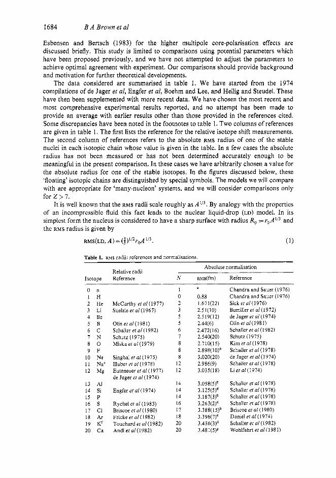
Esbensen and Bertsch (1983) for the higher multipole core-polarisation effects are discussed briefly. This study is limited to comparisons using potential parameters which have been proposed previously, and we have not attempted to adjust the parameters to achieve optimal agreement with experiment. Our comparisons should provide background and motivation for further theoretical developments.

The data considered are summarised in table 1. We have started from the 1974 compilations of de Jager et al, Engfer et al, Boehm and Lee, and Heilig and Steudel. These have then been supplemented with more recent data. We have chosen the most recent and most comprehensive experimental results reported, and no attempt has been made to provide an average with earlier results other than those provided in the references cited. Some discrepancies have been noted in the footnotes to table 1. Two columns of references are given in table 1. The first lists the reference for the relative isotope shift measurements. The second column of references refers to the absolute RMS radius of one of the stable nuclei in each isotopic chain whose value is given in the table. In a few cases the absolute radius has not been measured or has not been determined accurately enough to be meaningful in the present comparison. In these cases we have arbitrarily chosen a value for the absolute radius for one of the stable isotopes. In the figures discussed below, these 'floating' isotopic chains are distinguished by special symbols. The models we will compare with are appropriate for 'many-nucleon' systems, and we will consider comparisons only for Z > 7.

It is well known that the RMS radii scale roughly as A ' I 3 . By analogy with the properties of an incompressible fluid this fact leads to the nuclear liquid-drop (LD) model. In its simplest form the nucleus is considered to have a sharp surface with radius R, = r0A1/3 and the RMS radius is given by

RMS(LD, A ) = (?)'/'roA 'I3.

Table 1. RMS radii: references and normalisations.

Absolute normalisation Relative radii

Isotope Reference N RMs(fm) Reference

O n 1 H 2 He 3 Li 4 Be 5 B 6 C 7 N 8 0 9 F

10 Ne 11 NaC 12 Mg

13 AI 14 Si 15 P 16 S 17 C1 18 Ar 19 Kf 20 Ca

McCarthy et al(1977) Suelzle et a1 (1 967)

Olin et a1 (198 1) Schaller et a1 (1982) Schutz (1975) Miskaetal( l979)

Singhal et a1 (1975) Huber et a1 (1 978) Euteneuer et a1 (1977) de Jager et a1 (1974)

Engfer et a1 (1 974)

Rychel et a1 (1983) Briscoe et a1 (1980) Fricke et a1 (1982) Touchard et a1 (1982) And1 et al(1982)

1 0 2 3 5 5 6 7 8 8 8

12 12

14 14 14 16 17 18 20 20

a

0.88 1.671(22) 2.51(10) 2.5 19( 12) 2.44(6) 2.472( 16) 2.540(20) 2.7 10( 15) 2.898( 3.020(20) 2.986(9) 3.035( 18)

3.058(5)b 3.125(5)d 3. 187(3)b 3.263(2)d 3.388( 15)b 3.396(7)e 3.4 3 6(3)d 3.481(5)"

Chandra and Sauer (1976) Chandra and Sauer (1976) Sick et a1 (1976) Bumiller et a1 (1 972) de Jager et a1 (1 974) Olinetal(1981) Schaller et a1 (1982) Schutz (1975) Kim etal(1978) Schaller et a1 (1978) de Jager et a1 (1 974) Schaller et a1 (1 978) Li et a1 (1974)

Schaller et a1 (1978) Schaller et a1 (1978) Schaller et a1 (1978) Schaller et a1 (1978) Briscoe et a1 (1980) Daniel et a1 (1 974) Schaller et al(1982) Wohlfahrt et a1 (198 1)

Systematics of nuclear RMS charge radii 1685

Table 1. (continued)



21 22 23 24 25 26 27 28 29 30 31 32 33 34 35 36 37 38 39 40 41 42 43 44 45 46 47 48

s c Ti V Crh Mn Fe CO Ni cu Zn G a Gel As Se Br Kr Rb Srk Y Zr Nb MO Tc Ruk Rh Pdk Ag Cd

Wohlfahrt et a1 (1 98 1) Wohlfahrtetal(1981) Wohlfahrt et a1 (198 1) Wohlfahrt et a1 (198 1) Wohlfahrt et a1 (198 1) Wohlfahrt et a1 (1980)

Wohlfahrt et a1 (1980) Shera et a1 (1976) Wohlfahrt et al(1980)

24 28 28 28 30 28 32 30 34 34

3.550(5)b3 3.574(5)* 3.603(5)b3g 3.645(5)* 3.7 1 0(5)b3g 3.694(5)g 3.793(5)b" 3.777(5)' 3.888(5)' 3.932(5)

4.07(2)J

Wohlfahrt et al(1981) Wohlfahrt et al(1981) Wohlfahrt et a1 (1981) Wohlfahrt et al(1981) Wohlfahrt er a1 (1981) Wohlfahrt et a1 (1980) Sheraetal(1976) Sheraetal(1976) Sheraet al(1976) Wohlfahrt et a1 (1980)

Kline et a1 (1975) 38 Klineet al(1975)

Gerhardt et a1 (1 979) Thibault etal(1981a) Heilig and Steudel(l974)

50 50

4.160 4.180

Arbitrary Arbitrary

50 50 52 50

4.239(7)b 4.263(8) 4.318(3)b 4.317(4)

Engfer et a1 (1974) Rothhaas (1976) Engfer et a1 (1 974) Schellenberg et a1 (1980)

Rothhaas (1976)

Schellenberg et a1 (1980)

Heilig and Steudel(l974) 58 64

4.5 l(4) 4.595(3)

4.5 78(7)

4.6 19( 1 5)b 4.623( l)m

4.774(6) 4.763(6)b2" 4.784 4.800(7)" 4.832( 1)

4.86 l(8)b3" 4.883(9)b*" 4.881(9)b9" 4.9 13( IO)"

5.002(6) 5.104b 5.141(3)

-72 4.676(5)b

Engfer et a1 (1974) Lightbody et a1 (1976)

Gillespie et a1 (1975)

Heilig and Steudel (1974)

Heilig and Steudel(l974) Wenzetal( l981) '

62

49 50 51 52 53 54 55 56

In Sn Sb Te I Xe c s Ba

Lab' Ceb Pr Nd Pm Sm Eub Gd

66 66 70- 74 74 82 78 82

Engfer et a1 (1 974) Cavedon (1980) Engfer et a1 (1 974) Engfer et a1 (1 974) Engfer et a1 (1 974) Arbitrary Engfer et a1 (1974) Shera etal (1982)

Engfer et a1 (1974) Engfer et a1 (1974) Engfer et a1 (1 974) Engfer et a1 (1974)

Moinester et a1 (1 98 1) Arbitrary Laubacher et al(1983)

Heilig and Steudel(l974) Boehm and Lee (1 974) Boehm and Lee (1 974)

Boehm and Lee (1 974) Thibault et al(1981b)' Bekk et al(1979) Shera et a1 (1982) Heilig and Steudel(l974) Heilig and Steudel (1 974)

57 58 59 60 61 62 63 64

82 82 82 82 Heilig and Steudel (1974)

Heilig and Steudel(l974) Heilig and Steudel(l974) Heilig and Steudel(l974) Laubacher et a1 (1983)

86 90 92

65 66 67 68 69 70

Tb DY Ho Er Tm Yb

Neugart (1982)p 92 5.181 Arbitrary

Arbitrary Neugart (1982)p

Neugart (1982)p

92 5.220

92 5.260 Arbitrary


Table 1. (continued)



71 Lu 72 Hf 73 Ta 74 Wk 75 Rek 76 Os 77 Ir 78 Ptk 79 Au 80 Hg 81 TIk

82 Pb 83 Bik 84 Po 85 At 86 Rn 87 Fr 88 Ra 89 Ac 90 Thk 91 Pa 92 Uk 93 Np 94 Pu 95 Amk 96 Cmk

Heilig and Steudel(l974)

Heilig and Steudel(l974) Heilig and Steudel(l974) Heilig and Steudel (1 974)

Heilig and Steudel(l974) Kluge et a/ (1983) Bonn et a1(1976)q Heilig and Steudel(1974) Engfer et a l ( l974) Thompson et a1 (1983) Heilig and Steudel(l974)



Heilig and Steudel (1 974) Heilig and Steudel(l974) Heilig and Steudel(l974)

104

114

118 124 124

126 126

142

146

144

5.350

5.389

5.434(2) 5.496 5.484(6)

5.503(2) 5.5 2 1 (2)

5.773

5.843

5.860

Arbitrary

Arbitrary

Engfer et al(1974) Arbitrary Engfer et a1 (1 974)

Cavedon (1980) de Jager et a1 (1 974)

de Jager et a1 (1974)

de Jager et a1 (1974)

Arbitrary

a The mean-square charge radius for the neutron is -0.116 fm2.

tended to overlap those of longer neighbouring chains.

nuclei far from the stability line (Huber et a1 1978).

e The j6Ar radius given by Daniel et a/ (1974) does not agree with Finn et a1 (1976), perhaps because only the statistical errors are quoted in the latter work. 'We note in this case that the systematic errors due to uncertainties in the 'mass shift' are rather large for nuclei far from the stability line (Touchard et a1 1982). * The values are taken from table VI of Wohlfahrt et a1 (1981) and the errors are based on the typical errors given in table V of Wohlfahrt et a1 (1980).

The RMS radii given by Wohlfahrt et a1 for Cr isotopes are consistent with the work reported recently by

These data were not included in the figures since there were only a few points in the isotopic chain which

We note in this case that the systematic errors due to uncertainties in the 'mass shift' are rather large for

Corrections for the small isotopic abundances of other naturally occurring isotopes have been made.

Lightbody et al(1976, 1983). ' The values are taken from table VI1 of Shera et a1 (1976) and the errors are based on the typical errors . .

given in table V of Wohlfahrt et a1 (1980). Not used in the figures because of the relatively large error. Only relative isotope shifts are given by Heilig and Steudel(l974) in this case and are thus not included in our

analysis. ' The isotopes shifts given by Wenz et a1 (1 98 1) are consistent with those of van Eijk et a1 (1979).

" We do not include the systematic error seen in the two different analyses of '*'I given by Engfer er a1 (1974). ' These results are consistent with those of Schinzler et a1 (1978).

q The change in mean-square radii was taken from the 1 (exp) column in table 3 of Bonn et a1 (1976).

This value is somewhat inconsistent with ehe value of 4.642(6) fm given by Lightbody et a1 (1976).

Taken from figure 7 of the paper by Neugart (1982).

Systematics of nuclear R M S charge radii 1687

In figure 1 the experimental radii are compared with equation (1) using the value of r, = 1.2 fm which optimises the agreement for large values of A . The experimental RMS radii for smaller A are systematically larger than the liquid-drop-model prediction. This can be understood as being due to the surface diffuseness. Myers and Schmidt (1983) have taken the diffuseness into account in the 'extended-liquid-drop' model by folding the sharp- surface charge distribution with a normalised, spherically symmetric, short-ranged function. They used a gaussian function, exp(-r2/2b2), with a value of b = 0.99 fm obtained from a best fit to experiment. The parameter b is assumed to be independent of N and Z . The RMS radii in this extended-liquid-drop (ELD) model are given by (Myers and Schmidt 1983)

R M S ( E L D , A ) = ( { ) ' / * ( ~ . ~ ~ + 1.80A-2/3 - 1.20A-4/3)A1/3 fm. ( 2 )

In figure 1 the experimental radii are compared with equation (2 ) . The qualitative agreement is now much better for the lighter nuclei, but on a more quantitative level there are significant deviations relative to the ELD model. In order to emphasise these deviations, in figure 2(a) we plot the difference RMs(expt) - RMS(ELD). In the remainder of this paper, we will study the possible origins of these deviations with the help of more refined theoretical models. Graphical comparisons of experiment and theory are shown in figures 2 and 3.

In figures 2(a)-(e) the differences between experimental and theoretical RMS charge radii are plotted. The points representing nuclei of a given isotopic chain are connected by lines. The symbols at the beginning and end of each line indicate those with an even value

I , 1 I I 2 3 4 5 6

l3/5)"2 1 .2A1 ' j

Figure 1. Plot of the experimental RMS charge radii on they axis as a function of(4) ' I2 1.2 A ' I 3 on the x axis. On the y axis we also compare the calculation with the extended-liquid-drop model using equation (2).


-0.08

-0.12-

0 8 16 24 32 40 48 56 64 12 80 88 96 104 112 120 128 136 144 152 160

-

( b i

I 1 1 / , , , 1 , , , l , , , l , , , l , , , I , , , I , , , l o 8 1 , I / I , , , l , , / l , , l I I , , / , I 1 1 1 I I I I I , I , , , 1 1 1 / 1 1 1 1

0.28

0.24

0.20

0.16

Figure 2. Differences between experiment and theoretical RMS charge radii. The comparison is made for (a) the extended-liquid-drop model (ELD), (b) the droplet model (D), (c) the harmonic-oscillator potential model (HO), ( d ) the Woods-Saxon potential model (ws), (e) the Skyrme-3 Hartree-Fock potential model (SK3) and (f) the SGII Hartree-Fock potential model (SGII). Isotopic chains are connected by lines with special symbols at the ends. We use circles for the even-Z isotopes with experimental absolute normalisation, squares for the even-Z isotopes with arbitrary normalisation, triangles for the odd-Z isotopes with experimental absolute normalisation and diamonds for the odd-Z isotopes with arbitrary normalisation.


0.28

0.20

VI

1 0.04 e n. x

VI

6 -0.04

d "JP 1 -0.08 1 dd

0.28

0.24

0.20

-0.12 Id I I , I I , / l l , , / 1 , , , l , , , 1 , / , 1 , , / 1 / l , / , , , l , , , I l , , I , , , / , , , 1 / , , / / , , / , , ~ l , , / 1 , , , ~ , , , ~ , , ~

0 8 16 24 32 40 4 8 56 64 12 80 88 96 104 112 120 128 136 144 152 160 Neutrm number

Figure 2. (continued)

of Z (circles and squares) and those with an odd value of 2 (triangles and diamonds). The isotopes for which an experimental value was used for the absolute radius are indicated by the circles and triangles and the 'floating' isotopic chains are indicated by the squares and diamonds. The particular value of 2 of each chain can be inferred from the labels at the top


82 I

126 3

0 8 16 24 32 40 48 56 64 72 80 88 96 104 112 120 128 136 144 152 160

E L - - 0.12

- 0.08

I 0.04

* o B

- I 0 Ln

il

I

c CL x

I :::::I,, , I , , , I , , , , , , , , , , I , , , , , , , , , , , , , , , , I , , , , , , , , , / / , , , , , , , , , , , , , , , , , , , ~~~, , ,I -0.12

0 8 16 24 32 40 48 56 64 72 80 88 96 104 112 120 128 136 144 152 160 Neutron number

Figure 2. (continued)

of the figures which are placed directly above the data. For clarity, experimental error bars have not been included in the figures. The absolute errors are given in table 1 and the relative errors are given in the references cited there. In general the errors are small compared with the deviations between experiment and theory.


2.4

1.2

0.8

-0.4

-0.8

U

0.2 -0.2

0 I V I L~LL.u..__LL.II -.'-. !-L-,. -1 -1 .A _ _ _ I

32 40 48 56 Sb 72 80 3? 05 lil i , '"? 120 128 13b 14G IS: j::

Neutron number

Figure 3. Brix-Kopfermann plot for the isotope shift relative to that of the liquid-drop model (see equation (3)). In (a) the experimental relative isotope shift is compared with the results of the calculations based on the extended-liquid-drop model (chain line) and the droplet model (broken line). For the experiment, isotopes with even (odd) Z are indicated by circles (triangles) at the beginning and end of the lines. In @)-(e) the droplet-model predictions are compared with the results of the calculations based on single-particle potentials; (b) the harmonic-oscillator potential (HO); (c) the Woods-Saxon potential (ws); ( d ) the Skyrme-3 Hartree-Fock potential (SK3); (f) the SGII Hartree-Fock potential (SGII). The calculation shown in (e) is the same as that of ( d ) except that the neutron finite-size and relativistic spin-orbit contributions to the charge density are excluded.

Since the relative RMS radii within a given isotopic chain are sometimes known more accurately than the absolute radii, it is useful to present the comparisons for the isotope shifts in the form of a Brix-Kopfermann (Brix and Kopfermann 1958) plot. The quantities in the BK plot are the differences in the mean-square ( M S = R M S ~ ) charge radii between


isotopes differing by two neutrons divided by the differences expected from the liquid-drop (LD) model:

Ms(expt, 2, N ) - Ms(expt, 2, N - 2) BK(eXpt, 2, N ) =

MS(LD, A ) - MS(LD, A - 2) (3)

The quantities BK(expt), which we will refer to hereafter as the relative isotope shifts, are plotted in figure 3(a). The experimental points representing nuclei within a given isotopic chain are connected by lines. The symbols at the beginning and end of each line indicate those with an even value of Z (circles) and those with an odd value of Z (triangles). The particular value of Z for each chain can be inferred from the labels at the top of the figures which are placed directly above the data. An earlier comparison of the data in this form is given in figure 2 of the compilation of Heilig and Steudel (1974). In figures 3 ( a ) - ( f ) model predictions obtained by using equation (3) with theoretical values in place of experimental ones are shown.

In the following sections we will describe the models which we have used to calculate the RMS charge radii and discuss the comparison between experiment and theory. In Q 2 the droplet model of Myers (1977) and Myers and Schmidt (1983) is discussed. (Note that we use the terms liquid drop, extended liquid drop and droplet to refer to three distinct models.) The spherical single-particle potential models are described in Q 3. In Q 4 we discuss the comparison between theory and experiment and consider the additional contributions to the theoretical radii due to the effects of deformation and zero-point vibrational motion.

2. The droplet model

In figure 3(a) the experimental relative isotope shifts are compared with the predictions of the extended-liquid-drop (equation (2) ) model given by the chain line. There are large fluctuations, but on average the experimental relative isotope shift is about half of that expected from the ELD model. Conversely, it follows that the isotone shift must on average be greater than that of the ELD model in order that the radii be proportional on average to A 1/3,

This inadequacy of the ELD model has been overcome in the 'droplet' model of Myers by allowing for a neutron skin. We present here a summary of the spherical droplet-model equations which were obtained by Myers and Schmidt (1983) by minimising the macroscopic energy of the droplet. The sharp-surface radius R, for the matter density (the sum of neutrons and protons) is given by

R,=roA'/3(1 +i) (4) where

( N - Z)/A + &(c, /Q)ZA-2 /3 1 + $(J/Q)A - 1/3

F = and


The parameters have been obtained by a fit to nuclear binding energies and radii (Myers 1977): r,, = 1.18 fm (the nuclear radius constant), a2 = 20.69 MeV (the surface energy constant), J = 36.8 MeV (the symmetry energy constant), Q = 17 MeV (the effective surface stiffness), K = 240 MeV (the incompressibility coefficient) and L = 100 MeV (the density symmetry energy).

The proton and neutron sharp-surface radii are then given by

R , = R , - (Z/A)t

R , = R , + (N/A)t

where t i s the neutron skin thickness given by

t = f R , { [ ( N - 23/41 - J}. ( 9 )

Including diffuseness and ‘redistribution’ corrections, the RMS charge radius for the protons in the spherical droplet model (D) is given by

RMS(D, 2, N)= [3b2 + $(Rg + R;)]l/’. (10)

The first term on the left-hand side arises from folding the gaussian diffuseness described above in connection with the ELD model. The contribution from R, is the ‘redistribution’ term which results from a more exact treatment of the Coulomb potential

R; = &C’Rg

where

C‘=i[(9/2K) +(1/4J)]Z$/R,.

The differences RMs(expt) - RMS(D) are shown in figure 2(b) and the relative isotope shift is shown in figure 3(a) (broken line). The average isotope shift obtained in the droplet model is about half that obtained from the liquid-drop and ELD models and is in better agreement with the experimental average. The relative isotope shift is predicted to increase slightly with A from about 0.3 for A = 16 to 0.55 for A = 208. This is difficult to verify experimentally because of the large experimental flucations about the average. The values of RMs(expt)- RMS(D) (figure 2(b)) show much more clustering than was obtained in the RMs(expt) - RMS(ELD) comparison (figure 2(a)), indicating that the isotone shift is also better described in the droplet model.

The deviations in A R = RMs(expt) - RMS(D) (figure 2(b)) are clearly associated with the magic neutron numbers N = 8, 14, 28, 50, 82 and 126 in that the value of A R is small for these values of N . It is notable that there is a minimum at N = 14 (the Od,,, shell closure) rather than N = 20 (Od,,, shell closure). Small values of A R can also be associated with the 2 = 50 and 2 = 82 shell closures.

3. Single-particle potential models

The usual starting point for microscopic nuclear models is the Hartree-Fock mean-field theory. Each nucleon is assumed to move independently in a single-particle potential field. Ideally one would start with the experimental nucleon-nucleon interaction and calculate the mean-field potential. In practice this method is limited by the need to restrict the number of allowed Slater-determinant configurations (often to one). Then the effects of all the remaining configurations must be calculated in perturbation theory. Because of the


problems associated with the convergence of this perturbation expansion, calculations starting from the experimental nucleon-nucleon interaction are not very successful. The most successful mean-field calculations have used phenomenological two-body interactions instead. At a less fundamental level, one can also consider some phenomenological form for the mean-field potential itself. In each case a certain limited set of parameters is adjusted to reproduce chosen data. These parameters are usually taken as constants or are assumed to have a smoothly varying dependence on N and Z.

For a spherical potential the total radial density for the point nucleons is given by the orbit occupation times the radial density of the single-particle state IR(r)I2. The charge RMS radii are then obtained from these point-proton radii taking account of the corrections for the finite charge distribution of the protons and neutrons and for the relativistic spin-orbit and Darwin-Foldy corrections; for references and details concerning the method of calculation see Malaguti et a1 (1978, 1979a, b, 1982) and Brown et a1 (1979, 1983). For the orbit occupations we use the integer occupations of the extreme single-particle model obtained by filling the single-particle states in the order of the calculated single-particle energies. (For the harmonic-oscillator potential the order was taken to be Os,/, , Op,/, ,

The single-particle radial wavefunctions are calculated in a formulation which allows for non-local potentials generated from the Skyrme-type interactions (Vautherin and Brink 1972) as well as for the usual local potentials. The radial wavefunctions R(r) can be obtained from a set of equations (Dover and van Giai 1972) involving an equivalent local potential VL(r) and radial wavefunctions RL(r)

OP1/2, Od5/2, Od3/2, l s1 /2 , of,/,, Of,/,, IP3/2, IP1/2, * 3 etc*)

{ - (h2 d2/2p dr2) + [h21(l+ 1)/2pr2] + UL(r, &)}R, (r )= ER,@) (13)

where

R(r) = (m*(r)/m)1/2RL(r)

U, (r, E ) = (1 - m*(r)/m)& + (m*(r)/m)U(r).

and

All of the above functions and the single-particle energies E depend implicitly on the quantum numbers a (= proton/neutron), n, 1 a n d j of the single-particle state. The effective mass m*(r) is given in terms of the nucleon densities and the Skyrme parameters by equation (2.3) of Dover and van Giai (1972) (see also equation (33) of Brown et a1 (1982)).

The potential V(r) is divided in the usual way into central, spin-orbit and Coulomb components:

a> = V(r, a> + v,, (r, a)( l - 4 + VCoulomb (r, a). (16) Three forms for the central potential V(r) are considered: the harmonic-oscillator form

VHo, the Woods-Saxon form Vws and the form VSK obtained with the Skyrme-type interaction:

VHo(r, a)= i m o 2 r 2 (17)

and


The constants V,, R , and a, are the values of the well depth, radius and diffuseness, respectively, for the Woods-Saxon potential. The Skyrme function F of the proton and neutron densities p, and pn is given by equation (2.12) of Dover and van Giai (1972) (the quantity inside the first square bracket). (Note that in equation (2.5) of Dover and van Giai the term J ( t , + t 2 ) should be replaced by t ( t , + t2) . )

For the harmonic-oscillator potential, hw was assumed to depend smoothly on mass in the form given by Blomqvist and Molinari (1968):

= 45A - - 25A - 2/3. (20)

The harmonic-oscillator potential is assumed to be local (i.e., m*(r)/m = 1 in the equations above), and the spin-orbit and Coulomb potentials are not included.

The Woods-Saxon potential has six parameters: Vp, R,, up, V,, R , and a,. (The results presented here are insensitive to the neutron potential.) For the selected nuclei l 6 0 ,

40Ca and 208Pb, the three proton potential parameters have been uniquely adjusted to reproduce the ( r 2 ) and (r4) moments of the measured charge distribution and the empirical binding energy of the least bound filled proton orbit (Streets et a1 1982, Brown et a1 1982). For other nuclei with A > 40 the potential parameters were obtained from a smooth interpolation based on the formula

where the plus sign is for proton and the minus sign is for neutron. X,, X , and X2 are constants which are obtained from three sets of parameters: the proton parameters for 40Ca and the proton and neutron parameters for 208Pb (Streets et a1 1982). For A = 16-40 the interpolation was based on equation (2 1) with the same value of X , used for A > 40 and with X, and X 2 determined from the proton parameters for l60 and 40Ca (Brown et a1 1982). The Woods-Saxon potential is assumed to be local (i.e., m*(r)/m= 1 in the equations above).

For the Woods-Saxon calculations standard forms are used for the Coulomb and spin-orbit terms in equation (1 6). We use a Coulomb potential based on a uniform charge- density distribution which has total charge number 2 - 1 and the experimental RMS charge radius. The spin-orbit potential is based on the usual derivative of a Fermi shape and has strength (h /m ,~ )~V , , = 12 MeV, radius 1.lA'l3 fm and diffuseness 0.65 fm. The reduced mass is given by pa = m,(A - l)/A.

The Hartree-Fock calculations presented here were obtained with the Skyrme-3 (SK3) interaction of Beiner et a1 (1975) and with the SGII interaction of van Giai and Sagawa (198 la, b). Both the SK3 and SGII interactions give reasonable ground-state properties. However, by introducing a lower power of the density dependence and a modification of the velocity-dependent spin-exchange term, the SGII interaction is improved over SK3 in several respects. It gives a lower compression modulus (K= 215), in better agreement with the empirical value deduced from the energy of the giant monopole state, and also gives realistic properties for the other giant resonances including the spin-isospin modes. In addition, the SGII interaction has an attractive pairing matrix element for the particle-particle interaction (van Giai and Sagawa 1981a, b). The Coulomb and spin-orbit potentials were treated in the same way as in the previous Skyrme Hartree-Fock calculations. The Coulomb potential was calculated by folding the Coulomb interaction with the calculated charge density and then adding on the approximation for the exchange term given by Beiner et a1 (1975). We use the spin-orbit potential given by the first term on the right-hand side of equation (2.6) of Dover and van Giai (1972). By convention, the


reduced mass includes a centre-of-mass correction for the total energy (Vautherin and Brink 1972), pa =m,A/(A - 1).

4. Comparison between experiment and theory

The differences RMs(expt) - RMs(the0ry) with the theoretical radii calculated with the harmonic-oscillator (HO), Woods-Saxon (ws) and Skyrme Hartree-Fock (SK3 and SGII) models are shown in figures 2(c)-(f) . In order to evaluate the comparisons, we distinguish between two kinds of deviations from zero: (1) the average deviation as a smooth function of mass and ( 2 ) the local variations from this average. In general it is probably possible to ‘fine tune’ the potential parameters (which are assumed to be constants or smoothly varying functions of mass) in order to improve the agreement for the average deviation. On the other hand, the local variations are due to more fundamental inadequacies of the models.

Our calculations are strictly applicable only to the closed-shell configurations. Thus we may expect the difference between experiment and theory to be closest to zero for those nuclei which are expected in the extreme single-particle shell model to have closed-shell configurations for protons and/or neutrons. This expectation is born out most clearly with the SGII Hartree-Fock calculation shown in figure 2(f). In this case the deviation between experiment and theory is smallest for those nuclei which have neutron numbers 28, 50, 82 and 126, the well known magic numbers for the closed-shell configurations in nuclei. (These systematics suggest that the arbitrary absolute RMS radii chosen for the Dy ( Z = 68) and Er ( Z = 70) isotopes, whose differences are plotted in figure 2 by squares connected by a line, should be reduced by about 0.04 fm.) In addition, the deviation is small for the Sn (2 = 50) and Pb ( Z = 82) isotopes. The experimental RMS radii for the non- closed-shell nuclei are systematically larger than the SGII calculation.

The comparison with the SK3 calculation in figure 2(e) shows a pattern which is very similar to the SGII calculation (figure 2(f)) except that the average deviation for the closed-shell nuclei becomes increasingly larger with increasing mass. This difference may be simply due to the fact that the parameters of the SGII interaction were adjusted more accurately than those of the SK3 interaction to fit the RMS radius of *08Pb, and thus we cannot necessarily conclude from this comparison alone that the functional form of the SGII interaction is superior to that of the SK3 interaction.

Relative to these Hartree-Fock calculations the harmonic-oscillator (figure 2(c)) and Woods-Saxon (figure 2(d)) calculations are not as successful. Although the harmonic oscillator has historically provided a simple approximation with which to calculate nuclear properties, it is not as realistic as the other models we consider and will not be discussed further. The problem with the Woods-Saxon potential is connected with the fact that the calculated average isotope shift (figure 3(c)) is too small, especially for light nuclei. The shape and strength of the isovector potential is important in determining the isotope shift. The isovector shape and well depth of our Woods-Saxon potential are assumed, as usual, to vary as ( N - Z ) / A (equation (21)) and the parameters have been determined by fits to the neutron and proton single-particle levels and density distributions (see !j 3). Our comparisons suggest that the simple ( N - Z ) / A dependence is not adequate. It would be worthwhile to investigate other forms.

The droplet model (figure 2(b)) and SGII model (figure 2(f)) comparisons are qualitatively similar. However, they differ in detail, for example, in the region between N = 88 and N = 104 where the difference between experiment and theory increases for the


droplet model but decreases for the SGII model. The reason for this difference can be seen in the isotope shifts plotted in figure 3( f). Relative to the droplet model the SGII model has on average a larger isotope shift just after a closed shell (such as N=82). This shell dependence can be associated with the ‘pulling out’ of the core protons by the valence neutrons. Just after a closed shell the RMS radii of the valence neutron orbits are larger than the average RMS radii of the filled proton and neutron orbits. Due to the strong attractive proton-neutron interaction, the binding energy is maximised when the neutrons and protons overlap as much as possible. This overlap can be increased by ‘pulling out’ the core protons and/or ‘pulling in’ the valence neutrons, and the latter is limited to some extent by the density saturation requirements. This shell-dependent ‘monopole polarisation’ comes out of the Hartree-Fock calculation because of the self-consistency between the density and the potential, but of course does not appear in the non-self-consistent harmonic-oscillator and Woods-Saxon calculations (see figures 3(b) and (c)).

The monopole polarisation actually accounts for only a small part of the experimental isotope shift anomalies. In order to understand the remaining discrepancies, we need to investigate the role of the higher-multipole ground-state correlations. For nuclei, the quadrupole correlations, which are manifested in the form of vibrational and/or rotational Collective motion, are most important. In the vibrating and deformed liquid-droplet models it is well known that the increase in the RMS radius is proportional to the B(E2) value for the electromagnetic excitation of the collective 2’ state (Uher and Sorensen 1966, Bohr and Mottelson 1969). In the uniform-density sharp-surface approximation, the increase in the RMS radius up to order p2 in the deformation parameter is given by

ARMS = (27r//5)B(E2)/Z2~MS:. (22)

(The effect of including terms up to order p3 (Dobaczewski et a1 1984) is small (about a -10% correction to ARMS for p= 0.6) and will be ignored here.)

The quantities ARMS are plotted in figure 4. They were obtained from equation (22) for the even-even nuclei using experimental B(E2,O’ - + 2 + ) values for the lowest 2 + states and the extended-liquid-drop model (equation (2)) for the zeroth-order radii R M ~ . (The particular Z value of each chain in figure 4 can be inferred from the labels at the top of the figures which are placed directly above the data.) The experimental B(E2) values were taken from the standard compilations: the individual references given on page ii of Nuclear Data Sheets (1982) (for lifetimes and excitation energies) and Stelson and Grodzins (1966) (for internal conversion coefficients) for A > 44, Endt and van der Leun (1978) for A = 2 1-44 and Ajzenberg-Selove (1983) for A = 18-20. Unfortunately, some of the compilations for A > 44 are somewhat out of date and experimental B(E2) values are not known for all of the nuclei of interest. Nevertheless, comparison of figures 2(f) and 4 shows that equation (22) evaluated for the lowest 2 + states can account qualitatively for the deviation between the experimental RMS radii and those calculated in the spherical SGII Hartree-Fock model. A more quantitative comparison of this kind requires a more up-to- date evaluation of the B(E2) data for A > 44.

Equation (22) can be extended to states with non-zero spin J, by replacing B(E2, 0’ + 2 + ) with a sum over all possible final states J, and adding the diagonal quadrupole moment term Q for J, > 4 (Brown 1984):

B(E2)= B(E2, Ji -Jf) + (5/16${(5i + 1)(24 + 3)/[5,(2Ji - 1)]}Q2. (23)

It would be interesting to see if the odd-even staggering in the RMS radii is correlated with experimental B(E2) values. However, the B(E2) data needed for the odd-even nuclei are


0.16 r

Lo I

2 0.12

2 0.08

e Y)

0

c c

E 0.04 e 8 0 c

-0.08 ", Neutron number

Figure 4. The change in RMS radius based on equation (22) using experimental B(E2) values.

harder to obtain experimentally, and a critical evaluation and summary of the available data are needed.

Esbensen and Bertsch (1983) have recently investigated the ground-state correlation effects associated with the higher multipole vibrational states and the 'giant resonances'. They calculated the change of the mean-square radius in the uniform-density sharp-surface approximation in terms of the mean-square fluctuation of the nuclear radius U and obtained

(24) 2 ( r 2 ) - (r2>HF =3(U&'A - UHF)

where U' = ( R i / 4 ~ ) 1 /?;

and /?; =B(EL, 0' +L)[(3/4~)zR;]-'

and R, is the sharp-surface radius (Ri =3(r2)HF). The sum extends over all excited states. The quantity UHF is the mean-square fluctuation already present in the uncorrelated Hartree-Fock ground state and ORPA is the mean-square fluctuation due to the correlated states which can be calculated, for example, by the method of the random-phase approximation (RPA). Equation (24) is equivalent to equation (22) when a single L = 2 state is considered and oRPA > OHF.

It is useful to distinguish three regions of excitation energy for the collective excitations: (1) the 'high-energy' giant resonance vibrations starting at about 58A-'/3 in excitation energy, (2) the 'medium-energy' vibrations with L = 2-5 around 15A - ' I3 in excitation energy and (3) the 'low-energy' quadrupole vibrations and rotations below 2 MeV in excitation energy. Esbensen and Bertsch found that the contribution of the 'high- energy' giant resonance states in equation (24) was small due to a cancellation between


uRPA and uHF. They found that the largest contributions to equation (24) for 40Ca and 208Pb were from the ‘medium-energy’ states, and in particular from the lowest octupole state.

The total increases in the RMS radii obtained by Esbensen and Bertsch were A ~ ~ ~ z 0 . 1 3 fm for 40Ca and A ~ ~ s ~ 0 . 0 2 0 fm for 208Pb. Relative to the scale of figure 2, this increase for 40Ca is large and would make the deviation from zero much worse for all of the calculations. However, this is not surprising since the potential parameters have already been adjusted to fit the properties of these nuclei. Rather, what is most important for our comparisons is the detailed mass dependence of the B(E3) for the low-lying octupole vibrations. Unfortunately, systematic experimental information on this is difficult to obtain away from the ‘closed-shell’ nuclei because the octupole states become fragmented and embedded in a region of relatively high level density. We have not attempted to evaluate the data available. For the purpose of the present discussions, we have assumed that the contributions of these ‘medium-energy’ excitations to the RMS radii are smoothly mass dependent and have already been incorporated into the potential parameters.

Finally, we discuss the sharp discontinuities which appear in the experimental isotope shifts (figure 3(a)). These are usually attributed to a sudden transition from a spherical ground-state to a deformed ground-state configuration. The sharp discontinuities in the calculated isotope shifts (figures 3(c)-( f )) occur for a different reason. These appear when the highest j orbit from the unfilled shell passes through the orbits of the valence shell. This causes an irregular isotope shift directly in the case of protons due to the difference in the RMS radius of the orbits in the two major shells and indirectly in the case of neutrons due to the contribution from the neutron spin-orbit charge distribution. In the Hartree-Fock calculations the crossing of neutron orbits also contributes indirectly due to their influence on the proton potential. (For the SK3 calculations the isotope shifts are also shown without the addition of the neutron finite-size and neutron spin-orbit contributions (SK3b) in figure 3(e) in order to show their relative contribution to the isotope shifts.) The sharp discontinuities in the experimental isotope shift (figure 3(a)) do not occur in the same place as those calculated. However, this aspect of the calculation is particularly sensitive to the orbit occupations. We have assumed integer orbit occupations determined by the ordering of the levels in the spherical potentials (see 0 3). Configuration mixing in the open-shell nuclei will smooth out the orbit occupations and wash out the sharp structures in the calculation. In future studies it would be interesting to consider the effects of level crossing in a deformed potential.

Acknowledgments

We would like to thank Mr R J M Sweet for help in compiling the information on B(E2) values. This research was supported in part by National Science Foundation Grants Nos PHY-80-17605 and PHY-83-12245.

References

Ajzenberg-Selove F 1983 Nucl. Phys. A 392 1 And1 A, Bekk K, Goring S, Hanser A, Nowicki G, Rebel H, Schatz G and Thompson R C 1982 Znstitut fiir

Barrett R C and Jackson D F 1977 Nuclear Sires and Structure (Oxford: Clarendon) Angewandte Kernphysik, K f K Karlsruhe, Preprint


Beiner M, Flocard H, van Giai Nand Quentin P 1975 Nucl. Phys. A 238 29 Bekk K, And1 A, Goring S , Hanser A, Nowicki G, Rebel H and Schatz G 1979 Z. Phys. A 291 219 Blomqvist J and Molinari A 1968 Nucl. Phys. A 106 545 Boehm F and Lee P L 1974 Atomic and Nuclear Data Tables 14 605 Bohr A and Mottelson B R 1969 Nuclear Structure vol. I (New York: Benjamin) Bonn J, Huber G, Kluge H-J and Otten E W 1976 Z. Phys. A 276 203 Briscoe W J, Crannell H and Bergstrom J C 1980 Nucl. Phys. A 344 475 Brix P and Kopfermann H 1958 Rev. Mod. Phys. 30 5 17 Brown B A 1984 unpublished Brown B A? Massen S E, Escudero J I, Hodgson P E, Madurga G and Vinas J 1983 J. Phys. G: Nucl. Phys.

Brown B A, Massen S E and Hodgson P E 1979 J. Phys. G: Nucl. Phys. 5 1655 Brown B A, Wildenthal B H, Chung W, Massen S E, Bernas M, Bernstein A M, Miskimen R, Brown V R and

Bumiller F A, Buskirk F R, Dyer J N and Monson W A 1972 Phys. Rev. C 5 391 Cavedon J M 1980 PhD Thesis Orsay Chandra H and Sauer G 1976 Phys. Rev. C 13 245 Daniel H, Pfeiffer H-J, Springer K, Stoeckel P, Backenstoss G and Tauscher L 1974 Phys. Lett. 48B 109 Dobaczewski J, Vogel P and Winter A 1984 Phys. Rev. C 29 1540 Dover C B and van Giai N 1972 Nucl. Phys. A 190 373 van Eijk C W, Wijnhorst J, Popelier M A and Gillespie W A 1979 J . Phys. G: Nucl. Phys. 5 3 15 Endt P M and van der Leun C 1978 Nucl. Phys. A 310 1 Engfer R, Schneuwly H, Vuilleumier J L, Walter H K and Zehnder A 1974 Atomic and Nuclear Data Tables

Esbensen H and Bertsch G F 1983 Phys. Rev. C 28 355 Euteneuer H et a1 1977 Phys. Rev. C 16 1703 Finn J M, Crannell H, Hallowell P L, O’Brien J T and Penner S 1976 Nucl. Phys. A 274 28 Fricke G et a1 1982 SIN Newsletter no 14 61 Gerhardt H, Matthias E, Rinneberg H, Schneiderm F, Timmermann A, Wenz R and West P J 1979 Z. Phys.

van Giai N and Sagawa H 1981a Nucl. Phys. A 371 1 - 1981b Phys. Lett. 1068 379 Gillespie W A, Brain S W, Johnston A, Lees E W, Singhal R P, Slight A G. Brimicombe M W S, Stacey D N,

Heilig K and Steudel A 1974 Atomic and Nuclear Data Tables 14 613 Huber G e t a1 1978 Phys. Rev. C 18 2342 de Jager C W, de Vries H and de Vries C 1974 Atomic and Nuclear Data Tables 14 479 Kim J C, Hicks R S, Yen R, Auer I P, Caplan H S and Bergstrom J C 1978 Nucl. Phys. A 297 301 Kline F J, Auer I P, Bergstrom J C and Caplan H S 1975 Nucl. Phys. A 255 435 Kluge H-J, Kremmling H, Schuessler H A, Streib J and Wallmeroth K 1983 2. Phys. A 309 187 Laubacher D B, Tanaka Y, Steffen R M, Shera E B and Hoehn M Y 1983 Phys. Reu. C 27 1772 Li C G, Yearian M R and Sick I 1974 Phys. Rev. C 9 1861 and private communication Lightbody J W, Penner S , Fivozinsky S P, Hallowell P L and Crannell H 1976 Phys. Rev. C 14 952 Lightbody J W et a1 1983 Phys. Rev. C 27 113 McCarthy J S, Sick I and Whitney R R 1977 Phys. Rev. C 15 1396 Malaguti F, Uguzzoni A, Verondini E and Hodgson P E 1978 Nucl. Phys. A 297 206

~ 1979a Nuouo Cimento A 49 412 - 1979b Nuovo Cimento A 53 1 ~ 1982 Riv. Nuovo Cimento 5 1 Miska H, Norum B, Hynes M V, Bertozzi W, Kowalski S, Rad F N, Sargent C P, Sasanuma T and

Moinester M A, Alster J, Azuelos G, Bellicard J B, Frois B, Huet M, Leconte P and Ho P X 1981 Phys. Reo.

Myers W D 1977 Droplet Model of the Nucleus (New York: IFI/Plenum Data Co.) ~ 1982 Proc. ConJ on Lasers in Nuclear Physics ed. C E Bemis and H K Carter (New York: Harwood

Myers W A and Schmidt K H 1983 Nucl. Phys. A 410 61 Neugart R 1982 Proc. Con$ on Lasers in Nuclear Physics ed. C E Bemis and H K Carter (New York:

Harwood Academic) p 23 1 and references therein

9 423

Madsen V A 1982 Phys. Rev. C 26 2241

14 509

A 292 7

Stacey V and Huhnermann H 1975 J. Phys. G: Nucl. Phys. 1 L6

Berman B L 1979 Phys. Lett. 83B 165

C 24 80

Academic) p 437 and references therein


Nuclear Data Sheets 1982 vol. 36 no 2 O h A, Poffenberger R R, Beer G A, Macdonald J A, Mason G R, Pearce R M and Sperry W C 198 1 Nucl.

Reehal B S a n d Sorensen R A 1971 Nucl. Phys. A 161 385 Rothhaas H 1976 PhD Thesis Universitat Mainz Rychel D, Emrich H J, Miska H, Gyufko R and Weidner C A 1983 Phys. Lett. 130B 5 Schaller L A, Dubler T, Kaeser K, Rinker G A, Robert-Tissot B, Schellenberg L and Schneuwly H 1978 Nucl.

Schaller L A , Schellenberg L, Phanm, T Q, Piller G, Reutschi A and Schneuwly H 1982 Nucl. Phys. A 379 523 Schellenberg L, Robert-Tissot B, Kaeser K, Schaller L A, Schneuwly H, Fricke G, Gluckert S, Mallot G and

Schinzler B, Klempt W, Kaufman S L, Lochmann H, Moruzzi G, Neugart R, Otten E-W, Bonn J, Von Reisky L,

Schiitz W 1975 Z. Phys. A 273 69 Shera E B, Ritter E T, Perkins R B, Rinker G A, Wagner L K, Wohlfahrt H D, Fricke G and Steffen R M

1976 Phys. Rev. C 14 731 Shera E B, Wohlfahrt H D, Hoehn M V and Tanaka Y 1982 Phys. Lett. 112B 124 Sick I, McCarthy J S and Whitney R R 1976 Phys. Lett. 64B 33 Singhal R P, Caplan H S, Moreira J R and Drake T E 1975 Can. J . Phys. 5 1 2125 Sorensen R A 1966 Phys. Lett. 21 333 Stelson P H and Grodzins L 1966 Nuclear Data Tables 1 21 Streets J, Brown B A and Hodgson P E 1982 J. Phys. G: Nucl. Phys. 8 839 Suelzle L R, Yearian M R and Crannell H 1967 Phys. Rev. 162 992 Thibault C et a1 1981a Phys. Rev. C 23 2720

Thompson R C, Anselment M, Bekk K, Goring S, Hanser A, Meisel G, Rebel H, Schatz G and Brown B A 1983 J. Phys. G: Nucl. Phys. 9 443

Touchard F et a1 1982 Phys. Lett. 108B 169 Uher R A and Sorensen R A 1966 Nucl. Phys. 86 1 Vautherin D and Brink D M 1972 Phys. Rev. C 5 626 Wenz R, Timmermann A and Matthias E 198 1 Z. Phys. A 303 87 Wohlfahrt H D, Schwentker 0, Fricke G, Anderson H G and Shera E B 1980 Phys. Rev. C 22 264 Wohlfahrt H D, Shera E B, Hoehn M V, Yamazaki Y and Steffen R M 1981 Phys. Rev. C 23 533

Phys. A 360 426

Phys. A 300 225

Shera E B 1980 Nucl. Phys. A 333 333

Spath K P C, Steinacher J and Westkott D 1978 Phys. Lett. 798 209

- 1981bNucl. Phys. A 367 1

systematics of nuclear rms charge radii - directorybrown/brown-all-papers/065-1984-jpg... ·...

Documents