P . I . C . M . – 2018Rio de Janeiro, Vol. 1 (935–978)

SYSTEMS OF POINTS WITH COULOMB INTERACTIONS

S S

Abstract

Large ensembles of points with Coulomb interactions arise in various settings ofcondensed matter physics, classical and quantum mechanics, statistical mechanics,random matrices and even approximation theory, and give rise to a variety of ques-tions pertaining to calculus of variations, Partial Differential Equations and prob-ability. We will review these as well as “the mean-field limit” results that allowto derive effective models and equations describing the system at the macroscopicscale. We then explain how to analyze the next order beyond the mean-field limit,giving information on the system at the microscopic level. In the setting of statisti-cal mechanics, this allows for instance to observe the effect of the temperature andto connect with crystallization questions.

1 General setups

We are interested in large systems of points with Coulomb-type interactions, describedthrough an energy of the form

(1-1) HN (x1; : : : ; xN ) =1

2

Xi¤j

g(xi � xj ) +N

NXi=1

V (xi ):

Here the points xi belong to the Euclidean space Rd, although it is also interesting toconsider points on manifolds. The interaction kernel g(x) is taken to be

(Log2 case) g(x) = � log jxj; in dimension d = 2;(1-2)

(Coul case) g(x) = 1

jxjd�2; in dimension d � 3:(1-3)

This is (up to a multiplicative constant) the Coulomb kernel in dimension d � 2, i.e.the fundamental solution to the Laplace operator, solving

(1-4) � ∆g = cdı0

MSC2010: primary 60F05; secondary 60F15, 60K35, 60B30, 82B05, 82C22.Keywords: Coulomb gases, log gases, mean field limits, jellium, large deviations, point processes,crystallization, Gaussian Free Field.

935

936 SYLVIA SERFATY

where ı0 is the Dirac mass at the origin and cd is an explicit constant depending onlyon the dimension. It is also interesting to broaden the study to the one-dimensionallogarithmic case

(1-5) (Log1 case) g(x) = � log jxj; in dimension d = 1;

which is not Coulombic, and to more general Riesz interaction kernels of the form

(1-6) g(x) = 1

jxjss > 0:

The one-dimensional Coulomb interaction with kernel �jxj is also of interest, but wewill not consider it as it has been extensively studied and understood, see Lenard [1961],Lenard [1963], and Kunz [1974].

Finally, we have included a possible external field or confining potential V , whichis assumed to be regular enough and tending to 1 fast enough at 1. The factor N infront of V makes the total confinement energy of the same order as the total repulsionenergy, effectively balancing them and confining the system to a subset of Rd of fixedsize. Other choices of scaling would lead to systems of very large or very small size asN ! 1.

The Coulomb interaction and the Laplace operator are obviously extremely impor-tant and ubiquitous in physics as the fundamental interactions of nature (gravitationaland electromagnetic) are Coulombic. Coulomb was a French engineer and physicistworking in the late 18th century, who did a lot of work on applied mechanics (such asmodeling friction and torsion) and is most famous for his theory of electrostatics andmagnetism. He is the first one who postulated that the force exerted by charged par-ticles is proportional to the inverse distance squared, which corresponds in dimensiond = 3 to the gradient of the Coulomb potential energy g(x) as above. More preciselyhe wrote in Coulomb [1785] “ It follows therefore from these three tests, that the repul-sive force that the two balls [which were] electrified with the same kind of electricityexert on each other, follows the inverse proportion of the square of the distance.” Hedeveloped a method based on systematic use of mathematical calculus (with the helpof suitable approximations) and mathematical modeling (in contemporary terms) to pre-dict physical behavior, systematically comparing the results with the measurements ofthe experiments he was designing and conducting himself. As such, he is consideredas a pioneer of the “mathematization” of physics and in trusting fully the capacities ofmathematics to transcribe physical phenomena Blondel and Wolff [2015].

Here we are more specifically focusing on Coulomb interactions between points, orin physics terms, discrete point charges. There are several mathematical problems thatare interesting to study, all in the asymptotics of N ! 1:

(1) understand minimizers and possibly critical points of (1-1) ;

(2) understand the statistical mechanics of systems with energy HN and inverse tem-perature ˇ > 0, governed by the so-called Gibbs measure

(1-7) dPN;ˇ (x1; : : : ; xN ) =1

ZN;ˇ

e�ˇHN (x1;:::;xN )dx1 : : : dxN :

SYSTEMS OF POINTS WITH COULOMB INTERACTIONS 937

Here, as postulated by statistical mechanics, PN;ˇ is the density of probability ofobserving the system in the configuration (x1; : : : ; xN ) if the number of particlesis fixed to N and the inverse of the temperature is ˇ > 0. The constant ZN;ˇ

is called the “partition function” in physics, it is the normalization constant thatmakes PN;ˇ a probability measure, 1 i.e.

(1-8) ZN;ˇ =

Z(Rd)N

e�ˇHN (x1;:::;xN )dx1 : : : dxN ;

where the inverse temperature ˇ = ˇN can be taken to depend onN , as there areseveral interesting scalings of ˇ relative to N ;

(3) understand dynamic evolutions associated to (1-1), such as the gradient flow ofHN given by the system of coupled ODEs

(1-9) xi = �1

Nri HN (x1; : : : ; xN );

conservative dynamics given by the systems of ODEs

(1-10) xi =1

NJri HN (x1; : : : ; xN )

where J is an antisymmetric matrix (for example a rotation by �/2 in dimension2), or the Hamiltonian dynamics given by Newton’s law

(1-11) xi = �1

Nri HN (x1; : : : ; xN );

(4) understand the previous dynamic evolutions with temperature ˇ�1 in the form ofan added noise (Langevin-type equations) such as

(1-12) dxi = �1

Nri HN (x1; : : : ; xN )dt +

pˇ�1dWi

with Wi independent Brownian motions, or

(1-13) dxi =1

NJri HN (x1; : : : ; xN )dt +

pˇ�1dWi

with J as above, or

(1-14) dxi = vidt dvi = �1

Nri HN (x1; : : : ; xN )dt +

pˇ�1dWi :

From a mathematical point of view, the study of such systems touches on the fieldsof analysis (Partial Differential Equations and calculus of variations, approximationtheory) particularly for (1)-(3)-(4), probability (particularly for (2)-(4)), mathematicalphysics, and even geometry (when one considers such systems on manifolds or with

1One does not know how to explicitly compute the integrals (1-8) except in the particular case of (1-5) forspecific V ’s where they are called Selberg integrals (cf. Mehta [2004] and Forrester [2010])

938 SYLVIA SERFATY

curved geometries). Some of the crystallization questions they lead to also overlap withnumber theory as we will see below.

In the sequel we will mostly focus on the stationary settings (1) and (2), while men-tioning more briefly some results about (3) and (4), for which many questions remainopen. Of course these various points are not unrelated, as for instance the Gibbs mea-sure (1-7) can also be seen as an invariant measure for dynamics of the form (1-11) or

(1-12).The plan of the discussion is as follows: in the next section we review various mo-

tivations for studying such questions, whether from physics or within mathematics. InSection 3 we turn to the so-called “mean-field” or leading order description of systems(1) to (4) and review the standard questions and known results. We emphasize that thispart can be extended to general interaction kernels g, starting with regular (smooth) in-teractions which are in fact the easiest to treat. In Section 4, we discuss questions thatcan be asked and results that can be obtained at the next order level of expansion of theenergy. This has only been tackled for problems (1) and (2), and the specificity of theCoulomb interaction becomes important then.

2 Motivations

It is in fact impossible to list all possible topics in which such systems arise, as they arereally numerous. We will attempt to give a short, necessarily biased, list of examples,with possible pointers to the relevant literature.

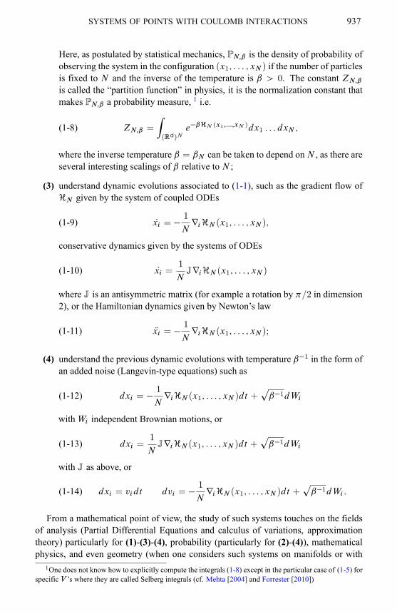
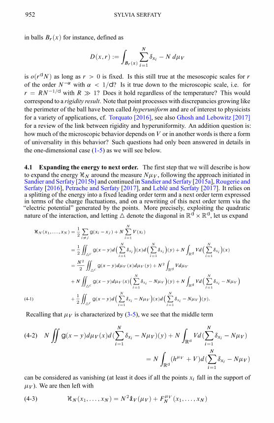
2.1 Vortices in condensed matter physics and fluids. In superconductors with ap-plied magnetic fields, and in rotating superfluids and Bose–Einstein condensates, oneobserves the occurrence of quantized “vortices” (which are local point defects of su-perconductivity or superfluidity, surrounded by a current loop). The vortices repeleach other, while being confined together by the effect of the magnetic field or rota-tion, and the result of the competition between these two effects is that, as predictedby Abrikosov [1957], they arrange themselves in a particular triangular lattice pattern,called Abrikosov lattice, cf. Fig. 12. Superconductors and superfluids are modelled bythe celebrated Ginzburg–Landau energy Landau and Ginzburg [1965], which in simpli-fied form 3 can be written

(2-1)Z

jr j2 +

(1 � j j2)2

2"2

where is a complex-valued unknown function (the “order parameter” in physics) and" is a small parameter, and gives rise to the associated Ginzburg–Landau equation

(2-2) ∆ +1

"2 (1 � j j

2) = 0

2For more pictures, see www.fys.uio.no/super/vortex/3The complete form for superconductivity contains a gauge-field, but we omit it here for simplicity.

SYSTEMS OF POINTS WITH COULOMB INTERACTIONS 939

Figure 1: Abrikosov lattice, H. F. Hess et al. Bell Labs Phys. Rev. Lett. 62, 214(1989)

and its dynamical versions, the heat flow

(2-3) @t = ∆ +1

"2 (1 � j j

2)

and Schrödinger-type flow (also called the Gross–Pitaevskii equation)

(2-4) i@t = ∆ +1

"2 (1 � j j

2):

When restricting to a two-dimensional situation, it can be shown rigorously (thiswas pioneered by Bethuel, Brezis, and Hélein [1994] for (2-1) and extended to the fullgauged model Bethuel and Rivière [1995] and Sandier and Serfaty [2007, 2012]) thatthe minimization of (2-1) can be reduced, in terms of the vortices and as " ! 0, to theminimization of an energy of the form (1-1) in the case (1-2) (for a formal derivation,see also Serfaty [2015, Chap. 1]) and this naturally leads to the question of understand-ing the connection between minimizers of (1-1) + (1-2) and the Abrikosov triangularlattice. Similarly, the dynamics of vortices under (2-3) can be formally reduced to (1-9),respectively under (2-4) to (1-10). This was established formally for instance in L. Peresand Rubinstein [1993] and E [1994a] and proven for a fixed number of vortices N andin the limit " ! 0 in F. H. Lin [1996], Jerrard and Soner [1998], Colliander and Jerrard[1998, 1999], F.-H. Lin and Xin [1999a,b], and Bethuel, Jerrard, and Smets [2008] untilthe first collision time and in Bethuel, Orlandi, and Smets [2005], Smets, Bethuel, andOrlandi [2007], Bethuel, Orlandi, and Smets [2007], and Serfaty [2007] including aftercollision.

Vortices also arise in classical fluids, where in contrast with what happens in su-perconductors and superfluids, their charge is not quantized. In that context the energy(1-1)+(1-2) is sometimes called the Kirchhoff energy and the system (1-10) with J takento be a rotation by �/2, known as the point-vortex system, corresponds to the dynam-ics of idealized vortices in an incompressible fluid whose statistical mechanics analysis

940 SYLVIA SERFATY

was initiated by Onsager, cf. Eyink and Sreenivasan [2006] (one of the motivations forstudying (1-13) is precisely to understand fluid turbulence as he conceived). It has thusbeen quite studied as such, see Marchioro and Pulvirenti [1994] for further reference.The study of evolutions like (1-11) is also motivated by plasma physics in which theinteraction between ions is Coulombic, cf. Jabin [2014].

2.2 Fekete points and approximation theory. Fekete points arise in interpolationtheory as the points minimizing interpolation errors for numerical integration Saff andTotik [1997]. More precisely, if one is looking for N interpolation points fx1; : : : ; xN g

in K such that the relation ZK

f (x)dx =

NXj=1

wjf (xj )

is exact when f is any polynomial of degree � N � 1, one sees that one needs tocompute the coefficients wj such that

RKxk =

PNj=1wjx

kj for 0 � k � N � 1,

and this computation is easy if one knows to invert the Vandermonde matrix of thefxj gj=1:::N . The numerical stability of this operation is as large as the condition numberof the matrix, i.e. as the Vandermonde determinant of the (x1; : : : ; xN ). The points thatminimize the maximal interpolation error for general functions are easily shown to bethe Fekete points, defined as those that maximizeY

i¤j

jxi � xj j

or equivalently minimize�

Xi¤j

log jxi � xj j:

They are often studied on manifolds, such as thed-dimensional sphere. In Euclideanspace, one also considers “weighted Fekete points” which maximizeY

i<j

jxi � xj je�NP

i V (xi )

or equivalently minimize

�1

2

Xi¤j

log jxi � xj j +N

NXi=1

V (xi )

which in dimension 2 corresponds exactly to the minimization of HN in the particularcase Log2. They also happen to be zeroes of orthogonal polynomials, see Simon [2008].

Since � log jxj can be obtained as lims!01s(jxj�s �1), there is also interest in study-

ing “Riesz s-energies”, i.e. the minimization of

(2-5)Xi¤j

1

jxi � xj js

SYSTEMS OF POINTS WITH COULOMB INTERACTIONS 941

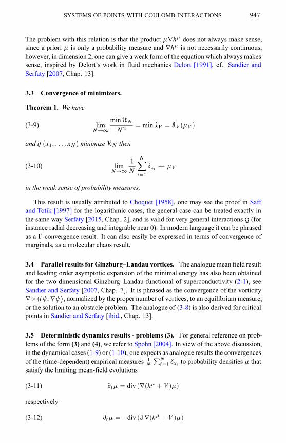
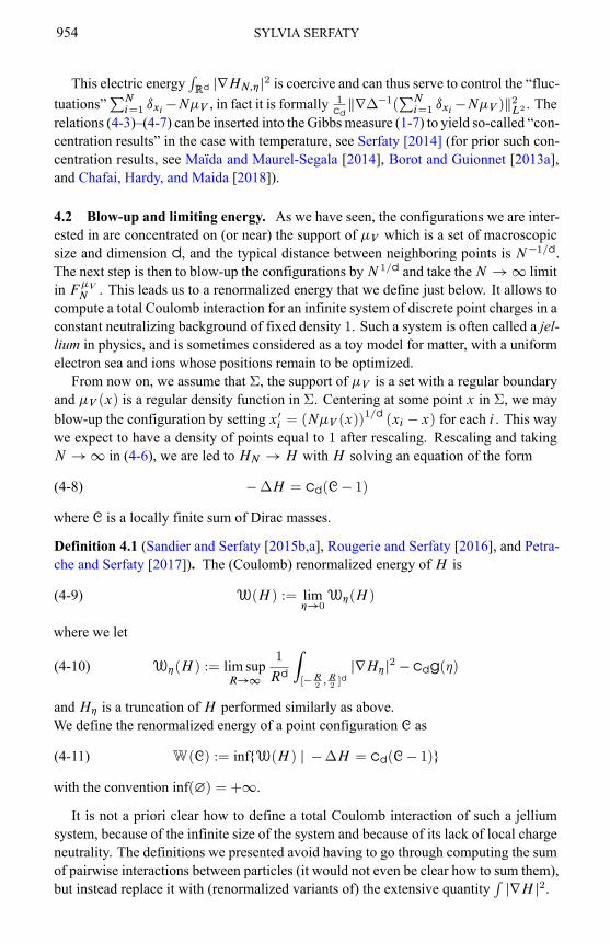
Figure 2: The triangular lattice solves the sphere packing problem in dimension2

for all possible s, hence a motivation for (1-6). For these aspects, we refer to the thereview papers Saff and Kuijlaars [1997] and Brauchart, Hardin, and Saff [2012] andreferences therein.

Varying s from 0 to1 connects Fekete points to the optimal sphere packing problem,which formally corresponds to the minimization of (2-5) with s = 1.

The optimal sphere packing problem has been solved in 1, 2 and 3 dimensions, aswell as in dimensions 8 and 24 in the recent breakthrough Viazovska [2017] and Cohn,Kumar, Miller, Radchenko, and Viazovska [2017] (we refer the reader to the nice pre-sentation in Cohn [2017] and the review Sloane [1998]). The solution in dimension 2 isthe triangular lattice Fejes [1940] (i.e. the same as the Abrikosov lattice, see Figure 2),in dimension 3 it is the FCC (face-centered cubic) lattice Hales [2005], in dimension 8the E8 lattice Viazovska [2017], and in dimension 24 the Leech lattice Cohn, Kumar,Miller, Radchenko, and Viazovska [2017].

In other dimensions, the solution is in general not known and it is expected that inhigh dimension, where the problem is important for error-correcting codes, it is not alattice (in dimension 10 already, the so-called “Best lattice”, a non-lattice competitor, isknown to beat the lattices), see Conway and Sloane [1999] for these aspects.

2.3 Statistical mechanics and quantum mechanics. The ensemble given by (1-7)in the Log2 case is called in physics a two-dimensionalCoulomb gas or one-componentplasma and is a classical ensemble of statistical mechanics (see e.g. Alastuey and Jan-covici [1981], Jancovici, Lebowitz, and Manificat [1993], Jancovici [1995], Sari andMerlini [1976], Kiessling [1993], and Kiessling and Spohn [1999]). The Coulomb casewith d = 3 can be seen as a toy (classical) model for matter (see e.g. Penrose andSmith [1972], Jancovici, Lebowitz, and Manificat [1993], Lieb and Lebowitz [1972],and Lieb and Narnhofer [1975]). Several additional motivations come from quantummechanics. Indeed, the Gibbs measure of the two-dimensional Coulomb gas happens tobe directly related to the Laughlin wave-function in the fractional quantum Hall effectGirvin [2004] and Stormer [1999]: this is the “plasma analogy”, cf. Laughlin [1983],Girvin [1999], and Laughlin [1999], and for recent mathematical progress using thiscorrespondence, cf. Rougerie, Serfaty, and Yngvason [2014], Rougerie and Yngvason[2015], and Lieb, Rougerie, and Yngvason [2018]. For ˇ = 2 it also arises as thewave-function density of the ground state for the system ofN non-interacting fermions

942 SYLVIA SERFATY

confined to a plane with a perpendicular magnetic field Forrester [2010, Chap. 15].The 1-dimensional log gas Log1 also arises as the wave-function density in several ex-actly solvable quantum mechanics systems: examples are the Tonks–Girardeau modelof “impenetrable” Bosons Girardeau,Wright, and Triscari [2001] and Forrester, Frankel,Garoni, and Witte [2003], the Calogero–Sutherland quantum many-body HamiltonianForrester, Jancovici, and McAnally [2001] and Forrester [2010] and finally the densityof the many-body wave function of non-interacting fermions in a harmonic trap Dean,Le Doussal, Majumdar, and Schehr [2016]. It also arises in several non-intersectingpaths models from probability, cf. Forrester [2010].

The general Riesz case (1-6) can be seen as a generalization of the Coulomb case,motivations for studying Riesz gases are numerous in the physics literature (in solidstate physics, ferrofluids, elasticity), see for instance Mazars [2011], Barré, Bouchet,Dauxois, and Ruffo [2005], Campa, Dauxois, and Ruffo [2009], and Torquato [2016],they can also correspond to systems with Coulomb interaction constrained to a lower-dimensional subspace: for instance in the quantum Hall effect, electrons confined to atwo-dimensional plane interact via the three-dimension Coulomb kernel.

In all cases of interactions, the systems governed by the Gibbs measure PN;ˇ areconsidered as difficult systems of statistical mechanics because the interactions are trulylong-range, singular, and the points are not constrained to live on a lattice.

As always in statistical mechanics K. Huang [1987], one would like to understandif there are phase-transitions for particular values of the (inverse) temperature ˇ in thelarge volume limit. For the systems studied here, one may expect, after a suitable blow-up of the system, what physicists call a liquid for small ˇ, and a crystal for large ˇ. Themeaning of crystal in this instance is not to be taken literally as a lattice, but rather as asystem of points whose 2-point correlation function �(2)(x; y) defined as the probabilityto have jointly one point at x and one point at y (see Section 3.1) does not decay toofast as x � y ! 1. A phase-transition at finite ˇ has been conjectured in the physicsliterature for the Log2 case (see e.g. Brush, Sahlin, and Teller [1966], Caillol, Levesque,Weis, and Hansen [1982], and Choquard and Clerouin [1983]) but its precise nature isstill unclear (see e.g. Stishov [1998] for a discussion).

2.4 Two component plasma case. The two-dimensional “one component plasma”,consisting of positively charged particles, has a “two-component” counterpart whichconsists in N particles x1; : : : ; xN of charge +1 and N particles y1; : : : ; yN of charge�1 interacting logarithmically, with energy

HN (x1; : : : ; xN ; y1; : : : ; yN ) = �Xi¤j

log jxi �xj j�Xi¤j

log jyi �yj j+Xi;j

log jxi �yj j

and the Gibbs measure1

ZN;ˇ

e�ˇHN (x1;:::;xN ;y1;:::;yN )dx1 : : : dxN dy1 : : : dyN :

Although the energy is unbounded below (positive and negative points attract), theGibbs measure is well defined for ˇ small enough, more precisely the partition func-tion converges for ˇ < 2. The system is then seen to form dipoles of oppositely

SYSTEMS OF POINTS WITH COULOMB INTERACTIONS 943

charged particles which attract but do not collapse, thanks to the thermal agitation.The two-component plasma is interesting due to its close relation to two importanttheoretical physics models: the XY model and the sine-Gordon model (cf. the re-view Spencer [1997]), which exhibit a Berezinski–Kosterlitz–Thouless phase transitionBietenholz and Gerber [2016] consisting in the binding of these “vortex-antivortex”dipoles. For further reference, see Fröhlich [1976], Deutsch and Lavaud [1974], Fröh-lich and Spencer [1981], and Gunson and Panta [1977].

2.5 Random matrix theory. The study of (1-7) has attracted a lot of attention dueto its connection with random matrix theory (we refer to Forrester [2010] for a compre-hensive treatment). Random matrix theory (RMT) is a relatively old theory, pioneeredby statisticians and physicists such as Wishart, Wigner and Dyson, and originally moti-vated by the study of sample covariance matrices for the former and the understandingof the spectrum of heavy atoms for the two latter, see Mehta [2004]. For more recentmathematical reference see Anderson, Guionnet, and Zeitouni [2010], Deift [1999], andForrester [2010]. The main question asked by RMT is : what is the law of the spectrumof a large random matrix ? As first noticed in the foundational papers of Wigner [1955]and Dyson [1962], in the particular cases (1-5) and (1-2) the Gibbs measure (1-7) cor-responds in some particular instances to the joint law of the eigenvalues (which can becomputed algebraically) of some famous random matrix ensembles:

• for Log2, ˇ = 2 and V (x) = jxj2, (1-7) is the law of the (complex) eigenvaluesof anN �N matrix where the entries are chosen to be normal Gaussian i.i.d. Thisis called the Ginibre ensemble Ginibre [1965].

• for Log1, ˇ = 2 and V (x) = x2/2, (1-7) is the law of the (real) eigenvalues ofan N � N Hermitian matrix with complex normal Gaussian iid entries. This iscalled the Gaussian Unitary Ensemble.

• for Log1, ˇ = 1 and V (x) = x2/2, (1-7) is the law of the (real) eigenvalues ofan N �N real symmetric matrix with normal Gaussian iid entries. This is calledthe Gaussian Orthogonal Ensemble.

• for Log1, ˇ = 4 and V (x) = x2/2, (1-7) is the law of the eigenvalues of anN �N quaternionic symmetric matrix with normal Gaussian iid entries. This iscalled the Gaussian Symplectic Ensemble.

• the general-ˇ case of Log1 can also be represented, in a slightly more compli-cated way, as a randommatrix ensemble Dumitriu and Edelman [2002] and Killipand Nenciu [2004].

One thus observes in these ensembles the phenomenon of “repulsion of eigenvalues”:they repel each other logarithmically, i.e. like two-dimensional Coulomb particles.

The stochastic evolution (1-12) in the case Log1 is (up to proper scaling) the DysonBrownian motion, which is of particular importance in random matrices since the GUEprocess is the invariant measure for this evolution, it has served to prove universalityfor the statistics of eigenvalues of general Wigner matrices, i.e. those with iid but not

944 SYLVIA SERFATY

necessarily Gaussian entries, see Erdős and Yau [2017] (and Tao and Vu [2011] foranother approach).

For the Log1 and Log2 cases, at the specific temperature ˇ = 2, the law (1-7) ac-quires a special algebraic feature: it becomes a determinantal process, part of a widerclass of processes (see Hough, Krishnapur, Y. Peres, and Virág [2009] and Borodin[2011]) for which the correlation functions are explicitly given by certain determinants.This allows for many explicit algebraic computations, and is part of integrable proba-bility on which there is a large literature Borodin and Gorin [2016].

2.6 Complex geometry and theoretical physics. Coulomb systems and higher-di-mensional analogues involving powers of determinantal densities are also of interest togeometers as a way to construct Kähler–Einstein metrics with negative Ricci curvatureon complex manifolds, cf. Berman [2017] and Berman, Boucksom, and Witt Nyström[2011].

Another important motivation is the construction of Laughlin states for the FractionalQuantum Hall effect on complex manifolds, which effectively reduces to the study of atwo-dimensional Coulomb gas on a manifold. The coefficients in the expansion of the(logarithm of the) partition function have interpretations as geometric invariants, cf. forinstance Klevtsov [2016].

3 The mean field limits and macroscopic behavior

3.1 Questions. The first question that naturally arises is to understand the limit asN ! 1 of the empirical measure defined by 4

(3-1) �N :=1

N

NXi=1

ıxi

for configurations of points that minimize the energy (1-1), critical points, solutions ofthe evolution problems, or typical configurations under the Gibbs measure (1-7), thushoping to derive effective equations or minimization problems that describe the averageor mean-field behavior of the system. The term mean-field refers to the fact that, fromthe physics perspective, each particle feels the collective field generated by all the otherparticles, averaged by dividing it by the number of particles. That collective field isg � �N , except that it is singular at each particle, so to evaluate it at xi one first has toremove the contribution of xi itself.

Another point of view is that of correlation functions. One may denote by

(3-2) �(k)N (x1; : : : ; xk)

the k-point correlation function, which is the probability density (for each specific prob-lem) of observing a particle at x1, a particle at x2, : : : , and a particle at xk (these func-tions should of course be symmetric with respect to permutation of the labels). For

4Note that the configurations contain N points which also implicitly depend on N themselves, but we donot keep track of this dependence for the sake of lightness of notation.

SYSTEMS OF POINTS WITH COULOMB INTERACTIONS 945

instance, in the case (1-7), �(N )N is simply PN;ˇ itself, and the �(k)N are its marginals

(obtained by integrating PN;ˇ with respect to all its variables but k). One then wantsto understand the limit as N ! 1 of each �(k)N , with fixed k. Mean-field results willtypically imply that the limiting �(k)’s have a factorized form

(3-3) �(k)(x1; : : : ; xk) = �(x1) : : : �(xk)

for the appropriate � which is also equal to �(1). This is called molecular chaos accord-ing to the terminology introduced by Boltzmann, and can be interpreted as the particlesbecoming independent in the limit. When looking at the dynamic evolutions of prob-lems (3) and (4), starting from initial data for which �(k)(0; �) are in such a factorizedform, one asks whether this remains true for �(k)(t; �) for t > 0, if so this is calledpropagation of (molecular) chaos. It turns out that the convergence of the empiricalmeasure (3-1) to a limit � and the fact that each �(k) can be put in factorized form areessentially equivalent, see Hauray andMischler [2014] and Golse [2016] and referencestherein — ideally, one would also like to find quantitative rates of convergences in N ,and they will typically deteriorate as k gets large. In the following we will focus on themean-field convergence approach, via the empirical measure.

In the case of minimizers (1), a major question is to obtain an expansion asN ! 1

for minHN . In the setting of manifolds, the coefficients in such an expansion havegeometric interpretations. In the same way, in the statistical mechanics setting (2), onesearches for expansions as N ! 1 of the so-called free energy �ˇ�1 logZN;ˇ . Thefree energy encodes a lot of the physical quantities of the system. For instance, points ofnon-differentiability of logZN;ˇ as a function of ˇ are interpreted as phase-transitions.

We will see below that understanding the mean-field behavior of the system essen-tially amounts to understanding the leading order term in the large N expansion of theminimal energy or respectively the free energy, while understanding the next order termin the expansion essentially amounts to understanding the next order (or fluctuations)of the system.

3.2 The equilibrium measure. The leading order behavior of HN is related to thefunctional

(3-4) IV (�) :=1

2

“Rd�Rd

g(x � y)d�(x)d�(y) +

ZRdV (x)d�(x)

defined over the space P (Rd) of probability measures on Rd (which may also takethe value +1). This is something one may naturally expect since IV (�) appears asthe continuum version of the discrete energy HN . From the point of view of statisticalmechanics, IV is the mean-field limit energy of HN , while from the point of view ofprobability, IV plays the role of a rate function.

Assuming some lower semi-continuity of V and that it grows faster than g at 1, itwas shown in Frostman [1935] that the minimum of IV over P (Rd) exists, is finite andis achieved by a unique �V (unique by strict convexity of IV ), which has compact sup-port and a density, and is uniquely characterized by the fact that there exists a constant

946 SYLVIA SERFATY

c such that

(3-5)

8<: h�V + V � c in Rd

h�V + V = c in the support of �V

where

(3-6) h�V (x) :=

ZRd

g(x � y)d�V (y) = g � �V

is the “electrostatic” potential generated by �V .This measure �V is called the (Frostman) equilibrium measure, and the result is true

for more general repulsive kernels than Coulomb, for instance for all regular kernels orinverse powers of the distance which are integrable.

Example 3.1. When g is the Coulomb kernel, applying the Laplacian on both sides of(3-5) gives that, in the interior of the support of the equilibrium measure, if V 2 C 2,

(3-7) cd�V = ∆V

i.e. the density of the measure on the interior of its support is given by ∆Vcd

. For exampleif V is quadratic, this density is constant on the interior of its support. If V (x) = jxj2

then by symmetry �V is the indicator function of a ball (up to a multiplicative factor),this is known as the circle law for the Ginibre ensemble in the context of RandomMatrixTheory. An illustration of the convergence to this circle law can be found in Figure 3.In dimension d = 1, with g = � log j � j and V (x) = x2, the equilibrium measure is�V (x) =

12�

p4 � x21jxj�2, which corresponds in the context of RMT (GUE and GOE

ensembles) to the famousWigner semi-circle law, cf. Wigner [1955] and Mehta [2004].

In the Coulomb case, the equilibrium measure �V can also be interpreted in termsof the solution to a classical obstacle problem (and in the Riesz case (1-6) with d � 2 �

s < d a “fractional obstacle problem”), which is essentially dual to the minimization ofIV , and better studied from the PDE point of view (in particular the regularity of �V

and of the boundary of its support). For this aspect, see Serfaty [2015, Chap. 2] andreferences therein.

Frostman’s theorem is the basic result of potential theory. The relations (3-5) can beseen as the Euler–Lagrange equations associated to the minimization of IV . They statethat in the static situation, the total potential, sum of the potential generated by �V andthe external potential V must be constant in the support of �V , i.e. in the set where the“charges” are present.

More generallyr(h�+V ) can be seen as the total mean-field force acting on chargeswith density � (i.e. each particle feels the average collective force generated by theother particles), and for the particle to be at rest one needs that force to vanish. Thusr(h� + V ) should vanish on the support of �, in fact the stationarity condition thatformally emerges as the limit for critical points of HN is

(3-8) �r(h� + V ) = 0:

SYSTEMS OF POINTS WITH COULOMB INTERACTIONS 947

The problem with this relation is that the product �rh� does not always make sense,since a priori � is only a probability measure and rh� is not necessarily continuous,however, in dimension 2, one can give a weak form of the equation which always makessense, inspired by Delort’s work in fluid mechanics Delort [1991], cf. Sandier andSerfaty [2007, Chap. 13].

3.3 Convergence of minimizers.

Theorem 1. We have

(3-9) limN !1

minHN

N 2= minIV = IV (�V )

and if (x1; : : : ; xN ) minimize HN then

(3-10) limN !1

1

N

NXi=1

ıxi* �V

in the weak sense of probability measures.

This result is usually attributed to Choquet [1958], one may see the proof in Saffand Totik [1997] for the logarithmic cases, the general case can be treated exactly inthe same way Serfaty [2015, Chap. 2], and is valid for very general interactions g (forinstance radial decreasing and integrable near 0). In modern language it can be phrasedas a Γ-convergence result. It can also easily be expressed in terms of convergence ofmarginals, as a molecular chaos result.

3.4 Parallel results forGinzburg–Landau vortices. The analoguemean field resultand leading order asymptotic expansion of the minimal energy has also been obtainedfor the two-dimensional Ginzburg–Landau functional of superconductivity (2-1), seeSandier and Serfaty [2007, Chap. 7]. It is phrased as the convergence of the vorticityr �hi ;r i, normalized by the proper number of vortices, to an equilibrium measure,or the solution to an obstacle problem. The analogue of (3-8) is also derived for criticalpoints in Sandier and Serfaty [ibid., Chap. 13].

3.5 Deterministic dynamics results - problems (3). For general reference on prob-lems of the form (3) and (4), we refer to Spohn [2004]. In view of the above discussion,in the dynamical cases (1-9) or (1-10), one expects as analogue results the convergencesof the (time-dependent) empirical measures 1

N

PNi=1 ıxi

to probability densities � thatsatisfy the limiting mean-field evolutions

(3-11) @t� = div (r(h� + V )�)

respectively

(3-12) @t� = �div (Jr(h� + V )�)

948 SYLVIA SERFATY

where again h� = g � � as in (3-6). These are nonlocal transport equations where thedensity� is transported along the velocity field�r(h�+V ) (respectively Jr(h�+V ))i.e. advected by the mean-field force that the distribution generates.

In the two-dimensional Coulomb case (1-2) with V = 0, (3-12) with J chosen asthe rotation by �/2 is also well-known as the vorticity form of the incompressible Eulerequation, describing the evolution of the vorticity in an ideal fluid, with velocity givenby the Biot–Savart law. As such, this equation is well-studied in this context, and theconvergence of solutions of (1-10) to (3-12), also known as the point-vortex approxi-mation to Euler, has been rigorously proven, see Schochet [1996] and Goodman, Hou,and Lowengrub [1990].

As for (3-11), it is a dissipative equation, that can be seen as a gradient flow on thespace of probability measures equipped with the so-called Wasserstein W2 (or Monge–Kantorovitch) metric. In the dimension 2 logarithmic case, it was first introduced byChapman, Rubinstein, and Schatzman [1996] and E [1994b] as a formal model for su-perconductivity, and in that setting the gradient flow description has been made rig-orous (see Ambrosio and Serfaty [2008]) using the theory of gradient flows in metricspaces of Otto [2001] and Ambrosio, Gigli, and Savaré [2005]. The equation can alsobe studied by PDE methods F. Lin and Zhang [2000] and Serfaty and Vázquez [2014],which generalize to the Coulomb interaction in any dimension. The derivation of thisgradient flow equation (3-11) from (2-3) can be guessed by variational arguments, i.e.“Γ-convergence of gradient flows”, see Serfaty [2011]. In the non Coulombic case, i.e.for (1-6), (3-11) is a “fractional porous medium equation”, analyzed in Caffarelli andVazquez [2011], Caffarelli, Soria, and Vázquez [2013], and Zhou and Xiao [2017].

We have the following result which states in slightly informal terms that the desiredconvergence holds provided the limiting solution is regular enough.

Theorem 2 (Serfaty and Duerinckx [2018]). For any d, any case (1-2), (1-5) or (1-6)withd�2 � s < d, let fxi g solve (1-9), respectively (1-10)with initial data xi (0) = x0i .Then if the limit �0 of the initial empirical measure 1

N

PNi=1 ıx0

iis regular enough so

that the solution �t of (3-11), resp. (3-12), with initial data �0 exists until time T > 0

and is regular enough, and if the initial condition is well-prepared in the sense that

limN !1

1

N 2HN (fx0i g) =

“Rd�Rd

g(x � y)d�0(x)d�0(y);

then we have that for all t 2 [0; T ),

1

N

NXi=1

ıxi (t) ! �t as N ! 1:

Note that the existence of regular enough solutions that exist for all time, providedthe initial data is regular enough, is known to hold for all Coulomb cases and all Rieszcases with s < d � 1 Zhou and Xiao [2017].

The difficulty in proving this convergence result is due to the singularity of theCoulomb interaction combined with the nonlinear character of the product h�� (andits discrete analogue) which prevents from directly taking limits in the equation.

SYSTEMS OF POINTS WITH COULOMB INTERACTIONS 949

Prior results existed for less singular interactions Hauray [2009], Carrillo, Choi, andHauray [2014], and Jabin and Wang [2017] or in dimension 1 Berman and Onnheim[2016]. Theorem 2 was first proven in the dissipative case in dimensions 1 and 2 inDuerinckx [2016], then in all dimensions and in the conservative case in Serfaty andDuerinckx [2018]. Both proofs rely on a “modulated energy” approach inspired fromSerfaty [2017]. It consists in considering a Coulomb-based (or Riesz-based) distancebetween probability densities, more precisely the distance defined by

dg(�; �)2 =

“Rd�Rd

g(x � y)d (� � �)(x)d (� � �)(y)

which is a good metric thanks to the particular properties of the Coulomb and Rieszkernels. One can prove a “weak-strong” stability result for the limiting equations (3-11),(3-12) in that metric: if � is a smooth enough solution to (3-11), resp. (3-12), and if �is any solution to the same equation, then

(3-13) dg(�(t); �(t)) � eC tdg(�(0); �(0));

which is proved by showing a Gronwall inequality. One may then exploit this stabilityproperty by taking� to be the smooth enough expected limiting solution, and � to be theempirical measure of the solution to the discrete evolution (1-9) or (1-10), after givingan appropriate renormalized meaning to the Coulomb distance (which is otherwiseinfinite) in that setting. We are able to prove that a relation similar to (3-13) holds, thusproving the desired convergence.

The analogue of the rigorous passage from (1-9) or (1-10) to (3-11) or (3-12) was ac-complished at the level of the full parabolic and Schrödinger Ginzburg–Landau PDEs(2-3) and (2-4) Kurzke and Spirn [2014], Jerrard and Spirn [2015], and Serfaty [2017].The method in Serfaty [2017] relies as above on a modulated energy argument whichconsists in finding a suitable energy, modelled on the Ginzburg–Landau energy, whichmeasures the distance to the desired limiting solution, and for which a Gronwall inequal-ity can be shown to hold.

As far as (1-11) is concerned, the limiting equation is formally found to be theVlasov–Poisson equation

(3-14) @t� + v � rx� + r(h� + V ) � rv� = 0

where �(t; x; v) is the density of particles at time t with position x and velocity v, and�(t; x) =

R�(t; x; v)dv is the density of particles. The rigorous convergence of (1-11)

to (3-14) and propagation of chaos are not proven in all generality (i.e. for all initialdata) but it has been established in a statistical sense (i.e. randomizing the initial condi-tion) and often truncating the interactions, see Kiessling [2014], Boers and Pickl [2016],Hauray and Jabin [2015], Lazarovici [2016], Lazarovici and Pickl [2017], and Jabin andWang [2016] and also the reviews on the topic Jabin [2014] and Golse [2016].

3.6 Noisy dynamics - problems (4). The noise terms in these equations gives rise toan additive Laplacian term in the limiting equations. For instance the limiting equation

950 SYLVIA SERFATY

for (1-12) is expected to be the McKean equation

(3-15) @t� =1

ˇ∆� � div (r(h� + V )�)

and the convergence is known for regular interactions since the seminal work ofMcKean[1967], see also the reviews Sznitman [1991] and Jabin [2014].

For singular interactions, the situation has been understood for the one-dimensionallogarithmic case Cépa and Lépingle [1997], then for all Riesz interactions (1-6) Bermanand Onnheim [2018]. Higher dimensions with singular interactions is largely open, butrecent progress of Jabin and Wang [2017] allows to treat possibly rough but boundedinteractions, as well as some Coulomb interactions, and prove convergence in an appro-priate statistical sense.

For the conservative case (1-13) the limiting equation is a viscous conservative equa-tion of the form

(3-16) @t� =1

ˇ∆� � div (r?(h� + V )�)

which in the two-dimensional logarithmic case (1-2) is the Navier–Stokes equation invorticity form. The convergence in that particular case was established in Fournier,Hauray, and Mischler [2014], while the most general available result is that of Jabinand Wang [2017].

For the case of (1-14), the limiting equation is the McKean–Vlasov equation

(3-17) @t� + v � rx� + r(h� + V ) � rv� �1

ˇ∆� = 0

with the same notation as for (3-14), and convergence in the case of bounded-gradientkernels is proven in Jabin and Wang [2016], see also references therein.

3.7 With temperature: statistical mechanics. Let us now turn to problem (2) andconsider the situation with temperature as described via the Gibbs measure (1-7). Onecan determine that two temperature scaling choices are interesting: the first is takingˇ independent of N , the second is taking ˇN = ˇ

Nwith some fixed ˇ. In the former,

which can be considered a “low temperature” regime, the behavior of the system is stillgoverned by the equilibrium measure �V . The result can be phrased using the languageof Large Deviations Principles (LDP), cf. Dembo and Zeitouni [2010] for definitionsand reference.

Theorem 3. The sequence fPN;ˇ gN of probability measures on P (Rd) satisfies a largedeviations principle at speed N 2 with good rate function ˇIV where IV = IV �

minP (Rd) IV = IV � IV (�V ). Moreover

(3-18) limN !+1

1

N 2logZN;ˇ = �ˇIV (�V ) = �ˇ min

P (Rd)IV :

The concrete meaning of the LDP is that if E is a subset of the space of probabilitymeasures P (Rd), after identifying configurations (x1; : : : ; xN ) in (Rd)N with their

SYSTEMS OF POINTS WITH COULOMB INTERACTIONS 951

empirical measures 1N

PNi=1 ıxi

, we may write

(3-19) PN;ˇ (E) � e�ˇN 2(minE IV �minIV );

which in view of the uniqueness of the minimizer of IV implies that configurationswhose empirical measure does not converge to �V as N ! 1 have exponentiallydecaying probability. In other words the Gibbs measure concentrates as N ! 1 onconfigurations for which the empirical measure is very close to�V , i.e. the temperaturehas no effect on the mean-field behavior.

This result was proven in the logarithmic cases in Petz and Hiai [1998] (in dimen-sion 2), Ben Arous and Guionnet [1997] (in dimension 1) and Ben Arous and Zeitouni[1998] (in dimension 2) for the particular case of a quadratic potential (and ˇ = 2), seealso Berman [2014] with results for general powers of the determinant in the setting ofmultidimensional complexmanifolds, or Chafaı, Gozlan, and Zitt [2014] which recentlytreated more general singularg’s and V ’s. This result is actually valid in any dimension,and is not at all specific to the Coulomb interaction (the proof works as well for moregeneral interaction potentials, see Serfaty [2015]).

In the high-temperature regime ˇN = ˇN, the temperature is felt at leading order and

brings an entropy term. More precisely there is a temperature-dependent equilibriummeasure �V;ˇ which is the unique minimizer of

(3-20) IV;ˇ (�) = ˇIV (�) +

Z� log�:

Contrarily to the equilibrium measure, �V;ˇ is not compactly supported, but decaysexponentially fast at infinity. This mean-field behavior and convergence of marginalswas first established for logarithmic interactions Kiessling [1993] and Caglioti, Lions,Marchioro, and Pulvirenti [1992] (see Messer and Spohn [1982] for the case of regularinteractions) using an approach based on de Finetti’s theorem. In the language of LargeDeviations, the same LDP as above then holds with rate function IV;ˇ �min IV;ˇ , and theGibbs measure now concentrates asN ! 1 on a neighborhood of�V;ˇ , for a proof seeGarcía-Zelada [2017]. Again the Coulomb nature of the interaction is not really needed.One can also refer to Rougerie [2014, 2016] for the mean-field and chaos aspects witha particular focus on their adaptation to the quantum setting.

4 Beyond the mean field limit: next order study

We have seen that studying systems with Coulomb (or more general) interactions atleading order leads to a good understanding of their limiting macroscopic behavior. Onewould like to go further and describe their microscopic behavior, at the scale of thetypical inter-distance between the points, N�1/d. This in fact comes as a by-product ofa next-to-leading order description of the energy HN , which also comes together witha next-to-leading order expansion of the free energy in the case (1-7).

Thinking of energy minimizers or of typical configurations under (1-7), since onealready knows that

PNi=1 ıxi

�N�V is small, one knows that the so-called discrepancy

952 SYLVIA SERFATY

in balls Br(x) for instance, defined as

D(x; r) :=

ZBr (x)

NXi=1

ıxi�N d�V

is o(rdN ) as long as r > 0 is fixed. Is this still true at the mesoscopic scales for rof the order N�˛ with ˛ < 1/d? Is it true down to the microscopic scale, i.e. forr = RN�1/d with R � 1? Does it hold regardless of the temperature? This wouldcorrespond to a rigidity result. Note that point processes with discrepancies growing likethe perimeter of the ball have been called hyperuniform and are of interest to physicistsfor a variety of applications, cf. Torquato [2016], see also Ghosh and Lebowitz [2017]for a review of the link between rigidity and hyperuniformity. An addition question is:howmuch of the microscopic behavior depends on V or in another words is there a formof universality in this behavior? Such questions had only been answered in details inthe one-dimensional case (1-5) as we will see below.

4.1 Expanding the energy to next order. The first step that we will describe is howto expand the energy HN around the measureN�V , following the approach initiated inSandier and Serfaty [2015b] and continued in Sandier and Serfaty [2015a], Rougerie andSerfaty [2016], Petrache and Serfaty [2017], and Leblé and Serfaty [2017]. It relies ona splitting of the energy into a fixed leading order term and a next order term expressedin terms of the charge fluctuations, and on a rewriting of this next order term via the“electric potential” generated by the points. More precisely, exploiting the quadraticnature of the interaction, and letting 4 denote the diagonal in Rd � Rd, let us expand

HN (x1; : : : ; xN ) =1

2

Xi¤j

g(xi � xj ) + N

NXi=1

V (xi )

=1

2

“4c

g(x � y)d� NX

i=1

ıxi

�(x)d

� NXi=1

ıxi

�(y) + N

ZRd

Vd� NX

i=1

ıxi

�(x)

=N 2

2

“4c

g(x � y)d�V (x)d�V (y) + N 2

ZRd

Vd�V

+ N

“4c

g(x � y)d�V (x)� NX

i=1

ıxi� N�V

�(y) + N

ZRd

Vd� NX

i=1

ıxi� N�V

�+

1

2

“4c

g(x � y)d� NX

i=1

ıxi� N�V

�(x)d

� NXi=1

ıxi� N�V

�(y):(4-1)

Recalling that �V is characterized by (3-5), we see that the middle term

(4-2) N

“g(x � y)d�V (x)d (

NXi=1

ıxi�N�V )(y) +N

ZRdVd (

NXi=1

ıxi�N�V )

= N

ZRd

(h�V + V )d (

NXi=1

ıxi�N�V )

can be considered as vanishing (at least it does if all the points xi fall in the support of�V ). We are then left with

(4-3) HN (x1; : : : ; xN ) = N 2IV (�V ) + F�V

N (x1; : : : ; xN )

SYSTEMS OF POINTS WITH COULOMB INTERACTIONS 953

with(4-4)

F�V

N (x1; : : : ; xN ) =1

2

“4c

g(x � y)d� NX

i=1

ıxi�N�V

�(x)d

� NXi=1

ıxi�N�V

�(y):

The relation (4-3) is a next-order expansion of HN (recall (3-9)), valid for arbitraryconfigurations. The “next-order energy” F �V

N can be seen as the Coulomb energy ofthe neutral system formed by the N positive point charges at the xi ’s and the diffusenegative charge �N�V of same mass. To further understand F �V

N let us introduce thepotential generated by this system, i.e.

(4-5) HN (x) =

ZRd

g(x � y)d� NX

i=1

ıxi�N�V

�(y)

(compare with (3-6)) which solves the linear elliptic PDE (in the sense of distributions)

(4-6) � ∆HN = cd� NX

i=1

ıxi�N�V

�and use for the first time crucially the Coulomb nature of the interaction to write

(4-7)“

4c

g(x � y)d� NX

i=1

ıxi�N�V

�(x)d

� NXi=1

ıxi�N�V

�(y)

' �1

cd

ZRdHN∆HN =

1

cd

ZRd

jrHN j2

after integrating by parts by Green’s formula. This computation is in fact incorrectbecause it ignores the diagonal terms which must be removed from the integral, andyields a divergent integral

RjrHN j2 (it diverges near each point xi of the configuration).

However, this computation can be done properly by removing the infinite diagonal termsand “renormalizing” the infinite integral, replacing

RjrHN j2 byZ

RdjrHN;�j

2�Ncdg(�)

where we replace HN by HN;� , its “truncation” at level � (here � = ˛N�1/d with˛ a small fixed number) — more precisely HN;� is obtained by replacing the Diracmasses in (4-5) by uniform measures of total mass 1 supported on the sphere @B(xi ; �)

— and then removing the appropriate divergent part cdg(�). The name renormalizedenergy originates in the work of Bethuel, Brezis, and Hélein [1994] in the context oftwo-dimensional Ginzburg–Landau vortices, where a similar (although different) renor-malization procedure was introduced. Such a computation allows to replace the doubleintegral, or sum of pairwise interactions of all the charges and “background”, by a singleintegral, which is local in the potentialHN . This transformation is very useful, and usescrucially the fact that g is the kernel of a local operator (the Laplacian).

954 SYLVIA SERFATY

This electric energyR

Rd jrHN;�j2 is coercive and can thus serve to control the “fluc-tuations”

PNi=1 ıxi

�N�V , in fact it is formally 1cd

kr∆�1(PN

i=1 ıxi�N�V )k

2L2 . The

relations (4-3)–(4-7) can be inserted into the Gibbsmeasure (1-7) to yield so-called “con-centration results” in the case with temperature, see Serfaty [2014] (for prior such con-centration results, see Maıda and Maurel-Segala [2014], Borot and Guionnet [2013a],and Chafai, Hardy, and Maida [2018]).

4.2 Blow-up and limiting energy. As we have seen, the configurations we are inter-ested in are concentrated on (or near) the support of �V which is a set of macroscopicsize and dimension d, and the typical distance between neighboring points is N�1/d.The next step is then to blow-up the configurations byN 1/d and take theN ! 1 limitin F �V

N . This leads us to a renormalized energy that we define just below. It allows tocompute a total Coulomb interaction for an infinite system of discrete point charges in aconstant neutralizing background of fixed density 1. Such a system is often called a jel-lium in physics, and is sometimes considered as a toy model for matter, with a uniformelectron sea and ions whose positions remain to be optimized.

From now on, we assume that Σ, the support of �V is a set with a regular boundaryand �V (x) is a regular density function in Σ. Centering at some point x in Σ, we mayblow-up the configuration by setting x0

i = (N�V (x))1/d (xi � x) for each i . This way

we expect to have a density of points equal to 1 after rescaling. Rescaling and takingN ! 1 in (4-6), we are led toHN ! H withH solving an equation of the form

(4-8) � ∆H = cd(C � 1)

where C is a locally finite sum of Dirac masses.

Definition 4.1 (Sandier and Serfaty [2015b,a], Rougerie and Serfaty [2016], and Petra-che and Serfaty [2017]). The (Coulomb) renormalized energy ofH is

(4-9) W(H ) := lim�!0

W�(H )

where we let

(4-10) W�(H ) := lim supR!1

1

Rd

Z[� R

2 ; R2 ]d

jrH�j2

� cdg(�)

andH� is a truncation ofH performed similarly as above.We define the renormalized energy of a point configuration C as

(4-11) W (C) := inffW(H ) j � ∆H = cd(C � 1)g

with the convention inf(¿) = +1.

It is not a priori clear how to define a total Coulomb interaction of such a jelliumsystem, because of the infinite size of the system and because of its lack of local chargeneutrality. The definitions we presented avoid having to go through computing the sumof pairwise interactions between particles (it would not even be clear how to sum them),but instead replace it with (renormalized variants of) the extensive quantity

RjrH j2.

SYSTEMS OF POINTS WITH COULOMB INTERACTIONS 955

The energy W can be proven to be bounded below and to have a minimizer; more-over, its minimum can be achieved as the limit of energies of periodic configurations(with larger and larger period), for all these aspects see for instance Serfaty [2015].

4.3 Crystallization questions for minimizers. Determining the value of minW isan open question, with the exception of the one-dimensional analogues for which theminimum is achieved at the lattice Z Sandier and Serfaty [2015a] and Leblé [2016].

The only question that we can completely answer so far is that of the minimizationover the restricted class of lattice configurations in dimensiond = 2, i.e. configurationswhich are exactly a lattice ZEu+ ZEv with det(Eu; Ev) = 1.

Theorem 4. The minimum of W over lattices of volume 1 in dimension 2 is achieveduniquely by the triangular lattice.

Here the triangular lattice means Z+Zei�/3, properly scaled, i.e. what is called theAbrikosov lattice in the context of superconductivity. This result is essentially equiva-lent (see Osgood, Phillips, and Sarnak [1988] and Chiu [1997]) to a result on the mini-mization of the Epstein � function of the lattice

�s(Λ) :=X

p2Λnf0g

1

jpjs

proven in the 50’s by Cassels, Rankin, Ennola, Diananda, cf. Montgomery [1988] andreferences therein. It corresponds to the minimization of the “height” of flat tori, in thesense of Arakelov geometry. In dimension d � 3 the minimization of W restrictedto the class of lattices is an open question, except in dimensions 4, 8 and 24 where astrict local minimizer is known Sarnak and Strömbergsson [2006] (it is the E8 latticein dimension 8 and the Leech lattice in dimension 24, which were already mentionedbefore).

One may ask whether the triangular lattice does achieve the global minimum of Win dimension 2. The fact that the Abrikosov lattice is observed in superconductors,combined with the fact that W can be derived as the limiting minimization problem ofGinzburg–Landau, see Sandier and Serfaty [2012], justify conjecturing this.

Conjecture 4.2. The triangular lattice is a global minimizer of W in dimension 2.

It was also recently proven in Bétermin and Sandier [2018] that this conjecture isequivalent to a conjecture of Brauchart, Hardin, and Saff [2012] on the next order termin the asymptotic expansion of the minimal logarithmic energy on the sphere (an im-portant problem in approximation theory, also related to Smale’s “7th problem for the21st century”), which is obtained by formal analytic continuation, hence by very differ-ent arguments. In addition, the result of Coulangeon and Schürmann [2012] essentiallyyields the local minimality of the triangular lattice within all periodic (with possiblylarge period) configurations.

Note that the triangular lattice, the E8 lattice in dimension 8 and Leech lattice in di-mension 24, mentioned above, are also conjectured by Cohn and Kumar [2007] to have

956 SYLVIA SERFATY

universally minimizing properties i.e. to be the minimizer for a broad class of interac-tions. The proof of this conjecture in dimensions 8 and 24 was recently announced bythe authors of Cohn, Kumar, Miller, Radchenko, and Viazovska [2017], and it shouldimply that these lattices also minimize W .

One may expect that in general low dimensions, the minimum of W is achievedby some particular lattice. Folklore knowledge is that lattices are not minimizing inlarge enough dimensions, as indicated by the situation for the sphere packing problemmentioned above.

These questions belongs to the more general family of crystallization problems, seeBlanc and Lewin [2015] for a review. A typical such question is, given an interactionkernel g in any dimension, to determine the point positions that minimizeX

i¤j

g(xi � xj )

(with some kind of boundary condition), or rather

limR!1

1

jBRj

Xi¤j;xi ;xj 2BR

g(xi � xj );

and to determine whether the minimizing configurations are lattices. Such questionsare fundamental in order to understand the crystalline structure of matter. There arevery few positive results in that direction in the literature, with the exception of Theil[2006] generalizing Radin [1981] for a class of very short range Lennard–Jones poten-tials, which is why the resolution of the sphere packing problem and the Cohn–Kumarconjecture are such breakthroughs.

4.4 Convergence results for minimizers. Given a (sequence of) configuration(s)(x1; : : : ; xN ), we examine as mentioned before the blow-up point configurations

f(�V (x)N )1/d (xi � x)g

and their infinite limits C. We also need to let the blow-up center x vary over Σ, thesupport of �V . Averaging near the blow-up center x yields a “point process” P x

N : apoint process is precisely defined as a probability distribution on the space of possiblyinfinite point configurations, denoted Config. Here the point process P x

N is essentiallythe Dirac mass at the blown-up configuration f(�V (x)N )1/d (xi � x)g. This way, weform a “tagged point process” PN (where the tag is the memory of the blow-up center),probability on Σ � Config, whose “slices” are the P x

N . Taking limits N ! 1 (up tosubsequences), we obtain limiting tagged point processes P , which are all stationary,i.e. translation-invariant. We may also define the renormalized Coulomb energy at thelevel of tagged point processes as

W (P ) :=1

2cd

ZΣ

ZW (C)dP x(C)dx:

In view of (4-3) and the previous discussion, wemay expect the following informallystated result (which we state only in the Coulomb cases, for extensions to (1-5) seeSandier and Serfaty [2015a] and to (1-6) see Petrache and Serfaty [2017]).

SYSTEMS OF POINTS WITH COULOMB INTERACTIONS 957

Theorem 5 (Sandier and Serfaty [2015b] and Rougerie and Serfaty [2016]). Considerconfigurations such that

HN (x1; : : : ; xN ) �N 2IV (�V ) � CN 2� 2d :

Then up to extraction PN converges to some P and

(4-12) HN (x1; : : : ; xN ) ' N 2IV (�V ) +N2� 2

d W (P ) + o(N 2� 2d )

5 and in particular

(4-13) minHN = N 2IV (�V ) +N2� 2

d minW + o(N 2� 2d ):

Since W is an average of W , the result (4-13) can be read as: after suitable blow-uparound a point x, for a.e. x 2 Σ, the minimizing configurations converge to minimizersof W . If one believes minimizers of W to ressemble lattices, then it means that mini-mizers of HN should do so as well. In any case, W can distinguish between differentlattices (in dimension 2, the triangular lattice has less energy than the square lattice)and we expect W to be a good quantitative measure of disorder of a configuration (seeBorodin and Serfaty [2013]).

The analogous result was proven in Sandier and Serfaty [2012] for the vortices inminimizers of the Ginzburg–Landau energy (2-1): they also converge after blow-upto minimizers of W , providing a first rigorous justification of the Abrikosov latticeobserved in experiments, modulo Conjecture 4.2. The same result was also obtained inGoldman, Muratov, and Serfaty [2014] for a two-dimensional model of small chargeddroplets interacting logarithmically called the Ohta–Kawasaki model – a sort of variantof Gamov’s liquid drop model, after the corresponding mean-field limit results wasestablished in Goldman, Muratov, and Serfaty [2013].

One advantage of the above theorem is that it is valid for generic configurationsand not just for minimizers. When using the minimality, better “rigidity results” (asalluded to above) of minimizers can be proven: points are separated by C

(N k�V k1)1/d

for some fixed C > 0 and there is uniform distribution of points and energy, down tothe microscopic scale, see Petrache and Serfaty [2017], Nodari and Serfaty [2015], andPetrache and Rota Nodari [2018].

Theorem 5 relies on two ingredients which serve to prove respectively a lower boundand an upper bound for the next-order energy. The first is a general method for provinglower bounds for energies which have two intrinsic scales (here the macroscopic scale1 and the microscopic scale N�1/d) and which is handled via the introduction of theprobability measures on point patterns PN described above. This method (see Sandierand Serfaty [2015b] and Serfaty [2015]), inspired by Varadhan, is reminiscent of Youngmeasures and of Alberti and Müller [2001]. The second is a “screening procedure”which allows to exploit the local nature of the next-order energy expressed in terms ofHN , to paste together configurations given over large microscopic cubes and computetheir next-order energy additively. To do so, we need to modify the configuration in aneighborhood of the boundary of the cube so as to make the cube neutral in charge and to

5In dimension d = 2, there is an additional additive term N4 logN in both relations

958 SYLVIA SERFATY

make rHN tangent to the boundary. This effectively screens the configuration in eachcube in the sense that it makes the interaction between the different cubes vanish, sothat the energy

RjrHN j2 becomes proportional to the volume. One needs to show that

this modification can be made while altering only a negligible fraction of the points anda negligible amount of the energy. This construction is reminiscent of Alberti, Choksi,and Otto [2009]. It is here crucial that the interaction is Coulomb so that the energyis expressed by a local function of HN , which itself solves an elliptic PDE, making itpossible to use the toolbox on estimates for such PDEs.

The next order study has not at all been touched in the case of dynamics, but it hasbeen tackled in the statistical mechanics setting of (1-7).

4.5 Next-order with temperature. Here the interesting temperature regime (to seenontrivial temperature effects) turns out to be ˇN = ˇN

2d �1.

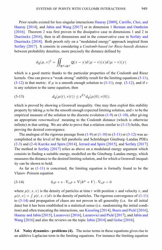
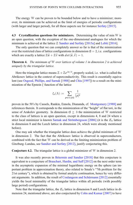
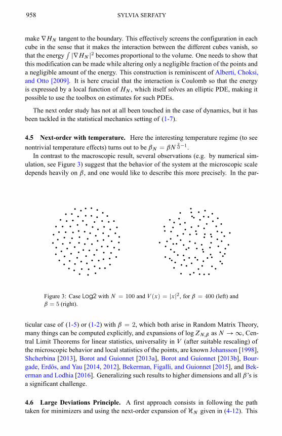
In contrast to the macroscopic result, several observations (e.g. by numerical sim-ulation, see Figure 3) suggest that the behavior of the system at the microscopic scaledepends heavily on ˇ, and one would like to describe this more precisely. In the par-

Figure 3: Case Log2 with N = 100 and V (x) = jxj2, for ˇ = 400 (left) andˇ = 5 (right).

ticular case of (1-5) or (1-2) with ˇ = 2, which both arise in Random Matrix Theory,many things can be computed explicitly, and expansions of logZN;ˇ as N ! 1, Cen-tral Limit Theorems for linear statistics, universality in V (after suitable rescaling) ofthe microscopic behavior and local statistics of the points, are known Johansson [1998],Shcherbina [2013], Borot and Guionnet [2013a], Borot and Guionnet [2013b], Bour-gade, Erdős, and Yau [2014, 2012], Bekerman, Figalli, and Guionnet [2015], and Bek-erman and Lodhia [2016]. Generalizing such results to higher dimensions and all ˇ’s isa significant challenge.

4.6 Large Deviations Principle. A first approach consists in following the pathtaken for minimizers and using the next-order expansion of HN given in (4-12). This

SYSTEMS OF POINTS WITH COULOMB INTERACTIONS 959

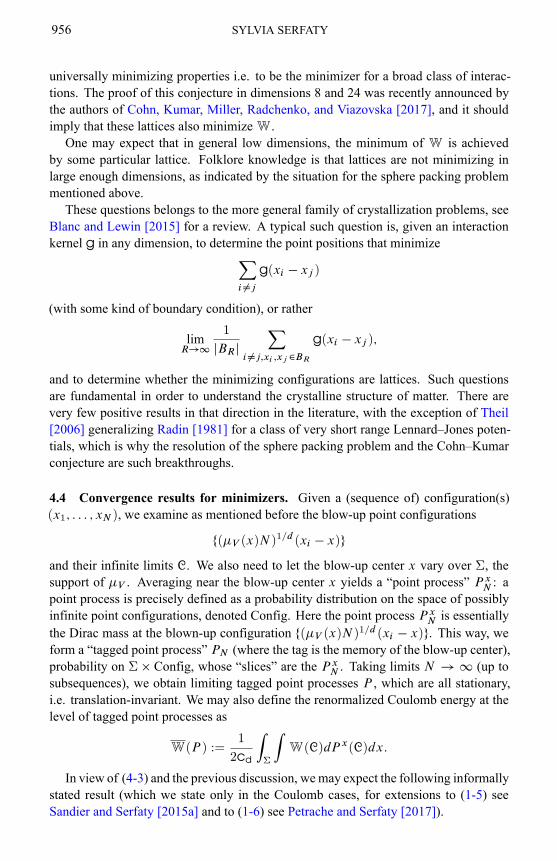
Figure 4: Simulation of the Poisson point process with intensity 1 (left), and theGinibre point process with intensity 1 (right)

expansion can be formally inserted into (1-7), however this is not sufficient: to get acomplete result, one needs to understand precisely how much volume in configurationspace (Rd)N is occupied near a given tagged point process P — this will give riseto an entropy term — and how much error (in both volume and energy) the screeningconstruction creates. At the end we obtain a Large Deviations Principle expressed atthe level of the microscopic point processes P , instead of the macroscopic empiricalmeasures � in Theorem 3. This is sometimes called “type-III large deviations” or largedeviations at the level of empirical fields. Such results can be found in Varadhan [1988],Föllmer [1988], the relative specific entropy that we will use is formalized in Föllmerand Orey [1988] (for the non-interacting discrete case), Georgii [1993] (for the interact-ing discrete case) and Georgii and Zessin [1993] (for the interacting continuous case).

To state the result precisely, we need to introduce the Poisson point process withintensity 1, denotedΠ, as the point process characterized by the fact that for any boundedBorel set B in Rd

Π(N (B) = n) =jBjn

n!e�jBj

whereN (B) denotes the number of points inB . The expectation of the number of pointsin B can then be computed to be jBj, and one also observes that the number of pointsin two disjoint sets are independent, thus the points “don’t interact”, see Figure 4 for apicture. The “specific” relative entropy ent with respect to Π refers to the fact that ithas to be computed taking an infinite volume limit, see Rassoul-Agha and Seppäläinen[2015] for a precise definition. One can just think that it measures how close the pointprocess is to the Poisson one.

For any ˇ > 0, we then define a free energy functional F ˇ as

(4-14) F ˇ (P ) :=ˇ

2W (P ) + ent[P jΠ]:

960 SYLVIA SERFATY

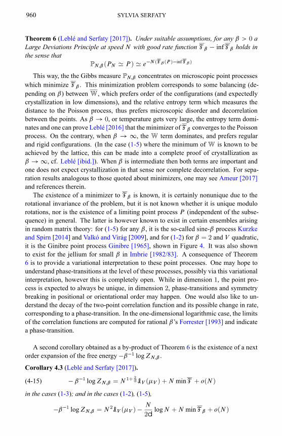
Theorem 6 (Leblé and Serfaty [2017]). Under suitable assumptions, for any ˇ > 0 aLarge Deviations Principle at speed N with good rate function F ˇ � inf F ˇ holds inthe sense that

PN;ˇ (PN ' P ) ' e�N (F ˇ(P )�infF ˇ)

This way, the the Gibbs measure PN;ˇ concentrates on microscopic point processeswhich minimize F ˇ . This minimization problem corresponds to some balancing (de-pending on ˇ) between W , which prefers order of the configurations (and expectedlycrystallization in low dimensions), and the relative entropy term which measures thedistance to the Poisson process, thus prefers microscopic disorder and decorrelationbetween the points. As ˇ ! 0, or temperature gets very large, the entropy term domi-nates and one can prove Leblé [2016] that the minimizer of F ˇ converges to the Poissonprocess. On the contrary, when ˇ ! 1, the W term dominates, and prefers regularand rigid configurations. (In the case (1-5) where the minimum of W is known to beachieved by the lattice, this can be made into a complete proof of crystallization asˇ ! 1, cf. Leblé [ibid.]). When ˇ is intermediate then both terms are important andone does not expect crystallization in that sense nor complete decorrelation. For sepa-ration results analogous to those quoted about minimizers, one may see Ameur [2017]and references therein.

The existence of a minimizer to F ˇ is known, it is certainly nonunique due to therotational invariance of the problem, but it is not known whether it is unique modulorotations, nor is the existence of a limiting point process P (independent of the subse-quence) in general. The latter is however known to exist in certain ensembles arisingin random matrix theory: for (1-5) for any ˇ, it is the so-called sine-ˇ process Kurzkeand Spirn [2014] and Valkó and Virág [2009], and for (1-2) for ˇ = 2 and V quadratic,it is the Ginibre point process Ginibre [1965], shown in Figure 4. It was also shownto exist for the jellium for small ˇ in Imbrie [1982/83]. A consequence of Theorem6 is to provide a variational interpretation to these point processes. One may hope tounderstand phase-transitions at the level of these processes, possibly via this variationalinterpretation, however this is completely open. While in dimension 1, the point pro-cess is expected to always be unique, in dimension 2, phase-transitions and symmetrybreaking in positional or orientational order may happen. One would also like to un-derstand the decay of the two-point correlation function and its possible change in rate,corresponding to a phase-transition. In the one-dimensional logarithmic case, the limitsof the correlation functions are computed for rational ˇ’s Forrester [1993] and indicatea phase-transition.

A second corollary obtained as a by-product of Theorem 6 is the existence of a nextorder expansion of the free energy �ˇ�1 logZN;ˇ .

Corollary 4.3 (Leblé and Serfaty [2017]).

(4-15) � ˇ�1 logZN;ˇ = N 1+ 2d IV (�V ) +N min F + o(N )

in the cases (1-3); and in the cases (1-2), (1-5),

�ˇ�1 logZN;ˇ = N 2IV (�V ) �N

2d logN +N min F ˇ + o(N )

SYSTEMS OF POINTS WITH COULOMB INTERACTIONS 961

or more explicitly

(4-16) � ˇ�1 logZN;ˇ =

= N 2IV (�V )�N

2d logN +NCˇ +N

�1

ˇ�

1

2d

� ZΣ

�V (x) log�V (x) dx+o(N );

where Cˇ depends only on ˇ, but not on V .

This formulae are to be compared with the results of Shcherbina [2013], Borot andGuionnet [2013a], Borot and Guionnet [2013b], and Bekerman, Figalli, and Guionnet[2015] in the Log1 case, the semi-rigorous formulae in Zabrodin andWiegmann [2006]in the dimension 2 Coulomb case, and are the best-known information on the free en-ergy otherwise. We recall that understanding the free energy is fundamental for thedescription of the properties of the system. For instance, the explicit dependence in Vexhibited in (4-16) will be the key to proving the result of the next section.

Finally, note that a similar result to the above theorem and corollary can be obtainedin the case of the two-dimensional two-component plasma alluded to in Section 2.4, seeLeblé, Serfaty, and Zeitouni [2017].

4.7 A Central Limit Theorem for fluctuations. Another approach to understand-ing the rigidity of configurations and how it depends on the temperature is to examinethe behavior of the linear statistics of the fluctuations, i.e. consider, for a regular testfunction f , the quantity

NXi=1

f (xi ) �N

Zfd�V :

Theorem 7 (Leblé and Serfaty [2018]). In the case (1-2), assume V 2 C 4 and theprevious assumptions on �V and @Σ, and let f 2 C 4

c (R2) or C 3

c (Σ). If Σ has m �

2 connected components Σi , add m � 1 conditionsR

@Σi∆f Σ = 0 where f Σ is the

harmonic extension of f outside Σ. Then

NXi=1

f (xi ) �N

ZΣ

f d�V

converges in law as N ! 1 to a Gaussian distribution with

mean =1

2�

�1

ˇ�

1

4

� ZR2

∆f (1Σ + log∆V )Σ variance=1

2�ˇ

ZR2

jrf Σj2:

The result can moreover be localized with f supported on any mesoscale N�˛ , ˛ < 12;

and it is true as well for energy minimizers, taking formally ˇ = 1.

This result can be interpreted in terms of the convergence ofHN (of (4-5)) to a suit-able so-called “Gaussian Free Field”, a sort of two-dimensional analogue of Brownianmotion. This theorem shows that if f is smooth enough, the fluctuations of linear statis-tics are typically of order 1, i.e. much smaller than the sum of N iid random variables

962 SYLVIA SERFATY

which is typically or orderpN . This a manifestation of rigidity, which even holds

down to the mesoscales. Note that the regularity of f is necessary, the result is false iff is discontinuous, however the precise threshold of regularity is not known.

In dimension 1, this theorem was first proven in Johansson [1998] for polynomialV and f analytic. It was later generalized in Shcherbina [2013], Borot and Guionnet[2013a], Borot and Guionnet [2013b], Bekerman and Lodhia [2016], Webb [2016], andBekerman, Leblé, and Serfaty [2017]. In dimension 2, this result was proven for thedeterminantal case ˇ = 2, first in Rider and Virág [2007] (for V quadratic), Berman[n.d.] assuming just f 2 C 1, and then Ameur, Hedenmalm, and Makarov [2011] un-der analyticity assumptions. It was then proven for all ˇ simultaneously as Leblé andSerfaty [2018] in Bauerschmidt, Bourgade, Nikula, and Yau [n.d.], with f assumed tobe supported in Σ. The approach for proving such results has generally been based onDyson–Schwinger (or “loop”) equations.

If the extra conditions do not hold, then the CLT is not expected to hold. Rather, thelimit should be a Gaussian convolved with a discrete Gaussian variable, as shown in theLog1 case in Borot and Guionnet [2013b].

To prove Theorem 7, following the approach pioneered by Johansson [1998], wecompute the Laplace transform of these linear statistics and see that it reduces to un-derstanding the ratio of two partition functions, the original one and that of a Coulombgas with potential V replaced by Vt = V + tf with t small. Thanks to Serfaty andSerra [n.d.] the variation of the equilibrium measure associated to this replacement iswell understood. We are then able to leverage on the expansion of the partition functionof (4-16) to compute the desired ratio, using also a change of variables which is a trans-port map between the equilibrium measure �V and the perturbed equilibrium measure.Note that the use of changes of variables in this context is not new, cf. Johansson [1998],Borot and Guionnet [2013a], Shcherbina [2013], and Bekerman, Figalli, and Guionnet[2015]. In our approach, it essentially replaces the use of the loop or Dyson–Schwingerequations.

4.8 More general interactions. It remains to understand how much of the behaviorwe described are really specific to Coulomb interactions. Already Theorems 5 and 6were shown in Petrache and Serfaty [2017] and Leblé and Serfaty [2017] to hold for themore general Riesz interactions with d � 2 � s < d. This is thanks to the fact that theRiesz kernel is the kernel for a fractional Laplacian, which is not a local operator but canbe interpreted as a local operator after adding one spatial dimension, according to theprocedure of Caffarelli and Silvestre [2007]. The results of Theorem 6 are also valid inthe hypersingularRiesz interactions s > d (see Hardin, Leblé, Saff, and Serfaty [2018]),where the kernel is very singular but also decays very fast. The Gaussian behavior ofthe fluctuations seen in Theorem 7 is for now proved only in the logarithmic cases, butit remains to show whether it holds for more general Coulomb cases and even possiblymore general interactions as well.

SYSTEMS OF POINTS WITH COULOMB INTERACTIONS 963

Acknowledgments. I am very grateful to Mitia Duerinckx, Thomas Leblé, MathieuLewin and Nicolas Rougerie for their helpful comments and suggestions on the firstversion of this text. I also thank Catherine Goldstein for the historical references andAlon Nishry for the pictures of Figure 4.

References

Alexei A. Abrikosov (1957). “On the magnetic properties of superconductors of thesecond group”. Sov. Phys. JETP 5, pp. 1174–1182 (cit. on p. 938).

A. Alastuey and B. Jancovici (1981). “On the classical two-dimensional one-componentCoulomb plasma”. J. Physique 42.1, pp. 1–12. MR: 604143 (cit. on p. 941).

Giovanni Alberti, Rustum Choksi, and Felix Otto (2009). “Uniform energy distributionfor an isoperimetric problem with long-range interactions”. J. Amer. Math. Soc. 22.2,pp. 569–605. MR: 2476783 (cit. on p. 958).

Giovanni Alberti and Stefan Müller (2001). “A new approach to variational problemswith multiple scales”. Comm. Pure Appl. Math. 54.7, pp. 761–825. MR: 1823420(cit. on p. 957).

Luigi Ambrosio, Nicola Gigli, and Giuseppe Savaré (2005). Gradient flows in met-ric spaces and in the space of probability measures. Lectures in Mathematics ETHZürich. Birkhäuser Verlag, Basel, pp. viii+333. MR: 2129498 (cit. on p. 948).

Luigi Ambrosio and Sylvia Serfaty (2008). “A gradient flow approach to an evolutionproblem arising in superconductivity”. Comm. Pure Appl. Math. 61.11, pp. 1495–1539. MR: 2444374 (cit. on p. 948).

Yacin Ameur (2017). “Repulsion in low temperature ˇ-ensembles”. arXiv: 1701 .04796 (cit. on p. 960).

Yacin Ameur, Håkan Hedenmalm, and Nikolai Makarov (2011). “Fluctuations of eigen-values of random normal matrices”. Duke Math. J. 159.1, pp. 31–81. MR: 2817648(cit. on p. 962).

Greg W. Anderson, Alice Guionnet, and Ofer Zeitouni (2010). An introduction to ran-dom matrices. Vol. 118. Cambridge Studies in Advanced Mathematics. CambridgeUniversity Press, Cambridge, pp. xiv+492. MR: 2760897 (cit. on p. 943).

Julien Barré, Freddy Bouchet, Thierry Dauxois, and Stefano Ruffo (2005). “Large de-viation techniques applied to systems with long-range interactions”. J. Stat. Phys.119.3-4, pp. 677–713. MR: 2151219 (cit. on p. 942).

Roland Bauerschmidt, Paul Bourgade, Miika Nikula, and Horng-Tzer Yau (n.d.). “Thetwo-dimensional Coulomb plasma: quasi-free approximation and central limit theo-rem”. arXiv: 1609.08582v2 (cit. on p. 962).

F. Bekerman, A. Figalli, and A. Guionnet (2015). “Transport maps for ˇ-matrix modelsand universality”. Comm. Math. Phys. 338.2, pp. 589–619. MR: 3351052 (cit. onpp. 958, 961, 962).

Florent Bekerman, Thomas Leblé, and Sylvia Serfaty (2017). “CLT for fluctuations ofˇ-ensembles with general potential”. arXiv: 1706.09663 (cit. on p. 962).

Florent Bekerman and Asad Lodhia (2016). “Mesoscopic central limit theorem for gen-eral ˇ-ensembles”. arXiv: 1605.05206 (cit. on pp. 958, 962).

964 SYLVIA SERFATY

G. Ben Arous and A. Guionnet (1997). “Large deviations for Wigner’s law andVoiculescu’s non-commutative entropy”. Probab. Theory Related Fields 108.4,pp. 517–542. MR: 1465640 (cit. on p. 951).

Gérard Ben Arous and Ofer Zeitouni (1998). “Large deviations from the circular law”.ESAIM Probab. Statist. 2, pp. 123–134. MR: 1660943 (cit. on p. 951).

R. J. Berman (n.d.). “Determinantal point processes and fermions on complexmanifolds:Bulk universality”. To appear in Conference Proceedings on Algebraic and AnalyticMicrolocal Analysis (Northwestern, 2015), M. Hitrik, D. Tamarkin, B. Tsygan, andS. Zelditch, (eds.) Springer. arXiv: 0811.3341 (cit. on p. 962).

Robert J. Berman (2014). “Determinantal point processes and fermions on complexmanifolds: large deviations and bosonization”. Comm. Math. Phys. 327.1, pp. 1–47.MR: 3177931 (cit. on p. 951).

– (2017). “Large deviations for Gibbs measures with singular Hamiltonians and emer-gence of Kähler-Einstein metrics”. Comm. Math. Phys. 354.3, pp. 1133–1172. MR:3668617 (cit. on p. 944).

Robert J. Berman, Sébastien Boucksom, andDavidWitt Nyström (2011). “Fekete pointsand convergence towards equilibrium measures on complex manifolds”. Acta Math.207.1, pp. 1–27. MR: 2863909 (cit. on p. 944).

Robert J. Berman and Magnus Onnheim (2016). “Propagation of chaos for a class offirst order models with singular mean field interactions”. arXiv: 1610.04327 (cit. onp. 949).

– (2018). “Propagation of chaos, Wasserstein gradient flows and toric Kähler-Einsteinmetrics”. Anal. PDE 11 (6), pp. 1343–1380. arXiv: 1501.07820 (cit. on p. 950).

Laurent Bétermin and Etienne Sandier (2018). “Renormalized Energy and AsymptoticExpansion of Optimal Logarithmic Energy on the Sphere”. Constr. Approx. 47.1,pp. 39–74. MR: 3742809 (cit. on p. 955).

F. Bethuel, G. Orlandi, and D. Smets (2005). “Collisions and phase-vortex interactionsin dissipative Ginzburg–Landau dynamics”. Duke Math. J. 130.3, pp. 523–614. MR:2184569 (cit. on p. 939).

– (2007). “Dynamics of multiple degree Ginzburg–Landau vortices”. Comm. Math.Phys. 272.1, pp. 229–261. MR: 2291808 (cit. on p. 939).

Fabrice Bethuel, Haım Brezis, and Frédéric Hélein (1994). Ginzburg–Landau vor-tices. Vol. 13. Progress in Nonlinear Differential Equations and their Applications.Birkhäuser Boston, Inc., Boston, MA, pp. xxviii+159. MR: 1269538 (cit. on pp. 939,953).

Fabrice Bethuel, Robert L. Jerrard, and Didier Smets (2008). “On the NLS dynamics forinfinite energy vortex configurations on the plane”.Rev. Mat. Iberoam. 24.2, pp. 671–702. MR: 2459209 (cit. on p. 939).

Fabrice Bethuel and Tristan Rivière (1995). “Vortices for a variational problem relatedto superconductivity”. Ann. Inst. H. Poincaré Anal. Non Linéaire 12.3, pp. 243–303.MR: 1340265 (cit. on p. 939).

W. Bietenholz and U. Gerber (2016). “Berezinskii–Kosterlitz–Thouless Transition andthe Haldane Conjecture: Highlights of the Physics Nobel Prize 2016”. RevistaCubana de Fısica 33.2, pp. 156–168. arXiv: 1612.06132 (cit. on p. 943).

SYSTEMS OF POINTS WITH COULOMB INTERACTIONS 965

Xavier Blanc and Mathieu Lewin (2015). “The crystallization conjecture: a review”.EMS Surv. Math. Sci. 2.2, pp. 225–306. MR: 3429164 (cit. on p. 956).

C. Blondel and B. Wolff (2015). “Coulomb et la difficile gestion du “mélange du Calculet de la Physique”. In: Sous la direction de C. Gilain et A. Guilbaud, CNRS éditions,pp. 1750–1850 (cit. on p. 936).

Niklas Boers and Peter Pickl (2016). “On mean field limits for dynamical systems”. J.Stat. Phys. 164.1, pp. 1–16. MR: 3509045 (cit. on p. 949).

Alexei Borodin (2011). “Determinantal point processes”. In: The Oxford handbook ofrandom matrix theory. Oxford Univ. Press, Oxford, pp. 231–249. MR: 2932631 (cit.on p. 944).

Alexei Borodin and Vadim Gorin (2016). “Lectures on integrable probability”. In: Prob-ability and statistical physics in St. Petersburg. Vol. 91. Proc. Sympos. Pure Math.Amer. Math. Soc., Providence, RI, pp. 155–214. MR: 3526828 (cit. on p. 944).

Alexei Borodin and Sylvia Serfaty (2013). “Renormalized energy concentration in ran-dom matrices”. Comm. Math. Phys. 320.1, pp. 199–244. MR: 3046995 (cit. onp. 957).

G. Borot and A. Guionnet (2013a). “Asymptotic expansion of ˇ matrix models in theone-cut regime”. Comm. Math. Phys. 317.2, pp. 447–483. MR: 3010191 (cit. onpp. 954, 958, 961, 962).

Gaëtan Borot and Alice Guionnet (Mar. 2013b). “Asymptotic expansion of beta matrixmodels in the multi-cut regime”. arXiv: 1303.1045 (cit. on pp. 958, 961, 962).

Paul Bourgade, László Erdős, and Horng-Tzer Yau (2012). “Bulk universality of generalˇ-ensembles with non-convex potential”. J. Math. Phys. 53.9, pp. 095221, 19. MR:2905803 (cit. on p. 958).

– (2014). “Universality of general ˇ-ensembles”.Duke Math. J. 163.6, pp. 1127–1190.arXiv: 0907.5605. MR: 3192527 (cit. on p. 958).

J. S. Brauchart, D. P. Hardin, and Edward B. Saff (2012). “The next-order term for op-timal Riesz and logarithmic energy asymptotics on the sphere”. In: Recent advancesin orthogonal polynomials, special functions, and their applications. Vol. 578. Con-temp. Math. Amer. Math. Soc., Providence, RI, pp. 31–61. MR: 2964138 (cit. onpp. 941, 955).

S. G. Brush, H. L. Sahlin, and E. Teller (1966). “Monte Carlo Study of aOne-ComponentPlasma. I”. The Journal of Chemical Physics 45.6, pp. 2102–2118 (cit. on p. 942).

Luis Caffarelli and Luis Silvestre (2007). “An extension problem related to the frac-tional Laplacian”.Comm. Partial Differential Equations 32.7-9, pp. 1245–1260.MR:2354493 (cit. on p. 962).

Luis Caffarelli, Fernando Soria, and Juan Luis Vázquez (2013). “Regularity of solutionsof the fractional porous medium flow”. J. Eur. Math. Soc. (JEMS) 15.5, pp. 1701–1746. MR: 3082241 (cit. on p. 948).

Luis Caffarelli and Juan Luis Vazquez (2011). “Nonlinear porous medium flow withfractional potential pressure”. Arch. Ration. Mech. Anal. 202.2, pp. 537–565. MR:2847534 (cit. on p. 948).

E. Caglioti, P.-L. Lions, C. Marchioro, and M. Pulvirenti (1992). “A special class of sta-tionary flows for two-dimensional Euler equations: a statistical mechanics descrip-tion”. Comm. Math. Phys. 143.3, pp. 501–525. MR: 1145596 (cit. on p. 951).

966 SYLVIA SERFATY

J. M. Caillol, D. Levesque, J. J. Weis, and J. P. Hansen (1982). “AMonte Carlo study ofthe classical two-dimensional one-component plasma”. Journal of Statistical Physics28.2, pp. 325–349 (cit. on p. 942).

Alessandro Campa, Thierry Dauxois, and Stefano Ruffo (2009). “Statistical mechanicsand dynamics of solvable models with long-range interactions”. Phys. Rep. 480.3-6,pp. 57–159. MR: 2569625 (cit. on p. 942).

José Antonio Carrillo, Young-Pil Choi, and Maxime Hauray (2014). “The derivationof swarming models: mean-field limit and Wasserstein distances”. In: Collective dy-namics from bacteria to crowds. Vol. 553. CISM Courses and Lect. Springer, Vienna,pp. 1–46. MR: 3331178 (cit. on p. 949).

Emmanuel Cépa andDominique Lépingle (1997). “Diffusing particles with electrostaticrepulsion”. Probab. Theory Related Fields 107.4, pp. 429–449. MR: 1440140 (cit.on p. 950).

Djalil Chafai, Adrien Hardy, and Myléne Maida (2018). “Concentration for Coulombgases and Coulomb transport inequalities”. J. Funct. Anal. 275, pp. 1447–1483.arXiv: 1610.00980 (cit. on p. 954).

Djalil Chafaı, Nathael Gozlan, and Pierre-André Zitt (2014). “First-order global asymp-totics for confined particles with singular pair repulsion”. Ann. Appl. Probab. 24.6,pp. 2371–2413. MR: 3262506 (cit. on p. 951).

S. J. Chapman, J. Rubinstein, and M. Schatzman (1996). “A mean-field model of su-perconducting vortices”. European J. Appl. Math. 7.2, pp. 97–111. MR: 1388106(cit. on p. 948).

Patrick Chiu (1997). “Height of flat tori”. Proc. Amer. Math. Soc. 125.3, pp. 723–730.MR: 1396970 (cit. on p. 955).

Ph. Choquard and J. Clerouin (1983). “Cooperative phenomena below melting of theone-component two-dimensional plasma”. Physical review letters 50.26, p. 2086 (cit.on p. 942).

Gustave Choquet (1958). “Diamètre transfini et comparaison de diverses capacités”.Séminaire Brelot–Choquet–Deny. Théorie du potentiel 3.4, pp. 1–7 (cit. on p. 947).

Henry Cohn (2017). “A conceptual breakthrough in sphere packing”. Notices Amer.Math. Soc. 64.2, pp. 102–115. MR: 3587715 (cit. on p. 941).

Henry Cohn and Abhinav Kumar (2007). “Universally optimal distribution of points onspheres”. J. Amer. Math. Soc. 20.1, pp. 99–148. MR: 2257398 (cit. on p. 955).

Henry Cohn, Abhinav Kumar, Stephen D. Miller, Danylo Radchenko, and Maryna S.Viazovska (2017). “The sphere packing problem in dimension 24”. Ann. of Math. (2)185.3, pp. 1017–1033. MR: 3664817 (cit. on pp. 941, 956).

J. E. Colliander and R. L. Jerrard (1998). “Vortex dynamics for the Ginzburg–Landau–Schrödinger equation”. Internat. Math. Res. Notices 7, pp. 333–358. MR: 1623410(cit. on p. 939).

– (1999). “Ginzburg–Landau vortices: weak stability and Schrödinger equation dynam-ics”. J. Anal. Math. 77, pp. 129–205. MR: 1753485 (cit. on p. 939).

J. H. Conway and N. J. A. Sloane (1999). Sphere packings, lattices and groups. Third.Vol. 290. Grundlehren der Mathematischen Wissenschaften [Fundamental Princi-ples of Mathematical Sciences]. With additional contributions by E. Bannai, R. E.

SYSTEMS OF POINTS WITH COULOMB INTERACTIONS 967

Borcherds, J. Leech, S. P. Norton, A. M. Odlyzko, R. A. Parker, L. Queen and B. B.Venkov. Springer-Verlag, New York, pp. lxxiv+703. MR: 1662447 (cit. on p. 941).

Renaud Coulangeon and Achill Schürmann (2012). “Energyminimization, periodic setsand spherical designs”. Int. Math. Res. Not. IMRN 4, pp. 829–848.MR: 2889159 (cit.on p. 955).

C. A. Coulomb (1785). “Premier Mémoire sur l’Electricité et le Magnétisme”. In:pp. 569–577 (cit. on p. 936).

Thierry Dauxois, Stefano Ruffo, Ennio Arimondo, and Martin Wilkens (2002). “Dy-namics and thermodynamics of systems with long-range interactions: an introduc-tion”. In: Dynamics and thermodynamics of systems with long-range interactions(Les Houches, 2002). Vol. 602. Lecture Notes in Phys. Springer, Berlin, pp. 1–19.MR: 2008176.

David S. Dean, Pierre Le Doussal, Satya N. Majumdar, and Grégory Schehr (2016).“Noninteracting fermions at finite temperature in a d-dimensional trap: Universalcorrelations”. Physical Review A 94.6, p. 063622 (cit. on p. 942).

P. A. Deift (1999). Orthogonal polynomials and random matrices: a Riemann–Hilbertapproach. Vol. 3. Courant Lecture Notes in Mathematics. New York University,Courant Institute of Mathematical Sciences, New York; American Mathematical So-ciety, Providence, RI, pp. viii+273. MR: 1677884 (cit. on p. 943).

Jean-Marc Delort (1991). “Existence de nappes de tourbillon en dimension deux”. J.Amer. Math. Soc. 4.3, pp. 553–586. MR: 1102579 (cit. on p. 947).

Amir Dembo and Ofer Zeitouni (2010). Large deviations techniques and applications.Vol. 38. Stochastic Modelling and Applied Probability. Corrected reprint of the sec-ond (1998) edition. Springer-Verlag, Berlin, pp. xvi+396. MR: 2571413 (cit. onp. 950).

Cl. Deutsch and M. Lavaud (1974). “Equilibrium properties of a two-dimensionalCoulomb gas”. Physical Review A 9.6, p. 2598 (cit. on p. 943).

Mitia Duerinckx (2016). “Mean-field limits for some Riesz interaction gradient flows”.SIAM J. Math. Anal. 48.3, pp. 2269–2300. MR: 3514713 (cit. on p. 949).

Ioana Dumitriu and Alan Edelman (2002). “Matrix models for beta ensembles”. J. Math.Phys. 43.11, pp. 5830–5847. MR: 1936554 (cit. on p. 943).

Freeman J. Dyson (1962). “Statistical theory of the energy levels of complex systems.III”. J. Mathematical Phys. 3, pp. 166–175. MR: 0143558 (cit. on p. 943).

Weinan E (1994a). “Dynamics of vortices in Ginzburg–Landau theories with appli-cations to superconductivity”. Phys. D 77.4, pp. 383–404. MR: 1297726 (cit. onp. 939).

– (1994b). “Dynamics of vortices in Ginzburg–Landau theories with applications tosuperconductivity”. Phys. D 77.4, pp. 383–404. MR: 1297726 (cit. on p. 948).

László Erdős and Horng-Tzer Yau (2017). A dynamical approach to random matrixtheory. Vol. 28. Courant Lecture Notes in Mathematics. Courant Institute of Math-ematical Sciences, New York; American Mathematical Society, Providence, RI,pp. ix+226. MR: 3699468 (cit. on p. 944).

Gregory L. Eyink and Katepalli R. Sreenivasan (2006). “Onsager and the theory ofhydrodynamic turbulence”. Rev. Modern Phys. 78.1, pp. 87–135. MR: 2214822 (cit.on p. 940).

968 SYLVIA SERFATY

L. Fejes (1940). “Über einen geometrischen Satz”. Math. Z. 46, pp. 83–85. MR:0001587 (cit. on p. 941).

Hans Föllmer (1988). “Random fields and diffusion processes”. In: École d’Été deProbabilités de Saint-Flour XV–XVII, 1985–87. Vol. 1362. Lecture Notes in Math.Springer, Berlin, pp. 101–203. MR: 983373 (cit. on p. 959).

Hans Föllmer and Steven Orey (1988). “Large deviations for the empirical field of aGibbs measure”. Ann. Probab. 16.3, pp. 961–977. MR: 942749 (cit. on p. 959).

P. J. Forrester (1993). “Exact integral formulas and asymptotics for the correlationsin the 1/r2 quantum many-body system”. Phys. Lett. A 179.2, pp. 127–130. MR:1230810 (cit. on p. 960).

– (2010). Log-gases and random matrices. Vol. 34. London Mathematical SocietyMonographs Series. Princeton University Press, Princeton, NJ, pp. xiv+791. MR:2641363 (cit. on pp. 937, 942, 943).

P. J. Forrester, N. E. Frankel, T. M. Garoni, and N. S. Witte (2003). “Finite one-dimensional impenetrable Bose systems: Occupation numbers”. Physical Review A67.4, p. 043607 (cit. on p. 942).

P. J. Forrester, B. Jancovici, and D. S. McAnally (2001). “Analytic properties of thestructure function for the one-dimensional one-component log-gas”. In: Proceedingsof the Baxter Revolution in Mathematical Physics (Canberra, 2000). Vol. 102. 3-4,pp. 737–780. MR: 1832069 (cit. on p. 942).

Nicolas Fournier, Maxime Hauray, and Stéphane Mischler (2014). “Propagation ofchaos for the 2D viscous vortex model”. J. Eur. Math. Soc. (JEMS) 16.7, pp. 1423–1466. MR: 3254330 (cit. on p. 950).

Jürg Fröhlich (1976). “Classical and quantum statistical mechanics in one and twodimensions: two-component Yukawa- and Coulomb systems”. Comm. Math. Phys.47.3, pp. 233–268. MR: 0434278 (cit. on p. 943).

Jürg Fröhlich and Thomas Spencer (1981). “The Kosterlitz–Thouless transition in two-dimensional abelian spin systems and the Coulomb gas”. Comm. Math. Phys. 81.4,pp. 527–602. MR: 634447 (cit. on p. 943).

O. Frostman (1935). “Potential d’équilibre et capacité des avec quelques applications àla thórie des functions”.Meddelanden Mat. Sem. Univ. Lund 3, p. 115 (cit. on p. 945).

David García-Zelada (Mar. 2017). “A large deviation principle for empirical measureson Polish spaces: Application to singular Gibbs measures on manifolds”. arXiv:1703.02680 (cit. on p. 951).

Hans-Otto Georgii (1993). “Large deviations and maximum entropy principle for inter-acting random fields on Zd ”. Ann. Probab. 21.4, pp. 1845–1875. MR: 1245292 (cit.on p. 959).

Hans-Otto Georgii and Hans Zessin (1993). “Large deviations and the maximum en-tropy principle for marked point random fields”. Probab. Theory Related Fields 96.2,pp. 177–204. MR: 1227031 (cit. on p. 959).

Subhro Ghosh and Joel L. Lebowitz (2017). “Number rigidity in superhomogeneousrandom point fields”. J. Stat. Phys. 166.3-4, pp. 1016–1027. MR: 3607597 (cit. onp. 952).

Jean Ginibre (1965). “Statistical ensembles of complex, quaternion, and real matrices”.J. Mathematical Phys. 6, pp. 440–449. MR: 0173726 (cit. on pp. 943, 960).

SYSTEMS OF POINTS WITH COULOMB INTERACTIONS 969

M. D. Girardeau, E. M. Wright, and J. M. Triscari (2001). “Ground-state properties ofa one-dimensional system of hard-core bosons in a harmonic trap”. Physical ReviewA 63.3, p. 033601 (cit. on p. 942).

V. L. Girko (1983). “The circle law”. Teor. Veroyatnost. i Mat. Statist. 28. English trans-lation in Girko [1984], pp. 15–21. MR: 727271 (cit. on p. 969).

– (1984). “Circle law”. Theory Probab. Appl. 29. Original in Russian in Girko [1983],pp. 694–706 (cit. on p. 969).

S. M. Girvin (1999). “The quantum Hall effect: novel excitations and broken symme-tries”. In: Aspects topologiques de la physique en basse dimension/Topological as-pects of low dimensional systems (Les Houches, 1998). EDP Sci., Les Ulis, pp. 53–175. MR: 1850417 (cit. on p. 941).

– (2004). “Introduction to the fractional quantum Hall effect”. Séminaire Poincaré 2,pp. 54–74 (cit. on p. 941).

Dorian Goldman, Cyrill B. Muratov, and Sylvia Serfaty (2013). “The Γ-limit of the two-dimensional Ohta–Kawasaki energy. I. Droplet density”. Arch. Ration. Mech. Anal.210.2, pp. 581–613. MR: 3101793 (cit. on p. 957).

– (2014). “The Γ-limit of the two-dimensional Ohta–Kawasaki energy. Droplet ar-rangement via the renormalized energy”. Arch. Ration. Mech. Anal. 212.2, pp. 445–501. MR: 3176350 (cit. on p. 957).

François Golse (2016). “On the dynamics of large particle systems in the mean fieldlimit”. In: Macroscopic and large scale phenomena: coarse graining, mean fieldlimits and ergodicity. Vol. 3. Lect. Notes Appl. Math. Mech. Springer, [Cham], pp. 1–144. MR: 3468297 (cit. on pp. 945, 949).

Jonathan Goodman, Thomas Y. Hou, and John Lowengrub (1990). “Convergence ofthe point vortex method for the 2-D Euler equations”. Comm. Pure Appl. Math. 43.3,pp. 415–430. MR: 1040146 (cit. on p. 948).

J. Gunson and L. S. Panta (1977). “Two-dimensional neutral Coulomb gas”. Comm.Math. Phys. 52.3, pp. 295–304. MR: 0452403 (cit. on p. 943).

Thomas C. Hales (2005). “A proof of the Kepler conjecture”. Ann. of Math. (2) 162.3,pp. 1065–1185. MR: 2179728 (cit. on p. 941).

Douglas P. Hardin, Thomas Leblé, Edward B. Saff, and Sylvia Serfaty (2018). “Largedeviation principles for hypersingular Riesz gases”. Constr. Approx. 48 (1), pp. 61–100 (cit. on p. 962).

Maxime Hauray (2009). “Wasserstein distances for vortices approximation of Euler-type equations”. Math. Models Methods Appl. Sci. 19.8, pp. 1357–1384. MR:2555474 (cit. on p. 949).

Maxime Hauray and Pierre-Emmanuel Jabin (2015). “Particle approximation of Vlasovequations with singular forces: propagation of chaos”. Ann. Sci. Éc. Norm. Supér. (4)48.4, pp. 891–940. MR: 3377068 (cit. on p. 949).

Maxime Hauray and StéphaneMischler (2014). “On Kac’s chaos and related problems”.J. Funct. Anal. 266.10, pp. 6055–6157. MR: 3188710 (cit. on p. 945).

J. Ben Hough, Manjunath Krishnapur, Yuval Peres, and Bálint Virág (2009). Zeros ofGaussian analytic functions and determinantal point processes. Vol. 51. UniversityLecture Series. American Mathematical Society, Providence, RI, pp. x+154. MR:2552864 (cit. on p. 944).

970 SYLVIA SERFATY

Jiaoyang Huang and Benjamin Landon (Dec. 19, 2016). “Local law and mesoscopicfluctuations of Dyson Brownian motion for general ˇ and potential”. arXiv: 1612.06306.

Kerson Huang (1987). Statistical mechanics. Second. John Wiley & Sons, Inc., NewYork, pp. xiv+493. MR: 1042093 (cit. on p. 942).

John Z. Imbrie (1982/83). “Debye screening for jellium and other Coulomb systems”.Comm. Math. Phys. 87.4, pp. 515–565. MR: 691043 (cit. on p. 960).

Pierre-Emmanuel Jabin (2014). “A review of themean field limits for Vlasov equations”.Kinet. Relat. Models 7.4, pp. 661–711. MR: 3317577 (cit. on pp. 940, 949, 950).

Pierre-Emmanuel Jabin and Zhenfu Wang (2016). “Mean field limit and propagation ofchaos for Vlasov systems with bounded forces”. J. Funct. Anal. 271.12, pp. 3588–3627. MR: 3558251 (cit. on pp. 949, 950).

– (June 2017). “Quantitative estimate of propagation of chaos for stochastic systemswith W �1;1 kernels”. arXiv: 1706.09564 (cit. on pp. 949, 950).

B. Jancovici (1995). “Classical Coulomb systems: screening and correlations revisited”.J. Statist. Phys. 80.1-2, pp. 445–459. MR: 1340566 (cit. on p. 941).

B. Jancovici, Joel L. Lebowitz, and G. Manificat (1993). “Large charge fluctuations inclassical Coulomb systems”. J. Statist. Phys. 72.3-4, pp. 773–787. MR: 1239571(cit. on p. 941).

Robert L. Jerrard andDaniel Spirn (2015). “Hydrodynamic limit of the Gross–Pitaevskiiequation”. Comm. Partial Differential Equations 40.2, pp. 135–190. MR: 3277924(cit. on p. 949).

Robert Leon Jerrard and Halil Mete Soner (1998). “Dynamics of Ginzburg–Landau vor-tices”. Arch. Rational Mech. Anal. 142.2, pp. 99–125. MR: 1629646 (cit. on p. 939).

Kurt Johansson (1998). “On fluctuations of eigenvalues of randomHermitian matrices”.Duke Math. J. 91.1, pp. 151–204. MR: 1487983 (cit. on pp. 958, 962).

Michael K.-H. Kiessling (1993). “Statistical mechanics of classical particles with loga-rithmic interactions”. Comm. Pure Appl. Math. 46.1, pp. 27–56. MR: 1193342 (cit.on pp. 941, 951).

– (2014). “The microscopic foundations of Vlasov theory for jellium-like NewtonianN -body systems”. J. Stat. Phys. 155.6, pp. 1299–1328.MR: 3207739 (cit. on p. 949).

Michael K.-H. Kiessling and Herbert Spohn (1999). “A note on the eigenvalue densityof randommatrices”. Comm. Math. Phys. 199.3, pp. 683–695. MR: 1669669 (cit. onp. 941).

Rowan Killip and Irina Nenciu (2004). “Matrix models for circular ensembles”. Int.Math. Res. Not. 50, pp. 2665–2701. MR: 2127367 (cit. on p. 943).

Rowan Killip and Mihai Stoiciu (2009). “Eigenvalue statistics for CMV matrices: fromPoisson to clock via random matrix ensembles”. Duke Math. J. 146.3, pp. 361–399.MR: 2484278.

SemyonKlevtsov (2016). “Geometry and largeN limits in Laughlin states”. In: Travauxmathématiques. Vol. XXIV. Vol. 24. Trav. Math. Fac. Sci. Technol. Commun. Univ.Luxemb., Luxembourg, pp. 63–127. MR: 3643934 (cit. on p. 944).

H. Kunz (1974). “The one-dimensional classical electron gas”. Ann. Physics 85,pp. 303–335. MR: 0426742 (cit. on p. 936).

SYSTEMS OF POINTS WITH COULOMB INTERACTIONS 971

Matthias Kurzke, Christof Melcher, Roger Moser, and Daniel Spirn (2009). “Dynamicsfor Ginzburg–Landau vortices under a mixed flow”. Indiana Univ. Math. J. 58.6,pp. 2597–2621. MR: 2603761.

Matthias Kurzke and Daniel Spirn (2014). “Vortex liquids and the Ginzburg–Landauequation”. Forum Math. Sigma 2, e11, 63. MR: 3264248 (cit. on pp. 949, 960).

L. D. Landau and V. L. Ginzburg (1965). On the theory of superconductivity,[in:] Col-lected papers of LD Landau, D. ter Haar [Ed.], 546–568 (cit. on p. 938).

Robert B. Laughlin (1983). “Anomalous quantum Hall effect: an incompressible quan-tum fluid with fractionally charged excitations”. Physical Review Letters 50.18,p. 1395 (cit. on p. 941).

– (1999). “Nobel lecture: fractional quantization”. Rev. Modern Phys. 71.4, pp. 863–874. MR: 1712324 (cit. on p. 941).

Dustin Lazarovici (2016). “The Vlasov–Poisson dynamics as the mean field limit ofextended charges”. Comm. Math. Phys. 347.1, pp. 271–289. MR: 3543184 (cit. onp. 949).

Dustin Lazarovici and Peter Pickl (2017). “A mean field limit for the Vlasov–Poissonsystem”. Arch. Ration. Mech. Anal. 225.3, pp. 1201–1231. MR: 3667287 (cit. onp. 949).

T. Leblé and Sylvia Serfaty (2018). “Fluctuations of Two-Dimensional CoulombGases”.Geom. Funct. Anal. (GAFA) 28 (2), pp. 443–508. arXiv: 1609.08088 (cit. on pp. 961,962).

Thomas Leblé (2016). “Logarithmic, Coulomb and Riesz energy of point processes”. J.Stat. Phys. 162.4, pp. 887–923. MR: 3456982 (cit. on pp. 955, 960).

Thomas Leblé and Sylvia Serfaty (2017). “Large deviation principle for empirical fieldsof Log and Riesz gases”. Invent. Math. 210.3, pp. 645–757. MR: 3735628 (cit. onpp. 952, 960, 962).

Thomas Leblé, Sylvia Serfaty, and Ofer Zeitouni (2017). “Large deviations for the two-dimensional two-component plasma”. Comm. Math. Phys. 350.1, pp. 301–360. MR:3606477 (cit. on p. 961).

A. Lenard (1961). “Exact statistical mechanics of a one-dimensional system withCoulomb forces”. J. Mathematical Phys. 2, pp. 682–693. MR: 0129874 (cit. onp. 936).

Andrew Lenard (1963). “Exact statistical mechanics of a one-dimensional system withCoulomb forces. III. Statistics of the electric field”. J. Mathematical Phys. 4, pp. 533–543. MR: 0148411 (cit. on p. 936).

Elliott H. Lieb and Joel L. Lebowitz (1972). “The constitution of matter: Existence ofthermodynamics for systems composed of electrons and nuclei”. Advances in Math.9, pp. 316–398. MR: 0339751 (cit. on p. 941).

Elliott H. Lieb and Michael Loss (1997). Analysis. Vol. 14. Graduate Studies inMathematics. American Mathematical Society, Providence, RI, pp. xviii+278. MR:1415616.

Elliott H. Lieb and Heide Narnhofer (1975). “The thermodynamic limit for jellium”. J.Statist. Phys. 12, pp. 291–310. MR: 0401029 (cit. on p. 941).

972 SYLVIA SERFATY

Elliott H. Lieb, Nicolas Rougerie, and Jakob Yngvason (June 2018). “Local incompress-ibility estimates for the Laughlin phase”. Communications in Mathematical Physics.arXiv: 1701.09064 (cit. on p. 941).

F.-H. Lin and J. X. Xin (1999a). “On the dynamical law of theGinzburg–Landau vorticeson the plane”.Comm. Pure Appl. Math. 52.10, pp. 1189–1212. MR: 1699965 (cit. onp. 939).

– (1999b). “On the incompressible fluid limit and the vortex motion law of the nonlin-ear Schrödinger equation”. Comm. Math. Phys. 200.2, pp. 249–274. MR: 1674000(cit. on p. 939).

Fang Hua Lin (1996). “Some dynamical properties of Ginzburg–Landau vortices”.Comm. Pure Appl. Math. 49.4, pp. 323–359. MR: 1376654 (cit. on p. 939).

Fanghua Lin and Ping Zhang (2000). “On the hydrodynamic limit of Ginzburg–Landauvortices”. Discrete Contin. Dynam. Systems 6.1, pp. 121–142. MR: 1739596 (cit. onp. 948).

Mylène Maıda and Édouard Maurel-Segala (2014). “Free transport-entropy inequali-ties for non-convex potentials and application to concentration for randommatrices”.Probab. Theory Related Fields 159.1-2, pp. 329–356. MR: 3201924 (cit. on p. 954).

Carlo Marchioro and Mario Pulvirenti (1994). Mathematical theory of incompressiblenonviscous fluids. Vol. 96. Applied Mathematical Sciences. Springer-Verlag, NewYork, pp. xii+283. MR: 1245492 (cit. on p. 940).

MartialMazars (2011). “Long ranged interactions in computer simulations and for quasi-2d systems”. Physics Reports 500.2-3, pp. 43–116 (cit. on p. 942).

H. P. McKean Jr. (1967). “Propagation of chaos for a class of non-linear parabolic equa-tions”. In: Stochastic Differential Equations (Lecture Series in Differential Equa-tions, Session 7, Catholic Univ., 1967). Air Force Office Sci. Res., Arlington, Va.,pp. 41–57. MR: 0233437 (cit. on p. 950).

Madan Lal Mehta (2004). Random matrices. Third. Vol. 142. Pure and Applied Math-ematics (Amsterdam). Elsevier/Academic Press, Amsterdam, pp. xviii+688. MR:2129906 (cit. on pp. 937, 943, 946).

Joachim Messer and Herbert Spohn (1982). “Statistical mechanics of the isothermalLane–Emden equation”. J. Statist. Phys. 29.3, pp. 561–578. MR: 704588 (cit. onp. 951).

Hugh L. Montgomery (1988). “Minimal theta functions”. Glasgow Math. J. 30.1,pp. 75–85. MR: 925561 (cit. on p. 955).

Simona Rota Nodari and Sylvia Serfaty (2015). “Renormalized energy equidistributionand local charge balance in 2D Coulomb systems”. Int. Math. Res. Not. IMRN 11,pp. 3035–3093. MR: 3373044 (cit. on p. 957).

B. Osgood, R. Phillips, and P. Sarnak (1988). “Extremals of determinants of Laplacians”.J. Funct. Anal. 80.1, pp. 148–211. MR: 960228 (cit. on p. 955).

Felix Otto (2001). “The geometry of dissipative evolution equations: the porousmediumequation”.Comm. Partial Differential Equations 26.1-2, pp. 101–174.MR: 1842429(cit. on p. 948).

O. Penrose and E. R. Smith (1972). “Thermodynamic limit for classical systems withCoulomb interactions in a constant external field”.Comm.Math. Phys. 26, pp. 53–77.MR: 0303866 (cit. on p. 941).

SYSTEMS OF POINTS WITH COULOMB INTERACTIONS 973

L. Peres and J. Rubinstein (1993). “Vortex dynamics in U(1)Ginzburg–Landaumodels”.Phys. D 64.1-3, pp. 299–309. MR: 1214555 (cit. on p. 939).

Mircea Petrache and Simona Rota Nodari (2018). “Equidistribution of Jellium En-ergy for Coulomb and Riesz Interactions”. Constr. Approx. 47.1, pp. 163–210. MR:3742814 (cit. on p. 957).

Mircea Petrache and Sylvia Serfaty (2017). “Next order asymptotics and renormal-ized energy for Riesz interactions”. J. Inst. Math. Jussieu 16.3, pp. 501–569. MR:3646281 (cit. on pp. 952, 954, 956, 957, 962).

Dénes Petz and Fumio Hiai (1998). “Logarithmic energy as an entropy functional”. In:Advances in differential equations and mathematical physics (Atlanta, GA, 1997).Vol. 217. Contemp. Math. Amer. Math. Soc., Providence, RI, pp. 205–221. MR:1606719 (cit. on p. 951).

Charles Radin (1981). “The ground state for soft disks”. J. Statist. Phys. 26.2, pp. 365–373. MR: 643714 (cit. on p. 956).

Firas Rassoul-Agha and Timo Seppäläinen (2015). A course on large deviations with anintroduction to Gibbs measures. Vol. 162. Graduate Studies in Mathematics. Amer-ican Mathematical Society, Providence, RI, pp. xiv+318. MR: 3309619 (cit. onp. 959).

Brian Rider and Bálint Virág (2007). “The noise in the circular law and the Gaussianfree field”. Int. Math. Res. Not. IMRN 2, Art. ID rnm006, 33. MR: 2361453 (cit. onp. 962).

Nicolas Rougerie (2014). “De Finetti theorems, mean-field limits and Bose-Einsteincondensation”. In: LMU lecture notes. arXiv: 1506.05263 (cit. on p. 951).

– (2016). Théorèmes de De Finetti, limites de champ moyen et condensation de Bose-Einstein. Paris: Les cours Peccot, Spartacus IHD (cit. on p. 951).

Nicolas Rougerie and Sylvia Serfaty (2016). “Higher-dimensional Coulomb gases andrenormalized energy functionals”. Comm. Pure Appl. Math. 69.3, pp. 519–605. MR:3455593 (cit. on pp. 952, 954, 957).

Nicolas Rougerie, Sylvia Serfaty, and J. Yngvason (2014). “Quantum Hall phases andplasma analogy in rotating trapped Bose gases”. J. Stat. Phys. 154.1-2, pp. 2–50. MR:3162531 (cit. on p. 941).

Nicolas Rougerie and Jakob Yngvason (2015). “Incompressibility estimates for theLaughlin phase”. Comm. Math. Phys. 336.3, pp. 1109–1140. MR: 3324139 (cit. onp. 941).

Edward B. Saff and A. B. J. Kuijlaars (1997). “Distributing many points on a sphere”.Math. Intelligencer 19.1, pp. 5–11. MR: 1439152 (cit. on p. 941).

Edward B. Saff and Vilmos Totik (1997). Logarithmic potentials with external fields.Vol. 316. Grundlehren der MathematischenWissenschaften [Fundamental Principlesof Mathematical Sciences]. Appendix B by Thomas Bloom. Springer-Verlag, Berlin,pp. xvi+505. MR: 1485778 (cit. on pp. 940, 947).

Etienne Sandier and Sylvia Serfaty (2007). Vortices in the magnetic Ginzburg–Landaumodel. Vol. 70. Progress in Nonlinear Differential Equations and their Applications.Birkhäuser Boston, Inc., Boston, MA, pp. xii+322. MR: 2279839 (cit. on pp. 939,947).

974 SYLVIA SERFATY

Etienne Sandier and Sylvia Serfaty (2012). “From theGinzburg–Landaumodel to vortexlattice problems”. Comm. Math. Phys. 313.3, pp. 635–743. MR: 2945619 (cit. onpp. 939, 955, 957).

– (2015a). “1D log gases and the renormalized energy: crystallization at vanishing tem-perature”. Probab. Theory Related Fields 162.3-4, pp. 795–846. MR: 3383343 (cit.on pp. 952, 954–956).

– (2015b). “2D Coulomb gases and the renormalized energy”. Ann. Probab. 43.4,pp. 2026–2083. MR: 3353821 (cit. on pp. 952, 954, 957).

R. R. Sari and D. Merlini (1976). “On the �-dimensional one-component classicalplasma: the thermodynamic limit problem revisited”. J. Statist. Phys. 14.2, pp. 91–100. MR: 0449401 (cit. on p. 941).

Peter Sarnak and Andreas Strömbergsson (2006). “Minima of Epstein’s zeta functionand heights of flat tori”. Invent. Math. 165.1, pp. 115–151. MR: 2221138 (cit. onp. 955).

David G. Schaeffer (1975). “A stability theorem for the obstacle problem”. Advancesin Math. 17.1, pp. 34–47. MR: 0380093.

Steven Schochet (1996). “The point-vortex method for periodic weak solutions of the2-D Euler equations”. Comm. Pure Appl. Math. 49.9, pp. 911–965. MR: 1399201(cit. on p. 948).

Sylvia Serfaty (2007). “Vortex collisions and energy-dissipation rates in the Ginzburg–Landau heat flow. I. Study of the perturbedGinzburg–Landau equation”. J. Eur.Math.Soc. (JEMS) 9.2, pp. 177–217. MR: 2293954 (cit. on p. 939).

– (2011). “Gamma-convergence of gradient flows on Hilbert and metric spaces andapplications”. Discrete Contin. Dyn. Syst. 31.4, pp. 1427–1451. MR: 2836361 (cit.on p. 948).

– (2014). “Ginzburg–Landau vortices, Coulomb gases, and renormalized energies”. J.Stat. Phys. 154.3, pp. 660–680. MR: 3163544 (cit. on p. 954).

– (2015).Coulomb gases andGinzburg–Landau vortices. Zurich Lectures inAdvancedMathematics. European Mathematical Society (EMS), Zürich, pp. viii+157. MR:3309890 (cit. on pp. 939, 946, 947, 951, 955, 957).

– (2017). “Mean field limits of the Gross–Pitaevskii and parabolic Ginzburg–Landauequations”. J. Amer. Math. Soc. 30.3, pp. 713–768. MR: 3630086 (cit. on p. 949).

Sylvia Serfaty and Mitia Duerinckx (Mar. 2018). “Mean Field Limit for CoulombFlows”. arXiv: 1803.08345 (cit. on pp. 948, 949).

Sylvia Serfaty and Joaquim Serra (n.d.). “Quantitative stability of the free boundary inthe obstacle problem”. To appear in Anal. and PDE. arXiv: 1708.01490 (cit. onp. 962).

Sylvia Serfaty and Juan Luis Vázquez (2014). “A mean field equation as limit of non-linear diffusions with fractional Laplacian operators”. Calc. Var. Partial DifferentialEquations 49.3-4, pp. 1091–1120. MR: 3168624 (cit. on p. 948).

M. Shcherbina (2013). “Fluctuations of linear eigenvalue statistics of ˇ matrix modelsin the multi-cut regime”. J. Stat. Phys. 151.6, pp. 1004–1034. MR: 3063494 (cit. onpp. 958, 961, 962).

SYSTEMS OF POINTS WITH COULOMB INTERACTIONS 975

Barry Simon (2008). “The Christoffel–Darboux kernel”. In: Perspectives in partial dif-ferential equations, harmonic analysis and applications. Vol. 79. Proc. Sympos. PureMath. Amer. Math. Soc., Providence, RI, pp. 295–335. MR: 2500498 (cit. on p. 940).

Neil J. A. Sloane (1998). “The sphere packing problem”. In: Proceedings of the Inter-national Congress of Mathematicians, Vol. III (Berlin, 1998). Extra Vol. III, pp. 387–396. MR: 1648172 (cit. on p. 941).

Didier Smets, Fabrice Bethuel, and Giandomenico Orlandi (2007). “Quantizationand motion law for Ginzburg–Landau vortices”. Arch. Ration. Mech. Anal. 183.2,pp. 315–370. MR: 2278409 (cit. on p. 939).

Thomas Spencer (1997). “Scaling, the free field and statistical mechanics”. In: TheLegacy of NorbertWiener: ACentennial Symposium (Cambridge,MA, 1994). Vol. 60.Proc. Sympos. Pure Math. Amer. Math. Soc., Providence, RI, pp. 373–389. MR:1460292 (cit. on p. 943).

Herbert Spohn (2004). Dynamics of charged particles and their radiation field. Cam-bridge University Press, Cambridge, pp. xvi+360. MR: 2097788 (cit. on p. 947).

S. M. Stishov (1998). “Does the phase transition exist in the one-component plasmamodel?” JJour. Exp. Theor. Phys. Lett 67.1, pp. 90–94 (cit. on p. 942).

Horst L. Stormer (1999). “Nobel lecture: the fractional quantum Hall effect”. Rev. Mod-ern Phys. 71.4, pp. 875–889. MR: 1712320 (cit. on p. 941).

Alain-Sol Sznitman (1991). “Topics in propagation of chaos”. In: École d’Été de Proba-bilités de Saint-Flour XIX—1989. Vol. 1464. Lecture Notes inMath. Springer, Berlin,pp. 165–251. MR: 1108185 (cit. on p. 950).

Terence Tao and Van Vu (2010). “Random matrices: universality of ESDs and the circu-lar law”. Ann. Probab. 38.5. With an appendix by Manjunath Krishnapur, pp. 2023–2065. MR: 2722794.

– (2011). “Random matrices: universality of local eigenvalue statistics”. Acta Math.206.1, pp. 127–204. MR: 2784665 (cit. on p. 944).

Florian Theil (2006). “A proof of crystallization in two dimensions”.Comm.Math. Phys.262.1, pp. 209–236. MR: 2200888 (cit. on p. 956).

Salvatore Torquato (2016). “Hyperuniformity and its generalizations”. Phys. Rev. E94.2, p. 022122 (cit. on pp. 942, 952).

Benedek Valkó and Bálint Virág (2009). “Continuum limits of random matrices andthe Brownian carousel”. Invent. Math. 177.3, pp. 463–508. MR: 2534097 (cit. onp. 960).

Srinivasa R. S. Varadhan (1988). “Large deviations and applications”. In: École d’Étéde Probabilités de Saint-Flour XV–XVII, 1985–87. Vol. 1362. Lecture Notes in Math.Springer, Berlin, pp. 1–49. MR: 983371 (cit. on p. 959).

Maryna S. Viazovska (2017). “The sphere packing problem in dimension 8”. Ann. ofMath. (2) 185.3, pp. 991–1015. MR: 3664816 (cit. on p. 941).

Christian Webb (2016). “Linear statistics of the circular ˇ-ensemble, Stein’s method,and circular Dyson Brownian motion”. Electron. J. Probab. 21, Paper No. 25, 16.MR: 3485367 (cit. on p. 962).

Eugene P. Wigner (1955). “Characteristic vectors of bordered matrices with infinite di-mensions”. Ann. of Math. (2) 62, pp. 548–564. MR: 0077805 (cit. on pp. 943, 946).

976 SYLVIA SERFATY

A. Zabrodin and P. Wiegmann (2006). “Large-N expansion for the 2D Dyson gas”. J.Phys. A 39.28, pp. 8933–8963. MR: 2240466 (cit. on p. 961).

Xuhuan Zhou and Weiliang Xiao (2017). “Well-posedness of a porous medium flowwith fractional pressure in Sobolev spaces”. Electron. J. Differential Equations, Pa-per No. 238, 7. MR: 3711191 (cit. on p. 948).

Received 2017-12-05.

S Sserfaty@cims.nyu.eduC I M SN Y U251 M S .N Y , NY 10012