systems & service guide - varian · abstract the paxscan® 3030cb / 4030cb systems &...
TRANSCRIPT
P/N 20099 Rev. D
February 2010
Systems & Service Guide
PaxScan® 3030CB / 4030CB
ii
Abstract The PaxScan® 3030CB / 4030CB Systems & Service Guide (P/N 20099) provides reference information and procedures for using the Varian PaxScan 3030CB / 4030CB digital imaging subsystem with a basic image processing workstation and communications interface software.
Technical Support If you cannot find information in this user guide, you can contact us in several ways:
n United States
Varian X-ray Products + 1 800 432 4422 Phone1678 So. Pioneer Rd + 1 801 972 5000 PhoneSalt Lake City, Ut 84104 + 1 801 973 5023 Fax
n Europe
Varian X-Ray Products + 31 0 575 566 093 PhoneZutphensestraat 160A + 31 0 575 566 538 Fax6971 ET BrummenThe Netherlands
n East Asia
Varian X-Ray Products + 81 03 5652 4711 Phone4th MY ARK Nihonbashi Bldg. + 81 03 5652 4713 Fax10-16 Tomizawa-choNihonbashi,Chuo-kuTokyo 103-0006, Japan
n China
Varian X-Ray Products + 86 10 8518 2160 PhoneOriental Plaza Tower W1, Suite 1004 + 86 10 8518 2165 Fax1 East Chang an AvenueBeijing 100738, P.R.China
You can find more information about Varian Imaging Products on our Website:http://www.varian.com. Click Products and then Imaging Products.
Notice Information in this user guide is subject to change without notice and does not represent a commitment on the part of Varian to update information. Varian is not liable for errors contained in this guide or for any damages incurred in connection with furnishing or use of this material.
This document contains proprietary information protected by copyright. No part of this document may be reproduced, translated, or transmitted without the express written permission of Varian Medical Systems, Inc.
The PaxScan® 3030CB / 4030CB is a Class 1 system per the Standard for Medical Electrical Equipment, UL 60601-1. Classified by the Canadian Standard for Medical Electrical Equipment, C22.2, No. 601.1-M90.
CE Mark Varian Medical Systems imaging products are designed and manufactured to meet the Low Voltage Directive 73/23/EEC and EMC 93/42/EEC. The product carries the CE mark through MDD compliance.
Trademarks PaxScan® , and ViVA™ are trademarks of Varian Medical Systems, Inc. Microsoft® is aregistered trademark and Windows™ is a trademark of Microsoft Corporation.
© 2008 Varian Medical Systems, Inc.All rights reserved. Printed in the United States of America.
iii
CHAPTER SUMMARY
Introduction 1
2
Getting Started 3
Calibration Procedures
System Overview
4
PaxScan Application Software 5
6
System Configuration 7
Command Processor Hardware Specifications
ViVA Help
8
9
10Maintenance
11Troubleshooting
Safety
12Technical Support
AAppendix A - Glossary of Terms
BAppendix B- Command Processor and Computer Interface
CAppendix C - Calibration Procedure for 3030CB / 4030CB High DR modes
DAppendix D- Multiple Gain Ranging

iv
CHAPTER 1 INTRODUCTION .......................................................................................................... 11
CHAPTER 2 SYSTEM OVERVIEW ...................................................................................................13Receptor.........................................................................................................................15
Amorphous Silicon: Features and Benefits .................................................... 16Properties of Amorphous Silicon..................................................................... 16
Command Processor ....................................................................................................18Offset and Gain Variations ..............................................................................19
Internal Power Supply .................................................................................................. 19Modes of Operation ...................................................................................................... 20
Default Mode .................................................................................................. 21Image Processing ........................................................................................... 21
CHAPTER 3 GETTING STARTED..................................................................................................... 23Shipment Contents ....................................................................................................... 23Connecting the Cables ................................................................................................. 24Mechanical Mounting ....................................................................................................26
Receptor Mounting ......................................................................................... 26Command Processor ...................................................................................... 26
Power On Sequence .................................................................................................... 27Establishing Connection ............................................................................................... 28Basic Offset Calibration ................................................................................................ 28Basic Gain Calibration .................................................................................................. 29Image Acquisition ..........................................................................................................30
Fluoroscopy - Normal ..................................................................................... 30
CHAPTER 4 CALIBRATION PROCEDURES ...................................................................................33Offset Calibration .......................................................................................................... 34Gain Calibration ............................................................................................................34Fluoroscopic Mode Gain Calibration ............................................................................ 36Defective Pixel Maps ......................................................................................................... 40Analog Offset Calibration ..............................................................................................40
Verification of Analog Offset Calibration ......................................................... 42
CHAPTER 5 PAXSCAN APPLICATION SOFTWARE ......................................................................43Software Programming Interfaces ................................................................................ 43
Ethernet Interface and High Level Serial Interface ........................................ 43Interface Files ................................................................................................. 44Initial Connection to the Command Processor ...............................................44
CHAPTER 6 ViVA Help ..................................................................................................................... 45Setup ............................................................................................................................ 46
System Requirements .................................................................................... 46Installation .......................................................................................................46Version ............................................................................................................46
View Menu & User Interface .........................................................................................46Image Window Types ..................................................................................... 47Image Layout .................................................................................................. 48Full Overlay .....................................................................................................48Status Bar ....................................................................................................... 48Message Option ..............................................................................................48Image Information ...........................................................................................50Toolbars .......................................................................................................... 51
File Menu & Image Files ...............................................................................................51Saving Images ................................................................................................ 51Opening Images ............................................................................................. 52Pixel Data Format & 3030CB / 4030CB Receptors ........................................55
Edit Menu & Preferences ..............................................................................................56
v
Edit Toolbars & Image Manipulation .............................................................................58Cursor Functions ............................................................................................ 58Mouse and Key Shortcuts .............................................................................. 59Context Menus ................................................................................................59Window/Level Scroll ....................................................................................... 61Auto & Invert W/L ........................................................................................... 61Edit W/L Dialog ............................................................................................... 62
Acquisition Menu/Toolbar ..............................................................................................65Communication Link ....................................................................................... 65Image Acquisition ............................................................................................66Offset & Gain Calibration ................................................................................67Gain Ratio Calibration .................................................................................... 68Extended Gain Calibration ..............................................................................69System Settings ..............................................................................................70Mode Settings .................................................................................................71Rad AutoSave .................................................................................................73Hardware Handshaking .................................................................................. 73
Video Menu/Toolbar ......................................................................................................74Rad Modes ..................................................................................................... 74Recording Sequences .................................................................................... 74Playing Sequences ......................................................................................... 76More Video Options: Video Menu ...................................................................76
Analysis Menu: Image Statistics ...................................................................................79ROI Basic ........................................................................................................79ROI Dialog ...................................................................................................... 80RoiList Commands ......................................................................................... 82
Tool Menu ..................................................................................................................... 83Receptor ......................................................................................................... 83Command Processor ...................................................................................... 84Defects ............................................................................................................85Image Operations ........................................................................................... 92Cone Beam .....................................................................................................95
CHAPTER 7 SYSTEM CONFIGURATION ........................................................................................97Configure Utility Application ..........................................................................................97Usage ........................................................................................................................... 98Main Screen ..................................................................................................................99Receptor Configuration Settings ................................................................................. 100Mode Selection ............................................................................................................102Mode Setup ................................................................................................................. 103
System Configuration: Hostdown Utility Application ......................................105System Configuration: ViVA Application ........................................................ 108
CHAPTER 8 COMMAND PROCESSOR HARDWARE SPECIFICATIONS .................................... 111Hardware Components ................................................................................................111Command Processor Hardware Configuration ........................................................... 112
Motherboard .................................................................................................. 112IPCU .............................................................................................................. 112External Synchronization: Hardware Handshaking .......................................11216-bit Video Output Signals ...........................................................................117Logic Levels ...................................................................................................117Frame Timing .................................................................................................118User Synchronization Mode .......................................................................... 123
Pulsed X-ray Beam Applications ................................................................................. 124Timing Information .........................................................................................124
Internal Power Supply Specifications .......................................................................... 124Control and Monitoring ................................................................................. 125Mechanical Specifications ............................................................................. 125
Command Processor Specifications ............................................................................126
vi
CHAPTER 9 SAFETY ...................................................................................................................... 129Receptor Module .........................................................................................................129
Receptor Mounting.........................................................................................129Command Processor .................................................................................................. 130
Rack Mounting the Command Processor ..................................................... 130Environmental Conditions ............................................................................. 130Cooling Requirements ...................................................................................131
Electro-Magnetic Compatibility ....................................................................................132Electro-Magnetic Interference ..................................................................................... 132Electrical Shock Protection ......................................................................................... 132X-Ray Leakage with Pb Barrier .................................................................................. 132Safety Agency Approvals ............................................................................................ 133
CHAPTER 10 MAINTENANCE ..........................................................................................................135Preventative Maintenance ...........................................................................................135Calibration Schedule ................................................................................................... 135Receptor Module .........................................................................................................135Repairs ........................................................................................................................136Cleaning, Disinfection and Sterilization .......................................................................136
CHAPTER 11 TROUBLESHOOTING ................................................................................................137HyperTerminal ............................................................................................................. 137Problems and Solutions .............................................................................................. 139
CHAPTER 12 TECHNICAL SUPPORT...............................................................................................141How To Reach Us ....................................................................................................... 141PaxScan 3030CB / 4030CB Problem Report ............................................................. 142
vii
Figures
PaxScan 3030CB / 4030CB Digital Imaging Subsystem . . . . . . . . . . . . . . . . . . . . . . . . . . . . . . 11
PaxScan Imager Configuration . . . . . . . . . . . . . . . . . . . . . . . . . . . . . . . . . . . . . . . . . . . . . . . . . . . . 14
Internal Configuration of the Receptor . . . . . . . . . . . . . . . . . . . . . . . . . . . . . . . . . . . . . . . . . . . . . . 15
Sensor Structure . . . . . . . . . . . . . . . . . . . . . . . . . . . . . . . . . . . . . . . . . . . . . . . . . . . . . . . . . . . . . . . . . 15
Offset and Gain Correction Algorithm . . . . . . . . . . . . . . . . . . . . . . . . . . . . . . . . . . . . . . . . . . . . . . . 19
Command Processor I/O . . . . . . . . . . . . . . . . . . . . . . . . . . . . . . . . . . . . . . . . . . . . . . . . . . . . . . . . . .24
ViVA - Open Ethernet Link . . . . . . . . . . . . . . . . . . . . . . . . . . . . . . . . . . . . . . . . . . . . . . . . . . . . . . . . 29
ViVA - Fluoroscopic Acquisition - Normal . . . . . . . . . . . . . . . . . . . . . . . . . . . . . . . . . . . . . . . . . . . . 30
ViVA - Retrieve Image . . . . . . . . . . . . . . . . . . . . . . . . . . . . . . . . . . . . . . . . . . . . . . . . . . . . . . . . . . . . 31
Selecting Fluoroscopic Mode Gain Calibration . . . . . . . . . . . . . . . . . . . . . . . . . . . . . . . . . . . . . . . 36
Gain Calibration - Fluoroscopy . . . . . . . . . . . . . . . . . . . . . . . . . . . . . . . . . . . . . . . . . . . . . . . . . . . . .37
Gain Fluoro - Frame Accumulation . . . . . . . . . . . . . . . . . . . . . . . . . . . . . . . . . . . . . . . . . . . . . . . . . 37
Offset Calibration: Dark Field Accumulation . . . . . . . . . . . . . . . . . . . . . . . . . . . . . . . . . . . . . . . . . .38
Dark Field Accumulation in Progress . . . . . . . . . . . . . . . . . . . . . . . . . . . . . . . . . . . . . . . . . . . . . . . 38
Imager Analyzing . . . . . . . . . . . . . . . . . . . . . . . . . . . . . . . . . . . . . . . . . . . . . . . . . . . . . . . . . . . . . . . . 39
Fluoroscopic Gain Calibration Complete . . . . . . . . . . . . . . . . . . . . . . . . . . . . . . . . . . . . . . . . . . . . 39
Analog Offset Settings . . . . . . . . . . . . . . . . . . . . . . . . . . . . . . . . . . . . . . . . . . . . . . . . . . . . . . . . . . . 41
Analog Offset Calibration Progress . . . . . . . . . . . . . . . . . . . . . . . . . . . . . . . . . . . . . . . . . . . . . . . . 41
Ethernet and High Level Serial Interface Architecture . . . . . . . . . . . . . . . . . . . . . . . . . . . . . . . . 43
ViVA Screen View . . . . . . . . . . . . . . . . . . . . . . . . . . . . . . . . . . . . . . . . . . . . . . . . . . . . . . . . . . . . . . . . 47
Message Options . . . . . . . . . . . . . . . . . . . . . . . . . . . . . . . . . . . . . . . . . . . . . . . . . . . . . . . . . . . . . . . . 49
Image Information: Image Tab . . . . . . . . . . . . . . . . . . . . . . . . . . . . . . . . . . . . . . . . . . . . . . . . . . . . . 50
Image Information: System Tab . . . . . . . . . . . . . . . . . . . . . . . . . . . . . . . . . . . . . . . . . . . . . . . . . . . . 50
Image Information: Video Tab . . . . . . . . . . . . . . . . . . . . . . . . . . . . . . . . . . . . . . . . . . . . . . . . . . . . . .51
File Format: Any Specification Dialog . . . . . . . . . . . . . . . . . . . . . . . . . . . . . . . . . . . . . . . . . . . . . . . 54
Preferences Dialog Box . . . . . . . . . . . . . . . . . . . . . . . . . . . . . . . . . . . . . . . . . . . . . . . . . . . . . . . . . . .56
Context Menu for Thumbview . . . . . . . . . . . . . . . . . . . . . . . . . . . . . . . . . . . . . . . . . . . . . . . . . . . . . .60
Context Menu for Imageview (Normal Mode) . . . . . . . . . . . . . . . . . . . . . . . . . . . . . . . . . . . . . . . . 60
Context Menu for Imageview in Defect Map Editor Mode . . . . . . . . . . . . . . . . . . . . . . . . . . . . . 60
Edit Window/Level Dialog . . . . . . . . . . . . . . . . . . . . . . . . . . . . . . . . . . . . . . . . . . . . . . . . . . . . . . . . . 62
Gray Level Mappings for Linear, PseudoFilm and Atan/S-curve Functions . . . . . . . . . . . . . . . 64
Gamma Curve Adjustment Dialog . . . . . . . . . . . . . . . . . . . . . . . . . . . . . . . . . . . . . . . . . . . . . . . . . . 64
Acquisition Menu . . . . . . . . . . . . . . . . . . . . . . . . . . . . . . . . . . . . . . . . . . . . . . . . . . . . . . . . . . . . . . . . .65
Acquisition Toolbar without link open . . . . . . . . . . . . . . . . . . . . . . . . . . . . . . . . . . . . . . . . . . . . . . . 65
Acquisition Toolbar with link open . . . . . . . . . . . . . . . . . . . . . . . . . . . . . . . . . . . . . . . . . . . . . . . . . . 66
Image Info: User Input . . . . . . . . . . . . . . . . . . . . . . . . . . . . . . . . . . . . . . . . . . . . . . . . . . . . . . . . . . . . 66
Gain Calibration Dialog . . . . . . . . . . . . . . . . . . . . . . . . . . . . . . . . . . . . . . . . . . . . . . . . . . . . . . . . . . . 68
Acquisition menu - dual read modes . . . . . . . . . . . . . . . . . . . . . . . . . . . . . . . . . . . . . . . . . . . . . . . .68
Acquisition menu - dynamic gain modes . . . . . . . . . . . . . . . . . . . . . . . . . . . . . . . . . . . . . . . . . . . . 69
Extended Gain Calibration dialog . . . . . . . . . . . . . . . . . . . . . . . . . . . . . . . . . . . . . . . . . . . . . . . . . . 69
System Settings - No Link Open . . . . . . . . . . . . . . . . . . . . . . . . . . . . . . . . . . . . . . . . . . . . . . . . . . . 70
System Settings - Link Open . . . . . . . . . . . . . . . . . . . . . . . . . . . . . . . . . . . . . . . . . . . . . . . . . . . . . . 71
Mode Settings - Fluoroscopy Modes . . . . . . . . . . . . . . . . . . . . . . . . . . . . . . . . . . . . . . . . . . . . . . . .72
Mode Settings - Radiography Modes . . . . . . . . . . . . . . . . . . . . . . . . . . . . . . . . . . . . . . . . . . . . . . . 72
Video Toolbar . . . . . . . . . . . . . . . . . . . . . . . . . . . . . . . . . . . . . . . . . . . . . . . . . . . . . . . . . . . . . . . . . . . .77
Allocate Buffer Dialog Box . . . . . . . . . . . . . . . . . . . . . . . . . . . . . . . . . . . . . . . . . . . . . . . . . . . . . . . . 75
viii
Video Menu . . . . . . . . . . . . . . . . . . . . . . . . . . . . . . . . . . . . . . . . . . . . . . . . . . . . . . . . . . . . . . . . . . . . . 76
Sequence Subset Info . . . . . . . . . . . . . . . . . . . . . . . . . . . . . . . . . . . . . . . . . . . . . . . . . . . . . . . . . . . . 76
Set AVI Quality . . . . . . . . . . . . . . . . . . . . . . . . . . . . . . . . . . . . . . . . . . . . . . . . . . . . . . . . . . . . . . . . . . 77
Region of Interest Statistics Dialog Box . . . . . . . . . . . . . . . . . . . . . . . . . . . . . . . . . . . . . . . . . . . . . 80
Analog Offset Settings . . . . . . . . . . . . . . . . . . . . . . . . . . . . . . . . . . . . . . . . . . . . . . . . . . . . . . . . . . . . 83
Defect Map Editor Screenshot . . . . . . . . . . . . . . . . . . . . . . . . . . . . . . . . . . . . . . . . . . . . . . . . . . . . . 86
Defect Threshold Tool . . . . . . . . . . . . . . . . . . . . . . . . . . . . . . . . . . . . . . . . . . . . . . . . . . . . . . . . . . . . 89
Defect Map Conversion Warning . . . . . . . . . . . . . . . . . . . . . . . . . . . . . . . . . . . . . . . . . . . . . . . . . . . 89
Find Noisy Pixels Dialog Box . . . . . . . . . . . . . . . . . . . . . . . . . . . . . . . . . . . . . . . . . . . . . . . . . . . . . . 90
Image Arithmetic Dialog . . . . . . . . . . . . . . . . . . . . . . . . . . . . . . . . . . . . . . . . . . . . . . . . . . . . . . . . . . .92
Pixel Editor Dialog . . . . . . . . . . . . . . . . . . . . . . . . . . . . . . . . . . . . . . . . . . . . . . . . . . . . . . . . . . . . . . . 93
Optimize Auto Level Parameter Dialog . . . . . . . . . . . . . . . . . . . . . . . . . . . . . . . . . . . . . . . . . . . . . .93
Extract from Image Information Dialog . . . . . . . . . . . . . . . . . . . . . . . . . . . . . . . . . . . . . . . . . . . . . . 95
Usage Dialog Box . . . . . . . . . . . . . . . . . . . . . . . . . . . . . . . . . . . . . . . . . . . . . . . . . . . . . . . . . . . . . . . .98
Main Screen Dialog Box . . . . . . . . . . . . . . . . . . . . . . . . . . . . . . . . . . . . . . . . . . . . . . . . . . . . . . . . . . 99
Open Dialog Box . . . . . . . . . . . . . . . . . . . . . . . . . . . . . . . . . . . . . . . . . . . . . . . . . . . . . . . . . . . . . . . . .99
Receptor Configuration Settings . . . . . . . . . . . . . . . . . . . . . . . . . . . . . . . . . . . . . . . . . . . . . . . . . 100
DCDS Line Length Dialog Box . . . . . . . . . . . . . . . . . . . . . . . . . . . . . . . . . . . . . . . . . . . . . . . . . . .102
Mode Selection Dialog Box . . . . . . . . . . . . . . . . . . . . . . . . . . . . . . . . . . . . . . . . . . . . . . . . . . . . . .103
Mode Setup Dialog Box . . . . . . . . . . . . . . . . . . . . . . . . . . . . . . . . . . . . . . . . . . . . . . . . . . . . . . . . .103
Hostdown Main Screen . . . . . . . . . . . . . . . . . . . . . . . . . . . . . . . . . . . . . . . . . . . . . . . . . . . . . . . . . .106
Auto Download File Set . . . . . . . . . . . . . . . . . . . . . . . . . . . . . . . . . . . . . . . . . . . . . . . . . . . . . . . . . 107
ViVA Transmit Files Selection . . . . . . . . . . . . . . . . . . . . . . . . . . . . . . . . . . . . . . . . . . . . . . . . . . . . 109
Command Processor Hardware Interconnection . . . . . . . . . . . . . . . . . . . . . . . . . . . . . . . . . . . . 112
Generic Opto-Coupler Interface . . . . . . . . . . . . . . . . . . . . . . . . . . . . . . . . . . . . . . . . . . . . . . . . . . 113
Frame Timing . . . . . . . . . . . . . . . . . . . . . . . . . . . . . . . . . . . . . . . . . . . . . . . . . . . . . . . . . . . . . . . . . . 118
Vsync Timing Diagram . . . . . . . . . . . . . . . . . . . . . . . . . . . . . . . . . . . . . . . . . . . . . . . . . . . . . . . . . .119
User Sync Fluoro Overall Timing . . . . . . . . . . . . . . . . . . . . . . . . . . . . . . . . . . . . . . . . . . . . . . . . . 120
Detailed View of One Hsync and Data Valid . . . . . . . . . . . . . . . . . . . . . . . . . . . . . . . . . . . . . . . .120
Full Resolution Overall Video Timing with User Sync . . . . . . . . . . . . . . . . . . . . . . . . . . . . . . . . 121
Full Resolution Detailed Video Timing . . . . . . . . . . . . . . . . . . . . . . . . . . . . . . . . . . . . . . . . . . . . . . 121
LVDS and CameraLink Connector Pin Assignments . . . . . . . . . . . . . . . . . . . . . . . . . . . . . . . . .122
LVDS Signal Termination Scheme . . . . . . . . . . . . . . . . . . . . . . . . . . . . . . . . . . . . . . . . . . . . . . . . 123
Timing for Systems with Pulsed X-ray Beam Delivery . . . . . . . . . . . . . . . . . . . . . . . . . . . . . . . 124
Receptor . . . . . . . . . . . . . . . . . . . . . . . . . . . . . . . . . . . . . . . . . . . . . . . . . . . . . . . . . . . . . . . . . . . . . . 125
Command Processor . . . . . . . . . . . . . . . . . . . . . . . . . . . . . . . . . . . . . . . . . . . . . . . . . . . . . . . . . . . 126
HyperTerminal Window . . . . . . . . . . . . . . . . . . . . . . . . . . . . . . . . . . . . . . . . . . . . . . . . . . . . . . . . . .137
ViVA WIndow . . . . . . . . . . . . . . . . . . . . . . . . . . . . . . . . . . . . . . . . . . . . . . . . . . . . . . . . . . . . . . . . . . 137
Com Port Configuration . . . . . . . . . . . . . . . . . . . . . . . . . . . . . . . . . . . . . . . . . . . . . . . . . . . . . . . . . 138
ix
Tables
Command Processor Component Boards . . . . . . . . . . . . . . . . . . . . . . . . . . . . . . . . . . . . . . 18
PaxScan 4030CB Standard Modes . . . . . . . . . . . . . . . . . . . . . . . . . . . . . . . . . . . . . . . . . . . 20
PaxScan 3030CB Standard Modes . . . . . . . . . . . . . . . . . . . . . . . . . . . . . . . . . . . . . . . . . . . 21
Cable Connections . . . . . . . . . . . . . . . . . . . . . . . . . . . . . . . . . . . . . . . . . . . . . . . . . . . . . . . 25
Power On Sequence . . . . . . . . . . . . . . . . . . . . . . . . . . . . . . . . . . . . . . . . . . . . . . . . . . . . . . 27
Basic Offset Calibration . . . . . . . . . . . . . . . . . . . . . . . . . . . . . . . . . . . . . . . . . . . . . . . . . . . 29
Gain Calibration: All Modes . . . . . . . . . . . . . . . . . . . . . . . . . . . . . . . . . . . . . . . . . . . . . . . . . 30
Gain Calibration: All Modes . . . . . . . . . . . . . . . . . . . . . . . . . . . . . . . . . . . . . . . . . . . . . . . . . 36
Analog Gain Settings - Target Values and Tolerence . . . . . . . . . . . . . . . . . . . . . . . . . . . . . . 41
Cursors . . . . . . . . . . . . . . . . . . . . . . . . . . . . . . . . . . . . . . . . . . . . . . . . . . . . . . . . . . . . . . . . 58
Shortcut Key Combinations . . . . . . . . . . . . . . . . . . . . . . . . . . . . . . . . . . . . . . . . . . . . . . . . . 59
Region of Interest Statistical Information . . . . . . . . . . . . . . . . . . . . . . . . . . . . . . . . . . . . . . . 81
Receptor Settings Data Description . . . . . . . . . . . . . . . . . . . . . . . . . . . . . . . . . . . . . . . . . . 101
Mode Selections . . . . . . . . . . . . . . . . . . . . . . . . . . . . . . . . . . . . . . . . . . . . . . . . . . . . . . . . . 104
System Configuration Software Package Files . . . . . . . . . . . . . . . . . . . . . . . . . . . . . . . . . 105
Pin Assignments of the External Synchronization Port . . . . . . . . . . . . . . . . . . . . . . . . . . . 113
Default Hardware Handshaking Interface . . . . . . . . . . . . . . . . . . . . . . . . . . . . . . . . . . . . . . 114
Default Hardware Handshaking Signals . . . . . . . . . . . . . . . . . . . . . . . . . . . . . . . . . . . . . . . 115
Video Interface Signals . . . . . . . . . . . . . . . . . . . . . . . . . . . . . . . . . . . . . . . . . . . . . . . . . . . . 117
Typical LVDS Levels . . . . . . . . . . . . . . . . . . . . . . . . . . . . . . . . . . . . . . . . . . . . . . . . . . . . . . 117
Recommended LVDS Parts . . . . . . . . . . . . . . . . . . . . . . . . . . . . . . . . . . . . . . . . . . . . . . . . 118
PixClk Timing Specifications . . . . . . . . . . . . . . . . . . . . . . . . . . . . . . . . . . . . . . . . . . . . . . . . 119
Vsync/Hsync/Data Valid Timing Specifications . . . . . . . . . . . . . . . . . . . . . . . . . . . . . . . . . . 119
Frame Rate vs. Vertical Blank Time . . . . . . . . . . . . . . . . . . . . . . . . . . . . . . . . . . . . . . . . . . 123
Internal Power Supply Specification . . . . . . . . . . . . . . . . . . . . . . . . . . . . . . . . . . . . . . . . . . 125
Serial Port One (P1) . . . . . . . . . . . . . . . . . . . . . . . . . . . . . . . . . . . . . . . . . . . . . . . . . . . . . . 126
Serial Port Two (P2) . . . . . . . . . . . . . . . . . . . . . . . . . . . . . . . . . . . . . . . . . . . . . . . . . . . . . . 127
Ethernet Connector (P3) . . . . . . . . . . . . . . . . . . . . . . . . . . . . . . . . . . . . . . . . . . . . . . . . . . .127
Environmental Conditions . . . . . . . . . . . . . . . . . . . . . . . . . . . . . . . . . . . . . . . . . . . . . . . . . . 130
Troubleshooting . . . . . . . . . . . . . . . . . . . . . . . . . . . . . . . . . . . . . . . . . . . . . . . . . . . . . . . . . 139

x
1–11
Chapter 1 Introduction
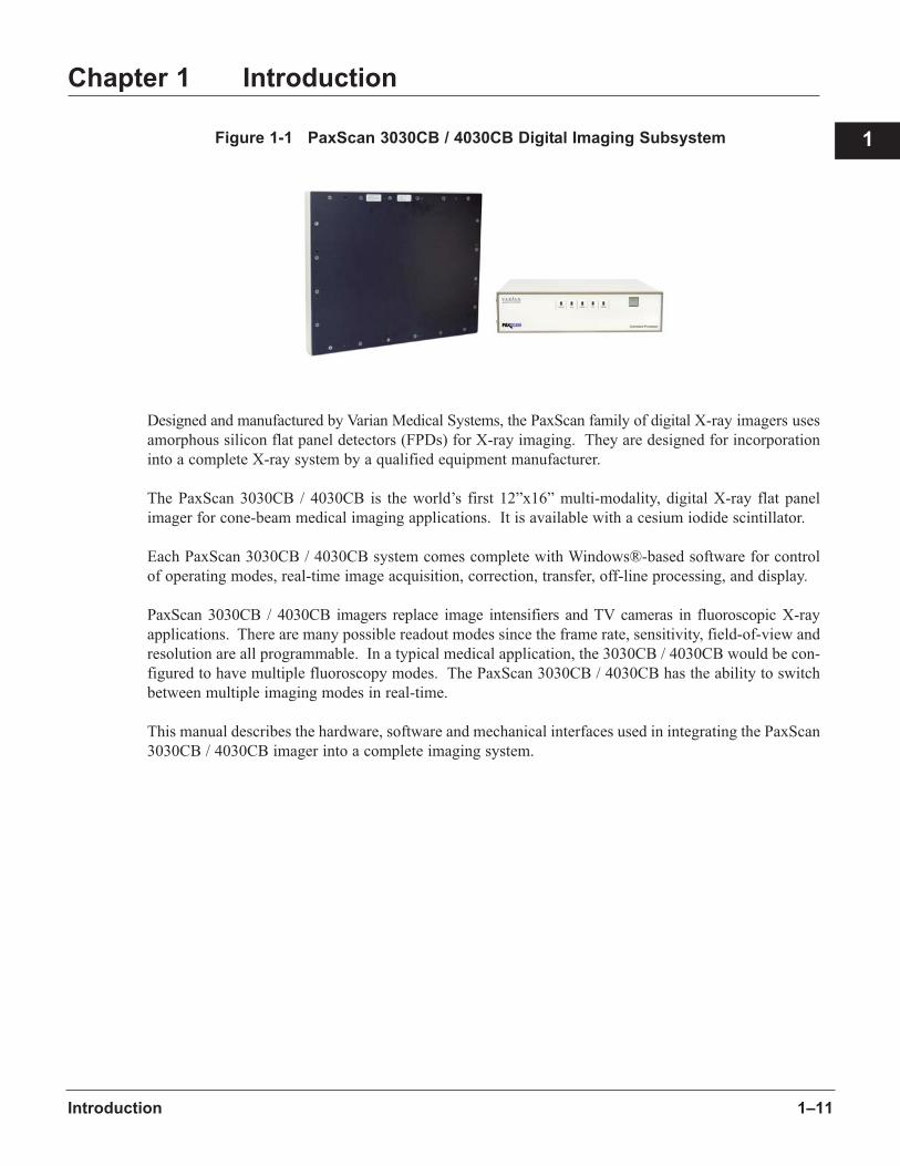
Figure 1-1 PaxScan 3030CB / 4030CB Digital Imaging Subsystem
Designed and manufactured by Varian Medical Systems, the PaxScan family of digital X-ray imagers uses
amorphous silicon flat panel detectors (FPDs) for X-ray imaging. They are designed for incorporation
into a complete X-ray system by a qualified equipment manufacturer.
The PaxScan 3030CB / 4030CB is the world’s first 12”x16” multi-modality, digital X-ray flat panel
imager for cone-beam medical imaging applications. It is available with a cesium iodide scintillator.
Each PaxScan 3030CB / 4030CB system comes complete with Windows®-based software for control
of operating modes, real-time image acquisition, correction, transfer, off-line processing, and display.
PaxScan 3030CB / 4030CB imagers replace image intensifiers and TV cameras in fluoroscopic X-ray
applications. There are many possible readout modes since the frame rate, sensitivity, field-of-view and
resolution are all programmable. In a typical medical application, the 3030CB / 4030CB would be con-
figured to have multiple fluoroscopy modes. The PaxScan 3030CB / 4030CB has the ability to switch
between multiple imaging modes in real-time.
This manual describes the hardware, software and mechanical interfaces used in integrating the PaxScan
3030CB / 4030CB imager into a complete imaging system.
1
Introduction

PaxScan 3030CB / 4030CB Systems & Service Guide1–12

2–13
Chapter 2 System Overview
The PaxScan 3030CB / 4030CB is a real-time, fluoroscopic digital X-ray imaging subsystem incorporating
a large area amorphous silicon TFT/photodiode sensor array with a cesium iodide scintillator.
The PaxScan 3030CB / 4030CB will acquire images at usual video frame rates over a wide range of dose.
The 3030CB / 4030CB is designed for diagnostic X-ray tube energies ranging from 40 kVp to 150 kVp.
Designed as a subsystem, it cannot be used as a stand-alone device. It must be incorporated into a com-
plete X-ray system by a qualified equipment manufacturer.
In This Chapter
Topic Page
Receptor 2-15
Command Processor 2-18
Internal Power Supply 2-19
Modes of Operation 2-20
Important: The PaxScan 3030CB / 4030CB is designed for maximum access to the patient, with a
minimum possible border on the active imaging area. No part of the PaxScan 3030CB /
4030CB is intended to be attached to a patient and/or to contact the patient.
The imaging system has three main components. The Receptor, which houses the solid-state, flat panel
sensor; the Command Processor, and the Power Supply. The Command Processor is the interface between
the Receptor and the imaging system.
In medical applications, the function of the Receptor is to absorb the X-rays that pass through the
patient’s anatomy, and to convert those X-rays into a digital image.
The Command Processor and Power Supply will typically be mounted in an equipment enclosure and will
not be in view or reach of the operator or patient. The Receptor is mounted into the OEM’s mounting
structure, such as a C-Arm, and will often be completely covered by the mounting and a contrast-
enhancing screen.
During operation, the C-Arm is often draped or bagged to ensure cleanliness and sterilization, and is
manipulated such that the Receptor’s input window is located near, but on the opposite side of the
patient, from the X-ray source.
Important: It is possible that during normal usage the Receptor could inadvertently contact the patient.
The closeness of the Receptor to the patient is dependent upon the operator and the technique
being performed.
2

PaxScan 3030CB / 4030CB Systems & Service Guide2–14
Note: PaxScan imagers are intended for continuous use.
Figure 2-1 shows the configuration of the Receptor in the context of the overall imaging system. The
Receptor measures 18 x 14 x 1.6 inches. The receptor thickness increases to 2.6 inches where the snap-on
box is located.
Note: The Receptor can be located up to 40 meters from the Command Processor. A bi-directional
fiber-optic link is used to pass all data and mode control signals to the Receptor. The
24V/3A power for the Receptor is provided on a separate copper cable with quick disconnect
connectors.
Figure 2-1 PaxScan Imager Configuration
The imager operation is controlled using software commands via Ethernet, or one of Serial ports. The
set of possible imager control operations is supplied to systems integrators in a C++ library of callable
functions, in the form of a Win32 DLL. The communications interface is at the level of IP sockets.
Control of the imager is platform-independent.
Note: The Command Processor has a set of I/O signals that can be used for hardware handshaking
and synchronization of critical tasks.
The primary output of the Command Processor is corrected 16-bit digital video or standard camera link
video. Raw data from the Receptor are corrected for offset and gain variations on a pixel-by-pixel basis.
The amorphous silicon panel has a finite number of dead pixels and lines, which are corrected in the
Command Processor through interpolation of the nearest neighbors. The Command Processor also pro-
vides a recursive filter to smooth frame-to-frame noise.
The Power Supply provides all the DC power necessary for both the Command Processor and the
Receptor. The Power Supply connects to any standard wall outlet and is connected to the Command
Processor through a 50-pin D sub-miniature connector. The Command Processor and Power Supply each
have a footprint of 10.2 x 11 inches, and when stacked for rack mounting occupy a height of 5.2 inches.

2–15System Overview
Receptor
The Receptor is based on amorphous silicon (a-Si) technology, which is very similar to that used in flat
panel liquid crystal displays. Because X-rays cannot be easily focused, it is a requirement that the detec-
tor be as large as the area to be imaged.
The PaxScan 3030CB / 4030CB a-Si devices are fabricated onto a glass substrate in the same manner as
TFTs in active matrix flat panel displays. The glass substrate is mounted on a base plate, which also
holds the readout and drive electronics for the Receptor.
Note: In CCD-based systems, a large X-ray conversion screen emitting visible radiation is coupled
to the camera through a mirror and lens. The drawback to such a system is the substantial
loss in signal due to the relatively small solid angle in which light is collected. The larger
the area to be imaged, the greater the loss
Varian’s amorphous silicon panels allow optimal coupling between the X-ray conversion screen and the
photo-detector.
Figure 2-2 Internal Configuration of the Receptor
The core of the detector is an array of amorphous silicon p-i-n photodiodes and thin film transistors
(TFTs), which are arranged as shown below.
Figure 2-3 Sensor Structure
2

PaxScan 3030CB / 4030CB Systems & Service Guide2–16
On top of the amorphous silicon (a-Si) array is an X-ray scintillator, which converts the X-ray photons
to visible radiation. This scintillator is typically a thallium-doped Cesium Iodide deposited directly on
the a-Si array. These X-ray conversion screens emit nearly 550 nm, which corresponds to the peak quan-
tum efficiency of the photodiodes.
Amorphous Silicon: Features and Benefits
Amorphous silicon devices have been shown to be extremely radiation hard. This feature makes a-Si tech-
nology attractive for both diagnostic energy imaging (40 to 150 kVp) as well as mega voltage energy
imaging, such as might be done in radiation therapy and high energy non-destructive test (NDT) appli-
cations, where the dose rate from the source typically exceeds 100 cGy/min.
Amorphous silicon devices have a number of additional features that make them well-suited to X-ray
sensor applications:
n a-Si can be deposited over a large area onto glass substrates
n A low dark current of the pin diodes
n Wide dynamic range
n A low leakage current of a-Si TFT
n Capable of tolerating > 10,000 Gy (1Mrad) total dose in the active area.
n Can image a wide range of X-ray energies in diagnostic imaging and non-destructive test (NDT)
n Very low pixel-to-pixel crosstalk
Note: A typical dark current for the photodiodes is on the order of 2pA/mm 2. The OFF current of
a TFT is less than 0.1pA for temperatures below 50°C. Such low dark currents equip the
devices for use as charge integrating detectors, allowing frame rates on the order of many
seconds per frame.
The large intrinsic dynamic range of the amorphous silicon pixel comes from the large charge capacity of
the photodiodes. For a 194 µm pixel, the charge capacity is over 0.7 pF, which gives over 50 million
electrons for a 5V reverse bias.
Properties of Amorphous Silicon
The same lack of long-range order in the amorphous silicon (a-Si) material that makes it radiation hard, also
means that charge does not move easily in amorphous silicon. Since the electron mobility in a-Si is less
than 1 cm2/V·sec, it is not practical to build extensive readout electronics into the a-Si plate.
As a consequence, every row and column connection must be brought out to the edge of the array where
it is connected to conventional integrated circuits. This poses a number of unique challenges when com-
pared to CCD or CMOS active pixel sensors where much of the sensitive readout electronics can be built
into the detector.
2–17System Overview
The first challenge is simply the mechanical connection to the thousands of signals, which come out to
the edge of the array. The second and more difficult challenge is that the architecture forces the readout
circuit to operate in the presence of the large parasitic resistance and capacitance of the a-Si array. The
dominant noise sources in the imager arise from these parasitics.
In the same way that the a-Si sensor technology is leveraging the huge investment that has been made in
displays, the interconnect technology used in flat panel displays is also available for sensors. Typically,
the row selection and readout electronics are put in TAB (tape automated bonding) packages. These
flexible packages are heat sealed to a conductive landing pattern on the glass using a z-axis conducting
epoxy. The chip is mounted somewhere in the middle of the package. At the other end of the package
the signal traces are either soldered or heat sealed to a printed circuit board.
Note: The advantage of a TAB package over a simple flexible circuit interconnect, is the dramatic
reduction in the number of pins required at the PCB end of the package.
The readout chips are heat sealed at the glass to 128 columns, where the landing pattern has a pitch of
100 µm. The readout chip multiplexes these 128 inputs down to one output, so on the PCB end of the
package only 30 pins at a pitch of 20 thousandths of an inch are necessary to carry the power, control
signals and output signal. Another advantage of the TAB package is that the electronics can be wrapped
around to the side or the backside of the array, as shown in Figure 2-2 for one of the gate driver chips.
The top and bottom halves of the-Si array are read in parallel, a single row at a time progressively. The
parallel scanning feature of the 3030CB / 4030CB is enabled by the use of split datalines and two sided
readout electronics. This feature offers lower electronic noise, faster scanning and an increased time win-
dow for pulsed X-ray beam delivery.
Referring to Figure 2-3, the gate driver chips select which row in the image is accessed, by applying a
positive voltage to a line of TFT gates. With the TFTs ON, charge collected on individual photodiodes
in the selected row is then discharged onto the corresponding dataline. Each dataline is held at a con-
stant potential by a charge integrating amplifier.
Note: In the PaxScan 3030CB / 4030CB, there are 1,536 rows and 2,048 columns at a pixel pitch
of 194 µm; therefore, 4,048 charge integrating amplifiers on an effective pitch less than 194
µm are required to readout the imager.
A second generation, custom 128-channel readout chip, the VENUS 4, has been designed
in a BiCMOS process for this purpose. The VENUS chips capture the charge on each
dataline, converting the signals to voltage levels, which are then multiplexed out to 14-bit
analog-to-digital converters (ADCs).
2
PaxScan 3030CB / 4030CB Systems & Service Guide2–18
To summarize the signal conversion chain:
n X-rays are converted to visible photons by the scintillator.
n The visible photons are absorbed by the pin photodiodes and converted to electron-hole pairs, which collect on the capacitance of the photodiodes.
n The pin photodiodes are discharged when the pixel’s TFT is turned ON. The charge is collected byan integrating amplifier and converted to a voltage.
n The signal voltage has a programmable gain applied, dependent upon operating conditions.
n The output voltage is converted to digital data by an ADC.
Command Processor
The Command Processor provides all hardware and software interfaces for the PaxScan 3030CB /
4030CB. It consists of an embedded computer, image correction hardware, and external hardware inter-
face connections.
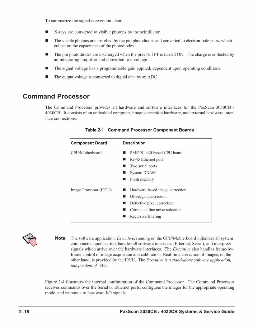
Table 2-1 Command Processor Component Boards
Note: The software application, Executive, running on the CPU/Motherboard initializes all system
components upon startup, handles all software interfaces (Ethernet, Serial), and interprets
signals which arrive over the hardware interfaces. The Executive also handles frame-by-
frame control of image acquisition and calibration. Real-time correction of images, on the
other hand, is provided by the IPCU. The Executive is a stand-alone software application, independent of ViVA.
Figure 2-4 illustrates the internal configuration of the Command Processor. The Command Processor
receives commands over the Serial or Ethernet ports, configures the imager for the appropriate operating
mode, and responds to hardware I/O signals.
Component Board Description
CPU/Motherboard n PM/PPC 440-based CPU board
n RJ-45 Ethernet port
n Two serial ports
n System DRAM
n Flash memory
Image Processor (IPCU) n Hardware-based image correction
n Offset/gain correction
n Defective pixel correction
n Correlated line noise reduction
n Recursive filtering
2–19System Overview
At the heart of the Command Processor is a PowerPC 440GP CPU, which runs the VxWorks real-time oper-
ating system (RTOS). Using an RTOS allows the imager to respond to events on a frame-by-frame basis.
The Command Processor contains three banks of memory:
n DRAM associated with the PowerPC 440GP CPU
n High Speed Synchronous DDR (SDRAM), used in the image processing section
n Non-volatile flash which stores the run-time application as well as the offset and gain correction values used on system start-up.
Offset and Gain Variations
The image processing unit (IPU) corrects for offset and gain variations as well as defective pixels, on a
pixel-by-pixel basis. Background and gain variations are due to non-uniformity in the dark current on
the array as well as intrinsic differences between the readout amplifiers.
Defective pixels originate on the array. To correct for this phenomenon, the IPU uses data from the
nearest neighbors to estimate and replace the defective pixel’s value. The offset and gain correction
algorithm can be reduced to the following formula:
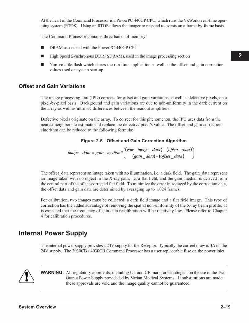
Figure 2-5 Offset and Gain Correction Algorithm
The offset_data represent an image taken with no illumination, i.e. a dark field. The gain_data represent
an image taken with no object in the X-ray path, i.e. a flat field, and the gain_median is derived from
the central part of the offset-corrected flat field. To minimize the error introduced by the correction data,
the offset data and gain data are determined by averaging up to 1,024 frames.
For calibration, two images must be collected: a dark field image and a flat field image. This type of
correction has the added advantage of removing the spatial non-uniformity of the X-ray beam profile. It
is expected that the frequency of gain data recalibration will be relatively low. Please refer to Chapter
4 for calibration procedures.
Internal Power Supply
The internal power supply provides a 24V supply for the Receptor. Typically the current draw is 3A on the
24V supply. The 3030CB / 4030CB Command Processor has a user replaceable fuse on the power inlet
WARNING: All regulatory approvals, including UL and CE mark, are contingent on the use of the Two-
Output Power Supply provideded by Varian Medical Systems. If substitutions are made,
these approvals are void and the image quality cannot be guaranteed.
2
PaxScan 3030CB / 4030CB Systems & Service Guide2–20
Modes of Operation
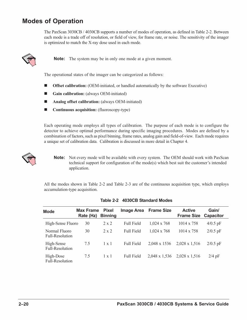
The PaxScan 3030CB / 4030CB supports a number of modes of operation, as defined in Table 2-2. Between
each mode is a trade off of resolution, or field of view, for frame rate, or noise. The sensitivity of the imager
is optimized to match the X-ray dose used in each mode.
Note: The system may be in only one mode at a given moment.
The operational states of the imager can be categorized as follows:
n Offset calibration: (OEM-initiated, or handled automatically by the software Executive)
n Gain calibration: (always OEM-initiated)
n Analog offset calibration: (always OEM-initiated)
n Continuous acquisition: (fluoroscopy-type)
Each operating mode employs all types of calibration. The purpose of each mode is to configure the
detector to achieve optimal performance during specific imaging procedures. Modes are defined by a
combination of factors, such as pixel binning, frame rates, analog gain and field-of-view. Each mode requires
a unique set of calibration data. Calibration is discussed in more detail in Chapter 4.
Note: Not every mode will be available with every system. The OEM should work with PaxScan
technical support for configuration of the mode(s) which best suit the customer’s intended
application.
All the modes shown in Table 2-2 and Table 2-3 are of the continuous acquisition type, which employs
accumulation-type acquisition.
Table 2-2 4030CB Standard Modes
Max Frame Pixel Image Area Frame Size Active Gain/ModeRate (Hz) Binning Frame Size Capacitor
High-Sense Fluoro 30 2 x 2 Full Field 1,024 x 768 1014 x 758 4/0.5 pF
Normal Fluoro 30 2 x 2 Full Field 1,024 x 768 1014 x 758 2/0.5 pFFull-Resolution
High-Sense 7.5 1 x 1 Full Field 2,048 x 1536 2,028 x 1,516 2/0.5 pFFull-Resolution
High-Dose 7.5 1 x 1 Full Field 2,048 x 1,536 2,028 x 1,516 2/4 pFFull-Resolution
2–21System Overview
2
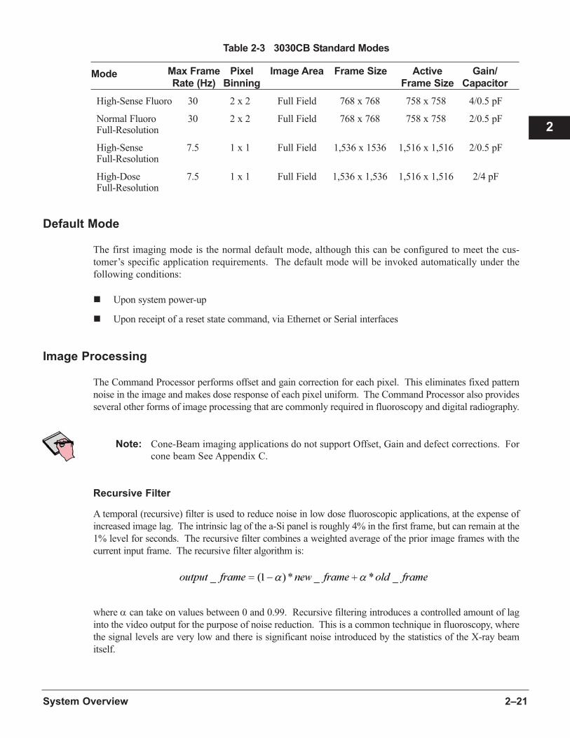
Table 2-3 3030CB Standard Modes
Max Frame Pixel Image Area Frame Size Active Gain/ModeRate (Hz) Binning Frame Size Capacitor
High-Sense Fluoro 30 2 x 2 Full Field 768 x 768 758 x 758 4/0.5 pF
Normal Fluoro 30 2 x 2 Full Field 768 x 768 758 x 758 2/0.5 pFFull-Resolution
High-Sense 7.5 1 x 1 Full Field 1,536 x 1536 1,516 x 1,516 2/0.5 pFFull-Resolution
High-Dose 7.5 1 x 1 Full Field 1,536 x 1,536 1,516 x 1,516 2/4 pFFull-Resolution
Default Mode
The first imaging mode is the normal default mode, although this can be configured to meet the cus-
tomer’s specific application requirements. The default mode will be invoked automatically under the
following conditions:
n Upon system power-up
n Upon receipt of a reset state command, via Ethernet or Serial interfaces
Image Processing
The Command Processor performs offset and gain correction for each pixel. This eliminates fixed pattern
noise in the image and makes dose response of each pixel uniform. The Command Processor also provides
several other forms of image processing that are commonly required in fluoroscopy and digital radiography.
Note: Cone-Beam imaging applications do not support Offset, Gain and defect corrections. For
cone beam See Appendix C.
Recursive Filter
A temporal (recursive) filter is used to reduce noise in low dose fluoroscopic applications, at the expense of
increased image lag. The intrinsic lag of the a-Si panel is roughly 4% in the first frame, but can remain at the
1% level for seconds. The recursive filter combines a weighted average of the prior image frames with the
current input frame. The recursive filter algorithm is:
where α can take on values between 0 and 0.99. Recursive filtering introduces a controlled amount of lag
into the video output for the purpose of noise reduction. This is a common technique in fluoroscopy, where
the signal levels are very low and there is significant noise introduced by the statistics of the X-ray beam
itself.
PaxScan 3030CB / 4030CB Systems & Service Guide2–22
Defective Pixel Replacement
The IPU uses nearest neighbor averaging to replace defective pixels. This can be done successfully for
single defective rows, for single and double defective columns, and for combinations of a number of
defective single pixels.
Saturation Threshold
The offset and gain calibration implemented in the PaxScan 3030CB / 4030CB will fail once the detector
has reached saturation, since the response to increasing dose is not linear. In images with large straight-
through radiation, this can lead to a stripe-like pattern in the saturated regions of the image. This effect can
be minimized by an appropriate choice of gamma function, or LUT, used for the display. Alternatively, the
PaxScan 3030CB / 4030CB has a saturation thresholding function at the input of the image processing sec-
tion. Pixels above a threshold value are set to a fixed, programmable value and no corrections are applied.
Note: In some applications, the unattenuated dose to the Receptor panel can far exceed the sat-
uration point. In these situations, an additional image artifact may also be seen. This
image artifact is a level shift between the upper and lower sections of the image. The dose
at which the artifact appears will depend on the beam energy and filtation.
3–23
Chapter 3 Getting Started
This chapter describes the major components and functions of the PaxScan 3030CB / 4030CB. The
hardware interface connections and an overview of the software used for image calibration and acqui-
sition is provided.
In This Chapter
Topic Page
Shipment Contents 3-23
Connecting the Cables 3-24
Mechanical Mounting 3-26
Power On Sequence 3-27
Establishing Connection 3-28
Basic Offset Calibration 3-28
Basic Gain Calibration 3-29
Image Acquisition 3-30
Shipment Contents
Immediately upon receipt, inspect the shipment and its contents against the Delivery Note enclosed with
the shipment for evidence of damage or missing components. Save all shipping containers in case a return
is warranted. If there is any discrepancy, please call the PaxScan Service Center at (800) 432-4422, or
(801) 972-5000.
3
PaxScan 3030CB / 4030CB Systems & Service Guide3–24
Varian
Part Number Component
18990/20786 PaxScan 3030CB / 4030CB Imager System with:
16272 CsI LN High Bright Receptor
14447 Fiber-optic Command Processor with ABS (LVDS)
11614 30 meter (100 ft.) 24V Receptor power cable
11615 30 meter (100 ft.) fiber-optic data cable
20099 PaxScan 3030CB / 4030CB Systems & Service Guide
11616 USA style Mains power cable, 110 VAC
Options:
17041 RoadRunner R3-PCI-DIF Frame Grabber
7550 Digital Video Cable to R3 Board
16541 7m Integrated fiber and 24V cable
17232 30m Integrated fiber and 24V cable
11229 Lead cap/primary barrier
45004101 1.8 m RJ45 to RJ45 Ethernet crossover cable
45004301 1.8 m Serial (straight type) 9-pin male-to-male cable
19333 5 m Serial (straight type) 9-pin male to female cable
660 Power cable mains, 220 VAC
18104 5 m Unterminated mains cable, 220 VAC
18061 5 m External sync 50-pin MDR/D-Sub cable
18105 40 m Receptor grounging cable
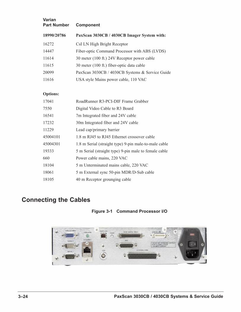
Connecting the Cables
Figure 3-1 Command Processor I/O
Table 3-1 Cable Connections
Step Action
1. Connect the power cable from the Command Processor power input port to the wall outlet.
2. Connect the 11615-series fiber-optic cable from the command processor to the receptor.
3. Connect the 11614-series 24V cable from the Receptor to the power supply.
Note: The fiber-optic cable connectors should be treated carefully. Do not over-stress
the strain relief section. Do not exceed the 5 cm minimum bend radius for the
fiber-optic cable.
4. Connect the Ethernet cable from the Command Processor Ethernet port to an Ethernet port on
the host computer.
Note: If the Ethernet connection is point-to-point between only the Command Processor
and host computer, an RJ45 to RJ45 crossover cable must be used. This is shipped
with the PaxScan 3030CB / 4030CB. 16-bit still images can be captured by the
Command Processor and transferred to the host computer over this Ethernet
cable.
5. If available, connect a digital video data cable from the 16 bit digital video output to an image
capture board in the host computer.
6. Connect either the camera link cable or LVDS digital video cable depending upon your
application from the Command Processor to the host computer.
7. Connect the serial cable from the host computer’s COM 1 port to the Command Processor serial
1 port.
Note: The serial cable must be the straight-through type, not the crossover type typically
used between computers.
Note: The serial connection is used for diagnostics and loading new software into the
Command Processor. This connection is often used during normal operation to
monitor communications between the Command Processor and the host computer.
3–25Getting Started
3

PaxScan 3030CB / 4030CB Systems & Service Guide3–26
Mechanical Mounting
WARNING: If the PaxScan 3030CB / 4030CB Receptor is to be used as a primary barrier to X-rays, the
X-rays must impinge only on the entrance window of the Receptor. The PaxScan 3030CB/
4030CB Receptor lead cap will not stop X-rays that do not hit the entrance window of the
Receptor.
WARNING: The equipment is not suitable for use in the presence of a flammable anaesthetic mixture
with air, oxygen or nitrous oxide.
Receptor Mounting
The Receptor should be mounted onto other pieces of equipment using the holes provided. The Receptor
has an optional lead cap which can be used as a primary barrier to X-rays. As noted above, this barrier is
only effective if the X-ray beam is collimated in such a way that X-rays impinge on the active surface of the
Receptor. See Figure 8-14 for more information
Important: The temperature at the back surface of the Receptor should not exceed 35ºC when the unit
is installed. This may necessitate air flow over the back surface of the Receptor. Humidity
levels should be between 10-90%, with higher limits for storage.
WARNING: The Receptor is not sealed against dripping moisture.
Command Processor
The Command Processor can be rack mounted in a standard 3U (5.2” high) slot using optional rack
mounting intended for a 19” wide rack. See Figure 8-15 and 8-16 for more information.
Important: The following precautions should be observed when rack mounting the Command Processor:
n Elevated operating ambient temperature: If installed in a closed or multi-unit rack assembly, the operating ambient temperature of the rack environment may be greater than room ambient. Equipment
should be installed in an environment compatible with the maximum rated ambient temperature.
n Reduced air flow: Install the equipment so that the amount of air flow required for safe operation is not compromised. Cooling air clearance is 10 cm (4 inches) minimum from each surface.

3–27Getting Started
3
n Mechanical loading: The equipment should be loaded evenly into the rack to avoid any hazardous conditions.
n Circuit overload: Consideration should be given to the connection to avoid overloading of circuits on the over-current protection and supply wiring.
n Reliable Grounding: Reliable grounding should be maintained. Particular attention should be given to the supply connection, other than the direct connection to the branch circuit. The use of surge
protectors are advised.
Power On Sequence
The PaxScan 3030CB / 4030CB requires no action or intervention from the operator or the host system
after power on, or before power off. The PaxScan will be fully operational and ready to receive a Start
Acquiring Image signal or command data within approximately three minutes after power on. Actual
startup time depends on the number of modes loaded and the system configuration.
When startup is complete and if the system is configured accordingly, a default mode test pattern will
be sent to the video outputs. Full specification is achieved within two hours after power up.
Note: The PaxScan 3030CB / 4030CB does not require any special warnings prior to power
down. No loss of data or setup information will result from unexpected shutdown.
Table 3-2 Power On Sequence
Step Action
1. Turn on the host computer and allow it to boot up and login.
2. Turn on the Command Processor.
The Command Processor must boot up before connection to the viewing application can occur. A success-
ful boot up can be identified in one of four ways:
1. The LEDs Power, Frame, and Run are illuminated on the front panel of the Command Processor.
2. The default set-up is to display a test pattern out the digital video port of the Command Processor,
if connected to a digital system.
3. The IP address is displayed over the serial port.
4. Panel_Ready becomes asserted on Hard Handshaking Port.
Once any of the four indicators are received, the Receptor is ready to acquire or view images.
PaxScan 3030CB / 4030CB Systems & Service Guide3–28
Establishing Connection
ViVA™ is the viewing application used to control the Command Processor. Varian Image Viewing and
Acquisition (ViVA) is a non-commercial GUI program for controlling the PaxScan 3030CB / 4030CB
"out of the box." It currently runs only under Windows 2000.
ViVA sends control commands to the Command Processor over a 10BaseT Ethernet connection. Some
of ViVA’s functions include acquiring images from the Receptor, viewing images, and saving images to
the hard disk. ViVA may also be used with a serial interface, but not for retrieving images.
Note: In order for ViVA to establish an Ethernet connection with the Command Processor, the
client IP address and server IP address parameters must be configured. If your system
configuration has not been factory-set, please see Appendix B, Command Processor and
Computer Interface, to configure your system.
Note: For additional assistance operating ViVA, use the ViVA Online Help file, or see Operation,
Chapter 6 of this guide.
Basic Offset Calibration
Prior to acquiring images, an offset calibration must be performed for each mode you intend to use.
n After the panel has been powered up for thirty minutes, calibration should be performed every ten minutes, and as needed for clean images thereafter.
n An offset calibration should be performed any time the panel is inactive for more than five minutes, or if the image seems to be degraded.
Standard calibration defaults:
n During idle periods of operation, auto offset calibration will occur every five minutes.
n Post-exposure offset is every two minutes.
n During continuous operation, an offset should be performed every five to thirty minutes, depending on image quality and application time constraints.
Note: Cone-Beam modes not supported. For cone beam See Appendix C.
3–29Getting Started
3
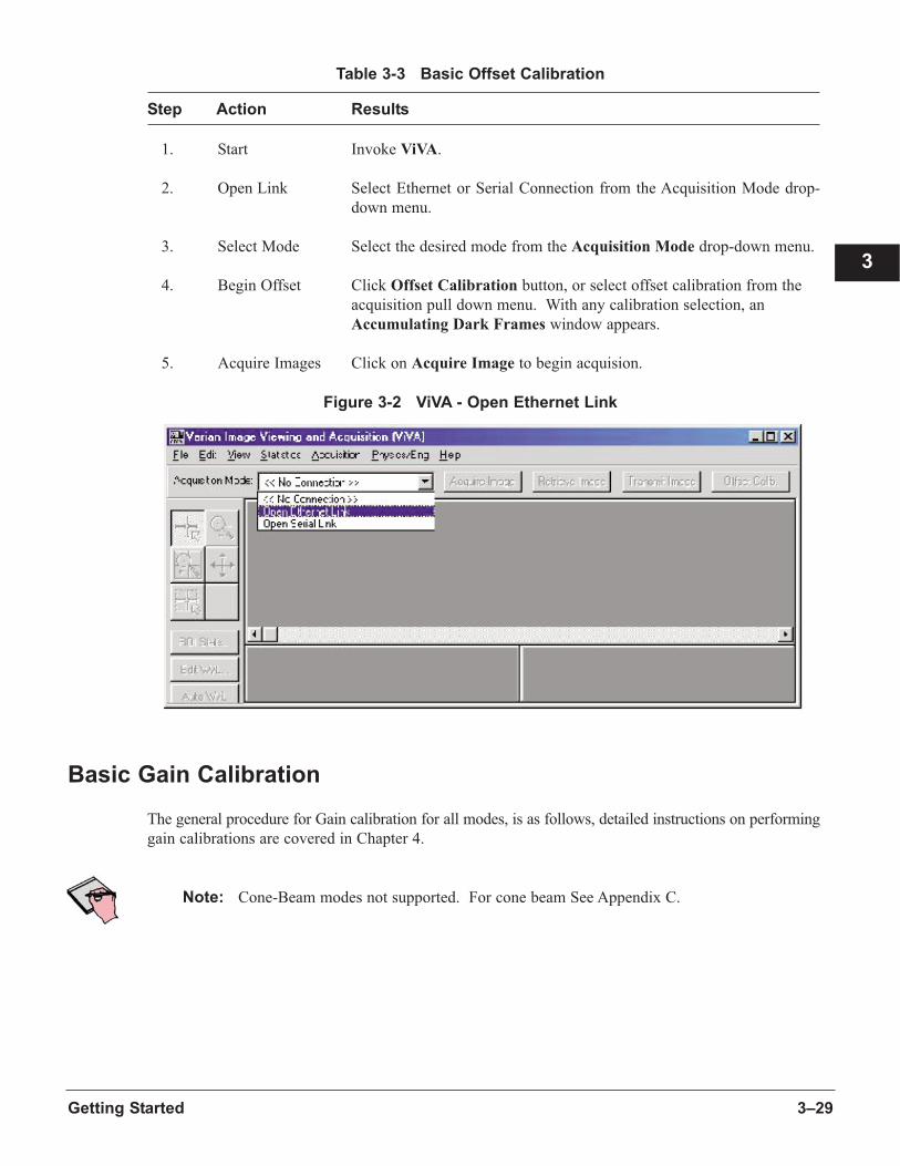
Table 3-3 Basic Offset Calibration
Step Action Results
1. Start Invoke ViVA.
2. Open Link Select Ethernet or Serial Connection from the Acquisition Mode drop-
down menu.
3. Select Mode Select the desired mode from the Acquisition Mode drop-down menu.
4. Begin Offset Click Offset Calibration button, or select offset calibration from the
acquisition pull down menu. With any calibration selection, an
Accumulating Dark Frames window appears.
5. Acquire Images Click on Acquire Image to begin acquision.
Figure 3-2 ViVA - Open Ethernet Link
Basic Gain Calibration
The general procedure for Gain calibration for all modes, is as follows, detailed instructions on performing
gain calibrations are covered in Chapter 4.
Note: Cone-Beam modes not supported. For cone beam See Appendix C.
PaxScan 3030CB / 4030CB Systems & Service Guide3–30
Table 3-4 Gain Calibration: All Modes
Step Action Results
1. Warm Up To ensure proper warm up, the PaxScan 3030CB / 4030CB Receptor
must be operational for at least two hours prior to Gain calibration.
2. Radiation A uniform flat field with no object in the path of the X-ray beam. The
radiation must be at a level and technique representative of the typical
radiation dose for the Receptor during typical procedures.
Note: The exact level of the radiation during calibration will not influencethe calibration as long as the signal level is not saturated.
3. Offset Software automatically performs a new Offset Calibration calibration
following the acquisition of the flat field image.
Note: X-rays must be disabled.
4. Repeat The above procedure must be repeated for each of the stored modes.
Image Acquisition
Once Offset and Gain Calibration is performed, you are ready to acquire images.
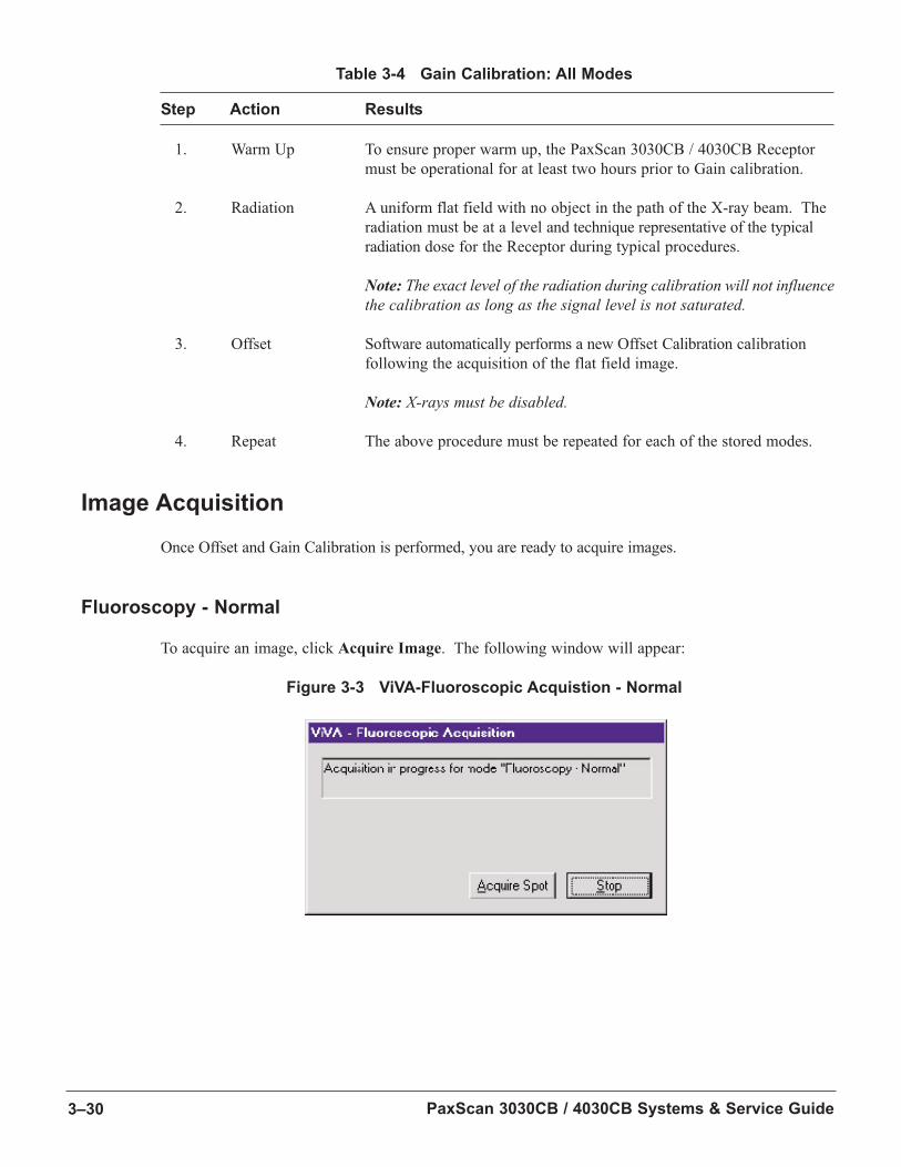
Fluoroscopy - Normal
To acquire an image, click Acquire Image. The following window will appear:
Figure 3-3 ViVA-Fluoroscopic Acquistion - Normal
3–31Getting Started
3
This window indicates that the Receptor is actively acquiring “live” images. Click Stop. The last frame
or accumulated frames will be captured and stored in the Command Processor memory.
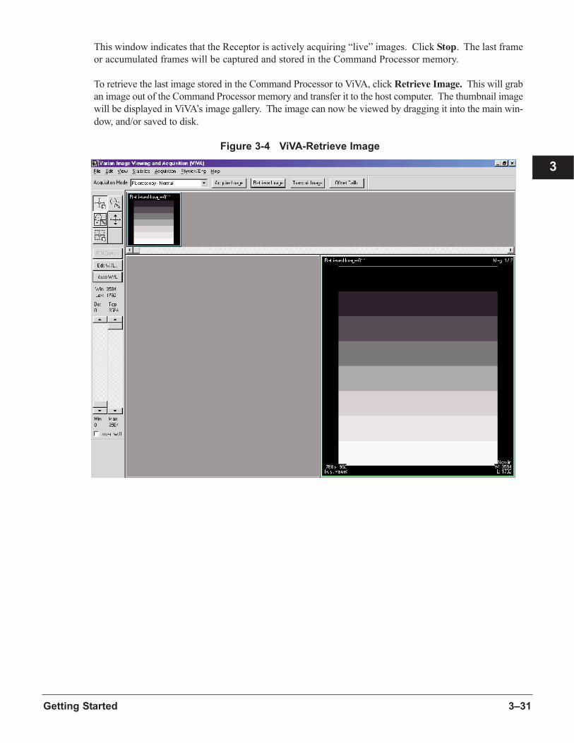
To retrieve the last image stored in the Command Processor to ViVA, click Retrieve Image. This will grab
an image out of the Command Processor memory and transfer it to the host computer. The thumbnail image
will be displayed in ViVA’s image gallery. The image can now be viewed by dragging it into the main win-
dow, and/or saved to disk.
Figure 3-4 ViVA-Retrieve Image

PaxScan 3030CB / 4030CB Systems & Service Guide3–32
4–33
4
Chapter 4 Calibration Procedures
The IPU in the Command Processor FPGA corrects for Gain, Offset and Analog variations between indi-
vidual pixels as well as globally across the image.
This non-uniformity compensation requires that a Gain reference image and an Offset reference image be
resident in the Command Processor’s high speed SDRAM memory prior to imaging procedures.
Note: Cone-Beam modes do not support Offset, Gain and Defect Corrections. For cone beam
See Appendix C.
In This Chapter
Topic Page
Offset Calibration 4-34
Gain Calibration 4-34
Fluoroscopic Mode Gain Calibration 4-36
Defective Pixel Maps 4-40
Analog Offset Calibration 4-40
Note: References to the OEM computer is as Client, while the PaxScan 3030CB / 4030CB
Command Processor is referred to as the Server.
Note: After Gain calibration is complete, an Offset calibration automatically follows.
Note: The Command Processor will not apply the Offset and Gain correction to pixels identified as
being saturated. This feature of the non-uniformity correction avoids inverse compensation
artifacts in regions where the image is saturated and where non-uniformities are no longer
present.
Offset calibration compensates for fixed pattern pixel intensity variations in the image, associated with the
dark current (Receptor) and electronic offsets introduced by the readout ASIC and the Analog Board.
The Offset reference image is an average of a series of frames acquired with no illumination, referred to as
dark fields. The Gain reference image is an average of a series of frames acquired with uniform X-ray illu-
mination, referred to as flat fields, across the active area.
PaxScan 3030CB / 4030CB Systems & Service Guide4–34
The larger the number of frames used in creating the Gain and Offset reference images, the lower the
amount of noise contributed to the image by the non-uniformity correction. The Analog offset calibra-
tion reduces DC offsets created by variations in electronic components, providing more dynamic range.
It is possible to download the Offset and Gain reference images to the Command Processor (Server) via the
Ethernet interface. The current Offset and Gain reference images can also be uploaded to the Client
computer, via the Ethernet interface.
Offset Calibration
The request to perform Offset calibration can be initiated by the client system, via a software command
across the Ethernet interface, or the Command Processor can handle the calibration procedure
autonomously. It performs all calculations of correction factors internally and stores the relevant data in
memory, without requiring action from the main system or the operator.
Some important points concerning Offset correction:
n Offset calibration should not occur while the X-ray is activated.
n The X-ray-to-digital conversion factor does not change as a result of calibration.
n A different offset reference image is necessary for each operating mode, therefore it is important to update the offset data for each of the operating modes.
n If the Prepare signal on the Command Processor’s external synchronization port is asserted, the PaxScan 3030CB / 4030CB is able to abandon an ongoing offset calibration with no loss in pre-
calibration image quality.
n After abandoning an offset calibration, the PaxScan 3030CB / 4030CB will be ready to acquire images within four frames. The ready to acquire condition is communicated via the PanelReady signal on
the synchronization interface.
Note: It is recommended that a delay of at least 20 seconds be allowed after an X-ray exposure,
before commencing with offset calibration. Since there is some inherent lag in the detector,
this delay avoids introduction of a latent image into the offset reference image.
Important: Since the offset characteristics of the detector vary during normal operation, the offset
reference image must be updated at least every two to five minutes while the PaxScan
3030CB / 4030CB is warming up, and at least every 15 minutes once it has reached its
steady state temperature, typically after about two hours of operation.
Gain Calibration
To compensate for non-uniformities in the Receptor, a gain reference image (flat field) is used by the Image
Processing Unit as required to correct all images in real-time. This flat field image must be captured by
the Command Processor prior to acquiring images, and stored in non-volatile memory. The process of cap-
turing the flat field image is known as Gain calibration.

4–35Calibration Procedures
Note: Gain calibration should take place at regular intervals, typically once every three months,
or whenever the X-ray source has been moved relative to the Receptor.
Gain calibration is based upon the linear response of the Receptor to dose. Normalization is achieved by
applying the flat field image acquired in the Gain calibration to all images passing through the Image
Processing Unit. Normalization will fail with pixels that are responding to dose in a non-linear manner.
Pixels responding to dose in a non-linear manner are usually caused by the saturation of the Receptor, or a
low signal-to-noise ratio. These non-linear pixels will be marked defective during the manufacturing
process and will be corrected by the Image Processing Unit.
Note: It is critical that the flat field image be acquired within a range that is large enough to be
higher than background noise created by the X-ray source and readout electronics of the
Receptor, but lower than the saturation point of the Receptor.
Flat field images acquired near or exceeding the saturation point will cause normalization failures with all
images acquired until a Gain calibration with the correct dose is performed. Varian recommends that flat
field images be acquired with a median count of 2000 - 4000 +/-500. This range will ensure that Gain cal-
ibration will meet both the upper and lower dose requirements under all modes of operation.
To reduce the effects of noise, the average of each pixel in the flat field image is calculated by accumu-
lating a number of frames into an internal buffer, then dividing the sum of each pixel by the number of
frames acquired.
Note: The larger the number of calibration frames used to capture the flat field image, the more
precise the calibration will be.
The number of calibration frames used during Gain and Offset calibrations can be adjusted under the Mode
Settings pull down menu. For more detailed information, refer to ViVA in the Operations section of this
Guide.
Varian recommends accumulating 128 frames in fluoroscopic modes, and 32 frames in full-resolution
modes. For low frame rates, such as one frame per second, this may be too long a period. In such cases, it
may be necessary to lower the number of calibration frames to a more tolerable time period, not going below
eight frames.
After completion of the calibration procedure, the following information will be viewable with ViVA via
the Ethernet interface, upon request from the client:
n The median pixel value of the Gain image
n Gain and Offset reference images
n The defect map image
n The median pixel value of the Dark Field image.
Note: Always use pulsed.
4
PaxScan 3030CB / 4030CB Systems & Service Guide4–36
Important: The PaxScan 3030CB / 4030CB imaging system requires a warm-up of two hours prior to
Gain calibration.
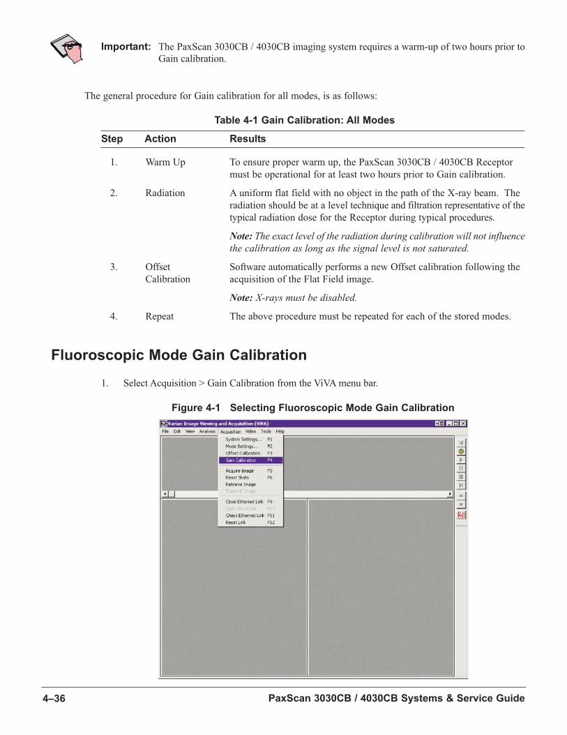
The general procedure for Gain calibration for all modes, is as follows:
Table 4-1 Gain Calibration: All Modes
Step Action Results
1. Warm Up To ensure proper warm up, the PaxScan 3030CB / 4030CB Receptor
must be operational for at least two hours prior to Gain calibration.
2. Radiation A uniform flat field with no object in the path of the X-ray beam. The
radiation should be at a level technique and filtration representative of the
typical radiation dose for the Receptor during typical procedures.
Note: The exact level of the radiation during calibration will not influencethe calibration as long as the signal level is not saturated.
3. Offset Software automatically performs a new Offset calibration following the
Calibration acquisition of the Flat Field image.
Note: X-rays must be disabled.
4. Repeat The above procedure must be repeated for each of the stored modes.
Fluoroscopic Mode Gain Calibration
1. Select Acquisition > Gain Calibration from the ViVA menu bar.
Figure 4-1 Selecting Fluoroscopic Mode Gain Calibration
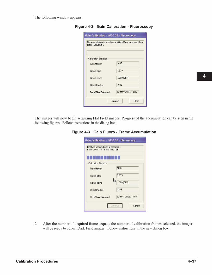
4–37Calibration Procedures
4
The following window appears:
Figure 4-2 Gain Calibration - Fluoroscopy
The imager will now begin acquiring Flat Field images. Progress of the accumulation can be seen in the
following figures. Follow instructions in the dialog box.
Figure 4-3 Gain Fluoro - Frame Accumulation
2. After the number of acquired frames equals the number of calibration frames selected, the imager
will be ready to collect Dark Field images. Follow instructions in the new dialog box:
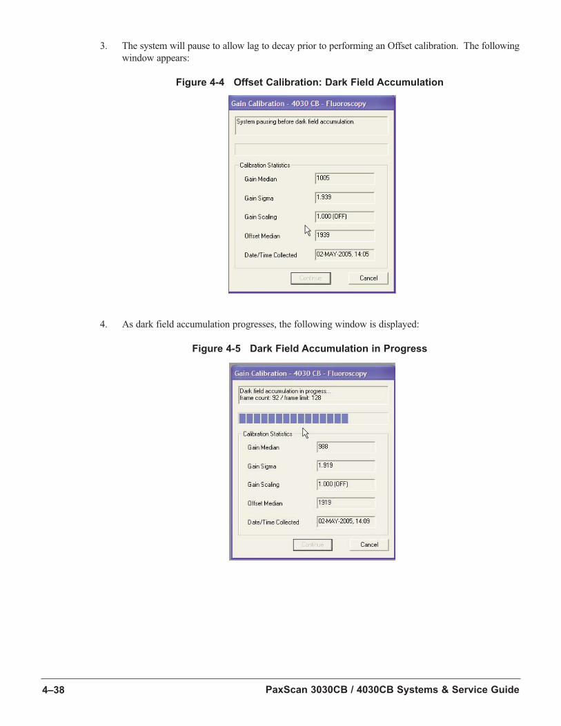
PaxScan 3030CB / 4030CB Systems & Service Guide4–38
3. The system will pause to allow lag to decay prior to performing an Offset calibration. The following
window appears:
Figure 4-4 Offset Calibration: Dark Field Accumulation
4. As dark field accumulation progresses, the following window is displayed:
Figure 4-5 Dark Field Accumulation in Progress
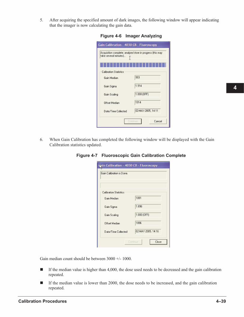
4–39Calibration Procedures
4
5. After acquiring the specified amount of dark images, the following window will appear indicating
that the imager is now calculating the gain data.
Figure 4-6 Imager Analyzing
6. When Gain Calibration has completed the following window will be displayed with the Gain
Calibration statistics updated.
Figure 4-7 Fluoroscopic Gain Calibration Complete
Gain median count should be between 3000 +/- 1000.
n If the median value is higher than 4,000, the dose used needs to be decreased and the gain calibration repeated.
n If the median value is lower than 2000, the dose needs to be increased, and the gain calibration repeated.

PaxScan 3030CB / 4030CB Systems & Service Guide4–40
Defective Pixel Maps
The defective pixel map is determined during Gain calibration, using information from both the Offset and
Gain reference images. The map of defects is stored in the Command Processor’s internal long term (flash)
memory. Using the defect map, the pixel correction algorithm uses nearest neighbor averaging to replace
all defects in each video frame.
Important: Points of note about defect correction:
n The pixel defect map is the combination of two defect maps:
¨ The first map, base, is determined at the factory and does not normally change.
¨ The second defect map, aux, is newly determined during each Gain calibration.
Both types of maps are bit-wise ORed, then supplied to the image correction
algorithm.
n After correction, no defective pixels should be visible in Flat Field images.
n It is possible to upload both defect maps from the PaxScan 3030CB / 4030CB to theclient computer, via the Ethernet interface. It is also possible to replace the base map,
resident in the Command Processor, with a map downloaded from the clientcomputer, via the Ethernet interface.
Analog Offset Calibration
Analog Offset calibrations are determined during imaging system configuration at the factory, or if a new
mode configuration file is loaded.
Analog Offset calibration reduces non-uniform pixel offsets created by differences in the readout com-
ponents located in the Receptor. By reducing the non-uniformity in the Receptor electronics, the over-
all dynamic range of the system can be optimized.
To initiate an Analog Offset calibration, the client computer must send a software command, via the
Ethernet interface or Serial interface, to the Command Processor. The Command Processor will then
initiate the Analog Offset, perform all necessary calculations, and store resulting offsets in non-volatile
memory.
1. Select Analog Offset Calibration from the Tools->Receptor pull down menu and the following
window will appear.
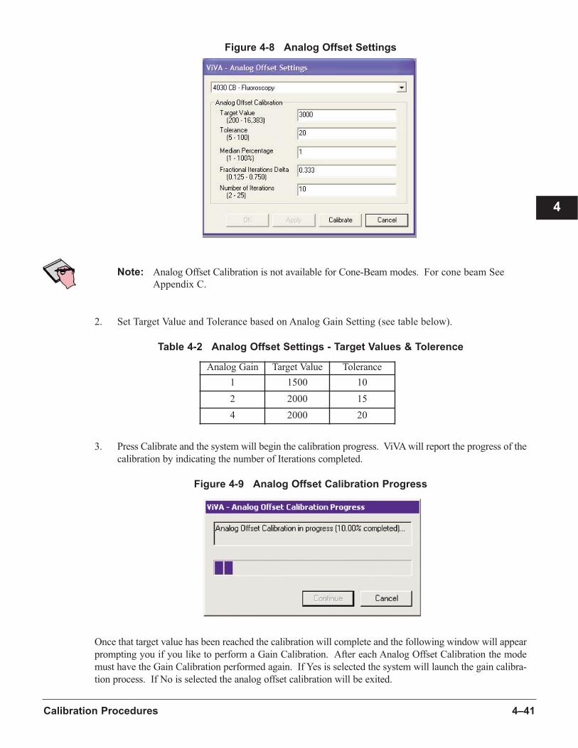
4–41Calibration Procedures
4
Figure 4-8 Analog Offset Settings
Note: Analog Offset Calibration is not available for Cone-Beam modes. For cone beam See
Appendix C.
2. Set Target Value and Tolerance based on Analog Gain Setting (see table below).
Table 4-2 Analog Offset Settings - Target Values & Tolerence
3. Press Calibrate and the system will begin the calibration progress. ViVA will report the progress of the
calibration by indicating the number of Iterations completed.
Figure 4-9 Analog Offset Calibration Progress
Once that target value has been reached the calibration will complete and the following window will appear
prompting you if you like to perform a Gain Calibration. After each Analog Offset Calibration the mode
must have the Gain Calibration performed again. If Yes is selected the system will launch the gain calibra-
tion process. If No is selected the analog offset calibration will be exited.
Analog Gain Target Value Tolerance
1 1500 10
2 2000 15
4 2000 20

PaxScan 3030CB / 4030CB Systems & Service Guide4–42
Verification of Analog Offset Calibration
1. Disable all image corrections via Acquisition->System Settings.
2. Acquire image.
3. Retrieve image.
4. Click Edit W/L button.
5. From Edit Values section, select Bottom\Top.
6. Set Top field based on the Analog Gain setting of the mode.
n If Analog Gain is set to 1, then set Top Field to 751 and Bottom Field to 750.
n If Analog Gain is set to 2, then set Top Field to 1001 and Bottom Field to 1000.
n If Analog Gain is set to 4, then set Top Field to 1001 and Bottom Field to 1000.
Note: To get analog gain setting select Acquisition->Mode Settings.
7. Image should appear all white, with the exception of defects.
8. If step 7 fails, repeat analog offset calibration procedure.
Important: n Analog Offset calibration requires no X-rays during the calibration procedure.
n It is recommended that the system be powered On for at least two hours prior toperforming an Analog Offset calibration.
n A different Analog Offset calibration is required for each mode.
n It is recommended that a delay of 60 seconds be allowed after an X-ray exposure, before performing an Analog Offset calibration.
n An Offset and Gain calibration must be performed after completing the Analog Offset calibration.
n The Receptor configuration file will be modified in the Command Processor. This new file should be uploaded to the Client computer.
n Verify Analog Offset calibration.
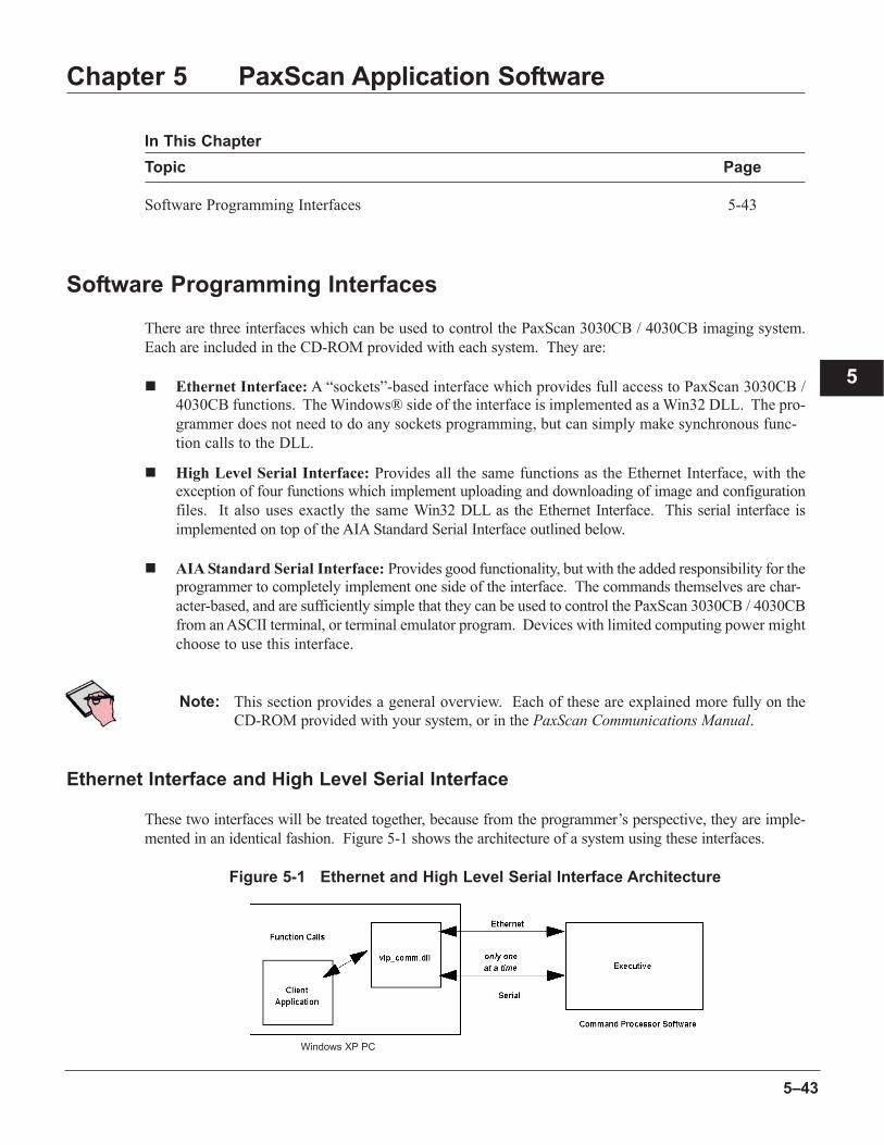
5–43
5
Chapter 5 PaxScan Application Software
In This Chapter
Topic Page
Software Programming Interfaces 5-43
Software Programming Interfaces
There are three interfaces which can be used to control the PaxScan 3030CB / 4030CB imaging system.
Each are included in the CD-ROM provided with each system. They are:
n Ethernet Interface: A “sockets”-based interface which provides full access to PaxScan 3030CB / 4030CB functions. The Windows® side of the interface is implemented as a Win32 DLL. The pro-
grammer does not need to do any sockets programming, but can simply make synchronous func-
tion calls to the DLL.
n High Level Serial Interface: Provides all the same functions as the Ethernet Interface, with the exception of four functions which implement uploading and downloading of image and configuration
files. It also uses exactly the same Win32 DLL as the Ethernet Interface. This serial interface is
implemented on top of the AIA Standard Serial Interface outlined below.
n AIA Standard Serial Interface: Provides good functionality, but with the added responsibility for the programmer to completely implement one side of the interface. The commands themselves are char-
acter-based, and are sufficiently simple that they can be used to control the PaxScan 3030CB / 4030CB
from an ASCII terminal, or terminal emulator program. Devices with limited computing power might
choose to use this interface.
Note: This section provides a general overview. Each of these are explained more fully on the
CD-ROM provided with your system, or in the PaxScan Communications Manual.
Ethernet Interface and High Level Serial Interface
These two interfaces will be treated together, because from the programmer’s perspective, they are imple-
mented in an identical fashion. Figure 5-1 shows the architecture of a system using these interfaces.
Figure 5-1 Ethernet and High Level Serial Interface Architecture
Windows XP PC
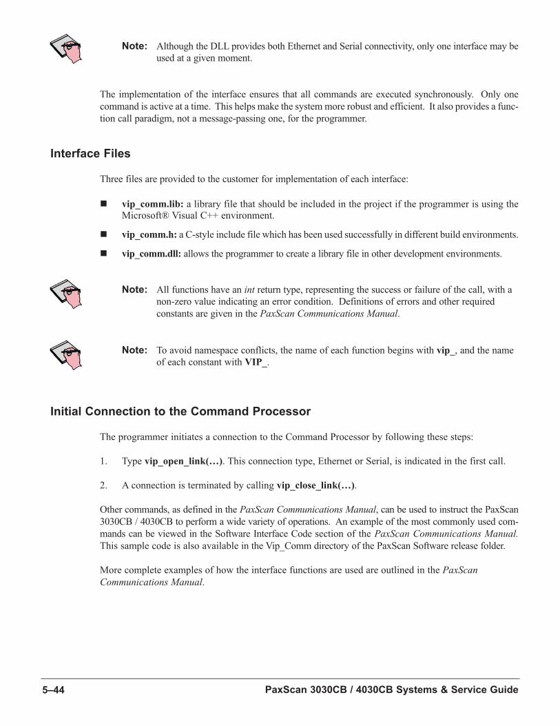
PaxScan 3030CB / 4030CB Systems & Service Guide5–44
Note: Although the DLL provides both Ethernet and Serial connectivity, only one interface may be
used at a given moment.
The implementation of the interface ensures that all commands are executed synchronously. Only one
command is active at a time. This helps make the system more robust and efficient. It also provides a func-
tion call paradigm, not a message-passing one, for the programmer.
Interface Files
Three files are provided to the customer for implementation of each interface:
n vip_comm.lib: a library file that should be included in the project if the programmer is using the Microsoft® Visual C++ environment.
n vip_comm.h: a C-style include file which has been used successfully in different build environments.
n vip_comm.dll: allows the programmer to create a library file in other development environments.
Note: All functions have an int return type, representing the success or failure of the call, with a
non-zero value indicating an error condition. Definitions of errors and other required
constants are given in the PaxScan Communications Manual.
Note: To avoid namespace conflicts, the name of each function begins with vip_, and the name
of each constant with VIP_.
Initial Connection to the Command Processor
The programmer initiates a connection to the Command Processor by following these steps:
1. Type vip_open_link(…). This connection type, Ethernet or Serial, is indicated in the first call.
2. A connection is terminated by calling vip_close_link(…).
Other commands, as defined in the PaxScan Communications Manual, can be used to instruct the PaxScan
3030CB / 4030CB to perform a wide variety of operations. An example of the most commonly used com-
mands can be viewed in the Software Interface Code section of the PaxScan Communications Manual.This sample code is also available in the Vip_Comm directory of the PaxScan Software release folder.
More complete examples of how the interface functions are used are outlined in the PaxScanCommunications Manual.

6–45
6
Chapter 6 ViVA Help
The ViVA software application is a Windows-based program designed to be used with PaxScan products to
perform basic tasks. ViVA can be used to control axquisitions with PaxScan products and also display and
manipulate images on a Windows PC that is not connected to a PaxScan system. ViVA targets medical
images ans exclusively displays 16-bit image formats.
This ViVA Help documentation is designed to assist users with use of the ViVA.
In This Help Document
Topic Page
Setup 6-46
View Menu & User Interface 6-46
File Menus & Image Files 6-51
Edit Menu & Preferences 6-56
Edit Toolbar & Image Manipulation 6-58
Acquisition Menu/Toolbar 6-65
Video Menu/Toolbar 6-74
Analysis Menu: Image Statistics 6-78
Tools Menu 6-82
Note: In this section primary ViVA commands from menus or toolbars are in bold type. For
increased clarity in places a menu and menu item may be specified with a vertical
separator (e.g. File|Close). Commands and controls found in dialog boxes are generally
in bold italic type. References to sections of this chapter are in bold underline.
ViVA uses a number of common terms and notations that have special meanings:
n Menu items ending with three periods (e.g. File|Open...) indicate that executing the commands will require further input from the user in a dialog box. Menu items without the periods normally require
no further involvement by the user and will be executed immediately.
n In a dialog box, a Cancel button implies closure of the dialog box without executing data on the dialog box. The Apply button implies execution of data on the dialog box that updates data and/or
the Command Processor. The OK button performs the same tasks as the Apply button if they have
not been executed, then closes the dialog box.
PaxScan 3030CB / 4030CB Systems & Service Guide6–46
Setup
System Requirements
ViVA will run on Intel-based PCs using Windows XP. Generally, acceptable performance in image viewing
and manipulation can be obtained with any Pentium CPU system. The number of open images is limited by
the combination of physical and virtual memory. The quality of the video card, hardware, firmware, and
driver software also impacts the perceived speed of operation.
When used with a frame grabber card, system requirements are more demanding; the following is provided
for guidance. A minimum system specification includes a Pentium III processor running at 1GHz or better
with at least 512MB RAM and preferably 1GB. It is also strongly suggested that you check the frame grab-
ber manufacturer’s recommendations regarding specific hardware. The intended use of the system may dic-
tate larger amounts of RAM since capturing video sequences generally requires at least enough memory to
store the largest expected sequence + an additional 128MB.
Installation
The Setup.exe in the root directory of the PaxScan CD provides an automated installation process for
ViVA and any dependent files. Setup.exe is automatically started when the CD is inserted into a CD
drive unless the Auto-Run CD option is turned off. To start Setup.exe manually, use the Run command
under the Windows Start button to execute X:/Setup.exe, where X is the drive letter of the CD drive that
contains the PaxScan CD. Setup.exe will create a shortcut of ViVA on the desktop.
To uninstall ViVA, run the Add/Remove application in the Control Panel and remove the entry PaxScan.
Note: Running this automatic uninstall program will also remove all other PaxScan components
such as Command Processor files and Hostdown files that were previously installed onto the
hard drive.
To run ViVA, locate and double click the shortcut of ViVA on the desktop.
Version
ViVA version information is available from the Help|About ViVA... command. This dialog will also
show information about any dlls in use. If a link to a Command Processor(CP) is open, the dialog will
also allow information on the CP software and firmware versions to be obtained.
View Menu & User Interface
Various commands described below allow customization of the image and toolbar layout. These set-
tings are stored in the viva.ini file when the program exits and ViVA will launch with the same prefer-
ences selected when next used. The viva.ini file is automatically created with default settings by ViVA
when it launches if none exists already.
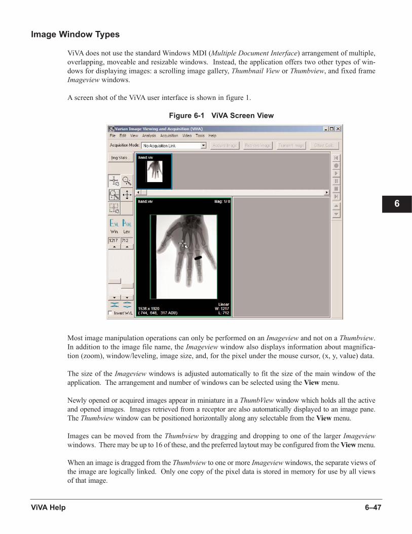
6–47ViVA Help
6
Image Window Types
ViVA does not use the standard Windows MDI (Multiple Document Interface) arrangement of multiple,
overlapping, moveable and resizable windows. Instead, the application offers two other types of win-
dows for displaying images: a scrolling image gallery, Thumbnail View or Thumbview, and fixed frame
Imageview windows.
A screen shot of the ViVA user interface is shown in figure 1.
Figure 6-1 ViVA Screen View
Most image manipulation operations can only be performed on an Imageview and not on a Thumbview.
In addition to the image file name, the Imageview window also displays information about magnifica-
tion (zoom), window/leveling, image size, and, for the pixel under the mouse cursor, (x, y, value) data.
The size of the Imageview windows is adjusted automatically to fit the size of the main window of the
application. The arrangement and number of windows can be selected using the View menu.
Newly opened or acquired images appear in miniature in a ThumbView window which holds all the active
and opened images. Images retrieved from a receptor are also automatically displayed to an image pane.
The Thumbview window can be positioned horizontally along any selectable from the View menu.
Images can be moved from the Thumbview by dragging and dropping to one of the larger Imageviewwindows. There may be up to 16 of these, and the preferred laytout may be configured from the View menu.
When an image is dragged from the Thumbview to one or more Imageview windows, the separate views of
the image are logically linked. Only one copy of the pixel data is stored in memory for use by all views
of that image.
PaxScan 3030CB / 4030CB Systems & Service Guide6–48
A Thumbview or Imageview can be selected by clicking on the view with the mouse pointer. The cur-
rently selected Imageview is normally indicated with a bright green selection rectangle. Other linked views
of the same image shown in the selected view are indicated with a bright blue selection rectangle. Many
menu items including File|Close or File|Save As... are applicable to the selected image.
Image Layout
Under the View menu, there are a number of options controlling the layout:
n Thumbview Position allows the user to place the Thumbview along any edge, while Show
Thumbview allows it to be shown or hidden.
n Single-Image Layout, Two-Across Layout and Four-Image Layout allow the user to choose from among common formats. Number Images Across and Number Images Down allow greater
flexibility in selecting other multi-image layouts.
n Show Border allows the user to hide or show certain borders that are normally shown.
¨ Image refers to the green border around the image itself.
¨ Select refers to the colored border around the image pane (applies to Imageview only).
¨ Pane refers to the Windows style setting that by default creates a bevelled look at the pane
edge.
Full Overlay
Certain information appears in the corners of each thumb or image pane. This is referred to as the over-
lay, and the more detailed information in the lower corners may be shown or hidden using the View|Full
Overlay command. This can be useful when displaying a large number of images.
Status Bar
The View|Status Bar command allows the user to display or hide the status bar on the bottom of the
main window. The status bar displays a short description of some pull-down menu commands when
highlighted by the cursor. Alternatively, the status bar displays the currently selected mode
(Fluoroscopy, Radiography...) when the cursor is placed in other sections of the application.
Message Options
Message boxes are displayed during ViVA operation. These are normally classified as one of three types:
Information or Info – the message box contains information that may be useful in the current context.
The title of the message box is ‘ViVA Message Box’.
Data Loss Warning or DataLoss – a warning that an operation risks loss of data. For example if an
attempt is made to close an image which has not been saved. The title of the message box is ‘ViVAMessage Box - Data Loss Warning’.
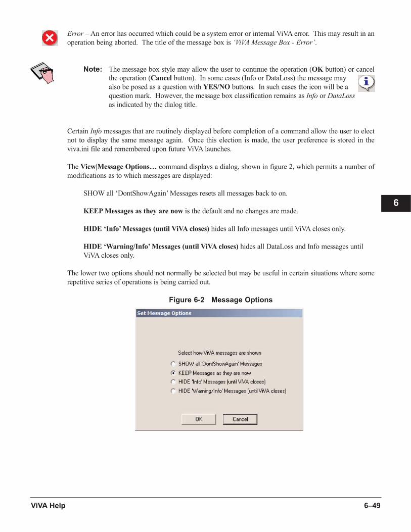
6–49ViVA Help
6
Error – An error has occurred which could be a system error or internal ViVA error. This may result in an
operation being aborted. The title of the message box is ‘ViVA Message Box - Error’.
Note: The message box style may allow the user to continue the operation (OK button) or cancel
the operation (Cancel button). In some cases (Info or DataLoss) the message may
also be posed as a question with YES/NO buttons. In such cases the icon will be a
question mark. However, the message box classification remains as Info or DataLossas indicated by the dialog title.
Certain Info messages that are routinely displayed before completion of a command allow the user to elect
not to display the same message again. Once this election is made, the user preference is stored in the
viva.ini file and remembered upon future ViVA launches.
The View|Message Options… command displays a dialog, shown in figure 2, which permits a number of
modifications as to which messages are displayed:
SHOW all ‘DontShowAgain’ Messages resets all messages back to on.
KEEP Messages as they are now is the default and no changes are made.
HIDE ‘Info’ Messages (until ViVA closes) hides all Info messages until ViVA closes only.
HIDE ‘Warning/Info’ Messages (until ViVA closes) hides all DataLoss and Info messages until
ViVA closes only.
The lower two options should not normally be selected but may be useful in certain situations where some
repetitive series of operations is being carried out.
Figure 6-2 Message Options
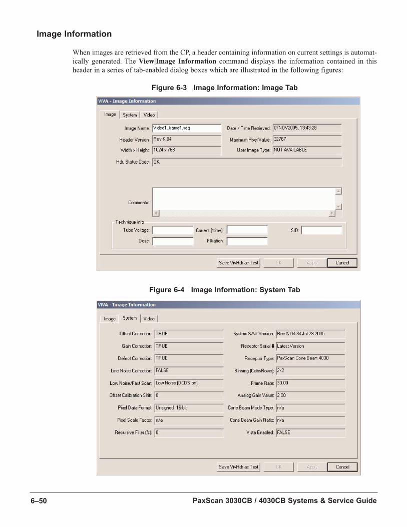
PaxScan 3030CB / 4030CB Systems & Service Guide6–50
Image Information
When images are retrieved from the CP, a header containing information on current settings is automat-
ically generated. The View|Image Information command displays the information contained in this
header in a series of tab-enabled dialog boxes which are illustrated in the following figures:
Figure 6-3 Image Information: Image Tab
Figure 6-4 Image Information: System Tab
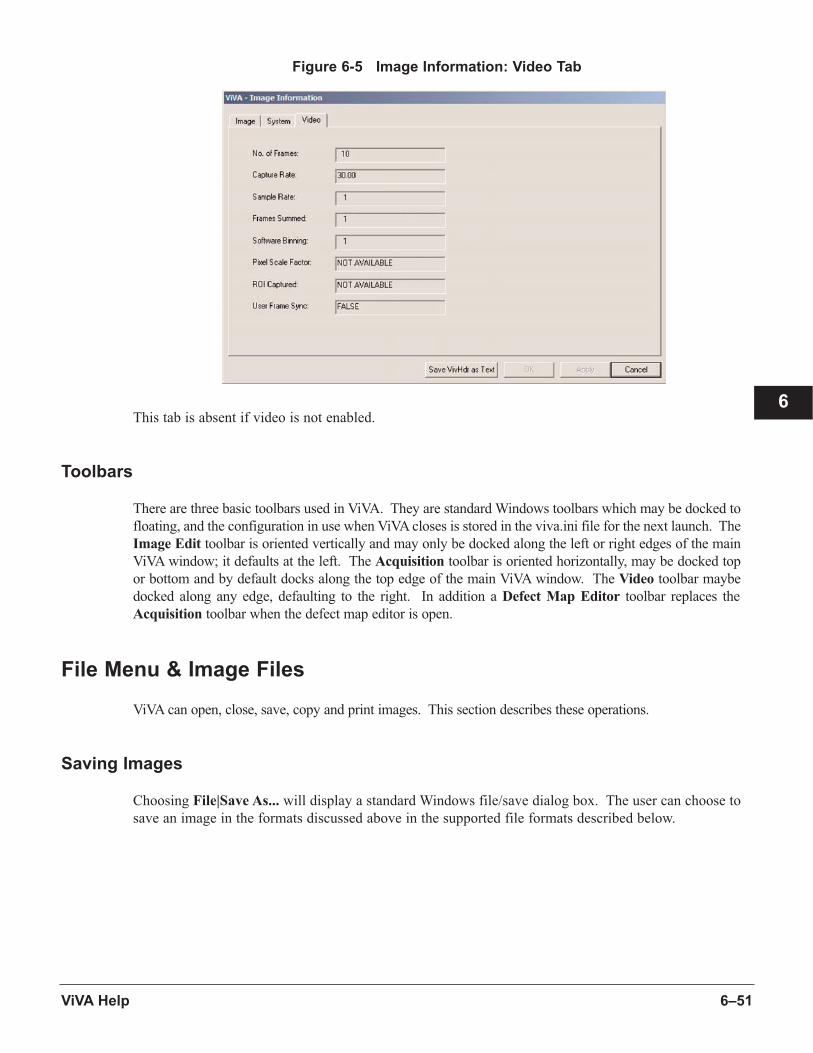
6–51ViVA Help
6
Figure 6-5 Image Information: Video Tab
This tab is absent if video is not enabled.
Toolbars
There are three basic toolbars used in ViVA. They are standard Windows toolbars which may be docked to
floating, and the configuration in use when ViVA closes is stored in the viva.ini file for the next launch. The
Image Edit toolbar is oriented vertically and may only be docked along the left or right edges of the main
ViVA window; it defaults at the left. The Acquisition toolbar is oriented horizontally, may be docked top
or bottom and by default docks along the top edge of the main ViVA window. The Video toolbar maybe
docked along any edge, defaulting to the right. In addition a Defect Map Editor toolbar replaces the
Acquisition toolbar when the defect map editor is open.
File Menu & Image Files
ViVA can open, close, save, copy and print images. This section describes these operations.
Saving Images
Choosing File|Save As... will display a standard Windows file/save dialog box. The user can choose to
save an image in the formats discussed above in the supported file formats described below.
PaxScan 3030CB / 4030CB Systems & Service Guide6–52
Saving Individual Images
The following file formats are supported for saving individual images:
n ViVA (.viv): uncompressed 16-bit unsigned data together with a custom 2,048 byte header containing both optional user-entered information as well as automatically retrieved settings in effect at the time
an image was obtained. This is the default.
n Raw (.raw): uncompressed 16-bit unsigned data are saved without any header or other information than the pixel values. ViVA only supports certain predefined image sizes for this format.
n Bitmap (.bmp): uncompressed 8-bit window-leveled Windows bitmap. the image is saved using the currently applied window/level and gray-mapping.
n JPEG (.jpg): compressed 8-bit window-leveled JPEG. The user is asked to supply a quality factor in the range 1-10 where 10 gives the highest quality and largest file size. The image is saved using the
currently applied window/level and gray-mapping.
n Internal Varian Format (.asi): uncompressed 16-bit unsigned data together with a custom 512 byte header. Similar to the .viv header but provided primarily to allow images to be exported to other Varian
products.
n Tiff 16-bit (.tif): uncompressed 16-bit unsigned data which may be opened by tiff readers that support 16-bit data. Note that ViVA, by default, scales the pixel values to utilize more fully the 16-bit range.
This generally results in a more satisfactory experience when opened by readers that do not perform
any automated window/leveling. This scaling may be turned off in the Preferences dialog. Note that
ViVA does not support opening tiff images in general, but will open 16-bit tiff images it has saved,
restoring the correct pixel scaling. Tiff images may be accessed from the open file dialog using the
‘Any Files’ filter or when applicable the most recently used files under the File menu.
Note: For the special 2MSBs are exponent pixel data format (see Pixel Data Format &
3030CB / 4030CB Receptors), a warning will be given that the image will first be
converted to a scaled image.
n Tiff 8-bit (.tif): uncompressed 8-bit unsigned data which may be opened by typical tiff readers. The image is saved using the currently applied window/level and gray-mapping.
Saving Video Sequences
The following file formats are supported for saving video sequences:
n Video Sequence (.seq): uncompressed 16-bit unsigned data together with the same 2048 byte headeras the .viv format.
n AVI Sequence (.avi): compressed 8-bit window-leveled AVI. As for .jpg a quality factor in range 1-10 should be entered.
Opening Images
Images can be opened for display and manipulation using the menu option File|Open.... The opened
image will appear in the Thumb View; and may be dragged to an Image View as required.

6–53ViVA Help
6
The opened image is first displayed with an automatic window-leveling setting which is intended to
show image features across a broad range of contrast.
If an image is successfully opened, the path and file name of the image is saved as the latest entry onto
the most recently used file list which can be used as a shortcut to open the file.
ViVA supports opening a number of file formats, some of which have specific purposes, and may not be
useful to most users. Except as note only formats having 16-bit unsigned data are supported generally.
File|Open... supports:
n ViVA (.viv): 16-bit unsigned data with 2048 byte header.
n Raw (.raw): since there is no header information, only particular predefined image sizes can be opened in .raw format.
n Img (.img): similar to .viv with 1024 byte header but only image dimensional data are read.
n Video Sequence (.seq): 16-bit unsigned data with 2048 byte header. Differs from .viv only by havingmore than one frame.
n CT 16-bit signed (.slice): This data format is signed with no header. Only the predefined image sizes used for the .raw format are supported.
n CT 16-bit unsigned (.prj): 16-bit unsigned data with 72 byte header. Image information from the header is displayed as the image opens.
n HNB compressed 16-bit unsigned (.hnb): 16-bit unsigned data in a compressed format. There is a 512 byte header, but only image dimensional data are read.
n HNC compressed 16-bit unsigned (.hnc): Similar to .hnb.
n HND compressed 32-bit unsigned (.hnd): hnd images are imported but it is assumed that only 17 bits are used. As described in 3030CB / 4030CB extensions, ViVA supports a custom format
designed to allow integer values up 17-bits to be handled.
n Any Files: (*.*): With limited scope, this allows generic file types to be opened for viewing; File|Open...permits opening any file which has uncompressed 16-bit unsigned data residing in a
contiguous block (assumes Little Endian/Intel byte arrangement). Additional information may be
present provided its disposition within the file is known. The user is asked for 3 fields of information:
header size, image width and image height. These are automatically initialized with best guess values
based upon the predefined .raw image size which minimizes the header size. When the user
changes one of the image dimension fields the other field is automatically adjusted the first time
but not subsequent times. This is to permit the possibility of trailing information after the pixel
block in the file. i.e. the header and image dimension fields are not forced to define the file size.
Header and trailer information is ignored and cannot be accessed by the Image Information
command. The dialog box illustrated in the following figure will be displayed when opening a file
with Any Files as the specified filter.
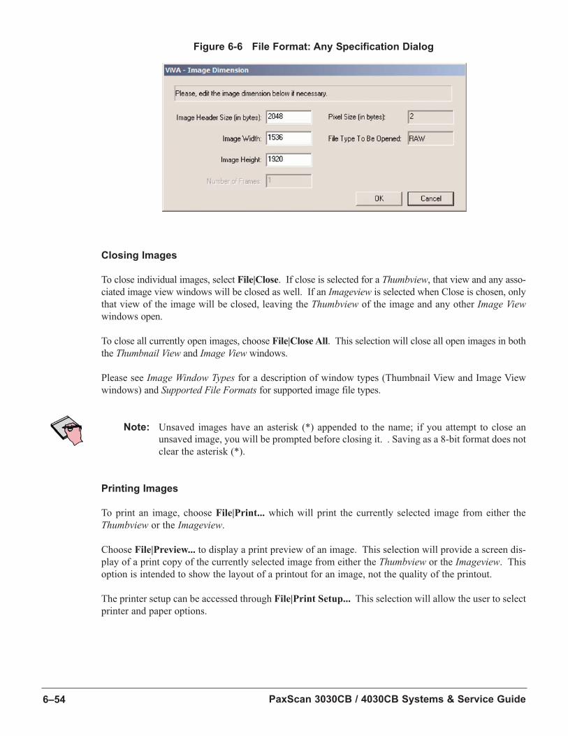
PaxScan 3030CB / 4030CB Systems & Service Guide6–54
Figure 6-6 File Format: Any Specification Dialog
Closing Images
To close individual images, select File|Close. If close is selected for a Thumbview, that view and any asso-
ciated image view windows will be closed as well. If an Imageview is selected when Close is chosen, only
that view of the image will be closed, leaving the Thumbview of the image and any other Image Viewwindows open.
To close all currently open images, choose File|Close All. This selection will close all open images in both
the Thumbnail View and Image View windows.
Please see Image Window Types for a description of window types (Thumbnail View and Image View
windows) and Supported File Formats for supported image file types.
Note: Unsaved images have an asterisk (*) appended to the name; if you attempt to close an
unsaved image, you will be prompted before closing it. . Saving as a 8-bit format does not
clear the asterisk (*).
Printing Images
To print an image, choose File|Print... which will print the currently selected image from either the
Thumbview or the Imageview.
Choose File|Preview... to display a print preview of an image. This selection will provide a screen dis-
play of a print copy of the currently selected image from either the Thumbview or the Imageview. This
option is intended to show the layout of a printout for an image, not the quality of the printout.
The printer setup can be accessed through File|Print Setup... This selection will allow the user to select
printer and paper options.
6–55ViVA Help
6
Copying Images
Select Edit|Copy to copy the image currently selected onto the clipboard memory.
Note: This function always copies the whole image using the current window-level settings, not
just the section of the image being displayed in the Imageview.
Pixel Data Format & 3030CB / 4030CB Receptors
A ‘Cone Beam Mode Type’ is displayed for 3030CB / 4030CB receptors (System tab, figure 4). This may
be one of: ‘n/a’ (i.e. a normal mode with pixel data format 16-bit unsigned), DUAL_READ or DYNAM-
IC_GAIN. This information field is stored in the viv header, and refers to the original mode type used to
acquire the image.
The current pixel data format is listed in the System tab (see figure 4). Prior to the 3030CB / 4030CB
receptor this has always been ‘Unsigned 16-bit’. Pixel information is still stored as 16-bit values, but
may not be interpreted necessarily as simple unsigned integers. The 3030CB / 4030CB still provides 14-
bit data, but it is capable of operating in dual gain modes. In dynamic gain modes the 15th bit specifies lo(0)
or hi(1) gain. In addition since the ratio of the gains normally exceeds 4, the range of values in an image
cannot be represented as 16-bit integers. A new corrected pixel data format is used for 3030CB / 4030CB
corrected images.
The pixel data format field which is stored in the .viv image header determines the pixel data format which
may be one of the following:
n 16-bit unsigned integer – normal format for all receptors except 3030CB / 4030CB (specifically dual read or dynamic gain mode images).
n 2 MSBs are exponent – the only corrected format currently supported for 3030CB / 4030CB. Here the 2 most significant bits are interpreted as forming an exponent (value n=0,1,2,3) for the other 14
bits. The pixel value is calculated as:
pix = mant * 2^n
where pix is the pixel value (0-131,064), mant is the 14-bit value formed by the 14 LSBs and n is the
exponent formed by the 2 MSBs.
n CB raw DUAL_READ – a raw uncorrected image obtained using a dual read mode where each pixel value is represented twice – for lo and hi gains.
n CB raw DYNAMIC_GAIN – a raw uncorrected image obtained using a dynamic gain mode where each
pixel value is represented only once and the gain is determined from the 15th bit as mentioned above.
n Unsgnd 16-bit, Split – Hi – a raw uncorrected image obtained using a dual gain mode, but only the hi gain pixel values are present.
n Unsgnd 16-bit, Split – Lo – a raw uncorrected image obtained using a dual gain mode, but only the lo gain pixel values are present.
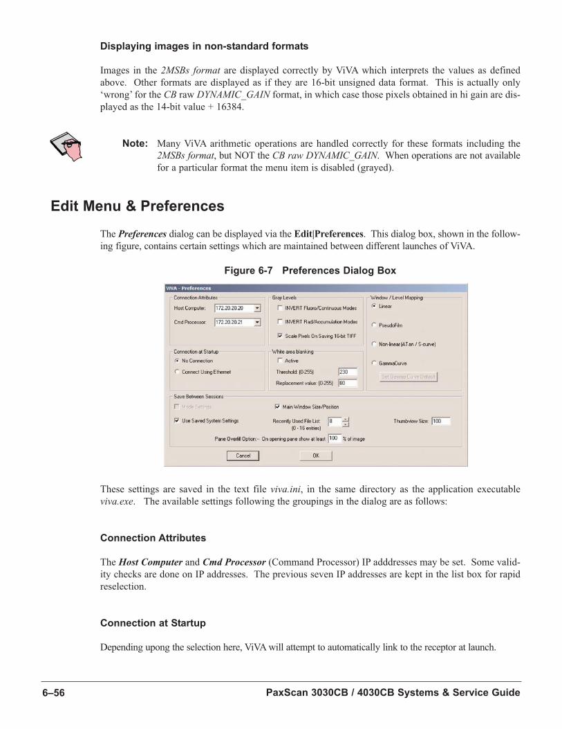
PaxScan 3030CB / 4030CB Systems & Service Guide6–56
Displaying images in non-standard formats
Images in the 2MSBs format are displayed correctly by ViVA which interprets the values as defined
above. Other formats are displayed as if they are 16-bit unsigned data format. This is actually only
‘wrong’ for the CB raw DYNAMIC_GAIN format, in which case those pixels obtained in hi gain are dis-
played as the 14-bit value + 16384.
Note: Many ViVA arithmetic operations are handled correctly for these formats including the
2MSBs format, but NOT the CB raw DYNAMIC_GAIN. When operations are not available
for a particular format the menu item is disabled (grayed).
Edit Menu & Preferences
The Preferences dialog can be displayed via the Edit|Preferences. This dialog box, shown in the follow-
ing figure, contains certain settings which are maintained between different launches of ViVA.
Figure 6-7 Preferences Dialog Box
These settings are saved in the text file viva.ini, in the same directory as the application executable
viva.exe. The available settings following the groupings in the dialog are as follows:
Connection Attributes
The Host Computer and Cmd Processor (Command Processor) IP adddresses may be set. Some valid-
ity checks are done on IP addresses. The previous seven IP addresses are kept in the list box for rapid
reselection.
Connection at Startup
Depending upong the selection here, ViVA will attempt to automatically link to the receptor at launch.

6–57ViVA Help
6
Gray Levels
User preferences for the display of pixel values in fluoroscopy and radiography modes. By default large
pixel values are white in the image and small values black.
As referred to above under Saving Images, pixel values are scaled by default when saving as tiff images.
This selection allows the user to turn this feature off if required.
White Area Blanking
Activate and select white area blanking threshold and replacement values. More information is given
on White Area Blanking in the description of the Edit W/L dialog in the Edit Toolbar section below.
Note: Certain selections such as White Area Blanking and Window/Level Mapping, appear to be
duplicated in the Edit W/L dialog. The distinction is in applicability. Choices made in the
Preferences dialog apply to all images opened subsequently. Choices made in the
Edit W/L dialog applies to the currently selected image only.
Window/Level Mapping
Here you may choose how the pixel values are mapped to gray levels in the display. Options are Linear,PseudoFilm, Non-Linear (A-tan / S-curve) or GammaCurve.
When GammaCurve is selected the Set Gamma Curve Default button is active and allows you to customize
the gamma curve as approximated by a multi-linear mapping function.
These settings are saved and used whenever an image is opened from a file or retrieved from the CP. They
are not applied to any images already open.
Note: More information is given on Window/Level Mapping in the description of the Edit W/L
dialog in the Edit Toolbar section below.
Save Between Sessions
Certain settings may be saved between sessions (ViVA launches) including Main Window Size/Position.
If Use Saved System Settings is checked, then options such as Offset Corrections and Gain Correctionswill be set from from the settings saved in the viva.ini file. If unchecked, existing system settings in the
Command Processor will be used.
The Recently Used File List determines the maximum number of file paths saved for rapid access from
the File menu, and may be set up to a limit of 16.
The Thumbview Size in screen pixels may be adjusted.
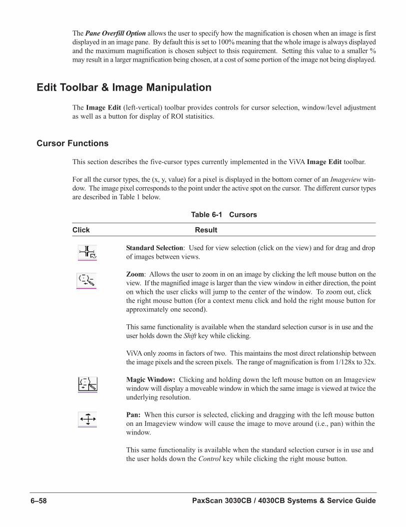
PaxScan 3030CB / 4030CB Systems & Service Guide6–58
The Pane Overfill Option allows the user to specify how the magnification is chosen when an image is first
displayed in an image pane. By default this is set to 100% meaning that the whole image is always displayed
and the maximum magnification is chosen subject to thsis requirement. Setting this value to a smaller %
may result in a larger magnification being chosen, at a cost of some portion of the image not being displayed.
Edit Toolbar & Image Manipulation
The Image Edit (left-vertical) toolbar provides controls for cursor selection, window/level adjustment
as well as a button for display of ROI statisitics.
Cursor Functions
This section describes the five-cursor types currently implemented in the ViVA Image Edit toolbar.
For all the cursor types, the (x, y, value) for a pixel is displayed in the bottom corner of an Imageview win-
dow. The image pixel corresponds to the point under the active spot on the cursor. The different cursor types
are described in Table 1 below.
Table 6-1 Cursors
Click Result
Standard Selection: Used for view selection (click on the view) and for drag and drop
of images between views.
Zoom: Allows the user to zoom in on an image by clicking the left mouse button on the
view. If the magnified image is larger than the view window in either direction, the point
on which the user clicks will jump to the center of the window. To zoom out, click
the right mouse button (for a context menu click and hold the right mouse button for
approximately one second).
This same functionality is available when the standard selection cursor is in use and the
user holds down the Shift key while clicking.
ViVA only zooms in factors of two. This maintains the most direct relationship between
the image pixels and the screen pixels. The range of magnification is from 1/128x to 32x.
Magic Window: Clicking and holding down the left mouse button on an Imageview
window will display a moveable window in which the same image is viewed at twice the
underlying resolution.
Pan: When this cursor is selected, clicking and dragging with the left mouse button
on an Imageview window will cause the image to move around (i.e., pan) within the
window.
This same functionality is available when the standard selection cursor is in use and
the user holds down the Control key while clicking the right mouse button.
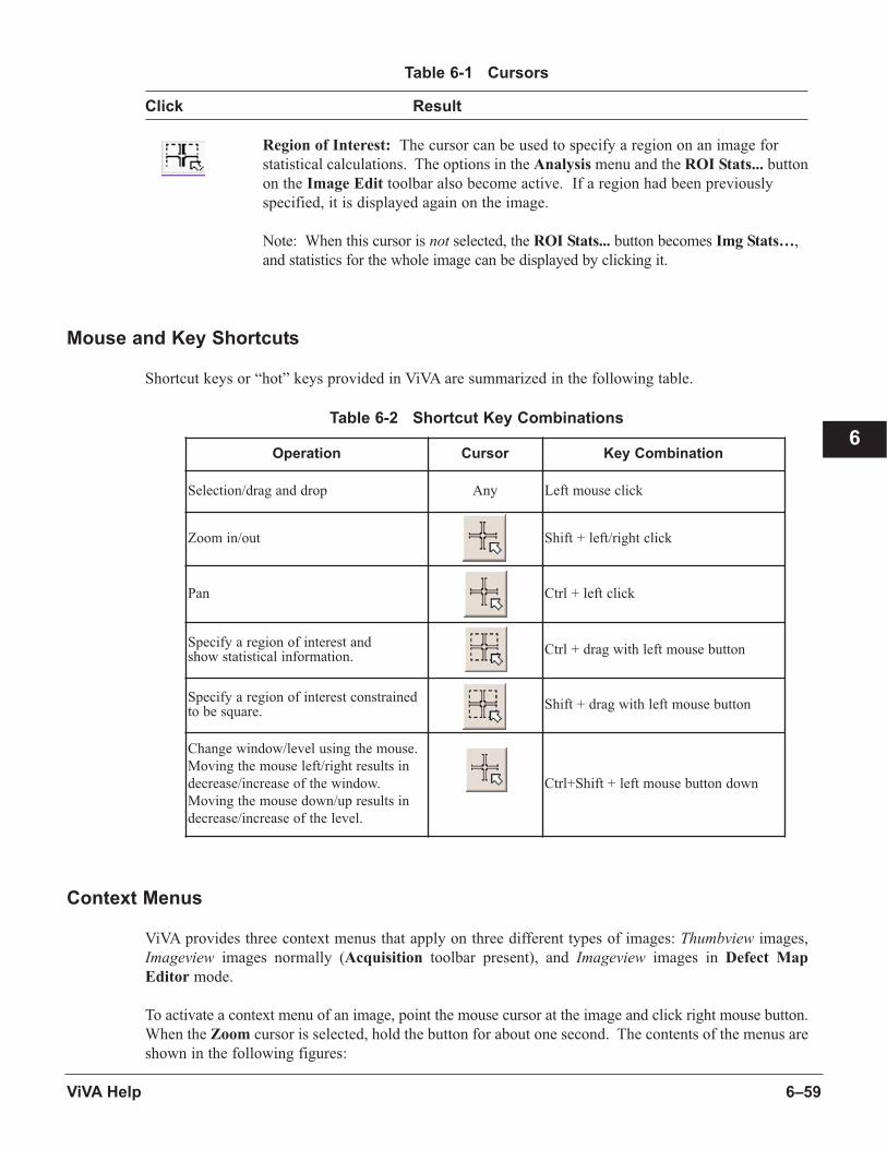
6–59ViVA Help
6
Table 6-1 Cursors
Click Result
Region of Interest: The cursor can be used to specify a region on an image for
statistical calculations. The options in the Analysis menu and the ROI Stats... button
on the Image Edit toolbar also become active. If a region had been previously
specified, it is displayed again on the image.
Note: When this cursor is not selected, the ROI Stats... button becomes Img Stats…,
and statistics for the whole image can be displayed by clicking it.
Mouse and Key Shortcuts
Shortcut keys or “hot” keys provided in ViVA are summarized in the following table.
Table 6-2 Shortcut Key Combinations
Context Menus
ViVA provides three context menus that apply on three different types of images: Thumbview images,
Imageview images normally (Acquisition toolbar present), and Imageview images in Defect Map
Editor mode.
To activate a context menu of an image, point the mouse cursor at the image and click right mouse button.
When the Zoom cursor is selected, hold the button for about one second. The contents of the menus are
shown in the following figures:
Operation Cursor Key Combination
Selection/drag and drop Any Left mouse click
Zoom in/out Shift + left/right click
Pan Ctrl + left click
Specify a region of interest and show statistical information.
Ctrl + drag with left mouse button
Specify a region of interest constrainedto be square.
Shift + drag with left mouse button
Change window/level using the mouse.
Moving the mouse left/right results in
decrease/increase of the window.
Moving the mouse down/up results in
decrease/increase of the level.
Ctrl+Shift + left mouse button down
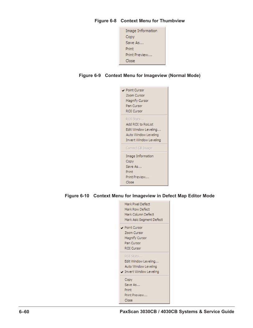
PaxScan 3030CB / 4030CB Systems & Service Guide6–60
Figure 6-8 Context Menu for Thumbview
Figure 6-9 Context Menu for Imageview (Normal Mode)
Figure 6-10 Context Menu for Imageview in Defect Map Editor Mode
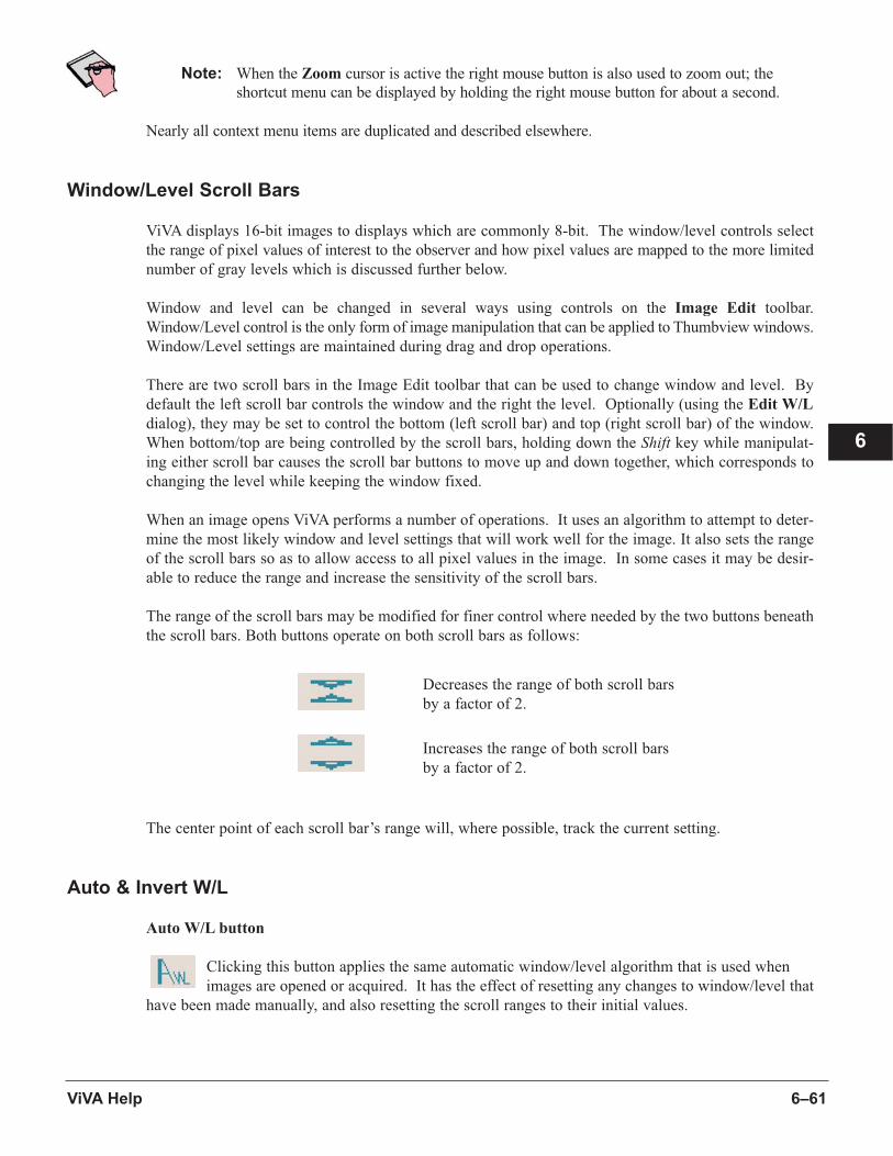
6–61ViVA Help
6
Note: When the Zoom cursor is active the right mouse button is also used to zoom out; the
shortcut menu can be displayed by holding the right mouse button for about a second.
Nearly all context menu items are duplicated and described elsewhere.
Window/Level Scroll Bars
ViVA displays 16-bit images to displays which are commonly 8-bit. The window/level controls select
the range of pixel values of interest to the observer and how pixel values are mapped to the more limited
number of gray levels which is discussed further below.
Window and level can be changed in several ways using controls on the Image Edit toolbar.
Window/Level control is the only form of image manipulation that can be applied to Thumbview windows.
Window/Level settings are maintained during drag and drop operations.
There are two scroll bars in the Image Edit toolbar that can be used to change window and level. By
default the left scroll bar controls the window and the right the level. Optionally (using the Edit W/L
dialog), they may be set to control the bottom (left scroll bar) and top (right scroll bar) of the window.
When bottom/top are being controlled by the scroll bars, holding down the Shift key while manipulat-
ing either scroll bar causes the scroll bar buttons to move up and down together, which corresponds to
changing the level while keeping the window fixed.
When an image opens ViVA performs a number of operations. It uses an algorithm to attempt to deter-
mine the most likely window and level settings that will work well for the image. It also sets the range
of the scroll bars so as to allow access to all pixel values in the image. In some cases it may be desir-
able to reduce the range and increase the sensitivity of the scroll bars.
The range of the scroll bars may be modified for finer control where needed by the two buttons beneath
the scroll bars. Both buttons operate on both scroll bars as follows:
The center point of each scroll bar’s range will, where possible, track the current setting.
Auto & Invert W/L
Auto W/L button
Clicking this button applies the same automatic window/level algorithm that is used when
images are opened or acquired. It has the effect of resetting any changes to window/level that
have been made manually, and also resetting the scroll ranges to their initial values.
Decreases the range of both scroll bars
by a factor of 2.
Increases the range of both scroll bars
by a factor of 2.

PaxScan 3030CB / 4030CB Systems & Service Guide6–62
Edit W/L Dialog
Clicking EWL (Edit W/L) button opens a dialog box which allows the user to adjust a number
of settings relating to the selected image. There are some exceptions as noted below where set-
tings are remembered for future images also. The dialog is shown in the folloing figure.
Figure 6-11 Edit Window/Level Dialog
Edit Values
As noted above most of the settings in this dialog apply only to the selected image. The exception to this is
how the scroll bars are used. They may be used either as Bottom/Top or Window/Level. The relationship
between bottom(bot)/top and window(win)/level(lev) is:
win = top - bot
lev = (top + bot) .2
If required, actual values for the bottom/top or window/level may be typed into the appropriate edit box
and applied to the selected image only.
The check box ‘Turn off Auto W/L..” turns off the automated window/level feature in ViVA and simply
opens all future images with the current values of window and level.
Window/Level Mapping
All possible pixel values are mapped to a gray level—typically 0-255—and are stored in a lookup table
(LUT). When an image is displayed the appropriate gray level is selected from the LUT for each pixel.
By default the relationship between pixel values and gray levels is linear; however, other options also exist
and all are described next:

6–63ViVA Help
6
n Linear: A linear relationship exists between the gray level (gry) and the pixel value (pix); i.e.
⎛pix - bot ⎞gry = mxgry* ⎜ ⎟⎝top - bot ⎠
If this equation yields a value of gry greater than the maximum number of gray levels (mxgry = 255
typically) then the value of gry is held at mxgry; negative values are clipped at zero.
n PseudoFilm: This is intended to simulate a film response and can be tailored by the user if desired. The relationship is:
gry = mxgry * (1 - exp((-X)/Y))
There are two user defined values which control the behavior of this equation.
Presently these are only settable by manually editing the viva.ini file. They are:
“PseudoFilmConstant”(pfc) and “PseudoFilmScalePcnt”(pfs*100) found in the [GammaSettings]
section. In the above equation, the exponential numerator is given by:
X = pix - pfs * bot
and the denominator by:
Y = pfc + pfs * (top - bot)
Any negative values (for pixel values below bot) are replaced by zero. The main control is exerted
by the denominator Y. The default is to set pfs=0.67 (67 in the viva.ini file) and pfc=0. In this case
window/level settings behave normally. Setting pfs=0 and putting in a value for pfc, e.g.500, will
result in a fixed response curve independent of the window/level settings. Intermediate behavior may
be obtained by setting both parameters to non-zero values. If both parameters are set to zero then the
default values are applied.
n Non-Linear (ATan/S-curve): This is based upon the trigonometric arctangent function. For each pixel value we calculate a value gval given by:
⎛ ⎛ (pic - lev) ⎞ ⎞ gval = 0.5 + (1/π ⎜ a tan ⎜ 2 ∗ ———— ⎟ ⎟
⎝ ⎝ win ⎠ ⎠
The values of gval obtained from this equation always lie within the range 0-1, but the actual range is
generally smaller depending on the values of win and lev. A linear transformation is applied to gval
such that the maximum range of possible pixel values produces the maximum range of possible gray
levels.
The above three responses are illustrated in the following figure for particular values of window and
level settings.
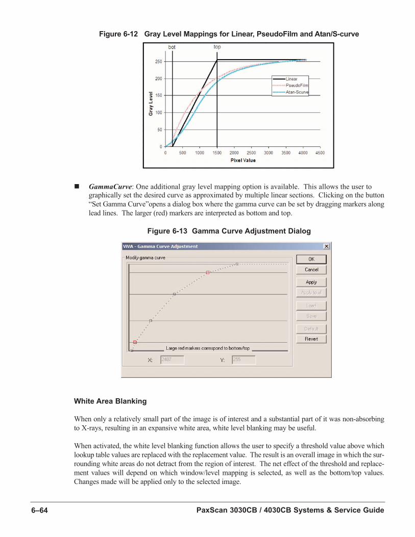
PaxScan 3030CB / 4030CB Systems & Service Guide6–64
Figure 6-12 Gray Level Mappings for Linear, PseudoFilm and Atan/S-curve
n GammaCurve: One additional gray level mapping option is available. This allows the user to graphically set the desired curve as approximated by multiple linear sections. Clicking on the button
“Set Gamma Curve”opens a dialog box where the gamma curve can be set by dragging markers along
lead lines. The larger (red) markers are interpreted as bottom and top.
Figure 6-13 Gamma Curve Adjustment Dialog
White Area Blanking
When only a relatively small part of the image is of interest and a substantial part of it was non-absorbing
to X-rays, resulting in an expansive white area, white level blanking may be useful.
When activated, the white level blanking function allows the user to specify a threshold value above which
lookup table values are replaced with the replacement value. The result is an overall image in which the sur-
rounding white areas do not detract from the region of interest. The net effect of the threshold and replace-
ment values will depend on which window/level mapping is selected, as well as the bottom/top values.
Changes made will be applied only to the selected image.
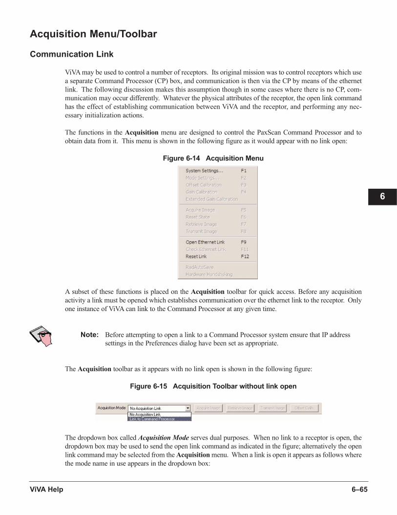
6–65ViVA Help
6
Acquisition Menu/Toolbar
Communication Link
ViVA may be used to control a number of receptors. Its original mission was to control receptors which use
a separate Command Processor (CP) box, and communication is then via the CP by means of the ethernet
link. The following discussion makes this assumption though in some cases where there is no CP, com-
munication may occur differently. Whatever the physical attributes of the receptor, the open link command
has the effect of establishing communication between ViVA and the receptor, and performing any nec-
essary initialization actions.
The functions in the Acquisition menu are designed to control the PaxScan Command Processor and to
obtain data from it. This menu is shown in the following figure as it would appear with no link open:
Figure 6-14 Acquisition Menu
A subset of these functions is placed on the Acquisition toolbar for quick access. Before any acquisition
activity a link must be opened which establishes communication over the ethernet link to the receptor. Only
one instance of ViVA can link to the Command Processor at any given time.
Note: Before attempting to open a link to a Command Processor system ensure that IP address
settings in the Preferences dialog have been set as appropriate.
The Acquisition toolbar as it appears with no link open is shown in the following figure:
Figure 6-15 Acquisition Toolbar without link open
The dropdown box called Acquisition Mode serves dual purposes. When no link to a receptor is open, the
dropdown box may be used to send the open link command as indicated in the figure; alternatively the open
link command may be selected from the Acquisition menu. When a link is open it appears as follows where
the mode name in use appears in the dropdown box:
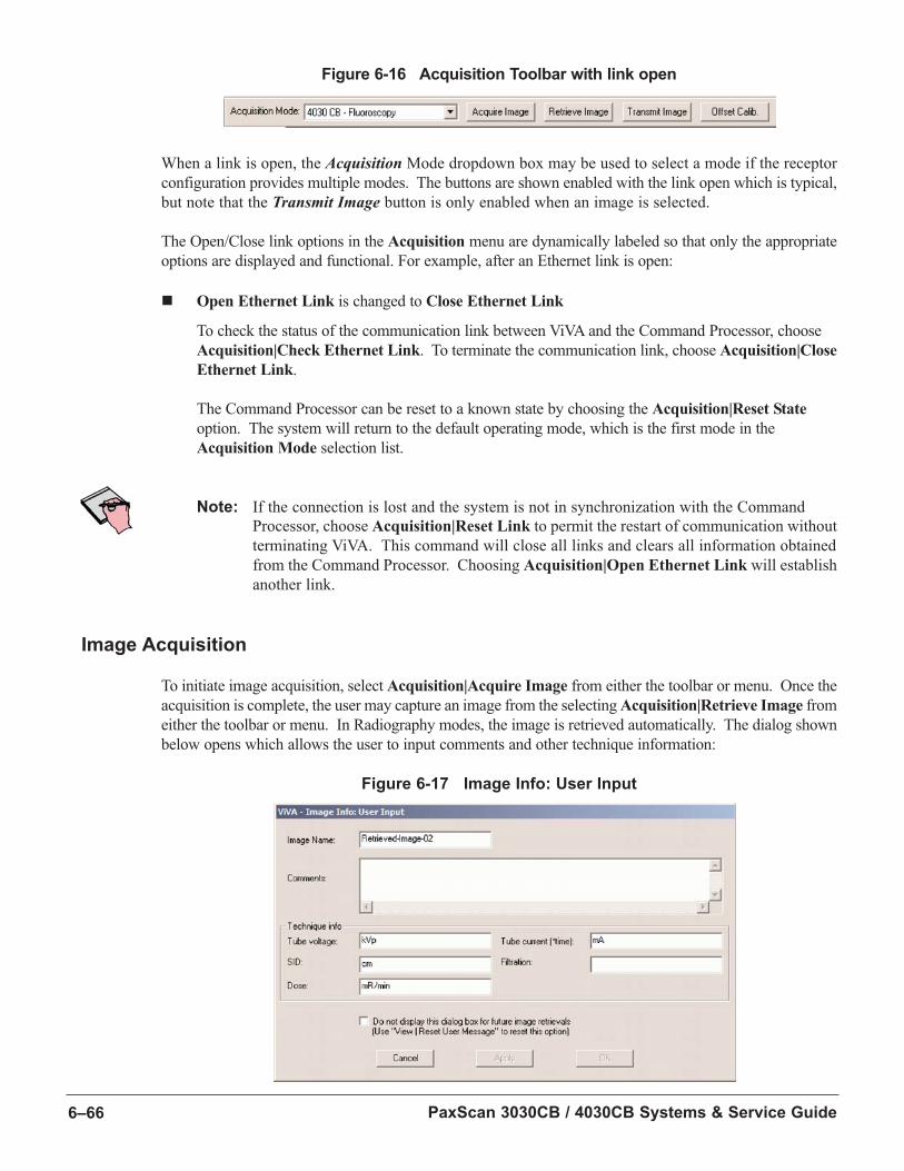
PaxScan 3030CB / 4030CB Systems & Service Guide6–66
Figure 6-16 Acquisition Toolbar with link open
When a link is open, the Acquisition Mode dropdown box may be used to select a mode if the receptor
configuration provides multiple modes. The buttons are shown enabled with the link open which is typical,
but note that the Transmit Image button is only enabled when an image is selected.
The Open/Close link options in the Acquisition menu are dynamically labeled so that only the appropriate
options are displayed and functional. For example, after an Ethernet link is open:
n Open Ethernet Link is changed to Close Ethernet Link
To check the status of the communication link between ViVA and the Command Processor, choose
Acquisition|Check Ethernet Link. To terminate the communication link, choose Acquisition|Close
Ethernet Link.
The Command Processor can be reset to a known state by choosing the Acquisition|Reset State
option. The system will return to the default operating mode, which is the first mode in the
Acquisition Mode selection list.
Note: If the connection is lost and the system is not in synchronization with the Command
Processor, choose Acquisition|Reset Link to permit the restart of communication without
terminating ViVA. This command will close all links and clears all information obtained
from the Command Processor. Choosing Acquisition|Open Ethernet Link will establish
another link.
Image Acquisition
To initiate image acquisition, select Acquisition|Acquire Image from either the toolbar or menu. Once the
acquisition is complete, the user may capture an image from the selecting Acquisition|Retrieve Image from
either the toolbar or menu. In Radiography modes, the image is retrieved automatically. The dialog shown
below opens which allows the user to input comments and other technique information:
Figure 6-17 Image Info: User Input

6–67ViVA Help
6
This information may also be entered or edited later using the View|Image Information command.
Note: This dialog may be turned off for future image retrievals if required by checking the ‘Do
not display..’ check box and then clicking ‘OK’.
Previously retrieved images may be sent to the output buffer of the Command Processor, where it takes the
place of the last image acquired. First, select the required image by clicking on it in the ViVA interface, then
select Acquisition|Transmit Image.
Offset & Gain Calibration
Correcting for non-uniform pixel response is essential to obtaining good quality images. Offset calibration
must be performed whenever the CP is powered up and generally it is desirable to perform offset calibra-
tions regularly during use for optimium results. Gain calibrations need not be performed nearly so often,
and the last gain calibration for each mode is stored by the CP when powered down.
To initiate Offset or Gain calibration, choose Acquisition|Offset Calibration or Acquisition|Gain
Calibration from the menu; offset calibrations may also be initiated from the toolbar.
Offset calibrations are completely automated, and require no further user intervention to complete. Gain
calibrations require X-ray exposure with no object in the beam. Simply follow the on-screen prompts,
and expose when prompted to do so. Rad modes allow the user to expose multiple times to allow sta-
tistical averaging of the gain image.
Offset & Gain Calibration with 3030CB / 4030CB Receptors
3030CB / 4030CB receptors provide dual gain modes. Calibration is accordingly more complicated. Offset
calibrations remain autonomous, but for dynamic gain modes multiple calibrations occur; a second ‘forced lo-
gain’ calibration is performed in addition to the normal one (which always occurs at high gain for all pixels in
the absence of X-rays). For dual read modes, a single calibration provides offsets in both gain settings.
Gain calibration requires the same offset operations as above for dark field acquisition followed by flat-field
acquisition with x-ray settings appropriate for each gain.
Note: Gain calibration should always be done at count levels low enough to avoid any possible
saturation, but high enough to achieve good statistical measurement of pixel response. For
14-bit receptors an offset-corrected value in the range 1600-4000 is suggested.
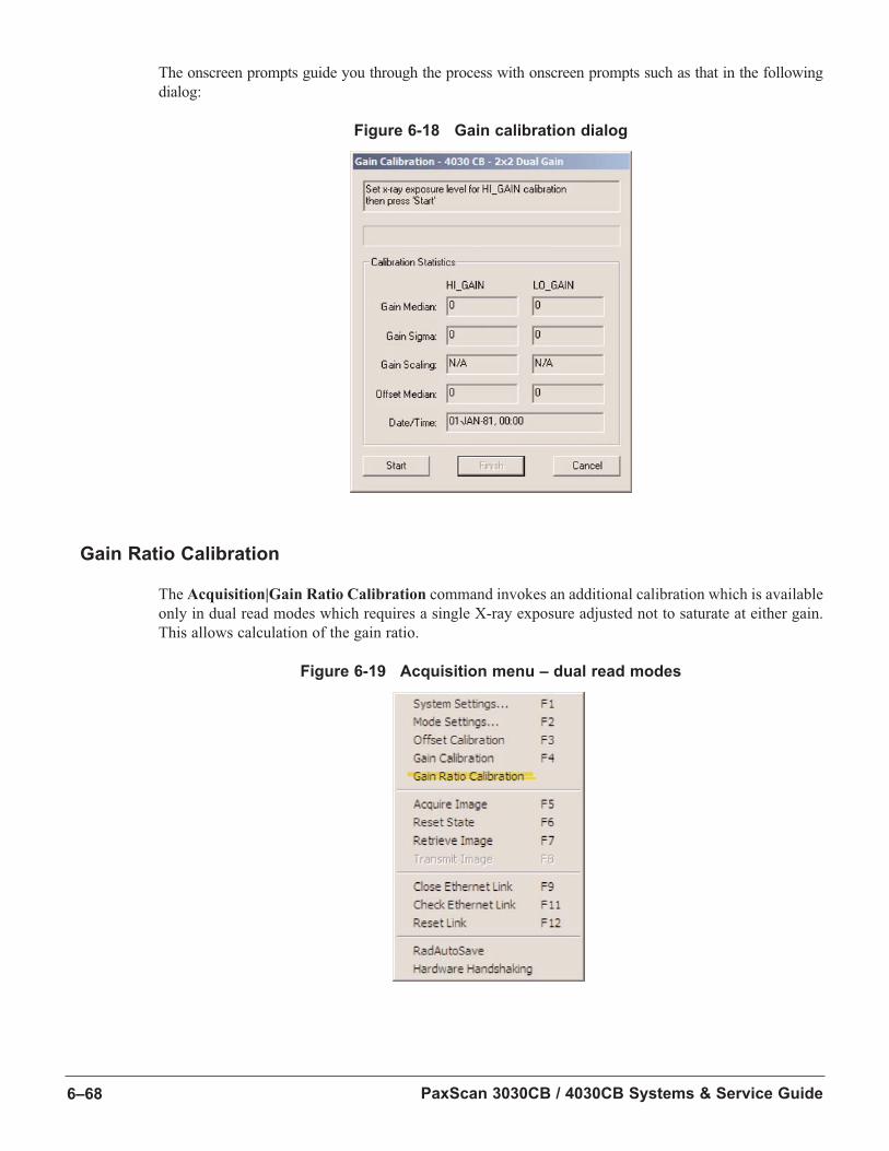
PaxScan 3030CB / 4030CB Systems & Service Guide6–68
The onscreen prompts guide you through the process with onscreen prompts such as that in the following
dialog:
Figure 6-18 Gain calibration dialog
Gain Ratio Calibration
The Acquisition|Gain Ratio Calibration command invokes an additional calibration which is available
only in dual read modes which requires a single X-ray exposure adjusted not to saturate at either gain.
This allows calculation of the gain ratio.
Figure 6-19 Acquisition menu – dual read modes
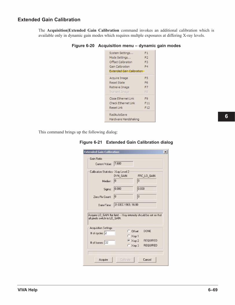
6–69ViVA Help
6
Extended Gain Calibration
The Acquisition|Extended Gain Calibration command invokes an additional calibration which is
available only in dynamic gain modes which requires multple exposures at differing X-ray levels.
Figure 6-20 Acquisition menu – dynamic gain modes
This command brings up the following dialog:
Figure 6-21 Extended Gain Calibration dialog
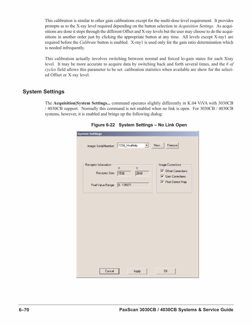
PaxScan 3030CB / 4030CB Systems & Service Guide6–70
This calibration is similar to other gain calibrations except for the multi-dose level requirement. It provides
prompts as to the X-ray level required depending on the button selection in Acquisition Settings. As acqui-
sitions are done it steps through the different Offset and X-ray levels but the user may choose to do the acqui-
sitions in another order just by clicking the appropriate button at any time. All levels except X-ray1 are
required before the Calibrate button is enabled. X-ray1 is used only for the gain ratio determination which
is needed infrequently.
This calibration actually involves switching between normal and forced lo-gain states for each Xray
level. It may be more accurate to acquire data by switching back and forth several times, and the # ofcycles field allows this parameter to be set. calibration statistics when available are show for the select-
ed Offset or X-ray level.
System Settings
The Acquisition|System Settings... command operates slightly differently in K.04 ViVA with 3030CB
/ 4030CB support. Normally this command is not enabled when no link is open. For 3030CB / 4030CB
systems, however, it is enabled and brings up the following dialog:
Figure 6-22 System Settings – No Link Open
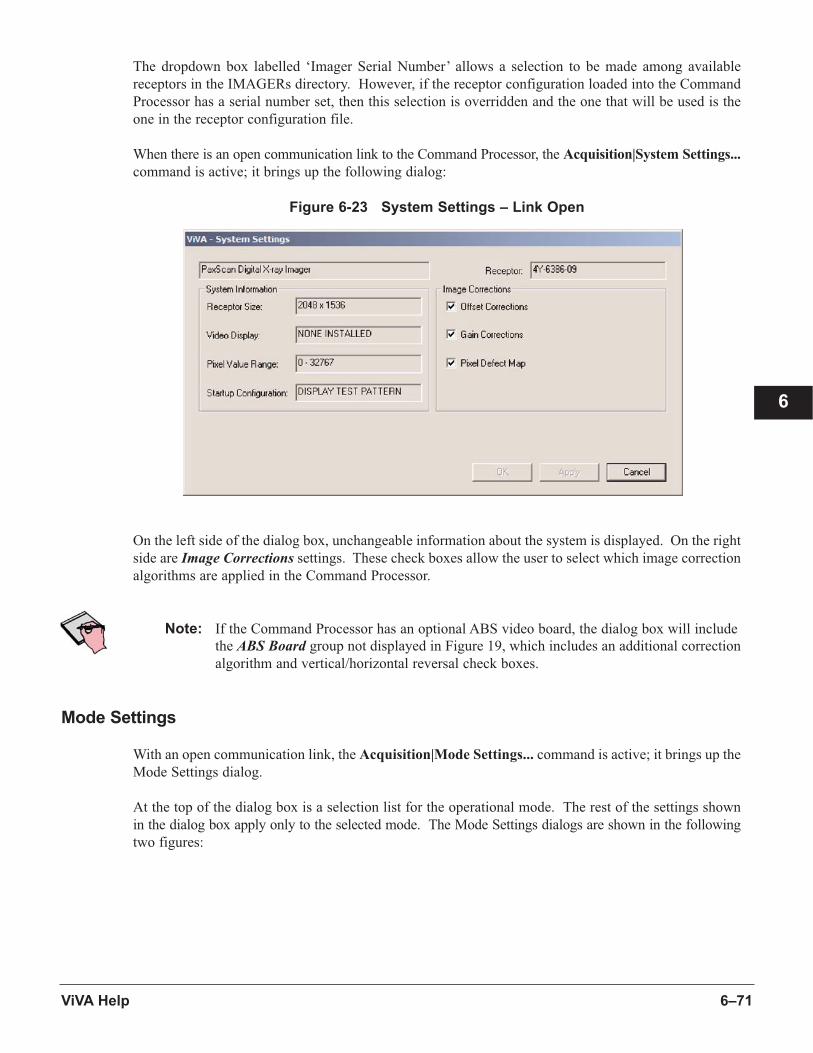
6–71ViVA Help
6
The dropdown box labelled ‘Imager Serial Number’ allows a selection to be made among available
receptors in the IMAGERs directory. However, if the receptor configuration loaded into the Command
Processor has a serial number set, then this selection is overridden and the one that will be used is the
one in the receptor configuration file.
When there is an open communication link to the Command Processor, the Acquisition|System Settings...
command is active; it brings up the following dialog:
Figure 6-23 System Settings – Link Open
On the left side of the dialog box, unchangeable information about the system is displayed. On the right
side are Image Corrections settings. These check boxes allow the user to select which image correction
algorithms are applied in the Command Processor.
Note: If the Command Processor has an optional ABS video board, the dialog box will include
the ABS Board group not displayed in Figure 19, which includes an additional correction
algorithm and vertical/horizontal reversal check boxes.
Mode Settings
With an open communication link, the Acquisition|Mode Settings... command is active; it brings up the
Mode Settings dialog.
At the top of the dialog box is a selection list for the operational mode. The rest of the settings shown
in the dialog box apply only to the selected mode. The Mode Settings dialogs are shown in the following
two figures:
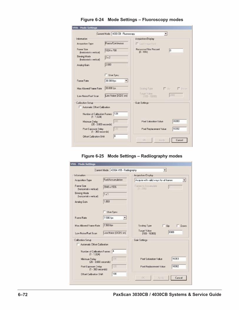
PaxScan 3030CB / 4030CB Systems & Service Guide6–72
Figure 6-24 Mode Settings – Fluoroscopy modes
Figure 6-25 Mode Settings – Radiiography modes
6–73ViVA Help
6
Information
Informational settings are not changeable except for the frame rate and user sync.
Calibration Setup
The user may specify the number of frames used during calibration and the settings for the optional auto-
matic offset calibration. In addition provision is made for an offset calibration shift to be applied dur-
ing offset calibrations. This will add a fixed offset to every pixel in the whole image if changed from
the zero default.
Acquisition/Display
This group shows different settings depending on whether a mode with fluoroscopy (continuous) acqui-
sition or radiography (accumulation) acquisition type is selected.
For a fluoroscopy mode: the user can set the recursive filter fraction.
For a radiography mode: the user can choose between letting the system automatically sense X-rays
start manually. Acquistion modes subdivide further by whether the user wishes to have a predeter-
mined number of frames accumulated (summed) or control stop manually. The Scaling Type option
allows the final image to be scaled to bring median pixel values near the target value. When Up is
checked scale factors greater than 1 are allowed; when Down is checked scale factors less than 1
are allowed. If both scaling options are selected, the resultant image may be scaled up or down,
and if neither is checked no scaling occurs.
Gain Settings
These allow the user to set a Pixel Saturation Value above which pixel values will be replaced by the
Pixel Replacement Value.
Rad AutoSave
This command allows the user to set up a file path and “base” name which is used when making Rad
mode acquisistions. Each time Acquire Image is pressed the image is automatically retrieved and saved.
For example if the base name is “radauto” the first acquisition might result in a file “radauto__001.viv”.
Hardware Handshaking
When the hardware configuration permits an X-ray valid signal to be sent to the command processor,
this menu item should be checked so that ViVA does not attempt to send the corresponding software
handshaking calls.

PaxScan 3030CB / 4030CB Systems & Service Guide6–74
Video Menu/Toolbar
ViVA K.04 supports operation with only Bitflow frame grabber cards. Currently the R3-PCI-DIF is sup-
ported for use with the standard (CP1) Command Processor. A camera link card is also supported for
use with CP1B. During installation an option is given to install the Bitflow support software.
Rad Modes
Most of this Video Menu/Toolbar section is applicable only to Fluoro modes of operation. ViVA auto-
matically takes advantage of the frame grabber where available to speed retrieval of rad images immediately
after acquisition into a new thumb pane; this is faster and more convenient than retrieval over the ethernet
connection. The Record Sequence command will remain inactive in Rad modes. All rad acquisitions must
be initiated using Acquire Image.
Recording Sequences
Note: This and following sections are applicable to Fluoro modes only.
Once the frame grabber and its associated driver/software libraries are properly installed, ViVA can record
sequences in any Fluoro mode.
The Video toolbar is by default docked at right side of the ViVA window. The following figure shows the
Video toolbar with annotations to show what each button does:
Figure 6-26 Video Toolbar
Many of the buttons also have duplicate commands in the Video menu. With the frame grabber installed
and a Command Processor link established, the Record Sequence button becomes active (on a color
monitor it will be green with a red border).
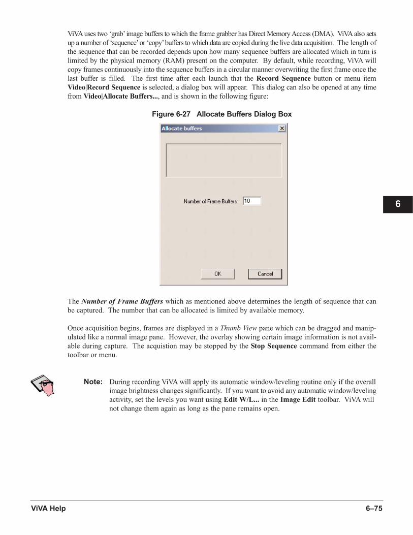
6–75ViVA Help
6
ViVA uses two ‘grab’ image buffers to which the frame grabber has Direct Memory Access (DMA). ViVA also sets
up a number of ‘sequence’ or ‘copy’ buffers to which data are copied during the live data acquisition. The length of
the sequence that can be recorded depends upon how many sequence buffers are allocated which in turn is
limited by the physical memory (RAM) present on the computer. By default, while recording, ViVA will
copy frames continuously into the sequence buffers in a circular manner overwriting the first frame once the
last buffer is filled. The first time after each launch that the Record Sequence button or menu item
Video|Record Sequence is selected, a dialog box will appear. This dialog can also be opened at any time
from Video|Allocate Buffers..., and is shown in the following figure:
Figure 6-27 Allocate Buffers Dialog Box
The Number of Frame Buffers which as mentioned above determines the length of sequence that can
be captured. The number that can be allocated is limited by available memory.
Once acquisition begins, frames are displayed in a Thumb View pane which can be dragged and manip-
ulated like a normal image pane. However, the overlay showing certain image information is not avail-
able during capture. The acquistion may be stopped by the Stop Sequence command from either the
toolbar or menu.
Note: During recording ViVA will apply its automatic window/leveling routine only if the overall
image brightness changes significantly. If you want to avoid any automatic window/leveling
activity, set the levels you want using Edit W/L... in the Image Edit toolbar. ViVA will
not change them again as long as the pane remains open.
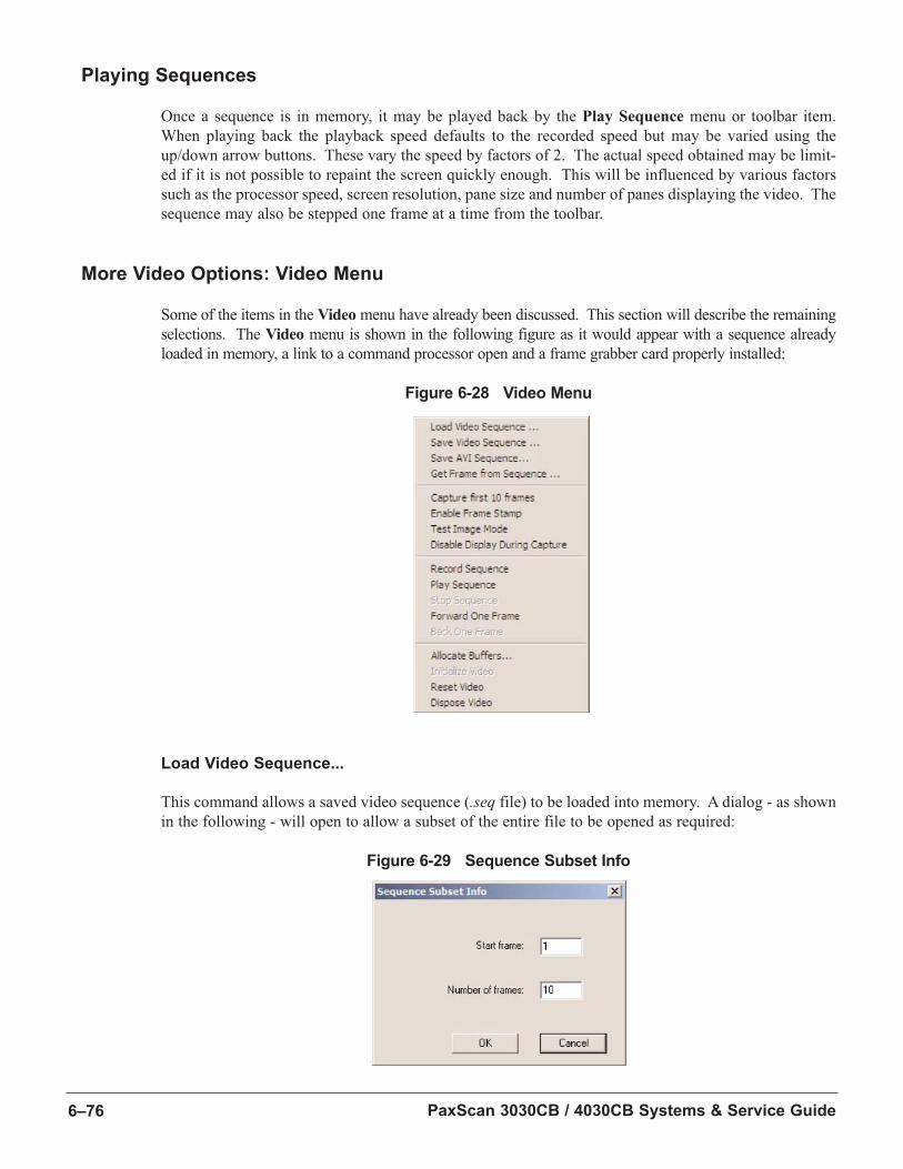
PaxScan 3030CB / 4030CB Systems & Service Guide6–76
Playing Sequences
Once a sequence is in memory, it may be played back by the Play Sequence menu or toolbar item.
When playing back the playback speed defaults to the recorded speed but may be varied using the
up/down arrow buttons. These vary the speed by factors of 2. The actual speed obtained may be limit-
ed if it is not possible to repaint the screen quickly enough. This will be influenced by various factors
such as the processor speed, screen resolution, pane size and number of panes displaying the video. The
sequence may also be stepped one frame at a time from the toolbar.
More Video Options: Video Menu
Some of the items in the Video menu have already been discussed. This section will describe the remaining
selections. The Video menu is shown in the following figure as it would appear with a sequence already
loaded in memory, a link to a command processor open and a frame grabber card properly installed:
Figure 6-28 Video Menu
Load Video Sequence...
This command allows a saved video sequence (.seq file) to be loaded into memory. A dialog - as shown
in the following - will open to allow a subset of the entire file to be opened as required:
Figure 6-29 Sequence Subset Info
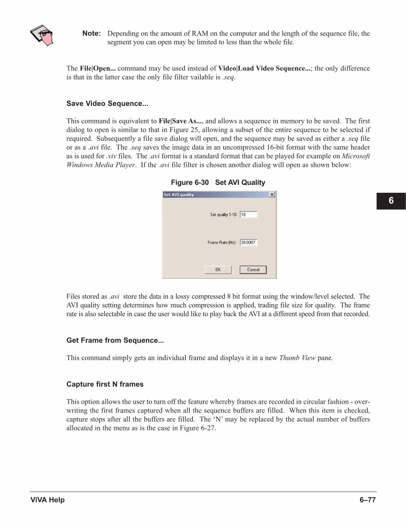
6–77ViVA Help
6
Note: Depending on the amount of RAM on the computer and the length of the sequence file, the
segment you can open may be limited to less than the whole file.
The File|Open... command may be used instead of Video|Load Video Sequence...; the only difference
is that in the latter case the only file filter vailable is .seq.
Save Video Sequence...
This command is equivalent to File|Save As..., and allows a sequence in memory to be saved. The first
dialog to open is similar to that in Figure 25, allowing a subset of the entire sequence to be selected if
required. Subsequently a file save dialog will open, and the sequence may be saved as either a .seq file
or as a .avi file. The .seq saves the image data in an uncompressed 16-bit format with the same header
as is used for .viv files. The .avi format is a standard format that can be played for example on MicrosoftWindows Media Player. If the .avi file filter is chosen another dialog will open as shown below:
Figure 6-30 Set AVI Quality
Files stored as .avi store the data in a lossy compressed 8 bit format using the window/level selected. The
AVI quality setting determines how much compression is applied, trading file size for quality. The frame
rate is also selectable in case the user would like to play back the AVI at a different speed from that recorded.
Get Frame from Sequence...
This command simply gets an individual frame and displays it in a new Thumb View pane.
Capture first N frames
This option allows the user to turn off the feature whereby frames are recorded in circular fashion - over-
writing the first frames captured when all the sequence buffers are filled. When this item is checked,
capture stops after all the buffers are filled. The ‘N’ may be replaced by the actual number of buffers
allocated in the menu as is the case in Figure 6-27.
PaxScan 3030CB / 4030CB Systems & Service Guide6–78
Test Image Mode
This allows a test pattern or other image to be retrieved from the command processor; all frames captured
are the same. You can for example use Transmit Image in the Acquisition toolbar to transmit a test pat-
tern for subsequent capture via the frame grabber. After changing modes or powering up the command
processor you should, in Test Image Mode, perform the following steps:
1. Press Acquire Image in the Acquisition toolbar followed by Stop in the Fluoroscopic Acquisition dialog.
2. Transmit Image as required.
3. Press Record Sequence and then Stop Sequence to capture the image via the frame grabber.
Note: Test Image Mode must be used with care. Since it disables commands to run the command
processor it is also possible for the command processor and ViVA to get out of synchro-
nization with respect to which mode is operating. If you have Test Image Mode selected,
you must run the command processor using Acquire Image in the Acquisition toolbar
before running video if you have just powered up or changed modes.
Disable Display During Capture
As indicated this option disables the display update during capture. It will rarely be found useful since ViVA
already gives priority to the activity of copying data to the sequence buffers over refeshing the display.
Allocate Buffers…
This dialog is discussed above under Recording Sequences.
Initialize Video
This command will not typically be found useful since ViVA automatically intializes the Video if a frame grab-
ber installation exists. However, frame grabbers do not generally permit more than one process (application)
to take control at a time. If another application is using the frame grabber when ViVA launches, ViVA will not
be able to initialize the video and this menu item will be active provided a link to a command processor exists.
This could be useful if you want to switch operation between applications.
Dispose Video
This command causes ViVA to relinquish control of the frame grabber and allows another application to
use it.
Reset Video
This command simply combines the Dispose Video and Initialize Video commands. It may be useful
if the frame grabber operation becomes unstable.

6–79ViVA Help
6
Analysis Menu: Image Statistics
ROI Basic
The Analysis menu allows the user to obtain statistical information on a specific region of an image
called the Region Of Interest (ROI). Generally the commands relating to the ROI are not active unless
the ROI cursor is selected (see Table 2).
Except for 2520M receptors, the Edit Toolbar contains a button at the top which is labeled either ‘Img
Stats…’ or ‘ROI Stats…’. It will be ‘Img Stats’ unless the ROI cursor is active and an ROI drawn. This
button allows statistics for the whole image to be displayed at any time.
An ROI may be selected by clicking the left mouse button anywhere in an image pane and holding while
a rectangle is defined. The ROI shows as a blue rectangle overlay which persists after the mouse button is
released until a difference cursor is selected or new ROI drawn. Even when not displayed, the last ROI
coordinates are remembered and displayed if the ROI cursor is reselected. If you attempt to drag outside
the image, the rectangle changes to red and snaps to the image border if the mouse is released.
Note: If you hold the Shift key while dragging, the ROI will be square.
Basic Menu Commands
Analysis|Select Whole Image allows the user to select the whole active image as a region of interest.
Analysis|Clear ROI allows the user to clear the selected ROI.
Analysis|Show ROI Statistics... allows the user to display statistical information. Alternatively this command
may be invoked from the ROI Stats... button on the Edit toolbar or the ROI Stats... menu item of the Context
Menu for Image View. Any of these will result in the dialog shown in the following figure:
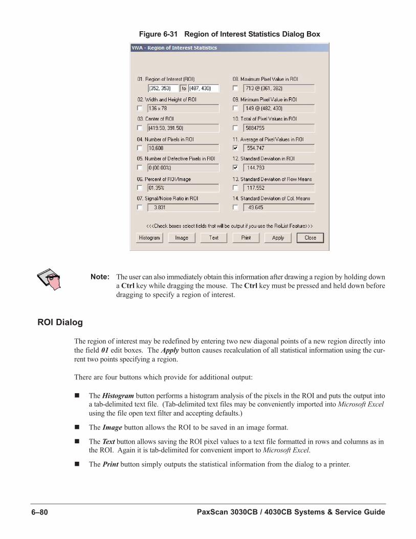
PaxScan 3030CB / 4030CB Systems & Service Guide6–80
Figure 6-31 Region of Interest Statistics Dialog Box
Note: The user can also immediately obtain this information after drawing a region by holding down
a Ctrl key while dragging the mouse. The Ctrl key must be pressed and held down before
dragging to specify a region of interest.
ROI Dialog
The region of interest may be redefined by entering two new diagonal points of a new region directly into
the field 01 edit boxes. The Apply button causes recalculation of all statistical information using the cur-
rent two points specifying a region.
There are four buttons which provide for additional output:
n The Histogram button performs a histogram analysis of the pixels in the ROI and puts the output into a tab-delimited text file. (Tab-delimited text files may be conveniently imported into Microsoft Excelusing the file open text filter and accepting defaults.)
n The Image button allows the ROI to be saved in an image format.
n The Text button allows saving the ROI pixel values to a text file formatted in rows and columns as in the ROI. Again it is tab-delimited for convenient import to Microsoft Excel.
n The Print button simply outputs the statistical information from the dialog to a printer.

6–81ViVA Help
6
The statistical information provided on this dialog box is explained in the following table:
Table 6-3 Region of Interest Statistical Information
Name Format Description
01. Region of Interest (x0 ,y0 ) to Two diagonally disposed points that
(ROI) (x1 ,y1 ) define the ROI rectangle.
02. Width and Height integer x Width and height dimensions
of Region integer of the ROI.
03. Center of ROI (x,y) Center location of the ROI.
04. Number of Pixels integer Number of pixels found in ROI.
in ROI
05. Number of Defective integer Number of defective pixels found in
Pixels in ROI the ROI. These are pixels with the 65535
value that ViVA intreprets as defective.
06. Percent of real Percent of the region over the whole
ROI/Image image.
07. Signal/Noise real Defined by formula average/standard
Ratio in ROI deviation.
08. Maximum Pixel integer @ Maximum pixel value first found in
Value in ROI (x,y) the ROI.
09. Minimum Pixel integer @ Minimum pixel value first found
Value in ROI (x,y) in the ROI.
10. Total of Pixel integer Total of all pixel values found
Values in ROI in the ROI.
11. Average of Pixel real Average of pixel values found
Values in ROI in the ROI.
12. Standard real Standard deviation of pixel values in
Deviation in ROI the ROI.
13. Standard Deviation real Standard deviation of the mean values
of Row Means of the rows.
14. Standard Deviation real Standard deviation of the mean values
of Column Means of the columns.
Note: The coordinates (x,y) of a point and the dimension width by height are limited by the size
of an image. Specifically, ranges of a pair (x,y) are from 0 to (width -1) and 0 to (height -1),
respectively. Pixel values are in range from 0 to maximum pixel value.

PaxScan 3030CB / 4030CB Systems & Service Guide6–82
RoiList Commands
The RoiList commands greatly extend the usefulness of the ROI analysis feature. This feature allows
you to set up multiple ROIs and then apply to multiple images. When an ROI is selected you may add
it to the RoiList by selecting Analysis|Add ROI to RoiList. This saves the ROI coordinates and causes
the ROI to be displayed as a cyan rectangle. By redrawing the ROI and adding to the RoiList, you can
select mulitple ROIs.
Note: The active ROI is the one in blue and is not necessarily a member of the RoiList until you add
it. The ROI statistics dialog will always refer to the active ROI.
When an RoiList has been established by selecting Analysis|Add ROI to RoiList one or more times, it
can be applied in a batch-like manner to multiple images. To apply the RoiList, select Analysis|Apply
RoiList.... This will first open a file save dialog box for the output file - again tab-delimited text. If the
active image is an individual image - as opposed to a video sequence - another file dialog box will then
open. This dialog allows you to select multiple image files. All the images selected must be .viv or .rawand must have the same image dimensions as the image in the selected image pane. Statistical infor-
mation will be determined for all the ROIs in the RoiList and for each image selected in the file dialog
and output to the text file.
The ROIList may be saved to and retrieved from a text file (which can be edited if required) using the
commands Analysis|Save RoiList to File… and Analysis|Load RoiList from File…
Notes on ROIList Use:
n If the selected image is a video pane and not an individual image pane, then instead of the second file dialog box you will be asked to select a video segment for processing.
n The actual image in the image pane is not necessarily processed. Only the image files or the video segment selected are processed.
n The output will by default consist of two fields for each ROI: 11. Average of Pixel Values in ROI and 12. Standard Deviation in ROI. Notice that in Figure 31 these two fields have checks in the
adjacent check boxes. You can select any or all or the fields to be output using the check boxes.
(01. Region of Interest has no check box but this information is always written to the text file.)
n The status of the check boxes is remembered when the ROI dialog is closed and this defines the fields that are output. ViVA will remember which fields were last selected even between launches.
n The RoiList itself is more volatile than the check box information. RoiList information is actually specific to each image pane. It will, however, generally be remembered even if you close the image
in the image pane. If you attempt to drag an image to the pane that has different dimensions than
the one for which the RoiList was defined, a message box will warn you that this action forces a
RoiList reset. All RoiList information is lost when ViVA closes (but not the check box information).
n The RoiList may be reset at any time by Analysis|Reset RoiList.

6–83ViVA Help
6
Tools Menu
The Tools menu is consists of a number of sub-menus each with multiple commands; these will generally
consist of the following which are described in detail below:
n Receptor
n Command Processor
n Defects
n Image Operations
n Cone Beam
CAUTION: Many of the commands in this section are intended for Engineering use and should be used
only by experienced users or under the direction of Varian Medical Systems technical staff.
Receptor
Analog Offset Calibration
The Analog Offset Calibration... command allows the user to change analog offset settings and perform
an analog offset calibration. When selected, this option will display an Analog Offset Settings dialog box
as shown in the following figure:
Figure 6-32 Analog Offset Settings
PaxScan 3030CB / 4030CB Systems & Service Guide6–84
The Apply or OK button only updates the setting information from the Edit boxes at the Command
Processor without performing a calibration. The Calibrate button initiates an analog offset calibration.
An analog offset calibration runs autonomously; it is an iterative process, and if the target range is
reached for all ASICs before completing the limiting number of iterations, it terminates early.
Note: After an analog offset calibration is done, it is essential to perform a gain calibration before
images can be properly corrected.
DCDS Enable
The Set DCDS Off command allows DCDS to be temporarily disabled which is useful in connection
with performing analog offset calibrations. DCDS will turn on again automatically when the mode is
changed, or when Offset/Gain calibration is performed.
Command Processor
Display Test Pattern
If ViVA has an open connection to the Command Processor, choosing the Display Test Pattern option
causes the Command Processor to display a test pattern consisting of eight horizontal bars of equal
height, with linear steps in intensity from zero at the top of the image, to 3,584 counts at the bottom. The
image size indicated relates to the currently selected mode.
Write ABS MailBox
The Write ABS MailBox... command should only be used under the direction of Varian Medical Systems
technical staff.
Transmit Files
The Transmit Files... command allows the user to transmit new files to the Command Processor. Currently,
ViVA can transmit the following file types:
n System Software file
n Global Control Firmware file
n Receptor Firmware file
n Receptor Configuration Data file
n Base Defect Map Image file
n Gain Calibrated Image file
n Offset Calibrated Image file
The file type to be transmitted should be checked, then browse to the file itself, and click ‘Transmit’.
6–85ViVA Help
6
Retrieve Files
The Retrieve Files... command allows the user to retrieve a file from the Command Processor. It operates
similarly to the Transmit Files function.
Debug Verbosity
Debug Verbosity can be toggled on/off. Turning this option on causes the Command Processor to print
debug information over a serial port which can be captured with Hyperterminal for example. Having
debug verbosity set to Off (default) will improve system performance. In addition ViVA will write a file
‘CmdTestLog.txt’ to the ViVA directory; it is written when Debug Verbosity is turned off, and any previous
file overwritten. It contains a log of calls made by ViVA while Debug Verbosity was on including
parameters and return values.
Reset
The Reset command sends a command to the Command Processor to re-boot and the link from ViVA is
also reset.
Enable IPU
This is a rarely needed, only for specialized receptor configurations.
Defects
Defect Map Editor
The Defect Map Editor is invoked by choosing Tools|Defects|Defect Map Editor.... This will switch
ViVA from image viewing mode to image editing mode. The Acquisition toolbar is replaced by the
Defect Map Editor toolbar.
The Status Bar displays the current mode in the Command Processor. All images in Image View are closed
and Image Layout is set to Two-Image Layout. ViVA then retrieves the Base Defect Map image and the
Auxiliary Defect Map image from the Command Processor and displays them in the Thumb View and the
Image View. The Base Defect Map image is placed in the right pane, and the Auxiliary Defect Map image
is placed in the left pane.
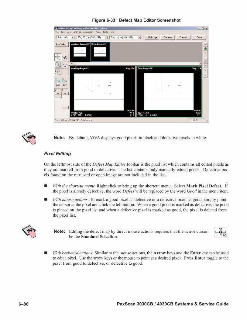
PaxScan 3030CB / 4030CB Systems & Service Guide6–86
Figure 6-33 Defect Map Editor Screenshot
Note: By default, ViVA displays good pixels in black and defective pixels in white.
Pixel Editing
On the leftmost side of the Defect Map Editor toolbar is the pixel list which contains all edited pixels as
they are marked from good to defective. The list contains only manually-edited pixels. Defective pix-
els found on the retrieved or open image are not included in the list.
n With the shortcut menu: Right click to bring up the shortcut menu. Select Mark Pixel Defect. If
the pixel is already defective, the word Defect will be replaced by the word Good in the menu item.
n With mouse actions: To mark a good pixel as defective or a defective pixel as good, simply point the cursor at the pixel and click the left button. When a good pixel is marked as defective, the pixel
is placed on the pixel list and when a defective pixel is marked as good, the pixel is deleted from
the pixel list.
Note: Editing the defect map by direct mouse actions requires that the active cursor
be the Standard Selection.
n With keyboard actions: Similar to the mouse actions, the Arrow keys and the Enter key can be used to edit a pixel. Use the arrow keys or the mouse to point at a desired pixel. Press Enter toggle to the
pixel from good to defective, or defective to good.
6–87ViVA Help
6
n With the pixel list:
¨ To add a pixel onto the pixel list, select <Pixel>, type the coordinates of the pixel in the point form (x,y), then press the Tab key to end the addition.
¨ To delete a pixel, select the desired pixel, press the Backspace key and press the Tab key to end the deletion.
¨ To change the coordinates of a pixel, select the pixel, edit the x and y coordinates, and press the Tab key to end the change.
Row Segment Editing
The second dropdown list in the Defect Map Editor toolbar is the row segment list. It contains defec-
tive row segments marked in the defect map editor. As with individual pixels, row segments found on
the retrieved or open image are not included in the list.
n With the shortcut menu: Right click to bring up the shortcut menu. Select Mark Row Defect. If the row is already defective, the word Defect will be replaced by the word Good in the menu item.
n With mouse actions: To mark a good row segment as defective or a defective row segment as good, simply point the cursor at the row and then click on the left button while holding down the Shift key.
When a row segment is marked as defective, the segment is placed on the row segment list and when
a defective row segment is marked as good; the segment is deleted from the row segment list.
n With keyboard actions: Similar to the mouse actions, the arrow keys and the Enter key can be used to edit a row. Use the Arrow keys or the mouse to point at a desired row. Then press Enter while
holding down the Shift key to toggle the whole row from good to defective or defective to good.
n With the row segment list:
¨ To add a row segment to the row segment list, select <Row Segment>, type in the coordinates in the row segment format (x1,y) to (x2,y) and press the Tab key to end the addition.
¨ To delete a row segment, select the desired row segment, press the Backspace key and press the Tab key to end the deletion.
¨ To change the coordinates of a row segment, select the row segment, edit the x and y coordinates and press the Tab key to end the change.
Note: ASIC-wide defects represent a special case of row defects. Some additional commands
allow ASIC-wide defects to be conveniently marked. From the keyboard press Shift/A or
from the shortcut menu select Mark Asic Segment Defect. ASIC-wide defects are listed
in the row segment list box.
Column Segment Editing
The third dropdown list in the Defect Map Editor toolbar is the column segment list. It contains defective
column segments marked in the defect map editor. As with individual pixels and rows, column segments
found on the retrieved or open image are not included in the list.
PaxScan 3030CB / 4030CB Systems & Service Guide6–88
n With the shortcut menu: Right click to bring up the shortcut menu. Select Mark Column Defect. If
the column is already defective, the word Defect will be replaced by the word Good in the menu item.
n With mouse actions: To mark a good column segment as defective or a defective column segment as good, simply point the cursor at the column and click the left button while holding down the
Control key. When a column segment is marked as defective, the segment is placed on the column
segment list and when a defective column segment is marked as good, the segment is deleted from
the column segment list.
n With keyboard actions: Similar to the mouse actions, the Arrow keys and the Enter key can be used to edit a row. Use the arrow keys or the mouse to point at a desired row. Press Enter while holding down
the Control key to toggle the whole column from good to defective, or defective to good.
n With the column segment list:
¨ To add a column segment onto the column segment list, select <Column Segment>, type in the coordinates in the column segment format (x,y1) to (x,y 2 ) and press the Tab key to end the
addition.
¨ To delete a column segment, select the desired column segment, press the Backspace key and press the Tab key to end the deletion.
¨ To change the coordinates of a column segment, select the column segment, edit the x and y coordinates, then the Tab key to end the change.
Note: On the 4030A receptor, because of the split readout, column defects only extend to the
midway point of the imager. If the cursor is in the top half of the image, the column defect
will be restricted to the top half; or if the cursor is in the bottom half, the column defect will
be restricted to the bottom half.
OR Image
To add all defective pixels on the Auxiliary Defect Map image on the left Image View pane to the Base DefectMap image on the right of the Image View pane, click OR Image. This command is useful when there is
an existing image with defective pixels that can be added onto the Base Defect Map image. The user
simply opens an image as usual, then drags and drops the thumbnail view of the image onto the left pane
before adding the two images.
Retrieve
To retrieve a new Base Defect Map image and an Auxiliary Defect Map image, click Retrieve. This
command deletes any previous changes to the defect maps and allows the user to start editing again without
terminating Defect Map Editor mode.
Transmit
To transmit the Base Defect Map image to the Command Processor, click Transmit. This moves the
image on the right Image View pane to the Command Processor and overwrites the current Base Defect
Map image with the new one.
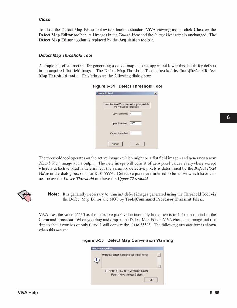
6–89ViVA Help
6
Close
To close the Defect Map Editor and switch back to standard ViVA viewing mode, click Close on the
Defect Map Editor toolbar. All images in the Thumb View and the Image View remain unchanged. The
Defect Map Editor toolbar is replaced by the Acquisition toolbar.
Defect Map Threshold Tool
A simple but effect method for generating a defect map is to set upper and lower thresholds for defects
in an acquired flat field image. The Defect Map Threshold Tool is invoked by Tools|Defects|Defect
Map Threshold tool.... This brings up the following dialog box:
Figure 6-34 Defect Threshold Tool
The threshold tool operates on the active image - which might be a flat field image - and generates a new
Thumb View image as its output. The new image will consist of zero pixel values everywhere except
where a defective pixel is determined; the value for defective pixels is determined by the Defect PixelValue in the dialog box or 1 for K.01 ViVA. Defective pixels are inferred to be those which have val-
ues below the Lower Threshold or above the Upper Threshold.
Note: It is generally necessary to transmit defect images generated using the Threshold Tool via
the Defect Map Editor and NOT by Tools|Command Processor|Transmit Files....
ViVA uses the value 65535 as the defective pixel value internally but converts to 1 for transmittal to the
Command Processor. When you drag and drop in the Defect Map Editor, ViVA checks the image and if it
detects that it consists of only 0 and 1 will convert the 1’s to 65535. The following message box is shown
when this occurs:
Figure 6-35 Defect Map Conversion Warning

PaxScan 3030CB / 4030CB Systems & Service Guide6–90
Find Noisy Pixels
The purpose of the Find Noisy Pixel... command is to identify pixels that may not appear defective for each
and every frame, but over a number of frames fluctuate significantly in intensity. The noisy pixel routine
collects a number of frames and attempts to identify noisy pixels statistically as those having a relatively
high standard deviation (SD) also referred to as sigma. The SD is calculated for each individual pixel or
binned grouping, according to the mode. The SD is formed on a temporal, not spatial, basis as would be the
case in ROI calculations.
Noisy pixel detection is invoked by Tools|Defects|Find Noisy Pixels.... Parameters are selected in the
top section of the dialog box entitled Acquisition, which is shown below:
Figure 6-36 Find Noisy Pixels Dialog
Acquisition
Each cycle will involve the acquisition of the specified number of frames, and the retrieval of the last.
This allows the user to spread the actual frames used in the computation out over a larger number of
frames, which could be useful if the fluctuations are clustered rather than random.
One frame is retrieved for each cycle.
Note: In order to compute the SD effectively, it is suggested that at least ten cycles be specified.
For initial familiarization purposes, five will be adequate. The acquisition may take some
time, particularly in modes where no binning is used and will be essentially proportional
to the number of cycles. The user may choose to save each individually-retrieved frame
to a disk file via the check box. This feature will probably not normally be selected.
To begin acquisition, click Acquire Noisy Pixel Data. The user is given the opportunity to save to disk
the SD image formed. The SD image is actually the calculated standard deviation scaled by ten to
improve precision. A Thumb View of the SD image is displayed.

6–91ViVA Help
6
Set Threshold and Display
When acquisition is complete, a threshold can be selected above which pixels are considered defective.
Changing the value of the threshold will normally result in a corresponding change in the indicated number
of pixels above the threshold. The displayed number is updated whenever the threshold is changed and
focus shifted away from the Set SD Threshold edit box; e.g., when finished typing, press the Tab key.
When the required threshold has been selected, a defect map can be created by pressing Display NoisyPixels.
Note: If this button is clicked when no acquisition is current (i.e. no acquisition done since the
dialog box opened), the user is given an opportunity to select a previously acquired SD
image from a disk file.
Identifying Noisy Pixels
One method to identify noisy pixels requires the following:
n Exiting the dialog box and inspect the acquired SD image
n Magnify some part of it and look for a featureless (normal) region
n Use the ROI facility to evaluate the average SD and the standard deviation of the SD itself in this region
n Repeat in other areas to get good numbers for the average normal SD and its distribution, as indicated in the standard deviation box of the ROI dialog.
A good choice for the threshold will likely be ~6x the standard deviation of this distribution plus the
average.
Note: This procedure is roughly that carried out by clicking the AutoSet button.
Updating the Base Defect Map
When the required threshold is identified, the Noisy Pixel dialog box can be reopened. Data of interest are
reactivated by pressing the Display Noisy Pixels button, and selecting the appropriate file. Set the
threshold and click Display Noisy Pixels again to ensure the defect map is created at the required threshold
setting.
When the defect map is correct, download it to the Command Processor by clicking OR With Aux Defect
Map or OR With Base Defect Map. This results in the logical OR operation being performed with either
the existing auxiliary defect map or the existing base defect map; the result is always a new base defect map
Note: If the threshold value is changed without creating a new map, and then one of the OR
buttons clicked, a new map is automatically created prior to updating the base defect map.
The result is downloaded to the Command Processor.
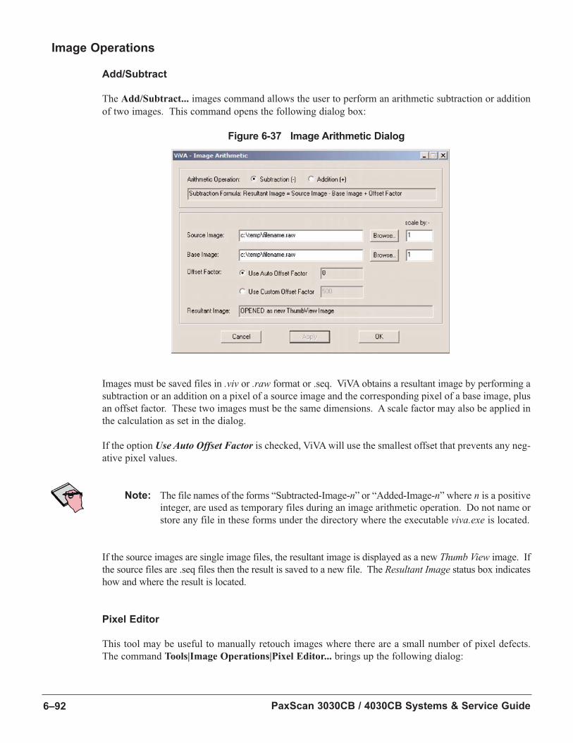
PaxScan 3030CB / 4030CB Systems & Service Guide6–92
Image Operations
Add/Subtract
The Add/Subtract... images command allows the user to perform an arithmetic subtraction or addition
of two images. This command opens the following dialog box:
Figure 6-37 Image Arithmetic Dialog
Images must be saved files in .viv or .raw format or .seq. ViVA obtains a resultant image by performing a
subtraction or an addition on a pixel of a source image and the corresponding pixel of a base image, plus
an offset factor. These two images must be the same dimensions. A scale factor may also be applied in
the calculation as set in the dialog.
If the option Use Auto Offset Factor is checked, ViVA will use the smallest offset that prevents any neg-
ative pixel values.
Note: The file names of the forms “Subtracted-Image-n” or “Added-Image-n” where n is a positive
integer, are used as temporary files during an image arithmetic operation. Do not name or
store any file in these forms under the directory where the executable viva.exe is located.
If the source images are single image files, the resultant image is displayed as a new Thumb View image. If
the source files are .seq files then the result is saved to a new file. The Resultant Image status box indicates
how and where the result is located.
Pixel Editor
This tool may be useful to manually retouch images where there are a small number of pixel defects.
The command Tools|Image Operations|Pixel Editor... brings up the following dialog:
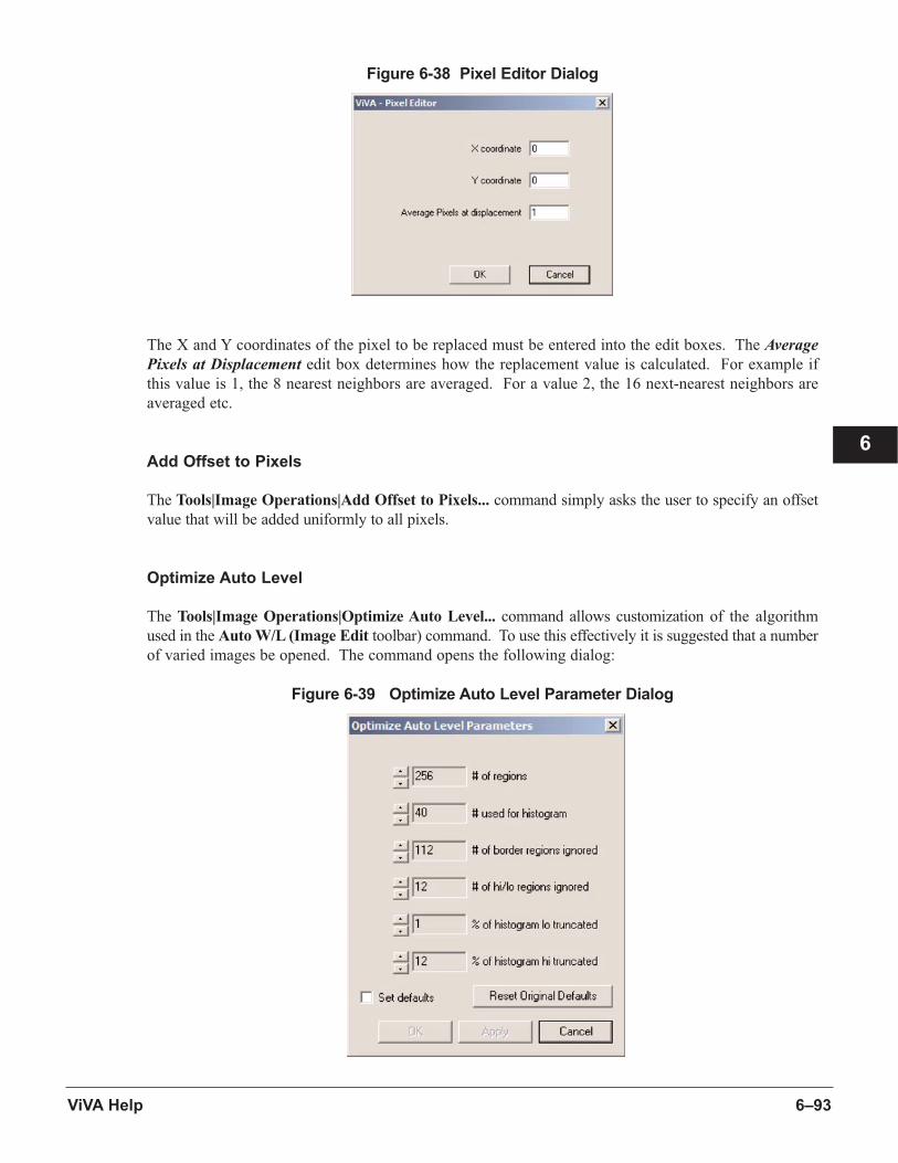
6–93ViVA Help
6
Figure 6-38 Pixel Editor Dialog
The X and Y coordinates of the pixel to be replaced must be entered into the edit boxes. The AveragePixels at Displacement edit box determines how the replacement value is calculated. For example if
this value is 1, the 8 nearest neighbors are averaged. For a value 2, the 16 next-nearest neighbors are
averaged etc.
Add Offset to Pixels
The Tools|Image Operations|Add Offset to Pixels... command simply asks the user to specify an offset
value that will be added uniformly to all pixels.
Optimize Auto Level
The Tools|Image Operations|Optimize Auto Level... command allows customization of the algorithm
used in the Auto W/L (Image Edit toolbar) command. To use this effectively it is suggested that a number
of varied images be opened. The command opens the following dialog:
Figure 6-39 Optimize Auto Level Parameter Dialog
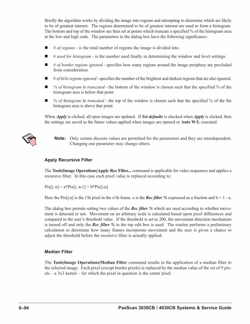
PaxScan 3030CB / 4030CB Systems & Service Guide6–94
Briefly the algorithm works by dividing the image into regions and attempting to determine which are likely
to be of greatest interest. The regions determined to be of greatest interest are used to form a histogram.
The bottom and top of the window are then set at points which truncate a specified % of the histogram area
at the low and high ends. The parameters in the dialog box have the following significance:
n # of regions - is the total number of regions the image is divided into.
n # used for histogram - is the number used finally in determining the window and level settings.
n # of border regions ignored - specifies how many regions around the image periphery are precludedfrom consideration.
n # of hi/lo regions ignored - specifies the number of the brightest and darkest regions that are also ignored.
n % of histogram lo truncated - the bottom of the window is chosen such that the specified % of the histogram area is below that point.
n % of histogram hi truncated - the top of the window is chosen such that the specified % of the the histogram area is above that point.
When Apply is clicked, all open images are updated. If Set defaults is checked when Apply is clicked, then
the settings are saved as the future values applied when images are opened or Auto W/L executed.
Note: Only certain discrete values are permitted for the parameters and they are interdependent.
Changing one parameter may change others.
Apply Recursive Filter
The Tools|Image Operations|Apply Rec Filter... command is applicable for video sequences and applies a
recursive filter. In this case each pixel value is replaced according to:
Pix[i, n] = a*Pix[i, n-1] + b*Pix[i,n]
Here the Pix[i,n] is the i’th pixel in the n’th frame. a is the Rec filter % expressed as a fraction and b = 1 - a.
The dialog box permits setting two values of the Rec filter % which are used according to whether move-
ment is detected or not. Movement on an arbitrary scale is calculated based upon pixel differences and
compared to the user’s threshold value. If the threshold is set to 200, the movement detection mechanism
is turned off and only the Rec filter % in the top edit box is used. The routine performs a preliminary
calculation to determine how many frames incorporate movement and the user is given a chance to
adjust the threshold before the recursive filter is actually applied.
Median Filter
The Tools|Image Operations|Median Filter command results in the application of a median filter to
the selected image. Each pixel (except border pixels) is replaced by the median value of the set of 9 pix-
els – a 3x3 kernel – for which the pixel in question is the center pixel.
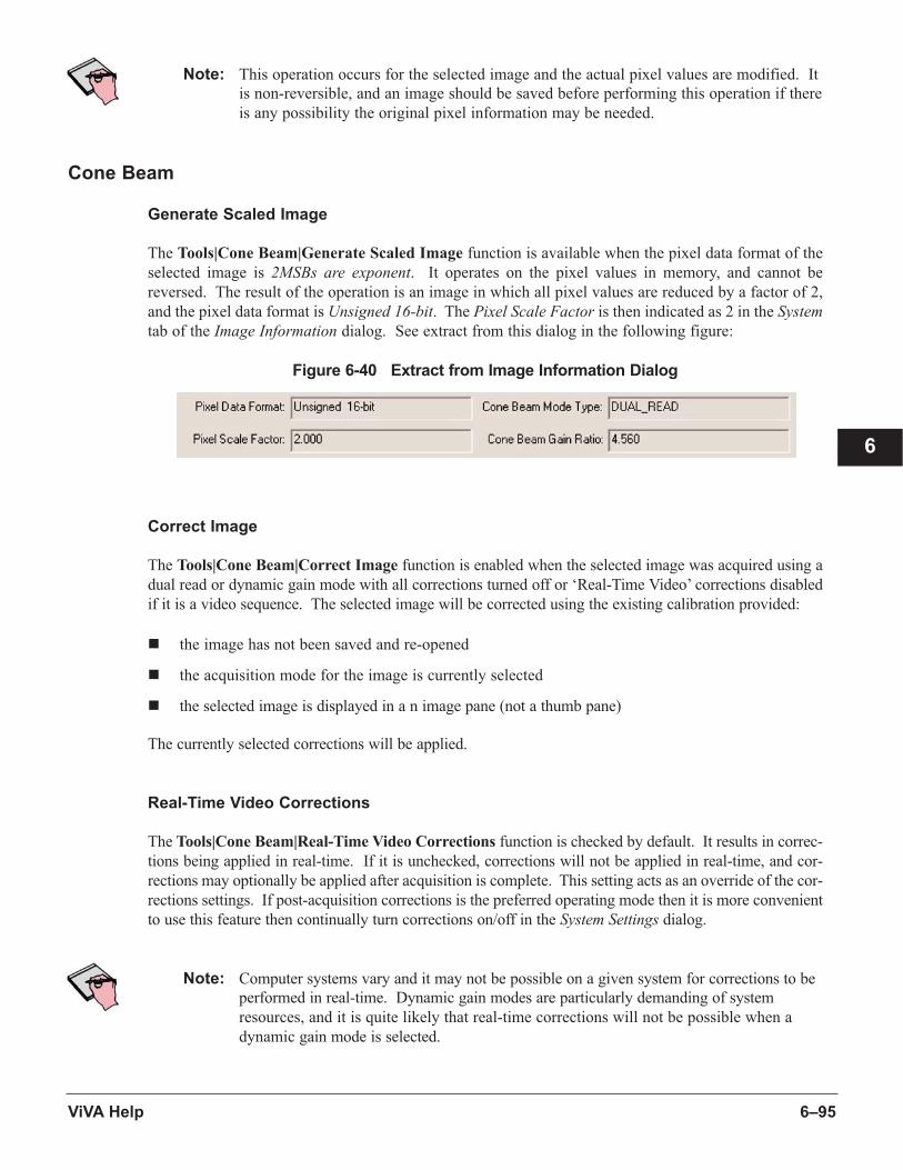
6–95ViVA Help
6
Note: This operation occurs for the selected image and the actual pixel values are modified. It
is non-reversible, and an image should be saved before performing this operation if there
is any possibility the original pixel information may be needed.
Cone Beam
Generate Scaled Image
The Tools|Cone Beam|Generate Scaled Image function is available when the pixel data format of the
selected image is 2MSBs are exponent. It operates on the pixel values in memory, and cannot be
reversed. The result of the operation is an image in which all pixel values are reduced by a factor of 2,
and the pixel data format is Unsigned 16-bit. The Pixel Scale Factor is then indicated as 2 in the Systemtab of the Image Information dialog. See extract from this dialog in the following figure:
Figure 6-40 Extract from Image Information Dialog
Correct Image
The Tools|Cone Beam|Correct Image function is enabled when the selected image was acquired using a
dual read or dynamic gain mode with all corrections turned off or ‘Real-Time Video’ corrections disabled
if it is a video sequence. The selected image will be corrected using the existing calibration provided:
n the image has not been saved and re-opened
n the acquisition mode for the image is currently selected
n the selected image is displayed in a n image pane (not a thumb pane)
The currently selected corrections will be applied.
Real-Time Video Corrections
The Tools|Cone Beam|Real-Time Video Corrections function is checked by default. It results in correc-
tions being applied in real-time. If it is unchecked, corrections will not be applied in real-time, and cor-
rections may optionally be applied after acquisition is complete. This setting acts as an override of the cor-
rections settings. If post-acquisition corrections is the preferred operating mode then it is more convenient
to use this feature then continually turn corrections on/off in the System Settings dialog.
Note: Computer systems vary and it may not be possible on a given system for corrections to be
performed in real-time. Dynamic gain modes are particularly demanding of system
resources, and it is quite likely that real-time corrections will not be possible when a
dynamic gain mode is selected.

PaxScan 3030CB / 4030CB Systems & Service Guide6–96

7–97
7
Chapter 7 System Configuration
Important: The following information details operations which should only be performed by
experienced imaging personnel. Please contact PaxScan Technical Support for more
information.
In This Chapter
Topic Page
Configure Utility Application 7-97
Usage 7-98
Main Screen 7-99
Receptor Configuration Settings 7-100
Mode Selection 7-102
Mode Setup 7-103
Configure Utility Application
WARNING: Use of this application program is strictly only for the purpose of viewing the factory -
installed configuration file settings. Failure to do otherwise without prior permission from Varian
Medical Systems will void the Varian Medical Systems standard warranty
The purpose of the Configure Application is to provide an interface for building the necessary configu-
ration files for the PaxScan Command Processor. There are two required configuration files, one for sys-
tem configuration and one for receptor configuration.
The system configuration file includes information that pertains to the entire system, such as the version
information, etc.
The receptor configuration file includes information needed to examine or if required correctly configure the
receptor for acquisition. Frame rate, binning, recursive filter percentage, etc. are examples of the data with-
in the receptor configuration file.
More specific information about the data contained within the configuration files will be discussed later
in this document.
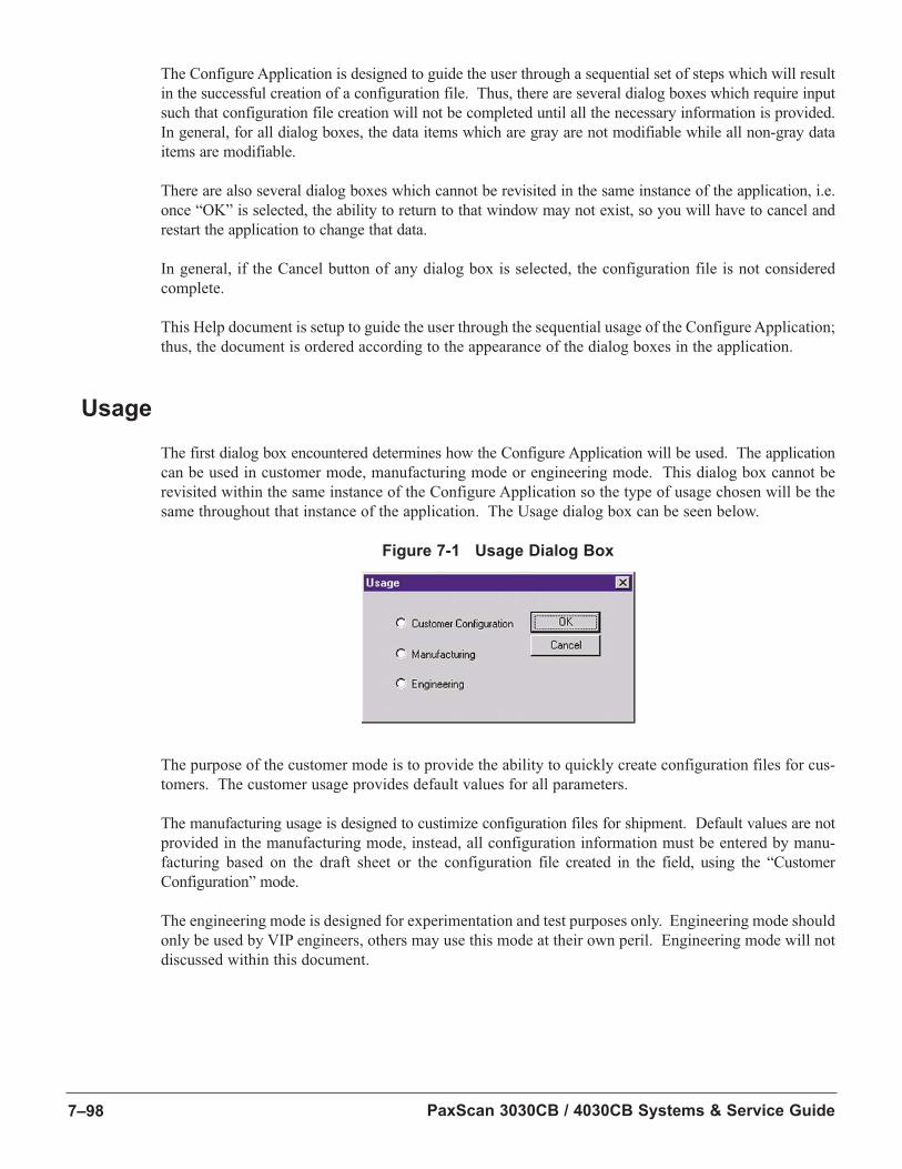
PaxScan 3030CB / 4030CB Systems & Service Guide7–98
The Configure Application is designed to guide the user through a sequential set of steps which will result
in the successful creation of a configuration file. Thus, there are several dialog boxes which require input
such that configuration file creation will not be completed until all the necessary information is provided.
In general, for all dialog boxes, the data items which are gray are not modifiable while all non-gray data
items are modifiable.
There are also several dialog boxes which cannot be revisited in the same instance of the application, i.e.
once “OK” is selected, the ability to return to that window may not exist, so you will have to cancel and
restart the application to change that data.
In general, if the Cancel button of any dialog box is selected, the configuration file is not considered
complete.
This Help document is setup to guide the user through the sequential usage of the Configure Application;
thus, the document is ordered according to the appearance of the dialog boxes in the application.
Usage
The first dialog box encountered determines how the Configure Application will be used. The application
can be used in customer mode, manufacturing mode or engineering mode. This dialog box cannot be
revisited within the same instance of the Configure Application so the type of usage chosen will be the
same throughout that instance of the application. The Usage dialog box can be seen below.
Figure 7-1 Usage Dialog Box
The purpose of the customer mode is to provide the ability to quickly create configuration files for cus-
tomers. The customer usage provides default values for all parameters.
The manufacturing usage is designed to custimize configuration files for shipment. Default values are not
provided in the manufacturing mode, instead, all configuration information must be entered by manu-
facturing based on the draft sheet or the configuration file created in the field, using the “Customer
Configuration” mode.
The engineering mode is designed for experimentation and test purposes only. Engineering mode should
only be used by VIP engineers, others may use this mode at their own peril. Engineering mode will not
discussed within this document.
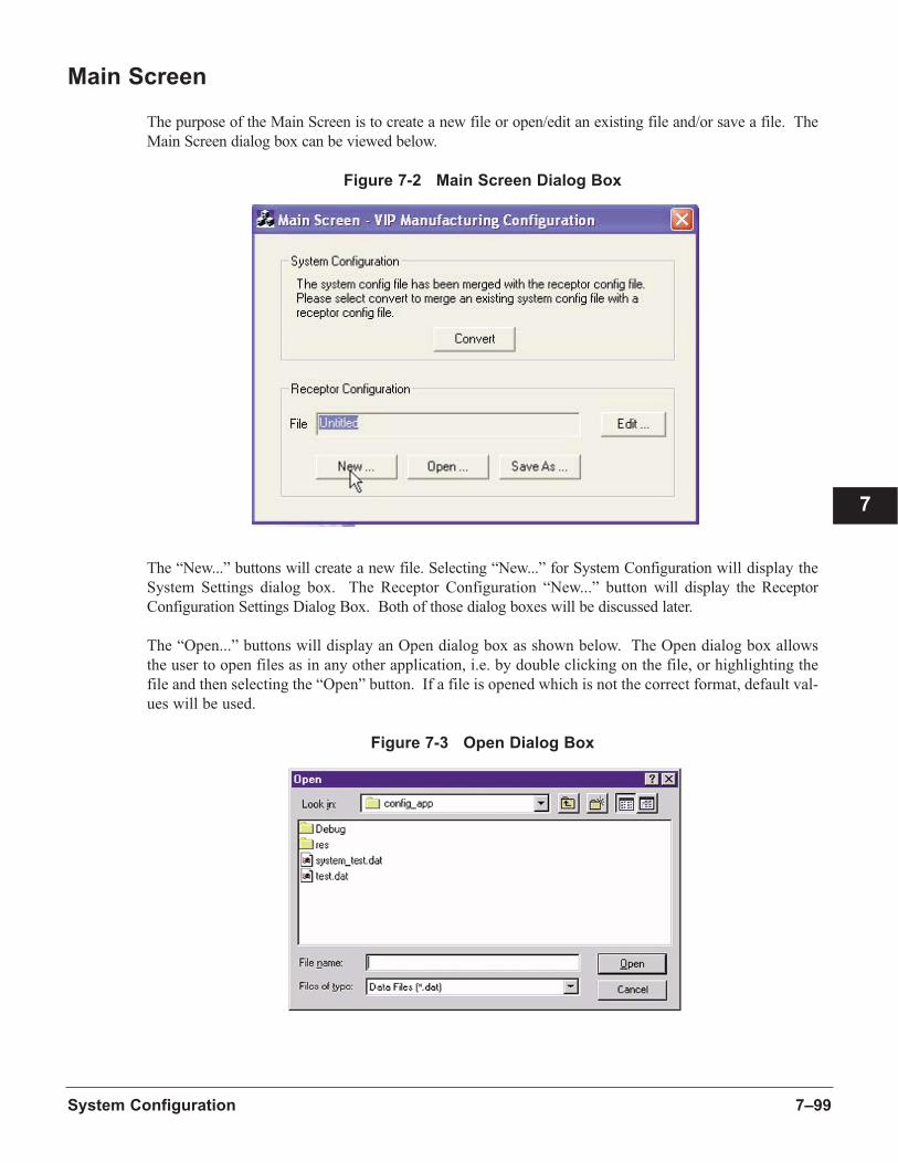
7–99System Configuration
Main Screen
The purpose of the Main Screen is to create a new file or open/edit an existing file and/or save a file. The
Main Screen dialog box can be viewed below.
Figure 7-2 Main Screen Dialog Box
The “New...” buttons will create a new file. Selecting “New...” for System Configuration will display the
System Settings dialog box. The Receptor Configuration “New...” button will display the Receptor
Configuration Settings Dialog Box. Both of those dialog boxes will be discussed later.
The “Open...” buttons will display an Open dialog box as shown below. The Open dialog box allows
the user to open files as in any other application, i.e. by double clicking on the file, or highlighting the
file and then selecting the “Open” button. If a file is opened which is not the correct format, default val-
ues will be used.
Figure 7-3 Open Dialog Box
7
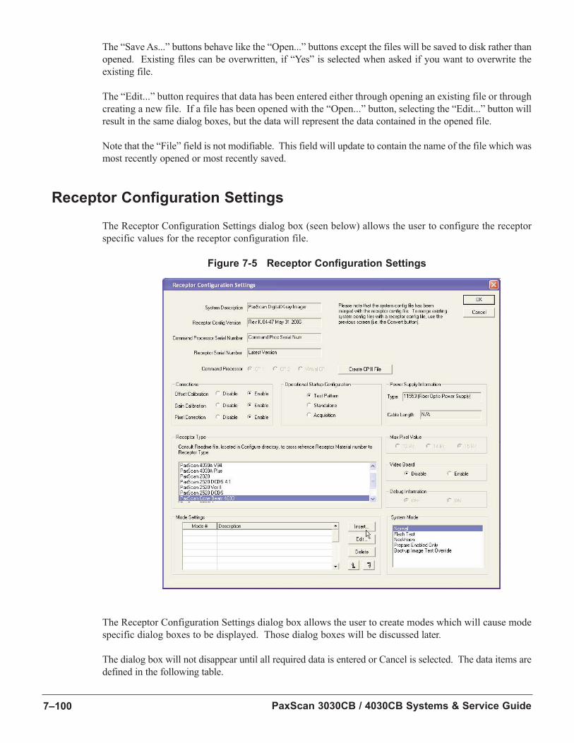
PaxScan 3030CB / 4030CB Systems & Service Guide7–100
The “Save As...” buttons behave like the “Open...” buttons except the files will be saved to disk rather than
opened. Existing files can be overwritten, if “Yes” is selected when asked if you want to overwrite the
existing file.
The “Edit...” button requires that data has been entered either through opening an existing file or through
creating a new file. If a file has been opened with the “Open...” button, selecting the “Edit...” button will
result in the same dialog boxes, but the data will represent the data contained in the opened file.
Note that the “File” field is not modifiable. This field will update to contain the name of the file which was
most recently opened or most recently saved.
Receptor Configuration Settings
The Receptor Configuration Settings dialog box (seen below) allows the user to configure the receptor
specific values for the receptor configuration file.
Figure 7-5 Receptor Configuration Settings
The Receptor Configuration Settings dialog box allows the user to create modes which will cause mode
specific dialog boxes to be displayed. Those dialog boxes will be discussed later.
The dialog box will not disappear until all required data is entered or Cancel is selected. The data items are
defined in the following table.
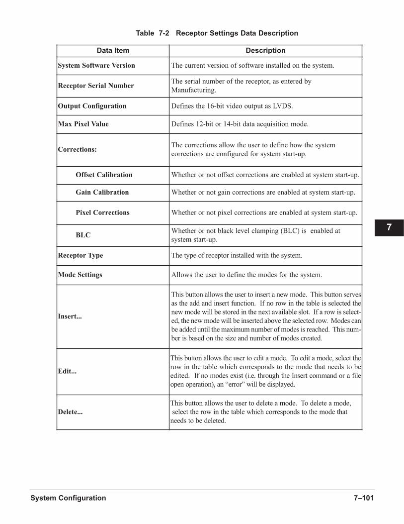
7–101System Configuration
Table 7-2 Receptor Settings Data Description
7
Data Item Description
System Software Version The current version of software installed on the system.
Receptor Serial NumberThe serial number of the receptor, as entered by
Manufacturing.
Output Configuration Defines the 16-bit video output as LVDS.
Max Pixel Value Defines 12-bit or 14-bit data acquisition mode.
Corrections:The corrections allow the user to define how the system
corrections are configured for system start-up.
Offset Calibration Whether or not offset corrections are enabled at system start-up.
Gain Calibration Whether or not gain corrections are enabled at system start-up.
Pixel Corrections Whether or not pixel corrections are enabled at system start-up.
BLCWhether or not black level clamping (BLC) is enabled at
system start-up.
Receptor Type The type of receptor installed with the system.
Mode Settings Allows the user to define the modes for the system.
Insert...
This button allows the user to insert a new mode. This button serves
as the add and insert function. If no row in the table is selected the
new mode will be stored in the next available slot. If a row is select-
ed, the new mode will be inserted above the selected row. Modes can
be added until the maximum number of modes is reached. This num-
ber is based on the size and number of modes created.
Edit...
This button allows the user to edit a mode. To edit a mode, select the
row in the table which corresponds to the mode that needs to be
edited. If no modes exist (i.e. through the Insert command or a file
open operation), an “error” will be displayed.
Delete...
This button allows the user to delete a mode. To delete a mode,
select the row in the table which corresponds to the mode that
needs to be deleted.
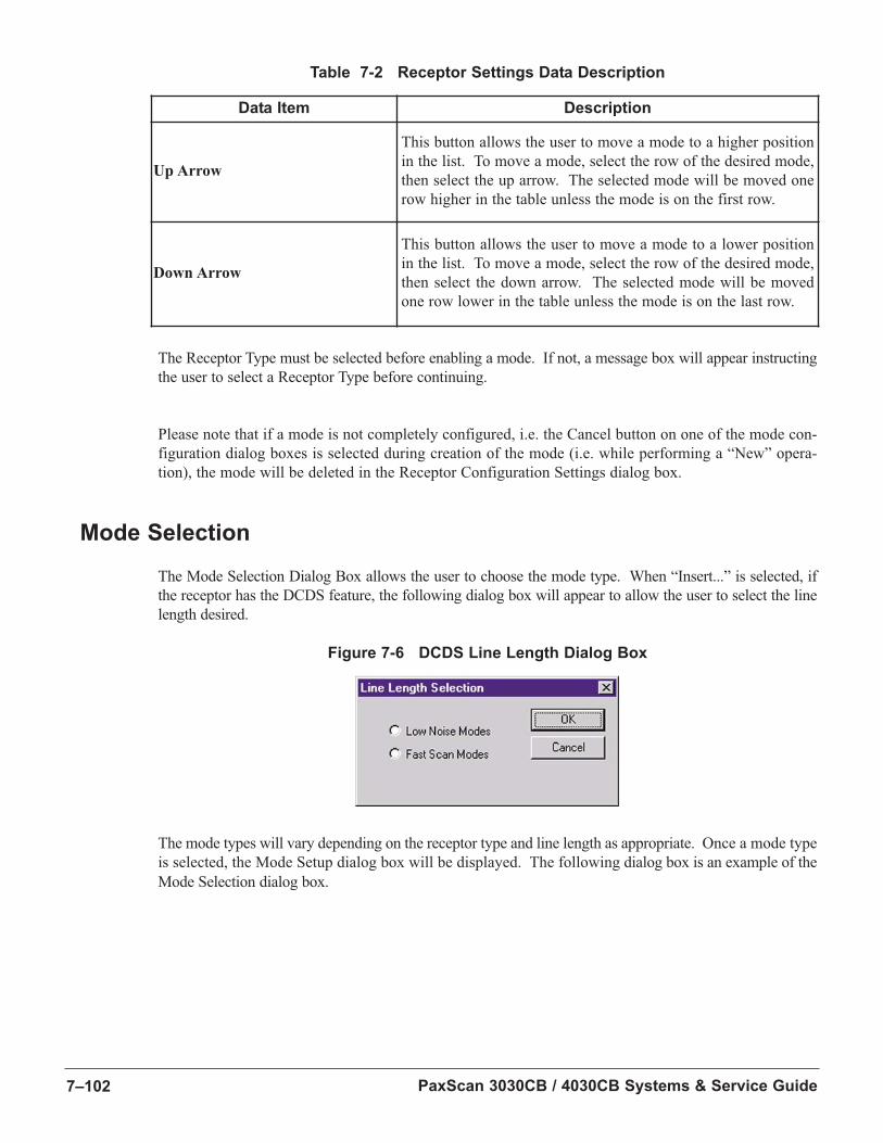
PaxScan 3030CB / 4030CB Systems & Service Guide7–102
Table 7-2 Receptor Settings Data Description
The Receptor Type must be selected before enabling a mode. If not, a message box will appear instructing
the user to select a Receptor Type before continuing.
Please note that if a mode is not completely configured, i.e. the Cancel button on one of the mode con-
figuration dialog boxes is selected during creation of the mode (i.e. while performing a “New” opera-
tion), the mode will be deleted in the Receptor Configuration Settings dialog box.
Mode Selection
The Mode Selection Dialog Box allows the user to choose the mode type. When “Insert...” is selected, if
the receptor has the DCDS feature, the following dialog box will appear to allow the user to select the line
length desired.
Figure 7-6 DCDS Line Length Dialog Box
The mode types will vary depending on the receptor type and line length as appropriate. Once a mode type
is selected, the Mode Setup dialog box will be displayed. The following dialog box is an example of the
Mode Selection dialog box.
Data Item Description
Up Arrow
This button allows the user to move a mode to a higher position
in the list. To move a mode, select the row of the desired mode,
then select the up arrow. The selected mode will be moved one
row higher in the table unless the mode is on the first row.
Down Arrow
This button allows the user to move a mode to a lower position
in the list. To move a mode, select the row of the desired mode,
then select the down arrow. The selected mode will be moved
one row lower in the table unless the mode is on the last row.
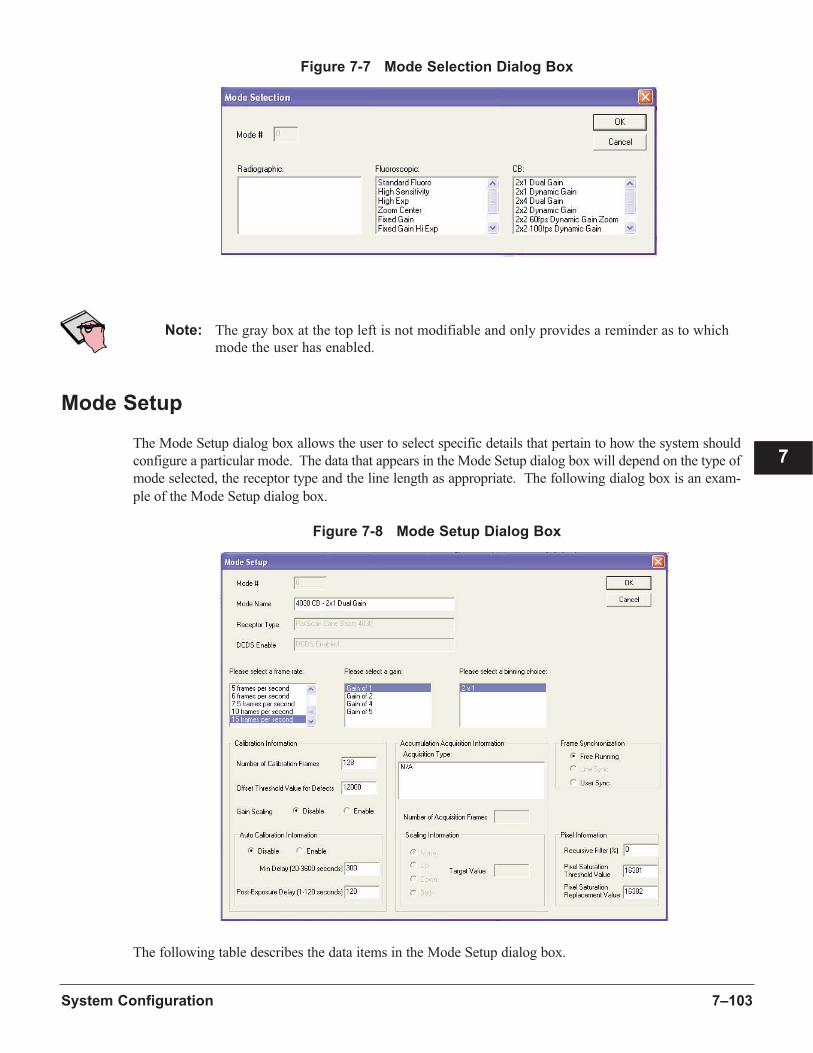
7–103System Configuration
7
Figure 7-7 Mode Selection Dialog Box
Note: The gray box at the top left is not modifiable and only provides a reminder as to which
mode the user has enabled.
Mode Setup
The Mode Setup dialog box allows the user to select specific details that pertain to how the system should
configure a particular mode. The data that appears in the Mode Setup dialog box will depend on the type of
mode selected, the receptor type and the line length as appropriate. The following dialog box is an exam-
ple of the Mode Setup dialog box.
Figure 7-8 Mode Setup Dialog Box
The following table describes the data items in the Mode Setup dialog box.
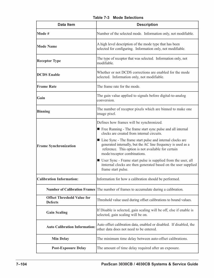
PaxScan 3030CB / 4030CB Systems & Service Guide7–104
Table 7-3 Mode Selections
Data Item Description
Mode # Number of the selected mode. Information only, not modifiable.
Mode NameA high level description of the mode type that has been
selected for configuring. Information only, not modifiable.
Receptor TypeThe type of receptor that was selected. Information only, not
modifiable.
DCDS EnableWhether or not DCDS corrections are enabled for the mode
selected. Information only, not modifiable.
Frame Rate The frame rate for the mode.
GainThe gain value applied to signals before digital-to-analog
conversion.
BinningThe number of receptor pixels which are binned to make one
image pixel.
Frame Synchronization
Defines how frames will be synchronized.
n Free Running - The frame start sync pulse and all internalclocks are created from internal circuits.
n Line Sync - The frame start pulse and internal clocks aregenerated internally, but the AC line frequency is used as a
reference. This option is not available for certain
mode/receptor combinations.
n User Sync - Frame start pulse is supplied from the user, all itnternal clocks are then generated based on the user supplied
frame start pulse.
Calibration Information: Information for how a calibration should be performed.
Number of Calibration Frames The number of frames to accumulate during a calibration.
Offset Threshold Value for
DefectsThreshold value used during offset calibrations to bound values.
Gain ScalingIf Disable is selected, gain scaling will be off, else if enable is
selected, gain scaling will be on.
Auto Calibration Information:Auto offset calibration data, enabled or disabled. If disabled, the
other data does not need to be entered.
Min Delay The minimum time delay between auto-offset calibrations.
Post-Exposure Delay The amount of time delay required after an exposure.
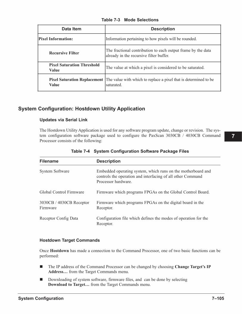
7–105System Configuration
7
Table 7-3 Mode Selections
System Configuration: Hostdown Utility Application
Updates via Serial Link
The Hostdown Utility Application is used for any software program update, change or revision. The sys-
tem configuration software package used to configure the PaxScan 3030CB / 4030CB Command
Processor consists of the following:
Table 7-4 System Configuration Software Package Files
Filename Description
System Software Embedded operating system, which runs on the motherboard and
controls the operation and interfacing of all other Command
Processor hardware.
Global Control Firmware Firmware which programs FPGAs on the Global Control Board.
3030CB / 4030CB Receptor Firmware which programs FPGAs on the digital board in the
Firmware Receptor.
Receptor Config Data Configuration file which defines the modes of operation for the
Receptor.
Hostdown Target Commands
Once Hostdown has made a connection to the Command Processor, one of two basic functions can be
performed:
n The IP address of the Command Processor can be changed by choosing Change Target’s IP
Address… from the Target Commands menu.
n Downloading of system software, firmware files, and can be done by selecting Download to Target… from the Target Commands menu.
Data Item Description
Pixel Information: Information pertaining to how pixels will be rounded.
Recursive FilterThe fractional contribution to each output frame by the data
already in the recursive filter buffer.
Pixel Saturation Threshold
ValueThe value at which a pixel is considered to be saturated.
Pixel Saturation Replacement
Value
The value with which to replace a pixel that is determined to be
saturated.

PaxScan 3030CB / 4030CB Systems & Service Guide7–106
Using the Download to Target command, the user can manually download any one of these files, or use
the Automated Download feature to download all the required files.
Note: Hostdown is also designed to support batch file downloading using the Auto Download
File Set feature shown in Figure 7-10.
There are several types of configuration files which reside permanently in the flash memory of the
Command Processor. The files listed above can be replaced by downloading new versions over a serial
link using the utility application hostdown.exe, by following these next steps.
1. Power Off the Command Processor.
2. Connect your computer COM port to the Command Processor’s serial 1 port.
3. On client computer, run the Hostdown.exe program located in the command_processor directory
in the PaxScan 3030CB / 4030CB Software release folder.
4. Click Hostdown. The following screen appears:
Figure 7-9 Hostdown Main Screen
5. From the menu bar choose Configure->Communications Port->COM X. COMX should be any
free COM port on the client computer.
6. Click Connect. The following window will appear:
7. Once this window appears, turn Command Processor power On. The following window will open
when a connection is established:
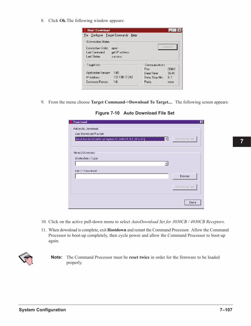
7–107System Configuration
7
8. Click Ok.The following window appears:
9. From the menu choose Target Command->Download To Target.... The following screen appears:
Figure 7-10 Auto Download File Set
10. Click on the active pull-down menu to select AutoDownload Set for 3030CB / 4030CB Receptors.
11. When download is complete, exit Hostdown and restart the Command Processor. Allow the Command
Processor to boot-up completely, then cycle power and allow the Command Processor to boot-up
again.
Note: The Command Processor must be reset twice in order for the firmware to be loaded
properly.

PaxScan 3030CB / 4030CB Systems & Service Guide7–108
System Configuration: ViVA Application
While the Hostdown Utility application may be used for any software upgrade, the ViVA application allows
upgrades without power cycling the Command Processor.
ViVA may be used as an engineering tool to modify small subsets of software files, or to change the
Receptor mode configuration from 15 to 30 frames per second for example. It is simply a matter of con-
venience. With the Hostdown Utility application, you must power down the Command Processor, and
power back up.
However, for ViVA to work properly the system must fully boot for ViVA to establish communication. If
the Command Processor doesn’t boot, then Hostdown must be used to download any files to flash.
Upgrades over the Ethernet Connection
The Command Processor uses flash memory to store various configuration files. Some of these files can
be updated through the ViVA software over the Ethernet connection. The following files can be updated
over the Ethernet Link:
n Receptor Configuration Data File
n Base Defect Image File (Defective Pixel Map)
n Gain Calibration File
n Offset Calibration File
n Firmware Files
n Configuration Files
The basic procedure for performing the update is very similar for each file. This example illustrates how
to download the Base Defect Image File.
1. Connect to the Command Processor with ViVA
2. From the ViVA menu bar, select Tools>CommandProcessor>Transmit Files. The following window
will open:
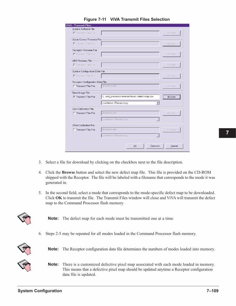
7–109System Configuration
7
Figure 7-11 ViVA Transmit Files Selection
3. Select a file for download by clicking on the checkbox next to the file description.
4. Click the Browse button and select the new defect map file. This file is provided on the CD-ROM
shipped with the Receptor. The file will be labeled with a filename that corresponds to the mode it was
generated in.
5. In the second field, select a mode that corresponds to the mode-specific defect map to be downloaded.
Click OK to transmit the file. The Transmit Files window will close and ViVA will transmit the defect
map to the Command Processor flash memory.
Note: The defect map for each mode must be transmitted one at a time.
6. Steps 2-5 may be repeated for all modes loaded in the Command Processor flash memory.
Note: The Receptor configuration data file determines the numbers of modes loaded into memory.
Note: There is a customized defective pixel map associated with each mode loaded in memory.
This means that a defective pixel map should be updated anytime a Receptor configuration
data file is updated.

PaxScan 3030CB / 4030CB Systems & Service Guide7–110
8–111
8
Chapter 8 Command Processor Hardware Specifications
This section outlines the hardware specifications needed to operate the PaxScan 3030CB / 4030CB imag-
ing system.
In This Chapter
Topic Page
Hardware Components 8-111
Command Processor Hardware Configuration 8-112
Pulsed X-ray Beam Applications 8-124
Internal Power Supply Specifications 8-124
Command Processor Specifications 8-126
Hardware Components
The PaxScan 3030CB / 4030CB digital imaging system consists of the following components:
n Receptor
n Command Processor
¨ external synchronization
¨ 16-bit video
¨ Fiber Optic Link (Receptor)
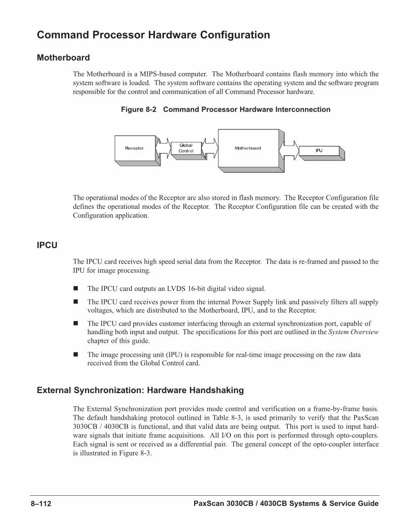
PaxScan 3030CB / 4030CB Systems & Service Guide8–112
Command Processor Hardware Configuration
Motherboard
The Motherboard is a MIPS-based computer. The Motherboard contains flash memory into which the
system software is loaded. The system software contains the operating system and the software program
responsible for the control and communication of all Command Processor hardware.
Figure 8-2 Command Processor Hardware Interconnection
The operational modes of the Receptor are also stored in flash memory. The Receptor Configuration file
defines the operational modes of the Receptor. The Receptor Configuration file can be created with the
Configuration application.
IPCU
The IPCU card receives high speed serial data from the Receptor. The data is re-framed and passed to the
IPU for image processing.
n The IPCU card outputs an LVDS 16-bit digital video signal.
n The IPCU card receives power from the internal Power Supply link and passively filters all supply voltages, which are distributed to the Motherboard, IPU, and to the Receptor.
n The IPCU card provides customer interfacing through an external synchronization port, capable of handling both input and output. The specifications for this port are outlined in the System Overviewchapter of this guide.
n The image processing unit (IPU) is responsible for real-time image processing on the raw data received from the Global Control card.
External Synchronization: Hardware Handshaking
The External Synchronization port provides mode control and verification on a frame-by-frame basis.
The default handshaking protocol outlined in Table 8-3, is used primarily to verify that the PaxScan
3030CB / 4030CB is functional, and that valid data are being output. This port is used to input hard-
ware signals that initiate frame acquisitions. All I/O on this port is performed through opto-couplers.
Each signal is sent or received as a differential pair. The general concept of the opto-coupler interface
is illustrated in Figure 8-3.
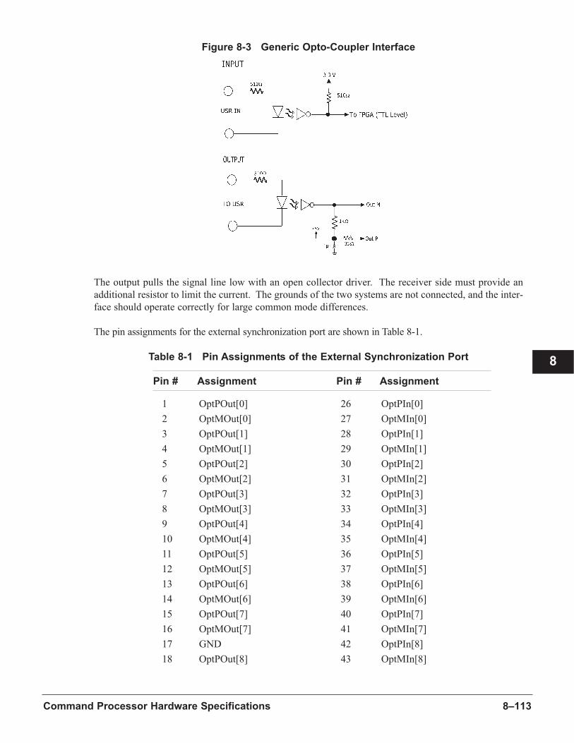
8–113Command Processor Hardware Specifications
8
Figure 8-3 Generic Opto-Coupler Interface
The output pulls the signal line low with an open collector driver. The receiver side must provide an
additional resistor to limit the current. The grounds of the two systems are not connected, and the inter-
face should operate correctly for large common mode differences.
The pin assignments for the external synchronization port are shown in Table 8-1.
Table 8-1 Pin Assignments of the External Synchronization Port
Pin # Assignment Pin # Assignment
1 OptPOut[0] 26 OptPIn[0]
2 OptMOut[0] 27 OptMIn[0]
3 OptPOut[1] 28 OptPIn[1]
4 OptMOut[1] 29 OptMIn[1]
5 OptPOut[2] 30 OptPIn[2]
6 OptMOut[2] 31 OptMIn[2]
7 OptPOut[3] 32 OptPIn[3]
8 OptMOut[3] 33 OptMIn[3]
9 OptPOut[4] 34 OptPIn[4]
10 OptMOut[4] 35 OptMIn[4]
11 OptPOut[5] 36 OptPIn[5]
12 OptMOut[5] 37 OptMIn[5]
13 OptPOut[6] 38 OptPIn[6]
14 OptMOut[6] 39 OptMIn[6]
15 OptPOut[7] 40 OptPIn[7]
16 OptMOut[7] 41 OptMIn[7]
17 GND 42 OptPIn[8]
18 OptPOut[8] 43 OptMIn[8]
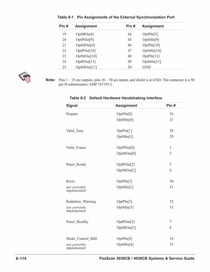
PaxScan 3030CB / 4030CB Systems & Service Guide8–114
Table 8-1 Pin Assignments of the External Synchronization Port
Pin # Assignment Pin # Assignment
19 OptMOut8] 44 OptPIn[9]
20 OptPOut[9] 45 OptMIn[9]
21 OptMOut[9] 46 OptPIn[10]
22 OptPOut[10] 47 OptMIn[10]
23 OptMOut[10] 48 OptPIn[11]
24 OptPOut[11] 49 OptMIn[11]
25 OptMOut[11] 50 GND
Note: Pins 1 – 25 are outputs, pins 26 – 50 are inputs, and shield is at GND. The connector is a 50
pin D-subminiature, AMP 747193-2.
Table 8-2 Default Hardware Handshaking Interface
Signal Assignment Pin #
Prepare OptPIn[0] 26
OptMIn[0] 27
Valid_Xray OptPin[1] 28
OptMin[1] 29
Valid_Frame OptPOut[0] 1
OptMOut[0] 2
Panel_Ready OptPOut[2] 5
OptMOut[2] 6
Reset OptPIn[2] 30
not currently OptMIn[2] 31implemented
Radiation_Warning OptPIn[3] 32
not currently OptMIn[3] 33implemented
Panel_Healthy OptPOut[3] 7
OptMOut[3] 8
Mode_Control_Bit0 OptPIn[4] 34
not currently OptMIn[4] 35implemented
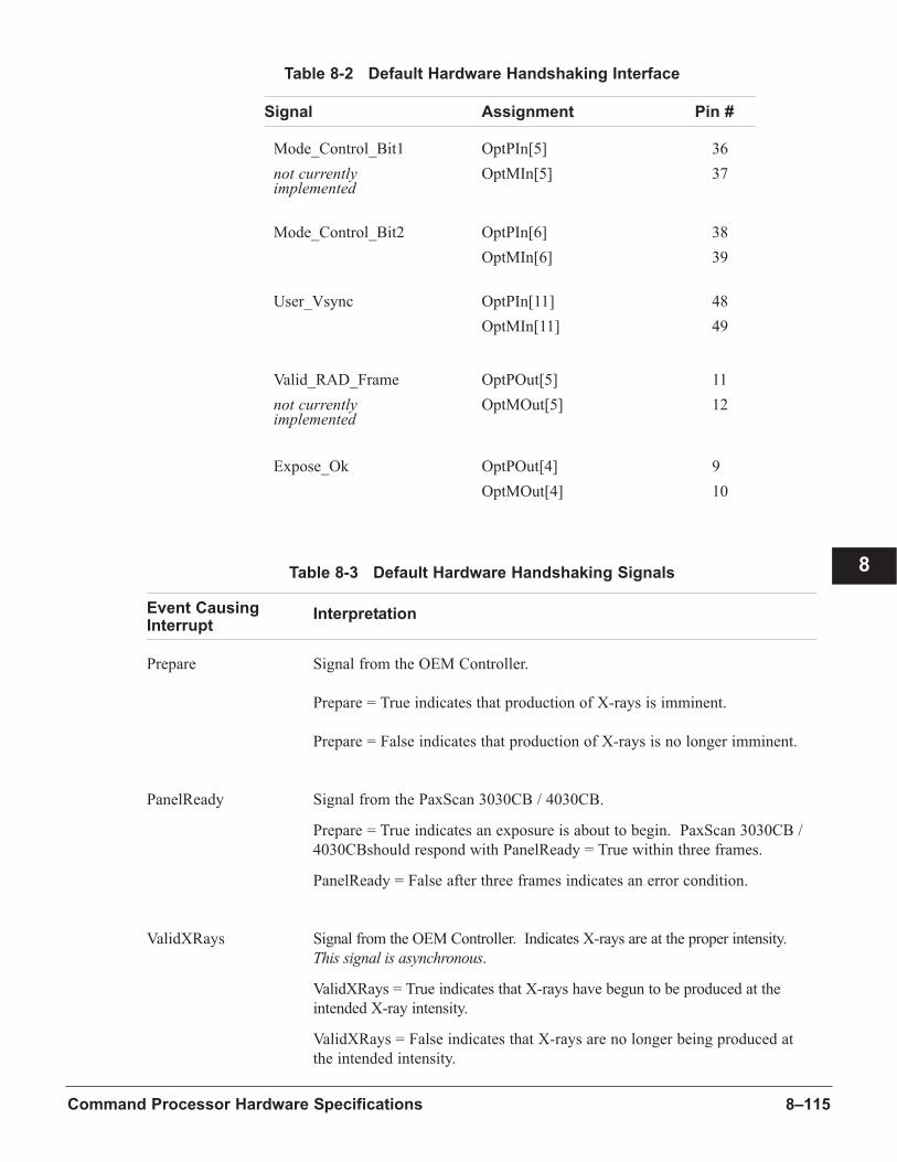
8–115Command Processor Hardware Specifications
8
Table 8-2 Default Hardware Handshaking Interface
Signal Assignment Pin #
Mode_Control_Bit1 OptPIn[5] 36
not currently OptMIn[5] 37implemented
Mode_Control_Bit2 OptPIn[6] 38
OptMIn[6] 39
User_Vsync OptPIn[11] 48
OptMIn[11] 49
Valid_RAD_Frame OptPOut[5] 11
not currently OptMOut[5] 12implemented
Expose_Ok OptPOut[4] 9
OptMOut[4] 10
Table 8-3 Default Hardware Handshaking Signals
Event Causing InterpretationInterrupt
Prepare Signal from the OEM Controller.
Prepare = True indicates that production of X-rays is imminent.
Prepare = False indicates that production of X-rays is no longer imminent.
PanelReady Signal from the PaxScan 3030CB / 4030CB.
Prepare = True indicates an exposure is about to begin. PaxScan 3030CB /
4030CBshould respond with PanelReady = True within three frames.
PanelReady = False after three frames indicates an error condition.
ValidXRays Signal from the OEM Controller. Indicates X-rays are at the proper intensity.
This signal is asynchronous.
ValidXRays = True indicates that X-rays have begun to be produced at the
intended X-ray intensity.
ValidXRays = False indicates that X-rays are no longer being produced at
the intended intensity.

PaxScan 3030CB / 4030CB Systems & Service Guide8–116
Table 8-3 Default Hardware Handshaking Signals
Event Causing InterpretationInterrupt
PanelHealthy A signal from the PaxScan 3030CB / 4030CB.
PanelHealthy = True indicates normal functioning. This signal should be
true within 30 seconds after startup.
ValidRADFrame Signal from the PaxScan 3030CB / 4030CB.
not currently ValidRADFrame = True indicates the radiographic acquisition has been
implemented fully processed and is currently being displayed on the 16-bit video port.
Expose_Ok An active low signal from the PaxScan 3030CB / 4030CB.
Expose_Ok = True notifies the OEM X-ray generator it is safe to deliver
pulsed X-rays.
ValidFrame Indicates the preceding frame has been fully exposed.
If a frame, N, has been read by the PaxScan 3030CB / 4030CB, where
ValidXrays = True during the entire preceding frame period, N-1, as well
as during the entire period in which the frame was read, then the PaxScan
3030CB / 4030CB will tag this frame as fully exposed with
ValidFrame = True.
If a frame is fully exposed, ValidFrame will be True during the first
Vblank succeeding this frame.
If a frame is only partially exposed, or not exposed at all, ValidFrame will
be False during the first Vblank succeeding this frame.
Note: Due to the nature of the flat panel, a frame must be exposed to
valid X-rays for at least two frame periods, and read out during
the second frame period, in order to be a fully exposed frame (one
capable of being tagged with the ValidFrame = True signal)
n The ValidFrame signal will not toggle during the Vblank period.
The PaxScan 3030CB / 4030CB will stay in active fluoroscopic mode as long
as Prepare = True, independent of the ValidXray/ ValidFrame signals.
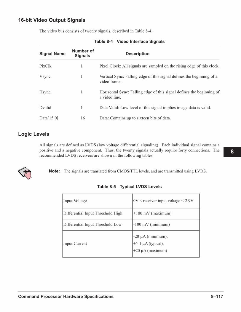
8–117Command Processor Hardware Specifications
8
16-bit Video Output Signals
The video bus consists of twenty signals, described in Table 8-4.
Table 8-4 Video Interface Signals
Number ofSignal Name DescriptionSignals
PixClk 1 Pixel Clock: All signals are sampled on the rising edge of this clock.
Vsync 1 Vertical Sync: Falling edge of this signal defines the beginning of a
video frame.
Hsync 1 Horizontal Sync: Falling edge of this signal defines the beginning of
a video line.
Dvalid 1 Data Valid: Low level of this signal implies image data is valid.
Data[15:0] 16 Data: Contains up to sixteen bits of data.
Logic Levels
All signals are defined as LVDS (low voltage differential signaling). Each individual signal contains a
positive and a negative component. Thus, the twenty signals actually require forty connections. The
recommended LVDS receivers are shown in the following tables.
Note: The signals are translated from CMOS/TTL levels, and are transmitted using LVDS.
Table 8-5 Typical LVDS Levels
Input Voltage 0V < receiver input voltage < 2.9V
Differential Input Threshold High +100 mV (maximum)
Differential Input Threshold Low -100 mV (minimum)
Input Current
-20 µA (minimum),
+/- 1 µA (typical),
+20 µA (maximum)
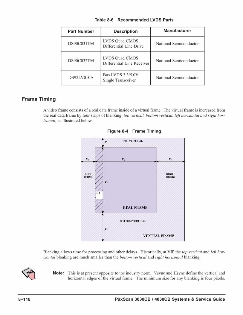
PaxScan 3030CB / 4030CB Systems & Service Guide8–118
Table 8-6 Recommended LVDS Parts
Frame Timing
A video frame consists of a real data frame inside of a virtual frame. The virtual frame is increased from
the real data frame by four strips of blanking: top vertical, bottom vertical, left horizontal and right hor-izontal, as illustrated below.
Figure 8-4 Frame Timing
Blanking allows time for processing and other delays. Historically, at VIP the top vertical and left hor-izontal blanking are much smaller than the bottom vertical and right horizontal blanking.
Note: This is at present opposite to the industry norm. Vsync and Hsync define the vertical and
horizontal edges of the virtual frame. The minimum size for any blanking is four pixels.
Part Number Description Manufacturer
DS90C031TMLVDS Quad CMOS
Differential Line DriveNational Semiconductor
DS90C032TMLVDS Quad CMOS
Differential Line ReceiverNational Semiconductor
DS92LV010ABus LVDS 3.3/5.0V
Single TransceiverNational Semiconductor
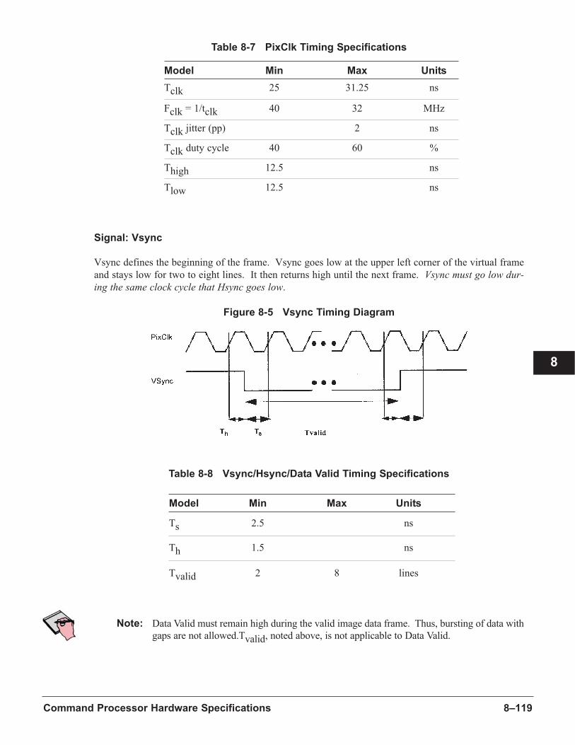
8–119Command Processor Hardware Specifications
8
Table 8-7 PixClk Timing Specifications
Model Min Max Units
Tclk 25 31.25 ns
Fclk = 1/tclk 40 32 MHz
Tclk jitter (pp) 2 ns
Tclk duty cycle 40 60 %
Thigh 12.5 ns
Tlow 12.5 ns
Signal: Vsync
Vsync defines the beginning of the frame. Vsync goes low at the upper left corner of the virtual frame
and stays low for two to eight lines. It then returns high until the next frame. Vsync must go low dur-ing the same clock cycle that Hsync goes low.
Figure 8-5 Vsync Timing Diagram
Table 8-8 Vsync/Hsync/Data Valid Timing Specifications
Model Min Max Units
Ts 2.5 ns
Th 1.5 ns
Tvalid 2 8 lines
Note: Data Valid must remain high during the valid image data frame. Thus, bursting of data with
gaps are not allowed.Tvalid, noted above, is not applicable to Data Valid.
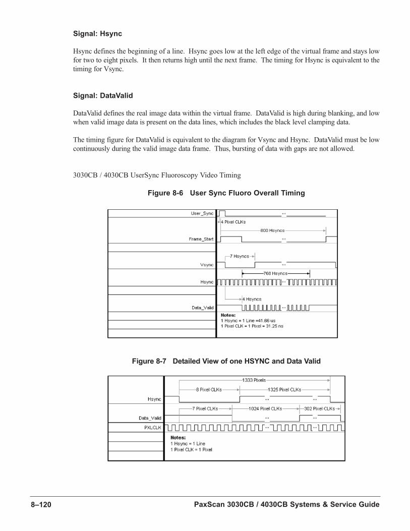
PaxScan 3030CB / 4030CB Systems & Service Guide8–120
Signal: Hsync
Hsync defines the beginning of a line. Hsync goes low at the left edge of the virtual frame and stays low
for two to eight pixels. It then returns high until the next frame. The timing for Hsync is equivalent to the
timing for Vsync.
Signal: DataValid
DataValid defines the real image data within the virtual frame. DataValid is high during blanking, and low
when valid image data is present on the data lines, which includes the black level clamping data.
The timing figure for DataValid is equivalent to the diagram for Vsync and Hsync. DataValid must be low
continuously during the valid image data frame. Thus, bursting of data with gaps are not allowed.
3030CB / 4030CB UserSync Fluoroscopy Video Timing
Figure 8-6 User Sync Fluoro Overall Timing
Figure 8-7 Detailed View of one HSYNC and Data Valid
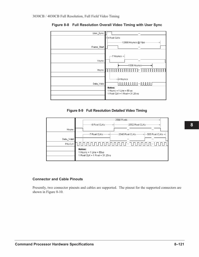
8–121Command Processor Hardware Specifications
8
3030CB / 4030CB Full Resolution, Full Field Video Timing
Figure 8-8 Full Resolution Overall Video Timing with User Sync
Figure 8-9 Full Resolution Detailed Video Timing
Connector and Cable Pinouts
Presently, two connector pinouts and cables are supported. The pinout for the supported connectors are
shown in Figure 8-10.
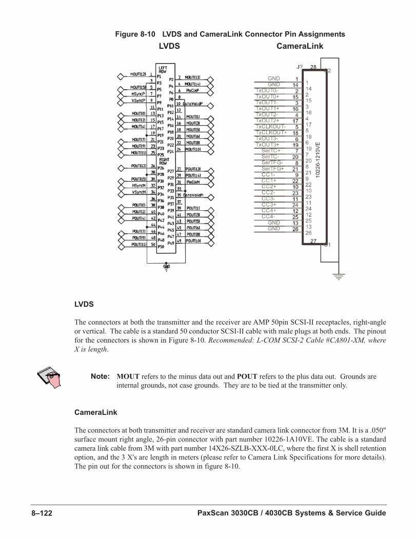
PaxScan 3030CB / 4030CB Systems & Service Guide8–122
Figure 8-10 LVDS and CameraLink Connector Pin Assignments
LVDS
The connectors at both the transmitter and the receiver are AMP 50pin SCSI-II receptacles, right-angle
or vertical. The cable is a standard 50 conductor SCSI-II cable with male plugs at both ends. The pinout
for the connectors is shown in Figure 8-10. Recommended: L-COM SCSI-2 Cable #CA801-XM, whereX is length.
Note: MOUT refers to the minus data out and POUT refers to the plus data out. Grounds are
internal grounds, not case grounds. They are to be tied at the transmitter only.
CameraLink
The connectors at both transmitter and receiver are standard camera link connector from 3M. It is a .050"
surface mount right angle, 26-pin connector with part number 10226-1A10VE. The cable is a standard
camera link cable from 3M with part number 14X26-SZLB-XXX-0LC, where the first X is shell retention
option, and the 3 X's are length in meters (please refer to Camera Link Specifications for more details).
The pin out for the connectors is shown in figure 8-10.
LVDS CameraLink
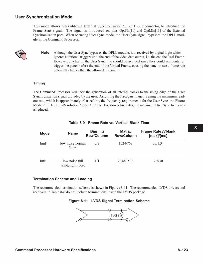
8–123Command Processor Hardware Specifications
8
User Synchronization Mode
This mode allows users utilizing External Synchronization 50 pin D-Sub connector, to introduce the
Frame Start signal. The signal is introduced on pins OptPIn[11] and OptMIn[11] of the External
Synchronization port. When operating User Sync mode, the User Sync signal bypasses the DPLL mod-
ule in the Command Processor.
Note: Although the User Sync bypasses the DPLL module, it is received by digital logic which
ignores additional triggers until the end of the video data output, i.e. the end the Real Frame.
However, glitches on the User Sync line should be avoided since they could accidentally
trigger the panel before the end of the Virtual Frame, causing the panel to see a frame rate
potentially higher than the allowed maximum.
Timing
The Command Processor will lock the generation of all internal clocks to the rising edge of the User
Synchronization signal provided by the user. Assuming the PaxScan imager is using the maximum read-
out rate, which is approximately 40 usec/line, the frequency requirements for the User Sync are: Fluoro
Mode < 30Hz; Full-Resolution Mode < 7.5 Hz. For slower line rates, the maximum User Sync frequency
is reduced.
Table 8-9 Frame Rate vs. Vertical Blank Time
Binning Matrix Frame Rate /VblankMode Name
Row/Column Row/Column [max]/[ms]
Innf low noise normal 2/2 1024/768 30/1.34
fluoro
Infr low noise full 1/1 2048/1536 7.5/30
resolution fluoro
Termination Scheme and Loading
The recommended termination scheme is shown in Figures 8-11. The recommended LVDS drivers and
receivers in Table 8-6 do not include terminations inside the LVDS package.
Figure 8-11 LVDS Signal Termination Scheme
100Ω
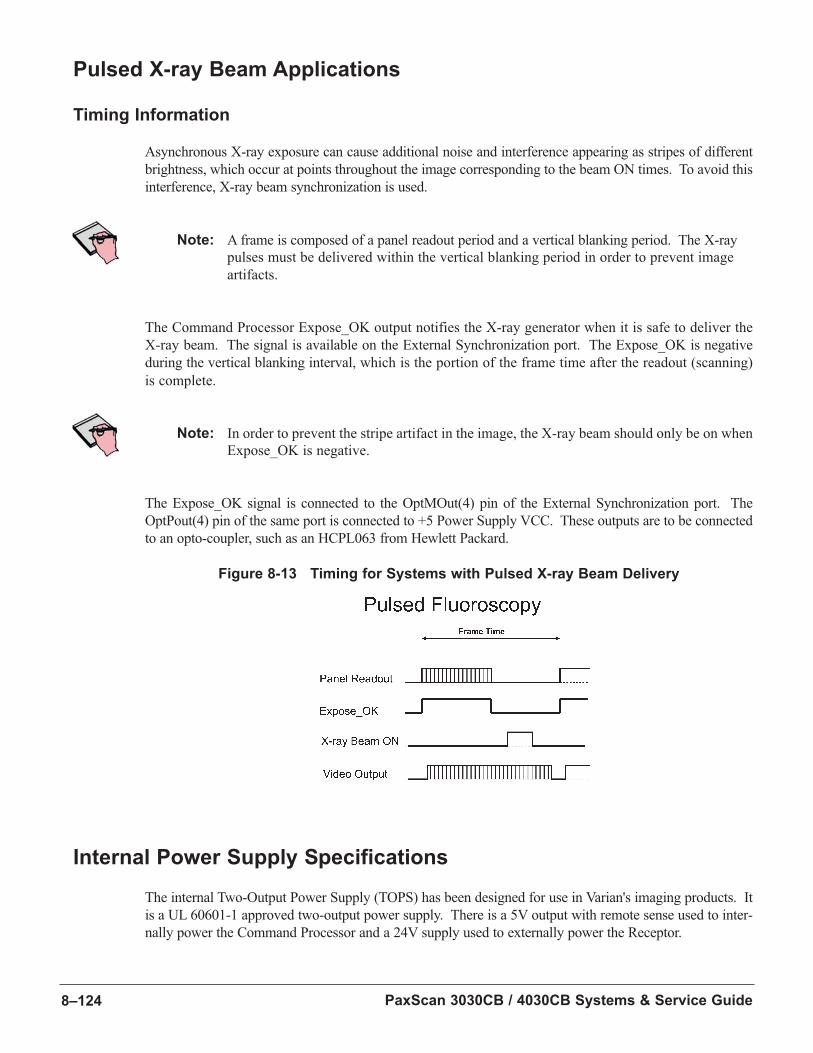
PaxScan 3030CB / 4030CB Systems & Service Guide8–124
Pulsed X-ray Beam Applications
Timing Information
Asynchronous X-ray exposure can cause additional noise and interference appearing as stripes of different
brightness, which occur at points throughout the image corresponding to the beam ON times. To avoid this
interference, X-ray beam synchronization is used.
Note: A frame is composed of a panel readout period and a vertical blanking period. The X-ray
pulses must be delivered within the vertical blanking period in order to prevent image
artifacts.
The Command Processor Expose_OK output notifies the X-ray generator when it is safe to deliver the
X-ray beam. The signal is available on the External Synchronization port. The Expose_OK is negative
during the vertical blanking interval, which is the portion of the frame time after the readout (scanning)
is complete.
Note: In order to prevent the stripe artifact in the image, the X-ray beam should only be on when
Expose_OK is negative.
The Expose_OK signal is connected to the OptMOut(4) pin of the External Synchronization port. The
OptPout(4) pin of the same port is connected to +5 Power Supply VCC. These outputs are to be connected
to an opto-coupler, such as an HCPL063 from Hewlett Packard.
Figure 8-13 Timing for Systems with Pulsed X-ray Beam Delivery
Internal Power Supply Specifications
The internal Two-Output Power Supply (TOPS) has been designed for use in Varian's imaging products. It
is a UL 60601-1 approved two-output power supply. There is a 5V output with remote sense used to inter-
nally power the Command Processor and a 24V supply used to externally power the Receptor.
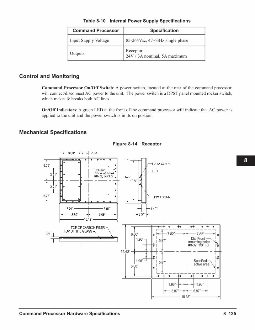
8–125Command Processor Hardware Specifications
8
Table 8-10 Internal Power Supply Specifications
Control and Monitoring
Command Processor On/Off Switch: A power switch, located at the rear of the command processor,
will connect/disconnect AC power to the unit. The power switch is a DPST panel mounted rocker switch,
which makes & breaks both AC lines.
On/Off Indicators: A green LED at the front of the command processor will indicate that AC power is
applied to the unit and the power switch is in its on postion.
Mechanical Specifications
Figure 8-14 Receptor
Command Processor Specification
Input Supply Voltage 85-264Vac, 47-63Hz single phase
OutputsReceptor:
24V / 3A nominal, 5A maximum
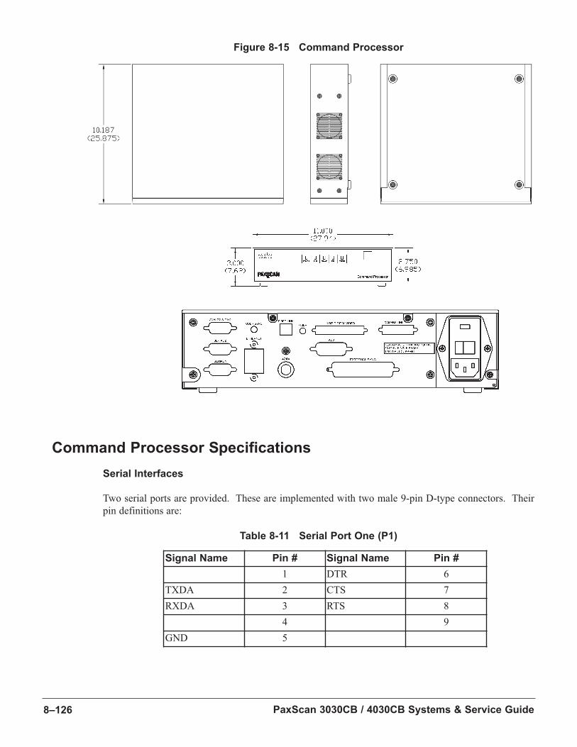
PaxScan 3030CB / 4030CB Systems & Service Guide8–126
Figure 8-15 Command Processor
Command Processor Specifications
Serial Interfaces
Two serial ports are provided. These are implemented with two male 9-pin D-type connectors. Their
pin definitions are:
Table 8-11 Serial Port One (P1)
Signal Name Pin # Signal Name Pin #
1 DTR 6
TXDA 2 CTS 7
RXDA 3 RTS 8
4 9
GND 5
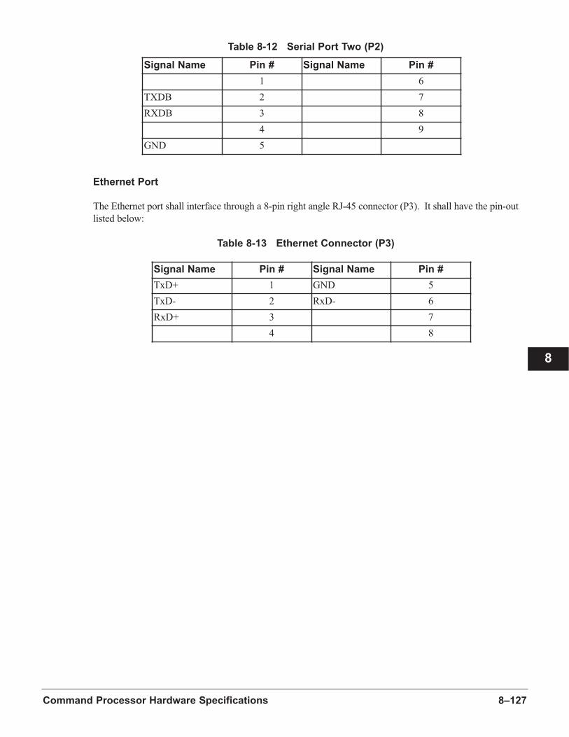
8–127Command Processor Hardware Specifications
8
Table 8-12 Serial Port Two (P2)
Ethernet Port
The Ethernet port shall interface through a 8-pin right angle RJ-45 connector (P3). It shall have the pin-out
listed below:
Table 8-13 Ethernet Connector (P3)
Signal Name Pin # Signal Name Pin #
1 6
TXDB 2 7
RXDB 3 8
4 9
GND 5
Signal Name Pin # Signal Name Pin #
TxD+ 1 GND 5
TxD- 2 RxD- 6
RxD+ 3 7
4 8

PaxScan 3030CB / 4030CB Systems & Service Guide8–128
9–129
Chapter 9 Safety
Receptor Module
WARNING: Precautions should be taken to not open the receptor module. Depending upon the type of
scintillator used, opening the receptor module may expose the user to potentially toxic
materials.
Receptor Mounting
The Receptor should be mounted onto other pieces of equipment using the holes provided in the
integral flange.
WARNING: The Receptor has an optional lead cap which can be used as a primary barrier to X-rays.
This barrier is only effective if the X-ray beam is collimated in such a way that X-rays
impinge on the active surface of the Receptor.
WARNING: If the Receptor is to be used as a primary barrier to X-rays, the X-rays must impinge on
only the entrance window of the Receptor. The optional lead cap will not stop X-rays that
do not hit the entrance window of the receptor.
CAUTION: The front surface of the Receptor is designed to be splash-proof, but the electrical connector
at the backside of the Receptor is not sealed against moisture.
9

PaxScan 3030CB / 4030CB Systems & Service Guide9–130
Command Processor
Rack Mounting the Command Processor
The Command Processor can be rack mounted in a standard 3U (5.2" high) slot using optional rack
mounting intended for a 19" wide rack. Optional sliding brackets are also available.
CAUTION: The following precautions should be observed when rack mounting the Command
Processor:
n Elevated operating ambient temperature: If installed in a closed or multi-unit rack assembly, the operating ambient temperature of the rack environment may be greater
than room ambient. Equipment should be installed in an environment compatible with
the maximum rated ambient temperature.
n Reduced air flow: Install the equipment so that the amount of air flow required for safe operation is not compromised.
n Mechanical loading: Mounting of the equipment in the rack should be loaded evenlyto avoid any hazardous conditions.
n Circuit overload: Consideration should be given to the connection to avoid overloadingof circuits on the over-current protection and supply wiring.
n Reliable grounding: Reliable grounding should be maintained, with particular attention given to the supply ground connection.
Environmental Conditions
Table 9-1 Environmental Conditions
Storage/Shipping Temperature -20°C to +70°C
Storage/Shipping Humidity 10% to 90%, non-condensing
Full-spec Operating Temperature (Measured at the
center of the back cover.)10 to 35°C
Operating Humidity (non-condensing) 10 to 90%
9–131Safety
Cooling Requirements
Important: The back surface temperature of the Receptor should not exceed 35ºC when the unit is
installed. This requirement may necessitate air flow over the back surface of the Receptor.
Important: Ambient air temperature should not exceed 40ºC for the Command Processor.
Important: The Command Processor do not have air filters, so the air should be free of dust and
particulates.
Important: Cooling air clearance requirements for the Command Processor are four inches minimum
from each surface.
WARNING: The unit must comply with those standards listed under each category to the levels detailed.
Assume the most stringent requirements prescribed by the standard if no levels are detailed.
WARNING: The PaxScan 3030CB / 4030CB is not classified for use in the presence of a flammable
anaesthetic mixture with air, or with oxygen or nitrous oxide.
CAUTION: The unit must comply with those standards listed under each category to the levels detailed.
If no levels are detailed, assume the most stringent requirements prescribed by the standard.
9

PaxScan 3030CB / 4030CB Systems & Service Guide9–132
Electro-Magnetic Compatibility
Under normal operating conditions, the imager will comply with IEC 60601-1-2.
Electro-Magnetic Interference
This equipment generates, uses and can radiate radio frequency energy and, if not installed and used in
accordance with the instructions, may cause harmful interference to other devices in the vicinity. However,
there is no guarantee that interference will not occur in a particular installation. If this equipment does cause
harmful interference to other devices, which can be determined by turning the equipment off and on, the user
is encouraged to try to correct the interference by one or more of the following measures listed in the
Troubleshooting section.
Electrical Shock protection
Class 1 Equipment per UL 60601-1
X-Ray Leakage with Pb barrier
Under normal operating conditions, no damage, and X-rays incident only on the active area: IEC 60601-1-3
Referenced Standard IEC 60601-1-2
EN61000-3-2 Class A
EN61000-3-3 Required
EN61000-4-2 +/- 6kV Contact, +/- 8kV Air
EN61000-4-3 80MHz-2.5GHz@3V/m
EN61000-4-4 +/-1kV@ I/O Cable, +/- 2kV @ PS
EN61000-4-5 +/-1kV DiffMode, +/-2kV ComMode
EN61000-4-6 150kHz - 80MHz @ 3Vrms
EN61000-4-11 Required

9–133Safety
9
Safety Agency Approvals
The imager willl comply with all of the following safety agency standards and be appropriately labeled:
US: UL 60601-1.
Canada: CSA 22.2 No. 601.1-M90.
Europe: IEC 60601-1-1.
CE marked.

PaxScan 3030CB / 4030CB Systems & Service Guide9–134
10–135Maintenance
Chapter 10 Maintenance
Preventative Maintenance
CAUTION: Substitution for any of the PaxScan components with units of a different type may cause
catastrophic damage to the PaxScan imaging system, and will degrade the minimum safety of
the PaxScan 3030CB / 4030CB.
No special preventative maintenance is required; however, prudent inspections should be carried out to
check for:
n Damaged and worn cables
n Signs of severe shock to the Receptor, lead cap, Command Processor
n Evidence that fans are clear and running
Calibration Schedule
Offset calibration is performed automatically during times when X-rays are not impinging on the
Receptor. Gain calibration needs to be performed with the assistance of an operator at regular intervals. If
the Offset calibration is controlled by the user, it should be performed as often as possible.
Note: It is recommended that Gain calibration be done at least monthly, and more often if image
quality degradation is observed. During Gain calibration, the map of defective pixels is
also updated.
Receptor Module
WARNING: Precautions should be taken to not open the receptor module. Depending upon the type of
scintillator used, opening the receptor module may expose the user to potentially toxic
materials.
10

PaxScan 3030CB / 4030CB Systems & Service Guide10–136
Repairs
Note: No user serviceable parts. If repairs are necessary, please contact the Varian Imaging
Products Service Center at 1.800.432.4422, or 1.801.972.5000.
The IEC receptacle fuses on the Command Processor are replaceable by Varian service personnel. These
fuses are identified by a label near the IEC receptacle, and must be replaced with the exact size and type
called out on the label.
The least replaceable units (LRU) are:
n Receptor Assembly
n Command Processor Assembly
n Receptor Power Cable
n Receptor Fiber Optic Cable
n Command Processor Power Cable
Cleaning, Disinfection and Sterilization
The Receptor is the only component that is likely to be in the area of a patient. Although this component
is not intended to come in contact with the patient, it is possible for the patient or user to touch the
Receptor face.
The material most likely to come in contact with the patient is X-ray grade carbon fiber in a cast aluminum
frame. The Receptor is not sealed against moisture.
Cleaning, disinfection and sterilization of the input window should be accomplished as needed, but
cleaning of the input window should be accomplished at a minimum of one month intervals. Proper
disinfection and sterilization requires that a disinfectant/sterilization solution be used. Wiping the sur-
faces with a soft cloth dampened with soap and water will generally clean the surfaces.
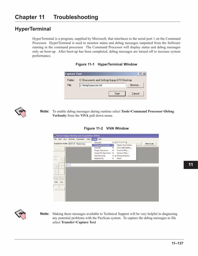
11–137
Chapter 11 Troubleshooting
HyperTerminal
HyperTerminal is a program, supplied by Microsoft, that interfaces to the serial port 1 on the Command
Processor. HyperTerminal is used to monitor status and debug messages outputted from the Software
running in the command processor. The Command Processor will display status and debug messages
only on boot-up. After boot-up has been completed, debug messages are turned off to increase system
performance.
Figure 11-1 HyperTerminal Window
Note: To enable debug messages during runtime select Tools>Command Processor>Debug
Verbosity from the ViVA pull down menu.
Figure 11-2 ViVA Window
Note: Making these messages available to Technical Support will be very helpful in diagnosing
any potential problems with the PaxScan system. To capture the debug messages to file
select Transfer>Capture Text
11

PaxScan 3030CB / 4030CB Systems & Service Guide11–138
Then enter a path and filename.
The COM port should be configured as follows:
Figure 11-3 Com Port Configuration
Note: HyperTerminal must be closed when attempting to use Hostdown. This is because both
programs access the same COM port for communication with the Command Processor.

11–139Troubleshooting
Problems and SolutionsTable 11-1 Troubleshooting
Problem Solution
Imager fails to respond. 1. Check the power and then Restart.
2. Check fuse and cables.
Imager causes 1.Reorient or relocate the receiving device. Electro-MagneticInterference 2.Increase the separation between the equipment.
3.Connect the equipment into an outlet on a curcuit different from that to which the other device (s) are connected.
4. Consult the manufacturer or field service technician for help.
Bad Pixel Correction fails. 1. Repeat measurement.
2. Re-acquire gain and offset images.
3. Assure that the acquired Light and MidField images fill the field of view and that the exposures are appropriate for Light and MidField images.
Software hangs up. Make sure the Power Supply module is switched On and the data cable to the PC is properly connected. If External Frame time was selected, make sure the input signal is generated.
Acquired image is Increase the frame time and acquire a new image. If the imagecompletely dark. is still dark, verify that the cables from the Power Supply to
the Receptor, and from the Receptor to the computer are properly connected. Turn the power Off and On. Acquire a new image.
Out of virtual memory. Close some of the windows that are currently open.
Residual X-ray image from Charge on the sensor pixels from a super saturated exposure may previous scan shows in cause a residual image. It can be erased by taking a scan or current scan. multiple scans without X-rays until the residual image is gone.
11

PaxScan 3030CB / 4030CB Systems & Service Guide11–140
12–141
12
Chapter 12 Technical Support
How To Reach Us
In order to provide you with the most comprehensive technical support, (hardware or software), please
complete the following problem report before contacting PaxScan technical support personnel.
If you prefer e-mailing the information to us, a .pdf version of this form is included on the CD ROM you
received with your system. You may also fax a completed copy of the problem report printed on the fol-
lowing page.
n To speak with our technical support personnel, call (800) 432-4422 or (801) 972-5000.
n E-mail the report to [email protected], then call the above number.
n Fax a copy of the Problem Report to (801) 973-5023.

PaxScan 3030CB / 4030CB Problem Report
Customer Information
Date: Your Name:
Company Name: Phone:
E-mail: Fax:
Product Information
PaxScan Part Number: Receptor Serial Number:
Software Revision #:
Operation I was trying to perform (be as specific as possible):
What happened (use additional sheets as necessary):
Fax this report to: (801) 973-5023 or e-mail [email protected].
PaxScan 3030CB / 4030CB Systems & Service Guide12–142

A–143
Appendix A Glossary
Aliasing Interference patterns produced by the interaction of high spatial requency information in the
image with the pixel matrix.
Amorphous Silicon Silicon that is deposited from vapor to form a thin, non-crystalline film. Common integrated
a-Si circuits are made from crystalline silicon wafers sliced from grown crystals. Amorphous
silicon devices can be much larger in area than the crystalline variety because no single
crystal is needed. Amorphous silicon is ideal for X-ray detectors because it is nearly immune
to radiation damage. For use in imaging devices, amorphous silicon is permeated with
hydrogen (a-Si:H) and diffused with P and N dopants to provide device junctions.
Cesium Iodide The most efficient scintillator in the diagnostic X-ray energy band. Cesium iodide has both high
X-ray absorption and high visible photon yield. The sodium-doped version (CsI:Na) produces
blue light and is used with photocathodes in nuclear particle detectors and X-ray image
intensifier tubes while the thallium-doped type (CsI:Tl) is used with silicon detectors because
it produces green light. CsI:Na is strongly hygroscopic and deliquescent and generally
unusable outside controlled environments. CsI:Tl is moderately hygroscopic but easily
protected making it suitable for use in air. For imaging, both types are grown in the form of
densely packed thin columns to provide a fiber-optic, light-guiding effect for improved
resolution.
Client or Client Refers to the OEM computer.
Computer
Contrast Transfer A measure of the ability of an imaging device to accurately reproduce patterns consisting
Function (CTF) of alternating dark and light bars of various widths. These bar patterns are calibrated in line
pairs (one black and one white bar of equal width together) per millimeter (lp/mm), called
spatial frequency. The difference between the maximum signal in the white bar and the
minimum signal in the black at several spatial frequencies divided by the difference when very
wide bars are used is plotted against the spatial frequency. The curve is the contrast transfer
function.
Correction May refer to offset, gain, defective pixel or digital line noise reduction. All are selectable
from the ViVA pulldown menu under Acquisition->Mode Settings.
Dark Current Signal resulting from leakage in the devices making up the sensor pixels.
Dark Field An image taken "in the dark;" no X-rays.
Detective Quantum A measure of the ability of an imaging device to convert an incoming image to an electrical
Efficiency signal without adding noise. Precisely, it is the square of the ratio of the outgoing signal-
to-noise (SNR) in the electrical signal divided by the incoming SNR in the X-ray signal. DQE
usually varies with spatial frequency because the shape of the noise spectrum almost always
differs from the shape of the modulation transfer function.
A
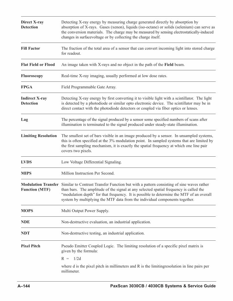
PaxScan 3030CB / 4030CB Systems & Service GuideA–144
Direct X-ray Detecting X-ray energy by measuring charge generated directly by absorption by
Detection absorption of X-rays. Gases (xenon), liquids (iso-octane) or solids (selenium) can serve as
the conversion materials. The charge may be measured by sensing electrostatically-induced
changes in surfacevoltage or by collecting the charge itself.
Fill Factor The fraction of the total area of a sensor that can convert incoming light into stored charge
for readout.
Flat Field or Flood An image taken with X-rays and no object in the path of the Field beam.
Fluoroscopy Real-time X-ray imaging, usually performed at low dose rates.
FPGA Field Programmable Gate Array.
Indirect X-ray Detecting X-ray energy by first converting it to visible light with a scintillator. The light
Detection is detected by a photodiode or similar opto electronic device. The scintillator may be in
direct contact with the photodiode detectors or coupled via fiber optics or lenses.
Lag The percentage of the signal produced by a sensor some specified numbers of scans after
illumination is terminated to the signal produced under steady-state illumination.
Limiting Resolution The smallest set of bars visible in an image produced by a sensor. In unsampled systems,
this is often specified at the 3% modulation point. In sampled systems that are limited by
the first sampling mechanism, it is exactly the spatial frequency at which one line pair
covers two pixels.
LVDS Low Voltage Differential Signaling.
MIPS Million Instruction Per Second.
Modulation Transfer Similar to Contrast Transfer Function but with a pattern consisting of sine waves rather
Function (MTF) than bars. The amplitude of the signal at any selected spatial frequency is called the
“modulation depth” for that frequency. It is possible to determine the MTF of an overall
system by multiplying the MTF data from the individual components together.
MOPS Multi Output Power Supply.
NDE Non-destructive evaluation, an industrial application.
NDT Non-destructive testing, an industrial application.
Pixel Pitch Pseudo Emitter Coupled Logic. The limiting resolution of a specific pixel matrix is
given by the formula:
R = 1/2d
where d is the pixel pitch in millimeters and R is the limitingresolution in line pairs per
millimeter.
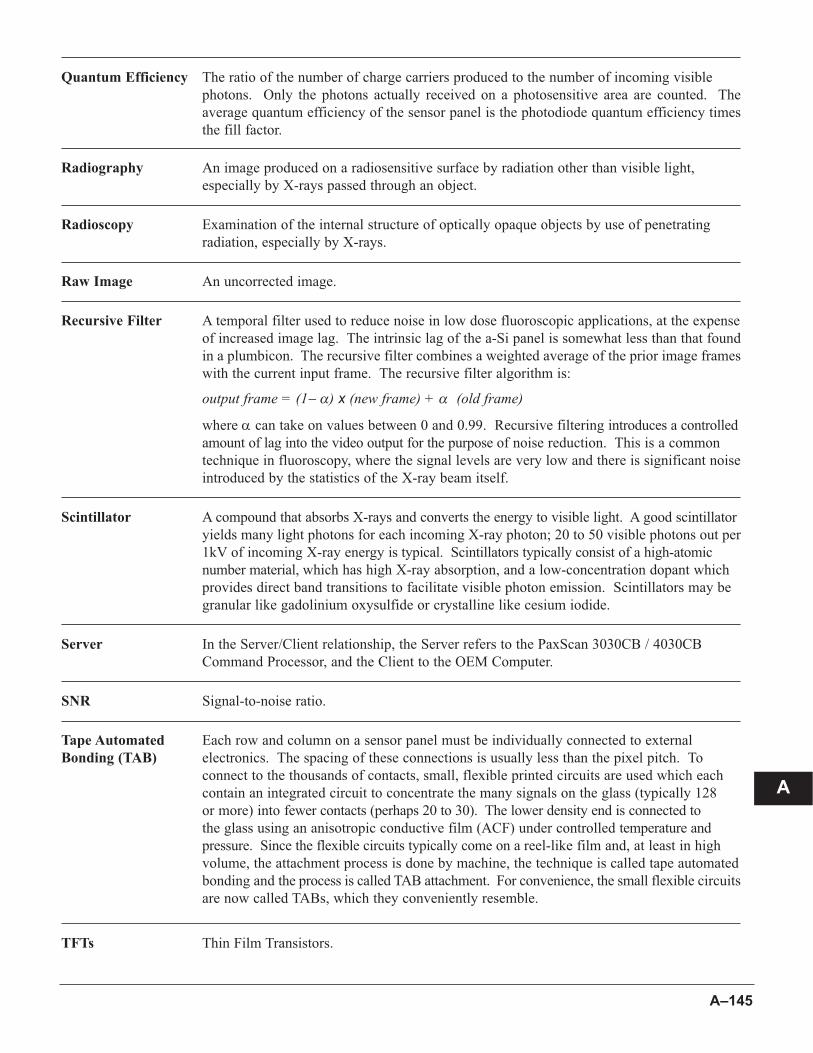
A–145
Quantum Efficiency The ratio of the number of charge carriers produced to the number of incoming visible
photons. Only the photons actually received on a photosensitive area are counted. The
average quantum efficiency of the sensor panel is the photodiode quantum efficiency times
the fill factor.
Radiography An image produced on a radiosensitive surface by radiation other than visible light,
especially by X-rays passed through an object.
Radioscopy Examination of the internal structure of optically opaque objects by use of penetrating
radiation, especially by X-rays.
Raw Image An uncorrected image.
Recursive Filter A temporal filter used to reduce noise in low dose fluoroscopic applications, at the expense
of increased image lag. The intrinsic lag of the a-Si panel is somewhat less than that found
in a plumbicon. The recursive filter combines a weighted average of the prior image frames
with the current input frame. The recursive filter algorithm is:
output frame = (1− α) x (new frame) + α (old frame)
where α can take on values between 0 and 0.99. Recursive filtering introduces a controlled
amount of lag into the video output for the purpose of noise reduction. This is a common
technique in fluoroscopy, where the signal levels are very low and there is significant noise
introduced by the statistics of the X-ray beam itself.
Scintillator A compound that absorbs X-rays and converts the energy to visible light. A good scintillator
yields many light photons for each incoming X-ray photon; 20 to 50 visible photons out per
1kV of incoming X-ray energy is typical. Scintillators typically consist of a high-atomic
number material, which has high X-ray absorption, and a low-concentration dopant which
provides direct band transitions to facilitate visible photon emission. Scintillators may be
granular like gadolinium oxysulfide or crystalline like cesium iodide.
Server In the Server/Client relationship, the Server refers to the PaxScan 3030CB / 4030CB
Command Processor, and the Client to the OEM Computer.
SNR Signal-to-noise ratio.
Tape Automated Each row and column on a sensor panel must be individually connected to external
Bonding (TAB) electronics. The spacing of these connections is usually less than the pixel pitch. To
connect to the thousands of contacts, small, flexible printed circuits are used which each
contain an integrated circuit to concentrate the many signals on the glass (typically 128
or more) into fewer contacts (perhaps 20 to 30). The lower density end is connected to
the glass using an anisotropic conductive film (ACF) under controlled temperature and
pressure. Since the flexible circuits typically come on a reel-like film and, at least in high
volume, the attachment process is done by machine, the technique is called tape automated
bonding and the process is called TAB attachment. For convenience, the small flexible circuits
are now called TABs, which they conveniently resemble.
TFTs Thin Film Transistors.
A

PaxScan 3030CB / 4030CB Systems & Service GuideA–146
ViVA Varian Image Viewing and Application software.
Workstation Workstation computer, also referred to as client.
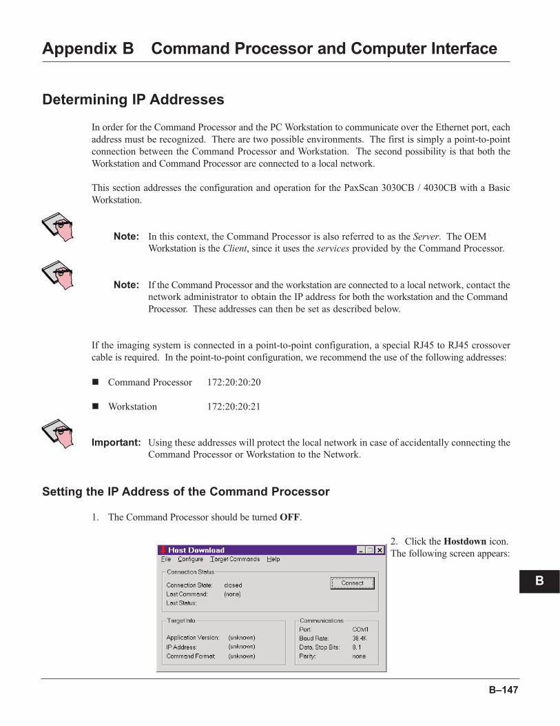
B–147
B
Appendix B Command Processor and Computer Interface
Determining IP Addresses
In order for the Command Processor and the PC Workstation to communicate over the Ethernet port, each
address must be recognized. There are two possible environments. The first is simply a point-to-point
connection between the Command Processor and Workstation. The second possibility is that both the
Workstation and Command Processor are connected to a local network.
This section addresses the configuration and operation for the PaxScan 3030CB / 4030CB with a Basic
Workstation.
Note: In this context, the Command Processor is also referred to as the Server. The OEM
Workstation is the Client, since it uses the services provided by the Command Processor.
Note: If the Command Processor and the workstation are connected to a local network, contact the
network administrator to obtain the IP address for both the workstation and the Command
Processor. These addresses can then be set as described below.
If the imaging system is connected in a point-to-point configuration, a special RJ45 to RJ45 crossover
cable is required. In the point-to-point configuration, we recommend the use of the following addresses:
n Command Processor 172:20:20:20
n Workstation 172:20:20:21
Important: Using these addresses will protect the local network in case of accidentally connecting the
Command Processor or Workstation to the Network.
Setting the IP Address of the Command Processor
1. The Command Processor should be turned OFF.
2. Click the Hostdown icon.
The following screen appears:
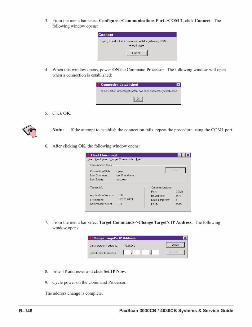
PaxScan 3030CB / 4030CB Systems & Service GuideB–148
3. From the menu bar select Configure->Communications Port->COM 2; click Connect. The
following window opens:
4. When this window opens, power ON the Command Processor. The following window will open
when a connection is established:
5. Click OK.
Note: If the attempt to establish the connection fails, repeat the procedure using the COM1 port.
6. After clicking OK, the following window opens:
7. From the menu bar select Target Commands->Change Target’s IP Address. The following
window opens:
8. Enter IP addresses and click Set IP Now.
9. Cycle power on the Command Processor.
The address change is complete.
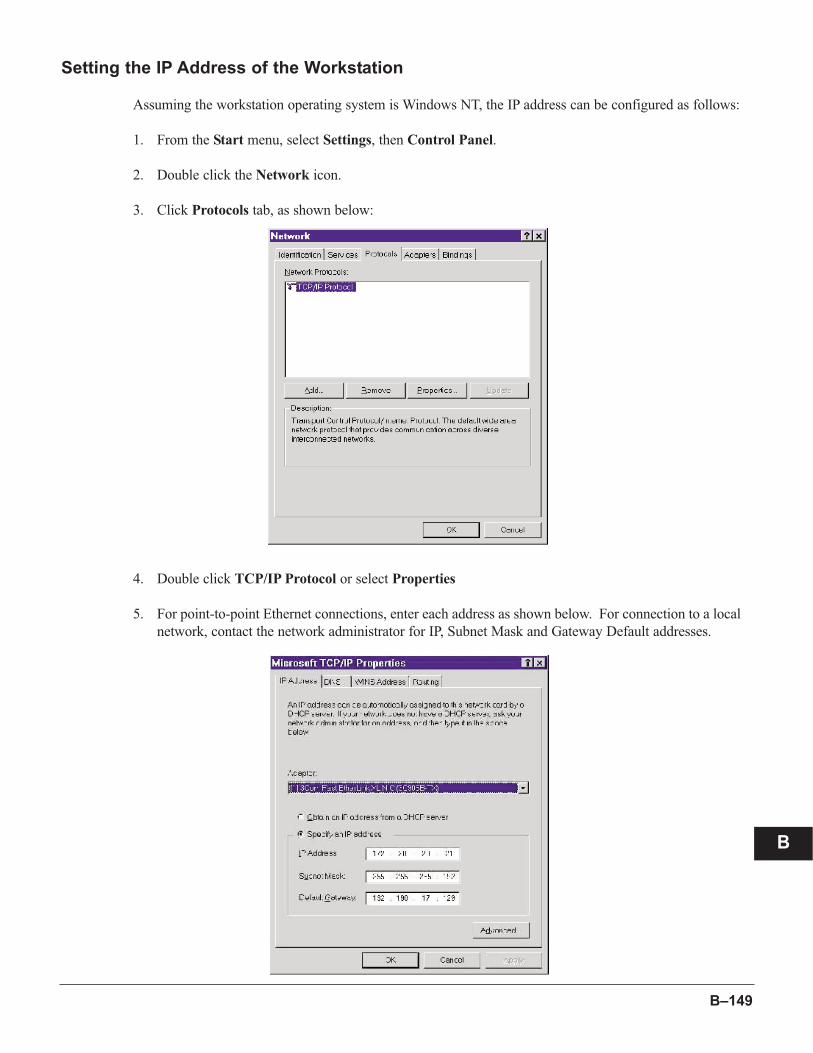
B–149
Setting the IP Address of the Workstation
Assuming the workstation operating system is Windows NT, the IP address can be configured as follows:
1. From the Start menu, select Settings, then Control Panel.
2. Double click the Network icon.
3. Click Protocols tab, as shown below:
4. Double click TCP/IP Protocol or select Properties
5. For point-to-point Ethernet connections, enter each address as shown below. For connection to a local
network, contact the network administrator for IP, Subnet Mask and Gateway Default addresses.
B

PaxScan 3030CB / 4030CB Systems & Service GuideB–150
C–151
C
Appendix C Calibration Procedure 3030CB / 4030CB - High
Dynamic Range modes
1.0 Introduction
This document describes the calibration and image normalization of the high dynamic range modes avail-
able from Paxscan 3030CB / 4030CB imagers. Calibration and normalization of 3030CB / 4030CB "nor-
mal" 14 bit modes (or "static gain" modes) can be handled by the command processor in the same way as
any Paxscan 4030A mode.
1.1 High dynamic range operation
The high dynamic range modes in the 3030CB / 4030CB are achieved by dynamically making multiple
gain selection for each image pixel. Normalization of images acquired in the Paxscan 3030CB /
4030CB high dynamic range modes, is not possible using the normalization capabilities of the
Paxscan command processor. These images have to be normalized on the host system computer.
To facilitate this normalization, a dynamically linked library file that contains the necessary functions
to calibrate and normalize these high dynamic range modes, is available.
1.1.1 Dual gain readout image format
n Signal from each pixel is "read" twice for each image frame, first at high gain and again at low gain.
n Only available as 2x2 binning option.
n Output images have 1024 x 1536 pixels (i.e. double height).
n The first line of each output image contains data for the first binned line of the imager, acquired in high gain selection. The second line contains data for the same imager lines,
but acquired in low gain selection. This sequence is maintained up to the middle of the
image, where two low gain lines are found, after which the low gain / high gain line
sequence is reversed.
1.1.2 Dynamic gain switching image format
n Pixel signals are read out once, at either high or low gain.
n The selection is made automatically by a level sensing circuit, pixel-by-pixel, based on its exposure level. The gain is reduced automatically for pixels with high exposure and
their pixel data are flagged with a gain bit for later normalization.
n Images will be standard size, but will appear wrong, due to image regions that were acquired at substantially lower gain.
n Images are standard size images containing 2048 x 1536, 1024 x 768 or 512 x 384 pixels (depending on binning).
n Each pixel contains 14 bits of pixel data (bits 0 though 13) and a gain bit (bit 14), which is set high if the pixel data was acquired at low gain.
n Images will have pixel values ranging from 0 to 16383 for high gain pixels and from 16384 to 32767 for low gain pixels.
PaxScan 3030CB / 4030CB Systems & Service GuideC–152
1.2 Function of the DLL
n The VIP_4030CB.DLL library helps the user's software application to normalize 3030CB / 4030CB high dynamic range images (establish a "software command processor" on the host
PC).
n Normalization involves:
¨ Compensation of the imager gain and offset non-uniformities.
¨ Interpolation of defective pixels.
¨ Re-interpretation of the multi-gain data from each pixel into single, linear data words. This reduces the double size images from dual gain readout, to standard size.
n In order to achieve optimum speed of operation and minimal use of PC resources, the DLL uses integer mathematics for almost all normalization and restoration calculations.
n Use of the DLL also requires access to its associated header (VIP_4030CB.h) and library (VIP_4030CB.lib) file during compilation of the user application and to the .ini file during
runtime. The VIP_4030CB.h file defines the class which provides the software support for the
3030CB / 4030CB. After creating the class, the user must call initialize() passing the path to
the directory containing the INI file and the calibration files, if they exist.
1.3 The .ini file
n Configuration and setup data relevant to the particular high dynamic range mode in use, is communicated to the DLL via VIP_4030CB.ini.
n The .ini file is supplied/edited by the user. Most of the parameters in the INI file are self explanatory.
n The initialization call to the DLL (initialize( const char base_dir[] )), supplies the directory where the .ini file is located. This directory will/must also be used to store calibration data,
such gain and offset data and defect maps.
n The Data_type parameter indicates whether the panel is operating in dual readout mode or dynamic switching mode (see VIP_4030CB.h file for defined values).
n The ROI parameters define the region which is used when determining the median value of an image (the ROI should at least exclude the 3 mm scintillator "shoulder" region of the imager,
as well as any regions that are not exposed to X-ray during gain calibration).
n The various limit parameters set the percentage of median that a pixel needs to exceed, to be considered a defect.
1.4 Defect map
n Locations of defective pixels are stored in defect map image files.
n A distinction is made between "auxiliary" defects and "base" defects. The base defect map is compiled at imager production and can only be changed by user editing, using the ViVA defect
editor. Auxiliary defects are detected during gain calibration. The auxiliary defect map is
calculated from scratch at every calculation and contains no history.
n For standard single gain modes (i.e. where the command processor is used for normalization), these defect maps are 16 bit image files that are stored on the command processor (exactly the
same as the Paxscan 4030A).
C–153
n For high dynamic range modes (i.e. where the DLL is used for normalization), defect maps are stored as more efficient binary image files, in a format that combines both base and
auxiliary defect information. One defect map is stored for each gain selection, on the host PC,
in the same directory as the .ini file (filenames Hi_G_defect_map.bin and Lo_G_defect_map.bin).
Each pixel on the imager is represented by 2 consecutive bits: one auxiliary defect bit, which
is recalculated by the DLL at every gain calibration and one base defect bit, which can only be
modified by the ViVA defect editor.
Note: Comprehensive defect detection is a complex process, requiring a range of computationally
intensive search algorithms to be performed on a set of images and image sequences that
are acquired over a range of conditions. Some of these algorithms require extensive
operator interaction. Comprehensive defect detection is thus not a process that should form
part of a user level calibration - it is best left to skilled flat panel production personnel. The
purpose of the base defect bit for each pixel is thus to store the comprehensive, production
level defect information, in a manner that will prevent modification during normal
calibration. The auxiliary defect bit for each pixel is re-calculated, at each gain calibration,
by a rudimentary algorithm that simply marks all pixels that fall outside a preset fractional
range of the gain and offset image medians. These defect thresholds are programmable
through the .ini file, by adjusting the XXX_offset_limit_XXX and XXX_gain_cal_limit_XXXparameters (these parameters indicate defect thresholds, as a percentage of the image
median). Should a defect appear during the life of the imager, but it is not reliably detected
by the auxiliary defect detector, it can be added to the base map, using the ViVA defect
editor.
2.0 Performing Calibration
2.1 Background info
n The user software application must initiate imager calibrations:
¨ Offset calibrations as frequently and as close to image acquisition time as possible. As a rule offset calibrations should be performed at least every 30 minutes, or prior to each
CBCT scan. More frequent offset calibrations are important while the imager temperature
is not stable (e.g. after power-up).
¨ Gain calibrations periodically - experience has shown once a month to be a good rule of thumb. More exact applications, such as CBCT, may require more frequent calibrations,
as determined through experience.
n "Calibration" requires the user software to accumulate 32 bit "sum" images from the receptor (the total of a sequence of frames) and passing them to either the gain or offset calibration
function in the DLL.
n All command processor normalization functions have to be turned off during acquisition of calibration images.
n Gain calibration requires the acquisition of a dark field sum image (no X-ray) and a flat field sum image (exposed to X-ray) for both gain selections used in the applicable high dynamic
range mode.
¨ The gain_calibrate() function in the DLL calculates the 32 bit difference between the flat field and dark field image. This gain image is scaled and stored as either
Hi_G_gain_img.viv or Lo_G_gain_img.viv, in the same directory as the .ini file.
C

PaxScan 3030CB / 4030CB Systems & Service GuideC–154
¨ Each file contains a value for either the relative high gain ( GHG ) or low gain ( GLG ) of each pixel (absolute values are not relevant).
¨ The median values for the high gain image ( GHG ) or low gain image ( GLG ) are also
calculated by the gain_calibrate() function and stored in the header of the applicable gain
image file.
¨ To allow the use of bow tie filters or non-uniform X-ray fields, the median is only calculated over the region defined by the ROI_XXX parameters in the .ini file.
¨ If it is deemed necessary, the user software application can now re-calculate the median gain ratio ( RG ) between high and low gain. The median value for both
XXX_ gain_img.viv images must be calculated (preferable in the ROI region only) and
the ratio of these numbers stored in the .ini file (as the HL_ratio parameter), using the
set_HL_ratio() function.
n Offset calibration requires the acquisition of a dark field sum image (no X-ray) only.
¨ When passing this sum image to the offset_calibrate() function in the DLL, the offset image is calculated by appropriate scaling and stored as either Hi_G_ofst_img.viv or
Lo_G_ofst_img.viv, in the same directory as the .ini file.
¨ Each file contains a value for the absolute offset of each pixel, in either high gain ( OHG ) or low gain ( OLG ) selection.
n Defective pixels are also detected by the gain_calibrate() function. The only defects detected,are those pixels falling outside the boundaries set by the applicable XXX_gain_cal_limit_XXXor XXX_offset_limit_XXX paramters in the .ini file. These defects are stored as auxiliary defects
only (see below).
n When using dual gain readout modes, the offset calibration and normalization capabilities of the command processor can be used, instead of the DLL normalization functions, as described
above. To use this shortcut, the Hi_G_ofst_img.viv and Lo_G_ofst_img.viv images must be
replaced by appropriate null images, with the same names, after completion of gain calibration.
Offset calibration in the command processor must be turned off prior to gain calibration and
turned back on after gain calibration. Offset calibrations then requires the transmission of a
single "offset calibrate" command to the command processor. This approach is not valid
when using dynamic gain switching modes. All command processor corrections must be
turned off when using these modes.
The calibration process requires a different sequence of actions, depending on whether dual gain
readout mode or dynamic gain switching mode is used.
2.2 Calibration of dual gain readout modes
Note: The DLL must be initialized for dual gain readout mode. This is done by pointing to an .ini file
with the parameter Data_type = 1 during the call to the initialize() function in the DLL.
2.2.1 Gain Calibration procedure
A. If not already selected, the user software selects the dual gain readout mode to be
calibrated. The mode may be described by a string such as "4030CB bin G1 0p5/4p
DGR" (where bin = 2x1 or 2x2).

C–155
B. With no X-ray exposure, the user software accumulates the sum of a sequence of images
(128 images will typically suffice) from the frame grabber.
C. This sum image is passed to the offset_calibrate() function twice - once with the
gain_mode function variable set to HI_G_MODE, to calculate and store the offset image
for the high gain selection and once with the gain_mode variable set to LO_G_MODE,
to calculate and store the offset image for the low gain selection.
D. Next, the user or user software must set up an X-ray exposure that is high enough for
most pixels to be near the saturation level in the high gain lines of the uncorrected
composite image. The absolute value of the exposure is not of importance, but a suitable
value may require some experimentation.
E. After the X-ray exposure is initiated, the user software accumulates the sum of a
sequence of images (128 images will typically suffice) from the frame grabber.
F. This sum image is passed to the gain_calibrate() function, with the gain_mode variable
set to HI_G_MODE, which calculates and stores a gain image for the high gain selection.
G. (OPTIONAL) If the ratio between low and high gains needs to be determined, the above
sum image can be passed to the gain_calibrate() function again, with the gain_modevariable set to LO_G_MODE, which will calculate and store a gain image for the low
gain selection. The user software application can now calculate the median gain ratio
( RG ) between high and low gain. The median value for both XXX_ gain_img.viv images
must be calculated (preferable in the ROI region only, as defined in the .ini file) and the
ratio of these numbers stored in the .ini file (as the HL_ratio parameter), using the
set_HL_ratio() function. In our limited experience, it is sufficient to calculate this value
once for each imager, during system manufacture.
H. It is recommended that a second gain calibration be performed at a much higher X-ray
exposure, for the low gain selection only.
I. Set up an exposure that is high enough for most pixels in the low gain lines of the
uncorrected image to be near, but below the saturation level.
J. After the X-ray exposure is initiated, the user software accumulates the sum of a
sequence of composite dual gain images (128 images will typically suffice).
K. This sum image is passed to the gain_calibrate() function, with the gain_mode variable
set to LO_G_MODE, which calculates and stores a gain image for the low gain selection.
2.2.2 Offset calibration procedure
A. If not already selected, the user software selects the dual gain read-out mode to be
calibrated. The mode may be described by a string such as "4030CB bin G1 0p5/4p DGR"
(where bin = 2x1 or 2x2).
B. With no X-ray exposure, the user software accumulates the sum of a sequence of
composite dual gain images (128 images will typically suffice).
C. This sum image is passed to the offset_calibrate() function twice - once with the
gain_mode variable set to HI_G_MODE, to calculate and store the offset image for the
high gain selection and once with the gain_mode variable set to LO_G_MODE, to
calculate and store the offset image for the low gain selection.
C

PaxScan 3030CB / 4030CB Systems & Service GuideC–156
2.3 Calibration of dynamic gain switching modes
Note: The dynamic gain switching mode is not supported at this time. The DLL must be initialized
for dynamic gain switching mode. This is done by pointing to an .ini file with the parameter
Data_type = 0 during the call to the initialize() function in the DLL.
3.0 Performing Image Normalization and Restoration
3.1 Background
n The 3030CB / 4030CB dll performs offset and gain correction and defective pixel correction.
n Command processor normalization functions are turned off during acquisition in high dynamicrange modes (except when using the command processor to perform offset correction in dual
gain readout modes - see above).
n Uncorrected raw images are passed to the correct_image() function in the DLL.
n Normalized X-ray intensity values for each pixel are calculated according to the formula (see paragraph 2.1 for a description of the symbols):
, for high gain pixel data (Dpixel, HG) and
, for low gain pixel data (Dpixel, LG).
n This calculation completes the normalization task for images acquired with dynamic gain switching modes. In this case, the decision to calculate and use either Ipixel, HG or Ipixel, LGis based solely on the value of the gain flag that is present in each pixel data word received
from the imager.
n For images acquired in dual gain readout modes, the decision to use either the low gain or high gain pixel data values is made for each pixel, as part of the normalization calculation. Two
software threshold levels, Tlow and Thigh are defined in the .ini file (parameters Threshold_Aand Threshold_B). For all pixels with Dpixel, HG below Tlow , the Ipixel, HG value is used
as the representative equivalent intensity. For all pixels with Dpixel, HG above Thigh , the
Ipixel,LG, value is used as the representative equivalent intensity. For pixels with Dpixel, HG between Tlow and Thigh , a linear interpolation of and Ipixel, HG and Ipixel, LG value is used,
thus guaranteeing a smooth transition in image regions with intensity near the transition
threshold.
n The effective image bit depth is now larger than 16 bits. To reduce data back to 16 bits per pixel, the correct_image() function will compress output images into a pseudo floating point
format. The corrected image will again contain 14 bits of pixel data and 2 bits indicating the
amount to shift the 14 data bits.
n To restore compressed images, the gain bit can be used as a look-up table address bit or it is anticipated that sufficient linearity may be achieved by multiplying pixels flagged by the gain
bit, by the gain ratio value (see "calibration" above). The result of this de-compression
operation will be more than 16 bits per pixel.

C–157
C
n Alternatively, the DLL also contains a function that can be used to provide a corrected, scaled, linear, 16 bit version of the raw image. This is achieved by scaling the data by a factor supplied
by the user. Any resulting values greater that 65535 will be set to 65535.
n The dll requires a directory in which the following files are stored (A sample .ini file is provided, the other files required in the directory will be generated by the dll when calibration
is performed.):
1. INI parameter file - This file communicates imager setup and user preference info to the DLL. It has to be edited by the user
2. High gain offset file - this file is calculated by the offset_calibrate() function, from a sum image accumulated by the user software as described below.
3. Low gain offset file -similar to High gain offset file.
4. High gain gain image file - this file is calculated by the gain_calibrate() function, from a sum image accumulated by the user software as described below.
5. Low gain gain image file - similar to High gain gain file.
6. High gain defective pixel map - this file contains an auxiliary defect map, as calculated by the gain_calibrate() function and a base defect map that is calculated at imager production and editable by the ViVA defect editor.
7. Low gain defective pixel map - similar to High gain defective pixel map file.
3.2 Performing normalization
n The correct_image() routine performs the offset and gain correction and defective pixel correction.
n The supplied 16 bit image is replaced by the corrected 16 bit image.
n Each pixel value contains the corrected pixel value in the low order 14 bits and a shift value in the high 2 bits.
n Whenever the true pixel value must be used in an application of for display, a table lookup must be performed to obtain the desired pixel value.
n For images acquired in dual gain readout modes, the corrected image is only half the size as the supplied image.
n The .ini parameters Threshold_A and Threshold_B are only used for dual readout images. The offset and gain corrected value for the high gain reading is first determined. If the high gain
value of a pixel is below Threshold_A, this is the corrected pixel value. If the high gain value
is above Threshold_B, the corrected pixel value is determined from the corrected low gain
reading. If the value is between Threshold_A and Threshold_B, interpolation is performed
between the high gain and low gain corrected readings to insure a smooth transition.
n The generate_scaled_image() function can be used to produce a linearized version of the compressed data format images produced by correct_image().

PaxScan 3030CB / 4030CB Systems & Service GuideC–158
D–159
Appendix D Multiple gain ranging readout method to extend the dynamic range
of amorphous silicon flat panel imagers.
Pieter G. Roos*a, Richard E Colbetha, Ivan Mollova, Peter Munrob, John Pavkovicha, Edward J.
Seppia, Edward G. Shapirob, Carlo A. Togninaa, Gary F. Virshupa, J. Michael Yua, George Zentaia,
Wolfgang Kaisslc, Evangelos Matsinosc, Jeroen Richtersc, Heinrich Riemc,
aVarian Medical Systems, Ginzton Technology Center, 2599 Garcia Ave, Mountain View, CA 94043
bVarian Medical Systems, Oncology Systems Division, 3100 Hansen Way, Palo Alto, CA 94304
cVarian Medical Systems, Imaging Laboratory, Neuenhoferstrasse 107,5400 Baden, Switzerland
ABSTRACT
The dynamic range of many flat panel imaging systems are fundamentally limited by the dynamic range of the charge
amplifier and readout signal processing. We developed two new flat panel readout methods that achieve extended
dynamic range by changing the readout charge amplifier feedback capacitance dynamically and on a real-time basis.
In one method, the feedback capacitor is selected automatically by a level sensing circuit, pixel-by-pixel, based on its
exposure level. Alternatively, capacitor selection is driven externally, such that each pixel is read out two (or more)
times, each time with increased feedback capacitance. Both methods allow the acquisition of X-ray image data with
a dynamic range approaching the fundamental limits of flat panel pixels. Data with an equivalent bit depth of better
than 16 bits are made available for further image processing. Successful implementation of these methods requires
careful matching of selectable capacitor values and switching thresholds, with the imager noise and sensitivity charac-
teristics, to insure X-ray quantum limited operation over the whole extended dynamic range. Successful implementa-
tion also depends on the use of new calibration methods and image reconstruction algorithms, to insure artifact free
rebuilding of linear image data by the downstream image processing systems.
The multiple gain ranging flat panel readout method extends the utility of flat panel imagers and paves
the way to new flat panel applications, such as cone beam CT. We believe that this method will provide
a valuable extension to the clinical application of flat panel imagers.
Keywords: Flat panel, cone beam CT, charge amplifier, gain switching, dynamic range, radiography,
dual gain, multiple gain
Copyright 2004 Society of Photo-Optical Instrumentation Engineers.This paper was published in Proceedings of SPIE, Vol. 5368, February 2004, San Diego CA and is made available as an electronic reprint withpermission of SPIE. One print or electronic copy may be made for personal use only. Systematic or multiple reproduction, distribution to multi-ple locations via electronic or other means, duplication of any material in this paper for a fee or for commercial purposes, or modification of thecontent of the paper is prohibited.
D
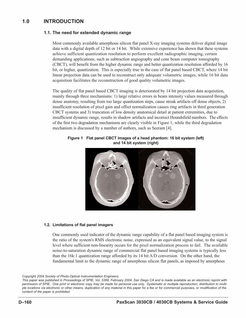
PaxScan 3030CB / 4030CB Systems & Service GuideD–160
1.0 INTRODUCTION
1.1. The need for extended dynamic range
Most commonly available amorphous silicon flat panel X-ray imaging systems deliver digital image
data with a digital depth of 12 bit or 14 bit. While extensive experience has shown that these systems
achieve sufficient quantization resolution to perform excellent radiographic imaging, certain
demanding applications, such as subtraction angiography and cone beam computer tomography
(CBCT), will benefit from the higher dynamic range and better quantization resolution afforded by 16
bit, or higher, quantization. This is especially true in the case of flat panel based CBCT, where 14 bit
linear projection data can be used to reconstruct only adequate volumetric images, while 16 bit data
acquisition facilitates the reconstruction of good quality volumetric images.
The quality of flat panel based CBCT imaging is deteriorated by 14 bit projection data acquisition,
mainly through three mechanisms: 1) large relative errors in beam intensity values measured through
dense anatomy, resulting from too large quantization steps, cause streak artifacts off dense objects, 2)
insufficient resolution of pixel gain and offset normalization causes ring artifacts in third generation
CBCT systems and 3) truncation of low density anatomical detail at patient extremities, due to
insufficient dynamic range, results in shadow artifacts and incorrect Houndsfield numbers. The effects
of the first two degradation mechanisms are clearly visible in Figure 1, while the third degradation
mechanism is discussed by a number of authors, such as Seeram [4].
Figure 1 Flat panel CBCT images of a head phantom: 16 bit system (left)
and 14 bit system (right)
1.2. Limitations of flat panel imagers
One commonly used indicator of the dynamic range capability of a flat panel based imaging system is
the ratio of the system's RMS electronic noise, expressed as an equivalent signal value, to the signal
level where sufficient non-linearity occurs for the pixel normalization process to fail. The available
noise-to-saturation dynamic range of commercial flat panel based imaging systems is typically less
than the 16k:1 quantization range afforded by its 14 bit A/D conversion. On the other hand, the
fundamental limit to the dynamic range of amorphous silicon flat panels, as imposed by amorphous
Copyright 2004 Society of Photo-Optical Instrumentation Engineers.This paper was published in Proceedings of SPIE, Vol. 5368, February 2004, San Diego CA and is made available as an electronic reprint withpermission of SPIE. One print or electronic copy may be made for personal use only. Systematic or multiple reproduction, distribution to multi-ple locations via electronic or other means, duplication of any material in this paper for a fee or for commercial purposes, or modification of thecontent of the paper is prohibited.
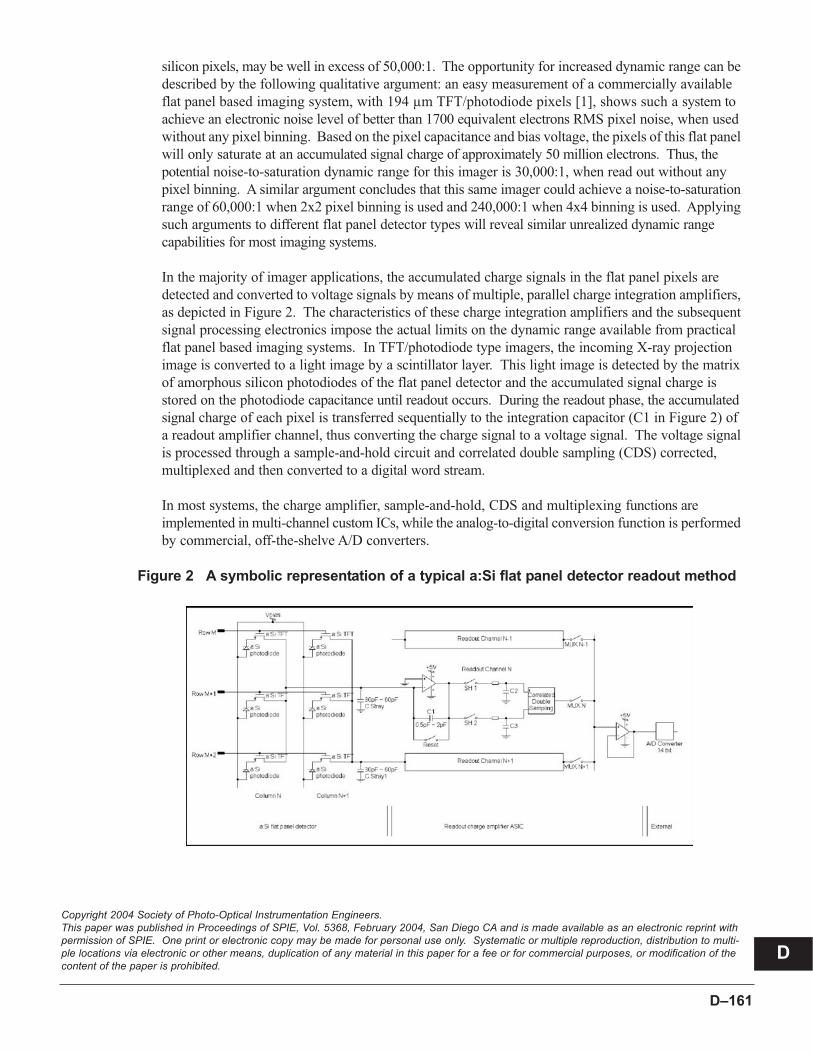
D–161
silicon pixels, may be well in excess of 50,000:1. The opportunity for increased dynamic range can be
described by the following qualitative argument: an easy measurement of a commercially available
flat panel based imaging system, with 194 µm TFT/photodiode pixels [1], shows such a system to
achieve an electronic noise level of better than 1700 equivalent electrons RMS pixel noise, when used
without any pixel binning. Based on the pixel capacitance and bias voltage, the pixels of this flat panel
will only saturate at an accumulated signal charge of approximately 50 million electrons. Thus, the
potential noise-to-saturation dynamic range for this imager is 30,000:1, when read out without any
pixel binning. A similar argument concludes that this same imager could achieve a noise-to-saturation
range of 60,000:1 when 2x2 pixel binning is used and 240,000:1 when 4x4 binning is used. Applying
such arguments to different flat panel detector types will reveal similar unrealized dynamic range
capabilities for most imaging systems.
In the majority of imager applications, the accumulated charge signals in the flat panel pixels are
detected and converted to voltage signals by means of multiple, parallel charge integration amplifiers,
as depicted in Figure 2. The characteristics of these charge integration amplifiers and the subsequent
signal processing electronics impose the actual limits on the dynamic range available from practical
flat panel based imaging systems. In TFT/photodiode type imagers, the incoming X-ray projection
image is converted to a light image by a scintillator layer. This light image is detected by the matrix
of amorphous silicon photodiodes of the flat panel detector and the accumulated signal charge is
stored on the photodiode capacitance until readout occurs. During the readout phase, the accumulated
signal charge of each pixel is transferred sequentially to the integration capacitor (C1 in Figure 2) of
a readout amplifier channel, thus converting the charge signal to a voltage signal. The voltage signal
is processed through a sample-and-hold circuit and correlated double sampling (CDS) corrected,
multiplexed and then converted to a digital word stream.
In most systems, the charge amplifier, sample-and-hold, CDS and multiplexing functions are
implemented in multi-channel custom ICs, while the analog-to-digital conversion function is performed
by commercial, off-the-shelve A/D converters.
Figure 2 A symbolic representation of a typical a:Si flat panel detector readout method
Copyright 2004 Society of Photo-Optical Instrumentation Engineers.This paper was published in Proceedings of SPIE, Vol. 5368, February 2004, San Diego CA and is made available as an electronic reprint withpermission of SPIE. One print or electronic copy may be made for personal use only. Systematic or multiple reproduction, distribution to multi-ple locations via electronic or other means, duplication of any material in this paper for a fee or for commercial purposes, or modification of thecontent of the paper is prohibited.
D
PaxScan 3030CB / 4030CB Systems & Service GuideD–162
The low end of a flat panel imager's dynamic range is limited by noise generated in the pixels and
signal processing chain. Noise sources include pixel kTC noise, thermal noise generated by imager
data lines, charge amplifier voltage noise and noise generated in the signal processing chain [2, 3]. In
Varian's Paxscan 3030CB / 4030CB imager, that was developed to take advantage of the read out
methods that are described here, these sources add up to approximately 1700 electrons RMS equiva-
lent integrator charge, as mentioned above. On the other hand, the high end of this dynamic range
is usually determined by the voltage swing that can be achieved by the charge amplifier and signal
processing chain, while maintaining sufficient linearity to facilitate subsequent pixel gain and offset
normalization. For the above system, this point is reached at about 2 volt swing, or 6 million electrons
stored on the 0.5 pF integration capacitor. This yields a 3,500:1 noise-to-saturation dynamic range,
which matches very well with the 16k quantization steps available from a 14 bit A/D converter. Using
a 1 pF integration capacitor, as in Varian's Paxscan 4030A imaging system, will achieve a dynamic
range in the order of 6,000:1. These ranges are however very substantially less than the actual
dynamic range available from the amorphous silicon flat panel detector.
Changing the capacitor will typically not result in an increase in dynamic range - decreasing the
capacitor may decrease equivalent electronic noise, but will cause saturation at lower exposure;
increasing the capacitor will increase the saturation exposure, but may cause alternate noise sources to
become dominant at low exposure levels. An alternative readout architecture is required in order to
realize the dynamic range capabilities of flat panel detectors in practical imaging systems.
2.0 MULTIPLE GAIN RANGING READOUT METHOD
In order to achieve a flat panel based imaging system with dynamic range approaching the capability of the
amorphous silicon flat panel, we developed a new charge readout amplifier IC that is capable of changing
the charge amplifier feedback capacitance of each channel dynamically and on a real-time, pixel-by-pixel
basis. Each amplifier channel also includes a latched comparator that can be enabled to change the feed-
back capacitance automatically, based on the amount of charge presented to the amplifier, by each indi-
vidual pixel. The architecture for this readout method, as implemented in Varian's Paxscan 3030CB /
4030CB flat panel imaging system, is depicted in Figure 3. Use of this readout architecture enables the
implementation of two alternative high dynamic range readout methods.
2.1. Dynamic Gain Switching
In the so-called Dynamic Gain Switching mode, a comparator is used to increase the feedback
capacitance automatically when pixels with large accumulated charge are selected for readout.
When the voltage accumulated in the charge integrator exceeds the dynamic threshold, which is a
global voltage set externally for all channels, the comparator switches an additional, much larger
feedback capacitor (C4 in Figure 3), in parallel with the fixed feedback capacitor (C1 in Figure 3).
In the 3030CB / 4030CB imager, capacitor values are selected to cause an 8x reduction in gain for
pixels that exceed the programmable signal level. Regardless of whether a pixel was acquired with
reduced gain, the signal from the charge amplifier is then processed through the standard correlated
double sampling circuit and converted to a digital word by the 14 bit A/D converter. To enable
recovery of linear pixel data by the downstream image processor, the output of the latched com-
parator is sampled by a separate multiplexer and inserted as an additional "gain bit" (bit 15 of 16
bits) into the digital video data word at the output of the A/D converter.
Copyright 2004 Society of Photo-Optical Instrumentation Engineers.This paper was published in Proceedings of SPIE, Vol. 5368, February 2004, San Diego CA and is made available as an electronic reprint withpermission of SPIE. One print or electronic copy may be made for personal use only. Systematic or multiple reproduction, distribution to multi-ple locations via electronic or other means, duplication of any material in this paper for a fee or for commercial purposes, or modification of thecontent of the paper is prohibited.
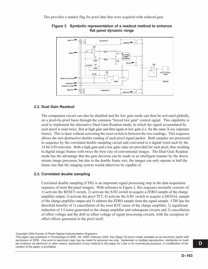
D–163
Copyright 2004 Society of Photo-Optical Instrumentation Engineers.This paper was published in Proceedings of SPIE, Vol. 5368, February 2004, San Diego CA and is made available as an electronic reprint withpermission of SPIE. One print or electronic copy may be made for personal use only. Systematic or multiple reproduction, distribution to multi-ple locations via electronic or other means, duplication of any material in this paper for a fee or for commercial purposes, or modification of thecontent of the paper is prohibited.
This provides a marker flag for pixel data that were acquired with reduced gain.
Figure 3 Symbolic representation of a readout method to enhance
flat panel dynamic range
2.2. Dual Gain Readout
The comparator circuit can also be disabled and the low gain mode can then be activated globally,
on a pixel-by-pixel basis through the common "forced low gain" control signal. This capability is
used to implement the alternative Dual Gain Readout mode, in which the signal accumulated by
each pixel is read twice, first at high gain and then again at low gain (i.e. for the same X-ray exposure
frame). This is done without activating the reset switch in between the two readings. This sequence
allows the non-destructive double reading of each pixel signal packet. Both samples are processed
in sequence by the correlated double sampling circuit and converted to a digital word each by the
14 bit A/D converter. Both a high gain and a low gain value are provided for each pixel, thus resulting
in digital image frames with twice the byte size of conventional images. The Dual Gain Readout
mode has the advantage that the gain decision can be made in an intelligent manner by the down-
stream image processor, but due to the double frame size, the imager can only operate at half the
frame rate that the imaging system would otherwise be capable of.
2.3. Correlated double sampling
Correlated double sampling (CDS) is an important signal processing step in the data acquisition
sequence of most flat panel imagers. With reference to Figure 2, this sequence normally consists of:
1) activate the RESET switch, 2) activate the S/H2 switch to acquire a ZERO sample of the charge
amplifier output, 3) activate the pixel TFT, 4) activate the S/H1 switch to acquire a SIGNAL sample
of the charge amplifier output and 5) subtract the ZERO sample from the signal sample. CDS has the
threefold benefits of 1) cancellation of the reset KTC noise of the charge amplifier, 2) significant
reduction of 1/f noise generated in the charge amplifier and subsequent circuits and 3) cancellation
of offset voltage and the drift in offset voltage of signal processing circuits, with the exception of
offset effects generated in the pixel itself.
D

PaxScan 3030CB / 4030CB Systems & Service GuideD–164
Since both high dynamic range modes described above involve changing the charge amplifier gain
after the TFT was activated, this may compromise the validity of the CDS subtraction for low gain
data, as the ZERO sample would always be acquired at high gain. Cancellation of undesirable
effects caused in subsequent circuits will obviously be left intact, but the design of the charge
amplifier circuit required special attention, to insure that its offset and 1/f noise characteristics don't
change with reduction in gain. Cancellation of the reset KTC noise will however be invalid for low
gain data and an increase in electronic noise will thus be inevitable for low gain data. As will be shown
in section 3, low gain data are only used where high levels of exposure are encountered and photon
noise is sufficiently high to insure quantum limited operation and the impact of this additional low gain
noise is thus negligible. This is only true however when the jump from high to low gain is not too
large. Low gain noise thus places the limit on the size of gain step and therefore on the amount of
dynamic range extension that can be achieved by any multiple gain ranging read out method.
2.4. Normalization
2.4.1. Imager calibration
When using these high dynamic range readout methods, each pixel is characterized by a
unique offset and gain calibration value for both low and high gain selections. We developed a
method of calibrating and correcting for these non-uniformities, without requiring an accurate
knowledge of the x-beam intensity during calibration exposures. This results in an easy to
perform on-site calibration that does not need any special equipment or advanced level of
training.
Dark field and flat field images are acquired, as during any flat panel calibration procedure
[5, 6], but this is done for both low and high gain settings of a high dynamic range mode. As
for a conventional flat panel, flat field and dark field images are the average of a sufficient
number of frames to reduce the image noise to an acceptable level [6]. A method exists
whereby the imager can be forced into simulated dynamic gain switching, even when no
X-ray exposure is present. For good calibration quality, two flat field exposures are acquired
for the low gain setting: one flat field image is acquired at the same exposure level as the
high gain flat field and a second flat field image is acquired at a significantly higher exposure.
In our method, "gain images" (a 2 dimensional map of relative pixel sensitivities) are calcu-
lated from each of the three flat field images, by subtracting the applicable dark field image.
The high gain image and the high exposure, low gain image are stored for use during image
acquisition. The low exposure, low gain image is used to calculate the ratio of high-to-low
gain ("gain ratio") for each pixel, by dividing it into the high gain image. This gain ratio
image is also stored for use during image acquisition. The dark field exposures acquired during
calibration are discarded. Dark field images, that are used for image offset calculation, are
then acquired for each gain setting, as close as possible to the time of the actual image acqui-
sition [5]. Five calibration parameters are thus stored for each pixel (in the form of five
calibration images): the relative high gain (GHG) and low gain (GLG) of each pixel (absolute
values are not important), the absolute offset of the high gain (OHG) and low gain (OLG)
settings and the gain ratio (RG). The median values for the high gain image (GHG) and low
gain image (GLG) are also calculated and stored.
Copyright 2004 Society of Photo-Optical Instrumentation Engineers.This paper was published in Proceedings of SPIE, Vol. 5368, February 2004, San Diego CA and is made available as an electronic reprint withpermission of SPIE. One print or electronic copy may be made for personal use only. Systematic or multiple reproduction, distribution to multi-ple locations via electronic or other means, duplication of any material in this paper for a fee or for commercial purposes, or modification of thecontent of the paper is prohibited.
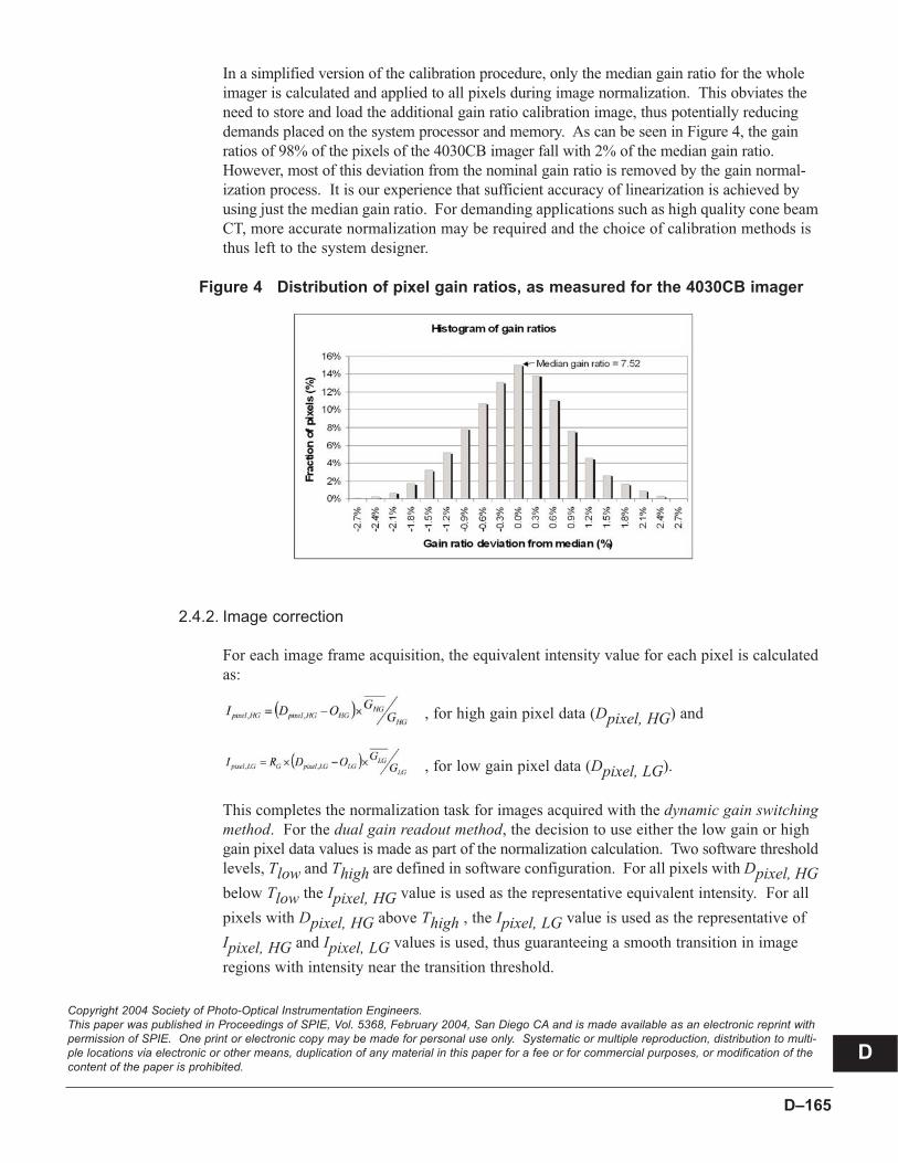
D–165
In a simplified version of the calibration procedure, only the median gain ratio for the whole
imager is calculated and applied to all pixels during image normalization. This obviates the
need to store and load the additional gain ratio calibration image, thus potentially reducing
demands placed on the system processor and memory. As can be seen in Figure 4, the gain
ratios of 98% of the pixels of the 4030CB imager fall with 2% of the median gain ratio.
However, most of this deviation from the nominal gain ratio is removed by the gain normal-
ization process. It is our experience that sufficient accuracy of linearization is achieved by
using just the median gain ratio. For demanding applications such as high quality cone beam
CT, more accurate normalization may be required and the choice of calibration methods is
thus left to the system designer.
Figure 4 Distribution of pixel gain ratios, as measured for the 4030CB imager
2.4.2. Image correction
For each image frame acquisition, the equivalent intensity value for each pixel is calculated
as:
, for high gain pixel data (Dpixel, HG) and
, for low gain pixel data (Dpixel, LG).
This completes the normalization task for images acquired with the dynamic gain switching method. For the dual gain readout method, the decision to use either the low gain or high
gain pixel data values is made as part of the normalization calculation. Two software threshold
levels, Tlow and Thigh are defined in software configuration. For all pixels with Dpixel, HGbelow Tlow the Ipixel, HG value is used as the representative equivalent intensity. For all
pixels with Dpixel, HG above Thigh , the Ipixel, LG value is used as the representative of
Ipixel, HG and Ipixel, LG values is used, thus guaranteeing a smooth transition in image
regions with intensity near the transition threshold.
Copyright 2004 Society of Photo-Optical Instrumentation Engineers.This paper was published in Proceedings of SPIE, Vol. 5368, February 2004, San Diego CA and is made available as an electronic reprint withpermission of SPIE. One print or electronic copy may be made for personal use only. Systematic or multiple reproduction, distribution to multi-ple locations via electronic or other means, duplication of any material in this paper for a fee or for commercial purposes, or modification of thecontent of the paper is prohibited.
D
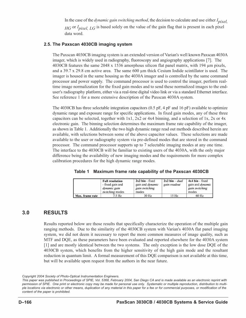
PaxScan 3030CB / 4030CB Systems & Service GuideD–166
In the case of the dynamic gain switching method, the decision to calculate and use either Ipixel, HG or Ipixel, LG is based solely on the value of the gain flag that is present in each pixel
data word.
2.5. The Paxscan 4030CB imaging system
The Paxscan 4030CB imaging system is an extended version of Varian's well known Paxscan 4030A
imager, which is widely used in radiography, fluoroscopy and angiography applications [7]. The
4030CB features the same 2048 x 1536 amorphous silicon flat panel matrix, with 194 µm pixels,
and a 39.7 x 29.8 cm active area. The same 600 µm thick Cesium Iodide scintillator is used. The
imager is housed in the same housing as the 4030A imager and is controlled by the same command
processor and power supply. The command processor is used to control the imager, perform real-
time image normalization for the fixed gain modes and to send these normalized images to the end-
user's radiography platform, either via a real-time digital video link or via a standard Ethernet interface.
See reference 1 for a more extensive description of the Paxscan 4030A system.
The 4030CB has three selectable integration capacitors (0.5 pF, 4 pF and 16 pF) available to optimize
dynamic range and exposure range for specific applications. In fixed gain modes, any of these three
capacitors can be selected, together with 1x1, 2x2 or 4x4 binning, and a selection of 1x, 2x or 4x
electronic gain. The binning selection determines the maximum frame rate capability of the imager,
as shown in Table 1. Additionally the two high dynamic range read out methods described herein are
available, with selections between some of the above capacitor values. These selections are made
available to the user or radiography system via pre-defined modes that are stored in the command
processor. The command processor supports up to 7 selectable imaging modes at any one time.
The interface to the 4030CB will be familiar to existing users of the 4030A, with the only major
difference being the availability of new imaging modes and the requirements for more complex
calibration procedures for the high dynamic range modes.
Table 1 Maximum frame rate capability of the Paxscan 4030CB
3.0 RESULTS
Results reported below are those results that specifically characterize the operation of the multiple gain
ranging methods. Due to the similarity of the 4030CB system with Varian's 4030A flat panel imaging
system, we did not deem it necessary to report the more common measures of image quality, such as
MTF and DQE, as these parameters have been evaluated and reported elsewhere for the 4030A system
[1] and are mostly identical between the two systems. The only exception is the low dose DQE of the
4030CB system, which benefits from the higher sensitivity of the high gain mode and the resultant
reduction in quantum limit. A formal measurement of this DQE comparison is not available at this time,
but will be available upon request from the authors in the near future.
Copyright 2004 Society of Photo-Optical Instrumentation Engineers.This paper was published in Proceedings of SPIE, Vol. 5368, February 2004, San Diego CA and is made available as an electronic reprint withpermission of SPIE. One print or electronic copy may be made for personal use only. Systematic or multiple reproduction, distribution to multi-ple locations via electronic or other means, duplication of any material in this paper for a fee or for commercial purposes, or modification of thecontent of the paper is prohibited.
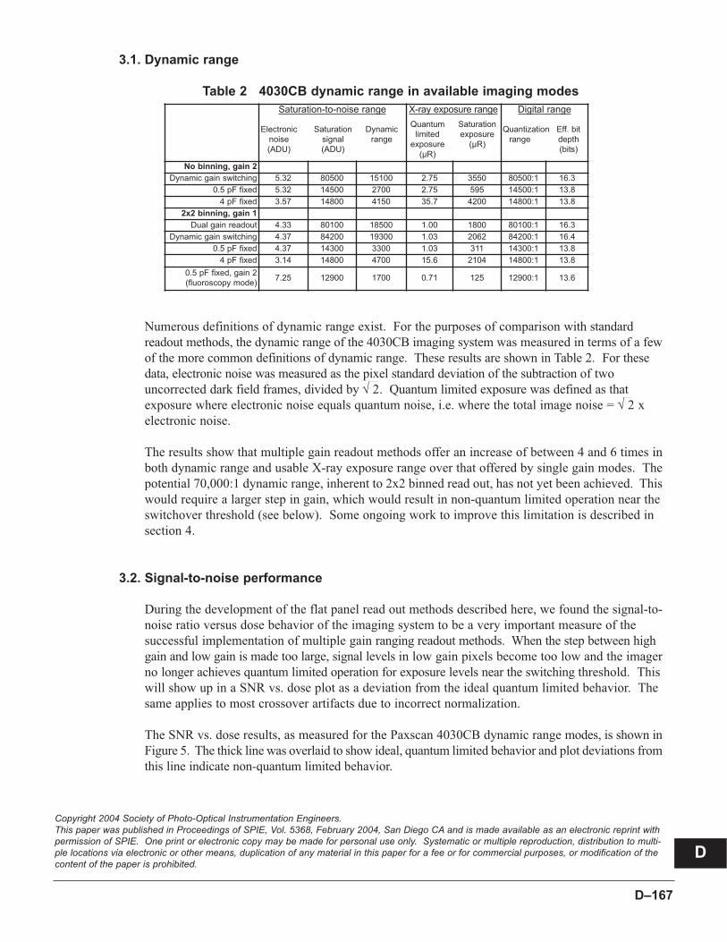
D–167
3.1. Dynamic range
Table 2 4030CB dynamic range in available imaging modes
Numerous definitions of dynamic range exist. For the purposes of comparison with standard
readout methods, the dynamic range of the 4030CB imaging system was measured in terms of a few
of the more common definitions of dynamic range. These results are shown in Table 2. For these
data, electronic noise was measured as the pixel standard deviation of the subtraction of two
uncorrected dark field frames, divided by √ 2. Quantum limited exposure was defined as that
exposure where electronic noise equals quantum noise, i.e. where the total image noise = √ 2 x
electronic noise.
The results show that multiple gain readout methods offer an increase of between 4 and 6 times in
both dynamic range and usable X-ray exposure range over that offered by single gain modes. The
potential 70,000:1 dynamic range, inherent to 2x2 binned read out, has not yet been achieved. This
would require a larger step in gain, which would result in non-quantum limited operation near the
switchover threshold (see below). Some ongoing work to improve this limitation is described in
section 4.
3.2. Signal-to-noise performance
During the development of the flat panel read out methods described here, we found the signal-to-
noise ratio versus dose behavior of the imaging system to be a very important measure of the
successful implementation of multiple gain ranging readout methods. When the step between high
gain and low gain is made too large, signal levels in low gain pixels become too low and the imager
no longer achieves quantum limited operation for exposure levels near the switching threshold. This
will show up in a SNR vs. dose plot as a deviation from the ideal quantum limited behavior. The
same applies to most crossover artifacts due to incorrect normalization.
The SNR vs. dose results, as measured for the Paxscan 4030CB dynamic range modes, is shown in
Figure 5. The thick line was overlaid to show ideal, quantum limited behavior and plot deviations from
this line indicate non-quantum limited behavior.
Copyright 2004 Society of Photo-Optical Instrumentation Engineers.This paper was published in Proceedings of SPIE, Vol. 5368, February 2004, San Diego CA and is made available as an electronic reprint withpermission of SPIE. One print or electronic copy may be made for personal use only. Systematic or multiple reproduction, distribution to multi-ple locations via electronic or other means, duplication of any material in this paper for a fee or for commercial purposes, or modification of thecontent of the paper is prohibited.
D
Saturation-to-noise range X-ray exposure range Digital range
Electronic Saturation Dynamic
noise signal range
(ADU) (ADU)
Quantum Saturation
limited exposure
exposure (µR)
(µR)
Quantization Eff. bit
range depth
(bits)
No binning, gain 2
Dynamic gain switching 5.32 80500 15100 2.75 3550 80500:1 16.3
0.5 pF fixed 5.32 14500 2700 2.75 595 14500:1 13.8
4 pF fixed 3.57 14800 4150 35.7 4200 14800:1 13.8
2x2 binning, gain 1
Dual gain readout 4.33 80100 18500 1.00 1800 80100:1 16.3
Dynamic gain switching 4.37 84200 19300 1.03 2062 84200:1 16.4
0.5 pF fixed 4.37 14300 3300 1.03 311 14300:1 13.8
4 pF fixed 3.14 14800 4700 15.6 2104 14800:1 13.8
0.5 pF fixed, gain 2
(fluoroscopy mode)7.25 12900 1700 0.71 125 12900:1 13.6

PaxScan 3030CB / 4030CB Systems & Service GuideD–168
Figure 5 Signal-to-noise performance over the extended dynamic range
The signal-to-noise versus dose results indicate that the choice of gain settings, as implemented in
the Paxscan 4030CB imager, is optimal, given the constraints of the rest of the system. This can be
concluded from the small deviation from ideal, quantum limited performance that is visible at exposure
levels of approximately 250 µR. This is the intensity neighborhood where low gain data starts
being used. As the signal levels are relatively low compared to the electronic noise characteristic of
the low gain setting, the imager is on the verge of reverting to non-quantum limited operation. A
larger feedback capacitor would have resulted in a too large gain reduction and electronic noise
would have dominated in the transition region. See paragraph 2.3 for an explanation of the high
level of electronic noise applicable to the low gain setting.
3.3. Image artifacts
Due to the risk of producing contour type artifacts in image regions with intensity levels near the gain
switchover threshold, subjective image quality serves as another important check on the applicability
of our methods to diagnostic imaging. Figure 6 shows a slice reconstructed from a CBCT scan of a
human pelvis and Figure 7 shows one of the projection images from this scan. These images were
acquired with a Paxscan 4030CB based CBCT system using the dual gain readout method. The
projection image was processed by a severe unsharp masking algorithm, to enhance any possible
boundary artifacts resulting from gain switching. No such boundary artifacts are visible in either
image. The general quality demonstrated by the CBCT slices of Figure 1 and Figure 6 also show in
general the suitability of the Paxscan 4030CB imaging system for CBCT applications.
Copyright 2004 Society of Photo-Optical Instrumentation Engineers.This paper was published in Proceedings of SPIE, Vol. 5368, February 2004, San Diego CA and is made available as an electronic reprint withpermission of SPIE. One print or electronic copy may be made for personal use only. Systematic or multiple reproduction, distribution to multi-ple locations via electronic or other means, duplication of any material in this paper for a fee or for commercial purposes, or modification of thecontent of the paper is prohibited.
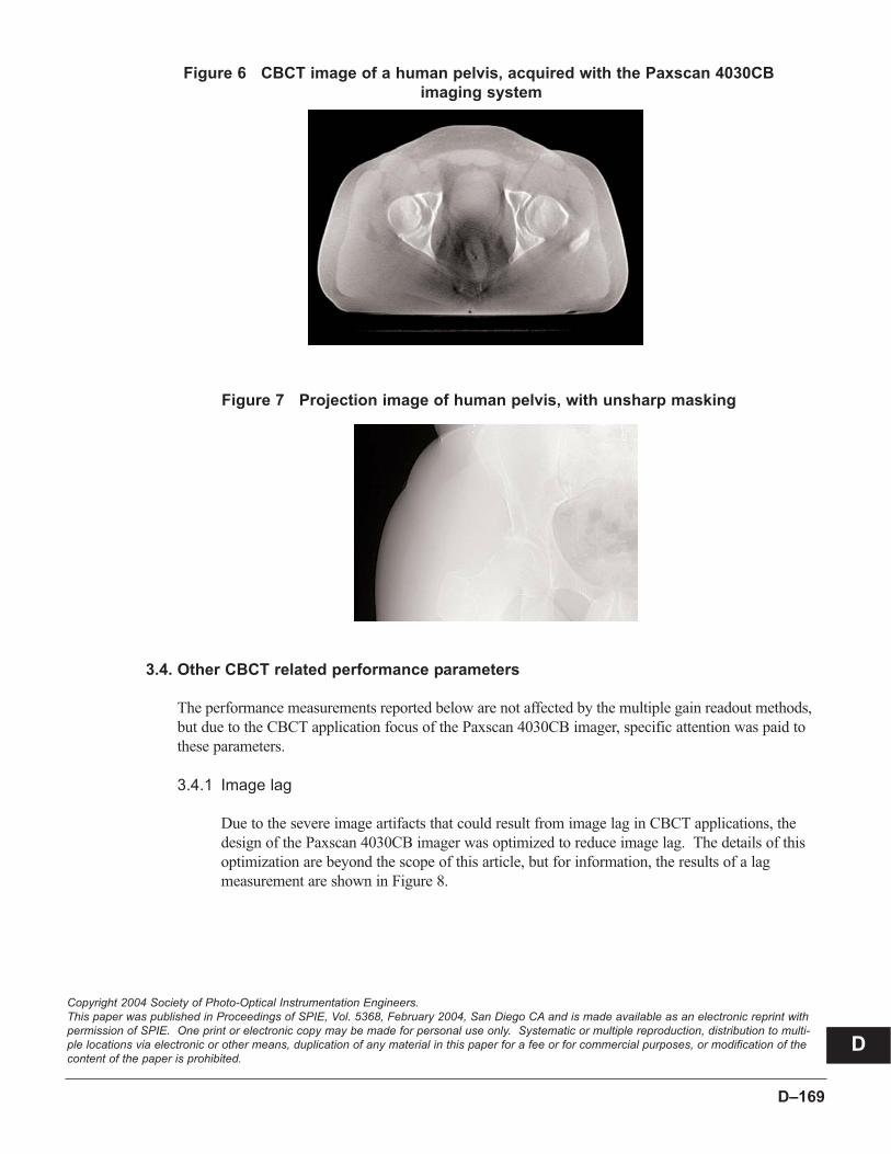
D–169
Copyright 2004 Society of Photo-Optical Instrumentation Engineers.This paper was published in Proceedings of SPIE, Vol. 5368, February 2004, San Diego CA and is made available as an electronic reprint withpermission of SPIE. One print or electronic copy may be made for personal use only. Systematic or multiple reproduction, distribution to multi-ple locations via electronic or other means, duplication of any material in this paper for a fee or for commercial purposes, or modification of thecontent of the paper is prohibited.
Figure 6 CBCT image of a human pelvis, acquired with the Paxscan 4030CB
imaging system
Figure 7 Projection image of human pelvis, with unsharp masking
3.4. Other CBCT related performance parameters
The performance measurements reported below are not affected by the multiple gain readout methods,
but due to the CBCT application focus of the Paxscan 4030CB imager, specific attention was paid to
these parameters.
3.4.1 Image lag
Due to the severe image artifacts that could result from image lag in CBCT applications, the
design of the Paxscan 4030CB imager was optimized to reduce image lag. The details of this
optimization are beyond the scope of this article, but for information, the results of a lag
measurement are shown in Figure 8.
D
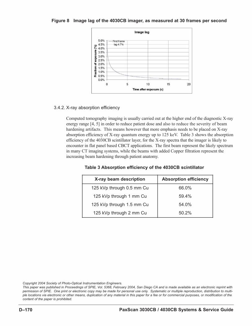
PaxScan 3030CB / 4030CB Systems & Service GuideD–170
Figure 8 Image lag of the 4030CB imager, as measured at 30 frames per second
3.4.2. X-ray absorption efficiency
Computed tomography imaging is usually carried out at the higher end of the diagnostic X-ray
energy range [4, 5] in order to reduce patient dose and also to reduce the severity of beam
hardening artifacts. This means however that more emphasis needs to be placed on X-ray
absorption efficiency of X-ray quantum energy up to 125 keV. Table 3 shows the absorption
efficiency of the 4030CB scintillator layer, for the X-ray spectra that the imager is likely to
encounter in flat panel based CBCT applications. The first beam represent the likely spectrum
in many CT imaging systems, while the beams with added Copper filtration represent the
increasing beam hardening through patient anatomy.
Table 3 Absorption efficiency of the 4030CB scintillator
Copyright 2004 Society of Photo-Optical Instrumentation Engineers.This paper was published in Proceedings of SPIE, Vol. 5368, February 2004, San Diego CA and is made available as an electronic reprint withpermission of SPIE. One print or electronic copy may be made for personal use only. Systematic or multiple reproduction, distribution to multi-ple locations via electronic or other means, duplication of any material in this paper for a fee or for commercial purposes, or modification of thecontent of the paper is prohibited.
X-ray beam description Absorption efficiency
125 kVp through 0.5 mm Cu 66.0%
125 kVp through 1 mm Cu 59.4%
125 kVp through 1.5 mm Cu 54.0%
125 kVp through 2 mm Cu 50.2%
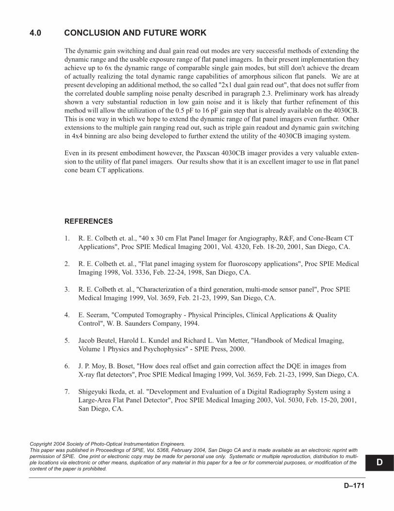
D–171
Copyright 2004 Society of Photo-Optical Instrumentation Engineers.This paper was published in Proceedings of SPIE, Vol. 5368, February 2004, San Diego CA and is made available as an electronic reprint withpermission of SPIE. One print or electronic copy may be made for personal use only. Systematic or multiple reproduction, distribution to multi-ple locations via electronic or other means, duplication of any material in this paper for a fee or for commercial purposes, or modification of thecontent of the paper is prohibited.
4.0 CONCLUSION AND FUTURE WORK
The dynamic gain switching and dual gain read out modes are very successful methods of extending the
dynamic range and the usable exposure range of flat panel imagers. In their present implementation they
achieve up to 6x the dynamic range of comparable single gain modes, but still don't achieve the dream
of actually realizing the total dynamic range capabilities of amorphous silicon flat panels. We are at
present developing an additional method, the so called "2x1 dual gain read out", that does not suffer from
the correlated double sampling noise penalty described in paragraph 2.3. Preliminary work has already
shown a very substantial reduction in low gain noise and it is likely that further refinement of this
method will allow the utilization of the 0.5 pF to 16 pF gain step that is already available on the 4030CB.
This is one way in which we hope to extend the dynamic range of flat panel imagers even further. Other
extensions to the multiple gain ranging read out, such as triple gain readout and dynamic gain switching
in 4x4 binning are also being developed to further extend the utility of the 4030CB imaging system.
Even in its present embodiment however, the Paxscan 4030CB imager provides a very valuable exten-
sion to the utility of flat panel imagers. Our results show that it is an excellent imager to use in flat panel
cone beam CT applications.
REFERENCES
1. R. E. Colbeth et. al., "40 x 30 cm Flat Panel Imager for Angiography, R&F, and Cone-Beam CT
Applications", Proc SPIE Medical Imaging 2001, Vol. 4320, Feb. 18-20, 2001, San Diego, CA.
2. R. E. Colbeth et. al., "Flat panel imaging system for fluoroscopy applications", Proc SPIE Medical
Imaging 1998, Vol. 3336, Feb. 22-24, 1998, San Diego, CA.
3. R. E. Colbeth et. al., "Characterization of a third generation, multi-mode sensor panel", Proc SPIE
Medical Imaging 1999, Vol. 3659, Feb. 21-23, 1999, San Diego, CA.
4. E. Seeram, "Computed Tomography - Physical Principles, Clinical Applications & Quality
Control", W. B. Saunders Company, 1994.
5. Jacob Beutel, Harold L. Kundel and Richard L. Van Metter, "Handbook of Medical Imaging,
Volume 1 Physics and Psychophysics" - SPIE Press, 2000.
6. J. P. Moy, B. Boset, "How does real offset and gain correction affect the DQE in images from
X-ray flat detectors", Proc SPIE Medical Imaging 1999, Vol. 3659, Feb. 21-23, 1999, San Diego, CA.
7. Shigeyuki Ikeda, et. al. "Development and Evaluation of a Digital Radiography System using a
Large-Area Flat Panel Detector", Proc SPIE Medical Imaging 2003, Vol. 5030, Feb. 15-20, 2001,
San Diego, CA.
D

Numerics
16-bit Video Output Signals 1173030CB Operational Modes, 214030CB Operational Modes, 20
A
Acquire Images, 27, 30Acquisition, 90Acquistion/Display, 73Acquisition Menu/Toolbar, 65Add All Defective Pixels, 87Add Offset to Pixels, 92Add/Subtract, 92AIA Standard Serial Interface, 43Allocate Buffers, 78Ambient Temperature, 26Amorphous Silicon, 16
Features and Benefits, 16vs. CCD or CMOS Sensors, 16
Amorphous Silicon, 11, 16Analog Gain, 20, 41, 42Analog Offset Calibration, 20, 34, 40, 83Analog Offset Settings Dialog Box, 83Analog-to-Digital Converters, 17Analysis Menu: Image Statistics, 79Apply Recursive Filter, 94Auto & Invert W/L, 61Auto W/L Button, 61
B
Basic Gain Calibration, 29Basic Image Manipulation, 58Basic Menu Commands, 79Basic Offset Calibration, 28Boot Up, 27
C
Cable Connections, 25Calibration, 19, 20, 33, 36Calibration Schedule, 135Calibration Setup, 73Capture first N frames, 77Capturing a Flat Field image, 34C-Arm, 13CCD-based Systems, 15CE, 19Cesium Iodide, 13, 16Charge Integrating Detectors, 16Circuit Overload, 27Client/Server Relationship, 147Close, 89Closing Images, 54Column Segment Editing, 87
With keyboard actions, 88With mouse actions, 88With the column segment list, 88
Command Processor, 13, 18, 19, 21, 84, 111
Connector and Cable Pinouts, 122Ethernet Port, 127Hardware Specifications, 111Hardware Configurations, 112Internal Configuration, 18Serial Interfaces, 126Specifications, 126Termination Scheme and Loading, 123
LVDS, 123Timing, 123User Synchronization Mode, 123
Command Processor and Computer Interface, 147Command Processor Component Boards, 18Communication Link, 65Communications Interface, 14Components, 13, 24Cone Beam, 95Configuration Files, 97, 105Configuration of the Receptor, 15Configure a Particular Mode, 103Configure Utility Application, 97Connecting the Cables, 24Connection Attributes, 56Connection at Startup, 56Context Menus, 59, 60Continuous Acquisition, 20Continuous Operation, 28Continuous Use, 14Control and Monitoring, 125Control Commands, 28Control of the Imager, 14Cooling Requirements, 131Copying Images, 55Correct Image, 95CPU, 19CPU/Motherboard, 18Cursor Functions, 58Customer Configuration Mode, 98
D
Dark Field, 19, 35, 37DataValid, 120DCDS Enable, 84, 104Dead Pixels, 14Debug Verbosity, 85Default Hardware Handshaking Interface, 114Default Mode, 21, 27Defects, 85Defect Correction, 40Defect Map Editor, 85Defect Map Threshold Tool, 89Defective Pixel Maps, 40Defective Pixel, 19, 22, 86, 89Definitions of Errors, 44Determining IP Addresses, 147Diagnostic Energy Imaging, 16Disable Display During Capture, 78Display Test Pattern, 84
PaxScan 3030CB / 4030CB Systems & Service GuideIndex-172

Index-173
Displaying Images in non-standard formats, 56Dispose Video, 78DRAM, 19Dripping Moisture, 26Dynamic Range, 16, 40
E
Edit Menu & Preferences, 56Edit Toolbar & Image Manipulation, 58Edit Values, 62Edit W/L, 62Electro-Magnetic Compatibility, 132Electron Mobility in a-Si, 16Electronics, 17Engineering Mode, 98Establishing Connection, 28Ethernet, 14Ethernet and High Level Serial Interface, 43Ethernet and High Level Serial Interface Architecture, 43Executive Software Application, 18Extended Gain Calibration, 69External Synchronization 112
Pin Assignments, 113
FFile Menu & Image Files, 51File Retrieval, 85File Transmittal, 84Find Noisy Pixels, 90Find Noisy Pixels Dialog, 90Fixed Pattern Noise, 21Flash Memory, 18, 106, 109, 112Flat Field, 19, 34Flat Panel Displays, 17Flat Panel Sensor, 13Fluoroscopic mode, 21, 30, 36, 72Fluoroscopy-High-Sense, 20,Fluoroscopy (Normal)-Full Resolution, 20Frame Rate, 20Frame Timing, 118Frame-to-frame Noise, 14Full Overlay, 48Full Specification, 27Full-resolution Mode, 123Function Call Paradigm, 44
G
Gain and Offset reference images, 34, 35Gain Calibration, 20, 29, 34, 36, 39, 40Gain Median, 39Gain Ratio Calibration, 68Gain Reference Image, 33Gain Settings, 73Gamma Function, 22Gate Driver Chips, 17Generate Scaled Image, 95
Get Frame from Sequence, 77Getting Started, 23Global Control Card, 112Glossary, 143Gray Levels, 57Gray Level Mappings for Linear and
Atan/s-curve Functions, 64
H
Hardware and Software Interface, 18Hardware Components, 111Hardware Handshaking, 14, 73, 112High Level Serial Interface, 43Hostdown Utility Application, 105, 108How To Reach Us, 141HSYNC, 117, 119, 120HyperTerminal, 137
I
Identifying Noisy Pixels, 91Idle Periods of Operation, 28Image Acquisition, 30, 66Image Arithmetic, 92Image Artifacts, 168Image Edit (vertical) Toolbar, 51, 58Image Information, 50
Image Tab, 50System Tab, 50Video Tab, 51
Image Intensifiers, 11Image Lag, 21, 169Image Layout, 48Image Operations, 92Image Processing, 21Image Processing Unit, 18, 19, 34, 112Image Quality, 19, 28Image Retrieval, 85Image Statistics, 79Image Transmittal, 84Image Window Types, 47Imager Operation, 14Imaging system configuration, 40Information, 73Inherent Lag, 34Initial Connection to the Command Processor, 44Initialize Video, 78Installation, 46Interface Files, 44Internal Configuration of the Receptor, 15Internal Power Supply, 19Internal Power Supply Specifications, 124Interpolation Of The Nearest Neighbors, 14Intrinsic Lag, 21Introduction, 11Inverse Compensation Artifacts, 33Invert W/L, 61
Invert W/LCheckbox, 62

Index-174 PaxScan 3030CB / 4030CB Systems & Service Guide
L
Lag, 38Latent Image, 34Lead Cap, 26, 129Loading Video Sequence, 76Logic Levels, 117Low Frame Rates, 35Low Signal-to-noise Ratio, 35LVDS, 112, 117, 122
M
Main Screen, 99Maintenance, 135Manufacturing Mode, 98Mechanical Loading, 27, 130Mechanical Mounting, 26Median Filter, 94Median Pixel Value, 35
Dark Field Image, 35Gain Image, 35
Medical Applications, 13Mega Voltage Energy Imaging, 16Memory, 19Menu Options, 48Message Options, 48Mode Control and Verification, 112Mode Selection, 102Mode Settings, 71, 72Mode Setup, 103Modes of Operation, 20More Video Options: Video Menu, 76Motherboard, 112Mounting, 26Mouse and Key Shortcuts, 59
N
Noise And Interference, 124Noise Reduction, 21Non-destructive Test, 16Non-uniformities In The Receptor, 34Non-uniformity Correction, 33Normalization Failures, 35Notes on ROIList Use, 82
O
Offset and Gain Calibration, 19, 22, 33, 42, 67Offset and Gain Calibration with 3030CB & 4030CBReceptors, 67Offset Calibration, 20, 28, 30, 34, 36, 38, 40, 67, 135Offset Characteristics, 34Offset Correction, 34Open/edit an existing file, 99Opening Images, 52Operational Modes - 3030CB , 21Operational Modes - 4030CB , 20Optimal Performance, 20Optimize Auto Level, 93
Opto-Coupler Interface, 113OR Image, 88Output Voltage, 18
P
Patient Contact, 13PaxScan Digital Imaging Subsystem, 11PaxScan Application Software, 43PaxScan Imager Configuration, 14Peak Quantum Efficiency, 16Photodiodes, 16Pixclk Timing Specifications, 119Pixel Binning, 20, 161Pixel Correction Algorithm, 40Pixel Data Format & 3030CB & 4030CB Receptors, 55Pixel Defect Map, 40Pixel Editing, 86Pixel Editor, 92Pixel Pitch, 17Playing Sequences, 76Post-exposure Offset, 28Power On Sequence, 27Power Up, 27Precautions, 26, 129Preferences, 56Primary Barrier to X-rays, 26, 129Printing Images, 54Problem Report form, 142Properties of Amophorous Silcon, 16Proper Warm Up, 30, 36Pulsed X-ray Beam Applications, 124
R
Rack Mounting, 14, 26, 130RAD AutoSave, 73Rad modes, 74Radiation, 16, 30, 36Readout Amplifiers, 19Readout And Drive Electronics, 15Readout Chips, 17Real-time, 11, 18, 95Real-Time Video Corrections, 95Receptor, 13, 15, 97Receptor Configuration file, 42, 97, 112Receptor Configuration Settings, 100Receptor Mounting, 26, 129Recording Sequences, 74Recursive Filter, 14, 21, 94Reduced Air Flow, 26, 130Reducing the Effects of Noise, 35Region of Interest Statistics, 79, 80, 81Regulatory Approvals, 19Reliable Grounding, 27Replace the Base Map, 40Reset, 85Reset Video, 78Resolution, 20

Index-175
Retrieve, 88Retrieve Files, 85Retrieve Image, 30RJ-45 Ethernet port, 18ROI Basic, 79ROI Dialog, 80RoiList Commands, 82Row Segment Editing, 87
S
Safety, 129Saturation of the Receptor, 35Saturation Threshold, 22Save a File, 99Save Between Sessions, 57Save Individual Images, 52Saving Images, 28, 51Save Video Sequence, 77Saving Video Sequences, 52Scintillator, 13, 16, 18SDRAM, 19Select Mode, 29Sensor Panel Imaging, 13Sensor Structure, 15Server, 33Set Threshold and Display, 91Setting the IP Address of the Command
Processor, 147Setting the IP Address of the Workstation, 149Setup, 46Shipment Contents, 23Shortcut Keys, 59Signal Conversion Chain, 18Signal Voltage, 18Software Interfaces, 18Software Program Update, 105Software Programming Interfaces, 43Spatial Non-uniformity, 19Special Warnings, 27Specify a Threshold Value, 64Standard Calibration Defaults, 28Standard Selection Cursor, 58Start, 29Statistics, 79Status Bar, 48Steady State Temperature, 34Sterilization, 13, 136Subsystem, 13Supported File Formats, 51, 54Synchronization Of Critical Tasks, 14System Configuration, 97
Hostdown Utility Application, 105ViVA Application, 108
System Control Using ViVA™, 45System Overview, 13System Requirements, 46System Settings, 70
T
TAB Package, 17Technical Support, 141Test Image Mode, 78Thin Film Transistors (TFTs), 15Timing Information, 124Toolbars, 51Tools Menu, 83Transmit, 88Transmit Files, 84Troubleshooting, 137TV Cameras, 11Typical Radiation Dose, 30
U
UL, 19Updates via Serial Link, 105Updating the Base Defect Map, 91Usage Dialog Box, 98Usage, 98User Synchronization Mode, 123
V
Varian Part Numbers, 24VENUS 4, 17Verification of Analog Offset Calibration, 42Versions, 46Video bus, 117Video Interface Signals, 117Video Menu, 76Video Menu/Toolbar, 74Viewing Images, 28View Menu & User Interface, 46View Options, 76ViVA, 28ViVA Application, 108ViVA Help, 45ViVA Screen View, 47ViVA Software Application, 45ViVA Transmit Files Selection, 109VSYNC, 117, 119
W
Warm-Up, 36White Area Blanking, 57, 64Window/Level Mapping, 57, 62Window/Level Scroll Bars, 61Windows 2000, 28Write ABS Mailbox, 84
X
X-ray Dose, 20X-ray-to-digital Conversion, 34