t adaptation in wlan -...
TRANSCRIPT
DEGREE PROJECT, IN , SECOND LEVELCOMMUNICATION SYSTEMSSTOCKHOLM, SWEDEN 2015
A study of the system impact fromdifferent approaches to link \tadaptation in WLAN
KEVIN PÉREZ MORENO
KTH ROYAL INSTITUTE OF TECHNOLOGY
SCHOOL OF INFORMATION AND COMMUNICATION TECHNOLOGY

Abstract
The IEEE 802.11 standards define several transmission rates that can be used at thephysical layer to adapt the transmission rate to channel conditions. This dynamicadaptation attempts to improve the performance in Wireless LAN (WLAN) and hencecan have impact on the Quality of Service (QoS) perceived by the users. In thiswork we present the design and implementation of several new link adaptation (LA)algorithms. The performance of the developed algorithms is tested and comparedagainst some existing algorithms such as Minstrel as well as an ideal LA.The evaluation is carried out in a network system simulator that models all the pro-cedures needed for the exchange of data frames according to the 802.11 standards.Different scenarios are used to simulate various realistic conditions. In particular, theClear Channel Assessment Threshold (CCAT) is modified in the scenarios and theimpact of its modification is also assessed. The algorithms are tested under identicalenvironments to ensure that the experiments are controllable and repeatable. Foreach algorithm the mean and 5th percentile throughput are measured under differenttraffic loads to evaluate and compare the performance of the different algorithms. Thetradeoff between signaling overhead and performance is also evaluated.It was found that the proposed link adaptation schemes achieved higher mean through-put than the Minstrel algorithm. We also found that the performance of some of theproposed schemes is close to that of the ideal LA.
Keywords: WLAN, link adaptation, medium reuse, channel estimation.


Referat
IEEE 802.11-standarderna definierar flera överföringshastigheter som kan användasvid det fysiska skiktet för att anpassa överföringshastigheten till kanal förhållanden.Denna dynamiska anpassning försöker förbättra prestandan i wireless LAN (WLAN)och därmed kan ha inverkan på Quality of Service (QoS) uppfattas av användarna.I detta examensarbete presenterar vi utformningen och genomförandet av flera nylink adaptation (LA) algoritmer. Prestandan hos de utvecklade algoritmer testas ochjämförs med vissa befintliga algoritmer så som Minstrel liksom en ideal LA.Utvärderingen genomförs i ett nätverkssystem simulator som ger alla de förfarandensom behövs för utbyte av dataramar enligt 802.11-standarderna. Olika scenarieranvänds för att simulera olika realistiska förhå llanden. Algoritmerna är testade underidentiska miljöer för att experimenten är styrbar och repeterbar. För varje algoritmgenomströmningen mättes under olika trafikbelastningar för att utvärdera och jämföraresultaten för de olika algoritmer. Den avvägning mellan signalering overhead ochprestanda utvärderas också .Det konstaterades att de system som föreslå s link adaptation uppnå s högre genom-snittlig throughput än Minstrel algoritm. Vi fann också att utförandet av vissa av deföreslagna systemen är nära den av ideal LA.
Nyckelord: WLAN, link adaptation, medium reuse, channel estimation.

Acknowledgements
The master thesis work was carried out at wireless access networks, Ericsson researchin Kista, Sweden. Foremost, I would like to express my sincere gratitude to mysupervisor Gustav Wikström for all the advice, patience, motivation, enthusiasm, andimmense knowledge. His guidance was of great help during the research and writingof this thesis. I could not have imagined having a better supervisor and mentor for mythesis work.My sincere thanks also go to my manager at Ericsson, Sara Landström, for giving methe opportunity to gain experience at Ericsson research and for continued support andunderstanding.The support and feedback received from the staff at Ericsson research during thepresentations and the research work had been invaluable. I am very thankful to JohanSöder and Soma Tayamon, just to name a few, for the stimulating discussions andenlightening me the first glance of research.I would also like to express my sincere gratitude to my supervisor and examiner atschool, Ben Slimane for the initial advice and guidance and for his valuable commentsafter reviewing my work. I am especially grateful for his suggestions for this study,his confidence, and the freedom he gave me to do this work.Last but not the least, I would like to thank my parents for supporting me spirituallythroughout my life and giving me everything I needed to carry out my universitystudies. I am also very grateful to my home university, Escuela Técnica Superiorde Ingenieros de Telecomunicación-Universidad Politécnica de Madrid (E.T.S.I.T.-U.P.M.), for giving me the opportunity to study abroad. It has been the best experienceof my life and it has contributed immensely to my education.


Table of contents
List of figures xi
List of tables xvii
Nomenclature xix
1 Introduction 11.1 Background . . . . . . . . . . . . . . . . . . . . . . . . . . . . . . . 11.2 Problem . . . . . . . . . . . . . . . . . . . . . . . . . . . . . . . . . 21.3 Purpose . . . . . . . . . . . . . . . . . . . . . . . . . . . . . . . . . 31.4 Goal . . . . . . . . . . . . . . . . . . . . . . . . . . . . . . . . . . . 3
1.4.1 Benefits, Ethics and Sustainability . . . . . . . . . . . . . . . 31.5 Methodology/Methods . . . . . . . . . . . . . . . . . . . . . . . . . 41.6 Delimitations . . . . . . . . . . . . . . . . . . . . . . . . . . . . . . 51.7 Outline . . . . . . . . . . . . . . . . . . . . . . . . . . . . . . . . . 5
2 IEEE 802.11 wireless LANs 72.1 IEEE 802.11 Medium Access Control layer . . . . . . . . . . . . . . 72.2 IEEE 802.11 physical layer . . . . . . . . . . . . . . . . . . . . . . . 9
2.2.1 IEEE 802.11 a/b/g/n . . . . . . . . . . . . . . . . . . . . . . 92.2.2 IEEE 802.11 ac and beyond . . . . . . . . . . . . . . . . . . 10
2.3 802.11 network architecture . . . . . . . . . . . . . . . . . . . . . . 112.4 802.11 medium access . . . . . . . . . . . . . . . . . . . . . . . . . 122.5 802.11 RTS/CTS access method . . . . . . . . . . . . . . . . . . . . 14
3 Link adaptation 153.1 Link adaptation: Motivation and main problems . . . . . . . . . . . . 153.2 Previous work . . . . . . . . . . . . . . . . . . . . . . . . . . . . . . 17
4 Existing measurements and feedback 214.1 Training sequences . . . . . . . . . . . . . . . . . . . . . . . . . . . 21
Table of contents
4.1.1 MMSE estimation . . . . . . . . . . . . . . . . . . . . . . . 224.1.2 ZF estimation . . . . . . . . . . . . . . . . . . . . . . . . . . 234.1.3 ML estimation . . . . . . . . . . . . . . . . . . . . . . . . . 23
4.2 Transmit beamforming . . . . . . . . . . . . . . . . . . . . . . . . . 244.2.1 Implicit feedback . . . . . . . . . . . . . . . . . . . . . . . . 254.2.2 Explicit feedback . . . . . . . . . . . . . . . . . . . . . . . . 25
4.3 Received Signal Strength Indicator . . . . . . . . . . . . . . . . . . . 254.3.1 Received Channel Power Indicator . . . . . . . . . . . . . . . 26
4.4 Feedback reporting in closed-loop approaches . . . . . . . . . . . . . 27
5 Simulation setup and performance metrics 295.1 Simulator overview . . . . . . . . . . . . . . . . . . . . . . . . . . . 295.2 Scenario layout . . . . . . . . . . . . . . . . . . . . . . . . . . . . . 30
5.2.1 Additional parameters . . . . . . . . . . . . . . . . . . . . . 315.3 Propagation modelling . . . . . . . . . . . . . . . . . . . . . . . . . 33
5.3.1 Multipath fading . . . . . . . . . . . . . . . . . . . . . . . . 335.3.2 Shadow fading . . . . . . . . . . . . . . . . . . . . . . . . . 345.3.3 Path loss model . . . . . . . . . . . . . . . . . . . . . . . . . 35
5.4 Error probability model . . . . . . . . . . . . . . . . . . . . . . . . . 365.4.1 Symbol information . . . . . . . . . . . . . . . . . . . . . . 365.4.2 Received Bit Information . . . . . . . . . . . . . . . . . . . . 37
5.5 Traffic model . . . . . . . . . . . . . . . . . . . . . . . . . . . . . . 385.6 Simulation logging and seed . . . . . . . . . . . . . . . . . . . . . . 395.7 Added functionalities . . . . . . . . . . . . . . . . . . . . . . . . . . 40
5.7.1 Block ACK implementation . . . . . . . . . . . . . . . . . . 405.7.2 Fast fading channel implementation . . . . . . . . . . . . . . 425.7.3 Error probability model . . . . . . . . . . . . . . . . . . . . . 435.7.4 Traffic model modification . . . . . . . . . . . . . . . . . . . 43
5.8 Overall simulator performance . . . . . . . . . . . . . . . . . . . . . 445.9 Performance metrics . . . . . . . . . . . . . . . . . . . . . . . . . . 45
5.9.1 User throughput . . . . . . . . . . . . . . . . . . . . . . . . 465.9.2 5th Percentile user throughput . . . . . . . . . . . . . . . . . 46
6 Link adaptation schemes 476.1 Minstrel algorithm . . . . . . . . . . . . . . . . . . . . . . . . . . . 47
6.1.1 The multi-rate retry chain . . . . . . . . . . . . . . . . . . . 476.1.2 Rate selection process . . . . . . . . . . . . . . . . . . . . . 486.1.3 Statistics calculation . . . . . . . . . . . . . . . . . . . . . . 48
viii

Table of contents
6.2 Ideal LA . . . . . . . . . . . . . . . . . . . . . . . . . . . . . . . . . 496.3 Proposed link adaptation schemes . . . . . . . . . . . . . . . . . . . 49
6.3.1 Common assumptions . . . . . . . . . . . . . . . . . . . . . 506.3.2 LA1 . . . . . . . . . . . . . . . . . . . . . . . . . . . . . . . 506.3.3 LA2 . . . . . . . . . . . . . . . . . . . . . . . . . . . . . . . 526.3.4 LA3 . . . . . . . . . . . . . . . . . . . . . . . . . . . . . . . 536.3.5 LA4 . . . . . . . . . . . . . . . . . . . . . . . . . . . . . . . 546.3.6 Periodic feedback (LA5) . . . . . . . . . . . . . . . . . . . . 546.3.7 General comparison . . . . . . . . . . . . . . . . . . . . . . 55
7 Simulation results 577.1 LA1 . . . . . . . . . . . . . . . . . . . . . . . . . . . . . . . . . . . 58
7.1.1 CCAT -82 dBm . . . . . . . . . . . . . . . . . . . . . . . . . 587.1.2 CCAT -62 dBm . . . . . . . . . . . . . . . . . . . . . . . . . 62
7.2 LA1 window . . . . . . . . . . . . . . . . . . . . . . . . . . . . . . 647.2.1 CCAT -82 dBm . . . . . . . . . . . . . . . . . . . . . . . . . 647.2.2 CCAT -62 dBm . . . . . . . . . . . . . . . . . . . . . . . . . 66
7.3 Remaining schemes with ACK piggybacked feedback . . . . . . . . . 677.3.1 CCAT -82 dBm . . . . . . . . . . . . . . . . . . . . . . . . . 677.3.2 CCAT -62 dBm . . . . . . . . . . . . . . . . . . . . . . . . . 69
7.4 LA5 . . . . . . . . . . . . . . . . . . . . . . . . . . . . . . . . . . . 707.4.1 CCAT -82 dBm . . . . . . . . . . . . . . . . . . . . . . . . . 717.4.2 CCAT -62 dBm . . . . . . . . . . . . . . . . . . . . . . . . . 72
7.5 Overall comparison . . . . . . . . . . . . . . . . . . . . . . . . . . . 747.5.1 CCAT -82 dBm . . . . . . . . . . . . . . . . . . . . . . . . . 747.5.2 CCAT -62 dBm . . . . . . . . . . . . . . . . . . . . . . . . . 757.5.3 Mixed numbers . . . . . . . . . . . . . . . . . . . . . . . . . 77
8 Conclusions and future work 79
Summary 83
References 85
Appendix A Model D NLOS power delay profile 93
Appendix B Additional supporting plots 95B.1 LA1 . . . . . . . . . . . . . . . . . . . . . . . . . . . . . . . . . . . 95
B.1.1 CCAT -62dBm . . . . . . . . . . . . . . . . . . . . . . . . . 95B.2 LA2 . . . . . . . . . . . . . . . . . . . . . . . . . . . . . . . . . . . 96
ix
Table of contents
B.2.1 CCAT -82dBm . . . . . . . . . . . . . . . . . . . . . . . . . 96B.2.2 CCAT -62dBm . . . . . . . . . . . . . . . . . . . . . . . . . 97
B.3 LA3 . . . . . . . . . . . . . . . . . . . . . . . . . . . . . . . . . . . 98B.3.1 CCAT -82dBm . . . . . . . . . . . . . . . . . . . . . . . . . 98B.3.2 CCAT -62dBm . . . . . . . . . . . . . . . . . . . . . . . . . 99
B.4 LA4 . . . . . . . . . . . . . . . . . . . . . . . . . . . . . . . . . . . 100B.4.1 CCAT -82dBm . . . . . . . . . . . . . . . . . . . . . . . . . 100B.4.2 CCAT -62dBm . . . . . . . . . . . . . . . . . . . . . . . . . 101
B.5 LA1 window . . . . . . . . . . . . . . . . . . . . . . . . . . . . . . 102B.5.1 CCAT -82dBm . . . . . . . . . . . . . . . . . . . . . . . . . 102B.5.2 CCAT -62 dBm . . . . . . . . . . . . . . . . . . . . . . . . . 104
B.6 LA2 window . . . . . . . . . . . . . . . . . . . . . . . . . . . . . . 107B.6.1 CCAT -82 dBm . . . . . . . . . . . . . . . . . . . . . . . . . 107B.6.2 CCAT -62 dBm . . . . . . . . . . . . . . . . . . . . . . . . . 110
B.7 LA3 window . . . . . . . . . . . . . . . . . . . . . . . . . . . . . . 113B.7.1 CCAT -82 dBm . . . . . . . . . . . . . . . . . . . . . . . . . 113B.7.2 CCAT -62 dBm . . . . . . . . . . . . . . . . . . . . . . . . . 116
B.8 LA4 window . . . . . . . . . . . . . . . . . . . . . . . . . . . . . . 119B.8.1 CCAT -82 dBm . . . . . . . . . . . . . . . . . . . . . . . . . 119B.8.2 CCAT -62 dBm . . . . . . . . . . . . . . . . . . . . . . . . . 122
x
List of figures
2.1 WLAN basic types of architectures. . . . . . . . . . . . . . . . . . . 122.2 802.11 medium access. . . . . . . . . . . . . . . . . . . . . . . . . . 132.3 RTS/CTS exchange. . . . . . . . . . . . . . . . . . . . . . . . . . . . 14
4.1 WLAN packet format [12]. . . . . . . . . . . . . . . . . . . . . . . . 214.2 Standard-compliant feedback mechanism [26]. . . . . . . . . . . . . 27
5.1 Enterprise scenario layout. . . . . . . . . . . . . . . . . . . . . . . . 325.2 Actual positions of the simulated APs (red circles) and STAs (blue
points). . . . . . . . . . . . . . . . . . . . . . . . . . . . . . . . . . 325.3 Shadow and multipath fading effects. . . . . . . . . . . . . . . . . . . 345.4 Average symbol information in bits per symbol as a function of the
SINR for different modulation schemes. . . . . . . . . . . . . . . . . 375.5 Offered traffic versus served traffic. . . . . . . . . . . . . . . . . . . . 405.6 Procedures performed during the simulation of a traffic load. . . . . . 45
7.1 Mean (solid lines) and 5th percentile (triangle lines) user throughputsfor Minstrel (blue lines), LA1 (red lines), and ideal LA (green lines)with CCAT -82 dBm . . . . . . . . . . . . . . . . . . . . . . . . . . 58
7.2 Average MCS used by Minstrel (blue line), LA1 (red line), and idealLA (green line) with CCAT -82 dBm . . . . . . . . . . . . . . . . . . 59
7.3 Average fraction of received (solid lines) and failed (triangle lines)packets for Minstrel (blue lines), LA1 (red lines), and ideal LA (greenlines) with CCAT -82 dBm . . . . . . . . . . . . . . . . . . . . . . . 60
7.4 Collision probability as a function of the served traffic per AP forMinstrel (blue lines), LA1 (red lines), and ideal LA (green lines) withCCAT -82 dBm . . . . . . . . . . . . . . . . . . . . . . . . . . . . . 61
7.5 Mean (solid lines) and 5th percentile (triangle lines) user throughputsfor Minstrel (blue lines), LA1 (red lines), and ideal LA (green lines)for CCAT -62 dBm . . . . . . . . . . . . . . . . . . . . . . . . . . . 62
xi

List of figures
7.6 Average MCS used by Minstrel (blue line), LA1 (red line), and idealLA (green line) with CCAT -62 dBm . . . . . . . . . . . . . . . . . . 63
7.7 Mean (solid lines) and 5th percentile (triangle lines) user throughputsfor Minstrel (blue lines), LA1 window (red lines), and ideal LA (greenlines) for CCAT -82 dBm . . . . . . . . . . . . . . . . . . . . . . . . 65
7.8 Average MCS used by Minstrel (blue line), LA1 window (red line),and ideal LA (green line) with CCAT -82 dBm . . . . . . . . . . . . . 66
7.9 Throughput gain as a function of the feedback period with the linkto system (L2S) ratemaps (blue line) and with the implemented fastfading (FF) channels (red line) for CCAT -82 dBm . . . . . . . . . . 71
7.10 Throughput gain as a function of the feedback period with the linkto system (L2S) ratemaps (blue line) and with the implemented fastfading (FF) channels (red line) for CCAT -62 dBm . . . . . . . . . . 73
7.11 Gains in term of mean throughput achieved by the different schemesand the benchmarks with CCAT -82 dBm (left side) and CCAT -62dBm (right side). . . . . . . . . . . . . . . . . . . . . . . . . . . . . 77
A.1 Model D NLOS power delay profile . . . . . . . . . . . . . . . . . . 93
B.1 Additional plots for LA1 with CCAT -62dBm . . . . . . . . . . . . . 95B.2 Comparison between LA2 and the benchmarks in terms of user through-
put, average MCS used, collision probability, and average fraction ofreceived and failed packets with CCAT -82 dBm . . . . . . . . . . . . 96
B.3 Comparison between LA2 and the benchmarks in terms of user through-put, average MCS used, collision probability, and average fraction ofreceived and failed packets with CCAT -62 dBm . . . . . . . . . . . . 97
B.4 Comparison between LA3 and the benchmarks in terms of user through-put, average MCS used, collision probability, and average fraction ofreceived and failed packets with CCAT -82 dBm . . . . . . . . . . . . 98
B.5 Comparison between LA3 and the benchmarks in terms of user through-put, average MCS used, collision probability, and average fraction ofreceived and failed packets with CCAT -62 dBm . . . . . . . . . . . . 99
B.6 Comparison between LA4 and the benchmarks in terms of user through-put, average MCS used, collision probability, and average fraction ofreceived and failed packets with CCAT -82 dBm . . . . . . . . . . . . 100
B.7 Comparison between LA4 and the benchmarks in terms of user through-put, average MCS used, collision probability, and average fraction ofreceived and failed packets with CCAT -62 dBm . . . . . . . . . . . . 101
xii

List of figures
B.8 Gain in mean (leftmost picture) and 5th percentile (rightmost picture)throughput at 100 Mbps per AP achieved by LA1 window as a functionof the window size for the maximum (red lines), minimum (blue lines)and mean SINR (green lines) stored in the transmitter window withCCAT -82 dBm . . . . . . . . . . . . . . . . . . . . . . . . . . . . . 102
B.9 Additional plots for LA1 window with CCAT -82dBm . . . . . . . . 102B.10 Comparison between LA1 and LA1 window in terms of user through-
put, average MCS used, collision probability, and average fraction ofreceived and failed packets with CCAT -82 dBm . . . . . . . . . . . . 103
B.11 Gain in mean (leftmost picture) and 5th percentile (rightmost picture)throughput at 100 Mbps per AP achieved by LA1 window as a functionof the window size for the maximum (red lines), minimum (blue lines)and mean SINR (green lines) stored in the transmitter window withCCAT -62 dBm . . . . . . . . . . . . . . . . . . . . . . . . . . . . . 104
B.12 Comparison between LA1 window and the benchmarks in terms ofuser throughput, average MCS used, collision probability, and averagefraction of received and failed packets with CCAT -62 dBm . . . . . . 105
B.13 Comparison between LA1 and LA1 window in terms of user through-put, average MCS used, collision probability, and average fraction ofreceived and failed packets with CCAT -62 dBm . . . . . . . . . . . . 106
B.14 Gain in mean (leftmost picture) and 5th percentile (rightmost picture)throughput at 100 Mbps per AP achieved by LA2 window as a functionof the window size for the maximum (red lines), minimum (blue lines)and mean SINR (green lines) stored in the transmitter window withCCAT -82 dBm . . . . . . . . . . . . . . . . . . . . . . . . . . . . . 107
B.15 Comparison between LA2 window and the benchmarks in terms ofuser throughput, average MCS used, collision probability, and averagefraction of received and failed packets with CCAT -82 dBm . . . . . . 108
B.16 Comparison between LA2 and LA2 window in terms of user through-put, average MCS used, collision probability, and average fraction ofreceived and failed packets with CCAT -82 dBm . . . . . . . . . . . . 109
B.17 Gain in mean (leftmost picture) and 5th percentile (rightmost picture)throughput at 100 Mbps per AP achieved by LA2 window as a functionof the window size for the maximum (red lines), minimum (blue lines)and mean SINR (green lines) stored in the transmitter window withCCAT -62 dBm . . . . . . . . . . . . . . . . . . . . . . . . . . . . . 110
xiii
List of figures
B.18 Comparison between LA2 window and the benchmarks in terms ofuser throughput, average MCS used, collision probability, and averagefraction of received and failed packets with CCAT -62 dBm . . . . . . 111
B.19 Comparison between LA2 and LA2 window in terms of user through-put, average MCS used, collision probability, and average fraction ofreceived and failed packets with CCAT -62 dBm . . . . . . . . . . . . 112
B.20 Gain in mean (leftmost picture) and 5th percentile (rightmost picture)throughput at 100 Mbps per AP achieved by LA3 window as a functionof the window size for the maximum (red lines), minimum (blue lines)and mean SINR (green lines) stored in the transmitter window withCCAT -82 dBm . . . . . . . . . . . . . . . . . . . . . . . . . . . . . 113
B.21 Comparison between LA3 window and the benchmarks in terms ofuser throughput, average MCS used, collision probability, and averagefraction of received and failed packets with CCAT -82 dBm . . . . . . 114
B.22 Comparison between LA3 and LA3 window in terms of user through-put, average MCS used, collision probability, and average fraction ofreceived and failed packets with CCAT -82 dBm . . . . . . . . . . . . 115
B.23 Gain in mean (leftmost picture) and 5th percentile (rightmost picture)throughput at 100 Mbps per AP achieved by LA3 window as a functionof the window size for the maximum (red lines), minimum (blue lines)and mean SINR (green lines) stored in the transmitter window withCCAT -62 dBm . . . . . . . . . . . . . . . . . . . . . . . . . . . . . 116
B.24 Comparison between LA3 window and the benchmarks in terms ofuser throughput, average MCS used, collision probability, and averagefraction of received and failed packets with CCAT -62 dBm . . . . . . 117
B.25 Comparison between LA3 and LA3 window in terms of user through-put, average MCS used, collision probability, and average fraction ofreceived and failed packets with CCAT -62 dBm . . . . . . . . . . . . 118
B.26 Gain in mean (leftmost picture) and 5th percentile (rightmost picture)throughput at 100 Mbps per AP achieved by LA4 window as a functionof the window size for the maximum (red lines), minimum (blue lines)and mean SINR (green lines) stored in the transmitter window withCCAT -82 dBm . . . . . . . . . . . . . . . . . . . . . . . . . . . . . 119
B.27 Comparison between LA4 window and the benchmarks in terms ofuser throughput, average MCS used, collision probability, and averagefraction of received and failed packets with CCAT -82 dBm . . . . . . 120
xiv
List of figures
B.28 Comparison between LA4 and LA4 window in terms of user through-put, average MCS used, collision probability, and average fraction ofreceived and failed packets with CCAT -62 dBm . . . . . . . . . . . . 121
B.29 Gain in mean (leftmost picture) and 5th percentile (rightmost picture)throughput at 100 Mbps per AP achieved by LA4 window as a functionof the window size for the maximum (red lines), minimum (blue lines)and mean SINR (green lines) stored in the transmitter window withCCAT -62 dBm . . . . . . . . . . . . . . . . . . . . . . . . . . . . . 122
B.30 Comparison between LA4 window and the benchmarks in terms ofuser throughput, average MCS used, collision probability, and averagefraction of received and failed packets with CCAT -62 dBm . . . . . . 123
B.31 Comparison between LA4 and LA4 window in terms of user through-put, average MCS used, collision probability, and average fraction ofreceived and failed packets with CCAT -62 dBm . . . . . . . . . . . . 124
xv

List of tables
5.1 Enterprise scenario parameters. . . . . . . . . . . . . . . . . . . . . . 315.2 Traffic model settings. . . . . . . . . . . . . . . . . . . . . . . . . . 39
6.1 Minstrel multi-rate retry chain [35]. . . . . . . . . . . . . . . . . . . 496.2 General comparison in terms of overhead, precision, expected perfor-
mance, and complexity. . . . . . . . . . . . . . . . . . . . . . . . . . 56
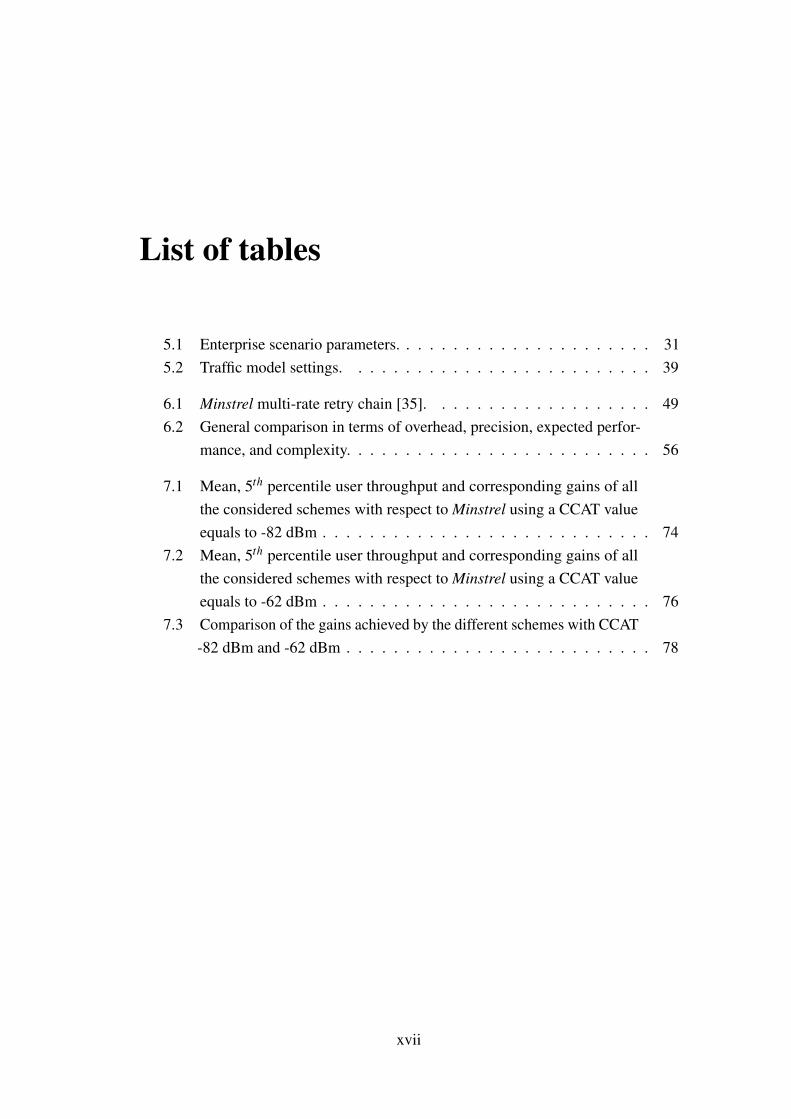
7.1 Mean, 5th percentile user throughput and corresponding gains of allthe considered schemes with respect to Minstrel using a CCAT valueequals to -82 dBm . . . . . . . . . . . . . . . . . . . . . . . . . . . . 74
7.2 Mean, 5th percentile user throughput and corresponding gains of allthe considered schemes with respect to Minstrel using a CCAT valueequals to -62 dBm . . . . . . . . . . . . . . . . . . . . . . . . . . . . 76
7.3 Comparison of the gains achieved by the different schemes with CCAT-82 dBm and -62 dBm . . . . . . . . . . . . . . . . . . . . . . . . . . 78
xvii

List of tables
Nomenclature
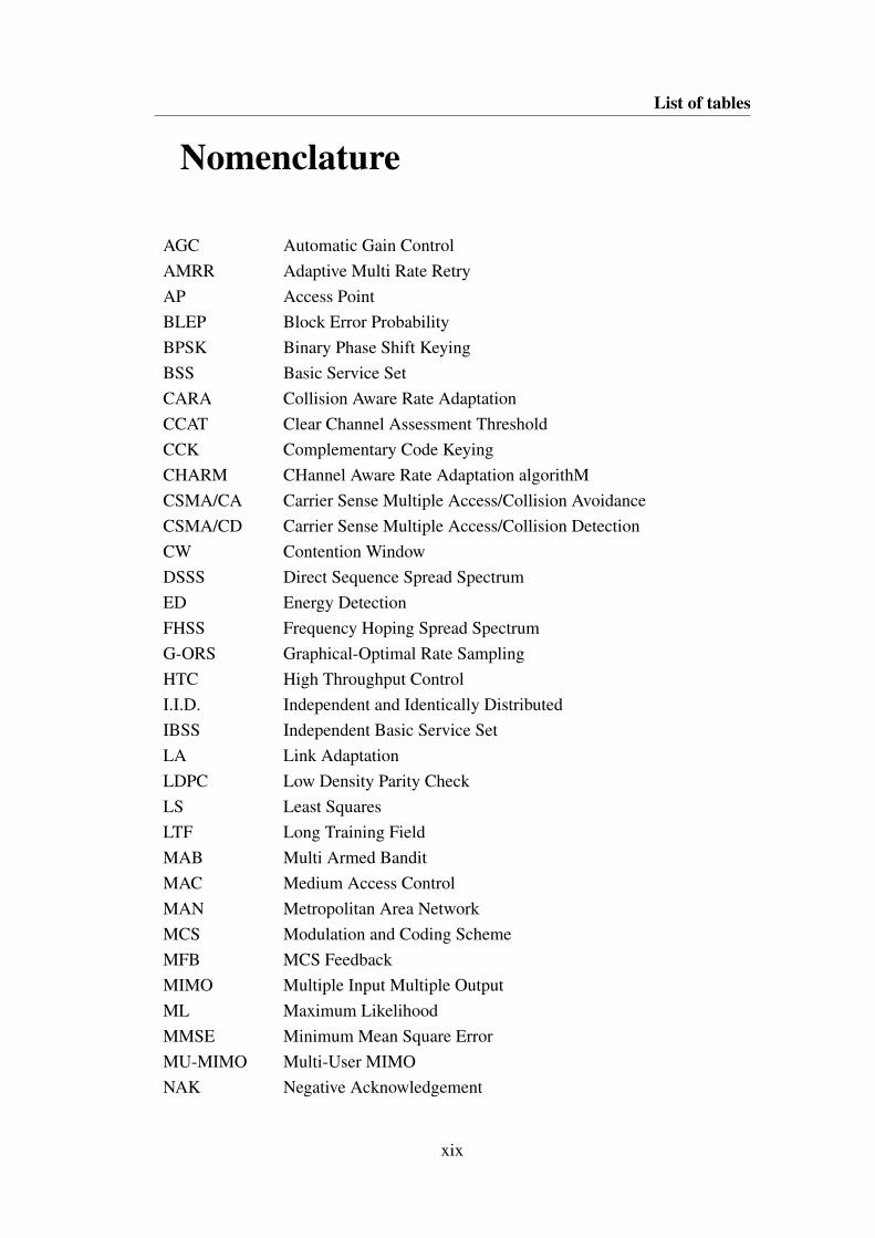
AGC Automatic Gain ControlAMRR Adaptive Multi Rate RetryAP Access PointBLEP Block Error ProbabilityBPSK Binary Phase Shift KeyingBSS Basic Service SetCARA Collision Aware Rate AdaptationCCAT Clear Channel Assessment ThresholdCCK Complementary Code KeyingCHARM CHannel Aware Rate Adaptation algorithMCSMA/CA Carrier Sense Multiple Access/Collision AvoidanceCSMA/CD Carrier Sense Multiple Access/Collision DetectionCW Contention WindowDSSS Direct Sequence Spread SpectrumED Energy DetectionFHSS Frequency Hoping Spread SpectrumG-ORS Graphical-Optimal Rate SamplingHTC High Throughput ControlI.I.D. Independent and Identically DistributedIBSS Independent Basic Service SetLA Link AdaptationLDPC Low Density Parity CheckLS Least SquaresLTF Long Training FieldMAB Multi Armed BanditMAC Medium Access ControlMAN Metropolitan Area NetworkMCS Modulation and Coding SchemeMFB MCS FeedbackMIMO Multiple Input Multiple OutputML Maximum LikelihoodMMSE Minimum Mean Square ErrorMU-MIMO Multi-User MIMONAK Negative Acknowledgement
xix

List of tables
NAV Network Allocation VectorNDP Null Data PacketNLOS No Line Of SightOAR Opportunistic Auto RateOBSS Overlapping Basic Service SetOFDM Orthogonal Frequency Division MultiplexingORS Optimal Rate SamplingPDP Power Delay ProfilePHY PhysicalPLCP Physical Layer Convergence ProcedurePMD Physical Medium DependentQAM Quadrature Amplitude ModulationRAMAS Rate Adaptation for Multi Antenna SystemsRBI Received Bit InformationRBIR Received Bit Information RateRCPI Received Channel Power IndicatorRSSI Received Signal Strength IndicatorRTS/CTS Request To Send/Clear To SendSD Signal DetectionSDM Spatial Division MultiplexingSF Shadow FadingSINR Signal to Interference plus Noise RatioSTA StationSTF Short Training FieldSW G-ORS Sliding Window Graphical-Optimal Rate SamplingTG Task GroupTx BF Transmit BeamformingTxOP Transmit OpportunityVHTC Very High Throughput ControlWLAN Wireless Local Area NetworkZF Zero Forcing
xx

Chapter 1
Introduction
In recent years, mobile computing devices have become ubiquitous. Due to theemergence of devices such as laptops, tablets or smart phones, people are no longertied by their desktop PCs to satisfy their computing needs. IEEE 802.11 WirelessLocal Area Network (WLAN) [1] has become one of the most common ways formobile devices to connect to each other and to the Internet. The success experiencedby 802.11 networks is mainly due to some key features such as low cost, ease ofinstallation and deployment, and the availability of high data rates.Nowadays, WLANs are used to provide internet connectivity in places ranging fromhomes or offices to restaurants, hotels, airports, hospitals, etc. Due to the increaseddemand together with the popularization of services like internet telephony or videostreaming, the data rates as well as the efficiency should be increased in order to satisfythe Quality of Service (QoS) requirements of those services [2].
1.1 Background
The IEEE 802.11 standards propose several data rates that can be used for the trans-mission of data. The different data rates are achieved by using various combinationsof modulation and coding schemes (MCS) at the physical layer [2]. Higher MCS giveshigh data rates that can transmit more information during a certain period of time thanlower MCS. However, high MCSs are more susceptible to errors. Instead, low MCSstake longer to transmit a packet over the link but they are more resistant to errorssince they use more robust modulation and coding schemes and the transmission ismore likely to be successful during the periods when the channel conditions are notfavorable. Nevertheless, a capacity increase is needed in order to handle the increaseduse of services such as voice over IP (VoIP) or video streaming. Hence, high data
1

Introduction
rates become necessary in order to serve more traffic per system and provide theaforementioned services.The availability of different MCSs allows the use of a mechanism that dynamicallyselects one of the multiple available MCSs. This functionality is referred to as rateadaptation or link adaptation (LA) [3]. Any link adaptation scheme consists of twoparts: channel estimation and rate adaptation. The channel estimation mechanism is incharge of assessing the channel conditions. The link adaptation mechanism consistof an algorithm that selects the best MCS according to the predetermined channelconditions [4].There are two main approaches to estimate the channel conditions, namely open-loop and closed-loop. In the open-loop approach, the sender estimates the channelquality based on its own perception of the channel by using metrics such as successor failure of the previous data frames, the Received Signal Strength Indicator (RSSI)of the received ACK frames, etc. On the other hand, closed-loop approaches rely onmeasurements performed on the receiver side. These measurements are sent back tothe sender so that the transmitter can estimate the channel conditions and select theappropriate MCS [4].
1.2 Problem
Link adaptation is a technique whose objective is to harvest the potential capacity of achannel [4]. As stated earlier, the channel conditions may vary with time and dependon many factors, such as mobility and environment. Therefore, a good LA algorithmshould adapt quickly and at the same time be accurate and robust over many possiblechannel situations. In addition, the LA will be performed in wireless devices whichare battery driven in most of the cases. So, the LA algorithm should also be energyefficient so that the battery life is not reduced drastically and it should maximize thecapacity at the same time.The main problem addressed in this work is the development of a robust and efficientLA algorithm that has a good performance in different situations. Coinciding withthe ongoing work of standardization of the 802.11ax amendment, the performance ofthe proposed algorithm will be evaluated in a simulator setup corresponding to botha standard system capturing both a likely 802.11ac setup and a scenario envisionedfor 802.11ax. In addition, the implementation of the LA algorithm may imply addingsome extra signaling between transmitter and receiver which leads to an increasedoverhead and therefore the efficiency would be lowered. To the best of our knowledge,this would be the first work that shows how these systems will be influenced by
2

1.3 Purpose
the insertion of an LA algorithm in terms of network level efficiency including theoverheads.
1.3 Purpose
The purpose is to investigate possible improvement strategies for LA in a high capacityWLAN system (IEEE 802.11ax [5]) by using new or existing feedback signals toestimate the channel conditions.
1.4 Goal
The main objective of this work is to implement and compare different LA algorithmsin a standard system (802.11ac [6]) and in a high capacity system (802.11ax). Thecomparison of the different schemes is mainly done in terms of achieved throughputat certain traffic load. The performance of the different schemes is tested in sev-eral scenarios with different propagation conditions as well as different densities ofWLAN stations (STAs) and access points (APs). Furhermore, the effect of introducingmeasurements and feedback and the tradeoff between signaling overhead (due to theintroduced feedback) and performance are evaluated as well.
1.4.1 Benefits, Ethics and Sustainability
Ethics is commonly defined as a set of concepts and principles that help distinguishingbetween acceptable and unacceptable behaviors [7]. According to the definition ofethics, there is a set of principles that should be followed while conducting research.Some of them define the aims of research, such as knowledge gaining, error avoidanceand intellectual property [8]. In most of the cases, research involves cooperation andcoordination among different people in different institutions. Ethics take into accountthis by promoting values that are essential to collaborative work, such as trust, fairness,and accountability [9]. Some other ethical principles aim at building public supportfor research since the quality of the research is suppossed to be improved by followingthe ethical principles [10]. Finally, there are some additional ethical principles such associal responsibility, compliance with law, health or safety (among others) that shouldalso be taken into account.By following the aforementioned ethical principles, a person skilled in this art canbenefit from the results presented in this work. On the other hand, if the principles arenot followed, the sustainability of the results can be compromised and it may lead tothe misuse of the work presented in this document.
3
Introduction
In order to preserve the aforementioned principles, the papers used in the literaturereview are properly referenced and the results shown in them are objectively reflected.Furthermore, the obtained results are made publicly available in order to gain knowl-edge and promote the research in the topic of link adaptation.
1.5 Methodology/Methods
The chosen method is the quantitative method because we are going to work with largeamounts of data, numbers and statistics [11].A suitable research method for this project is the experimental research since it issystematic and rigorous investigation of a problem [11]. The aim is to gain a newknowledge or test hypotheses about current knowledge. This method fits to the projectsince the purpose is to investigate possible improvement strategies for LA algorithms.The research approach connected to this study is the inductive approach. This approachis chosen because before doing the research, the potential improvements have to beidentified first based on literature study and assessed based on experiments [11].The data will be collected through simulations and after collecting the data, it will beanalysed using statistical methods and compared to the results of other simulations.The conclusions of the research will be formulated based on that.To sum up, this work focuses on evaluating the performance at system level of theproposed algorithms by means of Monte Carlo Simulations. In particular, the workis performed according to the following steps: first, the algorithms are developedin a theoretical manner by identifying possible ways of improving the performance.Then, some functionalities were added to the simulator. After that, the algorithmswere developed in the simulator and the performance was analysed. Eventually, acomparison of the proposed algorithms at a certain traffic load was carried out.In addition, the author also collaborated in a work where possible ways of increasingthe spectral reuse in wireless systems were evaluated. The results of this work werereflected on a conference paper accepted at the IEEE International Symposium onPersonal, Indoor and Mobile Radio Communications (PIMRC). In particular, the papercan be found under the following reference:Soma Tayamon, Gustav Wikström, Kevin Perez Moreno, Johan Söder, Yu Wang andFilip Mestanov. “Analysis of the potential for increased spectral reuse in wirelessLAN”, accepted at the 26th International Symposium on Personal, Indoor and MobileRadio Communications (PIMRC): Mobile and Wireless Networks, Hong Kong, China,August 30 – September 2, 2015.
4

1.6 Delimitations
1.6 Delimitations
The described work only considers the system performance, i.e. the performance on ascenario with multiple APs and a high number of STAs. However, scenarios with onlyone access point and several users are not considered. The results in such scenariosare expected to differ substantially from the results obtained in this work since thechannel conditions are different from the considered scenario. In particular, the delaysexperienced when accessing the medium as well as the time that packets wait untilbeing transmitted i.e. the queuing delay, among others, would differ substantially fromthe considered scenarios, and that would affect the results obtained. Therefore, theobtained conclusions may not apply under such conditions. In particular, the delayswhen accessing the medium and the queuing delays are supposed to be smaller inthose scenarios. Hence, higher throughputs could be obtained in those scenarios.
1.7 Outline
The remainder of the thesis is organized in the following parts:Chapter 2 provides an introduction to the 802.11 wireless networks where the generalconcepts about the physical and medium access control layers are provided.Chapter 3 presents the basics of link adaptation and a literature review of the previousresearch that has been carried out on that topic.Chapter 4 shows some details about the existing measurements and feedback mecha-nisms that can be used to perform link adaptation.Chapter 5 describes the experimental setup that is used in the simulations and themetrics used to compare the performance of the algorithms.Chapter 6 gives a description of the considered algorithms as well as the proposedschemes.Chapter 7 provides a comparison of the performance of the proposed LA against theother considered algorithms as well as the ideal LA.Chapter 8 draws the final conclusion about the results obtained in the previous chaptertogether with some suggestions for future work.
5

Chapter 2
IEEE 802.11 wireless LANs
IEEE 802.11 is a set of Medium Access Control (MAC) and physical layer (PHY)specifications that define an over-the-air interface for enabling Wireless Local AreaNetwork (WLAN) communication [1]. The initial version of the standard was releasedin 1997 [12]. This standard is member of the IEEE 802 family of local area networking(LAN) and metropolitan area networking (MAN) standards. This family is charac-terized by the use of the OSI reference model [12] and a 48-bit universal addressingscheme [1].
2.1 IEEE 802.11 Medium Access Control layer
The MAC layer is mainly in charge of coordinating the data transmissions of thedifferent nodes over the shared medium [1]. The first version of the MAC layeradopted the same distributed access protocol that was used in Ethernet, carrier sensemultiple access (CSMA) [12]. With CSMA, a station that wants to transmit data firstlistens to the medium for a predetermined period of time. If the medium is sensed"idle" then the station is allowed to transmit. If the medium is sensed "busy" then thestation has to defer its transmission.Ethernet used a variation of CSMA called carrier sense multiple access with collisiondetection (CSMA/CD). On an Ethernet network, a station is able to receive its owntransmission and detect collisions. If a collision is detected, the two stations involvedin the collision back off for a random period of time before transmitting again. Thebackoff time is likely to be different on both stations and therefore the probability of asecond collision is reduced [14].However, wireless devices are not able to detect collisions while transmitting [15].Instead, 802.11 uses a variation called carrier sense multiple access with collisionavoidance (CSMA/CA) [16]. Rather, before any new transmission a random backoff
7

IEEE 802.11 wireless LANs
is drawn. This improves the performance since the effect of collisions on wirelessnetworks is more severe than on wired networks. On wired networks collisions aredetected by the circuitry and almost immediately, while on wireless networks collisionsare inferred from the lack of an acknowledgement after transmitting the frame [15].For the channel sensing, a procedure called Clear Channel Assessment (CCA) [12] isused. CCA is used to determine whether the channel is idle or busy by measuring thereceived power and comparing it against some predefined thresholds. In particular, ifthe measured power is above the threshold, the medium is declared as busy, otherwisethe medium is considered idle. Since 802.11 networks operate in unlicensed bands [1]two thresholds should be applied, one for the non 802.11 signals and another for the802.11 signals. Here, a signal is denoted as an 802.11 signal when an 802.11 headercan be properly decoded, otherwise it is considered as a non 802.11 signal.The threshold applied to the non 802.11 signals is called Energy Detection (ED)threshold [17] and it has a value equal to -62 dBm. This threshold is used to reactto any interfering signal having a power greater than the aforementioned value. Inother words, ED is performing physical sensing since it monitors the RF power levelin the medium. Here, the channel is declared as busy if the received power is greaterthan the ED threshold. Otherwise, it is considered as idle. Similarly, the thresholdapplied to the 802.11 signals is called Signal Detection (SD) threshold [17] and it isequal to -82 dBm. The SD threshold is more sensitive than the ED threshold sinceit is more important to react to 802.11 signals in order to avoid collisions with suchtransmissions than reacting to any other signal. The SD threshold is here denoted asthe Clear Channel Assessment Threshold (CCAT). In addition, it is assumed that thenoise floor is below the CCAT value for the method to be fully effective [17].Rather, with SD a technique called virtual carrier sensing [18] is used. It uses somefields of the frames that indicate to the other stations the duration of the transmission.This information is carried on the duration field of the frame. If the received frame hasa power greater than the CCAT, the stations read the header and update their NetworkAllocation Vector (NAV) based on the duration field of the received frame. The NAV isa variable that contains the time during which the channel is supposed to be busy andtherefore transmissions are not allowed during that period of time. The stations use acountdown timer to count down from the current NAV value to zero. The channel isassumed to be idle when the NAV reaches zero.
8
2.2 IEEE 802.11 physical layer
2.2 IEEE 802.11 physical layer
The PHY layer defines what signals are sent over the wireless medium. It is dividedinto two sublayers, namely the Physical Layer Convergence Procedure (PLCP) and thePhysical Medium Dependent (PMD) sublayer [1]. The PLCP sublayer takes care ofthe frame exchange between the MAC and PHY layer. The PMD sublayer translatesthe frames received from the PLCP into bits for transmission over the wireless sharedmedium. As mentioned earlier, the CCA procedure is also performed at the PHYlayer.
2.2.1 IEEE 802.11 a/b/g/n
The original standard (802.11-1997) included three PHYs: infrared (IR), 2.4 GHzFrequency Hopping Spread Spectrum (FHSS), and 2.4 GHz Direct Sequence SpreadSpectrum (DSSS) [1]. In 1999, two standard amendments were presented: 802.11aand 802.11b. The purpose of 802.11a was to create a new PHY in 5 GHz and 802.11bwas aiming at increasing the data rate in 2.4 GHz by using enhanced DSSS withComplementary Code Keying (CCK) [12]. On the other hand, the IR and 2.4 GHzFHSS PHYs did not succeed and were not materialized.802.11a introduced the concept of Orthogonal Frequency Division Multiplexing(OFDM) which achieved data rates of up to 54 Mbps in the 5 GHz band [12]. Themain idea of OFDM is to split a high bandwidth channel into several subchannelshaving lower bandwidth. However, its adoption was slow since devices willing totake advantage of the higher data rates provided by 802.11a and keeping backwardcompatibility with 802.11b devices would need to implement two front-ends, one tooperate using 802.11b in the 2.4 GHz band and the other to operate in the 5 GHz bandusing 802.11a [19].The 802.11g standard incorporated the 802.11a OFDM PHY in the 2.4 GHz bandallowing data rates of up to 54 Mbps. It also provided backward compatibility with the802.11b devices. It experienced a large market success because of the aforementionedfeatures [19].The 802.11n standard [20] increased the data rate by using Multiple Input-MultipleOutput (MIMO) antennas [21] with up to 4 spatial streams, 40 MHz channels in thePHY and frame aggregation in the MAC layer.MIMO is a technology used to transmit independent data streams on different antennas.Data streams are defined as streams of bits transmitted over separate spatial dimensions.This is called spatial division multiplexing (SDM) [22]. With MIMO/SDM the datarate increases as increasing the number of independent data streams. Furthermore, by
9

IEEE 802.11 wireless LANs
doubling the channel width from 20 MHz to 40 MHz the data rate can be doubled[20].Frame aggregation is the process of packing multiple MAC Service Data Units (MS-DUs) or MAC Protocol Data Units (MPDUs) into a single frame to reduce the overheadand hence improve the efficiency [20]. MSDU aggregation (or A-MSDU) occurs atthe top of the MAC layer. It aggregates MSDUs destined for the same receiver and ofthe same service category into a single MPDU [23]. MPDU aggregation (or A-MPDU)occurs at the bottom of the MAC layer. It aggregates MDPUs to form the PhysicalSDU (PSDU) for transmission in a single PPDU. The aggregation techniques describedabove allow for long data transmission which increases the efficiency by reducing theoverhead and therefore the data rate is increased as well [23].The enhancement of the block acknowledgment (BA) technique was proposed togetherwith the frame aggregation. BA is a technique whose objective is to improve the MACefficiency. It was defined as optional in the 802.11e amendment and it was improvedand made mandatory in the 802.11n amendment [20]. BA allows the possibility toacknowledge multiple MPDUs using a single ACK frame, called block ACK, insteadof transmitting individual ACKs for every MPDU [20].The BA technique is often used with the transmit opportunity (TxOP) functionality.By using this functionality, the channel can be used for a period of time called TxOPupon gaining access to it according to the procedures specified in section 2.1. Thisfunctionality provides contention free access to the channel during that time interval.In addition, the station can transmit as many frames as possible during the TxOP [20].The use of the techniques described above allowed data rates of up to 300 Mbps in20 MHz and 600 Mbps in 40 MHz with the use of 4 spatial streams [20]. In addition,802.11n standard operates on both 2.4 GHz and 5 GHz bands. Support for 5 GHz isoptional.
2.2.2 IEEE 802.11 ac and beyond
The data rate was further increased by the 802.11ac standard. The standard has thegoal of achieving at least 1 Gbps on a WLAN with multiple users and a single linkthroughput of at least 500 Mbps [6]. New features have been added at both the PHYand MAC layer to achieve the proposed goals.At the PHY layer, new channel bandwidths of 80 MHz and 160 MHz are added toexploit the idea that the maximum theoretical PHY rate can be linearly increased by afactor of the number of spatial streams or channel bandwidth [24]. In addition, twoMCSs with higher order modulations and more efficient coding schemes are introduced
10
2.3 802.11 network architecture
to further increase the data rate [6]. The channelization structure and a more detaileddescription of the introduced features are presented in [24].At the MAC layer, the maximum size of A-MSDU and A-MPDU is increased toimprove the MAC efficiency and also take advantage of the proposed higher data rates[6]. The standard also provides additional features such as transmit beamforming(TxBF) and downlink multi-user MIMO (MU-MIMO) [25]. TxBF is a procedure thatmodifies the radiation pattern of the transmitting antenna to optimize the reception atone or more station. To do so, explicit channel state information is needed. This isachieved by using a sounding protocol and compressed beamforming feedback [24].With downlink MU-MIMO, one station is allowed to transmit up to four independentdata streams simultaneously that can be destined to different receivers [25].By using all the aforementioned features, 802.11ac provides a maximum data rateof 1733 Mbps with 80 MHz and four spatial streams and 6933 Mbps with 160MHzand eight spatial streams [24]. Recently, the IEEE Standards Association approvedthe 802.11ax amendment [26]. The purpose of this amendment, also known as HighEfficiency WLAN (HEW), is to define modifications on both the PHY and MAClayer that lead to the development of at least one mode of operation that is capable ofincreasing at least four times the average throughput per station (measured at the MAClayer) in a dense deployment scenario. The power efficiency should be maintainedor even improved. In addition, backward compatibility and coexistence with legacydevices operating on the same frequency band shall be provided as well [26].This amendment is focused on improving metrics related to user experience [26].The improvements should work on environments such as corporate offices, outdoorhotspots, dense residential apartments and stadiums [26]. The study group was initiatedin 2013. It is expected that the actual deployment of the standard will take place atthe earliest in late 2019 [26]. Currently, the possible technologies and challenges toachieve the proposed goal are being assessed [26].
2.3 802.11 network architecture
The 802.11 standards define two basic types of architectures: infrastructure modeor ad-hoc mode [12]. The Basic Service Set (BSS) is a key concept on the WLANarchitecture. It comprises all the stations that remain within a coverage area and formsome sort of association. In ad-hoc mode, stations communicate directly with oneanother; this is referred to as an Independent BSS (IBSS). This is the most basic formof association [1].
11

IEEE 802.11 wireless LANs
On the other hand, stations can associate with a central station in charge of managingthe BSS. The central station is referred to as an access point (AP). This scenario iscalled infrastructure BSS. Infrastructure BSSes can be interconnected via a distributionsystem (DS) that provides connectivity between the APs. This is known as extendedservice set (ESS) [12]. The concepts described below are shown in Figure 2.1.
Figure 2.1 WLAN basic types of architectures.
Furthermore, when the coverage area of nearby BSSes overlap with each other theybecome what is known as Overlapping BSSes (OBSSes) [12]. This is generallyconsidered as undesirable since members of the OBSSes may interfere with each otherand compete for channel access which can lead to a decreased performance.
2.4 802.11 medium access
Since the access to the medium is contention based [1], a mechanism to avoid collisionsis needed. To do so, the time is divided into slots to achieve coordination betweenall the stations within a BSS [12]. The access is prioritized by the use of inter framespaces (IFS). The IFS defines the period of time between the end of a transmission andthe beginning of the following transmission [1]. There are several inter frame spacesthat define different levels of priority. These are, from smallest to largest, reduced-IFS(RIFS), short-IFS (SIFS), Point Coordination Function-IFS (PIFS) and DistributedCoordination Function-IFS (DIFS). After SIFS or RIFS, only management frames canbe sent. On the other hand, data frames are sent after DIFS or PIFS [12].The mechanism used to avoid collisions is called binary exponential backoff [1]. Theobjective of the mechanism is to randomize the time instants at which the stations aretrying to transmit so that the collision probability is minimized [12]. To achieve low
12
2.4 802.11 medium access
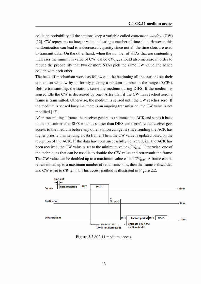
collision probability all the stations keep a variable called contention window (CW)[12]. CW represents an integer value indicating a number of time slots. However, thisrandomization can lead to a decreased capacity since not all the time slots are usedto transmit data. On the other hand, when the number of STAs that are contendingincreases the minimum value of CW, called CWmin, should also increase in order toreduce the probability that two or more STAs pick the same CW value and hencecollide with each other.The backoff mechanism works as follows: at the beginning all the stations set theircontention window by uniformly picking a random number in the range (0,CW ).Before transmitting, the stations sense the medium during DIFS. If the medium issensed idle the CW is decreased by one. After that, if the CW has reached zero, aframe is transmitted. Otherwise, the medium is sensed until the CW reaches zero. Ifthe medium is sensed busy, i.e. there is an ongoing transmission, the CW value is notmodified [12].After transmitting a frame, the receiver generates an immediate ACK and sends it backto the transmitter after SIFS which is shorter than DIFS and therefore the receiver getsaccess to the medium before any other station can get it since sending the ACK hashigher priority than sending a data frame. Then, the CW value is updated based on thereception of the ACK. If the data has been successfully delivered, i.e. the ACK hasbeen received, the CW value is set to the minimum value (CWmin). Otherwise, one ofthe techniques that can be used is to double the CW value and retransmit the frame.The CW value can be doubled up to a maximum value called CWmax. A frame can beretransmitted up to a maximum number of retransmissions, then the frame is discardedand CW is set to CWmin [1]. This access method is illustrated in Figure 2.2.
Figure 2.2 802.11 medium access.
13

IEEE 802.11 wireless LANs
2.5 802.11 RTS/CTS access method
The 802.11 standards include another way of accessing the medium based on theexchange of the request-to-send (RTS) and clear-to-send (CTS) frames. With thismethod, a station willing to transmit sends an RTS frame to the intended receiver ofthe data. If the intended receiver receives the RTS frame successfully, it sends backa CTS frame to the transmitter after SIFS interval. Upon reception of the CTS, thetransmitter sends the data after SIFS interval [12].It is important to note that all the stations hearing either the RTS or the CTS framesupdate their NAV based on the information carried on those frames and thereforecollisions are further reduced. This method is used to avoid the so called hidden nodeproblem in which two stations that are not within the carrier sensing range of eachother are trying to transmit data to another station at the same time. Without usingRTS/CTS a collision would occur at the receiver. On the other hand, if RTS/CTS isused, the collision is avoided. In addition, the RTS/CTS exchange is also used whenthe length of the transmitted frame is greater than a threshold value. This is done toavoid collisions of large frames that would incur into heavy retransmissions [12].Furthermore, RTS frames can collide with other frames. However, since the length ofRTS frames is smaller than that of data frames, the collision probability between RTSframes is small. Even so, if a collision between RTS frames occurs, retransmittingthe RTS frame would be more efficient than retransmitting a data frame. As a result,the use of RTS/CTS leads to a less wastage of bandwidth but the overall overhead isincreased because of the exchange of the RTS/CTS frames [12]. A data exchange withRTS/CTS method is depicted in Figure 2.3.
Figure 2.3 RTS/CTS exchange.
14

Chapter 3
Link adaptation
In this chapter, the concept of link adaptation is explained in more detail togetherwith its motivation and the main problems faced by the LA approaches. Furthermore,this chapter is concluded with a literature review of the research works in LA thatconstitute the starting point of this thesis work.
3.1 Link adaptation: Motivation and main problems
While LA algorithms significantly affect the system performance, the implementationof LA schemes is not specified by the IEEE standards [12] and the detailed implemen-tation of the algorithms is left up to the vendors [28]. This is one of the reasons whythis area has not been extensively studied.Basically, LA consists of solving the problem of when to increase and when to decreasethe data rate [28]. As stated in the introduction, there are two types of schemes: open-loop and closed-loop.In open-loop approaches, the data rate is mainly adapted based on the reception ofACK packets [29]. Although simple, open-loop schemes have three main problems,one of them is the lack of responsiveness against fast-varying channel conditions[29]. However, it has been shown that this problem can be solved by using open-loopapproaches based on delay spread [30].The second problem is related to the inability to determine whether the packet was lostdue to either poor channel conditions or a collision with another packet. As a result,an increased number of collisions may lead to rate degradations which significantlydeteriorate the system performance. Some algorithms such as Collision Aware RateAdaptation (CARA) [31] and the one proposed in [32] provide loss differentiation.This is mainly achieved by the use of RTS/CTS frames to decide if a collision hasoccurred or not. However, the use of RTS/CTS frames leads to an increased overhead
15

Link adaptation
and the performance can be reduced in highly congested situations. During congestion,the amount of RTS packets is increased and therefore the collision probability betweenRTS packets is also increased. As a result, the probability of receiving a CTS frame isreduced and therefore the amount of traffic handled by the network is also reduced[33].The third problem is related to the selection of the optimal decision to upshift ordownshift the MCS [29]. Different rules have been proposed in the literature [29],[34]-[47]. In [47], a decision algorithm that converges to the optimal solution ispresented. Furthermore, a study of the fundamental limits of algorithms that use ratesampling are presented.In closed-loop approaches, the receiver estimates the channel quality and sends thisinformation back to the transmitter [29]. Good indicators of the channel quality are,for example, the SINR and the Received Signal Strength Indicator (RSSI) [48]. Thebasic operation of these schemes is as follows, when receiving a packet, the receivercalculates one of the aforementioned indicators and sends it back to the transmitterpiggybacked in a CTS or ACK packet [28]. Then, the transmitter adjusts the MCSbased on the received feedback [28].Due to the introduction of measurements and feedback, closed-loop algorithms oftenachieve better performance than open-loop algorithms [49]. However, these algorithmspresent two main problems. One of them is related to obtaining accurate indicatorsof the channel quality on the receiver side. For instance, in [48] it is shown that theaccuracy of the RSSI is highly variable. This is because different chipset manufacturerscalculate it in different ways and the granularity of the results is also different [48].On the other hand, [50] presents a way of calculating the SINR based on the ReceivedChannel Power Indicator (RCPI) [51]. RCPI is an indicator defined in the 802.11-2012standard [51] that indicates the received power in a selected channel. The receivedpower is calculated over the preamble and the entire frame and therefore the accuracyachieved by this indicator is better than that of the RSSI. The accuracy and resolutionof this parameter were defined in the 802.11 k-2008 amendment [52].The second problem explains why closed-loop algorithms are rarely used in commer-cial devices. This is because most of the closed-loop schemes are not compliant withthe IEEE 802.11 standards since the standards need to be slightly modified in order toconvey the feedback information. One of the solutions is to modify the ACK and/orCTS frames so that they can carry feedback information [28]. However, the 802.11namendment includes an optional field in the control frames called High ThroughputControl field (HTC) [20]. The HTC field has a length of 4 bytes and it includes asubfield called MCS feedback (MFB). The MFB size is two bytes and it is used to carryfeedback information in link adaptation [20]. This field is also present in the 802.11ac
16
3.2 Previous work
standard named as Very High Throughput Control field (VHTC) [25]. Therefore, theuse of this field allows the possibility to exchange information related to the channelquality in a compliant way with the IEEE 802.11 standards.
3.2 Previous work
Link adaptation algorithms have been extensively studied. The previous work focuseseither on the implementation of new algorithms [34]-[40] [42] or the comparisonbetween algorithms or against fixed data rates [53], [29], [40].In [53], it is shown that Minstrel performs well in static channel conditions. However,Minstrel has difficulties selecting the optimal data rate when the channel conditionsare dynamically changing. It is shown that the performance of Minstrel is good whenthe channel conditions improve from bad to good conditions. But Minstrel has someproblems selecting the optimal data rate when the channel conditions worsen fromgood to bad quality. This is because Minstrel attempts to use rates that are higher thanthe optimal data rate resulting in an increased packet loss. Similar results are achievedin [29].In [40], a comparison between the four link adaptation algorithms, namely Onoe [41],Adaptive Multi-Rate Retry (AMRR) [42], and Minstrel, available in the MadWifi driver[43] is provided. A controller environment is used to compare the aforementionedalgorithms. In the environment, coaxial cables, variable attenuators, and combinersare used to simulate a wireless environment. Three different scenarios are used in thiscomparison: static channel conditions, scenario with interference that is dynamicallychanging, and a third scenario with interference coming from a hidden node. Theobtained results show that Minstrel achieves the overall best performance on the threescenarios. Therefore, Minstrel is selected as one of the algorithms that will be testedagainst the proposed algorithm.In [34] and [35] the SampleRate and Minstrel algorithms are described respectively. Inaddition, [36] and [37] show the implementation of closed-loop algorithms in whichthe receiver calculates an estimate of the SINR of the received frame, and sendsfeedback to the sender by appending the optimal MCS on a control or data frame.In [39] an LA algorithm that selects MCSs closer to the optimal ones than Minstrelis presented. This is achieved since the proposed scheme performs more accuratethroughput calculations than Minstrel. The performed simulations show that theproposed algorithm outperforms Minstrel. The study also shows that the performanceof the scheme also depends on how accurate the channel state information is.
17
Link adaptation
In [43] a scheme that estimates the channel quality based on packet loss is presented.This scheme is able to determine whether the packet was lost because of either poorchannel conditions or collisions and takes different actions based on that. To do so,the receiver can acknowledge the frame by sending an ACK frame indicating thatthe frame was successfully received or a NAK (negative acknowledgement) frameindicating that the MAC header was received but the receiver was not able to decodethe data properly. It is shown that the proposed scheme adapts quickly to changingconditions and it also outperforms some algorithms that use a similar approach toestimate the channel such as Opportunistic Auto Rate (OAR) [44].In [45] it is shown how inaccuracies occurred when estimating the channel conditionsaffect the performance of a link adaptation algorithm. In particular, the performanceof the CHARM [46] and SampleRate algorithms is tested in an environment withmultipath fast-fading and hidden nodes. It is shown that the algorithms are not ableto estimate the channel properly under these conditions and therefore non-optimalrates are used which leads to a lower performance. Two mechanisms that improvethe accuracy of the estimations are also proposed and tested. The obtained resultsshow that the proposed channel estimation approaches improve the performance of thealgorithms under test.The work presented in [47] shows the fundamental limits of algorithms that take sam-ples at different rates in order to learn the optimal rate. The limits are found by usingan approach called Multi Armed Bandit (MAB) [54]. An optimal way of exploring thesub-optimal rates is found by solving an MAB problem. Two algorithms are developedaccording to the limits previously found, namely Graphical-Optimal Rate Sampling(GORS) and Sliding Window (SW)-G-ORS. ORS is intended for scenarios where thechannel conditions are static and SW-ORS is a modified version of ORS intendedfor scenarios where the channel conditions are dynamically changing. The proposedalgorithms can be used in legacy systems as well as in MIMO systems (see section2.2.1) since they also take into account the MIMO mode.By using the proposed algorithms, the throughput loss due to the need to exploresub-optimal rates does not depend on the number of available rates; it only depends onthe number of rates that are adjacent to the currently selected rate. The algorithms arecompared against the SampleRate algorithm and the ideal LA (a hypothetical algorithmthat would always be using the MCS that achieves the highest throughput) under staticand dynamic channel conditions. The algorithms are compared in terms of throughputand amount of data that is not sent at the optimal rate. Since the ideal LA is alwayssending at the best rate, the amount of data that is not sent at the optimal rate is zerofor this scheme. It is shown that the proposed algorithms outperform SampleRate andthe performance of the proposed schemes is close to that of the ideal LA.
18
3.2 Previous work
However, the performance of the proposed schemes is tested by using previouslyrecorded traces. The used traces are either artificially generated or extracted fromtest-beds. These traces contain the obtained throughput at the available bit rates. Theschemes are then compared by feeding them with the traces and obtaining the chosenthroughput for each of them. Here, it can also be noticed that the algorithms are notrun in real-time since they are using previously recorded traces.In [55] a closed-loop LA for 802.11 Wireless Networks is presented. This schemejointly adapts the data rate and the bandwidth by exploiting the 802.11n compliantMCS feedback. The feedback is computed based on SNR measurements that aremapped into error probabilities for each pair of (bandwidth, MCS) values. It alsoshows a comparison between the proposed scheme and some existing schemes such asRAMAS [56], Minstrel and Ath9k [57]. The results show that the proposed schemeoutperforms the aforementioned LA algorithms.However, none of the previous works mentioned above shows the effects of introducingthe LA schemes in a complex system setup using the scenarios defined by the differentIEEE task groups. Some of the aforementioned schemes require the introduction offeedback which leads to larger overhead and a reduced efficiency. A study of howthe efficiency is affected would be interesting in order to evaluate the full effectsof introducing the proposed schemes in the system. In addition, it will bring thepossibility to modify the schemes so that the overall efficiency is improved.
19

Chapter 4
Existing measurements and feedback
In closed-loop approaches, the receiver performs some measurements in order toestimate the channel condition. These measurements are fed back to the transmitterthat uses them to select the proper modulation and coding scheme as well as the numberof spatial streams. There are several ways of estimating the channel condition at thereceiver side. Here, the training sequences, transmit beamforming and the ReceiverSignal Strength Indicator (RSSI) method are presented.
4.1 Training sequences
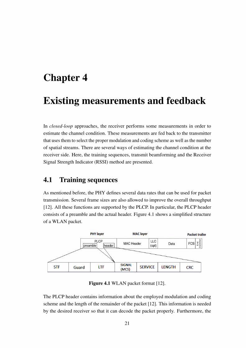
As mentioned before, the PHY defines several data rates that can be used for packettransmission. Several frame sizes are also allowed to improve the overall throughput[12]. All these functions are supported by the PLCP. In particular, the PLCP headerconsists of a preamble and the actual header. Figure 4.1 shows a simplified structureof a WLAN packet.
Figure 4.1 WLAN packet format [12].
The PLCP header contains information about the employed modulation and codingscheme and the length of the remainder of the packet [12]. This information is neededby the desired receiver so that it can decode the packet properly. Furthermore, the
21

Existing measurements and feedback
stations can benefit by detecting packets that are not addressed to them since they caninfer the amount of time that the medium will be busy by looking at the PLCP headerand update its NAV accordingly [12].The PLCP preamble is composed of a set of short training fields (STFs) and longtraining fields (LTFs). In particular, the short training fields (STFs) consist of tenrepetitions of a short training sequence [12]. They are used to perform packet detec-tion, automatic gain control (AGC) and coarse time and frequency synchronization[58]. In addition, the long training fields (LTFs) consist of two repetitions of a longtraining sequence preceded by a guard interval [12]. They are used to perform channelestimation and fine time and frequency synchronization [58].All these fields are known by both the transmitter and the receiver. Therefore, the well-known values together with the values received in the LTFs can be used to estimatethe channel [59]. There are several approaches to perform channel estimation, namelyminimum mean square error (MMSE) estimation [60], least square (LS) estimation[61], Zero forcing (ZF) estimation [62], and maximum likelihood (ML) estimation[63].
4.1.1 MMSE estimation
Denoting the channel impulse response, g(t), as
g(t) = ∑m
αmδ (t − τmTs) (4.1)
Where the amplitudes αm are complex valued, δ represents the Dirac delta function[64], τm denotes a random delay and Ts represents the sampling period. Now, thereceived signal can be expressed as follows [65]:
y = XFg+n (4.2)
Denoting by x = [x0,x1, . . . ,xN−1]T a vector containing the transmitted signals. X is
defined as the matrix containing the elements of x on its diagonal and F is the DFTmatrix defined as follows:
F =
W 00
N · · · W 0(N−1)N
... . . . ...
W (N−1)0N · · · W (N−1)(N−1)
N
(4.3)
22

4.1 Training sequences
Where W nkN = 1√
Ne− j2π
nkN g is a vector containing the sampled values of the channel
impulse response and n = [n0,n1, . . . ,nN−1]T is a vector containing independent and
identically distributed Gaussian random variables that represent the noise plus theinterference.Assuming that the channel vector g is Gaussian and uncorrelated with the noise. TheMMSE estimates the channel according to the following formula [66]:
gMMSE = RgyR−1yy y (4.4)
Where Rgy = EgyH is the covariance matrix between g and y and Rgg = EggH is theautocovariance matrix ofg.The frequency domain estimate hMMSE is generated byusing the following formula [66]:
hMMSE = FgMMSE (4.5)
4.1.2 ZF estimation
The ZF estimator aims at minimizing the estimation error y−XFgZF where gZF
is the estimated channel vector. In addition, the LS estimator is equivalent to theZero-Forcing estimator [60] since forcing the estimation error to take a value equalszero and minimizing the formula used for LS estimation are equivalent [66].
4.1.3 ML estimation
The ML estimation consists of computing the channel vector gML that minimizes thedistance between the received signal and the transmitted signal affected by the channelvector [66]. In particular, the following equation is to be maximized
gML = argming∥y−XFg∥2 (4.6)
In this case, since the transmitted y and received X sequences are known at thereceiver side this method reduces to the LS estimation method [67]. However, insituations where the transmitted sequence is not known a priori on the receiver sidethe complexity of this method is substantially increased [63]. The Viterbi algorithm[68] is used in these cases to help minimizing the equation presented above.
23

Existing measurements and feedback
To sum up, the estimation algorithms based on maximum likelihood computes a moreaccurate estimate of the channel state [63]. However, the channel estimation alsodepends on the actual channel state. This means that the channel is estimated moreaccurately when the channel conditions are favorable, i.e. the receiver SINR is high.On the other hand, estimation errors are likely to appear with poor channel conditions[69]. Having accurate channel estimates is important, since the overall performancewould be affected by estimation errors [62].
4.2 Transmit beamforming
Transmit beamforming (Tx BF) is a technique that aims at improving the quality ofthe received signal by performing directional signal transmission or reception [70]. Asa result, the communication range and the data rate are improved [58]. Tx BF relieson the principle that independent data streams can be constructively combined at thereceive antenna [71]. To do so, the phases of the received signals are manipulated sothat they can be combined and the directivity is improved [70]. This can be achievedby having knowledge of the channel between the transmitter and the receiver [72]. Inparticular, knowledge about the signal strength and the phase information for OFDMsubcarriers and between each pair of transmit-receive antennas is needed to performTx BF [71]. The aforementioned parameters are known as Channel State Information(CSI).Tx BF is specified in the 802.11n amendment [20] and takes advantage of the MIMOsystem specified in the same amendment. However, the feedback format for Tx BFwas specified in the 802.11ac amendment [24]. Typically, the AP beamforms to theclient which increases the quality of the received signal and therefore reduces thenumber of retries [72]. This allows the use of higher data rates that leads to an increaseof the overall system capacity [72].In order to perform beamforming, it is required that the transmitter has more than oneantenna [71]. In addition, a steering matrix containing the weights that are appliedto the transmitted signal is needed. The weights can be derived from the CSI. Theresulting matrix is used to steer the signal for a specific client [72]. For the sake ofsimplicity, the beamformer is defined as the device that applies the steering matrixto the transmitted signal and the beamformee is the device that the beamformer issteering toward [71]. Furthermore, Tx BF can also be used to perform MU-MIMO(see section 2.2.2) [25].Two types of feedback are defined in the 802.11n standard, namely implicit feedbackand explicit feedback [20].
24
4.3 Received Signal Strength Indicator
4.2.1 Implicit feedback
Implicit feedback relies on the assumption that the channel between the beamformerand the beamformee is reciprocal, i.e. equal in both directions. By using this approach,the beamformer transmits a regular packet and expects to receive an acknowledgementthat is used to estimate the channel and compute the steering matrix [72].However, the reciprocity assumption may not be adequate since the interference levelis different on the transmitter and the receiver sides. Therefore, calibration is neededto achieve the desired reciprocity [73]. As a result, the lack of reciprocity can leadto channel estimation errors in Tx BF. If the errors can be controlled by applyingcalibration, this feedback method incurs less overhead since the channel conditions ofthe downlink are inferred from the channel conditions of the uplink [71].
4.2.2 Explicit feedback
With explicit feedback, the beamformer transmits a sounding packet to the beam-formee. This packet is used by the beamformee to calculate the CSI and send it backto the beamformer. Then, the beamformer uses the received feedback to compute thesteering matrix [72].In particular, the packet used to sound the channel is called Null Data Packet (NDP).The NDP essentially consists of just a PHY header that includes the PLCP preambleand header [70]. While receiving an NDP, the channel is estimated by processingthe LTFs using a Zero forcing (ZF) estimator [65], a least square (LS) estimator [66]or a minimum mean square error (MMSE) estimator [67]. This approach providesmore accurate feedback than the implicit approach [58]. However, there is a tradeoffbetween the two methods. Implicit feedback leads to a reduced amount of overheadcompared to explicit feedback. Nevertheless, explicit feedback achieves better channelestimation due to the increased overhead.
4.3 Received Signal Strength Indicator
In IEEE 802.11 standards, the RSSI indicates the power level received by the antennain arbitrary units [48]. It is calculated during the reception of the preamble [74].Furthermore, the relationship between the RSSI value and the power level is notdefined in the standards [12]. It is left up to the vendors to define that relationship.Indeed, the aforementioned relationship and some other aspects such as the granularityof the measurements, accuracy and the range of the RSSI vary from one vendor to
25

Existing measurements and feedback
another [48]. The lack of uniformity between the RSSI computations of differentvendors makes it difficult to use it as an absolute indicator [48].
4.3.1 Received Channel Power Indicator
Because of the RSSI setbacks, another indicator called Received Channel PowerIndicator (RCPI) is defined. RCPI is an indicator defined in the 802.11-2012 standard[51] that indicates the received power in a selected channel. The received power iscalculated over the preamble and the entire frame and therefore the accuracy achievedby this indicator is better than that of the RSSI. The accuracy and resolution of thisparameter were defined in the 802.11 k-2008 amendment [52].
SINR measurement based on the Received Channel Power Indicator
In [75], it is shown that the RSSI and the RCPI provide a measure of the total receivedpower, i.e. the desired signal power plus the noise power plus the interference power.Therefore, those indicators do not provide accurate measurements of the channelconditions. A new way of calculating the SINR is proposed in that paper.According to the proposed method, two RCPI measurements are needed in order tocalculate the SINR. The first measurement is performing while receiving a frame and,as stated before, it contains the total received power. The second measurement isperformed right after receiving the frame and it is assumed that it only contains thesum of the noise power and the interference power. Denoting the first measurement asRCPI1 and the second measurement as RCPI2, their values are defined by thefollowing equations:
RCPI1 = S+N1 + I1 (4.7)
RCPI2 = N2 + I2 (4.8)
Where S is the desired signal power, N represents the noise power and I denotes theinterference power. Furthermore, assuming that the noise and the interference powerremain constant from the first measurement of the RCPI to the second measurement ofthe RCPI, i.e N1 = N2 = N and I1 = I2 = I, the SINR can be calculated as follows[76]:
SINR =RCPI1 −RCPI2
RCPI2=
S+N + I −N − IN + I
=S
N + I(4.9)
26

4.4 Feedback reporting in closed-loop approaches
This method provides a way of calculating the SINR relying on the assumption thatthe interference and noise remain constant between the two measurements and can beused as a good indicator of the SINR to calculate some system parameters such as thebit error rate (BER), frame error rate (FER). . . .
4.4 Feedback reporting in closed-loop approaches
The proposed link adaptation algorithms are closed-loop, i.e. the receiver is sendingback some explicit information about the channel state to the transmitter. To do so,the feedback containing the explicit information is piggybacked in the ACK frames.This can be done in a standard compliant way by using the High Throughput Control(HTC) field [25]. The HTC field is a 4 bytes optional field added to the managementframes (such as ACKs and block ACKs). It has a subfield called MCS feedback (MFB)whose length is 2 bytes. This subfield is used to carry explicit channel informationthat is used for closed-loop link adaptation approaches. The following figure shows ansketch of the HTC field.
Figure 4.2 Standard-compliant feedback mechanism [26].
27

Chapter 5
Simulation setup and performancemetrics
This chapter provides an introduction to the simulator that was used. In addition, abrief explanation of how the different parts of the system are modelled as well as someimportant simulation parameters are presented. The parameters and their values willbe used in the following chapters to present the results and draw the conclusions.
5.1 Simulator overview
An existing simulator developed in Matlab is used to run the simulations. This is anevent based simulator that implements the MAC layer of an 802.11 WLAN networktogether with the procedures needed for the exchange of data frames between multiplenodes in a WLAN network.The simulation is performed as follows: at the beginning of the simulation, the offeredtraffic per AP (in Megabits per second) is specified. Then, the total offered traffic iscomputed as the multiplication of the offered traffic per AP and the number of APs,this is called offered traffic. It is important to mention that during the simulations, atraffic model simulating a file exchange was used (see section 5.5). In particular, aPoisson process that models the file arrivals to the buffers is drawn.The devices are ready to transmit as soon as they have data stored in their respectivebuffers. Then, the files are divided into A-MPDUs consisting of several MPDUs (seesection 2.2.2) and the devices access the medium following the procedures specifiedin the 802.11 standardsIn addition to the existing simulator setup, new functionalities for block ACK (see2.2), an error probability model based on mutual information (see 5.4), fast fadingchannels (see 5.3.1) and a modified traffic model (see 5.5) were implemented. Also,
29
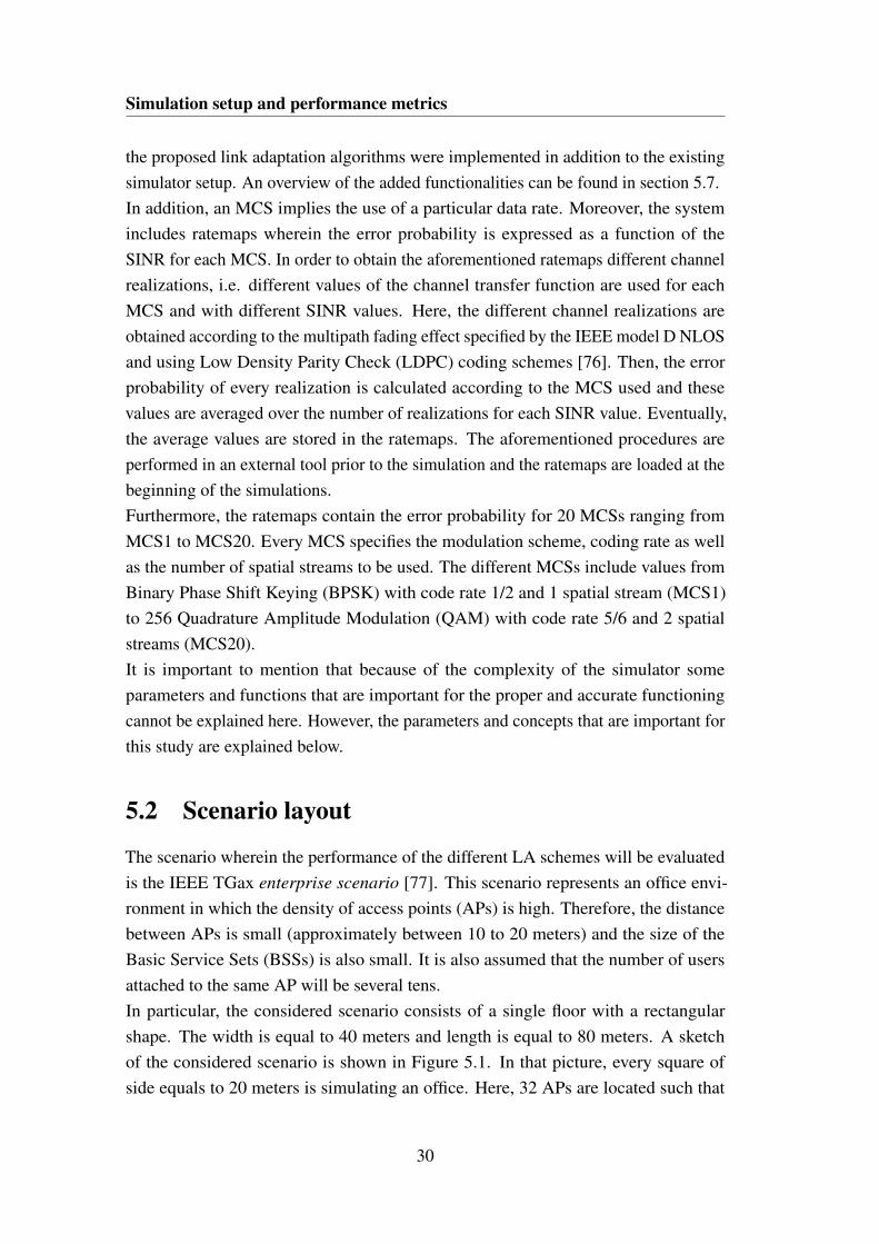
Simulation setup and performance metrics
the proposed link adaptation algorithms were implemented in addition to the existingsimulator setup. An overview of the added functionalities can be found in section 5.7.In addition, an MCS implies the use of a particular data rate. Moreover, the systemincludes ratemaps wherein the error probability is expressed as a function of theSINR for each MCS. In order to obtain the aforementioned ratemaps different channelrealizations, i.e. different values of the channel transfer function are used for eachMCS and with different SINR values. Here, the different channel realizations areobtained according to the multipath fading effect specified by the IEEE model D NLOSand using Low Density Parity Check (LDPC) coding schemes [76]. Then, the errorprobability of every realization is calculated according to the MCS used and thesevalues are averaged over the number of realizations for each SINR value. Eventually,the average values are stored in the ratemaps. The aforementioned procedures areperformed in an external tool prior to the simulation and the ratemaps are loaded at thebeginning of the simulations.Furthermore, the ratemaps contain the error probability for 20 MCSs ranging fromMCS1 to MCS20. Every MCS specifies the modulation scheme, coding rate as wellas the number of spatial streams to be used. The different MCSs include values fromBinary Phase Shift Keying (BPSK) with code rate 1/2 and 1 spatial stream (MCS1)to 256 Quadrature Amplitude Modulation (QAM) with code rate 5/6 and 2 spatialstreams (MCS20).It is important to mention that because of the complexity of the simulator someparameters and functions that are important for the proper and accurate functioningcannot be explained here. However, the parameters and concepts that are important forthis study are explained below.
5.2 Scenario layout
The scenario wherein the performance of the different LA schemes will be evaluatedis the IEEE TGax enterprise scenario [77]. This scenario represents an office envi-ronment in which the density of access points (APs) is high. Therefore, the distancebetween APs is small (approximately between 10 to 20 meters) and the size of theBasic Service Sets (BSSs) is also small. It is also assumed that the number of usersattached to the same AP will be several tens.In particular, the considered scenario consists of a single floor with a rectangularshape. The width is equal to 40 meters and length is equal to 80 meters. A sketchof the considered scenario is shown in Figure 5.1. In that picture, every square ofside equals to 20 meters is simulating an office. Here, 32 APs are located such that
30
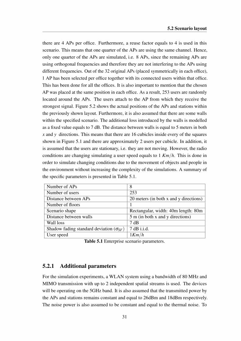
5.2 Scenario layout
there are 4 APs per office. Furthermore, a reuse factor equals to 4 is used in thisscenario. This means that one quarter of the APs are using the same channel. Hence,only one quarter of the APs are simulated, i.e. 8 APs, since the remaining APs areusing orthogonal frequencies and therefore they are not interfering to the APs usingdifferent frequencies. Out of the 32 original APs (placed symmetrically in each office),1 AP has been selected per office together with its connected users within that office.This has been done for all the offices. It is also important to mention that the chosenAP was placed at the same position in each office. As a result, 253 users are randomlylocated around the APs. The users attach to the AP from which they receive thestrongest signal. Figure 5.2 shows the actual positions of the APs and stations withinthe previously shown layout. Furthermore, it is also assumed that there are some wallswithin the specified scenario. The additional loss introduced by the walls is modelledas a fixed value equals to 7 dB. The distance between walls is equal to 5 meters in bothx and y directions. This means that there are 16 cubicles inside every of the squaresshown in Figure 5.1 and there are approximately 2 users per cubicle. In addition, itis assumed that the users are stationary, i.e. they are not moving. However, the radioconditions are changing simulating a user speed equals to 1 Km/h. This is done inorder to simulate changing conditions due to the movement of objects and people inthe environment without increasing the complexity of the simulations. A summary ofthe specific parameters is presented in Table 5.1.
Number of APs 8Number of users 253Distance between APs 20 meters (in both x and y directions)Number of floors 1Scenario shape Rectangular, width: 40m length: 80mDistance between walls 5 m (in both x and y directions)Wall loss 7 dBShadow fading standard deviation (σSF) 7 dB i.i.d.User speed 1Km/h
Table 5.1 Enterprise scenario parameters.
5.2.1 Additional parameters
For the simulation experiments, a WLAN system using a bandwidth of 80 MHz andMIMO transmission with up to 2 independent spatial streams is used. The deviceswill be operating on the 5GHz band. It is also assumed that the transmitted power bythe APs and stations remains constant and equal to 26dBm and 18dBm respectively.The noise power is also assumed to be constant and equal to the thermal noise. To
31
Simulation setup and performance metrics
Figure 5.1 Enterprise scenario layout.
−130 −120 −110 −100 −90 −80 −70 −60 −50−125
−120
−115
−110
−105
−100
−95
−90
−85
Distance [m]
Dis
tance [m
]
AP
STA
Figure 5.2 Actual positions of the simulated APs (red circles) and STAs (blue points).
calculate the noise, it is assumed that all the devices have a noise figure of 7 dB. Thenoise figure is a parameter used to take into account the deterioration of the SINRdue to the noise introduced by the electronic circuitry on the receiver. The resultingformula is:
N = k ·T · f ·B (5.1)
Where N is the noise level expressed in watts, k is the Boltzmann constant (k =
1.38 · 10−23), T is the noise temperature expressed in Kelvin degrees (by default,T = 290K is used), f is the noise figure expressed in linear units and B is the bandwidthexpressed in Hz. Using the values specified above, the resulting noise power is around-88dBm (∼ 1.6 ·10−23W ).
32

5.3 Propagation modelling
5.3 Propagation modelling
In this section, a detailed explanation of the models used to simulate the propagationis presented. In particular, the multipath fading, shadow fading and path loss modelsare explained below.
5.3.1 Multipath fading
Since the users are stationary but the conditions are changing according to a simulatedmovement, the channel transfer function, H( f ), between any pair of transmitter andreceiver is changing due to that simulated movement. In particular, fading models thefluctuation of the attenuation experienced by a signal in a certain environment [81].Due to the strong dependency on the environment, fading is modelled as a randomprocess. Furthermore, fading may be caused by multipath propagation, also known asmultipath fading, or due to the smooth variation of obstacles between the transmitterand the receiver, referred to as shadow fading [79].Multipath fading is present in any environment where there is multipath propagation.Here, the transmitted signal interacts with the objects and obstacles present in theenvironment. As a consequence, reflections and/or refractions (among other effects)can affect the signal leading to the effect that several replicas of the transmitted signalmay arrive at the receiver [79]. These replicas can have different amplitudes, phaseshifts, and they can arrive at the receiver at different time instants.The overall signal at the receiver is the summation of the variety of signals beingreceived. Since they have different amplitudes and phase shifts, the signals will add(constructive interference) or subtract (destructive interference) from the overall signalbased on their relative phase shifts. In addition, the fact that the different replicas arriveat the receiver at different time instants may cause interference with previously orsubsequently transmitted signals. This phenomenon is called intersymbol interference(ISI) [80].With multipath fading, the amplitudes of the signals that arrive at the receiver bythe different paths can be modelled by a Rayleigh distribution. In fact, multipathfading is also known as Rayleigh fading. Furthermore, if there is a line of sight (LOS)component between the transmitter and the receiver it is more suitable to use a modelwhere the amplitudes of the signals are Rician distributed. In this case, fading isdenoted as Rician fading [80].As a result, multipath fading can deteriorate the performance since the received powerlevel is varying with time and the variations can be sharp depending on the phase shiftsof the signals arriving at the receiver. Hence, the use of some techniques that mitigate
33

Simulation setup and performance metrics
the effects of fading is needed. For example, diversity techniques where the signal istransmitted over multiple uncorrelated channels can be used. Since the channels areuncorrelated, the several streams can be spatially separated on the receiver side [79].In addition, some other techniques such as MIMO or OFDM, among others, can beused to combat fading [80].
5.3.2 Shadow fading
During the simulations, the amount of large scale obstacles interfering the beambetween the transmitter and the receiver is smoothly varying and therefore the pathloss varies as well. As a consequence, the received power is also fluctuating [80]. Thevariations, also known as shadowing [81], are modeled by a log normal distributionwith a standard deviation equals to 7 dB i.i.d. across all links. This value is specifiedby the IEEE TGax and it was obtained empirically by performing measurements in anoffice propagation environment [82]. In the simulations, the shadow fading is assumedto be constant given a user position.Figure 5.3 shows a sketch of the received power (in arbitrary units) as a functionof the time (in arbitrary units). Here, by examining the received power over longperiods of time it can be seen that the received power is smoothly varying due tothe aforementioned effects introduced by the shadow fading. This is also denoted aslarge scale fading [80]. On the other hand, if the received power is examined overshort periods of time it can be noticed that the received power is sharply varying asa consequence of the multipath fading due to the rapid switching from constructiveto destructive interference. This phenomenon is also referred to as small scale fading[80].
Figure 5.3 Shadow and multipath fading effects.
34

5.3 Propagation modelling
5.3.3 Path loss model
There are several path loss models defined by the TGax according to the differentsimulation scenarios. For the simulation scenario under test, the path loss formula isexpressed as follows [77]:
PL(d) = 40.05+20 · log10
(fc
2.4
)+20 · log10(min(d,10))+
(d > 10) ·35 · log10
(d10
)+wall_loss ·W + shadowing
(5.2)
Where:
• fc carrier frequency in GHz
• d = max (distance_m, 1) where distance_m is the distance between thetransmitter and the receiver expressed in meters
• (d > 10) is a logical value that is set to one when the condition is true,otherwise it is set to zero
• wall_loss is the aforementioned loss introduced by walls equal to 7 dB
• W is the number of walls traversed in x direction plus the number of wallstraversed in y direction
• shadowing takes into account the shadowing effect discussed above
• In addition, 40.05 is the free space path loss (FSPL) at the frequency of 2.4 GHzand at a distance of 1 meter. Hence, this value is obtained from the followingequation:
40.05 ≈ 10log10
(4 ·π ·2.4 ·109 ·1
c
)2
(5.3)
Where c is the speed of light in vacuum, which is approximately equal to3 ·108m/s.
The path loss formula stated above is valid for both the 802.11ac and 802.11axsystems since the path loss only depends on the environment and the frequency, itdoes not depend on the system used. However, the path loss formulas are revised, andsometimes modified, when a new amendment is defined since the formulas have to becompliant with the amendments.
35
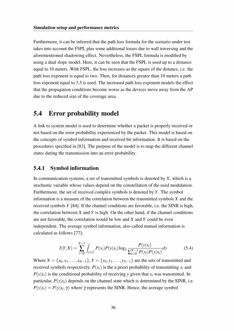
Simulation setup and performance metrics
Furthermore, it can be inferred that the path loss formula for the scenario under testtakes into account the FSPL plus some additional losses due to wall traversing and theaforementioned shadowing effect. Nevertheless, the FSPL formula is modified byusing a dual slope model. Here, it can be seen that the FSPL is used up to a distanceequal to 10 meters. With FSPL, the loss increases as the square of the distance, i.e. thepath loss exponent is equal to two. Then, for distances greater than 10 meters a pathloss exponent equal to 3.5 is used. The increased path loss exponent models the effectthat the propagation conditions become worse as the devices move away from the APdue to the reduced size of the coverage area.
5.4 Error probability model
A link to system model is used to determine whether a packet is properly received ornot based on the error probability experienced by the packet. This model is based onthe concepts of symbol information and received bit information. It is based on theprocedures specified in [83]. The purpose of the model is to map the different channelstates during the transmission into an error probability.
5.4.1 Symbol information
In communication systems, a set of transmitted symbols is denoted by X , which is astochastic variable whose values depend on the constellation of the used modulation.Furthermore, the set of received complex symbols is denoted by Y . The symbolinformation is a measure of the correlation between the transmitted symbols X and thereceived symbols Y [84]. If the channel conditions are favorable, i.e. the SINR is high,the correlation between X and Y is high. On the other hand, if the channel conditionsare not favorable, the correlation would be low and X and Y could be evenindependent. The average symbol information, also called mutual information iscalculated as follows [77]:
I(Y,X) =N−1
∑i=0
∫y∈C
P(xi)P(y|xi) log2P(y|xi)
∑N−1i=0 P(xi)P(y|xi)
dy (5.4)
Where X = {x0,x1, . . . ,xN−1}, Y = {y0,y1, . . . ,yN−1} are the sets of transmitted andreceived symbols respectively. P(xi) is the a priori probability of transmitting xi andP(y|xi) is the conditional probability of receiving y given that xi was transmitted. Inparticular, P(y|xi) depends on the channel state which is determined by the SINR, i.e.P(y|xi) = P(y|xi,γ) where γ represents the SINR. Hence, the average symbol
36

5.4 Error probability model
information also depends on the SINR, I(Y,X) = I(Y,X ,γ). For the sake of simplicity,the symbol information is denoted as I(γ).During the simulation, the symbol information (SI) is calculated as a function of theSINR and the modulation constellation by performing a lookup in a table calledSIR2SI:
SI = SIR2SI(SINR,modulation scheme) (5.5)
Figure 5.4 shows the symbol information for different modulation schemes usingBit-Interleaved Coded Modulation (BICM) as a function of the SINR.
Figure 5.4 Average symbol information in bits per symbol as a function of the SINRfor different modulation schemes.
5.4.2 Received Bit Information
In order to transmit information, the symbols obtained from the modulationconstellation are protected by a channel coding that adds some redundancy in order toensure the transmission [80]. The coding schemes basically take k information bits asinput and appends n− k redundancy bits. Hence, the output is composed by acodeword formed by n bits.The received bit information (RBI) takes into account the properties of the codingscheme. In particular, the RBI is calculated as the sum of the symbol information ofall the transmitted symbols within a codeword.
RBI(γ) =S−1
∑j=0
I(γ j) (5.6)
37

Simulation setup and performance metrics
Where γ j denotes the SINR experienced by the different symbols and S = nlog2 M
represents the number of symbols per codeword. Here, n denotes the codeword lengthmeasured in bits, log2 M is the number of bits per symbol, and M is the number ofsymbols of the used constellation.Furthermore, another parameter called Received Bit Information Rate (RBIR) is alsodefined. The RBIR is a measure of the average symbol information carried by everycoded bit, i.e. it is the normalized RBI. The RBIR is then defined by the followingequation:
RBIR(γ j) =RBI(γ j)
S ·n(5.7)
Finally, the error probability of the codeword, also known as block error probability(BLEP) is obtained by performing a table lookup with the RBIR and the code rate, i.e.kn , as follows:
BLEP = RBIR2BLEP(RBIR,code rate) (5.8)
It is also important to mention that the SIR2SI and the RBIR2BLEP maps weregenerated with an external tool prior to the simulations and loaded at te beginning ofthem.
5.5 Traffic model
To perform the simulations, a traffic model based on a Poisson process [85] is used. Ithas been shown that it is an accurate model to simulate file exchange using the FileTransfer Protocol (FTP) on top of the User Datagram Protocol (UDP) [86]. With thismodel, the time between data arrivals is exponentially distributed. The mean value ofthe inter arrival time, also called arrival intensity [85], depends on the amount ofoffered traffic to the system, i.e. the higher the offered traffic the lower the timebetween data arrivals.With this model, the amount of traffic to be handled by the system is taken as an input.This value is called offered traffic and it is specified in megabits per second. Then, thearrival intensity λ for every node within the system in downlink (AP to STA) anduplink (STA to AP) cases is calculated as follows:
λdownlink =o f f ered_tra f f ic(Mbps)
ob ject_size(bits) ·number_o f _nodes·Fdl (5.9)
λuplink =o f f ered_tra f f ic(Mbps)
ob ject_size(bits) ·number_o f _nodes· (1−Fdl) (5.10)
38

5.6 Simulation logging and seed
Where λdownlink and λuplink are the arrival intensities in downlink and uplinkrespectively, ob ject_size represents the size of the object, i.e. the file, arriving to thetransmission buffer of the nodes, number_o f _nodes denotes the number of devices(users and APs) in the system and Fdl specifies the fraction of downlink traffic, i.e. thefraction of data that is sent in the downlink direction.There are several simulation parameters affecting the traffic model that can beadjusted, for example the size of the objects that arrive to the transmission buffer. Thefollowing table shows the parameters used during the simulations.
Parameter ValueFraction of uplink traffic 50%Fraction of downlink traffic 50%Number of events 250000Offered traffic 4.8, 96, 192, 288, 432, 576, 720, 864, 1008, and 1152 MbpsSize of data objects 1 MBMaximum A-MPDU size 64000 B
Table 5.2 Traffic model settings.
5.6 Simulation logging and seed
During the simulation, it is assumed that the APs and the users have an unlimitedbuffer and the logging starts when the simulator starts. This means that the loggingstarts before the traffic model stabilizes. This could affect the results because of therandom nature of the traffic arrivals. However, the simulations are run for a longnumber of events in order to compensate for this.The simulator seed is used for the user placement and generating the random fadingamplitudes together with the power delay profile. To ensure that the simulations arerun in a controllable and repeatable environment, i.e. different simulations areexposed to the same conditions, the different loads of offered traffic are run with thesame seeds and for the same number of events. In particular, all the loads are run for250 000 events.Figure 5.5 represents the served traffic as a function of the offered traffic. The servedtraffic is calculated as the amount of data handled by the system during the simulationtime:
served_tra f f ic(Mbps) =handled_data(bits)
simulation_time ·106 (5.11)
39
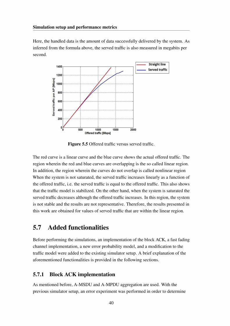
Simulation setup and performance metrics
Here, the handled data is the amount of data successfully delivered by the system. Asinferred from the formula above, the served traffic is also measured in megabits persecond.
Figure 5.5 Offered traffic versus served traffic.
The red curve is a linear curve and the blue curve shows the actual offered traffic. Theregion wherein the red and blue curves are overlapping is the so called linear region.In addition, the region wherein the curves do not overlap is called nonlinear regionWhen the system is not saturated, the served traffic increases linearly as a function ofthe offered traffic, i.e. the served traffic is equal to the offered traffic. This also showsthat the traffic model is stabilized. On the other hand, when the system is saturated theserved traffic decreases although the offered traffic increases. In this region, the systemis not stable and the results are not representative. Therefore, the results presented inthis work are obtained for values of served traffic that are within the linear region.
5.7 Added functionalities
Before performing the simulations, an implementation of the block ACK, a fast fadingchannel implementation, a new error probability model, and a modification to thetraffic model were added to the existing simulator setup. A brief explanation of theaforementioned functionalities is provided in the following sections.
5.7.1 Block ACK implementation
As mentioned before, A-MSDU and A-MPDU aggregation are used. With theprevious simulator setup, an error experiment was performed in order to determine
40

5.7 Added functionalities
whether the whole aggregated packet was lost or not. The error experiment wasperformed as follows: first, the SINR of the transmitted packet was calculated byusing the following formula for the ratemaps mentioned in section 5.1:
SINR =Pti ·Gi j
∑k ̸=i Ptk ·Gk j +N(5.12)
In the previous formula, the transmitter and the desired receiver are denoted by i and jrespectively. In addition, Pti denotes the transmitted power and Gi j represents thechannel gain between the transmitter i and the receiver j. Furthermore, ∑k ̸=i Ptk ·Gk j
represents the interference, i.e. the amount of received power coming from atransmitter other than the desired one and N represents the thermal noise that has avalue of -88 dBm (∼ 1.6 ·10−23W ). In addition, a matrix specifying the averagechannel gain between any node pair is computed in a separate simulator and theresulting values are imported into the used simulator. These values are used in theabove formula to compute the SINR. As mentioned before, the aforementioned valuesare average values and hence they are constant.After that, the error probability was calculated as a function of the SINR of thetransmitted packet and the MCS used:
Perror = f (SINR,MCS) (5.13)
Then, an error experiment is performed to determine if the packet was lost or not.Here, a random number is drawn. Thereafter, the random number is compared againstthe error probability. If the random number is lower or equal to the error probabilitythe packet is assumed to be lost and a retransmission is scheduled and the CW value isdoubled. Otherwise, the packet was successfully delivered and an ACK frame isgenerated and sent back to the transmitter. The same random experiment is alsoperformed for the ACK frame. However, if the ACK frame is lost the transmitterinterprets is as a packet failure and hence it doubles the CW value and schedules aretransmission of the data packet. Furthermore, the maximum number of transmissiontries is set to 10. A summary of the random experiment is provided in the equationsbelow.
i f rand ≤ Perror → packet was lost → double CW and schedule retransmission
i f rand > Perror → packet success f ully delivered → transmit ACK f rame
With the new block ACK functionality, the error experiment is performed on a perMPDU basis. In this case, the SINR and the error probability of every MPDU arecalculated. Then, the random experiment is performed for each MPDU. Here, the
41

Simulation setup and performance metrics
same random number is used for all the MPDUs since the channel variations are takeninto account during the SINR calculation, i.e. the SINR of the different MPDUs canbe different. In this case, only the failed MPDUs are retransmitted instead ofretransmitting the whole A-MPDU. This leads to lighter retransmissions whichimproves the efficiency and hence the performance.
5.7.2 Fast fading channel implementation
As mentioned in the previous section, the channel gain values are constant and hence,the fast fading effect due to multipath propagation is not considered. Here, themultipath fading specified in the power delay profile (PDP) of the IEEE model DNLOS is used to simulate the fading effect. This is the model proposed by the TGax tosimulate the fading effect in the enterprise scenario [77]. A table with the parametersspecified in the PDP of the IEEE model D NLOS can be found in Appendix A.To model the fading effect, the Rayleigh fading amplitudes are first derived from thePDP. In order to obtain the aforementioned amplitudes, the scenario is divided in gridswith a side equal to 5 centimeters. Then, a fading amplitude is calculated for each grid.The frequencies used by the system are taken into account to calculate the amplitudes.Eventually, the fading amplitudes are stored in a map as a function of the frequencyand the position within the scenario.During the simulations, the fading amplitudes are used as follows: at the beginning ofthe simulation, the users are placed randomly. Here, the users’ positions are stored ina variable together with the last time that the users changed their positions. Thesevalues are used to simulate movement within the scenario. Then, whenever atransmission occurs the new user position is calculated as the previous position plusthe position shift occurred since the last transmission. This is calculated according tothe following formula
Pos(t +∆t) = Pos(t)+∆t · speed (5.14)
Where ∆t is the difference between the current time and the time when the previoustransmission occurred both expressed in seconds and speed denotes the user speed inmeters per second
(1km/h
3.6 ∼ 0.28m/s)
.Then, the new fading amplitude is obtained by performing a table lookup with the newposition and the frequency as input parameters. Eventually, the channel gain isobtained as the multiplication of the average channel gain and the calculated fadingamplitude. The modified channel gain is used to compute the SINR.
42

5.7 Added functionalities
5.7.3 Error probability model
During the simulations, two error probability models are used depending on the fastfading channels are used or not. If the fast fading channels are not used a ratemap thatconsiders the fast fading effect is used. This is done in order to consider the variationsin the channel gain since the imported channel gain values are constant. Theseratemaps are obtained by performing different channel realizations modelling themultipath fading effect according to the IEEE model D NLOS and using LDPCcoding schemes (see section 5.1). Here, the error probability is mapped as a functionof the SINR for each MCS. Hence, the error probability is obtained by performing asingle table lookup with the SINR and the MCS used as input parameters according tothe following formula:
Perror = f (SINR,MCS) (5.15)
On the other hand, if the fast fading channels are used the channel gains aredynamically changing since the fading amplitudes are changing as a function of theposition of the nodes within the AP. In this case, a two-step model is used to calculatethe error probability according to the procedures specified in section 5.4. In thismodel, the RBIR is first calculated as a function of the SINR and the modulationscheme following the steps specified in section 5.4. Then, the error probability isobtained by performing a table lookup with the RBIR and the code rate as inputparameters. In this case, the needed tables as well as the required procedures to obtainRBIR and the error probability were added to the existing simulator setup. Thefollowing formula shows a summary of the steps performed in order to calculate theerror probability when the fast fading channels are used
(SINR,MCS)→ SI → BLEP (5.16)
It is important to notice that, when the implemented fast fading channels are used thetables used to calculate the RBIR and the error probability do not consider the fastfading, i.e. they just consider the Additive White Gaussian Noise (AWGN). Here, thefast fading effect is already considered since the channel gains are dynamicallychanging as a consequence of the fading.
5.7.4 Traffic model modification
A small modification on the traffic model was also added to the simulator. With theprevious model, the files arrived to the devices’ buffer following a Poisson processjust the first time. Then, the arrival time of the following file was determined by
43

Simulation setup and performance metrics
performing a new Poisson realization after completing the transmission of theprevious file. Hence, the inter-arrival times were not exponentially distributed, whichis a property of the Poisson processes, and the file arrivals were not actually followinga Poisson distribution.To solve this issue, a new Poisson realization was performed when a file arrived at thedevice’s buffer in order to determine the arrival time of the following file. By doing so,it is ensured that the inter-arrival time is exponentially distributed and the file arrivalsfollow a Poisson distribution.
5.8 Overall simulator performance
So far, the different procedures performed by the simulator are specified separately.However, the overall simulator behavior has not been explained and it is important toknow how the simulator works in order to understand the behavior of the proposed LAschemes. The overall behavior is explained in the following section.As mentioned before, the simulator is an event based simulator where the differentprocedures, such as the start and end of transmissions, are handled separately. Inparticular, all the procedures are considered as an event.At the beginning of the simulation, the offered traffic is specified and the uplink anddownlink arrival intensities are calculated following the formulas specified in 5.5.Then, a Poisson process that models the file arrivals is drawn taking the arrivalintensities as inputs. After that, the files are divided into A-MPDUs (consisting ofseveral MPDUs) and the devices start contending to gain access to the mediumaccording to the CSMA/CA procedures. A data transmission starts when the CWreaches zero. At the end of the transmission, the SINR and the error probability ofevery MPDU are calculated. Then, the error experiment is performed to determine theMPDUs that were lost. In addition to the random experiment, it is also assumed that ifa collision was detected, i.e. there are more than one simultaneous transmissionswithin the same BSS, the whole A-MPDU is scheduled for retransmission.If the A-MPDU was not affected by a collision, the block ACK containing theinformation about the lost and successfully received MPDUs is generated andtransmitted. At the end of the transmission, the SINR and the error probability arecalculated in order to perform the random experiment. In this case, if the block ACKwas lost or it collided with another frame the whole A-MPDU is retransmitted.Otherwise, only the failed MPDUs are retransmitted (if any) and the MPDUs thatwere successfully delivered are removed from the transmitter buffer.
44
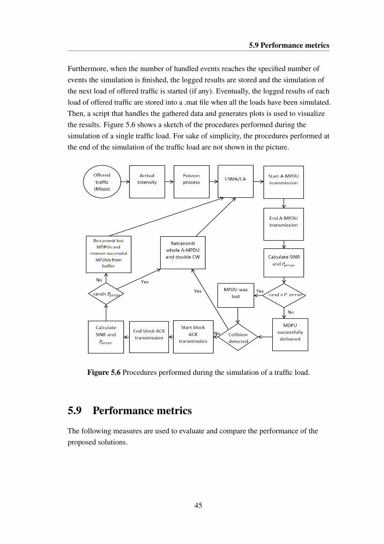
5.9 Performance metrics
Furthermore, when the number of handled events reaches the specified number ofevents the simulation is finished, the logged results are stored and the simulation ofthe next load of offered traffic is started (if any). Eventually, the logged results of eachload of offered traffic are stored into a .mat file when all the loads have been simulated.Then, a script that handles the gathered data and generates plots is used to visualizethe results. Figure 5.6 shows a sketch of the procedures performed during thesimulation of a single traffic load. For sake of simplicity, the procedures performed atthe end of the simulation of the traffic load are not shown in the picture.
Figure 5.6 Procedures performed during the simulation of a traffic load.
5.9 Performance metrics
The following measures are used to evaluate and compare the performance of theproposed solutions.
45
Simulation setup and performance metrics
5.9.1 User throughput
The user throughput is calculated as the size of the object i.e. the file that arrives to thebuffer over the elapsed time from the arrival to the buffer until it is completelyreceived by the other transmission end. It is measured in Megabits per second (Mbpsor Mb/s)
User throughput(Mbps) =ob ject_size(bits)elapsed_time(s)
1Mbit106bits
(5.17)
In particular, the graphs show the average user throughput which is the mean value ofthe throughput experienced by all the successfully delivered objects. It is shown as afunction of the served traffic per AP, i.e. the total amount of served traffic (see 5.6)divided by the number of APs. As expected, when the served traffic is increased theuser throughput is decreased since more users will attempt to transmit. Hence, thequeuing delays will increase since they are all contending to gain access to the sharedmedium. This leads to a decreased user throughput.
5.9.2 5th Percentile user throughput
The 5th percentile user throughput is a measure of the throughput of the 5%usersexperiencing the worst channel conditions. In particular, the 5th percentile userthroughput is the value below which 5% of the user population is found.
46

Chapter 6
Link adaptation schemes
In this section, an explanation of the proposed schemes is provided. Furthermoresome other existing schemes, such as Minstrel [87] and the Ideal LA, are alsoexplained since they will be used as a reference to compare the performance of theproposed schemes.
6.1 Minstrel algorithm
One of the most widely employed algorithms is called Minstrel [87]. It is anopen-loop LA algorithm that relies on long-term statistics. It has become the defaultalgorithm used in popular wireless card drivers since it is open-source and easy toimplement [34]. Minstrel is based on the SampleRate algorithm [35]. The algorithmconsists of three parts: the retry chain mechanism, the rate decision process and thestatistics calculation [53].
6.1.1 The multi-rate retry chain
Minstrel and SampleRate use a multi-rate retry chain that contains four rate/countpairs, named r0/c0, r1/c1, r2/c2, and r3/c3. First, the packet is transmitted at rate r0for c0 attempts. If the transmissions were not successful, the packet is transmitted atrate r1 for c1 attempts and so on until reaching c0 + c1 + c2 + c3 attempts at the ratesspecified by r0 through r3, or the packet has been successfully transmitted. Minstrelkeeps records of the previous transmission attempts at each rate to calculate theprobability of successful transmission and the throughput of each rate.
47
Link adaptation schemes
6.1.2 Rate selection process
In order to select the rate, Minstrel employs the following strategy: during 90% of thetime, Minstrel transmits using the rates specified in the retry chain, this is callednormal rate. These rates are chosen as follows: r0 is set to the rate with the highestexpected throughput, r1 is the rate with the second highest expected throughput, r2 isthe rate with the highest probability of success, and r3 is set to the lowest availabledata rate [35].During the remaining 10% of the time (called lookaround rate) Minstrel collectsstatistics about the success rate of transmissions at each rate. During the samplingtransmission, Minstrel picks a random rate(r) and updates the retry chain as follows:r0 is set to the higher rate out of the random rate and the rate with the highestexpected throughput and r1 is set to the lower out of the aforementioned rates. Thevalues of r2 and r3 remain the same [35]. An outline of the rate selection process isprovided in Table 6.1.
6.1.3 Statistics calculation
As stated earlier, Minstrel calculates the probability of successful transmission and thethroughput for each rate based on the transmission attempts at each rate. Bothparameters are calculated every 100ms and the retry chain is updated based on that.To keep track of the historical success rate Minstrel uses an Exponentially WeightedMoving Average (EWMA). The success Rate, Rs, is calculated as follows:
Rs =NsNt
(6.1)
Where Ns is the number of packets successfully transmitted at the given data rate andNt is the total number of attempted transmissions at that rate.According to [35], the probability of successful transmission at time t, P(t), at a givenrate is calculated as follows:
P(t +1) = Rs · (1−α)+P(t) ·α (6.2)
The current success rate, Rs, is used together with the previous value of the probabilityof successful transmission to calculate the current probability of successfultransmission at the given data rate. The EWMA parameter α is used to determine howmuch weight is given to the current Rs. The default value of α is 0.25. This meansthat the new probability of success consists of 25% of the previous probability of
48
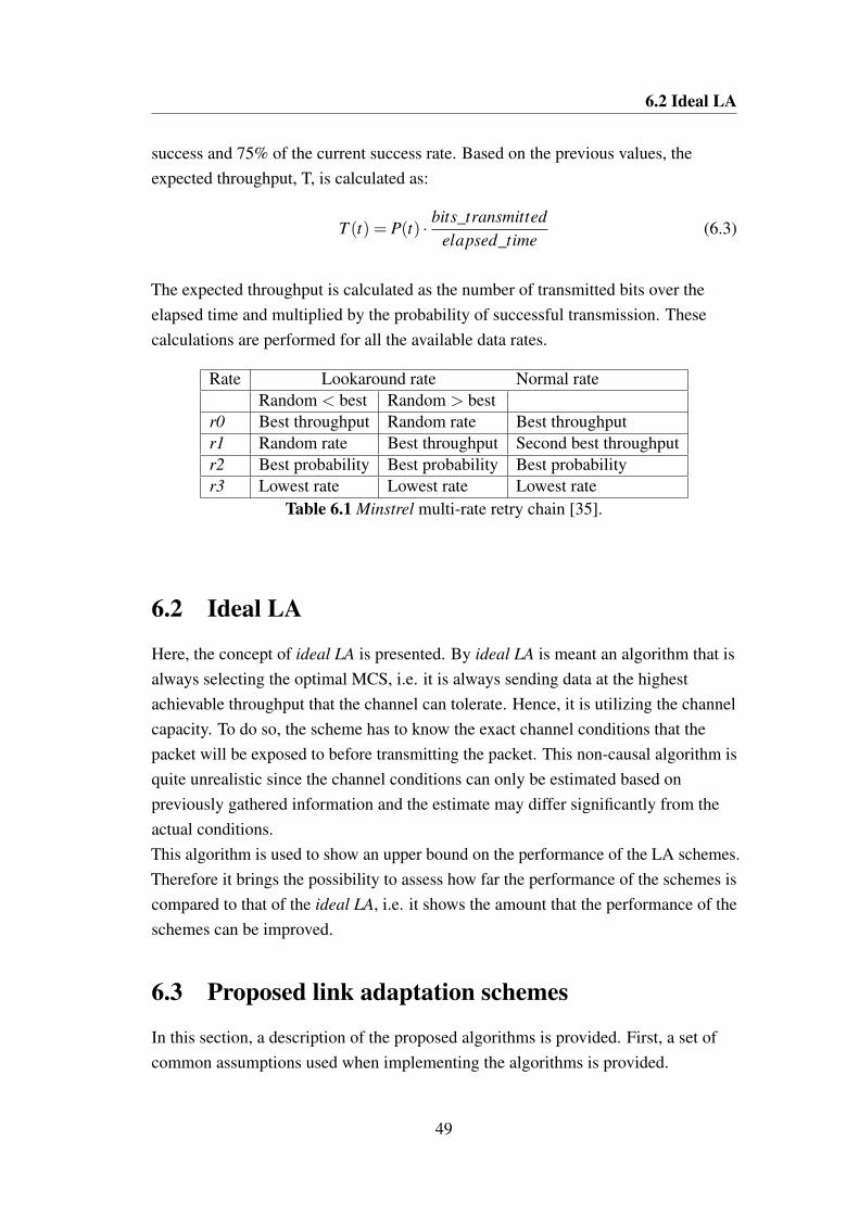
6.2 Ideal LA
success and 75% of the current success rate. Based on the previous values, theexpected throughput, T, is calculated as:
T (t) = P(t) · bits_transmittedelapsed_time
(6.3)
The expected throughput is calculated as the number of transmitted bits over theelapsed time and multiplied by the probability of successful transmission. Thesecalculations are performed for all the available data rates.
Rate Lookaround rate Normal rateRandom < best Random > best
r0 Best throughput Random rate Best throughputr1 Random rate Best throughput Second best throughputr2 Best probability Best probability Best probabilityr3 Lowest rate Lowest rate Lowest rate
Table 6.1 Minstrel multi-rate retry chain [35].
6.2 Ideal LA
Here, the concept of ideal LA is presented. By ideal LA is meant an algorithm that isalways selecting the optimal MCS, i.e. it is always sending data at the highestachievable throughput that the channel can tolerate. Hence, it is utilizing the channelcapacity. To do so, the scheme has to know the exact channel conditions that thepacket will be exposed to before transmitting the packet. This non-causal algorithm isquite unrealistic since the channel conditions can only be estimated based onpreviously gathered information and the estimate may differ significantly from theactual conditions.This algorithm is used to show an upper bound on the performance of the LA schemes.Therefore it brings the possibility to assess how far the performance of the schemes iscompared to that of the ideal LA, i.e. it shows the amount that the performance of theschemes can be improved.
6.3 Proposed link adaptation schemes
In this section, a description of the proposed algorithms is provided. First, a set ofcommon assumptions used when implementing the algorithms is provided.
49
Link adaptation schemes
6.3.1 Common assumptions
When developing the algorithms, it is assumed that all the simulated devices have a setof common features that are used in order to perform the measurements and send thefeedback to the transmitter.First of all, it is assumed that all the devices can calculate the SINR of the receivedpacket based on the RSSI field (see 4.3). However, since the actual value of the SINRexperienced by the packet is available in the simulator, it is used instead of the valueobtained from the RSSI field. Therefore, the actual SINR value and the valueindicated by the RSSI field may differ due to the granularity of the RSSI field andpossible errors when measuring the SINR.Furthermore, it is also supposed that all the devices have tables mapping the SINR topacket error probability for all the available MCSs. Both, the error probability and theSINR, are the main parameters used to compute the feedback and estimate the channelstate.Finally, all the algorithms have a mechanism to decrease the MCS when no feedbackis received during certain period of time. In particular, the MCS is lowered by oneafter two consecutive unsuccessful transmissions. This mechanism is similar to that ofAuto Rate Fallback (ARF) [88]. ARF is a link adaptation scheme wherein the MCS isincreased or lowered based on the successful or unsuccessful transmission of a fixednumber of consecutive transmissions. Here, the MCS is lowered by one after twoconsecutive unsuccessful transmissions. On the other hand, the MCS is increased byone after 10 consecutive successful transmissions. It relies on the assumption that twoor more consecutive packets are lost mainly due to poor channel conditions since theprobability of having two or more consecutive collisions is negligible [88]. However,this algorithm has a lack of responsiveness when the channel conditions are rapidlyvarying due to the use of fixed thresholds [89].The algorithms that were used during the simulations are described below. During thesimulations it is also assumed that all the devices are using the same LA scheme. Thefeedback is sent back according to the procedure explained in 4.4. In addition, it isimportant to mention that the feedback is applied as soon as it is received, i.e. thefollowing transmission will use the MCS specified in the previous ACK frame. Thedetails of every algorithm are decribed in the following sections.
6.3.2 LA1
LA1 is an algorithm based on throughput maximization. Here two approaches areproposed. In the first approach, called LA1, the feedback is applied as soon as it isreceived and in the second approach the transmitter stores several feedback values and
50
6.3 Proposed link adaptation schemes
applies them in order to calculate the MCS that will be used in the followingtransmission, this approach is called LA1 window.
ACK feedback
In the first approach, the algorithm performs the following steps:
1. The SINR of the received packet is calculated.
2. The packet error probability for each MCS is computed, this is calledPerrori(SINR,MCSi), where i indicates the MCS number. As stated in section5.4, the error probability is a function of the MCS and the SINR.
3. The achievable throughput of every MCS is calculated according to thefollowing formula:
T hroughputi = phyMaxRatei · (1−Perrori(SINR,MCSi) (6.4)
where phyMaxRatei is the maximum physical rate of MCSi.
4. The feedback is then computed as the MCS having the highest achievablethroughput, i.e. f eedback = argmaxi(T hroughputi).
5. The feedback is piggybacked in the ACK frame and it is sent back to thetransmitter of the data packet following the procedure specified in section 4.4.
Window approach
This approach is a modified version of LA1 adding memory to the algorithm. In theprevious approaches (LA1-LA4) the MCS is selected based on the channel state of thepreviously received data packet. With this approach, the MCS selection is based onthe channel state of the W previously received data packets, where W denotes thewindow size. In this approach, the MCS is selected as follows:
1. Upon reception of a data packet, the receiver computes the SINR of the packetand sends it back to the transmitter. This value is piggybacked in the ACKframes. Since the exact SINR value is available in the simulator, this value ispiggybacked and therefore no inaccuracies are assumed.
2. The transmitter stores the SINR value. It can store up to W values.
3. The transmitter uses the stored values to compute the MCS achieving thehighest available rate (same procedure as in LA1).
51

Link adaptation schemes
6.3.3 LA2
LA2 is an algorithm similar to the ideal scheme. However, since the channelconditions that will be experienced by the packet are not known before transmittingthe packet, the MCS selection is based on the conditions experienced by the previouspacket. Again, an approach wherein the feedback is applied as soon as it is receivedand an approach wherein some memory is added on the transmitter side are proposed.They are called LA2 and LA2 window respectively.
ACK feedback
In the first approach, the algorithm selects the MCS based on the following steps:
1. The SINR of the received packet is computed.
2. In this approach, the feedback is calculated as the MCS achieving the highestrate that ensures a successful delivery of the packet, i.e. the MCS is selectedaccording to the following equation:
phyMaxRatei · (1−Perrori(SINR,MCSi))|success f ul delivery (6.5)
3. The feedback is then piggybacked in the ACK frame and sent back to thetransmitter of the data packet.
Furthermore, LA2 is a special scheme in the sense that it cannot be implemented (likethe ideal LA) since the successful delivery is ensured by forcing the randomexperiment (see section 5.7.1) not to lose the packet. However, this condition cannotbe applied in reality where the loses are completely determined by the channelconditions instead (i.e. they are not governed by a random experiment as in thesimulation environment).
Window approach
This scheme is a modified version of LA2 where memory has been added on thetransmitter side. The idea behind this approach is similar to that of LA1 window.However, the MCS selection is based on the following steps:
1. Upon reception of a data packet, the receiver computes the MCS that obtains thehighest achievable throughput according to the procedures specified in 6.3.3 andsends this value back to the transmitter by piggybacking it in the ACK frame.
52

6.3 Proposed link adaptation schemes
2. The transmitter of the data packet stores the MCS value piggybacked in theACK frame. It can store up to W values.
3. The transmitter uses the stored values to compute the MCS that will be used forthe following transmission towards that receiver.
6.3.4 LA3
LA3 is a similar approach to LA1. In this case, LA3 focuses on throughputmaximization but it also makes sure that the error probability is kept as a moderatevalue. Once again, two approaches with and without memory on the transmitter sideare proposed. These approaches are called LA3 and LA3 window respectively.
ACK feedback
The algorithm details corresponding to this approach are described below:
1. The SINR of the received packet is computed.
2. The packet error probability for each MCS is computed, this is denoted asPerrori(SINR,MCSi), where i indicates the MCS number.
3. The achievable throughput of every MCS is calculated according to the sameformula as in LA1:
T hroughputi = phyMaxRatei · (1−Perrori(SINR,MCSi)) (6.6)
Where phyMaxRatei is the maximum physical rate of MCSi.
4. Select the MCSs whose achievable throughput is greater or equal to a certainpercentage, called T hroughputratio, of the highest achievable throughput, i.e.,the MCSs that satisfy the following formula ( T hroughputi
maxT hroughputi≥ T hroughputratio)
are selected as candidates to be used.
5. The feedback is calculated as the MCS having the lowest error probabilityamong the candidates selected in step 4. Eventually, the feedback ispiggybacked in the ACK frame and sent back to the transmitter.
Window approach
This approach is a modified version of LA3 wherein some additional memory wasadded on the transmitter side. Here, the first and second steps performed in this
53
Link adaptation schemes
algorithm are the same as that of LA1 window. However, the MCS is now selected asthe one having a high achievable throughput and a moderate error probabilityaccording to the procedure specified in LA3.
6.3.5 LA4
LA4 is a simple algorithm whose objective is to keep the packet error probabilitybelow a certain threshold. Similarly to the previous schemes, two approaches, calledLA4 and LA4 window, were proposed. They are explained in the followingsubsections.
ACK feedback
In the fisrt approach, the MCS selection is based on the following steps:
1. The SINR of the received packet is computed.
2. The packet error probability for each MCS is computed, this is denoted asPerrori(SINR,MCSi), where i indicates the MCS number.
3. The feedback is computed as the highest MCS achieving a packet errorprobability below the threshold, i.e. the selected MCS, denoted by i satisfies thefollowing equation:
argmaxi(Perrori(SINR,MCSi)< Perrortarget) (6.7)
4. The feedback is then piggybacked in the ACK frame and sent back to thetransmitter.
Window approach
This approach is a modified version of LA4. Here, the first and second stepsperformed in this algorithm are the same as that of LA1 window. However, the MCSis now selected as the one having the highest error probability below a certainthreshold according to the procedure specified in LA4.
6.3.6 Periodic feedback (LA5)
This approach, referred to as LA5, is based on a periodic reporting of the channel state.To do so, probing packets are sent periodically so that the receiver can assess thechannel state and select a suitable MCS to transmit data towards the transmitter of the
54
6.3 Proposed link adaptation schemes
probing packet. The idea behind this scheme is similar to that of transmitbeamforming with implicit feedback (see section 4.2.1). The procedures performed inthis algorithm are described below:
1. All the devices are sending probing packets periodically with a period equals toTf eedback. Two cases are differentiated depending on who transmits the probingpacket:
(a) If the AP is sending the probing packet, this packet is broadcasted so thatall the devices within that BSS (see section 2.3) can assess the channelstate between them and the AP.
(b) If the devices are sending the probing packet, this packet is sent towardsthe AP so as to the AP can assess the channel state between it and thatdevice.
2. The receivers of the probing packet compute the MCS as the one having thehighest achievable throughput (same procedure as in LA1). This MCS will beused to transmit data towards the transmitter of the probing packet.
The probing packets are assumed to have a length equals to that of the ACK packets,i.e. 14 bytes, they do not carry data and, as the control frames (ACKs, blockACKs. . . ), they are transmitted using the lowest MCS. This is a hypothetic packet andtherefore the structure of the packet is not accurately defined since it was not neededto perform the simulations.This approach implies sending of explicit packets to assess the channel state whichincurs into a greater overhead compared to the previous approaches where thefeedback was computed based on the data packets and it was sent back piggybacked inthe ACK frames. However, these additional packets can also be used to performdirectional transmission using transmit beamforming (see section 4.2) as well as toperform frequency selective scheduling in OFDMA systems [26]. Both techniques areconsidered in 802.11ax as possible techniques to achieve the proposed goal ofincreasing the user throughput by four times [27]. Therefore, the use of theaforementioned techniques together with the proposed periodic approach could helpreducing the overhead since the probing packets could be used for the three techniquesand there would not be need of sending additional packets.
6.3.7 General comparison
Here, a preliminary comparison of the proposed schemes in terms of precision,overhead, expected performance and complexity is provided in Table 6.2.
55

Link adaptation schemes
Scheme Overhead Precision Expected performance ComplexityLA1 Low Moderate Good LowLA1 window Low Moderate Good ModerateLA2 Low Moderate Good ModerateLA2 window Low Moderate Good ModerateLA3 Low Moderate Good LowLA3 window Low Moderate Good ModerateLA4 Low Low Poor LowLA4 window Low Low Poor ModerateLA5 High Moderate Good High
Table 6.2 General comparison in terms of overhead, precision, expected performance,and complexity.
First, it can be inferred that LA1 to LA4 and their corresponding window approachesachieve a low overhead since the information is piggybacked in the ACK messages.On the other hand, the use of LA5 leads to a high overhead since it requires theperiodic sending of probing packets to assess the channel state.Furthermore, LA1 to LA3 window and LA5 take into account the achievablethroughput in order to compute the selected MCS and therefore their precision andperformance is assumed to be better than that of LA4 and LA4 window since they donot consider the achievable throughput when computing the selected MCS.In addition, the complexity of LA1, LA3, and LA4 is assumed to be low since theyjust require the performance of table lookups and some simple mathematicaloperations. However, the complexity of LA2 is higher than that of the aforementionedschemes since it requires assessing the channel conditions and computing the highestMCS that would ensure a successful delivery. On the other hand, the windowapproaches are assumed to have a somewhat higher complexity than the non-windowapproaches since they require the insertion of memory and performance of additionaloperations on the transmitter side. Eventually, LA5 is supposed to have the highestcomplexity due to the periodic sending of probing packets to assess the channel state.
56
Chapter 7
Simulation results
The proposed LA schemes were run in the enterprise scenario (see section 5.2) and fortwo different CCAT values (see section 2.1). In particular, the CCAT values of-82dBm and -62dBm were considered in the 802.11ac and 802.11ax setup respectively.As can be inferred from section 2.1, the higher the CCAT value the higher theprobability of sensing the medium idle. This leads to a higher number oftransmissions since the contention window values would reach zero more quicklysince they are decremented more often (see section 2.4). As a result, the amount oftime that the medium is used is increased by increasing the CCAT value which resultsinto a higher medium reuse.Furthermore, it is important to mention that the simulations for LA1 to LA4 and theircorresponding window approaches were run with the ratemaps specified in section 5.1.With this approach, the fast fading is already considered by the ratemaps. On the otherhand, the simulations for LA5 were run with the aforementioned ratemaps andmodelling the fast fading according to the procedures shown in 5.7.2. Due to the timeconsumption, the latter model was only used with LA5.The following sections of this chapter present the results for the different schemesunder the considered medium reuse conditions. Furthermore, a benchmark should bechosen in order to compare the performance of the proposed algorithms. Since one ofthe objectives is to evaluate, if any, the gain in mean user throughput and 5th
percentile user throughput achievable by using closed-loop LA approaches, thecomparison is performed against Minstrel and the ideal LA in terms of mean and 5th
percentile user throughput. Finally, an overall comparison of the proposed schemes ispresented at the end of this chapter.Minstrel is considered as one of the benchmarks since it is an open-source algorithmthat has become the default algorithm used in popular wireless card drivers [34]. On
57
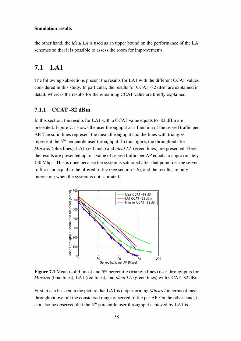
Simulation results
the other hand, the ideal LA is used as an upper bound on the performance of the LAschemes so that it is possible to assess the room for improvements.
7.1 LA1
The following subsections present the results for LA1 with the different CCAT valuesconsidered in this study. In particular, the results for CCAT -82 dBm are explained indetail, whereas the results for the remaining CCAT value are briefly explained.
7.1.1 CCAT -82 dBm
In this section, the results for LA1 with a CCAT value equals to -82 dBm arepresented. Figure 7.1 shows the user throughput as a function of the served traffic perAP. The solid lines represent the mean throughput and the lines with trianglesrepresent the 5th percentile user throughput. In this figure, the throughputs forMinstrel (blue lines), LA1 (red lines) and ideal LA (green lines) are presented. Here,the results are presented up to a value of served traffic per AP equals to approximately150 Mbps. This is done because the system is saturated after that point, i.e. the servedtraffic is no equal to the offered traffic (see section 5.6), and the results are onlyinteresting when the system is not saturated.
0 50 100 150 2000
100
200
300
400
500
600
700
Served traffic per AP [Mbps]
Use
r T
hro
ug
hp
ut
(Me
an
an
d 5
th p
erc
) [M
bp
s]
Ideal CCAT −82 dBm
LA1 CCAT −82 dBm
Minstrel CCAT −82 dBm
Figure 7.1 Mean (solid lines) and 5th percentile (triangle lines) user throughputs forMinstrel (blue lines), LA1 (red lines), and ideal LA (green lines) with CCAT -82 dBm
First, it can be seen in the picture that LA1 is outperforming Minstrel in terms of meanthroughput over all the considered range of served traffic per AP. On the other hand, itcan also be observed that the 5th percentile user throughput achieved by LA1 is
58
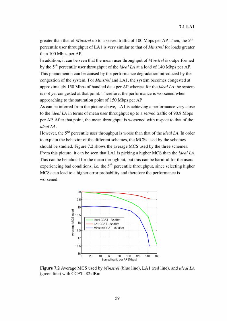
7.1 LA1
greater than that of Minstrel up to a served traffic of 100 Mbps per AP. Then, the 5th
percentile user throughput of LA1 is very similar to that of Minstrel for loads greaterthan 100 Mbps per AP.In addition, it can be seen that the mean user throughput of Minstrel is outperformedby the 5th percentile user throughput of the ideal LA at a load of 140 Mbps per AP.This phenomenon can be caused by the performance degradation introduced by thecongestion of the system. For Minstrel and LA1, the system becomes congested atapproximately 150 Mbps of handled data per AP whereas for the ideal LA the systemis not yet congested at that point. Therefore, the performance is worsened whenapproaching to the saturation point of 150 Mbps per AP.As can be inferred from the picture above, LA1 is achieving a performance very closeto the ideal LA in terms of mean user throughput up to a served traffic of 90.8 Mbpsper AP. After that point, the mean throughput is worsened with respect to that of theideal LA.However, the 5th percentile user throughput is worse than that of the ideal LA. In orderto explain the behavior of the different schemes, the MCSs used by the schemesshould be studied. Figure 7.2 shows the average MCS used by the three schemes.From this picture, it can be seen that LA1 is picking a higher MCS than the ideal LA.This can be beneficial for the mean throughput, but this can be harmful for the usersexperiencing bad conditions, i.e. the 5th percentile throughput, since selecting higherMCSs can lead to a higher error probability and therefore the performance isworsened.
0 20 40 60 80 100 120 140 16016
16.5
17
17.5
18
18.5
19
19.5
20
Served traffic per AP [Mbps]
Ave
rag
e M
CS
use
d
Ideal CCAT −82 dBm
LA1 CCAT −82 dBm
Minstrel CCAT −82 dBm
Figure 7.2 Average MCS used by Minstrel (blue line), LA1 (red line), and ideal LA(green line) with CCAT -82 dBm
59
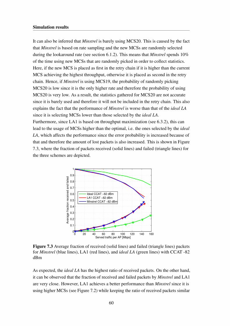
Simulation results
It can also be inferred that Minstrel is barely using MCS20. This is caused by the factthat Minstrel is based on rate sampling and the new MCSs are randomly selectedduring the lookaround rate (see section 6.1.2). This means that Minstrel spends 10%of the time using new MCSs that are randomly picked in order to collect statistics.Here, if the new MCS is placed as first in the retry chain if it is higher than the currentMCS achieving the highest throughput, otherwise it is placed as second in the retrychain. Hence, if Minstrel is using MCS19, the probability of randomly pickingMCS20 is low since it is the only higher rate and therefore the probability of usingMCS20 is very low. As a result, the statistics gathered for MCS20 are not accuratesince it is barely used and therefore it will not be included in the retry chain. This alsoexplains the fact that the performance of Minstrel is worse than that of the ideal LAsince it is selecting MCSs lower than those selected by the ideal LA.Furthermore, since LA1 is based on throughput maximization (see 6.3.2), this canlead to the usage of MCSs higher than the optimal, i.e. the ones selected by the idealLA, which affects the performance since the error probability is increased because ofthat and therefore the amount of lost packets is also increased. This is shown in Figure7.3, where the fraction of packets received (solid lines) and failed (triangle lines) forthe three schemes are depicted.
0 20 40 60 80 100 120 140 1600
0.1
0.2
0.3
0.4
0.5
0.6
0.7
0.8
0.9
1
Served traffic per AP [Mbps]
Avera
ge fra
ction r
eceiv
ed a
nd faile
d
Ideal CCAT −82 dBm
LA1 CCAT −82 dBm
Minstrel CCAT −82 dBm
Figure 7.3 Average fraction of received (solid lines) and failed (triangle lines) packetsfor Minstrel (blue lines), LA1 (red lines), and ideal LA (green lines) with CCAT -82dBm
As expected, the ideal LA has the highest ratio of received packets. On the other hand,it can be observed that the fraction of received and failed packets by Minstrel and LA1are very close. However, LA1 achieves a better performance than Minstrel since it isusing higher MCSs (see Figure 7.2) while keeping the ratio of received packets similar
60
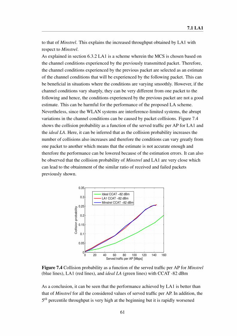
7.1 LA1
to that of Minstrel. This explains the increased throughput obtained by LA1 withrespect to Minstrel.As explained in section 6.3.2 LA1 is a scheme wherein the MCS is chosen based onthe channel conditions experienced by the previously transmitted packet. Therefore,the channel conditions experienced by the previous packet are selected as an estimateof the channel conditions that will be experienced by the following packet. This canbe beneficial in situations where the conditions are varying smoothly. However, if thechannel conditions vary sharply, they can be very different from one packet to thefollowing and hence, the conditions experienced by the previous packet are not a goodestimate. This can be harmful for the performance of the proposed LA scheme.Nevertheless, since the WLAN systems are interference-limited systems, the abruptvariations in the channel conditions can be caused by packet collisions. Figure 7.4shows the collision probability as a function of the served traffic per AP for LA1 andthe ideal LA. Here, it can be inferred that as the collision probability increases thenumber of collisions also increases and therefore the conditions can vary greatly fromone packet to another which means that the estimate is not accurate enough andtherefore the performance can be lowered because of the estimation errors. It can alsobe observed that the collision probability of Minstrel and LA1 are very close whichcan lead to the obtainment of the similar ratio of received and failed packetspreviously shown.
0 20 40 60 80 100 120 140 1600
0.05
0.1
0.15
0.2
0.25
0.3
0.35
Served traffic per AP [Mbps]
Co
llis
ion
pro
ba
bility
Ideal CCAT −82 dBm
LA1 CCAT −82 dBm
Minstrel CCAT −82 dBm
Figure 7.4 Collision probability as a function of the served traffic per AP for Minstrel(blue lines), LA1 (red lines), and ideal LA (green lines) with CCAT -82 dBm
As a conclusion, it can be seen that the performance achieved by LA1 is better thanthat of Minstrel for all the considered values of served traffic per AP. In addition, the5th percentile throughput is very high at the beginning but it is rapidly worsened
61
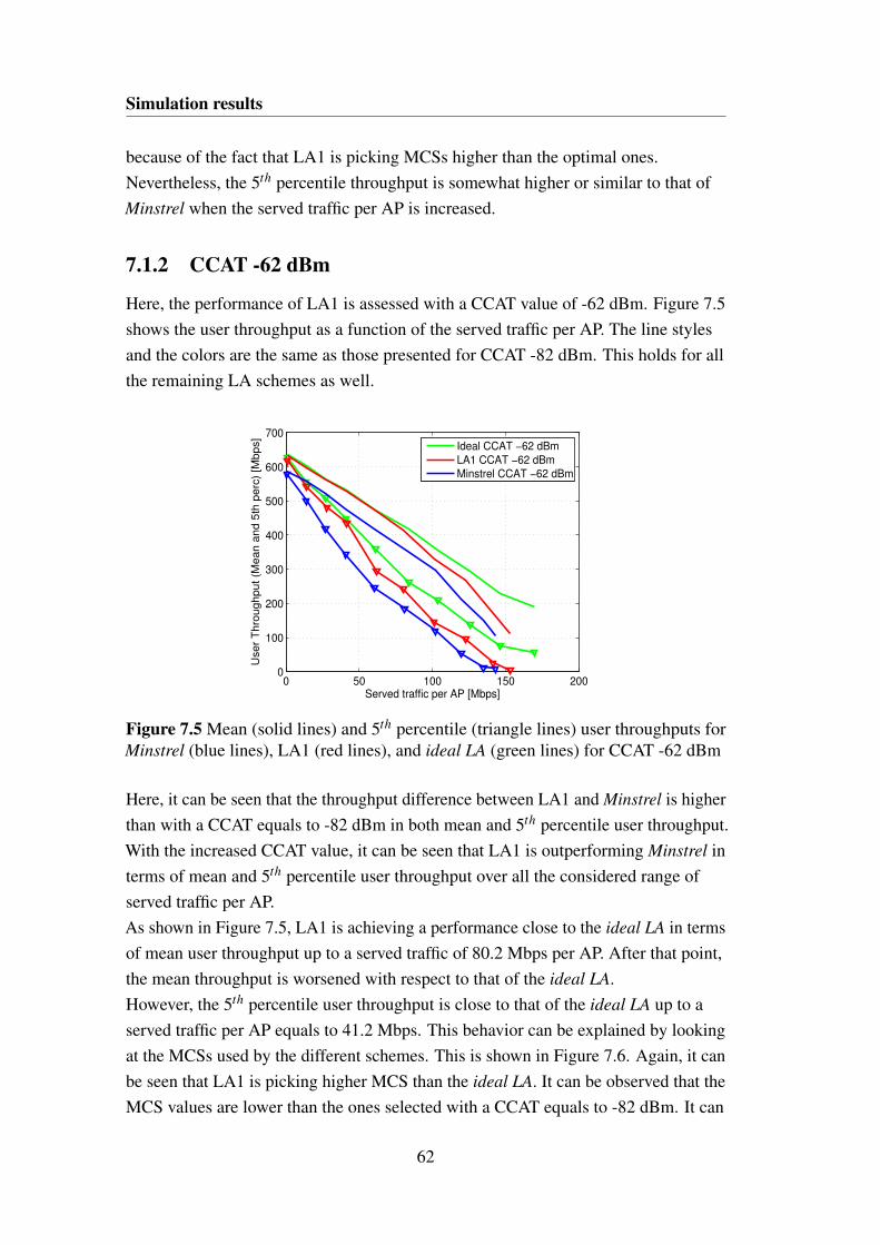
Simulation results
because of the fact that LA1 is picking MCSs higher than the optimal ones.Nevertheless, the 5th percentile throughput is somewhat higher or similar to that ofMinstrel when the served traffic per AP is increased.
7.1.2 CCAT -62 dBm
Here, the performance of LA1 is assessed with a CCAT value of -62 dBm. Figure 7.5shows the user throughput as a function of the served traffic per AP. The line stylesand the colors are the same as those presented for CCAT -82 dBm. This holds for allthe remaining LA schemes as well.
0 50 100 150 2000
100
200
300
400
500
600
700
Served traffic per AP [Mbps]
User
Thro
ughput (M
ean a
nd 5
th p
erc
) [M
bps]
Ideal CCAT −62 dBm
LA1 CCAT −62 dBm
Minstrel CCAT −62 dBm
Figure 7.5 Mean (solid lines) and 5th percentile (triangle lines) user throughputs forMinstrel (blue lines), LA1 (red lines), and ideal LA (green lines) for CCAT -62 dBm
Here, it can be seen that the throughput difference between LA1 and Minstrel is higherthan with a CCAT equals to -82 dBm in both mean and 5th percentile user throughput.With the increased CCAT value, it can be seen that LA1 is outperforming Minstrel interms of mean and 5th percentile user throughput over all the considered range ofserved traffic per AP.As shown in Figure 7.5, LA1 is achieving a performance close to the ideal LA in termsof mean user throughput up to a served traffic of 80.2 Mbps per AP. After that point,the mean throughput is worsened with respect to that of the ideal LA.However, the 5th percentile user throughput is close to that of the ideal LA up to aserved traffic per AP equals to 41.2 Mbps. This behavior can be explained by lookingat the MCSs used by the different schemes. This is shown in Figure 7.6. Again, it canbe seen that LA1 is picking higher MCS than the ideal LA. It can be observed that theMCS values are lower than the ones selected with a CCAT equals to -82 dBm. It can
62
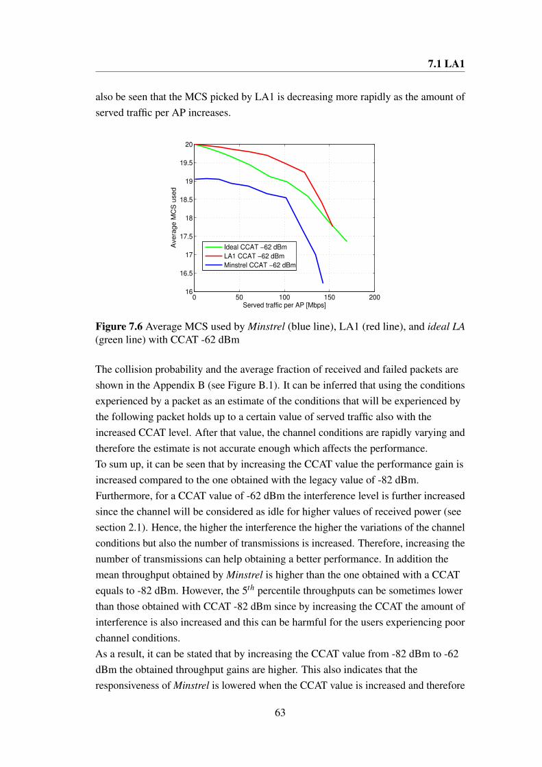
7.1 LA1
also be seen that the MCS picked by LA1 is decreasing more rapidly as the amount ofserved traffic per AP increases.
0 50 100 150 20016
16.5
17
17.5
18
18.5
19
19.5
20
Served traffic per AP [Mbps]
Avera
ge M
CS
used
Ideal CCAT −62 dBm
LA1 CCAT −62 dBm
Minstrel CCAT −62 dBm
Figure 7.6 Average MCS used by Minstrel (blue line), LA1 (red line), and ideal LA(green line) with CCAT -62 dBm
The collision probability and the average fraction of received and failed packets areshown in the Appendix B (see Figure B.1). It can be inferred that using the conditionsexperienced by a packet as an estimate of the conditions that will be experienced bythe following packet holds up to a certain value of served traffic also with theincreased CCAT level. After that value, the channel conditions are rapidly varying andtherefore the estimate is not accurate enough which affects the performance.To sum up, it can be seen that by increasing the CCAT value the performance gain isincreased compared to the one obtained with the legacy value of -82 dBm.Furthermore, for a CCAT value of -62 dBm the interference level is further increasedsince the channel will be considered as idle for higher values of received power (seesection 2.1). Hence, the higher the interference the higher the variations of the channelconditions but also the number of transmissions is increased. Therefore, increasing thenumber of transmissions can help obtaining a better performance. In addition themean throughput obtained by Minstrel is higher than the one obtained with a CCATequals to -82 dBm. However, the 5th percentile throughputs can be sometimes lowerthan those obtained with CCAT -82 dBm since by increasing the CCAT the amount ofinterference is also increased and this can be harmful for the users experiencing poorchannel conditions.As a result, it can be stated that by increasing the CCAT value from -82 dBm to -62dBm the obtained throughput gains are higher. This also indicates that theresponsiveness of Minstrel is lowered when the CCAT value is increased and therefore
63

Simulation results
it can be beneficial to use closed-loop approaches together with an increased value ofCCAT.
7.2 LA1 window
In this section, the simulation results obtained by LA1 window with the differentCCAT values are presented. In addition, a comparison between LA1 and LA1 windowis also provided in the following sections.
7.2.1 CCAT -82 dBm
As can be inferred from 6.3.2 this algorithm has 2 parameters to be optimized. Theyare the window size and the SINR value used to compute the MCS used whentransmitting the packet. Window sizes ranging from 2 to 20 with a step of 3 weretested together with the minimum, mean (in linear units) and maximum of the storedSINR values. To get the best combination of the two parameters, the throughput gainswith respect to Minstrel at a load of 100 Mbps per AP were computed. It was foundthat a window size of 2 together with the minimum SINR value stored in the windowachieved the best performance in the scenario under test. The throughput gainsobtained for the considered window sizes and SINR values are shown in the AppendixB (see Figure B.8).It can be seen from Figure B.8 that the highest gain in terms of mean throughput isobtained for a window size equals to 2 and selecting the minimum stored SINR. Onthe other hand, it can also be seen that a window size of 20 and picking the meanSINR of the values stored in the transmitter window is the only combination achievinga gain in terms of 5th percentile user throughput. In addition, the aforementionedcombination is achieving a gain of 8.13% in terms of mean throughput and a 5thpercentile user throughput that is 9% lower than that of Minstrel. Figure 7.7 shows theperformance of LA1 window in terms of user throughput for a window size of 2 andpicking the minimum SINR value stored in the transmitter side.From Figure 7.7, it can be observed that LA1 window is outperforming Minstrel interms of mean user throughput up to a served traffic around 115 Mbps per AP.Thereafter, the mean throughput of LA1 window is very similar to that of Minstrel.Besides, the 5th percentile user throughput achieved by LA1 window is greater thanthat of Minstrel up to a served traffic of 41 Mbps per AP. Then, it is very similar tothat of Minstrel for a served traffic per AP ranging from 41 to 68 Mbps per AP.Thereafter, the 5th percentile user throughput is worse than that of Minstrel.
64
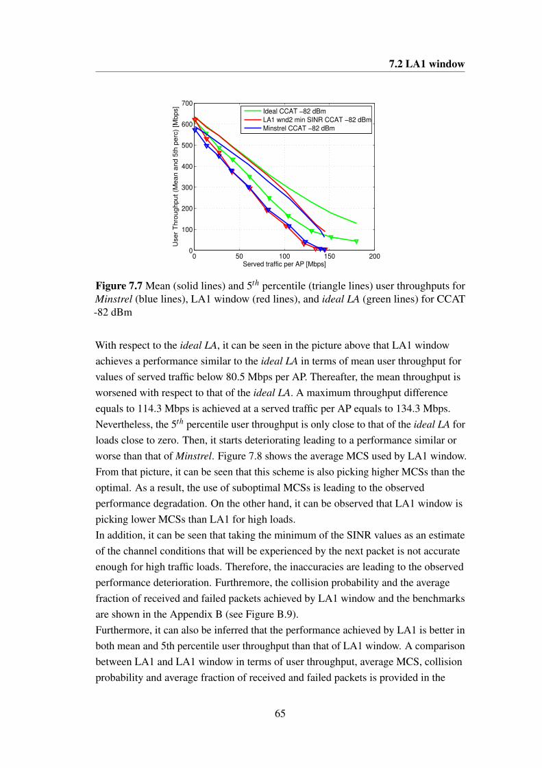
7.2 LA1 window
0 50 100 150 2000
100
200
300
400
500
600
700
Served traffic per AP [Mbps]
User
Thro
ughput (M
ean a
nd 5
th p
erc
) [M
bps]
Ideal CCAT −82 dBm
LA1 wnd2 min SINR CCAT −82 dBm
Minstrel CCAT −82 dBm
Figure 7.7 Mean (solid lines) and 5th percentile (triangle lines) user throughputs forMinstrel (blue lines), LA1 window (red lines), and ideal LA (green lines) for CCAT-82 dBm
With respect to the ideal LA, it can be seen in the picture above that LA1 windowachieves a performance similar to the ideal LA in terms of mean user throughput forvalues of served traffic below 80.5 Mbps per AP. Thereafter, the mean throughput isworsened with respect to that of the ideal LA. A maximum throughput differenceequals to 114.3 Mbps is achieved at a served traffic per AP equals to 134.3 Mbps.Nevertheless, the 5th percentile user throughput is only close to that of the ideal LA forloads close to zero. Then, it starts deteriorating leading to a performance similar orworse than that of Minstrel. Figure 7.8 shows the average MCS used by LA1 window.From that picture, it can be seen that this scheme is also picking higher MCSs than theoptimal. As a result, the use of suboptimal MCSs is leading to the observedperformance degradation. On the other hand, it can be observed that LA1 window ispicking lower MCSs than LA1 for high loads.In addition, it can be seen that taking the minimum of the SINR values as an estimateof the channel conditions that will be experienced by the next packet is not accurateenough for high traffic loads. Therefore, the inaccuracies are leading to the observedperformance deterioration. Furthremore, the collision probability and the averagefraction of received and failed packets achieved by LA1 window and the benchmarksare shown in the Appendix B (see Figure B.9).Furthermore, it can also be inferred that the performance achieved by LA1 is better inboth mean and 5th percentile user throughput than that of LA1 window. A comparisonbetween LA1 and LA1 window in terms of user throughput, average MCS, collisionprobability and average fraction of received and failed packets is provided in the
65

Simulation results
0 20 40 60 80 100 120 140 16016
16.5
17
17.5
18
18.5
19
19.5
20
Served traffic per AP [Mbps]
Avera
ge M
CS
used
Ideal CCAT −82 dBm
LA1 wnd2 min SINR CCAT −82 dBm
Minstrel CCAT −82 dBm
Figure 7.8 Average MCS used by Minstrel (blue line), LA1 window (red line), andideal LA (green line) with CCAT -82 dBm
Appendix B (see Figure B.10). From those pictures it can be seen that LA1 window isselecting MCSs that are slightly lower than those of LA1. Furthermore, LA1 windowis achieving a lower collision probability and a higher average fraction of receivedpackets than LA1. This means that, by selecting a more accurate estimate of the SINRexperienced by the next packet LA1 window could outperform LA1. On the otherhand, the achievement of a higher success ratio can be caused by the fact that LA1window is picking the lowest SINR value stored which is a conservative approach thatmight not be able to harvest the highest throughput when the channel conditions arefavourable. As a result, picking the lowest SINR value will lead to the use of lowerMCSs and it will help achieving a higher fraction of successfully delivered packets.
7.2.2 CCAT -62 dBm
With a CCAT equals to -62 dBm it was found that the best performance was achievedwith a window size equals to 5 and taking the minimum SINR of the stored values.The throughput gains at a load of 100 Mbps per AP versus the window size for theconsidered SINR values are shown in the Appendix B (see Figure B.11).It can be seen that the gains are higher than those achieved with CCAT -82 dBm,especially in 5th percentile user throughput. In this case, the highest gain in terms ofmean throughput is obtained for a window size equals to 5 and selecting the minimumstored SINR. This combination achieves a gain of 20.56% and 37.88% in terms ofmean and 5th percentile user throughput respectively. However, for the 5th percentileuser throughput the highest gain is obtained with a window size equals to 8 and taking
66

7.3 Remaining schemes with ACK piggybacked feedback
the mean of the stored SINR values. In that case, the gain is equal to 55.05% withrespect to Minstrel. The plots showing the performance of the algorithm with theincreased CCAT value can be found in the Appendix B (see Figure B.12).It can be seen that LA1 window achieves a lower collision probability and therefore ahigher amount of successfully received packets than Minstrel. Furthermore, it can alsobe seen that LA1 window is using higher MCSs than Minstrel. The aforementionedeffects leads to the observed throughput gains.Furthermore, it can also be inferred that the performance achieved by LA1 window issomewhat better in both mean and 5th percentile user throughput than that of LA1after a load of 80.1 Mbps per AP. A comparison between LA1 and LA1 window interms of throughput, average MCS used, collision probability and average fraction ofreceived and failed packets are shown in the Appendix B (see Figure B.13). Fromthose pictures it can be seen that LA1 is selecting MCSs that are slightly greater thanthose of LA1 window up to a load of 120.9 Mbps per AP. Then, LA1 window selectshigher MCSs than LA1. Furthermore, LA1 window is achieving a lower collisionprobability and a higher average fraction of received packets than LA1. Therefore, theinsertion of memory on the transmitter side is beneficial in this particular case since itis achieving a better performance.
7.3 Remaining schemes with ACK piggybackedfeedback
In this section, a summary of the performance obtained by the remaining schemes(LA2 to LA4 and their corresponding window approaches) with the considered CCATvalues is provided.
7.3.1 CCAT -82 dBm
The plots showing the performance of the remaining schemes in terms of userthroughput, average MCS used, collision probability and average fraction of receivedand failed packets can be found in Appendix B.In Figure B.2a it can be seen that LA2 outperforms Minstrel in terms of mean and 5th
percentile user throughput up to 130 Mbps per AP. Then, the performance is similar orworse than that of Minstrel.Regarding LA3, it can be seen that there is one parameter to be optimized, namely theT hroughputratio (see section 6.3.4). Several values for T hroughputratio ranging from70% to 95% with a step of 5% were tested through simulations. The 100% value was
67

Simulation results
not tested since it would always choose the MCS having the highest achievablethroughput and therefore LA3 would achieve the same performance as LA1. Thevalue of 80% achieved the best performance in the scenario under test and with aCCAT equal to -82 dBm. Furthermore, Figure B.4a shows that LA3 outperformsMinstrel in terms of mean throughput over all the range of served traffic per AP.Regarding the 5th percentile user throughput, LA3 outperforms Minstrel up to 100Mbps per AP. Then, it achieves a similar performance to that of Minstrel.With respect to LA4, it has 1 parameter to be optimized, namely the target errorprobability Perrortarget (see section 6.3.5). Several Perrortarget values ranging from0.05 to 0.25 with a step of 0.05 were tested through simulations. The valuePerrortarget = 0.1 achieved the best performance in the scenario under test and usingCCAT -82 dBm. Hence, that is the target value used in the results presented in theAppendix B. It can be seen in Figure B.6a that LA4 outperforms Minstrel in bothmean and 5th percentile user throughput. However, its performance is deteriorated forloads higher than 96 Mbps per AP.Regarding the window approaches, a similar parameter optimization to that performedfor LA1 is carried out (see section 7.2). In particular, window sizes ranging from 2 to20 with a step of 3 together with the maximum, mean and minimum SINR wereconsidered. In the case of LA2 window, the receiver is sending back the MCS thatshould be used instead of sending the SINR value. The reporting of the MCS is donebecause LA2 (see 6.3.3) is also ensuring a successful delivery of the packet andtherefore is more adequate to send back the MCS value ensuring the successful packetdelivery rather than the SINR value. It is important to mention that for LA3 windowand LA4 window a T hroughputratio equal to 0.8 and a Perrortarget equal to 0.1 wereused respectively.The throughput gains with respect to Minstrel at a load of 100Mbps per AP werecomputed to determine the best combination of the two parameters. The obtainedresults can be found in the Appendix B (see Figures B.14, B.20 and B.26). For LA2window, it was found that a window size equal to 5 and picking the maximum storedMCS achieved the highest gain (see Figure B.14). Regarding LA3 window, a windowsize equal to 11 and picking the mean of the stored SINR values achieved the bestperformance (see Figure B.20). With respect to LA4 window, a window size equal to11 and picking the maximum of the stored SINR values obtained the highest gain atthe comparison point (see Figure B.26).For the window approaches, it can be observed in Figures B.15a, B.21a and B.27a thatthey outperform Minstrel up to a served traffic approximately equal to 100 Mbps perAP except for LA2 window whose 5th percentile user throughput is higher than that ofMinstrel up to 52 Mbps per AP (see Figure B.15a). Then, for loads higher than 100
68

7.3 Remaining schemes with ACK piggybacked feedback
Mbps per AP their performance is worsened leading to a performance similar or worseto that of Minstrel.Furthermore, a comparison between LA2 to LA4 and their corresponding windowapproaches is provided in the Appendix B (see Figures B.16, B.22 and B.28). There, itcan be seen that the non-window approaches outperform the window approaches fortraffic loads higher than 100 Mbps per AP.To sum up, the throughput gains are obtained by using higher MCSs than Minstrel andkeeping a similar collision probability and average fraction of received and failedpackets as in LA2, LA3 and LA4 (see Figures B.2, B.4 and B.6). On the other hand,LA2 window to LA4 window achieve higher throughput than Minstrel by using higherMCSs and achieving a lower collision probability and a higher fraction of receivedand failed packets (see Figures B.15, B.21 and B.27).
7.3.2 CCAT -62 dBm
The performance of LA2 to LA4 and their corresponding window approaches with theincreased CCAT value can be found in Appendix B.Figure B.3a shows that LA2 outperforms Minstrel in terms of mean and 5th percentileover the considered range of served traffic per AP. It can also be observed that theperformance is degraded for loads higher than 100 Mbps per AP.Regarding LA3, the T hroughputratio should be optimized again since the behaviour ofthe schemes changes when increasing the CCAT values. Once again, several valuesfor T hroughputratio ranging from 70% to 95% with a step of 5% were tested throughsimulations. The value of 90% achieved the best performance in the scenario undertest and with the increased CCAT value. Furthermore, Figure B.5a shows that LA3clearly outperforms Minstrel in terms of mean and 5th percentile user throughput overall the range of served traffic per AP.With respect to LA4, the target error probability Perrortarget should be optimizedagain. Several Perrortarget values ranging from 0.05 to 0.25 with a step of 0.05 weretested through simulations. The value Perrortarget = 0.05 achieved the bestperformance in the scenario under test and using a CCAT equal to -62 dBm. Hence,that is the target value used in the results presented in the Appendix B. It can be seenin Figure B.7a that LA4 outperforms Minstrel in both mean and 5th percentile userthroughput. However, its performance is deteriorated for loads higher than 100 Mbpsper AP.Regarding the window approaches, a similar parameter optimization to that performedfor LA1 is carried out (see section 7.2). In this case, LA3 window and LA4 window
69

Simulation results
were using a T hroughputratio equal to 0.9 and a Perrortarget equal to 0.05 respectively.
Once again, the throughput gains with respect to Minstrel at a load of 100Mbps perAP were computed to determine the best combination of the two parameters. Thegains for the different window sizes and SINR (or MCS) values are shown inAppendix B (see Figures B.17, B.23 and B.29). For LA2 window, it was found that awindow size equal to 8 and picking the minimum stored MCS achieved the highestgain (see Figure B.17). Regarding LA3 window, a window size equal to 8 and pickingthe mean of the stored SINR values achieved the best performance (see Figure B.23).For LA4 window, a window size equal to 2 and picking the maximum of the storedSINR values obtained the highest gain at the comparison point (see Figure B.29).For the window approaches, it can be observed in Figures B.18a, B.24a and B.30a thatthey outperform Minstrel in terms of mean and 5th percentile user throughput over thewhole range of served traffic per AP.Furthermore, a comparison between LA2 to LA4 and their corresponding windowapproaches is provided in the Appendix B (see Figures B.19, B.25 and B.31). In thiscase, it can be seen that the window approaches outperform the non-windowapproaches especially for traffic loads higher than 100 Mbps per AP.To sum up, the throughput gains are obtained by using higher MCSs than Minstrel andkeeping a slightly higher collision probability and slightly lower average fraction ofreceived and failed packets as in LA2 (see Figure B.3). On the other hand, LA3, LA4and LA2 window to LA4 window achieve higher throughput than Minstrel by usinghigher MCSs and achieving a lower collision probability and a higher fraction ofreceived and failed packets (see Figures B.5, B.7, B.18, B.24 and B.30).
7.4 LA5
While using LA5, the devices are sending probing packets periodically so that thereceivers of those packets can assess the channel state between them and thecorresponding transmitters. Hence, the throughput gains depend on the period used tosend the probing packets. This means that, for this scheme, it is more interesting toshow the throughput gain as a function of the feedback period instead of showing thethroughput as a function of the served traffic per AP. In addition, this can be helpful toidentify the optimal period, i.e. the feedback period that is achieving the highestthroughput gain.Here, the throughput gain is defined as the gain in terms of mean throughput at theload of 100 Mbps of served traffic per AP, i.e. it is the ratio between the throughputs
70

7.4 LA5
achieved by LA5 and Minstrel at that particular load point and using a certainfeedback period. The gains for the different CCAT values are shown in the followingsections.
7.4.1 CCAT -82 dBm
In this section, the results for LA5 with a CCAT value equals to -82 dBm arepresented. It is important to notice that there is a tradeoff between the throughput gainand the feedback period. On the one hand, when small feedback periods are used theamount of probing packets is large since they are sent very often. In this situation, thechances of transmitting a data packet are low since the devices are transmittingprobing packets very often. This leads to an increased overhead which harms theperformance and therefore leads to a reduction of the obtained throughput. It explainsthe fact that throughput losses are obtained when using small feedback periods.On the other hand, when large feedback periods are used devices are barely sendingprobing packets and hence, the amount of probing packets is small. In this case, thechannel state is not assessed accurately due to the lack of probing packets. This leadsto a performance degradation and explains the encountered throughput losses when alarge feedback period is used. Figure 7.9 shows the gain in terms of mean userthroughput as a function of the feedback period at a load of 100 Mbps per AP. Here,the blue line represents the obtained gain with the ratemaps specified in 5.1 and thered line denotes the gain with the fast fading implementation (see 5.7.2).
0 50 100 150 200 2500.65
0.7
0.75
0.8
0.85
0.9
0.95
1
1.05
1.1
1.15
Feedback period [ms]
Ga
in in
me
an
th
rou
gh
pu
t a
t 1
00
Mb
ps p
er
AP
[%
]
Gain with L2S ratemaps
Gain with FF channels
Figure 7.9 Throughput gain as a function of the feedback period with the link tosystem (L2S) ratemaps (blue line) and with the implemented fast fading (FF) channels(red line) for CCAT -82 dBm
71
Simulation results
When using the L2S ratemaps, it can be observed in the picture above that throughputlosses are experienced when the feedback period is within the range 1 to 20milliseconds due to the increased overhead. After that, the throughput gains areincreasing until reaching the maximum gain of 12.4% obtained with a period equals to75ms. Then, the gains start decreasing due to the lack of accuracy of the channel statecaused by the increased feedback periods. Finally, throughput losses are encounteredagain as a consequence of the aforementioned lack of accuracy. As a conclusion, itcan be stated that the feedback period equals to 75ms is the optimal period for a CCATvalue of -82 dBm and the considered ratemaps since it is achieving the highest gain.On the other hand, when the implemented fast fading channels are used it can be seenthat throughput losses are obtained approximately within the same range as in the casewhere the L2S ratemaps are used. Then, a maximum throughput gain equals to10.25% is obtained with a period of 50ms. After that, the gains start decreasing due toinaccuracies when estimating the channel due to the increased feedback periods.Hence, a period equals to 50ms is the optimal value when the fast fading channels areused.In this case, it can be observed that higher gains are obtained from 25 to 50mscompared against the case wherein the L2S ratemaps are used. In addition, throughputlosses are also obtained with lower periods than in the previous case. Theaforementioned phenomena are explained by the fact that the channel gains aredynamically changing and hence more frequent updates are needed in order toestimate the channel state accurately.
7.4.2 CCAT -62 dBm
Here, the throughput gains obtained by LA5 with a CCAT value of -62 dBm arepresented. It is important to mention that the tradeoff between feedback period andthroughput gain holds for any CCAT value since it is independent on the CCAT value.Figure 7.10 shows the gain in mean user throughput for the considered CCAT value ata load of 100 Mbps per AP.When the L2S ratemaps are used, throughput losses are observed when the feedbackperiod is between 1 and 30ms. Then, the throughput gain increases until reaching itsmaximum value of 10.74% obtained with a feedback period of 125ms. After that, thegains are decreased due to inaccuracies occurred while estimating the channel state. Inthis case, the feedback period equals to 125ms is the optimal period for a CCAT valueof -82 dBm and the considered scenario since it is achieving the highest gain.It is important to notice that when the CCAT value is increased from -82 dBm to -62dBm the range wherein throughput losses are observed due to large overhead is
72
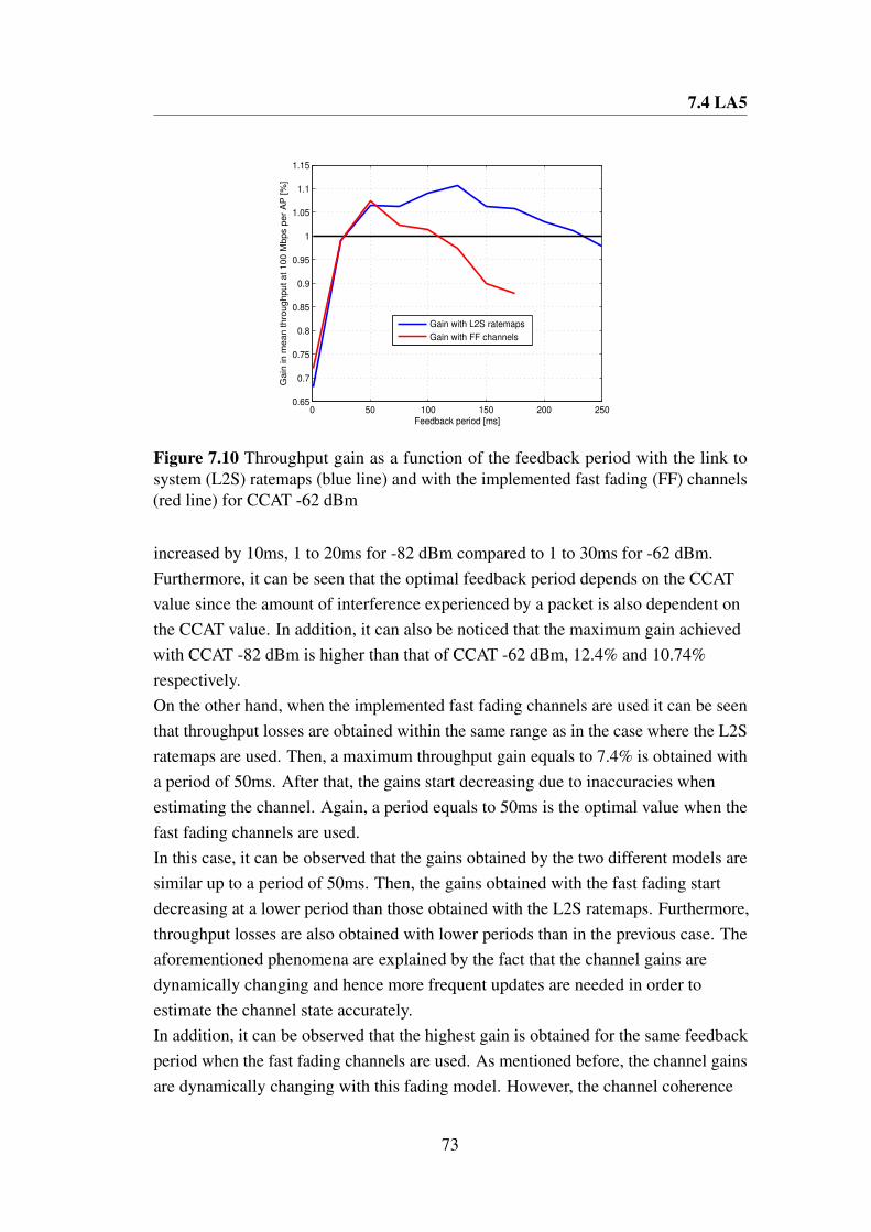
7.4 LA5
0 50 100 150 200 2500.65
0.7
0.75
0.8
0.85
0.9
0.95
1
1.05
1.1
1.15
Feedback period [ms]
Ga
in in
me
an
th
rou
gh
pu
t a
t 1
00
Mb
ps p
er
AP
[%
]
Gain with L2S ratemaps
Gain with FF channels
Figure 7.10 Throughput gain as a function of the feedback period with the link tosystem (L2S) ratemaps (blue line) and with the implemented fast fading (FF) channels(red line) for CCAT -62 dBm
increased by 10ms, 1 to 20ms for -82 dBm compared to 1 to 30ms for -62 dBm.Furthermore, it can be seen that the optimal feedback period depends on the CCATvalue since the amount of interference experienced by a packet is also dependent onthe CCAT value. In addition, it can also be noticed that the maximum gain achievedwith CCAT -82 dBm is higher than that of CCAT -62 dBm, 12.4% and 10.74%respectively.On the other hand, when the implemented fast fading channels are used it can be seenthat throughput losses are obtained within the same range as in the case where the L2Sratemaps are used. Then, a maximum throughput gain equals to 7.4% is obtained witha period of 50ms. After that, the gains start decreasing due to inaccuracies whenestimating the channel. Again, a period equals to 50ms is the optimal value when thefast fading channels are used.In this case, it can be observed that the gains obtained by the two different models aresimilar up to a period of 50ms. Then, the gains obtained with the fast fading startdecreasing at a lower period than those obtained with the L2S ratemaps. Furthermore,throughput losses are also obtained with lower periods than in the previous case. Theaforementioned phenomena are explained by the fact that the channel gains aredynamically changing and hence more frequent updates are needed in order toestimate the channel state accurately.In addition, it can be observed that the highest gain is obtained for the same feedbackperiod when the fast fading channels are used. As mentioned before, the channel gainsare dynamically changing with this fading model. However, the channel coherence
73
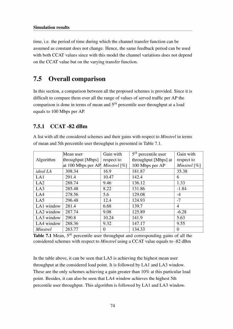
Simulation results
time, i.e. the period of time during which the channel transfer function can beassumed as constant does not change. Hence, the same feedback period can be usedwith both CCAT values since with this model the channel variations does not dependon the CCAT value but on the varying transfer function.
7.5 Overall comparison
In this section, a comparison between all the proposed schemes is provided. Since it isdifficult to compare them over all the range of values of served traffic per AP thecomparison is done in terms of mean and 5th percentile user throughput at a loadequals to 100 Mbps per AP.
7.5.1 CCAT -82 dBm
A list with all the considered schemes and their gains with respect to Minstrel in termsof mean and 5th percentile user throughput is presented in Table 7.1.
AlgorithmMean userthroughput [Mbps]at 100 Mbps per AP
Gain withrespect toMinstrel [%]
5th percentile userthroughput [Mbps] at100 Mbps per AP
Gain withrespect toMinstrel [%]
ideal LA 308.34 16.9 181.87 35.38LA1 291.4 10.47 142.4 6LA2 288.74 9.46 136.12 1.33LA3 285.48 8.22 131.86 -1.84LA4 278.56 5.6 129.08 -4LA5 296.48 12.4 124.93 -7LA1 window 281.4 6.68 139.7 4LA2 window 287.74 9.08 125.89 -6.28LA3 window 290.8 10.24 141.9 5.63LA4 window 288.36 9.32 147.17 9.55Minstrel 263.77 0 134.33 0
Table 7.1 Mean, 5th percentile user throughput and corresponding gains of all theconsidered schemes with respect to Minstrel using a CCAT value equals to -82 dBm
In the table above, it can be seen that LA5 is achieving the highest mean userthroughput at the considered load point. It is followed by LA1 and LA3 window.These are the only schemes achieving a gain greater than 10% at this particular loadpoint. Besides, it can also be seen that LA4 window achieves the highest 5thpercentile user throughput. This algorithm is followed by LA1 and LA3 window.
74
7.5 Overall comparison
However, some algorithms such as LA3, LA4, LA5, and LA2 window have a 5th
percentile user throughput lower than that of Minstrel at that load point.On the other hand, LA4 is the scheme achieving the lowest mean user throughputamong the proposed schemes. It is followed by LA1 window and LA3. Regarding the5th percentile user throughput, LA5 achieves the lowest value followed by LA2window and LA4.Furthermore, it can also be inferred that LA3 window and LA4 window achieve ahigher mean and 5th percentile user throughput than LA3 and LA4 respectively.However, it was shown in the previous sections that the performance of all windowapproaches is worsened at load points around 100 Mbps per AP. Therefore, theperformance of the window approaches is worse than that of the approaches withoutadditional memory after loads around 100 Mbps per AP.As a conclusion, LA1 and LA3 achieve the best overall performance for a CCAT valueequals to -82 dBm taking into account the mean and 5th percentile user throughput. Inaddition, it can be seen that they are the only algorithms that achieve a gain in terms of5th percentile user throughput over all the range of served traffic per AP. Furthermore,it can also be seen that LA3 achieves a better 5th percentile user throughput than LA1up to a load equals to 80 Mbps per AP. Thereafter, both achieve a similar performance.On the other hand, it can also be seen that LA1 achieves a better performance thanLA3 in terms of mean throughput for loads higher than 94 Mbps per AP.
7.5.2 CCAT -62 dBm
Table 7.2 shows the achieved gains with respect to Minstrel in terms of mean and 5thpercentile user throughput at a load of 100 Mbps per AP.It can be seen that the gains are generally higher with the increased CCAT valueespecially in terms of 5th percentile user throughput. It can also be observed that thereare no losses in terms of 5th percentile user throughput and the throughput differencesbetween the proposed schemes and Minstrel are higher with this CCAT value.Furthermore, the performance of the schemes is closer to that of the ideal LAespecially at loads higher than 100 Mbps per AP. Thus, we can conclude that the useof closed-loop approaches can be beneficial with the CCAT value equals to -62 dBm.In this case, it can be seen that LA1 window achieves the highest mean userthroughput at the considered load point. It is followed by LA3 and LA3 window.These are the only schemes achieving a gain greater than 20% at this particular loadpoint. Besides, it can also be seen that LA3 window achieves the highest 5th
percentile user throughput. This algorithm is followed by LA3 and LA4 window.
75

Simulation results
AlgorithmMean userthroughput [Mbps]at 100 Mbps per AP
Gain withrespect toMinstrel [%]
5th percentile userthroughput [Mbps] at100 Mbps per AP
Gain withrespect toMinstrel [%]
ideal LA 367.23 21.68 216.96 72.83LA1 333.9 10.64 150.27 19.7LA2 333.81 10.61 149.48 19.07LA3 363.73 20.52 196.56 56.58LA4 352.59 16.83 176.7 40.76LA5 334.22 10.74 143.9 14.62LA1 window 363.85 20.56 173.1 37.88LA2 window 357.2 18.36 192.8 53.58LA3 window 362.2 20.02 202.5 61.3LA4 window 359.2 19.02 193.96 54.51Minstrel 301.78 0 125.54 0
Table 7.2 Mean, 5th percentile user throughput and corresponding gains of all theconsidered schemes with respect to Minstrel using a CCAT value equals to -62 dBm
However, some algorithms such as LA3, LA4, LA5, and LA2 window have a 5thpercentile user throughput lower than that of Minstrel at that load point.On the other hand, LA2 is the scheme achieving the lowest mean user throughputamong the proposed schemes. It is followed by LA1 and LA5. Regarding the 5th
percentile user throughput, LA5 achieves the lowest value followed by LA2 and LA1.Furthermore, it can also be inferred that the window approaches outperform theapproaches having a memory equals to one, i.e. the ones where the MCS is selectedbased on the conditions experienced by the previously transmitted packet. Theimprovement is considerable for loads higher than 100 Mbps per AP. Therefore, theinsertion of memory is helping to improve the performance of the schemes when aCCAT value equals to -62 dBm is used.As a conclusion, LA3 window, LA4 window and LA3 achieve the best overallperformance. It can be seen that LA3 achieves the highest throughput at 100 Mbpsamong the aforementioned schemes. However, LA3 window and LA4 windowachieve a mean throughput closer to that of the ideal LA for loads higher than 100Mbps per AP. Furthermore, it can also be seen that LA4 window and LA3 are the onesachieving the best 5th percentile user throughput. In this case, LA4 window is theachieves the best 5th percentile user throughput up to a served traffic equals to 123Mbps per AP. Then, LA3 achieves a better performance than LA4 window.
76

7.5 Overall comparison
7.5.3 Mixed numbers
In this section, a comparison between the gains with respect to Minstrel in terms ofmean user throughput achieved with a CCAT equals to -82 dBm and -62 dBm arepresented in Figure 7.11. Furthermore, the numerical results are presented in Table7.3.
Figure 7.11 Gains in term of mean throughput achieved by the different schemes andthe benchmarks with CCAT -82 dBm (left side) and CCAT -62 dBm (right side).
In the figure above, it can be seen that gains are generally higher with CCAT -62 dBm.In Table 7.3, the highest gain of every algorithm is marked in bold. It can be seen thatthe periodic approach, i.e. LA5, achieves a higher gain in terms of mean userthroughput with CCAT -82 dBm instead. As mentioned before, when increasing theCCAT value the amount of interference is increased and hence the channel conditionsvary more rapidly. This can be harmful in this case where the channel state isperiodically updated and it is assumed to be constant between the times when thechannel is updated. As can be inferred, the channel state does not remain constantbetween the updates. Rather, the channel varies more sharply with the increasedCCAT value which leads to a performance degradation and hence the gain is reduced.Regarding the 5th percentile user throughput, it can be seen that the gains are muchhigher with the increased CCAT value. As discussed in the previous sections, the useof closed-loop approaches is beneficial in this case where the channel varies morerapidly since closed-loop approaches have better responsiveness than open-loopapproaches.
77

Simulation results
Algorithm
Gain in meanuser throughputat 100 Mbps perAP with CCAT-82 dBm [%]
Gain in meanuser throughputat 100 Mbps perAP with CCAT-62 dBm [%]
Gain in 5th
percentile userthroughputat 100 Mbps perAP with CCAT-82 dBm [%]
Gain in 5th
percentile userthroughputat 100 Mbps perAP with CCAT-62 dBm [%]
ideal LA 16.9 21.68 35.38 72.83LA1 10.47 10.64 6 19.7LA2 9.46 10.61 1.33 19.07LA3 8.22 20.52 -1.84 56.58LA4 5.6 16.83 -4 40.76LA5 12.4 10.74 -7 14.62LA1 window 6.68 20.56 4 37.88LA2 window 9.08 18.36 -6.28 53.58LA3 window 10.24 20.02 5.63 61.3LA4 window 9.32 19.02 9.55 54.51
Table 7.3 Comparison of the gains achieved by the different schemes with CCAT -82dBm and -62 dBm
To sum up, it can also be stated that LA1 window and LA3 window both with CCAT-62 dBm achieve the highest gain in terms of mean and 5th percentile user throughputrespectively. As a conclusion, it can be inferred that the insertion of memory on thetransmitter side is helping to improve the performance. However, this leads to anincreased complexity due to the need of more storage capacity on the transmitter sidein order to store the received feedback.
78

Chapter 8
Conclusions and future work
This work presents the implementation and comparison of the different proposed LAalgorithms in a standard system (802.11ac) and in a high capacity system (802.11ax).Furthermore, the effect of introducing measurements and feedback in order to estimatethe channel quality and the tradeoff between signaling overhead and performancewere also studied. The performance of the five proposed link adaptation schemes,named LA1 to LA5, was compared with the performance of Minstrel and an ideal LA.An initial study was carried out to add some functionalities to the simulator such as afading channels, block ACK, a modification on the traffic model, and a new link tosystem model. Then, the LA algorithms were implemented and tested in the standardsystem using the CCAT value equal to -82 dBm and in the high capacity system wherea CCAT value equal to -62 dBm was used. In order to report the feedback, the HighThroughput Control Field (HTC) was used. This is an optional field that can be usedin control frames such as ACKs, block ACKs, RTS/CTS, etc. This mechanism can beused by the algorithms LA1 to LA4 and their corresponding window approaches.However, in the case of LA5 the periodic feedback was reported using additionalprobing packets.In the standard system, it was found that LA5 achieved the best performance in termsof mean user throughput at the comparison point of 100 Mbps per AP. On the otherhand, LA4 window achieved the best 5th percentile user throughput at that point.Furthermore, LA5 incurs a larger overhead compared with the rest of the approacheswhere the feedback was piggybacked in the ACK frames increasing its length by 4bytes. The signalling overhead caused by the different LA schemes was taken intoaccount during the simulations. It was also shown that the insertion of some additionalmemory on the transmitter side helped to improve the performance of some of theproposed algorithms, namely LA3 and LA4.
79
Conclusions and future work
Nevertheless, it was also found that LA5 achieved worse performance than Minstrel interms of 5th percentile user throughput at the comparison point of 100 Mbps of servedtraffic per AP. With this approach, the channel state is updated with probing packetsand it is assumed to be constant between two consecutive updates. But for the usersexperiencing bad channel conditions, i.e. the ones achieving low throughputs, theconditions might be sharply varying and they might need more frequent updates inorder to estimate the channel properly and react against changes. The lack of accurateinformation may lead to the observed performance degradation in the 5th percentileuser throughput.LA5 uses probing packets that are sent periodically in order to assess the channel state.Therefore, it can be difficult to implement it in a real wireless card driver since it isusing periodical probing packets that are not standard compliant. The remainingalgorithms could be easier to implement in a real wireless card driver by adding tablesmapping the SINR to Perror values for the different MCS used and enabling the use ofthe HTC field.Regarding the high capacity system, it was shown that higher throughput gains than inthe standard scenario were obtained, especially in terms of 5th percentile userthroughput. In this case, LA1 window achieved the highest mean user throughput atthe load of 100 Mbps per AP. On the other hand, LA3 window achieved the highest5th percentile user throughput at that load point. In these algorithms, the feedback waspiggybacked in the ACK frames increasing its length by 4 bytes and additionalmemory was added on the transmitter side so that it could store the conditionsexperienced by several packets that were previously transmitted. The overhead wasalso taken into account during the simulations. In this case, it was also shown that theinsertion of some additional memory on the transmitter side improved theperformance of the schemes especially at loads higher than 100 Mbps per AP.It can also be seen that by increasing the CCAT value the performance gain isincreased. Furthermore, for a CCAT value equals to -62 dBm the interference level isincreased since the channel will be considered as idle for higher values of receivedpower . Hence, the higher the interference the higher the variations of the channelconditions but also the delays when accessing the medium are reduced. With theincreased CCAT value, the medium is considered as idle for higher values of receivedpower. Thus, the contention window values will be decremented more often and theywill reach zero faster than with the CCAT value of -82 dBm (see section 2.1).Therefore, increasing the CCAT value can help obtaining a better performance. Inaddition the increased amount of interference can be harmful for open-loopapproaches since they have less responsiveness than closed-loop approaches. Hence, itcan be beneficial to use closed-loop approaches in the high capacity scenario where a
80

higher CCAT value is used. With this CCAT value, it can also be seen that theapproaches reporting the feedback piggybacked in the ACK messages generallyachieve a better performance than the approach that periodically sends probingpackets to assess the channel state since the channel state is more outdated when it isperiodically reported.Regarding LA5, it can also be seen that when the implemented fast fading channelsare used the highest gains are achieved with lower periods than those achieved withthe ratemaps. This is due to the fact that with the implemented channels the gains arevarying with time according to the position and the PDP specified by the TGn model DNLOS whereas with the ratemaps the gains remain constant. Therefore, more frequentupdates are needed to estimate the channel conditions when the gains are dynamicallychanging. Furthermore, it was also shown that when using the implemented channelsthe maximum gain was achieved with a period of 50ms for both CCAT values. Thiseffect can be due to the fact that the channel coherence time remains constant whenthe CCAT value is increased and therefore the same period can be used in both cases.Regarding the window approaches, it can be seen that LA1 window and LA2 windowneed more memory when the CCAT value is increased. With the CCAT value equalsto -82 dBm, they achieve their highest gains with a window size equals to 2 and 5respectively. However, with CCAT -62 dBm they achieve their highest gains withwindow sizes of 5 and 8 respectively. Rather, LA3 window and LA4 window needless memory when the CCAT value is increased (window sizes equals to 11 and 11respectively with CCAT -82 dBm versus sizes equals to 8 and 2 respectively withCCAT -62 dBm). As an example, the values piggybacked in ACKs could be storedusing double precision floating points whose size is equal to 8 bytes [91]. Hence, theamount of memory needed to store the values is not large (maximum 88 bytes for thecases with a window size equals to 11 which is the highest used value).As an extension of the work carried out in this thesis, it would be interesting to test theperformance of the schemes in some other scenarios such as the residential scenario.In addition, a study of how the random backoff mechanism affects the link adaptationwould be interesting. Furthermore, it would also be interesting to test the algorithmstogether with techniques to increase the spectral reuse and dynamically modify theCCAT value, so called Dynamic Sensitivity Control (DSC). A description of thesetechniques can be found in [92].Furthermore, the results presented in this work were obtained through simulations inone of the simulation scenarios proposed by the TGax (the enterprise scenario). Itwould also be interesting to test the performance of the proposed schemes in a realtestbed and in different scenarios to check the robustness of the algorithms under realconditions in order to determine their feasibility and benefits.
81
Conclusions and future work
To sum up, it can be stated that the performance can be improved by adding someadditional calculations on the receiver side and reporting the results to the transmittereven though it requires the use of longer ACK frames to carry the computed feedbackor the sending of probing packets. In the standard system, a maximum gain in meanthroughput of 12.4% was achieved by LA5. In that scenario, a maximum potentialgain, i.e. the gain achieved by the ideal LA, equal to 16.9% could be achieved. Thus,there is still a gap equal to 4.5% until reaching the maximum gain. In the high capacitysystem, a maximum gain in mean throughput equal to 20.56% was achieved by LA1window. In this case, a maximum gain equal to 21.68% could be achieved. Here, thereis a gap equal to 1.12% until reaching the maximum gain. In addition, it can be seenthat in the high capacity system the achieved gains are closer to the maximum gains.These algorithms could be implemented in a real wireless card driver by adding tablesmapping the SINR to Perror values for the different MCSs used and enabling the use ofthe HTC field. However, LA5 would also require the use of probing packets sentperiodically.
82

Summary
As mentioned earlier, wireless channels vary with time. Due to these changes, theoverall system performance may change. The IEEE 802.11 standards propose severaldata rates that can be used at the physical layer. The different data rates are achievedby using various combinations of modulation and coding schemes (MCS). High datarates can transmit more information during a certain period of time than low data rates.However, high data rates are more susceptible to errors. On the other hand, low datarates take longer to transmit a packet over the link but they are more resistant to errorsand the transmission is more likely to be successful during the periods when thechannel conditions are not favorable.Link adaptation is a technique used to adapt the system parameters to differentsituations. The main goal of link adaptation is to improve the channel utilization byselecting the optimal data rate based on the channel conditions [32]. This techniquecan help improving the performance and therefore the Quality of Service perceived bythe users.There are several link adaptation schemes [34]-[40] explained in the literature. Acomparison between some of them shows that Minstrel is the one that achieves theoverall best performance [87]. However, in [32] it is shown that Minstrel hasdifficulties selecting the optimal data rate when the channel conditions are changing.The thesis project focuses on investigation of improvement strategies for linkadaptation in a high capacity WLAN system. A LA algorithm is designed andcompared with other existing algorithms. The proposed scheme should be robust andachieve a good performance in different scenarios. The different scenarios are used tosimulate various medium reuse conditions. The algorithms are tested under identicalenvironments to ensure that the experiments are controllable and repeatable.For each algorithm the throughput is measured under different traffic loads to evaluateand compare the performance of the different algorithms. The signalling overhead istaken into account during the simulations. Another performance metrics such as theaverage MCS used, collision probability and average fraction of received and failedpackets are also shown.We found that the proposed link adaptation schemes achieved higher throughput thanthe considered schemes. We also found that the schemes are robust since theygenerally achieve higher throughput than Minstrel and their performance is close tothat of the ideal LA up to a certain amount of served traffic per AP.

Conclusions and future work
Some interesting aspects such as the performance in another IEEE scenarios, the useof techniques to increase the spectral reuse, and the effect of the contention windowmechanism are not assessed in this thesis and are proposed as future work.
84
References
[1] IEEE Standard 802.11-1999: “Part 11: Wireless LAN Medium Access Control(MAC) and Physical Layer (PHY) Specifications”.
[2] S.A.A. Alshakhsi and H. Hasbullah. “Improving QoS of VoWLAN viacross-layer-based adaptive approach”. IEEE International Conference onInformation Science and Applications, pp. 1-8., 2011.
[3] T. Tao and A. Czylwik, “Performance analysis of Link Adaptation in LTEsystems”. In International ITG Workshop on Smart Antennas (WSA). IEEE, 2011,pp. 1–5.
[4] Defeng Xu and R. Bagrodia. “Impact of complex wireless environments on rateadaptation algorithms”. In Wireless Communications and NetworkingConference (WCNC), 2011 IEEE, pages 168 -173, march 2011.
[5] O. A. M. Yasuhiko Inoue. “Status of IEEE 802.11 HEW Study Group HighEfficiency WLAN (HEW)”. [Online] Available:http://www.ieee802.org/11/Reports/hew_update.htm. [Accessed: 06-Dec-2014].
[6] E. H. Ong, J. Kneckt, O. Alanen, Z. Chang, T. Huovinen and T. Nihtil. “IEEE802.11ac: Enhancements for very high throughput WLANs”. Proc., IEEE Int.Symp. Personal,Indoor, Mobile Radio Commun. (PIMRC), pp.849 -853 2011.
[7] John Deigh in Robert Audi (ed). “The Cambridge Dictionary of Philosophy”.1995.
[8] “Five principles for research ethics.”[Online]. Available:http://www.apa.org/monitor/jan03/principles.aspx. [Accessed: 28-Feb-2015].
[9] "What is Ethics in Research & Why is it Important?". [Online]. Available:http://www.niehs.nih.gov/research/resources/bioethics/whatis/. [Accessed:28-Feb-2015].
[10] “Ethical Considerations and Approval for Research Involving HumanParticipants — University of Leicester”. [Online]. Available: http://www2.le.ac.uk/departments/gradschool/training/eresources/study-guides/research-ethics.[Accessed: 28-Feb-2015].
[11] Håkansson, A. (2013). “Portal of Research Methods and Methodologies forResearch Projects and Degree Projects”. In: Hamid R. Arabnia Azita BahramiVictor A. Clincy Leonidas Deligiannidis George Jandieri (ed.), “Proceedings ofthe International Conference on Frontiers in Education: Computer Science andComputer Engineering FECS’13” (pp. 67-73). Las Vegas USA: CSREA PressU.S.A.
85

References
[12] IEEE LAN/MAN Standards Committee, “802.11-1997 - IEEE Standard forWireless LAN Medium Access Control (MAC) and Physical Layer (PHY)specifications”. [Online] Available:http://standards.ieee.org/findstds/standard/802.11-1997.html. [Accessed9-Feb-15].
[13] ITU-T-REC-X.Imp200-200612-I, “OSI Implementers’ Guide- Version 1.1” , 15December 2006. [Online] Available:http://www.itu.int/rec/T-REC-X.Imp200-200612-I/en. [Accessed 9-Feb-15].
[14] F. L. Lo, T. S. Ng, and T. I. Yuk , “Performance comparison of single andmulti-channel CSMA-CD wireless networks using equilibrium point analysis”.Vehicular Technology Conference, 1996. ’Mobile Technology for the HumanRace.’ IEEE 46th, vol.3, no., pp.1736-1740 vol.3, 28 Apr-1 May 1996.
[15] Shamim, H.M. and Al Masud, A. “Performance analysis and simulation of MAClayer in WLAN”. IEEE 9th Malaysia International Conference onCommunications (MICC).IEEE, 2009,pp 863-868.
[16] Oliver M. and Escudero A. “Study of different CSMA/CA IEEE 802.11-basedimplementations”. [Online] Available:http://www.eunice-forum.org/eunice99/027.pdf. [Accessed 9-Feb-15].
[17] B. Zhen, H.-B. Li, S. Hara and R. Kohno “Energy based carrier sensing inintegrated medical environments”, Proc. IEEE Int. Conf. Commun., pp.3110-3114 2008.
[18] Lichuan Liu, Kuo, S.M. and MengChu Zhou “Virtual sensing techniques andtheir applications”, Networking, Sensing and Control, 2009. ICNSC ’09.International Conference on, On page(s): 31 – 36.
[19] Behzad, A., “802.11 Flavors and System Requirements”. Wiley-IEEE Press 1stedition. ISBN: 9780470209301.
[20] “802.11n”, IEEE 802.11n Standard, 2009.
[21] Talebi, F., Pratt, T.G., “Performance Evaluation on Diversity Schemes overSpace-Polarization MIMO Channels”. National Wireless Research CollaborationSymposium (NWRCS). IEEE, 2014, pp. 59-63.
[22] A. Leroy et al., “Spatial Division Multiplexing: A Novel Approach forGuaranteed Throughput on NoCs”. Proc. IEEE/ACM/IFIP Int’,l Conf.Hardware/Software Codesign and System Synthesis (CODES+ISSS), pp. 81-86,2005.
[23] B. Ginzburg and A. Kesselman, “Performance Analysis of A-MPDU andA-MSDU Aggregation in IEEE 802.11n”. Proc. IEEE Sarnoff Symp., May 2007.
[24] IEEE P802.11ac. Specification framework for TGac. IEEE 802.11-09/0992r21.January 2011.
86
References
[25] IEEE LAN/MAN Standards Committee, “802.11ac-2013 - IEEE Standard forInformation technology– Telecommunications and information exchange betweensystems Local and metropolitan area networks– Specific requirements–Part 11:Wireless LAN Medium Access Control (MAC) and Physical Layer (PHY)Specifications–Amendment 4: Enhancements for Very High Throughput forOperation in Bands below 6 GHz”. IEEE, December 2013. E-ISBN:978-0-7381-8860-7.
[26] IEEE 802.11-14/0649r0: “P802.11ax Task Group Press Release”, 2014.
[27] Der-Jiunn Deng, Kwang-Cheng Chen, Rung-Shiang Cheng. “IEEE 802.11ax:Next generation wireless local area networks”. In International Conference onHeterogeneous Netowrking for Quality, Reliability, Security, and Robustness(QShine),2014. IEEE, 2014, pp. 77-82.
[28] Y. Song, X. Zhu, Y. Fang, H. Zhang, “Threshold Optimization for RateAdaptation Algorithms in IEEE 802.11 WLANs”, IEEE Transactions on WirelessCommunications, IEEE Press, 2010.
[29] S. H. Y. Wong, H. Yang, S. Lu, and V. Bharghavan, “Robust rate adaptation for802.11 wireless networks”, in ACM MobiCom, Sept. 2006.
[30] D. Qiao and S. Choi, “Fast-responsive link adaptation for IEEE 802.11WLANs”, in Proc. IEEE ICC, 2003.
[31] J. Kim, S. Kim, S. Choi and D. Qiao, “CARA: Collision-Aware Rate Adaptationfor IEEE 802.11 WLANs”, Proc. IEEE INFOCOM, 2006.
[32] J. Choi, J. Na, K. Park, and C. kwon Kim, “Adaptive optimization of rateadaptation algorithms in multi-rate WLANs,” in Proc. IEEE ICNP, 2007.
[33] Poudyal, N., Korea Aerosp. Univ., Goyang, Ha Cheol Lee, Byung Seub Lee andYoungjoon Byun. “The impact of RTS/CTS frames on TCP performance in mobilead hoc-based wireless LAN”. In 11th International Conference on AdvancedCommunication Technology. IEEE, 2009. Pages: 1554 – 1559.
[34] J. C. Bicket, “Bit-rate selection in wireless networks”, Ph.D. dissertation, MITMaster’s Thesis, 2005.
[35] Minstrel Rate Adaptation Algorithm Documentation, [Online] Available:http://sourceforge.net/p/madwifi/svn/HEAD/tree/madwifi/trunk/ath_rate/minstrel/minstrel.txt [Accessed: 2-Feb-15]
[36] Nagai, Y, Fujimura, A, Akihara, M, et al. “A SINR estimation for closedloop linkadaptation of 324 Mbit/sec WLAN system” [C]. IEEE 19th InternationalSymposium on Personal, Indoor and Mobile Radio Communications, 2008.Page(s): 1 – 6.
[37] Nagai, Y, Fujimura, A, Akihara, M, et al “A Closed-Loop Link AdaptationScheme for 324Mbit/sec WLAN System” [C]. IEEE 19th International Symposiumon Personal, Indoor and Mobile Radio Communications, 2008. Page(s): 1 – 5.
87

References
[38] Jain, P., Biswas, G.P., “Design and implementation of an enhanced rateadaptation scheme for wireless LAN IEEE-802.11”. IEEE 1st Internationalconference on Recent Advances in Information Technology (RAIT), 2012.Page(s): 336-340.
[39] Wei Yin, Peizhao Hu, Indulska, J., Portmann, M. and Guerin, J. “RobustMAC-layer rate control mechanism for 802.11 wireless networks”, LocalComputer Networks (LCN), 2012 IEEE 37th Conference on, On page(s): 419 –427.
[40] W. Yin, K. Bialkowski, J. Indulska, and P. Hu, “Evaluation of madwifi MAClayer rate control mechanisms”, in Proceedings of IWQoS2010, Beijing, China,June 2010.
[41] “MadWifi”, [Online] Available: http://sourceforge.net/projects/madwifi[Accessed: 2-Feb-15].
[42] Mathieu Lacage, Hossein Manshaei, Thierry Turletti.“IEEE 802.11 RateAdaptation: A Practical Approach”. [Research Report] RR-5208, 2004, pp.25.
[43] Ngugi, A.N., Yuanzhu Chen, and Qing Li, “Rate Adaptation with NAK-AidedLoss Differentiation in 802.11 Wireless Networks”, Global TelecommunicationsConference, 2009. GLOBECOM 2009 IEEE. Page(s): 1-6.
[44] B. Sadeghi, V. Kanodia, A. Sabharwal, and E. Knightly, “Opportunistic MediaAccess for Multirate Ad Hoc Networks”, in Proceedings of the 8th annualinternational conference on Mobile computing and networking(MobiCom), 2002,pp. 24–35.
[45] Defeng Xu and R. Bagrodia. “Impact of complex wireless environments on rateadaptation algorithms”. In Wireless Communications and NetworkingConference (WCNC), 2011 IEEE, pages 168 -173, march 2011.
[46] G. Judd, X. Wang, and P. Steenkiste. “Efficient channel-aware rate adaptation indynamic environments”. In Proc. of the ACM MobiSys Conf, pages 118–131,Breckenridge, CO, June 2008.
[47] Combes, R., Proutiere, A., Donggyu Yun, Jungseul Ok and Yung Yi. “OptimalRate Sampling in 802.11 systems”. In International Conference on ComputerCommunications (INFOCOM), 2014 IEEE, pages 2760-2767.
[48] G. Lui, T. Gallagher, L. Binghao, A. G. Dempster, and C. Rizos, “Differences inRSSI readings made by different Wi-Fi chipsets: A limitation of WLANlocalization”, in International Conference on Localization and GNSS(ICL-GNSS), 2011, pp. 53-57.
[49] Huehn, T. and Sengul, C. “Practical Power and Rate Control for WiFi”. In 21stInternational Conference on Computer Communications and Networks (ICCCN).2012 IEEE, pages: 1 – 7.
[50] Kwak, J.A., “Received signal to noise indicator”. [Online] Available:http://www.google.it/patents/US7738848 [Accessed: 7-Mar-15].
88

References
[51] IEEE LAN/MAN Standards Committee, “IEEE 802.11-2012”. [Online]Available: http://standards.ieee.org/about/get/802/802.11.html [Accessed:7-Mar-15].
[52] IEEE LAN/MAN Standards Committee, “IEEE Standard for InformationTechnology Telecommunications and Information Exchange Between SystemsLocal and Metropolitan Area Networks Specific Requirements Part 11: WirelessLan Medium Access Control (MAC) and Physical Layer (PHY) SpecificationsAmendment 1: Radio Resource Measurement of Wireless Lans”. [Online]Available:http://ieeexplore.ieee.org/xpl/mostRecentIssue.jsp?punumber=4544752[Accessed 7-Mar-15].
[53] D. Xia, J. Hart, and Q. Fu, “Evaluation of the Minstrel rate adaptationalgorithm in IEEE 802.11g WLANs”, in Communications (ICC), 2013 IEEEInternational Conference on, June 2013, pp. 2223–2228.
[54] S. Bubeck and N. Cesa-Bianchi. “Regret analysis of stochastic andnonstochastic multi-armed bandit problems”. Foundations and Trends in MachineLearning, 5(1):1–122, 2012.
[55] L. Deek, E. Garcia-Villegas, E. Belding, S.-J. Lee, and K. Almeroth. “Joint rateand channel width adaptation in 802.11 MIMO wireless networks”. InProceedings of IEEE SECON, 2013.
[56] D. Nguyen and J. Garcia-Luna-Aceves, “A practical approach to rateadaptation for multi-antenna systems”, in IEEE ICNP, Oct. 2011.
[57] M. Wong, J. M. Gilbert, and C. H. Barratt, “Wireless LAN using RSSI and BERparameters for transmission rate adaptation”, US patent 7,369,510,2008.
[58] Xia, Pengfei, Ghosh, Monisha, Lou, Hanqing and Olesen, Robert. “Improvedtransmit beamforming for WLAN systems”. Wireless Communications andNetworking Conference (WCNC), 2013 IEEE. Page(s): 3500 – 3505.
[59] W.U.Bajwa, A.M.Sayeed, R.Nowak. “Sparse multipath channels: Modeling andestimation”,[J]. IEEE Digital Signal Processing Workshop, 2009, 1:1-6.
[60] J. van de Beek, O. Edfors, M. Sandell, S. K. Wilson, P. O. Borjesson, “OnChannel Estimation in OFDM Systems”, IEEE VTC Conf. 1995.
[61] M. Ghosh and V. Gaddam, “Bluetooth interference cancellation for 802.11gWLAN receivers”, IEEE ICC Conf., May 2003.
[62] C. Wang, E.K.S. Au, R. D. Murch, Wai Ho Mow, R. S. Cheng, V. Lau, “On theperformance of the MIMO zero-forcing receiver in the presence of channelestimation error”, IEEE Trans. Wireless Commun., vol. 6, no. 3, pp.805 -8102007
[63] E. G. Larsson, P. Stoica and J. Li, “On the maximum-likelihood detection anddecoding for space-time coding system”, IEEE Trans. Signal Processing, vol. 50,pp. 937-944, Apr. 2002.
89

References
[64] Arfken, G. B. and Weber, H. J. “Mathematical Methods for Physicists (5th ed.)”,Boston, Massachusetts: Academic Press, ISBN 978-0-12-059825-0.
[65] Leonard J. Cimini, Jr., “Analysis and simulation of a digital mobile channelusing orthogonal frequency-division multiplexing”, IEEE Duns. Comm., Vol. 33,no. 7, pp 665-675, July 1985.
[66] Oppenheim, A.V., Willsky, A.S., Nawab, S.H., “Signals andSystems”.Prentice-Hall signal processing series, 1997. ISBN: 9780138147570.
[67] W. Shieh “Maximum-likelihood phase and channel estimation for coherentoptical OFDM”, Photon.Technol. Lett., vol. 20, no. 8, pp.605 -607 2008.
[68] L. Wei, “On bootstrap iterative Viterbi algorithm”, IEEE Int. CommunicationsConf. (ICC’,99), pp.1187 -1192 1999
[69] Q. H. Spencer, A. L. Swindlehurst, and M. Haardt, “Zero-forcing methods fordownlink spatial multiplexing in multiuser MIMO channels”, IEEE Transactionson Signal Processing, vol. 52, Feb. 2004.
[70] V. B. D. Veen, K. M. Buckley, “Beamforming: A Versatile Approach to SpatialFiltering”, IEEE Acoustic Speech Signal Processing Magazine, vol. 5, no. 2, pp.4–24, Apr. 1988.
[71] John E. Piper. “Beamforming Narrowband and Broadband Signals”. In SonarSystems, InTech, Sept. 2011. [Online] Available:http://cdn.intechweb.org/pdfs/18871.pdf.[Accessed: 02-March-2015].
[72] Bhama Vemuru, “Transmit Smart with Transmit Beamforming”, white paper.[Online] Available:http://www.marvell.com/wireless/assets/Marvell-TX-Beamforming.pdf.[Accessed 02-March-2015].
[73] E. Perahia, R. Stacey, “Next Generation Wireless LANs: Throughput, Robustnessand Reliability in 802.11n 2nd edition”,Cambridge University Press, 2008. ISBN:9781139474696.
[74] Yongjiu Du, Pengda Huang, Rajan, D. and Camp, J. “CIPRA: Coherence-awarechannel indication and prediction for rate adaptation”. In 9th Internationalconference on Wireless Communications and Mobile Computing (IWCMC).IEEE2013, pp: 47 – 52.
[75] Kwak, J.A., “Received signal to noise indicator”. [Online] Available:http://www.google.it/patents/US7738848 .[Accessed: 7-Mar-15].
[76] IEEE 802.11 Wireless LANs Task Group ac, doc.: IEEE 802.11-09/0308r87“TGac Channel Model Addendum”, September 2009.
[77] IEEE 802.11 Wireless LANs Task Group ax, doc.: IEEE 802.11-14/0980r5,“TGax Simulation Scenarios”, July 2014.
[78] IEEE 802.11 Wireless LANs Task Group n, doc.: IEEE 802.11-03/940r43,“TGn Channel Models”, May 2004 .
90

References
[79] K. Daniel Wong, “Fundamentals of Wireless Communication EngineeringTechnologies”, pp. 125-158. ISBN: 978-0-470-56544-5
[80] Lars Ahlin, Jens Zander and Ben Slimane, “Principles of WirelessCommunications”, pp.126-130. ISBN: 9789144030807.
[81] M. Awad, K. T. Wong and Z. Li, “An Integrative Overview of the OpenLiterature’s Empirical Data on the Indoor Radiowave Channel’s TemporalProperties”. IEEE Transactions on Antennas & Propagation, vol. 56, no. 5, pp.1451–1468, May 2008.
[82] T. S. Rappaport. “Wireless communications principles and practices”, 2ndedition. 2002, Prentice-Hall. ISBN: 0130422320.
[83] M. Pauli, U. Wachsmann and S. Tsai “Quality determination for a wirelesscommunications link”, US 2004/0219883, 2004.
[84] H. Song, R. Kwan and J. Zhang “General results on SNR statistics involvingEESM-based frequency selective feedbacks”, IEEE Trans. Wireless Commun., vol.9, no. 5, pp.1790 -1798 2010.
[85] P. Barford and M. Crovella, “Generating Representative Web Workloads forNetwork and Server Performance Evaluation”, Measurement and Modeling ofComputer Systems: Proc. ACM SIGMETRICS Conf., pp. 151-160, July 1998.
[86] S. Sohail, C. Chou, S. Kanhere and S. Jha, “On Large Scale Deployment ofParallelized File Transfer Protocol”, Proc. IEEE Int’,l Performance Computingand Comm. Conf. (IPCCC), pp. 225-232, 2005.
[87] D. Xia, J. Hart and Q. Fu, “On the performance of rate control algorithmminstrel”, Proceedings of the 23rd IEEE International Symposium on Personal,Indoor and Mobile Radio Communications (PIMRC), 9-12 September 2012,Sydney, Australia.
[88] A. Kamerman, L. Monteban. “WaveLAN II: A high-performance wireless LANfor the unlicensed band”, Bell Labs Technical Journal, pp.118-133, 1997.
[89] Y. Xi, B. S. Kim, J. Wei and Q. Y. Huang. “Adaptive multirate auto rate fallbackprotocol for IEEE 802.11 WLANs”, Proc. IEEE Military Commun. Conf., pp.1 -72006
[90] Amir Qayyum. M. U. Saleem. Touseef-Ul-Islum, Mubbashir Ahmad. M. AzeemKhan, “Performance Increase in CSMA/CA with RTS-CTS”. In Proc. IEEEINMlC 2003, pp.182-185.
[91] IEEE Computer Society (August 29, 2008). “IEEE Standard for Floating-PointArithmetic”. IEEE. doi:10.1109/IEEESTD.2008.4610935. ISBN978-0-7381-5753-5. IEEE Std 754-2008
[92] Soma Tayamon, Gustav Wikström, Kevin Perez Moreno, Johan Söder, Yu Wangand Filip Mestanov. “Analysis of the potential for increased spectral reuse inwireless LAN”, accepted at the 26th International Symposium on Personal, Indoorand Mobile Radio Communications (PIMRC): Mobile and Wireless Networks,Hong Kong, China, August 30 – September 2, 2015.
91


Appendix A
Model D NLOS power delay profile
Figure A.1 Model D NLOS power delay profile
93


Appendix B
Additional supporting plots
B.1 LA1
B.1.1 CCAT -62dBm
0 50 100 150 2000
0.1
0.2
0.3
0.4
0.5
0.6
0.7
0.8
0.9
1
Served traffic per AP [Mbps]
Avera
ge fra
ction r
eceiv
ed a
nd faile
d
Ideal CCAT −62 dBm
LA1 CCAT −62 dBm
Minstrel CCAT −62 dBm
(a) Average fraction of received (solid lines)and failed (triangle lines) packets
0 50 100 150 2000
0.05
0.1
0.15
0.2
0.25
0.3
0.35
Served traffic per AP [Mbps]
Colli
sio
n p
robabili
ty
Ideal CCAT −62 dBm
LA1 CCAT −62 dBm
Minstrel CCAT −62 dBm
(b) Collision probability as a function of theserved traffic per AP
Figure B.1 Additional plots for LA1 with CCAT -62dBm
95

Additional supporting plots
B.2 LA2
B.2.1 CCAT -82dBm
0 50 100 150 2000
100
200
300
400
500
600
700
Served traffic per AP [Mbps]
User
Thro
ughput (M
ean a
nd 5
th p
erc
) [M
bps]
Ideal CCAT −82 dBm
LA2 CCAT −82 dBm
Minstrel CCAT −82 dBm
(a) Mean (solid lines) and 5th percentile (trian-gle lines) user throughput
0 20 40 60 80 100 120 140 16016
16.5
17
17.5
18
18.5
19
19.5
20
Served traffic per AP [Mbps]
Avera
ge M
CS
used
Ideal CCAT −82 dBm
LA2 CCAT −82 dBm
Minstrel CCAT −82 dBm
(b) Average MCS used as a function of theserved traffic per AP
0 20 40 60 80 100 120 140 1600
0.05
0.1
0.15
0.2
0.25
0.3
0.35
Served traffic per AP [Mbps]
Colli
sio
n p
robabili
ty
Ideal CCAT −82 dBm
LA2 CCAT −82 dBm
Minstrel CCAT −82 dBm
(c) Collision probability as a function of theserved traffic per AP
0 20 40 60 80 100 120 140 1600
0.2
0.4
0.6
0.8
1
Served traffic per AP [Mbps]
Avera
ge fra
ction r
eceiv
ed a
nd failed
Ideal CCAT −82 dBm
LA2 CCAT −82 dBm
Minstrel CCAT −82 dBm
(d) Average fraction of received (solid lines)and failed (triangle lines) packets
Figure B.2 Comparison between LA2 and the benchmarks in terms of user throughput,average MCS used, collision probability, and average fraction of received and failedpackets with CCAT -82 dBm
96
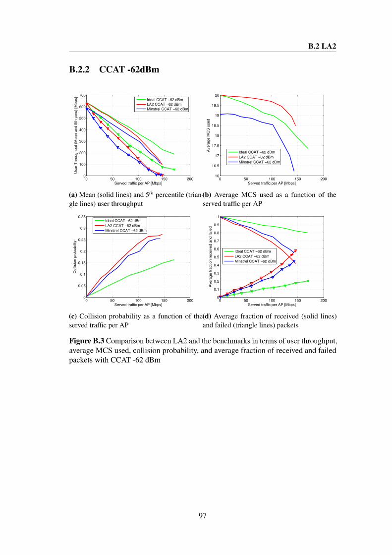
B.2 LA2
B.2.2 CCAT -62dBm
0 50 100 150 2000
100
200
300
400
500
600
700
Served traffic per AP [Mbps]
User
Thro
ughput (M
ean a
nd 5
th p
erc
) [M
bps]
Ideal CCAT −62 dBm
LA2 CCAT −62 dBm
Minstrel CCAT −62 dBm
(a) Mean (solid lines) and 5th percentile (trian-gle lines) user throughput
0 50 100 150 20016
16.5
17
17.5
18
18.5
19
19.5
20
Served traffic per AP [Mbps]
Avera
ge M
CS
used
Ideal CCAT −62 dBm
LA2 CCAT −62 dBm
Minstrel CCAT −62 dBm
(b) Average MCS used as a function of theserved traffic per AP
0 50 100 150 2000
0.05
0.1
0.15
0.2
0.25
0.3
0.35
Served traffic per AP [Mbps]
Colli
sio
n p
robabili
ty
Ideal CCAT −62 dBm
LA2 CCAT −62 dBm
Minstrel CCAT −62 dBm
(c) Collision probability as a function of theserved traffic per AP
0 50 100 150 2000
0.1
0.2
0.3
0.4
0.5
0.6
0.7
0.8
0.9
1
Served traffic per AP [Mbps]
Avera
ge fra
ction r
eceiv
ed a
nd faile
d
Ideal CCAT −62 dBm
LA2 CCAT −62 dBm
Minstrel CCAT −62 dBm
(d) Average fraction of received (solid lines)and failed (triangle lines) packets
Figure B.3 Comparison between LA2 and the benchmarks in terms of user throughput,average MCS used, collision probability, and average fraction of received and failedpackets with CCAT -62 dBm
97

Additional supporting plots
B.3 LA3
B.3.1 CCAT -82dBm
0 50 100 150 2000
100
200
300
400
500
600
700
Served traffic per AP [Mbps]
User
Thro
ughput (M
ean a
nd 5
th p
erc
) [M
bps]
Ideal CCAT −82 dBm
LA3 CCAT −82 dBm
Minstrel CCAT −82 dBm
(a) Mean (solid lines) and 5th percentile (trian-gle lines) user throughput
0 20 40 60 80 100 120 140 16016
16.5
17
17.5
18
18.5
19
19.5
20
Served traffic per AP [Mbps]
Avera
ge M
CS
used
Ideal CCAT −82 dBm
LA3 CCAT −82 dBm
Minstrel CCAT −82 dBm
(b) Average MCS used as a function of theserved traffic per AP
0 20 40 60 80 100 120 140 1600
0.05
0.1
0.15
0.2
0.25
0.3
0.35
Served traffic per AP [Mbps]
Colli
sio
n p
robabili
ty
Ideal CCAT −82 dBm
LA3 CCAT −82 dBm
Minstrel CCAT −82 dBm
(c) Collision probability as a function of theserved traffic per AP
0 20 40 60 80 100 120 140 1600
0.1
0.2
0.3
0.4
0.5
0.6
0.7
0.8
0.9
1
Served traffic per AP [Mbps]
Avera
ge fra
ction r
eceiv
ed a
nd faile
d
Ideal CCAT −82 dBm
LA3 CCAT −82 dBm
Minstrel CCAT −82 dBm
(d) Average fraction of received (solid lines)and failed (triangle lines) packets
Figure B.4 Comparison between LA3 and the benchmarks in terms of user throughput,average MCS used, collision probability, and average fraction of received and failedpackets with CCAT -82 dBm
98

B.3 LA3
B.3.2 CCAT -62dBm
0 50 100 150 2000
100
200
300
400
500
600
700
Served traffic per AP [Mbps]
User
Thro
ughput (M
ean a
nd 5
th p
erc
) [M
bps]
Ideal CCAT −62 dBm
LA3 CCAT −62 dBm
Minstrel CCAT −62 dBm
(a) Mean (solid lines) and 5th percentile (trian-gle lines) user throughput
0 50 100 150 20016
16.5
17
17.5
18
18.5
19
19.5
20
Served traffic per AP [Mbps]
Avera
ge M
CS
used
Ideal CCAT −62 dBm
LA3 CCAT −62 dBm
Minstrel CCAT −62 dBm
(b) Average MCS used as a function of theserved traffic per AP
0 50 100 150 2000
0.05
0.1
0.15
0.2
0.25
0.3
0.35
Served traffic per AP [Mbps]
Colli
sio
n p
robabili
ty
Ideal CCAT −62 dBm
LA3 CCAT −62 dBm
Minstrel CCAT −62 dBm
(c) Collision probability as a function of theserved traffic per AP
0 50 100 150 2000
0.1
0.2
0.3
0.4
0.5
0.6
0.7
0.8
0.9
1
Served traffic per AP [Mbps]
Avera
ge fra
ction r
eceiv
ed a
nd faile
d
Ideal CCAT −62 dBm
LA3 CCAT −62 dBm
Minstrel CCAT −62 dBm
(d) Average fraction of received (solid lines)and failed (triangle lines) packets
Figure B.5 Comparison between LA3 and the benchmarks in terms of user throughput,average MCS used, collision probability, and average fraction of received and failedpackets with CCAT -62 dBm
99

Additional supporting plots
B.4 LA4
B.4.1 CCAT -82dBm
0 50 100 150 2000
100
200
300
400
500
600
700
Served traffic per AP [Mbps]
User
Thro
ughput (M
ean a
nd 5
th p
erc
) [M
bps]
Ideal CCAT −82 dBm
LA4 CCAT −82 dBm
Minstrel CCAT −82 dBm
(a) Mean (solid lines) and 5th percentile (trian-gle lines) user throughput
0 20 40 60 80 100 120 140 16016
16.5
17
17.5
18
18.5
19
19.5
20
Served traffic per AP [Mbps]
Avera
ge M
CS
used
Ideal CCAT −82 dBm
LA4 CCAT −82 dBm
Minstrel CCAT −82 dBm
(b) Average MCS used as a function of theserved traffic per AP
0 20 40 60 80 100 120 140 1600
0.05
0.1
0.15
0.2
0.25
0.3
0.35
Served traffic per AP [Mbps]
Colli
sio
n p
robabili
ty
Ideal CCAT −82 dBm
LA4 CCAT −82 dBm
Minstrel CCAT −82 dBm
(c) Collision probability as a function of theserved traffic per AP
0 20 40 60 80 100 120 140 1600
0.1
0.2
0.3
0.4
0.5
0.6
0.7
0.8
0.9
1
Served traffic per AP [Mbps]
Avera
ge fra
ction r
eceiv
ed a
nd faile
d
Ideal CCAT −82 dBm
LA4 CCAT −82 dBm
Minstrel CCAT −82 dBm
(d) Average fraction of received (solid lines)and failed (triangle lines) packets
Figure B.6 Comparison between LA4 and the benchmarks in terms of user throughput,average MCS used, collision probability, and average fraction of received and failedpackets with CCAT -82 dBm
100
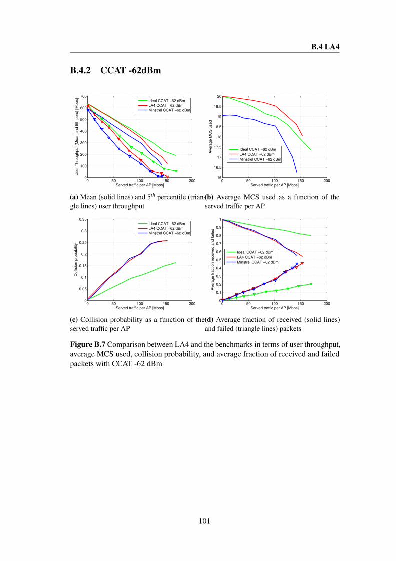
B.4 LA4
B.4.2 CCAT -62dBm
0 50 100 150 2000
100
200
300
400
500
600
700
Served traffic per AP [Mbps]
User
Thro
ughput (M
ean a
nd 5
th p
erc
) [M
bps]
Ideal CCAT −62 dBm
LA4 CCAT −62 dBm
Minstrel CCAT −62 dBm
(a) Mean (solid lines) and 5th percentile (trian-gle lines) user throughput
0 50 100 150 20016
16.5
17
17.5
18
18.5
19
19.5
20
Served traffic per AP [Mbps]
Avera
ge M
CS
used
Ideal CCAT −62 dBm
LA4 CCAT −62 dBm
Minstrel CCAT −62 dBm
(b) Average MCS used as a function of theserved traffic per AP
0 50 100 150 2000
0.05
0.1
0.15
0.2
0.25
0.3
0.35
Served traffic per AP [Mbps]
Colli
sio
n p
robabili
ty
Ideal CCAT −62 dBm
LA4 CCAT −62 dBm
Minstrel CCAT −62 dBm
(c) Collision probability as a function of theserved traffic per AP
0 50 100 150 2000
0.1
0.2
0.3
0.4
0.5
0.6
0.7
0.8
0.9
1
Served traffic per AP [Mbps]
Avera
ge fra
ction r
eceiv
ed a
nd faile
d
Ideal CCAT −62 dBm
LA4 CCAT −62 dBm
Minstrel CCAT −62 dBm
(d) Average fraction of received (solid lines)and failed (triangle lines) packets
Figure B.7 Comparison between LA4 and the benchmarks in terms of user throughput,average MCS used, collision probability, and average fraction of received and failedpackets with CCAT -62 dBm
101
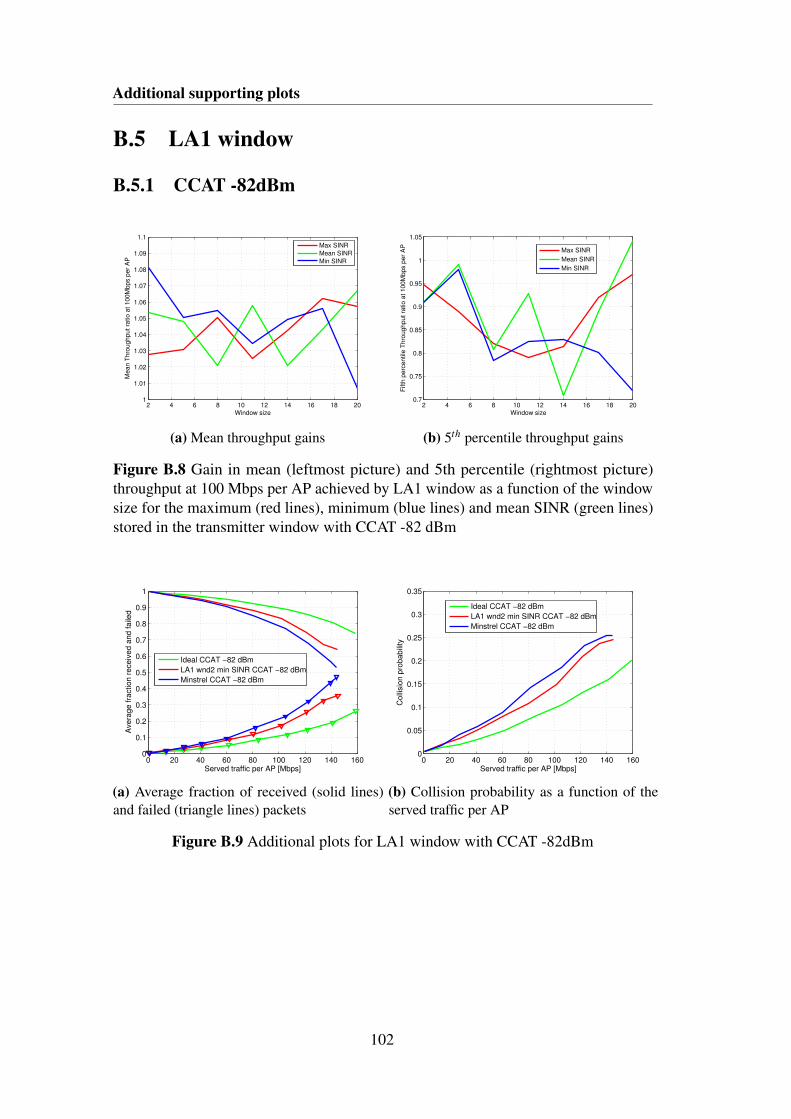
Additional supporting plots
B.5 LA1 window
B.5.1 CCAT -82dBm
2 4 6 8 10 12 14 16 18 201
1.01
1.02
1.03
1.04
1.05
1.06
1.07
1.08
1.09
1.1
Window size
Me
an
Th
rou
gh
pu
t ra
tio
at
10
0M
bp
s p
er
AP
Max SINR
Mean SINR
Min SINR
(a) Mean throughput gains
2 4 6 8 10 12 14 16 18 200.7
0.75
0.8
0.85
0.9
0.95
1
1.05
Window size
Fifth
pe
rce
ntile
Th
rou
gh
pu
t ra
tio
at
10
0M
bp
s p
er
AP
Max SINR
Mean SINR
Min SINR
(b) 5th percentile throughput gains
Figure B.8 Gain in mean (leftmost picture) and 5th percentile (rightmost picture)throughput at 100 Mbps per AP achieved by LA1 window as a function of the windowsize for the maximum (red lines), minimum (blue lines) and mean SINR (green lines)stored in the transmitter window with CCAT -82 dBm
0 20 40 60 80 100 120 140 1600
0.1
0.2
0.3
0.4
0.5
0.6
0.7
0.8
0.9
1
Served traffic per AP [Mbps]
Avera
ge fra
ction r
eceiv
ed a
nd faile
d
Ideal CCAT −82 dBm
LA1 wnd2 min SINR CCAT −82 dBm
Minstrel CCAT −82 dBm
(a) Average fraction of received (solid lines)and failed (triangle lines) packets
0 20 40 60 80 100 120 140 1600
0.05
0.1
0.15
0.2
0.25
0.3
0.35
Served traffic per AP [Mbps]
Colli
sio
n p
robabili
ty
Ideal CCAT −82 dBm
LA1 wnd2 min SINR CCAT −82 dBm
Minstrel CCAT −82 dBm
(b) Collision probability as a function of theserved traffic per AP
Figure B.9 Additional plots for LA1 window with CCAT -82dBm
102

B.5 LA1 window
0 50 100 1500
100
200
300
400
500
600
700
Served traffic per AP [Mbps]
User
Thro
ughput (M
ean a
nd 5
th p
erc
) [M
bps]
LA1 CCAT −82 dBm
LA1 wnd2 min SINR CCAT −82 dBm
(a) Mean (solid lines) and 5th percentile (trian-gle lines) user throughput
0 50 100 15019.3
19.4
19.5
19.6
19.7
19.8
19.9
20
Served traffic per AP [Mbps]
Avera
ge M
CS
used
LA1 CCAT −82 dBm
LA1 wnd2 min SINR CCAT −82 dBm
(b) Average MCS used as a function of theserved traffic per AP
0 50 100 150 2000
0.05
0.1
0.15
0.2
0.25
0.3
0.35
Served traffic per AP [Mbps]
Colli
sio
n p
robabili
ty
LA1 CCAT −82 dBm
LA1 wnd2 min SINR CCAT −82 dBm
(c) Collision probability as a function of theserved traffic per AP
0 50 100 1500
0.1
0.2
0.3
0.4
0.5
0.6
0.7
0.8
0.9
1
Served traffic per AP [Mbps]
Avera
ge fra
ction r
eceiv
ed a
nd faile
d
LA1 CCAT −82 dBm
LA1 wnd2 min SINR CCAT −82 dBm
(d) Average fraction of received (solid lines)and failed (triangle lines) packets
Figure B.10 Comparison between LA1 and LA1 window in terms of user throughput,average MCS used, collision probability, and average fraction of received and failedpackets with CCAT -82 dBm
103
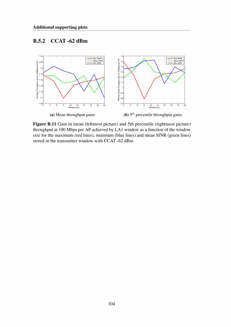
Additional supporting plots
B.5.2 CCAT -62 dBm
2 4 6 8 10 12 14 16 18 201.08
1.1
1.12
1.14
1.16
1.18
1.2
1.22
1.24
Window size
Ave
rag
e T
hro
ug
hp
ut
ratio
at
10
0M
bp
s p
er
AP
Max SINR
Mean SINR
Min SINR
(a) Mean throughput gains
2 4 6 8 10 12 14 16 18 200.7
0.8
0.9
1
1.1
1.2
1.3
1.4
1.5
1.6
Window size
Fifth
pe
rce
ntile
th
rou
gh
pu
t ra
tio
at
10
0M
bp
s p
er
AP
Max SINR
Mean SINR
Min SINR
(b) 5th percentile throughput gains
Figure B.11 Gain in mean (leftmost picture) and 5th percentile (rightmost picture)throughput at 100 Mbps per AP achieved by LA1 window as a function of the windowsize for the maximum (red lines), minimum (blue lines) and mean SINR (green lines)stored in the transmitter window with CCAT -62 dBm
104
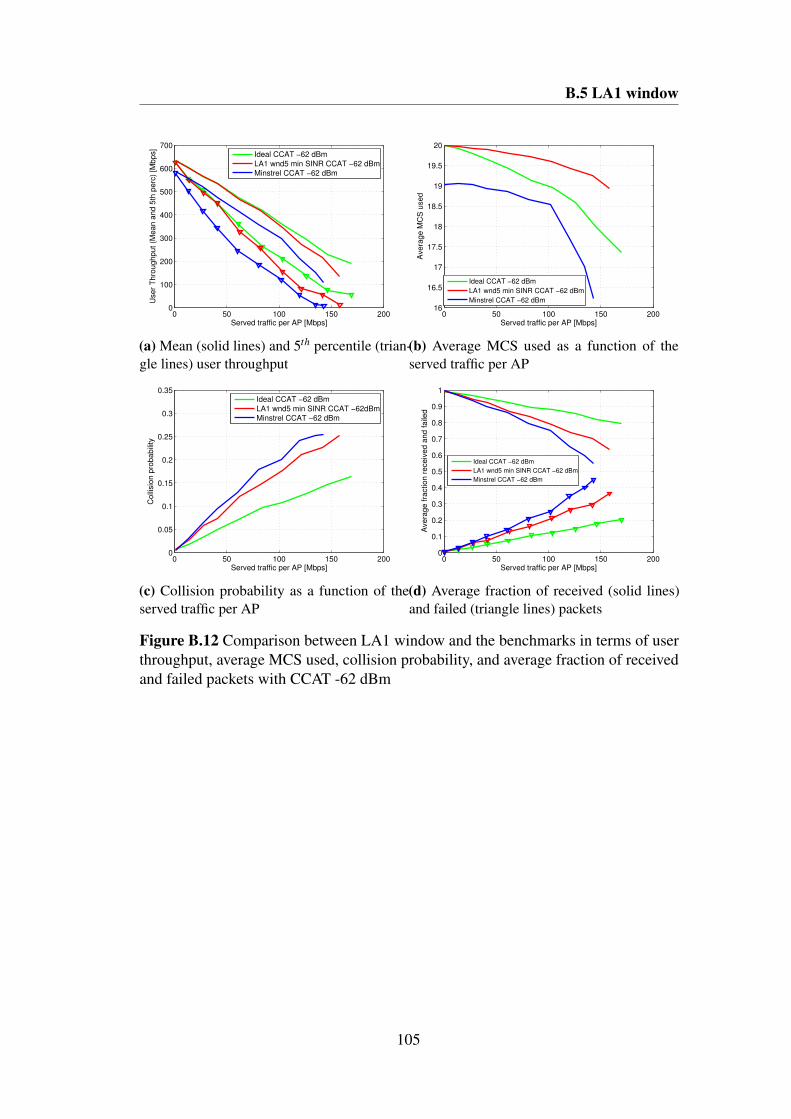
B.5 LA1 window
0 50 100 150 2000
100
200
300
400
500
600
700
Served traffic per AP [Mbps]
User
Thro
ughput (M
ean a
nd 5
th p
erc
) [M
bps]
Ideal CCAT −62 dBm
LA1 wnd5 min SINR CCAT −62 dBm
Minstrel CCAT −62 dBm
(a) Mean (solid lines) and 5th percentile (trian-gle lines) user throughput
0 50 100 150 20016
16.5
17
17.5
18
18.5
19
19.5
20
Served traffic per AP [Mbps]
Avera
ge M
CS
used
Ideal CCAT −62 dBm
LA1 wnd5 min SINR CCAT −62 dBm
Minstrel CCAT −62 dBm
(b) Average MCS used as a function of theserved traffic per AP
0 50 100 150 2000
0.05
0.1
0.15
0.2
0.25
0.3
0.35
Served traffic per AP [Mbps]
Colli
sio
n p
robabili
ty
Ideal CCAT −62 dBm
LA1 wnd5 min SINR CCAT −62dBm
Minstrel CCAT −62 dBm
(c) Collision probability as a function of theserved traffic per AP
0 50 100 150 2000
0.1
0.2
0.3
0.4
0.5
0.6
0.7
0.8
0.9
1
Served traffic per AP [Mbps]
Avera
ge fra
ction r
eceiv
ed a
nd faile
d
Ideal CCAT −62 dBm
LA1 wnd5 min SINR CCAT −62 dBm
Minstrel CCAT −62 dBm
(d) Average fraction of received (solid lines)and failed (triangle lines) packets
Figure B.12 Comparison between LA1 window and the benchmarks in terms of userthroughput, average MCS used, collision probability, and average fraction of receivedand failed packets with CCAT -62 dBm
105

Additional supporting plots
0 20 40 60 80 100 120 140 1600
100
200
300
400
500
600
700
Served traffic per AP [Mbps]
User
Thro
ughput (M
ean a
nd 5
th p
erc
) [M
bps]
LA1 CCAT −62 dBm
LA1 wnd5 min SINR CCAT −62 dBm
(a) Mean (solid lines) and 5th percentile (trian-gle lines) user throughput
0 20 40 60 80 100 120 140 16017.5
18
18.5
19
19.5
20
Served traffic per AP [Mbps]
Avera
ge M
CS
used
LA1 CCAT −62 dBm
LA1 wnd5 min SINR CCAT −62 dBm
(b) Average MCS used as a function of theserved traffic per AP
0 20 40 60 80 100 120 140 1600
0.05
0.1
0.15
0.2
0.25
0.3
0.35
Served traffic per AP [Mbps]
Colli
sio
n p
robabili
ty
LA1 CCAT −62 dBm
LA1 wnd5 min SINR CCAT −62dBm
(c) Collision probability as a function of theserved traffic per AP
0 20 40 60 80 100 120 140 1600
0.1
0.2
0.3
0.4
0.5
0.6
0.7
0.8
0.9
1
Served traffic per AP [Mbps]
Avera
ge fra
ction r
eceiv
ed a
nd faile
d
LA1 CCAT −62 dBm
LA1 wnd5 min SINR CCAT −62 dBm
(d) Average fraction of received (solid lines)and failed (triangle lines) packets
Figure B.13 Comparison between LA1 and LA1 window in terms of user throughput,average MCS used, collision probability, and average fraction of received and failedpackets with CCAT -62 dBm
106
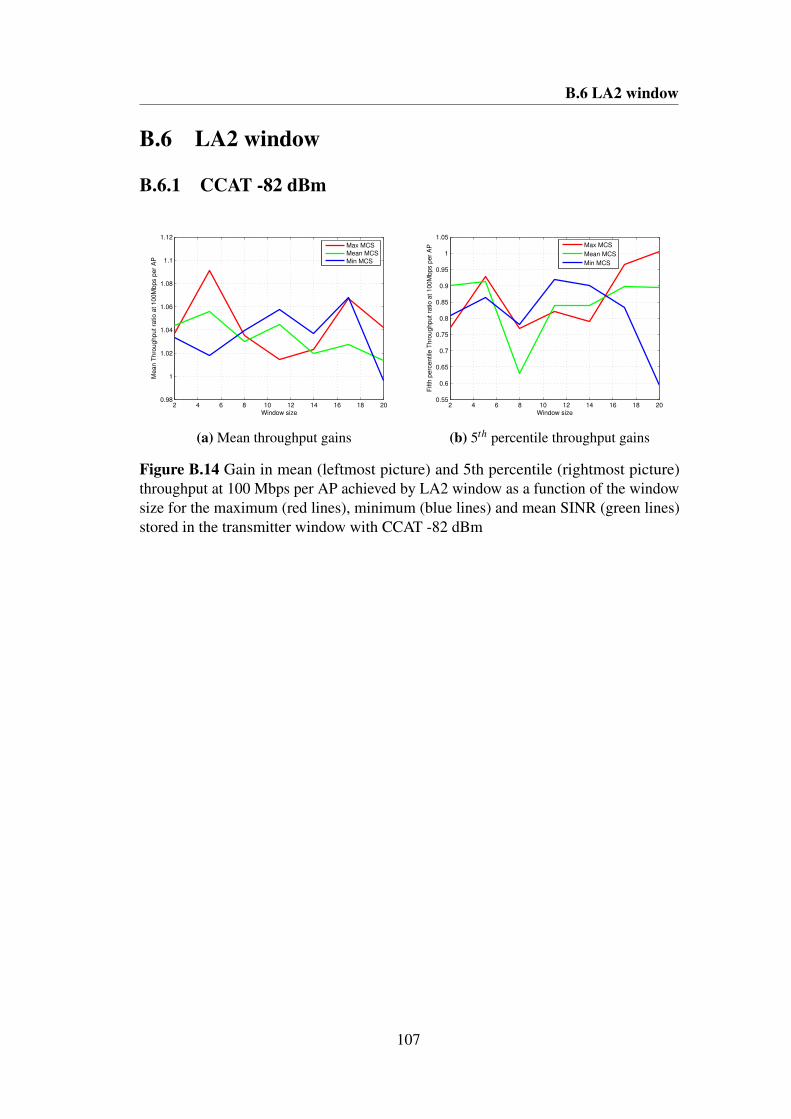
B.6 LA2 window
B.6 LA2 window
B.6.1 CCAT -82 dBm
2 4 6 8 10 12 14 16 18 200.98
1
1.02
1.04
1.06
1.08
1.1
1.12
Window size
Me
an
Th
rou
gh
pu
t ra
tio
at
10
0M
bp
s p
er
AP
Max MCS
Mean MCS
Min MCS
(a) Mean throughput gains
2 4 6 8 10 12 14 16 18 200.55
0.6
0.65
0.7
0.75
0.8
0.85
0.9
0.95
1
1.05
Window size
Fifth
pe
rce
ntile
Th
rou
gh
pu
t ra
tio
at
10
0M
bp
s p
er
AP
Max MCS
Mean MCS
Min MCS
(b) 5th percentile throughput gains
Figure B.14 Gain in mean (leftmost picture) and 5th percentile (rightmost picture)throughput at 100 Mbps per AP achieved by LA2 window as a function of the windowsize for the maximum (red lines), minimum (blue lines) and mean SINR (green lines)stored in the transmitter window with CCAT -82 dBm
107

Additional supporting plots
0 50 100 150 2000
100
200
300
400
500
600
700
Served traffic per AP [Mbps]
User
Thro
ughput (M
ean a
nd 5
th p
erc
) [M
bps]
Ideal CCAT −82 dBm
LA2 wnd5 max MCS CCAT −82 dBm
Minstrel CCAT −82 dBm
(a) Mean (solid lines) and 5th percentile (trian-gle lines) user throughput
0 20 40 60 80 100 120 140 16016
16.5
17
17.5
18
18.5
19
19.5
20
Served traffic per AP [Mbps]
Avera
ge M
CS
used
Ideal CCAT −82 dBm
LA2 wnd5 max MCS CCAT −82 dBm
Minstrel CCAT −82 dBm
(b) Average MCS used as a function of theserved traffic per AP
0 20 40 60 80 100 120 140 1600
0.05
0.1
0.15
0.2
0.25
0.3
0.35
Served traffic per AP [Mbps]
Colli
sio
n p
robabili
ty
Ideal CCAT −82 dBm
LA2 wnd5 max MCS CCAT −82 dBm
Minstrel CCAT −82 dBm
(c) Collision probability as a function of theserved traffic per AP
0 20 40 60 80 100 120 140 1600
0.1
0.2
0.3
0.4
0.5
0.6
0.7
0.8
0.9
1
Served traffic per AP [Mbps]
Avera
ge fra
ction r
eceiv
ed a
nd faile
d
Ideal CCAT −82 dBm
LA2 wnd5 max MCS CCAT −82 dBm
Minstrel CCAT −82 dBm
(d) Average fraction of received (solid lines)and failed (triangle lines) packets
Figure B.15 Comparison between LA2 window and the benchmarks in terms of userthroughput, average MCS used, collision probability, and average fraction of receivedand failed packets with CCAT -82 dBm
108

B.6 LA2 window
0 50 100 1500
100
200
300
400
500
600
700
Served traffic per AP [Mbps]
User
Thro
ughput (M
ean a
nd 5
th p
erc
) [M
bps]
LA2 CCAT −82 dBm
LA2 wnd5 max MCS CCAT −82 dBm
(a) Mean (solid lines) and 5th percentile (trian-gle lines)user throughput
0 50 100 15018.4
18.6
18.8
19
19.2
19.4
19.6
19.8
20
20.2
Served traffic per AP [Mbps]
Avera
ge M
CS
used
LA2 CCAT −82 dBm
LA2 wnd5 max MCS CCAT −82 dBm
(b) Average MCS used as a function of theserved traffic per AP
0 50 100 1500
0.05
0.1
0.15
0.2
0.25
0.3
0.35
Served traffic per AP [Mbps]
Colli
sio
n p
robabili
ty
LA2 CCAT −82 dBm
LA2 wnd5 max MCS CCAT −82 dBm
(c) Collision probability as a function of theserved traffic per AP
0 50 100 1500
0.1
0.2
0.3
0.4
0.5
0.6
0.7
0.8
0.9
1
Served traffic per AP [Mbps]
Avera
ge fra
ction r
eceiv
ed a
nd faile
d
LA2 CCAT −82 dBm
LA2 wnd5 max MCS CCAT −82 dBm
(d) Average fraction of received (solid lines)and failed (triangle lines) packets
Figure B.16 Comparison between LA2 and LA2 window in terms of user throughput,average MCS used, collision probability, and average fraction of received and failedpackets with CCAT -82 dBm
109

Additional supporting plots
B.6.2 CCAT -62 dBm
2 4 6 8 10 12 14 16 18 201.1
1.11
1.12
1.13
1.14
1.15
1.16
1.17
1.18
1.19
1.2
Window size
Ave
rag
e T
hro
ug
hp
ut
ratio
at
10
0M
bp
s p
er
AP
Max MCS
Mean MCS
Min MCS
(a) Mean throughput gains
2 4 6 8 10 12 14 16 18 200.9
1
1.1
1.2
1.3
1.4
1.5
1.6
1.7
1.8
Window size
Fifth
pe
rce
ntile
th
rou
gh
pu
t ra
tio
at
10
0M
bp
s p
er
AP
Max MCS
Mean MCS
Min MCS
(b) 5th percentile throughput gains
Figure B.17 Gain in mean (leftmost picture) and 5th percentile (rightmost picture)throughput at 100 Mbps per AP achieved by LA2 window as a function of the windowsize for the maximum (red lines), minimum (blue lines) and mean SINR (green lines)stored in the transmitter window with CCAT -62 dBm
110

B.6 LA2 window
0 50 100 150 2000
100
200
300
400
500
600
700
Served traffic per AP [Mbps]
User
Thro
ughput (M
ean a
nd 5
th p
erc
) [M
bps]
Ideal CCAT −62 dBm
LA2 wnd8 min MCS CCAT −62 dBm
Minstrel CCAT −62 dBm
(a) Mean (solid lines) and 5th percentile (trian-gle lines) user throughput
0 50 100 150 20016
16.5
17
17.5
18
18.5
19
19.5
20
Served traffic per AP [Mbps]
Avera
ge M
CS
used
Ideal CCAT −62 dBm
LA2 wnd8 min MCS CCAT −62 dBm
Minstrel CCAT −62 dBm
(b) Average MCS used as a function of theserved traffic per AP
0 50 100 150 2000
0.05
0.1
0.15
0.2
0.25
0.3
0.35
Served traffic per AP [Mbps]
Colli
sio
n p
robabili
ty
Ideal CCAT −62 dBm
LA2 wnd8 min MCS CCAT −62 dBm
Minstrel CCAT −62 dBm
(c) Collision probability as a function of theserved traffic per AP
0 50 100 150 2000
0.1
0.2
0.3
0.4
0.5
0.6
0.7
0.8
0.9
1
Served traffic per AP [Mbps]
Avera
ge fra
ction r
eceiv
ed a
nd faile
d
Ideal CCAT −62 dBm
LA2 wnd8 min MCS CCAT−62 dBm
Minstrel CCAT −62 dBm
(d) Average fraction of received (solid lines)and failed (triangle lines) packets
Figure B.18 Comparison between LA2 window and the benchmarks in terms of userthroughput, average MCS used, collision probability, and average fraction of receivedand failed packets with CCAT -62 dBm
111

Additional supporting plots
0 20 40 60 80 100 120 140 1600
100
200
300
400
500
600
700
Served traffic per AP [Mbps]
Use
r T
hro
ug
hp
ut
(Me
an
an
d 5
th p
erc
) [M
bp
s]
LA2 CCAT −62 dBm
LA2 wnd8 min MCS CCAT −62 dBm
(a) Mean (solid lines) and 5th percentile (trian-gle lines) user throughput
0 20 40 60 80 100 120 140 16018.4
18.6
18.8
19
19.2
19.4
19.6
19.8
20
20.2
Served traffic per AP [Mbps]
Avera
ge M
CS
used
LA2 CCAT −62 dBm
LA2 wnd8 min MCS CCAT −62 dBm
(b) Average MCS used as a function of theserved traffic per AP
0 20 40 60 80 100 120 140 1600
0.05
0.1
0.15
0.2
0.25
0.3
0.35
Served traffic per AP [Mbps]
Colli
sio
n p
robabili
ty
LA2 CCAT −62 dBm
LA2 wnd8 min MCS CCAT −62 dBm
(c) Collision probability as a function of theserved traffic per AP
0 20 40 60 80 100 120 140 1600
0.1
0.2
0.3
0.4
0.5
0.6
0.7
0.8
0.9
1
Served traffic per AP [Mbps]
Avera
ge fra
ction r
eceiv
ed a
nd faile
d
LA2 CCAT −62 dBm
LA2 wnd8 min MCS CCAT −62 dBm
(d) Average fraction of received (solid lines)and failed (triangle lines) packets
Figure B.19 Comparison between LA2 and LA2 window in terms of user throughput,average MCS used, collision probability, and average fraction of received and failedpackets with CCAT -62 dBm
112

B.7 LA3 window
B.7 LA3 window
B.7.1 CCAT -82 dBm
2 4 6 8 10 12 14 16 18 200.85
0.9
0.95
1
1.05
1.1
1.15
1.2
Window size
Ave
rag
e T
hro
ug
hp
ut
ratio
at
10
0M
bp
s p
er
AP
Max SINR
Mean SINR
Min SINR
(a) Mean throughput gains
2 4 6 8 10 12 14 16 18 20
0.65
0.7
0.75
0.8
0.85
0.9
0.95
1
1.05
1.1
Window size
Fifth
pe
rce
ntile
th
rou
gh
pu
t ra
tio
at
10
0M
bp
s p
er
AP
Max SINR
Mean SINR
Min SINR
(b) 5th percentile throughput gains
Figure B.20 Gain in mean (leftmost picture) and 5th percentile (rightmost picture)throughput at 100 Mbps per AP achieved by LA3 window as a function of the windowsize for the maximum (red lines), minimum (blue lines) and mean SINR (green lines)stored in the transmitter window with CCAT -82 dBm
113

Additional supporting plots
0 50 100 150 2000
100
200
300
400
500
600
700
Served traffic per AP [Mbps]
User
Thro
ughput (M
ean a
nd 5
th p
erc
) [M
bps]
Ideal CCAT −82 dBm
LA3 wnd11 mean SINR CCAT −82 dBm
Minstrel CCAT −82 dBm
(a) Mean (solid lines) and 5th percentile (trian-gle lines) user throughput
0 20 40 60 80 100 120 140 16016
16.5
17
17.5
18
18.5
19
19.5
20
Served traffic per AP [Mbps]
Avera
ge M
CS
used
Ideal CCAT −82 dBm
LA3 wnd11 mean SINR CCAT −82 dBm
Minstrel CCAT −82 dBm
(b) Average MCS used as a function of theserved traffic per AP
0 20 40 60 80 100 120 140 1600
0.05
0.1
0.15
0.2
0.25
0.3
0.35
Served traffic per AP [Mbps]
Co
llisio
n p
rob
ab
ility
Ideal CCAT −82 dBm
LA3 wnd11 mean SINR CCAT −82 dBm
Minstrel CCAT −82 dBm
(c) Collision probability as a function of theserved traffic per AP
0 20 40 60 80 100 120 140 1600
0.1
0.2
0.3
0.4
0.5
0.6
0.7
0.8
0.9
1
Served traffic per AP [Mbps]
Avera
ge fra
ction r
eceiv
ed a
nd faile
d
Ideal CCAT −82 dBm
LA3 wnd11 mean SINR CCAT −82 dBm
Minstrel CCAT −82 dBm
(d) Average fraction of received (solid lines)and failed (triangle lines) packets
Figure B.21 Comparison between LA3 window and the benchmarks in terms of userthroughput, average MCS used, collision probability, and average fraction of receivedand failed packets with CCAT -82 dBm
114

B.7 LA3 window
0 50 100 1500
100
200
300
400
500
600
700
Served traffic per AP [Mbps]
User
Thro
ughput (M
ean a
nd 5
th p
erc
) [M
bps]
LA3 CCAT −82 dBm
LA3 wnd11 mean SINR CCAT −82 dBm
(a) Mean (solid lines) and 5th percentile (trian-gle lines)user throughput
0 50 100 15019.4
19.5
19.6
19.7
19.8
19.9
20
20.1
Served traffic per AP [Mbps]
Avera
ge M
CS
used
LA3 CCAT −82 dBm
LA3 wnd11 mean SINR CCAT −82 dBm
(b) Average MCS used as a function of theserved traffic per AP
0 50 100 1500
0.05
0.1
0.15
0.2
0.25
0.3
0.35
Served traffic per AP [Mbps]
Co
llisio
n p
rob
ab
ility
LA3 CCAT −82 dBm
LA3 wnd11 mean SINR CCAT −82 dBm
(c) Collision probability as a function of theserved traffic per AP
0 50 100 1500
0.2
0.4
0.6
0.8
1
Served traffic per AP [Mbps]
Ave
rag
e f
ractio
n r
ece
ive
d a
nd
fa
iled
LA3 CCAT −82 dBm
LA3 wnd11 mean SINR CCAT −82 dBm
(d) Average fraction of received (solid lines)and failed (triangle lines) packets
Figure B.22 Comparison between LA3 and LA3 window in terms of user throughput,average MCS used, collision probability, and average fraction of received and failedpackets with CCAT -82 dBm
115

Additional supporting plots
B.7.2 CCAT -62 dBm
2 4 6 8 10 12 14 16 18 200.95
1
1.05
1.1
1.15
1.2
1.25
Window size
Ave
rag
e T
hro
ug
hp
ut
ratio
at
10
0M
bp
s p
er
AP
Max SINR
Mean SINR
Min SINR
(a) Mean throughput gains
2 4 6 8 10 12 14 16 18 201
1.1
1.2
1.3
1.4
1.5
1.6
1.7
1.8
Window size
Fifth
pe
rce
ntile
th
rou
gh
pu
t ra
tio
at
10
0M
bp
s p
er
AP
Max SINR
Mean SINR
Min SINR
(b) 5th percentile throughput gains
Figure B.23 Gain in mean (leftmost picture) and 5th percentile (rightmost picture)throughput at 100 Mbps per AP achieved by LA3 window as a function of the windowsize for the maximum (red lines), minimum (blue lines) and mean SINR (green lines)stored in the transmitter window with CCAT -62 dBm
116
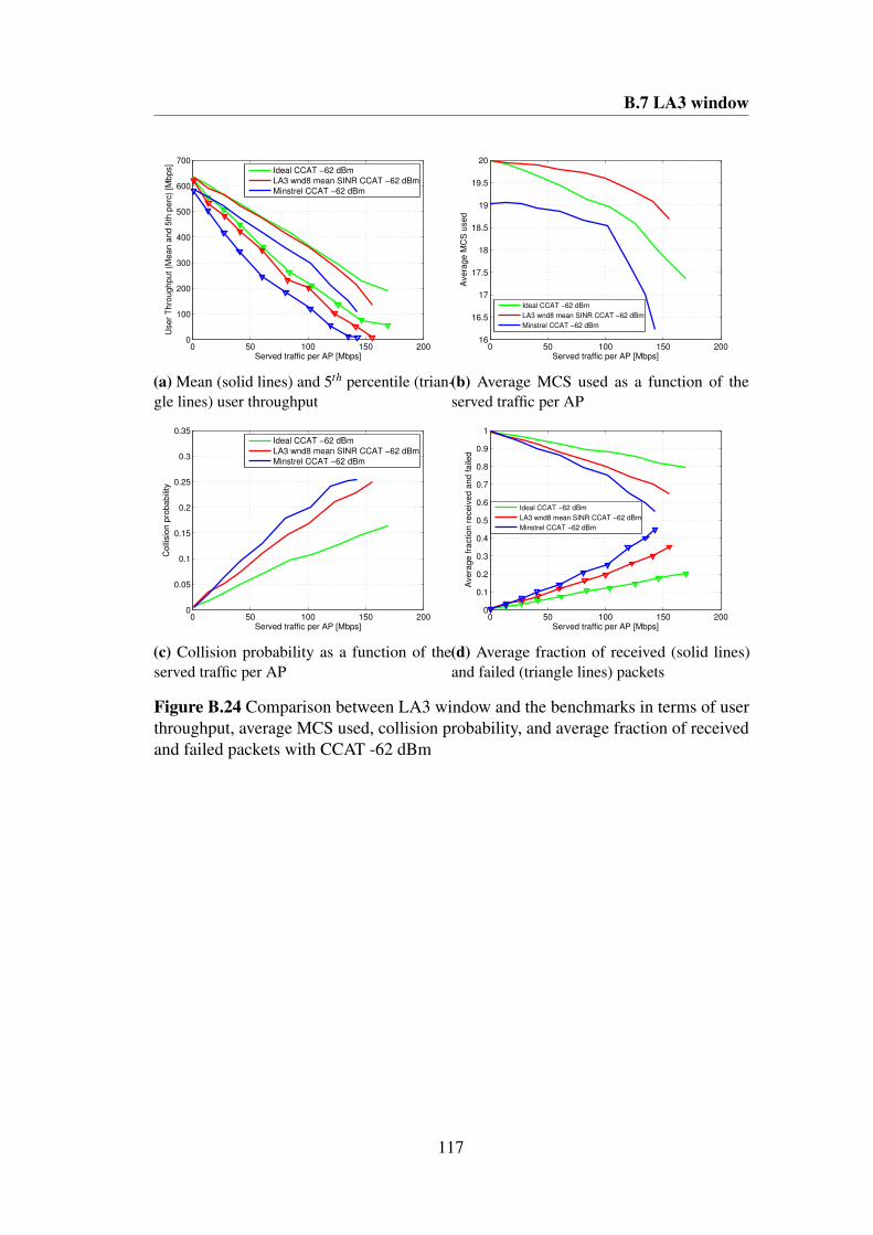
B.7 LA3 window
0 50 100 150 2000
100
200
300
400
500
600
700
Served traffic per AP [Mbps]
User
Thro
ughput (M
ean a
nd 5
th p
erc
) [M
bps]
Ideal CCAT −62 dBm
LA3 wnd8 mean SINR CCAT −62 dBm
Minstrel CCAT −62 dBm
(a) Mean (solid lines) and 5th percentile (trian-gle lines) user throughput
0 50 100 150 20016
16.5
17
17.5
18
18.5
19
19.5
20
Served traffic per AP [Mbps]
Avera
ge M
CS
used
Ideal CCAT −62 dBm
LA3 wnd8 mean SINR CCAT −62 dBm
Minstrel CCAT −62 dBm
(b) Average MCS used as a function of theserved traffic per AP
0 50 100 150 2000
0.05
0.1
0.15
0.2
0.25
0.3
0.35
Served traffic per AP [Mbps]
Colli
sio
n p
robabili
ty
Ideal CCAT −62 dBm
LA3 wnd8 mean SINR CCAT −62 dBm
Minstrel CCAT −62 dBm
(c) Collision probability as a function of theserved traffic per AP
0 50 100 150 2000
0.1
0.2
0.3
0.4
0.5
0.6
0.7
0.8
0.9
1
Served traffic per AP [Mbps]
Avera
ge fra
ction r
eceiv
ed a
nd faile
d
Ideal CCAT −62 dBm
LA3 wnd8 mean SINR CCAT −62 dBm
Minstrel CCAT −62 dBm
(d) Average fraction of received (solid lines)and failed (triangle lines) packets
Figure B.24 Comparison between LA3 window and the benchmarks in terms of userthroughput, average MCS used, collision probability, and average fraction of receivedand failed packets with CCAT -62 dBm
117

Additional supporting plots
0 20 40 60 80 100 120 140 1600
100
200
300
400
500
600
700
Served traffic per AP [Mbps]
User
Thro
ughput (M
ean a
nd 5
th p
erc
) [M
bps]
LA3 CCAT −62 dBm
LA3 wnd8 mean SINR CCAT −62 dBm
(a) Mean (solid lines) and 5th percentile (trian-gle lines) user throughput
0 20 40 60 80 100 120 140 16016
16.5
17
17.5
18
18.5
19
19.5
20
Served traffic per AP [Mbps]
Avera
ge M
CS
used
LA3 CCAT −62 dBm
LA3 wnd8 mean SINR CCAT −62 dBm
(b) Average MCS used as a function of theserved traffic per AP
0 20 40 60 80 100 120 140 1600
0.05
0.1
0.15
0.2
0.25
Served traffic per AP [Mbps]
Colli
sio
n p
robabili
ty
LA3 CCAT −62 dBm
LA3 wnd8 mean SINR CCAT −62 dBm
(c) Collision probability as a function of theserved traffic per AP
0 20 40 60 80 100 120 140 1600
0.1
0.2
0.3
0.4
0.5
0.6
0.7
0.8
0.9
1
Served traffic per AP [Mbps]
Avera
ge fra
ction r
eceiv
ed a
nd faile
d
LA3 CCAT −62 dBm
LA3 wnd8 mean SINR CCAT −62 dBm
(d) Average fraction of received (solid lines)and failed (triangle lines) packets
Figure B.25 Comparison between LA3 and LA3 window in terms of user throughput,average MCS used, collision probability, and average fraction of received and failedpackets with CCAT -62 dBm
118

B.8 LA4 window
B.8 LA4 window
B.8.1 CCAT -82 dBm
2 4 6 8 10 12 14 16 18 201
1.02
1.04
1.06
1.08
1.1
1.12
Window size
Me
an
Th
rou
gh
pu
t ra
tio
at
10
0M
bp
s p
er
AP
Max SINR
Mean SINR
Min SINR
(a) Mean throughput gains
2 4 6 8 10 12 14 16 18 20
0.65
0.7
0.75
0.8
0.85
0.9
0.95
1
1.05
1.1
Window size
Fifth
pe
rce
ntile
Th
rou
gh
pu
t ra
tio
at
10
0M
bp
s p
er
AP
Max SINR
Mean SINR
Min SINR
(b) 5th percentile throughput gains
Figure B.26 Gain in mean (leftmost picture) and 5th percentile (rightmost picture)throughput at 100 Mbps per AP achieved by LA4 window as a function of the windowsize for the maximum (red lines), minimum (blue lines) and mean SINR (green lines)stored in the transmitter window with CCAT -82 dBm
119
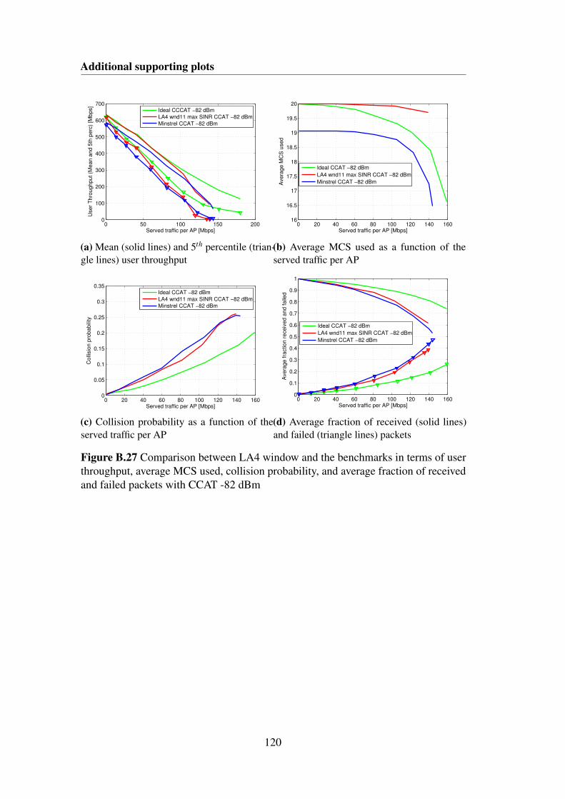
Additional supporting plots
0 50 100 150 2000
100
200
300
400
500
600
700
Served traffic per AP [Mbps]
User
Thro
ughput (M
ean a
nd 5
th p
erc
) [M
bps]
Ideal CCCAT −82 dBm
LA4 wnd11 max SINR CCAT −82 dBm
Minstrel CCAT −82 dBm
(a) Mean (solid lines) and 5th percentile (trian-gle lines) user throughput
0 20 40 60 80 100 120 140 16016
16.5
17
17.5
18
18.5
19
19.5
20
Served traffic per AP [Mbps]
Avera
ge M
CS
used
Ideal CCAT −82 dBm
LA4 wnd11 max SINR CCAT −82 dBm
Minstrel CCAT −82 dBm
(b) Average MCS used as a function of theserved traffic per AP
0 20 40 60 80 100 120 140 1600
0.05
0.1
0.15
0.2
0.25
0.3
0.35
Served traffic per AP [Mbps]
Co
llisio
n p
rob
ab
ility
Ideal CCAT −82 dBm
LA4 wnd11 max SINR CCAT −82 dBm
Minstrel CCAT −82 dBm
(c) Collision probability as a function of theserved traffic per AP
0 20 40 60 80 100 120 140 1600
0.1
0.2
0.3
0.4
0.5
0.6
0.7
0.8
0.9
1
Served traffic per AP [Mbps]
Avera
ge fra
ction r
eceiv
ed a
nd faile
d
Ideal CCAT −82 dBm
LA4 wnd11 max SINR CCAT −82 dBm
Minstrel CCAT −82 dBm
(d) Average fraction of received (solid lines)and failed (triangle lines) packets
Figure B.27 Comparison between LA4 window and the benchmarks in terms of userthroughput, average MCS used, collision probability, and average fraction of receivedand failed packets with CCAT -82 dBm
120

B.8 LA4 window
0 50 100 1500
100
200
300
400
500
600
700
Served traffic per AP [Mbps]
User
Thro
ughput (M
ean a
nd 5
th p
erc
) [M
bps]
LA4 CCAT −82 dBm
LA4 wnd11 max SINR CCAT −82 dBm
(a) Mean (solid lines) and 5th percentile (trian-gle lines) user throughput
0 50 100 15018
18.2
18.4
18.6
18.8
19
19.2
19.4
19.6
19.8
20
Served traffic per AP [Mbps]
Avera
ge M
CS
used
LA4 CCAT −82 dBm
LA4 wnd11 max SINR CCAT −82 dBm
(b) Average MCS used as a function of theserved traffic per AP
0 50 100 1500
0.05
0.1
0.15
0.2
0.25
0.3
0.35
Served traffic per AP [Mbps]
Co
llisio
n p
rob
ab
ility
LA4 CCAT −82 dBm
LA4 wnd11 max SINR CCAT −82 dBm
(c) Collision probability as a function of theserved traffic per AP
0 50 100 1500
0.1
0.2
0.3
0.4
0.5
0.6
0.7
0.8
0.9
1
Served traffic per AP [Mbps]
Avera
ge fra
ction r
eceiv
ed a
nd faile
d
LA4 CCAT −82 dBm
LA4 wnd11 max SINR CCAT −82 dBm
(d) Average fraction of received (solid lines)and failed (triangle lines) packets
Figure B.28 Comparison between LA4 and LA4 window in terms of user throughput,average MCS used, collision probability, and average fraction of received and failedpackets with CCAT -62 dBm
121
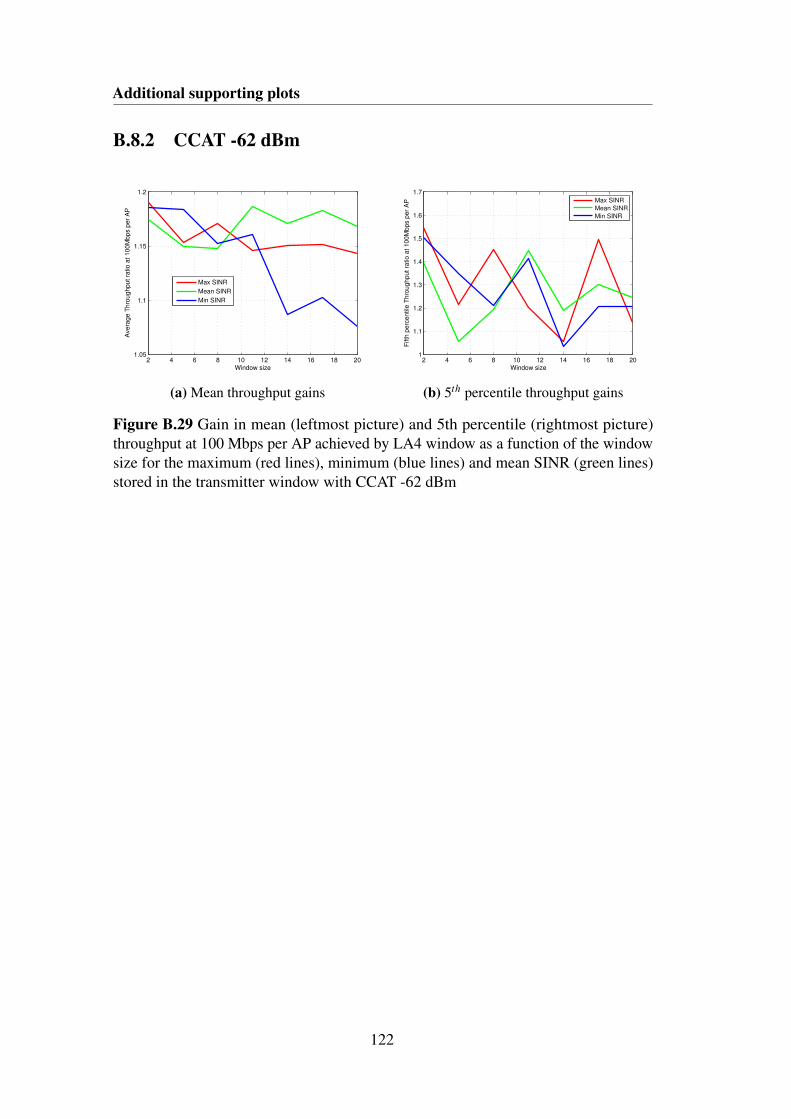
Additional supporting plots
B.8.2 CCAT -62 dBm
2 4 6 8 10 12 14 16 18 201.05
1.1
1.15
1.2
Window size
Ave
rag
e T
hro
ug
hp
ut
ratio
at
10
0M
bp
s p
er
AP
Max SINR
Mean SINR
Min SINR
(a) Mean throughput gains
2 4 6 8 10 12 14 16 18 201
1.1
1.2
1.3
1.4
1.5
1.6
1.7
Window size
Fifth
pe
rce
ntile
Th
rou
gh
pu
t ra
tio
at
10
0M
bp
s p
er
AP
Max SINR
Mean SINR
Min SINR
(b) 5th percentile throughput gains
Figure B.29 Gain in mean (leftmost picture) and 5th percentile (rightmost picture)throughput at 100 Mbps per AP achieved by LA4 window as a function of the windowsize for the maximum (red lines), minimum (blue lines) and mean SINR (green lines)stored in the transmitter window with CCAT -62 dBm
122

B.8 LA4 window
0 50 100 150 2000
100
200
300
400
500
600
700
Served traffic per AP [Mbps]
User
Thro
ughput (M
ean a
nd 5
th p
erc
) [M
bps]
Ideal CCAT −62 dBm
LA4 wnd2 max SINR CCAT −62 dBm
Minstrel CCAT −62 dBm
(a) Mean (solid lines) and 5th percentile (trian-gle lines) user throughput
0 50 100 150 20016
16.5
17
17.5
18
18.5
19
19.5
20
Served traffic per AP [Mbps]
Avera
ge M
CS
used
Ideal CCAT −62 dBm
LA4 wnd2 max SINR CCAT −62 dBm
Minstrel CCAT −62 dBm
(b) Average MCS used as a function of theserved traffic per AP
0 50 100 150 2000
0.05
0.1
0.15
0.2
0.25
0.3
0.35
Served traffic per AP [Mbps]
Colli
sio
n p
robabili
ty
Ideal CCAT −62 dBm
LA4 wnd2 max SINR CCAT −62 dBm
Minstrel CCAT −62 dBm
(c) Collision probability as a function of theserved traffic per AP
0 50 100 150 2000
0.1
0.2
0.3
0.4
0.5
0.6
0.7
0.8
0.9
1
Served traffic per AP [Mbps]
Avera
ge fra
ction r
eceiv
ed a
nd faile
d
Ideal CCAT −62 dBm
LA4 wnd2 max SINR CCAT −62 dBm
Minstrel CCAT −62 dBm
(d) Average fraction of received (solid lines)and failed (triangle lines) packets
Figure B.30 Comparison between LA4 window and the benchmarks in terms of userthroughput, average MCS used, collision probability, and average fraction of receivedand failed packets with CCAT -62 dBm
123

Additional supporting plots
0 20 40 60 80 100 120 140 1600
100
200
300
400
500
600
700
Served traffic per AP [Mbps]
User
Thro
ughput (M
ean a
nd 5
th p
erc
) [M
bps]
LA4 CCAT −62 dBm
LA4 wnd2 max SINR CCAT −62 dBm
(a) Mean (solid lines) and 5th percentile (trian-gle lines) user throughput
0 20 40 60 80 100 120 140 16018
18.2
18.4
18.6
18.8
19
19.2
19.4
19.6
19.8
20
Served traffic per AP [Mbps]
Avera
ge M
CS
used
LA4 CCAT −62 dBm
LA4 wnd2 max SINR CCAT −62 dBm
(b) Average MCS used as a function of theserved traffic per AP
0 20 40 60 80 100 120 140 1600
0.05
0.1
0.15
0.2
0.25
0.3
0.35
Served traffic per AP [Mbps]
Colli
sio
n p
robabili
ty
LA4 CCAT −62 dBm
LA4 wnd2 max SINR CCAT −62 dBm
(c) Collision probability as a function of theserved traffic per AP
0 20 40 60 80 100 120 140 1600
0.1
0.2
0.3
0.4
0.5
0.6
0.7
0.8
0.9
1
Served traffic per AP [Mbps]
Avera
ge fra
ction r
eceiv
ed a
nd faile
d
LA4 CCAT −62 dBm
LA4 wnd2 max SINR CCAT −62 dBm
(d) Average fraction of received (solid lines)and failed (triangle lines) packets
Figure B.31 Comparison between LA4 and LA4 window in terms of user throughput,average MCS used, collision probability, and average fraction of received and failedpackets with CCAT -62 dBm
124


TRITA -ICT-EX-2015:106
www.kth.se