Braids, 3-manifolds, elementary particles: number

theory and symmetry in particle physics

T. Asslmeyer-Maluga (German Aerospace Center, Berlin)

October 23, 2019

Abstract

In this paper, we will describe a topological model for elementary par-ticles based on 3-manifolds. Here, we will use Thurston’s geometrizationtheorem to get a simple picture: fermions as hyperbolic knot comple-ments (a complement C(K) = S3 \ (K × D2) of a knot K carrying ahyperbolic geometry) and bosons as torus bundles. In particular, hyper-bolic 3-manifolds have a close connection to number theory (Bloch group,algebraic K-theory, quaternionic trace fields), which will be used in thedescription of fermions. Here, we choose the description of 3-manifolds bybranched covers. Every 3-manifold can be described by a 3-fold branchedcover of S3 branched along a knot. In case of knot complements, onewill obtain a 3-fold branched cover of the 3-disk D3 branched along a3-braid or 3-braids describing fermions. The whole approach will un-cover new symmetries as induced by quantum and discrete groups. Usingthe Drinfeld–Turaev quantization, we will also construct a quantizationso that quantum states correspond to knots. Particle properties like theelectric charge must be expressed by topology, and we will obtain the rightspectrum of possible values. Finally, we will get a connection to recentmodels of Furey, Stoica and Gresnigt using octonionic and quaternionicalgebras with relations to 3-braids (Bilson–Thompson model).

Contents

1 Introduction 2

2 Preliminaries: Branched Coverings of 3- and 4-Manifolds 42.1 As Warmup: Branched Coverings of 2-Manifolds . . . . . . . . . 52.2 Branched Coverings of 3-Manifolds . . . . . . . . . . . . . . . . . 52.3 Branched Covering of 4-Manifolds . . . . . . . . . . . . . . . . . 62.4 Branched Coverings of Knot Complements . . . . . . . . . . . . . 7

3 Reconstructing a Spacetime: The K3 Surface and Particle Physics 8

1

arX

iv:1

910.

0996

6v1

[ph

ysic

s.ge

n-ph

] 1

6 O

ct 2

019

4 From K3 Surfaces to Octonions, 3-Braids and Particles 134.1 K3 Surfaces and Octonions . . . . . . . . . . . . . . . . . . . . . 134.2 From Immersed Surfaces in K3 Surfaces to Fermions and Knot

Complements . . . . . . . . . . . . . . . . . . . . . . . . . . . . . 154.3 Fermions as Knot Complements . . . . . . . . . . . . . . . . . . . 164.4 Torus Bundle as Gauge Fields . . . . . . . . . . . . . . . . . . . . 184.5 Fermions, Bosons and 3-Braids . . . . . . . . . . . . . . . . . . . 22

5 Electric Charge and Quasimodularity 235.1 Electric Charge as Dehn Twist of the Boundary . . . . . . . . . . 235.2 Electric Charge as a Frame of the Knot Complement . . . . . . . 245.3 The Charge Spectrum . . . . . . . . . . . . . . . . . . . . . . . . 265.4 Vanishing of the Magnetic Charge and Quasimodularity . . . . . 26

6 Drinfeld–Turaev Quantization and Quantum States 27

7 Fermions and Number Theory 29

8 The K3 Surface and the Number of Generations 29

9 Conclusions and Outlook 31

1 Introduction

General relativity (GR) deepens our view on space-time. In parallel, the appear-ance of quantum field theory (QFT) gives us a different view of particles, fieldsand the measurement process. One approach for the unification of QFT and GR,to a quantum gravity, starts with a proposal to quantize GR and its underlyingstructure, space-time. Here, there is a unique opinion in the community aboutthe relation between geometry and quantum theory: the geometry as used inGR is classical and should emerge from a quantum gravity in the usual limit thatPlanck’s constant tends to zero. Most theories went a step further and try to getthe spacetime directly from quantum theory. As a consequence, the used modelof a smooth manifold cannot be used to describe quantum gravity. However,currently, there is no real sign for a discrete spacetime structure or higher di-mensions in current experiments [1]. Therefore, in this work, we conjecture thatthe model of spacetime as a smooth 4-manifold can be also used in the quantumgravitational regime. As a consequence, one has to find geometrical/topologicalrepresentations for quantities in QFT (submanifolds for particles or fields, etc.)as well in order to quantize GR. In this paper, we will tackle this problem to geta geometrical/topological description of the standard model of elementary par-ticle physics. Recently, there were efforts by Furey [2, 3, 4, 5], Gresnigt [6, 7, 8]and Stoica [9] to use octonions and Clifford algebras to get a coherent modelto describe the particle generations in the standard model. In the past, thestability of matter was related to topology like in the approach of Lord Kelvin[10] with knotted aether vortices. The proposal to derive matter from space was

2

considered by Clifford as well by Einstein, Eddington, Schrodinger and Wheelerwith only partial success (see [11, 12]). Giulini [13] discussed the status of ge-ometrodynamics in establishing particle properties like spin from spacetime byusing special solutions of general relativity. The usage of knots and links tomodel particles, like the electron, neutrinos, etc., was firstly observed by Jehle[14]. The phenomenological description of particle properties by using the quan-tum group SUq(n) is given in the work of Gavrilik [15]. Here, the (deformation)parameter q of SUq(n) was linked with the flavor mixing angle (Cabibbo an-gle). Furthermore, torus knots as given by 2-braids were associated with vectormesons (vector quarkonia) of different flavors. Later, Finkelstein [16] used therepresentation of knots by quantum groups for his particle model. Similar ideasare discussed in the model of Bilson–Thompson [17] in its loop theoretic exten-sion [18]. Even for the Bilson–Thompson model, Gresnigt found a link betweenFurey’s approach and this model. However, some properties of the Bilson–Thompson model remained mysterious, like the definition of the charge. Openis also the meaning of the braiding. If there is a connection between spacetimeand matter, then one has to construct the known fermions and bosons directly.Here, it seems that the main problem is the determination of the underlyingspacetime. In this paper, we will follow this way with an heuristic argumentfor the spacetime to be the K3 surface in Section 3. Then, we will analyze thisspacetime by using branched covers to find two suitable substructures, a knotcomplement representing the fermions and a link complement to represent thebosons. Here, we profit from ideas by Duston [19, 20, 21] as well from the workof Denicola, Marcolli and al-Yasry [22]. As a byproduct, we also found interest-ing relations to octonions. The representation of the knot and link complementsby branched covers gives the link to the original Bilson–Thompson model [17]but also to Gresnigt’s work [6]. In Section 5, we will discuss the electric chargeand construct the corresponding operator by using the underlying U(1) gaugetheory by using the Hirzebruch defect. Finally, we will obtain the correct chargespectrum: fermions carry the charges 0,± 1

3 ,±23 ,±1 in units of the unit charge

e. Here, the factor 13 is related to 4-dimensional topology (Hirzebruch signa-

ture theorem). In Section 6, we will discuss the independence of the particularbraid from the particle. The braid is connected with the state of the particle asshown by using the Drinfeld–Turaev quantization. Finally, we finish the paperwith some speculations about the number of generations, given by the numberof S2 × S2 parts in the spacetime (K3 surface), and a global symmetry, thegroup PGL(3, 4) of 3 × 3 matrices of the 4-element field F4, induced from theK3 surface by using umbral moonshine.

Before we start with the description of the model, we will discuss the keyarguments and scope of the model. The model is based on a smooth spacetimethat is described by a smooth 4-manifold. First, it is argued that this spacetimeis the K3 surface where the evolution of the cosmos is submanifold. By usingthis model, the calculation of cosmic parameters (cosmological constant, infla-tion parameters, etc.) matches with the experimental results. For the following,we use the characterization of 4-manifold (i.e., the spacetime) by surfaces thatare connected to complements of links and knots (3-manifolds with boundary).

3

Interestingly, both 3-manifolds have a meaning by our previous work: knotcomplements are fermions and link complements are bosons. Here, we find arepresentation of both 3-manifolds by braids of three strands (3-braids), whichis the connection to the work of Bilson–Thompson and Gresnigt. In case ofthe K3 surface as spacetime, the surfaces mentioned above are arranged witha strong connection to octonions, which is the link to Furey’s work. To con-nect fermions, one needs a special class of link complements, so-called torusbundles, which can be interpreted as gauge fields. Interestingly, there are onlythree classes of torus bundles and we were able to connect them with the gaugegroups U(1), SU(2), SU(3). The main result of the paper is definition and in-terpretation of the electric charge. The electric charge is a topological invariant(Hirzebruch defect). For the fermions (knot complements), we obtained thespectrum 0,±1,±2,±3 which agrees with the observation (normalized in e/3units). The discussion about the quantization of the model and the number ofgenerations closes the paper.

The model uses a classical spacetime. Quantum properties are not includedin an obvious way. We obtained the correct charge spectrum, but we do notknow the direct connection between knot complement and fermion (electron,neutrino, quark). There are ideas to use a quantization by a change of thesmoothness structure, known as Smooth Quantum Gravity [23]. In principle,the number of generations is connected with the spacetime. We got the minimalvalue of three generations, but it is only a lower bound. The model producesonly the particles of the standard model. No supersymmetry or other extensionsof the standard model can be derived by this model. Currently, we also haveno idea to calculate the coupling constants and masses. It seems that theseparameters are connected with the topological property of the spacetime.

2 Preliminaries: Branched Coverings of 3- and4-Manifolds

According to Alexander (see [24] for instance), every manifold Mn can be rep-resented as p-fold branched covering π : Mn → Sn along an n− 2 dimensionalsubcomplex Nn−2 ⊂ Sn, the branching set. In detail, the map π is a coveringexcept for the branching set, i.e., for every point b ∈ Sn \Nn−2 the map π−1(b)consists of p points and the neighborhood U(b) is homeomorphic to one com-ponent π−1U(b). Then, Mn \ π−1(Nn−2) → Sn \ Nn−2 is a p−fold covering.Usually, Nn−2 has the structure of a simplicial subcomplex. The p−fold cover-ing is completely determined by the representation π1(Sn \Nn−2)→ Sp in thepermutation group Sp of p symbols. Before going into the details, we will lookat some examples. First, there are no branched coverings for 1-manifolds exceptfor a trivial one. The first interesting example is given by a compact 2-manifold,i.e., by a surface of genus g. Here, the branching set consists of a finite num-ber of points (0-dimensional branching set). The branching set of 3-manifoldsis a one-dimensional, complex and we will later see that knots and links are

4

Figure 1: 2-fold covering of torus, α is the equator and the four-point branchingset.

the appropriated structures. In case of 4-manifolds, one has a two-dimensionalcomplex as a branching set that was shown to be a surface. These facts are easyto understand, but one parameter of a branched covering is open: how manyfolds are minimally needed to represent every manifold in a fixed dimension, or,how large is p minimally for a manifold of dimension n?

2.1 As Warmup: Branched Coverings of 2-Manifolds

Let us start with the simplest case, the surface. By results of Riemann and Hur-witz, every surface can be represented by a 2-fold covering of S2. As example,let us take the torus T 2 with the 2-fold covering T 2 → S2 branched along fourpoints. The idea of the construction is simple: choose a symmetry axis so thatthe genus g surface can be generated by a rotation (see Figure 1). This axismeets the surface in 4g points which are the branching points of the covering.

2.2 Branched Coverings of 3-Manifolds

For a 3-manifold, one has a one-dimensional, branching set and a result ofAlexander states that this branching set is a link with a finite number of com-ponents. Later, Hirsch, Hilden and Montesinos [25, 26, 27] obtained indepen-dently the result that every closed, compact 3-manifold can be represented asa 3-fold branched covering of the 3-sphere branched along a knot. As an exam-ple, consider the Poincare sphere Σ(2, 3, 5) that can be represented by a 3-foldcovering Σ(2, 3, 5)→ S3 branched along the (2, 5) or (5, 2) torus knot. Now, letus consider a closed, compact 3-manifold N3 with a 3-fold branched coveringN3 → S3 branched along a knot K. It means that the map N3 \K → S3 \K isa real 3 : 1 map. Interestingly, there is a diffeomorphism between N3 \K andS3 \K so that the 3 : 1 covering map is now given by S3 \K → S3 \K. Further-more, the 3-fold covering is completely determined by the map π1(S3\K)→ S3,the representation of the fundamental group into the permutation group S3 ofthree letters. A simple extension of the S3 by considering the order of the per-mutations gives the braid group B3 of three strands. In principle, the minimalnumber of folds p = 3 is the root for the description of particles by 3-braids, asshown later on.

5

Figure 2: Branching set changes, Left: Move 1, Right: Move 2 (so-called Mon-tesino moves).

Figure 3: Boundary of the branching set change—Left: Move 1 leading to theTrefoil knot, Right: Move 2 leading to the Hopf link.

2.3 Branched Covering of 4-Manifolds

In a similar manner, one would expect that every 4-manifold M4 can be repre-sented as 4-fold branched covering of S4 branched along a surface. Piergallini[28] was able to show something similar, but the surface is only immersed and ad-mits a finite number of singularities (cusps and nodes). If one adds an additionalsheet, getting a 5-fold branched covering, then one can omit these singularities(thus getting a locally flat embedded surface) [29]. For a better understanding,we will discuss the way to this result shortly. In [28], Piergallini consideredthe possible transformations or changes of the branching set for a 3-manifoldN3, i.e., the knot. Amazingly, he found two possible changes (see Figure 2).All changes do not affect the underlying 3-manifold N3, i.e., he found differentknots and links representing the same 3-manifold as a 3-fold branched cover.Then, he used this result to find a branched covering for a 4-manifold. For thatpurpose, he introduced the concept of an additional leaf or fold in the covering,i.e., if a 3-manifold N3 is represented by a 3-fold covering, then it is also repre-sented by a 4-fold covering. Then, he extended this 4-fold covering of N3 to a4-fold covering of N3 × [0, 1] (i.e., a trivial cobordism). At the same time, theknot K1 as branching set of N3at one side of N3×[0, 1] (i.e., N3×0) is relatedto the changed knot K2 as branching set of N3 on the other side of N3 × [0, 1](i.e., N3 × 1). For the covering of N3 × [0, 1], one will get a surface withtwo boundaries, the disjoint union K1 tK2 of the two branching knots. Thisprocedure can be done for the two possible changes [30]. For the first change,Piergallini got the trefoil knot at the boundary, whereas, for the second case, heobtained the Hopf link (see the Figures 3). In dimension 4, one will get the coneover the trefoil, also known as cusp, and the cone over the Hopf link, also knownas node, as singularities of the surface as a branching set of the 4-manifold. Ex-

6

Figure 4: 3-fold covering torus.

pressed differently, the trefoil knot is the link of the cusp singularity z2 + w3;the Hopf link (oriented correctly) is the link of the node singularity z2 + w2. Asexplained in the previous subsection, we have to consider the two fundamentalgroups GP = π1(S3 \ trefoil) and GWW = π1(S3 \ Hopf) for the corre-sponding branched cover. Both groups are known and can be simply calculatedto be

GP = 〈a, b | aba = bab〉 = B3 GWW = 〈a, b, c | ab−1a−1b〉 = Z⊕ Z, (1)

which is a surprising result. From the point of 4-manifolds we will get two pos-sible 3-manifolds as boundary of the singularities: a 3-manifold (knot comple-ment) with one boundary and a 3-manifold (link complement) with two bound-aries. These two 3-manifolds can be simply interpreted: the knot complementhas one boundary component and can be seen as a fermion (see also [31]) andthe link complement has two boundary components and can be interpreted asinteraction (see also [32]).

2.4 Branched Coverings of Knot Complements

Now, we will describe the case of a 3-manifold (the knot complement) withboundary a torus T 2. First, we will change the 2-fold covering of the torus toa 3-fold covering by adding a trivial sheet. For that purpose, we consider the2-fold branched covering T 2 → S2 and add a 2-sphere T 2#S2 → S2#S2 whichchanges nothing (S#S2 is diffeomorphic to S for every surface S). However, atthe same time, we will obtain a 3-fold covering (see Figure 4).

For a 3-manifold Σ with boundary T 2, one has to consider a branched cov-ering Σ → S3 \D3(3-sphere with one puncture or p punctures for p boundarycomponents). For the construction of the covering, one needs another represen-tation of a 3-manifold, the Heegard decomposition. There, one considers twohandle bodies Hg, H

′g of genus g, i.e., the sum of g copies of the solid torus

D2×S1. The gluing Hg ∪φH ′g of these handle bodies along the boundary usinga diffeomorphism φ : ∂Hg → ∂H ′g(to be precise: φ is an element of the mappingclass group) produces every compact, closed 3-manifold. For the 3-sphere, oneobtains a decomposition H1 ∪ H ′1 using two solid tori where the meridian ofH1 is mapped to the longitude of H ′1 and vice versa. Hg can be obtained by abranched covering Hg → D3 with a branching set g+2 arcs (see Figure 5). Thediffeomorphism φ is represented by a braid connecting the two handle bodieswhere the braid closes above and below to get a link. In case of a 3-manifold

7

Figure 5: Covering of the handle body.

Figure 6: Left: branching set of knot complement (6-plat), Right: 3-Braid as6-Braid.

with a boundary, the braid closes only on one side and we obtain a braid again(or, more generally, a tangle), see Figure 6. The underlying braid must be alsoa 3-braid but represented as a 6-braid.

3 Reconstructing a Spacetime: The K3 Surfaceand Particle Physics

After so many years of experimental research, the standard model of particlephysics and of cosmology as well general relativity are confirmed with high preci-sion. There is no real contradicting result which shows the necessity to introducenew physics. An exception may be cosmology with the unknown componentsof dark matter and dark energy. However, this situation is by no means satisfy-ing. Both standard models have a bunch of free parameters (19 parameters inparticle physics, for instance). If there is no sign for new physics, how did weget these parameters? Here, we will argue that these parameters can be deter-mined by topology. However, at first glance, this idea seems hopeless. There areinfinitely many suitable topologies for the spacetime, seen as 4-manifold, and,for the space, seen as 3-manifold. Here, we will go a different way. Why nottry to determine the space M of all possible spacetime-events? Thus, let mestart with a definition: letM be the space of all possible spacetime events, i.e.,the set of all spacetime events carrying a manifold structure. In principle, Mcan be identified with the spacetime. Then, a specific physical situation is anembedding of a 3-manifold intoM, a dynamics is an embedding of a cobordismbetween 3-manifolds into M. Here, we assume implicitly that everything canbe geometrically/topologically expressed as submanifolds (see [32, 31]). In thefollowing, we will try to discuss this approach and how far one can go. Someheuristic arguments are rather obvious:

8

1. M is a smooth 4-manifold,

2. any sequence of spacetime event has to converge to a spacetime event and

3. any loop (time-like or not) must be contracted.

A dynamics is a mapping of a spacetime event to a new spacetime event. Itis usually smooth (differential equations), motivating the first argument. Thesecond argument expresses the fact that any initial spacetime event must con-verge to a final spacetime event, or the limit of any sequence of spacetime eventsmust converge to a spacetime event. Then,M is a compact, smooth 4-manifold.The usual spacetime is an open subset ofM. The third argument above is mo-tivated to neglect time-like loops. The spacetime is an open subset ofM or thespacetime is embedded inM. Now, consider a loop in the spacetime. By chang-ing the embedding via diffeomorphisms (this procedure is called isotopy), everyloop is contractable. Therefore, this argument implies that there is no time-likeloops (implying causality). Finally,M is a compact, simply connected, smooth4-manifold.

Now, we will restrict M in a manner so that we are able to determine it.For the following, we implicitly assume that the equations of general relativityare valid without any restrictions. Then, the vacuum equations are equivalentto

Rµν = 0,

demanding Ricci-flatness. However, as shown in [33, 34] and in recent yearsin [32, 31, 23], the coupling to matter can be described by a change of thesmoothness structure. Therefore, the modification of the smoothness structurewill produce matter (or sources of gravity). However, at the same time, we needa smoothness structure that can be interpreted as a vacuum given by a Ricci-flatmetric. Therefore, we will demand that

1. M has to admit a smoothness structure with Ricci-flat metric representingthe vacuum.

Interestingly, these four demands are restrictive enough to determine thetopology of M. With the help of Yau’s seminal work [35], we will obtain thatM is homeomorphic to the K3 surface, using Yaus’s work that there is only onecompact, simply connected Ricci-flat 4-manifold. However, it is known by thework of LeBrun [36] that there are non-Ricci-flat smoothness structures. In thenext step, we will determine the smoothness structure ofM. For that purpose,we will present some deep results in differential topology of 4-manifolds:

• there is a compact, contactable submanifold A ⊂M (called Akbulut cork)so that cutting out Aand reglue it (by an involution) will produce a newsmoothness structure,

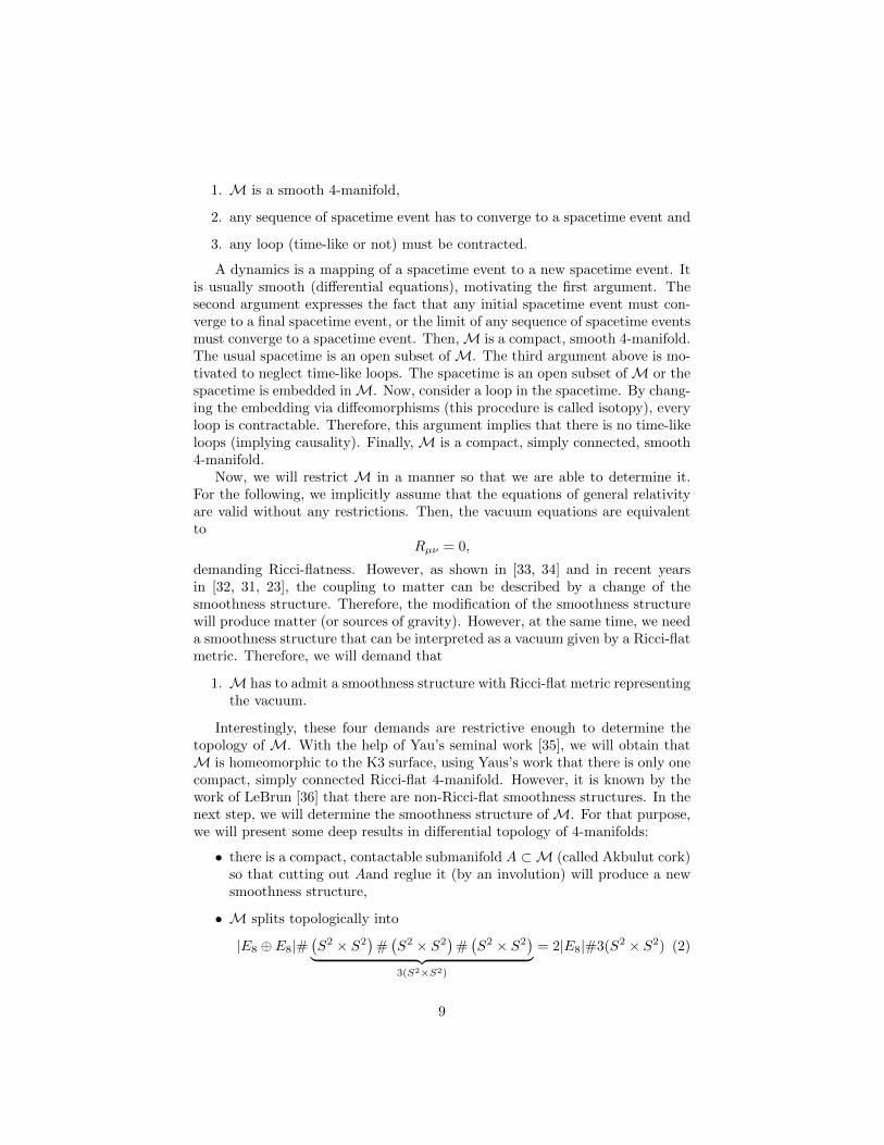
• M splits topologically into

|E8 ⊕E8|#(S2 × S2

)#(S2 × S2

)#(S2 × S2

)︸ ︷︷ ︸3(S2×S2)

= 2|E8|#3(S2 × S2) (2)

9

two copies of the E8 manifold and three copies of S2 × S2 and

• the 3-sphere S3 is a submanifold of A.

In [37], we already discussed this case. Interestingly, there is always a topo-logical 4-manifold for all combinations of E8 and S2×S2, but not all topological4-manifolds are smooth manifolds. Let us consider the 4-manifold that splitstopologically into p copies of the |E8| manifold and q copies of S2 × S2 or

p|E8|#q(S2 × S2

).

Then, this 4-manifold is smoothable for every q but p = 0 and the first combina-tion for p 6= 0 is the pair of numbers p = 2, q = 3 (which is the K3 surface). Anyother combination (p = 2, q < 3 or every q and p = 1) is forbidden as shown byDonaldson [38].

Now, we consider the smooth K3 surface that is Ricci-flat, simply connected,smooth. The main part in the following discussion will be the use of the smooth-ness condition. As discussed above, the smoothness structure is determined bythe Akbulut cork A. Furthermore, as argued above, the smoothness structureis strongly related to the appearance of matter and this process is stronglyconnected to the evolution of our cosmos. It is known as reheating after the in-flationary phase. Therefore, the Akbulut cork (including its embedding) shouldrepresent the inflationary phase with reheating.

The Akbulut cork is built from a homology 3-sphere that will become theboundary ∂A. The difference to a usual 3-sphere S3 is given by the so-calledfundamental group, the equivalence class of closed loops up to deformation(homotopy) with concatenation as group operation. In principle, one constructsa cobordism between S3 and the homology 3-sphere ∂A. All elements of thefundamental group will be killed by adding appropriate disks. At the end, onecan add a 4-disk to get the full contractable cork A. After this short discussion,we are able to identify the first topological transition: if the cosmos starts assmall 3-sphere (conjectural of Planck size), then the space changes to ∂A, or

S3 → ∂A.

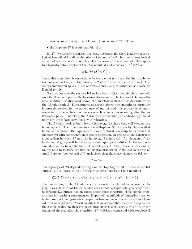
The topology of ∂A depends strongly on the topology of M. In case of the K3surface, ∂A is known to be a Brieskorn spheres, precisely the 3-manifold

Σ(2, 5, 7) =x, y, z ∈ C |x2 + y5 + z7 = 0 |x|2 + |y|2 + |z|2 = 1

.

The embedding of the Akbulut cork is essential for the following results. In[39], it was shown that the embedded cork admits a hyperbolic geometry if theunderlying K3 surface has an exotic smoothness structure. This simple prop-erty has far-reaching consequences. Hyperbolic manifolds of dimension three orhigher are rigid, i.e., geometric properties like volume or curvature are topologi-cal invariants (Mostow-Prasad rigidity). If we assume that the cork A representsthe cosmic evolution, then geometric properties like the curvature of ∂A or thechange of the size after the transition S3 → ∂A are connected with topological

10

properties of the embedded cork A and of the underlying K3 surface by usingMostow–Prasad rigidity. This simple idea opens the door to explicit calcula-tions. In case of the transition S3 → ∂A = Σ(2, 5, 7), the corresponding resultscan be found in [39]. If one assumes a Planck-size (LP ) 3-sphere at the BigBang, then the scale a of Σ(2, 5, 7) changes like

a = LP · exp

(3

2 · CS(Σ(2, 5, 7))

)with the Chern–Simons invariant

CS(Σ(2, 5, 7)) =9

4 · (2 · 5 · 7)=

9

280

and the Planck scale of order 10−34m changes to 10−15m. Obviously, thistransition has an exponential or inflationary behavior. Surprisingly, the numberof e-folds can be explicitly calculated (see [40]) to be

N =3

2 · CS(Σ(2, 5, 7))+ ln(8π2) ≈ 51, (3)

and we also obtain the energy and time scale of this transition (see [40, 41])

EGUT =EP

1 +N + N2

2 + N3

6

≈ 1015GeV t = tP

(1 +N +

N2

2+N3

6

)≈ 10−39s

(4)right at the conjectured scale of the Grand Unified Theory (GUT) (EP , tPPlanck energy and time, respectively). In our recent work [41], this transitionwas analyzed in a detailed manner. There, it was shown that the transitioncan be described by a scalar field model which conformally agrees (as shown in[42]) with the Starobinsky-R2 theory [43]. However, then, the dimension-lessfree parameter α ·M−2

P as well as spectral tilt ns and the tensor-scalar ratio rcan be determined to be

α ·M−2P = 1 +N +

N2

2+N3

6≈ 10−5, ns ≈ 0.961 r ≈ 0.0046,

using equation (3), which is in good agreement with current measurements. Theembedding of the cork A is based on the topological structure of the K3 surfaceM. As discussed above,M splits topologically into a 4-manifold |E8⊕E8| andthe sum of three copies of S2×S2 (see [44]). In the topological splitting (2), the4-manifold |E8 ⊕ E8| has a boundary that is the sum of two Poincare spheresP#P . Here, we used the fact that a smooth 4-manifold of type |E8| must havea boundary (which is the Poincare sphere P ); otherwise, it would contradictthe Donaldson’s theorem [38]. Then, any closed version of |E8 ⊕ E8| does notexist and this fact is the reason for the existence of an exotic R4. To express itdifferently, the neighborhood of the embedded cork lies between the 3-manifoldΣ(2, 5, 7) (boundary of the cork) and the sum of two Poincare spheres P#P .Therefore, we have two topological transitions resulting from the embedding

S3 cork−→ Σ(2, 5, 7)gluing−→ P#P . (5)

11

The transition Σ(2, 5, 7) → P#P has a different character as discussed in [39].A direct consequence is the appearance of a cosmological constant as a directconsequence of the topological invariance of the curvature of a hyperbolic man-ifold. With respect to the critical density, the final formula for normalizedcosmological constant, denoted by ΩΛ, reads

ΩΛ =c5

24π2hGH20

· exp

(− 3

CS(Σ(2, 5, 7))− 3

CS(P#P )− χ(A)

4

).

The Chern–Simons invariants CS(P#P ) = 160 , CS(Σ(2, 5, 7)) = 9

280 and theEuler characteristics of the cork χ(A) = 1 together with the Hubble constant(see [45, 46] combined with [47])

(H0)Planck+Hubble = 69, 2km

s ·Mpc

gives the valueΩΛ ≈ 0.7029,

which is in excellent agreement with the measurements. The numerical resultsabove illustrate the power of the main idea to use topology to fit the parameterin the standard model of cosmology. Interestingly, these parameters are alsoimportant for particle physics. The existence of two transitions (5) implies inthe formalism above the existence of two different energy scales, the GUT scaleof the first transition and a scale of Higgs mass order 126GeV for the secondtransition. These two scales are the right input for the see-saw mechanism togenerate a tiny neutrino mass (see [40]). Secondly, the formalism also providesa favor regarding the existence of a right-handed neutrino. The energy scale ofthe two transitions S3 → Σ(2, 5, 7) → P#P can be expressed as a mass (viaMc2), and we obtain

M =

√4~cG

exp(− 1

2·CS(P#P )

)1 +N + N2

2 + N3

6

≈ 126.4GeV, (6)

which agrees with the mass of the Higgs boson (see [40]). Then, the Higgs bosoncan be expressed as the result of a topological transition (see [48]). Now, wewill use the two energy scales to generate the neutrino mass. For that purpose,we start with the non-diagonal mass matrix(

0 MM B

)with two mass scales B and M fulfilling M B. This matrix has eigenvalues

λ1 ≈ B λ2 ≈ −M2

B

so that λ1 is the mass of the right-handed neutrino, and λ2 represents the massof the left-handed neutrino. Now, we will use the two scales (4) and (6)

B ≈ 0.67 · 1015GeV, M ≈ 126.4GeV,

12

and we will obtain for the neutrino mass

m =M2

B≈ 0.024eV,

which is in good agreement with the constraints from the PLANCK mission.These results seem to support our view that the K3 surface can be the

underlying spacetime (as seen as the set of all possible spacetime events). Theevolution of the cosmos is a suitable subset of this space.

4 From K3 Surfaces to Octonions, 3-Braids andParticles

The results of the previous section illustrated the power of the approach andits relation to particle physics. In this section, we will discuss the topologicalreasons and the relation to the models of Furey, Gresnigt and Bilson–Thompson.In these models, 3-braids, octonions and quaternions play a key role. Therefore,we have to understand how these structures will naturally appear in the K3surface.

4.1 K3 Surfaces and Octonions

The starting point for the description of any K3 surface is the topological split-ting (2)

2|E8|#3(S2 × S2).

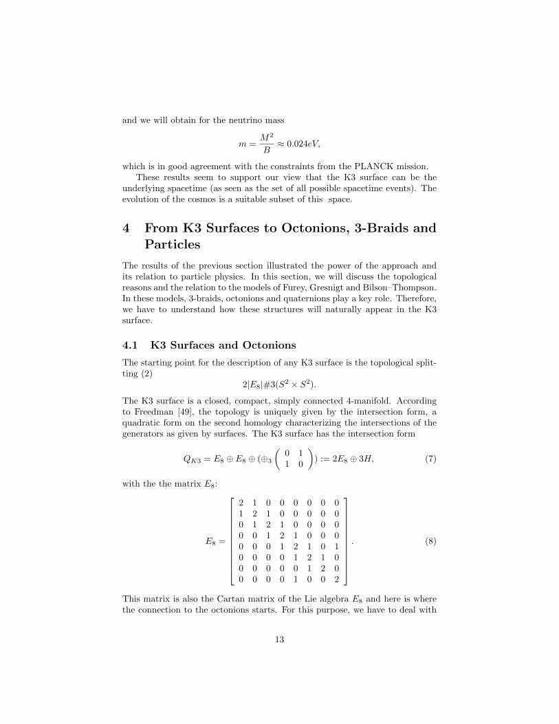
The K3 surface is a closed, compact, simply connected 4-manifold. Accordingto Freedman [49], the topology is uniquely given by the intersection form, aquadratic form on the second homology characterizing the intersections of thegenerators as given by surfaces. The K3 surface has the intersection form

QK3 = E8 ⊕ E8 ⊕ (⊕3

(0 11 0

)) := 2E8 ⊕ 3H, (7)

with the the matrix E8:

E8 =

2 1 0 0 0 0 0 01 2 1 0 0 0 0 00 1 2 1 0 0 0 00 0 1 2 1 0 0 00 0 0 1 2 1 0 10 0 0 0 1 2 1 00 0 0 0 0 1 2 00 0 0 0 1 0 0 2

. (8)

This matrix is also the Cartan matrix of the Lie algebra E8 and here is wherethe connection to the octonions starts. For this purpose, we have to deal with

13

the root system of the Lie algebra E8. Consider a semi-simple Lie algebra Gand its Cartan subalgebra H = (H1, . . . ,Hr), where r is the rank of G. Thissubalgebra is usually considered in the Cartan basis with the non-Hermitiangenerators Ek and their conjugates E−k. Ek is associated with the root vector

r(k)m such that

[Hm, E±k] = ±r(k)m E±m.

When the rank r is 1; 2; 4 or 8, we can combine the operators Hm and the

vectors r(k)m (or eigenvalues) into elements of a division algebra with imaginary

units ei:H = H0 + eiHi r(k) = r

(k)0 + eir

(k)i

so that[H,E±k] = ±r(k)E±k.

For the Lie algebras of the groups SU(2), O(4), O(8), one can construct thereal numbers R, the complex numbers C and the quaternions H, respectively.Interestingly, the triality of the O(8) group reflects the symmetry of the threequaternionic units ei = −iσi, where σi are the Pauli matrices. The case of E8

was worked out by Coxeter [50] in connection with 8-dimensional regular solidsand corresponds to the octonions O. There are 240 rational points on the unitsphere S7 represented by integer octonions that correspond to the 240 roots ofE8. We first introduce octonionic imaginary units eα (α = 1, . . . , 7) with themultiplication rule

eαeβ = −δαβ + ψαβγeγ ,

with ψαβγ as a third rank antisymmetric tensor that is non-zero and equal toone for the index triples 123, 246, 435, 367, 651, 572, 714. Now, we define thespecial element

h =1

2(e1 + e2 + e3 + e7) .

Then, 1; e7; e2; e6, together with h; eh; e2h; e7h correspond to one possible set ofprincipal positive roots. These elements are also forming the Dynkin diagramof the root system of the E8. The matrix E8 in equation (8) above is the Cartanmatrix with entry (i, j) defined by

2〈ri, rj〉〈ri, ri〉

the scalar products between the root vectors ri. Then, the whole approachshowed that simple combinations of the octonionic imaginary units are corre-sponding to generators of the second homology groups for a 4-manifold havingthe matrix E8 as an intersection form. In case of the K3 surface, one has theintersection form containing the matrix E8⊕E8 which corresponds to two copiesof octonions O × O. Here, there is a link to the recent work [8] of complex se-dions. Now, every element of O is related to a surface (unique up to homotopy).In the next section, we will present a connection of these surfaces to spinors.

14

4.2 From Immersed Surfaces in K3 Surfaces to Fermionsand Knot Complements

In the previous subsection, we described a relation between the octonions anda system of eight intersecting surfaces in the K3 surface. In this system of sur-faces, every surface has two self-intersections (the diagonal of the matrix (8)).Therefore, every surface is not embedded but immersed in the K3 surface. Forimmersed surfaces, there is a whole theory, called Weierstrass representation,with a close connection between immersed surfaces and spinors. The followingdiscussion is borrowed from [32], and we will present it here again for complete-ness. First, we start with the immersion I : Σ → R3 of a surface Σ into R3.This immersion I can be defined by a spinor ϕ on Σ fulfilling the Dirac equation

Dϕ = Hϕ, (9)

with |ϕ|2 = 1 (or an arbitrary constant) (see Theorem 1 of [51]). A spinorbundle over a surface splits into two sub-bundles S = S+ ⊕ S−, representingspinors of different helicity, with the corresponding splitting of the spinor ϕ incomponents

ϕ =

(ϕ+

ϕ−

),

and we have the Dirac equation

Dϕ =

(0 ∂z∂z 0

)(ϕ+

ϕ−

)= H

(ϕ+

ϕ−

)with respect to the coordinates (z, z) on Σ. In dimension 3, the spinor bundlehas the same fiber dimension as the spinor bundle S (but without a splittingS = S+ ⊕ S−into two sub-bundles). Now, we define the extended spinor φ overthe 3-torus Σ× [0, 1] via the restriction φ|T 2 = ϕ. The spinor φ is constant alongthe normal vector ∂Nφ = 0 fulfilling the three-dimensional Dirac equation

D3Dφ =

(∂N ∂z∂z −∂N

)φ = Hφ (10)

induced from the Dirac equation (9) via restriction and where |φ|2 = const. Inthis picture, we shift the description from surfaces to 3-manifolds. The descrip-tion above showed that the essential information is contained in the surface,but fermions are at least three-dimensional objects: fermions and bosons ap-pear beginning with dimension 3 (irreducible representation of the group SO(3)as given by the lift to SU(2)). In dimension 2, we have anyons with a spin ofany rational number. However, how did we get the corresponding 3-manifoldrepresenting the fermion?

To answer this question, we consider the branched covering of the K3 surfaceM . As explained above, it must be a 4-fold covering M → S4 branched along asurface with singularities of two types cusp and fold. The cusp can be describedas a cone over the trefoil knot, whereas the fold is the cone over the Hopf

15

link (see Figure 9 in [30]). Now, we consider a 4-manifold with boundary, forinstance by cutting out a 4-disk D4 form M to get 4-manifold M \ D4 withboundary ∂(M \ D4) = S3, the 3-sphere. Then, the branched covering ofM induced a branched covering of the boundary ∂M , so that the branchingset of M , a surface, induces a branching set of ∂M , a knot or link. In ourcase, the singularities of the surface (cusp and fold) given as cones over thetrefoil knot and Hopf link will correspond to the trefoil knot and Hopf link inthe 3-sphere. Then, the branched covering is given by the mappings of thecomplements S3 \ trefoil and S3 \ Hopf − link to the permutation groupS3. We see the appearance of these two complements as a sign to use thesestructures as particles and interactions. The complement of the knot is a 3-manifold with one boundary component. In contrast, the complement of thelink looks like a cylinder T 2 × [0, 1] which can connect two knot complements.Therefore, we have the conjecture that knot complements are fermions and linkcomplements are bosons.

4.3 Fermions as Knot Complements

In this section, we will discuss the topological reasons for the identification ofknot complements with fermions. In our paper [31], we obtained a relation be-tween an embedded 3-manifold and a spinor in the spacetime. The main idea canbe simply described by the following line of argumentation. Let ι : Σ → M bean embedding of the 3-manifold Σ into the 4-manifold M with the normal vector~N so that a small neighborhood Uε of ι(Σ) ⊂ M looks like Uε = ι(Σ) × [0, ε].Every 3-manifold admits a spin structure with a spin bundle, i.e., a principalSpin(3) = SU(2) bundle (spin bundle) as a lift of the frame bundle (principalSO(3) bundle associated with the tangent bundle). Furthermore, there is a(complex) vector bundle associated with the spin bundle (by a representation ofthe spin group), called spinor bundle SΣ. Now, we meet the usual definitionin physics: a section in the spinor bundle is called a spinor field (or a spinor).In general, the unitary representation of the spin group in D dimensions is2[D/2]-dimensional. From the representational point of view, a spinor in fourdimensions is a pair of spinors in dimension 3. Therefore, the spinor bundleSM of the 4-manifold splits into two sub-bundles S±M where one sub-bundle,say S+

M , can be related to the spinor bundle SΣ of the 3-manifold. Then, thespinor bundles are related by SΣ = ι∗S+

M with the same relation φ = ι∗Φ for thespinors (φ ∈ Γ(SΣ) and Φ ∈ Γ(S+

M )). Let ∇MX ,∇ΣX be the covariant derivatives

in the spinor bundles along a vector field X as section of the bundle TΣ. Then,we have the formula

∇MX (Φ) = ∇ΣXφ−

1

2(∇X ~N) · ~N · φ (11)

with the embedding φ 7→(

0φ

)= Φ of the spinor spaces from the relation

φ = ι∗Φ. Here, we remark that, of course, there are two possible embeddings.For later use, we will use the left-handed version. The expression ∇X ~N is the

16

second fundamental form of the embedding where the trace tr(∇X ~N) = 2H isrelated to the mean curvature H. Then, from (11), one obtains the followingrelation between the corresponding Dirac operators

DMΦ = DΣφ−Hφ (12)

with the Dirac operator DΣ on the 3-manifold Σ. In [32], we extend the spinorrepresentation of an immersed surface into the 3-space to the immersion of a3-manifold into a 4-manifold according to the work in [51]. Then, the spinor φdefines directly the embedding (via an integral representation) of the 3-manifold.Then, the restricted spinor Φ|Σ = φ is parallel transported along the normalvector and Φ is constant along the normal direction (reflecting the productstructure of Uε). However, then the spinor Φ has to fulfill

DMΦ = 0 (13)

in Uε i.e., Φ is a parallel spinor. Finally, we get

DΣφ = Hφ (14)

with the extra condition |φ|2 = const. (see [51] for the explicit construction ofthe spinor with |φ|2 = const. from the restriction of Φ). The idea of the paper[31] was the usage of the Einstein–Hilbert action for a spacetime with boundaryΣ. The boundary term is the integral of the mean curvature for the boundary;see [52, 53]. Then by the relation (14) we will obtain

ˆ

Σ

H√h d3x =

ˆ

Σ

φDΣφ√hd3x (15)

using |φ|2 = const. As shown in [31], the extension of the spinor φ to the 4-dimensional spinor Φ by using the embedding

Φ =

(0φ

)(16)

can be only seen as embedding, if (and only if) the 4-dimensional Dirac equation

DMΦ = 0 (17)

onM is fulfilled (using relation (12)). This Dirac equation is obtained by varyingthe action

δ

ˆ

M

ΦDMΦ√g d4x = 0. (18)

In [31], we went a step further and discussed the topology of the 3-manifoldleading to a fermion. On general grounds, one can show that a fermion is givenby a knot complement admitting a hyperbolic structure. However, for hyper-bolic manifolds (of dimension greater than 2), one has the important property

17

of Mostow rigidity where geometric expressions like the volume are topologicalinvariants. This rigidity is a property which we should expect for fermions. Theusual matter is seen as dust matter (incompressible p = 0). The scaling behav-ior of the energy density ρ for dust matter is determined by the time-dependentscaling parameter a to be ρ ∼ a−3. Thus, if one represents matter by very smallregions in the space equipped with a geometric structure, then this scaling canbe generated by an invariance of these small regions with respect to a rescaling.Mostow rigidity now singles out the hyperbolic geometry (and the hyperbolic3-manifold as the corresponding small region) to have the correct behavior. Allother geometries allow a scaling at least along one direction. Finally, Fermionsare represented by hyperbolic knot complements.

4.4 Torus Bundle as Gauge Fields

Now, we have the following situation: two knot complements C(K1) and C(K2)can be connected by a so-called tube T (K1,K2) along the boundary, a torus.This tube T (K1,K2) can be described by the complement of a link with twocomponents defined by the knots K1,K2. In the simplest case, it is the 3-manifold T 2 × [0, 1]. The knot complements are fermions. Therefore, bothknot complements have to carry a hyperbolic structure, i.a. a space of constantnegative curvature. The frame bundle of a 3-manifold is always trivial, so thatwe need a flat connection of this bundle to describe this space. Let Isom(H3) =SO(3, 1) be the isometry group of the three-dimensional hyperbolic space. Thereare suitable subgroups G1, G2 ⊂ Isom(H3) so that (the interior of)C(K1) isdiffeomorphic to Isom(H3)/G1 (and similar with C(K2)). As usual, the spaceof all flat SO(3, 1) connections of C(K1) is the space of all representationsπ1(C(K1)) → SO(3, 1), where SO(3, 1) acts in the adjoint representation onthis space (as gauge transformations). We note the fact that every SO(3, 1)connections lifts uniquely to a SL(2,C) connection. Now, near the boundary, wehave a flat SL(2,C) connection in C(K1) which is connected to a flat SL(2,C)connection in C(K2) by T (K1,K2). The action for a flat connection A withvalues in the Lie algebra g of the Lie group G as a subgroup of the SL(2,C) ina 3-manfold Σ (with vanishing curvature F = DA = 0) is given by

ˆ

Σ

A ∧ F

also known as background field model (BF model). By a small redefinition ofthe connection, one can also choose the Chern–Simons action:

CS(A,Σ) =

ˆ

Σ

(A ∧ dA+

2

3A ∧A ∧A

).

The variation of the Chern–Simons action CS(A,Σ) gets flat connections DA =0 as solutions. The flow of solutions A(t) in T (K1,K2)× [0, 1] (parametrized bythe variable t) between the flat connection A(0) in T (K1,K2)× 0 to the flat

18

connection A(1) in T (K1,K2)×1 will be given by the gradient flow equation(see [54] for instance)

d

dtA(t) = ± ∗ F (A) = ± ∗DA, (19)

where the coordinate t is normal to T (K1,K2). Therefore, we are able to in-troduce a connection A in T (K1,K2) × [0, 1] so that the covariant derivativein the t-direction agrees with ∂/∂t. Then, we have for the curvature F = DAwhere the fourth component is given by F4µ = dAµ/dt. Thus, we will get theinstanton equation with (anti-)self-dual curvature

F = ± ∗ F .

However, now we have to extend the Chern–Simons action (of the 3-manifold)to the 4-manifold. It follows that

CS(A, T (K1,K2)× 1)− CS(A, T (K1,K2)× 0) =

ˆ

T (K1,K2)×[0,1]

tr(F ∧ F )

i.e., we obtain the second Chern class and finally

SEH([0, 1]×T (K1,K2)) =

ˆ

T (K1,K2)×[0,1]

tr(F ∧F ) = ±ˆ

T (K1,K2)×[0,1]

tr( F ∧∗F )

i.e., the action of the gauge field. The whole procedure remains true for anextension, i.e.,

SEH(R× T (K1,K2)) = ±ˆ

T (K1,K2)×R

tr( F ∧ ∗F ) . (20)

The gauge field action (20) is only defined along the tubes T (K1,K2). For theextension of the action to the whole 4-manifold M , we need some non-trivialfacts from the theory of 3-manifolds. We presented the ideas in [32]. Finally,we obtain the gauge field action

ˆ

M

tr(F ∧ ∗F ). (21)

Now, we will discuss the possible gauge group. Again, for completeness, we willpresent the argumentation in [32] again. The gauge field in the action (21) hasvalues in the Lie algebra of the maximal compact subgroup SU(2) of SL(2,C).However, in the derivation of the action, we used the connecting tube T (K1,K2)between two tori, which is a cobordism. This cobordism T (K1,K2) is also knownas torus bundle (see [55] Theorem 1.15), which can be always decomposed intothree elementary pieces—finite order, Dehn twist and the so-called Anosov map(named after the russian mathematician Dmitri Anosov).

19

The idea of this construction is very simple: one starts with two trivialcobordisms T 2 × [0, 1] and glues them together by using a diffeomorphism g :T 2 → T 2, which we call gluing diffeomorphism. From the geometrical point ofview, we have to distinguish between three different types of torus bundles. Thethree types of torus bundles are distinguished by the splitting of the tangentbundle:

• finite order (orders 2, 3, 4, 6): the tangent bundle is three-dimensional,

• Dehn-twist (left/right twist): the tangent bundle is a sum of a two-dimensional and a one-dimensional bundle,

• Anosov: the tangent bundle is a sum of three one-dimensional bundles.

Following Thurston’s geometrization program (see [56]), these three torusbundles are admitting a geometric structure, i.e., it has a metric of constantcurvature. Apart from this geometric properties, all torus bundles are deter-mined by the gluing diffeomorphism g : T 2 → T 2, which also determines thefundamental group of the torus bundle. Therefore, this gluing diffeomorphismalso has an influence on the structure of the diffeomorphism group of the torusbundle, which will be discussed now. From the physical point of view, we havetwo types of diffeomorphisms: local and global. Any coordinate transformationcan be described by an infinitesimal or local diffeomorphism (coordinate trans-formation). In contrast, there are global diffeomorphisms like an orientationreversing diffeomorphism. Two diffeomorphisms not connected via a sequenceof local diffeomorphism are part of different connecting components of the dif-feomorphism group, i.e., the set of isotopy classes π0(Diff(M)) (also called themapping class group). Isotopy classes are important in order to understand theconfiguration space topology of general relativity (see Giulini [57]). In princi-ple, the state space in geometrodynamics is the set of all isotopy classes, whereevery class represents one physical situation, or isotopy classes label two differ-ent physical situations. By definition, the two 3-manifolds in different isotopyclasses cannot be connected by a sequence of local diffeomorphisms (local coor-dinate transformations). Again, these two different isotopy classes represent twodifferent physical situations; see [13] for the relation of isotopy classes to particleproperties like spin. In case of the torus bundle, we consider the isotopy classesπ0(Diff(M,∂M)) relative to the boundary represented by the automorphismsof the fundamental group. Using the geometrization program, we obtain a re-lation between the isotopy classes π0(Diff(M,∂M)) and the isometry classes(connecting components of the isometry group) with respect to the geometricstructure of the torus bundle (see, for instance, [58, 59]). Then, the isotopyclasses of the torus bundles are given by

• finite order: 2 isotopy classes (= no/even twist or odd twist),

• Dehn-twist: 2 isotopy classes (= left or right Dehn twists),

• Anosov: 8 isotopy classes (= all possible orientations of the three linebundles forming the tangent bundle).

20

From the geometrical point of view, we can rearrange the scheme above:

• torus bundle with no/even twists: one isotopy class,

• torus bundle with twist (Dehn twist or odd finite twist): three isotopyclasses,

• torus bundle with Anosov map: eight isotopy classes.

This information creates a starting point for the discussion on how to derivethe gauge group. Given a Lie group G with Lie algebra g, the rank of g isthe dimension of the maximal abelian subalgebra, also called Cartan algebra(see above for a definition). It is the same as the dimension of the maximaltorus Tn ⊂ G. The curvature F of the gauge field takes values in the adjointrepresentation of the Lie algebra and the action tr(F ∧ ∗F ) forms an elementof the Cartan subalgebra (the Casimir operator). However, each isotopy classcontributes to the action and therefore we have to take the sum over all possibleisotopy classes. Let ta be the generator in the adjoint representation; then, weobtain for the Lie algebra part of the action tr(F ∧ ∗F )

• torus bundle with no twists: one isotopy class with t2,

• torus bundle with twist: three isotopy classes with t21 + t22 + t23,

• torus bundle with Anosov map: eight isotopy classes with∑8a=1 t

2a.

The Lie algebra with one generator t corresponds uniquely to the Lie groupU(1) where the three generators t1, t2, t3 form the Lie algebra of the SU(2)group. Then, the last case with eight generators ta has to correspond to the Liealgebra of the SU(3) group. We remark the similarity with an idea from branetheory: n parallel branes (each decorated with an U(1) theory) are describedby an U(n) gauge theory (see [60]). Finally, we obtain the maximal groupU(1) × SU(2) × SU(3) as a gauge group for all possible torus bundles (in themodel: connecting tubes between the solid tori).

At the end, we will speculate about the identification of the isotopy classesfor the torus bundle with the vector bosons in the gauge field theory. Obviously,the isotopy class of the torus bundle with no twist must be the photon. Then,the isotopy class of the other bundle of finite order should be identified with theZ0 boson and the two isotopy classes of the Dehn twist bundles are the W±

bosons. Here, we remark that this identification is consistent with the definitionof the charge lateron. Furthermore, we remark that this scheme contains auto-matically the mixing between the photon and the Z0 boson (the correspondingtorus bundle are both of finite order). The isotopy classes of the Anosov mapbundle have to correspond to the eight gluons. Later, we expect that these ideaswill lead to an additional relation for the scattering amplitudes induced by thegeometry of the torus bundles.

21

Figure 7: Branching sets—Left: 6-Plat for the knot cpomplement, Center: a3-Braid as 6-Braid as example, Right: 6-Braid for the link complement

4.5 Fermions, Bosons and 3-Braids

In the previous subsection, we identified the hyperbolic knot complement with afermion and the torus bundle between them as gauge bosons. The first naturalquestion is then: which knot is related to a fermion like the electron? How-ever, this question is meaningless in our approach. The knot/link complementsare induced from the singularities of the branching set of the 4-fold branchedcovering of the K3 surface. However, these singularities are another expressionof the change of the branching set of the 3-manifolds. With other words: thebranching set, a knot or link, of a 3-manifold is not unique. There are trans-formations of the branching sets representing the same 3-manifold. Therefore,these complements are not uniquely connected to particles/fermions. Later, wewill see that the knots represent mainly the state. However, what are the in-variant properties? For that purpose, we will study the branched covering ofthe knot/link complement to understand the invariant properties.

Let C(K) = S3 \ (K × D2) be a knot complement which is a compact3-manifold with boundary ∂C(K) = T 2 the 2-torus. C(K) is given by a 3-fold branched covering C(K)→ D3 inducing a 3-fold branched covering of theboundary ∂C(K) → ∂D3 or T 2 → S2. The 3-fold covering T 2 → S2 has sixpoints as a branching set, the end points of a 6-plat or tangle (see Figure 7). Ina similar manner, let C(L) = C(K1,K2) = S3 \

(L×D2

)be a link complement

of a link with two linked knots K1,K2 (the two linking components). C(L)is a compact 3-manifold with two boundaries given by two tori. Then, the 3-fold branched covering C(L) → S3 \

(D3 tD3

)induces again 3-fold branched

coverings T 2 → S2 of the two boundaries. Every covering T 2 → S2 has sixpoints as a branching set again. The corresponding branching set of C(L) isa braid of six strands but represented as a 3-braid (see Figure 7). Finally,bosons and fermions are represented as 3-braids. Our model agrees with theBilson–Thompson model but with the exception that we do not fix the braid.In particular, we do not believe that the difference between an electron andmyon is given by a different braid.

22

5 Electric Charge and Quasimodularity

We argued above that all knot complements admitting a hyperbolic geome-try (geometry of negative, constant scalar curvature) have the properties offermions, i.e., spin 1

2 , are pressureless p = 0 in cosmology and fulfill the Diracequation (see also the previous section for the action functional). However, aparticle can carry charges (electrical or others like color, etc.).

5.1 Electric Charge as Dehn Twist of the Boundary

We described above the knot complement as a branched covering branched alonga braid. What is the meaning of a charge in this description? Let us start withthe case of an electric charge. Given a complex line bundle over C(K) × (0, 1)with connection A and curvature F = dA, we then have the Maxwell equations:

dF = 0 d ∗ F = ∗j,

with the Hodge operator ∗ and the 4-current 1-form j. The electric charge Qeis given by

Qe =

ˆ

∂C(K)=T 2

∗F

in the temporal gauge (normal to the boundary of C(K)) using d ∗ F = ∗j andStokes theorem. The magnetic charge Qm is defined in an analogous way

Qm =

ˆ

∂C(K)=T 2

F = 0,

but it is zero because of dF = 0. By the formulas above, we obtain a restrictionof the complex line bundle to the boundary ∂C(K) = T 2. A complex linebundle over T 2 is determined by the twists of the fibers w.r.t. the lattice Z2

in the definition of the torus T 2 = C/Z2. However, which twist is related tothe electric charge? Consider a cylinder S1 × [0, 1] and identify the ends of theinterval to get T 2 again. A complex line bundle over S1 × [0, 1] with curvatureF gives the integral

ˆ

S1×[0,1]

F =

ˆ

S1×1

A−ˆ

S1×0

A

using F = dA, which is only non-trivial if the two integrals differ. It can berealized by a twist of one side (say S1 × 1), also called a Dehn twist. Duallyby using d ∗ F = ∗j, we get

Qe =

ˆ

[0,1]

∗j =

ˆ

[0,1]

d ∗ F = ∗F |1 − ∗F |0,

23

which is non-zero by a Dehn twist along [0, 1]. Therefore, charges can be de-tected by Dehn twists along the boundary. A Dehn twist along the meridianrepresents the magnetic charge, whereas a Dehn twist along the longitude is anelectric charge. The number of twists is the charge, i.e., we obtain automati-cally a quantization of the electric and magnetic charge. Furthermore, there isa simple algebraic description of the twists, which agrees with the descriptionof electromagnetic duality using SL(2,Z). As noted above, the torus can beobtained by T 2 = C/Z2 w.r.t. the lattice Z2. An automorphism of the torus isgiven by a the group SL(2,Z) acting via rational transformations on C, i.e.,(

a bc d

)∈ SL(2,Z), ad− bc = 1→

(a bc d

)· z =

az + b

cz + d.

Then, the two possible Dehn twists are given by

z 7→ z + 1,

z 7→ −1

z,

which is known from electromagnetic duality. However, this group also hasanother meaning. Let Diff(T 2) be the diffeomorphism group of the torus.All coordinate transformations, known as diffeomorphisms connected to theidentity, are forming a (normal) subgroup Diff0(T 2) ⊂ Diff(T 2). Then, thefactor space MCG(T 2) = Diff(T 2)/Diff0(T 2) is a group, known as a mappingclasses group, and generated by Dehn twists, i.e., MCG(T 2) = SL(2,Z) or themapping class group is the modular group. An element of the mapping classgroup is a global diffeomorphism (also called isotopy) that cannot be describedby coordinate transformations, i.e., full twists cannot be undone by a sequenceof infinitesimal rotations. Then, different charges belong to different mapping(or isotopy) classes. Up to now, we have a full symmetry between electric andmagnetic charges (geometrically expressed by the torus). Now, we will show thatthis behavior changed for the extension to the knot complement. Technically,it will be expressed by a change from modular to quasimodular functions.

5.2 Electric Charge as a Frame of the Knot Complement

However, what does change in the knot complement and in the branched cov-ering? As a toy example, we consider the complement of the unknot D2 × S1.Then, the Dehn twist along the meridian of the boundary torus will be triv-ialized. By a result of McCullough (see for instance [61]), every Dehn twistalong the longitude induces a diffeomorphism of the solid torus. Then, the com-plement of the unknot can carry an electric charge (by a Dehn twist) but nomagnetic charge. This result can be generalized to all knot complements (whichare homologically equivalent to the solid torus). The effect on the branchedcovering can also be obtained by considering the boundary. The boundary is atorus written as two-fold branched covering branched along 4 points. A Dehntwist is given by a permutation of the branching points that leads to a twist of

24

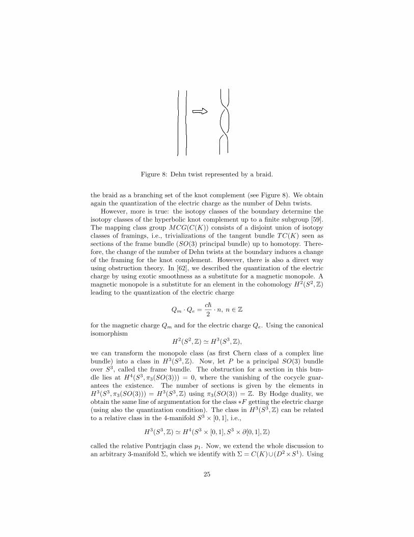
Figure 8: Dehn twist represented by a braid.

the braid as a branching set of the knot complement (see Figure 8). We obtainagain the quantization of the electric charge as the number of Dehn twists.

However, more is true: the isotopy classes of the boundary determine theisotopy classes of the hyperbolic knot complement up to a finite subgroup [59].The mapping class group MCG(C(K)) consists of a disjoint union of isotopyclasses of framings, i.e., trivializations of the tangent bundle TC(K) seen assections of the frame bundle (SO(3) principal bundle) up to homotopy. There-fore, the change of the number of Dehn twists at the boundary induces a changeof the framing for the knot complement. However, there is also a direct wayusing obstruction theory. In [62], we described the quantization of the electriccharge by using exotic smoothness as a substitute for a magnetic monopole. Amagnetic monopole is a substitute for an element in the cohomology H2(S2,Z)leading to the quantization of the electric charge

Qm ·Qe =c~2· n, n ∈ Z

for the magnetic charge Qm and for the electric charge Qe. Using the canonicalisomorphism

H2(S2,Z) ' H3(S3,Z),

we can transform the monopole class (as first Chern class of a complex linebundle) into a class in H3(S3,Z). Now, let P be a principal SO(3) bundleover S3, called the frame bundle. The obstruction for a section in this bun-dle lies at H4(S3, π3(SO(3))) = 0, where the vanishing of the cocycle guar-antees the existence. The number of sections is given by the elements inH3(S3, π3(SO(3))) = H3(S3,Z) using π3(SO(3)) = Z. By Hodge duality, weobtain the same line of argumentation for the class ∗F getting the electric charge(using also the quantization condition). The class in H3(S3,Z) can be relatedto a relative class in the 4-manifold S3 × [0, 1], i.e.,

H3(S3,Z) ' H4(S3 × [0, 1], S3 × ∂[0, 1],Z)

called the relative Pontrjagin class p1. Now, we extend the whole discussion toan arbitrary 3-manifold Σ, which we identify with Σ = C(K)∪(D2×S1). Using

25

this 4-dimensional interpretation, we obtain the framing as the Hirzebruch defect[63]. For that purpose, we consider the 4-manifold M with ∂M = Σ. Let σ(M)be the signature of M , i.e., the number of positive minus negative eigenvalues ofthe intersection form of M . Furthermore, let p1(M,Σ) be the relative Pontrjaginclass as an element of H4(M,∂M = Σ,Z). Then, the Hirzebruch defect h isgiven by

h = 3σ(M)− p1(M,Σ) = Qe (22)

and identified with the framing, i.e., with the charge. This definition is mo-tivated by the Hirzebruchs signature formula for a closed 4-manifold relatingthe signature σ(M) and the first Pontrjagin class p1(M) (of the tangent bundleTM) via σ(M) = 1

3p1(M) (see [64]).

5.3 The Charge Spectrum

Now, we will discuss the expression (22) for the electric charge. By the argu-mentation above, the relative Pontrjagin class gives an integer expressing theframing of the knot complement for a fixed time. The appearance of the signa-ture σ(M) added a 4-dimensional element which describes more complex caseswith many components. In [65], this case was also considered with a similarresult: this formula is valid for links where σ(M) is now the signature of thelinking matrix and p1 is the sum of framings for each component. The signa-ture can be minimally changed by ±1 leading to a change of the charge by ±3.Therefore, the minimal change for one component can be

Qe mod 3Z = 0,±1,±2,±3 ,

i.e., we obtain a spectrum containing four possible values. If we normalize thecharge to be a multiple of e/3, then we have the charge spectrum

Qe =

0,±1

3e,±2

3e,±e

in agreement with the experiment. Then, we have the description of one particlegeneration: two leptons (neutrino of charge 0 and lepton of charge −1) and twoquarks (quark of charge − 1

3 and quark of charge + 23 ).

5.4 Vanishing of the Magnetic Charge and Quasimodular-ity

One may wonder whether there is no magnetic charge anymore. Our argumentis only partially satisfying because there are many incompressible surfaces insideof a hyperbolic knot complement serving as representatives for magnetic charges.Therefore, we need a stronger argument why the symmetry between electric andmagnetic charge is broken. As explained above, the Dehn twists of the boundarytorus are the generators of the mapping class (or isotopy) group. According toAtiyah [63], the framing can be used to define a central extension Γ

1→ Z→ Γ→ Γ→ 1

26

of the mapping class group Γ so that there is a section s : Γ → Γ inducinga splitting of the sequence above. This section defines a canonical 2-cocyclec for the central extension that is given by the signature of the corresponding4-manifold (see [63] for the details). However, in case of the torus, for thegroup Γ = SL(2,Z), there is no non-zero homomorphism Γ → Z and so thesplitting s1 : Γ → Γ is unique. Therefore, the canonical section s is not ahomomorphism and the framing (used in the definition of this section) leadsto a breaking of the modular invariance i.e., the invariance w.r.t. Γ. This factis simply expressed by considering the difference of the two sections s(γ) ands1(γ) for γ ∈ Γ, which is given by the logarithm of the Dedekind η−function,related to quasimodular functions. Thus, our definition of the electric chargebreaks explicitly the electro-magnetic duality and we get a vanishing magneticcharge.

6 Drinfeld–Turaev Quantization and QuantumStates

In [66, 67], we discussed the appearance of quantum states from knots knownas Turaev–Drinfeld quantization. The idea for the following construction canbe simply expressed. We start with two 3-manifolds and consider a cobor-dism between them. This cobordism is a 4-manifold with a branched cover-ing branched over a surface with self-intersections. Here, it is enough to re-strict to a special class of these surfaces, so-called ribbon surfaces (see [68]).The 3-manifolds are chosen to be hyperbolic knot complements, denoted byY1, Y2. A hyperbolic structure is defined by a homomorphism π1(Yi)→ SL(2,C)(∈ Hom(π1(Yi), SL(2,C))) up to conjugation. Now, we extend this structure tothe entire cobordism, denoted by Cob(Y1, Y2). The branching set of Cob(Y1, Y2)is a surface S with non-trivial fundamental group π1(S). This surface can bechanged without any change of Cob(Y1, Y2). One change can be described ascrossing change. Now, we have all ingredients for the Drinfeld–Turaev quanti-zation:

• The surface S (branching set of Cob(Y1, Y2)) is inducing a representationπ1(S)→ SL(2,C).

• The space of all representationsX(S, SL(2,C)) = Hom(π1(S), SL(2,C))/SL(2,C)has a natural Poisson structure (induced by the bilinear on the group) andthe Poisson algebra (X(S, SL(2,C), ) of complex functions over themis the algebra of observables.

• The Skein module K−1(S × [0, 1]) (i.e., t = −1) has the structure of analgebra isomorphic to the Poisson algebra (X(S, SL(2,C)), ). (see also[69, 70]).

• The skein algebra Kt(S× [0, 1]) is the quantization of the Poisson algebra(X(S, SL(2,C)), ) with the deformation parameter t = exp(h/4) (seealso [69]) .

27

Figure 9: Crossings L∞, Lo, Loo.

To understand these statements, we have to introduce the skein moduleKt(M) of a 3-manifold M (see [71]). For that purpose, we consider the set oflinks L(M) in M up to isotopy and construct the vector space CL(M) withbasis L(M). Then, one can define CL[[t]] as ring of formal polynomials havingcoefficients in CL(M). Now, we consider the link diagram of a link, i.e., theprojection of the link to the R2 having the crossings in mind. Choose a diskin R2 so that one crossing is inside this disk. If the three links differ by thethree crossings Loo, Lo, L∞ (see figure 9) inside of the disk, then these links areskein related. Then, in CL[[t]], one writes the skein relation L∞− tLo− t−1Loowhich depends only on the group SL(2,C), . Furthermore, let L t O be thedisjoint union of the link with a circle. Then, one writes the framing relationLtO+ (t2 + t−2)L. Let S(M) be the smallest submodule of CL[[t]] containingboth relations. Then, we define the Kauffman bracket skein module by Kt(M) =CL[[t]]/S(M). The modification of S by using the skein relations is one of theallowed changes of the branching set to keep Cob(Y1, Y2).

Now, we list the following general results about this module:

• The module K−1(M) for t = −1 is a commutative algebra.

• Let S be a surface. Then, Kt(S× [0, 1]) carries the structure of an algebra.

The algebra structure of Kt(S × [0, 1]) can be simply seen by using thediffeomorphism between the sum S × [0, 1] ∪S S × [0, 1] along S and S × [0, 1].Then, the product ab of two elements a, b ∈ Kt(S × [0, 1]) is a link in S ×[0, 1] ∪S S × [0, 1] corresponding to a link in S × [0, 1] via the diffeomorphism.The algebra Kt(S × [0, 1]) is in general non-commutative for t 6= −1. For thefollowing, we will omit the interval [0, 1] and denote the skein algebra by Kt(S).

As shown in [72, 66, 23], the skein algebra serves as the observable algebra ofa quantum field theory. For this approach via branched coverings, the branchingsets of knot complements (representing the fermions) are special braids (6-plats,see above). Any different braid is a different state or better than a differentquantum state but not a different particle. As explained above, the charge

28

spectrum is enough to describe one generation of particles (two leptons, twoquarks). The appearance of different generations will be discussed below.

7 Fermions and Number Theory

In this section, we will present some ideas to uncover some explicit relationsbetween fermions, given as hyperbolic knot complements, and number theory,notable quaternionic trace fields and algebraic K theory/Bloch group. However,we first need some definitions.

A quaternion algebra over a field F is a four-dimensional central simpleF -algebra. A quaternion algebra has a basis 1, i, j, ij where i2, j2 ∈ F× andij = −ji. A subgroup of PSL(2,C), the isometry group of the three-dimensionalhyperbolic space isomorphic to the Lorentz group SO(3, 1), is said to be derivedfrom a quaternion algebra if it can be obtained through the following construc-tion. Let F be a number field that has exactly two embeddings into C whoseimage is not contained in R. Let A be a quaternion algebra over F such that,for any embedding τ : F → R, the algebra A⊗τ R is isomorphic to the quater-nions. Let O1 be the group of elements in the order of A with a 1. An order of aquaternionic algebra A is a finitely generated submodule O of A of reduced norm1 and let Γ be its image in the 2 × 2 matrices M2(C) via φ : A → M2(C). Wethen consider the Kleinian group obtained as the image inPSL(2,C) of φ(O1).This subgroup is called an arithmetic Kleinian group. An arithmetic hyperbolicthree-manifold is the quotient of hyperbolic space H3 by an arithmetic Kleiniangroup. The complement of the figure 8 knot is one example of an arithmetichyperbolic 3-manifold.

This class of 3-manifolds shows the strong relation between quaternions and3-manifolds. We discussed above the relation between the K3 surface and theoctonions. The starting point for the use of number theory in Kleinian groupsis Mostow’s rigidity theorem. A consequence of this theorem is that the matrixentries in SL(2,C) of a finite covolume Kleinian group Γ may be taken to liein a number field that is a finite extension of Q. However, it is true that thereis a strong relation between certain number theoretic functions (Bloch–Wignerfunction, dilogarithm) and the volume of the hyperbolic 3-manifolds: the volumeis the sum over all Bloch–Wigner functions for the ideal tetrahedrons formingthis 3-manifold. For more information about the relation between hyperbolic3-manifolds and number theory, consult the book [73]. We hope to use thisrelation in the future to obtain more properties of fermions by using numbertheory.

8 The K3 Surface and the Number of Genera-tions

In Section 4.1, we discussed a relation between the K3 surface and octonions byusing the intersection form. Here, we use only the E8 matrix, i.e., the Cartan

29

matrix of the Lie algebra E8. In this section, we will speculate about the otherpart

H =

(0 −1−1 0

)of the intersection form (now with a different orientation). H is the intersectionform of the 4-manifold S2 × S2. To express it explicitly, there are homologyclasses α, β ∈ H2(S2 × S2) with α2 = β2 = 0 and α · β = −1. Therefore,every S2 of this manifold has no self-intersections. For the topology of theK3 surface with intersection form (7), this form has the desired form, but, asexplained above, we will change the smoothness structure. The central ideais the usage of Casson handles CH for the 4-manifolds S2 × S2 \ pt, the one-point complement of S2 × S2. Here, the homology classes α, β are given (up tohomotopy) by α2, β2 = 0 mod 2 and α · β = −1; see [74]. However, then onehas α2 = 2n. Interestingly, the existence of a spin structure is connected tothe property that the squares of the homology classes are even. Here, we willconsider the simplest realization which has non-zero squares, i.e., we get theform

H =

(2 −1−1 2

). (23)

This form cannot be an intersection form because H has determinant 3. There-fore, only the H mod 2 reduction has the meaning to be an intersection. How-ever, for the moment, we will consider H and apply the same construction asfor the E8, i.e., we see H as the Cartan matrix for a Lie algebra. In this case,we get the Lie algebra of SU(3) or the color group. The whole discussion usessome hand-waving arguments, but it is a sign that the 3

(S2 × S2

)part of the

K3 surfaces is connected with the generations. Every part S2 × S2 has onecolor group and realizes the electric charge spectrum 0,± 1

3 ,±23 ,±1. Thus, ev-

ery S2 × S2 is the 4-dimensional expression for one generation. This resultagrees with the discussion in [31] where we generate fermions from a Cassonhandle. Let us assume that the number of generations is given by the numberof S2 × S2 summands. How many generations are possible? Here, we have thesurprising result: if the underlying spacetime is a smooth manifold, then theminimal number of generations must be three! A spacetime with only one ortwo generations is not a smooth manifold. Then, the K3 surface is the minimalmodel.

We will close this paper with another speculation, a global symmetry inducedfrom the K3 surface. Starting point is the intersection form again. From thepoint of number theory, this form is an even unimodular positive-definite latticesof rank 24, the so-called Niemeier lattice. In 2010, Eguchi–Ooguri–Tachikawaobserved that the elliptic genus of the K3 surface decomposes into irreduciblecharacters of the N = 4 superconformal algebra. The corresponding q-series isa mock modular form related to the sporadic group M24, the Mathieu group,a simple group of order 244823040. The whole theory is known as Mathieumoonshine or umbral moonshine [75]. The interesting point here is the maximalsubgroup of M24, the split extension of PGL(3, 4) by S3. The group is the

30

projective group of 3 × 3 matrices with values in the field of four elements. Itseems that this maximal subgroup acts in some sense on the K3 surface, andwe conjecture that this group acts on the S2×S2 part. If our idea of a relationbetween the three generations and the 3

(S2 × S2

)part of the K3 surfaces is

true, then we hope to get the mixing matrix for quarks and neutrinos from thisaction.

9 Conclusions and Outlook

In this paper, we presented a top-down approach to fermions and bosons, inparticular the standard model. What was done in the paper?

• We constructed a spacetime, the K3 surface and derive some numberslike the cosmological constant or some energy scales and neutrino massesagreeing with experimental data.

• We derived from a representation of K3 surfaces by branched covering asimple picture: fermions are hyperbolic knot complements, whereas bosonsare link complements (torus bundles).

• We obtained the gauge group from this picture (at least in principle).

• We derived the correct charge spectrum and obtained one generation.

• We conjectured about the number of generations and global symmetry(the PGL(3, 4)) to get the mixing between the generations.

What are the consequences for physics? The model only has a few directconsequences. We introduced fermions and bosons in a geometric way. Exceptfor the right-handed neutrino (needed for the see-saw mechanism to generatethe masses), we only got the fermions and gauge bosons of the standard model.No extension is needed. The usage of torus bundles for the gauge bosons shouldgenerate additional relations for the corresponding scattering amplitudes. Theappearance of the global symmetry PGL(3, 4) should be related the mixing ofquarks and neutrinos. In [40], we also discussed the appearance of an asymmetrybetween particles and anti-particles induced by the topology of the spacetime.This idea is also valid in this model, but we cannot match it to the observations.

Is there an outline on some new experiments derived by this model? Cur-rently, this model makes some predictions about the neutrino masses, chargespectrum and the existence of a right-handed neutrino. However, these predic-tions can be checked by a better measurement in known experiments. Now,there are no new ideas about special experiments connected with this model.

Among these results, there are, of course, many open points of the kind: whatis the color and weak charge? How can we implement the Higgs mechanism?What is mass? For the Higgs mechanism, we had found a possible scheme in ourprevious work [76, 40], but it is only a beginning. Many aspects of this paperare related to the ideas of Furey and Gresnigt. It is a future project to extendit and bridge our approach with these ideas.

31

Acknowledgments

I first want to thank the anonymous referees for all helpful remarks and com-ments to make this work more readable. Furthermore, I want to thank CarlBrans for an uncountable number of delightful discussions over so many years. Ialso want to give a special thanks to Chris Duston for discussions about branchedcoverings, in particular to draw my attention towards branched coverings. Inaddition, I want to acknowledge all of my discussions with Jerzy Krol over theyears. Finally, I want to give a huge thank you to my family, in particular tomy daughter Lucia, for painting the figures.

References

[1] Collaborations, F.G. Testing Einstein’s Special Relativity with Fermi’sShort Hard Gamma-Ray Burst GRB090510. Nature 2009, 462, 331–334.arXiv:0908.1832.

[2] Furey, C. Towards a Unified Theory of Ideals. Phys. Rev. D 2012,86, 025024. arXiv:1002.1497.

[3] Furey, C. Generations: Three Prints, in Colour. JHEP 2014, 10, 046.arXiv:1405.4601.

[4] Furey, C. Charge Quantization from a Number Operator. Phys. Lett. B2015, 742, 195–199. arXiv:1603.04078.

[5] Furey, C. Standard Model Physics from an Algebra? Ph.D. Thesis,University of Waterloo, Waterloo, ON, Canada, 2015. arXiv:1611.09182.

[6] Gresnigt, N. Braids, Normed Division Algebras, and Stan-dard Model Symmetries. Phys. Lett. B 2018, 783, 212–221.doi:10.1016/j.physletb.2018.06.057., arXiv:1803.02202.

[7] Gresnigt, N. Braided Fermions from Hurwitz Algebras. J. Phys.Conf. Ser. 2019, 1194, 012040. doi:10.1088/1742-6596/1194/1/012040.arXiv:1901.01312.

[8] Gillard, A.; Gresnigt, N. Three Fermion Generations with Two UnbrokenGauge Symmetries from the Complex Sedenions. Eur. Phys. J. C 2019,79, 446. doi:10.1140/epjc/s10052-019-6967-1. arXiv:1904.03186.

[9] Stoica, O. Leptons, Quarks, and Gauge from the Complex Clifford AlgebraC`6. Adv. Appl. Cliff. Alg. 2018, 28, 52. doi:10.1007/s00006-018-0869-4.arXiv:1702.04336.

[10] Thomson, W. On Vortex Motion. Trans. R. Soc. Ed. 1869, 25, 217–260.

[11] Misner, C.; Thorne, K.; Wheeler, J. Gravitation; Freeman: San Francisco,CA, USA, 1973.

32

[12] Mielke, E. Knot Wormholes in Geometrodynamics? Gen. Relat. Grav.1977, 8, 175–196. doi:10.1007/BF00763546.

[13] Giulini, D. Matter from Space. Based on a talk delivered at the con-ference “Beyond Einstein: Historical Perspectives on Geometry, Gravita-tion, and Cosmology in the Twentieth Century”, September 2008 at theUniversity of Mainz in Germany. appeared in the Einstein-Studies Series,Birkhaeuser, Boston. arXiv 2008, arXiv:0910.2574.

[14] Jehle, H. Topological characterization of leptons, quarks and hadrons.Phys. Lett. B 1981, 104, 207–211. doi:10.1016/0370-2693(81)90592-X.

[15] Gavrilik, A.M. Quantum algebras in phenomenological description of par-ticle properties. Nucl. Phys. B (Proc. Suppl.) 2001, 102/103, 298–305.doi:10.1016/S0920-5632(01)01570-5. [arXiv:hep-ph/0103325],

[16] Finkelstein, R. Knots and Preons. Int. J. Mod. Phys. A 2009, 24, 2307–2316. arXiv:0806.3105 [hep-th].

[17] Bilson-Thompson, S. A Topological Model of Composite Preons. arXiv2005, arXiv:0503213v2.

[18] Bilson-Thompson, S.; Markopoulou, F.; Smolin, L. Quantum Gravity andthe Standard Model. Class. Quant. Grav. 2007, 24, 3975–3994. arXiv:hep-th/0603022v2.

[19] Duston, C. Exotic Smoothness in 4 Dimensions and Semiclassical Eu-clidean Quantum Gravity. Int. J. Geom. Meth. Mod. Phys. 2010, 8, 459–484. arXiv: 0911.4068.

[20] Duston, C.L. Topspin Networks in Loop Quantum Gravity. Class. Quant.Grav. 2012, 29, 205015. arXiv:1111.1252.

[21] Duston, C.L. The Fundamental Group of a Spatial Section Representedby a Topspin Network. Based on Work Presented at the LOOPS 13 Con-ference at the Perimeter Institute. arXiv 2013, arXiv:1308.2934.

[22] Denicola, D.; Marcolli, M.; al Yasry, A. Spin Foams and NoncommutativeGeometry. Class. Quant. Grav. 2010, 27, 205025. arXiv:1005.1057.

[23] Asselmeyer-Maluga, T. Smooth Quantum Gravity: Exotic Smooth-ness and Quantum Gravity. In At the Frontiers of Spacetime: Scalar-Tensor Theory, Bell’s Inequality, Mach’s Principle, Exotic Smoothness;Asselmeyer-Maluga, T., Ed.; Springer: Basel, Switzerland, 2016. in honorof Carl Brans’s 80th birthday, arXiv:1601.06436.

[24] Rolfson, D. Knots and Links; Publish or Prish: Berkeley, CA, USA, 1976.

[25] Hilden, H. Every Closed Orientable 3-Manifold is a 3-Fold Branched Cov-ering Space of S3. Bull. Am. Math. Soc. 1974, 80, 1243–1244.

33

[26] Hirsch, U. Uber Offene Abbildungen Auf Die 3-Sphare. Math. Z. 1974,140, 203–230.

[27] Montesinos, J. A Representation of Closed, Orientable 3-Manifolds as 3-Fold Branched Coverings of S3. Bull. Am. Math. Soc. 1974, 80, 845–846.

[28] Piergallini, R. Four-Manifolds as 4-Fold Branched Covers of S4. Topology1995, 34, 497–508.

[29] Iori, M.; Piergallini, R. 4-Manifolds as Covers of S4 Branched over Non-Singular Surfaces. Geom. Topol. 2002, 6, 393–401.

[30] Piergallini, R.; Zuddas, D. On Branched Covering Representation of 4-Manifolds. J. Lond. Math. Soc. 2018, 99, in press. doi:10.1112/jlms.12187.arXiv:1602.07459.

[31] Asselmeyer-Maluga, T.; Brans, C. How to Include Fermions Into Gen-eral Relativity by Exotic Smoothness. Gen. Relat. Grav. 2015, 47, 30.doi:10.1007/s10714-015-1872-x. arXiv: 1502.02087.

[32] Asselmeyer-Maluga, T.; Rose, H. On the Geometrization of Mat-ter by Exotic Smoothness. Gen. Relat. Grav. 2012, 44, 2825–2856.doi:10.1007/s10714-012-1419-3. arXiv:1006.2230.

[33] Brans, C. Localized exotic smoothness. Class. Quant. Grav. 1994,11, 1785–1792.

[34] Brans, C. Exotic smoothness and physics. J. Math. Phys. 1994, 35, 5494–5506.

[35] Yau, S.T. On the Ricci Curvature of a Compact Kahler Manifold and theComplex Monge-Ampere Equation. Commun. Pure Appl. Math. 1978,31, 339–411.

[36] LeBrun, C. Four-Manifolds Without Einstein Metrics. Math. Res. Lett.1996, 3, 133–147.

[37] Asselmeyer-Maluga, T.; Krol, J. On Topological Restrictions of theSpacetime in Cosmology. Mod. Phys. Lett. A 2012, 27, 1250135.arXiv:1206.4796.

[38] Donaldson, S. An Application of Gauge Theory to the Topology of 4-Manifolds. J. Diff. Geom. 1983, 18, 269–316.

[39] Asselmeyer-Maluga, T.; Krol, J. How to Obtain a Cosmological Con-stant from Small Exotic R4. Phys. Dark Universe 2018, 19, 66–77.arXiv:1709.03314.

[40] Asselmeyer-Maluga, T.; Krol, J. A Topological Approach to Neu-trino Masses by Using Exotic Smoothness. Mod. Phys. Lett. A 2019,34, 1950097. doi:10.1142/S0217732319500974. arXiv:1801.10419.

34

[41] Asselmeyer-Maluga, T.; Krol, J. A Topological Model for Inflation. arXiv2018, arXiv:1812.08158.

[42] Whitt, B. Fourth Order Gravity as General Relativity Plus Matter. Phys.Lett. 1984, 145B, 176–178.

[43] Starobinski, A. A New Type of Isotropic Cosmological Models WithoutSingularity. Phys. Lett. B 1980, 91, 99–102.

[44] Gompf, R.; Stipsicz, A. 4-Manifolds and Kirby Calculus; American Math-ematical Society: Providence, RI, USA, 1999.

[45] Ade, P.A.; Aghanim, N.; Armitage-Caplan, C.; Arnaud, M.; Ashdown, M.;Atrio-Barandela, F.; Aumont, J.; Baccigalupi, C.; Banday, A.J.; Barreiro,R.B.; et al. Planck 2013 Results. XVI. Cosmological Parameters. Astron.Astrophys. 2013, 571, A16.

[46] Ade, P.C.P.; Aghanim, N.; Arnaud, M.; Ashdown, M.; Aumont, J.; Bac-cigalupi, C.; Banday, A.J.; Barreiro, R.B.; Bartlett, J.G.; Bartolo, N.Planck 2015 Results. XIII Cosmological Parameters. Astron. Astrophys.2016, 594, A13. arXiv:1502.01589[astro-ph.CO].

[47] Bonvin, V.; Courbin, F.; Suyu, S.H.E.A. H0LiCOW-V. New COSMO-GRAIL Time Delays of HE 0435-1223: H0 to 3.8 Per Cent Precision fromStrong Lensing in a Flat ΛCDM Model. Mon. Not. R. Astron. Soc. 2016,465, 4914–4930. arXiv:1607.01790.

[48] Asselmeyer-Maluga, T.; Krol, J. Inflation and Topological PhaseTransition Driven by Exotic Smoothness. Adv. HEP 2014, 14.doi:10.1155/2014/867460.

[49] Freedman, M. The topology of four-dimensional manifolds. J. Diff. Geom.1982, 17, 357 – 454.

[50] Coxeter, H. Integral Caleay Numbers. Duke Math. J. 1946, 13, 561–578.

[51] Friedrich, T. On the Spinor Representation of Surfaces in Euclidean 3-Space. J. Geom. Phys. 1998, 28, 143–157. arXiv:dg-ga/9712021v1.

[52] Ashtekar, A.; Engle, J.; Sloan, D. Asymptotics and Hamiltoniansin a First, Order Formalism. Class. Quant. Grav. 2008, 25, 095020.arXiv:0802.2527.

[53] Ashtekar, A.; Sloan, D. Action and Hamiltonians in Higher DimensionalGeneral Relativity: First, Order Framework. Class. Quant. Grav. 2008,25, 225025. arXiv:0808.2069.

[54] Floer, A. An instanton Invariant for 3-manifolds. Commun. Math. Phys.1988, 118, 215–240.

35

[55] Calegari, D. Foliations and the Geometry of 3-Manifolds; Oxford Univer-sity Press: Oxford, UK, 2007.

[56] Thurston, W. Three-Dimensional Geometry and Topology, 1st ed.; Prince-ton University Press: Princeton, NJ, USA, 1997.

[57] Giulini, D. Properties of 3-Manifolds for Relativists. Int. J. Theor. Phys.1994, 33, 913–930. arXiv:gr-qc/9308008.

[58] Kalliongis, J.; McCullough, D. Isotopies of 3-Manifolds. Top. Appl. 1996,71, 227–263.

[59] Hatcher, A.; McCullough, D. Finiteness of Classi-fying Spaces of Relative Diffeomorphism Groups of 3-Manifolds. Geom. Top. 1997, 1, 91–109. Available online:http://www.math.cornell.edu/ hatcher/Papers/bdiffrel.pdf

[60] Giveon, A.; Kutasov, D. Brane Dynamics and Gauge Theory. Rev. Mod.Phys. 1999, 71, 983–1084. arXiv:hep-th/9802067.

[61] Hong, S.; McCullough, D. Mapping Class Groups of 3-Manifolds,Then and Now. In Geometry and Topology Down Under; Hodgson,C.D., Jaco, W.H., Scharlemann, M.G., Tillmann, S., Eds.; AMS: Prov-idence, RI, USA, 2013; Volume 597. Contemporary Math., pp. 53–63.doi:10.1090/conm/597/11769.

[62] Asselmeyer-Maluga, T.; Krol, J. Abelian Gerbes, Generalized Geometriesand Foliations of Small Exotic R4. arXiv 2014, arXiv:0904.1276v5.

[63] Atiyah, M. On Framings of 3-Manifolds. Topology 1990, 29, 1–7.

[64] Hirzebruch, F. Topological Methods in Algebraic Geometry; Springer:Berlin/Heidelberg, Germany; New York, NY, USA, 1973.

[65] Freed, D.; Gompf, R. Computer calculation of Witten’s 3-manifold invari-ant. Commun. Math. Phys. 1991, 141, 79–117.

[66] Asselmeyer-Maluga, T.; Krol, J. Quantum Geometry and Wild Embed-dings as Quantum States. arXiv 2013, arXiv:1211.3012.

[67] Asselmeyer-Maluga, T. Hyperbolic Groups, 4-Manifolds and QuantumGravity. J. Phys. Conf. Ser. 2019, 1194, 012009. arXiv: 1811.04464.

[68] Piergallini, R.; Zuddas, D. A Universal Ribbon Surface in B4. Proc.Lond. Math. Soc. 2005, 90, 763–782. doi:10.1112/S0024611504015072.arXiv:math/0308222.

[69] Bullock, D.; Przytycki, J. Multiplicative Structure of Kauffman BracketSkein Module Quantization. Proc. AMS 1999, 128, 923–931.

36

[70] Bullock, D. A Finite Set of Generators for the Kauffman Bracket SkeinAlgebra. Math. Z. 1999, 231, 91–101.

[71] Prasolov, V.; Sossinisky, A. Knots, Links, Braids and 3-Manifolds; AMS:Providence, RI, USA, 1997.

[72] Asselmeyer-Maluga, T.; Mader, R. Exotic R4 and Quantum Field The-ory. In Proceedings of the 7th International Conference on QuantumTheory and Symmetries (QTS7), Prague, Czech Republic, 7–13 August2011; Al, C.B.E., Ed.; IOP Publishing: Bristol, UK, 2012; p. 012011.arXiv:1112.4885, doi:10.1088/1742-6596/343/1/012011.

[73] Maclachlan, C.; A.W., R. The Arithmetic of Hyperbolic 3-Manifolds;Graduate Texts in Math., Springer Publisher: New York, NY, USA, 2003;Volume 219.

[74] Casson, A. Three Lectures on New Infinite Constructions in 4-Dimensional Manifolds, Progress in Mathematics ed.; Notes by LucianGuillou; Birkhauser Boston: 1986; Volume 62. First Published 1973.

[75] Cheng, M.; Duncan, J.; Harvey, J. Umbral Moonshine and the NiemeierLattices. Res. Math. Sci. 2014, 1, 3. arXiv:1307.5793.

[76] Asselmeyer-Maluga, T.; Krol, J. Higgs Potential and Confinement inYang-Mills Theory on Exotic R4. arXiv 2013, arXiv:1303.1632.

37