An introduction to internal waves

T. Gerkema

J.T.F. Zimmerman

Lecture notes, Royal NIOZ, Texel, 2008

Por que me preguntan las olaslo mismo que yo les pregunto?

Quien puede convencer al marpara que sea razonable?

Pablo Neruda, El libro de las preguntas.

Contents

1 Introduction 91.1 The ocean’s inner unrest . . . . . . . . . . . . . . . . . . . . . . . 91.2 Restoring forces . . . . . . . . . . . . . . . . . . . . . . . . . . . . 12

1.2.1 The ocean’s stratification . . . . . . . . . . . . . . . . . . 131.2.2 The Earth’s diurnal rotation . . . . . . . . . . . . . . . . 14

1.3 Origins of internal waves . . . . . . . . . . . . . . . . . . . . . . . 161.4 Dissipation and mixing . . . . . . . . . . . . . . . . . . . . . . . . 191.5 Overview . . . . . . . . . . . . . . . . . . . . . . . . . . . . . . . 20Further reading . . . . . . . . . . . . . . . . . . . . . . . . . . . . . . . 21

2 The equations of motion 232.1 Introduction . . . . . . . . . . . . . . . . . . . . . . . . . . . . . . 232.2 Fluid mechanics . . . . . . . . . . . . . . . . . . . . . . . . . . . . 242.3 A brief introduction to thermodynamics . . . . . . . . . . . . . . 26

2.3.1 Fundamentals . . . . . . . . . . . . . . . . . . . . . . . . . 262.3.2 Open systems . . . . . . . . . . . . . . . . . . . . . . . . . 282.3.3 Some definitions . . . . . . . . . . . . . . . . . . . . . . . 292.3.4 The Gibbs potential and the equation of state . . . . . . . 30

2.4 Complete set of governing equations . . . . . . . . . . . . . . . . 312.5 Internal-wave dynamics . . . . . . . . . . . . . . . . . . . . . . . 34Further reading . . . . . . . . . . . . . . . . . . . . . . . . . . . . . . . 35Appendix A: a closer look at the Coriolis Force . . . . . . . . . . . . . 36Appendix B: sound waves . . . . . . . . . . . . . . . . . . . . . . . . . 37

3 Local static stability 393.1 The buoyancy frequency . . . . . . . . . . . . . . . . . . . . . . . 393.2 N in terms of density . . . . . . . . . . . . . . . . . . . . . . . . 413.3 N in terms of temperature and salinity . . . . . . . . . . . . . . . 423.4 A practical example . . . . . . . . . . . . . . . . . . . . . . . . . 433.5 Special types of stratification . . . . . . . . . . . . . . . . . . . . 44

3.5.1 A fluid in thermodynamic equilibrium . . . . . . . . . . . 453.5.2 A turbulently mixed fluid . . . . . . . . . . . . . . . . . . 46

3.6 Potential density . . . . . . . . . . . . . . . . . . . . . . . . . . . 473.6.1 Generalized potential density . . . . . . . . . . . . . . . . 47

5

3.6.2 The common concept of potential density . . . . . . . . . 483.7 Limitations of the concept of local stability . . . . . . . . . . . . 49

4 Approximations 514.1 Introductory remarks . . . . . . . . . . . . . . . . . . . . . . . . . 514.2 Overview . . . . . . . . . . . . . . . . . . . . . . . . . . . . . . . 524.3 Quasi-incompressibility . . . . . . . . . . . . . . . . . . . . . . . . 53

4.3.1 Momentum equations . . . . . . . . . . . . . . . . . . . . 534.3.2 Mass and energy equations . . . . . . . . . . . . . . . . . 554.3.3 Resulting equations . . . . . . . . . . . . . . . . . . . . . 57

4.4 The ‘Traditional Approximation’ . . . . . . . . . . . . . . . . . . 584.5 Linearization . . . . . . . . . . . . . . . . . . . . . . . . . . . . . 59

4.5.1 Resulting equations . . . . . . . . . . . . . . . . . . . . . 604.5.2 Energy equation . . . . . . . . . . . . . . . . . . . . . . . 61

4.6 Rigid-lid approximation . . . . . . . . . . . . . . . . . . . . . . . 624.7 Preview: methods of solution . . . . . . . . . . . . . . . . . . . . 64

5 Internal-wave propagation I: method of vertical modes 675.1 General formulation . . . . . . . . . . . . . . . . . . . . . . . . . 67

5.1.1 Oscillatory versus exponential behaviour . . . . . . . . . . 685.1.2 Orthogonality . . . . . . . . . . . . . . . . . . . . . . . . . 695.1.3 Hydrostatic approximation . . . . . . . . . . . . . . . . . 70

5.2 Uniform stratification . . . . . . . . . . . . . . . . . . . . . . . . 705.2.1 Dispersion relation . . . . . . . . . . . . . . . . . . . . . . 715.2.2 Modal structure . . . . . . . . . . . . . . . . . . . . . . . 745.2.3 Superposition of modes . . . . . . . . . . . . . . . . . . . 77

5.3 Varying N : two layers . . . . . . . . . . . . . . . . . . . . . . . . 785.3.1 Refraction and internal reflection . . . . . . . . . . . . . . 805.3.2 Trapping of high-frequency waves (ω > |f |) . . . . . . . . 825.3.3 Trapping of low-frequency waves (ω < |f |) . . . . . . . . . 82

5.4 A simple model for the ocean’s stratification . . . . . . . . . . . . 845.4.1 Dispersion relation and vertical modes . . . . . . . . . . . 855.4.2 Scattering at the thermocline . . . . . . . . . . . . . . . . 875.4.3 Interfacial waves . . . . . . . . . . . . . . . . . . . . . . . 88

5.5 Linearly varying N2: Airy functions . . . . . . . . . . . . . . . . 915.6 Non-traditional effects . . . . . . . . . . . . . . . . . . . . . . . . 93

5.6.1 Frequency range . . . . . . . . . . . . . . . . . . . . . . . 955.6.2 Dispersion relation for constant N . . . . . . . . . . . . . 965.6.3 Expressions of other fields . . . . . . . . . . . . . . . . . . 975.6.4 Superposition of modes . . . . . . . . . . . . . . . . . . . 98

Appendix: the delta-distribution . . . . . . . . . . . . . . . . . . . . . 99

6 Internal wave-propagation II: method of characteristics 1016.1 Basic properties of internal waves . . . . . . . . . . . . . . . . . . 101

6.1.1 Dispersion relation and corollaries . . . . . . . . . . . . . 1016.1.2 General solution . . . . . . . . . . . . . . . . . . . . . . . 1046.1.3 Kinetic and potential energy . . . . . . . . . . . . . . . . 105

6.2 Reflection from a sloping bottom . . . . . . . . . . . . . . . . . . 1066.3 Propagation between two horizontal boundaries . . . . . . . . . . 1086.4 Three-dimensional reflection . . . . . . . . . . . . . . . . . . . . . 1096.5 Non-uniform stratification . . . . . . . . . . . . . . . . . . . . . . 111

6.5.1 WKB approximation . . . . . . . . . . . . . . . . . . . . . 1126.5.2 Characteristic coordinates . . . . . . . . . . . . . . . . . . 114

6.6 Non-traditional effects . . . . . . . . . . . . . . . . . . . . . . . . 114

7 Internal tides 1197.1 Barotropic tides . . . . . . . . . . . . . . . . . . . . . . . . . . . . 1197.2 Boundary vs. body forcing . . . . . . . . . . . . . . . . . . . . . . 1247.3 Generation over a step-topography . . . . . . . . . . . . . . . . . 1267.4 Solutions for infinitesimal topography . . . . . . . . . . . . . . . 130

7.4.1 Uniform stratification . . . . . . . . . . . . . . . . . . . . 1327.4.2 Three-layer model . . . . . . . . . . . . . . . . . . . . . . 1347.4.3 Interfacial tides . . . . . . . . . . . . . . . . . . . . . . . . 137

7.5 Energetics and conversion rates . . . . . . . . . . . . . . . . . . . 139Appendix A: Integral expressions I . . . . . . . . . . . . . . . . . . . . 143Appendix B: Integral expressions II . . . . . . . . . . . . . . . . . . . . 143

8 Internal solitons 1458.1 Observations . . . . . . . . . . . . . . . . . . . . . . . . . . . . . 1458.2 Korteweg-de Vries (KdV) equation . . . . . . . . . . . . . . . . . 147

8.2.1 Effect of nonlinearity . . . . . . . . . . . . . . . . . . . . . 1488.2.2 Effect of dispersion . . . . . . . . . . . . . . . . . . . . . . 1518.2.3 KdV for interfacial waves . . . . . . . . . . . . . . . . . . 1528.2.4 A heuristic ‘derivation’ . . . . . . . . . . . . . . . . . . . . 1528.2.5 Soliton solution . . . . . . . . . . . . . . . . . . . . . . . . 153

8.3 Derivation of the KdV equation . . . . . . . . . . . . . . . . . . . 1578.3.1 Basic equations . . . . . . . . . . . . . . . . . . . . . . . . 1578.3.2 Scaling and small parameters . . . . . . . . . . . . . . . . 1598.3.3 Lowest order . . . . . . . . . . . . . . . . . . . . . . . . . 1618.3.4 Next order . . . . . . . . . . . . . . . . . . . . . . . . . . 1628.3.5 Final result . . . . . . . . . . . . . . . . . . . . . . . . . . 164

8.4 Inverse-scattering theory . . . . . . . . . . . . . . . . . . . . . . . 1648.4.1 The scattering problem . . . . . . . . . . . . . . . . . . . 1658.4.2 The meaning of the discrete spectrum . . . . . . . . . . . 1688.4.3 Calculation of the number of emerging solitons . . . . . . 169

8.5 Internal tides and solitons . . . . . . . . . . . . . . . . . . . . . . 1718.5.1 Disintegration of an interfacial tide . . . . . . . . . . . . . 172

8.5.2 ’Local generation’ by internal-tide beams . . . . . . . . . 1748.5.3 Decay and dissipation . . . . . . . . . . . . . . . . . . . . 175

8.6 Limitations of KdV . . . . . . . . . . . . . . . . . . . . . . . . . . 176Further reading . . . . . . . . . . . . . . . . . . . . . . . . . . . . . . . 179Appendix: Form-preserving solutions of the extended KdV equation . 180

9 Miscellaneous topics 1839.1 Internal-wave attractors . . . . . . . . . . . . . . . . . . . . . . . 183

9.1.1 Vertical wall . . . . . . . . . . . . . . . . . . . . . . . . . 1859.1.2 Slope . . . . . . . . . . . . . . . . . . . . . . . . . . . . . 1869.1.3 Discussion . . . . . . . . . . . . . . . . . . . . . . . . . . . 186

9.2 Nonlinear effects – or the absence thereof: general remarks . . . 1889.3 Generation of higher harmonics . . . . . . . . . . . . . . . . . . . 190

9.3.1 Formulation of the problem . . . . . . . . . . . . . . . . . 1909.3.2 General solution . . . . . . . . . . . . . . . . . . . . . . . 1929.3.3 Solutions for reflection from a uniform slope . . . . . . . . 1949.3.4 Examples . . . . . . . . . . . . . . . . . . . . . . . . . . . 195

9.4 Wave-wave interactions . . . . . . . . . . . . . . . . . . . . . . . 1959.5 Internal-wave spectra . . . . . . . . . . . . . . . . . . . . . . . . . 197

Bibliography 201

8

Chapter 1

Introduction

Waves are all around us, but it is actually hard to say what a wave is. This is be-cause it is an immaterial thing: a signal, a certain amount of energy propagatingthrough a medium. The medium we consider is water, seawater in particular.Even though water waves as such are immaterial, they are supported by theoscillatory movement of the water parcels, and this indeed forms a way of de-tecting them. But it is always important not to confuse the water motion withthe wave itself. The following analogies may help to clarify this point:

“A bit of gossip starting in London reaches Edinburgh very quickly, even

though not a single individual who takes part in spreading it travels be-

tween these two cities. There are two quite different motions involved,

that of the rumour, London to Edinburgh, and that of the persons who

spread the rumour.

The wind, passing over a field of grain, sets up a wave which spreads

out across the whole field. Here again we must distinguish between the

motion of the wave and the motion of the separate plants, which undergo

only small oscillations.

We have all seen the waves that spread in wider and wider circles when

a stone is thrown into a pool of water. The motion of the wave is very

different from that of the particles of water. The particles merely go up

and down. The observed motion of the wave is that of a state of matter

and not of matter itself. A cork floating on the wave shows this clearly,

for it moves up and down in imitation of the actual motion of the water,

instead of being carried along by the wave.” [16, pp. 104-105]

1.1 The ocean’s inner unrest

Waves at the ocean’s surface are a familiar sight. These lecture notes deal withwaves that propagate beneath the surface; they are mostly hidden from eyesight.Occasionally, however, they produce a visible response at the ocean’s surface.

9

An example is shown in Figure 1.1, a photograph taken from the Apollo-Soyuzspacecraft in 1975, when it passed over Andaman Sea, north of Sumatra.

Fig. 1.1: A photograph from the Apollo-Soyuz spacecraft, made over Andaman Sea,

showing stripes due to internal waves. The stripes stretch over 100 km or more, and

have a mutual distance of the order of a few tens of kilometers; they propagate slowly

(at a speed of about 2 m s−1) to the northeast.

The stripes can be observed from a ship as well; they appear as long bandsof breaking waves, typically about 1 meter high. Spacecraft or satellite picturesshowing such stripes have since been obtained from many other locations; anexample from the Bay of Biscay is shown in Figure 8.11. Figure 1.2 providesa look into the ocean’s interior, and brings us to the origin of the stripes, inthis case in Lombok Strait. The echosounder signal shows the elevation anddepression of levels of equal density (isopycnals); in the course of just 20 min-utes, they descend more than 100 m, and rise again to their original levels.1

The isopycnals closer to the surface, however, undergo a much smaller verticaldisplacement. This is the defining characteristic of internal waves: that theirlargest vertical amplitudes occur in the interior of the fluid.

Internal waves were discovered more than a century ago. One of the firstobservations is due to Helland-Hansen & Nansen [41]. They found that temper-ature profiles may change substantially within the course of just hours (Figure1.3); they ascribed this to the presence of ”puzzling waves”, an example of whichis shown in Figure 1.4. They stressed the importance of this newly discoveredphenomenon:

”The knowledge of the exact nature and causes of these ”waves” and their

movements would, in our opinion, be of signal importance to Oceanogra-

phy, and as far as we can see, it is one of its greatest problems that most

urgently calls for a solution” [p. 88]

1The horizontal currents associated with these waves extend to the surface; these sur-face currents modify the roughness of the surface waves, thus rendering the internal waves(indirectly) detectable by satellite remote sensing imagery.

10

Fig. 1.2: Isopycnal movements associated with the passage of an internal wave, ob-

served with an echosounder in Lombok Strait, covering the upper 250 m of the water

column. Colours indicate levels of backscatter and can be used to distinguish levels

of density. Horizontal is time; the spacing between two vertical lines corresponds to 6

minutes. From [82].

Although the internal waves shown in Figure 1.2 are perhaps unusually large,their presence as such is not at all unusual; they are a ubiquitous phenomenonin the ocean (and in the atmosphere as well). Internal waves provide the ‘innerunrest’ in the oceans, at time scales ranging from tens of minutes to a day.These oscillations are a nuisance when one attempts to establish the ocean’s‘background state’ (i.e. patterns of large-scale circulation, tracer distributionetc.). This was already recognized by Helland-Hansen & Nansen. The puzzlingwaves, they noted,

”make it much more difficult than has hitherto generally been believed, to

obtain trustworthy representations of the volumes of the different kinds of

water; they certainly cannot be attained by observations at a small num-

ber of isolated stations, chosen more or less at random. Such irregularities,

great or small, are seen in most vertical sections where the stations are

sufficiently numerous and not too far apart. The equilines (isotherms,

isohalines, as well as isopyknals) of the sections hardly ever have quite

regular courses, but form bends or undulations, like waves, sometimes

great, sometimes small.” [p. 87]

From measurements made at any one moment it is thus impossible to deducewhat the background isopycnal levels and current velocities are; the backgroundstate is continually being perturbed by internal-wave activity, which may pro-duce isopycnal variations of the order of 100 m, and current velocities of tens ofcm s−1. An example of such a variation is shown in Figure 1.5. Only prolongedmeasurements allow for a meaningful estimate of the ’mean background state’.

Before we continue our discussion on internal waves, we first take a closerlook at the medium in which they propagate. Two properties are of primary

11

Fig. 1.3: Temporal changes in temperature profiles, at two different locations. The

curves were constructed on the basis of the measurements shown in dots. Profiles

a’ and a”: northeast of Iceland, on August 5, 1900; variations at 20 m depth were

measured during about 2 1/2 hours, but sometimes rapid changes occurred in just five

minutes. Profiles b and b’: north of the Faeroes, on 25-26 July, 1900. From [41].

Fig. 1.4: Isopycnal variations with time. The dominant period is about half a semi-

diurnal tidal period. For comparison, open and black circles have been added, denoting

the spacing between high and low waters. From [41].

importance: 1) the vertical stratification in density, and 2) the diurnal rotation.

1.2 Restoring forces

Waves in fluids owe their existence to restoring forces; these forces push parcelsthat are brought out of their equilbrium position, back towards that position,thus bringing them into oscillation. Sound waves, for example, exist due tocompression; here pressure (gradients) act as the restoring force. In internalwaves, two restoring forces are at work: 1) buoyancy (i.e. reduced gravity in the

12

Fig. 1.5: Variation of the depth of the Chlorophyll maximum (shaded region) due to

the presence of internal waves, in the Bay of Biscay. Horizontal is time (in hours), but

the variations are both temporal and spatial, since the measurements were made from

a moving ship. From [43].

ocean’s interior), due to the ocean’s stratification, and 2) the Coriolis force, dueto the Earth’s diurnal rotation.

1.2.1 The ocean’s stratification

The bulk of the ocean is very cold; the ocean’s mean temperature is only 3.5C.The variation with depth, however, is large: below 1000 m depth, temperatureis less than 5C, but in the upper 200 m it rises strongly, especially in the tropics(see Figure 2.2a), and during summer at mid-latitudes. Together with variationsin salinity (Figure 2.2b), this determines in-situ density ρ, being a function ofpressure, temperature, and salinity (Figure 2.2e). The steady increase of in-situ density with depth does not in itself guarantee that the water column isgravitationally stable. As explained in Chapter 3, the stability of the watercolumn is determined by

N2 = g2(∂ρ

∂p− 1

c2s

), (1.1)

where p is pressure, cs the speed of sound (Figure 2.2f), and g the accelerationdue to gravity. The water column is stably stratified if N2 > 0. The quantity N

is called the Brunt-Vaisala or buoyancy frequency; its unit is radians per second(but also common are cycles per hour, or cycles per day).

A typical distribution of N in the ocean is shown in Figure 1.6. It showsthat N varies greatly: from O(10−4) in the deepest layers to O(10−2) rad s−1 inthe upper 200 m. The latter region includes the thermocline, corresponding to apeak in N due to the rapid decrease of temperature with depth; the thermocline

13

Fig. 1.6: The stratification N (in rad s−1), derived from temperature and salinity

profiles in the Pacific Ocean, for a south-north section near 179E (WOCE section

P14, from the Fiji Islands into the Bering Sea, July/August 1993). Adapted from [30].

has a permanent character in the tropics and is seasonal at mid-latitudes. Wesee from Figure 1.6 that N decreases again in the upper 50 m or so, the uppermixed layer, which is due to the mixing by the wind.

In the atmosphere, values range from 0.01 in the troposphere to 0.02 rad s−1

in the stratosphere. Both in the ocean and atmosphere, N becomes locally verysmall in turbulently mixed, convective layers.

1.2.2 The Earth’s diurnal rotation

The Earth undergoes a diurnal rotation on its axis. After one full rotationalperiod it regains the same orientation with respect to the ‘fixed stars’; thisperiod of 23 h 56 min 4 s (=86164 s) is called a sidereal day, dsid. It is distinctfrom the solar day (i.e. 24 hours) because, as the Earth traverses its path aroundthe sun (in what as such is a translational motion), it takes slightly more2 thanthe sidereal day to regain the same orientation with respect to the sun – whichis what defines the solar day.

The Earth angular velocity thus is

Ω =2π

dsid= 7.292× 10−5 rad s−1 .

2The Earth’s diurnal rotation is prograde; if it were retrograde, the solar day would beshorter than the sidereal day.

14

(Note that the last two decimals would be different if one mistakenly uses thesolar day.)

We can now express the vectorial character of the diurnal rotation as ~Ω,aligned to the axis of rotation (pointing northward), and with magnitude |~Ω| =Ω. To find the effects of rotation at a certain latitude φ, we can decompose thevector as indicated in Figure 1.7. Thus we find the Coriolis frequencies

f = 2Ω sin φ ; f = 2Ω cos φ . (1.2)

These components determine the Coriolis force, which is formed by the outerproduct of 2~Ω with velocity (see Chapter 2). The Coriolis force acts as a purelydeflecting force: it never initiates a motion (the force does no work since it isperpendicular to velocity), it only deflects an existing motion.

Fig. 1.7: Decomposition of the rotation vector ~Ω at latitude φ, giving rise to the

Coriolis components f = 2Ω⊥ and f = 2Ω‖.

The perpendicularity with velocity has still another consequence: the compo-nent f , being itself horizontal (see Figure 1.7), deflects downward moving parcelseastward (e.g. if you drop a stone from a tower, it will undergo a slight deflectionto the east), and produces an upward force on eastward moving parcels (i.e. theweight of an eastward moving object is reduced, the so-called Eotvos effect).In either case, there is a vertical direction involved. Now, the currents in theocean are predominantly horizontal, due to the fact that the ocean constitutesa thin layer compared to the Earth’s radius. This diminishes the importance off ; the effect of f usually far exceeds that of f , despite the fact that f and f assuch are of similar magnitude at mid-latitudes. We continue this discussion inlater chapters, but for the moment we assume that f is negligible, so that theeffects of the Earth’s diurnal rotation are represented solely by f . Notice thatf is negative in the Southern Hemisphere.

We have thus established two fundamental frequencies, N and f , each ofthem associated with a restoring force. These two restoring forces, gravity andthe Coriolis force, lie at the heart of the phenomenon of internal waves; this is

15

reflected by the fact that N and f are key parameters in internal-wave theory.We note that in most parts of the ocean, N exceeds |f |.

Finally, a few words on nomenclature. Internal waves for which only gravityacts as the restoring force, are called internal gravity waves; this situation occursfor example in laboratory experiments on a non-rotating platform, or in theocean for waves at frequencies much higher than |f |, in which case the Coriolisforce can be neglected. Conversely, if only the Coriolis force is at work, they arecalled gyroscopic (or inertial) waves; this situation occurs in neutrally stratifiedlayers (N = 0). Finally, if both forces are at work – as is commonly the case –they are called internal inertio-gravity waves.

1.3 Origins of internal waves

Where does the ubiquitous ‘inner unrest’ originate from? As it turns out, thereare two principal sources of internal waves.

One is the atmospheric disturbance of the ocean’s upper mixed layer by thewind; this was already recognized by Helland-Hansen & Nansen [41]:

”It is a striking fact, and apparently not merely an accidental one, that

by far the greatest ”waves” of this kind in our sections, occurred in 1901,

when the atmosphere was unusually stormy; and it appears probable that

the ”waves” in that year might have been due to stirring of the water

masses, caused by disturbances in the atmosphere.” [p. 88]

As the wind resides, variations of the base of the mixed layer slowly evolvetowards equilibrium, in a process called geostrophic adjustment [33]. Duringthis process, internal waves are emitted, predominantly at frequencies close to|f |, the inertial frequency. These waves are called near-inertial waves; theyare usually clearly present in internal-wave spectra, as a peak centered around|f |. They form indeed the most energetic part of the internal-wave spectrum.Notwithstanding their importance, it would seem that a comprehensive under-standing of their generation and propagation is still lacking.

This is very different for the other source of internal waves, also at lowfrequencies: the internal tides. They are formed by the flow of barotropic (i.esurface) tides over sloping bottom.

The origin of barotropic tides themselves lies in the astronomical tide-generatingforces: the gravitational pull by the moon and, to a lesser extent, the sun. Theseforces, together with the diurnal rotation of the Earth, produce the barotropictides, which traverse the oceans as surface waves (an example is shown in Figure7.1). This movement acts as drag to the moon, and thus slows down its angularvelocity. Conservation of angular momentum implies that the moon must recedefrom the Earth. This has been confirmed by observations: the distance betweenthe moon and Earth increases by 3.8 cm per year.3 From this, one can calculate

3Measured using laser beams reflecting from mirrors that were placed on the moon duringthe Apollo 11 mission, in July 1969, and later missions. The drag not only retards the moon’s

16

how much energy goes into the barotropic tides in the ocean (the amount goinginto tides in the atmosphere and the Earth’s mantle is small by comparison):about 3.5 TW for all tidal components together (1 TeraWatt = 1012 Watt). Thebarotropic tide, in turn, loses its energy mostly by bottom friction in shallowseas, but also for a significant part, about 30% (1 TW), over ridges in the ‘openocean’ (and for another, yet unknown part, over the continental slopes); herethe energy is transferred to internal tides. This is illustrated in Figure 1.8.

Fig. 1.8: Regions where dissipation of the semi-diurnal lunar barotropic tide (M2)

occurs, determined using data from satellite altimetry. There is a clear correspondence

with bottom topography; noticeable dissipation occurs over, for example, the Mid-

Atlantic Ridge and the Hawaiian Ridge. The results are less reliable in shallow regions

(because of uncertainties in the estimates of tidal currents), where errors may lead to

spots of negative values (in blue). From [15].

The idea behind this process is as follows. Barotropic tidal currents arepredominantly horizontal (U), but over bottom slopes a vertical component mustarise (U∇h, with bottom topography h), which, like the horizontal component,oscillates at the tidal frequency. This vertical tidal current brings isopycnalsurfaces into oscillation; they are periodically lifted up and pulled down. Thesevertical oscillations act as a wavemaker, emitting waves at the forcing frequency:the internal tides. We may compare this process with that of wave generationin a stretched string or rope: if it is forced into vertical oscillation at one point,waves are generated which propagate away from that point.

But how do internal tides propagate away from the region of forcing? Thisbrings us to what is perhaps the most remarkable (and in any case the mostcounter-intuitive) property of internal waves: their energy propagates at oncehorizontally and vertically, quite unlike surface waves, whose energy propagatesonly horizontally. The difference is due to the different nature of the stratifi-cation supporting the waves. Surface waves owe their existence to the sharpchange in density between air and water, which is restricted to the surface –and so is their energy propagation. Internal waves, on the other hand, owe

movement around the Earth, but also lengthens the terrestrial day. The combined effect oflunar and solar tides amounts to an increase of 2.4 milliseconds per century (see [7], p. 249).

17

Fig. 1.9: The path of an internal tidal beam generated over the continental shelf

break in the Bay of Biscay. The depth of maximum vertical isopycnal excursion was

determined at various horizontal positions by CTD yoyoing; these depths are indicated

by circles. They follow a path that coincides with the theoretical path of internal-tide

propagation (dashed line). From [69].

their existence to the stratification of the ocean’s interior, which is smoothlydistributed over the vertical (see Figure 1.6), and so energy is carried from onedepth level to the other. A vivid illustration of the path of energy propagationis shown in Figure 1.9: the internal tide generated over the continental slopepropagates into the deep ocean, following a diagonal path. The arrows indicatethe vertical extent of the energy, showing that the internal tide propagates in abeam-like manner.

To summarize, there are two main generation mechanisms: atmosphericforcing, and barotropic tidal flow over topography. Both generate low-frequencywaves. However, interactions among these waves lead to internal waves at higherfrequencies. As a result, internal waves are found at all frequencies between |f |and N , although those at low frequencies dominate the spectrum.

18

1.4 Dissipation and mixing

In the previous section we have seen that the Earth-moon system loses energy tobarotropic tides, which, in turn, lose part of their energy to internal tides. Thequestion then arises where their energy goes. We have also seen that much of theinternal-wave energy originates from the upper layer of the ocean (near-inertialwaves generated by the wind, internal tides generated over the continental shelfbreak). However, the vertical component in their energy propagation opens upthe possibility that their energy, though originating from the upper layer, mayfinally be dissipated in the abyssal ocean.

This, indeed, seems to be what is happening. The precise pathways todissipation are yet to be established quantitatively, but the general picture hasbecome clearer in recent years, see Figure 1.10. Internal waves can becomeunstable due to the presence of a background shear field, leading to internal-wave breaking and mixing.

Fig. 1.10: Sketch of the pathway of internal-wave energy: from its origin, by the wind

and by tidal flow over topography, to dissipation as small-scale mixing. From [21].

Figure 1.10 thus illustrates how energy is transferred to smaller scales. Sur-prisingly, this has important implications for the large-scale ocean circulation.For a large part, this circulation is wind-driven, but part of it consists in asinking of cold water at high latitudes (deep convection), specifically in theLabrador, Greenland and Weddell Seas; this water spreads horizontally overthe ocean basins, hence the low temperatures in the deep layers at all latitudes.If this were the only factor determining the ocean’s vertical temperature distri-bution, one would find low temperatures extending upwards until the ocean’smost upper layer, where direct warming by the sun takes place. In reality, thetemperature gradient is much more gradual (see Figure 2.2a). This shows that

19

there must be downward mixing of heat (Figure 1.11). The combined effects ofdownward mixing and deep convection keep the ocean in a stationary state. Themixing is thought to be largely due to internal waves; at any rate, the numbersare consistent. The estimate of the required energy input into mixing is 2 TW;near-inertial waves and internal tides each contribute about 1 TW.

Fig. 1.11: Near-inertial waves (not depicted), along with internal tides generated over

bottom topography by the barotropic tidal current, feature in the deep ocean. These

internal waves can lead to turbulence and mixing. This mixing plays a role in main-

taining a gradual transition between the sun-warmed surface layer of the ocean and the

upwelling cold, dense water formed at high latitudes. T (z) denotes the temperature

profile as a function of depth z. From [20].

1.5 Overview

As a guide through later chapters, we may use Figure 1.9 and the questions itraises: “the facts which call for explanation”. To answer most of these ques-tions, it suffices to consider linear theory, i.e. the theory of small-amplitudeinternal waves (Chapters 5 and 6). This theory explains the remarkable diago-nal propagation as well as the reflection from the bottom. Examining Figure 1.9more closely, we see that the beam becomes slightly steeper in deeper waters,i.e. refraction occurs; this, too, is explained by linear theory. At the origin ofthe beam lies the barotropic tidal flow over a slope; this generation mechanismis studied in Chapter 7. Not visible in Figure 1.9 is what happens after thebeam has reflected from the bottom. Other observations, to be discussed later,show that the beam, with upward energy propagation, finally impinges on theseasonal thermocline (in the upper 100 m of the water column); this gener-ates high-frequency high-amplitude internal waves, called internal solitons. Todescribe these waves, which are beyond the assumption of small amplitudes,nonlinear theory is required (Chapter 8).

First of all, however, we need to establish the basic equations of internal-wave

20

theory (Chapter 2), put the notion of stratification in an exact form (Chapter3), and discuss the approximations underlying internal-wave theory (Chapter4). To do this properly, we also need to examine carefully the thermodynamicprinciples that form part of the governing equations.

Further reading

Although these lecture notes are meant to be self-contained, it is of course usefulto consult other literature as well; here we give some suggestions for furtherreading. More references follow in later chapters as appropriate.

Most textbooks on ocean physics or dynamical meteorology pay some at-tention to internal waves. Three older textbooks deal exclusively with internalwaves in the ocean: Krauss [47], Roberts [72] and Miropol’sky [58]. Of these,the third is the most advanced text. The second is probably the most accessibleand also provides an admirably complete reference list of the literature up to1975. A lot of useful material on internal waves can be found in the textbook byLeblond & Mysak [48]. Chapters on internal waves can be found in the books byTurner [84], Phillips [67], and Lighthill [51]; on gyroscopic (i.e. inertial) waves,see Greenspan [35]. See Vlasenko et al. [88] for a recent monograph on themodelling of internal tides. The review papers by Garrett & St. Laurent ondeep-ocean mixing [24] and by Garrett & Kunze on internal tides [23] providea valuable account of the current understanding of these subjects. On shortinternal waves and internal-wave spectra, see the review paper by Munk [61].

We focus on the ocean, and will only in passing discuss internal waves in theatmosphere. More on this subject can be found in the textbook by Gossard &Hooke [34], and the review paper by Fritts & Alexander [19].

21

22

Chapter 2

The equations of motion

2.1 Introduction

In early 1913, Vilhelm Bjerknes gave his inaugural lecture at the University ofLeipzig, which was titled “Die Meteorologie als exakte Wissenschaft” (Meteo-rology as an exact science). In it, he drew attention to the fact that the physicallaws governing the motions of the atmosphere, together form a closed set; i.e.there are as many equations as unknowns. Meteorology, Bjerknes argues, hasthus become an exact science. This offers the prospect, at least in principle,that a solution to the equations may be obtained, which would provide a math-ematical description, and even prediction, of the motions in the atmosphere[5].

Fig. 2.1: Vilhelm Bjerknes (1862-1951), and the front page of his inaugural lecture.

The variables in question are the three velocity components, pressure, den-sity, temperature and humidity (or, for the ocean: salinity). They feature in

23

the following laws, seven in total:

1-3: the three momentum equations;

4: conservation of mass;

5: the equation of state;

6-7: the two laws of thermodynamics.

If we consider the ocean instead of the atmosphere, the laws remain the sameexcept the equation of state, which is specific for the medium in question.

We only briefly discuss the laws 1-4, for they belong to the standard ma-terial in textbooks on (geophysical) fluid dynamics; they form the subject ofSection 2.2. Much more attention needs to be paid to the equations relating tothermodynamics, 5-7, for two reasons. First, thermodynamic aspects are usu-ally dealt with cursorily in the oceanographic literature; as a result, neither themeaning nor the importance of thermodynamics is properly conveyed. Second,a recent development calls for a new approach. This development is the usageof the so-called Gibbs potential in ocean physics. At first, it may seem to makethings more complicated, but once grasped, it brings out the structure of ther-modynamics, and the way thermodynamics enters the equations of motion, moreclearly than would otherwise be attainable. We discuss this in Sections 2.3 and2.4. Finally, in Section 2.5, we arrive at the equations governing internal-wavedynamics.

2.2 Fluid mechanics

The forces that feature in the momentum equations governing fluid motionsare pressure gradients, gravity, frictional forces, and external forces. Togetherthey determine the acceleration that fluid parcels undergo in coordinate sys-tems which are at rest or in uniform rectilinear motion with respect to ‘absolutespace’, the ‘fixed stars’. The Earth, however, spins on its axis, and thus rotateswith respect to the ‘fixed stars’. If we use a coordinate system that co-rotateswith the Earth, we have to add two apparent forces: the Coriolis and the cen-trifugal force. The momentum equations then become

D~u

Dt= −1

ρ∇p−∇Φg + ~F − 2~Ω× ~u− ~Ω× (~Ω× ~r) . (2.1)

Here we use a right-handed orthogonal Cartesian coordinate system which hasits origin at the centre of the Earth, the x and y axes span the equatorialplane, and the z axis points towards the north pole. The Earth spins at angularvelocity Ω = 7.292 10−5 rad s−1 on the z axis, and ~Ω = (0, 0, Ω); the position ofthe fluid parcel is denoted by ~r = (x, y, z). The velocity field is denoted by thevector ~u; ρ is density; p pressure; Φg the gravitational potential; and ~F denotes

24

any frictional or external forces, which need not be specified here. D/Dt and ∇denote the material derivative and gradient:

D

Dt=

∂

∂t+ ~u · ∇ , ∇ =

( ∂

∂x,

∂

∂y,

∂

∂z

).

The centrifugal force, the last term on the right-hand side of (2.1), can bewritten as (minus) the gradient of the potential Φc = − 1

2Ω2(x2 +y2), and hencewe can write (bringing the Coriolis force, the penultimate term in (2.1), to theleft-hand side, as is customary)

D~u

Dt+ 2~Ω× ~u = −1

ρ∇p−∇(Φg + Φc) + ~F . (2.2)

The coordinate system adopted here is inconvenient in that we would rather havethe origin at the surface of the Earth, and the axes oriented to it in a naturalway. Before this can be done, we have to find an appropriate representation ofthe shape of the Earth.

On long geological time scales the Earth is not quite a solid object; ratherlike a fluid, it has adjusted itself to the state of rotation. It thus has taken anoblate shape such that the gradient of the geopotential Φ (i.e. the gravitationalplus centrifugal potential: Φ = Φg + Φc) has no components tangential to thesurface. In other words, the surface of the Earth coincides with a level ofconstant geopotential. This is important for the dynamics of the atmosphereand ocean, since otherwise a fluid parcel would experience a tangential forcedue to the geopotential. This level of constant geopotential closely resembles anellipsoid of revolution. The ellipticity is small (about 0.08), which suggests thatwe may pretend the surface of the earth to be spherical (with radius R ≈ 6371km). In this new representation, the Earth’s surface (now a sphere) shouldact as a level of constant geopotential; otherwise the dynamics would becomedistorted.

The equations of motion can now be cast in terms of spherical coordinates.A simpler form can however be obtained if the phenomena of interest are sosmall that the curvature of the Earth’s surface becomes insignificant; this yieldsthe so-called f -plane approximation. The corresponding equations can be de-rived either by employing a local approximation to the equations in sphericalcoordinates (see [48]), or directly from (2.2) by moving the origin of the Carte-sian coordinate system to the position of interest (r = R, φ = φ0, say), andthen tilting it such that the x,y plane becomes tangential to the Earth’s sur-face (with x pointing eastward, y northward, and z positive in the outwardradial direction). Since this new coordinate system is at rest with respect tothe original system, the equations remain the same, except that ~Ω now becomes~Ω = Ω(0, cosφ, sinφ), and the gradient of the geopotential ∇Φ = (0, 0, g). Themomentum equations thus become

D~u

Dt+ 2~Ω× ~u = −1

ρ∇p− gz + ~F , (2.3)

25

where z is the unit vector in the z direction (positive, outward). The f -planederives its name from the common notation 2~Ω = (0, f , f), in which f = 2Ωcos φ

and f = 2Ω sin φ are regarded constant.A following order of approximation would lead to the so-called β-plane, in

which variations of the Coriolis parameter with latitude are taken into accountwhile metric terms are still ignored. This amounts to replacing f by f0 + βy,with f0 constant and β = (2Ω cos φ)/R; to ensure the conservation of angularmomentum, f should be taken constant, as on the f -plane, see [38].

To complete the mechanical part, we need an equation that expresses theconservation of mass; in local Cartesian coordinates it reads

Dρ

Dt+ ρ∇ · ~u = 0 . (2.4)

We now have four equations in total, but five unknowns: three velocity com-ponents, pressure, and density. Hence the set is not closed, unless density weresimply assumed to be constant (incompressible fluid). However, variations in thedensity field are essential to the existence of internal waves, so we have to com-plete the set in a different way: by including thermodynamic principles, whichprovide relationships between thermodynamic state variables such as pressureand density. This will be elaborated on in the remainder of this chapter.

2.3 A brief introduction to thermodynamics

This section provides a resume of thermodynamic principles, with a view toocean physics and meteorology. It serves as a preparation for Section 2.4, wherethe set of governing equations is completed. In line with common usage inthermodynamics, we use here specific volume ν = 1/ρ, instead of density ρ.

2.3.1 Fundamentals

Thermodynamics deals with transitions from one thermodynamic state to an-other. In the simplest case, both are equilibrium states; states, that is, whichwould remain unchanged if the system were isolated. Equilibrium states are de-fined by a certain number of thermodynamic state variables (such as pressure,temperature, density, internal energy or entropy).

For example, the equilibrium state of an ideal gas is defined by two suchvariables; pressure p and temperature T , say. All other state variables are thena function of those two; such a functional relationship is called an equation ofstate. Specific volume ν, for instance, is given by the following expression:

ν(p, T ) =RdT

p, (2.5)

26

in which Rd = R∗/m, where m is the mass (in kg) of 1 mol, and R∗ the universalgas constant:1 R∗ = 8.31 J K−1 mol−1. The constant Rd thus depends on thetype of gas. For dry air2 one finds Rd = 287 J K−1 kg−1.

Despite the fact that the actual state of the ocean, or atmosphere, consideredin its entirety, is far removed from thermodynamic equilibrium, the concept ofthermodynamic equilibrium still proves very useful in the geophysical context.This is because we can adopt the ‘local equilibrium assumption’ [46, §15.1]. Itsmeaning is most easily grasped by supposing the opposite: that it were not valid.This would be the case if specific volume ν were not only dependent on tem-perature and pressure, like in (2.5), but also on spatial gradients of temperatureand pressure. This would call for an extended non-equilibrium thermodynam-ics. The ‘local equilibrium assumption’ amounts to assuming that such spatialgradients are negligible; this allows us to apply, locally, the thermodynamicequilibrium relations, such as the equation of state.

In thermodynamics two types of processes are distinguished: according towhether they are reversible or irreversible. In a reversible process all interme-diate states are equilibrium states, whereas in an irreversible process they arenot. Strictly speaking, the former is not a process (since the only way to changean equilibrium state is by bringing the system out of equilibrium), but rathera chain of disconnected equilibrium states. Nevertheless, it is often useful toconsider quasi-static processes, as practical approximations to reversible pro-cesses, which take place slowly enough for the state to be always very close tothermodynamic equilibrium; one can then assume that the equation of stateis valid throughout the process. In the applications, discussed here and in thefollowing chapter, we assume this to be the case.

Besides state variables, which characterize the state of a system indepen-dently of how it came into that state, there are also quantities – heat and work– which are the exact reverse in that they do not refer to a state, but to the wayin which one state transforms into another. The First Law of thermodynamicsconnects the two; in it, the state variable (specific) internal energy ε is postu-lated, which can change either by heat (dQ) or by work done on the system(dW ):

dε = dQ + dW .

All quantities are here taken per unit of mass, hence the dimension J kg−1. If,after some process, a system returns to its initial state (a cyclic process), thenthe First Law guarantees that ε takes again its original value; but in the courseof the process heat may have been partly converted into work – the principle ofa heat engine.

For quasi-static processes, the work done on the system can be expressed as

dW = −pdν .

In the Second Law another state variable, (specific) entropy η, is postulated,

11 mol contains 6.02× 1023 molecules.278% N2, 21% O2, 1% Ar, with respective molmasses (in grams) of 28, 32 and 40.

27

which has the property that

dη ≥ dQ

T,

where the equality sign holds for reversible processes. Here η denotes the entropyper unit of mass, hence the adjective ‘specific’; its dimension is J K−1 kg−1. Forreversible processes, we can combine both laws to obtain

dε = Tdη − pdν . (2.6)

This important equation is often referred to as the thermodynamic identity.

2.3.2 Open systems

We speak of an open system if the material substance in question is subjectto change; this happens for instance if, in addition to the main substance, asecond constituent is present whose concentration can change by gain, loss, orredistribution. In the geophysical context, this role is played by salinity inthe ocean and humidity in the atmosphere, assuming that we may conceiveseawater, or air, simply as a two-component fluid. This is a valid approach, forthe following reasons. In the case of seawater, the primary substance (water) ispure; the secondary substance has many constituents, but throughout the oceanthey contribute in a nearly fixed proportion,3 and this is why we can simplythink of it as one substance (‘salt’). In the troposphere it is the other wayround: the primary substance is a composite, but in fixed proportions (see noteon p. 27), and hence can be thought of as one substance (‘dry air’); the secondarysubstance, water vapour, is pure. The concentration of the secondary substanceis expressed by the state variable S, a dimensionless quantity, which stands for‘salinity’.4 In what follows, one may as well read S as ‘specific humidity’ ifone has in mind the troposphere instead of the ocean.5 Notice that there arenow three (instead of two) independent state variables; specific volume ν, forexample, is now a function of the three state variables p, T and S.

For open systems, an extra term has to be added to the thermodynamicidentity (2.6), representing the effect on the energetics of the system of anychanges in the concentration of the second constituent:

dε = Tdη − pdν + µdS . (2.7)

3The main constituents are: chloride, 55%; sodium, 30%; sulfate, 8%; magnesium, 4%;potassium, and calcium, 1%.

4It is expressed in ‘PSU’, Practical Salinity Unit, or in g/kg, or in promille.5Here and elsewhere, we ignore the thermodynamic complexities of phase changes such as

condensation, although they have some relevance to the study of internal waves: in the crestsof large-amplitude waves in the atmosphere, condensation may take place in the rising parcels(due to adiabatic cooling), producing nice patterns of clouds. In Australia, this phenomenonis known as ‘Morning Glory’, see Figure 8.2.

28

Here µ is the chemical potential (dimension: J kg−1).6 It is important to notethat µ involves two arbitrary constants, A and B, say: there is no empirical wayto distinguish µ from µ′ = µ + A + BT . Apart from these arbitrary additiveterms, µ can be determined empirically by indirect means [18]. At first sight, itmay seem as if the indeterminacy of µ renders (2.7) utterly meaningless; uponcloser examination, however, this problem evaporates (see Section 2.3.4).

A two-component system in a gravity field is in a state of thermodynamicequilibrium when it satisfies the following three conditions, which were firstformulated by Gibbs, in 1876 [31, pp. 144-147]:

i) hydrostatic equilibrium;

ii) a uniform temperature: T = const;

iii) a uniform chemical potential: µ = const .

The third condition implies a remarkably strong vertical salinity gradient, ofabout 4 PSU per km! This is illustrated in the fictitious example of Figure3.4, upper panels. In reality, salinity shows no such gradient (see Figure 2.2b),indicating that the ocean is far removed from thermodynamic equilibrium.

The state of thermodynamic equilibrium would be approached if the systemwere isolated for a sufficiently long time; molecular diffusion would then act tomake temperature and the chemical potential (not salinity!) uniform.

2.3.3 Some definitions

The specific heat (heat capacity per unit of mass) at constant pressure is definedas

cp =dQ

dT

∣∣∣pS

. (2.8)

The indices denote which state variables are held fixed. An alternative expres-sion for cp can be derived as follows. Since η is a state variable, we may write

dη =(∂η

∂p

)TS

dp +( ∂η

∂T

)pS

dT +( ∂η

∂S

)Tp

dS . (2.9)

In particular, for an isobaric and isohaline process (dp = dS = 0), we obtain

cp = T( ∂η

∂T

)pS

, (2.10)

where we also used the Second Law (dQ = Tdη).The thermal expansion coefficient α, the haline expansion coefficient β, and

the speed of sound cs (see also Appendix B) are defined by

α =1ν

( ∂ν

∂T

)pS

; β = −1ν

( ∂ν

∂S

)pT

; c−2s =

(∂ρ

∂p

)ηS

. (2.11)

6More precisely, µ is the difference between the chemical potentials for salt and pure water[55, §15].

29

2.3.4 The Gibbs potential and the equation of state

The Gibbs potential, also called free enthalpy, is defined as G = ε − Tη + pν.Together with the thermodynamic identity (2.7), this implies

dG = νdp− ηdT + µdS . (2.12)

So, changes in G are expressed in terms of changes in pressure, temperatureand salinity (or specific humidity). Observationally, these are the variables mostdirectly accessible in the ocean or atmosphere; this places the Gibbs potentialat the center of our thermodynamic considerations. We shall assume that theGibbs potential – as a function of pressure, temperature and salinity – is known:

G = G(p, T, S) . (2.13)

This is the fundamental equation of state. Unlike the thermodynamic identity(2.7), or (2.12), whose form remains the same whatever the medium, the equa-tion of state depends in its form on the type of medium under consideration.For dry air, regarded as an ideal gas, we would have

G(p, T ) = RdT log p + 72RdT (1− log T )

(apart from two arbitrary constants, see below). For seawater, any reasonablyaccurate form involves lengthy polynomial expressions. The task of such aconstruction, based on measurements, was accomplished by Feistel & Hagen[17], who were the first to fully exploit the usefulness of the Gibbs potential inthe thermodynamics of seawater; this section is indeed largely based on theirwork. For the present discussion, the main point is that we can regard G(p, T, S)as empirically established; its possibly unappealing functional form need notconcern us here.

We should add the proviso that G involves four arbitrary constants, A to D:

G′ = G + (A + BT )S + (C + DT )

is empirically indistinguishable from G. One can choose these constants ar-bitrarily. Crucially, they leave the thermodynamic identity, (2.7) or (2.12),unaffected (‘gauge-invariance’).7

For known G(p, T, S), all other relevant thermodynamic variables are ob-tained simply by taking derivatives; we summarize the main expressions inTable 2.1 (without proof; they follow, directly or indirectly, from the thermo-dynamic identity (2.12)). Partial derivatives of G are indicated by indices; it isunderstood that the two state variables to be kept fixed are the complementaryones, so, e.g.,

Gp =(∂G

∂p

)TS

.

7Specifically, one finds ε′ = ε + AS + C, η′ = η−BS −D, µ′ = µ + A + BT , implying therequired invariance.

30

specific volume ν = Gp

specific heat cp = −TGTT

thermal expansion α = GpT /Gp

haline expansion β = −GpS/Gp

entropy η = −GT

internal energy ε = G− TGT − pGp

chemical potential µ = GS

speed of sound cs c2s = G2

pGTT /(G2pT −GppGTT )

Table 2.1: Expressions of various state variables in terms of the Gibbs potentialand its derivatives.

This procedure provides us with a collection of equations, each of which can beregarded as an ‘equation of state’ in its own right. The myriad of equations ofstate thus obtained is perhaps bewildering; it is therefore important to realizethat there is, in essence, only one equation of state, that for the Gibbs potential,from which all the others derive. Another strength of employing the Gibbspotential lies in the fact that the ensuing equations of state are, by construction,mutually consistent. To illuminate this point, let us pretend (falsely) that theyare independent of one another; we consider a system whose specific volume isgiven by ν = c0 +c1p+C2T +c3T

2, while we also assume that cp = const. Now,the first expression implies that G depends quadratically on T , which, in turn,implies that cp must depend linearly on T . Hence our choice of constant cp wasinconsistent with that of ν. Such an inconsistency could never have arisen if wehad derived ν and cp from one and the same Gibbs potential G.

Figure 2.2 shows vertical profiles of state variables that are important inocean physics. A few comments are in order. From Figure 2.2a,b we see thattemperature and salinity vary little below 3 km depth. So, in the lowest 7 km,the steady decrease with depth of µ and cp, and the steady increase of ρ, cs andα, can be ascribed to increasing pressure. In the upper 1 km, on the other hand,cs and α decrease with depth; here the rapid decrease of temperature dominatesthe effect of increasing pressure. Notice, finally, the near constancy of entropyin the lowest 7 km, as well as the small increase of temperature with depth.We return to these aspects in the following chapter, where we also discuss theconcepts of potential density and potential temperature.

2.4 Complete set of governing equations

Section 2.2, the mechanics part, left us with four equations – (2.3) and (2.4) –for the five unknowns ~u , p and ρ. We can now add the equation of state interms of the Gibbs potential, (2.13), which also provides us with an expressionfor density ρ, via ν = Gp(p, T, S). By introducing the additional variables T

and S, however, we are now left with five equations and seven unknowns!

31

0 10 20 30−10

−8

−6

−4

−2

0a

TΘ

34.25 34.5 34.75 35

b

S

0 100 200 300 400

c

η

−25 0 25 50 75 100

d

µ

1020 1040 1060 1080−10

−8

−6

−4

−2

0e

ρρ

Θ

1500 1550 1600 1650

f

cs

1 2 3 4

x 10−4

g

α

3700 3800 3900 4000

h

cp

Fig. 2.2: Several thermodynamic state variables as a function of depth (in km), in

the Mindanao Trench. The measured profiles of temperature T (in C) and salinity S

(in PSU), shown in panels a and b, are taken from [39, Table 6]. From these profiles,

other thermodynamic variables are derived, using the equation of state for the Gibbs

potential (2.13), as determined by [17], along with the relations from Table 2.1. Thus

the following profiles are obtained: a) potential temperature Θ; c) entropy η (J kg−1

K−1); d) chemical potential µ (J kg−1 PSU−1); e) in-situ density ρ and potential

density ρΘ (kg m−3); f) the speed of sound cs (m s−1); g) the thermal expansion

coefficient α (K−1); h) specific heat cp (J K−1 kg−1). We note that the profiles for

entropy and the chemical potential (panels c and d) are not unique in the sense that

they depend on the arbitrary constants in the Gibbs potential, see the footnote on p.

30; the profiles shown here follow from the choices made in [17].

Clearly, what is still missing is information about sources (or sinks) of saltand heat. Prescribing them provides two equations. However, the set is then stillnot closed because the sources of heat are prescribed via the Second Law, whichinvolves entropy, so that an eighth variable is added to the list of unknowns.But this is resolved by using η = −GT , which follows from (2.12) and thusimplicitly hinges on the thermodynamic identity (2.7), and hence on the FirstLaw. With this, the set is closed.

32

To work out these ideas in some detail, we prescribe possible sources andsinks of salinity, as well as any irreversible processes which may distribute it,by a term Q1; thus

DS

Dt= Q1 . (2.14)

For the present purposes, Q1 need not be specified, but, if needed, it could beexpressed in terms of the state variables that have already been introduced.Irreversible changes, for example, can be expressed by a so-called constitutiverelation; in its simplest form it can be taken as a diffusive term.8

Similarly, we express sources and sinks of heat, and irreversible processesenhancing the entropy, by a term Q2, which features in the Second Law:

TDη

Dt= Q2 + Tη

SQ1 . (2.15)

Here we presumed that, like Q1, Q2 is itself invariant with respect to the fourarbitrary constants in the Gibbs potential (e.g., Q2 consists of a diffusive termin temperature). Since η, on the left-hand side, is not invariant, this necessitatesthe inclusion of the second term on the right-hand side.9

Finally, we use the implicit form of the First Law:

η = −GT (p, T, S) . (2.16)

All in all, we have gathered eight equations – (2.3) and (2.4) from fluid me-chanics; (2.13) and (2.16) from equilibrium thermodynamics; (2.14) and (2.15)from non-equilibrium thermodynamics – for the eight unknowns ~u , p , ρ , T , S

and η, so that the set is now formally closed.

As a preparation for the next section, we derive a useful expression connect-ing the thermodynamic state variables η, S, p and ν. This is done as follows.

8As explained above, molecular diffusion strives to make the chemical potential uniform,suggesting a term like Q1 ∼ ∇2µ. However, this would violate the requirement of invariancefor the constant B, which stems from the Gibbs potential (see Section 2.3.4). To resolve this,we must introduce an extra term, such that Q1 ∼ ∇2µ− µT∇2T (the subscript denotes thepartial derivative with respect to T ), in which case invariance is ensured. Interestingly, thisnaturally couples the diffusion of the chemical potential to that of temperature, reflectingtheir coupling in the conditions for thermodynamic equilibrium, see p. 29.

9We note that in convective equilibrium, as opposed to thermodynamic equilibrium, theentropy is near-uniform, and it is generally assumed that turbulent mixing produces sucha state. Now, interestingly, diffusion of entropy cannot stand by itself, because Q2 ∼ ∇2ηviolates the requirement of invariance. This necessitates the form Q2 ∼ ∇2η − ηS∇2S,ensuring invariance. This couples the diffusion of entropy to that of salinity. Note that in thedeep ocean both are indeed nearly uniform, see Figure 2.2b,c.

33

Since ν is a state variable, we can write

Dν

Dt= Gpp

Dp

Dt+ GpT

DT

Dt+ GpS

DS

Dt,

where we expressed all coefficients in terms of derivatives of the Gibbs potential.Combining this with (2.9), cast in terms of material derivatives (d → D/Dt),we can eliminate DT/Dt to obtain, after some rewriting,

− 1ν2

Dν

Dt=

1c2s

Dp

Dt− αT

νcp

[Dη

Dt− η

S

DS

Dt

]+

β

ν

DS

Dt,

where we used the expressions from Table 2.1. With (2.14) and (2.15), thisbecomes

− 1ν2

Dν

Dt=

1c2s

Dp

Dt− α

νcpQ2 +

β

νQ1 . (2.17)

2.5 Internal-wave dynamics

The only state which – from a fundamental point of view – requires no expla-nation is the state of thermodynamic equilibrium (characterized by a uniformtemperature and chemical potential, and by hydrostatic equilibrium). Obvi-ously the oceans and atmosphere are far removed from such a state; there arediabatic processes at work,10 which find their origin in the differential heatingby the sun, and which directly or indirectly drive the large-scale circulations inthe oceans and atmosphere. All in all, these processes are responsible for thecreation and maintenance of the distribution of temperature (and salinity orhumidity) that we find in the oceans and atmosphere.

This distribution, in turn, determines the stratification in density. The dy-namics of internal waves, and indeed their very existence, depends crucially onthis stratification. While recognizing the all-important role of the stratifica-tion for our subject, we shall however not pursue the question of what givesthe stratification the form it has. In other words, we shall regard the strati-fication as something which needs no further explanation, as something given.This allows us to ignore henceforth the diabatic processes, so that we can takeQ1 = Q2 = 0 (i.e. processes are isohaline and isentropic). The assumptionunderlying this approach is that the time scale characteristic of internal waves(the wave period), is much smaller than that characteristic of diabatic processes.This means that at the time-scale of internal waves, the state of the mediumwould not change significantly if diabatic processes were momentarily ‘switchedoff’. Furthermore, the motions of the fluid parcels, insofar they are due to thepresence of an internal wave, can be regarded as an adiabatic process.11

10In this section we use the term ‘diabatic process’ in the loose sense of referring to anychanges in heat or salinity.

11While this approach is sensible as a first-order approximation, it clearly cannot be morethan that, given the role internal waves play in ocean mixing! (See the qualitative discussionin Section 1.4.)

34

With Q1 = Q2 = 0, then, (2.17) reduces to

Dρ

Dt=

1c2s

Dp

Dt, (2.18)

where we replaced ν with density, ρ = 1/ν.It is now convenient to formally eliminate temperature from the problem by

using ρ = G−1p (p, T, S) and assuming that we can express T in terms of ρ, p and

S. This would then allow us to obtain an expression of the form cs = Γ(ρ, p, S),for some function Γ.

The complete set of equations now consists of the momentum equations (2.3)(for the moment, we ignore the mechanical forcing/friction term ~F , which were-introduce in later chapters if needed), the equation for conservation of mass(2.4), the ’energy’ equation (2.18), the advection equation for salinity (2.14), andthe equation of state for cs (derived from the Gibbs potential). The startingpoint for the study of internal waves thus becomes:

D~u

Dt+ 2~Ω× ~u = −1

ρ∇p− gz (2.19a)

Dρ

Dt+ ρ∇ · ~u = 0 (2.19b)

Dρ

Dt=

1c2s

Dp

Dt(2.19c)

DS

Dt= 0 (2.19d)

cs = Γ(ρ, p, S) . (2.19e)

The set consists essentially of the five equations (2.19a,b,c) for the five unknowns~u, ρ and p, while (2.19e) serves as an auxiliary identity for calculating cs, inwhich S is needed from (2.19d).

In conclusion, it is worthwhile to emphasize that (2.19b) and (2.19c), whileboth featuring Dρ/Dt, stem from very different physical principles: the formerexpresses conservation of mass, the latter originates from the First and SecondLaws of thermodynamics, as is clear from its earlier form (2.17), and is thusassociated with an energy equation.

Further reading

Many subtleties of the fundamentals of fluid mechanics are discussed in theencyclopedic overview by Serrin [76]. Rewarding is also the book by Lin &Segel [52] and its companion volume by Segel [75].

There are many good books on thermodynamics; especially lucid is Sommer-feld’s textbook [78]; it provides both an axiomatic approach to thermodynamics(first part) and a treatment based on statistical mechanics, in particular thekinetic theory of gases (second part).

35

Thermodynamics is often treated somewhat negligibly in oceanographic text-books, but in meteorology this is different; a good example is the book by Dutton[13].

Appendix A: a closer look at the Coriolis Force

In the momentum equation (2.3) we have the Coriolis force 2~Ω× ~u, which givesrise to four terms, with coefficients f = 2Ω cos φ and f = 2Ω sin φ. These termsrepresent a deflecting force, which produces an acceleration perpendicular tovelocity, as summarized in Table 2.2. Each of the terms can be derived fromelementary mechanical principles, in the following way.

Initial velocity: Induced Coriolis acceleration (in NH):

eastward (u) southward (−fv) & vertically upward (fw)northward (v) eastward (fu)vertically upward (w) westward (−fu)

Table 2.2: The effect of the components of the Coriolis force in the NorthernHemisphere (NH). In the Southern Hemisphere (SH), f is negative, so in thecolumn on the right, ‘southward’ is then replaced by ‘northward’, and ‘eastward’by ‘westward’.

From the terrestrial perspective, a fluid parcel, at rest on the Earth, issubject to a balance of forces. From the perspective of the ‘fixed stars’, the parceltraverses a latitudinal circle of radius Rφ = R cosφ, at an eastward velocity U =ΩRφ. The centripetal force (U2/Rφ) required for this circular motion is providedby gravity and pressure gradients. We now consider three cases in which theparcel, instead of being at rest, has a velocity of its own. (I) If the parcel hasan eastward velocity u, its total velocity will be U + u, enhancing the requiredcentripetal force by an amount 2Uu/Rφ (to first order, assuming u ¿ U), or,using the definition of U , 2Ωu. From the terrestrial perspective, this incrementacts as a centrifugal force, tending to sweep the parcel outward in the latitudinalplane. This outward acceleration can be decomposed into a radial component2Ωu cosφ = fu and a southward one, −2Ωu sin φ = −fu, in the NorthernHemisphere (northward in the SH). This is precisely the result stated in thefirst row of Table 2.2. (II) If, in the NH, the parcel moves northward to latitudeφ′ = φ + δφ, its latitudinal circle becomes smaller by an amount −R sin φ δφ

(to first order). By conservation of angular momentum (URφ = (U + u)Rφ′), itwill obtain an eastward velocity of its own: u = Ω sin φRδφ. Parcels at rest atlatitude φ′, meanwhile, rotate at U ′ = ΩRφ′ ≈ U −Ωsin φRδφ. With respect tothose parcels, the initially northward moving parcel will thus get an excess ofeastward velocity of 2Ω sin φRδφ = fRδφ, equivalent to an eastward accelerationfv, as stated in the second row of Table 2.2. (III) Finally, we consider a parcelthat moves initially upward (i.e. radially outward), to R′ = R+δR. Again from

36

the perspective of the ‘fixed stars’ and by conservation of angular momentum(URφ = (U + u)R′φ), the parcel will get a smaller eastward velocity by anamount u = −Ω cos φδR. Ambient parcels at rest at this higher altitude havean eastward velocity U ′ = ΩR′φ, an excess compared to U , that is, of Ω cos φδR.With respect to those parcels, the initially upward moving parcel will thus get anexcess of westward velocity of −2Ω cos φδR = −f δR, equivalent to a westwardacceleration −fw, as stated in the third row of Table 2.2.

Appendix B: sound waves

In Eq. (2.11) we have introduced the “speed of sound” cs as yet another ther-modynamic state variable. We have yet to show that it indeed acts as the speedof sound. In the set (2.19) there are a number of restoring forces at work;the two that are essential to internal waves are gravity (i.e. buoyancy) and theCoriolis force. For sound waves, on the other hand, pressure gradients act asthe restoring force. In order to isolate pure sound waves from the problem, weshould therefore abandon the other restoring forces; hence we take g = 0 and~Ω = 0. We moreover ignore salinity, for the sake of simplicity. We consider amotionless state of thermodynamic equilibrium; both ρ and p are uniform insuch a state, and we denote their values by ρc and pc, respectively. Furthermore~u = 0. We now consider small perturbations with respect to this equilibriumstate: ρ = ρc + ρ′, p = pc + p′ and a velocity ~u′. The ‘smallness’ means thatwe may neglect products of perturbation (i.e. primed) terms; hence we obtainfrom (2.19):

ρc∂~u′

∂t= −∇p′ (2.20a)

∂ρ′

∂t+ ρc∇ · ~u′ = 0 (2.20b)

∂ρ′

∂t=

1c2s

∂p′

∂t(2.20c)

cs = Γ(ρc, pc) . (2.20d)

The first three of these equations are easily combined into one:

∂2p′

∂t2− c2

s∇2p′ = 0 , (2.21)

which is the wave-equation. The simplest case occurs if we restrict the problemto one spatial dimension, x say, in which case the general solution can be written

p′ = F (x + cst) + G(x− cst) ,

for arbitrary functions F and G, describing left- and rightward propagatingwaves, respectively. This bornes out the role of cs as the speed of sound.

A few inferences are in order. First, sound waves are dispersionless, i.e.their phase speed does not depend on wavelength. This is, in fact, obvious from

37

everyday experience: if sound waves were dispersive, speech, not to speak ofmusic, would result in an unintelligible cacophony. (Some would argue thatmodern music occasionally attains this quality even with dispersionless soundwaves.) The color of a voice – that what allows us tell one voice from another– stems from the intensity of “overtones”, i.e. the tones whose frequencies area multiple of the basic tone. If they would travel at different speeds, the signalwould entirely lose its coherence.

Second, the speed of sound cs is the “Laplacian” one, defined by (2.11):

c−2s =

(∂ρ

∂p

)∣∣∣ηS

,

i.e. (de)compression of fluid parcels is assumed to take place under constantentropy η (and salinity). This expression is another way of writing (2.18), whichwas, after all, based on the assumption that entropy and salinity are constant.Without proof, we note that for an ideal diatomic gas (dry air), the expressionreduces to c2

s = 75RdT .

Historically, this expression was preceded by the “Newtonian” speed ofsound, in which temperature instead of entropy was assumed to be constantduring (de)compression. For dry air, this assumption leads to a smaller speed,given by c2

s = RdT . This would have been correct if parcels move so slowly thattheir excess in temperature during compression is annulled by the exchangeof heat with their surroundings. This is however not the case [70, §246]; theobserved speed of sound in dry air agrees with the “Laplacian” one.

38

Chapter 3

Local static stability

3.1 The buoyancy frequency

In later chapters we will think of internal waves as oscillatory motions in anocean or atmosphere that is otherwise at rest, in other words as perturbations toa static background state. This is why we must first consider in detail the staticstate itself (this chapter), before turning to internal waves. Central in the theoryof internal waves stands the so-called Brunt-Vaisala or buoyancy frequency (N),which is a measure of the strength of the vertical stratification in density; it isan indicator for the local gravitational stability of the stratification. A typicaldistribution of N in the ocean is shown in Figure 1.6.

Generally, the concept of ‘stability’ tells us how a system responds to a per-turbation. To use the concept in a meaningful way, one has to specify preciselywhat sort of perturbations one is looking at. Here, in dealing with the questionof local static stability, we consider perturbations in the form of infinitesimalvertical displacements of fluid parcels (we will see in a moment that this speci-fication is not sufficient). We call a fluid stably stratified if the displaced parceltends to return to its original position, unstably stratified if it tends to movefurther away from its original position, and neutrally stratified if it tends to staywhere it is. A naive look at Figure 2.2e (solid line) would perhaps suggest thatthe density distribution is quite stable since the parcels are denser at deeperpositions. The real question, however, is whether they would still be denserif they were displaced to a higher position; we have to take into account theeffect that quantities like the parcel’s temperature and density may change by(de)compression as the parcel is vertically displaced. To make the argumentexplicit, let us assume that the vertical density distribution, belonging to thestatic state, is known: ρ = ρ0(z). Let a parcel be moved from its initial positionz−δz, where its density was ρ0(z−δz), upwards to a new position z; we denoteits change in density by δρ (Figure 3.1). The parcel will move back towards itsinitial position when it is heavier than the surrounding fluid; hence the criterion

39

for stability is:

ρ0(z − δz) + δρ > ρ0(z) (3.1)

or, in a Taylor expansion about z,

ρ0(z)− dρ0

dzδz + · · ·+ δρ > ρ0(z) .

For infinitesimal displacements (δz → 0) this becomes

−dρ0

dz+

δρ

δz> 0 . (3.2)

This expression contains two types of density gradients: the first term simplygives the rate at which the static density varies with height; the second, the rateat which the parcel’s own density changes during its vertical displacement. Itis the difference between the two that determines whether the stratification isstable or not.

Fig. 3.1: A fluid parcel (black blob) is moved upward from position z − δz to z.

At this stage we can formally introduce the buoyancy frequency N as

N2 = − g

ρ0

(dρ0

dz− δρ

δz

)(3.3)

where g is the acceleration due to gravity. Hence, in terms of N , the criterionfor local static stability becomes

N2 > 0 . (3.4)

Similarly, the fluid is unstably stratified if N2 < 0, and neutrally stratified ifN2 = 0.

The next problem is to find an expression for δρ/δz. It is here that ther-modynamic principles come into play: the problem cannot be resolved unlesswe specify the perturbation also from a thermodynamic point of view. We willassume that the displacement of the parcel is such that its entropy and salinity

40

(or humidity) are conserved. The conservation of entropy is guaranteed if theparcel exchanges no heat and salinity with its surroundings and moves suffi-ciently slowly to remain (nearly) in thermodynamic equilibrium (see eq. (2.15)).This does not contradict the fact that the fluid as a whole may well be far re-moved from thermodynamic equilibrium: the ‘thermodynamic system’ that weconsider is the parcel, and the surrounding fluid plays a role merely in providingthe pressure that the parcel experiences.

Before we proceed to derive expressions for N in terms of observable quanti-ties (temperature, salinity, density), we furnish N with a simple interpretation.We consider again the vertical displacement of the parcel (δz), and denote itsvertical acceleration by δz (i.e. the second time derivative of δz). After its dis-placement from z−δz to z (see Figure 3.1), the parcel experiences a buoyancy (orArchimedean) force, which is gravity g times the difference in density betweenthe ambient fluid and the parcel. To a first approximation, this force is givenby g(δz dρ0/dz − δρ). By Newton’s second law, the force equals the accelera-tion of the parcel (times its density); the latter is, again to first approximation,ρ0(z) δz. Hence

δz + N2 δz = 0 .

This equation describes a harmonic oscillator, similarly as for a spring in classicalmechanics: for N2 > 0, the parcel oscillates vertically at frequency N about itsequilibrium position, the role of N being analogous to the stiffness of a spring.

3.2 N in terms of density

The criterion for stability (3.4) attains its meaning from the definition of N in(3.3). We now have to find expressions for N in terms of observable quantities.Using the results from thermodynamics that were discussed in Chapter 2, wederive an expression for N in terms of the static temperature and salinity profiles(see next section), and one in terms of the static density profile ρ = ρ0(z) alone.1

In practice, density is not measured directly but obtained via the equationof state ν = Gp(p, T, S) (see Section 2.3.4), using known vertical profiles ofpressure, temperature and salinity.

In the static state, pressure and density satisfy the hydrostatic balance (see(2.19a) with ~u = 0):

dp0

dz= −ρ0g . (3.5)

By assumption, the parcel’s entropy and salinity are conserved during its dis-placement, hence we can use (2.18) to express its change in density; this implies

δρ = c−2s δp . (3.6)

1Here and in the rest of this chapter, the index ‘0’ refers to static profiles, while δ refers tochanges concerning the displaced parcel.

41

Here cs is the speed of sound in the parcel, not that in the fluid surrounding it.At each instant during the displacement, the pressure that the parcel experiencesis given by the local static value p0; hence, by the hydrostatic balance (3.5), thechange in pressure δp becomes δp = −ρ0gδz. Collecting these results in (3.3),we obtain

N2 = − g

ρ0

(dρ0

dz+

ρ0g

c2s

). (3.7)

The terms on the right-hand side have opposite signs, the first term on the right-hand side having a stabilizing effect, while the second term has a destabilizingeffect. In the larger part of the ocean (i.e. outside the thermocline), as well asin the troposphere, the two terms are of the same order of magnitude. This iseasily verified for the ocean, using Figure 2.2e,f. Density ρ increases from 1022at the surface to 1070 kgm−3 at 10 km depth (testifying to the compressibilityof seawater!), giving a gradient dρ0/dz = −0.0048 kgm−2. The mean speedof sound is cs = 1545 m s−1, so that ρ0g/c2

s becomes 0.0043 kgm−2, being ofabout the same magnitude, but of opposite sign, as the density gradient. Inother words, the second term cannot be neglected; in fact, it acts as an essential’correction’ to the first term, to annul the effects of compressibility.

3.3 N in terms of temperature and salinity

Here we derive an alternative expression for N2, in terms of the (more directlyobservable) distributions of static temperature and salinity. Choosing pressure,temperature and salinity as the independent state variables, we can express theparcel’s change in density δρ (see Figure 3.1) as

δρ =(∂ρ

∂p

)TS

δp +( ∂ρ

∂T

)pS

δT +( ∂ρ

∂S

)pT

δS . (3.8)

By assumption, the parcel’s salinity is conserved (δS = 0), so the last termvanishes. Because of the conservation of entropy and salinity, (2.9) and (2.16)together imply that the parcel’s change in temperature can be expressed asδT = −δp GpT /GTT . Using Table 2.1 gives

δT =αT

ρcpδp . (3.9)

The quantities in the coefficient of δp refer to the parcel’s state, and thus changeas the parcel is moved. The change in pressure δp follows from the hydrostaticbalance (3.5); using this and (3.9), we obtain from (3.8):

δρ = −((∂ρ

∂p

)TS

+( ∂ρ

∂T

)pS

αT

ρcp

)ρ0gδz . (3.10)

42

We assume the static temperature profiles T0(z) and S0(z) to be known; thestatic density gradient can then be written as

dρ0

dz=

(∂ρ

∂p

)TS

dp0

dz+

( ∂ρ

∂T

)pS

dT0

dz+

( ∂ρ

∂S

)pT

dS0

dz. (3.11)

Substitution of (3.10) and (3.11) in (3.3) gives

N2 = g[α

(dT0

dz+

αT0g

cp

)− β

dS0

dz

](3.12)

where we used the definitions of α and β in (2.11), and the hydrostatic balance(3.5). The thermodynamic parameters α, β and cp are functions of pressure,temperature and salinity, for which we can use the local static values p0, T0 andS0, because the displacement of the parcel is assumed to be infinitesimal.

3.4 A practical example

In the ocean, vertical distributions of temperature and salinity are obtainedfrom CTD profiling, a device that measures conductivity (hence salinity), tem-perature, and depth (or pressure, rather). For example, Figure 1.6 is based on185 such profiles, made at a range of latitudes. In this section we look furtherinto the practical usage of (3.7); as it turns out, obtaining respectable profilesof N is a little less straightforward than it may seem. (The usage of (3.12) issimilar, and is not further discussed.)

We consider the profile at latitude 40N in Figure 1.6. From the measuredprofiles of temperature and salinity (Figure 3.2a,b) we calculate density ρ andthe speed of sound cs using the equation of state for the Gibbs potential, seeSection 2.3.4. This yields the profiles shown in Figure 3.2c,d.2 Next we calculatethe gradient of density, using a 2nd-order central difference scheme:

∂ρ

∂p

∣∣∣k

=ρk+1 − ρk−1

2∆p,

i.e. the gradient at pressure level k is calculated by taking the difference ofdensity at levels k + 1 and k− 1 divided by the pressure difference between thelevels, 2∆p; here ∆p = 2 dbar = 2× 104 Pa.

We can now use (1.1), which is the equivalent of (3.7); this produces the noisyline in Figure 3.3a. The noisiness is caused by small-scale fluctuations in thedensity gradient. They are of some interest in themselves; they are sometimesdue to small steps in temperature and salinity caused by double diffusion. It is

2Plots like these commonly have depth as the vertical coordinate rather than pressure,even though the latter is used in the equation of state; a convenient and accurate formulafor the conversion of pressure (in dbar) to depth (in m) is z = (1 − c1)p − c2p2 with c1 =(5.92 + 5.25 sin2 φ)× 10−3 and c2 = 2.21× 10−6, where φ is latitude [74].

43

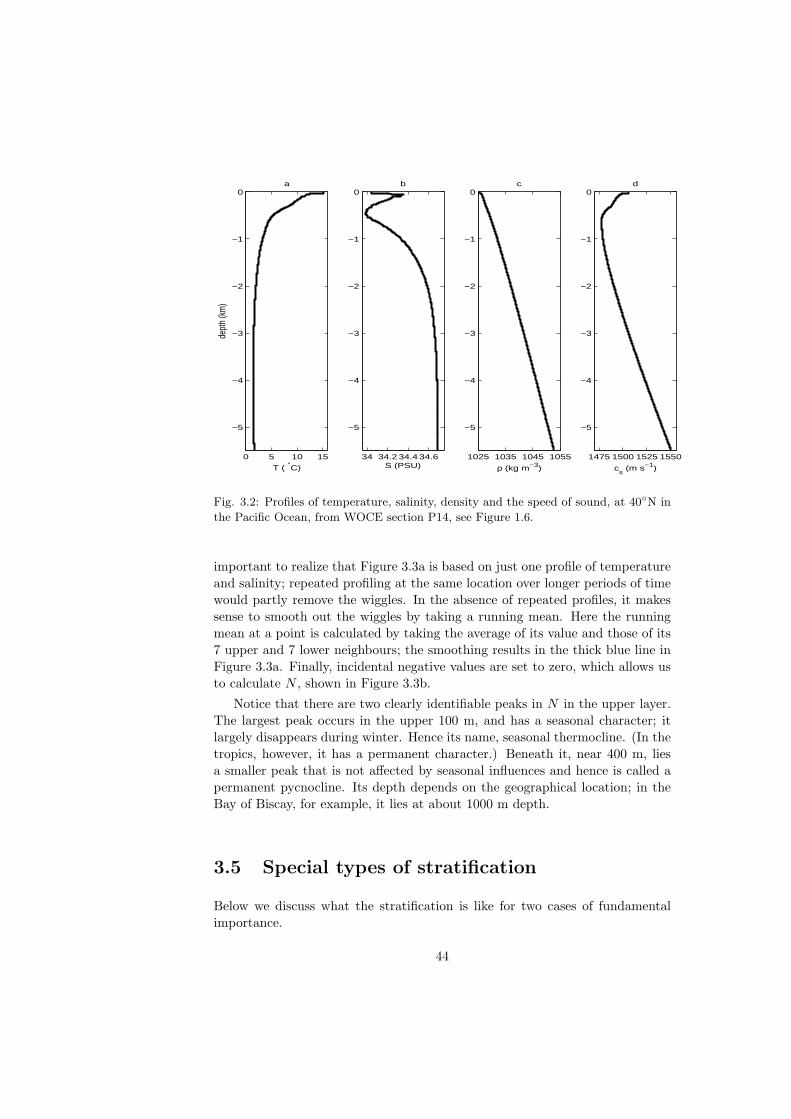
0 5 10 15

−5

−4

−3

−2

−1

0

T ( °C)

dept

h (k

m)

a

34 34.2 34.4 34.6

−5

−4

−3

−2

−1

0

S (PSU)

b

1025 1035 1045 1055

−5

−4

−3

−2

−1

0

ρ (kg m−3)

c

1475 1500 1525 1550

−5

−4

−3

−2

−1

0

cs (m s−1)

d

Fig. 3.2: Profiles of temperature, salinity, density and the speed of sound, at 40N in

the Pacific Ocean, from WOCE section P14, see Figure 1.6.

important to realize that Figure 3.3a is based on just one profile of temperatureand salinity; repeated profiling at the same location over longer periods of timewould partly remove the wiggles. In the absence of repeated profiles, it makessense to smooth out the wiggles by taking a running mean. Here the runningmean at a point is calculated by taking the average of its value and those of its7 upper and 7 lower neighbours; the smoothing results in the thick blue line inFigure 3.3a. Finally, incidental negative values are set to zero, which allows usto calculate N , shown in Figure 3.3b.

Notice that there are two clearly identifiable peaks in N in the upper layer.The largest peak occurs in the upper 100 m, and has a seasonal character; itlargely disappears during winter. Hence its name, seasonal thermocline. (In thetropics, however, it has a permanent character.) Beneath it, near 400 m, liesa smaller peak that is not affected by seasonal influences and hence is called apermanent pycnocline. Its depth depends on the geographical location; in theBay of Biscay, for example, it lies at about 1000 m depth.

3.5 Special types of stratification

Below we discuss what the stratification is like for two cases of fundamentalimportance.

44

0 0.5 1 1.5 2 2.5

x 10−4

−5

−4

−3

−2

−1

0

N2 (rad2 s−2)

dept

h (k

m)

a

0 1 2 3

x 10−5

−5

−4

−3

−2

−1

0

N2, raw

N2, smoothed

0 0.005 0.01 0.015

−5

−4

−3

−2

−1

0

N (rad s−1)

dept

h (k

m)

b

N, smoothed

Fig. 3.3: Profiles of N2 (panel a) and N (panel b) at 40N in the Pacific Ocean (WOCE

section P14, see Figure 1.6). In a, the noisy thin black line shows N2 obtained from

(1.1), using the original data at pressure intervals of 2 dbar; the inserted figure shows

a zoom. The blue thick line shows the result of smoothing by taking the running mean

over 15 points (i.e. stretches of 30 dbar); moreover, incidental negative values are set

equal to zero. Panel b shows the square root of the smoothed profile of panel a.

3.5.1 A fluid in thermodynamic equilibrium

The state of thermodynamic equilibrium is special from a fundamental point ofview, because of all the states with the same energy (i.e. internal plus potentialenergy) and the same mass, the equilibrium state has the largest entropy. Anyisolated body of fluid will evolve toward thermodynamic equilibrium, due tomolecular diffusion; the eventual state is one in which temperature and chemicalpotential are uniform (Figure 3.4, upper panels).

In thermodynamic equilibrium, then, temperature is uniform, T0(z) = Tc.If no salt is present (Sc = 0), then the stratification follows from (3.12) as

N2 =α2Tcg

2

cp. (3.13)

The right-hand side is always positive, so a fluid in thermodynamic equilibriumis always stably stratified. This conclusion holds a fortiori if salinity is present,since in thermodynamic equilibrium salinity increases strongly with depth (seethe end of Section 2.3.2, and Figure 3.4, upper panels), the chemical potential

45

being uniform. The last term in (3.12) then makes the stratification even morestable.

3 4 5 6−10

−8

−6

−4

−2

0a

T

20 40 60 80−10

−8

−6

−4

−2

0b

S

0 20 40 60 80−10

−8

−6

−4

−2

0c

η

0 20 40 60 80−10

−8

−6

−4

−2

0d

thermo−

dynamic

equilibrium

µ

3 4 5 6−10

−8

−6

−4

−2

0e

T

20 40 60 80−10

−8

−6

−4

−2

0f

S

0 20 40 60 80−10

−8

−6

−4

−2

0g

η

0 20 40 60 80−10

−8

−6

−4

−2

0h

convective

equilibrium

µ

Fig. 3.4: Two fictitious ocean states. Upper panels: thermodynamic equilibrium; lower

panels: convective equilibrium. In the upper panels temperature is chosen uniform (a),

while salinity (b) is chosen such that the chemical potential µ (d) is uniform; hence

a state of thermodynamic equilibrium. In the lower panels, salinity is chosen uniform

(f), while temperature (e) is chosen such that entropy η (g) is uniform; this describes

a state in which entropy and salinity are mixed, as in “convective equilibrium”. Units

as in Figure 2.2.

3.5.2 A turbulently mixed fluid

Molecular diffusion is a rather slow process. In geophysical fluid dynamics, itis turbulent (rather than molecular) mixing that often stamps the state of thefluid; it presumably tends to mix entropy and salinity, instead of temperatureand chemical potential (see also footnotes on p. 33).

Let the static entropy profile be given by η0(z). We can then express thestatic density gradient as

dρ0

dz=

(∂ρ

∂p

)ηS

dp0

dz+

(∂ρ

∂η

)pS

dη0

dz+

( ∂ρ

∂S

)pη

dS0

dz(3.14)

= −ρ0g

c2s

+(∂ρ

∂η

)pS

dη0

dz+

( ∂ρ

∂S

)pη

dS0

dz(3.15)

46

where we used (3.5) and (3.6). Thus (3.7) can be rewritten as

N2 = − g

ρ0

[(∂ρ

∂η

)pS

dη0

dz+

( ∂ρ

∂S

)pη

dS0

dz

]. (3.16)

Now, if entropy and salinity are uniform – a state called “convective equilibrium”(Figure 3.4, lower panels) – we obtain N2 = 0, i.e. the stratification is neutrallystable.

Such a state is sometimes referred to as ‘adiabatic’ or ‘isentropic’.3 Thisterminology is misleading, for contrary to what the terms may suggest, dia-batic processes must be involved to maintain such a state; otherwise the systemwould evolve towards thermodynamic equilibrium – an isothermal state. Putdifferently, for the state to stay away from thermodynamic equilibrium, it isnecessary that the entropy that is inevitably being continually produced in theinterior of the fluid, be expulsed to its surroundings; this is accomplished by aflow of heat through the system, with low-entropic incoming and high-entropicoutgoing energy. The Earth’s atmosphere/ocean system is a case in point; low-entropic short-wave radiation is received from the sun, while the Earth emitshigh-entropic long-wave radiation. The flow of energy is energetically neutral,but allows entropy to be expulsed. Similarly, living organisms do not eat to gainenergy, but to keep down entropy (and thus to postpone as long as possible thesorry state of thermodynamic equilibrium).4

3.6 Potential density

The relation between potential density and static stability is a complicated one.It is instructive to introduce first the concept of a ‘generalized’ potential density,which does provide a simple connection to static stability. From it, the potentialdensity, in its ordinary sense, can be deduced, but then the simple connectionto static stability is lost.

3.6.1 Generalized potential density

Imagine that a fluid parcel were moved from its initial vertical position z to acertain reference level zr, under conservation of its entropy and salinity. Thenwe define the density that the parcel would attain at its new position (i.e. at zr)as its potential density ρr(zr, z). Usually one takes zr fixed (see next section),but here we shall regard zr as a variable (hence the adjective ‘generalized’).

The potential density can be obtained by integrating (3.6); this gives

ρr(zr, z) = ρ0(z) + g

∫ z

zr

dz′ρ0(z′)

c2s(z, z′)

.

3The terms ‘adiabatic’ and ‘isentropic’ are not equivalent and should therefore not be usedinterchangeably. For example, the free expansion of a gas in a cylinder, being an irreversibleprocess, is adiabatic (i.e. there is no heat exchange with its surroundings), but not isentropic.

4See also the thought-provoking discussion of Emden’s ”Warum heizen wir im Winter?”by Sommerfeld [78, p. 38].

47

The left-hand side thus denotes the density a parcel, originally at z, would attainwhen brought adiabatically to zr. The speed of sound in the parcel, cs, dependson its original height z, as well as on the height z′, which it passes during thedisplacement. This is because the speed of sound depends on the state variablespressure, entropy and salinity, the first of which takes the ambient value p0(z′),whereas the last two retain their original values η0(z) and s0(z). This is animportant point, because differentiation to z now still yields an integral-term:

∂ρr

∂z(zr, z) =

dρ0

dz+

ρ0g

c2s

+ g

∫ z

zr

dz′ ρ0(z′)∂c−2

s

∂z(z, z′) .

Comparison with (3.7) shows that

N2(z) = − g

ρ0

∂ρr

∂z(zr, z) +

g2

ρ0

∫ z

zr

dz′ ρ0(z′)∂c−2

s

∂z(z, z′) . (3.17)

The quantity ρr depends on two independent variables: zr and z. By travers-ing the zr, z-plane along a certain line, we obtain a transect of the surfaceρr(zr, z). Of special importance is the transect along the line zr = z; this yieldsthe static density profile, since ρr(z, z) = ρ0(z). Furthermore, for zr = z, allthat remains of (3.17) is the simple expression

N2(z) = − g

ρ0

∂ρr

∂z(z, z) . (3.18)

Notice that the derivative on the right-hand side is not the gradient of the staticdensity ρ0. We follow the line zr = z, along which (as we saw above) the valuesof ρr are indeed equal to ρ0; the partial derivative in (3.18), however, doesnot produce the gradient of this curve, but rather the derivative in an obliquedirection (i.e. in a direction parallel to the z-axis).5

3.6.2 The common concept of potential density

Potential density, in its ordinary sense, is defined in the same way as was ρr

above, except that zr is taken to be fixed. To be specific, we shall choosezr = 0 (sea surface, level of standard atmospheric pressure), but the followingstatements are equally valid for any other fixed value. To make this change inthe meaning of zr explicit, we introduce the symbol

ρΘ(z) = ρr(0, z) .

Notice the difference from the previous section (where we followed the line zr =z): we now travers the zr, z-plane along a line zr = const.

The difference between (in-situ) density ρ and potential density ρΘ is shownin Figure 2.2e. In an incompressible fluid the two profiles would be identical;

5One may introduce a function ρl(z), the ‘local’ potential density [87], defined by equatingdρl/dz with the partial derivative on the right-hand side of (3.18); this provides us with afunction whose gradient is proportional to N2.

48

thus, the fact that the profiles (and their gradients, in particular) are quitedistinct testifies to the importance of compressibility.

It now follows immediately from (3.17) that

N2(z) = − g

ρ0

dρΘ

dz(z) +

g2

ρ0

∫ z

0

dz′ ρ0(z′)∂c−2

s

∂z(z, z′) . (3.19)

Due to the presence of the second term on the right-hand side, the signs of N2

and −dρΘ/dz need not be the same; in other words, the sign of the gradientof ρΘ is not, in principle, indicative of static (in)stability. In practice, however,the second term on the right-hand side usually turns out to be negligible unlessthe stratification comes close to neutral stability, N ≈ 0. In other words, itis a fact of experience that the gradient of potential density is indicative of(in)stability under most, but not all oceanographic conditions. The deeper partsof the South-Atlantic Ocean provide a negative example; here the exact criterionproves that the stratification is stable, whereas the sign of dρΘ/dz is positive(see [68, §7.352]). One usually deals with this problem by dividing the watercolumn in a certain number of layers, and choosing a separate reference levelzr for each layer. This is certainly more accurate, but it still does not producethe exact result, for this requires the introduction of infinitely many referencelevels, as in the previous section. Hence it is advisable to use always the exactcriterion (3.4), together with either (3.7) or (3.12).

It is only for the special case of uniform salinity that one finds a simpleexpression in terms of potential density. From its definition it follows thatpotential density ρΘ is a function only of the parcel’s entropy and salinity.Thus we can write

dρΘ

dz=

(∂ρΘ

∂η

)S

dη0

dz+

(∂ρΘ

∂S

)η

dS0

dz.

Recalling (3.16), we see that if salinity is uniform (S0(z) = Sc), the followingidentity holds:

N2 = − g

ρ0

(∂ρ

∂η

)pS

(∂ρΘ

∂η

)−1

S

dρΘ

dz. (3.20)

If the partial derivatives on the right-hand side have constant signs through-out the fluid, then one can conclude that the sign of dρΘ/dz is indicative of(in)stability.

3.7 Limitations of the concept of local stability

So far we have assumed that vertical displacements are infinitesimal, hencewe speak of local stability. This concept works fine if the entire column isstably stratified. However, layers that are locally unstable will collapse and besubject to turbulent mixing. This means that we have to take into account thefinite displacement of parcels; the criterion of local stability is then no longer

49

necessarily meaningful. In fact, convective mixing may extend into locally stablelayers.

To find the vertical extent of the region affected by local instability, a simplerule can be established. Parcels at the top of the locally unstable layer willdescend, parcels at its base will rise. These descending and rising movements arenot necessarily limited to the locally unstable layer itself; they will continue untilthe parcels arrive in a surrounding that matches their instanteneous density.This is illustrated in Figure 3.5. In this atmospheric example, effects of humidityare neglected. Local stability can then be defined by the gradient of potentialdensity (see (3.20)), or of the similarly defined potential temperature. Thecriterion of local stability identifies a layer of unstable stratification (Figure3.5a). The descending parcel from the top of this layer, and the rising parcelfrom its base (denoted by circles), will continue their vertical motion until theyarrive at a level at which the potential temperature equals their own (Figure3.5b). So, the effectively unstable layer is much thicker than the criterion oflocal stability would suggest.

Fig. 3.5: A fictitious atmospheric profile of potential temperature. Negative (positive)

gradients are indicative of locally unstable (stable) layers, as shown in a. However,

descending and rising parcels from the locally unstable layer will continue their move-

ment until they arrive at a level that matches their own potential temperature (b). As

a result, neighbouring locally stable layers will be subject to convective mixing as well.

(The question marks in b refer to the possibility that surface heating may render the

locally neutrally stratified bottom layer unstable.) From [81].

50

Chapter 4

Approximations

4.1 Introductory remarks

The fundamental equations of geophysical fluid dynamics defy direct analyticaltreatment. Even in a numerical approach one faces formidable complications.Hence it is desirable to introduce approximations and thereby to simplify theproblem. The procedure by which this is done usually consists of a series ofsteps. First each variable in the equation is replaced by its typical scale times adimensionless variable. Then, by collecting scales in each term, certain dimen-sionless parameters are identified, some of which may be considered small onempirical grounds, or just by assumption. Finally, the terms involving a smallparameter are neglected.

Implicit in this procedure is the idea ‘the smaller a term, the less important’.An utterly trivial example may serve to make this look less obvious. Considerthe algebraic equation a = b + c, and let us assume that all terms are of orderone; hence none of them is negligible. Next we rewrite the equation by definingb = b + 1000 and c = c − 1000, giving a = b + c. The term on the left-handside is now three orders of magnitude smaller than either of the terms on theright, and (according to a naive way of reasoning) can therefore be considerednegligible. At the same time, obviously, the term cannot have become negligiblemerely by rewriting the equation.

The problem lies in the mistaken notion that terms can be negligible in anequation as such. Upon closer examination, what happens in an approximatingprocedure is this: we approximate, i.e. replace, the exact fields (e.g. currentvelocity, density etc.) by slightly different ones. Not surprisingly, these ap-proximated fields satisfy an equation that differs from the original one. Thismay seem a rather scholastic point, but the following example will illustrate itsspecific meaning.

In a later section we will encounter an equation that provides the boundary

51

condition at the upper surface; after having been scaled, the equation reads:

ε∂p′

∂t= w , (4.1)

where a ’hat’ indicates that the variable is scaled and dimensionless (p′ denotesthe departure of pressure from its hydrostatic value). Empirically it is knownthat the dimensionless parameter ε is much smaller than one. What can we inferfrom that? Obviously, one cannot say that “the left-hand side is small comparedwith the right” (a lapsus in a famous textbook); the equality sign, after all, tellsus that the two sides are equal. What we can do, however, is to expand thevariables p′ and w in a series, in which ε serves as the small parameter:

p′ = p(0) + εp(1) + ε2p(2) + · · · w = w(0) + εw(1) + ε2w(2) + · · · ,

where all the p(i) and w(i) are assumed to be of order one. Subsitution in (4.1)then gives, to first order,

w(0) = 0 , (4.2)

showing that w(0) vanishes at the surface. This is a simpler equation than (4.1),but notice that (4.1) and (4.2) are about different variables; the former dealswith the original vertical velocity w, the latter with its first-order approximationw(0).

However, this precise way of writing becomes unwieldy when several approx-imations are made, involving different small parameters; in the end, we would beworking with things like w(0,0,0,0,0,0). This is why the explicit expansion is usu-ally left out altogether, so that we jump directly from (4.1) to (4.2), the lattermoreover being written as w = 0 (incorrectly suggesting that we are still dealingwith the original variable; and opening the trap of substituting approximatedexpressions back into the original equations. . . ). Furthermore, we describe theprocess somewhat fuzzily by saying that we have approximated (4.1) by (4.2);in the next sections we often follow this parlance, for the sake of brevity.

4.2 Overview

Our starting point is the set (2.19). For later convenience, we rewrite the con-tinuity equation (2.19b) using the energy equation (2.19c):

ρ(D~u

Dt+ 2~Ω× ~u

)= −∇p− ρgz (4.3a)

ρ∇ · ~u = − 1c2s

Dp

Dt(4.3b)

Dρ

Dt=

1c2s

Dp

Dt(4.3c)

DS

Dt= 0 (4.3d)

cs = Γ(ρ, p, S) , (4.3e)

52

Approximation: meaning: removes:

Quasi-incompressibility divergence-free velocity, a.o. sound wavesLinearization (*) advective terms removed wave interactionsf -plane fixed latitude Rossby/planetary waves

’Traditional Approx.’ (*) f -terms neglected short low-freq. int. IGWHydrostaticity (*) vertical acceleration neglected gyroscopic wavesGeostrophy (**) Coriolis balances pressure grad. (internal) IGW

Table 4.1: Various approximations, what they mean, and what phenomenon isremoved by making them. ’IGW’ stands for inertio-gravity waves.

from which the unknowns ~u, ρ, p and S are to be solved.This set appears intractable; in an attempt to derive analytical solutions, we

would encounter a number of hurdles. Mathematically, the hurdles appear in theform of nonlinear terms, as well as terms with non-constant coefficients. Belowwe discuss under what circumstances these terms can be neglected. Physically,the hurdles just mean that the equations in their present form are ’too rich’;they contain phenomena in which we are not (or not primarily) interested, suchas sound waves, large-amplitude waves etc. By making the approximationsdiscussed below, we discard these phenomena one by one.

Common approximations and their consequences to wave phenomena arelisted in Table 4.1; approximations marked by an asterisk will not (**), or notalways (*), be adopted in this book.

4.3 Quasi-incompressibility

All approximations discussed in this section rest on the assumption that den-sity varies relatively little in the domain under consideration.1 In other words,we assume that the (vertical) scale over which density varies by one order ofmagnitude is much larger than the scale of the phenomena we are looking at.This requirement is very well satisfied in the ocean, and reasonably well in theatmosphere if we restrict ourselves to vertical scales of the order of 100 m.

4.3.1 Momentum equations

In classical mechanics, two concepts of mass are sometimes distinguished: in-ertial and gravitational mass.2 Inertial mass is a measure of how strongly abody resists a change in velocity when subjected to a force; gravitational massdetermines the force by which a body is attracted in a field of gravity. Theformer has a passive connotation, the latter an active one.

1In the literature, these approximations, or a subset of them, are often referred to as “the”Boussinesq approximation. Since opinions differ on exactly what is to be understood by thisterm, its usage tends to confuse rather than to clarify the issue; for this reason, we avoid theterm altogether.

2It was shown observationally by Eotvos that the two can be identified numerically; later,conceptual equality was implied by Einstein’s theory of general relativity.

53

It is instructive to consider first a simple mechanical problem: Atwood’smachine, see Figure 4.1. The net force working on the connected bodies isg∆m; this force pulls at a total mass of 2m + ∆m. Hence the acceleration is

a =g∆m

2m + ∆m.

Now, if ∆m ¿ m, then we can approximate this expression by

a ≈ g∆m

2m.

This amounts to neglecting the difference in mass, but only so far as the inertialmass is concerned; in the gravitational mass the difference remains essentialsince otherwise their would be no net force.

Fig. 4.1: Atwood’s machine: two bodies are connected by a string passing over a

pulley. The mass of body II, m + ∆m, slightly exceeds that of body I, m.

In the ocean, density varies by at most a few percentage points (see Figure2.2e, solid line). This suggests that we may replace density by a constant ref-erence value ρ∗ in the momentum equations (4.3a), but of course only wheredensity plays its “inertial” role. Hence

ρ∗(D~u

Dt+ 2~Ω× ~u

)= −∇p− ρgz . (4.4)

This natural and seemingly innocent approximation deserves further comment.One important quantity in fluid dynamics is vorticity, ∇ × ~u. Now, how canvorticity be created? According to (4.3a) we have

∂

∂t(∇× ~u) + · · · = −∇×

(∇p

ρ

), (4.5)

54

stating that pressure gradients can create vorticity, while gravity cannot. (Theadvective and Coriolis terms play no role in this argument and are rendered bydots.)

Repeating the same procedure in (4.4), we find

∂

∂t(∇× ~u) + · · · = −∇×

(ρgz

ρ∗

), (4.6)

stating that gravity can create vorticity, while pressure gradients cannot – theexact reverse of what we found in the original equation (4.5)!

Lest we conclude that this consequence wholly discredits the validity of theapproximation, we should realize that gravity and pressure gradients are closelyconnected in geophysical flows. For example, horizontal density gradients resultin pressure gradients due to gravity. In practice, the reversal of roles is thusfairly harmless.

4.3.2 Mass and energy equations

As in the previous chapter, we will think of internal waves as a perturbation ofa (known) static background state that has only vertical dependences; thus

p = p0(z) + p′(t, ~x) (4.7)

ρ = ρ0(z) + ρ′(t, ~x) (4.8)

(and similarly for salinity); the primed fields are associated with the internal-wave motion. The static fields obey the hydrostatic balance:

dp0

dz= −ρ0g . (4.9)

At this stage, these steps neither presume nor imply anything, for the fields p

and ρ can always be written like this. The right-hand side of (4.4) can now bewritten as

−∇p′ − ρ′gz

and (4.3b,c) become

ρ∇ · ~u = − 1c2s

Dp′

Dt+ w

ρ0g

c2s

(4.10)

Dρ′

Dt+ w

dρ0

dz=

1c2s

Dp′

Dt− w

ρ0g

c2s

. (4.11)

To proceed, we must assume something about the time-scale of the motionin question.3 In geophysical fluid dynamics, one may (roughly) distinguish two

3In scaling procedures like this, there is always an element of reasoning in a circle: theresulting approximated equations we “prove” to be valid simply reflect the primary balance weassumed in the first place; in other words, ’what you want is what you get’. Indeed, nothingis strictly proven; we only delineate the conditions under which the approximated equationscan be expected to be valid; and, in the end, only a comparison with empirical observationcan bear out their validity.

55

types of motion. One is the large-scale flows, with time scales (much) largerthan f−1; here, the primary balance in the horizontal momentum equations isbetween the Coriolis force and the pressure gradient (geostrophy). The otherone is inertio-gravity waves, with time scales smaller than f−1; here the primarybalance is typically between acceleration and the pressure gradient. For ourpurposes, the second assumption is the most appropriate one. Denote the scalesof t, x, u and p′ by T , L, U and P ; then, by assumption:

ρ∗U

T∼ P

L.

Since we are dealing with waves, the length and time scales are related byL/T = C, the phase speed, which for internal waves in the oceans typically isof the order of 1 m s−1. We may thus write

P ∼ ρ∗CU . (4.12)

At this stage, it is useful to introduce one more type of velocity, namely thephase speed of long surface waves: csf = (gD)1/2, where D is water depth. Wesummarize the typical orders of magnitude of the four speeds we have introducedso far, all in meters per second:

U ∼ O(10−1) ; C ∼ O(1) ; csf ∼ O(101 , 102) ; cs ∼ O(103) m s−1 .

They denote the particle velocity and phase speed of internal waves, the phasespeed of surface waves, and the speed of sound in seawater, respectively. Wethus have

U ¿ C ¿ csf ¿ cs . (4.13)

These estimates form an important guide to the approximations made below.We first consider (4.10), and denote the typical scales above each term:

ρ∗U/L︷︸︸︷ρ∂u

∂x+

ρ∗U/L︷︸︸︷ρ∂v

∂y+

ρ∗W/H︷ ︸︸ ︷ρ∂w

∂z= −

P/(Tc2s)︷ ︸︸ ︷

1c2s

∂p′

∂t−

UP/(Lc2s)︷ ︸︸ ︷

u

c2s

∂p′

∂x−

UP/(Lc2s)︷ ︸︸ ︷

v

c2s

∂p′

∂y−

WP/(Hc2s)︷ ︸︸ ︷

w

c2s

∂p′

∂z+

ρ∗Wg/c2s︷ ︸︸ ︷

wρ0g

c2s

.

Here we introduced the vertical internal-wave scales W and H,4 as yet unrelatedto the other scales. By comparing the first term on the right with the first termon the left, we find from (4.12) and (4.13) that their ratio is C2/c2

s ¿ 1, sothe latter dominates. We find the same for the first two advective terms on theright, even if we would take U ∼ C (as is the case for strongly nonlinear waves,see next section). Similarly, we find that the third term on the left dominatesthe fourth term on the right. It also dominates the fifth term on the right, since

4For clarity, we emphasize that H does not represent the scale of the amplitude of theinternal wave, but rather the vertical scale over which the internal-wave field varies by oneorder of magnitude; this may often be simply water depth itself.

56

gH < gD = c2sf ¿ c2

s. 5 In other words, each of the terms on the right is muchsmaller than at least one of the terms on the left, so we can conclude that thevelocity field is to a close approximation given by a field ~u(0) that obeys (cf.Section 4.1)

∇ · ~u(0) = 0 . (4.14)

An immediate consequence is that volumes of water parcels are now conserved,which combines awkwardly with the variation in density that is still allowed.As a result, mass is no longer conserved. For wave-phenomena, this problem isnot too serious, because the oscillatory nature of the motion implies that massgains are followed by, and indeed annulled by mass losses, and vice versa.

For later usage, we note that the scale W can be expressed via (4.14) as

W ∼ UH/L . (4.15)

We now consider the energy equation (4.11), and focus our attention on theright-hand side:

· · · = +

P/(Tc2s)︷ ︸︸ ︷

1c2s

∂p′

∂t+

UP/(Lc2s)︷ ︸︸ ︷

u

c2s

∂p′

∂x+

UP/(Lc2s)︷ ︸︸ ︷

v

c2s

∂p′

∂y+

WP/(Hc2s)︷ ︸︸ ︷

w

c2s

∂p′

∂z−

Wρ∗g/c2s︷ ︸︸ ︷

wρ0g

c2s

Using (4.12) and (4.15), we find that the ratio of the first and last term scales asC2/(gH). Now, the vertical scale of internal waves is often nearly waterdepthitself, in which case C2/(gD) = C2/c2

sf ¿ 1 by (4.13). Even if we have muchsmaller scales (for example when an internal-wave is trapped in the thermocline),then we would still have H ∼ 101 to 102 m, so that the condition is still met.The first term on the right is thus much smaller than the last one; the advectiveterms too are much smaller, as one sees by a similar argument. Hence, the fieldsare to a good approximation given by

Dρ′(0)

Dt+ w(0)

(dρ0

dz+

ρ0g

c2s

)= 0 , (4.16)

where we brought the remaining term from the right-hand side to the left.

4.3.3 Resulting equations

In summary, we have reduced (4.3a-c) – via (4.4), (4.14) and (4.16) – to

D~u

Dt+ 2~Ω× ~u = − 1

ρ∗∇p′ + bz (4.17a)

∇ · ~u = 0 (4.17b)Db

Dt+ N2w = 0 , (4.17c)

5Notice that this condition may pose a problem in the atmosphere, where the speed ofsound is much smaller than in the ocean: cs ∼ 300m s−1. In that case one must assumethat H, the vertical scale of the internal-wave, is sufficiently small (i.e. much smaller than thethickness of the troposphere); otherwise the approximation (4.14) will be invalid.

57

where we dropped the scripts ·(0), and introduced a convenient quantity calledbuoyancy:

b = −gρ′/ρ∗ . (4.18)

Buoyancy can be interpreted as (minus) the effective gravity, associated withthe Archimedean force. We also used the definition of the buoyancy frequencyfrom (3.7):

N2 = − g

ρ∗

(dρ0

dz+

ρ0g

c2s

), (4.19)

but with ρ0 replaced by ρ∗ in the denominator on the right-hand side, in line withthe approximation made in the previous section. Since N refers to the staticstate, we can evaluate the speed of sound cs as a function of the prescribedstatic fields, i.e. cs = Γ(ρ0, p0, S0); cs can thus be regarded as a known functionof z.

The upshot is that effects of compressibility can be neglected except in thedefinition of the background stratification (4.19). The importance of the secondterm on the right-hand side of (4.19) was earlier demonstrated in Section 3.2.

The simplifications introduced in this section come at a price, in that theydistort a number of fundamental balances; we discussed this already for thevorticity balance and mass conservation. It is beyond the scope of this textto discuss in detail that the energy balance, too, can get distorted. If diabaticprocesses were included, one would find that a supply (or loss) of heat is repre-sented by an extraction (or supply) of mass; in other words, in the approximatedequations heat is represented as a form of mass, not energy (an ironic reversalof 19th-century progress in thermodynamics). In thermodynamic cycles, e.g.thermal convection, one then finds that gravity is doing net work in the modelequations, as opposed to pressure in reality [89].

Notwithstanding these problems, the set (4.17) has the merit that soundwaves have been filtered out from the equations; this is due to the approximationof (4.3b) by (4.17b).

4.4 The ‘Traditional Approximation’

The so-called ‘Traditional Approximation’ consists in neglecting the terms withf , i.e. the Coriolis terms involving the cosine of latitude. In the momentumequations (4.17a), written out in its components, there are two such terms:

Du

Dt− fv + fw = − 1

ρ∗

∂p′

∂x(4.20a)

Dv

Dt+ fu = − 1

ρ∗

∂p′

∂y(4.20b)

Dw

Dt− fu = − 1

ρ∗

∂p′

∂z+ b . (4.20c)

At mid-latitudes the parameter f is of course equally large as f ; it seems odd,then, to neglect the terms with f while retaining those with f . However, the

58

difference between the two is that f is always associated with vertical motions(either a vertical velocity or a vertical acceleration), whereas f is associatedwith horizontal motions alone. Low-frequency motions are usually predomi-nantly horizontal, so that the effects of f are generally slight. Moreover, strongstratification, in the sense that N À Ω, tends to suppress vertical motions, thusdiminishing the role of f . Still, weakly stratified regions occur in the abyssalocean (see Figure 1.6); in these regions, ‘non-traditional’ effects can be quitesignificant, especially for near-inertial internal waves (i.e. internal waves at fre-quencies close to |f |). More generally, other kinds of motions can be affected aswell, such as deep convection, Ekman layers, and equatorial flows, see [30].

The mathematical structure of the problem depends on whether one makesthe Traditional Approximation or not. With f included, solutions can no longerbe obtained by separation of horizontal and vertical variables. For the standardinternal-wave problems, however, this obstacle proves illusory. In the followingchapters, we therefore include sections on ‘non-traditional’ results, which areobtained without any difficulty.

4.5 Linearization

Nonlinear terms are those that contain products of unknowns. So in (4.17a),we identify the nonlinear term (~u · ∇)~u; (4.17c) similarly contains advectiveterms. These terms are responsible for interactions among waves. Omittingthem greatly simplifies the problem, for this allows wave solutions to be super-posed, the superposition being a solution, too. Generally speaking, nonlinearterms are negligible if the wave amplitude is sufficiently small. In the remainderof this section, we specify what is here meant by ‘small’.

In (4.17a), we consider the material derivative Du/Dt:

U/T︷︸︸︷∂u

∂t+

U2/L︷︸︸︷u

∂u

∂x+

U2/L︷︸︸︷v∂u

∂y+

UW/H︷ ︸︸ ︷w

∂u

∂z+ · · ·

where the dots stand for the Coriolis terms and pressure gradient. Using thescales of Section 4.3.2, we find that the ratio of each of the nonlinear terms andthe time-derivative is U/C, where C = L/T is the phase speed of the internalwave. Thus, nonlinear terms can be neglected if U ¿ C, i.e. if the horizontalvelocity of the water parcels is much smaller than the phase speed. Typically,internal-wave phase speeds are of the order of 1 meter per second, so horizontalcurrents should be less than, say, 10 cm per second, for nonlinear terms to benegligible. The other momentum equations yield the same criterion, and so does(4.17c).

59

4.5.1 Resulting equations

Under the assumption, then, that all nonlinear terms can be neglected, (4.17)reduces to

∂u

∂t− fv + fw = − 1

ρ∗

∂p′

∂x(4.21a)

∂v

∂t+ fu = − 1

ρ∗

∂p′

∂y(4.21b)

∂w

∂t− fu = − 1

ρ∗

∂p′

∂z+ b (4.21c)

∂u

∂x+

∂v

∂y+

∂w

∂z= 0 (4.21d)

∂b

∂t+ N2w = 0 . (4.21e)

From these five equations, it is easy to derive a single equation for one of theunknowns. Taking ∂/∂z of (4.21b), and ∂/∂y of (4.21c), and subtracting theresults, gives

∂

∂t

(∂w

∂y− ∂v

∂z

)=

(f

∂

∂y+ f

∂

∂z

)u +

∂b

∂y. (4.22)

Similarly, taking ∂/∂z of (4.21a), and ∂/∂x of (4.21c), gives

∂

∂t

(∂u

∂z− ∂w

∂x

)=

(f

∂

∂y+ f

∂

∂z

)v − ∂b

∂x, (4.23)

where we used the continuity equation, (4.21d). Finally, combining ∂/∂y of(4.21a) and ∂/∂x of (4.21b):

∂

∂t

(∂v

∂x− ∂u

∂y

)=

(f

∂

∂y+ f

∂

∂z

)w , (4.24)

where we used, again, (4.21d). On the left-hand sides of (4.22), (4.23) and(4.24), we recognize the vorticity, ∇ × ~u, discussed in Section 4.3.1. Vorticityis a measure of the rotation of water parcels, i.e. their change in orientation.6

We noted earlier that the creation of vorticity by gravity (here represented bybuoyancy b), rather than by pressure gradients, is an artifact of assuming quasi-incompressibility.

Subtracting ∂2/∂y∂t of (4.22) and ∂2/∂x∂t of (4.23), gives

∂2

∂t2

(∇2

hw − ∂

∂z

[∂u

∂x+

∂v

∂y

])+

(f

∂

∂y+ f

∂

∂z

) ∂

∂t

(∂v

∂x− ∂u

∂y

)−∇2

h

∂b

∂t= 0 ,

where we defined

∇2h =

∂2

∂x2+

∂2

∂y2.

6This type of movement should not be confused with those of parcels traversing for examplea circle in a translational movement, in which case the orientation of the parcels stays thesame.

60

The term in square brackets can be rewritten with (4.21d); the Coriolis terms,with (4.24); and the last term, with (4.21e). The end result is an equation forw alone:

∂2

∂t2∇2w + (~f · ∇)2w + N2∇2

hw = 0 , (4.25)

where ~f = (0, f , f) and

∇2 =∂2

∂x2+

∂2

∂y2+

∂2

∂z2.

It can be shown that the other variables (u, v, p′ and b) satisfy the same equa-tion. The reason for selecting the vertical velocity component lies in the factthat the boundary conditions, to be introduced later, are most easily posed interms of this variable.

Eq. (4.25) will be the starting point for further analysis in following chapters.We note that the buoyancy frequency N is allowed to vary with z, in which case(4.25) has a non-constant coefficient.

4.5.2 Energy equation

A simple but instructive equation can be derived from (4.17a,b,c,e); multiplyingthem by u, v, w and b/N2, respectively, and adding up the resulting equations,one obtains

12

ρ∗∂

∂t

[u2 + v2 + w2 + b2/N2

]+ ~u · ∇p′ = 0 . (4.26)

This is an energy equation: the energy density E, being the sum of kinetic andpotential energy, is given by7

E =12

ρ∗[u2 + v2 + w2 + b2/N2

]. (4.27)

The other term in (4.26), ~u · ∇p′, can also be written as ∇ · (~up′) (because of(4.21d)) and thus represents the divergence of a flux. If we integrate (4.26)over a volume, we find that temporal changes in the volume-integrated energydensity must be equal to the flux through the boundaries of the volume. Inother words, (4.26) expresses conservation of energy. Note that the Coriolisforce plays no role in this equation; it acts as a deflecting force, perpendicularto the motion itself, and hence does no work.

7It is important to note that (4.27) is only valid if one of the following conditions is fulfilled:a) waves are linear, or b) the buoyancy frequency N is constant, or both. For nonlinear waves ina medium with variable N , the expression becomes more complicated, and involves derivativesin N : E = 1

2ρ∗ [u2 + v2 + w2 + b2/N2 − 1

3(b3/N6) d(N2)/dz + · · · ], see [42] and [58, p. 211].

61

4.6 Rigid-lid approximation

The ocean supports not only internal waves, but of course also surface waves.We wish to concentrate on the former. Yet, we cannot simply assume that thesurface is still, because internal-wave propagation is accompanied by small ele-vations and depressions of the surface; this merely reflects the pressure gradientsinherent to the passage of an internal wave. These vertical excursions of thesurface are very small compared to those in the ocean’s interior. The reasonfor this is simple: the same force that is able to give isopycnals in the interiorlarge vertical excursions, can only produce a very small excursion of the surface,because the latter has a much larger vertical density gradient (that between airand water) than has the ocean’s interior. This fact can be exploited to sim-plify the boundary condition at the surface, leading to the so-called ’rigid-lidapproximation’.

Let the free surface be described by

z = η(t, x, y) ,

whence follows

w(t, x, y, η) =Dη

Dt

=∂η

∂t+ u

∂η

∂x+ v

∂η

∂y.

Moreover, we suppose that the atmospheric pressure at the free surface, pa, isconstant:

p(t, x, y, η) = p0(η) + p′(t, x, y, η) = pa .

where we wrote pressure p as the sum of the static (p0) and dynamic (p′) parts,as in (4.7). A Taylor expansion about z = 0 gives

w(t, x, y, 0) + η∂w

∂z+ · · · =

∂η

∂t+ u(t, x, y, 0)

∂η

∂x+ · · ·

+ v(t, x, y, 0)∂η

∂y+ · · ·

p0(0) + p′(t, x, y, 0) + η(dp0

dz+

∂p′

∂z

)+ · · · = pa .

Assuming amplitudes to be small, we can, like in Section 4.5, neglect productof perturbation terms (i.e. involving u, v, w, η and p′), so that

w =∂η

∂tat z = 0

p0 + p′ + ηdp0

dz= pa at z = 0 .

Using the hydrostatic balance, (4.9), we can combine the two equations into

∂p′

∂t= wρ0g at z = 0 . (4.28)

62

We cast this equation in a nondimensional form, by using the scale for pressurep′ from (4.12), and that for w from (4.15). Moreover, we take for the constantreference density, ρ∗, the static surface value: ρ0(0) = ρ∗. By writing w = Ww,p′ = P p′ and t = T t, we then obtain

C2

c2sf

∂p′

∂t= w at z = 0 . (4.29)

Recall that C = L/T is a measure of the phase speed of internal waves, whilecsf is that of surface gravity waves (c2

sf = gH, H water depth). Now, accordingto (4.13), the ratio of the two is small. The underlying reason is that thesephase speeds are proportional to the square root of effective gravity; for surfacewaves, this is simply g, but for internal waves, it is the much smaller g′, beingproportional to relative differences in density in the ocean’s interior. HenceC ¿ csf , or expressed in terms of a small parameter ε,

ε =C2

c2sf

¿ 1 .

We thus arrive at (4.1). As explained in Section 4.1, we can now expand p andw in a series in which ε serves as the small parameter, and to lowest order onefinds

w(0) = 0 at z = 0 . (4.30)

This is the so-called ’rigid-lid approximation’. It means that surface elevationsare neglected, as if the surface were covered by a rigid plate. At such a plate,vertical velocities would be zero, as in (4.30). The pressure, however, is not zeroat the plate: pressure variations that would otherwise have been associated withelevations of the free surface, are now exerted by the rigid plate, in response tothe internal-wave motions. (An example of the pressure field is shown in Figure5.4).

At the bottom, the boundary condition is more straightforward, namely that ofno normal flow. We describe the bottom by

z = −h(x, y) .

The boundary condition can then be written as

w = −u∂h

∂x− v

∂h

∂yat z = −h . (4.31)

Slopes of the ocean floor are predominantly less than 0.02, see Figure 4.2.In many cases we will assume, for the sake of simplicity, that the bottom is

horizontal, with water depth H, in which case (4.31) becomes

w = 0 at z = −H . (4.32)

The idealized character of this assumption is evident from a look at real oceantopography, see for example Figure 1.6!

63

0 0.01 0.02 0.03 0.04 0.05 0.06 0.07 0.08 0.09 0.10

10

20

30

40

50

60

70

80

tangent of slope, γ

dist

ribut

ion

D(γ

)

Fig. 4.2: Slope distribution based on several profiles from a topographic database.

Slopes are mostly gentle; 67% of the slopes is less than 0.02. The red curve shows a

fit with a Burr distribution a(1 + γb)−c, with a = 91, b = 0.65 and c = 25. From [29].

4.7 Preview: methods of solution

As a preparation for the following two chapters, in which we discuss linearinternal-wave solutions, we first take a closer look at (4.25):

∂2

∂t2∇2w + (~f · ∇)2w + N2∇2

hw = 0 . (4.33)

Supposing waves to be sinusoidal in time, at frequency ω, i.e.

w ∼ exp(−iωt) ,

we find from (4.25), 8

(N2 − ω2 + f2)wyy + 2ffwyz + (f2 − ω2)wzz + (N2 − ω2)wxx = 0 . (4.34)

Recall that x is the west-east coordinate, and y, south-north. These coordinatesplay different roles in (4.34). In other words, there is an anisotropy in thehorizontal plane: northward propagating waves, say, behave differently fromeastward propagating ones.

However, under the Traditional Approximation, where f is neglected, theanisotropy disappears, since (4.34) then becomes

(N2 − ω2)∇2hw − (ω2 − f2)wzz = 0 . (4.35)

8Strictly, another symbol than w should be used in (4.34); from the context it will howeverbe always clear whether w is meant to indicate the time-dependent w from (4.33), or thepurely spatially dependent one from (4.34).

64

Here x and y play identical roles. This means that if we consider propagating inthe x-direction, taking ∂/∂y = 0, we may apply the results thus obtained alsoto any other direction of wave propagation.

Taking ∂/∂y = 0, then, (4.35) becomes

(N2 − ω2)wxx − (ω2 − f2)wzz = 0 . (4.36)

There are now two main roads to solution, which we briefly outline here; adetailed discussion follows in Chapters 5 and 6.

For uniform stratification, i.e. N = const, all coefficients of (4.36) are con-stant, and the general solution can be written

w = F (µ+x− z) + G(µ−x− z) , (4.37)

where F and G are arbitrary functions. The coefficients µ± are given by

µ± = ±( ω2 − f2

N2 − ω2

)1/2

. (4.38)

As discussed below, the physical significance of the coordinates µ±x − z, theso-called characteristic coordinates, lies in the fact that internal-wave energypropagates along lines µ±x − z = const., which are diagonals in the x, z-plane(cf. Figure 1.9).

This method of characteristics forms the subject of Chapter 6. It rests on theassumption of constant N , but involves no assumption concerning the bound-aries of the system. It can therefore be applied to, for example, the problem ofinternal-wave reflection from a sloping bottom.

If, on the other hand, the buoyancy frequency varies with the vertical – as itdoes particularly strongly in the seasonal thermocline, see Figures 1.6 and 3.3b– then another method may be used that involves no assumption on N(z), butdoes require boundaries (bottom, surface) to be horizontal. This is the methodof vertical modes, in which we write

w = W (z) exp ikx , (4.39)

substitution of which into (4.36) gives

W ′′ + k2 N2(z)− ω2

ω2 − f2W = 0 . (4.40)

(Primes denotes derivatives to z.) Together with the boundary conditions W =0 at z = −H, 0 (bottom, surface), this constitutes a Sturm-Liouville problem.Its solution is formed by a set of eigenvalues kn and corresponding eigenfunctionsWn. For some special choices of N(z), Wn can be obtained in analytical form;otherwise (4.40) has to be solved numerically. Either way, the general solutionconsists of an arbitrary superposition of modes. This method forms the subjectof the next chapter.

We thus have two methods at our disposal, involving different assumptions.The case of overlapping validity occurs when stratification is constant and

65

boundaries are horizontal. Despite their different appearances, (4.37) on theone hand, and the solution to (4.39,4.40) on the other, are then entirely equiv-alent (see Section 6.3). There is however also a case in which neither methodworks: when both stratification and water depth vary. This occurs, for example,in the upper part of the water column, near the seasonal thermocline, over thecontinental slope. This is a very important region in the study of internal waves,since internal tides are generated here. To treat this problem satisfactorily, onethus has to resort to numerical methods. Nonetheless, the two analytical meth-ods discussed in the following chapters already provide important clues to howinternal waves propagate. We also discuss how the two methods of solution canbe applied in the more general ’non-traditional’ case.

66

Chapter 5

Internal-wave propagation

I: method of vertical modes

The ocean’s boundaries in the vertical, bottom and surface, naturally confinethe propagation of internal waves; the boundaries act as a waveguide. A moresubtle form of waveguide is a region of strong stratification in the water column,which acts as a waveguide for high-frequency internal waves. In either case, theinternal wave has the character of a standing wave in the vertical, while itpropagates in the horizontal. These properties are exploited in the method ofvertical modes. It has the advantage that it works for any buoyancy profileN(z), but it requires boundaries to be horizontal, since the solution is obtainedby a separation of the horizontal and vertical variables.

5.1 General formulation

The starting point is (4.25),

∂2

∂t2∇2w + (~f · ∇)2w + N2∇2

hw = 0 . (5.1)

Recall that ~f = (0, f , f). We assume first that f = 0 (Traditional Approxi-mation), and defer a discussion of non-traditional effects to Section 5.6. Thisassumption renders the horizontal plane isotropic, in the sense that the direc-tion of wave propagation becomes immaterial. Withous loss of generality, then,we can consider wave propagation in the west-east direction, i.e. along x; theresults will similarly apply to any other direction. We seek solutions of the form

w = W (z) exp i(kx− ωt) . (5.2)

67

(We take ω to be positive.) Substitution in (5.1), with f = 0, results in anordinary differential equation for W :

W ′′ + k2 N2(z)− ω2

ω2 − f2W = 0 . (5.3)

Primes denote derivatives to z. Since k here occurs as a square, k2, solutionswith positive k (describing rightward propagating waves), which we will denoteby k+, imply that another solution exists with k− = −k+, describing leftwardpropagating waves. So, without loss of generality, we can assume k to be posi-tive, adding afterward solutions with −k, if needed.

In addition to (5.3), we pose the boundary conditions at the surface (regardedas a rigid-lid, see Section 4.6) and the horizontal bottom:

W = 0 at z = 0, −H . (5.4)

Together, (5.3) and (5.4) form a Sturm-Liouville problem, which for fixed ω

has an infinite number of solutions Wn (eigenfunctions, vertical modes) withcorresponding eigenvalues kn.

The other variables u, v, p and b can be expressed similarly as (5.2), with

U =i

kW ′ ; V =

f

ωkW ′ ; P = iρ∗

ω2 − f2

ωk2W ′ ; B = − iN2

ωW . (5.5)

These expressions follow from (4.21). Notice that (5.4) and (5.5) imply that thevertically integrated horizontal velocities are zero, i.e.,

∫ 0

−H

dz u = 0 ;∫ 0

−H

dz v = 0 .

This property distinguishes internal waves from surface waves.The general solution of w consists of the superposition

w =∑

n

Wn(z)[a±n exp i(k±nx− ωt)

], (5.6)

with arbitrary complex constants a±n . The terms with index ’plus’ describerightward propagating waves, those with ’minus’, leftward propagating ones. Itis understood that the real part is being taken.

5.1.1 Oscillatory versus exponential behaviour

For convenience, we introduce

m2(z) = k2 N2(z)− ω2

ω2 − f2. (5.7)

Solutions to (5.3) may exhibit two kinds of behaviour, depending on the sign ofm2. Firstly, oscillatory in those parts of the water column where m is real, i.e.

68

m2(z) ≥ 0. For this to be possible, one of the two following inequalities musthold throughout this part of the water column:

(I) N(z) ≤ ω ≤ |f | or (II) |f | ≤ ω ≤ N(z) . (5.8)

The prevailing situation in the ocean and atmosphere is N > |f |, but |f | mayexceptionally exceed N in extremely weakly stratified regions, such as convectivelayers. In either case, the range of allowable wave frequencies is delineated bya lower and upper bound.

For internal waves, of a given frequency ω, to exist at all, one of the in-equalities in (5.8) should be satisfied in at least part of the water column.Elsewhere, the opposite may hold, m2(z) < 0, which gives rise to the secondtype of behaviour: exponential-like decay, describing the rapid decrease of thewave-amplitude outside the waveguide. Here neither of the inequalities (5.8) isfulfilled.

5.1.2 Orthogonality

Suppose Wn satisfies (5.3), with eigenvalue kn:

W ′′n + k2

n

N2(z)− ω2

ω2 − f2Wn = 0 . (5.9)

Let Wl be another eigenfunction , with kl 6= kn. Multiplying W ′′n by Wl, and

applying partial integration twice, gives∫ 0

−H

dz WlW′′n = WlW

′n|0−H −

∫ 0

−H

dz W ′l W

′n

= −W ′l Wn|0−H +

∫ 0

−H

dz W ′′l Wn

=∫ 0

−H

dz W ′′l Wn ,

where we used the boundary conditions (5.4), stating that W vanishes at thesurface and bottom. Hence, multiplying (5.9) by Wl gives

∫ 0

−H

dz W ′′l Wn + k2

n

∫ 0

−H

dzN2(z)− ω2

ω2 − f2WlWn = 0 . (5.10)

Since Wl with associated kl, too, satisfies (5.9), we have

(k2n − k2

l )∫ 0

−H

dzN2(z)− ω2

ω2 − f2WlWn = 0 .

Since, by assumption, kl 6= kn, it follows that∫ 0

−H

dzN2(z)− ω2

ω2 − f2WlWn = 0 . (5.11)

69

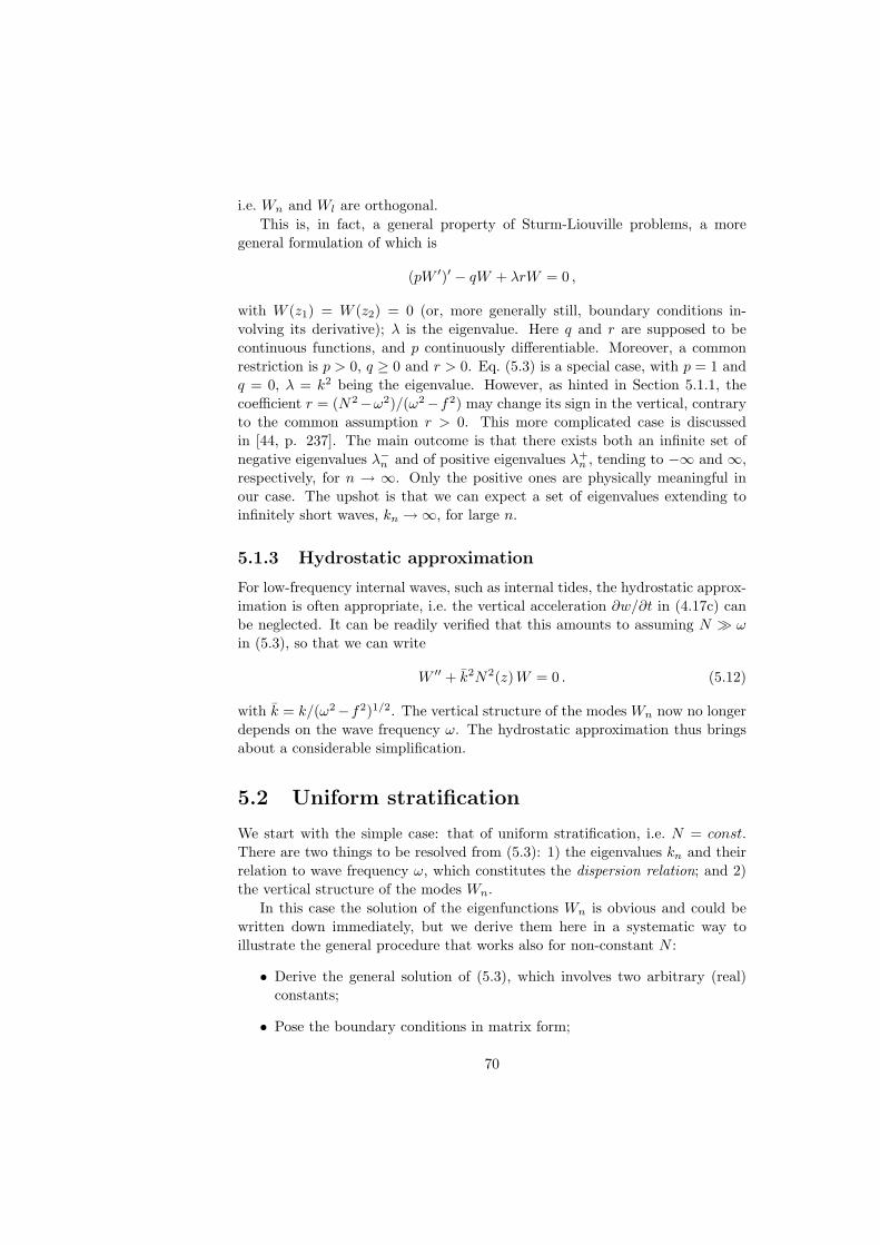
i.e. Wn and Wl are orthogonal.This is, in fact, a general property of Sturm-Liouville problems, a more

general formulation of which is

(pW ′)′ − qW + λrW = 0 ,

with W (z1) = W (z2) = 0 (or, more generally still, boundary conditions in-volving its derivative); λ is the eigenvalue. Here q and r are supposed to becontinuous functions, and p continuously differentiable. Moreover, a commonrestriction is p > 0, q ≥ 0 and r > 0. Eq. (5.3) is a special case, with p = 1 andq = 0, λ = k2 being the eigenvalue. However, as hinted in Section 5.1.1, thecoefficient r = (N2−ω2)/(ω2−f2) may change its sign in the vertical, contraryto the common assumption r > 0. This more complicated case is discussedin [44, p. 237]. The main outcome is that there exists both an infinite set ofnegative eigenvalues λ−n and of positive eigenvalues λ+

n , tending to −∞ and ∞,respectively, for n → ∞. Only the positive ones are physically meaningful inour case. The upshot is that we can expect a set of eigenvalues extending toinfinitely short waves, kn →∞, for large n.

5.1.3 Hydrostatic approximation

For low-frequency internal waves, such as internal tides, the hydrostatic approx-imation is often appropriate, i.e. the vertical acceleration ∂w/∂t in (4.17c) canbe neglected. It can be readily verified that this amounts to assuming N À ω

in (5.3), so that we can write

W ′′ + k2N2(z)W = 0 . (5.12)

with k = k/(ω2−f2)1/2. The vertical structure of the modes Wn now no longerdepends on the wave frequency ω. The hydrostatic approximation thus bringsabout a considerable simplification.

5.2 Uniform stratification

We start with the simple case: that of uniform stratification, i.e. N = const.There are two things to be resolved from (5.3): 1) the eigenvalues kn and theirrelation to wave frequency ω, which constitutes the dispersion relation; and 2)the vertical structure of the modes Wn.

In this case the solution of the eigenfunctions Wn is obvious and could bewritten down immediately, but we derive them here in a systematic way toillustrate the general procedure that works also for non-constant N :

• Derive the general solution of (5.3), which involves two arbitrary (real)constants;

• Pose the boundary conditions in matrix form;

70

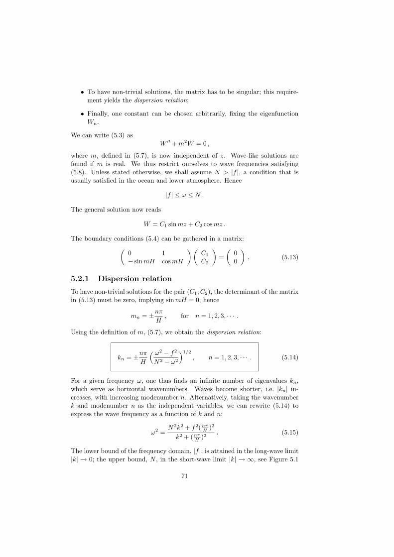
• To have non-trivial solutions, the matrix has to be singular; this require-ment yields the dispersion relation;

• Finally, one constant can be chosen arbitrarily, fixing the eigenfunctionWn.

We can write (5.3) asW ′′ + m2W = 0 ,

where m, defined in (5.7), is now independent of z. Wave-like solutions arefound if m is real. We thus restrict ourselves to wave frequencies satisfying(5.8). Unless stated otherwise, we shall assume N > |f |, a condition that isusually satisfied in the ocean and lower atmosphere. Hence

|f | ≤ ω ≤ N .

The general solution now reads

W = C1 sinmz + C2 cosmz .

The boundary conditions (5.4) can be gathered in a matrix:(

0 1− sinmH cosmH

)(C1

C2

)=

(00

). (5.13)

5.2.1 Dispersion relation

To have non-trivial solutions for the pair (C1, C2), the determinant of the matrixin (5.13) must be zero, implying sin mH = 0; hence

mn = ±nπ

H, for n = 1, 2, 3, · · · .

Using the definition of m, (5.7), we obtain the dispersion relation:

kn = ±nπ

H

( ω2 − f2

N2 − ω2

)1/2

, n = 1, 2, 3, · · · . (5.14)

For a given frequency ω, one thus finds an infinite number of eigenvalues kn,which serve as horizontal wavenumbers. Waves become shorter, i.e. |kn| in-creases, with increasing modenumber n. Alternatively, taking the wavenumberk and modenumber n as the independent variables, we can rewrite (5.14) toexpress the wave frequency as a function of k and n:

ω2 =N2k2 + f2(nπ

H )2

k2 + (nπH )2

. (5.15)

The lower bound of the frequency domain, |f |, is attained in the long-wave limit|k| → 0; the upper bound, N , in the short-wave limit |k| → ∞, see Figure 5.1

71

(upper panel). For positive k, the function ω(k) is monotonically increasing,as is clear from the fact that its derivative is positive. This derivative, thehorizontal group velocity cg = dω/dk, is obtained from differentiating (5.15):

cg =k(nπ

H )2(N2 − f2)[N2k2 + f2(nπ

H )2]1/2 [k2 + (nπH )2]3/2

(5.16)

= ±( H

nπ

) (ω2 − f2)1/2(N2 − ω2)3/2

ω(N2 − f2). (5.17)

In (5.17), the plus-sign applies if k is positive, the minus-sign if k is negative.We thus see that k and cg have the same horizontal direction if |f | < N , andthe opposite direction if |f | > N . The horizontal phase speed c = ω/k is givenby

c =[N2k2 + f2(nπ

H )2]1/2

k[k2 + (nπH )2]1/2

(5.18)

= ±(Hω

nπ

)(N2 − ω2

ω2 − f2

)1/2

. (5.19)

The group velocity cg indicates how fast the wave energy travels; the phasespeed c, how fast the wave’s crests and troughs travel. Clearly, the former is themost relevant quantity because it determines where the internal waves manifestthemselves (there are no waves if there is no wave-energy).

For fixed ω, we see from (5.17) and (5.19) that the group velocity and phasespeed both are inversely proportional to modenumber n; higher modes propagatemore slowly. Eq. (5.17) moreover implies that the group velocity vanishes atthe extremes of the frequency domain, i.e. for ω = |f |, N . The phase speed, onthe other hand, tends to infinity at the lower bound |f |. This is illustrated inFigure 5.2.

Next we consider how cg and c vary if we take modenumber n fixed (n = 1,say) and choose k as the independent variable; here we use (5.16) and (5.18),see Figure 5.1 (middle and lower panels). The phase speed c varies with k,i.e. internal waves are dispersive. Differentiating c = ω/k to k, we obtain thegenerally valid identity

kdc

dk= cg − c .

So, for dispersive waves the group and phase velocity are unequal. The dis-persiveness means that a superposition of first-mode waves (or any other fixedmode-number) involving different wavenumbers, and hence different frequen-cies, cannot propagate as a coherent entity, but will disperse, because differentcomponents have different phase and group speeds.

Finally, we consider the low-frequency limit, or equivalently, long-wave limit.Assuming kH ¿ 1, we can expand (5.15) as

ω2 = f2 +(NH

nπ

)2

k2 + · · · , (5.20)

72

−|f|

−N

k →

↑ω

k→

↑cg

−c0

k →

↑c

−c0

Fig. 5.1: Profiles of wave frequency ω, group velocity cg, and phase speed c, each as

a function of wavenumber k (chosen positive), for arbitrary but fixed modenumber n;

these plots illustrate (5.15), (5.16) and (5.18), respectively. In the middle and lower

panels, the behaviour for f = 0 is also shown (dashed line). The value c0 = NH/nπ

denotes the linear long-wave phase and group speed for f = 0.

cg

c

||f|

|N

ω →

Fig. 5.2: Group and phase speeds as a function of wave frequency ω, illustrating (5.17)

and (5.19) for arbitrary but fixed modenumber n, taking N > |f | and k positive.

73

where we retained only the first two terms of the expansion. This expressionfollows also directly from (5.14), if we suppose ω ¿ N . Still another way ofobtaining (5.20) would have been to make the hydrostatic approximation (seeSection 5.1.3); these are all different renderings of the same statement. In (5.14),the waves are still dispersive (i.e. c = ω/k depends on k), but this is now entirelydue to Coriolis effects. If f = 0, long waves become dispersionless, having agroup and phase speed c0 ≡ NH/nπ (see dashed lines in Figure 5.1, middle andlower panels). Typical values for c0 in the ocean are of the order of 1 m s−1 (take,for example, n = 1, N = 1 × 10−3 rad s−1, H = 4000m). A useful measure ofthe importance of Coriolis effects is the ratio rd = c0/|f |, the so-called internalRossby radius of deformation. Internal waves having a wavelength of the orderof rd, or larger, are significantly affected by Coriolis effects. For waves muchshorter than rd, Coriolis effects can generally be neglected (but see Section5.6.2!). Notice that short waves are dispersive due to gravity, an effect neglectedin (5.20), but present in the exact dispersion relation (5.15).

5.2.2 Modal structure

Returning to (5.13), we see that C2 must be zero, while C1 may take any (real)value. Without loss of generality, we can choose C1 = 1 for all n (thus nor-malizing the amplitude at 1), since we already included an arbitrary (complex)constant an in the series (5.6). With this, the vertical modes become

Wn = sin(nπz

H

), n = 1, 2, 3, · · · . (5.21)

They have the remarkable property of being independent of the wave frequencyω. This is a peculiarity of the case N = const; for general profiles N(z), themodes take different structures for different frequencies (see following sections).The first three verical modes of (5.21) are shown in Figure 5.3.

−1 −0.5 0 0.5 1−4

−3

−2

−1

0

Wn

z (k

m)

n=1 n=2 n=3

Fig. 5.3: The first three vertical modes Wn, from (5.21), for H = 4000 m.

74

With (5.21), the general solution for rightward propagating waves is ob-tained from (5.6), by selecting positive k (i.e. k+; hereafter, we drop the ’plus’).Assuming an to be real, and taking the real part of (5.6), we find

w =∑

n

an sin(nπz

H

)cos(knx− ωt) . (5.22)

Using (5.5), we obtain for the horizontal velocity component u, the tranversevelocity v, pressure p and buoyancy b,

u = −∑

n

annπ

knHcos

(nπz

H

)sin(knx− ωt) (5.23)

v =f

ω

∑n

annπ

knHcos

(nπz

H

)cos(knx− ωt) (5.24)

p = −ρ∗ω2 − f2

ω

∑n

annπ

k2nH

cos(nπz

H

)sin(knx− ωt) (5.25)

b =N2

ω

∑n

an sin(nπz

H

)sin(knx− ωt) . (5.26)

Another important quantity is the displacement of the isopycnals (levels of con-stant potential density, strictly speaking). Let the isopycnal that lies at depthz0 in the state of rest be described by

z = z0 + ζ(t, x, z0) .

Thenw(t, x, z) =

∂ζ

∂t(t, x, z0) + u(t, x, z)

∂ζ

∂x.

Making a Taylor expansion about z = z0, and neglecting nonlinear terms, gives

w(t, x, z0) =∂ζ

∂t(t, x, z0) .

Hence the solution for ζ,

ζ = − 1ω

∑n

an sin(nπz

H

)sin(knx− ωt) , (5.27)

where we substituted z0 by z. Comparing this with (5.26), we see that ζ =−b/N2.

We now show examples of u, v, w, b and ζ for the first three modes individ-ually, using (5.22)–(5.27) at t = 0, with an = 1. From (5.23) and (5.25) we seethat u and p differ only by a positive coefficient; they have identical structuresand are therefore represented in one and the same plot. Similarly, b and ζ differin essence only by a minus sign. The results are shown in Figure 5.4. Noticethat v owes its presence to the Coriolis force, and would be zero for f = 0. Forthe n-th mode, u changes its sign n times in the vertical (as does v); w and ζ

75

n=1

0 20 40 60 80−4

−2

0n=2

0 20 40 60 80−4

−2

0n=3

u, p

0 20 40 60 80−4

−2

0

0 20 40 60 80−4

−2

0

0 20 40 60 80−4

−2

0

v

0 20 40 60 80−4

−2

0

0 20 40 60 80−4

−2

0

0 20 40 60 80−4

−2

0

w

0 20 40 60 80−4

−2

0

0 20 40 60 80−4

−2

0

0 20 40 60 80−4

−2

0

ζ, −b

0 20 40 60 80−4

−2

0

Fig. 5.4: Spatial structure of the first three modes, for constant stratification, at t = 0.

Upper panels show the horizontal velocity component u; the second row, the tranverse

velocity v; the third row, the vertical velocity w; and the lowest panels the isopycnal

elevation ζ. The first and fourth rows also represent pressure p and minus buoyancy

b, respectively. White denotes negative values; black, positive ones. Parameters are:

N = 1 × 10−3, f = 1 × 10−4, and ω = 1.405 × 10−4 (the semi-diurnal lunar tidal

frequency, M2), all in rad s−1. Along the vertical is water depth, with H = 4 km;

horizontal distances are also in km.

each n−1 times. So, for example, at a certain horizontal position the isopycnalscorresponding to the second mode are elevated in one part of the water column,and depressed in the other part.

Notice that the pressure is not zero at the surface (rigid-lid); on the contrary,it has a local extremum there. If the surface were allowed to move freely, theseregions of high (low) pressure at z = 0 would be associated with an elevation(depression) of the surface. By comparing the pattern of p with that of ζ forthe first mode, we see that depressions in the interior are accompanied by anelevated pressure at z = 0, and vice versa. In other words, surface displacementswould be in anti-phase with the displacements in the interior.

In time, the patterns all move steadily to the right (not shown), but at lowerspeeds for higher modenumbers, because the phase speed c in (5.19) is inversely

76

proportional to n.

5.2.3 Superposition of modes

We also see from Fig. 5.21 that the second mode is twice as short as the first one;the third three times as short, etc. Indeed, (5.14) implies that the wavenumbersare commensurable:

kn/kl = n/l .

(We note that this property does not hold for general N(z); it is a peculiarity ofthe case of constant N .) As a consequence, a superposition of modes must behorizontally periodic. An example of a superposition of 10 modes, representingu, is shown in Figure 5.5 at several stages during half a period (for clarity, wehave enlarged the horizontal domain by a factor of two). At first sight, Figure 5.5is very surprising: it shows that the modes – each of which travels to the right atits own phase speed cn –, when superposed give rise to ’beams’ that stay in place!The water parcels oscillate predominantly within these beams, in a paralleldirection, as is shown by the red arrows depicting the (u,w) vectorial velocityfield. (Due to Coriolis effects, there is also a component v in the transversedirection, which is not shown.)

Upon closer examination, we see that phase propagation is in a directionperpendicular to the beam. For example, in the interval x = 0 − 40 km, thephases move up- and rightward, perpendicularly to the beam itself. The energy,meanwhile, must flow along the beam, which is, in this interval, down- andrightward. Vertical opposition of direction in phase and energy propagation isfound in the other intervals as well. As shown in Chapter 6, this rule holdsgenerally when N > |f |.

The regular pattern of diagonals of Figure 5.5 invites the question as to whatunderlying principle imposes this orderliness. For this, we have to reconsider thenature of the modal solution. With (5.2), we consider rightward propagatingwaves, whose vertical structure is described by W (z). This structure turns outto be sinusoidal, as shown in (5.21) and Figure 5.3. We can thus interpret eachWn as a standing wave in the vertical, i.e. a combination of up- and downwardpropagating waves; here, mn = nπ/H serves as the vertical wavenumber. Now,from (5.7), we find that the ratio of the vertical and horizontal wavenumbers,mn and kn, is given by

mn

kn= ±N2 − ω2

ω2 − f2, (5.28)

which is independent of modenumber n. In other words, one and the sameangle, in the x, z-plane, pervades all modes. So it is, after all, not surprising tofind a well-defined pattern of diagonals in Figure 5.5. More specifically, (5.28)denotes the tangent of the angle that the wavevector ~k = (k, m) makes with thehorizontal, the wavevector pointing in the direction of phase propagation. Weinferred earlier that energy propagates perpendicularly to this; hence its slopemust be given by the inverse of (5.28), namely ±(ω2 − f2)/(N2 − ω2). Theseproperties will be established in a much more direct way in Chapter 6.

77

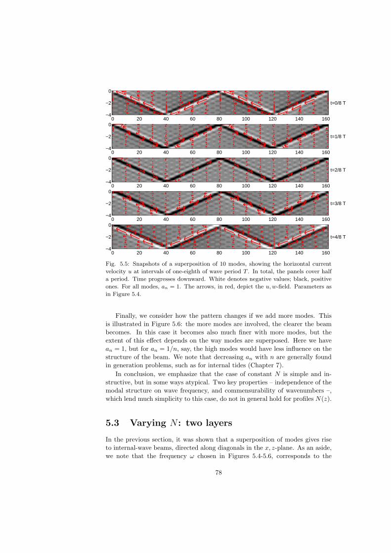
t=0/8 T

0 20 40 60 80 100 120 140 160−4

−2

0

t=1/8 T

0 20 40 60 80 100 120 140 160−4

−2

0

t=2/8 T

0 20 40 60 80 100 120 140 160−4

−2

0

t=3/8 T

0 20 40 60 80 100 120 140 160−4

−2

0

t=4/8 T

0 20 40 60 80 100 120 140 160−4

−2

0

Fig. 5.5: Snapshots of a superposition of 10 modes, showing the horizontal current

velocity u at intervals of one-eighth of wave period T . In total, the panels cover half

a period. Time progresses downward. White denotes negative values; black, positive

ones. For all modes, an = 1. The arrows, in red, depict the u, w-field. Parameters as

in Figure 5.4.

Finally, we consider how the pattern changes if we add more modes. Thisis illustrated in Figure 5.6: the more modes are involved, the clearer the beambecomes. In this case it becomes also much finer with more modes, but theextent of this effect depends on the way modes are superposed. Here we havean = 1, but for an = 1/n, say, the high modes would have less influence on thestructure of the beam. We note that decreasing an with n are generally foundin generation problems, such as for internal tides (Chapter 7).

In conclusion, we emphasize that the case of constant N is simple and in-structive, but in some ways atypical. Two key properties – independence of themodal structure on wave frequency, and commensurability of wavenumbers –,which lend much simplicity to this case, do not in general hold for profiles N(z).

5.3 Varying N : two layers

In the previous section, it was shown that a superposition of modes gives riseto internal-wave beams, directed along diagonals in the x, z-plane. As an aside,we note that the frequency ω chosen in Figures 5.4-5.6, corresponds to the

78

one mode

0 20 40 60 80 100 120 140 160−4

−2

0

two modes

0 20 40 60 80 100 120 140 160−4

−2

0

three modes

0 20 40 60 80 100 120 140 160−4

−2

0

four modes

0 20 40 60 80 100 120 140 160−4

−2

0

ten modes

0 20 40 60 80 100 120 140 160−4

−2

0

25 modes

0 20 40 60 80 100 120 140 160−4

−2

0

Fig. 5.6: Superpositions with an increasing number of modes, each at t = 0, showing

the horizontal current velocity u. White denotes negative values; black, positive ones.

Parameters as in Figure 5.4.

semi-diurnal lunar frequency M2. It is therefore interesting to compare thepattern found in Figure 5.5 with that of an observed internal-tide beam, shownin Figure 1.9. We see that the angles are roughly similar: for every kilometerthe beam traverses in the vertical, it traverses about 10 km in the horizontal. Anoticeable difference between the figures is, however, that the beams in Figure5.5 are straight, while the observed beam is bended; it becomes steeper in thedeep ocean. A clue to this behaviour is found in Figure 1.6, which shows thatstratification N generally decreases with depth in the abyssal ocean.

To take into account this effect, we have to abandon the assumption ofconstant N . A simple way of doing this is to take two layers of different constants

79

N1 and N2:

N(z) =

N1 −d < z < 0 (upper layer)N2 −H < z < −d (lower layer) .

(5.29)

The governing equation is still (5.3), which we now apply to each layer sepa-rately. Accordingly, we define, as in (5.7),

m21,2 = k2

N21,2 − ω2

ω2 − f2.

The solution to (5.3) can now be written, with arbitrary constants C1 and C2,

W (z) =

C1 sin m1z −d < z < 0 (upper layer)C2 sin m2(z + H) −H < z < −d (lower layer) ,

(5.30)

where the boundary conditions at surface and bottom, W (0) = W (−H) = 0, arealready satisfied. However, continuity of W and W ′ at the transition betweenthe layers has to be imposed as well. These conditions can together be writtenin matrix form as

(sin m1d sin m2(H − d)m1 cosm1d −m2 cosm2(H − d)

)(C1

C2

)=

(00

). (5.31)

Requiring the determinant to be zero yields the dispersion relation

m2 sin m1d cos m2(H − d) + m1 cos m1d sin m2(H − d) = 0 . (5.32)

For given wave frequency ω (and constants f , N1, N2, d and H), we find thewavenumbers k as zeros of this equation, whence we obtain m1,2. However, theequation is transcendent (i.e. cannot be solved by analytical means), so we haveto resort to numerical methods to find the eigenvalues k. In fact, one can simplyplot the left-hand side and pick out the zeros, see, e.g., Figure 5.8. Finally, using(5.31), we can express C2 in terms of C1:

C2 = − sin m1d

sin m2(H − d)C1 .

The remaining coefficient C1, which fixes the amplitude, can be chosen arbitrar-ily.

The physics contained in this simple solution is already rich; in the nextsections, we consider three cases to illustrate this.

5.3.1 Refraction and internal reflection

We choose the lower layer to be less strongly stratified than the upper one, seeFigure 5.7a. Furthermore, we take f = 1 × 10−4 and ω = 1.4 × 10−4 rad s−1.As result the following inequalities are satisfied:

f < ω < N1,2 ,

80

0 0.5 1 1.5 2 2.5

x 10−3

−4

−3

−2

−1

0

N (rad/s)

z (k

m)

||f|

|ω

(a)

−1 0 1−4

−3

−2

−1

0

Wn

z (k

m)

(b)

123

x (km)

z (k

m)

(c)

0 100 200−4

−3

−2

−1

0

Fig. 5.7: Stratification with two layers of constant N , with |f | < ω < N2 < N1

(a). Panel b shows the first three eigenmodes (5.30), with C1,n chosen such that their

amplitudes are one. Modal coefficients are an = 1/n. The resulting superposition of

20 modes, representing the amplitude of u, is shown in c. White denotes zero; black,

maximum values.

which implies that internal waves of the chosen frequency can propagate in bothlayers.

Eigenvalues are easily found as the zeros of (5.32), as shown in Figure 5.8;the first three corresponding vertical modes are shown in Figure 5.7b. From(5.2) and (5.5), we obtain u as

u = −∑

n

1kn

W ′n sin(knx− ωt) ,

with Wn given by (5.30), and normalized to one. A superposition of 20 modes,representing the amplitude of u, is shown in Figure 5.7c. It demonstrates thatthe beam is slightly steeper in the lower layer (in qualitative agreement withFigure 1.9), which must be due to the weaker stratification in that layer. So,non-uniformity in N causes refraction.

Moreover, we see that internal reflections occur at the transition betweenthe two layers, yielding a complex pattern. Clearly, the pattern is no longerperiodic in x (as it was for constant N , Section 5.2). This reflects the fact thatthe wavenumbers are now incommensurable: kn/kl 6= n/l. Indeed, the kn’sobtained from Figure 5.8 yield: k2/k1 = 2.34, k3/k1 = 3.52, k4/k1 = 4.40 etc.

81

0 2 4

x 10−4

−0.01

0

0.01

kle

ft−ha

nd s

ide

of d

ispe

rsio

n re

latio

n

lhsk

n

Fig. 5.8: The left-hand side of (5.32) plotted against k; zeros denote eigenvalues kn,

with n increasing from 1 to 12, from left to right.

5.3.2 Trapping of high-frequency waves (ω > |f |)We now choose a higher wave frequency such that |f | < N2 < ω < N1. Thismeans that m2 becomes imaginary: m2 = i=(m2). Cosines and sines containingm2 can be rewritten using the identities

sin(ix) = i sinh(x) ; cos(ix) = cosh(x) . (5.33)

As a consequence, the modal solution becomes exponential in z in the lowerlayer. (Notice that C2 too becomes imaginary, hence the factor i drops outfrom (5.30), which thus remains real.)

The dispersion relation (5.32) remains the same, but we can rewrite it as

=(m2) sin m1d cosh=(m2)(H − d) + m1 cosm1d sinh=(m2)(H − d) = 0 .

We choose the same parameters as in Figure 5.7, except that the wave fre-quency ω is now higher, see Figure 5.9a. The first three modes are shown inpanel Figure 5.9b. Their structure clearly is very different from that in Figure5.7b. This demonstrates that the modal structure now depends on the wave fre-quency, in contrast to the absence of any such dependence in the case of uniformN (Section 5.2.2). Specifically, the modes now oscillate only in the upper layer,and decay exponentially in the lower one. Since higher modes have larger kn,and hence larger |m2|, they decay more rapidly than lower modes. Figure 5.9cshows a superposition of 15 modes; they add up to form a beam that is trappedin the upper layer. In other words, the upper layer now acts as a waveguide.

5.3.3 Trapping of low-frequency waves (ω < |f |)In contrast with the previous case, internal waves can also be trapped in thelayer of weakest stratification. For this to happen, wave frequencies need tobe sub-inertial, i.e. ω < |f |. As an extreme example, we consider a neutrallystratified lower layer, N2 = 0. Furthermore, we take f = 1 × 10−4 and N1 =

82

0 0.5 1 1.5 2 2.5

x 10−3

−4

−3

−2

−1

0

N (rad/s)

z (k

m)

||f|

|ω

(a)

−1 0 1−4

−3

−2

−1

0

Wn

z (k

m)

(b)

123

x (km)

z (k

m)

(c)

0 2 4 6 8 10 12−4

−3

−2

−1

0

Fig. 5.9: Stratification with two layers of constant N ; parameters are as in Figure

5.7, except for the wave frequency, which is now such that |f | < N2 < ω < N1 (a).

Panel b shows the first three eigenmodes (5.30), normalized to one. The resulting

superposition of 15 modes, representing the amplitude of u, is shown in c. White

denotes zero; black, maximum values.

5×10−4 rad s−1. For the wave frequency ω we choose the diurnal tidal frequencyK1(= Ω), 7.292× 10−5 rad s−1. So we have

N2 < ω < |f | < N1 .

According to (5.8), wave propagation can now only occur in the lower layer.Moreover, since N2 = 0, the Coriolis force acts as the sole restoring force, inwhich case internal waves are called gyroscopic (Section 1.2.2).

Figure 5.10c confirms that it is now the lower layer that acts as a waveguide;hardly any signal penetrates into the upper layer. This is confirmed by the factthat the eigenvalues are very nearly given by

kn ≈ nπ

H/2

(ω2 − f2

−ω2

)1/2

,

as if the total water depth were just that of the lower layer, H/2.From (5.16) we see that group velocity is now negative, implying that energy

propagates to the left, while phase propagation is to the right (k being positive).This horizontal opposition is typical of gyroscopic waves.

A final comment concerns the effect of the hydrostatic approximation, brieflydiscussed in Section 5.1.3. This approximation amounts to assuming N À ω.

83

0 2 4 6

x 10−4

−4

−3

−2

−1

0

N (rad/s)

z (k

m)

||f|

|ω

(a)

−1 0 1−4

−3

−2

−1

0

Wn

z (k

m)

(b)

123

x (km)

z (k

m)

(c)

0 2 4 6 8−4

−3

−2

−1

0

Fig. 5.10: Stratification with two layers of constant N , the lower layer being neutrally

stable, N2 = 0, with N2 < ω < |f | < N1 (a). Panel b shows the first three eigenmodes

(5.30), normalized to one. A superposition of 15 modes, representing the amplitude

of u, is shown in c. White denotes zero; black, maximum values.

Obviously, one cannot assume this and later take N = 0. This indicates thatthe hydrostatic approximation is inappropriate in the presence of very weaklystratified layers; in fact, it would remove the entire class of sub-inertial waves.

5.4 A simple model for the ocean’s stratification

There is not, in principle, a limitation to extending the procedure of the previ-ous section to any number of layers. There is a good reason, indeed, to considera three-layer system. The models of stratification discussed in Sections 5.2 and5.3 miss an important feature of the ocean’s stratification as depicted in, forexample, Figure 3.3b, namely the strong peak in N , representing the seasonalthermocline. Schematically the structure, from surface to bottom, is as follows:a very weakly stratified upper mixed layer, a seasonal thermocline, and a fairlyweakly stratified abyssal ocean, in which N decreases slowly with depth (apartfrom the presence of a second, less pronounced maximum, the permanent pycn-ocline, which we will ignore here). These features can be captured, though in anidealized way, by a model of stratification consisting of three layers of constant

84

N :

N2(z) =

0 −d < z < 0 (mixed layer)g′/ε −d− ε < z < −d (thermocline)N2

c −H < z < −d− ε (abyss) .

(5.34)

see Figure 5.11. In the upper mixed layer, we take N = 0. The thermocline isrepresented by a thin layer of thickness ε and amplitude N2 = g′/ε. Notice thatthe area of N2 enclosed by the thermocline equals g′, irrespective of the value ofε; this property makes it easy to estimate the key parameter g′ from empiricalprofiles of N2. The whole ’abyssal’ lower layer, finally, is simply represented byconstant N = Nc.

|N

c2

|g′/ε N2→

−−d ε

−−H

Fig. 5.11: Three-layer representation of the ocean’s stratification: an upper mixed

layer of thickness d, a thermocline of thickness ε, and a weakly stratified deep layer.

Notice that the area enclosed by the thermocline is g′, which serves as a measure of

its strength.

We take the idealization one step further by taking ε → 0; this reduces thethermocline to an interface. In this limit, g′ has a simple interpretation: it is g

times the relative jump in density across the interface (this will be demonstratedin Section 8.3.2). We can now write (5.34) succinctly as

N2(z) = g′δ(z + d) + N2c Θ(−z − d) , (5.35)

where δ and Θ are the delta-distribution and Heaviside stepfunction, respec-tively (see Appendix).

5.4.1 Dispersion relation and vertical modes

We assume wave frequencies to lie in the interval

|f | < ω < Nc .

85

We solve (5.3) separately for the mixed and abyssal layer. In the mixed layer,where N = 0, the solution to (5.3) is exponential and can be written

Wu = C1 sinh quz , for − d < z < 0 , (5.36)

with

qu = k( ω2

ω2 − f2

)1/2

.

The other solution, cosh(· · · ) can be ignored a priori in view of the bound-ary condition at the surface, (5.4). In the abyssal layer, solutions to (5.3) aresinusoidal:

Wl = C2 sin ql(z + H) , for −H < z < −d , (5.37)

with

ql = k(N2

c − ω2

ω2 − f2

)1/2

.

The cosine solution cos(· · · ) can be ignored in view of the boundary conditionat the bottom.

We now have two pieces of the solution, Wu and Wl; they need to be matchedat the thermocline. One obvious matching condition is continuity of W , i.e.

Wu(−d) = Wl(−d) . (5.38)

We have yet to take into account the presence of the thermocline. This can bedone by returning to the original profile (5.34), and taking the integral of (5.3)over the thermocline:

∫ −d

−d−ε

dz

W ′′ + k2 N2(z)− ω2

ω2 − f2W

= W ′(−d)−W ′(−d− ε) + k2 g′/ε− ω2

ω2 − f2

∫ −d

−d−ε

dz W = 0 .

For small ε, the last integral reduces to εW (−d); hence in the limit ε → 0,

W ′u(−d)−W ′

l (−d) +g′k2

ω2 − f2W (−d) = 0 . (5.39)

For the evaluation of the last term, it is immaterial which of the two, Wu orWl, is taken, because of (5.38). Without a thermocline (g′ = 0), the firstderivative of W would be continuous. We see from (5.39) that the presence ofthe thermocline creates a discontinuity in W ′, and hence, by (5.5), a jump inthe horizontal velocities u and v across the interface. Thus, the thermocline isaccompanied by a strong vertical shear.

We gather (5.38) and (5.39) in a matrix(

sinh qud sin ql(H − d)qu cosh qud− g′q2

u

ω2 sinh qud −ql cos ql(H − d)

)(C1

C2

)=

(00

).

(5.40)

86

The dispersion relation follows from the requirement that the determinant bezero:

ql cos ql(H−d) sinh qud+qu sin ql(H−d)[cosh qud− g′qu

ω2sinh qud

]= 0 . (5.41)

One can obtain numerically the zeros kn of this transcendental equation. Wechoose C2 = 1; using (5.36), (5.37) and (5.51), we obtain the vertical modes

Wn(z) =

− sin ql(H−d)

sinh qud sinh quz −d < z < 0sin ql(z + H) −H < z < −d .

(5.42)

Notice that the coefficients qu and ql depend on modenumber n, via kn.

5.4.2 Scattering at the thermocline

An example of the first five vertical modes is shown in Figure 5.12a, and asuperposition of 25 modes in 5.12b. The value used here for g′ is 0.005m s−2.

−1 0 1−4

−3

−2

−1

0

Wn

z (k

m)

(a)

12345

x (km)

(b)

0 100 200 300−4

−3

−2

−1

0

Fig. 5.12: The first five modes for the three-layer system (a), here with g′ =

0.005m s−2. Other parameters are: d = 60m (mixed-layer depth), Nc = 2 × 10−3,

f = 1 × 10−4 and ω = 1.4 × 10−4, all in rad s−1; modal coefficients are an = 1/n. In

b, a superposition of 25 modes, representing the amplitude of u. White denotes zero;

black, maximum values.

In the lower layer internal-wave beams are clearly visible, as in previoussections, but where they impinge on the thermocline, strong currents appearin the mixed layer; the beam, meanwhile, becomes slightly less intense. Fur-ther rightward, we see broad, rather weak beams radiating downward from thethermocline. There is not really a transfer of energy, of course; this is a linearsolution, and there is no interaction among modes. It is just the superposition ofmodes that at some places yields strong currents in the mixed layer. A different

87

way to look at this is as the occurrence of internal reflections, discussed in Sec-tion 5.3.1. The thermocline forms a strong inhomogeneity in the stratification,and causes an impinging beam to scatter, due to internal reflections. Observa-tional evidence from the Bay of Biscay, discussed in Chapter 8, demonstratesthat this process may lead to the generation of so-called solitary waves.

In is instructive to consider also the case of an extremely strong thermocline,taking, for example, g′ = 0.5m s−2 (this is an admittedly unrealistic value!). Theresult is shown in Figure 5.13. The thermocline is now so strong that beamsin the lower layer reflect from it as if it were a rigid surface, leaving almost notrace in the mixed layer (Figure 5.13c). The first mode, on the other hand, isaccompanied by strong currents in the upper mixed layer, which show a periodicpattern (Figure 5.13b). The interpretation of these results is further exploredin the next section.

−1 0 1−4

−3

−2

−1

0

Wn

z (k

m)

(a)

12345

(b)

0 100 200 300 400 500 600 700−4

−3

−2

−1

0

x (km)

(c)

0 100 200 300 400 500 600 700−4

−3

−2

−1

0

Fig. 5.13: The first five modes for the three-layer system (a), now with g′ = 0.5m s−2.

Other parameters as in previous figure. In b, the contribution of the first mode to u,

at t = 0, is shown; in c, a superposition of modes 2 to 14. In b and c, white denotes

negative values; black, positive.

5.4.3 Interfacial waves

A special case of interest is Nc = 0. Obviously, we then have to drop therestriction ω < Nc. The other restriction, ω > |f |, is however retained. WithNc = 0, the stratification of (5.35) becomes that of a so-called two-layer model,

88

i.e. there are two neutrally stratified layers (N = 0) separated by an interface.1

This model can sometimes be applied to internal waves in shallow regions suchas the continental shelf, or to high-frequency internal waves trapped at thethermocline, such as solitons (see Chapter 8). A two-layer model is howeverwholly unsuitable for the description of internal waves in the deep ocean.

With Nc = 0, ql becomes imaginary, and we can write ql = iqu. Using theidentities (5.33), we can derive the dispersion relation for the two-layer systemfrom (5.41):

ω2 =g′qu

coth qud + coth qu(H − d)(5.43)

= f2 +g′k2

qu(coth qud + coth qu(H − d)). (5.44)

The connection between ω and k is implicitly contained in (5.43),2 which yieldsω as a function of qu; then k follows from

k = qu

(ω2 − f2

ω2

)1/2

.

The result is shown in Fig 5.14. For any choice of ω, there is now only one k,and hence only one mode, the interfacial mode,

W (z) =

− sinh qu(H−d)

sinh qud sinh quz −d < z < 0sinh qu(z + H) −H < z < −d .

(5.45)

This expression follows from (5.42), leaving out the factor i. The maximumof W occurs at the interface (thermocline); from there, it decreases steadilytowards the surface and bottom. This means that W ′ scales as [W ]/d in theupper layer ([W ] being the scale of W ), and as [W ]/(H − d) in the lower layer.The continuity equation (4.21d) implies that u must scale with d−1 in the upperlayer, and with (H − d)−1 in the lower layer. Typically d is much smaller thanH, and this explains the strong currents in the mixed layer in Figure 5.13b.

Without rotation (f = 0), we can replace qu with k in (5.44). For long

1This is not be confused with the stratification considered in Section 5.3, which consists oftwo layers with constant buoyancy frequency N ; there N is discontinuous, but density itself iscontinuous. In the present section, the latter is no longer the case: a jump in density occursacross the interface, at which N is infinite, i.e. a delta-peak.

2Notice that an explicit dependence is found for high-frequency waves (ω À |f |), in whichcase qu ≈ k. In fact, replacing qu by k in (5.44) yields a relation that turns out to be veryaccurate even for low-frequency waves.

89

−|f|

k

ω

Fig. 5.14: The dispersion relation (5.44), plotted as ω vs. k. Here for the parameter

values g′ = 0.01m s−2, d = 100 m, H = 4000m, and f = 1×10−4 rad s−1. The function

is monotonically increasing; hence for every ω > |f | there is only one wavenumber k.

waves, kH ¿ 1, we then find3

ω2 =g′k2d(H − d)

(H − d)[kd coth kd] + d[k(H − d) coth k(H − d)]

=g′k2d(H − d)

(H − d)[1 + 13 (kd)2 + · · · ] + d[1 + 1

3 (k(H − d))2 + · · · ]

= g′k2 d(H − d)H

11 + 1

3k2d(H − d) + · · ·= c2

0k2 [1− 1

3k2d(H − d) + · · · ] , (5.46)

with

c20 = g′

d(H − d)H

,

the linear long-wave phase speed for interfacial waves. Interfacial waves propa-gate horizontally, just like surface waves. The main difference between the twois the strongly reduced effective gravity, g′ instead of g. For surface waves, thelong-wave phase speed is given by gH; so g is here replaced with g′, and totalwater depth H with an ’equivalent’ depth d(H − d)/H, i.e. the product of thethickness of each layer, divided by the total water depth. In practice, we oftenhave d ¿ H so that c2

0 ≈ g′d. Typical values are g′ = 0.01 m s−2 and d = 100 m,giving a phase speed of one meter per second.

Returning now to the interpretation of Figure 5.13, we first notice that modes2 to 4 strongly resemble modes 1 to 3 for a layer of constant stratification, cf.Figure 5.3; in particular, the second mode in Figure 5.13a has one maximumhalfway down the water column, and vanishes at the thermocline, as if it werea rigid surface. Thus, a superposition of modes 2, 3, 4 · · · creates beams in thelower layer, as illustrated in Figure 5.13c. The first mode in Figure 5.13a stands

3Using the Taylor expansion, for x ¿ 1, x coth x = 1 + 13x2 − 1

45x4 + · · · .

90

apart from the higher modes in that it has its maximum at the thermocline; inthis, we recognize the interfacial mode (5.45). Thus, the wave propagation inFigure 5.13b,c consists of two distinct, independent elements: 1) an interfacialmode, and 2) the higher modes which form beams in the lower, constantly strati-fied layer. The two kinds of motion are here uncoupled, because the thermoclineis extremely strong. For a weaker, and indeed more realistic thermocline, likein Figure 5.12, the two are coupled, as is clear from the fact that the third andfifth modes also have a local extremum at the thermocline. So, in that case,one cannot really speak of pure interfacial waves or pure beams; they appear inmixed form.

To conclude the discussion on interfacial waves, we mention that there is acaveat to the notion that the two-layer system supports only one mode. If werelax the restriction ω > |f |, we find that there is an infinite number of sub-inertial modes, ω < |f |, both in the upper mixed layer and in the lower neutrallystratified layer (Nc = 0). These are the gyroscopic waves already discussed inSection 5.3.3.

5.5 Linearly varying N 2: Airy functions

There are various choices of profiles N(z) that allow for a solution in terms ofspecial functions. Several of them are conveniently listed in [72, §3.4]. We willnot repeat them here; the physics contained in these solutions is not essentiallydifferent from what has been discussed in previous sections. There is howeverone case that deserves our attention, because it provides a generic descriptionof the behaviour near a ’turning point’, i.e. the depth where internal waves turnfrom oscillatory to exponentially decaying.

We consider continuous profiles N(z), and assume that N(z) > |f | through-out the water column. Suppose that at some depth z∗, a transition occurs fromN(z) > ω to N(z) < ω. A Taylor expansion around this depth gives

N2(z) = N20 + λz + · · · , (5.47)

with λ = N2′(z∗) and N20 = N2(z∗)−λz∗. In other words, in the vicinity of the

depth where internal waves turn from oscillatory to exponentially decaying, wemay regard the profile of N2 as linear in z.

This provides the motivation for examining the case (5.47) more closely. Wedo this by applying (5.47) to the whole water column. The equation for verticalmodes, (5.3), can then be written

W ′′ + k2 (z + A0)W = 0 . (5.48)

with k2 = k2λ/(ω2− f2) and A0 = (N20 −ω2)/λ. With the coordinate transfor-

mation z = −k2/3[z + A0], (5.48) reduces to the Airy equation:

d2W

dz2− zW = 0 . (5.49)

91

Its general solution can be written in terms of the Airy functions Ai and Bi:

W = C1Ai(z) + C2Bi(z) .

As illustrated in Figure 5.15, Ai and Bi are oscillatory for z < 0; for z > 0, Ai

| | | | | |−10 −2 2

−

−

−

−1

1

2AiBi

Fig. 5.15: The Airy functions Ai and Bi, which are two independent solutions of

(5.49).

decays exponentially, while Bi grows exponentially.4 Transformed back to theoriginal coordinate z, the solution reads

W = C1Ai(−k2/3[z + A0]) + C2Bi(−k2/3[z + A0]) . (5.50)

Application of the boundary conditions (5.4) gives(

Ai(−k2/3A0) Bi(−k2/3A0)Ai(−k2/3[A0 −H]) Bi(−k2/3[A0 −H])

)(C1

C2

)=

(00

). (5.51)

The determinant has to be zero to have non-trivial solutions for (C1, C2); thisrequirement yields the dispersion relation

Ai(−k2/3A0)Bi(−k2/3[A0 −H])−Bi(−k2/3A0)Ai(−k2/3[A0 −H]) = 0 . (5.52)

This transcendent equation can be solved numerically (for example by simplyplottoing the left-hand side and picking out the zeros), and yields the eigenvalueskn, n = 1, 2, 3 . . . .

Using (5.51), we can express C2 in terms of C1 (which we give an additionalindex n, because different values may be chosen for different modes); the vertical

4We do not here dwell on the analytical properties of Airy functions; for integral represen-tations, Taylor series, asymptotic expansions etc., see [4].

92

modes (5.50) can then be written

Wn = C1,n

(Ai(−k2/3

n [z + A0])− Ai(−k2/3n A0)

Bi(−k2/3n A0)

Bi(−k2/3n [z + A0])

). (5.53)

In the examples discussed below, we choose C1,n such that maxWn = 1.We consider two examples, for different wave frequencies; the first showing

refraction, the second, trapping. In both cases, we choose H = 4000 m, N0 =1.5 × 10−3 rad s−1, λ = 5 × 10−10 rad2 m−1 s−2, and f = 10−4 rad s−1. Thebuoyancy frequency N thus decreases from N0 at the surface to 5×10−4 rad s−1

at the bottom; this covers more or less the range of values found in the deeperlayers of the ocean, see Figure 1.6.

x (km)

z (k

m)

(a)

0 20 40 60 80 100 120 140 160 180−4

−3

−2

−1

0

x (km)

(b)

0 2 4 6 8−4

−3

−2

−1

0

Fig. 5.16: Solution for a linearly varying N(z); the amplitude of u is shown for a

superposition 15 modes, with modal coefficients a(n) = 1/n. White denotes zero;

black, maximum values. In a, internal-wave beams can propagate at any depth, but

are refracted due to the decrease of N with depth. In b, a higher wave frequency is

chosen, such that |f | < N < ω in the deeper part of the water column; hence, internal

waves are trapped in the upper layer.

First we choose ω = 1.4 × 10−4 rad s−1 (semi-diurnal internal tides). Forthis value, we have |f | < ω < N(z) for all z; the waves can thus propagatethroughout the water column. A superposition of 15 modes, depicting the am-plitude of u, is shown in Figure 5.16a. The beams are slightly bended due tothe decreasing stratification N with depth.

Taking now a higher frequency, ω = 1.0 × 10−3 rad s−1, for which the in-equality N(z) > ω is satisfied only in the upper 2500m of the water column,so that the waves are trapped there; they reflect at the base of that layer, as isillustrated in Figure 5.16b.

5.6 Non-traditional effects

To conclude this chapter, we briefly discuss how the results obtained so farwould change if one abandons the Traditional Approximation. We return to

93

(5.1):∂2

∂t2∇2w + (~f · ∇)2w + N2∇2

hw = 0 , (5.54)

where ~f = (0, f , f). It is convenient to rotate the coordinate system in thehorizontal plane, at an arbitrary angle α in anti-clockwise direction:

x′ = x cos α + y sin α ; y′ = −x sin α + y cosα ,

as illustrated in Figure 5.17. Hence

∂

∂x=

∂x′

∂x

∂

∂x′+

∂y′

∂x

∂

∂y′= cos α

∂

∂x′− sin α

∂

∂y′

∂

∂y=

∂x′

∂y

∂

∂x′+

∂y′

∂y

∂

∂y′= sin α

∂

∂x′+ cos α

∂

∂y′.

With this transformation, (5.54) becomes

∂2

∂t2∇′2w + (~f ′ · ∇′)2w + N2∇′h2w = 0 , (5.55)

with

∇′2 =∂2

∂x′2+

∂2

∂y′2+

∂2

∂z2; ∇′h2 =

∂2

∂x′2+

∂2

∂y′2; ~f ′ ≡ (f sin α, f cosα, f) .

Notice that the angle α is exclusively connected to the non-traditional f , con-firming the fact that the angle becomes immaterial under the Traditional Ap-proximation (isotropy).

x

y

east →

north↑

x′

y′

α

Fig. 5.17: Coordinate transformation to the primed system, at an angle α with respect

to the original east-north system.

We consider waves travelling in the x′-direction, with ∂/∂y′ = 0; this leavesthe geographical direction of propagation still arbitrary, via α. Moreover, weassume

w ∼ exp(−iωt) .

94

With this, (5.55) reduces to

A∂2w

∂x′2+ 2B

∂2w

∂x′∂z+ C

∂2w

∂z2= 0 . (5.56)

The coefficients A, B and C are defined by

A = N2 − σ2 + f2s ; B = ffs ; C = f2 − σ2 ; with fs = f sin α .

Non-traditional effects are now represented by fs. Of particular significanceis the mixed derivative in (5.56), which would disappear under the TraditionalApproximation (fs = 0, hence B = 0). This term precludes solutions obtainedby separation of variables, i.e. real solutions of the form F (x)G(z). Still, it isstraightfoward to solve (5.56) if we use the transformation

w = W (z) exp ik(x′ −Bz/C) , (5.57)

by which (5.56) becomes

d2W

dz2+ k2 B2 −AC

C2W = 0 . (5.58)

This expression replaces the ’traditional’ (4.40), and solutions are obtained sim-ilarly as in previous sections. We consider here the case of constant N , so thatA is constant.

5.6.1 Frequency range

For sinusoidal solutions to be possible in (5.58), B2−AC must be positive. Thiscondition can be rewritten as

ωmin < ω < ωmax ,

with

ωmin,max =1√2

([N2 + f2 + f2

s ]∓

[N2 + f2 + f2s ]2 − (2fN)2

1/2)1/2

. (5.59)

A principal difference with the ’traditional’ range (i.e. ωmin = min(|f |, N) andωmax = max(|f |, N)) is that both bounds now depend on both latitude (via f

and fs) and stratification N . Moreover, it can be proven that the range is, ingeneral, enhanced:

ωmin ≤ min(|f |, N) < ω < max(|f |, N) ≤ ωmax .

The only exception is for waves travelling in the west-east direction, so thatα = 0, in which case (5.59) reduces to the traditional bounds.

The width of the extension of the range depends on stratification N ; in astrongly stratified fluid, N À Ω, (5.59) can be approximated by

ωmin = |f |[1− f2

s

2N2+ O

( Ω4

N4

)]; ωmax = N

[1 +

f2s

2N2+ O

( Ω4

N4

)]. (5.60)

95

Thus, in this limit, the lower and upper bounds approach the traditional values.However, it can be seen from Figure 1.6 that the condition N À 2Ω = 1.5 ×10−4 (rad s−1) is not satisfied in the deeper layers of the ocean, and here non-traditional effects can be expected to be important.

The contrast between traditional and non-traditional ranges is most clearlyseen for south-north propagation (α = π/2) in regions where N ≈ 0 ¿ |f | (inconvective layers, for example); then we have, taking N = 0,

0 < ω < |f | (Traditional Approximation) ; 0 < ω < 2Ω (non-traditional) .

The difference is stark for an important class of internal waves: the semi-diurnalinternal tides, whose frequency is slightly less than 2Ω. The latter range indi-cates that they can exist at all latitudes in neutrally stratified waters, whereasthe former range resticts their habitat to polar seas.

More generally, under the Traditional Approximation the ranges N > |f | andN < |f | are mutually exclusive; internal waves existing in one range are pre-cluded from the other. Without the Traditional Approximation, however, thereis always an overlap, especially around near-inertial frequencies; this overlapincludes a band of sub-inertial (ω < |f |) and super-inertial (ω > |f |) frequen-cies. In stratified fluids, the former range may be small (as indicated by (5.60)),but as will be demonstrated in the following sections, the behaviour of thesesub-inertial waves is altogether different from that of ’traditional’ low-frequencyinternal waves.

5.6.2 Dispersion relation for constant N

For constant stratification, solutions of (5.58), satisfying the boundary condi-tions (5.4), are given by

Wn = sin(nπz

H

). (5.61)

This is identical to the traditional expression (5.21), but notice that it no longerrepresents the sole dependence on z; there is now an extra vertical dependencevia (5.57). Substitution of (5.61) in (5.58) yields the dispersion relation

kn = ∓nπ

H

C

(B2 −AC)1/2= ±nπ

H

ω2 − f2

[(ω2 − ω2min)(ω2

max − ω2)]1/2, (5.62)

where ωmin,max are given by (5.59). (The second equality is readily verified bynoticing that the zeros of B2 − AC occur, by definition, at ω = ωmin, ωmax.)One important consequence of (5.62) is immediately clear: waves become shortnot only in the high-frequency limit ω → ωmax (as under the Traditional Ap-proximation), but now also in the low-frequency limit ω → ωmin. This affects,moreover, the vertical scale as well, via (5.57). The sub-inertial short-wave limitis illustrated in Figure 5.18.

It is also clear that the thick solid and dashed lines in Figure 5.18 crossthe frequency |f | at an angle, instead of horizontally as under the Traditional

96

−ωmin

−ωmax

k →

↑ω

− |f|

−N

Fig. 5.18: The dispersion relation (5.62), showing both the plus-branch (solid thick

line), and the minus-branch (dashed thick line). For comparison, the traditional result

(5.14) is also shown (thin solid and dashed lines). After [28].

Approximation. This indicates the group velocity does not vanish at ω = |f |if non-traditional terms are included; indeed, it vanishes only at the upper andlower bounds, ωmax and ωmin. (This can be verified by actually deriving cg,which we leave as an exercise for the reader.)

5.6.3 Expressions of other fields

The expressions listed in (5.5) undergo a modification if non-traditional termsare included. To derive them, we need to return to (4.21), now in terms of therotated coordinate system (Figure 5.17):

∂u

∂t− fv + fcw = − 1

ρ∗

∂p′

∂x′(5.63a)

∂v

∂t+ fu− fsw = − 1

ρ∗

∂p′

∂y′(5.63b)

∂w

∂t+ fsv − fcu = − 1

ρ∗

∂p′

∂z+ b (5.63c)

∂u

∂x′+

∂v

∂y′+

∂w

∂z= 0 (5.63d)

∂b

∂t+ N2w = 0 . (5.63e)

Here u and v now denote the velocity components in the x′ and y′ direction,respectively. In line with (5.57), we take w of the form

w =∑

n

anWn(z) exp[ikn(x′ −Bz/C)− iωt] . (5.64)

97

From this, incidentally, the non-separable nature of the solution is evident.Using (5.64), we obtain from (5.63):

Un =i

knW ′

n −ffs

ω2 − f2Wn (5.65a)

Vn =f

ωknW ′

n +iωfs

ω2 − f2Wn (5.65b)

Pn = iρ∗ω2 − f2

ωk2n

W ′n + iρ∗

fc

knWn (5.65c)

Bn = − iN2

ωWn . (5.65d)

Notice that all expressions except the one for Bn have an extra term with respectto the ’traditional’ (5.5). The full expression for u is now formed by replacingWn with Un in (5.64), and similarly for the other variables.

5.6.4 Superposition of modes

We show two examples of internal-wave beams as they manifest themselveswithout the Traditional Approximation. Starting from the general solution forrightward propagating waves (5.64), with kn positive, we obtain the expressionfor u using (5.65a). We assume N constant with N > |f |, and consider asub-inertial and super-inertial case.

z (k

m)

(a) non−traditional, super−inertial: ω=1.2×f

0 50 100 150 200−4

−3

−2

−1

0

x (km)

z (k

m)

(b) non−traditional, sub−inertial: ω=0.98×f

0 50 100 150 200−4

−3

−2

−1

0

Fig. 5.19: A superposition of 25 modes, showing |u| at t = 0. In a the wave frequency

is super-inertial, in b, sub-inertial. In both panels, parameter values are: N = 5 ×10−4 rad s−1, φ = 45N (latitude), and α = π/2 (i.e. the x-axis is directed south-north,

positive northward). The modal coefficients are an = 1/n. White denotes zero; black,

maximum values.

98

The sub-inertial case shown in Figure 5.19b would not exist under the Tradi-tional Approximation. It is marked by a curious retrograde kind of propagation.Phase propagation is of course to the right, since we have chosen kn positive.The direction of energy propagation can be inferred from Figure 5.18. We havehere a sub-inertial wave, ω < |f |, with k positive, so the dashed thick line onthe right applies. It descends, hence dω/dk is negative, implying that energypropagates to the left, opposite to phase propagation.

In the super-inertial case (Figure 5.19a), the thick solid line applies, so energypropagates to the right. An obvious difference from earlier ’traditional’ examples(see, e.g., Figure 5.6) is that there is now an asymmetry in the zigzag patternof beams; the up- and downward beams are not equally steep. This fact will bederived in a straightfoward way in the following chapter, Section 6.6.

Appendix: the delta-distribution

Consider the family of functions fε, with ε > 0, defined by

fε(x) =

12ε |x| ≤ ε

0 |x| > 0 .

This family forms a δ-approximation, i.e. fε(x) → δ(x). Because of its singularcharacter, δ is not a function in the proper sense of the word (unlike fε), buta so-called distribution (an object that maps a function onto a number). Themathematical details need not concern us here. One property of practical im-portance can be derived us follows. For an arbirary continuous function g, wefind ∫ ∞

−∞dx fε(x)g(x) =

12ε

∫ ε

−ε

dx g(x) = g(c) ,

for a certain −ε < c < ε (mean-value theorem for integrals). In the limit ε → 0we thus find ∫ ∞

−∞dx δ(x)g(x) = g(0) . (5.66)

A second useful property of the δ-distribution follows from the the primitive ofthe family fε:

Fε(x) =

0 x < −εx+ε2ε |x| ≤ ε

1 x > ε ,

so F ′ε = fε. In the limit ε → 0, Fε becomes the Heaviside stepfunction:

Θ(x) =

0 x < 01 x ≥ 0 .

Thus, the δ-distribution can be interpreted as the derivative of stepfunction:

dΘdx

(x) = δ(x) . (5.67)

99

100

Chapter 6

Internal wave-propagation

II: method of characteristics

In the previous chapter, we found that a superposition of modes producesinternal-wave beams, which propagate diagonally in the x, z-plane. In this chap-ter we derive this fact in a much more direct way. Also, we treat problems thatare beyond the scope of the method of vertical modes, such as reflection fromsloping boundaries, which is a particularly relevant topic, given the distinctlybumpy nature of ocean bottom topography (as illustrated in Figure 1.6).

6.1 Basic properties of internal waves

Our starting point is (4.35), which governs the spatial structure of internalwaves:

(N2 − ω2)∇2hw − (ω2 − f2)wzz = 0 . (6.1)

This expression is based on the Traditional Approximation; we defer a discussionof non-traditional effects to Section 6.6. We first consider plane waves, i.e.∂/∂y = 0. Since the roles of x and y are entirely similar in (6.1), the resultsobtained for propagation in the x direction will equally apply to any otherhorizontal direction. We note that a fully three-dimensional problem is discussedin Section 6.4. Hereafter we assume N to be constant; effects of verticallyvarying N are discussed in Section 6.5.

6.1.1 Dispersion relation and corollaries

With ∂/∂y = 0, then, (6.1) reduces to

(N2 − ω2)∂2w

∂x2− (ω2 − f2)

∂2w

∂z2= 0 . (6.2)

101

The dispersion relation, which provides the connection between wave frequencyand wavenumbers, can be found by substituting w = exp i(kx + mz) into (6.2):

ω2 =N2k2 + f2m2

k2 + m2. (6.3)

We can simplify this expression by writing the wavevector in polar coordinates,

~k = (k, m) = κ(cos θ, sin θ) ; κ = (k2 + m2)1/2 , (6.4)

where κ is the length of the wavevector, and θ the angle between the wavevectorand the horizontal. With this, (6.3) becomes

ω2 = N2 cos2 θ + f2 sin2 θ . (6.5)

This relation lies at the heart of internal-wave theory. It contains the two keyparameters N and f , which represent the two restoring forces at work in internalwaves: buoyancy and the Coriolis force. Remarkably, (6.5) shows that the wavefrequency depends on the direction θ of the wavevector, but not on its length κ.This has as an immediate and important consequence that the group velocityvector

~cg =(∂ω

∂k,

∂ω

∂m

)

must be perpendicular to the wavevector. In other words, the propagation ofinternal-wave energy is perpendicular to that of lines of constant phase, seeFigure 6.1. To prove this, we write, in a general way,

ω(k(κ, θ),m(κ, θ)) = ω(κ, θ) .

(Here we introduce a new symbol ω, to be identified with (6.5), because itsfunctional dependence on κ and θ is formally different from that of ω(k,m).)Hence

∂ω

∂κ=

∂ω

∂k

∂k

∂κ+

∂ω

∂m

∂m

∂κ= ~cg · ~k/κ .

Now, since ω in (6.5) does not depend on κ, it follows that ~cg · ~k = 0, i.e.

~cg ⊥ ~k . (6.6)

As a result, the group velocity makes an angle θ with the vertical.Another way to arrive at this property is of course by calculating the com-

ponents of the group velocity explicitly from (6.3); cast in polar coordinates,the result is

~cg =(N2 − f2) cos θ sin θ

κω(sin θ,− cos θ) . (6.7)

This confirms (6.6). It does, however, provide some extra information. The signof the horizontal component of the group velocity vector is determined by (N2−

102

cg

kx

z

→

→

Fig. 6.1: Properties of an internal-wave beam, depicted schematically. The dashed

and solid diagonals denote lines of constant phase; they propagate in the direction of

the wavevector, ~k, which in this example points right- and downward. The energy, on

the other hand, propagates in the direction of the group velocity vector, ~cg, which is

perpendicular to ~k. In this example, we assume N > |f |; the vectors ~k and ~cg then

point in the same horizontal direction, but are vertically opposite. (If N < |f |, it is

the other way round.)

f2) cos θ (the remaining factor being positive), implying that it has the samesign as k if N > |f |, and the opposite sign if N < |f |. The sign of the verticalcomponent of the group velocity vector is determined by −(N2−f2) sin θ, whichis opposed to the sign of m if N > |f |, and the same if N < |f |.

Writing ω2 = ω2(cos2 θ + sin2 θ) in (6.5), we obtain an alternative form ofthe dispersion relation,

cot2 θ =ω2 − f2

N2 − ω2. (6.8)

This implies that the right-hand side must be non-negative, hence either

(I) N ≤ ω ≤ |f | or (II) |f | ≤ ω ≤ N (6.9)

must hold, depending on which of the two, |f | or N , is the largest. Theseexpressions delineate the range of allowable internal-wave frequencies, and arein agreement with the earlier result (5.8). Two extreme cases can occur: ω → |f |if θ → π/2, see (6.5); then the wavevector ~k becomes vertical, and the groupvelocity vector ~cg, horizontal. The other extreme is ω → N (if θ → 0), then thewavevector becomes horizontal, and the group velocity vector, vertical.

Wave motions in fluids are of course associated with oscillating parcels. Theirmovements follow directly from the continuity equation (4.21d), by substituting~u = exp i(kx + ly + mz − ωt), which implies

~u ⊥ ~k . (6.10)

103

In this section we assumed l = 0, and so the parcels oscillate parallel to thelines of constant phase (the dashed and solid lines in Figure 6.1), so far as thex, z-plane is concerned. Due to Coriolis effects, there is also a component v

perpendicular to that plane.

6.1.2 General solution

The steepness of the group velocity ~cg follows from (6.7) as − cos θ/ sin θ =− cot θ. We denote this steepness by µ±, with two possible signs, according to(6.8),

µ± = ±( ω2 − f2

N2 − ω2

)1/2

. (6.11)

Given the physical significance of µ± as the steepness at which energy propagatesin the x, z-plane, it makes sense to introduce new coordinates that are in linewith this propagation:

ξ± = µ±x− z , (6.12)

see Figure 6.2. Energy thus propagates along lines ξ± = const.

x

z

ξ+= 0ξ

−= 0

ξ+

ξ−

Fig. 6.2: Characteristic coordinates ξ+ = µ+x − z and ξ− = µ−x − z (solid thick

lines), here for |µ±| = 0.4. Internal-wave energy propagates along lines ξ+ = const or

ξ− = const, two examples of which are shown as dashed lines; they have steepness µ±.

Notice that lines with ξ± = const > 0 lie below the ones sketched here, implying that

both ξ+ and ξ− increase in the downward direction, as indicated by the arrows.

Adopting ξ+ and ξ− as the new independent variables, instead of x and z,in fact translates into a mathematical simplification of (6.2). Writing

w(x, z) = w(ξ+(x, z), ξ−(x, z)) ,

we have∂w

∂x=

∂w

∂ξ+

∂ξ+

∂x+

∂w

∂ξ−

∂ξ−∂x

= µ+

∂w

∂ξ+

+ µ−∂w

∂ξ−,

104

and similarly for ∂w/∂z and second derivatives. As a result, (6.2) reduces tothe simple form

∂2w

∂ξ+∂ξ−= 0 . (6.13)

The general solution of this equation can be written (dropping the bar)

w = F (ξ+) + G(ξ−) , (6.14)

for arbitrary functions F and G.To show an example, we take

F = exp(−ξ2+) exp ikξ+ , (6.15)

and the same functional dependence for G(ξ−). Together with the time factorexp−iωt, the real part becomes

w = exp(−ξ2+) cos(kξ+ − ωt) + exp(−ξ2

−) cos(kξ− − ωt) , (6.16)

and is illustrated in Figure 6.3 for t = 0. (Notice that positive k here meansdownward phase propagation, corresponding to the direction of increasing ξ±,see Figure 6.2.) The Gaussian factor gives the beams their confined form, whilethe cosine describes the phase propagation within the beams, in a directionperpendicular to the beams themselves (as sketched in Figure 6.1).

x

z

F

x

z

FG

Fig. 6.3: On the right, the magnitude of the solution (6.16), |w|, shown at t = 0 for

k = 5 and µ+ = −µ− = 0.4 (cf. Figure 6.2). On the left, only F is shown.

6.1.3 Kinetic and potential energy

From (4.27) we have the expressions for kinetic and potential energy,

Ek =12

ρ∗[u2 + v2 + w2

]; Ep =

12

ρ∗ b2/N2 .

105

From the general solution for w, (6.14), we can derive the expressions for u, v

and b, using (4.21b,d,e), with ∂/∂y = 0 and f = 0; this gives

u = µ−1+ F (ξ+) + µ−1

− G(ξ−) (6.17)

v = −if

ω

[µ−1

+ F (ξ+) + µ−1− G(ξ−)

](6.18)

b = −iN2

ω

[F (ξ+) + G(ξ−)

]. (6.19)

Selecting now either F or G, but not both, we find for the ratio of potential andkinetic energy,1

Ep

Ek=

N2(ω2 − f2)ω2(N2 − f2) + f2(N2 − ω2)

. (6.20)

This expression is remarkably simple; in particular, it is spatially uniform. How-ever, this would no longer be the case if one includes both F and G. The easiestway to see this is by considering a basin of finite depth (such as the ocean!), inwhich case it does not suffice to include just F , because wave reflections fromthe boundaries (bottom or surface) will result in propagation along the othercharacteristic, and hence require the inclusion of G. In particular, near a hori-zontal bottom the potential energy must vanish (hence Ep/Ek → 0) because novertical excursions can occur there; in that case, (6.20) is clearly not applicable.Still, (6.20) would remain valid in a depth-averaged sense, as can be checkedusing the modal expressions (5.5) with constant N .

6.2 Reflection from a sloping bottom

In the previous section we considered plane waves extending into infinity, spa-tially. Physical boundaries like a (sloping) bottom of course render these so-lutions invalid. However, they can be easily modified to accomodate for thepresence of such boundaries. We consider here the effect of a uniformly slop-ing bottom whose normal lies in the same vertical plane as the wavevector~k = (k, 0,m); a more general situation is examined in Section 6.4.

We have seen from the dispersion relation (6.5) that the wave frequency isdetermined by the angle of propagation (θ). Vice versa, for a given frequency ω,the angle θ is fixed (modulo π). This has an important implication for internal-wave reflection from boundaries, such as a sloping bottom: after reflection,energy must again propagate at an angle θ with the vertical, since the wavefrequency has not changed. This property is quite unlike that of for examplereflection of light from a mirror, where the angle of incidence also equals that ofreflection but with both angles being defined with respect to the normal of thereflecting surface.

1In view of the complex nature of the expressions, we calculate Ep as Ep = 12ρ∗bb∗/N2

etc.

106

The precise way in which internal waves reflect can be readily establishedfrom the general solution (6.14). Without loss of generality, we take F to rep-resent the incident wave. We consider reflection from a uniform slope z = γx,with γ < 0. Applying the boundary condition at the slope enables us to expressthe reflected wave G in terms of F . Let u be the velocity component in thedirection x; using the continuity equation ux + wz = 0, we obtain

u = µ−1+ F (ξ+) + µ−1

− G(ξ−) .

The boundary condition to be posed at the slope is that of zero normal velocity,i.e. w = γu at z = γx. Hence

(1− γ/µ+)F ([µ+ − γ]x) + (1− γ/µ−)G([µ− − γ]x) = 0 for all x .

Since this must hold for all x, we can express G in terms of F as

G(ξ−) = λF (λξ−) with λ =µ+ − γ

µ− − γ. (6.21)

(Here we used µ−/µ+ = −1, implied by (6.11).) This expression has no meaningif λ →∞, or

µ− = γ ,

i.e. the direction of energy propagation of the reflected wave coincides with thebottom slope; this is called critical reflection. The linear solution then breaksdown because G becomes infinite; to treat this case properly, nonlinear andviscous effects need to be included. We restrict ourselves to examining the caseof non-critical reflection, µ− 6= γ.

Substituting (6.21) into (6.14) provides the general solution of the linearinternal-wave reflection problem:

w = F (ξ+) + λF (λξ−) . (6.22)

Figure 6.4 shows two examples, with the incident beam F as defined in (6.15).The upper panel shows a case of sub-critical reflection, i.e. the slope is less steepthan the reflected beam (G); as a result, the reflected beam continues in thesame horizontal direction as the incident beam. In the lower panel, reflectionis super-critical, the slope being steeper than the reflected beam, which nowbounces back horizontally. In both cases, the reflected beam is less wide, andmore intense than the incident beam; that this must be so is readily understoodfrom geometric arguments (trace the lines within which the incident beam isconfined, and follow their reflection from the sloping wall). Conversely, reflectionfrom a slope with positive γ would result in defocussing. This is also evidentfrom the way λ modifies the argument in the reflected F (λξ−) in (6.22); writingµ ≡ µ+ = −µ−, we have |λ| = |(µ − γ)/(µ + γ)|, which is smaller than 1 forpositive γ, and larger than 1 for negative γ.

107

FG

(a)

F

G(b)

Fig. 6.4: Reflection from a uniform slope, showing |w|, for µ+ = 0.4. The incident

beam F (ξ+), entering from the upper right corner, is prescribed by (6.15), with k =

−5 (i.e. upward phase propagation); the total solution then follows from the general

expression (6.22). In a, the slope is γ = −0.2, so |γ| < |µ−|, in which case we

speak of sub-critical reflection; here λ < 0, so the reflected beam has downward phase

propagation. In b, we have γ = −0.8, so |γ| > |µ−|, giving super-critical reflection; here

λ > 0, so the reflected beam has upward phase propagation, like the incident beam.

This is consistent with the assumption that F (ξ+) is the incident beam, provided that

N > |f |; for N < |f |, consistency requires a reversal of roles.

6.3 Propagation between two horizontal bound-

aries

A special case of reflection occurs for a horizontal boundary, γ = 0. Thenλ = µ+/µ− = −1, and the solution (6.22) becomes

w = F (ξ+)− F (−ξ−) . (6.23)

We interpret this as a reflection from the surface (rigid-lid), at z = 0. If wemoreover include a horizontal bottom, placed at z = −H where w = 0, then(6.23) implies

F (µ+x + H) = F (−µ−x−H) for all x .

With −µ− = µ+ ≡ µ, this condition means that F must be periodic in x, withperiod 2H/µ. This is the distance between subsequent reflections at the surface(or bottom).

Since F is periodic, we can write it as a (complex) Fourier series of period

108

2H:

F (ξ+) =∞∑

n=0

an exp(inπξ+/H) ,

with complex coefficients an. Using this series in (6.23) gives

w =∞∑

n=0

an

[exp(inπξ+/H)− exp(−inπξ−/H)

]

=∞∑

n=0

an

[exp(inπ(µx− z)/H)− exp(inπ(µx + z)/H)

]

= −2i

∞∑n=0

an sin(nπz/H) exp(inπxµ/H) .

Adding the time-factor finally results in

w = −2i

∞∑n=0

an sin(nπz

H

)exp(i[knx− ωt]) . (6.24)

where we introduced horizontal wavenumbers kn = nπµ/H. In this expression,we recognize the solution for rightward propagating waves in terms of verticalmodes, (5.22). This proves the equivalence between the two methods of Chapters5 and 6; the present configuration, viz. horizontal boundaries and constantN , allows both methods to be applied. At the same time, each has its ownadvantage. The usage of the coordinates x and z, in the method of verticalmodes, is natural in view of the geometry of the problem, but makes it lesseasy to grasp how the waves actually propagate. In this respect, the solution iseasier to interpret when expressed in terms of characteristic coordinates, sincethey reflect the direction of energy propagation.

6.4 Three-dimensional reflection

So far we have considered plane waves propagating in the x, z-plane, and theirreflection from a sloping boundary whose normal lies in the same vertical plane.We now examine the more general case of a given incident wave

wi = exp i(kx + ly + mz − ωt)

reflecting from an arbitrarily oriented uniform slope

z = γx + δy .

The incident wave w satisfies (6.1), as does the reflected wave

wr = Q exp i(Kx + Ly + Mz − ωt) ,

where Q, K, L and M are to be found. The total vertical velocity is w = wi+wr.In view of the boundary condition, we need the other velocity components as

109

−200

2040

−200

2040

−5

0

5

10

15

xy

z

Fig. 6.5: A schematic view of the three-dimensional reflection problem: an incident

wave (in red), with wavevector ~k = (k, l, m) reflects from a uniform slope whose normal

does not lie in the same vertical plane as the wavevector ~k. The problem is to find the

reflected wave (in blue), i.e. its wavevector ~K as well as its amplitude Q.

well. They can be obtained from (4.21d) and (4.24), with f = 0 (TraditionalApproximation):

ui =m(fl − iωk)iω(k2 + l2)

wi ; vi = −m(fk + iωl)iω(k2 + l2)

wi , (6.25)

and analogous expressions for the reflected wave (replace index i by r, and k, l,m

by K, L,M). These expressions, incidentally, determine also the polarization ofthe horizontal velocity field.

The boundary condition to be applied is that of zero normal velocity at theslope, i.e.

w = γu + δv at z = γx + δy . (6.26)

This condition takes the form

(· · · ) exp i([k + γm]x + [l + δm]y

)+ (· · · ) exp i

([K + γM ]x + [L + δM ]y

)= 0 ,

for all x and y. For this to hold, we must have

k + γm = K + γM ; l + δm = L + δM .

Writing M = qm (q to be found) gives

K = k + γ(1− q)m ; L = l + δ(1− q)m. (6.27)

The problem has thus been reduced to finding just two coefficients: q and Q.Both the incident and reflected wave have to satisfy the dispersion relation thatfollows from (6.1),

(N2 − ω2)(k2 + l2)− (ω2 − f2)m2 = 0 , (6.28)

110

or, in short-hand notation,

Cm2 + D(k2 + l2) = 0 , (6.29)

with C = f2 − ω2 and D = N2 − ω2. The wavevector (K, L,M) too satisfies(6.29); hence, using (6.27),

C[qm]2 + D([k + γ(1− q)m]2 + [l + δ(1− q)m]2) = 0 .

Here the terms D(k2 + l2) can be replaced using (6.29); this produces a commonfactor (1 − q). Since q = 1 represents the trivial but unphysical solution of anincident wave passing through the slope, which we ignore, we can divide by thisfactor to obtain

q =D((k + γm)2 + (l + δm)2)

m2(C + D(γ2 + δ2)). (6.30)

Applying the boundary condition (6.26), finally, yields the complex amplitudefactor of the reflected wave; after some rewriting

Q = −qω[Cm−D(γk + δl)] + iDf(δk − γl)

ω[CM −D(γK + δL)] + iDf(δK − γL). (6.31)

With this, the reflected wave has been fully determined.Critical reflection occurs when the factor q, and hence Q, becomes infinite,

i.e.

γ2 + δ2 = −C

D=

ω2 − f2

N2 − ω2, (6.32)

stating that the bottom slope has the same angle with the horizontal plane ashas energy propagation. This can be seen as follows. The direction of energypropagation is found by differentiating (6.28) to k, l and m, respectively,

~cg =(∂ω

∂k,

∂ω

∂l,

∂ω

∂m

)=

1ωκ2

((N2 − ω2)k, (N2 − ω2)l, (f2 − ω2)m

), (6.33)

with κ the length of the wavevector, κ2 = k2+l2+m2. As in the two-dimensionalcase, we have ~cg ⊥ ~k; this can be seen by taking the inner product of (6.33) with~k and using (6.28). Now, the angle θ of the wavevector ~k with the horizontalplane follows from (6.29): tan2 θ = −D/C. Since this angle depends only onthe wave frequency, it must be the same for the reflected wavevector (K, L, M).Hence the energy propagation of both the incident and reflected waves has anangle with the horizontal plane whose tangent is given by the square root of theright-hand side of (6.32).

Finally, we note that taking l = 0 and using (6.5) leads us from (6.33) tothe earlier expression (6.7).

6.5 Non-uniform stratification

So far we have assumed N to be constant. We now return to (6.2) to see whathappens when N is allowed to vary vertically:

(N2(z)− ω2)∂2w

∂x2− (ω2 − f2)

∂2w

∂z2= 0 . (6.34)

111

6.5.1 WKB approximation

We will first assume that N varies weakly with z (the meaning of ’weak’ isspecified below), and proceed in a heuristic way. Trying a solution of the form

w = exp i[kx + ϕ(z)] , (6.35)

we find from substitution in (6.34):

−k2(N2(z)− ω2)− (ω2 − f2)[−(ϕ′)2 + iϕ′′] = 0 ,

(primes denote derivatives to z). Or, in short-hand notation,

−(ϕ′)2 + iϕ′′ + q2(z) = 0 , with q2 = k2 N2 − ω2

ω2 − f2. (6.36)

If N were constant, we would have ϕ(z) = mz, and hence ϕ′′ = 0. So, for weaklyvarying N , it makes sense to assume that this second derivative is a relativelysmall term in (6.36). We thus find by successive approximation:

(ϕ′1)2 = q2

(ϕ′2)2 = q2 + iϕ′′1

(ϕ′n)2 = q2 + iϕ′′n−1 (n ≥ 3) .

Here ϕ1, ϕ2 etc are increasingly accurate representations of ϕ. The lowest-orderapproximation satisfies ϕ′1 = ±q, hence

ϕ1 = ±∫

dz q .

(More precisely, the integrals are to be read as∫ z

0dz q(z).) The second-order

approximation ϕ2 now satisfies

ϕ′2 = ±(q2 ± iq′

)1/2

= ±q(1± i q′

q2

)1/2

≈ ±q(1± iq′

2q2

)(6.37)

= ±q + iq′

2q .

(In the first three expressions, the two ±’s must have the same sign, so eitherboth +, or both −, because of the relation between the ϕ’s: ϕ2 = ϕ1 + · · · .)Hence

ϕ2 =i

2ln q ±

∫dz q .

We thus find for the z-dependent part of w in (6.35),

w ∼ C−1√q

e−iR

dz q + C+

1√q

e+iR

dz q , (6.38)

112

with arbitrary constants C±. This describes vertically propagating waves. Wemay interpret q as a kind of vertical wavenumber, since for constant N wewould have found ϕ = mz. The approximation (6.37) hinges on the assumptionq′ ¿ q2. Now, q′ is related to the vertical variation of N , so the inequality canbe interpreted as requiring that N varies slowly compared to the vertical scaleof the wave, q−1. In other words, waves have to be sufficiently short for theapproximation to be valid.

The assumption breaks down, of course, near vertical positions where N(z)approaches ω, in which case q → 0. These are the so-called turning points, atwhich the local behaviour can be described by Airy functions (see also Section5.5, and, in particular, Figure 5.16b). The solution then consists of variousparts, close to and away from the turning point; they can matched by techniquescommonly used in quantum mechanics (see, e.g., [56]). We do not pursue thistopic here.

If we assume q2 > 0, then no turning points occur. Still, as pointed out abovealready, the approximation (6.38) loses its validity if N varies too strongly.Physically, this can be interpreted as follows. In (6.38), the terms describeup- and downward propagating waves, which are entirely independent of oneanother; this is expressed by the fact that the constants C+ and C− can beprescribed independently. Now, if N varies strongly, this will no longer be thecase because internal reflections occur, as sketched in Figure 6.6.

Fig. 6.6: A schematic view of how an upward propagating beam (on the left), in a

vertically varying medium, undergoes not only refraction but also internal reflections;

these reflected beams, in turn, also undergo reflections, giving rise to an increasingly

complicated pattern of beams. On the right, the same for a downward main beam.

From [6].

Having outlined the restrictions of the approximation, we now turn to thecase in which all the assumptions are satisfied. The vertical wavenumber m(z)can then be defined by

m(z) =dϕ

dz≈ q(z) = ±k

(N2(z)− ω2

ω2 − f2

)1/2

.

So, whereas the horizontal wavenumber remains constant, the vertical wavenum-ber is affected by the vertically varying medium.2

2This is a special case of the more general ‘ray theory’, see [48, §6].

113

6.5.2 Characteristic coordinates

We start with a short mathematical excursion. We can still define characteristiccoordinates ξ±; they are constant along the curves

dz

dx= µ±(z) ≡ ±

( ω2 − f2

N2(z)− ω2

)1/2

. (6.39)

This equation cannot be solved analytically except for very special choices ofN(z); thus, one cannot, in general, obtain the characteristic coordinates inexplicit form. Whether explicitly obtainable or not, using these coordinates asthe independent variables does not reduce (6.34) to the previous simple form(6.13); its right-hand side is no longer zero. Hence (6.14) no longer providesa solution.3 This is, again, due to the occurrence of internal reflections, whichconnects the flow of energy on one characteristic ξ+ = const with that on theother ξ− = const; thus the two can no longer be independently prescribed, aswas the case in (6.14).

However, if the stratification varies sufficiently weakly, we may ignore inter-nal reflections, and find the path of energy propagation by numerically integrat-ing (6.39). This is a sensible approach in the deep ocean, but is bound to beinvalid in the seasonal thermocline (see Figure 1.6 for a typical distribution ofN). For strongly varying N , the method of vertical modes (Chapter 5) is themore suitable one, at least in the absence of strongly varying depth.

6.6 Non-traditional effects

To conclude this chapter, we briefly discuss how the results obtained so farwould change if one abandons the Traditional Approximation. We return to(5.56),

A∂2w

∂x′2+ 2B

∂2w

∂x′∂z+ C

∂2w

∂z2= 0 , (6.40)

with A = N2 − ω2 + f2s , B = ffs, C = f2 − ω2, and fs = f sin α. We recall

that α is the angle of the axis x′ with the west-east direction (Figure 5.17). Weassume N = const.

Requiring hyperbolicity of (6.40), B2 − AC > 0, translates into the boundsof the frequency domain as stated in (5.59).

We can again introduce characteristics coordinates as in (6.12) and Figure6.2 (but now respect to the x′, z-system rather than x, z),

ξ± = µ±x′ − z . (6.41)

However, µ± are now defined differently:

µ± =−B ± (B2 −AC)1/2

A. (6.42)

3For a special class of profiles with (ω2 − f2)/(N2(z)− ω2) = (c1z + c2)2, with arbitraryc1,2, a simple solution can still be obtained, see [47, §151].

114

An important departure from traditional theory is that they are not equallylarge: |µ+| 6= |µ−|. This means that internal-wave energy propagates at twodifferent slopes, depending on which of the two, ξ+ = const or ξ− = const,applies. This is sketched in Figure 6.7.

ξ+

ξ−

super−inertial

ξ+

ξ−

inertial

ξ+

ξ−

sub−inertial

Fig. 6.7: A schematic view of the direction of the lines of constant ξ+ and ξ−, assuming

|f | < (N2 + f2s )1/2 (a condition usually satisfied in the ocean). Three important cases

are distinguished, from left to right: (N2 + f2s )1/2 > ω > |f |, ω = |f |, and ω < |f |.

Notice that the first and third cases are in qualitative agreement with the direction of

the beams shown in Figure 5.19a and 5.19b, respectively.

Using the characteristic coordinates instead of x′ and z, (6.40) transformsinto wξ+ξ− = 0; hence the general solution has the same form as the traditionalexpression (6.14):

w = F (ξ+) + G(ξ−) . (6.43)

The problem of reflection from a uniform slope can thus be easily solved, as inSection 6.3. However, the expressions derived there are not all carried over tothe non-traditional case, because we no longer have µ−/µ+ = −1.

Assuming solutions of the form w = exp i(kx + mz), we find that the tradi-tional dispersion relation (6.5) is now to be replaced by

ω2 = N2 cos2 θ + (fs cos θ + f sin θ)2 . (6.44)

But, again, ω depends only on the angle θ of the wavector, not on its length κ,so ~cg ⊥ ~k still holds. From this, the group velocity can be easily derived; thequalitative behaviour of the components is shown in Figure 6.8.

Segments where the wave frequency increases (decreases) as a function of θ

correspond to energy propagation along a µ+ (µ−) characteristic. The wavevec-tor and group velocity vector are either vertically or horizontally opposed, butnot both (Figure 6.8b,c). In Figure 6.8a, dotted lines are drawn at two fre-quency levels: ω = (N2 + f2

s )1/2 and ω = |f |. These are precisely the valuesat which the coefficients A and C in (6.40) change sign, respectively. Theirspecial significance is furthermore seen from the simple rule that one can distillfrom Figure 6.8: for the µ+ characteristic, the wavevector and group velocityare vertically opposed if ωmin < ω < (N2 + f2

s )1/2, and horizontally opposed if(N2 + f2

s )1/2 < ω < ωmax; for the µ− characteristic, they are vertically opposedif |f | < ω < ωmax, and horizontally opposed if ωmin < ω < |f |. This ruleis modified for weak stratification, when (N2 + f2

s )1/2 < |f |. All the possiblesituations are summarized in Table 6.1.

115

0 1 2 3 4 5 6ω

frequency

(N2+fs2)1/2

|f|

−

−

−

−

ωmax

ωmin

0 1 2 3 4 5 6−1

0

1wavevector

horvert

0 1 2 3 4 5 6−1

0

1

θ

group velocity

horvert

Fig. 6.8: The dispersion relation (6.44) for internal inertio-gravity, and related quanti-

ties, for |f | < (N2+f2s )1/2 (regime I of Table 6.1). In a, wave frequency ω versus θ, the

angle of the wavevector with the horizontal. Segments where ω increases (decreases)

correspond to the characteristic µ+ (µ−). In b, the horizontal and vertical components

of the wavevector are shown (normalized), also as a function of θ. Panel c shows the

components of the group velocity factor (multiplied by ω and normalized). Parameter

values are φ = 45N and α = π/2 (i.e. the x-axis is directed south-north, positive

northward); for optimal clarity, N has been chosen only marginally larger than 2Ω

(N = 1.5× 10−4rad s−1).

Parameter regime: Frequency intervals: Characteristics:regime I: ωmin < ω < |f | µ+ > 0 (V) & µ− > 0 (H)|f | < (N2 + f2

s )1/2 |f | < ω < (N2 + f2s )1/2 µ+ > 0 (V) & µ− < 0 (V)

(N2 + f2s )1/2 < ω < ωmax µ+ < 0 (H) & µ− < 0 (V)

regime II: ωmin < ω < (N2 + f2s )1/2 µ+ > 0 (V) & µ− > 0 (H)

(N2 + f2s )1/2 < |f | (N2 + f2

s )1/2 < ω < |f | µ+ < 0 (H) & µ− > 0 (H)|f | < ω < ωmax µ+ < 0 (H) & µ− < 0 (V)

Table 6.1: The two possible regimes, depending on which of the two, |f | or(N2 + f2

s )1/2, is the largest. Each regime gives rise to three frequency inter-vals, for which the signs of µ+ and µ− are listed, as well as the correspondingbehaviour of the wavevector and group velocity vector: ‘H’ indicates that theyare horizontally opposed; ’V’, that they are vertically opposed.

This variety of behaviour is to be contrasted with the traditional limit (fs =0), where one finds that they are always vertically opposed in the ‘strongly’

116

stratified regime (i.e. N > |f |), and always horizontally opposed in the ‘weakly’stratified regime (N < |f |).

Finally, we emphasize that properties such as the steepness of characteris-tics, the dispersion relation, and the lower and upper bounds of the frequencywindow, all depend on the angle α in fs = f sin α, i.e. on the orientation inthe horizontal geographical plane. There is a horizontal anistropy, unlike underthe Traditional Approximation, where internal waves behave the same way forall horizontal directions of wave propagation. Non-traditional effects are weak-est for zonal propagation (α = 0, π) and strongest for meridional propagation(α = ±π/2).

117

118

Chapter 7

Internal tides

At the origin of internal waves in the ocean lie two major sources: the wind,which generates near-inertial internal waves, and the barotropic tide, whichgenerates internal tides. In this chapter we discuss the latter. We start witha simple model of the barotropic tide, propagating along a continental slope,which serves as a basis for developing the theory of internal-tide generation.

7.1 Barotropic tides

There are many tidal components, but the two main classes are those of diurnaland semi-diurnal periods, and of the latter, the lunar component M2 is themost important one. Although surface tides have been measured for centuriesin coastal regions, it has only recently become clear exactly how they propagatein the deep ocean. The advancements in satellite altimetry now make it possibleto measure ocean surface displacements as small as a centimeter. An exampleof how the surface tides propagate is shown in Figure 7.1.

As explained qualitatively in Section 1.3, the surface tides are responsiblefor the generation of internal tides. To put this idea into a more quantitativebut tractable form, we need first of all a simple model for the propagation ofbarotropic tides near topographic features. We shall consider a barotropic tidepropagating along a continental slope, described by z = −h(x). The equationsto be satisfied are the linear shallow-water equations,

Ut − fV = −gηx ; Vt + fU = −gηy ; ηt + (hU)x + hVy = 0 . (7.1)

Here U is the cross-slope component, V the along-slope one, and η the surfacedisplacement, all associated with the barotropic tide.

Suppose first that this slope were a vertical wall (at x = 0), covering theentire water column. Clearly, we must require U = 0 at the wall. If we further-more assume that there is no cross-slope component away from the slope either,then we arrive at the well-known Kelvin-wave solution:

U = 0 ; V =ag

c0efx/c0 exp i(ly − ωt) ; η = aefx/c0 exp i(ly − ωt) ,

119

Fig. 7.1: The pattern of the semi-diurnal lunar tidal component M2, established

using Topex/Poseidon altimetry data. Colours indicate the amplitude of the surface

elevation (in cm); white lines represent lines of constant phase. They are organized

around so-called amphidromic points: points where the amplitude vanishes and at

which phase lines come together. Phases move counterclockwise around amphidromic

points in the Northern Hemisphere, and clockwise in the Southern Hemisphere. Figure

from http://svs.gsfc.nasa.gov/stories/topex/tides.html.

with c0 = (gH)1/2 (with H the water depth in the deep ocean, typically 4 km),l = ω/c0, ω the tidal frequency, and a an arbitrary amplitude factor. The wavepropagates as a long wave in the along-slope direction, with the wall on itsright-hand side (Northern Hemisphere). Both the surface excursion η and thealong-slope velocity V decay exponentially off the wall, obeying the geostrophicbalance. These features are illustrated in Figure 7.2.

A real continental slope, even if conceived as purely vertical, differs cruciallyfrom the previous model in that it does not cover the whole water column, butleaves a narrow opening in the upper part of it (typically of a height of the orderof 200 m), connecting the deep ocean to a continental shelf. This opening, smallas it may seem in comparison with H, profoundly changes the solution.

To see this, consider the configuration shown in Figure 7.3, where the shelfhas width L. The equations to be satisfied are again (7.1); here h(x) equals H

in the deep ocean (x < 0) and Hs on the shelf (x > 0). We anticipate that, notunlike the Kelvin wave, the tide propagates along the continental slope, i.e. eachof the fields is proportional to exp i(ly−ωt). This implies that the x dependentparts (denoted by hats) must satisfy

U =ig

ω2 − f2(flη − ωη′) ; V =

g

ω2 − f2(ωlη − fη′) ,

120

y (k

m)

a) surface elevation, η

0

3000

6000

9000

−1

−0.5

0

0.5

1y

(km

)

b) cross−slope velocity, U

0

3000

6000

9000

−0.1

−0.05

0

0.05

0.1

x (km)

y (k

m)

c) along−slope velocity, V

−2000 −1000 0 2000

3000

6000

9000

−0.05

−0.025

0

0.025

0.05

Fig. 7.2: The classical Kelvin wave (top view), travelling over uniform depth along

a vertical wall at x = 0. Propagation is in the positive y-direction. The fields η and

V decay exponentially off the wall. Note the total absence of a cross-slope velocity

component. Units are: η in m, U and V in m s−1. Parameters are ω = 1.4 × 10−4

rad s−1, f = 1 × 10−4 rad s−1, H = 4 km. The along-slope wavenumber is l =

7.071× 10−7 radm−1.

and

η′′ −[l2 − ω2 − f2

gh

]η = 0 ,

where primes denote derivatives to x. We assume the factor in brackets to bepositive in the deep ocean (and denote it by m2), and negative on the shelf(−m2

s).1 We thus impose an exponential solution in the deep ocean, and a

1This assumption presupposes that we are considering super-inertial tides, i.e. ω > |f |,which applies to diurnal tides at latitudes lower than approximately 30N/S, and to semi-diurnal tides everywhere except in polar regions. For sub-inertial tides, on the other hand, adifferent type of solution applies, the so-called double Kelvin-wave, see [48].

121

x=0

x=L

H

Hs

Fig. 7.3: A schematic representation of the transition between the deep ocean and the

continental shelf.

sinusoidal one on the shelf:

η =

a exp mx x < 0a(cos msx + γ sin msx) x > 0 .

Here a is an arbitrary coefficient, fixing the amplitude of the signal; γ is de-termined below. The choice on m and ms implies a restriction on l; it is nowbounded by

ω2 − f2

gH< l2 <

ω2 − f2

gHs.

The two conditions to be imposed at x = 0 are continuity of η (already satisfied)and continuity of cross-slope transport: HU |0− = HsU0+ ; the latter implies

H(fl − ωm) = Hs(fl − ωγms) ,

so that

γ =Hωm− (H −Hs)fl

Hsωms.

Finally, we impose the condition U |x=L = 0 (zero normal velocity at the end ofthe shelf), implying

(fl − ωmsγ) cos msL + (flγ + ωms) sin msL = 0 . (7.2)

This is the dispersion relation; it yields wavenumber l for given tidal frequencyω (and fixed constants f , H, Hs and L). The equation is transcendental andcannot be solved by analytical means, but it can easily be solved numerically(e.g. using the Newton algorithm, or simply by inspection, plotting the left-handside as a function of l).

An example is shown in Figure 7.4. The presence of the shelf has twoprincipal consequences: the wave is shortened (i.e. l is larger) and hence its phasespeed is decreased; and, more importantly, there is now a cross-slope velocity.

122

y (k

m)

a) surface elevation, η

0

3000

6000

9000

−1

−0.5

0

0.5

1y

(km

)

b) cross−slope velocity, U

0

3000

6000

9000

−0.1

−0.05

0

0.05

0.1

y (k

m)

c) along−slope velocity, V

0

3000

6000

9000

−0.05

−0.025

0

0.025

0.05

x (km)

y (k

m)

d) cross−slope transport, Q=Uh

−2000 −1000 0 2000

3000

6000

9000

−30−20−100102030

Fig. 7.4: The presence of a continental shelf (at x > 0) leads to a modified Kelvin

wave. Note the presence of a cross-slope velocity component in b, and the associated

cross-slope transport (m2s−1) in d. Here Hs = 200 m and L = 200 km; remaining

parameters as in Figure 7.2. The dispersion relation (7.2) gives l = 7.968 × 10−7

radm−1.

From Figure 7.4b this is obvious for the shelf-region, although in the deep oceanthe component is too weak to be visible. Yet, it is there, too, as becomes clearwhen we look at the cross-slope transport, Q (Figure 7.4d). In accordance withthe boundary conditions we imposed, the transport is continuous over the shelfbreak (x = 0), where it takes its largest values, and vanishes at the end of the

123

shelf (x = L).Despite the utter simplicity of the model, the value for the cross-slope trans-

port in Figure 7.4d is realistic (given that we have chosen a realistic value forthe surface amplitude, η, cf. Figure 7.1). In the Bay of Biscay, for example, thecross-slope transport near the shelf break typically lies in the range 30-40 m2 s−1

[49], although at some locations values as high as 100 m2 s−1 may be attained[27].

The presence of a cross-slope velocity component, in combination with varia-tion in depth, implies the presence of a vertical velocity, because of the boundarycondition W = Uhx at the bottom. In the present case, the vertical veloc-ity has a singular character (a δ-peak), being concentrated at x = 0. For asmoother topography, this singularity disappears. In either case, the presenceof this barotropically induced vertical velocity in a stratified fluid means thatthe isopycnal surfaces are periodically lifted up and pulled down. Like in astretched rope or string, an imposed oscillation at one point engenders wavestravelling away from that point. Here these waves are the internal tides, whichpropagate away from their source according to the laws established in previouschapters. In the remainder of this chapter, we work out some specific examples.

First, we will simplify the problem a bit further. As can be seen from Figure7.4d, the cross-slope transport Q varies spatially, both in the along- and cross-slope direction. However, so far as the generation of internal tides is concerned,the transport matters only in the generation region itself, i.e. over the slope(which in the above example is concentrated at x = 0). The transport typicallyvaries over scales of order thousand km in the along-slope direction, and of orderhundred km in the cross-slope direction. So, if we zoom in into a region aroundthe shelf break, within a distance of the order of a few tens of km, the transportwill appear nearly spatially uniform. This leads us to a somewhat crude butvery convenient idealization: we will henceforth ignore the spatial variabilityaltogether, and prescribe the cross-slope transport simply as Q = Q0 sin ωt,with amplitude Q0, a constant.

7.2 Boundary vs. body forcing

Our starting point is, again, (4.25),

∂2

∂t2∇2w + (~f · ∇)2w + N2∇2

hw = 0 . (7.3)

To simplify matters, we adopt the Traditional Approximation (f = 0); moreover,we assume uniformity in one of the horizontal directions, ∂/∂y = 0. Notice thata velocity component v will still be present in the y direction, due to Corioliseffects.

The assumption ∂/∂y = 0 allows us to introduce a streamfunction Ψ, de-fined via u = Ψz and w = −Ψx, by which the continuity equation (4.21d) is

124

automatically satisfied. In terms of the streamfunction, (7.3) becomes

∇2Ψtt + f2Ψzz + N2Ψxx = 0 . (7.4)

with ∇2 = ∂2/∂x2 + ∂2/∂z2.In previous chapters we have interpreted w in (7.3) as an internal-wave field,

but it need not be restricted to that, as is clear from the derivation in Section4.5.1. In this chapter, w, or Ψ, will stand for the internal-tide field plus aprescribed barotropic tide field. We can effectuate this by imposing the followingboundary condition for Ψ:

Ψ = 0 at z = 0 ; Ψ = Q0 exp(−iωt) at z = −h(x) , (7.5)

where −h(x) describes the bottom topography; Q0 is a constant, and ω, thetidal frequency. Together, these conditions impose a spatially uniform, time-oscillating transport, as envisaged at the end of the previous section. This isimmediately clear from vertically integrating u = Ψz, which gives

∫ 0

−h(x)

dz u = Ψ|0−h(x) = −Q0 exp(−iωt) .

Moreover, (7.5) imply that the boundary conditions (4.30) and (4.31) are ful-filled. For the latter, this can be seen by writing the second condition in (7.5)as

Ψ(t, x, z)|z=−h(x) = Ψ(t, x,−h(x)) = Q0 exp(−iωt) ,

whose total derivative to x is zero, hence

Ψx − hxΨz = 0 at z = −h(x) ,

which is equivalent to (4.31).The problem is to solve, for given N(z) and h(x), eq. (7.4) along with the

boundary conditions (7.5). The solution Ψ will contain the prescribed barotropictide (here simplified to an oscillating transport), which acts as the forcing mech-anism, and a baroclinic field, which is the response to the forcing.

In this formulation of the problem, the forcing is imposed via the boundaryconditions. An alternative, equivalent way of posing the problem is to includethe forcing in the equation itself, as a body-force term. Following [22], we write

Ψ = Ψ0 + ψ , with Ψ0 = − zQ0

h(x)exp(−iωt) , (7.6)

substitution of which into (7.4) gives

∇2ψtt + f2ψzz + N2ψxx = zQ0(N2 − ω2)( 1

h

)xx

exp(−iωt) . (7.7)

In terms of ψ, the boundary conditions (7.5) become

ψ = 0 at z = 0 ; ψ = 0 at z = −h(x) . (7.8)

125

The forcing is no longer present in the boundary conditions; instead, it is nowimposed via the right-hand side of (7.7).

From (7.8) it is immediately clear that the vertically integrated horizontalvelocity associated with ψ must be zero. Still, we cannot interpret ψ as apurely baroclinic field; over the slope, it also contains the nonhydrostatic partof the barotropic field [22]. However, under the hydrostatic approximation (i.e.assuming ω ¿ N), the interpretation of ψ as the baroclinic field is correct.

7.3 Generation over a step-topography

We return to the configuration shown in Figure 7.3, with one important modi-fication: we remove the vertical boundary on the continental shelf, so that theshelf is now open and extends to x →∞. Assuming constant N , we reproduce,in slightly modified form, the solution previously derived by [79].

The problem is to solve (7.4), subject to the boundary conditions (7.5).Without loss of generality, we may write Ψ as in (7.6). Since the deep ocean(x < 0) and the continental shelf (x > 0) both have a horizontal bottom, wecan, for each separately, write ψ in terms of the modal expressions of Section5.2. Thus,

Ψ =

− zQ0

H exp(−iωt) +∑

n an sin(nπzH ) exp i(−knx− ωt) for x < 0 ;

− zQ0Hs

exp(−iωt) +∑

n as,n sin(nπzHs

) exp i(ks,nx− ωt) for x > 0 ,

(7.9)where an and as,n are arbitrary complex coefficients; kn and ks,n are positivewavenumbers defined by (5.14):

k(s,)n =nπ

H(s)

( ω2 − f2

N2 − ω2

)1/2

, n = 1, 2, 3, · · · . (7.10)

In (7.9) we anticipate that waves will propagate away from the source, i.e. tothe left in the deep ocean, and to the right over the shelf. Also, by using sineseries in (7.9), the boundary conditions (7.5) are automatically satisfied.

The problem has thus been reduced to finding the coefficients an and as,n.They are obtained from imposing appropriate matching conditions at x = 0.Moreover, the second boundary condition in (7.5) is to be taken into accountat x = 0; specifically, this means that the ‘deep-sea’ solution Ψ− (i.e. the upperexpression in (7.9)) should satisfy, at the vertical slope,

Ψ−|x=0 = Q0 exp(−iωt) for −H < z < −Hs .

Hence−zQ0

H+

∑n

an sin(nπz

H

)= Q0 for −H < z < −Hs . (7.11)

Moreover, above the slope, we impose continuity of the streamfunction Ψ aswell as of its horizontal derivative Ψx (the latter condition implies continuity of

126

the vertical velocity, w). So, for −Hs < z < 0,

−zQ0

H+

∑n

an sin(nπz

H

)= −zQ0

Hs+

∑n

as,n sin(nπz

Hs

)(7.12)

−∑

n

ankn sin(nπz

H

)=

∑n

as,nks,n sin(nπz

Hs

). (7.13)

Since (7.11)–(7.13) contain no complex parts, the coefficients an and as,n willbe real.

The conditions (7.11) and (7.12) have identical left-hand sides, and can becombined to

−zQ0

H+

∑n

an sin(nπz

H

)=

Q0 for −H < z < −Hs

− zQ0Hs

+∑

n as,n sin(nπzHs

) for −Hs < z < 0 .

We multiply this expression by sin(mπz/H) and integrate over the verticalinterval (−H, 0) to obtain, after some rewriting,

am = − 2Q0

α(mπ)2sin(mπα) +

2α

πsin(mπα)

∑n

n(−1)n

(mα)2 − n2as,n . (7.14)

with α = Hs/H. Here we used the integral identities listed in Appendix A, atthe end of this chapter.

We multiply the remaining condition (7.13) by sin(mπz/Hs) and integrateover (−Hs, 0); this yields

as,m = −2α(−1)m

π

∑n

n sin(nπα)(nα)2 −m2

an , (7.15)

where we used (7.10) and the last two expressions of Appendix A.If we truncate the series at a certain modenumber M , we can write (7.14)

and (7.15) in matrix form as a = F + Aas and as = Ba, respectively, whereA and B are M × M matrices, and F a vector. Hence a can be obtained bymatrix inversion: a = (I − AB)−1F , where I is the identity matrix. For givenparameters, this is easily done using numerical tools.

A solution thus obtained, involving 25 modes, is shown in Figure 7.5. Herethe horizontal baroclinic velocity is shown,

u′ = ∑

n annπH cos(nπz

H ) exp i(−knx− ωt) for x < 0 ;∑n as,n

nπHs

cos(nπzHs

) exp i(ks,nx− ωt) for x > 0 .(7.16)

Figure 7.5 demonstrates that there are two beams, one propagating into thedeep ocean, the other onto the shelf. The extent (i.e. width) of the former is inthis case determined by the two oceanward characteristics that can be drawnfrom the shelf break: one left- and downward, the other, left- and upward. Thelatter leads, after reflection from the surface, to a characteristic parallel to theformer; the beam is confined precisely between these two characteristics. We

127

t=0/8 T−4

−2

0

−0.1

0

0.1

t=1/8 T−4

−2

0

−0.1

0

0.1

t=2/8 T−4

−2

0

−0.1

0

0.1

t=3/8 T−4

−2

0

−0.1

0

0.1

t=4/8 T

−200 −100 0 100−4

−2

0

−0.1

0

0.1

Fig. 7.5: Internal-tide generation over a steep continental slope: the horizontal baro-

clinic velocity (in m s−1) at five instances during half a tidal period. Parameter values

are: N = 2 × 10−3, f = 1.0 × 10−4 (latitude φ = 45N), ω = 1.4 × 10−4 rad s−1;

H = 4000 m, Hs = 300 m, and Q0 = 100m2 s−1; 25 modes are included.

note that this is rather due to the presence of a sharp corner; for a more realistic,smoother topography, no such surface reflection occurs (see Section 7.5).

From the development in time in Figure 7.5, we see that in the beam de-scending into the deep ocean, phase propagation is upward, implying that en-ergy must propagate downward (see Section 6.1.1); after bottom reflection, thisis reversed.

As noted before (Section 7.1), the present value of Q0 = 100m2 s−1 is rep-resentative for some locations the Bay of Biscay. Apart from a qualitiativesimilarity between the descending beams in Figures 1.9 and 7.5, the horizontal

128

velocities found here, of a few tens of cm s−1, indeed correspond to observedvalues [69]. This similarity even extends to the so-called conversion rate, theamount of energy transferred from barotropic to baroclinic tides, per unit oftime and unit of lateral extent. This amount must be equal to the vertically-integrated energy flux in the deep ocean and over the shelf together. As notedin Section 4.5.2, the energy flux is given by u′p′, the primes here denoting baro-clinic fields. Without entering into the technical details here, we mention theresult from [79], which states the vertically-integrated flux in terms of the modalcoefficients,

F =∫

dz 〈u′p′〉 =ρ∗π4ω

[(N2 − ω2)(ω2 − f2)]1/2∑

n

n(a2n + a2

s,n) .

Here 〈·〉 denotes the mean over a tidal period. The outcome for the parametersof Figure 7.5 is 9.7 × 103 kWm−1. By far the largest part goes into the deepocean; the energy flux onto the shelf is only 2% of the total amount.

Finally, we look at the convergence of the solution. There are two aspectsto this. First, how quickly the coefficient an, for any fixed n, converges asone increases the number of modes (M) involved in the matrix inversion. Thisconvergence is rapid; for example, for the first mode a1, the difference betweenusing M = 1 or M = 25 amounts to an increase of only 0.2%. Second, andphysically more interesting, the behaviour of an with n. This is illustrated inFigure 7.6, where we plot |nan| (the reason for including a factor n is that thehorizontal velocity u′ is proportional to nan rather than to an). Clearly, thelowest modes are the most important ones. We note, however, that this resulthinges on the assumption of constant N . In the Bay of Biscay, for example, itwas found that the third mode is the dominant one [69]; this can be explainedby the fact that this mode has a local maximum in the seasonal thermocline(cf. Figure 5.12), and is more strongly forced than other modes. In this respect,it is worthwhile to note that the forcing of internal tides tends to be strongerin regions of high N , as is seen from the fact that the body-force term on theright-hand side of (7.7) increases with increasing N .

0 2 4 6 8 100

10

20

30

40

50

60

70

modenumber n

|n×

a n|

Fig. 7.6: The contribution of the lowest modes to u′, for the parameters of Figure 7.5.

129

7.4 Solutions for infinitesimal topography

Our starting point is again the equation for internal tides, with the barotropicforcing term on its right-hand side, (7.7),

∇2ψtt + f2ψzz + N2ψxx = zQ0(N2 − ω2)( 1

h

)xx

exp(−iωt) , (7.17)

which is to be solved subject to the boundary conditions (7.8),

ψ = 0 at z = 0 ; ψ = 0 at z = −h(x) . (7.18)

In the previous section, the problem was solvable due to the fact that the deep-ocean basin and continental shelf were both assumed to be of constant depth.In this section, we make an even more radical assumption: we assume thetopography to be infinitesimal, so that we can solve the equation with the sameset of vertical modes for the entire domain. However, the topographic form isleft arbitrary (provided that it has a small amplitude); moreover, we pose theproblem in terms of an arbitrary profile of stratification, N(z).

For constant h the forcing term in (7.17) would of course vanish altogether.However, if we write

h(x) = H − r(x) , with |r| ¿ H ,

and constant H, we can make the following approximation in the forcing term,using the Taylor expansion (1 + y)α = 1 + αy + · · · ,

1h

=1

H − r(x)=

1/H

1− r(x)/H≈ 1

H

(1 +

r(x)H

).

Eq. (7.17) then becomes

∇2ψtt + f2ψzz + N2ψxx = zQ0(N2 − ω2)H−2rxx exp(−iωt) . (7.19)

Furthermore, we may apply the second boundary condition in (7.18) simply atz = −H, so

ψ = 0 at z = 0 ; ψ = 0 at z = −H . (7.20)

The problem to be solved is now (7.19), subject to (7.20), for arbitrary r(x) andN(z). We try a solution of the form

ψ =∑

n

an(x)φn(z) exp(−iωt) , (7.21)

where φn are solutions of (5.3),

φ′′n + k2n

N2(z)− ω2

ω2 − f2φn = 0 , (7.22)

and hence are orthogonal (see Section 5.1.2). Substitution of (7.21) in (7.19),then multiplication by φm and vertical integration, gives,

a′′n(x) + k2nan(x) =

dnQ0

H2rxx , (7.23)

130

with

dn =

∫ 0

−Hdz z φ′′n∫ 0

−Hdz φ′′nφn

. (7.24)

The problem has thus been reduced to solving (7.22) and (7.23). In Chapter5 several examples were given of profiles N(z) for which (7.22) can be solvedanalytically; we will consider some of them in the following sections.

The other equation, (7.23), is easy to solve; its general solution reads

an = C1,n exp(iknx)+C2,n exp(−iknx)+dnQ0

H2

∫ x

0

dy cos kn(x−y)ry(y) , (7.25)

in which the first two terms (with arbitrary complex coefficients C1,n and C2,n)describe free left- and rightward propagating waves; the third term is a particularsolution to (7.23), as can be verified by substitution.

However, this is not by itself an appropriate solution to our problem; inorder that the solution contain only waves emanating from the forcing region,we need to exclude unforced waves entering from ±∞. This is done by imposingradiation conditions; for kn > 0, they read2

an ∼

exp(−iknx) as x → −∞exp(iknx) as x → +∞ .

These requirements allow us to determine the constants C1,n and C2,n. Writing,in (7.25), the cosine in terms of complex exponential functions, we have

∫ x

0

dy cos kn(x− y)ry(y) = 12 exp(iknx)

∫ x

0

dy exp(−ikny) ry(y)

+ 12 exp(−iknx)

∫ x

0

dy exp(ikny) ry(y) ,

so that an becomes

an = exp(iknx)[C1,n +

dnQ0

2H2

∫ x

0

dy exp(−ikny) ry(y)]

+exp(−iknx)[C2,n +

dnQ0

2H2

∫ x

0

dy exp(ikny) ry(y)].

To satisfy the radiation conditions, we must choose

C1,n =dnQ0

2H2

∫ 0

−∞dy exp(−ikny) ry(y)

C2,n = −dnQ0

2H2

∫ ∞

0

dy exp(ikny) ry(y) .

2NB: The radiation conditions concern the direction of energy propagation. We implicitlyassume here that |f | < N , in which case phases and energy have the same horizontal directionof propagation (see Sections 5.2.1 and 6.1.1), so that we may pose the conditions by requiringthat phases leave the domain at infinity.

131

Hence

an =dnQ0

2H2

[An(x) exp(iknx)−Bn(x) exp(−iknx)

], (7.26)

with

An(x) =∫ x

−∞dy exp(−ikny) ry(y)

Bn(x) =∫ ∞

x

dy exp(ikny) ry(y) .

With this, a closed solution satisfying the radiation conditions has been obtainedfor general (small) topography r(x).

|L

|−L

r0

x→

z↑

Fig. 7.7: A seamount, defined by (7.27).

As an example, we consider a symmetric seamount, described by a continu-ously differentiable function:

r(x) =

0 for x < −L12r0[1 + cos(πx/L)] for − L < x < L

0 for x > L ,

(7.27)

with amplitude r0 and width 2L (Figure 7.7). For this r, the functions An(x)and Bn(x) can be evaluated (Appendix B). One important feature deservesmention: it turns out that the modes travelling away from the topography areproportional to

R(knL) =sin(knL)

π2 − (knL)2,

which is one of the two factors determining the strength of each mode (the otherone being dn in (7.26)). The dependence of R on the product knL is shown inFigure 7.8; the response is strong for a certain range of values (2 to 5, say), andvery weak as knL becomes large. Still, even for certain low values the responsemay vanish altogether.

7.4.1 Uniform stratification

Here and in later sections, we consider various types of stratification. Thesimplest choice is, of course, a constant N , as in Section 5.2.2. We then have

132

knL

R(knL)

|5

|10

|15

|20

−0.1

−0.2

Fig. 7.8: The response function R, one of the factors determing how strongly each

mode contributes to the internal tidal signal.

from (7.22),φn = sin

(nπz

H

), n = 1, 2, 3, · · · . (7.28)

and, from the dispersion relation (5.14),

kn =nπ

H

( ω2 − f2

N2 − ω2

)1/2

, n = 1, 2, 3, · · · . (7.29)

where we selected positive kn, in accordance with the way the solution wasconstructed in the previous section.

Notice that we need not include a constant coefficient in (7.28), since it wouldautomatically disappear from the problem through the combination dnφn. So,the solution is fully determined by (7.21),

ψ =∑

n

an(x)φn(z) exp(−iωt) , (7.30)

with an from (7.26), and φn from (7.28). The real part of (7.30) is implied. Thecoefficient dn is here given by

dn = −2H

nπ(−1)n .

It follows from the expressions in Appendix B that An, Bn ∼ k−2n for large n.

Together with dn ∼ n−1 and φ′n ∼ n, this means that, for mode n, un = ψn,z ∼n−2, implying convergence of the series u =

∑n un. (This, however, depends on

the choice of the topography, r(x); if it were not continuously differentiable, i.e.if it were having sharp corners, the series would yield logarithmic singularitieson the characteristics emanating from these corners.)

The baroclinic horizontal cross-slope velocity,

u =∑

n

an(x)φ′n(z) exp(−iωt) . (7.31)

133

z (k

m)

t=0/8 T

−4

−2

0

−0.02

0

0.02

z (k

m)

t=1/8 T

−4

−2

0

−0.02

0

0.02

z (k

m)

t=2/8 T

−4

−2

0

−0.02

0

0.02

z (k

m)

t=3/8 T

−4

−2

0

−0.02

0

0.02

z (k

m)

x (km)

t=4/8 T

−150 −100 −50 0 50 100 150−4

−2

0

−0.02

0

0.02

Fig. 7.9: Internal-tide generation over a small seamount (depicted in Figure 7.7):

the horizontal baroclinic velocity u (in m s−1) at five instances during half a tidal

period. Parameter values are: N = 2 × 10−3, f = 1.0 × 10−4 (latitude φ = 45N),

ω = 1.4052× 10−4 rad s−1 (M2 tidal frequency); H = 4000m, r0 = 500 m, L = 10 km,

and Q0 = 100 m2 s−1; 25 modes are included.

is shown in Figure 7.9, at five different moments during half a tidal cycle. We seethat two beams emanate from the seamount, which is centered around x = 0:one leftward propagating, the other, rightward. This fact is easily deducedfrom the direction of phase propagation and the rules for energy and phasepropagation established in Section 5.2.1, here for N > |f |.

7.4.2 Three-layer model

The assumption of constant N , made in the previous section, provides a ratherinadequate description of the ocean’s stratification; notably, it lacks the ther-mocline. To capture this important feature, we return to the 3-layer modeldiscussed in Section 5.4:

N2(z) =

0 −d < z < 0 (mixed layer)g′/ε −d− ε < z < −d (thermocline)N2

c −H < z < −d− ε (abyss) ,

134

see also Figure 5.11. Again, we will take the middle, representing the thermo-cline, to be infinitely thin (ε → 0), thus reducing it to an interface.

We recapitulate the earlier results that we need here. The wavenumbers kn

are solved (numerically) from the dispersion relation (5.41),

ql cos ql(H−d) sinh qud+qu sin ql(H−d)[cosh qud− g′qu

ω2sinh qud

]= 0 , (7.32)

where H is water depth, d the thickness of the upper mixed layer, g′ a measureof the strength of the thermocline. The abyssal stratification Nc (a constant)features in

ql = kn

(N2c − ω2

ω2 − f2

)1/2

.

The vertical wavenumber associated with the mixed layer is

qu = kn

( ω2

ω2 − f2

)1/2

.

The vertical modes are given by (5.42),

φn(z) =

− sin ql(H−d)

sinh qud sinh quz −d < z < 0sin ql(z + H) −H < z < −d .

(7.33)

The coefficients dn are defined by (7.24); the integral expressions needed here arelisted in Appendix B. With kn and dn thus obtained, (7.21) is fully determined,with an given by (7.26). From this, we can derive u as in (7.31). Its real part isshown in Figure 7.10.

The presence of the thermocline clearly has a marked influence on the wavepattern, as is evident from a comparison with Figure 7.9, which lacked a ther-mocline. As in the previous example, the beams emanate from the seamount,but when they impinge on the thermocline (near x = ±80 km), they are strongly’scattered’. As a result, the energy is no longer concentrated in one beam, butis spread out widely. The physical mechanism behind this is the occurrence ofinternal reflections, which are due to the strong inhomogeneity of the medium,i.e. the strongly vertically varying N(z). Successive internal reflections thencause the spreading, as sketched in Figure 6.6.

The effect of the beams, as they hit the thermocline, can also be seen fromthe interfacial displacement itself. They follow from w = ηt, where w canexpressed in terms of the streamfunction. To find the total displacement, wehave to return to the original streamfunction Ψ = Ψ0 + ψ, as introduced in(7.6); we then have ηt = −Ψx. Since we assume the topography to be small(h = H − r, |r| ¿ H), we can approximate the derivative Ψ0,x as

Ψ0,x = −( zQ0

h(x)

)x

exp(−iωt) ≈ −zQ0

H2rx exp(−iωt) .

Hence

η = izQ0

ωH2rx exp(−iωt)− i

ω

∑n

an,x(x)φn(z) exp(−iωt) . (7.34)

135

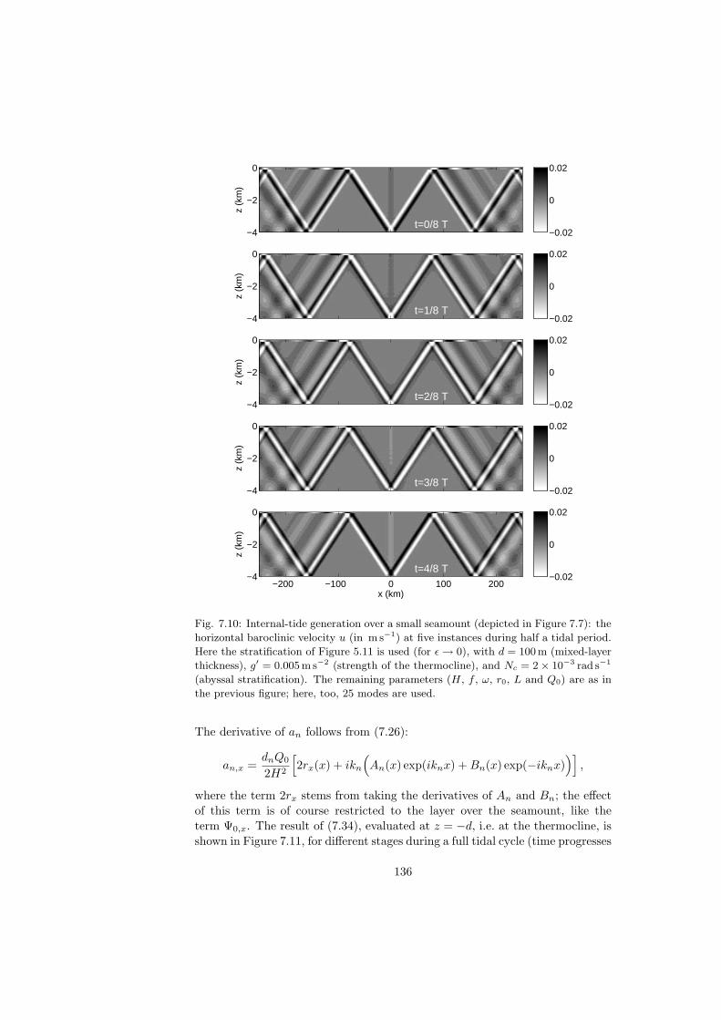
z (k

m)

t=0/8 T

−4

−2

0

−0.02

0

0.02

z (k

m)

t=1/8 T

−4

−2

0

−0.02

0

0.02

z (k

m)

t=2/8 T

−4

−2

0

−0.02

0

0.02

z (k

m)

t=3/8 T

−4

−2

0

−0.02

0

0.02

z (k

m)

x (km)

t=4/8 T

−200 −100 0 100 200−4

−2

0

−0.02

0

0.02

Fig. 7.10: Internal-tide generation over a small seamount (depicted in Figure 7.7): the

horizontal baroclinic velocity u (in m s−1) at five instances during half a tidal period.

Here the stratification of Figure 5.11 is used (for ε → 0), with d = 100m (mixed-layer

thickness), g′ = 0.005m s−2 (strength of the thermocline), and Nc = 2× 10−3 rad s−1

(abyssal stratification). The remaining parameters (H, f , ω, r0, L and Q0) are as in

the previous figure; here, too, 25 modes are used.

The derivative of an follows from (7.26):

an,x =dnQ0

2H2

[2rx(x) + ikn

(An(x) exp(iknx) + Bn(x) exp(−iknx)

)],

where the term 2rx stems from taking the derivatives of An and Bn; the effectof this term is of course restricted to the layer over the seamount, like theterm Ψ0,x. The result of (7.34), evaluated at z = −d, i.e. at the thermocline, isshown in Figure 7.11, for different stages during a full tidal cycle (time progresses

136

downward). Clearly, the interface is virtually at rest over the seamount, and atsome distance away from it. However, at the location where the beam impingeson the thermocline (x = ±80 km), the interface is brought into oscillation; wavespropagate away from this point. They become gradually smaller, and the causeof this attenuation is seen in Figure 7.10: they leak into the deep ocean asbeams. The upshot of this simple example is that internal tides are neitherpurely interfacial nor pure beams for this kind of stratification; they appear inmixed form. This is an important feature of some internal-tide observations, asis further discussed in Section 8.5.2.

−200 −100 0 100 200−45

−40

−35

−30

−25

−20

−15

−10

−5

0

5

η (m

)

x (km)

Fig. 7.11: The evolution of the interfacial (i.e. thermocline) displacement, at intervals

of 1/8 tidal period; time progresses downward; subsequent profiles are given a shift of

-5, for better visibility. The same parameters as in the previous figure.

7.4.3 Interfacial tides

A special case of the stratification used in the previous section is that withNc = 0; the stratification is then confined to the interface (Section 5.4.3). As aconsequence, there is only one mode (as long as ω > |f |): the interfacial mode.The barotropic tidal forcing will in this case produce purely interfacial tides.Its wavenumber follows from (5.44), and the modal structure is given by (5.45):

φ(z) =

− sinh qu(H−d)

sinh qud sinh quz −d < z < 0sinh qu(z + H) −H < z < −d .

(7.35)

The expression for dn is given in Appendix B.

137

The two-layer system, which involves only one mode, is rather inadequate fora description of internal tides in the deep ocean, but can sometimes be applied toshallower regions such as the continental shelf. We therefore choose parameterssuitable for this region. In the modal sum of the velocity field u, (7.31), there isnow of course only one mode involved; the result is shown in Figure 7.12. Thepropagation is purely horizontal, with oppositely directed currents in upperand lower layer. The currents are approximately inversely proportional to thethickness of the respective layers; hence the stronger currents in the thin uppermixed layer.

z (m

)

t=0/8 T

−200

−100

0

−0.05

0

0.05

z (m

)

t=1/8 T

−200

−100

0

−0.05

0

0.05

z (m

)

t=2/8 T

−200

−100

0

−0.05

0

0.05

z (m

)

t=3/8 T

−200

−100

0

−0.05

0

0.05

z (m

)

x (km)

t=4/8 T

−100 −50 0 50 100−200

−100

0

−0.05

0

0.05

Fig. 7.12: Internal-tide generation over a small ridge (depicted in Figure 7.7) on

the continental shelf: the horizontal baroclinic velocity u (in m s−1) at five instances

during half a tidal period. Here the stratification of Figure 5.11 is used (for ε → 0),

with d = 50m (mixed-layer thickness), g′ = 0.01m s−2 (strength of the thermocline),

and Nc = 0. The remaining parameters are H = 200 m and r0 = 50m; L, f , ω, and

Q0 are as in previous figures.

The total interfacial displacement η is given by (7.34), involving now onlyone mode. The result and is shown in Figure 7.13, for 8 different phases of thetide.

138

−100 −50 0 50 100−18

−16

−14

−12

−10

−8

−6

−4

−2

0

2

η (m

)

x (km)

←

←

.

→

→

→

.

←

←

Fig. 7.13: Internal-tide generation over a small ridge, showing the total interfacial

displacement η0 + η at t = 0 and at later stages separated by intervals of 1/8 tidal

period. Time progresses downward; subsequent profiles are given a shift of -2, for

better visibility. On the right, arrows indicate the direction of the barotropic tidal

flow at each stage.

7.5 Energetics and conversion rates

One can roughly distinguish two main regions of internal-tide generation: 1) thecontinental slope, where generation is concentrated near the shelf break, and 2)deep ocean ridges and seamounts. For the latter, the geographical distributionof internal-tide sources is obtained from estimates of barotropic tidal energydissipation, based on satellite altimetry; an example is shown in Figure 1.8.

This pattern is reproduced fairly well by results from numerical modelling,see Figure 7.14. Here the topography was assumed to be infinitesimal, as inpreceding sections, but two-dimensionality was taken into account. The threeessential ingredients of any internal-tide generation model are stratification,topography, and the barotropic flow. The three were here based on empiricaldata sets; for the stratification, a constant value, representative of the deepestlayer, was used for each position. Despite all the caveats and simplications, theresulting pattern looks sensible, and the total amount internal-tide energy fluxwas found to be about 1 TW, in agreement with estimates based on satellitealtimetry. The major influence of topographic features such as the Mid-AtlanticRidge is obvious from Figures 1.8 and 7.14.

As briefly discussed in Section 1.4, internal tides (and, more generally, inter-nal waves) are thought to play an important role in ocean mixing. This happensthrough a transfer of energy to shorter scales, the first stage of which may be, forexample, near-critical reflection from slopes, or nonlinear evolution to shorterwaves such as solitons (see the next chapter). This goes down to the scales atwhich waves break and turbulent mixing occurs (Figure 1.10). The very un-even distribution of internal-tide sources, as demonstrated in Figures 1.8 and

139

Fig. 7.14: Global distribution of M2 internal tidal energy fluxes, in W/m2, calculated

numerically from an internal-tide generation model. The color scale is logarithmic,

e.g., -3 means 10−3 W/m2. From [63].

7.14, means that deep ocean mixing, too, must be distributed unevenly. Thisis an important point in the modelling of ocean circulation; it means that oneshould not prescribe a simple uniform eddy diffusivity throughout the ocean, butrather take into account the geographical distribution of the mixing intensity.The ocean circulation, in turn, contributes to the meridional heat transport(the lion share of which, though, is due to atmospheric circulation). So theheat transport, too, is influenced by the way mixing is distributed through thegeographical spreading of internal-wave sources. This is illustrated in Figure7.15.

Fig. 7.15: The meridional heat transport for the global ocean. The gray band and

circles are indirectly based on empirical data. The solid and dashed lines are results

from a global circulation model, one with uniform mixing (dashed), in the other (solid),

the geographical distribution of internal tide generation sources was taken into account.

The latter seems to correspond better to the data; at any rate, the difference between

the solid and dashed lines is conspicuous. From [77].

The continental slope, too, forms an important source region of internal tides.A very simplified analysis of this problem was made in Section 7.3. Attempts to

140

model analytically a more realistic setting are thwarted by the complications ofvariable topography and stratification, which imply that neither the method ofvertical modes (Chapter 5) nor that of characteristics (Chapter 6) is applicable.However, the equations can be solved numerically, and this provides valuableinsights. For one thing, the steepness of the slope matters; in Section 6.2 we dis-cussed the distinction between sub- an supercritical slopes. Continental slopesare, generally, supercritical (apart from, of course, the upper and lower parts).An example of internal tide generation at a supercritical slope is shown in Figure7.16 (left). We see a beam emanating from the shelf break; by comparison, verylittle goes onto the continental shelf. It is now interesting to see how the ocean-ward energy flux (F1) depends on the steepness of the slope. This is illustratedin Figure 7.16 (right); note that the vertical scale is logarithmic. The angle α isa measure of the steepness of the slope; α > 1 means supercritical slopes; α < 1,subcritical slopes. We see that the flux varies only weakly with the angle of theslope as long as we are in the supercritical regime. The most extreme case of asupercritical slope would be the vertical slope considered in Section 7.3, and, asnoticed there, the energy flux derived from this model is fairly close to resultsfrom more sophisticated modelling, involving realistically shaped slopes. Thisfits in with the result from Figure 7.16 for supercritical slopes. For subcriticalslopes, on the other hand, we see that the oceanward flux is much smaller, andnow depends strongly on the angle of the slope.

Fig. 7.16: Results from a numerical model. Left: The streamfunction showing internal-

tide generation over a supercritical slope. Right: Dependence of the oceanward energy

flux (F1) on the steepness of the slope, α (α < 1, subcritical; α > 1, supercritical).

The dashed lines are from numerical model calculations; the solid lines are from a

representation in terms of powers of α: F1 ∼ α5 for the subcritical domain, F1 ∼ α

for the supercritical domain. From [8].

Turning, finally, to a more realistic setting, we show model results basedon topography and stratification in the Bay of Biscay (Figure 7.17). In theleft panel we see the conversion rate, in W/m3. It shows where the energy isconverted from barotropic into baroclinic tides. The conversion rate forms asource term in the energy equation, which can be written,

Et +∇(p′~u) = −ρ∗bW ,

141

where E is the energy density, p′ baroclinic pressure, ~u the baroclinic velocity,ρ∗ a constant reference value for density, b the buoyancy, and W the verticalvelocity component of the barotropic tide. We derived earlier an energy equationbut without source term (Section 4.5.2); now the barotropic tide is responsiblefor an input of energy, represented by the term on the right-hand side. Sinceinternal tides are periodic in time, time-averaging over a tidal period will makethe first term disappear (in other words, at every position, the mean energydensity stays the same), resulting in a balance between the flux gradient andthe source term. Stated otherwise, we may take a surface (or volume) integral,implying that the nett flux through the boundaries of the chosen area mustequal the integral input of energy by the source. In this sense we can takethe surface integral in 7.17 (left panel). This gives the value of the integratedconversion rate, as stated at the bottom of the figure, in W/m. The ’per meter’refers to the transverse direction; so if the slope would stretch over one thousandkilometers (say) in the Bay of Biscay, we would have to multiply by this numberto get the total conversion for this region.

distance (km)

dept

h (k

m)

Cint

= 8.84 kW/m

−15 −10 −5 0 5 10 15 20−1.4

−1.2

−1

−0.8

−0.6

−0.4

−0.2

0

0

0.5

1

1.5

2

2.5x 10−3

distance (km)

dept

h (k

m)

−150 −100 −50 0−5

−4

−3

−2

−1

0

0

0.04

0.08

0.12

0.16

0.2

Fig. 7.17: Results from a numerical model, here applied to the Bay of Biscay. Left:

The spatial distribution tidally-averaged conversion rate, C = −ρ∗〈bW 〉, in W/m3

(the brackets stand for tide averaging); the integrated value over the entire area is also

stated. Right: The internal tide emanating from the continental slope, here depicted

in terms of the amplitude of the cross-slope velocity u, in m/s. The white dots denote

the position of the observed beam, derived from Figure 1.9. From [27].

An important aspect of the conversion rate is its dependence on buoyancyb, which contains the baroclinic field itself. In other words, we cannot derivethe conversion rate from the barotropic field (W ) alone, one needs to know theinternal tide as well. This means that the conversion rate at any position is notonly determined by the local barotropic forcing, but also by the internal tidegenerated there as well as by internal tides passing that position but generatedelsewhere.

The resulting field is shown in Figure 7.17 (right panel), representing thecross-slope baroclinic velocity. A clear beam is present, emanating from theslope, propagating downward, and then reflecting from the bottom. The circlesfrom the observations shown in Figure 1.9 have been inserted for comparison.

142

We note that these model results were obtained for winter stratification, lackingthe seasonal thermocline. The beam is generated too deeply to be influenced bythe thermocline (which occupies a layer from about 50 to 150 meters beneath thesurface), but after bottom reflection the beam returns to the surface, and would,in summer, cross the thermocline. This gives rise to an interesting phenomenondiscussed in Section 8.5.2.

Appendix A: Integral expressions I

Here we list the identities used in Section 7.3 to solve the internal-tide generationproblem over a step-topography. To obtain (7.14), we used

∫ 0

−H

dz z sin(mπz

H

)= −H2 (−1)m

mπ∫ 0

−H

dz sin(nπz

H

)sin

(mπz

H

)=

H

2δnm

∫ −Hs

−H

dz sin(mπz

H

)=

H

mπ

[(−1)m − cos(mπα)

]

∫ 0

−Hs

dz z sin(mπz

H

)=

( H

mπ

)2[sin(mπα)−mπα cos(mπα)

]

∫ 0

−Hs

dz sin(nπz

Hs

)sin

(mπz

H

)=

Hsn

π

(−1)n sin(mπα)(mα)2 − n2

.

and to obtain (7.15),∫ 0

−Hs

dz sin(nπz

H

)sin

(mπz

Hs

)=

Hsm

π

(−1)m sin(nπα)(nα)2 −m2

∫ 0

−Hs

dz sin(nπz

Hs

)sin

(mπz

Hs

)=

Hs

2δnm .

Appendix B: Integral expressions II

The solution (7.26) contains the integral expressions An(x) and Bn(x). For theseamount given by (7.27), they read:

An = r0

0 for x < −Lπ2 exp(iknL)+[iπknL sin(πx/L)+π2 cos(πx/L)] exp(−iknx)

2[π2−(knL)2] for − L < x < Liπ2 sin(knL)π2−(knL)2 for x > L ,

and

Bn = r0

− iπ2 sin(knL)π2−(knL)2 for x < −L

−π2 exp(iknL)+[iπknL sin(πx/L)−π2 cos(πx/L)] exp(iknx)2[π2−(knL)2] for − L < x < L

0 for x > L .

143

In Sections 7.4.2 and 7.4.3 we use the three-layer model, in which the middlelayer (describing the thermocline) is in fact reduced to an interface. We providehere the technical details of the calculation of dn for these cases. Recall that dn

is given by (7.24):

dn =

∫ 0

−Hdz z φ′′n∫ 0

−Hdz φ′′nφn

. (7.36)

The function φn is given by (7.33); φn itself is continuous, but its derivative isnot: at the thermocline (z = −d) it jumps from one value to another. As aconsequence, its second derivative will contain a delta-distribution. This is alsoevident from (7.22), since N2 can here be written as

N2(z) = g′δ(z + d) + N2c Θ(−z − d) .

So, the integrals that feature in (7.36) can be split up into three parts: a termdue to the presence of the thermocline (concentrated at z = −d), and integralsover the upper and lower layers (

∫ 0

−dand

∫ −d

−H, respectively). The latter are

given by

I1 =∫ 0

−d

dz z φ′′n = cq2u

∫ 0

−d

dz z sinh(quz)

= c[qud cosh(qud)− sinh(qud)] ,

I2 =∫ −d

−H

dz z φ′′n = −q2l

∫ −d

−H

dz z sin ql(z + H)

= qlH − sin ql(H − d)− qld cos ql(H − d) ,

I3 =∫ 0

−d

dz φ′′nφn = c2q2u

∫ 0

−d

dz sinh2(quz)

= 14c2qu[sinh(2qud)− 2qud] ,

I4 =∫ −d

−H

dz φ′′nφn = −q2l

∫ −d

−H

dz sin2 ql(z + H)

= 14ql[sin 2ql(H − d)− 2ql(H − d)] ,

with

c = − sin ql(H − d)sinh qud

.

The coefficient dn is thus given by

dn =k2

ng′d(ω2 − f2)−1 sin ql(H − d) + I1 + I2

−k2ng′(ω2 − f2)−1 sin2 ql(H − d) + I3 + I4

, (7.37)

where the first term in the numerator and denominator represents the effect ofthe thermocline.

These expressions are to be modified for the case examined in Section 7.4.3;there the stratification in the lower layer is removed (Nc = 0), making φn

hyperbolic in the lower layer, as expressed in (7.35). Replacing ql by iqu in(7.37), including the integrals I1,2,3,4, we obtain a complex dn; multiplying itby i then yields the proper expression for the interfacial case.

144

Chapter 8

Internal solitons

In previous chapters we considered the linear equations, which can be assumedto be valid as long as the amplitude of the waves is small (Section 4.5). Thisassumption is however not always satisfied in observed internal waves. In thischapter, we turn to a particular class of waves in which nonlinearity is essential,the so-called internal solitons. They consist of a single depression (or elevation),and retain their form while propagating, and even when interacting with othersolitons. They are often observed in the oceans and atmosphere.

Linear problems are relatively easy to solve because the sum of any twosolutions is itself a solution (the superposition of modes in Chapter 5 is a case inpoint); thus, one solution engenders an infinite number of solutions. In nonlinearproblems, this convenient property holds no longer. However, soliton equationsare special in that a method has been developed to obtain the evolution of agiven initial profile by analytical means. This is discussed in this chapter forthe most well-known soliton equation, the Korteweg-de Vries equation, which iswidely applied to describe oceanic internal solitons.

8.1 Observations

One of many observations of solitons was made in the Andaman Sea [64]. Asingle soliton is shown in Figure 8.1 (left panel). Its largest vertical excursionsoccur in the thermocline, which here lies between 50 and 200m depth. Thedepression forms, in fact, part of a train of solitons (right panel); an increasein temperature at a given depth means that isotherms undergo a depression, inagreement with the panel on the left. One noticeable property is the amplitude-ordering of the train: the largest peak arrives first, and each subsequent peakis smaller than its predecessor. A surface manifestation of a group of solitonsin the Andaman Sea is shown in Figure 1.1. Further observations (not shownhere) reveal that such groups appear every tidal period, suggesting a relationto the internal tide, which is further discussed in Section 8.5.

In this chapter we focus on solitons in the ocean, but spectacular manifesta-

145

Fig. 8.1: Observations of solitons in the Andaman Sea. Left: Isothermal displace-

ments showing a large depression, with vertical excursions of more than 60m in the

course of just ten minutes. Levels of isotherms were here determined by using expend-

able bathythermographs (XBTs), giving a series of vertical temperature profiles, from

which follows the temporal evolution of selected isotherms. Right: A train of solitons;

temperature was measured continuously at certain fixed depths: a 53, b 87, c 116, d

164, and e 254m. The total water depth at this location is about 1100m. From [64].

146

tions have also been observed in the atmosphere. In Australia, this phenomenonis known as ’Morning Glory’ (Figures 8.2 and 8.3). In the atmosphere, solitons(and internal waves, in general) are rendered visible by adiabatic cooling of ris-ing parcels, leading to condensation of water vapour in the crests of the waves,and hence cloud formation.

Fig. 8.2: Interacting ‘Morning Glories’ over Northern Australia. Left: Map of the

location and sketch of the passage in time of two trains of solitary waves, coming from

northeastern and southern directions. Right: NOAA-12AVHRR satellite imagery at

the early morning of 3 October 1991, showing two interacting trains. From [71].

In the atmosphere, two main types of solitons can be distinguished [73]. Thefirst type is confined to the lower few kilometers of the troposphere, and has hor-izontal length scales of 100m to a few kilometers; the ’Morning Glory’ solitonsbelong to this category. They may be generated by, for example, gravity currentsor katabatic winds. The second type extends over the entire troposphere andhas a much larger horizontal scale, of the order of 100 km; proposed generationmechanisms are shear instability or geostrophic adjustment of large-scale frontalsystems. The vertical confinement of solitons, either to the lower few kilometersor to the troposphere as a whole, invites the question as to what causes thisconfinement. The atmosphere, unlike the ocean, has of course no well-definedupper boundary. Mechanisms that may nevertheless impose a waveguide are aneutrally stratified upper layer, or a very strongly stratified upper layer (caus-ing internal reflections), as discussed in Sections 5.3 and 5.4; shear layers maysimilarly cause reflections (from so-called critical levels). For a more extensivediscussion on the two types of solitons, we refer to [73].

8.2 Korteweg-de Vries (KdV) equation

One of the most well-known equations admitting solitons is the Korteweg-deVries equation, which was derived at the end of the 19th century, but receivedlittle attention until remarkable properties were discovered numerically somesixty years later. It was found that localized solutions exist which regain theirform after interactions with similar waves; to emphasize their robust character,

147

Fig. 8.3: Surface pressure signatures of interacting Morning Glory waves on 3 October

1991 from an array of portable microbarograph stations deployed over the southern

Gulf of Carpentaria region of Northern Queensland. The passage of a soliton is marked

by a change in pressure of about 1 mb. (’LST’ stands for Australian Eastern Standard

time, i.e. UTC plus 10 h.) From [71].

the name ’soliton’ was coined, the suffix “-on” giving it the flavour of an elemen-tary particle [91]. A second discovery, made soon after, concerned the evolutionof a given initial profile; it turned out that this problem can be reduced tosolving two linear equations [59], as is further discussed in Section 8.4.1 Theequation surfaces in many branches of physics, such as fluid mechanics, plasmaphysics, and quantum gravity [9].

The KdV equation contains two effects that together allow for the existenceof a soliton solution: nonlinearity and dispersion. We first discuss each of themseparately.

8.2.1 Effect of nonlinearity

The simplest equation describing the propagation of nonlinear waves is

∂η

∂t+

∂η

∂x+ ε η

∂η

∂x= 0 . (8.1)

1For more on the history of the KdV equation, see [86, 57]. In fact, the history of theKdV equation (and the question how the paper by Korteweg and De Vries relates to previousworks, notably by Boussinesq) seems to get more intricate as more documents, among themnotes by De Vries, are unearthed; for a recent overview, see [11].

148

Here we have some dimensionless parameter ε (the precise form of which isimmaterial in the present discussion) serving as a coefficient of the nonlinearterm. The field η may describe, for example, an isopycnal excursion.

In implicit form, the general solution of (8.1) can be expressed in terms ofan arbitrary function F :

η(x, t) = F (ξ) , with ξ = x− (1 + εη(x, t)) t . (8.2)

It is easily verified that this is indeed a solution; differentiation of (8.2) gives

∂η

∂t=

∂ξ

∂tF ′ = −

(1 + εη + εt

∂η

∂t

)F ′ ,

∂η

∂x=

∂ξ

∂xF ′ =

(1− εt

∂η

∂x

)F ′ ,

with F ′ = dF/dξ. Hence

∂η

∂t= − (1 + εη)F ′

1 + εtF ′

∂η

∂x=

F ′

1 + εtF ′. (8.3)

Substitution now demonstrates that (8.1) is satisfied.We have here introduced a ’characteristic’ coordinate ξ, which in a mathe-

matical sense is analogous to the characteristics of Chapter 6. Physically, themeaning is of course very different, for in Chapter 6 only spatial coordinateswere involved in the transformation, whereas ξ = const here represents a pathin x,t-space, on which η is constant. For constant ξ = x0, we have the charac-teristic

x = x0 + (1 + εη(x, t)) t . (8.4)

On it, we must have, according to (8.2),

η(x, t) = F (x0) = constant .

Hence (8.4) describes a straight line,

x = x0 + (1 + εF (x0)) t . (8.5)

This expression indicates where, at a certain moment t, the value η = F (x0)is to be found. It moreover shows that higher elevations (i.e. larger F (x0))propagate faster. An example is shown in Figure 8.4. On the left we have theline

x = xA + (1 + εF (xA)) t ,

and the other lines are similarly defined. (Notice that time is shown on thevertical axis in Figure 8.4.) The line in the middle, starting at x = 0 shows thelocation of the wave crest, η = F (xB), as time passes. The crest propagatesfaster than the neighbouring elevations F (xA) and F (xC); in other words, the

149

Fig. 8.4: Lower panel: An initial profile of η. Upper panel: Characteristics indicating

where, at time t, the elevation F is located that was initially at xA, xB , or xC . The

intersection of lines is indicative of a multi-valued η at that point in t, x-space, and

signals wave breaking.

phase speed depends on the elevation F . At a certain moment the lines B andC cross; this is the moment of wave breaking.

This wave breaking is clearly a result of the nonlinear term, since the char-acteristics would all be equally steep if ε = 0. The moment of breaking can alsoderived directly from (8.3). If the wave breaks, ∂η/∂x becomes infinite, andthis happens at

t = − 1εF ′

= O(ε−1) .

(The minus sign indicates that a rightward propagating wave of elevation willbreak on its descending side, i.e. where F ′ is negative.) This expression revealsalso that a time scale, of order 1/ε, is associated with wave breaking. So, nomatter how small ε, the nonlinear term will become important after a sufficientlylong time. In other words, for the linear approximation to be valid, smallnessof ε is not sufficient; a limit is posed as well on the stretch of time that one mayconsider.

150

8.2.2 Effect of dispersion

In (5.46), we found that long interfacial waves in a rotationless system (f = 0)satisfy the dispersion relation

ω2 = c20k

2 [1− 13d(H − d)k2 + · · · ] (8.6)

with

c20 = g′

d(H − d)H

. (8.7)

Here H is the total water depth, d the thickness of the upper layer, and g′

reduced gravity, measuring the strength of the thermocline, here represented byan interface. If we restrict ourselves to rightward propagating waves, we canapproximate (8.6) by

ω = c0k [1− 16d(H − d)k2 + · · · ] . (8.8)

From this expression we see that interfacial are dispersive, i.e. the phase speed

c(k) =ω

k= c0 [1− 1

6d(H − d)k2 + · · · ] (8.9)

varies with wavenumber k. This type of dispersion may be termed non-hydrostaticdispersion, since it disappears in the hydrostatic (or long-wave limit, or shallow-water) limit, i.e. if kd, k(H − d) → 0.

A certain initial profile, such as in Figure 8.4 (upper panel), can be describedin terms of a Fourier integral,

η(x, 0) =∫ ∞

−∞dk F (k) eikx ,

for a certain function F . The profile evolves in time according to

η(x, t) =∫ ∞

−∞dk F (k) ei(kx−ω(k)t)

=∫ ∞

−∞dk F (k) eik(x−c(k)t) .

Because of the dispersive character of (8.9), different Fourier components willtravel at different speeds. As a result, the the initial profile will lose its form asit falls apart in its Fourier components.

It is easy to verify by substitution of the Fourier integral, that the evolutionequation associated with the dispersion relation (8.8) reads

∂η

∂t+ c0

∂η

∂x+

16

c0d(H − d)∂3η

∂x3= 0 . (8.10)

The third term represents the effect of non-hydrostatic dispersion.

151

8.2.3 KdV for interfacial waves

From the previous two sections it is clear that

• non-linearity alone will make a solitary wave profile steepen and break;

• non-hydrostatic dispersion alone will make a solitary wave profile fall apartin its Fourier components.

So, neither of the effects, taken in isolation, can sustain a solitary wave. The cruxof the KdV equation is that a combination of the effects can. Intuitively this canbe understood as follows: nonlinearity, by its steepening effect, tends to driveenergy to a short scale; dispersion, on the other hand, tends to spread it out.In a sense, then, the effects are opposed, and the KdV equation demonstratesthat they can balance to produce form-preserving waves.

For interfacial waves, described by η, the displacement of the interface fromits level of rest, the KdV equation reads

∂η

∂t+ c0

∂η

∂x+

32

h1 − h2

h1h2c0 η

∂η

∂x+

16

c0h1h2∂3η

∂x3= 0 . (8.11)

Here we write the thickness of the upper layer as h1 = d, and that of the lowerlayer as h2 = H − d. The linear long-wave speed for interfacial waves, c0, isagain defined by (8.7), which in terms of h1,2 reads

c20 = g′

h1h2

h1 + h2. (8.12)

The effects of nonlinearity and non-hydrostatic dispersion, discussed in the pre-vious sections, recur in the second and third term of (8.11), respectively.

This form of the KdV equation will be derived in Section 8.3. The essentialunderlying assumption is that nonlinear and non-hydrostatic effects are weakand of the same order of strength. The derivation then proceeds in two steps; atlowest order, a linear hydrostatic equation is derived, consisting of the first twoterms of (8.11). Then, at the next order, nonlinear and non-hydrostatic effectsappear, completing (8.11).

From this outline of the derivation it will already be clear that the KdVequation is not exact. It is sometimes indeed necessary to proceed to a higherorder. A configuration in which h1 = h2 (i.e. the upper and lower layer are ofequal thickness) is a case in point: the nonlinear term in (8.11) then vanishesaltogether. A higher-order extension is then needed (Section 8.6).

8.2.4 A heuristic ‘derivation’

If we cast the linear dispersive equation (8.10) in terms of the parameters h1 = d

and h2 = H − d, we obtain

∂η

∂t+ c0

∂η

∂x+

16

c0h1h2∂3η

∂x3= 0 , (8.13)

152

which is (8.11), except for the nonlinear term. There is a simple heuristic wayto obtain the correct form of this term from (8.13), apart from a numericalfactor. So, although the equation thus obtained will not be entirely correct, thereasoning leading to it gives some more insight in the nature of the nonlinearterm.

The starting point is the term c0∂η/∂x, in which c0 is given by (8.12),

c20 = g′

h1h2

h1 + h2.

Here h1 and h2 are the thickness of the upper and lower layer, respectively. Theimportant thing to realize is that if waves attain an appreciable amplitude η,the actual thickness of the upper layer will not be h1 but h1 − η. Similarly,the thickness of the lower layer becomes h2 + η. If we substitute this in theexpression for c0, we get

[g′

(h1 − η)(h2 + η)h1 + h2

]1/2

=[g′

h1h2 + η(h1 − h2)− η2

h1 + h2

]1/2

= c0

[1 + η

h1 − h2

h1h2− η2 1

h1h2

]1/2

= c0

[1 + η

h1 − h2

2h1h2+ · · ·

],

where we neglected quadratic terms in η. If replace c0∂η/∂x in (8.13) with thelast expression, we obtain the nonlinear term

c0h1 − h2

2h1h2η

∂η

∂x,

which is of the same form as the nonlinear term in (8.11), but lacks the factorthree.

This ’derivation’ makes clear why the nonlinear term cancels if h1 = h2; theincrease of the phase speed by the enlargement of one layer is then preciselycompensated by the decrease of the phase speed due to the thinner other layer.

8.2.5 Soliton solution

In short-hand notation, we write (8.11) as

∂η

∂t+ c0

∂η

∂x+ Aη

∂η

∂x+ B

∂3η

∂x3= 0 . (8.14)

We seek form-preserving solutions,

η(x, t) = F (ξ) , with ξ = x− Ct .

The function F and phase speed C are to be determined. We denote the deriva-tive of F by a prime, F ′ = dF/dξ. The derivatives of η can be written

∂η

∂t= −CF ′ ,

∂η

∂x= F ′ .

153

Substitution in (8.14) gives

−(C − c0)F ′ + AFF ′ + BF ′′′ = 0 .

The second term can be written as 12A(F 2)′, so that we can integrate the equa-

tion to obtain

−(C − c0)F + 12AF 2 + BF ′′ = 0 .

Here we have taken the constant of integration equal to zero, as we are lookingfor solitary-wave solutionsz, for which F and derivatives vanish as |ξ| → ∞.Multiplying by F ′ now gives

−(C − c0)FF ′ + 12AF 2F ′ + BF ′′F ′ = 0 ,

or, equivalently,

− 12 (C − c0)(F 2)′ + 1

6A(F 3)′ + 12B(F ′2)′ = 0 .

After one more integration (and again setting the constant of integration equalto zero), we obtain

−(C − c0)F 2 + 13AF 3 + B(F ′)2 = 0 .

Taking the square root,

B1/2 F ′ = [(C − c0)F 2 − 13AF 3]1/2 ,

so that

dξ =B1/2 dF

[(C − c0)F 2 − 13AF 3]1/2

=B1/2 dF

(C − c0)1/2 F [1− A3(C−c0)

F ]1/2. (8.15)

The second square root can be removed via the transformation

F =3(C − c0)

Asech 2q , (8.16)

and using the identitytanh2 q = 1− sech 2q .

Using moreover the identity

d

dqsech q = −sech q tanh q ,

we havedF = −2F tanh q dq ,

154

so that (8.15) reduces to

dξ = −2 dq[ B

C − c0

]1/2

,

or integrated,

q = −ξ[C − c0

4B

]1/2

,

where we left out the constant of integration, which would give a mere phaseshift. Finally, substitution in (8.16) gives

F =3(C − c0)

Asech 2

(ξ[C − c0

4B

]1/2)

.

This is the soliton solution. It can be more conveniently written in terms of theamplitude and length of the wave,

a =3(C − c0)

Al =

[ 4B

C − c0

]1/2

.

With this, the soliton solution becomes

η = a sech 2(x− Ct

l

), (8.17)

where

C = c0 +aA

3, l =

(12B

aA

)1/2

.

Using the explicit form of the coefficients A and B for the two-layer system,

C = c0

[1 + 1

2 ah1 − h2

h1h2

], l =

2h1h2

[3a(h1 − h2)]1/2. (8.18)

An example of a soliton profile is shown in Figure 8.5.Eq. (8.18) demonstrates that the phase speed C (as well as the length l)

depend on the wave amplitude; this is a manifestation of the nonlinear characterof the soliton. It furthermore follows from the second expression in (8.18) that

a (h1 − h2) > 0 , (8.19)

since the argument of the square root must be positive. From (8.18) and (8.19)follow four important properties of KdV solitons:

1. The phase speed of the soliton, C, exceeds the linear long-wave phase speedc0;

155

2. Eq. (8.19) implies that the amplitude a must be negative if h1 < h2 (i.e. ifthe upper layer is relatively thin, as is normally the case in the ocean); thesoliton then manifests itself as a depression, as in Figure 8.1 (left panel);

3. Larger solitons (i.e. larger |a|) propagate faster than smaller ones. Thismeans that a train of solitons emanating from the same source will beordered in amplitude, the largest leading the group. We recall that thiswas indeed observed in Figure 8.1 (right panel);

4. Larger solitons are shorter than smaller ones, since l is inversely propor-tional to a1/2; an example is shown in Figure 8.5.

η↑

|−5

|5

x →

−

−

−

−

−

−

−

−

10

−10

−70

Fig. 8.5: Examples of the soliton solution (8.17), with different amplitudes: a =

−60m (solid line) and a = −20m (dashed line). For both, the parameters are g′ =

0.01m s−2, h1 = 200m, h2 = 1200m. The phase speeds C are 1.47m s−1 (solid

line) and 1.37m s−1 (dashed line); for comparison, the linear long-wave phase speed

is c0 = 1.31m s−1. On the horizontal axis, distances are in kilometers; on the vertical,

in meters.

Apart from a single-soliton solution, the KdV equation also admits multi-soliton solutions, involving solitons of different amplitudes. We will not dwellon this, but remark that they pass each other (since the phase speed depends onthe amplitude), yet come out of the interaction with unchanged shape. Duringthe interaction, they do of course not superpose in a linear way; in fact, the totalamplitude during interaction is less than the sum of their amplitudes before (orafter) the interaction.

156

8.3 Derivation of the KdV equation

8.3.1 Basic equations

Our starting point is the set (4.17), where nonlinear terms are retained,

D~u

Dt+ 2~Ω× ~u = − 1

ρ∗∇p′ + bz (8.20a)

∇ · ~u = 0 (8.20b)Db

Dt+ N2w = 0 . (8.20c)

We simplify the problem by neglecting Coriolis effects altogether (a short dis-cussion on Coriolis effects and solitons follows in Section 8.5); moreover, weassume ∂/∂y = 0. In the two-layer system, the upper and lower layer are eachneutrally stratified (N = 0), the stratification being concentrated as a δ-peakat the interface that separates the layers (see Section 5.4.3). So, if we considerthe upper and lower layers separately, we have N = 0 in each, and hence b = 0,so that (8.20) becomes

ui,t + uiui,x + wiui,z = − 1ρ∗

p′i,x (8.21)

wi,t + uiwi,x + wiwi,z = − 1ρ∗

p′i,z (8.22)

ui,x + wi,z = 0 . (8.23)

Here index i takes the value 1 for the upper layer, and 2 for the lower layer.We choose the z-axis such that the level of rest of the interface lies at z = 0;

the upper surface (rigid-lid) lies at z = h1, the bottom at z = −h2. We introducea new notation for these levels, which proves convenient in later scaled forms:h1 = αH and h2 = (1 − α)H, where H = h1 + h2 is the total water depth(Figure 8.6).

The the upper surface (rigid-lid) and bottom the vertical velocity w mustvanish,

w1|z=αH = 0 (8.24)

w2|z=(α−1)H = 0 . (8.25)

At the interface, z = η(t, x), we find by taking D/Dt,

wi|z=η = ηt + ηxui|z=η (i = 1, 2) . (8.26)

We have yet to to take into account the presence of a density jump acrossthe interface, which produces the delta-peak in N2. This is done by requiringcontinuity of total pressure, for which we have to return to (4.7),

p = p0(z) + p′(t, ~x) , (8.27)

157

z=h1=αH

z=−h2=(α−1)H

z=η(t,x)

upper surface (rigid−lid)

interface

bottom

layer 1

layer 2

Fig. 8.6: The two-layer system for which the KdV equation is derived. Both upper

and lower layer are neutrally stratified, N = 0. Across the interface there is a jump

in density, giving a delta-peak N2 = g′δ(z). The horizontal dotted line indicates the

level z = 0, the level at which the interface resides at rest.

in which p0 is given by the hydrostatic balance (4.9),

dp0

dz= −ρ0g . (8.28)

To obtain p0 we need to know the static density profile ρ0. In a two-layersystem, the densities in each layer are commonly assumed to be constant. Thisis however in contradiction with the assumption that N = 0 in each layer, as iseasily seen from (4.19),

N2 = − g

ρ∗

(dρ0

dz+

ρ0g

c2s

). (8.29)

Assuming ρ0 to be constant produces a layer in which N2 < 0, i.e. an unstablystratified layer. So, if we stick to the assumption N = 0, we cannot also assumethat ρ0 is constant.

We thus proceed from (8.28), integrating for each layer to obtain the hydro-static pressure:

p0,1(z) = g

∫ h1

z

dζ ρ0,1(ζ) , p0,2(z) = g

∫ h1

0

dζ ρ0,1(ζ) + g

∫ 0

z

dζ ρ0,2(ζ) .

Requiring now the total pressure, p0,i + p′i to be continuous at the interface,gives

p′2|z=η − p′1|z=η = g

∫ η

0

dζ ρ0,2(ζ)− g

∫ η

0

dζ ρ0,1(ζ) .

158

For small η, the right-hand side can be expanded as

g

∫ η

0

dζ[ρ0,2(0) + ζ

dρ0,2

dz(0) + · · ·

]− g

∫ η

0

dζ[ρ0,1(0) + ζ

dρ0,1

dz(0) + · · ·

]

g[ηρ0,2(0) + 1

2η2 dρ0,2

dz(0) + · · ·

]− g

[ηρ0,1(0) + 1

2η2 dρ0,1

dz(0) + · · ·

]

g[ηρ0,2(0)− 1

2η2 ρ0,2g

c2s,2

+ · · ·]− g

[ηρ0,1(0)− 1

2η2 ρ0,1g

c2s,1

+ · · ·].

In the last expression, we used the fact that N2 = 0 within each layer, and(8.29). Now, the quadratic terms in square brackets scale with the linear termsas ηg/c2

s, which even for large solitons (η ∼ 100m) is very small, namely oforder O(10−3). We will therefore neglect them; we can thus write the conditionfor continuity of pressure as

p′2|z=η − p′1|z=η = (ρ0,2(0)− ρ0,1(0))gη . (8.30)

(Hereafter we will drop the argument in ρ0,i, it be understood that they areevaluated at the interface.) This condition states that baroclinic pressure is dis-continuous across the interface, due to a jump in density. It is clear from (8.21)that this discontinuity will similarly create a discontinuity in the horizontalvelocity ui.

8.3.2 Scaling and small parameters

For ui we introduce the scale [ui] = εc, where c is a measure of the phase speedof the wave (to be specified below). Here ε acts as the parameter of nonlinearity,in accordance with the argument presented in Section 4.5, according to whichthe ratio of particle velocity and phase speed is a measure of the strength ofnonlinearity. Time and length scales of the waves are denoted by [t] = T and[x] = cT = L. We scale the vertical with H, the water depth.

As we assume nonlinear terms to be weak, the dominant balance in (8.21)will be between the linear acceleration term and the pressure gradient, givingas a scale for pressure: [p′i] = ρ∗εc2. The scale for wi follows from (8.23) as[wi] = εcH/L, and hence from (8.26), [η] = εH. This provides us with analternative interpretation of the parameter of nonlinearity, namely as the ratioof the wave amplitude and water depth.

Using these scales, we can cast the equations (8.21)–(8.23) in a nondimen-sional form,

ui,t + εuiui,x + εwiui,z = −p′i,x (8.31)

δ(wi,t + εuiwi,x + εwiwi,z) = −p′i,z (8.32)

ui,x + wi,z = 0 , (8.33)

where we used the same symbols as for the dimensional variables, for conve-nience. (No confusion will arise from this as we will consider only the nondimen-

159

sional form in the remainder of this section.) We introduced a new parameter

δ =(H

L

)2

,

which is a measure of the strength of non-hydrostatic dispersion; the limit δ → 0corresponds to the hydrostatic (or long-wave) limit, in which case the wavesbecome dispersionless (Section 8.2.2).

The boundary conditions (8.24)-(8.26) and (8.30) become, in nondimensionalform,

w1|z=α = 0 (8.34)

w2|z=α−1 = 0 (8.35)

wi|z=εη = ηt + εηxui|z=εη (8.36)

p′2|z=εη − p′1|z=εη = η . (8.37)

Here we identified c, the measure of the phase speed, with c2 = g′H, where g′

is the reduced gravity g′ = g(ρ0,2 − ρ0,1)/ρ∗; the last expression provides aninterpretation of g′ in terms of density, rather than in terms of N2, as in Figure5.11.

The crucial assumption, which leads to the KdV equation, is

ε = O(δ) ¿ 1 . (8.38)

This means we consider weakly nonlinear, weakly non-hydrostatic effects, whichare of similar strength. The last assumption means that we are, in essence,dealing with only one small parameter, and we can write

δ = εδ∗

with δ∗ = O(1).The goal is now to reduce the set (8.31)–(8.37) to a single equation for the

interfacial displacement η. We thus seek an equation of the form

D0(η) + εD1(η) + ε2D2(η) + · · · = 0 (8.39)

where Di are differential operators. To obtain the KdV equation, it suffices todetermine D0 and D1.

We develop the variables p′i, ui, wi and η in a series, in which ε serves as thesmall parameter; so, for example,

p′i = pi(0) + εpi

(1) + ε2pi(2) + · · ·

with pi(n) = O(1).

160

As a preparation for the following sections, we develop the boundary condi-tions (8.36) and (8.37) in a Taylor series about z = 0; for the left-hand side of(8.36), this gives

wi|z=εη = wi|z=0 + εηwi,z|z=0 +O(ε2)

= wi|z=0 − εηui,x|z=0 +O(ε2)

(in the second equality we used (8.33)), so (8.36) becomes

wi = ηt + ε(ηui)x +O(ε2) at z = 0 . (8.40)

Similarly, we obtain from (8.37):

η = (p′2 − p′1)|z=0 + εη(p′2,z − p′1,z)|z=0 +O(ε2) . (8.41)

For later reference, we define the jump in u (’shear’) across the interface asu = (u2 − u1)|z=εη, the Taylor expansion of which is

u = (u2 − u1)|z=0 + εη(u2,z − u1,z)|z=0 +O(ε2) . (8.42)

8.3.3 Lowest order

At the lowest order, ε0, (8.31)–(8.33) read

ui,t(0) + pi,x

(0) = 0

pi,z(0) = 0

ui,x(0) + wi,z

(0) = 0 .

So, at this order, pi(0) and ui

(0) are independent of z, which is characteristicof the hydrostatic approximation, which applies at this order because we haveneglected the terms with δ∗. The boundary conditions (8.34), (8.35), (8.40) and(8.41) are, at lowest order,

w1(0)|z=α = 0

w2(0)|z=α−1 = 0

wi(0)|z=0 = ηt

(0)

p2(0) − p1

(0) = η(0) .

The horizontal momentum equation and boundary condition for pressurecan be combined into

ut(0) + ηx

(0) = 0 . (8.43)

where u(0) is the lowest-order shear from (8.42).Integration of the continuity equation over the upper and lower layers gives,

respectively,

ηt(0) − αu1,x

(0) = 0

ηt(0) + (1− α)u2,x

(0) = 0 .

161

Multiplying the first by 1−α, the second by α, and adding up the results gives

ηt(0) + ν2ux

(0) = 0 (8.44)

with ν2 = α(1− α).We combine (8.43) and (8.44) to

ηtt(0) − ν2ηxx

(0) = 0 .

This equation decribes linear long waves, both left- and rightward propagat-ing. Its general solution can be written as F (x + νt) + G(x − νt) (cf. Section6.1.2 for a mathematically similar problem). We restrict ourselves to rightwardpropagating waves; they are described by

ηt(0) + νηx

(0) = 0 . (8.45)

At lowest order, (8.39) reads

D0(η(0)) = 0 . (8.46)

Comparing this with (8.45), we see that the operator D0 is given by

D0(η) = ηt + νηx . (8.47)

Finally, we derive some expressions that are useful at the next order. From(8.44) and (8.45), we have

η(0) = νu(0) . (8.48)

The integrated continuity equations imply

u1(0) = (α− 1)u(0) u2

(0) = αu(0) (8.49)

w1(0) =

α− z

αηt

(0) w2(0) =

α− 1− z

α− 1ηt

(0) . (8.50)

From (8.49) we see that the horizontal velocities in each layer are inverselyproportional to their thickness. Thus, in a shallow upper layer, the currents willbe strongest. Moreover, they are directionally opposed, with the total transportbeing zero.

8.3.4 Next order

At the next order, ε1, (8.31) and (8.33) read

ui,t(1) + ui

(0)ui,x(0) = −pi,x

(1)

δ∗wi,t(0) = −pi,z

(1)

ui,x(1) + wi,z

(1) = 0 .

162

In the first equaion we used ui,z(0) = 0. The boundary conditions (8.34), (8.35),

(8.40) and (8.41) read

w1(1)|z=α = 0

w2(1)|z=α−1 = 0

wi(1)|z=0 = ηt

(1) + (ui(0)η(0))x

p2(1)|z=0 − p1

(1)|z=0 = η(1) .

(In the last equation we used pi,z(0) = 0.) The vertical shear, (8.42), becomes

at this order u(1) = (u2(1) − u1

(1))|z=0.From the horizontal momentum equation, together with the boundary con-

dition for pressure, we find, using also (8.49):

ut(1) + (2α− 1)u(0)ux

(0) + ηx(1) = 0 . (8.51)

We now take ∂/∂z of the horizontal momentum equation (by which the nonlin-ear terms disappear because ui,z

(0) = 0), and ∂/∂x of the vertical momentumequation, and substract the results; after one time integration, this gives

ui,z(1) = δ∗wi,x

(0) .

Substitution of (8.50) gives, after one intergration to z,

u1(1) = δ∗

αz − z2/2α

ηxt(0) + u1

(1)|z=0

u2(1) = δ∗

(α− 1)z − z2/2α− 1

ηxt(0) + u2

(1)|z=0 .

Using these expressions, we integrate the continuity equation over the upperand lower layers, to obtain,

ηt(1) + (u1

(0)η(0))x − αu1,x(1)|z=0 − 1

3δ∗α2ηxxt

(0) = 0

ηt(1) + (u2

(0)η(0))x + (1− α)u2,x(1)|z=0 − 1

3δ∗(1− α)2ηxxt(0) = 0 .

where we used the boundary conditions for wi(1). Multiplying these expressions

by 1− α en α, respectively, and adding up the results, yields

ηt(1) + (2α− 1)(u(0)η(0))x + ν2ux

(1) − 13δ∗ν

2ηxxt(0) = 0 (8.52)

where we simplified the nonlinear term using (8.49).Combining (8.51) and (8.52) gives

ηtt(1) − ν2ηxx

(1) + 3(1− 2α)(η(0)ηx(0))x − 1

3δ∗ν4ηxxxx

(0) = 0 , (8.53)

where we used (8.45) and (8.48). Because of (8.45), we may split the spatialderivative at lowest order as

ηx(0) = − 1

2ν (ηt(0) − νηx

(0)) .

163

Hence we can extract the operator ∂/∂t− ν∂/∂x from (8.53):

ηt(1) + νηx

(1) + 32ν (2α− 1)η(0)ηx

(0) + 16δ∗ν

3ηxxx(0) = 0 . (8.54)

At this order, (8.39) reads

D0(η(1)) + D1(η(0)) = 0 . (8.55)

Comparing this with (8.54), we find that the operator D1 is given by

D1(η) = 32ν (2α− 1)ηηx + 1

6δ∗ν3ηxxx . (8.56)

8.3.5 Final result

Now that we have obtained the operators D0 and D1, we can write (8.39) inexplicit form as

ηt + νηx + 32ν ε (2α− 1)ηηx + 1

6δν3ηxxx + · · · = 0 . (8.57)

The KdV equation now follows if we neglect the higher-order terms (cubic etc.),which are here rendered by dots. When we cast this equation back into dimen-sional variables, we obtain (8.11). With this, the derivation has been completed.

8.4 Inverse-scattering theory

So far, we have obtained only one solution of the KdV equation, the soliton(8.17), which preserves its form while propagating. Other initial profiles thanthe soliton will not, in general, be form-preserving. Yet, they may give rise tosolitons during their evolution. The question is now, how we can determinewhether this is the case, and, more specifically, how many solitons are to beexpected. At the end of this section, it will become clear that these questionsare surprisingly easy to answer, but to arrive at that simple result, we first needto go through a subject from quantum mechanics, called ’inverse scatteringtheory’.

In the following sections, we briefly explain this method, which is remark-able because it reduces the initial-value problem for the KdV equation, which isnonlinear, to the problem of solving two linear equations, the Schrodinger andMarchenko equations. In practice, the method is applicable in only some cases,because these linear equations are not, in general, easy to solve. However, if weare only interested in the number of solitons that will appear from an arbitraryinitial profile, then, as it turns out, we need to solve only part of the problem(namely determine the number of discrete eigenvalues of the Schrodinger equa-tion). What is more, it actually turns out that we do not even have to solvethat problem, because the number of eigenvalues depends merely on the overallintegral shape of the initial profile; its specifics are immaterial. So, finally, a

164

simple expression is obtained for the number of solitons, N , arising from aninitial profile η ≤ 0:

N ∼∫ ∞

−∞dx

√|η(x, 0)| . (8.58)

In Section 8.5.1 we adapt this expression to conform with the parameters in atwo-layer system.

8.4.1 The scattering problem

We start in medias res and consider the scattering problem of the Schrodingerequation:

−d2ψ

dx2+ qψ = λψ . (8.59)

The problem is to determine, for a given localized potential q(x),2 the eigen-functions ψ, along with its corresponding eigenvalues λ.

As we assume q be localized, (8.59) becomes for large |x|

−d2ψ

dx2∼ λψ . (8.60)

There are two cases to be distinguished: λ > 0 and λ < 0. In the first casewe write λ = k2 (k being real). One solution of (8.60) then is e−ikx, which weinterpret as a wave coming from +∞. When it arrives in the region where thepotential is active, part of the wave will be reflected, giving R(k)eikx as x →∞,and the other part will be transmitted, giving T (k)e−ikx as x → −∞ (Figure8.7). The reflection coefficient R(k) and transmission coefficient T (k) dependon the potential q. Asymptotically, we thus have

ψ(x, k) ∼

e−ikx + R(k)eikx x →∞T (k)e−ikx x → −∞ .

The second case, λ < 0, gives rise to a finite number of discrete eigenvalues,together with the corresponding eigenfunctions ψ describing bound states; bothwill be labeled by n. We write λ = −p2

n, with pn real, and choose, without lossof generality, pn to be positive. For x →∞, the bound state ψn looks like

ψn(x) ∼ cne−pnx .

We fix the constant cn by the requirement that∫∞−∞dxψ2

n(x) = 1.The direct scattering problem consists in determining R(k), T (k), cn for a

given potential q. The inverse scattering problem consists in determining q fromgiven ’scattering data’. For the class of potentials considered here, it sufficesto know R(k), cn, pn to uniquely determine the potential (see [1, Theorem2.5.1]).

2i.e. q → 0 for |x| → ∞; some of the later theorems also presumeR∞−∞dx (1+|x|) |q(x)| < ∞.

165

←→

←

R(k)eikx

e−ikxT(k)e−ikx

q(x)

x→

Fig. 8.7: The scattering problem in quantum mechanics: an incoming wave, from

the right, is partially reflected at the potential q, and partially transmitted; hence the

reflection and transmission coefficients R(k) and T (k).

We now briefly outline. how the inverse scattering problem is solved.3 Forgiven scattering data R(k), cn, pn, we define

M(x) =∑

n

c2ne−pnx +

12π

∫ ∞

−∞dk R(k)eikx . (8.61)

Then we solve the function K(x, y) from the so-called Marchenko equation,

K(x, y) + M(x + y) +∫ ∞

x

dz K(x, z)M(y + z) = 0 (8.62)

for y > x. Finally, we calculate K(x, x) ≡ limy→x K(x, y), from which thepotential q is found as

q(x) = −2d

dxK(x, x) . (8.63)

We now show that there is a connection, indeed a very useful one, betweenthe KdV equation and this scattering problem. We first slightly generalize thescattering problem, by allowing the potential in (8.59) to depend on a certainparameter, τ say. (This parameter will later be taken to represent time.) Theeigenfunction ψ and scattering data R(k), cn, pn will then, in general, alsodepend on τ . However, the eigenvalue λ (and hence pn) are independent of τ

for certain classes of potentials; for example, for q’s satisfying

qτ − 6qqx + qxxx = 0 (8.64)

which is, in scaled form, the KdV equation!Stated more generally, we define operator L by

L = − d2

dx2+ q(x; τ) ,

3Proofs of the correctness of the method are beyond the scope of this text; see, e.g., [1].

166

and suppose thatψτ = Bψ (8.65)

for a certain differential operator B (which may contain derivatives to x only).We then find by taking the derivative of (8.59) to τ ,

(qτ + [L, B])ψ = λτψ , (8.66)

where [L,B] = LB − BL. The eigenvalues λ are independent of τ if B is suchthat the left-hand side of (8.66) is zero. This is the case if, for example,

B = −4d3

dx3+ 6q

d

dx+ 3qx (8.67)

in which case the left-hand side of (8.66) becomes the KdV equation (8.64).The procedure for solving the KdV equation (8.64) for a given initial profile

q(x; 0) is now as follows. First, we use q(x; 0) as the potential in (8.59), andsolve the direct scattering problem, which yields R(k; 0), cn(0), pn. Then, in away yet to be specified, we derive from this the time-dependent scattering data,R(k; τ), cn(τ), pn. This forms the starting point of the inverse problem, inwhich we solve (8.61), to determine K, in which τ now serves as a parameter;with (8.63), this yields q(x; τ), the evolution of the initial profile.

It remains to be explained, how the τ -dependence in the scattering data maybe obtained. Since k and pn are, by construction, τ -independent, we need onlydetermine R(k; τ) and cn(τ). Asymptotically, the expression for B, in (8.67), is

B ∼ −4d3

dx3.

Eq. (8.65) then impliesψτ ∼ −4ψxxx (8.68)

for |x| → ∞. For the continuous spectrum, we try an expression of the form

ψ(x, k; τ) ∼ h(τ)

e−ikx + R(k; τ)eikx x →∞T (k; τ)e−ikx x → −∞ .

By substitution in (8.68), we find h(τ) = exp(−4ik3τ) and

R(k; τ) = R(k; 0)e8ik3τ , T (k; τ) = T (k; 0) . (8.69)

For the discrete spectrum, we have

ψn(x; τ) ∼ cn(τ)e−pnx

as x →∞, so thatcn(τ) = cn(0)e4p3

nτ . (8.70)

With this, the τ -dependence of the spectrum has been established.

167

8.4.2 The meaning of the discrete spectrum

We now show that the presence of a single discrete eigenvalue p in the scatteringdata implies the emergence of one soliton. Let the scattering data, correspondingto the initial profile, be given by p > 0, c(0) and R(k; 0) = 0, a reflectionlesscase with one bound state. From (8.69) and (8.70), one finds their evolution intime,

c(τ) = c(0)e4p3τ

R(k; τ) = R(k; 0)e8ik3τ = 0 .

Hereafter, we will write c = c(τ), for the sake of brevity.We now solve the inverse problem. The definition of M , in (8.61), gives

M(x) = c2e−px .

(The τ dependence of M and c is implied.) With this M , we solve the Marchenkoequation, (8.62),

K(x, y) + c2e−p(x+y) + c2

∫ ∞

x

dz K(x, z)e−p(y+z) = 0 ,

which we rewrite as

K(x, y) = −c2e−py

e−px +∫ ∞

x

dz K(x, z)e−pz

.

Substitution of K(x, y) = e−pyw(x) gives

w(x) = −c2e−px − c2w(x)∫ ∞

x

dz e−2pz

= −c2e−px − c2

2pw(x)e−2px ,

from which we obtain w, and hence

K(x, y) = − c2e−py

epx + c2

2pe−px.

The limit y → x gives

K(x, x) = − c2e−px

epx + c2

2pe−px= − c2

e2px + c2

2p

.

Finally, the potential is obtained from (8.63):

q(x) = −2d

dxK(x, x) = − 4pc2

(epx + c2

2pe−px)2

= − 8p2

(√

2pc epx + c√

2pe−px)2

= − 8p2

(epx+γ + e−px−γ)2

= −2p2sech 2(px + γ) ,

168

with γ = ln√

2pc . Restoring the τ -dependence, due to c = c(0)e4p3τ , we find,

q(x; τ) = −2p2sech 2(p[x− 4p2τ ] + γ0) ,

with γ0 = ln√

2pc(0) . This is the soliton. Here p2 serves as the amplitude, which

is proportional to the phase speed, and inversely proportional to the square ofthe length scale, precisely as in (8.18).

This straightforward derivation shows that a single discrete eigenvalue, witha reflectionless potential, corresponds to one soliton. In fact, this connectioncan be generalized: irrespective of whether the reflection coefficient is zero ornot, the number of solitons always equals the number of discrete eigenvalues.4

This is a very convenient result, since it means that it suffices to determine thenumber of discrete eigenvalues for the initial profile if we want to know howmany solitons will arise from it. An example of such a calculation is given inthe next section.

8.4.3 Calculation of the number of emerging solitons

We now calculate the number of discrete eigenvalues for the initial profile de-scribing a ’aquare well’,

q(x; 0) = −A0 |x| < L

0 |x| > L ,(8.71)

for constant A0 > 0 (Figure 8.8).

|L

|−L

−A0

x→

Fig. 8.8: The initial profile for which the number of emerging solitons is calculated.

The discrete eigenvalues of (8.59) follow from

−d2ψ

dx2+ q(x; 0)ψ = −p2

nψ .

For |x| > L,d2ψ

dx2= p2

nψ ,

so that the bound solution is there given by

ψ =

c+ne−pnx x > L

c−nepnx x < −L ,

4The demonstration of this fact is beyond the scope of this text, but see [14, §2.8].

169

with constants c±n . For |x| < L,

d2ψ

dx2+ (A0 − p2

n)ψ = 0 .

We assume p2n < A0 (otherwise there would be no bound states), and write

r2n = A0 − p2

n. The solution in the interval |x| < L is then

ψ = an sin rnx + bn cos rnx ,

with arbitrary constants an and bn. We now require continuity of ψ and dψ/dx

at x = ±L. This gives four conditions,

c+ne−pnL = an sin rnL + bn cos rnL

c−ne−pnL = −an sin rnL + bn cos rnL

−pnc+ne−pnL = anrn cos rnL− bnrn sin rnL

pnc−ne−pnL = anrn cos rnL + bnrn sin rnL .

The third equation plus pn times the first one, and the fourth equation minuspn times the second one, gives, respectively,

an(pn sin rnL + rn cos rnL) + bn(pn cos rnL− rn sin rnL) = 0

an(pn sin rnL + rn cos rnL)− bn(pn cos rnL− rn sin rnL) = 0 .

For non-trivial solutions (i.e. an and bn not both zero), the determinant has tobe zero. Hence

pn

rn= tan rnL , or − rn

pn= tan rnL .

The first equality implies an = 0, giving an even solution, cos rnx; the secondone implies bn = 0, giving the odd solution, sin rnx. Introducing y = rnL, wecan write these equalities more conveniently as

[(L√

A0)2 − y2]1/2

y= tan y , or − y

[(L√

A0)2 − y2]1/2= tan y . (8.72)

It is now easy to see by graphical inspection (see Figure 8.9), that there are N

intersections (excluding y = 0) for

(N − 1)π2

≤ L√

A0 <Nπ

2.

(For convenience, we treat the special case L√

A0 = (2n+1)π/2 as if there werean intersection on the asymptote, at −∞.) The number of bound states is thusthe largest integer satisfying

N ≤ 1 +2L√

A0

π. (8.73)

170

|π

|2π

|3π

y→

L(A0)1/2=π/2

L(A0)1/2=π

L(A0)1/2=2π

L(A0)1/2=3π

Fig. 8.9: The expressions in (8.72): the right-hand sides (tan y) are shown as thick solid

lines; the left-hand sides give a positive profile (first expression) and a negative one

(second expression). Four cases are shown, clarifying how the number of intersections

depends on the value of L√

A0.

The means that, for large N , the number of emerging solitons is proportionalto the length scale of the initial profile, and to the square root of its amplitude.

This result holds more generally. For arbitrary initial profiles q ≤ 0, decayingfor x → ±∞, the number of solitons is given by

N ≈ 1π

∫ ∞

−∞dx

√|q(x)| , (8.74)

again for large N , see [90, p. 598]. The specifics of its form are thus immaterialto the number of emerging solitons; it is the overall size that matters.

8.5 Internal tides and solitons

Groups of internal solitons, like in Figure 8.1, have been observed at manylocations in the oceans, and also in shallow seas. The passage of such groups isnot a unique event; on the contrary, they usually appear every tidal period (anexample is shown in Figure 8.15). This suggests that their origin is related tothe internal tide. Two mechanisms have been identified by which an internaltide may give rise to internal solitons. In the first, a low-mode internal tidesteepens by nonlinear effects, and at some point splits up into a train of solitons(Section 8.5.1). In the other, the starting point is an internal-tide beam, whichnecessarily involves several modes; if such a beam impinges on the (seasonal)

171

thermocline, it locally creates a wave-like disturbance, which may evolve into atrain of internal solitons (Section 8.5.2).

8.5.1 Disintegration of an interfacial tide

To get an idea of how many solitons may arise from an internal tide, we applythe result (8.73) from Section 8.4.3, which was obtained for the initial profile(8.71), Figure 8.8. First we have to bring the KdV equation for the two-layersystem, (8.11), or its short-hand form (8.14),

∂η

∂t+ c0

∂η

∂x+ Aη

∂η

∂x+ B

∂3η

∂x3= 0 ,

into the canonical form (8.64):

qτ − 6qqy + qyyy = 0 ,

(where we replaced x with y, for convenience). This is done via the transforma-tions

η = −6B1/3

Aq − c0

A, x = B1/3y .

In (8.73) we found that the number of solitons emerging from a square well ofamplitude A0 and length 2L equals the largest integer N satisfying

N ≤ 1 +2L√

A0

π.

Using the inverse transformation, we find

A0 =c0 −Aa0

6B1/3, L =

l

B1/3,

where a0 > 0 and l are the depth and halflength of the initial profile in the two-layer system. Substituting the coefficients of the nonlinear and nonhydrostaticterms from (8.11), A and B, respectively, we find for the number of solitons:

N ≤ 1 +2l

π(h1h2)1/2

(1− a0

3(h1 − h2)2h1h2

)1/2

. (8.75)

This expression is remarkable for its absence of c0, and hence of g′, the impor-tant parameter determining the strength of the stratification at the interface.This absence is, however, only apparent, since the initial profile with amplitude−a0 and halflength l does itself depend on the stratification, via the generationmechanism of internal tides. There is a further caveat, for in the transforma-tion which led to (8.75) it must be assumed that A 6= 0 (the coefficient of thenonlinear term), so we may not afterward choose h1 = h2 in (8.75). Restrict-ing its usage to h1 < h2, we find for realistic parameters such as h1 = 50m,h2 = 150 m, a0 = 10 m and 2l = 5 km, the following number of solitons: N ≈ 21.This suggests that solitons should be quite ubiquitous in the ocean. They are,

172

−50 −40 −30 −20 −10 0 10 20 30 40 50 60−375

−350

−325

−300

−275

−250

−225

−200

−175

−150

−125

−100

−75

−50

−25

0

25

→→

→

.

←

←

←←

←

.

→

→

→

η, interfacial displacement (in m)

distance (km)

Fig. 8.10: Numerical model results simulating the generation of internal tides in the

Celtic Sea (northern part of the Bay of Biscay), here during neap tides (i.e. weak

forcing). Successive moments during a tidal cycle are shown in a downward sequence

of profiles, at an offset of 25 m. At the bottom of the figure the continental slope is

shown, whose real height is 3830m. The actual simulation is shown as thick lines;

clearly, no solitons emerge from the internal tide. However, if Coriolis effects are

artificially switched off (as if the Celtic Sea were at the equator), then solitons do arise

(blue thin lines). This demonstrates that Coriolis dispersion may prevent the internal

tide from disintegrating into solitons. We note that during periods of stronger forcing

(spring tides), internal solitons do appear even in the presence of rotation (not shown).

The arrows on the right indicate the direction of the barotropic flow at each moment.

Notice the effect of the barotropic flow on the propagation of internal tides and soliton

packets over the continental shelf; when the flow is leftward, they are nearly blocked.

After [25].

indeed, but trains of solitons usually consist of much fewer solitons. There isan effect, ignored in this chapter so far, which tends to diminish the number ofsolitons considerably: the Coriolis force.

This force also produces a dispersive effect, as is clear from (5.44). However,it differs in a fundamental way from non-hydrostatic dispersion: whereas thelatter becomes stronger at shorter length scales, Coriolis dispersion becomesstronger at longer length scales. So, even if one would not expect a strongeffect on the relatively short internal-soliton scales, Coriolis dispersion is stillimportant because the solitons emerge from the much longer internal-tide scale.Specifically, Coriolis dispersion tends to counteract nonlinearity, in the sense

173

that it diminishes the latter’s steepening effect. As a result, less solitons appearthan would have been the case without Coriolis effects. It is not accidental thatmost of the largest solitons have been observed in tropical regions (such as theAndaman and Sulu Seas), where f is nearly zero.

Two examples from a numerical model are shown in Figure 8.10, one withand one without Coriolis effects, all other things being the same. This figureillustrates how internal solitons emerge from the internal tide, and how Corioliseffects affect this process. This numerical model solves a set of equations thatcombines the KdV effects of nonlinearity and nonhydrostatic dispersion withthe generation mechanism of internal internal tides in a rotating system, asdescribed in Chapter 7.

Fig. 8.11: Composite of internal solitary wave packets observed in SAR (Synthetic

Aperture Radar) images. The packets are largely concentrated in two distinct regions:

close to the shelf break (the dashed 200m line), and near 150 km off the shelf break,

in the deep central part of the basin. The latter are due to an impinging internal-tide

beam coming from the deep (‘local generation’). Significantly, all the observations

were made during summer (July to early September), when the seasonal thermocline

is well-developed, a sine qua non for internal solitons. From [62].

8.5.2 ’Local generation’ by internal-tide beams

In the previous section we have treated the internal tide as an interfacial wave.This is only one way in which internal solitons can arise from internal tides. Avery different mechanism was discovered in the Bay of Biscay. Figure 8.11 showsa collection of renderings of SAR images. As in Figure 1.1, the stripes are surfacemanifestations of internal solitons. Near the continental shelf break (dashed

174

line), i.e. close to where internal tides are generated, trains of internal solitonsappear. Further off the slope, oceanward, they tend to disappear. However, inthe central bay, about 150 kilometers off the shelf break, new groups of internalsolitons appear. The site of their generation turns out to coincide with theposition where the internal tidal beam, after having reflected from the bottom,impinges on the seasonal thermocline. This is illustrated in another example,from the southern Bay of Biscay (Figure 8.12).

Fig. 8.12: Illustration of the process of local generation. One particular group of

solitary waves (along the staight line in the left panel) arises near the location where

the internal tidal beam hits the seasonal thermocline (right panel). From [10].

The mechanism of local generation can be regarded as a two-stage process.We showed above that even in linear theory, the internal tidal beam is stronglyperturbed as it encounters the seasonal thermocline (Figure 7.10). The beambrings the seasonal thermocline into oscillation (Figure 7.11). So the first stageis essentially linear. It is followed by a second stage, in which nonlinear andnonhydrostatic effects come into play, allowing the depressions to evolve intointernal solitons [26, 2].

8.5.3 Decay and dissipation

Little is yet known about the decay and dissipation of internal solitons. Somepropagate all the way from the deep ocean into shallow harbours, causing no-ticeable surface oscillations there [32].

In any case, the generation of internal solitons implies a transfer of energyfrom the long internal-tide scale to the much shorter soliton scale, and thusforms one step in a chain towards ever shorter scales, down to the one at whichviscous dissipation takes place. Since solitons have large amplitudes, and hencea strong shear, instabilities may develop as illustrated particularly clearly inFigure 8.13. By processes like these, turbulent mixing may occur in and around

175

the seasonal thermocline – a process that is also of biological significance asit brings nutrients upward from the nutrient-rich deeper layers into the upperlayer where light penetrates and photosynthesis takes place; solitons thus act asa ’nutrient-pump’.

Fig. 8.13: An acoustic backscatter record showing an internal soliton accompanied

by Kelvin-Helmholtz billows arising from shear instabilities; the wave is propagating

from left to right. This observation was made off the Oregon coast. From [60].

8.6 Limitations of KdV

Apart from the neglect of Coriolis dispersion, the KdV equation has two otherlimitations. One is that waves are assumed to be long. One can think ofconfigurations in which this assumption is not valid, for example a two-layersystem with a very deep lower layer. For such a system, too, a soliton equationcan be derived, the so-called Benjamin-Ono equation. To this end, we return to(5.44), with f = 0 (hence qu = k),

ω2 =g′k

coth kd + coth k(H − d). (8.76)

We assume that waves are long with respect to the upper layer (|kd| ¿ 1), butshort with respect to the total water depth (|kH| → ∞). This implies, of course,H À d. We can now use the fact that coth kH → sgn(k) for |kH| → ∞; thedenominator of (8.76), multiplied by kd, can thus be approximated as

kd coth kd + kd coth k(H − d) = 1 + 13 (kd)2 + · · ·+ kd sgn(k) + · · · ≈ 1 + |k|d .

Selecting rightward propagating waves, we find

ω = c0k(1− 12 |k|d + · · · ) , (8.77)

176

with c20 = g′d. For d ¿ H, the nonlinear term in (8.11) becomes−(3c0)/(2d)ηηx.

Thus, we expect the governing equation to be given by

∂η

∂t+ c0

∂η

∂x− 3c0

2dη

∂η

∂x+

c0d

2π

∫ ∞

−∞dx′

η(t, x′)x′ − x

= 0 , (8.78)

where the integral is a Cauchy Principal Value integral (which in this particularform is also known as the Hilbert transform). The linearized form of (8.78) leadsto the dispersion relation (8.77) via the identity

∫ ∞

−∞dx′

eikx′

x′ − x= iπeikx sgn(k) .

The Benjamin-Ono equation (8.78) admits an algebraic soliton solution,

η(t, x) =−Ar2

r2 + (x− Ct)2,

with C = c0(1 + 38A/d), r = 4

3d2/A and A > 0. Here, too, the solitons appearas a depression. The Benjamin-Ono is largely of theoretical interest, becausethe observed solitons are usually better described by the KdV equation.

Fig. 8.14: Examples of solitary wave solutions (here as elevations) of the extended KdV

equation; they are given by (8.80). As the wave amplitude approaches its maximum

value (here normalized at 1), the wave crest becomes increasingly broad. From [40].

However, a sometimes severe limitation of the KdV equation is the under-lying assumption of weak nonlinearity. Observed solitons may have amplitudesso large as to render this assumption inappropriate. An extended form of theKdV equation can be derived by proceeding to a higher order, which producesa cubic nonlinear term,

∂η

∂t+ c0

∂η

∂x+

32

h1 − h2

h1h2c0η

∂η

∂x+

16c0h1h2

∂3η

∂x3= c0

h21 + 6h1h2 + h2

2

8(h1h2)2∂

∂x(η3) .

(8.79)Notice that the coefficient of the cubic term is always positive.5 Equation (8.79)

5In the literature, the coefficient appears in various forms; in [12], for example, it is statedwithout recourse to the assumption that the difference in density between the layers is small.For (ρ2 − ρ1)/ρ2 ¿ 1, their coefficient reduces to the form given in (8.79).

177

is called the extended KdV equation. In the appendix to this chapter, we demon-strate that (8.79) admits solitons of the form

η =1

c + a cosh[b(x− Ct)]. (8.80)

This soliton solution departs from the classical KdV soliton in several ways; wehere summarize its main properties (for proofs and details, see the Appendix).

As in the classical KdV equation, the amplitude a has the same sign as thequadratic nonlinear term; so, for h1 < h2, solitons will be depressions. However,a crucial difference is that the amplitude cannot now take arbitrary large values;it has an upper bound, which depends solely on h1 and h2. As the solitarywave approaches this upper bound, it becomes increasingly broad (as opposedto small-amplitude, classical KdV solitons, which become slightly narrower withincreasing amplitude); the top becomes a broad plateau, terminated at each endby dissipationless bores, as illustrated in Figure 8.14.

Although the extended KdV equation contains a higher-order nonlinearterm, it is based on a perturbation approach, and thus still subject to theassumption of weak nonlinearity. Yet, in practice, it turns out that the range ofvalidity is widened considerably by the inclusion of the cubic term. Specifically,it is found that the soliton solution of the extended KdV equation, and thecorresponding dependences of phase speed and length scale on amplitude, arefairly close to those found in fully nonlinear theories, as long as h1 and h2 arenot very different [40]. The extended KdV equation then provides a satisfactorydescription of large-amplitude solitons. An example of such solitons is shown inFigure 8.15; they have amplitudes of about 25m, whereas the thickness of theupper layer is only 7 m. (Notice that for thin upper layers the coefficient of thequadratic nonlinear term scales with 1/h1; the strength of nonlinearity is thendetermined by a/h1.) They are due to a disintegration of the internal tide, asis clear from the fact that groups of solitons are separated by a tidal period.

Stanton & Ostrovsky compared observed solitons from Figure 8.15 with so-lutions from the KdV and extended KdV equations; they found that the formerproduces solitons that are much narrower than observed; the broader solitonsfrom the extended KdV equation, on the other hand, give a good match [80].

They also found that observed amplitudes slightly exceed the theoreticalmaximum amplitude (which for their parameters is about 20 m). This discrep-ancy may be due to the simplified nature of the two-layer stratification adoptedhere, rather than being a limitation of the extended KdV equation per se. Asa matter of fact, for other types of stratification N(z), too, an extended KdVequation can be derived; it takes the same form, but with the coefficients defineddifferently [50]. One caveat should be noted. As will be shown in Section 9.2, forconstant stratification the nonlinear terms vanish for a uni-modal solution. Thismeans that one has either to drop the assumption of constant N , or (implicitly)include higher modes to arrive at a KdV equation.

178

Fig. 8.15: An observation of two groups of solitons, separated by the semi-diurnal

tidal period. The lower panel shows an enlargement, covering the first 100 minutes;

the solitons have a period of about ten minutes. These measurements were made off

the coast of Northern Oregon, over the continental shelf, at a water depth 147m. The

upper 35 m were covered by a Loose-tethered Microstructure Profiler (LMP), which

measured temperature and salinity (the latter not shown here), and was raised and

then allowed to free-fall through the water column; thus vertical profiles were obtained

every 40 seconds. From [80].

Further reading

Good introductory papers on solitons in the ocean are those by Osborne &Burch [64] and Ostrovsky & Stepanyants [65]; much on theory and observationscan also be found in the review report by Apel et al. [3]. On solitons inthe atmosphere, see Rottmann & Grimshaw [73]. An overview on generalizedKdV equations (including, for example, a dissipative term) can be found inGrimshaw [36]. More general reviews on long nonlinear internal waves are thoseby Grimshaw et al. [37] (on the effects of rotation), and Helfrich & Melville [40].Many interesting pictures can be found on the soliton atlas website

179

http://www.internalwaveatlas.com/Atlas2_index.html.

Appendix: Form-preserving solutions of the ex-

tended KdV equation

In this appendix we derive form-preserving solutions of the extended KdV equa-tion (8.79),6 which we write in short-hand notation as

∂η

∂t+ c0

∂η

∂x+ Aη

∂η

∂x+ B

∂3η

∂x3= D

∂

∂x(η3) . (8.81)

Seeking, then, solutions of the form η = F (x − Ct), we obtain, after one inte-gration,

−(C − c0)F + 12AF 2 + BF ′′ = DF 3 + µ , (8.82)

where primes denote derivatives to the argument ξ = x−Ct; we included a con-stant of integration µ, in order not to restrict ourselves to solutions that vanishat infinity. The point is that (8.82) admits a solution describing a stationaryshock wave,

F = a tanh(bξ) + c . (8.83)

This can be seen by substitution in (8.82), which gives

−(C − c0)(a tanh bξ + c) + 12A(a tanh bξ + c)2 − 2ab2B sech2bξ tanh bξ

= D(a tanh bξ + c)3 + µ .

Using sech2y = 1− tanh2 y, and gathering equal powers of tanh, we find

−c(C − c0) + 12c2A− c3D − µ + [−a(C − c0) + acA− 2ab2B − 3ac2D] tanh bξ

+[ 12a2A− 3a2cD] tanh2 bξ + [2ab2B − a3D] tanh3 bξ = 0 .

Hence,

c =A

6D; b = a

( D

2B

)1/2

; C = c0 +A2

12D− a2D ; µ =

A

6D

(a2D − A2

36D

).

The constant c depends only on the thickness of the layers, h1 and h2. We canchoose the amplitude a arbitrarily. The wavenumber b then follows from thesecond expression; it is proportional to the wave amplitude. The phase speed C

follows from the third expression; it contains a term proportional to the squareof the wave amplitude. The essential role of the cubic nonlinear term, via D,is evident. The constant of integration µ, finally, follows from the fourth ex-pression. Notice that the solution has a zero nett mass (c, µ = 0) when thequadratic nonlinear term vanishes (A = 0), which happens when the two layers

6These solutions are mentioned in the literature, e.g. in [45], but with no derivation orproof being given; here we fill this gap.

180

are of equal thickness.

Seeking now localized solutions – i.e., F and its derivatives vanish at infinity –we must take µ = 0 in (8.82). Multiplying by F ′ and integrating once (againleaving out the constant of integration), we obtain

− 12 (C − c0)F 2 + 1

6AF 3 + 12B(F ′)2 = 1

4DF 4 ,

or, equivalently,

B1/2F ′ = ±F[(C − c0)− 1

3AF + 12DF 2

]1/2

.

It is convenient to introduce F = 1/G, so that

B1/2G′ = ∓[(C − c0)G2 − 1

3AG + 12D

]1/2

. (8.84)

In order to get rid of the square root on the right-hand side, we introduce

G = c + a cosh(bξ) . (8.85)

(The idea is to bring the part in square brackets in a form proportional to[cosh2 bξ − 1]1/2, which equals sin bξ, and cancels against G′.) Substituting(8.85) in (8.84), we find for the part in square brackets,

[· · · ] = (C − c0)(c + a cosh bξ)2 − 13A(c + a cosh bξ) + 1

2D

= a2(C − c0) cosh2 bξ + (2ac(C − c0)− 13aA) cosh bξ

+c2(C − c0)− 13cA + 1

2D . (8.86)

For the last expression to take the form

a2(C − c0)[cosh2 bξ − 1] , (8.87)

we must pose the following two requirements,

C − c0 =A

6c; c2(C − c0)− 1

3cA + 12D = −a2(C − c0) . (8.88)

Combining the two gives

c2A− 3cD − a2A = 0 .

Hence

c =3D ± (9D2 + 4a2A2)1/2

2A.

In order that C > c0, the signs of A and c have to be the same, which impliesthat we must select the plus-sign in ±:

c =3D + (9D2 + 4a2A2)1/2

2A. (8.89)

181

We first consider the limit D → 0, in which case we should find the earlierresults of the classical KdV equation. In this limit, we have c → a, so

F =1G

=1

c + a cosh(bξ)→ 1

a(1 + cosh(bξ))=

12a cosh2(bξ/2)

(In the last step we used an identity for hyperbolic functions.) This is indeedthe classical KdV soliton, in which (2a)−1 serves as the amplitude; the corre-sponding expression for the phase speed C is then readily recovered from thefirst equation in (8.88).

Returning now to the general result, with D included, we have c given by(8.89). Substition of (8.85) in (8.84) gives

b = ∓(C − c0

B

)1/2

. (8.90)

where we used G′ = ab sinh(bξ). (The sign in ∓ is immaterial because cosh isan even function.) This expression is, in fact, identical to that found for theclassical KdV equation. To summarize, we have obtained a soliton solution ofthe form

F =1

c + a cosh(bξ), (8.91)

with c given by (8.89), the phase speed C by the first expression in (8.88), andthe wavenumber b by (8.90).

An interesting limit is a → 0, the large-amplitude limit. We then have, forsufficiently small ξ,

F ≈ 1c→ 1

3D/A=

A

3D,

showing that the soliton becomes constant around its crest, giving the plateau-like shape depicted in Figure 8.14; this expression implies that solitons cannothave amplitudes larger than A/(3D). The presence of such an upper boundforms a radical departure from the classical KdV soliton.

It is clear from (8.89) that c has the same sign as A (D being always positive),and so has a, otherwise singularities would occur. This means that the sign of A

determines whether the soliton is a depression or an elevation, as in the classicalKdV equation.

182

Chapter 9

Miscellaneous topics

In this chapter we discuss various topics. We saw already above, in Section 6.2,that an internal-wave beam becomes more intense (or the opposite), when itreflects from a sloping boundary. In Section 9.1 it is shown how, in a closedbasin, a repetition of this process may lead to an increasingly focussed pattern,the so-called internal-wave attractor. Including nonlinear effects, one finds thatreflection from boundaries is accompanied by the generation of higher harmonics(Section 9.3). More generally, interactions among waves of different frequenciesmay occur (Section 9.4), and these processes are thought to be reponsible forthe distribution of energy throughout the internal-wave spectrum (Section 9.5).

9.1 Internal-wave attractors

In Chapter 6 it was explained how internal-wave energy propagates along charac-teristic coordinates, i.e. lines defined by ξ± = const. Reflection from a boundaryinvolves a change from one characteristic to the other: if the incident wave prop-agates along ξ+ = const, then the reflected one will propagate along ξ− = const,and vice versa. In a closed basin, there will be successive reflections from theboundaries the wave encounters, giving rise to a ‘web’ of characteristics. Thesewebs have some remarkable properties that have been confirmed in laboratoryexperiments. We outline them in this section.

Our starting point is the equation for linear internal-wave dynamics (6.2),now written as

∂2w

∂z2− α2 ∂2w

∂x2= 0 , (9.1)

with

α2 =N2 − ω2

ω2 − f2.

In this section we assume N to be constant. This is, of course, a crude assump-tion with regard to the stratification in the ocean (depicted in Figure 1.6), and

183

this puts some limitations on the applicability of the theory (see Section 9.1.3).We consider a basin of length 2L and height H, and introduce new spatial

coordinates, indicated by primes,

x = Lx′ ; z =L

αz′ .

With this, (9.1) becomes

∂2w

∂z′2− ∂2w

∂x′2= 0 .

The characteristic coordinates associated with this equation are

ξ± = ±x′ − z′ .

So, in this scaled system, the characteristics make an angle of 45 with thevertical; the internal-wave energy thus propagates at this angle. The bottom,originally at z = −H, is now given by

z′ = −τ = −αH

L.

We will regard H and L, as well as N and f , as fixed parameters; the scaledwater depth τ then varies only with wave frequency ω, via α. The closed basinconsidered here is depicted in Figure 9.1; the wall on the right-hand side is tilted.The parameter defining the tilt is s (= 1 − d), being the horizontal distancecovered by the slope. For s = 1 we have the slope shown in Figure 9.1, while fors = 0 we get a rectangular basin of width 2 and height τ . We shall assume thatthe slope is supercritical, i.e. the slope τ/s is steeper than the characteristics:

τ > s .

We now construct a web, starting from an arbitrary point at the surface,(x0, 0), see Figure 9.1. From this point, we follow the characteristic in the right-ward direction (I); it meets the slope at a certain point (x1, z1). From there,a characteristic (II) departs downward (since the slope is supercritical), meet-ing the bottom at (x2,−τ). Next we follow the upward characteristic (III),which encounters the vertical wall at (−1, z3). From there, finally, goes a char-acteristic IV towards the surface, arriving at (x4, 0). (In Figure 9.1 this pointcoincides with the starting point, but this is, of course, not in general the case.)Specifically, we can describe the characteristics by

I: z′ = −x′ + bI with bI = x0 = z1 + x1

II: z′ = x′ + bII with bII = z1 − x1 = −τ − x2

III: z′ = −x′ + bIII with bIII = −τ + x2 = z3 − 1

IV: z′ = x′ + bIV with bIV = z3 + 1 = −x4 .

Combining the expressions for the b’s, we find

x4 = −2 + 2τ − 2x1 + x0 .

184

Fig. 9.1: A closed basin with a slope, filled with a stratified fluid. The dimensions

have been scaled such that characteristics have a slope of 45 with the horizontal. The

scaled depth is τ = αH/L, which depends on the wave frequency via α. The thick

lines depict a closed web of characteristics. This is a special case; in general, starting

from a horizontal position x0 at the surface, one will reach a different point x4 after

traversing the basin once in a clockwise direction. From [54].

Moreover, since (x1, z1) lies both on characteristic I and on the slope, which isgiven by z′ = τ(x′ − 1)/s, it follows that

x1 =sx0 + τ

τ + s.

Combining the last two expressions,

x4 = 2(τ − 1)(τ + s)− τ

τ + s+ x0

τ − s

τ + s. (9.2)

This expression provides the connection between the starting point at the sur-face, x0, and the arrival point x4, reached after traversing the basin once in aclockwise direction. Of special interest are those points x∗ for which the start-ing and arrival points coincide (x∗ = x4 = x0); the web is then closed. Thishappens when

x∗ =(τ − 1)(τ + s)− τ

s. (9.3)

9.1.1 Vertical wall

If the sloping wall is vertical, i.e. if s = 0, then (9.2) reduces to

x4 = 2(τ − 2) + x0 .

There is only one value of τ for which the web is closed, namely τ = 2. Thevalue of x0 is then immaterial, indicating that the web is closed for every starting

185

point at the surface. The fact that there is only one value of τ , implies thatthere is only one frequency ω for which this situation occurs.

The solution corresponding to this case can be interpreted as a standingwave, of mode one. This can be seen as follows. The criterion for a standingwave is, for a basin of length 2L: mλ/2 = 2L, for m = 1, 2, 3 · · · . Here λ denotesthe wavelength, which is given by λn = 2π/kn = 2αH/n, for n = 1, 2, 3 · · · ,where we used (5.14). Using the definition of τ , we can write this criterion asτ = 2n/m. Here we have the lowest-mode case, with n = m = 1. The bottomline is that we have a discrete set of eigenvalues, which leads to discrete valuesof τ for which the web is closed.

9.1.2 Slope

The situation becomes very different if there is a slope; we examine the cases = 1, depicted in Figure 9.1. Closed webs occur when (9.3) is fulfilled,

x∗ = (τ − 1)(τ + 1)− τ .

We should of course require that −1 < x∗ < 1; hence

1 < τ < 2 .

There is now a continuum of frequencies for which a closed web occurs. Thesewebs have a remarkable property: they form an attractor. Starting from somenearby point, x0 = x∗ + ε, and traversing the basin once clockwise, the charac-teristic IV meets the surface at

x4 = x∗ + ε(τ − 1

τ + 1

),

as follows from (9.2). The factor in brackets lies between 0 and 1, implying thatx4 is nearer to x∗ than is x0. Repeating this procedure, one find that, after K

cycles, the distance with x∗ has become

ε(τ − s

τ + s

)K

.

In the limit K → ∞, the point x∗ is thus reached. Physically, this means thatinternal-wave energy, originally distributed over the basin, tends to converge tothe closed web shown in Figure 9.1. The energy thus gets increasingly concen-trated. As an aside, we note that the above reasoning can be reversed if we takethe anti-clockwise direction; the roles of x0 and x4 are then interchanged andwe find a defocusing of energy.

This notion of internal-wave atttractors in closed basins has been confirmedexperimentally; an example is shown in Figure 9.2.

9.1.3 Discussion

The notion of an internal-wave attractor has thus been firmly established boththeoretically and experimentally (for an insightful overview, see [53]). In the

186

Fig. 9.2: The result of a laboratory experiment, with τ = 1.74. The basin, filled with

a constantly stratified fluid, was brought into a gentle vertical oscillation, at frequency

ω0; this creates instabilities, in the form of internal waves, of half the forcing frequency

(i.e. ω = ω0/2). Initially, they are spread over the entire basin, but by the process of

focussing, described in this section, the energy finally gets concentrated near a closed

web, the attractor, as predicted by theory. Using optical techniques, the isopycnal

displacements are visualized; they are largest in the light areas. From [54].

ocean, however, they have not yet been observed. In fact, there are a number offactors at work that may make their appearance unlikely. First of all, N variesin the ocean, especially in the thermocline (see Figures 1.6 and 3.3b). Theseinhomogeneities cause internal-wave beams to suffer from internal reflections,as sketched in Figure 6.6. As a result, the beams become less intense; see, forexample, Figure 7.10. These internal reflections counteract the focusing effectthat would otherwise lead to attractors. Another factor lies in the requiredlongevity of the waves; they may be dissipated, or be severely weakened bywave-wave interactions, before having traversed the basin a couple of times.Finally, basins need to have an appropriate shape for attractors to occur; inpractice, channel-shape basins, for example, are not entirely closed, and internal-wave beams propagating in a cross-section of the channel may escape onto theshelves. Three-dimensional effects further add to the complexity of the problem.

Still, the discovery of internal-wave attractors calls for a revised view oninternal-wave propagation in general. In Chapter 5 we examined internal wavesusing vertical modes; this is convenient because it leads to a description in termsof a discrete set of modes. It is tempting to extend this notion of discreteness tosituations where separation of variables no longer applies: over sloping bottoms,notably. However, the suggestion from the theory of internal-wave attractors, asoutlined above, is that the occurrence of a discrete set of modes is the exceptionrather than the rule; only for a very special geometry, namely rectangular basins,do discrete modes appear (Section 9.1.1). The general case is that where slopesoccur, and there we find a continuum (here exemplified by a range of τ), alongwith a novel kind of wave forms.

187

9.2 Nonlinear effects – or the absence thereof:

general remarks

We return to the set of nonlinear equations (4.17), written out in full, but underthe Traditional Approximation (i.e. f = 0),

Du

Dt− fv = − 1

ρ∗

∂p′

∂x(9.4a)

Dv

Dt+ fu = − 1

ρ∗

∂p′

∂y(9.4b)

Dw

Dt= − 1

ρ∗

∂p′

∂z+ b (9.4c)

ux + vy + wz = 0 (9.4d)Db

Dt+ N2w = 0 . (9.4e)

Recall that the material derivative D/Dt stands for ∂/∂t + ~u · ∇ and containsthe advective terms, which render the equations nonlinear.

If we assume uniformity in the y-direction, i.e. ∂/∂y = 0, we can introducea streamfunction, defined via u = ψz and w = −ψx. Eq. 9.4d) is then automat-ically satisfied. Furthermore, we can combine (9.4a) and (9.4c) to obtain

∇2ψt + J(∇2ψ, ψ)− fvz + bx = 0 , (9.5)

where J(a, b) = axbz − azbx (the Jacobian), and ∇2 = ∂2x + ∂2

z . In terms of thestreamfunction, (9.4b) and (9.4e) become

vt + J(v, ψ) + fψz = 0 (9.6)

bt + J(b, ψ)−N2ψx = 0 . (9.7)

In Chapters 5 and 6 we have derived solutions of the linear equations. Sur-prisingly, some of them also satisfy the nonlinear equations! In the remainderof this section, we examine for which classes of solution this is the case.1

For constant N , we have the modal solutions from Section 5.2.2:

ψ = −∑

n

ank−1n sin mnz sin(knx− ωt) (9.8)

v =f

ω

∑n

ank−1n mn cosmnz cos(knx− ωt) (9.9)

b =N2

ω

∑n

an sin mnz sin(knx− ωt) , (9.10)

1We should note at the outset that the approximation made in Section 4.3.1 removed adifferent kind of nonlinearity, namely ρ∂~u/∂t + · · · in the momentum equations, to which thefollowing arguments do not apply.

188

where mn = nπ/H denotes the vertical wavenumber. We will now select justone mode. Dropping the index n, we elaborate on the Jacobian J(∇2ψ, ψ).First, notice that ∇2ψ = −(k2 + m2)ψ; hence

J(∇2ψ, ψ) = (∇2ψx)ψz − (∇2ψz)ψx = −(k2 + m2)[ψxψz − ψzψx] = 0 .

Also, since b ∼ sin mz sin(kx−ωt) and ψ ∼ sin mz sin(kx−ωt) (leaving out theconstant factors), it is clear that J(b, ψ) = 0 in (9.10).

However, with v ∼ cos mz cos(kx− ωt), we find that

J(v, ψ) = vxψz − vzψx ∼ km(cos2(kx− ωt)− cos2 mz) ,

which does not vanish. From this we can conclude that, in the absence ofCoriolis effects (so that v plays no role), we are left with the equations (9.8) and(9.10), which are satisfied by a uni-modal solution, provided that N is constant.If N were variable, this would no longer be true: not even a uni-modal solutionwould in that case satisfy the nonlinear equations.

Next we consider the general solution in terms of the characteristics, (6.14),which also rests on the assumption of constant N . We will show in the nextsection that this is not a solution of the nonlinear equations. However, if weselect just one the functions, F say, and take the other zero (G = 0), then thenonlinear equations (9.8)-(9.10) are automatically satisfied. This assumptionimplies that we are now considering a medium of infinite extension, since anyboundary would engender a reflection and hence a non-zero G (see Section 6.2).

We use the expressions (6.17)–(6.19), with G = 0,

u = µ−1F (ξ)

v = −if

ωµ−1 F (ξ)

b = −iN2

ωF (ξ) ,

along with w = F (ξ). For convenience, we have dropped the ’plus’ in µ+ andξ+. We recall that ξ = µx− z. Calculating now the Jacobians, we find,

J(∇2ψ,ψ) = −u∇2w + w∇2u = −µ−1F (µ2 + 1)F ′′ + Fµ−1(µ2 + 1)F ′′ = 0

J(v, ψ) = uvx + wvz = −if

ωµ−1FF ′ + i

f

ωµ−1FF ′ = 0

J(b, ψ) = ubx + wbz = −iN2

ωFF ′ + i

N2

ωFF ′ = 0 .

Hence a beam F (ξ), taken in isolation (as in Figure 6.3, panel on the left),also fulfills the nonlinear equations! The same holds, of course, for G if F = 0.However, wherever F and G occur together (as in Figure 6.3, panel on the right),nonlinear effects will, in general, set in. This forms the topic of the next section.

189

9.3 Generation of higher harmonics

In Chapter 6 we discussed internal-wave beams, whose general form is (6.14)

w = F (ξ+) + G(ξ−) ,

where F and G are arbitrary functions, and ξ+ and ξ− the characteristic coor-dinates. This was a solution of the linear equations. We now examine nonlineareffects. Specifically, two key properties will be demonstrated: 1) in the previoussection it was shown that all nonlinear terms cancel if only one of the two, F

or G, is present; now we show that nonlinear effects do arise at junctions ofF and G; 2) these interactions between F and G generate higher harmonics,i.e. waves at frequencies that are a multiple of the basic frequency ω: 2ω, 3ω

etc. Such junctions occur, for example, when an internal-wave beam reflectsfrom a (sloping) bottom; the incident F (ξ+) is then reflected as G(ξ−), andin the region where the reflection occurs, the two interact. Notice that higherharmonics must travel more steeply than the basic wave, as follows from thedispersion relation (6.8), which shows that the steepness of energy propagationincreases with frequency. These features have been demonstrated in laboratoryexperiments, see Figures 9.3 and 9.4.

Fig. 9.3: Experimental setup: a wavemaker in a constantly stratified fluid, creating

beams, one which reflects from the slope. In the region where the primary incident

and reflected beams interact, higher harmonics are created. From [66].

Junctions of two crossing beams can also occur, of course, in the interior ofthe fluid. This may be due to the presence of different internal-wave sources, ordue to internal reflections in regions of strongly varying N .

9.3.1 Formulation of the problem

An elegant derivation has been given by [83], which we generalize here by in-cluding Coriolis effects, under the Traditional Approximation. We thus start

190

Fig. 9.4: Results from the laboratory experiments of Figure 9.3: from the region

where interaction between the incident and reflected beam occurs, a steeper higher

harmonic emanates. In a, a case of sub-critical reflection, for parameters N = 1.28 and

ω = 0.536 rad s−1, with a slope of 15; in b, super-critical reflection, with parameters

N = 1.16 and ω = 0.538 rad s−1, and a slope at 35. Horizontal and vertical scales are

in meters. From [66].

with (9.5)–(9.7):

∇2ψt + J(∇2ψ, ψ)− fvz + bx = 0 (9.11)

vt + J(v, ψ) + fψz = 0 (9.12)

bt + J(b, ψ)−N2ψx = 0 , (9.13)

where ψ is the streamfunction, v the tranverse velocity, and b buoyancy. Thebuoyancy frequency N is assumed constant. Recall that the Jacobian is definedby J(a, b) = axbz − azbx, and ∇2 = ∂2

x + ∂2z .

We consider weakly nonlinear waves, monochromatic (with frequency ω) atlowest order, and write the fields in a formal expansion in which ε, a measureof the intensity of the wave, serves as the small parameter:

ψ = εΨexp(−iωt) + c.c.+ ε2Ψ0 + [Ψ2 exp(−2iωt) + c.c.]+ · · · (9.14)

v = εV exp(−iωt) + c.c.+ ε2V0 + [V2 exp(−2iωt) + c.c.]+ · · · (9.15)

b = εΓ exp(−iωt) + c.c.+ ε2Γ0 + [Γ2 exp(−2iωt) + c.c.]+ · · · (9.16)

where we anticipate that mean fields (with index 0) and second harmonics (withindex 2) will appear at order ε2; the former is time-independent, the latter hasfrequency 2ω. (Notice that no complex conjugates are added to the mean fields;they will be found to be real by themselves.)

191

9.3.2 General solution

Lowest order

By substituting (9.14)–(9.16) into (9.11)–(9.13), we obtain, at lowest order,

−iω∇2Ψ− fVz + Γx = 0 (9.17)

−iωV + fΨz = 0 (9.18)

−iωΓ−N2Ψx = 0 , (9.19)

implying

(N2 − ω2)Ψxx − (ω2 − f2)Ψzz = 0 , (9.20)

which is the familiar linear equation, (6.2). Its general solution is given by

Ψ = F (ξ+) + G(ξ−) , (9.21)

for arbitrary functions F and G, each describing propagation of wave-energyalong one of the two characteristic coordinates, which are given by

ξ+ = µ+x− z ; ξ− = µ−x− z ,

with

µ± = ±( ω2 − f2

N2 − ω2

)1/2

.

The other fields can be expressed in terms of Ψ:

Γ =iN2

ωΨx ; V = − if

ωΨz . (9.22)

With this, the lowest-order problem has been fully solved.

Order ε2; mean field

Gathering the time-independent terms resulting from the substitution of (9.14)–(9.16) in (9.11)–(9.13), we find

[J(∇2Ψ, Ψ∗) + c.c.]− fV0,z + Γ0,x = 0 (9.23)

[J(V, Ψ∗) + c.c.] + fΨ0,z = 0 (9.24)

[J(Γ, Ψ∗) + c.c.]−N2Ψ0,x = 0 . (9.25)

We can use (9.22) to rewrite the Jacobian in (9.25), and then use the generalidentity iJ(Px, P ∗) + c.c. = iJ(P, P ∗)x to obtain

Ψ0 =i

ωJ(Ψ, Ψ∗) . (9.26)

Specifically, substitution of the lowest-order general solution (9.21) yields

Ψ0 =2ω

(µ+ − µ−)Im[F ′(ξ+)G′(ξ−)∗] . (9.27)

192

(Primes denote derivatives with respect to the characteristic coordinates.) Thisexpression confirms that no nonlinear contributions arise from an interactionof one plane internal wave (F , say) with itself; only junctions of plane waves,involving both F and G, provide nonlinear terms.

Equation (9.24) is now automatically satisfied, too. The remaining fields V0

and Γ0 cannot be uniquely determined because of geostropic degeneracy, as isclear from (9.23). This is a common problem in rectification studies; we do notpursue this point further, because the residual fields play no role in finding thesecond harmonics, which is the primary aspect of this section.

Order ε2; second harmonic

Gathering the second harmonics exp(−2iωt) resulting from the substitution of(9.14)–(9.16) in (9.11)–(9.13), we find

−iω2∇2Ψ2 + J(∇2Ψ, Ψ)− fV2,z + Γ2,x = 0 (9.28)

−iω2V2 + J(V, Ψ) + fΨ2,z = 0 (9.29)

−iω2Γ2 + J(Γ, Ψ)−N2Ψ2,x = 0 , (9.30)

where we introduced ω2 = 2ω, the second harmonic. The set can be reduced to

(N2 − ω22)Ψ2,xx − (ω2

2 − f2)Ψ2,zz = 2iωJ(∇2Ψ,Ψ)− fJ(V, Ψ)z + J(Γ, Ψ)x .

The left-hand side is identical to that in the lowest order, (9.20), but with ω

replaced by the double frequency ω2. The last two terms on the right-hand sidecan be simplified using the lowest-order eqs. (9.17)–(9.19), giving

(N2 − ω22)Ψ2,xx − (ω2

2 − f2)Ψ2,zz = 3iωJ(∇2Ψ,Ψ) . (9.31)

The left-hand side of this equation describes the propagation of free waves atfrequency 2ω; the right-hand side, the nonlinear forcing by the lowest-orderterms. The general solution can be written

Ψ2 = F2(ξ2,+) + G2(ξ2,−) + Ψ2,p , (9.32)

where F2 and G2 are arbitrary functions, representing solutions in the absenceof forcing; ξ2,+ and ξ2,− are the characteristic coordinates defined similarly asξ+ and ξ−, but now for frequency ω2:

ξ2,+ = µ2,+x− z ; ξ2,− = µ2,−x− z ; µ2,± = ±( ω2

2 − f2

N2 − ω22

)1/2

.

The forcing, on the right-hand side of (9.31), is taken into account via Ψ2,p, aparticular solution to (9.31); an expression for Ψ2,p is derived below.

For later reference, we note that the right-hand side of (9.31) can be writtenin a more explicit form by using the lowest-order general solution (9.21), withµ = µ+ = −µ−:

J(∇2Ψ, Ψ) = −2µ(1 + µ2)[F ′′′(ξ+)G′(ξ−)−G′′′(ξ−)F ′(ξ+)

]. (9.33)

Again we see that only products of F and G contribute.

193

9.3.3 Solutions for reflection from a uniform slope

We now introduce a uniform slope z = γx, at which we require ψ = 0 (implyingw = γu). In the following sections we derive the solution for internal-wavereflection from the slope. The procedure is straightforward: we use the generalsolution obtained at first and second order, viz. (9.21), (9.27) and (9.32), andimpose the boundary condition at each order.

Order ε; primary wave

We use the general solution (9.21), and require Ψ = 0 at the slope (therebysatisfying the boundary condition). This provides a coupling between F and G:

F ([µ+ − γ]x) + G([µ− − γ]x) = 0 for all x ,

as is natural since one of them (G, say) now results from a reflection of the other(F ). Hence, for all ξ−,

G(ξ−) = −F (λξ−) , (9.34)

withλ =

µ+ − γ

µ− − γ. (9.35)

Without loss of generality, we may write F as

F (ξ+) =∫ ∞

0

dk a(k) eikξ+ . (9.36)

It is crucial that k be either exclusively positive or exclusively negative, sinceotherwise F cannot represent a purely incident wave. (We can ensure later thatF (ξ+) actually does describe an incident wave by giving the frequency ω theappropriate sign.) The reflected wave is then represented by G in (9.34), so thetotal solution (9.21) becomes

Ψ = F (ξ+) + G(ξ−) =∫ ∞

0

dk a(k)[eikξ+ − eikλξ−

]. (9.37)

Hereafter it will be understood that integrals are taken from zero to infinitywithout explicitly stating so.

Order ε2; mean field

From (9.27), with (9.36) and (6.21), we obtain:

Ψ0 = −4λµ

ω

∫ ∫dkdk′a(k)a(k′)kk′ sin(kξ+ − k′λξ−) . (9.38)

The boundary condition is automatically satisfied. (This can be seen by splittingthe sine into the sum of its two halves, and interchanging k and k′ in the secondterm; one then finds that the two terms cancel at the slope.)

194

Order ε2; second harmonic

The right-hand side (9.33) can now be written

J(∇2Ψ,Ψ) = 2λµ(1 + µ2)∫ ∫

dkdk′a(k)a(k′)kk′[(k2 − (k′λ)2

]ei(kξ++k′λξ−) .

Hence a particular solution to (9.31) is

Ψ2,p = 6iωλµ

∫ ∫dkdk′S(k, k′)ei(kξ++k′λξ−) , (9.39)

with

S(k, k′) = −(1 + µ2)a(k)a(k′)kk′

[k2 − (k′λ)2

]

µ2(N2 − ω22)(k − k′λ)2 − (ω2

2 − f2)(k + k′λ)2. (9.40)

However, (9.39) does not by itself satisfy the boundary condition at the slope.We must add a solution of the homogeneous part of (9.31), which is given byF2 + G2 in (9.32). Moreover, it must be associated with the reflected wave,so we take F2 = 0, and select the appropriate form of G2(2, ξ−); this will bethe higher harmonic that travels away from the region of interaction. We thusarrive at

Ψ2 = 6iωλµ

∫ ∫dkdk′S(k, k′)

[ei(kξ++k′λξ−) − eiR(k,k′)ξ2,−

], (9.41)

whereR(k, k′) =

µ− γ

µ2,− − γ(k + k′) .

9.3.4 Examples

We show an example in Figure 9.5, corresponding qualitatively to the experi-mental situation in Figure 9.4a. We evaluate the integrals from Section 9.3.3numerically, choosing a(k) = 1 in a certain range (k1, k2), and a(k) = 0 else-where. In Figure 9.4, the wavemaker is a cylinder with a diameter of 12.5 mm;using this value, we find k = 5.0× 102 m−1. We take this to be k2, and choosek1 = k2/2. The strength of the harmonics depends on the amplitude of theprimary wave (ε); however, for a qualitative comparison it suffices to show thenormalized solutions of Ψ and Ψ2. Also, we plot the streamfunction rather thanthe isopycnal displacements.

This qualitative comparison suggests that reflected beams are more confinedin the theoretical results than in the laboratory experiments, probably due toviscous effects in the latter.

9.4 Wave-wave interactions

In the previous section we examined interactions between two waves of the samefrequency. The concept of wave interaction is however more general. Here weheuristically outline the idea of resonant triads.

195

Primary wave, incident and reflected: Ψ

0 0.1 0.2 0.30

0.05

0.1

0.15

0.2

Second harmonic: Ψ2

0 0.1 0.2 0.30

0.05

0.1

0.15

0.2

Fig. 9.5: On the left, the primary incident and reflected waves (9.37); the incident

wave enters from the left. On the right, the nonlinearly generated second harmonic,

(9.41). Parameters as in Figure 9.4a.

Suppose we have two waves with wavevectors ~k1 and ~k2, and frequencies ω1

and ω2. Each of them, exp i(~k1,2 · ~x − ω1,2t), is assumed to satisfy the linearwave equation,

∇2wt + f2wzz + N2∇2hw = 0 ,

which means that each must satisfy the dispersion relation

H(ω,~k) = (N2 − ω2)(k2 + l2)− (ω2 − f2)m2 = 0 .

Now, nonlinear terms like the Jacobians in (9.5)–(9.7), give rise ’forcing’ termsto the linear remainder, symbolically written as L(w),

L(w) = exp i(~k1 · ~x− ω1t)[exp i(~k2 · ~x− ω2t) + c.c.]

= exp i([~k1 + ~k2] · ~x− [ω1 + ω2]t) + exp i([~k1 − ~k2] · ~x− [ω1 − ω2]t) .

If either the sum or the difference is itself a solution of the linear equation, i.e.either H(ω1 + ω2,~k1 + ~k2) = 0 or H(ω1 − ω2,~k1 − ~k2) = 0, then the right-handside will act as a resonant forcing, giving rise to a rapid growth of a wave withwavevector ~k3 = ~k1 ±~k2 and frequency ω3 = ω1 ± ω2 (the plus or minus chosenaccording to which of them satisfies the dispersion relation).

In such cases it is necessary to modify the solution from the start to allowfor a ’slow’ growth or decay; in other words, to include an amplitude factordepending on a long time-scale T = εt. At lowest order, this term acts simplyas a constant factor; but at the next order, it gives rise to a time-derivativeε∂/∂T , which should match the resonant forcing terms, appearing at the sameorder. This yields the amplitude equations describing the interaction among thethree waves.

One important case is ’parametric subharmonic instability’ in which energyis transferred from low to high wavenumbers of half the basic frequency. Thismechanism may be at work near ’critical latitudes’. At 28.8N/S, for example,half the semi-diurnal lunar frequency, 1

2ωM2 , exactly matches the local Coriolis

196

parameter |f |. Equatorward of this latitude these diurnal tides can exist as afree internal wave. Numerical and observational evidence suggests that they areresonantly forced by M2 in the vicinity of this latitude.

9.5 Internal-wave spectra

The previous sections described mechanisms that transfer internal-wave energyto other frequencies. As discussed in Section 1.3, the principal sources of internalwaves – wind, and tidal flow over slopes – produce low-frequency waves. Thetransfer to other, mostly higher frequencies causes the internal-wave spectrumto be filled and smoothed; as a result, internal waves are found in the wholerange of possible frequencies, |f | to N . Internal-wave spectra deduced fromobservations usually share some general characteristics, which are described bythe so-called Garrett-Munk spectrum (of which various versions exist). Thisspectrum has not been derived on theoretical grounds, but is rather based on –as one of its creators has put it – “rank empiricism” [61].

Fig. 9.6: The Garrett-Munk spectrum, at different latitudes, showing a peak at the

inertial frequency (f), and a steady fall-off for higher frequencies. From [61].

The form given by [61] for the energy-density distribution is

EGM (ω, n, z) = b2N0N(z)E0B(ω)H(n) , (9.42)

197

which contains the following functions

B(ω) =2f

πω

1(ω2 − f2)1/2

(9.43)

H(n) =(n2 + n2

∗)−1

∑∞m=1(m2 + n2∗)−1

(9.44)

N(z) = N0 exp(z/b) . (9.45)

The constant parameters are

b = 1.3 km ; N0 = 5.2× 10−3 rad s−1 ; n∗ = 3 ; E0 = 6.3× 10−5 .

The profile N(z) gives a model profile of the stratification in the ocean belowthe seasonal thermocline; n is the modenumber. An example is shown in Figure9.6. The important features are that most energy is contained at the lowerfrequencies, with a decay for higher frequencies at a power -2.

However, in observed internal-wave spectra, the inertial peak is often morepronounced than in the Garrett-Munk spectrum. As matter of fact, the inertialband – the generation and propagation of near-inertial waves – is not yet wellunderstood. Other departures from the Garrett-Munk spectrum occur closeto generation regions of internal tides; there one finds a strong peak at thedominant tidal frequency (usually M2), as well as peaks at frequencies thatare multiples of the basic frequency (e.g., M4, M6, etc). That they shouldbe present is not surprising in the light of the analysis of the generation ofhigher harmonics in Section 9.3. An internal-wave spectrum derived from ADCP(current) measurements in the Bay of Biscay is shown in Figure 9.7; the tidalpeak and corresponding higher harmonics are conspicuous.

198

Fig. 9.7: Mean power spectrum of the horizontal velocity, obtained by summing the

power spectra of the east and north velocity components. The inserted figure shows

the entire internal-wave band (the arrows delineate the range of N). The main figure

shows the low-frequency part, containing the inertial and tidal peaks; D2 stands for

“semi-diurnal”. The grey line is added to show that the overall decay follows a ω−0.9

curve. From [85].

199

200

Bibliography

[1] M. J. Ablowitz and P. A. Clarkson. Solitons, nonlinear evolution equationsand inverse scattering. Cambridge University Press, 1991.

[2] T. R. Akylas, R. H. J. Grimshaw, S. R. Clarke, and A. Tabaei. Reflect-ing tidal wave beams and local generation of solitary waves in the oceanthermocline. J. Fluid Mech., 593:297–313, 2007.

[3] J. R. Apel, L. A. Ostrovsky, Y. A. Stepanyants, and J. F. Lynch. Internalsolitons in the ocean. Technical Report WHOI-2006-04, Woods Hole., 2006.

[4] C. M. Bender and S. A. Orszag. Advanced mathematical methods for sci-entists and engineers. McGraw-Hill, New York, 1978.

[5] V. Bjerknes. Die Meteorologie als exakte Wissenschaft. Vieweg, Braun-schweig, 1913.

[6] L. M. Brekhovskikh. Waves in layered media. Academic Press, New York,1960.

[7] D. E. Cartwright. Tides: a scientific history. Cambridge University Press,1999.

[8] P. D. Craig. Solutions for internal tidal generation over coastal topography.J. Mar. Res., 45:83–105, 1987.

[9] D. G. Crighton. Applications of KdV. Acta Appl. Math., 39:39–67, 1995.

[10] J. C. B. Da Silva, A. L. New, and A. Azevedo. On the role of SAR forobserving ”local generation” of internal solitary waves off the Iberian Penin-sula. Can. J. Remote Sensing, 33(5):388–403, 2007.

[11] E. M. De Jager. On the origin of the Korteweg-deVries equation. arXiv:math/0602661, v1:1–23, 2006. [seehttp://arxiv.org/abs/math/0602661].

[12] V. D. Djordjevic and L. G. Redekopp. The fission and disintegration ofinternal solitary waves moving over two-dimensional topography. J. Phys.Oceanogr., 8:1016–1024, 1978.

201

[13] J. A. Dutton. Dynamics of atmospheric motion. Dover, 1995. [NB: formerlytitled The ceaseless wind].

[14] W. Eckhaus and A. van Harten. The inverse scattering transformation andthe theory of solitons: an introduction. North-Holland Publishing Com-pany, 1981.

[15] G. D. Egbert and R. D. Ray. Semi-diurnal and diurnal tidal dissi-pation from TOPEX/Poseidon altimetry. Geophys. Res. Lett., 30, 17,1907:doi:10.1029/2003GL017676, 2003.

[16] A. Einstein and L. Infeld. The evolution of physics. Simon and Schuster,New York, 1938.

[17] R. Feistel and E. Hagen. On the Gibbs thermodynamic potential of seawa-ter. Prog. Oceanog., 36:249–327, 1995.

[18] N. P. Fofonoff. Physical properties of sea-water. In M. N. Hill, editor, TheSea, Vol. I, pages 3–30. Wiley, New York, 1962.

[19] D. C. Fritts and M. J. Alexander. Gravity wave dynamicsand effects in the middle atmosphere. Rev. Geophys., 41(1):1003,doi:10.1029/2001RG000106, 2003.

[20] C. Garrett. Internal tides and ocean mixing. Science, 301:1858–1859, 2003a.

[21] C. Garrett. Mixing with latitude. Nature, 422:477–478, 2003b.

[22] C. Garrett and T. Gerkema. On the body-force term in internal-tide gen-eration. J. Phys. Oceanogr., 37(8):2172–2175, 2007.

[23] C. Garrett and E. Kunze. Internal tide generation in the deep ocean. Annu.Rev. Fluid Mech., 39:57–87, 2007.

[24] C. Garrett and L. St. Laurent. Aspects of deep ocean mixing. J. Oceanogr.,58:11–24, 2002.

[25] T. Gerkema. A unified model for the generation and fission of internal tidesin a rotating ocean. J. Mar. Res., 54(3):421–450, 1996.

[26] T. Gerkema. Internal and interfacial tides: beam scattering and local gen-eration of solitary waves. J. Mar. Res., 59(2):227–255, 2001.

[27] T. Gerkema, F. P. A. Lam, and L. R. M. Maas. Internal tides in theBay of Biscay: conversion rates and seasonal effects. Deep-Sea Res. II,51(25/26):2995–3008, 2004.

[28] T. Gerkema and V. I. Shrira. Near-inertial waves in the ocean: beyond the’Traditional Approximation’. J. Fluid Mech., 529:195–219, 2005.

202

[29] T. Gerkema and V. I. Shrira. Non-traditional reflection of internal wavesfrom a sloping bottom, and the likelihood of critical reflection. Geophys.Res. Lett., 33(L06611):doi:10.1029/2005GL025627, 2006.

[30] T. Gerkema, J. T. F. Zimmerman, L. R. M. Maas, and H. van Haren.Geophysical and astrophysical fluid dynamics beyond the Traditional Ap-proximation. Rev. Geophys., doi:10.1029/2006RG000220, 2008. [in press].

[31] J. W. Gibbs. The Collected Works of J. Willard Gibbs. Volume I: Ther-modynamics. Yale University Press, New Haven, 1948.

[32] G. S. Giese, D. C. Chapman, M. G. Collins, R. Encarnacion, and G. Jac-into. The coupling between harbor seiches at Palawan Island and Sulu Seainternal solitons. J. Phys. Oceanogr., 28:2418–2426, 1998.

[33] A. E. Gill. On the behavior of internal waves in the wakes of storms. J.Phys. Oceanogr., 14:1129–1151, 1984.

[34] E. E. Gossard and W. H. Hooke. Waves in the atmosphere. Elsevier,Amsterdam, 1975.

[35] H. P. Greenspan. The theory of rotating fluids. Cambridge University Press,1968.

[36] R. Grimshaw. Internal solitary waves. In R. Grimshaw, editor, Environ-mental stratified flows, pages 1–27. Kluwer, 2001.

[37] R. Grimshaw, L. A. Ostrovsky, V. I. Shrira, and Yu. A. Stepanyants. Longnonlinear surface and internal gravity waves in a rotating ocean. Surv.Geophys., 19:289–338, 1998.

[38] R. H. J. Grimshaw. A note on the β-plane approximation. Tellus,27(4):351–356, 1975.

[39] P. Groen. The Waters of the Sea. Van Nostrand, London, 1967.

[40] K. R. Helfrich and W. K. Melville. Long nonlinear internal waves. Annu.Rev. Fluid Mech., 38:395–425, 2006.

[41] B. Helland-Hansen and F. Nansen. The Norwegian Sea – its PhysicalOceanography based upon the Norwegian researches 1900-1904. (Reporton Norwegian Fishery and Marine Investigations, Vol. II, No. 2). DetMallingske Bogtrykkeri, Kristiania, 1909.

[42] D. Holliday and M. E. McIntyre. On potential energy density in an incom-pressible, stratified fluid. J. Fluid Mech., 107:221–225, 1981.

[43] P. M. Holligan, R. D. Pingree, and G. T. Mardell. Ocean solitons, nutrientpulses and phytoplankton growth. Nature, 314:348–350, 1985.

[44] E. L. Ince. Ordinary differential equations. Dover, 1956.

203

[45] T. Kakutani and N. Yamasaki. Solitary waves on a two-layer fluid. J. Phys.Soc. Jap., 45(2):674–679, 1978.

[46] D. K. Kondepudi and I. Prigogine. Modern thermodynamics: from heatengines to dissipative structures. Wiley, 1998.

[47] W. Krauss. Methoden und Ergebnisse der theoretischen Ozeanographie II:Interne Wellen. Gebruder Borntrager, Berlin, 1966.

[48] P. H. LeBlond and L. A. Mysak. Waves in the ocean. Elsevier, Amsterdam,1978.

[49] B. LeCann. Barotropic tidal dynamics of the Bay of Biscay shelf: observa-tions, numerical modelling and physical interpretation. Cont. Shelf Res.,10(8):723–758, 1990.

[50] C. Lee and R. C. Beardsley. The generation of long nonlinear internal wavesin a weakly stratified shear flow. J. Geophys. Res., 1974.

[51] M. J. Lighthill. Waves in fluids. Cambridge University Press, 1978.

[52] C. C. Lin and L. A. Segel. Mathematics applied to determinisitic problemsin the natural sciences. Macmillan, New York, 1974.

[53] L. R. M. Maas. Wave attractors: linear yet nonlinear. Int. J. Bifurc. Chaos,15(9):2757–2782, 2005.

[54] L. R. M. Maas, D. Benielli, J. Sommeria, and F. P. A. Lam. Observationof an internal wave attractor in a confined, stably stratified fluid. Nature,388:557–561, 1997.

[55] O. I. Mamayev. Temperature-salinity analysis of world ocean waters. Else-vier, Amsterdam, 1975.

[56] E. Merzbacher. Quantum mechanics. Wiley, New York, 3rd edition, 1998.

[57] J. W. Miles. The Korteweg-de Vries equation: a historical essay. J. FluidMech., 106:131–147, 1981.

[58] Yu. Z. Miropol’sky. Dynamics of internal gravity waves in the ocean.Kluwer, Dordrecht, 2001. [The Russian original dates from 1981].

[59] R. M. Miura. The Korteweg-de Vries equation: a survey of results. SIAMRev., 18:412–459, 1976.

[60] J. N. Moum, D. M. Farmer, W. D. Smyth, L. Armi, and S. Vagle. Struc-ture and generation of turbulence at interfaces strained by internal solitarywaves propagating shoreward over the continental shelf. J. Phys. Oceanogr.,33:2093–2112, 2003.

204

[61] W. Munk. Internal waves and small-scale processes. In B. A. Warren andC. Wunsch, editors, Evolution of physical oceanography, pages 264–291.MIT press, 1981.

[62] A. L. New and J. C. B. Da Silva. Remote-sensing evidence for the localgeneration of internal soliton packets in the central Bay of Biscay. Deep-SeaRes., 49(5):915–934, 2002.

[63] J. Nycander. Generation of internal waves in the deep ocean by tides. J.Geophys. Res, 110(C10028):doi:10.1029/2004JC002487, 2005.

[64] A. R. Osborne and T. L. Burch. Internal solitons in the Andaman Sea.Nature, 208:451–460, 1980.

[65] L. A. Ostrovsky and Yu. A. Stepanyants. Do internal solitons exist in theocean? Rev. Geophys., 27(3):293–310, 1989.

[66] T. Peacock and A. Tabaei. Visualization of nonlinear effects in reflectinginternal wave beams. Phys. Fluids, 17(061702):1–4, 2005.

[67] O. M. Phillips. The dynamics of the upper ocean. Cambridge UniversityPress, 1966.

[68] G. L. Pickard and W. J. Emery. Descriptive physical oceanography. Perg-amon Press, Oxford, 5th edition, 1990.

[69] R. D. Pingree and A. L. New. Abyssal penetration and bottom reflection ofinternal tide energy in the Bay of Biscay. J. Phys. Oceanogr., 21(1):28–39,1991.

[70] Lord Rayleigh. The theory of sound. Macmillan, London, 1929.

[71] M. J. Reeder, D. R. Christie, R. K. Smith, and R. Grimshaw. Interacting”Morning Glories” over Northern Australia. Bull. Amer. Meteor. Soc.,76(7):1165–1171, 1995.

[72] J. Roberts. Internal gravity waves in the ocean. Marcel Dekker, Inc., NewYork, 1975.

[73] J. W. Rottman and R. Grimshaw. Atmospheric internal solitary waves. InR. Grimshaw, editor, Environmental stratified flows, pages 61–88. Kluwer,2001.

[74] P. M. Saunders. Practical conversion of pressure to depth. J. Phys.Oceanogr., 11:573–574, 1981.

[75] L. A. Segel. Mathematics applied to continuum mechanics. Macmillan, NewYork, 1977.

205

[76] J. B. Serrin. Mathematical principles of classical fluid mechanics. InS. Flugge, editor, Handbuch der Physik, VIII/1, pages 125–263. SpringerVerlag, Berlin, 1959.

[77] H. L. Simmons, S. R. Jayne, L. C. St. Laurent, and A. J. Weaver. Tidallydriven mixing in a numerical model of the ocean general circulation. OceanModell., 6:245–263, 2004.

[78] A. Sommerfeld. Vorlesungen uber theoretische Physik, Band V: Thermo-dynamik und Statistik. Dieterich’sche Verlagsbuchhandlung, Wiesbaden,1952. [English translation: Lectures on theoretical physics, Volume V: ther-modynamics and statistical mechanics, Academic Press, 1956].

[79] L. St. Laurent, S. Stringer, C. Garrett, and D. Perrault-Joncas. The gener-ation of internal tides at abrupt topography. Deep-Sea Res. I, 50:987–1003,2003.

[80] T. P. Stanton and L. A. Ostrovsky. Observations of highly nonlinear inter-nal solitons over the continental shelf. Geophys. Res. Lett., 25(14):2695–2698, 1998.

[81] R. B. Stull. Static stability – an update. Bull. Amer. Meteor. Soc.,72(10):1521–1529, 1991.

[82] R. D. Susanto, L. Mitnik, and Q. Zheng. Ocean internal waves observed inthe Lombok Strait. Oceanogr., 18(4):80–87, 2005.

[83] A. Tabaei, T. R. Akylas, and K. G. Lamb. Nonlinear effects in reflectingand colliding internal wave beams. J. Fluid Mech., 526:217–243, 2005.

[84] J. S. Turner. Buoyancy effects in fluids. Cambridge University Press, 1973.

[85] H. M. van Aken, H. van Haren, and L. R. M. Maas. The high-resolutionvertical structure of internal tides and near-inertial waves measured withan ADCP over the continental slope in the Bay of Biscay. Deep-Sea Res.I, 54:533–556, 2007.

[86] F. van der Blij. Some details of the history of the Korteweg-de Vriesequation. Nieuw Archief voor Wiskunde, 3(XXVI):54–64, 1978.

[87] G. Veronis. On properties of seawater defined by temperature, salinity, andpressure. J. Mar. Res., 30(2):227–255, 1972.

[88] V. Vlasenko, N. Stashchuk, and K. Hutter. Baroclinic tides: theoreticalmodeling and observational evidence. Cambridge University Press, 2005.

[89] P. Welander. On the ocean heat engine, stiffness of chaotic systems andclimate prediction. Tellus, 43AB:116–120, 1991.

[90] G. B. Whitham. Linear and nonlinear waves. Wiley, 1974.

206

[91] N. J. Zabusky and M. D. Kruskal. Interaction of ”solitons” in a collisionlessplasma and the recurrence of initial states. Phys. Rev. Lett, 15(6):240–243,1965.

207