t thhee rreeaall--ttiimmee mmuullttii- …orennahum.dyndns.org/files/phd.pdf · tthhee...
TRANSCRIPT

TThhee RReeaall--TTiimmee MMuullttii--OObbjjeeccttiivveeVVeehhiiccllee RRoouuttiinngg PPrroobblleemm
Oren Nahum
Department Of Management
PhD. Thesis
Submitted to the Senate of Bar-Ilan University
Ramat-Gan, Israel March, 2013

This work was carried out under the supervision of Prof. Uriel Spiegel (Department of
Management) and Prof. Reuven Cohen (Department of Mathematics), Bar-Ilan
University.


I would like to thank my thesis supervisors, prof. Uriel Spiegel and Prof. Reuven Cohen,
and to Dr. Yuval Hadas for their supervision of this work. Their constant encouragement,
helpful suggestions, and good advice played a key role during the past four years while
this research was being conducted.
I would also like to thank the anonymous referees and prof. Joseph Deutsch, for
reviewing the final draft and for their comments, which increased the quality of this
work.

Table of ContentAbstract ........................................................................................................................ I
1. Introduction...............................................................................................................1
1.1. Background and Motivation................................................................................1
1.2. Problem Statement..............................................................................................3
1.3. Research Objective and Scope............................................................................4
1.4. Research Approach.............................................................................................5
1.5. Organization of the Dissertation .........................................................................5
2. Theoretical Background ............................................................................................7
2.1. Exact Methods for CVRP ...................................................................................9
2.1.1. Branch-and-bound algorithms......................................................................9
2.1.2. Set-Covering and Column Generation Algorithms .....................................12
2.1.3. Branch-and-cut algorithms.........................................................................17
2.1.4. Dynamic Programming..............................................................................19
2.2. Heuristic Methods ............................................................................................22
2.2.1. The Savings Algorithm ..............................................................................22
2.2.2. The Sweep Algorithm................................................................................22
2.2.3. The Fisher and Jaikumar algorithm ............................................................23
2.3. Meta-heuristics Algorithms ..............................................................................23
2.3.1. Simulated Annealing..................................................................................24
2.3.2. Tabu Search...............................................................................................24
2.3.3. Genetic Algorithms....................................................................................25
2.3.4. Ant Systems Algorithms ............................................................................27
2.3.5. Neural Networks........................................................................................30
2.4. Important Variants of the Vehicle Routing Problem..........................................30
2.4.1. Split Delivery Vehicle Routing Problem ....................................................31
2.4.2. Vehicle Routing Problem with Time Windows ..........................................31
2.4.3. Multi-Depot Vehicle Routing Problem.......................................................32
2.4.4. Time Dependent Vehicle Routing Problem ................................................33
2.4.5. Stochastic Vehicle Routing Problem ..........................................................35
2.5. Multi-Objective Vehicle routing .......................................................................37

2.5.1. Extending Classic Academic Problems ......................................................37
2.5.2. Generalizing Classic Problems...................................................................38
2.5.3. Studying Real-Life Cases...........................................................................39
2.5.4. Most Common Objectives..........................................................................41
2.5.5. Multi-Objective Optimization Algorithms..................................................46
2.6. Real-Time Vehicle routing ...............................................................................48
2.7. Summary..........................................................................................................50
3. Problem Formulation...............................................................................................52
3.1. Assumptions and Limitations............................................................................52
3.1.1. Demand Characteristics .............................................................................52
3.1.2. System Characteristics ...............................................................................53
3.2. Variables and Problem Definition.....................................................................55
3.3. Objectives ........................................................................................................57
3.3.1. Minimizing the Travel Time ......................................................................57
3.3.2. Minimizing Number of Vehicles ................................................................59
3.3.3. Maximizing Customers' Satisfaction ..........................................................59
3.3.4. Maximizing the Balance of the Tours.........................................................63
3.3.5. Minimizing the Arrival Time of the Last Vehicle.......................................64
3.4. Constraints .......................................................................................................64
3.4.1. Vehicle constraints.....................................................................................64
3.4.2. Demand Constraints...................................................................................66
3.4.3. Routing Constraints ...................................................................................67
3.5. The Real-Time Multi-Objective VRP Mix LP Model .......................................68
3.6. Summary..........................................................................................................71
4. Coping with Dynamic VRP .....................................................................................73
4.1. Dynamic vs. Static Planning .............................................................................73
4.1.1. Evolution of information............................................................................74
4.1.2. Rolling horizon..........................................................................................74
4.1.3. Impreciseness of model representation.......................................................75
4.1.4. Interactivity ...............................................................................................76
4.1.5. Response time............................................................................................77
4.1.6. Measuring performance .............................................................................77

4.2. DVRP Interests.................................................................................................78
4.3. Related Works..................................................................................................79
4.4. Solution Methods .............................................................................................85
4.4.1. Assignment Methods .................................................................................85
4.4.2. Construction Methods................................................................................85
4.4.3. Improvement Methods ...............................................................................86
4.4.4. Meta-heuristics ..........................................................................................87
4.4.5. Mathematical Programming Based Methods ..............................................89
4.5. Summary..........................................................................................................89
5. Solving Multi-Objective Optimization Problems .....................................................91
5.1. Concepts and Notations ....................................................................................92
5.2. Traditional Multi-Objective Algorithms............................................................94
5.2.1. No-Preference Methods .............................................................................94
5.2.2. Posteriori Methods.....................................................................................95
5.2.3. Priori Methods ...........................................................................................96
5.2.4. Interactive Methods ...................................................................................97
5.3. Multi-Objective Evolutionary Algorithms.........................................................97
5.3.1. Overview ...................................................................................................97
5.3.2. Non-Elitism Approach ...............................................................................98
5.3.3. Elitism Approach.......................................................................................99
5.3.4. Selected MOEAs .....................................................................................100
5.3.5. Performance Assessments ........................................................................104
5.3.6. Statistical Testing ....................................................................................108
5.4. Summary........................................................................................................108
6. Evolutionary Algorithms for Solving Real-Time Multi-Objective Vehicle Routing
Problems .....................................................................................................................110
6.1. Evolutionary Algorithms ................................................................................110
6.1.1. Genetic Algorithms..................................................................................111
6.1.2. Artificial Bee Colony...............................................................................128
6.2. Representation and Genetic Operations...........................................................134
6.2.1. Representation .........................................................................................134
6.2.2. Genetic Operations ..................................................................................136
6.3. Summary........................................................................................................144
7. Fitness Functions and Algorithm Convergence......................................................147
7.1.1. Convergence............................................................................................148
7.1.2. Metrics Comparison Results ....................................................................151
7.1.3. TOPSIS Comparison................................................................................153
7.2. Travel time characteristics ..............................................................................155
7.3. Summary........................................................................................................167
8. Setting Wait Time Parameter.................................................................................169
8.1. Summary........................................................................................................175
9. The Customer Satisfaction Function ......................................................................177
9.1. Summary........................................................................................................187
10. Case Study ..........................................................................................................188
10.1. Network........................................................................................................188
10.1.1. Collecting Real-World Travel Time Information....................................193
10.2. The Time-Dependent Shortest Path Algorithm (TDSP).................................195
10.3. Assumptions.................................................................................................197
10.4. Simulation ....................................................................................................198
10.5. Strategy of the Case Study............................................................................202
10.6. Case Study 1.................................................................................................204
10.6.1. Priority Comparison...............................................................................205
10.6.2. Strategies Comparison – VEGA algorithm.............................................209
10.6.3. Strategies Comparison – SPEA2 algorithm ............................................213
10.6.4. Strategies Comparison – VE-ABC algorithm .........................................217
10.6.5. Algorithms Comparison .........................................................................220
10.6.6. Conclusions ...........................................................................................221
10.7. Case Study 2.................................................................................................221
10.7.1. Priority Comparison...............................................................................222
10.7.2. Strategies Comparison – VEGA algorithm.............................................226
10.7.3. Strategies Comparison – SPEA2 algorithm ............................................230
10.7.4. Strategies Comparison – VE-ABC algorithm .........................................233
10.7.5. Algorithms Comparison .........................................................................237
10.7.6. Conclusions ...........................................................................................238
10.8. Case Study 3 – Israel ....................................................................................238
10.8.1. Priority Comparison...............................................................................238
10.8.2. Strategies Comparison – VEGA algorithm.............................................242
10.8.3. Strategies Comparison – SPEA2 algorithm ............................................246
10.8.4. Strategies Comparison – VE-ABC algorithm .........................................250
10.8.5. Algorithms Comparison .........................................................................253
10.8.6. Conclusions ...........................................................................................254
10.9. Case Study 4.................................................................................................254
10.9.1. Priority Comparison...............................................................................255
10.9.2. Strategies Comparison – VEGA algorithm.............................................259
10.9.3. Strategies Comparison – SPEA2 algorithm ............................................263
10.9.4. Strategies Comparison – VE-ABC algorithm .........................................266
10.9.5. Algorithms Comparison .........................................................................270
10.9.6. Conclusions ...........................................................................................270
10.10. Summary ....................................................................................................271
11. Summary.............................................................................................................273
11.1. Summary and Conclusions............................................................................273
11.2. Recommendations for Future Research.........................................................281
12. Bibliography .......................................................................................................284
............................................................................................................................

List of Tables
Table 2.1 – Summary of recent multi-objective VRP and related problems....................44
Table 2.2 – Summary of objectives found in recent multi-objective TSP .......................44
Table 2.3 – Summary of objectives found in recent multi-objective VRP.......................46
Table 7.1 – A comparison of SC(X’,X’’) and SC(X’’,X’) using paired-samples t-tests 152
Table 7.2 - A comparison of ER(X’) and ER(X’’) using paired-samples t-tests............153
Table 7.3 - Pearson product-moment correlation coefficients between the first and second
objectives, for w=1 and w=1000........................................................................... 154
Table 7.4 - A comparison of TOPSIS results for w=1 and w=1000 using paired-samples t-
tests .....................................................................................................................155
Table 7.5 - A comparison of TOPSIS results for w=1 and w=100 using paired-samples t-
tests .....................................................................................................................157
Table 7.6 - A comparison of TOPSIS results for w=1 and w=100 using paired-samples t-
tests .....................................................................................................................158
Table 8.1 – Linear regression results............................................................................172
Table 8.2 - Predicted values of objective functions, based on regression ......................173
Table 8.3 – Average values of objective functions, based on experiments....................175
Table 10.1 – Paired T-Test resuls for comparison of the total travel time for all three
algorithms when all customers have the same priority vs. each customer has a
different priority ..................................................................................................205
Table 10.2 – Paired T-Test resuls for comparison of the number of vehicles needed for all
three algorithms when all customers have the same priority vs. each customer has a
different priority ..................................................................................................206
Table 10.3 – Paired T-Test results for comparison of the balance of the tours for all three
algorithms when all customers have the same priority vs. each customer has a
different priority ..................................................................................................207
Table 10.4 – Paired T-Test results for comparison of the total dissatisfaction of the
customers for all three algorithms when all customers have the same priority vs.
each customer has a different priority...................................................................208
Table 10.5 – Paired T-Test results for comparison of the arrival time of the last vehicle
for all three algorithms when all customers have the same priority vs. each customer
has a different priority..........................................................................................209
Table 10.6 – Paired T-Test results for comparison of the results of the different objectives
functions when using strategies 1 and 2, when all customers have the same and
different priorities ................................................................................................210
Table 10.7 – Paired T-Test results for comparison of the results of the different objectives
functions when using strategies 1 and 3, when all customers have the same and
different priorities ................................................................................................210
Table 10.8 – Paired T-Test results for comparison of the results of the different objectives
functions when using strategies 2 and 3, when all customers have the same and
different priorities ................................................................................................211
Table 10.9 – Paired T-Test results for comparison of the results of the different objectives
functions when using strategies 2 and 4, when all customers have the same and
different priorities ................................................................................................211
Table 10.10 – Paired T-Test results for comparison of the results of the different
objectives functions when using strategies 3 and 5, when all customers have the
same and different priorities................................................................................. 212
Table 10.11 - Best strategy for each of the objective functions.....................................213
Table 10.12 – Paired T-Test results for comparison of the results of the different
objectives functions when using strategies 1 and 2, when all customers have the
same or different priorities ...................................................................................213
Table 10.13 – Paired T-Test results for comparison of the results of the different
objectives functions when using strategies 1 and 3, when all customers have the
same or different priorities ...................................................................................214
Table 10.14 – Paired T-Test results for comparison of the results of the different
objectives functions when using strategies 2 and 3, when all customers have the
same or different priorities ...................................................................................215
Table 10.15 – Paired T-Test results for comparison of the results of the different
objectives functions when using strategies 2 and 4, when all customers have the
same or different priorities ...................................................................................215

Table 10.16 – Paired T-Test results for comparison of the results of the different
objectives functions when using strategies 3 and 5, when all customers have the
same or different priorities ...................................................................................216
Table 10.17 - Best strategy for each of the objective functions.....................................216
Table 10.18 – Paired T-Test results for comparison of the results of the different
objectives functions when using strategies 1 and 2, when all customers have the
same or different priorities ...................................................................................217
Table 10.19 – Paired T-Test results for comparison of the results of the different
objectives functions when using strategies 1 and 3, when all customers have the
same or different priorities ...................................................................................218
Table 10.20 – Paired T-Test results for comparison of the results of the different
objectives functions when using strategies 2 and 3, when all customers have the
same or different priorities ...................................................................................218
Table 10.21 – Paired T-Test results for comparison of the results of the different
objectives functions when using strategies 2 and 4, when all customers have the
same or different priorities ...................................................................................219
Table 10.22 – Paired T-Test results for comparison of the results of the different
objectives functions when using strategies 3 and 5, when all customers have the
sameor different priorities ....................................................................................219
Table 10.23 - Best strategy for each of the objective functions.....................................220
Table 10.24 - Comparison of the 5th strategy used in all three algorithms....................221
Table 10.25 – Paired T-Test results for comparison of the total travel time for all three
algorithms when all customers have the same priority vs. each customer has a
different priority ..................................................................................................222
Table 10.26 – Paired T-Test results for comparison of the number of vehicles needed for
all three algorithms when all customers have the same priority vs. each customer has
a different priority................................................................................................ 223
Table 10.27 – Paired T-Test results for comparison of the balance of the tours for all three
algorithms when all customers have the same priority vs. each customer has a
different priority ..................................................................................................224
Table 10.28 – Paired T-Test results for comparison of the total dissatisfaction of the
customers for all three algorithms when all customers have the same priority vs.
each customer has a different priority...................................................................225
Table 10.29 – Paired T-Test results for comparison of the arrival time of the last vehicle
for all three algorithms when all customers have the same priority vs. each customer
has a different priority..........................................................................................226
Table 10.30 – Paired T-Test results for comparison of the results of the different
objectives functions when using strategies 1 and 2, when all customers have the
same or different priorities ...................................................................................227
Table 10.31 – Paired T-Test results for comparison of the results of the different
objectives functions when using strategies 1 and 3, when all customers have the
same or different priorities ...................................................................................227
Table 10.32 – Paired T-Test results for comparison of the results of the different
objectives functions when using strategies 2 and 3, when all customers have the
same or different priorities ...................................................................................228
Table 10.33 – Paired T-Test results for comparison of the results of the different
objectives functions when using strategies 2 and 4, when all customers have the
same or different priorities ...................................................................................228
Table 10.34 – Paired T-Test results for comparison of the results of the different
objectives functions when using strategies 3 and 5, when all customers have the
same or different priorities ...................................................................................229
Table 10.35 - Best strategy for each of the objective functions.....................................230
Table 10.36 – Paired T-Test results for comparison of the results of the different
objectives functions when using strategies 1 and 2, when all customers have the
same or different priorities ...................................................................................230
Table 10.37 – Paired T-Test results for comparison of the results of the different
objectives functions when using strategies 1 and 3, when all customers have the
same or different priorities ...................................................................................231
Table 10.38 – Paired T-Test results for comparison of the results of the different
objectives functions when using strategies 2 and 3, when all customers have the
same or different priorities ...................................................................................231

Table 10.39 – Paired T-Test results for comparison of the results of the different
objectives functions when using strategies 2 and 4, when all customers have the
same or different priorities ...................................................................................232
Table 10.40 – Paired T-Test results for comparison of the results of the different
objectives functions when using strategies 3 and 5, when all customers have the
same or different priorities ...................................................................................232
Table 10.41 - Best strategy for each of the objective functions.....................................233
Table 10.42 – Paired T-Test results for comparison of the results of the different
objectives functions when using strategies 1 and 2, when all customers have the
same or different priorities ...................................................................................234
Table 10.43 – Paired T-Test results for comparison of the results of the different
objectives functions when using strategies 1 and 3, when all customers have the
same or different priorities ...................................................................................234
Table 10.44 – Paired T-Test results for comparison of the results of the different
objectives functions when using strategies 2 and 3, when all customers have the
same or different priorities ...................................................................................235
Table 10.45 – Paired T-Test results for comparison of the results of the different
objectives functions when using strategies 2 and 4, when all customers have the
same or different priorities ...................................................................................235
Table 10.46 – Paired T-Test results for comparison of the results of the different
objectives functions when using strategies 3 and 5, when all customers have the
same or different priorities ...................................................................................236
Table 10.47 - Best strategy for each of the objective functions.....................................236
Table 10.48 - Comparison of the 5th strategy used in all three algorithms....................237
Table 10.49 – Paired T-Test results for comparison of the total travel time for all three
algorithms when all customers have the same priority vs. each customer has a
different priority ..................................................................................................239
Table 10.50 – Paired T-Test results for comparison of the number of vehicles needed for
all three algorithms when all customers have the same priority vs. each customer has
a different priority................................................................................................ 240

Table 10.51 – Paired T-Test results for comparison of the balance of the tours for all three
algorithms when all customers have the same priority vs. each customer has a
different priority ..................................................................................................240
Table 10.52 – Paired T-Test results for comparison of the total dissatisfaction of the
customers for all three algorithms when all customers have the same priority vs.
each customer has a different priority...................................................................241
Table 10.53 – Paired T-Test results for comparison of the arrival time of the last vehicle
for all three algorithms when all customers have the same priority vs. each customer
has a different priority..........................................................................................242
Table 10.54 – Paired T-Test results for comparison of the results of the different
objectives functions when using strategies 1 and 2, when all customers have the
same or different priorities ...................................................................................243
Table 10.55 – Paired T-Test results for comparison of the results of the different
objectives functions when using strategies 1 and 3, when all customers have the
same or different priorities ...................................................................................243
Table 10.56 – Paired T-Test results for comparison of the results of the different
objectives functions when using strategies 2 and 3, when all customers have the
same or different priorities ...................................................................................244
Table 10.57 – Paired T-Test results for comparison of the results of the different
objectives functions when using strategies 2 and 4, when all customers have the
same or different priorities ...................................................................................245
Table 10.58 – Paired T-Test results for comparison of the results of the different
objectives functions when using strategies 3 and 5, when all customers have the
same or different priorities ...................................................................................245
Table 10.59 - Best strategy for each of the objective functions.....................................246
Table 10.60 – Paired T-Test results for comparison of the results of the different
objectives functions when using strategies 1 and 2, when all customers have the
same or different priorities ...................................................................................247
Table 10.61 – Paired T-Test results for comparison of the results of the different
objectives functions when using strategies 1 and 3, when all customers have the
same or different priorities ...................................................................................247

Table 10.62 – Paired T-Test results for comparison of the results of the different
objectives functions when using strategies 2 and 3, when all customers have the
same or different priorities ...................................................................................248
Table 10.63 – Paired T-Test results for comparison of the results of the different
objectives functions when using strategies 2 and 4, when all customers have the
same or different priorities ...................................................................................248
Table 10.64 – Paired T-Test results for comparison of the results of the different
objectives functions when using strategies 3 and 5, when all customers have the
same or different priorities ...................................................................................249
Table 10.65 - Best strategy for each of the objective functions.....................................249
Table 10.66 – Paired T-Test results for comparison of the results of the different
objectives functions when using strategies 1 and 2, when all customers have the
same or different priorities ...................................................................................250
Table 10.67 – Paired T-Test results for comparison of the results of the different
objectives functions when using strategies 1 and 3, when all customers have the
same or different priorities ...................................................................................251
Table 10.68 – Paired T-Test results for comparison of the results of the different
objectives functions when using strategies 2 and 3, when all customers have the
same or different priorities ...................................................................................251
Table 10.69 – Paired T-Test results for comparison of the results of the different
objectives functions when using strategies 2 and 4, when all customers have the
same or different priorities ...................................................................................252
Table 10.70 – Paired T-Test results for comparison of the results of the different
objectives functions when using strategies 3 and 5, when all customers have the
same or different priorities ...................................................................................252
Table 10.71 - Best strategy for each of the objective functions.....................................253
Table 10.72 - Comparison of the 5th strategy used in all three algorithms....................254
Table 10.73 – Paired T-Test resuls for comparison of the total travel time for all three
algorithms when all customers have the same priority vs. each customer has a
different priority ..................................................................................................255
Table 10.74 – Paired T-Test resuls for comparison of the number of vehicles needed for
all three algorithms when all customers have the same priority vs. each customer has
a different priority................................................................................................ 256
Table 10.75 – Paired T-Test results for comparison of the balance of the tours for all three
algorithms when all customers have the same priority vs. each customer has a
different priority ..................................................................................................257
Table 10.76 – Paired T-Test results for comparison of the total dissatisfaction of
customers for all three algorithms when all customers have the same priority vs.
each customer has a different priority...................................................................258
Table 10.77 – Paired T-Test results for comparison of the arrival time of the last vehicle
for all three algorithms when all customers have the same priority vs. each customer
has a different priority..........................................................................................258
Table 10.78 – Paired T-Test results for comparison of the results of the different
objectives functions when using strategies 1 and 2, when all customers have the
same or different priorities ...................................................................................259
Table 10.79 – Paired T-Test results for comparison of the results of the different
objectives functions when using strategies 1 and 3, when all customers have the
same or different priorities ...................................................................................260
Table 10.80 – Paired T-Test results for comparison of the results of the different
objectives functions when using strategies 2 and 3, when all customers have the
same or different priorities ...................................................................................261
Table 10.81 – Paired T-Test results for comparison of the results of the different
objectives functions when using strategies 2 and 4, when all customers have the
same or different priorities ...................................................................................261
Table 10.82 – Paired T-Test results for comparison of the results of the different
objectives functions when using strategies 3 and 5, when all customers have the
same or different priorities ...................................................................................262
Table 10.83 - Best strategy for each of the objective functions.....................................262
Table 10.84 – Paired T-Test results for comparison of the results of the different
objectives functions when using strategies 1 and 2, when all customers have the
same or different priorities ...................................................................................263
Table 10.85 – Paired T-Test results for comparison of the results of the different
objectives functions when using strategies 1 and 3, when all customers have the
same or different priorities ...................................................................................264
Table 10.86 – Paired T-Test results for comparison of the results of the different
objectives functions when using strategies 2 and 3, when all customers have the
same or different priorities ...................................................................................264
Table 10.87 – Paired T-Test results for comparison of the results of the different
objectives functions when using strategies 2 and 4, when all customers have the
same or different priorities ...................................................................................265
Table 10.88 – Paired T-Test results for comparison of the results of the different
objectives functions when using strategies 3 and 5, when all customers have the
same or different priorities ...................................................................................265
Table 10.89 - Best strategy for each of the objective functions.....................................266
Table 10.90 – Paired T-Test results for comparison of the results of the different
objectives functions when using strategies 1 and 2, when all customers have the
same or different priorities ...................................................................................267
Table 10.91 – Paired T-Test results for comparison of the results of the different
objectives functions when using strategies 1 and 3, when all customers have the
same or different priorities ...................................................................................267
Table 10.92 – Paired T-Test results for comparison of the results of the different
objectives functions when using strategies 2 and 3, when all customers have the
same priority........................................................................................................ 268
Table 10.93 – Paired T-Test results for comparison of the results of the different
objectives functions when using strategies 2 and 4, when all customers have the
same or different priorities ...................................................................................268
Table 10.94 – Paired T-Test results for comparison of the results of the different
objectives functions when using strategies 3 and 5, when all customers have the
same or different priorities ...................................................................................269
Table 10.95 - Best strategy for each of the objective functions.....................................269
Table 10.96 - Comparison of the 5th strategy used in all three algorithms....................270

List of FiguresFigure 3.1 – The service level function of a hard time window ......................................60
Figure 3.2 – The service level function of fuzzy time windows......................................61
Figure 6.1 - One site crossover ....................................................................................115
Figure 6.2 – Two site crossover operation....................................................................115
Figure 6.3 - VEGA's criterion-based ranking mechanism.............................................120
Figure 6.4 - A possible solution to VRP with 10 customers .........................................135
Figure 6.5 – Representation of a solution to VRP with 10 customers ...........................135
Figure 6.6 - One site crossover ....................................................................................137
Figure 6.7 – Two site crossover operation....................................................................138
Figure 6.8 – Crossover operation .................................................................................139
Figure 6.9 - An example of merge route operation .......................................................140
Figure 6.10 - An example of a swap operation .............................................................141
Figure 6.11 - An example of a swap operation that decreases the number of routes......142
Figure 6.12 - An example of split route operation ........................................................142
Figure 7.1 - Algorithm convergence when w=1 (left) and w=100 (right) for problem C101
during the first 30 minutes ...................................................................................159
Figure 7.2 - Algorithm convergence when w=1 (left) and w=100 (right) for problem C201
during the first 30 minutes ...................................................................................160
Figure 7.3 - Algorithm convergence when w=1 (left) and w=100 (right) for problem R101
during the first 30 minutes ...................................................................................160
Figure 7.4 - Algorithm convergence when w=1 (left) and w=100 (right) for problem R201
during the first 30 minutes ...................................................................................161
Figure 7.5 - Algorithm convergence when w=1 (left) and w=100 (right) for problem
RC101 during the first 30 minutes .......................................................................162
Figure 7.6 - Algorithm convergence when w=1 (left) and w=100 (right) for problem
RC201 during the first 30 minutes .......................................................................162
Figure 7.7 - Algorithm convergence when w=1 (left) and w=100 (right) for problem C101
during the first 30 minutes ...................................................................................163
Figure 7.8 - Algorithm convergence when w=1 (left) and w=100 (right) for problem C201
during the first 30 minutes ...................................................................................164

Figure 7.9 - Algorithm convergence when w=1 (left) and w=100 (right) for problem R101
during the first 30 minutes ...................................................................................164
Figure 7.10 - Algorithm convergence when w=1 (left) and w=100 (right) for problem
R201 during the first 30 minutes ..........................................................................165
Figure 7.11 - Algorithm convergence when w=1 (left) and w=100 (right) for problem
RC101 during the first 30 minutes .......................................................................166
Figure 7.12 - Algorithm convergence when w=1 (left) and w=100 (right) for problem
RC201 during the first 30 minutes .......................................................................167
Figure 9.1 – The service level function of a hard time window ....................................177
Figure 9.2 – The service level function of fuzzy time windows....................................178
Figure 9.3 – Various satisfaction functions for supplier earliness .................................184
Figure 9.4 – Various satisfaction functions for supplier lateness ..................................186
Figure 10.1 – Locations of 45 customers in the greater Tel-Aviv metropolitan area .....190
Figure 10.2 - Locations of 39 customers in Israel.........................................................192
Figure 10.3 – "Google Maps" with real-time traffic information ..................................193
Figure 10.4 – "Google Maps" with shortest route between two points..........................194
Figure 10.5 – "Google Maps" with route travel time information .................................194
Figure 10.6 – The relationsheep between the algorithm process and the simulation
process.................................................................................................................202

- I -
AbstractOne of most important logistics problems in the field of transportation and distribution
is the Vehicle Routing Problem (VRP). In general, VRP is concerned with the
determination of a minimum-cost set of routes for distribution and pickup of goods for a
fleet of vehicles, while satisfying given constraints.
Today, most VRPs are set up with a single objective function, minimizing costs,
ignoring the fact that most problems encountered in logistics are multi-objective in nature
(maximizing customers’ satisfaction and so on), and that for both deterministic and
stochastic VRPs, the solution is based on a pre-determined set of routes. Technological
advancements make it possible to operate vehicles using the real-time information.
The problem considered in this research is the Real-Time Multi-Objective VRP. In this
research, the following objectives will be addressed: (1) Minimizing the total traveling
time, (2) Minimizing the number of vehicles, (3) Maximizing customers' satisfaction and
(4) Maximizing drivers' satisfaction, while considering constraints such as (1) Time
Dependency and (2) Soft time windows.
The first stage in solving the multi-objective vehicle routing problem was to formulate
the problem as a mixed integer linear programming problem on a network. This includes
the mathematical formulation of both the five objectives as well as the various
constraints.
Since VRP is a NP-Hard problem, it cannot be solved to optimality using conventional
methods. It is therefore, essential to develop an efficient heuristic algorithm for solving it.
Based on literature review, three evolutionary algorithms have been chosen for solving
the real-time multi-objective VRP. The three algorithms are an improved version of the
vector evaluated genetic algorithm (VEGA), the SPEA2 algorithm and a vector evaluated
artificial bee colony based algorithm. For all three algorithms, since a candidate solution
to an instance of the VRP must specify the number of vehicles required, the partition of
the demands through all these vehicles; the delivery order for each route as well as
waiting time at each customer; therefore, solution's representation was considered and
described.

- II -
A fitness function is a particular type of objective function that is used to summarize, as
a single figure of merit, how close a given design solution is to achieving the set aims.
Evolutionary algorithms, at each iteration, delete the n worst solutions, and replace them
with n new ones. Each solution, therefore, needs to be awarded a figure of merit, to
indicate how close it came to meeting the overall specification; this is done using the
fitness function.
Sometimes, fitness approximation may be appropriate, especially if (1) fitness
computation time of a single solution is extremely high, (2) precise model for fitness
computation is missing or (3) the fitness function is uncertain or noisy. In all three
algorithms presented, the fitnesses of all five objective functions have to be calculated.
Due to the stochastic nature of travel time, to get accurate values from the fitness
functions, simulation has to be used. However, simulation is a time-consuming process,
while a fast algorithm is necessary when coping with real-time problems, which is the
final goal of this study.
Usually, when solving a multi-objective optimization problem, the result is a set of non-
dominated solutions, from which, the decision maker has to choose his preferred
alternative. However, since the final goal is an automated system, the TOPSIS method, a
mechanism for choosing a preferred solution from a set of non-dominated solutions has
been implemented. It was shown that the running time of the algorithms can be increased
by use an "approximated" fitness function, without influencing their accuracy.
Furthermore, when using "approximated" fitness functions, the algorithms converge to
the best solution, much faster than when using exact fitness functions.
Other parameters of the algorithms, such as waiting time, and shape of the satisfaction /
dissatisfaction functions were also tested.
Finally, the three algorithms were compared using a case study, based on two real-world
transportation networks (urban and interurban). The case study was performed using
simulation.
The result of the case study shows that in an urban network, when using a linear
dissatisfaction function, the VEGA algorithm performs best. When each customer has a
different priority, under the same conditions, best results were obtained using either the
SPEA2 or the VE-ABC algorithms.

- III -
In an urban network and a dissatisfaction function that represents customers who don't
like that a supplier is either early or late, and in an interurban network with both types of
dissatisfaction network, the results of all algorithms were the same.
From the result, it can be concluded, that the VEGA algorithm when used, although
considered old and with inferior results, can provide solutions equal in quality to the
solutions obtained from more sophisticated and more recent algorithms. This is
important, since the VEGA algorithm has an advantage in the simplicity of
implementation and running speed compared with other algorithms.
- 1 -
1. Introduction
1.1. Background and Motivation
A supply chain is defined as a set of three or more entities (organizations or
individuals) directly involved in the upstream and downstream flows of products,
services, finances, and/or information from a source to a customer (Mentzer et al., 2001).
The supply chain encompasses every effort involved in producing and delivering a final
product or service, from the supplier's supplier to the customer's customer (Koctas, 2006).
Supply-chain management (SCM) refers to the management of materials, information,
and funds across the entire supply chain, from suppliers through manufacturing and
distributing, to the final consumer. It also includes after-sales services and reverse flows
such as handling customer returns and recycling of packaging and discarded products
(Pyke & Johnson, 2001).
Supply chain management has generated substantial interest in recent years. Managers
in many industries now realize that actions taken by one member of the chain can
influence the profitability of all others in the chain (Pyke & Johnson, 2001).
Organizations that have achieved supply chain integration success report lower
investments in inventory, a reduction in the cash flow cycle time, reduced cycle times,
lower material acquisition costs, higher employee productivity, increased ability to meet
customer requested dates (including short-term increases in demand), and lower logistics
costs (Lummus & Vokurka, 1999).
While supply chain planning has attracted significant attention due to its critical impact
on customer service, cost effectiveness, and, thus, competitiveness in increasingly
demanding global markets (Giaglis, Minis, Tatarakis & Zeimpekis, 2004), supply chain
execution has received less attention, at least as far as real-time decision making and risk
management are concerned. Processes such as stock control and warehouse management
have been thoroughly investigated and supported; improvement opportunities still lie in
the area of distribution management (Ehrgott, 2005; Gendreau & Potvin, 1998; Ichoua,
Gendreau & Potvin, 2003). The importance of distribution management has motivated
intense theoretical work and the development of efficient models and algorithms. The
most important model in distribution management is the vehicle routing problem (VRP).

- 2 -
In general, VRP concerns the determination of a minimum-cost assignment of a number
of vehicles to deliver goods to (or pick up goods from) a set of n customers while
satisfying given constraints. Each of the vehicles is assigned to a route, which specifies
an ordered subset of the customers, with each route starting and ending at a fixed point
called the depot (Administration, 2004).
VRPs are frequently used to model real cases. However, they are often set up with the
single objective of minimizing the cost of the solution, despite the fact that the majority
of the problems encountered in industry, particularly in logistics, are multi-objective in
nature. In real-life, for instance, there may be several costs associated with a single tour.
Moreover, the objectives may not always be limited to cost. In fact, numerous other
aspects, such as balancing workloads (time, distance ...), can be taken into account simply
by adding new objectives (Jozefowiez, Semet & Talbi, 2008).
Traditionally, vehicle routing plans are based on deterministic information about
demands, vehicle locations and travel times on the roads. What is likely to distinguish
most distribution problems today from equivalent problems in the past, is that
information that is needed to come up with a set of good vehicle routes and schedules is
dynamically revealed to the decision maker (Psaraftis, 1995). Until recently, the cost of
obtaining real-time traffic information was deemed too high in comparison with the
benefits of real time control of the vehicles. Furthermore, some of the information needed
for real time routing was impossible to acquire. Advancement of the technology in
communication systems, the geographic information system (GIS) and the intelligent
transportation system (ITS) make it possible to operate vehicles using the real-time
information about travel times and the vehicles' locations (Ghiani, Guerriero, Laporte &
Musmanno, 2003).
While traditional VRPs have been thoroughly studied, limited research has to date been
devoted to multi-objective, real-time management of vehicles during the actual execution
of the distribution schedule, in order to respond to unforeseen events that often occur and
may deteriorate the effectiveness of the predefined and static routing decisions.
Furthermore, in cases when traveling time is a crucial factor, ignoring travel time
fluctuations (due to various factors, such as peak hour traveling time, accidents, weather
conditions, etc.) can result in route plans that can take the vehicles into congested urban
traffic conditions. Considering time-dependent travel times as well as information

- 3 -
regarding demands that arise in real time in solving VRPs can reduce the costs of
ignoring the changing environment (Haghani & Jung, 2005).
1.2. Problem StatementThe problem considered in this research is the Real-Time Multi-Objective VRP. The
Real-Time Multi-Objective VRP is defined as a vehicle fleet that has to serve customers
of fixed demands from a central depot. Customers must be assigned to vehicles, and the
vehicles routed so that the a number of objectives are minimized/maximized (Malandraki
& Daskin, 1992). The travel time between two customers or a customer and the depot
depends on the distance between the points and the time of day, and it also has stochastic
properties.
This research attempts to adjust the vehicles' routes at certain times in a planning period.
This adjustment considers new information about the travel times, current location of
vehicles, and new demand requests (that can be deleted after being served or added, since
they arise after the initial service began) and more. This results in a dynamic change in
the demand and traveling time information as time changes, which has to be taken into
consideration in order to provide optimized real-time operation of vehicles.
According to the literature review (presented later), we believe that the following
objectives should be addressed: (1) Minimizing the total traveling time (e.g.
(Malandraki & Daskin, 1992)) - Minimizing the total traveling time can reduce the cost
of an organization among other things, for the following reasons: (a) the less time a driver
spends driving the less chances there are for being involved in a car accident (b)
maintenance has to be performed less often. (2) Minimizing the number of vehicles
(e.g., (Corberan, Fernandez, Laguna & Mart, 2002)) - Since in a real world, the fixed cost
of using additional vehicles is much more than the routing operations costs, we can
reduce the total cost by minimizing the number of vehicles in service. (3) Maximizing
customers' satisfaction (e.g. (Sessomboon, Watanabe, Irohara & Yoshimoto, 1998)) -
Customers who are not satisfied with the level of service may switch to a different
provider, which results in a reduction of manufacturing and delivery. (4) Maximizing
drivers' satisfaction (e.g. (Lee & Ueng, 1998)) - In a similar manner, drivers who are not
satisfied with their work schedule may feel frustrated, which may affect their work,
which in turn may influence customers’ satisfaction. (5) Minimizing the arrival time of
- 4 -
the last vehicle – each vehicle, on its return back to the depot, can be assigned to a new
route (meaning more routes with fewer vehicles). Minimizing the arrival time of the last
vehicle arriving at the depot, ensures that all other vehicles are present at the depot before
the arrival of the last vehicle, and therefore, can be assigned to new routes.
Besides the regular constraints of VRP, the following constraints should be satisfied as
well: (1) Time Dependency – since we are interested in minimizing traveling time, we
should consider that in the real world, traveling time is dependent on both the distance
between two customers and the time of day, and that ignoring the fact that for some
routes, the traveling time changes throughout the day, we may get solutions that are far
from optimal. (2) Soft time windows – soft time windows allow vehicles to arrive at the
demand point before or after the required service time; however, in such cases, a penalty
is incurred.
1.3. Research Objective and Scope
The major goals of this research are to formulate the real-time multi-objective vehicle
routing problem as described in section 1.2 and to find a proper solution algorithm for it.
In order to achieve this goal, the following objectives will be pursued:
Developing a model for the real-time multi-objective vehicle routing
problem stated in Section 1.2.
Study of various dynamic VRPs, and the methods used for solving them.
Study of various methods known in the literature for solving multi-objective
optimization problems.
Incorporating methods used for solving dynamic VRPs and multi-objective
optimization problems and developing an algorithm for the real-time multi-
objective vehicle routing problem. The main idea here is that this algorithm
must find a reasonable solution for the problem at hand within a reasonable
time, so that it can be used in a dynamic real-time situation.
Collecting real travel time information, and generating transportation
networks based on this information.
Apply the algorithm on the generated networks, and perform a sensitivity
analysis.

- 5 -
1.4. Research Approach
The first step of this research is to formulate the problem described in section 1.2. This
formulation step is one of the most important parts of this research, because a good
formulation with fewer variables and constraints can reduce the calculation time for the
exact solution.
Next, based on knowledge gathered from work on dynamic VRPs and multi-objective
problems, a proper heuristic method for the real-time multi-objective VRP is developed.
As it is well known, vehicle routing problems are NP-hard, and therefore, an exact
solution cannot be found. Moreover, because of the real-time nature of the problem as
well as being a multi-objective problem, general heuristic methods may not be very
efficient. The soft time windows constraint and the penalty from the time windows
violations make this problem even more complicated. In this study, three evolutionary
algorithms (EAs) are proposed as the heuristic method for the problem formulated in this
research. In designing the algorithm two objectives were carefully considered, the
calculation time as well as the accuracy of the results. These two objectives are important
since in a real-time problem, decisions regarding vehicle control have to be made
efficiently and within a reasonable time.
The third step is algorithm calibration. In each of the algorithms presented, there are
several parameters that may affect the algorithm performance. In the third step, the
influences of these parameters are tested, and the best option is chosen.
The fourth step, involves model testing by comparing the results of three EAs. The
proposed EAs are applied on a network built using real-world data, with an attempt to
mimic a real-world situation. The last part is the case study that involves a whole day
simulation where the network situation and the demand information change dynamically.
1.5. Organization of the Dissertation
The organization of this dissertation is as follows.
Chapter 1 introduces the background and the motivation for this research. It also
presents the problem statement and the research approach.
Chapter 2 discusses other research in vehicle routing problems. The review is focused
on the basic capacitated VRP, for which it reviews some exact methods such as branch-

- 6 -
and-bound, set-covering and column generation, branch-and-cut and dynamic
programming. It also reviews some heuristics, such as the Saving algorithm, Sweep
algorithms and the Fisher and Jaikumar algorithm, as well as some meta-heuristics
algorithms, such as simulated annealing, Tabu search, genetic algorithms and more. Some
of the most common extensions to the basic VRP, such as the split delivery VRP and
VRP with time windows are also reviewed. This chapter also provides an extended
review on multi-objective VRP and Real-Time VRP.
Chapter 3 presents the proposed formulation of the real-time multi-objective vehicle
routing problems as a mixed integer linear programming model.
Chapter 4 provides an overview of some of the common and most recent methods for
handling dynamic VRPs.
Chapter 5 provides an overview of some of the common and most recent methods for
solving multi-objective optimization problems.
Chapter 6 presents an overview of the evolutionary algorithms, including general
background and general structure of evolutionary algorithms. This chapter also presents
the proposed algorithms, which were developed especially to solve the problem presented
in Chapter 3. It describes the representations used to describe the problem accurately, the
algorithm methods for selection and replacement, and some other operators developed for
the purposes of this research.
Chapter 7 deals with issues regarding the fitness functions and convergence of the
algorithm.
Chapter 8 deals with the calibration of the wait-time parameter present in the
formulation presenter in chapter 3, and used by the algorithm presenter in chapter 6.
Chapter 9 describes some customers’ satisfaction functions based on information
supplied by logistics managers.
Chapter 10 describes the case study for the whole day simulation. It discusses the time
dependent shortest path algorithm that is developed based on Dijkstra's algorithm. It also
compares the whole day case study results from the five different strategies used.
Finally, Chapter 11 presents the summary, conclusions and recommendations for future
research.

- 7 -
2. Theoretical Background The Vehicle-Routing Problem (VRP) is a common name for problems involving the
construction of a set of routes for a fleet of vehicles. The vehicles start their routes at a
depot, call at customers, to whom they deliver goods, and return to the depot. The
objective function for the vehicle-routing problem is to minimize delivery cost by finding
optimal routes, which are usually the shortest delivery routes (Boding, 1983). The basic
VRP consists of designing a set of delivery or collection routes, such that (1) each route
starts and ends at the depot, (2) each customer is called at exactly once and by only one
vehicle, (3) the total demand on each route does not exceed the capacity of a single
vehicle, and (4) the total routing distance is minimized. It is common to address the basic
VRP as Capacitated Vehicle-Routing Problem (CVRP).
Since the VRP was first introduced formally by Dantzig and Ramser (1959), the
problem has been extensively discussed and a large number of algorithms, based on exact
methods, heuristics and meta-heuristics, have been developed for solving it. We start with
a formal definition, as a graph theoretic model, of the basic problems of the vehicle
routing class.
Let G=(V,E) be a complete graph, where V={0,…,n} is the vertex set and E is the edge
set. Each vertex i V\{0} represents a customer, having a non-negative demand di,
whereas vertex 0 corresponds to the depot. Each edge , : , ,e E i j i j V i j is
associated with a nonnegative cost, Cij, which represents the travel cost spent to go from
vertex i to vertex j. Generally, the use of the loop edges, (i,i), is not allowed (this is
imposed by defining cii=+ for all i V). A fixed fleet of M identical vehicles, each of
capacity Q, is available at the depot. The VRP calls for the determination of a set of no
more than M routes whose total travel cost is minimized and such that: (1) each customer
is visited exactly once by one route; (2) each route starts and ends at the depot, (3) the
total demand of the customers served by a route does not exceed the vehicle capacity Q,
and (4) the length of each route does not exceed a preset limit L. (It is common to assume
constant speed so that distances, travel times and travel costs are considered as
synonymous.) A solution can be viewed as a set of M cycles sharing a common vertex at
the depot (Cordeau, Laporte, Savelsbergh & Vigo, 2005).

- 8 -
If G is a directed graph, the cost matrix C is asymmetric, and the corresponding
problem is called asymmetric CVRP (ACVRP). Otherwise, we have cij=cji for all (i,j) E,
the problem is called symmetric CVRP (SCVRP). (Toth & Vigo, 2001b)
min ij ijV Vi j
C x (2.1)
subject to
1 \{0}iji V
x j V (2.2)
\ {0}1ijj V
i Vx (2.3)
0i
iV
x N (2.4)
0 jj V
x N (2.5)
0 ,\iji jS S
S V Sx r S (2.6)
0,1 ,ij i j Vx (2.7)
The in-degree and out-degree constraints (2.2) and (2.3) impose that exactly one edge
enters and leaves each vertex associated with a customer, respectively. Analogously,
constraints (2.4) and (2.5) impose the degree requirements for the depot vertex.
Constraint (2.6), capacity-cut constraints (CCCs), impose both the connectivity of the
solution and the vehicle capacity requirements. In fact, they stipulate that each cut (V\S,S)
defined by a customer set S is crossed by a number of edges not smaller than r(S)
(minimum number of vehicles needed to serve set S). The value of r(S) may be
determined by solving an associated Bin Packing Problem (BPP - the bin packing
problem is a combinatorial NP-hard problem, in which objects of different volumes must
be packed into a finite number of bins of capacity Q in a way that minimizes the number
of bins used) with an item set S and bins of capacity Q.
This model can be easily adapted to the symmetric problem. To this end, it should be
noted that in SCVRP the routes are not oriented (i.e., the customers along a route may be
visited indifferently clockwise or counterclockwise). Therefore, it is not necessary to
know in which direction edges are traversed by the vehicles, and for each undirected edge

- 9 -
(i,j) E, i,j 0, only one of the two variables xij and xji must be used, for example, that with
i<j. Note that when single-customer routes are not allowed, the edges incident to the
depot can be traversed at most once. When, instead, a single-customer route is allowed
for customer j, one may either include in the model both binary variables x0j and xj0 or use
a single integer variable, which may take value {0,1,2}. In this latter case, if x0j=2, then a
route including the single customer j is selected in the solution. In the following models
we assume that single-customer routes are allowed. The symmetric version of model
VRP1 then reads
\
min ij iji jV in
C x (2.8)
subject to
2 0hi ijh i j i
x x i V (2.9)
\0
0
2jj V
x k (2.10)
,2 \ 0hi iji j i i j i
jS
hS
S S
S Vx x r S S (2.11)
0,1 , \ 0 ,ij i j V i jx (2.12)
0 0,1, \2 0j j Vx (2.13)
The degree constraints (2.9) and (2.10) impose that exactly two edges are incident into
each vertex associated with a customer and that 2K edges are incident into the depot
vertex, respectively. The CCCs (2.11) impose both the connectivity of the solution and
the vehicle capacity requirements by forcing that a sufficient number of edges enter each
subset of vertices. Constraints (2.10)-(2.12) may be adapted to SCVRP in a similar way.
2.1. Exact Methods for CVRP
2.1.1. Branch-and-bound algorithms
Branch-and-bound is a general algorithm for finding optimal solutions of various
optimization problems, especially in discrete and combinatorial optimization. It consists
of a systematic enumeration of all candidate solutions, where large subsets of fruitless
- 10 -
candidates are discarded, by using upper and lower estimated bounds of the quantity
being optimized.
The branch-and-bound method has been used extensively in recent decades to solve the
CVRP and its main variants. In many cases, these algorithms still represent the state of
the art with respect to the exact solution methods. In their extensive survey of exact
methods, Laporte and Nobert (1987) provide a complete and detailed analysis of the
branch-and-bound algorithms proposed until the late 1980s. Recently, more sophisticated
bounds have been developed, mainly those based on Lagrangean relaxations or on the
additive bounding procedure, which have substantially increased the size of the problems
that can be solved to optimality.
Many different elementary combinatorial relaxations were used in early branch-and-
bound algorithms. A first family of relaxations is obtained from the integer programming
formulations of these problems by dropping the connectivity and capacity constraints.
The first branch-and-cut algorithm, proposed by Laporte, Mercure and Nobert (1986),
which used this relaxation, was developed for solving asymmetrical CVRP (ACVRP). In
the asymmetric case, the relaxed problem is the well-known transportation problem,
calling for a min-cost collection of circuits of G visiting once all the vehicles in V\{0},
and K times vertex 0, which may be transformed into an assignment problem (AP) by
introducing copies of the depot. The counterpart, for the symmetric case, is the so-called
b-matching relaxation, which requires the determination of a min-cost collection of
cycles covering all the vertices and such that the degree of each vertex i is equal to bi,
where bi=2 for all the customer vertices, and b0=2K for the depot vertex. This relaxation
was used by Miller (1995), after the development of efficient algorithms for the b-
matching problem (see e.g.,(Miller & Pekny, 1995)). The relaxed problems may then be
solved in polynomial time (see e.g., (Miller & Pekny, 1995) and (Dell'Amico & Toth,
2000)).
The second family of relaxations is based on degree-constrained spanning trees. These
relaxations extend the well known k-tree relaxation proposed by Held and Karp (1971)
for the TSP. The earliest branch-and-bound algorithm based on this relaxation, proposed
by Christofides, Mingozzi and Toth (1981a), can only solve relatively small instances.
More recently, Fisher (1994) presented another tree- based relaxation requiring the
determination of a k-tree, defined as a minimum cost set of n+k edges spanning the graph.

- 11 -
The approach used by Fisher is based on formulation VRP3 (Toth & Vigo, 2001a) with
the additional assumption that single-customer routes are not allowed. This is imposed by
defining as binary all the variables associated with edges incident into the depot.
However, as Fisher observed, in many cases this assumption is not constraining. Fisher
modeled the SCVRP as the problem of determining a k-tree with degree equal to 2k at the
depot vertex, and with additional constraints imposing the vehicle capacity requirements
and the degree of each customer vertex, which must be equal to 2.
The previously described basic combinatorial relaxations, for both ACVRP and
SCVRP, are of poor quality, and, when used within branch-and-bound approaches, they
only allow for the optimal solution of small instances. Therefore, different improved
bounding techniques were proposed, which considerably increased the size of the
instances solvable by branch-and-bound algorithms.
Two relaxations were introduced by Fischetti, Toth and Vigo (1994), who embedded
them into overall additive bounding procedures. The additive approach proposed by
Fischetti and Toth (1989) allows for the combination of different lower bounding
procedures, each exploiting different substructures of the problem under consideration.
The first relaxation is based on a disjunction on infeasible arc subsets, and the second
lower bound is a projective bound based on a min-cost flow relaxation of ACVRP. The
resulting branch-and-bound approach is able to solve randomly generated instances
containing up to 300 vertices and four vehicles. Fisher (1994) proposed a way of
extending to the asymmetric CVRP the Lagrangean bound based on m-trees. No
computational testing for this bound was presented by Fisher.
Hadjiconstantinou, Christofides and Mingozzi (1995a) proposed a branch-and-bound
algorithm where the lower bound is computed by heuristically solving the dual of the
linear programming relaxation of the Set-Partitioning (SP) formulation of the SCVRP.
Almoustafa, Hanafi and Mladenovic (2011) suggested a new Branch and Bound
algorithm for solving ADVRP. In this algorithm, the lower bounds are obtained by
relaxation of sub-tour elimination and maximum distance constraints. Thus the
Assignment problem (AP) is solved in each node of the B&B tree. A best-first-search
strategy and adapted tolerance based rules are used for branching. That is, the next node
in the tree is one with the smallest relaxed objective function value. In case of a tie, two
tie-breaking rules are used: (1) the last one in the list; (2) the random one among them.

- 12 -
Computational results show that the algorithm can provide exact solutions for instances
with up to 1000 nodes.
2.1.2. Set-Covering and Column Generation Algorithms
A classical method, first suggested by Balinski and Quandt (1964), for solving the
CVRP is based on formulating the problem as a set-covering problem. The idea is as
follows: Enumerate all feasible routes, where a feasible route is one that starts and ends at
the depot and picks up a total load not exceeding Q. Let the index set of all feasible routes
be 1, 2,..., R . Let rc be the cost (e.g., length) of route r, and let rS V denote
those customers appearing in route r for all r . ir is defined as 1, if customer i is
served in route r, and 0 otherwise, for each customer i V and each route r . Also,
for every r , let 1ry if route r is in the optimal solution and 0 otherwise.
In the set-covering formulation of the CVRP, the objective is to select a minimum-cost
set of feasible routes such that each customer is included in some route. It is
min r rr
P c y (2.14)
subject to
1r
ir ry i V (2.15)
rr
y K (2.16)
0,1r ry (2.17)
Constraint (2.15) requires that each customer appear in at least one route, while
constraint (2.16) imposes that at most K routes be used. Constraints (2.15) is written as
inequality constraints instead of equality constraints. The formulation with equality
constraints is equivalent, since it is assumed that the distance matrix ijt satisfies the
triangle inequality, and therefore each customer will be visited exactly once in the

- 13 -
optimal solution. The formulation with inequality constraints is used here since it turns
out to be easier to work with for implementation.
This mathematical programming formulation was used successfully by Cullen, Jarvis
and Ratliff (1981) to design heuristic methods for the VRP. Exact algorithms based on
this method were developed by Agarwal, Mathur and Salkin (1989) and later by Bixby
and Adviser-Coullard (1999) and Hadjiconstantinou, Christofides and Mingozzi (1995b).
Column generation is an efficient algorithm for solving larger linear programs. The
overarching idea is that many linear programs are too large to consider all the variables
explicitly. Since most of the variables will be non-basic and assume a value of zero in the
optimal solution, only a subset of variables need to be considered in theory when solving
the problem. Column generation leverages this idea to generate only the variables which
have the potential to improve the objective function - that is, to find variables with
negative reduced cost (assuming without loss of generality that the problem is a
minimization problem).
The problem being solved is split into two problems: the master problem and the
subproblem. The master problem is the original problem with only a subset of variables
being considered. The subproblem is a new problem created to identify a new variable.
The objective function of the subproblem is the reduced cost of the new variable with
respect to the current dual variables, and the constraints require that the variable obey the
naturally occurring constraints.
The process works as follows. The master problem is solved - from this solution, we are
able to obtain dual prices for each of the constraints in the master problem. This
information is then utilized in the objective function of the subproblem. The subproblem
is solved. If the objective value of the subproblem is negative, a variable with negative
reduced cost has been identified. This variable is then added to the master problem, and
the master problem is re-solved. Re-solving the master problem will generate a new set of
dual values, and the process is repeated until no negative reduced cost variables are
identified. If the subproblem returns a solution with non-negative reduced cost, we can
conclude that the solution to the master problem is optimal.
To solve the linear programming relaxation of problem P, described earlier, without
enumerating all the routes, column generation technique can be used. A detailed
explanation of this method is given below, but the general idea is as follows: A portion of
- 14 -
all possible routes is enumerated, and the linear relaxation with this partial route set is
solved. The solution to this linear program is then used to determine if there are any
routes not included in the formulation that can further reduce the objective function
value. This is the column generation step. Using the values of the optimal dual variables
(with respect to the partial route set), we solve a simpler optimization problem where we
identify if there is a route that should be included in the formulation. Then the linear
relaxation of this expanded problem is resolved. This is continued until no additional
routes are found that can reduce the objective function value. In that case, we can show
that an optimal solution to the linear program is found, one that is optimal for the
complete route set.
Specifically, we first enumerate a partial set of routes ' and formulate the
corresponding linear relaxation of the set-covering problem with respect to this set:
'
' min r rr
P c y (2.18)
subject to
'
1r
ir ry i V (2.19)
'r
rKy (2.20)
0 'r ry (2.21)
Let y be the optimal solution to problem P', and let 1 2, ,..., n be the
corresponding optimal dual variables associated with constraints (2.19). Let be the
optimal dual variable associate with constraint (2.20). We would like to know whether y
(or, equivalently, , ) is optimal for the linear relaxation of problem P (respectively,
the dual of the linear relaxation of problem P). To answer this question, observe that the
dual of the linear relaxation of problem P is
- 15 -
max iDi V
P K (2.22)
subject to
, , 0, 0ir i r ii V
c r i V (2.23)
Clearly, if , satisfies constraint (2.23), then it is optimal for problem PD and
therefore y is optimal for the linear programming relaxation of problem P. The vector
, is not feasible in problem PD if there exists a single constraint, r, such that
ir i ri V
c (2.24)
Consequently, if there exists a column r that minimizes the quantity ri
ir iV
c and
this quantity is less than , then a violated constraint is found. In that case the current
vector , is not optimal for problem PD. The corresponding column just found can be
added to the formulation of problem P, which is solved again. The process repeats itself
until no violated constraint (negative reduced cost column) is found; in this case the
optimal solution to the linear relaxation of problem P (the vector y ) and the optimal
solution to problem PD (the vector , ) is found.
The column-generation problem is to identify a feasible route r that satisfies (2.24)
. Define rc to be the reduced cost of column r, i.e.,r
irS
ri
c c for each r .
Also define ii S
d s d for any S V . The task is then to solve the column generation
problem, which is
min :r rCG c d S C (2.25)

- 16 -
It is not clear how this column-generation problem, CG, should be solved. Problem CG
is itself NP-hard since, even given rS , evaluating rc (or rc ) requires solving the
Traveling Salesman Problem (TSP) with respect to vertex set 0rS .
In summary, the column-generation algorithm for solving the linear relaxation of
problem P can be described as follows:
1. Generate an initial set of columns ' .
2. Solve problem P' and get optimal primal variables, y , and optimal dual variables,
, .
3. Solve problem CG, or identify routes r satisfying 0rc .
4. For every r with 0rc add the column r to and go to 2.
5. If no routes r have 0rc , i.e., min 0c , then stop.
The procedure produces a vector y which is the optimal solution to the linear relaxation
of problem P. The objective function value'
r rr
c y is then a lower bound on the optimal
solution value to the CVRP, i.e., the optimal integer solution value to P.
The column generation step (step 3) usually turns out to be the most time consuming.
To reduce the computation time of this step, the following additional features can be
implemented. First, it is important to generate a good set of initial routes in step 1. To do
this, a large number of quick heuristics for the CVRP can be used. In fact, if a good dual
solution is available, then it can be used to help generate routes with low reduced cost
(with respect to this dual solution). Several methods for estimating good dual variables
were given by Agarwal et al. (1989) and Hadjiconstantinou et al. (1995b). It is also
important that in each iteration of step 3 a number of routes with negative reduced cost be
generated, not just one. In addition, it is particularly helpful to generate sets of new
columns that are disjoint (as in an integer solution).

- 17 -
2.1.3. Branch-and-cut algorithms
Branch-and-cut is a method of combinatorial optimization for solving integer linear
programming problems, where some or all the unknowns are restricted to integer values.
The method is a hybrid of branch and bound and cutting plane methods.
Branch-and-cut has been very successful in solving many combinatorial optimization
problems (see (Caprara & Fischetti, 1997)); however, there are situations in which it may
perform poorly. This unpleasant situation happens, for example, when (1) we do not have
a good algorithm with which to perform the cutting plane phase, (2) the number of
iterations of the cutting plane phase is too high, (3) the linear program becomes
unsolvable because of its size, or (4) the tree generated by the branching procedure
becomes too large and termination seems unlikely within a reasonable amount of time.
Nevertheless, branch-and-cut algorithms currently constitute the best available exact
approach for the solution of the CVRP. However, the amount of research effort spent to
solve CVRP by this method is not comparable with what has been dedicated to the TSP,
and is still quite limited and most of it is not yet published.
The use of branch-and-cut for the CVRP is rooted in the exact algorithm of Laporte,
Nobert and Desrochers (1985). Augerat et al. (1995) developed the first complete branch-
and-cut approach for the CVRP. They described several heuristic separation procedures
for the classes of valid inequalities proposed by Cornuejols and Harche (1993), as well as
four new classes of valid in-equalities. Separation procedures were further investigated
by both Augerat (1995) and Augerat, Belenguer, Benavent, Corberan and Naddef (1998).
Augerat et al. (1998) presented a computational study that uses a branch-and-cut
algorithm that makes use of many of the separation procedures and strategies. The
algorithm, developed by three groups of researchers, was not done with the purpose of
being efficiently implemented. Rather than state-of-the-art software, the code is a kind of
experimental environment that can easily accommodate various separation routines and
algorithmic strategies, with the purpose of making comparison testing readily available.
The main drawback of such a code is the lack of several components that are common
to most branch-and-cut codes, like, among others, pool management and the possibility of
having only subsets of variables active in the solution of the linear programs. In addition,
the visit of the enumeration tree is done using the depth-first, which is the easiest to

- 18 -
implement but also the least effective. Last but not least, the algorithm was implemented
via independent pieces of code communicating through files written in the mass storage.
Such an algorithmic design provided some flexibility to the developers but has, of course,
a price in terms of efficiency.
Due to these facts, the computational results and the performance indicators reported by
Augerat (1995) are not to be taken as reliable evidence of the actual potential of the
technique. Nevertheless, it is the first algorithm which found an optimal solution (and
proved its optimality) for two instances of 135 nodes proposed by Fisher (1994). To the
best of our knowledge, these are still the largest instances for which a certified optimal
solution has been computed.
Lysgaard, Letchford and Eglese (2004) developed new separation procedures for most
of the families of valid inequalities proposed so far. Their overall branch-and-cut
approach is able to solve within moderate computing times previously solved instances
and three new medium size ones.
In a further computational study, Ralphs T. K. , Kopman, Pulleyblank and Trotter
(2003) (see also (Ralphs T. K., 1995) and (Kopman, 1999)) have presented a parallel
branch-and-cut algorithm for the CVRP in which an exact separation of valid m-TSP
inequalities is used in addition to heuristic separation of capacity inequalities. Such an
algorithm is able to find optimal solutions (and prove their optimality) and improve the
best known solutions for some of the test problems.
Another, more recent, study was reported by Blasum and Hochstattler (2000), who
developed an algorithm using the same branching strategy and separation procedures as
in Augerat (1995) with some modifications. For example, they developed a heuristic
procedure for separating the rounded capacity inequalities based on their algorithm for
the separation of the multi-star inequalities. However, they used the state-of-the-art
branch-and-cut framework ABACUS, developed by Junger and Thienel (1998). It is
remarkable, however, that the algorithm can solve two difficult 76-node problems to
optimality with computing times considerably shorter than previous algorithms.
Fukasawa et al. (2006) proposed a successful branch-and-cut-and-price algorithm
combining branch-and-cut with the q-routes relaxation of Christofides et al. (1981a). This
method produces tighter bounds than other branch-and-cut algorithms and is capable of
solving several previously unsolved instances with up to 75 customers. Baldacci, Bodin

- 19 -
and Mingozzi (2006) have used their set partitioning algorithm to solve difficult CVRP
instances. Their approach yields bounds whose quality is comparable to those of
Fukasawa et al. (2006), but seems much quicker.
Other branch-and-cut algorithms are described in Achuthan, Caccetta and Hill (1996),
Achuthan, Caccetta and Hill (2003) and Blasum and Hochstattler (2000). The polyhedral
structure of the special case of CVRP, where all the customers have a unit demand, is
described in Campos, Corberan and Mota (1991) and by Araque, Hall and Magnanti
(1990). Branch-and-cut algorithms for this problem are presented by Araque G, Kudva,
Morin and Pekny (1994) and by Ghiani, Laporte and Semet (2006).
2.1.4. Dynamic Programming
Dynamic programming (Bellman, 1954; Bertsekas, Bertsekas, Bertsekas & Bertsekas,
1995; Dreyfus & Law, 1977) was first proposed for VRPs by Eilon, Watson-Gandy and
Christofides (1971). Consider a VRP with a fixed number m of vehicles. Let c S denote
the cost (length) of a vehicle route through vertex 1 and all vertices of a subset S of
1\V . Let kf U be the minimum cost achievable using k vehicles and delivering to a
subset U of 1\V . Then the minimum cost can be determined through the following
recursion:
*
* *1
\ 1
1
min \ U 1kkU U V
c U kf k f U c U k (2.26)
The solution cost is equal to \ 1mf V and the optimal solution corresponds to the
optimization subsets *U in (2.26).
It is apparent that if kf U has to be computed for all k and for all subsets U of 1\V ,
the number of computations required is likely to be excessive in most problems. Efficient
use of dynamic programming requires a substantial reduction of the number of states by
means of a relaxation procedure, or by using feasibility or dominance criteria.
Christofides, Mingozzi and Toth (1981b) introduced a state-space relaxation, which is
an efficient way of reducing the number of states. It provides a longer bound on the cost

- 20 -
of the optimal solution. The optimum can then be reached by embedding the bounding
procedure in an enumerative scheme. The method can be summarized as follows:
Consider the general dynamic programming recursion
10, 0, 1min 0, ,k ji i if f k c k j (2.27)
where 0, 0,if j is the least cost of going from state 0 at stage 0 to state j at stage i,
1 j is the set of all possible states from which state j can be reached directly, and
,ic k j is the cost of going from state k at stage i-1 to state j at stage i. Let g be a
mapping from state space S associated with (2.27) to a state space T of smaller
cardinality, and let 1F g i be a set satisfying
1 1g g F g jk k . (2.28)
Recursion (2.27) then becomes
10, 0, 10 , min 0 , ,iF g it jif g g j f c tg t g j (2.29)
where
, min , : ,i ic t g j c k l g k t g j g l . (2.30)
It results that
00, ,0 , 0,iif g g i f i . (2.31)
This relaxation is useful only if (1) 1F can easily be determined, this will be so if
g is separable, so that given g U and r, \g U r can be computed; (2) g is

- 21 -
such that the optimization of (2.30) is over a small domain or that a good lower bound on
,ic t g j can be computed.
Christofides et al. (1981b) used the following relaxation for CVRPs. Let ,kf U r be
the least cost of supplying a set U of vertices, using k vehicles, where the last vehicle of
the k corresponding routes belong to 2,..., r ( k r n ). Let ,c U r be the cost of the
TSP solution through 1U , where the last vertex before the depot is r. The recursion
is then
*
* *1min , 1 , min \ U , 1 , , 1
,, 1
U Uk kk
f U r f U r c U r k rf U r
c U r k (2.32)
subject to
\ 1
1,...,iV i U
ii
d m k D d kD k m . (2.33)
For this problem, is given by
Ui
ig U d (2.34)
Recursion (2.29) then becomes
1, min , 1 , min , 1 ,k k kpf g U r f g U r f c pg U rp r (2.35)
subject to
1 min ,pg V m g DD U (2.36)
Using this and other relaxations, lower bounds on optimal VRP solutions were obtained
for problems with up to 25 vertices. The ration "lower bound / optimum" varied between

- 22 -
93.1% and 100%. In a later study, Christofides (1985) reported that CVRPs with up to 50
vertices can be solved systematically with this approach.
2.2. Heuristic MethodsAn impressive number of heuristics have been proposed for the VRP. In this chapter,
there is a description of the most important heuristic methods.
2.2.1. The Savings Algorithm
The Savings heuristic, proposed by Clarke and Wright (1964), is based on the concept
of saving. If i is the last customer of a route and j is the first customer of another route,
the associated saving is defined as Sij=Ci0+C0j Cij. An initial solution is defined as a set
of routes, each of which starts at the depot, visits one customer and returns to the depot.
An iterative process merges all routes that can be feasibly merged into a single route,
when in each step the two routes with the highest non negative value of savings are
merged.
This algorithm naturally applies to problems for which the number of vehicles is a
decision variable, and it works equally well for directed or undirected problems.
However, according to Vigo (1996) the behavior of the method worsens considerably in
the directed case, although the number of potential route merges is then halved.
One drawback of the original Savings algorithm is that it tends to produce good routes
at the beginning but less interesting routes toward the end, including some
circumferential routes. To remedy this, Gaskell (1967) and Yellow (1970) proposed
generalized savings of the form Sij=Ci0+C0i Cij where is a route shape parameter. The
larger the , the more emphasis is put on the distance between the vertices to be
connected. Golden, Magnanti and Nguyen (1977) reported that using =0.4 or 1.0 yields
good solutions, taking into account the number of routes and the total length of the
solution.
2.2.2. The Sweep Algorithm
The sweep algorithm, proposed by Gillett and Miller (1974), is a two-phase process
applied to planar VRP instances. Assume each vertex i is represented by its polar
coordinates ( i,li), where i is the angle and li is the ray length. The algorithm starts with

- 23 -
an arbitrary customer and then sequentially assigns the remaining customers to the
current vehicle by considering them in order of increasing polar angle with respect to the
depot and the initial customer. As soon as the current customer cannot be feasibly
assigned to the current vehicle, a new route is initialized with it. Once all customers are
assigned to vehicles, each route is separately defined by solving a TSP.
Some implementations include a post-optimization phase in which vertices are
exchanged between adjacent clusters, and routes are re-optimized. To our knowledge, the
first mentions of this type of method are found in a book by Wren (1971) and in a paper
by Wren and Holliday (1972).
2.2.3. The Fisher and Jaikumar algorithm
The Fisher and Jaikumar (1981) algorithm, as the Swap algorithm, is a two-phase
process in which feasible clusters of customers are first created by solving a generalized
assignment problem (GAP). The GAP is solved either optimally or heuristically. The
final routes are determined by solving a TSP on each cluster.
To formulate the GAP, it is first necessary to determine a seed for each route from
which customer distances are computed. Since the GAP is NP-hard, it is usually solved
by means of a Lagrangian relaxation technique. Fisher and Jaikumar (1981) provided
integer solutions values without providing the rounding or truncating rule. Their solutions
cannot be verified, which makes the assessment of the algorithm difficult.
Bramel and Simchi-Levi (1995) optimized the choice of seeds in the Fisher and
Jaikumar algorithm by solving a capacitated location problem. Their results on the seven
CMT instances containing only capacity constraints show a significant average deviation
(3.29%) from the best known results.
2.3. Meta-heuristics Algorithms
Several meta-heuristics have been applied to the VRP. With respect to classical
heuristics, they perform a more thorough search of the solution space and are less likely
to end with a local optimum. These can be broadly divided into three classes: (1) local
search, including simulated annealing, deterministic annealing, and tabu search; (2)
population search, including genetic algorithm and adaptive memory procedures; (3)
learning mechanisms, including neural networks and ant colony optimization. The best

- 24 -
heuristics often combine ideas borrowed from different meta-heuristic principles. Recent
surveys of VRP meta-heuristics can be found in (Gendreau, Laporte & Potvin, 2001),
(Cordeau & Laporte, 2004), and (Cordeau, Gendreau, Hertz, Laporte & Sormany, 2005).
2.3.1. Simulated Annealing
Simulated annealing (Kirkpatrick, Gelatt & Vecchi, 1983) is a generic probabilistic
meta-heuristic for a global optimization problem of applied mathematics, namely locating
a good approximation to global minimum (or maximum) of a given function in a large
search space.
A simulated annealing algorithm consists of a discrete-time inhomogeneous Markov
chain x(t), whose evolution is the following:. At t=0, a random feasible solution is
chosen. Let x(t)=i, choose a neighbor j of i at random. Once j is chosen, the next state
x(t+1) is determined as follow: (1) if C(j C(i) then x(t+1)=j, (2) if C(j)>C(i) then
x(t+1)=j with probability exp[-(C(j)-C(i))/T(t)], otherwise x(t+1)=i, where C is a cost
function and T is a non increasing function (Bertsimas Dimitris & Tsitsiklis, 1993).
A limited number of simulated annealing heuristics for the CVRP were proposed in the
early 1990s. Two early implementations are those of Robuste, Daganzo and Souleyrette
(1990), and Alfa, Heragu and Chen (1991). Robuste et al. (1990) tested their algorithm on
four instances (n=80, 100, 120, 500), but no comparisons with alternative methods are
available. The algorithm proposed by Alfa et al. (1991) was applied to three instances
(n=30, 50, 75) and did not produce competitive results.
Osman’s implementation (Osman, 1993) is the most involved and also the most
successful. This algorithm succeeded in producing good solutions, but was not
competitive with the best tabu search implementations available at the same period.
2.3.2. Tabu Search
The roots of tabu search go back to the 1970’s. However, it was first presented in its
current form by Glover (1986) and by Hansen M. P. (1986).
The first step (k=0, where k is the iteration counter) of tabu search is choosing a feasible
solution, i. Let i* denote the best solution found so far, at k=0, i* is equal to i. The
following iterative procedure is carried out: At each iteration a subset V* of solution in
N(i,k) is generated, where N(i,k) denotes the neighborhood of solution i, in which some

- 25 -
recently visited solutions are removed (the tabu list). Then, i is assigned with the best
solution found in V*, with respect to a cost function C. If C(i)>C(i*) (for maximization
problems), i* is set to i. The tabu list is updated with the new solution. The iterative
process is repeated until a stopping condition is met.
A large number of tabu search algorithms have been produced over the past twenty
years. The first known implementation is of Willard (1989), but it was soon superseded
by more powerful algorithms, including those of Osman (1993), Taillard E. (1993), and
Gendreau, Hertz and Laporte (1994). To this day, Taillard’s algorithm remains one of the
most successful tabu search implementations for the CVRP.
Deterministic annealing was first applied to the VRP by Golden, Wasil, Kelly and Chao
(1998) and more recently by Li F., Golden and Wasil (2005).
A limited number of heuristics based on learning mechanisms have been proposed for
the VRP. None of the known neural networks based methods is satisfactory, and the early
ant colony based heuristics could not compete with the best available approaches.
However, recently Reimann, Doerner and Hartl (2004) have proposed a well-performing
heuristics called D-ants.
2.3.3. Genetic Algorithms
A genetic algorithm (GA) is a randomized global search technique used in computing to
find exact or approximate solutions to optimization and search problems by imitating
processes observed during natural evolution, such as mutations and crossover. GAs are
categorized as global search heuristics, and are a particular class of evolutionary
algorithms (EA) that use techniques inspired by evolutionary biology such as inheritance,
mutation, selection, and crossover. GAs were first introduced by Holland (1975).
Basically, a GA evolves a population, also known as chromosomes, where each
chromosome encodes a solution to a particular instance. This evolution takes place
through the application of operators that mimic natural phenomena observed in nature
(e.g., reproduction, mutation). For more information about GAs refer to (Mitchell, 1996).
Homberger and Gehring (1999) described two GAs for the VRPTW. Starting from a
population with individuals, subsets of individuals are randomly selected and
recombined to yield a total of offspring. Each offspring is then subjected to a
mutation operator, and the fittest are selected to form the new population. In the first

- 26 -
algorithm, new individuals are generated directly through mutations and no
recombination takes place. In the second algorithm, offspring are generated through a
two-step recombination procedure in which three individuals are involved. In both
algorithms, the fitness of an individual depends first on the number of vehicles used and
second on the total distance traveled.
In a later work, Gehring and Homberger (2002) proposed a two-phase meta-heuristic in
which the first phase uses GA to minimize the number of vehicles, while the second one
minimizes the total distance through tabu search.
Berger and Barkaoui (2003) developed a GA that concurrently evolves two distinct
populations pursuing different objectives under partial constraint relaxation. The first
population aims to minimize the total distance traveled while the second one focuses on
minimizing the violations of the time window constraints. The maximum number of
vehicles imposed in the first population is equal to kmin whereas the second population is
allowed only kmin 1 vehicles, where kmin refers to the number of routes in the best known
feasible solution. Whenever a new feasible solution emerges from the second population,
the first population is replaced with the second and the value of kmin is updated
accordingly. Two recombination operators and five mutation operators are used to evolve
the populations. This approach has proved to be rather efficient in minimizing the number
of vehicles used.
More recently, Mester and Bräysy (2005) developed an iterative meta-heuristic that
combines guided local search and evolution strategies. An initial solution is first created
by an insertion heuristic. This solution is then improved by the application of a two-stage
procedure. The first stage consists of a guided local search procedure in which 2-opt* and
Or-opt exchanges are performed together with 1-interchanges. This local search is guided
by penalizing long arcs appearing often in local minima. The second stage iteratively
removes a selected set of customers from the current solution and reinserts the removed
customers at minimum cost. These two stages are themselves repeated iteratively until no
further improvement can be obtained. Very good results are reported by the authors on
large-scale instances. According to Bräysy and Gendreau (2005b), the three approaches
just described seem to produce the best results among genetic algorithms. Other such

- 27 -
algorithms have also been proposed by a number of researchers including Potvin and
Bengio (1996), Thangiah and Petrovic (1998) and Tan K., Lee, Zhu and Ou (2001).
Wilck and Cavalier (2012) developed two hybrid genetic algorithms, each with a
different fitness approach, for the SDVRP for which they provided computational results
for thirty-two data sets from previous literature. Of the two fitness approaches, the second
fitness approach, ration of demand unit vs. distance unit, performed better than the first
fitness approach, shortest route, for most of the 32 data sets in terms of solution quality.
Neither fitness approach was better than the other in solution time.
Shen Y. and Murata (2012) presented a genetic algorithm (GA) for the basic vehicle
routing problem with two-dimensional loading constraints, which is a combination of the
Bin Packing Problem and the Vehicle Routing Problem (2L-CVRP). In the field of
combinatorial optimization, loading and routing problems have been studied intensively
but separately. 2L-CVRP is a generalization of the Capacitated Vehicle Routing Problem,
in which customer demand is formed by a set of rectangular, weighted items.
A GA developed for solving the problem performs well, although it does not equal the
mathematic model that ran by MIP in terms of solution quality, but it only takes 8.92%
on average of the computing time. By changing the Two-point crossover to a One-point
crossover, the algorithm was able to get an acceptable result that can accurately calculate
the vehicle numbers up to 75 customers, while consuming only 4.31% cost on average
and greatly reducing the computing time (8.23%).
2.3.4. Ant Systems Algorithms
Ant systems (AS) is a probabilistic technique for solving optimization problems, which
can be reduced to finding good paths through graphs. AS methods are inspired by an
analogy with real ant colonies foraging for food. In their search for food, ants mark the
paths they travel by leaving an aromatic essence called pheromone. The quantity of
pheromone left on a path depends on the length of the path and the quality of the food
source. This pheromone provides information to other ants that are attracted to it. With
time, paths leading to the more interesting food sources, i.e., those close to the nest and
with large quantities of food become more frequented and are marked with larger
amounts of pheromone. Overall, this process leads to an efficient procedure for procuring
food by ant colonies.
- 28 -
This observation led Colorni, Dorigo and Maniezzo (1991) to propose a new class of
meta-heuristics for solving combinatorial problems based on the following
correspondences: Artificial ants searching the solution space simulate real ants exploring
their environment, objective function values are associated with the quality of food
sources, and values recorded in an adaptive memory mimic the pheromone trails.
The number of papers with an application of AS to the VRP is very limited. Kawamura,
Yamamoto, Mitamura, Suzuki and Ohuchi (1998) proposed a complex hybrid variant of
AS that involves 2-opt improvement procedures and probabilistic acceptance rules
reminiscent of simulated annealing. The method was applied to two geometric instances
of 30 and 60 customers, and it identified the optimal solution in both cases.
Bullnheimer, Hartl and Strauss (1997) developed a hybrid AS in which each vehicle
route produced in a given iteration is improved by the 2-opt heuristic before the trail
update. This algorithm also uses terms related to vehicle capacity and distance savings
with respect to the depot when selecting the next vertex to be visited. In the trail update
step, they use a number of "elitist ants" to account for the best solution found so far (these
ants are assumed to always travel on this best solution). Their computational experiments
on the 14 problems of Christofides, Mingozzi and Toth (1979) indicate that the addition
of a 2-opt step and the use of elitist ants are clearly beneficial. The best results obtained
over 30 distinct runs range from 0 to 14.09% above the best known solutions to the
problems with an average error of 4.43%.
In a later paper (Bullnheimer, Hartl & Strauss, 1999), the authors refined their algorithm
in several ways: (1) the capacity term previously used in the vertex selection rule, which
was quite expensive to compute, is dropped, and the saving term is incorporated directly
in the visibility term in a parametric fashion, (2) Only the 4n nearest neighbors of any
vertex are considered when choosing the next customer to visit, (3) Only the five best
solutions found in each iteration are used for trail update, and the pheromone quantity
laid is further weighted according to the solution's rank. These various changes have led
to shorter run times and improved solutions. The computational results obtained on the 14
benchmark problems are quite good with an average error of only 1.51% above the best
known solutions and CPU times that are very reasonable.

- 29 -
Montemanni, Gambardella, Rizzoli and Donati (2003) studied a dynamic vehicle
routing problem, and proposed an Ant Colony System based algorithm for solving it. The
algorithm proposed is based on three main elements: (1) Event manager, which collects
new orders and keeps track of the already served orders and of the current position of
each vehicle. (2) Ant Colony System (ACS) algorithm. The information collected by the
event manager is used to construct a sequence of static VRP-like instances, which are
solved heuristically by the an ACS algorithm. (3) Pheromone conservation procedure,
which is strictly connected with the ACS algorithm, and is used to pass information about
characteristics of good solutions from a static VRP to the following one.
The method has been tested on a set of benchmarks defined starting from a set of
widely available problems. Computational results confirm the effectiveness and the
efficiency of the strategy proposed.
Yu, Yang and Yao (2009) proposed an improved ant colony optimization (IACO),
which possesses a new strategy to update the increased pheromone, called ant-weight
strategy, and a mutation operation; the mutation operator is designed to conduct customer
exchanges in a random fashion, to solve VRP. The computational results of 14
benchmark problems reveal that the proposed IACO is effective and efficient.
Erfianto and Indrawan (2012) considered a new parameter of road congestion level as
an obstacle to the VRP, and presented the Multiobjective Ant Colony System (MOACS).
In this modified algorithm, the level of congestion affects the probability of route
selection in MOACS. MOACS itself has been used to solve the VRP, and is based on Ant
Colony System with Pareto approach (Baran & Schaerer, 2003).
The idea of this algorithm is to construct a feasible solution using the vehicle as much
as needed. Having obtained a feasible solution, the algorithm then performs checking of
the feasibility of such solutions to get into the Pareto set. This is done repeatedly until the
entire solution generated from one generation has been checked to obtain a Pareto set
Solution.
Simulation results showed that a higher level of road congestion can affect the value of
the probability of the road path to be selected. A congestion level of 0.9 makes the
probability of selecting a road (33-22) decrease to 0.013, from 0.117 in conditions
without the congestion.
- 30 -
Variations in the number of congested roads with a congestion level of 0.9 on the best
roads from the a state without congestion, can affect the total travel time required by a
vehicle. The more the number of congested roads the greater the total travel time required
by a vehicle. In a congestion scenario, MOACS that involve the level of congestion can
produce solutions with a total route travel time better than the original MOACS
algorithm.
2.3.5. Neural Networks
Neural networks are computational models composed of units that are richly
interconnected through weighted connections, like neurons in the human brain: a signal is
sent from one unit to another along a connection and is modulated through the associated
weight. Although superficially related to their biological counterpart, artificial neural
networks exhibit characteristics related to human cognition. In particular, they can learn
from experience and induce general concepts from specific examples through an
incremental adjustment of their weights. These models were originally designed for tasks
associated with human intelligence and where traditional computation has proven
inadequate, like artificial vision and speech comprehension. More recently, they have
been applied to combinatorial problems as well, starting with the pioneering work of
Hopfield and Tank (1985). The TSP, in particular, has been the subject of many
investigations with the Hopfield-Tank model, the elastic net (EN) (Durbin & Willshaw,
1987), and the self-organizing map (SOM) (Kohonen, 1988). The EN and SOM models
are quite remote from classical neural networks, but they have proved to be more
effective on the TSP than the Hopfield-Tank model. However, neither of these methods is
yet competitive with other meta-heuristics (Potvin, 1993).
2.4. Important Variants of the Vehicle Routing Problem
As research developed a number of researchers developed extensions to the basic VRP.
The goal was to develop more realistic models, to adapt to the larger number of
constraints of the real world. The following is a description of the most common variants.

- 31 -
2.4.1. Split Delivery Vehicle Routing Problem
In the CVRP, one of the constraints states that each customer is serviced by exactly one
visit of a single vehicle. In the split delivery VRP (SDVRP), a customer can be serviced
by more than one vehicle, that is, a customer’s demand can be split among several
vehicles. By allowing split deliveries, the potential exists to use fewer vehicles and to
reduce the total distance traveled by the fleet. However, we should note that in general,
for both the VRP and SDVRP, using fewer vehicles does not necessarily reduce the total
distance.
Research such as Burrows (1988) and Dror and Trudeau (1989) showed that by
allowing split deliveries, the total length of routes can be smaller by up to 10% compared
to CVRP.
A Savings based algorithm for solving SDVRP was introduced by Burrows (1988).
Wilck and Cavalier (2012) developed two hybrid genetic algorithms, each with a
different fitness approach, for the SDVRP for which they provided computational results
for thirty-two data sets from previous literature. Of the two fitness approaches, the second
fitness approach, ration of demand unit vs. distance unit, performed better than the first
fitness approach, shortest route, for most of the 32 data sets in terms of solution quality.
Neither fitness approach was better than the other in solution time.
2.4.2. Vehicle Routing Problem with Time Windows
The VRP with Time Windows (VRPTW) is an important extension of the CVRP in
which service at every customer i must start within a given time window [ai,bi]. A vehicle
is allowed to arrive before ai and wait until the customer becomes available, but arrivals
after bi are prohibited. Time windows constraints are hard constraints when a route is not
feasible, if the service of a customer either starts before the earliest time or ends after the
latest time of the day established by the time window. These are Vehicle Routing
Problems with Hard Time Windows. In other cases, both lower and upper bounds of the
time window need not be satisfied, but can be violated at a penalty. These are Vehicle
Routing Problems with Soft Time Windows.
The VRPTW has numerous applications in distribution management. Common
examples are beverage and food delivery, newspaper delivery, and commercial and

- 32 -
industrial waste collection (see e.g., (Golden, Assad & Wasil, 2002)). Solomon’s work
(Solomon, 1987) was one of the first studies done on VRPTW. In his work, Solomon
presented a number of extensions to existing algorithms, such as the Savings algorithm,
for solving VRPTW.
Optimal solutions for small instances of the VRPTW, in which the single objective of
minimizing the total travel distance is considered, can be obtained using exact methods
(Desrochers, Desrosiers & Solomon, 1992). Current state of the art exact algorithms are
proposed by Chabrier (2006), Irnich and Villeneuve (2003), Jepsen, Petersen,
Spoorendonk and Pisinger (2006), Jepsen, Petersen, Spoorendonk and Pisinger (2008)
and Kallehauge, Larsen and Madsen (2006). To date, 45 out of 56 instances in Solomon's
benchmarks have been solved to optimality (Jepsen et al., 2006) using exact methods.
Although exact methods can guarantee the optimality of the solution, they require
considerable computer resources in terms of both computational time and memory. As a
result, research on the VRPTW has concentrated on heuristics and meta-heuristics. For an
extensive list of studies of different heuristics and meta-heuristics for solving VRP, as
well as a comparison of the results obtained, the reader is referred to Bräysy and
Gendreau (2005a), Bräysy and Gendreau (2005b), Cordeau, Desaulniers, Desrosiers,
Solomon and Soumis (2001) and Golden, Raghavan and Wasil (2008).
As of today, state-of-the-art heuristics for the VRPTW consist of evolution strategies
(Homberger & Gehring, 2005; Mester & Bräysy, 2005), large neighborhood searches
(Bent & Van Hentenryck, 2004; E., G. & M., 2009; Pisinger & Ropke, 2007), iterated
local searches (Ibaraki et al., 2008; Ibaraki, Kubo, Masuda, Uno & Yagiura, 2001) and
multi-start local searches (Ibaraki et al., 2001; Lim & Zhang, 2007). It should be noted
that in all of these algorithms the hierarchical objective is considered and therefore these
state-of-the-art heuristics are all based on a two-stage approach, where the number of
routes is minimized in the first stage and the total travel distance is then minimized in the
second stage, allowing us to independently develop algorithms for the route, and for the
distance, minimization.
2.4.3. Multi-Depot Vehicle Routing Problem
Whereas the CVRP has been studied widely, the multi-depot VRP (MDVRP) has
attracted less attention. In the MDVRP, customers must be serviced by one of several

- 33 -
depots. As with the CVRP, each vehicle must leave and return to the same depot and the
fleet size at each depot must range between a specified minimum and maximum.
Early branch and bound algorithms were proposed by Laporte, Nobert and Arpin (1984)
for the case where the travel time matrix is symmetric, and by Laporte, Nobert and
Taillefer (1988) for the asymmetric case. The largest problems reported solved to
optimality involved 50 customers in the first case and 80 customers in the second case.
The first heuristics were proposed by Tillman (1969), Tillman and Hering (1971),
Tillman and Cain (1972), Wren and Holliday (1972), Gillett and Johnson (1976), Gillett
and Miller (1974), Golden et al. (1977) and Raft (1982), all using adaptations of standard
VRP procedures. Chao, Golden and Wasil (1993) proposed a better approach based again
on the record-to-record method. Renaud, Laporte and Boctor (1984) described a tabu
search heuristic yielding highly competitive results. It constructs an initial solution by
assigning each customer to its nearest depot and solving the resulting VRPs by means of
the Improved Petal heuristic (Renaud, Boctor & Laporte, 1996).
2.4.4. Time Dependent Vehicle Routing Problem
In the real world, especially in urban areas, the travel time is dependent on both the
distance between two customers and the time of day. Ignoring the fact that for some
routes the travel time changes throughout the day, we may obtain solutions that are far
from optimal. The Time-Dependent VRP (TDVRP) was developed in order to avoid just
such a mistake. Whereas most VRP variants look for the shortest paths in terms of length,
the TDVRP seeks the shortest paths in terms of travel time.
There has been limited research related to time-dependent vehicle routing compared to
other VRP models (Ichoua et al., 2003; Ji & Wu, 2011).
The time dependent VRP was first formulated by Malandraki (1989) and Malandraki
and Daskin (1992), using a mixed integer linear programming formulation. Malandraki
and Daskin treated travel time as a function of both distance and the time of the day
resulting in a piecewise constant distribution of the travel time. Although they only
incorporated the temporal component of traffic-density variability, they acknowledged its
importance. They developed two algorithms for solving the time-dependent vehicle-
routing problem. The first algorithm was a greedy nearest-neighbor algorithm (three
- 34 -
variants of the algorithm were introduced), and the second was a branch and bound-based
algorithm that provided better solutions, but was suitable only for small problems.
Hill and Benton (1992) considered a time dependent VRP (without time windows) and
proposed a model based on time dependent traveling speeds that alleviates both the data
collection and data storage problems inherent in time-dependent travel speed vehicle
scheduling models. They also discussed the issue of developing algorithms to find near-
optimal vehicle schedules with time-dependent travel speeds .Computational results for
one vehicle and five customers were reported. Ahn and Shin (1991) discussed
modifications to the Savings, insertion, and local improvement algorithms to better deal
with TDVRP. In randomly generated instances, they reported computation time
reductions as a percentage of “unmodified” Savings, insertion, and local improvement
algorithms. Malandraki and Dial (1996) proposed a “restricted” dynamic programming
algorithm for the time dependent traveling salesman problem, i.e. for a fleet of just one
vehicle. A nearest-neighbor type heuristic was used to solve randomly generated
problems. Although it is argued that many different types of travel time functions can be
handled by this algorithm, results are only reported for step functions.
An important property for time dependent problems is the First In - First Out (FIFO)
principal (Ahn & Shin, 1991; Ichoua et al., 2003). A model with a FIFO property
guarantees that if two vehicles left the same location for the same destination (and
traveled along the same path), the one that left first would never arrive later than the
other. This is an intuitive and desirable property though it is not present in all models.
Earlier formulations and solutions methods (Geiger, 2001; Held & Karp, 1971; Hill &
Benton, 1992; Hong & Park, 1999; Malandraki, 1989; Malandraki & Daskin, 1992;
Malandraki & Dial, 1996) do not guarantee the FIFO property.
Ichoua et al. (2003) introduced a model that guarantees the FIFO principle. This model
is satisfied by working with step-like speed distributions and adjusting the travel speed
whenever a vehicle crosses the boundary between two consecutive time periods. The
algorithms that they developed, which were based on tabu-search meta-heuristics,
provided better solutions for most test scenarios.
Fleischmann, Gietz and Gnutzmann (2004) utilized route construction methods already
proposed in the literature, savings and insertion, to solve un-capacitated time dependent
VRP with and without time windows. Fleischmann et al. (2004) assume travel times to be
- 35 -
known between all pairs of interesting locations and constant within given time slots.
Neighbor slots with similar travel times are joined to reduce memory requirements, and
the transitions between slots are smoothed to ensure a FIFO property on travel times.
Fleischmann et al. (2004) tested their algorithms in instances created from Berlin travel
time data. Time dependent VRP with time windows was also addressed by Hashimoto,
Yagiura and Ibaraki (2008), who proposed an iterated local search algorithm.
Jung and Haghani (2001) and Haghani and Jung (2005) proposed a genetic algorithm to
solve time dependent problems. By formulating the problem as a mixed integer linear
programming problem, they obtain lower bounds by relaxing most of the integer
requirements. The lower bounds are compared with the primal solutions from the genetic
algorithm to evaluate the quality of the solutions. Using randomly generated test
problems, the performance of the genetic algorithm was evaluated by comparing its
results with exact solutions.
Van Woensel, Kerbache, Peremans and Vandaele (2008) used a tabu search to solve
CVRP with time dependent travel times (with no time windows). Approximations based
on queuing theory and the volumes of vehicles in a link were used to determine the travel
speed. Donati, Montemanni, Casagrande, Rizzoli and Gambardella (2008) proposed an
algorithm based on the ant colony heuristic approach and a local search improvement
approach. The algorithm was tested using a real life network in Padua, Italy, and some
variations of the Solomon problem set.
Ji and Wu (2011) proposed a revised scheme for the Artificial Bee Colony algorithm (a
new population-based metaheuristic approach proposed by Karaboga Dervis (2005),
inspired by the intelligent foraging behavior of a honeybee swarm), with improved
performance for solving Capacitated VRP with Time-dependent Travel Times. Using a
set of instances of different size, Ji and Wu (2011) showed that the ABC algorithm is
improved in terms of better solution achieved, greater robustness and higher
computational efficiency.
2.4.5. Stochastic Vehicle Routing Problem
A stochastic VRP arises when at least one of the problem's variables is random
(Gendreau, Laporte & Seguin, 1996). Over the years, different solution frameworks have
been developed for solving the problem (Shen Z., Ordónez & Dessouky, 2006). A

- 36 -
taxonomy of these frameworks classifies them into dynamic or static types (Secomandi &
Margot, 2009).
Stochastic VRP can be divided into the following classes (Li X., Tian & Leung, 2010):
(1) VRP with stochastic demand (VRPSD), in which the vehicles serve a set of customers
with stochastic and uncertain demands (Bertsimas D. J., 1992; Gendreau, Laporte &
Seguin, 1995; Stewart, 1983; Tillman, 1969). (2) VRP with stochastic customers
(VRPSC), in which each customer has a deterministic demand and a probability p of
being present. (3) VRP with stochastic customers and demands, a combination of VRPSD
and VRPSC. For a detailed survey of the SVRP, one may refer to Gendreau et al. (1996).
A stochastic model is usually modeled in two stages. In the first stage, a planned a
priori route is determined, followed by a realization of the random variables. In the
second stage, corrective action is applied to the solution of the first stage base on actual
information.
Methods modeled in two stages include a branch-and-bound method based on the
integer L-shaped algorithm for solving VRP with stochastic demands, proposed by
Laporte, Louveaux and Van Hamme (2002). In a more recent work, Rei, Gendreau and
Soriano (2007) tackled the single VRPSD (SVRPSD), a variant where only one route is
to be designed. Their method consists of using local branching to generate optimality cuts
on an integer L-shaped algorithm. Although successful, these approaches are limited to
solving instances of up to 100 customer nodes.
Stochastic travel times were introduced into the vehicle-routing problem by Laporte,
Louveaux and Mercure (1992), who presented a CCP model. Their aim was to find a set
of paths that had a travel time that was no longer than a given constant value. The
problem was solved optimally by means of an Integer L-shaped algorithm for 10 n 20
and two to five travel time scenarios (each scenario corresponds to a different travel
speed for the entire network).
In VRP with Stochastic Travel Times (VRPSTT), vehicles follow their planned routes
and may incur a penalty if the route duration exceeds a given deadline. It is natural to
make this penalty proportional to the elapsed route duration in excess of the deadline
(Laporte et al., 1992). Another possibility is to define a penalty proportional to the
uncollected demand within the time limit, as is the case in a money collection application
- 37 -
studied by Lambert, Laporte and Louveaux (1993). Wang X. and Regan (2001) have
proposed models for this class of problems in the presence of time windows.
In a more recent study, Kenyon and Morton (2003) have investigated properties of
VRPSTT solutions and have developed bounds on the objective function value. They
have developed two models for the stochastic VRP with random travel and service times
and an unknown distribution. The first model minimizes the expected completion time,
and the second model maximizes the probability that the operation is complete prior to a
pre-set target time T. Both models are based on a heuristic that combines branch-and-cut
and Monte-Carlo simulation which, if run to completion, terminates with a solution value
within a preset percentage of the optimum. Using small instances (9-nodes and 28-nodes)
Kenyon and Morton showed that using their models' solutions to VRPSTT can be
significantly better than solutions obtained by solving the associated mean-value model.
2.5. Multi-Objective Vehicle routing
VRPs are frequently used to model real cases. However, they are often set up with the
single objective of minimizing the cost of the solution, despite the fact that the majority
of the problems encountered in industry, particularly in logistics, are multi-objective in
nature. For instance, in real life there may be several costs associated with a single tour.
In these cases, it is possible to transform them into a single objective, using a common
factor, such as cost value. However, objectives may not always be limited to cost. In fact,
numerous other aspects, such as balancing of workloads (time, distance ...), can be taken
into account simply by adding new objectives (Jozefowiez et al., 2008).
Multi-objective routing problems are used mainly in three ways: (1) to extend classic
academic problems in order to improve their practical application, (2) to generalize
classic problems, and (3) to study real-life cases in which the objectives have been clearly
identified by the decision-maker and are dedicated to a specific real-life problem or
application.
2.5.1. Extending Classic Academic Problems
Multi-objective optimization is one possible way to study other objectives other than the
one initially defined, which is often related to solution cost. In this context, the problem
definition remains unchanged, and new objectives are added. The purpose of such

- 38 -
extensions is often to enhance the practical applications of the model by recognizing that
logistics problems are not only cost driven. As an example of such an objective, we can
consider the following: (1) Driver workload – an extension to VRP in which the balance
of tour lengths is considered. This balance objective was added to increase the fairness of
the solution (Jozefowiez, Semet & Talbi, 2002; Jozefowiez N., Semet F. & Talbi E. G.,
2006b; Lee & Ueng, 1998). (2) Customer Satisfaction – an objective added to VRP with
time windows in order to improve customer satisfaction with regard to delivery dates
(Sessomboon et al., 1998). (3) Commercial Distribution – an extension of the periodic
VRP that takes into account diverse objectives, including cost, balancing, and marketing
issues (Ribeiro, Louren o & Fargas, 2001).
Some multi-objective routing problems do not share common objectives with classic
routing problems at all. For example, Jozefowiez, Semet and Talbi (2009) proposed a
meta-heuristic method based on an evolutionary algorithm for solving a bi-objective
vehicle routing problem in which the total length of routes is minimized as well as the
balance of routes, i.e. the di erence between the maximal route length and the minimal
route length.
Chitty and Hernandez (2004) define a dynamic VRP in which the total mean transit
time and the total variance in transit time are minimized simultaneously. Likewise,
Murata and Itai (2005, 2007) define a bi-objective VRP which seeks to minimize both the
number of vehicles and the maximum routing time of those vehicles (makespan).
2.5.2. Generalizing Classic Problems
Another way to use multi-objective optimization is to generalize a problem by adding
objectives instead of one or several constraints and/or parameters. In the literature, this
strategy has notably been applied to VRP with time windows constraints, where the time
windows are replaced by one or several objectives (Baran & Schaerer, 2003; Gendreau &
Laporte, 1997; Hong & Park, 1999; Ombuki, Ross & Hanshar, 2006; Rahoual, Kitoun,
Mabed, Bachelet & Benameur, 2001; Tan K. C., Chew & Lee, 2006a).
Feillet, Dejax and Gendreau (2005) have described a class of problems, called traveling
salesman problems with profits (TSPP), which belong to this category. In these problems,
a profit, associated with each customer, can be collected when the customer is visited, but

- 39 -
it is not necessary to visit all customers. The two conflicting objectives in such problems
are: (1) Maximize the profit by visiting the maximum number of customers, thus
increasing the length of the solution. (2) Minimize the length of the solution by visiting
fewer customers, thus decreasing the profit generated by the solution. An attempt to
address the traveling salesman problem with profits in its explicitly multi-objective form
was made by Keller C.P. (1985), and later by Keller C. P. and Goodchild (1988), who
referred to the problem as the multi-objective vending problem.
Another example of routing problem generalization is the bi-objective covering tour
problem (CTP) (Jozefowiez, Semet & Talbi, 2007a), which generalizes the covering tour
problem (Gendreau & Laporte, 1997). In the CTP, the goal is to find a tour on a network
subset, such that certain nodes are a given distance c from visited nodes. In the bi-
objective generalization, the parameter c is removed and replaced by an objective to
optimize the cover. The cover of the solutions is then computed according to the visited
nodes.
The traveling purchaser problem consists of determining a route through a subset of
markets in order to collect a set of products, while simultaneously minimizing the
traveling distance and the purchasing cost. This problem is usually solved as a single-
objective problem in which a single composite function is obtained by adding the
traveling distance and the purchasing cost. Riera-Ledesma and Salazar-Gonzalez (2005)
formulated the problem as a bi-objective mixed-integer linear program.
2.5.3. Studying Real-Life Cases
Multi-objective routing problems are also studied for a specific real-life situation, in
which decision makers define several clear objectives that they would like to see
optimized. As an example we can consider the two following real-life situations.
Bowerman, Hall and Calamai (1995) looked at schoolbus route planning for urban
areas, which is more complex than the classic VRP. The problem is to find a collection of
schoolbus routes that will ensure fair distribution of services to all eligible students, who
are located in different areas. The authors proposed a multi-objective mathematical model
with four objectives: (1) the minimization of the total route length, (2) the minimization
of the total student walking distance, (3) the fair distribution of the load, and (4) the fair
division between the buses of the total distance traveled.
- 40 -
Similarly, Gupta, Singh and Pandey (2010) presented a case study with the overall goal
of developing a plan for the Jain University bus service to be able to serve all customers
in the most efficient way. In this study four objectives were considered: (1) the
minimization of the total route length, (2) the minimization of the fleet size, (3) the
maximization of average grade of customer satisfaction, and (4) the minimization of total
waiting time over vehicles.
In Lacomme, Prins and Sevaux (2006), trash had to be collected in the streets of the
town of Troyes (France) and delivered to a waste treatment facility. This problem was
modeled as an arc-routing problem. The trucks left the factory at 6 a.m. and had to return
to the factory before a given hour since the workers had to sort the waste afterwards. The
authors considered two objectives: (1) the minimization of the total route length and (2)
the minimization of the longest route.
Motivated by the case of Lantmannen, a large distributor operating in Sweden, Wen,
Cordeau, Laporte and Larsen (2010) proposed a model to solve the dynamic multi-period
vehicle routing problem (DMPVRP). In the DMPVRP, customers place orders
dynamically over a planning horizon consisting of several periods. Each request specifies
a demand quantity, a delivery location and a set of consecutive periods during which
delivery can take place. The distributor must plan its delivery routes over several days so
as to (1) minimize the total travel time and (2) customer waiting, and (3) to balance the
daily workload over the planning horizon.
Faccio, Persona and Zanin (2011) studied the problem of municipality solid waste
collection optimization considering real time input data, homogeneous and variable fleet
size based in a single depot. In the study three objective functions were addressed: (1) the
minimization of the number of vehicles, (2) the minimization of travel time and (3) the
minimization of total distance covered.
Anbuudayasankar, Ganesh, Lenny Koh and Ducq (2011) addressed the bi-objective
vehicle routing problems with forced backhauls, in which the optimization of the process
of replenishing money in ATMs is considered as a bi-objective problem which minimizes
the total routing cost and the span of travel tour.

- 41 -
2.5.4. Most Common Objectives
The different objectives studied in the literature can be presented and classified
according to the component of the problem with which they are associated. The following
is a summary of the most common objectives. (1) Objectives related to the tour: (a)
Cost: Minimizing the cost of the solutions generated is the most common objective.
Generally speaking, minimizing cost is linked to an economic criterion; however, other
motivations are possible. For instance, in studies by Park and Koelling (1986; 1989), the
distance traveled must be minimized to avoid damaging the product being transported. (b)
Makespan: Corberan et al. (2002) and Pacheco and Marti (2005) presented a VRP in
which the makespan is minimized (i.e., to minimize the length of the longest tour). This
choice was motivated by the environment: a rural area in Spain, where due to the large
distances between pick-up locations, the bus routes tend to be long and the bus never full.
Minimizing the makespan ensures some fairness in terms of time spent on the bus by the
first student picked up, compared to the time spent by the last one. Minimizing the
makespan was also an objective for Lacomme et al. (2006), because the trash collection
had to be finished as soon as possible so that the workers would have time to sort the
trash. (b) Balance: Some objectives are designed to even out disparities between the
tours. Such objectives are often introduced in order to bring an element of fairness into
play. Lee and Ueng (1998) incorporated balance to enhance fairness between drivers’
assignments. Balance was also an issue for Ribeiro et al. (2001). In their study, the tour
workload was equal to the volume transported during the period. (2) Objectives related
to node/arc activity: Most of the studies dealing with objectives related to node/arc
activity involve time windows (Augerat et al., 1998; Cordeau, Laporte, et al., 2005; Deb,
2001; Gendreau et al., 1994; Knowles J. D. & Corne, 2000). In such studies, the time
windows are replaced by an objective that minimizes either the number of violated
constraints (Rahoual et al., 2001), the total customer and/or driver’s wait time due to
earliness or lateness (Baran & Schaerer, 2003; El-Sherbeny, 2001; Hong & Park, 1999),
or both objectives at the same time (Geiger, 2001, 2008). (3) Objectives related to
resources: The main resources encountered in the literature are vehicles and goods. One
objective that often appears is the minimization of the number of vehicles. For VRP with
time windows, the classic model has two objectives that are treated lexicographically

- 42 -
(mining, in order of their importance). First, the number of vehicles is minimized, and
then the length of the solution is minimized for that given number of vehicles. The
existing research on multi-objective VRPs with time windows assigns the same level of
priority for both objectives, rather than considering them lexicographically. Other
vehicle-related objectives can be used to maximize vehicle cost-effectiveness in terms of
time (El-Sherbeny, 2001; Sessomboon et al., 1998) or capacity (Sutcliffe & Board, 1990),
while goods-related objectives can be introduced to take the nature of the goods into
account (merchandise is perishable and we want to avoid its deterioration (Park Y. &
Koelling, 1986; Park Y. B. & Koelling, 1989)).
Authors Problem Objectives
Current and Schilling(1994)
Median tour problem,Maximal covering tourproblem
(1) Min. the total length; (2) Max. theaccessibility of the nodes not included on thetour
Doerner, Focke andGutjahr (2007)
Mobile healthcare facilitytour planning
(1) Min. the ineffectiveness of the personnel;(2) Min. the average distance for aninhabitant to walk; (3) Max. the size of thepopulation covered
Lee and Ueng (1998) VRP (1) Min. the traveled distance; (2) Optimizethe balance of the load (length)
Park Y. and Koelling(1986); Park Y. B. andKoelling (1989)
VRP (1) Min. the travel distance; (2) Max. the totalfulfillment of emergent services andconditions; (3) Min. the total deterioration ofgoods
Sessomboon et al. (1998) VRPTW (1) Min. the traveled distance; (2) Max. thecustomer satisfaction; (3) Min. the number ofvehicles; (4) Min. the vehicle waiting times
Sutcliffe and Board (1990) VRP (1) Min. the traveled distance; (2) Min. traveland boarding time; (3) Max. the equalizationof the vehicle travel times; (4) Max. theequalization of the number of unused placesin each vehicle; (5) Max. the equalization ofthe use of the ambulance to carry trainees inwheelchairs.
Hansen M. P. (2000) Multi-Objective TSP (1) Min. the total costs (each objective isassociated with a different cost matrix)
Ribeiro et al. (2001) Multi-period VRP (1) Min. the traveled distance; (2) Optimizethe balance (number of visited customers);(3) Marketing: driver/customer relationship
(Jozefowiez et al., 2002,2006b; Jozefowiez, Semet& Talbi, 2007b;Jozefowiez et al., 2009)
VRP with tour balance (1) Min. the traveled distance; (2) Optimizethe balance of the tours (length)

- 43 -
Authors Problem Objectives
Borges and Hansen (2002) Multi-objective TSP (1) Min. the total costs
Paquete and Stutzle (2003) Multi-objective TSP (1) Min. the total costs
Zhenyu, L., Lishan andGuangming (2003)
Multi-objective TSP (1) Min. the total costs
Angel, Bampis and Gourv s(2003)
Multi-objective TSP (1) Min. the total costs
Chitty and Hernandez(2004)
Dynamic VRP (1) Min. the total mean transit time; (2) Min.the total variance in transit time
Li W. (2005) Bi-objective TSP (1) Min. the total costs
Murata and Itai (2005,2007)
Multi-objective VRP (1) Optimize makespan; (2) Min. the numberof vehicles
Keller C.P. (1985), KellerC. P. and Goodchild (1988)
TSP with profit (1) Min. the tour length; (2) Max. the profit
Hong and Park (1999) VRPTW (1) Min. the total travel time; (2) Min. thetotal customer waiting times
Geiger (2001) VRPTW (1) Min. the total distance; (2) Min. the timewindow violation; (3) Min. number ofviolated time windows; (4) Min. the numberof vehicles
Rahoual et al. (2001) VRPTW (1) Min. the traveled distance; (2) Min. thenumber of violated constraints; (3) Min. thenumber of vehicles
Baran and Schaerer (2003) VRPTW (1) Min. the total time; (2) Min. the totaldelivery times; (3) Min. the number ofvehicles
Tan K. C., Chew and Lee(2006b)
VRPTW (1) Min. the total length; (2) Min. the numberof vehicles
Jozefowiez, Semet andTalbi (2004); Jozefowiez etal. (2007a)
Covering tour problem (1) Min. the length; (2) Min. the cover
Riera-Ledesma andSalazar-Gonzalez (2005)
Traveling purchaserproblem
(1) Min. the length; (2) Min. the purchasingcost
Ombuki et al. (2006) VRPTW (1) Min. the total length; (2) Min. the numberof vehicles
Bowerman et al. (1995) Urban school bus routing (1) Min. the total length; (2) Min. the loadbalance; (3) Min. the length balance; (4) Min.the student walking distance
Giannikos (1998) Location and routing forhazardous wastetransportation and treatment
(1) Min. of the total cost; (2) Min. of the totalperceived risk; (3) Equitable distribution ofrisk among population centers; (4) Equitabledistribution of the disutility caused by theoperation of the treatment facilities
El-Sherbeny (2001) VRP adapted to the case ofa Belgian Transportationcompany
(1) Min. the total time; (2) Optimize thebalance (length); (3) Max. the flexibility; (4)Min. the waiting times; (5) Min. the number

- 44 -
Authors Problem Objectives
of trucks; (6) Min. the number of coveredtrucks; (7) Min. the number of uncoveredtrucks; (8) Min. the unused working hours
Corberan et al. (2002) Rural school bus routingproblem
(1) Min. the makespan; (2) Min. the numberof vehicles
Lacomme et al. (2006) Capacitated arc routingproblem
(1) Min. the total length; (2) Min. themakespan
Pacheco and Marti (2005) Rural school bus routingproblem
(1) Min. the makespan; (2) Min. the numberof vehicles
Zografos andAndroutsopoulos (2004)
VRPTW for hazardousproduct transportation
(1) Min. the travel time; (2) Min. thetransportation risk
Tan K. C. et al. (2006a) Truck and trailer VRP (1) Min. the total length; (2) Min. the numberof vehicles
Mourgaya (2004) Multi-period VRP (1) Optimize the regionalization (clustering)of the customers; (2) Optimize the balance ofthe load
Gupta et al. (2010) Urban school bus routing (1) Min. the total length; (2) Min. fleet size;(3) Max. average customer satisfaction; (4)Min. total waiting time
Wen et al. (2010) Dynamic multi-period VRP (1) Min. total travel time; (2) Min. customerswaiting time; (3) Max. the balance of thedaily workload over the planning horizon.
Faccio et al. (2011) Municipality solid wastecollection
(1) Min. number of vehicles; (2) Min. totaltravel time; (3) Min. total travel length
Anbuudayasankar et al.(2011)
Bi-objective VRP withforced backhauls
(1) Min. total routing cost; (2) Min. maxspan
Table 2.1 – Summary of recent multi-objective VRP and related problems
Objective Authors
Min. the total costs (each objective isassociated with a different cost matrix)
Hansen M. P. (2000), Borges and Hansen (2002),Paquete and Stutzle (2003), Zhenyu et al. (2003), Angelet al. (2003), Li W. (2005), Keller C.P. (1985), Keller C.P. and Goodchild (1988), Riera-Ledesma and Salazar-Gonzalez (2005)
Max. The profit Keller C.P. (1985), Keller C. P. and Goodchild (1988)
Min. The purchasing cost Riera-Ledesma and Salazar-Gonzalez (2005)
Table 2.2 – Summary of objectives found in recent multi-objective TSP
Objective Authors
Marketing: driver/customer relationship Ribeiro et al. (2001)
Max. the equalization of the use of theambulance to carry trainees in wheelchairs.
Sutcliffe and Board (1990)
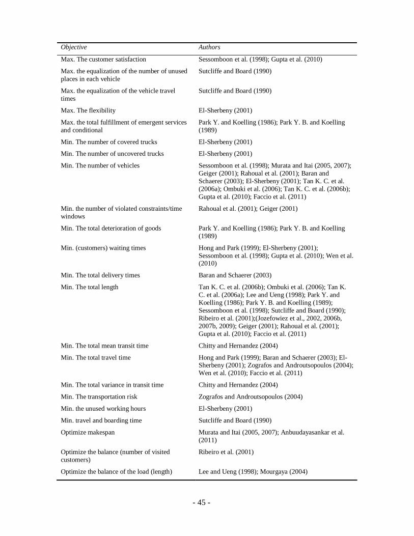
- 45 -
Objective Authors
Max. The customer satisfaction Sessomboon et al. (1998); Gupta et al. (2010)
Max. the equalization of the number of unusedplaces in each vehicle
Sutcliffe and Board (1990)
Max. the equalization of the vehicle traveltimes
Sutcliffe and Board (1990)
Max. The flexibility El-Sherbeny (2001)
Max. the total fulfillment of emergent servicesand conditional
Park Y. and Koelling (1986); Park Y. B. and Koelling(1989)
Min. The number of covered trucks El-Sherbeny (2001)
Min. The number of uncovered trucks El-Sherbeny (2001)
Min. The number of vehicles Sessomboon et al. (1998); Murata and Itai (2005, 2007);Geiger (2001); Rahoual et al. (2001); Baran andSchaerer (2003); El-Sherbeny (2001); Tan K. C. et al.(2006a); Ombuki et al. (2006); Tan K. C. et al. (2006b);Gupta et al. (2010); Faccio et al. (2011)
Min. the number of violated constraints/timewindows
Rahoual et al. (2001); Geiger (2001)
Min. The total deterioration of goods Park Y. and Koelling (1986); Park Y. B. and Koelling(1989)
Min. (customers) waiting times Hong and Park (1999); El-Sherbeny (2001);Sessomboon et al. (1998); Gupta et al. (2010); Wen et al.(2010)
Min. The total delivery times Baran and Schaerer (2003)
Min. The total length Tan K. C. et al. (2006b); Ombuki et al. (2006); Tan K.C. et al. (2006a); Lee and Ueng (1998); Park Y. andKoelling (1986); Park Y. B. and Koelling (1989);Sessomboon et al. (1998); Sutcliffe and Board (1990);Ribeiro et al. (2001);(Jozefowiez et al., 2002, 2006b,2007b, 2009); Geiger (2001); Rahoual et al. (2001);Gupta et al. (2010); Faccio et al. (2011)
Min. The total mean transit time Chitty and Hernandez (2004)
Min. The total travel time Hong and Park (1999); Baran and Schaerer (2003); El-Sherbeny (2001); Zografos and Androutsopoulos (2004);Wen et al. (2010); Faccio et al. (2011)
Min. The total variance in transit time Chitty and Hernandez (2004)
Min. The transportation risk Zografos and Androutsopoulos (2004)
Min. the unused working hours El-Sherbeny (2001)
Min. travel and boarding time Sutcliffe and Board (1990)
Optimize makespan Murata and Itai (2005, 2007); Anbuudayasankar et al.(2011)
Optimize the balance (number of visitedcustomers)
Ribeiro et al. (2001)
Optimize the balance of the load (length) Lee and Ueng (1998); Mourgaya (2004)

- 46 -
Objective Authors
Optimize the balance of the tours (length) Jozefowiez et al. (2002, 2006b); Jozefowiez, Semet andTalbi (2007c); Jozefowiez et al. (2009); El-Sherbeny(2001); Wen et al. (2010)
Optimize the regionalization (clustering) of thecustomers
Mourgaya (2004)
Min. total route costs Anbuudayasankar et al. (2011)
Table 2.3 – Summary of objectives found in recent multi-objective VRP
2.5.5. Multi-Objective Optimization Algorithms
Over the last several years, many techniques have been proposed for solving multi-
objective problems. These strategies can be divided into three general categories: (1)
scalar methods, (2) Pareto methods, and (3) methods that belong to neither the first nor
the second category.
The most popular scalar method is weighted linear aggregation. However, this method
has several disadvantages. Nevertheless, this technique is relatively simple to implement
and can be used with any of the single-objective heuristics or meta-heuristics described in
the literature. For multi-objective routing problems, weighted linear aggregation has been
used with specific heuristics (Blasum & Hochstattler, 2000; Haghani & Jung, 2005;
Murata & Itai, 2005), local search algorithms (Paquete & Stutzle, 2003; Ribeiro et al.,
2001), and genetic algorithms (Ombuki et al., 2006).
Being a population-based approach, GAs are well suited to solve multi-objective
optimization problems. A generic single-objective GA can be modified to find a set of
multiple non-dominated solutions in a single run. The ability of GA to simultaneously
search different regions of a solution space makes it possible to find a diverse set of
solutions for difficult problems with non-convex, discontinuous, and multi-modal
solutions spaces. The crossover operator of GA may exploit structures of good solutions
with respect to different objectives to create new non-dominated solutions in unexplored
parts of the Pareto front. In addition, most multi-objective GAs do not require the user to
prioritize, scale, or weigh objectives. Therefore, GAs have been the most popular
heuristic approach to multi-objective design and optimization problems. Jones, Mirrazavi
and Tamiz (2002) reported that 90% of the approaches to multi-objective optimization
aimed to approximate the true Pareto front for the underlying problem. A majority of
- 47 -
these used a meta-heuristic technique, and 70% of all meta-heuristics approaches were
based on evolutionary approaches.
Pareto methods use the notion of Pareto dominance directly. This approach was mainly
introduced by Goldberg (1989) for genetic algorithms. Though it does not allow one
compromise to be favored over another, it can be a useful aid for the decision-makers. In
multi-objective vehicle routing problems, the Pareto concept is frequently used within an
evolutionary framework. Many authors (Doerner et al., 2007; Geiger, 2001; Jozefowiez et
al., 2002, 2004; Jozefowiez N., Semet F. & Talbi E .G., 2006a; Jozefowiez et al., 2007a;
Lacomme et al., 2006; Murata & Itai, 2005, 2007; Ombuki et al., 2006; Rahoual et al.,
2001; Sessomboon et al., 1998; Tan K., Lee, Chew & Lee, 2003; Tan K. C. et al., 2006b;
Zhenyu et al., 2003) have used evolutionary algorithms with Pareto methods to solve
multi-objective routing problems. Some of them have proposed hybrids based on
evolutionary algorithms and local searches, heuristics, and/or exact methods for the
considered problem (Doerner et al., 2007; Jozefowiez et al., 2002; Jozefowiez et al.,
2006a; Jozefowiez et al., 2007a, 2007b; Lacomme et al., 2006; Sessomboon et al., 1998;
Tan K. et al., 2003; Tan K. C. et al., 2006a, 2006b).
Some studies do not employ either scalar or Pareto methods to solve multi-objective
routing problems. In this case, these non-scalar and non-Pareto methods are based on
genetic algorithms, lexicographic strategies, ant colony mechanisms, or specific
heuristics. Doerner et al. (2007) proposed using VEGA (Vector Evaluated Genetic
Algorithm) to solve their problem. In VEGA, at each iteration, the population is divided
into n subpopulations, where n is the number of objectives, which are mixed together to
obtain a smaller population to which genetic operators are applied. In lexicographic
methods, the objectives are each assigned a priority value, and the problems are solved in
order of decreasing priority. When one objective has been optimized, its value cannot be
changed and it becomes a new constraint for the problem. Such a lexicographic approach
has been used by Keller C.P. (1985), Keller C. P. and Goodchild (1988) and Current and
Schilling (1994). Baran and Schaerer (2003) do not use a standard multi-objective
approach, but rather consider the multi-objective nature of the problem via mechanisms
in the ant colony system they propose. Chitty and Hernandez (2004) also use an ant
colony system. The ant colony paradigm is adapted to the bi-objective situation by using
two types of pheromones, one for the total mean transit time and one for the variance in

- 48 -
the transit time. Alternatively, to solve their problem, Doerner et al. (2007) treat the
location and routing aspects simultaneously by means of P-ACO (Pareto Ant Colony
Optimization). P-ACO is a multi-objective meta-heuristic that generalizes the Ant Colony
Optimization (ACO) meta-heuristic to the case of several objective functions,
determining approximations to the set of optimal Pareto solutions.
2.6. Real-Time Vehicle routing
Due to recent advances in information and communication technologies, vehicle fleets
can now be managed in real-time. When jointly used, devices like geographic
information systems (GIS), global positioning systems (GPS), traffic flow sensors and
cellular telephones are able to provide relevant real-time data, such as current vehicle
locations, new customer requests and periodic estimates of road travel times (Brotcorne,
Laporte & Semet, 2003). If suitably processed, this large amount of data can, in principle,
be used to reduce cost and improve service level. To this end, revised routes have to be
timely generated as soon as new events occur.
In recent years, three main developments have contributed to the acceleration and
quality of algorithms relevant in a real-time context: (1) Increase in computing power due
to better hardware. (2) Development of powerful meta-heuristics whose main impact has
been on solution accuracy, even if this gain has sometimes been achieved at the expense
of computing time. (3) Development has arisen in the field of parallel computing. The
combination of these three features has yielded a new generation of powerful algorithms
that can effectively be used to provide real-time solutions in dynamic contexts (Ghiani et
al., 2003).
A real-time VRP, also known as dynamic VRP, due to the nature of information needed
to come up with a set of good vehicle routes and schedules, which is dynamically
revealed to the decision maker, can be either deterministic or stochastic (Powell W. B.,
Jaillet & Odoni, 1995). In deterministic-dynamic problems, all data are known in advance
and some elements of information depend on time. For instance, the VRP with time
windows reviewed in (Cordeau et al., 2001) belongs to this class of problems. In
stochastic-dynamic problems uncertain data are represented by stochastic processes. For
instance, user requests can behave as a Poisson process (as in (Bertsimas D. & Van
Ryzin, 1990)). Since uncertain data are gradually revealed during the operational interval,
- 49 -
routes are not constructed beforehand. Instead, user requests are dispatched to vehicles in
an on-going fashion as new data arrive (Psaraftis, 1988).
The events that lead to a plan modification can be (1) arrival of new user requests (or
cancellations), (2) arrival of a vehicle at a destination and (3) update of travel times.
Every event must be processed according to the policies set by the vehicle fleet operator.
When a new request is received, one must decide whether it can be serviced immediately,
delayed or rejected. If the request is accepted, it is assigned to a position in a vehicle
route. If another event occurs, the request might be assigned to a different position in the
same vehicle route, or even dispatched to a different vehicle. At any time each driver
needs to know his next stop. Hence, when a vehicle reaches a destination it has to be
assigned a new destination. Due to advances in communication technologies, route
diversions and reassignments are now a feasible option and should take place if this
results in a cost saving or in an improved service level (Gendreau & Potvin, 1998;
Ichoua, Gendreau, Potvin, op?rationnelle & Universit? de, 2000). Finally, if an improved
estimation of vehicle travel times is available, it may be useful to modify the current
routes or even the decision of accepting a request or not.
Most solution approaches to the VRP are in practice implemented in a centralized
computer resource, producing a daily plan to be provided to the vehicles before the
beginning of the distribution execution. Some of these approaches have been
implemented in commercial systems successfully used by numerous transportation,
logistics and manufacturing companies over the last 20 years.
These systems have not, however, been designed to address the case in which the
execution of delivery cannot follow the plan as prescribed, due to some unforeseen event.
When there is need for real-time intervention, it may be necessary to re-compute the plan
using new input data. If a typical VRP approach is used for re-planning (i.e. re-planning
the whole schedule from scratch), many vehicle schedules may be affected, thus causing
significant performance inefficiencies (high overhead, nervousness, errors, and high
costs).
Thus, re-planning based on classical VRP solution methods may not be a realistic
option. In the absence of algorithms capable of “isolating” the part of the VRP affected
by the unexpected event in order to minimize the disturbance to the overall schedule,
interventions are typically performed manually (for example, through voice
- 50 -
communication between drivers and the logistics manager) and the quality of decisions
taken is naturally affected.
As pointed out by Psaraftis (1988) and Psaraftis (1995), real-time VRPs possess a
number of unique features, some of which have just been described.; The remaining
characteristics are: (1) Quick response - Real-time routing and dispatching algorithms
must provide a quick response so that route modifications can be transmitted timely to the
fleet. To this end, two approaches can be used, simple policies (like the first-come first
served (FCFS) policy (Bertsimas D. & Van Ryzin, 1990)), or more involved algorithms
running on parallel hardware (like the tabu search heuristics described in (Gendreau,
Guertin, Potvin & S?guin, 2006; Gendreau, Guertin, Potvin & Taillard, 1999)). The
choice between them depends mainly on the objective, the degree of dynamism and the
demand rate. For each real-time problem, it is important to specify the time horizon (also
know as planning horizon) – a fixed point in time at which certain processes will be
evaluated - in order to determine how long to wait before taking action; in other words,
we have to define the term “quick response.” (2) Denied or deferred service - In some
applications it is valid to deny service to some users, or to forward them to a competitor,
in order to avoid excessive delays or unacceptable costs. For instance, in Gendreau et al.
(1999) requests that cannot be serviced within a given time window are rejected. When
no time windows are imposed, some user requests can be postponed indefinitely because
of their unfavorable location. This phenomenon can be avoided by imposing dummy time
windows, or by adding a non-linear delay penalty to the objective function. (3)
Congestion - If the demand rate exceeds a given threshold, the system becomes saturated,
i.e., the expected waiting time of a request grows to infinity.
2.7. SummaryThe Vehicle-Routing Problem (VRP) is a common name for problems involving the
construction of a set of routes for a fleet of vehicles. The vehicles start their routes at a
depot, call at customers, to whom they deliver goods, and return to the depot. The
objective function for the vehicle-routing problem is to minimize delivery cost by finding
optimal routes, which are usually the shortest delivery routes.
The basic VRP consists of designing a set of delivery or collection routes, such that (1)
each route starts and ends at the depot, (2) each customer is called at exactly once and by

- 51 -
only one vehicle, (3) the total demand on each route does not exceed the capacity of a
single vehicle, and (4) the total routing distance is minimized. It is common to address the
basic VRP as Capacitated Vehicle-Routing Problem (CVRP).
VRP has been solved optimally using Branch-and-Bound algorithms, Set-Covering and
Column Generation algorithms, Branch-and-Cut algorithms, Dynamic algorithms and
more.
Since VRP is an NP-Hard problem, many heuristics have been developed for solving it.
The classic algorithms include, among others, the Savings algorithms, Swap algorithm
and the Fisher and Jaikumar algorithm. Meta-heuristics algorithms, such as Simulated
Annealing, Tabu Search, Genetic Algorithms, Ant Systems Algorithms and Neural
Networks are also used in solving VRPs.
As research developed a number of researchers developed extensions to the basic VRP.
The goal was to develop more realistic models, to adapt to the larger number of
constraints of the real world. The following is a description of the most common variants.
Such extensions include the Split Delivery Vehicle Routing Problems (a customer can be
served by more than one vehicle), Vehicle Routing Problems with Time Windows (a
customer must be served within a given time window), Multi-Depot Vehicle Routing
Problems, Time Dependent Vehicle Routing Problems (traveling time may change during
the day), Stochastic Vehicle Routing Problems, Multi-Objective Vehicle Routing
problems and Real-Time Vehicle Routing Problems.

- 52 -
3. Problem Formulation This chapter describes the formulation of the real-time multi-objective vehicle routing
problem stated in chapter 1. The problem is formulated as a mixed integer linear
programming problem on a network. This chapter is divided into four sections. The first
section explains the assumptions and limitations of the model. The second section deals
with the notations and variables used in the model formulation. The third section
introduces the objective function. The fourth section deals with the constraints of the
formulation. We summarize this chapter in the last section.
3.1. Assumptions and Limitations
3.1.1. Demand Characteristics
The problem formulated in this research considers a system with dynamic conditions.
These conditions include the real-time variation in travel times between the depot and the
customers as well as between the customers themselves and real-time service requests.
Since there is no end of service time constraint, demands can be requested at any time
during the day.
When rerouting during the day, demands can be divided into two groups, recent
demands and longstanding demands. The demands already assigned to the vehicles in the
last routing process are the longstanding demands, and demands that are requested after
the last routing process are the recent demands. All demands, longstanding and recent,
have to be served. New demands can be assigned to any of the vehicles without any
restriction, as long as the remaining capacity of the vehicles allows it; otherwise, a new
vehicle has to be delivered.
All demands have specified service times and service time intervals (generally time
windows are described with intervals such as [a, b]). We consider soft time windows for
service around the desired service time because soft time windows are more realistic and
more flexible than hard time windows. A soft time windows formulation can have
solutions in cases where a hard time windows formulation fails.

- 53 -
Each customer is assigned with a satisfaction or penalty function. These functions
describe customers’ satisfaction/dissatisfaction when customers’ demands are not
fulfilled on time as a function of the deviation from the customer’s time window.
3.1.2. System Characteristics
Network: In this study a transportation network is considered. While there may exist
more than one trajectory between two nodes (customers and the depot) with shortest
traveling times, each for a different time of the day, this case is not considered
(however, this should not be a problem if a large number of customers are
considered). For every two nodes the shortest path is calculated. Based on distance
between every two nodes and information about traveling time, the average driving
speed between every two nodes can be calculated. Time-dependent travel time
information is supplied in the form of a matrix of travel times between the demand
nodes.
Travel Time: Travel times are lognormally distributed. Using lognormal distribution
is more suitable than normally distributed because (1) the positive skew shape (i.e.,
right skewed) is more suitable for travel time description; that is, a higher probability
exists for long travel time than for short travel time, and (2) the range [0, ) of the
distribution is more natural than a truncated normal distribution (the probability
distribution of a normally distributed random variable whose value is either bounded
below, above or both), because negative travel times are impossible.
According to Law and Kelton (1991), let ~ ( , )xxx Log , and ~ , )( y yy ,
such that the following relations exist:
lny x (3.1)
2ln1
2
21
y
y
x
y
f x ex
(3.2)
12y y
x e (3.3)
2 222 1y y yx e e (3.4)
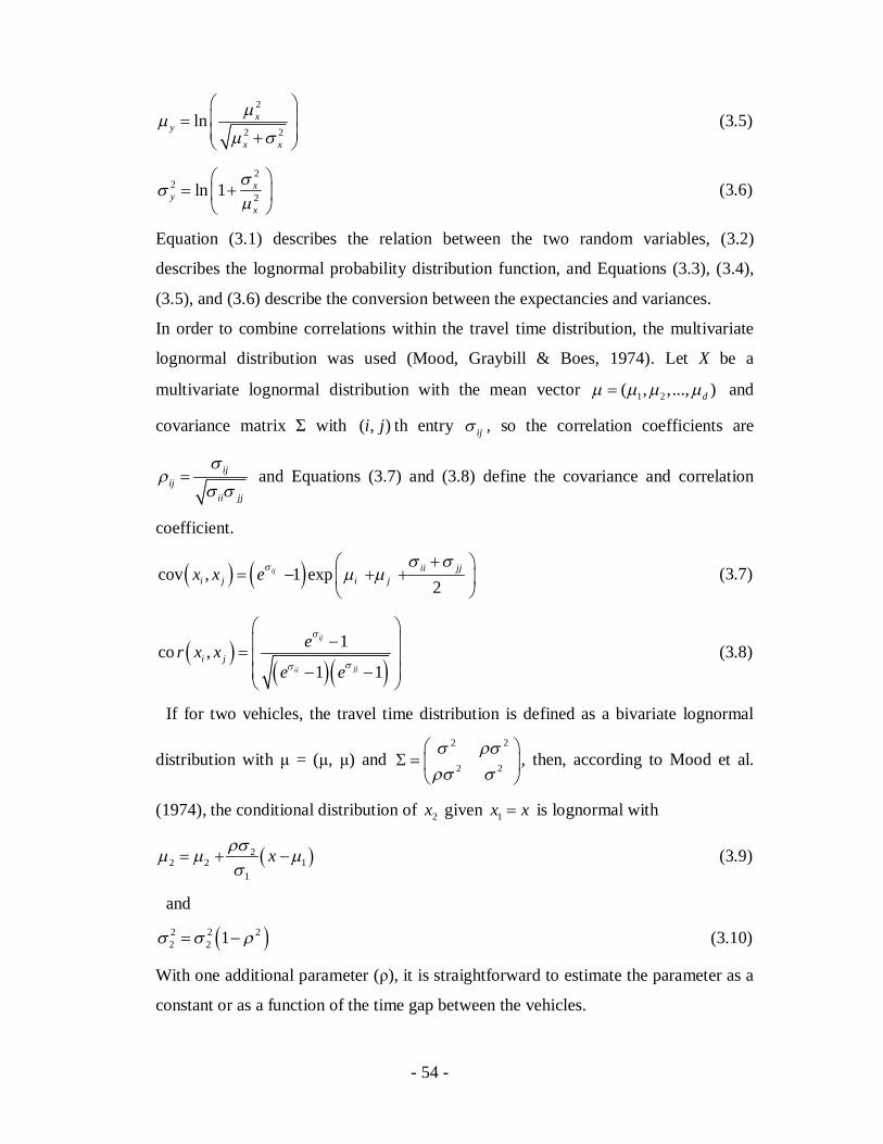
- 54 -
2
2 2ln
x
xy
x
(3.5)
22
2ln 1 xy
x
(3.6)
Equation (3.1) describes the relation between the two random variables, (3.2)
describes the lognormal probability distribution function, and Equations (3.3), (3.4),
(3.5), and (3.6) describe the conversion between the expectancies and variances.
In order to combine correlations within the travel time distribution, the multivariate
lognormal distribution was used (Mood, Graybill & Boes, 1974). Let X be a
multivariate lognormal distribution with the mean vector 1 2( , ,..., )d and
covariance matrix with ( , )i j th entry ij , so the correlation coefficients are
ij
ii ji
jj and Equations (3.7) and (3.8) define the covariance and correlation
coefficient.
cov , 1 exp2
iji j i
iij
jjx x e (3.7)
1co ,1 1
ij
jjiii j
er x xe e
(3.8)
If for two vehicles, the travel time distribution is defined as a bivariate lognormal
distribution with = ( , ) and2 2
2 2, then, according to Mood et al.
(1974), the conditional distribution of 2x given 1x x is lognormal with
22 1
12 x (3.9)
and2 2 22 2 1 (3.10)
With one additional parameter ( ), it is straightforward to estimate the parameter as a
constant or as a function of the time gap between the vehicles.

- 55 -
Vehicles: All vehicles in the proposed model have the same capacity.
Information System: We assume that there is a real-time communication system
between the vehicles and the control center. The control center has information about
the location of all vehicles as well as real-time traveling time information. All
vehicles are equipped with route guidance systems.
Number of depots: The real-time multi-objective VRP in this dissertation is a single
depot problem.
3.2. Variables and Problem DefinitionThe following is a list of variables used in the problem formulation presented next, the
objective functions and the constraints.
V Set of nodes, including the depot and the demand nodes
E Set of edges
N Number of customers (customer number 0 denotes the depot)tid Demand of demand node i requested at time t.
tiD The total demand of customer i at time t . t
iD is defined as
1
0 0 1 1 0
S St tN N Mt t mti j ij
t i j m td d x , which means that the demand of a customer equals the
sum of all customers’ demands received between time interval of 0t to time
St t minus the demands that already have been served. For customer 0, which is
the depot, 0Stid for all St .
mtijx A decision variable, defined as 1 if vehicle m traveled from node i to node j at
time t. where st t , and 0, otherwise.
mtijx Known decision variable, defined as 1 if vehicle m traveled from node i to node j
at time t. where st t , and 0, otherwise.
St Time of routing plan. The time of routing plan can start at 0st and end at
St T .
tijC A stochastic time-dependent nonnegative cost function, which represents the
- 56 -
travel cost from vertex i to vertex j starting at time t.t
ijC Known cost for traveling from node i to node j at time t, where st t
M The maximum number of vehicles available
Q capacity of a vehicle (all vehicles have the same capacity)mSt The last departure time of vehicle m from the depot. m
St is defined as
max 0,..., SmSt t t which satisfies 0
0
1N
mtj
jx , and there is no 0,. .,ˆ . St t ,
such that t̂ t and ˆ0
0
1N
mtj
jx . If such m
St does not exist, then mS St t .
Stiv
Does a customer require a visit at time St . Stiv is defined as
1 00
SS
tt ii
dv
otherwise.
SiTW Start of time window of customer i
EiTW End of time window of customer i
iEET Endurable earliness time - the earliest service time that customer i can endure
when a service starts earlier than SiTW .
iELT Endurable lateness time - the latest service time that customer i can endure when
a service starts later than EiTW .
iST Service time at customer i.
iST Known service time at customer i.
iWT Waiting time at customer i.
iWT Known waiting time at customer i.
Using the previously described variables, the real-time multi-objective VRP can be
defined as follows.
At time st , let ,G V E be a complete graph, where 0,1,...,V n is the nodes set
and E is the edge set. Each node \ 0i V represents a customer (or a demand node),
having a non-negative (0 or higher) demand StiD , whereas vertex 0 corresponds to the
depot. Each edge , : , ,e E i j i j V i j is associated with a stochastic time-
- 57 -
dependent nonnegative cost, tijC , which represents the travel cost (equal to the travel
time) spent to go from vertex i to vertex j starting at time t. The use of the loop edges,
(i,i), is not allowed (this is imposed by defining tiic for all i V ). A fixed fleet of
M identical vehicles, each of capacity Q, is available at the depot.
The real-time multi-objective VRP calls for the determination of a set of at most M
vehicles that optimizes the following objectives:
(1) Minimizing the total traveling time.
(2) Minimizing the number of vehicles used.
(3) Maximizing customers' satisfaction, or minimizing customers' dissatisfaction.
(4) Maximizing tour's balance
satisfying the following constraints:
(1) Each customer, whose demand at time st equals 0 is not visited at all.
(2) Each customer, whose demand at time st is higher than 0, is visited exactly once by
one route.
(3) For every driving vehicle at time st , whose destination node is a customer, there must
exist a corresponding route, which starts at the vehicle’s destination node.
(4) For every vehicle whose current location, at time st , is a demand node, there must
exist a corresponding route, which starts at the vehicle’s current location.
(5) All other routes start at the depot.
(6) All routes end at the depot.
(7) The total demand of the customers, known at time st , served by a route does not
exceed the vehicle capacity Q.
3.3. Objectives
Since this is a multi-objective problem, several objective functions are considered.
3.3.1. Minimizing the Travel Time
The first objective considered is minimizing the total travel time, and is described in
equation (3.11).

- 58 -
1
0 0 1 0
0 0 1
min max ,
max ,
S
S
tN N Mt S mt
j jij j iji j m t
N N M Tt S mtij j j j ij
i j m t t
SZ C TW t
C TW t ST W
T
T x
T W x (3.11)
The time passed since a vehicle left node i (either the depot or a customer) towards node
j and the time it left node j can be calculated in the following way.
Consider the traveling cost (time) from node i to node j when leaving node i at time t. If
by leaving node i at time t a vehicle reaches node j before its time window's start time
(meaning t Sij jt C TW ), then the vehicle has to wait until the beginning of the time
window in order to start serving. Otherwise, it starts serving upon arrival. The time
between the time the vehicle left node i towards node j, denoted as t, and the time it starts
serving node j can be formulated as max ,t Sij jC TW t . If node j is a customer, then both
service time at customer j, jST , and waiting time at customer j, jWT , have to be added to
the traveling time. But, if node j is the depot, then both service time, jST , and waiting
time, jWT , equal 0. Therefore, the time passed since a vehicle left node i towards node j
and the time it left node j can be defined as max ,t Sij j j jC TW t ST WT .
For each edge , : , ,e E i j i j V i j , there exists a decision variable mtijx ,
defined as 1 if edge e was traveled at time t by vehicle m, otherwise it is 0. Multiplying
the above notation, max ,t Sij j j jC TW t ST WT , by the decision variable mt
ijx , gives us
the time passed since vehicle m left node i towards node j at time t and the time it left
node j, if such vehicle exists, otherwise it is 0.
Let's refer to the time passed since vehicle m left node i towards node j at time t and the
time it left node j multiplied by the decision variable,
max ,t S mtij j j j ijC TW t ST WT x , as the true travel time from node i to node j. By
summing all possible true travel times,0 0 1 0
max ,N N M T
t S mtij j j j ij
i j m t
C TW t ST WT x ,
we get the total travel time, which is to be minimized.
- 59 -
The total travel time can be decomposed into two parts, the known travel time and the
unknown travel time. If the planning time st is not equal to 0, then we are not at the
beginning of the day, and some vehicles have already been sent to customers. In this case,
information regarding traveled edges, travel costs, service time and waiting time is
already known for every edge traveled and for every customer visited before st .
Let tijC denote the known cost from traveling from node i to node j at time t, where
st t . Similarly, let mtijx denote the known decision variable, defined as 1 if vehicle m
traveled from node i to node j at time t. where st t , and 0, otherwise. The known
traveled cost can be defined as1
0 0 1 0max ,
StN N Mt S mt
j jij j iji j m t
SC T T WTW t x .
The unknown traveling cost can be defined as
0 0 1
max ,S
N N M Tt S mtij j j j ij
i j m t t
C TW t ST WT x , therefore, the total traveling cost is the
sum of the known traveling cost and the unknown traveling cost,1
0 0 1 0
0 0 1
max ,
max ,
S
S
tN N Mt S mt
j jij j iji j m t
N N M Tt S mtij j j j ij
i j m t t
C TW t
C TW t ST WT
ST W
x
T x
3.3.2. Minimizing Number of Vehicles
Since in the real world, the fixed cost of using additional vehicles is higher then the
routing operation costs, we can reduce the total cost by minimizing the number of
vehicles in service.1
0 01 1 0 1 1
mins
s
t tN M N M Tmt mt
j jj m t j m t t
Z x x (3.12)
The total number of vehicles can be defined as the number of vehicle leaving the depot.
3.3.3. Maximizing Customers' Satisfaction
In a traditional VRPTW, a feasible solution must satisfy all time windows. When a
customer is served within his specified time window, the supplier’s service level is
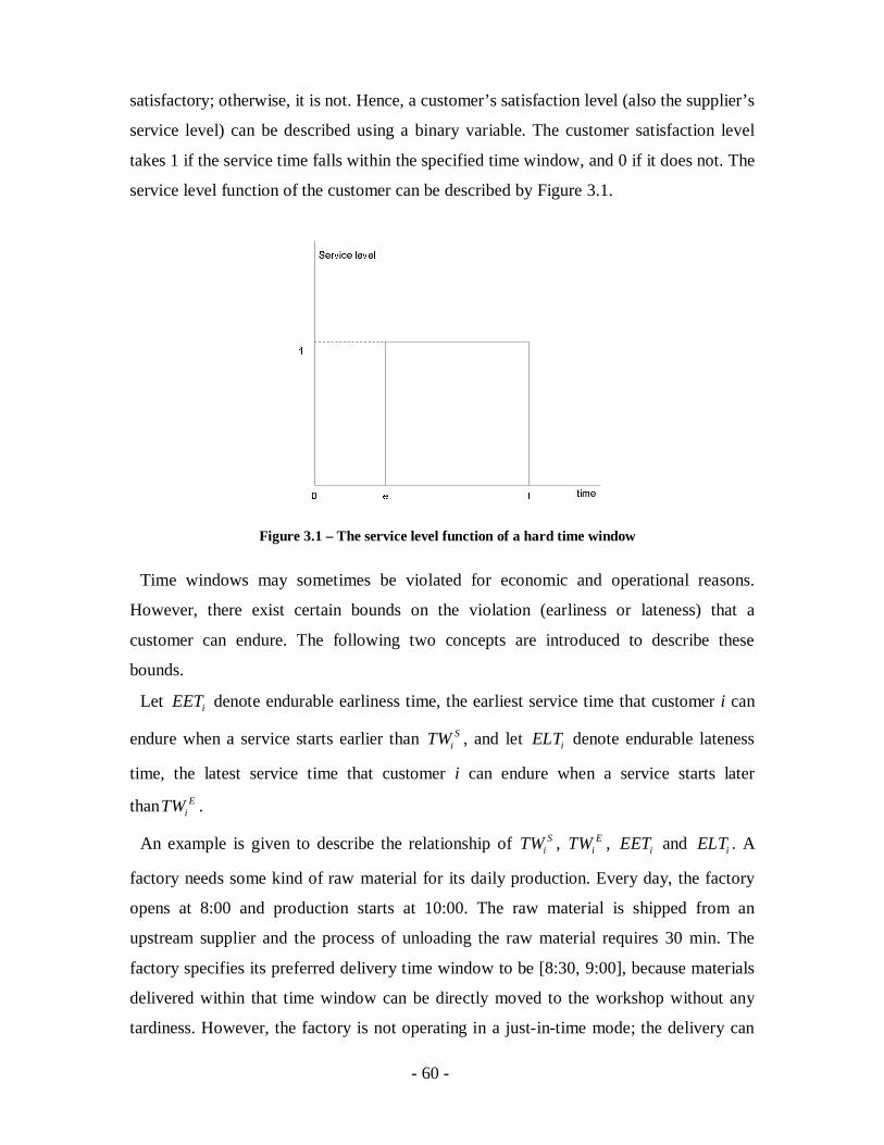
- 60 -
satisfactory; otherwise, it is not. Hence, a customer’s satisfaction level (also the supplier’s
service level) can be described using a binary variable. The customer satisfaction level
takes 1 if the service time falls within the specified time window, and 0 if it does not. The
service level function of the customer can be described by Figure 3.1.
Figure 3.1 – The service level function of a hard time window
Time windows may sometimes be violated for economic and operational reasons.
However, there exist certain bounds on the violation (earliness or lateness) that a
customer can endure. The following two concepts are introduced to describe these
bounds.
Let iEET denote endurable earliness time, the earliest service time that customer i can
endure when a service starts earlier than SiTW , and let iELT denote endurable lateness
time, the latest service time that customer i can endure when a service starts later
than EiTW .
An example is given to describe the relationship of SiTW , E
iTW , iEET and iELT . A
factory needs some kind of raw material for its daily production. Every day, the factory
opens at 8:00 and production starts at 10:00. The raw material is shipped from an
upstream supplier and the process of unloading the raw material requires 30 min. The
factory specifies its preferred delivery time window to be [8:30, 9:00], because materials
delivered within that time window can be directly moved to the workshop without any
tardiness. However, the factory is not operating in a just-in-time mode; the delivery can
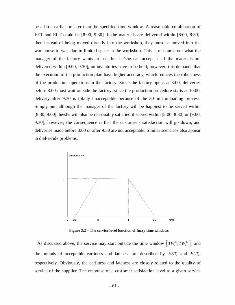
- 61 -
be a little earlier or later than the specified time window. A reasonable combination of
EET and ELT could be [8:00, 9:30]. If the materials are delivered within [8:00, 8:30],
then instead of being moved directly into the workshop, they must be moved into the
warehouse to wait due to limited space in the workshop. This is of course not what the
manager of the factory wants to see, but he/she can accept it. If the materials are
delivered within [9:00, 9:30], no inventories have to be held; however, this demands that
the execution of the production plan have higher accuracy, which reduces the robustness
of the production operations in the factory. Since the factory opens at 8:00, deliveries
before 8:00 must wait outside the factory; since the production procedure starts at 10:00,
delivery after 9:30 is totally unacceptable because of the 30-min unloading process.
Simply put, although the manager of the factory will be happiest to be served within
[8:30, 9:00], he/she will also be reasonably satisfied if served within [8:00, 8:30] or [9:00,
9:30]; however, the consequence is that the customer’s satisfaction will go down, and
deliveries made before 8:00 or after 9:30 are not acceptable. Similar scenarios also appear
in dial-a-ride problems.
Figure 3.2 – The service level function of fuzzy time windows
As discussed above, the service may start outside the time window ,S Ei iTW TW , and
the bounds of acceptable earliness and lateness are described by iEET and iELT ,
respectively. Obviously, the earliness and lateness are closely related to the quality of
service of the supplier. The response of a customer satisfaction level to a given service

- 62 -
time may not be simply “good” or “bad”; instead, it may be between “good” and “bad”.
For example, the customer might say, “it’s all right” to be served within , Si iEET TW or
,Ei iTW ELT . In either case, the service level cannot be described by only two states (0
or 1).
For problems involving personal human feelings, fuzzy set theory is a strong tool.
Intuitively, with the concepts of iEET and iELT , the supplier’s service level for each
customer can be described by a fuzzy membership function:
1,(
0,,
),0,
Si
S Ei i
i
ii
Ei i
i
i
i
t TW
T
t EET
EETfW t TW
g t TW t ELTEL
tS t
T t
(3.13)
when in most recent research, if t is defined as
ii S
i i
t EETf tTW EET
(3.14)
and ig t is defined as
( ) ii E
i i
ELT tg tELT TW
(3.15)
However, since customer’s satisfaction level, as a function of the deviation from the
customer’s time window, in most cases cannot be described as a linear function, the
following function, which better describes customer's satisfaction, is used.
1
1
ini
Sj i i
i n
j
ji
ji
t EETTW EET
f t (3.16)

- 63 -
1
1
( )
im
Ej i
i
ji
ji
m
j
ELT tELT TW
g t (3.17)
Assuming that each customer has his own satisfaction function, iS t , and that the
service provider assigns an importance factor, i , to each customer that states how
important it is to satisfy customer i compared to all other customers, the maximizing
customers’ satisfaction objective can be described as
1
0 0 1 0min
S
S
mt mti ji ji
tn N M Tt t
i ji iji j m t t t
Z S t C tx xC (3.18)
3.3.4. Maximizing the Balance of the Tours
This objective function seeks to balance the work between vehicles. The idea of making
a multi-objective model that balances the work and minimizes cost has been explored in
the work of Lee and Ueng (1998). Ribeiro et al. (2001) balanced the work by minimizing
the difference between the work of each vehicle and the work of the vehicle with the
lowest work level.
In this model, the work of a single vehicle is defined as the total length the vehicle
traveled in a single day.
The standard deviation of the work of each vehicle at the end of the period is
minimized. The model allows one vehicle to work more than another on a given route, as
long as the total work of a vehicle at the end of the day (t=T) is balanced.
1
0 1 0
S
S
mt mtji ji
tN M Tt t
m ji ijj m t t t
w C x xC (3.19)
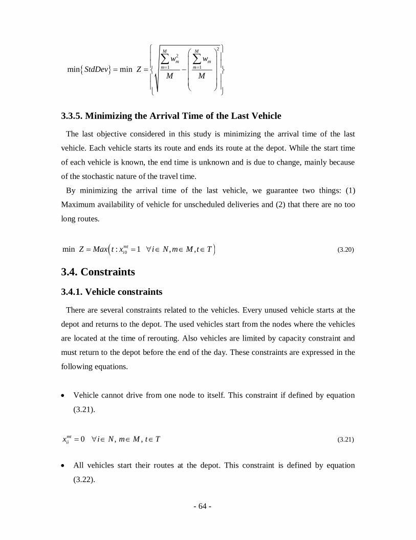
- 64 -
22
1 1min min
M M
m mm m
w wStdDev Z
M M
3.3.5. Minimizing the Arrival Time of the Last Vehicle
The last objective considered in this study is minimizing the arrival time of the last
vehicle. Each vehicle starts its route and ends its route at the depot. While the start time
of each vehicle is known, the end time is unknown and is due to change, mainly because
of the stochastic nature of the travel time.
By minimizing the arrival time of the last vehicle, we guarantee two things: (1)
Maximum availability of vehicle for unscheduled deliveries and (2) that there are no too
long routes.
0 ,n ,mi : 1mtiZ M iax t M Tx N m t (3.20)
3.4. Constraints
3.4.1. Vehicle constraints
There are several constraints related to the vehicles. Every unused vehicle starts at the
depot and returns to the depot. The used vehicles start from the nodes where the vehicles
are located at the time of rerouting. Also vehicles are limited by capacity constraint and
must return to the depot before the end of the day. These constraints are expressed in the
following equations.
Vehicle cannot drive from one node to itself. This constraint if defined by equation
(3.21).
, ,0mtii i Mx N m t T (3.21)
All vehicles start their routes at the depot. This constraint is defined by equation
(3.22).

- 65 -
1
0 01
1S
mSS
tN Tmt mtj j
j t tt t
x x m M (3.22)
Each vehicle, m, is associated with a start time, mst , equal to the latest time vehicle m
left the depot. Mathematically, mSt can be defined as max 0,..., S
mSt t t which
satisfies 00
1N
mtj
jx , and there is no 0,. .,ˆ . St t , such that t̂ t and ˆ
00
1N
mtj
jx . If
such mSt does not exist, then m
S St t .
Each vehicle m can belong to one of the following states: (1) it has never been
assigned to any route, (2) it has been assigned to one route or more in the past and is
currently waiting at the depot and (3) it is currently assigned to a route. If vehicle m
has never been assigned to a route, and is therefore waiting at the depot, then mS St t ,
and therefore1
01
0S
mS
tNmt
jj t t
x and 01
0S
N Tmt
jj t t
x as well.
If vehicle m is assigned to a route, then there are two options. First, vehicle m left the
depot before St ( mS St t ). In this case,
1
01
1S
mS
tNmt
jj t t
x and 01
0S
N Tmt
jj t t
x . Second,
vehicle m left the depot at St or later ( mS St t ). In this case,
1
01
0S
mS
tNmt
jj t t
x and
01
0S
N Tmt
jj t t
x .
From the above we can conclude, that in any case the sum1
0 01
S
mSS
tN Tmt mtj j
j t tt t
x x is
either 0 or 1.
All vehicles end their routes at the depot. This constraint is defined by equation (3.23)
.

- 66 -
1
0 0 01 1
S
mS SS
tN T N Tmt mt mt
j j ij t t i t tt t
m Mx x x (3.23)
As defined in equation (3.22), each vehicle m can either be assigned to a route or not.
If vehicle m is assigned to a route then the term1
0 01
S
mSS
tN Tmt mt
j jj t tt t
x x is equal to 1,
otherwise it is equal to 0. For a vehicle m that is not assigned to a route, the term
01 S
N Tmt
ii t t
x is equal to 0. However, for a vehicle m that is assigned to a route, the term
01 S
N Tmt
ii t t
x is equal to 1 if the vehicle ends its route at the depot, and 0 otherwise. By
defining that1
0 0 01 1
S
mS SS
tN T N Tmt mt mt
j j ij t t i t tt t
x x x for every vehicle m, we ensure that
every route which starts at the depot also ends at the depot.
3.4.2. Demand Constraints
The demand constraints ensure that only one visit is made to each demand node by only
one vehicle.
All customers require a visit, are visited exactly once, while all other customers are
not visited. This constraint is defined by equations (3.24) and (3.25).
1
0 1,
SS
mSS
tN M Ttmt mt
ij ij ji m t tt t
j N i jx x v (3.24)
1
0 1,
SS
mSS
tN M Ttmt mt
ij ij ij m t tt t
i N i jx x v (3.25)
- 67 -
Constraint (3.24) states that every customer, who's demand at time St is higher than 0,
is visited by a vehicle arriving from either the depot (i=0) or another customer
( , 0i N i ).
Let tiv denote whether customer i requires a visit at time t, when 1t
iv states that
customer i requires a visit at time t, and 0tiv states that he/she doesn't. The value of
tiv is implied from the total demand of customer i at time t, t
iD . tjD , the total demand
of demand node j is defined as the sum of all demands made by customer j from time
0t to time St t ,0
Sttj
td , minus all demands made by customer j that have been
served before time St t ,1
0 1 0
StN Nt mtj ij
i j td x . If t
jD is equal to 0, then tiv is 0, otherwise
tiv is 1.
Similarly, constraint (3.25) states that a vehicle serving customer i, must continue to
either the depot (j=0) or another customer ( , 0j N j ).
A demand constraint (constraint (3.26)) is also added. This constraint states that the
total demand of all customers visited by the same vehicle must be less than or equal
to the capacity of the vehicle.
0 0
S
S
N N Tt mti ij
i j t tQ m Md x (3.26)
3.4.3. Routing Constraints
If node j is visited after visiting node i, then the departure time, t, from node j is equal
to or greater than the departure time from node i plus the travel time from node i to
node j at time t. This is described by constraint (3.27).
1
0 1
1
0 10, 0
S
mSS
S
mSS
mt mtjk jk
mt mti
tN M T
k m t tt t
tN M Tt tij j ijij
j m t tt t
t t
t C t
x
x x i jC
x
(3.27)

- 68 -
A vehicle, visiting node i, that leaves node p and a vehicle visiting node p, that leaves
to node j, is the same vehicle. This constraint (3.28) is a route continuity constraint.
1 1
0 00 , , 0
S S
m mS SS S
t tN T N Tmt mt mt mt
ip ip pj pji t t j t tt t t t
m M p N px x x x (3.28)
If node j is visited after visiting node i, then the departure time, t, from node j is equal
to or greater than the departure time from node i plus the travel time from node i to
node j at time t. This is described by constraint (3.29).
1
0 1
1
0 10, 0
S
mSS
S
mSS
mt mtjk jk
mt mti
tN M T
k m t tt t
tN M Tt tij j ijij
j m t tt t
t t
t C t
x
x x i jC
x
(3.29)
3.5. The Real-Time Multi-Objective VRP Mix LP Model
The travel time cost function, tijC , is stochastic in nature, meaning that it may vary from
one day to another. Therefore, the cost function, tijC , is associated with a mean, t
ijC ,
which describes the average travel time from customer i to customer j at time t and a
standard deviation, tijC , which shows how much variation there is from the mean. As
an estimation of tijC the mean t
ijC can be used. However, for a route based on this
estimation, the total travel time of the route will not reflect the possibility of arriving at a
customer earlier or later than expected, and the changes in travel time it may cause. For
that reason, a different estimation of the stochastic cost function, tijC , is suggested. Let
t be an impact factor, which defines how much the value of tijC is affected by
possible changes in travel time (compared to the mean) in previous and future time
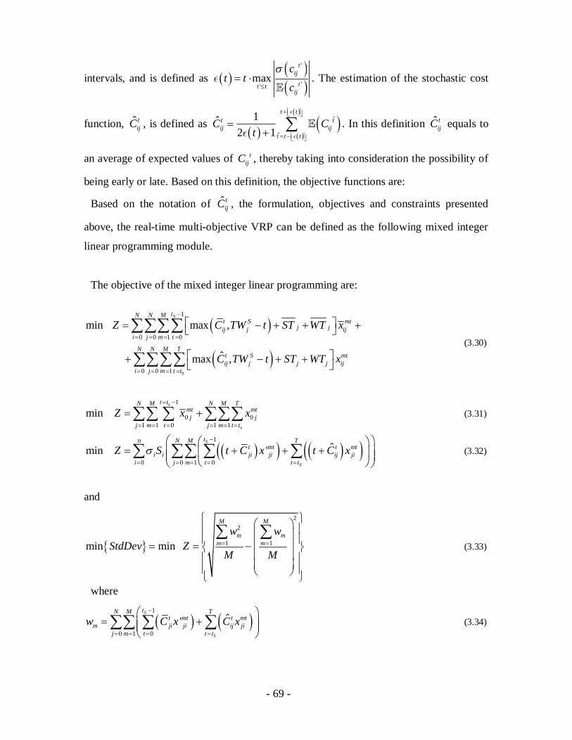
- 69 -
intervals, and is defined as'
''max
tij
tt tij
ct t
c. The estimation of the stochastic cost
function, ˆ tijC , is defined as ˆ
ˆ
1ˆ2 1
t tt tij ij
t t t
C Ct
. In this definition ˆ tijC equals to
an average of expected values of tijC , thereby taking into consideration the possibility of
being early or late. Based on this definition, the objective functions are:
Based on the notation of ˆ tijC , the formulation, objectives and constraints presented
above, the real-time multi-objective VRP can be defined as the following mixed integer
linear programming module.
The objective of the mixed integer linear programming are:
1
0 0 1 0
0 0 1
min max ,
ˆmax ,
S
S
tN N Mt S mt
j jij j iji j m t
N N M Tt S mtij j j j ij
i j m t t
Z C TW t
C TW t ST WT
ST W x
x
T (3.30)
1
0 01 1 0 1 1
mins
s
t tN M N M Tmt mt
j jj m t j m t t
Z x x (3.31)
1
0 0 1 0
ˆn 'miS
S
mt mti ji j
tn N M Tt t
i ji iji j m t t t
iZ S t C x C xt (3.32)
and
22
1 1min min
M M
m mm m
w wStdDev Z
M M (3.33)
where1
0 1 0' ˆ
S
S
mt mtji j
tN M Tt t
m ji ijm t t
ij t
w C x C x (3.34)
- 70 -
0: , ,1mti iMin Z Max Mx N t Tt m (3.35)
and the constraints are:
,1mtii i N m Mx (3.36)
1
0 01
1S
mSS
tN Tmt mtj j
j t tt t
x x m M (3.37)
1
0 0 01 1
S
mS SS
tN T N Tmt mt mt
j j ij t t i t tt t
m Mx x x (3.38)
1 1
0 1 1,
S SS
m mSS S
t tN M T Mtmt mt t mt
ij ij j j ijj m t t mt t t t
x x v v i jx N i (3.39)
1 1
0 1 1,
S SS
m mSS S
t tN M T Mtmt mt t mt
ij ij i i iji m t t mt t t t
x x v v j jx N i (3.40)
1 1
0 00 , , 0
S S
m mS SS S
t tN T N Tmt mt mt mt
ip ip pj pji t t j t tt t t t
m M p N px x x x (3.41)
1
0 1
1
0 10, 0
S
mSS
S
mSS
mt mtjk jk
mt mti
tN M T
k m t tt t
tN M Tt tij j ijij
j m t tt t
t t
t t
x x
C x C x i j
(3.42)
0 0
S
S
m
N N Tt mti ij
i j t tD m Md x (3.43)
0 1
*1
0
S
mSS
tN N M Tt mt t mtij ij ij ij
i j m t tt t
P x cC cx (3.44)

- 71 -
0,1 , , ,mtij m V i N tx j T (3.45)
Constraint (3.44) is a chance constraint stating that we are looking for a set of routes, that
for a given probability, , the traveling time will not be higher than *c . A method for the
determination of the value of *c is described next in this chapter.
3.6. Summary
This chapter describes the formulation of the real-time multi-objective vehicle routing
problem stated in chapter 1. The problem is formulated as a mixed integer linear
programming problem on a network.
Several assumptions and limitations are considered, such as a system with dynamic
conditions (real-time variation in travel times and real-time service requests), all demands
have specified service times and service time intervals, soft time windows for service
around the desired service time are considered, and more.
Five objectives functions are described and formulated:
1. Minimizing the total travel time
2. Minimizing number of vehicles - in the real world, since the fixed cost of using
additional vehicles is higher than the routing operation costs, we can reduce the total
cost by minimizing the number of vehicles in service.
3. Maximizing customers' satisfaction – In VRPTW with soft time windows, time
windows may sometimes be violated. However, there exist certain bounds on the
violation that a customer can endure. Each customer can be assigned with a
customer’s satisfaction function, which can describe his/her satisfaction vs. the
deviation from his time window.
4. Maximizing the balance of the tours - This objective function seeks to balance the
work between vehicles by minimizing the difference between the work of each
vehicle and the work of the vehicle with the lowest work level.
5. Minimizing the arrival time of the last vehicle - Each vehicle starts its route and
ends its route at the depot. While the start time of each vehicle is known, the end
time is unknown and is subject to changes, mainly because of the stochastic nature

- 72 -
of the travel time. By minimizing the arrival time of the last vehicle, we guarantee
two things: (1) Maximum availability of vehicles for unscheduled deliveries and (2)
that there are no ‘too long’ routes.
The various constraints applied to this problem are also described and formulated as
well:
1. Vehicle cannot drive from one node to itself.
2. All vehicles start their routes at the depot.
3. All vehicles end their routes at the depot.
4. All customers require a visit, are visited exactly once, while all other customers are
not visited.
5. The total demand of all customers visited by the same vehicle must be less than or
equal to the capacity of the vehicle.
6. If node j is visited after visiting node i, then the departure time, t, from node j is
equal to or greater than the departure time from node i plus the travel time from
node i to node j at time t.
7. A vehicle, visiting node i, that leaves for node p and a vehicle visiting node p, that
leaves for node j, is the same vehicle.
8. If node j is visited after visiting node i, then the departure time, t, from node j is
equal to or greater than the departure time from node i plus the travel time from
node i to node j at time t.
- 73 -
4. Coping with Dynamic VRPIn many real-life applications relevant data changes during the execution of
transportation processes and schedules have to be updated dynamically. Thanks to recent
advances in information and communication technologies, vehicle fleets can now be
managed in real-time. When jointly used, devices like geographic information systems
(GIS), global positioning systems (GPS), traffic flow sensors and cellular phones are able
to provide real-time data, such as current vehicle locations, new customer requests, and
periodic estimates of road travel times. If suitably processed, this large amount of data
can be used to reduce the cost and improve the service level of a modern company. To
this end, revised routes have to be timely generated as soon as new events occur (Ghiani
et al., 2003).
In this context, Dynamic Vehicle Routing Problems (DVRPs), also known as on-line or
real-time Vehicle Routing Problems, are becoming increasingly important (Hanshar &
Ombuki-Berman, 2007; Housroum, Hsu, Dupas & Goncalves, 2006; Montemanni,
Gambardella, Rizzoli & Donati, 2005; Psaraftis, 1995). It is possible to define several
dynamic features which introduce dynamism into the classical VRP: roads between two
customers could be blocked off, customers could modify their orders, the travel time for
some routes could be increased due to bad weather conditions, etc. This implies that
Dynamic VRPs constitute in fact a set of different problems, which are of crucial
importance in today’s industry, accounting for a significant portion of many distribution
and transportation systems.
The main goal of this chapter is to present the problem of DVRP and methods from the
literature for its resolution.
4.1. Dynamic vs. Static PlanningThis section discusses the main differences between dynamic and static vehicle routing.
Although some of the issues discussed apply to dynamic and static planning, their impact
on dynamic planning is often much more severe. A comprehensive discussion of dynamic
vehicle routing can be found in (Psaraftis, 1988) and (Psaraftis, 1995). Psaraftis gives the
following definition of a dynamic problem: a problem is dynamic if information on the

- 74 -
problem is made known to the decision maker or is updated concurrently with the
determination of the solution. By contrast, if all inputs are received before the
determination of the solution and do not change thereafter, the problem is termed static.
4.1.1. Evolution of information
Obviously, the major difference between dynamic and static problems is the evolution
of information. In static problems information is assumed to be known for the entire
duration of the transportation process. In dynamic problems, however, some input is not
known at the time of planning, and some input is not known with certainty. For example,
traffic conditions change, the number of vehicles available may change due to vehicle
break-down, new transportation requests become known, or attributes of transportation
requests may change.
Most of the literature on dynamic vehicle routing only considers one type of
uncertainty: the arrival of a new transportation request. Few works consider problems
with several sources of uncertainty. Among them are the works by Carvalho and Powell
(2000) and Fleischmann et al. (2004), who consider the arrival of new transportation
requests and uncertain travel times.
Another issue in dynamic planning is the reliability of future information. Long-term
information is more likely to change than short-term information. For example, long-term
estimations of travel times can only be based on historical data. In the short-term,
however, actual traffic conditions can be used to estimate travel times. Those short-term
forecasts allow a much better estimation of what is going to happen and thus help in
improving punctuality.
4.1.2. Rolling horizon
In static planning, schedules are generated for a certain finite planning horizon. The
duration of the planning process is bounded by the time between data collection and the
start of transportation processes. Given the input data, a static planning system must be
capable of calculating high quality solutions in the time available for optimization.
In dynamic planning, the planning horizon may not be bounded or even known. In fact,
a typical dynamic planning scenario is that of an open-ended process, going on for an
indefinite period of time. Usually, near-term events are more important than long-term

- 75 -
events. The consideration of requirements which have to be satisfied long into the future
would not be very wise, because such future information may change anyway. In a
typical rolling horizon framework, only information relevant to planning decisions within
a horizon of a certain length is considered. As time unfolds, parts of the tentative
schedule are applied and new information may enter the planning horizon.
4.1.3. Impreciseness of model representation
Real-life vehicle routing problems usually cannot be precisely represented by an
analytical model which is required for computer-based decision support. Even if the
analytical model is of high quality, discrepancies between model representation and real-
life problems arise as a result of the sheer cost of getting information into the computer.
Telematics systems can be used to improve the timely availability of information
regarding the actual transportation processes. Electronic Data Interchange (EDI) can be
used to integrate information systems of shippers, e.g. to obtain all relevant data
regarding transportation requests and customer locations. Despite the improved
possibilities of getting data into the model, the information is generally not only
incomplete but also imprecise. A shipper, for example, may ask that a shipment be picked
up in the morning before noon, when his dock is not as busy. In the model such
restrictions are usually treated as time window constraints. The computer system has no
way of interpreting whether such a request for early pickup is a hard constraint or
whether the shipper was only trying to express a preference.
The impreciseness of the model representation results in two fundamental problems: (1)
some solutions which are feasible according to the model may not be feasible in reality
and vice versa, (2) a solution with high quality in the model may not have the same high
quality in reality.
Although these problems occur in static as well as in dynamic planning, the impact is
quite different. In static planning there is usually more time for the collection of data,
resulting in a more accurate representation of the real-life problem. Furthermore, there is
more time to manually verify and validate a solution recommended by the planning
system.
- 76 -
4.1.4. Interactivity
Due to the impreciseness of any model representation and the fact that a significant
amount of relevant information is not available to the computer, but only to the
dispatchers who are in direct contact with drivers and shippers, model recommendations
cannot always be fully implemented. According to Carvalho and Powell (2000), several
motor carriers report that the average usage of model recommendations is below 60%,
and good performance is considered around 70%.
In order to deal with this issue, Kopfer and Schonberger (2002) have presented a
framework for interactive problem solving. The concept is founded on posting a problem
to a planning method in order to let it generate a solution. The returned solution usually
does not satisfy all real-life requirements. Therefore, dispatchers may add, modify, or
remove certain constraints in the analytical model. The modified problem is again posted
to the planning method, and after a solution has been found, further modifications to the
model can be made. Although this approach can be used for static and dynamic problems,
this iterative decision making is much harder in dynamic planning due to the lack of time.
In a similar approach, instead of having an iterative decision making process, a real-
time decision support system allows dispatchers and dynamic planning systems to
simultaneously modify the current solution. Dispatchers may add, modify, or remove
certain constraints in the analytical model at any time. All changes made by the
dispatchers are directly considered by the dynamic planning system which continuously
searches for improved solutions. Whenever the dynamic planning system finds a better
solution, the current solution is immediately updated and shown to the dispatchers. An
optimistic locking scheme is used in order to maintain data consistency.
Humans use a form of cache memory for processing information, called working
memory. This working memory must be regularly updated in order to consider changes in
problem data and solution. A dynamic planning system must support dispatchers in
quickly updating their working memory. Therefore, besides providing algorithmic
optimization techniques, a dynamic planning system must also provide sophisticated
graphical user interfaces (GUI), allowing dispatchers to quickly identify modified parts of
the solution, and to efficiently verify feasibility and profitability of an automatically
generated schedule.
- 77 -
4.1.5. Response time
The response time of an algorithm is the time which is needed until a newly calculated
solution can be applied. Algorithms for dynamic planning must have fast response times
for two reasons. First, a solution calculated for a dynamic problem can only be applied if
the input data have not changed significantly during the planning process. Second, the
longer it takes to calculate a new solution, the higher the probability that dispatchers may
concurrently change the current solution.
In many cases dispatchers have to decide about load acceptance or rejection while the
shipper is on the phone making the request. Dynamic planning systems should be capable
of supporting dispatchers in the load acceptance decision while the shipper is on the
phone. In other words, the system should give support within a couple of seconds in
deciding whether a transportation request can be served feasibly and efficiently.
The main advantage in dynamic planning is that there is usually plenty of time for
optimization. As noted by Kilby, Prosser and Shaw (1998), ten minutes spent to find a
solution for a small problem may seem like a long time in the static case. In the dynamic
case, however, ‘one has all day’, so the time might as well be used. A dynamic planning
system can be used to successively improve the current solution. Obviously, fast response
times cannot be achieved if new solutions are calculated from scratch every time the
dynamic planning method is invoked. Therefore, a dynamic planning system should have
a restart capability, i.e. the planning system should be able to continue from the current
solution. Furthermore, dynamic planning methods require efficient information update
mechanisms in order to efficiently consider modified input data.
4.1.6. Measuring performance
Measuring performance in dynamic planning is much more complicated than in static
planning. A method for static planning can be evaluated by comparing the solution
obtained with solutions obtained by other methods. In dynamic planning, however, the
decisions made at one point in time determine the options and alternatives at a later point
in time. It is possible to compare alternative decisions at one point in time, but then
carrying the effects of those decisions forward in time creates a problem.

- 78 -
In dynamic planning with rolling horizons, any evaluation of operating efficiencies
must address the issue of time period evaluation. The state of the system at the end of the
evaluation period may have a dramatic impact on future performance. A dynamic
planning method may perform quite well over a day or a week, but can have poor long-
term performance, e.g. if all vehicles are sent to very distant regions where there is little
hope of picking up a new load.
As mentioned above, dynamic planning methods must be interactive, enabling
dispatchers to verify model recommendations. In many cases dispatchers will agree with
model recommendations. However, differing problem knowledge and solution methods
of computer vs. human dispatchers may result in contradictory decisions. Under the time
constraints in dynamic planning, it is often very difficult or even impossible to find out
why the recommendation is being made. Is the discrepancy a result of “higher reasoning”
or a simple data error ? Typically, dispatchers will follow their own intuition and not the
model recommendation. As noted by Powell W.B., Marar, Gelfand and Bowers (2002), a
dynamic planning system is often considered successful if dispatchers agree with model
recommendations, but dispatchers often do not follow model recommendations.
Obviously, the question arises that if dispatchers do not comply with model
recommendations, are the solutions produced any good at all ?
4.2. DVRP Interests
There are several important problems that must be solved in real-time. In (Gendreau &
Potvin, 1998), (Larsen, 2000) and (Ghiani et al., 2003), the authors list a number of real-
life applications that motivate the research in the domain of dynamic vehicle routing
problems.
Supply and distribution companies: In seller-managed systems, distribution
companies estimate customer inventory levels in such a way as to replenish them
before stock depletion. Hence, demands are known beforehand in principle and all
customers are static. However, because demand is uncertain, some customers might
run out of their stock and have to be serviced urgently.
Courier Services: This refers to the international express mail services that must
respond to customer requests in real-time. The load is collected at different customer
- 79 -
locations and has to be delivered at another location. The package to be delivered is
brought back to a remote terminal for further processing and shipping. The deliveries
form a static routing problem, since recipients are known by the driver. However,
most pickup requests are dynamic because neither the driver nor the planner knows
where the pickups are going to take place.
Rescue and repair service companies: Repair services usually involve a utility firm
(broken car rescue, electricity, gas, water and sewer, etc.) that responds to customer
requests for maintenance or repair of its facilities.
Dial-a-ride systems: Dial-a-ride systems are mostly found in demand-responsive
transportation systems aimed at servicing small communities or passengers with
specific requirements (elderly, disabled). These problems are of the many-to-many
when any node can serve as a source or destination for any commodity or service.
Customers can book a trip one day in advance (static customers) or make a request at
short notice (dynamic customers).
Emergency services: These includes the police, firefighting and ambulance services.
By definition, the problem is purely dynamic, since all customers are unknown
beforehand and arrive in real-time. In most situations, routes are not formed because
the requests are usually served before a new request appears. The problem then is to
assign the best vehicle (for instance the nearest) to the new request. Solving methods
are based on location analysis for deciding where to dispatch the emergency vehicles
or to escape the downtown traffic jam.
Taxicab services: Managing taxicabs is still another example of a real-life dynamic
routing problem. In most taxicab systems the percentage of dynamic customers is
very high, i.e., only a very few customers are known by the planner before the taxicab
leaves the central station at the beginning of its working day.
4.3. Related Works
In this section, we present a classification and an overview on the state-of-the-art of
dynamic vehicle routing problems. Naturally, this chapter cannot cover all aspects of
vehicle routing problems with dynamic or stochastic elements. The goal of this chapter is
rather to provide a brief introduction to the literature on these subjects. Also, this chapter
- 80 -
is meant to provide the reader with an overview of the methodological approaches to
these problems.
Different surveys have been proposed on DVRPs (Bianchi & Bianchi-idsia, 2000;
Ghiani et al., 2003; Moretti Branchini, Amaral Armentano & Løkketangen, 2009).
Psaraftis (1988, 1995) was among the first to study dynamic versions of the VRP.
Psaraftis defines that a vehicle routing problem is dynamic when some inputs to the
problem are revealed during the execution of the algorithm. Demand information is not
known when vehicles are assigned, and demand information is revealed on-line. Problem
solution evolves as inputs are revealed to the algorithm and to the decision maker.
Possible information attributes might include evolution of information (static/dynamic),
quality of information (known-deterministic/forecast/probabilistic/unknown), availability
of information (local/global), and processing of information (centralized/decentralized).
Powell W. B. et al. (1995) concentrate on stochastic programming based models, but
also provide an excellent survey on various dynamic vehicle routing problems. For
example, the dynamic traffic assignment problem consists of finding the optimal routing
of some goods from origin to their destination through a network of links which could
have time-dependent capacities. The authors also discuss how to evaluate the solutions,
since it is an important issue that distinguishes static from dynamic models. They note
that in static models finding an appropriate objective function is fairly easy and that the
objective function is usually a good measure for evaluating the solution. However, for
dynamic models the objective function used to find the solution over a rolling horizon
often has little to do with the measures developed to evaluate the overall quality of a
solution.
Bertsimas DJ and Simchi-Levi (1996) provide a survey of deterministic and static as
well as dynamic and stochastic vehicle routing problems for which they examine the
robustness and the asymptotic behavior of the known algorithms. Bertsimas and Simchi-
Levi argue that analytical analysis of the vehicle routing problem offers new insights into
the algorithmic structure, making performance analysis of classical algorithms possible
and leading to a better understanding of models that integrate vehicle routing with other
issues like inventory control. The authors conclude that a-priori optimization is an
attractive policy if intensive computational power is not present. Furthermore, they point
out that dealing with stochasticity in the VRP provides insights that can be useful when

- 81 -
constructing practical algorithms for the VRP within a dynamic and stochastic
environment.
Gendreau and Potvin (1998) note that the work on local area vehicle routing and
dispatching still leaves a number of questions to be answered. In particular, research on
demand forecasting used for constructing routes with look-ahead is needed in the future.
Furthermore, the authors point out that it is relevant to consider several sources of
uncertainty like cancellation of requests and service delays rather than just to focus on
uncertainty in the time-space occurrence of service requests. Gendreau and Potvin also
note that the issue of diversion deserves more attention. Due to the large amount of online
information it has become possible to redirect the vehicle while on-route to the new
customer. Finally, the authors advocate further research on parallel implementations and
worst-case analysis, in order to be able to assess the loss in not having full information
available at the time of planning.
The following is a classification of DVRPs according to the degree of knowledge that
we have on the input data of the problem and quality of the available information. A
dynamic problem can be either deterministic or stochastic. DVRP is deterministic if all
data related to the customers are known when the customer demands arrive; otherwise it
is stochastic. Both of these classes can be subject to different factors such as service time
window, traffic jam, road maintenance, weather changes, breakdown of vehicles and so
on. These factors often change the speed of vehicles and the travel time for arriving at the
depot.
1. Deterministic: In a deterministic case, all the data related to the inputs are known.
For instance, when a new customer demand appears, customer location and the
quantity of his demand are known. Different types of deterministic DVRP can be
found in the literature as:
a. Dynamic Capacitated Vehicle Routing Problem (DCVRP): An important
number of works exist on this variant (Gendreau et al., 1999; Kilby et al., 1998;
Montemanni et al., 2005) which represents the conventional definition of the
problem, and where the existence of all customers and their localizations are
deterministic, but their order can arrive at any time. The objective is to find a set

- 82 -
of routes with the lowest traveled distance, and with respect to vehicle capacity
limit.
The Dynamic Traveling Repairman Problem (DTRP) (Bertsimas D.J. & Van
Ryzin, 1991, 1993) belongs to this class of problems. It is described as a problem
in which demands arrive according to Poisson process in a Euclidean service
region, and their locations are distributed throughout the service region. The goal
is to minimize the expected time that the demand spends in the system (i.e. the
average time a customer must wait before his/her request is completed), as
opposed to the expected distance that the vehicle travels. The service times of
requests are not known to the dispatcher, until the service at the respective
customers is completed.
Where all demands are dynamic in DTRP, i.e. all customers are immediate
request customers. Larsen, Madsen and Solomon (2002) define the Partially
Dynamic Traveling Repairman Problem (PDTRP) that is a variant of this problem
involving both advance and immediate request customers. Furthermore, the
problem seeks to optimize different objective functions. The dispatcher is more
interested in minimizing the distance traveled by the repairman than in
minimizing the overall system time.
b. Dynamic Vehicle Routing Problem with Time Windows (DVRPTW): It is one
of the most well-studied variants of DVRP (Alvarenga, de Abreu Silva & Mateus,
2005; Fabri & Recht, 2006; Housroum et al., 2006; Larsen, Madsen & Solomon,
2004; Mitrovi -Mini , Krishnamurti & Laporte, 2004; Oliveira, de Souza & Silva,
2008; Wang J., Tong & Li, 2007). Besides the possibility of requiring services in
real time, the time window associated with each customer i follows a specific
interval time ,i ia b , that must be satisfied. Larsen et al. (2002) proposed on-line
policies for the Partially Dynamic Traveling Salesman Problem with Time
Windows (PDTSPTW) that could be considered as an instance of DVRPTW with
a single vehicle. The objective is to minimize lateness at customer locations. A
simple policy of requiring the vehicle to wait at the current customer location
until it can service another customer without being early. Other policies may
- 83 -
suggest repositioning the vehicle at a location different from that of the current
customer, based on prior information on future requests.
c. Dynamic Vehicle Routing Problem with time-dependent Travel Times
(DVRPTT): Described in (Haghani & Jung, 2005), it assumes that the travel time
from customer i to customer j is variable across time. This variation could occur
due to the type of the road, weather and traffic conditions that may strongly
influence the speed of vehicles and hence travel times.
d. Dynamic Pickup and Delivery Vehicle Routing Problem (DPDVRP): Based
on the conventional Pickup and Delivery Vehicle Routing Problem (PDVRP)
(Savelsbergh M. W. P. & Sol, 1995). The problem consists of determining a set of
optimal routes for a fleet of vehicles in order to serve transportation requests
(Mitrovi -Mini et al., 2004). The objective is to minimize total route length, i.e.,
the sum of the distances traveled by all the vehicles, under the following
constraints: all requests must be served, each request must be served entirely by
one vehicle (pairing constraint), and each pickup location has to be served before
its corresponding delivery location (precedence constraint). The dynamic version
arises when not all requests are known in advance. Swihart and Papastavrou
(1999) have introduced a new variant of the DTRP where each service request has
a pickup and a delivery location. The objective is to minimize the expected
system time. The authors consider the unit-capacity case where the vehicle can
carry no more than one item, as well as the case where the vehicle can carry an
arbitrarily large number of items. Attanasio, Cordeau, Ghiani and Laporte (2004)
present a parallel implementation of a tabu search method developed previously
by Cordeau and Laporte (2003) for the Dynamic Dial-a-Ride Problem (DDARP).
In the latter, requests are received throughout the day and the primary objective is
to accommodate as many requests as possible according to the available fleet of
vehicles. Furthermore, the routes are designed under the constraint that customers
specify pick-up and drop-off requests between origins and destinations. Yang,
Jaillet and Mahmassani (2004) introduce a real-time multi-vehicle truck-load
pickup and delivery problem. They propose a mixed-integer programming

- 84 -
formulation for the off-line version of the problem and propose a new rolling
horizon re-optimization strategy for a dynamic version.
2. Stochastic: In stochastic dynamic problems (also known as probabilistic dynamic
problems) uncertain data are related to customer locations, demands or travel times
and are represented by stochastic processes.
a. Dynamic and Stochastic Capacitated Vehicle Routing Problem (DSCVRP): It
considers the situation where customer requests are unknown and revealed over
time. In addition, customer locations and service times are random variables and
are realized dynamically during plan execution. Bent and Van Hentenryck (2004)
considered DVRP with stochastic customers. They proposed a multiple scenario
approach that continuously generates routing plans for scenarios including known
and immediate requests to maximize the number of serviced customers. The
approach was adapted from Solomon benchmarks, with a varying degree of
dynamism. Hvattum, Løkketangen and Laporte (2006) addressed this variant of
the problem. The authors assume that both customer locations and demands may
be unknown in advance. They formulate the problem as a multi-stage stochastic
programming problem, and a heuristic method was developed to generate routes
by exploiting the information gathered on future customer demand.
b. Dynamic and Stochastic Vehicle Routing Problem with Time Windows
(DSVRPTW): Proposed by Pavone, Bisnik, Frazzoli and Isler (2009), in this
problem, each service request is generated according to a stochastic process; once
a service request appears, it remains active for a certain deterministic amount of
time, and then expires. The objective is to minimize the number of possible
vehicles and ensure that each demand is visited before its expiration. Furthermore,
this problem has been considered by Bent and Van Hentenryck (2007).
c. Dynamic Vehicle Routing Problem with Stochastic Travel Times
(DVRPSTT): It assumes that the problem is subject to a stochastic travel time
which represents a random variable in an interval. The travel times change from
one period to the next. Some works present this version of the problem as in
(Potvin, Xu & Benyahia, 2006), where the travel time to the next destination is
perturbed by adding a value generated with a normal probability law. This
- 85 -
perturbation represents any unforeseen events that may occur along the current
travel journey. It is known to the dispatching system only when the vehicle arrives
at its planned destination.
d. Dynamic and Stochastic Pickup and Delivery Vehicle Routing Problem
(DSPDVRP): In this version of the problem a stochastic process concerns the
quantity of demand that the vehicle must pick up or delivery to each customer.
Thus, we have vagueness in quantities to pick up or deliver at the customer’s
location (Xu, Goncalves & Hsu, 2008). The demand of each customer is revealed
only when the vehicle reaches the customer. The distribution can be modeled by
using a probabilistic law, such as a normal law, for example, or by using fuzzy
logic.
4.4. Solution MethodsThis section gives an overview of algorithms for solving vehicle routing problems,
based on solution methods which can be used for rich problems in which problem data
may change dynamically. The solution methods discussed in this section can be
categorized into assignment methods, construction methods, improvement methods,
meta-heuristics and mathematical programming based methods.
4.4.1. Assignment Methods
Assignment methods are methods that assign transportation requests to vehicles for
immediate execution. They are used in highly dynamic problems where problem data
change very fast and no foresighted planning is likely to perform well. Assignment
algorithms that simultaneously assign several open orders to idle vehicles are studied by
Spivey and Powell (2004) and Fleischmann et al. (2004).
4.4.2. Construction Methods
Construction methods gradually build tours while keeping an eye on the objective
function value, but they do not contain an improvement phase (Laporte & Semet, 2002).
A comprehensive survey on construction methods for the VRPTW is given by Bräysy
and Gendreau (2005b). One of the best-known tour construction methods for the VRP is
the Savings algorithm by Clarke and Wright (1964).

- 86 -
Insertion methods are methods that successively insert open transportation requests into
partially constructed tours. They are well suited for dynamic planning, because they
permit incorporation of a new order that considers the set of tours which are currently
implemented. Insertion methods are very fast and can be used for dynamic vehicle
routing problems in which there may not be enough time to employ more sophisticated
methods. Furthermore, insertion methods can often be applied to problems incorporating
various real-life requirements without losing efficiency. A discussion of efficient
insertion methods for vehicle routing problems incorporating complicating constraints
can be found in (Campbell & Savelsbergh, 2004).
Early examples of insertion methods have been proposed by Solomon (1987) for the
VRPTW. Parallel insertion methods for the static VRPTW which simultaneously
constructs several tours via insertions are proposed by Potvin and Rousseau (1993) and
Antes and Derigs (1995). Recently Lu and Dessouky (2006) presented an insertion
method for the PDPTW which not only considers the classical incremental costs, but also
the cost of reducing the time window slack so that more opportunities are left for future
insertions. Insertion methods for the dynamic PDP are also studied by Mitrovic-Minic,
Adviser-Krishnamurti and Adviser-Laporte (2001) and Fleischmann et al. (2004).
4.4.3. Improvement Methods
Many solution techniques for combinatorial optimization problems are based on a
simple and general idea. Let s be a feasible solution of the problem considered and let f(s)
denote the objective function value of s. For each feasible solution s the neighborhood of
s is defined by the solutions s* which can be obtained by applying an appropriately
defined neighborhood operator to the solution s. So-called local search or neighborhood
search methods explore the neighborhood of the current solution s by searching for a
feasible solution s* of high quality in the neighborhood of the current solution s. This
solution may be accepted as a new current solution, and in this case, the process is
iterated by considering s* as a new current solution.
In maximization (minimization) problems, a new solution s* is typically only accepted
if ( *) ( )f s f s ( ( *) ( )f s f s ) . If no solution s* with ( *) ( )f s f s ( ( *) ( )f s f s )
exists in the neighborhood of s, a local optimum has been reached. A comprehensive

- 87 -
work on local search methods is given by Aarts and Lenstra (1997). A survey and
comparison of local search methods for the VRPTW has been presented by Bräysy and
Gendreau (2005a).
Improvement methods are local search methods which start with a feasible solution and
gradually modify the current solution in order to improve the solution quality. The most
simple improvement methods operate on a single tour and optimize the sequence in
which the locations are visited. They are often based on methods developed for the TSP,
e.g. 2-opt by Lin (1965) and Or-opt by Or (1976). Others consider several tours
simultaneously, e.g. the operators relocate, exchange, and cross originally proposed by
Salesbergh (1992) for the classical VRP. Local optima produced by an improvement
method can be very far from the optimal solution, as they only accept solutions that
produce an improvement in the objective function value. Thus, the outcome depends
heavily on the initial solution and the neighborhood definition.
4.4.4. Meta-heuristics
Meta-heuristics are general solution procedures that often embed some of the standard
tour construction and improvement methods, as well as techniques to escape from local
optima of low quality (Cordeau, Gendreau, Laporte, Potvin & Semet, 2002). A
comprehensive survey on the use of meta-heuristics for the VRPTW is given by Bräysy
and Gendreau (2005b). Examples of meta-heuristics are Simulated Annealing, Genetic
Algorithms, Ant Systems, Tabu Search, and Iterated Local Search (Blum & Roli, 2003).
The fundamental idea of Simulating Annealing is to allow moves resulting in solutions
of worse quality in order to escape from locally optimal solutions (Kirkpatrick et al.,
1983). The probability of doing such a move is decreased during the search. Although
successful for many static problems, it is not clear how to effectively change this
probability in dynamic problems, as input data may change during the search.
Genetic Algorithms, Ant Systems, and Tabu Search are memory-based methods
classified as Adaptive Memory Programming (AMP) methods by Taillard É. D.,
Gambardella, Gendreau and Potvin (1998). Particularly in highly dynamic problems,
AMP methods require methods to efficiently update the memory. The memory can only
be used effectively if there are only minor changes to the problem data. Examples of
AMP methods are the Genetic Algorithm for the dynamic PDP presented by Pankratz

- 88 -
(2004), an Ant Colony System for the dynamic VRP by Montemanni et al. (2003), the
Tabu Search algorithm for the dynamic VRP by Gendreau et al. (1999), and the Tabu
Search algorithms for the dynamic PDP by Gendreau and Potvin (1998) and Mitrovic-
Minic et al. (2001).
The essence of Iterated Local Search (ILS) is to iteratively build a sequence of solutions
generated by an embedded heuristic. It applies the heuristic until it finds a local optimum.
Then it perturbs the solution and restarts the heuristic. This generally leads to far better
solutions than if one would use repeated random trials of that heuristic (Lourenço, 2002).
Variable Neighborhood Search (VNS) can be interpreted as a specialized ILS based on
the idea of systematically changing the neighborhood structure during the search (Hansen
P. & Mladenovi , 2003; Mladenovi & Hansen, 1997). VNS systematically exploits the
following observations: (1) a local optimum with respect to one neighborhood structure is
not necessarily so for another; (2) a global optimum is a local optimum with respect to all
possible neighborhood structures; (3) for many problems local optima with respect to one
or several neighborhoods are relatively close to each other. An example of a VNS
algorithm for vehicle routing problems is the algorithm for the multi-depot VRPTW
presented by Polacek, Hartl, Doerner and Reimann (2004).
As noted by Ahuja, Ergun, Orlin and Punnen (2002), a critical issue in the design of a
neighborhood search approach is the size of the chosen neighborhood. Large
neighborhoods increase the quality of the locally optimal solutions; however, locally
optimal solutions are difficult to find in very large neighborhoods. In each iteration of the
Large Neighborhood Search (LNS) algorithm presented by Shaw (1997) for the VRPTW,
k customers are first removed from their tours and then re-inserted using a branch and
bound procedure. Schrimpf, Schneider, Stamm-Wilbrandt and Dueck (2000) and Ropke
and Pisinger (2006) present similar LNS algorithms using fast insertion heuristics for the
re-insertion of transportation requests. The use of fast insertion heuristics is more
appropriate for dynamic planning, as fast response times can be easily achieved. The LNS
approach is very well suited for highly constrained vehicle routing problems and rich
vehicle routing problems in which data may change dynamically.

- 89 -
4.4.5. Mathematical Programming Based Methods
Finding optimal solutions for vehicle routing problems is generally too time consuming,
particularly in dynamic planning. However, mathematical programming based methods
can be used in dynamic vehicle routing if the number of decision variables is reduced
dramatically or sub-problems are only solved approximately.
Mathematical programming based methods for the dynamic Full-Truckload PDP have
been presented by Yang et al. (2004). To guarantee robustness and time-lines of the
methods, the number of transportation requests involved in each optimization was limited
to a fixed upper-bound. Thus, the resulting mathematical program is significantly reduced
in size and is solved using a branch-and-cut procedure.
The most popular mathematical programming based methods for rich vehicle routing
problems is the Column Generation approach. Column Generation has been applied to the
VRPTW by Desrochers et al. (1992), the HFVRP by Taillard É. D. (1996), the PDP by
Dumas, Desrosiers and Soumis (1991), a generalized PDP by Savelsbergh M. and Sol
(1998). Column Generation approaches for dynamic vehicle routing problems have been
presented by Savelsbergh M. and Sol (1998) and more recently by Potvin et al. (2006).
4.5. Summary
In many real-life applications relevant data change during the execution of
transportation processes and schedules have to be updated dynamically. Thanks to recent
advances in information and communication technologies, vehicle fleets can now be
managed in real-time. In this context, Dynamic Vehicle Routing Problems (DVRPs), also
known as on-line or real-time Vehicle Routing Problems, are becoming increasingly
important.
There are several differences between static and dynamic vehicle routing problems.
Obviously, the major difference is the evolution of information. In static problems
information is assumed to be known for the entire duration of the transportation process.
In dynamic problems, however, some input is not known at the time of planning, and
some input is not known with certainty. In static planning, schedules are generated for a
certain finite planning horizon, while in dynamic planning, the planning horizon may
neither be bounded, nor known.

- 90 -
The response time of an algorithm, which is the time which is needed until a newly
calculated solution can be applied, must be fast for two reasons: (1) a solution calculated
for a dynamic problem can only be applied if the input data have not changed
significantly during the planning process, and (2) the longer it takes to calculate a new
solution the higher the probability that dispatchers concurrently change the current
solution.
Several dynamic VRPs have been reviewed, which include the Dynamic Capacitated
VRP, Dynamic VRP with Time Windows, Dynamic VRP with time-dependent Travel
Times, Dynamic Pickup and Delivery VRP, Dynamic and Stochastic Capacitated VRP,
Dynamic and Stochastic VRP with Time Windows, Dynamic VRP with Stochastic Travel
Times and Dynamic and Stochastic Pickup and Delivery VRP.
Next, the various solution methods, including heuristics and meta-heuristics methods
were reviewed.
- 91 -
5. Solving Multi-Objective Optimization ProblemsReal-world problems often have multiple conflicting objectives. For example, when
purchasing computing equipment, we would usually like to have a high-performance
system, but we also want to spend less money buying it. Obviously, in these problems,
there is no single, best solution when measured on all objectives. These problems are
examples of a special class of optimization problems called multi-objective optimization
problems (MOPs).
In single objective problems, an optimum solution is a solution for which the criterion
value is maximized (or minimized) when compared to any other alternative in the set of
all feasible alternatives. In multi-objective problems, the notion of an “optimum solution”
does not usually exist in the context of conflicting, multiple objectives. In general, it is
called a Pareto optimal solution if no other feasible solution exists that would decrease
some objectives (suppose a minimization problem) without causing a simultaneous
increase in at least one other objective (Coello C. A. C., 2006).
With this definition of optimality, we usually find several trade-off solutions (called the
Pareto optimal set or Pareto optimal front (POF)). In that sense, the search for an optimal
solution has fundamentally changed from what we see in the case of single-objective
problems. The task of solving MOPs is called multi-objective optimization.
However, practically speaking, users need only one solution from the set of optimal
trade-off solutions. Therefore, solving MOPs can be seen as the combination of both
searching and decision-making (Horn, 1997). In order to support this, there are four main
approaches in the literature (Miettinen, 1999).
1. No-preference - These methods solve a problem and give a solution directly to the
decision maker without using preference information.
2. Decision making after search / Posteriori – These methods find all possible solutions
of the non-dominated set and use the user preference to determine the most suitable
one.
3. Decision making before search / Priori – These methods incorporate the use of
preference before the optimization process, and thus will result in only one solution at
the end. With this approach, the bias (from the user preference) is imposed all the
time.

- 92 -
4. Decision making during search / Interactive – These methods are a hybridization of
the second and third methods, in which human decision making is periodically used
to refine the obtained trade-off solutions and thus to guide the search.
In general, the second method is preferred mostly within the research community since it
is less subjective than the other two.
5.1. Concepts and Notations
This section will define some common concepts that have been widely used in the
literature. Interested readers might refer to (Coello C. A. C., Lamont & Van Veldhuizen,
2007; Deb, 2001; Ehrgott, 2005) or (Miettinen, 1999) for a more detailed description.
Mathematically, in a k-objective optimization problem, a vector function f x of k
objectives is defined as:
1 2, ,..., nf x f x f x f x (5.1)
in which x is a vector of decision variables in the n-dimensional space n ; n and k are
not necessarily the same. A solution is assigned a vector x and therefore the
corresponding objective vector, f. Therefore, a general MOP is defined as follows:
min i x Df x (5.2)
where 1,2,...,i k and nD , is called the feasible search region. All solutions
(including optimal solutions) that belong to D are called feasible solutions.
In general, when dealing with MOPs, a solution 1x is said to dominate solution 2x if 1x
is better than 2x when measured on all objectives. If 1x does not dominate 2x and 2x also
does not dominate 1x , they are said to be non-dominated. If we use between 1x and 2x
as 21x x to denote that 1x dominates 2x and between two scalars a and b, as a b
to denote that a is better than b (similarly, a b to denote that a is worse than b, and
a b to denote that a is not worse than b), then the dominance concept is formally
defined as follows.

- 93 -
Definition 5.1: 21x x if the following conditions are held:
1. 1 2 1,2,...,jj f x jf x k
2. 1, 2,...,j k in which 1 2j jf x f x
The concept defined in definition 5.1 is sometimes referred to as weak dominance. For
the strict dominance concept, solution 1x must be strictly better than 2x in all objectives.
However, we follow the weak dominance concept as defined in definition 5.1.
Several optimization algorithms, mainly EAs, use a population of individuals during the
optimization process. At the end, we usually have a set of individuals where no single
individual dominates any other in the set. This set is an approximation of the real optimal
solutions for the problem.
In general, if an individual in a population is not dominated by any other individual in
the population, it is called a non-dominated individual. All non-dominated individuals in
a population form the non-dominated set (as formally described in definition 5.2). Note
that these definitions are equivalent to that from (Deb, 2001).
Definition 5.2: A set S is said to be the non-dominated set of a population P if the
following conditions are held:
1. S P
2. , :s S x P x s
When the set P represents the entire search space, the set of non-dominated solutions S
is called the global Pareto optimal set. If P represents a subspace, S will be called the
local Pareto optimal set. There is only one global Pareto optimal set, but there could be
multiple local ones. However, in general, we simply refer to the global Pareto optimal set
as the Pareto optimal set. Although there are several conditions established in the
literature for optimality (Ehrgott, 2005; Miettinen, 1999), for practical black-box
optimization problems, these conditions generally cannot be easily verified.

- 94 -
Finally, we define two special objective vectors (assuming that the problem is
minimization) that are related to the Pareto optimal set (Ehrgott, 2005). For the sake of
simplicity, these vectors are also called “solutions.”
Ideal solution: This represents the lower bound of each objective in the Pareto
optimal set. It can be obtained by optimizing each objective individually in the entire
feasible objective space.
Nadir solution: This contains all the upper bounds of each objective in the Pareto
optimal set. Obtaining the Nadir solution over the Pareto optimal set is not an easy
task. One of the common approaches is to estimate the Nadir point by a pay-off table
based on the Ideal solution.
5.2. Traditional Multi-Objective AlgorithmsThere are many traditional methods (the term “traditional” is used to differentiate such
methods from evolutionary ones), such as the method of global criterion, weighted-sum
(Cohon, 2004; Miettinen, 1999), -constraint (Haimes, Lasdon & Wismer, 1971),
weighted metric (Miettinen, 1999) and goal programming (Steuer, 1986). This section
will only summarize several approaches that represent four different categories.
5.2.1. No-Preference Methods
In no-preference methods, in which user preference is not considered, the decision
maker receives the solution of the optimization process, which he can either accept or
reject. No-preference methods are suitable in the case that the decision maker does not
have specific assumptions on the solution.
As an example we consider the global criterion method (Miettinen, 1999; Zeleny,
1982). The global criterion method transforms MOPs into single objective optimization
problems by minimizing the distance between some reference points and the feasible
objective region. In the simplest form, the reference point is the ideal solution and the
problem is represented as follows:
1
*
1
minpk p
i ii
f x z (5.3)
- 95 -
where z* is the ideal vector, and k is the number of objectives.
From the equation, one can see that the obtained solutions depend very much on the
choice of the p’s value. Also, in the end the method will only give one solution to the
decision maker.
5.2.2. Posteriori Methods
In posteriori methods, the decision maker is given a set of Pareto optimal solutions and
the most suitable one is selected based on the decision maker’s preference. Here, the two
most popular approaches, weighted sum and -constraint, are summarized.
In the weighted-sum method, all the objectives are combined into a single objective by
using a weight vector. The problem in equation (5.2) is now transformed as in equation
(5.4).
1 1 2 2min ... |k kf x w f x w f x Dw f x x (5.4)
where i = 1, 2, …, k and D n .
The weight vector is usually normalized such that 1iw .
Although the weighted-sum method is simple and easy to use, there are two inherent
problems. First, there is the difficulty of selecting the weights in order to deal with
scaling problems since the objectives usually have different magnitudes. Therefore, when
combining them together, it is easy to cause biases when searching for tradeoff solutions.
Secondly, the performance of the method is heavily dependent on the shape of the POF.
Consequently, it cannot find all the optimal solutions for problems that have a non-
convex POF.
To overcome the difficulty of non-convexity, the -constraint method has been
introduced, where only one objective is optimized while the others are transformed as
constraints. The problem in equation (5.2) is now transformed as in equation (5.5). Again,
the problem is now transformed into a single objective one.
min |jf x x D (5.5)
- 96 -
subject to ijf x where i=1,2, …,k, i j and D n .
In this method, the vector is determined and uses the boundary (upper bound in the
case of minimization) for all objectives i. For a given vector, this method will find an
optimal solution by optimizing objective j. By changing , we will obtain a set of optimal
solutions. Although this method alleviates the difficulty of non-convexity, it still has to
face the problem of selecting appropriate values for the vector, since it can happen that
for a given vector, no feasible solution exists.
5.2.3. Priori Methods
In priori methods, the decision maker must indicate the assumption about the
preferences before the optimization process. Therefore, the issue is how to quantify the
preference and incorporate it into the problem before the optimization process.
One obvious method is the weighted-sum method, described in the previous section,
where the weights can be used to represent the decision maker’s preference.
We also consider the lexicographic ordering and goal programming (Fishburn, 1974;
Ignizio, 1983; Miettinen, 1999) as examples of priori preference methods.
When using the lexicographic method, the decision maker is asked to arrange the
objective functions by their importance. The optimization process is performed
individually on each objective following the order of importance, when the result of each
optimization process is used as constraints for the next process.
When using goal programming, aspiration levels of the objective functions have to be
specified by the decision maker. Optimizing the objective function with an aspiration
level is seen as a goal to be achieved. In its simplest and general form, goal programming
can be stated as follows:
1min
k pi i
if x z (5.6)
where z is the vector indicating the aspiration levels.
- 97 -
5.2.4. Interactive Methods
This section on traditional methods is concluded by looking at the class of interactive
methods, which allows the decision maker to interact with the optimization algorithm. In
general, the interaction can be described step-by-step as follows (Miettinen, 1999):
1. Find an initial feasible solution
2. Interact with the decision maker, and
3. Obtain a new solution (or a set of new solutions). If the new solution (or one of them)
or one of the previous solutions is acceptable to the decision maker, stop. Otherwise,
go to (2).
As indicated in Miettinen (1999), using the interaction between the algorithm and the
decision maker, , many weaknesses of the above approaches can be alleviated. To date,
there are many approaches using an interactive style, namely, GDF (Geoffrion, Dyer &
Feinberg, 1972), Tchebycheff method (Steuer, 1986), Reference point method
(Wierzbiki, 1980), NIMBUS (Miettinen, 1994). Recently, interactive methods have also
been incorporated with MOEAs (Abbass, 2006).
5.3. Multi-Objective Evolutionary Algorithms
5.3.1. Overview
Multi-objective evolutionary algorithms (MOEAs) are stochastic optimization
techniques. Similar to other optimization algorithms, MOEAs are used to find Pareto
optimal solutions for a particular problem, but differ by using a population-based
approach. The majority of existing MOEAs employ the concept of dominance in their
courses of action (however, see VEGA (Miettinen, 1999) for an example of not using a
dominance relation); therefore, the focus here is on the class of dominance-based
MOEAs.
The optimization mechanism of MOEAs is quite similar to that of EAs, except for the
use of the dominance relation. In more detail, at each iteration, the objective values are
calculated for every individual and are then used to determine the dominance
relationships within the population, in order to select potentially better solutions for the
- 98 -
production of the offspring population. This population might be combined with the
parent population to produce the population for the next generation. Further, the existence
of the objective space might give MOEAs the flexibility to apply some conventional
supportive techniques such as niching.
Generally, MOEAs have to deal with two major issues (Deb, 2001): (1) How to get
close to the Pareto optimal front, which is not an easy task, because converging to the
POF is a stochastic process. (2) The second is how to maintain the diversity of solutions
in the obtained set. These two issues have become common criteria for most current
algorithmic performance comparisons (Deb, Zitzler & Thiele, 2000). A diverse set of
solutions will give more options for decision makers, designers and so forth. However,
working on a set of solutions instead of only one, makes the measurement of the
convergence of a MOEA harder, since the closeness of one individual to the optima does
not act as a measure for the entire set.
To date, many MOEAs have been developed. Generally speaking, there are several
ways to classify MOEAs. However, this chapter follows the one used by Coello C. A. C.
(2006), where they are classified into two broad categories: Non-elitism and Elitism.
5.3.2. Non-Elitism Approach
In the non-elitism approach, best solutions of current population are not preserved when
the next generation, based on the individuals of the current population, is created (Deb,
2001). Instead, selected individuals from the current generation are used to exclusively
generate solutions for the next generation by crossover and mutation operators as in EAs.
Coello C. A. C. (2006) refers to all algorithms using this approach as instances of the first
generation of MOEAs which implies simplicity. The only difference from conventional
EAs is that they use the dominance relation when assessing solutions. Instances of this
category include MOGA (Fonseca C. M. & Fleming, 1993), NPGA (Horn, Nafpliotis &
Goldberg, 1994) and NSGA (Deb, 2001).
Although MOEAs are different from each other, the common steps of these algorithms
can be summarized as follows:
1. Initialize a population P
- 99 -
2. Select elitist solutions from P to create/update an external set FP (For non-elitism
algorithms, FP is empty) (optional)
3. Create mating pool from one or both of P and FP
4. Perform reproduction based on the pool to create the next generation P
5. Possibly combine FP into P
6. Go to (2) if the termination condition is not satisfied.
Note that Steps (2) and (5) are used for elitism approaches that will be summarized in
the next subsection.
5.3.3. Elitism Approach
Elitism is a mechanism to preserve the best individuals from generation to generation.
In this way, the system never loses the best individuals found during the optimization
process. Elitism was used at quite an early stage of evolutionary computing (De Jong,
1975); and to date, it has been used widely with EAs. Elitism can be done by placing one
or more of the best individuals directly into the population for the next generations, or by
comparing the offspring individual with its parents and then the offspring will only be
considered if it is better than the parent (Storn & Price, 1995).
In the domain of evolutionary multi-objective optimization, elitist MOEAs usually (but
not necessarily) employ an external set (the archive) to store the non-dominated solutions
after each generation. In general, when using the archive, there are two important aspects,
as follows:
1. Interaction between the archive and the main population: This is about how we
use the archive during the optimization process; for example, one such way is to
combine the archive with the current population to form the population for the next
generation (Zitzler, Laumanns & Thiele, 2001).
2. Updating the archive: This is about the methodology to build the archive; one such
method is by using the neighborhood relationship between individuals using crowded
dominance (Deb et al., 2002), clustering (Zitzler et al., 2001), or geographical grid
(Knowles J. D. & Corne, 2000), while another method is by controlling the size of the
archive through truncation when the number of non-dominated individuals are over a
predefined threshold.
- 100 -
Obviously, the current archive might then be a part of the next generation; however, the
way to integrate this archive may be different from one algorithm to another. In general,
with elitism, the best individuals in each generation are always preserved, and this helps
the algorithms to get closer to the POF; a proof of convergence for MOEAs using elitism
can be found in (Rudolph & Agapie, 2000). Algorithms such as PAES (Knowles J. D. &
Corne, 2000), SPEA2 (Zitzler et al., 2001), PDE (Abbass, Sarker & Newton, 2001),
NSGA-II (Deb et al., 2002) and MOPSO (Coello CAC, Pulido & Lechuga, 2004) are
typical examples of this category.
5.3.4. Selected MOEAs
This section will summarize several approaches in the literature.
5.3.4.1 Non-Dominated Sorting Genetic Algorithms Version 2: NSGA-II
NSGA-II is an elitism algorithm (Deb, 2001; Deb et al., 2002). The main feature of
NSGA-II lies in its elitism-preservation operation. Note that NSGA-II does not use an
explicit archive; a population is used to store both elitist and non-elitist solutions for the
next generation. However, for consistency, it is still considered as an archive. Firstly, the
archive size is set equal to the initial population size. The current archive is then
determined based on the combination of the current population and the previous archive.
To do this, NSGA-II uses dominance ranking to classify the population into a number of
layers, such that the first layer is the non-dominated set in the population, the second
layer is the non-dominated set in the population with the first layer removed, the third
layer is the non-dominated set in the population with the first and second layers removed
and so on. The archive is created based on the order of ranking layers: the best rank being
selected first. If the number of individuals in the archive is smaller than the population
size, the next layer will be taken into account and so forth. If adding a layer makes the
number of individuals in the archive exceed the initial population size, a truncation
operator is applied to that layer using crowding distance.
The crowding distance D of a solution x is calculated as follows: the population is
sorted according to each objective to find adjacent solutions to x; boundary solutions are
assigned infinite values; the average of the differences between the adjacent solutions in
- 101 -
each objective is calculated; the truncation operator removes the individual with the
smallest crowding distance.
1 1
max min1
m mx xI IM
m m
m m m
F FD xF F
(5.7)
in which F is the vector of objective values, and mxI returns the sorted index of solution x,
according to objective mth.
An offspring population of the same size as the initial population is then created from
the archive, by using crowded tournament selection, crossover, and mutation operators.
Crowded tournament selection is a traditional tournament selection method, but when
two solutions have the same rank, it uses the crowding distance to break the tie.
5.3.4.2 A Pareto-Frontier Differential Evolution Algorithm for MOPs:
PDE
This algorithm works as follows (Abbass et al., 2001): an initial population is generated
at random from a Gaussian distribution with a predefined mean and standard deviation.
All dominated solutions are removed from the population. The remaining non-dominated
solutions are retained for reproduction. If the number of non-dominated solutions exceeds
some threshold, a distance metric relation is used to remove those parents who are very
close to each other. Three parents are selected at random. A child is generated from the
three parents as in conventional single-objective Differential Evolution and is placed into
the population if it dominates the first selected parent; otherwise a new selection process
takes place. This process continues until the population is completed. A maximum
number of non-dominated solutions in each generation was set to 50. If this maximum is
exceeded, the following nearest neighbor distance function is adopted:
min min2
i jx x x xD x (5.8)
- 102 -
where i jx x x . That is, the nearest neighbor distance is the average Euclidean
distance between the closest two points. The non-dominated solution with the smallest
neighbor distance is removed from the population until the total number of non-
dominated solutions is retained at 50.
5.3.4.3 Strength Pareto Evolutionary Algorithm: SPEA2
SPEA2 is actually an extension of an elitism MOEA called “The Strength Pareto
Evolution Algorithm” - SPEA (Zitzler & Thiele, 1999). This section only concentrates on
the main points of SPEA2 (Zitzler et al., 2001). The initial population, representation and
evolutionary operators are standard: uniform distribution, binary representation, binary
tournament selection, single-point crossover, and bit-flip mutation. However, the distinctive
feature of SPEA2 lies in the elitism-preserved operation.
An external set (archive) is created for storing primarily non-dominated solutions. It is
then combined with the current population to form the next archive that is then used to
create offspring for the next generation. The size of the archive is fixed. It can be set to be
equal to the population size. Therefore, two special situations exist when filling solutions
in the archive:.If the number of non-dominated solutions is smaller than the archive size,
other dominated solutions taken from the remainder part of the population are filled in.
This selection is carried out according to a fitness value, specifically defined for SPEA.
That is, the individual fitness value defined for a solution x, is the total of the SPEA-
defined strengths of solutions which dominate x, plus a density value.
The second situation happens when the number of non-dominated solutions is over the
archive size. In this case, a truncation operator is applied. For that operator, the solution
which has the smallest distance to the other solutions will be removed from the set. If
solutions have the same minimum distance, the second nearest distance will be
considered, and so forth. This is called the k-th nearest distance rule.
5.3.4.4 Pareto Archived Evolutionary Strategy: PAES
This algorithm uses an evolutionary strategy for solving multi-objective problems
(Knowles J. D. & Corne, 2000). Therefore, it uses the mutation operator only, and the
parental solutions are mutated to generate offspring. Similar to evolutionary strategies, it

- 103 -
also has different versions such as (1+1), (1+ ), or ( , ). The unique property of PAES is
the way it uses and maintains elitism. We consider the case (1+1) as an example.
If the newly generated offspring dominates the parent, it replaces its parent. Conversely,
if the parent dominates the offspring, it is discarded and new offspring will be generated.
However, if both of them are non-dominated, there is a further mechanism to compare
them (note that PAES also has an archive to store the non-dominated solutions over
time). To do this, the offspring will be compared against all of the non-dominated
solutions found so far in the archive. There will be several possible cases as follows:
Offspring is dominated by a member of the archive: It is discarded and the parent
is mutated again.
Offspring dominates some members of the archive: These members are deleted
from the archive and the offspring is included into the archive. It also will be a parent
in the next generation.
Offspring is non-dominated with all members of the archive: Offspring will be
considered to be included into the archive depending on the current size of the
archive. Note that the parent is also a non-dominated solution and belongs to the
archive. Therefore, it is necessary to calculate the density in the areas of both
solutions in order to decide which one will be the parent of the next generation. For
this, a hyper-grid is built in the area of the objective occupied by the archive, where
all solutions in the archive will belong to different hyper-cells of the grid depending
on their locations. Thus, the offspring is selected if its cell is less crowded than that of
the parent.
To keep the size of the archive always below its limit, PAES also uses a density
measure. The solution associated with the highest-density cell will be replaced by the
newcomer (the offspring).
5.3.4.5 Multi-Objective Particle Swarm Optimizer: MOPSO
This is an MOEA which incorporates Pareto dominance into a particle swarm
optimization algorithm in order to allow the PSO algorithm to handle problems with
several objective functions (Coello CAC et al., 2004). In PSO, a population of solutions
(particles) are used without either crossover or mutation operators. Each solution is

- 104 -
assigned a velocity and uses this velocity to make a move in the search space. The
determination of the velocity of a particle is dependent on both the best position the
particle has achieved (the local best) and the best position the population has found so far
(the global best). Applying PSO to multi-objective optimization relies very much on how
to define the local and global best positions.
MOPSO keeps tracking the local best for every solution over time. In order to find the
global best position for each solution, MOPSO uses an external archive (secondary
repository) of particles to store all non-dominated particles. Each particle will be assigned
to a selected one in the archive (as the global best). The selection of a particle in the
archive is dependent on the density of the areas surrounding the particle. Further, the
archive is updated continuously and its size is controlled by using the grid technique
proposed in PAES where a hyper-grid is built in the area of the objective occupied by the
archive, and all solutions in the archive will belong to different hyper-cells of the grid
depending on their locations.
5.3.5. Performance Assessments
Performance metrics are usually used to compare algorithms in order to form an
understanding of which one is better and in what aspects. However, it is hard to define a
concise definition of algorithmic performance. In general, when doing comparisons, a
number of criteria are employed (Zitzler, Deb & Thiele, 2000):
Closeness of the obtained non-dominated set to the Pareto optimal front.
A good (in most cases, uniform) distribution of solutions within the set.
Spread of the obtained non-dominated front, that is, for each objective, a wide range
of values should be covered by the non-dominated solutions.
Based on these criteria, the community of evolutionary multi-objective optimization has
developed a number of performance metrics. Recently, there have been a number of
works to develop platforms for performance assessments including the most popular
metrics such as the PISA system (Bleuler, Laumanns, Thiele & Zitzler, 2003). This
section will provide a summary of the most popular of these metrics.

- 105 -
5.3.5.1 Metric Evaluation Closeness to the POF
The first obvious metric is the error rate, ER, introduced by Veldhuizen (1999). It is
calculated by the percentage of solutions that are not in the POF:
1
N
ii
eER
N (5.9)
where N is the size of the obtained set and 1ie if the solution i is not in the POF,
otherwise 0ie . The smaller the ER, the better the convergence to the POF. However,
this metric does not work in the case when all the solutions of two compared sets are not
in the POFs. In this case, a threshold is employed, such that if the distance from a
solution i to the POF is greater than the threshold, 1ie , otherwise 0ie .
The second metric is the generation distance, GD, which is the average distance from
the set of solutions found by evolution to the POF (Veldhuizen, 1999)
2
1
N
ii
dGD
N (5.10)
where id is the Euclidean distance (in objective space) from solution i to the nearest
solution in the POF. If there is a large fluctuation in the distance values, it is also
necessary to calculate the variance of the metric. Finally, the objective values should be
normalized before calculating the distance.
5.3.5.2 Metric Evaluating Diversity among Obtained Non-Dominated
Solutions
The spread metric is also animport performance comparison. One of its instances is
introduced by Schott (1995), called the spacing method.

- 106 -
2
1
1 N
ii
d dNS
d (5.11)
where
1,..., 1min
Mi j
i m mj N md f f (5.12)
and mf is the mth objective function. N is the population size and M is the number of
objectives. The interpretation of this metric is that the smaller the value of S, the better
the distribution in the set. For some problems, this metric might be correlated with the
number of obtained solutions. In general, this metric focuses on the distribution of the
Pareto optimal set, not the extent of the spread.
Deb et al. (2002) proposed another method to alleviate the problem of the above spacing
method. The spread of a set of non-dominated solutions is calculated as follows:
1 1
1
M Nei i
i iM
ei
i
d d d
d Nd (5.13)
where id can be any distance measure between neighboring solutions and d is the mean
value of these distances. eid is the distance between extreme solutions of the obtained
non-dominated set and the true Pareto optimal set. ranges from 0 to 1. If it is close to
1, the spread is bad.
5.3.5.3 Metric Evaluation: both Closeness and Diversity
All the metrics discussed in the previous section focus on a single criterion only. This
section summarizes two metrics that take into account both closeness and diversity. The
first one is the hyper-volume ratio (Zitzler & Thiele, 1999), one of the most widely
accepted by the research community of MOEAs. To calculate the hyper-volume, an area
of objective space covered by the obtained POF is measured, called the hyper-area.
- 107 -
Calculating the hyper-volume is a time consuming process, although recently several
attempts have been made to speed up this process (While, Bradstreet, Barone &
Hingston, 2005; While, Hingston, Barone & Huband, 2006). In general, for two sets of
solutions, whichever has the greater value of hyper-volume will be the best. However,
when using hyper-volume it is sometimes difficult to understand the quality of the
obtained POF in comparison with the true POF.
As recommended by Coello C. A. C. (2006) and Veldhuizen (1999), it is considered
better to use the hyper-volume ratio (HR) that is measured by the ratio between the
hyper-volumes of hyper-areas covered by the obtained POF and the true POF, called H1
and H2 respectively. HR is calculated as in equation (5.14). For this metric, the greater the
value of HR, the better the convergence the algorithm provides.
1
2
HHRH
(5.14)
There are some questions on how to determine the reference point for the calculation of
the hyper-volume. For example, it can be the origin (Veldhuizen, 1999). However,
generally it is dependent on the area of the objective space that is visited by all comparing
algorithms. In this revised version, as suggested elsewhere (Deb, 2001), the reference
point is the one associated with all the worst values of objectives found by all the
algorithms under investigation.
The second metric uses a statistical comparison method. It was first introduced by
Fonseca C. and Fleming (1996). For experiments of MOEAs which generate a large set
of solutions, this metric is often the most suitable, as their data can easily be assessed by
statistical methods. Knowles J. D. and Corne (2000) modified this metric and instead of
drawing parallel lines, all lines originate from the origin. The basic idea is as follows:
suppose that two algorithms (A1, A2) result in two non-dominated sets: P1 and P2. The
lines that join the solutions in P1 and P2 are called attainment surfaces. The comparison is
carried out in the objective space. In order to do the comparison, a number of lines are
drawn from the origin (assuming a minimization problem), such that they intersect with
the surfaces. The comparison is then individually done for each sampling line to
determine which one outperforms the other. Each intersection line will then yield a
- 108 -
number of intersection points. In this case, statistical tests are necessary to determine the
percentage an algorithm outperformed the other in each section. For both of these
methods, the final results are two numbers that show the percentage of the space where
each algorithm outperforms the other.
5.3.6. Statistical Testing
Since MOEAs (and EAs in general) are stochastic, we cannot rely on the results
obtained from only one run tested on a particular problem. Therefore, it is necessary that
every algorithm involved in the comparison be tested on the problem for a number of
independent runs (equivalent to using different random seeds). In general, all algorithms
were usually tested for a number of runs. By applying the aforementioned metrics (except
the one using attainment surfaces), at the end, a set of numerical values was obtained for
each algorithm. All comparisons will be done on these sets. From the statistical point of
view, there are a number of concepts that can be used to compare the sets, including the
mean, standard deviation, and median. However, the confidence on using these concepts
in comparison is questionable. In general, the final decision on the performance of
algorithms will be made after completing statistical testing.
5.4. SummaryReal-world problems often have multiple conflicting objectives. In single objective
problems, an optimum solution is a solution for which the criterion value is maximized
(or minimized) when compared to any other alternative in the set of all feasible
alternatives. In multi-objective problems, the notion of an “optimum solution” does not
usually exist in the context of conflicting, multiple objectives. In general, it is called a
Pareto optimal solution if no other feasible solution exists which would decrease some
objectives (suppose a minimization problem) without causing a simultaneous increase in
at least one other objective.
Several traditional multi-objective optimization algorithms have been reviewed, such as
the global criterion method, which transforms MOPs into single objective optimization
problems by minimizing the distance between some reference points and the feasible
objective region, or the weighted-sum method, in which all the objectives are combined
into a single objective by using a weight vector.
- 109 -
Multi-objective Evolutionary algorithms have also been reviewed. Some of the
evolutionary algorithms discussed use a non-elitism approach, such as MOGA, NPGA
and NSGA. In a non-elitism approach the best solutions of the current population are not
preserved when the next generation is created. Other evolutionary algorithms do use an
elitisim approach, such as the NSGA2, SPEA2, PAES and others.
Finally, performance assessment methods have been discussed as well as statistical
testing.

- 110 -
6. Evolutionary Algorithms for Solving Real-TimeMulti-Objective Vehicle Routing Problems
6.1. Evolutionary Algorithms Evolutionary Algorithms belong to the Evolutionary Computation field of study
concerned with computational methods inspired by the process and mechanisms of
biological evolution. The process of evolution by means of natural selection (descent with
modification) was proposed by Darwin to account for the variety of life and its suitability
(adaptive fit) for its environment. The mechanisms of evolution describe how evolution
actually takes place through the modification and propagation of genetic material
(proteins). Evolutionary Algorithms are concerned with investigating computational
systems that resemble simplified versions of the processes and mechanisms of evolution,
toward achieving the effects of these processes and mechanisms, namely the development
of adaptive systems. Additional subject areas that fall within the realm of Evolutionary
Computation are algorithms that seek to exploit the properties from the related fields of
Population Genetics, Population Ecology, Coevolutionary Biology, and Developmental
Biology.
Evolutionary Algorithms share properties of adaptation through an iterative process that
accumulates and amplifies beneficial variation through trial and error. Candidate
solutions represent members of a virtual population striving to survive in an environment
defined by a problem specific objective function. In each case, the evolutionary process
refines the adaptive fit of the population of candidate solutions in the environment,
typically using surrogates for the mechanisms of evolution such as genetic recombination
and mutation.
There are many excellent texts on the theory of evolution, although Darwin’s original
source can be an interesting and surprisingly enjoyable read (Darwin, 1859). Huxley’s
book defined the modern synthesis in evolutionary biology that combined Darwin’s
natural selection with Mendel’s genetic mechanisms (Huxley, 1942), although any good
textbook on evolution will suffice. Popular science books on evolution are an easy place
to start, such as Dawkins’ “The Selfish Gene” that presents a gene-centric perspective on
- 111 -
evolution (Dawkins, 2006), and Dennett’s “Darwin’s Dangerous Idea” that considers the
algorithmic properties of the process (Dennett, 1996).
6.1.1. Genetic Algorithms
6.1.1.1 Introduction
Genetic Algorithms (Mitchell, 1996; Sivanandam & Deepa, 2007) are a family of
computational models inspired by evolution. These algorithms encode a potential solution
to a specific problem on a simple chromosome-like data structure and apply
recombination operators to these structures in order to preserve critical information.
An implementation of a genetic algorithm begins with a population of (typically
random) chromosomes. One then evaluates these structures and allocated reproductive
opportunities in such a way that these chromosomes which represent a better solution to
the target problem are given more chances to ‘reproduce’ than those chromosomes which
are poorer solutions. The ’goodness’ of a solution is typically defined with respect to the
current population.
6.1.1.2 Biological Background
Genetic Algorithms (GA) search by simulating evolution, starting from an initial set of
solutions, and generating successive ”generations” of solutions. Genetic Algorithms are
inspired by the way living things evolved into more successful organisms in nature. The
main idea is survival of the fittest, a.k.a. natural selection.
A chromosome is a long, complicated thread of DNA (deoxyribonucleic acid).
Hereditary factors that determine particular traits of an individual are strung along the
length of these chromosomes, like beads on a necklace. Each trait is coded by some
combination of nucleotides (A (Adenine), C (Cytosine), T (Thymine) and G (Guanine)).
Like an alphabet in a language, meaningful combinations of the nucleotides produce
specific instructions to the cell.
Changes occur during reproduction. The chromosomes from the parents exchange
information randomly by a process called crossover. Therefore, the offsprings exhibit
some traits of the father and some traits of the mother. A rarer process called mutation
also changes some traits. Sometimes an error may occur during copying of chromosomes

- 112 -
(mitosis). As an example, the parent cell may have A-C-G-C-T but an accident may occur
and changes the new cell to A-C-T-C-T. Usually this results in a nonsensical sequence of
nonsensical and the cell does not survive. But over millions of years, sometimes the
accidental mistake produces a meaningful sequence of nonsensical, thus producing a
better species.
In nature, the individual that has better survival traits will survive for a longer period of
time. This in turn provides it a better chance to produce offspring with its genetic
material. Therefore, after a long period of time, the entire population will consist of lots
of genes from the superior individuals and less from the inferior individuals. In a sense,
the fittest survived and the unfit died out. This force of nature is called natural selection.
6.1.1.3 Genetic Algorithms
The major steps of genetic algorithms are the generation of a population of solutions,
finding the objective function and fitness function and the application of genetic
operators. These aspects are described next in this section. The working principle of a
traditional GA is as follows:
1. Set Population .
2. Add PopulationSize randomly created feasible individuals to Population.
3. While stop condition is not met do
a. Evaluate the fitness value of each individual in Population.
b. Set NewPopulation .
c. While the size of NewPopulation is less than PopulationSize do
i. Select Parent1 and Parent2 from Population based on the fitness
values of each individual.
ii. Apply crossover operation, with probability Cp , on Parent1 and
Parent2 to create Child1 and Child2.
iii. Apply mutation operation, with probability Mp , on Child1.
iv. Apply mutation operation, with probability Mp , on Child2.
v. Add Child1 and Child2 to NewPopulation.
d. Replace Population with NewPopulation.
- 113 -
An important characteristic of genetic algorithm is the coding of variables that
describethe problem. The most common coding method is to transform the variables to a
binary string or vector; GAs perform best when solution vectors are binary. If the
problem has more than one variable, a multi-variable coding is constructed by
concatenating as many single variables coding as the number of variables in the problem.
Genetic Algorithm processes a number of solutions simultaneously. Hence, in the first
step a population having P individuals is generated by pseudo-random generators whose
individuals represent a feasible solution. This is a representation of a solution vector in a
solution space and is called initial solution. This ensures that the search is robust and
unbiased, as it starts from a wide range of points in the solution space.
In the next step, individual members of the population are evaluated to find the
objective function value. In this step, the exterior penalty function method is utilized to
transform a constrained optimization problem to an unconstrained one. This is
exclusively problem specific. In the third step, the objective function is mapped into a
fitness function that computes a fitness value for each member of the population. This is
followed by the application of GA operators.
There are three main operators: reproduction, crossover and mutation to create a new
population. The purpose of these operators is to create new solutions by selection,
combination or alteration of the current solutions that have shown to be good temporary
solutions. The new population is further evaluated and tested until termination. If the
termination criterion is not met, the population is iteratively operated by the above three
operators and evaluated. This procedure is continued until the termination criterion is
met. One cycle of these operations and the subsequent evaluation procedure is known as a
generation in GAs terminology.
Reproduction (or selection) is an operator that makes more copies of better solutions in
a new population. Reproduction is usually the first operator applied on a population.
Reproduction selects good solutions in a population and forms a mating pool. This is one
of the reasons that the reproduction operation is sometimes known as the selection
operator. Thus, in the reproduction operation the process of natural selection causes those
individuals that encode successful structures to produce copies more frequently. To
sustain the generation of a new population, the reproduction of the individuals in the
- 114 -
current population is necessary. For better individuals, these should come from the fittest
individuals of the previous population. There are a number of reproduction operators in
GA literature, but the essential idea in all of them is that the above average solutions are
picked from the current population, and their multiple copies are inserted in the mating
pool in a probabilistic manner.
The commonly-used reproduction operator is the proportionate reproduction operator
(Roulette-Wheel selection), where a solution is selected for the mating pool with a
probability proportional to its fitness. Thus, the ith solution in the population is selected
with a probability proportional to Fi. Since the population size is usually kept fixed in a
simple GA, the sum of the probability of each solution being selected for the mating
pools must be one. Therefore, the probability for selecting the ith string is
1
ii n
jj
FpF
(6.1)
where n is the population size.
A crossover operator is used to recombine two solutions to get a better solution. In a
crossover operation, the recombination process creates different individuals in the
successive generations by combining material from two individuals from the previous
generation. In reproduction, good solutions in a population are probabilistically assigned
a larger number of copies and a mating pool is formed. It is important to note that no new
solutions are formed in the reproduction phase. In the crossover operator, new solutions
are created by exchanging information among solutions of the mating pool.
The two solutions participating in the crossover operation are known as parent
solutions, and the resulting solutions are known as children solutions. Children solutions
produced by the crossover may or may not be better than the parent solutions, but this is
not a matter of serious concern, because if good solutions are created by crossover, there
will be more copies of them in the next mating pool generated by crossover. It is clear
from this discussion that the effect of crossover may be detrimental or beneficial. Thus, in
order to preserve some of the good solutions that are already present in the mating pool,
all solutions in the mating pool are not used in crossover. When a crossover probability,

- 115 -
defined here as Cp is used, only 100 Cp per cent solutions in the population are used in
the crossover operation and 100 1 Cp per cent of the population remains as they are in
the current population.
Many crossover operators exist in the GA literature. One site crossover and two site
crossover are the most common ones adopted. As noted before, solutions are usually
encoded using a string of binary digits. In most crossover operators, two strings
(solutions) are picked from the mating pool at random and some portion of the strings are
exchanged between the strings.
Figure 6.1 - One site crossover
Figure 6.2 – Two site crossover operation
In the one site crossover, a crossover site is selected randomly. The portions on the right
of the selected site of these two strings are exchanged to form a new pair of strings. The

- 116 -
new strings are thus a combination of the old strings (Figure 6.1). Two site crossover is a
variation of the one site crossover, except that two crossover sites are chosen and the bits
between the sites are exchanged as shown in Figure 6.2.
One site crossover is more suitable when string length is small, while two site crossover
is suitable for large strings. Hence, the present work adopts a two site crossover. The
underlying objective of crossover is to exchange information between strings to get a
string that is possibly better than the parents.
Mutation adds new information in a random way to the genetic search process and
ultimately helps to avoid getting trapped at local optima. It is an operator that introduces
diversity in the population whenever the population tends to become homogeneous due to
repeated use of reproduction and crossover operators. Mutation may cause the
chromosomes of individuals to be different from those of their parent individuals.
In a sense, mutation is the process of randomly disturbing genetic information. They
operate at the bit level; when the bits are being copied from the current string to the new
string, there is a probability that each bit may become mutated. This probability is usually
quite a small value, referred to as mutation probability Mp . A coin toss mechanism is
employed; if a random number between zero and one is less than the mutation
probability, then the bit is inverted, so that zero becomes one and one becomes zero. This
helps in introducing a bit of diversity to the population by scattering the occasional
points. This random scattering could result in a better optima, or even modify a part of
the genetic code that would be beneficial in later operations. On the other hand, it might
produce a weak individual that will never be selected for further operations.
These three operators are simple and straightforward. The reproduction operator selects
good solutions and the crossover operator recombines them, to create better solutions.
The mutation operator alters a solution locally expecting a better solution. Even though
none of these claims are guaranteed and/or tested while creating a solution, it is expected
that if bad solutions are created they will be eliminated by the reproduction operator in
the next generation and if good solutions are created, they will be increasingly
emphasized.
Application of these operators on the current population creates a new population. This
new population is used to generate subsequent populations and so on, yielding solutions

- 117 -
that are closer to the optimum solution. The values of the objective function of the
individuals of the new population are again determined by decoding the strings. These
values express the fitness of the solutions of the new generations. This completes one
cycle of a genetic algorithm called a generation. In each generation if the solution is
improved, it is stored as the best solution. This is repeated until convergence.
Problems with multiple objectives arise in a natural fashion in most disciplines, and
their solution has long been a challenge to researchers. Despite the considerable variety
of techniques developed in Operations Research (OR) and other disciplines to tackle
these problems, the complexities of their solution calls for alternative approaches.
The use of evolutionary algorithms (EAs) to solve problems of this nature has been
motivated mainly because of the population-based nature of EAs which allows the
generation of several elements of the Pareto optimal set in a single run (Coello C. A. C. et
al., 2007). Additionally, the complexity of some multi-objective optimization problems
(MOPs) (e.g., very large search spaces, uncertainty, noise, disjoint Pareto curves, etc.)
may prevent use (or application) of traditional OR MOP-solution techniques.
In this study, two multi-objective Genetic algorithms are used, VEGA and SPEA2.
6.1.1.4 VEGA
The Vector Evaluated Genetic Algorithm (VEGA proposed by David Schaffer (Schaffer
J. D., 1985; Schaffer & Grefenstette, 1985), is normally considered the first
implementation of a multi-objective evolutionary algorithm (MOEA). The vector is by
definition the vector of k objective functions of the MOP. The VEGA approach is an
example of a criterion or objective selection technique where a fraction of each
succeeding population is selected based on separate objective performance. The specific
objectives for each fraction are randomly selected at each generation. VEGA tends to
converge to solutions close to local optima with regard to each individual objective.
The VEGA concept is that, for a problem with NumObj objectives, NumObj sub-
populations of size PopSize/NumObj each would be generated (assuming a total
population size of PopSize). Each sub-population uses only one of the NumObj objective
functions for fitness assignment. The proportionate selection operator is used to generate
the mating pool. These sub-populations are then shuffled together to obtain a new

- 118 -
population of size PopSize, on which the GA would apply the crossover and mutation
operators in the usual way. Shuffling is done prior to sub-population partitioning in order
to reduce positional population bias. This process is illustrated in Algorithm 1. The
complexity of VEGA is clearly the same as the single-objective GA.
1. Set Population .
2. Add PopSize randomly created feasible individuals to Population.
3. While stop condition is not met do
a. For each individual Popul ni atio , evaluate ikf , which is the fitness value
of individual i in regard to objective function k, for all k NumObj , where
NumObj is the number of objective functions.
b. Set MatingPool .
c. While the size of MatingPool is less than PopSize do
i. Set k=1.
ii. Select PopSizeNumObj individuals from Population, based on the fitness
value of each individual calculated for objective function k, ikf , and
add them to MatingPool.
iii. Increase k by 1.
d. Shuffle the MatingPool.
e. Set NewPopulation .
f. While the size of NewPopulation is less than PopSize do
i. Select Parent1 and Parent2 from MatingPool.
ii. Apply crossover operation, with probability Cp , on Parent1 and
Parent2 to create Child1 and Child2.
iii. Apply mutation operation, with probability Mp , on Child1.
iv. Apply mutation operation, with probability Mp , on Child2.
v. Add Child1 and Child2 to NewPopulation.
g. Replace Population with NewPopulation.
4. The result of the algorithm is the set of all non-dominated solutions in
Population.

- 119 -
Algorithm 1 - VEGA algorithm
Schaffer realized that the solutions generated by VEGA were non-dominated in a local
sense, because their non-dominance was limited to the current population. And while a
locally dominated individual is also globally dominated, the converse is not necessarily
true (Schaffer J. D., 1985). An individual that is not dominated in one generation may
become dominated by an individual who emerges in a later generation. Also, Schaffer
noted a problem that in genetics is known as “speciation” (i.e., one could have the
evolution of “species” within the population which excel on different aspects of
performance). This problem arises because this technique selects individuals that excel in
one dimension of performance, without considering other dimensions. The potential
danger is that one could have individuals with what Schaffer called “middling”
performance in all dimensions, which could be very useful for compromise solutions, but
that would not survive under this selection scheme, since they are not at the extreme for
any dimension of performance (i.e., they do not produce the best value for any objective
function, but only moderately good values for all of them). Speciation is undesirable
because it is opposed to our goal of finding a compromise solution. Schaffer suggested
some heuristics to deal with this problem. For example, one could use a heuristic
selection preference approach for non-dominated individuals in each generation, to
protect the “middling” chromosomes. Also, crossbreeding among the “species” could be
encouraged by adding some mate selection heuristics instead of using the random mate
selection of the traditional GA (i.e., the use of mating restrictions). In accordance with the
discussion, VEGA uses a localized criterion for ranking as depicted in Figure 6.3.

- 120 -
Figure 6.3 - VEGA's criterion-based ranking mechanism
Norris and Crossley (1998) and Crossley, Cook, Fanjoy and Venkayya (1999) believe
this technique reduces the diversity of any given PFcurrent(t). They implemented elitist
selection to ensure PFknown(t) endpoints (or in other words, PFknown(t)’s extrema) survive
between generations. Otherwise, the MOEA converges to a single design rather than
maintaining a number of alternatives. In other attempts to preserve diversity in PFcurrent(t)
they also employ a VEGA variant. Here, “k”-branch tournaments (where k is the number
of MOP objectives) allow each solution to compete once in each of k tournaments, where
each set of tournaments selects 1k
th of the next population (Khuri, Bäck & Heitkötter,
1994).
Criticism of criterion selection techniques - VEGA is very simple and easy to
implement, since only the selection mechanism of a traditional GA has to be modified.
One of its main advantages is that despite its simplicity, this sort of approach can
generate several solutions in one run of the MOEA. However, note that the shuffling and
merging of all the sub-populations that VEGA performs corresponds to averaging the
fitness components associated with each of the objectives (Knowles J. & Corne, 2002).
Since Schaffer uses proportional fitness assignment (Goldberg, 1989), these fitness
components are in turn proportional to the objectives themselves (Fonseca C.M. &
Fleming, 1995). Therefore, the resulting expected fitness corresponds to a linear
- 121 -
combination of the objectives where the weights depend on the distribution of the
population at each generation as shown by Richardson, Palmer, Liepins and Hilliard
(1989). This means that VEGA has the same problems as the aggregating approaches
previously discussed (i.e., it is not able to generate concave portions of the Pareto front).
Nevertheless, VEGA has been found useful in other domains such as constraint-handling,
where its biased behavior can be of great help (Coello C., Aguirre & Buckles, 2000;
Coello Coello & Aguirre, 2002; Surry, Radcliffe & Boyd, 1995). Note that these
algorithmic developments were in part based upon consideration of the computational
hardware performance at the time. Other variations and extensions of the VEGA concept
included the Vector Optimized Evolution Strategy (VOES) by Kursawe (1991). His
approach was based on an evolution strategy along with a fitness evaluation process
similar to VEGA. It also employed a diploid chromosome scheme with preservation of
non-dominated solutions using an elitist approach. The WBGA (weight-based genetic
algorithm) proposed by Hajela and Lin (1992) is related to VEGA’s sampling approach,
but it uses a set of weights (each individual is assigned a vector containing such weights).
These vectors remain diverse across the population through niching and appropriately
selected sub-populations that are evaluated for different objectives in a way analogous to
VEGA. Again, this MOEA is simple, but the use of weighted vectors has the same
disadvantages as the independent sampling approach.
An Improved VEGA Algorithm
Elitism guarantees that the best solutions found in each iteration are passed on to the
next iteration and not lost. The original VEGA algorithm does not use elitism.
Conventionally, elitism is achieved by simply copying the solutions directly into the new
generation; Next, an extended version of the VEGA algorithm, which uses elitism, is
presented. In this version of the algorithm, the set of non-dominated chromosomes is
passed on to the next generation.
In order to describe how the elitism, or the preservation of high performance solutions,
is done in the enhanced VEGA algorithm, the concepts of dominated and non-dominated
solution have to be defined first. In single objective optimization problems, the “best”
solution is defined in terms of an “optimum solution” for which the objective function

- 122 -
value is optimized when compared to any other alternative in the set of all feasible
alternatives. In multi-objective optimization problems, however, the notion of an
“optimum solution” does not usually exist, since the optimum of each criterion does not
usually point to the same alternative. The optimal solution in a multi-objective
optimization problem is usually equivalent to choosing the best compromise solution. In
the absence of an optimal solution, the concepts of dominated and non-dominated
solutions become relevant.
A feasible solution, x1, dominates another feasible solution, x2, if x1 is at least as good as
x2 with respect to all objective functions and is better than x2 with respect to at least one
objective function. A non-dominated solution is a feasible solution that is not dominated
by any other feasible solution. Hence the solution of a multi-objective problem is a set of
non-dominated feasible solutions.
Using the definition above, the set of high performance solutions can be defined as the
set of non-dominated solutions obtained in all iterations of the algorithm. This set of non-
dominated solutions, denoted as E, can be obtained if, in each iteration, any newly
obtained solution is added to the set E if it is not dominated by any solution already in E.
Moreover, if a newly obtained solution should be added to the set E, then any solution
already in E that is dominated by the newly obtained solution is removed from E. After
the last iteration, the result of the algorithm is the set E, which is the set of non-dominated
solutions obtained in all of the algorithm’s iterations.
The process of the improved VEGA algorithm is illustrated in Algorithm 2.
1. Set Population .
2. Set E .
3. Add PopSize randomly created feasible individuals to Population.
4. Add all dominated solution in Population into E.
5. While stop condition is not met do
a. For each individual Popul ni atio , evaluate ikf , which is the fitness value of
individual i in regard to objective function k, for all k NumObj , where NumObj
is the number of objective functions.
b. Set MatingPool .

- 123 -
c. While the size of MatingPool is less than PopSize do
i. Set k=1.
ii. Select PopSizeNumObj individuals from Population, based on the fitness value of
each individual calculated for objective function k, ikf , and add them to
MatingPool.
iii. Increase k by 1.
d. Shuffle the MatingPool.
e. Set NewPopulation .
f. While the size of NewPopulation is less than PopSize do
i. Select Parent1 and Parent2 from MatingPool.
ii. Apply crossover operation, with probability Cp , on Parent1 and Parent2
to create Child1 and Child2.
iii. Apply mutation operation, with probability Mp , on Child1.
iv. Apply mutation operation, with probability Mp , on Child2.
v. Add Child1 and Child2 to NewPopulation.
g. Replace Population with NewPopulation.
h. Set E .
i. Add all non dominated solution in Population E into E .
j. Replace E with E .
6. The result of the algorithm is the set of all non-dominated solution E.
Algorithm 2 - Improved VEGA algorithm
6.1.1.5 Strength Pareto Evolutionary Algorithm: SPEA2
The Strength Pareto Evolutionary Algorithm (SPEA) was introduced by Zitzler and
Thiele (1999). This approach was conceived as a way of integrating different MOEAs.
SPEA uses an external archive containing non-dominated solutions previously found (the
so-called external non-dominated set). At each generation, non-dominated individuals are
copied to the external non-dominated set. For each individual in this external set, a
- 124 -
strength value is computed. This strength is similar to the ranking value of MOGA
(Fonseca C. M. & Fleming, 1993), since it is proportional to the number of solutions
where a certain individual dominates. In SPEA, the fitness of each member of the current
population is computed according to the strengths of all external non-dominated solutions
that dominate it. The fitness assignment process of SPEA considers both closeness to the
true Pareto front and even distribution of solutions at the same time. Thus, instead of
using niches based on distance, Pareto dominance is used to ensure that the solutions are
properly distributed along the Pareto front. Although this approach does not require a
niche radius, its effectiveness relies on the size of the external non-dominated set. In fact,
since the external non-dominated set participates in the selection process of SPEA, if its
size grows too large, it might reduce the selection pressure, thus slowing down the search.
Because of this, the authors decided to adopt a technique that prunes the contents of the
external non-dominated set so that its size remains below a certain threshold. The
approach adopted for this sake was a clustering technique called average linkage method
(Morse, 1980).
A revised version of SPEA, called SPEA2, has three main differences with respect to its
predecessor (Zitzler et al., 2001): (1) it incorporates a fine-grained fitness assignment
strategy which takes into account for each individual the number of individuals that
dominate it and the number of individuals which it dominates; (2) it uses a nearest
neighbor density estimation technique which guides the search more efficiently, and (3) it
has an enhanced archive truncation method that guarantees the preservation of boundary
solutions.
The following pseudo code describes how SPEA2 works (Zitzler et al., 2001).
1. Set 0P , where P0 denotes the population set at generation 0.
2. Set 0P , where P denotes an archive (external set).
3. Set t=0.
4. Add PopSize randomly created feasible individuals to P0.
5. For each individual t ti P P , evaluate its fitness value.
6. Set 1tP .

- 125 -
7. Copy all non-dominated individuals from t tP P to 1tP . If 1tP ArchiveSize then
reduce 1tP by means of the truncation operator, otherwise if 1tP ArchiveSize then
fill 1tP with dominated individuals in t tP P
8. If stopping condition is met then the result of the algorithm is the set of all non-
dominated individuals in 1tP . Stop.
9. Perform binary tournament selection with replacement on 1tP in order to fill the
mating pool.
10. Apply recombination and mutation operators to the mating pool and set 1tP to the
resulting population.
11. Set t=t+1
12. Go to Step 5.
Algorithm 3 – SPEA Algorithm
In step 5 of the SPEA2 pseudo code, the fitness value of each individual in t tP P is
evaluated. To avoid the situation where individuals dominated by the same archive
members have identical fitness values, with SPEA2 for each individual both dominating
and dominated solutions are taken into account. In detail, each individual i in the archive
tP and the population tP is assigned a strength value S(i), representing the number of
solutions it dominates:
: t tPi j j iS P j (6.2)
where denotes the cardinality of a set, + stands for multi-set union and the symbol
corresponds to the Pareto dominance relation. On the basis of the S values, the raw fitness
R(i) of an individual i is calculated:
,t tP ij P j
R i S j (6.3)
- 126 -
In other words, the raw fitness is determined by the strengths of its dominators in both
archive and population, as opposed to SPEA where only archive members are considered
in this context. It is important to note that fitness is to be minimized here, i.e., 0R i
corresponds to a non-dominated individual, while a high R(i) value means that i is
dominated by many individuals (which in turn dominate many individuals).
Although the raw fitness assignment provides a sort of niching mechanism based on the
concept of Pareto dominance, it may fail when most individuals do not dominate each
other. Therefore, additional density information is incorporated to discriminate between
individuals having identical raw fitness values. The density estimation technique used in
SPEA2 is an adaptation of the kth nearest neighbor method (Silverman, 1986), where the
density at any point is a (decreasing) function of the distance to the kth nearest data point.
Here, we simply take the inverse of the distance to the kth nearest neighbor as the density
estimate. To be more precise, for each individual i the distances (in objective space) to all
individuals j in archive and population are calculated and stored in a list. After sorting the
list in increasing order, the kth element gives the distance sought, denoted as ki . As a
common setting, we use k equal to the square root of the sample size (Silverman, 1986),
thus, k N N . Afterwards, the density D(i) corresponding to i is defined by
21
ki
d i (6.4)
In the denominator, two is added to ensure that its value is greater than zero and that
1D i . Finally, adding D(i) to the raw fitness value R(i) of an individual i yields its
fitness F(i):
F i R i D i (6.5)

- 127 -
The archive update operation (Step 7 in the algorithm's pseudo code) in SPEA2 differs
from the one in SPEA in two respects: (1) the number of individuals contained in the
archive is constant over time, and (2) the truncation method prevents boundary solutions
from being removed.
During environmental selection, the first step is to copy all non-dominated individuals,
i.e., those which have a fitness lower than one, from archive and population to the archive
of the next generation:
1 : 1t t tP FP i i P i (6.6)
If the non-dominated front fits exactly into the archive ( 1tP N ) the environmental
selection step is completed. Otherwise, there can be two situations: Either the archive is
too small ( 1tP N ) or too large ( 1tP N ). In the first case, the best 1tN P
dominated individuals in the previous archive and population are copied to the new
archive. This can be implemented by sorting the multi-set t tP P according to the fitness
values and copy the first 1tN P individuals i with 0F i from the resulting ordered
list to 1tP . In the second case, when the size of the current non-dominated (multi)set
exceeds N , an archive truncation procedure is invoked which iteratively removes
individuals from 1tP until j 1tP N . Here, at each iteration that individual i is chosen
for removal for which di j for all 1tj P with
1
1
0 :
0 : 0:
:
k kt i j
d l l k kt i j i j
ik P
jk P l k
(6.7)
where ki denotes the distance of i to its kth nearest neighbor in 1tP . In other words, the
individual which has the minimum distance to another individual is chosen at each stage;

- 128 -
if there are several individuals with minimum distance, the tie is broken by considering
the second smallest distances and so forth.
6.1.2. Artificial Bee Colony
The artificial bee colony (ABC) algorithm proposed by Karaboga Dervis (2005) and
later modified by Karaboga D. and Akay (2011) is a new evolutionary meta-heuristic
technique inspired by the intelligent behavior of natural honey bees in their search for
nectar.
6.1.2.1 Biological Background
A bee colony can be thought of as a swarm whose individual agents are bees. Each bee
at the low-level component works through a swarm at the global level of component to
form a system. Thus, the system’s global behavior is determined from its individual's
local behavior, where the different interactions and coordination among individuals leads
to an organized teamwork system. This system is characterized by nteracting collective
behavior through labor division, distributed simultaneous task performance, specialized
individuals, and self- organization.
The exchange of information among bees leads to the formation of a tuned collective
knowledge. A colony of honey bees consists of a queen, many drones (males) and
thousands of workers (non-reproductive females). The queen's job is to lay eggs and to
start new colonies. The sole function of the drones is to mate with the queen and during
the fall they are ejected from the colony. The worker bees build honeycomb, and the
young bees clean the colony, feed the queen and drones, guard the colony, and collect
food.
As nectar is the bees' energy source, two kinds of worker bees are responsible for food.
These are scout bees and forager bees. A bee does many things in its life history, and
does not become a scout/work bee until late in its life.
While scout bees carry out the exploration process of the search space, forager bees
control the exploitation process. However, exploration and exploitation processes must be
carried out together by the colony’s explorers and the colony’s exploiters. As the increase
- 129 -
in the number of scouts encourages the exploration process, the increase of foragers
encourages the exploitation process.
Studying the foraging behavior leads to optimal foraging theory that directs activities
towards achieving goals. This theory states that organisms forage in such a way as to
maximize their intake energy per unit of time. In other words, the swarm of bees behaves
in such a way as to find and capture the food containing the most energy while expending
the least possible amount of time in real variables. There are two forms of scenarios for
any bee in the forging process, either scout or forager. The following subsections present
these two scenarios:
The Behavior of Scouts Scenario
Scouts fly around and search for food. When they find a source of nectar or pollen, they
fly back to the colony and start dancing to communicate with other bees on a particular
region in the comb.
Hence the behavior of the scout scenario is summarized according to the following
activities:
The scout flies from its colony searching for food sources in a random way. Once it
finishes a full trip, it returns back to its colony. When a scout arrives at the colony, it goes
inside and announces its presence by the wing vibrations. This means that it has a
message to communicate.
If it has found a nearby source of nectar or pollen, it performs a circular dance. The
nearby bees follow it through this circular dance and smell it for the identity of the
flowers. They listen to the intensity of the wing vibrations to indicate the value of the
food source.
If the source is very close, no directions are given. Alternatively, if the flower source is
far away, careful directions must be given.
The abstract convention that the scout makes is that the up position on the comb is the
position of the sun. Because bees can see polarized light, they can tell sun position
without actually seeing the sun. The scout dances in a precise angle from the vertical.
This equals to the horizontal angle of the sun with reference to the colony exit with the
location of the food source.

- 130 -
Next, the scout bee must tell the other bees how far away the flower source is. This is
done by waggling the abdomen from side to side. The slower the waggling, the further
away is the distance of the food flower.
Thus, the dance of scouts points to the direction, distance, and quality of food source.
Since various groups of scouting bees compete with each other, the decision is finally
made in favor of the best domicile.
The Behavior of Foragers Scenario
The reaction of the forager bees to this show concludes in the following steps:
The bees in the colony closely follow the scout to learn their directions, and also learn
the odor of the flower on the scout bee, so they can find the flower when they arrive at
the source location.
Because the sun is moving in the sky, the bees should use an accurate clock sense to
adjust for the changing sun position with reference to the food source and the colony exit.
Even more remarkable, if a trained bee is removed from the colony to another location
where the flower is not visible, but the colony is, the bee does not return to the colony to
get its bearing, but reads sun position, triangulates, and flies directly to the flower.
Subsequently, the forager bees take a load of nectar from the source and return to the
colony and unload the nectar to the store of food.
Foraging requires energy and the honeybee’s evaluation as to where, what, and how
long to forage are all related to the economics of energy consumption and the net gain of
food to the colony.
Generally bees fly only as far as necessary to secure an acceptable food source from
which there is a net-gain. Therefore, these are the factors that influence foraging behavior
and determine profitability. The net rate of energy intake is defined as the energy gained
while foraging minus the energy spent on foraging, divided by time spent foraging.
6.1.2.2 Artificial Bee Colony Algorithm
In the ABC algorithm, the colony of artificial bees consists of three groups of bees: (1)
employed bees - bees that are currently exploiting a food source; (2) onlookers - bees that
- 131 -
are waiting in the hive for the employed bees to share information about the food sources;
and (3) scouts - bees that are searching for new food sources in the neighborhood of the
hive.
The ABC algorithm is an iterative algorithm. It starts by assigning each employed bee
to a randomly generated solution (known as a food source). Next, in each iteration, each
employed bee, using a neighborhood operator, finds a new food source near its assigned
food source. The nectar amount (defined as a fitness function) of the new food source is
then evaluated. If the amount of nectar in the new food source is higher than the amount
of nectar in the old one, then the older source is replaced by the newer one. Next, the
nectar information of the food sources is shared with the onlookers (real bees do this by
dancing in the dance area inside the hive). The onlooker chooses a food source according
to the probability proportional to the quality of that food source. Roulette wheel selection
is the usual method. Therefore, good food sources, as opposed to bad ones, attract more
onlooker bees. Subsequently, using a neighborhood operator, each onlooker finds a food
source near its selected food source and calculates its nectar amount. Then, for each old
food source, the best food source among all the food sources near the old one is
determined. The employed bee associated with the old food source is assigned to the best
food source and abandons the old one if the best food source is better than the old food
source. A food source is also abandoned by an employed bee if the quality of the food
source has not improved in the course of a predetermined and limited number of
successive iterations. The employed bees then become scouts and randomly search for
new food source. After a scout finds a new food source, it becomes an employed bee
again. After each employed bee is assigned to a food source, another iteration of the ABC
algorithm begins. The iterative process is repeated until a stopping condition is met.
Szeto, Wu and Ho (2011) describe the steps of the ABC algorithm as follows:
1. Randomly generate a set S of i solutions as initial food sources, where i is the number
of employed bees. Assign an employed bee to each food source.
2. Evaluate the nectar amount (fitness), if s , of each food source, for each objective
function j.
3. Repeat until a stopping condition is met:

- 132 -
a. For each food source is S , apply the neighborhood operator to generate a
neighbor food source, is . If the fitness of the neighbor food source is better than
that of the original food source, i.e., i if s f s for maximization problems,
then replace the original food source with this neighbor food source.
b. Set 0 1, ,... ,iG G G where i is the number of employed bees.
c. For each onlooker, use the fitness-based roulette wheel selection method to select
a food source, is . Apply a neighborhood operator to is to find a neighbor food
source, say is . Add is to iG , i.e. { }i i iG G s .
d. For each food source is S , if iG then let s be the source food with best
fitness value in iG . If the fitness of s is better than that of is , then replace is
with s .
e. Replace any food sources is S whose fitness has not been improved for limit
iterations with randomly generated solutions.
4. Output the best food source (solution) found (meaning the set E).
Algorithm 4 - ABC Algorithm
Vector Evaluated Artificial Bee Colony Algorithm
Since ABC algorithms share common characteristics with GAs, simple modifications
made to the basic GAs can be adopted and applied to ABC algorithms in order to solve
multi-objective Real-Time VRPs. The vector evaluated genetic algorithm (VEGA)
proposed by Schaffer J. (1985) is an example of such modification that can easily be
applied to ABC algorithms.
Assuming NumObj represents the number of objective functions and NumEmpBees
represents the number of employed bees, and based on the structure of the ABC
algorithm, the vector evaluated technique and the use of elitism, which is the process of
preserving previous high performance solutions from one generation to the next, the new
combined VE-ABC algorithm that we propose is defined as follows:

- 133 -
1. Set E .
2. Randomly generate a set S of i solutions as initial food sources, where i is the number
of employed bees. Assign an employed bee to each food source.
3. Evaluate the nectar amount (fitness), j if s , of each food source, for each objective
function j.
4. For each s S , if s is a non-dominated solution add s to E.
5. Repeat until a stopping condition is met
a. For each food source is S , apply the neighborhood operator to generate a
neighbor food source, is . If the fitness of the neighbor food source is better than
that of the original food source, based on objective function j, i.e. j i j if s f s
for maximization problems, when modij NumObjNumEmpBees
NumObj
, then
replace the original food source with this neighbor food source.
b. Set 0 1, ,... ,iG G G where i is the number of employed bees.
c. For each onlooker, use the fitness-based roulette wheel selection method to select
a food source, is , using objective function j, where
modij NumObjNumEmpBees
NumObj
. Apply a neighborhood operator to is to
find a neighbor food source, say is . Add is to iG , i.e. { }i i iG G s .
d. For each food source is S , if iG then let s be the source food with best
fitness value in iG , when the fitness is evaluated regarding objective j, when
ijNumEmpBees
NumObj
. If the fitness of s is better than that of is , then replace
is with s .

- 134 -
e. For each s S , if s is not dominated by any solution e E , add s to E and check
each solution e E . If e is dominated by s, remove e from E.
f. Replace any food sources is S whose fitness has not been improved for limit
iterations with randomly generated solutions.
2. Output the best food source (solution) found (meaning the set E).
6.2. Representation and Genetic Operations
6.2.1. Representation
The first step in designing an Evolutionary Algorithm (EA) for a particular problem is
to devise a suitable representation scheme. This is very important because the rest of the
algorithm depends on this representation. Traditionally, solutions are represented by a
simple binary string. This simple representation is not appropriate for the VRP. During
the last few years several representations have been considered in connection with the
VRP. A very popular, if not the most popular, representation method for the VRPs (or
TSPs) that are solved by EAs is permutation representation. The permutation
representation is easy to understand and to represent a simple TSP tour for a single
vehicle. The problem we want to solve in this research is a real-time multi-vehicle
problem, and therefore, the permutation representation method needs some modifications.
A candidate solution to an instance of the VRP must specify the number of vehicles
required, the partition of the demands through all these vehicles, the delivery order for
each route as well as waiting time at each customer. Let a node object define an object
that has two properties, customer number and waiting time at customer. A solution to the
multi-objective real-time VRPs can be encoded using an array of node objects, and based
on the permutation representation. A solution contains several routes, each one of them
composed by an ordered subset of the costumers. All demands belonging to the problem
being solved must be present in one of the routes (Pereira, Tavares, Machado & Costa,
2002; Szeto et al., 2011). As an example, consider a VRP in which 10 customers have to
be served from a central depot. A possible solution to the problem is presented in Figure
6.4.

- 135 -
03
2
7
49
1
10
8
6
5
Figure 6.4 - A possible solution to VRP with 10 customers
As stated earlier, the solution presented in Figure 6.4 can be encoded using an array of
node objects. The solution from
Figure 6.5 represents the encoding of the solution presented in Figure 6.4.
Figure 6.5 – Representation of a solution to VRP with 10 customers
As seen in the above example, ten customers have to be served from a central depot.
This is done using three vehicles, each assigned to a different route. The first route starts
at the depot, and visits customers 3, 2 and 7 in that same order. The first route ends at the
depot. The second route starts at the depot, and visits customers 4, 9, 1 and 10 in that
same order and ends at the depot. The third and last route starts at the depot, visits
customers 8, 6 and 6 in that same order and ends at the depot. Since all routes end at the
depot, it is possible to define a solution using an array of integers in the following way:
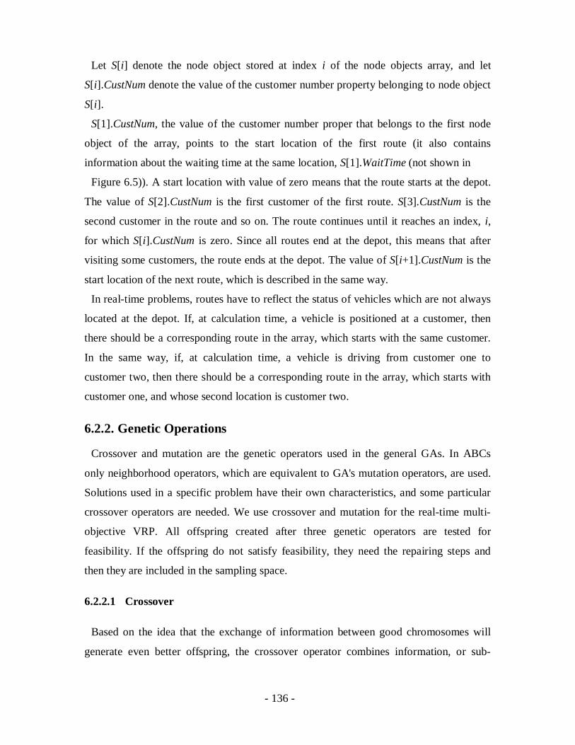
- 136 -
Let S[i] denote the node object stored at index i of the node objects array, and let
S[i].CustNum denote the value of the customer number property belonging to node object
S[i].
S[1].CustNum, the value of the customer number proper that belongs to the first node
object of the array, points to the start location of the first route (it also contains
information about the waiting time at the same location, S[1].WaitTime (not shown in
Figure 6.5)). A start location with value of zero means that the route starts at the depot.
The value of S[2].CustNum is the first customer of the first route. S[3].CustNum is the
second customer in the route and so on. The route continues until it reaches an index, i,
for which S[i].CustNum is zero. Since all routes end at the depot, this means that after
visiting some customers, the route ends at the depot. The value of S[i+1].CustNum is the
start location of the next route, which is described in the same way.
In real-time problems, routes have to reflect the status of vehicles which are not always
located at the depot. If, at calculation time, a vehicle is positioned at a customer, then
there should be a corresponding route in the array, which starts with the same customer.
In the same way, if, at calculation time, a vehicle is driving from customer one to
customer two, then there should be a corresponding route in the array, which starts with
customer one, and whose second location is customer two.
6.2.2. Genetic Operations
Crossover and mutation are the genetic operators used in the general GAs. In ABCs
only neighborhood operators, which are equivalent to GA's mutation operators, are used.
Solutions used in a specific problem have their own characteristics, and some particular
crossover operators are needed. We use crossover and mutation for the real-time multi-
objective VRP. All offspring created after three genetic operators are tested for
feasibility. If the offspring do not satisfy feasibility, they need the repairing steps and
then they are included in the sampling space.
6.2.2.1 Crossover
Based on the idea that the exchange of information between good chromosomes will
generate even better offspring, the crossover operator combines information, or sub-

- 137 -
solutions, from two solutions to create a better solution. As mentioned earlier, children
solutions, produced by the crossover, may or may not be better than the parents solutions,
but this is not a matter of serious concern, because if good solutions are created by
crossover, there will be more copies of them in the next mating pool generated by
crossover. Since, from the above, the effect of crossover may be detrimental or beneficial,
in order to preserve some of the good solutions that are already present in the mating
pool, none of the solutions in the mating pool are used in crossover. When a crossover
probability, defined here as Cp is used, only 100 Cp per cent solutions in the population
are used in the crossover operation and 100 1 Cp per cent of the population remains as
they are in the current population.
Many crossover operators exist in the GA literature. One site crossover and two site
crossovers are the most common ones adopted.
In a one site crossover, two parent solutions, Parent1 and Parent2, are picked from the
mating pool. Assuming that the solutions are encoded using a bit-string of size N, a single
crossover point¸ C, is randomly selected. Two new children solutions are not built based
on the parents solutions in the following ways: Bits 1 to C, of Child1 bit-string encoding,
are equal to bits 1 to C of Parent1 bit-string encoding. Bits C+1 to N, of Child1 bit-string
encoding, are equal to bits C+1 to N of Parent2 bit-string encoding. Similarly, bits 1 to C,
of Child2 bit-string encoding, are equal to bits 1 to C of Parent2 bit-string encoding and
bits C+1 to N, are equal to bits C+1 to N of Parent1 bit-string encoding.
Figure 6.6 - One site crossover
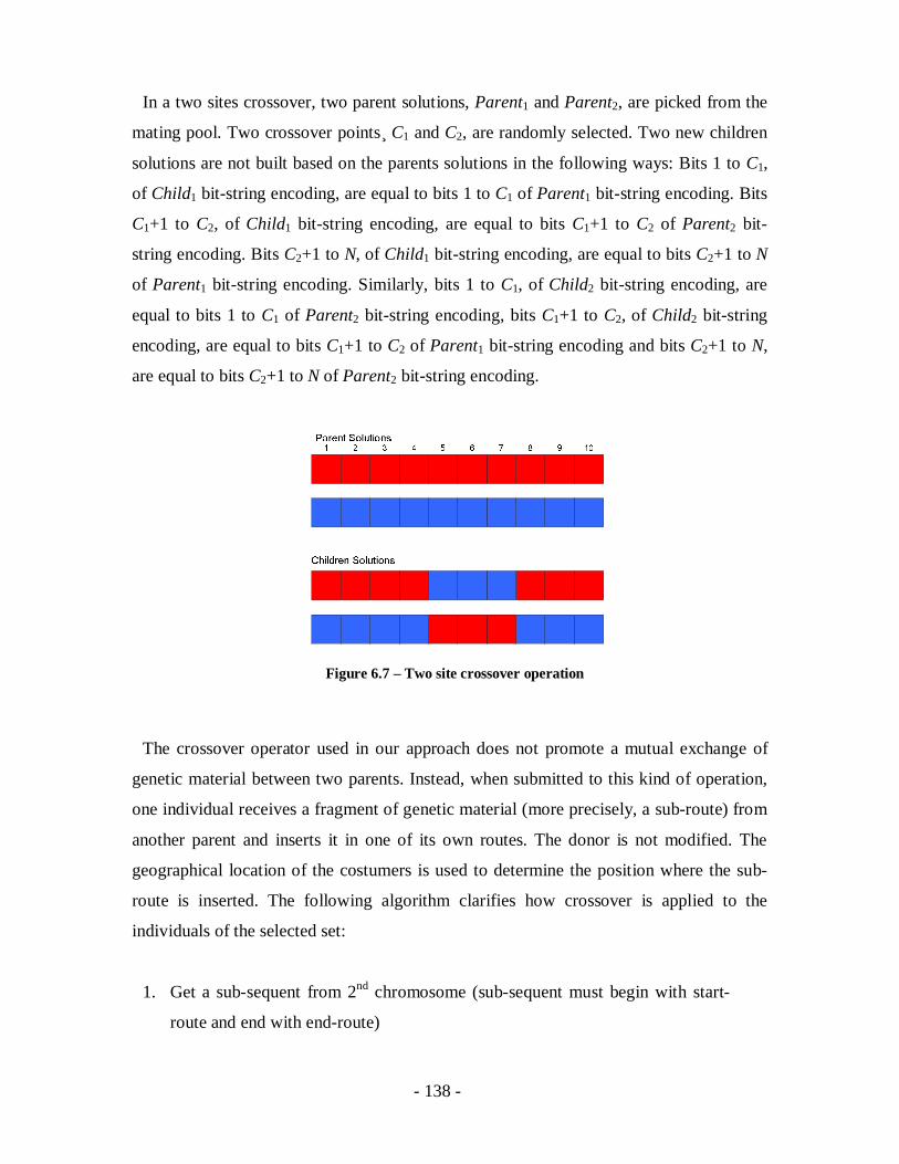
- 138 -
In a two sites crossover, two parent solutions, Parent1 and Parent2, are picked from the
mating pool. Two crossover points¸ C1 and C2, are randomly selected. Two new children
solutions are not built based on the parents solutions in the following ways: Bits 1 to C1,
of Child1 bit-string encoding, are equal to bits 1 to C1 of Parent1 bit-string encoding. Bits
C1+1 to C2, of Child1 bit-string encoding, are equal to bits C1+1 to C2 of Parent2 bit-
string encoding. Bits C2+1 to N, of Child1 bit-string encoding, are equal to bits C2+1 to N
of Parent1 bit-string encoding. Similarly, bits 1 to C1, of Child2 bit-string encoding, are
equal to bits 1 to C1 of Parent2 bit-string encoding, bits C1+1 to C2, of Child2 bit-string
encoding, are equal to bits C1+1 to C2 of Parent1 bit-string encoding and bits C2+1 to N,
are equal to bits C2+1 to N of Parent2 bit-string encoding.
Figure 6.7 – Two site crossover operation
The crossover operator used in our approach does not promote a mutual exchange of
genetic material between two parents. Instead, when submitted to this kind of operation,
one individual receives a fragment of genetic material (more precisely, a sub-route) from
another parent and inserts it in one of its own routes. The donor is not modified. The
geographical location of the costumers is used to determine the position where the sub-
route is inserted. The following algorithm clarifies how crossover is applied to the
individuals of the selected set:
1. Get a sub-sequent from 2nd chromosome (sub-sequent must begin with start-
route and end with end-route)

- 139 -
2. remove all customers found in the sub-sequent from the first chromosome
3. insert the sub-sequent at the end of the 1st chromosome
Figure 6.8 – Crossover operation
The example from Figure 6.8 helps to illustrate how crossover acts. In the example two
parent solutions, Parent1 and Parent2, were chosen. In the example, both Parent1 and
Parent2 represent solutions with four routes. The first route of Parent1 is 0-15-2-4-3-0,
the second route is 0-12-16-14-8-0, the third route is 9-10-11-5-0 and the fourth and last
route is 0-13-7-1-0. Similarly, the first route of Parent2 is 9-10-3-7-15-0, the second route
is 0-8-6-11-12-0, the third route is 0-1-5-14-0 and the fourth and last route is 0-13-4-2-0.
In order to create the child solution (the result of the crossover operation), we first make a
copy of Parent1. Second, a route is randomly selected from Parent2. While in the
example, one route, 0-8-6-11-12-0, was selected, the crossover allows for more than one
route to be selected, as long as they are sequential routes. The next step is to remove all
customers found in the selected route(s) from the copy of Parent1. This operation may
result in empty routes in the copy of Parent1, so a cleanup procedure has to be applied on
it. Next, a route in the copy of Parent1 is randomly selected, and the selected route(s)
from Parent2 are inserted before or after it. In the example, the randomly selected route
from the copy of Parent1 is the last route, and the select route from Parent2 is inserted
after it, meaning, added to the end of the solution. The result of the last operation is the
result of the crossover operation, the child route.
Since each parent solution represents a feasible solution, applying the described
crossover operation results in a new feasible solution.

- 140 -
6.2.2.2 Mutation
Mutation adds new information in a random way to a given solution and ultimately
helps to avoid getting trapped at local optima. It is an operator that introduces diversity in
the population whenever the population tends to become homogeneous due to repeated
use of reproduction and crossover operators.
In the multi-objective real-time VRPs, a mutation operation applied to a given solution
can result in one of the following: (1) Change the order of customers in a route encoded
by the solution. (2) Reduce the number of routes encoded by the solution, by merging two
routes together; or (3) Increase the number of routes encoded by the solution by splitting
a single route into two routes.
6.2.2.2.1 Merge Routes operation
The merge operation, takes two routes from the solution and merges them into one new
route. This operation is used to reduce the number of vehicles used by the solution.
Figure 6.9 - An example of merge route operation
A candidate solution to an instance of the VRP is encoded using an array of node
objects (node object is an object that has two properties, customer number and waiting
time at customer), and based on the permutation representation.
A route is a sequence of node objects in the array of node objects. The first node in the
route corresponds to the first location of the route (which can be either the depot, denoted
as 0, or a customer). The last node of the route must be a depot, since all routes end at the
depot.
In the example illustrated in Figure 6.9, two routes were randomly selected, 0-12-6-14-
8-0 and 0-13-7-1-0. Next, the two routes are merged into a single route, 0-12-6-14-8-13-
7-1-0. This is done by removing the end location of the first route and the start location of

- 141 -
the second route, which in both cases is the depot, and concatenating the second route to
the first route. Next, the second route is removed from the solution's array of node
objects, and the first route in the solution's array of objects is replaced with the new
merged route.
The merge route operation can be applied to two routes, only if the first location of the
second route is the depot, and there is no truck driving from the deport to the second
location of the route. Otherwise, the solution will not reflect real-life information.
6.2.2.2.2 Swap operation
A candidate solution to an instance of the VRP, is encoded using an array of node
objects (node object is an object that has two properties, customer number and waiting
time at customer), and based on the permutation representation. The swap operation
randomly selects two node objects from the nodes objects array, and swaps them. The
swap operation is used to change the order of customers in a route. It can also decrease
the number of routes in the solution, as illustrated later in this chapter.
An example of the swap operation is illustrated in Figure 6.10.
Figure 6.10 - An example of a swap operation
The solution shown in Figure 6.10 contains four routes. Two of the routes are 0-12-6-
14-8-0 and 9-10-11-5-0. Two node objects are randomly selected, the first node object
corresponds to customer 12, and the seconds corresponds to customer 5. As stated before,
the swap operation interchanges the two randomly selected node objects, so the result is
two new routes, 0-5-6-14-8-0 and 9-10-11-12-0.
An example of the swap operation is illustrated in Figure 6.10.

- 142 -
Figure 6.11 - An example of a swap operation that decreases the number of routes
The solution shown in Figure 6.11 contains two routes, 0-1-2-3-4-0 and 0-5-0. Two
node objects are randomly selected, the first node object corresponds to the last location
in the first route (the depot), and the seconds corresponds to customer 5. After swapping
the two randomly selected node objects, the result is two new routes, 0-1-2-3-4-5-0 and
0-0. The second route, 0-0, is an empty route, since there are no customers to visit in the
route. Therefore, this route should be removed from the solution, and we are left with
only one route, instead of two.
If by swapping two node objects, the new solution does not reflect real-life information
(a vehicle driving from customer i to customer j is no longer present in the solution), the
swapping is not allowed.
6.2.2.2.3 Split Routes operation
The split operation, takes one route from the solution and splits it into two new routes.
This operation is used to increase the number of vehicles used by the solution.
Figure 6.12 - An example of split route operation
Since a candidate solution to an instance of the VRP is encoded using an array of node
objects (node object is an object that has two properties, customer number and waiting
time at customer), splitting a route into two routes is a simple operation – randomly select
- 143 -
a node object from the node objects array, and insert two nodes that represent depots after
it.
In the example illustrated in Figure 6.12, there are four routes, 0-2-4-3-0, 0-6-8-0, 9-10-
5-0 and 0-7-1-0. A node object has to be randomly selected; in the example the selected
node object corresponds to customer 6. Two node objects, each represents a depot, are
inserted after the selected node object. The result is two near routes, 0-6-0 and 0-8-0.
If the selected node object represents the depot, the result of the split operation may be
an empty route, which will have to be removed from the solution.
Mutation may cause a vehicle to exceed its capacity. When this happens, and to
guarantee that the interpretation yields a valid solution, we split the route that exceeds
capacity into several ones. An example illustrates this adjustment: assume that the
original route 0-1-2-3-4-5-6-0 causes the vehicle to exceed its capacity at node 4. When
this situation occurs, the itinerary is divided in two sections: 0-1-2-3-0 and 0-4-5-6-0, and
a new vehicle is added to the solution. If necessary, further divisions can be made in the
second section. Notice that these changes only occur at the interpretation level, and
therefore the information codified in the chromosome is not altered.
6.2.2.2.4 Change Wait Time operation
The last operation described is the change wait time operation. The change wait time
operation changes the waiting time for a randomly chosen customer, to a random value in
the range of 0 to T, where T is a predefined value. This operation is much simpler than
the previously described operations.
A candidate solution to an instance of the VRP must specify, among others, waiting
times at each customer. Node object is an object that has two properties, customer
number and waiting time at customer. A solution to the multi-objective real-time VRPs is
encoded using an array of node objects, and based on the permutation representation.
The change wait time operation is therefore a simple operation. Randomly select a node
object, N, from the node objects array. For the randomly selected node object N, change
the waiting time property to a random value in the range of 0 to T.
When this operation is applied on a solution, it does not change its feasibility.

- 144 -
6.3. Summary
Evolutionary Algorithms belong to the Evolutionary Computation field of study
concerned with computational methods inspired by the process and mechanisms of
biological evolution. Evolutionary Algorithms share properties of adaptation through an
iterative process that accumulates and amplifies beneficial variation through trial and
error. Candidate solutions represent members of a virtual population striving to survive in
an environment defined by a problem specific objective function. In each case, the
evolutionary process refines the adaptive fit of the population of candidate solutions in
the environment, typically using surrogates for the mechanisms of evolution such as
genetic recombination and mutation.
In this chapter three evolutionary algorithms for solving the real-time multi objective
vehicle routing problem were presented. The first two algorithms are genetic algorithms.
These algorithms encode a potential solution to a specific problem on a simple
chromosome-like data structure and apply recombination operators to these structures in
order to preserve critical information.
The first genetic algorithm is an improved version of the vector evaluated genetic
algorithm (VEGA). The VEGA concept is that, for a problem with NumObj objectives,
NumObj sub-populations of size PopSize/NumObj each would be generated (assuming a
total population size of PopSize). Each sub-population uses only one of the NumObj
objective functions for fitness assignment. The proportionate selection operator is used to
generate the mating pool. These sub-populations are then shuffled together to obtain a
new population of size PopSize, on which the GA would apply the crossover and
mutation operators in the usual way. In each generation the set of not-dominated
solutions is added to the optimal solutions set, from which non-dominated solutions are
removed.
The second genetic algorithm is the SPEA2 algorithm. SPEA2 is actually an extension
of an elitism MOEA called “The Strength Pareto Evolution Algorithm” – SPEA.The
distinctive feature of SPEA2 lies in the elitism-preserved operation. An external set (archive) is
created for storing primarily non-dominated solutions. It is then combined with the
current population to form the next archive that is then used to create offspring for the
next generation. The size of the archive is fixed. It can be set to be equal to the population
- 145 -
size. Therefore, two special situations exist when filling solutions in the archive. If the
number of non-dominated solutions is smaller than the archive size, other dominated
solutions taken from the remainder part of the population are filled in. This selection is
carried out according to a fitness value, specifically defined for SPEA. In other words, the
individual fitness value defined for a solution x, is the total of the SPEA-defined strengths
of solutions which dominate x, plus a density value.
The second situation happens when the number of non-dominated solutions is over the
archive size. In this case, a truncation operator is applied. For that operator, the solution
which has the smallest distance to the other solutions will be removed from the set. If
solutions have the same minimum distance, the second nearest distance will be
considered, and so forth. This is called the k-th nearest distance rule.
The third revolutionary algorithm is a combination of the vector evaluated technique
and artifical bee colony algorithm. In the ABC algorithm, the colony of artificial bees
consists of three groups of bees: (1) employed bees - bees that are currently exploiting a
food source; (2) onlookers - bees that are waiting in the hive for the employed bees to
share information about the food sources; and (3) scouts - bees that are searching for new
food sources in the neighborhood of the hive. The ABC algorithm starts by assigning
each employed bee to a randomly generated solution. Next, in each iteration, each
employed bee, using a neighborhood operator, finds a new food source near its assigned
food source. The nectar amount of the new food source is then evaluated. If the amount
of nectar in the new food source is higher than the amount of nectar in the old one, then
the older source is replaced by the newer one. Next, the nectar information of the food
sources is shared with the onlookers. The onlooker chooses a food source according to
the probability proportional to the quality of that food source. Roulette wheel selection is
the usual method. Therefore, good food sources, as opposed to bad ones, attract more
onlooker bees. Subsequently, using a neighborhood operator, each onlooker finds a food
source near its selected food source and calculates its nectar amount. Then, for each old
food source, the best food source among all the food sources near the old one is
determined. The employed bee associated with the old food source is assigned to the best
food source and abandons the old one if the best food source is better than the old food
source. A food source is also abandoned by an employed bee if the quality of the food
source has not improved in the course of a predetermined and limited number of

- 146 -
successive iterations. The employed bees then become scouts and randomly search for
new food source. After a scout finds a new food source, it again becomes an employed
bee. After each employed bee is assigned to a food source, another iteration of the ABC
algorithm begins. The iterative process is repeated until a stopping condition is met.
Next, solutions representation was described. A candidate solution to an instance of the
VRP must specify the number of vehicles required, the partition of the demands through
all these vehicles, the delivery order for each route as well as waiting time at each
customer. Let a node object define an object that has two properties, customer number
and waiting time at customer. A solution to the multi-objective real-time VRPs can be
encoded using an array of node objects, and based on the permutation representation. A
solution contains several routes, each one of them composed by an ordered subset of the
costumers. All demands belonging to the problem being solved must be present in one of
the routes.
Methods such as crossover and mutations, which are needed for diversity purposes,
were also described. Crossover and mutation are the genetic operators used in the general
GAs. In ABCs only neighborhood operators, which are equivalent to GA's mutation
operators, are used. Solutions used in a specific problem have their own characteristics,
and some particular crossover operators are needed.

- 147 -
7. Fitness Functions and Algorithm Convergence A fitness function is a particular type of objective function that is used to summarize, as
a single figure of merit, how close a given design solution is to achieving the set aims.
In the field of evolutionary algorithms, at each iteration, the idea is to delete the n worst
design solutions, and to breed n new ones out of the best design solutions. Therefore,
each design solution needs to be awarded a figure of merit to indicate how close it came
to meeting the overall specifications, which is generated by applying the fitness function
to the test, or simulation, results obtained from that solution.
Evolutionary algorithms work mainly due to the effort involved in designing a workable
fitness function. Even though it is no longer the human designer, but the computer, that
comes up with the final design, it is the human designer who has to design the fitness
function. If this is designed wrongly, the algorithm will either converge to an
inappropriate solution, or will have difficulty converging at all.
Furthermore, the fitness function must not only correlate closely with the designer's
goal; it must also be computed quickly. Speed of execution is very important, as a typical
evolutionary algorithm must be iterated many times in order to produce a usable result for
a non-trivial problem.
In some cases, fitness approximation may be appropriate, especially if (1) the fitness
computation time of a single solution is extremely high, (2) a precise model for fitness
computation is missing or (3) the fitness function is uncertain or noisy.
Two main classes of fitness functions exist: one where the fitness function does not
change, as in optimizing a fixed function or testing with a fixed set of test cases; and one
where the fitness function is mutable, as in niche differentiation or co-evolving the set of
test cases.
In both the improved VEGA algorithm and the VE-ABC algorithm, in each generation,
a number of sub-populations are generated by performing proportional selection
according to each objective function in turn. Thus, for a problem with q objectives, q sub-
populations of size N/q each would be generated, assuming a population size of N. This
means that for each objective function, a corresponding fitness function has to be
designed and calculated for all proposed solutions.
- 148 -
In the case of the SPEA2 algorithm, in order to avoid the situation that individuals
dominated by the same archive members have identical fitness values, each individual is
assigned a strength value S(i), representing the number of solutions it dominates. A
solution dominates another solution if for all objective functions, the first solution is
better than the second solution. Therefore, in order to compute S(i), for each individual,
the values of all objective functions need to be computed.
Five objective functions are addressed in this study; four of which rely on travel time:
(1) minimizing the total travel time; (2) minimizing the difference of travel times among
the routes of the solution, (3) Minimizing the total dissatisfaction of all customers and (4)
Minimizing the arrival time of the latest vehicle.
Due to the stochastic nature of travel time, in order to get an accurate value, or accurate
fitness functions for the previously mentioned objectives, simulation has to be used.
Simulation works by traveling paths. Each path is traveled w times, when w is pre-
determined by the user. The traveling times are stored in a sorted array. The returned
traveling time, C, returned by the simulation is defined as the traveling time stored in
entry w· of the array. Assuming that =0.95, this means that in 95% of all cases, the
actual traveling time will be shorter than C. A higher value of w will usually increase the
accuracy of the result obtained from the simulation.
Usually, a high value of w results in accurate results of the simulation; however, it
dramatically increases the running time of the algorithm. For example, in this study,
values of w=1 and w=1000 were used. Using the improved VEGA algorithm, several
problems were solved. The average running time when w=1 was about 20 minutes, and
when w=1000, about 8 hours. In this study, it will be shown that w=1 (fitness
approximation) can be used without affecting the algorithm performance (meaning that
for different values of w the algorithm converges to the same results).
7.1.1. Convergence
To validate this approach, a methodology normally adopted in the evolutionary multi-
objective optimization literature was used.
Using performance measures (or metrics) allows the assessment (in a quantitative way)
of an algorithm’s performance. For multi objective optimization problems, measures tend
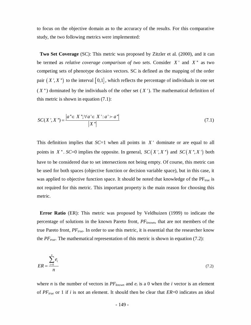
- 149 -
to focus on the objective domain as to the accuracy of the results. For this comparative
study, the two following metrics were implemented:
Two Set Coverage (SC): This metric was proposed by Zitzler et al. (2000), and it can
be termed as relative coverage comparison of two sets. Consider 'X and ''X as two
competing sets of phenotype decision vectors. SC is defined as the mapping of the order
pair ', ''X X to the interval 0,1 , which reflects the percentage of individuals in one set
( ''X ) dominated by the individuals of the other set ( 'X ). The mathematical definition of
this metric is shown in equation (7.1):
'' ''; ' ' : ' ''( ', '')
''a X a X a a
SC X XX
(7.1)
This definition implies that SC=1 when all points in 'X dominate or are equal to all
points in ''X . SC=0 implies the opposite. In general, ', ''SC X X and '', 'SC X X both
have to be considered due to set intersections not being empty. Of course, this metric can
be used for both spaces (objective function or decision variable space), but in this case, it
was applied to objective function space. It should be noted that knowledge of the PFtrue is
not required for this metric. This important property is the main reason for choosing this
metric.
Error Ratio (ER): This metric was proposed by Veldhuizen (1999) to indicate the
percentage of solutions in the known Pareto front, PFknown, that are not members of the
true Pareto front, PFtrue. In order to use this metric, it is essential that the researcher know
the PFtrue. The mathematical representation of this metric is shown in equation (7.2):
0
n
ii
eER
n (7.2)
where n is the number of vectors in PFknown and ei is a 0 when the i vector is an element
of PFtrue or 1 if i is not an element. It should then be clear that ER=0 indicates an ideal
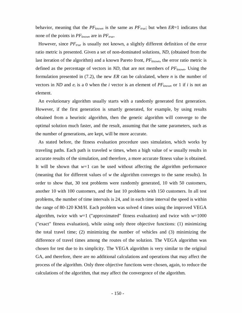
- 150 -
behavior, meaning that the PFknown is the same as PFtrue; but when ER=1 indicates that
none of the points in PFknown are in PFtrue.
However, since PFtrue is usually not known, a slightly different definition of the error
ratio metric is presented. Given a set of non-dominated solutions, ND, (obtained from the
last iteration of the algorithm) and a known Pareto front, PFknown, the error ratio metric is
defined as the percentage of vectors in ND, that are not members of PFknown. Using the
formulation presented in (7.2), the new ER can be calculated, where n is the number of
vectors in ND and ei is a 0 when the i vector is an element of PFknown or 1 if i is not an
element.
An evolutionary algorithm usually starts with a randomly generated first generation.
However, if the first generation is smartly generated, for example, by using results
obtained from a heuristic algorithm, then the genetic algorithm will converge to the
optimal solution much faster, and the result, assuming that the same parameters, such as
the number of generations, are kept, will be more accurate.
As stated before, the fitness evaluation procedure uses simulation, which works by
traveling paths. Each path is traveled w times, when a high value of w usually results in
accurate results of the simulation, and therefore, a more accurate fitness value is obtained.
It will be shown that w=1 can be used without affecting the algorithm performance
(meaning that for different values of w the algorithm converges to the same results). In
order to show that, 30 test problems were randomly generated, 10 with 50 customers,
another 10 with 100 customers, and the last 10 problems with 150 customers. In all test
problems, the number of time intervals is 24, and in each time interval the speed is within
the range of 80-120 KM/H. Each problem was solved 4 times using the improved VEGA
algorithm, twice with w=1 ("approximated" fitness evaluation) and twice with w=1000
("exact" fitness evaluation), while using only three objective functions: (1) minimizing
the total travel time; (2) minimizing the number of vehicles and (3) minimizing the
difference of travel times among the routes of the solution. The VEGA algorithm was
chosen for test due to its simplicity. The VEGA algorithm is very similar to the original
GA, and therefore, there are no additional calculations and operations that may affect the
process of the algorithm. Only three objective functions were chosen, again, to reduce the
calculations of the algorithm, that may affect the convergence of the algorithm.

- 151 -
7.1.2. Metrics Comparison Results
In this section, the results of the metrics comparison, using paired-samples t-tests are
reported. Throughout this section X’ refers to a solution obtained when w=1 and X’’ to a
solution obtained when w=1000. In evolutionary algorithms, since the way the first
generation was generated may change the algorithm's results, each comparison was
conducted twice, once using a randomly generated first population and the second using a
Savings based first population.
Eight paired-samples t-tests were conducted to compare the results of the two set
coverage metric (SC(X’,X’’) vs. SC(X’’,X’)). The results are listed in Table 7.1.
The results show that for problems with 50 and 100 customers, when the first generation
was randomly generated or Savings based, there is no significant difference in the scores
for SC(X’,X’’) and SC(X’’,X’). However, for problems with 150 customers, there is a
significant difference in the scores for SC(X’,X’’) and SC(X’’,X’). This indicates that on
average, 59% of the non-dominated solutions, when the first generation was randomly
generated, and 29% of the non-dominated solutions, when the first generation was
Savings based, obtained from the last iteration of the genetic algorithm, when w=1, are
dominated by the non-dominated solutions obtained when w=1000. In addition, 26% of
the non-dominated solutions, when the first generation was randomly generated, and 54%
of the non-dominated solutions, when the first generation was Savings based, obtained
when w=1000, are dominated by the non-dominated solutions obtained when w=1. From
the above, it can be concluded that for problems with 150, the results obtained when
w=1000 are better than the results obtained when w=1 when using a randomly generated
first generation. However, if the first generation is Savings based, then the results
obtained when w=1 are better than the results obtained when w=1000. Two paired-
samples t-tests, in which all groups of problems are combined into a single sample, show
that there is no significant difference in the scores for SC(X’,X’’) and SC(X’’,X’).

- 152 -
SC(X’,X’’) SC(X’’,X’)Problem Size M SD M SD t df Sig.
Randomly generated fist population
50 0.479 0.411 0.493 0.459 -0.112 39 0.911100 0.349 0.447 0.397 0.447 -0.382 39 0.705150 0.59 0.458 0.258 0.411 2.654 39 0.011All 0.411 0.424 0.416 0.411 -0.064 119 0.949
Savings based first population50 0.535 0.41 0.452 0.376 0.690 39 0.494
100 0.408 0.435 0.254 0.365 1.427 39 0.162150 0.29 0.399 0.541 0.446 -2.199 39 0.034All 0.473 0.447 0.389 0.446 1.235 119 0.219
Table 7.1 – A comparison of SC(X’,X’’) and SC(X’’,X’) using paired-samples t-tests
As with the results of the two set coverage metric, paired-samples t-tests were used to
check if there are any differences in the results of the error ratio metric for w=1 and for
w=1000. The results are listed in Table 7.2.
The results show that for problems with 50 customers, when the first generation was
randomly generated or Savings based, there is no significant difference in the scores for
ER(X’) and ER(X’’). This is also the case for problems with 100 customers, when the first
generation was randomly generated and for problems with 150 customers, when the first
generation is Savings based.
However, for problems with 150 customers, when the first generation was randomly
generated and for problems with 100 customers, when the first generation is Savings
based, there is a significant difference in the scores for ER(X’) and ER(X’’). This means
that for problems with 150 customers, when the first generation was randomly generated,
on average 55% of the non-dominated solutions do not belong to PFknown when w=1,
whereas when w=1000, 80% of the non-dominated solutions do not belong to PFknown.
Similarly, for problems with 100 customers, when the first generation is Savings based,
on average 49% of the non-dominated solutions do not belong to PFknown when w=1 but
when w=1000, 73% of the non-dominated solutions do not belong to PFknown.
This means that for problems with 150 customers, when the first generation was
randomly generated and for problems with 100 customers, when the first generation was
Savings based, the chance for a non-dominated solution that belongs to PFknown is twice
as high when w=1 than when w=1000.
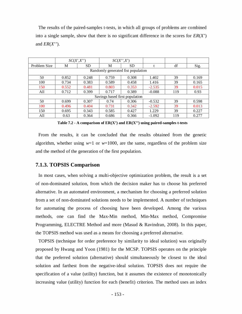
- 153 -
The results of the paired-samples t-tests, in which all groups of problems are combined
into a single sample, show that there is no significant difference in the scores for ER(X’)
and ER(X’’).
SC(X’,X’’) SC(X’’,X’)Problem Size M SD M SD t df Sig.
Randomly generated fist population
50 0.852 0.248 0.759 0.308 1.402 39 0.169100 0.734 0.383 0.589 0.458 1.416 39 0.165150 0.552 0.481 0.803 0.353 -2.535 39 0.015All 0.712 0.399 0.717 0.389 -0.088 119 0.93
Savings based first population50 0.699 0.307 0.74 0.306 -0.532 39 0.598
100 0.496 0.404 0.731 0.342 -2.592 39 0.013150 0.695 0.343 0.585 0.427 1.229 39 0.227All 0.63 0.364 0.686 0.366 -1.092 119 0.277
Table 7.2 - A comparison of ER(X’) and ER(X’’) using paired-samples t-tests
From the results, it can be concluded that the results obtained from the genetic
algorithm, whether using w=1 or w=1000, are the same, regardless of the problem size
and the method of the generation of the first population.
7.1.3. TOPSIS Comparison
In most cases, when solving a multi-objective optimization problem, the result is a set
of non-dominated solution, from which the decision maker has to choose his preferred
alternative. In an automated environment, a mechanism for choosing a preferred solution
from a set of non-dominated solutions needs to be implemented. A number of techniques
for automating the process of choosing have been developed. Among the various
methods, one can find the Max-Min method, Min-Max method, Compromise
Programming, ELECTRE Method and more (Masud & Ravindran, 2008). In this paper,
the TOPSIS method was used as a means for choosing a preferred alternative.
TOPSIS (technique for order preference by similarity to ideal solution) was originally
proposed by Hwang and Yoon (1981) for the MCSP. TOPSIS operates on the principle
that the preferred solution (alternative) should simultaneously be closest to the ideal
solution and farthest from the negative-ideal solution. TOPSIS does not require the
specification of a value (utility) function, but it assumes the existence of monotonically
increasing value (utility) function for each (benefit) criterion. The method uses an index

- 154 -
that combines the closeness of an alternative to the positive-ideal solution with its
remoteness from the negative-ideal solution. The alternative maximizing this index value
is the preferred alternative.
In the previous section, it has been shown that a set of non-dominated solutions
obtained when w=1 is as good as a set of non-dominated solutions obtained when
w=1000. However, this does not mean that the same results exist in both sets, and
therefore, it is not guaranteed that the TOPSIS method selects similar results from both
sets. In this section, a comparison of the results of TOPSIS method applied on the
solution sets obtained from the 30 test cases is presented.
A solution is a set of three results, each for every objective function. The analysis
begins with correlation analysis. Correlation analysis is used to check whether or not
there is a correlation between the three values of a result. As with the metrics comparison,
each comparison is conducted twice, once using a randomly generated first population,
and the second using a Savings based first population.
Eight Pearson product-moment correlation coefficients were computed to assess the
relationship between the results of the first objective function and the second objective
function. The results are listed in Table 7.3.
w=1 w=1000Problem Size Obj. 2 Obj. 2
Randomly generated first population50 Obj. 1 r=0.94, n=40, p=0 Obj. 1 r=0.954, n=40, p=0100 Obj. 1 r=0.973, n=40, p=0 Obj. 1 r=0.986, n=40, p=0150 Obj. 1 r=0.909, n=40, p=0 Obj. 1 r=0.944, n=40, p=0All Obj. 1 r=0.81, n=120, p=0 Obj. 1 r=0.785, n=120, p=0
Savings based first population50 Obj. 1 r=0.835, n=40, p=0 Obj. 1 r=0.814, n=40, p=0100 Obj. 1 r=0.82, n=40, p=0 Obj. 1 r=0.865, n=40, p=0150 Obj. 1 r=0.281, n=40, p=0.079 Obj. 1 r=0.174, n=40, p=0.282All Obj. 1 r=0.716, n=120, p=0 Obj. 1 r=0.716, n=120, p=0
Table 7.3 - Pearson product-moment correlation coefficients between the first and second
objectives, for w=1 and w=1000
For problems with 50, 100 and 150 customers, whether the first generation was
randomly created or Savings based, a positive correlation between the two variables was
found for solutions obtained when w=1 and for solutions obtained when w=1000. Since a
strong positive correlation exists between the two variables, a correlation analysis was
- 155 -
performed, using the results of all problems as a single result. The results show a positive
correlation when using w=1 and when using w=1000.
A second set of eight Pearson product-moment correlation coefficients was computed to
assess the relationship between the results of the first objective function and the third
objective function. All tests, whether the first generation was randomly created or
Savings based, show a negative correlation. However, since the third objective minimizes
the difference of travel times among the routes of the solution, and is defined by means of
standard deviation, and since the maximum value obtained for this objective is 0.05 when
w=1 and 0.009 when w=1000, it can be assumed that the value of the third objective is
always 0, and therefore, can be ignored in the analysis.
Since it has been shown that a correlation exists between the first and second objectives,
and that the third objective can be ignored, since it can be treated as zero, a paired t-test
can be used to compare the results obtained by using the TOPSIS method.
Eight paired-samples t-tests were conducted to compare the results obtained by using
the TOPSIS method when w=1 and when w=1000. The results are listed in Table 7.4.
All paired-samples t-tests show that there is no significant difference in the scores for
w=1 and for w=1000.
w=1 w=1000Problem Size M SD M SD t df Sig.
Randomly generated fist population
50 31.2 10.6 30.9 10.2 0.429 39 0.67100 72.1 28.8 70.9 26.3 0.899 39 0.374150 76.3 15.8 79.1 14.2 -1.967 39 0.056All 59.8 28.2 60.3 27.8 -0.676 119 0.5
Savings based first population50 24.9 12.3 24.8 11.9 0.02 39 0.984
100 52.7 31.7 51.9 30.6 0.244 39 0.808150 42.2 27.0 40.6 26.4 0.34 39 0.736All 39.9 27.4 39.1 26.6 0.417 119 0.678
Table 7.4 - A comparison of TOPSIS results for w=1 and w=1000 using paired-samples t-tests
7.2. Travel time characteristics
The previous analysis shows that it is possible to increase the running time of the
algorithm by using an "approximated" fitness function, without influencing the accuracy
of the algorithm. The analysis was done using 30 randomly generated test problems, with
- 156 -
50, 100 and 150 customers, all having 24 time intervals, when for each time interval the
travel speed ranges from 80-120 KM/H, with empiric probability. However, travel time is
more likely to be lognormally distributed because (1) the positive skew shape (i.e., right
skewed) is more suitable for travel time description; that is, a higher probability exists for
long travel time than for short travel time, and (2) the range [0, ) of the distribution is
more natural than a truncated normal distribution (because negative travel times are
impossible) (Hadas & Ceder, 2008).
For that reason, a second set of tests was conducted, this time using Solomon’s
instances. Since Solomon’s instances were designed for TWVRP, a simple modification
had to be done. Solomon’s instances provide the location of each customer, assuming that
the travel speed is constant. Since this is not the case in this problem, time intervals were
added (24 of them) and for each time interval a lognormal random travel time function
was assigned for which =0.03 and =4.1 (theses values may change slightly between
time intervals) and therefore the average traveling speed is 60 KM/H. In order to decrease
running time, Solomon’s instances were solved using the improved VEGA algorithm,
using 500 generations and population size of 200, once when w=1 and next when w=100.
The results of the test are presented in Table 7.5.
w=1 w=100
Problem
SizeProblem
Type M SD M SD t df Sig.
Randomly generated first population
C1 3.35 0.03 3.34 0.04 0.641 35 0.526C2 2.47 0.09 2.45 0.1 0.561 31 0.579R1 4.14 0.86 3.63 0.22 3.912 47 0R2 3.15 0.28 3.15 0.22 -0.059 43 0.953
RC1 3.96 0.24 3.84 0.21 2.492 31 0.018
25
RC2 2.57 0.13 2.59 0.15 -0.69 31 0.495C1 6.6 0.22 6.61 0.44 -0.133 35 0.895C2 5.4 0.55 4.94 0.1 4.616 31 0R1 11.83 1.21 11.4 1.45 1.466 47 0.149R2 11.63 0.67 11.54 0.94 0.538 43 0.593
RC1 9.46 0.69 9.27 0.78 0.931 31 0.395
50
RC2 8.6 0.72 8.46 0.41 1.027 31 0.312C1 16.44 1.01 16.35 0.94 0.467 35 0.643C2 14.4 1.00 13.85 0.94 2.292 31 0.029R1 38.94 2.38 37.43 1.85 3.462 47 0.001R2 35.74 3.01 32.37 2.71 5.224 43 0
100
RC1 32.88 2.45 30.99 0.29 3.514 31 0.001

- 157 -
w=1 w=100
Problem
SizeProblem
Type M SD M SD t df Sig.
RC2 28.41 3.29 24.76 1.96 5.604 31 0Savings based first population
C1 3.38 0.07 3.37 0.07 0.453 35 0.653C2 2.38 0.09 2.35 0.08 1.544 31 0.133R1 4.36 1.07 3.66 0.28 4.413 47 0R2 3.32 0.3 3.23 0.31 1.427 43 0.161
RC1 4.11 0.26 4 0.19 1.971 31 0.058
25
RC2 2.51 0.1 2.54 0.1 -1.275 31 0.212C1 6.4 0.08 6.34 0.01 4.128 35 0C2 5.34 0.85 4.96 0.26 2.42 31 0.022R1 12.56 1.26 11.21 0.8 6.353 47 0R2 11.91 0.6 11.27 0.63 5.16 43 0
RC1 9.17 0.63 8.89 0.22 2.412 31 0.022
50
RC2 8.61 0.67 8.42 0.53 1.258 31 0.218C1 14.92 0.63 14.53 0.08 4.253 35 0C2 12.33 0.57 11.45 0.54 6.486 31 0R1 38.88 2.42 37.81 1.78 2.466 47 0.017R2 35.76 2.19 32.16 2.27 7.837 43 0
RC1 29.82 2.17 28.54 1.34 2.894 31 0.007
100
RC2 28.21 4.07 24.22 1.74 4.836 31 0
Table 7.5 - A comparison of TOPSIS results for w=1 and w=100 using paired-samples t-tests
As seen from the results, for problems with 25 and 50 customers, when using a
randomly generated first generation, and for problems with 25 customers when using a
Savings based first generation, there is no difference in the TOPSIS results when using
w=1 and w=100. However, for problems with 100 customers, when using a randomly
generated first generation, and for problems with 50 and 100 customers when using a
Savings based first generation, a better solution is obtained when w=100 compared to the
solution obtained when w=1.
As stated before, in order to decrease running time, Solomon’s instances were solved
using the improved VEGA algorithm, using 500 generations and population size of 200.
It is known that the number of generations used by an evolutionary algorithm may affect
its results. Generally, a high number of generations gives the algorithm more chance to
converge towards the optimal solution than a low number of generations. However, in
real-time applications, the number of generations is bounded by the time given to the
algorithm to come up with a solution. Therefore, the algorithm was tested again, this time
with a stopping condition of 30 minutes running time, instead of the 500 generations.
Results for problems with 100 customers are reported in Table 7.6.

- 158 -
w=1 w=100Problem Size Problem Type M SD M SD t df Sig.
Randomly generated first generation100 C1 14.85 0.67 16.43 0.81 -8.883 35 0100 C2 12.64 1.58 14.19 0.74 -4.814 31 0100 R1 33.67 2.08 39.61 1.69 -14.488 47 0100 R2 32.77 4.57 38.62 2.94 -7.073 43 0100 RC1 30.14 2.23 33.22 1.07 -7.905 31 0100 RC2 27.13 4.42 28.14 2.49 -0.979 31 0.335
Savings based first generation100 C1 14.56 0.4 14.5 0.45 -0.411 35 0.684100 C2 11.72 1.31 12.15 2.03 0.985 31 0.332100 R1 34.44 2.56 40.09 1.53 -13.098 47 0100 R2 31.25 2.79 39.58 2.31 -16.071 43 0100 RC1 27.29 1.12 30.16 2.11 -6.568 31 0100 RC2 24.92 4.21 26.27 1.4 -1.841 31 0.075
Table 7.6 - A comparison of TOPSIS results for w=1 and w=100 using paired-samples t-tests
As it can be seen from Table 7.6, when using a randomly generated first generation, the
results obtained by the algorithm when w=1 were better than the results obtained when
w=100, except for RC2, in which no significant differences were found between the
results. When using a Savings based first generation, the results obtained by the algorithm
when w=1 were better than the results obtained when w=100, for problems R1, R2 and
RC1, while for problems C1, C2 and RC2, no significant differences were found between
the results.
Furthermore, an analysis of the convergence of the algorithm shows, that when w=100,
the best solution is reached after almost 30 minutes of running, while the same solution is
found much earlier when w=1. To illustrate these finding, the analysis of problems C101,
C201, R101, R201, RC101 and RC201 is given for both randomly generated and Savings
based first generation.
For problem C101, when w=100 the algorithm, using TOPSIS, reached its best solution
in which objective one equals 16.52, objective two equals 10 and objective three equals 0,
after 422 generations (see Figure 7.1). Since the algorithm, when w=100, was able to
generate 486 generations in 30 minutes, this means that the algorithm’s best solution was
reached after 26 minutes and 10 seconds. For the same problem, C101, when w=1, the
algorithm reached the best solution after 326 generations out of 7916 generations that
were generated during 30 minutes, namely, after one minute and ten seconds. Moreover,

- 159 -
when using w=1, the algorithm was able to reach a better solution than the best solution,
in which objective one equals 19.95, objective two equals 10 and objective three equals 0,
after 7394 generations, i.e., after 28 minutes and one second.
Generation
Valu
e
0 800 1600 2400 3200 4000 4800 5600 6400 7200 80000
10
20
30
40
50
60
70
80
Generation
Valu
e
0 50 100 150 200 250 300 350 400 450 5000
10
20
30
40
50
60
70
80
Figure 7.1 - Algorithm convergence when w=1 (left) and w=100 (right) for problem C101 during the
first 30 minutes
For problem C201, when w=100 the algorithm, using TOPSIS, reached its best solution
in which objective one equals 13.23, objective two equals 3 and objective three equals 0,
after 422 generations (see Figure 7.2). Since the algorithm, when w=100, was able to
generate 464 generations in 30 minutes, this means that the algorithm's best solution was
reached after 27 minutes and 17 seconds. For the same problem, C201, when w=1, the
algorithm reached the best solution after 733 generations out of 7397 generations that
were generated during 30 minutes, i.e., after 9 minutes and ten seconds. Furthermore,
when using w=1, the algorithm was able to reach a better solution than the best solution,
in which objective one equals 10.54, objective two equals 3 and objective three equals 0,
after 1799 generations, i.e., after 22 minutes and 30 seconds.
- 160 -
Generation
Valu
e
0 250 500 750 1000 1250 1500 1750 2000 2250 25000
10
20
30
40
50
60
70
80
Generation
Valu
e
0 50 100 150 200 250 300 350 400 450 5000
10
20
30
40
50
60
70
80
Figure 7.2 - Algorithm convergence when w=1 (left) and w=100 (right) for problem C201 during the
first 30 minutes
For problem R101, when w=100 the algorithm, using TOPSIS, reached its best solution
in which objective one equals 38.72, objective two equals 8 and objective three equals 0,
after 345 generations (see Figure 7.3). Since the algorithm, when w=100, was able to
generate 365 generations in 30 minutes, this means that the algorithm's best solution was
reached after 28 minutes and 21 seconds. For the same problem, R101, when w=1, the
algorithm reached the best solution after 309 generations out of 1692 generations that
were generated during 30 minutes, i.e., after 5 minutes and 28 seconds. Furthermore,
when using w=1, the algorithm was able to reach a better solution than the best solution,
in which objective one equals 32.07, objective two equals 8 and objective three equals 0,
after 1052 generations, i.e., after 18 minutes and 39 seconds.
Generation
Valu
e
0 200 400 600 800 1000 1200 1400 1600 1800 20000
10
20
30
40
50
60
70
80
Generation
Valu
e
0 40 80 120 160 200 240 280 320 360 4000
10
20
30
40
50
60
70
80
Figure 7.3 - Algorithm convergence when w=1 (left) and w=100 (right) for problem R101 during the
first 30 minutes

- 161 -
For problem R201, when w=100 the algorithm, using TOPSIS, reached its best solution
in which objective one equals 39.15, objective two equals 2 and objective three equals
0.00047, after 207 generations (see Figure 7.4). Since the algorithm, when w=100, was
able to generate 215 generations in 30 minutes, this means that the algorithm’s best
solution was reached after 28 minutes and 53 seconds. For the same problem, R201,
when w=1, the algorithm reached the best solution after 154 generations out of 1246
generation that were generated during 30 minutes, i.e., after 3 minutes and 42 seconds.
Furthermore, when using w=1, the algorithm was able to reach a better solution than the
best solution, in which objective one equals 32.91, objective two equals 2 and objective
three equals 0.00008, after 785 generations, or after 18 minutes and 54 seconds.
Generation
Valu
e
0 150 300 450 600 750 900 1050 1200 1350 15000
10
20
30
40
50
60
70
80
Generation
Valu
e
0 25 50 75 100 125 150 175 200 225 2500
10
20
30
40
50
60
70
80
Figure 7.4 - Algorithm convergence when w=1 (left) and w=100 (right) for problem R201 during the
first 30 minutes
For problem RC101, when w=100 the algorithm, using TOPSIS, reached its best
solution in which objective one equals 30.53, objective two equals 10 and objective three
equals 0, after 321 generations (see Figure 7.5). Since the algorithm, when w=100, was
able to generate 327 generations in 30 minutes, this means that the algorithm’s best
solution was reached after 29 minutes and 26 seconds. For the same problem, RC101,
when w=1, the algorithm reached the best solution after 432 generations out of 806
generation that were generated during 30 minutes, i.e., after 16 minutes and 4 seconds.
Furthermore, when using w=1, the algorithm was able to reach a better solution than the
best solution, in which objective one equals 28.52, objective two equals 10 and objective
three equals 0, after 704 generations, or after 26 minutes and 12 seconds.
- 162 -
Generation
Valu
e
0 100 200 300 400 500 600 700 800 900 10000
10
20
30
40
50
60
70
80
Generation
Valu
e
0 40 80 120 160 200 240 280 320 360 4000
10
20
30
40
50
60
70
80
Figure 7.5 - Algorithm convergence when w=1 (left) and w=100 (right) for problem RC101 during
the first 30 minutes
For problem RC201, when w=100 the algorithm, using TOPSIS, reached its best
solution in which objective one equals 26.99, objective two equals 2 and objective three
equals 0.00001, after 307 generations (see Figure 7.6). Since the algorithm, when w=100,
was able to generate 323 generations in 30 minutes, this means that the algorithm’s best
solution was reached after 28 minutes and 30 seconds. For the same problem, RC201,
when w=1, the algorithm reached the best solution after 425 generations out of 979
generation that were generated during 30 minutes, i.e., after 13 minutes and one second.
Furthermore, when using w=1, the algorithm was able to reach a better solution than the
best solution, in which objective one equals 24.22, objective two equals 2 and objective
three equals 0, after 967 generations, or after 29 minutes and 37 seconds.
Generation
Valu
e
0 100 200 300 400 500 600 700 800 900 10000
10
20
30
40
50
60
70
80
Generation
Valu
e
0 40 80 120 160 200 240 280 320 360 4000
10
20
30
40
50
60
70
80
Figure 7.6 - Algorithm convergence when w=1 (left) and w=100 (right) for problem RC201 during
the first 30 minutes
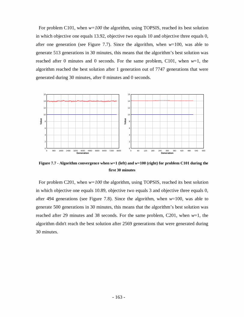
- 163 -
For problem C101, when w=100 the algorithm, using TOPSIS, reached its best solution
in which objective one equals 13.92, objective two equals 10 and objective three equals 0,
after one generation (see Figure 7.7). Since the algorithm, when w=100, was able to
generate 513 generations in 30 minutes, this means that the algorithm’s best solution was
reached after 0 minutes and 0 seconds. For the same problem, C101, when w=1, the
algorithm reached the best solution after 1 generation out of 7747 generations that were
generated during 30 minutes, after 0 minutes and 0 seconds.
Generation
Valu
e
0 800 1600 2400 3200 4000 4800 5600 6400 7200 80000
2
4
6
8
10
12
14
16
Generation
Valu
e
0 60 120 180 240 300 360 420 480 540 6000
2
4
6
8
10
12
14
16
Figure 7.7 - Algorithm convergence when w=1 (left) and w=100 (right) for problem C101 during the
first 30 minutes
For problem C201, when w=100 the algorithm, using TOPSIS, reached its best solution
in which objective one equals 10.89, objective two equals 3 and objective three equals 0,
after 494 generations (see Figure 7.8). Since the algorithm, when w=100, was able to
generate 500 generations in 30 minutes, this means that the algorithm’s best solution was
reached after 29 minutes and 38 seconds. For the same problem, C201, when w=1, the
algorithm didn't reach the best solution after 2569 generations that were generated during
30 minutes.
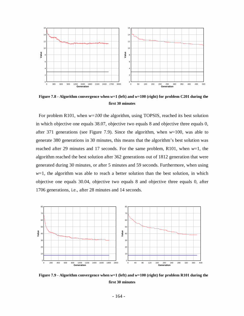
- 164 -
Generation
Valu
e
0 300 600 900 1200 1500 1800 2100 2400 2700 30000
2
4
6
8
10
12
14
16
Generation
Valu
e
0 50 100 150 200 250 300 350 400 450 5000
2
4
6
8
10
12
14
16
Figure 7.8 - Algorithm convergence when w=1 (left) and w=100 (right) for problem C201 during the
first 30 minutes
For problem R101, when w=100 the algorithm, using TOPSIS, reached its best solution
in which objective one equals 38.07, objective two equals 8 and objective three equals 0,
after 371 generations (see Figure 7.9). Since the algorithm, when w=100, was able to
generate 380 generations in 30 minutes, this means that the algorithm’s best solution was
reached after 29 minutes and 17 seconds. For the same problem, R101, when w=1, the
algorithm reached the best solution after 362 generations out of 1812 generation that were
generated during 30 minutes, or after 5 minutes and 59 seconds. Furthermore, when using
w=1, the algorithm was able to reach a better solution than the best solution, in which
objective one equals 30.04, objective two equals 8 and objective three equals 0, after
1706 generations, i.e., after 28 minutes and 14 seconds.
Generation
Valu
e
0 200 400 600 800 1000 1200 1400 1600 1800 20000
10
20
30
40
50
60
70
80
Generation
Valu
e
0 40 80 120 160 200 240 280 320 360 4000
10
20
30
40
50
60
70
80
Figure 7.9 - Algorithm convergence when w=1 (left) and w=100 (right) for problem R101 during the
first 30 minutes
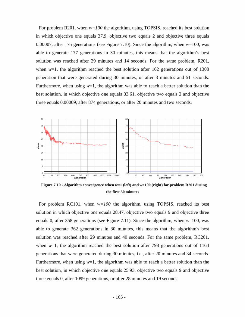
- 165 -
For problem R201, when w=100 the algorithm, using TOPSIS, reached its best solution
in which objective one equals 37.9, objective two equals 2 and objective three equals
0.00007, after 175 generations (see Figure 7.10). Since the algorithm, when w=100, was
able to generate 177 generations in 30 minutes, this means that the algorithm’s best
solution was reached after 29 minutes and 14 seconds. For the same problem, R201,
when w=1, the algorithm reached the best solution after 162 generations out of 1308
generation that were generated during 30 minutes, or after 3 minutes and 51 seconds.
Furthermore, when using w=1, the algorithm was able to reach a better solution than the
best solution, in which objective one equals 33.61, objective two equals 2 and objective
three equals 0.00009, after 874 generations, or after 20 minutes and two seconds.
Generation
Valu
e
0 150 300 450 600 750 900 1050 1200 1350 15000
8
16
24
32
40
48
56
64
Generation
Valu
e
0 20 40 60 80 100 120 140 160 180 2000
10
20
30
40
50
60
70
80
Figure 7.10 - Algorithm convergence when w=1 (left) and w=100 (right) for problem R201 during
the first 30 minutes
For problem RC101, when w=100 the algorithm, using TOPSIS, reached its best
solution in which objective one equals 28.47, objective two equals 9 and objective three
equals 0, after 358 generations (see Figure 7.11). Since the algorithm, when w=100, was
able to generate 362 generations in 30 minutes, this means that the algorithm's best
solution was reached after 29 minutes and 40 seconds. For the same problem, RC201,
when w=1, the algorithm reached the best solution after 798 generations out of 1164
generations that were generated during 30 minutes, i.e., after 20 minutes and 34 seconds.
Furthermore, when using w=1, the algorithm was able to reach a better solution than the
best solution, in which objective one equals 25.93, objective two equals 9 and objective
three equals 0, after 1099 generations, or after 28 minutes and 19 seconds.

- 166 -
Generation
Valu
e
0 150 300 450 600 750 900 1050 1200 1350 15000
10
20
30
40
50
60
70
80
Generation
Valu
e
0 40 80 120 160 200 240 280 320 360 4000
10
20
30
40
50
60
70
80
Figure 7.11 - Algorithm convergence when w=1 (left) and w=100 (right) for problem RC101 during
the first 30 minutes
For problem RC201, when w=100 the algorithm, using TOPSIS, reached its best
solution in which objective one equals 26.95, objective two equals 2 and objective three
equals 0.00002, after 343 generations (see Figure 7.12). Since the algorithm, when
w=100, was able to generate 363 generations in 30 minutes, this means that the
algorithm's best solution was reached after 28 minutes and 20 seconds. For the same
problem, RC201, when w=1, the algorithm reached the best solution after 314
generations out of 1057 generations that were generated during 30 minutes, or after 8
minutes and 54 seconds. Furthermore, when using w=1, the algorithm was able to reach a
better solution than the best solution, in which objective one equals 21.69, objective two
equals 2 and objective three equals 0, after 930 generations, i.e., after 26 minutes and 23
seconds.

- 167 -
Generation
Valu
e
0 150 300 450 600 750 900 1050 1200 1350 15000
8
16
24
32
40
48
56
64
Generation
Valu
e
0 40 80 120 160 200 240 280 320 360 4000
8
16
24
32
40
48
56
64
Figure 7.12 - Algorithm convergence when w=1 (left) and w=100 (right) for problem RC201 during
the first 30 minutes
7.3. Summary
A fitness function is a particular type of objective function that is used to summarize, as
a single figure of merit, how close a given design solution is to achieving the set aims.
In the field of evolutionary algorithms, at each iteration, the idea is to delete the n worst
design solutions, and to breed n new ones from the best design solutions. Each design
solution, therefore, needs to be awarded a figure of merit, to indicate how close it came to
meeting the overall specification, and this is generated by applying the fitness function to
the test, or simulation, results obtained from that solution.
In some cases, fitness approximation may be appropriate, especially if (1) the fitness
computation time of a single solution is extremely high, (2) a precise model for fitness
computation is missing or (3) the fitness function is uncertain or noisy.
In all three algorithms presented, the fitnesses of all five objective functions have to be
calculated. Due to the stochastic nature of travel time, in order to get an accurate value, or
accurate fitness functions, simulation has to be used. Simulation is a time consuming
process.
It was shown that it is possible to increase the running time of the algorithm by using an
"approximated" fitness function, without influencing the accuracy of the algorithm. A fast
algorithm is necessary when coping with real-time problems, which is the final goal of
this study.

- 168 -
Usually, when solving a multi-objective optimization problem, the result is a set of non-
dominated solutions, from which the decision maker has to choose his preferred
alternative. Since the final goal is to create an automated algorithm for solving a real-time
multi-objective vehicle routing problem, the TOPSIS method, a mechanism for choosing
a preferred solution from a set of non-dominated solutions, has been implemented. It was
shown that there is no difference in the quality of the results obtained using the
"approximated" or "accurate" methods, but this does not mean that the same results exist
in both sets, and therefore it is not guaranteed that the TOPSIS method selects similar
results from both sets. It was shown, by means of correlation testing and paired-samples
t-tests, that the solutions selected by the TOPSIS methods are similar regardless of the
method used for calculating the fitness functions.
Since travel time is more likely to be lognormally distributed, a second set of tests was
done, using Solomon’s instances. Using 500 generations and a population of 200
chromosomes, the result of the improved VEGA algorithm showed that for problems with
a large number of chromosomes (50 and 100 customers) using w=100 results was a better
solution than when using w=1, while for problems with a small number of customers (25
and 50), no significant difference was found. Since it is known that the number of
generations used by a genetic algorithm may affect its results, and since in real-time
applications, the number of generations is bounded by the time given to the algorithm to
come up with a solution, the algorithm was tested again, this time when the stopping
condition was 30 minutes of running time, instead of the 500 generations. In all cases, the
result obtained by the algorithm when w=1 are better than the results obtained when
w=100. Furthermore, when w=1, the algorithm converges to the best solution much faster
than when w=100.

- 169 -
8. Setting Wait Time Parameter The first objective function considered in chapter 3.3.1 is minimizing the total travel
time, and is defined as
1
0 0 1 0
0 0 1
min max ' , ' ' '
max ,
S
S
tN N Mt S mtij j j j ij
i j m t
N N M Tt S mtij j j j ij
i j m t t
Z C TW t ST WT x
C TW t ST WT x (8.1)
where the total traveling time is composed from two parts, (1) the known traveling time,1
0 0 1 0max ' , ' ' '
StN N Mt S mtij j j j ij
i j m tC TW t ST WT x , and (2) the unknown traveling time,
0 0 1
max ,S
N N M Tt S mtij j j j ij
i j m t t
C TW t ST WT x .
If by leaving node i at time t a vehicle reaches node j before its time window's start time
(meaning t Sij jt C TW , where ijC is the traveling time for traveling from node i to node
j and SjTW customer j's time window's start time), then the vehicle has to wait until the
beginning of the time window in order to start serving. Otherwise, it starts serving when
it arrives. The time between the time the vehicle left node i towards node j, denoted as t,
and the time it starts serving node j can be formulated as max ,t Sij jC TW t . If node j is a
customer, then both service time at customer j, jST , and waiting time at customer j, jWT ,
have to be added to the traveling time. But if node j is the depot, then both service time,
jST , and waiting time, jWT , are equal to 0. Therefore, the time passed since a vehicle left
node i towards node j and the time it left node j can be defined as
max ,t Sij j j jC TW t ST WT .
For each edge , : , ,e E i j i j V i j , there exists a decision variable mtijx ,
defined as 1 if edge e was traveled at time t by vehicle m, and otherwise it is defined as 0.

- 170 -
Multiplying the above notation, max ,t Sij j j jC TW t ST WT , by the decision variable
mtijx , gives us the time passed since vehicle m left node i towards node j at time t and the
time it left node j, if such a vehicle exists, otherwise it is 0.
Let’s refer to the time passed since vehicle m left node i towards node j at time t and the
time it left node j multiplied by the decision variable,
max ,t S mtij j j j ijC TW t ST WT x , as the true travel time from node i to node j. By
summing all possible true travel times,0 0 1 0
max ,N N M T
t S mtij j j j ij
i j m t
C TW t ST WT x ,
we get the total travel time, which we want to minimize.
The total travel time can be decomposed into two parts, the known travel time and the
unknown travel time. If the planning time, st , is not equal to 0, then we are not at the
beginning of the day, and some vehicles have already been sent to customers. In this case,
information regarding traveled edges, travel costs, service time and waiting time is
already known for every edge traveled and for every customer visited before st .
Let 'tijC donate the known cost from traveling from node i to node j at time t, where
st t . Similarly, let 'mtijx denote the known decision variable, defined as 1 if vehicle m
traveled from node i to node j at time t. where st t , and 0, otherwise. The known
traveled cost can be defined as1
0 0 1 0max ' , ' ' '
StN N Mt S mtij j j j ij
i j m tC TW t ST WT x .
The unknown traveling cost can be defined as
0 0 1
max ,S
N N M Tt S mtij j j j ij
i j m t t
C TW t ST WT x , therefore, the total traveling cost is the
sum of the known traveling cost and the unknown traveling cost,1
0 0 1 0
0 0 1
max ' , ' ' '
max ,
S
S
tN N Mt S mtij j j j ij
i j m t
N N M Tt S mtij j j j ij
i j m t t
C TW t ST WT x
C TW t ST WT x
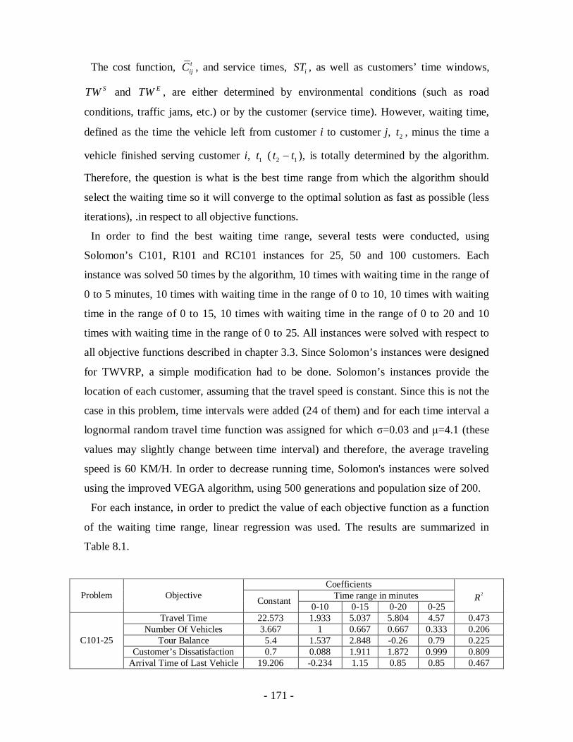
- 171 -
The cost function, tijC , and service times, iST , as well as customers’ time windows,
STW and ETW , are either determined by environmental conditions (such as road
conditions, traffic jams, etc.) or by the customer (service time). However, waiting time,
defined as the time the vehicle left from customer i to customer j, 2t , minus the time a
vehicle finished serving customer i, 1t ( 2 1t t ), is totally determined by the algorithm.
Therefore, the question is what is the best time range from which the algorithm should
select the waiting time so it will converge to the optimal solution as fast as possible (less
iterations), .in respect to all objective functions.
In order to find the best waiting time range, several tests were conducted, using
Solomon’s C101, R101 and RC101 instances for 25, 50 and 100 customers. Each
instance was solved 50 times by the algorithm, 10 times with waiting time in the range of
0 to 5 minutes, 10 times with waiting time in the range of 0 to 10, 10 times with waiting
time in the range of 0 to 15, 10 times with waiting time in the range of 0 to 20 and 10
times with waiting time in the range of 0 to 25. All instances were solved with respect to
all objective functions described in chapter 3.3. Since Solomon’s instances were designed
for TWVRP, a simple modification had to be done. Solomon’s instances provide the
location of each customer, assuming that the travel speed is constant. Since this is not the
case in this problem, time intervals were added (24 of them) and for each time interval a
lognormal random travel time function was assigned for which =0.03 and =4.1 (these
values may slightly change between time interval) and therefore, the average traveling
speed is 60 KM/H. In order to decrease running time, Solomon's instances were solved
using the improved VEGA algorithm, using 500 generations and population size of 200.
For each instance, in order to predict the value of each objective function as a function
of the waiting time range, linear regression was used. The results are summarized in
Table 8.1.
CoefficientsTime range in minutesProblem Objective Constant 0-10 0-15 0-20 0-25
2R
Travel Time 22.573 1.933 5.037 5.804 4.57 0.473Number Of Vehicles 3.667 1 0.667 0.667 0.333 0.206
Tour Balance 5.4 1.537 2.848 -0.26 0.79 0.225Customer’s Dissatisfaction 0.7 0.088 1.911 1.872 0.999 0.809
C101-25
Arrival Time of Last Vehicle 19.206 -0.234 1.15 0.85 0.85 0.467

- 172 -
CoefficientsTime range in minutesProblem Objective Constant 0-10 0-15 0-20 0-25
2R
Travel Time 10.664 1.734 1.228 3.993 4.273 0.711Number Of Vehicles 8.333 -1 -1.333 0 0 0.183
Tour Balance 0.386 0.179 0.348 -0.123 0.093 0.149Customer’s Dissatisfaction 1.471 0.334 0.752 1.475 0.702 0.507
R101-25
Arrival Time of Last Vehicle 10.711 0.261 0.528 0.795 0.584 0.371Travel Time 11.633 -0.267 3.227 3.473 6.366 0.933
Number Of Vehicles 7 -2.333 -1.667 0.667 1 0.718Tour Balance 0.512 2.577 -0.157 -0.131 -0.096 0.328
Customer’s Dissatisfaction 0.982 -0.343 1.072 1.201 1.156 0.609RC101-25
Arrival Time of Last Vehicle 10.933 1.289 0.489 1.033 0.639 0.178Travel Time 52.256 2.26 11.049 17.622 14.061 0.474
Number Of Vehicles 7.667 0.333 3.333 4 1 0.3Tour Balance 6.814 -4.465 -4.349 -5.079 -2.461 0.363
Customer’s Dissatisfaction 4.599 9.201 4.373 6.423 4.491 0.33C101-50
Arrival Time of Last Vehicle 19.6 2.806 2.461 2.744 3.322 0.761Travel Time 29.101 0.799 9.831 8.339 13.843 0.777
Number Of Vehicles 21 -1.667 6 2.333 4.667 0.515Tour Balance 0.094 0.028 -0.005 0.03 0.022 0.159
Customer’s Dissatisfaction 2.376 0.495 0.515 0.813 1.699 0.316R101-50
Arrival Time of Last Vehicle 10.65 0.245 0.439 0.45 0.672 0.402Travel Time 36.339 -0.301 2.265 6.928 12.679 0.714
Number Of Vehicles 26.667 -4333 -3.667 -1 -1 0.233Tour Balance 0.076 0.045 0.054 0.064 0.027 0.497
Customer’s Dissatisfaction 1.191 0.9 1.181 2.09 1.703 0.533RC101-50
Arrival Time of Last Vehicle 10.861 0.578 0.489 0.678 0.861 0.592Travel Time 328.573 39.44 14.238 65.881 37.271 0.762
Number Of Vehicles 67.333 6.333 -1.333 6.667 1 0.674Tour Balance 0.147 -0.067 -0.053 -0.068 0.073 0.584
Customer’s Dissatisfaction 3.552 -0.266 1.659 0.734 1.117 0.226C101-100
Arrival Time of Last Vehicle 20.8 -0.317 1.205 0.577 -0.095 0.363Travel Time 120.922 10.309 18.671 29.994 40.312 0.903
Number Of Vehicles 94 1 -0.667 0 0.333 0.027Tour Balance 0.015 0.002 0.003 0.006 0.007 0.612
Customer’s Dissatisfaction 0.018 0.213 0.881 1.529 2.355 0.976R101-100
Arrival Time of Last Vehicle 10.239 0.134 0.317 0.517 0.995 0.9Travel Time 119.993 -5.981 24.803 25.344 40.512 0.967
Number Of Vehicles 93.333 -11.333 1 -2.667 0 0.629Tour Balance 0.016 0.008 -0.001 0.002 0.004 0.343
Customer’s Dissatisfaction 0.064 0.306 -0.037 0.23 0.473 0.706RC101-100
Arrival Time of Last Vehicle 10.222 0.411 0.25 0.406 0.844 0.911
Table 8.1 – Linear regression results
Based on the results of the linear regression the expected value of each objective for
every instance was calculated for the different waiting time ranges. The results are
summarized in Table 8.2.
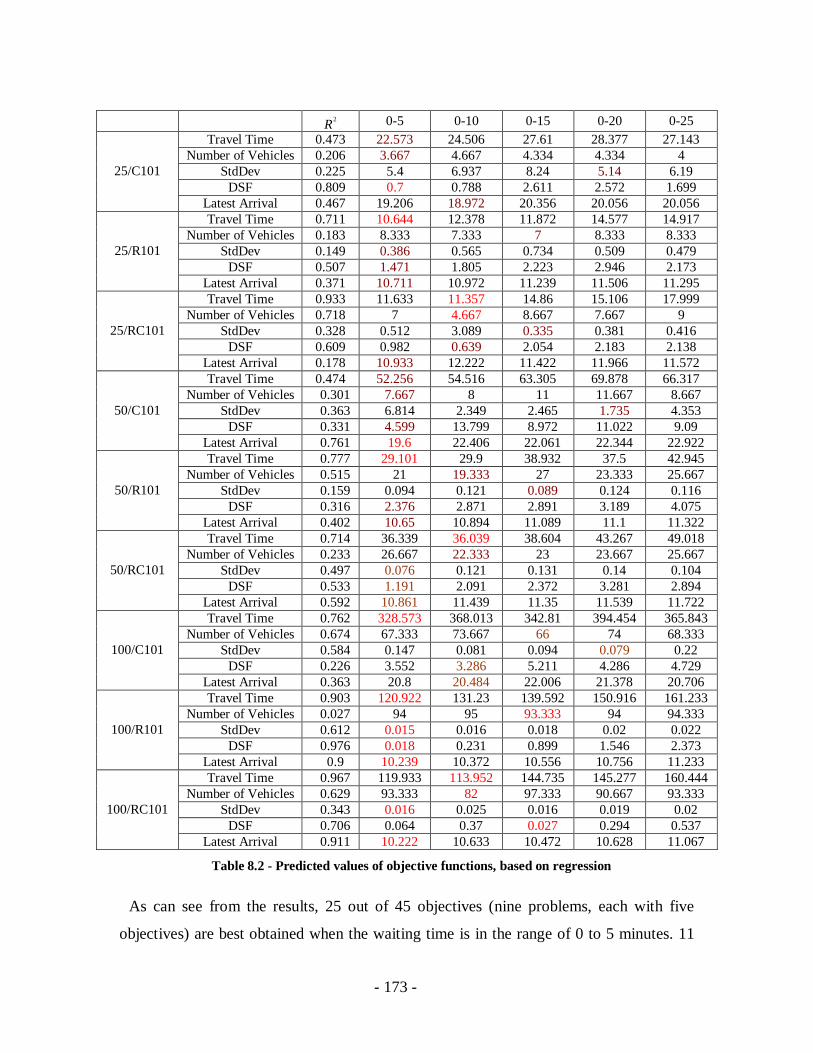
- 173 -
2R 0-5 0-10 0-15 0-20 0-25Travel Time 0.473 22.573 24.506 27.61 28.377 27.143
Number of Vehicles 0.206 3.667 4.667 4.334 4.334 4StdDev 0.225 5.4 6.937 8.24 5.14 6.19
DSF 0.809 0.7 0.788 2.611 2.572 1.69925/C101
Latest Arrival 0.467 19.206 18.972 20.356 20.056 20.056Travel Time 0.711 10.644 12.378 11.872 14.577 14.917
Number of Vehicles 0.183 8.333 7.333 7 8.333 8.333StdDev 0.149 0.386 0.565 0.734 0.509 0.479
DSF 0.507 1.471 1.805 2.223 2.946 2.17325/R101
Latest Arrival 0.371 10.711 10.972 11.239 11.506 11.295Travel Time 0.933 11.633 11.357 14.86 15.106 17.999
Number of Vehicles 0.718 7 4.667 8.667 7.667 9StdDev 0.328 0.512 3.089 0.335 0.381 0.416
DSF 0.609 0.982 0.639 2.054 2.183 2.13825/RC101
Latest Arrival 0.178 10.933 12.222 11.422 11.966 11.572Travel Time 0.474 52.256 54.516 63.305 69.878 66.317
Number of Vehicles 0.301 7.667 8 11 11.667 8.667StdDev 0.363 6.814 2.349 2.465 1.735 4.353
DSF 0.331 4.599 13.799 8.972 11.022 9.0950/C101
Latest Arrival 0.761 19.6 22.406 22.061 22.344 22.922Travel Time 0.777 29.101 29.9 38.932 37.5 42.945
Number of Vehicles 0.515 21 19.333 27 23.333 25.667StdDev 0.159 0.094 0.121 0.089 0.124 0.116
DSF 0.316 2.376 2.871 2.891 3.189 4.07550/R101
Latest Arrival 0.402 10.65 10.894 11.089 11.1 11.322Travel Time 0.714 36.339 36.039 38.604 43.267 49.018
Number of Vehicles 0.233 26.667 22.333 23 23.667 25.667StdDev 0.497 0.076 0.121 0.131 0.14 0.104
DSF 0.533 1.191 2.091 2.372 3.281 2.89450/RC101
Latest Arrival 0.592 10.861 11.439 11.35 11.539 11.722Travel Time 0.762 328.573 368.013 342.81 394.454 365.843
Number of Vehicles 0.674 67.333 73.667 66 74 68.333StdDev 0.584 0.147 0.081 0.094 0.079 0.22
DSF 0.226 3.552 3.286 5.211 4.286 4.729100/C101
Latest Arrival 0.363 20.8 20.484 22.006 21.378 20.706Travel Time 0.903 120.922 131.23 139.592 150.916 161.233
Number of Vehicles 0.027 94 95 93.333 94 94.333StdDev 0.612 0.015 0.016 0.018 0.02 0.022
DSF 0.976 0.018 0.231 0.899 1.546 2.373100/R101
Latest Arrival 0.9 10.239 10.372 10.556 10.756 11.233Travel Time 0.967 119.933 113.952 144.735 145.277 160.444
Number of Vehicles 0.629 93.333 82 97.333 90.667 93.333StdDev 0.343 0.016 0.025 0.016 0.019 0.02
DSF 0.706 0.064 0.37 0.027 0.294 0.537100/RC101
Latest Arrival 0.911 10.222 10.633 10.472 10.628 11.067
Table 8.2 - Predicted values of objective functions, based on regression
As can see from the results, 25 out of 45 objectives (nine problems, each with five
objectives) are best obtained when the waiting time is in the range of 0 to 5 minutes. 11

- 174 -
out of 45 objectives are best obtained when the waiting time is in the range of 0 to 10
minutes. 6 out of 45 objectives are best obtained when the waiting time is in the range of
0 to 15 minutes. 3 out of 45 objectives are best obtained when the waiting time is in the
range of 0 to 20 minutes. None of the objectives are best obtained when the waiting time
is in the range of 0 to 25 minutes. However, half of functions found by the linear
regression (23 out of 45), have an R2 value lower than 0.75. This means that the value of
half of the objective functions calculated based on the functions found by the regression,
are probably not close to the true value expected.
As a result, averages comparison was done and used as well. The results are
summarized in Table 8.3.
0-5 0-10 0-15 0-20 0-25Travel Time 22.573 24.506 27.611 28.378 27.144
Number of Vehicles 3.667 4.667 4.333 4.333 4.000StdDev 5.400 6.936 8.248 5.140 6.189
DSF 0.700 0.787 2.610 2.571 1.69825/C101
Latest Arrival 19.206 18.972 20.355 20.055 20.056Travel Time 10.644 12.378 11.872 14.577 14.917
Number of Vehicles 8.333 7.333 7.000 8.333 8.333StdDev 0.386 0.565 0.733 0.509 0.479
DSF 1.471 1.804 2.223 2.946 2.17325/R101
Latest Arrival 10.711 10.972 11.239 11.506 11.295Travel Time 11.633 11.366 14.860 15.106 17.999
Number of Vehicles 7.000 4.667 8.667 7.667 9.000StdDev 0.512 3.089 0.355 0.381 0.416
DSF 0.982 0.639 2.053 2.183 2.13825/RC101
Latest Arrival 10.933 12.222 11.422 11.967 11.572Travel Time 52.256 54.516 63.305 69.877 66.317
Number of Vehicles 7.667 8.000 11.000 11.667 8.667StdDev 6.814 2.349 2.465 1.735 4.353
DSF 4.599 13.799 8.972 11.022 9.09050/C101
Latest Arrival 19.600 22.406 22.061 22.344 22.922Travel Time 29.101 29.900 38.932 37.500 42.945
Number of Vehicles 21.000 19.333 27.000 23.333 25.667StdDev 0.094 0.121 0.089 0.124 0.116
DSF 2.376 2.871 2.891 3.189 4.07550/R101
Latest Arrival 10.650 10.894 11.089 11.100 11.322Travel Time 36.339 36.039 38.604 43.267 49.018
Number of Vehicles 26.667 22.333 23.000 23.667 25.667StdDev 0.076 0.121 0.131 0.140 0.104
DSF 1.191 2.091 2.372 3.281 2.89450/RC101
Latest Arrival 10.861 11.439 11.350 11.539 11.722Travel Time 328.573 368.013 342.810 394.454 365.843
Number of Vehicles 67.333 73.667 66.000 74.000 68.333StdDev 0.147 0.081 0.094 0.079 0.220
100/C101
DSF 3.552 3.286 5.211 4.286 4.729

- 175 -
0-5 0-10 0-15 0-20 0-25Latest Arrival 20.800 20.484 22.006 21.378 20.706Travel Time 120.922 131.230 139.592 150.916 161.233
Number of Vehicles 94.000 95.000 93.333 94.000 94.333StdDev 0.015 0.016 0.018 0.020 0.022
DSF 0.018 0.231 0.899 1.546 2.373100/R101
Latest Arrival 10.239 10.372 10.556 10.756 11.233Travel Time 119.933 113.952 144.735 145.277 160.444
Number of Vehicles 93.333 82.000 97.333 90.667 93.333StdDev 0.016 0.025 0.016 0.019 0.020
DSF 0.064 0.370 0.027 0.294 0.537100/RC101
Latest Arrival 10.222 10.633 10.472 10.628 11.067
Table 8.3 – Average values of objective functions, based on experiments
The results are similar to the results obtained by using the functions found by the linear
regression. 25 out of 45 objectives (nine problems, each with five objectives) are best
obtained when the waiting time is in the range of 0 to 5 minutes. 11 out of 45 objectives
are best obtained when the waiting time is in the range of 0 to 10 minutes. 6 out of 45
objectives are best obtained when the waiting time is in the range of 0 to 15 minutes. 3
out of 45 objectives are best obtained when the waiting time is in the range of 0 to 20
minutes. None of the objectives are best obtained when the waiting time is in the range of
0 to 25 minutes.
When comparing averages, statistical tests usually have to be done in order to verify
that there is a difference between two populations. In this case, such tests were not
conducted for the following reasons:
1. Assuming that there is a difference between two populations. In this case, it is
obvious that the population with the lower average value is better (assuming
minimization).
2. On the other hand, if there is no difference between the two populations, then there is
no advantage or disadvantage in choosing the population with the lower average.
It can therefore be concluded that in all cases, it is possible , to choose the population
whose results have a lower average value.
8.1. Summary
This chapter deals with the waiting time parameter. Waiting time is the time a vehicle
waits after it has finished serving a customer before it starts driving to the next customer.
Service time is determined by the algorithm, and can be any value in a pre-determined
- 176 -
range. Therefore, the question is, What is the best time range from which the algorithm
should select the waiting time so it will converge to the optimal solution as fast as
possible (less iterations), with respect to all objective functions?
In order to find the best waiting time range, a set of tests was done using Solomon’s
C101, R101 and RC101 instances for 25, 50 and 100 customers, each solved 10 times.
Based on the results of the test instances, for each instance, in order to predict the value
of each objective function as a function of the waiting time range, linear regression was
used. The results of the linear regression showed that in more than half of the cases, the
best results were obtained when the waiting time range was between 0 and 5 minutes.
However, half of functions found by the linear regression (23 out of 45), have a value of
R2 < 0.75. This means that the value of half of the objective functions calculated based on
the functions found by the regression, are probably not close to the true value expected,
so therefore, a comparison of averages was conducted and used as well.
The results of the averages comparison were similar to the results obtained by using the
functions found by the linear regression. More than half of the objectives (25 out of 45)
are best obtained when the waiting time is in the range of 0 to 5 minutes.
Based on the results obtained using linear regression and the results obtained using
comparison of averages, it is best to use a waiting time within the range of 0 to 5 minutes.
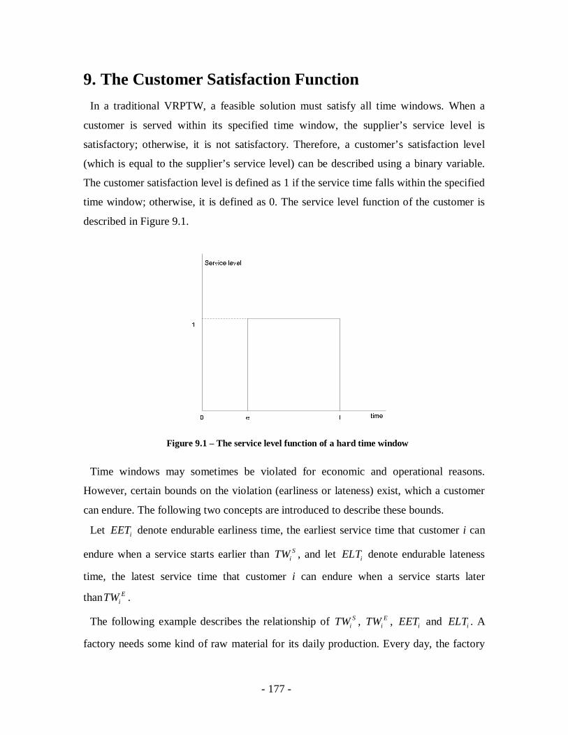
- 177 -
9. The Customer Satisfaction FunctionIn a traditional VRPTW, a feasible solution must satisfy all time windows. When a
customer is served within its specified time window, the supplier’s service level is
satisfactory; otherwise, it is not satisfactory. Therefore, a customer’s satisfaction level
(which is equal to the supplier’s service level) can be described using a binary variable.
The customer satisfaction level is defined as 1 if the service time falls within the specified
time window; otherwise, it is defined as 0. The service level function of the customer is
described in Figure 9.1.
Figure 9.1 – The service level function of a hard time window
Time windows may sometimes be violated for economic and operational reasons.
However, certain bounds on the violation (earliness or lateness) exist, which a customer
can endure. The following two concepts are introduced to describe these bounds.
Let iEET denote endurable earliness time, the earliest service time that customer i can
endure when a service starts earlier than SiTW , and let iELT denote endurable lateness
time, the latest service time that customer i can endure when a service starts later
than EiTW .
The following example describes the relationship of SiTW , E
iTW , iEET and iELT . A
factory needs some kind of raw material for its daily production. Every day, the factory

- 178 -
opens at 8:00 and production starts at 10:00. The raw material is sent from an upstream
supplier and the process of unloading the raw material requires 30 minutes. The factory
specifies its preferred delivery time window to be [8:30, 9:00], because materials
delivered within that time window can be directly moved to the workshop without any
tardiness. However, the factory is not operating in a just-in-time mode; the delivery can
be a little earlier or later than the specified time window. A reasonable combination of
EET and ELT could be [8:00, 9:30]. If the materials are delivered within [8:00, 8:30],
instead of being moved directly into the workshop, they must be stored in the warehouse
because of limited space in the workshop. Of course, this is not what the manager of the
factory wishes to see, but it is acceptable. If the materials are delivered within [9:00,
9:30], no inventories have to be held; however, this requires that the execution of the
production plan will have a higher accuracy, which will reduce the robustness of the
production operations in the factory. Since the factory opens at 8:00, deliveries before
8:00 must wait outside the factory. When production procedure starts at 10:00, delivery
after 9:30 is totally unacceptable because of the 30-minutes unloading process. Simply
put, although the manager of the factory will be happiest to be served within [8:30, 9:00],
the manager will also be reasonably satisfied if served within [8:00, 8:30] or [9:00, 9:30];
however, the result of this is that the customer’s satisfaction declines, and deliveries made
before 8:00 or after 9:30 are not acceptable. Similar scenarios also appear in dial-a-ride
problems.
Figure 9.2 – The service level function of fuzzy time windows

- 179 -
As discussed, the service may start outside the time window ,S Ei iTW TW , and the
bounds of acceptable earliness and lateness are described by iEET and iELT ,
respectively. Obviously, the earliness and lateness are highly related to the quality of the
supplier's service. The customer's level of satisfaction response to a given service time
will no longer simply be “good” or “bad”; but between “good” and “bad”. For example,
the customer may say, “it’s alright” to be served within , Si iEET TW or ,E
i iTW ELT .
In either case, the service level cannot be described only by two states (0 or 1).
For problems involving personal human emotions, fuzzy set theory is a strong tool.
Intuitively, with the concepts of iEET and iELT , the supplier’s service level for each
customer can be described by a fuzzy membership function:
1,(
0,,
),0,
Si
S Ei i
i
ii
Ei i
i
i
i
t TW
T
t EET
EETfW t TW
g t TW t ELTEL
tS t
T t
(8.2)
when in most recent research, if t is defined as
ii S
i i
t EETf tTW EET
(8.3)
and ig t is defined as
( ) ii E
i i
ELT tg tELT TW
(8.4)
However, since customer’s satisfaction level, as a function of the deviation from the
customer’s time window, usually cannot be described as a linear function, the following
function, which better describes customer's satisfaction, is used.

- 180 -
1
1
ini
Sj i i
i n
j
ji
ji
t EETTW EET
f t (8.5)
1
1
( )
im
Ej i
i
ji
ji
m
j
ELT tELT TW
g t (8.6)
Assuming that each customer has his/her own satisfaction function, iS t , and that the
service provider assigns as an importance factor, i , to each customer that states how
important it is to satisfy customer i compared to all other customers, the maximizing
customers’ satisfaction objective can be described as
1
0 0 1 0min
S
S
mt mti ji ji
tn N M Tt t
i ji iji j m t t t
Z S t C tx xC (8.7)
As stated before, customer satisfaction or dissatisfaction (which is equal to one minus
satisfaction value) involves personal human emotions. The satisfaction function may be
decomposed to several functions; each focusing on a different factor which influences the
overall satisfaction. For example, if a supplier is late and workers have to stay after their
regular working hours, one function may consider physiological aspects, such as the
dissatisfaction due to workers' loss of family time. Another function may consider
financial aspects, such as workers' overtime salary. While there might be several
satisfaction (or dissatisfaction) functions, in this study, one satisfaction function is
considered, which includes all satisfaction aspects as perceived by the customers.
In order to get an impression of the possible values of and , 38 customers (people),
were asked, using questionnaires, about their general satisfaction value when a supplier
or other service provider arrives earlier than expected, between 30 minutes to four hours,
with 30 minute intervals. Similarly, they were asked for their general satisfaction value
- 181 -
when a supplier or other service provider arrives later than expected, from 30 minutes to
four hours, with 30 minute intervals.
Based on the results of the questionnaires, the following analysis was conducted for
each customer.
1. Each customer is assigned to a satisfaction function, using curve fitting. CenterSpace
Software’s NMath numerical library provides object-oriented components for
mathematical, engineering, scientific, and financial applications on the .NET
platform. One of the components provided by CenterSpace Software’s NMath
numerical library is the PolynomialLeastSquares class, which performs a least
squares fit of a Polynomial to a set of points. The data provided by each customer was
used as an input to the PolynomialLeastSquares, which was used to calculate five
degree polynomial curve fitting functions (for both earliness and lateness).
2. For each customer, using the five degree polynomials computed, the values of 400
sample points were collected. These sample points represent the satisfaction value of
the customer for supplier earliness and lateness, from 0 minutes up to 4 hours, with
0.01 minutes time interval.
3. Since the functions obtained are not presented in the form of the functions described
in (8.5) and (8.6), , the least squares method is used in order to find a function in the
form of (8.5) and (8.6) for each customer, which best approximates the customer’s
satisfaction functions. In order to approximate the customer's satisfaction functions,
each sample point was evaluated using the 4 / 4t satisfaction function, with
various values of , starting with (-1000) and ending with 1000, with an interval of
0.1. The value of each sample point obtained from the satisfaction function is
subtracted from the value obtained from the five degree polynomial. The difference
value is then squared, and all the squared values are summed. The value of is
chosen so that the sum of all squared differences is minimal.
The functions calculated for all 38 customers based on the questionnaires are presented
in Figure 9.3 and Figure 9.4.

- 182 -

- 183 -

- 184 -
Figure 9.3 – Various satisfaction functions for supplier earliness
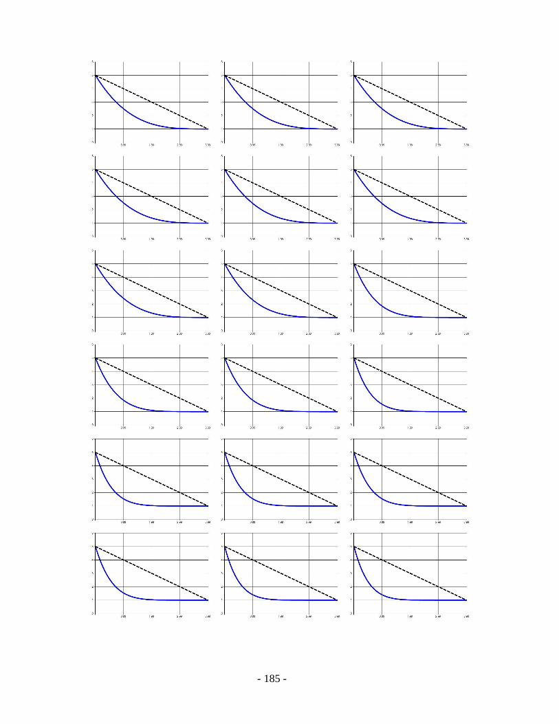
- 185 -

- 186 -
Figure 9.4 – Various satisfaction functions for supplier lateness
The results can be summarized as follows:
1. For earliness, 6 out of the 38 customers feel indifferent to the supplier being early.
This means that although the supplier arrives much earlier than expected, the
customer's satisfaction is minimally influenced.
2. For earliness, for 6 out of the 38 customers, the customer's satisfaction correlates
linearly with the supplier being early.
3. For earliness, 18 out of the 38 customers are sensitive to the supplier being early. This
means that their satisfaction level declines dramatically when the supplier arrives
earlier than expected.

- 187 -
4. For lateness, for 1 out of the 38 customers, the customer's satisfaction changed
linearly, and correlates with the supplier being late.
5. For lateness, 34 out of the 38 customers are sensitive to the supplier being late. This
means that their satisfaction level declines dramatically when the supplier arrives
later than expected.
9.1. Summary
In a traditional VRPTW, a feasible solution must satisfy all time windows. When a
customer is served within his/her specified time window, the supplier’s service level is
satisfactory or equal to 1; otherwise, the service is not satisfactory or equal to 0. Time
windows may sometimes be violated for economic and operational reasons. However,
certain bounds exist on the violation (earliness or lateness) that a customer can endure.
Obviously, the earliness and lateness are closely related to the supplier service level, and
therefore, the service level cannot be described by only two states (0 or 1).
To get an impression of how the service level, known as customer's satisfaction,
changes as a function of bounds on the violation (earliness or lateness), 38 customers,
using questionnaires, were asked for their overall satisfaction value when a supplier or
other service provider arrives within 30 minutes to four hours, with 30 minutes intervals,
earlier than expected. Similarly, they were asked for their overall satisfaction value when
a supplier or other service provider arrives 30 minutes to four hours, in 30 minutes
intervals, later than expected.
Each customer, based on the results of his questionnaire, was assigned a satisfaction
function. From these functions, it can be concluded that most customers are sensitive to
suppliers being either early or late, and their satisfaction level declines dramatically when
the supplier arrives earlier/later than expected.
- 188 -
10. Case StudyIn previous chapters, the vehicle routing problem has been described and various
algorithms based on exact methods; heuristics and meta-heuristics have been reviewed.
The real-time multi-objective vehicle routing problem has been described and formulated,
and three evolutionary algorithms for solving it were also presented. Various tests using
randomly generated networks were done on the three algorithms, mainly for calibration
purposes. These tests showed that each of the three algorithms when applied on a
randomly generated network converge towards a better solution.
The goal of this chapter is to compare the results of the three algorithms using a case
study. The case study is based on two networks that are based on a real-world
transportation network, including the locations of the depot, the customers and
information about travel time between the different customers. The case study is
performed using simulation.
10.1. Network
Two transportation networks, each based on real-file information, each with different
characteristics, were generated. Both networks are based on Israel’s road network.
The first network is based on the greater Tel-Aviv metropolitan area’s urban road
network. In this network, there are 45 customers (not including the depot).
“Mega Ba’ir” (Mega in the city) is a super-market chain store, with more than 80
branches (as reported in their Internet site). In order to make the network as realistic as
possible, the locations of each one of the 45 customers were chosen according to the
locations of the stores throughout the greater Tel-Aviv metropolitan area. Using “Google
Maps”, the shortest distance (based on actual network) between every two customers was
found.
Next, for each edge in the network, the traveling time for different times of the day was
collected (see 10.1.1).
Each customer is also associated with a time window. The time windows are randomly
generated, and are based on the following assumptions:
- 189 -
1. The minimum possible time window start time, PSTW, is equal to 8:00 am plus the
travel time it takes to get from the depot to the customer (when leaving the depot at
8:00 am), assuming that the distance from the depot to the customer is known, and the
travel speed is 15 kilometers per hour.
2. The time window start time, STW, is based on the possible time windows start time,
and is a random value within the range of PSTW to PSTW+1.5 (plus one and a half
hour).
3. The time window end time, ETW, is based on the time windows start time, and is a
random value within the range of STW+0.5 to STW+3.
Each customer is also associated with a randomly generated demand, in the range of 10
to 50, similar to the demands used in Solomon's instances.
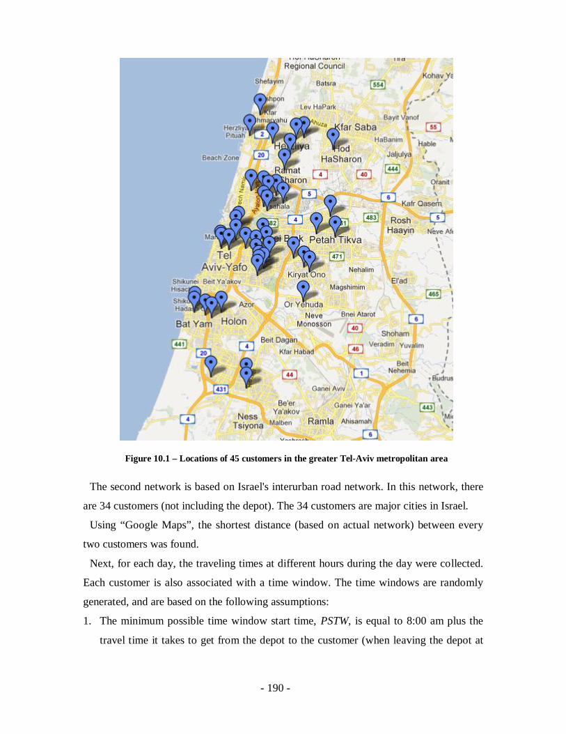
- 190 -
Figure 10.1 – Locations of 45 customers in the greater Tel-Aviv metropolitan area
The second network is based on Israel's interurban road network. In this network, there
are 34 customers (not including the depot). The 34 customers are major cities in Israel.
Using “Google Maps”, the shortest distance (based on actual network) between every
two customers was found.
Next, for each day, the traveling times at different hours during the day were collected.
Each customer is also associated with a time window. The time windows are randomly
generated, and are based on the following assumptions:
1. The minimum possible time window start time, PSTW, is equal to 8:00 am plus the
travel time it takes to get from the depot to the customer (when leaving the depot at

- 191 -
8:00 am), assuming that the distance from the depot to the customer is known, and the
travel speed is 70 kilometers per hour.
2. The time window start time, STW, is based on the possible time windows start time,
and is a random value within the range of PSTW to PSTW+1.5 (plus one and a half
hour).
3. The time window end time, ETW, is based on the time windows start time, and is a
random value within the range of STW+0.5 to STW+3.
Each customer is also associated with a randomly generated demand, in the range of 10
to 50, once again, similar to the demands used in Solomon's instances.

- 192 -
Figure 10.2 - Locations of 39 customers in Israel
In each test problem, half of the customers are considered as customers with unknown
demands. The customers who are considered as customers with unknown demands are
the customers with the latest time window start time. Each unknown demand is revealed
to the simulation at least two hours before the beginning of the time window.

- 193 -
10.1.1. Collecting Real-World Travel Time Information
The main problem in building a real-world network is knowing how travel time changes
during the day for each of the edges in the network. In recent years, "Google" started
providing real-time traffic information in their "Google Maps" service.
Figure 10.3 – "Google Maps" with real-time traffic information
When querying "Google Map" service for a route between two locations, it now
provides several possible routes, for each of which it provides its length, its average
travel time and its travel time in current traffic conditions. Based on this information, it is
possible to calculate the travel speed for each route based on its length and travel time.

- 194 -
Figure 10.4 – "Google Maps" with shortest route between two points
In order to collect travel time information using Google maps service, a small
application has been written. This application works as follows:
1. A text file containing a list of routes is read by the application.
2. In turn each route queries “Google maps” service.
3. The result of each query is then analyzed, and the information is saved (time of day,
travel time and speed).
4. After all routes have been queried, the process starts from the beginning (stage 2).
Figure 10.5 – "Google Maps" with route travel time information
It was noticed that when querying "Google Map" service for a route between two
locations, at different times of the day, “Google Maps” may sometimes provide two or
more different routes. This happens because “Google Maps" considers traffic conditions
when calculating and suggesting a route. This behavior is problematic when collecting
data for statistical analysis. To avoid this problem, mid-points were used. Mid-points are
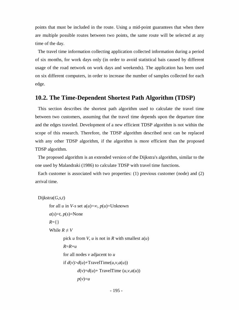
- 195 -
points that must be included in the route. Using a mid-point guarantees that when there
are multiple possible routes between two points, the same route will be selected at any
time of the day.
The travel time information collecting application collected information during a period
of six months, for work days only (in order to avoid statistical bais caused by different
usage of the road network on work days and weekends). The application has been used
on six different computers, in order to increase the number of samples collected for each
edge.
10.2. The Time-Dependent Shortest Path Algorithm (TDSP)
This section describes the shortest path algorithm used to calculate the travel time
between two customers, assuming that the travel time depends upon the departure time
and the edges traveled. Development of a new efficient TDSP algorithm is not within the
scope of this research. Therefore, the TDSP algorithm described next can be replaced
with any other TDSP algorithm, if the algorithm is more efficient than the proposed
TDSP algorithm.
The proposed algorithm is an extended version of the Dijkstra's algorithm, similar to the
one used by Malandraki (1986) to calculate TDSP with travel time functions.
Each customer is associated with two properties: (1) previous customer (node) and (2)
arrival time.
Dijkstra(G,s,t)
for all u in V-s set a(u)= , p(u)=Unknown
a(s)=t, p(s)=None
R={}
While R V
pick u from V, u is not in R with smallest a(u)
R=R+u
for all nodes v adjacent to u
if d(v)>d(u)+TravelTime(u,v,a(u))
d(v)=d(u)+ TravelTime (u,v,a(u))
p(v)=u

- 196 -
The first stage of the Dijkstra's algorithm is an initialization stage. In the initialization
stage each node (u), except the first node, is assigned with the following values: (1)
previous customer (p(u)): unknown and (2) arrival time (a(u)): unknown, represented by
the value of positive infinity. The first node, which is the origin node is assigned with the
following values: (1) previous customer: none and (2) arrival time: the time that a vehicle
leaves the current node (t).
After the initialization stage, an iterative stage begins. In each iteration, a node is
selected. The selected node, u, is the node with the smallest arrival time, which has not
been selected earlier (not present in R) .Next, the selected node, u, is added to the set of
selected nodes, R. For all nodes v adjacent to u, the arrival time is calculated using the
TravelTime function described next. If the known arrival time of node v is higher than the
calculated arrival time, then the arrival time of node v is set to the calculated arrival time
and the value of the previous customer associated with node v is set to u. This process
continues until the set R contains all the nodes of the graph.
TravelTime(u,v,t)
TempLength = length of edge (u,v)
TimeIntervalIndex = t/ LengthOfTimeInterval
TimeLeft = LengthOfTimeInterval*(TimeIntervalIndex)-t
TravelTime = 0
Start loop
Speed = Get random speed of edge in time period = TimeIntervalIndex
TravelTime = TravelTime+TempLength/Speed
if TempLength/Speed <= TimeLeft then
exit loop and return TravelTime as edge travel time
TempLength = TempLength-(TimeLeft*Speed)
TimeIntervalIndex = TimeIntervalIndex +1
TimeLeft = LengthOfTimeInterval
repeat loop
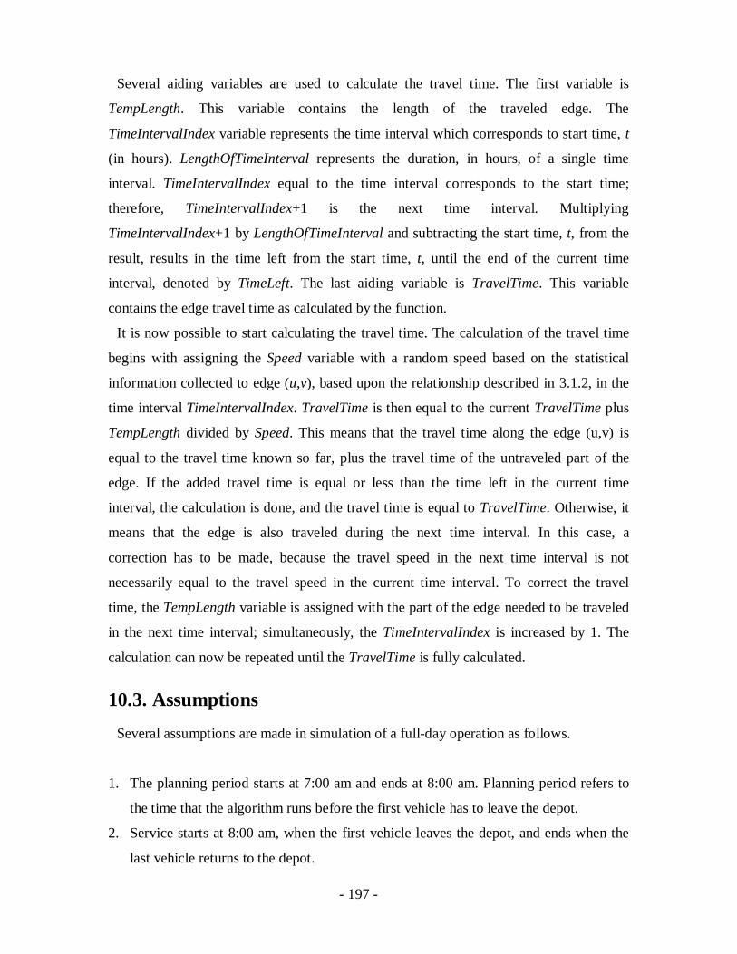
- 197 -
Several aiding variables are used to calculate the travel time. The first variable is
TempLength. This variable contains the length of the traveled edge. The
TimeIntervalIndex variable represents the time interval which corresponds to start time, t
(in hours). LengthOfTimeInterval represents the duration, in hours, of a single time
interval. TimeIntervalIndex equal to the time interval corresponds to the start time;
therefore, TimeIntervalIndex+1 is the next time interval. Multiplying
TimeIntervalIndex+1 by LengthOfTimeInterval and subtracting the start time, t, from the
result, results in the time left from the start time, t, until the end of the current time
interval, denoted by TimeLeft. The last aiding variable is TravelTime. This variable
contains the edge travel time as calculated by the function.
It is now possible to start calculating the travel time. The calculation of the travel time
begins with assigning the Speed variable with a random speed based on the statistical
information collected to edge (u,v), based upon the relationship described in 3.1.2, in the
time interval TimeIntervalIndex. TravelTime is then equal to the current TravelTime plus
TempLength divided by Speed. This means that the travel time along the edge (u,v) is
equal to the travel time known so far, plus the travel time of the untraveled part of the
edge. If the added travel time is equal or less than the time left in the current time
interval, the calculation is done, and the travel time is equal to TravelTime. Otherwise, it
means that the edge is also traveled during the next time interval. In this case, a
correction has to be made, because the travel speed in the next time interval is not
necessarily equal to the travel speed in the current time interval. To correct the travel
time, the TempLength variable is assigned with the part of the edge needed to be traveled
in the next time interval; simultaneously, the TimeIntervalIndex is increased by 1. The
calculation can now be repeated until the TravelTime is fully calculated.
10.3. Assumptions
Several assumptions are made in simulation of a full-day operation as follows.
1. The planning period starts at 7:00 am and ends at 8:00 am. Planning period refers to
the time that the algorithm runs before the first vehicle has to leave the depot.
2. Service starts at 8:00 am, when the first vehicle leaves the depot, and ends when the
last vehicle returns to the depot.

- 198 -
3. During the planning period, new information about customers’ demand is not
acceptable.
4. The workday is divided into 24 time intervals, each one hour long, starting at 0:00
am.
5. For each edge in the transportation network, the travel time is given using log-normal
distribution functions, for each time internal.
6. Information about real travel times is known two in advance (i.e., for the next two
time intervals), and is updated 15 minutes before the beginning of the hour.
7. Every half an hour on the hour, new vehicles that have to leave the depot, leave the
depot to their first customers (this can happen due to new customers demands or due
to route splitting made by the algorithm).
8. New customers demands are acceptable only if there is at least one vehicle which is
not driving to the depot.
9. If all vehicles are either at the depot or driving to the depot, the algorithm stops
working (end of the case study).
10. The capacity of a single vehicle is equal to 200 units, as in Solomon's instances.
10.4. Simulation
In order to perform the case study, simulation was used. The simulation is based on two
processes running in parallel, that are exchanging information between each other. The
two processes are the algorithm process and the simulation process.
The algorithm process is an implementation of each of the three EAs described earlier
for exchanging information with the simulation process.
The steps of the algorithm process are as follows:
1. Generate set of initial solutions.
2. If there are pending operations in the operations queue, process the operations.
3. Generate the next set of solutions from current solutions.
4. If there are pending operations in the operations queue, process the operations.
5. If stop condition is met, finish, otherwise go to step 3.

- 199 -
Operations are requests raised by the simulation process, and stored in a special shared
memory known as the operations queue, that have to be performed by the algorithm
process. The algorithm process can handle four such operations there:
1. Add customer – when the simulation process identifies a new demand request from a
new customer it raises an “Add customer” request. Adding a new customer means
that in all solutions generated by the algorithm, there should be a route which includes
the newly added customers. The simplest way to ensure that is by adding a new route
to each one of the solutions. This new route is a simple route which starts at the depot,
visits the newly added customer, and returns to the depot. Since various operations
are then applied on each of the solutions, the newly added customer will be quickly
managed in two other routes.
2. Remove customer - The simulation process keeps track of each of the vehicles that
has left the depot. Each vehicle that has left the depot can be in one of the following
two states, (1) "driving" and (2) "at the customer". When the vehicle changes its state
from "at the customer" to "driving", it means that the previous customer has already
been served, and therefore does not have to be visited anymore. As a result, the
previously visited customer has to be removed from all the solutions evolved by the
algorithm. The "remove customer" operation gets the number of the customer who
has to be removed and then removes it from all the solutions evolved by the
algorithm. It also makes sure that by removing the customer, there are no empty
routes left in any of the solutions.
3. Request route - When a vehicle has finished serving a customer it is required to
continue with its route toward the next customer. However, the vehicle, when leaving
the depot, is not given a route, but instead is given only the first customer in the route.
This is done since while the vehicle is driving towards its destination, the algorithm
continues improving the solutions, and by providing a route to the vehicle it is likely
to be given a route which will later be replaced with a better one. For that reason,
whenever a vehicle has to start driving towards its next destination, the simulation
process asks the algorithm process for the best routes known so far. From the routes,
the simulation process determines the vehicle's next destination.
4. Fix solutions based on current route - The simulation process supervises all available
vehicles. This is done using information provided by the algorithm process. When
- 200 -
choosing routes using the "request routes" operation, it is necessary that the selected
routes will also appear in all other solutions evolved by the algorithm. The "fix
solutions based on current routes" operation goes over each of the solutions evolved
by the algorithm, and makes any necessary changes according to the selected routes.
The simulation process simulates an entire workday. It does so by handling each of the
vehicles, collecting data about travel times and new customers’ demands. The simulation
process uses a timer to simulate an entire workday. A single timer event simulates one
second in the real-world. When a timer event is fired, a special time variable, called
SimTime, is increased by one second. Next, SimTime is compared against another variable
called NextDepartureTime. The NextDepartureTime variable represents the time when
new vehicles have to leave the depot on the new routes (usually, every half an hour on the
hour). If SimTime is greater than NextDepartureTime, then the value of
NextDepartureTime is recalculated. CalcTime is another variable maintained by the
simulation process. CalcTime is the time that an operation has to be performed, and it can
either be equal to the value of the NextDepartureTime variable, or to the earliest time that
an assigned vehicle (a vehicle currently located at a customer) has to leave the customer
to drive to another customer, whichever is earlier. If SimTime is equal or greater than
CalcTime, and there are no pending operations in the operations queue, the following is
done:
If CalcTime equals NextDepartureTime, then the "Request route", "Assign routes" and
the "Fix solutions based on current route" operators are added to the operations queue.
Otherwise, for each assigned vehicle, the following is done:
1. If a vehicle is located at the customer, and according to SimTime, it has to leave and
start driving to the next customer, then "Request route", "Assign routes" and the "Fix
solutions based on current route" operators are added to the operations queue.
2. If a vehicle is driving to a customer, and according to SimTime it has arrived at the
customer, then the vehicle's number is added to the "change vehicle status from
driving to at customer" queue, and a "change vehicle status from driving to at
customer" operator is added to the operators queue.
3. If a vehicle is located at the depot and is due to leave the depot at SimTime, then the
vehicle's number is added to the "change vehicle status from waiting to driving"

- 201 -
queue, and a "change vehicle status from waiting to queue" operator is added to the
operators queue.
As seen earlier, pending operations have to be processed before the simulation process
can continue. There are several operators stored in the operators queue, that can be
processed by the simulation process:
1. Assign route - the "assign routes" to vehicles operator is performed after a "request
routes" operator has been performed by the algorithm process. After receiving a set of
routes from the algorithm process, the simulation process must make sure that a
vehicle is assigned to each route in the set of routes received from the algorithm
process. Some of the routes already have vehicles assigned to them, while all the
other routes, which are new routes, have to be assigned to new vehicles.
2. Change status from driving to “at a customer” - The "change status from driving to at
customer operator" does the following for each vehicle whose status is changed from
"driving" to "at a customer": first, it changes the status of the vehicle from "driving"
to "at a customer", next the customer to whom the vehicle was driving is marked for
deletion by adding it to the "remove customers" queue, and the "remove customer"
and "fix solution based on current routes" are added to the operators queue.
3. Change status from waiting to driving– The "change status from waiting to driving" is
a simple operator which changes the status of a waiting vehicle from waiting at the
depot to driving.
4. New customer - The "new customer" operator gets a demand request from the user,
adds the new customer and its request to the "new customers" queue, and adds an
"add customer" operator to the operators queue.
5. Stop algorithm – The "stop algorithm" operator tells the algorithm process to stop. It
is called when all vehicles are back at the depot.
6. Update time interval – The "update time interval" operator gets travel time
information from the the algorithm process used and updated with it.

- 202 -
Figure 10.6 – The relationsheep between the algorithm process and the simulation process
10.5. Strategy of the Case Study
In this case study, five strategies for constructing the routing plan are considered. The
five strategies are as follows:
1. The first strategy assumes that all information, including customers’ demands and
traveling time, is known in advanced. Based on this information, the algorithm runs
for a pre-defined period of time, after that, using the TOPSIS mechanism, a set of
routes is selected from the set of non-dominated solutions found by the algorithm. All
vehicles follow this set of routes.
2. The second strategy assumes that all information, including customer's demands and
traveling time, is known in advanced. Based on this information, the algorithm runs
for a pre-defined period of time; after that, using the TOPSIS mechanism, a set of
routes is selected from the set of non-dominated solutions found by the algorithm.
Vehicles start driving according to this set of routes, while the algorithm continues to
run. Whenever a vehicle arrives sat a customer, the customer is removed from all

- 203 -
solutions evolved by the algorithm. Whenever a vehicle has to leave a customer and
drive to the next customer (or the depot), or at pre-defined time intervals, using the
TOPSIS mechanism, a new set of routes is selected from the set of non-dominated
solutions found by the algorithm. Driving vehicles are then rerouted according to the
new set of routes, and new vehicles are assigned as needed. This operation is repeated
until all customers have been served, and all vehicles have returned to the depot.
3. In the third strategy traveling time is unknown; however, all other information,
including customers’ demands, is known in advance. However, at pre-defined
intervals, traveling time information for the next pre-defined time period is revealed
to the algorithm. Based on this information, the algorithm runs for a pre-defined
period of time, after that, using the TOPSIS mechanism, a set of routes is selected
from the set of non-dominated solutions found by the algorithm. Vehicles start
driving according to this set of routes, while the algorithm continues to run.
Whenever a vehicle at a customer, the customer is removed from all solutions
evolved by the algorithm. Whenever a vehicle has to leave a customer and drive to
the next customer (or the depot), or at pre-defined time intervals, using the TOPSIS
mechanism, a new set of routes is selected from the set of non-dominated solutions
found by the algorithm. Driving vehicles are then rerouted according to the new set of
routes, and new vehicles are assigned as needed. This operation is repeated until all
customers have been served, and all vehicles have returned to the depot.
4. In the fourth strategy customers’ demands are unknown, while all other information,
including traveling time, is known in advance. When the algorithm starts, demands of
some of the customers are known. Based on this information, the algorithm runs for a
pre-defined period of time; after that, using the TOPSIS mechanism, a set of routes is
selected from the set of non-dominated solutions found by the algorithm. Vehicles
start driving according to this set of routes, while the algorithm continues to run.
Whenever a vehicle arrives at a customer, the customer is removed from all solutions
evolved by the algorithm. Simultaneously, new customers’ demands are revealed to
the algorithm, which, accordingly adds the new customers to the evolved solutions.
Whenever a vehicle has to leave a customer and drive to the next customer (or the
depot), or at pre-defined time intervals, using the TOPSIS mechanism, a new set of
routes is selected from the set of non-dominated solutions found by the algorithm.

- 204 -
Driving vehicles are then rerouted according to the new set of routes, and new
vehicles are assigned as needed. This operation is repeated until all customers have
been served, and all vehicles returned to the depot.
5. In the fifth strategy, neither customers’ demands nor traveling times are known in
advance. When the algorithm starts, some of the customers’ demands are known. In
regard to traveling time, at pre-defined intervals, traveling time information for the
next pre-defined time period is revealed to the algorithm. Based on this information,
the algorithm runs for a pre-defined period of time, after that, using the TOPSIS
mechanism, a set of routes is selected from the set of non-dominated solutions found
by the algorithm. Vehicles start driving according to this set of routes, while the
algorithm continues to run. Whenever a vehicle arrives at a customer, the customer is
removed from all solutions evolved by the algorithm. Simultaneously, new
customers’ demands are revealed to the algorithm, which accordingly adds the new
customers to the evolved solutions. Whenever a vehicle has to leave a customer and
drive to the next customer (or the depot), or at pre-defined time intervals, using the
TOPSIS mechanism, a new set of routes is selected from the set of non-dominated
solutions found by the algorithm. Driving vehicles are then rerouted according to the
new set of routes, and new vehicles are assigned as needed. This operation is repeated
until all customers have been served, and all vehicles have returned to the depot.
10.6. Case Study 1In the first case study the test scenario is defined as follows:
1. Network: The greater Tel-Aviv metropolitan area transportation network.
2. Dissatisfaction function: It is assumed that the dissatisfaction functions of all
customers are linear, meaning1
1 ii S
i i
t EETf tTW EET
and
1
( ) 1i Ei
ELT tg tELT TW
.
The test scenario is solved 100 times. In the first 50 times, it is assumed that all
customers have the same priority. Under this assumption, the test scenario is solved 100
times using each of the 5 strategies described earlier. In the next 50 times, it is assumed
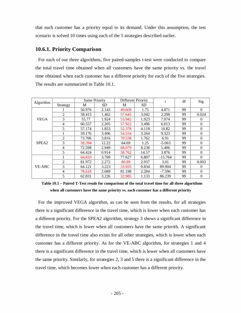
- 205 -
that each customer has a priority equal to its demand. Under this assumption, the test
scenario is solved 10 times using each of the 5 strategies described earlier.
10.6.1. Priority Comparison
For each of our three algorithms, five paired-samples t-test were conducted to compare
the total travel time obtained when all customers have the same priority vs. the travel
time obtained when each customer has a different priority for each of the five strategies.
The results are summarized in Table 10.1.
Same Priority Different PriorityAlgorithm Strategy M SD M SDt df Sig.
1 50.976 2.143 49.608 1.75 4.871 99 02 58.415 1.462 57.645 3.042 2.298 99 0.0243 55.77 1.924 53.942 1.923 7.074 99 04 60.557 2.205 57.922 3.496 6.013 99 0
VEGA
5 57.174 1.853 52.378 4.118 10.82 99 01 59.176 3.406 54.554 3.264 9.323 99 02 73.706 3.816 70.538 1.762 6.91 99 03 58.394 12.22 64.69 1.25 -5.063 99 04 72.598 2.949 68.079 8.238 5.406 99 0
SPEA2
5 64.424 0.914 58.762 14.57 3.876 99 01 64.833 3.769 77.627 6.807 -15.764 99 02 81.972 2.272 80.89 2.937 3.01 99 0.0033 64.121 3.223 33.935 0.834 89.904 99 04 78.618 2.689 81.198 2.284 -7.596 99 0
VE-ABC
5 62.831 3.226 32.985 1.133 86.239 99 0
Table 10.1 – Paired T-Test resuls for comparison of the total travel time for all three algorithms
when all customers have the same priority vs. each customer has a different priority
For the improved VEGA algorithm, as can be seen from the results, for all strategies
there is a significant difference in the travel time, which is lower when each customer has
a different priority. For the SPEA2 algorithm, strategy 3 shows a significant difference in
the travel time, which is lower when all customers have the same priorith. A significant
difference in the travel time also exists for all other strategies, which is lower when each
customer has a different priority. As for the VE-ABC algorithm, for strategies 1 and 4
there is a significant difference in the travel time, which is lower when all customers have
the same priority. Similarly, for strategies 2, 3 and 5 there is a significant difference in the
travel time, which becomes lower when each customer has a different priority.

- 206 -
For each of our three algorithms, five paired-samples t-tests were conducted to compare
the number of vehicles needed when all customers have the same priority vs. the number
of vehicles needed when each customer has a different priority for each of the five
strategies. The results are summarized in Table 10.2.
Same Priority Different PriorityAlgorithm Strategy M SD M SD t df Sig.
1 11 0.853 10.44 0.499 5.789 99 02 19.91 2.332 20.29 2.775 -1.023 99 0.3093 26.81 5.59 25.78 3.126 1.552 99 0.1244 21.95 2.928 20.6 3.83 2.834 99 0.006
VEGA
5 29.85 2.267 24.75 3.825 12.333 99 01 15.4 1.463 13.46 1.167 9.779 99 02 32.55 3.937 31.99 2.385 1.176 99 0.2423 34.25 6.838 37.47 1.784 -4.509 99 04 31.84 2.905 31.62 5.548 0.375 99 0.709
SPEA2
5 37.63 1.412 31.56 7.296 7.984 99 01 15.33 1.67 35.42 8.761 -22.177 99 02 34.21 2.54 38.98 0.804 -17.667 99 03 34.67 3.785 19.63 1.125 36.232 99 04 31.62 3.09 38.9 1.567 -20.261 99 0
VE-ABC
5 33.15 5.456 18.26 1.515 24.625 99 0
Table 10.2 – Paired T-Test resuls for comparison of the number of vehicles needed for all three
algorithms when all customers have the same priority vs. each customer has a different priority
For the improved VEGA algorithm, as can be seen from the results for strategies 1, 4
and 5, there is a significant difference in the number of vehicles needed, which is lower
when each customer has a different priority. For the SPEA2 algorithm, for strategies 1, 3
and 5 there is a significant difference in the travel time, which is lower when each
customer has a different priority. As for the VE-ABC algorithm, for all strategies there is
a significant difference in the travel time. For strategies 1, 2 and 4, there is a significant
difference in the travel time, which is lower when all customers have the same priority.
Similarly, for strategies 3 and 5 there is a significant difference in the travel time, which
becomes lower when each customer has a different priority.
For each of our three algorithms, five paired-samples t-tests were conducted to compare
the balance of the tours when all customers have the same priority vs. the number of
vehicles needed when each customer has a different priority for each of the five
strategies. The results are summarized in Table 10.3.

- 207 -
Same Priority Different PriorityAlgorithm Strategy M SD M SD t df Sig.
1 0.768 0.311 0.632 0.056 4.237 99 02 0.394 0.262 0.368 0.284 0.715 99 0.4763 0.334 0.387 0.259 0.266 1.533 99 0.1284 0.49 0.324 0.46 0.31 0.732 99 0.466
VEGA
5 0.235 0.289 0.451 0.356 -5.038 99 01 0.365 0.179 0.363 0.2 0.053 99 0.9582 0.288 0.295 0.287 0.305 0.031 99 0.9753 0.286 0.319 0.19 0.229 2.337 99 0.0214 0.309 0.35 0.34 0.31 -0.666 99 0.507
SPEA2
5 0.258 0.307 0.214 0.273 1.175 99 0.2431 0.64 0.342 0.351 0.392 5.628 99 02 0.294 0.288 0.145 0.188 4.646 99 03 0.252 0.269 0.326 0.311 -1.891 99 0.0624 0.343 0.304 0.255 0.332 2.254 99 0.026
VE-ABC
5 0.294 0.307 0.122 0.021 5.537 99 0
Table 10.3 – Paired T-Test results for comparison of the balance of the tours for all three
algorithms when all customers have the same priority vs. each customer has a different priority
For the improved VEGA algorithm, as can be seen from the results, for strategies 1 and
5 there is a significant difference in the tour balance. In strategy 1 the tour balance is
lower (meaning more balanced) when each customer has a different priority. However, in
strategy 5 the tour balance is lower when all customers have the same priority. For the
SPEA2 algorithm, only strategy 3 shows a significant difference in the tour balance,
which is lower when each customer has different priority. As for the VE-ABC algorithm,
for all strategies but stratedy 3, there is a significant difference in the tour balance, which
is lower when each customer has a different priority.
For each of our three algorithms, five paired-samples t-tests were conducted to compare
the total dissatisfaction of the customers when all customers have the same priority vs.
the total dissatisfaction of the customers when each customer has a different priority, for
each of the five strategies. The results are summarized in Table 10.4.
Same Priority Different PriorityAlgorithm Strategy M SD M SD t df Sig.
1 58.685 22.198 64.729 15.394 -2.147 99 0.0342 7.512 8.336 3.539 2.047 4.769 99 03 9.518 9.492 5.218 3.125 4.154 99 04 12.981 10.097 2.796 1.567 9.879 99 0
VEGA
5 7.317 9.767 5.01 4.866 2.078 99 0.041 40.797 10.131 0.147 0.225 40.139 99 02 68.786 48.423 0.24 0.298 14.159 99 0
SPEA2
3 53.119 25.344 0.174 0.229 20.894 99 0

- 208 -
Same Priority Different PriorityAlgorithm Strategy M SD M SD t df Sig.
4 56.901 27.795 0.3 0.271 20.411 99 05 38.33 9.592 0.249 0.356 39.645 99 01 1785.667 538.197 0.549 0.609 33.167 99 02 73.677 24.78 0.306 0.345 29.598 99 03 38.366 19.664 0.188 0.269 19.404 99 04 78.169 37.324 0.236 0.255 20.875 99 0
VE-ABC
5 78.448 71.603 0.032 0.025 10.951 99 0
Table 10.4 – Paired T-Test results for comparison of the total dissatisfaction of the customers for all
three algorithms when all customers have the same priority vs. each customer has a different priority
For the improved VEGA algorithm, as can be seen from the results, for strategy 1, there
is a significant difference in the total dissatisfaction of the customers, which is lower
when all customers have the same priority. For all other strategies, there is also a
significant difference in the total dissatisfaction of the customers, which is lower when
each customer has a different priority. For both the SPEA2 algorithm and the VE-ABC
algorithm, in all strategies there is a significant difference in the total dissatisfaction of
the customers obtained when all customers have the same priority and when each
customer has a different priority, which is lower when each customer has a different
priority.
For each of our three algorithms, five paired-samples t-tests were conducted to compare
the arrival time of the last vehicle when all customers have the same priority vs. the
arrival time of the last vehicle when each customer has a different priority, for each of the
five strategies. The results are summarized in Table 10.5.
Same Priority Different PriorityAlgorithm Strategy M SD M SDt df Sig.
1 14.262 0.343 14.728 0.575 -7.619 99 02 12.866 0.4 12.841 0.414 0.454 99 0.6513 12.342 0.571 12.753 0.546 -4.914 99 04 12.817 0.462 12.867 0.555 -0.677 99 0.5
VEGA
5 12.179 0.469 12.605 0.587 -6.298 99 01 13.041 0.407 12.943 0.329 1.845 99 0.0682 12.176 0.451 12.18 0.315 -0.059 99 0.9533 11.637 0.491 11.996 0.427 -5.401 99 04 12.163 0.35 12.098 0.439 1.202 99 0.232
SPEA2
5 11.816 0.423 11.979 0.472 -2.669 99 0.0091 14.364 0.555 12.491 1.022 16.089 99 02 12.345 0.442 11.868 0.288 8.783 99 03 12.069 0.454 11.16 0.328 14.824 99 04 12.338 0.549 11.855 0.305 7.502 99 0
VE-ABC
5 12.078 0.535 11.246 0.216 14.655 99 0

- 209 -
Table 10.5 – Paired T-Test results for comparison of the arrival time of the last vehicle for all three
algorithms when all customers have the same priority vs. each customer has a different priority
For the improved VEGA algorithm, as can be seen from the results, for strategies 1, 3
and 5 there is a significant difference in the arrival time of the last vehicle, which is
earlier when all customers have the same priority. For the SPEA2 algorithm, for
strategies 3 and 5 there is a significant difference in the arrival time of the last vehicle,
which is earlier when all customers have the same priority. As for the VE-ABC
algorithm, in all strategies there is a significant difference in the arrival time of the last
vehicle, which is later when each customer has a different priority.
10.6.1.1 Conclusions
For the first objective function, total travel time, a significant difference in the solutions
was found for the improved VEGA and SPEA2 algorithms, which is better when each
customer has a different priority. However when using the VE-ABC algorithm, no
significant difference in the solutions was found. Similar results were found for the 2nd
objective function, number of vehicles needed and 4th objective function, customers'
dissatisfaction.
For the 3rd objective function, tour balance, a significant difference in the solutions was
found only for the VE-ABC algorithm, which is better when each customer has a
different priority.
For the fifth objective, arrival time at the last customer, the best solutions are obtained
when when all customers have the same priority, for the improved VEGA and SPEA2
algorithms, and when each customer has a different objective function, when using the
VE-ABC algorithm.
10.6.2. Strategies Comparison – VEGA algorithm
In order to examine the effect of each of the strategies of the algorithm's results, several
paired t-tests were used.
The first set of paired t-tests was used to compare the results obtained by using
strategies 1 and 2. The results are summarized in Table 10.6.
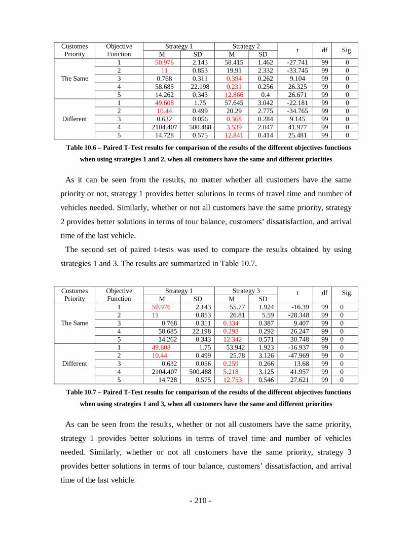
- 210 -
Strategy 1 Strategy 2CustomesPriority
ObjectiveFunction M SD M SD t df Sig.
1 50.976 2.143 58.415 1.462 -27.741 99 02 11 0.853 19.91 2.332 -33.745 99 03 0.768 0.311 0.394 0.262 9.104 99 04 58.685 22.198 0.231 0.256 26.325 99 0
The Same
5 14.262 0.343 12.866 0.4 26.671 99 01 49.608 1.75 57.645 3.042 -22.181 99 02 10.44 0.499 20.29 2.775 -34.765 99 03 0.632 0.056 0.368 0.284 9.145 99 04 2104.407 500.488 3.539 2.047 41.977 99 0
Different
5 14.728 0.575 12.841 0.414 25.481 99 0
Table 10.6 – Paired T-Test results for comparison of the results of the different objectives functions
when using strategies 1 and 2, when all customers have the same and different priorities
As it can be seen from the results, no matter whether all customers have the same
priority or not, strategy 1 provides better solutions in terms of travel time and number of
vehicles needed. Similarly, whether or not all customers have the same priority, strategy
2 provides better solutions in terms of tour balance, customers’ dissatisfaction, and arrival
time of the last vehicle.
The second set of paired t-tests was used to compare the results obtained by using
strategies 1 and 3. The results are summarized in Table 10.7.
Strategy 1 Strategy 3CustomesPriority
ObjectiveFunction M SD M SD
t df Sig.
1 50.976 2.143 55.77 1.924 -16.39 99 02 11 0.853 26.81 5.59 -28.348 99 03 0.768 0.311 0.334 0.387 9.407 99 04 58.685 22.198 0.293 0.292 26.247 99 0
The Same
5 14.262 0.343 12.342 0.571 30.748 99 01 49.608 1.75 53.942 1.923 -16.937 99 02 10.44 0.499 25.78 3.126 -47.969 99 03 0.632 0.056 0.259 0.266 13.68 99 04 2104.407 500.488 5.218 3.125 41.957 99 0
Different
5 14.728 0.575 12.753 0.546 27.621 99 0
Table 10.7 – Paired T-Test results for comparison of the results of the different objectives functions
when using strategies 1 and 3, when all customers have the same and different priorities
As can be seen from the results, whether or not all customers have the same priority,
strategy 1 provides better solutions in terms of travel time and number of vehicles
needed. Similarly, whether or not all customers have the same priority, strategy 3
provides better solutions in terms of tour balance, customers’ dissatisfaction, and arrival
time of the last vehicle.
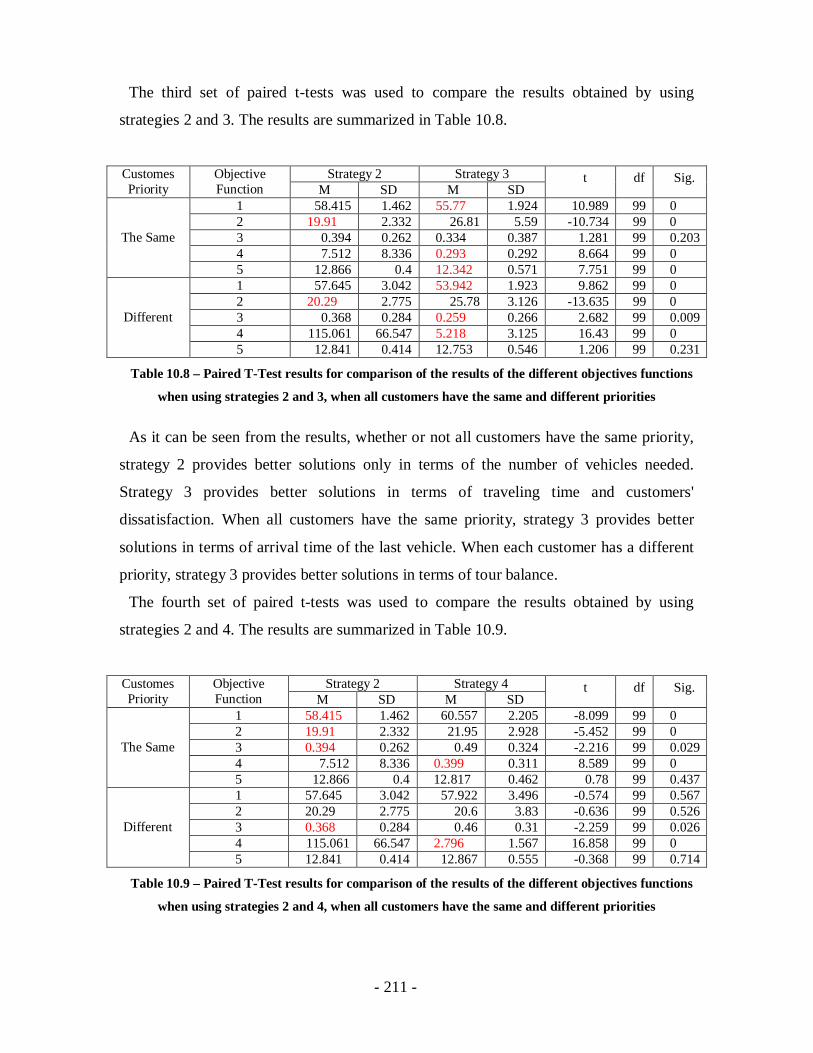
- 211 -
The third set of paired t-tests was used to compare the results obtained by using
strategies 2 and 3. The results are summarized in Table 10.8.
Strategy 2 Strategy 3CustomesPriority
ObjectiveFunction M SD M SD
t df Sig.
1 58.415 1.462 55.77 1.924 10.989 99 02 19.91 2.332 26.81 5.59 -10.734 99 03 0.394 0.262 0.334 0.387 1.281 99 0.2034 7.512 8.336 0.293 0.292 8.664 99 0
The Same
5 12.866 0.4 12.342 0.571 7.751 99 01 57.645 3.042 53.942 1.923 9.862 99 02 20.29 2.775 25.78 3.126 -13.635 99 03 0.368 0.284 0.259 0.266 2.682 99 0.0094 115.061 66.547 5.218 3.125 16.43 99 0
Different
5 12.841 0.414 12.753 0.546 1.206 99 0.231
Table 10.8 – Paired T-Test results for comparison of the results of the different objectives functions
when using strategies 2 and 3, when all customers have the same and different priorities
As it can be seen from the results, whether or not all customers have the same priority,
strategy 2 provides better solutions only in terms of the number of vehicles needed.
Strategy 3 provides better solutions in terms of traveling time and customers'
dissatisfaction. When all customers have the same priority, strategy 3 provides better
solutions in terms of arrival time of the last vehicle. When each customer has a different
priority, strategy 3 provides better solutions in terms of tour balance.
The fourth set of paired t-tests was used to compare the results obtained by using
strategies 2 and 4. The results are summarized in Table 10.9.
Strategy 2 Strategy 4CustomesPriority
ObjectiveFunction M SD M SD
t df Sig.
1 58.415 1.462 60.557 2.205 -8.099 99 02 19.91 2.332 21.95 2.928 -5.452 99 03 0.394 0.262 0.49 0.324 -2.216 99 0.0294 7.512 8.336 0.399 0.311 8.589 99 0
The Same
5 12.866 0.4 12.817 0.462 0.78 99 0.4371 57.645 3.042 57.922 3.496 -0.574 99 0.5672 20.29 2.775 20.6 3.83 -0.636 99 0.5263 0.368 0.284 0.46 0.31 -2.259 99 0.0264 115.061 66.547 2.796 1.567 16.858 99 0
Different
5 12.841 0.414 12.867 0.555 -0.368 99 0.714
Table 10.9 – Paired T-Test results for comparison of the results of the different objectives functions
when using strategies 2 and 4, when all customers have the same and different priorities
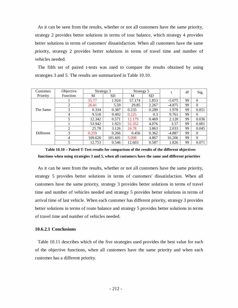
- 212 -
As it can be seen from the results, whether or not all customers have the same priority,
strategy 2 provides better solutions in terms of tour balance, which strategy 4 provides
better solutions in terms of customers' dissatisfaction. When all customers have the same
priority, strategy 2 provides better solutions in terms of travel time and number of
vehicles needed.
The fifth set of paired t-tests was used to compare the results obtained by using
strategies 3 and 5. The results are summarized in Table 10.10.
Strategy 3 Strategy 5CustomesPriority
ObjectiveFunction M SD M SD
t df Sig.
1 55.77 1.924 57.174 1.853 -5.075 99 02 26.81 5.59 29.85 2.267 -4.875 99 03 0.334 0.387 0.235 0.289 1.978 99 0.0514 9.518 9.492 0.225 0.3 9.761 99 0
The Same
5 12.342 0.571 12.179 0.469 2.128 99 0.0361 53.942 1.923 52.352 4.076 3.57 99 0.0012 25.78 3.126 24.78 3.863 2.033 99 0.0453 0.259 0.266 0.456 0.362 -4.887 99 04 169.626 101.601 5.008 4.867 16.206 99 0
Different
5 12.753 0.546 12.603 0.587 1.826 99 0.071
Table 10.10 – Paired T-Test results for comparison of the results of the different objectives
functions when using strategies 3 and 5, when all customers have the same and different priorities
As it can be seen from the results, whether or not all customers have the same priority,
strategy 5 provides better solutions in terms of customers' dissatisfaction. When all
customers have the same priority, strategy 3 provides better solutions in terms of travel
time and number of vehicles needed and strategy 5 provides better solutions in terms of
arrival time of last vehicle. When each customer has different priority, strategy 3 provides
better solutions in terms of route balance and strategy 5 provides better solutions in terms
of travel time and number of vehicles needed.
10.6.2.1 Conclusions
Table 10.11 describes which of the five strategies used provides the best value for each
of the objective functions, when all customers have the same priority and when each
customer has a different priority.
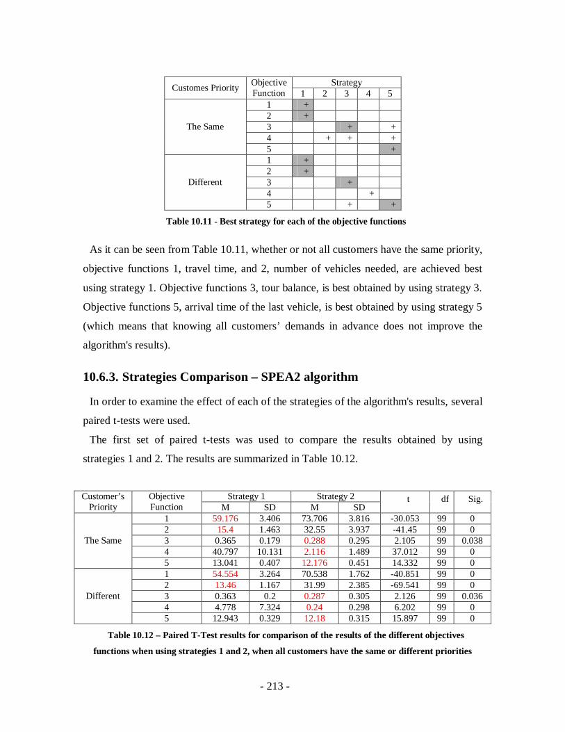
- 213 -
StrategyCustomes Priority ObjectiveFunction 1 2 3 4 5
1 +2 +3 + +4 + + +
The Same
5 +1 +2 +3 +4 +
Different
5 + +
Table 10.11 - Best strategy for each of the objective functions
As it can be seen from Table 10.11, whether or not all customers have the same priority,
objective functions 1, travel time, and 2, number of vehicles needed, are achieved best
using strategy 1. Objective functions 3, tour balance, is best obtained by using strategy 3.
Objective functions 5, arrival time of the last vehicle, is best obtained by using strategy 5
(which means that knowing all customers’ demands in advance does not improve the
algorithm's results).
10.6.3. Strategies Comparison – SPEA2 algorithm
In order to examine the effect of each of the strategies of the algorithm's results, several
paired t-tests were used.
The first set of paired t-tests was used to compare the results obtained by using
strategies 1 and 2. The results are summarized in Table 10.12.
Strategy 1 Strategy 2Customer’sPriority
ObjectiveFunction M SD M SD
t df Sig.
1 59.176 3.406 73.706 3.816 -30.053 99 02 15.4 1.463 32.55 3.937 -41.45 99 03 0.365 0.179 0.288 0.295 2.105 99 0.0384 40.797 10.131 2.116 1.489 37.012 99 0
The Same
5 13.041 0.407 12.176 0.451 14.332 99 01 54.554 3.264 70.538 1.762 -40.851 99 02 13.46 1.167 31.99 2.385 -69.541 99 03 0.363 0.2 0.287 0.305 2.126 99 0.0364 4.778 7.324 0.24 0.298 6.202 99 0
Different
5 12.943 0.329 12.18 0.315 15.897 99 0
Table 10.12 – Paired T-Test results for comparison of the results of the different objectives
functions when using strategies 1 and 2, when all customers have the same or different priorities
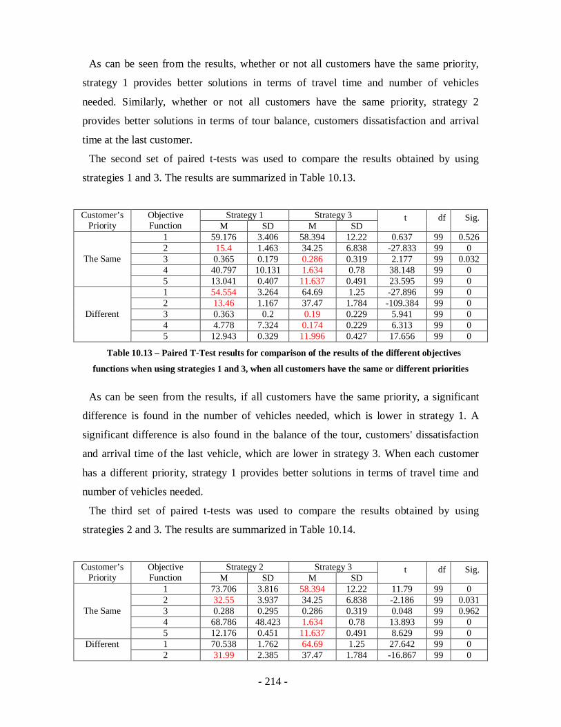
- 214 -
As can be seen from the results, whether or not all customers have the same priority,
strategy 1 provides better solutions in terms of travel time and number of vehicles
needed. Similarly, whether or not all customers have the same priority, strategy 2
provides better solutions in terms of tour balance, customers dissatisfaction and arrival
time at the last customer.
The second set of paired t-tests was used to compare the results obtained by using
strategies 1 and 3. The results are summarized in Table 10.13.
Strategy 1 Strategy 3Customer’sPriority
ObjectiveFunction M SD M SD
t df Sig.
1 59.176 3.406 58.394 12.22 0.637 99 0.5262 15.4 1.463 34.25 6.838 -27.833 99 03 0.365 0.179 0.286 0.319 2.177 99 0.0324 40.797 10.131 1.634 0.78 38.148 99 0
The Same
5 13.041 0.407 11.637 0.491 23.595 99 01 54.554 3.264 64.69 1.25 -27.896 99 02 13.46 1.167 37.47 1.784 -109.384 99 03 0.363 0.2 0.19 0.229 5.941 99 04 4.778 7.324 0.174 0.229 6.313 99 0
Different
5 12.943 0.329 11.996 0.427 17.656 99 0
Table 10.13 – Paired T-Test results for comparison of the results of the different objectives
functions when using strategies 1 and 3, when all customers have the same or different priorities
As can be seen from the results, if all customers have the same priority, a significant
difference is found in the number of vehicles needed, which is lower in strategy 1. A
significant difference is also found in the balance of the tour, customers' dissatisfaction
and arrival time of the last vehicle, which are lower in strategy 3. When each customer
has a different priority, strategy 1 provides better solutions in terms of travel time and
number of vehicles needed.
The third set of paired t-tests was used to compare the results obtained by using
strategies 2 and 3. The results are summarized in Table 10.14.
Strategy 2 Strategy 3Customer’sPriority
ObjectiveFunction M SD M SD
t df Sig.
1 73.706 3.816 58.394 12.22 11.79 99 02 32.55 3.937 34.25 6.838 -2.186 99 0.0313 0.288 0.295 0.286 0.319 0.048 99 0.9624 68.786 48.423 1.634 0.78 13.893 99 0
The Same
5 12.176 0.451 11.637 0.491 8.629 99 01 70.538 1.762 64.69 1.25 27.642 99 0Different2 31.99 2.385 37.47 1.784 -16.867 99 0
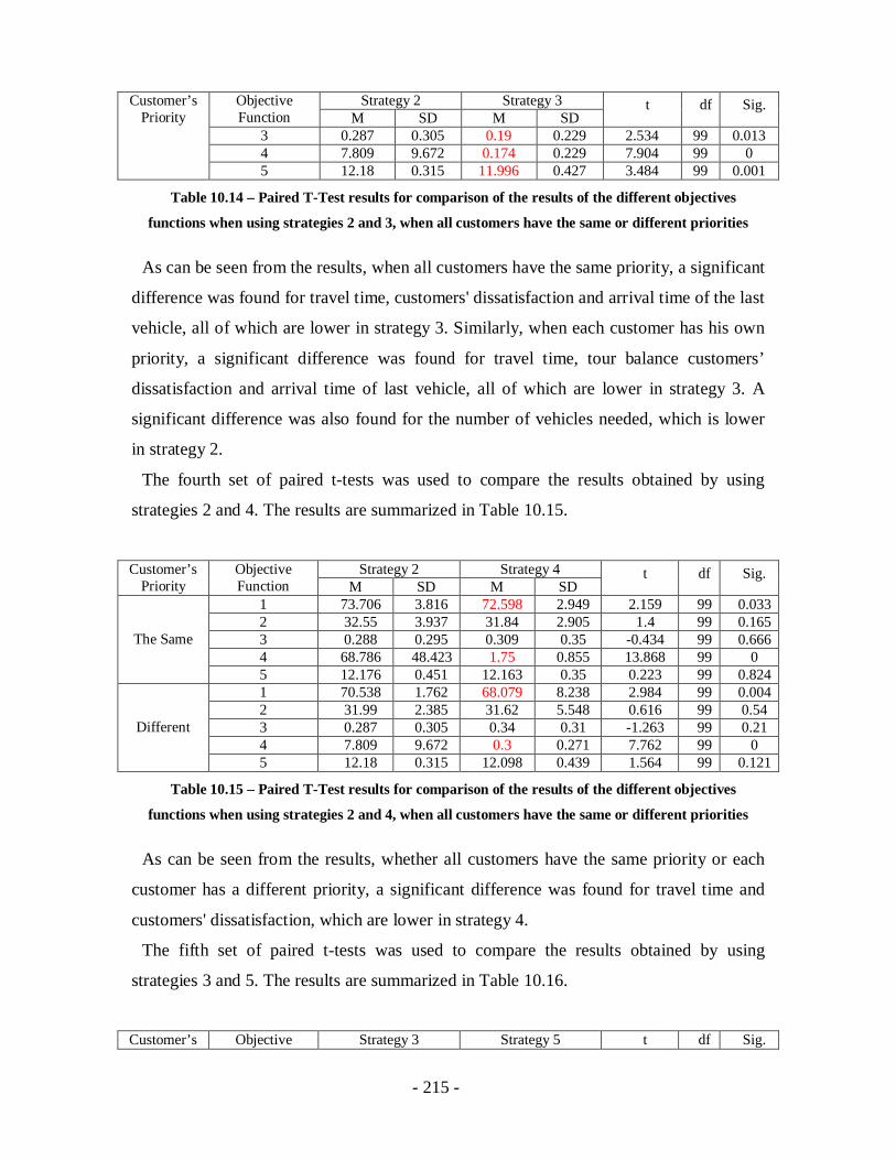
- 215 -
Strategy 2 Strategy 3Customer’sPriority
ObjectiveFunction M SD M SD
t df Sig.
3 0.287 0.305 0.19 0.229 2.534 99 0.0134 7.809 9.672 0.174 0.229 7.904 99 05 12.18 0.315 11.996 0.427 3.484 99 0.001
Table 10.14 – Paired T-Test results for comparison of the results of the different objectives
functions when using strategies 2 and 3, when all customers have the same or different priorities
As can be seen from the results, when all customers have the same priority, a significant
difference was found for travel time, customers' dissatisfaction and arrival time of the last
vehicle, all of which are lower in strategy 3. Similarly, when each customer has his own
priority, a significant difference was found for travel time, tour balance customers’
dissatisfaction and arrival time of last vehicle, all of which are lower in strategy 3. A
significant difference was also found for the number of vehicles needed, which is lower
in strategy 2.
The fourth set of paired t-tests was used to compare the results obtained by using
strategies 2 and 4. The results are summarized in Table 10.15.
Strategy 2 Strategy 4Customer’sPriority
ObjectiveFunction M SD M SD
t df Sig.
1 73.706 3.816 72.598 2.949 2.159 99 0.0332 32.55 3.937 31.84 2.905 1.4 99 0.1653 0.288 0.295 0.309 0.35 -0.434 99 0.6664 68.786 48.423 1.75 0.855 13.868 99 0
The Same
5 12.176 0.451 12.163 0.35 0.223 99 0.8241 70.538 1.762 68.079 8.238 2.984 99 0.0042 31.99 2.385 31.62 5.548 0.616 99 0.543 0.287 0.305 0.34 0.31 -1.263 99 0.214 7.809 9.672 0.3 0.271 7.762 99 0
Different
5 12.18 0.315 12.098 0.439 1.564 99 0.121
Table 10.15 – Paired T-Test results for comparison of the results of the different objectives
functions when using strategies 2 and 4, when all customers have the same or different priorities
As can be seen from the results, whether all customers have the same priority or each
customer has a different priority, a significant difference was found for travel time and
customers' dissatisfaction, which are lower in strategy 4.
The fifth set of paired t-tests was used to compare the results obtained by using
strategies 3 and 5. The results are summarized in Table 10.16.
Customer’sPriority
ObjectiveFunction
Strategy 3 Strategy 5 t df Sig.

- 216 -
M SD M SD1 58.394 12.22 64.424 0.914 -4.914 99 02 34.25 6.838 37.63 1.412 -4.92 99 03 0.286 0.319 0.258 0.307 0.66 99 0.5114 53.119 25.344 1.179 0.295 20.493 99 0
The Same
5 11.637 0.491 11.816 0.423 -2.847 99 0.0051 64.69 1.25 58.762 14.57 4.019 99 02 37.47 1.784 31.56 7.296 7.899 99 03 0.19 0.229 0.214 0.273 -0.638 99 0.5254 5.661 7.442 0.249 0.356 7.311 99 0
Different
5 11.996 0.427 11.979 0.472 0.266 99 0.791
Table 10.16 – Paired T-Test results for comparison of the results of the different objectives
functions when using strategies 3 and 5, when all customers have the same or different priorities
As can be seen from the results, whether all customers have the same priority or not, a
significant difference was found for customers' dissatisfaction, which is lower in strategy
5. When all customers have the same priority, a significant difference was found for
travel time, number of vehicles needed and arrival time of the last vehicle, all of which
are lower in strategy 3. Similarly, when each customer has his own priority, a significant
difference was found for travel time and number of vehicles, all of which are lower in
strategy 5.
10.6.3.1 Conclusions
Table 10.17 describes which of the five strategies used provides the best value for each
of the objective functions, when all customers have the same priority and when each
customer has a different priority.
StrategyCustomer’sPriority
ObjectiveFunction 1 2 3 4 5
1 + +2 +3 + + + +4 + +
The Same
5 +1 +2 +3 + +4 + +
Different
5 + + +
Table 10.17 - Best strategy for each of the objective functions

- 217 -
As can be seen from Table 10.17, whether or not all customers have the same priority,
objective functions 1, travel time, 2, number of vehicles needed and 4, customers'
dissatisfaction, are best obtained using strategy 1. Objective functions 3, tour balance,
and 5, arrival time of the last vehicle, are best obtained by using strategy 3.
10.6.4. Strategies Comparison – VE-ABC algorithm
In order to examine the effect of each of the strategies of the algorithm's results, several
paired t-tests were used.
The first set of paired t-tests was used to compare the results obtained by using
strategies 1 and 2. The results are summarized in Table 10.18.
Strategy 1 Strategy 2Customer’sPriority
ObjectiveFunction M SD M SD
t df Sig.
1 64.833 3.769 81.972 2.272 -39.757 99 02 15.33 1.67 34.21 2.54 -65.027 99 03 0.64 0.342 0.294 0.288 7.515 99 04 1785.667 538.197 2.266 0.762 33.136 99 0
The Same
5 14.364 0.555 12.345 0.442 30.018 99 01 77.627 6.807 80.89 2.937 -4.596 99 02 35.42 8.761 38.98 0.804 -4.027 99 03 0.351 0.392 0.145 0.188 5.17 99 04 17.861 19.803 0.306 0.345 8.895 99 0
Different
5 12.491 1.022 11.868 0.288 5.588 99 0
Table 10.18 – Paired T-Test results for comparison of the results of the different objectives
functions when using strategies 1 and 2, when all customers have the same or different priorities
As can be seen from the results, whether all customers have the same priority or not,
strategy 1 provides better solutions in terms of travel time and number of vehicles
needed. Similarly, strategy 2 provides better solutions in terms of tour balance,
customers’ dissatisfaction, and arrival time of the last vehicle.
The second set of paired t-tests was used to compare the results obtained by using
strategies 1 and 3. The results are summarized in Table 10.19.
Strategy 1 Strategy 3Customer’sPriority
ObjectiveFunction M SD M SD
t df Sig.
1 64.833 3.769 64.118 3.202 1.494 99 0.1382 15.33 1.67 34.68 3.792 -48.151 99 03 0.64 0.342 0.251 0.27 9.047 99 04 1785.667 538.197 1.157 0.562 33.159 99 0
The Same
5 14.364 0.555 12.073 0.451 29.452 99 0

- 218 -
Strategy 1 Strategy 3Customer’sPriority
ObjectiveFunction M SD M SD
t df Sig.
1 77.627 6.807 33.935 0.834 62.504 99 02 35.42 8.761 19.63 1.125 17.839 99 03 0.351 0.392 0.326 0.311 0.522 99 0.6034 17.861 19.803 0.188 0.269 8.931 99 0
Different
5 12.491 1.022 11.16 0.328 12.066 99 0
Table 10.19 – Paired T-Test results for comparison of the results of the different objectives
functions when using strategies 1 and 3, when all customers have the same or different priorities
As can be seen from the results, a significant difference was found in customers'
dissatisfaction and arrival time of last vehicle, which is lower in 3, whether all customers
have the same priority or not. In the case of the number of vehicles needed, a significant
difference also exiss using strategy 1, when all customers have the same priority. When
each customer has a different priority, strategy 3 provides a better solution in terms of
tour balance.
The third set of paired t-tests was used to compare the results obtained by using
strategies 2 and 3. The results are summarized in Table 10.20.
Strategy 2 Strategy 3Customer’sPriority
ObjectiveFunction M SD M SD
t df Sig.
1 81.972 2.272 63.612 3.995 35.333 99 02 34.21 2.54 34.49 4.089 -0.559 99 0.5783 0.294 0.288 0.251 0.27 1.083 99 0.2814 73.677 24.78 1.146 0.573 29.267 99 0
The Same
5 12.345 0.442 12.066 0.458 4.292 99 01 80.89 2.937 33.935 0.834 152.175 99 02 38.98 0.804 19.63 1.125 138.676 99 03 0.145 0.188 0.326 0.311 -4.904 99 04 9.942 11.218 0.188 0.269 8.713 99 0
Different
5 11.868 0.288 11.16 0.328 17.427 99 0
Table 10.20 – Paired T-Test results for comparison of the results of the different objectives
functions when using strategies 2 and 3, when all customers have the same or different priorities
As can be seen from the results, strategy 2 provides a better solution in terms of balance
of the tour, when each customer has a different priority. Strategy 3 provides better
solutions in terms of travel time customers’ dissatisfaction and arrival time of last
vehicle, wether all customers have the same priority or not.
The fourth set of paired t-tests was used to compare the results obtained by using
strategies 2 and 4. The results are summarized in Table 10.21.
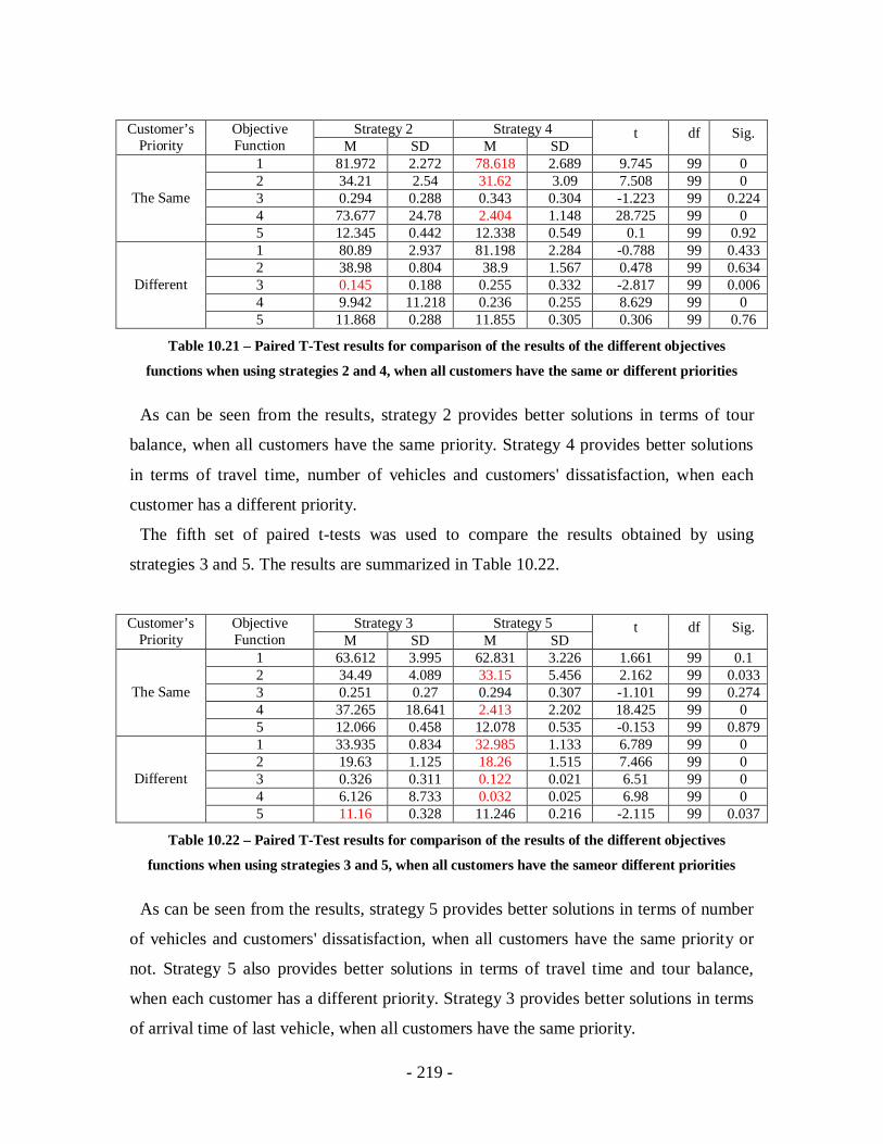
- 219 -
Strategy 2 Strategy 4Customer’sPriority
ObjectiveFunction M SD M SD
t df Sig.
1 81.972 2.272 78.618 2.689 9.745 99 02 34.21 2.54 31.62 3.09 7.508 99 03 0.294 0.288 0.343 0.304 -1.223 99 0.2244 73.677 24.78 2.404 1.148 28.725 99 0
The Same
5 12.345 0.442 12.338 0.549 0.1 99 0.921 80.89 2.937 81.198 2.284 -0.788 99 0.4332 38.98 0.804 38.9 1.567 0.478 99 0.6343 0.145 0.188 0.255 0.332 -2.817 99 0.0064 9.942 11.218 0.236 0.255 8.629 99 0
Different
5 11.868 0.288 11.855 0.305 0.306 99 0.76
Table 10.21 – Paired T-Test results for comparison of the results of the different objectives
functions when using strategies 2 and 4, when all customers have the same or different priorities
As can be seen from the results, strategy 2 provides better solutions in terms of tour
balance, when all customers have the same priority. Strategy 4 provides better solutions
in terms of travel time, number of vehicles and customers' dissatisfaction, when each
customer has a different priority.
The fifth set of paired t-tests was used to compare the results obtained by using
strategies 3 and 5. The results are summarized in Table 10.22.
Strategy 3 Strategy 5Customer’sPriority
ObjectiveFunction M SD M SD
t df Sig.
1 63.612 3.995 62.831 3.226 1.661 99 0.12 34.49 4.089 33.15 5.456 2.162 99 0.0333 0.251 0.27 0.294 0.307 -1.101 99 0.2744 37.265 18.641 2.413 2.202 18.425 99 0
The Same
5 12.066 0.458 12.078 0.535 -0.153 99 0.8791 33.935 0.834 32.985 1.133 6.789 99 02 19.63 1.125 18.26 1.515 7.466 99 03 0.326 0.311 0.122 0.021 6.51 99 04 6.126 8.733 0.032 0.025 6.98 99 0
Different
5 11.16 0.328 11.246 0.216 -2.115 99 0.037
Table 10.22 – Paired T-Test results for comparison of the results of the different objectives
functions when using strategies 3 and 5, when all customers have the sameor different priorities
As can be seen from the results, strategy 5 provides better solutions in terms of number
of vehicles and customers' dissatisfaction, when all customers have the same priority or
not. Strategy 5 also provides better solutions in terms of travel time and tour balance,
when each customer has a different priority. Strategy 3 provides better solutions in terms
of arrival time of last vehicle, when all customers have the same priority.

- 220 -
10.6.4.1 Conclusions
Table 10.23 describes which of the five strategies used provides the best value for each
of the objective functions, whether all customers have the same priority or each customer
has a different priority.
StrategyCustomer’sPriority
ObjectiveFunction 1 2 3 4 5
1 +2 +3 + + +4 +
The Same
5 + +1 +2 +3 + +4 +
Different
5 +
Table 10.23 - Best strategy for each of the objective functions
As can be seen from Table 10.23, when all customers have the same priority, objective
functions 1, travel time, and 3, tour balance are best obtained using strategy 5. Objective
function 5, arrival time of the last vehicle, is best obtained either using strategy 3.
When all customers have the same priority, objective function 2, number of vehicles
needed, is best obtained using strategy 1. Objective function 4, customers' dissatisfaction,
is best obtained by using strategy 3.
When each customer has different priority, objective functions 2, number of vehicles
needed and 4, customers' dissatisfaction, are best obtained using strategy 5.
10.6.5. Algorithms Comparison
Since in the real-world, information on travel time and customers’ demands are not
known in advance, strategy 5 has to be used. Table 10.24 compares the results obtained
for each of the five objectives, using paired t-tests, functions by each one of the three
algorithms when applying the 3rd strategy. For each objective function, the best value
obtained is highlighted in red.
AlgorithmCustomer’sPriority Objective Function Imp. VEGA SPEA2 VE-ABC

- 221 -
AlgorithmCustomer’sPriority Objective Function Imp. VEGA SPEA2 VE-ABC
1 57.174 64.424 62.8312 29.85 37.63 33.153 0.235 0.258 0.2944 0.225 1.179 2.413
The Same
5 12.179 11.816 12.0781 52.377 58.762 32.9852 24.67 31.56 18.263 0.446 0.214 0.1224 4.997 0.249 0.032
Different
5 12.589 11.979 11.246
Table 10.24 - Comparison of the 5th strategy used in all three algorithms
As can be seen, when all customers have the same priority, most objective functions are
best obtained by using the improved VEGA algorithm. However, if used when each
customer has a different priority, all objective functions are best obtained first by using
the improved VE-VEGA algorithm.
10.6.6. Conclusions
For all three algorithms, whether all customers have the same priority or not, objective
functions 1, travel time, and 2, number of vehicles needed, are best obtained using
strategy 1. Objective functions 3, tour balance, 4, customers’ dissatisfaction, and 5,
arrival time of the last vehicle, are best obtained by using either strategy 3 or by using
strategy 5 (which means that knowing all customers’ demands in advance does not
improve the algorithm's results).
Also, in all objective function, except the 5th, arrival time of last vehicle, better solutions
are obtained when each customer has a different priority.
Since in the real-world, information on travel time and customers’ demands are not
known in advance, strategy 3 has to be used. From the results obtained, it is not clear
whether one algorithm can provide the best solution in all cases.
10.7. Case Study 2In the second case study the test scenario is defined as follows:
1. Network: The greater Tel-Aviv metropolitan area transportation network.

- 222 -
2. Dissatisfaction function: It is assumed that all customers dislike it when the supplier
is either early or late. Therefore, the dissatisfaction functions of all customers are in
the form of5
1 ii S
i i
t EETf tTW EET
and5
( ) 1i Ei
ELT tg tELT TW
.
The test scenario is solved 100 times. In the first 50 times, it is assumed that all
customers have the same priority. Under this assumption, the test scenario is solved 100
times using each of the 5 strategies described earlier. In the next 50 times, it is assumed
that each customer has a priority equal to his demand. Under this assumption, the test
scenario is solved 10 times using each of the 5 strategies described earlier.
10.7.1. Priority Comparison
For each of our three algorithms, five paired-samples t-tests were conducted to compare
the total travel time obtained when all customers have the same priority vs. the travel
time obtained when each customer has a different priority for each of the five strategies.
The results are summarized in Table 10.25.
Same Priority Different PriorityAlgorithm Strategy M SD M SDt df Sig.
1 50.235 2.12 49.383 2.051 2.77 99 0.0072 56.78 2.381 58.053 2.34 -3.782 99 03 53.754 2.328 56.329 1.853 -8.907 99 04 58.366 2.827 57.412 1.972 2.762 99 0.007
VEGA
5 53.321 3.497 54.425 6.048 -1.734 99 0.0861 59.456 3.87 57.281 2.432 4.527 99 02 72.54 2.967 72.854 1.718 -0.905 99 0.3683 63.069 1.61 58.479 12.283 3.74 99 04 72.937 2.7 72.343 3.561 1.306 99 0.194
SPEA2
5 65.885 1.274 64.9 2.162 3.675 99 01 62.574 2.528 51.812 17.456 6.141 99 02 78.716 2.862 79.773 2.033 -2.971 99 0.0043 63.547 2.61 63.372 2.33 0.481 99 0.6314 79.326 1.982 74.508 10.636 4.591 99 0
VE-ABC
5 63.902 2.405 63.653 1.841 0.782 99 0.436
Table 10.25 – Paired T-Test results for comparison of the total travel time for all three algorithms
when all customers have the same priority vs. each customer has a different priority
For the improved VEGA algorithm, as can be seen from the results, for strategies 2 and
3, a significant difference exists in the solution obtained when all customers have the
same priority vs. the solution obtained when each customer has a different priority: it is

- 223 -
better when all customers have the same priority. While for strategies 1 and 4 a better
solution is obtained when each customer has a different priority.
For the SPEA2 algorithm, for strategies 1, 3 and 5, a significant difference exists in the
solution. The best solutions are obtained when each customer has a different priority.
As for the VE-ABC algorithm, for strategies 1 and 4, the best solutions are obtained
when each customer has a different priority, while for strategy 2 the best solution is
obtained when all customers have the same priority.
For each of our three algorithms, five paired-samples t-tests were conducted to compare
the number of vehicles needed when all customers have the same priority vs. the number
of vehicles needed when each customer has a different priority for each of the five
strategies. The results are summarized in Table 10.26.
Same Priority Different PriorityAlgorithm Strategy M SD M SDt df Sig.
1 9.92 0.787 9.98 0.778 -0.537 99 0.5932 19.61 3.025 18.99 2.97 1.584 99 0.1163 24.18 2.794 28.48 2.402 -12.096 99 04 20.67 3.327 19.46 1.684 3.286 99 0.001
VEGA
5 24.32 4.075 28.06 4.419 -6.475 99 01 14.73 2.265 14.01 1.396 2.578 99 0.0112 33.04 4.122 33.64 2.41 -1.178 99 0.2423 37.38 1.797 33.77 7.558 4.815 99 04 32.16 3.936 32.92 1.947 -1.754 99 0.082
SPEA2
5 39.5 1.078 36.86 2.697 9.534 99 01 14.6 1.583 13.77 2.733 2.657 99 0.0092 34.23 1.874 34.4 2.361 -0.588 99 0.5583 34.71 3.361 33.47 3.096 2.714 99 0.0084 34.1 2.607 31.93 5.044 3.967 99 0
VE-ABC
5 33.93 4.344 32.2 4.355 2.778 99 0.007
Table 10.26 – Paired T-Test results for comparison of the number of vehicles needed for all three
algorithms when all customers have the same priority vs. each customer has a different priority
For the improved VEGA algorithm, as can be seen from the results, for strategies 3 and
5 there are significant differences in the number of vehicles needed, which is lower when
all customers have the same priority, while for strategy 4 it is lower when each customer
has a different priority. For the SPEA2 algorithm, for strategy 1, 3 and 5 there is a
significant difference in the number of vehicles needed, which is lower when each
customer has a different priority. As for the VE-ABC algorithm, a significant difference
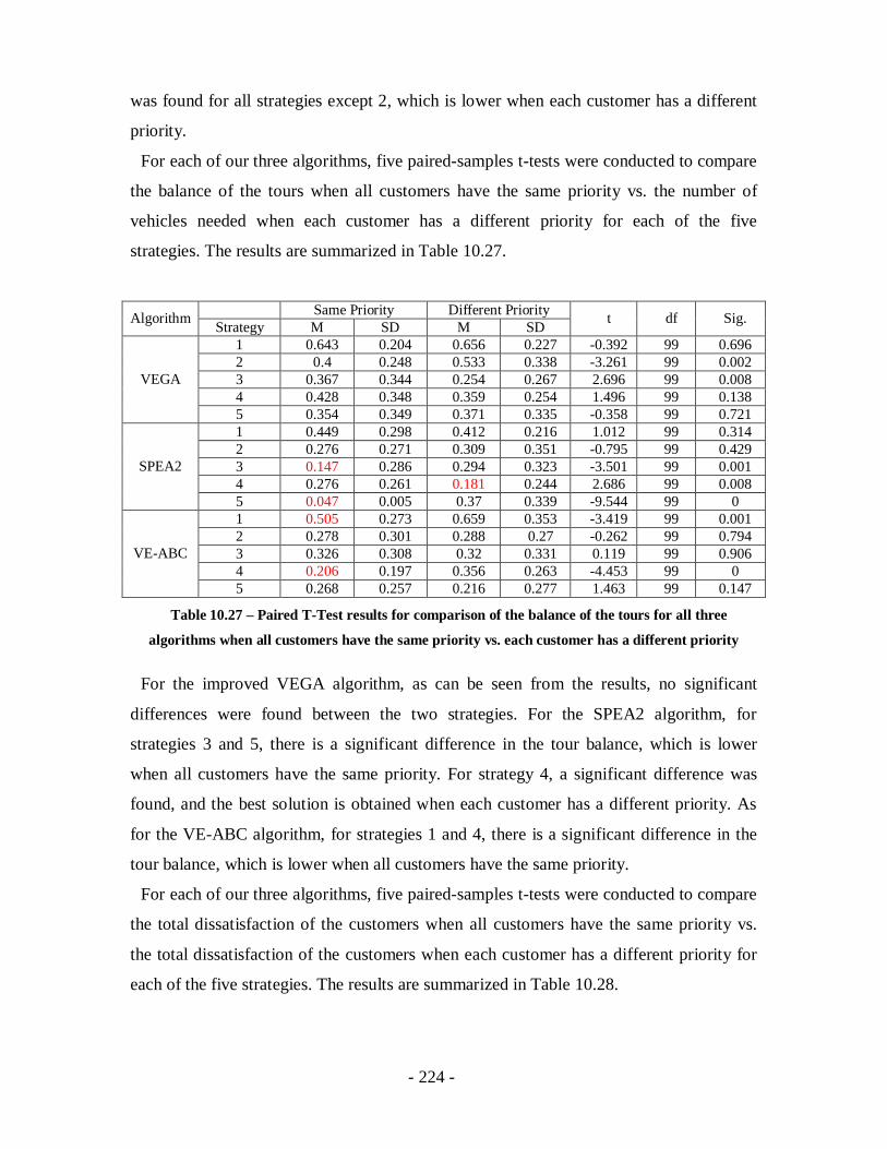
- 224 -
was found for all strategies except 2, which is lower when each customer has a different
priority.
For each of our three algorithms, five paired-samples t-tests were conducted to compare
the balance of the tours when all customers have the same priority vs. the number of
vehicles needed when each customer has a different priority for each of the five
strategies. The results are summarized in Table 10.27.
Same Priority Different PriorityAlgorithm Strategy M SD M SD t df Sig.
1 0.643 0.204 0.656 0.227 -0.392 99 0.6962 0.4 0.248 0.533 0.338 -3.261 99 0.0023 0.367 0.344 0.254 0.267 2.696 99 0.0084 0.428 0.348 0.359 0.254 1.496 99 0.138
VEGA
5 0.354 0.349 0.371 0.335 -0.358 99 0.7211 0.449 0.298 0.412 0.216 1.012 99 0.3142 0.276 0.271 0.309 0.351 -0.795 99 0.4293 0.147 0.286 0.294 0.323 -3.501 99 0.0014 0.276 0.261 0.181 0.244 2.686 99 0.008
SPEA2
5 0.047 0.005 0.37 0.339 -9.544 99 01 0.505 0.273 0.659 0.353 -3.419 99 0.0012 0.278 0.301 0.288 0.27 -0.262 99 0.7943 0.326 0.308 0.32 0.331 0.119 99 0.9064 0.206 0.197 0.356 0.263 -4.453 99 0
VE-ABC
5 0.268 0.257 0.216 0.277 1.463 99 0.147
Table 10.27 – Paired T-Test results for comparison of the balance of the tours for all three
algorithms when all customers have the same priority vs. each customer has a different priority
For the improved VEGA algorithm, as can be seen from the results, no significant
differences were found between the two strategies. For the SPEA2 algorithm, for
strategies 3 and 5, there is a significant difference in the tour balance, which is lower
when all customers have the same priority. For strategy 4, a significant difference was
found, and the best solution is obtained when each customer has a different priority. As
for the VE-ABC algorithm, for strategies 1 and 4, there is a significant difference in the
tour balance, which is lower when all customers have the same priority.
For each of our three algorithms, five paired-samples t-tests were conducted to compare
the total dissatisfaction of the customers when all customers have the same priority vs.
the total dissatisfaction of the customers when each customer has a different priority for
each of the five strategies. The results are summarized in Table 10.28.
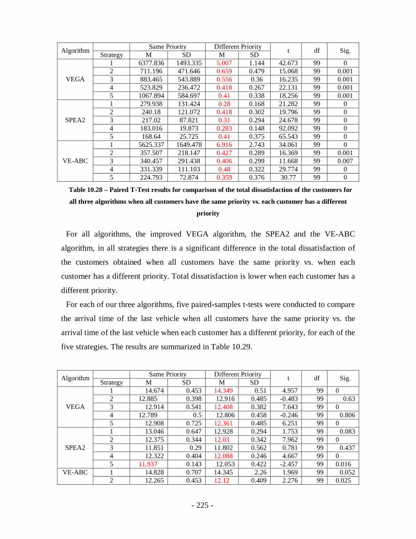
- 225 -
Same Priority Different PriorityAlgorithm Strategy M SD M SD t df Sig.
1 6377.836 1493.335 5.007 1.144 42.673 99 02 711.196 471.646 0.659 0.479 15.068 99 0.0013 883.465 543.889 0.556 0.36 16.235 99 0.0014 523.829 236.472 0.418 0.267 22.131 99 0.001
VEGA
5 1067.894 584.697 0.41 0.338 18.256 99 0.0011 279.938 131.424 0.28 0.168 21.282 99 02 240.18 121.072 0.418 0.302 19.796 99 03 217.02 87.821 0.31 0.294 24.678 99 04 183.016 19.873 0.283 0.148 92.092 99 0
SPEA2
5 168.64 25.725 0.41 0.375 65.543 99 01 5625.337 1649.478 6.916 2.743 34.061 99 02 357.507 218.147 0.427 0.289 16.369 99 0.0013 340.457 291.438 0.406 0.299 11.668 99 0.0074 331.339 111.103 0.48 0.322 29.774 99 0
VE-ABC
5 224.793 72.874 0.359 0.376 30.77 99 0
Table 10.28 – Paired T-Test results for comparison of the total dissatisfaction of the customers for
all three algorithms when all customers have the same priority vs. each customer has a different
priority
For all algorithms, the improved VEGA algorithm, the SPEA2 and the VE-ABC
algorithm, in all strategies there is a significant difference in the total dissatisfaction of
the customers obtained when all customers have the same priority vs. when each
customer has a different priority. Total dissatisfaction is lower when each customer has a
different priority.
For each of our three algorithms, five paired-samples t-tests were conducted to compare
the arrival time of the last vehicle when all customers have the same priority vs. the
arrival time of the last vehicle when each customer has a different priority, for each of the
five strategies. The results are summarized in Table 10.29.
Same Priority Different PriorityAlgorithm Strategy M SD M SD t df Sig.
1 14.674 0.453 14.349 0.51 4.957 99 02 12.885 0.398 12.916 0.485 -0.483 99 0.633 12.914 0.541 12.408 0.382 7.643 99 04 12.789 0.5 12.806 0.458 -0.246 99 0.806
VEGA
5 12.908 0.725 12.361 0.485 6.251 99 01 13.046 0.647 12.928 0.294 1.753 99 0.0832 12.375 0.344 12.03 0.342 7.962 99 03 11.851 0.29 11.802 0.562 0.781 99 0.4374 12.322 0.404 12.088 0.246 4.667 99 0
SPEA2
5 11.937 0.143 12.053 0.422 -2.457 99 0.0161 14.828 0.707 14.345 2.26 1.969 99 0.052VE-ABC2 12.265 0.453 12.12 0.409 2.276 99 0.025

- 226 -
Same Priority Different PriorityAlgorithm Strategy M SD M SD t df Sig.
3 12.069 0.477 12.281 0.444 -3.184 99 0.0024 12.28 0.373 12.139 0.476 2.275 99 0.0255 11.941 0.412 12.165 0.341 -4.176 99 0
Table 10.29 – Paired T-Test results for comparison of the arrival time of the last vehicle for all
three algorithms when all customers have the same priority vs. each customer has a different priority
For the improved VEGA algorithm, as can be seen from the results, for strategies 1, 3
and 5 there is a significant difference in the arrival time of the last vehicle, which is
earlier when each customer has a different priority. For the SPEA2 algorithm, for
strategies 1, 3 and 5 there is a significant difference in the arrival time of the last vehicle,
which is earlier when each customer has a different priority. Strategy 5 provides better
solutions when all customers have the same priority. As for the VE-ABC algorithm,
strategies 3 and 5 provide better solutions when all customers have the same priority,
while strategies 2 and 4 provide better solutions when each customer has a different
priority.
10.7.1.1 Conclusions
For the first objective function, total travel time, a significant difference in the solutions
was found for the improved VEGA, SPEA2 and VE-ABC algorithms, which is better
when each customer has a different priority. Similar results were found for the 2nd
objective function, number of vehicles needed, 4th objective function, customers'
dissatisfaction and 5th objective function, arrival time at the last vehicle.
For the 3rd objective function, tour balance, no significant difference in the solutions
was found.
10.7.2. Strategies Comparison – VEGA algorithm
In order to examine the effect of each of the strategies of the algorithm's results, several
paired t-tests were used.
The first set of paired t-tests was used to compare the results obtained by using
strategies 1 and 2. The results are summarized in Table 10.30.
Strategy 1 Strategy 2Customer’sPriority
ObjectiveFunction M SD M SD t df Sig.

- 227 -
Strategy 1 Strategy 2Customer’sPriority
ObjectiveFunction M SD M SD t df Sig.
1 50.235 2.12 56.78 2.381 -21.565 99 02 9.92 0.787 19.61 3.025 -31.832 99 03 0.643 0.204 0.4 0.248 8.047 99 04 6377.836 1493.335 21.875 14.507 42.487 99 0
The Same
5 14.674 0.453 12.885 0.398 30.295 99 01 49.383 2.051 58.053 2.34 -27.2 99 02 9.98 0.778 18.99 2.97 -29.572 99 03 0.656 0.227 0.533 0.338 2.999 99 0.0034 162.778 37.18 0.659 0.479 43.575 99 0
Different
5 14.349 0.51 12.916 0.485 19.518 99 0
Table 10.30 – Paired T-Test results for comparison of the results of the different objectives
functions when using strategies 1 and 2, when all customers have the same or different priorities
As can be seen from the results, whether or not all customers have the same priority,
strategy 1 provides better solutions in terms of travel time and number of vehicles
needed. Similarly, whether all customers have the same priority or not, strategy 2
provides better solutions in term of tour balance, customers’ dissatisfaction and arrival
time of the last vehicle.
The second set of paired t-tests was used to compare the results obtained by using
strategies 1 and 3. The results are summarized in Table 10.31.
Strategy 1 Strategy 3CustomesPriority
ObjectiveFunction M SD M SD t df Sig.
1 50.235 2.12 53.754 2.328 -10.918 99 02 9.92 0.787 24.18 2.794 -47.002 99 03 0.643 0.204 0.367 0.344 6.803 99 04 6377.836 1493.335 27.174 16.729 42.597 99 0
The Same
5 14.674 0.453 12.914 0.541 24.223 99 01 49.383 2.051 56.329 1.853 -25.204 99 02 9.98 0.778 28.48 2.402 -74.225 99 03 0.656 0.227 0.254 0.267 11.818 99 04 162.778 37.18 0.556 0.36 43.714 99 0
Different
5 14.349 0.51 12.408 0.382 30.631 99 0
Table 10.31 – Paired T-Test results for comparison of the results of the different objectives
functions when using strategies 1 and 3, when all customers have the same or different priorities
As can be seen from the results, whether or not all customers have the same priority,
strategy 1 provides better solutions in terms of travel time and number of vehicles
needed. Similarly, whether or not all customers have the same priority, strategy 3
provides better solutions in terms of tour balance, customers’ dissatisfaction, and arrival
time of the last vehicle.

- 228 -
The third set of paired t-tests was used to compare the results obtained by using
strategies 2 and 3. The results are summarized in Table 10.32.
Strategy 2 Strategy 3Customer’sPriority
ObjectiveFunction M SD M SD t df Sig.
1 56.78 2.381 53.754 2.328 8.758 99 02 19.61 3.025 24.18 2.794 -10.121 99 03 0.4 0.248 0.367 0.344 0.792 99 0.434 711.196 471.646 27.174 16.729 14.463 99 0
The Same
5 12.885 0.398 12.914 0.541 -0.42 99 0.6751 58.053 2.34 56.329 1.853 5.372 99 02 18.99 2.97 28.48 2.402 -25.12 99 03 0.533 0.338 0.254 0.267 6.773 99 04 21.429 15.564 0.556 0.36 13.412 99 0
Different
5 12.916 0.485 12.408 0.382 8.316 99 0
Table 10.32 – Paired T-Test results for comparison of the results of the different objectives
functions when using strategies 2 and 3, when all customers have the same or different priorities
As can be seen from the results, whether all customers have the same priority or not,
strategy 2 provides better solutions only in terms of number of vehicles needed and
strategy 3 provides better solutions in terms of travel time and customers' dissatisfaction.
When when each customer has a different priority, strategy 3 provides better solutions in
terms of tour balance and arrival time of last vehicle as well.
The fourth set of paired t-tests was used to compare the results obtained by using
strategies 2 and 4. The results are summarized in Table 10.33.
Strategy 2 Strategy 4Customer’sPriority
ObjectiveFunction M SD M SD t df Sig.
1 56.78 2.381 58.366 2.827 -4.402 99 02 19.61 3.025 20.67 3.327 -2.458 99 0.0163 0.4 0.248 0.428 0.348 -0.635 99 0.5274 711.196 471.646 16.112 7.274 14.697 99 0
The Same
5 12.885 0.398 12.789 0.5 1.519 99 0.1321 58.053 2.34 57.412 1.972 1.952 99 0.0542 18.99 2.97 19.46 1.684 -1.27 99 0.2073 0.533 0.338 0.359 0.254 3.932 99 04 21.429 15.564 0.418 0.267 13.517 99 0
Different
5 12.916 0.485 12.806 0.458 1.7 99 0.092
Table 10.33 – Paired T-Test results for comparison of the results of the different objectives
functions when using strategies 2 and 4, when all customers have the same or different priorities
As can be seen from the results, when all customers have the same priority, strategy 2
provides better solutions in terms of travel time and number of vehicles needed and

- 229 -
strategy 4 provides better solutions in terms of customers' dissatisfaction. When each
customer has a different priority, strategy 4 provides better solutions in terms of tour
banalce and customers' dissatisfaction.
The fifth set of paired t-tests was used to compare the results obtained by using
strategies 3 and 5. The results are summarized in Table 10.34.
Strategy 3 Strategy 5Customer’sPriority
ObjectiveFunction M SD M SD t df Sig.
1 53.754 2.328 53.321 3.497 0.971 99 0.3342 24.18 2.794 24.32 4.075 -0.271 99 0.7873 0.367 0.344 0.354 0.349 0.28 99 0.784 883.465 543.889 32.847 17.985 15.594 99 0
The Same
5 12.914 0.541 12.908 0.725 0.06 99 0.9521 56.329 1.853 54.425 6.048 3.104 99 0.0022 28.48 2.402 28.06 4.419 0.847 99 0.3993 0.254 0.267 0.371 0.335 -2.68 99 0.0094 18.074 11.721 0.41 0.338 15.116 99 0
Different
5 12.408 0.382 12.361 0.485 0.796 99 0.428
Table 10.34 – Paired T-Test results for comparison of the results of the different objectives
functions when using strategies 3 and 5, when all customers have the same or different priorities
As can be seen from the results, when all customers have the same priority, strategy 5
provides better solutions in terms of customers' dissatisfaction. When each customer has
a different priority, strategy 3 provides better solutions in terms of tour banalce and
strategy 5 provides better solutions in terms of travel time and customers' dissatisfaction.
10.7.2.1 Conclusions
Table 10.35 describes which of the five strategies used provides the best value for each
of the objective functions, when all customers have the same priority and when each
customer has a different priority.
StrategyCustomer’sPriority
ObjectiveFunction 1 2 3 4 5
1 +2 +3 + + + +4 +
The Same
5 + + + +1 +2 +3 +
Different
4 + +
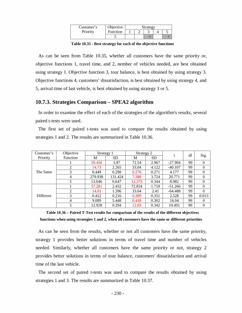
- 230 -
StrategyCustomer’sPriority
ObjectiveFunction 1 2 3 4 5
5 + +
Table 10.35 - Best strategy for each of the objective functions
As can be seen from Table 10.35, whether all customers have the same priority or,
objective functions 1, travel time, and 2, nember of vehicles needed, are best obtained
using strategy 1. Objective function 3, tour balance, is best obtained by using strategy 3.
Objective functions 4, customers’ dissatisfaction, is best obtained by using strategy 4, and
5, arrival time of last vehicle, is best obtained by using strategy 3 or 5.
10.7.3. Strategies Comparison – SPEA2 algorithm
In order to examine the effect of each of the strategies of the algorithm's results, several
paired t-tests were used.
The first set of paired t-tests was used to compare the results obtained by using
strategies 1 and 2. The results are summarized in Table 10.36.
Strategy 1 Strategy 2Customer’sPriority
ObjectiveFunction M SD M SD t df Sig.
1 59.456 3.87 72.54 2.967 -27.904 99 02 14.73 2.265 33.04 4.122 -40.107 99 03 0.449 0.298 0.276 0.271 4.177 99 04 279.938 131.424 7.388 3.724 20.771 99 0
The Same
5 13.046 0.647 12.375 0.344 8.982 99 01 57.281 2.432 72.854 1.718 -51.266 99 02 14.01 1.396 33.64 2.41 -64.488 99 03 0.412 0.216 0.309 0.351 2.528 99 0.0134 9.089 5.448 0.418 0.302 16.04 99 0
Different
5 12.928 0.294 12.03 0.342 19.491 99 0
Table 10.36 – Paired T-Test results for comparison of the results of the different objectives
functions when using strategies 1 and 2, when all customers have the same or different priorities
As can be seen from the results, whether or not all customers have the same priority,
strategy 1 provides better solutions in terms of travel time and number of vehicles
needed. Similarly, whether all customers have the same priority or not, strategy 2
provides better solutions in terms of tour balance, customers' dissatisfaction and arrival
time of the last vehicle.
The second set of paired t-tests was used to compare the results obtained by using
strategies 1 and 3. The results are summarized in Table 10.37.
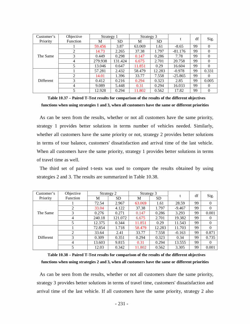
- 231 -
Strategy 1 Strategy 3Customer’sPriority
ObjectiveFunction M SD M SD t df Sig.
1 59.456 3.87 63.069 1.61 -8.65 99 02 14.73 2.265 37.38 1.797 -81.176 99 03 0.449 0.298 0.147 0.286 7.78 99 04 279.938 131.424 6.675 2.701 20.758 99 0
The Same
5 13.046 0.647 11.851 0.29 16.604 99 01 57.281 2.432 58.479 12.283 -0.978 99 0.3312 14.01 1.396 33.77 7.558 -25.865 99 03 0.412 0.216 0.294 0.323 2.85 99 0.0054 9.089 5.448 0.31 0.294 16.033 99 0
Different
5 12.928 0.294 11.802 0.562 17.82 99 0
Table 10.37 – Paired T-Test results for comparison of the results of the different objectives
functions when using strategies 1 and 3, when all customers have the same or different priorities
As can be seen from the results, whether or not all customers have the same priority,
strategy 1 provides better solutions in terms number of vehicles needed. Similarly,
whether all customers have the same priority or not, strategy 2 provides better solutions
in terms of tour balance, customers' dissatisfaction and arrival time of the last vehicle.
When all customers have the same priority, strategy 1 provides better solutions in terms
of travel time as well.
The third set of paired t-tests was used to compare the results obtained by using
strategies 2 and 3. The results are summarized in Table 10.38.
Strategy 2 Strategy 3Customer’sPriority
ObjectiveFunction M SD M SD t df Sig.
1 72.54 2.967 63.069 1.61 28.59 99 02 33.04 4.122 37.38 1.797 -9.467 99 03 0.276 0.271 0.147 0.286 3.293 99 0.0014 240.18 121.072 6.675 2.701 19.382 99 0
The Same
5 12.375 0.344 11.851 0.29 11.543 99 01 72.854 1.718 58.479 12.283 11.703 99 02 33.64 2.41 33.77 7.558 -0.163 99 0.8713 0.309 0.351 0.294 0.323 0.34 99 0.7354 13.603 9.815 0.31 0.294 13.555 99 0
Different
5 12.03 0.342 11.802 0.562 3.305 99 0.001
Table 10.38 – Paired T-Test results for comparison of the results of the different objectives
functions when using strategies 2 and 3, when all customers have the same or different priorities
As can be seen from the results, whether or not all customers share the same priority,
strategy 3 provides better solutions in terms of travel time, customers' dissatisfaction and
arrival time of the last vehicle. If all customers have the same priority, strategy 2 also

- 232 -
provides better solutions in terms of number of vehicles needed, and strategy 3 provides
better solutions in terms of tour balance.
The fourth set of paired t-tests was used to compare the results obtained by using
strategies 2 and 4. The results are summarized in Table 10.39.
Strategy 2 Strategy 4Customer’sPriority
ObjectiveFunction M SD M SD t df Sig.
1 72.54 2.967 72.937 2.7 -0.925 99 0.3572 33.04 4.122 32.16 3.936 1.532 99 0.1293 0.276 0.271 0.276 0.261 0 99 14 240.18 121.072 5.629 0.611 19.372 99 0
The Same
5 12.375 0.344 12.322 0.404 1.027 99 0.3071 72.854 1.718 72.419 3.433 1.144 99 0.2552 33.64 2.41 32.82 2.091 2.638 99 0.013 0.309 0.351 0.187 0.247 2.836 99 0.0064 13.603 9.815 0.345 0.616 13.481 99 0
Different
5 12.03 0.342 12.1 0.272 -1.726 99 0.087
Table 10.39 – Paired T-Test results for comparison of the results of the different objectives
functions when using strategies 2 and 4, when all customers have the same or different priorities
As can be seen from the results, whether or not all customers share the same priority,
strategy 4 provides better solutions in terms of customers' dissatisfaction. When each
customer has a different priority strategy 4 provides better solutions in term of number of
vehicles needed and tour balance, as well.
The fifth set of paired t-tests was used to compare the results obtained by using
strategies 3 and 5. The results are summarized in Table 10.40.
Strategy 3 Strategy 5Customer’sPriority
ObjectiveFunction M SD M SD t df Sig.
1 63.069 1.61 65.885 1.274 -14.827 99 02 37.38 1.797 39.5 1.078 -9.228 99 03 0.147 0.286 0.047 0.005 3.501 99 0.0014 217.02 87.821 5.187 0.791 24.103 99 0
The Same
5 11.851 0.29 11.937 0.143 -2.658 99 0.0091 58.479 12.283 64.9 2.162 -5.216 99 02 33.77 7.558 36.86 2.697 -3.959 99 03 0.294 0.323 0.37 0.339 -1.635 99 0.1054 10.079 9.55 0.41 0.375 10.08 99 0
Different
5 11.802 0.562 12.053 0.422 -3.634 99 0
Table 10.40 – Paired T-Test results for comparison of the results of the different objectives
functions when using strategies 3 and 5, when all customers have the same or different priorities
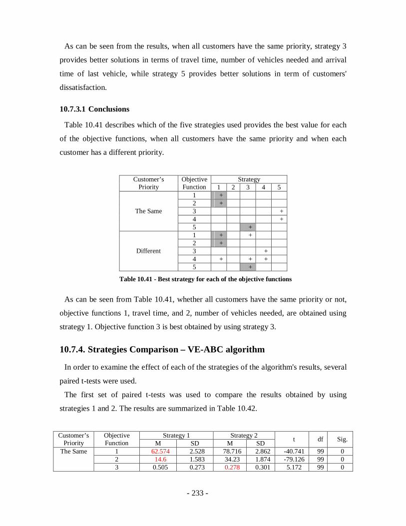
- 233 -
As can be seen from the results, when all customers have the same priority, strategy 3
provides better solutions in terms of travel time, number of vehicles needed and arrival
time of last vehicle, while strategy 5 provides better solutions in term of customers'
dissatisfaction.
10.7.3.1 Conclusions
Table 10.41 describes which of the five strategies used provides the best value for each
of the objective functions, when all customers have the same priority and when each
customer has a different priority.
StrategyCustomer’sPriority
ObjectiveFunction 1 2 3 4 5
1 +2 +3 +4 +
The Same
5 +1 + +2 +3 +4 + + +
Different
5 +
Table 10.41 - Best strategy for each of the objective functions
As can be seen from Table 10.41, whether all customers have the same priority or not,
objective functions 1, travel time, and 2, number of vehicles needed, are obtained using
strategy 1. Objective function 3 is best obtained by using strategy 3.
10.7.4. Strategies Comparison – VE-ABC algorithm
In order to examine the effect of each of the strategies of the algorithm's results, several
paired t-tests were used.
The first set of paired t-tests was used to compare the results obtained by using
strategies 1 and 2. The results are summarized in Table 10.42.
Strategy 1 Strategy 2Customer’sPriority
ObjectiveFunction M SD M SD t df Sig.
1 62.574 2.528 78.716 2.862 -40.741 99 02 14.6 1.583 34.23 1.874 -79.126 99 0
The Same
3 0.505 0.273 0.278 0.301 5.172 99 0
- 234 -
Strategy 1 Strategy 2Customer’sPriority
ObjectiveFunction M SD M SD t df Sig.
4 5625.337 1649.478 10.996 6.71 34.049 99 05 14.828 0.707 12.265 0.453 30.287 99 01 51.812 17.456 79.773 2.033 -16.1 99 02 13.77 2.733 34.4 2.361 -57.21 99 03 0.659 0.353 0.288 0.27 7.668 99 04 224.849 89.19 0.427 0.289 25.153 99 0
Different
5 14.345 2.26 12.12 0.409 9.784 99 0
Table 10.42 – Paired T-Test results for comparison of the results of the different objectives
functions when using strategies 1 and 2, when all customers have the same or different priorities
As can be seen from the results, whether or not all customers have the same priority,
strategy 1 provides better solutions in terms of travel time and number of vehicles
needed. Similarly, whether all customers have the same priority or not, strategy 2
provides better solutions in terms of tour balance, customers’ dissatisfaction, and arrival
time of the last vehicle.
The second set of paired t-tests was used to compare the results obtained by using
strategies 1 and 3. The results are summarized in Table 10.43.
Strategy 1 Strategy 3Customer’sPriority
ObjectiveFunction M SD M SD t df Sig.
1 62.574 2.528 63.547 2.61 -2.888 99 0.0052 14.6 1.583 34.71 3.361 -54.262 99 03 0.505 0.273 0.326 0.308 4.606 99 04 5625.337 1649.478 10.472 8.964 34.004 99 0
The Same
5 14.828 0.707 12.069 0.477 30.767 99 01 51.812 17.456 63.372 2.33 -6.5 99 02 13.77 2.733 33.47 3.096 -45.959 99 03 0.659 0.353 0.32 0.331 7.002 99 04 224.849 89.19 0.406 0.299 25.16 99 0
Different
5 14.345 2.26 12.281 0.444 8.982 99 0
Table 10.43 – Paired T-Test results for comparison of the results of the different objectives
functions when using strategies 1 and 3, when all customers have the same or different priorities
As can be seen from the results, whether or not all customers have the same priority,
strategy 1 provides better solutions in terms of travel time and number of vehicles
needed. Similarly, whether all customers have the same priority or not, strategy 3
provides better solutions in terms of tour balance, customers’ dissatisfaction, and arrival
time of the last vehicle.
- 235 -
The third set of paired t-tests was used to compare the results obtained by using
strategies 2 and 3. The results are summarized in Table 10.44.
Strategy 2 Strategy 3Customer’sPriority
ObjectiveFunction M SD M SD t df Sig.
1 78.716 2.862 63.547 2.61 38.245 99 02 34.23 1.874 34.71 3.361 -1.223 99 0.2243 0.278 0.301 0.326 0.308 -1.143 99 0.2564 357.507 218.147 10.472 8.964 15.929 99 0
The Same
5 12.265 0.453 12.069 0.477 2.865 99 0.0051 79.773 2.033 63.372 2.33 49.484 99 02 34.4 2.361 33.47 3.096 2.457 99 0.0163 0.288 0.27 0.32 0.331 -0.787 99 0.4334 13.89 9.408 0.406 0.299 14.285 99 0
Different
5 12.12 0.409 12.281 0.444 -2.887 99 0.005
Table 10.44 – Paired T-Test results for comparison of the results of the different objectives
functions when using strategies 2 and 3, when all customers have the same or different priorities
As can be seen from the results, strategy 3 provides better solutions in terms of travel
time and customers' dissatisfaction, whether all customers have the same priority or not.
The fourth set of paired t-tests was used to compare the results obtained by using
strategies 2 and 4. The results are summarized in Table 10.45.
Strategy 2 Strategy 4Customer’sPriority
ObjectiveFunction M SD M SD t df Sig.
1 78.716 2.862 79.326 1.982 -1.701 99 0.0922 34.23 1.874 34.1 2.607 0.4 99 0.693 0.278 0.301 0.206 0.197 1.997 99 0.0494 357.507 218.147 10.192 3.417 15.923 99 0
The Same
5 12.265 0.453 12.28 0.373 -0.252 99 0.8011 79.773 2.033 74.508 10.636 4.972 99 02 34.4 2.361 31.93 5.044 4.604 99 03 0.288 0.27 0.356 0.263 -1.862 99 0.0664 13.89 9.408 0.48 0.322 14.189 99 0
Different
5 12.12 0.409 12.139 0.476 -0.292 99 0.771
Table 10.45 – Paired T-Test results for comparison of the results of the different objectives
functions when using strategies 2 and 4, when all customers have the same or different priorities
As can be seen from the results, when all customers have the same priority, Strategy 4
provides better solutions in terms of tour balance and customers' dissatisfaction. When
each customer has a different priority, strategy 4 provides better solutions in terms of
travel time, number of vehicles and customers' dissatisfaction.

- 236 -
The fifth set of paired t-tests was used to compare the results obtained by using
strategies 3 and 5. The results are summarized in Table 10.46.
Strategy 3 Strategy 5Customer’sPriority
ObjectiveFunction M SD M SD t df Sig.
1 63.547 2.61 63.902 2.405 -0.956 99 0.3412 34.71 3.361 33.93 4.344 1.363 99 0.1763 0.326 0.308 0.268 0.257 1.622 99 0.1084 340.457 291.438 6.914 2.242 11.464 99 0
The Same
5 12.069 0.477 11.941 0.412 2.03 99 0.0451 63.372 2.33 63.653 1.841 -0.909 99 0.3652 33.47 3.096 32.2 4.355 2.298 99 0.0243 0.32 0.331 0.216 0.277 2.692 99 0.0084 13.196 9.725 0.359 0.376 13.268 99 0
Different
5 12.281 0.444 12.165 0.341 2.033 99 0.045
Table 10.46 – Paired T-Test results for comparison of the results of the different objectives
functions when using strategies 3 and 5, when all customers have the same or different priorities
As can be seen from the results, whether all customers have the same priority or each
customer has a different priority, for objective function 4 and 5, the best solutions are
obtained using strategy 5. When each customer has a different priority, for objectives 2
and 3, the best solutions are obtained using strategy 5, as well.
10.7.4.1 Conclusions
Table 10.47 describes which of the five strategies used provides the best value for each
of the objective functions, when all customers have the same priority and when each
customer has a different priority.
StrategyCustomes Priority ObjectiveFunction 1 2 3 4 5
1 +2 +3 + +4 +
The Same
5 +1 +2 +3 + +4 + + +
Different
5 + + +
Table 10.47 - Best strategy for each of the objective functions

- 237 -
As can be seen from Table 10.47, whether or not all customers have the same priority,
objective functions 1, travel time, and 2, number of vehicles needed, are best obtained by
using strategy 1. Objective functions 3, tour balance, 4, customers’ dissatisfaction, and 5,
arrival time of the last vehicle, are obtained by using strategy 5.
10.7.5. Algorithms Comparison
Since in the real-world, information on travel time and customers’ demands are not
known in advance, strategy 5 has to be used. Table 10.24 compares the results obtained
for each of the five objectives, using paired t-tests, functions by each one of the three
algorithms when applying the 3rd strategy. For each objective function, the best value
obtained is highlighted in red.
AlgorithmCustomer’sPriority Objective Function Imp. VEGA SPEA2 VE-ABC
1 64.833 50.235 59.4562 15.33 9.92 14.733 0.64 0.643 0.4494 54.925 196.174 8.611
The Same
5 14.364 14.674 13.0461 77.627 49.383 57.2812 35.42 9.98 14.013 0.351 0.656 0.4124 0.549 5.007 0.28
Different
5 12.491 14.349 12.928
Table 10.48 - Comparison of the 5th strategy used in all three algorithms
As it can be seen, whether all customers have the same priority or not, objective
function 1, travel time, and objective function 2, number of vehicles needed, , are best
obtained using the SPEA2 algorithm, while objective functions 3, tour balance, and 4,
customers' dissatisfaction are best obtained using the VE-ABC algorithm.
When all customers have the same priority, objective function 5, arrival time of last
vehicle, is best obtained by using the VE-ABC algorithm. When each customer has a
different priority, objective function 5 is best obtained by using the improved improved
VEGA algorithm.

- 238 -
10.7.6. Conclusions
For all three algorithms, whether all customers have the same priority or not, objective
functions 1, travel time, and 2, number of vehicles needed, are best obtained using
strategy 1. Objective functions 3, tour balance, 4, customers’ dissatisfaction, and 5,
arrival time of the last vehicle, are best obtained either by using strategy 3 or by using
strategy 5.
Also, in all objective function, except the 3rd, tour balance, better solutions are obtained
when each customer has a different priority.
Since in the real-world, information on travel time and customers’ demands are not
known in advance, strategy 5 has to be used.
10.8. Case Study 3 – Israel
In the first case study the test scenario is defined as follows:
1. Network: Israeli transportation network.
2. Dissatisfaction function: It is assumed that the dissatisfaction functions of all
customers are linear, meaning1
1 ii S
i i
t EETf tTW EET
and
1
( ) 1i Ei
ELT tg tELT TW
.
The test scenario is solved 100 times. For the first 50 times, it is assumed that all
customers have the same priority. Under this assumption, the test scenario is solved 100
times using each of the 5 strategies described earlier. In the next 50 times, it is assumed
that each customer has a priority equal to his demand. Under this assumption, the test
scenario is solved 10 times using each of the 5 strategies described earlier.
10.8.1. Priority Comparison
For each of our three algorithms, five paired-samples t-tests were conducted to compare
the total travel time obtained when all customers have the same priority vs. the travel
time obtained when each customer has a different priority for each of the five strategies.
The results are summarized in Table 10.49.

- 239 -
Same Priority Different PriorityAlgorithm Strategy M SD M SD t df Sig.
1 74.974 5.924 72.845 3.976 0.901 99 0.3912 96.128 3.969 90.521 23.406 0.703 99 0.53 86.641 8.965 95.254 7.626 -2.329 99 0.0444 95.456 7.829 93.787 6.484 0.5 99 0.626
VEGA
5 84.384 7.974 90.053 16.162 -1.204 99 0.2561 98.488 9.378 91.669 3.735 2.743 99 0.0222 104.88 23.569 106.365 12.749 -0.147 99 0.8883 92.095 19.482 99.452 2.965 -1.157 99 0.2774 115.649 7.46 107.252 12.717 1.761 99 0.111
SPEA2
5 86.673 15.228 97.353 8.663 -1.946 99 0.0841 103.968 16.345 115.347 6.932 -1.98 99 0.082 134.079 6.567 131.377 6.612 0.793 99 0.453 90.844 17.594 95.083 18.005 -0.432 99 0.6774 131.438 6.422 128.261 9.603 0.786 99 0.454
VE-ABC
5 93.226 18.392 100.054 3.977 -1.106 99 0.299
Table 10.49 – Paired T-Test results for comparison of the total travel time for all three algorithms
when all customers have the same priority vs. each customer has a different priority
For the improved VEGA algorithm, as evident from the results, for strategy 3 there
exists a significant difference in travel time, which is lower when all customers have the
same priority. For the SPEA2 algorithm, there is a significant difference in the travel time
only for strategy 1, which is lower when each customer has a different priority.
For each of our three algorithms, five paired-samples t-tests were conducted to compare
the number of vehicles needed when all customers have the same priority vs. the number
of vehicles needed when each customer has a different priority, for each of the five
strategies. The results are summarized in Table 10.50.
Same Priority Different PriorityAlgorithm Strategy M SD M SD t df Sig.
1 8.622 1.153 8.01 0.787 1.244 99 0.2432 14.747 1.334 14.284 2.861 0.478 99 0.6463 15.991 2.464 17.878 1.116 -2.374 99 0.0444 15.154 1.789 14.45 1.504 1.172 99 0.273
VEGA
5 15.584 1.686 16.791 2.981 -1.208 99 0.2611 13.339 1.825 12.707 1.202 1.154 99 0.282 18.105 2.346 18.789 2.727 -0.459 99 0.6553 19.503 3.212 19.296 0.854 0.17 99 0.8694 18.662 1.019 17.738 2.529 0.863 99 0.41
SPEA2
5 17.628 2.596 19.914 1.13 -2.724 99 0.0211 13.105 2.53 14.513 1.754 -1.497 99 0.1692 21.824 1.367 21.11 1.288 1.261 99 0.2383 18.419 4.148 18.366 3.572 0.101 99 0.9214 21.181 1.33 20.657 1.409 0.898 99 0.393
VE-ABC
5 18.592 3.484 19.341 1.144 -0.811 99 0.437
- 240 -
Table 10.50 – Paired T-Test results for comparison of the number of vehicles needed for all three
algorithms when all customers have the same priority vs. each customer has a different priority
For the improved VEGA algorithm, as apparent from the results for strategy 3, there is a
significant difference in the number of vehicles needed, which is lower when all
customers have the same priority. For the SPEA2 algorithm, for strategy 5 there is a
significant difference in travel time, which, again, is lower when all customers have the
same priority.
For each of our three algorithms, five paired-samples t-tests were conducted to compare
the balance of the tours when all customers have the same priority vs. the number of
vehicles needed when each customer has a different priority, for each of the five
strategies. The results are summarized in Table 10.51.
Same Priority Different PriorityAlgorithm Strategy M SD M SD t df Sig.
1 2.323 1.089 1.714 0.667 1.066 99 0.3132 1.535 0.539 1.428 0.752 0.284 99 0.7823 1.007 0.531 0.8 0.554 0.388 99 0.7054 1.602 0.928 1.495 0.381 0.463 99 0.655
VEGA
5 1.048 0.525 0.715 0.147 1.641 99 0.1341 0.947 0.488 0.929 0.597 -0.442 99 0.6682 1.091 0.485 1.163 0.424 -0.03 99 0.9763 0.446 0.081 0.713 0.117 -2.989 99 0.0164 1.303 0.456 1.319 0.51 0.267 99 0.796
SPEA2
5 0.722 0.26 0.694 0.414 -0.716 99 0.491 1.681 1.06 1.513 0.526 0.17 99 0.8682 0.691 0.458 1.005 0.244 -1.249 99 0.2423 0.713 0.697 0.855 0.174 -0.346 99 0.744 1.107 0.411 0.681 0.404 2.158 99 0.057
VE-ABC
5 5.463 9.673 0.873 0.382 1.466 99 0.176
Table 10.51 – Paired T-Test results for comparison of the balance of the tours for all three
algorithms when all customers have the same priority vs. each customer has a different priority
Only for the SPEA2 algorithm with strategy 3 shows a significant difference in the tour
balance, which is lower when all customers have the same priority.
For each of our three algorithms, five paired-samples t-tests were conducted to compare
the total dissatisfaction of the customers when all customers have the same priority vs.
the total dissatisfaction of the customers when each customer has a different priority for
each of the five strategies. The results are summarized in Table 10.52.
- 241 -
Same Priority Different PriorityAlgorithm Strategy M SD M SD t df Sig.
1 3026.267 1079.539 4.606 2.096 8.851 99 02 180.668 185.374 0.121 0.154 3.079 99 0.0113 989.097 510.017 0.115 0.174 6.13 99 0.0024 173.122 241.857 0.177 0.135 2.264 99 0.049
VEGA
5 990.146 476.367 0.218 0.288 6.572 99 0.0021 81.914 76 0.179 0.17 3.407 99 0.0092 38.053 20.122 0.008 0.058 5.989 99 0.0013 348.95 175.098 0.122 -0.021 6.303 99 0.0024 34.289 7.813 0.059 0.07 13.919 99 0.001
SPEA2
5 516.48 338.355 0.075 0.122 4.826 99 0.0031 3094.087 1660.215 2.947 1.204 5.89 99 02 48.242 10.91 0.151 0.033 13.881 99 0.0013 949.718 594.273 0.013 0.234 5.052 99 0.0014 66.352 56.454 0.074 0.037 3.721 99 0.006
VE-ABC
5 777.402 518.056 0.027 0.135 4.746 99 0
Table 10.52 – Paired T-Test results for comparison of the total dissatisfaction of the customers for
all three algorithms when all customers have the same priority vs. each customer has a different
priority
For all algorithms and for all strategies, there are significant differences in the total
dissatisfaction of the customers, which are lower when each customer has a different
priority.
For each of our three algorithms, five paired-samples t-test were conducted to compare
the arrival time of the last vehicle when all customers have the same priority vs. the
arrival time of the last vehicle when each customer has a different priority for each of the
five strategies. The results are summarized in Table 10.53.

- 242 -
Same Priority Different PriorityAlgorithm Strategy M SD M SD t df Sig.
1 21.31 0.807 21.348 1.001 0.068 99 0.9492 20.092 0.682 19.275 2.021 1.065 99 0.3163 21.682 0.631 21.199 0.71 1.635 99 0.1364 19.986 1.206 20.17 0.947 -0.399 99 0.696
VEGA
5 21.241 1.517 20.682 1.781 0.775 99 0.4611 19.45 0.167 19.448 0.003 0.302 99 0.7722 18.346 2.258 19.282 1.394 -0.966 99 0.3623 20.571 2.678 21.083 0.53 -0.537 99 0.6044 19.268 1.2 19.103 1.261 0.241 99 0.814
SPEA2
5 20.972 2.753 20.792 1.994 0.106 99 0.9181 21.764 1.463 21.158 1.35 0.7 99 0.5022 19.823 0.733 19.812 0.686 -0.019 99 0.9863 20.283 2.173 20.438 1.976 -0.145 99 0.8864 19.746 0.941 19.666 0.273 0.071 99 0.944
VE-ABC
5 20.794 2.415 20.999 0.662 -0.418 99 0.686
Table 10.53 – Paired T-Test results for comparison of the arrival time of the last vehicle for all
three algorithms when all customers have the same priority vs. each customer has a different priority
For all algorithms and for all strategies, there are no significant differences in the arrival
time of the last vehicle.
10.8.1.1 Conclusions
For the fourth objective function, customers’ dissatisfaction, the best solution is
obtained when each customer has a different objective function, for all strategies and all
algorithms.
For the other objectives, no significant differences were found between the results
obtained when all customers have the same priority, and the results obtained when each
customer has a different priority, for all strategies and algorithms
10.8.2. Strategies Comparison – VEGA algorithm
In order to examine the effect of each of the strategies of the algorithm's results, several
paired t-tests were used.
The first set of paired t-tests was used to compare the results obtained by using
strategies 1 and 2. The results are summarized in Table 10.54.

- 243 -
Strategy 1 Strategy 2Customer’sPriority
ObjectiveFunction M SD M SD t df Sig.
1 74.917 5.738 96.128 3.976 -7.58 99 0.0022 8.539 1.113 14.739 1.428 -10.464 99 03 2.33 1.112 1.367 0.627 2.475 99 0.0334 93.131 33.104 5.591 5.781 8.558 99 0
The Same
5 21.304 0.749 19.984 0.577 4.192 99 0.0041 72.816 3.989 90.538 23.562 -2.345 99 0.0432 8.177 0.859 14.223 2.919 -6.017 99 0.0013 1.693 0.67 1.421 0.806 1.102 99 0.2974 4.631 2.078 0.115 0.109 7.178 99 0.001
Different
5 21.347 0.945 19.4 2.045 2.867 99 0.02
Table 10.54 – Paired T-Test results for comparison of the results of the different objectives
functions when using strategies 1 and 2, when all customers have the same or different priorities
As evident from the results, whether or not all customers have the same priority,
strategy 1 provides better solutions in terms of travel time and number of vehicles
needed. Similarly, whether all customers have the same priority or not, strategy 2
provides better solutions in terms of customers’ dissatisfaction and arrival time of the last
vehicle. When all customers have the same priority, strategy 2 also provides better
solutions in terms of tour balance.
The second set of paired t-tests was used to compare the results obtained by using
strategies 1 and 3. The results are summarized in Table 10.55.
Strategy 1 Strategy 3Customer’sPriority
ObjectiveFunction M SD M SD t df Sig.
1 74.998 5.735 86.641 9.06 -2.946 99 0.0152 8.668 1.047 15.887 2.608 -6.66 99 03 2.289 1.21 0.908 0.576 4.61 99 0.0024 93.073 33.216 30.392 15.752 5.641 99 0.001
The Same
5 21.396 0.759 21.722 0.652 -0.957 99 0.3631 72.759 4.011 95.29 7.676 -7.574 99 0.0012 8.167 0.909 17.985 1.197 -25.211 99 0.0023 1.845 0.646 0.936 0.486 4.146 99 04 4.732 2.031 0.106 0.072 7.059 99 0.001
Different
5 21.293 1.068 21.173 0.717 0.413 99 0.687
Table 10.55 – Paired T-Test results for comparison of the results of the different objectives
functions when using strategies 1 and 3, when all customers have the same or different priorities
As may be seen from the results, whether or not all customers have the same priority,
strategy 1 provides better solutions in terms of travel time and number of vehicles

- 244 -
needed. Similarly, whether all customers have the same priority or not, strategy 2
provides better solutions in terms of tour balance and customers’ dissatisfaction.
The third set of paired t-tests was used to compare the results obtained by using
strategies 2 and 3. The results are summarized in Table 10.56.
Strategy 2 Strategy 3Customer’sPriority
ObjectiveFunction M SD M SD t df Sig.
1 96.015 3.923 86.604 9.079 3.516 99 0.0092 14.702 1.358 15.968 2.535 -1.16 99 0.2753 1.385 0.582 0.974 0.501 2.405 99 0.0394 5.482 5.633 30.411 15.647 -5.492 99 0.001
The Same
5 20.003 0.688 21.591 0.734 -5.28 99 0.0011 90.435 23.557 95.391 7.713 -0.609 99 0.5572 14.319 2.882 17.997 1.211 -3.553 99 0.0053 1.34 0.729 0.883 0.429 1.87 99 0.0944 0.038 0.184 0.228 0.117 -2.626 99 0.027
Different
5 19.319 1.894 21.123 0.764 -2.729 99 0.023
Table 10.56 – Paired T-Test results for comparison of the results of the different objectives
functions when using strategies 2 and 3, when all customers have the same or different priorities
As evident from the results, whether or not all customers have the same priority,
strategy 2 provides better solutions only in terms of customer dissatisfaction and arrival
time of the last vehicle. When all customers have the same priority, strategy 3 provides
better solutions in terms of travel time and tour balance. When each customer has
different priorities, strategy 2 provides better solutions in terms of the number of vehicles
needed.
The fourth set of paired t-tests was used to compare the results obtained by using
strategies 2 and 4. The results are summarized in Table 10.57.

- 245 -
Strategy 2 Strategy 4Customer’sPriority
ObjectiveFunction M SD M SD t Df Sig.
1 96.13 3.931 95.468 7.887 0.211 99 0.8382 14.751 1.381 15.093 1.781 -0.52 99 0.6183 1.442 0.548 1.623 1.004 -0.464 99 0.6534 5.536 5.691 5.361 7.345 0.068 99 0.949
The Same
5 19.944 0.606 19.967 1.16 0.184 99 0.8581 90.565 23.404 93.932 6.541 -0.431 99 0.6762 14.352 2.793 14.386 1.653 -0.094 99 0.9283 1.429 0.796 1.373 0.282 -0.106 99 0.924 0.106 0.081 0.047 0.144 -0.44 99 0.668
Different
5 19.349 2.022 20.213 0.924 -1.146 99 0.281
Table 10.57 – Paired T-Test results for comparison of the results of the different objectives
functions when using strategies 2 and 4, when all customers have the same or different priorities
As may be seen from the results, no significant difference was found for any of the
objective functions.
The fifth set of paired t-tests was used to compare the results obtained by using
strategies 3 and 5. The results are summarized in Table 10.58.
Strategy 3 Strategy 5Customer’sPriority
ObjectiveFunction M SD M SD t df Sig.
1 86.78 8.919 84.353 8.035 0.648 99 0.5352 15.923 2.528 15.607 1.861 0.26 99 0.8013 0.954 0.519 0.935 0.478 -0.098 99 0.9244 30.452 15.672 30.4 14.666 -0.007 99 0.993
The Same
5 21.619 0.687 21.203 1.508 0.647 99 0.5351 95.238 7.577 89.941 16.223 1.058 99 0.3162 17.85 1.28 16.752 2.833 1.177 99 0.2683 0.83 0.533 0.664 0.148 1.127 99 0.294 0.16 0.17 0.107 0.197 0.018 99 0.986
Different
5 21.142 0.622 20.654 1.811 0.637 99 0.54
Table 10.58 – Paired T-Test results for comparison of the results of the different objectives
functions when using strategies 3 and 5, when all customers have the same or different priorities
As seen from the results, no significant difference was found for any of the objective
functions.
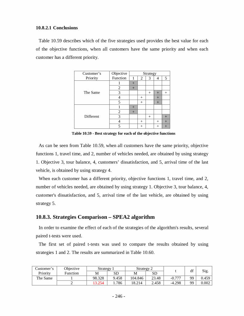
- 246 -
10.8.2.1 Conclusions
Table 10.59 describes which of the five strategies used provides the best value for each
of the objective functions, when all customers have the same priority and when each
customer has a different priority.
StrategyCustomer’sPriority
ObjectiveFunction 1 2 3 4 5
1 +2 +3 + + +4 + +
The Same
5 + +1 +2 +3 + +4 + + +
Different
5 + + +
Table 10.59 - Best strategy for each of the objective functions
As can be seen from Table 10.59, when all customers have the same priority, objective
functions 1, travel time, and 2, number of vehicles needed, are obtained by using strategy
1. Objective 3, tour balance, 4, customers’ dissatisfaction, and 5, arrival time of the last
vehicle, is obtained by using strategy 4.
When each customer has a different priority, objective functions 1, travel time, and 2,
number of vehicles needed, are obtained by using strategy 1. Objective 3, tour balance, 4,
customer's dissatisfaction, and 5, arrival time of the last vehicle, are obtained by using
strategy 5.
10.8.3. Strategies Comparison – SPEA2 algorithm
In order to examine the effect of each of the strategies of the algorithm's results, several
paired t-tests were used.
The first set of paired t-tests was used to compare the results obtained by using
strategies 1 and 2. The results are summarized in Table 10.60.
Strategy 1 Strategy 2Customer’sPriority
ObjectiveFunction M SD M SD t df Sig.
1 98.328 9.458 104.846 23.48 -0.777 99 0.459The Same2 13.254 1.786 18.214 2.458 -4.298 99 0.002

- 247 -
Strategy 1 Strategy 2Customer’sPriority
ObjectiveFunction M SD M SD t df Sig.
3 0.764 0.421 1.187 0.547 -1.913 99 0.0874 2.514 2.364 1.223 0.521 1.647 99 0.1335 19.635 0.227 18.208 2.198 1.73 99 0.121 91.628 3.761 106.35 12.629 -3.561 99 0.0062 12.755 1.306 18.684 2.75 -6.902 99 0.0023 0.893 0.46 1.222 0.465 -0.619 99 0.5534 0.055 0.15 0.011 -0.06 1.869 99 0.096
Different
5 19.549 0.058 19.174 1.382 0.686 99 0.509
Table 10.60 – Paired T-Test results for comparison of the results of the different objectives
functions when using strategies 1 and 2, when all customers have the same or different priorities
As reflected in the results, whether or not all customers have the same priority, strategy
1 provides better solutions in terms of the number of vehicles needed. When each
customer has a different priority, strategy 1 provides better solutions in terms of travel
time as well.
The second set of paired t-tests was used to compare the results obtained by using
strategies 1 and 3. The results are summarized in Table 10.61.
Strategy 1 Strategy 3Customer’sPriority
ObjectiveFunction M SD M SD t df Sig.
1 98.349 9.374 92.17 19.5 0.935 99 0.3762 13.222 1.73 19.537 3.158 -5.424 99 0.0023 0.901 0.434 0.581 0.229 2.55 99 0.0324 2.493 2.288 10.69 5.37 -3.961 99 0.004
The Same
5 19.642 0.306 20.585 2.643 -1.268 99 0.2391 91.589 3.763 99.389 2.978 -4.847 99 0.0012 12.687 1.259 19.394 1.033 -13.863 99 0.0023 0.929 0.592 0.802 0.126 1.162 99 0.2754 0.185 0.041 0.143 0.056 2.009 99 0.074
Different
5 19.437 0.165 21.098 0.362 -11.042 99 0.001
Table 10.61 – Paired T-Test results for comparison of the results of the different objectives
functions when using strategies 1 and 3, when all customers have the same or different priorities
As may be seen from the results, whether or not all customers have the same priority,
strategy 1 provides better solutions in terms of the number of vehicles needed. When all
customers have the same priority, strategy 1 provides better results in terms of customers’
dissatisfaction. When each customer has a different priority, strategy 1 provides better
solutions in terms of travel time and arrival time of the last vehicle.
The third set of paired t-tests was used to compare the results obtained by using
strategies 2 and 3. The results are summarized in Table 10.62.
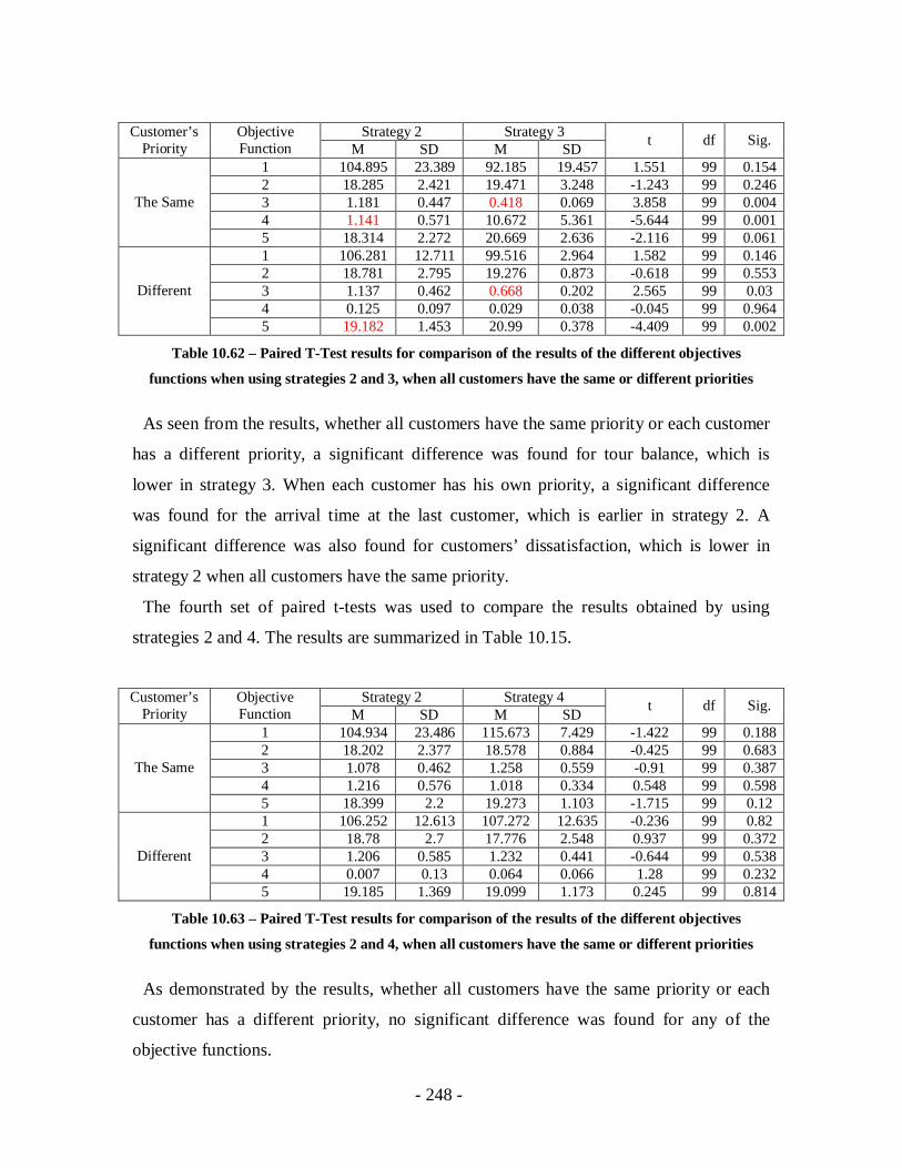
- 248 -
Strategy 2 Strategy 3Customer’sPriority
ObjectiveFunction M SD M SD t df Sig.
1 104.895 23.389 92.185 19.457 1.551 99 0.1542 18.285 2.421 19.471 3.248 -1.243 99 0.2463 1.181 0.447 0.418 0.069 3.858 99 0.0044 1.141 0.571 10.672 5.361 -5.644 99 0.001
The Same
5 18.314 2.272 20.669 2.636 -2.116 99 0.0611 106.281 12.711 99.516 2.964 1.582 99 0.1462 18.781 2.795 19.276 0.873 -0.618 99 0.5533 1.137 0.462 0.668 0.202 2.565 99 0.034 0.125 0.097 0.029 0.038 -0.045 99 0.964
Different
5 19.182 1.453 20.99 0.378 -4.409 99 0.002
Table 10.62 – Paired T-Test results for comparison of the results of the different objectives
functions when using strategies 2 and 3, when all customers have the same or different priorities
As seen from the results, whether all customers have the same priority or each customer
has a different priority, a significant difference was found for tour balance, which is
lower in strategy 3. When each customer has his own priority, a significant difference
was found for the arrival time at the last customer, which is earlier in strategy 2. A
significant difference was also found for customers’ dissatisfaction, which is lower in
strategy 2 when all customers have the same priority.
The fourth set of paired t-tests was used to compare the results obtained by using
strategies 2 and 4. The results are summarized in Table 10.15.
Strategy 2 Strategy 4Customer’sPriority
ObjectiveFunction M SD M SD t df Sig.
1 104.934 23.486 115.673 7.429 -1.422 99 0.1882 18.202 2.377 18.578 0.884 -0.425 99 0.6833 1.078 0.462 1.258 0.559 -0.91 99 0.3874 1.216 0.576 1.018 0.334 0.548 99 0.598
The Same
5 18.399 2.2 19.273 1.103 -1.715 99 0.121 106.252 12.613 107.272 12.635 -0.236 99 0.822 18.78 2.7 17.776 2.548 0.937 99 0.3723 1.206 0.585 1.232 0.441 -0.644 99 0.5384 0.007 0.13 0.064 0.066 1.28 99 0.232
Different
5 19.185 1.369 19.099 1.173 0.245 99 0.814
Table 10.63 – Paired T-Test results for comparison of the results of the different objectives
functions when using strategies 2 and 4, when all customers have the same or different priorities
As demonstrated by the results, whether all customers have the same priority or each
customer has a different priority, no significant difference was found for any of the
objective functions.

- 249 -
The fifth set of paired t-tests was used to compare the results obtained by using
strategies 3 and 5. The results are summarized in Table 10.16.
Strategy 3 Strategy 5Customer’sPriority
ObjectiveFunction M SD M SD t df Sig.
1 92.027 19.434 86.593 15.166 0.562 99 0.5912 19.466 3.112 17.766 2.537 1.129 99 0.2893 0.51 0.099 0.671 0.377 -1.268 99 0.2374 10.722 5.297 15.877 10.311 -1.336 99 0.214
The Same
5 20.66 2.695 20.791 2.761 -0.197 99 0.8491 99.35 3.041 97.33 8.619 0.727 99 0.4882 19.335 0.917 20.097 1.089 -1.411 99 0.1913 0.686 0.272 0.843 0.386 -0.034 99 0.9744 0.038 0.01 0.04 0.167 -0.737 99 0.48
Different
5 21.038 0.537 20.729 2.118 0.373 99 0.719
Table 10.64 – Paired T-Test results for comparison of the results of the different objectives
functions when using strategies 3 and 5, when all customers have the same or different priorities
As reflected by the results, whether all customers have the same priority or each
customer has a different priority, no significant difference was found for any of the
objective functions.
10.8.3.1 Conclusions
Table 10.65 describes which of the five strategies used provides the best value for each
of the objective functions, when all customers have the same priority and when each
customer has a different priority.
StrategyCustomer’sPriority
ObjectiveFunction 1 2 3 4 5
1 + + + +2 +3 + +4 + + +
The Same
5 + + + + +1 + +2 +3 + + +4 + + + +
Different
5 + + +
Table 10.65 - Best strategy for each of the objective functions
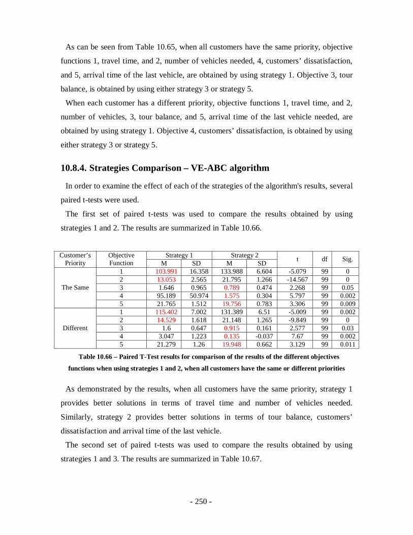
- 250 -
As can be seen from Table 10.65, when all customers have the same priority, objective
functions 1, travel time, and 2, number of vehicles needed, 4, customers’ dissatisfaction,
and 5, arrival time of the last vehicle, are obtained by using strategy 1. Objective 3, tour
balance, is obtained by using either strategy 3 or strategy 5.
When each customer has a different priority, objective functions 1, travel time, and 2,
number of vehicles, 3, tour balance, and 5, arrival time of the last vehicle needed, are
obtained by using strategy 1. Objective 4, customers’ dissatisfaction, is obtained by using
either strategy 3 or strategy 5.
10.8.4. Strategies Comparison – VE-ABC algorithm
In order to examine the effect of each of the strategies of the algorithm's results, several
paired t-tests were used.
The first set of paired t-tests was used to compare the results obtained by using
strategies 1 and 2. The results are summarized in Table 10.66.
Strategy 1 Strategy 2Customer’sPriority
ObjectiveFunction M SD M SD t df Sig.
1 103.991 16.358 133.988 6.604 -5.079 99 02 13.053 2.565 21.795 1.266 -14.567 99 03 1.646 0.965 0.789 0.474 2.268 99 0.054 95.189 50.974 1.575 0.304 5.797 99 0.002
The Same
5 21.765 1.512 19.756 0.783 3.306 99 0.0091 115.402 7.002 131.389 6.51 -5.009 99 0.0022 14.529 1.618 21.148 1.265 -9.849 99 03 1.6 0.647 0.915 0.161 2.577 99 0.034 3.047 1.223 0.135 -0.037 7.67 99 0.002
Different
5 21.279 1.26 19.948 0.662 3.129 99 0.011
Table 10.66 – Paired T-Test results for comparison of the results of the different objectives
functions when using strategies 1 and 2, when all customers have the same or different priorities
As demonstrated by the results, when all customers have the same priority, strategy 1
provides better solutions in terms of travel time and number of vehicles needed.
Similarly, strategy 2 provides better solutions in terms of tour balance, customers’
dissatisfaction and arrival time of the last vehicle.
The second set of paired t-tests was used to compare the results obtained by using
strategies 1 and 3. The results are summarized in Table 10.67.
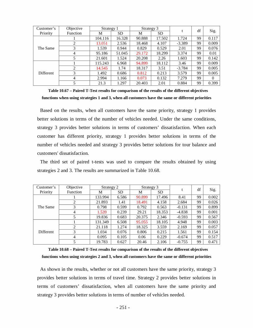
- 251 -
Strategy 1 Strategy 3Customer’sPriority
ObjectiveFunction M SD M SD t df Sig.
1 104.116 16.328 90.888 17.502 1.724 99 0.1172 13.051 2.536 18.468 4.107 -3.389 99 0.0093 1.539 0.944 0.829 0.529 2.01 99 0.0764 95.186 51.045 29.172 18.299 3.374 99 0.01
The Same
5 21.601 1.524 20.208 2.26 1.603 99 0.1421 115.243 6.968 94.899 18.112 3.46 99 0.0092 14.545 1.74 18.317 3.51 -3.784 99 0.0053 1.492 0.686 0.812 0.213 3.579 99 0.0054 2.994 1.166 0.073 0.132 7.279 99 0
Different
5 21.3 1.297 20.403 2.01 0.884 99 0.399
Table 10.67 – Paired T-Test results for comparison of the results of the different objectives
functions when using strategies 1 and 3, when all customers have the same or different priorities
Based on the results, when all customers have the same priority, strategy 1 provides
better solutions in terms of the number of vehicles needed. Under the same conditions,
strategy 3 provides better solutions in terms of customers’ dissatisfaction. When each
customer has different priority, strategy 1 provides better solutions in terms of the
number of vehicles needed and strategy 3 provides better solutions for tour balance and
customers' dissatisfaction.
The third set of paired t-tests was used to compare the results obtained by using
strategies 2 and 3. The results are summarized in Table 10.68.
Strategy 2 Strategy 3Customer’sPriority
ObjectiveFunction M SD M SD t df Sig.
1 133.994 6.586 90.899 17.496 8.41 99 0.0022 21.893 1.41 18.491 4.158 2.684 99 0.0263 0.798 0.599 0.792 0.563 -0.131 99 0.8994 1.539 0.239 29.21 18.353 -4.838 99 0.001
The Same
5 19.836 0.683 20.375 2.346 -0.593 99 0.5671 131.349 6.508 95.055 18.105 4.948 99 0.0032 21.118 1.274 18.325 3.559 2.169 99 0.0573 1.034 0.076 0.806 0.215 1.561 99 0.1544 0.095 0.105 0.06 0.229 -0.674 99 0.517
Different
5 19.783 0.627 20.46 2.106 -0.755 99 0.471
Table 10.68 – Paired T-Test results for comparison of the results of the different objectives
functions when using strategies 2 and 3, when all customers have the same or different priorities
As shown in the results, whether or not all customers have the same priority, strategy 3
provides better solutions in terms of travel time. Strategy 2 provides better solutions in
terms of customers’ dissatisfaction, when all customers have the same priority and
strategy 3 provides better solutions in terms of number of vehicles needed.

- 252 -
The fourth set of paired t-tests was used to compare the results obtained by using
strategies 2 and 4. The results are summarized in Table 10.69.
Strategy 2 Strategy 4Customer’sPriority
ObjectiveFunction M SD M SD t df Sig.
1 134.024 6.593 131.596 6.335 0.817 99 0.4332 21.838 1.244 21.109 1.243 0.969 99 0.3573 0.835 0.617 1.077 0.393 -1.863 99 0.0934 1.449 0.401 1.989 1.723 -0.969 99 0.358
The Same
5 19.926 0.74 19.7 1.077 0.167 99 0.8721 131.484 6.625 128.319 9.714 0.863 99 0.4132 21.249 1.394 20.589 1.487 0.942 99 0.373 1.044 0.259 0.607 0.424 1.793 99 0.1044 0.119 0.124 0.016 0.037 0.8 99 0.445
Different
5 19.818 0.573 19.859 0.322 0.468 99 0.651
Table 10.69 – Paired T-Test results for comparison of the results of the different objectives
functions when using strategies 2 and 4, when all customers have the same or different priorities
As reflected in the results, whether all customers have the same priority or each
customer has a different priority, no significant difference was found for any objective
function.
The fifth set of paired t-tests was used to compare the results obtained by using
strategies 3 and 5. The results are summarized in Table 10.70.
Strategy 3 Strategy 5Customer’sPriority
ObjectiveFunction M SD M SD t df Sig.
1 90.824 17.516 93.046 18.414 -0.322 99 0.7522 18.474 4.281 18.437 3.5 -0.002 99 13 0.78 0.509 5.412 9.818 -1.532 99 0.1594 29.197 18.32 23.96 15.936 0.656 99 0.531
The Same
5 20.373 2.242 20.609 2.535 -0.457 99 0.6591 94.99 18.101 99.951 3.93 -0.827 99 0.4322 18.24 3.474 19.422 1.142 -0.856 99 0.4143 0.876 0.292 0.913 0.298 -0.394 99 0.7024 0.074 0.159 0.157 -0.005 0.191 99 0.853
Different
5 20.507 2.068 21.059 0.708 -0.975 99 0.356
Table 10.70 – Paired T-Test results for comparison of the results of the different objectives
functions when using strategies 3 and 5, when all customers have the same or different priorities
As seen from the results, whether all customers have the same priority or each customer
has a different priority, no significant difference was found for any of the objective
functions.

- 253 -
10.8.4.1 Conclusions
Table 10.71 describes which of the five strategies used provides the best value for each
of the objective functions, when all customers have the same priority and when each
customer has a different priority.
StrategyCustomer’sPriority
ObjectiveFunction 1 2 3 4 5
1 + + +2 +3 + + + +4 + +
The Same
5 + + + +1 + +2 +3 + + + +4 + + + +
Different
5 + + +
Table 10.71 - Best strategy for each of the objective functions
As seen in Table 10.71, when all customers have the same priority, objective functions
1, travel time, and 2, number of vehicles needed, are obtained by using strategy 1.
Objective 3, tour balance, 4, customers’ dissatisfaction, and 5, arrival time of the last
vehicle, are best obtained by using either strategy 2 or strategy 4.
When each customer has a different priority, objective 2, number of vehicles is best
obtained using strategy 2. Objective functions 1, travel time, 3, tour balance, 4,
customers’ dissatisfaction and 5, arrival time of the last vehicle needed, are obtained by
using strategy 3.
10.8.5. Algorithms Comparison
Since in the real-world, information on travel time and customers’ demands are not
known in advance, strategy 3 has to be used. Table 10.72 compares the results obtained
for each of the five objectives, using paired t-tests, functions by each one of the three
algorithms when applying the 3rd strategy. For each objective function, the best value
obtained is highlighted in red.

- 254 -
AlgorithmCustomer’sPriority Objective Function Imp. VEGA SPEA2 VE-ABC
1 84.353 86.593 93.0462 15.607 17.766 18.4373 0.935 0.671 5.4124 30.4 15.877 23.96
The Same
5 21.203 20.791 20.6091 89.941 97.33 99.9512 16.752 20.097 19.4223 0.664 0.843 0.9134 0.107 0.04 0.157
Different
5 20.654 20.729 21.059
Table 10.72 - Comparison of the 5th strategy used in all three algorithms
As may be seen, whether all customers have the same priority or not, objective 1, travel
time, and objective 2, number of vehicles needed are best obtained by using the improved
VEGA algorithm. Objective 4, customers' dissatisfaction is best obtained by using the
SPEA2 algorithm.
10.8.6. Conclusions
Since in the real-world, information on travel time and customers’ demands are not
known in advance, strategy 5 has to be used. From the results obtained, one should use
the improved VEGA algorithm, which for most objective functions returns the best
solutions. When looking at the different strategies, there is no dominant strategy which
provides the best solution for most scenarios.
10.9. Case Study 4
In the second case study the test scenario is defined as follows:
1. Network: Israeli transportation network.
2. Dissatisfaction function: It is assumed that all customers don’t like the supplier to
arrive either early or late. Therefore, the dissatisfaction functions of all customers are
in the form of5
1 ii S
i i
t EETf tTW EET
and5
( ) 1i Ei
ELT tg tELT TW
.
The test scenario is solved 100 times. In the first 50 times, it is assumed that all
customers have the same priority. Under this assumption, the test scenario is solved 100
times using each of the 5 strategies described earlier. In the next 50 times, it is assumed

- 255 -
that each customer has a priority equal to his demand. Under this assumption, the test
scenario is solved 10 times using each of the 5 strategies described earlier.
10.9.1. Priority Comparison
For each of our three algorithms, five paired-samples t-tests were conducted to compare
the total travel time obtained when all customers have the same priority vs. the travel
time obtained when each customer has a different priority, for each of the five strategies.
The results are summarized in Table 10.73.
Same Priority Different PriorityAlgorithm Strategy M SD M SD t df Sig.
1 74.415 4.496 115.336 6.93 -15.094 99 0.0012 93.706 5.252 133.965 6.583 -16.923 99 0.0013 96.545 4.561 90.816 17.427 0.915 99 0.3844 95.298 5.347 131.458 6.299 -21.316 99 0
VEGA
5 92.853 6.377 93.129 18.483 -0.041 99 0.971 103.661 6.878 92.417 6.592 3.493 99 0.0062 116.254 13.96 113.64 23.399 0.394 99 0.73 88.067 15.175 92.171 18.351 -0.633 99 0.5424 117.739 16.571 117.688 16.552 0.999 99 0.344
SPEA2
5 82.621 27.741 98.836 4.102 -1.796 99 0.1061 90.767 28.797 93.073 31.142 -0.153 99 0.8822 134.134 4.239 134.21 7.174 0.037 99 0.973 105.067 10.563 97.619 5.944 1.868 99 0.0954 136.467 5.37 137.561 7.623 -0.291 99 0.781
VE-ABC
5 96.543 17.545 100.716 13.303 -0.567 99 0.584
Table 10.73 – Paired T-Test resuls for comparison of the total travel time for all three algorithms
when all customers have the same priority vs. each customer has a different priority
For the improved VEGA algorithm, as seen from the results, for strategy 1, 2 and 4,
there exists a significant difference in the solution obtained when all customers have the
same priority vs. the solution obtained when each customer has a different priority, which
is better when all customers have the same priority. For the SPEA2 algorithm, for
strategy 1 there exists a significant difference in the solution obtained when all customers
have the same priority vs. the solution obtained when each customer has a different
priority, which is better when each customer has a different priority.
For each of our three algorithms, five paired-samples t-tests were conducted to compare
the number of vehicles needed when all customers have the same priority vs. the number

- 256 -
of vehicles needed when each customer has a different priority, for each of the five
strategies. The results are summarized in Table 10.74.
Same Priority Different PriorityAlgorithm Strategy M SD M SD t df Sig.
1 8.408 0.753 14.536 1.704 -10.464 99 0.0012 14.85 1.835 21.898 1.328 -9.391 99 0.0013 17.684 0.74 18.407 4.158 -0.564 99 0.5854 14.537 1.695 21.122 1.337 -14.178 99 0.001
VEGA
5 16.933 1.464 18.546 3.404 -1.191 99 0.2651 13.727 1.096 12.579 1.409 2.01 99 0.0772 19.589 1.098 19.327 3.098 0.225 99 0.8293 19.1 2.125 19.914 1.658 -1.431 99 0.1874 19.833 1.242 19.869 1.306 1 99 0.344
SPEA2
5 18.274 3.944 19.373 1.277 -0.838 99 0.4251 11.735 3.556 11.022 4.14 0.386 99 0.7092 21.788 1.127 21.837 1.022 -0.288 99 0.783 20.423 1.466 19.174 2.337 1.815 99 0.1034 22.871 1.632 21.735 1.202 1.673 99 0.128
VE-ABC
5 19.35 2.701 18.778 2.36 0.372 99 0.719
Table 10.74 – Paired T-Test resuls for comparison of the number of vehicles needed for all three
algorithms when all customers have the same priority vs. each customer has a different priority
For the improved VEGA algorithm, as seen in the results, for strategies 1, 2 and 4, there
are significant differences in the number of vehicles needed, which is lower when all
customers have the same priority.
For each of our three algorithms, five paired-samples t-tests were conducted to compare
the balance of the tours when all customers have the same priority vs. the number of
vehicles needed when each customer has a different priority, for each of the five
strategies. The results are summarized in Table 10.75.

- 257 -
Same Priority Different PriorityAlgorithm Strategy M SD M SD t df Sig.
1 1.738 0.651 1.55 0.569 0.667 99 0.5192 1.437 0.396 0.699 0.458 8.801 99 0.0013 0.757 0.136 0.666 0.524 -0.24 99 0.8164 1.372 0.659 1.062 0.434 1.812 99 0.104
VEGA
5 0.968 0.365 5.496 9.861 -1.442 99 0.1831 0.774 0.185 0.897 0.143 -3.021 99 0.0132 1.238 0.396 1.078 0.341 1.161 99 0.2753 0.703 0.224 0.533 0.148 1.696 99 0.1254 1.037 0.455 1.029 0.4 0.999 99 0.344
SPEA2
5 0.467 0.194 0.784 0.209 -3.224 99 0.0121 1.551 0.677 6.272 13.275 -1.119 99 0.2932 1.019 0.457 0.655 0.313 2.149 99 0.0623 2.21 5.521 0.697 0.359 0.845 99 0.4214 0.71 0.253 0.944 0.382 -0.345 99 0.739
VE-ABC
5 2.929 7.77 0.85 0.46 0.868 99 0.408
Table 10.75 – Paired T-Test results for comparison of the balance of the tours for all three
algorithms when all customers have the same priority vs. each customer has a different priority
For the improved VEGA algorithm, as may be seen from the results, for strategy 2,
there is a significant difference in the tour balance, which is lower (meaning more
balanced) when each customer has a different priority. For the SPEA2 algorithm, for
strategies 1 and 5, there is also a significant difference in the tour balance, which is lower
when all customers have the same priority. As for the VE-ABC algorithm, for all
strategies there is a significant difference in the tour balance.
For each of our three algorithms, five paired-samples t-tests were conducted to compare
the total dissatisfaction of the customers when all customers have the same priority vs.
the total dissatisfaction of the customers when each customer has a different priority, for
each of the five strategies. The results are summarized in Table 10.76.
Same Priority Different PriorityAlgorithm Strategy M SD M SD t df Sig.
1 60.446 42.088 3.039 1.229 4.255 99 0.0032 0.767 0.696 1.431 0.411 -2.982 99 0.0133 1.075 0.825 29.241 18.272 -4.862 99 0.0024 0.548 0.698 2.101 1.688 -2.291 99 0.046
VEGA
5 29.526 15.461 23.993 15.882 0.69 99 0.5081 433.871 383.07 0.287 0.147 3.578 99 0.0052 156.154 24.675 0.048 0.08 19.93 99 0.0023 1336.587 475.511 0.281 0.262 8.882 99 0.0014 134.412 30.199 4.074 0.905 14.051 99 0.001
SPEA2
5 1159.944 758.856 0.224 0.125 4.832 99 0.001

- 258 -
Same Priority Different PriorityAlgorithm Strategy M SD M SD t df Sig.
1 6287.886 3250.649 6.563 3.637 6.11 99 02 281.695 116.615 0.313 0.205 7.623 99 0.0023 2017.89 426.099 0.575 0.377 14.967 99 0.0024 353.173 302.496 0.245 0.108 3.689 99 0.004
VE-ABC
5 1526.441 772.201 0.451 0.489 6.248 99 0.001
Table 10.76 – Paired T-Test results for comparison of the total dissatisfaction of customers for all
three algorithms when all customers have the same priority vs. each customer has a different priority
For the improved VEGA algorithm, as seen from the results, for strategy 1, there is a
significant difference in total dissatisfaction, which is lower when each customer has a
different priority. For strategies 2, 3 and 4, there is a significant difference in total
dissatisfaction, which is lower when all customers have the same priority.
For the SPEA2 and the VE-ABC algorithm, in all strategies there is a significant
difference in the total dissatisfaction of customers obtained when all customers have the
same priority and when each customer has a different priority, which is lower when each
customer has a different priority.
For each of our three algorithms, five paired-samples t-tests were conducted to compare
the arrival time of the last vehicle when all customers have the same priority vs. the
arrival time of the last vehicle when each customer has a different priority, for each of the
five strategies. The results are summarized in Table 10.77.
Same Priority Different PriorityAlgorithm Strategy M SD M SD t df Sig.
1 20.538 0.779 21.262 1.241 -1.141 99 0.2812 20.133 0.757 19.882 0.719 0.597 99 0.5653 21.032 0.859 20.301 2.197 0.958 99 0.3644 19.768 0.208 19.766 0.972 0.076 99 0.941
VEGA
5 21.621 0.923 20.775 2.431 1.108 99 0.2971 19.916 0.279 19.461 0.126 3.464 99 0.0072 19.186 1.85 19.339 2.177 -0.395 99 0.7023 20.374 2.3 19.792 2.627 0.468 99 0.6534 19.253 1.806 19.195 1.756 0.999 99 0.345
SPEA2
5 19.321 3.914 20.582 0.313 -1.061 99 0.3181 21.291 2.444 21.477 1.065 -0.056 99 0.9582 19.779 0.717 19.775 0.521 0.049 99 0.9633 22.56 1.972 21.013 0.498 2.311 99 0.0454 20.178 0.502 20.114 0.87 0.116 99 0.908
VE-ABC
5 20.938 2.3 20.926 0.743 -0.066 99 0.95
Table 10.77 – Paired T-Test results for comparison of the arrival time of the last vehicle for all
three algorithms when all customers have the same priority vs. each customer has a different priority
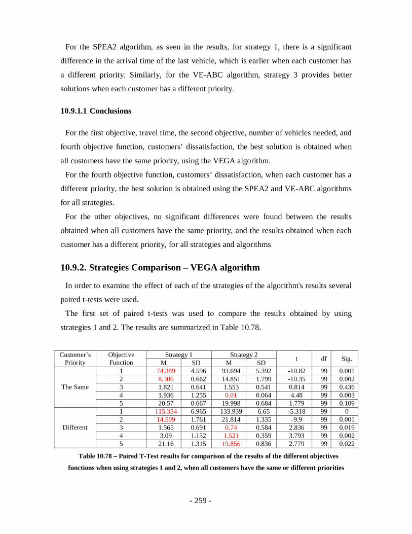
- 259 -
For the SPEA2 algorithm, as seen in the results, for strategy 1, there is a significant
difference in the arrival time of the last vehicle, which is earlier when each customer has
a different priority. Similarly, for the VE-ABC algorithm, strategy 3 provides better
solutions when each customer has a different priority.
10.9.1.1 Conclusions
For the first objective, travel time, the second objective, number of vehicles needed, and
fourth objective function, customers’ dissatisfaction, the best solution is obtained when
all customers have the same priority, using the VEGA algorithm.
For the fourth objective function, customers’ dissatisfaction, when each customer has a
different priority, the best solution is obtained using the SPEA2 and VE-ABC algorithms
for all strategies.
For the other objectives, no significant differences were found between the results
obtained when all customers have the same priority, and the results obtained when each
customer has a different priority, for all strategies and algorithms
10.9.2. Strategies Comparison – VEGA algorithm
In order to examine the effect of each of the strategies of the algorithm's results several
paired t-tests were used.
The first set of paired t-tests was used to compare the results obtained by using
strategies 1 and 2. The results are summarized in Table 10.78.
Strategy 1 Strategy 2Customer’sPriority
ObjectiveFunction M SD M SD t df Sig.
1 74.389 4.596 93.694 5.392 -10.82 99 0.0012 8.306 0.662 14.851 1.799 -10.35 99 0.0023 1.821 0.641 1.553 0.541 0.814 99 0.4364 1.936 1.255 0.01 0.064 4.48 99 0.003
The Same
5 20.57 0.667 19.998 0.684 1.779 99 0.1091 115.354 6.965 133.939 6.65 -5.318 99 02 14.509 1.761 21.814 1.335 -9.9 99 0.0013 1.565 0.691 0.74 0.584 2.836 99 0.0194 3.09 1.152 1.521 0.359 3.793 99 0.002
Different
5 21.16 1.315 19.856 0.836 2.779 99 0.022
Table 10.78 – Paired T-Test results for comparison of the results of the different objectives
functions when using strategies 1 and 2, when all customers have the same or different priorities

- 260 -
As shown in the results, whether or not all customers have the same priority, strategy 1
provides better solutions in terms of travel time and number of vehicles needed.
Similarly, whether all customers have the same priority or not, strategy 2 provides better
solutions in terms of customers' dissatisfaction. When each customer has a different
priority, strategy 2 provides better solutions in terms of tour balance and arrival time of
the last vehicle.
The second set of paired t-tests was used to compare the results obtained by using
strategies 1 and 3. The results are summarized in Table 10.79.
Strategy 1 Strategy 3Customer’sPriority
ObjectiveFunction M SD M SD t df Sig.
1 74.464 4.508 96.481 4.721 -9.927 99 0.0012 8.381 0.675 17.72 0.9 -25.363 99 0.0023 1.819 0.695 0.77 0.293 4.569 99 0.0024 1.956 1.327 0.101 0.058 4.468 99 0.003
The Same
5 20.557 0.677 21.149 0.881 -1.402 99 0.1961 115.369 7.093 90.901 17.526 3.982 99 0.0042 14.581 1.777 18.501 4.169 -2.994 99 0.0153 1.503 0.604 0.76 0.532 3.445 99 0.0074 3.048 1.152 29.186 18.338 -4.446 99 0
Different
5 21.256 1.302 20.339 2.166 1.073 99 0.308
Table 10.79 – Paired T-Test results for comparison of the results of the different objectives
functions when using strategies 1 and 3, when all customers have the same or different priorities
As reflected in the results, whether or not all customers have the same priority, strategy
1 provides better solutions in terms of the number of vehicles needed. Similarly, whether
all customers have the same priority or not, strategy 3 provides better solutions in terms
of tour balance and customers’ dissatisfaction. If all customers have the same priority,
strategy 1 provides better solutions in terms of travel time, but if each customer has a
different priority, then better travel time is obtained by using strategy 3.
The third set of paired t-tests was used to compare the results obtained by using
strategies 2 and 3. The results are summarized in Table 10.80.
Strategy 2 Strategy 3Customer’sPriority
ObjectiveFunction M SD M SD t df Sig.
1 93.803 5.308 96.484 4.649 -1.771 99 0.1112 14.892 1.821 17.668 0.844 -4.41 99 0.0023 1.566 0.48 0.723 0.308 4.65 99 0.0024 0.082 0.001 0.022 0.06 -0.726 99 0.487
The Same
5 19.992 0.751 21.105 0.82 -3.049 99 0.014
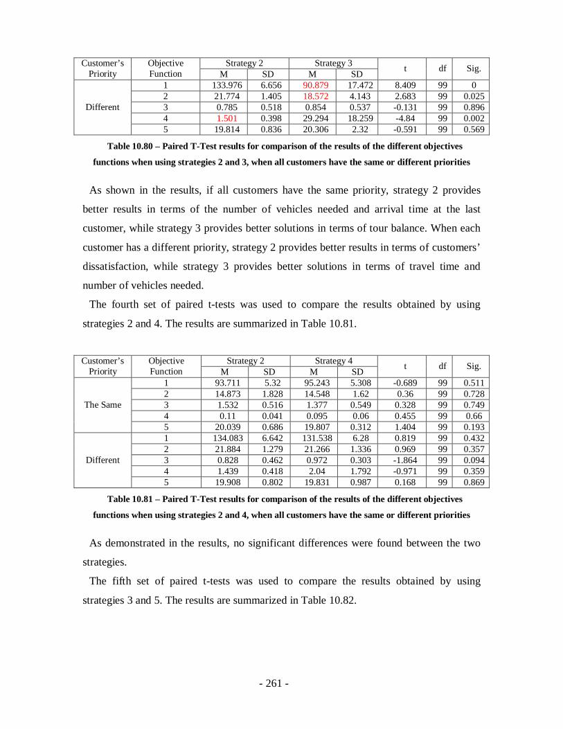
- 261 -
Strategy 2 Strategy 3Customer’sPriority
ObjectiveFunction M SD M SD t df Sig.
1 133.976 6.656 90.879 17.472 8.409 99 02 21.774 1.405 18.572 4.143 2.683 99 0.0253 0.785 0.518 0.854 0.537 -0.131 99 0.8964 1.501 0.398 29.294 18.259 -4.84 99 0.002
Different
5 19.814 0.836 20.306 2.32 -0.591 99 0.569
Table 10.80 – Paired T-Test results for comparison of the results of the different objectives
functions when using strategies 2 and 3, when all customers have the same or different priorities
As shown in the results, if all customers have the same priority, strategy 2 provides
better results in terms of the number of vehicles needed and arrival time at the last
customer, while strategy 3 provides better solutions in terms of tour balance. When each
customer has a different priority, strategy 2 provides better results in terms of customers’
dissatisfaction, while strategy 3 provides better solutions in terms of travel time and
number of vehicles needed.
The fourth set of paired t-tests was used to compare the results obtained by using
strategies 2 and 4. The results are summarized in Table 10.81.
Strategy 2 Strategy 4Customer’sPriority
ObjectiveFunction M SD M SD t df Sig.
1 93.711 5.32 95.243 5.308 -0.689 99 0.5112 14.873 1.828 14.548 1.62 0.36 99 0.7283 1.532 0.516 1.377 0.549 0.328 99 0.7494 0.11 0.041 0.095 0.06 0.455 99 0.66
The Same
5 20.039 0.686 19.807 0.312 1.404 99 0.1931 134.083 6.642 131.538 6.28 0.819 99 0.4322 21.884 1.279 21.266 1.336 0.969 99 0.3573 0.828 0.462 0.972 0.303 -1.864 99 0.0944 1.439 0.418 2.04 1.792 -0.971 99 0.359
Different
5 19.908 0.802 19.831 0.987 0.168 99 0.869
Table 10.81 – Paired T-Test results for comparison of the results of the different objectives
functions when using strategies 2 and 4, when all customers have the same or different priorities
As demonstrated in the results, no significant differences were found between the two
strategies.
The fifth set of paired t-tests was used to compare the results obtained by using
strategies 3 and 5. The results are summarized in Table 10.82.
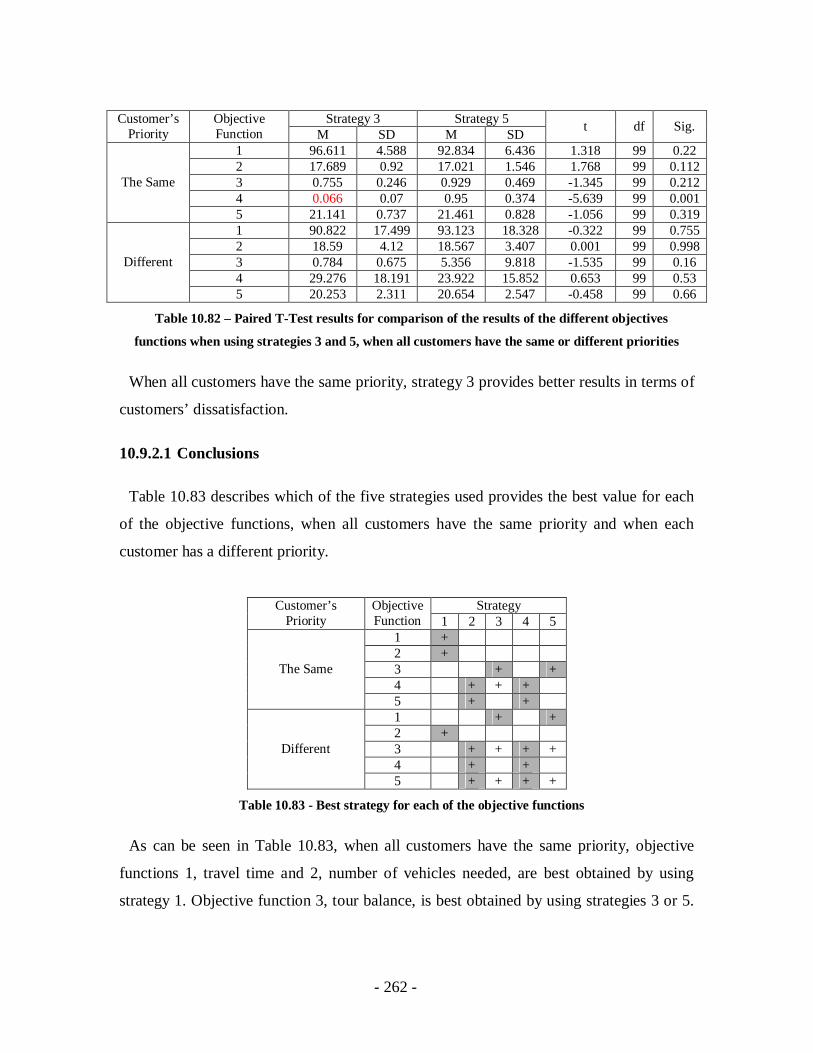
- 262 -
Strategy 3 Strategy 5Customer’sPriority
ObjectiveFunction M SD M SD t df Sig.
1 96.611 4.588 92.834 6.436 1.318 99 0.222 17.689 0.92 17.021 1.546 1.768 99 0.1123 0.755 0.246 0.929 0.469 -1.345 99 0.2124 0.066 0.07 0.95 0.374 -5.639 99 0.001
The Same
5 21.141 0.737 21.461 0.828 -1.056 99 0.3191 90.822 17.499 93.123 18.328 -0.322 99 0.7552 18.59 4.12 18.567 3.407 0.001 99 0.9983 0.784 0.675 5.356 9.818 -1.535 99 0.164 29.276 18.191 23.922 15.852 0.653 99 0.53
Different
5 20.253 2.311 20.654 2.547 -0.458 99 0.66
Table 10.82 – Paired T-Test results for comparison of the results of the different objectives
functions when using strategies 3 and 5, when all customers have the same or different priorities
When all customers have the same priority, strategy 3 provides better results in terms of
customers’ dissatisfaction.
10.9.2.1 Conclusions
Table 10.83 describes which of the five strategies used provides the best value for each
of the objective functions, when all customers have the same priority and when each
customer has a different priority.
StrategyCustomer’sPriority
ObjectiveFunction 1 2 3 4 5
1 +2 +3 + +4 + + +
The Same
5 + +1 + +2 +3 + + + +4 + +
Different
5 + + + +
Table 10.83 - Best strategy for each of the objective functions
As can be seen in Table 10.83, when all customers have the same priority, objective
functions 1, travel time and 2, number of vehicles needed, are best obtained by using
strategy 1. Objective function 3, tour balance, is best obtained by using strategies 3 or 5.
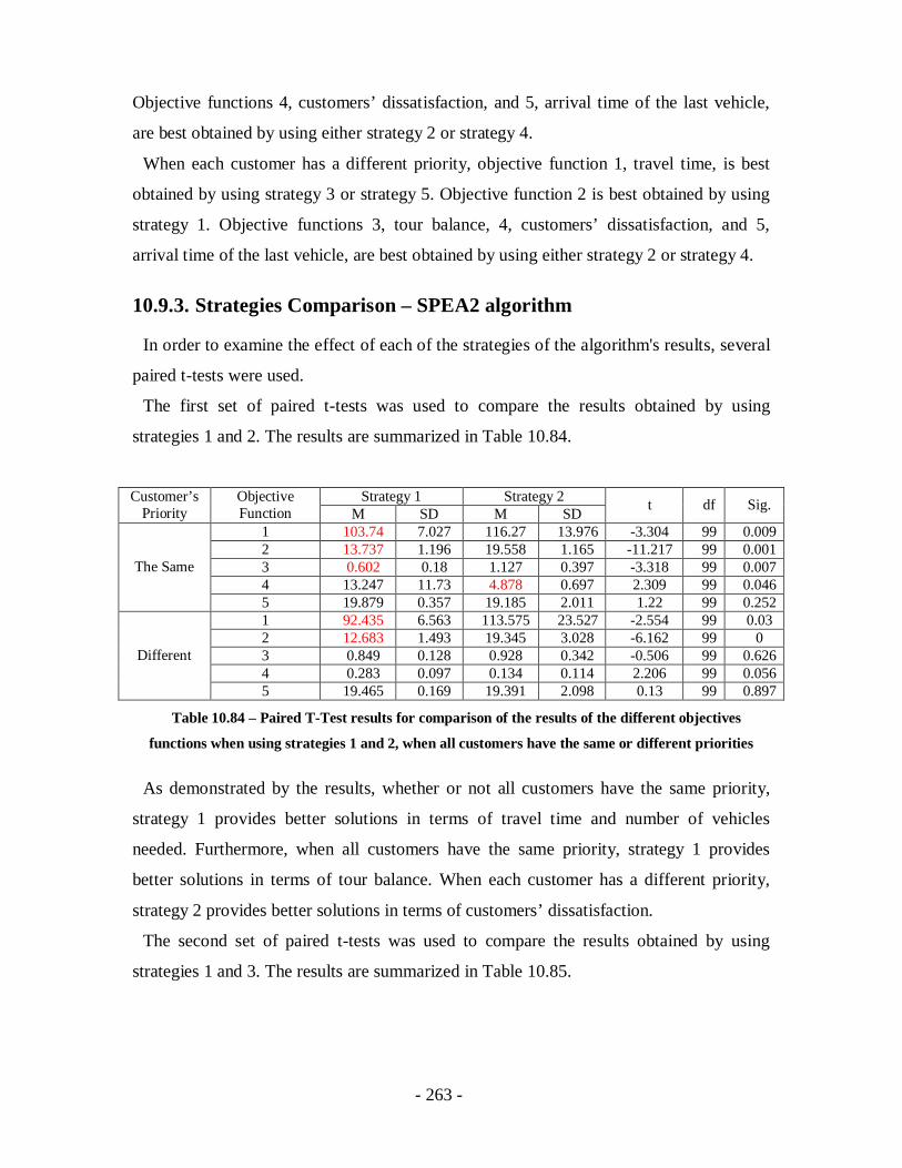
- 263 -
Objective functions 4, customers’ dissatisfaction, and 5, arrival time of the last vehicle,
are best obtained by using either strategy 2 or strategy 4.
When each customer has a different priority, objective function 1, travel time, is best
obtained by using strategy 3 or strategy 5. Objective function 2 is best obtained by using
strategy 1. Objective functions 3, tour balance, 4, customers’ dissatisfaction, and 5,
arrival time of the last vehicle, are best obtained by using either strategy 2 or strategy 4.
10.9.3. Strategies Comparison – SPEA2 algorithm
In order to examine the effect of each of the strategies of the algorithm's results, several
paired t-tests were used.
The first set of paired t-tests was used to compare the results obtained by using
strategies 1 and 2. The results are summarized in Table 10.84.
Strategy 1 Strategy 2Customer’sPriority
ObjectiveFunction M SD M SD t df Sig.
1 103.74 7.027 116.27 13.976 -3.304 99 0.0092 13.737 1.196 19.558 1.165 -11.217 99 0.0013 0.602 0.18 1.127 0.397 -3.318 99 0.0074 13.247 11.73 4.878 0.697 2.309 99 0.046
The Same
5 19.879 0.357 19.185 2.011 1.22 99 0.2521 92.435 6.563 113.575 23.527 -2.554 99 0.032 12.683 1.493 19.345 3.028 -6.162 99 03 0.849 0.128 0.928 0.342 -0.506 99 0.6264 0.283 0.097 0.134 0.114 2.206 99 0.056
Different
5 19.465 0.169 19.391 2.098 0.13 99 0.897
Table 10.84 – Paired T-Test results for comparison of the results of the different objectives
functions when using strategies 1 and 2, when all customers have the same or different priorities
As demonstrated by the results, whether or not all customers have the same priority,
strategy 1 provides better solutions in terms of travel time and number of vehicles
needed. Furthermore, when all customers have the same priority, strategy 1 provides
better solutions in terms of tour balance. When each customer has a different priority,
strategy 2 provides better solutions in terms of customers’ dissatisfaction.
The second set of paired t-tests was used to compare the results obtained by using
strategies 1 and 3. The results are summarized in Table 10.85.
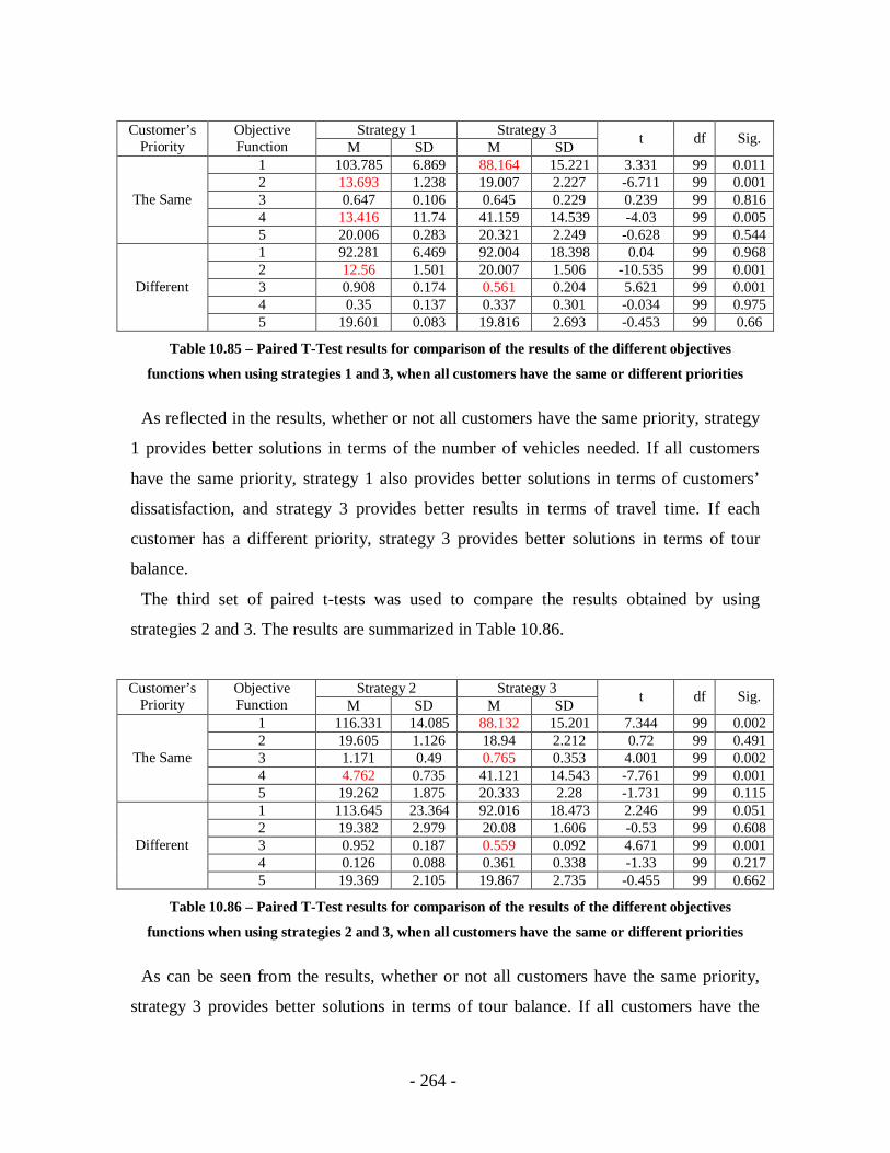
- 264 -
Strategy 1 Strategy 3Customer’sPriority
ObjectiveFunction M SD M SD t df Sig.
1 103.785 6.869 88.164 15.221 3.331 99 0.0112 13.693 1.238 19.007 2.227 -6.711 99 0.0013 0.647 0.106 0.645 0.229 0.239 99 0.8164 13.416 11.74 41.159 14.539 -4.03 99 0.005
The Same
5 20.006 0.283 20.321 2.249 -0.628 99 0.5441 92.281 6.469 92.004 18.398 0.04 99 0.9682 12.56 1.501 20.007 1.506 -10.535 99 0.0013 0.908 0.174 0.561 0.204 5.621 99 0.0014 0.35 0.137 0.337 0.301 -0.034 99 0.975
Different
5 19.601 0.083 19.816 2.693 -0.453 99 0.66
Table 10.85 – Paired T-Test results for comparison of the results of the different objectives
functions when using strategies 1 and 3, when all customers have the same or different priorities
As reflected in the results, whether or not all customers have the same priority, strategy
1 provides better solutions in terms of the number of vehicles needed. If all customers
have the same priority, strategy 1 also provides better solutions in terms of customers’
dissatisfaction, and strategy 3 provides better results in terms of travel time. If each
customer has a different priority, strategy 3 provides better solutions in terms of tour
balance.
The third set of paired t-tests was used to compare the results obtained by using
strategies 2 and 3. The results are summarized in Table 10.86.
Strategy 2 Strategy 3Customer’sPriority
ObjectiveFunction M SD M SD t df Sig.
1 116.331 14.085 88.132 15.201 7.344 99 0.0022 19.605 1.126 18.94 2.212 0.72 99 0.4913 1.171 0.49 0.765 0.353 4.001 99 0.0024 4.762 0.735 41.121 14.543 -7.761 99 0.001
The Same
5 19.262 1.875 20.333 2.28 -1.731 99 0.1151 113.645 23.364 92.016 18.473 2.246 99 0.0512 19.382 2.979 20.08 1.606 -0.53 99 0.6083 0.952 0.187 0.559 0.092 4.671 99 0.0014 0.126 0.088 0.361 0.338 -1.33 99 0.217
Different
5 19.369 2.105 19.867 2.735 -0.455 99 0.662
Table 10.86 – Paired T-Test results for comparison of the results of the different objectives
functions when using strategies 2 and 3, when all customers have the same or different priorities
As can be seen from the results, whether or not all customers have the same priority,
strategy 3 provides better solutions in terms of tour balance. If all customers have the

- 265 -
same priority, strategy 2 also provides better solutions in terms of customers’
dissatisfaction, and strategy 3 provides better solutions in terms of travel time.
The fourth set of paired t-tests was used to compare the results obtained by using
strategies 2 and 4. The results are summarized in Table 10.87.
Strategy 2 Strategy 4Customer’sPriority
ObjectiveFunction M SD M SD t df Sig.
1 116.331 14.078 117.686 16.549 -0.198 99 0.8482 19.51 1.128 19.82 1.263 -0.606 99 0.563 1.213 0.471 1.043 0.427 0.49 99 0.6354 4.817 0.834 4.212 0.885 1.714 99 0.119
The Same
5 19.129 1.825 19.257 1.652 -0.062 99 0.9491 113.49 23.469 117.783 16.433 -0.464 99 0.6532 19.314 3.105 19.817 1.306 -0.437 99 0.6713 0.959 0.379 1.215 0.436 -0.703 99 0.4994 0.202 0.118 4.105 0.997 -13.5 99 0.002
Different
5 19.347 2.066 19.21 1.828 0.185 99 0.855
Table 10.87 – Paired T-Test results for comparison of the results of the different objectives
functions when using strategies 2 and 4, when all customers have the same or different priorities
As seen from the results, when each customer has a different priority, strategy 2
provides better results in terms of customers’ dissatisfaction.
The fifth set of paired t-tests was used to compare the results obtained by using
strategies 3 and 5. The results are summarized in Table 10.88.
Strategy 3 Strategy 5Customer’sPriority
ObjectiveFunction M SD M SD t df Sig.
1 87.989 15.243 82.654 27.675 0.57 99 0.5842 19.008 2.084 18.293 4.092 0.668 99 0.5233 0.706 0.38 0.454 0.041 2.146 99 0.064 41.134 14.722 35.596 23.297 0.574 99 0.581
The Same
5 20.448 2.237 19.375 3.96 0.733 99 0.481 92.176 18.467 98.894 4.221 -1.045 99 0.3212 19.925 1.498 19.367 1.322 1.075 99 0.313 0.508 0.199 0.659 0.178 -2.753 99 0.0224 0.249 0.362 0.152 0.095 0.738 99 0.482
Different
5 19.944 2.683 20.656 0.394 -0.858 99 0.413
Table 10.88 – Paired T-Test results for comparison of the results of the different objectives
functions when using strategies 3 and 5, when all customers have the same or different priorities
As seen from the results, when each customer has a different priority, strategy 3
provides better results in terms of tour balance.

- 266 -
10.9.3.1 Conclusions
Table 10.89 describes which of the five strategies used provides the best value for each
of the objective functions, when all customers have the same priority and when each
customer has a different priority.
StrategyCustomer’sPriority
ObjectiveFunction 1 2 3 4 5
1 + +2 +3 + +4 + +
The Same
5 + + + + +1 + + + +2 +3 +4 + + + +
Different
5 + + + +
Table 10.89 - Best strategy for each of the objective functions
As may be seen from Table 10.89, when all customers have the same priority, objective
functions 1, travel time and 3, route balance, are best obtained by using strategy 3 or
strategy 5. Objective function 2, number of vehicles needed, is best obtained by using
strategy 1. Objective 4, customers’ dissatisfaction, and 5, arrival time of the last vehicle,
are best obtained by using either strategy 2 or strategy 4.
When each customer has a different priority, objective functions 1, travel time, 3, route
balance, 4, customers’ dissatisfaction, and 5, arrival time of the last vehicle, are best
obtained by using strategy 3. Objective function 2, number of vehicles needed, is best
obtained by using strategy 1.
10.9.4. Strategies Comparison – VE-ABC algorithm
In order to examine the effect of each of the strategies of the algorithm's results, several
paired t-tests were used.
The first set of paired t-tests was used to compare the results obtained by using
strategies 1 and 2. The results are summarized in Table 10.90.

- 267 -
Strategy 1 Strategy 2Customer’sPriority
ObjectiveFunction M SD M SD t df Sig.
1 90.786 28.831 134.21 4.302 -4.668 99 0.0022 11.784 3.588 21.736 1.066 -8.506 99 0.0023 1.561 0.851 1.152 0.367 1.487 99 0.1724 193.456 99.895 8.659 3.533 5.858 99 0.001
The Same
5 21.309 2.507 19.863 0.649 1.971 99 0.0781 93.092 31.195 134.188 7.129 -4.176 99 0.0032 10.929 4.15 21.959 1.082 -8.476 99 0.0023 6.441 13.183 0.749 0.369 1.37 99 0.2044 6.601 3.777 0.374 0.185 5.521 99 0
Different
5 21.479 1.066 19.8 0.648 5.031 99 0.002
Table 10.90 – Paired T-Test results for comparison of the results of the different objectives
functions when using strategies 1 and 2, when all customers have the same or different priorities
As seen in the results, whether or not all customers have the same priority, strategy 1
provides better solutions in terms of travel time and number of vehicles needed.
Similarly, whether all customers have the same priority or not, strategy 2 provides better
solutions in terms of customers’ dissatisfaction. When each customer has a different
priority, strategy 2 provides better results in terms of arrival time of the last vehicle.
The second set of paired t-tests was used to compare the results obtained by using
strategies 1 and 3. The results are summarized in Table 10.91.
Strategy 1 Strategy 3Customer’sPriority
ObjectiveFunction M SD M SD t df Sig.
1 90.69 28.898 105.09 10.594 -1.637 99 0.1372 11.703 3.728 20.43 1.413 -7.832 99 03 1.519 0.853 2.2 5.521 -0.358 99 0.7294 193.353 99.996 62.032 13.019 4.123 99 0.002
The Same
5 21.323 2.514 22.604 1.891 -1.529 99 0.1631 92.993 31.113 97.512 5.943 -0.434 99 0.6752 10.977 4.13 19.218 2.418 -4.942 99 03 6.396 13.217 0.735 0.24 1.356 99 0.2094 6.521 3.736 0.56 0.334 5.193 99 0.003
Different
5 21.518 1.037 21.169 0.502 0.963 99 0.36
Table 10.91 – Paired T-Test results for comparison of the results of the different objectives
functions when using strategies 1 and 3, when all customers have the same or different priorities
As reflected in the results, whether or not all customers have the same priority, strategy
1 provides better solutions in terms of the number of vehicles needed. Similarly, whether
all customers have the same priority or not, strategy 3 provides better solutions in terms
of customers’ dissatisfaction.
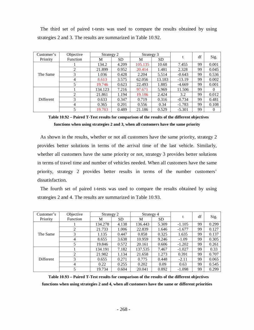
- 268 -
The third set of paired t-tests was used to compare the results obtained by using
strategies 2 and 3. The results are summarized in Table 10.92.
Strategy 2 Strategy 3Customer’sPriority
ObjectiveFunction M SD M SD t df Sig.
1 134.2 4.209 105.135 10.68 7.455 99 0.0012 21.899 0.952 20.414 1.481 2.328 99 0.0453 1.036 0.428 2.204 5.514 -0.643 99 0.5364 8.613 3.575 62.056 13.183 -13.19 99 0.002
The Same
5 19.746 0.623 22.493 1.885 -4.669 99 0.0011 134.123 7.216 97.671 5.969 11.506 99 02 21.861 1.194 19.186 2.424 3.2 99 0.0123 0.633 0.347 0.719 0.316 -0.734 99 0.4814 0.365 0.201 0.556 0.34 -1.783 99 0.108
Different
5 19.783 0.489 21.186 0.529 -5.301 99 0
Table 10.92 – Paired T-Test results for comparison of the results of the different objectives
functions when using strategies 2 and 3, when all customers have the same priority
As shown in the results, whether or not all customers have the same priority, strategy 2
provides better solutions in terms of the arrival time of the last vehicle. Similarly,
whether all customers have the same priority or not, strategy 3 provides better solutions
in terms of travel time and number of vehicles needed. When all customers have the same
priority, strategy 2 provides better results in terms of the number customers’
dissatisfaction.
The fourth set of paired t-tests was used to compare the results obtained by using
strategies 2 and 4. The results are summarized in Table 10.93.
Strategy 2 Strategy 4Customer’sPriority
ObjectiveFunction M SD M SD t df Sig.
1 134.278 4.138 136.443 5.309 -1.105 99 0.2992 21.733 1.006 22.839 1.646 -1.677 99 0.1273 1.135 0.447 0.858 0.325 1.635 99 0.1374 8.655 3.638 10.959 9.246 -1.09 99 0.305
The Same
5 19.846 0.572 20.161 0.606 -1.202 99 0.2611 134.191 7.182 137.535 7.467 -1.027 99 0.332 21.982 1.134 21.658 1.273 0.391 99 0.7073 0.655 0.271 0.775 0.448 -2.11 99 0.0654 0.22 0.255 0.202 0.09 0.63 99 0.545
Different
5 19.734 0.604 20.041 0.892 -1.098 99 0.299
Table 10.93 – Paired T-Test results for comparison of the results of the different objectives
functions when using strategies 2 and 4, when all customers have the same or different priorities

- 269 -
As reflected in the results, no significant differences were found between the two
strategies.
The fifth set of paired t-tests was used to compare the results obtained by using
strategies 3 and 5. The results are summarized in Table 10.94.
Strategy 3 Strategy 5Customer’sPriority
ObjectiveFunction M SD M SD t df Sig.
1 105.076 10.62 96.584 17.507 1.394 99 0.1982 20.567 1.493 19.226 2.705 1.217 99 0.2573 2.201 5.51 2.907 7.796 -0.244 99 0.8154 62.051 13.2 46.852 23.676 2.279 99 0.048
The Same
5 22.505 1.92 20.881 2.332 2.14 99 0.0631 97.505 5.881 100.742 13.307 -0.871 99 0.4052 19.113 2.398 18.718 2.386 0.63 99 0.5433 0.703 0.227 0.785 0.385 -0.337 99 0.7434 0.406 0.28 0.463 0.435 -0.14 99 0.889
Different
5 21.109 0.395 20.831 0.755 0.693 99 0.506
Table 10.94 – Paired T-Test results for comparison of the results of the different objectives
functions when using strategies 3 and 5, when all customers have the same or different priorities
As may be seen from the results, when each customer has a different priority, strategy 5
provides better results in terms of customers’ dissatisfaction.
10.9.4.1 Conclusions
Table 10.95 describes which of the five strategies used provides the best value for each
of the objective functions, when all customers have the same priority and when each
customer has a different priority.
StrategyCustomer’sPriority
ObjectiveFunction 1 2 3 4 5
1 + + +2 +3 + + + +4 + +
The Same
5 + + + +1 + + +2 +3 + + + + +4 + + + +
Different
5 + +
Table 10.95 - Best strategy for each of the objective functions
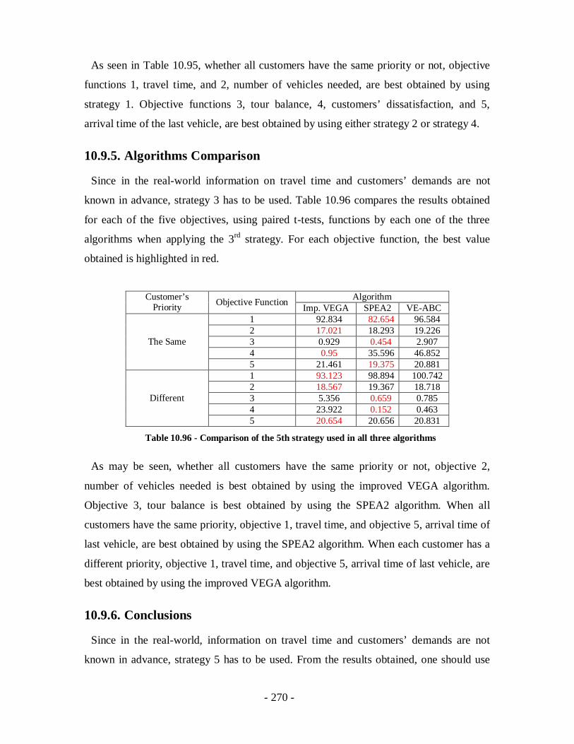
- 270 -
As seen in Table 10.95, whether all customers have the same priority or not, objective
functions 1, travel time, and 2, number of vehicles needed, are best obtained by using
strategy 1. Objective functions 3, tour balance, 4, customers’ dissatisfaction, and 5,
arrival time of the last vehicle, are best obtained by using either strategy 2 or strategy 4.
10.9.5. Algorithms Comparison
Since in the real-world information on travel time and customers’ demands are not
known in advance, strategy 3 has to be used. Table 10.96 compares the results obtained
for each of the five objectives, using paired t-tests, functions by each one of the three
algorithms when applying the 3rd strategy. For each objective function, the best value
obtained is highlighted in red.
AlgorithmCustomer’sPriority Objective Function Imp. VEGA SPEA2 VE-ABC
1 92.834 82.654 96.5842 17.021 18.293 19.2263 0.929 0.454 2.9074 0.95 35.596 46.852
The Same
5 21.461 19.375 20.8811 93.123 98.894 100.7422 18.567 19.367 18.7183 5.356 0.659 0.7854 23.922 0.152 0.463
Different
5 20.654 20.656 20.831
Table 10.96 - Comparison of the 5th strategy used in all three algorithms
As may be seen, whether all customers have the same priority or not, objective 2,
number of vehicles needed is best obtained by using the improved VEGA algorithm.
Objective 3, tour balance is best obtained by using the SPEA2 algorithm. When all
customers have the same priority, objective 1, travel time, and objective 5, arrival time of
last vehicle, are best obtained by using the SPEA2 algorithm. When each customer has a
different priority, objective 1, travel time, and objective 5, arrival time of last vehicle, are
best obtained by using the improved VEGA algorithm.
10.9.6. Conclusions
Since in the real-world, information on travel time and customers’ demands are not
known in advance, strategy 5 has to be used. From the results obtained, one should use
- 271 -
the SPEA2 algorithm, which returns the best solutions for all objective functions. When
looking at the different strategies, there is no dominant strategy which provides the best
solution in the majority of scenarios.
10.10. SummaryThe goal of this chapter is to compare the results of the three algorithms using a case
study. The case study is based on two networks (urban and interurban) based on real-
world transportation network, including the locations of the depot and the customers and
information about travel time between the different customers. The case study is
performed using simulation.
In order to perform the case study, simulation was used. The simulation is based on two
processes running in parallel, the algorithm process and the simulation process, which
exchange information between each other.
The simulation process simulates an entire work today. It does so by handling each of
the vehicles, collecting data about travel times and new customers’demands.
In the case study, 5 different strategies of using the evolutionary algorithms were tested,
where the fifth strategy represents a situation in which both travel times and customers’
demands are unknown (desired real-world situation).
The VEGA algorithm is a well known multi-objective algorithm, but since its
development more sophisticated and accurate multi-objective algorithms, such as the
SPAE2, towere introduced. Also, the VE-ABC algorithm is a new, slower algorithm, and
is therefore able to make far fewer iterations in a given time period, compared to the two
other algorithms. It was therefore expected that the best results would be obtained when
using the SPEA2 algorithm. However, the case study shows that this is not the case. In an
urban network when using a linear dissatisfaction function, it was found that the VEGA
algorithms performs best when all customers have the same priority. When each customer
has a different priority, using the same network and the same dissatisfaction function,
best results were obtained using either the SPEA2 or the VE-ABC algorithms.
In an urban network and a dissatisfaction function that represents customers who don’t
like that the supplier is either early or late, and in an interurban network with both types
of dissatisfaction network, the results of all algorithms were the same.
- 272 -
This shows that the VEGA algorithm when used can provide solutions equal in quality
to the the solutions obtained from more sophisticated, more recent algorithms. This is
important, since the VEGA algorithm has an advantage in the simplicity of its
implementation, running speed compared to other algorithms (and as a result, more
iterations in a given time period), and its capacity for modifications.
- 273 -
11. Summary
11.1. Summary and Conclusions
The Vehicle-Routing Problem (VRP) is a common name for problems involving the
construction of a set of routes for a fleet of vehicles. The vehicles start their routes at a
depot, call at customers to whom they deliver goods, and return to the depot. The
objective function for the vehicle-routing problem is to minimize delivery cost by finding
optimal routes, which are usually the shortest delivery routes.
The basic VRP consists of designing a set of delivery or collection routes, such that (1)
each route starts and ends at the depot, (2) each customer is called at exactly once and by
only one vehicle, (3) the total demand on each route does not exceed the capacity of a
single vehicle, and (4) the total routing distance is minimized. It is common to address the
basic VRP as the Capacitated Vehicle-Routing Problem (CVRP).
VRP has been solved optimally using Branch-and-Bound algorithms, Set-Covering and
Column Generation algorithms, Branch-and-Cut algorithms, Dynamic algorithms and
other exact algorithms.
Since VRP is an NP-Hard problem, many heuristics have been developed for solving it.
The classic algorithms include, among others, the Savings algorithms, Swap algorithm
and the Fisher and Jaikumar algorithm. Meta-heuristics algorithms, such as Simulated
Annealing, Tabu Search, Genetic Algorithms, Ant Systems Algorithms and Neural
Networks are also used in solving VRPs.
As research developed, extensions to the basic VRP were introduced. The goal was to
develop more realistic models, to adapt to the larger number of constraints of the real
world. Such extensions include the Split Delivery Vehicle Routing Problems, Vehicle
Routing Problems with Time Windows, Multi-Depot Vehicle Routing Problems, Time
Dependent Vehicle Routing Problems, Stochastic Vehicle Routing Problems, Mutli-
Objective Vehicle Routing problems and Real-Time Vehicle Routing Problems.
VRPs are often used to model real cases. However, they are often set up with the single
objective of minimizing the cost of the solution, despite the fact that the majority of the
problems encountered in industry, particularly in logistics, are multi-objective in nature.
In real-life, for instance, there may be several costs associated with a single tour.
- 274 -
Moreover, the objectives may not always be limited to cost. In fact, numerous other
aspects, such as balancing workloads (time, distance ...), can be considered simply by
adding new objectives (Jozefowiez et al., 2008).
Traditionally, vehicle routing plans are based on deterministic information about
demands, vehicle locations and travel times on the roads. What is likely to distinguish
most distribution problems today from equivalent problems in the past, is that
information that is needed to come up with a set of good vehicle routes and schedules is
dynamically revealed to the decision maker (Psaraftis, 1995). Until recently, the cost of
obtaining real-time traffic information was deemed too high to compare with the benefits
from the real time control over the vehicles. Furthermore, some of the information needed
for the real time routing was impossible to get. The advancement of technology in
communication systems, the geographic information system (GIS) and the intelligent
transportation system (ITS) make is possible to operate vehicles using the real-time
information about the travel times and the vehicles' locations (Ghiani et al., 2003).
While traditional VRPs have been thoroughly studied, limited research has, to date,
been devoted to multi-objective real-time management of vehicles during the actual
execution of the distribution schedule to respond to unforeseen events that often occur
and may deteriorate the effectiveness of the predefined and static routing decisions.
Furthermore, in cases when traveling time is a crucial factor, ignoring travel time
fluctuations (due to various factors, such as peak hour traveling time, accidents, weather
conditions, etc.) can result in route plans that can take the vehicles into congested urban
traffic conditions. Considering time-dependent travel times as well as information
regarding demands that arise in real time in solving VRPs can reduce the costs of
ignoring the changing environment (Haghani & Jung, 2005).
The problem considered in this research is the Real-Time Multi-Objective VRP. The
Real-Time Multi-Objective VRP is defined as a vehicle fleet that has to serve customers
of fixed demands from a central depot. Customers must be assigned to vehicles, and the
vehicles routed so that the a number of objectives are minimized/maximized (Malandraki
& Daskin, 1992). The travel time between two customers or a customer and the depot
depends on the distance between the points and the time of day, and it also has stochastic
properties.

- 275 -
This research attempts to adjust the vehicles' routes at certain times in a planning period.
This adjustment considers new information about the travel times, current location of
vehicles, and new demand requests (that can be deleted after being served, or added since
they arise after the initial service began) and more. This result in a dynamic change in the
demand and traveling time information as time changes, which has to be taken into
consideration in order to provide optimized real-time operation of vehicles.
According to the vast literature review, the following objectives were addressed: (1)
Minimizing the total traveling time (e.g. (Malandraki & Daskin, 1992)) - Minimizing
the total traveling time can reduce the cost of an organization for, among others, the
following seasons: (a) the less time a driver spends driving the less chances there are for
being involved in a car accident (b) maintenance has to be performed less often. (2)
Minimizing the number of vehicles (e.g. (Corberan et al., 2002)) - Since in a real world,
the fixed cost of using additional vehicles is much more than the routing operations cost,
we can reduce the total cost by minimizing the number of vehicles in service. (3)
Maximizing customers' satisfaction (e.g. (Sessomboon et al., 1998)) - Customers who
are not satisfied with the level of service can switch to a different provider, which results
in a reduction of manufacturing and delivery. (4) Maximizing drivers' satisfaction (e.g.
(Lee & Ueng, 1998)) - In a similar manner, drivers who are not satisfied with their work
schedule may feel frustrated, which may damage their work, which in turn may influence
customers' satisfaction. (5) Minimizing the arrival time of the last vehicle – each
vehicle, on its return back to the depot, can be assigned to a new route (meaning more
routes with fewer vehicles). Minimizing the arrival time of the last vehicle arriving to the
depot, ensures that all other vehicles are present at the depot before the arrival of the last
vehicle, and can therefore be assigned to new routes.
The first stage in solving the real-time multi-objective vehicle routing problem was to
formulate the problem as a mixed integer linear programming problem on a network.
Several assumptions and limitations were considered, such as a system with dynamic
conditions (real-time variation in travel times and real-time service requests); all demands
have specified service times and service time intervals; soft time windows for service
around the desired service times are considered, and more. Next the five objectives were
mathematically formulated, as well as the various constraints.
- 276 -
Since VRP is a NP-Hard problem, it cannot be solved to optimality using conventual
methods. It is therefore essential to develop an efficient heuristics algorithm for solving
the problem. In order to do so, various methods and algorithms for solving dynamic
vehicle routing problems as well as for solving multi-objective optimization problems
were studied.
Finally, three evolutionary algorithms for solving the real-time multi-objective vehicle
routing problem were described.
The first algorithm is an improved version of the vector evaluated genetic algorithm
(VEGA). It is based on the concept that for a problem with NumObj objectives, NumObj
sub-populations of size PopSize/NumObj each would be generated (assuming a total
population size of PopSize). Each sub-population uses only one of the NumObj objective
functions for fitness assignment. The proportionate selection operator is used to generate
the mating pool. These sub-populations are then shuffled together to obtain a new
population of size PopSize, on which the GA would apply the crossover and mutation
operators in the usual way. In each generation, the set of not-dominated solutions is
added to the optimal solutions set, from which non-dominated solutions are removed.
The second algorithm is an implementation of the SPEA2 algorithm. The distinctive
feature of SPEA2 lies in the elitism-preserved operation. An external set (archive) is created
for storing primarily non-dominated solutions. It is then combined with the current
population to form the next archive that is then used to create offspring for the next
generation. The size of the archive is fixed. It can be set to be equal to the population
size. Therefore, there exist two special situations when filling solutions in the archive. If
the number of non-dominated solutions is smaller than the archive size, other dominated
solutions taken from the remainder part of the population are filled in. This selection is
carried out according to a fitness value, specifically defined for SPEA. In other words, the
individual fitness value defined for a solution x, is the total of the SPEA-defined strengths
of solutions, which dominate x, plus a density value.
The second situation happens when the number of non-dominated solutions is over the
archive size. In this case, a truncation operator is applied. For that operator, the solution
which has the smallest distance to the other solutions will be removed from the set. If
solutions have the same minimum distance, the second nearest distance will be
considered, and so forth. This is called the k-th nearest distance rule.

- 277 -
The third evolutionary algorithm is a combination of the vector evaluated technique and
artifical bee colony algorithm. In the ABC algorithm, the colony of artificial bees consists
of three groups of bees: (1) employed bees - bees that are currently exploiting a food
source; (2) onlookers - bees that are waiting in the hive for the employed bees to share
information about the food sources; and (3) scouts - bees that are searching for new food
sources in the neighborhood of the hive. The ABC algorithm starts by assigning each
employed bee to a randomly generated solution. Next, in each iteration, each employed
bee, using a neighborhood operator, finds a new food source near its assigned food
source. The nectar amount of the new food source is then evaluated. If the amount of
nectar in the new food source is higher than the amount of nectar in the old one, then the
older source is replaced by the newer one. Next, the nectar information of the food
sources is shared with the onlookers. The onlooker chooses a food source according to
the probability proportional to the quality of that food source. Roulette wheel selection is
the usual method. Therefore, good food sources, as opposed to bad ones, attract more
onlooker bees. Subsequently, using a neighborhood operator, each onlooker finds a food
source near its selected food source and calculates its nectar amount. Then, for each old
food source, the best food source among all the food sources near the old one is
determined. The employed bee associated with the old food source is assigned to the best
food source and abandons the old one if the best food source is better than the old food
source. A food source is also abandoned by an employed bee if the quality of the food
source has not improved in the course of a predetermined and limited number of
successive iterations. The employed bees then become scouts and randomly search for
new food source. After a scout finds a new food source, it becomes an employed bee
again. After each employed bee is assigned to a food source, another iteration of the ABC
algorithm begins. The iterative process is repeated until a stopping condition is met.
Next, solutions representation was described. A candidate solution for an instance of the
VRP must specify the number of vehicles required, the partition of the demands through
all these vehicles; the delivery order for each route as well as waiting time at each
customer. Let a node object define an object that has two properties, customer number
and waiting time at customer. A solution to the multi-objective real-time VRPs can be
encoded using an array of node objects, and based on the permutation representation. A
solution contains several routes, each one of them composed by an ordered subset of the

- 278 -
customers. All demands belonging to the problem being solved must be present in one of
the routes.
Methods, such as crossover and mutations, which are needed for diversity purposes,
were also described. Crossover and mutation are the genetic operators used in the general
GAs. In ABCs only neighborhood operators, which are equivalent to GA's mutation
operators, are used. Solutions used in a specific problem have their own characteristics,
and some particular crossover operators are needed.
A fitness function is a particular type of objective function that is used to summarize, as
a single figure of merit, how close a given design solution is to achieving the set aims.
In the field of evolutionary algorithms, at each iteration, the idea is to delete the n worst
design solutions, and to breed n new ones from the best design solutions. Each design
solution, therefore, needs to be awarded a figure of merit, to indicate how close it came to
meeting the overall specification, and this is generated by applying the fitness function to
the test or simulation results obtained from that solution.
In some cases, fitness approximation may be appropriate, especially if (1) fitness
computation time of a single solution is extremely high, (2) precise model for fitness
computation is missing or (3) the fitness function is uncertain or noisy.
In all three algorithms presented, the fitnesses of all five objective functions have to be
calculated. Due to the stochastic nature of travel time, in order to get an accurate value, or
accurate fitness functions, simulation has to be used. Simulation is a time-consuming
process.
It was shown that it is possible to increase the running time of the algorithm by using an
"approximated" fitness function, without influencing the accuracy of the algorithm. A fast
algorithm is necessary when coping with real-time problems, which is the final goal of
this study.
Usually, when solving a multi-objective optimization problem, the result is a set of non-
dominated solutions, from which the decision maker has to choose his preferred
alternative. Since the final goal is to create an automated algorithm for solving a real-time
multi-objective vehicle routing problem, the TOPSIS method, a mechanism for choosing
a preferred solution from a set of non-dominated solutions, has been implemented. It was
shown that there is no difference in the quality of the results obtained using the
"approximated" or "accurate" methods; however, this does not mean that the same results
- 279 -
exist in both sets, and therefore, it is not guaranteed that the TOPSIS method selects
similar results from both sets. It was shown, by means of correlation testing and paired-
samples t-tests, that the solutions selected by the TOPSIS methods are similar regardless
of the method used for calculating the fitness functions.
Since travel time is more likely to be log-normally distributed, a second set of tests was
done, using Solomon’s instances. Using 500 generations and a population of 200
chromosomes, the result of the improved VEGA algorithm showed that for problems with
a large number of chromosomes (50 and 100 customers) using w=100 results with a
better solution than when using w=1, while for problems with a small number of
customers (25 and 50), no significant difference was found. Since it is known that the
number of generations used by a genetic algorithm may affect its results, and since in
real-time applications, the number of generations is bounded by the time given to the
algorithm to come up with a solution, the algorithm was tested againThis time the
stopping condition was 30 minutes of running time, instead of the 500 generations. The
result showed that in all cases, the result obtained by the algorithm when w=1 are better
than the results obtained when w=100. Moreover, when w=1, the algorithm converges to
the best solution much faster than when w=100.
Another parameter of the algorithm that has to be addressed is the waiting time
parameter. Waiting time is the time a vehicle waits after it has finished serving a
customer before it starts driving to the next customer. Service time is determined by the
algorithm, and can be any value in a pre-determined range. Therefore, the question asked
is, What is the best range from which the algorithm should select the waiting time so that
the algorithm will converge to the optimal solution in respect to all objective functions,
and do it as fast as possible (fewer iterations)?.
In order to find the best waiting time range, a set of tests was done, using Solomon’s
C101, R101 and RC101 instances for 25, 50 and 100 customers, each solved 10 times.
Based on the results of the test instances, for each instance, in order to predict the value
of each objective function as a function of the waiting time range, linear regression was
used. The results of the linear regression showed that in more than half of the cases, the
best results were obtained when the waiting time range was between 0 and 5 minutes.
However, half of the functions found by the linear regression (23 out of 45), had a value
of R2 lower than 0.75. This means that the value of half of the objective functions

- 280 -
calculated based upon the functions found by the regression, are probably not close to the
true value expected. Because of that, averages comparison was done and used as well.
The results of the averages comparison were similar to the results obtained by using the
functions found by the linear regression. More than half of the objectives (25 out of 45)
are best obtained when the waiting time is in the range of 0 to 5 minutes.
Based on the results obtained by using linear regression and the results obtained by
using averages comparison, optimal use of waiting time is within the range of 0 to 5
minutes.
In a traditional VRPTW, a feasible solution must satisfy all time windows. When a
customer is served within a specified time window, the supplier’s service level is
satisfactory or equal to 1; otherwise, it is unsatisfactory, or equal to 0. Time windows
may sometimes be violated for economic and operational reasons. However, there are
certain limits to this violation (earliness or lateness) that a customer can tolerate.
Obviously, the earliness and lateness are closely related with the quality of service of the
supplier, and therefore, the service level cannot be described by only two states (0 or 1).
In order to get a feeling for how the service level, also known as customer satisfaction,
changes as a function of limits on such violations (earliness or lateness), 38 customers
(people), using questionnaires, were asked for their general satisfaction level when a
supplier or other service provider arrives 30 minutes to four hours, in 30 minutes
intervals, earlier than expected. Similarly, they were asked for their general satisfaction
level when a supplier or other service provider arrives later than expected.
Each customer, based upon the results of his questionnaire, was assigned a satisfaction
function. From these functions, it seems that most customers are sensitive to suppliers
arriving either early or late ( their satisfaction level drops dramatically when the supplier
arrives earlier/later than expected).
Finally, the results of the three algorithms were compared using a case study. The case
study is based on two networks (urban and interurban) based on a real-world
transportation network; this includes the locations of the depot and the customers and
information about travel time between the different customers. In order to perform the
case study, simulation was used. The simulation is based on two processes running in
parallel, the algorithm process and the simulation process, which exchange information
between each other.
- 281 -
The simulation process simulates an entire work today. It does so by handling each of
the vehicles, collecting data about travel times and new customers’demands.
In the case study, five different strategies for using the evolutionary algorithms were
tested, where the fifth strategy represents a situation in which both travel times and
customers’ demands are unknown (desired real-world situation).
The VEGA algorithm is a well-known, multi-objective algorithm. However, since its
development, more sophisticated and accurate multi-objective algorithms, such as the
SPAE2, algorithms were introduced. Furthermore, the VE-ABC algorithm is a new
algorithm, which is slower, and therefore, is able make far fewer iterations in a given
time period, compared to the two other algorithms. It was therefore expected that the best
results would be obtained when using the SPEA2 algorithm. However, the case study
shows that this is not true. In an urban network, when using a linear dissatisfaction
function, it was found that the VEGA algorithm performs best when all customers have
the same priority. When each customer has a different priority, using the same network
and the same dissatisfaction function, best results were obtained using either the SPEA2
or the VE-ABC algorithms.
In an urban network and a dissatisfaction function that represents customers who don’t
like when a supplier is either early or late, and in an interurban network with both types
of dissatisfaction network, the results of all algorithms were the same.
This shows that the VEGA algorithm when used can provide solutions equal in quality
to the solutions obtained from more sophisticated and more recent algorithms. This is
important, since the VEGA algorithm has an advantage in its simplicity of
implementation and running speed as compared with other algorithms (and as a result, the
number of iterations in a given time period), and the capacity for modifications.
11.2. Recommendations for Future Research
Although the proposed solution algorithm works well for the real-time multi-objective
vehicle routing problem, there are several fruitful avenues for future research- These are
described below.
The proposed EAs provide good results for the problems on the generated test network.
In this research, among other tests, the Solomon's test instances with 100 customers were
used. When the number of customers is increased, calculations of various aspects of the

- 282 -
algorithms, such as finding the set of nondominated solutions, become more complex and
more time-consuming. This generates a large search space for the EAs and increases the
calculation time significantly.
The dynamic nature of the problem considered in this research required that the
algorithms described would converge toward the optimal solution as fast as possible,
since in many case the algorithm has less than 30 minutes to come up with a solution.
There are several ways that can be used and studied that can reduce calculation time.
1. Improving Seeding Methods
Usually the initial population is randomly generated. However, if an initial population
with high-quality solutions that are known a priori in some ways can be used, the
algorithms may provide better solutions more quickly than if the population is randomly
generated.
By adopting the construction heuristics that are traditionally used in routing problems,
the EAs may start in the regions of the solution space that may be good candidates for
locating the optimum. This approach has already been used throughout this research – the
initial population was constructed using the Savings algorithm. However, the Savings
algorithm is not intended for solving VRP with time windows, and it is certainly not
intended for solving multi-objective problems.
2. Using Parallel Algorithm
Some research is devoted to developing EAs that can be implemented in parallel
machines. There are two ways to implement parallel EAs. The first approach is to
evaluate the fitness value of each solution of the population by parallel processors. If
there is the same number of processors, N, as the number of solutions, the calculation
time for the fitness value can be reduced to 1/N time compared to the sequential
algorithm. The second way of using a parallel algorithm is to allocate a sub-population of
solutions to parallel processors which proceed independently for a certain number of
generations.
- 283 -
It seems that using the second approach in implementation of parallel EAs is more
useful. To implement a parallel EA, a way to redistribute information among the
subpopulations has to be studied.
3. Comparisons to Other Real-World Data
In the case study, presented in chapter 10, two transportation networks were used. The
first is based on Israel's the greater Tel-Aviv metropolitan area urban network and the
second on Israel's interurban network. It is interesting to compare the result obtained with
the result of other networks from various places around the world. These networks can be
constructed using the same method presented in chapter 10, or using other methods for
collecting information on the network.
4. Other Fitness Functions
The algorithms proposed, and the problems described, can be used with other fitness
functions. These functions can represent the existing objectives or can be introduced as
part of new objectives. It would be interesting to know if by using other fitness functions,
the overall conclusions would be changed.
5. Modification of the Vector Evaluated Aproach
Both the improved VEGA algorithm and the VE-ABC algorithm are based on the
concept that for a problem with NumObj objectives, NumObj subpopulations of size
PopSize/NumObj each would be generated (assuming a total population size of PopSize).
How would the two algorithms perform and what would be the results if the
subpopulations are not equal in size? This may enable prioritizing the different objectives
considered by the algorithm.
- 284 -
12. BibliographyAbbass H. A. (2006). An Economical Cognitive Approach for Bi-Objective Optimization
Using Bliss Points, Visualization, and Interaction. Soft Computing-A Fusion ofFoundations, Methodologies and Applications, 10(8), 687-698.
Abbass H. A., Sarker R. & Newton C. (2001). Pde: A Pareto-Frontier DifferentialEvolution Approach Formulti-Objective Optimization Problems.
Achuthan N. R., Caccetta L. & Hill S. P. (1996). A New Subtour Elimination Constraintfor the Vehicle Routing Problem. European Journal of Operational Research,91(3), 573-586.
Achuthan N. R., Caccetta L. & Hill S. P. (2003). An Improved Branch-and-CutAlgorithm for the Capacitated Vehicle Routing Problem. Transportation Science,37(2), 153.
Administration B. (2004). Developing State-Dependent Routes for the Vehicle RoutingProblem under Uncertainty. The Pennsylvania State University.
Agarwal Y., Mathur K. & Salkin H. M. (1989). A Set-Partitioning-Based ExactAlgorithm for the Vehicle Routing Problem. Networks, 19(7), 731-749.
Ahn B. H. & Shin J. Y. (1991). Vehicle-Routeing with Time Windows and Time-VaryingCongestion. The journal of the Operational Research Society, 42(5), 393-400.
Ahuja R. K., Ergun Ö., Orlin J. B. & Punnen A. P. (2002). A Survey of Very Large-ScaleNeighborhood Search Techniques. Discrete Applied Mathematics, 123(1), 75-102.
Alfa A. S., Heragu S. S. & Chen M. (1991). A 3-Opt Based Simulated AnnealingAlgorithm for Vehicle Routing Problems. Computers & Industrial Engineering,21, 635-639.
Almoustafa S., Hanafi S. & Mladenovic N. (2011). Multistart Branch and Bound forLarge Asymmetric Distance-Constrained Vehicle Routing Problem.
Alvarenga G. B., de Abreu Silva R. M. & Mateus G. R. (2005). A Hybrid Approach forthe Dynamic Vehicle Routing Problem with Time Windows.
Anbuudayasankar S. P., Ganesh K., Lenny Koh S. C. & Ducq Y. (2011). ModifiedSavings Heuristics and Genetic Algorithm for Bi-Objective Vehicle RoutingProblem with Forced Backhauls. Expert Systems With Applications.
Angel E., Bampis E. & Gourv s L. (2003). Approximating the Pareto Curve with LocalSearch for the Bicriteria Tsp (1, 2) Problem.
Antes J. & Derigs U. (1995). A New Parallel Tour Construction Algorithm for theVehicle Routing Problem with Time Windows. Department of InformationSystems and Operations Research, University of Cologne, Cologne, Germany.
Araque G J. R., Kudva G., Morin T. L. & Pekny J. F. (1994). A Branch-and-CutAlgorithm for Vehicle Routing Problems. Annals of Operations Research, 50(1),37-59.

- 285 -
Araque J. R., Hall L. A. & Magnanti T. L. (1990). Capacitated Trees, CapacitatedRouting, and Associated Polyhedra.
Attanasio A., Cordeau J. F., Ghiani G. & Laporte G. (2004). Parallel Tabu SearchHeuristics for the Dynamic Multi-Vehicle Dial-a-Ride Problem. ParallelComputing, 30(3), 377-387.
Augerat P. (1995). Approche Polyedrale Du Probleme De Tournees De Vehicules.(Ph.D), Institut National Polytechnique de Grenoble, France.
Augerat P., Belenguer J. M., Benavent E., Corberan A. & Naddef D. (1998). SeparatingCapacity Constraints in the Cvrp Using Tabu Search. European Journal ofOperational Research, 106(2-3), 546-557.
Augerat P., Belenguer J. M., Benavent E., Corberan A., Naddef D. & Rinaldi G. (1995).Computational Results with a Branch and Cut Code for the Capacitated VehicleRouting Problem. Rapport de recherche- IMAG.
Baldacci R., Bodin L. & Mingozzi A. (2006). The Multiple Disposal Facilities andMultiple Inventory Locations Rollon–Rolloff Vehicle Routing Problem.Computers and Operations Research, 33(9), 2667-2702.
Balinski M. L. & Quandt R. E. (1964). On an Integer Program for a Delivery Problem.Operations Research, 12(2), 300-304.
Baran B. & Schaerer M. (2003). A Multiobjective Ant Colony System for Vehicle RoutingProblem with Time Windows.
Bellman R. (1954). The Theory of Dynamic Programming: DTIC Document.Bent R. & Van Hentenryck P. (2004). A Two-Stage Hybrid Local Search for the Vehicle
Routing Problem with Time Windows. Transportation Science, 38(4), 515-530.Bent R. & Van Hentenryck P. (2007). Waiting and Relocation Strategies in Online
Stochastic Vehicle Routing.Berger J. & Barkaoui M. (2003). A New Hybrid Genetic Algorithm for the Capacitated
Vehicle Routing Problem. Journal of the Operational Research Society, 54, 1254-1262.
Bertsekas D. P., Bertsekas D. P., Bertsekas D. P. & Bertsekas D. P. (1995). DynamicProgramming and Optimal Control (Vol. 1): Athena Scientific Belmont, MA.
Bertsimas D. & Simchi-Levi D. (1996). A New Generation of Vehicle Routing Research:Robust Algorithms, Addressing Uncertainty. Operations Research, 286-304.
Bertsimas D. & Tsitsiklis J. (1993). Simulated Annealing. Statistical Science, 8(1), 10-15.Bertsimas D. & Van Ryzin G. (1990). A Stochastic and Dynamic Vehicle Routing
Problem in the Euclidean Plane. Operations Research, 39, 601-615.Bertsimas D. J. (1992). A Vehicle Routing Problem with Stochastic Demand. Operations
Research, 40(3), 574-585.Bertsimas D. J. & Van Ryzin G. (1991). A Stochastic and Dynamic Vehicle Routing
Problem in the Euclidean Plane. Operations Research, 39(4), 601-615.

- 286 -
Bertsimas D. J. & Van Ryzin G. (1993). Stochastic and Dynamic Vehicle Routing withGeneral Demand and Interarrival Time Distributions. Advances in AppliedProbability, 947-978.
Bianchi L. & Bianchi-idsia L. (2000). Notes on Dynamic Vehicle Routing-the State ofthe Art.
Bixby A. E. & Adviser-Coullard C. (1999). Polyhedral Analysis and Effective Algorithmsfor the Capacitated Vehicle Routing Problem (Set Partitioning, ColumnGeneration): Northwestern University.
Blasum U. & Hochstattler W. (2000). Application of the Branch and Cut Method to theVehicle Routing Problem. Zentrum fur Angewandte Informatik Koln TechnicalReport zpr2000-386.
Bleuler S., Laumanns M., Thiele L. & Zitzler E. (2003). Pisa—a Platform andProgramming Language Independent Interface for Search Algorithms.
Blum C. & Roli A. (2003). Metaheuristics in Combinatorial Optimization: Overview andConceptual Comparison. ACM Computing Surveys (CSUR), 35(3), 268-308.
Boding L. (1983). Routing and Scheduling of Vehicles and Crew: The State of the Art.Computer and Operations Research, 10, 63-211.
Borges P. C. & Hansen M. P. (2002). 6 a Study of Global Convexity for a MultipleObjective Travelling Salesman Problem. Essays and surveys in metaheuristics,129.
Bowerman R., Hall B. & Calamai P. (1995). A Multi-Objective Optimization Approachto Urban School Bus Routing: Formulation and Solution Method. TransportationResearch Part A, 29(2), 107-123.
Bramel J. B. & Simchi-Levi D. (1995). A Location Based Heuristic for General RoutingProblems. Opns Res, 43, 649-660.
Bräysy O. & Gendreau M. (2005a). Vehicle Routing Problem with Time Windows, PartI: Route Construction and Local Search Algorithms. Transportation Science,39(1), 104-118.
Bräysy O. & Gendreau M. (2005b). Vehicle Routing Problem with Time Windows, PartIi: Metaheuristics. Transportation Science, 39(1), 119-139.
Brotcorne L., Laporte G. & Semet F. (2003). Ambulance Location and RelocationModels. European Journal of Operational Research, 147(3), 451-463.
Bullnheimer B., Hartl R. F. & Strauss C. (1997, July). Applying the Ant System to theVehicle Routing Problem. Paper presented at the 2nd International Conference onMetaheuristics, Sophia-Antipolis, France.
Bullnheimer B., Hartl R. F. & Strauss C. (1999). An Improved Ant System Algorithm forThevehicle Routing Problem. Annals of Operations Research, 89, 319-328.
Burrows W. (1988). The Vehicle Routing Problem with Loadsplitting; a HeuristicApproach. Paper presented at the 24th Annual Conference of the OperationalResearch Society of New Zealand.

- 287 -
Campbell A. M. & Savelsbergh M. (2004). Efficient Insertion Heuristics for VehicleRouting and Scheduling Problems. Transportation science, 38(3), 369-378.
Campos V., Corberan A. & Mota E. (1991). Polyhedral Results for a Vehicle RoutingProblem. European Journal of Operational Research, 52(1), 75-85.
Caprara A. & Fischetti M. (1997). Branch-and-Cut Algorithms. In Dell'Amico, M.,Maffioli, F. & Martello, S. (Eds.), Annotated Bibliographies in CombinatorialOptimization (pp. 45-64): Wiley.
Carvalho T. & Powell W. (2000). A Multiplier Adjustment Method for DynamicResource Allocation Problems. Transportation Science, 34(2), 150-164.
Chabrier A. (2006). Vehicle Routing Problem with Elementary Shortest Path BasedColumn Generation. Computers & Operations Research, 33(10), 2972-2990.
Chao I. M., Golden B. L. & Wasil E. A. (1993). A New Heuristic for the Multi-DepotVehicle Routing Problem That Improves Upon Best-Known Solutions. Am. J.Math. Mgmt. Sci. , 13, 371–406.
Chitty D. M. & Hernandez M. L. (2004). A Hybrid Ant Colony Optimisation Techniquefor Dynamic Vehicle Routing. LECTURE NOTES IN COMPUTER SCIENCE,48-59.
Christofides N. (1985). Vehicle Scheduling and Routing. Paper presented at the 12thInternational Symposium on Mathematical Programming, Cambridge, MA.
Christofides N., Mingozzi A. & Toth P. (1979). The Vehicle Routing Problem.Combinatorial optimization, 11, 315-338.
Christofides N., Mingozzi A. & Toth P. (1981a). Exact Algorithms for the VehicleRouting Problem, Based on Spanning Tree and Shortest Path Relaxations.Mathematical Programming, 20(1), 255-282.
Christofides N., Mingozzi A. & Toth P. (1981b). State-Space Relaxation Procedures forthe Computation of Bounds to Routing Problems. Networks, 11(2), 145-164.
Clarke G. & Wright J. (1964). Scheduling of Vehicles from a Central Depot to a Numberof Delivery Points. Operations Research, 12, 568-581.
Coello C., Aguirre A. & Buckles B. (2000). Evolutionary Multiobjective Design ofCombinational Logic Circuits. Paper presented at the Evolvable Hardware, 2000.Proceedings. The Second NASA/DoD Workshop on.
Coello C., Pulido G. & Lechuga M. (2004). Handling Multiple Objectives with ParticleSwarm Optimization. IEEE Trans. Evolutionary Computation, 8(3), 256-279.
Coello C. A. C. (2006). Evolutionary Multi-Objective Optimization: A Historical View ofthe Field. IEEE Computational Intelligence Magazine, 1(1), 28-36.
Coello C. A. C., Lamont G. B. & Van Veldhuizen D. A. (2007). Evolutionary Algorithmsfor Solving Multi-Objective Problems: Springer-Verlag New York Inc.
Coello Coello C. A. & Aguirre A. H. (2002). Design of Combinational Logic Circuitsthrough an Evolutionary Multiobjective Optimization Approach. AI EDAM,16(01), 39-53.
- 288 -
Cohon J. L. (2004). Multiobjective Programming and Planning: Dover Pubns.
Colorni A., Dorigo M. & Maniezzo V. (1991). Distributed Optimization by Ant Colonies.Corberan A., Fernandez E., Laguna M. & Mart R. (2002). Heuristic Solutions to the
Problem of Routing School Buses with Multiple Objectives. Journal of theOperational Research Society, 427-435.
Cordeau J. F., Desaulniers G., Desrosiers J., Solomon M. M. & Soumis F. (2001). TheVehicle Routing Problem with Time Windows. In Toth, P. & Vigo, D. (Eds.), TheVehicle Routing Problem (pp. 157–193). Philadelphia: SIAM Monographs onDiscrete Mathematics and Applications.
Cordeau J. F., Gendreau M., Hertz A., Laporte G. & Sormany J. (2005). New Heuristicsfor the Vehicle Routing Problem. Logistics Systems: Design and Optimization, A.Langevin and D. Riopel, Eds: Springer, New York.
Cordeau J. F., Gendreau M., Laporte G., Potvin J. Y. & Semet F. (2002). A Guide toVehicle Routing Heuristics. Journal of the Operational Research society, 53, 512-522.
Cordeau J. F. & Laporte G. (2003). A Tabu Search Heuristic for the Static Multi-VehicleDial-a-Ride Problem. Transportation Research Part B, 37(6), 579-594.
Cordeau J. F. & Laporte G. (2004). Tabu Search Heuristics for the Vehicle RoutingProblem. Metaheuristic Optimization via Memory and Evolution: Tabu Searchand Scatter Search, 145–163.
Cordeau J. F., Laporte G., Savelsbergh M. W. P. & Vigo D. (2005). Vehicle Routing.Cornuejols G. & Harche F. (1993). Polyhedral Study of the Capacitated Vehicle Routing
Problem. Mathematical Programming, 60(1), 21-52.Crossley W. A., Cook A. M., Fanjoy D. W. & Venkayya V. B. (1999). Using the Two-
Branch Tournament Genetic Algorithm for Multiobjective Design. AIAA journal,37(2), 261-267.
Cullen F. H., Jarvis J. J. & Ratliff H. D. (1981). Set Partitioning Based Heuristics forInteractive Routing. Networks, 11(2), 125-143.
Current J. R. & Schilling D. A. (1994). The Median Tour and Maximal Covering TourProblems: Formulations and Heuristics. European Journal of OperationalResearch, 73(1), 114-126.
Dantzig G. B. & Ramser J. H. (1959). The Truck Dispatching Problem. ManagementScience, 6(1), 80-91.
Darwin C. (1859). On the Origin of Species by Means of Natural Selection, Or. ThePreservation of Favoured Races in the Struggle for Life, London/Die Entstehungder Arten durch natürliche Zuchtwahl, Leipzig oJ.
Dawkins R. (2006). The Selfish Gene: --with a New Introduction by the Author: OxfordUniversity Press, USA.
De Jong K. A. (1975). An Analysis of the Behavior of a Class of Genetic AdaptiveSystems: University Microfilms International.
- 289 -
Deb K. (2001). Multi-Objective Optimization Using Evolutionary Algorithms: Wiley.
Deb K., Pratap A., Agarwal S., Meyarivan T., Fast A. & Algorithm E. M. G. (2002). AFast and Elitist Multi-Objective Genetic Algorithm: Nsga-Ii. IEEE transactionson evolutionary computation, 6(2).
Deb K., Zitzler E. & Thiele L. (2000). Comparison of Multi-Objective EvolutionaryAlgorithms: Empirical Results. Evolutionary Computation, 8(2), 173-195.
Dell'Amico M. & Toth P. (2000). Algorithms and Codes for Dense AssignmentProblems: The State of the Art. Discrete Applied Mathematics, 100(1-2), 17-48.
Dennett D. C. (1996). Darwin's Dangerous Idea: Evolution and the Meanins of Life:Simon & Schuster.
Desrochers M., Desrosiers J. & Solomon M. M. (1992). A New Optimization Algorithmfor the Vehicle Routing Problem with Time Windows. Operations Research,40(2), 324-354.
Doerner K., Focke A. & Gutjahr W. J. (2007). Multicriteria Tour Planning for MobileHealthcare Facilities in a Developing Country. European Journal of OperationalResearch, 179(3), 1078-1096.
Donati A. V., Montemanni R., Casagrande N., Rizzoli A. E. & Gambardella L. M.(2008). Time Dependent Vehicle Routing Problem with a Multi Ant ColonySystem. European Journal of Operational Research, 185(3), 1174-1191.
Dreyfus S. E. & Law A. M. (1977). Art and Theory of Dynamic Programming: AcademicPress, Inc.
Dror M. & Trudeau P. (1989). Savings by Split Delivery Routing. Tansportation Science,23, 141-145.
Dumas Y., Desrosiers J. & Soumis F. (1991). The Pickup and Delivery Problem withTime Windows. European Journal of Operational Research, 54(1), 7-22.
Durbin R. & Willshaw D. (1987). An Analogue Approach to the Travelling SalesmanProblem Using an Elastic Net Method. Nature, 326(6114), 689-691.
E. P. G., G. D. & M. R. L. (2009). A Branch and Price Based Large NeighborhoodSearch Algorithm for the Vehicle Routing Problem with Time Windows.Networks, 54(4), 190-204.
Ehrgott M. (2005). Multicriteria Optimization: Springer Verlag.Eilon S., Watson-Gandy C. D. T. & Christofides N. (1971). Distribution Managment:
Mathematical Modelling and Practical Analysis. London: Griffin.El-Sherbeny N. (2001). Resolution of a Vehicle Routing Problem with Multi-Objective
Simulated Annealing Method. Ph. D. Dissertation. Faculte Polytechnique deMons.
Erfianto B. & Indrawan J. R. (2012). Implementation of Vehicle Routing Problem UsingMulti-Objective Ant Colony System with Obstacle.
- 290 -
Fabri A. & Recht P. (2006). On Dynamic Pickup and Delivery Vehicle Routing withSeveral Time Windows and Waiting Times. Transportation Research Part B:Methodological, 40(4), 335-350.
Faccio M., Persona A. & Zanin G. (2011). Waste Collection Multi Objective Model withReal Time Traceability Data. Waste Management.
Feillet D., Dejax P. & Gendreau M. (2005). Traveling Salesman Problems with Profits.Transportation Science, 39(2), 188-205.
Fischetti M. & Toth P. (1989). An Additive Bounding Procedure for CombinatorialOptimization Problems. Operations Research, 319-328.
Fischetti M., Toth P. & Vigo D. (1994). A Branch-and-Bound Algorithm for theCapacitated Vehicle Routing Problem on Directed Graphs. Operations Research,42(5), 846-859.
Fishburn P. C. (1974). Lexicographic Orders, Utilities and Decision Rules: A Survey.Management Science, 20(11), 1442-1471.
Fisher M. L. (1994). Optimal Solution of Vehicle Routing Problems Using Minimum K-Trees. Operations Research, 626-642.
Fisher M. L. & Jaikumar R. (1981). A Generalized Assignment Heuristic for VehicleRouting. Networks, 11, 109-124.
Fleischmann B., Gietz M. & Gnutzmann S. (2004). Time-Varying Travel Times inVehicle Routing. Transportation Science, 38(2), 160.
Fonseca C. & Fleming P. (1996). On the Performance Assessment and Comparison ofStochastic Multiobjective Optimizers. Parallel problem solving from nature—ppsn iv, 584-593.
Fonseca C. M. & Fleming P. J. (1993). Genetic Algorithms for MultiobjectiveOptimization: Formulation, Discussion and Generalization.
Fonseca C. M. & Fleming P. J. (1995). An Overview of Evolutionary Algorithms inMultiobjective Optimization. Evolutionary computation, 3(1), 1-16.
Fukasawa R., Longo H., Lysgaard J., Arag o M. P., Reis M., Uchoa E. & Werneck R. F.(2006). Robust Branch-and-Cut-and-Price for the Capacitated Vehicle RoutingProblem. Mathematical Programming, 106(3), 491-511.
Gaskell T. J. (1967). Bases for Vehicle Fleet Scheduling. Operational ResearchQuarterly, 18, 281-295.
Gehring H. & Homberger J. (2002). Parallelization of a Two-Phase Metaheuristic forRouting Problems with Time Windows. Journal of heuristics, 8(3), 251-276.
Geiger M. J. (2001). Genetic Algorithms for Multiple Objective Vehicle Routing.Geiger M. J. (2008). Genetic Algorithms for Multiple Objective Vehicle Routing. Arxiv
preprint arXiv:0809.0416.Gendreau M., Guertin F., Potvin J. Y. & S?guin R. (2006). Neighborhood Search
Heuristics for a Dynamic Vehicle Dispatching Problem with Pick-Ups andDeliveries. Transportation Research Part C, 14(3), 157-174.

- 291 -
Gendreau M., Guertin F., Potvin J. Y. & Taillard E. (1999). Parallel Tabu Search forReal-Time Vehicle Routing and Dispatching. Transportation Science, 33(4), 381-390.
Gendreau M., Hertz A. & Laporte G. (1994). A Tabu Search Heuristic for the VehicleRouting Problem. Management Science, 40(10), 1276-1290.
Gendreau M. & Laporte G. (1997). The Covering Tour Problem. Operations Research,45(4), 568-576.
Gendreau M., Laporte G. & Potvin J.-Y. (2001). Metaheuristics for the Capacitated Vrp.In Toth, P. & Vigo, D. (Eds.), The Vehicle Routing Problem (pp. 129-154).Philadelphia: Siam.
Gendreau M., Laporte G. & Seguin R. (1995). An Exact Algorithm for the VehicleRouting Problem with Stochastic Demands and Customers. TransportationScience, 29(2), 143.
Gendreau M., Laporte G. & Seguin R. (1996). Stochastic Vehicle Routing. EuropeanJournal of Operational Research, 88, 3-12.
Gendreau M. & Potvin J. Y. (1998). Dynamic Vehicle Routing and Dispatching. FleetManagement and Logistics, 115.
Geoffrion A. M., Dyer J. S. & Feinberg A. (1972). An Interactive Approach for Multi-Criterion Optimization, with an Application to the Operation of an AcademicDepartment. Management Science, 19(4), 357-368.
Ghiani G., Guerriero F., Laporte G. & Musmanno R. (2003). Real-Time Vehicle Routing:Solution Concepts, Algorithms and Parallel Computing Strategies. EuropeanJournal of Operational Research, 151(1), 1-11.
Ghiani G., Laporte G. & Semet F. (2006). The Black and White Traveling SalesmanProblem. Operations Research, 54(2), 366.
Giaglis G. M., Minis I., Tatarakis A. & Zeimpekis V. (2004). Minimizing Logistics Riskthrough Real-Time Vehicle Routing and Mobile Technologies. InternationalJournal of Physical Distribution & Logistics Management, 34(9), 749-764.
Giannikos I. (1998). A Multiobjective Programming Model for Locating Treatment Sitesand Routing Hazardous Wastes. European Journal of Operational Research,104(2), 333-342.
Gillett B. E. & Johnson J. G. (1976). Multi-Terminal Vehicle-Dispatch Algorithm.Omega, 4(6), 711-718.
Gillett B. E. & Miller. (1974). A Heuristic Algorithm for the Vehicle-Dispatch Problem.Operations Research, 22(2), 340-349.
Glover F. (1986). Future Paths for Integer Programming and Links to ArtificialIntelegence. Computers and Operations Research, 13, 533-549.
Goldberg D. E. (1989). Genetic Algorithms in Search, Optimization and MachineLearning. Massachusetts: Addison-Wesley.

- 292 -
Golden B. L., Assad A. A. & Wasil E. A. (2002). Routing Vehicles in the Real World:Applications in the Solid Waste, Beverage, Food, Dairy, and NewspaperIndustries. The vehicle routing problem, 245-286.
Golden B. L., Magnanti T. L. & Nguyen H. Q. (1977). Implementing Vehicle RoutingAlgorithms. Networks, 7, 113-148.
Golden B. L., Raghavan S. & Wasil E. A. (2008). The Vehicle Routing Problem: LatestAdvances and New Challenges (Vol. 43): Springer Verlag.
Golden B. L., Wasil E. A., Kelly J. P. & Chao I. M. (1998). Metaheuristics in VehicleRouting. Fleet Management and Logistics, 33-56.
Gupta R., Singh B. & Pandey D. (2010). Multi-Objective Fuzzy Vehicle RoutingProblem: A Case Study. Int. J. Contemp. Math. Sciences, 5(29), 1439-1454.
Hadas Y. & Ceder A. A. (2008). Improving Bus Passenger Transfers on Road Segmentsthrough Online Operational Tactics. Transportation Research Record: Journal ofthe Transportation Research Board, 2072(-1), 101-109.
Hadjiconstantinou E., Christofides N. & Mingozzi A. (1995a). A New Exact Algorithmfor the Vehicle Routing Problem Based Onq-Paths and K-Shortest PathsRelaxations. Annals of Operations Research, 61(1), 21-43.
Hadjiconstantinou E., Christofides N. & Mingozzi A. (1995b). A New Exact Algorithmfor the Vehicle Routing Problem Based Onq-Paths Andk-Shortest PathsRelaxations. Annals of Operations Research, 61(1), 21-43.
Haghani A. & Jung S. (2005). A Dynamic Vehicle Routing Problem with Time-Dependent Travel Times. Computers and Operations Research, 32(11), 2959-2986.
Haimes Y. Y., Lasdon S. & Wismer D. A. (1971). On a Bicriteriion Formulation of theProblem of Integrated System Identifcation and System Optimization. IEEETransactions on Systems, Man, and Cybernetics, 1(3), 296-297.
Hajela P. & Lin C. Y. (1992). Genetic Search Strategies in Multicriterion OptimalDesign. Structural and Multidisciplinary Optimization, 4(2), 99-107.
Hansen M. P. (1986). The Steepest Ascent Mildest Descent Heuristic for CombintorialProgramming. Paper presented at the Congress on Numerical Methods inCombinatorial Optimization, Capri, Italy.
Hansen M. P. (2000). Use of Substitute Scalarizing Functions to Guide a Local SearchBased Heuristic: The Case of Motsp. Journal of Heuristics, 6(3), 419-431.
Hansen P. & Mladenovi N. (2003). Variable Neighborhood Search. Handbook ofmetaheuristics, 145-184.
Hanshar F. T. & Ombuki-Berman B. M. (2007). Dynamic Vehicle Routing Using GeneticAlgorithms. Applied Intelligence, 27(1), 89-99.
Hashimoto H., Yagiura M. & Ibaraki T. (2008). An Iterated Local Search Algorithmfor the Time-Dependent Vehicle Routing Problem with Time Windows.Discrete Optimization, 5(2), 434-456.

- 293 -
Held M. & Karp R. M. (1971). The Traveling-Salesman Problem and MinimumSpanning Trees: Part Ii. Mathematical Programming, 1(1), 6-25.
Hill A. V. & Benton W. C. (1992). Modelling Intra-City Time-Dependent Travel Speedsfor Vehicle Scheduling Problems. The journal of the Operational ResearchSociety, 43(4), 343-351.
Holland J. H. (1975). Adaptation in Natural and Artificial Systems: University ofMichigan Press Ann Arbor.
Homberger J. & Gehring H. (1999). Two Evolutionary Metaheuristics for the VehicleRouting Problem with Time Windows. Infor-Information Systems andOperational Research, 37(3), 297-318.
Homberger J. & Gehring H. (2005). A Two-Phase Hybrid Metaheuristic for the VehicleRouting Problem with Time Windows. European Journal of OperationalResearch, 162(1), 220-238.
Hong S. C. & Park Y. B. (1999). A Heuristic for Bi-Objective Vehicle Routing withTime Window Constraints. International Journal of Production Economics,62(3), 249-258.
Hopfield J. J. & Tank D. W. (1985). “Neural” Computation of Decisions in OptimizationProblems. Biological cybernetics, 52(3), 141-152.
Horn J. (1997). Multicriteria Decision Making and Evolutionary Computation. Handbookof Evolutionary Computation.
Horn J., Nafpliotis N. & Goldberg D. (1994). A Niched Pareto Genetic Algorithm forMulti-Objective Optimization. Paper presented at the First IEEE Conference onEvolutionary Computation, Piscataway, New Jersey.
Housroum H., Hsu T., Dupas R. & Goncalves G. (2006). A Hybrid Ga Approach forSolving the Dynamic Vehicle Routing Problem with Time Windows.
Huxley J. (1942). Evolution. The Modern Synthesis. Evolution. The Modern Synthesis.
Hvattum L. M., Løkketangen A. & Laporte G. (2006). Solving a Dynamic and StochasticVehicle Routing Problem with a Sample Scenario Hedging Heuristic.Transportation Science, 40(4), 421-438.
Hwang C. & Yoon K. (1981). Multiple Attribute Decision Making: Methods andApplications: A State-of-the-Art Survey (Vol. 13): Springer-Verlag New York.
Ibaraki T., Imahori S., Nonobe K., Sobue K., Uno T. & Yagiura M. (2008). An IteratedLocal Search Algorithm for the Vehicle Routing Problem with Convex TimePenalty Functions. Discrete Applied Mathematics, 156(11), 2050-2069.
Ibaraki T., Kubo M., Masuda T., Uno T. & Yagiura M. (2001). Effective Local SearchAlgorithms for the Vehicle Routing Problem with General Time WindowConstraints.
Ichoua S., Gendreau M. & Potvin J.-Y. (2003). Vehicle Routing with Time-DependentTravel Times. European Journal of Operational Research, 144, 379-396.

- 294 -
Ichoua S., Gendreau M., Potvin J. Y., op?rationnelle D. p. d. i. e. d. r. & Universit? de M.a. (2000). Diversion Issues in Real-Time Vehicle Dispatching. TransportationScience, 34(4), 426-438.
Ignizio J. P. (1983). Generalized Goal Programming - an Overview. Computers andOperation Research, 10(4), 277-289.
Irnich S. & Villeneuve D. (2003). The Shortest Path Problem with Resource Constraintsand K-Cycle Elimination for K>[Ou]: Groupe d'études et de recherche en analysedes décisions, HEC Montréal.
Jepsen M., Petersen B., Spoorendonk S. & Pisinger D. (2006). A Non-Robust Branch-and-Cut-and-Price Algorithm for the Vehicle Routing Problem with TimeWindows. Oper. Res. Forthcoming.
Jepsen M., Petersen B., Spoorendonk S. & Pisinger D. (2008). Subset-Row InequalitiesApplied to the Vehicle-Routing Problem with Time Windows. OperationsResearch, 56(2), 497.
Ji P. & Wu Y. (2011). An Improved Artificial Bee Colony Algorithm for the CapacitatedVehicle Routing Problem with Time-Dependent Travel Times.
Jones D. F., Mirrazavi S. K. & Tamiz M. (2002). Multi-Objective Meta-Heuristics: AnOverview of the Current State-of-the-Art. European Journal of OperationalResearch, 137(1), 1-9.
Jozefowiez N., Semet F. & Talbi E. G. (2002). Parallel and Hybrid Models for Multi-Objective Optimization: Application to the Vehicle Routing Problem. ParallelProblem Solving from Nature—PPSN VII, 271-280.
Jozefowiez N., Semet F. & Talbi E. G. (2004). A Multi-Objective EvolutionaryAlgorithm for the Covering Tour Problem, Chapter 11 in” Applications of Multi-Objective Evolutionary Algorithms”, Ca Coello and Gb Lamont (Editors), P 247-267: World Scientific.
Jozefowiez N., Semet F. & Talbi E. G. (2006a). Enhancements of Nsga Ii and ItsApplication to the Vehicle Routing Problem with Route Balancing.
Jozefowiez N., Semet F. & Talbi E. G. (2006b). Enhancements of Nsga Ii and ItsApplication to the Vehicle Routing Problem with Route Balancing. LECTURENOTES IN COMPUTER SCIENCE, 3871, 131.
Jozefowiez N., Semet F. & Talbi E. G. (2007a). The Bi-Objective Covering TourProblem. Computers and Operations Research, 34(7), 1929-1942.
Jozefowiez N., Semet F. & Talbi E. G. (2007b). The Bi-Objective Covering TourProblem. Computers & Operations Research, 34(7), 1929-1942.
Jozefowiez N., Semet F. & Talbi E. G. (2007c). Target Aiming Pareto Search and ItsApplication to the Vehicle Routing Problem with Route Balancing. Journal ofHeuristics, 13(5), 455-469.
Jozefowiez N., Semet F. & Talbi E. G. (2008). Multi-Objective Vehicle RoutingProblems. European Journal of Operational Research, 189(2), 293-309.
- 295 -
Jozefowiez N., Semet F. & Talbi E. G. (2009). An Evolutionary Algorithm for theVehicle Routing Problem with Route Balancing. European Journal ofOperational Research, 195(3), 761-769.
Jung S. & Haghani A. (2001). Genetic Algorithm for the Time-Dependent VehicleRouting Problem. Transportation Research Record: Journal of theTransportation Research Board, 1771(-1), 164-171.
Junger M. & Thienel S. (1998). Introduction to Abacus?A Branch-and-Cut System.Operations Research Letters, 22(2-3), 83-95.
Kallehauge B., Larsen J. & Madsen O. B. G. (2006). Lagrangian Duality Applied to theVehicle Routing Problem with Time Windows. Computers & OperationsResearch, 33(5), 1464-1487.
Karaboga D. (2005). An Idea Based on Honey Bee Swarm for NumericalOptimization Technical Report TR06: Computer Engineering Department, ErciyesUniversity, Turkey.
Karaboga D. & Akay B. (2011). A Modified Artificial Bee Colony (Abc) Algorithm forConstrained Optimization Problems. Applied Soft Computing, 11(3), 3021-3031.
Kawamura H., Yamamoto M., Mitamura T., Suzuki K. & Ohuchi A. (1998). CooperativeSearch Based on Pheromone Communication for Vehicle Routing Problems.IEICE TRANSACTIONS on Fundamentals of Electronics, Communications andComputer Sciences, 81(6), 1089-1096.
Keller C. P. (1985). Multiobjective Routing through Space and Time: The Mvp and TdvrpProblems. (Ph.D.), University of Western Ontario, Ontario, Canada.
Keller C. P. & Goodchild M. F. (1988). The Multiobjective Vending Problem: AGeneralisation of the Traveling Salesman Problem. Environment and Planning B:Planning and Design, 15, 447–460.
Kenyon A. S. & Morton D. P. (2003). Stochastic Vehicle Routing with Random TravelTimes. Transportation Science, 37(1), 69-82.
Khuri S., Bäck T. & Heitkötter J. (1994). The Zero/One Multiple Knapsack Problem andGenetic Algorithms. Paper presented at the Proceedings of the 1994 ACMsymposium on Applied computing.
Kilby P., Prosser P. & Shaw P. (1998). Dynamic Vrps: A Study of Scenarios. DynamicVRPs: a study of scenarios.
Kirkpatrick S., Gelatt C. D. & Vecchi M. P. (1983). Optimization by SimulatedAnnealing. Science, 220(4598), 671-680.
Knowles J. & Corne D. (2002). Towards Landscape Analyses to Inform the Design of aHybrid Local Search for the Multiobjective Quadratic Assignment Problem. Softcomputing systems: design, management and applications, 2002, 271-279.
Knowles J. D. & Corne D. W. (2000). Approximating the Nondominated Front Using thePareto Archived Evolution Strategy. Evolutionary Computation, 8(2), 149-172.

- 296 -
Koctas O. (2006). Optimization for Supply Chain Management-Scm Using VehicleRouting Problem-Vrp and an Application in Fmcg Industry. Dokuz EylülUniversity, ZM R.
Kohonen T. (1988). Self-Organization and Associative Memory. Self-Organization andAssociative Memory, 100 figs. XV, 312 pages.. Springer-Verlag Berlin HeidelbergNew York. Also Springer Series in Information Sciences, volume 8, 1.
Kopfer H. & Schonberger J. (2002). Interactive Solving of Vehicle Routing andScheduling Problems: Basic Concepts and Qualification of Tabu SearchApproaches.
Kopman L. (1999). A New Generic Separation Routine and Its Application in a Branchand Cut Algorithm for the Capacitated Vehicle Routing Problem. CornellUniversity, Ithaca, NY.
Kursawe F. (1991). A Variant of Evolution Strategies for Vector Optimization. ParallelProblem Solving from Nature, 193-197.
Lacomme P., Prins C. & Sevaux M. (2006). A Genetic Algorithm for a Bi-ObjectiveCapacitated Arc Routing Problem. Computers and Operations Research, 33(12),3473-3493.
Lambert V., Laporte G. & Louveaux F. (1993). Designing Collection Routes throughBank Branches. Computers and Operations Research, 20(7), 783-791.
Laporte G., Louveaux F. & Mercure H. (1992). The Vehicle Routing Problem withStochastic Travel Times. Transportation Science, 26(3), 161-170.
Laporte G., Louveaux F. V. & Van Hamme L. (2002). An Integer L-Shaped Algorithmfor the Capacitated Vehicle Routing Problem with Stochastic Demands.Operations Research, 415-423.
Laporte G., Mercure H. & Nobert Y. (1986). An Exact Algorithm for the AsymmetricalCapacitated Vehicle Routing Problem. Networks, 16(1), 33-46.
Laporte G. & Nobert Y. (1987). Exact Algorithms for the Vehicle Routing Problem.Annls of Discrete Mathematics, 31, 147-184.
Laporte G., Nobert Y. & Arpin D. (1984). Optimal Solutions to Capacitated Multi-DepotVehicle Routing Problems. Congress. Num., 44, 283–292.
Laporte G., Nobert Y. & Desrochers M. (1985). Optimal Routing under Capacity andDistance Restrictions. Operations Research, 1050-1073.
Laporte G., Nobert Y. & Taillefer S. (1988). Solving a Family of Multi-Depot VehicleRouting and Location-Routing Problems. Transportation Science, 22(3), 161-172.
Laporte G. & Semet F. (2002). Classical Heuristics for the Capacitated Vrp. The vehiclerouting problem, 9, 109-128.
Larsen A. (2000). The Dynamic Vehicle Routing Problem. (Ph.D), Technical Universityof Denmark
Larsen A., Madsen O. & Solomon M. (2002). Partially Dynamic Vehicle Routing-Modelsand Algorithms. Journal of the Operational Research Society, 637-646.

- 297 -
Larsen A., Madsen O. B. G. & Solomon M. M. (2004). The a Priori Dynamic TravelingSalesman Problem with Time Windows. Transportation Science, 38(4), 459-472.
Law A. M. & Kelton W. D. (1991). Simulation Modeling and Analysis (Vol. 2):McGraw-Hill New York.
Lee T.-R. & Ueng J.-H. (1998). A Study of Vehicle Routing Problem with LoadBalancing. International Journal of Physical Distribution and LogisticsManagement, 29, 646-648.
Li F., Golden B. L. & Wasil E. (2005). Very Large-Scale Vehicle Routing: New TestProblems, Algorithms, and Results. Computers and Operations Research, 32(5),1165-1179.
Li W. (2005). Finding Pareto-Optimal Set by Merging Attractors for a Bi-ObjectiveTraveling Salesmen Problem.
Li X., Tian P. & Leung S. C. H. (2010). Vehicle Routing Problems with Time Windowsand Stochastic Travel and Service Times: Models and Algorithm. InternationalJournal of Production Economics, 125(1), 137-145.
Lim A. & Zhang X. (2007). A Two-Stage Heuristic with Ejection Pools and GeneralizedEjection Chains for the Vehicle Routing Problem with Time Windows. INFORMSJournal on Computing, 19(3), 443-457.
Lin S. (1965). Computer Solutions of the Traveling Salesman Problem. Bell SystemTechnical Journal, 44(10), 2245-2269.
Lourenço P. B. (2002). Computations on Historic Masonry Structures. Progress inStructural Engineering and Materials, 4(3), 301-319.
Lu Q. & Dessouky M. M. (2006). A New Insertion-Based Construction Heuristic forSolving the Pickup and Delivery Problem with Time Windows. European Journalof Operational Research, 175(2), 672-687.
Lummus R. R. & Vokurka R. J. (1999). Defining Supply Chain Management: AHistorical Perspective and Practical Guidelines. Industrial Management and DataSystems, 99(1), 11-17.
Lysgaard J., Letchford A. N. & Eglese R. W. (2004). A New Branch-and-Cut Algorithmfor the Capacitated Vehicle Routing Problem. Mathematical Programming,100(2), 423-445.
Malandraki C. (1989). Time Dependent Vehicle Routing Problems: Formulations,Solution Algorithms and Computational Experiments. Northwestern University.
Malandraki C. & Daskin M. S. (1992). Time Dependent Vehicle Routing Problems:Formulations, Properties and Heuristic Algorithms. Transportation Science,26(3), 185-200.
Malandraki C. & Dial R. B. (1996). A Restricted Dynamic Programming HeuristicAlgorithm for the Time Dependent Traveling Salesman Problem. EuropeanJournal of Operational Research, 90(1), 45-55.

- 298 -
Masud A. S. M. & Ravindran A. R. (2008). Multiple Criteria Decision Making. InRavindran, A. R. (Ed.), Operations Research and Management ScienceHandbook: Taylor & Francis Group, LLC.
Mentzer J. T., DeWitt W., Keebler J. S., Min S., Nix N. W., Smith C. D. & Zacharia Z.G. (2001). Defining Supply Chain Management. Journal of Business Logistics,22(2), 1-26.
Mester D. & Bräysy O. (2005). Active Guided Evolution Strategies for Large-ScaleVehicle Routing Problems with Time Windows. Computers & OperationsResearch, 32(6), 1593-1614.
Miettinen K. (1994). On the Methodology of Multi-Objective Optimization withApplications. (Ph.D.), University of JyvÄaskylÄa.
Miettinen K. (1999). Nonlinear Multiobjective Optimization: Springer.
Miller D. L. (1995). A Matching Based Exact Algorithm for Capacitated Vehicle RoutingProblems. INFORMS Journal on Computing, 7(1), 1.
Miller D. L. & Pekny J. F. (1995). A Staged Primal-Dual Algorithm for Perfect B-Matching with Edge Capacities. INFORMS Journal on Computing, 7(3), 298.
Mitchell M. (1996). An Introduction to Genetic Algorithms: Bradford Books.Mitrovic-Minic S., Adviser-Krishnamurti R. & Adviser-Laporte G. (2001). The Dynamic
Pickup and Delivery Problem with Time Windows: Simon Fraser University.Mitrovi -Mini S., Krishnamurti R. & Laporte G. (2004). Double-Horizon Based
Heuristics for the Dynamic Pickup and Delivery Problem with Time Windows.Transportation Research Part B: Methodological, 38(8), 669-685.
Mladenovi N. & Hansen P. (1997). Variable Neighborhood Search. Computers &Operations Research, 24(11), 1097-1100.
Montemanni R., Gambardella L., Rizzoli A. & Donati A. (2003). A New Algorithm for aDynamic Vehicle Routing Problem Based on Ant Colony System.
Montemanni R., Gambardella L. M., Rizzoli A. E. & Donati A. V. (2005). Ant ColonySystem for a Dynamic Vehicle Routing Problem. Journal of CombinatorialOptimization, 10(4), 327-343.
Mood A. M., Graybill F. & Boes D. (1974). Introduction to the Theory of Statistics 3rdEd: McGraw–Hill, New York.
Moretti Branchini R., Amaral Armentano V. & Løkketangen A. (2009). AdaptiveGranular Local Search Heuristic for a Dynamic Vehicle Routing Problem.Computers & Operations Research, 36(11), 2955-2968.
Morse J. N. (1980). Reducing the Size of the Nondominated Set: Pruning by Clustering.Computers & Operations Research, 7(1), 55-66.
Mourgaya M. (2004). The Periodic Vehicle Routing Problem: Planning before Routing.PhD thesis, Laboratoire de Math matiques Appliqu es de Bordeaux, Universit deBordeaux 1, Bordeaux, France.

- 299 -
Murata T. & Itai R. (2005). Multi-Objective Vehicle Routing Problems Using Two-FoldEmo Algorithms to Enhance Solution Similarity on Non-Dominated Solutions.
Murata T. & Itai R. (2007). Local Search in Two-Fold Emo Algorithm to EnhanceSolution Similarity for Multi-Objective Vehicle Routing Problems. LECTURENOTES IN COMPUTER SCIENCE, 4403, 201.
Norris S. R. & Crossley W. A. (1998). Pareto-Optimal Controller Gains Generated by aGenetic Algorithm. American Institute of Aeronautics and Astronautics.
Oliveira S., de Souza S. R. & Silva M. A. L. (2008). A Solution of Dynamic VehicleRouting Problem with Time Window Via Ant Colony System Metaheuristic.
Ombuki B., Ross B. J. & Hanshar F. (2006). Multi-Objective Genetic Algorithm forVehicle Routing Problem with Time Windows. Applied Intell, 24, 17-30.
Or I. (1976). Traveling Salesman-Type Combinatorial Problems and Their Relation tothe Logistics of Regional Blood Banking. Northwestern University.
Osman I. H. (1993). Metastrategy Simulated Annealing and Tabu Search Algorithms forthe Vehicle Routing Problem. Annals of Operations Research, 41(4), 421-451.
Pacheco J. & Marti R. (2005). Tabu Search for a Multi-Objective Routing Problem.Journal of the Operational Research Society, 57(1), 29-37.
Pankratz G. (2004). Dynamic Planning of Pickup and Delivery Operations by Means ofGenetic Algorithms.
Paquete L. & Stutzle T. (2003). A Two-Phase Local Search for the Bi-ObjectiveTraveling Salesman Problem. Evolutionary Multi-criterion Optimization, LectureNotes in Computer Science, 2632, 479–493.
Park Y. & Koelling C. (1986). A Solution of Vehicle Routing Problems in MultipleObjective Environment. Engineering Costs and Production Economics, 10, 121-132.
Park Y. B. & Koelling C. P. (1989). An Interactive Computerized Algorithm forMulticriteria Vehicle Routing Problems. Computers and Industrial Engineering,16(4), 477-490.
Pavone M., Bisnik N., Frazzoli E. & Isler V. (2009). A Stochastic and Dynamic VehicleRouting Problem with Time Windows and Customer Impatience. MobileNetworks and Applications, 14(3), 350-364.
Pereira F. B., Tavares J., Machado P. & Costa E. (2002). Gvr: A New GeneticRepresentation for the Vehicle Routing Problem. LECTURE NOTES INCOMPUTER SCIENCE, 2464, 95-102.
Pisinger D. & Ropke S. (2007). A General Heuristic for Vehicle Routing Problems.Computers & Operations Research, 34(8), 2403-2435.
Polacek M., Hartl R. F., Doerner K. & Reimann M. (2004). A Variable NeighborhoodSearch for the Multi Depot Vehicle Routing Problem with Time Windows.Journal of Heuristics, 10(6), 613-627.

- 300 -
Potvin J. Y. (1993). The Traveling Salesman Problem: A Neural Network Perspective:Centre for Research on Transportation.
Potvin J. Y. & Bengio S. (1996). The Vehicle Routing Problem with Time Windows PartIi: Genetic Search. INFORMS Journal on Computing, 8(2), 165-172.
Potvin J. Y. & Rousseau J. M. (1993). A Parallel Route Building Algorithm for theVehicle Routing and Scheduling Problem with Time Windows. European Journalof Operational Research, 66(3), 331-340.
Potvin J. Y., Xu Y. & Benyahia I. (2006). Vehicle Routing and Scheduling with DynamicTravel Times. Computers & Operations Research, 33(4), 1129-1137.
Powell W. B., Jaillet P. & Odoni A. (1995). Stochastic and Dynamic Networks andRouting. Network routing, 8, 141-295.
Powell W. B., Marar A., Gelfand J. & Bowers S. (2002). Implementing Real-TimeOptimization Models: A Case Application from the Motor Carrier Industry.Operations Research, 50(4), 571-581.
Psaraftis H. N. (1988). Dynamic Vehicle Routing Problems. Vehicle routing: Methodsand studies, 16, 223-248.
Psaraftis H. N. (1995). Dynamic Vehicle Routing: Status and Prospects. Annals ofOperations Research, 61(1), 143-164.
Pyke D. F. & Johnson M. E. (2001). Supply Chain Management: Integration andGlobalization in the Age of Ebusiness.
Raft O. M. (1982). A Modular Algorithm for an Extended Vehicle Scheduling Problem.European Journal of Operational Research, 11(1), 67-76.
Rahoual M., Kitoun B., Mabed M. H., Bachelet V. & Benameur F. (2001). MulticriteriaGenetic Algorithms for the Vehicle Routing Problem with Time Windows.
Ralphs T. K. (1995). Parallel Branch and Cut for Vehicle Routing. (Ph.D), CornellUniversity, Ithaca, NY.
Ralphs T. K., Kopman L., Pulleyblank W. R. & Trotter L. E. (2003). On the CapacitatedVehicle Routing Problem. Mathematical Programming, 94(2-3), 343-359.
Rei W., Gendreau M. & Soriano P. (2007). Local Branching Cuts for the 0-1 Integer L-Shaped Algorithm: Technical Report CIRRELT-2007.
Reimann M., Doerner K. & Hartl R. F. (2004). D-Ants: Savings Based Ants Divide andConquer the Vehicle Routing Problem. Computers and Operations Research,31(4), 563-591.
Renaud J., Boctor F. F. & Laporte G. (1996). An Improved Petal Heuristic for theVehicle Routeing Problem. Journal of the Operational Research Society, 329-336.
Renaud J., Laporte G. & Boctor F. F. (1984). A Tabu Search for the Period VehicleRouting Problem. Omega 12, 497-504.

- 301 -
Ribeiro R., Louren o H. R. D. & Fargas R. T. (2001). A Multi-Objective Model for aMulti-Period Distribution Management Problem. Paper presented at theMetaheuristic International Conference 2001 (MIC’2001).
Richardson J. T., Palmer M. R., Liepins G. E. & Hilliard M. (1989). Some Guidelines forGenetic Algorithms with Penalty Functions. Paper presented at the Proceedings ofthe third international conference on Genetic algorithms.
Riera-Ledesma J. & Salazar-Gonzalez J. J. (2005). The Biobjective Travelling PurchaserProblem. European Journal of Operational Research, 160(3), 599-613.
Robuste F., Daganzo C. F. & Souleyrette R. (1990). Implementing Vehicle RoutingModels. Transportation Research B, 24, 263-286.
Ropke S. & Pisinger D. (2006). An Adaptive Large Neighborhood Search Heuristic forthe Pickup and Delivery Problem with Time Windows. Transportation Science,40(4), 455-472.
Rudolph G. & Agapie A. (2000). Convergence Properties of Some Multi-ObjectiveEvolutionary Algorithms.
Salesbergh M. (1992). An Efficient Approximation Algorithm for the Fixed RoutesProblem. Atlanta: Georgia. University of Georgia.
Savelsbergh M. & Sol M. (1998). Drive: Dynamic Routing of Independent Vehicles.Operations Research, 46(4), 474-490.
Savelsbergh M. W. P. & Sol M. (1995). The General Pickup and Delivery Problem.Transportation science, 29(1), 17-29.
Schaffer J. (1985). Multi-Objective Optimization with Vector Evaluated GeneticAlgorithms.
Schaffer J. D. (1985). Multiple Objective Optimization with Vector Evaluated GeneticAlgorithms. Paper presented at the Proceedings of the 1st international Conferenceon Genetic Algorithms.
Schaffer J. D. & Grefenstette J. J. (1985). Multi-Objective Learning Via GeneticAlgorithms. Paper presented at the Proceedings of the Ninth International JointConference on Artificial Intelligence.
Schott J. R. (1995). Fault Tolerant Design Using Single and Multicriteria GeneticAlgorithm Optimization: Storming Media.
Schrimpf G., Schneider J., Stamm-Wilbrandt H. & Dueck G. (2000). Record BreakingOptimization Results Using the Ruin and Recreate Principle. Journal ofComputational Physics, 159(2), 139-171.
Secomandi N. & Margot F. (2009). Reoptimization Approaches for the Vehicle-RoutingProblem with Stochastic Demands. Operations Research, 57(1), 214-230.
Sessomboon W., Watanabe K., Irohara T. & Yoshimoto K. (1998). A Study on Multi-Objective Vehicle Routing Problem Considering Customer Satisfaction with Due-Time (the Creation of Pareto Optimal Solutions by Hybrid Genetic Algorithm).Transaction of the Japan Society of Mechanical Engineers.
- 302 -
Shaw P. (1997). A New Local Search Algorithm Providing High Quality Solutions toVehicle Routing Problems. Department of Computer Sciences, University ofStrathclyde, Glasgow, Scottland, Tech. Rep, APES group.
Shen Y. & Murata T. (2012). Pick-up Scheduling of Two-Dimensional Loading in VehicleRouting Problem by Using Ga.
Shen Z., Ordónez F. & Dessouky M. (2006). The Minimum Unmet Demand StochasticVehicle Routing Problem: Working paper 2006-07, University of SouthernCalifornia.
Silverman B. W. (1986). Density Estimation for Statistics and Data Analysis (Vol. 26):Chapman & Hall/CRC.
Sivanandam S. N. & Deepa S. N. (2007). Introduction to Genetic Algorithms: SpringerPublishing Company, Incorporated.
Solomon M. M. (1987). Algorithms for the Vehicle Routing and Scheduling Problemswith Time Window Constraints. Operations Research, 35(2), 254-265.
Spivey M. Z. & Powell W. B. (2004). The Dynamic Assignment Problem.Transportation Science, 38(4), 399-419.
Steuer R. E. (1986). Multiple Criteria Optimization: Theory, Computation, andApplications: John Wiley & Sons, Inc.
Stewart W. R. (1983). Stochastic Vehicle Routing: A Comprehensive Approach.European Journal of Operational Research, 14(4), 371-385.
Storn R. & Price K. (1995). Differential Evolution-a Simple and Efficient AdaptiveScheme for Global Optimization over Continuous Spaces. INTERNATIONALCOMPUTER SCIENCE INSTITUTE-PUBLICATIONS-TR.
Surry P., Radcliffe N. & Boyd I. (1995). A Multi-Objective Approach to ConstrainedOptimisation of Gas Supply Networks: The Comoga Method. EvolutionaryComputing, 166-180.
Sutcliffe C. & Board J. (1990). Optimal Solution of a Vehicle-Routeing Problem:Transporting Mentally Handicapped Adults to an Adult Training Centre. Journalof the Operational Research Society, 41(1), 61-67.
Swihart M. R. & Papastavrou J. D. (1999). A Stochastic and Dynamic Model for theSingle-Vehicle Pick-up and Delivery Problem. European Journal of OperationalResearch, 114(3), 447-464.
Szeto W., Wu Y. & Ho S. C. (2011). An Artificial Bee Colony Algorithm for theCapacitated Vehicle Routing Problem. European Journal of OperationalResearch.
Taillard E. (1993). Parallel Iterative Search Methods for Vehicle Routing Problems.Networks, 23(8).
Taillard É. D. (1996). A Heuristic Column Generation Method for the HeterogeneousFleet Vrp: Cambridge Univ Press.
- 303 -
Taillard É. D., Gambardella L. M., Gendreau M. & Potvin J. Y. (1998). ProgrammationÀ Mémoire Adaptative. Calculateurs parallèles, Réseaux et Systèmes répartis, 10,117-140.
Tan K., Lee L., Zhu Q. & Ou K. (2001). Heuristic Methods for Vehicle Routing Problemwith Time Windows. Artificial Intelligence in Engineering, 15(3), 281-295.
Tan K., Lee T., Chew Y. & Lee L. (2003). A Multiobjective Evolutionary Algorithm forSolving Vehicle Routing Problem with Time Windows.
Tan K. C., Chew Y. H. & Lee L. H. (2006a). A Hybrid Multi-Objective EvolutionaryAlgorithm for Solving Truck and Trailer Vehicle Routing Problems. EuropeanJournal of Operational Research, 172(3), 855-885.
Tan K. C., Chew Y. H. & Lee L. H. (2006b). A Hybrid Multiobjective EvolutionaryAlgorithm for Solving Vehicle Routing Problem with Time Windows.Computational Optimization and Applications, 34(1), 115-151.
Thangiah S. R. & Petrovic P. (1998). Introduction to Genetic Heuristics and VehicleRouting Problems with Complex Constraints. Advances in computational andstochastic optimization, logic programming, and heuristic search, Oper.Res./Comput. Sci. Interfaces Ser, 9, 253-286.
Tillman F. A. (1969). The Multiple Terminal Delivery Problem with ProbabilisticDemands. Transportation Science, 3(3), 192-204.
Tillman F. A. & Cain T. M. (1972). An Upperbound Algorithm for the Single andMultiple Terminal Delivery Problem. Management Science, 664-682.
Tillman F. A. & Hering R. W. (1971). A Study of Look-Ahead Procedure for Solving theMultiterminal Delivery Problem. Trans. Res., 5, 225–229.
Toth P. & Vigo D. (2001a). An Overview of Vehicle Routing Problems. In Toth, P. &Vigo, D. (Eds.), The Vehicle Routing Problem (pp. 1-26). Philadelphia: Siam.
Toth P. & Vigo D. (2001b). The Vehicle Routing Problem. Philadelphia: Siam.
Van Woensel T., Kerbache L., Peremans H. & Vandaele N. (2008). Vehicle Routing withDynamic Travel Times: A Queueing Approach. European Journal of OperationalResearch, 186(3), 990-1007.
Veldhuizen D. (1999). Multi-Objective Evolutionary Algorithms: Classifications,Analyses, and New Innovation. (PhD), Air-force Institute of Technology, Ohio.
Vigo D. (1996). A Heuristic Algorithm for the Asymmetric Capacitated Vehicle RoutingProblem. European Journal of Operational Research, 89, 108-126.
Wang J., Tong X. & Li Z. (2007). An Improved Evolutionary Algorithm for DynamicVehicle Routing Problem with Time Windows. Computational Science–ICCS2007, 1147-1154.
Wang X. & Regan A. C. (2001). Assignment Models for Local Truckload TruckingProblems with Stochastic Service Times and Time Window Constraints.Transportation Research Record, 1171, 61-68.
- 304 -
Wen M., Cordeau J. F., Laporte G. & Larsen J. (2010). The Dynamic Multi-PeriodVehicle Routing Problem. Computers & Operations Research, 37(9), 1615-1623.
While L., Bradstreet L., Barone L. & Hingston P. (2005). Heuristics for Optimizing theCalculation of Hypervolume for Multi-Objective Optimization Problems.
While L., Hingston P., Barone L. & Huband S. (2006). A Faster Algorithm forCalculating Hypervolume. IEEE transactions on evolutionary computation, 10(1),29-38.
Wierzbiki A. P. (1980). Optimization Techniques, Part 1. Metholodlogical Guide toMulti-Objective Optimisation. Lecture notes in control and information sciences,22, 99-123.
Wilck J. H. & Cavalier T. M. (2012). A Genetic Algorithm for the Split Delivery VehicleRouting Problem. American Journal of Operations Research, 2, 207-216.
Willard J. A. G. (1989). Vehicle Routing Using R-Optimal Tabu Search. Master's thesis,The ManagementSchool, ImperialCollege, London.
Wren A. (1971). Computers in Transport Planning and Operation. London: Ian Allan.Wren A. & Holliday A. (1972). Computer Scheduling of Vehicles from One or More
Depots to a Number of Delivery Points. Operational Research Quarterly, 23(3),333-344.
Xu J., Goncalves G. & Hsu T. (2008). Genetic Algorithm for the Vehicle RoutingProblem with Time Windows and Fuzzy Demand.
Yang J., Jaillet P. & Mahmassani H. (2004). Real-Time Multivehicle Truckload Pickupand Delivery Problems. Transportation Science, 38(2), 135-148.
Yellow P. C. (1970). A Computational Modification to the Savings Method of VehicleScheduling. Operational Research Quarterly(21), 281-283.
Yu B., Yang Z. Z. & Yao B. (2009). An Improved Ant Colony Optimization for VehicleRouting Problem. European Journal of Operational Research, 196(1), 171-176.
Zeleny M. (1982). Multiple Criteria Decision Making: McGraw-Hill New York.Zhenyu Y., L. Z., Lishan K. & Guangming L. (2003). A New Moea for Multi-Objective
Tsp and Its Convergence Property Analysis.Zitzler E., Deb K. & Thiele L. (2000). Comparison of Multiobjective Evolutionary
Algorithms: Empirical Results. Evolutionary Computation, 8(2), 195.Zitzler E., Laumanns M. & Thiele L. (2001). Spea2: Improving the Strength Pareto
Evolutionary Algorithm.Zitzler E. & Thiele L. (1999). Multiobjective Evolutionary Algorithms: A Comparative
Case Study and the Strength Pareto Approach. IEEE transactions on evolutionarycomputation, 3(4), 257.
Zografos K. G. & Androutsopoulos K. N. (2004). A Heuristic Algorithm for SolvingHazardous Materials Distribution Problems. European Journal of OperationalResearch, 152(2), 507-519.

- 305 -

- -
)vehicle routing problem – VRP (
. ,
, , .
" ,
.
, , , ,
.)1 ( ,)2 (
-)3 (
. , ,
, .
)capacitated vehicle routing problem – CVRP.(
.
branch-and-bound ,set-covering-column
generation ,branch-and-cut ,.
,NP- ,
.
-Savings ,-Swap ,
FisherJaikumar . ,- ,
Simulated Annealing ,Tabu Search , ,Ant systems ,
.
,
, ,
, .
) :1()split delivery vehicle
routing problem (–
. ,, .)2 (
)vehicle routing problem with time windows (–
."
) .3 ()multi-
depot vehicle routing problem (- ,
, . ,

- -
, . ,
) .4 ()time dependent
vehicle routing problem (– ,
,.)5 (
)stochastic vehicle routing problem(– , ,
, ,' .)6 (
)multi-objective vehicle routing problem (–
, ,
, , ,
) .7 ()real-time vehicle routing problem(–
, , ,.
, ,.
. ,,– ,
, ,
,. , ,
) , ,' .( ,
.,
,) ,
((Jozefowiez et al., 2008).
,,
,.,,
,,
,,(Psaraftis, 1995).,
.,.
,(GIS)
(ITS), ,
, ,(Ghiani et al., 2003).
, ,
,
., ,

- -
) ,, ,
,' (
.
,
(Haghani & Jung, 2005) .
-
)real-time multi-objective vehicle routing problem .(-
, , .
, ,
, /
(Malandraki & Daskin, 1992). , ,
.
,"
) .(
, ,
) ,
( .,
,.
, ,) .1 (
)(Malandraki & Daskin, 1992) (–
, ,) (
, .
) ( .
)2 ()(Corberan et al., 2002) (–
,
") .3 (
)(Sessomboon et al., 1998) (–
., ,
)( ,.)4 (
)()(Lee &
Ueng, 1998) (– , ,
. ,
,' . , ,

- -
,
. , , ,
.)5 (– ,
,)
.(
,.
,
. , ,
)
( , ,
, , ,
.
NP- ,
. ,
. ,
.
)
,(.
,
.
VEGA)vector evaluated
genetic algorithm .(NumObj
,NumObj-PopSize/NumObj)
PopSize .(-
-fitness)
( , -
.-PopSize ,
.VEGA
) .(VEGA ,
,
.

- -
," "
.
VEGA .
, , ,
SPEA2 .SPEA2 , ,
.
, ,
. , .
, . ,
. , ,
, .
-fitness"
SPEA2 ,
).(
, . ,
. ,
,.
, -vector evaluated)
VEGA (") "artificial
bee colony .("" ,
"") :1 (–
)() .2 (–
) .3 (– .
"" ,
)( . , .
,) () (
.") (
, ,.
" .)
( ,fitness.
,
) .( ,
.

- -
) ,
,.( , ,
, . ,
, ,
."
, ,
. ,
. ,
.
)(.
, ,
.VEGA ,
, .
," "
.
, .
,
,
. ,
. ,
" . ,"
' . ,
. ,
. , ,
.
, , , .
" ."
" , .
, .
, ,
, ,
) ,.(
fitness , ,
,.

- -
, ,n ,
,n . ,
-fitness.
,-fitness ,
.-fitness) :1 (
-fitness) .2 (-fitness) .3 (
-fitness" ".
,-fitness . , ,
,-fitness , .
.
"fitness , , ,
.
,.
, ,
, .
,-TOPSIS ,
, . ,,
"fitness ,
. , ,
,-TOPSIS ,.
T-
TOPSIS ,fitness ,.
,-TOPSIS ,-fitness
, .VEGA ,20030 .
,)
Solomon ,25 ,50-100( ,
fitness.

- -
.
,.
,.,
,,
,,).(
,
C101, R101RC101-Solomon ,25 ,50-100.
,
.,
0-5.,
)2345 (R2-0.75.,
, , ,.
,. .
)2545(0
5 .
,
,05
.
,.
,
1,, ,-0. ,
". ,
,) (.
, , , ,,)01.(
,,)( ,38
, ,-30
,30,. ,

- -
,-30
,30,. , , .
, ,
.
,
)case study(.)(
, ,
..,,
.
,,
.
,
)(.
VEGA .,
,SPAE2,
.,VE-ABC,,
,.
,"SPEA2.,
.,,
,"
VEGA . ,)
(,,
SPEA2-VE-ABC.
, ,
.
,VEGA ,)
(,
.

- -
,VEGA
,VEGA)
()
,(,.
).................. (.......................................................................................... ........I1 .............................................................................................................................. ..1
1.1 .................................................................................................. .11.2 .......................................................................................... .31.3 ..................................................................................................... .41.4 ................................................................................................. ........51.5 ...................................................................................... ........5
2 ...................................................................................................... ...............72.1 ........................................ ..........92.2 ................................................... .........222.3 .-................................................. ..232.4 ......................................................... ........302.5 ...................................................................................372.6 ........................................................................... .............482.7 ........................................................................................................... .....50
3 .......................................................................... ...........523.1 ................................................................................... ................523.2 ................................................... ..........553.3 .................................................................................... ............573.4 ........................ .....................................................................................643.5 . .683.6 ................................................................................................ ................71
4 ............................................................................ ...............734.1 ..................................................................... ...734.2 ................................................................ ..784.3 ................................................ ...794.4 .................................................... ......854.5 ........................................................................................................ ........89
5 ............................................................ ...........915.1 ................................................................................ .................925.2 .................... ...945.3 .................. .945.4 ....................................................................................................... .......108
6 ................ ...1106.1 ............................................................................... ..1106.2 ............................................................ ...............1346.3 .......................................................................................... ....................144
7 .-Fitness.................................................. ..................1477.2 ................................................................... .........1557.3 ..................................................................................................... .........166
8 ...................................................................................... .....1698.1 ...................................................................................................... ........175
9 .............................................................. ...........................1779.1 ....................................................................................................... .......187
10 ................................................................................................ ................18810.1 ................................................................................................. ...18810.2 . ..................................................................19510.3 . ...........................................................................................................19710.4 . .....................................................................................................19810.5 . ..........................................................................................20210.6 .1........ ........................................................................................204

- -
10.7 .2 ................................................................................................22110.8 .3...................... ..........................................................................23710.9 .4 ................................................................................................253
10.10 ........................................... ................................................................26911 . ........................................................................................................................271
11.1 ................................ ...............................................................27111.2 . ..................................................................................279
12 ................................................................. ......................................................282) .................................................................................................................... (

- -
- -
' '
-

- -

- -
--
""
:
-
,"