1

2

Table of contents 1. Preliminary steps ............................................................................................................................. 4

1.1. General design ......................................................................................................................... 4

1.2. Operating concept ................................................................................................................... 4

2. Study management ......................................................................................................................... 6

2.1. Managing studies and data ..................................................................................................... 6

2.1.1. Creating a new study ....................................................................................................... 6

2.1.2. Opening a study ............................................................................................................... 6

2.1.3. Importing study data ....................................................................................................... 7

2.1.4. Exporting study data........................................................................................................ 7

3. D-Lab settings ................................................................................................................................ 10

3.1. Layouts .................................................................................................................................. 10

4. PLAN - preparing a study ............................................................................................................... 11

4.1. Study Explorer ....................................................................................................................... 11

4.1.1. Determining the test person structure ......................................................................... 11

4.2. Displaying Live Views ............................................................................................................. 12

4.3. Configuring recording sources............................................................................................... 13

4.3.1. Configuring the Dikablis eye tracker ............................................................................. 13

4.3.2. Configuring the Tobii eye-tracker .................................................................................. 18

4.3.3. Configuring the Data Stream connection ...................................................................... 20

4.3.4. Configuring network tasks ............................................................................................. 21

4.3.5. Configuring videos ......................................................................................................... 22

4.4. Creating a test procedure ...................................................................................................... 24

4.4.1. Creating a new test procedure ...................................................................................... 24

5. MEASURE – recording study data ................................................................................................. 27

5.1. Recording data ...................................................................................................................... 27

5.1.1. Configuring live views .................................................................................................... 27

5.1.2. Dikablis calibration during recording ............................................................................ 30

5.1.3. Marking tasks ................................................................................................................ 30

5.1.4. Add comments .............................................................................................................. 31

6. ANALYSE – analyzing study data.................................................................................................... 33

3

6.1. Visualizing the data ............................................................................................................... 33

6.1.1. Visualizing glance data .................................................................................................. 33

6.1.1. Visualizing videos ........................................................................................................... 34

6.1.2. Visualizing data stream channels .................................................................................. 34

6.1.3. Timelines ....................................................................................................................... 35

6.1.4. Player ............................................................................................................................. 36

6.2. Managing tasks ...................................................................................................................... 37

6.3. Marker detection ................................................................................................................... 38

6.4. Eye tracking module .............................................................................................................. 39

6.4.1. Manual calibration ........................................................................................................ 39

6.4.2. Adjusting the pupil recognition feature ........................................................................ 41

6.4.3. Automated pupil recognition ........................................................................................ 42

6.4.4. Creating areas of interest .............................................................................................. 43

6.4.5. AOI management ........................................................................................................... 46

6.4.6. Creating AOI sets ........................................................................................................... 46

6.4.7. Calculating glances at AOIs ............................................................................................ 47

6.4.8. Calculating the glance statistics..................................................................................... 48

6.4.9. Special visualizations for eye tracking data ................................................................... 53

6.4.9.1. Heat map ................................................................................................................... 54

6.4.9.2. Shadow map .............................................................................................................. 55

6.4.9.3. Visualizing the gaze path ........................................................................................... 56

6.4.9.4. Bee swarm ................................................................................................................. 56

6.5. Data stream module .............................................................................................................. 57

6.5.1. Calculating data stream statistics .................................................................................. 57

4

1. Preliminary steps

1.1. General design

D-Lab allows you to plan, measure and analyze your experiments both individually and

systematically. Even during the planning phase, D-Lab will assist you with its numerous useful

functions, such as its test-person selection, definition of the test range or configuration of the

sensors to be recorded. During the measurement process, all of the data are recorded in

synchronization. You can monitor and visualize all of the sensors in real time, mark the results and

add notes. These functions provide you with the ability to detect and record dependencies

immediately. To analyze your performance data, a feature is provided that allows you to

synchronously play all of the recorded data, as well as a range of module-specific analysis functions.

Glance behavior, tasks, verbal comments, physiological reactions, movements such as gestures and

facial expressions can thus be precisely analyzed. You can also benefit from the diverse statistics

functions provided by D-Lab. The creation of significant statistics, diagrams and demonstration

videos will optimally round off your test-series analysis. D-Lab will help you to systematically monitor

all project stages and gain valuable results.

1.2. Operating concept

D-Lab provides you with the correct layout for each project phase: planning, measurement or

analysis. You can select each of these areas individually by clicking on the corresponding tab. The

layout corresponding to the area you have selected will appear and will contain the functions

required for the selected project phase. It is then possible to select the functions you require. Only

the windows related to your selection are opened. They can be freely positioned and individually

docked at a position within the main window (small arrows will appear to assist docking), or you are

free to arrange them as you like (see Figure 1).

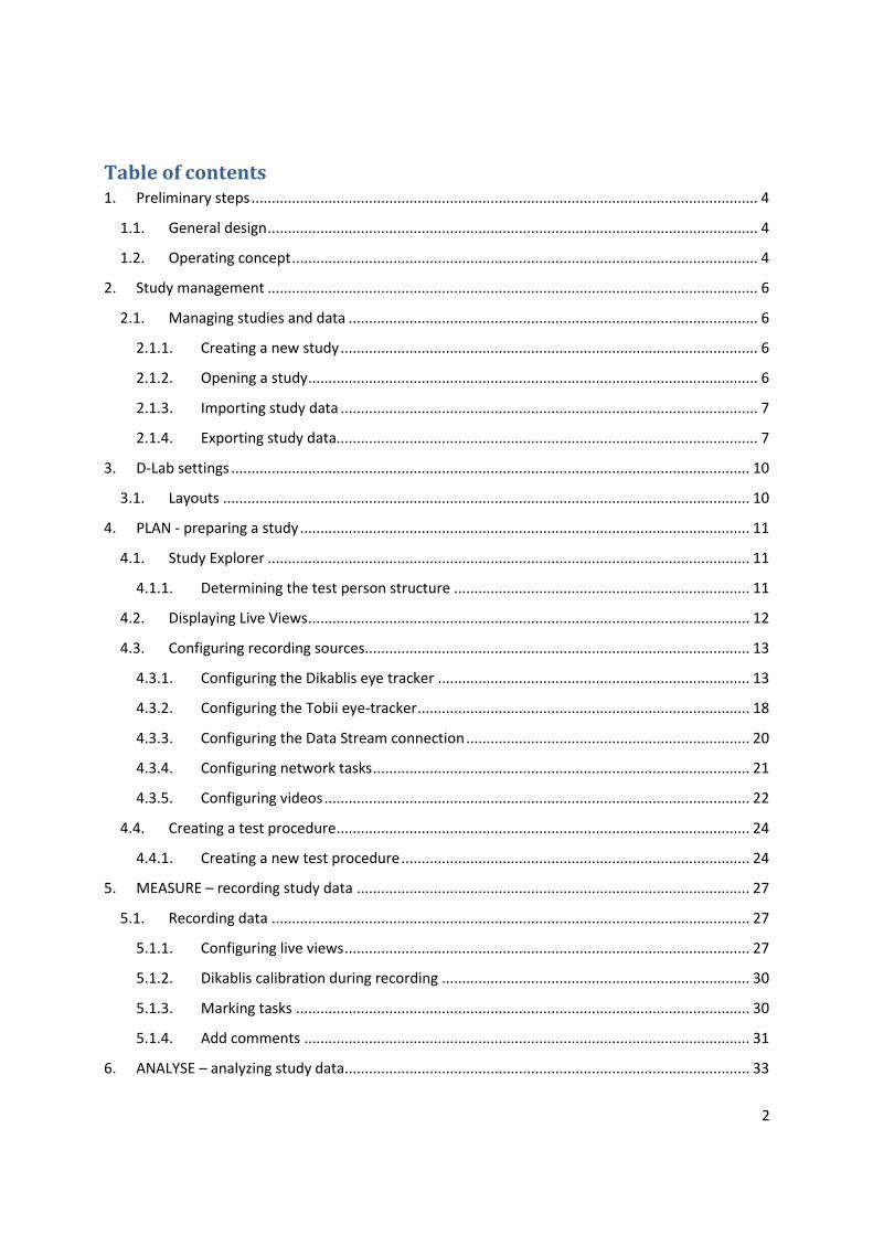
In the center of the D-Lab main window there is a visualization area in which the individual

visualization windows can be freely positioned and arranged. If two windows are positioned one

above the other in the left or right area of the work window, a cursor will appear. Shifting the

window to the center of the cursor superimposes the windows and they then appear as individual

tabs at the bottom edge of the window (see Figure 1). Pull the tab out again to display the tabs as

individual windows again. The pin symbol on the top right corner of the windows allows you to

minimize them and pin them in place. The x symbol on the right next to it is used to close the

window.

You can find functions for managing your studies in the "File" menu. Here, you can create a new

study or open a study previously created. In addition, it is possible to archive studies or selected

study data by selecting "Export" or, using "Import” to open it in D-Lab and add it to your current

project.

5

Figure 1: Docking a window

Figure 2: Tabs

The following sections of this manual will explain the functions in the three phases of a case study

(PLAN, MEASURE and ANALYSE) one after another.

6

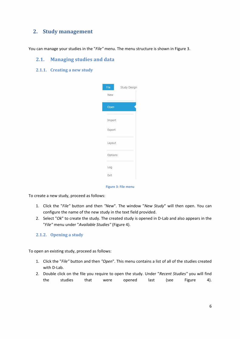
2. Study management

You can manage your studies in the "File" menu. The menu structure is shown in Figure 3.

2.1. Managing studies and data

2.1.1. Creating a new study

Figure 3: File menu

To create a new study, proceed as follows:

1. Click the "File" button and then "New". The window "New Study" will then open. You can

configure the name of the new study in the text field provided.

2. Select "Ok" to create the study. The created study is opened in D-Lab and also appears in the

"File" menu under "Available Studies" (Figure 4).

2.1.2. Opening a study

To open an existing study, proceed as follows:

1. Click the "File" button and then "Open". This menu contains a list of all of the studies created

with D-Lab.

2. Double click on the file you require to open the study. Under "Recent Studies" you will find

the studies that were opened last (see Figure 4).

7

Figure 4: Opening a study

2.1.3. Importing study data

To import a study, proceed as follows: Click on the "File" button and then on "Import". In this menu

you can import a study ("Study") or all of the definitions ("Definitions") of the study (task definitions,

formulas used and defined macros, or the coding pattern of the video analysis).

2.1.3.1. Importing a complete study

To import an entire study, proceed in the "Study" menu item as follows:

1. In the "Import Study" sub-menu, you can select and import your archived study by clicking on

the magnifying glass symbol.

2. Confirming with the "Import Study" button will load the study in D-Lab.

2.1.3.2. Importing definitions

To import the definitions saved in another study, proceed in the "Definitions" menu item as follows:

1. Using the "Import Definitions" sub-menu, you can select and import the definitions you

require by clicking on the magnifying glass symbol.

2. Confirming with the "Import" button will load the data into the current project.

2.1.4. Exporting study data

To export a study or specific parts of it, click the "File" button and then "Export". In this menu you

can export the entire study ("Entire Study"), parts of it ("Data") or the study's definitions

("Definitions").

2.1.4.1. Exporting a complete study

To export and archive an entire study, proceed as follows:

8

1. Click on the "Entire Study" button. Under "Study", you can switch between the existing

studies. Once you have selected a study, you can use "Export Location" to select a user-

defined storage location with the aid of the magnifying glass symbol.

2. You can define the maximum file size under "Maximum Size Per File".

3. Confirming with the "Export" button will compress the study and, where necessary, export it

into several files.

2.1.4.2. Exporting selected data

To export selected data of a study, proceed as follows:

1. Click on the "Data" button. You will then be able to choose from the following data packages

which can be exported individually:

"Subjects": Here you can select all of the test persons ("All"), individual ones, or

groups by clicking on the corresponding designation.

"Tasks": Here you can select for which areas (tasks) you wish to export the data.

Data can be exported for the complete recording ("All Recording"), or for selected

tasks. "Recorded Data": Here you can select the data to be exported for each

module (e.g. Eye Tracking, Data Stream Video) (see Figure 5).

In the "Special Exports" area you can select the marked tasks ("Triggered Tasks"), the

behavior coded as part of the video analysis ("Behavior Observations"), the glances

at AOIs ("Glance Intervals on AOIs") and the comments ("Export Notes"), and export

them separately.

"Export Frequency": Here you can select the frequency with which the data are to be

exported. Once the data from different sensors has been selected (meaning that

different frequencies are possible), the frequency for the data export must be

indicated. You have the following options: select the frequency of a module in order

to use the frequency of its data for export purposes. With the option "All

frequencies, No Sampling"“, all of the selected data are exported at the full

frequency.

"Export Configuration Name": Here you can assign a name to the "txt" file to be

exported.

Select the field "Export Each Task in a Different File" to export the data in individual

files for the duration of each of the tasks selected.

2. Confirming by pressing the "Export" button will export the data. The export progress is

displayed in the "Data" window.

The target directory is opened following the export. It can be found under "C:\data\".

2.1.4.3. Exporting study definitions

To export the definitions of a study, proceed as follows:

9

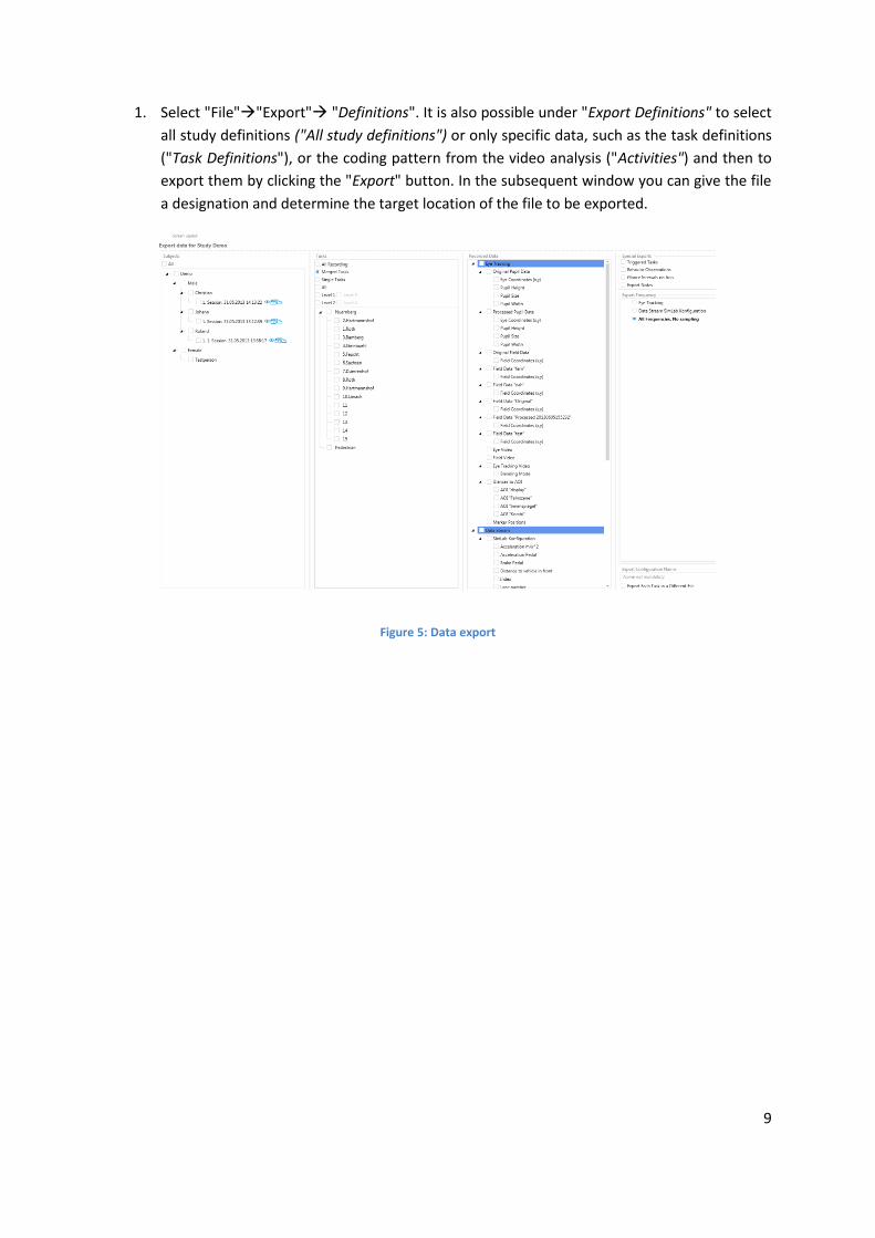
1. Select "File""Export" "Definitions". It is also possible under "Export Definitions" to select

all study definitions ("All study definitions") or only specific data, such as the task definitions

("Task Definitions"), or the coding pattern from the video analysis ("Activities") and then to

export them by clicking the "Export" button. In the subsequent window you can give the file

a designation and determine the target location of the file to be exported.

Figure 5: Data export

10

3. D-Lab settings

In the "File" menu you can also adjust the settings for the D-Lab. The following options are available:

3.1. Layouts

In this menu item you can save a number of user-specific window arrangements that you can

subsequently revert back to for new projects. To save a layout, proceed as follows:

1. Open the project if you do not already have an open project with a layout that you would like

to save.

2. Click on the "Layouts" button.

3. Press the "Save Current Layout" button. A window will then open and you can specify the

name of the layout in the text box displayed.

4. Select "OK" to save the layout. You can then find the layout with the same name in the "File"

menu under „Layout“.

11

4. PLAN - preparing a study

A structured study preparation is absolutely necessary for ensuring that an experiment will be

performed with success. Structured preparation includes the test set-up, the drawing up of a test

procedure and the preparation of the test environment. D-Lab provides a number of functions which

can guarantee optimum study preparation: the "Study Explorer", "Task Definition", "Recording

Devices" and "Live Views" functions.

4.1. Study Explorer

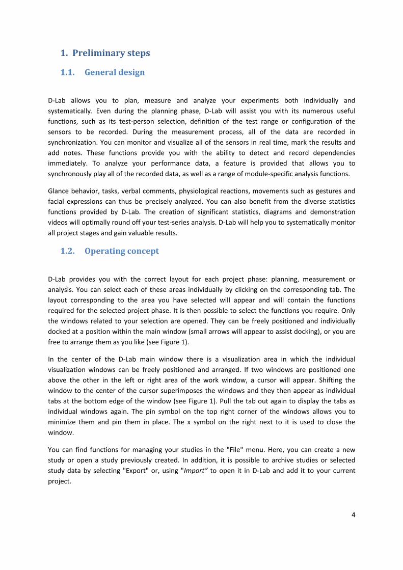
The Study Explorer is used for managing your study (see Creating test persons). Here it is possible to

add new test persons and create new groups, or to delete them. This allows you to split up the test

persons into different groups, for example based on their gender, age groups, etc.

This function is already available for use before you perform your study ("Plan"), however it can also

be used during or after the end of an experiment ("Measure" and "Analyse").

4.1.1. Determining the test person structure

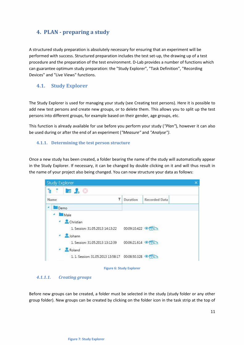
Once a new study has been created, a folder bearing the name of the study will automatically appear

in the Study Explorer. If necessary, it can be changed by double clicking on it and will thus result in

the name of your project also being changed. You can now structure your data as follows:

Figure 6: Study Explorer

4.1.1.1. Creating groups

Before new groups can be created, a folder must be selected in the study (study folder or any other

group folder). New groups can be created by clicking on the folder icon in the task strip at the top of

Figure 7: Study Explorer

12

the window. You can create either groups belonging to the same level, or groups in the next level

down. The name and arrangement of the group folders can be flexibly changed at a later date. If you

click on a particular folder, you use the mouse pointer to move it to another level or arrange it in a

new sequence. To do so, simply move the folder to the new position.

4.1.1.2. Creating test persons

To create test persons, the study or a group must be selected. New test persons can be added by

clicking on the test person icon in the top task strip. A test person symbol will appear in the Study

Explorer and you can immediately assign a name to this test person. You call also allocate the test

persons to another group later. To do so, use the mouse pointer to move the test person symbol into

the intended group folder.

There are other icons in the Study Explorer strip that can be used for managing the test person

structure. You can display all of the levels with the "Expand All" icon. You can display only the main

folders with the "Collapse All” icon. You can delete any group folders and test persons previously

created with the "Delete" icon. When doing so, please note that if you remove a folder, all of its

subordinate group folders and its assigned test persons will also be deleted. It is not possible to

restore the deleted data!

In addition to the "Expand All" and "Collapse All" icon, you can manually display and hide individual

higher and lower-level folders. As you can see in Creating test persons, small file symbols are

displayed on the left next to the group folder symbols. Clicking on the arrow will display or hide the

folder's subordinate categories.

You can execute the afore-mentioned Study Explorer functions by clicking on the icons or

alternatively by clicking on the folder symbol with the right mouse button. If you do so, a new

window will appear in which you can execute, among other things, the functions "New Folder" (for

creating a new folder), "New Subject" (for creating a new test person), "Delete" (for deleting) and

"Rename" (for changing the name). These functions are already explained in chapter 3.1.1. In

addition to this, you can copy the newly created folders and test persons by clicking on "Copy" and

then inserting them at another position in your test person structure. Again, click on the selected

folder with the right mouse button. Now you can use "Paste“ to select if you really want to copy the

copied file or copied test person ("Copy") – a duplicate copy is created -, move it ("Move"), or

generate a link to it ("Link"– a link to the selected data is created, but the data only exist once and

the changes take effect in all of the links).

4.2. Displaying Live Views

The Live View function allows you to immediately display the data from the configured sensors. The

visualization systems are opened by clicking in the "Recording Sensors" window.

13

With the menu item "Screen Layout" it is also possible to display the numerical data of all of the

sensors in different diagrams, e.g. line charts, point charts and step line charts, pointer instrument

diagrams, status diagrams and value displays. A detailed description of how the live views can be

activated for each module can be found in chapter 5.1.1.

4.3. Configuring recording sources

The preparation of an eye tracking study must include commissioning the Dikablis eye tracking

system and checking that it is working properly under test environment conditions.

To configure the recording sources, click on the "Recording Sensors" button. You will find all of the

configuration settings in this window.

The hardware sources are immediately displayed if the hardware is connected (provided, of course,

the devices have been correctly installed and configured on the computer). Examples of the afore-

mentioned devices are Dikablis and Tobii eye trackers, PAL videos, webcams, audio devices and IP

cameras. However the data stream network sources and the connection to the task remote control

must be configured first. You can select which sources are to be recorded by ticking the check box of

the sources you require.

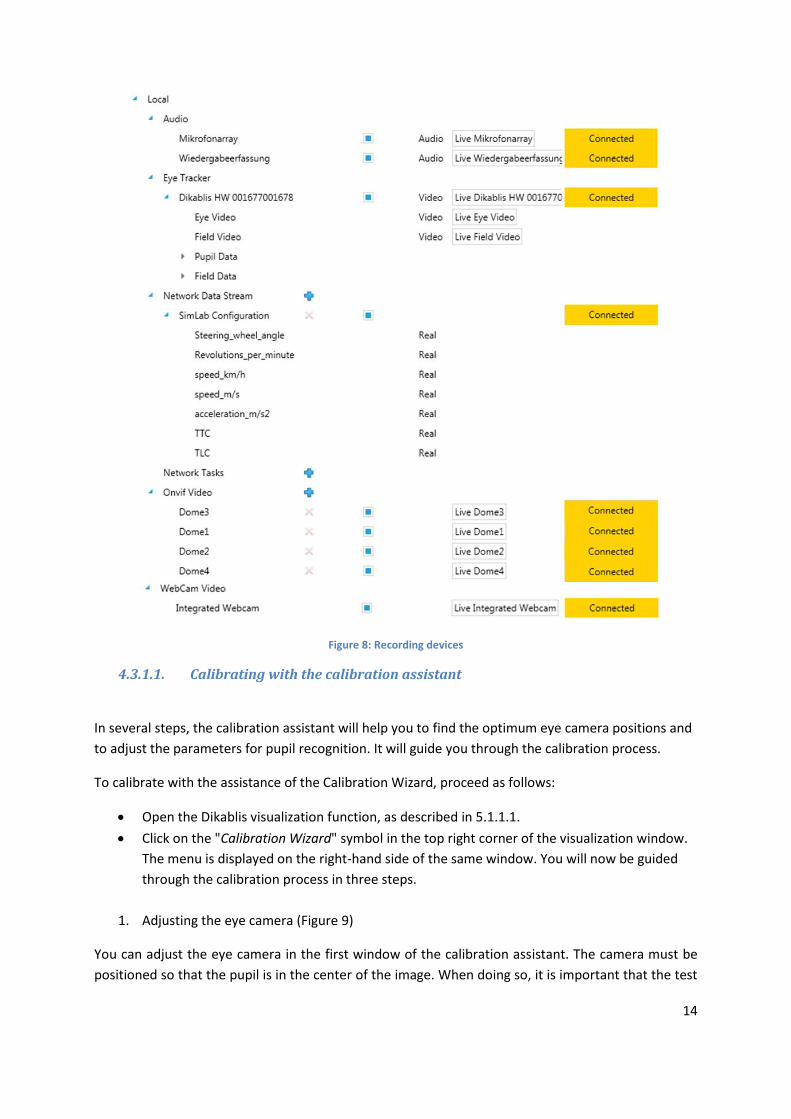
4.3.1. Configuring the Dikablis eye tracker

Connect the eye tracker to the D-Lab computer. The Dikablis eye tracker will be listed automatically

under "Recording Devices", as shown in Figure 8. The next step is to calibrate the eye tracking system

for recording. To do so, use the calibration assistant to perform automatic calibration. Alternatively

you can also calibrate the eye tracker manually.

Before starting data recording, you must make sure that the calibration has been individually

adjusted and adapted to suit the current test person.

To view the live image from the eye tracker, open the Dikablis visualization system by clicking on the

"Dikablis" button in the "Visualization" column of the "Recording Sensors" window.

In the live view, you have the option of having only the eye camera, the field camera or a blended

view of both videos displayed in blending mode. You can select the required view using the icons

below the eye tracking video. The next step is calibration.

14

Figure 8: Recording devices

4.3.1.1. Calibrating with the calibration assistant

In several steps, the calibration assistant will help you to find the optimum eye camera positions and

to adjust the parameters for pupil recognition. It will guide you through the calibration process.

To calibrate with the assistance of the Calibration Wizard, proceed as follows:

Open the Dikablis visualization function, as described in 5.1.1.1.

Click on the "Calibration Wizard" symbol in the top right corner of the visualization window.

The menu is displayed on the right-hand side of the same window. You will now be guided

through the calibration process in three steps.

1. Adjusting the eye camera (Figure 9)

You can adjust the eye camera in the first window of the calibration assistant. The camera must be

positioned so that the pupil is in the center of the image. When doing so, it is important that the test

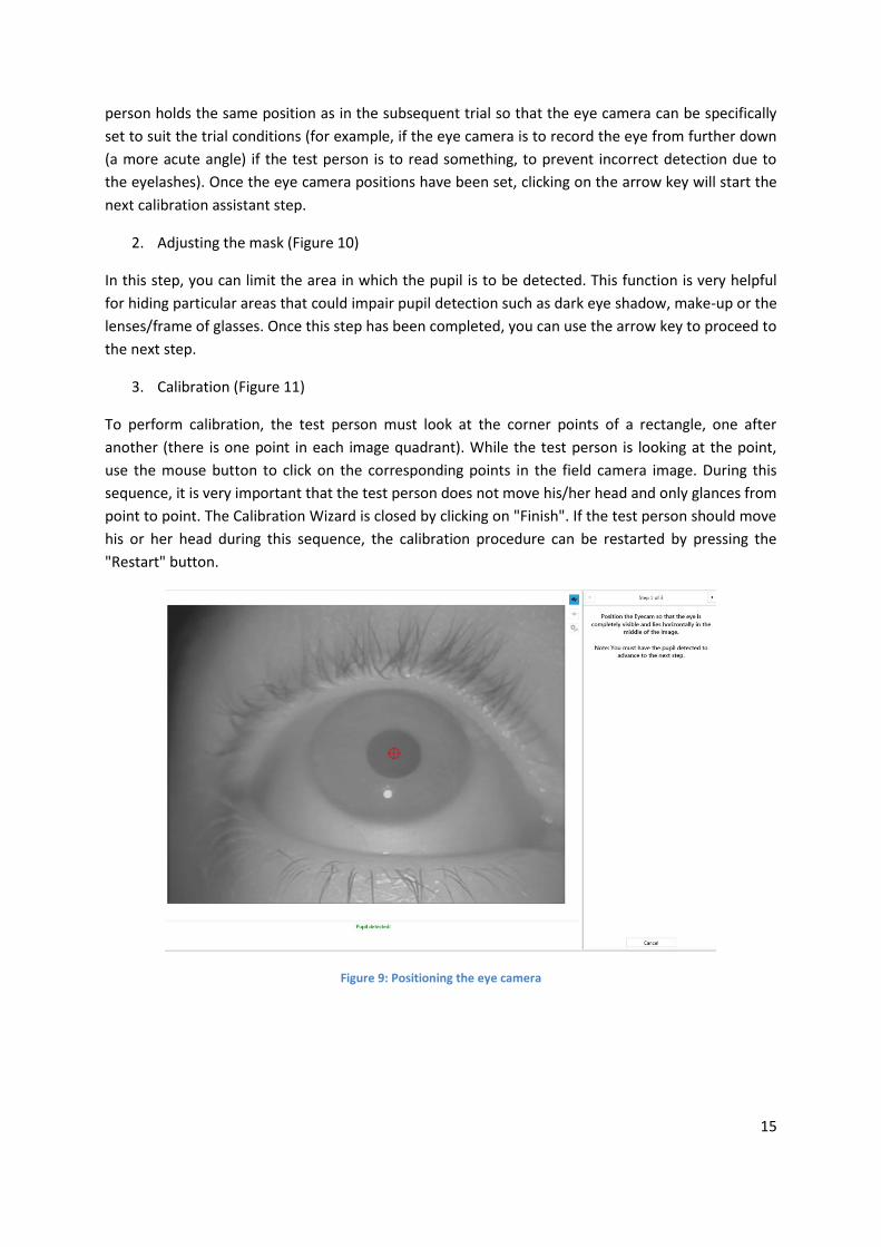
15

person holds the same position as in the subsequent trial so that the eye camera can be specifically

set to suit the trial conditions (for example, if the eye camera is to record the eye from further down

(a more acute angle) if the test person is to read something, to prevent incorrect detection due to

the eyelashes). Once the eye camera positions have been set, clicking on the arrow key will start the

next calibration assistant step.

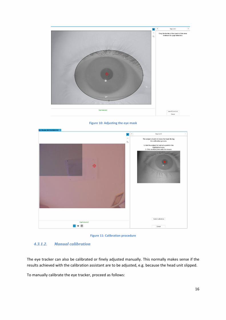
2. Adjusting the mask (Figure 10)

In this step, you can limit the area in which the pupil is to be detected. This function is very helpful

for hiding particular areas that could impair pupil detection such as dark eye shadow, make-up or the

lenses/frame of glasses. Once this step has been completed, you can use the arrow key to proceed to

the next step.

3. Calibration (Figure 11)

To perform calibration, the test person must look at the corner points of a rectangle, one after

another (there is one point in each image quadrant). While the test person is looking at the point,

use the mouse button to click on the corresponding points in the field camera image. During this

sequence, it is very important that the test person does not move his/her head and only glances from

point to point. The Calibration Wizard is closed by clicking on "Finish". If the test person should move

his or her head during this sequence, the calibration procedure can be restarted by pressing the

"Restart" button.

Figure 9: Positioning the eye camera

16

Figure 10: Adjusting the eye mask

Figure 11: Calibration procedure

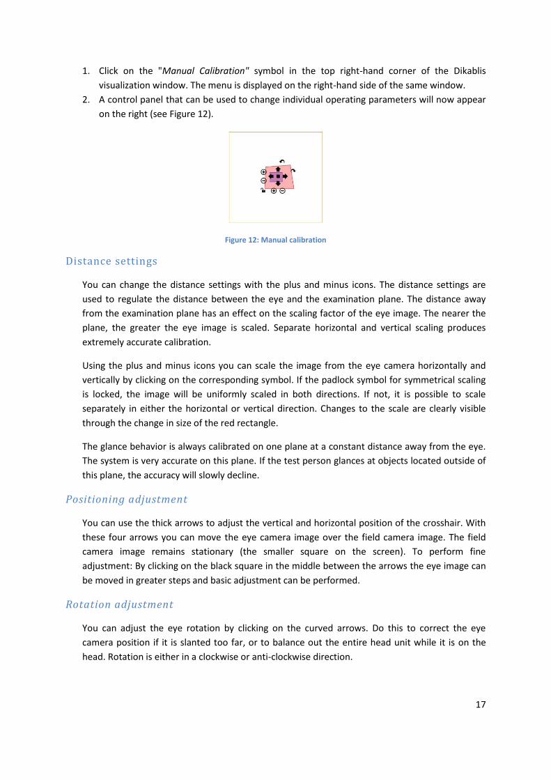
4.3.1.2. Manual calibration

The eye tracker can also be calibrated or finely adjusted manually. This normally makes sense if the

results achieved with the calibration assistant are to be adjusted, e.g. because the head unit slipped.

To manually calibrate the eye tracker, proceed as follows:

17

1. Click on the "Manual Calibration" symbol in the top right-hand corner of the Dikablis

visualization window. The menu is displayed on the right-hand side of the same window.

2. A control panel that can be used to change individual operating parameters will now appear

on the right (see Figure 12).

Figure 12: Manual calibration

Distance settings

You can change the distance settings with the plus and minus icons. The distance settings are

used to regulate the distance between the eye and the examination plane. The distance away

from the examination plane has an effect on the scaling factor of the eye image. The nearer the

plane, the greater the eye image is scaled. Separate horizontal and vertical scaling produces

extremely accurate calibration.

Using the plus and minus icons you can scale the image from the eye camera horizontally and

vertically by clicking on the corresponding symbol. If the padlock symbol for symmetrical scaling

is locked, the image will be uniformly scaled in both directions. If not, it is possible to scale

separately in either the horizontal or vertical direction. Changes to the scale are clearly visible

through the change in size of the red rectangle.

The glance behavior is always calibrated on one plane at a constant distance away from the eye.

The system is very accurate on this plane. If the test person glances at objects located outside of

this plane, the accuracy will slowly decline.

Positioning adjustment

You can use the thick arrows to adjust the vertical and horizontal position of the crosshair. With

these four arrows you can move the eye camera image over the field camera image. The field

camera image remains stationary (the smaller square on the screen). To perform fine

adjustment: By clicking on the black square in the middle between the arrows the eye image can

be moved in greater steps and basic adjustment can be performed.

Rotation adjustment

You can adjust the eye rotation by clicking on the curved arrows. Do this to correct the eye

camera position if it is slanted too far, or to balance out the entire head unit while it is on the

head. Rotation is either in a clockwise or anti-clockwise direction.

18

Any changes made to the calibration will become effective once the "Apply Calibration" button has

been clicked. Any adjustments made are then displayed in a list in the bottom window area. Manual

corrections are marked with "M", adjustments made with the calibration assistant are marked with a

"W".

4.3.2. Configuring the Tobii eye-tracker

Connect the eye tracker to the D-Lab computer. The Tobii eye tracker will be listed automatically

under "Recording Sources", as shown in Figure 13. The next step is to calibrate the eye tracking

system for recording. To do so, use the calibration assistant to perform automatic calibration.

Figure 13: Recording sensors - Tobii video

To view the live image from the eye tracker, open the Tobii visualization system by clicking on

the "Live Screen Capture" button in the "visualization" column of the "Recording Sensors"

window.

4.3.2.1. Configuring the video source

In the "Recording Sensors" window, under "Tobii Video", click on the connected Tobii eye tracker

with the right mouse button and then select "Configure".

You now principally have the option of choosing between the monitor, or one or more external

cameras or monitors in combination with one or more external cameras as your video source.

19

Figure 14: Editing the Tobii configuration

Select the corresponding icon in the "Edit Tobii configuration" window. Then, for the monitor,

select the display to be used and, for cameras, select the "+" symbol to use an external camera as

a video source. If you wish to add another camera, select the "+" symbol once again.

Each selected video source will then appear under "Tobii Video" in the "Recording Sensors".

4.3.2.2. Calibrating the monitor as an image source

To calibrate the eye tracker with the monitor as a video source, either use the right mouse

button to click in the "Recording Sensors" on the corresponding video source and select

"Calibrate", or open the "Live View" display of the video source under "Recording Sensors" and

click on the symbol on the top right, in the corner.

Follow the instructions on the screen. Once you click Start, one red point after another must be

glanced at. When doing so, it is important that the head of the test person is kept as still as

possible.

Confirm successful calibration by clicking on "OK". If calibration was unsuccessful, confirm with

"OK" and repeat the calibration procedure.

4.3.2.3. Calibrating external cameras as an image source

Under "Recording Sensors", open the live view of the camera to be calibrated. The calibration

sheet must be printed out for calibration. If you have not already done so, select "Print

Calibration Sheet" in the live view. The calibration sheet must be completely visible during the

calibration procedure and the printed markers must be detected.

Once you have moved the external camera to its final position, click on "Calibrate Camera".

20

Then select "Calibrate Eye Tracker". Follow the instructions on the screen. Once you have clicked

"Start", the test person must look at the first red point on the calibration sheet. After the audio

signal, the test person's gaze must move to the next red point. When doing so, it is important

that the test person keeps his/her head as still as possible.

Confirm successful calibration by clicking on "OK". If calibration was unsuccessful, confirm with

"OK" and repeat the calibration procedure.

The calibration sheet can now be removed from the image for data recording. However, for

automatic glance evaluation, one or more markers will be required in the image.

Data are recorded, AOIs are created and glance data are calculated in a similar manner to a Dikablis

eye tracker.

4.3.3. Configuring the Data Stream connection

The Data Stream module provides you with the option of recording any data stream synchronously

with the other modules. This involves data packets, which are received via a TCP/IP connection. The

following describes how the connection is configured and the format that the data packets must

have.

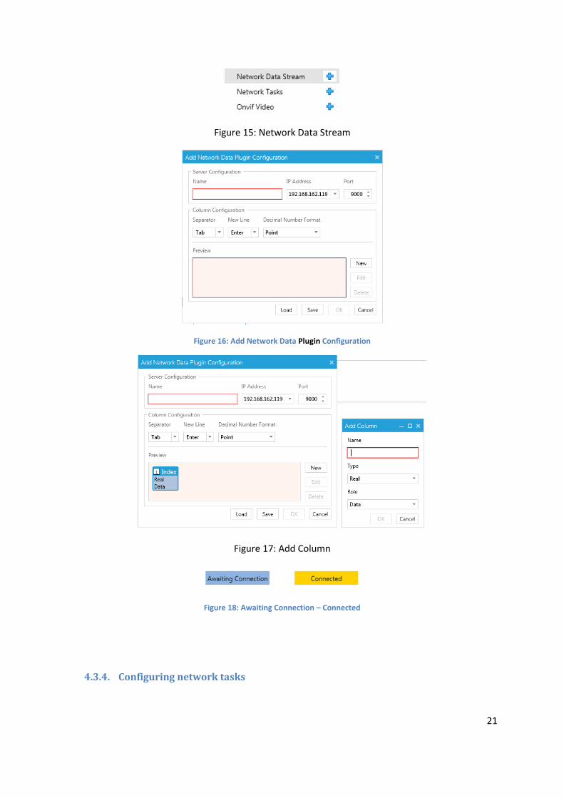
To set up the connection for receiving Data Stream data, the "Add Network Data Plugin

Configuration" dialog box must be filled in. This can be found by going to "Recorded Sensors" and

then clicking on the "plus" symbol after "Network Data Stream” (see Figure 15). In the opened dialog

box (see Figure 16), enter the following information:

Name: Name of the configuration

IP address: IP of the D-Lab computer to which the data are to be sent

Port: Port number via which the connection is to be set up

Separator: Sign used to separate the individual values in the data packet, e.g. TAB

New Line: Sign for marking the end of the data packet, e.g. ENTER

Decimal Number Format: Information as to whether floating-point numbers in the data

packet are written with a point or comma

Channel definition: By clicking on "New", you can add data channels to be transmitted

through the connection, e.g. speed, steering angle, etc. Please note that the order of the

definition must be the same as the order in which the values are transmitted. The same

applies for the number of channels. You can change the order by shifting the configured

channels in the preview window with drag&drop.

A configuration can be saved (save) and loaded if necessary (load). Once D-Lab is started, the

application will wait for a connection query. Once the data transmitter responds, the status changes

from "Awaiting Connection" to "Connected" (see Figure 18).

21

Figure 15: Network Data Stream

Figure 16: Add Network Data Plugin Configuration

Figure 17: Add Column

Figure 18: Awaiting Connection – Connected

4.3.4. Configuring network tasks

22

D-Lab offers you the possibility of marking tasks by remote control. For example, it is possible to

trigger an event from a simulation and send it to D-Lab where the corresponding task is then

marked. This also happens through a TCP/IP connection via a user-defined port.

To produce a network task, go to the "Recording Sources" window and click on the plus symbol

after "Network Tasks". In the "Add Network Tasks Configuration" window that is then opened,

enter a name for the configuration, the IP of the D-Lab computer and the port for setting up the

connection. Once the connection is set up, it is displayed via the status.

4.3.4.1. Triggering tasks through the network

To mark tasks using network control, the following format must be observed on the transmitter side:

To mark a task, send the network name of the task (as indicated in the "Task Definition")

with the ending ‚\0‘ through the configured connection (see chapter 4.4). Example: <task

network name>\0

You can also activate several tasks at once by switching several network names one after

another. Example: <task1 network name>\0<task2 network name>\0

For interval tasks, the first time a network name appears it is interpreted as the start and the

following one as the end, etc.

4.3.5. Configuring videos

The first step for recording video data is to start up the hardware. Set up your camera system and

check that it is working properly. Position the cameras so that the relevant areas are covered. If the

video is recorded with a webcam, no configuration is normally needed. A configuration is normally

only needed when using IP or PAL cameras.

4.3.5.1. PAL cameras via integrated grabber (for workstations, e. g. Falcon grabber

cards)

Once the drivers for the integrated grabber card are installed, the video channels are automatically

displayed in the recording devices window. No further configuration is necessary.

4.3.5.2. PAL cameras with USB grabber (for workstations and laptops, e.g. Axis

Q7404 grabber)

The PAL cameras are normally driven via a quad splitter and have the addresses 192.168.0.90 to

192.168.0.93. This can be changed using the "Axis Camera Management" software from the camera

manufacturer, which is included separately.

To set up a PAL camera, please use the ONVIF interface in D-Lab 3. The exact way to proceed is

described in the following chapter.

4.3.5.3. Network cameras (axis)

Network cameras are connected to the D-Lab computer via a switch. The cameras' IP addresses can

be manually adjusted using the "Axis Camera Management" software included separately. The

23

following addresses are already pre-configured: 192.168.0.90, 192.168.0.91., etc., depending on the

number of cameras.

To set up a PAL or network camera, please use the ONVIF interface in the Recording Devices window.

The plus sign opens up the corresponding window. (Figure 19)

Figure 19: ONVIF settings

The user name and password have each been pre-set to "root". Please do not change this setting.

Each camera must be configured in this window and called using the IP address. (Figure 20)

Figure 20: ONVIF configuration

Confirm the window with the "OK" button. The configured camera is then listed in the Recording

Devices window. After a few seconds, the camera status changes to "Connected". The camera is now

ready to record. You can display/hide the camera image by clicking on the visualization button.

(Figure 21)

Figure 21: Configuration status connected

24

Figure 22: Camera visualization

If you have a PTZ (Pan-Tilt-Zoom) camera, D-Lab offers you the possibility of controlling it directly

using software. Use the arrows to move the camera in the x and y direction. To zoom, use the +/-

symbol. (Figure 22)

4.4. Creating a test procedure

Another step to be taken when planning a case study is to create a test procedure. D-Lab also has a

suitable function that allows you to create such a test procedure with ease. A test procedure is a set

of instructions informing the test person about how to carry out the study. The procedure must

include all parts of the test and all of the use cases (tasks) to be fulfilled, and must conform to the

ISO/TS 15007-2 standard. D-Lab thus provides you with the ability to plan eye tracking studies and

general case studies in a non-conforming manner. The "Task Definition" function is provided for this.

It is not imperative that a study be performed in accordance with a pre-defined test procedure and

the choice to do so or not greatly depends on the area of application. The advantage of carrying out a

study in accordance with a test procedure is that it is then possible to mark tasks while recording the

data. Using this structure, it is possible to evaluate the data in D-Lab based on the particular task.

4.4.1. Creating a new test procedure

To create a new test procedure, proceed as follows:

1. In the "Plan" module, switch to the "Study Design" tab and select the "Task Definitions"

button there.

2. To create an interval task, go to the "Task Definitions" window and click on the "New

Interval" symbol. To define a single task, select the "New Single" button in the window's

toolbar.

25

3. The corresponding task is then created. The entry can be edited and you can enter any name

you wish for the first task of the procedure. Press the Enter key to complete the editing

process.

Figure 23: Task definition window

It is possible to define tasks on four levels. To define a subtask, select the task from the top level

and proceed as described above.

Tasks can be copied, moved and edited. To do so, use the functions available in the context menu

(click on the task with the right mouse button).

To mark the tasks by remote control, enter a distinct and unambiguous network name for each

task (Network Name column in the Task Definition window). The default setting for the network

name is the task's path in the task tree, but it can be changed to a user-defined setting. The task

can only be activated during recording.

The test procedure can be saved using the "Save" and "Load" buttons in the window's toolbar

and can be imported into other projects.

You can activate the following functions with the check boxes in the "Same Root" and "Diff Root"

columns:

"Same Root": Within a task group (all subtasks belonging to a first-level task), if a

new task has been activated, the task that is already active will be deactivated.

This makes it easier for the test manager to mark the tasks via the "Task

Triggering" window while the test is in progress.

26

"Diff Root": If a task from a task group other than the one that is currently active

is marked, then all of the active tasks in this task group will be automatically

deactivated.

The use of these rules is study-dependent and can be deactivated by the user if necessary.

27

5. MEASURE – recording study data

Once all the afore-mentioned measures have been taken, the study can begin. D-Lab allows you to

synchronously record the data for all of the modules. During the recording you can check the data at

any time using the live views of the data streams. Tasks and events can also be marked. These marks

are stored in the recorded data and can be used later for analysis purposes. You can also change the

layout during a recording. It is possible to open and then configure new functions. Selected diagrams

or videos can be activated depending on the application and comments can be added during

recording.

5.1. Recording data

To start data recording, proceed as follows:

1. If you have not yet opened up a study, do so as described under point 2.1.2 .

2. Switch to the "Data Recording" tab and select a test person from the "Study Explorer", or

generate a new test person (see point Fehler! Verweisquelle konnte nicht gefunden

werden.). When doing so, make sure that the Study Explorer is selected under "Study

Design" to ensure that the window is visible.

3. Click on the red "Record" symbol located in the "Data Recording" tab, at the top left (see

Figure 24). A new window will then open ("Data Session Recording"), which displays the time

when recording was started and the recording duration. You can stop the recording with the

blue "Stop" button. The "Data Session Recording" window is then closed. A new "data

session" is created for this test person. You can start another recording for the test person

already created (to do so, proceed as described in point 2), or you can select a new test

person or study for another recording.

Figure 24: Data recording

5.1.1. Configuring live views

It is possible to track all of the data live and optimize it if possible while the data are being recorded.

To visualize the data, proceed as follows:

In the "Study Design" tab, open the "Recording Devices" window. A window will then open in which

you can view all of the connected devices and the configured connections (see Figure 25). Please

28

ensure that the sources to be recorded are activated! To do so, you have to activate the box next to

the data source with a mouse click.

Figure 25: Recording sensors window

5.1.1.1. Eye Tracking Live View

To track the glance behavior of an eye tracker in real time, open the glance visualization by going to

the "Recorded Sensors" window and clicking on the button in the "Visualization" column of the eye

tracker in question. Alternatively, open an “empty glance” visualization in the "Screen Layout" tab

and pull the glance data source into the visualization. You can find details about the content of the

visualization window in chapter 6.4.

5.1.1.2. Video Live View

To view a recorded video in real time, open the video visualization by going to the "Recorded

Sensors" window and clicking on the button in the "Visualization" column of the video in question.

Alternatively, open an empty video visualization in the "Screen Layout" tab and pull the video source

into the visualization.

5.1.1.3. Audio Live View

29

To open the amplitude diagram of a recorded audio source, go to the “Recording Sensors” window

and click on the visualization button of the corresponding audio source. Alternatively, open an empty

audio visualization and then pull the source into the visualization window.

5.1.1.4. Data Stream Live View

To visualize data streams during recording, open an empty visualization window (see the following

diagram illustrations) and pull the data streams you require out of the "Recording Sensors" window

and into the visualization. Depending on the diagram types involved, one or more data channels can

be visualized in one diagram.

To visualize numerical data, the following illustration options are available to you in the "Screen

Layout":

Eye Tracker

Here you have the option of displaying an eye tracking video with an aim to configuring different

visualizations such as the heat map, gaze path, shadow map or bee swarm. To do so, simply pull the

data source into the window. The corresponding glance data will be shown in the list. See section

6.4.9 Special visualizations for eye tracking data

Line Chart, Point Chart, Step Line Chart

You can choose to display the data in the form of a line chart, point chart, or step line chart here. To

do so, simply pull the data source into the window. You can change the seconds’ interval in the

display under “Settings”. In addition, you can determine the auto limits, minimum and maximum

values of the axis, color and axis position.

List

You can choose to display your data in a list here. To do so, simply pull the data source into the

window. The time and the corresponding data value are displayed here.

Peak Gauge

You can choose to display your data in scale form here. To do so, simply pull the data source into the

window. Under "Settings", you can have the values displayed with decimal places. You can also

determine the minimum and maximum value, and the intervals.

Round Gauge, Semicircle Gauge

Figure 26: Visualization options

30

Here you have the option of visualizing the data in an instrument display diagram. To do so, simply

pull the data source into the window. Under "Settings", you can have the values displayed with

decimal places. You can also determine the minimum and maximum value, and the intervals.

State diagram

Here you have the option of visualizing your data in a state diagram. To do so, simply pull the data

source into the window. Under "Settings", you can determine the number of states (e.g. number of

lanes, indicator on/off) that can be used during the test and you can define what is to be displayed

when the corresponding data value is active.

Value

Here you have the option of visualizing your data as a value. To do so, simply pull the data source

into the window.

Take Snapshot

You can use this function to take a screen shot of the work area. If you click on the symbol, a window

will appear. Click on "OK" here to take the screen shot. Confirming the "Ok" key will open up a

window in which you can select the file path.

Record Workspace

You can generate a film of the entire visualization area with this function. To do so, configure the

required diagrams and visualizations and then play back the data in the player. Press the "Record

Workspace" function to start the recording. The visualization area is then recorded. To stop the

recording, press the "Stop" button. A video that you can then use for presentation purposes is saved

in mp4 format.

5.1.2. Dikablis calibration during recording

It is possible to track your data streams live and optimize them while the data are being recorded. To

do so, proceed as described in chapter 4.3.1, to optimize the calibration. You can use either the

Wizard or the manual calibration feature.

5.1.3. Marking tasks

To trigger tasks during recording, they need to have been previously generated (see point 4.4.1

Creating tasks). Then proceed as follows:

1. Click on "Task Triggering" in the "Data Recording" tab. A new window will then open. The

tasks (single or interval triggers) already created will be displayed as buttons in this window.

The single trigger buttons have slightly rounded corners compared to the interval trigger

buttons. These buttons are inactive (grayed out) if the recording has not yet been started.

31

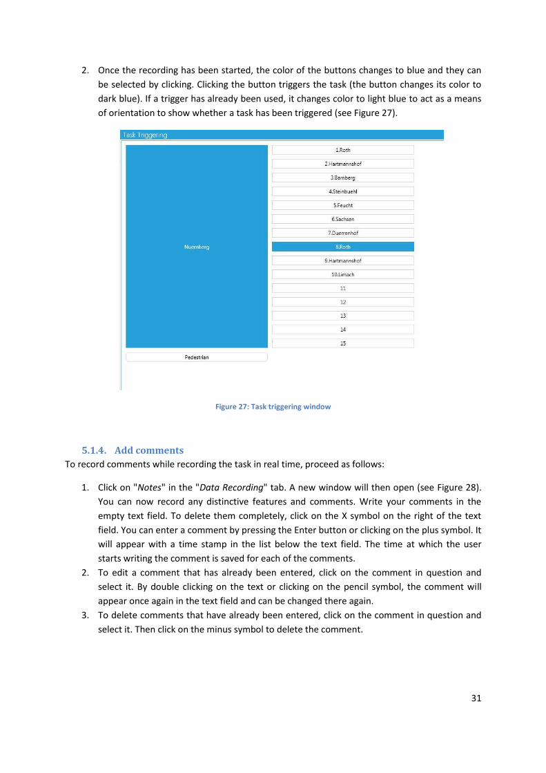
2. Once the recording has been started, the color of the buttons changes to blue and they can

be selected by clicking. Clicking the button triggers the task (the button changes its color to

dark blue). If a trigger has already been used, it changes color to light blue to act as a means

of orientation to show whether a task has been triggered (see Figure 27).

Figure 27: Task triggering window

5.1.4. Add comments

To record comments while recording the task in real time, proceed as follows:

1. Click on "Notes" in the "Data Recording" tab. A new window will then open (see Figure 28).

You can now record any distinctive features and comments. Write your comments in the

empty text field. To delete them completely, click on the X symbol on the right of the text

field. You can enter a comment by pressing the Enter button or clicking on the plus symbol. It

will appear with a time stamp in the list below the text field. The time at which the user

starts writing the comment is saved for each of the comments.

2. To edit a comment that has already been entered, click on the comment in question and

select it. By double clicking on the text or clicking on the pencil symbol, the comment will

appear once again in the text field and can be changed there again.

3. To delete comments that have already been entered, click on the comment in question and

select it. Then click on the minus symbol to delete the comment.

32

Figure 28: Notes window

33

6. ANALYSE – analyzing study data

In the analysis mode all of the data can be played back synchronously and analyzed specifically for a

particular module.

6.1. Visualizing the data

Different visualization options are available to you in D-Lab, depending upon the data type. These

will now be explained in the following subchapters.

The general procedure for data visualization is the following:

In the "Study Explorer" window, select the recording (data session) that holds the content

you would like to visualize.

Open the "Data Session Explorer" window. The content of the selected recording is listed

here. In the Data Session Explorer you can open the visualizations by clicking on the

visualization button for the data you require or by pulling the data to be displayed with

drag&drop into an open visualization.

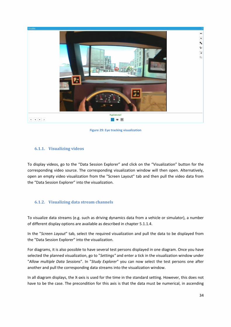
6.1.1. Visualizing glance data

To visualize the glance data of an Eye Tracker, click the visualization button of the corresponding

source in the Data Session Explorer. The corresponding visualization window will then open (see

Figure 29). Alternatively, open an empty eye tracking visualization from the "Screen Layout" tab and

then pull the eye tracking data from the Data Session Explorer into the visualization.

In the visualization window, the symbols in the bottom section can be used to display the field video

with the crosshair for the glance, the eye video or the blending mode (in which the field and eye

video are superimposed to form a semi-transparent image).

The video can also be replayed forwards and backwards in the same way as in the player. It is also

possible to jump forward or backward one frame. The corresponding symbols can be found at the

bottom left of the window.

To optimize pupil detection and prepare more detailed calculations, a number of icons can be found

in the top right area of the window. The functions of these icons are described in section 6.4.

34

Figure 29: Eye tracking visualization

6.1.1. Visualizing videos

To display videos, go to the “Data Session Explorer” and click on the “Visualization” button for the

corresponding video source. The corresponding visualization window will then open. Alternatively,

open an empty video visualization from the "Screen Layout" tab and then pull the video data from

the “Data Session Explorer” into the visualization.

6.1.2. Visualizing data stream channels

To visualize data streams (e.g. such as driving dynamics data from a vehicle or simulator), a number

of different display options are available as described in chapter 5.1.1.4.

In the "Screen Layout" tab, select the required visualization and pull the data to be displayed from

the "Data Session Explorer" into the visualization.

For diagrams, it is also possible to have several test persons displayed in one diagram. Once you have

selected the planned visualization, go to "Settings" and enter a tick in the visualization window under

"Allow multiple Data Sessions". In "Study Explorer" you can now select the test persons one after

another and pull the corresponding data streams into the visualization window.

In all diagram displays, the X-axis is used for the time in the standard setting. However, this does not

have to be the case. The precondition for this axis is that the data must be numerical, in ascending

35

order and unambiguous (e.g. a kilometer counter). This means that you can also structure the X-axis

according to your own specifications if required.

6.1.3. Timelines

In D-Lab, you have the option of having specific timelines displayed in individual windows or grouped

together in one window. The timelines show the recorded data in its temporal order and are used for

displaying tasks, events, glances or encoded activities.

6.1.3.1. Task timelines

The task timeline specifies which tasks have been performed, at which position and for which

duration they are included in the recording. To open the task timelines, proceed as follows:

1. In the "Screen Layout" tab, click on the "Task Timelines” button.

A new window will appear which displays the tasks listed one below the other (see Figure 30).

The length of the task is shown with a bar. Single triggers are represented by points. The small

arrow on the left next to the individual timeline bar indicates whether there are additional

subtasks below the task. Clicking on the arrow allows them to be displayed or hidden.

2. Clicking on the magnifying glass signal enlarges the view. Clicking on the arrow symbol

displays or hides the task timeline in the player.

3. To display the time segment in the player, move the mouse over the task and click with the

middle mouse button. The timeline zoom bar in the player adjusts to the task duration.

Figure 30: Task timelines

6.1.3.2. Glance timelines

36

The glance timeline provides information about the distribution of the glances at the individual

AOIs. Here it is important to calculate the glance at the individual AOIs beforehand. This is

described under chapter 6.4.5.

To open the glance timeline, proceed as follows:

1. Go to the "Screen Layout" tab and click on the "Glance Timelines" button. A new window will

open in which the AOIs are listed one below another, together with the individual glance

distributions. The length and frequency of the glance distribution is visualized using

individual bars (see Figure 31).

Figure 31: Glance timelines

2. Clicking on the magnifying glass signal enlarges the display. Clicking on the arrow symbol

displays or hides the glance timeline in the player.

6.1.4. Player

The player is the central constituent for time-based navigation in the recorded data. To open the

player, proceed as follows:

1. Under the "Data Analysis" tab, click on the "Player" button. The player window will then open

(see Figure 32).

Figure 32: Player

The following options are available for operating the player:

1. The control buttons are on the left. You can use the black arrows to play, rewind or stop the

recording. You can adjust the speed as you wish from 10% of the speed to 10 times the

speed using the scroll bar.

2. You can playback the recording one frame at a time in a forward or reverse direction with

single clicks on the gray arrows.

3. You will find three timelines on the right. The top timeline shows the total length of the

recording as a gray line. The red line indicates your current position in the recording.

4. You can individually determine a particular time segment in the white timeline. This timeline

appears as a timeline zoom bar with which you can enlarge or minimize the time segment by

pulling the sides (Figure 33). In the top area of the timeline zoom bar, you can see your

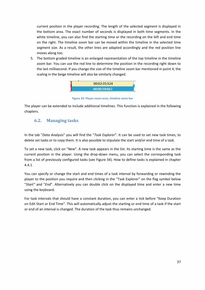
37

current position in the player recording. The length of the selected segment is displayed in

the bottom area. The exact number of seconds is displayed in both time segments. In the

white timeline, you can also find the starting time or the recording on the left and end time

on the right. The timeline zoom bar can be moved within the timeline in the selected time

segment size. As a result, the other lines are adapted accordingly and the red position line

moves along too.

5. The bottom graded timeline is an enlarged representation of the top timeline in the timeline

zoom bar. You can use the red line to determine the position in the recording right down to

the last millisecond. If you change the size of the timeline zoom bar mentioned in point 4, the

scaling in the beige timeline will also be similarly changed.

Figure 33: Player zoom-area, timeline zoom bar

The player can be extended to include additional timelines. This function is explained in the following

chapters.

6.2. Managing tasks

In the tab "Data Analysis" you will find the "Task Explorer". It can be used to set new task times, to

delete set tasks or to copy them. It is also possible to stipulate the start and/or end time of a task.

To set a new task, click on "New". A new task appears in the list. Its starting time is the same as the

current position in the player. Using the drop-down menu, you can select the corresponding task

from a list of previously configured tasks (see Figure 34). How to define tasks is explained in chapter

4.4.1.

You can specify or change the start and end times of a task interval by forwarding or rewinding the

player to the position you require and then clicking in the “Task Explorer” on the flag symbol below

"Start" and "End". Alternatively you can double click on the displayed time and enter a new time

using the keyboard.

For task intervals that should have a constant duration, you can enter a tick before "Keep Duration

on Edit Start or End Time". This will automatically adjust the starting or end time of a task if the start

or end of an interval is changed. The duration of the task thus remains unchanged.

38

Figure 34: Task explorer window

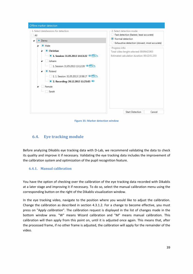
6.3. Marker detection

If the online detection of the markers is insufficient (e.g. because the test was recorded under poor

lighting conditions), it is possible to have the markers detected again at a later stage using the

marker detector.

To start marker detection, go to "Data Analysis" and select "Marker Detection". Here you can select

for which test persons the marker detection is to be optimized. When doing so, you can also make

use of three different modes (see Figure 35).

Under "Progress Info" you can see how much video material is to be scanned and approximately how

long marker detection will take.

Once you have decided in favor of a mode, click on "Start Detection".

39

Figure 35: Marker detection window

6.4. Eye tracking module

Before analyzing Dikablis eye tracking data with D-Lab, we recommend validating the data to check

its quality and improve it if necessary. Validating the eye tracking data includes the improvement of

the calibration system and optimization of the pupil recognition feature.

6.4.1. Manual calibration

You have the option of checking over the calibration of the eye tracking data recorded with Dikablis

at a later stage and improving it if necessary. To do so, select the manual calibration menu using the

corresponding button on the right of the Dikablis visualization window.

In the eye tracking video, navigate to the position where you would like to adjust the calibration.

Change the calibration as described in section 4.3.1.2. For a change to become effective, you must

press on "Apply calibration". The calibration request is displayed in the list of changes made in the

bottom window area. "W" means Wizard calibration and "M" means manual calibration. This

calibration will then apply from this point on, until it is adjusted once again. This means that, after

the processed frame, if no other frame is adjusted, the calibration will apply for the remainder of the

video.

40

To complete processing, click on "Finished" or close the menu by clicking on the "Manual Calibration"

button once again.

Figure 36: Manual calibration

You also have the option of performing calibration on more than one plane by using the "Calibration

Plane" function. This allows you to correct parallax errors by allowing different calibrations to be

defined for different distance planes. If you would like to have the greatest possible measurement

accuracy on, for example, a close plane (vehicle interior) and simultaneously on a plane which is

further away (vehicle surroundings, e.g. crossroads, traffic lights, etc.), define one calibration plane

for near surroundings and one for those far away and then make the necessary calibration

adjustments independently for each layer. When defining the areas of interest, enter which

calibration plane each area of interest relates to.

To create a new calibration plane, click on "Calibration Plane" and then "New". You will now be

requested to provide a designation. Alternatively, the "Duplicate" button can be used to copy the

selected calibration plane and then edit the copy. All of the calibration adjustments are always made

in relation to the selected calibration plane.

You can set which calibration plane is to be displayed as the default setting on the player in "Data

Session Explorer". There, underneath "Dikablis", a new sub-item will be created for each new

41

calibration plane. Using the right mouse button, click on the calibration that you wish to use as the

default setting and then select "Set as default".

6.4.2. Adjusting the pupil recognition feature

The second icon in the Dikablis visualization window opens up the menu for the manual optimization

of the pupil recognition feature (see Figure 38).

"Detection Rate" indicates in what percentage of the frames the pupil was detected. Clicking on

"Show Options" will open up a new window that contains a number of settings to simplify the pupil

preparation process. If you click on "Show Adjustment" you will return to the previous menu. Putting

a tick in the check box in front of "Only no Detection" will mean that, if you click on the area of the

eye tracking video with the right mouse button, only those frames will be shown in which no pupil

was detected. Putting a tick in the check box in front of "Only within Tasks" will mean that, if you

click on the area of the eye tracking video with the right mouse button, only those frames that make

up a particular task will be shown. If you select both check boxes, this will allow you to only view

those frames in which no pupils were detected and which were also included in a particular task (see

Figure 37). All of the other frames, which are normally irrelevant, will be faded out as a result.

Using the task menu located below, you can select the tasks that should include the frames you wish

to display. The tasks can be specified in more detail here. For example, only certain levels (test

procedure levels, see chapter 4.4.1) or individual tasks can be selected by entering a tick in the

corresponding check box.

If you click on "Show Adjustments" you will return to the previous settings window. There it is

possible by selecting "Is Blink" to mark the current frame as one in which the test person blinked

(and as a result no glance is coded for this frame). It is also possible to remove the pupil recognition

feature for the current frame by clicking on "Delete" (as a result no glance will be coded for this

frame if the center of the pupil is not set).

To newly set the pupil in a frame, click in the eye tracking video with the left mouse button. The pupil

is automatically set at the position where you clicked and the video jumps forward one frame.

Clicking with the right mouse button causes the video to jump to the next frame without changing

the pupil recognition.

All manually set pupils are specified with the time and type in the list on the right-hand side.

Once manual pupil optimization is complete, click on "Finished" to return to the "Eye Tracking"

window.

42

Figure 37: Settings for manual pupil recognition

6.4.3. Automated pupil recognition

The third icon in the Dikablis visualization window opens the control window for automatic pupil

recognition. This allows the user to subsequently change the configuration used for automatic pupil

recognition. To do so, adjust the mask for determining pupil recognition in a similar way to that

shown in chapter 4.3.1.1. As in "Pupil Adjustment", it is also possible here to perform a new

calculation only for frames included in specific tasks and for frames that so far have not included

pupil recognition. To start automatic pupil recognition, click on "Run detection". Once pupil

recalculation is complete, it can be saved with "Save Data" or can be reversed with "Clear Data".

Clicking on "Finish" allows you to exit this mode. Once a change has been carried out, a dialog box

will appear in which you can retain the changes with “Save and Close“, or can discard them by

selecting "Discard and Close".

43

Figure 38: Setting the pupil manually

Figure 39: Automatic adjustment of the pupil recognition feature

6.4.4. Creating areas of interest

Areas of interest (AOIs) are defined to identify areas for which the glance behavior is of interest. To

create one, select the fourth icon in the eye tracking menu "AOI definition".

44

Figure 40: AOI definition

To define a new AOI, proceed as follows:

1. Wind the current video in the player to the position in which the object to be defined as an

AOI, and the marker(s) to which it is to be linked, are completely in the image.

2. You can use the mouse to draw in the AOI in the image as a polygon with convex and

concave corners (see Figure 40). The mouse buttons have the following functions:

- Left click: sets a corner point of the AOI.

- Right click: ends drawing the AOI and closes the area.

- Once an AOI has been drawn, a double click on a corner point or an AOI edge will

release the corner point or edge. The free point can now be moved and as a result

the AOI can be changed. The point can be anchored in position again with the right

mouse button.

3. Using the topmost button, you can select in which color the AOI should be displayed in the

video.

4. Enter the AOI's designation in the text field provided in the "Name" area. The designation

should be clear and unambiguous.

5. In the "Key" field, an alphanumeric button (0-9, a-z) can be assigned to the defined AOI. In

the same way as for the name, it is important that the key is clear. No attention is paid to

the use of capital and small letters. This makes it easy to manually code the glances.

6. Under "Reference", select the type of AOI. You can choose from the following options:

45

- "Marker Bounded": Standard for Dikablis eye tracking data, is always used when the

eye tracking data are to be automatically calculated in relation to the AOIs using the

markers.

- Fixed: AOIs from this category are always anchored at the same position in the field

video and are used, for example, together with a remote tracker or head-mounted

tracker if the head movement is to be ignored.

- "Manual": If no markers are used and you would still like to evaluate glances at

certain AOIs or those directed at moving objects are relevant, this can be done using

manual AOIs. These AOIs are not displayed in the video. Glances directed at these

areas must be set manually.

7. You must then select the markers in the definition catalog to which the AOI is to be linked.

When doing so, please note the following:

- If you have positioned one or more markers in the area of the AOI, link the AOI to

this marker. Only use markers for an AOI that are positioned at the same distance

away as the AOI and are located directly next to the AOI.

- If not all of the markers are available all of the time (e.g. because head movement

means that a selected marker is not in the picture), the AOI is linked to all of the

remaining visible markers.

8. You can determine the validity range of the AOI by ticking the check box next to "Study AOI"

or "Subject AOI". The area of validity of an area of interest (AOI) either extends over the

entire study ("Study AOI") or only one test person for which the AOI has been defined

("Subject AOI").

"Study AOI" is suitable for the majority of applications. They can always be used when the

markers and AOIs are located on the same plane or on planes that are near to one another.

If a "Study AOI" and "Subject AOI" have been defined with the same name, the AOI will

always be at the lowest level, which means that the “Subject AOI” will be valid.

9. Under "Calibration Plane" you can select the calibration plane to be used for calculating the

test person's gazes in the direction of the AOI. Information about how to define the

calibration planes can be found in chapter 6.4.1. The calibration plane that was set as the

default setting in the Data Session Explorer, is also the default setting here.

10. To create a new AOI, finish off by clicking on "Create". Click on "Cancel" to cancel the

procedure.

11. The AOI just defined is listed in the "AOI management" window and displayed in the player

as a polygon. During the video playback it will appear in a dark color when the test person's

gaze is within this area. The color of the AOI is less intensive once the gaze is outside of the

AOI.

46

6.4.5. AOI management

The AOIs created in the project are displayed in "AOI Management". Here you can manage the AOIs

and create AOI sets, as well as calculating and managing the test person's glances. You can reach the

"AOI Management" window (see Figure 41) via the "Data Analysis" tab. To do so, press the "AOI

Management" button.

In the sub-item "AOIs" you can view a list of all of the AOIs already created. This list provides you

with information about the AOIs displayed as well as the assigned color, designation, type and

calibration plane. You can change and adjust the characteristics by selecting the AOI and clicking on

the "Edit" button. Clicking on the "Delete" button allows you to delete individual AOIs. You can also

define new AOIs here by clicking on the "New" button (to find out how to edit them, see chapter

6.4.4 ).

6.4.6. Creating AOI sets

AOIs can be combined to form a group and then analyzed together as a single unit (e.g. the AOIs

rear-view mirror, left wing mirror and right wing mirror can be grouped together to form the AOI set

"mirror"). You can combine the AOIs to form a set in the sub-item "AOIs-Set". To do so, proceed as

follows:

1. If you would like to add different areas of interest (AOI together, you first need to select the

"New" button. The window "Create New AOI Set" will then appear.

2. You can now give your AOI set a name by entering a name in the test field "Set name". All of

the AOIs available will be displayed. You must select at least two of them.

3. Confirming your choice with the "Create" button will then generate a new AOI set which will

then appear in the list.

4. You can change AOI sets that have already been created by clicking on the "Edit" button. If

you do so, the "Edit AOI Set" window will appear and it is here that you can enter the name

of the AOI set and change the combination of AOIs. You can confirm your change with the

"Apply" button.

5. Pressing the "Delete" button will delete the selected AOI sets.

47

Figure 41: AOI management window

6.4.7. Calculating glances at AOIs

After AOI definition, the calculation of the glances at the AOIs can be started. In the area "Glance

Behavior" (see Figure 41), select whether you would like to perform the calculations for the entire

study ("Entire Study") or for a selected test person ("Data Session"). Please also note that, in "Data

Session" the test person who is currently selected in the "Study Explorer" will always be used for the

calculation. In the menu item "AOIs" or "AOIs-Set", select the AOIs you would like to use as the basis

for the calculation.

Calculate glances

To calculate the glances at the AOIs, proceed as follows:

1. Click on the "Calculate Glances" button. A window will appear which will inform you about

the progress and whether the calculation was successful.

2. During the calculation, you have the option of cancelling individual calculations by pressing

the "Cancel" button.

3. Once the calculation has been successful, the eye tracking data will appear in the menu item

"Glance durations". Here you can find the start and end times, and the duration of the

individual glances.

4. You can also have the sequence of the glances visualized in the "Glance Time Line" (see

chapter 6.1.3.2).

48

Eliminate blinks

When a person blinks, the eye is closed for several milliseconds, meaning that no pupil recognition is

possible for this period. If the test person blinks while glancing in a particular direction, this will lead

to a split in the glance. Deleting blinks can prevent this from happening. To do so, press the

"Eliminate blinks" button. The maximum duration of a blink can be set in the "File" menu under

"Options" "Eye Tracking". The standard-compliant default setting for this is 300ms.

Eliminate “Fly Throughs”

A "Fly Through” is a very short sequence of glances at an AOI, which cannot however be regarded as

a proper glance. The test person's gaze simply wanders past an AOI, which does not mean that he or

she has glanced directly at it. "Fly Throughs" can be eliminated by pressing the "Eliminate Fly

Throughs" button. The maximum duration of a "cross-through" can be set in the "File" menu under

"Options" "Eye Tracking". The standard-compliant default setting for this is 120ms.

6.4.8. Calculating the glance statistics

The glance statistics allow you to calculate different glance statistical values for all or selected test

persons in your study. Proceed as follows:

1. In the "Data Analysis" tab, open the window "Eye Tracking Statistics" by clicking on the "Eye

Tracking Statistics" button. The window containing individual statistical values for selection

will then be opened.

2. In the "Config" tab, first select the test person data under "Subjects". You can now select the

entire study ("All") groups or individual test persons. Mark the data you need by clicking on

the square next to the designation.

3. Under "Tasks" you can select whether you would like to have the statistical values calculated

for the entire eye tracking video or if you would like to perform an analysis based on a

particular task. The following selection options are available here:

Entire Data Session: The calculation is performed for the entire video. Tasks are

ignored.

Merged Tasks: The calculation is performed on a use case basis with all of the

selected tasks being grouped together to form one single use case. The statistical

values are calculated for the collective use case.

Single Tasks: The calculation is performed on a task basis, meaning that the statistical

values are calculated for each task individually.

All / Level: This function is only possible if task-based analysis has been selected.

Here you can choose whether all of the tasks are to be calculated or only those tasks

on a particular level. Individual levels or level combinations can be selected here.

49

Figure 42: Eye tracking statistics

4. Under "AOIs and AOIs-Set" you can select all AOIs ("All") or just specific AOIs/AOI sets.

5. You can also select which eye tracking data are to be used for the calculation. To do so, you

can select the data source from the drop-down menu (e.g. Dikablis or another connected eye

tracker).

6. Under "Metrics", select the statistical values you require or press the "All" button to select all

of the statistical values. If you position the mouse over the small symbol at the right next to

the designation, a short explanation of this statistical value will appear. The following options

are available when selecting the statistical values:

• Duration [s]

Duration of the task (for "Single" and "Merged" mode) or duration of the eye

tracking video in "Entire Data Session" mode. The value is specified in seconds.

• Total glance time [s]

Accumulated glance duration in the direction of an AOI for the selected time interval

(task or entire video) in seconds.

Accumulated glance duration = ∑(glance duration 1, glance duration 2, …, glance

duration n)

Unit [s]

Example: 18.77s

• Number of glances

50

Number of glances at the AOI for the selected time interval.

Unit [glances]

Example: 9 glances

• Number of glances > 2s

Number of glances lasting longer than 2 seconds, in the direction of the AOI and for

the selected time interval.

Unit [glances]

Example: 9 glances longer than 2 seconds

• Mean glance duration [s]

The average glance duration in the direction of an AOI for selected time interval in

seconds.

Mean glance duration = total glance duration / number of glances

Unit [s]

Example: 1.28s

• AOI Attention ratio [%]

Percentage of glances at the AOI in the selected time interval.

Percentage of glances at the AOI = ∑(glance duration 1, glance duration 2, …, glance

duration n) / duration of the selected time interval x 100%

Unit [%]

Example: 53.47%

• Glance rate [1/s]

Number of glances per time unit in which the glance is in an AOI or AOI set during

the selected time interval

Number of glances per time unit = number for glances / duration of the selected time

interval

Unit [1/s]

Example: 0.52 1/s

• Glance location probability [%]

51

Probability in percent that the test person will gaze at an AOI or AOI set during a

particular time interval.

Glance location probability = number of glances at an AOI during a particular time

interval/number of all of the glances in a time interval x 100%

Unit [%]

Example: 7.85%

• Time to first glance [s]

Time in seconds from the start of the video or the selected task until the first glance

at a selected AOI or AOI set.

• Maximum glance duration [s]

Maximum glance duration (longest glance) at the AOI in the selected time interval in

seconds.

Maximum glance duration = maximum [glance duration 1, glance duration 2, …,

glance duration n]

Unit [s]

Example: 2.,72s

• Minimum glance duration [s]

Minimum glance duration (shortest glance) at the AOI in the selected time interval in

seconds.

• Link value probability [%]

Probability of a glance switching between two different AOIs during a time interval in

percent.

Probability of a glance switching between AOI A and AOI B = (number of glance

switches from A to B + number of glance switches from B to A) / number of all glance

switches between all AOIs x 100%

Unit [%]

Example: 17.39%

• Horizontal / vertical eye activity [pixel]

Standard deviation of pupil in the X-axis (horizontal) or Y-axis (vertical) in pixels. This

is a measurement of the eye's search activity.

• Percentage transition times [%]

52

Percentage for the time that the glance switches between different AOIs.

Percentage transition times = ∑(switch time 1, switch time 2, …, switch time n) /

duration of the selected time interval x 100%

Unit [%]

Example: 3.23%

Percentage of eyelid closure [%]

Number of frames without pupil recognition divided by the total number of frames

for a specific time interval. A prerequisite for this is that all frames without a

detected pupil are blinks.

Fixation duration [s]

Length of time that a glance is fixed on a particular AOI in seconds (such fixations are

calculated according to the principle of Dario D. Salvucci and Joseph H. Goldberg, see

also: http://doi.acm.org/10.1145/355017.355028)

Number of fixations

Number of fixations on the AOI for the selected time interval.

Saccade length [pixel]

Average length of a saccade in pixels for the selected time interval.

Number of saccades

Number of saccades for the selected time interval.

• Time to first fixation [s]

Time in seconds from the start of the video or the selected task until the first glance

at a selected AOI or AOI set.

• Eye activity [pixel/s]

Standard deviation of the pupil in pixels per second in the selected time interval. This

is a measurement of the eye's search activity.

• Glance Percentile [s]

The nth percentile covering the glances at selected AOIs within the selected period.

7. Press the "Calculate" button to calculate the eye tracking data. To do so, at least one value

must be selected in each tab.

53

8. Depending on which statistical values are selected, either one or two new tabs containing

the calculated results will open up in the "Eye Tracking Statistics" window (see Figure 43).

The statistical values are arranged in columns. The test persons are entered in the table's

horizontal rows. The last six rows contain descriptive statistics about all of the test persons

with the statistical values: sum, mean value, maximum, minimum, standard deviation and

variance.

9. The eye tracking statistics can be exported in text format so that they can then be further

examined using other applications such as Excel or SPSS. To do so, press the "Export" button

below the table. A "CSV Export" window will then open.

10. In the "CSV Export" window you can select whether you wish to use a decimal point or

comma for separation under "Data Format". Please select the path you wish to use under

"Select File Save Location". Confirm the export with the "Export Data" button.

Figure 43: Result of eye tracking data statistics

6.4.9. Special visualizations for eye tracking data

In the "Analyse" layout in the "Screen Layout" tab, click on the "Eye Tracker" button. An empty

window will then open up. Use the mouse pointer to move the eye tracking source (Dikablis or Tobii)

from the "Data Session Explorer" into the newly opened window. The eye tracking video will then be

shown. Open up the visualization options by clicking on the arrow symbol in the top right corner of

the window (see Figure 44).

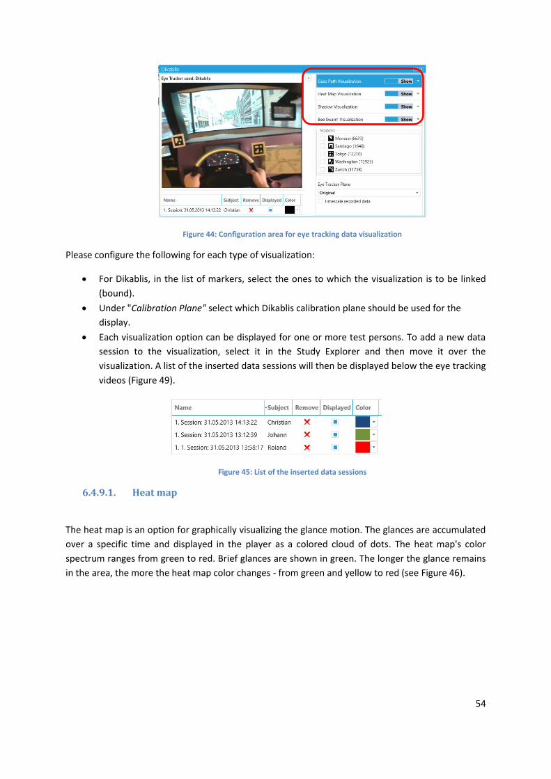
54

Figure 44: Configuration area for eye tracking data visualization

Please configure the following for each type of visualization:

For Dikablis, in the list of markers, select the ones to which the visualization is to be linked

(bound).

Under "Calibration Plane" select which Dikablis calibration plane should be used for the

display.

Each visualization option can be displayed for one or more test persons. To add a new data

session to the visualization, select it in the Study Explorer and then move it over the

visualization. A list of the inserted data sessions will then be displayed below the eye tracking

videos (Figure 49).

Figure 45: List of the inserted data sessions

6.4.9.1. Heat map

The heat map is an option for graphically visualizing the glance motion. The glances are accumulated

over a specific time and displayed in the player as a colored cloud of dots. The heat map's color

spectrum ranges from green to red. Brief glances are shown in green. The longer the glance remains

in the area, the more the heat map color changes - from green and yellow to red (see Figure 46).

55

Figure 46: Heat map display

To activate the heat map, move the corresponding controller from "Hide" to "Show" and start the

playback feature on the player. The selected eye tracking video is now played back with the heat

map. You can have the heat map displayed in two ways - it can either be continually built up

("Constructive") or displayed with a particular temporal history ("Time Based"). By clicking on the

"Time Based" button you can adjust the maximum time interval for which the heat map is to be

displayed ("Maximum Age"). You can also indicate the size of the heat map spots in pixels under the

point "Spot Radius".

6.4.9.2. Shadow map

In the shadow map, the glance motion is superimposed with a black layer. The longer a glance

remains on an area, the more transparent this area becomes (see Figure 48).

To activate the shadow map, move the controller from for "Shadow Map" from "Hide" to "Show" and

start the playback feature on the player. The selected eye tracking video is now played back with the

heat map.

Figure 47: Shadow visualization

56

You can have the shadow map displayed in two ways - it can either be continually built up

("Constructive") or displayed with a particular temporal history ("Time Based"). By clicking on the

"Time Based" button you can adjust the maximum time interval for which the shadow map is to be

displayed ("Maximum Age"). The time taken until the glanced at area becomes transparent can be

set with "Time until transparent". Under "Size of transparent disk" you can set the size of the

transparent area. Furthermore, the minimum transparency of the superimposed layer by the shadow

map can be set with "Minimum transparency".

6.4.9.3. Visualizing the gaze path

The gaze path is a representation of the glance motion. When a glance jumps from one fixed position

to the next, this is shown with a straight line. The fixed position of the glance is shown with a circle.

The longer the fixation lasts, the larger the circle (see Figure 48).

Figure 48: Gaze path visualization

To display the gaze path, move the controller from for "Gaze Path" from "Hide" to "Show" and start

the playback feature on the player. The selected eye tracking video is now played back with the gaze

path. You now have the option to display the time a glance is fixed at a position by activating "Show

fixation duration".

You can choose to display the gaze path as either being "Fixation-based" or "Time-based". With

"Fixation-based" the number of displayed fixations can be set. The number of displayed fixations

must be between 1 and 10. By activating "Time Based" you can set the maximum time interval for

which the gaze path is to be displayed.

6.4.9.4. Bee swarm

The bee swarm displays the glance motion with a small circle for each test person (see Figure 49).

57

Figure 49: Bee swarm visualization

To activate the bee swarm, move the corresponding controller from "Hide" to "Show" and start the

playback feature on the player. The selected eye tracking video is now played back with the bee

swarm superimposed over the image.

6.5. Data stream module

6.5.1. Calculating data stream statistics

The data stream statistics allow you to calculate different statistical values for the recorded data

channels using all or selected test persons involved in your study. Proceed as follows:

1. In the "Data Analysis" tab, open the window "Data Stream Statistics" by clicking on the "Data

Stream Statistics" button. The window containing individual statistical values for selection

will then be opened (see Figure 50).

2. In the "Config" tab, first select the data under "Subjects". You can now select an entire study

("All"), groups of test persons or individual test persons. Mark the data you need by clicking

on the square next to the designation.

3. Under "Tasks" you can select whether you would like to have the statistical values calculated

for the entire recording or if you would like to perform an analysis based on a particular task.

The following selection options are available here:

a. Entire Data Session: The calculation is performed for the entire recording. Tasks are

ignored.

b. Merged Tasks: The calculation is performed on an use case basis with all of the

selected tasks being grouped together to form one single use case. The statistical

values are calculated for the merged task interval.

c. Single Tasks: The calculation is performed on a task basis meaning that the statistical

values are calculated for each task individually.

58

d. All / Level: This function is only possible if task-based analysis has been selected.

Here you can choose whether all of the tasks are to be calculated or only those tasks

on a particular level. Individual levels or level combinations can be selected here.

Figure 50: Data stream statistics

4. You can select all or individual data channels under "Data Channels".

5. Under "Metrics", select the statistical values you require or press the "All" button to select all

of the statistical values. If you position the mouse over the small symbol at the right next to

the designation, a short explanation of this statistical value will appear.

6. Press the "Calculate" button to calculate the statistical values. To do so, at least one value

must be selected in each tab.

Figure 51: Result of the data stream statistics

7. A new tab will open up in the "Data Stream Statistics" window in which the calculated results

can be found (see Figure 51). The statistical values are arranged in columns. The test persons

are entered in the table's horizontal rows. The last six rows contain descriptive statistics

about all of the test persons with the statistical values: sum, mean value, maximum,

minimum, standard deviation and variance.

59

8. The data stream statistics can be exported in text format so that they can then be further

examined using other applications such as Excel or SPSS. To do so, press the "Export" button

below the table. A "CSV Export" window will then open.

9. In the "CSV Export" window you can select whether you wish to use a decimal point or

comma for separation under "Data Format". Please select the path you wish to use under

"Select File Save Location". Confirm the export with the "Export Data" button.

60