table of contents - macquarie universityphysics.mq.edu.au/astronomy/space2grow/software/vsp… ·...
TRANSCRIPT
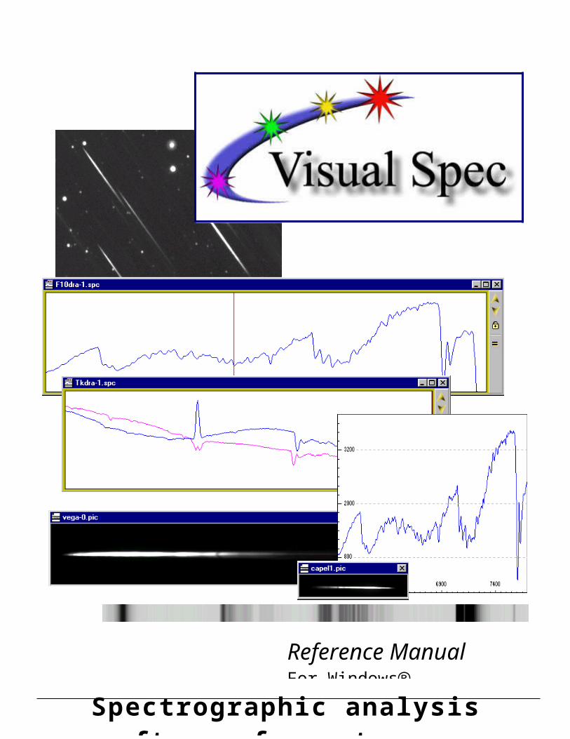
Spec
Spectrographic analysis software for astronomy
Reference ManualFor Windows
Manuel de Référence Introduction
Table of Contents
Table of Contents......................................................2
Introduction..............................................6Installation.................................................................6
Before installation.................................................7Verifying hardware and system compatibility7
Installing Visual Specs..........................................7How this manual is organized...................................8
Examples of applications......................................8Spectral Imagery Concepts.......................................8
Spectral Image.......................................................8The spectral profil.................................................9Spectral Analysis.................................................10
Your first spectral profile.......................12Launching Visual Specs..........................................12
Visual Specs files................................................12Image Documents........................................13Profil Document...........................................13Information windows...................................14Other documents generated by the application14
Activation of a document....................................14Interface elements...................................................14
Preferences..........................................................15Default folder for image files.......................16Default folder for profile files......................16Wavelength of spectral reference lines........17Spectral area of calculation of continuum. . .18Default Comments.......................................18Geographic position.....................................19Archive folder..............................................19Language......................................................19Link with SPECTRUM................................20Atmosphere..................................................20
VisualSpec Help......................................................21Steps for creating a profile......................................21
Display an image.................................................21Dztau-1.pic...................................................22aDztau-2.pic.................................................22
Extract the spectral profile..................................22Dztau-1.spc..................................................23
Fill in the Header.................................................23Save the profile...................................................24
Image......................................................25Document................................................................25
Image Format......................................................25
Visual Spec Table of Contents | 2
Manuel de Référence Introduction
Image Folder.......................................................25Open and close an image.........................................25
Open an image.....................................................25Close an image....................................................26Search for a reference image...............................26
Obtain information about the image.......................26Position of cursor................................................27Change the Thresholds........................................27
Change the thresholds by directly editing....27Change the thresholds by using the cursor. .28
View an image line..............................................28Select an image area................................................28Export to Excel........................................................29
Profile.....................................................31Profile Document....................................................31Profile Format.........................................................31
Profile Folder......................................................32Create and open a profile........................................32
Create a profile....................................................32Object binning..............................................32Reference binning........................................33Creation of a profile.....................................34
Open a profile......................................................34Search for a profile.......................................35
Close and Save a profile..........................................37Close a profile..............................................37Save a profile...............................................37Save under a different name........................37
Archive a profile.................................................37The spectral series...................................................38
Display a series...................................................38Selecting a series.................................................39Cursor position....................................................39Selecting a spectral area......................................40
Spectral calibration..................................................40Calibration using reference.................................41
Add an external reference spectral profile...41Create a spectral reference profile from a star spectrum 42Calibrate in wavelength...............................43
Calibration without reference..............................45Application to an image containing a star....46
Non linear calibration..........................................47d dispersion law.........................................51
Changing the appearance of a profile document.....52Enlarging, reducing a window............................52Thumbnails..........................................................52Adjusting Format................................................53Pre-defined Format..............................................53Display graduated axes and a title.......................54
Graph title...................................................56Doppler shift scale.......................................57
Changing the color and font................................58
Visual Spec Table of Contents | 3

Manuel de Référence Introduction
Export to other applications....................................59.bmp Image..........................................................59.txt Profile............................................................60.dat File................................................................61.gif or .png file.....................................................61
Clipboard.................................................................61
Spectral Series........................................62Format.....................................................................62
Modify the scale..................................................63X Axis Scale................................................64Y Axis Scale................................................65Vertical toolbar of the profile document......65Zoom............................................................66Interactif zoom.............................................66
Applying the same format...................................66Clear a series.......................................................67Label the wavelength of a line............................67Crop a serie.........................................................67
Adding, replacing, and deleting..............................68Copy a series.......................................................68Paste a series:......................................................68Replace a series...................................................69Delete a series.....................................................69
Modifying a series...................................................70Arithmetic operations..........................................70Low-pass Filtering..............................................70High-pass Filtering..............................................71Spline Filtering....................................................72Gaussian filter.....................................................73Mmse filter..........................................................74Recalibrate a series..............................................75Operations on two series.....................................76
Divide two series..........................................76Multiply two series......................................76Add two series..............................................76Subtract two series.......................................77
Translate a series.................................................77Normalize a series...............................................78Derive a series.....................................................78Stack several series.............................................78Join two series.....................................................79Modify the intensity of a pixel............................79
Measurements.........................................................80Infos… Window...........................................81Signal to Noise Ratio...................................82Average........................................................82Std deviation................................................82Line center...................................................82FWMH.........................................................82Barycenter....................................................83Intensity........................................................83Equivalent width (LEQ)...............................83Surface.........................................................83
Visual Spec Table of Contents | 4
Manuel de Référence Introduction
Resampling..........................................................83Fit Photosphere....................................................84Heliocentric Speed..............................................85
Radiometry.............................................88Spectral library........................................................88Spectral type............................................................89Continuum...............................................................90
Continuum by area suppression..........................91Continuum by points....................................91
Automatic Extraction..........................................92Compensation of the continuum.........................92
By dividing by the continuum......................92By subtracting the continuum......................92
Suppresion of atmospheric lines.........................93Synthethic atmospheric correction...............93Synthethic atmospheric correction...............95
Radiometric correction by a standard spectrum......97Automatic Correction..........................................99
Planck Profile........................................................100To determine the Planck temperature of a body101
Instrumental Response..........................................102Flux calibration.....................................................102Atmospheric extinction correction........................103
Tools.....................................................104Animation..............................................................104
Linear animation...............................................104Time scaled animation......................................105
Date and time formatting...........................106Synthesis of spectral image...................................107Coordinates...........................................................108Identification of chemical elements......................109
Identification by element...........................111Identification over a defined domain.........111Automatic identification............................111Changing database.....................................111Element sorting..........................................112Exporting a synthetic spectrum..................112Exporting a synthetic spectrum as a new document112Hires lines database....................................113Other aids to identification.........................113
GnuPlot.................................................................113Console..................................................................117
How to use the command-line...................117List of available commands.......................117
Music.....................................................................118
Spectral Analysis..................................119Comparison of spectra...........................................119Quantitative parameters........................................120
Equivalent width...............................................120
Visual Spec Table of Contents | 5
Manuel de Référence Introduction
Doppler shift......................................................121Speed of expansion...........................................122
Identification of elements......................................122Solar spectrum...........................................123Stars of spectral type M.............................124Planetary nebula.........................................124Atmospheric lines......................................125
Link with SPECTRUM software..........................125
What's new since…..............................131Version 3.3.0.........................................................131
Reference..............................................133Useful Spectral Lines............................................133Reference stars for flux calibration.......................133
Buttons..................................................134Principal Toolbar.......................................134Image Toolbar............................................134
Calibration Toolbar...........................................134Continuum Toolbar...........................................135Profile Toolbar..................................................135
Reference list of menus and functions137Visual Spec........................................................137Image.................................................................137Profile................................................................138
Application Messages...........................142
Acknowledgements...............................145
Translation Notes..................................146
Visual Spec Table of Contents | 6
Manuel de Référence Introduction
Visual Spec Table of Contents | 7

Manuel de Référence Introduction
C H A P T E R 1
Introduction
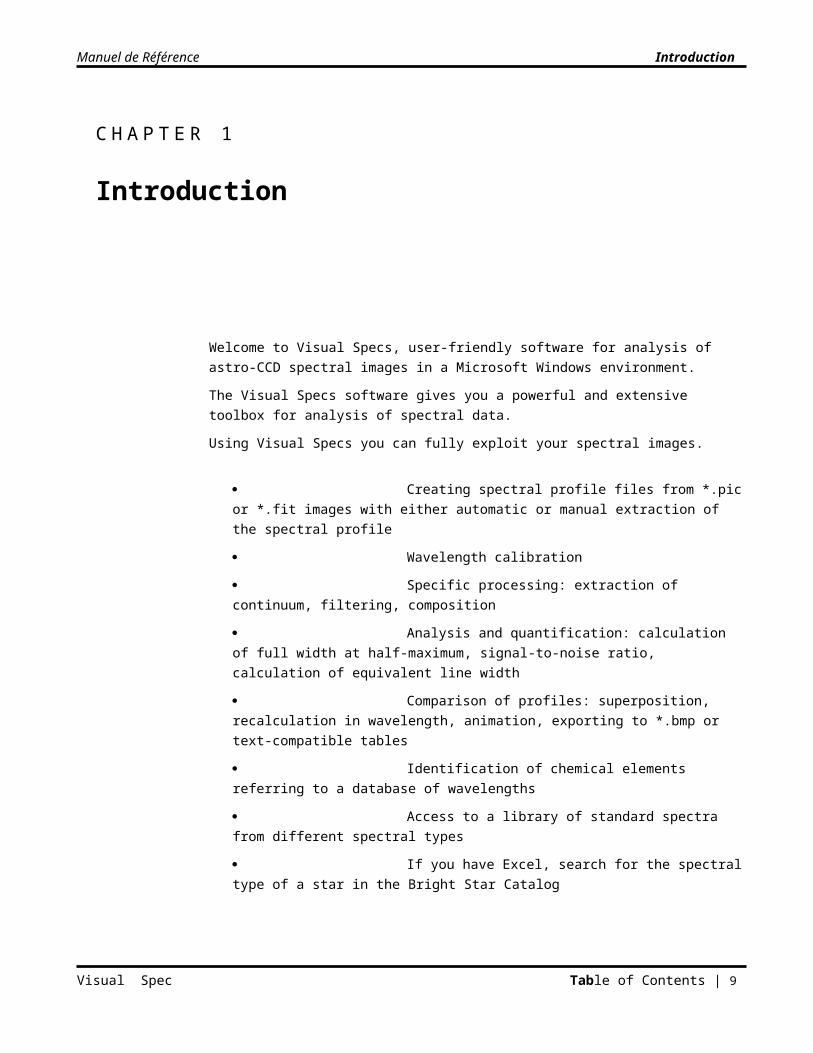
Welcome to Visual Specs, user-friendly software for analysis of astro-CCD spectral images in a Microsoft Windows environment.
The Visual Specs software gives you a powerful and extensive toolbox for analysis of spectral data.
Using Visual Specs you can fully exploit your spectral images.
Creating spectral profile files from *.pic or *.fit images with either automatic or manual extraction of the spectral profile
Wavelength calibration
Specific processing: extraction of continuum, filtering, composition
Analysis and quantification: calculation of full width at half-maximum, signal-to-noise ratio, calculation of equivalent line width
Comparison of profiles: superposition, recalculation in wavelength, animation, exporting to *.bmp or text-compatible tables
Identification of chemical elements referring to a database of wavelengths
Access to a library of standard spectra from different spectral types
If you have Excel, search for the spectral type of a star in the Bright Star Catalog
This chapter shows how to install Visual Specs on your computer, introduces other sections of the document, and describes some fundamental processing of spectral analysis. If you are new to CCD spectro-astronomical imaging, you should read this chapter completely. If you are familiar with CCD spectral imaging, you can skip the section “The Spectral Image”.
InstallationVisual Spec uses the standard Windows installation method.
Visual Spec Table of Contents | 8
Manuel de Référence Introduction
Before installation
Before installing Visual Specs, ensure that your computer meets the minimum configuration required and read the LISEMOI (README) file, located in the root directory of the application.
Verifying hardware and system compatibility
To run Visual Specs you should have a certain hardware and system configuration installed on your computer. The system configuration includes:
Completely IBM-compatible computer with an 80486 or better processor
Hard disk with minimum of 10 Mbytes of available space
Display supported by Windows 95
8 Mbytes of memory
Mouse
Windows 95 or better
Optional: Microsoft Excel for exporting data in Excel format and for access to the Bright Star Catalog
Installing Visual Specs To install Visual Spec, launch “Setup.exe”. Follow the instructions given during installation.
Besides the executable, Vspec should contain:
Element.txtDatabase of atomic lines for which the atomic number is lower than that of Iron
Sun.txtDatabase of Sun lines
Vide.bmpBlack and white image for managing 256-color screen palettes
Pic.xlsExcel document for exporting image areas
Brscat2.xlsBright Star Catalog in Excel format
Aide.pdfHelp document in *.pdf format, readable using the free Acrobat reader software (www.adobe.com/acrobat)
Libspec directoryContains normalized spectra of different spectral types, Pickle et.al.
Visual Spec Table of Contents | 9
Manuel de Référence Introduction
H20.datFile Intensity-wavelength of the water to eliminate atmospheric lines
How this manual is organizedThe chapters of this manual can be grouped as:
Chapter 1: Introduction and installation
Chapters 2-4: Basic concepts of Visual Spec
Chapter 5: Spectral series – how to create, save-to-file, and modify spectra
Chapters 6-8: Using the data
Examples of applicationsIn addition to this manual, Visual Specs includes several images and profiles that you can use with Visual Specs.
Spectral images obtained of T60 from the Pic du Midi Observatory (France) with the “Bardin” spectrograph
Spectral images obtained by C.Buil and Morata's family
Spectral images sent by Jack Martin (UK) et Don Mais (USA
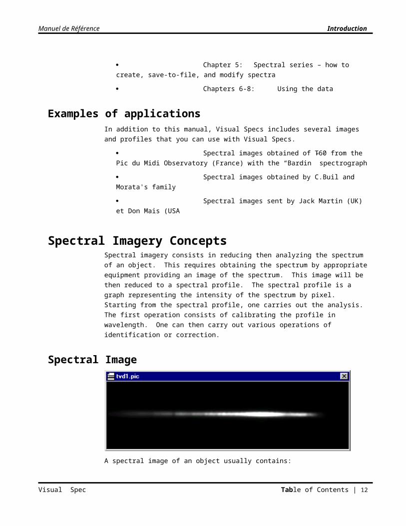
Spectral Imagery ConceptsSpectral imagery consists in reducing then analyzing the spectrum of an object. This requires obtaining the spectrum by appropriate equipment providing an image of the spectrum. This image will be then reduced to a spectral profile. The spectral profile is a graph representing the intensity of the spectrum by pixel. Starting from the spectral profile, one carries out the analysis. The first operation consists of calibrating the profile in wavelength. One can then carry out various operations of identification or correction.
Spectral Image
A spectral image of an object usually contains:
The spectrum of the object
Visual Spec Table of Contents | 10
Manuel de Référence Introduction
The background
Some surrounding stars in the case of a assembly “without slit”.
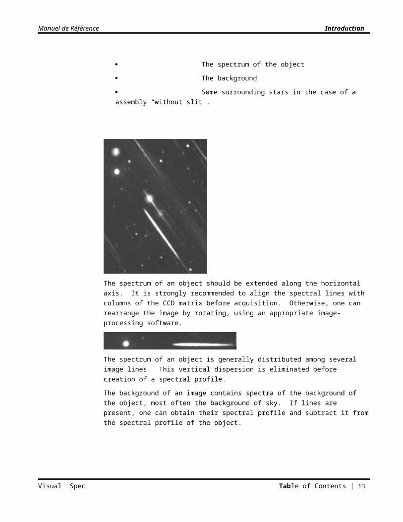
The spectrum of an object should be extended along the horizontal axis. It is strongly recommended to align the spectral lines with columns of the CCD matrix before acquisition. Otherwise, one can rearrange the image by rotating, using an appropriate image-processing software.
The spectrum of an object is generally distributed among several image lines. This vertical dispersion is eliminated before creation of a spectral profile.
The background of an image contains spectra of the background of the object, most often the background of sky. If lines are present, one can obtain their spectral profile and subtract it from the spectral profile of the object.
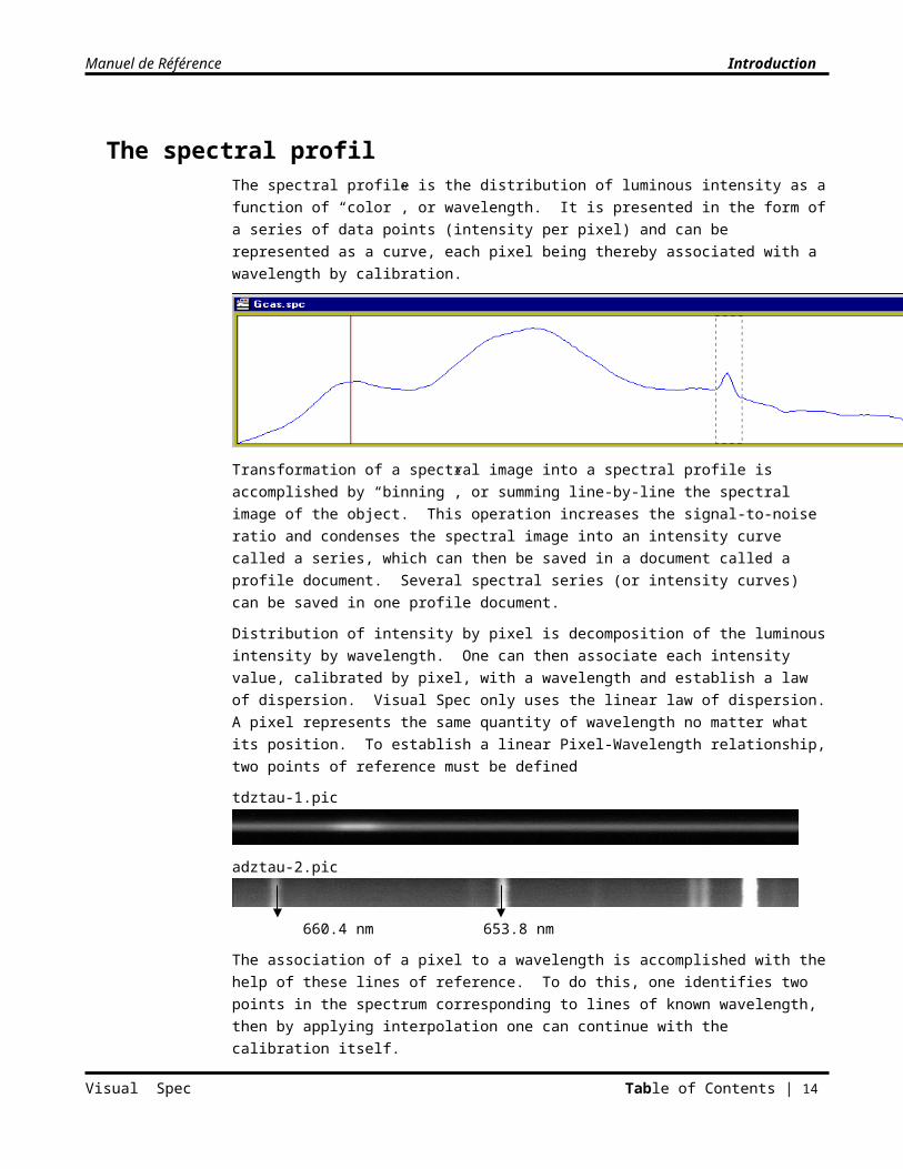
The spectral profilThe spectral profile is the distribution of luminous intensity as a function of “color”, or wavelength. It is presented in the form of a series of data points (intensity per pixel) and can be represented as a curve, each pixel being thereby associated with a wavelength by calibration.
Visual Spec Table of Contents | 11
Manuel de Référence Introduction
Transformation of a spectral image into a spectral profile is accomplished by “binning”, or summing line-by-line the spectral image of the object. This operation increases the signal-to-noise ratio and condenses the spectral image into an intensity curve called a series, which can then be saved in a document called a profile document. Several spectral series (or intensity curves) can be saved in one profile document.
Distribution of intensity by pixel is decomposition of the luminous intensity by wavelength. One can then associate each intensity value, calibrated by pixel, with a wavelength and establish a law of dispersion. Visual Spec only uses the linear law of dispersion. A pixel represents the same quantity of wavelength no matter what its position. To establish a linear Pixel-Wavelength relationship, two points of reference must be defined
tdztau-1.pic
adztau-2.pic
660.4 nm 653.8 nm
The association of a pixel to a wavelength is accomplished with the help of these lines of reference. To do this, one identifies two points in the spectrum corresponding to lines of known wavelength, then by applying interpolation one can continue with the calibration itself.
The calibration is done using a spectrum called the reference; this spectrum can be one of a known set (calibration lamps) or could be spectrum of an object if its lines are easily identifiable although this latter method is less precise.
Spectral AnalysisSpectral analysis of an object includes several categories of operations
Identification of the lines
Modification of the spectral response, absolute flux, normalization, correction of the continuum, Planck’s Law
Measurements: center of the line, equivalent width, full width at half-maximum
Identification of the lines is done based on their wavelengths. Each chemical element produces a unique set of lines (its spectrum) of wavelengths, of which each line is the result of an atomic transition between two energy levels characteristic of the atom under consideration. One who is interested can consult the literature for an explanation of the physics of this phenomenon.
Visual Spec Table of Contents | 12
Manuel de Référence Introduction
The resolution of a spectrum is defined as the smallest domain of wavelength associated with a pixel. An insufficient resolution impedes determination of the chemical elements having lines in this area. To help identify lines, Visual Spec includes a database of spectral lines between 3000 and 11000 angstroms for elements with atomic numbers less than or equal to that of Iron.
The intensity of a spectrum is affected by:
The spectral response of the CCD
Its own continuum, distribution of energy into wavelength as a function of temperature (Planck’s Law)
Atmospheric extinction
One can correct for the spectral response of a CCD by using the spectrum of one of the 24 flux-calibration stars included with Visual Specs. Comparing experimental flux with theoretical flux provides the curve of spectral sensitivity of the equipment used. This response curve can then be used for correcting spectra obtained under the same conditions of observation.
If one can’t create a photometric calibration spectrum from one of the 24 stars in Visual Spec, one can correct with one of the standard spectra in the library by selecting a spectrum of the same spectral type. To determine the spectral type of a star, the Bright Star Catalog database is available if one has previously installed Excel.
One can also simply carry out the elimination of the continuum by approximating the continuum of the profile by a continuous law. This operation yields a “flat” spectrum despite the response of the CCD, but also eliminates the physical continuum of the object which is a function of the temperature of the object (Planck’s Law).
To obtain the “Planck profile” of an object one must perform a true flux calibration.
Finally, it is always possible to normalize a spectrum with respect to a spectral area that contains no lines. Normalization removes variations in intensity due to different exposure times by calculating only the relative intensity compared to the same spectral domain. This simple operation is often sufficient for profiles having little variation of continuum during extended spectral recording.
The following measurements can be made on spectral lines:
Center of the line
Full width at half-maximum
Equivalent width
The center of the line is determined with precision by calculating the barycenter. It is important to be careful with the selection of the line to avoid introducing error into the measurement.
The Full Width at Half Maximum (FWMH) of a line can be used to determine the speed of expansion or rotation of the body under observation. It can also be used as an indication of the resolution of the instrument, if it is taken on a reference line of a body under known physical conditions (calibrated lamp).
The equivalent width of a spectral line is a spectroscopic measurement that can characterize the “power” of the line. This measurement allows one to precisely follow the development of a line over the course of time for the same object as it presents variations.
Visual Spec Table of Contents | 13
Manuel de Référence Introduction
C H A P T E R 2
Your first spectral profile
It will take you several minutes to obtain your first spectral profile from a CCD image. You open a *.pic or *.fit file, the image will be displayed, you can adjust the thresholds of visualization and obtain information about the intensity of the pixels. Then, you extract and visualize the spectral profile, which you can save as a “Profil” document. You continue by preparing wavelength calibration based on a reference image, and you finish by filling in the document header.
This chapter provides an overview of these operations, describes the necessary documents and knowledge you will need to use Visual Specs
ExamplesAn example from a spectrum obtained as Spectrum of T60, Picture of the Day of the star Dzeta Tau, is included with the application. You can find it in the application folders. It consists of:
Dztau-1.pic – spectral image
ADztau-2.pic – reference spectral image, Argon lamp
Dztau-1.spc – spectral profile calibrated in wavelength
Launching Visual SpecsTo execute Visual Specs, double-click on the Visual Specs icon
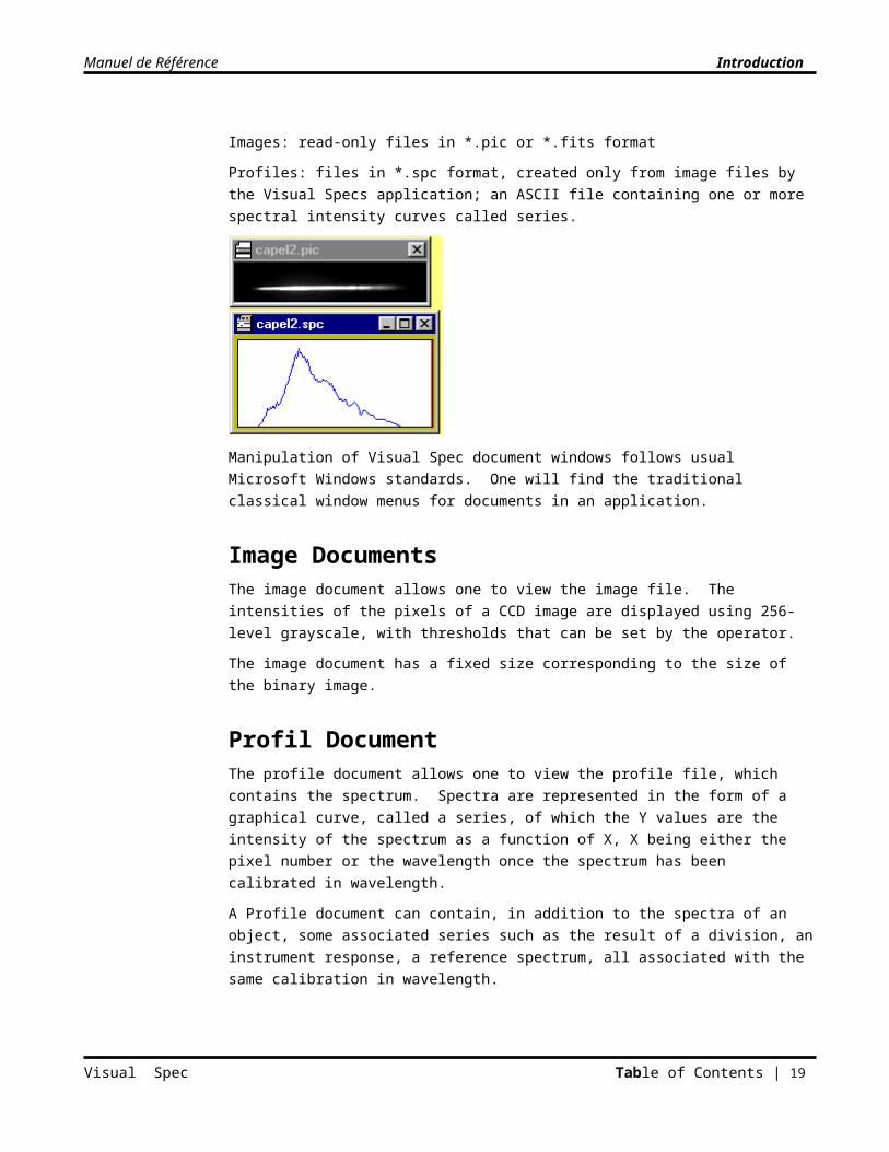
Visual Specs filesThe Visual Spec application manages two types of documents through Windows windows:
Images: read-only files in *.pic or *.fits format
Profiles: files in *.spc format, created only from image files by the Visual Specs application; an ASCII file containing one or more spectral intensity curves called series.
Visual Spec Table of Contents | 14

Manuel de Référence Introduction
Manipulation of Visual Spec document windows follows usual Microsoft Windows standards. One will find the traditional classical window menus for documents in an application.
Image DocumentsThe image document allows one to view the image file. The intensities of the pixels of a CCD image are displayed using 256-level grayscale, with thresholds that can be set by the operator.
The image document has a fixed size corresponding to the size of the binary image.
Profil Document The profile document allows one to view the profile file, which contains the spectrum. Spectra are represented in the form of a graphical curve, called a series, of which the Y values are the intensity of the spectrum as a function of X, X being either the pixel number or the wavelength once the spectrum has been calibrated in wavelength.
A Profile document can contain, in addition to the spectra of an object, some associated series such as the result of a division, an instrument response, a reference spectrum, all associated with the same calibration in wavelength.
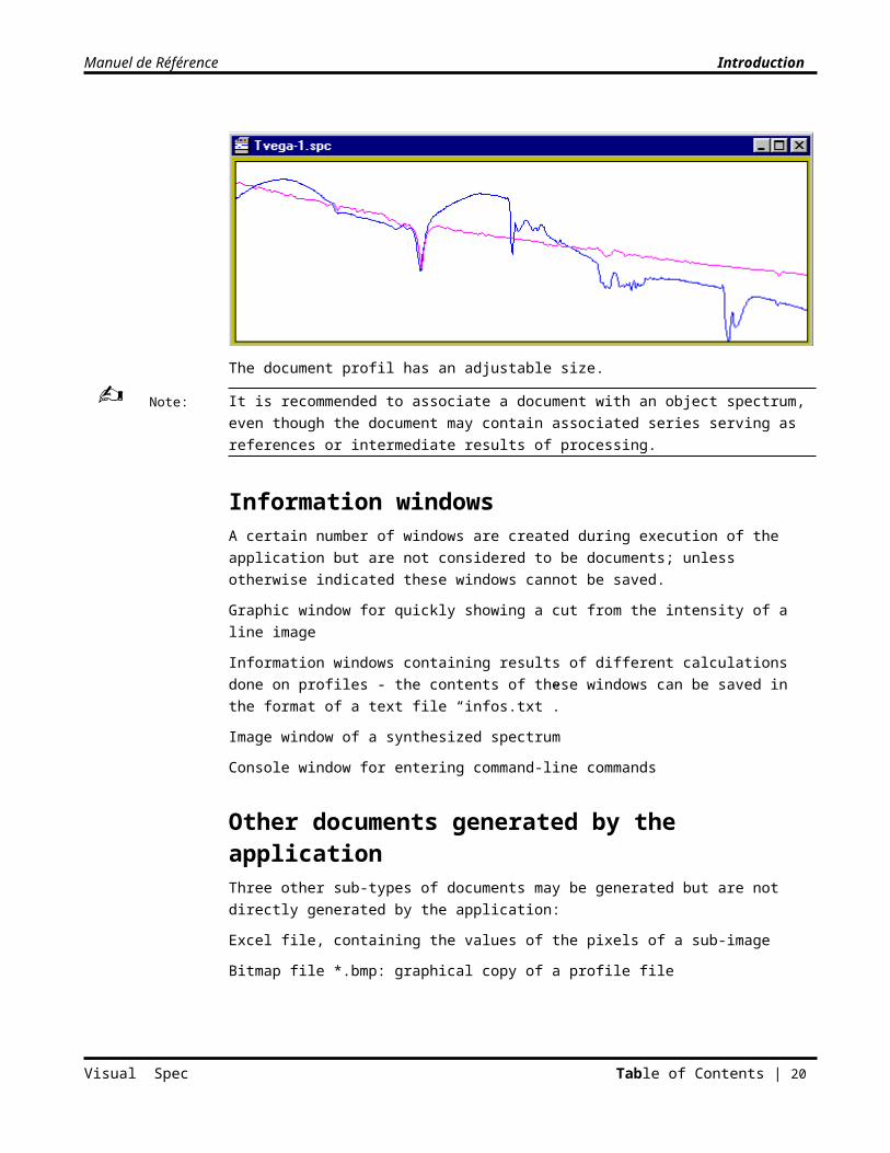
The document profil has an adjustable size.
It is recommended to associate a document with an object spectrum, even though the document may contain associated series serving as references or intermediate results of processing.
Visual Spec Table of Contents | 15
Note:

Manuel de Référence Introduction
Information windowsA certain number of windows are created during execution of the application but are not considered to be documents; unless otherwise indicated these windows cannot be saved.
Graphic window for quickly showing a cut from the intensity of a line image
Information windows containing results of different calculations done on profiles - the contents of these windows can be saved in the format of a text file “infos.txt”.
Image window of a synthesized spectrum
Console window for entering command-line commands
Other documents generated by the applicationThree other sub-types of documents may be generated but are not directly generated by the application:
Excel file, containing the values of the pixels of a sub-image
Bitmap file *.bmp: graphical copy of a profile file
Text file *.txt: exported values from a profile file, following formatting rules for an Excel table so the file can be read using this application
.dat file: exported data into an ASCII file from the Intensity series: X=intensity, Y=associated wavelength
Activation of a documentTo make a document active, click one time within the document, preferably in the bar at the top of the window.
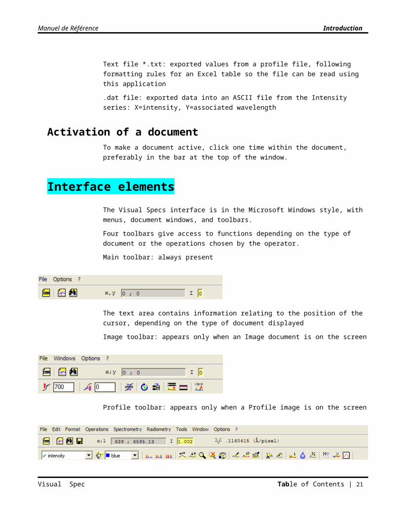
Interface elementsThe Visual Specs interface is in the Microsoft Windows style, with menus, document windows, and toolbars.
Four toolbars give access to functions depending on the type of document or the operations chosen by the operator.
Main toolbar: always present
The text area contains information relating to the position of the cursor, depending on the type of document displayed
Image toolbar: appears only when an Image document is on the screen
Visual Spec Table of Contents | 16

Manuel de Référence Introduction
Profile toolbar: appears only when a Profile image is on the screen
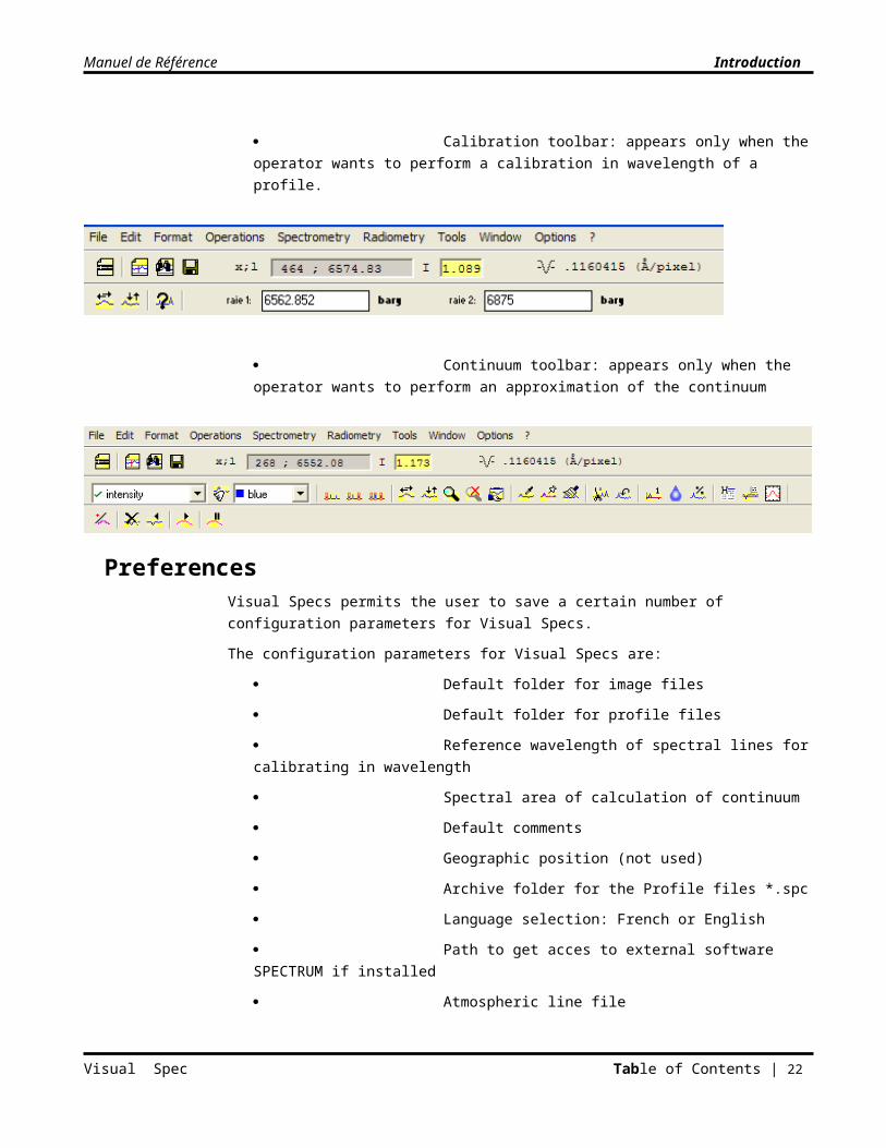
Calibration toolbar: appears only when the operator wants to perform a calibration in wavelength of a profile.
Continuum toolbar: appears only when the operator wants to perform an approximation of the continuum
PreferencesVisual Specs permits the user to save a certain number of configuration parameters for Visual Specs.
The configuration parameters for Visual Specs are:
Default folder for image files
Default folder for profile files
Reference wavelength of spectral lines for calibrating in wavelength
Spectral area of calculation of continuum
Default comments
Geographic position (not used)
Archive folder for the Profile files *.spc
Visual Spec Table of Contents | 17
Manuel de Référence Introduction
Language selection: French or English
Path to get acces to external software SPECTRUM if installed
Atmospheric line file
These configuration parameters are used by Visual Specs while it executes. They are saved in the Registry.
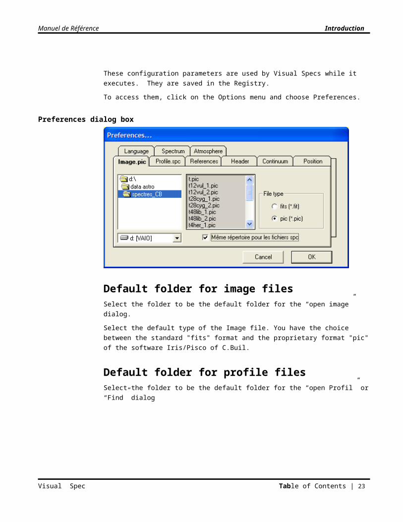
To access them, click on the Options menu and choose Preferences.
Preferences dialog box
Default folder for image filesSelect the folder to be the default folder for the “open image” dialog.
Select the default type of the Image file. You have the choice between the standard "fits" format and the proprietary format "pic" of the software Iris/Pisco of C.Buil.
Default folder for profile filesSelect the folder to be the default folder for the “open Profil” or “Find” dialog
Visual Spec Table of Contents | 18
Manuel de Référence Introduction
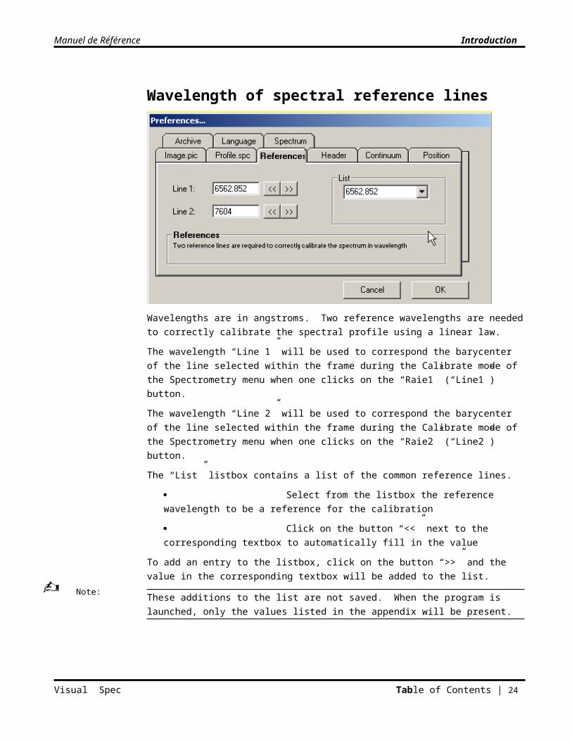
Wavelength of spectral reference lines
Wavelengths are in angstroms. Two reference wavelengths are needed to correctly calibrate the spectral profile using a linear law.
The wavelength “Line 1” will be used to correspond the barycenter of the line selected within the frame during the Calibrate mode of the Spectrometry menu when one clicks on the “Raie1” (“Line1”) button.
The wavelength “Line 2” will be used to correspond the barycenter of the line selected within the frame during the Calibrate mode of the Spectrometry menu when one clicks on the “Raie2” (“Line2”) button.
The “List” listbox contains a list of the common reference lines.
Select from the listbox the reference wavelength to be a reference for the calibration
Click on the button “<<” next to the corresponding textbox to automatically fill in the value
To add an entry to the listbox, click on the button “>>” and the value in the corresponding textbox will be added to the list.
These additions to the list are not saved. When the program is launched, only the values listed in the appendix will be present.
Visual Spec Table of Contents | 19
Note:
Manuel de Référence Introduction
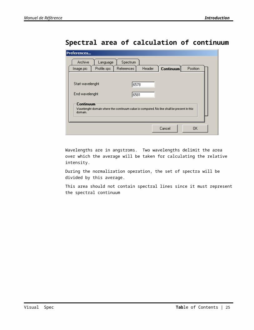
Spectral area of calculation of continuum
Wavelengths are in angstroms. Two wavelengths delimit the area over which the average will be taken for calculating the relative intensity.
During the normalization operation, the set of spectra will be divided by this average.
This area should not contain spectral lines since it must represent the spectral continuum
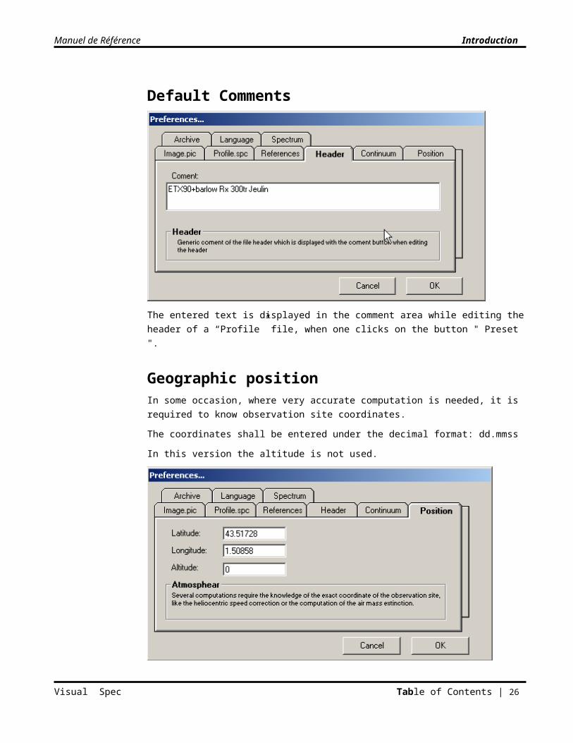
Default Comments
The entered text is displayed in the comment area while editing the header of a “Profile” file, when one clicks on the button " Preset ".
Visual Spec Table of Contents | 20
Manuel de Référence Introduction
Geographic positionIn some occasion, where very accurate computation is needed, it is required to know observation site coordinates.
The coordinates shall be entered under the decimal format: dd.mmss
In this version the altitude is not used.
Archive folderThis function is eliminated since the 3.3.0 version
Select the folder which will be the default folder for archiving Profile documents when the “Archive…” command is given.
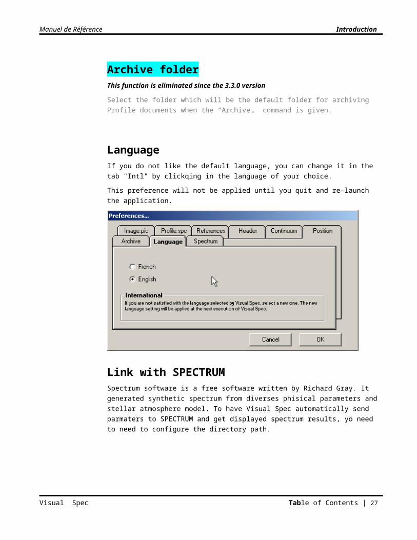
LanguageIf you do not like the default language, you can change it in the tab "Intl" by clickqing in the language of your choice.
This preference will not be applied until you quit and re-launch the application.
Visual Spec Table of Contents | 21
Manuel de Référence Introduction
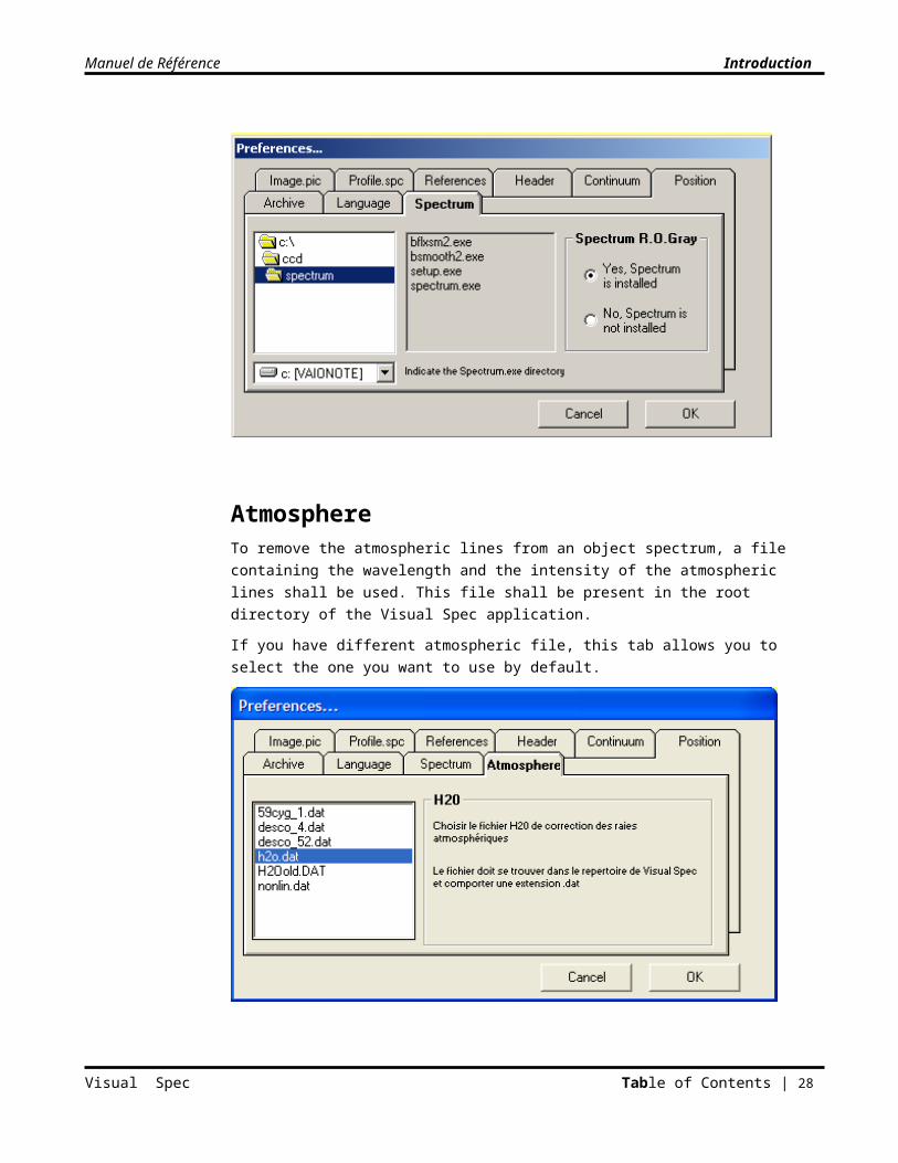
Link with SPECTRUMSpectrum software is a free software written by Richard Gray. It generated synthetic spectrum from diverses phisical parameters and stellar atmosphere model. To have Visual Spec automatically send parmaters to SPECTRUM and get displayed spectrum results, yo need to need to configure the directory path.
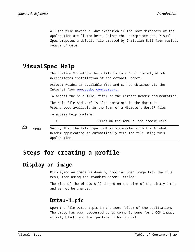
AtmosphereTo remove the atmospheric lines from an object spectrum, a file containing the wavelength and the intensity of the atmospheric lines shall be used. This file shall be present in the root directory of the Visual Spec application.
Visual Spec Table of Contents | 22
Manuel de Référence Introduction
If you have different atmospheric file, this tab allows you to select the one you want to use by default.
All the file having a .dat extension in the root directory of the application are listed here. Select the appropriate one. Visual Spec proposes a default file created by Christian Buil from various source of data.
VisualSpec HelpThe on-line VisualSpec help file is in a *.pdf format, which necessitates installation of the Acrobat Reader.
Acrobat Reader is available free and can be obtained via the Internet from www.adobe.com/acrobat.
To access the help file, refer to the Acrobat Reader documentation.
The help file Aide.pdf is also contained in the document Vspcman.doc available in the form of a Microsoft Word97 file.
To access help on-line:
Click on the menu ?, and choose Help
Verify that the file type .pdf is associated with the Acrobat Reader application to automatically read the file using this application.
Steps for creating a profile
Display an imageDisplaying an image is done by choosing Open Image from the File menu, then using the standard “open…” dialog.
Visual Spec Table of Contents | 23
Note:
Manuel de Référence Introduction
The size of the window will depend on the size of the binary image and cannot be changed.
Dztau-1.picOpen the file Dztau-1.pic in the root folder of the application. The image has been processed as is commonly done for a CCD image, offset, black, and the spectrum is horizontal
aDztau-2.picOpen the file aDztau-2.pic in the root folder of the application. The image is the spectrum in the same domain of wavelength obtained with an argon calibration lamp.
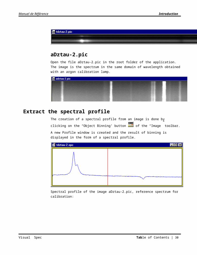
Extract the spectral profileThe creation of a spectral profile from an image is done by clicking on the “Object Binning’ button
of the “Image” toolbar.
A new Profile window is created and the result of binning is displayed in the form of a spectral profile.
Spectral profile of the image aDztau-2.pic, reference spectrum for calibration:
Visual Spec Table of Contents | 24
Manuel de Référence Introduction
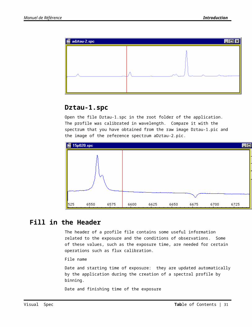
Dztau-1.spcOpen the file Dztau-1.spc in the root folder of the application. The profile was calibrated in wavelength. Compare it with the spectrum that you have obtained from the raw image Dztau-1.pic and the image of the reference spectrum aDztau-2.pic.
Fill in the HeaderThe header of a profile file contains some useful information related to the exposure and the conditions of observations. Some of these values, such as the exposure time, are needed for certain operations such as flux calibration.
File name
Date and starting time of exposure: they are updated automatically by the application during the creation of a spectral profile by binning.
Date and finishing time of the exposure
Duration of exposure: it is entered automatically by the application during the creation of a spectral profile by binning.
Alpha: right ascension of the object, entered by the operator. Used to calculate the zenithal height of an object for correcting for atmospheric absorption and for heliocentric speed in accurate Doppler measurements.
Visual Spec Table of Contents | 25
Manuel de Référence Introduction
Delta: declination of the object, entered by the operator. Used to calculate the zenithal height of an object for correcting for atmospheric absorption and for heliocentric speed in accurate Doppler measurements.
Comment: textbox. There is a function for searching for “Profile” documents containing a specified search-string within these comments. It is advisable to include, for example, the name of the star.
Save the profileSave the profile document by using the File menu, then choose Save or Save As…
Visual Spec Table of Contents | 26
Manuel de Référence Introduction
C H A P T E R 3
Image
DocumentThe Image documents must contain the spectral image to be analyzed. These documents are used to create the Profile document that contains their spectral profile.
Image Format
The Image files accessible by this application are limited to format “.pic” generated by the program Pisco or “.fit”,".fts", ".fits" traditional FITS format.
The thresholds of visualization by default are those that are entered in the header of the .pic or .fit file.
If the automatically-provided thresholds from the header of the image do not give anticipated results, adjust the thresholds manually.
Image Folder
The default folder to contain “Image” files can be set in the “Preferences…” dialog box.
Open and close an image
Open an image
To access the dialog box for opening an Image document:
Click on the menu File, choose Open Image
Visual Spec Table of Contents | 27
Note:
Manuel de Référence Introduction
Or
Click on the “Open Image” button in the main toolbar of the application.
The standard Microsoft dialog box will be displayed. It is possible to select several documents using the SHIFT or CTRL buttons.
It is possible to select the image file format in the filter area of the dialog box:
Qmips (*.pic)
Fits (*.fit)
Close an image
To close an Image document:
Click on the File menu, chose Close
Or
Click on the close symbol in the frame of the document window.
To temporarily close a Image document, click on the “Minimize Window” symbol in the frame of the document window. The minimized document will be placed at the lower left of the application.
Search for a reference image
In the case where a calibration lamp or other source of external calibration (standard lamp) is used, before or after each spectrum, a reference spectrum will have been created to calculate the law of dispersion of the set in the same configuration.
If the user saves the reference image which is used for the wavelength calibration using the convention: name of image = prefix “a” + name of spectral image of the object, and if the reference image is in the same folder, this function will automatically find files corresponding to the criteria:
Name of active displayed image, with the prefix “a”
To recover the reference images identified by the prefix “a”:
Click on the File menu and choose Find References…
Example: if the image “Dztau.pic” in the Image folder is active, the search function will select all files aDztau*.pic which are present in the Image folder.
Obtain information about the image
Visual Spec Table of Contents | 28
Manuel de Référence Introduction
Position of cursor
The cursor placed within the image area takes the shape of a cross.
The x,y position and the intensity of the image pixel under the cursor are indicated in the main toolbar of the application.
Change the ThresholdsThe thresholds of an image, high threshold and low threshold, define the “contrast” of the rendering of the image, also called scale of visualization.
All the pixels whose values are included between the low and high threshold are rendered using a 256-value grayscale.
A smaller scale augments the contrast of the image, but reduces the visualization of the total dynamics of the image.
A larger scale diminishes the contrast of the image.
To find the optimal thresholds:
Search, by moving the cursor, for the maximum values of the image where a signal is present.
Use a value slightly higher than this value as the high threshold.
Search, by moving the cursor, for the minimum values of the image, values of the black areas of the image.
Use a value slightly lower than this value as the low threshold.
To increase contrast, gradually tighten the thresholds around the average value of the image.
The thresholds are modifiable by manually entering values for “high threshold” and “low threshold” in the text area of the Image toolbar (directly editing)
Or
By using the cursor.
Change the thresholds by directly editing
The area for directly editing the rendering thresholds is located in the Image toolbar.
To edit a threshold
Click in the edit area of the threshold
Enter a value between 0 and 32000
Click on the “apply threshold” buttons so the value is accepted.
One can return to the original thresholds of the Image file by clicking on the button “original
thresholds”.
Visual Spec Table of Contents | 29
Manuel de Référence Introduction
Change the thresholds by using the cursor
To modify the thresholds using the cursor, move the mouse while holding the left mouse button.
Moving upward: the high threshold will be increased
Moving downward: the threshold will be decreased
Moving rightward: the low threshold will be increased
Moving leftward: the low threshold will be decreased
The new thresholds are not applied until the mouse button is released.
The thresholds are limited to values between –32000 and 32000, and the difference between the two thresholds cannot exceed 32000. Visual Spec corrects them automatically.
One can return to the original thresholds of the Image file by clicking on the button “Original
threshold”.
The mouse may move outside the document window.
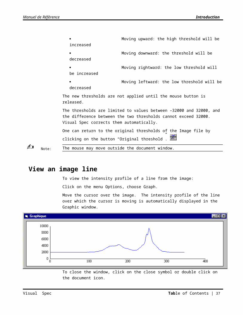
View an image lineTo view the intensity profile of a line from the image:
Click on the menu Options, choose Graph.
Move the cursor over the image. The intensity profile of the line over which the cursor is moving is automatically displayed in the Graphic window.
To close the window, click on the close symbol or double click on the document icon.
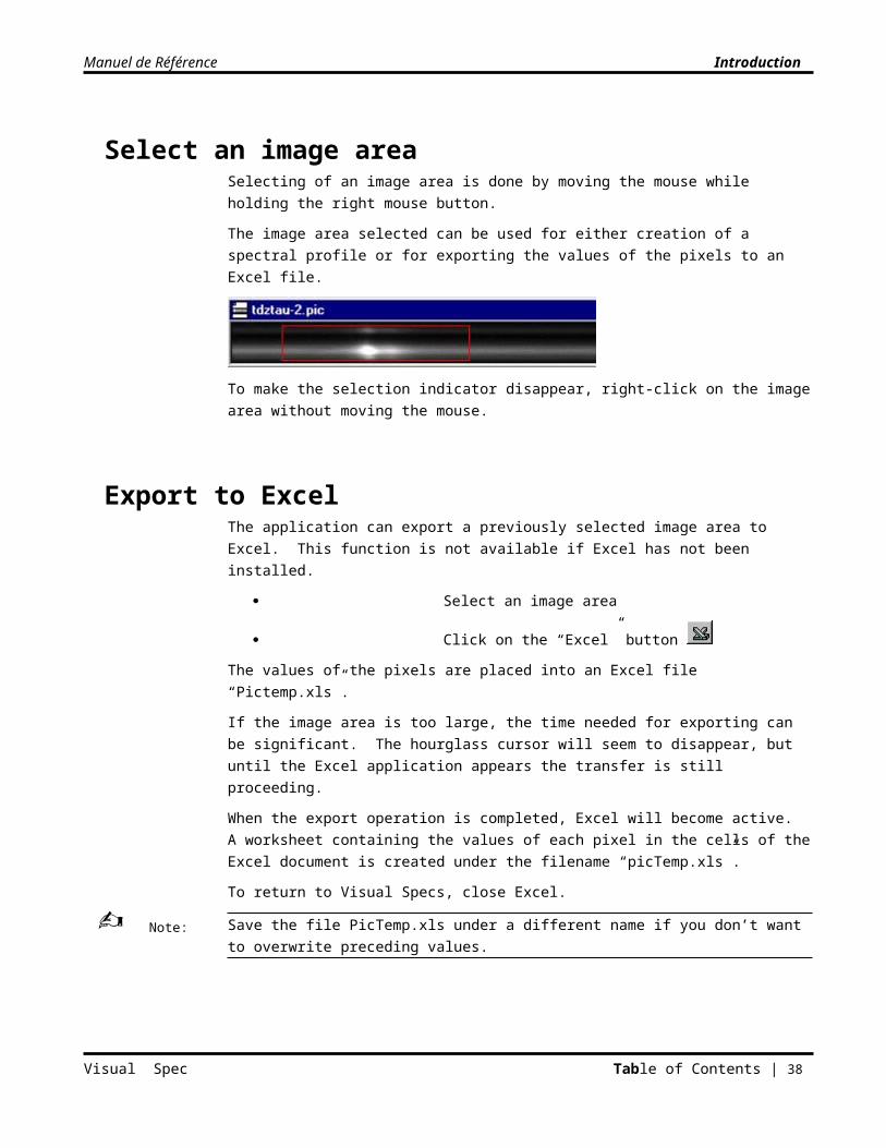
Select an image areaSelecting of an image area is done by moving the mouse while holding the right mouse button.
The image area selected can be used for either creation of a spectral profile or for exporting the values of the pixels to an Excel file.
Visual Spec Table of Contents | 30
Note:
Manuel de Référence Introduction
To make the selection indicator disappear, right-click on the image area without moving the mouse.
Export to ExcelThe application can export a previously selected image area to Excel. This function is not available if Excel has not been installed.
Select an image area
Click on the “Excel” button
The values of the pixels are placed into an Excel file “Pictemp.xls”.
If the image area is too large, the time needed for exporting can be significant. The hourglass cursor will seem to disappear, but until the Excel application appears the transfer is still proceeding.
When the export operation is completed, Excel will become active. A worksheet containing the values of each pixel in the cells of the Excel document is created under the filename “picTemp.xls”.
To return to Visual Specs, close Excel.
Save the file PicTemp.xls under a different name if you don’t want to overwrite preceding values.
Visual Spec Table of Contents | 31
Note:
Manuel de Référence Introduction
C H A P T E R 4
Profile
Profile DocumentThe Profile documents of the Visual Spec application contain one or more spectral intensity curves, called a series in the application. They are the fundamental documents of the application with which most of the processing and analysis operations will be done.
Profile FormatIt is valuable to make the distinction between the format of a *.spc file and a Profile document.
The Profile document is the window of the application that allows one to visualize, process, and compare spectra. A spectrum is a graphic visualization of intensity as a function of pixel number, or of wavelength after the spectrum is calibrated. The graph of a spectrum in a profile document is represented by a spectral series. These spectral series are graphic profiles constructed from a table containing:
The wavelength of the point or, if the series has not been calibrated, the sequence number of the pixel
The intensity at each point
Each profile document has the capacity to contain four spectra or basic spectral series which are saved by the application, identified by the symbol , and an unlimited number of “temporary” series, which are not saved, identified by the symbol in the Select Series control box of the Profile toolbar. These spectra share the same spectral sampling.
The files Profil.spc accessible to and created by this application are in “.spc” format, a proprietary format of Visual Spec but based on ASCII format.
When saved as a “Profile” file, along with the four basic series are recorded:
the sequence number of each pixel
the wavelength in angström of each pixel
an index which invalidates the value of the pixel of the profile if the index value is –1 (otherwise the index value is 0)
Visual Spec Table of Contents | 32
Manuel de Référence Introduction
Profile FolderThe default folder containing the Profile files in format *.spc is defined using the “Preferences…” dialog box.
Create and open a profile
Create a profileThe creation of a profile is always done from an image, by the operation of binning.
Binning is a simple summation by column of the pixels selected within the image area. It increases the quality of the spectrum as compared to a simple extraction by line of the image.
Two types of binning are suggested:
Object binning: summation of lines containing the spectral
signal, by clicking on the button of the Image toolbar.
Reference binning: summation of a sub-set of lines, by clicking
on the button of the Image toolbar. This reference notion is useful when working with calibration lamp as a spectral reference.
It is advisable to rectify any spectral image having tilted lines using Qmips 32. It is also required that the spectrum beeing oriented in the direction from blue to red (from left to righ).
Object binningThe Objec binning creates a profile in the basic serie "Intensity" of profile document. The binning can be done according to two strategies: Automatic or by user zone selection. In this last case, two methods are proposed to select the zone before clicking the binning button.
Automatic BinningThe automatic binning do not requires user actions. It extracts the lines of the iahe which contains the spectral signal signal and add them. The algorithm of lines selection is based on the mean signal comparison to the added noise. If the signal level is superior to the added noise then the lne is added. In the contrary, the line is not added as it probably contains only sky background. This algorithm can added not necessarily contiguous.
The binning constraint is that no other signal than the one from the spectrum or its background shall be present in the image. If another spectrum or a star are present, the algorithm will not make any difference and will add the high signal lines whether it belongs to the spectrum or not.
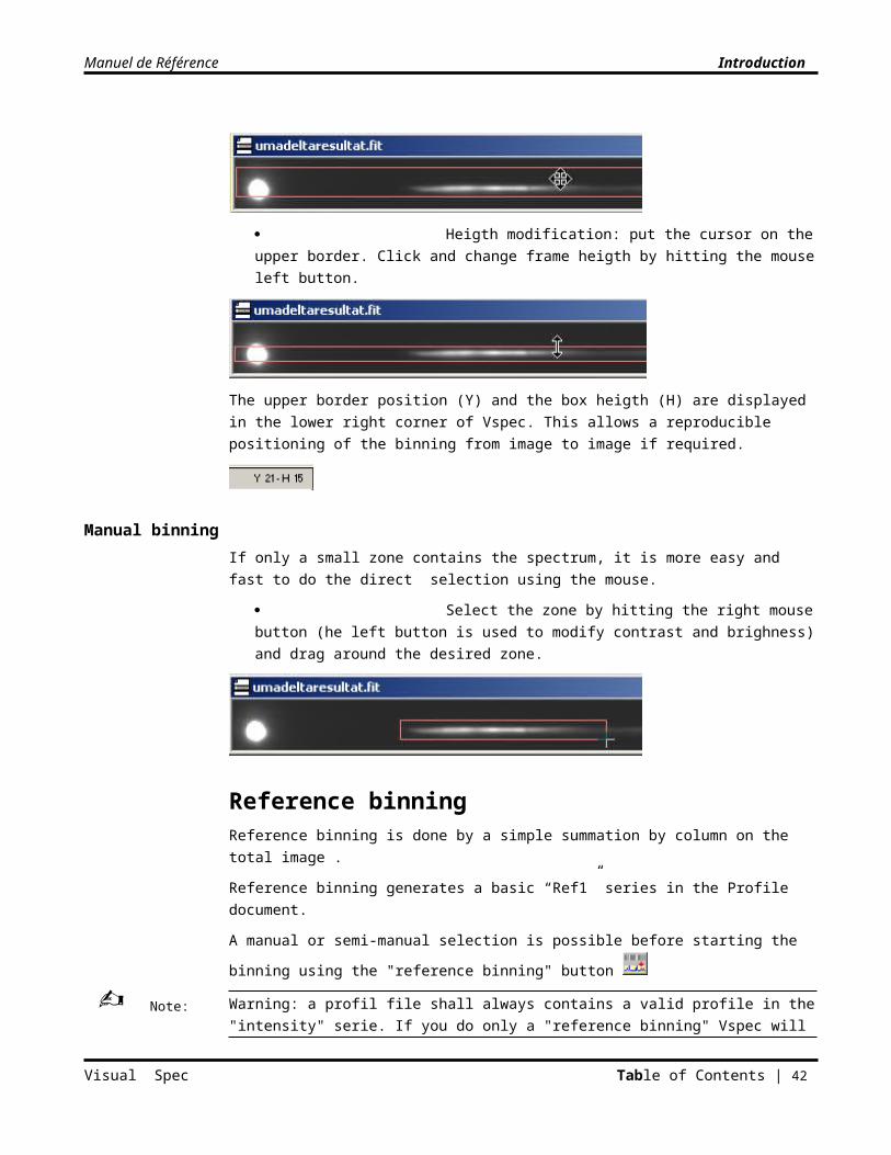
Semi-manual binningThe semi-manual binning allows the user to display a pre-defined box to define the binning zone. The box extend on the entire width of the image. The user can move the box up and down and change the heigth.
Visual Spec Table of Contents | 33
Note:
Manuel de Référence Introduction
The box zone is displayed by clicking on the button the button of the Image toolbar. It is then possible to move the area vertically using the cursor.
Vertical move of the entire box: put the cursor over the binning box. The cursor looks like a cross. Click and drag by hitting the mouse left button.
Heigth modification: put the cursor on the upper border. Click and change frame heigth by hitting the mouse left button.
The upper border position (Y) and the box heigth (H) are displayed in the lower right corner of Vspec. This allows a reproducible positioning of the binning from image to image if required.
Manual binningIf only a small zone contains the spectrum, it is more easy and fast to do the direct selection using the mouse.
Select the zone by hitting the right mouse button (he left button is used to modify contrast and brighness) and drag around the desired zone.
Reference binningReference binning is done by a simple summation by column on the total image .
Reference binning generates a basic “Ref1” series in the Profile document.
A manual or semi-manual selection is possible before starting the binning using the "reference
binning" button
Warning: a profil file shall always contains a valid profile in the "intensity" serie. If you do only a "reference binning" Vspec will not allow you to save the document. You shall have perform an "Object binning" or moved the "ref" serie into the "intensity". See the move a serie section.
Visual Spec Table of Contents | 34
Note:
Manuel de Référence Introduction
Creation of a profileWhen the binning is completed the profil is created. Several options are available depending whether a Profile document is already open.
If no profile document is displayed a new profile document is created. It is positioned under the Image window and takes the name of the image with the *.spc extension.
If a Profile document is already present, a dialog box is displayed:
If the operator answers “yes” to the question “Do you want to recover the file from existing and lose your changes?” then the binning will replace the preceding values.
If the operator answers “no” then a new Profile document will be created with the same name as the active profile document to which a letter “n” is appended.
Open a profileTo open a Profile document
Click on the File menu and choose Open Profile
Or
Click on the “Open profile” button of the main toolbar of the application.
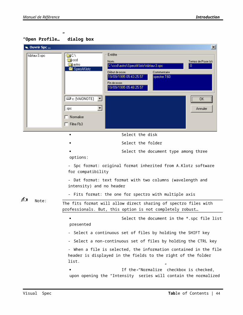
“Open Profile…” dialog box
Select the disk
Select the folder
Select the document type among three options:
- Spc format: original format inherited from A.Klotz software for compatibility
Visual Spec Table of Contents | 35
Manuel de Référence Introduction
- Dat format: text format with two columns (wavelength and intensity) and no header
- Fits format: the one for spectro with multiple axis
The fits format will allow direct sharing of spectro files with professionals. But, this option is not completely robust…
Select the document in the *.spc file list presented
- Select a continuous set of files by holding the SHIFT key
- Select a non-continuous set of files by holding the CTRL key
- When a file is selected, the information contained in the file header is displayed in the fields to the right of the folder list.
If the “Normalize” checkbox is checked, upon opening the “Intensity” series will contain the normalized spectral profile starting from the continuum area that has been preset in the “Preferences…” dialog box.
The document must contain a spectrum calibrated in wavelength.
If the “Fb3 filter” checkbox is checked, upon opening the “Intensity” series will contain the spectral profile filtered by a third-order low-pass filter.
If both checkboxs are checked, filtering will be done after normalization.
Click on the Cancel button to cancel the operation.
Click on the OK button to close the dialog box and display the file.
Search for a profileThe Search function allows one to find the set of files in a set of folders, whose “comments” header field contains the search-string specified in the search criteria area (see section “Fill in the header”).
To search for a Profile document
Click on the File menu, choose Find…
Or
Click on the Find button of the main toolbar of the application
Visual Spec Table of Contents | 36
Note:
Note:
Manuel de Référence Introduction
“Search…” dialog box
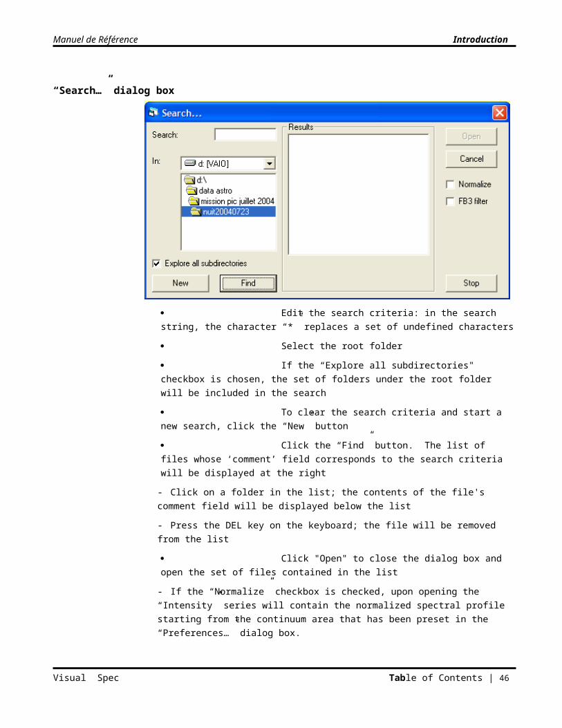
Edit the search criteria: in the search string, the character “*” replaces a set of undefined characters
Select the root folder
If the “Explore all subdirectories" checkbox is chosen, the set of folders under the root folder will be included in the search
To clear the search criteria and start a new search, click the “New” button
Click the “Find” button. The list of files whose ‘comment’ field corresponds to the search criteria will be displayed at the right
- Click on a folder in the list; the contents of the file's comment field will be displayed below the list
- Press the DEL key on the keyboard; the file will be removed from the list
Click "Open" to close the dialog box and open the set of files contained in the list
- If the “Normalize” checkbox is checked, upon opening the “Intensity” series will contain the normalized spectral profile starting from the continuum area that has been preset in the “Preferences…” dialog box.
- If the “FB3 filter” checkbox is checked, upon opening the “Intensity” series will contain the spectral profile filtered by a third-order low-pass filter.
- If both boxes are checked, filtering is done after normalization.
Click on the Cancel button to cancel the operation.
Click on the Stop button to stop search operation.
Visual Spec Table of Contents | 37
Manuel de Référence Introduction
Close and Save a profile
Close a profileTo completely close a Profile document
Click on the File menu, choose Close
Or
Click on the close symbol of the document window frame
To temporarily close a Profile document, click on the minimize symbol of the document window frame. The minimized document will be placed at the lower left of the application.
To close all the Profile documents:
Click on the File menu, choose "Close all"
If a document was modified since it was last saved, a confirmation dialog is displayed.
Save a profileTo save a Profile document
Click on the File menu, choose "Save…"
Or
Click on the button in the principal toolbar
The .spc file will be created in the current working directory.
If the file was modified, a confirmation dialog is displayed.
Save under a different nameTo save a Profile document under a different name
Click on the File menu, choose "Save As…"
The “Profile Save As…” dialog box will be displayed
This is a standard Microsoft Windows dialog box.
If the file already exists, a notification will be displayed to the screen.
Archive a profileThis function is eliminated since the 3.3.0 version
To ensure good management of the spectra generated by Visual Spec, one can set a folder where the spectrum of the object will be saved using a name of the format “name of object” + automatically incremented index.
Click on the File menu, choose Archive- a data-entry window is displayed
Visual Spec Table of Contents | 38
Manuel de Référence Introduction
Enter the object name in the text area “Nom de l’objet” (“Object Name”)
Click on OK
The document will be saved in the archive folder under the name “object name” + an automatically incremented index.
The index is defined automatically by the application, which searches for all documents having the same name already archived, and the using the most recent index + 1
If the folder contains the documents “Lcyg-1” and “Lcyg-2” and one wishes to archive “Lcyg”, the document will take the name “Lcyg-3”.
Creating a good archive requires that one define a method for naming spectra. The suggested method here uses the convention of the Bright Star Catalog with either the Greek letter following the constellation abbreviation, or the star number always followed by the constellation abbreviation without a space.
The spectral seriesA spectral series is a spectrum for which the intensity of each point is associated either with an order number for the point, or with the wavelength once the series is calibrated. The wavelengths are regularly spaced, the interval defining the spectral sampling.
Each Profile document contains four spectra or series, each having the same sampling. In addition to the basic series "Intensity", one can save the reference spectrum in the series "Ref1", the relative spectral intensity compared to the continuum in "standardized" and a second reference spectrum in "Ref2".
For the benefit of the application, one can create and superposition temporary series, but can only save them by using them to replace one of the four basic series. These temporary series are created by the application after certain operations such as filtering, cut/paste, division, calculation of a Planck profile, addition of a chemical spectrum or one of the library of spectra. A temporary series may not have the same spectral sampling as the base series.
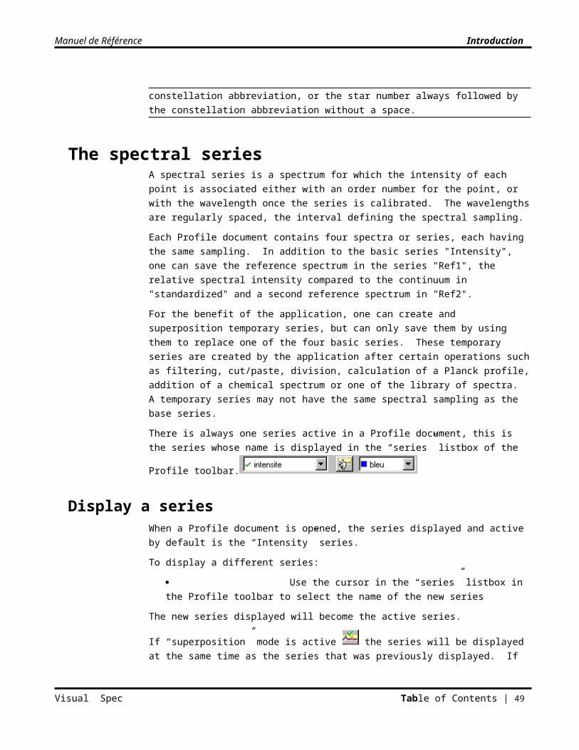
There is always one series active in a Profile document, this is the series whose name is displayed in
the “series” listbox of the Profile toolbar.
Display a seriesWhen a Profile document is opened, the series displayed and active by default is the “Intensity” series.
To display a different series:
Use the cursor in the “series” listbox in the Profile toolbar to select the name of the new series
The new series displayed will become the active series.
If “superposition” mode is active the series will be displayed at the same time as the series that
was previously displayed. If “superposition” mode is inactive the series to be displayed will
Visual Spec Table of Contents | 39
Note:
Manuel de Référence Introduction
replace the series which was previously displayed.
To change the superposition mode of the series, click on the button “Superpose” in the Profile toolbar.
To change the color of a series:
Use the cursor in the “color” listbox in the Profile toolbar to select the new color from the list of colors provided.
To change the display mode to by-point of a series, click on the Format menu and choose Plot.
To change the display mode to histogram of a series, click on the Format menu and choose Histoplot.
To return the display mode to by-line-segment, click on the Format menu and choose Line.
To clear the display, click on the “Erase graphic” button of the Profile toolbar.
Selecting a seriesTo select a new series:
Place the cursor in the area of the “series” listbox in the Profile toolbar and select the name of the new series
Or
Place the cursor over the graphic of the new series and click. When the cursor is correctly positioned, the cursor changes to arrow-shaped. The newly selected series will flash one time.
Or
Move from one active series to another in the series listbox of the profile document by pushing the Tab key or Shift-Tab key of the keyboard. Each series in the list will in turn become active.
Selecting a series makes it the “active” series; that is to say that its spectral profile is displayed and when one moves the cursor along the profile, the position, the wavelength, and the intensity of the pixel are displayed in the upper toolbar. The spectral sampling is displayed in the area of the main toolbar:
Also, arithmetic and format changes are performed on the active series.
Cursor positionThis function applies to the active series.
On a profile document, only the X position of the cursor is changeable. The cursor takes the shape of a hand holding a red line.
Each new position is displayed in the main toolbar:
Visual Spec Table of Contents | 40
Manuel de Référence Introduction
the pixel number
the wavelength, if it was previously calibrated
the spectral intensity
To temporarily display the “comments” field of the document header, left-click on the yellow border around the image and hold the left mouse button; the comments will appear in a yellow rectangle at the cursor position. It will disappear when the mouse button is released.
Selecting a spectral areaThis operation applies to the active series.
To select a spectral area:
Position the cursor at the start of the area to be selected
Drag the mouse holding the left mouse button
Release the button at the end of the area to be selected. The selected area is framed by a gray dotted rectangle.
Selecting a spectral area defines:
The spectral area to enlarge
The spectral domain on which calculations will be effective
The spectral domain of the database of wavelengths
The zone of selection in the toolbar displays: the starting wavelength of the selection, the ending wavelength and the distance bewteen the two
Spectral calibrationSpectral calibration consists of establishing the dispersion relationship of Pixel to Wavelength of the profile. Without this operation, it is impossible to analyze the results obtained.
To establish the Pixel-wavelength relationship, several methods are available, the most precise using empirical reference spectra based only on instrumentation parameters defined by the user.
To calculate the law of dispersion, Visual Spec assumes that the law is linear. Whatever the domain of wavelength, the spectrum always has the same calibration.
Visual Spec Table of Contents | 41
Note:
Manuel de Référence Introduction
A database of wavelengths of simple elements is available to help in identifying the lines.
It is not always necessary to calibrate a spectrum in wavelength to identify some simple lines, such as the Balmer lines of hydrogen. But this operation is needed to make possible the corrections, calculations and comparisons of the spectral processing
Calibration using referenceTo calibrate a spectrum in wavelength, one uses a Reference spectrum. This spectrum should contain one or two spectral lines of which the wavelength is previously known.
This reference spectrum can come from:
A calibration lamp, standard lamp, or lamp of known composition such as argon
A star of which one knows the lines, and whose spectrum was obtained under the same experimental conditions
The spectrum itself, if it contains identifiable characteristic lines
In each step of preliminary research for identification of reference lines, one can also perform a manual calibration from a simple reference point and a preliminary knowledge of the sampling of the device (see section “Calibration without reference”).
Visual Spec requires that the reference spectrum be included in the profile document, in the form of the basic series “Ref1”.
Add an external reference spectral profileTo add a reference spectrum based on an image as the “Ref1” series:
Open the profile document of the spectrum to calibrate. If the document does not exist, create the spectral profile as indicated in the section ‘Create a Profile’ in the chapter ‘Profile”.
Visual Spec Table of Contents | 42
360nm360nm 760nm760nm
1 2 3 4 5 6 7…...638
pixelpixel
Pixel n°5 raie =360nmPixel n°638 raie =760nm
(638-5) = Echx * (760-360)Echx= 400 / 633Echx= 0.632 nm
Note:
Manuel de Référence Introduction
Open the reference spectrum image
Click on the button “Reference Binning”. Refer to the section ‘Create a Profile’ in the chapter ‘Profile”.
The reference spectral profile will be placed automatically in the series “Ref1” of the document. The four basic series share the same calibration.
This function calculates the spectral profile from a simple sum on the whole image or on a predefined zone (see section “Reference Binning”). In the case of a spectrum obtained from a calibration lamp, the spectral image extends throughout the image, and binning with extraction is not useful.
Create a spectral reference profile from a star spectrumIt is not always possible to have access to a reference spectrum whose elements are simple and known.
One can, in certain cases, use the spectrum of a star obtained under the same experimental conditions and from which one can identify at least two lines with precision. The spectrum of the object itself can thus be used for its own calibration.
If one calibrates a spectrum based on its own lines, no calculation of Doppler shift is possible because it is not absolutely calibrated by an external reference.
Some useful wavelengths of spectral lines are given in the appendix.
To use the spectrum of an object itself for calibration:
Select the “intensity” series of the document:
Click on the Edit menu, choose Replace
Or
Click on the button of the Profile toolbar. The “Replace…” dialog box will be displayed
Visual Spec Table of Contents | 43
Note:
Note:
Manuel de Référence Introduction
Click on “Reference 1”
Click on OK
This operation permits duplication of the series “Intensity” to the series “Ref1”, which is the basic series used for calibration.
It is possible to let the application do the job itself by clicking in the menu Spectrometry, sub menu Calibration. To the question "do you want to use the current serie ?", click on "yes" and the "Intensity" serie will be automatically copied in the "ref1" serie.
It is also possible to copy a series from a different document, as long as the spectrum was obtained under the same experimental conditions…
Atmospheric linesIf the spectrum contains atmospheric lines contained between 6875 and 7604 angstroms, these can be easily used to calibrate the spectrum because they are easily recognizable.
02 Line 6875 angstromsH20 Line large line, can specify 6950 and 7250 angstroms02 Line 7590 angstroms
Calibrate in wavelengthOnce the “Ref1” series is filled, activate “Calibration” mode.
Click on the Spectrometry menu, choose "Calibration…"
Visual Spec Table of Contents | 44
Note:
Manuel de Référence Introduction
The Calibration toolbar will replace the Profile toolbar, and the active series will become the “Ref1” series.
Verify the reference wavelengths in the fields "raie 1" ("line 1") and "raie 2" ("line 2"). By default, they contain the values that were predefined in the “Preference” menu.
Edit these values directly if the default values are not OK.
Using the cursor, select the line that is identified as the first reference line. Its wavelength will correspond to the absolute wavelength shown in the field “raie1” (“line1”).
Calculation of the barycenter is very sensitive to the selected area. It is recommended to select an area balanced around the minimum and maximum of the line, and not including other neighboring lines.
Select with the mouse the first line identified as the first reference line. Its wavelength will correspond to the absolute wavelength of the filed "line1" of the toolbar. At the end of the selection operation, a text box is displayed close to the selection. It contains by default the value of the "line2" field from the toolbar.
Type "Enter" from the keyboard to validate the value. You can edit it before validating. Once validated, the barycenter position is displayed next to the line1 field in the toolbar.
Select the seconf line the same way, enter or keep the displayed value which corresponds now to the second line "line2" field. Validate
Visual Spec Table of Contents | 45
Note:
Manuel de Référence Introduction
If you don not know by advance the exact wavelength of the identified line, you can be helped by the element database. Display the Element wavelength list and click on the wavelentgth you want to have it automatically displayed in the edit box. Just then type enter to have the value validated. See the section "Elements" later in the manual
Done ! – as long as you have validated the second wavelength, Visual Spec calibrate the sptrum, exits the calibration mode and display the "intensity" serie.
The linear interpolation calculations will associate to each point in the series a wavelength based on the two reference points thus calibrated. The X position of the cursor now gives access to the wavelength for each data point.
To facilitate selection of the reference lines, it is possible to:
Zoom on an area
Change the scale of the X and Y axes
Display the database of atomic lines (refer to the section “Elements”)
At any time it is possible to quit Calibration mode and return to the “Line” menu by choosing the "Calibration…" sub-item on the "Spectronometry" menu.
Calibration without referenceThis calibration operation is described by the section title. It is not recommended. It can, however, contribute to identification of the reference lines before performing the complete calibration, or make it possible to use the data in the absence of any access to a reference spectrum.
This method is based on identifying only one point in the profile and on assuming the device sampling in angstroms per pixel.
Select the reference line
Click on the Spectrometry menu, choose "Define…"
Or
Right-click in the selected area. A pop-up menu will appear. Choose “Define".
A dialog box will appear. The pixel position of the barycenter is indicated.
Visual Spec Table of Contents | 46
Note:
Manuel de Référence Introduction
In the Barycenter textbox, the barycenter of the selection area is automatically calculated and displayed. To change this value, click in the textbox and enter the new value of the barycenter of the selection.
Enter in the “Wavelength” textbox the wavelength of the reference line
Enter in the “Sampling" textbox the assumed calibration of the device, in angstroms per pixel.
Click on the “Apply” button. The X axis will immediately be calibrated in wavelength. Without clicking in the profile window, drag the mouse over the profile and verify the coherence of the wavelengths of the lines.
Redo the operation, adjusting the values, until a satisfactory result is obtained. Do not change the selected line.
Click on the button “Close” to save the new calibration and close the dialog box.
Click on the button ““Cancel” to return to the original calibration.
Help in identifying the lines is available by clicking on the button. This is described in the section “identification”, below in this chapter.
For this method it is not necessary to create a reference profile.
To restart using a different line, leave by clicking on “cancel” then “close”.
Application to an image containing a star.In case one has obtained a spectrum using an assembly without a slit, the star and its spectrum are present. If one knows the dispersion of the device in angstroms per pixel, it is then possible to use the position of the star to calibrate its spectrum.
Display the image containing the star and its spectrum.
Perform Object Binning, or manual binning by framing. The base series “Intensity” then contains the spectrum.
Visual Spec Table of Contents | 47
Note:

Manuel de Référence Introduction
1. Replace the base series “Ref1” with the series “Intensity”
2. Select by framing the line which indicates the position of the star
3. Click on the Spectrometry menu, select ““Define…”
4. Enter 0 in the “wavelength” area; the dispersion will start from the star
5. Enter the number of angstroms per pixel of the device in the “sampling” area
6. Click on the “Apply” button
7. Drag the mouse over the document; the wavelengths will be displayed in the main toolbar
8. Change the value of calibration as needed
9. To save the calibration, click on the button “Close”
10. Select the useful area of the spectrum
11. Click on the Edit menu, choose “Crop"
12. Save the result
Non linear calibrationNon linear calibration is useful when the dispersion system used does not shift the wavelength of the same pixel-length quantity. Up to now, all the proposed method was assuming that each pixel was seeing the same wavelength quantity.
To proceed with a non linear calibration, one can cut the spectrum into small pieces, small enougth to have the linear assumption beeign correct.
Visual Spec proposes a more powerfull interpolation function on the entire spectrum based on a multiple reference lines identification. This function still permit the linear calibration if wanted.
Click on the menu Spectrométry, choose Non-lin calibration
A dialog box appears to enter the reference wavelengths.
Visual Spec Table of Contents | 48
Manuel de Référence Introduction
Dialog box non linear calibration
Select the first line by click-drag on the serie to calibrate.
A small text box appears close to the cursor. Enter the wavelength value of the line. Validate by hitting the Enter keyboard key.
Instead of entering data with keyboard, you can directly use the element database from Visual Spec.
- For this, you need to have displayed the "Element" window and have selected the appropriate database. See the Element section later in this manual.
- In the Element window, click on the line from you want to copy the wavelength
- The value will automatically be set in the text box
- Click back on the text box and press Enter
Visual Spec Table of Contents | 49
Manuel de Référence Introduction
In the dialog box, the wavelength table is filled with the wavelength and the position of the barycenter, along with a reference ID
Repeat the line identification operation for each known lines
Select the polynome degree
Click on the "Calcul" button. The interpolation of the wavelength law are displayed in the bottom of the dialogn box and the profile is calibrated. The profile is linearly re-sampled with a sampling factor close to the linear coefficient of the equation.
Visual Spec Table of Contents | 50

Manuel de Référence Introduction
If the number of lines is not enougth to match the inerpolation degree selected, the lower order is automatically selected and applied.
Degree Minimum number of lines
Interpolation equation
Degree 1 2 lines lambda = ax + b (x= cursor position)Degree 2 3 lines lambda = ax2 + bx + cDegree 3 4 lines ax3 +bx2 +cx +dDegree 4 5 lines ax4 +bx3+cx2+dx+e
The equation coefficient are displayed in the bottom frame
Save an equation To save the equation coefficient , click on the button "Save" in the Interpolation bottom section. A dialog box will appear to allow the user to enter the file name.
The interpolation equation coefficients are mainly function of the dispersion system used. They do not vary from one spectrum to another if no change is made on the isntrumental configuration. Only the constant (wavelength domain offset) will have to be re-computed.
To re-use the interpolation coefficients:
Load the spectral profiles, enter the non-linear calibration mode.
Load the coefficient by clicking the "Load" button in the interpolation section. The coefficients are updated.
Enter "0" in the constant field box
Visual Spec Table of Contents | 51
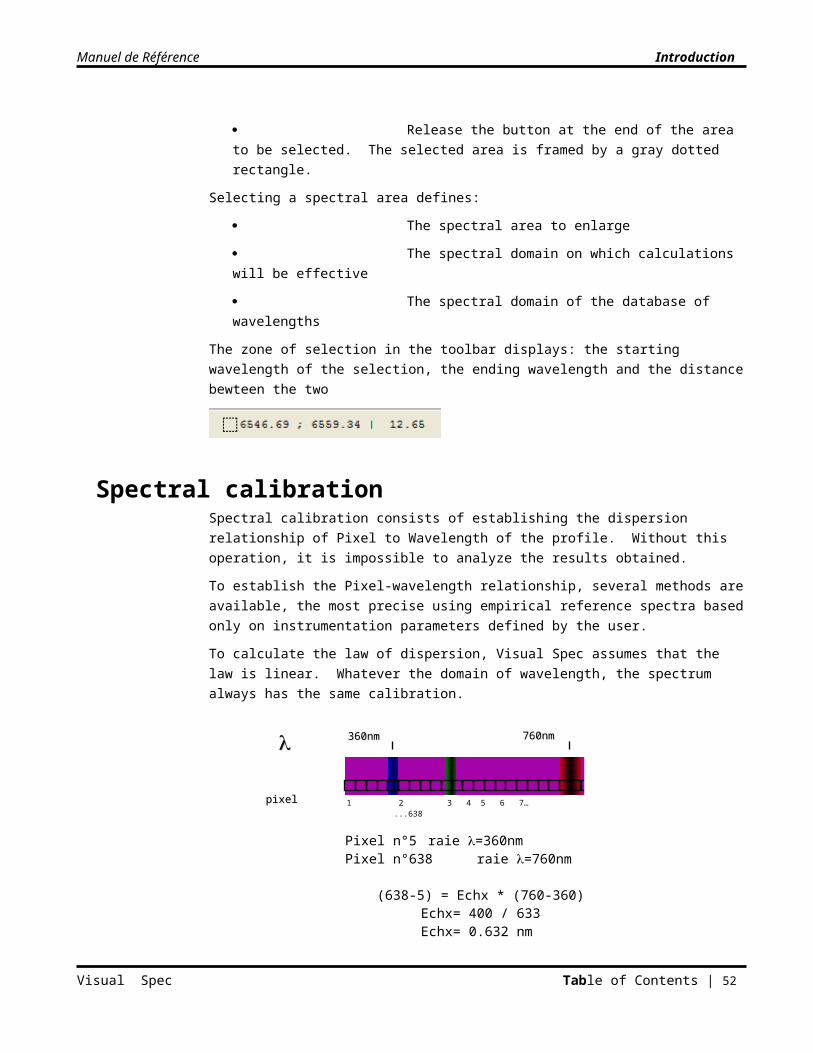
Manuel de Référence Introduction
Select one line in the spectral profile and fills the wavelength
Click on Apply – the calibration is made and the cursor position on the profile references the wavelength.
To reset all coefficients, click on the "Reset" button
The "Apply" button in the interpolation section recompute the calibration if one of the coefficient is changed, like the cosntant. If one on the wavelength table value is modified, the "Calcul" shall be hitted again to re-compute the interpolation law.
Save a list of wavelengthList of wavelengths can be saved and then re-loaded if a set of lines are used regularly to calibrate the spectrum. As for the equation, use the button LOAD and SAVE on the side of the wavelength list frame
Inflexion pointSi the dispersion law has an inflexion point, Visual spec inhibits the calibration . A sound is emitted and the word "inflexion" is written in red under the graphical representation of the dispersion law.
To modify values in the wavelength table:
Click one time on the line to edit the wavelength
Click two times to edit the barycenter (pixel position)
d dispersion lawFor a greater accuracyin the calibration, more reference lines than the minimum required by th einteroplation degree can be added. For each line, the difference between the calculated value and the observed value is displayed.
The difference are listed in the d_lambda column.
Visual Spec Table of Contents | 52
Note:
Manuel de Référence Introduction
In order to take those differences into account in the final dispersion law:
Check the box "delta lambda" in the "Lambda" frame
Click on the bouton "Calcul" to compute the dispersion law
The dispersion computation apply a linear interpolation between each difference and add it to the lambda computation.
The lambda difference are not saved with the interpolation law coefficients. They shall be re-computed at each time.
Changing the appearance of a profile document
Enlarging, reducing a windowThe Profile document has an adjustable size. Adjustment of the size is done as for standard Microsoft windows. To maximize the window, click on the “maximize” symbol of the window.
ThumbnailsTo view a collection of profile documents, it is possible to reduce all the windows to a small thumbnail format.
Click on the “Windows” menu, choose “Small Windows".
Visual Spec Table of Contents | 53
Note:
Manuel de Référence Introduction
Adjusting FormatOne can automatically put the document window into the format of its original image.
Click on the “Windows” menu, select “Adjust”.
Or
Click on the "Medium Size" button of the Profile toolbar
A pixel in the graphic area of the profile will correspond to a pixel of the original image if the series is viewed in its entirety, from first to last pixel.
Pre-defined FormatIt is possible to define and apply a particular size, different from the Small or Adjusted size, to a profile document.
To apply a pre-defined size:
Click on the "User Defined Size" button in the Profile toolbar
Or
Click on the “Windows” menu, select ““Predefined”
The default size can be modified by using the “General” tab in the “Graphic” dialog box.
Click on the Format menu, select "Graphic…"
Visual Spec Table of Contents | 54
Note:
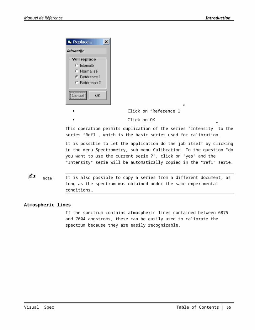
Manuel de Référence Introduction
Select the “General” tab
Edit the X and Y size fields, in units of pixels
View the results by clicking on the “Preview” button
Click on the button “Cancel” to return to the original size
Click on the button “OK” to close the dialog box.
Display graduated axes and a titleTo display the graduated axes of the active series of a profile:
Click on the Format menu, select "Graphic…"
The "Graphic…" dialog box is displayed
Click on the tab "Axis X” and check the checkbox “Display X Axis” to view the X axis graduations.
Visual Spec Table of Contents | 55
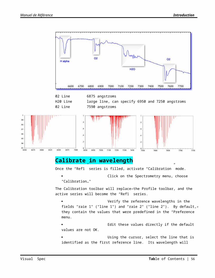
Manuel de Référence Introduction
- Check the checkbox to “Display title” so the title of the graph will be displayed in the predefined corner of the application.
- The title of the graph is entered in a textbox on the General tab
Click on the tab “Axis Y”
- check the checkbox “Display Y Axis” to view the Y axis graduations.
- Check the checkbox "Display gridlines” to view the grid in horizontal dashes for each major graduation
The axes display two types of graduations:
Simple graduations or “ticks” are displayed by plain dashes. The distance between two simple graduations is defined by the value of the tick. If no value is entered into the textbox “tick” then this value will be automatically calculated.
Labeled graduations are defined by the number of simple graduations or “ticks” separating them, and are displayed using a longer dash and the X or Y value.
If no value is present in the “Tick” text area, the application automatically determines the most suitable value.
The graduations apply to a document and not to a series. If one selects a different series, the graduation of the axes may give less desirable results. Then adjust the graduations to display.
On the Y axis, if the application detects a difference too large between the value automatically proposed by the application and that entered by the user, it will use the automatic value.
Click on “Apply” to view the result
Click “OK” to close the dialog box and save the result.
Visual Spec Table of Contents | 56
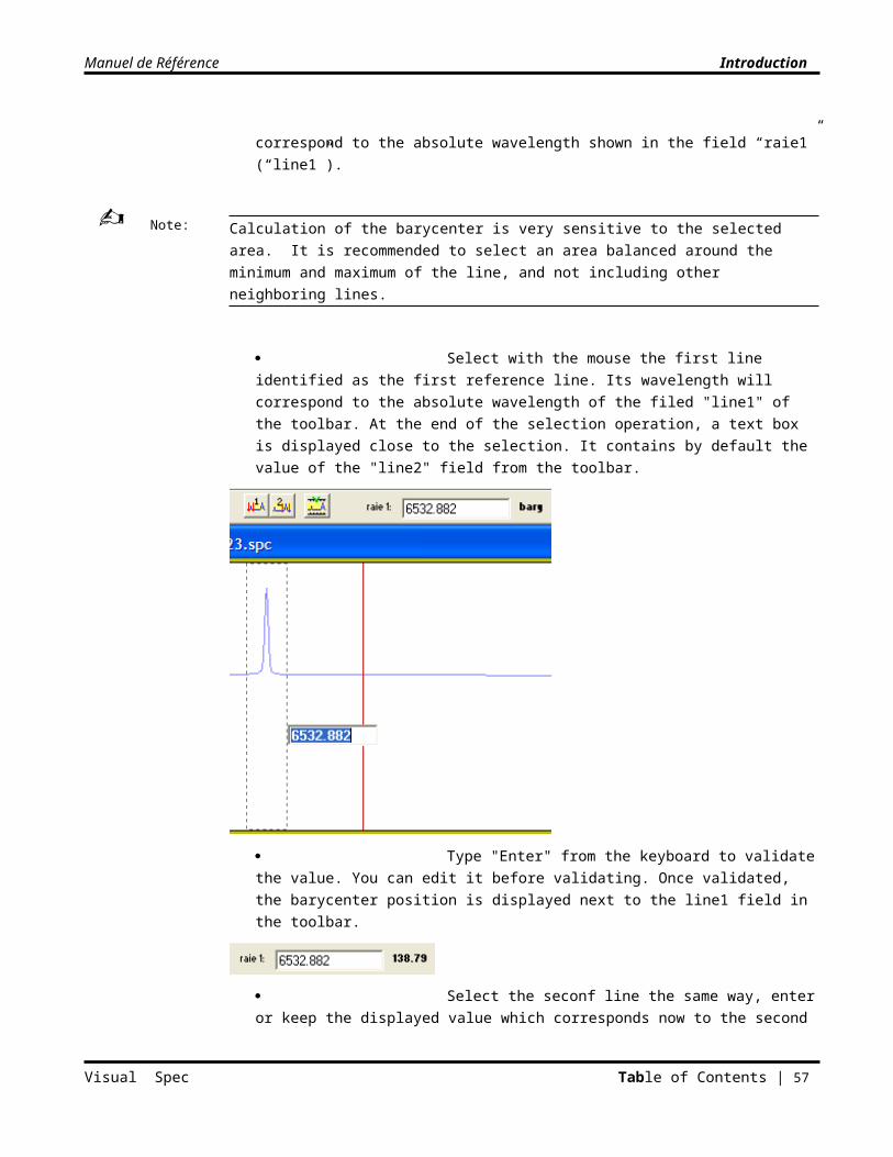
Manuel de Référence Introduction
Graph titleVisual Spec offers the possibility to add a title and two lines of comment superimposed onto the image
Click on the “General” tab
Enter the graph title in the field “Graphic title”
To automatically display the date or comments from the header, click on the button “Entete” (“Header”).
Freely edit, as needed, the date and comments lines, which will be displayed underneath the title.
Check the checkbox “Display title” in the tab “Axis X”.
Once the title is displayed, it is possible to move it within the image.
Place the cursor in the area of the title, and the cursor will become cross-shaped
Visual Spec Table of Contents | 57
Manuel de Référence Introduction
Click and hold the left mouse button while moving the title to the desired place.
After resizing, the title will always return to the upper right corner.
Doppler shift scaleTo graduate the profile in Doppler shift (km/s) relative to a given wavelength on the X axis:
In the tab "Axis X", mark the Doppler box and enter the wavelength value in the lambda text field.
Click on Apply to check the result. Adjust the ticks and Ticks Nb if needed.
Visual Spec Table of Contents | 58
Note:
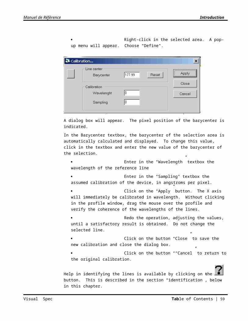
Manuel de Référence Introduction
The doppler shift values are computed versus a reference wavelegth Lamda following the equation formule ((Lambda – Lambda ref ) / Lambda ref) * c, c beeing the light speed in en km/s – 300000km/s
The document is not modified, only the display takes into account the new X values. To save the serie along with the Doppler shift export the current document in .dat format. (Doppler shift – intensity").
Click on menu File, choose Export .dat
A .dat file will e created with the same name but the .dat extension in the current directory.
Changing the color and fontTo change the background color of the Profile document
Click on the Format menu, select “Background color…”
The “Color” dialog box will be displayed.
Click on the color to display as the background of the document
Click on “OK” to close the dialog box and apply the selection
As needed, also change the colors of the series by selecting from the color control of the Profile toolbar to apply a new color to the active series.
The color is specific to the active document. Redo the operation to change the background colors of the other Profile documents.
To change the text font
Click on the Format menu, choose Font…”
The “Font” dialog box will be displayed
Select the font and font style options
Click on “OK” to close the dialog box and apply the selection
The text font applies to the axis graduations or line labels.
Visual Spec Table of Contents | 59
Note:
Note:
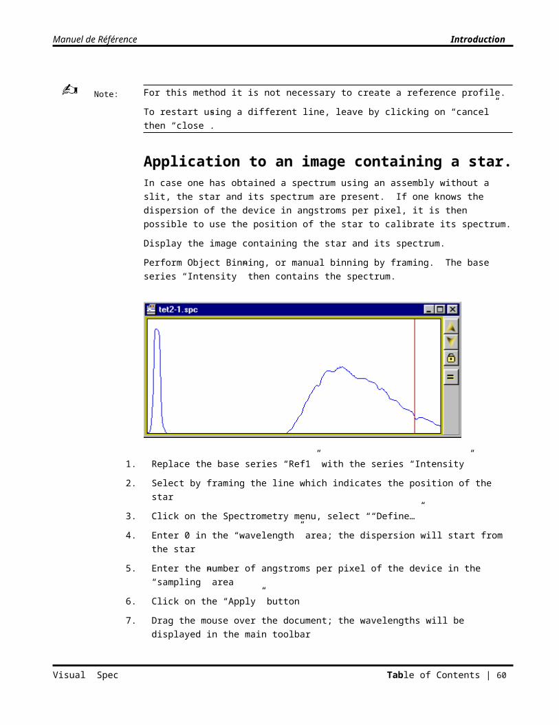
Manuel de Référence Introduction
Export to other applicationsThe Visual Spec application offers a certain number of links to standard applications by generating files compatible with the formats used by these applications. There are two such formats:
.bmp files, for saving the spectral profile
.txt file, compatible with spreadsheets, for exporting values from .spc files to other applications for data processing.
.dat file, text format that contains only the active series in the form of two columns.
.bmp ImageTo create a .bmp image of the active Profile document:
Click on the "File” menu, select “Export bmp”
A dialog box to enter the file name will appear.
Visual Spec Table of Contents | 60
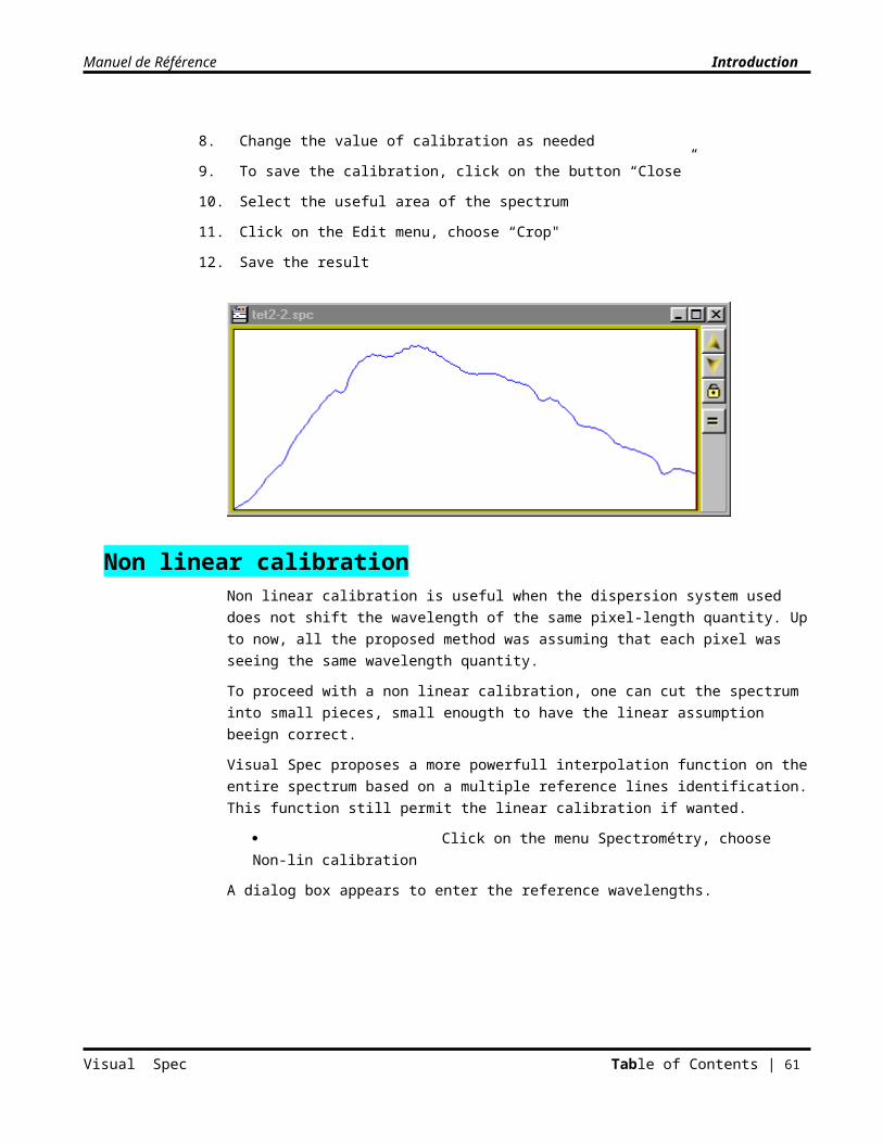
Manuel de Référence Introduction
By default, the .bmp file will take the name of the .spc document with the .bmp extension, and will be saved in the working directory.
The saved image is a copy of the image area of the active document, graduations, cursor and color included.
.txt ProfileTo create a .txt file from the active Profile document:
Click on the “File” menu, select “Export txt”
The .txt file will take the name of the .spc document with the .txt extension, and will be saved in the working directory.
The text file contains the set of values of each series of the .spc document, each line being formatted in the following manner:
0768 number of pixels in the seriesvalue that is not used22/04/1998 00:09:45.84 date and time of start of pose (exposure?)22/04/1998 00:09:51.84 date and time of end of pose6 times de pose in secondsSpectroCB Véga comments0 value not used0 value not used0 value not used0 value not used0 value not used.spc extension of original file
pixel tab angström tab intensité tab Ref1 tab Ref2 tab normalise tab repère cr series name
Visual Spec Table of Contents | 61
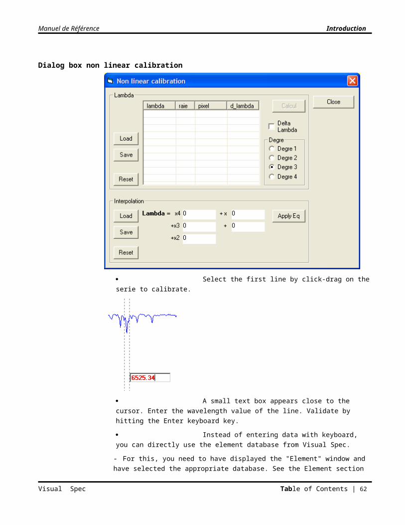
Manuel de Référence Introduction
1 tab 5925.349 tab 29612.8163 tab 10733710 tab 0 tab 0 tab 0 cr values by pixel2 tab 5927.968 tab 32720.3065 tab 10733710 tab 0 tab 0 tab 0 cr...
The tab characters tab and line-returns cr are placed to facilitate reading of the .txt file by a spreadsheet application such as Excel. Each cell will contain one value for the set of lines.
.dat Fileto create a .dat file from the active Profile document:
click on the “File” menu, select “Export dat”
The .dat file will take the name of the .spc document with the extension .dat, and will be saved in the working directory.
The format of the .dat file is ASCII, comprised of two columns. The first column contains the wavelength, the second column contains the spectral intensity of the active series.
.gif or .png fileSee the "GnuPlot" section later in this manual.
ClipboardTo rapidly copy the image window of a profile document, one can use the Clipboard.
Click on the Edit menu, select Copy
Select an application that supports the image-copying function of the Clipboard
Paste the contents of the Clipboard; a .bmp image of the active profile document is pasted.
To display an image frame, display the graduated axes.
Visual Spec Table of Contents | 62
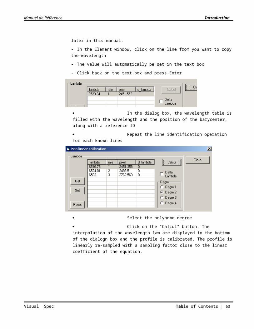
Manuel de Référence Introduction
Chapter 5
Spectral Series
The creation of a spectral series is at the base of the set of functionalities of Visual Specs.
A spectral series is a curve representing spectral intensity as a function of wavelength.
One can modify their format: scale in X and Y, zoom to an exact area, clear the display of a series, display the wavelength of a selected line. These operations only modify the way in which the series is viewed.
It is also possible to add series by copy/paste, to suppress a temporary series, or to replace one of the basic series with one of the temporary series.
One can modify a series by applying transformation operations such as translation or by applying simple arithmetic operations with a constant. One can combine several series to achieve a re-sampling or a composite.
One can create temporary series as a result of an operation applied to the selected series, such as filtering, normalization, derivation, calculation of a Planck profile, and some operations such as division that combine the active series with another series. It is possible to save a temporary series by replacing one of the four basic series with the temporary series to be saved.
One can modify, pixel by pixel, the intensities of a series.
A toolbox dedicated to measurement of an area of the spectrum, such as a line or a continuum, contains the basic calculations of spectrometry or statistics: full width at half-maximum, signal-to-noise ratio, center of a line, equivalent width, average, standard deviation.
FormatIt is possible to modify the scale of the series displayed in the profile document using the vertical toolbar of the document.
Visual Spec Table of Contents | 63
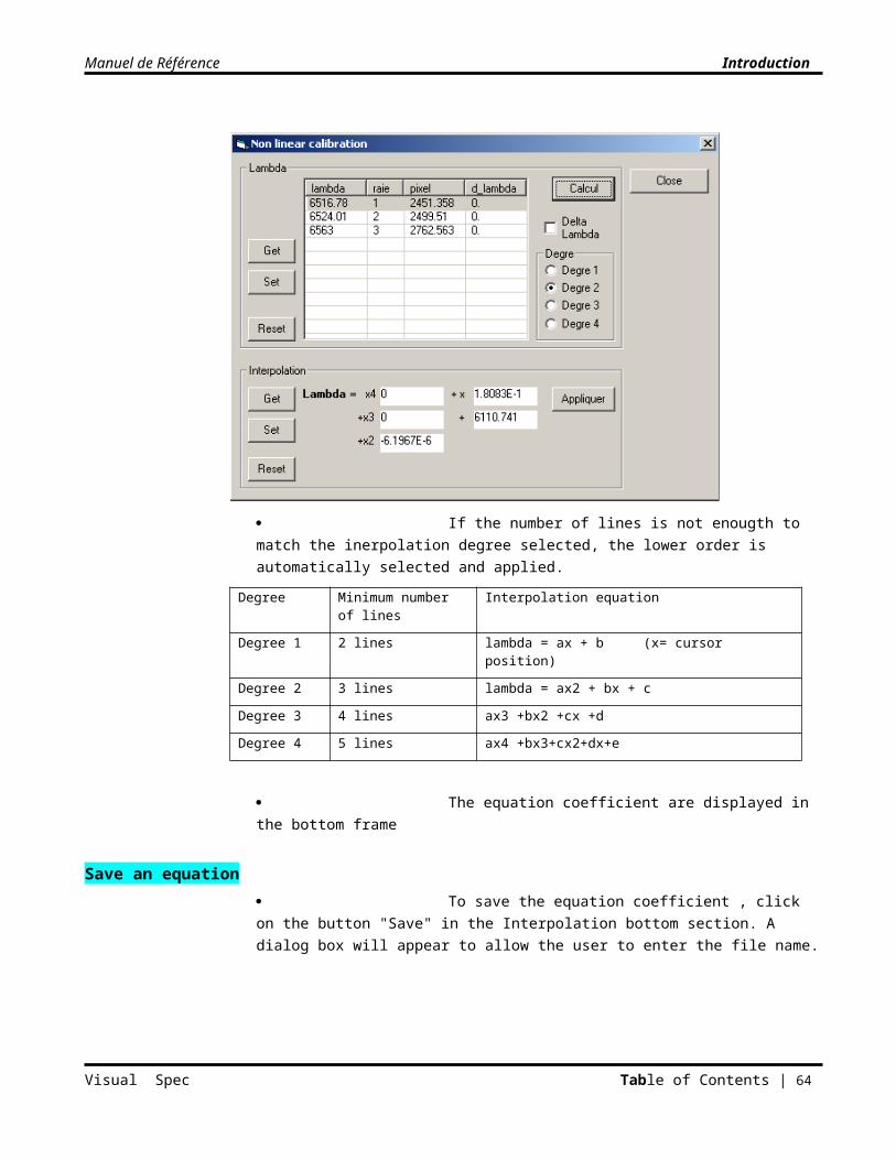
Manuel de Référence Introduction
Or, by using the "Graphic…" dialog box.
Click on the Format menu, choose "Graphic…"
Modify the scaleThis operation concerns, needless to say, the active series.
The scales of the series are:
In X: min and max value of the domain in wavelength, or min and max pixel number
In Y: min and max value of the intensity of the profile
The Y axis of a series is scaled automatically when it is displayed, starting from the maximum intensity of the profile multiplied by 1.1 (the min value being fixed at 0).
The X scale of a series is scaled automatically when it is displayed, based on the min and max wavelengths or pixel numbers of the profile.
If the min and max values of these scales are modified, the new values are used.
Modification of the min and max values of these scales is done using the “Graphic…" dialog box.
Visual Spec Table of Contents | 64
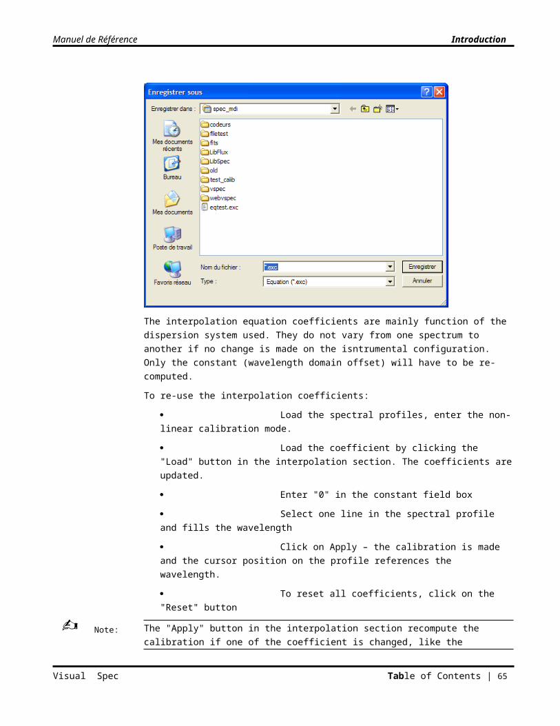
Manuel de Référence Introduction
Click on the Format menu, choose “Graphic…", and click on the tab “Axis X” or “Axis Y”
Or
Click on the buttons “Scale X" or “Scale Y” in the profile toolbar.
X Axis Scale
Click on the tab “Axis X”
Enter the new thresholds "X min" and "X max" for the X scale of the profile into the editable fields
Or
Click on the Right/Left control arrows to increase/decrease the value by ten percent.
Click on the checkbox “Angstrom units” to edit the thresholds in Angstroms. By default, the min and max values represent the pixel number in the profile or the coordinates of the min and max pixel.
Click on the checkbox “Apply to all windows" to make the change in scale apply to all displayed profile documents.
Click on the button “Apply" to instruct the application to apply the scaling.
Click on the button “Reset” to return to default values
Click on “OK” or in the close symbol of the dialog box to make it disappear.
When the min and max values of the X scale are lower, higher than the real min and max values of the profile, cursor movement is limited to the effective area of the spectral profile.
Visual Spec Table of Contents | 65
Note:
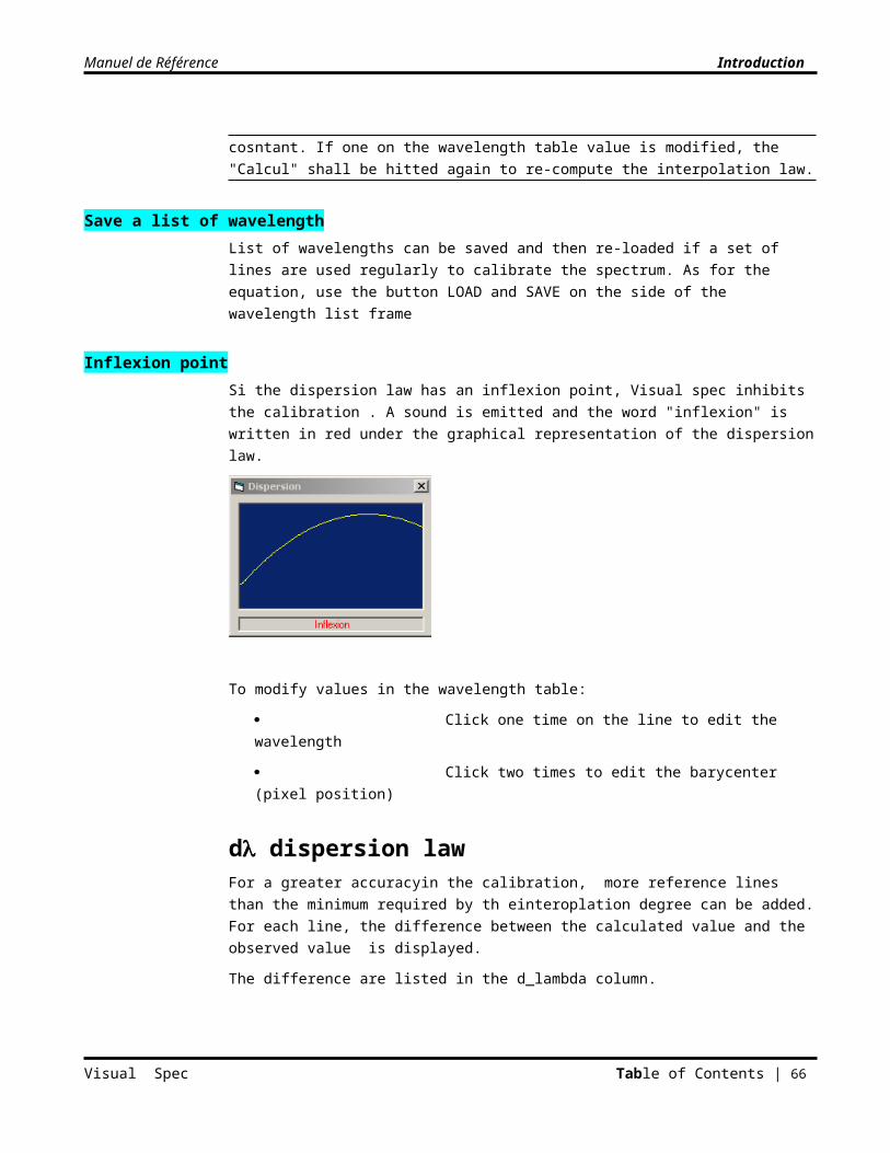
Manuel de Référence Introduction
Y Axis Scale
Enter the new high and low thresholds Y scale of the profile into the editable fields
Or
Click on the Right/Left control arrows to increase/decrease the value by ten percent.
Click on the checkbox “Apply to all windows" to make the change in scale apply to all displayed profile documents.
Click on the checkbox “Apply to all series" to make the change in scale apply to all the series
Click on the button “Apply" to instruct the application to apply the scaling.
Click on the button “Reset” to return to default values
Click on “OK” or in the close symbol of the dialog box to make it disappear.
Vertical toolbar of the profile documentIt is also possible to make adjustments to the Y scale very quickly using the vertical toolbar of each Profile document.
DDecrease the max threshold of the active series by 10%
Increase the max threshold of the active series by 10%
Apply these changes to all series
Apply the max threshold of the active series to all the series
Display the graduated axes
Erase all overlayed graphics like label lines
Visual Spec Table of Contents | 66
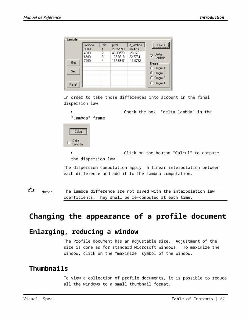
Manuel de Référence Introduction
It can happen that the changes or equalization of thresholds does not permit viewing certain series in the document. To return to the original display, select the invisible series in the control listbox of the Profile toolbar, then display the "Graphic…" dialog box and click on Cancel.
ZoomA more direct method for changing the X scale is available using the zoom function.
Select a spectral area
Click on the button “Zoom” of the Profile toolbar
The X scale will be automatically adjusted to the lower and upper borders of the selected spectral area.
To cancel the zoom, click on the "Cancel zoom" button of the Profile toolbar.
Interactif zoomThis function of zooming and translating the spectrum ease the visual correlation between to spectra or to simply explore a large spectrum.
Click on the menu Format, choose Zoom…
or
Use the shortcut Ctrl+Z
A dialog box appears
Move the zoom slider to modify real time the zoom factor of the current profile document.
The same way, move the Axe X slider to translate the display of the spectrum;
The Xmin and Xmax values represents the start and end values (either wavelength if calibrated or pixel number is not). Above the spectral extent is displayed .
Applying the same formatThis function is an alternative to the option “Apply to all windows" of the Axis X dialog box with in addition the setting of all the windows size to the active window size
To apply the X scale and the window size of the active window to all the windows:
Visual Spec Table of Contents | 67
Note:
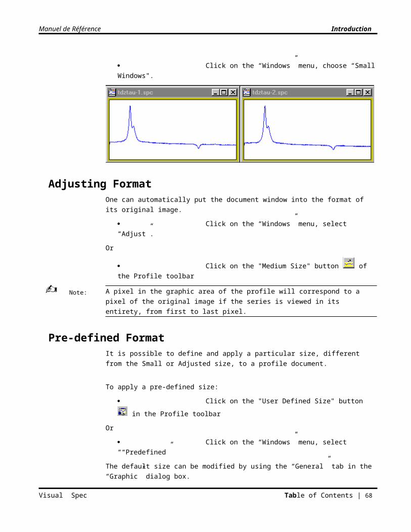
Manuel de Référence Introduction
Select the window from which one would like to extend the format to the other windows
Click on the Edit menu, choose "Apply format"
Or
Click on the "Paste format" button of the Profile toolbar
Clear a seriesClearing a series makes it disappear from the display, but does not remove it from the listbox of series.
To clear a series:
Select the series to clear
Click on the Edit menu, choose Clear
Or
Enter Ctrl+D at the keyboard
Label the wavelength of a lineLabeling a line consists of displaying, under the barycenter of the line, a label indicating the wavelength of that line.
Select the line to label
Click on the menu Tools, choose Label
Or
Right-Click in the selected area. The pop-up menu will be displayed. Select the item Label
Visual Spec Table of Contents | 68
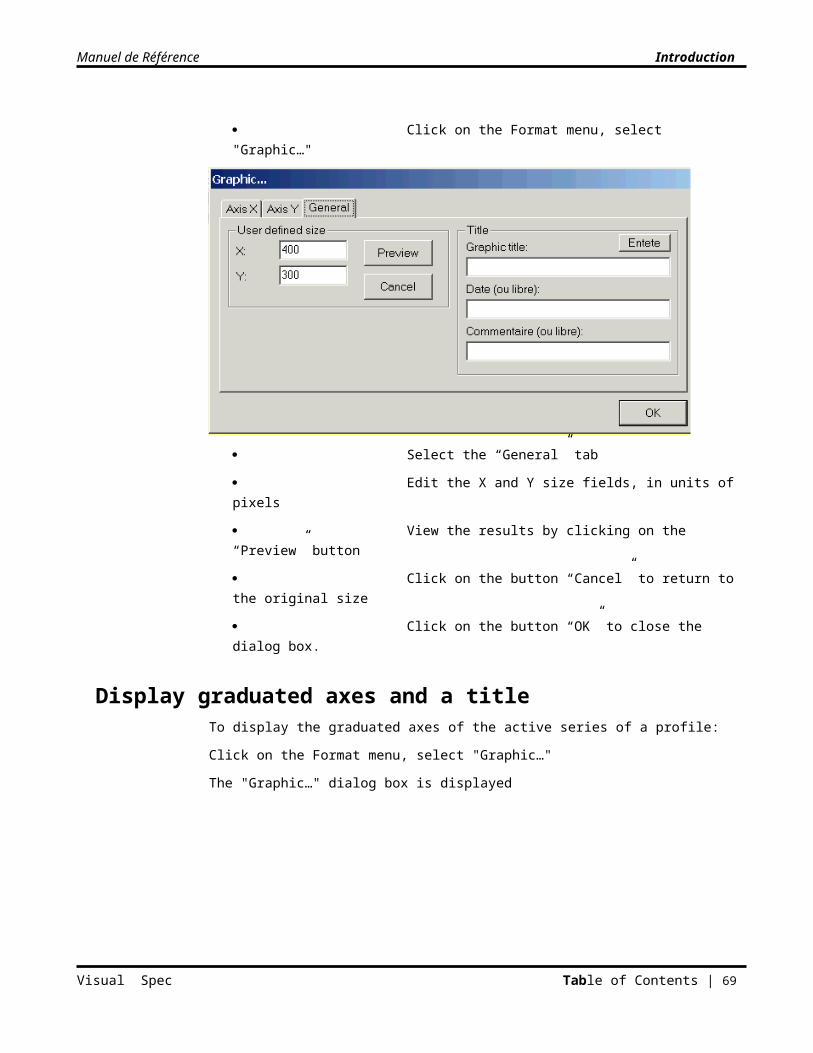
Manuel de Référence Introduction
The line label will disappear each time the window is refreshed. Refreshing a window happens when one changes its size, displays a new series, or activates a new window.
Crop a serieThe crop function allows for keeping only a section of the profile
Select the spectral zone to keep
Click on the menu Edition, Choose Crop
or
Click on the button in the profile toolbar
Caution: this operation is not reversible. It definitively invalidates non-included pixels after saving.
Adding, replacing, and deleting
Copy a seriesTo copy a series:
Select the series to copy
Click on the Edit menu, choose Copy
Or
Click on the Copy button of the Profile toolbar
Or
Enter Ctrl+C on the keyboard
The copy operation can also copy a bitmap of the document to the Clipboard. Open an application that will accept a bitmap image and paste into it the contents of the Clipboard.
Paste a series:To paste a series:
Select the document to which the series will be added
Click on the menu Edit, choose Paste
Or
Click on the button Paste of the Profile toolbar
Or
Visual Spec Table of Contents | 69
Note:
Note:
Note:
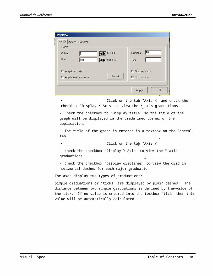
Manuel de Référence Introduction
Enter Ctrl+V on the keyboard
The series will be added to the list of series in the Profile document and become the active series. It will have a generic name “SerieX” where X is an incremented number.
If both the series to be pasted and the Profile document to receive the series are calibrated in wavelength, it will be resampled using the wavelength calibration of the “intensity” series of the destination document.
If the destination Profile document is not calibrated in wavelength or if the series to be pasted is not calibrated, and if the serie to be pasted has the same number of pixels as the destination document, then it will be displayed without scaling as a function of the number of pixels. If the number of pixels is different, the operation is not possible and a warning message will announce that the series are not compatible.
When no series is copied, the Paste button is inactive.
Replace a seriesTo replace a basic series with the active series:
Click on the Edit menu, choose Replace
Or
Click on the Replace button of the Profile toolbar
The “Replace…" dialog box is displayed.
Only the active series of a document can replace a basic series within the same document.
The series is resampled using the calibration of the “Intensity” series.
To replace a series by a series from a different document, use Copy/Paste between the two documents.
“Replace…" dialog box First select the active series that will replace one of the basic series. (See section “Selecting a Series”.)
Visual Spec Table of Contents | 70
Note:
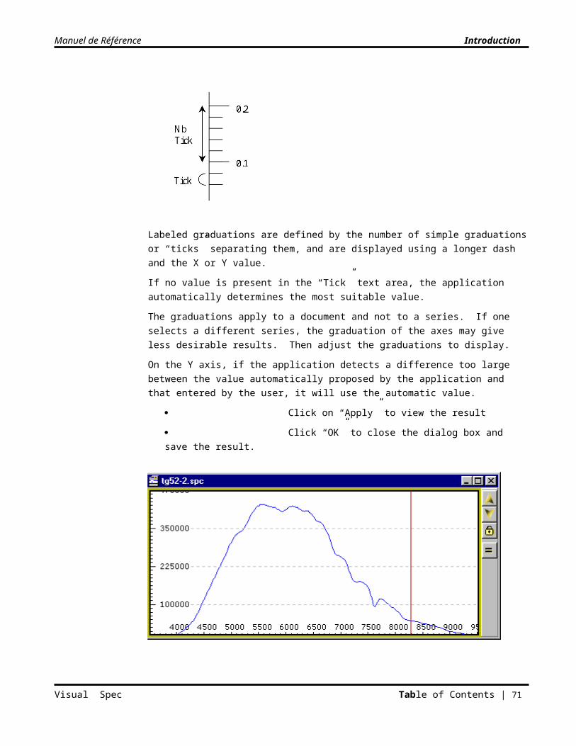
Manuel de Référence Introduction
Click on the radio button corresponding to the basic series whose values are to contain the values from the active series
Click on the “OK” button to close the dialog box and replace the series
Click on the “Cancel” button to cancel the operation
Delete a seriesDuring execution, certain temporary series are generated and added to the list of series of a document. To delete a temporary series
Select the series to delete
Click on the Edit menu, choose Delete
Or
Press the DEL key on the keyboard
Modifying a series
Arithmetic operationsTo apply a simple calculation using a constant:
Click on the Operations menu, choose "Arithmetic Operation"
A dialog box is displayed
Select the arithmetic operation to perform
Enter the parameter
Click on the button Apply to view the result
Click on the button Cancel to cancel the operation
Click on the button Close to close the dialog box.
Low-pass FilteringLow-pass filtering consists of replacing the value of the pixel by the average of the n pixels surrounding it. To apply a low-pass filter to a series:
Visual Spec Table of Contents | 71
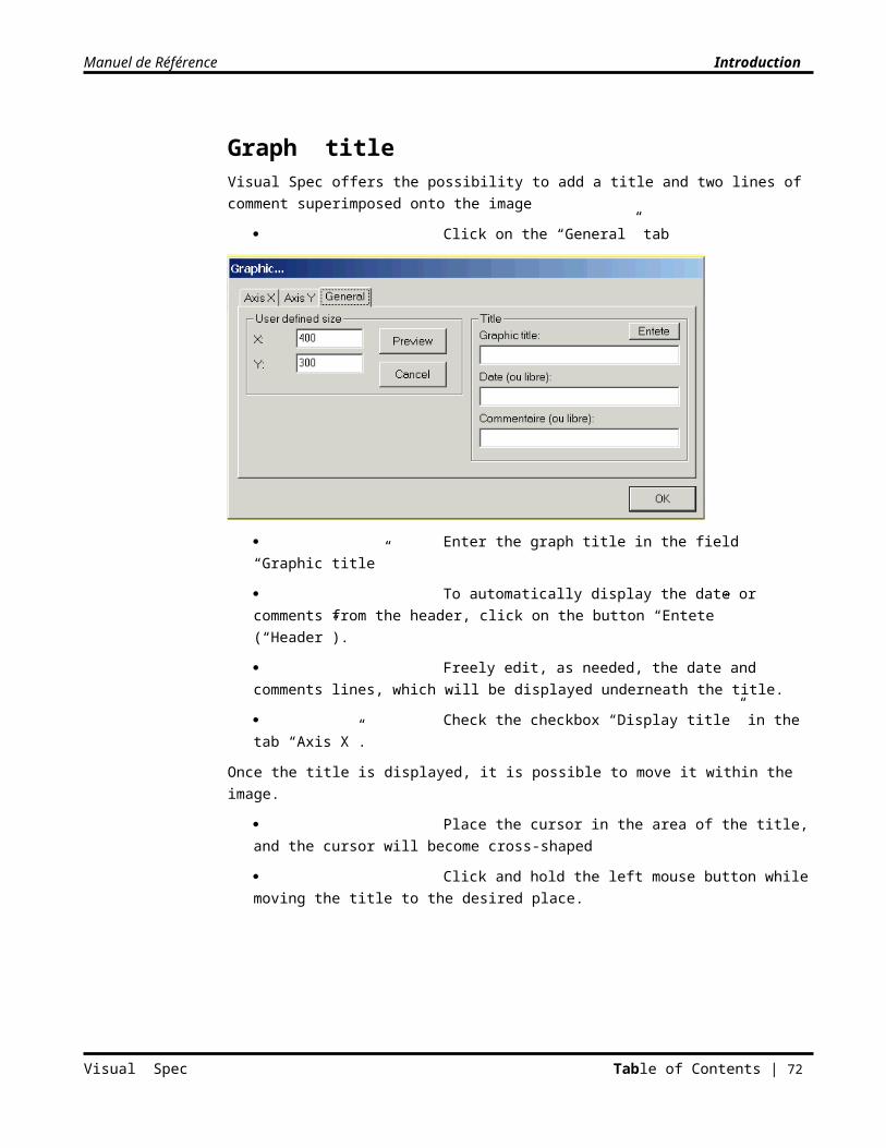
Manuel de Référence Introduction
Select the series to filter
Click on the Operations menu, choose Low-Pass Filter
Or
Click on the “Filter” button in the Profile toolbar
Or
Enter Ctrl+F at the keyboard
A dialog box for selecting the order of the filter is displayed. The cursor is positioned automatically on the OK button.
Change the order of the filter by clicking on the Up/Down control arrows. The value will always be odd. The value area is not manually editable.
Click on Cancel to cancel.
Click on OK to apply the filter and close the dialog box.
The new series that was created by filtering the active series will be added as a temporary series to the list of series of the document.
Its name is composed of the initial name of the active series to which a prefix Fb+<filter order > is prepended. This operation can be repeated several times; each time a temporary series is added and becomes the active series.
Example:
Fb3.intensityFb3.fb5.Ref1
High-pass FilteringTo better highlight the area where lines are present, it is possible to eliminate slow modulation from the spectral profile by dividing the spectrum by its spectrum filtered by a low-pass filter. The function OptiDiv applies this type of automatic filtering.
Click on the Spectrometry menu, choose OptiDiv
The application will automatically apply a low-pass filter of order 3 to the active series, and then divide the original series by the filtered series. The result is a new temporary series of the name Division which is added to the list of series. The series fb3.<series name> is also added to the list.
Visual Spec Table of Contents | 72

Manuel de Référence Introduction
Spline FilteringSpline Filtering interpolation is a powerful filtering which initially calculates the Spline coefficients and then rebuilds the profile starting from these coefficients with a softening factor.
Click on the Operations menu, choose "Spline Filter"
The rebuilt profile is displayed in violet, superimposed. A control for adjusting the softening parameter is displayed.
Drag the slider with the mouse to modify the softening coefficient. The value of the coefficient is displayed in the control’s header area. The affect on the series is visible in real-time in the document window.
You can edit the adjustment bounds of the coefficient by entering the new values in the editable textboxes above and below the slider.
Visual Spec Table of Contents | 73
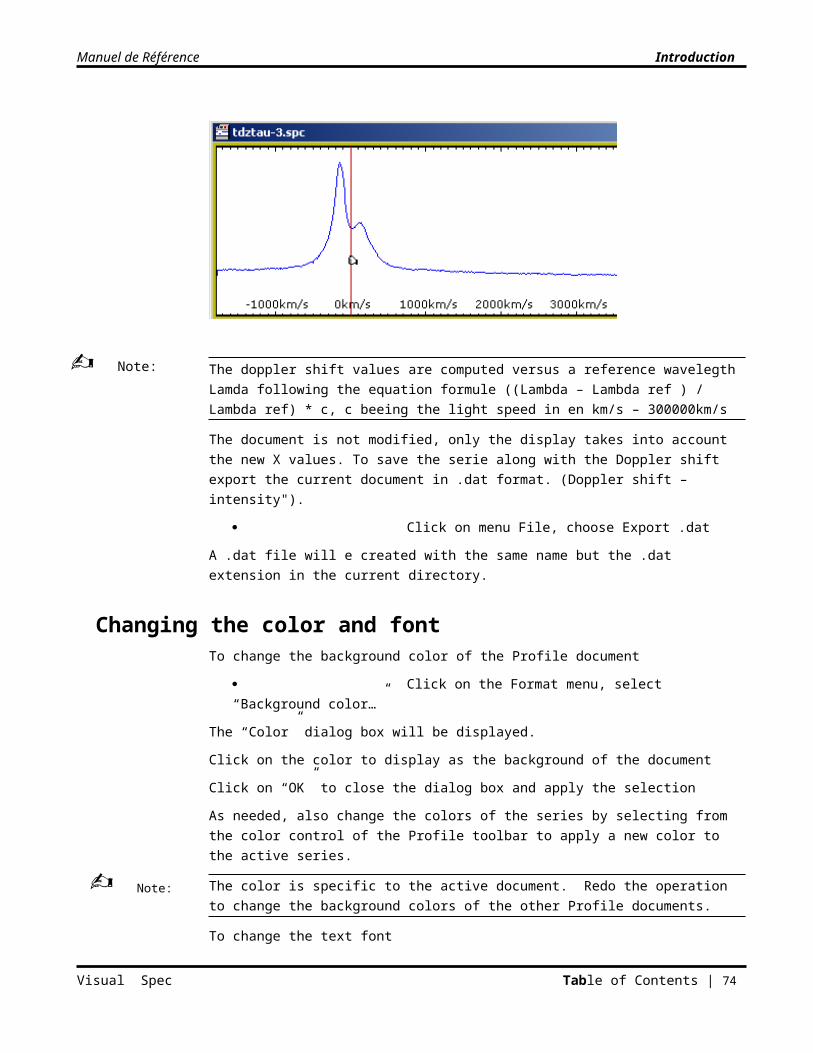
Manuel de Référence Introduction
If you click on “Enter” while the cursor is in one of the editable areas, the slider and the softening parameter itself will be automatically adjusted to the new value.
Click on the Page Up and Page Down keys to move from one tabulated value to the next.
If the max value of 30000 is not strong enougth to correctly smooth th eprofile, click in the x10 box to multiply by 10 all the slider values
Click on the Up and Down keys to move from one tabulated value towards the next by increments.
Click on the close symbol of the control to save the adjustment.
The new filtered series based on the active series will be added as a temporary series to the series list of the document.
Its name is made of the initial name of the active series preceded by the prefix Sp.
Example:
Sp.intensity
Gaussian filterThe gaussian filter is another type of filtering which atenuates the noise of the spectrum by smoothing with a gaussian.
To apply the filter
Select the series to filter
Click on the Operations menu, choose Gaussian Filter
A dialog box for selecting the power of the filter is displayed
Visual Spec Table of Contents | 74
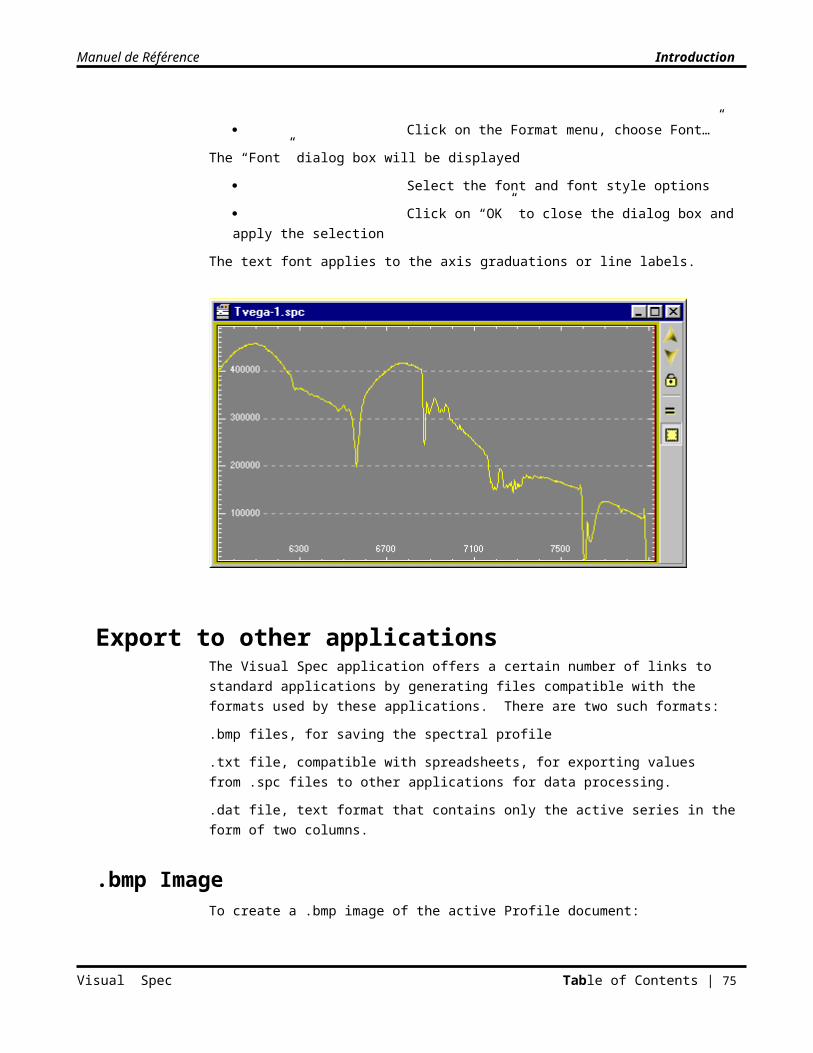
Manuel de Référence Introduction
Dialog box Gaussian filter
Enter the sigma value as a non-decimal value defining the strength of the filtering.
Click on Apply – Appliquer to apply the filter
The new series that was created by filtering the active series will be added as a temporary series to the list of series of the document under the name serie.<g>
Click on OK to apply the filter and close the dialog box.
Mmse filterThe mmse filter is another type of filtering which atenuates the noise of the spectrum
To apply the filter
Select the series to filter
Click on the Operations menu, choose Gaussian Filter
A dialog box for selecting the power of the filter is displayed
Dialog box mmse filter
Enter the sigma value as a non-decimal value defining the strength of the filtering.
Click on Apply – Appliquer to apply the filter
Visual Spec Table of Contents | 75
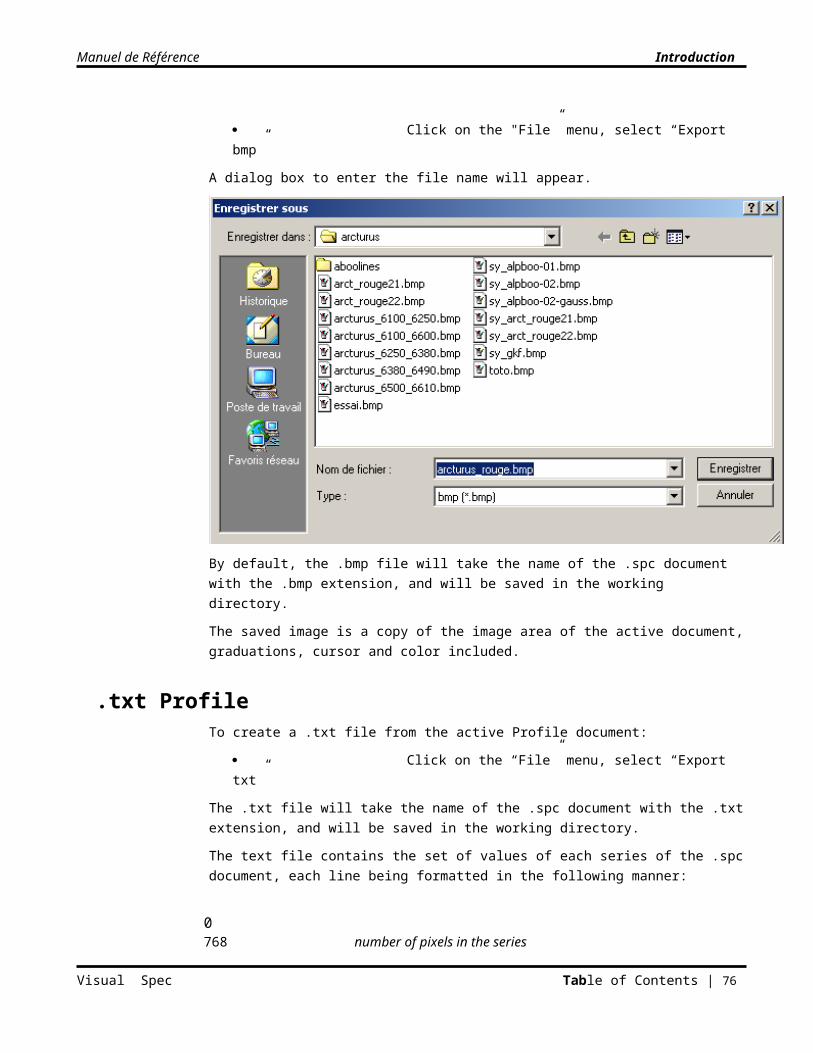
Manuel de Référence Introduction
The new series that was created by filtering the active series will be added as a temporary series to the list of series of the document under the name serie.<m>
Click on OK to apply the filter and close the dialog box.
If the coeeficient is not strong enougth the orange serie covers entirely the original serie
Recalibrate a seriesRecalibrating a series with respect to another allows the two series to share the same calibration in wavelength. This operation consists of resampling the active series by Spline interpolation based on calibration of another series.
To readjust a series with respect to another:
Select the series to re-sample
Click on the Operations menu, select Recalibrate profil by a profil…
A dialog box for selecting the series to be used for recalibration is displayed.
Each Profile document open in the current session is listed in the left area. The available series are displayed here. Only the series that are calibrated in wavelength are listed. The selected series is viewed in the graphic area and information on its spectral extent and sampling are displayed in the “Infos” area
Visual Spec Table of Contents | 76
Note:
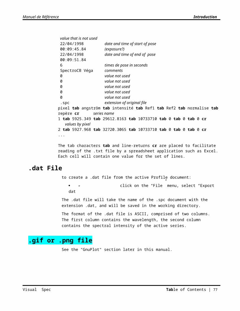
Manuel de Référence Introduction
To select a document, click on the document icon. The list of series will appear
To select a series, click on the series icon. Its profile will be displayed in the graphic area and the "Infos" will be updated.
To perform the recalibration with respect to the spectral calibration of the selected series, click on OK.
To cancel the operation, click on Cancel.
Once started, the operation cannot be cancelled. To return to the original profile, reload the document. The option "Normalize and replace" is inactive.
Operations on two series
Divide two seriesTo divide one series by another:
Select the series to divide
Click on the Operations menu, choose "Divide profile by a profile…"
Or
Enter Ctrl+D on the keyboard
A dialog box will appear to select the series by…” (See section “Selection Dialog Box”.)
The new series, corresponding to the result of the point-to-point division of the active series by the series selected in the dialogue box, is added as a temporary series to the list of the series of the document under the name "Division", and becomes the active series.
Multiply two seriesTo multiply one series by another:
Select the series to multiply
Click on the Operations menu, choose "Multiply profile by a profile…"
Or
Enter Ctrl+D on the keyboard
A dialog box will appear to select the series by…” (See section “Selection Dialog Box”.)
The new series, corresponding to the result of the point-to-point multiplication of the active series by the series selected in the dialogue box, is added as a temporary series to the list of the series of the document under the name "Multiplication", and becomes the active series.
Visual Spec Table of Contents | 77
Note:
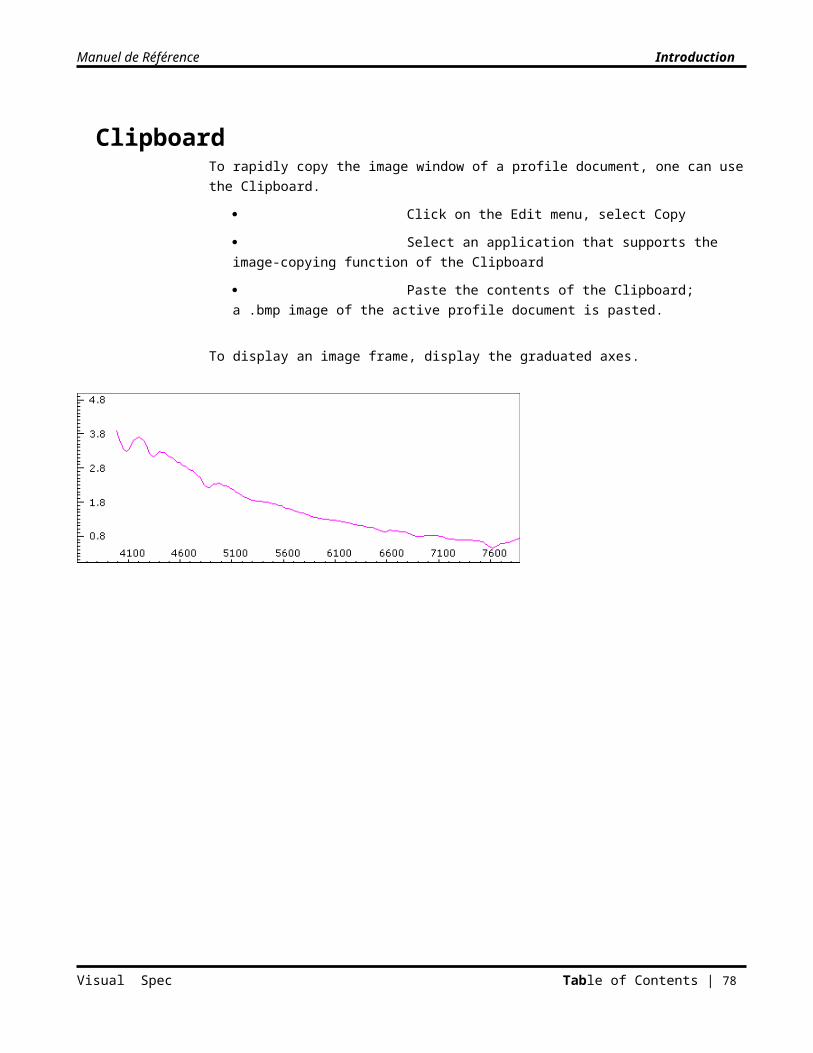
Manuel de Référence Introduction
Add two seriesTo add one series to another:
Select the series to add
Click on the Operations menu, select "Add profile by a profile …"
Or
Enter Ctrl+D on the keyboard
A dialog box will appear to select the series by…” (See section “Selection Dialog Box”.)
The new series, corresponding to the result of the point-to-point addition of the active series to the series selected in the dialogue box, is added as a temporary series to the list of the series of the document under the name "Addition", and becomes the active series.
Subtract two seriesTo subtract one series from another:
Select the series to subtract
Click on the Operations menu, choose "Subtract profile by a profile …"
Or
Enter Ctrl+D on the keyboard
A dialog box will appear to select the series by…” (See section “Selection Dialog Box”.)
The new series corresponding to the result of the point-to-point subtraction of the active series from the series selected in the dialogue box is added as a temporary series to the list of the series of the document under the name "Subtraction", and becomes the active series.
Translate a seriesThis operation shifts the absolute value of pixels or angströms of all the data points in the series.
Click on the Operations menu, choose "Translate…"
The dialog box for adjusting the translation will be displayed
Enter the amount of the shift into the text area
- If the profile is calibrated in wavelength, the shift will be displayed in angstroms
Visual Spec Table of Contents | 78
Manuel de Référence Introduction
- If the profile is not calibrated in wavelength, the shift will be displayed in pixels
Click on the "Apply" button to display the result
Or
Click on the Up/Down control arrows to increase or decrease the translation. The absolute shift is then immediately applied.
Click on the "Cancel" button to cancel the operation, close the dialog box, and return to the values of the series before the start of the operation.
Click on the "Close" button to save the translation and close the dialog box.
To enter a decimal value less than 1, enter 0.2 and not .2.
Normalize a seriesNormalization of a profile allows one to obtain the relative intensity of the profile with respect to a reference continuum of 1. This continuum is calculated based on the average of the area of the profile whose boundaries in angstroms are defined :
- If no profil selection is in progress; by the values defined in the “Preferences…” dialog box, “Continuum” tab. (See section “Preferences” in chapter “Introduction”.)
- if a profil zone is selected (gray visible rectangle), by the limit of the selection.
To normalize a series:
Select the series to normalize
Click on the Operations menu, choose Normalizeation
Or
Click on the button “Normalise” in the Profile toolbar.
The normalized series will automatically take the place of the basic series “Normalisee” (Normalized) and will become the active series.
This step of normalization is needed to calculate the equivalent width of a line or to compare two spectra of the same object taken at different times without requiring a spectro-photometric calibration. (See section “Comparison of Profiles”.)
The information window is displayed with the exact boundaries of the spectral zone where the average signal has been computed.
Derive a seriesTo derive the active series
Select the series to derive
Click on the Operations menu, choose “Derive”
Visual Spec Table of Contents | 79
Note:
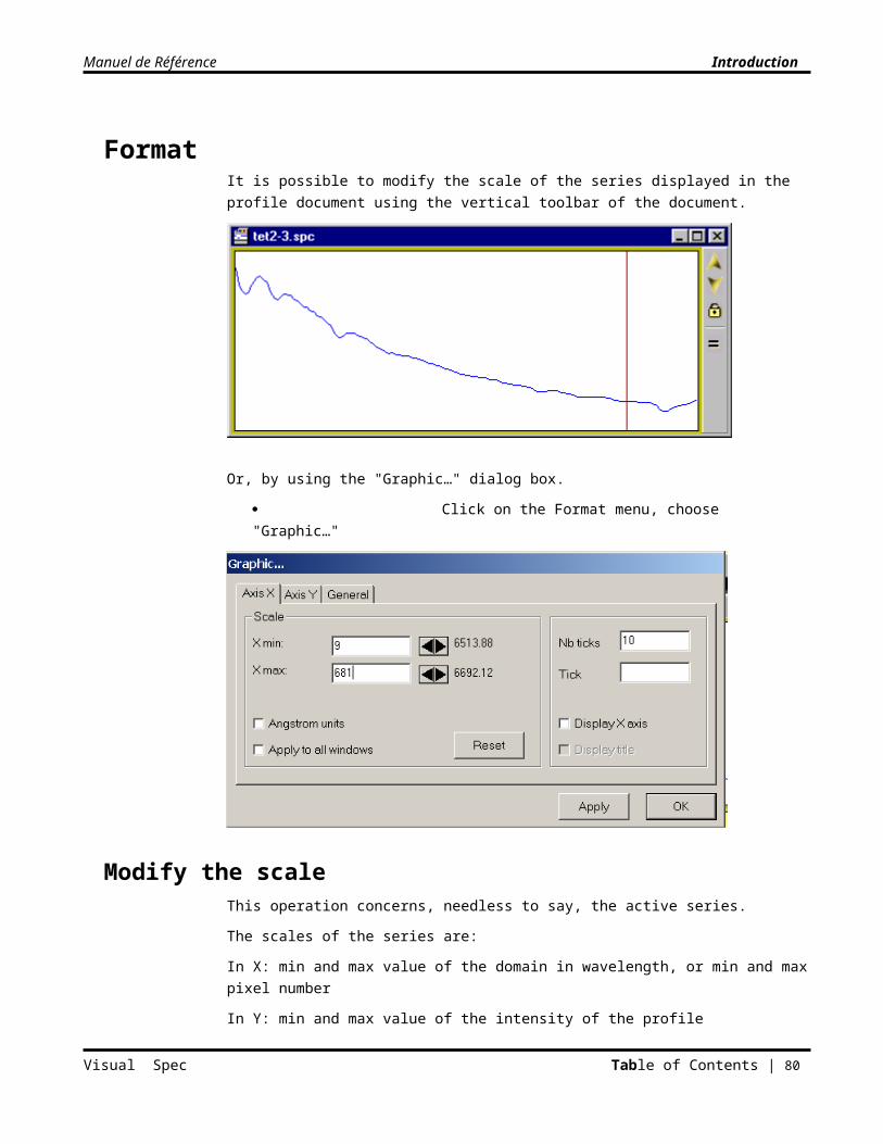
Manuel de Référence Introduction
The new series corresponding to the result of derivation performed on the active series is added as a temporary series to the list of series of the document with the name “derivee.<active series>”, and it becomes the active series.
If the series does not appear in the window, verify that the scale in X is correct.
Stack several seriesStacking permits addition of several series of the same object in order to increase the final signal-to-noise ratio. The operation is performed starting from the “Intensite” series of each document.
If the spectral sampling is different, rescale the spectra before adding.
To stack a set of spectral profiles:
Open the set of documents to stack
Ensure that each has been calibrated in wavelength
Click on the Operations menu, select Compose
Each “intensity” series of the displayed documents will be rescaled in wavelength with respect to the “intensity” series of the active profile and added to it.
The active document then contains in its “intensity” series the result of stacking the set of profiles.
Save the new profile under a different name
You can then verify that the signal-to-noise ratio has been improved with respect to that of similar non-stacked profiles.
Join two seriesJoining two series creates a new Profile document whose “intensity” series contains the two joined series, normalized over the area of overlap. This operation is only possible if one of the series was calibrated in wavelength.
To join two series
Select the first series
Click on the Operations menu, select Join
A dialog box for selecting the series “by…” allows the choice of the second series. (See section “Selection dialog box”.)
A new Profile document is created under the name “newspc”. The “intensity” series contains the results of the operation.
The reconciling of the two series is done in the following manner:
The overlapping area of the two series is detected
- If there is no overlapping area, the operation is cancelled. The message “no area of overlap” is displayed.
- If one series is completely included within the other, the operation is cancelled. The message “series a includes series b” is displayed.
Visual Spec Table of Contents | 80
Note:
Note:
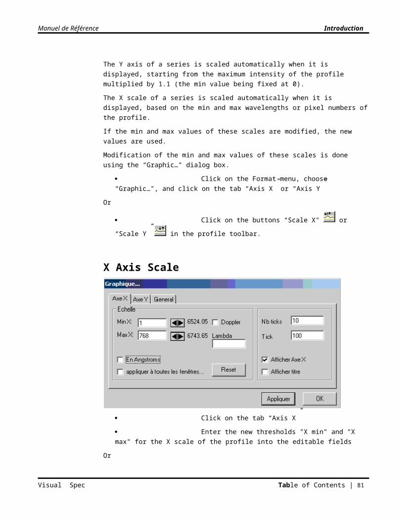
Manuel de Référence Introduction
- If the two series overlap strictly, the operation is cancelled. The message “the two series are super-imposable” is displayed.
The normalization of the two series is carried out starting at the area of overlap. Each series is normalized at the start of the area to be joined.
The first points of the new series will contain the first points of one series until the start of the area of overlap is reached. The subsequent points will be those of the other series.
To save the result, save the new Profile document with the command “Save” or “Save As…”.
Modify the intensity of a pixelAberrant points may interfere with correct execution of the automatic processing of Visual Spec. For this reason, it is possible to individually modify the intensity of each pixel.
To modify the intensity of a pixel:
Click on the menu Edit, choose Pixel
A window appears. It contains the complete table of pixels and their intensity.
To modify the value of an individual pixel:
Click twice on the pixel to modify, the intensity is highlighted and is then editable.
Modify the value.
Repeat as needed for other pixels.
To more easily find a pixel whose order number one knows:
Visual Spec Table of Contents | 81
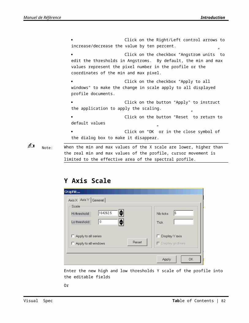
Manuel de Référence Introduction
Enter the pixel number in the search area
Click on “Select”
To terminate the operation
Click on OK to save the modifications. The series will be updated automatically.
Click on Cancel to cancel all modification.
MeasurementsA certain number of simple measurements are possible on a spectrum calibrated in wavelength. These measurements can be used to characterize the quality of the spectrum or to identify and/or measure the spectral lines.
The measurements are made on the spectral profile area selected with the cursor.
To select the type of measurements to execute:
Click on the menu Spectrometry, choose Computation preferences
The dialog box that allows the selection of measurements to perform will be displayed.
Check each checkbox corresponding to the measurement whose result is desired.
Click on the button Cancel to cancel.
Click on OK to save the list of measurements and make the dialog box disappear.
To change the list, redisplay the dialog box by clicking on the menu Spectrometry, choose Computation
To execute the list of calculations and view the results:
Click on the Statistics button on the Profile toolbar
The list of measurements to perform is reused each time the operator requests measurements on a
profile zone using the Statistics button
Visual Spec Table of Contents | 82
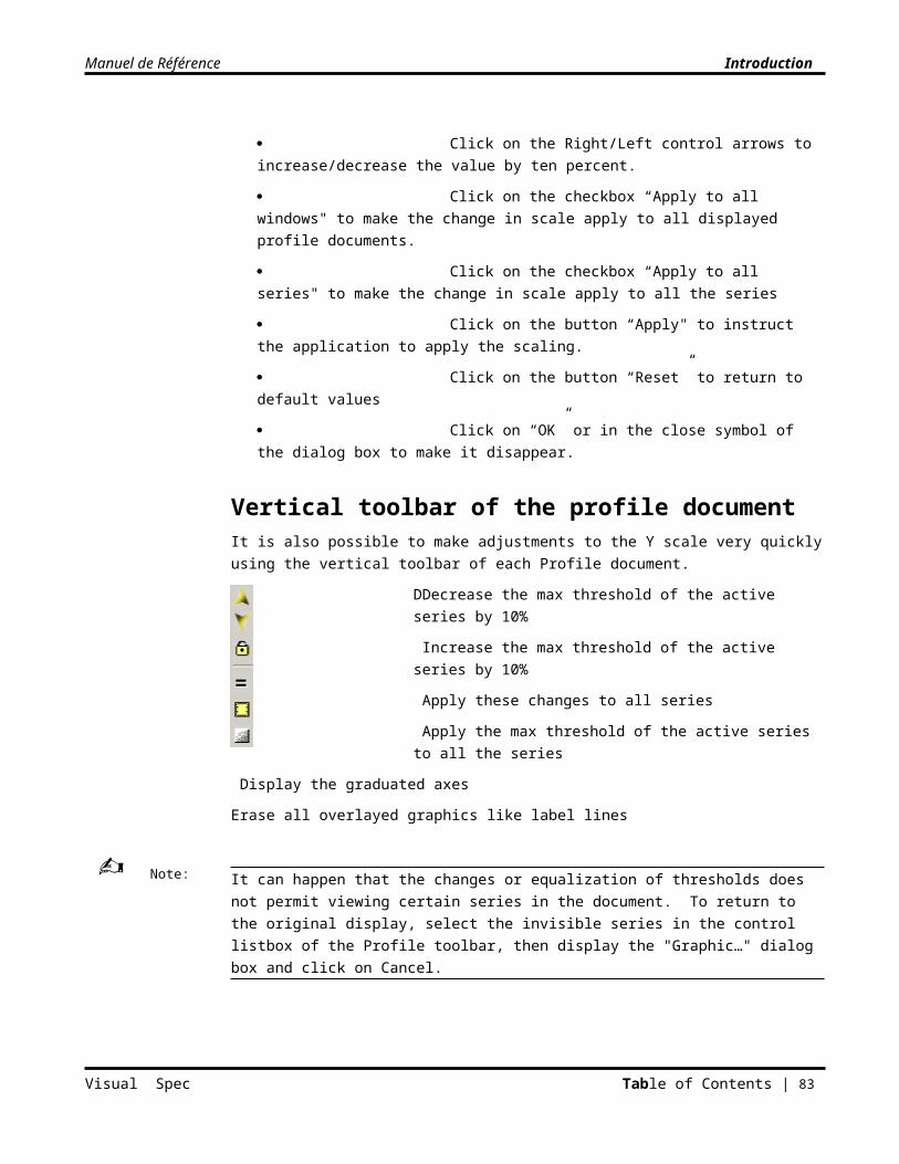
Manuel de Référence Introduction
The results are displayed in the “Infos…” window, which appears if it was not already displayed.
By default, no measurement is active in the list; if one requests measurements then the dialog box of calculations will be automatically displayed.
Infos… Window
The Info window permits viewing and tracing the results of measurements made on a spectral profile. It is possible to modify the size of the window with the mouse.
The name of the document on which measurements were taken is noted in red. Then the result of each measurement is displayed.
Click on the “Reset” button to clear all displayed results.
Click on the “Header” button to display the ‘date’, ‘pose’ (exposure), and ‘comments’ field of the active document.
Click on the button “Save” to save the results in the text file “Infos.txt”. This file will be found in the application directory.
Click on the close symbol of the window to hide the window
Or
Go in the tools menu and select the sub-menu "infos" to hide the window
Use the scrollbar to access preceding results, if they were not cleared.
Signal to Noise Ratio Calculates the signal-to-noise ratio over the selected spectral area. The signal-to-noise ratio is the report of the standard deviation of the average.
Average Calculates the average over the spectral area.
Visual Spec Table of Contents | 83
Note:
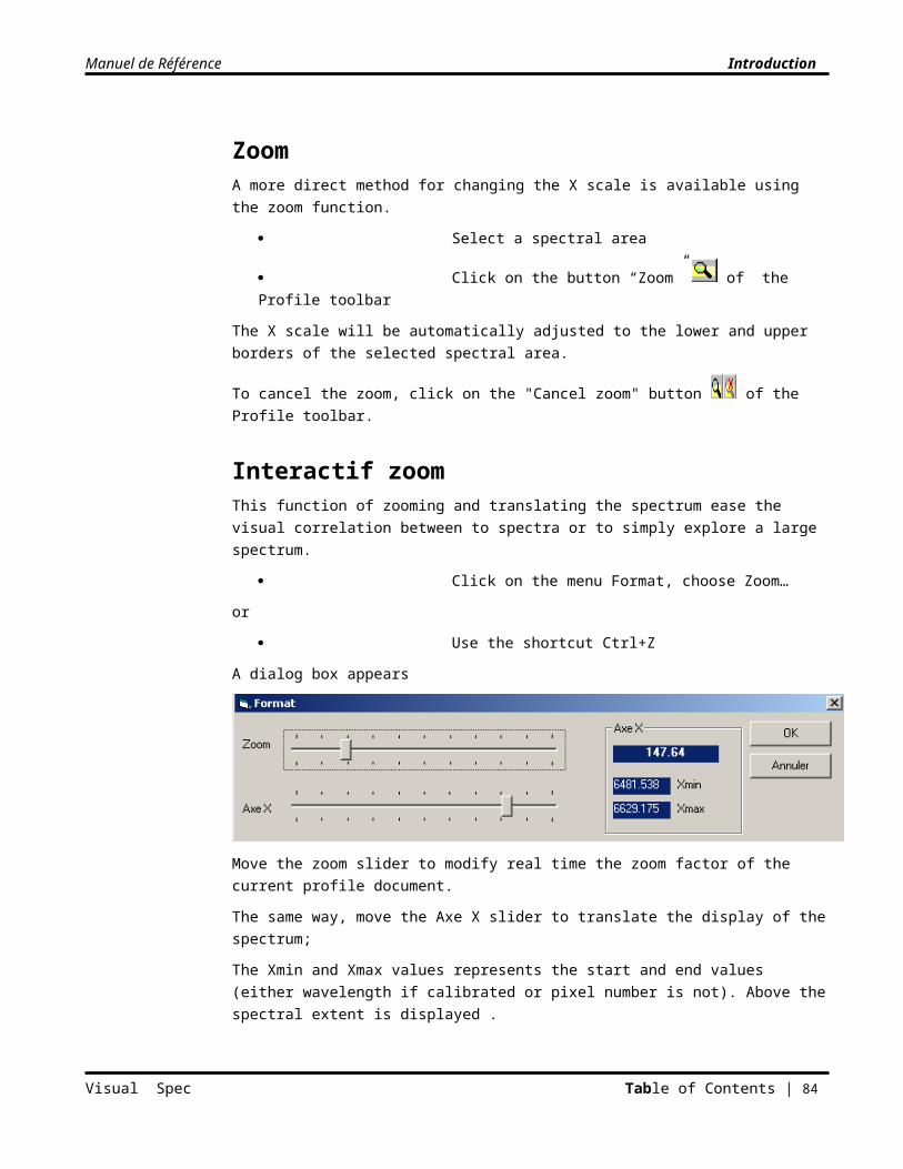
Manuel de Référence Introduction
Std deviation Calculates the standard deviation of the average over the spectral area.
Line center Calculates the wavelength that corresponds to the barycenter of the selected area. This wavelength defines the wavelength of a spectral line.
FWMHCalculates the full width at half-maximum over the spectral area.
The half-maximum of a line is defined as (the maximal intensity of a line with respect to a reference taken on the points on each side of the line) divided by two.
The full width at half-maximum of a line is defined as the deviation in wavelength (or in pixel if the series is not calibrated) between the two borders of the lines at mid-height.
This measurement is only possible on an area with a minimum of three points. The reference of the continuum is the average between the first and last point in the selection.
This calculation is fragile if the first and last points are those of the line itself, if the selection is too tight, or if other lines are present at the borders of the line to measure.
BarycenterCalculates the barycenter in pixels of the spectral area
The barycenter is defined as the sum of the points multiplied by their index divided by the area of the zone.
The area of the zone is delimited by the spectral profile and a straight line joining the first to the last point.
IntensityThe line intensity is the line surface.
Equivalent width (LEQ)To calculate the equivalent width of a line, it is necessary to normalize the profile. Otherwise the results make no physical sense.
The Width Equivalent is a computation of the line surface normalized to the background.
The calculation takes place over the spectral area delimited with the cursor in the active series.
An equivalent width of the line will be displayed in the “Infos…” window, expressed in angstroms. It characterizes the power (calculation of area) of a line with respect to the continuum.
Visual Spec Table of Contents | 84
Note:
Manuel de Référence Introduction
SurfaceSurface computation of the profil included in the selection. The surface computation is a simple sum of the intensity of the pixel.
ResamplingTo resample the profil, you need to define the new sampling step and the starting limit
Click on the menu Spectrometry, select "Resampling"
A dialog box "sampling" is displayed
The current value of the beginning and end of the profil are displayed in gray
Enter the new value of the sampling step
Modify or not the start and end limits
Click on OK to execute
Click on Cancel to quit without executing or exit
The intensity serie is replaced by the new resampled serie. If you want to keep the result, save the file under the same name or change the name by doing a "Save As…".
Fit PhotosphereIn some rare occasion, it can be of interest to suppress the contribution of the photosphere in a line profile.
Click on the menu Spectrometry, choose "Fit Photospher"
A dialog box "Fit Phosotospher" appears
Visual Spec Table of Contents | 85
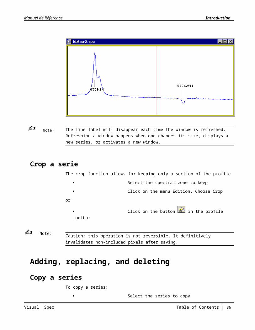
Manuel de Référence Introduction
By adjusting the different sliders, it is possible to generate a gaussian profil centered to the Lamb Ref field value which is subtracted to the current serie.
The purple profile is the gaussian profile and the serie Fphot.intensity is added to the serielist.
The green profile is the result of the correction and is added in the serie list as Soustnorm serie.
To exit the function, click on the close box in the dialog box.
This function shall be applied on a significant line profile.
There is no modification of the current serie. To suppress the addded serie, just select it and press the delete button
Visual Spec Table of Contents | 86
Note:
Note:
Manuel de Référence Introduction
Heliocentric SpeedTo produce accurate measurements of Doppler Shit, the Doppler Shift of the Earth around the Sun in the direction of the object has to be taken.
Visual Spec computesthis shift by taking into account the observation site coordinates, the date and time of the observation and the celestial coordinates of the star, alpha and delta.
Click on the menu Spectrometry, choose " Helio Correction"
A dialog box appears
Enter the latitude and longitude coordinates of the observation site in decimal degrees. If the coordinates have been updated in the preferences dialog box, they will be automatically updated at the display.
Enter the Right ascension and the declinaison of the star – if the coordinates have been entered in the header of the spc document, those values will be displayed automatically.
Enter the date and time of the observation in day, month year. The day is a decimale value wich will take inton acount the time of the observation.
Example:
Date = 9 Sept 2001Time (Heure) = 3h 32 mn 5s
Month (Mois)= 9Year (Année)=2001
Day (Jour) non-decimal part = 9
Visual Spec Table of Contents | 87
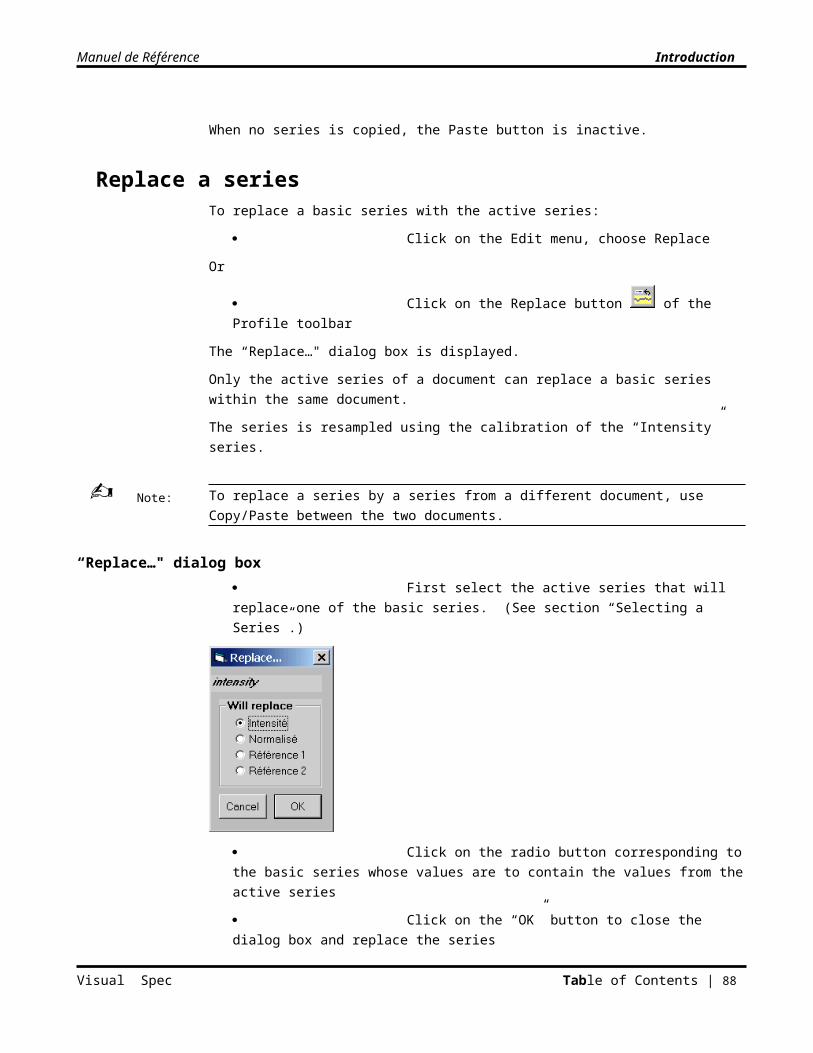
Manuel de Référence Introduction
Day (Jour) decimal part = (3 + 32/60 + 5/3600 )/ 24 = 0.147Day (Jour) = 9.147
Enter the reference value of the wavelength to compute the doppler shift which shall be applied to offset the Earth moving.
Click on "Calcul" to display the results in the Infos… window
Or
Click on "Fermer" to temporary hide the dialog box without loosing the data entered: alpha, delta, and date/time.
or
Click in the close box of te dialog box to definitively close it and allow at next loading an automatic update of the alphe, delta, date/time of the current spc document.
The results are displayed in the Infos… window, which can be then saved. See the Infos… Window section.
Julian Day - Jour Julien: date and time transformed in Julian Day– for info
Corr. Lambda (Angstrom): Agnstrom shift to apply to the serie to offset the Earth moving doppler shift.
Speed - Vitesse: Speed motion in the direction of the object – for info
Corr. JJ: Time correction equivalence – for info
Azimuth: azimuth of the object during the observation – for info
Heigth - Hauteur: heigth of the object during the observation – for info
Air section - Masse d'air: Air section crossed by the light of the star during the observation – useful to correct from the atmospheric extinction.. See Extinction section in Radiometry.
Visual Spec Table of Contents | 88
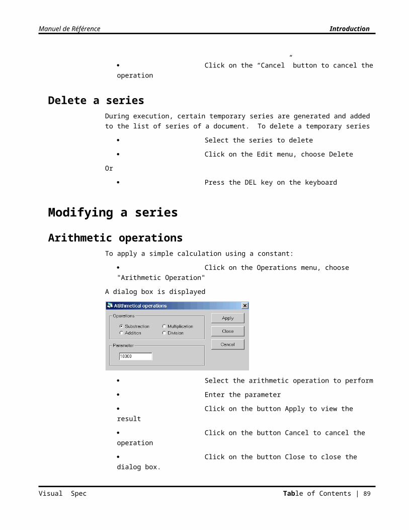
Manuel de Référence Introduction
C H A P T E R 6
Radiometry
Radiometry concerns processing that corrects the intensity of the spectral profile.
The raw intensity of a spectral profile is not only a function of the physical characteristics of the object observed. It includes also local attenuation caused by the equipment used, spectral sensitivity of the capture device, and even attenuation caused by the atmosphere. To compare spectra from different equipment, to reconstruct the physical continuum of the object, it is often necessary to first carry out a radiometric correction. This correction is the equivalent of a Flat Field in direct imagery.
To correct a raw spectrum it is necessary to determine the instrument response curve. This instrument response can be obtained in several ways:
From the spectrum of one of the 24 stars calibrated photometrically within Visual Spec
From a standard spectrum of the sample spectral type, from the library
Once the spectrum has been corrected radiometrically, one can eliminate its physical continuum by synthesizing the Planck profile at the temperature of the object.
Spectral libraryVisual Spec provides a database of 131 spectra corresponding to different spectral types. This database comes from the Centre de Données Stellaire of Strasbourg. The 131 spectra are in the folder libspec. The files are in “.dat” text format and extend from 1200 to 10600 angstroms. The intensity is normalized from 1 to approximately 5550 angstroms.
To access the library:
Click on the Tools menu, choose “Library…”
The “Spectral library” dialog box will be displayed.
Visual Spec Table of Contents | 89
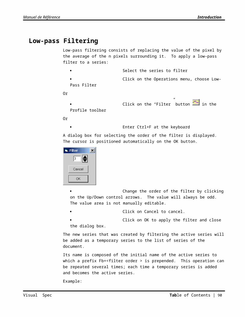
Manuel de Référence Introduction
Dialog box Library
Select a spectrum by its spectral type. It will be displayed in the graphic area at the bottom.
Drag the name of the spectrum to the active profile document to add the profile to the list of series.
To enlarge part of the spectrum in the graphic area, right-click near the part of the spectrum to be enlarged.
To quickly scroll through the spectral types, use the “Spectral type” slider.
To end the operation, click on the close symbol of the dialog box.
The spectrum is added in the form of a temporary series whose name is that of the spectrum in the dialog box. These series keeps its original sampling which is 5 angstroms. To resample the spectrum to the sampling of the document, perform a resample (see section “Resampling”).
It is impossible to add a spectrum from the library to a document which is not calibrated.
Spectral typeThis function is only available if the Excel application is installed.
To determine the spectral type of a star:
Visual Spec Table of Contents | 90
Note:
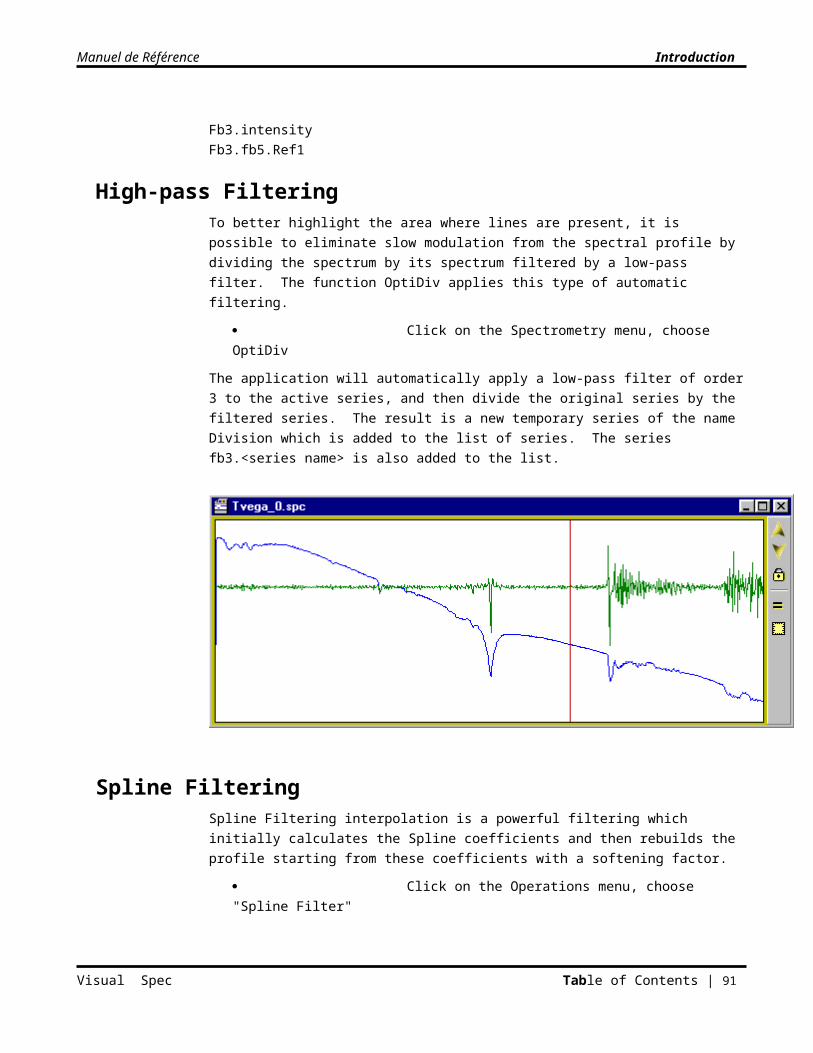
Manuel de Référence Introduction
Click on the Tools menu, choose “Spectral type…”
Or
Enter Ctrl+T using the keyboard
A dialog box is displayed which asks for the name of the star to search for in the Bright Star Catalog.
The syntax to be followed when entering the name of the star to search for is the following:
Three first letters of the Greek designation: Gam, Alp, Omi, Ome … or star number followed (without a space) by the three-letter constellation abbreviation .
The result of the search is displayed in the Type Spectral (Spectral Type) dialog box.
The Bright Star Catalog is available in the form of an Excel file “brscat2.xls” in the application folder. In addition to spectral type, it contains other information such as the coordinates, magnitude, HD reference.
ContinuumTo more easily read the spectrum, it is sometimes useful to “flatten” its profile. If one cannot suppress the “continuum” using a Planck profile, nor calculate the instrumental response from one of the reference stars in Visual Spec, it is still possible to calculate an artificial continuum by interpolation on some points of the raw profile.
Click on the Radiometry menu, “Extract Continuum…”
A new toolbar will replace the Profile toolbar.
To leave continuum mode at any time:
Click on the Stop button to leave Continuum mode
Or
Visual Spec Table of Contents | 91
Note:
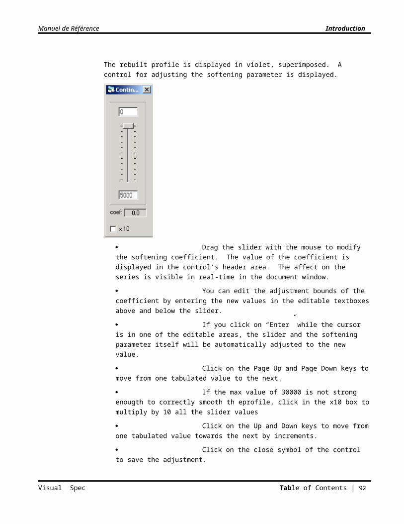
Manuel de Référence Introduction
Click on the Radiometry menu, choose “Extract Continuum…”. The checkmark on the menu will disappear
Two methods are provided to obtain the continuum. To toggle between them, click on the
point/curbe button .
Continuum by area suppressionThe continuum toolbar will change to look like this:
Select the area of the spectrum containing lines to eliminate.
Click on the eliminate zone button of the toolbar to eliminate the selected area.
Repeat the operation to eliminate additional areas.
Click on the annule button to replace the areas that were eliminated.
Click on the execute button to activate reconstruction of the profile.
The temporary series “Fit.<active series>” is added to the list of series and is displayed in the window in orange color. The eliminated areas are interpolated by a straight line. The dialog box for adjusting softening is displayed. Once the adjustment is made, click in the close symbol of the control. (See section “Filtering by Spline”.) The toolbar disappears and is replaced by the Profile toolbar.
Continuum by pointsTo access this mode, click on the point/curbe button
The continuum toolbar will change to look like this:
Place the mouse on the profile and left-click on the profile to place an input point.
Continue this operation until all input points have been placed.
Click on the Cancel button of the toolbar to eliminate all points and restart.
Click on the execute button of the toolbar to activate the reconstruction of the profile.
The temporary series “Fit.<active series>” is added to the list of series and is displayed in the window in cyan color. The toolbar disappears and is replaced by the Profile toolbar.
Visual Spec Table of Contents | 92
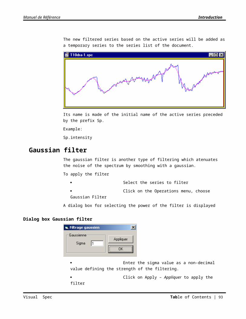
Manuel de Référence Introduction
Interpolation between points is by Spline interpolation. It automatically uses the first and last point of the series. If these points are aberrant, it is possible to edit them manually using the function Edit Pixel, or by cutting them from the Profile.
It is possible to save the list of points by clicking on the
“Enregistre liste” (“Save list”) button . The coordinates of each point are saved into the file “liste.txt” in the root folder of the application. The list is used by the “Extraire…” (“Extract…”) function.
Automatic ExtractionThis function is eliminated since the 3.3.0 version
Automatic extraction of a continuum is done based on the list of wavelengths. Each of the wavelengths must correspond to a place in the spectrum or else it is assumed that no line is present.
Click on the menu Radiometry, choose “Extraire…” (“Extract…”)
From this list, Visual Spec calculates an interpolation by spline and displays the new spectrum in the series extract_ followed by a sequence number.
The list of points comes from:
A text file “liste.txt”, if it is present in the root folder of the application.
Or
One of the pre-defined lists if the file “liste.txt” is not found. These lists contain the following wavelengths:
3390, 3448, 3509, 3571, 3636, 4032, 4167, 4255, 4464, 4566, 4785, 5000, 5263, 5556, 5882, 6055, 6370, 6800, 7100, 7530, 7850, 8080, 8400, 8805, 9700, 9950, 10250, 10400, 10800
It is possible to manually edit the file “liste.txt” with a simple text editor, following the format of a wavelength in angstroms per line. If one or more wavelengths are outside the domain of wavelengths, the value is ignored. If all the values are ignored, the default list is used.
Compensation of the continuum
By dividing by the continuumIn only one operation it is possible to remove the continuum of a spectral profile.
Click on the Radiometry menu, choose “Continuum division”
The continuum toolbar is displayed
Perform the operations on the continuum (see the section “Continuum”).
Once the artificial continuum is calculated, the intensity series is automatically divided by this continuum.
Visual Spec Table of Contents | 93
Note:

Manuel de Référence Introduction
The intensity series is automatically replaced by the result of the operation. If you don’t want to overwrite this series, copy it into a different basic series or save the document under a different name.
By subtracting the continuumIt is mandatory that the serie has been normalized
Click on the menu Radiométrie sub-menu Continuum Substraction…
Same as above for the division. but the continuum is subtracted the intensity serie and a value of 1 is added to avoid negative values.
Suppresion of atmospheric linesTwo functions are proposed:
Synthesis of an atmospheric spectrum from a file containing the atmosphere lines which has been defined in the preferences. The file included in the Vspec package covers a wavelength range from 6408 to 6628 angströms.
Correction by using a real spectrum of the atmosphere extracted from a star observation during the night
Synthethic atmospheric correctionThe goal of this function is to reduce or suppress completely the water atmospheric lines in the spectral extent 6400- 6600 angstroms
Click on the menu Radiométry, choose H20
To proceed with the interactive adjustment a diaoog box is displayed
Dialog box H2O
Start by moving the Sigma slider to make appear the base line of the H20 profile
Visual Spec Table of Contents | 94
Note:
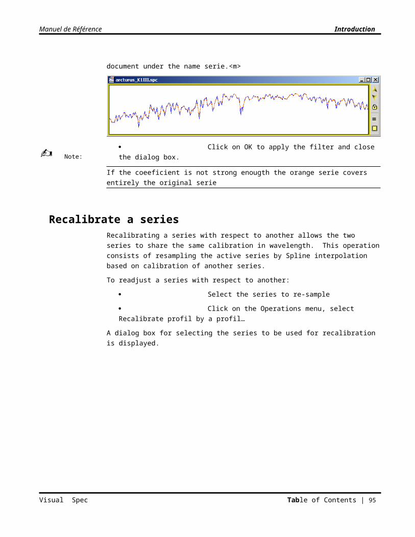
Manuel de Référence Introduction
Follow by moving the instensity slider to increase the intensity of the lines
Adjust agin the sigma slider to more or less filter the lines. The H20 lines shall meet the spectrum lines to be corrected
Compare the two profiles, you shall be in position to match the two profiles. Repeat the process until satisfaction is reached.
In some cases, a slight shift in wavelength can be visible. In this case, adjust the shift in the shift section of the dialog box. The shift is applied on the original spectrum, not on the H20 spectrum.
- Click on the up/down arow box to change value by 1
- One can enter directly decimal value and press enter to validate and apply the shift
To fine tune the overall matching process, check the "display division result" – "Afficher resultat division" box. A green serie is added as the result of the division of the two spectra. The interactive process shall drive to the elimination of the H20 lines.
Visual Spec Table of Contents | 95
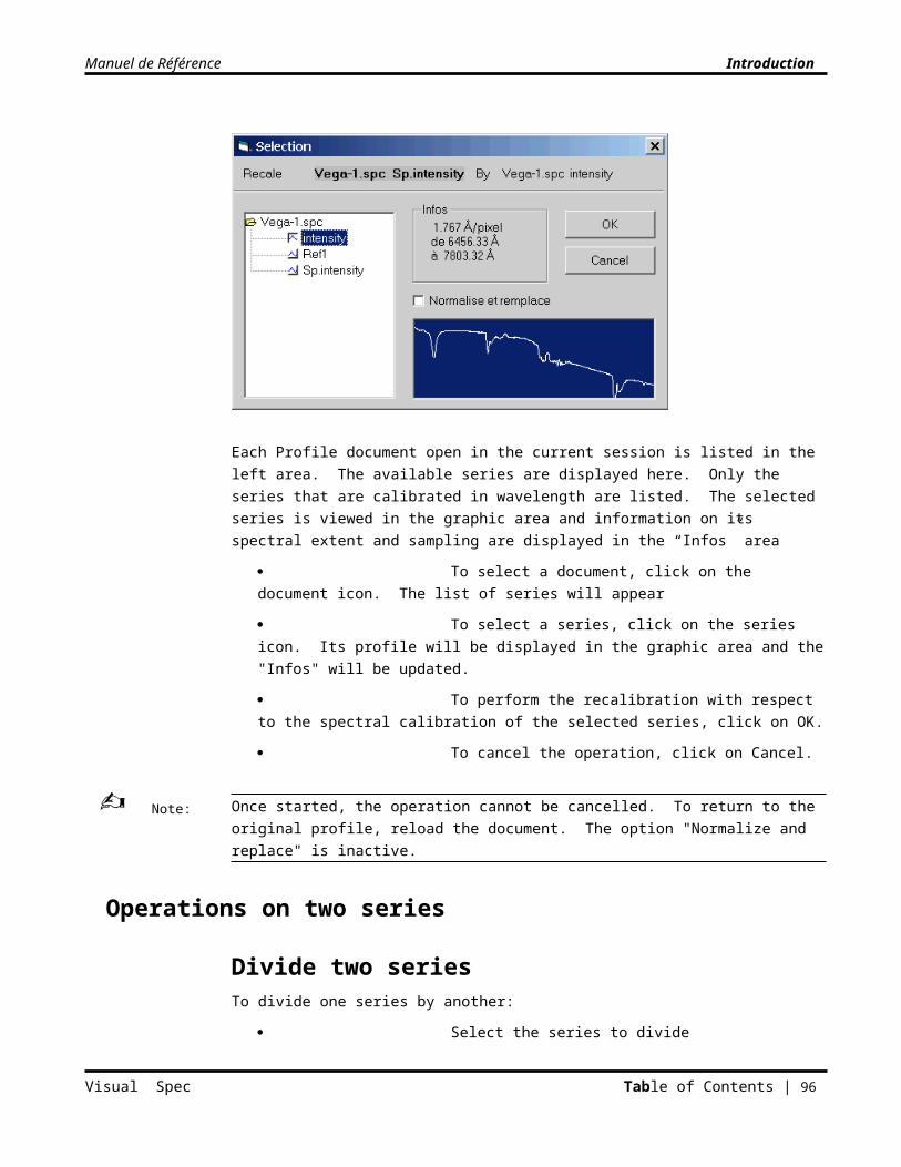
Manuel de Référence Introduction
Click on cancel to cancel the operation and come back to the original document
Click on OK to keep the result and come back to the original document
The corrected serie is added under the form of a temporary serie with name Division in the serie list.
From one use to the next one, the paramters "sigma" and "intensity" are kept in memory. If the intensity value has to be adjusted during the night, the "sigma" value is quite often the same for a given night and configuration
Synthethic atmospheric correctionThe goal of this function is to reduce or suppress the atmospheric lines created by the water from a real spectrum of the atmophere of the night of observation. This spectrum is extracted from a star which has not a lot of lines.
Before running this correction, the atmospheric spectrum shall have been computed and displayed.
Visual Spec Table of Contents | 96
Note:
Manuel de Référence Introduction
To extract the atmospheric spectrum:
Acquire a spectrum of a star which has not a lot of lines (type A, like altair, or Vega) and for whom you have an already corrected spectrum. See in the ELODIE database from the Haute-Provence Observatory at http://atlas.obs-hp.fr/elodie/ .
Normalise, then divide the ral object profile by the ELODIE profile: the resultating profile is the atmospheric profile
Move this profile into a serie wich will be saved, like the "intensity" serie, and save the document, like "profile_atm_x". Keep the document open
Go back to the profile to be corrected
Click on the menu Radiométry, choose H2O correction real spectrum…
A dialog box to select the real atmospheric spectrum is opened
Boîte de dialogue sélection de profil réel
select the document and the serie which contain the atmospheric spectrum
click OK la série qui contient le spectre réel de l'atmosphère
The function will proceed with the interactive adjustment, a dialog box is displayed
Visual Spec Table of Contents | 97
Manuel de Référence Introduction
Dialog box H2O intensity adjustment
The intensity level of the ral atmospheric spectrum can thus be adjusted. The result of the correction can be seen real time by checking the "display division result" box. wavelength shift can also be adjusted.
Report to the previous section on the synthetic correction for a more detailed description of the all controls.
Once the parameters adjusted, the serie "division" in green, contain the corrected profile. To save it, replace one of the non-temporary serie (like the "intensity" serie) by the result with the "replace" fonction, and save the file.
Radiometric correction by a standard spectrumTo correct the active series radiometrically by using a spectrum from the library:
1. Obtain the spectral type of the object
2. Add the standard spectrum from the library which corresponds to the spectral type of the object
Visual Spec Table of Contents | 98
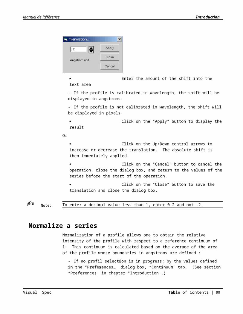
Manuel de Référence Introduction
3. Extract the continuum of the standard spectrum, either by Spline filtering or by using the continuum function, in violet.
13. Select the series “intensity”.
14. Divide the “Intensity” series by the series “Fit.spectre_standard”. One thereby obtains the instrumental response to the lines of the spectrum near to the series “Division”, in dark green.
Visual Spec Table of Contents | 99
Manuel de Référence Introduction
15. To eliminate the spectral lines, perform a Spline filtering or apply the Continuum function on the series “Division”. The new series “Fit.division” will be added, containing the instrumental response, in orange.
16. Select the series “intensity”.
17. Divide the series “intensity” by the instrumental response “Fit.division”. The series “division” then contains the radiometrically-corrected spectrum, in dark green.
18. To save the series, replace one of the basic series by the series “Division”.
Visual Spec Table of Contents | 100
Manuel de Référence Introduction
The intensities obtained are not the absolute intensities of the object. For an absolute spectro-photometric calibration, it is necessary to use a real spectrum of one of the 24 stars calibrated in Flux. (See section “Flux Calibration”.)
Automatic CorrectionThis function is eliminated since the 3.3.0 version
Visual Spec offers the capability to automatically make the radiometric correction using a standard spectrum by automating the correction procedure. So that this operation may be performed, it is advisable to take the following precautions:
The standard spectrum must be displayed, either in one of the series of the active document or in another open document
A list of wavelengths to be used for automatic extraction of the continuum must be valid in the file “liste.txt” or else the default list will be applied (see "section “Automatic Extraction of the Continuum”).
If the “Normalise et remplace” (normalize and replace) option will be active, the normalization area must be valid (see section “Normalize”).
Once these precautions have been taken:
Click on the Radiometry menu, choose Corrige… (Correct…)
The dialog box for selecting the series containing the standard spectrum is displayed.
Select the series which contains the standard spectrum.
Click on the option “Normalise et remplace” (Normalize and replace) so the resulting series replaces the intensity series after it is normalized
If this option is not selected, the result will be placed into a temporary series added to the list under the name Unflat
Click on Cancel to cancel the operation.
Using this function demands a good understanding of the mechanics of correction. To better understand these mechanics, perform the operations one-by-one manually, following the procedure described in the section “Radiometric correction by a standard spectrum”.
Visual Spec Table of Contents | 101
Note:
Note:
Manuel de Référence Introduction
Planck ProfileThe absolute intensity profile of a spectrum follows a law which is a function of the temperature of the star (dark-body temperature, Planck’s Law). Based on this law, and thus on a temperature, it is possible to calculate the theoretical profile of energy per unit of wavelength this star would have.
To display the Planck profile of a star of temperature T:
Click on the Radiometry menu, choose “Planck…”
Or
Click on theTemperature button of the profile toolbar.
A dialog box is displayed.
Enter the desired temperature, or increment/decrement the temperature by clicking on the Up/Down control arrows.
Click OK to display the theoretical profile; a temporary series “P_<temp>”, where <temp> is the temperature, is added to the list.
Click on Cancel to cancel the operation.
To determine the Planck temperature of a bodyCorrect the intensity of the profile in order to obtain the theoretical intensity.
Visual Spec Table of Contents | 102
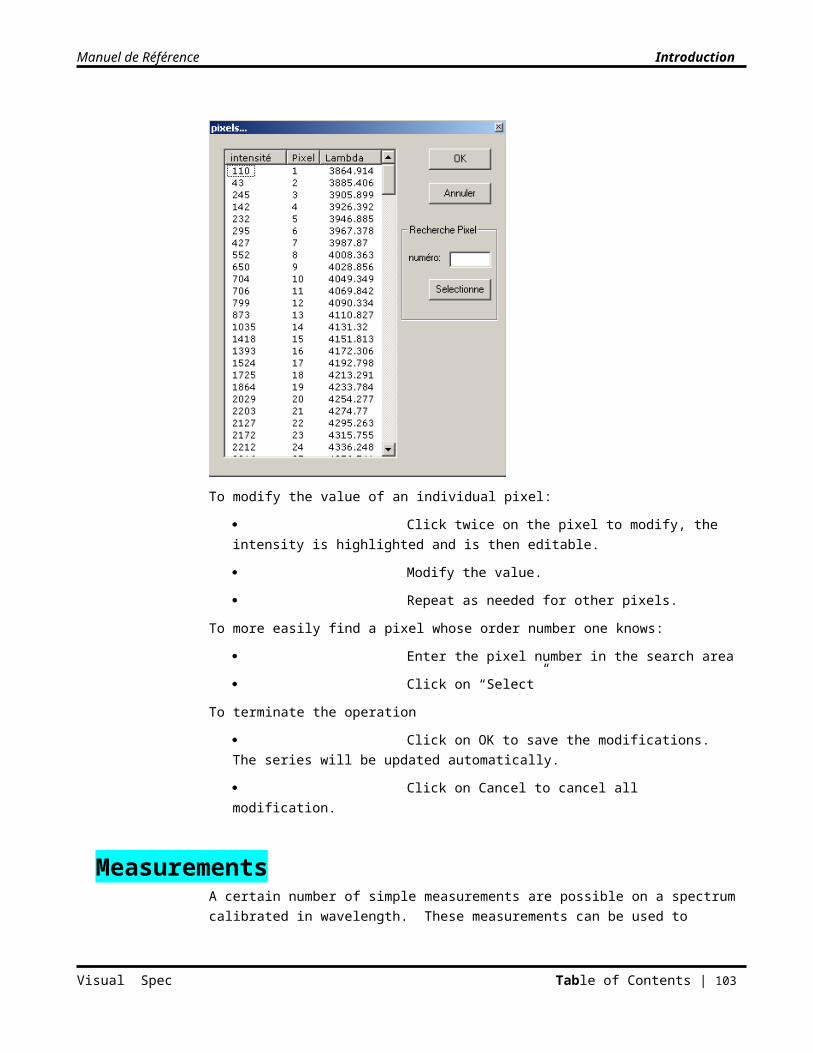
Manuel de Référence Introduction
Superpose the Planck profile for different temperatures until the two profiles have the same slope. To do this one can adjust the respective scales of each of the series.
Note the temperature which gives the best match – this is the temperature of the body observed …
One can then “flatten” the spectral profile by dividing by the Planck profile, which then suppresses the “continuum”.
To save the Planck series, replace one of the basic series with the series “P_<temp>”.
Instrumental ResponseTo eliminate the instrumental response, it is necessary to divide the theoretical intensity of a star by its saved real intensity in order to obtain the spectral response of the instrument. This instrumental response can then be used to correct raw intensity profiles obtained under the same conditions.
It is suggested to re-determine the spectral response of the instrument each time it may be necessary: setup/breakdown, changing wavelength domain …
Visual Spec includes a library of absolute flux for 24 stars. (See appendix for the complete list).
19. Acquire the spectrum of one of the stars in the Visual Spec library.
20. Process the spectrum like any spectrum, up to calibration in wavelength (needed).
21. Click on the Radiometry menu, choose “Response…”
22. Select the star in the list of proposed stars.
23. Click on OK.
24. The instrument response is added as the temporary series “RepInstru”.
25. To save the series, replace one of the basic series with the series “RepInstru”.
The instrumental response is obtained by interpolation of the profile in equivalent theoretical flux divided by the observed flux.
Visual Spec Table of Contents | 103
Note:
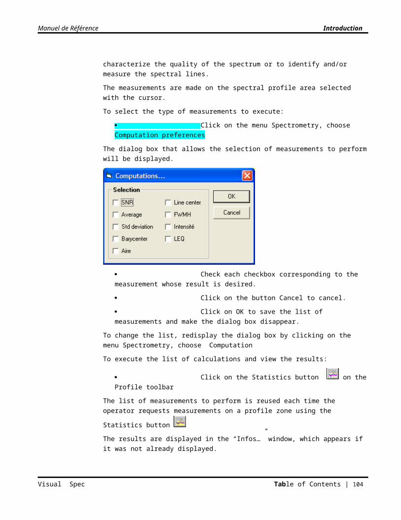
Manuel de Référence Introduction
Flux calibrationTo correct the raw intensity of a spectral profile in order to determine the absolute intensity, it is necessary to calculate the instrument response following the method in the section “Instrumental Response”.
Calculate the instrument response.
Select the “Intensity” series.
Divide the series by the series “RepInstru”.
The temporary series “Division” is added to the list of series; it contains the contents of the intensity series corrected by the instrumental response.
To save the series, replace one of the basic series by the series “Division”.
Atmospheric extinction correctionThis correction only makes sense for excellent quality spectra and for very accurate measurements. It can only be performed once the instrumental response has been corrected. This correction has anyway small effect on the intensities.
Click on the menu Radiometry, choose Extinction
A dialog box appears
Enter the Air section (Masse d'air)
Click on OK
To obtain the Air section value, one can get it from the Speed Heliocentric calculation. See section Speed Helio.
The Air section value is listed in the infos… window.
Visual Spec Table of Contents | 104
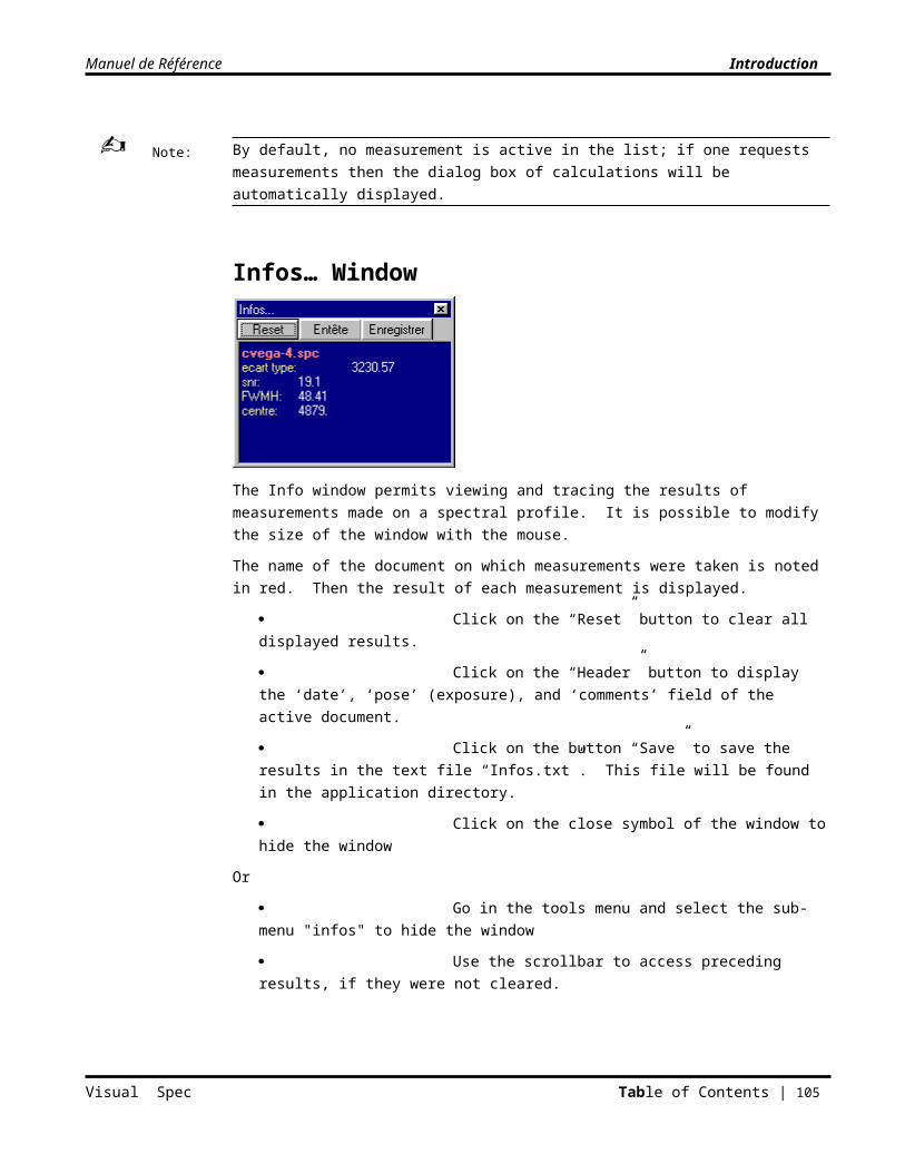
Manuel de Référence Introduction
C H A P T E R 7
Tools
A certain number of tools are provided to facilitate spectral analysis.
To compare spectra, several methods are available:
An animation function allows viewing of changes over time of a set of profiles
Synthesis of the spectral image for comparison with the original image
To identify different lines present, one can use a database of atomic lines of chemical elements whose atomic numbers are less than or equal to 26 – Iron. Some prohibited lines of oxygen and nitrogen are also included, as well as the position of the principal molecular bands of Titanium Oxide TiO.
For those who prefer keyboard commands, a special command-line console is available.
It is also possible to get the coordinate of an object from the on-line Brigth Star Catalog.
AnimationAnimation of a set of profiles allows viewing of the evolution of the same profile over time.
There are two types of animation. One very simple, which does not take into account the time interval between the observation, and another one which scale the time display to the time of obsevrations.
Linear animationCette fonction n'éxiste plus dans Visual Spec à partir des versions 3.2.x
This function does not exist anymore starting from Visual Spec version 3.2.x
Elle est remplacé par la fonction d'animation temporelle.
It is replaced by the temporal animation function
The button is now use to launch the GnuPlot application – see later on in this manual.
Open the set of profiles containing the spectra of the same object, saved at different times.
Normalize the profiles in order to compare the profiles using the same relative scale.
Visual Spec Table of Contents | 105
Manuel de Référence Introduction
Put all of the profiles into the same format, using the function “Apply Format” (on the Edit menu) and as needed using the function Y-Scale (menu Format, choose “Graphic…”, use tab “Axis Y), applied to all windows.
Select the window in which the animation will be created.
Click on the Tools menu and choose Animation, or click on the Animation button of the Profile toolbar.
The animation will stop automatically.
Time scaled animationThis animation function requires that date and time of the spectrum are correctly entered in the document profil header.
Open the set of profiles containing the spectra of the same object, saved at different times.
Normalize the profiles in order to compare the profiles using the same relative scale.
Put all of the profiles into the same format, using the function “Apply Format” (on the Edit menu) and as needed using the function Y-Scale (menu Format, choose “Graphic…”, use tab “Axis Y), applied to all windows.
Open the animation dialog box – the date and time will be read from the document header
Click on the OK button to run the animation
Click on the close box to close the windows and go back to the application
The files will be arranged by increasing time in the list before the animation starts. The overall animation time will the time in the "max duration" field. The number of loop in case of loop selection can also be modified.
The animation is displayed in a separated window. The name of the file currently displayed is showned in the bottom of the animation window.
You can run again the animation by clicking again the OK button.
Visual Spec Table of Contents | 106
Manuel de Référence Introduction
Date and time formattingThe date and time shall have the following format: dd/mm/yy hh:mm:ss
If the format is not recognized by Vspec, the files will be highlighted in gray in the dialog box after you clicked on the OK button
To edit the date and time, select the file and double-click with the right mouse to make appear the edit field.
Edit the data and press the enter keyboard button to validate the data.
None of the updates will be saved in the header of the file. If you want to save time the next time, it is much better to edit the file header directly with the header function in the Edit menu.
Visual Spec Table of Contents | 107
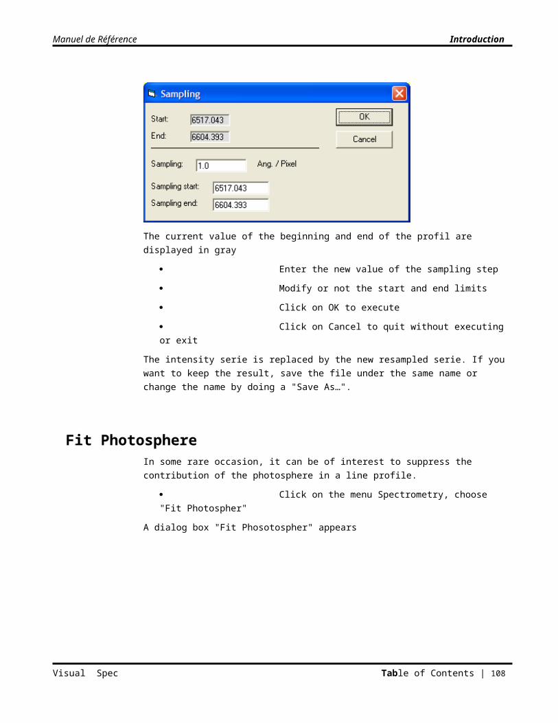
Manuel de Référence Introduction
Synthesis of spectral imageSynthesizing a spectral image is creating an image reconstructed from the active spectral series, which may be the result of several processes such as composition or filtering a set of profiles of the same object.
The grayscale values are determined directly from the Y scale of the series. Several attempts are sometimes needed to obtain a synthesized image with good contrast. The image can be resize din width.
This image can be then compared to one of the raw images that was used to create the spectral profile.
When moving the cursor on the document profil spectrum, a white cursor will move on the spectral image at the corresponding position
To export, display the spectrum with colors corresponding to wavelength, or update the scale, display the popup menu by clicking on the right mouse button while the cursor is over the image.
Visual Spec Table of Contents | 108
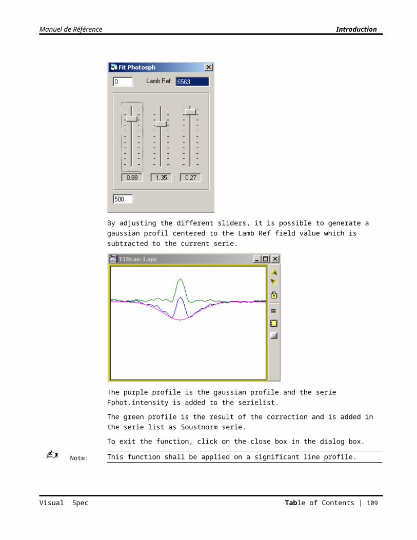
Manuel de Référence Introduction
Select the popup menu item Colorer (Color) to display the colors.
Select the popup menu item Exporter (Export) to save the image in the form of a .bmp A dialog bow allows you pick the directory and the file name. By default, the file will have the name of the profile document followed by the suffix “-s.bmp”.
It is now possible to match the scale of the spectral image to the wavelength domain of the spectrum.
Select the popup menu Update (Mettre à jour) to update the image display scale after a change in the spectrum profil scale change like a zoom.
Select the popup menu Close (Fermer) to close the window or click in the close box in the window itself.
CoordinatesThis function is only available if the Excel application is installed.
To find the coordinates of a star:
Click on the Tools menu, choose Coordinates
A dialog box is displayed which asks for the name of the star to search for in the Bright Star Catalog.
The syntax to be followed when entering the name of the star to search for is the following:
Three first letters of the Greek designation: Gam, Alp, Omi, Ome … or star number followed (without a space) by the three-letter constellation abbreviation .
The result of the search is displayed in the Coordinates dialog box.
Visual Spec Table of Contents | 109
Note:
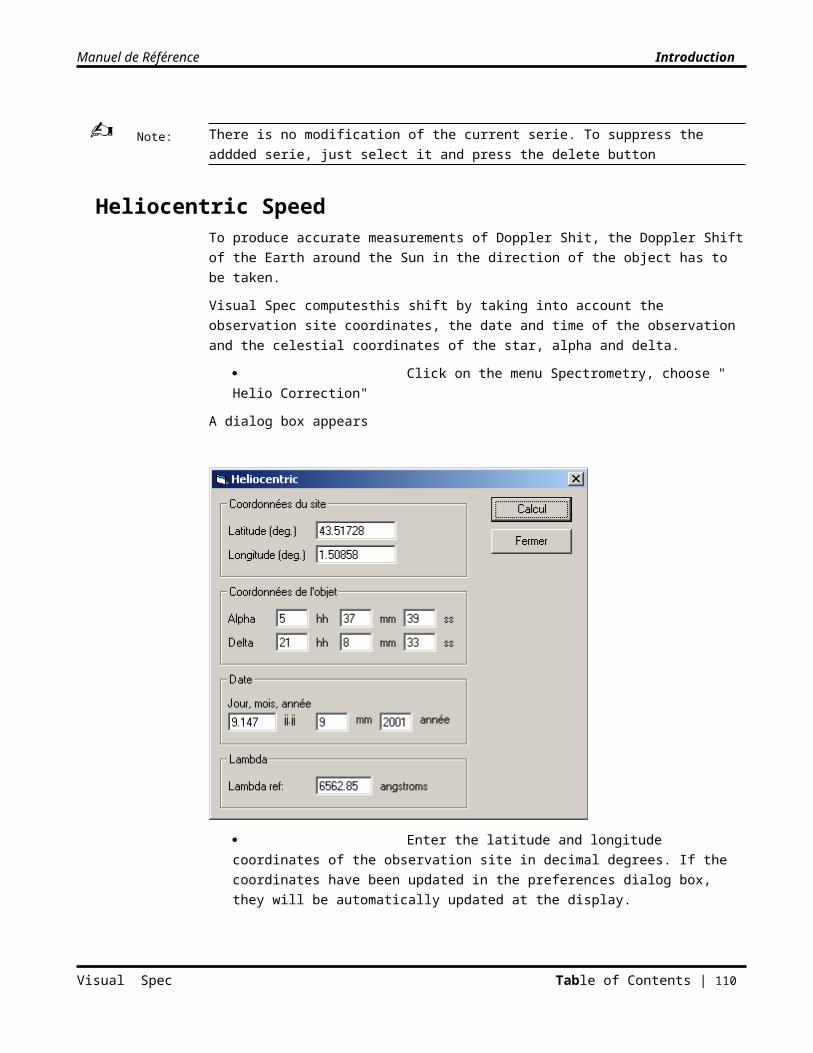
Manuel de Référence Introduction
The Bright Star Catalog is available in the form of an Excel file “brscat2.xls” in the application folder. In addition to spectral type, it contains other information such as the coordinates, magnitude, HD reference.
The profile file header is automatically updated with the values. If you want to keep the values recorded in the header, you'll have to save the file again.
Identification of chemical elementsIdentification of a chemical element based on wavelength is facilitated by the presence of a database included with Visual Spec.
Element.txt
This a short version of the CRC Handbook of Chemistry & Physics - only lines from element up to Iron is reproduced.VI/16 Line Spectra of the Elements (Reader+ 1980-1981)Reader J. & Corliss Ch.H. <61st ed., CRC Handbook of Chemistry & Physics (1980--81)>
lineident.txt
This a formatted version of a catalog of lines in stellar objectsVI/71A Revised version of the ILLSS Catalogue (Coluzzi 1993-1999)COLUZZI R: 1993 <Bull. Inf. CDS 43, 7>
sun.txt
This a formatted version of the sun lines catalogJ/A+AS/131/431 Accurate wavelengths in the Sun spectrum (Allende Prieto+ 1998)Allende Prieto C., Garcia Lopez R.J. <Astron. Astrophys. Suppl. Ser. 131, 431 (1998)>
Hires
The newly added "Hires" database if the transcription of the luke.lst file from Richard Gray's SPECTRUM software. It includes 38 text files and requires the 3.0.4 Vspec version at a minimum to be read as well as the separated zipped database file to be downloaded
Atmos
The file atmos.txt has been made by Christian Buil from various source of data: national weather forecast tables, observatories tables, and personal data from the professional Coralie Neiner.
At the exception of Atmos and Hires databalse, all database are available from the Centre de Données Stellaire of Strasbourg, the CDS. By default, the database is the element list of the “Chemical Handbook”. It includes only the wavelengths of the atomic elements whose number is less than or equal to that of Iron and for which the wavelengths are included between 3000 and 11000 angstroms.
It is possible to add to the elements in this list by editing the file “Element.txt”. It is suggested to follow the format of the database.
To display the databases:
Click on the menu Tools, choose “Elements…”
Visual Spec Table of Contents | 110
Manuel de Référence Introduction
or
Click on the button from the toolbar
A dialog box "Elements" appears
Dialog box "Elements"
The lines of chemical elements whose wavelengths are included in the entire spectral area of the profile appear in the list.
The column “lambda” gives the wavelength in angstroms of the line
The column “ion” indicates the ionization state of the atom.
The column “intensity” gives the laboratory intensity of the line.
The column “element” gives the chemical symbol of the atom.
Visual Spec Table of Contents | 111
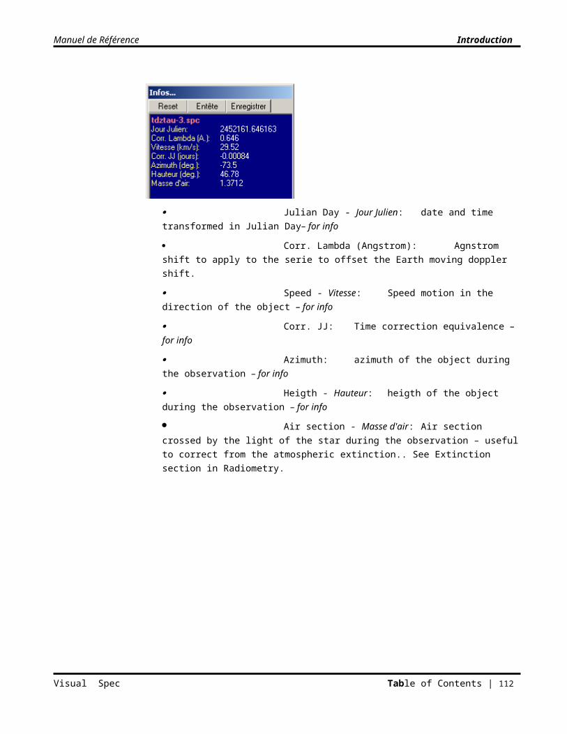
Manuel de Référence Introduction
To close the dialog box, click on the “close” symbol of the window frame.
You can click on one line and the cursor will move on the spectrum at the position of the element wavelength. If you do not see any move, click on the profil document and then again on the element window. You can also use the "up" and "down" arrows.
Identification by elementTo view the spectral lines by element, click on the column header “Element”. The elements will be rearranged in alphabetical order.
To return to a list ordered by wavelength, click on the column header “Lambda”.
Identification over a defined domainTo view the lines included in a defined spectral domain, enter into the textboxes “from” and “to” the values in angstroms of the first and last wavelength in the list. Then click on the button “Find”.
To return the all set of wavelength, click on the button from the frame "list"
Automatic identificationAutomatic identification allows automatic selection of the line whose wavelength is that defined by the cursor position.
For this, it is necessary to:
Click on the selection box Selection in the list frame from the element window
Select a spectral area
Click on the database window to display the selection of elements in the list
To suppress the automatic identification mode, unselect the selection box
When the cursor is within the selected area, between the gray dashed lines, the closest line to the cursor position whose wavelength is included in the wavelength domain plus or minus the sampling factor is automatically selected in the list.
Multiple lines can be highlighted. This is due to low resolution of the spectrum which prevent the accurate determination of one unique line.
This automatic identification is only an indication, and is highly sensitive to imperfections of calibration and resolution of the equipment.
Changing databaseTo pick another database:
Select the database name from the dropdown list in the source frame
Visual Spec Table of Contents | 112
Note:
Manuel de Référence Introduction
Element sortingTo only see some of the lines of certain chemical elements:
In the “Elements” area, click the symbol of the element that one wishes to see.
Click on the button “Sort”.
It is possible to select multiple entries in order to view a set of elements from the list.
To re-display all the elements
Click on the “Reset” button
Exporting a synthetic spectrumIt is possible to only display the lines of one or several chemical elements, then to synthesize the spectrum of corresponding lines in order to superimpose it on existing series. To accomplish this:
In the Elements area, click the checkbox in front of the elements illustrated in the list
Click on the button “Sort”
Once the list is created, click on the “Export” button to export it
The synthetic spectrum is added as a temporary series named “spc.<chemical element symbol>” of the selected element.
Verify and modify, as needed, the spectral extent of the list.
Exporting a synthetic spectrum as a new documentIf the calibration process is not certain, it is possible to export the synthetic spectrum of a choosen element on the all spectral extent defined in the from/to fields in a separated profile document.
Click on the button to export the list of lines of the element list as synthetic emission spectrum
A new pofile document is created under the name "Newspc-<id>.spc"
Visual Spec Table of Contents | 113
Note:
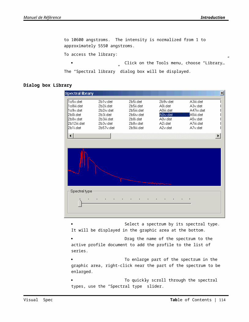
Manuel de Référence Introduction
It is then very convenient to pick the interactive zoom and to search for evident correlation between lines pattern.
Hires lines databaseThis database is extracted from the luke.lst file from SPECTRUM software. It includes all the lines retained by Richard Gray to generate theoretical spectrum. As this database is huge, it has been splitted in several sub files with 100 angstroms domain wavelength.
You have to select the Hiresxxx file where xxx correspond to the domain wavelength of your study.
If you did not have installed the hires.zip package, you will not see the files in the dropdown list.
Other aids to identificationWhile the program is running, other calls to the database of atomic spectral lines can be made using the button containing the question mark. The chemical handbook database is used by default.
When calibrating in wavelength. Then only the lines corresponding to the chemical body of calibration are displayed
During manual calibration. Then the whole database is displayed in the list
GnuPlotThe GnuPlot application is a "grapher", a free sofwtare running on Linux and Windows. To fully benefits from the powerful GnuPLot function, please refer to the website http://www.gnuplot.info/
* Copyright 1986 - 1993, 1998, 2004 Thomas Williams, Colin Kelley * * Permission to use, copy, and distribute this software and its * documentation for any purpose with or without fee is hereby granted, * provided that the above copyright notice appear in all copies and * that both that copyright notice and this permission notice appear * in supporting documentation. * * Permission to modify the software is granted, but not the right to * distribute the complete modified source code. Modifications are to * be distributed as patches to the released version. Permission to * distribute binaries produced by compiling modified sources is granted, * provided you * 1. distribute the corresponding source modifications from the * released version in the form of a patch file along with the binaries, * 2. add special version identification to distinguish your version * in addition to the base release version number, * 3. provide your name and address as the primary contact for the * support of your modified version, and * 4. retain our contact information in regard to use of the base * software. * Permission to distribute the released version of the source code along * with corresponding source modifications in the form of a patch file is * granted with same provisions 2 through 4 for binary distributions. * * This software is provided "as is" without express or implied warranty * to the extent permitted by applicable law.
Visual Spec uses the possibility to run GnuPLot by a command file and a script.
Visual Spec Table of Contents | 114
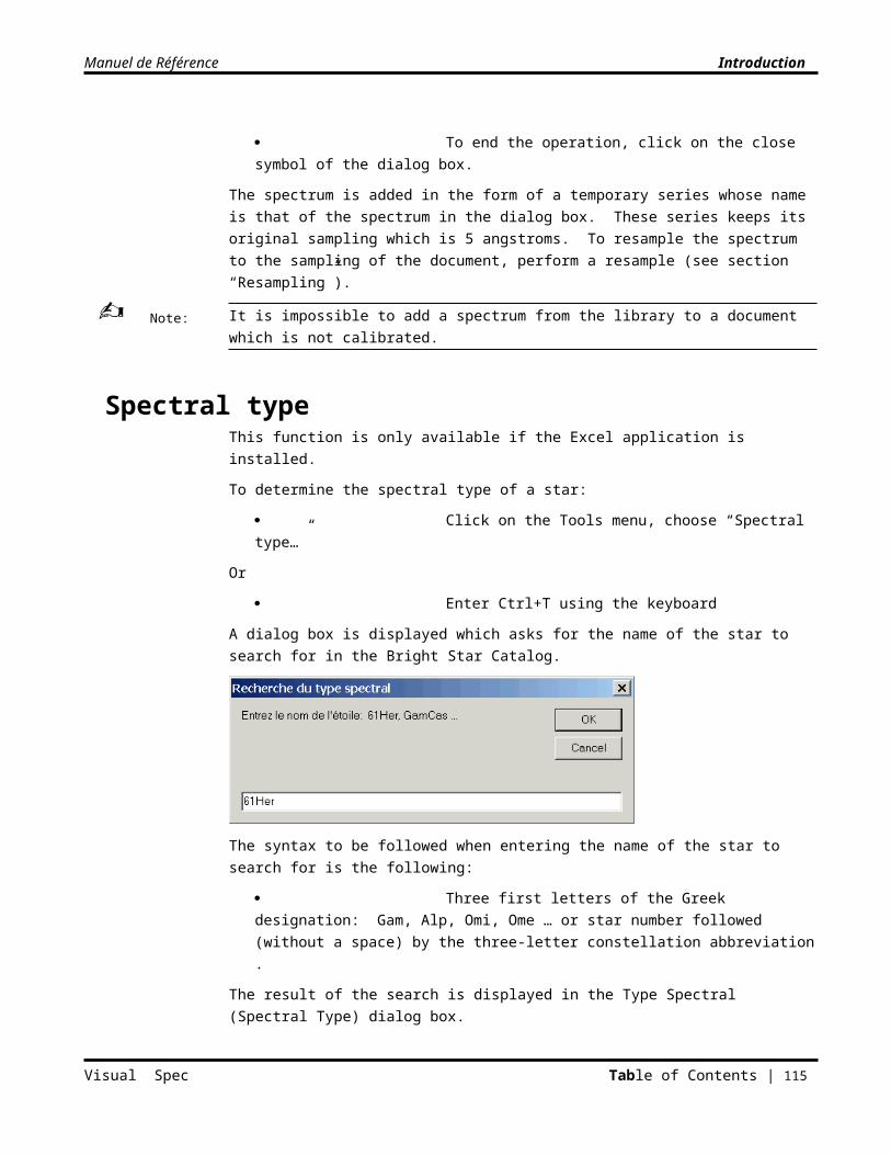
Manuel de Référence Introduction
Visual spec distributes the Version 4.0 but with only the mandatory file to run batch mode. To use the full application, one need to get the official package from the official website. The Vspec distribution also includes specific file required by Vspec to run correctly GnuPlot like the command file "Gnutest.txt" and a script file "std.gnu".
The style file "*.gnu" are in fact the GnuPlot scripts. It is a text file. You can edit and create other files, but shall give them the .gnu extension to be recognized by Vspec.
cliquer sur le menu Outils, sous-menu "Run GnuPlot"
Click on the meno Tool, sub-item "Run Gnuplot"
or
Click on the button in the toolbar
A dialog box is displaeyd
GnuPlot Dialog box
GnuPlot use the .dat file format to create the graph. If a profil with the .spc format is currently displayed, the .dat format will be automatically created and displayed. If the serie to plot is not the intensity serie, you need to replace the intensity serie by the desired serie before launching GnuPlot.
The style file is displayed in the frame "Style". If you want to
select another file, click on the button to open the "open file…" dialog box.
The image file name is indicated in the field "Image file name". The name can be edited. It is not required to add extension. The extension is automatically added by Visual Spec (.gif) or (.png) if the check box png is checked.
Visual Spec Table of Contents | 115
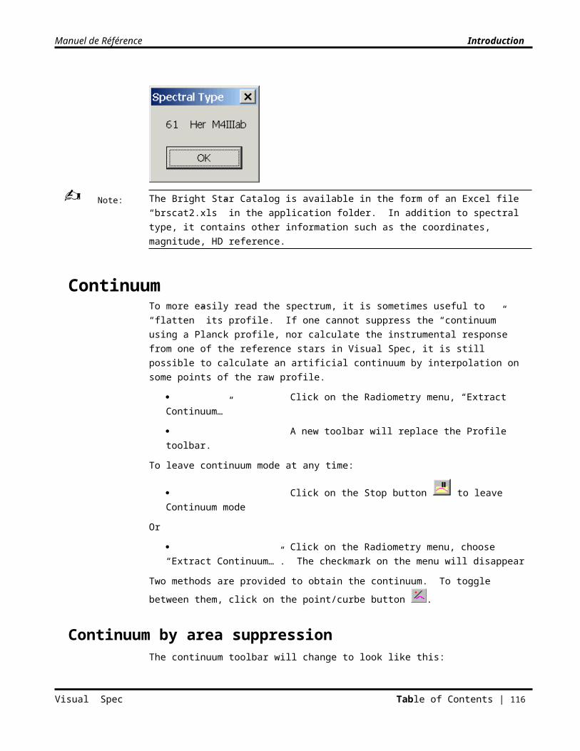
Manuel de Référence Introduction
The field Title contains the text to be displayed at the top of the graph.
The frame parameters manage the limits and the graduations of the graph.
- You can let GnuPlot select the best scale parameters by checking the check box Auto Y scale and/or Auto X scale
- If these checkboxes are not checked, you have to specifies the Y and X limits. For X axis, the graduations spacing can also be specified.
- If your script forces the X and Y values, these values will have no effect.
Once the parameters are defined, click on the button "Plot" to create the graph.
When GnuPLot has completed the script execution, a Pause dailog box is displayed
This box is managed by GnuPlot. It allows to keep the display on your screen, if your script is using it as a terminal. To close the GnuPlot window, click on OK
Visual Spec Table of Contents | 116
Manuel de Référence Introduction
To close the Visual Spec GnuPlot window, click on the Close button
File style "std.gnu"Visual Spec proposes a script file by default: "std.gnu" – it creates both a graph on the screen and record it under a .gif file in the same directory than the profile file.
#============================================================
# Script de trace GnuPlot des profils spectro de Visual Spec
#============================================================
# ParamŠtre 1 : nom du fichier
# ParamŠtre 2 : intitul‚ du titre
# ParamŠtre 3 : valeur min en Y
# ParamŠtre 4 : valeur max en Y
# ParamŠtre 5 : valeur min en X
# ParamŠtre 6 : valeur max en X
# ParamŠtre 7 : valeur ticks en X
# Paramètre 8: nom du fichier png
#
# Exemples :
# call "std.gnu" "140699.dat" "88Her" 6500 7000 .2 1.8
# call "std.gnu" "140699.dat" "88her" * * * * (echelle automatique)
#============================================================
set terminal windows "Arial" 9 -> display the graph on the screen
set xlabel "" -> defines the x label, here, none
set ylabel "" -> defines the y label, here, none
set yrange [$2:$3] -> defines the limits of the Y axis
set xtics $6 -> defines the space between X axis graduations
set xrange [$4:$5] # zone libre -> defines the limits of the X axis
set tmargin 2 -> defines the margin around the graph
set grid -> Display a grid in the back of the graph
set title '$1' ,-0.5 -> dsiplay the title of the graph
plot "$0" notitle with lines -> plot the graph from the file
#et maintenant le fichier
set terminal gif small size 640,480 -> display the graph in a gif file format
Visual Spec Table of Contents | 117
Manuel de Référence Introduction
set output '$7' -> save the file under the name $7
set xlabel ""
set ylabel ""
set yrange [$2:$3]
set xtics $6
set xrange [$4:$5] # zone libre
set tmargin 2
set grid
set title '$1' ,-0.5
plot "$0" notitle with lines
The Gif format is more or less yet in the public domain. If you have difficulties, you need to check the png checkbox and modify the script std.gnu to replace set terminal gif by set terminal png
ConsoleThe console (menu Tools, choose “Console”) permits execution control by command-line.
The console is only accessible if the spectrum has been calibrated in wavelength.
How to use the command-lineTo enter a command
Click in the console window
Enter the name of the command with or without associated parameters
To execute the command, press “Enter”
If the command is not known, the error message “syntaxe inconnue” (“unknown syntax”) is displayed.
Visual Spec Table of Contents | 118
Note:
Manuel de Référence Introduction
If the command is not followed by the needed number of parameters, the message “nombre d’argument incorrect” (“number of parameters is incorrect”) is displayed.
If one of the parameters violates syntax, the error message “Erreur syntaxe” will be displayed.
To display the list of commands, enter “help ?”.
List of available commandsThe command-line commands currently available are:
Command Parameters DescriptionHelp ? Display the list of commandsHelp name of a command Describe the commandDir <none> List the .spc files in the current directoryCd Directory name or .. to go
up one levelChange the directory path
Load filename Open the file <filename>.spc (the suffix .spc is automatically appended)
Select windowname Make the open document in the window named “windowname” active. If the document isn’t open the message “Erreur de syntaxe” is displayed
Affichserie seriesname Make the series <seriesname> in the active document the active series. If a series named <seriesname> does not exist in the active document the message “Erreur de syntaxe” is displayed
Formatx real value L1 real value L2
Display the series of the active document between wavelengths L1 and L2
Allformatx <none> Apply the wavelength domain displayed in the active series to all open documents
Norma real value L1real value L2
Normalize the active series with, for area of continuum, the area included between L1 and L2
Leq real value L1real value L2
Calculate and display in the info window the equivalent width included between L1 and L2. This calculation is only valid if the series is normalized
Decoupe real value L1real value L2
Eliminate from the series the points outside the wavelength area included between L1 and L2
Comp Operation: one charactera:surfaceb:barycenterc:center of the linef:Fwmhi: intensityl:Equivalent Widthm:means:snrl1: real valuel2: real value
Execute the operation between the value l1 and l2. Example: comp b l1 l2Compute the barycenter entre between the value l1 and l2.
Visual Spec Table of Contents | 119
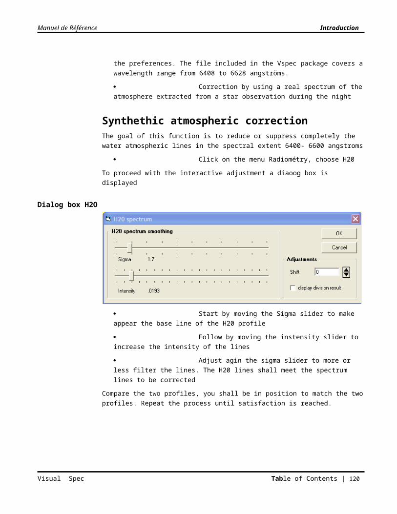
Manuel de Référence Introduction
MusicThis function is eliminated since the 3.3.0 version
This function is just for fun… It transforme the spectral profile into a music play. Each sounds is generated following the frequency and the intensity of the spectrum.
One can select only a portion of the spectrum to only play ths section.
Click on the menu Outils, choose Music
If the spectrum contains a lot of points the song duration can be quite long… You can still cancel when prompting the confirmation message.
Visual Spec Table of Contents | 120
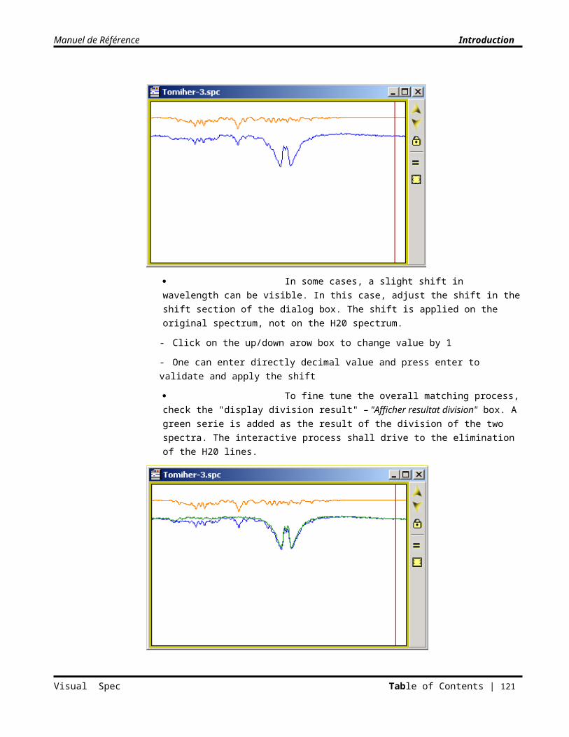
Manuel de Référence Introduction
C H A P T E R 8
Spectral Analysis
Spectral analysis consists of processing the data of a profile calibrated in wavelength in order to extract significant spectroscopic information. This chapter describes various strategies for processing and spectral analysis.
The first application consists of comparing spectra with each other, or with spectra of the same object having changed over time. These comparisons are qualitative.
A second application consists of a quantitative comparison of certain measurements such as equivalent width or Doppler shift.
Finally, it is always interesting to try to identify different spectral lines of an object a posteriori.
To complete the analysies, Visual Spec provides use a user friendly link to the SPECTRUM software from Richard Gray. This software can be download from the web site xxx. SPECTRUM allows you to generate theoretical spectrum of a star knowing physical parameters like temperature, pression… To have an extensive description of SPECTRUM usage, please refer to Vspec web site in the "theoretical spectrum" section.
Comparison of spectraTo compare spectra with each other, it is necessary to first perform operations of correction and normalization so the spectra are really comparable with each other.
These corrections are:
1. Calibration in wavelength: needed
2. Radiometric: suggested if the spectrum extends over a spectral domain sensitive to the difference of the sensitivity to wavelength of the sensor.
3. Normalization with respect to the continuum: done so that the calculation of the continuum is carried out on the same wavelength domain of both spectra and to ensure that no lines are present in this area
One can compare several spectra:
By simple superposition, by Cut/Paste, even if the samplings are different (see section “Cut/Paste of a spectral series”).
By animation, after having applied the same format all spectra to be compared.
By division, the signature of a difference having resulted in a line outside the noise in the vicinity of the difference.
Visual Spec Table of Contents | 121
Manuel de Référence Introduction
Quantitative parametersIf the spectra are sufficiently resolved that the shape of a line is not solely dependant on the characteristics of the equipment, it is possible to measure and compare:
Equivalent widths of lines
Doppler shift
Speed of expansion
Equivalent widthTo follow the evolution of the same line over time, calculating the equivalent width gives an indication of the power of the line. If the equivalent width changes, this indicates changes in the physical conditions of the layers that produced the line.
An example of evolution of the line H<alpha> of 28 Tau (B8Ve)
1. Search with the File|Find function for all the profile documents containing “28Tau” in their comment area.
2. Open the documents.
3. View the set of spectra using the function Window|”Small Windows”
4. Select one of the spectra, and apply the same format to the others (Format|”Graphic…”|”Axis X” and check “Apply to all windows” and then click “Apply”).
5. Verify the predefined area for calculating the continuum in the “continuum” tab of the Options|“Preferences…” dialog box. This area should be common to all the spectra and should not contain lines.
6. Normalize each of the spectra (Operations|Normalize).
7. For each spectrum, select the line to measure and choose the menu item Weq (Equivalent Width) in the Spectrometry menu. The result is displayed in the “Infos…” window below the name of each document.
8. Click on the “Save” button of the “Infos…” window.
9. Open the file Infos.txt in a text editor.
LEQ: 37.9115p004.spcLEQ: 34.6814p005.spcLEQ: 32.5412p009.spcLEQ: 31.6611p007.spcLEQ: 30.5509p021.spcLEQ: 22.9206p015.spc
Visual Spec Table of Contents | 122
Manuel de Référence Introduction
Doppler shiftMeasuring the Doppler shift requires a bit of care because it is based on the measurement of deviation in wavelength of a line with respect to its theoretical position.
It is impossible to perform this measurement if the spectrum was calibrated in wavelength based on its own lines.
The Doppler shift to be measured must also be from 2 to 3 times more significant than spectral sampling.
For very accurate measurements, correct the spectrum from the doppler shift from Earth moving. See the section "Helio Speed correction"
It is also possible to graduate the X axis in doppler shift (km/s) centered around a reference wavelength value.
To measure a Doppler shift:
1. Calibrate the spectrum carefully using an external reference spectrum.
2. Select the line to measure.
3. Calculate the center of the line; the position is given in angstroms.
4. Calculate the ratio: Measured Position – Theoretical Position / Theoretical Position.
5. Multiply by c=3,000,000 km/s to obtain a shift in km/s.
Example of a detail of the line H<alpha> of 59 Cyg (Ble)
center1: 6559.47center2: 6564.61center: 6562.33 theoretical position at 6562.852FWMH: 12.7612p010.spc Ech= 0.286 A/pixel
Yields:
Shift 1 = (6559.47 - 6562.852) / 6562.852 * 300000= -154.6 km/s
Shift 2 = (6564.61 - 6562.85) / 6562.852 * 300000= 80.6 km/s
Resolution = (0.286) / 6562.852 * 300000 = 14 km/s
Visual Spec Table of Contents | 123
Manuel de Référence Introduction
A precise measurement should take into account the Doppler shift due to movement of the Earth in its orbit. This calculation is available with the heliocentric speed correction function.
Speed of expansionAs for calculation of Doppler shift, this measurement demands the same precautions for calibration and resolution.
The measurement of speed of expansion or rotation is defined by increase in the line caused by the Doppler effect.
1. Calibrate the spectrum carefully using an external reference spectrum.
2. Select the line to measure.
3. Measure the center of the line, the position is given in angstroms
4. Measure the full width at half-maximum of the line: FWMH.
5. Calculate FWMH/center
6. Multiply by c=3,000,000 km/s to obtain shift in km/s
Example of the nova Cygnii 1995
center: 6562.75 FWMH: 43.92 tnvcy-48.spc
Yields:
Speed = (43.92) / 6562.852 * 300000 = 2008 km/s
Identification of elementsThe identification of element is a difficult exercise. It is not a question here of discoving new elements, but to recognize well the original chemical elements of the lines observed.
Visual Spec Table of Contents | 124
Note:
Manuel de Référence Introduction
Ability to identify with precision which chemical element produces which line depends largely on the resolution. Indeed, a great number of lines of various elements are possible in a very small domain of wavelength, such as shown below in an area of 10 angströms / 1 Nm.
It is necessary to research, referring to the literature, to gain preliminary knowledge of the physical conditions of the object of study, with reference to its spectral type.
A useful technique consists of superimposing the theoretical spectrum of the presumed elements in order to verify whether they correspond to the lines.
Click on one the line to see the profile document cursor moving at the line wavelength on the active serie. If no move is observed, click on the profile document then come back in the element list. You can also move the line selection by using the up and down keyboard arrows.
Solar spectrumExample: Solar spectrum and lines of Sodium, Na. One can recognize the double of Sodium, at the left.
Visual Spec Table of Contents | 125
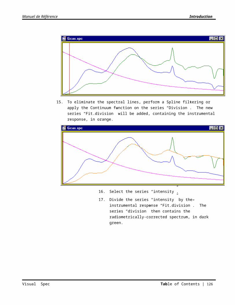
Manuel de Référence Introduction
Superposed with the lines of Iron, one sees some correspondence.
Superposed with the lines of Calcium.
Stars of spectral type MExample of a spectrum of an M star, 10 Dra (M3.5III) with the start of lines of TiO
Planetary nebulaExample of the spectrum of a planetary nebula M57 and missing lines (NIII).
Visual Spec Table of Contents | 126
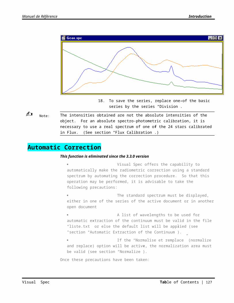
Manuel de Référence Introduction
Atmospheric linesAtmospheric lines have a characteristic profile and are easily identifiable. They can be used for spectral calibration.
Link with SPECTRUM softwareVisual Spec allows you to directly use the SPECTRUM software by providing a user-friendly interface using the script facility of the SPECTRUM software.
This requires that you have correctly installed SPECTRUM and declared it in the preference dialog box.
Visual Spec Table of Contents | 127
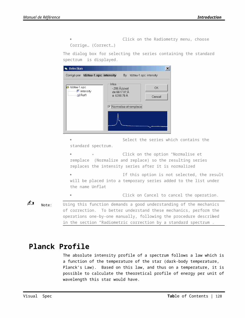
Manuel de Référence Introduction
Preference settings for SPECTRUM
Select the tab "spectrum"
Select the hardrive and the directory where spectrum.exe is installed
Click the option button "Yes, Spectrum is installed" on the right frame
This will become the referenced path for Visual Spec to find the executable of SPECTRUM. If you change this directory, make sure you update the preferences settings in Vspec again.
If you did not have installed Spectrum and not selected the installation path, the Run Spectrum sub-menu will not appear in the Options menu.
Click on the Run Spectrum sub-menu in the Options menu to get access to the SPECTRUM interface and run SPECTRUM
SPECTRUM interface dialog box
Visual Spec Table of Contents | 128
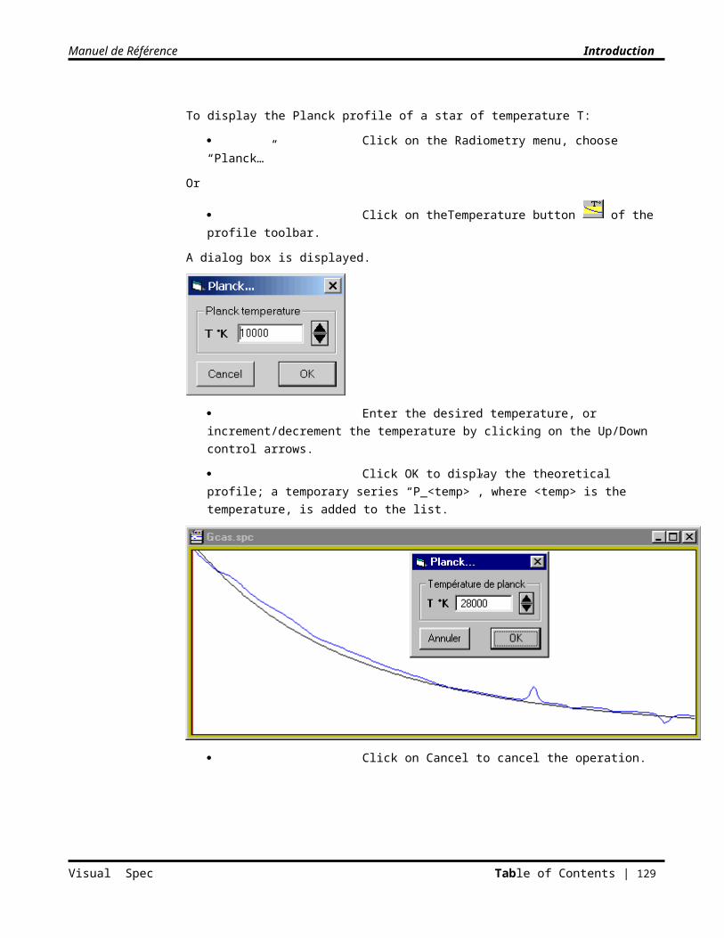
Manuel de Référence Introduction
You have to enter the parameters required by SPECTRUM to run correctly.
Enter the Atmosphere model. Either you type directly the file name or you click on the side button to open a "open dialog" box
Only the files with extension *.mod will be listed.They shall meet the SPECTRUM atmosphere file format as described on its web site.
Enter the turbulence velocity – usually this value is known from the name of the model you picked
Usual convention for model file names45045k4p00.mod450: 4500°K temperature45: log(g)4.5cm/sec²k4: 4km/s turbulence velocityp00: metallicity [M/H]=0.0 (solar abundance)m05: [M/H]=-0.5 (0.32 x solar abundance)p05: [M/H]=0.5 (3.2 x solar abundance)
The model files shall be find on the web, mainly from Kurucz site. (See Vspec site).
Enter the start and end wavelength
Enter the wavelength steps – use 0.01 angström as a minimum value
You can compute the number of points in the output files by clicking on the "Nb points" button. This is useful to prevent too huge file generation.
Vspec can only manage 16382 points spectrum file.
Visual Spec Table of Contents | 129
Note:
Manuel de Référence Introduction
Enter the name of the output file – the file format will be a "dat" file (two columns: wavelength, intensity) – You can select the directory and the file name by clickling the side button.
Here is an example of the window correctly filled
Click on the OK button to launch SPECTRUM
A small script is written on the hardisk and then executed by SPECTRUM. The DOS windows of SPECTRUM execution is temporary displayed over Vspec
Visual Spec Table of Contents | 130
Manuel de Référence Introduction
Once the execution is completed, the synthetic spectrum is automatically displayed in Visual Spec and saved as a "dat" file.
A great Thanks to Richard Gray who wrote SPECTRUM free software with adequate documentation and script function…
Visual Spec Table of Contents | 131
Note:
Manuel de Référence Introduction
C H A P T E R 9
What's new since…
This section will describe modifications per new version. The reference is the version 3.2.5
Version 3.3.0In addition to some internal bug fixes to improve the robustness of the software, this version is mainly a clean-up in the menu labels, and the buttons interface.
AdditionsPreferences… New check box in preference dialog box to link the two directories of the images and the profiles.
Gnuplot… Format .png preset in the gnuplot dialog box
Correction with real atmospheric spectrum… if the domain cover by the file of the atmospheric line, this function allows the user to use a real atmospheric spectrum, extracted from the observation of a reference star. The intensity of this real spectrum can thus be adjusted interactively, the same way.
ModificationsDirectory set-up in the preference menu is the default working directory.
Atmosphere… back to focus on the H20 interpolation dialog box after a shift, no need to reselect the dialog box to change the shift value
Multi-lines calibration… define a different extension for the equation ascii file. Was before .lst as for lines list, now will have its own .exc extension
Renaming of some menu labels, for a better understanding
EliminationsThe function "archive" is eliminated to simplify the software
The 'old way with buttons' for the 2 lines calibration is eliminated and definitively replaced by the box label edition close to the line selection.
No more "song" from a spectrum
The capability to extract a continuum from a preset list of wavelength is also supressed
Visual Spec Table of Contents | 132
Manuel de Référence Introduction
No more superimpose switch modes
Visual Spec Table of Contents | 133
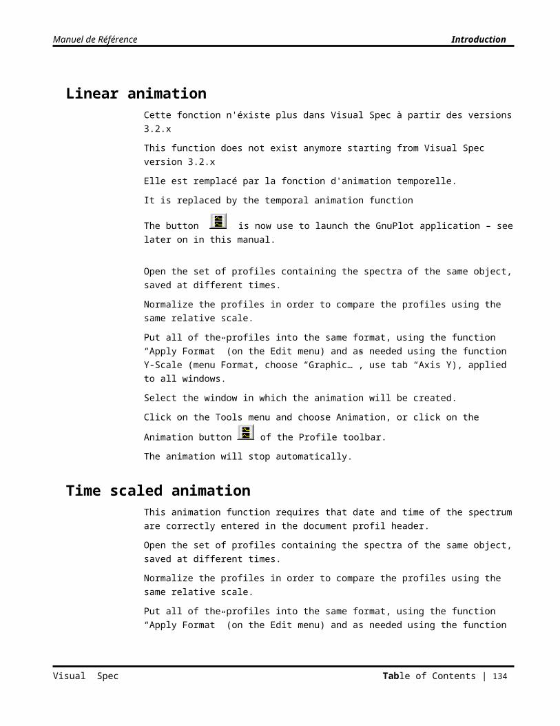
Manuel de Référence Introduction
A P P E N D I X 1
Reference
Useful Spectral Lines5889.95 NaI5895.924 NaI6562.852 H Alpha4340.47 H Bêta4861.33 H Gamma4101.74 H Delta3970.072 H Epsilon6875 Atm 027594 Atm 02
Reference stars for flux calibration
Visual Spec Table of Contents | 134
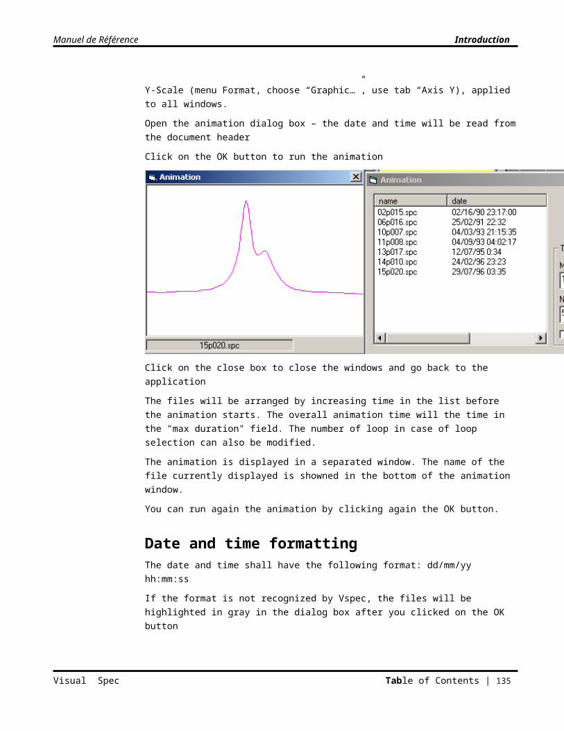
Manuel de Référence Introduction
Appendix 2
Buttons
Principal Toolbar
Open a .pic or .fit image
Open a .spc Profile file
Display a search window for all profiles which contain the search string
Image Toolbar
Apply a new low threshold, new high threshold to the visualization image
Apply new thresholds to the visualization image
Reset the thresholds to default values
Extract a spectral profile
Extract a reference profile
Export a sub-image to Excel
Calibration Toolbar
Display the list of lines of the reference element (Argon)
Display a dialog window for applying new thresholds in Y, in X
Zoom/Cancel Zoom on scale X of the profiles in the area selected using the cursor
Visual Spec Table of Contents | 135

Manuel de Référence Introduction
Continuum Toolbar
Toggle the method of calculation of the continuum between area-suppression mode and point-mode
Eliminate the selected area from the profile of the continuum
Reset the areas eliminated from the continuum
Execute interpolation of the continuum
Reinitialize the list of intake points of the continuum
Execute interpolation of the continuum by points
Leave continuum mode
Save the list of continuum points
Profile Toolbar
Display a dialog window for applying new thresholds in X, in Y
Zoom on scale X of the profiles in the area selected using the cursor
Erase all displayed series
One line calibration
Two lines calibration
Multi-lines calibration
Redimension the profile document to a predefined format
Cut the profil according to the selection
Copy the active series
Paste the series previously copied
Apply the X format of the active series to all windows
Display a window of dialogue to add a series containing the active series filtered by a low-pass filter
Display Element window
Normalize the active series
Atmosphere spectrum correction
Divide a profile by another profile
Display a dialog window to add a series containing a theoretical profile of the Planck temperature
Display a selection window of calculations to be carried out on a selected area
Replace one of the base series with the active series
Launch Gnuplot application
Visual Spec Table of Contents | 136
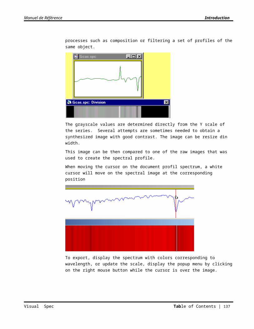
Manuel de Référence Introduction
Visual Spec Table of Contents | 137
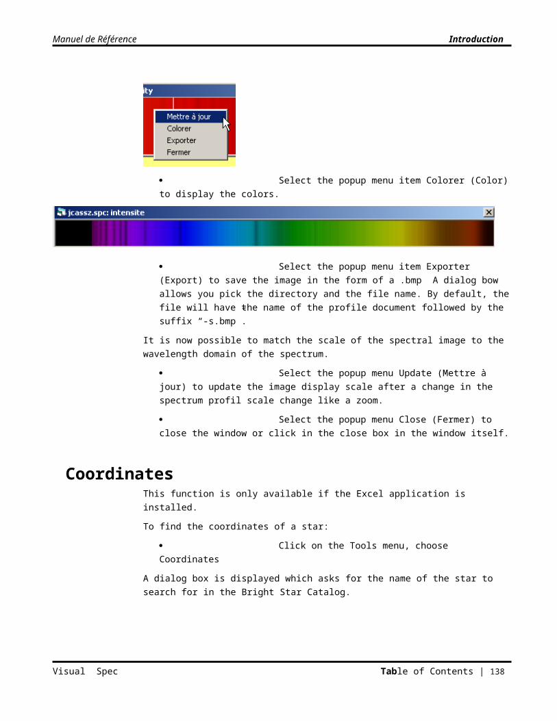
Manuel de Référence Introduction
A P P E N D I X 3
Reference list of menus and functions
Visual Spec
MenuFunction Description
File Open image… Open a .pic or .fit imageOpen profile… Open a .spc documentFind Search for a .spc document whose header contains the search-stringImport dat Open a .dat document containing profile dataImport fit Open a .fit spectro file (Work in Progress…)Quit Quit the application
Options Preferences… Display the Preferences dialog box? About… Display the window “About Visual Spec”
Help Launch the Acrobat Reader to display the help file Aide.pdf
ImageMenu Function DescriptionFile Open profile… Open a .spc document
Open image… Open a .pic or .fit imageFind references… Search for an associated .pic image beginning with the prefix
“a”Export bmp Export the Image document into a bmp file under name<-
I>.bmp in the same directoryClose Close the current documentClose All Close all image windowsQuit Quit the application
Window Arrange Cascade the windowsMosaic Tile the windowsAlign Align the windows at the left of the screen one over another
Options Graph Display a graphic containing the profile of the outline of the place in the image where the cursor is situated
Visual Spec Table of Contents | 138
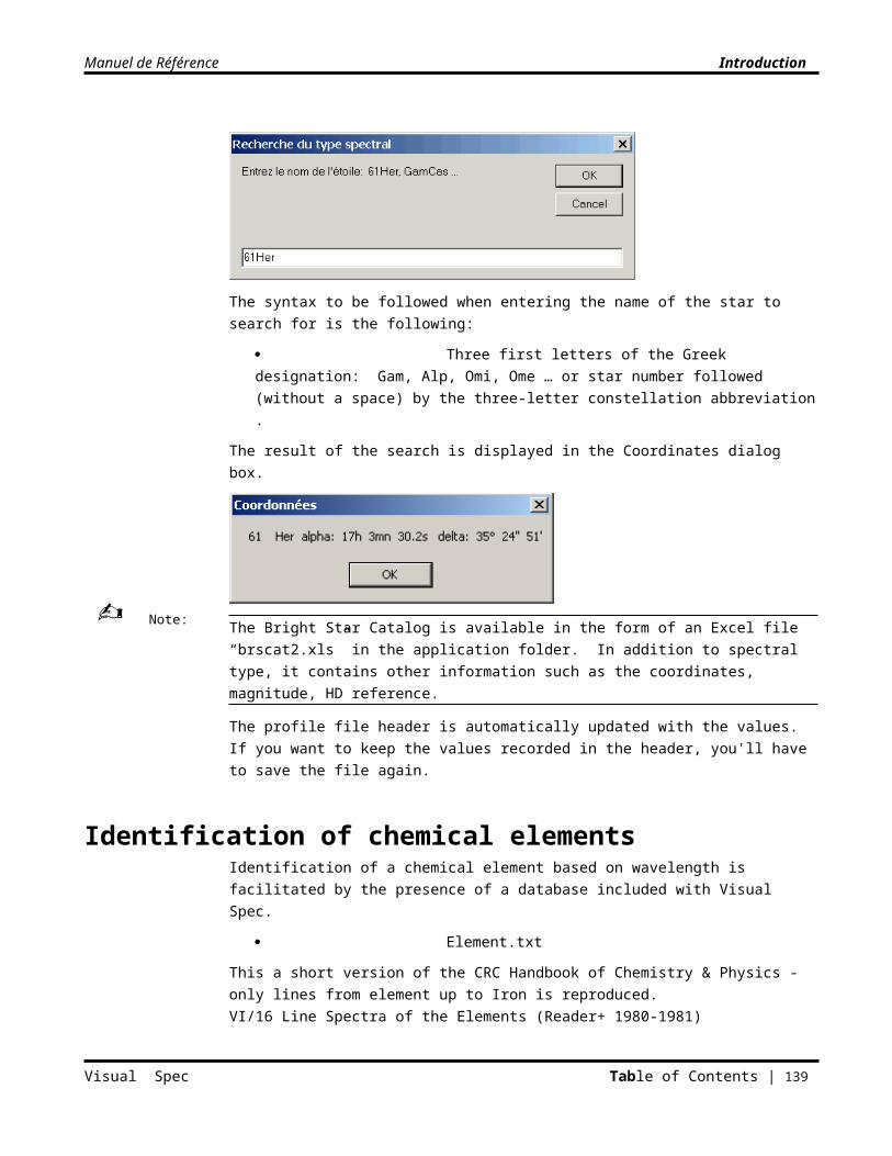
Manuel de Référence Introduction
Preferences Display the Preferences dialog box
? About… Display the window “About Visual Spec”Help Launch the Acrobat Reader to display the help file Aide.pdf
Profile
Menu Function DescriptionFile Open image… Open a .pic or .fit image
Open profile… Open a .spc documentFind… Search for a .spc document whose header contains the search-stringSave Save the document without changing its nameSave As… Save the document, asking for a new nameExport dat Export the active window as a .dat documentExport txt Export the .spc document as a .txt DocumentExport bmp Export the active window as a .bmp DocumentClose Close the current documentClose All Close all image windowsQuit Quit the application
Edit Copy Copy the seriesPaste Paste the seriesApply format Apply to all windows the X format of the active seriesClear Clear the active series from the windowReplace Dialog box: replace one of the predefined series with the active series Suppress Suppress the active series from the list, if it is a temporary seriesCrop Eliminate areas outside the selected area from the active seriesPixel… Dialog box: edit the intensity of the pixelsHeader Dialog box: edit the .spc document Header
Format Graphic… Dialog box: Modify the graphic format, scale and graduationsLine Display the spectral profile as a lineDot Display each pixel with a symbolBar Display the spectral profile in a small rectangleZoom… Interactive zoom and translation controlsFont… Dialog box: Modify the font of the GraphBackground color Dialog box: Modify the color of the graphic background
Operations Normalize Normalize the series with respect to a predefined continuum
Visual Spec Table of Contents | 139
Manuel de Référence Introduction
Divide profile by a profile…
Divide the active series by a series in memory
Multiply profile by a profile …
Multiply the active series by a series in memory
Add profile by a profile …
Add the active series to a series in memory
Subtract profile by a profile …
Subtract the active series from a series in memory
Recalibrate profile by a profile
Recalibrate the active series based on calibration of a series in memory
Arithmetic Operations
Dialog box: Arithmetic operations with constant
Derive Derive the active seriesTranslate… Dialog box: Translate series in XJoin Concatenate two series to form one seriesCompose Add the displayed profiles to the active seriesLow-Pass Filter Dialog box: apply a low-pass filterSpline Filter Dialog box: apply a spline filterGaussian Filter Dialog box: apply a gaussian filterMMSE Filter Dialog box: apply a mmse filter
Spectrometry Calibration 1 lines…
Display the one line calibration toolbox
Calibration 2 lines…
Toolbar: manual calibration based on instrumental parameters
Calibration multi-lines lines…
Dialog box non-linear calibration
Computation preferences
On a selection of lines, dialog box: measurement
Heliocentric correction
Dialog box: Apply the heliocentric correction due to the Earth moving
Fit Photosphere Dialog box: Adjustement and subtraction ofa gaussian profil to suppress the photospheric contribution (Work in Progress…)
Resampling Dialog Box: resample the profilRadiometry Continuum… Display the Continuum toolbox
Continuum division Call the function Continuum then replace the intensity series by its division by a continuum
Continuum subtraction
Call the function Continuum then replace the intensity series by its substraction by a continuum
H20 correction Dialog box: suppress the atmospheric lines of the waterH20 correction real spectrum…
Dialog box: select the atmospheric profile then link with the intensity adjustment dialog box
Planck… Dialog box: calculate the Planck profile for a temperatureExtinction Dialog box: correct the atmospheric extinction
Visual Spec Table of Contents | 140
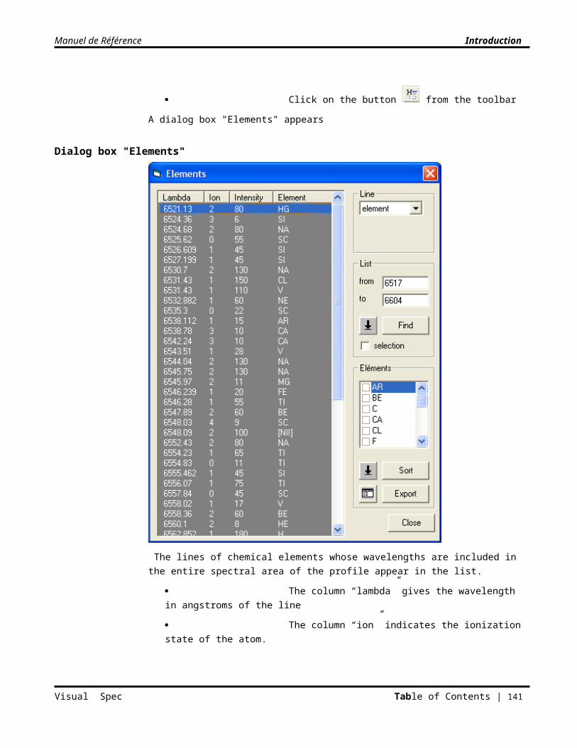
Manuel de Référence Introduction
Compute flux of eference star…
Dialog box: Calculate the instrumental response for a reference star
Absolute Flux calibration
Correct the active series from the instrumental response
Tools Elements… Dialog box: display the database of elementsSpectral type Dialog Box: search for the spectral type of a starCoordinates Dialog Box: search for coordinates of a starLibrary… Dialog box: display the database of standard spectraRun GnuPLot Dialog Box: launch the GnuPLot applicationRun Spectrum© Dialog Box: lanuch the Spectrum applicationLabel On the selection of lines and calibrated profile: display the wavelengthSynthesis Display the spectral image reconstructed from the active seriesConsole Display the command-line windowInfos… Display the calculation windows on the lines
Window Small windows Reduce the set of windows to “thumbnail” sizeAdjust Enlarge the set of windows to normal sizeArrange Cascade the windowsTile Tile the windowsAlign Align the windows at the left of the screen one over another
Options Preferences Display the Preferences dialog box? About… Display the window “About Visual Spec”
Help Launch the Acrobat Reader to display the help file Aide.pdf
Visual Spec Table of Contents | 141
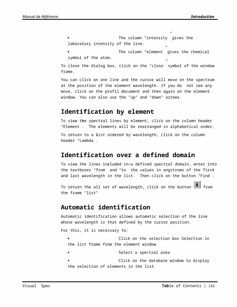
Manuel de Référence Introduction
A P P E N D I X 4
Application Messages
Message Casual Translation Recommended ActionLe fichier a été modifié, voulez-vous l’enregistrer ?
The file has not been saved, would you like to save it?
Yes: the file will be replaced by the new versionNo: the document will be closed without saving
Le fichier à été modifié, voulez-vous l’écraser ?
The file has been modified, would you like to overwrite it?
Yes: the file will be replaced by the new versionNo: a dialog box will be displayed to obtain a new file name
Le fichier est déjà ouvert, voulez-vous le recharger?
The file is already open, would you like to refresh it?
Yes: the file will be replaced by the new versionNo: the document is unchanged
Voulez-vous écrasez le profil en cours ?
Would you like to overwrite the current profile?
Yes: the binning will replace the seriesNo: a new document is opened
Entrez un nom de fichier Enter a filename There is not a valid name in the textbox, select a fileDisque non disponible Disk not available The peripheral selected is not active, select another
peripheralSélectionnez une zone image... Select an image area… The operation needed to select an image areaLe fichier n'est pas un fichier pic The file is not a .pic file The format of the file to be read is incorrect, so it is
unreadablePas plus de 5 images affichées... Not more than 5 images
displayed…The application cannot display more than 5 images at a time. Close one of the images to make space in memory.
Référence saturée, faites une sélection manuelle
Reference is saturated, make a manual selection
The spectrum is too complex for the automatic binning calculation. Select an area manually, with less than 30 lines
L'application Excel n'est pas disponible
The application Excel is not available
The application cannot detect the presence of the Excel function. This function is not available.
Pas de profil de référence... voulez-vous utilisez le profil en cours
No reference profile … would you like to use the current profile?
The calibration operation needs a non-empty series Ref1.Yes: the series “intensity” is automatically copied to the series “Ref1”No: perform a reference binning on the desired image
Le fichier n'est pas un fichier spc The file is not an .spc file The extension of the file is not “.spc”. Select a different file
Le fichier n'est pas calibré The file is not calibrated. The stacking operation needs the series to be calibrated in wavelength; it will not be added
Pas de fichier trouvé No file found The search function has not found the search string in the header comment field of any file in the active directory.
Visual Spec Table of Contents | 142
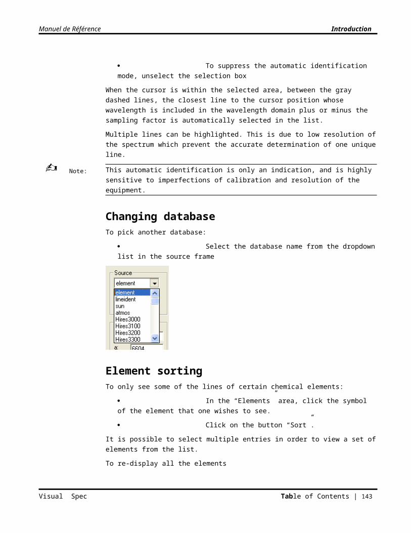
Manuel de Référence Introduction
Seuls les 15 premiers seront ouverts...
Only the first 15 will be opened…
Only the 15 first documents in the list of files corresponding to the criterion will be opened
Le fichier n'est pas étalonné en longueur d'onde
The file is not calibrated in wavelength
The operation needs the series to be calibrated in wavelength. Perform the calibration.
Les séries ne sont pas compatibles
The series are not compatible The operation is impossible; the spectral profiles have different numbers of pixels and are not calibrated in wavelength
Pas de zone de recouvrement No area of overlap The two series cannot be merged because there is no area of overlap between their two spectral domains
La série a est inclue dans la série b
Series a is included within series b
The two series cannot be merged because the spectral domain of one is totally included within the spectral domain of the other
Les séries sont superposables The series are superposable The merge operation is not useful because the two series have exactly the same spectral domain. Occurs, for example, if one tries to merge a series with itself.
Profil non calibré... Profile not calibrated… The operation needs the series to be calibrated in wavelength
Cette série n'est pas supprimable...
This series cannot be deleted The basic series Intensity, Ref1, Ref2, and Normalized cannot be deleted
Afficher les fichiers profils à compositer
Display the profile files to stack The stacking operation uses opened documents
Temps de pose nul, modifier l’entête
Exposure time missing, modify header
He function uses exposure time. Update the exposure time by editing the document header.
Sélectionnez un domaine de longueur d'onde...
Select a domain of wavelength…
For the active function, use the mouse to select an area of the profile.
Domaine spectral trop réduit Spectral domain too small The flux-calibrated spectrum does not overlap the real spectrum. The operation of flux calibration is not possible.
Zone du continuum incorrecte, changer les paramètres dans le menu Préférences...
Area of continuum incorrect, change the parameters in the Preference menu…
The area of continuum is outside the spectrum. Edit the valid borders using the Preferences dialog box.
Faire une sélection sur plus de 10 pixels
Select more than 10 pixels The selection of spectral domain is too small for calculation of LEQ; select a larger area.
Sélectionnez au moins 5 points Select at least 5 points The selection of a spectral domain is too small for the calculation of FWMH; select a larger area
Il n'y a pas d'éléments à exporter...
There are no elements to export…
Choose other elements or modify the spectral area.
Erreur de saisie Data error The character is not a valid character in this function.Impossible d'afficher le fichier d'aide
Unable to display the help file. If the file Aide.pdf is not in the root folder of Vspec, then the application cannot make the on-line .pdf help fileAvailable.
Entrez un paramètre différent de 0
Enter a parameter other than 0 Enter a number other than 0.
Visual Spec Table of Contents | 143
Manuel de Référence Introduction
A P P E N D I X 5
Acknowledgements
This software was created after having extensively used the software “Spec” by Alain Klotz, which runs under DOS. Some functions were reproduced here, but unfortunately not all of them since the objective was to develop a mainly “Visual” interface for the most-often-used functions.
Since then, many functions were added, with the arrival of data of various "spectroscopists" of the Aude list, in particular C.Buil, the Morata family and th emembers of Astroqueyras with Jacques Boussugues, Oliver Thizy and the CALA. A special mention to Dale Mais for his patience and tenacity. The database of standard spectra comes from Pickle et.al. and was found at the Centre de Données Stellaire de Strasbourg: http://cdsweb.u-strasbg.fr
The atmos file is derived from personal data of Coralie Neiner.
They are thanked here for it.
A special thanks to those who have done the complete translation and production of this manual in English (Thanks to Barbara…). This opens a door to VisualSpecs and we are very happy if this software, through this initiative, allows a lot of amateurs all around the world to have fun with Spectroscopy
Visual Spec Table of Contents | 144
Manuel de Référence Introduction
A P P E N D I X T O T H E E N G L I S H T R A N S L A T I O N
Translation Notes
The translator of this document is not export in either spectroscopy or French/English translation. Mistakes are undoubtedly present. If something seems wrong, the user may find that a better translation will provide better help.
Some useful French-English vocabulary:
La longeur d’onde = wavelength
Raie = line (spectral line)
Étalonnage = calibration
Calibrer = gauge
Repartition = distribution
Recaler = readjust
Decaler = shift
Affiché = displayed
Bascule = toggle
Seuil = threshold
Onglet = tab
Cocher = check (a checkbox)
Enregistrer = save (record)
Visualiser = view
Decalage = shift
Barycentre = barycenter
Pose = exposure
A useful site for translating words and phrases (don’t forget that human language does not follow strict syntax, so automatic translation is not completely reliable):
http://translator.go.com/
Visual Spec Table of Contents | 145