table of contents · afrl-ry-wp-tr-2017-0097 . range compressed holographic aperture ladar . jason...
TRANSCRIPT

AFRL-RY-WP-TR-2017-0097
RANGE COMPRESSED HOLOGRAPHIC APERTURE LADAR Jason Stafford, Dave Rabb, and Ben Dapore Ladar Technology Branch Multispectral Sensing & Detection Division
JUNE 2017 Interim Report
Approved for public release; distribution unlimited.
See additional restrictions described on inside pages
STINFO COPY
AIR FORCE RESEARCH LABORATORY SENSORS DIRECTORATE
WRIGHT-PATTERSON AIR FORCE BASE, OH 45433-7320 AIR FORCE MATERIEL COMMAND
UNITED STATES AIR FORCE

NOTICE AND SIGNATURE PAGE
Using Government drawings, specifications, or other data included in this document for any purpose other than Government procurement does not in any way obligate the U.S. Government. The fact that the Government formulated or supplied the drawings, specifications, or other data does not license the holder or any other person or corporation; or convey any rights or permission to manufacture, use, or sell any patented invention that may relate to them. This report was cleared for public release by the USAF 88th Air Base Wing (88 ABW) Public Affairs Office (PAO) and is available to the general public, including foreign nationals. Copies may be obtained from the Defense Technical Information Center (DTIC) (http://www.dtic.mil). AFRL-RY-WP-TR-2017-0097 HAS BEEN REVIEWED AND IS APPROVED FOR PUBLICATION IN ACCORDANCE WITH ASSIGNED DISTRIBUTION STATEMENT. // Signature// // Signature// JASON W. STAFFORD HECTOR J. GUEVARA, Chief Program Manager LADAR Technology Branch LADAR Technology Branch Multispectral Sensing & Detection Division Multispectral Sensing & Detection Division // Signature// TRACY W. JOHNSTON, Chief Multispectral Sensing & Detection Division Sensors Directorate This report is published in the interest of scientific and technical information exchange, and its publication does not constitute the Government’s approval or disapproval of its ideas or findings. *Disseminated copies will show “//Signature//” stamped or typed above the signature blocks.

REPORT DOCUMENTATION PAGE Form Approved OMB No. 0704-0188
The public reporting burden for this collection of information is estimated to average 1 hour per response, including the time for reviewing instructions, searching existing data sources, searching existing data sources, gathering and maintaining the data needed, and completing and reviewing the collection of information. Send comments regarding this burden estimate or any other aspect of this collection of information, including suggestions for reducing this burden, to Department of Defense, Washington Headquarters Services, Directorate for Information Operations and Reports (0704-0188), 1215 Jefferson Davis Highway, Suite 1204, Arlington, VA 22202-4302. Respondents should be aware that notwithstanding any other provision of law, no person shall be subject to any penalty for failing to comply with a collection of information if it does not display a currently valid OMB control number. PLEASE DO NOT RETURN YOUR FORM TO THE ABOVE ADDRESS.
1. REPORT DATE (DD-MM-YY) 2. REPORT TYPE 3. DATES COVERED (From - To)
June 2017 Interim 1 October 2010 – 1 February 2017 4. TITLE AND SUBTITLE
RANGE COMPRESSED HOLOGRAPHIC APERTURE LADAR 5a. CONTRACT NUMBER
In-house 5b. GRANT NUMBER
5c. PROGRAM ELEMENT NUMBER 62204F
6. AUTHOR(S) Jason Stafford, Dave Rabb, and Ben Dapore
5d. PROJECT NUMBER 2003
5e. TASK NUMBER 11
5f. WORK UNIT NUMBER Y023
7. PERFORMING ORGANIZATION NAME(S) AND ADDRESS(ES) 8. PERFORMING ORGANIZATION REPORT NUMBER
Ladar Technology Branch, Multispectral Sensing & Detection Division Air Force Research Laboratory, Sensors Directorate Wright-Patterson Air Force Base, OH 45433-7320 Air Force Materiel Command, United States Air Force
AFRL-RY-WP-TR-2017-0097
9. SPONSORING/MONITORING AGENCY NAME(S) AND ADDRESS(ES) 10. SPONSORING/MONITORING AGENCY ACRONYM(S)
Air Force Research Laboratory Sensors Directorate Wright-Patterson Air Force Base, OH 45433-7320 Air Force Materiel Command United States Air Force
AFRL/RYMM 11. SPONSORING/MONITORING AGENCY REPORT NUMBER(S)
AFRL-RY-WP-TR-2017-0097
12. DISTRIBUTION/AVAILABILITY STATEMENT Approved for public release; distribution is unlimited.
13. SUPPLEMENTARY NOTES PAO Case Number 88ABW-2016-5822, Clearance Date 16Nov2016. Report contains color.
14. ABSTRACT Specific steps for 3-D holographic ladar are described so that phase gradient algorithms (PGA) can be applied to 3-D holographic ladar data for phase corrections across multiple temporal frequency samples. Substantial improvement of range compression is demonstrated in a laboratory experiment where our modified PGA technique is applied. Additionally, the PGA estimator is demonstrated to be efficient for this application and the maximum entropy saturation behavior of the estimator is analytically described. Simultaneous range-compression and aperture synthesis is experimentally demonstrated with a stepped linear frequency modulated waveform and holographic aperture ladar. The resultant 3D data has high resolution in the aperture synthesis dimension and is recorded using a conventional low bandwidth focal plane array. Individual cross-range field segments are coherently combined using data driven registration, while range-compression is performed without the benefit of a coherent waveform. Furthermore, a synergistically enhanced ability to discriminate image objects due to the coaction of range-compression and aperture synthesis is demonstrated.
15. SUBJECT TERMS digital holography, laser, active imaging, remote sensing, laser imaging
16. SECURITY CLASSIFICATION OF: 17. LIMITATION OF ABSTRACT:
SAR
8. NUMBER OF PAGES 76
19a. NAME OF RESPONSIBLE PERSON (Monitor) a. REPORT Unclassified
b. ABSTRACT Unclassified
c. THIS PAGE Unclassified
Jason Stafford 19b. TELEPHONE NUMBER (Include Area Code)
N/A Standard Form 298 (Rev. 8-98)
Prescribed by ANSI Std. Z39-18

i Approved for public release; distribution is unlimited.
TABLE OF CONTENTS Section Page LIST OF FIGURES ......................................................................................................................... iii LIST OF TABLES ............................................................................................................................ v 1 INTRODUCTION .................................................................................................................... 1
1.1 Motivation ............................................................................................................................ 1
2 THEORY ................................................................................................................................... 4
2.1 Circular and Inverse-Circular HAL ..................................................................................... 4 2.2 Range Compression ............................................................................................................. 9 2.3 Single Aperture, Multi-λ Imaging ...................................................................................... 14 2.4 Simultaneous Range Compression and HAL ..................................................................... 18
3 THE PHASE GRADIENT ALGORITHM METHOD FOR 3D HOLOGRAPHIC LADAR IMAGING ........................................................................................................................ 24
3.1 Introduction ........................................................................................................................ 24 3.2 3D Holographic Ladar: Range Resolution and Ambiguity ................................................ 25 3.3 Application of Phase Gradient Autofocus Algorithms ...................................................... 26
3.3.1 Assemble complex image plane data cube ................................................................. 27 3.3.2 Apply a cross-range target support mask .................................................................... 27 3.3.3 Range compress (1D IDFT) ........................................................................................ 27 3.3.4 Centershift brightest range values ............................................................................... 27 3.3.5 Window in the range dimension ................................................................................. 28 3.3.6 Decompress in range (1D DFT) .................................................................................. 28 3.3.7 Compute the phase gradient estimate ......................................................................... 28 3.3.8 Integrate the phase gradient to recover the phase aberration estimate ....................... 29 3.3.9 Detrend ........................................................................................................................ 29 3.3.10 Apply phase correction to complex image plane data ................................................ 29 3.3.11 Corrected? ................................................................................................................... 29
3.4 Experiment and Results ...................................................................................................... 29 3.5 PGA Performance for 3D Holographic Data ..................................................................... 34 3.6 Conclusion.......................................................................................................................... 38
4 RANGE COMPRESSION FOR HAL .................................................................................. 39
4.1 Background ........................................................................................................................ 40 4.2 Low Contrast Range Compressed HAL ............................................................................. 41 4.3 Point Targets with Range Compressed HAL ..................................................................... 47
4.3.1 Experimental design ................................................................................................... 48 4.3.2 Experimental results ................................................................................................... 52
5 CONCLUSION ....................................................................................................................... 58
5.1 Summary of Findings ......................................................................................................... 58
REFERENCES ................................................................................................................................ 60

ii Approved for public release; distribution is unlimited.
Section Page APPENDIX A: DIGITAL HOLOGRAPHY ................................................................................ 63 APPENDIX B: EXPERIMENTAL EQUIPMENT ..................................................................... 65 APPENDIX C: SOME DETAILS OF THE EIGENVECTOR METHOD FOR 3D HOLOGRAPHY ............................................................................................................................. 66 LIST OF SYMBOLS, ABBREVIATIONS, AND ACRONYMS ............................................... 67

iii Approved for public release; distribution is unlimited.
LIST OF FIGURES Figure Page 1. Circular HAL Mode. ..................................................................................................................... 5 2. The Inverse Circular HAL (IC-HAL) Geometry. ......................................................................... 6 3. Pulse Envelope And IPR (i.e., F-1{|P(Ω)|2}) for A Transform Limited Pulse. ........................... 12 4. Matched Filter Transfer Function (F{Pt
*(-T)} ) of a LFM Pulse. .............................................. 13 5. Matched Filter Transfer Function ( F{Pt
*(-T)} ) of a Transform Limited Pulse. ....................... 13 6. Pulse Envelope and IPR (i.e., F-1{|P(Ω)|2} ) for a LFM Pulse.................................................... 14 7. Fourier Volume Consisting of a Sequence of 2D Pupil Plane Angular Spectra Collected for
Many Temporal Frequencies (νn). .............................................................................................. 16 8. Discretely Sampled LFM Pulse (α = 500 GHz/s). ...................................................................... 17 9. Synthetic and Actual LFM IPR Comparison. ............................................................................. 18 10. Notional Range Compression Scenario for Circular or Spotlight HAL. .................................... 19 11. Two Range Compression Methods. ............................................................................................ 20 12. 3D Holographic Ladar. ............................................................................................................... 25 13. Processing Steps for Applying the PGA Method to 3-D Holographic Ladar for Correction of
Temporal Frequency Phase Errors. ............................................................................................. 27 14. Experimental Setup. .................................................................................................................... 30 15. Digital Hologram Image ............................................................................................................. 31 16. Range Compressed Dataset Before our PGA Method is Applied .............................................. 31 17. Range Compressed Dataset After our PGA Method is Performed ............................................. 32 18. 3D Solid Data Presentation. ........................................................................................................ 33 19. IPR Estimates for the Uncorrected Data (left), and PGA Corrected (center) ............................. 34 20. The CRLB, Mean Square Phase Error, and Theoretical Phase Error for Random Phasor Sum
Plus a Constant Phasor. ............................................................................................................... 35 21. The CRLB and Mean Square Phase Error Using the Eigenvector PGA Estimator .................... 37 22. Layout for Range-Compressed HAL Experiment. ..................................................................... 41 23. Diffuse Helix Target. .................................................................................................................. 42 24. Close-Up Images of the Diffuse Helix Target. ........................................................................... 43 25. Speckle Averaged Sub-Aperture Image (left) and Synthetic Aperture Image (right). ............... 44 26. 3D Surfaces (rendered in Matlab) from the Range-Compressed Sub-Aperture Data (a) and
Range-Compressed Synthetic Aperture (b). ............................................................................... 44 27. A Comparison of Numerically Modeled Data to Experimental Data. ........................................ 45 28. Low Contrast 3D Target ............................................................................................................. 46 29. Experimental Geometry. ............................................................................................................. 48 30. Reconstructed Pupil Plane Data Showing Simultaneous Capture of Independent Speckle
Realizations. ................................................................................................................................ 49 31. 3D Drawing of the Target. .......................................................................................................... 50 32. Cross-Range Target Details ........................................................................................................ 51 33. Range IPRs and Azimuth/Elevation PSFs for the 3D HAL Experiment. ................................... 53 34. 3D Reconstructions of the (R0, R1) Target Pair. ........................................................................ 55 35. Normalized 1D Target Profiles. .................................................................................................. 56 36. Reshaping the 3D Holographic Data .......................................................................................... 66

iv Approved for public release; distribution is unlimited.
LIST OF TABLES Table Page 1. Experimental Performance Metrics ............................................................................................ 53 2. Object Discrimination Enhancement .......................................................................................... 57

1 Approved for public release; distribution is unlimited.
1 INTRODUCTION Range compression is commonly used in coherent detection schemes to provide high range resolution using large time-bandwidth product pulses. It is generally used in situations where high peak powers must be avoided, but long dwell times on target (high average power) are desired to increase SNR. Range compression overcomes the poor resolution that usually results from long pulse-lengths. In conventional ladar systems, 2D information is collected in range (along the line of sight) and azimuth (along the platform velocity direction). Range compression is then employed to simultaneously boost dwell times and resolution as mentioned above and cross-range compression may also be performed. Holographic Aperture Ladar (HAL) systems collect images that are resolved in the two cross-range dimensions, azimuth and elevation. In principle, range information is present in these images as well; however, it is ambiguous at the optical sensing wavelength. The research presented here will employ range compression techniques to recover the range dimension for HAL images, providing full 3D imaging capabilities.
1.1 Motivation Fourier analysis of propagating electromagnetic fields has led to a deep and broad understanding that has prompted many highly sophisticated techniques for remote sensing. Linear systems modeling is valuable for providing relatively simple yet accurate expressions that describe electromagnetic propagation in terms of angular spectra and transfer functions [1]. With these tools, the disciplines of radar, and its optical counterpart, ladar, now have at their disposal such exotic techniques as aperture synthesis, phased arrays and pulse compression, to name only a few [3,4]. Now, the theoretical resolution of a small aperture can be overcome, and, using frequency diversity, long pulses can provide exceptional range resolution as if they had been high bandwidth, short pulses. These significant advances resoundingly demonstrate the utility of applying Fourier and linear system techniques to remote sensing. Radar systems, in their most primitive form, have been in operation for over 70 years [5]. The long wavelengths associated with RF sensing have been readily accessible with available electronics from its inception. Initially radar was used for ranging and tracking only, not imaging, but with more modern electronics, direct access to the phase of the interrogating pulse led to the ability to precisely place sequential samples of the pupil plane allowing the creation of a synthetic aperture. This technique was called synthetic aperture radar or SAR [5,6]. SAR makes use of a travelling point detector and, typically, collects 2D information in the range and azimuth dimensions. There are several different modalities that have been implemented, the most basic of which are stripmap and spotlight. In stripmap SAR, the beam is swept across the target over the data collection interval, while in spotlight the beam is held steady on the target as the receiver translates [7]. Both seek to exploit a fundamental Fourier principle of introducing angular diversity to the received signal in order to improve cross-range resolution. Simultaneously, while synthesizing a spatial aperture in cross-range, SAR also implements range compression, which effectively synthesizes a temporal aperture in range. This is accomplished by introducing frequency diversity to the transmitted signal. The net result is a 2D image in range and cross-range which can often be difficult to interpret because common ground targets are specular at long RF wavelengths and those long wavelengths result in low resolution imagery. Those same frequencies, however, have excellent atmospheric transmittance, and SAR

2 Approved for public release; distribution is unlimited.
also benefits from available high power sources. SAR imaging is a well-established expansion of basic radar that has been successfully implemented in many fielded systems. The optical counterpart of SAR is Synthetic Aperture Ladar (SAL). Optical wavelengths are 10,000 times shorter than RF and since resolution goes as λz/d, SAL is capable of resolution gains of 10,000X, given the same aperture diameter d and range z [8-10]. This makes ladar an obvious choice when seeking significant performance enhancement; however, optical waves are at such high frequencies (hundreds of THz) that direct phase measurement, which is required for many advanced sensing modalities, is well beyond the ability of state of the art electronics. To overcome sensor bandwidth limitations, interferometric measurements are made of the backscattered field coherently mixed in the temporal domain with a reference or local oscillator (LO). The complex field information can then be reconstructed as in SAR [11]. Recent advances in SAL have led to full 3D imaging capabilities [12]. Fourier spectrum analysis has led to other developments in diverse fields of optical interrogation. In microscopy, aperture synthesis is commonly used in conjunction with Optical Coherence Tomography and its variants [13,14]. Novel ladar techniques, such as chirped amplitude modulated imaging and spectral ladar have been proposed and demonstrated [15,16]. In the temporal domain, the corollary to spatial aperture synthesis has been shown with sparse frequency linear frequency modulation waveforms [17]. Also in the optical domain, holography has long captured the interest of both the public and the scientific communities. First proposed in 1948 by Gabor, the technique has been rigorously developed and extended to digital processing and reconstruction [1,18,19]. Holographic ladar, where 2D spatial mixing of the backscattered laser field is conducted (as opposed to single pixel, temporal mixing in SAL), has been demonstrated using phase stepping interferometry [20]. Here, the two dimensions recorded are azimuth and elevation. Range is also recorded; however, it is ambiguous at greater than one wavelength of range extent. Full 3D holography, using multiple frequencies to disambiguate the range dimension, has also been demonstrated [21,22]. A relatively recent advance in ladar imaging is the creation of synthetic apertures using digital holography [23,24]. Mathematical expressions for the physical transforms that occur with synchronous motion of the transmitter and receiver have been rigorously developed and the technique named Holographic Aperture Ladar (HAL) [25,26]. The technique has been demonstrated in its most basic form and has been expanded to include interesting variants such as the use of multiple transmitters [27-29]. The physical dimensions of the synthetic aperture have also been expanded to gigapixel formats [30]. With the exception of [23], all of these demonstrations use the off-axis or spatial heterodyne configuration. While not required, this configuration takes advantage of one of HAL’s key advantages over SAL, namely, the ability to capture 2D data in a single shot. This allows fast integration times which limit temporal atmospheric and Doppler effects, making this an attractive modality in many imaging scenarios. There are a number of reasons that aperture synthesis combined with range compression is attractive. Whether in microscopy or long range imaging from an airborne platform, size constraints limit, often severely, the size of the pupil aperture. Large optics are also costly and heavy. For these reasons, a small sub-aperture that can be used to create a large synthetic

3 Approved for public release; distribution is unlimited.
aperture is highly desirable. The addition of range compression will allow multiple range detections in a single pixel. This provides the ability to discern target information when the object of interest is obscured behind partial obstructions such as camouflage or tree canopies. Three dimensions can also increase the interpretability of coherent images which are often highly speckled and difficult to process in only two dimensions. Although difficult to quantify, image interpretation is the often the ultimate metric of any imaging system. Automated correlation algorithms also benefit from the addition of the third dimension as distortion and pose induced errors are mitigated in 3D object recognition [31]. The full utility of HAL will be unrealized until it is capable of full 3D imaging. Indeed, the ability to extract this information is envisioned by the authors of this technique [25,26]. In this report, a new high resolution 3D ladar imaging technique is proposed and demonstrated. HAL is used to increase cross-range resolution, and holographic aperture range compression is used to recover high resolution range information. Significant challenges exist in capturing this third dimension. Because HAL records spatial fringes at each sub-aperture location, temporal frequency modulation (used in SAL/SAR) cannot be utilized since it will cause the spatial fringes to wash out (as the frequency is shifted the fringes evolve). A hybrid temporal/spatial sampling of a LFM pulse will be employed to overcome this hurdle.

4 Approved for public release; distribution is unlimited.
2 THEORY This section will review background theory relevant to range compression for HAL. Circular and inverse circular modes of synthetic aperture imaging are first presented. Next, pulsed range imaging and conventional range compression are reviewed. From there, multi-λ imaging, a subset of full range compression, is reviewed in order to highlight key characteristics and metrics that will be used to analyze and evaluate range compression for HAL.
2.1 Circular and Inverse-Circular HAL Lenses and optical systems are often analyzed as linear systems whose effects on an optical field can be determined with Fourier and other closely related transforms. Furthermore, a propagating optical field, presumably one that has reflected from a scene of interest, can be analyzed by use of Fourier optics techniques in terms of its angular spectrum. As in other linear systems the bandwidth of the spectrum that is sampled determines the sampling rate in the opposite transform space. Consequently, when the angular spectrum is collected in the pupil of an optical system, it is the extent of the pupil that determines the sampling rate in the image plane. This sampling rate is otherwise known as resolution, and the most direct way to increase the resolution is to increase the pupil extent. However, there are many situations where a large monolithic pupil is not practical. To address these scenarios, synthetic aperture techniques have been developed, where a small sub-aperture is swept across the pupil plane in order to sample a larger portion of the angular spectrum. The real challenge lies in properly placing those sub-samples of the pupil in a synthetic pupil aperture plane. Different modalities of aperture synthesis generally reflect the different geometries of the transmit/receive system as well as the observing platform’s spatial relationship with the scene throughout the collection sequence. Figure 1 shows a nominal depiction of the circular HAL mode. In this mode the platform follows a circular arc defined by R0. The phase accumulation due to the rountrip path is constant over the entire collection period. It is clear that the platform path resides on a surface that is normal to R0 and surrounds the target; i.e., a cylinder that collapses to a circle if there are no platform deviations in elevation. The red dashed line represents a slice of the (xa,ya) plane, as described in [25,26]. This is called the aperture plane (hence the a subscript) because the stripmap and spotlight HAL transforms require that the receiver aperture be located in this plane. This condition is clearly violated here. However, at optical wavelengths, the aperture to range ratio required for adequate imaging resolution is exceedingly small. Ratios of 1/10,000 are not uncommon. In other words, the arc length traversed by the platform is very small. For these typical scenarios, the receiver can be approximately confined to the (xa,ya) plane where it will be virtually indistinguishable from spotlight mode. Circular HAL can also be demonstrated in the lab by holding the transceiver stationary and rotating the target. This is called inverse circular HAL or IC-HAL.

5 Approved for public release; distribution is unlimited.
The geometry of the paraxial IC-HAL problem, described in the ya = η = 0 plane, is shown in Figure 2. A point transmitter (TX) is centered at (xa,ya) = (0,0) in the receiver aperture plane, and at a range z = R0 , the target f(ξ,η) is centered in the target plane at (ξ,η) = (0,0). Note that as in both the stripmap and spotlight HAL cases, the location of the receiver (RX) aperture is arbitrary and therefore left unspecified. The only requirement is that the RX aperture lies in the (xa,ya) plane and that its location, size and shape be known. Also note that through application of Snell’s law of reflection a target rotation of θ results in the nominal outgoing propagation vector 𝑘𝑘�⃗ 𝑜𝑜𝑜𝑜𝑜𝑜 being rotated by θ with respect to the surface normal vector 𝑛𝑛�⃗ , or 2θ with respect to the nominal illumination propagation vector 𝑘𝑘�⃗ 𝑖𝑖𝑛𝑛. In keeping with the effective rotation direction that would be observed if the target was non-rotating and the TX was instead translated in the positive xa direction the rotation angle θ is taken to be positive in the clockwise (CW) direction.
Figure 1: Circular HAL Mode

6 Approved for public release; distribution is unlimited.
Assuming that target rotation takes place only about the η-axis, the field gIC(xa,ya), where the subscript “IC” indicates the inverse-circular HAL case, in the plane of the RX aperture can be expressed paraxially as
𝑔𝑔𝐼𝐼𝐼𝐼 = 𝐶𝐶 �𝑓𝑓(𝜉𝜉, 𝜂𝜂) 𝑒𝑒𝑒𝑒𝑒𝑒 �𝑗𝑗
𝜋𝜋𝜆𝜆𝑅𝑅0
[𝜉𝜉2
+ 𝜂𝜂2]� 𝑒𝑒𝑒𝑒𝑒𝑒 �−𝑗𝑗2𝜋𝜋𝜆𝜆𝜉𝜉 𝑠𝑠𝑠𝑠𝑛𝑛(2𝜃𝜃)�⨂ℎ𝑅𝑅0(𝜉𝜉, 𝜂𝜂)�,
(1)
where C is a complex constant, ⨂ is the convolution operation ℎ𝑅𝑅0 represents the free-space impulse response given by
ℎ𝑅𝑅0 = exp�𝑗𝑗𝜋𝜋𝜆𝜆𝑅𝑅0
(𝜉𝜉2 + 𝜂𝜂2)�. (2)
In addition, the first exponential factor in Eq. (1) represents the spherical illumination phase and the second exponential factor represents a linear phase tilt in the reflected wave due to the target being rotated by angle θ. Assuming for now that f(ξ,η) is separable, we can proceed with the details of the IC-HAL transformation in only one dimension. Expanding and simplifying Eq. (1) in one dimension then yields
Figure 2: The Inverse Circular HAL (IC-HAL) Geometry

7 Approved for public release; distribution is unlimited.
𝑔𝑔𝐼𝐼𝐼𝐼(𝑒𝑒𝑎𝑎)
= 𝐶𝐶 � 𝑓𝑓(𝜉𝜉) exp �𝑗𝑗𝜋𝜋𝜆𝜆𝑅𝑅0
𝜉𝜉2� exp �−𝑗𝑗2𝜋𝜋𝜆𝜆𝜉𝜉 𝑠𝑠𝑠𝑠𝑛𝑛(2𝜃𝜃)� exp �𝑗𝑗
𝜋𝜋𝜆𝜆𝑅𝑅0
(𝑒𝑒𝑎𝑎
∞
−∞
− 𝜉𝜉)2� 𝑑𝑑𝜉𝜉
= 𝐶𝐶𝑒𝑒𝑒𝑒𝑒𝑒 �𝑗𝑗 𝜋𝜋𝜆𝜆𝑅𝑅0
𝑒𝑒𝑎𝑎2� ∫ 𝑓𝑓(𝜉𝜉) exp �𝑗𝑗 𝜋𝜋𝜆𝜆𝑅𝑅0
𝜉𝜉2� exp�−𝑗𝑗 2𝜋𝜋𝜆𝜆𝑅𝑅0
𝜉𝜉( 𝑒𝑒𝑎𝑎 +∞−∞
𝑅𝑅0 𝑠𝑠𝑠𝑠𝑛𝑛(2𝜃𝜃) )�𝑑𝑑𝜉𝜉,
= 𝐶𝐶𝑒𝑒𝑒𝑒𝑒𝑒 �𝑗𝑗𝜋𝜋𝜆𝜆𝑅𝑅0
𝑒𝑒𝑎𝑎2� � 𝑓𝑓(𝜉𝜉) exp �𝑗𝑗𝜋𝜋𝜆𝜆𝑅𝑅0
𝜉𝜉2� exp(−𝑗𝑗𝑗𝑗𝜉𝜉)𝑑𝑑𝜉𝜉∞
−∞
= 𝐶𝐶𝑒𝑒𝑒𝑒𝑒𝑒 �𝑗𝑗𝜋𝜋𝜆𝜆𝑅𝑅0
𝑒𝑒𝑎𝑎2� 𝐹𝐹(𝑒𝑒𝑎𝑎 + 𝑅𝑅0 sin(2𝜃𝜃))
(3)
where the next to last step in Eq. (3) is recognized as a Fourier transform integral with radian spatial frequency variable ρ given by
𝑗𝑗 =2𝜋𝜋𝜆𝜆𝑅𝑅0
( 𝑒𝑒𝑎𝑎 + 𝑅𝑅0 𝑠𝑠𝑠𝑠𝑛𝑛(2𝜃𝜃) ) �𝑟𝑟𝑟𝑟𝑑𝑑𝑚𝑚
�, (4)
and where F in the last step is the Fourier transform of 𝑓𝑓(𝜉𝜉)exp (𝑗𝑗2𝜋𝜋𝜉𝜉2/𝜆𝜆𝑅𝑅0). Now, in the stripmap and spotlight HAL scenarios, where both the TX and RX aperture were in motion, the goal was to develop a transformation that would remove the effects of TX motion, thereby allowing multiple field segments collected across the synthetic aperture to be properly phased together in a coherent composite array. The IC-HAL situation is similar, but in this case both the TX and RX aperture are held stationary while field segments are collected as the target rotates. For IC-HAL then, the goal is to develop a transformation which allows one, in part, to determine for each field segment where the RX aperture would have needed to be if the TX remained fixed at the origin of the RX aperture plane and target was not subject to rotation (i.e., if θ = 0). As will be shown, in addition to describing how individually collected field segments must be repositioned in the composite array, as with the other HAL transforms, the IC-HAL transformation will include a phase compensation term which must first be applied to all measured field segments. Setting θ = 0 in the last step of Eq. (3) yields the ideal field, expressed as
𝑔𝑔0(𝑒𝑒𝑎𝑎) = 𝐶𝐶𝑒𝑒𝑒𝑒𝑒𝑒 �𝑗𝑗𝜋𝜋𝜆𝜆𝑅𝑅0
𝑒𝑒𝑎𝑎2� 𝐹𝐹(𝑒𝑒𝑎𝑎). (5)
R0sin(2θ) is now added to xa in Eq. (5), and simplified, to find

8 Approved for public release; distribution is unlimited.
𝑔𝑔0(𝑒𝑒𝑎𝑎 + 𝑅𝑅0 sin(2𝜃𝜃))
= 𝐶𝐶𝑒𝑒𝑒𝑒𝑒𝑒 �𝑗𝑗𝜋𝜋𝜆𝜆𝑅𝑅0
(𝑒𝑒𝑎𝑎2 + 𝑅𝑅0 sin(2𝜃𝜃))2 � 𝐹𝐹(𝑒𝑒𝑎𝑎 + 𝑅𝑅0 sin(2𝜃𝜃))
= 𝑔𝑔𝐼𝐼𝐼𝐼(𝑒𝑒𝑎𝑎) exp �𝑗𝑗 𝜋𝜋𝜆𝜆𝑅𝑅0
(𝑅𝑅02 𝑠𝑠𝑠𝑠𝑛𝑛2(2𝜃𝜃) + 2𝑒𝑒𝑎𝑎𝑅𝑅0 𝑠𝑠𝑠𝑠𝑛𝑛(2𝜃𝜃) )� .
(6)
In one dimension, the second step in Eq. (6) is in fact the IC-HAL transformation sought. Expressed in two dimensions, the final form of the paraxial IC-HAL transformation is then
𝑔𝑔0(𝑒𝑒𝑎𝑎 + 𝑅𝑅0 sin(2𝜃𝜃),𝑦𝑦𝑎𝑎)
= 𝑔𝑔𝐼𝐼𝐼𝐼(𝑒𝑒𝑎𝑎,𝑦𝑦𝑎𝑎) exp�𝑗𝑗𝜋𝜋𝜆𝜆𝑅𝑅0
(𝑅𝑅02 𝑠𝑠𝑠𝑠𝑛𝑛2(2𝜃𝜃)
+ 2𝑒𝑒𝑎𝑎𝑅𝑅0 𝑠𝑠𝑠𝑠𝑛𝑛(2𝜃𝜃) )�.
(7)
As with the other HAL transformations, Eq. (7) is quite simple and involves applying piston (i.e., the first term in the exponential phase factor) and linear phase (i.e., the second term in the exponential phase factor) corrections to the detected pupil plane field segments gIC(xa,ya), after which the phase corrected field segment is repositioned. In particular, notice from the left hand side of Eq. (7) that if θ is positive (i.e., CW), then the phase corrected field segment is shifted in the direction of positive xa (i.e., to the right in Figure 2) prior to insertion into the composite coherent array. Also notice that Eq. (7) has an identical form to the spotlight HAL transform in [26], if the following variable substitution is made for the transmitter coordinates xT and yT
𝑒𝑒𝑇𝑇 = 𝑅𝑅0 sin(2𝜃𝜃) 𝑦𝑦𝑇𝑇 = 0. (8)
Based upon this observation and as described earlier, it may be concluded that spotlight and inverse-circular HAL systems will behave in analogous ways and exhibit identical image sharpening potential. For example, the effective synthetic aperture DSAR for the IC-HAL case can easily be determined by analogy as follows
𝐷𝐷𝑆𝑆𝑆𝑆𝑅𝑅𝑠𝑠𝑠𝑠 = 𝑒𝑒𝑇𝑇𝑚𝑚𝑚𝑚𝑚𝑚 − 𝑒𝑒𝑇𝑇𝑚𝑚𝑚𝑚𝑚𝑚 𝐷𝐷𝑆𝑆𝑆𝑆𝑅𝑅𝐼𝐼𝐼𝐼 = 𝑅𝑅0(sin(2𝜃𝜃𝑚𝑚𝑎𝑎𝑚𝑚) − sin(2𝜃𝜃𝑚𝑚𝑖𝑖𝑛𝑛)).
(9)
Based upon Eq. (9) the image sharpening ratio ISRIC for the IC-HAL case can be written as
𝐼𝐼𝐼𝐼𝑅𝑅𝐼𝐼𝐼𝐼 =2𝐷𝐷𝑆𝑆𝑆𝑆𝑅𝑅𝐼𝐼𝐼𝐼𝐷𝐷𝑎𝑎𝑎𝑎
+ 1 =2𝑅𝑅0𝐷𝐷𝑎𝑎𝑎𝑎
[sin(2𝜃𝜃𝑚𝑚𝑎𝑎𝑚𝑚) − sin(2𝜃𝜃𝑚𝑚𝑖𝑖𝑛𝑛)] + 1, (10)
where Dap is the subaperture diameter. In addition, the maximum allowable target rotation Δθmax for the IC-HAL case, under the condition that neighboring field segments in the composite array are contiguous, can be found as follows

9 Approved for public release; distribution is unlimited.
or 𝛥𝛥𝑒𝑒𝑇𝑇𝑚𝑚𝑚𝑚𝑚𝑚 =
𝐷𝐷𝑎𝑎𝑎𝑎2
= 𝑅𝑅0 𝑠𝑠𝑠𝑠𝑛𝑛(2𝛥𝛥𝜃𝜃𝑚𝑚𝑎𝑎𝑚𝑚)
𝛥𝛥𝜃𝜃𝑚𝑚𝑎𝑎𝑚𝑚 =12𝑠𝑠𝑠𝑠𝑛𝑛−1 �
𝐷𝐷𝑎𝑎𝑎𝑎2𝑅𝑅0
� ≅𝐷𝐷𝑎𝑎𝑎𝑎4𝑅𝑅0
[𝑟𝑟𝑟𝑟𝑑𝑑]. (11)
Lastly, in many cases it will be reasonable to assume that the target in the IC-HAL case will be rotated symmetrically from left to right about θ = 0. That is, θmax = -θmin = θ0. In that case the last three results will simplify as follows
𝐷𝐷𝑆𝑆𝑆𝑆𝑅𝑅𝐼𝐼𝐼𝐼 = 2𝑅𝑅0 sin(2𝜃𝜃0)
𝐼𝐼𝐼𝐼𝑅𝑅𝐼𝐼𝐼𝐼 = 1 +4𝑅𝑅0𝐷𝐷𝑎𝑎𝑎𝑎
sin(2𝜃𝜃) .
𝛥𝛥𝜃𝜃𝑚𝑚𝑎𝑎𝑚𝑚 ≅𝐷𝐷𝑎𝑎𝑎𝑎4𝑅𝑅0
[𝑟𝑟𝑟𝑟𝑑𝑑]
(12)
2.2 Range Compression So far, imaging has been discussed for only the x and y dimensions, but clearly, to recover 3D data, the z or range dimension must also be imaged. While x-y imaging involves the collection and transformation of spatial frequencies, range imaging entails the collection and processing of temporal frequencies. Range (or pulse) compression is frequently employed in SAR/SAL pulsed range imaging to overcome problems associated with high peak power pulses or alternatively, low pulse energy on target. Here, range compression is explained in terms of pulsed range imaging, as it is easiest to understand it in this context. Closely following Soumekh’s notation [6], the idea of range imaging is briefly discussed, followed by a matched filtering introduction and finally, range compression. Range imaging begins with the recording of a transmitted pulse pt(t) 𝑒𝑒𝑜𝑜(𝑡𝑡) = 𝑟𝑟𝑜𝑜(𝑡𝑡) 𝑒𝑒𝑒𝑒𝑒𝑒�𝑗𝑗�𝜔𝜔𝑐𝑐𝑡𝑡 + 𝜃𝜃(𝑡𝑡)��, (13)
where t is the time coordinate, at(t) is the transmitted pulse amplitude, ωc is the center frequency and θt(t) represents any phase modulation. The transmitted pulse then propagates to the target (or a collection of targets). The simplified target range distribution function f(z) can be expressed as
𝑓𝑓(𝑧𝑧) = �𝜎𝜎𝑎𝑎𝛿𝛿�𝑧𝑧 − 𝑧𝑧𝑎𝑎�𝑎𝑎
(14)
where σp is the pth target point’s reflectivity and zp is its range coordinate. This expression is sufficient for a discrete set of target points as well as a distributed target. Note that while Eq. (14) is a function of range, it is also a function of time by way of the simple linear transformation 𝑧𝑧 =
𝑐𝑐𝑡𝑡2
, (15)

10 Approved for public release; distribution is unlimited.
where c is the speed of light and t is the round trip time of the pulse. Now the pulse from Eq. (13) travels to the target and is reflected. The reflected signal sr(t) is a convolution in time of the transmitted pulse and the target’s range distribution function f(ct/2)
𝑠𝑠𝑟𝑟(𝑡𝑡) = 𝑓𝑓 �𝑐𝑐𝑡𝑡2�⨂𝑒𝑒𝑜𝑜(𝑡𝑡). (16)
Equation (16) is true in general, not just for a collection of point targets [6]. Note, though, that a perfect point reflector simply returns a delayed copy of the transmitted pulse. A matched filter impulse response pt*(-t), which is optimum for detecting signals in the presence of white noise, is used to correlate the return signal with the transmitted signal. That is, the matched filter output smf(t) is given by 𝑠𝑠𝑚𝑚𝑚𝑚(𝑡𝑡) = 𝑠𝑠𝑟𝑟(𝑡𝑡)⨂𝑒𝑒𝑜𝑜∗(−𝑡𝑡). (17)
The matched filter transfer function Ht(ω), is simply given as 𝐻𝐻𝑜𝑜(𝜔𝜔) = 𝑃𝑃∗(𝜔𝜔) = ℱ{𝑒𝑒𝑜𝑜∗(−𝑡𝑡)}. (18)
The matched filter is especially useful because it results in an optimum SNR that depends solely on the energy of the pulse for the type of signal modulation [5]. From Eqs. (16) and (18), the matched filter output can be written as
𝑠𝑠𝑚𝑚𝑚𝑚(𝑡𝑡) = ��𝜎𝜎𝑎𝑎𝛿𝛿 �𝑐𝑐𝑡𝑡2−𝑐𝑐𝑡𝑡𝑎𝑎2�⨂𝑟𝑟𝑜𝑜(𝑡𝑡)exp�𝑗𝑗�𝜔𝜔𝑐𝑐𝑡𝑡
𝑎𝑎
+ 𝜃𝜃(𝑡𝑡)���⨂𝑟𝑟𝑜𝑜 (−𝑡𝑡)exp�−𝑗𝑗�𝜔𝜔𝑐𝑐𝑡𝑡 − 𝜃𝜃(−𝑡𝑡)��
= ℱ−1{𝐹𝐹(𝜔𝜔)𝑃𝑃(𝜔𝜔)𝑃𝑃∗(𝜔𝜔)}
= ℱ−1 ��2𝜎𝜎𝑎𝑎𝑐𝑐
exp�−𝑗𝑗𝜔𝜔𝑡𝑡𝑎𝑎�|𝑃𝑃(𝜔𝜔)|2𝑎𝑎
�
= 𝑓𝑓 �𝑐𝑐𝑡𝑡2�⨂𝐼𝐼𝑃𝑃𝑅𝑅,
(19)
where tp is the roundrip time to the pth target, F(ω) is the Fourier transform of f(ct/2) and the IPR is the temporal impulse response function defined as 𝐼𝐼𝑃𝑃𝑅𝑅 = ℱ−1{|𝑃𝑃(𝜔𝜔)|2} = 𝑒𝑒𝑜𝑜(𝑡𝑡)⨂𝑒𝑒𝑜𝑜∗(−𝑡𝑡). (20)

11 Approved for public release; distribution is unlimited.
Note that Eq. (20) is the autocorrelation of the pulse pt(t). The IPR performs the same function as that of the PSF a conventional imaging system in that it is convolved with the object/target, but this time in the range dimension. Clearly, from Eq. (20) the width of the pulse energy spectral density |𝑃𝑃(𝜔𝜔)|2 will impact the range resolution of the matched filtered image. For example, if the bandwidth B of the pulse is defined as the set of frequencies 𝜔𝜔 ∈ [𝜔𝜔𝑐𝑐 − 𝜔𝜔0,𝜔𝜔𝑐𝑐 + 𝜔𝜔0], (21)
then the resolution Δz is generally found by [5,6]
Δ𝑧𝑧 =𝜋𝜋𝑐𝑐𝜔𝜔0
=𝑐𝑐
2𝐵𝐵, (22)
As an example, Figure 3 shows the amplitude of a transform limited rectangle pulse; i.e., at(t) = rect(t/τ) where τ = 50 μs and θ(t) = 0. The matched filter transfer function for the same transform limited pulse is shown in Figure 4. As expected, the bandwidth of the waveform is very limited. The resolution can be estimated by using Eq. (22) and the IPR FWHM to be 7.5 km with a corresponding pulse bandwidth of only 20 kHz. Now that matched filtering and basic range imaging have been defined, consider the phase modulation function θ(t) from Eq. (13). This can take many forms, one of most common of which is linear frequency modulation (LFM), described by 𝜃𝜃𝐿𝐿𝐿𝐿𝐿𝐿(𝑡𝑡) = 𝛼𝛼𝑡𝑡2, (23)
where α is some constant, sometimes called the chirp rate, with units [Hz/s]. Inserting Eq. (23) into Eq. (13) gives 𝑒𝑒𝑜𝑜(𝑡𝑡) = 𝑟𝑟𝑜𝑜(𝑡𝑡) exp[𝑗𝑗(𝜔𝜔𝑐𝑐𝑡𝑡 + 𝛼𝛼𝑡𝑡2)]. (24)
Since instantaneous frequency is the derivative of the phase, it is clear from Eq. (24) that the frequency will be linear in time (with a slope α and a y-intercept at ωc ), hence the name LFM. Now, the pulse will have a bandwidth dominated by the bandwidth of the chirp if at(t) is temporally long. This is in contrast to the transform limited pulse which relies solely on pulse duration for its bandwidth. One immediately apparent benefit of LFM is that it allows a high bandwidth waveform to be transmitted for relatively long durations. This in turn allows for more energy to be delivered to the target which ultimately increases SNR. The resolution afforded by the LFM waveform is realized through the pulse compression technique. As a simple case, if a point target with σ = 1 is assumed, the received signal then becomes a delayed copy of the LFM pulse pLFM(t-trt) 𝑠𝑠𝑟𝑟(𝑡𝑡) = 𝑒𝑒𝐿𝐿𝐿𝐿𝐿𝐿(𝑡𝑡 − 𝑡𝑡𝑟𝑟𝑜𝑜) = 𝑟𝑟𝑜𝑜(𝑡𝑡 − 𝑡𝑡𝑟𝑟𝑜𝑜) exp[𝑗𝑗(𝜔𝜔𝑐𝑐(𝑡𝑡 − 𝑡𝑡𝑟𝑟𝑜𝑜) + 𝛼𝛼(𝑡𝑡 − 𝑡𝑡𝑟𝑟𝑜𝑜)2)], (25)

12 Approved for public release; distribution is unlimited.
where trt is the round trip time. Performing the matched filter operation gives
𝑠𝑠𝑚𝑚𝑚𝑚(𝑡𝑡) = 𝑠𝑠𝑟𝑟(𝑡𝑡)⨂𝑒𝑒𝐿𝐿𝐿𝐿𝐿𝐿∗ (−𝑡𝑡) = 𝑒𝑒𝐿𝐿𝐿𝐿𝐿𝐿(𝑡𝑡 − 𝑡𝑡𝑟𝑟𝑜𝑜)⨂𝑒𝑒𝐿𝐿𝐿𝐿𝐿𝐿∗ (−𝑡𝑡)
= ℱ−1{𝑃𝑃𝐿𝐿𝐿𝐿𝐿𝐿(𝜔𝜔)𝑃𝑃𝐿𝐿𝐿𝐿𝐿𝐿∗ (𝜔𝜔) exp[−𝑗𝑗𝜔𝜔𝑡𝑡𝑟𝑟𝑜𝑜]} = 𝐼𝐼𝑃𝑃𝑅𝑅𝐿𝐿𝐿𝐿𝐿𝐿⨂ℱ−1{exp[−𝑗𝑗𝜔𝜔𝑡𝑡𝑟𝑟𝑜𝑜]},
(26)
By the Fourier transform shift theorem, the result of Eq. (26) can be viewed as an autocorrelation of the pulse, shifted and centered at trt. However, this is no longer the transform limited case and the waveform will have extra bandwidth due to the LFM.
-50 -40 -30 -20 -10 0 10 20 30 40 500
0.2
0.4
0.6
0.8
1
IPR
t [µs]
Norm
aliz
ed M
odul
us
-50 -40 -30 -20 -10 0 10 20 30 40 500
0.2
0.4
0.6
0.8
1
Tranform Limited Pulse Envelope
t [µs]
Norm
aliz
ed A
mpl
itude
Figure 3: Pulse Envelope and IPR (i.e., F-1{|P(ω)|2}) for a Transform Limited Pulse

13 Approved for public release; distribution is unlimited.
This is evident in Figure 5 (as compared to Figure 4) where, for the same pulse amplitude as the previous example, the width of the filter has been broadened to nearly 25 MHz due to a linear frequency modulation of α = 500 GHz/s. The pulse amplitude and IPR are shown in Figure 6, where the sharpened peak of the IPR is clearly evident. The resolution is improved dramatically and is estimated to be about 6 m for this example. So, the IPR will have a narrow peak, inversely proportional to the extra bandwidth imparted by the LFM waveform, thereby enhancing the resolution. This process of using phase modulation along with matched filtering is known as range/pulse compression.
-60 -40 -20 0 20 40 600
0.2
0.4
0.6
0.8
1
Matched Filter Transfer Function Tranform limited pulse
f [kHz]
Norm
aliz
ed M
odul
us
Figure 5: Matched Filter Transfer Function ( F{pt*(-t)} ) of a Transform Limited Pulse
-30 -20 -10 0 10 20 300
0.1
0.2
0.3
0.4
0.5
0.6
0.7
0.8
0.9
1
Matched Filter Transfer Function LFM pulse
f [MHz]
Norm
aliz
ed M
odul
us
Figure 4: Matched Filter Transfer Function (F{pt*(-t)} ) of a LFM Pulse

14 Approved for public release; distribution is unlimited.
2.3 Single Aperture, Multi-λ Imaging The previous discussion of range compression assumes continuous pulse and target spectra as well as a continuous LFM waveform. For this research, the waveform will be discretely frequency tuned. In this section, the equations will be adjusted to reflect the discrete nature of the system, and two key imaging parameters will be derived from properties of the discrete Fourier transform (DFT). The other two dimensions, azimuth and elevation, will be combined with range information and full 3D imaging capability will be discussed. Last, an alternative interpretation of the process, pulse synthesis, will be presented. From Eq. (19), we have, for a single target at a range of ct0/2
-50 -40 -30 -20 -10 0 10 20 30 40 500
0.2
0.4
0.6
0.8
1
LFM PulseEnvelope
t [µs]
Norm
aliz
ed A
mpl
itude
-300 -200 -100 0 100 200 300-40
-35
-30
-25
-20
-15
-10
-5
0
IPR
t [ns]
Mag
nitu
de [d
B]
Figure 6: Pulse Envelope and IPR (i.e., F-1{|P(ω)|2} ) for a LFM Pulse

15 Approved for public release; distribution is unlimited.
𝑠𝑠𝑚𝑚𝑚𝑚(𝑡𝑡) = ℱ−1 �2𝜎𝜎0𝑐𝑐
|𝑃𝑃(𝜔𝜔)|2 exp[−𝑗𝑗𝜔𝜔𝑡𝑡0]�. (27)
For a discrete set of frequency/wavelength samples, this becomes an inverse DFT
𝑠𝑠𝑚𝑚𝑚𝑚(𝑘𝑘Δ𝑡𝑡) = �2𝜎𝜎0𝑐𝑐
|𝑃𝑃(𝑛𝑛Δ𝜔𝜔)|2 exp[−𝑗𝑗𝑛𝑛𝛥𝛥𝜔𝜔𝑡𝑡0] exp �𝑗𝑗2𝜋𝜋𝑁𝑁𝑛𝑛𝑘𝑘�
𝑁𝑁
𝑛𝑛=1
, (28)
where Δt is the time sampling interval, Δω is the frequency sampling interval and the sum is over N total frequency samples. Now the temporal spacing of samples Δt is dependent on the total bandwidth
Δ𝑡𝑡 =2𝜋𝜋𝑁𝑁Δ𝜔𝜔
, (29)
and is related to range by
Δ𝑡𝑡 =2Δ𝑅𝑅𝑐𝑐
, (30)
where ΔR is the range sample spacing. Inserting Eq. (30) into (29) gives the smallest range measurement (range resolution) Δ𝑅𝑅 =
𝑐𝑐𝜋𝜋𝑁𝑁Δ𝜔𝜔
. (31)
Note that NΔω/2π is the total pulse bandwidth B, allowing us to write Δ𝑅𝑅 =
𝑐𝑐2𝐵𝐵
, (32)
which is identical to Eq. (22). Equation (32) is an expression of range resolution arising from the properties of the DFT. Clearly, increasing pulse bandwidth improves (decreases) range resolution. The inverse DFT of a regularly sampled function (in frequency) results in a periodic function in time. A sampled function is the product of a comb function, representing the sampling locations, and the original continuous function. The DFT, then, results in widely spaced comb function convolved with DFT of the original function; i.e., a periodic function whose period Tamb is related to the frequency sampling by
𝑇𝑇𝑎𝑎𝑚𝑚𝑎𝑎 =2𝜋𝜋𝛥𝛥𝜔𝜔
. (33)

16 Approved for public release; distribution is unlimited.
Any time samples separated by Tamb will have the same value and therefore be ambiguous. Again, relating time to range, we can find from Eq. (33) 𝑅𝑅𝑎𝑎𝑚𝑚𝑎𝑎 =
𝑐𝑐𝜋𝜋Δ𝜔𝜔
. (34)
Ramb is the range ambiguity or the unambiguous range of the matched filter operation. This sets a practical limit on the scene depth to be imaged. Equation (28) is a 1D function in time or range; i.e., it produces a range profile for a single pixel. This research will utilize a 2D detector array along with digital holography to record complex images in elevation and azimuth. Now, one can imagine sampling the object’s spatial spectrum in azimuth and elevation (fx and fy) at a particular temporal frequency νn = ω/2π. One plane of Fourier space has now been filled. Then the spectrum can be sampled at the next temporal frequency νn+1, and so on. The end result is a Fourier volume that is now filled as shown in Figure 7.
Equation (28) can then be applied across the νn = ω/2π dimension for each pixel, transforming the data to the range compressed domain (fx,fy,z). Next, ignoring some scaling factors that depend on the imaging system, a 2D Fourier transform in fx and fy propagates the volume of spectrum samples to a 3D image space (x,y,z). Note that, practically, a DFT is used to propagate to image space and that, analogous to the range dimension, cross-range resolution is determined by (again ignoring scaling factors)
Δ𝑒𝑒 =1
𝑁𝑁𝑚𝑚Δ𝑓𝑓𝑚𝑚, (35)
Figure 7: Fourier Volume Consisting of a Sequence of 2D Pupil Plane Angular Spectra Collected for Many Temporal Frequencies (νn)

17 Approved for public release; distribution is unlimited.
where Nx is the number of samples in the fx-dimension and Δfx is the sample spacing. Equations (31) and (35) demonstrate that the greater the frequency extent that can be collected, the better the resolution; i.e., increasing the filled space in Figure 7. Adding temporal frequency diversity (LFM) improves range resolution, while increasing aperture size (physically or using HAL) improves cross-range resolution.
An alternative interpretation of this process is to view it as pulse synthesis, where the IPR is synthesized in the frequency domain by coherently combining many narrowband, single frequency samples of the linear frequency ramp, into a broadband spectrum. Imagine Figure 5 multiplied by a comb function to get Figure 8. If each peak of Figure 8 can be coherently recorded (one at a time), then the ensemble can be assembled and the discrete matched filter operation of Eq. (28) can be performed. (Here again, we will assume simple point targets for simplicity). The result of Eq. (28) would then be
𝑠𝑠𝑚𝑚𝑚𝑚(𝑘𝑘Δ𝑡𝑡) = 𝐼𝐼𝑃𝑃𝑅𝑅𝐿𝐿𝐿𝐿𝐿𝐿(𝑘𝑘Δ𝑡𝑡) × ���2𝜎𝜎𝑎𝑎𝑐𝑐
exp�−𝑗𝑗𝑛𝑛𝛥𝛥𝜔𝜔𝑡𝑡𝑎𝑎�𝑎𝑎
� exp �𝑗𝑗2𝜋𝜋𝑁𝑁𝑛𝑛𝑘𝑘�
𝑁𝑁
𝑛𝑛=1
. (36)
Notice that we have recovered the discrete LFM pulse IPR; i.e., we have synthesized the pulse. We can compare this synthetic IPR with the actual IPR as is done in Figure 2.9. The mainlobe width for the synthetic IPR is equal to that of the real pulse (about 40 ns), yielding a range resolution of ΔR = 6 m. Also, as predicted in Eq. (33), the DFT results in a periodic function with peaks separated by Tamb = 1μs (Ramb = 150 m). So it seems that if the artifacts of sparse sampling and the DFT (periodic peaks that cause ambiguity) can be mitigated or managed, then discrete frequency/wavelength tuning can be utilized to create truly three dimensional holograms. The process can be understood as a range
-30 -20 -10 0 10 20 300
0.1
0.2
0.3
0.4
0.5
0.6
0.7
0.8
0.9
1Discretely Sampled LFM Spectrum
f [MHz]
Norm
aliz
ed M
agni
tude
Figure 8: Discretely Sampled LFM Pulse (α = 500 GHz/s)

18 Approved for public release; distribution is unlimited.
compression operation performed on a collection of holograms, each of a different wavelength, or as pulse synthesis via an ensemble of 2D spectrum samples. Whichever interpretation is chosen, the end result is improved resolution in the range dimension.
2.4 Simultaneous Range Compression and HAL The state of the art in aperture synthesis is outlined in [25,26] where a translating aperture samples a monochromatic complex return field in the pupil and then properly phases those samples to create a synthetic aperture. As shown earlier, in this situation a single shot must be collected at least once every time the subaperture has traversed half of its diameter. This ensures
-1.5 -1 -0.5 0 0.5 1 1.5-25
-20
-15
-10
-5
0Synthetic IPR
t [µs]
Mag
nitu
de [d
B]
-1.5 -1 -0.5 0 0.5 1 1.5-25
-20
-15
-10
-5
0LFM IPR
t [µs]
Mag
nitu
de [d
B]
Figure 9: Synthetic and Actual LFM IPR Comparison

19 Approved for public release; distribution is unlimited.
a fully filled synthetic pupil. In practice, the shots are often collected at half again of this spacing which allows the sub-pupils to be registered using their overlapping speckle patterns.
Figure 10 shows a notional range compression scenario for HAL. The complex valued pupil field is sampled at many frequencies at multiple locations across the pupil plane, three of which are shown in the figure. The general procedure then, is to perform conventional HAL, properly phasing each set of frequency samples, while also using the multiple frequencies to perform range compression. In practice, collection of the subaperture pupil data happens while the sensor is moving. Now, multiple samples of the return field (each at a sequential frequency) must be collected at each nominal subaperture location. Since the imaging sensor is simultaneously translating, the multiple frequency samples will not be of exactly the same portion of the pupil, resulting in a collection of sheared pupil field samples. This will in turn place constraints on the maximum sensor velocity or alternately, the minimum frame rate of the sensor, but for now it will be assumed that the system is capable of an adequate collection rate. Once all of the data has been collected; i.e., all of the frequency samples at all of the subaperture locations across the synthetic pupil, there are two methods of processing possible. As shown in Figure 11, each of the subapertures can be range compressed and then phased together to create the synthetic pupil for each range bin. Or, a synthetic pupil can be created at each frequency, and then the synthetic pupils can be range compressed. To develop a signal model for the latter method, the IC-HAL transform from Eq. (7) is recast (for yT = 0) as
𝑔𝑔0;𝑚𝑚,𝑛𝑛(𝑒𝑒𝑎𝑎 + 𝑅𝑅0 sin(2𝜃𝜃𝑚𝑚),𝑦𝑦𝑎𝑎; 𝑘𝑘𝑛𝑛) = 𝑔𝑔𝐼𝐼𝐼𝐼;𝑚𝑚,𝑛𝑛(𝑒𝑒𝑎𝑎,𝑦𝑦𝑎𝑎; 𝑘𝑘𝑛𝑛)
× exp�𝑗𝑗𝑘𝑘𝑛𝑛
2𝑅𝑅0(𝑅𝑅02 𝑠𝑠𝑠𝑠𝑛𝑛2(2𝜃𝜃𝑚𝑚) + 2𝑒𝑒𝑎𝑎𝑅𝑅0 𝑠𝑠𝑠𝑠𝑛𝑛(2𝜃𝜃𝑚𝑚) )�,
(37)
Figure 10: Notional Range Compression Scenario for Circular or Spotlight HAL

20 Approved for public release; distribution is unlimited.
where kn = ωn/c is the wavenumber for each discrete frequency and m is the particular shot number, out of M total shots across the pupil. Now at the nth frequency, all of the subaperture field segments can be properly placed by Eq. (37) if θm is known to sub-pixel accuracy (achieved through speckle registration techniques). This produces a synthetic pupil Gsynth
𝐺𝐺𝑠𝑠𝑠𝑠𝑛𝑛𝑜𝑜ℎ;𝑛𝑛(𝑒𝑒𝑎𝑎,𝑦𝑦𝑎𝑎; 𝑘𝑘𝑛𝑛)
= � 𝑔𝑔𝐼𝐼𝐼𝐼;𝑚𝑚,𝑛𝑛(𝑒𝑒𝑎𝑎 − 𝑅𝑅0 𝑠𝑠𝑠𝑠𝑛𝑛(2𝜃𝜃𝑚𝑚) ,𝑦𝑦𝑎𝑎; 𝑘𝑘𝑛𝑛) 𝐿𝐿
𝑚𝑚=1
× exp �𝑗𝑗𝑘𝑘𝑛𝑛
2𝑅𝑅0[2𝑒𝑒𝑎𝑎𝑅𝑅0 𝑠𝑠𝑠𝑠𝑛𝑛(2𝜃𝜃𝑚𝑚) − 𝑅𝑅02 𝑠𝑠𝑠𝑠𝑛𝑛2(2𝜃𝜃𝑚𝑚) ]� ,
(38)
where the shift R0sin(2θm) from the left hand side of Eq. (37) has been moved to right hand side in (38). Moving the variable R0sin(2θm) has no physical significance and is done purely for mathematical reasons; i.e., the sum is over m and all variables of that parameter have been moved within the summation. Equation (38) is simply stating, explicitly, the IC-HAL transformation for M sub-apertures. As the proper shifts and phase corrections are applied to each field segment gIC;m,n, the synthetic pupil is assembled by coherently summing them. These complex pupil plane field records have been recovered via digital holography and it may be useful, here, to review the off-axis digital holography process in Appendix A. Essentially, digital holography consists of taking the Fourier transform (FT) of an interference intensity pattern that is caused by the mixing of a local oscillator (LO) and a target signal. This results in four terms (see Eq. (A.2)), one of which is of interest, that can be physically separated by offsetting the LO appropriately. For now, we call the term of interest sn which, from Eq. (A.5) can be expressed
Figure 11: Two Range Compression Methods

21 Approved for public release; distribution is unlimited.
𝑠𝑠𝑛𝑛(𝑒𝑒,𝑦𝑦) = ℱ−1�𝐺𝐺𝑛𝑛�𝑓𝑓𝑚𝑚,𝑓𝑓𝑠𝑠�𝐹𝐹𝐿𝐿𝐿𝐿;𝑛𝑛∗ �𝑓𝑓𝑚𝑚,𝑓𝑓𝑠𝑠�� = 𝑔𝑔𝑛𝑛(𝑒𝑒,𝑦𝑦) ⊗𝑓𝑓𝐿𝐿𝐿𝐿;𝑛𝑛
∗ (𝑒𝑒, 𝑦𝑦). (39) for the nth frequency, where gn and f*LO;n are the inverse Fourier transforms of Gn and F*LO;n , respectively. Gn and F*LO;n are, as detailed in the appendix, the signal spectrum and LO spectrum in the pupil plane. Note that since the holography system has a pupil of finite size, there is an implicit pupil window function in Eq. (39). So, sn is the complex signal convolved with the LO field. It can now be digitally extracted and propagated to the pupil plane by a FT. This is how each pupil plane field segment gIC from Eq. (7) or gIC;m,n from Eq. (37) is collected for all frequencies. In other words 𝑔𝑔𝐼𝐼𝐼𝐼;𝑚𝑚,𝑛𝑛�𝑓𝑓𝑚𝑚 ,𝑓𝑓𝑠𝑠� = 𝐺𝐺𝑚𝑚,𝑛𝑛�𝑓𝑓𝑚𝑚,𝑓𝑓𝑠𝑠�𝐹𝐹𝐿𝐿𝐿𝐿;𝑚𝑚,𝑛𝑛
∗ �𝑓𝑓𝑚𝑚, 𝑓𝑓𝑠𝑠�, (40) where the coordinate system for gIC;m,n has been renamed (fx,fy) to reflect the fact that detection is occurring in frequency space. Furthermore, since Gsynth;n from Eq. (38) has simply created a larger pupil plane field segment from the same system (same target, LO, pixel size, range, etc.), we can write 𝐺𝐺𝑠𝑠𝑠𝑠𝑛𝑛𝑜𝑜ℎ;𝑛𝑛�𝑓𝑓𝑚𝑚,𝑓𝑓𝑠𝑠� = 𝐺𝐺𝑛𝑛�𝑓𝑓𝑚𝑚,𝑓𝑓𝑠𝑠�𝐹𝐹𝐿𝐿𝐿𝐿;𝑛𝑛
∗ �𝑓𝑓𝑚𝑚,𝑓𝑓𝑠𝑠�. (41) This is still the product of the pupil plane signal and LO spectra; the only difference between Eqs. (41) and (40) is that the implicit window function has been increased in size. Also, as described in Appendix A, the LO spectrum manifests only as an easily corrected DC offset in a well-designed system. Therefore, it can be omitted and Eq. (41) becomes 𝐺𝐺𝑠𝑠𝑠𝑠𝑛𝑛𝑜𝑜ℎ;𝑛𝑛�𝑓𝑓𝑚𝑚,𝑓𝑓𝑠𝑠� = 𝐺𝐺𝑛𝑛�𝑓𝑓𝑚𝑚 ,𝑓𝑓𝑠𝑠�. (42)
So, now we see how digital holography is used to collect the field segments gIC;m,n. Once those segments have been properly located with the IC-HAL transform to create the larger pupil plane Gsynth;n, we also see that the result is simply what we would have achieved with the same holographic setup, except with a larger pupil. Indeed, this is exactly the point of the transform. Finally, recall the Fourier volume discussion and Figure 7 from Sec. 2.3. The preceding process has produced Gsynth;n which can be interpreted as one 2D sample (along fx and fy) of the volume in Figure 2.7 or one synthetic pupil at frequency νn from Figure 11. To fill the entire volume, the synthetic pupils are created for the rest of the frequencies. Now range compression must be performed. Equations (37)-(42) were restricted to describing the IC-HAL process in the transverse dimensions of x,y or fx,fy. The model, now, should be expanded to include the third dimension of temporal frequency νn. To do so, Eq. (42) is revised to include the temporal frequency and expressed in continuous form as 𝐺𝐺𝑠𝑠𝑠𝑠𝑛𝑛𝑜𝑜ℎ�𝑓𝑓𝑚𝑚,𝑓𝑓𝑠𝑠, 𝜈𝜈� = 𝐺𝐺�𝑓𝑓𝑚𝑚,𝑓𝑓𝑠𝑠, 𝜈𝜈�, (43)
where the discrete sampling aspect of the design will be revisited shortly. Previously, G(fx,fy,ν) was described as the signal spectrum but to be more precise, the fact that it must be illuminated

22 Approved for public release; distribution is unlimited.
by some method and is therefore the product of the actual target spectrum with the illuminating pulse spectrum, must be accurately represented. Therefore, Eq. (43) becomes 𝐺𝐺𝑠𝑠𝑠𝑠𝑛𝑛𝑜𝑜ℎ(𝜈𝜈) = 𝐹𝐹(𝜈𝜈)𝐻𝐻(𝜈𝜈), (44)
where we have assumed the function is separable in fx,fy and ν, F(ν) is the actual target spectrum and H(ν) is the pulse spectrum. Equation (44) makes sense from a conventional range imaging perspective where a pulse is transmitted to the target and then convolves with the target’s range distribution function, as in Eq. (16). The convolved pair then propagates back to the receiver where, under far field conditions, it is the product of the two spectra. But the proposed system does not use complete temporal pulses for illumination. By complete, we mean that the pulses contain no substantial bandwidth from either pulse duration or frequency modulation. Instead, holograms will be recorded at sequential frequencies under CW illumination. Then, pulse synthesis will be attempted. To illustrate this, we again acknowledge the constraints of the system (discrete sampling of ν) and Eq. (44) becomes 𝐺𝐺𝑠𝑠𝑠𝑠𝑛𝑛𝑜𝑜ℎ;𝑛𝑛(𝜈𝜈𝑛𝑛) = 𝐹𝐹(𝜈𝜈)𝐻𝐻𝑛𝑛(𝜈𝜈𝑛𝑛). (45)
Note that F(ν) is independent of the illumination frequency; its spectral content is solely a function of its geometry assuming its complex reflectivity has a flat spectral response over the bandwidth of interest. Hn(νn) is a single sample of some pulse spectrum. Subsequent Gsynth;n(νn) samples will be linearly stepped in frequency with the expectation that a LFM pulse can be synthesized which has a spectrum like that in Figure 8. Therefore, we write 𝐻𝐻𝑛𝑛(𝜈𝜈𝑛𝑛) = 𝑃𝑃𝐿𝐿𝐿𝐿𝐿𝐿;𝑛𝑛(𝜈𝜈𝑛𝑛), (46)
where PLFM;n(νn) is a single sample of a LFM pulse spectrum. Inserting Eq. (46) into (45) gives 𝐺𝐺𝑠𝑠𝑠𝑠𝑛𝑛𝑜𝑜ℎ;𝑛𝑛(𝜈𝜈𝑛𝑛) = 𝐹𝐹(𝜈𝜈)𝑃𝑃𝐿𝐿𝐿𝐿𝐿𝐿;𝑛𝑛(𝜈𝜈𝑛𝑛). (47)
From Eq. (18), the matched filter for this situation is simply P*LFM(ν), which is known from the desired synthetic pulse spectrum and can be applied digitally here to give 𝐺𝐺𝑠𝑠𝑠𝑠𝑛𝑛𝑜𝑜ℎ;𝑛𝑛(𝜈𝜈𝑛𝑛) = 𝐹𝐹(𝜈𝜈)𝑃𝑃𝐿𝐿𝐿𝐿𝐿𝐿;𝑛𝑛(𝜈𝜈𝑛𝑛)𝑃𝑃𝐿𝐿𝐿𝐿𝐿𝐿;𝑛𝑛
∗ (𝜈𝜈𝑛𝑛). (48) Recall that at this point in the data processing, we have an ensemble of synthetic pupils, each recorded and synthesized at discrete sequential frequencies as in Figure 10. After all of the samples are properly arranged, we have what appears to be a discretely sampled representation of a continuous LFM pulse spectrum multiplied by the true target spectrum; i.e., a large collection of Gsynth;n(νn) from Eq. (36). The two components of range compression, frequency modulation and matched filtering, have therefore been implemented. So, the range compressed signal Grc is found by

23 Approved for public release; distribution is unlimited.
𝐺𝐺𝑟𝑟𝑐𝑐 = �𝐺𝐺𝑠𝑠𝑠𝑠𝑛𝑛𝑜𝑜ℎ;𝑛𝑛(𝜈𝜈𝑛𝑛)𝑒𝑒𝑗𝑗2𝜋𝜋𝑛𝑛/𝑁𝑁𝑁𝑁
𝑛𝑛=0
. (49)
Finally, while Grc is now compressed in range, it still exists in the pupil plane. Propagation to the image plane yields a compressed image Gcomp and is accomplished by 2D Fourier transform across the fx,fy dimensions 𝐺𝐺𝑐𝑐𝑜𝑜𝑚𝑚𝑎𝑎 = ℱ𝑚𝑚𝑚𝑚,𝑚𝑚𝑦𝑦
−1 {𝐺𝐺𝑟𝑟𝑐𝑐}, (50) where the fx,fy subscript denotes the dimensions of the transform operation. To be precise, Eq. (50) is implemented digitally, which is a discrete operation, but here, it is assumed that cross-range sampling is sufficient such that the transform is nearly continuous. This also helps to distinguish it from the, possibly sparse, DFT required for range compression. So, the entire process of range compression for HAL just described, consists of collecting subaperture pupil plane data at a single frequency, synthesizing a larger pupil according to Eq. (38), repeating these two steps for multiple, linearly increasing frequencies and, finally, performing a DFT across the frequency dimension. These steps will result in a data cube that can be interpreted as a the geometric image convolved with the narrow PSF in azimuth, a potentially broad PSF in elevation and an IPR in range with a width determined by the chosen frequency separation, ideally as narrow as the azimuth PSF. These are separable, continuous functions with sidelobe structure determined by the system parameters and sampling rates. The aperture shape influences the azimuth/elevation dimensions, while the sparse swept frequencies and total bandwidth of the frequency ensemble influence the range dimension. While the dimension of elevation will have lower resolution, it is likely that the other two high resolution dimensions will allow high precision location of details in elevation.

24 Approved for public release; distribution is unlimited.
3 THE PHASE GRADIENT ALGORITHM METHOD FOR 3D HOLOGRAPHIC LADAR IMAGING
3.1 Introduction Digital holography is a well-known method for recovering the complex electromagnetic field backscattered from a potentially distant target. The reconstructed field is, however, in effect only 2-D because phase information (i.e., depth) wraps modulo 2π on the order of the optical wavelength. A significant advancement in the field was the development of 3-D reconstruction methods by the introduction of frequency diversity during hologram recording [22]. With this technique, a series of 2-D complex images of differing temporal frequencies are range compressed by performing an inverse discrete Fourier transform (IDFT) over the temporal frequency spectrum. This has been demonstrated with up to 64 discrete frequencies in both phase stepping interferometry and spatial heterodyne (or, off-axis recording) configurations [21,32,33]. In a scenario where this technique is implemented at extended ranges, which we call 3-D holographic ladar, important issues arise that have not been fully addressed in the literature to date. A key challenge is that when individual frequency samples are not recorded simultaneously, differential phase aberrations may exist between them. Over long ranges, the cumulative effect of atmospheric phase disturbances makes these aberrations even more probable. In addition, other key sources of phase aberrations arise from performance limitations of the illumination source such as imperfect linear frequency steps and laser decoherence over the time required to collect multiple frequency samples. These challenges make it difficult to combine the frequency samples to achieve a range compressed 3-D image. An early solution to this problem was shown in [32], where prominent scatters were used to estimate local phase corrections. This method often works well but requires a prominent point, which is not always available. Another approach recently demonstrated in [33], is to monitor aberrations in situ using a monitor (or “pilot”) laser at a stationary frequency to calculate the phase errors. Whatever the method, to realize maximum performance, the phase errors must be estimated and corrected before the IDFT is performed. In synthetic aperture ladar (SAL), which uses a temporal interferometric technique analogous to the spatial one of digital holography, many sophisticated algorithms have been developed to address the problem of aberration correction over the synthetic aperture [34,35]. Of particular interest here, is the phase gradient algorithm (PGA) [36]. The PGA method efficiently provides phase corrections between neighboring cross-range (or azimuth) bins, ultimately allowing an aberration corrected synthetic aperture to be formed. In fact, PGA (or digital shearing) has been previously applied to 2-D digital holography to correct for phase errors across the image [37]. In this section, we seek corrections for the range, or temporal frequency bins, so that they can be coherently combined. To accomplish this, the concepts of the PGA method could prove useful for estimating the range phase errors present in 3-D holographic ladar. The research presented here will detail the processing steps necessary for proper phasing of discrete temporal frequency samples in 3-D holographic ladar. In Sec. 3.2, we briefly describe range resolution and range ambiguity using properties of the DFT, before stepping through the processing chain in detail in Sec. 3.3. The different detection geometries of SAL and 3-D holographic ladar lead to differences in data handling and in the application of some of the steps of the PGA method, both of which are discussed in this section.

25 Approved for public release; distribution is unlimited.
In Sec. 3.4, experimental data is presented that clearly demonstrates the benefit of applying our PGA method to the temporal frequency bins of 3-D holographic ladar data. Finally, in Sec. 3.5, a simple model with a canonical target is simulated to show the theoretical phase variance of the PGA estimator. In particular, we demonstrate saturation at low signal-to-noise ratio (SNR) due to the modulo 2π nature of the phase. While this is usually disregarded in the literature, it is important for 3D holographic ladar since it is advantageous to minimize pulse energy with the expectation of compression gain in the final image.
3.2 3D Holographic Ladar: Range Resolution and Ambiguity For this chapter we assume that we begin with a digital hologram image dataset, collected over some temporal frequency range, with equal spacing Δω between the discrete frequencies. Furthermore, the complex image data is assumed to be arranged in increasing temporal frequency order and focused, or sharpened, in both cross-range dimensions. Sharpening eliminates cross-range phase aberrations; what remains is a piston-like phase uncertainty between neighboring frequency plane images. There are many excellent references for digital holography processing, and the method used to obtain the data is immaterial if the above conditions are met [38,39].
Figure 12 shows the general principle of 3D holographic ladar. By using the relationship between temporal frequency and time, along with a simple coordinate transformation from time to range, a set of complex valued digital hologram images of sequential temporal frequency can be compressed via an IDFT to yield a full 3D data set. Note in Figure 12 the convention, used throughout this chapter, of explicitly treating only temporal frequency nΔω and range kΔz as discrete variables. We acknowledge the discrete nature of the sampling sensor elements in the cross-range dimensions but assume them to be of consistent size and response, coherent with respect to each other and of sufficient sampling period to be nearly continuous. Also, for a particular frame, all cross-range samples are simultaneously collected. Temporal frequency, however, is assumed to have an unknown and random phase relationship among the samples. Furthermore, the frequency separation is user selectable.
Figure 12: 3D Holographic Ladar

26 Approved for public release; distribution is unlimited.
Now, consider a signal S0(nΔω) from a single cross-range location (x0,y0) of Figure 12. The relationship between S0(nΔω) and its time domain signal s0(kΔt) can be expressed in discrete form by use of the IDFT according to
𝑠𝑠0(𝑘𝑘Δ𝑡𝑡) =1𝑁𝑁� 𝐼𝐼0(𝑛𝑛Δ𝜔𝜔) exp �𝑗𝑗
2𝜋𝜋𝑁𝑁𝑛𝑛𝑘𝑘� ,
𝑁𝑁
𝑛𝑛=1 (51)
where kΔt is the discrete temporal variable, Δω is the frequency sampling interval and the sum is over N total frequency samples. Equation (51) is simply a recasting of Eq. (28) where S0(nΔω) is extracted from the reconstructed holograms rather than the raw holograms shown in Figure 2.7. Now the temporal spacing of samples is dependent on the total frequency range or bandwidth according to (29) and is related to range by Eq. (30) [6,40]. Equation (30) is the coordinate transform that, when applied to Eq. (51), produces the explicit relationship between the left and right datasets of Figure 12. Furthermore, the smallest achievable differential range measurement (range resolution) is again given by Eq. (32) and the range ambiguity is given by Eq. (34). So in theory, a set of digital hologram images collected at regularly spaced temporal frequencies can be range compressed with an IDFT to produce a 3D image. Due to the properties of the DFT, the separation of the frequencies has important impacts on the scene depth, while the total bandwidth affects range resolution. Of course, in the process of collecting actual data, noise with both amplitude and phase is often introduced and simply applying an IDFT may no longer correctly compress the signal. The process to estimate and correct this noise is the subject of the next section.
3.3 Application of Phase Gradient Autofocus Algorithms As detailed previously, the steps to combine and transform a set of multi-frequency digital hologram images into a 3D image are straightforward; however, differential phase aberrations across the frequency bins can lead to poor compression. These errors can be induced by temporal atmospheric effects as well as phase wander of the laser illumination source, or platform jitter. To correct the errors, we can exploit existing algorithms designed for SAL. Perhaps the best known of these is the phase gradient auto-focus algorithm. The central assumption in the PGA method is that the field returning from a point target centered in the scene will manifest as a plane wave at the pupil of the sensor; in other words, it will possess a phase which is flat across the entire synthetic aperture. The algorithm requires organizing the complex image data so that the brightest point targets are registered to the central cross-range bin and then windowed so that weaker targets’ contributions are minimized. It is designed to force any aberrations to be revealed in the synthetic aperture plane as deviations from the flat phase just described. Then, a phase correction can be estimated and refined as the algorithm is repeated. We seek to apply the PGA technique to 3D holographic ladar data, not for correcting cross-range phase aberrations but for phase errors across multiple temporal frequency images. Figure 13 shows the steps required to accomplish this.

27 Approved for public release; distribution is unlimited.
3.3.1 Assemble complex image plane data cube We begin with a data set arranged as shown in Figure 12, where a set of cross-range complex images of equal frequency separation are assembled into a complex data cube. Within this dataset, a phase aberration across the temporal frequencies exists that is assumed to be spatially invariant over the (x,y) plane. Since all of the cross-range samples of each hologram are simultaneously recorded, each contains a copy of this common mode aberration along with any pixel specific noise inherent to the detection process. The PGA method, although designed for other applications, is well suited for data with these characteristics.
3.3.2 Apply a cross-range target support mask This is an optional step. Since each image already contains a 2D projection of the target whose cross-range extent is often readily delimited, a spatial support filter can be applied by masking around the desired cross-range target information. Note that this will affect information in the range phase dimension. The support filter simply removes known cross-range clutter data from the algorithm.
3.3.3 Range compress (1D IDFT) Step 3 requires that the data cube be range compressed, pixel by pixel, via 1D IDFT over nΔω. The data is now entirely in 3D complex image space.
3.3.4 Centershift brightest range values Now, the brightest value in range of each cross-range pixel, assumed to be a high confidence measurement of a point target, is located and centershifted in range to the central range bin. The result of this step yields a data cube whose intensity appears to be a single bright plane (the central range bin) in a 3D volume of noise and clutter. Centershifting will eliminate phase corresponding to the depth dimension of the target’s 3D structure. The remaining phase profile of each pixel will then contain registered common mode aberration content along with
Figure 13: Processing Steps for Applying the PGA Method to 3-D Holographic Ladar for Correction of Temporal Frequency Phase Errors

28 Approved for public release; distribution is unlimited.
independent realizations of noise and clutter. With the target depth information removed, we can accurately estimate the aberration. With the many independent pixel realizations available, through averaging we can enhance the accuracy of the aberration estimate while simultaneously suppressing the noise.
3.3.5 Window in the range dimension After the centershifting step, above, the other weaker pixels are effectively treated as noise or clutter. An optional window can therefore be applied around the central range plane. Just as with SAL data, it is important not to overly truncate the centered response while minimizing the contributions due to the weaker pixels. Windowing is performed to increase signal to clutter ratio (SCR); however, step 5 is designated optional since in holographic remote sensing applications clutter is often minimal along the range dimension. This occurs because, in most cases, the pulse will be completely reflected (neglecting target absorption effects) upon incidence with a target, leading to one strong return in each cross-range pixel. Also recall the assumption that the data is focused in cross-range. If cross-range defocus is present, target content from different range locations can overlap in cross-range, making it appear as if multiple range bins within a pixel are occupied when in fact only one may contain true target information. In this case, the apparent clutter in the data, due to defocus, can be mitigated by applying a range window. If the data is well focused and SNR is also adequate, then the benefit of windowing is minimal. As SNR decreases, windowing again becomes more effective as noise begins to contribute more significantly to the point response.
3.3.6 Decompress in range (1D DFT) For SAL, the preceding steps are designed such that any aberrations will now be manifest across the synthetic aperture as a deviation from an expected flat phase. For 3D holographic ladar, the phase deviations occur instead across nΔω. The windowed, centershifted data is decompressed in step 6 via a 1D DFT, in order to allow us to estimate the phase error in subsequent steps.
3.3.7 Compute the phase gradient estimate In step 7, a phase gradient vector is estimated. There are a number of estimation methods (also called kernels) in the literature from which to choose. We selected the maximum likelihood estimator (MLE) 𝝍𝝍�𝐿𝐿𝐿𝐿 which is compactly written as [41]
𝝍𝝍�𝐿𝐿𝐿𝐿 = ∠���𝑺𝑺(𝑒𝑒,𝑦𝑦,𝑛𝑛Δ𝜔𝜔)𝑺𝑺∗(𝑒𝑒,𝑦𝑦, (𝑛𝑛 + 1)Δ𝜔𝜔)𝑠𝑠𝑚𝑚
�, (52)
where the outer operator indicates the angle function and the double sum is over all of the detector array pixels. Equation (52) can be understood as the combination of three steps, the first of which is used to compute an N-element phase difference vector S0 for each pixel, where the first sample is arbitrarily set to zero. For example, at some pixel (x0,y0) a complex vector is computed 𝑺𝑺0 = 𝑺𝑺(𝑒𝑒0,𝑦𝑦0,𝑛𝑛Δ𝜔𝜔)𝑺𝑺∗(𝑒𝑒0,𝑦𝑦0, (𝑛𝑛 + 1)Δ𝜔𝜔), (53)

29 Approved for public release; distribution is unlimited.
where the data from each frequency bin is multiplied by its conjugated neighbor. The phase of this vector contains one realization of an estimate of the phase gradient over temporal frequency. Once this is done for all pixels, we have an ensemble of phase gradient estimates. To minimize the variance of the uncorrelated noise, an average is then calculated by performing a complex sum over all of the pixels. This is important because holographic ladar, like all coherent processes, is susceptible to speckle and Eq. (53) appropriately weights the phase gradient measurement based on the amplitude of the samples. Note that since the phase is the quantity of interest, the modulus scaling factor can be omitted from the averaging step of Eq. (52). After correcting the phase of the ensemble average, the final result of step 7 is a single N-element phase gradient vector, where again the first element is arbitrarily set to zero. Lastly, we reiterate that the phase gradient estimated here is over temporal frequency bins, unlike SAL where the gradient is over cross-range aperture bins.
3.3.8 Integrate the phase gradient to recover the phase aberration estimate Once the phase gradient vector has been calculated, the temporal frequency phase aberration estimate is retrieved by integrating the result of step 7.
3.3.9 Detrend Any piston phase offset and linear phase trend in the phase aberration vector is now removed before its conjugate is applied to the complex image plane data. Failure to remove any residual linear phase trend may result in data that is circularly shifted in range. This has no effect on the algorithm accuracy, and if present can be removed once processing is completed. However, an algorithm exit decision may be based on a correction metric that benefits from detrended phase, leading to unnecessary algorithm iterations if the trend is not removed.
3.3.10 Apply phase correction to complex image plane data At this point a single N-element vector containing the phase aberration estimate has been created. The conjugate of this estimate is then applied across every pixel of the data cube created in step 1.
3.3.11 Corrected? The decision step implicitly includes a correction metric of the user’s choosing. This can be simple visual scrutiny, be based on residual phase error or be image content driven (e.g., morphological analysis or image entropy minimization). In any case, once it has been determined that the algorithm has sufficiently converged, the loop is exited and the final 3D holographic ladar image is formed through a final IDFT step. The steps outlined above will allow conventional PGA estimators to be directly applied to 3D holographic data. Application as described here will enable range compression when phase aberrations are present. In Sec. 3.4, the results of applying the algorithm to real laboratory data will be discussed.
3.4 Experiment and Results Figure 14 shows the experimental setup designed to acquire 3D holographic data on which our PGA method was then applied for range compression. (See Appendix B for equipment details such as manufacturer and model number.) As shown in Figure 14, an image plane spatial

30 Approved for public release; distribution is unlimited.
heterodyne configuration was used with an f/40 imaging optic (a) placed in the pupil plane at zi = 0.7 m from a 320 x 256 InGaAs detector array (b) having a 30 μm pixel pitch. A tunable laser (c), at center wavelength λ0 = 1.55 μm, was split (d) into local oscillator (LO) and transmitter (TX) fiber optic paths. The TX path was first directed into an (e) erbium doped fiber amplifier (EDFA) and, along the way, was tapped for wavelength monitoring (f). The EDFA output fiber was terminated at the pupil plane, where the beam then propagated in free space to the target (zo = 1.75 m). The LO was also inserted as a bare fiber tip at the pupil plane and directed back to the detector. There it mixed with the image of the target on the focal plane, where the resulting intensity of the interference pattern was then recorded. The LO power was adjusted to ensure shot noise limited performance.
The target (g), a pair of overlapped and reversed pennies, was mounted to a rotation stage. The rotation stage was used to acquire data at multiple aspect angles for purposes of speckle averaging. For this arrangement, small rotations of approximately 3 mrad were sufficient to provide uncorrelated speckle realizations. Complete datasets were collected and processed at each rotation. Then the 3D intensities were registered and incoherently combined (i.e., added together) to mitigate speckle. The imaging optic had a clear aperture diameter of dc = 11.43 mm giving a theoretical cross-range resolution of approximately λzo/dc = 237 μm. The laser was tuned over 4.77 THz in 159 steps of 30 GHz separation. Using Eqs. (32) and (34), this gives a range resolution and range ambiguity of 31.6 μm and 5 mm, respectively. In its fastest (lowest precision) mode, the laser required up to 45 seconds to tune between consecutive frequencies, leading to total data collection times of over 2 hours. The long tuning time guaranteed loss of phase coherency across the multiple holograms, and no attempt was made to track the phase migration.
Figure 14: Experimental Setup

31 Approved for public release; distribution is unlimited.
Figure 15 shows a speckle averaged intensity image from the experimental data. It is the result of incoherently combining multiple data planes from Figure 13, step 1. This image can be obtained through any digital holography processing technique and contains no range information. Since the penny has a homogenous material surface, any contrast is due to surface normal variations, or shadows from off-axis illumination. For near on-axis illumination, as is used in this experiment, most shadows are eliminated, leading to the low contrast seen in the Figure 15. Finally, note that as described in Figure 13, step 2, the target boundaries are readily apparent, allowing a mask to be designed for implementation during the PGA algorithm.
Before attempting to correct any phase errors, a 3D image was formed prior to applying steps 3-12 of the PGA technique of Figure 13. As described in Sec. 3.3.1, the individual hologram images were first assembled into an ascending frequency data cube. After applying the mask of step 2, the data was range compressed via a 1D IDFT. Figure 16 shows the result for a single speckle realization. To form this range image, the range bin containing the maximum intensity was located for each pixel. Range bin number is then displayed as a grayscale value, where
Figure 15: Digital Hologram Image
Figure 16: Range Compressed Dataset Before our PGA Method is Applied
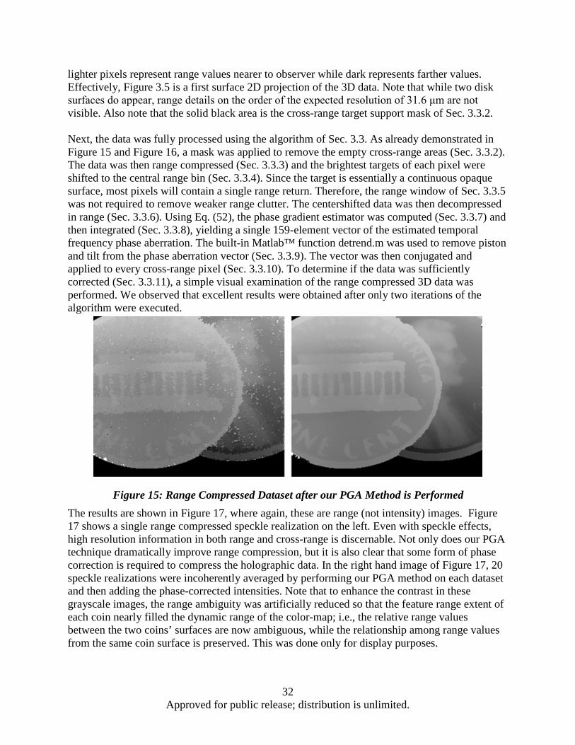
32 Approved for public release; distribution is unlimited.
lighter pixels represent range values nearer to observer while dark represents farther values. Effectively, Figure 3.5 is a first surface 2D projection of the 3D data. Note that while two disk surfaces do appear, range details on the order of the expected resolution of 31.6 μm are not visible. Also note that the solid black area is the cross-range target support mask of Sec. 3.3.2. Next, the data was fully processed using the algorithm of Sec. 3.3. As already demonstrated in Figure 15 and Figure 16, a mask was applied to remove the empty cross-range areas (Sec. 3.3.2). The data was then range compressed (Sec. 3.3.3) and the brightest targets of each pixel were shifted to the central range bin (Sec. 3.3.4). Since the target is essentially a continuous opaque surface, most pixels will contain a single range return. Therefore, the range window of Sec. 3.3.5 was not required to remove weaker range clutter. The centershifted data was then decompressed in range (Sec. 3.3.6). Using Eq. (52), the phase gradient estimator was computed (Sec. 3.3.7) and then integrated (Sec. 3.3.8), yielding a single 159-element vector of the estimated temporal frequency phase aberration. The built-in Matlab™ function detrend.m was used to remove piston and tilt from the phase aberration vector (Sec. 3.3.9). The vector was then conjugated and applied to every cross-range pixel (Sec. 3.3.10). To determine if the data was sufficiently corrected (Sec. 3.3.11), a simple visual examination of the range compressed 3D data was performed. We observed that excellent results were obtained after only two iterations of the algorithm were executed.
The results are shown in Figure 17, where again, these are range (not intensity) images. Figure 17 shows a single range compressed speckle realization on the left. Even with speckle effects, high resolution information in both range and cross-range is discernable. Not only does our PGA technique dramatically improve range compression, but it is also clear that some form of phase correction is required to compress the holographic data. In the right hand image of Figure 17, 20 speckle realizations were incoherently averaged by performing our PGA method on each dataset and then adding the phase-corrected intensities. Note that to enhance the contrast in these grayscale images, the range ambiguity was artificially reduced so that the feature range extent of each coin nearly filled the dynamic range of the color-map; i.e., the relative range values between the two coins’ surfaces are now ambiguous, while the relationship among range values from the same coin surface is preserved. This was done only for display purposes.
Figure 15: Range Compressed Dataset after our PGA Method is Performed

33 Approved for public release; distribution is unlimited.
The apparent contrast of Figure 17 is entirely due to differential range values across pixels and is not at all dependent on reflectance differences. This suggests that range compression of holographic ladar is useful for extracting detail from low contrast targets, even before fully exploiting the 3D nature of the data.
Next, in Figure 18, the data was rotated to highlight the surface relief and the targets’ separation in range. The image was generated using the surfl routine in Matlab™. Range compression reveals fine details that are highlighted at this angle, including the buttresses and tripods flanking the stairs of the Lincoln Memorial, and the carved scroll on the memorial’s cornice. To confirm the range resolution achieved by applying our PGA technique, the ideal point response (IPR) was estimated, as shown in Figure 19. To do so, a known flat area of the target was identified, in this case, the region below the memorial steps. This was done to ensure only one range bin of the data would be occupied. Furthermore, to ensure maximum signal, a single pixel from that region containing a strong return, or bright speckle, was then isolated. Finally, the intensity, as a function of range, was extracted from this pixel to estimate the IPR. As is evident in the left plot of Figure 19, no significant range compression was accomplished with the uncorrected data, while the IPR peak is prominent in the center plot when PGA corrections were applied. The theoretical IPR is shown with the data estimate in the right-most plot where the estimate of the range resolution achieved was approximately 35 μm. This was calculated from the 3 dB full width of the peak and is in good agreement with theory. The effects of the strong sidelobes manifested in the data as relatively bright ghosting artifacts within the ambiguity range. Fortunately, these ghost images were easily identified and removed. To do so, the fully corrected 3D intensity data was rotated and viewed from the side, where the main target image and the
Figure 16: 3D Solid Data Presentation

34 Approved for public release; distribution is unlimited.
fainter ghost images were readily apparent. A range window was then applied to remove the unwanted images.
3.5 PGA Performance for 3D Holographic Data To determine the theoretical performance of our PGA technique for 3D holographic ladar, a Monte-Carlo simulation was created. Twenty-eight SNR values were selected and, for each value, a dataset was created and corrected as follows. A uniform amplitude planar target of 128x128 pixels was created and located in the central range bin of a 3D volume. A Gaussian phase representing a surface roughness on the order of the nominal wavelength (λ0 = 1.55 μm) was then applied. The complex field of the target was then propagated by a FFT to the sensor plane at 64 equally spaced frequencies (Δν = Δω/2π = 75.7 GHz). This led to an unambiguous 3D volume of 2 mm with a range resolution of 31.6 μm. The resolution matches our experiment, while the number of frequencies and their spacing was changed for reasons discussed below. The complex field at the sensor plane was then cropped to a pupil size of 22x22 pixels (again, to be explained shortly), simulating the physical process of a finite aperture sampling a field with a much larger spatial extent. When implemented properly, this lowpass filtering step ensures that realistic speckle statistics are realized [42]. At each frequency, a single random phase value ψp(nΔω) was then added to the entire field, where the p subscript signifies prescribed. This number simulated an unknown phase error for that frequency. In addition, to simulate shot noise, a circularly complex Gaussian random number was added to the field (as described in [42]). The noise power was in turn scaled according the SNR value of the iteration. Our PGA technique, as defined in Sec. 3.3, was then performed. Since the model contained no clutter and the target was confined to the central range bin, neither centershifting nor windowing was necessary. Therefore, only one iteration of the algorithm was required. The residual phase gradient mean square error (MSE) ϵ of the corrected field was then calculated according to 𝜖𝜖 = ⟨ �∇𝑎𝑎(𝑛𝑛Δ𝜔𝜔) − ∇𝐿𝐿𝐿𝐿(𝑛𝑛Δ𝜔𝜔)�
2 ⟩ , (54)
where ∇p and ∇ML are the gradients of the prescribed phase and the phase correction estimate given by the PGA estimator, respectively. Finally, 50 trials were run over which a new random draw of the speckle, noise and prescribed phase were implemented, after which the MSE was
Figure 17: IPR Estimates for the Uncorrected Data (left), and PGA Corrected (center)

35 Approved for public release; distribution is unlimited.
calculated and stored. This process was repeated for each SNR value. The resulting average MSE ϵ̂, as a function of SNR, is plotted in Figure 20. The phase gradient estimator of Eq. (52) can be shown to be a maximum likelihood estimator
[41,43,44]. A MLE is asymptotically efficient, meaning that for sufficiently large data records, its MSE approaches the theoretical minimum, known as the Cramer-Rao lower bound (CRLB) [45]. The CRLB for the gradient between two neighboring phasors of the model described here, in terms of SNR and number of image pixels Lpix, has been shown to be [41,45-47]
𝐶𝐶𝐶𝐶𝑅𝑅𝐵𝐵 =1 + 2𝐼𝐼𝑁𝑁𝑅𝑅2𝐶𝐶𝑎𝑎𝑖𝑖𝑚𝑚𝐼𝐼𝑁𝑁𝑅𝑅2
. (55)
Figure 20 shows the CRLB for Lpix = 484 corresponding to an image dimension of 22 x 22 pixels. The number of pixels as well as the number of frequencies was chosen so that CRLB and ϵ plots in the central portion of Figure 20 are virtually identical to those in Figure 2 of [41]. As is evident in the figure, the mean square residual error ϵ̂ approaches the CRLB. Although not shown in Figure 20, ϵ̂ will diverge from the CRLB at higher SNR. This phenomenon is due to speckle saturation and has been well documented [46]. As SNR decreases, the estimator can be seen to diverge a bit from the CRLB, first by producing slightly higher MSE and then by asymptotically approaching 5.17 dB. As alluded to in Sec. 3.1, it may be advantageous to operate 3D holographic ladar systems in the low SNR regime where the algorithm begins to degrade in performance, as shown in the upper left of Figure 20. To gain greater insight into the algorithm’s behavior there, we propose another method of analyzing the phase statistics of our model. The goal of applying PGA techniques to our data is to estimate some phase that is constant over all pixels of the same frequency which must be computed from a measurement of the vector sum of the desired phasor and a noise phasor. The sum of Eq. (52) over the pixels allows us to invoke the Central Limit Theorem and declare a Gaussian distribution for the noise, independent of the actual underlying distributions. Alternately, we can show that in a shot noise limited scenario (a goal of all well designed holography systems), the Poisson statistics of the shot noise are well approximated by a Gaussian
Figure 18: The CRLB, Mean Square Phase Error, and Theoretical Phase Error for Random Phasor Sum Plus a Constant Phasor

36 Approved for public release; distribution is unlimited.
distribution. So, the challenge for the algorithm is to estimate a constant signal phasor in the presence of Gaussian noise. Goodman describes exactly this scenario in [42], calling it “a random phasor sum plus a known phasor.” He gives the marginal probability density function for the estimator phase as
𝑒𝑒𝜃𝜃(𝜃𝜃) =𝑒𝑒−
12𝛽𝛽
2𝜋𝜋+ �
12𝜋𝜋𝜋𝜋
�𝑒𝑒−sin2 𝜃𝜃2𝛽𝛽 �
1 + erf�𝑐𝑐𝑐𝑐𝑠𝑠𝜃𝜃�2𝜋𝜋
�
2cos 𝜃𝜃,
(56)
where β is the estimator’s SNR and the error function is defined as
erf(𝑒𝑒) =2√𝜋𝜋
� e−𝑜𝑜2𝑑𝑑𝑡𝑡𝑚𝑚
0. (57)
To better define β, recall that Eq. (55) defines the minimum MSE and, for unbiased estimators, the MSE and variance of the estimator are equal. This suggests that the inverse of the CRLB is a normalized SNR for 𝜓𝜓�𝐿𝐿𝐿𝐿. Furthermore, for a given detection SNR, it is the maximum achievable estimator SNR. Accordingly, we define
𝜋𝜋 =1
𝐶𝐶𝑅𝑅𝐶𝐶𝐵𝐵. (58)
Finally, using Eq. (56), the phase variance can be calculated according to
𝜎𝜎𝜃𝜃2 = � 𝜃𝜃2𝑒𝑒𝜃𝜃(𝜃𝜃)𝑑𝑑𝜃𝜃𝜋𝜋
−𝜋𝜋 . (59)
Equation (59) is also plotted in Figure 20 and is seen to accurately predict the behavior of ϵ̂ in the low SNR regime. The saturation of the average MSE occurs as the angle of the resultant phasor becomes dominated by the contributions of the noise phasor. The phase distribution converges to a uniform distribution over (-π ,π] which has a variance of 5.17dB. Since the phase is modulo 2π, this represents a state of maximum entropy. we therefore call this behavior the maximum entropy saturation of the estimator. The plots of ϵ̂ and Eq. (59) can both be seen asymptotically approaching this value in Figure 3.9. This suggests that operation at detection SNR values lower than -10dB, for the modeled parameters, is intractable. That is the range phase aberration cannot be computed. Equation (55) does suggest that a larger detector array; i.e., increasing Lpix, will lower the CRLB thereby improving estimation performance. To realize any further improvements, an estimator other than the one described here must be found. For clarity, we have described the algorithm and its performance using a conceptually simple form of the phase gradient estimator. As mentioned earlier, we have chosen a phase gradient MLE based only upon consideration of nearest neighbor phase differences. However, a MLE for the phase differences between temporal frequency images, of arbitrary separation, can be found by considering the covariance matrix of the data resulting from the range decompression step (step 6) of Figure 13 [41]. Given N frequency images, the N x N, covariance matrix is computed

37 Approved for public release; distribution is unlimited.
and its principle (i.e., largest) eigenvalue is determined. The phase of the corresponding eigenvector is the estimate of the temporal frequency image phase differences we seek. In practice, implementation of these steps is straightforward; we simply use the Matlab™ functions cov.m and eigs.m to calculate the covariance matrix and eigenvectors, respectively. The above steps are then inserted into the algorithm in lieu of steps 7-8 of Figure 13 and offer the advantage of now allowing more than just adjacent phasor pairs to be considered when calculating the phase aberration correction. For this estimator, the CRLB is generalized to
𝐶𝐶𝐶𝐶𝑅𝑅𝐵𝐵 =1 + 𝑀𝑀 × 𝐼𝐼𝑁𝑁𝑅𝑅𝑀𝑀 × 𝐶𝐶𝑎𝑎𝑖𝑖𝑚𝑚𝐼𝐼𝑁𝑁𝑅𝑅2
, (60)
where (M-1)Δω is the maximum temporal frequency image separation considered in the calculation of the covariance matrix. This is implemented by calculating the full covariance matrix and then setting all values of the diagonals exceeding (M-1) to zero. Note that M = 2 in Eq. (55) since only the covariance (phase difference) of nearest neighbor samples was considered. To evaluate the performance of this estimator in our algorithm, the Monte-Carlo simulation was
again performed using the eigenvector phase difference estimation method; all other parameters were unchanged. As shown in Figure 21, and predicted by Eq. (60), when the parameter M is increased, the CRLB is decreased. As with Eq. (55), Eq. (60) shows that the CRLB can be decreased by increasing Lpix. 3-D holographic datasets are often much larger than those of 2-D SAR making large Lpix and M values easy to achieve. As shown in Figure 21, the eignvector method is much more robust in low SNR environments. Finally, we have observed that increasing M and Lpix reduces the number of iterations required; however, the computation load per iteration is often increased.
3.6 Conclusion Range compressed holographic ladar is sensitive to phase aberrations distributed over temporal frequency. To address this, we have described a novel application of the PGA technique to range
Figure 19: The CRLB and Mean Square Phase Error Using the Eigenvector PGA Estimator

38 Approved for public release; distribution is unlimited.
compressed holographic ladar. Holographic images formed before range compression provide the opportunity to apply a cross-range target support mask. With reasonable detection SNRs, it is not usually necessary to window the strongest range returns because of the limited number of scatterers in that dimension. While the PGA method is an iterative process, typically only a few iterations are required for range compressed holographic ladar. In a laboratory experiment, we demonstrated a significant improvement in range compression when the modified PGA steps described were applied to the data. In fact, for this configuration, where discrete temporal frequencies with unknown phase offsets are used, it was determined that a phase correction algorithm was essential for range compression. To help quantify the performance, the IPRs for the uncorrected and PGA corrected data were estimated and improvement of the IPR is clearly shown for the latter case. With a numerical model and a canonical target, the estimator was demonstrated to be asymptotically efficient for this application. Additionally, the maximum entropy saturation behavior of the estimator was analytically described. This has implications for 3-D holographic ladar operation at low SNR and a possible solution was proposed with the use of a more sophisticated and generalized form of the estimator. As clearly demonstrated in Figure 20, the modified PGA method using the MLE of Eq. (52) yields optimal results for phase aberration correction along the temporal frequency bins of 3-D holographic ladar. The maximum entropy saturation of the estimator at low SNR can also be accounted for analytically. For improved performance in low SNR environments a more efficient phase estimation kernel such as the eigenvector method can be utilized, as demonstrated in Figure 21. For range compressed holographic ladar, phase correction of aberrations across temporal frequency is critical. Whether due to the discrete stepped frequency waveform imposed on the laser or to atmospheric effects, the stochastic nature of the aberration lends itself to estimation methods already developed for SAR. We have presented a modified version of the PGA method, tuned specifically for the data format of holographic ladar, which leverages some of its unique aspects and rapidly converges to an accurate solution that enables excellent range compression performance.

39 Approved for public release; distribution is unlimited.
4 RANGE COMPRESSION FOR HAL Holographic aperture ladar (HAL) is a 2D aperture synthesis technique that improves resolution in the azimuth cross-range dimension [25,26]. Due to the increased size of the synthetic aperture, the cutoff frequency of the modulation transfer function (MTF) is improved, allowing higher object spatial frequencies to be present in the image. Venable et al., mapped the HAL MTF using high contrast Ronchi ruling targets and demonstrated near diffraction limited performance [28]. However, as its name implies, the MTF is dependent on modulation depth (i.e., contrast) of the object, and if that contrast is low for the newly accessible spatial frequencies, then the full benefit of HAL cannot be realized without additional information and processing. Introducing temporal frequency diversity to the HAL method can address the low contrast challenge, while also providing other benefits such as improved object recognition and image interpretation, associated with the resulting 3D output imagery. This is a natural extension of the stationary (i.e., no aperture synthesis) method demonstrated by Marron and Gleichman where up to 62 frequencies were used to obtain 3D images in a phase-stepping interferometry system [21,22,32]. A variant of this method has been shown to achieve motion compensated imagery despite the long integration times required by the low bandwidth detector array normally used in digital holography [12,33]. While the details of these 3D digital holography approaches differ, they are all capable of range resolving multiple targets that exist within the same pixel; however, the cross-range extent of those pixels is limited by the receiver aperture. Two methods of range compression for holographic aperture synthesis have recently been demonstrated. The first performed HAL with a spatial heterodyne technique to increase azimuth cross-range resolution while also using 256 discrete frequencies to create 3D imagery [51]. The discrete frequencies allowed for the use of a conventional low bandwidth detector array. Aperture synthesis was accomplished by a hybrid spatial/temporal method where object rotation was used to increase angular diversity and each subaperture record was temporally separated. This method is distinct from spatial-only methods where subapertures are physically separated, with no reliance on platform or target motion, and ostensibly, can be collected simultaneously [29]. A low contrast target was used, giving 2D HAL imagery that possessed virtually no discernable content. Once the range information was added however, the HAL-sharpened azimuth cross-range content was clearly visible. The second method demonstrated holographic aperture synthesis along with range compression in the more traditional sense; i.e., with a temporally heterodyned chirped waveform [52]. This required the use of a “fast” focal plane array (FPA). The local oscillator was not only offset in temporal frequency, it was also spatially offset. Aperture synthesis was performed by temporally isolating different regions of the FPA and then digitally reassembling them later in a coherent manner. In this chapter the results of the first range compressed HAL experiment using discrete frequencies and a rotating target are presented. Additional experimental results are then presented where point targets are used to quantitatively demonstrate the performance of 3D HAL. By purposefully limiting the range and elevation resolution of the experiment, so that the targets are unresolved in those dimensions, we demonstrate a remarkable synergistic effect whereby two targets can be discriminated and precisely located due to the coaction of range compression while simultaneously using HAL to resolve the targets in the azimuth cross-range dimension.

40 Approved for public release; distribution is unlimited.
4.1 Background As detailed in Sec. 2.3, 2D holographic images can be collected utilizing discrete, sequential frequencies. These images can then be compressed, by way of a Fourier transform, to recover true 3D scene information. However, capturing many discrete sequential frequencies while simultaneously synthesizing a pupil, as is required for HAL, has never been demonstrated and is the principal challenge to implementing range compression for HAL. In other words, this is the first demonstration of simultaneous aperture and pulse synthesis for spatial heterodyne systems. Discrete frequency 3D HAL methods consist of collecting a series of digital holograms at sequential temporal frequencies while the sensor and illumination source are moved with respect to a scene of interest. To realize resolution gains through HAL processing and to augment the data set with range information, the pupil plane complex field segments must first be properly placed in a composite 3D array. Additionally, each field segment will require a phase correction to compensate for any errors or undesirable piston offsets between it and its neighbors. Among segments of the same frequency, these offsets can be due to the evolving geometrical relationship between the target and the sensor. Atmospheric induced phase effects or unknown laser phase drifts may also affect the phase relationship between segments of differing temporal frequency. If the exact values of R0, θ, and λ are all known for each field segment, then the transformation of Eq. (7) can be digitally applied and the composite field array can be transformed via a 3D inverse discrete Fourier transform (IDFT) to yield a 3D target image. In practice, however, these values may not be known with the precision required for the data to be coherently combined. Instead, the 2D pupil plane field segments are first inserted into a composite array based on estimated values for these parameters and then data driven methods are used for final precision alignment [28,Sec. 3.3]. Each 2D pupil plane field segment is first placed in the composite array along a 3rd dimension according to its temporal frequency. It is then preliminarily shifted in the azimuth cross-range dimension according to the left hand side of Eq. (7). To achieve diffraction limited performance, this shift will need to be refined further to sub-pixel accuracy and the tilt and piston phase of the right hand side of Eq. (7) will need to computed and applied. The steps to determine and apply these necessary fine corrections, using data driven algorithms, are described in detail in [28]. After these steps are implemented, the resulting 3D composite array will contain a set of 2D synthetic apertures, ordered in the third dimension according to increasing temporal frequency. To compress along the range dimension, further corrections are required to compensate for unknown phase errors due to laser drift and atmospheric induced aberrations. As described in Sec. 3.3, a modified form of the phase gradient algorithm (PGA) can be applied to the dataset to correct for these effects. Since discrete frequencies are used in this experiment, where no attempt was made to track the phase of the laser, either this or some other phasing method is required in order to achieve range compression. These two data driven compression steps allow the use of conventional low bandwidth detectors and slow speed tunable lasers, while relaxing the need to precisely track the transceiver or target motion. In the following section we describe a scenario where the two compression algorithms are used to completely image a low contrast target.

41 Approved for public release; distribution is unlimited.
4.2 Low Contrast Range Compressed HAL Figure 22 shows the general layout for a range compressed HAL experiment with a focal plane spatial heterodyne configuration (see Appendix B for additional specs). The setup and hardware was virtually identical to Figure 14. The range was increased to 22 m (indoors) and the distance to the detector was adjusted appropriately to satisfy the imaging condition for the f = 500 mm imaging optic.
To demonstrate resolution gains in both cross-range and range, a custom target was designed with fine inner details only resolvable through aperture synthesis and range compression. The target also contained coarse outer details that were just resolvable by a single subaperture. Figure 23 shows the target mounted to the rotation stage and tilted vertically away from the sensor by 40o. The target consists of 36 aluminum blades (360 mm X 25.4 mm X 1.57 mm), stacked and rotated by 5° each. A flat surface finish was achieved by lightly sandblasting the blades before assembly. By design, this is a low contrast target which is evident in Figure 23 and 24, even when it is illuminated with off-axis incoherent lighting.
Figure 20: Layout for Range-Compressed HAL Experiment

42 Approved for public release; distribution is unlimited.
The data was collected at a nominal illumination frequency of 191.6 THz ( λ0 = 1.565 μm). Here, a sweep of 213.33 GHz was used, giving a range resolution of approximately 700 µm. A step size of 0.8328 GHz was also found from Eq. (33). In this case, due to known target symmetry, an ambiguity equal to just over half of the tilted target’s range extent was allowed and later unwrapped. This decreased the amount of data collected by a factor of two.
Figure 21: Diffuse Helix Target

43 Approved for public release; distribution is unlimited.
The most important distinction between this experiment and the one described in Sec. 3.4 is the data processing. In particular, the rotation of the target was used here for the primary purpose of aperture synthesis; i.e., the data was later coherently combined in the azimuth cross-range dimension. As described in Sec. 2.1, an inverse-circular configuration was used where the target was rotated and the receiver/transmitter remained stationary. The square sub-apertures, each with a side length of 3.1mm spanned 32 speckles in each cross-range dimension yielding a theoretical cross-range resolution of 1.125 cm. The target was rotated such that consecutive sub-apertures
Figure 22: Close-Up Images of the Diffuse Helix Target
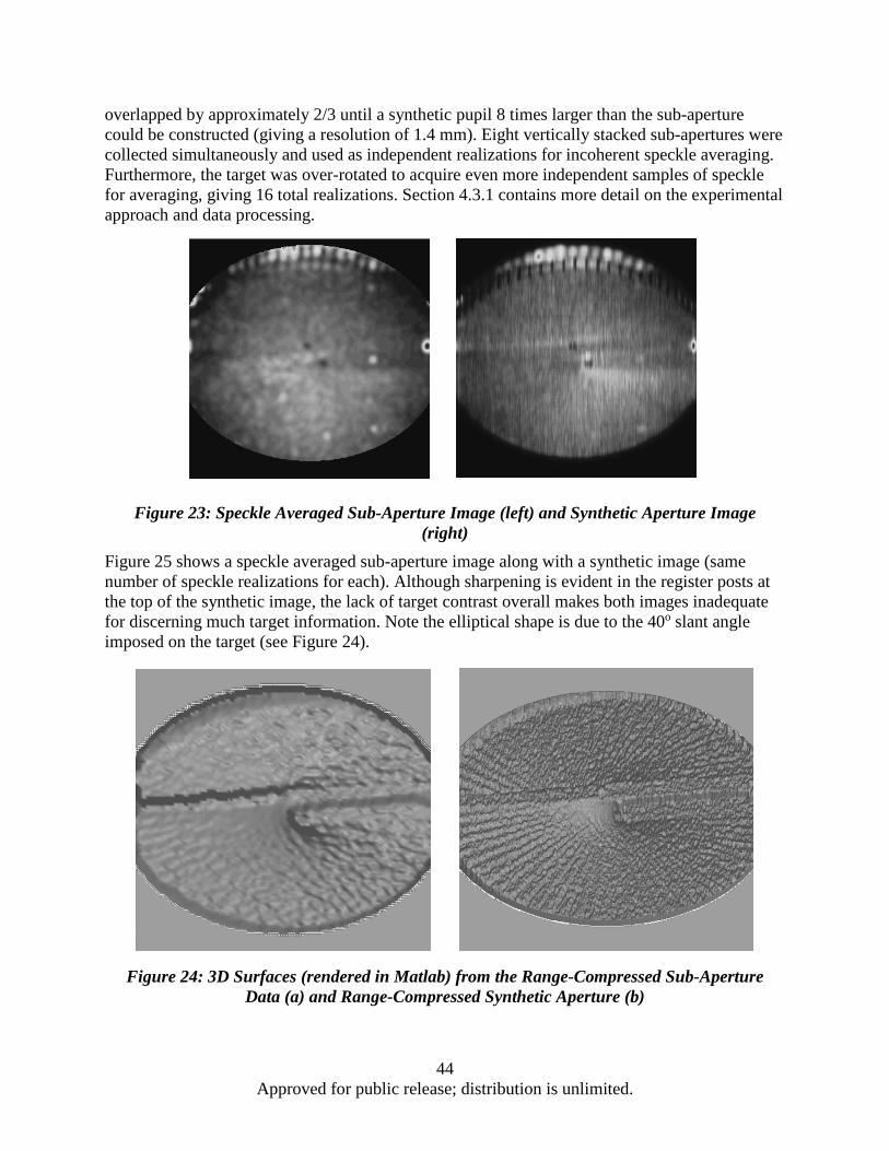
44 Approved for public release; distribution is unlimited.
overlapped by approximately 2/3 until a synthetic pupil 8 times larger than the sub-aperture could be constructed (giving a resolution of 1.4 mm). Eight vertically stacked sub-apertures were collected simultaneously and used as independent realizations for incoherent speckle averaging. Furthermore, the target was over-rotated to acquire even more independent samples of speckle for averaging, giving 16 total realizations. Section 4.3.1 contains more detail on the experimental approach and data processing.
Figure 25 shows a speckle averaged sub-aperture image along with a synthetic image (same number of speckle realizations for each). Although sharpening is evident in the register posts at the top of the synthetic image, the lack of target contrast overall makes both images inadequate for discerning much target information. Note the elliptical shape is due to the 40o slant angle imposed on the target (see Figure 24).
Figure 23: Speckle Averaged Sub-Aperture Image (left) and Synthetic Aperture Image (right)
Figure 24: 3D Surfaces (rendered in Matlab) from the Range-Compressed Sub-Aperture Data (a) and Range-Compressed Synthetic Aperture (b)

45 Approved for public release; distribution is unlimited.
Figure 26 shows a surface interpolation of the full 3D dataset for both apertures. The target blades can just be resolved in the lower left of the sub-aperture image. In the synthetic image, they can be resolved deep into the center in many locations, clearly demonstrating significant aperture gain. A hallmark of synthetic aperture imagery is asymmetric pixels caused by resolution gain in only one dimension. While close inspection of the speckle of Figure 26 confirms this, we would also expect this to be manifest in Figure 26, where resolution is unchanged in the vertical dimension; i.e., the horizontal blades should be blurred out to a larger radius than the vertical ones. However, this is not fully evident in Figure 26 due to the addition of high range resolution, the slant angle of the target and human visual interpolation. Clearly though, full 3D data is critical to resolving this target’s content as is evident in a comparison of Figure 25 and Figure 26.
To further validate the results, a numerical model was used to generate imagery for comparison. A 3D CAD model of the target was imported into MATLAB where a surface roughness (modeled as a normal Gaussian random variable with σ = 2 λ0) was then added. The backscattered complex field at the target was then generated in the same manner as Sec. 3.5. All experimental parameters such as number of frequencies, frequency sweep, range, aperture size, etc. were accurately simulated in the numerical model. No phase noise or frequency jitter was applied to the model. Instead of simulating target rotation to accomplish aperture synthesis, a very large pupil plane field that accommodated the entire synthetic pupil was generated. An aperture window, appropriately sized for either the synthetic or sub-aperture, was then applied. This ensured a diffraction limited estimate for both cases in the simulation. Figure 27 shows a comparison of the modeled and experimental data. The top row is sub-aperture data and the bottom contains the synthetic apertures, while the left column is the modeled data and the right is from the experiment. Again, the modeled data contains no noise (other than speckle) and has no
Figure 25: A Comparison of Numerically Modeled Data to Experimental Data

46 Approved for public release; distribution is unlimited.
residual phase errors due to aperture synthesis or temporal frequency errors. The same speckle averaging and filtering was used all cases. Due to the similarity of the model and the data, it is clear that the experimental images are nearly diffraction limited.
Figure 28 shows the data (reprocessed) to qualitatively illustrate the challenges with independently performing either range compression or aperture synthesis, in isolation, on low contrast targets. In Figure 28(a), a conventional photograph of our target is shown. The holes in
Figure 26: Low Contrast 3D Target

47 Approved for public release; distribution is unlimited.
the radial blades, not visible with the original processing method (see Figure 27), are separated by approximately 15 mm. Recall that, by design, this is a low contrast target and the contrast of Figure 28(a) is almost entirely due to overhead illumination, resulting in shadowing of the range discontinuities of the radial blades. The boxed region of Figure 28(a) was cropped and enlarged to create Figure 28(b). Figure 28(b)-(f) then all have the same fields of view. In Figure 28(c), a single subaperture reconstructed hologram image of the target is displayed. Here, the target was placed at a range of z = 22 m and flatly illuminated at a nominal wavelength λ0 = 1.55 μm. The subaperture pupil diameter was Dap = 3.2 mm and the image represents an average of 64 independent speckle realizations. Despite sufficient cross-range resolution of λ0z/Dap = 10 mm and speckle averaging, no structure is evident. The illumination of the target was nearly on-axis, virtually eliminating all shadows, which along with the lack of target contrast, explains the lack of discernable features. As shown in Figure 28(d), multiple frequencies were then used to reconstruct a 3D surface according to [21,51]. Since we now possess range information about the target, we no longer have to rely solely on contrast to form an image. To create Figure 28(d), the range value corresponding to the maximum intensity of each cross-range pixel was recorded and then displayed using the surfl routine in Matlab. This image has the same cross-range resolution as Figure 28(c) and a range resolution of c/2B = 2.9 mm, where c is the speed of light and B = 51.7 GHz is the overall bandwidth of the multiple frequencies used. The improvement of Figure 28(d) over (c) is noticeable. A target is now conspicuously visible. Ultimately, though, the addition of range resolution is enough to delineate the boundary of the target and little else. Next, Figure 28(e) is a single frequency reconstructed IC-HAL image with ISRIC = 8 in both the azimuth and elevation cross-range dimensions. This image also represents an average of 4 independent speckle realizations. Again, despite excellent azimuth cross-range resolution of λ0z/(8Dap) = 1.25 mm and some speckle averaging, no detail is evident. Figure 28(d) and (e) clearly demonstrate the limitations of applying, in isolation, either range or cross-range compression for low contrast targets. Finally, though, in Figure 28(f) we show the reconstructed 3D HAL image, where cross-range and range compression have both been simultaneously performed. This image has the same range and cross-range resolution as Figure 28(d) and (e), respectively, yet has far more visible detail than either. While HAL provides the potential to discern fine cross-range details, it is ineffective here due to the lack of target contrast. Similarly, range-compression can provide direct range information with no reliance on contrast, but here it is insufficient to resolve the cross-range details that make a useful image. Applying the two techniques in concert however, unlocks the full image formation potential of each. The improvement in image quality due to the coaction of range compression and aperture synthesis is dramatic and cannot be accounted for when either is performed in isolation. This synergistic phenomenon will be quantitatively explored in the following sections.
4.3 Point Targets with Range Compressed HAL A new experiment was designed with the goal of not only demonstrating 3D HAL but also to analyze the object discrimination enhancement this imaging modality affords.

48 Approved for public release; distribution is unlimited.
4.3.1 Experimental design In this section we describe the experimental setup and the data processing.
4.3.1.1 Setup and target Figure 4.8(a) shows the general layout of the experimental apparatus. An image plane spatial heterodyne configuration was used with an imaging optic placed in the pupil plane 0.5 m from a 320 x 256 InGaAs focal plane array (FPA) having a 30 μm pixel pitch. A tunable laser (not shown) at center wavelength λ0 = 1.55 μm, was split into local oscillator (LO) and transmitter (TX) fiber optic paths. The TX output was collimated at the pupil plane, after which the beam propagated in free space to the target, located approximately 22 m from the pupil.
The pupil plane is shown in Figure 29(b), where an imaging optic was masked to create a rectangular pupil 5.7 mm wide in the azimuth cross-range dimension. This was later digitally cropped to create a square subaperture with Dap = 5.5 mm. The subaperture, or native, resolution of the system was therefore λ0z/Dap = 6.2 mm. The vertical extent of the rectangular pupil was used to simultaneously collect multiple independent speckle realizations, after additional cropping. Also in the pupil plane, the LO was inserted as a bare fiber tip and directed back toward the detector. Vertically centered and placed adjacent to the rectangular mask, it was propagated through the imaging lens, toward the detector. On arrival at the detector, the LO mixed with the image of the target on the focal plane, where the resulting intensity of the interference pattern was then recorded. In all cases, the LO power was adjusted to ensure shot noise limited performance. The target, described in detail later, was mounted to a high precision rotation stage (PI M-038.DG1) capable of discrete rotation angles as small as θ = 0.0017°. From the geometry of
Figure 27: Experimental Geometry

49 Approved for public release; distribution is unlimited.
Figure 29(a), we find that the resulting subaperture shift for this angle is R0tan(2θ) = 1.3 mm. For a subaperture diameter of 5.5 mm, this rotation angle provided consecutive pupil field data segments that nominally overlapped in the azimuth cross-range dimension by 76%, ensuring accurate pupil plane field segment registration for the data driven HAL algorithm. After propagation to the target, a hologram of the TX field backscatter was captured by the detector FPA. The reconstructed pupil plane image of Figure 30 was then created by 2D inverse transforming the corresponding fringe data. (For details of the digital holography processing used to create Figure 30, the reader is referred to [38,39]). As previously mentioned, and as illustrated in Figure 30, a rectangular pupil was used so that multiple independent speckle realizations of the subaperture could be collected simultaneously.
The two vertical rectangles of brighter speckle in Figure 30 are the conjugate images of the masked pupil of Figure 29(b). Their horizontal separation from the autocorrelation terms centered in the image are proportional to the horizontal offset of the LO as shown in Figure 29(b). The vertical stacked boxes overlaid on Figure 4.9 represent five digitally cropped subapertures, each having an independent speckle realization. Every cropped subaperture contained 48x48 speckles which, due to rotation of the target, appeared to sweep from right to left through the boxes, simulating an opposing sensor motion in the aperture synthesis direction shown. Subapertures were then combined to create synthetic apertures as in [25, 26, 28]. The five vertically stacked synthetic apertures were processed independently; e.g., the top subaperture in Figure 30 was coherently combined with only the other top subapertures from the collection of discrete angular steps. The final synthetic apertures consisted of Nap = 18 overlapping sets of complex pupils. Given an overlap of 76%, the synthetic aperture width was nominally 𝐷𝐷𝑆𝑆𝑆𝑆𝑅𝑅𝐼𝐼𝐼𝐼 = 𝐷𝐷𝑎𝑎𝑎𝑎�𝑁𝑁𝑎𝑎𝑎𝑎(1 − .76) + 1� = 29.26 𝑚𝑚𝑚𝑚, (61)
Figure 28: Reconstructed Pupil Plane Data Showing Simultaneous Capture of Independent Speckle Realizations

50 Approved for public release; distribution is unlimited.
or 5.3X larger than the subaperture in the azimuth cross-range dimension. This gives a theoretical azimuth resolution of λ0z/DSAR,IC = 1.17 mm. The actual size of the synthetic pupil showed some variance (<5%) due to the precision of the stage and stability of the target. While the rotation stage was used to introduce the angular frequency diversity necessary for aperture synthesis, the tunable laser was simultaneously used to introduce temporal frequency diversity necessary for range compression. To accomplish this, multiple holograms were recorded at discrete wavelengths for every target pose angle. Here, we used four separate wavelengths, each separated by Δf = 7.5 GHz for a total bandwidth of B = 30 GHz. The frequency separation was chosen so that the range ambiguity zamb encompassed all of the target points according to
𝑧𝑧𝑎𝑎𝑚𝑚𝑎𝑎 =𝑐𝑐
2𝛥𝛥𝑓𝑓= 20 𝑚𝑚𝑚𝑚, (62)
where c is the speed of light and the factor of ½ is due to the round trip travel of the pulse from the transceiver to the target and back. The total bandwidth provided a theoretical range resolution of 𝛥𝛥𝑧𝑧 = 𝑐𝑐
2𝐵𝐵= 5 mm. Notice that by design this is not sufficient to resolve, in range, the two most
closely spaced target points (separated by 2.5 mm) in our 3D target, which we will describe in detail next. To do so would have required a bandwidth of B > 74 GHz. (We should note that in practice we actually recorded data at 64 discrete frequencies (B = 480GHz) and used them all to mitigate phase errors over temporal frequency, as in Sec. 3.3. Doing so decreased the Cramer-Rao lower bound and allowed improved accuracy. However, for the experiment described herein we coherently combined images using only collections of four wavelengths, after which we then incoherently averaged over the full data set).
Instead of using a distributed diffuse, low contrast target, this experiment was designed to use discrete retro-reflective point targets. This eliminated the low contrast concerns described in Sec. 4.2 allowing us to measure key system performance metrics such as the cross-range point spread functions (PSF), range ideal point response (IPR) and the ISR. Figure 31 shows the 3D structure of the target. Three point targets were located at distinct ranges on the structure, where relative ranges to target points R1 and R2 are 2.5 mm and 12 mm, respectively, closer to the transmitter
Figure 29: 3D Drawing of the Target

51 Approved for public release; distribution is unlimited.
than is target point R0, itself located at relative range R0 from the transmitter. Target point R2 was intentionally isolated from the other two targets by a large separation in both range and cross-range dimension. This was sufficient to later extract uncorrupted cross-range PSFs as well as the range equivalent ideal point response (IPR). To create the targets, the stepped structure was first covered with 3M 8910 retro-reflective material. It was then covered with black gaffer tape with three small nominally rectangular areas left exposed. These areas were sized to appear as point targets; i.e., they are much smaller in all dimensions than the native single subaperture resolution, and are even narrower along the azimuth cross-range dimension to accommodate HAL image sharpening. These asymmetric resolution cells are a hallmark of any system where single dimension aperture synthesis is performed.
Figure 32 shows the cross-range detail of the targets. Figure 32(a) is a photograph of the full target showing all three of the retroreflective point target regions described above. Figure 32(c)
Figure 30: Cross-Range Target Details

52 Approved for public release; distribution is unlimited.
shows a cropped image of only the (R0, R1) pair which were spaced so that the native resolution due to a single subaperture would be insufficient to resolve them in either cross-range dimension. This is clearly demonstrated in the single subaperture reconstructed hologram images of Figure 32(b) and (d). Recall from Figure 31 that the target points were also separated by 2.5 mm in range, information that would be unrecoverable with conventional 2D HAL. Also, notice the diagonal fringes of the central autocorrelation terms in Figure 30. These are due to interference between the unresolved point target pair (R0, R1) and the isolated target (R2). The angle and separation of the fringes are directly related to the offset angle of the targets and the target separation/range ratio, respectively. Finally, recall the theoretical azimuth resolution is 1.17 mm after HAL processing, sufficient to resolve the (R0, R1) pair; however, since no aperture synthesis was performed in the elevation dimension, the (R0, R1) pair will always remain unresolved in that dimension.
4.3.1.2 Data processing The general data collection routine and coherent processing steps are summarized as follows. The laser was tuned to the first frequency and a hologram like that of Figure 30 was reconstructed. Five independent speckle realizations of the subaperture were digitally cropped and stored in separate datacubes. This was repeated as the target was rotated through 18 discrete angular poses. At each rotation the five speckle realizations were stored in their respective datacubes and nominally placed in the correct location based on Eq. (7) and the current laser frequency. The target was then rotated back to the original position, the laser was tuned to the next frequency and the process was repeated. Once the laser was tuned over all of the desired frequencies, the data driven compression routines described in [28] and Sec. 3.3 were implemented. This yielded five independent range compressed and HAL sharpened datasets. Finally, the intensities of the datasets were added to mitigate speckle. For point targets, speckle averaging was not necessary, but it was performed to be consistent with previous experiments, such as the one in 4.2. Also note that additional speckle realizations could be easily acquired by over-rotating the target, provided that the total target rotation was kept very small with respect to the scene width we used. This method was used to double the amount of speckle averaging.
4.3.2 Experimental results In this section we report some key system performance metrics that demonstrate the performance of applying image compression in both the range and azimuth cross-range dimensions. We also demonstrate object discrimination enhancement due to simultaneous range compression and aperture synthesis.
4.3.2.1 IPR, PSF and ISR measurements As noted above, the isolated target (R2) was used to verify the azimuth and range compression capabilities of the experiment. Figure 33 shows the corresponding range IPRs and cross-range PSFs for the system.

53 Approved for public release; distribution is unlimited.
In general, given the rectangular aperture shape, the sinc-squared function is expected for both the elevation and azimuth PSFs [1]. The azimuth PSF of the synthetic aperture is also expected to be 5.3X narrower than that of a single subaperture due to aperture synthesis. For all of the measured PSFs, the first sidelobe was below -12 dB, and in most cases it was near the ideal -13.26 dB. The sidelobes of the azimuth PSF for the synthetic aperture showed some asymmetry, however. This was most likely due to a residual asymmetric phase term over the synthetic pupil [53]. The range IPR, in both cases, has the same general shape as the PSFs. The temporal frequency spectrum of the properly phased ensemble of discrete frequency holograms is that of a sparsely sampled linear frequency modulated spectrum of uniform amplitude; i.e., a discretely sampled rectangle function. Therefore, the modulus squared of its Fourier transform is also a sinc-squared function, which the measured IPRs exhibited, although with slightly higher sidelobes at approximately -10 dB. Table 1 summarizes the range compression and aperture synthesis performance metrics of the experiment, where we report the 3dB and 6dB mainlobe widths for the various IPRs and PSFs.
Table 1: Experimental Performance Metrics Subaperture Synthetic Aperture Theoretical
3dB width [mm]
Measured 3dB width
[mm]
Theoretical 6dB width
[mm]
Measured 6dB width
[mm]
Theoretical 3dB width
[mm]
Measured 3dB width
[mm]
Theoretical 6dB width
[mm]
Measured 6dB width
[mm] Range 4.4 4.6 6.0 6.3 4.4 4.6 6.0 6.3 Azimuth 5.5 6.0 7.4 8.3 1.0 1.2 1.4 1.6 Elevation 5.5 6.1 7.4 8.5 5.5 6.0 7.4 8.3
It can be shown that the theoretical 3dB width Δx3dB reported in Table 1is
Figure 31: Range IPRs and Azimuth/Elevation PSFs for the 3D HAL Experiment

54 Approved for public release; distribution is unlimited.
𝛥𝛥𝑒𝑒3𝑑𝑑𝐵𝐵 = .88𝛥𝛥𝑒𝑒, (63) where Δx = λ0z/D and where D was either 5.5 mm or 29 mm for the subaperture or the synthetic aperture, respectively. Equation (63) also holds for the range IPR where Δx = Δz. Likewise, the theoretical 6dB width, Δx6dB can be shown to be 𝛥𝛥𝑒𝑒6𝑑𝑑𝐵𝐵 = 1.2𝛥𝛥𝑒𝑒. (64)
We observed that the system performance was nearly diffraction limited. The two key metrics of the range compressed HAL experiment are IPR mainlobe width and ISRIC from Eq. (10). The range IPR 3dB width for both the subaperture and synthetic aperture was 4.6 mm, which was within 4.5% of theory. The 6dB width showed slightly degraded performance. The ISR of the experiment was estimated to be 5.1 and was within 4.5% of theoretical expectations (ISRIC = 5.3). This was computed from the ratio of the synthetic to subaperture mainlobe widths and then averaged for the 3db and 6dB ratios. Sidelobes were reasonably well behaved in the range and cross-range responses, and the system performance allowed excellent image reconstruction, as demonstrated in the following section.
4.3.2.2 Object discrimination enhancement As illustrated in Sec. 4.2, range compressed HAL is a powerful technique for imaging low contrast targets. As shown in Figure 28, augmenting holographic ladar with range compression relaxes the dependence of image reconstruction on target contrast, enabling the full benefit of aperture synthesis to be realized. Furthermore, the coaction of range compression and aperture synthesis leads to unexpected imaging performance gains that are difficult to attribute to either of the compression methods alone. Figure 34, a 3D reconstruction of the (R0, R1) target pair, demonstrates this synergistic effect more precisely. In Figure 34(a) the subaperture intensity data is shown, while Figure 34(b) shows the corresponding synthetic aperture data. To create this image, the 3D intensity data was projected onto three orthogonal planes. Each plane was then rotated and appropriately placed to create the isometric images shown. The data cubes are approximately 30 mm X 30 mm X 20 mm (el, az, range) in size. In the subaperture image of Figure 34(a) the (R0, R1) pair is unresolved in all dimensions. Recall from Figure 31 that the pair is separated by 4 mm in both the elevation and azimuth cross-range dimensions, while the theoretical resolution of the subaperture is 6.5 mm. While range compression for holographic ladar can be beneficial in many cases, the theoretical range resolution of 5 mm is insufficient to resolve the pair, as they are separated by only 2.5 mm. Discerning the targets is made even more difficult by a phenomenon known as target masking [5] wherein a dim target (R0) is in close proximity to a bright one (R1) resulting in the former being concealed in the latter’s sidelobes. Despite the challenges posed by insufficient resolution and target masking, the mainlobe is distorted and asymmetrically stretched which, while inconclusive, suggests the presence of multiple targets. However, as we will demonstrate shortly, even a priori knowledge of target locations is insufficient to quantitatively identify them without the benefit of aperture synthesis.

55 Approved for public release; distribution is unlimited.
In Figure 34(b), the synthetic aperture image, two targets are readily identifiable. Note that the range and elevation resolutions are unchanged between the subaperture and synthetic aperture images. The only parameter that changed is the azimuth resolution, which has been improved by a factor of 5.1. The side projection of the synthetic aperture image clearly shows the two targets remain unresolved in the elevation and range dimensions. Remarkably, though, the top and front projections suggest that the two targets’ relative locations can now be precisely determined in all three dimensions. Furthermore, the target masking phenomenon has been significantly mitigated due to aperture synthesis along the azimuth cross-range dimension; not only has the R1 mainlobe width decreased, but its first sidelobe has retreated enough that target point R0 is no longer coincident with it. In this case, aperture synthesis appears to be a better solution for target masking than implementing a filter for sidelobe control, since the latter usually increases mainlobe width, thereby sacrificing some resolution gains. Figure 35 shows the normalized 1D target profiles for both targets and in all three dimensions. These were extracted from the 3D intensity data by extracting the three orthogonal intensity profiles that intersect with the peak intensity location for each target point. Since the targets are completely unresolved in the subaperture image, the peak locations were first found from the synthetic aperture data.
Figure 32: 3D Reconstructions of the (R0, R1) Target Pair

56 Approved for public release; distribution is unlimited.
As expected, there is significant overlap of the profiles in the subaperture data; i.e., the target points are very poorly resolved. Even with foreknowledge of the target locations, it is virtually impossible to distinguish them. The bottom row of Figure 35 contains the synthetic aperture results. Though distinguishable in the synthetic aperture data, the (R0, R1) pair are poorly resolved in the range and elevation dimensions. Recall that the peak of one profile should fall exactly on the first zero of the other in order to be considered well resolved, according to the Rayleigh criteria. Also, the mainlobes of a well resolved pair would intersect at a normalized magnitude of approximately 0.4. In the synthetic aperture data, the profiles intersect at 0.837 and 0.795 in the range and elevation dimensions, respectively. In the azimuth cross-range dimension, the (R0, R1) pair are well resolved, however, due to aperture synthesis in that direction. Here, R0 appears smaller than R1 despite the fact that both profiles have been normalized. This is because the targets are unresolved in the other two dimensions. That is, the azimuth profile for R0 also encounters the mainlobe energy of R1, which is greater than the former. This can also be seen in Figure 34 by visualizing an azimuth trace of the synthetic aperture front (or top) projection that intersects the peak of R0; such a trace will also traverse the mainlobe of R1. Figure 35 also demonstrates a more subtle enhancement effect that was first shown in Figure 28. The only parameter that has been changed in the bottom row of Figure 35 is the azimuth resolution. However, the synthetic aperture range and elevation profiles for the target pair have become noticeably differentiated when compared to those of the subaperture data. It seems counterintuitive that improvement in azimuth resolution would have any effect on the ability to locate the targets in the other orthogonal dimensions. Heuristically, this can be explained by
Figure 33: Normalized 1D Target Profiles

57 Approved for public release; distribution is unlimited.
considering the effect of resolution improvement on the energy (i.e. intensity) distribution of the system response. Better resolution is measured by the narrowing of the mainlobe of the system PSF or IPR. More energy is localized in the mainlobe, meaning the target is now brighter, relative to the background and to other targets in the vicinity. The search area for the peak has also been reduced and this increases the precision of the location estimate even in the orthogonal dimensions where resolution has not improved. Furthermore, two-point resolution in coherent imaging is dependent on the relative phase of the targets [1]. Constructive interference can cause the peaks to pull in towards each other. As resolution is improved however, this interference effect is mitigated.
Table 2: Object Discrimination Enhancement
Subaperture Synthetic Aperture Physical
Separation [mm]
Measured Separation [mm]
Δ [mm]
Physical Separation [mm]
Measured Separation [mm]
Δ [mm]
Range 2.50 1.68 0.8 2.50 2.42 0.1 Azimuth 4.00 0.76 3.2 4.00 3.72 0.3 Elevation 4.00 1.11 2.9 4.00 3.79 0.2
Table 2 summarizes the object discrimination enhancement of the 3D HAL experiment. In it, an actual physical separation between the (R0, R1) target pair is reported which was measured using a precision micrometer. The measured separation in the table was determined by finding the peak locations of the target profiles from Figure 35. The difference, or error, between measured and theoretical separations is shown in the Δ column. This was done for both the subaperture and synthetic aperture data. There is significant improvement in all of the measurements from the synthetic aperture data. The root-sum-square (RSS) error for the measured target separation was 4.39 mm and 0.37 mm for the subaperture and synthetic aperture, respectively. The RSS can be interpreted as a positional error in 3D space. The reported errors represent an order of magnitude improvement in the ability to discriminate the two targets in 3D space.

58 Approved for public release; distribution is unlimited.
5 CONCLUSION
5.1 Summary of Findings Range compressed holographic ladar is sensitive to phase aberrations distributed over temporal frequency. To address this, we have described a novel application of the PGA technique to range compressed holographic ladar. Holographic images formed before range compression provide the opportunity to apply a cross-range target support mask. With reasonable detection SNRs, it is usually not necessary to window the strongest range returns because of the limited number of scatterers in that dimension. While the PGA method is an iterative process, typically only a few iterations are required for range compressed holographic ladar. In a laboratory experiment, we demonstrated a significant improvement in range compression when the modified PGA steps described were applied to the data. In fact, for this configuration, where discrete temporal frequencies with unknown phase offsets are used, it was determined that a phase correction algorithm was essential for range compression. To help quantify the performance, the IPRs for the uncorrected and PGA corrected data were estimated and improvement of the IPR is clearly shown for the latter case. With a numerical model and a canonical target, the estimator was demonstrated to be asymptotically efficient for this application. Additionally, the maximum entropy saturation behavior of the estimator was analytically described. This has implications for 3-D holographic ladar operation at low SNR and a possible solution was proposed with the use of a more sophisticated and generalized form of the estimator. As clearly demonstrated in Figure 20, the modified PGA method using the MLE of Eq. (52) yields optimal results for phase aberration correction along the temporal frequency bins of 3D holographic ladar. The maximum entropy saturation of the estimator at low SNR can also be accounted for analytically. For improved performance in low SNR environments a more efficient phase estimation kernel such as the eigenvector method can be utilized, as demonstrated in Figure 21. For range compressed holographic ladar, phase correction of aberrations across temporal frequency is critical. Whether due to the discrete stepped frequency waveform imposed on the laser or to atmospheric effects, the stochastic nature of the aberration lends itself to estimation methods already developed for SAR. we have presented a modified version of the PGA method, tuned specifically for the data format of holographic ladar, which leverages some of its unique aspects and rapidly converges to an accurate solution that enables excellent range compression performance. Here, we have shown the theoretical framework for the inverse circular HAL geometry to have identical results to spotlight HAL, with a simple variable substitution. A 3D IC-HAL experiment was then designed to quantify the performance of the technique and to explore image quality enhancement. The use of motion and discrete frequencies required data driven compression methods to compute the proper placement and phasing of complex pupil fields in the composite

59 Approved for public release; distribution is unlimited.
array. This experiment demonstrated simultaneous range compression and aperture synthesis using discrete frequencies and target motion with nearly diffraction limited performance, while also highlighting the ability of the system to overcome low contrast challenges by the addition of range resolution. Object discrimination enhancement was demonstrated with two point targets that were intentionally unresolved in range and elevation. By using HAL methods to resolve the targets in only the azimuth cross-range dimension, the orthogonal dimensions were also unexpectedly affected. Range and elevation location estimates were noticeably improved when compared to those of the 3D subaperture data. This effect is attributed to the coaction of range and azimuth compression leading to an increase of energy localization in the mainlobe, and thereby increasing the precision of peak location in all dimensions, while also mitigating coherent interference between the targets. Simultaneously performing HAL and range compression led to an order of magnitude improvement in the 3D location of the two, otherwise indistinguishable, target points.

60 Approved for public release; distribution is unlimited.
REFERENCES [1] Goodman, J. W., Introduction to Fourier Optics (Roberts & Company, Greenwood Village,
CO, 2005). [2] Gaskill, J. D, Linear Systems, Fourier Transforms, and optics (Wiley, New York, 1978). [3] Reynolds, G.O., Cronin, D.J., “Imaging with optical synthetic apertures,” JOSA 60(5), 634-
640 (1970). [4] Kashiwagi, K. et. al., “Tunable pulse compression technique using optical pulse
synthesizer,” OSA/CLEO/IQEC (2009). [5] Richards, M. A., Fundamentals of Radar signal Processing (McGraw-Hill Electronic
Engineering, New York, 2005). [6] Soumekh, M., Synthetic Aperture Radar Signal Processing (Wiley-Interscience, New
Jersey, 1999). [7] Jakowatz, C. V., Jr., Spotlight-mode synthetic aperture radar: a signal processing approach
(Kluwer Academic, Boston, MA, 1996). [8] Beck, S. M., Buck, J. R. et. al., “Synthetic-aperture imaging laser radar: laboratory
demonstration and signal processing,” Appl. Opt. 44(35), 7621-7629 (2005). [9] Dierking, M. P., Duncan, B. D., “Periodic, pseudonoise waveforms for multifunction
coherent ladar,” Appl. Opt. 49(10), 1908-1922 (2010). [10] Crouch, S., Barber, Z. W., “Laboratory demonstrations of interferometric and spotlight
synthetic aperture ladar techniques,” Opt. Exp. 20(22) 24237-24246 (2012). [11] Piracha, M. U., Nguyen,D. et. al., “Range resolved lidar for long distance ranging with sub-
millimeter resolution,” Opt. Exp. 18(7) 7184-7189 (2010). [12] Krause, B. W., Tiemann, B. G., Gatt, P., “Motion compensated frequency modulated
continuous wave 3D coherent imaging ladar with scannerless architecture,” Appl. Opt. 51(36) 8745-8761 (2012).
[13] Glastre, W., Jacquin, O., et. al., “Synthetic aperture laser optical feedback imaging using a translational scanning with galvanometric mirrors,” JOSA A 29(8) 1639-1647 (2012).
[14] Ralston, T. S., Marks,D. L. et. al., “Real-time interferometric synthetic aperture microscopy,” Opt. Exp. 16(4) 2555-2569 (2008).
[15] Redman, B., Stann,B. et. al., “Chirped AM ladar for 3D imaging and range-doppler tracking at 1550 nm wavelength,” OSA/PhAST (2005).
[16] Powers, M. A., Davis, C. C., “Spectral LADAR: active range-resolved three-dimensional imaging spectroscopy,” Appl. Opt. 51(10) 1468-1478 (2012).
[17] Chimenti, R. V., Dierking,M. P. et. al., “Sparse frequency LFM signals,” Opt. Exp. 17(10) 8302-8309 (2009).
[18] Gabor, D., “A new microscope principle,” Nature 161(777) (1948). [19] Lee, W. H., “Computer-generated holograms: Techniques and applications,” Progress in
Optics, 16 121-232 (1978). [20] Marron, J. C., Schroeder, K. S., “Holographic laser radar,” Opt. Let. 18(5) 385-387 (1993). [21] Marron, J. C., Gleichmann, K. W., “ Three-dimensional imaging using a tunable laser
source,” Opt. Eng. 39(1) 47-51 (2000). [22] Marron, J. C., Schroeder, K. S., “ Three-dimensional lensless imaging using ladar frequency
diversity,” Appl. Opt. 31(2) 255-262 (1992). [23] Binet, R., Colinea, J., Lehureau, J. C., “Short-range synthetic aperture imaging at 633 nm by
digital holography,” Appl. Opt. 41(23) 4775-4782 (2002).

61 Approved for public release; distribution is unlimited.
[24] Massig, J. H., “Digital off-axis holography with a synthetic aperture,” Opt. Let. 27(24) 2179-2181 (2002).
[25] Duncan, B. D., Dierking, M. P., “Holographic aperture ladar,” Appl. Opt. 48(6) 1168-1177 (2009).
[26] Duncan, B. D., Dierking, M. P., “Holographic aperture ladar: erratum,” Appl. Opt. 52(4) 706-708 (2013).
[27] Stafford, J. W., Duncan, B. D., Dierking, M. P., “Experimental demonstration of a stripmap holographic aperture ladar system,” Appl. Opt. 49(12) 2262-2270 (2010).
[28] Venable, S. M., Duncan,B. D. et. al., “Demonstrated resolution enhancement capability of a stripmap holographic aperture ladar system,” Appl. Opt. 51(22) 5531-5542 (2012).
[29] Rabb, D. J., Jameson,D. F. et. al., “Multi-transmitter aperture synthesis,” Opt. Exp. 18(24) 24937-24945 (2010).
[30] Tippie, A. E., Kumar, A., Fienup, J. R., “High-resolution synthetic-aperture digital holography with digital phase and pupil correction,” Opt. Exp. 19(13) 12027-12038 (2011).
[31] Kim, D., Javidi, B.,”Distortion-tolerant 3-D object recognition by using single exposure on-axis digital holography,” Opt. Exp. 12(22) 5539-5548 (2004).
[32] Marron, J. C., and Gleichman, K. W., Method and Apparatus for Three-dimensional Imaging Using Laser Illumination Interferometry. Erim International, Inc., Ann Arbor, MI, assignee. Patent 5880841. 09 Mar. (1999).
[33] Krause, B., “Motion compensated Multi-wavelength Digital Holography,” Lockheed Martin Coherent Technologies Inc, 135 S Taylor Ave, Louisville, CO 80027 (personal communication, 2016).
[34] Carrara, W. G., Majewski, R. M., Goodman, R. S., Spotlight Synthetic Aperture Radar: Signal Processing Algorithms, Artech House Remote Sensing Library (1995).
[35] Jakowatz, C. V., Wahl, D. E., Eichel, P. H., Ghighlia, D. C., & Thompson, P. A., Spotlight-Mode Synthetic Aperture Radar: A Signal Processing Approach, Springer Science & Business Media (2012).
[36] Eichel, P. H., Jakowatz, C. V., “Phase-gradient algorithm as an optimal estimator of the phase derivative,” Opt. Lett. 14, 1101-1103 (1989).
[37] Cederquist, J. N., Fienup, J. R., Marron, J. C., “Digital shearing laser interferometry for hererodyne array phasing,” Laser Radar VI, Proc. of SPIE 1416 (1991).
[38] Cuche, E., Marguet, P., & Depeursinge, C., “Spatial filtering for zero-order and twin-image elimination in digital off-axis holography,” Appl. Opt. 39, 4070-4075 (2000).
[39] Kreis, T., Handbook of Holographic Interferometry: Optical and Digital Methods, Wiley-VCH Verlag GmbH & Co. KGaA (2005).
[40] Stremler, F. G., Introduction to Communication Systems, 3rd ed., Addison-Wesley Publishing, Inc. (1992).
[41] Jakowatz, C. V., Wahl, D. E., “Eigenvector method for maximum-likelihood estimation of phase errors in synthetic-aperture-radar imagery,” JOSA A 10(12) 2539-2546 (1993).
[42] J. W. Goodman, Speckle Phenomena in Optics: Theory and Applications (Roberts & Company, Greenwood Village, CO, 2005).
[43] Fienup, J., “Phase error correction by shear averaging,” Signal Recovery and Synthesis II in OSA Technical Digest Series 15, (1989).
[44] Attia, E. H., Steinberg, B. D., “Self-cohering large antenna arrays using the spatial correlation properties of radar clutter,” IEEE Trans. Antaennas Propagat. 37, (1989).

62 Approved for public release; distribution is unlimited.
[45] Kay, S. M., Fundamental of Statistical Signal Processing: Estimation Theory, Prentice Hall PTR, (2011).
[46] Gatt, P., Jacob, D., Bradford, B., Marron, J., Krause, B., “Performance bounds of the phase gradient autofocus algorithm for synthetic aperture,” Laser Radar Technology and Application XIV, Proc. of SPIE 7323, (2009).
[47] Van Trees, H., Detection, Estimation, and Modulation Theory Part I, John Wiley and Sons (2001). [48] Stafford, J. W., Duncan, B. D. and Rabb, D. J., “Phase gradient algorithm method for 3-D
holographic ladar imaging,” Appl. Opt. 55, 4611-4620 (2016). [49] M. Guizar, Efficient Subpixel Image Registration by Cross-correlation (Matlab Central,
MathWorks Inc., 1994-2013). [50] J. W. Stafford, Perturbation Analysis and Experimental Demonstration of Holographic
Aperture Ladar Systems (University of Dayton M. S. Thesis, Dayton, OH 2009). [51] Stafford, J. W., Duncan, B. D. and Rabb, D. J., “Range-compressed Holographic Aperture Ladar,”
in Imaging and Applied Optics 2015, OSA Technical Digest (online) (Optical Society of America, 2015), paper LM1F.3.
[52] Crouch, S., Kaylor, B. M., Barber, Z. W. and Reibel, R. R., “Three dimensional digital holographic aperture synthesis,” Opt. Express 23, 23811-23816 (2015).
[53] Elliott, R., S., “Design of line source antennas for narrow beamwidth and asymmetric low sidelobes,” IEEE Transaction on Antennas and Propagation 23, 100-107 (1975).

63 Approved for public release; distribution is unlimited.
APPENDIX A: DIGITAL HOLOGRAPHY Measurement of the complex information of an optical field is required to perform aperture synthesis, to digitally correct wavefront aberrations and to perform high resolution measurements of target geometry. One way to access this information is through digital holography. When a CCD is placed in the pupil plane, an intensity image of fringes is recorded there which is the modulus squared of the mixed complex return fields of the local oscillator (FLO) and target (G)
𝐼𝐼𝐼𝐼𝐼𝐼𝐶𝐶 = �𝐺𝐺�𝑓𝑓𝑚𝑚 ,𝑓𝑓𝑠𝑠� + 𝐹𝐹𝐿𝐿𝐿𝐿�𝑓𝑓𝑚𝑚,𝑓𝑓𝑠𝑠��2
= |𝐺𝐺|2 + |𝐹𝐹𝐿𝐿𝐿𝐿|2 + 𝐺𝐺𝐹𝐹𝐿𝐿𝐿𝐿∗ + 𝐺𝐺∗𝐹𝐹𝐿𝐿𝐿𝐿 (A.1)
where * denotes complex conjugate and the fx,fy notation has been omitted for simplicity. If the target is placed in the far field, then G can be viewed as the spectrum of the complex reflectivity of the target and FLO as the spectrum of the LO. To be even more precise, the spectrum G is a product of the illuminating pulse spectrum and the target spectrum; however, with an optimized LO, this is only of concern in the z dimension, which is not measured here. The inverse Fourier transform of Eq. (A.1) is ℱ−1{𝐼𝐼𝐼𝐼𝐼𝐼𝐶𝐶} = ℱ−1{|𝐺𝐺|2 + |𝐹𝐹𝐿𝐿𝐿𝐿|2 + 𝐺𝐺𝐹𝐹𝐿𝐿𝐿𝐿∗ + 𝐺𝐺∗𝐹𝐹𝐿𝐿𝐿𝐿}. (A.2)
By the linear properties of Fourier transforms, Eq. (A.2) becomes ℱ−1{𝐼𝐼𝐼𝐼𝐼𝐼𝐶𝐶} = ℱ−1{|𝐺𝐺|2} + ℱ−1{|𝐹𝐹𝐿𝐿𝐿𝐿|2} + ℱ−1{𝐺𝐺𝐹𝐹𝐿𝐿𝐿𝐿∗ } + ℱ−1{𝐺𝐺∗𝐹𝐹𝐿𝐿𝐿𝐿}. (A.3)
The first two terms are autocorrelations of the local oscillator and target fields, respectively, which will appear centered in the Fourier plane. Eq. (A.3) then becomes ℱ−1{𝐼𝐼𝐼𝐼𝐼𝐼𝐶𝐶} = ℱ−1{|𝐺𝐺|2} + ℱ−1{|𝐹𝐹𝐿𝐿𝐿𝐿|2} + 𝑓𝑓𝐿𝐿𝐿𝐿∗ ⨂𝑔𝑔 + 𝑓𝑓𝐿𝐿𝐿𝐿⨂𝑔𝑔∗, (A.4)
where fLO and g are the inverse Fourier transforms of FLO and target G and denotes a convolution. A well designed digital holography setup utilizes a LO that, in the pupil plane, is constant amplitude with only some tilt phase; i.e., F*LO is a tilted plane wave. This means that f*LO is a δ-function which acts only to shift g in the image plane. If the local oscillator is tilted correctly, then the last two terms in Eq. (A.4) will be shifted from the center of the Fourier plane and easily viewed. The third term now contains the complex target field information mixed with local oscillator information. It can be isolated from the other terms by way of a masking or cropping operation. If the term is cropped and centered, then any tilt phase due to the local oscillator will be removed when it is propagated back to the pupil plane. In fact, this propagation is accomplished by way of the Fourier transform ℱ{𝑓𝑓𝐿𝐿𝐿𝐿∗ ⨂𝑔𝑔} = 𝐹𝐹𝐿𝐿𝐿𝐿∗ 𝐺𝐺. (A.5)
⊗

64 Approved for public release; distribution is unlimited.
Equation (A.5) is the target’s complex field in the pupil plane, still mixed with the local oscillator. However, since the local oscillator is a uniform amplitude plane wave, and the tilt has been removed as previously described, then the target field is un-modulated with only a DC bias added due to the local oscillator’s amplitude.

65 Approved for public release; distribution is unlimited.
APPENDIX B: EXPERIMENTAL EQUIPMENT Below is a list of the equipment used in the experiments with some relevant manufacturers specifications.
a) f/40 Imaging optic. Several different focal lengths were used depending on the setup, but all were ~ f/40. They were AR coated biconvex singlets.
b) InGaAs detector. The model used was a FLIR SC2500 with 14-bit digital data and <150 e- RMS noise. Well capacity was 0.17Me- in high gain mode. The 320x256 array (windowed to 256x256) had a 30 μm pixel pitch. Temperature control is by TEC.
c) Tunable Laser. Teraxion Pure Spectrum PS-TNL. The laser had a linewidth of <1 kHz and could be tuned from 1527.6 nm to 1565.5 nm (4.75 THz) with a tuning resolution of 1 MHz.
d) Beamsplitters. Oz Optics in-line PM fiber splitters. e) EDFA. The amplifier was a dual stage 27dBm Keopsys. f) Wavemeter. Bristol 621A with an absolute accuracy of ± 0.2 ppm (0.3 pm @ 1550 nm). g) Rotation stage. PI M-038.DG1 with a minimum incremental rotation of 3.5 μrad at a
design resolution of 0.6 μrad.

Approved for public release; distribution is unlimited. 66
APPENDIX C: SOME DETAILS OF THE EIGENVECTOR METHOD FOR 3D HOLOGRAPHY
When implementing the eigenvector method on 3D holographic data, one question that might arise is how to calculate the covariance matrix of a 3D array. The answer is to reshape the array into a suitable 2D form. Recall that we seek a correction for phase errors across the temporal frequency/range dimension. Since all pixels for a single frequency have been simultaneously recorded, they all contain redundant measurements of the phase error. Therefore, their position in the x-y plane is immaterial in the context of estimating an error along nΔω since this dimension is orthogonal to the plane. So, the 3D array can be reshaped as long as the temporal frequency dimension is not perturbed. Figure C.1 shows one such permutation. In Matlab, the cov.m function expects an array where the columns are the variables (nΔω) and the rows are observations. Reshaping the array in this way, allows us to directly pass the output to the cov.m function. Furthermore, this step can be implemented immediately following step 2 of the algorithm (see Figure 13) no matter which PGA kernel is chosen for steps 7 and 8.
Figure 34: Reshaping the 3D Holographic Data

Approved for public release; distribution is unlimited. 67
LIST OF SYMBOLS, ABBREVIATIONS, AND ACRONYMS ACRONYM DESCRIPTION SNR Signal to Noise Ratio HAL Holographic Aperture Ladar IC-HAL Inverse Circular HAL 2D Two Dimensional 3D Three Dimensional RF Radio Frequency SAR Synthetic Aperture Radar SAL Synthetic Aperture Ladar LO Local Oscillator LFM Linear Frequency Modulation CW Clockwise ISR Image Sharpening Ratio IPR Ideal Point Response FWHM Full width half maximum DFT Discrete Fourier Transform IDFT Inverse Discrete Fourier Transform FT Fourier Transform FFT Fast Fourier Transform DC Direct Current PSF Point Spread Function PGA Phase Gradient Algorithm SCR Signal to Clutter Ratio MLE Maximum Likelihood Estimator EDFA Erbium Doped Fiber Amplifier FPA Focal Plane Array MSE Mean Square Error CRLB Cramer-Rao Lower Bound MTF Modulation Transfer Function CAD Computer Aided Design RSS Root Sum Square

Approved for public release; distribution is unlimited. 68
SYMBOL DESCRIPTION R Range TX Transmitter RX Receiver λ Optical wavelength ω Optical angular frequency ν Optical frequency k Optical wavenumber θ Reflection angle
𝑛𝑛�⃗ Surface normal vector
𝑘𝑘�⃗ 𝑜𝑜𝑜𝑜𝑜𝑜 Propagation vector (target to RX)
ρ Radian spatial frequency
Ƒ−1{} Inverse Fourier Transform
Ƒ{} Inverse Fourier Transform ( )∗ Complex conjugate
⨂ Convolution ξ,η Target plane coordinates xa,ya RX aperture coordinates xT,yT TX coordinates fx, fy Spatial frequency coordinates DSAR Effective synthetic aperture z Distance along optical axis Δ Change in (prefix) t Time T Period σp Point target reflectivity c Speed of light B Bandwidth
𝝍𝝍� Phase gradient estimator ϵ MSE of phase gradient
∇ Gradient