Tabulate and plot measures of association after

restricted cubic spline models

Nicola Orsini

Institute of Environmental Medicine Karolinska Institutet

3rd Nordic and Baltic countries Stata Users Group meeting

Stockholm, 18 September, 2009

Outline

• Categorical model

• Restricted cubic spline

• Tabulate and plot associations

• Strengths and limitations

Whitehall I study Large prospective cohort of male British Civil Servants Response: 10 years mortality Continuous exposure: systolic blood pressure Acknowledgement for use of the Whitehall I dataset: Michael Marmot and Martin Shipley.

. use http://nicolaorsini.altervista.org/data/whitehall1 . tabulate all10 y: 10-year | mortality | Freq. Percent Cum. ------------+----------------------------------- 0 | 15,590 90.32 90.32 1 | 1,670 9.68 100.00 ------------+----------------------------------- Total | 17,260 100.00 // Risk of death

1670/17260 = 0.10 // Odds of death

1670/15590 = 0.11

. table sysbpc , c(freq sum all10 median sysbp mean odds) row ---------------------------------------------------------- Levels of | systolic | blood | pressure | Freq. sum(all10) med(sysbp) mean(odds) ----------+----------------------------------------------- <=90 | 27 3 89 12.5 91-100 | 283 22 98 8.4 101-110 | 1,079 84 107 8.4 111-120 | 2,668 164 116 6.5 121-130 | 3,516 233 126 7.1 131-140 | 3,456 289 135 9.1 141-160 | 4,197 470 148 12.6 161-180 | 1,437 252 167 21.3 181-200 | 438 108 188 32.7 201-280 | 159 45 211 39.5 | Total | 17,260 1670 133 10.9865 ----------------------------------------------------------

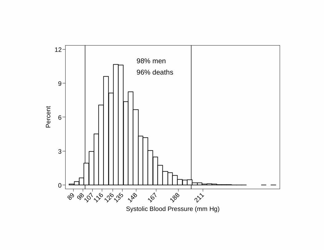
98% men96% deaths

0

3

6

9

12P

erce

nt

89 98 107

116

126

135

148

167

188

211

Systolic Blood Pressure (mm Hg)

0

5

10

15

20

25

30

35

40

45

50O

dds

of d

eath

with

in 1

0-ye

ars

(%)

89 98 107

116

126

135

148

167

188

211

Systolic Blood Pressure (mm Hg)

0.0

0.5

1.0

1.5

2.0

2.5

3.0

3.5

4.0

4.5

5.0O

dds

ratio

of d

eath

with

in 1

0-ye

ars

89 98 107

116

126

135

148

167

188

211

Systolic Blood Pressure (mm Hg)

A measure of association between a continuous covariate or exposure X and the response variable is the difference or ratio of some transformation of the expected or average responses in subpopulations defined by different exposure values. For instance the ratio of odds comparing categories (141-160) vs (101-110) is (470/3727) / (84/995) =

.12 / .08 = 1.5

. table sysbpc5, c(freq sum all10 median sysbp) row ---------------------------------------------- RECODE of | sysbp | (x2: | systolic | blood | pressure | (mm Hg)) | Freq. sum(all10) med(sysbp) ----------+----------------------------------- <90 | 15 3 88 90-119 | 3,617 241 113 120-139 | 7,049 524 130 140-159 | 4,389 478 147 >=160 | 2,190 424 171 | Total | 17,260 1670 133 ----------------------------------------------

0.0

0.5

1.0

1.5

2.0

2.5

3.0

3.5

4.0

4.5

5.0O

dds

ratio

of d

eath

with

in 1

0-ye

ars

89 98 107

116

126

135

148

167

188

211

Systolic Blood Pressure (mm Hg)

The shape of the dose-response function is sensitive to location and number of cut-points. For instance the ratios of odds comparing categories (140-159) vs (90-119) mm Hg is (478/3911) / (241/3376) =

.12 / .07 = 1.7

Problems Unrealistic step-function Distortion of inferences Location and number of cut-points Loss of information in contrasting categories

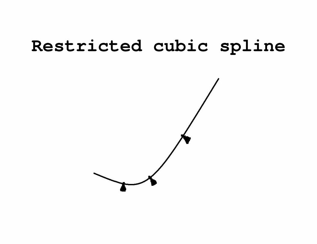
Restricted cubic spline

polynomial line segments boundaries of these segments are called knots straight line before the first and after the last knot continuous and smooth at the knot boundaries

A logistic regression model with n knots includes the coefficients for n-1 transformations of the original exposure variable X

Log odds = logit(Y=1|X) =

= b0 + b1*X1 + b2*X2 + ... + bn-1*Xn-1

To contrast the log odds of the response at two distinct exposure values z1 and z2 we need to know the corresponding values of the restricted cubic splines

Log odds ratio (X=z1 vs X=z2) =

logit(Y=1|X=z1) - logit(Y=1| X=z2)

Odds ratio (X=z1 vs X=z2) =

exp(logit(Y=1|X=z1)-logit(Y=1| X=z2)) =

exp(b1*(X1(z1)-X1(z2))+ b2*(X2(z1)-X2(z1))

+ … + bn-1*(Xn-1(z1)-Xn-1(z1)))

The first spline X1 is the original exposure variable X The remaining splines X2, … , Xn-1 are complex functions of the location of X between knots.

Let ki , i=1, …, n be the knots. To calculate the values of the n-1 restricted cubic splines Xi for a certain value X equal to z

ui = max(z-ki, 0)3 with i = 1,..,n

X1(z) = X(z)

Xi(z) = [ ui-1 – un-1 * (kn- ki-1)/ (kn- kn-1)

+ un * (kn-1- ki-1)/ (kn – kn-1) ] / (kn – k1)2

with i = 2,..,n-1

Let’s use 4 knots at fixed and equally spaced percentiles (5%, 35%, 65%, 95%). . mkspline sysbps = sysbp , nknots(4) cubic displayknots | knot1 knot2 knot3 knot4 -------------+-------------------------------------------- sysbp | 107 126 141 175 . mat knots = r(knots)

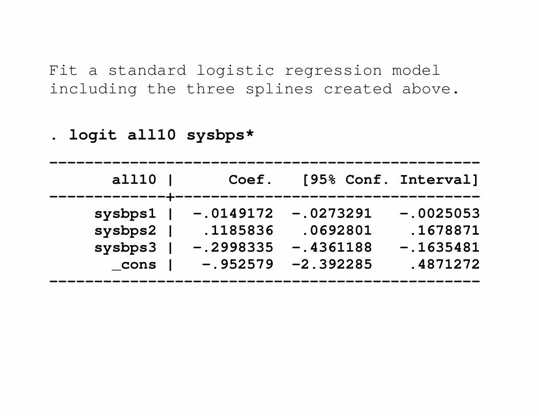
Fit a standard logistic regression model including the three splines created above.

. logit all10 sysbps*

------------------------------------------------ all10 | Coef. [95% Conf. Interval] -------------+---------------------------------- sysbps1 | -.0149172 -.0273291 -.0025053 sysbps2 | .1185836 .0692801 .1678871 sysbps3 | -.2998335 -.4361188 -.1635481 _cons | -.952579 -2.392285 .4871272 ------------------------------------------------

. testparm sysbps2 sysbps3 ( 1) [all10]sysbps2 = 0 ( 2) [all10]sysbps3 = 0 chi2( 2) = 32.12 Prob > chi2 = 0.0000

The small p-value of the Wald-test type test with 2 degrees of freedom is indicating strong evidence against linearity.

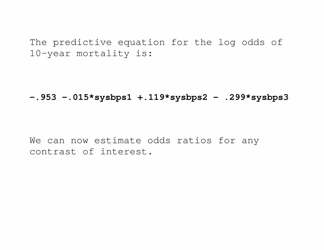
The predictive equation for the log odds of 10-year mortality is: -.953 -.015*sysbps1 +.119*sysbps2 - .299*sysbps3

We can now estimate odds ratios for any contrast of interest.

For instance, let’s calculate the odds ratio of 10-year mortality comparing men with systolic blood pressure 148 vs. 107 (mm Hg).

exp(-.015*(148-107)+.119*(14.76-0)-.299*(2.2-0))

= 1.6

where the values of the three splines at 148 and 107 are calculated using the formulas given above.

The 3 splines at 148 mm Hg are

sysbps1(148) = 148

sysbps2(148) = [ max(148-107,0)^3 – max(148-141,0)^3*(175-107)/(175-141)+ max(148-175,0)^3*(141-107)/(175-141) ] / (175-107)^2 = 14.76 sysbps3(148) = [ max(148-126,0)^3 – max(148-141,0)^3*(175-126)/(175-141)+ max(148-175,0)^3*(141-126)/(175-141) ] / (175-107)^2 = 2.20

We can use the lincom (help lincom) post-estimation command to obtain the predicted odds or ratios of odds together with 95% confidence limits. For example, to calculate the odds of 10-year mortality for men with systolic blood pressure of 148 and 107 (mm Hg) we plug in these values in the predictive equation.

// Odds of death at 148 mm Hg . lincom _b[_cons] + _b[sysbps1]*148+_b[sysbps2]*14.76+ _b[sysbps3]*2.2 , eform ( 1) 148*[all10]sysbps1 + 14.76*[all10]sysbps2 + 2.2*[all10]sysbps3 + [all10]_cons = 0 ------------------------------------------------------------------------------ all10 | exp(b) Std. Err. z P>|z| [95% Conf. Interval] -------------+---------------------------------------------------------------- (1) | .1262277 .0050646 -51.58 0.000 .1166815 .1365548 ------------------------------------------------------------------------------

// Odds of death at 107 mm Hg . lincom _b[_cons] + _b[sysbps1]*107+_b[sysbps2]*0+ _b[sysbps3]*0 , eform ( 1) 107*[all10]sysbps1 + [all10]_cons = 0 ------------------------------------------------------------------------------ all10 | exp(b) Std. Err. z P>|z| [95% Conf. Interval] -------------+---------------------------------------------------------------- (1) | .0781815 .0057198 -34.84 0.000 .0677376 .0902357 ------------------------------------------------------------------------------

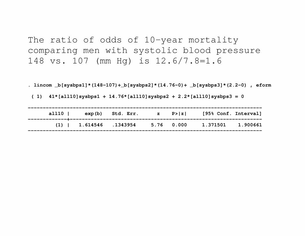
The ratio of odds of 10-year mortality comparing men with systolic blood pressure 148 vs. 107 (mm Hg) is 12.6/7.8=1.6 . lincom _b[sysbps1]*(148-107)+_b[sysbps2]*(14.76-0)+ _b[sysbps3]*(2.2-0) , eform ( 1) 41*[all10]sysbps1 + 14.76*[all10]sysbps2 + 2.2*[all10]sysbps3 = 0 ------------------------------------------------------------------------------ all10 | exp(b) Std. Err. z P>|z| [95% Conf. Interval] -------------+---------------------------------------------------------------- (1) | 1.614546 .1343954 5.76 0.000 1.371501 1.900661 ------------------------------------------------------------------------------

One can use the above approach to estimate odds ratios for any subpopulation of men defined by a fine grid of values spaced across the exposure range of interest using any value as referent. The post-estimation command xbrcspline greatly facilitates this task.

. xbrcspline sysbps , matknots(knots) /// values(89 98 107 116 126 135 148 167 188 211) /// ref(107) eform Reference value for sysbp = 107 sysbp exp(XB) LB UB 89 1.31 1.05 1.64 98 1.14 1.02 1.28 107 1.00 1.00 1.00 116 0.89 0.80 0.99 126 0.90 0.76 1.06 135 1.10 0.93 1.30 148 1.62 1.37 1.90 167 2.50 2.13 2.94 188 3.81 3.15 4.60 211 6.03 4.64 7.83

Systolic blood

pressure mm Hg

Median No. of men at risk

No. of deaths within

10-years

Categorical Model

OR (95% CI)

Restricted Cubic Spline OR (95% CI)

<=90 89 27 3 1.48 (0.44-5.02) 1.31 (1.05-1.64)

91-100 98 283 22 1.00 (0.61-1.63) 1.14 (1.02-1.28)

101-110 107 1,079 84 1.00 1.00

111-120 116 2,668 164 0.78 (0.59-1.02) 0.89 (0.80-0.99)

121-130 126 3,516 233 0.84 (0.65-1.09) 0.90 (0.76-1.06)

131-140 135 3,456 289 1.08 (0.84-1.39) 1.10 (0.93-1.30)

141-160 148 4,197 470 1.49 (1.17-1.90) 1.62 (1.37-1.90)

161-180 167 1,437 252 2.52 (1.94-3.27) 2.50 (2.13-2.94)

181-200 188 438 108 3.88 (2.84-5.29) 3.81 (3.15-4.60)

201-280 211 159 45 4.68 (3.10-7.05) 6.03 (4.64-7.83)

0.0

1.0

2.0

3.0

4.0

5.0

6.0

7.0

8.0

Odd

s ra

tio o

f dea

th w

ithin

10-

year

s

89 98 107 116 126 135 148 167 188 211Systolic Blood Pressure (mm Hg)

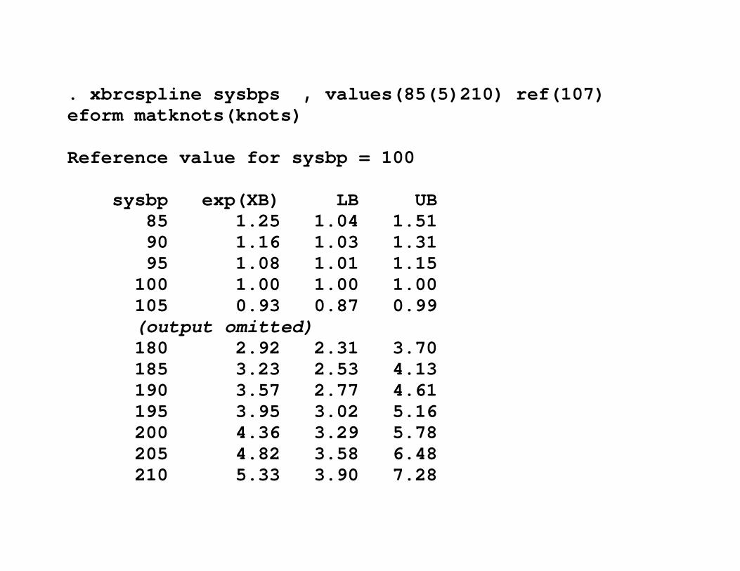
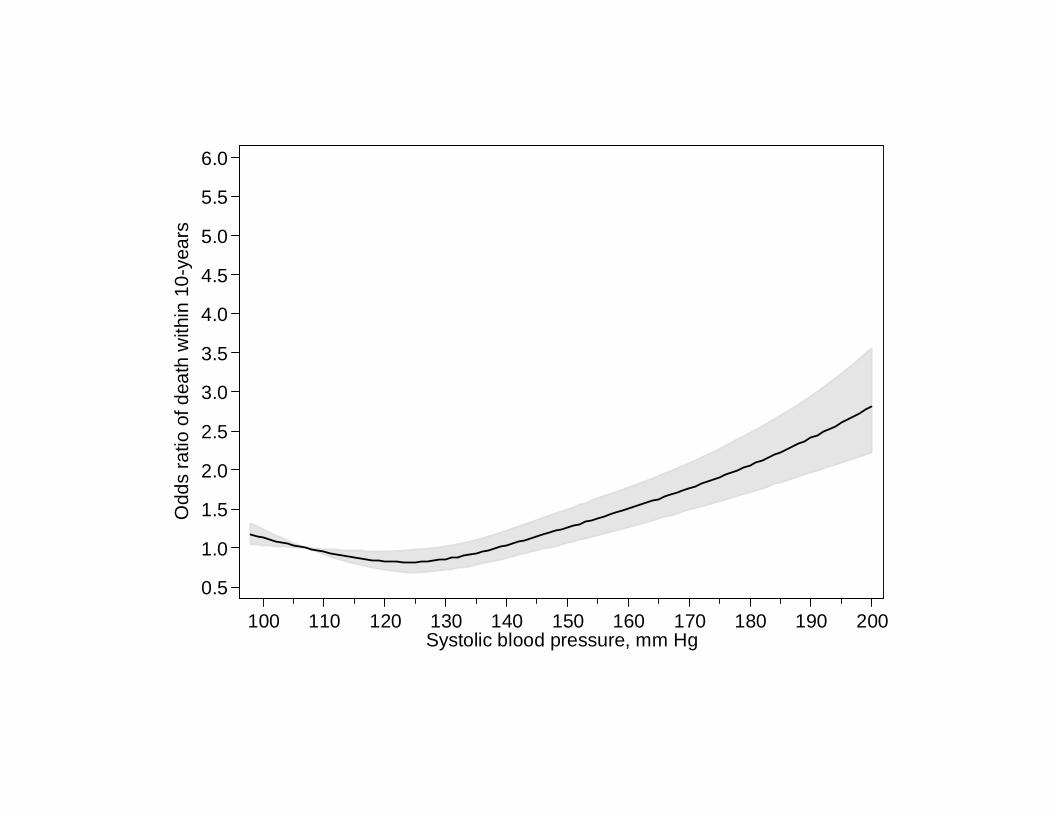
. xbrcspline sysbps , values(85(5)210) ref(107) eform matknots(knots) Reference value for sysbp = 100 sysbp exp(XB) LB UB 85 1.25 1.04 1.51 90 1.16 1.03 1.31 95 1.08 1.01 1.15 100 1.00 1.00 1.00 105 0.93 0.87 0.99

(output omitted) 180 2.92 2.31 3.70 185 3.23 2.53 4.13 190 3.57 2.77 4.61 195 3.95 3.02 5.16 200 4.36 3.29 5.78 205 4.82 3.58 6.48 210 5.33 3.90 7.28

0.0

1.0

2.0

3.0

4.0

5.0

6.0

7.0

8.0O

dds

ratio

of d

eath

with

in 1

0-ye

ars

89 98 107 116 126 135 148 167 188 211Systolic Blood Pressure (mm Hg)

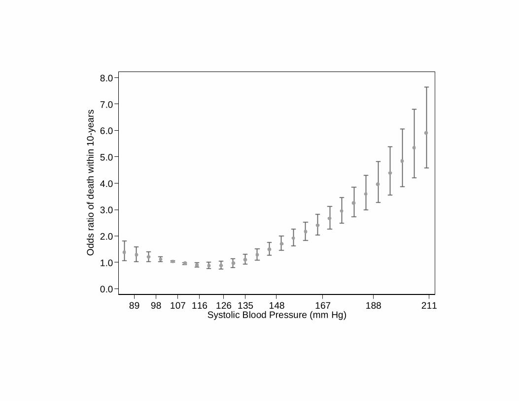
One can estimate odds ratios and 95% CI for each distinct observed value of the exposure. levelsof sysbp xbrcspline sysbps , values(`r(levels)') ///

ref(107) matknots(knots) eform This is what you get by using predictnl post-estimation command.

Similarly to the use of lincom command predictnl xb= _b[sysbps1]*(sysbps1-107)+ ///

_b[sysbps2]*(sysbps2-0)+ /// _b[sysbps3]*(sysbps3-0) /// , ci(lo hi)

gen or = exp(xb) gen lb = exp(lo) gen ub = exp(hi)

0.5

1.0

1.5

2.0

2.5

3.0

3.5

4.0

4.5

5.0

5.5

6.0O

dds

ratio

of d

eath

with

in 1

0-ye

ars

100 110 120 130 140 150 160 170 180 190 200Systolic blood pressure, mm Hg

Categorical vs Spline

0.5

1.0

1.5

2.0

2.5

3.0

3.5

4.0

4.5

5.0

5.5

6.0O

dds

ratio

of d

eath

with

in 1

0-ye

ars

100 110 120 130 140 150 160 170 180 190 200 210Systolic blood pressure, mm Hg

Confounder Age is strongly related to mortality as well as systolic blood pressure. We include age in the model assuming a linear trend. The steps requires to tabulate and plot adjusted measure of association are the same as for crude association.

. logit all10 sysbps* age ------------------------------------------------ all10 | Coef. [95% Conf. Interval] -------------+---------------------------------- sysbps1 | -.0176534 -.0303369 -.00497 sysbps2 | .0976037 .0472509 .1479566 sysbps3 | -.237395 -.3766578 -.0981323 age | .1099985 .1008947 .1191023 _cons | -6.340506 -7.87899 -4.802022 ------------------------------------------------

. xbrcspline sysbps , values(89 98 107 116 126 135 148 167 188 211) ref(107) eform matknots(knots) Reference value for sysbp = 107 sysbp exp(XB) LB UB 89 1.37 1.09 1.73 98 1.17 1.05 1.31 107 1.00 1.00 1.00 116 0.87 0.78 0.96 126 0.83 0.69 0.98 135 0.93 0.79 1.11 148 1.22 1.03 1.44 167 1.68 1.42 1.99 188 2.33 1.92 2.84 211 3.34 2.54 4.38

0.5

1.0

1.5

2.0

2.5

3.0

3.5

4.0

4.5

5.0

5.5

6.0O

dds

ratio

of d

eath

with

in 1

0-ye

ars

100 110 120 130 140 150 160 170 180 190 200Systolic blood pressure, mm Hg

Systolic blood

pressure mm Hg

Median No. of men at risk

No. of deaths within

10-years

Crude * OR (95% CI)

Age-adjusted * OR (95% CI)

<=90 89 27 3 1.31 (1.05-1.64) 1.37 (1.09-1.73)

91-100 98 283 22 1.14 (1.02-1.28) 1.17 (1.05-1.31)

101-110 107 1,079 84 1.00 1.00

111-120 116 2,668 164 0.89 (0.80-0.99) 0.87 (0.78-0.96)

121-130 126 3,516 233 0.90 (0.76-1.06) 0.83 (0.69-0.98)

131-140 135 3,456 289 1.10 (0.93-1.30) 0.93 (0.79-1.11)

141-160 148 4,197 470 1.62 (1.37-1.90) 1.22 (1.03-1.44)

161-180 167 1,437 252 2.50 (2.13-2.94) 1.68 (1.42-1.99)

181-200 188 438 108 3.81 (3.15-4.60) 2.33 (1.92-2.84)

201-280 211 159 45 6.03 (4.64-7.83) 3.34 (2.54-4.38)

* Systolic blood pressure was modeled by restricted cubic splines with 4 knots

(107; 126; 141; 175) at percentiles 5%, 35%, 65%, and 95% in a logistic regression model.

The value of 107 mm Hg was used as referent for the estimation of all odds ratios.

Strengths Flexibility to describe simple or arbitrarily complex dose-response patterns of association. Possibility to use the post-estimation commands available for simpler parametric models for testing hypothesis, calculating predictions, and evaluating the goodness-of-fit of the model.

Potential limitations Restricting splines is not always a safe assumption Instability with sparse data Limited ability to predict future observations Increase chance of over-interpretation and over-fitting

46

Alternatives Simpler splines (linear) Fractional polynomials Royston P, Sauerbrei W. Multivariable Model-building: A

pragmatic approach to regression analysis based on fractional polynomials for modelling continous variables Wiley Series in Probability and Statistics, 2008.

Royston P, Sauerbrei W. Multivariable modeling with cubic

regression splines: A principled approach. Stata Journal 2007;7:45-70.

Royston P, Ambler G, Sauerbrei W. The use of fractional

polynomials to model continuous risk variables in epidemiology. Int J Epidemiol 1999;28:964-74.

47

Ongoing A joint work with Sander Greenland (Dept. Epidemiology and Statistics, University of California, USA) will be submitted to the Stata Journal.

48