tackling 3d tof artifacts through learning and the flat ... · tackling 3d tof artifacts 3 rately...

Tackling 3D ToF Artifacts Through Learningand the FLAT Dataset

Qi Guoa,b, Iuri Frosioa, Orazio Galloa, Todd Zicklerb, Jan Kautza

aNVIDIA, bHarvard SEAS

Abstract. Scene motion, multiple reflections, and sensor noise intro-duce artifacts in the depth reconstruction performed by time-of-flightcameras. We propose a two-stage, deep-learning approach to address allof these sources of artifacts simultaneously. We also introduce FLAT, asynthetic dataset of 2000 ToF measurements that capture all of thesenonidealities, and allows to simulate different camera hardware. Usingthe Kinect 2 camera as a baseline, we show improved reconstructionerrors over state-of-the-art methods, on both simulated and real data.

Keywords: Time-of-Flight, MPI artifacts, motion artifacts.

1 Introduction

Depth estimation is central to several computer vision applications. Among themany existing strategies for extracting a scene’s 3D information, Time-of-Flight(ToF) cameras are particularly popular due to their robustness and affordability.

ToF cameras leverage the relation between an object’s distance from the sen-sor and the amount of time required for photons to travel to that object andback. In particular, Amplitude-Modulated Continuous-Wave (AMCW) camerasemit a periodic light signal and measure its phase delay upon return: the phasedelay offers an estimate of the time of flight and, in turn, of depth. Any imple-mentation of this approach requires several careful considerations.

First and foremost, the phase delay wraps at distances that correspond tomultiples of the modulation period. A common approach is to combine infor-mation from different modulation frequencies: longer modulation periods extendthe unambiguous range, while shorter periods allow resolving finer details. Usingmultiple frequencies, however, is not without consequences. The dynamic partsof the scene may be displaced between sequential measurements at different fre-quencies, causing depth estimation errors1 that are particularly strong along thedepth discontinuities. These artifacts can be identified and removed, at the costof missing depth information at the corresponding pixels.

Another consideration is multi-path light transport. In addition to the directemitter-object-sensor path, light may follow other paths and bounce multipletimes before being recorded by one pixel. This phenomenon, called multiple-path

1 Some cameras use spatial multiplexing instead, and synchronize neighboring pixelswith specific emission frequencies, thus sacrificing spatial resolution.

2 Q. Guo, I. Frosio, O. Gallo, T. Zickler, and J. Kautz

Raw measurement

Depth reconstruction

Real ToF camera FLAT dataset

Training and validationTesting

Motion module

Multi-re�ection module

Motion

Depth error (m) Depth (m)

0

1.5

0.5

0

Warping

.*

Per-pixel kernelArctan, Eq. 3

Unwrap, Eq. 4

Depth

384

5129

32 64128 256 512 256 128 64 32

18 18 18512

384

7x7

5x5 5x53x3 3x3 3x3 3x3 3x3

5x5 5x57x7

3x3

Convolution kernel Convolutional layer + 2x2 max pooling layerConvolution layer Upsampling layer + skip connection

384

512

964128256

512256

1286481

3x3

512

384

9

7x75x55x5

3x33x33x35x55x5

9

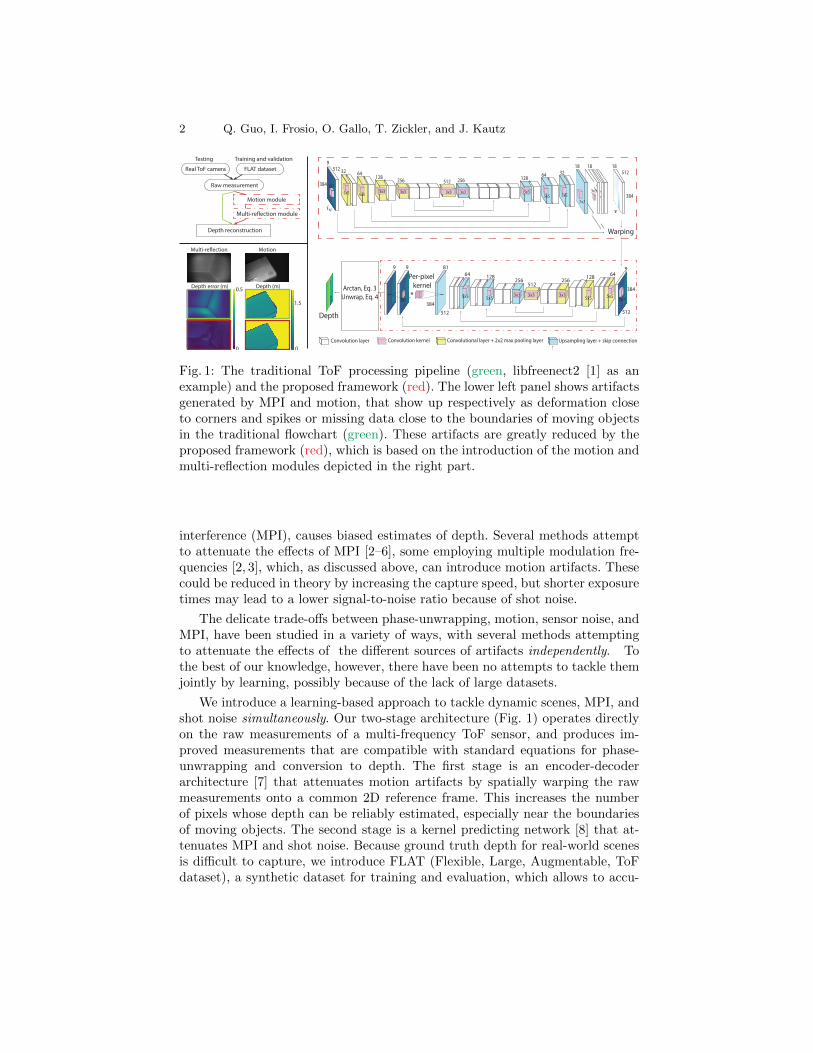
Fig. 1: The traditional ToF processing pipeline (green, libfreenect2 [1] as anexample) and the proposed framework (red). The lower left panel shows artifactsgenerated by MPI and motion, that show up respectively as deformation closeto corners and spikes or missing data close to the boundaries of moving objectsin the traditional flowchart (green). These artifacts are greatly reduced by theproposed framework (red), which is based on the introduction of the motion andmulti-reflection modules depicted in the right part.

interference (MPI), causes biased estimates of depth. Several methods attemptto attenuate the effects of MPI [2–6], some employing multiple modulation fre-quencies [2, 3], which, as discussed above, can introduce motion artifacts. Thesecould be reduced in theory by increasing the capture speed, but shorter exposuretimes may lead to a lower signal-to-noise ratio because of shot noise.

The delicate trade-offs between phase-unwrapping, motion, sensor noise, andMPI, have been studied in a variety of ways, with several methods attemptingto attenuate the effects of the different sources of artifacts independently. Tothe best of our knowledge, however, there have been no attempts to tackle themjointly by learning, possibly because of the lack of large datasets.

We introduce a learning-based approach to tackle dynamic scenes, MPI, andshot noise simultaneously. Our two-stage architecture (Fig. 1) operates directlyon the raw measurements of a multi-frequency ToF sensor, and produces im-proved measurements that are compatible with standard equations for phase-unwrapping and conversion to depth. The first stage is an encoder-decoderarchitecture [7] that attenuates motion artifacts by spatially warping the rawmeasurements onto a common 2D reference frame. This increases the numberof pixels whose depth can be reliably estimated, especially near the boundariesof moving objects. The second stage is a kernel predicting network [8] that at-tenuates MPI and shot noise. Because ground truth depth for real-world scenesis difficult to capture, we introduce FLAT (Flexible, Large, Augmentable, ToFdataset), a synthetic dataset for training and evaluation, which allows to accu-

Tackling 3D ToF Artifacts 3

rately simulate the raw measurements of different AMCW ToF cameras (includ-ing the Kinect 2) in the presence of MPI artifacts and shot noise; FLAT datacan be augmented to approximate motion artifacts as well. Our contributionsare:

(i) FLAT, a large, synthetic dataset of ToF measurements that simulatesMPI, motion artifacts, shot noise, and different camera response functions.

(ii) A Deep Neural Network (DNN) architecture for attenuating motion,MPI, and shot noise artifacts that can be trained both in the raw measurementor depth domain.

(iii) A thorough validation, including an ablation study and a comparisonwith state-of-the-art algorithms for reducing MPI and motion artifacts.

(iv) A complete characterization of the Kinect 2 camera, including its cameraresponse function and sensor noise characteristics.

Our DNN model, dataset and characterization of the Kinect 2 are availableat http://research.nvidia.com/publication/2018-09_Tackling-3D-ToF.

2 Related Work

Several works separately reduce artifacts due to MPI, motion, or shot noise inAMCW ToF imaging. We group them into four categories.

Measurement noise reduction. Raw ToF measurements suffer from bothsystematic and random noise [9]. Systematic errors are often associated with im-perfect sinusoidal modulations and can be reduced through calibration [9–11].Shot noise and other types of random noise are typically addressed through bilat-eral filtering of the raw measurements, the depth map, or both sometimes usingother images for guidance [12]. The performance of these approaches is generallysatisfactory, and any system that intends to replace them, ours included, shouldnot perform noticeably worse.

Motion artifacts reduction. Motion artifacts occur when objects moveand ToF raw measurements are captured sequentially. Gottfried et al. [13] iden-tify three ways to attenuate them: reduce the number of sequential measure-ments; detect and correct the regions affected by motion, both in the raw mea-surement domain and in the depth domain; or estimate the 2D motion fieldsbetween raw 2D measurement maps and apply corrective spatial warping. Oneway to detect affected pixels in raw measurements is by checking the Plus andMinus rules [14, 15] that derive from physical constraints on the light measuredin a static scene. After detection, pixels affected by motion blur can be corrected,for example, by interpolation [14]. Object motion also affects the frequency ofreflected signals due to Doppler effect; however, to use the frequency shift tomeasure object motion requires a higher number of measurements and extensiveprocessing [16].

Physics-based MPI reduction. Algorithms for recovering depth fromToF correlations usually assume the pure measurement of direct, single-bounce(emitter-surface-sensor) light paths. In practice, many photons bounce multi-ple times, causing “erroneous” measurements [2, 10]. If multiple modulation


frequencies are used, the problem can be tackled by processing the temporalchange of each pixel of the raw measurements in the Fourier domain. For in-stance, in the absence of noise, K interfering paths can be resolved by 2K + 1frequency measurements [3]. Other techniques for the per-pixel temporal pro-cessing of raw ToF measurements include Prony’s method, the matrix pencilmethod, orthogonal matching pursuit, EPIRIT/MUSIC, and atomic norm regu-larization [2]. Freedman et al. propose a real-time temporal processing techniquethat uses per-pixel optimization based on a light transport model with sparseand low-rank components [17]. Phasor Imaging exploits the fact that the effectsof MPI are diminished at much higher modulation frequencies, and shows thatsimple temporal processing can succeed with as few as two such frequencies,albeit with a reduced unambiguous working range [18].

Learning-based MPI reduction. The difficulty of modeling MPI analyti-cally makes machine learning an enticing alternative for its reduction. However,one obstacle is the lack of large, physically-accurate datasets for training, whichare difficult to capture [19] and prohibitively expensive to simulate, until recently.Marco et al. use an encoder to learn a mapping from captured ToF measure-ments to a representation of (MPI-corrupted) depth, and then combine this witha limited number of simulated, direct-only ToF measurements to train a decoderthat produces MPI-corrected depth maps [4]. Mutny et al. focus on corners ofdifferent materials and use a dataset of such corners to train a random forestwith hand-crafted features [5]. A different strategy is taken by Son et al., whouse a robotic arm and structured light system to capture ToF measurementswith registered ground-truth depth [6]. They then train two neural networks tocorrect depth and refine edges through geodesic filtering.

We leverage the availability of computational power and advances in transientrendering [20, 10] to synthesize a training dataset sufficiently large and diverse toexplore a much larger class of learned models. In addition to physically-accurateMPI effects, the dataset provides realistic shot noise, supports augmentationwith approximate motion models, and allows for efficient generation of raw mea-surements from AMCW ToF sensors with arbitrary modulation signals.

3 Time-of-Flight Camera Models

In this section we first review the theory of ToF reconstruction in the idealcase. We show that equations for depth reconstruction are differentiable, whichallows for backpropagation. We then show the effect of MPI and motion ondepth reconstruction, which helps framing the learning problem and definingthe important factors for training. We leverage these elements to train a neuralnetwork, working in the domain of the raw measurements and before unwrap-ping, aimed at correcting these artifacts. The section is closed by an accuratecharacterization of the Kinect 2, which is our hardware testbed; this serves toproduce accurate simulations for training and reduce the shift between syntheticand real data. All the math details for the section are in the Supplementary.


3.1 Ideal Camera Model

An AMCW ToF camera illuminates the scene with an amplitude-modulated,sinusoidal signal g(t) = g1cos(ωt) + g0, [16]. If camera and light source are co-located, and the scene static, the signal coming back to a pixel is

s (t) =

∫ t

−∞a(τ)cos(ωt− 2ωτ)dτ, (1)

where a(τ) is the scene response function, i.e. the signal reaching the pixel attime τ . In an ideal scenario, the light is reflected once and the scene response isan impulse, a(τ) = aδ(τ − τ0). The travel time τ0 directly translates to depth.

A homodyne ToF camera modulates the incident signal with a phase-delayedreference signal at the same frequency, b cos (ωt− ψ). The exposure time of thecamera is usually set to T >> 2π/ω. Simple trigonometry allows writing theraw correlation measurement iψ,ω as:

iψ,ω =

∫ T/2

−T/2s(t)b cos (ωt− ψ) dt ≈ a(τ0)b cos(ψ − 2ωτ0) = afψ,ω(τ0), (2)

where we denote fψ,ω(τ) = b cos(ψ−2ωτ) as the camera function. Using raw mea-surements captured at a single frequency ω and K ≥ 2 phases ψ = (ψ1, . . . , ψK),the depth d can be recovered at each pixel as:

d = c/(2ω) arctan [(sinψ · iψ,ω)/(cosψ · iψ,ω)] , (3)

where iψ,ω is the K-vector of per-phase measurements.However, d wraps for depths larger than πc/ω, and additional measurements

at L ≥ 2 different frequencies ω = (ω1, . . . , ωL) are required. Denoting the mea-surements at frequency ωl as iψ,ωl

, an analytical expression for d was providedby Goshov and Solodkin [21] based on the Chinese remainder theorem:

d =∑ω

Al(ω) arctan [(sinψ · iψ,ωl)/(cosψ · iψ,ωl

)] +B(ω), (4)

where {Al(ω)}l=1,...,L and B(ω) are constants. Based on Eq. 4, one can easilyobtain the derivative ∂d/∂iψ,ωl

, which makes it possible to backpropagate theerror on d and to perform end-to-end training.

3.2 The Impact of Multiple Paths

In a realistic scenario, the signal that reaches the sensor is corrupted by multi-ple light paths that undergo different reflection events and have different pathlengths. This means that the scene response a(τ) is not an impulse anymore, asit measures the arrival of the light reaching a pixel from all the possible lightpaths that connect it to the emitter. In this case, Eq. 2 becomes:

iψ,ω =

∫ T/2

−T/2

(∫ t

−∞a(τ)cos(ωt− 2ωτ)dτ

)b cos (ωt− ψ) dt

≈∫ t

−∞a(τ)b cos(ψ − 2ωτ)dτ =

∫ t

−∞a(τ)fψ,ω(τ)dτ.

(5)


When sinusoidal reference signals with different frequencies ωl and phases ψkare measured sequentially, one obtains multiple channels of raw measurements.The multi-channel measurements at any pixel iψ,ω can be interpreted as a pointin a multi-dimensional space, and while difficult to model analytically, there isstructure in this space that can be exploited through learning.

In the ideal case of a single bounce, the set of all possible measurement vectorsiψ,ω forms a “single-bounce measurement manifold” defined by Eq. 2. If onlyone frequency is used, measurements affected by MPI lie on the same manifold,and it is therefore impossible to identify and correct them. On the other hand,in the case of multiple frequencies, the manifold becomes a non-linear subspace,and MPI-affected vectors do not lie on it anymore. The MPI problem can thenbe recast as one of mapping real measurements, possibly affected by MPI, tothe ideal one-bounce manifold, which is also the idea behind many existingapproaches for MPI correction.

3.3 The Impact of Motion

Real scenes are rarely static. Because of the lateral and axial motion of objectswith respect to the camera, sequential correlation measurements iψ,ω are mis-aligned. Moreover, the axial component of the motion also changes the sceneresponse function a(τ): for example, even in the simple case of a single bounce,the term τ0 in Eq. 2 changes with the axial motion of the object, whereas themeasured intensity varies proportionally to the inverse-square of distance. Inour indoor experimental setting we found both these phenomena to contributesignificantly to the depth reconstruction error. Motion can even generate blurand Doppler within each raw correlation measurement, but we found these lasteffects negligible when compared to the previous ones.

3.4 Characterization of Kinect 2

The Kinect 2 is a well-documented, widely used ToF camera, with an open-source SDK (libfreenect2 [1]) that exposes raw correlation measurements andprovides a baseline algorithm for benchmarking (indicated as LF2 in the fol-lowing). We carefully characterize the camera functions, shot noise, vignetting,and per-pixel delay, to produce accurate simulations and mitigate the data shiftbetween synthetic data from the FLAT dataset and real scenarios.

The Kinect 2 uses three modulation frequencies, each with three phases,for a total of nine camera functions fψ,ω(τ). To calibrate the camera func-tions, we carefully align the optical axis to be normal to a Lambertian calibra-tion plane. We place a light absorption tube in front of Kinect’s light sourceto narrow down the beam emission angle and limit MPI. We translate theplane to known distances {dj}j=1..N to obtain a series of raw measurements{iψ,ω(dj)}j=1..N that approximate (dj)

−2fψ,ω(2dj/c) up to a constant scale,for every pixel. After removing the squared-distance intensity decay (dj)

−2, wehave a series of observations of the camera functions {fψ,ω(2dj/c)}. Fig. 2 shows


Fig. 2: Calibrated camerafunctions for Kinect 2; thepoints represent experimentaldata, the continuous line arethe fitted camera functions.

three camera functions fitted by this method,parameterized as b cos(ψ − 2ωτ) (red and bluecurve in Fig. 2), and max(min(b1 cos(ψ −2ωτ), b2),−b2) (green curve in Fig. 2).

As for the shot noise, we assume each pixel tobe independent from the others. We acquire datafrom 15 scenes; for each raw correlation measure-ment, we compute the per-pixel expected valueas the average of 100 measurements. For any ex-pected value, we collect the empirical distribu-tion of the noisy samples in a lookup table, thatis used to generate noisy data in simulation.

For the complete explanation of the calibra-tion procedure, including vignetting and per-pixel time delay, we invite the reader to referto the Supplementary, which also includes moreexperimental results.

4 The FLAT Dataset

An ideal dataset for training and validating ToF algorithms is large; allows sim-ulating different camera response functions (like those in Section 3.4); allowsincluding MPI, shot noise and motion; and exposes raw correlation measure-ments. We created the FLAT dataset with these principles in mind.

FLAT contains 2000 scene response functions, {aj(τ, x, y)}j=1..2000, where wemake the dependence on pixel (x, y) explicit. Each of these is computed throughtransient rendering [20], which simulates the irradiance received by the camerasensor at every time frame, after sending an impulse of light to the environment.The output of the renderer is a nτ × nx × ny tensor, i.e. a discretized versionof aj(τ, x, y). The scenes in the dataset are generated from 70 object setups;each setup has 1 to 5 objects with lambertian surface and uniform albedo; their3D models are from the Stanford 3D Scanning Repository [22] and the onlinecollection [23]. We render each setup from approximately 30 point of views andorientations, at a spatial resolution of (nx = 424) × (ny = 512) pixels andfor nτ = 1000 consecutive time intervals (each interval is 5e−11sec long); thehorizontal field of view is 70 degrees (corresponding to the Kinect 2 camera).Since bi-directional path tracing is used to sample and simulate each light ray,aj(τ, x, y) does simulate MPI. From the discretized version of aj(τ, x, y), any rawmeasurement iψ,ω can be obtained as in Eq. 5, for any user-provided camerafunction fψ,ω(t) (like, for instance, the ones we estimated for Kinect 2).

The FLAT dataset offers the possibility to augment the raw measurementwith shot noise, textures, vignetting, and motion. Within FLAT, we provide thecode to apply any vignetting function and shot noise coherently with the simu-lated camera, while MPI and camera functions are handled as described in theprevious paragraph. As a consequence, a physically correct simulation of differ-


ent camera functions, MPI, vignetting, and shot noise is a computationally lighttask within FLAT. On the other hand, texture and motion are more expensiveto render exactly. Since each scene in the FLAT dataset takes on the average10 CPU hours to render, creating a large set of scenes with different texturesand motions would require tens to hundreds of times longer. We handle this byproviding tools to approximate texture and motion in real time (as specializedforms of data augmentation), while still providing a small testing set withinFLAT with exact motion, texture, and rendering.

We approximate textures on the training data, by pixel-by-pixel multiplica-tion of the rendered iψ,ω with texture maps from the CURET texture dataset [24].This is an approximation that ignores the recursive impact that real textureshave on MPI, but we have found that it is nonetheless useful as a form of dataaugmentation.

The FLAT dataset offers two different methods to augment the simulated rawmeasurements with approximate motion. To illustrate the first one, let us con-sider the Kinect 2, where nine correlation measurements of a static scene, iψ,ω =(iψ1,ω1

, . . . , iψ9,ω9) are simulated. We generate a random 2D affine transform T

and apply it to create a smooth motion as i′ψj ,ωj(x, y) = iψj ,ωj

(T j−5(x, y)), where

Tn(x, y) is transforming (x, y) by T for n times, and T−n(Tn(x, y)) = (x, y). No-tice that the first and last measurement will achieve the largest movement. Toobtain a more complex movement, we simulate the motion of two or more objectswith different affine transforms and composite the scene based on their depths.This approximate motion model is fast, but does not reproduce the MPI interac-tion between the objects in the scene. The second motion approximation methodtakes in input a rendered scene response function, a(τ, x, y). We generate thena random, 3D affine transformation and apply the corresponding displacement(vx, vy, vz) to it, i.e., a′(τ, x, y) = a(τ + vz/c, x+ vx, y + vy). Then we use Eq. 5to compute one of the nine raw measurements. As in the previous method, thetransform is applied multiple times to create a smooth motion between the ninemeasurements. This method is computationally more expensive compared to theprevious one, but physically more accurate.

5 Network Architecture

We propose a two-module DNN (Fig. 1), to deal with MPI, motion, and shotnoise in the domain of raw correlation measurements. We demonstrate the useof the modules on data from the Kinect 2. The two modules can be integratedinto the LF2 [1] reconstruction pipeline, which is basically an implementation ofEq. 4 on Kinect 2. We leverage the differentiability of Eq. 4 to exploit, amongother forms of training for the DNN, training using a loss function in the depthdomain.

The first module (MOtion Module, MOM) is an encoder-decoder inspiredby Flownet [7]. The aim of MOM is to output a velocity map to align thenine raw channels measured by Kinect2. Differently from the original designof Flownet, which computes the optical flow between two images in the same


Name MOM + LF2 MOM-MRM + LF2∗ MRM + LF2∗

Training Data Motion, MPI Motion, MPI Static, MPI

Architecture Encoder-DecoderEncoder-Decoder-

KPN(1× 1× 9)KPN(3× 3× 1)

Depth Reconstruction LF2 LF2, no filter LF2, no filterTraining Loss L2, Velocity L2, Raw Intensity L2, Raw Intensity

Fine Tuning Loss L2, Depth L2, Depth

Table 1: Training specification.

100150200250300350

(a) True depth (b) Motion (c) Shot noise

10.07.55.02.5

0.02.55.07.510.0

(d) MPI

Fig. 3: Effect of non-idealities on the LF2 depth reconstruction error, in cm.

domain, MOM aligns raw correlation measurements taken with different cam-era functions, and therefore correlated, but visually different. Moreover, MOMtakes in input nine misaligned channels and outputs eight optical flows at thesame time, while Flownet deals with only one pair of images and one opticalflow. The second module (Multi-Reflection Module, MRM) is based on a kernel-predicting network (KPN), that has been effectively used for burst denoising onshot noise [25]. MRM outputs nine spatially varying kernels for every pixel; eachkernel is locally convolved with the input raw measurements, to produce a cleanraw measurement by jointly removing shot and MPI noise on every channel.

Table 1 shows the details of different variations of the basic DNN architec-ture that we consider in our experiments. Notice that, when we use the MRMmodule, we modify the LF2 pipeline to remove bilateral filtering from it, be-cause denoising is already performed by MRM; we indicate this variation of theLF2 pipeline as LF2∗. The MOM-MRM (followed by LF2∗) network inherits theencoder-decoder from MOM; training of MRM is performed with the output ofMOM as input, the weights of MOM being fixed. We start training using theL2 error of the raw correlation measurements as loss. Then, we fine tune MRMusing the L2 depth loss propagated through LF2∗. Motion in the training datais generated using the first approximation method in the FLAT dataset. Wealso tried fine tuning using the second approximation, which is physically moreaccurate, obtaining similar results.

6 Experiments

To better illustrate the typical distribution of the artifacts introduced by mo-tion, shot noise, and MPI, we show in Fig. 3 a scene from the FLAT dataset,rendered with motion, shot noise, or MPI only, and then reconstructed by theLF2 pipeline. Over/under shootings can be observed at the border of moving


Median IQR Prctile (90th)(error) (absolute error)

LF2 2.92 (1.62%) 3.01 (2.34%) 6.55 (5.36%)MRM -0.01 (0.00%) 2.63 (1.70%) 4.19 (2.52%)DToF -2.48 (1.80%) 12.36 (7.13%) 19.56 (9.84%)Phasor -0.29 (0.12%) 1.62 (0.71%) 1.83 (1.16%)

Fig. 4: The upper left panel shows the CDFof the depth error for LF2, MRM, DToF, andPhasor, for simulated data from FLAT, affectedby shot noise and MPI. The upper right panelshows the histogram of the error. All pixelswhose real depth is in the [1.5m, 5m] rangehave been considered. Our MRM outperformsLF2 and DToF, and it comes much closer tothe accuracy achieved using the MPI-dedicated,higher-frequency modulations of Phasor. The ta-ble shows corresponding median and Inter Quar-tile Range (IQR) of the depth error, and 90th

percentile of the absolute error, in cm. The num-bers in the brackets indicate the relative errors.

objects, where raw measure-ments from the foregroundand the background mix dueto motion. Shot noise in iψ,ωcreates random noise in thedepth map, especially in darkregions like background andimage borders. MPI generatesa low frequency noise in ar-eas affected by light reflec-tion, like the wall corner inFig. 3.

6.1 MPI Correction

We first measure the effect ofthe MRM module on staticscenes affected by MPI inthe FLAT dataset, and com-pare it to LF2 [1], DToF [4],and Phasor [18], that arebased respectively on multi-frequency, deep learning, andcustom hardware. LF2 im-plements Eq. 4 on Kinect 2and it constitutes our base-line to evaluate the improve-ment provided by our DNNon the same platform. DToFand Phasor require differentsensor platforms than Kinect2, but thanks to the flexibility of the FLAT dataset, we can simulate raw mea-surements using their specific modulation frequency and phase, and add the samelevel of noise for testing. As DToF and Phasor do not mask unreliable outputpixels (like LF2 does), and Phasor’s working range is limited to [1.5m, 5m], wecompare the depth error for all those pixels in this range only. Furthermore, asPhasor does not deal with shot noise, we apply a bilateral filter to remove noisefrom its output depth.

Results reported in Fig. 4 show that DToF produces the less accurate depthmap. The median error of LF2 is biased because of the presence of MPI in the rawdata—in fact, the LF2 pipeline does not include any mechanism to correct suchnon-ideality. This bias is effectively removed by MRM. Our method approachesthe Phasor’s accuracy, without requiring expensive hardware to create very highmodulation frequencies (1063.3MHz and 1034.1MHz): MRM works with Kinect2, which uses frequencies below 50MHz. Fig. 5 shows the results of typical scenesfrom the FLAT dataset, where Phasor and MRM outperform other methods in


120140160180200220240260

050100150200

(a) True

Med:-1.50, IQR:6.74

Med:-11.38, IQR:14.28

(b) DToF

Med:0.53, IQR:0.96

Med:0.93, IQR:1.25

(c) Phasor

Med:2.09, IQR:2.41

Med:1.29, IQR:2.32

(d) LF2

Med:-0.46, IQR:2.25

40302010

010203040

Med:0.05, IQR:2.07

40302010

010203040

(e) MRM

Fig. 5: Depth error for scenes from the FLAT dataset, corrupted by shot noiseand MPI and reconstructed by DToF [10], Phasor Imaging [18], LF2 [1] andMRM, in cm. Errors are computed only in the unanbiguous reconstruction rangeof Phasor Imaging, [1.5m, 5m]; no mask is used to remove unreliable pixels. Theblue boxes in the first row show the receptive field for DToF and MRM.

removing MPI. It is worth noticing that high frequency modulation signals, likethose used in Phasor, are very susceptible to noise. In fact, we use a bilateralfilter to reduce the effect of shot noise on the output of Phasor. Although thiseffectively reduces random noise, any misalignment on raw correlation measure-ments (like the one occurring in case of motion) creates a systematic noise thatcannot be eliminated by bilateral filtering, which dramatically reduces the accu-racy of Phasor (Fig. 7c). Our MRM appears much more reliable in this situation(Fig. 7e).

The case of a real scene of a corner, acquired in static conditions with aKinect 2, is depicted in Fig. 8. The ground truth shape of the scene could beestimated by checkerboard calibration applied to each of the three planes ofthe corner. This figure shows that MRM can significantly reduce MPI artifacts(compared to LF2) not only in simulation, but also in realistic conditions.

6.2 Motion Artifact Correction and Ablation Study

We perform an ablation study to quantify the benefits of MOM and MOM-MRM, on a test set from the FLAT dataset corrupted by MPI, shot noise, andrandom motion. For this experiment, the motion between the nine correlationsmeasurement is fully simulated by moving the objects in 3D space. This allowstesting the MOM and MOM-MRM on simulated raw correlation measurementsaffected by a real motion field, even if the modules are trained on approxi-mated motion data. We compare depth reconstruction through LF2, MOM, andMOM-MRM, each using the same masking method provided by LF2 to elimi-nate unreliable pixels, like those along misaligned object boundaries due to mo-tion. The density (i.e., percentage of reconstructed pixels) reported in Fig. 6 is


Median IQR Prctile (90th) Density(error) (absolute error) -

LF2 2.57 (1.11%) 2.65 (1.14%) 5.62 (2.51%) 93.56%MOM 2.50 (1.08%) 2.55 (1.10%) 5.48 (2.44%) 95.50%

MOM-MRM 1.02 (0.45%) 2.43 (1.06%) 4.12 (1.82%) 97.67%

Fig. 6: The upper left panel shows the CDF of thedepth error for LF2, MOM and MOM-MRM, forsimulated data from the FLAT dataset, affected byshot noise, MPI, and motion. The upper right panelshows the histogram of the error. Only those pix-els that have been reconstructed contribute to thestatistics. The table shows the corresponding recon-struction errors (median, 90th percentile, and InterQuartile Range (IQR), in cm). The numbers in thebrackets indicate the relative errors.

therefore representative ofhow well objects bound-aries are re-aligned byMOM. The depth accu-racy is slightly higherfor MOM compared toLF2, but the main ad-vantage for MOM is areduction of the unreli-able pixels, as density in-creases from 93.56% to95.50%. Red boxes inFig. 9 demonstrate in sim-ulation how introducingthe MOM module can re-duce the presence of holesin the reconstructed scene,especially close to objectboundaries. The introduc-tion of the MRM modulefurther increases the den-sity and reduces the biasin the depth error causedby MPI. Also this effect isclearly visible in the green boxes in Fig. 9, where the introduction of the MRMmodule leads to the reduction of the MPI artifact in the corner of the room.

6.3 Putting Everything Together

Fig. 7 shows a simulation from the FLAT dataset, where the scene has beencorrupted by shot noise, MPI, and a small motion (an average of 10 pixelsbetween the first and last raw correlation measurements). Phasor imaging cannotproduce a reliable depth map in this case: even a small motion changes themeasured phase significantly, because of the fast modulation frequency. MRMstill outperforms LF2, reducing the MPI, whereas the architecture trained tocorrect both motion and MPI, MOM-MRM, performs best (lowest median andIQR). The reconstruction of the depth scene using the MOM-MRM approachtakes approximately 90ms on a NVIDIA TitanV GPU.

Our DNN architecture, which operates on raw measurements, is the resultof a thorough investigation. We tested several architectures, including one thatdirectly outputs depth as suggested in the recent work by Su et al. [26], but thereconstruction error was consistently larger than that of the proposed DNN. Webelieve this is due to the fact a DNN that outputs the depth directly would beforced to learn the non-linear mapping from raw measurements to depth, insteadof leveraging the fact that such relation is dictated by physics and known (see theinverse-tangent of Eq. 4). An additional benefit of working in the raw domain is


175200225250275300325350

(a) True

Med:-15.44, IQR:9.63

(b) DToF

Med:162.9, IQR:193.30

(c) Phasor

Med:2.70, IQR:2.48

(d) LF2

Med:1.60, IQR:2.11

(e) MRM

Med:1.28, IQR:1.79

302010

0102030

(f) MOM-MRM

Fig. 7: Depth error for different reconstruction methods and a simulated scenefrom FLAT, corrupted by shot noise, MPI, and small motion. Units in cm.

(a) Scene

80100120140160180200

(b) True

Med:8.47, IQR:8.51

(c) LF2

Med:-1.97, IQR:4.62

4020

02040

(d) MRM

Fig. 8: A real scene of a corner captured by a Kinect 2 (a) with ground truthdepth (b) and depth errors for LF2 (c), and MRM (d). MPI artifacts show upas lobes close to the corner in LF2, and are reduced by MRM. Units in cm.

(a) True

Med:1.70, IQR:1.52

(b) LF2

Med:1.69, IQR:1.51

(c) MOM

100120140160180200220240

Med:0.90, IQR:1.72

2015105

05101520

(d) MOM-MRM

Fig. 9: A simulated scene from FLAT, corrupted by shot noise, MPI, and motion.The upper row shows the depth maps. The lower left panel is the intensity image,other panels in the row are depth errors. MOM aligns object boundaries andallows a more dense reconstruction (red boxes in b, c). MRM mostly correctsMPI artifacts in the smooth areas (green boxes in c, d). Units in cm.

(a) Scene (b) Raw (c) LF2

020406080100120140160

(d) MOM-MRM (e) Flow

Fig. 10: Panel (a) shows the average of nine raw correlation measurements ac-quired by Kinect 2, with a moving ball (blue box); panel (b) shows one of theraw measurements. Our method (d) reduces the motion artifacts compared toLF2 (c). The optical flow generated from MOM is shown in panel (e). The redbox highlights the reflective hand bar with specular reflections; if not maskedout, our method fails on these pixels. Units in cm.


that, beyond depth, we can estimates uncertainty as in the LF2 pipeline, whichis useful, for instance, to mask out bad depth values.

Fig. 10 shows an example of a real scene with moving objects (ball in the bluebox), captured by Kinect 2. Notice that Fig. 10a is blurred as it averages nineraw measurements, whereas each individual raw measurement is still sharp, as inFig. 10b. Coherently with simulations, the main effect of MOM is the reductionof the holes close to the boundaries of the moving object.

6.4 Method Limitations

Our method has some limitations that could be overcome with further devel-opment. The receptive field of MRM (blue box in Fig. 5) is 72×72 pixels, intheory not large enough to capture global geometric information and correctlong-range MPI; furthermore, our loss function naturally emphasizes short-rangeMPI correction because the signal is substantially stronger for shorter travelingdistances. Nonetheless, MRM does reduce many long-range MPI artifacts (seethe windshield of the car in Fig. 5). This can be explained with the a prioriinformation about object appearance learned by MRM, or assuming that MRMlearns to project measurements corrupted by long-range MPI onto the single-bounce manifold (details in the Supplementary).

Another limitation is that FLAT only includes diffuse materials. ThereforeMRM cannot reconstruct surfaces with strong specular reflections, as the doorhandle (red box) in Fig. 10.

Fig. 10 also highlights the limitations of MOM for large motions: while MOMeffectively warps pixels of the foreground moving object, it is not designed toinpaint missing data of the partially occluded background. This results in onlypartial elimination of the motion artifacts for large motion fields.

As our experiments with Kinect 2 and rapid motion showed it to be negligible(Fig. 10b), we did not consider blur within a single raw measurement. In the casemotion blur becomes significant for other platforms, approximate blur can beeasily included when simulating measurements from FLAT.

Lastly, our method assumes constant ambient light (as in typical indoorconditions) to model the camera noise. Characterizing the noise induced byambient light separately may lead to a more accurate noise model.

7 Conclusion

Motion, MPI and shot noise can significantly affect the accuracy of depth re-construction in ToF imaging. We have shown that deep learning can be used toreduce motion and MPI artifacts jointly, on an off-the-shelf ToF camera, in thedomain of raw correlation measurements. We demonstrated the effectiveness ofour MOM and MRM modules through an ablation study, and reported resultson both synthetic and real data. Alternative methods to tackle these artifactsare still to be explored; we believe that our flexible FLAT dataset represents ahelpful instrument along this research line.


References

1. Xiang, L., Echtler, F., Kerl, C., Wiedemeyer, T., Lars, hanyazou, Gordon, R.,Facioni, F., laborer2008, Wareham, R., Goldhoorn, M., alberth, gaborpapp, Fuchs,S., jmtatsch, Blake, J., Federico, Jungkurth, H., Mingze, Y., vinouz, Coleman, D.,Burns, B., Rawat, R., Mokhov, S., Reynolds, P., Viau, P., Fraissinet-Tachet, M.,Ludique, Billingham, J., Alistair: libfreenect2: Release 0.2 (April 2016)

2. Bhandari, A., Raskar, R.: Signal processing for time-of-flight imaging sensors:An introduction to inverse problems in computational 3-d imaging. IEEE SignalProcessing Magazine (2016)

3. Feigin, M., Bhandari, A., Izadi, S., Rhemann, C., Schmidt, M., Raskar, R.: Re-solving multipath interference in kinect: An inverse problem approach. sensors(2016)

4. Marco, J., Hernandez, Q., Munoz, A., Dong, Y., Jarabo, A., Kim, M.H., Tong, X.,Gutierrez, D.: DeepToF: Off-the-shelf real-time correction of multipath interferencein time-of-flight imaging. In: ACM Transactions on Graphics (SIGGRAPH ASIA).(2017)

5. Mutny, M., Nair, R., Gottfried, J.: Learning the correction for multi-path devia-tions in time-of-flight cameras. arXiv preprint arXiv:1512.04077 (2015)

6. Son, K., Liu, M., Taguchi, Y.: Automatic learning to remove multipath dis-tortions in time-of-flight range images for a robotic arm setup. arXiv preprintarXiv:1601.01750 (2016)

7. Dosovitskiy, A., Fischer, P., Ilg, E., Hausser, P., Hazırbas, C., Golkov, V., v.d.Smagt, P., Cremers, D., Brox, T.: Flownet: Learning optical flow with convolutionalnetworks. In: Proceedings of the IEEE International Conference on ComputerVision (ICCV). (2015)

8. Bako, S., Vogels, T., McWilliams, B., Meyer, M., Novak, J., Harvill, A., Sen, P.,DeRose, T., Rousselle, F.: Kernel-predicting convolutional networks for denoisingmonte carlo renderings. In: ACM Transactions on Graphics (SIGGRAPH). (2017)

9. Jiyoung Jung, Joon-Young Lee, I.S.K.: Noise aware depth denoising for a time-of-flight camera. In: Korea-Japan Joint Workshop on Frontiers of Computer Vision.(2014)

10. Jarabo, A., Masia, B., Marco, J., Gutierrez, D.: Recent advances in transientimaging: A computer graphics and vision perspective. Visual Informatics (2017)

11. Ferstl, D., Reinbacher, C., Riegler, G., Rther, M., Bischof, H.: Learning depthcalibration of time-of-flight cameras. In: Proceedings of the British Machine VisionConference (BMVC). (2015)

12. Lenzen, F., Kim, K.I., Schafer, H., Nair, R., Meister, S., Becker, F., Garbe, C.S.,Theobalt, C.: Denoising strategies for time-of-flight data. In: Time-of-Flight andDepth Imaging. (2013)

13. Gottfried, J.M., Nair, R., Meister, S., Garbe, C.S., Kondermann, D.: Time offlight motion compensation revisited. In: IEEE International Conference on ImageProcessing (ICIP). (2014)

14. Lee, S.: Time-of-flight depth camera motion blur detection and deblurring. IEEESignal Processing Letters (2014)

15. Hansard, M., Lee, S., Choi, O., Horaud, R.: Time-of-Flight Cameras: Principles,Methods and Applications. Springer Publishing Company, Incorporated (2012)

16. Heide, F., Heidrich, W., Hullin, M., Wetzstein, G.: Doppler time-of-flight imaging.In: ACM Transactions on Graphics (SIGGRAPH). (2015)


17. Freedman, D., Krupka, E., Smolin, Y., Leichter, I., Schmidt, M.: SRA: fast removalof general multipath for tof sensors. arXiv preprint arXiv:1403.5919 (2014)

18. Gupta, M., Nayar, S.K., Hullin, M.B., Martin, J.: Phasor imaging: A generalizationof correlation-based time-of-flight imaging. ACM Transactions on Graphics (2015)

19. Nair, R., Meister, S., Lambers, M., Balda, M., Hofmann, H., Kolb, A., Konder-mann, D., Jahne, B.: Ground truth for evaluating time of flight imaging. Time-of-Flight and Depth Imaging. Sensors, Algorithms, and Applications (2012)

20. Jarabo, A., Marco, J., Munoz, A., Buisan, R., Jarosz, W., Gutierrez, D.: A frame-work for transient rendering. In: ACM Transactions on Graphics (SIGGRAPHASIA). (2014)

21. Gushov, V., Solodkin, Y.N.: Automatic processing of fringe patterns in integerinterferometers. Optics and Lasers in Engineering (1991)

22. Curless, B., Levoy, M.: A volumetric method for building complex models fromrange images. In: Proceedings of the 23rd annual conference on Computer graphicsand interactive techniques, ACM (1996) 303–312

23. Burkardt, J.: Obj files: A 3d object format. https://people.sc.fsu.edu/

~jburkardt/data/obj/obj.html (2016)24. Dana, K.J., Van Ginneken, B., Nayar, S.K., Koenderink, J.J.: Reflectance and

texture of real-world surfaces. (1999)25. Mildenhall, B., Barron, J.T., Chen, J., Sharlet, D., Ng, R., Carroll, R.: Burst

denoising with kernel prediction networks. In: Proceedings of the IEEE Conferenceon Computer Vision and Pattern Recognition (CVPR). (2018)

26. Su, S., Heide, F., Wetzstein, G., Heidrich, W.: Deep end-to-end time-of-flightimaging. In: The IEEE Conference on Computer Vision and Pattern Recognition(CVPR). (June 2018)

tackling 3d tof artifacts through learning and the flat ... · tackling 3d tof artifacts 3 rately...

Documents