Tail Approximations for Portfolio Credit Risk

Paul Glasserman∗

Columbia Business School

September 2003; revised October 2004

Abstract

This paper develops approximations for the distribution of losses from default in a normalcopula framework for credit risk. We put particular emphasis on approximating smallprobabilities of large losses, as these are the main requirement for calculation of value atrisk and related risk measures. Our starting point is an approximation to the rate of decay ofthe tail of the loss distribution for multifactor, heterogeneous portfolios. We use this decayrate in three approximations: a homogeneous single-factor approximation, a saddlepointheuristic, and a Laplace approximation. The first of these methods is the fastest, but thelast two can be surprisingly accurate at very small loss probabilities. The accuracy ofthe methods depends primarily on the structure of the correlation matrix in the normalcopula. Calculation of the decay rate requires solving an optimization problem in as manyvariables as there are factors driving the correlations, and this is the main computationalstep underlying these approximations. We also derive a two-moment approximation thatfits a homogeneous portfolio by matching the mean and variance of the loss distribution.Whereas the complexity of the other approximations depends primarily on the number offactors, the complexity of the two-moment approximation depends primarily on the size ofthe portfolio.

1 Introduction

This paper develops approximations for the distribution of losses from default, with particular

emphasis on small probabilities of large losses. The approximations are developed in a normal

copula framework for credit risk of the type associated with CreditMetrics (Gupton, Finger,

and Bhatia [1997]) and now in widespread use. Calculation of the distribution of losses —

especially the tail of the distribution — is a prerequisite to calculation of value at risk, shortfall

risk, and related risk measures.

Our starting point is an exponential upper bound on the tail of the loss distribution and an

approximation to its rate of decay. We use these to develop several related approximations to

the entire distribution. The simplest uses the decay rate to match a single-factor homogeneous∗Paul Glasserman is the Jack R. Anderson Professor at Columbia Business School, 403 Uris Hall, New York,

NY 10027, pg20@columbia.edu

1

portfolio to a general portfolio. The loss distribution for the homogeneous portfolio (more

precisely, its limit as the number of obligors increases) is then used to approximate the loss

distribution of the original portfolio. A second approximation is based on a heurisitic application

of a saddlepoint method for approximating tail probabilities, and a third applies the classical

Laplace method for approximating integrals. We also derive a two-moment approximation that

fits a homogeneous portfolio by matching the mean and variance of the loss distribution; this

approximation is largely unrelated to the others.

In numerical tests, we find that none of these methods is consistently more accurate than

the others. It does appear, however, that in cases when the various methods give similar results

they are all consistent with the exact values (as estimated by Monte Carlo). Thus, the approx-

imations serve as informal checks on each other; getting very different values from the various

approximations serves as a warning that at least one of them is not accurate. The saddlepoint

heuristic and the Laplace approximation are particularly well suited to approximating very

small probabilities.

The key determinant of the accuracy of the approximations (excluding the two-moment

method) is the correlation structure in the normal copula used to model dependence among

obligors. The approximations work best with “smoothly distributed” correlations and have

difficulty with problems in which the correlations fall into a small number of widely dispersed

clumps. The correlation matrix is often specified through a matrix of factor loadings; the

approximations work best when these loadings are such that large losses tend to result from

movement of the factors in a single, most likely direction. The approximations work less well

when different directions of factor movements can result in losses of similar magnitude with

similar probability, as can occur with highly structured block-diagonal loading matrices.

Computationally, the most demanding step in evaluating the exponential upper bound and

the approximate decay rate is the solution of an unconstrained nonlinear optimization prob-

lem. If the correlation matrix is specified through a factor model, then the dimension of the

optimization problem equals the number of factors. For models with say 50 factors, the opti-

mization problem can usually be solved in seconds from an arbitrary starting point, much faster

from a good starting point. Good starting points are determined primarily by the matrix of

factor loadings. As this matrix is unlikely to change much from one day to the next, a bank

calculating risk measures on a daily basis would have a good starting point available from the

previous day’s calculation.

The two-moment approximation requires evaluation of bivariate normal probabilities for the

calculation of the variances of the exact and approximating loss distributions. For the exact

2

distribution, the variance calculation involves O(m2) bivariate normal probabilities, with m the

number of obligors in the portfolio. The complexity of this method is thus primarily determined

by the size of the portfolio rather than the number of factors.

In developing approximations, we have in mind applications in risk measurement and risk

management. This influences the modeling framework we consider and also our focus on tail

probabilities. It should be noted, however, that for pricing many CDOs, the key step is calcu-

lating the distribution of losses at multiple dates (as in Andersen, Sidenius, and Basu [2003]).

The methods we propose here are thus potentially relevant to valuing CDOs as well.

The rest of this paper is orgainized as follows. Section 2 reviews the normal copula model

in which we work. Section 3 presents the main tools we use to approximate the decay rate

of the loss distribution. Sections 4–6 present approximations that use the decay rate to fit a

homogeneous portfolio, evaluate a saddlepoint heuristic, or apply Laplace’s method. Section 7

presents the two-moment approximation. Section 8 summarizes the paper and the appendices

contain a proof and expressions for derivatives that are useful in implementation. Numerical

examples are interspersed with the approximations.

2 Portfolio Credit Risk: Normal Copula Model

We consider the distribution of losses from default over a fixed time horizon — one year, for

example. We use the following notation:

m = number of obligors to which portfolio is exposed;

Yk = default indicator for kth obligor

= 1 if kth obligor defaults, 0 otherwise;

pk = marginal probability that kth obligor defaults;

ck = loss resulting from default of kth obligor;

L = c1Y1 + · · ·+ cmYm = total loss from defaults.

Our objective is to calculate (or approximate) the tail distribution P (L > x), especially for

large values of x. (We take the loss to be a positive quantity and thus look at the upper tail

of the distribution.) The individual default probabilities pk are assumed known, either from

credit ratings or from the market prices of corporate bonds or credit default swaps. We take

the ck to be known constants for simplicity, though it would suffice to know the distribution of

ckYk.

3

The focus of most credit risk modeling lies in capturing the dependence among the default

indicators Y1, . . . , Ym. In the normal copula model (used in Gupton et al. [1997] and Li [2000]),

dependence is introduced through a multivariate normal vector (X1, . . . , Xm) of latent variables.

Each default indicator is represented as

Yk = 1{Xk > xk}, k = 1, . . . , m,

with xk chosen to match the marginal default probability pk. The threshold xk is sometimes

interpreted as a default boundary of the type arising in Merton [1974]. Without loss of gener-

ality, we take each Xk to have a standard normal distribution and set xk = Φ−1(1 − pk), with

Φ the cumulative normal distribution. Thus,

P (Yk = 1) = P (Xk > −Φ−1(pk)) = Φ(Φ−1(pk)) = pk.

Through this construction, the correlations among the Xk determine the dependence among

the Yk . The underlying correlations are often specified through a factor model of the form

Xk = ak1Z1 + · · ·+ akdZd + bkεk , (1)

in which

◦ Z1, . . . , Zd are systematic risk factors, each having an N(0, 1) (standard normal) distri-

bution;

◦ εk is an idiosyncratic risk associated with the kth obligor, also N(0, 1) distributed;

◦ ak1, . . . , akd are the factor loadings for the kth obligor, assumed nonnegative;

◦ bk =√

1 − (a2k1 + · · ·+ a2

kd) so that Xk is N(0, 1).

Write A for the m× d loading matrix with (k, j)th entry akj . The correlation between Xk and

X`, ` 6= k, is given by the (k, `)th entry of AA>. The underlying factors Zj are sometimes given

economic interpretations (as industry or regional risk factors, for example), but not always.

3 Approximating the Decay Rate

We now turn to the problem of approximating the rate of decay of the tail of the loss distribution

P (L > x) as x increases. The random variable L is bounded by the maximum loss

`max =m∑

k=1

ck,

4

so P (L > x) = 0 for all x larger than this maximum. But because default probabilities are

generally small, the tail probability P (L > x) becomes negligible at values of x much smaller

than `max. It is therefore meaningful to discuss the rate of decrease of the tail, even though L

is bounded.

We will proceed as follows. First, we will define a family of upper bounds on P (L > x|Z),

the tail of the conditional loss distribution given the factor outcome Z. These bounds depend

on a parameter θ. Next, we find the value of the parameter giving the tightest bound for given

x and Z. Then, we remove the dependence on the factor outcome Z by finding the “most

likely” value of Z leading to losses larger than x. This provides our basic approximation to the

tail of the loss distribution near a given threshold x, which we then extend in various ways.

3.1 A Tail Bound

An important tool in our analysis is the conditional cumulant generating function of L,

ψ(θ, z) = log E[exp(θL)|Z = z], θ ∈ <, z ∈ <d.

Here, Z = (Z1, . . . , Zd)> is the vector of risk factors in (1). This function becomes relevant to

bounding the tail of the loss distribution through the observation that for any θ ≥ 0 and any

loss level x,

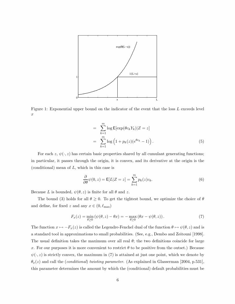
1{L > x} ≤ eθ(L−x); (2)

this is illustrated in Exhibit 1. Taking the conditional expectation of both sides of (2), we get

P (L > x|Z) ≤ E[eθ(L−x)|Z] = eψ(θ,Z)−θx, (3)

so ψ(θ, Z) contains information about the tail of the conditional loss distribution.

To calculate the conditional cumulant generating function, observe that conditional on the

risk factors, the default indicators Y1, . . . , Yd become independent. The conditional default

probabilities are

pk(z) = P (Yk = 1|Z = z) = P (Xk > Φ−1(1 − pk)|Z = z) = Φ

(akz + Φ−1(pk)

bk

), (4)

where ak = (ak1, . . . , akd) is the (row) vector of factor loadings for the kth obligor, and

Φ−1(1 − pk) = −Φ−1(pk) by the symmetry of the normal distribution. The conditional cu-

mulant generating function is then

ψ(θ, z) = logE

[exp

(θ

m∑

k=1

ckYk

)|Z = z

]

5

0

11{L>x}

exp(θ(L−x))

x L

Figure 1: Exponential upper bound on the indicator of the event that the loss L exceeds levelx

=m∑

k=1

logE[exp(θckYk)|Z = z]

=m∑

k=1

log(1 + pk(z)(eθck − 1)

). (5)

For each z, ψ(·, z) has certain basic properties shared by all cumulant generating functions;

in particular, it passes through the origin, it is convex, and its derivative at the origin is the

(conditional) mean of L, which in this case is

∂

∂θψ(0, z) = E[L|Z = z] =

m∑

k=1

pk(z)ck. (6)

Because L is bounded, ψ(θ, z) is finite for all θ and z.

The bound (3) holds for all θ ≥ 0. To get the tightest bound, we optimize the choice of θ

and define, for fixed z and any x ∈ (0, `max)

Fx(z) = minθ≥0

(ψ(θ, z)− θx) = −maxθ≥0

(θx − ψ(θ, z)) . (7)

The function x 7→ −Fx(z) is called the Legendre-Fenchel dual of the function θ 7→ ψ(θ, z) and is

a standard tool in approximations to small probabilities. (See, e.g., Dembo and Zeitouni [1998].

The usual definition takes the maximum over all real θ; the two definitions coincide for large

x. For our purposes it is more convenient to restrict θ to be positive from the outset.) Because

ψ(·, z) is strictly convex, the maximum in (7) is attained at just one point, which we denote by

θx(z) and call the (conditional) twisting parameter. (As explained in Glasserman [2004, p.531],

this parameter determines the amount by which the (conditional) default probabilities must be

6

adjusted or “twisted” to make the (conditional) expected loss greater than or equal to x.) If

the slope of ψ(·, z) at the origin is greater than x, then the maximum is attained at θx(z) = 0;

otherwise, it is attained at the unique solution to the first-order condition

∂

∂θψ(θ, z)− x = 0.

Using (6), we may therefore write

θx(z) =

{unique θ such that ∂ψ(θ, z)/∂θ = x, x > E[L|Z = z];0, x ≤ E[L|Z = z].

(8)

The twisting parameter θx(z) may loosely be interpreted as a measure of how much larger the

loss level x is than the conditionally expected loss E[L|Z = z]. With (8) we may write Fx as

Fx(z) = ψ(θx(z), z)− θx(z)x. (9)

Our interest in this function stems from the following observations.

Proposition 1 (i) For any 0 < x < `max,

P (L > x) ≤ E[eFx(Z)

].

(ii) The function z 7→ Fx(z) is (coordinatewise) increasing in z, decreasing in x, and Fx(z) ≤ 0

for all z.

(iii) Fx(z) = 0 if and only if E[L|Z = z] ≥ x.

(iv) If Fx(·) is concave, then

P (L > x) ≤ e−J(x) (10)

where

J(x) = −maxz

{Fx(z)− 12z

>z}. (11)

These assertions are substantiatied in Appendix A; here we offer some interpretation. For

each loss level x, exp(Fx(z)) should be viewed as a measure of the rarity or likelihood of the

event {L > x}, conditional on the factors Z taking the value z (recall (3) and Exhibit 1). For

this reason, we call Fx(z) (or |Fx(z)|) the conditional rate at x. When E[L|Z = z] ≥ x, (iii)

says that the event is not rare because exp(Fx(z)) = 1. Also, (ii) says that the event {L > x}becomes less likely as x increases and more likely as the factor level z increases. (Recall that all

7

the factor loadings akj are nonnegative.) Similarly, exp(−J(x)) should be viewed as a measure

of the unconditional rarity of {L > x}. The point zx at which the maximum in (11) occurs,

zx = argmaxz

{Fx(z) − 12z

>z}, (12)

may be interpreted as the most likely value of the factors leading to losses greater than x.

When (10) holds, it seems reasonable to take

J(x) = − d

dx

(maxz

{Fx(z) − 12z

>z})

(13)

as an approximation to the decay rate of P (L > x), in the sense that (an upper bound on)

logP (L > x) has a slope of −J(x) at the point x — the derivative J(x) tells us something

about how quickly the tail of the loss distribution P (L > x) is decreasing at x. This is the

premise of our first approximation. In fact, we view the rate J(x) as potentially more useful

than the bound itself in (10): even when the bound is too loose to be informative, the decay of

the bound will often parallel the decay of the probability itself.

The validity of the concavity assumption underlying (10) is determined primarily by the

loading matrix A, and fully satisfying this condition turns out to be restrictive. Concavity

holds in a single-factor model of identical obligors, but it virtually never holds in a multifactor

model. It would hold if all rows of the loading matrix A were multiples of each other, but such

a case could be reduced to a single-factor model. We will see some evidence of the ways in

which the structure of the matrix A determines deviations from concavity and the accuracy of

our approximations.

Inspection of the proof of the proposition shows, however, that concavity is a bit more than

what we need to justify (10). It would be enough for (36) to hold at z = zx, the maximizer of

Fx(z) − z>z/2. What we need, speaking loosely, is for Fx(z) − z>z/2 to drop off quickly as z

moves away from zx, and this (admittedly vague) property can hold even if concavity fails. There

are also ways to justify expressions like the right side of (10) as asymptotic approximations (as

is done in Glasserman, Heidelberger, and Shahabuddin [1999] and Glasserman and Li [2003]),

but we will not pursue that route here.

3.2 Properties of the Bound and Rate

From the expression in (13), it is not evident how one would calculate the derivative defin-

ing J(x). It turns out that this derivative is calculated automatically as a byproduct of the

maximization over z required to calculate J(x).

Before explaining this point, we discuss some further properties of the rate Fx and its

calculation. Evaluation of Fx(z) requires finding the twisting parameter θx(z) by solving the

8

equation in (8) if x >∑k pk(z)ck. Although θx(z) does not have a simple closed-form expression,

finding it numerically is just a scalar root-finding problem. The derivatives of ψ(·, z) can be

written out explicitly (see Appendix B) and used to implement a second-order Newton method,

for example. If some of the ck are very large, then terms of the form exp(θck) can create

numerical difficulties, so it is a good idea to choose units for the losses in which the ck are not

too large.

Evaluation of J(x) requires optimization of Fx(z) − z>z/2 over z and this is the most

computationally demanding step in our approximations. The optimization is faciliated by

the availability of explicit expressions for the first- and second-order derivatives of Fx(z) with

respect to the components of z. These are detailed in Appendix B. With these expressions,

we optimize using a line search Newton method with Armijo backtracking as in Nocedal and

Wright [1999], pp.35–42. When the number of factors (the dimension of z) is very large, it may

be preferable to use a quasi-Newton method to avoid evaluation of the full Hessian.

Let zx maximize Fx(z) − z>z/2, so that

J(x) = −(Fx(zx) − 1

2z>x zx

). (14)

In Appendix B, we show that

J(x) = θx(zx). (15)

To evaluate Fx(z) we need to find the twisting parameter θx(z), so in the course of computing the

optimizer zx we evaluate θx(zx) anyway. Thus, the derivative J(x) is available as a byproduct

of the optimization. This is an important simplification, particularly for the method of the next

section.

4 Fitting a Homogeneous Portfolio

In this section and the next two, we present strategies for converting the properties in Propo-

sition 1 to approximations for P (L > x). The approach of this section uses the infinite-obligor

limit of a homogeneous portfolio to approximate P (L > x). The decay rate J(x) is used to

select the approximating portfolio.

For this, we first need to discuss the case of a single-factor, homogeneous portfolio. Consider,

then, a model with identical default probabilities (pk ≡ p), identical exposures (ck ≡ 1), and

identical loadings (ak1 ≡ ρ) on a single factor Z. Each default indicator takes the form

Yk = 1{ρZ +√

1− ρ2εk > Φ−1(1− p)}, k = 1, . . . , m, (16)

9

with conditional default probabilities

pk(z) = p(z) = P (Yk = 1|Z = z) = Φ

(ρz + Φ−1(p)√

1 − ρ2

).

Let Lm = Y1+· · ·+Ym denote the loss for this portfolio and extend the Yk to an infinite sequence

Y, Y1, Y2, . . . of the form in (16) using i.i.d. N(0, 1) random variables ε, ε1, ε2, . . .. Because the

Yk are conditionally i.i.d. (given Z) and the ck are all equal to 1, we have

P (Lm/m > q) → P (E[Y |Z] > q) = P (p(Z) > q) = 1− Gp,ρ(q),

where

Gp,ρ(q) = Φ

(Φ−1(q)

√1− ρ2 − Φ−1(p)ρ

)(17)

for 0 < q < 1 and Gp,ρ(0) = 0. This is the loss distribution for the infinite-obligor limit of a

homogeneous portfolio. This distribution has two parameters, p and ρ.

This distribution has been derived and applied by several authors including Vasicek [1991],

Schonbucher [2001], Kalkbrenner, Lotter, and Overbeck [2004], Lucas, Klaasen, Spreij, and

Straetmans [2001]. It has also been incorporated into the Basel Committee’s internal ratings-

based approach to credit risk.

4.1 The Approximation

In using this distribution as an approximation for a general portfolio, we interpret q to be

the loss level expressed as a fraction of the maximum possible loss `max. Thus, we seek an

approximation of the form

P (L > x) ≈ 1 −Gp,ρ(x/`max), 0 < x < `max,

for which we need to select the parameters p and ρ.

We choose p to match the expected loss E[L]. On one hand we have∫ `max

0P (L > x) dx = E[L] =

m∑

k=1

pkck,

and on the other hand we have∫ `max

0[1−Gp,ρ(x/`max)] dx = `max

∫ 1

0[1−Gp,ρ(q)] dq = p`max = p

m∑

k=1

ck.

In order to equate these two means, we choose p = p with

p =m∑

k=1

pkck

/m∑

k=1

ck. (18)

10

This is the exposure-weighted average of the default probabilities and is thus appealing on

intuitive grounds as well.

We choose ρ to match the approximate decay rate of the tail of L. For this, we pick

a relatively large loss level x1 and calculate J(x1) for the original portfolio. Recall that we

interpret this as an approximate decay rate in the sense that

d

dxlogP (L > x1) ≈ −J(x1). (19)

We therefore choose ρ so that

d

dqlog(1 −Gp,ρ(x1/`max)) ≈ −J(x1)`max. (20)

(Because L is discrete, its distribution is not differentiable and we are ingoring this in (19).

The function J(x) is, in a sense, a smoothed approximation to logP (L > x).)

Given the value of J(x1) one can solve numerically for a value of ρ that makes the two

sides of (20) equal. A further approximation makes it possible to write the required value of ρ

explicitly, with no evident impact on the quality of the overall approximation. At large values of

x, 1− Φ(x) is well approximated by φ(x)/x, with φ the standard normal density. Accordingly,

from (17) we have

log(1− Gp,ρ(q)) ≈ −12

(Φ−1(q)

√1 − ρ2 − Φ−1(p)ρ

)2

.

Differentiating with respect to q and using the resulting derivative on the left side of (20) yields

a quadratic equation for δ =√

1 − ρ2. The required root is given by

δ =−b+

√b2 + 4aJ(x1)2a

, (21)

with

a = J(x1) +Φ−1(q1)

φ(Φ−1(q1))`max, b = −Φ−1(p)/φ(Φ−1(q1))`max,

q1 = x1/`max, and then ρ =√

1 − δ2.

We summarize the approximation in the following steps:

1. Choose a large value of x1 (where P (L > x1) ≈ 0.001–0.01) and find

zx1 = argmaxz

{Fx1(z)− z>z/2},

using, e.g., a Newton method with derivatives as in Appendix B.

11

2. Set J(x1) = θx1(zx1) with θx(z) as in (8). (This is available as a byproduct of Step 1.)

3. Set ρ1 =√

1 − δ2 with δ the root of the quadratic equation given in (21).

4. Set p =∑k pkck/`max.

5. Return the approximation

P (L > x) ≈ 1 − Φ

Φ−1(x/`max)

√1 − ρ2

1 − Φ−1(p)

ρ1

, (22)

for all 0 < x < `max.

It should be noted that this procedure requires just one optimization over z to compute a

single decay rate J(x1). Once ρ1 is selected using this decay rate, (22) provides an approximation

to the entire curve of P (L > x).

In choosing x1, we use a rule of the form

x1 =m∑

k=1

pkck + νm∑

k=1

ck

√pk(1 − pk). (23)

If Y1, . . . , Yk were perfectly correlated, this would set x1 at ν standard deviations above the

mean. We usually use ν = 1/2 or ν = 2 because this usually results in a small value for

P (L > x1). However, (23) and these values of ν are fairly arbitrary, and we will see that one

can often do better with better information about where P (L > x) becomes small. There is

usually a wide range of values of x1 that produce very similar approximations. If J(x1) < 0

then x1 is too small and should be increased.

As x decreases toward 0, the approximation on the right side of (22) approaches 1: the

distribution for the infinite-obligor limit assigns probability 0 to a loss of exactly 0. In contrast,

the actual loss L is 0 with positive probability. We therefore cannot expect the approximation

to be accurate for small values of x. But even though the approximation in (22) invariably starts

at a higher level than the true tail probability, it drops very quickly and can be surprisingly

accurate for even moderately large values of x. We illustrate this through examples, starting

in Section 4.2.

The optimization problem that defines J(x) may have multiple local maxima, but these

are ignored by (22). A natural way to try to incorporate them in (22) uses a mixture of M

homogeneous distributions of the form

P (L > x) ≈M∑

i=1

wi(1− Gp,ρi(x/`max)), (24)

12

with weights wi summing to 1. Each ρi is the value fit using a local maximum zi. The wi should

give less weight to zi far from the origin, for example weighting them in inverse proportion to

their norms. We have found this extension helpful in some examples with two local maxima,

but to limit the number of alternatives we consider we do not pursue this extension here.

4.2 Numerical Examples

We illustrate the approximations discussed so far with some numerical results for test portfolios.

These will be used in subsequent sections as well.

Portfolios A1 and A2

As a first illustration, we consider a portfolio (which we call A1) of m = 1000 obligors in a

10-factor model. The marginal default probabilities and exposures have the following form:

pk = 0.01 · (1 + sin(16πk/m)), k = 1, . . . , m; (25)

ck = (d5k/me)2, k = 1, . . . , m. (26)

Thus, the marginal default probabilities fluctuate between 0 and 2% with a mean of 1%, and

the possible exposures are 1, 4, 9, 16, and 25, with 200 obligors at each level. This is a lumpy

exposure profile compared with the fixed value of ck implicit in the homogeneous approximation.

Finally, for the factor loading matrix we generate the akj independently and uniformly from

the interval (0, 1/√d), d = 10; the upper limit of this interval ensures that the sum of squared

entries in each row of A does not exceed 1.

In fitting a homogeneous portfolio, we need a rule for selecting the point x1 at which to

match the decay rate. In order to provide a systematic comparison, we use (23) with ν = 1/2

and ν = 2. As already noted, these values are fairly arbitrary, and they do not necessarily

provide the best possible approximation.

The left panel of Exhibit 2 compares the approximations with loss probabilities estimated

using Monte Carlo simulation. The horizontal axis shows loss levels and the vertical axis shows

the probability that the loss exceeds each level, on a logarithmic scale. The solid line shows the

Monte Carlo estimates, the dashed line is the approximation at ν = 1/2 (x1 = 579, ρ1 = .4889)

and the dotted line is the approximation at ν = 2 (x1 = 2005, ρ1 = .4859). The three curves

are nearly identical over a wide range of loss levels and tail probabilities.

The right panel of Exhibit 2 shows a magnified view of the distributions at small loss levels.

As explained above, the homogeneous approximations have no chance of matching the correct

13

0 500 1000 1500 2000 2500 3000 3500 4000 4500 500010

−6

10−5

10−4

10−3

10−2

10−1

100

Loss Level

Tai

l Pro

babi

lity

0 10 20 30 40 50 60 70 80 90 1000.2

0.3

0.4

0.5

0.6

0.7

0.8

0.9

1

Loss Level

Tai

l Pro

babi

lity

Figure 2: Homogeneous approximations (dashed and dotted lines) for Portfolio A1. The solidline shows Monte Carlo estimates. The left panel displays probability on a log scale. The rightpanel gives a magnified view at low loss levels.

value at 0, but they catch up with the correct values remarkably quickly. (The wobbly pattern

in the Monte Carlo curve results from the lumpy exposure profile.)

The excellent performance of the approximation in Exhibit 2 is typical of many examples

we have tested in which the elements of A are randomly generated. To illustrate this point,

we consider a modification which we refer to as Portfolio A2. The modified portfolio has just

100 obligors. The marginal default probabilities are as in (25) but multiplied by 2.5 so that

they lie between 0 and 5%. These changes should make the portfolio less amenable to the

approximation. The exposures have the lumpy form in (26). We consider a 5-factor version of

the model, with each entry of the loading matrix A uniformly distributed between 0 and 1/√

5.

The results are displayed in Exhibit 3. The two approximating curves (calculated at ν = 1/2

and ν = 2) are virtually indistinguishable and are indicated by the dashed line. The solid line

shows Monte Carlo estimates.

Portfolio B

Our next example has five factors and 496 obligors, grouped into sets of sizes 256, 128, 64, 32,

and 16. Within each group, the obligors have identical factor loadings, given by the following

row vectors:

(1/√

6, 1/√

6, 1/√

6, 1/√

6, 1/√

6), (1/√

5, 1/√

5, 1/√

5, 1/√

5, 0), (1/√

4, 1/√

4, 1/√

4, 0, 0),

(1/√

3, 1/√

3, 0, 0, 0), (1/√

2, 0, 0, 0, 0).

14

0 100 200 300 400 500 600 70010

−7

10−6

10−5

10−4

10−3

10−2

10−1

100

Loss Level

Tai

l Pro

babi

lity

0 500 1000 1500 2000 2500 3000 3500 4000 4500 5000

10−3

10−2

10−1

100

Loss Level

Tai

l Pro

babi

lity

Fit at 946.3

Fit at 255.5

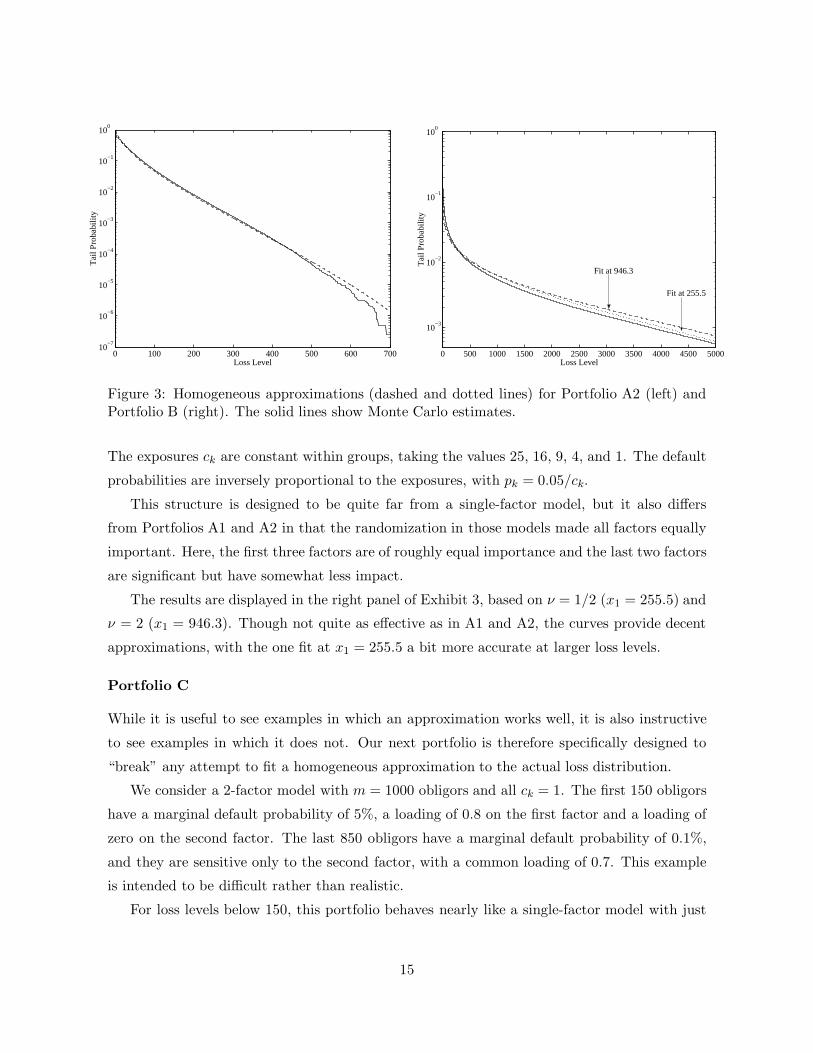
Figure 3: Homogeneous approximations (dashed and dotted lines) for Portfolio A2 (left) andPortfolio B (right). The solid lines show Monte Carlo estimates.

The exposures ck are constant within groups, taking the values 25, 16, 9, 4, and 1. The default

probabilities are inversely proportional to the exposures, with pk = 0.05/ck.

This structure is designed to be quite far from a single-factor model, but it also differs

from Portfolios A1 and A2 in that the randomization in those models made all factors equally

important. Here, the first three factors are of roughly equal importance and the last two factors

are significant but have somewhat less impact.

The results are displayed in the right panel of Exhibit 3, based on ν = 1/2 (x1 = 255.5) and

ν = 2 (x1 = 946.3). Though not quite as effective as in A1 and A2, the curves provide decent

approximations, with the one fit at x1 = 255.5 a bit more accurate at larger loss levels.

Portfolio C

While it is useful to see examples in which an approximation works well, it is also instructive

to see examples in which it does not. Our next portfolio is therefore specifically designed to

“break” any attempt to fit a homogeneous approximation to the actual loss distribution.

We consider a 2-factor model with m = 1000 obligors and all ck = 1. The first 150 obligors

have a marginal default probability of 5%, a loading of 0.8 on the first factor and a loading of

zero on the second factor. The last 850 obligors have a marginal default probability of 0.1%,

and they are sensitive only to the second factor, with a common loading of 0.7. This example

is intended to be difficult rather than realistic.

For loss levels below 150, this portfolio behaves nearly like a single-factor model with just

15

the first 150 obligors. At higher loss levels, the second factor and the remaining obligors become

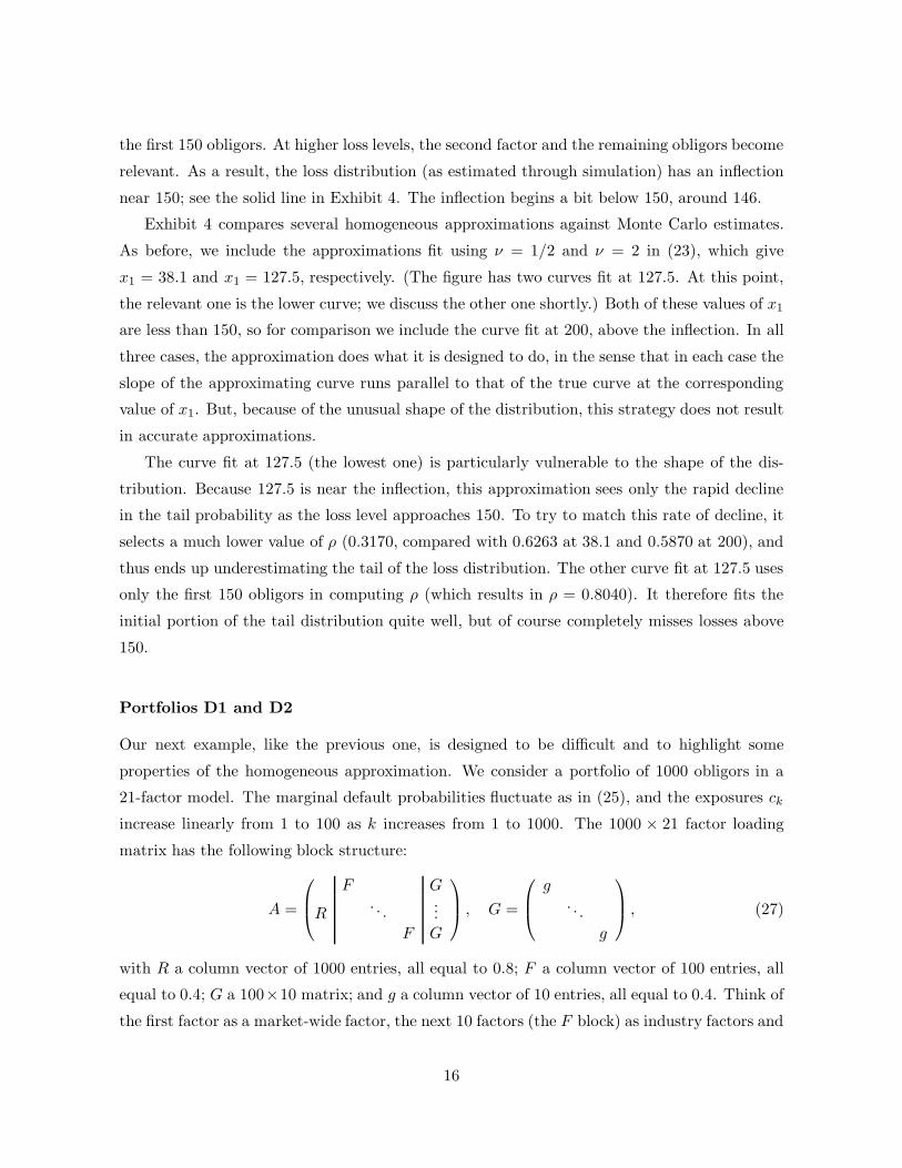
relevant. As a result, the loss distribution (as estimated through simulation) has an inflection

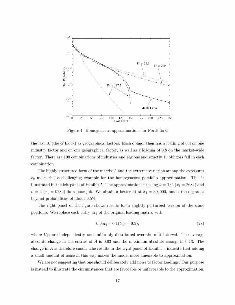
near 150; see the solid line in Exhibit 4. The inflection begins a bit below 150, around 146.

Exhibit 4 compares several homogeneous approximations against Monte Carlo estimates.

As before, we include the approximations fit using ν = 1/2 and ν = 2 in (23), which give

x1 = 38.1 and x1 = 127.5, respectively. (The figure has two curves fit at 127.5. At this point,

the relevant one is the lower curve; we discuss the other one shortly.) Both of these values of x1

are less than 150, so for comparison we include the curve fit at 200, above the inflection. In all

three cases, the approximation does what it is designed to do, in the sense that in each case the

slope of the approximating curve runs parallel to that of the true curve at the corresponding

value of x1. But, because of the unusual shape of the distribution, this strategy does not result

in accurate approximations.

The curve fit at 127.5 (the lowest one) is particularly vulnerable to the shape of the dis-

tribution. Because 127.5 is near the inflection, this approximation sees only the rapid decline

in the tail probability as the loss level approaches 150. To try to match this rate of decline, it

selects a much lower value of ρ (0.3170, compared with 0.6263 at 38.1 and 0.5870 at 200), and

thus ends up underestimating the tail of the loss distribution. The other curve fit at 127.5 uses

only the first 150 obligors in computing ρ (which results in ρ = 0.8040). It therefore fits the

initial portion of the tail distribution quite well, but of course completely misses losses above

150.

Portfolios D1 and D2

Our next example, like the previous one, is designed to be difficult and to highlight some

properties of the homogeneous approximation. We consider a portfolio of 1000 obligors in a

21-factor model. The marginal default probabilities fluctuate as in (25), and the exposures ckincrease linearly from 1 to 100 as k increases from 1 to 1000. The 1000 × 21 factor loading

matrix has the following block structure:

A =

F G

R. . .

...F G

, G =

g

. . .g

, (27)

with R a column vector of 1000 entries, all equal to 0.8; F a column vector of 100 entries, all

equal to 0.4; G a 100×10 matrix; and g a column vector of 10 entries, all equal to 0.4. Think of

the first factor as a market-wide factor, the next 10 factors (the F block) as industry factors and

16

0 25 50 75 100 125 150 175 200 225 25010

−5

10−4

10−3

10−2

10−1

100

Loss Level

Tai

l Pro

babi

lity

Fit at 127.5

Fit at 38.1 Fit at 200

Monte Carlo

Figure 4: Homogeneous approximations for Portfolio C

the last 10 (the G block) as geographical factors. Each obligor then has a loading of 0.4 on one

industry factor and on one geographical factor, as well as a loading of 0.8 on the market-wide

factor. There are 100 combinations of industies and regions and exactly 10 obligors fall in each

combination.

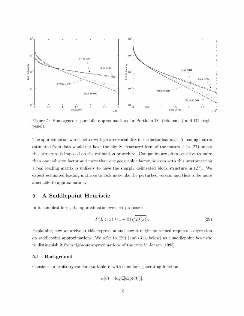
The highly structured form of the matrix A and the extreme variation among the exposures

ck make this a challenging example for the homogeneous portfolio approximation. This is

illustrated in the left panel of Exhibit 5. The approximations fit using ν = 1/2 (x1 = 2684) and

ν = 2 (x1 = 9282) do a poor job. We obtain a better fit at x1 = 30, 000, but it too degrades

beyond probabilities of about 0.5%.

The right panel of the figure shows results for a slightly perturbed version of the same

portfolio. We replace each entry akj of the original loading matrix with

0.9akj + 0.1(Ukj − 0.5), (28)

where Ukj are independently and uniformly distributed over the unit interval. The average

absolute change in the entries of A is 0.03 and the maximum absolute change in 0.13. The

change in A is therefore small. The results in the right panel of Exhibit 5 indicate that adding

a small amount of noise in this way makes the model more amenable to approximation.

We are not suggesting that one should deliberately add noise to factor loadings. Our purpose

is instead to illustrate the circumstances that are favorable or unfavorable to the approximation.

17

0 0.5 1 1.5 2 2.5 3

x 104

10−4

10−3

10−2

10−1

100

Loss Level

Tai

l Pro

babi

lity

Fit at 2684

Fit at 9282

Fit at 30,000

Monte Carlo

0 0.5 1 1.5 2 2.5 3

x 104

10−4

10−3

10−2

10−1

100

Loss Level

Tai

l Pro

babi

lity

Fit at 2684

Fit at 9282

Fit at 30,000

Monte Carlo

Figure 5: Homogeneous portfolio approximations for Portfolio D1 (left panel) and D2 (rightpanel).

The approximation works better with greater variability in the factor loadings. A loading matrix

estimated from data would not have the highly structured form of the matrix A in (27) unless

this structure is imposed on the estimation procedure. Companies are often sensitive to more

than one industry factor and more than one geographic factor, so even with this interpretation

a real loading matrix is unlikely to have the sharply delineated block structure in (27). We

expect estimated loading matrices to look more like the perturbed version and thus to be more

amenable to approximation.

5 A Saddlepoint Heuristic

In its simplest form, the approximation we next propose is

P (L > x) ≈ 1 − Φ(√

2J(x)). (29)

Explaining how we arrive at this expression and how it might be refined requires a digression

on saddlepoint approximations. We refer to (29) (and (31), below) as a saddlepoint heuristic

to distinguish it from rigorous approximations of the type in Jensen [1995].

5.1 Background

Consider an arbitrary random variable V with cumulant generating function

κ(θ) = logE[exp(θV )].

18

The argument used in part (i) of Proposition 1 similarly shows that P (V > v) ≤ exp(−I(v))where

I(v) = maxα

(αv − κ(α)) = αvv − κ(αv) (30)

and αv the point at which the maximum is attained. Saddlepoint methods convert this bound

on tail probabilities into approximations using higher-order derivatives of κ.

Of the many possible saddlepoint approximations in the literature, we consider the Lugannani-

Rice formula, which is

P (V > v) ≈ 1 − Φ(r) + φ(r)(

1λ− 1r

),

with

r =√

2(αvv − κ(αv)) =√

2I(v)

and

λ = αv

√κ′′(αv) = I ′(v)/

√I ′′(v).

The last equality follows from the Legendre-Fenchel transformation in (30), along the same

lines used to derive (40) in Appendix B.

Saddlepoint approximations have been used to measure portfolio credit risk by Martin,

Thompson, and Browne [2001] in a model with independent obligors (or in a finite mixture

of such models) and by Gordy [2002] in the CreditRisk+ model for which the cumulant gen-

erating function is known. A direct application in the framework of Section 2 is not possible

because of the intractability of the cumulant generating function of L. Rather than try to eval-

uate or approximate this cumulant generating function, we approximate its Legendre-Fenchel

transform.

5.2 The Approximation

Set V = Φ−1(L/`max). Proposition 1 implies that

P (V < v) ≤ exp (−J(Φ(v)`max)) ,

so let

I(v) = J(Φ(v)`max).

As a purely heuristic approximation, we proceed as though I(v) were in fact the Legendre-

Fenchel transform of the cumulant generating function of V . The resulting approximation

is

P (L > x) = 1 − Φ(√

2J(x)) + φ(√

2J(x))

(√I ′′(v)I ′(v)

− 1√2J(x)

), (31)

19

with v = Φ−1(x/`max)

I ′(v) = J(x)φ(v)`max

and

I ′′(v) = J(x)φ2(v)`2max − J(x)φ(v)v`max.

We noted previously that J(x) = θx(zx). Although an explicit expression is also available for

J in (46), it is somewhat simpler to use a central difference approximation of the form

J(x) ≈ J(x+ h) − J(x− h)2h

.

If I(v) were in fact the Legendre-Fenchel dual of a cumulative generating function, it would

be convex, I ′′(v) would always be positive, and the√I ′′(v) appearing in the approximation

would always be meaningful. But no such guarantee applies to our heuristic use of J . Also, the

last term in (31) is often quite small; omitting it yields the simplified approximation in (29).

5.3 Adjusting the Mean

In contrast to the approximation of Section 4.1, neither (29) nor (31) is consistent with the

known value of the expected loss, E[L] =∑k pkck. In Section 4.1, we were able to ensure

consistency through the choice of the parameter p in (18). To make (29) and (31) consistent

with E[L], we propose scaling these approximations. This sometimes improves accuracy.

Consider any approximation of the form P (L > x) ≈ 1 − G(x). If we could calculate

mG =∫ ∞

0(1 −G(x)) dx,

then we could make the approximation consistent with the mean loss through the adjustment

P (L > x) ≈ 1mG

m∑

k=1

pkck (1 −G(x))) ;

integrating both sides over x from 0 to ∞ now yields E[L]. In practice, accurate calculation of

mG may be difficult, especially if each evaluation of G is time-consuming. Also, the approxima-

tions in (29) and (31) are intended for large values of x, but the integral of the approximations

would be heavily influenced by their values at small x where the probabilities P (L > x) are

largest and the approximations least accurate.

To avoid undertaking a numerical integration of the approximations, we apply a simple

adjustment based on the homogeneous-portfolio distribution Gp,ρ. We fix p as in (18) and

choose ρ to fit a multiple of 1−Gp,ρ to the approximation 1−G. We then use this multiple to

scale 1 − G. In more detail, we apply the following steps:

20

1. Choose points xi and evaluate G(xi), i = 1, . . . , n (e.g., n = 20);

2. Find ρ to minimize the sum of squared differencesn−1∑

i=1

(log

1 −Gp,ρ(xi+1/`max)1− Gp,ρ(xi/`max)

− log1− G(xi+1)1 −G(xi)

)2

;

3. Calculate the average ratio

r =1n

n∑

i=1

log1 −Gp,ρ(xi/`max)

1 − G(xi);

4. Return the scaled approximation er(1− G(xi)), i = 1, . . . , n.

Step 2 finds the value of ρ for which log(1−Gp,ρ(x/`max) is most nearly parallel to log(1−G(x)). Step 3 calculates the average displacement between the two curves and Step 4 shifts

log(1−G) by this amount. If 1−G(x) were exactly equal to a multiple of some 1−Gp,ρ(x/`max),

then the adjusted approximation would integrate to E[L].

A drawback of this adjustment is that it is very sensitive to the choice of points xi at which

the approximation is evaluated. In numerical examples we find that the adjustment can improve

the accuracy of the approximation, but it can also make it worse. Its application requires care.

6 Laplace Approximation

The method of this section uses part (i) of Proposition 1. Calculating the upper bound

E[exp(Fx(Z))] is in principle a problem of integrating over the distribution of the vector of

risk factors Z. This is impractical unless the number of risk factors is small, especially since a

separate integration is required at each loss level x.

The Laplace approximation (as in, e.g., Section IX.5 of Wong [1989]) provides an alternative

to numerical integration. It is based on a quadratic approximation to the logarithm of the

integrand in

E[eFx(Z)] = (2π)−d/2∫

<deFx(z)−z>z/2 dz.

The quadratic approximation results from a Taylor expansion of the exponent Fx(z) − z>z/2

near the point at which this expression is maximized; i.e., near

zx = argmaxz

{Fx(z) − 12z

>z}.

This is precisely the optimization problem that appears in the definition of J(x). The Laplace

approximation is then

E[eFx(Z)] ≈ e−J(x)

√det(I − ∇2Fx(zx))

, (32)

21

where ∇2Fx denotes the Hessian of Fx with respect to z. The Hessian can be calculated using

formulas in Appendix B.

We apply the right side of (32) as an approximation to P (L > x), though we have derived

it as an approximation to a bound on this tail probability. The method of Section 5.3 can be

used to adjust the approximation to try to match the known value of E[L].

Because the Laplace approximation is based on a quadratic approximation to Fx(z)−z>z/2,

it works best if this function is at least concave. To put it another way, the approximation only

uses information about the integrand near its maximum, ignoring the possibility of local max-

ima. The impact of local maxima is driven primarily by the structure of the factor loading

matrix A. We can reasonably expect that Fx(z) − z>z/2 will be strictly concave in a neigh-

borhood of the global maximizer zx, so that ∇2Fx(zx) − I will be negative definite and the

denominator in (32) strictly positive.

We summarize the approximation as follows. At each x,

1. Solve the optimization problem in (12) to find zx and evaluate J(x) = Fx(zx)− z>x zx/2.

2. Compute the Hessian ∇2Fx(zx) using (43).

3. Evaluate the determinant det(I − ∇2Fx(zx)) and return the approximation

P (L > x) ≈ e−J(x)

√det(I −∇2Fx(zx))

.

After the approximation has been evaluated at multiple values of x, one may optionally apply

the mean adjustment in Section 5.3.

This method, like the saddlepoint heuristic, requires re-solving the optimization over z (and

over θ) at each x at which the approximation is evaluated. Fortunately, the optimal points

(zx, θx(zx)) usually change slowly with x, so the optimal value for each point provides an

excellent starting value for the optimization at the next point. Starting each optimization at

the previous optimum can thus reduce the total time required.

Exhibit 6 shows both the saddlepoint heuristic (29) and the Laplace approximation for

Portfolios A1 and A2 from Section 4.2. For Portfolio A1, the two approximations give nearly

identical results, and both are very close to the true probabilities as estimated by Monte Carlo

(the solid line in the figure). For Portfolio A2, the saddlepoint heuristic is nearly exact, but

the Laplace approximation appears to be off by a constant factor (a constant displacement on

a log scale). The mean adjustment of Section 5.3 produces the points marked by squares in

the figure. The mean adjustment has a negligible effect on the saddlepoint heuristic in this

example, so that case is omitted for clarity.

22

0 500 1000 1500 2000 2500 3000 3500 4000 4500 500010

−6

10−5

10−4

10−3

10−2

10−1

100

Loss Level

Tai

l Pro

babi

lity

0 100 200 300 400 500 600 70010

−7

10−6

10−5

10−4

10−3

10−2

10−1

100

Loss Level

Tai

l Pro

babi

lity

Figure 6: Saddlepoint heuristic (filled circles) and Laplace approximation (empty circles) forPortfolios A1 (left panel) and A2 (right panel). The squares in the right panel show the mean-adjusted Laplace approximation. The solid shows Monte Carlo estimates.

The left panel of Exhibit 7 similarly illustrates the saddlepoint heuristic and Laplace ap-

proximation for Portfolio B. As in the previous example, the saddlepoint heuristic is quite

accurate. The Laplace approximation sags near the middle of the distribution. Though not

shown in the figure, the values of E[exp(Fx(Z))] are quite close to the true loss probabilities

P (L > x). This indicates that the main source of error in the Laplace approximation is the

method used to approximate the integral over the normal distribution, rather than the error in

using Proposition 1(i) as an approximation.

Portfolio C of Section 4.2 provides a more interesting example. Exhibit 7 compares the

saddlepoint heuristic (the filled circles) and the Laplace approximation (the empty circles) with

Monte Carlo estimates (the solid line). The figure shows the distribution over a very wide

range of loss levels. Despite the unusual shape of the distribution, the saddlepoint heuristic

is nearly exact over the full range. The Laplace approximation also manages to trace the

shape of the distribution, though it again appears to be displaced over most of the range.

Both approximations are remarkably accurate even at probabilities as small as 10−10. (We

obtain precise Monte Carlo estimates of such small probabilities using the importance sampling

method in Glasserman and Li [2003], which draws on some of the same tools used here to derive

approximations.)

Because of the special structure of this portfolio, the optimal solution zx in (12) undergoes

an abrupt change as x approaches 150. As x increases from 0 toward the inflection, the first

component of zx increases while the second stays close to 0 — losses in this range are most

23

0 1000 2000 3000 4000 5000 6000 7000 8000 9000 1000010

−7

10−6

10−5

10−4

10−3

10−2

10−1

100

Loss Level

Tai

l Pro

babi

lity

0 100 200 300 400 500 600 700 800 900

10−10

10−8

10−6

10−4

10−2

100

Loss Level

Tai

l Pro

babi

lity

Figure 7: Saddlepoint heuristic (filled circles) and Laplace approximation (empty circles) forPortfolios B (left) and C (right). The solid lines are Monte Carlo estimates

likely to occur because of large moves in the first factor. At x = 146, we get an optimal

solution of zx = (3.4230, 0.0086) but at x = 147 the optimum flips to (0.0345, 3.4412), because

at larger loss levels the second factor becomes more important than the first. As x continues to

increase, both components of zx increase. These features are automatically detected by both

the saddlepoint heuristic and the Laplace approximation and permit these methods to capture

the shape of the loss distribution.

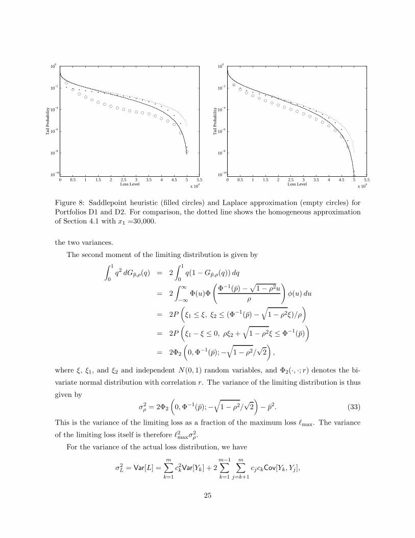
Exhibit 8 shows results for Portfolios D1 (left panel) and D2 (right panel). The filled

circles show the saddlepoint heuristic and the empty circles show the Laplace approximation.

The dotted line shows the approximation of Section 4 fit at x1 = 30, 000 and is included for

comparison. As with the previous approximations, we see greater accuracy in the perturbed

case. The saddlepoint heuristic and the Laplace approximation do particularly well at small

probabilities.

7 Matching Two Moments

The approximation proposed in this section differs from the previous ones in that it does not use

the decay rate from Proposition 1. Like the method of Section 4, it uses the limiting distribution

for a homogeneous portfolio, but it selects ρ by matching variances rather than decay rates.

We noted previously that the distribution Gp,ρ has mean p. That leaves the parameter

ρ free for the choice of variance. We will choose ρ so that the variance of the approximating

distribution matches that of the actual distribution. In order to do this, we first need to evaluate

24

0 0.5 1 1.5 2 2.5 3 3.5 4 4.5 5 5.5

x 104

10−10

10−8

10−6

10−4

10−2

100

Loss Level

Tai

l Pro

babi

lity

0 0.5 1 1.5 2 2.5 3 3.5 4 4.5 5 5.5

x 104

10−10

10−8

10−6

10−4

10−2

100

Loss Level

Tai

l Pro

babi

lity

Figure 8: Saddlepoint heuristic (filled circles) and Laplace approximation (empty circles) forPortfolios D1 and D2. For comparison, the dotted line shows the homogeneous approximationof Section 4.1 with x1 =30,000.

the two variances.

The second moment of the limiting distribution is given by∫ 1

0q2 dGp,ρ(q) = 2

∫ 1

0q(1 −Gp,ρ(q)) dq

= 2∫ ∞

−∞Φ(u)Φ

(Φ−1(p) −

√1 − ρ2u

ρ

)φ(u) du

= 2P(ξ1 ≤ ξ, ξ2 ≤ (Φ−1(p) −

√1 − ρ2ξ)/ρ

)

= 2P(ξ1 − ξ ≤ 0, ρξ2 +

√1 − ρ2ξ ≤ Φ−1(p)

)

= 2Φ2

(0,Φ−1(p);−

√1 − ρ2/

√2),

where ξ, ξ1, and ξ2 and independent N(0, 1) random variables, and Φ2(·, ·; r) denotes the bi-

variate normal distribution with correlation r. The variance of the limiting distribution is thus

given by

σ2ρ = 2Φ2

(0,Φ−1(p);−

√1 − ρ2/

√2)− p2. (33)

This is the variance of the limiting loss as a fraction of the maximum loss `max. The variance

of the limiting loss itself is therefore `2maxσ2ρ.

For the variance of the actual loss distribution, we have

σ2L = Var[L] =

m∑

k=1

c2kVar[Yk ] + 2m−1∑

k=1

m∑

j=k+1

cjckCov[Yk, Yj ],

25

with

Var[Yk] = pk(1− pk)

and

Cov[Yk, Yj ] = P (Xk ≤ Φ−1(pk), Xj ≤ Φ−1(pj))− pkpj

= Φ2(Φ−1(pk),Φ−1(pj); aka>j ) − pkpj ,

in light of (1). We now solve numerically for ρ satisfying `maxσ2ρ = σ2

L.

The most time-consuming step in this approximation is the calculation of the loss variance

σ2L, which requires O(m2) evaluations of the bivariate normal distribution. Agca and Chance

[2003] compare several methods for evaluating the bivariate normal and report that 125,000

evaluations take 7–20 seconds. At these speeds, calculation of σ2L takes less than two seconds

for m = 100 and about 30-90 seconds for m = 1000 — not instantaneous, but not prohibitively

slow either. The calculation could be accelerated by bucketing the marginal probabilities pkand correlations aka>j and computing just one value of the bivariate normal for each bucket.

Kalkbrenner, Lotter, and Overbeck [2004] use similar information to fit a homogeneous

distribution Gp,ρ. They select p = p as we do, but they select ρ so that the value of

Var

[m∑

k=1

pkckXk

](34)

is the same in the approximating single-factor portfolio as in the original portfolio. This results

in the explicit formula

ρ2 =∑mj,k=1 pkck(aka

>j )pjcj −

∑mk=1 p

2kc

2kb

2k

(∑mk=1 pkck)

2 −∑mk=1 p

2kc

2k

, (35)

and taking the square root yields ρ. The motivation for matching the variance (34) is unclear,

though this may serve as a proxy for the variance of the loss L. Because the variance in (34)

requires the covariances between pairs (Xj , Xk) but not pairs (Yj , Yk), this method does not

require calculation of bivariate normal probabilities and is thus extremely fast.

Matching two moments gives results for portfolios A1 and A2 similar to those in previ-

ous sections, so we proceed to the other cases. Exhibit 9 shows two-moment approximations

(dashed lines) for Portfolios B and C. For comparison, the figure also includes the best approx-

imations from Section 4 (fit at 255.5 and 200). The two-moment approximations do quite well.

Although no homogeneous approximation can capture the inflection in the actual distribution

for Portfolio C, the one selected through the two-moment approximation does a pretty good

26

0 1000 2000 3000 4000 5000 6000 7000 8000 9000 1000010

−8

10−7

10−6

10−5

10−4

10−3

10−2

10−1

100

Loss Level

Tai

l Pro

babi

lity

2−Moment

KLO

Fit at 255.5

Monte Carlo

0 100 200 300 400 500 600 700 800 900

10−10

10−8

10−6

10−4

10−2

100

Loss Level

Tai

l Pro

babi

lity KLO

Fit at 200

2−Moment

Monte Carlo

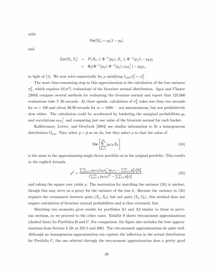
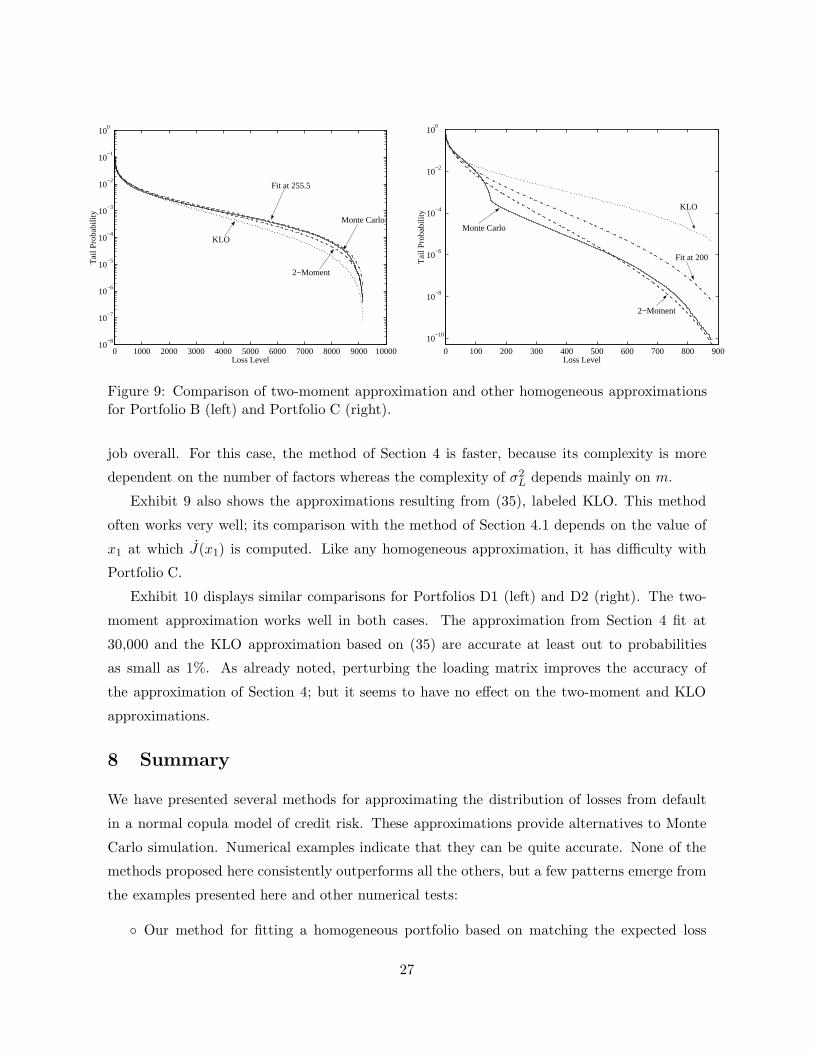
Figure 9: Comparison of two-moment approximation and other homogeneous approximationsfor Portfolio B (left) and Portfolio C (right).

job overall. For this case, the method of Section 4 is faster, because its complexity is more

dependent on the number of factors whereas the complexity of σ2L depends mainly on m.

Exhibit 9 also shows the approximations resulting from (35), labeled KLO. This method

often works very well; its comparison with the method of Section 4.1 depends on the value of

x1 at which J(x1) is computed. Like any homogeneous approximation, it has difficulty with

Portfolio C.

Exhibit 10 displays similar comparisons for Portfolios D1 (left) and D2 (right). The two-

moment approximation works well in both cases. The approximation from Section 4 fit at

30,000 and the KLO approximation based on (35) are accurate at least out to probabilities

as small as 1%. As already noted, perturbing the loading matrix improves the accuracy of

the approximation of Section 4; but it seems to have no effect on the two-moment and KLO

approximations.

8 Summary

We have presented several methods for approximating the distribution of losses from default

in a normal copula model of credit risk. These approximations provide alternatives to Monte

Carlo simulation. Numerical examples indicate that they can be quite accurate. None of the

methods proposed here consistently outperforms all the others, but a few patterns emerge from

the examples presented here and other numerical tests:

◦ Our method for fitting a homogeneous portfolio based on matching the expected loss

27

0 0.5 1 1.5 2 2.5 3 3.5 4 4.5 5 5.5

x 104

10−8

10−6

10−4

10−2

100

Loss Level

Tai

l Pro

babi

lity

KLO

Fit at 30,000

2−Moment

Monte Carlo

0 0.5 1 1.5 2 2.5 3 3.5 4 4.5 5 5.5

x 104

10−8

10−6

10−4

10−2

100

Loss Level

Tai

l Pro

babi

lity

Fit at 30,000

Monte Carlo

KLO

2−Moment

Figure 10: Comparison of two-moment approximation and other homogeneous approximationsfor Portfolio D1 (left) and D2 (right).

and a decay rate is fast. It requires solution of an unconstrained optimization problem

in as many variables as there are systematic risk factors. It gives very accurate results

with randomly generated factor loading matrices. It works less well with block-diagonal

loading matrices, for which different combinations of movements in the underlying factors

can have similar effects.

◦ The saddlepoint heuristic and Laplace approximation are particularly well suited for very

small loss probabilities. They are computationally more demanding because they require

a separate optimization for each point at which they are evaluated. The saddlepoint

heuristic is often more accurate than the Laplace approximation, though not always. The

simplified version of the saddlepoint heuristic in (29) appears to be at least as accurate

as the full version.

◦ Fitting a homogeneous portfolio by matching two moments often works well. This method

requires O(m2) evaluations of the bivariate normal distribution, with m the number of

obligors. In contrast to the other methods, this one is relatively insensitive to the number

of factors.

A shortcoming of all of these methods is the absence of error bounds. This makes it impos-

sible to know whether a particular approximation works well with a particular portfolio without

comparing the approximation to results from Monte Carlo simulation. But the effectiveness of

the approximations appears to be determined primarily by general features of the factor loading

28

matrix which are unlikely to change often. This makes it possible to test an approximation

against Monte Carlo and, if it is found to work well, to continue to use the approximation in

the future with only occasional checks against Monte Carlo.

Finally, we should note that our analysis is limited to the normal copula. The normal copula

has zero tail dependence, which in our context means that the default indicators become nearly

independent when the marginal default probabilities are very small. It seems reasonable to

expect that some of the tools discussed here extend to the t copula, which has strictly positive

tail dependence, but that remains a topic for investigation.

Appendix A: Proof of Proposition 1

Proof of Proposition 1. (i) Because (3) holds for all θ ≥ 0, it also holds for the minimum over

θ ≥ 0, so

P (L > x|Z) ≤ eFx(Z).

Taking expectations of both sides yields the first assertion in the proposition.

(ii) Because we have assumed that all factor loadings akj are nonnegative, every pk(z) in (4)

is an increasing function of z, so ψ(θ, z) is an increasing function of z for all θ ≥ 0. Because the

maximum in (7) is achieved at θ ≥ 0, Fx(·) is also an increasing function. That Fx is decreasing

in x is most easily seen from equation (44) in Appendix B. Taking θ = 0 in (7) yields 0, so in

taking the maximum over θ we get Fx(z) ≤ 0.

(iii) If x ≤ E[L|Z = z] then the twisting parameter θx(z) is 0 and thus Fx(z) = 0. If

x > E[L|Z = z] then θx(z) > 0. The strict convexity of ψ(·, z) implies that for any θ 6= θx(z),

ψ(θ, z) > ψ(θx(z), z) +∂

∂θψ(θx(z), z)(θ− θx(z)) = ψ(θx(z), z) + x(θ − θx(z)),

the second equality following from (8). At θ = 0 (where ψ(0, z) = 0) this reads

0 > ψ(θx(z), z)− xθx(z);

i.e., Fx(z) < 0.

For assertion (iv), we use the fact that if Fx(·) is concave, then for any z,

Fx(Z) ≤ Fx(z) + ∇Fx(z)(Z − z), (36)

where the row vector ∇Fx is the gradient of Fx with respect to z. (More generally, the argument

holds using subgradients if differentiability were to fail.) Exponentiating both sides and taking

expectations, we get

E[eFx(Z)] ≤ exp(Fx(z)− ∇Fx(z)z + 1

2∇Fx(z)∇Fx(z)>). (37)

29

Now suppose zx maximizes the concave function Fx(z)−z>z/2. Then zx satisfies the first-order

conditions z>x = ∇Fx(zx). Because (37) holds, in particular, at z = zx, we then have

E[eFx(Z)] ≤ exp(Fx(zx) − 1

2zxz>x

),

which is exp(−J(x)). 2

Appendix B: Calculation of Derivatives

In this appendix, we record expressions for derivatives that are useful in optimizing over θ (to

evaluate Fx), optimizing over z (to evaluate J), and computing approximations. We use the

symbol ∇ to denote gradients with respect to z and we use a dot (as in J) to denote derivatives

with respect to x. We follow the convention that gradients are row vectors. As in (4), akdenotes the kth row of the loading matrix A and is therefore a row vector. All other vectors

are assumed to be column vectors.

Derivatives of ψ and θ

Directly from (5) we get∂

∂θψ(θ, z) =

m∑

k=1

pk(z)ckeθck

1 + pk(z)(eθck − 1), (38)

and∂2

∂θ2ψ(θ, z) =

m∑

k=1

pk(z)(1− pk(z))c2keθck

[1 + pk(z)(eθck − 1)]2.

Also,

∇ψ(θ, z) =m∑

k=1

eθck − 11 + pk(z)(eθck − 1)

∇pk(z), (39)

where (4) gives

∇pk(z) = φ

akz + Φ−1(pk)√

1− aka>k

ak√

1− aka>k

.

For all z at which E[L|z] < x, the relation (8) defines θx(z) as a differentiable function of

x and z. The expressions that follow apply on this set. Where E[L|z] > x, θx(z) is identically

zero and so too are its derivatives. By differentiating both sides of (8) with respect to x, we get

∂2

∂θ2ψ(θx(z), z)θx(z) = 1,

so

θx(z) = 1

/∂2

∂θ2ψ(θx(z), z). (40)

30

For the gradient with respect to z, we instead differentiate (8) with respect to z to get

∇ ∂

∂θψ(θx, z) +

∂2

∂θ2ψ(θx, z)∇θx = 0.

In the first term, ∇ takes the gradient with respect to the second argument of ψ. By rearranging

this equation we get

∇θx(z) = −∇ ∂

∂θψ(θx, z)/

∂2

∂θ2ψ(θx, z). (41)

Derivatives of Fx

We continue to work on the set {(x, z) : E[L|z] < z} because Fx(z) is identically 0 on the

complement of this set. By differentiating (9), we get

∇Fx(z) =∂

∂θψ(θx(z), z)∇θx(z) + ∇ψ(θx(z), z)− ∇θx(z)x

= ∇ψ(θx(z), z), (42)

in view of (8).

Write ∇2Fx for the Hessian of Fx. From (42) we get

∇2Fx(z) = ∇2ψ(θx, z) +∂

∂θ∇ψ(θx, z)>∇θx(z). (43)

The second term is the matrix formed by the outer product of (38) and (41). The first term is

∇2ψ(θ, z) =m∑

k=1

eθck (1 + pk(eθck − 1))∇2pk(z) − e2θck∇pk(z)>∇pk(z)[1 + pk(z)(eθck − 1)]2

,

with

∇2pk(z) = −(akz + Φ−1(pk)

1 − aka>k

)φ

akz + Φ−1(pk)√

1− aka>k

a>k ak

and

∇p>k (z)∇pk(z) = φ2

akz + Φ−1(pk)√

1 − aka>k

a>k ak.

Also,∂

∂xFx(z) =

∂

∂θψ(θx, z)θx − θxx− θx(z) = −θx(z). (44)

Derivatives of J

With zx as in (14), we have

J(x) = θx(zx)x− ψ(θx(zx), zx) + 12z

>x zx.

31

Differentiation yields

J(x) = θxx+ ∇θxzxx+ θx −∂

∂θψ(θx(z), z)[θx + ∇θxzx] −∇ψ(θx, zx)zx + z>x zx

= θx − [∇ψ(θx, zx)− z>x ]zx

= θx,

with θx evaluated at zx in each instance. Here, the second equality follows from (8) and the third

from (42) and the first-order condition ∇Fx(zx) = z>x . We have thus verified the important

simplification in (15).

For the second derivative of J , we have

J(x) = θx(zx) + ∇θx(zx)zx. (45)

To evaluate zx (the derivative of zx with respect to x), we differentiate both sides of the first-

order conditions ∇Fx(zx) = z>x to get

∂

∂x∇Fx(zx)> + ∇2Fx(zx)zx = ˙ zx.

We can use (44) to replace the first term with −∇θx(zx)> and thus get

zx = −(I −∇2Fx(zx))−1∇θx(zx)>,

provided the indicated matrix inverse exists. Using this in (45) we get

J(x) = θx −∇θx(I −∇2Fx(zx))−1∇θx(zx)>. (46)

The derivatives of θx can be evaluated as in (40) and (41).

Acknowledgements. I thank Steve Figlewski for his many detailed comments that helped im-

prove this paper. This work is supported in part by NSF grants DMS007463 and DMI0300044.

References

[1] Agca, S., and D.M. Chance. “Speed and Accuracy Comparison of Bivariate Normal Distri-bution Approximations for Option Pricing.” Journal of Computational Finance, 6 (2003),pp. 61–96.

[2] Andersen, L., J. Sidenius, and S. Basu, S. “All Hedges in One Basket.” Risk, 16 (2003),pp. 67–72.

[3] Dembo, A., and O. Zeitouni. Large Deviations Techniques and Applications, Second Edi-tion, Springer-Verlag, New York, (1998).

32

[4] Glasserman, P. Monte Carlo Methods in Financial Engineering Springer-Verlag, New York,(2004).

[5] Glasserman P., P. Heidelberger, and P. Shahabuddin. “Asymptotically Optimal ImportanceSampling and Stratification for Pricing Path-Dependent Options.” Mathematical Finance,9 (1999), pp. 117–152.

[6] Glasserman, P., and J. Li “Importance sampling for Portfolio Credit Risk” ManagementScience, (2003), to appear.

[7] Gordy, M.B. “Saddlepoint Approximation of CreditRisk+.” Journal of Banking & Finance,26, (2002), pp. 1335–1353.

[8] Gupton, G., C. Finger, and M. Bhatia. CreditMetrics Technical Document, J.P. Morgan &Co., New York, (1997).

[9] Jensen, J.L. Saddlepoint Approximations, Oxford University Press, Oxford, UK, (1995).

[10] Kalkbrenner, M., H. Lotter, and L. Overbeck. “Sensible and Efficient Capital Allocationfor Credit Portfolios,” Risk, 17 (2004), pp. S19–S24.

[11] Li, D. “On Default Correlation: A Copula Function Approach.” Journal of Fixed Income,9 (2000), pp. 43–54.

[12] Martin, R., K. Thompson, and C. Browne. “Taking to the Saddle.” Risk, 14 (2001) pp.91–94.

[13] Lucas, A., P. Klaasen, P. Spreij, and S. Straetmans. “An Analytical Approach to CreditRisk in Large Corporate Bond and Loan Portfolios.” Journal of Banking and Finance, 25(2001), pp. 1635–1664.

[14] Merton, R.C. “On the Pricing of Corporate Debt: The Risk Structure of Interest Rates.”Journal of Finance, 29 (1974), pp. 449–470.

[15] Nocedal, J. and M. Wright. Numerical Optimization, Springer-Verlag, New York, (1999).

[16] Shonbucher, P. “Factor Models: Portfolio Credit Risks When Defaults Are Correlated.”Journal of Risk Finance, 3 (2001), pp. 45–56.

[17] Vasicek, O. “Limiting Loan Loss Probability Distribution,” KMV Corporation, San Fran-cisco, California, (1991).

[18] Wong, R. Asymptotic Approximations of Integrals, Academic Press, San Diego, California,(1989).

33