Tail Risk Premia and Return Predictability∗

Tim Bollerslev†, Viktor Todorov‡, and Lai Xu §

First Version: May 9, 2014This Version: February 18, 2015

Abstract

The variance risk premium, defined as the difference between the actual and risk-neutral expectations of the forward aggregate market variation, helps predict futuremarket returns. Relying on new essentially model-free estimation procedure, we showthat much of this predictability may be attributed to time variation in the part of thevariance risk premium associated with the special compensation demanded by investorsfor bearing jump tail risk, consistent with idea that market fears play an importantrole in understanding the return predictability.

Keywords: Variance risk premium; time-varying jump tails; market sentiment andfears; return predictability.

JEL classification: C13, C14, G10, G12.

∗The research was supported by a grant from the NSF to the NBER, and CREATES funded by the DanishNational Research Foundation (Bollerslev). We are grateful to an anonymous referee for her/his very usefulcomments. We would also like to thank Caio Almeida, Reinhard Ellwanger and seminar participants atNYU Stern, the 2013 SETA Meetings in Seoul, South Korea, the 2013 Workshop on Financial Econometricsin Natal, Brazil, and the 2014 SCOR/IDEI conference on Extreme Events and Uncertainty in Insurance andFinance in Paris, France for their helpful comments and suggestions.†Department of Economics, Duke University, Durham, NC 27708, and NBER and CREATES; e-mail:

boller@duke.edu.‡Department of Finance, Kellogg School of Management, Northwestern University, Evanston, IL 60208;

e-mail: v-todorov@northwestern.edu.§Department of Finance, Whitman School of Management, Syracuse University, Syracuse, NY 13244-

2450; e-mail: lxu100@syr.edu.

”When the VIX is high, it’s time to buy, when the VIX is low, it’s time to go.”

Wall Street adage

1 Introduction

The VIX is popularly referred to by market participants as the “investor fear gauge.” Yet,

on average only a small fraction of the VIX is arguably attributable to market fears. We

show that rather than simply buying (selling) when the VIX is high (low), the genuine

fear component of the index provides a much better guide for making “good” investment

decisions.

Volatility clustering in asset returns is ubiquitous. This widely documented temporal

variation in volatility (Schwert, 2011; Andersen, Bollerslev, Christoffersen, and Diebold,

2013) represents an additional source of risk over and above the variation in the actual

asset prices themselves.1 For the market as whole, this risk is also rewarded by investors, as

directly manifest in the form of a wedge between the actual and risk-neutralized expectations

of the forward variation of the return on the aggregate market portfolio (Bakshi and Kapadia,

2003). Not only is the variance risk premium on average significantly different from zero, like

the variance itself it also fluctuates non-trivially over time (Carr and Wu, 2009; Todorov,

2010). Mounting empirical evidence further suggests that unlike the variance, the variance

risk premium is useful for predicting future aggregate market returns over and above the

predictability afforded by more traditional predictor variables such as the dividend-price

and other valuation ratios, with the predictability especially strong over relatively short

quarterly to annual horizons (Bollerslev, Tauchen, and Zhou, 2009).2

The main goals of the present paper are twofold. First, explicitly recognizing the preva-

lence of different types of market risks, we seek to nonparametrically decompose their sum

1Following the classical ICAPM of Merton (1973), variance risk has traditionally been associated withchanges in the investment opportunity set, which in turn induce a hedging component in the asset demands.

2Recent studies corroborating and extending the predictability results in Bollerslev, Tauchen, and Zhou(2009) include Drechsler and Yaron (2011), Han and Zhou (2011) Du and Kapadia (2012), Eraker andWang (2014), Almeida, Vicente, and Guillen (2013), Bekaert and Hoerova (2014), Bali and Zhou (2014),Camponovo, Scaillet, and Trojani (2013), Kelly and Jiang (2014), Li and Zinna (2014), Vilkov and Xiao(2013) and Bollerslev, Marrone, Xu, and Zhou (2014), among others. The empirical results in Andreou andGhysels (2013) and Bondarenko (2014) also suggest that the variance risk premium cannot be explained byother traditional risk factors.

1

total as embodied in the variance risk premium into separate diffusive and jump risk compo-

nents with their own distinct economic interpretations. Second, relying on this new decom-

position of the variance risk premium, we seek to clarify where the inherent market return

predictability is coming from and how it plays out over different return horizons and for

different portfolios with different risk exposures.

Extending the long-run risk model of Bansal and Yaron (2004) to allow for time-varying

volatility-of-volatility, Bollerslev, Tauchen, and Zhou (2009) and Drechsler and Yaron (2011)

have previously associated the temporal variation in the variance risk premium with notions

of time-varying economic uncertainty. On the other hand, extending the habit formation type

preferences of Campbell and Cochrane (1999), Bekaert and Engstrom (2010) and Bekaert,

Hoerova, and Lo Duca (2013) have argued that the variance risk premium may be interpreted

as a proxy for aggregate risk-aversion. Meanwhile, as emphasized by Bollerslev and Todorov

(2011b), the variance risk premium formally reflects the compensation for two very different

types of risks: continuous and discontinuous price moves. The possibility of jumps, in par-

ticular, adds an additional unique source of market variance risk stemming from the locally

non-predictable nature of jumps. This risk is still present even if the investment opportunity

set does not change over time (i.e., even in a static economy with independent and identically

distributed returns), and it remains a force over diminishing investment horizon (i.e., even

for short time-intervals where the investment opportunity set is approximately constant).

As discussed more formally below, these distinctly different roles played by the two types

of risks allows us to uniquely identify the part of the variance risk premium attributable to

market fears and the special compensation for jump tail risk.

Our estimation of the separate components of the variance risk premium builds on and ex-

tends the new econometric procedures recently developed by Bollerslev and Todorov (2014).

The basic idea involves identifying the shape of the risk-neutral jump tails from the rate at

which the prices of short maturity options decay for successively deeper out-of-the-money

contracts. Having identified the shape of the tails, their levels are easily determined by the

actual prices of the options. In contrast to virtually all parametric jump-diffusion models

hitherto estimated in the literature, which restrict the shape of the tail decay to be constant

over time, we show that the shapes of the nonparametrically estimated jump tails vary signif-

2

icantly over time, and that this variation contributes non-trivially to the temporal variation

of the variance risk premium. The statistical theory underlying our new estimation proce-

dure is formally based on an increasing cross-section of options. Importantly, this allows for

a genuine predictive analysis avoiding the look-ahead bias which invariably plagues other

more traditional parametric-based estimation procedures relying on long-span asymptotics

for the tail estimation.

The two separately estimated components of the variance risk premium each exhibit

their own unique dynamic features. Although both increase during times of financial cri-

sis and distress (e.g., the 1997 Asian crisis, the 1998 Russian default, the 2007-08 global

financial crisis, and the 2010 European sovereign debt crisis), the component due to jump

risk typically remains elevated for longer periods of time.3 By contrast, the part of the

variance risk premium attributable to “normal” risks rises significantly during other time

periods that hardly register in the jump risk component (e.g., the end of the dotcom era in

2002-03). Counter to the implications from popular equilibrium-based asset pricing models,

nonparametric regression analysis also suggests that neither of the two components of the

variance risk premium can be fully explained as nonlinear functions of the aggregate market

volatility.4 Hence, nonlinearity of the pricing kernel cannot be the sole explanation for the

previously documented predictability inherent in the variance risk premium.5

The distinctly different dynamic dependencies in the two components of the variance

risk premium also naturally suggests that the return predictability for the aggregate mar-

ket portfolio afforded by the total variance risk premium may be enhanced by separately

considering the two components in the return predictability regressions. Our empirical re-

sults confirm this conjecture. In particular, we find that most of the predictability for the

aggregate market portfolio previously ascribed to the variance risk premium stems from the

jump tail risk component, and that this component drives out most of the predictability

stemming from the part of the variance risk premium associated with “normal” sized price

3The overall level of the market volatility also tends to mean revert more quickly than the jump riskpremia following all of these events.

4The habit persistence model of Campbell and Cochrane (1999), for example, and its extension in Du(2010), imply such a nonlinear relationship.

5Similarly, nonlinearity cannot explain the empirically weak mean-variance tradeoff widely documentedin the literature; see, e.g., Bollerslev, Sizova, and Tauchen (2012) and the many references therein.

3

fluctuations. Replicating the predictability regressions for the aggregate market portfolio for

size, value, and momentum portfolios comprised of stocks sorted on the basis of their market

capitalizations, book-to-market values, and past annual returns, we document even greater

increases in the degree of return predictability by separately considering the two variance

risk premium components. The predictability patterns for the corresponding zero-cost high-

minus-low arbitrage portfolios are generally also supportive of our interpretation of the jump

tail risk component of the variance risk premium as providing a proxy for market fears.

Our empirical findings pertaining to the predictability of the aggregate market portfolio

are related to other recent empirical studies, which have argued that various options-based

measures of jump risk are useful for forecasting future market returns. Santa-Clara and

Yan (2010), in particular, find that an estimate of the equity risk premium due to jumps, as

implied from options and a one-factor stochastic volatility jump diffusion model, significantly

predict subsequent market returns. Similarly, Andersen, Fusari, and Todorov (2014) relying

on a richer multi-factor specification find that a factor directly related to the risk-neutral

jump intensity helps forecast future market returns. Allowing for both volatility jumps and

self-exciting jump intensities, Li and Zinna (2014) report that the predictive performance

of the variance risk premium estimated within their model may be improved by separately

considering the estimated jump component. All of these studies, however, rely on specific

model structures and long time-span asymptotics for parameter estimation and extraction of

the state variables that drive the jump and stochastic volatility processes. By contrast, our

empirical investigations are distinctly non-parametric in nature, thus imbuing our findings

with a built-in robustness against model misspecification.6 Moreover, our approach for

estimating the temporal variation in the jump tail risk measures is based on the cross-

section of options at a given point-in-time, thus circumventing the usual concerns about

6A plethora of competing parametric models have been used in the empirical option pricing literature. Forinstance, while one factor models, as in, e.g., Pan (2002), Broadie, Chernov, and Johannes (2007), and Santa-Clara and Yan (2010), are quite common, the empirical evidence in Bates (2000), Christoffersen, Heston, andJacobs (2009) among others, clearly suggests that multiple volatility factors are needed. Correspondingly,in models that do allow for jumps, the jump arrival rates are typically taken to be constant, althoughthe estimates in Christoffersen, Jacobs, and Ornthanalai (2012), Andersen, Fusari, and Todorov (2014)among others, clearly point to time-varying jump intensities. Related to this, Duffie, Pan, and Singleton(2000), Eraker (2004) among others, further advocate allowing for volatility jumps. Moreover, despiteample empirical evidence favoring log-volatility formulations when directly modeling returns, virtually allparametric option pricing models have been based on either affine or linear-quadratic specifications.

4

structural-stability and “look-ahead” biases that invariably plague conventional parametric-

based procedures.

Other related nonparametric-based approaches includes Vilkov and Xiao (2013), who ar-

gue that a conditional Value-at-Risk (VaR) type measure extracted from options through

the use of Extreme Value Theory (EVT) predicts future market returns, although the pre-

dictability documented in that study is confined to relatively short weekly horizons. Also,

Du and Kapadia (2012) find that a tail index measure for jumps defined as the difference

between the sum of squared log-returns and the square of summed log-returns affords some

additional predictability for the market portfolio over and above that of the variance risk

premium. In contrast to these studies, the new nonparametric jump risk measures proposed

and analyzed here are all economically motivated, with direct analogs in popular equilibrium

consumption-based asset pricing models. Moreover, the predictability results for the mar-

ket portfolio and the interpretation thereof are further corroborated by our new empirical

findings pertaining to other portfolio sorts and priced risk factors.

The rest of the paper is organized as follows. Section 2 presents our formal setup and

definitions of the variance risk premium and its separate components. We also discuss how

the jump tail risk component manifests within two popular stylized equilibrium setups. Sec-

tion 3 outlines our new estimation strategy for nonparametrically extracting the jump tails.

Section 4 describes the data that we use in our empirical analysis. The actual estimation

results for the new jump tail risk measures is discussed in Section 5. Section 6 presents

the results from the return predictability regressions, beginning with the aggregate market

portfolio followed by the results for the different portfolio sorts and systematic risk factors.

Section 7 concludes.

2 General Setup and Assumptions

The continuous-time dynamic framework, and corresponding variation measures, underlying

our empirical investigations is very general. It encompasses almost all parametric asset

pricing models hitherto used in the literature as special cases.

5

2.1 Returns and Variance Risk Premium

Let Xt denote the price of some risky asset defined on the filtered probability space (Ω,F ,P),

where (Ft)t≥0 refers to the filtration. We will assume the following dynamic continuous-time

representation for the instantaneous arithmetic return on X,

dXt

Xt−= atdt+ σtdWt +

∫R(ex − 1)µP(dt, dx), (2.1)

where the drift and diffusive processes, at and σt, respectively, are both assumed to have

cadlag paths, but otherwise left unspecified, Wt is a standard Brownian motion, and µ(dt, dx)

is a counting measure for the jumps in X with compensator dt⊗νPt (dx), so that µP(dt, dx) ≡

µ(dt, dx)− dt⊗ νPt (dx) is a martingale measure under P.7

The continuously compounded return from time t to t + τ , say r[t,t+τ ] ≡ log(Xt+τ ) −

log(Xt), implied by the formulation in (2.1) may be expressed as,

r[t,t+τ ] =

∫ t+τ

t

(as + qs)ds+

∫ t+τ

t

σsdWs +

∫ t+τ

t

∫RxµP(ds, dx), (2.2)

where qt represents the standard convexity adjustment term associated with the transfor-

mation from arithmetic to logarithmic returns. Correspondingly, the variability of the price

over the [t, t+ τ ] time-interval is naturally measured by the quadratic variation,

QV[t,t+τ ] =

∫ t+τ

t

σ2sds+

∫ t+τ

t

∫Rx2µ(ds, dx). (2.3)

Even though the diffusive price increments associate with σ and the jumps controlled by the

counting measure µ both contribute to the total variation of returns and the pricing thereof,

they do so in distinctly different ways.

In order to more formally investigate the separate pricing of the diffusive and jump

components, we will assume the existence of the alternative risk-neutral probability measure

Q, under which the dynamics of X takes the form,

dXt

Xt−= (rf,t − δt)dt+ σtdW

Qt +

∫R(ex − 1)µQ(dt, dx), (2.4)

where rf,t and δt refer to the instantaneous risk-free rate and the dividend yield, respectively,

WQt is a Brownian motion under Q, and µQ(dt, dx) ≡ µ(dt, dx)−dt⊗νQt (dx) where dt⊗νQt (dx)

7This implicitly assumes that Xt does not have fixed times of discontinuities. This assumption is satisfiedby virtually all asset pricing models hitherto used in the literature.

6

denotes the compensator for the jumps under Q. The existence of Q follows directly from the

lack of arbitrage under mild technical conditions (see, e.g., the discussion in Duffie, 2001).

Importantly, while the no-arbitrage condition restricts the diffusive volatility process σt to

be the same under the P and Q measures, the lack of arbitrage puts no restrictions on the

dt ⊗ νQt (dx) jump compensator for the “larger” (in absolute value) sized jumps. In that

sense, the two different sources of risk manifest themselves in fundamentally different ways

in the pricing of the asset.

Consider the (normalized by horizon) variance risk premium on X defined by,

V RPt,τ =1

τ

(EPt (QV[t,t+τ ])− EQ

t (QV[t,t+τ ])). (2.5)

This mirrors the definition of the variance risk premium most commonly used in the options

pricing literature (see, e.g., Carr and Wu, 2009), where the difference is also sometimes

referred to as a volatility spread (see, e.g., Bakshi and Madan, 2006).8 Let

CV[t,t+τ ] =

∫ t+τ

t

σ2sds,

denote the total continuous variation over the [t, t + τ ] time-interval, and denote the corre-

sponding total predictable jump variation under the P and Q probability measures by,9

JV P[t,t+τ ] =

∫ t+τ

t

∫Rx2νPs (dx)ds JV Q

[t,t+τ ] =

∫ t+τ

t

∫Rx2νQs (dx)ds.

The variance risk premium may then be decomposed as,

V RPt,τ =1

τ

(EPt (CV[t,t+τ ] + JV P

[t,t+τ ])− EQt (CV[t,t+τ ] + JV Q

[t,t+τ ]))

=1

τ

[(EPt (CV[t,t+τ ])− EQ

t (CV[t,t+τ ]))

+(EPt (JV

P[t,t+τ ])− EQ

t (JV P[t,t+τ ])

)]

+1

τ

(EQt (JV P

[t,t+τ ])− EQt (JV Q

[t,t+τ ])).

8This difference also corresponds directly to the expected payoff on a (long) variance swap contact.Empirically, the variance risk premium for the aggregate market portfolio as defined in (2.5) is on averagenegative. In the discussion of the empirical results below we will refer to our estimate of −V RPt,τ as thevariance risk premium for short.

9The quadratic variation due to jumps equals∫ t+τt

∫R x

2µ(ds, dx), which does not depend on the prob-

ability measure. JV P[t,t+τ ] and JV Q

[t,t+τ ] denote the predictable components of the jump variation, which do

depend on the respective probability measure. By contrast, for the continuous component CV[t,t+τ ] thequadratic variation and its predictable component coincide.

7

The first parenthesis inside the square brackets on the right-hand-side involves the differ-

ences between the P and Q expectations of the continuous variation. Analogously, the second

parenthesis inside the square brackets involves the differences between the P and Q expec-

tations of the same P jump variation measure. These two terms account for the pricing of

the temporal variation in the diffusive risk σ2t and the jump intensity process νPt (dx), respec-

tively. For the aggregate market portfolio, these differences in expectations under the P and

Q measures are naturally associated with investors willingness to hedge against changes in

the investment opportunity set. By contrast, the very last term on the right-hand-side in

the above decomposition involves the difference between the expectations of the objective P

and risk-neutral Q jump variation measures evaluated under the same probability measure

Q. As such, this term is effectively purged from the compensation for time-varying jump

intensity risk. It has no direct analogue for the diffusive price component, but instead reflects

the “special” treatment of jump risk.10

Without additional parametric assumptions about the underlying model structure it is

generally impossible to empirically identify and estimate the separate diffusive and jump risk

components.11 However, by focussing on the jump “tails” of the distribution, it is possible

(under very weak additional semi-nonparametric assumptions) to estimate a measure that

parallels the second term in the above decomposition and the part of the variance risk

premium due to the special compensation for jump tail risk. Moreover, as we argue in the

10Formally, the total quadratic variation in (2.3) may alternatively be expressed as,

QV[t,t+τ ] = 〈log(X), log(X)〉[t,t+τ ] +

∫ t+τ

t

∫Rx2µP(ds, dx),

where the first term on the right-hand side corresponds to the so-called predictable quadratic variation, andthe second term is a martingale; see e.g., Protter (2004). The first predictable quadratic variation termcaptures the risk associated with the temporal variation in the stochastic volatility and its analogue for thejumps; i.e., the jump intensity νPt (dx). The second martingale term associated with the compensated, ordemeaned, jump process µP(dt, dx) ≡ µ(dt, dx) − dt ⊗ νPt (dx) stems solely from the the fact that jumps, orprice discontinuities, may occur. This term has no analogue for the diffusive price component. The “special”compensation for jumps refer to the price attached to this second term. In theory, all jumps, “small” and“large,” will contribute to this term. Empirically, however, with discretely sample prices and options data,it is impossible to uniquely identify and distinguish the “small” jumps from continuous price moves. Hence,in our empirical investigations, we restrict our attention to the “special” compensation for jump tail risk.

11Andersen et al. (2014) have recently estimated the separate components based on a standard two-factorstochastic volatility model augmented with a third latent time-varying jump intensity factor.

8

next section, this new measure may be interpreted as a proxy for investor fears.12

2.2 Jump Tail Risk

The general dynamic representations in (2.1) and (2.4) do not formally distinguish between

different sized jumps. However, there is ample anecdotal as well as more rigorous empirical

evidence that “large” sized jumps, or tail events, are viewed very differently by investors than

more “normal” sized price fluctuations (see, e.g. Bansal and Shaliastovich, 2011, and the

references therein). Motivated by this observation, we will focus on the pricing of unusually

“large” sized jumps, with the notion of “large” defined in a relative sense compared to the

current level of risk in the economy.13 Empirically, of course, without an explicit parametric

model it would also be impossible to separately identify the “small” jump moves from the

diffusive price increments.

Specifically, define the left and right risk-neutral jump tail variation over the [t, t + τ ]

time-interval by,

LJV Q[t,t+τ ] =

∫ t+τ

t

∫x<−kt

x2νQs (dx)ds, RJV Q[t,t+τ ] =

∫ t+τ

t

∫x>kt

x2νQs (dx)ds, (2.6)

where kt > 0 is a time-varying cutoff pertaining to the log-jump size.14 Let the corresponding

left and right jump tail variation measures under the actual probability measure P, say

LJV P[t,t+τ ] and RJV P

[t,t+τ ], be defined analogously from the dt⊗νPt (dx) jump tail compensator.

In parallel to the definition of the variance risk premium in (2.5), the (normalized by horizon)

left and right jump tail risk premia are then naturally defined by,

LJPt,τ = 1τ

(EPt (LJV

P[t,t+τ ])− EQ

t (LJV Q[t,t+τ ])

),

RJPt,τ = 1τ

(EPt (RJV

P[t,t+τ ])− EQ

t (RJV Q[t,t+τ ])

),

(2.7)

12Intuitively, for τ ↓ 0,

limτ↓0

V RPt,τ =

∫Rx2(νPt (dx)− νQt (dx)),

corresponding to the second term on the right-hand-side in the decomposition of V RPt,τ , and the lack ofcompensation for changes in the investment opportunity set over diminishing horizons.

13That is, our definition of what constitute “large” sized jumps and our jump tail risk measures arerelative as opposed to absolute concepts.

14The use of a time-varying cutoff kt for identifying the “large” jumps directly mirrors the use of a time-varying threshold linked to the diffusive volatility σt in the tests for jumps based on high-frequency intradaydata pioneered by Mancini (2001).

9

both of which contribute to V RPt,τ . Correspondingly, the difference V RPt,τ − (LJPt,τ +

RJPt,τ ) may be interpreted as the part of the variance risk premium attributable to “normal”

sized price fluctuations.

Mimicking the decomposition of the variance risk premium discussed in the previous

section, the left and right tail jump premia defined above may be decomposed as,

LJPt,τ =1

τ

[EPt (LJV

P[t,t+τ ])− EQ

t (LJV P[t,t+τ ])

]+

1

τ

[EQt (LJV P

[t,t+τ ])− EQt (LJV Q

[t,t+τ ])],

and

RJPt,τ =1

τ

[EPt (RJV

P[t,t+τ ])− EQ

t (RJV P[t,t+τ ])

]+

1

τ

[EQt (RJV P

[t,t+τ ])− EQt (RJV Q

[t,t+τ ])],

respectively. The first term on the right-hand-side in each of the two expressions involves the

difference between the P and Q expectations of the same jump variation measures. Again,

this directly mirrors the part of the variance risk premium associated with the difference

between the P and Q expectations of the future diffusive risk CV[t,t+τ ]. By contrast, the

second term on the right-hand-side in each of the two expressions involves the difference

between the expectations of the respective P and Q jump tail variation measures under the

same probability measure Q, reflecting the “special” treatment of jump tail risk.15

Under the additional assumption that the P jump intensity process is approximately

symmetric for “large” sized jumps, we have LJV P[t,t+τ ] ≈ RJV P

[t,t+τ ]. Hence, the first terms on

the right-hand-sides in the above decompositions of LJPt,τ and RJPt,τ will be approximately

the same.16 Therefore, for sufficiently large values of the cutoff kt, the difference between

the two jump tail premia,

LJPt,τ−RJPt,τ ≈1

τ

[EQt (LJV P

[t,t+τ ])− EQt (LJV Q

[t,t+τ ])]−1

τ

[EQt (RJV P

[t,t+τ ])− EQt (RJV Q

[t,t+τ ])],

15In parallel to the expression for the variance risk premium above, it follows that for τ ↓ 0,

limτ↓0

LJPt,τ =

∫x<−kt

x2(νPt (dx)− νQt (dx)), limτ↓0

RJPt,τ =

∫x>kt

x2(νPt (dx)− νQt (dx)),

corresponding to the second term on the right-hand-side in the respective decompositions.16The assumption that the P jump intensity process is approximately symmetric deep in the tails is

supported empirically by the EVT-based estimates for the S&P 500 market portfolio reported in Bollerslevand Todorov (2011a). This evidence, however, is based on jumps of much smaller magnitude than thecutoffs kt that we use below. As such, the statistical uncertainty associated with the symmetry of the Pjump tail intensities remains nontrivial. Nevertheless, given the small size of the P jumps relative to their Qcounterparts, some asymmetry in the P jump tail intensities will not materially affect the results.

10

will be largely void of the compensation for temporal variation in jump intensity risk. As

such, LJPt,τ − RJPt,τ may be interpreted as a proxy for investor fears. This mirrors the

arguments behind the investor fear index proposed by Bollerslev and Todorov (2011b).17

However, in contrast to the estimates reported in Bollerslev and Todorov (2011b), which

restrict the shape of the jump tails to be time-invariant, we explicitly allow for empirically

more realistic time-varying tail shape parameters, relying on the information in the cross-

section of options for identifying the temporal variation in the Q jump tails.

Going one step further, it follows readily that for approximately symmetric P jump tails,

LJPt,τ −RJPt,τ ≈1

τEQt (RJV Q

[t,t+τ ])−1

τEQt (LJV Q

[t,t+τ ]),

thus expressing the fear component of the tail risk premia as a function of the Q jump tails

alone.18 As such, this conveniently avoids any tail estimation under P, which inevitably

is plagued by a dearth of “large” sized jumps and a “law-of-small-numbers,” or Peso-type

problem. Moreover, for the aggregate market portfolio the magnitude of the risk-neutral

left jump tail dwarfs that of the right jump tail, so that empirically LJPt,τ − RJPt,τ is

approximately equal to the Q expectation of the negative left jump variation only,

LJPt,τ −RJPt,τ ≈ − 1

τEQt (LJV Q

[t,t+τ ]), (2.8)

affording a particularly simple expression for the fear component.

2.3 Equilibrium Interpretations of the Jump Tail Measures

The definition of the jump tail risk premia and their interpretation discussed above hinge

solely on the general continuous-time specification for the price process in (2.1) and the

17A similar decomposition has recently been explored by Li and Zinna (2014) within a more restrictive fullyparametric framework. The interpretation of the difference between the left and right jump tail variation as aproxy for investor fears is also broadly consistent with the stylized partial equilibrium model in Gabaix (2012),discussed further below, although the underlying one-factor representation does not formally distinguishbetween the different variation measures explicitly defined here. Also, Schneider (2012) has argued thatempirically the fear index is highly correlated with the fixed leg of a simple skew swap trading strategy.

18Of course, this same approximate expression for LJPt,τ − RJPt,τ also holds true under assumptionthat the Q jump tails are orders of magnitude larger than the P jump tails, even if the P jump tails are notnecessarily symmetric. For the values of the cutoff kt used in the empirical analysis below this is clearlythe case. Note also that in order to reach this approximation from (2.7), we do not need the precedingadditional decompositions of LJPt,τ and RJPt,τ . We merely include these additional steps to help illustratethe different types of risk premia embodied in LJPt,τ and RJPt,τ , and the fact that the compensation forchanges in the investment opportunity set, in particular, approximately cancels out in their difference.

11

corresponding no-arbitrage condition. Importantly, our empirical estimation of the different

measures also do not require us to to specify any other aspects of the underlying economy.

Nonetheless, in order to gain some intuition for the different measures, and LJPt,τ in par-

ticular, we briefly consider their manifestation within the context of two popular stylized

equilibrium consumption-based asset pricing frameworks.

To begin, we consider a setup build on a representative agent with time non-separable

Epstein-Zin preferences and affine dynamics for consumption and dividends. This setup

has been analyzed extensively by Eraker and Shaliastovich (2008). It includes the long-

run risks models of Bansal and Yaron (2004) and Drechsler and Yaron (2011), as well as

the rare disaster model with time-varying probabilities for disasters of Gabaix (2012) and

Wachter (2013) as special cases. In this general setup, the jump intensity under the statistical

probability measure P may be conveniently expressed as,

νPt (dx) =(νPt,1 ∗ · · · ∗ νPt,i ∗ · · · ∗ νPt,n

)(dx), (2.9)

where ∗ denotes the convolution operator, νPt,i controls the intensity of different sources of

jumps in the economy (e.g., jumps in consumption growth), which by assumption takes the

form,

νPt,i(x) = (α′iVt)νPi (x), (2.10)

for some time-invariant jump intensity measures νPi (x) and the Vt vector of state variables

that drive the dynamics of the fundamentals in the economy. The pricing kernel in this

economy in turn implies that the jump intensity process under the risk-neutral probability

measure Q takes the form,

νQt (dx) =(νQt,1 ∗ · · · ∗ ν

Qt,i ∗ · · · ∗ ν

Qt,n

)(dx), (2.11)

where

νQt,i(x) = eλixνPt,i(x). (2.12)

Comparing (2.9) and (2.10) with (2.11) and (2.12), the pricing of all jump risk in this

economy is formally based on exponential tilting of the P jump distribution, with the extent

of the tilting and the pricing of the different sources of risks determined by the λi-s. The

actual values of the λi-s will depend on the structural parameters and the risk aversion of the

12

representative agent in particular. Importantly, the temporal variation in the priced jump

risk is driven by the same factors that drive the actual market jump risks.

Further specializing this setup along the lines of the recent rare disaster models of Gabaix

(2012) and Wachter (2013) involving a single source of (negative) jumps, the expression for

the Q jump intensity simplifies to νQt (x) = e−γxνPt (x), where γ refers to the risk-aversion of

the representative agent. It follows readily from the definition of LJPt,τ that in this situation,

LJPt,τ =1

τ

∫ t+τ

t

∫Rx2(EPt (ν

Ps (dx))− EQ

t (νPs (dx)))ds+

1

τ

∫ t+τ

t

∫R(1− e−γx)x2EQ

t (νPs (dx)).

(2.13)

The second term on the right-hand-side arises solely from the representative agent’s special

attitude towards jump risk. Moreover, as this expression shows, any variation in this term

is intimately related to the state variables that drive the fundamentals in the economy.

As an alternative equilibrium framework, consider now the generalization of the habit for-

mation model of Campbell and Cochrane (1999) recently proposed by Du (2010), in which

the representative agent faces disaster risks in consumption. In this setup consumption

growth is assumed to be i.i.d. and subject to the possibility of rare disasters in the form

of extreme negative jumps, while the agent’s risk-aversion γt varies with the level of (exter-

nal) habits determined by aggregate consumption. Correspondingly, the risk-neutral jump

intensity may be expressed as,

νQt (x) = f(γt)νPt (dx), (2.14)

for some nonlinear function f(·). Within this model the pricing of jump risk is therefore

directly related to γt and the pricing of risk in the economy more generally. In contrast to

the framework based on an agent with Epstein-Zin preferences, the jump distribution also

does not change between the P and Q measures. Again, from the definition of LJPt,τ it

follows that in this situation,

LJPt,τ =1

τ

∫ t+τ

t

∫Rx2(EP

t (νPs (dx))−EQ

t (νPs (dx)))ds+1

τ

∫ t+τ

t

∫Rx2EQ

t [(1− f(γs))νPs (dx)]ds.

(2.15)

Thus, unlike the Epstein-Zin setup discussed above where the temporal variation in the

second term that reflects the special attitude towards jump risk is driven solely by νPt (x), this

term now also varies explicitly with the time-varying risk-aversion of the representative agent.

13

However, since νPt (x) and f(γt) both depend nonlinearly on the risk-aversion coefficient,

LJPt,τ may simply be expressed as a nonlinear function of γt. The market volatility in this

economy also depends nonlinearly on γt. Consequently, LJPt,τ and the market volatility are

effectively “tied” together in a nonlinear relationship.

Even though the exact form and interpretation of the LJPt,τ measure differ across the

different equilibrium settings, it clearly conveys important information about the pricing of

tail risk in the economy. We turn next to a discussion of the new tail approximations and

related estimation procedures that we use for empirically quantifying LJPt,τ and the other

tail risk measures introduced above.

3 Jump Tail Estimation

Our estimation of the Q jump tail measures builds on the specification for the νQt (dx) jump

intensity process proposed by Bollerslev and Todorov (2014),

νQt (dx) =(φ+t × e−α

+t x1x>0 + φ−t × e−α

−t |x|1x<0

)dx. (3.1)

This specification explicitly allows the left (−) and right (+) jump tails to differ. Although it

formally imposes the same structure on all sized jumps, the results that follow only requires

that νQt (x) satisfies (3.1) for “large” jumps beyond some threshold, say |x| > kt.

The specification in (3.1) is very general, allowing for two separate sources of independent

variation in the jump tails, in the form of “level shifts” governed by φ±t , and shifts in the

rate of decay, or the “shape,” of the tails governed by α±t . By contrast, the assumption

of constant tail shape parameters, or α+t = α−t = α, employed in essentially all parametric

models estimated in the literature to date imply that the relative importance of differently

sized jumps is time invariant, so that the only way for the intensity of “large” sized jumps to

change over time is for the intensity of all sized jumps to change proportionally.19 In most

models hitherto employed in the literature that do allow for temporal variation in the jump

intensity process νQt (dx), it is also assumed that the dynamic dependencies in the left and

right tails may be described by the identical level-shift process, with the temporal variation

19This includes the affine jump diffusion models of Duffie, Pan, and Singleton (2000), the time-changedtempered stable models of Carr, Geman, Madan, and Yor (2003), along with the nonparametric estimationprocedure employed in Bollerslev and Todorov (2011b).

14

in φ+t = φ−t driven by a simple affine function of the diffusive variance σ2

t .20 By contrast, the

temporal variation in φ±t is left completely unspecified in the present setup.

The jump intensity process in (3.1) readily allows for closed-form solutions for the in-

tegrals that define LJV Q[t,t+τ ] and RJV Q

[t,t+τ ] in equation (2.6) in terms of the α±t and φ±t

tail parameters and the cutoff kt defining “large” jumps. In particular, assuming that the

tail parameters remain constant over the horizon τ , the left and right jump tail variation

measures may be succinctly expressed as,

LJV Q[t,t+τ ] = τφ−t e

−α−t |kt|(α−t kt(α

−t kt − 2) + 2)/(α−t )3,

RJV Q[t,t+τ ] = τφ+

t e−α+

t |kt|(α+t kt(α

+t kt + 2) + 2)/(α+

t )3.

(3.2)

Our estimation of α±t and φ±t , and in turn the LJV Q[t,t+τ ] and RJV Q

[t,t+τ ] measures, will be

based on out-of-the-money (OTM) puts and calls for the left and right tails, respectively.

Intuitively, the α±t parameters may be uniquely identified from the rate at which the prices

of the options decay in the tail, while for given tail shapes the φ±t parameters may be inferred

from the actual option price levels.

Formally, let Ot,τ (k) denote the time t price of an OTM option on X with time to

expiration τ and log-moneyness k. It follows then from Bollerslev and Todorov (2011b) that

for two put options with the same maturity τ ↓ 0, but different strikes k1 ↓ −∞ < k2 ↓ −∞,

log(Ot,τ (k2)/Ot,τ (k1)) ≈ (1 + α−t )(k2 − k1). Similarly, for two call options with strikes k1 ↑

∞ < k2 ↑ ∞, log(Ot,τ (k2)/Ot,τ (k1)) ≈ (1 − α+t )(k2 − k1). Utilizing these approximations,

Bollerslev and Todorov (2014) show how the time-varying tail shape parameters α±t may be

consistently estimated from an ever increasing number of deep OTM short-maturity options

by,21

α±t = argminα±1

N±t

N±t∑

i=1

∣∣∣∣ log

(Ot,τ (kt,i)

Ot,τ (kt,i−1)

)(kt,i − kt,i−1)−1 −

(1± (−α±)

) ∣∣∣∣, (3.3)

where N±t denotes the total number of calls (puts) used in the estimation with moneyness

0 < kt,1 < ... < kt,N+t

(0 < −kt,1 < ... < −kt,N−t

). In the results reported on below, we

implement this estimator on a weekly basis, thus implicitly assuming that the α±t parameters

only change from week to week.

20This approach is exemplified by the jump-diffusion models estimated in Pan (2002) and Eraker (2004).21The use of a robust M-estimator effectively downweighs the influence of any “outliers.”

15

The estimates for α±t in (3.3) put no restrictions on the φ±t parameters that shift the

level of the jump intensity process through time. Meanwhile, let rt,τ denote the risk-free

interest rate over the [t, t+ τ ] time-interval, and Ft,τ the time t futures price of Xt+τ . It then

follows from Bollerslev and Todorov (2014) that for τ ↓ 0 and k < 0, ert,τOt,τ (k)/Ft−,τ ≈

τφ−t ek(1+α−

t )/(α−t (α−t + 1)), while for k > 0, ert,τOt,τ (k)/Ft−,τ ≈ τφ+t e

k(1−α+t )/(α+

t (α+t − 1)).

Utilizing these approximations, the “level shift” parameters may be estimated in a second

step by,

φ±t = argminφ±1

N±t

N±t∑

i=1

∣∣∣∣ log

(ert,τOt,τ (kt,i)

τFt−,τ

)−(1∓ α±t

)kt,i

+ log(α±t ∓ 1

)+ log

(α±t)− log(φ±)

∣∣∣∣.(3.4)

Taken together these estimates completely characterize the Q jump intensity process in (3.1),

and in turn all of the jump tail risk measures defined in Section 2.

4 Data

The data used in our empirical analysis comes from three different sources. The raw options

data is obtained from OptionMetrics, and consists of closing bid and ask quotes for all S&P

500 options traded on the Chicago Board of Options Exchange (CBOE), along with the

corresponding zero coupon rates. The options span the period from January 1996 to August

2013, for a total of 4,445 trading days.22

The estimates for the jump tail parameters in (3.3) and (3.4) formally rely on an increas-

ing number of arbitrarily short-lived OTM options to eliminate the impact of the diffusive

price component. In an effort to best mimic this condition, we restrict our analysis to op-

tions with no more than 45 days until expiration. To help alleviate the impact of market

microstructure complications for the shortest lived options, we also rule out any options

with less than eight days to maturity. In practice, of course, for a given fixed maturity,

these OTM option prices will still reflect some diffusive risk. To help mitigate this risk,

for the estimation of the left jump tail parameters, we only use puts with log-moneyness

22Following standard “cleaning” procedures to rule out arbitrage, starting from the closest at-the-moneyoptions we omit any out-of-the-money options for which the midquotes do not decrease with the strike price.We also omit any zero bid option prices.

16

less than minus two-and-a-half times the maturity-normalized Black-Scholes at-the-money

implied volatility. Similarly, for the right jump tail parameters, we only use call options with

log-moneyness in excess of the maturity-normalized Black-Scholes implied volatility.23 In the

end, this leaves us with an average of 100.2 and 51.0 puts and calls per week, respectively,

over the full sample.

Our construction of the actual realized variation measures and the variance risk premium

rely on high-frequency S&P 500 futures prices obtained from Tick Data Inc. The intraday

prices are recorded at five-minute intervals, starting at 8:35 CST until the last price of the

day at 15:15 CST, for a total of 81 observations per trading day. We also use these same high-

frequency data in testing whether the option-based Q jump tail expectations are consistent

with the subsequently observed P jump tail realizations.

Our aggregate market return predictability regressions are based on a broad value-

weighted portfolio of all CRSP firms incorporated in the U.S. and listed on the NYSE,

AMEX, or NASDAQ stock exchanges. The relevant time series of daily returns are obtained

from Kenneth R. French’s data library.24 We also rely on that same data source for daily

returns on various size, book-to-market and momentum sorted portfolios. Lastly, we obtain

data on the monthly dividend-price ratio for the aggregate market from CRSP.

5 Empirical Tail Measures

The left and right Q jump variation measures introduced above, including the approximate

fear component in (2.8), may all be expressed as explicit functions of the jump tail parameters

in (3.1). We begin our empirical analysis with a discussion of these parameters and the time-

varying left and right “large” jump intensities implied by the estimates.

23By explicitly relating the threshold of the moneyness for the options used in the estimation to theoverall level of the volatility, we screen out more relatively close to at-the-money options in periods of highvolatility, thereby effectively minimizing the impact of the on average larger diffusive price component inthe OTM option price when the volatility is high. Since the market for call options is less liquid than themarket for puts, we rely on a more lenient cutoff for the right tail estimation.

24Website: http://mba.tuck.dartmouth.edu/pages/faculty/ken.french.

17

5.1 Tail Parameters

Our estimates for the weekly left and right jump tail “shape” parameters are based on

equation (3.3) and all of the qualifying options within each calendar week. The resulting

sample mean of α−t equals 16.23 compared to 61.81 for α+t , indicative of the on average much

slower tail decay inherent in the put versus call OTM option prices. Further to this effect, the

top two panels in Figure 1 show 1/α±t corresponding to the left and right jump tail indexes.

The estimates for the left tail index varies almost ten-fold over the sample, ranging from a

low of around 0.03 in 1997 and 2007, to a high of more than 0.25 in 2008-09 at the height of

the recent financial crisis. Although less dramatic, the estimates for the right tail index also

exhibit substantial variation over time. These temporal dependencies are directly manifest

in the form of first order autocorrelations for the left and right tail “shape” parameters equal

to 0.59 and 0.67, respectively.25

The jump intensity process, of course, also depends on the “level” parameters. Our

weekly estimates for these are based on the expression in (3.4). Rather than plotting the

estimates for φ±t , the bottom two panels in Figure 1 show the annualized left and right

“large” jump intensities implied by α±t and φ±t ,

LJIt =

∫x<−|kt|

νQt (dx) = φ−t e−α−

t |kt|/α−t , RJIt =

∫x>|kt|

νQt (dx) = φ+t e−α+

t |kt|/α+t . (5.1)

The calculation of these measures also necessitates a choice for the cutoff kt pertaining to the

log-jump size and the start of the jump “tails.” For both of the plots in the figure, as well

as the RJVt and LJVt jump variation measures reported on below, we fix kt at 6.868 times

the normalized Black-Scholes ATM volatility at time t. This specific cutoff corresponds to

the median strike price for the deepest OTM puts in the sample.26

Allowing the α±t tail “shape” parameters to vary over time, results in fairly stable and

25Our finding of time-varying α±t parameters is consistent with the evidence for serially correlated “ex-treme” returns based on the so-called extremogram estimator in Davis and Mikosch (2009) and Davis et al.(2012). The recent cross-sectional based tail index estimates reported in Chollete and Lu (2011), Kelly andJiang (2014) and Ruenzi and Weigert (2011) also point to strong dynamic dependencies. All of these studies,however, pertain to the actual return distributions and the shape of the tails under P. Recent studies thathave estimated somewhat simpler dynamic dependencies in the tails under Q include Almeida, Vicente, andGuillen (2013), Du and Kapadia (2012), Hamidieh (2011), Siriwardane (2013), and Vilkov and Xiao (2013).

26We also experimented with other choices for this “tail” cutoff, resulting in qualitatively very similardynamic features and predictability regressions to the ones reported below. Further details concerning theseadditional results are available in a Supplementary Appendix.

18

mildly serially correlated intensities for the “large” negative jumps. Meanwhile, there is

a sense of “euphoria” and relatively high jump intensities for the “large” positive jumps

embedded in the OTM call option prices leading up to the financial crisis. Of course, the

right jump tail intensities are orders of magnitude less than those for the left jump tail. We

turn next to a discussion of the jump tail variation measures and risk premia implied by

these estimates for the νQt (dx) “large” jump intensity process.

5.2 Jump Tail Variation Measures

Our estimates for the weekly left and right Q jump variation measures, as implied by equation

(3.2), are depicted in Figure 2. Looking first at LJVt in the top panel, the measure inherits

many of the same key dynamic dependencies evident in the left tail index shown in the top

left panel in Figure 1. However, referring to Panel B in Table 1, the sample correlation

between LJVt and LJIt is only equal to 0.26. By contrast, the correlation between RJVt

and the right tail intensity RJIt equals 0.89. Of course, as Figure 2 and Table 1 both make

clear, RJVt is orders of magnitude less than LJVt, so the fear component defined as the

difference between the two is effectively equal to −LJVt, as previously stated in (2.8).

To underscore the importance of explicitly allowing both the “shape” and the “level” of

the jump tails to change over time in the estimation of this new fear component, the left panel

in Figure 3 shows the estimates for the left jump tail variation LJV ∗t obtained by restricting

α−t = α− to be constant, but allowing φ−t to change over time. Correspondingly, the right

panel shows the estimates for LJV ∗∗t obtained by restricting φ−t = φ− to be constant, but

allowing α−t to be time-varying. Restricting the “shape” parameter to be constant, as is

commonly done in the literature, clearly mutes the temporal variation and cuts the sample

standard deviation of LJV ∗t in half compared to LJVt. By contrast, restricting the temporal

variation to be solely driven by the “shape” of the jump tails, results in an even more

dramatic increase in the magnitude of the fear component during the recent financial crisis.

Along these lines, it is also worth noting that the first order sample autocorrelation for LJVt

is larger than the autocorrelations of both LJV ∗t and LJV ∗∗t . Consistent with the return

predictability results discussed below, LJVt also correlates more strongly with LJV ∗∗t than

19

LJV ∗t .27

The stylized equilibrium models discussed in Section 2.3 imply that the variation in LJVt,

is a direct, possibly nonlinear, function of the spot volatility. To investigate this conjecture

empirically, Figure 4 presents the results from a nonparametric kernel regression of our

nonparametric estimate of LJVt on the at-the-money implied variance from the shortest-

maturity options available on the day (with at least eight days to maturity), where the

latter serves as a proxy for the unobservable spot volatility.28,29 As the figure shows, there

is a substantial amount of variation in LJVt that cannot be explained by the current market

volatility, even when allowing for a highly nonlinear relation between the two series. Further,

as directly seen from the right panel in Figure 4, forcing LJVt to have the same value for a

given market volatility produces a fitted variation measure with a much more pronounced

spike than the actual LJVt series in the aftermath of the dot-com bubble and the mild

economic recession in the early 2000s. On the other hand, since the spot volatility is generally

faster mean reverting than the actual LJVt series, the nonlinear projection of LJVt on the

volatility series results in a shorter-lived impact of the recent financial crises. In sum, LJVt

contains its own unique dynamic dependencies and which cannot be spanned by the volatility.

5.3 Jump Tail Variation and Return Correlations

The sample correlations between the weekly returns on the aggregate market portfolio MRK

and the different jump tail variation measures, reported in the first row in Panel B of Table 1,

are all negative.30 This mirrors the contemporaneous asymmetric return-volatility relation-

ship, or so-called “leverage effect,” widely documented in the literature for other volatility

measures and models; see, e.g., the discussion in Bollerslev, Sizova, and Tauchen (2012) and

27The correlation between LJVt and the fear index estimated in Bollerslev and Todorov (2011b) relyingon long-span asymptotics and the more restrictive assumption of constant tail “shape” parameters equals0.75.

28The reported kernel density estimates are based on a Gaussian kernel with the bandwidth parameterset according to the prescription in Bowman and Azzalini (1997). We also experimented with the use ofalternative nonparametric estimates for the spot volatility obtained from high-frequency data on the S&P500 index futures, resulting in very similar nonparametric regression estimates for LJVt.

29As the time to maturity converges to zero, the at-the-money implied volatility formally converges tothe diffusive spot volatility; see, e.g., Durrleman (2008).

30All of the weekly variation measures are based on data available at the 15:15 CST close of the CBOEon Fridays, while the weekly aggregate market returns span the period from 16:00 EST the previous Mondayto 16:00 EST the following Monday.

20

the references therein. At the same time, the contemporaneous correlations between the

different tail variation measures and the weekly returns on the SMB, HML and WML

zero-cost portfolios, further analyzed below, are all smaller (in absolute value) and some

even positive.

Meanwhile, with the exceptions of RJVt, the sample correlations between the jump tail

variation measures and the market return over the subsequent week, reported in the first

row in Panel C of Table 1, are all positive. This suggests that a risk-return tradeoff, or

“volatility feedback effect,” may also be operative, whereby an increase (decrease) in one

of the variation measures causes an immediate drop (rise) in the price in order to allow

for higher (lower) future returns as a compensation for the increased (decreased) risk. Of

course, these unconditional sample correlations do not distinguish whether the higher (lower)

returns are indeed associated with an increase (decrease) in systematic risk or a change in

the attitude towards risk, or both.

5.4 Tail “Shape” Variation: Risk or Attitude to Risk?

Our interpretation of LJVt as a measure of market fears hinges on the standard no-arbitrage

condition and the fact that it does not restrict the form of the dt⊗νQt (dx) jump compensator

for the “large” sized jumps in (2.4) vis-a-vis the dt⊗νPt (dx) jump compensator in (2.1). If, on

the other hand, jumps and diffusive price moves were treated as identical risks by investors,

the jump intensity process should be the same under the P and Q measures. Consequently,

the mapping from νPt (dx) to νQt (dx) directly reflects the “special” compensation for jump

tail risk in the economy, as exemplified by the exponential tilting in equation (2.12) implied

by the stylized long-run risk and rare disaster models, or the proportional shift from P to Q

in equation (2.14) implied by the habit formation model.

The estimation of a general process for νPt (dx) that parallels that of νQt (dx) in (3.1)

is inevitable plagued by a dearth of “large” jump tail realizations over short weekly time

intervals. Instead, as a way to meaningfully test whether the “shape” of the risk-neutral and

actual jump tails are indeed the same, as implied for example by the habit persistence model

with measure change given in (2.14), we consider the time-series of actual high-frequency-

based tail realizations over the full sample. In particular, let ηs denote the threshold for

21

defining the “large” negative jump realizations. Provided the jump tail “shape” parameter

for νPt (dx) equals α−t , the integral pertaining to the realized jumps,∫ t+τ

t

∫x<−ηs

[|x| − (1 + α−t ηs)

α−t

]µ(ds, dx),

should then be a martingale under the statistical probability measure P.31 Importantly, this

condition does not depend on the overall “level” of the actual jump tails, but only on their

“shape.”

Substituting the weekly estimates of α−t for the Q jump tails in place of α−t , the above

martingale condition is readily operationalized as a test for identical jump tail “shapes”

under the P and Q measures. Specifically, define the vector of sample moments,

m =1

T

∑s∈[0,T ):∆ log(Xs)<−ηs

[|∆ log(Xs)| −

(1 + α−s ηs)

α−s

]⊗ ψs

,

where ψs refers to any vector of valid instruments. Also, let W denote an estimate for the

corresponding asymptotic variance-covariance matrix for m.32 If the martingale condition is

satisfied, Tm′W−1m should be (asymptotically for increasing sample size T ) distributed as

a Chi-square distribution with degrees of freedom equal to the dimension of the instrument

vector ψs.

In implementing the test we rely on high-frequency intraday five-minute returns along

with a time-varying threshold for determining the “large” sized jumps.33 In particular, fixing

ηs at six times the estimated continuous five-minute return variation, together with a two-

dimensional instrument vector comprised of a constant and an estimate of the integrated

volatility over the previous day relative to the occurrence of a jump at time s, results in

a test statistic of 175.6, thus strongly rejecting the null hypothesis that diffusive and jump

31An analogous martingale condition obviously holds for the right jump tails.32By standard arguments, the covariance matrix may be consistently estimated by,

W =1

T

∑s∈[0,T ):∆ log(Xs)<−ηs

(|∆ log(Xs)| −

(1 + α−s ηs)

α−s

)2

⊗ ψsψ′s

.

33The threshold that we use explicitly adjust for the temporal variation in the daily continuous volatilitybased on the realized bipower variation over the previous day as well as the strong intraday volatility patternbased on an estimate of the time-of-day effect; for additional details see Bollerslev and Todorov (2011b).

22

risks are treated the same by investors.34

At a general level, the test therefore also supports the idea that LJVt affords a “cleaner”

proxy for market fears than the variance risk premium, let alone the popularly used VIX

“investor fear gauge.” To further explore this, we turn next to the results from a series of

standard monthly-based return predictability regressions for returns horizons ranging up to

a year, using different variation measures as explanatory variables.

6 Return Predictability Regressions

Several recent studies have argued for the existence of a statistically significant link be-

tween the variance risk premium and future returns on the aggregate market portfolio, with

this predictive relationship especially strong over 3-6 months horizons (see, e.g., Bollerslev,

Tauchen, and Zhou, 2009; Drechsler and Yaron, 2011; Du and Kapadia, 2012; Bekaert and

Hoerova, 2014; Bollerslev, Marrone, Xu, and Zhou, 2014; Camponovo, Scaillet, and Trojani,

2013; Vilkov and Xiao, 2013, among several other studies). The results from our predictabil-

ity regressions complement and expand on these findings by explicitly considering the new

jump tail variation measures, and the part of the variance risk premium due to jump tail

risk, as separate predictor variables.

Following standard practice in the literature, we rely on a monthly observation frequency

for all of our return predictability regressions. Specifically, let r[t,t+τ ] denote the continuously

compounded return from time t to t + τ formally defined in equation (2.2) above, with the

unit time interval corresponding to a month. The return regressions discussed below may

then be expressed as,

r[t,t+h] = ah + bhVt + ut,t+h, t = 1, 2, ..., T − h, (6.1)

where Vt refers to one or more of the variation measures and other explanatory variables,

and the horizon range from h = 1 (one-month) to h = 12 (one year). To account for the

overlap that occur for h > 1, we rely on the standard robust Newey-West t-statistics with

34This particular choice of threshold results in a total of 285 left tail jumps over the full sample. We alsoexperimented with other choices of ηs, resulting in equally strong rejections. The corresponding test for theright jump tails equals 87.0, which also strongly rejects the null of identical jump tail “shapes” under the Pand Q measures.

23

a lag length equal to two times the return horizon. In addition, to help alleviate concerns

about size distortions and over-rejections known to plague inference in overlapping return

regressions with persistent predictor variables (see, e.g., Ang and Bekaert, 2007), following

Hodrick (1992) we also report robust t-statistics for the null of no predictability from the

reverse regressions.35 Further, to aid with the interpretation of the results from the multiple

regressions involving more than one explanatory variable, we report Newey-West and Hodrick

Wald-tests for the null of no predictability by any of the predictor variables included in the

regression.36 We turn next to a discussion of the specific explanatory variables considered in

the return predictability regressions.

6.1 Variation Measures and Other Explanatory Variables

Our estimation of the jump tail parameters α±t and φ±t , and the resulting new jump tail

variation measures discussed above, closely follows the approach developed in Bollerslev and

Todorov (2014) and the choice of a weekly estimation frequency advocated therein. Even

though this results in unbiased parameter estimates, the estimates are invariably somewhat

noisy. To help smooth out this estimation error, and directly match the observation frequency

of the jump tail variation measures to the observation frequency of the return regressions, in

the empirical results reported on below we rely on the monthly variation measures obtained

by averaging the within month weekly values.37 Comparing the plot for the resulting monthly

LJVt series given in the top panel in Figure 5 to the weekly series shown in the top panel in

Figure 2 clearly shows the effect of smoothing out the estimation error, and the implicit use

of a coarser monthly estimation frequency. Still, the weekly and monthly series obviously

share the same general features and dynamic dependencies.

35As forcefully emphasized by Hodrick (1992), the Hodrick-based t-statistics are only formally valid underthe null of no predictability, not just by the regressor in question but by any predictor variable. As such,they are difficult to interpret even in simple regressions when more than one explanatory variable is usefulfor predicting the returns, let alone in multiple regressions. By contrast, the Newey-West t-statistics arealways (asymptotically) justified and interpretable.

36With two predictor variables, the five- and one-percent critical values in the corresponding asymptoticChi-square distribution with two degrees of freedom equal 5.991 and 9.210, respectively.

37For reasons of symmetry, we apply the same monthly averaging to all of the variation measures used asexplanatory variables in the return regressions. We also performed predictive regressions where V RPt andV IX2

t were not averaged over the month with the results being very similar to the ones reported below fortheir monthly-averaged counterparts.

24

The second panel in Figure 5 plots the monthly V IX2t series. The V IX, of course,

represents an approximation to the risk-neutral expectation of the total quadratic variation

in (2.3), and as such reflects the compensation for both time-varying diffusive volatility and

jump intensity risks, as well as market expectations about future jump tail events and the

“special” pricing thereof. Meanwhile, comparing our LJVt fear proxy to the V IX2t reveals

a strong coherence between the two series. At the same time, however, there are also some

important differences. In particular, even though both series attained their maximum in-

sample values around October 2008, the V IX fairly quickly reverted to pre-crisis levels, while

LJVt remained elevated for a much longer period of time. LJVt also experienced another

more prolonged period of elevated jump tail risk in 2010 in connection with the European

sovereign debt crisis. Similarly, LJVt remained unusually high over a longer period of time

than V IX2t in the aftermath of the East Asian crises starting in July 1997 and the August

1998 Russian default. Conversely, the collapse of the tech bubble and the declining equity

valuations in 2002 clearly resulted in higher values of the V IX, but hardly affected the left

jump variation.38

The third panel in Figure 5 shows the variance risk premium minus the left jump tail vari-

ation V RPt−LJVt, or the part of the variance risk premium attributable to “normal” sized

price fluctuations.39 Our estimate of the variance risk premium is based on the difference be-

tween the V IX2t and the expectation of the forward variation aggregated over the month, as

derived from the same multivariate forecasting model for the high-frequency based realized

variation measures developed in Bollerslev and Todorov (2011b).40 Interestingly, the figure

reveals a much less dramatic impact of the recent financial crisis on V RPt − LJVt than on

LJVt and V IX2t . On the other hand, V RPt − LJVt was relatively high for part of 2002-03,

while this period hardly registered for the left jump tail variation measure. These differ-

ences in the variation measures also directly manifest in the return predictability regressions

38These differences between the V IX and LJV mirror the differences between the option-based estimatesfor the time-varying diffusive and jump intensity risks in the fully parametric three-factor stochastic volatilitymodel recently estimated by Andersen et al. (2014).

39Following a number of recent studies in the empirical asset pricing literature, we will refer to −V RPt asthe variance risk premium, and correspondingly V RPt − LJVt as the part of the premium due to “normal”sized price moves. This, of course, is immaterial for the fit of the return predictability regressions.

40Consistent with the idea that on average it is profitable to sell volatility, the sample mean of V RPtequals 1.20 in annualized percentage form.

25

discussed below.

As previously noted, the log dividend-price ratio arguable represents the most widely used

predictor variable in the literature. Although, it is commonly thought that the dividend-

price ratio offers the most predictability over longer multi-year horizons, the results in Ang

and Bekaert (2007) suggest that the predictability is actually the strongest over shorter

within-year horizons as analyzed here. In parallel to the variation-based measures, the log

dividend-price ratio log(Dt/Pt) shown in the bottom panel in Figure 5 also increased quite

dramatically during the recent financial crisis and the accompanying precipitous drop in

equity valuations. Meanwhile, comparing the plot of log(Dt/Pt) to the plots of the variation-

based measures in the first three panels reveals a much more smoothly evolving series void of

most of the other clearly discernible peaks associated with other readily identifiable economic

and financial events.41

The next section presents the results from the return predictability regressions based on

our new LJVt measure and these other explanatory variables. We begin by discussing the

results for the aggregate market portfolio MRK.

6.2 Aggregate Market Return

As noted above, the predictability afforded by the variance risk premium appears to be the

strongest over intermediate 3-6 months return horizons. Focussing on the 6-months horizon,

the left panel in Table 2 reports the results from simple predictability regressions with

standard Newey-West t-statistics in parentheses and Hodrick t-statistics in square brackets.

The sixth column, in particular, confirms the existing empirical evidence that a higher (lower)

variance risk premium tends to be associated with higher (lower) returns over the next six

months. Meanwhile, comparing the results to the regression reported in the first column,

the degree of predictability inherent in V RPt is dominated by that of the LJVt left jump

tail variation measure. Further to this effect, subtracting LJVt from V RPt results in less

significant t-statistic for V RPt−LJVt, and lowers the R2 relative to the regression based on

V RPt by a factor of a-half.

41The first order autocorrelation for each of the four monthly series shown in Figure 5 equal 0.67, 0.79,0.53, and 0.96, respectively.

26

The regressions for the left jump variation measures LJV ∗t and LJV ∗∗t that restrict either

α−t or φ−t to be constant show that allowing for temporal variation in both the “shape” and

the “level” of the jump tails enhances the predictability. Indeed, the regression coefficient

associated with the LJV ∗t jump tail variation measure extracted under the conventional

assumption of time-invariant tail “shapes” is insignificant.42 Also, the right jump variation

measure RJVt does not help in predicting the future returns.

The results from the multiple regressions reported in the right panel of the table further

corroborates these findings. Including either RJVt or V RPt − LJVt in a multiple regression

together with LJVt, leaves only LJVt significant.43 Also, even though the inclusion of V IX2t

in the multiple regression with LJVt renders the t-statistics for LJVt insignificant at the

conventional five-percent level, the joint Wald-tests for the null of no predictability are

overwhelmingly significant. Moreover the R2 from the multiple regression based on LJVt

and V IX2t hardly increases relative to the R2 from the simple regression based on LJVt

only.

Altogether, this suggests that much of the return predictability previously ascribed to

the variance risk premium is effectively coming from the part of the premium due to the

left jump tail variation. Further along these lines, it is worth noting that replacing LJVt

with the nonparametric kernel density estimate thereof discussed in Section 5.2, reduces

the R2 from 6.54 to 4.54. Moreover, when including both the fitted value of LJVt and the

corresponding residual from the nonparametric regression as explanatory variables in the

same return predictability regression, both remain significant with Newey-West t-statistics

of 2.17 and 2.13, respectively, underscoring the fact that LJVt and the predictability therein

cannot be spanned by the market spot volatility.

As an additional robustness check, we also include the log dividend-price ratio as a

possible predictor variable. In line with the existing literature (see, e.g., Ang and Bekaert,

2007, and the many additional references therein), the t-statistics for log(Dt/Pt) in the simple

42The plots of 1/α−t and LJIt previously discussed in Figure 1 also suggest that most of the discernablevariation in LJVt reside in the “shape” as opposed to the intensity of the “large” negative jumps.

43Including LJVt and V RPt in the same regression, obviously results in the same R2 as the regressionsbased on LJVt and V RPt − LJVt. The Newey-West t-statistics for V RPt and V RPt − LJVt are also thesame, while the t-statistics for LJVt drops from 4.39 for the regression reported in Table 2 to 3.66 for theregression based on LJVt and V RPt.

27

regression reported in the last column in the first part of Table 2 are highly significant.

Consistent with the results for the return horizons in excess of three months reported in

Bollerslev, Tauchen, and Zhou (2009), the R2 of 18.9 also far exceeds that of the variance

risk premium and the other return variation measures. Meanwhile, including log(Dt/Pt)

and LJVt in the same multiple regression further increases the R2 to 21.4, and even though

the t-statistics for log(Dt/Pt) and LJVt are reduced somewhat compared to the two simple

regressions, the Wald tests for their joint significance are highly significant. As such, this

supports the idea that the dividend yield is not able to fully span the predictive information

in the LJV tail variation measure. This, of course, is also the case for the stylized theoretical

equilibrium models discussed in Section 2.3.

Turning to Table 3 and the regression results for other return horizons reveal the same

general patterns vis-a-vis the predictability in the variance risk premium and its jump tail

component. In particular, while V RPt − LJVt is significant in all of the simple regressions,

except for the one-month horizon, the simple regressions based on LJVt generally results

in larger t-statistics and the R2s are also much higher.44 The plots of the corresponding

Newey-West t-statistics and adjusted regression R2s for all of the one through 12-months

return regressions shown in Figure 6 further illustrate this. The t-statistics from the simple

regressions based on LJVt are all significant, and the R2s increase with the return horizons.

On the other hand, the R2s from the simple regressions based on V RPt − LJVt plateaus at

the four-month horizon, while the R2s from the multiple regressions based on both predictor

variables are fairly close to those from the simple regressions based on LJVt only.

The general setup and discussion in Section 2, along with the test in Section 5.4, suggest

that the V RPt − LJVt predictor variable may be interpreted as a measure of economic un-

certainty, while LJVt is more readily associated with notions of market fears and the special

compensation for jump tail risk. To further buttress this interpretation and help explain

where the predictability is coming from, we turn next to a series of predictability regressions

for various portfolio sorts and the three common Fama-French-Carhart risk factors.

44To put the monthly R2s reported in the table into perspective, Huang, Jiang, Tu, and Zhou (2013)have recently shown that a properly aligned version of the investor sentiment index originally proposed byBaker and Wurgler (2006) results in a statistically and economically significant predictive relationship forthe monthly aggregate market returns with an R2 of 1.54 percent.

28

6.3 Portfolio Sorts and Risk Factors

Different portfolios may respond differently to changes in risk and risk aversion depending

on their risk exposures. To this end, Table 4 reports the results from the same multiple

regressions based on LJVt and V RPt−LJVt reported in Tables 2 and 3, replacing the aggre-

gate market portfolio with portfolios comprised of stocks sorted according to their market

capitalization, book-to-market value, and most recent annual return. For considerations of

space, we focus our discussion on the six equally weighted portfolios made up of the top and

bottom quintiles for each of the three different sorts.

Beginning with the results pertaining to the size-sorted portfolios reported in the first two

columns of Table 4, a clear distinction emerges in the influences of LJVt and V RPt−LJVt. In

particular, while V RPt−LJVt is not as significant as LJVt for the aggregate market portfolio,

it is the most significant predictor for the small-stock portfolio. The regression R2s for the

small-stock portfolio reach an impressive 19.3 percent at the annual level. Meanwhile, the

results for the large-stock portfolio more closely mirror those for the aggregate market, with

the predictability primarily driven by LJVt.

To purge the returns from systematic market risks, the third column reports the regression

results from the Small Minus Big (SMB) zero-cost portfolio defined by the returns on

the previously discussed small minus large-stock portfolios. In contrast to the aggregate

market portfolio, the longer-run predictability for this portfolio is exclusively coming from

the V RPt − LJVt variation measure. The results from the simple regressions for the SMB

portfolio shown in Figure 7 further underscore this point. While the t-statistics associated

with V RPt − LJVt for predicting the three through 12-months returns are all significant at

conventional levels, the t-statistics for LJVt are all insignificant. Moreover, the R2s from the

multiple regressions that include both V RPt − LJVt and LJVt, shown in the bottom panel

of the figure, are very close to the R2s from the simple regressions based on V RPt − LJVtonly.

The SMB portfolio has previously been associated with variables that describe changes

in the investment opportunity set (e.g., Petkova, 2006). As such, our finding that the pre-

dictability of the SMB portfolio is solely driven by V RPt−LJVt is consistent with the idea

29

that this measure is most directly associated with notions of economic uncertainty. Along

these lines, a number of studies have also argued that smaller firms tend to be more strongly

affected by credit market conditions than larger firms and therefore also more susceptible to

general economic conditions (see, e.g., Perez-Quiros and Timmermann, 2000), thus further

helping to explain why V RPt − LJVt is a better predictor for the return on the small-stock

portfolio.

The results for the value and growth portfolios along with the corresponding High Minus

Low (HML) book-to-market portfolio reported in the next three columns in Table 4 convey

a very different picture. The predictability pattern for the low book-to-market portfolio, in

particular, fairly closely mirror that of the aggregate market portfolio. On the other hand,

the R2s for the HML portfolio in Figure 8 appear to be maximized at the intermediate four

months horizon, with all of the predictability attributable to the LJVt jump tail variation

measure.

The returns on portfolios comprised of growth stocks have previously been related to

measures of funding liquidity risk (e.g., Asness et al., 2013). Thus, to the extend that liquidity

conditions reflect market sentiment, the results in Figure 8 for the the HML portfolio again

indirectly corroborate the interpretation of LJVt as a measure of market fears.

Turning to the results for the momentum portfolios, reported in the last three columns

in Table 4, reveal some very high R2s for the “loser” portfolio made up of the stocks that

performed the worst over the previous 12 months. As shown in Figure 9, this also translates

into very impressive R2s for the Winners Minus Losers (WML) portfolio in excess of thirty

percent at the 6-8 months horizons. In contrast to the predictability of the SMB portfo-

lio, which appears to be driven solely by V RPt − LJVt, and the predictability of HML,

which is solely attributable to LJVt, both of the two variation measures contribute to the

predictability of the WML portfolio.

The return on momentum portfolios, and “loser” portfolios in particular, have also pre-

viously been associated with funding liquidity risk (e.g., Pastor and Stambaugh, 2003; Ko-

rajczyk and Sadka, 2004). The returns on momentum portfolios have also been shown to

exhibit option like characteristics and be predictable by the “state” of the economy and the

volatility of the aggregate market (e.g., Daniel et al., 2012; Daniel and Moskowitz, 2013), as

30

well as the magnitude of the volatility risk premium (Nagel, 2012; Fan et al., 2013, e.g.,).

Consistent with these earlier findings, the much stronger predictability for the “loser” and

WML portfolio based on the decomposition of V RPt reported here again support the inter-

pretation of V RPt − LJVt and LJVt as separate proxies for market uncertainty and fears,

respectively, both of which help predict the momentum returns.

7 Conclusion

The variance risk premium, defined as the difference between the actual and risk-neutral

expectations of the forward variation of the aggregate market portfolio, is naturally decom-

posed into two fundamentally different sources of market variance risk: “normal” sized price

fluctuations and jump tail risk. We argue that the part of the variance risk premium associ-

ated with the compensation for left jump tail risk, in particular, may be seen as a proxy for

market fears. We develop new procedures for empirically estimating this component of the

variance risk premium from the options surface at a given point in time. Consistent with

the idea that this jump risk component represents separate state variables that drive the

market risk premium, we find that the explanatory power of return predictability regressions

based on the total variance risk premium, as previously reported in the literature, may be

significantly enhanced by including the jump tail risk component as a separate predictor

variable. Our empirical findings corroborate the theoretical equilibrium-based interpreta-

tion of the jump tail risk component as being more closely associated with changes in risk

aversion, as opposed to changes in market risks. The predictability patterns observed for

other commonly studied portfolio sorts and systematic risk factors convey a similar message:

the predictability of the approximately market-neutral small-minus-big portfolio appears to

be driven solely by the non-jump component, the high-minus-low book-to-market portfolio

is only predicted by the jump risk component, while both components are highly significant

for predicting the winners-minus-losers portfolio returns.

Our new jump tail risk measure is obviously related to the pricing of tail risk in the

economy and investors’ attitude toward risk more generally. It would be interesting to more

fully explore these relations, and how the new measure relates to other directly observ-

able economic variables and market-based sentiment indicators. Further along these lines,

31

while the theoretical arguments underlying our interpretation of the variance risk premium

components and the econometric procedures underlying their separate estimation are both

essentially model-free, a more structural-based estimation might afford a deeper understand-

ing of the economic mechanisms that drive the temporal variation in the separate components

and help shed new light on the validity of competing equilibrium-based asset pricing models.

We leave further work along these lines for future research.

32

References

Almeida, C., J. Vicente, and O. Guillen (2013). Nonparametric Tail Risk and Stock Returns:Predictability and Risk Premia. Getulio Vargas Foundation, Rio de Janeiro, Working paper.

Andersen, T. G., T. Bollerslev, P. C. Christoffersen, and F. X. Diebold (2013). Finacial RiskMeasurement for Financial Risk Management. In M. H. G. Constantinides and R. Stulz (Eds.),Handbook of the Economics of Finance. Elsevier Inc.

Andersen, T. G., N. Fusari, and V. Todorov (2014). The Risk Premia Embeddded in Index Options.Journal of Financial Economics. Forthcoming.

Andreou, E. and E. Ghysels (2013). What Drives the VIX and the Volatility Risk Premium?University of North Carolina, Working paper.

Ang, A. and G. Bekaert (2007). Stock Return Predictability: Is it There? Review of FinancialStudies 20, 651–707.

Asness, C. S., T. Moskowitz, and L. H. Pedersen (2013). Value and Momemtum Everywhere.Journal of Finance 68, 929–985.

Baker, M. and J. Wurgler (2006). Investor Sentiment and the Cross-section of Stock Returns.Journal of Finance 61, 1645–1680.

Bakshi, G. and N. Kapadia (2003). Delta-Hedge Gains and the Negative Market Volatility RiskPremium. Review of Financial Studies 16, 527–566.

Bakshi, G. and D. Madan (2006). A Theory of Volatility Spreads. Management Science 52, 1945–1956.

Bali, T. G. and H. Zhou (2014). Risk, Uncertainty, and Expected Returns. Journal of Financialand Quantitative Analysis. Forthcoming.

Bansal, R. and I. Shaliastovich (2011). Learning and Asset-Price Jumps. Review of FinancialStudies 24, 2738–2780.

Bansal, R. and A. Yaron (2004). Risks for the Long Run: A Potential Resolution of Asset PricingPuzzles. Journal of Finance 59, 1481–1509.

Bates, D. S. (2000). Post-’87 Crash Fears in S&P 500 Future Options. Journal of Econometrics 94,181–238.

Bekaert, G. and E. Engstrom (2010). Asset Return Dynamics under Bad Environment - GoodEvironment Fundamentals. Columbia University, Working paper.

Bekaert, G. and M. Hoerova (2014). The VIX, the Varince Premium and Stock Market Volatility.Journal of Econometrics 183, 181–192.

Bekaert, G., M. Hoerova, and M. Lo Duca (2013). Risk, Uncertainty and Monetary Policy. Journalof Monetary Economics 60, 771–788.

33

Bollerslev, T., J. Marrone, L. Xu, and H. Zhou (2014). Stock Return Predictability and Vari-ance Risk Premia: Statistical Inference and International Evidence. Journal of Financial andQuantitative Analysis 49, 633–661.

Bollerslev, T., N. Sizova, and G. Tauchen (2012). Volatility in Equilibrium: Asymmetries andDynamic Dependencies. Review of Finance 16, 31–80.

Bollerslev, T., G. Tauchen, and H. Zhou (2009). Expected Stock Returns and Variance Risk Premia.Review of Financial Studies 22, 4463–4492.

Bollerslev, T. and V. Todorov (2011a). Estimation of Jump Tails. Econometrica 79, 1727–1783.

Bollerslev, T. and V. Todorov (2011b). Tails, Fears and Risk Premia. Journal of Finance 66,2165–2211.

Bollerslev, T. and V. Todorov (2014). Time-Varying Jump Tails. Journal of Econometrics 183,168–180.

Bondarenko, O. (2014). Variance Trading and Market Price of Variance Risk. Journal of Econo-metrics 180, 81–97.

Bowman, A. and A. Azzalini (1997). Applied Smoothing Techniques for Data Analysis. OxfordUniversity Press.

Broadie, M., M. Chernov, and M. Johannes (2007). Specification and Risk Premiums: The Infor-mation in S&P 500 Futures Options. Journal of Finance 62, 1453–1490.

Campbell, J. and J. Cochrane (1999). By Force of Habit: A Consumption Based Explanation ofAggregate Stock Market Behavior. Journal of Political Economy 107, 205–251.

Camponovo, L., O. Scaillet, and F. Trojani (2013). Predictive Regression and Robust HypothesisTesting: Predictability Hidden by Anomalous Observations. University of Lugano, Workingpaper.

Carr, P., H. Geman, D. Madan, and M. Yor (2003). Stochastic Volatility for Levy Processes.Mathematical Finance 13, 345–382.

Carr, P. and L. Wu (2009). Variance Risk Premiums. Review of Financial Studies 22, 1311–1341.

Chollete, L. and C. Lu (2011). The Market Premium for Dynamic Tail Risk. University of Stavanger,Norway, Working paper.

Christoffersen, P., S. Heston, and K. Jacobs (2009). The Shape and Term Structure of the In-dex Option Smirk: Why Multifactor Stochastic Volatility Models Work so Well. ManagementScience 55, 1914–1932.

Christoffersen, P., K. Jacobs, and C. Ornthanalai (2012). Dynamic Jump Intensities and RiskPremiums: Evidence from S&P 500 Returns and Options. Journal of Financial Economics 106,447–472.

Daniel, K., R. Jagannathan, and S. Kim (2012). Tail Risk in Momentum Strategy Returns. Uni-versity of Chicago and Northwestern University, Working paper.

34

Daniel, K. and T. Moskowitz (2013). Momentum Crashes. University of Chicago and ColumbiaUniversity, Working paper.

Davis, R. and T. Mikosch (2009). The Extremogram: A Correlogram for Extreme Events.Bernoulli 15, 977–1009.

Davis, R., T. Mikosch, and I. Cribben (2012). Towards, Estimating Extremal Serial Dependencevia the Bootstrapped Extremogram. Journal of Econometrics 170, 142–152.

Drechsler, I. and A. Yaron (2011). What’s Vol Got to Do with It? Review of Financial Studies 24,1–45.

Du, D. (2010). General Equilibrium Pricing of Options with Habit Formation and Event Risks.Journal of Financial Economics 99, 400–426.

Du, J. and N. Kapadia (2012). Tail and Volatility Indices from Option Prices. University ofMassachusetts, Amhurst, Working paper.

Duffie, D. (2001). Dynamic Asset Pricing Theory (3rd ed.). Princeton University Press.

Duffie, D., J. Pan, and K. Singleton (2000). Transform Analysis and Asset Pricing for AffineJump-Diffusions. Econometrica 68, 1343–1376.

Durrleman, V. (2008). Convergence of at-the-money Implied Volatilities to the Spot Volatility.Journal of Applied Probability 45, 542–550.

Eraker, B. (2004). Do Stock Prices and Volatility Jump? Reconciling Evidence from Spot andOption Prices. Journal of Finance 59, 1367–1403.

Eraker, B. and I. Shaliastovich (2008). An Equilibrium Guide to Designing Affine Pricing Models.Mathematical Finance 18, 519–543.

Eraker, B. and J. Wang (2014). A Non-Lineaer Dynamic Model of the Variance Risk Premium.Journal of Econometrics. Forthcoming.

Fan, J., M. B. Imerman, and W. Dai (2013). What Does the Volatility Risk Premium Say AboutLiquidity Provision and Demand for Hedging Tail Risk? Princeton University, Working paper.

Gabaix, X. (2012). Variable Rare Disasters: An Exactly Solved Framework for Ten Puzzles inMacro-Finance. Quarterly Journal of Economics 127, 645–700.

Hamidieh, K. (2011). Estimating the Tail Shape Parameter from Option Prices. California StateUniversity Fullerton, Working paper.

Han, B. and Y. Zhou (2011). Variance Risk Premium and Cross-Section of Stock Returns. Universityof Texas at Austin, Working paper.

Hodrick, R. J. (1992). Dividend Yields and Expected Stock Returns: Alternative Procedures forInference and Measurement. Review of Financial Studies 5, 357–368.

Huang, D., F. Jiang, J. Tu, and G. Zhou (2013). Investor Sentiment Aligned: A Powerful Predictorof Stock Returns. Washington University St.Louis, Working paper.

35

Kelly, B. and H. Jiang (2014). Tail Risk and Asset Prices. Review of Financial Studies 27, 2841–2871.

Korajczyk, R. and R. Sadka (2004). Are Momentum Profits Robust to Trading Costs? Journal ofFinance 59, 1039–1082.

Li, J. and G. Zinna (2014). Variance Components, Term Structure of Variance Risk Premia, andExpected Asset Returns. ESSEC Business School, Working paper.

Mancini, C. (2001). Disentangling the Jumps of the Diffusion in a Geometric Brownian Motion.Giornale dell’Istituto Italiano degi Attuari LXIV, 19–47.

Merton, R. (1973). An Intertemporal Capital Asset Pricing Model. Econometrica 41, 867–887.

Nagel, S. (2012). Evaporating Liquidity. Review of Financial Studies 25, 2005–2039.

Pan, J. (2002). The Jump-Risk Premia Implicit in Options: Evidence from an Integrated Time-Series Study. Journal of Financial Economics 63, 3–50.

Pastor, L. and R. F. Stambaugh (2003). Liquidity Risk and Expected Stock Returns. Journal ofPolitical Economy 111, 642–685.

Perez-Quiros, P. and A. Timmermann (2000). Firm Size and Cyclical Variations in Stock Returns.Journal of Finance 55, 1229–1262.

Petkova, R. (2006). Do the Fama-French Factors Proxy for Innovatins in Predictive Variables.Journal of Finance 61, 581–612.

Protter, P. (2004). Stochastic Integration and Differential Equations (2nd ed.). Berlin: Springer-Verlag.

Ruenzi, S. and F. Weigert (2011). Crash Sensitivity and the Cross-Section of Expected StockReturns. University of Mannheim, Working paper.

Santa-Clara, P. and S. Yan (2010). Crashes, Volatility, and the Equity Premium: Lessons fromS&P 500 Options. Review of Economics and Statistics 92, 435–451.

Schneider, P. (2012). Fear Trading. University of Lugano, Working paper.

Schwert, G. W. (2011). Stock Volatility during the Recent Financial Crisis. European FinancialManagement 17, 789–805.

Siriwardane, E. (2013). The Probability of Rare Disasters: Estimation and Implications. NYUStern School of Business, Working paper.

Todorov, V. (2010). Variance Risk Premia Dynamics: The Role of Jumps. Review of FinancialStudies 23, 345–383.

Vilkov, K. and Y. Xiao (2013). Option-Implied Information and Predictability of Extreme Returns.Goethe University Frankfurt, Working paper.

Wachter, J. A. (2013). Can Time-Varying Risk of Rare Disasters Explain Aggregate Stock MarketVolatility? Journal of Finance 68, 987–1035.

36

Table 1: Summary Statistics

The table reports summary statistics for weekly returns, estimated jump tail parameters, and jump tail

variation measures. The data ranges from January 1996 to August 2013. The variation measures are

recorded at the end-of-the-week, with the returns spanning the corresponding Monday close-to-close. The

returns are in weekly percentage form. All of the variation measures are in annualized percentage form,

except for the right tail variation measure which is in annualized percentage square form.

Panel A: Univariate StatisticsMRK SML HML WML α− α+ LJI RJI LJV RJV LJV∗ LJV∗∗

Mean 0.14 0.03 0.06 0.21 16.23 61.81 3.61 0.55 0.45 0.02 0.37 0.52Std. Dev 2.89 2.15 2.50 4.83 5.33 19.68 3.19 2.04 0.54 0.05 0.23 0.72Skewness -0.33 -0.83 0.11 -0.95 0.43 0.65 1.94 6.10 5.41 5.03 2.21 6.02Kurtosis 6.35 10.32 5.24 11.48 3.00 3.52 8.90 44.99 48.62 32.80 12.04 63.49

Max 14.12 9.98 12.07 28.76 33.57 145.92 28.32 18.68 7.20 0.46 2.14 10.40Min -15.06 -14.83 -11.33 -34.40 3.87 18.93 0.02 0.00 0.01 0.00 0.00 0.00

AR(1) -0.16 0.07 -0.10 -0.03 0.59 0.67 0.24 0.07 0.69 0.11 0.28 0.52

Panel B: Contemporaneous CorrelationsMRK SML HML WML α− α+ LJI RJI LJV RJV LJV∗ LJV∗∗

MRK 1.00 -0.15 0.07 -0.25 -0.02 0.01 -0.16 -0.02 -0.23 -0.05 -0.26 -0.11SML 1.00 0.36 0.00 0.05 0.04 -0.03 0.00 -0.09 -0.01 -0.03 -0.02HML 1.00 -0.32 0.03 0.06 0.01 0.01 -0.13 -0.02 -0.03 -0.06WML 1.00 0.05 0.05 0.01 -0.02 0.06 0.00 0.06 0.05α− 1.00 0.68 0.17 0.17 -0.53 0.12 -0.00 -0.54α+ 1.00 0.42 0.10 -0.35 -0.01 0.12 -0.25LJI 1.00 0.45 0.26 0.44 0.71 0.21RJI 1.00 -0.02 0.89 0.10 0.04LJV 1.00 0.04 0.42 0.72RJV 1.00 0.19 0.06LJV∗ 1.00 0.18LJV∗∗ 1.00

Panel C: One-Week-Ahead Return Correlations

α− α+ LJI RJI LJV RJV LJV∗ LJV∗∗

MRK -0.01 -0.03 0.02 -0.01 0.05 -0.00 0.06 0.01SML -0.00 -0.05 -0.02 -0.12 -0.03 -0.09 -0.06HML -0.02 0.03 -0.05 0.06 -0.05 -0.01WML -0.00 -0.02 -0.01 0.06 -0.04

37

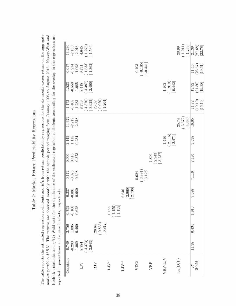
Tab

le2:

Mar

ket

Ret

urn

Pre

dic

tabilit

yR

egre

ssio

ns

Th

eta

ble

rep

orts

the

esti

mat

edre

gres

sion

coeffi

cien

tsan

dR

2s

from

retu

rnp

red

icta

bil

ity

regre

ssio

ns

for

the

six-m

onth

exce

ssre

turn

on

the

aggre

gate

mar

ket

por

tfol

ioMRK

.T

he

retu

rns

are

obse

rved

month

lyw

ith

the

sam

ple

per

iod

ran

gin

gfr

om

Janu

ary

1996

toA

ugu

st2013.

New

ey-W

est

an

d

Hod

rick

t-st

atis

tics

andχ

2(2

)W

ald

test

sfo

rth

esi

gn

ifica

nce

of

the

esti

mate

dre

gre

ssio

nco

effici

ents

acc

ou

nti

ng

for

the

over

lap

inth

ere

gre

ssio

ns

are

rep

orte

din

par

enth

eses

and

squ

are

bra

cket

s,re

spec

tive

ly.

Con

stan

t-0

.749

2.75

6-0

.755

-0.2

37

-0.1

72

0.9

06

2.1

45

-14.3

72

-1.1

73

-1.5

23

-0.6

17

-13.2

36

-0.2

901.

095

-0.1

66-0

.081

-0.0

75

0.4

16

1.1

15

-2.7

19

-0.4

05

-0.5

50

-0.2

74

-2.1

56

-1.0

690.

460

-0.6

28-0

.680

-0.6

98

-0.3

73

0.2

34

-2.6

18

-1.2

83

-1.0

85

-1.0

98

-2.0

13

LJV

8.78

48.7

49

8.4

18

9.7

41

4.6

45

(4.

373)

(4.3

70)

(4.3

87)

(1.5

33)

(1.2

75)

[3.

943]

[3.9

25]

[2.4

00]

[1.3

62]

[1.5

36]

RJV

28.6

425.3

2(

0.83

3)(

0.9

20)

[0.

812]

[1.2

64]

LJV∗

10.8

8(

1.15

9)[

1.15

5]L

JV∗∗

6.6

46

(2.9

60)

[2.7

38]

VIX

20.6

24

-0.1

03

(3.8

91)

(-0

.185)

[3.1

28]

[-0

.441]

VR

P1.8

96

(2.9

43)

[3.2

37]

VR

P-L

JV

1.4

16

1.2

02

(2.1

16)

(1.9

19)

[2.4

71]

[0.4

42]

log(

D/P

)25.7

420.9

9(

3.5

72)

(1.9

11)

[3.3

30]

[1.2

99]

R2

11.3

80.

434

1.91

09.5

88

7.1

16

7.1

94

3.5

38

18.8

511.7

213.9

211.4

521.3

9Wald

(19.1

9)

(21.8

0)

(23.6

7)

(27.6

8)

[16.1

9]

[19.3

8]

[19.6

1]

[22.7

8]

38

Tab

le3:

Mar

ket

Ret

urn

Pre

dic

tabilit

yR

egre

ssio

ns

atD

iffer

ent

Hor

izon

s

Th

eta

ble

rep

orts

one-

totw

elve

-mon

ths

retu

rnp

red

icta

bil

ity

regre

ssio

ns

for

the

aggre

gate

mark

etp

ort

foli

o,

an

alo

gou

sto

the

six-m

onth

regre

ssio

ns

rep

orte

din

Tab

le2.

On

eM

onth

Th

ree

Month

sN

ine

Month

sT

wel

veM

onth

sC

onst

ant

-0.0

490.

308

-0.2

26-0

.163

0.9

23

-0.6

92

-0.6

15

3.2

45-1

.664

-0.4

22

4.3

46

-1.6

48

-0.1

140.

878

-0.4

65-0

.127

1.0

11

-0.5

30

-0.1

51

1.0

73-0

.379

-0.0

82

1.0

61

-0.2

97

-0.1

140.

878

-0.4

65-0

.532

0.4

85

-0.7

08

-1.0

81

-0.0

05-1

.064

-1.2

38

-0.1

20

-1.1

87

LJV

1.34

31.

245

3.99

93.7

29

11.6

911.2

114.2

113.6

7(

2.68

9)(

2.66

7)(

2.61

3)

(2.8

35)

(3.5

02)

(3.3

35)

(3.8

12)

(3.5

79)

[2.

689]

[2.

667]

[2.

539]

[1.8

49]

[3.2

29]

[1.6

92]

[3.2

49]

[1.4

66]

VR

P-L

JV

0.329

0.29

40.9

49

0.8

51

1.8

79

1.6

00

2.1

74

1.8

36

(1.

503)

(1.

337)

(2.4

54)

(2.3

82)

(2.4

16)

(2.

121)

(2.7

62)

(2.3

78)

[1.

503]

[1.

337]

[2.4

88]

[1.6

47]

[2.4

16]

[0.

128]

[2.6

61]

[0.1

09]

R2

1.70

71.

234

2.68

85.

125

3.4

71

7.8

91

12.9

73.9

9715.

85

14.1

83.9

49

16.9

8Wald

(8.4

98)

(17.6

1)

(12.

42)

(15.7

5)

[8.4

98]

[12.3

6]

[14.

19]

[15.8

2]

39

Table 4: Portfolio Return Predictability Regressions

The table reports the results from one- to twelve-months return predictability regressions for size (twenty

percent smallest and biggest firms), book-to-market (twenty percent highest and lowest B/M ratios), and

momentum (twenty percent top and bottom performers over the past 2-12 months) portfolios, along with

the corresponding zero-cost portfolios, analogous to the results for the aggregate market in Tables 2 and 3.

Small Big SMB High Low HML Winners Losers WMLOne Month Returns

Constant 0.569 0.012 0.557 0.601 -0.180 0.781 1.132 -2.278 3.410( 0.980) ( 0.024) ( 1.462) ( 1.126) ( -0.368) ( 2.395) ( 1.163) ( -1.273) ( 2.369)[ 0.980] [ 0.024] [ 1.462] [ 1.126] [ -0.368] [ 2.395] [ 1.163] [ -1.273] [ 2.369]

LJV 0.027 1.179 -1.151 0.260 1.430 -1.169 1.281 4.327 -3.045( 0.037) ( 2.666) ( -2.040) ( 0.463) ( 3.244) ( -2.761) ( 1.337) ( 1.606) ( -1.189)[ 0.037] [ 2.666] [ -2.040] [ 0.463] [ 3.244] [ -2.761] [ 1.337] [ 1.606] [ -1.189]

VRP-LJV 0.411 0.252 0.159 0.303 0.377 -0.074 0.270 1.817 -1.547( 1.744) ( 1.163) ( 0.960) ( 1.321) ( 1.792) ( -0.425) ( 0.601) ( 2.060) ( -1.692)[ 1.744] [ 1.163] [ 0.960] [ 1.321] [ 1.792] [ -0.425] [ 0.601] [ 2.060] [ -1.692]

R2 1.134 2.449 1.780 0.900 3.867 2.551 0.521 4.518 4.156Wald (3.042) (7.795) (7.592) (1.865) (13.73) (8.388) (1.842) (5.066) (2.871)

[3.042] [7.795] [7.592] [1.865] [13.73] [8.388] [1.842] [5.066] [2.871]

Three Months ReturnsConstant 0.546 0.174 0.373 1.459 -0.548 2.008 3.656 -10.59 14.25

( 0.362) ( 0.133) ( 0.381) ( 1.001) ( -0.420) ( 1.918) ( 1.448) ( -2.019) ( 3.389)[ 0.144] [ -0.141] [ 0.451] [ 0.765] [ -0.724] [ 2.106] [ 1.054] [ -2.003] [ 3.137]

LJV 2.473 3.248 -0.776 1.366 4.880 -3.514 3.317 19.46 -16.14( 1.686) ( 2.358) ( -0.567) ( 1.089) ( 3.412) ( -2.423) ( 0.953) ( 3.534) ( -2.409)[ 0.723] [ 1.623] [ -1.015] [ 0.278] [ 2.650] [ -2.709] [ 0.719] [ 2.559] [ -2.041]

VRP-LJV 1.277 0.703 0.574 0.987 0.723 0.264 0.690 6.232 -5.542( 2.710) ( 2.108) ( 2.311) ( 2.451) ( 2.079) ( 1.032) ( 1.069) ( 2.554) ( -2.275)[ 2.428] [ 1.440] [ 2.598] [ 2.166] [ 1.139] [ 1.594] [ 0.756] [ 2.359] [ -2.323]

R2 4.644 6.374 1.531 3.420 9.862 6.477 1.183 19.93 22.78Wald (13.59) (11.11) (7.248) (6.371) (19.39) (11.38) (1.784) (13.63) (6.129)

[13.30] [8.299] [6.886] [6.023] [14.19] [8.387] [1.497] [13.46] [6.701]

Six Months ReturnsConstant -0.339 0.357 -0.696 2.078 -0.522 2.600 5.871 -23.27 29.14

( -0.112) ( 0.127) ( -0.386) ( 0.614) ( -0.200) ( 1.127) ( 1.222) ( -2.085) ( 3.660)[ -0.516] [ -0.522] [ -0.164] [ 0.188] [ -0.993] [ 1.367] [ 0.555] [ -2.189] [ 2.902]

LJV 7.697 7.285 0.412 5.339 9.196 -3.857 9.253 50.34 -41.09( 2.663) ( 3.708) ( 0.167) ( 1.772) ( 4.723) ( -1.303) ( 1.833) ( 3.669) ( -2.587)[ 0.940] [ 2.323] [ -1.238] [ 0.991] [ 2.762] [ -2.046] [ 1.104] [ 2.420] [ -1.894]

VRP-LJV 2.437 0.861 1.576 1.462 0.917 0.545 1.536 7.693 -6.157( 2.970) ( 1.419) ( 3.474) ( 1.673) ( 1.569) ( 0.969) ( 1.486) ( 2.484) ( -2.401)[ 2.004] [ 0.145] [ 3.879] [ 1.337] [ -0.093] [ 1.668] [ 0.429] [ 0.771] [ -0.831]

R2 12.93 10.33 5.835 6.651 14.34 3.836 3.850 32.93 34.22Wald (17.76) (14.40) (12.38) (3.732) (24.52) (7.408) (6.223) (13.96) (7.439)

[17.76] [12.89] [16.65] [3.732] [21.90] [5.839] [4.639] [15.17] [9.702]

Nine Months ReturnsConstant 0.015 1.107 -1.092 3.275 0.137 3.138 8.196 -27.825 36.021

( 0.003) ( 0.240) ( -0.368) ( 0.617) ( 0.032) ( 0.877) ( 1.030) ( -1.903) ( 4.291)[ -0.512] [ -0.605] [ -0.076] [ 0.016] [ -0.963] [ 1.155] [ 0.185] [ -1.951] [ 2.798]

LJV 11.20 9.582 1.621 8.055 11.48 -3.421 13.96 63.60 -49.64( 2.182) ( 2.975) ( 0.561) ( 1.382) ( 3.912) ( -0.806) ( 2.703) ( 3.364) ( -2.862)[ 0.649] [ 1.759] [ -1.083] [ 0.793] [ 1.956] [ -1.875] [ 1.200] [ 1.767] [ -1.707]

VRP-LJV 2.976 1.111 1.865 1.755 1.335 0.421 2.581 8.964 -6.383( 2.802) ( 1.446) ( 2.506) ( 1.658) ( 1.959) ( 0.573) ( 2.013) ( 2.701) ( -2.402)[ 1.082] [ -0.129] [ 2.586] [ 0.770] [ -0.141] [ 1.485] [ 0.479] [ 0.085] [ 0.093]

R2 16.07 11.01 5.620 8.480 14.726 1.777 6.116 33.26 29.55Wald (15.03) (8.862) (8.707) (2.897) (16.06) (6.497) (10.11) (13.40) (8.979)

[10.26] [10.06] [8.404] [2.516] [19.85] [7.204] [9.543] [13.25] [9.221]

Twelve Months ReturnsConstant 0.872 2.020 -1.148 5.120 0.818 4.303 10.76 -28.06 38.83

( 0.171) ( 0.339) ( -0.261) ( 0.812) ( 0.145) ( 0.924) ( 1.029) ( -1.752) ( 4.902)[ -0.458] [ -0.799] [ 0.352] [ -0.140] [ -1.110] [ 1.002] [ -0.121] [ -1.742] [ 2.489]

LJV 13.18 11.61 1.577 9.995 13.86 -3.860 18.99 68.61 -49.63( 2.245) ( 3.122) ( 0.458) ( 1.399) ( 4.325) ( -0.675) ( 2.989) ( 3.449) ( -2.848)[ 0.428] [ 1.547] [ -1.754] [ 0.822] [ 1.744] [ -1.054] [ 1.318] [ 1.421] [ -1.387]

VRP-LJV 3.714 1.147 2.566 1.450 1.571 -0.121 2.953 9.317 -6.364( 3.222) ( 1.382) ( 2.817) ( 1.341) ( 2.012) ( -0.120) ( 1.928) ( 3.089) ( -2.399)[ 0.967] [ -0.354] [ 3.675] [ -0.028] [ -0.300] [ 0.871] [ 0.061] [ -0.159] [ 0.249]

R2 19.31 11.16 7.616 8.101 15.30 1.537 7.629 30.30 22.72Wald (26.43) (9.768) (12.03) (2.580) (18.98) (0.839) (10.30) (18.33) (9.889)

[9.841] [11.89] [16.83] [2.520] [18.13] [1.979] [9.894] [10.99] [6.422]

40

0

0.05

0.1

0.15

0.2

0.25

0.3

0.35Left Tail Index

0

0.01

0.02

0.03

0.04

0.05

0.06Right Tail Index

95 00 05 10 150

5

10

15

20

25

30Left Jump Tail Intensity

× 10

−2

95 00 05 10 150

5

10

15

20Right Jump Tail Intensity

× 10

−4

Figure 1: Tail Shape Parameters and Jump Intensities

The top two panels plot the estimated left and right tail indexes, 1/α±t , defined by the estimator in equation

(3.3). The bottom two panels plot the estimated left and right jump intensities for “large” jumps beyond

the threshold kt, LJIt = φ−t e−α−

t |kt|/α−t and RJIt = φ+t e−α+

t |kt|/α+t , defined in equation (5.1). LJI and RJI

are both reported in annualized square form.

41

0

1

2

3

4

5

6

7

8LJV

× 10−2

96 98 00 02 04 06 08 10 12 140

0.05

0.1

0.15

0.2

0.25

0.3

0.35

0.4

0.45

0.5RJV

× 10−4

Figure 2: Jump Variation

This figure plots the left and right jump variation, LJVt and RJVt, defined in equation (3.2). LJV and RJV

are both reported in annualized square form.

42

95 00 05 10 150

1

2

3

4

5

6

7

8LJV*

× 10−2

95 00 05 10 150

1

2

3

4

5

6

7

8LJV**

× 10−2

Figure 3: Left Jump Variation with Restricted Tail Parameters

The left panel plots the left jump variation LJV ∗t obtained by restricting the “shape” parameter α− to be

constant, but allowing φ−t to change over time. The right panel shows LJV ∗∗t obtained by restricting the

“level” parameter φ− to be constant, but allowing α−t to be time-varying. The estimates are reported in

annualized square form.

0 0.2 0.4 0.60

1

2

3

4

5

6

7

8LJV

σ2ATM

× 10−2

95 00 05 10 150

1

2

3

4

5

6

7

8

× 10−2

LJV Fitted Values

Figure 4: Nonparametric Regression of Left Jump Variation on Volatility

The left panel displays a scatterplot of LJVt against σ2ATM,t (circles), along with the fit from a nonparametric

kernel regression of LJVt on σ2ATM,t (line), where σATM,t denotes the at-the-money implied volatility from

the shortest-maturity options available on day t. The right panel shows a time series plot of the corresponding

fitted values of LJVt.

43

0

1

2

3

4LJV

× 10

−2

0

10

20

30

40

50VIX2

× 10

−2

−5

0

5

10VRP−LJV

× 10

−2

96 98 00 02 04 06 08 10 12 14−4.5

−4

−3.5

−3log(D/P)

Figure 5: Predictor Variables

All of the series are plotted at a monthly frequency, and span the period from January 1996 to August

2013. The top panel shows the estimated left jump tail variation measure LJVt. The second panel shows

the CBOE V IX2t volatility index. The third panel plots the estimated variance risk premium V RPt minus

LJVt. All of the monthly variation measures are aggregated from the weekly option-based estimates and

reported in annualized squared form. The bottom panel plots the log dividend-price ratio for the aggregate

market log(Dt/Pt).

44

0

1

2

3

4

5t−statistics

1 2 3 4 5 6 7 8 9 10 11 120

5

10

15

R2

Figure 6: Market Return Predictability Regressions

The top panel shows the Newey-West t-statistics from from simple return predictability regressions for the

aggregate market portfolio MRK based on the left jump tail variation LJV (solid line) and the difference

between the variance risk premium and the left jump variation V RP − LJV (dashed line). The bottom

panel shows the corresponding R2s, along with the R2s from multiple regressions including both LJV and

V RP − LJV (dotted line).

45

−4

−2

0

2

4

6SMB t−statistics

1 2 3 4 5 6 7 8 9 10 11 120

2

4

6

8SMB R2

Figure 7: SMB Return Predictability Regressions

The top panel shows the Newey-West t-statistics from simple return predictability regressions for the Small

Minus Big (SMB) market capitalization sorted zero-cost portfolio based on the left jump tail variation LJV

(solid line) and the difference between the variance risk premium and the left jump variation V RP − LJV(dashed line). The bottom panel shows the corresponding R2s, along with the R2s from multiple regressions

including both LJV and V RP − LJV (dotted line).

46

−4

−3

−2

−1

0

1

2HML t−statistics

1 2 3 4 5 6 7 8 9 10 11 120

2

4

6

8HML R2

Figure 8: HML Return Predictability Regressions

The top panel shows the Newey-West t-statistics from simple return predictability regressions for the High

Minus Low (HML) book-to-market sorted zero-cost portfolio based on the left jump tail variation LJV

(solid line) and the difference between the variance risk premium and the left jump variation V RP − LJV(dashed line). The bottom panel shows the corresponding R2s, along with the R2s from multiple regressions

including both LJV and V RP − LJV (dotted line).

47

−3.5

−3

−2.5

−2

−1.5

−1

−0.5WML t−statistics

1 2 3 4 5 6 7 8 9 10 11 120

5

10

15

20

25

30

35WML R2

Figure 9: WML Return Predictability Regressions

The top panel shows the Newey-West t-statistics from simple return predictability regressions for the Winners

Minus Losers (WML) sorted zero-cost portfolio based on the left jump tail variation LJV (solid line) and

the difference between the variance risk premium and the left jump variation V RP − LJV (dashed line).

The bottom panel shows the corresponding R2s, along with the R2s from multiple regressions including both

LJV and V RP − LJV (dotted line).

48