takaaki yanagawa- on ribbon 2-knots: the 3-manifold bounded by the 2-knots
TRANSCRIPT
8/3/2019 Takaaki Yanagawa- On Ribbon 2-Knots: The 3-Manifold Bounded by the 2-Knots
http://slidepdf.com/reader/full/takaaki-yanagawa-on-ribbon-2-knots-the-3-manifold-bounded-by-the-2-knots 1/18
Yanagawa, T.Osaka, J. Math.6 (1969), 447-464
ON RIBBON 2-KNOTS
THE 3-MANIFOLD BOUNDED BY THE 2-KNOTS
T A K A A K I YANAGAWA
(Received February 24, 1969)
(Revised May 19, 1969)
1. Introduction
It is known that any locally flat, orientable, closed 2-manifold M2
in a 4-space
7?4bounds an orientable 3-manifold W
3in R\ see [1]. Nevertheless, the
question "what type of 3-manifolds can be bounded" seems to be still an open
question, for which we will give a partial answer in Theorem (2, 3) in this paper:
I f the 2-manifold M2
is a 2-sphere oj a special type of 2-knots, which will be called
a ribbon 2-knoty
see (2, 2), it bounds a ^-manifold W3
homeomorphic to Φ(S1X S
2)
—Δ3.0) Moreover, a little inspection on the 3-manifold W3
shows that thereexists a trivial system of the 2-spheres in W
3, see (3, 5), and we can easily prove
a converse of the above theorem in Theorem (3, 3). In §4, we will define the
following concepts;
JR(3): A 2-knot K2
satisfies that c({K})=0,
R(4): A 2-knot K2
bounds a ^-ribbon in jR4,
R(5): A 2-knot K2
bounds a monotone 3-ball in H + .
Since it is easily seen that the concepts R(4) and R(5) are the natural extensions
of the definition and the property of the ribbon (1-) knots, we can explain thereason why we denominate simply knotted 2-knots defined in [2] as ribbon 2-knots
in this paper, after we will have accomplished the proof of the equivalence of
these three concepts in Theorem (4, 5). In §5, we will introduce a normal-
form for ribbon 2-knots and an equivalence relation between 2-knots. The
equivalence relation is a cobordism relation between 2-knots with the strong
restriction, although ribbon 2-knots are equivalent to a trivial 2-knot under the
relation.
In this paper, everything is considered from the combinatorial stand point
of view.
0) = H = means the connected sum, and A 3a 3-simplex and Δ
3is its interior.
8/3/2019 Takaaki Yanagawa- On Ribbon 2-Knots: The 3-Manifold Bounded by the 2-Knots
http://slidepdf.com/reader/full/takaaki-yanagawa-on-ribbon-2-knots-the-3-manifold-bounded-by-the-2-knots 2/18
448 T. Y A N A G A W A
2. Ribbon 2-knots
An orthogonal pro ject ion/) of a 4-space R\ containing a locally flat 2-sphere
K2
which will be called a 2-knot, onto an hyperplane R3
is called a regular
projection, or simply a projection, if the locally linear map p \ K2
of K2
into R3
is
normal.13
The homeomorphism class of (K2, R
4) of 2-knots in R* will be called
the knot-type containing K2, and will be denoted by {K}.
D E F I N I T I O N (2.1). c(K) is the minimal number of the triple points and
the branch-lines20
of p(K) in R\ where the projection p ranges over the set con-
sisting of all the projections for the 2-knot K. c({K}) is the minimal number of
c(K), where K ranges over the knot-type {K}. A pair (p, K) will be called a
simple pair for the knot-type {K}, if it realizes the number c({K}).
D E F I N I T I O N (2.2).3)
A 2-knot K2
will be called a ribbon 2-knot, if and only
ifc({K})=0.
Theorem (2.3). A ribbon 2-knot K2
bounds a ^-manifold W3
which is home-
omorphίc either to a 3-ball or to #(S1X S
2) — Δ
3.
Proof. According to the result in [2], we can find a 2-knot K' belonging to
{K} and satisfying the following (1),(2) and (3):(1). K
1Π Rl=k is a ribbon knot in #?.4)
(2). K Π H\ and K' Π Hi. are symmetric with respect to the hyperplane
RO , and necessarily each of them is a locally flat 2-ball.
(3). each saddle point transformation^ on K' Π H+ increases the number of
components of the cross-sections of K' Π - R J as the height t increases; in other
words, K' Π H\ has no minimal point.
In the following three-steps, we illustrate the construction of the 3-manifold
W\
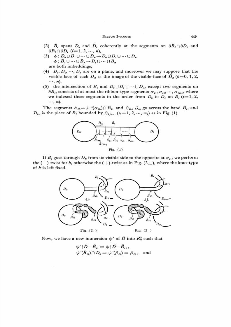
First-step. Since k is a ribbon knot, there is an immersion -ψ of a 2-ball
ΰ=A>UAU— UA UA U — U - S n
onaP
aneinto^o such that
(1) ι/r(8/5)=A, ψ(D) is a ribbon,
1) See p. 3 of [8].2) An arc whose end-points are branch-points is called a branchline.
3 ) I n [2], this type of 2— knots is denned as "simply-knotted 2— sphere"
4) X means the interior, and dX the boundary of a set X.
H\ = {(#!, Λ ?2, Λ C
3, X
4) |*4 0}
Hi = {(ad, a c 2 , *a, * 4 > 1*4^0}
5) See [5], p.136.
8/3/2019 Takaaki Yanagawa- On Ribbon 2-Knots: The 3-Manifold Bounded by the 2-Knots
http://slidepdf.com/reader/full/takaaki-yanagawa-on-ribbon-2-knots-the-3-manifold-bounded-by-the-2-knots 3/18
R IB B O N 2 -KNO Ts
(2) B£
spans Z) 0 and D{
coherently at the segments on
(3)il 449
5z
-n3A and
are both imbeddings,
(4) D0, Z)j, • • • , D
nare on a plane, and moreover we may suppose that the
visible face of each Dk
is the image of the visible-face of ΐ)k
(k=0, 1, 2,
.... n) .
(5) the intersection of B{
and DΌ\jD
l(J (jD
n, except two segments on
QBj, consists of at most the ribbon-type segments αil9
αi2J
•••, αim., where
we indexed these segments in the order from D0 to D{ on B{ (ί=l, 2,
The segments aiλ=\Jr
1(a
ίλ)Γ\B
ί> and β
iλίβio
go across the band Biy
and
j§, λ
is the piece of Bf
bounded by β^χ^ (λ=l, 2, •••, m^ as in Fig. (1).
Fig. (1)
If .β goes through Dk
from its visible side to the opposite at αiιy
we perform
the (—)-twist for Λ , otherwise the (+)-twist as in Fig. (2±), where the knot-type
of k is left fixed.
U bziίΐ
Fig . (2+) Fig. ( 2 _ )
Now, we have a new immersion ψ ' of D into 7?o such that
= γ'(£„) = y8ή , and

8/3/2019 Takaaki Yanagawa- On Ribbon 2-Knots: The 3-Manifold Bounded by the 2-Knots
http://slidepdf.com/reader/full/takaaki-yanagawa-on-ribbon-2-knots-the-3-manifold-bounded-by-the-2-knots 4/18
450 T. Y A N A G A W A
^'(B^) is the shaded portion in Fig.
v/r'(Z5) is a ribbon and ψ'(dD) is the twisted k .
Moreover, if there is α,2, we perform the twist of the same type as before con-
sidering Bi2,β
ί2, β
izyβil}
ψ' asBiιyβίιyβil9βio, ψ . Repeat successively these
processes for λ=3, 4, •••, miy
ί=l, 2, •••, n.
Second-step. In the first-step, we have finally a ribbon ψ*(D)=D0\jD
1\J
- U A . U Λ f U Uβ?, where BγΓ\(DQ\jD
1\J^\jD
M) = β
iί\j'' \Jβ
imt\J \J
aiM.. Remove the mutually disjoint 2-balls Q
iκand Q'
ixfrom D
0UA U• • • UAt
such that
Combine 9j3fλ
and 3 {x
with a tube Tiλ
coherently so that Γίλn
or λφ ), and that Γίλn(ψ*(/))- U» , λ
Finally, we have an orientable 2-surface F0
such that
)- u (ρΛuρίx» u{fif u - u *} u{ur,.
λ},
I,λ «,λ
see Fig. (3).
Fig. (3)
Third-step. To construct the 3-manifold W3
bounded by K', we make use
of the method described schematically in Fig. (4),which was already used in
the proof of the theorem in [4],p. 267~269, Fig. 5.
W+=\jF% and W_= ( j F2
tare both homeomorphic to a solid torus perhaps
O ^f < ^0
with a large genus, therefore Wz
gained by the natural identification on F*=W+
Π R\= W _f\ Rl is homeomorphic either to a 3-ball or to Φ(S1X S
2)—Δ3, since
K' is symmetric with respect to Rl.
This completes the proof.

8/3/2019 Takaaki Yanagawa- On Ribbon 2-Knots: The 3-Manifold Bounded by the 2-Knots
http://slidepdf.com/reader/full/takaaki-yanagawa-on-ribbon-2-knots-the-3-manifold-bounded-by-the-2-knots 5/18
RIBBON 2-KN θτs 451
Fig. (4)
3. A fusion of 2-knots6:>
A collection of the mutually disjoint 2-knots [K\, K\, •••, K% } is called
a splίtted 2-link, if there exists a collection of the mutually disjoint combinatorial
4-balls V19
V2y •••, V
nsuch that V^Kf (ί=l, 2, •••, n) in R\ Especially, a
splitted 2-link is called a trivial 2-link, if each component K{
is unknotted?:)
in
#(1=1, 2, ...,»).
DEFI NI T I ON (3.1). If there are a collection of the 3-balls Bιy
B2, •••, B
n_
1and
a splitted 2-link {K\, K\, • • • , K*} such that, for each Bg, B^K^dB^Kj isa 2-ball E
{Jfor just two 2-knots K. of the 2-link (/=!, 2, •••, n—1, l j n),
and that th e 2-sρhere K=( U K—U #/ ,y) U ( U QB
{— U £ " ίf y) is a 2-knot in Λ
4,
i i,j ' i i,j
then the 2-knot K is called a fusion of the splίtted 2-link.
Lemma (3.2). If a 2-knot K2
is a fusion of the splitted 2-link {5f, SI •••,
Proof. Since the 2-link is splitted, there is an ambient isotopy ξ of R4
under which the pair ( / > , ξ(Sj)) is a simple pair for the knot-type {Sy} by apro je c t ion/ ) for all {Sj} (j=l, 2, • • - , n\ and moreover p(ζ (5y))Π p(ξ (Sk))=φ
(yφyfe). For convenience' sake, we denote |(5y), ξ(B
i)
yξ(E
iJ) by S
JyB
iyE
{ y,again, where the 3-balls J5, (/=!, 2, •••, w — 1) belong to the collection of the 3-
balls in the construction of the fusion K.
Let the 2-balls Ef J
=BίΓ( 5
yand E k B Sk be the intersection of 95,-
a n d U ^ y and let α, be the arc in B{
spanning Ei}J
. and ί1,. , where α
fn 9 - B / =
l/
>jfe)=
:3 ^
tand α, is unknotted
8)in β, (ί=l, 2, •••, n— 1). We may
6) The concept "fusion" is introduced in [6], p. 364 for 1—knots, but now we will con-
sider an analogy of this concept fo r 2—knots.7) Ki bounds a combinatorial 3-ball in R
4.
8) A circle αtU α bounds a 2-ball in B} for an arc a on dB
if
8/3/2019 Takaaki Yanagawa- On Ribbon 2-Knots: The 3-Manifold Bounded by the 2-Knots
http://slidepdf.com/reader/full/takaaki-yanagawa-on-ribbon-2-knots-the-3-manifold-bounded-by-the-2-knots 6/18
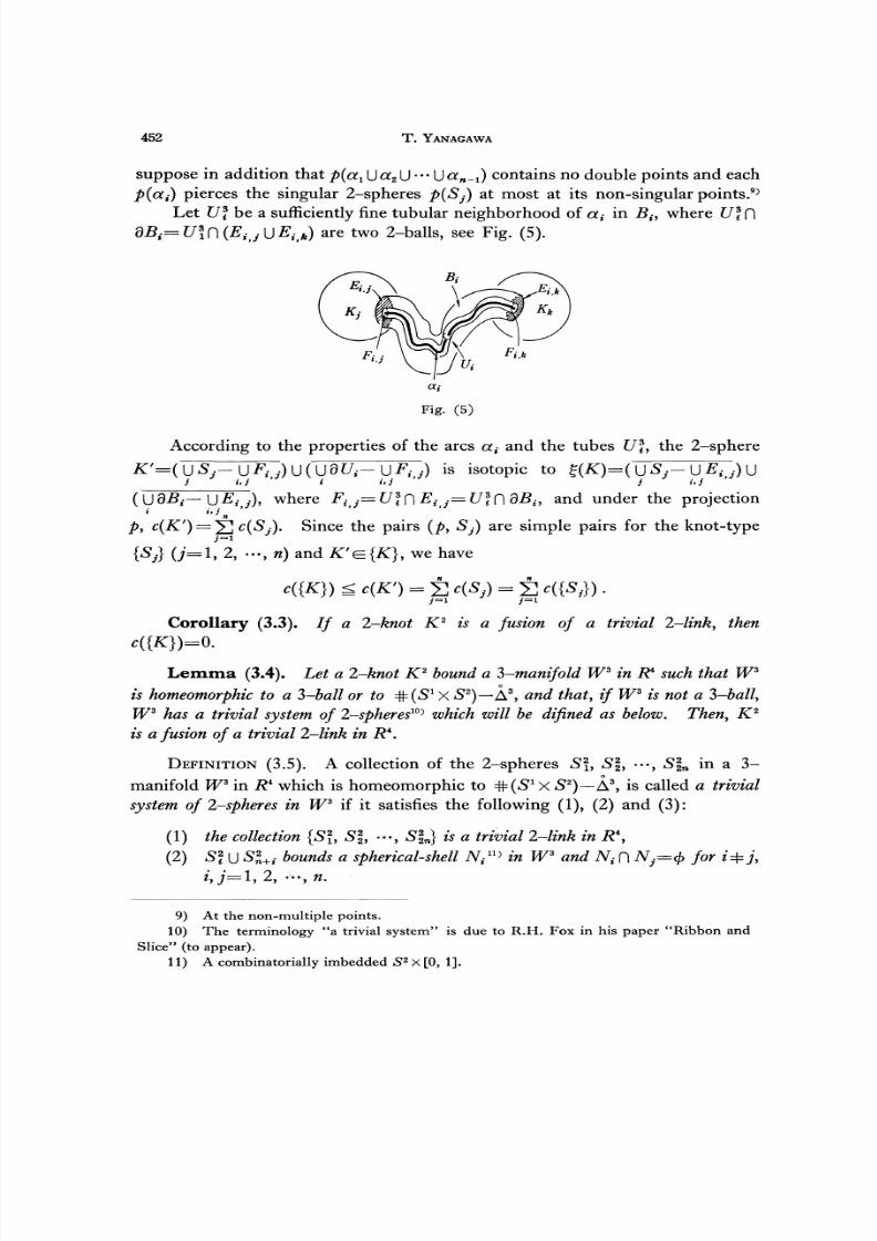
452 T . Y A N A G A W A
suppose in addition that p(a1
U t f2U • • • U « » _ ι ) contains no double points and each
p(cίi) pierces the singular 2-spheres p(Sj) at most at its non-singular points.9)
Let U\ be a sufficiently f ine tubular neighborhood of af
in Bίy
where Z 7 J f ΊdB~UlΓ\(E
iJE
itk) are two 2-balls, see Fig. (5).
F i g . (5)
According to the properties of the arcs α, and the tubes C / f , the 2-sphere
—\jFf j) is isotopic to £(*:)=( u Sy-U£,-,,-) U
'
( \ J d B f — \jEij), where F^—U^Π E —U^ndB^ and under the projectionί i'J
n
py
c(K') —Σc(Sj). Since the pairs (p , Sj) are simple pairs for the knot-type
0=1, 2, .-, n) and ICe }, we have
c({K}) £ c(K') = Σ c(Sj) =Σc({5 ,}) .
Corollary (3.3). If a 2-knot K2
is a fusion of a trivial 2-link, then
Lemma (3.4). Let a 2-knot K2
bound a Z-manifold W * in R4
such that W*
is homeomorphic to a 3-ball or to (S1
X S2)— Δ
3, and that, if W
3is not a 3-ball,
W3
has a trivial system of 2-spheres1^ which will be dίfined as below. Then, K
2
is a fusion of a trivial 2-link in R* .D E F I N I T I O N (3.5). A collection of the 2-sρheres Sf, Sξ, ••• , S%
nin a 3-
manifold W3
in R4
which is homeomorphic to Φ(5 f lx S2)— Δ
3, is called a trivial
system of 2-spheres in W3
if it satisfies the following (1), (2) and (3):
(1) the collection {5?, 5|, •••, S|n} is a trivial 2-link in R\
(2) 5f USS+f bounds a spherical-shell Λ Γf
U)in W
3and N
£Π Nj=φ for ί
ί,y=l, 2, n.
9 ) At the non-multiple points.
10) The terminology "a trivial system" is due to R.H. Fox in his paper "Ribbon and
Slice" (to appear).
11) A combinatorially imbedded S2
X [0, 1].
8/3/2019 Takaaki Yanagawa- On Ribbon 2-Knots: The 3-Manifold Bounded by the 2-Knots
http://slidepdf.com/reader/full/takaaki-yanagawa-on-ribbon-2-knots-the-3-manifold-bounded-by-the-2-knots 7/18
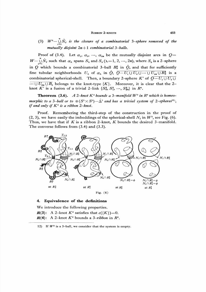
RIBBON 2-KN θτs 45 3
(3) W3—\jN
ί
is the closure of a combinatorial 3-sphere removed of theί=*l
mutually disjoint 2n-\-\ combinatorial 3-balls.
Proof of (3.4). Let a^ α2, •••, a
2nbe the mutually disjoint arcs in £)—
W o
W — \jNg such that aλ
spans Sλ
and 50(λ=l, 2, •••, 2/z), where 5
0is a 2-sphere
ί=l
in Q which bounds a combinatorial 3-ball Bl in Q, and that for sufficiently
fine tubular neighborhoods Uλ
of αλ in £), £)—t^U Z /2U UZ / 2 l lU 5 o is a
combinatorial spherical-shell. Then, a boundary 2-sphere K' of £)— ί7xUU
2U
• • • UU2n
\jB0
belongs to the knot-type {K}. Moreover, it is clear that the 2-
knot K' is a fusion of a trivial 2-link {S§, 5f, •••, 5 } in R* .
Theorem (3.6). A 2-knot K2
bounds a 3-manifold W3
in J R4
which is homeo-
morphίc to a 3-ball or to Φ(S1xS
2)—Δ3
and has a trivial system of 2-spheres^,
if and only if K2
is a ribbon 2-knot.
Proof. Remembering the third-step of the construction in the proof of
(2, 3), we have easily the imbeddings of the spherical-shell ^Vf
in J/F3, see Fig. (6).
Thus, we have that if K is a ribbon 2-knot, K bounds the desired 3-manifold.
The converse follows from (3.4) and (3.3).
Fig. (6)
4. Equivalence of the definitions
We introduce the following properties.
Λ(3): A 2-knot K2
satisfies that c({K})=0.
Λ(4): A 2-knot K2
bounds a 3-ribbon in R*.
12) If W3
is a 3-ball, we consider that the system is empty.

8/3/2019 Takaaki Yanagawa- On Ribbon 2-Knots: The 3-Manifold Bounded by the 2-Knots
http://slidepdf.com/reader/full/takaaki-yanagawa-on-ribbon-2-knots-the-3-manifold-bounded-by-the-2-knots 8/18
454 T. Y A N A G A W A
Λ(5): A 2-knot K2
bounds a monotone 3-ball in H^.
DEFI NI T I ON (4.1). An image of a 3-ball B3
into R4
by an immersion φ
will be called a 3-ribbon bounded by a 2-knot K2, if it satisfies the following (1),
(2) and (3):
(1) φ I Q B is an imbedding and φ(9B)=K2
y
(2) the self-intersection of φ(B) consists of a finite number of the mutually
disjoint 2-balls Dv
D2J
—, Dn,
(3) for each Di9
the inverse image φ~l(D
i) consists of a pair of 2-balls
D't, Dy, satisfying that
DyndB ( 1 = 1 , 2 , - . . , ? * ) .
Fig. (7 )
DEF INITION (4.2). A 3-ball D3
will be called a monotone 3-ball bounded
by a 2-knot K2 in H5
+, if it satisfies the following (1), (2) and(3):
(1) K2=9D=DnR*
y
(2) D3
is locally flat and has no minimal point in //+ ,
(3) in a neighborhood of each (non-maximal) critical point pi(x
xγ\ ^4°), D3
is represented by the equation:
{'\
z-xy=0
For convenience' sake, we will say that
F: A 2-knot K2
is a fusion of a trivial 2-link.
Lemma (4.3). Λ(4) is equivalent to F.
Proof. Λ(4) =^ F. Let V\ be 3-balls in B3
such that FtθD , Γ (Ί K φ
) and that th e annulus V f Γ \ dB contains 8Z>7 in its interior (i,j=l, 2, •••, n).
Let Pf, Pi, •••, P^+1 be the boundary 2-spheres of B3— ^ U— UK Λ , then
{^>(P?), 9>(P1), —, 9>(P2+ι)} is a trivial 2-link in R\ and it is clear that K2
is a
fusion of the trivial 2-link.
Remembering the technique in the proof of (3.2), we have a3-ribbon J\ U — U / £ U V\ U• • • Uf/Li bounded by K
2in P4, where /? ,••-, Jl
are disjoint 3-balls bounded by the 2-knots Sιy
•••, Sn
respectively and 3-balls
8/3/2019 Takaaki Yanagawa- On Ribbon 2-Knots: The 3-Manifold Bounded by the 2-Knots
http://slidepdf.com/reader/full/takaaki-yanagawa-on-ribbon-2-knots-the-3-manifold-bounded-by-the-2-knots 9/18
RIBBON 2-KN θτs 455
/;_! are so fine that ί/ϊΠ/J are small 2-balls in J] (l i n—l,
Lemma (4.4). R(5) is equivalent to F.
Proof. R(5) = = > F. Let D?
be a monotone 3-ball bounded by K2
in H5
+.
We may suppose that the coordinates of all (non-maximal) critical points of D3
satisfy that a£°=l (ί=l, 2, • • • , ra— 1). Then, by the property (3) in (4.2), it is
not so difficult to prove the followings: for a sufficiently small positive number £ ,
(1) £>3n#ί+ε
is a trivial 2-link {Sf, Si, ...,S* } in #ί+ε,
(2) the equations
s—*s l ) ==0, #5=1—£
-ai'Ίv'T ('=1,2, ...,n-l)
give the disjoint 3-balls 5^ in Λ J _ ε ,
(3) Z )3Π #ί_s is a fusion of a trivial 2-link {Si, SJ, •••, S£} by the 3-balls
.Bf, •••, #;Lι> where trivial 2-knots SΊ are the image of S? by theorthogonal projection of R
5onto Λ J _ ε .
(4) D3Π #ί_ε and K
2belong to the same knot-type.
F R(5). By the result (4.3), if K2 satisfies F, K2 satisfies 72(4); that is,
K2
bounds a 3-ribbon φ(E). Let F? be 3-balls such that fi ID Ff ^V^D^ and
J 7 ? n FJ=Φ (ίΦ Ί *=1> 2> -> w) Snce
φ imbeds S 8 - F f U - U F J into Λ gand {<p(dVl), —9<p(QVl)} is a trivial 2-link in R% , we can suspend these 2-
spheres φ(dV\), •••, 9?(3F2) from w points of R\. With a little modification,
we have a monotone 3-ball D3
bounded by K2
in H5+ .
Remembering (3.3) and (3.4), we have that R(3)*=>F, and with (4.3) and
(4.4), finally we have the following
Theorem(4.5). JB(3), R(4) and Λ(5) are equivalent to F.
We refer to the following results.
All 2-knots are "slice-knot", see [7].
There is a 2-knot which is not "simply -knotted 2-knot", see [2].
Then, we can assert that the concept "ribbon knot" is different from the concept
"slice knot" for 2-knots, while we have not yet succeeded to distinguish one
from another for 1-knots.
5. An equivalence relation
Let K2
be a ribbon 2-knot which is knotted in R4
. Then, by (3.6)and(3.4), K
2is a fusion of a trivial 2-link {Sg, S?, —, Sf
n} in R
4. In the following,
we will use the same notations as in the proof of (3.4). We may suppose that
8/3/2019 Takaaki Yanagawa- On Ribbon 2-Knots: The 3-Manifold Bounded by the 2-Knots
http://slidepdf.com/reader/full/takaaki-yanagawa-on-ribbon-2-knots-the-3-manifold-bounded-by-the-2-knots 10/18
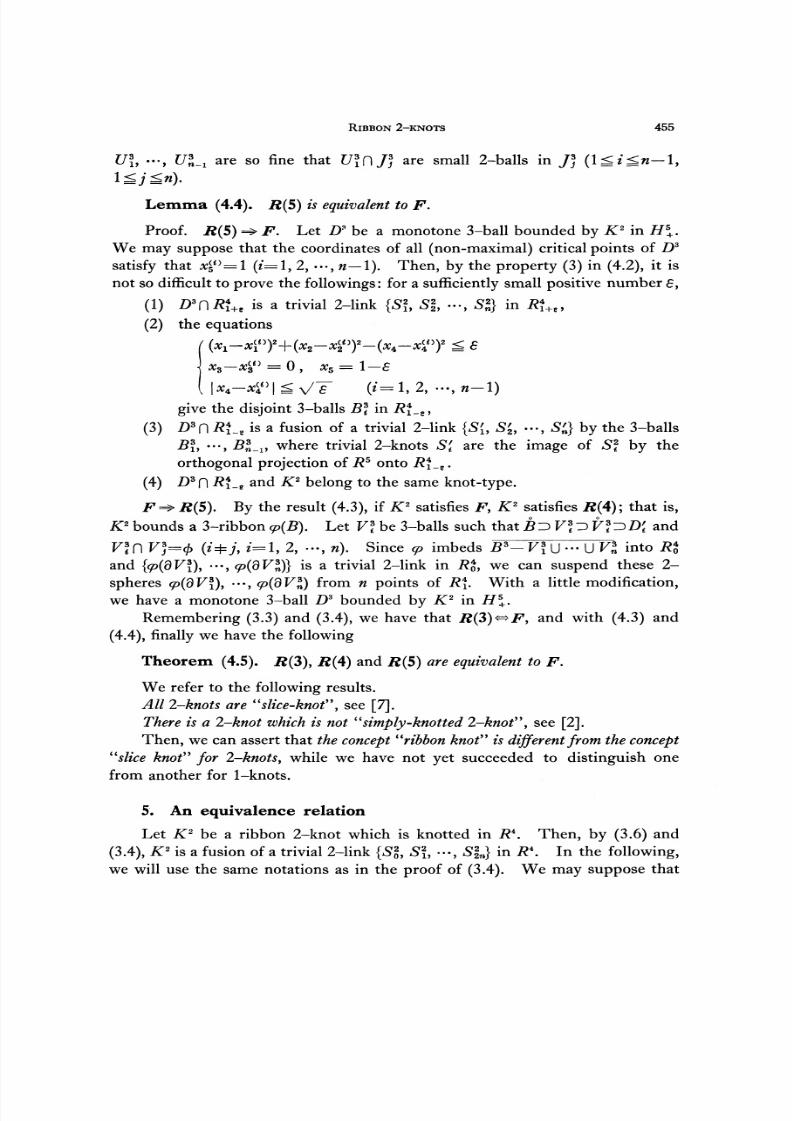
456 T. Y A N A G A W A
P1: A 2-sρhere S* and the spherical-shells N
19
N2
, •••, Nn
are splitted in
R*9
where dNt=Sΐ\jS*+i
(*=1, 2, • • • , n).
P3: Λ ^Π Λ Q , •••, Λ f
MΓ l RO are annuli on a plane in R*.
The 3-balls B\, •••, Z?l n and the arcs a19
•••, α2M
which cause the fusion
have the following properties P4, P
5 and P6:
P 4: Since the 2-link {SJ, SI , •••, *S1n} is trivial, the arcs a
19•••, α2w are
moved into R % by an ambient isotopy of R4. Since άλ is contained in
Bl (λ=l, 2, •••, 2/z), if we suppose that a finite subcomplex B% of
Λ4 is in a general position with respect to the hyperplane R% , there is a
sufficiently narrow band b % containing αλ in Bl Π ^ R o which spans a
circle £0=SoΓlΛ? and a circle c
λ=*SJn^o (λ=l, 2, •••, 2ri).
P5: For a sufficiently small positive number 8
9BlΓ\H
4[—6
96] contains a
3-ball Ul which is level-preserving-isotopic to b* X [—£, £] leaving the
2-balls UlΓίS2, and C/^n Si fixed (λ=l, 2, -, 2n).
P6: In fusing {5o, Sf, •••, *S
W} to get a 2-knot ^
2
,we make use of the
3-balls If*, •••, U\n
instead of the 3-balls B\, •••, B\n, and we will
denote the new 2-knot belonging to {K2} by K
2.
We want to s impli fy the cross-sections of the 2-knot K2
as follows.
Let θ be an orthogonal projection of R* onto a plane R2, and if θ(b%)Γ(θ(bfy
Φ φ (15^λ, μ<z2ri)9
we may suppose that Ul and L / J are in the position as shown
in (8J in Fig. (8). Move Ul and U* isotopically in R4
so as to be in the posi-
tion in (82). In the next step, li ft up the tube in the level Rl as shown in (83).
Replace these in a general position again, and we have the situation in (84).
Thus, we have the following lemma.
(82) (8
3) (8
4)
Fig. (8)
8/3/2019 Takaaki Yanagawa- On Ribbon 2-Knots: The 3-Manifold Bounded by the 2-Knots
http://slidepdf.com/reader/full/takaaki-yanagawa-on-ribbon-2-knots-the-3-manifold-bounded-by-the-2-knots 11/18
RIBBON 2-KN θτs 457
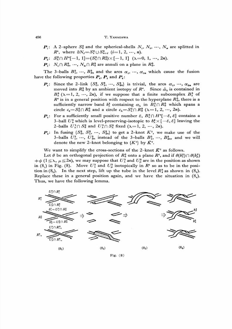
Lemma (5.1). We can exchange the over-and-under passing relation with
respect to x^-coordinate between bl and b* (l λ, μ^2n) preserving the 2-knot
type of K2.
We will consider how to eliminate the twists of the band b\ in the following
three steps.
(1) If b\ contains an even number of twists, we perform a modification as
follows :
F i g . (9)
This modification is an isotopy only in the subspace Rl in 7?4, but in each level
R* (—£ ί g £ <j£ ) , t he similar modification can be performed for t / J f l R * > therefore
we can understand this modification as an isotopy of 7?4.
(2) If b\ contains only one twist, we consider an orientable 2-surface
F = {(Bl U NI U U NH) Π RO } U bl U U *L Since the fusion in the present
step depends on the 3-manifold W3, and since F U (K
2Π H\) bounds an orien-
table 3-manifold (Bl [JN, U • • • l)Nn\jUl\J • • • U E/Ϊ»)ΓI H\ (a solid torus with alarge genus), the surface F should be orientable, see Satz I, §64 in [9].
Therefore, there must be another twist on a band b^ (μ~\=ri). Hence, we
consider the following replacement of F in R% , see Fig. (10).
A ft e r this replacement, the twist on b * , is transferred on b\. This move can be
easily extended to a modification of W3
in R\ and the band bl (, more precisely
the tube U l) is left fixed through the modification, even if bl links with 7VλΓ l Rl
(o r Λ^Π Rl) in Rl as shown in Fig. (10).
(3) A f t e r the modifications in (1) and (2), each band b\ contains a finite
8/3/2019 Takaaki Yanagawa- On Ribbon 2-Knots: The 3-Manifold Bounded by the 2-Knots
http://slidepdf.com/reader/full/takaaki-yanagawa-on-ribbon-2-knots-the-3-manifold-bounded-by-the-2-knots 12/18
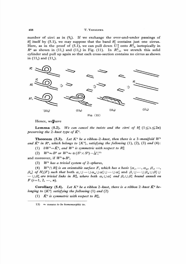
4 5 8 T. Y A N A G A W A
number of cirri as in (92
). If we exchange the over-and-under passings of
b\ itself by (5.1), we may suppose that the band b\ contains just one cirrus.
Here, as in the proof of (5.1), we can pull down U\ onto Λ18isotopically in
R4
as shown in (11J and (112) in Fig. (11). In /? L ε, we stretch this solid
cylinder and pull up again so that each cross-section contains no cirrus as shown
in(l l3)and(H
4) .
'(111)
Hence, wejhave
(H) (H3)
Fig . (11)
Lemma (5.2). We can cancel the twists and the cirri of b\ (\<L\ ζ2ri)
preserving the 2-knot type of K2.
Theorem (5.3). Let K2
be a ribbon-2-knot, then there is a Z-manίfold W3
and K2
in R\ which belongs to {K2}, satisfying the following (1), (2), (3) and(4):
(1) dW3=K
2, and W
3is symmetric with respect to R %
(2) W3
B3
or W3
^Φ(Sl x S
2)-Δ
3,13)
and moreover, if W3 B3,
(3) W3
has a trivial system of 2-spheres,
(4) W3Γ \ RO is an orientable surface F, which has a basis {α^ •••, αw, β^ •••,
βn} of H^F) such that both a,U — U a
nU αί U — Uαi and β
lU — U β
nUβί U
• • • Uβn are trivial links in Rl, where both α/U^ί an d yβ, U/3ί bound annuli on
F (i=l,2, ...,n).
Corollary (5.4). Let K2
be a ribbon 2-knoΐ, there is a ribbon 2-knot K2
be-
longing to {K2} satisfying the following (1) and (2)
(1) R
2
is symmetric with respect to R% ,
13) = ϊs means to be homemorphic to.

8/3/2019 Takaaki Yanagawa- On Ribbon 2-Knots: The 3-Manifold Bounded by the 2-Knots
http://slidepdf.com/reader/full/takaaki-yanagawa-on-ribbon-2-knots-the-3-manifold-bounded-by-the-2-knots 13/18
RIBBON 2-KN θτs 459
(2) there is a locally flat 2-ball D2
in Hi. such that a 2-knot (K2
Π H\) (J D2
is an unknotted 2-knot in R4.
Proof of (5.3). If K2
is unknotted in /? 4, the theorem is trivial. Hence
we will consider the case that K2
is knotted inR\ Let K2
be a 2-knot satisfying
P V ~,P6
described in the beginning of this section. Let W3
be a 3-manifold
-U^Ut/ΪU-UC/i,. Then, W^Rl={(Bl u Λ ^ U - (jNn)nRl}
U ^iw Let al9
α£ , /3, and β't(i=l, 2, •••, rc) be the simple closed curves
on F described in Fig. (12), then by (5.1) and (5.2) they satisfy the conditions
(4) in (5.3).
Fig.(12)
Proof of (5.4). If K2
is unknotted in R4, it is obvious. If K
2is knotted in
-R4
, we consider the 3-manifold W3
and K2
in R4
in (5.3). Then, the constructionof the 2-ball D
2is described in Fig. (13). Moreover if we apply the method
in the proof of Theorem in [4], see Fig. 5, p. 269 in [4], it is not so difficult to
construct a 3-ball bounded by (K2ΓiH^)[jD
2in R* .
Rl.
F i g - (13)
Now, we will define an equivalence relation between 2-knots.
D E F I N I T I O N (5.5). Two 2-knots Kl and K\ will be called cobordant and
denoted by Kl~K\, if and only if there exists a 3-mamfold M 3satisfying the
following (\\(2\ (3) and (4):
(1) ΛP is homeomorphίc to S2
x [0, 1],
8/3/2019 Takaaki Yanagawa- On Ribbon 2-Knots: The 3-Manifold Bounded by the 2-Knots
http://slidepdf.com/reader/full/takaaki-yanagawa-on-ribbon-2-knots-the-3-manifold-bounded-by-the-2-knots 14/18
460 T. Y A N A G A W A
(2) M3
is locally flat in #5[0, 1],
14>
(3) QM*=KI\J(-K\\ andK\=M*[\R\ (ί=0, 1),15)
(4) M3
Π Rϊ is connected for each t (0 t 1).
Clearly we have
Theorem (5.6). The cobordant relation " < —" w an equivalence relation.
Lemma (5.7). If a 2-knot K2
is a ribbon 2-knot, then ^2~0
2, where O
2
is a trivial 2-knot in R4.
Proof. Let X* be a compact, orientable 3-manifold in R5. The ordinary
cross-section of X3
by a hyperplane Rf is a compact, orientable 2-manifold.
I f X3
is represented by the next equation (*) in a neighborhood of a point
the transformation from the ordinary cross-section X3Γ\ RΛ-Z
ontotneordinary
cross-section ^ f 3 n^_ ε (for a small number £>0) is a hyperbolic transforma-
tion in R5.
In the following, we want to construct a 3-manifold M3 which satisfies not
only the conditions (1), (2), (3) and (4) in (5.5) but Λ P f l R*=K2, M
3(Ί #t=02.
I f K2
is unknotted in R$, the existence of the 3-manifold is clear, therefore we
will suppose that K2
is knotted in R% . The 3-manifold will be obtained by the
fol lowing six steps.
(1) Consider a 2-knot K2
belonging to {.K2} and bounding the 3-manifold
W3
in (5.3), see (14,) in Fig. (14).
(2 ) Between R % an d /?ί/2, we perform the hyperbolic transformations asshown schematically in (14J, (14
2) and (143). In (14
2), we show the exceptional
cross-section of M3 by JR} /4 and the cross-section by R % in Λ}/4 is similar to
that by 7?ls in Fig. (13). The cross-section by Rζ
in R\/2
is similar to that
by .Rig in Fig. (13), and the cross-section by Rl in R\ /2
is similar to that by
7?l2e
mFig- (13). This transformation satisfies the equation (*) in a sufficientlysmall neighborhood in R
5of each saddle point at RQ in R .
14) Rj ={(#1,*2,#3, *4> *5>l*5=0
H5. = { (Λ?I, Λ2, #3, Λ !4, 5c5)|ac5
0}
The 3-manifold M3is /OCΛ % y?αί in H5[0, 1] if the pair (Lk(p, M
3), Lk(p, H
5[0, 1]) is a
t rivial sphere pair for p M and a trivial ball pair for p dM.
15 ) Ident i f y 2-knot (K*, R4) with a 2-knot (K
2, Rf). ( — K
2) is the reversely-oriented
2-knot for K2.

8/3/2019 Takaaki Yanagawa- On Ribbon 2-Knots: The 3-Manifold Bounded by the 2-Knots
http://slidepdf.com/reader/full/takaaki-yanagawa-on-ribbon-2-knots-the-3-manifold-bounded-by-the-2-knots 15/18
RIBBON 2-KNθτs 461
by
(3) As shown in the proof of (5.3), the cross-section of the 2-surface
o in R\/2
is a trivial 1-link, say γ 0 U 7 ι U U 7 Mwith n+l components.
(4) Between R\/2
and R\/^ we will contract n circles γ1? •••, j
nto points
continuously as shown in (143) and (14
4) so that in a small neighborhood in R
5
of each pinching point at R % in R\/^ th e transformation is given by the equation
(**):
( * * ) xa—x
3= 0
(5) We have finally constructed a 2-knot K2 in R\ which satisfies the
following three properties:
(5J K2
is symmetric with respect to Rl in R\y
(52) K2Γi Rl is a trivial 1-knot γ0 in Rl in R*,
(53) If we remind the proof of (5.4), a 2-knot K\ is unknotted in //+ , where
K\ is a union of a 2-ball K2
Π H\ and a 2-ball D2
which is bounded by
T oίnRl
(6) Then, K2=Kl*(-K\γ is a trivial 2-knot in Λ J . By the same
method as in the proof of theorem in [4], we can construct the desirable 3-
manifold M 3 in H 5[Q , 1] which is bounded by K2 and the trivial 2-knot K2.This completes the proof of (5.7).
(14ι) (142) (143)
Fig. (14)
(144) (145)
Lemma (5.8). For an arbitrary 2-knot K2, K
2*(—K
2) is cobordant to a
ribbon 2-knot.
Proof. A 2-knot K2
in R$ can be placed in a position as follows:
(16) * means the knot-product', that is, K2=K\*K\ if there exists a hyperplane P
3in R
4
such that k=K2 Π P3 is a 1-knot bounding a 2-ball D2 in P3 and that a 2-knot D2 U (P4+ Π K2)belongs to {K\} and a 2-knot Z) 2 U(Pi Π ^
2) to {K}, where P^ are half 4-spaces bounded by
P3in R
4. Cf. the argument in §1 in [10].
8/3/2019 Takaaki Yanagawa- On Ribbon 2-Knots: The 3-Manifold Bounded by the 2-Knots
http://slidepdf.com/reader/full/takaaki-yanagawa-on-ribbon-2-knots-the-3-manifold-bounded-by-the-2-knots 16/18
462 T. Y A N A G A W A
(1) K2
Π R\z
is a knot k in #iε
,
(2 ) K2Γ ( H*[3ε, oo) has no minimal point,
(3 ) K2
Π H4[€ , 36] has no maximal point,
(4) all minimal points are at the level R% .
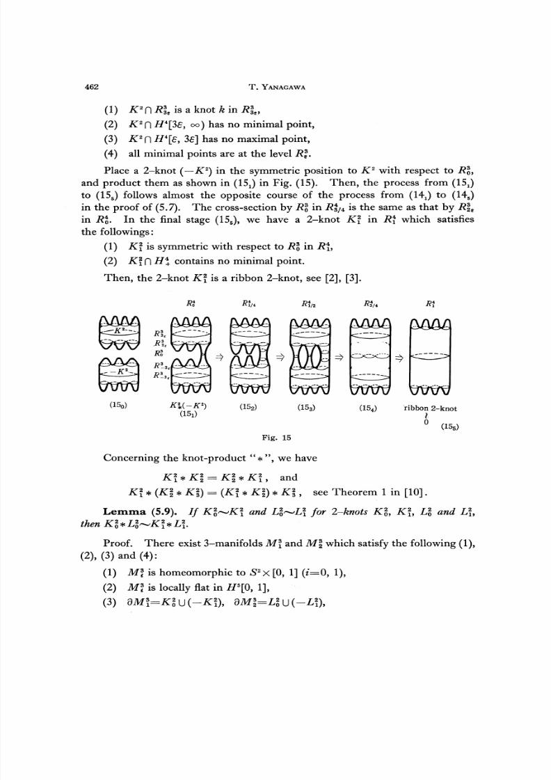
Place a 2-knot ( — K2) in the symmetric position to K
2with respect to R% ,
and product them as shown in (15J in Fig. (15). Then, the process from (15X )
to (155) follows almost the opposite course of the process from (14^ to (145)
in the proof of (5.7). The cross-section by R % in ^3/4 is the same as that by Rle
in RQ. In the final stage (155), we have a 2-knot K\ in R\ which satisfies
the followings:
(1) K\ is symmetric with respect to RQin R\,
(2) KI Π H\ contains no minimal point.
Then, the 2-knot K\ is a ribbon 2-knot, see [2], [3].
Π4•ίM/4
(15o)(15ι)
(152) (153) (154) ribbon 2-knot
° (155)
Fig. 15
Concerning the knot-product"*", we have
K\ *K\ =K\*K\, and
K\ *(K\ *X|)-(K\ see Theorem 1 in [10].
Lemma (5.9). // K*~K\ and L\~L\ for 2-knots K2
Ό, K\, LI and L\,
thenKl*Ll~Kl*L\.
Proof. There exist 3-manifolds M\ and M\ which satisfy the following (1),
(2), (3) and (4):
(1) M\ is homeomorphic to S2X [0, 1] (z'=0, 1),
(2) M\ is locally flat in #5[0,1],
(3)

8/3/2019 Takaaki Yanagawa- On Ribbon 2-Knots: The 3-Manifold Bounded by the 2-Knots
http://slidepdf.com/reader/full/takaaki-yanagawa-on-ribbon-2-knots-the-3-manifold-bounded-by-the-2-knots 17/18
RIBBON 2-κκoτs 463
] and Z,;=Mίn*} (j=0, 1),
(4) Ml and Mf are splitted by an hyperplane Y4
in 7?5which is orthogonal
to the hyperplane R* (O^ί^l).
Then, it is not difficult to see that Kl*Ll~K\, where K\ is a fusion of
th e 2-knots K\ and L\ in R\ by a sufficiently fine tube t/3
for which C73Π ( Y
4Π #ί)
is a 2-ball Z ) 2. Since f and L\ are splitted by a hyperplane Y 4 Π #ί in R\,
the fusion in the present step is surely the product; that is, K\=K\*L{. This
completes the proof.
As the consequence of (5.9), the set ©=(all 2-knots)/~ has an abelian semi-
group structure, where the group operation is inherited from the knot-product
operation * of 2-knots. Since we can find the inverse element for each element
of the semigroup © by (5.8), we have the final theorem in this paper:
Theorem (5.10). ® is an abelian group.
In comerison with the result by M. A. Kervaire in [7], we must have a
question : Does there exist a 2-knot non-cobordant to O2
in the present sense ?
Nevertheless, it is true that if a 2-knot K2
is cobordant to O2, then there exists a
locally flat 3-ball B3
in H\ satisfying the fol lowing (1) and (2):
(1) B3nR$=dB
3=K
2,
(2) Bz
has only one maximal point but no minimal point.
Therefore, if we conjecture that "the method of the calculation of π1(R
4—K
2)
in p. 133~139 in [5] is available for the calculation of πJJί^—B3)", then we
will be able to conclude the following:
(5.11).πι(H\-B*) =Z.
KOBE UNIVERSITY
References
[1] H. Gluck: The embedding two-spheres in the four-sphere, Trans. Amer. Math.
Soc. 104 (1962), 308-333.
[2] T. Yajima: On simply -knotted spheres in R4, Osaka J. Math. 1 (1964), 133-152.
[3] F. Hosokawa and T. Yanagawa: Correction to "Is every slice knot a ribbon knot?"
(to appear).
[4] H. Terasaka and F. Hosokawa: On the unknotted sphere S2
in E4, Osaka Math.
J. 13 (1961), 265-270.
[5] R.H. Fox: A quick trip through knot theory, Topology of 3-manifolds and Related
Topics, edited by M.K. Fort Jr. Prentice Hall, 1963.[6] F. Hosokawa: A concept of cobordism between links, Ann. of Math. 86 (1965), 362-
373.

8/3/2019 Takaaki Yanagawa- On Ribbon 2-Knots: The 3-Manifold Bounded by the 2-Knots
http://slidepdf.com/reader/full/takaaki-yanagawa-on-ribbon-2-knots-the-3-manifold-bounded-by-the-2-knots 18/18
464 T. Y A N A G A W A
[7] M.A. Kervaire: Les noeds de dimension superioures, Bull. Soc. Math. France
93(1965), 225-271.
[8] C.D. Papakyriakopoulos: On Dehn's Lemma and the asphericity of knots y Ann. of
Math. 66 (1957), 1-26.
[9] H. Seifert und W. Threlfall: Lehrbuch der Topologie, Springer Verlag, 1935.
[10] H. Noguchi: Obstructions to locally flat embeddings of combinatorial manifolds,
Topology 5 (1966), 203-213.