tamás f. görbe - u-szeged.hu
TRANSCRIPT

INTEGRABLE MANY-BODY SYSTEMSINTEGRABLE MANY-BODY SYSTEMS
OF CALOGERO-RUIJSENAARS TYPEOF CALOGERO-RUIJSENAARS TYPE
Tamás F. GörbeTamás F. Görbe
Classical
Qua
ntum
I II III IV
α→ 0 α→ iαω → π/2αω′ → i∞
Relativ
istic
β → 0
~→ 0
Classical
Qua
ntum
I II III IV
Nonrelat
ivisti
c

INTEGRABLE MANY-BODY SYSTEMS
OF CALOGERO-RUIJSENAARS TYPE
Ph.D. thesis
Tamás F. Görbe
Department of Theoretical Physics, University of Szeged
Tisza Lajos krt 84-86, H-6720 Szeged, Hungary
website: www.staff.u-szeged.hu/∼tfgorbe
e-mail: [email protected]
Supervisor: Prof. László Fehér
Department of Theoretical Physics, University of Szeged
Doctoral School of Physics
Department of Theoretical Physics
Faculty of Science and Informatics
University of Szeged
Szeged, Hungary
2017

Author’s declaration
This thesis is submitted in accordance with the regulations for the Doctor of Philosophy
degree at the University of Szeged. The results presented in the thesis are the author’s
original work (see Publications) with the exceptions of Section 1.1, which reviews some
pre-existing material, and Subsections 4.2.2, 4.3.1, 4.3.3, 4.3.4, 4.3.5 that contain results
obtained by B.G. Pusztai. These are included to make the exposition self-contained.
The research was carried out within the Ph.D. programme “Geometric and field-
theoretic aspects of integrable systems” at the Department of Theoretical Physics,
University of Szeged between September 2013 and August 2016.
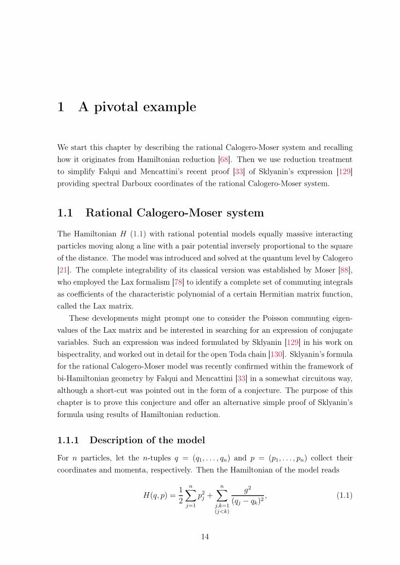
On the cover
A schematic diagram of the various versions of Calogero-Ruijsenaars type integrable
systems with dots and lines indicating the ones studied in the thesis.
Eprint
An eprint of the thesis is freely available in the SZTE Repository of Dissertations:
http://doktori.bibl.u-szeged.hu/3595/
Keywords
integrable systems, many-body systems, Hamiltonian reduction, action-angle duality,
action-angle variables, Calogero-Moser-Sutherland, Ruijsenaars-Schneider-van Diejen,
Poisson-Lie group, Heisenberg double, Lax matrix, spectral coordinates, compact phase
space, root system
2010 Mathematics Subject Classification (MSC2010)
14H70, 37J15, 37J35, 53D20, 70E40, 70G65, 70H06
2010 Physics and Astronomy Classification Scheme (PACS2010)
02.30.Ik, 05.45.-a, 45.20.Jj, 47.10.Df
Please cite this thesis as
T.F. Görbe, Integrable many-body systems of Calogero-Ruijsenaars type, PhD thesis
(2017); doi:10.14232/phd.3595
Copyright c© 2017 Tamás F. Görbe

Orsinak

Acknowledgements
I consider myself very lucky for I have so many people to thank.
First of all, it is with great pleasure that I express my deepest gratitude to my
Ph.D. supervisor László Fehér for the persistent support, guidance, and inspiration
he provided me throughout my studies. He introduced me to the fascinating world
of Integrable Systems and taught me the importance of honesty, modesty, and having
high standards when it comes to research. I feel privileged to have worked with him.
I am grateful to my academic brother Gábor Pusztai for the work we did together.
His superb lectures on Functional Analysis gave me a great appreciation of not only
the subject, but also what didactic skill can achieve.
Thanks are due to Martin Hallnäs for making my research visit to Loughborough
University possible and for being such a great host. Our joint project helped me to
delve into the related area of Multivariate Orthogonal Polynomials.
I am very thankful to Simon Ruijsenaars for hosting me at the University of Leeds.
His insightful comments improved my work substantially.
I also want to thank everyone at the Department of Theoretical Physics for creating
such a stimulating work environment. I especially enjoyed working alongside my fellow
inhabitants of office 231, Gergő Roósz and Lóránt Szabó.
I am indebted to my high school maths teacher János Mike for the unforgettable
classes, which shifted my interest towards mathematics and physics.
The work was supported in part by the Hungarian Scientific Research Fund (OTKA)
under the grant no. K-111697, and was sponsored by the EU and the State of Hungary,
co-financed by the European Social Fund in the framework of TÁMOP-4.2.4.A/2-11/1-
2012-0001 National Excellence Program. The support by the ÚNKP-16-3 New National
Excellence Program of the Ministry of Human Capacities is also acknowledged. Several
short term study programs, made possible by Campus Hungary Scholarships and the
Hungarian Templeton Program, contributed to my work.
Last but most important, I am grateful to my wonderful parents and brothers for
their encouragement and support. I want to thank all my family and friends. Finally,
this thesis is dedicated to my fiancée Orsi, without whom it would not have been
possible.

Contents
Introduction 1
0.1 The golden age of integrable systems . . . . . . . . . . . . . . . . . . . 1
0.2 Definition of Liouville integrability . . . . . . . . . . . . . . . . . . . . 2
0.3 Solitary splendor: The renascence of integrability . . . . . . . . . . . . 4
0.4 Calogero-Ruijsenaars type systems . . . . . . . . . . . . . . . . . . . . 6
0.5 Basic idea of Hamiltonian reduction . . . . . . . . . . . . . . . . . . . . 10
0.6 Action-angle dualities . . . . . . . . . . . . . . . . . . . . . . . . . . . . 11
0.7 Outline of the thesis . . . . . . . . . . . . . . . . . . . . . . . . . . . . 12
I Reduction approach, action-angle duality, applications 13
1 A pivotal example 14
1.1 Rational Calogero-Moser system . . . . . . . . . . . . . . . . . . . . . . 14
1.1.1 Description of the model . . . . . . . . . . . . . . . . . . . . . . 14
1.1.2 Calogero particles from free matrix dynamics . . . . . . . . . . . 15
1.2 Application: Canonical spectral coordinates . . . . . . . . . . . . . . . 16
1.3 Discussion . . . . . . . . . . . . . . . . . . . . . . . . . . . . . . . . . . 19
2 Trigonometric BCn Sutherland system 20
2.1 Physical interpretation . . . . . . . . . . . . . . . . . . . . . . . . . . . 22
2.2 Definition of the Hamiltonian reduction . . . . . . . . . . . . . . . . . . 23
2.3 Action-angle duality . . . . . . . . . . . . . . . . . . . . . . . . . . . . 27
2.3.1 The Sutherland gauge . . . . . . . . . . . . . . . . . . . . . . . 27
2.3.2 The Ruijsenaars gauge . . . . . . . . . . . . . . . . . . . . . . . 31
2.4 Applications . . . . . . . . . . . . . . . . . . . . . . . . . . . . . . . . . 53
2.4.1 On the equilibrium position of the Sutherland system . . . . . . 53
2.4.2 Maximal superintegrability of the dual system . . . . . . . . . . 54
2.4.3 Equivalence of two sets of Hamiltonians . . . . . . . . . . . . . 56
2.5 Discussion . . . . . . . . . . . . . . . . . . . . . . . . . . . . . . . . . . 62
i

Contents
3 A Poisson-Lie deformation 66
3.1 Definition of the Hamiltonian reduction . . . . . . . . . . . . . . . . . . 69
3.1.1 The unreduced free Hamiltonians . . . . . . . . . . . . . . . . . 69
3.1.2 Generalized Marsden-Weinstein reduction . . . . . . . . . . . . 71
3.2 Solution of the momentum equation . . . . . . . . . . . . . . . . . . . . 74
3.2.1 A crucial equation implied by the constraints . . . . . . . . . . 74
3.2.2 Consequences of equation (3.51) . . . . . . . . . . . . . . . . . . 76
3.3 Characterization of the reduced system . . . . . . . . . . . . . . . . . . 79
3.3.1 Smoothness of the reduced phase space . . . . . . . . . . . . . . 79
3.3.2 Model of a dense open subset of the reduced phase space . . . . 81
3.3.3 Liouville integrability of the reduced free Hamiltonians . . . . . 83
3.3.4 The global structure of the reduced phase space . . . . . . . . . 84
3.4 Full phase space of the hyperbolic version . . . . . . . . . . . . . . . . 90
3.4.1 Definitions and first steps . . . . . . . . . . . . . . . . . . . . . 91
3.4.2 The reduced phase space . . . . . . . . . . . . . . . . . . . . . . 94
3.5 Discussion . . . . . . . . . . . . . . . . . . . . . . . . . . . . . . . . . . 100
II Developments in the Ruijsenaars-Schneider family 105
4 Lax representation of the hyperbolic BCn van Diejen system 106
4.1 Preliminaries from group theory . . . . . . . . . . . . . . . . . . . . . . 108
4.2 Algebraic properties of the Lax matrix . . . . . . . . . . . . . . . . . . 111
4.2.1 Lax matrix: explicit form, inverse, and positivity . . . . . . . . 112
4.2.2 Commutation relation and regularity . . . . . . . . . . . . . . . 115
4.3 Analyzing the dynamics . . . . . . . . . . . . . . . . . . . . . . . . . . 119
4.3.1 Completeness of the Hamiltonian vector field . . . . . . . . . . . 120
4.3.2 Dynamics of the vector F . . . . . . . . . . . . . . . . . . . . . 123
4.3.3 Lax representation of the dynamics . . . . . . . . . . . . . . . . 127
4.3.4 Geodesic interpretation . . . . . . . . . . . . . . . . . . . . . . . 131
4.3.5 Temporal asymptotics . . . . . . . . . . . . . . . . . . . . . . . 136
4.4 Spectral invariants of the Lax matrix . . . . . . . . . . . . . . . . . . . 139
4.4.1 Link to the 5-parameter family of van Diejen systems . . . . . . 140
4.4.2 Poisson brackets of the eigenvalues of L . . . . . . . . . . . . . . 141
4.5 Discussion . . . . . . . . . . . . . . . . . . . . . . . . . . . . . . . . . . 144
5 Trigonometric and elliptic Ruijsenaars-Schneider models on CPn−1 147
5.1 Embedding of the local phase space into CPn−1 . . . . . . . . . . . . . 149
5.2 Global extension of the trigonometric Lax matrix . . . . . . . . . . . . 154
5.3 New compact forms of the elliptic Ruijsenaars-Schneider system . . . . 160
5.4 Discussion . . . . . . . . . . . . . . . . . . . . . . . . . . . . . . . . . . 163
ii
Contents
Appendices 165
A Appendix to Chapter 1 166
A.1 An alternative proof of Theorem 1.2 . . . . . . . . . . . . . . . . . . . . 166
B Appendices to Chapter 2 168
B.1 Application of Jacobi’s theorem on complementary minors . . . . . . . 168
B.2 HvDl as elementary symmetric function . . . . . . . . . . . . . . . . . . 171
C Appendices to Chapter 3 173
C.1 Links to systems of van Diejen and Schneider . . . . . . . . . . . . . . 173
C.2 Proof of Proposition 3.2 . . . . . . . . . . . . . . . . . . . . . . . . . . 175
C.3 Proof of Lemma 3.6 . . . . . . . . . . . . . . . . . . . . . . . . . . . . . 178
C.4 Auxiliary material on Poisson-Lie symmetry . . . . . . . . . . . . . . . 179
C.5 On the reduced Hamiltonians . . . . . . . . . . . . . . . . . . . . . . . 180
D Appendices to Chapter 4 182
D.1 Lax matrix with spectral parameter . . . . . . . . . . . . . . . . . . . . 182
D.2 Lax matrix with three couplings . . . . . . . . . . . . . . . . . . . . . . 183
E Appendix to Chapter 5 185
E.1 Explicit form of the functions Λyj,ℓ . . . . . . . . . . . . . . . . . . . . . 185
Summary 187
Összefoglaló 191
Publications 196
Bibliography 198
iii

Introduction
Integrable Systems is a broad area of research that joins seemingly unrelated problems
of natural sciences amenable to exact mathematical treatment1. It serves as a busy
crossroad of many subjects ranging from pure mathematics to experimental physics.
As a result, the notion of ‘integrability’ is hard to pinpoint as, depending on context, it
can refer to different phenomena, and “where you have two scientists you have (at least)
three different definitions of integrability”2. Fortunately, the systems of our interest
are integrable in the Liouville sense, which has a precise definition (see below). Loosely
speaking, in such systems an abundance of conservation laws restricts the motion and
allows the solutions to be exactly expressed with integrals, hence the name.
0.1 The golden age of integrable systems
Studying integrable systems is by no means a new activity as its origins can be traced
back to the early days of modern science, when Newton solved the gravitational two-
body problem and derived Kepler’s laws of planetary motion (for more, see [128]).
With hindsight, one might say that the solution of the Kepler problem was possible
due to the existence of many conserved quantities, such as energy, angular momentum,
and the Laplace-Runge-Lenz vector. In fact, the Kepler problem is a prime example
of a (super)integrable system (also to be defined). As the mathematical foundations of
Newtonian mechanics were established through work of Euler, Lagrange, and Hamilton,
more and more examples of integrable/solvable mechanical problems were discovered.
Just to name a few, these systems include the harmonic oscillator, the “spinning tops”/
rigid bodies [8] of Euler (1758), Lagrange (1788), and Kovalevskaya (1888), the geodesic
motion on the ellipsoid solved by Jacobi (1839), and Neumann’s oscillator model (1859).
This golden age of integrable systems was ended abruptly in the late 1800s, when
Poincaré, while trying to correct his flawed work on the three-body problem, realized
that integrability is a fragile property, that even small perturbations can destroy [28].
This subsided scientific interest and the subject went into a dormant state for more
than half a century.
1For those who are unfamiliar with Integrable Systems, we recommend reading the survey [121].2A quote from another good read, the article Integrability – and how to detect it [74, pp. 31-94].
1

Introduction
0.2 Definition of Liouville integrability
In the Hamiltonian formulation of Classical Mechanics the state of a physical system,
which has n degrees of freedom, is encoded by 2n real numbers. These numbers consist
of (generalised) positions q = (q1, . . . , qn) and (generalised) momenta p = (p1, . . . , pn)
and are collectively called canonical coordinates of the space of states, the phase space.
The time evolution of an initial state (q0, p0) ∈ R2n is governed by Hamilton’s equations
of motion, a first-order system of ordinary differential equations that can be written as
qj =∂H
∂pj, pj = −
∂H
∂qj, j = 1, . . . , n,
whereH is the Hamiltonian, i.e. the total energy of the system. In modern terminology,
a Hamiltonian system is a triple (M,ω,H), where the phase space (M,ω) is a 2n-
dimensional symplectic manifold3 and H is a sufficiently smooth real-valued function
on M . An initial state x0 ∈ M evolves along integral curves of the Hamiltonian vector
field XH of H defined via ω(XH , ·) = dH . Darboux’s theorem [2, 3.2.2 Theorem]
guarantees the existence of canonical coordinates4 (q, p) locally, in which by definition
the symplectic form ω can be written as
ω =n∑
j=1
dqj ∧ dpj ,
and the equations of motion take the canonical form displayed above. The symplectic
form ω gives rise to a Poisson structure on M , which is a handy device that takes two
observables f, g : M → R and turns them into a third one f, g, the Poisson bracket
of f and g given by f, g = ω(Xf , Xg). In canonical coordinates, we have
f, g =n∑
j=1
(∂f
∂qj
∂g
∂pj− ∂f
∂pj
∂g
∂qj
).
It is bilinear, skew-symmetric, satisfies the Jacobi identity and the Leibniz rule. The
equations of motion, for any f : M → R, can be rephrased using the Poisson bracket
f = f,H.
Consequently, if f,H = 0, that is f Poisson commutes with the Hamiltonian H , then
f is a constant of motion. In fact, this relation is symmetric, since f,H = 0 ensures
that H is constant along the integral curves of the Hamiltonian vector field Xf .
3A symplectic manifold (M,ω) is a manifold M equipped with a non-degenerate, closed 2-form ω.4Notice the slight and customary abuse of notation as we use the symbols qj , pj for representing
real numbers as well as coordinate functions on M . Hopefully, this does not cause any confusion.
2

Introduction
Having conserved quantities can simplify things, since it restricts the motion to
the intersection of their level surfaces, selected by the initial conditions. Thus one
should aim at finding as many independent Poisson commuting functions as possible.
By independence we mean that at generic points (on a dense open subset) of the
phase space the functions have linearly independent derivatives. Of course, the non-
degeneracy of the Poisson bracket limits the maximum number of independent functions
in involution to n. If this maximum is reached, we found a Liouville integrable system.
Definition. A Hamiltonian system (M,ω,H), with n degrees of freedom, is called
Liouville integrable, if there exists a family of independent functions H1, . . . , Hn in
involution, i.e. Hj, Hk = 0 for all j, k, and H is a function of H1, . . . , Hn.
The most prominent feature of Liouville integrable systems is the existence of
action-angle variables. This is a system of canonical coordinates I = (I1, . . . , In),
ϕ = (ϕ1, . . . , ϕn), in which the (transformed) Hamiltonians H1, . . . , Hn depend only on
the action variables I, which are themselves first integrals, while the angle variables ϕ
evolve linearly in time. An important result is the following
Liouville-Arnold theorem. [2, 5.2.24 Theorem] Consider (M,ω,H) to be a Liouville
integrable system with the Poisson commuting functions H1, . . . , Hn. Then the level set
Mc = x ∈M | Hj(x) = cj , j = 1, . . . , n
is a smooth n-dimensional submanifold of M , which is invariant under the Hamiltonian
flow of the system. Moreover, if Mc is compact and connected, then it is diffeomorphic
to an n-torus Tn = (ϕ1, . . . , ϕn) mod 2π, and the Hamiltonian flow is linear on Mc,
i.e. the angle variables ϕ on Mc satisfy ϕj = νj, for some constants νj, j = 1, . . . , n.
The action variables I are also encoded in the level set Mc. Roughly speaking, they
determine the size of Mc, since Ij is obtained by integrating the canonical 1-form the
phase space over the j-th cycle of the torus Mc.
Another relevant notion is superintegrability, which requires the existence of extra
constants of motion.
Definition. A Liouville integrable system is called superintegrable, if in addition to the
Hamiltonians H1, . . . , Hn there exist independent first integrals f1, . . . , fk (1 ≤ k < n).
If k = n− 1, then the system is maximally superintegrable.
Examples of maximally superintegrable systems include the Kepler problem, the
harmonic oscillator with rational frequencies, and the rational Calogero-Moser system
considered in Chapter 1. For more on the theory of integrable systems, see [11].
Remark. It should be noted that, although there is no generally accepted notion of
integrability at the quantum level, there are quantum mechanical systems that are
called integrable.
3
Introduction
0.3 Solitary splendor: The renascence of integrability
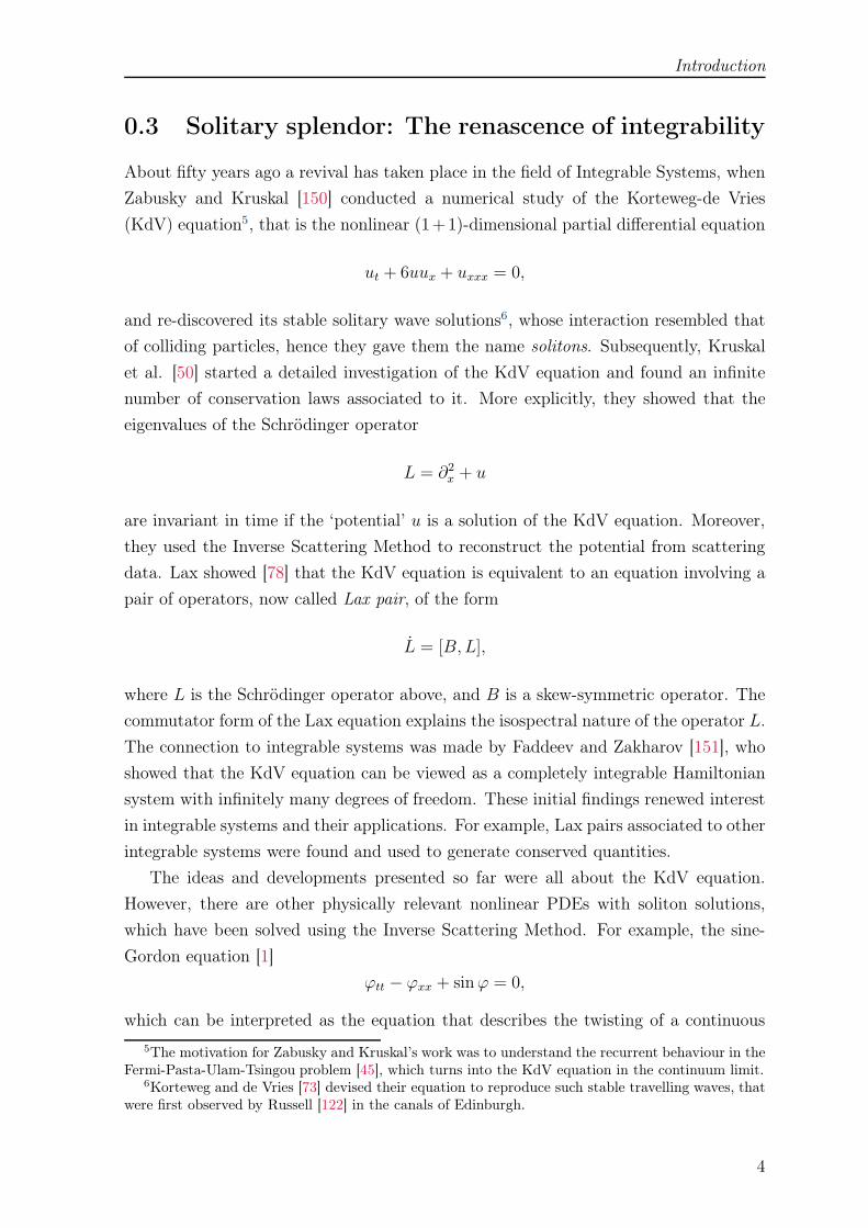
About fifty years ago a revival has taken place in the field of Integrable Systems, when
Zabusky and Kruskal [150] conducted a numerical study of the Korteweg-de Vries
(KdV) equation5, that is the nonlinear (1+1)-dimensional partial differential equation
ut + 6uux + uxxx = 0,
and re-discovered its stable solitary wave solutions6, whose interaction resembled that
of colliding particles, hence they gave them the name solitons. Subsequently, Kruskal
et al. [50] started a detailed investigation of the KdV equation and found an infinite
number of conservation laws associated to it. More explicitly, they showed that the
eigenvalues of the Schrödinger operator
L = ∂2x + u
are invariant in time if the ‘potential’ u is a solution of the KdV equation. Moreover,
they used the Inverse Scattering Method to reconstruct the potential from scattering
data. Lax showed [78] that the KdV equation is equivalent to an equation involving a
pair of operators, now called Lax pair, of the form
L = [B,L],
where L is the Schrödinger operator above, and B is a skew-symmetric operator. The
commutator form of the Lax equation explains the isospectral nature of the operator L.
The connection to integrable systems was made by Faddeev and Zakharov [151], who
showed that the KdV equation can be viewed as a completely integrable Hamiltonian
system with infinitely many degrees of freedom. These initial findings renewed interest
in integrable systems and their applications. For example, Lax pairs associated to other
integrable systems were found and used to generate conserved quantities.
The ideas and developments presented so far were all about the KdV equation.
However, there are other physically relevant nonlinear PDEs with soliton solutions,
which have been solved using the Inverse Scattering Method. For example, the sine-
Gordon equation [1]
ϕtt − ϕxx + sinϕ = 0,
which can be interpreted as the equation that describes the twisting of a continuous
5The motivation for Zabusky and Kruskal’s work was to understand the recurrent behaviour in theFermi-Pasta-Ulam-Tsingou problem [45], which turns into the KdV equation in the continuum limit.
6Korteweg and de Vries [73] devised their equation to reproduce such stable travelling waves, thatwere first observed by Russell [122] in the canals of Edinburgh.
4
Introduction
chain of needles attached to an elastic band. It has different kinds of soliton solutions,
called kink, antikink, and breather, that can interact with one another. It is a relativistic
equation, since its solutions are invariant under the action of the Poincaré group of
(1 + 1)-dimensional space-time.
The nonlinear Schrödinger equation [153] is another famous example. It reads
iψt +1
2ψxx − κ|ψ|2ψ = 0,
where ψ is a complex-valued wave function and κ is constant. It is also an exactly
solvable Hamiltonian system [152]. The equation is nonrelativistic (Galilei invariant).
Now let us list some applications of these soliton equations. The Korteweg-de
Vries equation can be applied to describe shallow-water waves with weakly non-linear
restoring forces and long internal waves in a density-stratified ocean. It is also useful
in modelling ion acoustic waves in a plasma and acoustic waves on a crystal lattice.
The kinks and breathers of the sine-Gordon equation can used as models of nonlinear
excitations in complex systems in physics and even in cellular structures. The nonlinear
Schrödinger equation is of central importance in fluid dynamics, plasma physics, and
nonlinear optics as it appears in the Manakov system, a model of wave propagation in
fibre optics.
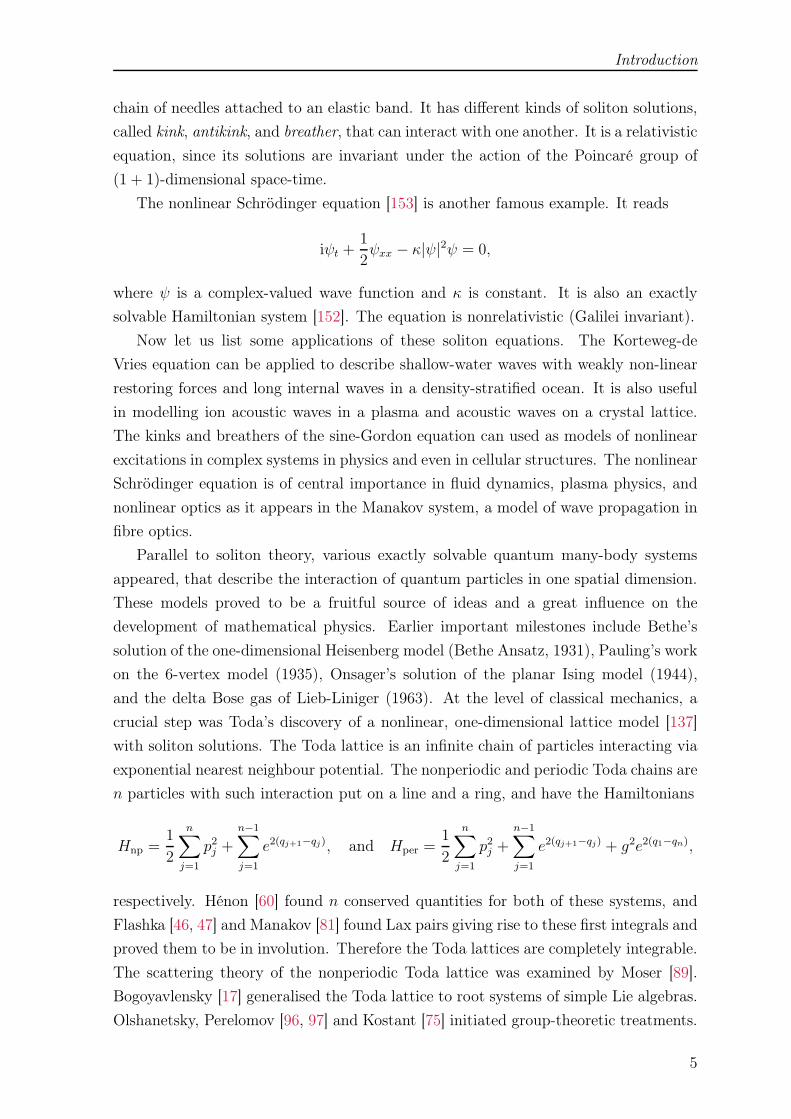
Parallel to soliton theory, various exactly solvable quantum many-body systems
appeared, that describe the interaction of quantum particles in one spatial dimension.
These models proved to be a fruitful source of ideas and a great influence on the
development of mathematical physics. Earlier important milestones include Bethe’s
solution of the one-dimensional Heisenberg model (Bethe Ansatz, 1931), Pauling’s work
on the 6-vertex model (1935), Onsager’s solution of the planar Ising model (1944),
and the delta Bose gas of Lieb-Liniger (1963). At the level of classical mechanics, a
crucial step was Toda’s discovery of a nonlinear, one-dimensional lattice model [137]
with soliton solutions. The Toda lattice is an infinite chain of particles interacting via
exponential nearest neighbour potential. The nonperiodic and periodic Toda chains are
n particles with such interaction put on a line and a ring, and have the Hamiltonians
Hnp =1
2
n∑
j=1
p2j +
n−1∑
j=1
e2(qj+1−qj), and Hper =1
2
n∑
j=1
p2j +
n−1∑
j=1
e2(qj+1−qj) + g2e2(q1−qn),
respectively. Hénon [60] found n conserved quantities for both of these systems, and
Flashka [46, 47] and Manakov [81] found Lax pairs giving rise to these first integrals and
proved them to be in involution. Therefore the Toda lattices are completely integrable.
The scattering theory of the nonperiodic Toda lattice was examined by Moser [89].
Bogoyavlensky [17] generalised the Toda lattice to root systems of simple Lie algebras.
Olshanetsky, Perelomov [96, 97] and Kostant [75] initiated group-theoretic treatments.
5

Introduction
0.4 Calogero-Ruijsenaars type systems
In the early 1970s further exactly solvable quantum many-body systems were found by
Calogero [20, 21] and Sutherland [132, 133]. Calogero considered particles on a line in
harmonic confinement with a pairwise interaction inversely proportional to the square
of their relative distances (rational case). Sutherland solved the corresponding problem
of particles on a ring, i.e. interacting via a periodic pair-potential (trigonometric case).
The classical versions were examined by Moser [88], who provided Lax pairs, analysed
the particle scattering in the rational case, which he proved to be Liouville integrable7.
Models with short-range interaction (hyperbolic case) [26] and with elliptic potentials
(elliptic case) [22] were also formulated (see Figures 1 and 2).
We give a short description of the classical systems. Let the number of particles n
be fixed, q = (q1, . . . , qn) ∈ Rn collect the particle-positions and p = (p1, . . . , pn) ∈ Rn
the conjugate momenta. The configuration space is usually some open domain C ⊆ Rn,
and the phase space M is its cotangent bundle
M = T ∗C = (q, p) | q ∈ C, p ∈ Rn,
equipped with the canonical symplectic form
ω =n∑
j=1
dqj ∧ dpj .
The Hamiltonian of the models can be written in the general form
Hnr =1
2m
n∑
j=1
p2j +g2
m
∑
j<k
V (qj − qk),
where m > 0 denotes the mass of particles, g is a positive coupling constant regulating
the strength of particle repulsion8, and the pair-potential V can be one of four types:
V (q) =
1/q2, rational (I),
α2/ sinh2(αq), hyperbolic (II),
α2/ sin2(αq), trigonometric (III),
℘(q;ω, ω′), elliptic (IV).
Here ℘ stands for Weierstrass’s elliptic function with half-periods (ω, ω′) ∈ R+ × iR+.
By taking the parameter α→ iα, II and III are exchanged, while α→ 0 produces I.
7The rational three-body system was treated by Marchioro [82] and to some extent by Jacobi [65].8The interaction is attractive, if g2 < 0. Setting g = 0 yields free particles.
6

Introduction
1 2 3
1
2
0 q
V (q)
q−1 Coulombq−2 Rationalsinh−2(q) Hyperbolic
Figure 1: Three repulsive potential functions. The Coulomb potential V (q) = q−1 (solidblue) and rational potential V (q) = q−2 (dashed red) express long-range interaction incomparison to the hyperbolic potential V (q) = sinh−2(q) (dotted black).
1 2 3
1
2
3
0 q
V (q)q−2 + q2/2 Calogerosin−2(q) Trigonometric℘(q; π/2, i) Elliptic
Figure 2: Three confining potential functions. Calogero potential V (q) = q−2 + q2/2(solid blue), trigonometric potential V (q) = sin−2(q) (dashed red), and elliptic potentialV (q) = ℘(q;ω, ω′) (dotted black) with half-periods ω = π/2, ω′ = i.
The elliptic potential degenerates to the other ones in various limits9
℘(q;ω, ω′)→
1/q2, if ω →∞, ω′ → i∞,α2/3 + α2/ sinh2(αq), if ω →∞, ω′ → iπ/2α,
−α2/3 + α2/ sin2(αq), if ω → π/2α, ω′ → i∞.9It is worth mentioning that the Toda lattices (both periodic and nonperiodic) can be also obtained
from the elliptic model. For details, see [64, 115, 118].
7

Introduction
These models are nonrelativistic, that is invariant under the Galilei group of (1 + 1)-
dimensional space-time. Relativistic (i.e. Poincaré-invariant) integrable deformations
were constructed10 by Ruijsenaars and Schneider [111], and Ruijsenaars [112]. The
Hamiltonians of the relativistic systems read
Hrel =1
β2m
n∑
j=1
cosh(βpj)∏
k 6=j
f(qj − qk),
where β = 1/mc > 0 is the deformation parameter (c can be interpreted as the speed
of light), and the function f can be one of the following
f(q) =
(1 + β2g2/q2)1/2, rational (I),
(1 + sin2(αβg)/ sinh2(αq))1/2, hyperbolic (II),
(1 + sinh2(αβg)/ sin2(αq))1/2, trigonometric (III),
(σ2(iβg;ω, ω′)[℘(iβg;ω, ω′)− ℘(q;ω, ω′)])1/2, elliptic (IV).
Here σ is the Weierstrass sigma function. In the nonrelativistic limit β → 0 we get
limβ→0
(Hrel −n
β2m) = Hnr.
The quantum Hamiltonians at the nonrelativistic level consist of commuting partial
differential operators, obtained from classical Hamiltonians by canonical quantization.
For example, the Hamiltonian operator can be written as
Hnr = −~2
2m
n∑
j=1
∂2
∂q2j+g(g − ~)
m
∑
j<k
V (qj − qk).
The corresponding Hilbert space, on which these operators act, is the space L2(C, dq)
of square integrable complex-valued functions over the classical configuration space C.
In contrast, the relativistic quantum Hamiltonians have an exponential dependence on
the momentum operators, resulting in analytic differential operators, such as
Hrel =1
2β2m(S1 + S−1), with S±1 =
n∑
j=1
[∏
k 6=j
f∓(qj − qk)]e∓i~β∂j
[∏
k 6=j
f±(qj − qk)].
In the elliptic case f±(q) = σ(iβg+ q)/σ(q) and the other cases are obtained as limits.
Therefore these operators act on functions that have an analytic continuation to an
at least 2~β wide strip in the complex plane. For more details on these models, the
reader is referred to the articles [25, 119, 120] or the exhaustive surveys [115, 118].
10With the motivation to reproduce the scattering of sine-Gordon solitons using interacting particles.
8

Introduction
A scheme of the Calogero-Ruijsenaars type systems is depicted in Figure 3.
Classical
Qua
ntum
I II III IV
α→ 0 α→ iαω → π/2αω′ → i∞
Relativ
istic
β → 0
~→ 0
Classical
Qua
ntum
I II III IV
Nonrelat
ivisti
c
Figure 3: Schematics of Calogero-Ruijsenaars type systems.
The above-mentioned models have generalisations formulated using root systems11.
To this end, notice that in the Hamiltonians presented above qj − qk = a · q are the
inner product of q and the root vectors a ∈ An−1 of the simple Lie algebra sl(n,C).
It turns out that if An−1 is replaced with any root system the resulting system is
still integrable. Such root system generalisations were introduced by Olshanetsky and
Perelomov [98, 99], who found Lax pairs and proved integrability for models attached
to the classical root systems Bn,Cn,Dn (and BCn). For arbitrary root systems, the
integrability of non-elliptic quantum systems was showed by Heckman and Opdam
[57], and Sasaki et al. [69], and for classical systems (including the elliptic case) by
Khastgir and Sasaki [70]. Integrable Ruijsenaars-Schneider models attached to non-A
type root systems were found by van Diejen [140, 141, 142, 143]. It is a remarkable
fact that the eigenfunctions of these generalised Calogero-Ruijsenaars type operators
are multivariate orthogonal polynomials, and the equilibrium positions of the classical
systems are given by the zeros of classical orthogonal polynomials [23, 94].
There are other ways to generalise the Calogero-Ruijsenaars type systems, e.g. by
allowing internal degrees of freedom (spins) [51, 110] or supersymmetry [127, 19, 14].
11A short summary of facts about root systems can be found in [123]. For more details, see [61].
9
Introduction
0.5 Basic idea of Hamiltonian reduction
In their pioneering work, Kazhdan, Kostant, and Sternberg [68] offered a key insight
into the origin of the Poisson commuting first integrals of Calogero-Moser-Sutherland
models. In a nutshell, they derived the complicated motion of these many-body systems
by applying Marsden-Weinstein reduction [85] to a higher dimensional free particle.
The reduction framework and its application to Hamiltonian systems have undergone
considerable development since then [101, 83]. Here we only present a description of
the reduction machinery that is tailored to our purposes. Part I of the thesis contains
specific implementations of this approach.
The reduction procedure starts with choosing a ‘big phase space’ of group-theoretic
origin. This might be, say, the cotangent bundle P = T ∗X of a matrix Lie group or
algebra X. The natural symplectic structure Ω of the cotangent bundle P permits
one to define a Hamiltonian system (P,Ω,H) by specifying a Hamiltonian H : P → R.
If H is simple enough, then the equations of motion can be solved, or even better, a
family of Poisson commuting functions Hj be found, which H is a member/function
of. Then by choosing an appropriate group action (of some group G) on X (hence P ),
under which Hj are invariant12, one can construct the momentum map Φ: P → g∗
corresponding to this action. Fixing the value µ of the momentum map Φ produces
a level surface Φ−1(µ) in the ‘big phase space’. This constraint surface is foliated by
the orbits of the isotropy/gauge group Gµ ⊂ G of the momentum value. The reduced
phase space (Pred, ωred) consists of these orbits. The point is that the flows of the
commuting ‘free’ Hamiltonians Hj preserve the momentum surface and are constant
along obits. Therefore they admit reduced versions Hj : Pred → R, which still Poisson
commute13 and the resulting Hamiltonian system (Pred, ωred, H) is Liouville integrable.
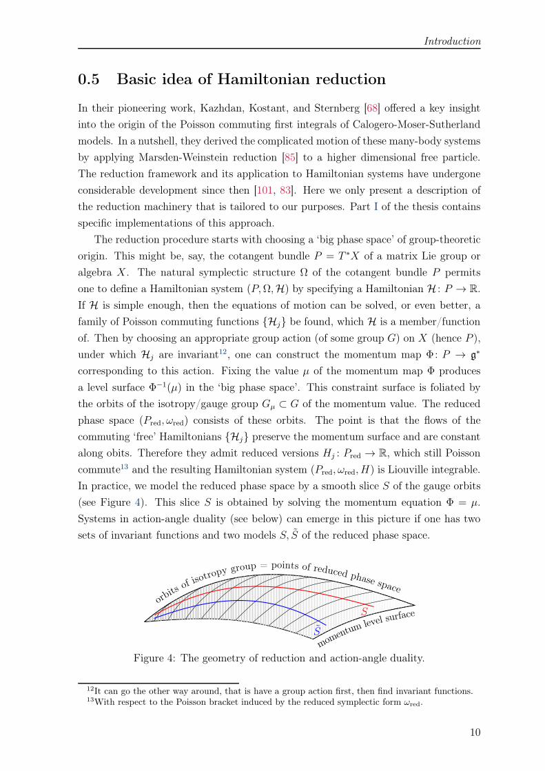
In practice, we model the reduced phase space by a smooth slice S of the gauge orbits
(see Figure 4). This slice S is obtained by solving the momentum equation Φ = µ.
Systems in action-angle duality (see below) can emerge in this picture if one has two
sets of invariant functions and two models S, S of the reduced phase space.
moment
umlevel
surface
orbit
s ofisot
ropy group = points of reduced phase space
S
S
Figure 4: The geometry of reduction and action-angle duality.
12It can go the other way around, that is have a group action first, then find invariant functions.13With respect to the Poisson bracket induced by the reduced symplectic form ωred.
10

Introduction
0.6 Action-angle dualities
Action-angle duality is a relation between two Liouville integrable systems, say (M,ω,H)
and (M, ω, H), requiring the existence of canonical coordinates (q, p) on M and (q, p)
on M (or on dense open submanifolds of M and M) and a global symplectomorphism
R : M → M , the action-angle map, such that (q, p) R are action-angle variables for
the Hamiltonian H and (q, p) R−1 are action-angle variables for the Hamiltonian H .
This means that H R−1 depends only on q and H R only on q. Then one says
that the systems (M,ω,H) and (M, ω, H) are in action-angle duality. In addition, for
the systems of our interest it also happens that the Hamiltonian H , when expressed
in the coordinates (q, p), admits interpretation in terms of interacting ‘particles’ with
position variables q, and similarly, H expressed in (q, p) describes the interacting points
with positions q. Thus q are particle positions for H and action variables for H , and
the q are positions for H and actions for H . The significance of this curious property
is clear for instance from the fact that it persists at the quantum mechanical level as
the bispectral character of the wave functions [30, 114], which are important special
functions.
Rational Calogero-Moser Rational Calogero-Moser
Hyperbolic Calogero-Moser Rational Ruijsenaars-Schneider
Hyperbolic Ruijsenaars-Schneider Hyperbolic Ruijsenaars-Schneider
β → 0
R
α→ 0
R
α→ 0
Rβ → 0
Figure 5: Action-angle dualities among Calogero-Ruijsenaars type systems.
Dual pairs of many-body systems were exhibited by Ruijsenaars (see Figure 5) in
the course of his direct construction [113, 115, 117, 118] of action-angle variables for
the many-body systems (of non-elliptic Calogero-Ruijsenaars type and non-periodic
Toda type) associated with the root system An−1. The idea that dualities can be
interpreted in terms of Hamiltonian reduction can be distilled from [68] and was put
forward explicitly in several papers in the 1990s, e.g. [48, 54]. These papers contain
a wealth of interesting ideas and results, but often stated without full proofs. In the
last decade or so, Fehér and collaborators undertook the systematic study of these
dualities within the framework of reduction [36, 35, 9, 37, 38, 34, 40]. It seems natural
to expect that action-angle dualities exist for many-body systems associated with other
root systems. Substantial evidence in favour of this expectation was given by Pusztai
[105, 106, 107, 108, 109]. This thesis presents results (see Publications) that were
obtained in connection to these earlier developments.
11

Introduction
0.7 Outline of the thesis
The main content of the thesis is divided into two parts with a total of five chapters.
Part I takes the reduction approach to Calogero-Ruijsenaars type systems. In each
of its chapters the basic idea of reduction that we just sketched is put into practice, only
at an increasing level of complexity. In particular, Chapter 1 presents a streamlined
derivation of the rational Calogero-Moser system using reduction. Section 1.2 exhibits
the utility of the reduction perspective, as we give a simple proof of a formula providing
action-angle coordinates. Chapter 2 is a study of the trigonometric BCn Sutherland
system. We provide a physical interpretation of the model in Section 2.1 and prepare
the ingredients of reduction in Section 2.2. In Section 2.3, we solve the momentum
equations and obtain the action-angle dual of the BCn Sutherland system. In Section
2.4, we apply our duality map to various problems, such as equilibrium configurations,
proving superintegrability, and showing the equivalence of two sets of Hamiltonians.
Chapter 3 generalises certain results of the previous chapter as it derives a 1-parameter
deformation of the trigonometric BCn Sutherland system using Hamiltonian reduction
of the Heisenberg double of SU(2n). We define the pertinent reduction in Section 3.1,
solve the momentum constraints in Section 3.2, and characterize the reduced system in
Section 3.3. In Section 3.4, we complete a recent derivation of the hyperbolic analogue.
Part II is a collection of work motivated by, but not involving reduction techniques.
Chapter 4 reports our discovery of a Lax pair for the hyperbolic van Diejen system with
two independent coupling parameters. The preparatory Section 4.1 is followed by the
explicit formulation of our Lax matrix in Section 4.2. In Section 4.3, we show that the
dynamics can be solved by a projection method, which in turn allows us to initiate the
study of the scattering properties. We prove the equivalence between the first integrals
provided by the eigenvalues of the Lax matrix and the family of van Diejen’s commuting
Hamiltonians in Section 4.4. Chapter 5 is concerned with the explicit construction of
compactified versions of trigonometric and elliptic Ruijsenaars-Schneider systems. In
Section 5.1, we embed the local phase space of the model into the complex projective
space CPn−1. Section 5.2 contains our proof of the global extension of the trigonometric
Lax matrix to CPn−1. We use our direct construction to introduce new compactified
elliptic systems in Section 5.3.
The chapters are complemented by Appendices collecting supplementary material
(alternative proofs, detailed derivations, etc.). A Summary presents the most important
results in a concise form. A list of Publications, on which this thesis is based, and a
Bibliography are also included.
12

Part I
Reduction approach, action-angle
duality, applications
13
1 A pivotal example
We start this chapter by describing the rational Calogero-Moser system and recalling
how it originates from Hamiltonian reduction [68]. Then we use reduction treatment
to simplify Falqui and Mencattini’s recent proof [33] of Sklyanin’s expression [129]
providing spectral Darboux coordinates of the rational Calogero-Moser system.
1.1 Rational Calogero-Moser system
The Hamiltonian H (1.1) with rational potential models equally massive interacting
particles moving along a line with a pair potential inversely proportional to the square
of the distance. The model was introduced and solved at the quantum level by Calogero
[21]. The complete integrability of its classical version was established by Moser [88],
who employed the Lax formalism [78] to identify a complete set of commuting integrals
as coefficients of the characteristic polynomial of a certain Hermitian matrix function,
called the Lax matrix.
These developments might prompt one to consider the Poisson commuting eigen-
values of the Lax matrix and be interested in searching for an expression of conjugate
variables. Such an expression was indeed formulated by Sklyanin [129] in his work on
bispectrality, and worked out in detail for the open Toda chain [130]. Sklyanin’s formula
for the rational Calogero-Moser model was recently confirmed within the framework of
bi-Hamiltonian geometry by Falqui and Mencattini [33] in a somewhat circuitous way,
although a short-cut was pointed out in the form of a conjecture. The purpose of this
chapter is to prove this conjecture and offer an alternative simple proof of Sklyanin’s
formula using results of Hamiltonian reduction.
1.1.1 Description of the model
For n particles, let the n-tuples q = (q1, . . . , qn) and p = (p1, . . . , pn) collect their
coordinates and momenta, respectively. Then the Hamiltonian of the model reads
H(q, p) =1
2
n∑
j=1
p2j +n∑
j,k=1(j<k)
g2
(qj − qk)2, (1.1)
14

1. A pivotal example
where g is a real coupling constant tuning the strength of particle interaction. The
pair potential is singular at qj = qk (j 6= k), hence any initial ordering of the particles
remains unchanged during time-evolution. The configuration space is chosen to be the
domain C = q ∈ Rn | q1 > · · · > qn, and the phase space is its cotangent bundle
T ∗C = (q, p) | q ∈ C, p ∈ Rn, (1.2)
endowed with the standard symplectic form
ω =
n∑
j=1
dqj ∧ dpj . (1.3)
1.1.2 Calogero particles from free matrix dynamics
The Hamiltonian system (T ∗C, ω,H), called the rational Calogero-Moser system, can
be obtained as an appropriate Marsden-Weinstein reduction of the free particle moving
in the space of n× n Hermitian matrices as follows.
Consider the manifold of pairs of n× n Hermitian matrices
M = (X,P ) | X,P ∈ gl(n,C), X† = X, P † = P, (1.4)
equipped with the symplectic form
Ω = tr(dX ∧ dP ). (1.5)
The Hamiltonian of the analogue of a free particle reads
H(X,P ) = 1
2tr(P 2). (1.6)
The equations of motion can be solved explicitly for this Hamiltonian system (M,Ω,H),and the general solution is given by X(t) = tP0 + X0, P (t) = P0. Moreover, the
functions Hk(X,P ) = 1ktr(P k), k = 1, . . . , n form an independent set of commuting
first integrals.
The group of n× n unitary matrices U(n) acts on M (1.4) by conjugation
(X,P )→ (UXU †, UPU †), U ∈ U(n), (1.7)
leaves both the symplectic form Ω (1.5) and the Hamiltonians Hk invariant, and the
matrix commutator (X,P ) → [X,P ] is a momentum map for this U(n)-action. Con-
sider the Hamiltonian reduction performed by factorizing the momentum constraint
15

1. A pivotal example
surface
[X,P ] = ig(vv† − 1n) = µ, v = (1 . . . 1)† ∈ Rn, g ∈ R, (1.8)
with the stabilizer subgroup Gµ ⊂ U(n) of µ, e.g. by diagonalization of the X compo-
nent. This yields the gauge slice S = (Q(q, p), L(q, p)) | q ∈ C, p ∈ Rn, where
Qjk = (UXU †)jk = qjδjk, Ljk = (UPU †)jk = pjδjk + ig1− δjkqj − qk
, j, k = 1, . . . , n.
(1.9)
This S is symplectomorphic to the reduced phase space and to T ∗C (1.2) since it in-
herits the reduced symplectic form ω (1.3). The unreduced Hamiltonians project to a
commuting set of independent integrals Hk =1ktr(Lk), k = 1, . . . , n, such that H2 = H
(1.1) and what’s more, the completeness of Hamiltonian flows follows automatically
from the reduction. Therefore the rational Calogero-Moser system is completely inte-
grable.
The similar role of matrices X and P in the derivation above can be exploited to
construct action-angle variables for the rational Calogero-Moser system. This is done
by switching to the gauge, where the P component is diagonalized by some matrix
U ∈ Gµ, and it boils down to the gauge slice S = (Q(φ, λ), L(φ, λ)) | φ ∈ Rn, λ ∈ C,where
Qjk = (UXU †)jk = φjδjk − ig1− δjkλj − λk
, Ljk = (UP U †)jk = λjδjk, j, k = 1, . . . , n.
(1.10)
By construction, S with the symplectic form ω =∑n
j=1 dφj ∧ dλj is also symplecto-
morphic to the reduced phase space, thus a canonical transformation (q, p)→ (φ, λ) is
obtained, where the reduced Hamiltonians depend only on λ, viz. Hk =1k(λk1+· · ·+λkn),
k = 1, . . . , n.
1.2 Application: Canonical spectral coordinates
Now, we turn to the question of variables conjugate to the Poisson commuting eigen-
values λ1, . . . , λn of L (1.9), i.e. such functions θ1, . . . , θn in involution that
θj, λk = δjk, j, k = 1, . . . , n. (1.11)
At the end of Subsection 1.1.2 we saw that the variables φ1, . . . , φn are such functions.
These action-angle variables λ, φ were already obtained by Moser [88] using scatter-
ing theory, and also appear in Ruijsenaars’s proof of the self-duality of the rational
Calogero-Moser system [113].
Let us define the following functions over the phase space T ∗C (1.2) with dependence
16

1. A pivotal example
on an additional variable z:
A(z) = det(z1n − L), C(z) = tr(Q adj(z1n − L)vv†), D(z) = tr(Q adj(z1n − L)),(1.12)
where Q and L are given by (1.9), v = (1 . . . 1)† ∈ Rn and adj denotes the adjugate
matrix, i.e. the transpose of the cofactor matrix. Sklyanin’s formula [129] for θ1, . . . , θnthen reads
θk =C(λk)
A′(λk), k = 1, . . . , n. (1.13)
In [33] Falqui and Mencattini have shown that
µk =D(λk)
A′(λk), k = 1, . . . , n (1.14)
are conjugate variables to λ1, . . . , λn, and
θk = µk + fk(λ1, . . . , λn), k = 1, . . . , n, (1.15)
with such λ-dependent functions f1, . . . , fn that
∂fj∂λk
=∂fk∂λj
, j, k = 1, . . . , n (1.16)
thus θ1, . . . , θn given by Sklyanin’s formula (1.13) are conjugate to λ1, . . . , λn. This was
done in a roundabout way, although the explicit form of relation (1.15) was conjectured.
Here we take a different route by making use of the reduction viewpoint of Sub-
section 1.1.2. From this perspective, the problem becomes transparent and can be
solved effortlessly. First, we show that µ1, . . . , µn (1.14) are nothing else than the angle
variables φ1, . . . , φn.
Lemma 1.1. The variables µ1, . . . , µn defined in (1.14) are the angle variables φ1, . . . , φn
of the rational Calogero-Moser system.
Proof. Notice that, by definition, µ1, . . . , µn are gauge invariant, thus by working in
the gauge, where the P component is diagonal, that is with the matrices Q, L (1.10),
we get
D(z)
A′(z)=
∑nj=1 φj
∏nℓ=1(ℓ 6=j)
(z − λℓ)∑n
j=1
∏nℓ=1(ℓ 6=j)
(z − λℓ). (1.17)
Substituting z = λk into (1.17) yields µk = φk, for each k = 1, . . . , n.
Next, we prove the relation of functions A, C, D (1.12), that was conjectured in
[33].
17

1. A pivotal example
Theorem 1.2. For any n ∈ N, (q, p) ∈ T ∗C (1.2), and z ∈ C we have
C(z) = D(z) +ig
2A′′(z). (1.18)
Proof. Pick any point (q, p) in the phase space T ∗C and consider the corresponding
point (λ, φ) in the space of action-angle variables. Since A(z) = (z − λ1) . . . (z − λn)we have
ig
2A′′(z) = ig
n∑
j,k=1(j<k)
n∏
ℓ=1(ℓ 6=j,k)
(z − λℓ). (1.19)
The difference of functions C and D (1.12) reads
C(z)−D(z) = tr(Q adj(z1n − L)(vv† − 1n)
). (1.20)
Since this is a gauge invariant function, we are allowed to work with Q, L (1.10) instead
of Q,L (1.9). Therefore (1.20) can be written as the sum of all off-diagonal components
of Q adj(z1n − L), that is
C(z)−D(z) = ign∑
j,k=1(j 6=k)
−1λj − λk
n∏
ℓ=1(ℓ 6=k)
(z − λℓ) = ign∑
j,k=1(j<k)
n∏
ℓ=1(ℓ 6=j,k)
(z − λℓ). (1.21)
This concludes the proof.
Our theorem confirms that indeed relation (1.15) is valid with
fk(λ1, . . . , λn) =ig
2
A′′(λk)
A′(λk)= ig
n∑
ℓ=1(ℓ 6=k)
1
λk − λℓ, k = 1, . . . , n, (1.22)
for which (1.16) clearly holds. An immediate consequence, as we indicated before, is
that θ1, . . . , θn (1.13) are conjugate variables to λ1, . . . , λn, thus Sklyanin’s formula is
verified.
Corollary 1.3 (Sklyanin’s formula). The variables θ1, . . . , θn defined by
θk =C(λk)
A′(λk), k = 1, . . . , n (1.23)
are conjugate to the eigenvalues λ1, . . . , λn of the Lax matrix L.
18

1. A pivotal example
1.3 Discussion
There seem to be several ways for generalisation. For example, one might consider
rational Calogero-Moser models associated to root systems other than type A. The
hyperbolic Calogero-Moser systems as well as, the ‘relativistic’ Calogero-Moser systems,
also known as Ruijsenaars-Schneider systems, are also of considerable interest.
In Appendix A.1, we give another proof for Theorem 1.2 based on the scattering
theory of particles in the rational Calogero-Moser system.
19

2 Trigonometric BCn Sutherland system
In this chapter, we present a new case of action-angle duality between integrable many-
body systems of Calogero-Ruijsenaars type. This chapter contains our results reported
in [P1, P8, P5].
The two systems live on the action-angle phase spaces of each other in such a
way that the action variables of each system serve as the particle positions of the
other one. Our investigation utilizes an idea that was exploited previously to provide
group-theoretic interpretation for several dualities discovered originally by Ruijsenaars.
In the group-theoretic framework one applies Hamiltonian reduction to two Abelian
Poisson algebras of invariants on a higher dimensional phase space and identifies their
reductions as action and position variables of two integrable systems living on two
different models of the single reduced phase space. Taking the cotangent bundle of
U(2n) as the upstairs space, we demonstrate how this mechanism leads to a new dual
pair involving the BCn trigonometric Sutherland system. Thereby we generalise earlier
results pertaining to the An−1 trigonometric Sutherland system [35] as well as a recent
work by Pusztai [107] on the hyperbolic BCn Sutherland system.
The specific goal in this chapter is to find out how this result can be generalised if one
replaces the hyperbolic BCn system with its trigonometric analogue. A similar problem
has been studied previously in the An−1 case, where it was found that the dual of the
trigonometric Sutherland system possesses intricate global structure [35, 117]. The
global description of the duality necessitates a separate investigation also in the BCn
case, since it cannot be derived by naive analytic continuation between trigonometric
and hyperbolic functions. This problem turns out to be considerably more complicated
than those studied in [35, 107].
The trigonometric BCn Sutherland system is defined by the Hamiltonian
H =1
2
n∑
j=1
p2j +∑
1≤j<k≤n
[γ
sin2(qj − qk)+
γ
sin2(qj + qk)
]+
n∑
j=1
γ1sin2(qj)
+
n∑
j=1
γ2sin2(2qj)
.
(2.1)
Here (q, p) varies in the cotangent bundle M = T ∗C1 = C1 × Rn of the domain
C1 =
q ∈ Rn
∣∣∣∣π
2> q1 > · · · > qn > 0
, (2.2)
20
2. Trigonometric BCn
Sutherland system
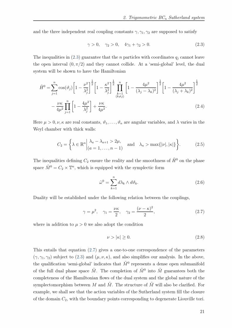
and the three independent real coupling constants γ, γ1, γ2 are supposed to satisfy
γ > 0, γ2 > 0, 4γ1 + γ2 > 0. (2.3)
The inequalities in (2.3) guarantee that the n particles with coordinates qj cannot leave
the open interval (0, π/2) and they cannot collide. At a ‘semi-global’ level, the dual
system will be shown to have the Hamiltonian
H0 =n∑
j=1
cos(ϑj)
[1− ν2
λ2j
]12[1− κ2
λ2j
]12
n∏
k=1(k 6=j)
[1− 4µ2
(λj − λk)2]12[1− 4µ2
(λj + λk)2
]12
− νκ
4µ2
n∏
j=1
[1− 4µ2
λ2j
]+νκ
4µ2. (2.4)
Here µ > 0, ν, κ are real constants, ϑ1, . . . , ϑn are angular variables, and λ varies in the
Weyl chamber with thick walls:
C2 =
λ ∈ Rn
∣∣∣∣λa − λa+1 > 2µ,
(a = 1, . . . , n− 1)and λn > max|ν|, |κ|
. (2.5)
The inequalities defining C2 ensure the reality and the smoothness of H0 on the phase
space M0 = C2 × Tn, which is equipped with the symplectic form
ω0 =n∑
k=1
dλk ∧ dϑk. (2.6)
Duality will be established under the following relation between the couplings,
γ = µ2, γ1 =νκ
2, γ2 =
(ν − κ)22
, (2.7)
where in addition to µ > 0 we also adopt the condition
ν > |κ| ≥ 0. (2.8)
This entails that equation (2.7) gives a one-to-one correspondence of the parameters
(γ, γ1, γ2) subject to (2.3) and (µ, ν, κ), and also simplifies our analysis. In the above,
the qualification ‘semi-global’ indicates that M0 represents a dense open submanifold
of the full dual phase space M . The completion of M0 into M guarantees both the
completeness of the Hamiltonian flows of the dual system and the global nature of the
symplectomorphism between M and M . The structure of M will also be clarified. For
example, we shall see that the action variables of the Sutherland system fill the closure
of the domain C2, with the boundary points corresponding to degenerate Liouville tori.
21

2. Trigonometric BCn
Sutherland system
The integrable systems (M,ω,H) and (M, ω, H) as well as their duality relation
will emerge from an appropriate Hamiltonian reduction. Specifically, we will reduce
the cotangent bundle T ∗U(2n) with respect to the symmetry group G+ × G+, where
G+∼= U(n) × U(n) is the fix-point subgroup of an involution of U(2n). This enlarges
the range of the reduction approach to action-angle dualities [48, 53, 92].
2.1 Physical interpretation
The trigonometric BCn Sutherland model has the following physical interpretation.
Consider a circle of radius 1/2 with centre O. First, put one particle on the circle to an
arbitrary point Q0, hence creating reference direction−−→OQ0, which coordinates a point
Q on the circle with the angle φ(Q) = ∠QOQ0 ∈ (−π, π], i.e. φ(Q0) = 0. Next, place
n particles on the circle at some points Q1, . . . , Qn, such that their angles φj = φ(Qj)
(j = 1, . . . , n) satisfy π > φ1 > · · · > φn > 0. Put n additional particles on the circle
at ‘mirror images’ Q−j of Qj with respect to the point Q0, that is φ(Qj) = −φ(Q−j).
O
R=1/2
Q0
Qk
Qj
Q−k
Q−j
φkφj
φ−j
qj
qk
sin(qj − qk )
sin(q j
+q k)
sin(2q j)
sin(qj )
Figure 6: The schematics of trigonometric BCn Sutherland model.
Now, let these particles interact via a pair-potential that is inversely proportional to the
square of the chord-distance. This interaction clearly preserves the initial symmetric
configuration. Therefore Q0 is fixed and acts as a boundary. Let us use the arc lengths
qj = φj/2 instead of the angles. Due to the symmetry, the configuration is specified by
q1, . . . , qn, which satisfy the inequalities in C1 (2.2). Let γ1, γ2, γ be particle-boundary,
particle-mirror particle, and bulk interaction couplings, respectively.
22
2. Trigonometric BCn
Sutherland system
One can distinguish four types of chord-distances corresponding to these couplings
(see Figure 6), namely
γ1 : sin(qj), γ2 : sin(2qj), γ : sin(qj − qk), sin(qj + qk). (2.9)
Let p1, . . . , pn stand for the generalised momenta of the particles at q1, . . . , qn. Then
the total energy of the system is given by the Hamiltonian H (2.1), which exhibits
symmetry under the Weyl group of the BCn root system.
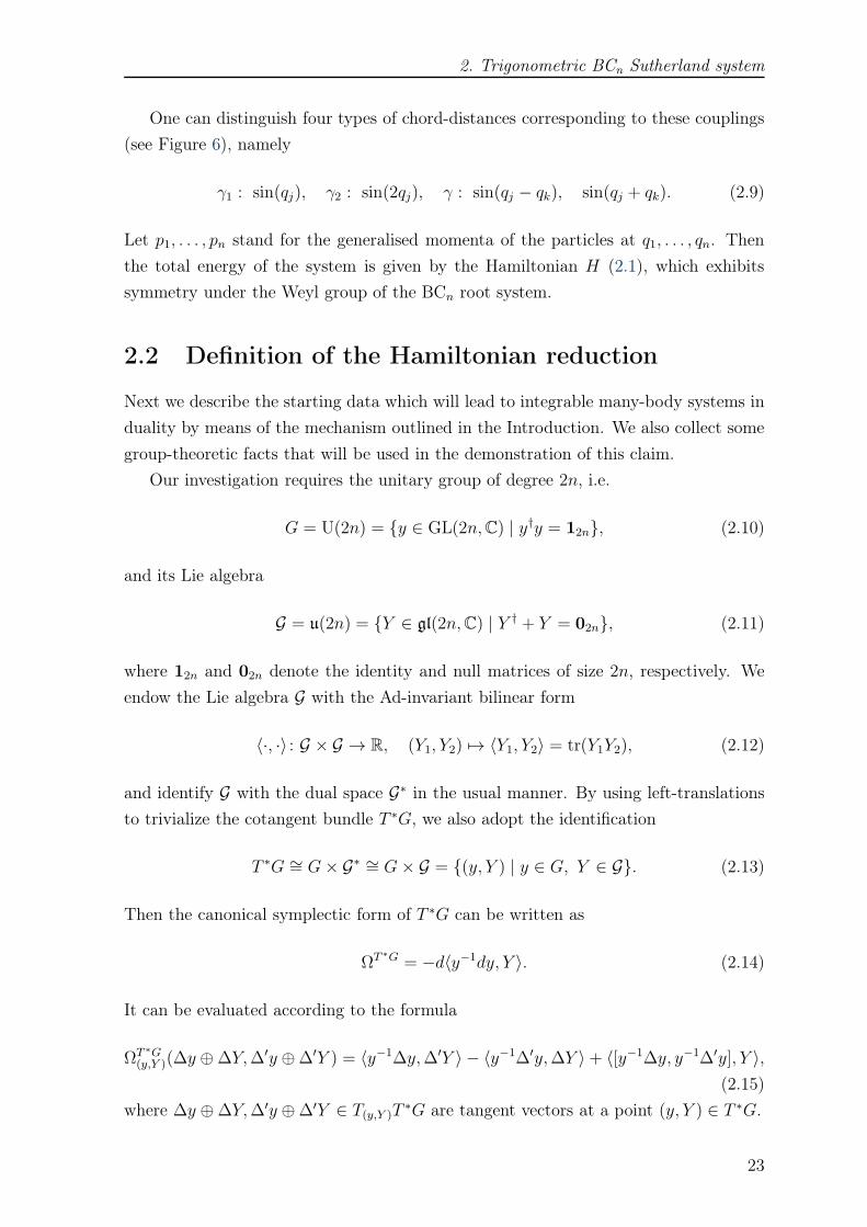
2.2 Definition of the Hamiltonian reduction
Next we describe the starting data which will lead to integrable many-body systems in
duality by means of the mechanism outlined in the Introduction. We also collect some
group-theoretic facts that will be used in the demonstration of this claim.
Our investigation requires the unitary group of degree 2n, i.e.
G = U(2n) = y ∈ GL(2n,C) | y†y = 12n, (2.10)
and its Lie algebra
G = u(2n) = Y ∈ gl(2n,C) | Y † + Y = 02n, (2.11)
where 12n and 02n denote the identity and null matrices of size 2n, respectively. We
endow the Lie algebra G with the Ad-invariant bilinear form
〈·, ·〉 : G × G → R, (Y1, Y2) 7→ 〈Y1, Y2〉 = tr(Y1Y2), (2.12)
and identify G with the dual space G∗ in the usual manner. By using left-translations
to trivialize the cotangent bundle T ∗G, we also adopt the identification
T ∗G ∼= G× G∗ ∼= G× G = (y, Y ) | y ∈ G, Y ∈ G. (2.13)
Then the canonical symplectic form of T ∗G can be written as
ΩT∗G = −d〈y−1dy, Y 〉. (2.14)
It can be evaluated according to the formula
ΩT∗G
(y,Y )(∆y ⊕∆Y,∆′y ⊕∆′Y ) = 〈y−1∆y,∆′Y 〉 − 〈y−1∆′y,∆Y 〉+ 〈[y−1∆y, y−1∆′y], Y 〉,(2.15)
where ∆y ⊕∆Y,∆′y ⊕∆′Y ∈ T(y,Y )T∗G are tangent vectors at a point (y, Y ) ∈ T ∗G.
23
2. Trigonometric BCn
Sutherland system
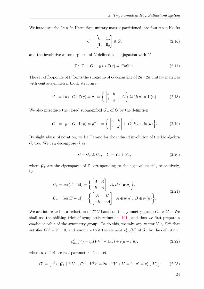
We introduce the 2n×2n Hermitian, unitary matrix partitioned into four n×n blocks
C =
[0n 1n
1n 0n
]∈ G, (2.16)
and the involutive automorphism of G defined as conjugation with C
Γ: G→ G, y 7→ Γ(y) = CyC−1. (2.17)
The set of fix-points of Γ forms the subgroup of G consisting of 2n×2n unitary matrices
with centro-symmetric block structure,
G+ = y ∈ G | Γ(y) = y =[
a b
b a
]∈ G
∼= U(n)× U(n). (2.18)
We also introduce the closed submanifold G− of G by the definition
G− = y ∈ G | Γ(y) = y−1 =[
a b
c a†
]∈ G
∣∣∣∣ b, c ∈ iu(n)
. (2.19)
By slight abuse of notation, we let Γ stand for the induced involution of the Lie algebra
G, too. We can decompose G as
G = G+ ⊕ G−, Y = Y+ + Y−, (2.20)
where G± are the eigenspaces of Γ corresponding to the eigenvalues ±1, respectively,
i.e.
G+ = ker(Γ− id) =
[A B
B A
] ∣∣∣∣ A,B ∈ u(n)
,
G− = ker(Γ + id) =
[A B
−B −A
] ∣∣∣∣ A ∈ u(n), B ∈ iu(n)
.
(2.21)
We are interested in a reduction of T ∗G based on the symmetry group G+ ×G+. We
shall use the shifting trick of symplectic reduction [101], and thus we first prepare a
coadjoint orbit of the symmetry group. To do this, we take any vector V ∈ C2n that
satisfies CV + V = 0, and associate to it the element υℓµ,ν(V ) of G+ by the definition
υℓµ,ν(V ) = iµ(V V † − 12n
)+ i(µ− ν)C, (2.22)
where µ, ν ∈ R are real parameters. The set
Oℓ =υℓ ∈ G+ | ∃ V ∈ C2n, V †V = 2n, CV + V = 0, υℓ = υℓµ,ν(V )
(2.23)
24

2. Trigonometric BCn
Sutherland system
represents a coadjoint orbit of G+ of dimension 2(n− 1). We let Or = υr denote the
one-point coadjoint orbit of G+ containing the element
υr = −iκC with some constant κ ∈ R, (2.24)
and consider
O = Oℓ ⊕Or ⊂ G+ ⊕ G+ ∼= (G+ ⊕ G+)∗, (2.25)
which is a coadjoint orbit1 of G+ × G+. Our starting point for symplectic reduction
will be the phase space (P,Ω) with
P = T ∗G×O and Ω = ΩT∗G + ΩO, (2.26)
where ΩO denotes the Kirillov-Kostant-Souriau symplectic form on O. The natural
symplectic action of G+ ×G+ on P is defined by
Φ(gL,gR)(y, Y, υℓ ⊕ υr) =
(gLyg
−1R , gRY g
−1R , gLυ
ℓg−1L ⊕ υr
). (2.27)
The corresponding momentum map J : P → G+ ⊕ G+ is given by the formula
J(y, Y, υℓ ⊕ υr) =((yY y−1)+ + υℓ
)⊕(− Y+ + υr
). (2.28)
We shall see that the reduced phase space
Pred = P0/(G+ ×G+), P0 = J−1(0), (2.29)
is a smooth symplectic manifold, which inherits two Abelian Poisson algebras from P .
Using the identification G∗ ∼= G, the invariant functions C∞(G)G form the center
of the Lie-Poisson bracket. Denote by C∞(G)G+×G+ the set of smooth functions on G
that are invariant under the (G+×G+)-action on G that appears in the first component
of (2.27). Let us also introduce the maps
π1 : P → G, (y, Y, υℓ, υr) 7→ y, (2.30)
and
π2 : P → G, (y, Y, υℓ, υr) 7→ Y. (2.31)
It is clear that
Q1 = π∗1(C
∞(G)G+×G+) and Q2 = π∗2(C
∞(G)G) (2.32)
1The same coadjoint orbit was used in [107].
25

2. Trigonometric BCn
Sutherland system
are two Abelian subalgebras in the Poisson algebra of smooth functions on (P,Ω) and
these Abelian Poisson algebras descend to the reduced phase space Pred.
Later we shall construct two models of Pred by exhibiting two global cross-sections
for the action of G+ × G+ on P0. For this, we shall apply two different methods
for solving the constraint equations that, according to (2.28), define the level surface
P0 ⊂ P :
(yY y−1)+ + υℓ = 02n and − Y+ + υr = 02n, (2.33)
where υℓ = υℓµ,λ(V ) (2.22) for some vector V ∈ C2n subject to CV + V = 0, V †V = 2n
and υr = −iκC. We below collect the group-theoretic results needed for our construc-
tions. To start, let us associate the diagonal 2n× 2n matrix
Q(q) = diag(q,−q) (2.34)
with any q ∈ Rn. Notice that the set
A = iQ(q) | q ∈ Rn ⊂ G− (2.35)
is a maximal Abelian subalgebra in G−. The corresponding subgroup of G has the form
exp(A) =eiQ(q) = diag
(eiq1, . . . , eiqn, e−iq1, . . . , e−iqn
)| q ∈ Rn
. (2.36)
The centralizer of A inside G+ (2.18) (with respect to conjugation) is the Abelian
subgroup
Z = ZG+(A) =eiξ = diag
(eix1 , . . . , eixn, eix1, . . . , eixn
)| x ∈ Rn
< G+. (2.37)
The Lie algebra of Z is
Z = iξ = i diag(x, x) | x ∈ Rn < G+. (2.38)
The results that we now recall (see e.g. [59, 87, 124]) will be used later. First, for
any y ∈ G there exist elements yL, yR from G+ and unique q ∈ Rn satisfying
π
2≥ q1 ≥ · · · ≥ qn ≥ 0 (2.39)
such that
y = yLeiQ(q)y−1
R . (2.40)
If all components of q satisfy strict inequalities, then the pair yL, yR is unique precisely
up to the replacements (yL, yR)→ (yLζ, yRζ) with arbitrary ζ ∈ Z. The decomposition
(2.40) is referred to as the generalised Cartan decomposition corresponding to the
26
2. Trigonometric BCn
Sutherland system
involution Γ.
Second, every element g ∈ G− can be written in the form
g = ηe2iQ(q)η−1 (2.41)
with some η ∈ G+ and uniquely determined q ∈ Rn subject to (2.39). In the case of
strict inequalities for q, the freedom in η is given precisely by the replacements η → ηζ ,
∀ ζ ∈ Z.
Third, every element Y− ∈ G− can be written in the form
Y− = gRiDg−1R , D = diag(d1, . . . , dn,−d1, . . . ,−dn), (2.42)
with gR ∈ G+ and uniquely determined real di satisfying
d1 ≥ · · · ≥ dn ≥ 0. (2.43)
If the dj (j = 1, . . . , n) satisfy strict inequalities, then the freedom in gR is exhausted
by the replacements gR → gRζ , ∀ ζ ∈ Z.
The first and the second statements are essentially equivalent since the map
G→ G−, y 7→ y−1CyC (2.44)
descends to a diffeomorphism from
G/G+ = G+g | g ∈ G (2.45)
onto G− [59].
2.3 Action-angle duality
2.3.1 The Sutherland gauge
We here exhibit a symplectomorphism between the reduced phase space (Pred,Ωred)
and the Sutherland phase space
M = T ∗C1 = C1 × Rn (2.46)
equipped with its canonical symplectic form, where C1 was defined in (2.2). As prepa-
ration, we associate with any (q, p) ∈M the G-element
Y (q, p) = K(q, p)− iκC, (2.47)
27

2. Trigonometric BCn
Sutherland system
where K(q, p) is the 2n× 2n matrix
Kj,k = −Kn+j,n+k = ipjδj,k − µ(1− δj,k)/ sin(qj − qk),Kj,n+k = −Kn+j,k = (ν/ sin(2qj) + κ cot(2qj))δj,k + µ(1− δj,k)/ sin(qj + qk),
(2.48)
with j, k = 1, . . . , n. We also introduce the 2n-component vector
VR = (1, . . . , 1︸ ︷︷ ︸n times
,−1, . . . ,−1︸ ︷︷ ︸n times
)⊤. (2.49)
Notice from (2.21) that K(q, p) ∈ G−.
Throughout the chapter we adopt the conditions (2.8) and take µ > 0, although
the next result requires only that the real parameters µ, ν, κ satisfy
µ 6= 0 and |ν| 6= |κ|. (2.50)
Theorem 2.1. Using the notations introduced in (2.22), (2.34) and (2.47), the subset
S of the phase space P (2.26) given by
S =(eiQ(q), Y (q, p), υℓµ,ν(VR), υ
r) | (q, p) ∈M, (2.51)
is a global cross-section for the action of G+ × G+ on P0 = J−1(0). Identifying Pred
with S, the reduced symplectic form is equal to the Darboux form ω =∑n
k=1 dqk ∧ dpk.Thus the obvious identification between S and M provides a symplectomorphism
(Pred,Ωred) ≃ (M,ω). (2.52)
Proof. We saw in Section 2.2 that the points of the level surface P0 satisfy the equations
(yY y−1)+ + υℓµ,ν(V ) = 02n and − Y+ − iκC = 02n, (2.53)
for some vector V ∈ C2n subject to CV + V = 0, V †V = 2n. Remember that the
block-form of any Lie algebra element Y ∈ G is
Y =
[A B
−B† D
]with A+ A† = 0n = D +D†, B ∈ Cn×n. (2.54)
Now the second constraint equation in (2.53) can be written as
2Y+ =
[A+D B −B†
B − B† A+D
]=
[0n −2iκ1n
−2iκ1n 0n
]= −2iκC, (2.55)
28

2. Trigonometric BCn
Sutherland system
which implies that
D = −A and B† = B + 2iκ1n. (2.56)
Thus every point of P0 has G-component Y of the form
Y =
[A B
−B − 2iκ1n −A
]with A + A† = 0n, B ∈ Cn×n. (2.57)
By using the generalised Cartan decomposition (2.40) and applying a gauge transfor-
mation (the action of G+ × G+ on P0), we may assume that y = eiQ(q) with some
q satisfying (2.38). Then the first equation of the momentum map constraint (2.53)
yields the matrix equation
1
2i
(eiQ(q)Y e−iQ(q) + e−iQ(q)CY CeiQ(q)
)+ µ(V V † − 12n) + (µ− ν)C = 02n. (2.58)
If we introduce the notation V = (u,−u)⊤, u ∈ Cn, and assume that Y has the form
(2.57) then (2.58) turns into the following equations for A and B
1
2i
(eiqAe−iq − e−iqAeiq
)+ µ(uu† − 1n) = 0n, (2.59)
and1
2i
(eiqBeiq − e−iqBe−iq
)− κe−2iq − µuu† + (µ− ν)1n = 0n. (2.60)
Since µ 6= 0, equation (2.59) implies that |uj|2 = 1 for all j = 1, . . . , n. Therefore we
can apply a ‘residual’ gauge transformation by an element (gL, gR) = (eiξ(x), eiξ(x)), with
suitable eiξ(x) ∈ Z (2.37) to transform υℓµ,ν(V ) into υℓµ,ν(VR). This amounts to setting
uj = 1 for all j = 1, . . . , n. After having done this, we return to equations (2.59)
and (2.60). By writing out the equations entry-wise, we obtain that the diagonal
components of A are arbitrary imaginary numbers (which we denote by ip1, . . . , ipn)
and we also obtain the following system of equations
Aj,k sin(qj − qk) = −µ = −Bj,k sin(qj + qk), j 6= k,
Bj,j sin(2qj) = ν + κ cos(2qj)− iκ sin(2qj), j, k = 1, . . . , n.(2.61)
So far we only knew that q satisfies π/2 ≥ q1 ≥ · · · ≥ qn ≥ 0. By virtue of the
conditions (2.50), the system (2.61) can be solved if and only if π/2 > q1 > · · · > qn >
0. Substituting the unique solution for A and B back into (2.57) gives the formula
Y = Y (q, p) as displayed in (2.47).
The above arguments show that every gauge orbit in P0 contains a point of S (2.51),
and it is immediate by turning the equations backwards that every point of S belongs
to P0. By using that q satisfies strict inequalities and that all components of VR are
29

2. Trigonometric BCn
Sutherland system
non-zero, it is also readily seen that no two different points of S are gauge equivalent.
Moreover, the effectively acting symmetry group, which is given by
(G+ ×G+)/U(1)diag (2.62)
where U(1) contains the scalar unitary matrices, acts freely on P0.
It follows from the above that Pred is a smooth manifold diffeomorphic to M . Now
the proof is finished by direct computation of the pull-back of the symplectic form Ω
of P (2.26) onto the global cross-section S.
Let us recall that the Abelian Poisson algebras Q1 and Q2 (2.32) consist of (G+ ×G+)-invariant functions on P , and thus descend to Abelian Poisson algebras on the re-
duced phase space Pred. In terms of the model M ≃ S ≃ Pred, the Poisson algebra Q2red
is obviously generated by the functions (q, p) 7→ tr((−iY (q, p)))m for m = 1, . . . , 2n.
It will be shown in the following section2 that these functions vanish identically for
the odd integers, and functionally independent generators of Q2red are provided by the
functions
Hk(q, p) =1
4ktr(−iY (q, p))2k, k = 1, . . . , n. (2.63)
The first of these functions reads
H1(q, p) =1
4tr(−iY (q, p))2 =
1
2
n∑
j=1
p2j +∑
1≤j<k≤n
(µ2
sin2(qj − qk)+
µ2
sin2(qj + qk)
)
+1
2
n∑
j=1
νκ
sin2(qj)+
1
2
n∑
j=1
(ν − κ)2sin2(2qj)
.
(2.64)
That is, upon the identification (2.7) it coincides with the Sutherland Hamiltonian
(2.1). This implies the Liouville integrability of the Hamiltonian (2.1). Since its spec-
tral invariants yield a commuting family of n independent functions in involution that
include the Sutherland Hamiltonian, the Hermitian matrix function −iY (q, p) (2.47)
serves as a Lax matrix for the Sutherland system (M,ω,H).
As for the reduced Abelian Poisson algebra Q1red, we notice that the cross-section
S permits to identify it with the Abelian Poisson algebra of the smooth functions of
the variables q1, . . . , qn. This is so since the level set P0 lies completely in the ‘regular
part’ of the phase space P , where the G-component y of (y, Y, υℓ, υr) is such that Q(q)
in its decomposition (2.40) satisfies strict inequalities π/2 > q1 > · · · > qn > 0. It is
a well-known fact that in the regular part the components of q are smooth (actually
real-analytic) functions of y (while globally they are only continuous functions). To
2In fact, we shall see that Y (q, p) is conjugate to a diagonal matrix iΛ of the form in equation(2.71).
30

2. Trigonometric BCn
Sutherland system
see that every smooth function depending on q ∈ C1 is contained in Q1red, one may
further use that every (G+ × G+)-invariant smooth function on P0 can be extended
to an invariant smooth function on P . Indeed, this holds since G+ × G+ is compact
and P0 ⊂ P is a regular submanifold, which itself follows from the free action property
established in the course of the proof of Theorem 2.1.
We can summarize the outcome of the foregoing discussion as follows. Below, the
generators of Poisson algebras are understood in the functional sense, i.e. if some
f1, . . . , fn are generators then all smooth functions of them belong to the Poisson
algebra.
Corollary 2.2. By using the model (M,ω) of the reduced phase space (Pred,Ωred) pro-
vided by Theorem 2.1, the Abelian Poisson algebra Q2red (2.31) can be identified with
the Poisson algebra generated by the spectral invariants (2.62) of the ‘Sutherland Lax
matrix’ −iY (q, p) (2.47), which according to (2.64) include the many-body Hamiltonian
H(q, p) (2.1), and Q1red can be identified with the algebra generated by the corresponding
position variables qj (j = 1, . . . , n).
2.3.2 The Ruijsenaars gauge
It follows from the group-theoretic results quoted in Section 2.2 that the Abelian Pois-
son algebra Q1 is generated by the functions
Hk(y, Y, υℓ, υr) =
(−1)k2k
tr(y−1CyC
)k, k = 1, . . . , n, (2.65)
and thus the unitary and Hermitian matrix
L = −y−1CyC (2.66)
serves as an ‘unreduced Lax matrix’. It is readily seen in the Sutherland gauge (2.51)
that these n functions remain functionally independent after reduction. Here, we shall
prove that the evaluation of the invariant function H1 in another gauge reproduces the
dual Hamiltonian (2.4). The reduction of the matrix function L will provide a Lax
matrix for the corresponding integrable system. Before turning to details, we advance
the group-theoretic interpretation of the dual position variable λ that features in the
Hamiltonian (2.4), and sketch the plan of this section.
To begin, recall that on the constraint surface Y = Y−− iκC, and for any Y− ∈ G−there is an element gR ∈ G+ such that
g−1R Y−gR = diag(id1, . . . , idn,−id1, . . . ,−idn) = iD ∈ A with d1 ≥ · · · ≥ dn ≥ 0.
(2.67)
31
2. Trigonometric BCn
Sutherland system
Then introduce the real matrix λ = diag(λ1, . . . , λn) whose diagonal components
are3
λj =√d2j + κ2, j ∈ Nn. (2.68)
One can diagonalize the matrix D − κC by conjugation with the unitary matrix
h(λ) =
[α(λ) β(λ)
−β(λ) α(λ)
], (2.69)
where the real functions α(x), β(x) are defined on the interval [|κ|,∞) ⊂ R by the
formulae
α(x) =
√x+√x2 − κ2√2x
, β(x) = κ1√2x
1√x+√x2 − κ2
, (2.70)
at least if κ 6= 0. If κ = 0, then we set α(x) = 1 and β(x) = 0. Indeed, it is easy to
check that
h(λ)Λh(λ)−1 = D − κC with Λ = diag(λ1, . . . , λn,−λ1, . . . ,−λn). (2.71)
Note that h(λ) belongs to the subset G− of G (2.19).
The above diagonalization procedure can be used to define the map
L : P0 → Rn, (y, Y, υℓ, υr) 7→ λ. (2.72)
This is clearly a continuous map, which descends to a continuous map Lred : Pred → Rn.
One readily sees also that these maps are smooth (even real-analytic) on the open
submanifolds P reg0 ⊂ P0 and P reg
red ⊂ Pred, where the 2n eigenvalues of Y− are pairwise
different.
The image of the constraint surface P0 under the map L will turn out to be the
closure of the domain
C2 =
λ ∈ Rn
∣∣∣∣λa − λa+1 > 2µ,
(a = 1, . . . , n− 1)and λn > ν
. (2.73)
By solving the constrains through the diagonalization of Y , we shall construct a
model of the open submanifold of Pred corresponding to the open submanifold L−1(C2) ⊂P0. This model will be symplectomorphic to the semi-global phase-space C2 × Tn of
the dual Hamiltonian (2.4).
In the rest of this section, we present the construction of the aforementioned model
of L−1red(C2) ⊂ Pred. We demonstrate that L−1
red(C2) is a dense subset of Pred and present
the global characterization of the dual model of Pred.
3From now on we frequently use the notations Nn = 1, . . . , n and N2n = 1, . . . , 2n.
32

2. Trigonometric BCn
Sutherland system
Many of the local formulae that appear in this section have analogues in [105, 106,
107], which inspired our considerations. However, the global structure is different.
The dual model of the open subset L−1red(C2) ⊂ Pred
We first prepare some functions on C2 × Tn. Denoting the elements of this domain as
pairs
(λ, eiϑ) with λ = (λ1, . . . , λn) ∈ C2, eiϑ = (eiϑ1, . . . , eiϑn) ∈ Tn, (2.74)
we let
fc =
[1− ν
λc
] 12
n∏
a=1(a6=c)
[1− 2µ
λc − λa
] 12[1− 2µ
λc + λa
] 12
, ∀c ∈ Nn,
fn+c = eiϑc[1 +
ν
λc
] 12
n∏
a=1(a6=c)
[1 +
2µ
λc − λa
] 12[1 +
2µ
λc + λa
] 12
. (2.75)
For λ ∈ C2 (2.73), all factors under the square roots are positive. Using the column
vector f = (f1, . . . , f2n)⊤ together with Λc = λc and Λc+n = −λc for c ∈ Nn, we define
the 2n× 2n matrices A(λ, ϑ) and B(λ, ϑ) by
Aj,k =2µfj(Cf)k − 2(µ− ν)Cj,k
2µ+ Λk − Λj, j, k ∈ N2n, (2.76)
and
B(λ, ϑ) = −(h(λ)A(λ, ϑ)h(λ)
)†. (2.77)
We shall see that these are unitary matrices from G− ⊂ G (2.19). Then we write B in
the form
B = ηe2iQ(q)η−1 (2.78)
with some η ∈ G+ and unique q = q(λ, ϑ) subject to (2.39). (It turns out that
q(λ, ϑ) ∈ C1 (2.2) and thus η is unique up to replacements η → ηζ with arbitrary
ζ ∈ Z (2.37).) Relying on (2.78), we set
y(λ, ϑ) = ηeiQ(q(λ,ϑ))η−1 (2.79)
and introduce the vector V (λ, ϑ) ∈ C2n by
V (λ, ϑ) = y(λ, ϑ)h(λ)f(λ, ϑ). (2.80)
33

2. Trigonometric BCn
Sutherland system
It will be shown that V + CV = 0 and |V |2 = 2n, which ensures that υℓµ,ν(V ) ∈ Oℓ(2.23).
Note that A, y and V given above depend on ϑ only through eiϑ and are C∞
functions on C2 × Tn. It should be remarked that although the matrix element An,2n(2.76) has an apparent singularity at λn = µ, the zero of the denominator cancels.
Thus A extends by continuity to λn = µ and remains smooth there, which then also
implies the smoothness of y and V .
Theorem 2.3. By using the above notations, consider the set
S0 = (y(λ, ϑ), ih(λ)Λ(λ)h(λ)−1, υℓµ,ν(V (λ, ϑ)), υr) | (λ, eiϑ) ∈ C2 × Tn. (2.81)
This set is contained in the constraint surface P0 = J−1(0) and it provides a cross-
section for the G+ ×G+-action restricted to L−1(C2) ⊂ P0. In particular, C2 ⊂ L(P0)
and S0 intersects every gauge orbit in L−1(C2) precisely in one point. Since the ele-
ments of S0 are parametrized by C2 ×Tn in a smooth and bijective manner, we obtain
the identifications
L−1red(C2) ≃ S0 ≃ C2 × Tn. (2.82)
Letting σ0 : S0 → P denote the tautological injection, the pull-backs of the symplectic
form Ω (2.26) and the function H1 (2.65) obey
σ∗0(Ω) =
n∑
c=1
dλc ∧ dϑc, (H1 σ0)(λ, ϑ) =1
2tr(h(λ)A(λ, ϑ)h(λ)
)= H0(λ, ϑ) (2.83)
with the RSvD type Hamiltonian H0 in (2.4). Consequently, the Hamiltonian reduction
of the system (P,Ω, H1) followed by restriction to the open submanifold L−1red(C2) ⊂ Pred
reproduces the system (M0, ω0, H0) defined in (2.4)-(2.5).
Remark 2.4. Referring to (2.66), we have the Lax matrix
L(y(λ, ϑ)) = h(λ)A(λ, ϑ)h(λ). (2.84)
Later we shall also prove that L−1red(C2) is a dense subset of Pred, whereby the reduction
of (P,Ω, H1) may be viewed as a completion of (M0, ω0, H0).
Proof of Theorem 2.3
The proof will emerge from a series of lemmas. Our immediate aim is to construct
gauge invariant functions that will be used for parametrizing the orbits of G+×G+ in
(an open submanifold of) P0. For introducing gauge invariants we can restrict ourselves
34

2. Trigonometric BCn
Sutherland system
to the submanifold P1 ⊂ P0 where Y in (y, Y, υℓ, υr) has the form
Y = h(λ)iΛ(λ)h(λ)−1 (2.85)
with some λ ∈ Rn for which
λ1 ≥ · · · ≥ λn ≥ |κ|. (2.86)
Indeed, every element of P0 can be gauge transformed into P1. It will be advantageous
to further restrict attention to P reg1 ⊂ P1 where we have
λ1 > · · · > λn > |κ|. (2.87)
The residual gauge transformations that map P reg1 to itself belong to the groupG+×Z <
G+×G+ with Z defined in (2.37). Since υr is constant and υℓ = υℓµ,ν(V ), we may label
the elements of P1 by triples (y, Y, V ), with the understanding that V matters up to
phase. Then the gauge action of (gL, ζ) ∈ G+ × Z operates by
(y, V ) 7→ (gLyζ−1, gLV ), (2.88)
while Y is already invariant. Now we can factor out the residual G+-action by intro-
ducing the G−-valued function
A(y, Y, V ) = h(λ)−1L(y)h(λ)−1 (2.89)
and the C2n-valued function
F (y, Y, V ) = h(λ)−1y−1V. (2.90)
Here λ = L(y, Y, V ), which means that (2.85) holds, and we used L(y) in (2.66). Like
V , F is defined only up to a U(1) phase. We obtain the transformation rules
A(gLyζ−1, Y, gLV ) = ζA(y, Y, V )ζ−1, (2.91)
F (gLyζ−1, Y, gLV ) = ζF (y, Y, V ), (2.92)
and therefore the functions
Fk(y, Y, V ) = |Fk(y, Y, V )|2, k = 1, . . . , 2n (2.93)
are well-defined, gauge invariant, smooth functions on P reg1 . They represent (G+×G+)-
invariant smooth functions on P reg0 . We shall see shortly that the functions Fk depend
only on λ = L(y, Y, V ) and shall derive explicit formulae for this dependence. Then the
35

2. Trigonometric BCn
Sutherland system
non-negativity of Fk will be used to gain information about the set L(P0) of λ values
that actually occurs.
Before turning to the inspection of the functions Fk, we present a crucial lemma.
Lemma 2.5. Fix λ ∈ Rn subject to (2.86) and set Λ = diag(λ,−λ) and Y = hiΛh−1.
If y ∈ G and υℓµ,ν(V ) ∈ Oℓ solve the momentum map constraint given according to the
first equation in (2.53) by
yY y−1 + CyY y−1C + 2υℓµ,ν(V ) = 0, (2.94)
then A ∈ G− and F ∈ C2n defined by (2.89) and (2.90) solve the following equation:
2µA+ AΛ− ΛA = 2µF (CF )† − 2(µ− ν)C. (2.95)
Conversely, for any A ∈ G−, F ∈ C2n that satisfy |F |2 = 2n and equation (2.95), pick
y ∈ G such that L(y) = h(λ)Ah(λ) and define V = yh(λ)F . Then CV + V = 0 and
(y, Y, υℓµ,ν(V )) solve the momentum map constraint (2.94).
Proof. If eq. (2.94) holds, then we multiply it by h(λ)−1y−1 on the left and by CyCh(λ)−1
on the right. Using (2.58), with CV + V = 0 and |V |2 = 2n, and the notations (2.89)
and (2.90), this immediately gives (2.95). Conversely, suppose that (2.95) holds for
some A ∈ G− and F ∈ C2n with |F |2 = 2n. Since h(λ)Ah(λ) belongs to G−, there
exists y ∈ G such that
h(λ)Ah(λ) = L(y). (2.96)
Such y is unique up to left-multiplication by an arbitrary element of G+ (whereby one
may bring y into G− if one wishes to do so). Picking y according to (2.96), and then
setting
V = yh(λ)F, (2.97)
it is an elementary matter to show that (2.95) implies the following equation:
yY y−1 + CyY y−1C + 2iµ(−V (CV )† − 12n) + 2i(µ− ν)C = 0. (2.98)
It is a consequence of this equation that
(V (CV )†)† = (CV )V † = V (CV )†. (2.99)
This entails that CV = αV for some α ∈ U(1). Then V † = α(CV )† also holds, and
thus we must have α2 = 1. Hence α is either +1 or −1. Taking the trace of the equality
(2.98), and using that |V |2 = 2n on account of |F |2 = 2n, we obtain that α = −1, i.e.
CV + V = 0. This means that equation (2.98) reproduces (2.94).
36

2. Trigonometric BCn
Sutherland system
To make progress, now we restrict our attention to the subset of P reg1 , where the
eigenvalue-parameter λ of Y verifies in addition to (2.87) also the conditions
|λa ± λb| 6= 2µ and (λa − ν)(λa − |2µ− ν|) 6= 0, ∀a, b ∈ Nn. (2.100)
We call such λ values ‘strongly regular’, and let P vreg1 ⊂ P1 and P vreg
0 ⊂ P0 denote
the corresponding open subsets. Later we shall prove that P vreg0 is dense in P0. The
above conditions will enable us to perform calculations that will lead to a description
of a dense subset of the reduced phase space. They ensure that we never divide by zero
in relevant steps of our arguments. The first such step is the derivation of the following
consequence of equation (2.95).
Lemma 2.6. The restriction of the matrix function A (2.89) to P vreg1 has the form
Aj,k =2µFj(CF )k − 2(µ− ν)Cj,k
2µ+ Λk − Λj, j, k ∈ N2n, (2.101)
where F ∈ C2n satisfies |F |2 = 2n and Λ = diag(λ,−λ) varies on P vreg1 according to
(2.85).
Lemma 2.7. For any strongly regular λ and a ∈ Nn define
wa =n∏
b=1(b6=a)
(λa − λb)(λa + λb)
(2µ− (λa − λb))(2µ− (λa + λb)), wa+n =
n∏
b=1(b6=a)
(λa − λb)(λa + λb)
(2µ+ λa − λb)(2µ+ λa + λb),
(2.102)
and set Wk = wkFk with Fk = |Fk|2. Then the unitarity of the matrix A as given
by (2.101) implies the following system of equations for the pairs of functions Wc and
Wc+n for any c ∈ Nn:
(µ+ λc)Wc + (µ− λc)Wn+c − 2(µ− ν) = 0, (2.103)
λ2cWcWn+c − µ(µ− ν)(Wc +Wn+c) + (µ− ν)2 + µ2 − λ2c = 0. (2.104)
For fixed c ∈ Nn and strongly regular λ, this system of equations admits two solutions,
which are given by
(Wc,Wn+c) = (W+c ,W
+n+c) = (wcF+
c , wc+nF+c+n) = (1− ν
λc, 1 +
ν
λc), (2.105)
and by
(Wc,Wn+c) = (W−c ,W
−n+c) = (wcF−
c , wc+nF−c+n) = (−1 + 2µ− ν
λc,−1− 2µ− ν
λc).
(2.106)
37

2. Trigonometric BCn
Sutherland system
The functions F±k satisfy the identities
2n∑
k=1
F+k (λ) = 2n and
2n∑
k=1
F−k (λ) = −2n. (2.107)
Proof. The derivation of equations (2.103), (2.104) follows a similar derivation due to
Pusztai [105], and is summarized in the appendix. We then solve the linear equation
(2.103) say for Wc+n and substitute it into (2.104). This gives a quadratic equation
for Wc whose two solutions we can write down. We note that the derivation of the
equations (2.103) and (2.104) presented in the appendix utilizes the full set of the
conditions (2.100).
To verify the identities (2.107), we first extend λ to vary in the open subset of Cn
subject to the conditions λ2a 6= λ2b and λc 6= 0, and then consider the sums that appear
in (2.107) as functions of a chosen component of λ with the other components fixed.
These explicitly given sums are meromorphic functions having only first order poles,
and one may check that all residues at the apparent poles vanish. Hence the sums are
constant over Cn, and the values of the constants can be established by looking at a
suitable asymptotic limit in the domain C2 (2.73), whereby all wk tend to 1 and the
pre-factors in (2.105) and (2.106) tend to 1 and −1, respectively.
Observe that neither any wk nor any F±k (k ∈ N2n) can vanish if λ is strongly
regular. We know that the value of Fk (2.93) is uniquely defined at every point of P reg1 .
Therefore only one of the solutions (F±c ,F±
c+n) can be acceptable at any λ ∈ L(P vreg1 ).
The identities in (2.107) and analyticity arguments strongly suggest that the acceptable
solutions are provided by F+k . The first statement of the following lemma confirms that
this is the case for λ ∈ C2 (2.73).
Lemma 2.8. The formulae (2.105) and (2.106) can be used to define F±k as smooth
real functions on the domain C2, and none of these functions vanishes at any λ ∈ C2.
Then for any λ ∈ C2 and c ∈ Nn at least one out of F−c and F−
c+n is negative, while
F+k > 0 for all k ∈ N2n. Hence for λ ∈ C2 ∩ L(P0) only F+
k (λ) can give the value of
the function Fk as defined in (2.93). Taking any λ ∈ C2 and any F ∈ C2n satisfying
|Fk|2 = F+k (λ), the formula (2.101) yields a unitary matrix that belongs to G− (2.19).
This matrix A and vector F ∈ C2n solve equation (2.95).
Proof. It is easily seen that wk(λ) > 0 for all λ ∈ C2 and k ∈ N2n. The statement about
the negativity of either F−c or F−
c+n thus follows from the identity W−c +W−
n+c = −2.The positivity of F+
k is easily checked. It is also readily verified that A† = CAC, which
entails that A ∈ G− once we know that A is unitary. For λ ∈ C2 and |Fk|2 = F+k (λ), the
unitarity of A (2.101) can be shown by almost verbatim adaptation of the arguments
proving Proposition 6 in [106].
38

2. Trigonometric BCn
Sutherland system
If λ ∈ C2 is such that the denominators in (2.101) do not vanish, then the formula
(2.101) is plainly equivalent to (2.95). Observe that only those elements λ ∈ C2 for
which λn = µ fail to satisfy this condition. At such λ the matrix element An,2n has an
apparent ‘first order pole’, but one can check by inspection of the formula (2.76) that
An,2n actually remains finite and smooth even at such exceptional points, and thus
solves also (2.95) because of continuity.
Before presenting the proof of Theorem 2.3, note that at the point of S0 labelled
by (λ, eiϑ) the value of the function F (2.90) is equal to f(λ, eiϑ) given in (2.75).
Proof of Theorem 2.3. It follows from Lemma 2.5 and Lemma 2.8 that S0 is a subset
of P reg1 and L(S0) = C2. Taking into account Theorem 2.1, this implies that y(λ, ϑ)
(2.79) and V (λ, ϑ) (2.80) are well-defined smooth functions on C2×Tn. We next show
that S0 is a cross-section for the residual gauge action on L−1(C2) ∩ P1. To do this,
pick an arbitrary element
(y, h(λ)iΛh(λ)−1, υℓµ,ν(V ), υr) ∈ L−1(C2) ∩ P1. (2.108)
Because Fk(λ) 6= 0, we can find a unique element eiϑ ∈ Tn and an element ζ ∈ Z (2.37)
(which is unique up to scalar multiple) such that
Fk(yζ−1, h(λ)iΛh(λ)−1, V ) = fk(λ, e
iϑ), ∀k ∈ N2n, (2.109)
up to a k-independent phase. We then see from (2.95) that L(yζ−1) = L(y(λ, ϑ)),
which in turn implies the existence of some (unique after ζ was chosen) η+ ∈ G+ for
which
η+yζ−1 = y(λ, ϑ). (2.110)
Using also that ζ−1h(λ)ζ = h(λ), we conclude from the last two equations that
η+V = η+yh(λ)F (y, h(λ)iΛh(λ)−1, V ) = y(λ, ϑ)h(λ)f(λ, ϑ) = V (λ, eiϑ). (2.111)
Thus we have shown that the element (2.108) can be gauge transformed into a point
of S0, and this point is uniquely determined since (2.109) fixes eiϑ uniquely. In other
words, S0 intersects every orbit of the residual gauge action on L−1(C2)∩P1 in precisely
one point.
The map from C2 into P , given by the parametrization of S0, is obviously smooth,
and hence we obtain the identifications
C2 ≃ S0 ≃ (L−1(C2) ∩ P1)/(G+ × Z) ≃ L−1(C2)/(G+ ×G+) = L−1red(C2). (2.112)
To establish the formula (2.83) of the reduced symplectic structure, we proceed as
39

2. Trigonometric BCn
Sutherland system
follows. We define G+ ×G+ invariant real functions on P by
ϕm(y, Y, V ) =1
mRe(tr(Y m)
), m ∈ N, (2.113)
and
χk(y, Y, υ) = Re(tr(Y ky−1V V †yC)
), k ∈ N ∪ 0. (2.114)
The restrictions of these functions to S0 are the respective functions ϕredm and χred
k :
ϕredm (λ, ϑ) =
0, if m is odd,
(−1)m22
m
n∑
j=1
λmj , if m is even,(2.115)
and
χredk (λ, ϑ) =
−2(−1)k−12
n∑
j=1
λkj
[1− κ2
λ2j
] 12
Xj sin(ϑj), if k is odd,
2(−1)k2
n∑
j=1
λkj
[1− κ2
λ2j
] 12
Xj cos(ϑj)− κλk−1j
(Fj − Fn+j
), if k is even,
(2.116)
where
Xj =√FjFn+j = e−iϑj
[1− ν2
λ2j
]12
n∏
k=1(k 6=j)
[1− 4µ2
(λj − λk)2]12[1− 4µ2
(λj + λk)2
]12
. (2.117)
Then we calculate the pairwise Poisson brackets of the set of functions ϕm, χk on P and
restrict the results to S0. This must coincide with the results of the direct calculation
of the Poisson brackets of the reduced functions ϕredm , χred
k based on the pull-back of the
symplectic form Ω onto S0 ⊂ P . Inspection shows that the required equalities hold if
and only if we have the formula in (2.83) for the pull-back in question. This reasoning
is very similar to that used in [106] to find the corresponding reduced symplectic form.
Since the underlying calculations are rather laborious, we break them up into smaller
pieces and only detail them following this proof. As for the formula for the restriction
of H1 to S0 displayed in (2.83), this is a matter of direct verification.
The following line of thought is an appropriate adaptation of an argument presented
by Pusztai in [106] which since has been applied in the simpler case of An root system in
[P9]. Differences between these earlier results and the calculations below are highlighted
in the Discussion.
Consider the families of real-valued smooth functions ϕm (2.113), χk (2.114) on
the phase space P (2.26), and the corresponding reduced functions ϕredm (2.115), χred
k
40
2. Trigonometric BCn
Sutherland system
(2.116) on S0 (2.81). Now let us take an arbitrary point x = (y, Y, υℓ, υr) ∈ P and an
arbitrary tangent vector δx = δy ⊕ δY ⊕ δυℓ ⊕ 0 ∈ TxP . The derivative of ϕm can be
easily obtained and has the form
(dϕm)x(δx) =
0, if m is odd,
〈Y m−1, δY 〉, if m is even.(2.118)
The derivative of χk can be written as
(dχk)x(δx) =
⟨[[Y k, C]±, y
−1Z(υℓ)y]
2, y−1δy
⟩
+
⟨ k−1∑
j=0
Y k−j−1[y−1Z(υℓ)y, C]±Yj
2, δY
⟩
+
⟨y[C, Y k]±y
−1 + Cy[C, Y k]±y−1C
4iµ, δυℓ
⟩,
(2.119)
where [A,B]± = AB±BA with the sign of (−1)k. The Hamiltonian vector field of ϕmis
(Xϕm)x = ∆y ⊕∆Y ⊕∆υℓ ⊕ 0 = yY m−1 ⊕ 0⊕ 0⊕ 0, (2.120)
while the Hamiltonian vector field corresponding to χk is
(Xχk)x = ∆′y ⊕∆′Y ⊕∆′υℓ ⊕ 0, (2.121)
where
∆′y =y
2
k−1∑
j=0
Y k−j−1[y−1Z(υℓ)y, C]±Yj, (2.122)
∆′Y =1
2
[[Y k, y−1Z(υℓ)y]±, C
], (2.123)
∆′υℓ =1
4iµ
[(y[C, Y k]±y
−1 + Cy[C, Y k]±y−1C
), υℓ]. (2.124)
Lemma 2.9. λa, λb = 0 for any a, b ∈ 1, . . . , n.
Proof. Using (2.118) one has ϕm, ϕl ≡ 0 for any m, l ∈ N which implies that
ϕredm , ϕred
l ≡ 0. Let m, l ∈ N be arbitrary even numbers. Direct calculation of the
Poisson bracket ϕredm , ϕred
l using (2.115) and the Leibniz rule results in the formula
ϕredm , ϕred
l = (−1)m+l2 4
n∑
a,b=1
λm−1a λa, λbλl−1
b . (2.125)
41

2. Trigonometric BCn
Sutherland system
By introducing the n× n matrices
P a,b = λa, λb and U a,b = λ2b−1a , a, b ∈ 1, . . . , n (2.126)
and choosing m and l from the set 1, . . . , 2n, the equation ϕredm , ϕred
l ≡ 0 can be
cast into the matrix equation
(−1)m+l2 U †PU = 0n. (2.127)
Since U is an invertible Vandermonde-type matrix it follows from (2.127) that P = 0n
which reads as λa, λb = 0 for all a, b ∈ 1, . . . , n.
Lemma 2.10. λa, ϑb = δa,b for any a, b ∈ 1, . . . , n.
Proof. By choosing two even numbers, k and m, and calculating the Poisson bracket
χk, ϕm at an arbitrary point x = (y, Y, υℓ, υr) ∈ P the results (2.120)-(2.124) imply
that
χk, ϕm(x) = χk+m−1(x) +1
2tr((Y kCY m−1 − Y m−1CY k)y−1Z(υℓ)y
). (2.128)
The computation of the reduced form of (2.128) shows that
χredk , ϕred
m = 2χredk+m−1. (2.129)
By utilizing (2.115), (2.116) and the result of the previous lemma one can write the
l.h.s. of (2.129) as
χredk , ϕred
m = (−1)k+m2 4
n∑
b=1
λkb
[1− κ2
λ2b
]12
|Xb(λ)| sin(ϑb)n∑
a=1
λa, ϑbλm−1a . (2.130)
Now, returning to equation (2.129) together with (2.130) one can obtain the following
equivalent form
n∑
b=1
λkb
[1− κ2
λ2b
]12
|Xb(λ)| sin(ϑb)( n∑
a=1
λa, ϑbλm−1a − λm−1
b
)= 0. (2.131)
By introducing the n× n matrices
V b,d =
[1− κ2
λ2b
]12
|Xb(λ)| sin(ϑb)( n∑
a=1
λa, ϑbλ2d−1a − λ2d−1
b
), b, d ∈ 1, . . . , n
(2.132)
and using the Vandermonde-type matrix U defined in (2.126) one is able to write
(2.131) into the matrix equation U †V = 0n. Since U is invertible V = 0n and
42

2. Trigonometric BCn
Sutherland system
therefore in the dense subset of C2 × Tn where sin(ϑb) 6= 0 the following holds
n∑
a=1
λa, ϑbλm−1a − λm−1
b = 0, ∀ b ∈ 1, . . . , n. (2.133)
With the matrices U and
Qb,a = λa, ϑb, a, b ∈ 1, . . . , n (2.134)
equation (2.133) can be written equivalently as QU − U = 0n, which immediately
implies that Q = 1n. Due to the continuity of Poisson bracket Q = 1n must hold for
every point in C2 × Tn, therefore one has λa, ϑb = δa,b for all a, b ∈ 1, . . . , n.
Lemma 2.11. ϑa, ϑb = 0 for any a, b ∈ 1, . . . , n.
Proof. Let k and l be two arbitrary odd integers, and calculate the Poisson bracket
χredk , χred
l indirectly, that is, work out the Poisson bracket χk, χl = Ω(Xχl,Xχk
)
explicitly and restrict it to the gauge (2.81). The first term 〈y−1∆y,∆′Y 〉 in (2.15)
reads
〈y−1∆y,∆′Y 〉 =(−1)k+l+2
2 2 l
n∑
a=1
λk+l−1a
[1− κ
λ2a
]|Xa(λ)|2 sin(2ϑa)
(−1)k+l+2
2 2
n∑
a,b=1(a6=b)
λkaλlb
[1− κ2
λ2a
]12[1− κ2
λ2b
]12
|Xa||Xb|sin(ϑa − ϑb)λa + λb
(−1)k−l+2
2 2
n∑
a,b=1(a6=b)
λkaλlb
[1− κ2
λ2a
]12[1− κ2
λ2b
]12
|Xa||Xb|sin(ϑa + ϑb)
λa − λb.
(2.135)
Due to antisymmetry in the indices 〈y−1∆′y,∆Y 〉 in (2.15) is obtained by interchanging
k and l
〈y−1∆′y,∆Y 〉 =(−1)k+l+2
2 2 k
n∑
a=1
λk+l−1a
[1− κ
λ2a
]|Xa(λ)|2 sin(2ϑa)
(−1)k−l+2
2 2
n∑
a,b=1(a6=b)
λkaλlb
[1− κ2
λ2a
]12[1− κ2
λ2b
]12
|Xa||Xb|sin(ϑa − ϑb)λa + λb
(−1)k+l+2
2 2
n∑
a,b=1(a6=b)
λkaλlb
[1− κ2
λ2a
]12[1− κ2
λ2b
]12
|Xa||Xb|sin(ϑa + ϑb)
λa − λb.
(2.136)
43

2. Trigonometric BCn
Sutherland system
One can easily check that the third term in (2.15) vanishes. The last term takes the
form
〈[Dυ, D′υ], υ〉 =(−1)
k+l+22 4
n∑
a,b=1(a6=b)
λkaλlb
[1− κ2
λ2a
]12[1− κ2
λ2b
]12|Xa||Xb|
sin(ϑa − ϑb)(4µ2 − (λa + λb)2
)(λa + λb)
(−1)k−l+2
2 4
n∑
a,b=1(a6=b)
λkaλlb
[1− κ2
λ2a
]12[1− κ2
λ2b
]12
|Xa||Xb|sin(ϑa + ϑb)(
4µ2 − (λa − λb)2)(λa − λb)
.
(2.137)
As a result of this indirect calculation one obtains the following expression for χredk , χred
l
χredk , χred
l = (−1)k−l+2
2 2(k − l)n∑
a=1
λk+l−1a
[1− κ2
λ2a
]|Xa|2 sin(2ϑa)
(−1)k+l+2
2 16µ2n∑
a,b=1(a6=b)
λkaλlb
[1− κ2
λ2a
]12[1− κ2
λ2b
]12
|Xa||Xb|sin(ϑa − ϑb)(
4µ2 − (λa + λb)2)(λa + λb)
(−1)k−l+2
2 16µ2n∑
a,b=1(a6=b)
λkaλlb
[1− κ2
λ2a
]12[1− κ2
λ2b
]12|Xa||Xb|
sin(ϑa + ϑb)(4µ2 − (λa − λb)2
)(λa − λb)
.
(2.138)
One can also carry out a direct computation of χredk , χred
l by using basic properties
of the Poisson bracket and the previous two lemmas
χredk , χred
l = (−1)k−l+2
2 2(k − l)n∑
a=1
λk+l−1a
[1− κ2
λ2a
]|Xa|2 sin(2ϑa)
(−1)k+l+2
2 16µ2
n∑
a,b=1(a6=b)
λkaλlb
[1− κ2
λ2a
]12[1− κ2
λ2b
]12
|Xa||Xb|sin(ϑa − ϑb)(
4µ2 − (λa + λb)2)(λa + λb)
(−1)k−l+2
2 16µ2n∑
a,b=1(a6=b)
λkaλlb
[1− κ2
λ2a
]12[1− κ2
λ2b
]12
|Xa||Xb|sin(ϑa + ϑb)(
4µ2 − (λa − λb)2)(λa − λb)
(−1)k−l2 4
n∑
a,b=1
λkaλlb
[1− κ2
λ2a
]12[1− κ2
λ2b
]12
|Xa||Xb| cos(ϑa) cos(ϑb)ϑa, ϑb.
(2.139)
Now it is obvious that (2.138) and (2.139) must be equal therefore the extra term must
44

2. Trigonometric BCn
Sutherland system
vanish
n∑
a,b=1
λkaλlb
[1− κ2
λ2a
]12[1− κ2
λ2b
]12
|Xa||Xb| cos(ϑa) cos(ϑb)ϑa, ϑb = 0. (2.140)
By utilizing the n× n matrices
W a,b = λba
[1− κ2
λ2a
]12
|Xa(λ)| cos(ϑa), Ra,b = ϑa, ϑb, a, b ∈ 1, . . . , n (2.141)
one can reformulate (2.140) as the matrix equation
W †RW = 0n. (2.142)
Since W is easily seen to be invertible in a dense subset of the phase space C2×Tn, eq.
(2.142) and the continuity of Poisson bracket imply R = 0n for the full phase space,
i.e. ϑa, ϑb = 0 for all a, b ∈ 1, . . . , n.
Lemmas 2.9, 2.10, and 2.11 together imply the following (claimed in Theorem 2.3)
Theorem 2.12. The reduced symplectic structure on S0 (2.81), given by the pull-
back of Ω (2.26) by the tautological injection σ0 : S0 → P , has the canonical form
σ∗0(Ω) =
∑na=1 dλa ∧ dϑa.
Density properties
So far we dealt with the open subset L−1red(C2) of the reduced phase space. Here we
show that Theorem 2.3 contains ‘almost all’ information about the dual system since
L−1red(C2) ⊂ Pred is a dense subset. This key result will be proved by combining two
lemmas.
Lemma 2.13. The subset P vreg0 ⊂ P0 of the constraint surface where the range of the
eigenvalue map L (2.72) satisfies the conditions (2.87) and (2.100) is dense.
Proof. Let us first of all note that P0 is a connected regular analytic submanifold of P .
In fact, it is a regular (embedded) analytic submanifold of the analytic manifold P since
the momentum map is analytic and zero is its regular value (because the effectively
acting gauge group (2.62) acts freely on P0). The connectedness follows from Theorem
2.1, which implies that P0 is diffeomorphic to the product of S (2.50) and the group
(2.62), and both are connected.
For any Y ∈ G denote by iΛa2na=1 the set of its eigenvalues counted with multi-
45

2. Trigonometric BCn
Sutherland system
plicities. Then the following formulae
R(y, Y, V ) =2n∏
a,b=1(a6=b)
(Λa − Λb)
2n∏
a=1
(Λ2a − κ2), (2.143)
S(y, Y, V ) =2n∏
a,b=1(a6=b)
[(Λa−Λb)2−4µ2]
2n∏
a=1
[(Λ2
a − µ2)(Λ2a − ν2)(Λ2
a − (2µ− ν)2)]. (2.144)
define analytic functions on P0. Indeed, R and S are symmetric polynomials in the
eigenvalues of Y , and hence can be expressed as polynomials in the coefficients of
the characteristic polynomial of Y , which are polynomials in the matrix elements of
Y . The product RS is also an analytic function on P0, and the subset P vreg0 , can be
characterized as
P vreg0 = x ∈ P0 | R(x)S(x) 6= 0. (2.145)
It is clear from Theorem 2.3 that RS does not vanish identically on P0. Since the zero
set of a non-zero analytic function on a connected analytic manifold cannot contain
any open set, equation (2.145) implies that P vreg0 is a dense subset of P0.
Let C2 be the closure of the domain C2 ⊂ Rn. Eventually, it will turn out that
L(P0) = C2. For now, we wish to prove the following.
Lemma 2.14. For every boundary point λ0 ∈ ∂C2 there exist an open ball B(λ0) ⊂ Rn
around λ0 that does not contain any strongly regular λ which lies outside C2 and belongs
to L(P0).
Proof. We start by noticing that for any boundary point λ0 ∈ ∂C2 there is a ball B(λ0)
centred at λ0 such that any strongly regular λ ∈ B(λ0) \ C2 is subject to either of the
following: (i) there is an index a ∈ 1, . . . , n− 1 such that
λa − λa+1 < 2µ and λb − λb+1 > 2µ ∀ b < a, (2.146)
or (ii) we have
λa − λa+1 > 2µ, a = 1, . . . , n− 1 and λn < ν. (2.147)
Let us consider a strongly regular λ ∈ B(λ0) that falls into case (i) (2.146) and is
so close to C2 that we still have
λk − λk+1 > µ, ∀ k ∈ 1, . . . , n− 1. (2.148)
It then follows that
λa − λb > 2µ, ∀ b > a + 1, (2.149)
46

2. Trigonometric BCn
Sutherland system
and
λa + λb > 2µ, ∀ b ∈ 1, . . . , n. (2.150)
Inspection of the signs of wa(λ) and wa+n(λ) in (2.102) gives
wa(λ) < 0 < wa+n(λ). (2.151)
Since every boundary point λ0 ∈ ∂C2 satisfies λ0a > λ0n ≥ ν for all a ∈ 1, . . . , n − 1,we may choose a small enough ball centred at λ0 to ensure that for λ inside that ball
the above inequalities as well as λa > ν hold. On account of λa > ν > 0 and µ > 0 we
then have
1− ν
λa> 0 and − 1− 2µ− ν
λa< 0. (2.152)
By combining (2.104) and (2.105) with (2.151) and (2.152) we conclude that
F+a (λ) < 0 and F−
a+n(λ) < 0. (2.153)
By Lemma 2.7, these inequalities imply that Fa(λ) and Fa+n(λ) cannot be both non-
negative, which contradicts the defining equation (2.93). This proves the claim in the
case (i) (2.146).
Let us consider a strongly regular λ satisfying (ii) (2.147). In this case we can verify
that
1− ν
λn< 0, wn(λ) > 0, wn+a(λ) > 0. (2.154)
Thus we see from (2.105) that F+2n(λ) < 0. Since the sum of the two components on
the right hand side of (2.106) is negative, we also see that at least one out of F−n (λ)
and F−2n(λ) is negative. Therefore equations (2.103) and (2.104) exclude the unitarity
of A (2.101) in the case (ii) (2.147) as well.
Proposition 2.15. The λ-image of the constraint surface is contained in C2, i.e. we
have
L(P0) ⊆ C2. (2.155)
As a consequence, L−1red(C2) is dense in Pred.
Proof. Since P vreg0 ⊂ P0 is dense and L : P0 → Rn (2.72) is continuous, L(P vreg
0 ) ⊂L(P0) is dense. Thus it follows from Lemma 2.14 that for any λ0 ∈ ∂C2 there exists a
ball around λ0 that does not contain any element of L(P0) lying outside C2.
Suppose that (2.155) is not true, which means that there exists some λ∗ ∈ L(P0)\C2.
Taking any element λ ∈ L(P0) that lies in C2, it is must be possible to connect λ∗ to λ
by a continuous curve in L(P0), since P0 is connected. Starting from the point λ∗, any
such continuous curve must pass through some point of the boundary ∂C2. However,
this is impossible since we know that L(P0) \ C2 does not contain any series that
47

2. Trigonometric BCn
Sutherland system
converges to a point of ∂C2. This contradiction shows that (2.155) holds.
By (2.155) we have P vreg0 ⊂ L−1(C2), and we know from Lemma 2.13 that P vreg
0 ⊂ P0
is dense. These together entail that L−1red(C2) ⊂ Pred is dense.
Global characterization of the dual system
We have seen that
P vreg0 ⊂ L−1(C2) ⊂ P0 (2.156)
is a chain of dense open submanifolds. These project onto dense open submanifolds of
Pred and their images under the map L (2.72) are dense subsets of L(P0) = Lred(Pred):
L(P vreg0 ) ⊂ C2 ⊂ L(P0). (2.157)
Now introduce the set
Cn6= = z ∈ Cn |
n∏
k=1
zk 6= 0. (2.158)
The parametrization
zj =√λj − λj+1 − 2µ
j∏
a=1
eiϑa, j = 1, . . . , n− 1, zn =√λn − ν
n∏
a=1
eiϑa (2.159)
provides a diffeomorphism between C2 × Tn and Cn6=. Thus we can view z ∈ Cn
6= as
a variable parametrizing C2 × Tn that corresponds to the semi-global cross-section S0
by Theorem 2.3. Below, we shall exhibit a global cross-section in P0, which will be
diffeomorphic to Cn. In other words, the ‘semi-global’ model of the dual systems will
be completed into a global model by allowing the zero value for the complex variables
zk. This completion results from the symplectic reduction automatically.
First of all, let us note that the inverse of the parametrization (2.159) gives
λk(z) = ν + 2(n− k)µ+
n∑
j=k
zj zj , k = 1, . . . , n, (2.160)
which extend to smooth functions over Cn. The range of the extended map z 7→(λ1, . . . , λn) is the closure C2 of the polyhedron C2. The variables eiϑk are well-defined
only over Cn6=, where the parametrization (2.159) entails the equality
n∑
k=1
dλk ∧ dϑk = in∑
k=1
dzk ∧ dzk. (2.161)
48

2. Trigonometric BCn
Sutherland system
An easy inspection of the formulae (2.75) shows that the functions fa can be recast as
fk(λ, eiϑ) = |zk|gk(z), fn+k(λ, e
iϑ) = eiϑk |zk−1|gn+k(z), k = 1, . . . , n, z0 = 1,
(2.162)
with uniquely defined functions g1(z), . . . , g2n(z) that extend to smooth (actually real-
analytic) positive functions on Cn. Note that these functions depend on z only through
λ(z), i.e. one has
ga(z) = ηa(λ(z)), a = 1, . . . , 2n, (2.163)
with suitable functions ηa that one could display explicitly. The absolute values |zk|that appear in (2.162) are not smooth at zk = 0, and the phases eiϑk are not well-
defined there. The crux is that both of these ‘troublesome features’ can be removed by
applying suitable gauge transformations to the elements of the cross-section S0 (2.81).
To demonstrate this, we define m = m(eiϑ) ∈ ZG+(A) by
mk(eiϑ) =
k∏
j=1
e−iϑj , k = 1, . . . , n. (2.164)
Conforming with (2.37), we also set mk+n = mk. Then the gauge transformation by
(m,m) ∈ G+ × G+ operates on the C2n-valued vector f(λ, eiϑ) and on the matrix
A(λ, eiϑ) according to
f(λ, eiϑ)→ m(eiϑ)f(λ, eiϑ) ≡ φ(z), A(λ, eiϑ) → m(eiϑ)A(λ, eiϑ)m(eiϑ)−1 ≡ A(z),
(2.165)
which defines the functions φ(z) and A(z) over Cn6=. The resulting functions have the
form
φk(z) = zkgk(z), φn+k(z) = zk−1gn+k(z), k = 1, . . . , n, (2.166)
and
Aa,b(z) = −2µzazb−1ga(z)gn+b(z)
λa(z)− λb(z)− 2µ, 1 ≤ a, b ≤ n, (2.167)
Aa,n+b(z) = −2µzazbga(z)gb(z)
λa(z) + λb(z)− 2µ+ δa,b
µ− νλa(z)− µ
, (2.168)
An+a,b(z) =2µza−1zb−1gn+a(z)gn+b(z)
λa(z) + λb(z) + 2µ− δa,b
µ− νλa(z) + µ
, (2.169)
An+a,n+b(z) =2µza−1zbgn+a(z)gb(z)
λa(z)− λb(z) + 2µ. (2.170)
Now the important point is that, as is easily verified, the apparent singularities coming
from vanishing denominators in A all cancel, and both φ(z) and A(z) extend to smooth
49

2. Trigonometric BCn
Sutherland system
(actually real-analytic) functions on the whole of Cn. In particular, note the relation
Ak,k+1(z) = Ak+n+1,k+n(z) = −2µgk(z)gk+n+1(z), k = 1, . . . , n− 1. (2.171)
Corresponding to (2.77), we also have the matrix B(z) ≡ −(h(λ(z))A(z)h(λ(z)))†.This is smooth over Cn since both A(z) and h(λ(z)) (2.69) are smooth. It follows from
their defining equations that the induced gauge transformations of y(λ, eiϑ) (2.79) and
V (λ, eiϑ) (2.80) are given by
y(λ, eiϑ)→ m(eiϑ)y(λ, eiϑ)m(eiϑ)−1 ≡ y(z), (2.172)
and
V (λ, eiϑ)→ m(eiϑ)V (λ, eiϑ) = y(z)h(λ(z))φ(z) ≡ V (z). (2.173)
Since y(z) is a uniquely defined smooth function of B(z), both y(z) and V (z) are
smooth functions on the whole of Cn.
After these preparations, we are ready to state the main result of this chapter.
Theorem 2.16. By using the above notations, consider the set
S = (y(z), ih(λ(z))Λ(λ(z))h(λ(z))−1, υℓµ,ν(V (z)), υr) | z ∈ Cn . (2.174)
This set defines a global cross-section for the G+×G+-action on the constraint surface
P0. The parametrization of the elements of S by z ∈ Cn gives rise to a symplectic
diffeomorphism between (Pred,Ωred) and Cn equipped with the Darboux form i∑n
k=1 dzk∧dzk. The spectral invariants of the ‘global RSvD Lax matrix’
L(z) ≡ h(λ(z))A(z)h(λ(z)) (2.175)
yield commuting Hamiltonians on Cn that represent the reductions of the Hamiltonians
spanning the Abelian Poisson algebra Q1 (2.32).
Proof. Let us denote by
z 7→ σ(z) (2.176)
the assignment of the element of S to z ∈ Cn as given in (2.174). The map σ : Cn → P
(2.26) is smooth (even real-analytic) and we have to verify that it possesses the following
properties. First, σ takes values in the constraint surface P0. Second, with Ω in (2.26),
σ∗(Ω) = i
n∑
k=1
dzk ∧ dzk. (2.177)
Third, σ is injective. Fourth, the image S of σ intersects every orbit of G+×G+ in P0
50
2. Trigonometric BCn
Sutherland system
in precisely one point.
Let us start by recalling from Theorem 2.3 the map (λ, θ) 7→ σ0(λ, θ) that denotes
the assignment of the general element of S0 (2.81) to (λ, θ) ∈ C2 × Tn, where now we
defined
θ = eiϑ. (2.178)
Then the first and second properties of σ follow since we have
σ(z(λ, θ)) = Φ(m(θ),m(θ)) (σ0(λ, θ)) , for all (λ, θ) ∈ C2 × Tn. (2.179)
We know that σ0(λ, θ) ∈ P0 for all (λ, θ) ∈ C2 × Tn, which implies the first property
since σ is continuous and P0 is a closed subset of P . The restriction of the pull-back
(2.177) to Cn6= is easily calculated using the parametrization (λ, θ) 7→ z(λ, θ) and using
that by Theorem 2.3 σ∗0(Ω) =
∑nk=1 dλk ∧ dϑk. Indeed, this translates into (2.177)
restricted to Cn6=, which implies the claimed equality because σ∗(Ω) is smooth on Cn.
Before continuing, we remark that the map (λ, θ) 7→ z(λ, θ) naturally extends to
a continuous map on the closed domain C2 × Tn and its ‘partial inverse’ z 7→ λ(z)
extends to a smooth map Cn → C2. We will use these extended maps without further
notice in what follows. (The extended map (λ, θ) 7→ z(λ, θ) is not differentiable at the
points for which λ ∈ ∂C2.)
In order to show that σ is injective, consider the equality
σ(z) = σ(ζ) for some z, ζ ∈ Cn. (2.180)
Looking at the ‘second component’ of this equality according to (2.174) we see that
λ(z) = λ(ζ). Then the first component of the equality implies A(z) = A(ζ). The
special case Aa,1(z) = Aa,1(ζ) of this equality gives
zaηa(λ(z))ηn+1(λ(z))
λa(z)− λ1(z)− 2µ=ζaηa(λ(ζ))ηn+1(λ(ζ))
λa(ζ)− λ1(ζ)− 2µ, 1 ≤ a ≤ n. (2.181)
We know that the factors multiplying za and ζa are equal and non-zero (actually neg-
ative). Thus z = ζ follows, establishing the claimed injectivity.
Next we prove that no two different element of S are gauge equivalent to each other,
i.e. S can intersect any orbit of G+ ×G+ at most in one point. Suppose that
Φ(gL,gR)(σ(z)) = σ(ζ) (2.182)
for some (gL, gR) ∈ G+ ×G+ and z, ζ ∈ Cn. We conclude from the second component
of this equality that λ(z) = λ(ζ). Because λ(z) ∈ C2 holds, λ(z) is regular in the
sense that it satisfies (2.87). Thus we can also conclude from the second component of
51

2. Trigonometric BCn
Sutherland system
the equality (2.182) that gR belongs to the Abelian subgroup Z of G+ given in (2.37).
Then we infer from the first component
gLy(z)g−1R = y(ζ) (2.183)
of the equality (2.182) that gL = gR. We here used that A(ζ) can be represented
in the form (2.41) with strict inequalities in (2.39), which holds since S (2.51) is a
global cross-section. Now denote gL = gR = eiξ ∈ Z referring to (2.37). Then we have
eiξA(z)e−iξ = A(ζ), and in particular
eixaAa,a+1(z)e−ixa+1 = Aa,a+1(ζ), ∀a = 1, . . . , n− 1. (2.184)
By using (2.162) and (2.171)
Aa,a+1(z) = −2µηa(λ(z))ηn+a+1(λ(z)) 6= 0, (2.185)
and thus we obtain from λ(z) = λ(ζ) that eiξ must be equal to a multiple of the identity
element of G+. Hence we have established that σ(z) = σ(ζ) is implied by (2.182).
It remains to demonstrate that S intersects every gauge orbit in P0. We have seen
previously that L−1(C2) is dense in P0 and S0 (2.81) is a cross-section for the gauge
action in L−1(C2). These facts imply that for any element x ∈ P0 there exists a series
x(k) ∈ L−1(C2), k ∈ N, such that
limk→∞
(x(k)) = x, (2.186)
and there also exist series (gL(k), gR(k)) ∈ G+ × G+ and (λ(k), θ(k)) ∈ C2 × Tn such
that
x(k) = Φ(gL(k),gR(k)) (σ0(λ(k), θ(k))) . (2.187)
Since L : P0 → Rn is continuous, we have
L(x) = limk→∞
L(x(k)) = limk→∞
λ(k). (2.188)
This limit belongs to C2 and we denote it by λ∞. The non-trivial case to consider is
when λ∞ belongs to the boundary ∂C2. Now, since G+ × G+ × Tn is compact, there
exists a convergent subseries
(gL(ki), gR(ki), θ(ki)), i ∈ N, (2.189)
of the series (gL(k), gR(k), θ(k)). We pick such a convergent subseries and denote its
52
2. Trigonometric BCn
Sutherland system
limit as
(g∞L , g∞R , θ
∞) = limi→∞
(gL(ki), gR(ki), θ(ki)). (2.190)
Then we define z∞ ∈ Cn by
z∞ = limi→∞
z(λ(ki), θ(ki)) = z(λ∞, θ∞). (2.191)
Since z 7→ σ(z) is continuous, we can write
σ(z∞) = limi→∞
σ(z(λ(ki), θ(ki))) = limi→∞
Φ(m(θ(ki)),m(θ(ki))) (σ0(λ(ki), θ(ki))) , (2.192)
where m(θ) is defined by (2.164), with θ = eiϑ. By combining these formulae, we finally
obtain
x = limi→∞
Φ(gL(ki),gR(ki)) (σ0(λ(ki), θ(ki)))
= limi→∞
Φ(gL(ki)m(θ(ki))−1,gR(ki)m(θ(ki))−1) (σ(z(λ(ki), θ(ki))))
= Φ(g∞Lm(θ∞)−1,g∞
Rm(θ∞)−1)(σ(z
∞)).
(2.193)
Therefore S is a global cross-section in P0.
The final statement of Theorem 2.16 about the global RSvD Lax matrix (2.175)
follows since L is just the restriction of the ‘unreduced Lax matrix’ L of (2.66) to
the global cross-section S, which represents a model of the full reduced phase space
Pred.
2.4 Applications
2.4.1 On the equilibrium position of the Sutherland system
Since the Sutherland Lax matrix is diagonalizable, that is
Y (q, p) and iΛ(λ) = i diag(λ,−λ) (2.194)
are similar matrices, we have the following for the Sutherland Hamiltonians H1, . . . , Hn
Hk(q, p) =1
4ktr((−iY (q, p))2k) = 1
4ktr(Λ(λ)2k) =
1
2k
n∑
j=1
λ2kj = hk(λ), k = 1, . . . , n.
(2.195)
In particular, for the main Hamiltonian H1(q, p) the above formula reads as
H(q, p) = H1(q, p) = h1(λ) =1
2(λ21 + · · ·+ λ2n). (2.196)
53

2. Trigonometric BCn
Sutherland system
It is obvious that h1 has a global minimum on C2 and
min(q,p)∈C1×Rn
H(q, p) = minλ∈C2
h1(λ) = h1(λ0), (2.197)
where λ0 is the point in C2 with the smallest (Euclidean) norm. Clearly, λ0 is the
boundary point of C2 at which
λ0a − λ0a+1 − 2µ = 0, a = 1, . . . , n− 1 λ0n − ν = 0, (2.198)
hold, i.e.
λ0a = (n− a)2µ+ ν, a = 1, . . . , n. (2.199)
In terms of the “oscillator variables” z1, . . . , zn ∈ C this means that the equilibrium
point (q, p) = (qe, 0) of the Sutherland system corresponds to z1 = · · · = zn = 0. In
fact, each function Hk (k = 1, . . . , n) possesses a global minimum at z = 0.
Now, remember that the matrices
− (h(λ)A(λ, eiϑ)h(λ))† and eiQ(q) (2.200)
are similar. By using this and the fact that h(λ) and m commute for any m ∈ ZG+(A),one concludes that (with the special choice m = m(eiϑ))
σ(−(hAh)†(z)) = σ(e2iQ(q)) = e2iq1, . . . , e2iqn, e−2iq1, . . . , e−2iqn, (2.201)
where σ(M) denotes the spectrum of M . In particular, for z = 0 the above spectral
identity provides a useful method to determine the equilibrium coordinates qe. An
interesting characterization of this equilibrium point in terms of the (q, p) variables
can be found in [29].
2.4.2 Maximal superintegrability of the dual system
We have seen that the ‘unreduced RSvD Hamiltonians’
H(y, Y, V ) = (−1)k2k
tr(y−1CyC
)k, k = 1, . . . , n (2.202)
take the following form in the ‘Sutherland gauge’
hk(q) = Hk|S = Hk R =(−1)kk
n∑
j=1
cos(2kqj), k = 1, . . . , n. (2.203)
Note that the RSvD-type Hamiltonians depend only on the ‘action variables’ q1, . . . , qn.
Our objective is to show that the RSvD-type dual model is maximally superintegrable.
54

2. Trigonometric BCn
Sutherland system
In particular, the construction presented in [P9] will be taken out. Let us consider the
n× n matrix
Xa,b =∂ha(q)
∂qb, a, b = 1, . . . , n. (2.204)
As a first step we verify that X(q) is invertible at every q ∈ C1.
Proposition 2.17. For any q ∈ C1 = q ∈ Rn | π/2 > q1 > · · · > qn > 0 we have
detX(q) 6= 0.
Proof. Let us first compute the matrix entries Xa,b = Xa,b(q). Simple differentiation
shows that
Xa,b = (−1)a+12 sin(2aqb), a, b = 1, . . . , n. (2.205)
Since in each row contains the constants (−1)a+12 (a = 1, . . . , n) we have
det(Xa,b) = (−1)(1+1)+···+(n+1)2n det(sin 2aqb) = (−1)n(n+3)
2 2n det(sin 2aqb). (2.206)
By introducing the notation
αb = 2qb, b = 1, . . . , n, (2.207)
the above determinant takes a somewhat simpler form
det(Xa,b) = (−1)n(n+3)
2 2n det(sin aαb). (2.208)
The trigonometric identity
2r cosr α sinα =
⌈r−12
⌉∑
s=0
[(r
s
)−(
r
s− 1
)]sin(r − 2s+ 1)α (2.209)
(which can be easily proven using de Moivre’s formula) implies that applying suitable
column-operations on the determinant (2.208), it can be written as
det(Xa,b) = (−1)n(n+3)
2 2n det(2a−1 cosa−1 αb sinαb). (2.210)
Hence the problem can be reduced to the computation of a Vandermonde-determinant
det(Xa,b) = (−1)n(n+3)
2 2n(n+1)
2
n∏
b=1
sinαb det(cosa−1 αb)
= (−1)n(n+3)
2 2n(n+1)
2
n∏
b=1
sinαb∏
1≤b<c≤n
(cosαc − cosαb).
(2.211)
55

2. Trigonometric BCn
Sutherland system
Now, by substituting back the q’s according to (2.207) we get
det(Xa,b(q)) = (−1)n(n+3)
2 2n(n+1)
2
n∏
b=1
sin 2qb∏
1≤b<c≤n
(cos 2qc − cos 2qb), (2.212)
which is an obviously non-vanishing function on C1 due to monotonicity.
Now, by referring to [P9] and using the previous proposition for any Hk one can
construct the functions mentioned in the Discussion of [P1]
fi(q, p) =
n∑
j=1
pj(X−1(q))j,i, i ∈ 1, . . . , n \ k. (2.213)
2.4.3 Equivalence of two sets of Hamiltonians
In this subsection, we prove the equivalence of two complete sets of Poisson commut-
ing Hamiltonians of the (super)integrable rational BCn Ruijsenaars-Schneider system.
Specifically, the commuting Hamiltonians constructed by van Diejen are shown to be
linear combinations of the Hamiltonians generated by the characteristic polynomial of
the Lax matrix obtained recently by Pusztai, and the explicit formula of this invertible
linear transformation is found.
Hamiltonians due to van Diejen
In [140, 143] the following complete set of Poisson commuting Hamiltonians was given:
HvDl (λ, θ) =
∑
J⊂1,...,n, |J |≤lεj=±1, j∈J
cos(θεJ)V1/2εJ ;JcV
1/2−εJ ;JcUJc,l−|J |, l = 1, . . . , n, (2.214)
with
θεJ =∑
j∈J
εjθj ,
VεJ ;K =∏
j∈J
w(εjλj)∏
j,j′∈Jj<j′
v2(εjλj + εj′λj′)∏
j∈Jk∈K
v(εjλj + λk)v(εjλj − λk),
UK,p = (−1)p∑
I⊂K, |I|=pεi=±1, i∈I
(∏
i∈I
w(εiλi)∏
i,i′∈Ii<i′
v(εiλi + εi′λi′)v(−εiλi − εi′λi′)
×∏
i∈Ik∈K\I
v(εiλi + λk)v(εiλi − λk)).
(2.215)
56

2. Trigonometric BCn
Sutherland system
We note that Jc in (2.214) denotes the complementary set of J , and the contribution
to HvDl coming from J = ∅ is U∅c,l. The relatively simple form of UK,p above was found
in [143]. Equation (2.214) makes sense for l = 0, as well, giving HvD0 ≡ 1. In the
rational case the functions v and w take the following form4
v(x) =x+ iµ
x, w(x) =
[x+ iν
x
][x+ iκ
x
]. (2.216)
Up to irrelevant constants, HvD1 reproduces the rational BCn Ruijsenaars-Schneider
Hamiltonian
HP(λ, θ) =
n∑
j=1
cosh(θj)
[1 +
ν2
λ2j
]12[1 +
κ2
λ2j
]12
n∏
k=1(k 6=j)
[1 +
µ2
(λj − λk)2]12[1 +
µ2
(λj + λk)2
]12
+νκ
µ2
n∏
j=1
[1 +
µ2
λ2j
]− νκ
µ2. (2.217)
Indeed, one can check that HvD1 = 2(HP − n). Here µ, ν, κ are real parameters for
which we impose the conditions µ 6= 0, ν 6= 0 and νκ ≥ 0. The generalised momenta
θ = (θ1, . . . , θn) run over Rn and the ‘particle positions’ λ = (λ1, . . . , λn) vary in the
Weyl chamber
c = x ∈ Rn | x1 > · · · > xn > 0. (2.218)
Now, take any point (λ, θ) ∈ c×Rn in the phase space and set (q, p) = S−1(λ, θ) to
be the corresponding action-angle coordinates5. Consider the HP-trajectory (λ(t), θ(t))
with initial condition (λ, θ). Notice that the Hamiltonian HvDl (2.214) is constant along
the HP-trajectory. By utilizing the asymptotics (proved in [108])
λk(t) ∼ t sinh(qk)− pk and θk(t) ∼ qk, k = 1, . . . , n, (2.219)
one can readily check that
(S∗HvDl )(q, p) = lim
t→∞HvDl (λ(t), θ(t)) =
∑
J⊂1,...,n, |J |≤lεj=±1, j∈J
(−2)l−|J |
(n− |J |l − |J |
)cosh(qεJ).
(2.220)
From now on we let HvDl stand for the pull-back S∗HvD
l just computed, and stress that
it depends only on the variables q.
4The parameter β appearing in [140, 143] can be introduced via replacing λ, θ, µ, ν, κ byβ−1λ, βθ, βµ, βν, βκ, respectively. In the convention of [108], our µ, θ and q correspond to 2µ, 2θand 2q.
5Here S : c× Rn → c× Rn is the action-angle map, that was constructed by Pusztai [107].
57

2. Trigonometric BCn
Sutherland system
Hamiltonians obtained from the Lax matrix
We recall some relevant objects of [107]. First, prepare the 2n×2n Hermitian, unitary
matrix
C =
[0n 1n
1n 0n
](2.221)
and the 2n× 2n Hermitian matrix
h(λ) =
[a(diag(λ)) b(diag(λ))
−b(diag(λ)) a(diag(λ))
](2.222)
containing the smooth functions a(x), b(x) given on the interval (0,∞) ⊂ R by
a(x) =
√x+√x2 + κ2√2x
, b(x) = iκ1√2x
1√x+√x2 + κ2
. (2.223)
Then introduce the vectors z(λ) ∈ Cn, F (λ, θ) ∈ C2n by the formulae
zl(λ) = −[1 +
iν
λl
] n∏
m=1(m6=l)
[1 +
iµ
λl − λm
][1 +
iµ
λl + λm
], (2.224)
and
Fl(λ, θ) = e−θl2 |zl(λ)|
12 , Fn+l(λ, θ) = zl(λ)Fl(λ, θ)
−1, (2.225)
l = 1, . . . , n. With these notations at hand, the 2n× 2n matrix
Aj,k(λ, θ) =iµFjFk + i(µ− 2ν)Cj,k
iµ+ Λj − Λk, j, k ∈ 1, . . . , 2n, (2.226)
with Λ = diag(λ,−λ) is used to define the ‘RSvD Lax matrix’ [107]:
L(λ, θ) = h(λ)−1A(λ, θ)h(λ)−1. (2.227)
The matrices h, A, and L are invertible and satisfy the relations
ChC = h−1, CAC = A−1, CLC = L−1. (2.228)
Their determinants are
det(h) = det(A) = det(L) = 1. (2.229)
58

2. Trigonometric BCn
Sutherland system
Let Km denote the coefficients of the characteristic polynomial of L (2.227),
det(L(λ, θ)− x12n) = K0(λ, θ)x2n +K1(λ, θ)x
2n−1 + · · ·+K2n−1(λ, θ)x+K2n(λ, θ).
(2.230)
An immediate consequence of (2.228),(2.229) is that
K2n−m ≡ Km, m = 0, 1, . . . , n, (2.231)
thus the functions K0 ≡ 1, K1, . . . , Kn fully determine the characteristic polynomial
(2.230). The first non-constant member of this family is proportional to HP (2.217),
that is K1 = −2HP. The asymptotic form of the Lax matrix L (2.229) is the diagonal
matrix
diag(e−q, eq), (2.232)
hence the action-angle transforms of the functions Km (m = 0, 1, . . . , n) can be easily
computed to be
(S∗Km)(q, p) = (−1)m⌊m2
⌋∑
a=0
∑
J⊂1,...,n, |J |=m−2aεj=±1, j∈J
(n− |J |a
)cosh(qεJ). (2.233)
Of course, we used the asymptotics (2.219), and that Km is constant along the flow of
HP. Now we introduce the shorthand Km = S∗Km, and observe that it only depends
on q.
It is worth emphasizing that finding a formula relating the families HvDl nl=0 and
Kmnm=0 is equivalent to finding a relation between their action-angle transforms
HvDl nl=0 and Kmnm=0.
Proposition 2.18. There exists an invertible linear relation between the two families
HvDl nl=0 and Kmnm=0.
Proof. Let us introduce the auxiliary functions
Mk(q) =∑
J⊂1,...,n, |J |=kεj=±1, j∈J
cosh(qεJ), q ∈ Rn, k = 0, 1, . . . , n. (2.234)
For any l ∈ 0, 1, . . . , n the Hamiltonian HvDl (2.220) is a linear combination of
M0,M1, . . . ,Ml,
HvDl (q) =
l∑
k=0
(−2)l−k(n− kl − k
)Mk(q). (2.235)
This shows that the matrix of the linear map transforming Mknk=0 into HvDl nl=0
is lower triangular with ones on the diagonal, hence the above relation is invertible.
59

2. Trigonometric BCn
Sutherland system
Similarly, any function Km (2.233), m ∈ 0, 1, . . . , n can be expressed as a linear
combination of Mm,Mm−2, . . . ,M3,M1 or Mm,Mm−2, . . . ,M2,M0 depending on
the parity of m, that is
Km(q) = (−1)m⌊m2
⌋∑
a=0
(n− (m− 2a)
a
)Mm−2a(q). (2.236)
Hence the linear transformation relating Mknk=0 to Kmnm=0 has a lower triangu-
lar matrix with diagonal components ±1, implying that it is invertible. This proves
the existence of an invertible linear relation between the two families HvDl nl=0 and
Kmnm=0.
Now, we prove an explicit formula expressingHvDl as linear combination of Kmlm=0.
Proposition 2.19. For any fixed n ∈ N, l ∈ 1, . . . , n and q ∈ Rn we have
(−1)lHvDl (q) = Kl(q) +
l−1∑
m=0
2(n−m)
2(n−m)− (l −m)
((n− l) + (n−m)
l −m
)Km(q). (2.237)
Proof. Substitute Km (2.233) into the right-hand side of the expression above to obtain
l−1∑
k=0
⌊k2
⌋∑
a=0
∑
J⊂1,...,n, |J |=k−2aεj=±1, j∈J
(−1)k 2(n− k)2(n− k)− (l − k)
((n− l) + (n− k)
l − k
)×
×(n− (k − 2a)
a
)cosh(qεJ) +
⌊l2
⌋∑
a=0
∑
J⊂1,...,n, |J |=l−2aεj=±1, j∈J
(−1)l(n− (l − 2a)
a
)cosh(qεJ).
(2.238)
Since k = |J |+ 2a it is obvious that (−1)k = (−1)−|J |. Multiply (2.238) by (−1)l and
change the order of summations over a and J to get
∑
J⊂1,...,n, |J |<lεj=±1, j∈J
(−1)l−|J |
⌊ l−|J |2
⌋∑
a=0
2[n− (|J |+ 2a)]
2[n− (|J |+ 2a)]− [l − (|J |+ 2a)]×
×((n− l) + (n− (|J |+ 2a))
l − (|J |+ 2a)
)(n− |J |a
)cosh(qεJ) +
∑
J⊂1,...,n, |J |=lεj=±1, j∈J
cosh(qεJ).
(2.239)
60

2. Trigonometric BCn
Sutherland system
Now, comparison of (2.235) with (2.239) leads to a relation equivalent to (2.237),
⌊ l−|J |2
⌋∑
a=0
2[n− (|J |+ 2a)]
2[n− (|J |+ 2a)]− [l − (|J |+ 2a)]×
×(2n− (l + |J |+ 2a)
l − (|J |+ 2a)
)(n− |J |a
)/(n− |J |l − |J |
)= 2l−|J |. (2.240)
For n = l in (2.240) one obtains
2
⌊l−|J |2
⌋∑
a=0
(l − |J |a
)= 2l−|J |, if l − |J | is odd,
2
l−|J |2
−1∑
a=0
(l − |J |a
)+
(l − |J |l−|J |2
)= 2l−|J |, if l − |J | is even,
(2.241)
which are well-known identities for the binomial coefficients. This means that (2.237)
holds for l = n for all n ∈ N, which implies that if we consider n + 1 variables it is
sufficient to check the cases l < n+ 1. With that in mind let us progress by induction
on n and suppose that (2.237) is verified for all 1 ≤ l ≤ n for some n ∈ N.
First, notice that the Hamiltonians HvDl (2.220) satisfy the following recursion
HvDl (q1, . . . , qn, qn+1) = HvD
l (q1, . . . , qn) + 4 sinh2(qn+1
2)HvD
l−1(q1, . . . , qn). (2.242)
This can be checked either directly or by utilizing that HvDl is the l-th elementary sym-
metric function with variables sinh2( qi2) (see Appendix B.2). Similarly, the functions
Kk (2.233) satisfy
Kk(q1, . . . , qn, qn+1) = Kk(q1, . . . , qn)− 2 cosh(qn+1)Kk−1(q1, . . . , qn) +Kk−2(q1, . . . , qn),
(2.243)
with K−1 ≡ 0. Let us introduce some shorthand notation, such as the Rl+1 vectors
~HvD(n) = (HvD0 ,−HvD
1 , . . . , (−1)lHvDl )⊤ and ~K(n) = (K0,K1, . . . ,Kl)⊤ (2.244)
and the R(l+1)×(l+1) matrices
A(n)j+1,k+1 =
2(n− k)2(n− k)− (j − k)
((n− j) + (n− k)
j − k
), if j ≥ k,
0, if j < k,
(2.245)
61

2. Trigonometric BCn
Sutherland system
where j, k ∈ 0, . . . , l and
HvD(n, n+ 1) = 1l+1 − 4 sinh2(qn+1
2)I−1, K(n, n+ 1) = 1l+1 − 2 cosh(qn+1)I−1 + I−2
(2.246)
with (I−m)j+1,k+1 = δj,k+m, m > 0. The relations (2.242) and (2.243) can be written
in the concise form
~HvD(n + 1) = HvD(n, n+ 1) ~HvD(n), ~K(n+ 1) = K(n, n + 1)~K(n) (2.247)
and our assumption is condensed into
~HvD(n) = A(n)~K(n). (2.248)
Using this notation it is clear that the desired induction step is equivalent to the matrix
equation
HvD(n, n+ 1)A(n) = A(n+ 1)K(n, n + 1). (2.249)
Spelling this out at some arbitrary (j, k)-th entry gives us
A+B
A
(A
B
)− 4 sinh2
(α
2
)A+B
A + 1
(A+ 1
B − 1
)=
=A +B + 2
A+ 2
(A+ 2
B
)− 2 cosh(α)
A+B
A+ 1
(A + 1
B − 1
)+A+B − 2
A
(A
B − 2
), (2.250)
where
A = 2n− j − k, B = j − k, α = qn+1. (2.251)
A simple direct calculation shows that (2.250) indeed holds implying that (2.237) is
also true for n+1 for any l ≤ n. The case l = n+1 is given by the argument preceding
induction. This completes the proof.
Remark 2.20. We showed in Proposition 2.18 that the relation (2.237) is invertible.
Without spending space on the proof, we note that the inverse relation can be written
explicitly as
(−1)mKm(q) =m∑
l=0
(2(n− l)m− l
)HvDl (q). (2.252)
2.5 Discussion
In this chapter, we characterized a symplectic reduction of the phase space (P,Ω) (2.26)
by exhibiting two models of the reduced phase space Pred (2.29). These are provided
by the global cross-sections S and S described in Theorem 2.1 and in Theorem 2.16.
62
2. Trigonometric BCn
Sutherland system
The two cross-sections naturally give rise to symplectomorphisms
(M,ω) ≃ (Pred,Ωred) ≃ (M, ω), (2.253)
whereM = T ∗C1 (2.2) with the canonical symplectic form ω =∑n
k=1 dqk∧dpk and M =
Cn with ω = i∑n
k=1 dzk ∧ dzk. The Abelian Poisson algebras Q1 and Q2 on P (2.32)
descend to reduced Abelian Poisson algebras Q1red and Q2
red on Pred. The construction
guarantees that any element of the reduced Abelian Poisson algebras possesses complete
Hamiltonian flow. These flows can be analysed by means of the standard projection
algorithm as well as by utilization of the symplectomorphism (2.253).
To further discuss the interpretation of our results, consider the gauge invariant
functions
Hk(y, Y, V ) =1
4k(−iY )2k and Hk(y, Y, V ) =
(−1)k2k
tr(y−1CyC)k, k = 1, . . . , n.
(2.254)
The restrictions of the functions Hk to the global cross-sections S and S take the form
Hk|S =1
4k(−iY (q, p))2k = Hk(q, p) and Hk|S =
1
2k
n∑
j=1
λj(z)2k. (2.255)
According to (2.64), the Hk yield the commuting Hamiltonians of the Sutherland sys-
tem, while the λj as functions on S ≃ Cn are given by (2.160). Since any smooth
function on a global cross-section encodes a smooth function on Pred, we conclude that
the Sutherland Hamiltonians Hk and the ‘eigenvalue-functions’ λj define two alterna-
tive sets of generators for Q2red.
The restrictions of the functions Hk read
Hk|S =(−1)kk
n∑
j=1
cos(2kqj) and Hk|S =1
2ktr(L(z)k) (2.256)
with L(z) is defined in (2.175). On the semi-global cross-section S0 of Theorem 2.3,
which parametrizes the dense open submanifold L−1red(C2) ⊂ Pred, we have
H1|S0 = H0, (2.257)
where H0 is the RSvD Hamiltonian displayed in (2.4). We see from (2.256) that the
functions qj ∈ C∞(S) and the commuting Hamiltonians Hk|S engender two alternative
generating sets for Q1red. On account of the relations
M0 ≃ S0 ≃ C2 × Tn ≃ Cn6= ⊂ Cn ≃ S ≃ M, (2.258)
63

2. Trigonometric BCn
Sutherland system
H1|S yields a globally smooth extension of the many-body Hamiltonian H0.
It is immediate from our results that both Q1red and Q2
red define Liouville inte-
grable systems on Pred, since both have n functionally independent generators. The
interpretations of these Abelian Poisson algebras that stem from the models S and S
underlie the action-angle duality between the Sutherland and RSvD systems as follows.
First, the generators qk of Q1red can be viewed alternatively as particle positions for the
Sutherland system or as action variables for the RSvD system. Their canonical con-
jugates pk are of non-compact type. Second, the generators λk of Q2red can be viewed
alternatively as action variables for the Sutherland systems or as globally well-defined
‘particle positions’ for the completed RSvD system. In conclusion, the symplectomor-
phism R : M → M naturally induced by (2.253) satisfies all properties required by the
notion of action-angle duality outlined in the Introduction.
We end this chapter by pointing out some further consequences. First of all, we note
that the dimension of the Liouville tori of the Sutherland system drops on the locus
where the action variables encoded by λ belong to the boundary of the polyhedron C2.
This is a consequence of the next statement, which can be proved by direct calculation.
Proposition 2.21. Consider the Sutherland Hamiltonians6 Hk(z) =12k
∑nj=1 λj(z)
2k
and for any z ∈ Cn define D(z) = #zk 6= 0 | k = 1, . . . , n. Then one has the equality
dim (spandλk(z) | k = 1, . . . , n) = dim (spandHk(z) | k = 1, . . . , n) = D(z).(2.259)
Being in control of the action-angle variables for our dual pair of integrable systems,
the following result is readily obtained.
Proposition 2.22. Any ‘Sutherland Hamiltonian’ Hk ∈ C∞(M) (k = 1, . . . , n) given
by (2.63) defines a non-degenerate Liouville integrable system, i.e. the commutant
of Hk in the Poisson algebra C∞(M) is the Abelian algebra generated by the action
variables λ1, . . . , λn. Any ‘RSvD Hamiltonian’ Hk ∈ C∞(M), k = 1, . . . , n, which by
definition coincides with Hk|S in (2.253) upon the identification M ≃ S, is maximally
degenerate (‘superintegrable’) since its commutant in the Poisson algebra C∞(M) is
generated by (2n− 1) elements.
Proof. The subsequent argument relies on the ‘action-angle symplectomorphisms’ be-
tween (M,ω) and (M, ω) corresponding to (2.253).
Let us first restrict the Sutherland HamiltonianHk to the submanifold parametrized
by the action-angle variables varying in C2 × Tn. For generic λ, we see from (2.255)
that the flow of Hk is dense on the torus Tn. Therefore any smooth function f that
6Here Hk(z) denotes the reduction of the Hamiltonian Hk expressed in terms of the model M ,cf. (2.255).
64

2. Trigonometric BCn
Sutherland system
Poisson commutes with Hk must be constant on the non-degenerate Liouville tori of
the Sutherland system. By smoothness, this implies that f Poisson commutes with all
the action variables λj on the full phase space. Consequently, it can be expressed as a
function of those variables.
Maximal superintegrability for the dual model was proved in Subsection 2.4.2.
In the end, we remark that the matrix functions −iY (q, p) and L(z), which nat-
urally arose from the Hamiltonian reduction, serve as Lax matrices for the pertinent
dual pair of integrable systems. We also notice that the zj can be viewed as ‘oscillator
variables’ for the Sutherland system since the actions λk are linear combinations in
|zj|2 (j = 1, . . . , n) and the form ω coincides with the symplectic form of n indepen-
dent harmonic oscillators. It could be worthwhile to inspect the quantization of the
Sutherland system based on these oscillator variables and to compare the result to the
standard quantization [58, 57, 100]. We plan to return to this issue in the future.
We demonstrated that the commuting Hamiltonians of the rational BCn Ruijsenaars-
Schneider system, constructed originally by van Diejen, are linear combinations of the
coefficients of the characteristic polynomial of the Lax matrix found recently by Pusz-
tai, and vice versa. The derivation utilized the action-angle map and the scattering
theory results of [107, 108]. Our Proposition 2.18 gives rise to a determinantal repre-
sentation of the somewhat complicated expressions HvDl in (2.214). It could be of some
interest to provide a purely algebraic proof of the resulting formula of the characteristic
polynomial of the Lax matrix.
The configuration space c (2.218) is an open Weyl chamber associated with the
Weyl group W (BCn), and after extending this domain all Hamiltonians that we dealt
with enjoy W (BCn) invariance. In particular, the sets HvDl nl=0, Klnl=0 and Mlnl=0
represent different free generating sets of the invariant polynomials in the functions
e±qk (k = 1, . . . , n) of the action variables qk acted upon by the sign changes and
permutations that form W (BCn). In order to verify this, it is useful to point out that
the W (BCn) invariant polynomials in the variables e±qk are the same as the ordinary
symmetric polynomials in the variables cosh(qk). The statement that HvDl nl=0 is a
free generating set for these polynomials then follows, for example, from the identity
presented in Appendix B.2.
Analogous statements hold obviously also for our trigonometric version.
An interesting open problem for future work is to extend the considerations reported
here to the hyperbolic RSvD system having five independent coupling parameters.
65

3 A Poisson-Lie deformation
In this chapter, which based on our results reported in [P2, P3], a deformation of the
classical trigonometric BCn Sutherland system is derived via Hamiltonian reduction
of the Heisenberg double of SU(2n). We apply a natural Poisson-Lie analogue of the
Kazhdan-Kostant-Sternberg type reduction of the free particle on SU(2n) that led to
the BCn Sutherland system in the previous chapter. We prove that this yields a Liou-
ville integrable Hamiltonian system and construct a globally valid model of the smooth
reduced phase space wherein the commuting flows are complete. We point out that the
reduced system, which contains 3 independent coupling constants besides the deforma-
tion parameter, can be recovered (at least on a dense submanifold) as a singular limit
of the standard 5-coupling deformation due to van Diejen. Our findings complement
and further develop those obtained recently by Marshall [86] on the hyperbolic case by
reduction of the Heisenberg double of SU(n, n).
Here, we shall deal with a reduction of the Heisenberg double of SU(2n) and derive
a Liouville integrable Hamiltonian system related to Marshall’s one in a way similar
to the connection between the original trigonometric Sutherland system and its hy-
perbolic variant. Although this is essentially analytic continuation, it should be noted
that the resulting systems are qualitatively different in their dynamical characteristics
and global features. In addition, what we hope makes our work worthwhile is that
our treatment is different from the one in [86] in several respects and we go consider-
ably further regarding the global characterization of the reduced phase space and the
completeness of the relevant Hamiltonian flows.
The main Hamiltonian of the system that we obtain can be written as
H =ea+b + ea−b
2
n∑
j=1
e−2pj −n∑
j=1
cos(qj)w(pj; a)12
n∏
k=1(k 6=j)
[1− sinh2(x)
sinh2(pj − pk)
]12
(3.1)
with the (external) Morse potential
w(pj; a) = 1− (1 + e2a)e−2pj + e2ae−4pj , (3.2)
66

3. A Poisson-Lie deformation
and the real coupling constants a, b, x satisfying
a > 0, b 6= 0, and x 6= 0. (3.3)
The components of q parametrize the torus Tn by eiq, and p belongs to the domain
Cx := p ∈ Rn | 0 > p1, pk − pk+1 > |x|/2 (k = 1, . . . , n− 1). (3.4)
The dynamics is then defined via the symplectic form
ω =n∑
j=1
dqj ∧ dpj . (3.5)
It will be shown that this system results by restricting a reduced free system on a
dense open submanifold of the pertinent reduced phase space. The Hamiltonian flow is
complete on the full reduced phase space, but it can leave the submanifold parametrized
by Cx×Tn. By glancing at the form of the Hamiltonian, one may say that it represents
an RS type system coupled to external fields. Since differences of the ‘position variables’
pk appear, one feels that this Hamiltonian somehow corresponds to an A-type root
system.
To better understand the nature of this model, let us now introduce new Darboux
variables qk, pk following essentially [86] as
exp(pk) = sin(qk) and qk = pk tan(qk). (3.6)
In terms of these variables H(p, q; x, a, b) = H1(q, p; x, a, b) with the ‘new Hamiltonian’
H1 =ea+b + ea−b
2
n∑
j=1
1
sin2(qj)
−n∑
j=1
cos(pj tan(qj))
[1− 1 + e2a
sin2(qj)+
4e2a
4 sin2(qj)− sin2(2qj)
]12
×n∏
k=1(k 6=j)
[1− 2 sinh2
(x2
)sin2(qj) sin
2(qk)
sin2(qj − qk) sin2(qj + qk)
]12. (3.7)
Remarkably, only such combinations of the new ‘position variables’ qk appear that
are naturally associated with the BCn root system and the Hamiltonian H1 enjoys
symmetry under the corresponding Weyl group. Thus now one may wish to attach the
Hamiltonian H1 to the BCn root system. Indeed, this interpretation is preferable for
the following reason. Introduce the scale parameter (corresponding to the inverse of
the velocity of light in the original Ruijsenaars-Schneider system) β > 0 and make the
67

3. A Poisson-Lie deformation
substitutions
a→ βa, b→ βb, x→ βx, p→ βp, ω → βω. (3.8)
Then consider the deformed Hamiltonian Hβ defined by
Hβ(q, p; x, a, b) = H1(q, βp; βx, βa, βb). (3.9)
The point is that one can then verify the following relation:
limβ→0
Hβ(q, p; x, a, b)− nβ2
= HSuth
BCn(q, p; γ, γ1, γ2), (3.10)
where HSuth
BCnstands for the standard trigonometric BCn Sutherland Hamiltonian (2.1)
with coupling constants
γ =x2
4, γ1 = (b2 − a2)/2, γ2 = 2a2. (3.11)
Note that the domain of the variables q, p, and correspondingly that of q, p also depends
on β, and in the β → 0 limit it is easily seen that we recover the usual BCn configuration
space (2.2). In conclusion, we see that H (3.1) in its equivalent form Hβ (3.9) is a 1-
parameter deformation of the trigonometric BCn Sutherland Hamiltonian. We remark
in passing that the conditions (3.3) imply that γ2 > 0 and 4γ1+γ2 > 0, which guarantee
that the flows of HSuth
BCnare complete on the domain (2.2).
Marshall [86] obtained similar results for an analogous deformation of the hyperbolic
BCn Sutherland Hamiltonian. His deformed Hamiltonian differs from (3.1) above in
some important signs and in the relevant domain of the ‘position variables’ p. Although
in our impression the completeness of the reduced Hamiltonian flows was not treated in
a satisfactory way in [86], the completeness proof that we shall present can be adapted
to Marshall’s case as well, as demonstrated in Section 3.4.
It is natural to ask how the system studied in this chapter (and its cousin in [86])
is related to van Diejen’s [140] 5-coupling trigonometric BCn system? It was shown
already in [140] that the 5-coupling trigonometric system is a deformation of the BCn
Sutherland system, and later [143] several other integrable systems were also derived
as its (‘Inozemtsev type’ [64]) limits1. Motivated by this, we can show that the Hamil-
tonian (3.1) is a singular limit of van Diejen’s general Hamiltonian. Incidentally, a
Hamiltonian of Schneider [125] can be viewed as a subsequent singular limit of the
Hamiltonian (3.1). Schneider’s system was mentioned in [86], too, but the relation to
van Diejen’s system was not described.
The original idea behind the present work and [86] was that a natural Poisson-Lie
1It should be mentioned that the so-called ‘Inozemtsev limit’ was discovered by Ruijsenaars [115].
68

3. A Poisson-Lie deformation
analogue of the Hamiltonian reduction treatment [43] of the BCn Sutherland system
should lead to a deformation of this system. It was expected that a special case of
van Diejen’s standard 5-coupling deformation will arise. The expectation has now
been confirmed, although it came as a surprise that a singular limit is involved in the
connection.
The outline of the chapter is as follows. We start in Section 3.1 by defining the
reduction of interest. In Section 3.2 we observe that several technical results of [37]
can be applied for analyzing the reduction at hand, and solve the momentum map
constraints by taking advantage of this observation. The heart of the chapter is Section
3.3, where we characterize the reduced system. In Subsection 3.3.1 we prove that the
reduced phase space is smooth, as formulated in Theorem 3.9. Then in Subsection
3.3.2 we focus on a dense open submanifold on which the Hamiltonian (3.1) lives.
The demonstration of the Liouville integrability of the reduced free flows is given in
Subsection 3.3.3. In particular, we prove the integrability of the completion of the
system (3.1) carried by the full reduced phase space. Our main result is Theorem 3.14
(proved in Subsection 3.3.4), which establishes a globally valid model of the reduced
phase space. We stress that the global structure of the phase space on which the
flow of (3.1) is complete was not considered previously at all, and will be clarified as
a result of our group theoretic interpretation. Section 3.5 contains our conclusions,
further comments on the related paper by Marshall [86] and a discussion of open
problems. This chapter is complemented by four appendices. Appendix C.1 deals with
the connection to van Diejen’s system; the other 3 appendices contain important details
relegated from the main text.
3.1 Definition of the Hamiltonian reduction
We below introduce the ‘free’ Hamiltonians and define their reduction. We restrict the
presentation of this background material to a minimum necessary for understanding
our work. The conventions follow [37], which also contains more details. As a general
reference, we recommend [27].
3.1.1 The unreduced free Hamiltonians
We fix a natural number2 n ≥ 2 and consider the Lie group SU(2n) equipped with its
standard quadratic Poisson bracket defined by the compact form of the Drinfeld-Jimbo
classical r-matrix,
rDJ = i∑
1≤α<β≤2n
Eαβ ∧ Eβα, (3.12)
2The n = 1 case would need special treatment and is excluded in order to simplify the presentation.
69

3. A Poisson-Lie deformation
where Eαβ is the elementary matrix of size 2n having a single non-zero entry 1 at the
αβ position. In particular, the Poisson brackets of the matrix elements of g ∈ SU(2n)
obey Sklyanin’s formula
g ⊗, gSU(2n) = [g ⊗ g, rDJ]. (3.13)
Thus SU(2n) becomes a Poisson-Lie group, i.e. the multiplication SU(2n)×SU(2n)→SU(2n) is a Poisson map. The cotangent bundle T ∗SU(2n) possesses a natural Poisson-
Lie analogue, the so-called Heisenberg double [126], which is provided by the real Lie
group SL(2n,C) endowed with a certain symplectic form [3], ω. To describe ω, we
use the Iwasawa decomposition and factorize every element K ∈ SL(2n,C) in two
alternative ways
K = gLb−1R = bLg
−1R (3.14)
with uniquely determined
gL, gR ∈ SU(2n), bL, bR ∈ SB(2n). (3.15)
Here SB(2n) stands for the subgroup of SL(2n,C) consisting of upper triangular ma-
trices with positive diagonal entries. The symplectic form ω reads
ω =1
2Imtr(dbLb
−1L ∧ dgLg−1
L ) +1
2Imtr(dbRb
−1R ∧ dgRg−1
R ). (3.16)
Before specifying free Hamiltonians on the phase space SL(2n,C), note that any smooth
function h on SB(2n) corresponds to a function h on the space of positive definite
Hermitian matrices of determinant 1 by the relation
h(bb†) = h(b), ∀b ∈ SB(2n). (3.17)
Then introduce the invariant functions
C∞(SB(2n))SU(2n) ≡ h ∈ C∞(SB(2n)) | h(bb†) = h(gbb†g−1), ∀g ∈ SU(2n), b ∈ SB(2n).(3.18)
These in turn give rise to the following ring of functions on SL(2n,C):
H ≡ H ∈ C∞(SL(2n,C)) | H(gLb−1R ) = h(bR), h ∈ C∞(SB(2n))SU(2n), (3.19)
where we utilized the decomposition (3.14). An important point is that H forms an
Abelian algebra with respect to the Poisson bracket associated with ω (3.16).
The flows of the ‘free’ Hamiltonians contained in H can be obtained effortlessly.
To describe the result, define the derivative dRf ∈ C∞(SB(2n), su(2n)) of any real
70

3. A Poisson-Lie deformation
function f ∈ C∞(SB(2n)) by requiring
d
ds
∣∣∣∣s=0
f(besX) = Imtr(XdRf(b)
), ∀b ∈ SB(2n), ∀X ∈ Lie(SB(2n)). (3.20)
The Hamiltonian flow generated byH ∈ H through the initial valueK(0) = gL(0)bR(0)−1
is in fact given by
K(t) = gL(0) exp[− tdRh(bR(0))
]b−1R (0), (3.21)
where H and h are related according to (3.19). This means that gL(t) follows the orbit
of a one-parameter subgroup, while bR(t) remains constant. Actually, gR(t) also varies
along a similar orbit, and bL(t) is constant.
The constants of motion bL and bR generate a Poisson-Lie symmetry, which allows
one to define Marsden-Weinstein type [85] reductions.
3.1.2 Generalized Marsden-Weinstein reduction
The free Hamiltonians in H are invariant with respect to the action of SU(2n)×SU(2n)on SL(2n,C) given by left- and right-multiplications. This is a Poisson-Lie symmetry,
which means that the corresponding action map
SU(2n)× SU(2n)× SL(2n,C)→ SL(2n, C), (3.22)
operating as
(ηL, ηR, K) 7→ ηLKη−1R , (3.23)
is a Poisson map. In (3.22) the product Poisson structure is taken using the Sklyanin
bracket on SU(2n) and the Poisson structure on SL(2n,C) associated with the sym-
plectic form ω (3.16). This Poisson-Lie symmetry admits a momentum map in the
sense of Lu [80], given explicitly by
Φ: SL(2n,C)→ SB(2n)× SB(2n), Φ(K) = (bL, bR). (3.24)
The key property of the momentum map is represented by the identity
d
ds
∣∣∣∣s=0
f(esXKe−sY ) = Imtr(Xf, bLb−1
L + Y f, bRb−1R
), ∀X, Y ∈ su(2n), (3.25)
where f ∈ C∞(SL(2n,C)) is an arbitrary real function and the Poisson bracket is the
one corresponding to ω (3.16). The map Φ enjoys an equivariance property and one can
[80] perform Marsden-Weinstein type reduction in the same way as for usual Hamilto-
nian actions (for which the symmetry group has vanishing Poisson structure). To put it
in a nutshell, any H ∈ H gives rise to a reduced Hamiltonian system by fixing the value
71

3. A Poisson-Lie deformation
of Φ and subsequently taking quotient with respect to the corresponding isotropy group.
The reduced flows can be obtained by the standard restriction-projection algorithm,
and under favorable circumstances the reduced phase space is a smooth symplectic
manifold.
Now, consider the block-diagonal subgroup
G+ := S(U(n)×U(n)) < SU(2n). (3.26)
Since G+ is also a Poisson submanifold of SU(2n), the restriction of (3.23) yields a
Poisson-Lie action
G+ ×G+ × SL(2n,C)→ SL(2n,C) (3.27)
of G+×G+. The momentum map for this action is provided by projecting the original
momentum map Φ as follows. Let us write every element b ∈ SB(2n) in the block-form
b =
[b(1) b(12)
0n b(2)
](3.28)
and define G∗+ < SB(2n) to be the subgroup for which b(12) = 0n. If π : SB(2n)→ G∗
+
denotes the projection
π :
[b(1) b(12)
0n b(2)
]7→[b(1) 0n
0n b(2)
], (3.29)
then the momentum map Φ+ : SL(2n,C)→ G∗+ ×G∗
+ is furnished by
Φ+(K) = (π(bL), π(bR)). (3.30)
Indeed, it is readily checked that the analogue of (3.25) holds with X, Y taken from
the block-diagonal subalgebra of su(2n) and bL, bR replaced by their projections. The
equivariance property of this momentum map means that in correspondence to
K 7→ ηLKη−1R with (ηL, ηR) ∈ G+ ×G+, (3.31)
one has
(π(bL)π(bL)
†, π(bR)π(bR)†)7→(ηLπ(bL)π(bL)
†η−1L , ηRπ(bR)π(bR)
†η−1R
). (3.32)
We briefly mention here that, as the notation suggests, G∗+ is itself a Poisson-Lie group
that can serve as a Poisson dual of G+. The relevant Poisson structure can be obtained
by identifying the block-diagonal subgroup of SB(2n) with the factor group SB(2n)/L,
where L is the block-upper-triangular normal subgroup. This factor group inherits
72

3. A Poisson-Lie deformation
a Poisson structure from SB(2n), since L is a so-called coisotropic (or ‘admissible’)
subgroup of SB(2n) equipped with its standard Poisson structure. The projected mo-
mentum map Φ+ is a Poisson map with respect to this Poisson structure on the two
factors G∗+ in (3.30). The details are not indispensable for us. The interested reader
may find them e.g. in [18].
Inspired by the papers [43, 37, 86], we wish to study the particular Marsden-
Weinstein reduction defined by imposing the following momentum map constraint:
Φ+(K) = µ ≡ (µL, µR), where µL =
[euν(x) 0n
0n e−u1n
], µR =
[ev1n 0n
0n e−v1n
](3.33)
with some real constants u, v, and x. Here, ν(x) ∈ SB(n) is the n×n upper triangular
matrix defined by
ν(x)jj = 1, ν(x)jk = (1− e−x)e (k−j)x2 , j < k, (3.34)
whose main property is that ν(x)ν(x)† has the largest possible non-trivial isotropy
group under conjugation by the elements of SU(n).
Our principal task is to characterize the reduced phase space
M ≡ Φ−1+ (µ)/Gµ, (3.35)
where Φ−1+ (µ) = K ∈ SL(2n,C) | Φ+(K) = µ and
Gµ = G+(µL)×G+ (3.36)
is the isotropy group of µ inside G+ ×G+. Concretely, G+(µL) is the subgroup of G+
consisting of the special unitary matrices of the form
ηL =
[ηL(1) 0n
0n ηL(2)
], (3.37)
where ηL(2) is arbitrary and
ηL(1)ν(x)ν(x)†ηL(1)
−1 = ν(x)ν(x)†. (3.38)
In words, ηL(1) belongs to the little group of ν(x)ν(x)† in U(n). We shall see that
Φ−1+ (µ) and M are smooth manifolds for which the canonical projection
πµ : Φ−1+ (µ)→ M (3.39)
is a smooth submersion. Then M (3.35) inherits a symplectic form ωM from ω (3.16),
73

3. A Poisson-Lie deformation
which satisfies
ι∗µ(ω) = π∗µ(ωM), (3.40)
where ιµ : Φ−1+ (µ)→ SL(2n,C) denotes the tautological embedding.
3.2 Solution of the momentum equation
The description of the reduced phase space requires us to solve the momentum map
constraints, i.e. we have to find all elements K ∈ Φ−1+ (µ). Of course, it is enough
to do this up to the gauge transformations provided by the isotropy group Gµ (3.36).
The solution of this problem will rely on the auxiliary equation (3.51) below, which
is essentially equivalent to the momentum map constraint, Φ+(K) = µ, and coincides
with an equation studied previously in great detail in [37]. Thus we start in the next
subsection by deriving this equation.
3.2.1 A crucial equation implied by the constraints
We begin by recalling (e.g. [87]) that any g ∈ SU(2n) can be decomposed as
g = g+
[cos q i sin q
i sin q cos q
]h+, (3.41)
where g+, h+ ∈ G+ and q = diag(q1, . . . , qn) ∈ Rn satisfies
π
2≥ q1 ≥ · · · ≥ qn ≥ 0. (3.42)
The vector q is uniquely determined by g, while g+ and h+ suffer from controlled
ambiguities.
First, apply the above decomposition to gL in K = gLb−1R ∈ Φ−1
+ (µ) and use the
right-handed momentum constraint π(bR) = µR. It is then easily seen that up to gauge
transformations every element of Φ−1+ (µ) can be represented in the following form:
K =
[ρ 0n
0n 1n
][cos q i sin q
i sin q cos q
][e−v1n α
0n ev1n
]. (3.43)
Here ρ ∈ SU(n) and α is an n × n complex matrix. By using obvious block-matrix
notation, we introduce Ω := K22 and record from (3.43) that
Ω = i(sin q)α + ev cos q. (3.44)
74

3. A Poisson-Lie deformation
For later purpose we introduce also the polar decomposition of the matrix Ω,
Ω = ΛT, (3.45)
where T ∈ U(n) and the Hermitian, positive semi-definite factor Λ is uniquely deter-
mined by the relation ΩΩ† = Λ2.
Second, by writing K = bLg−1R the left-handed momentum constraint π(bL) = µL
tells us that bL has the block-form
bL =
[euν(x) χ
0n e−u1n
](3.46)
with an n × n matrix χ. Now we inspect the components of the 2 × 2 block-matrix
identity
KK† = bLb†L, (3.47)
which results by substituting K from (3.43). We find that the (22) component of this
identity is equivalent to
ΩΩ† = Λ2 = e−2u1n − e−2v(sin q)2. (3.48)
On account of the condition (3.3), this uniquely determines Λ in terms of q, and shows
also that Λ is invertible. A further important consequence is that we must have
qn > 0, (3.49)
and therefore sin q is an invertible diagonal matrix. Indeed, if qn = 0, then from (3.44)
and (3.48) we would get (ΩΩ†)nn = e2v = e−2u, which is excluded by (3.3).
Next, one can check that in the presence of the relations already established, the
(12) and the (21) components of the identity (3.47) are equivalent to the equation
χ = ρ(i sin q)−1[e−u cos q − eu+vΩ†]. (3.50)
Observe that K uniquely determines q, T and ρ, and conversely K is uniquely defined
by the above relations once q, T and ρ are found.
Now one can straightforwardly check by using the above relations that the (11)
component of the identity (3.47) translates into the following equation:
ρ(sin q)−1T †(sin q)2T (sin q)−1ρ† = ν(x)ν(x)†. (3.51)
This is to be satisfied by q subject to (3.42), (3.49) and T ∈ U(n), ρ ∈ SU(n). What
makes our job relatively easy is that this is the same as equation (5.7) in the paper
75

3. A Poisson-Lie deformation
[37] by Fehér and Klimčík. In fact, this equation was analyzed in detail in [37], since
it played a crucial role in that work, too. The correspondence with the symbols used
in [37] is
(ρ, T, sin q)⇐⇒ (kL, k†R, e
p). (3.52)
This motivates to introduce the variable p ∈ Rn in our case, by setting
sin qk = epk , k = 1, . . . , n. (3.53)
Notice from (3.42) and (3.49) that we have
0 ≥ p1 ≥ · · · ≥ pn > −∞. (3.54)
If the components of p are all different, then we can directly rely on [37] to establish
both the allowed range of p and the explicit form of ρ and T . The statement that
pj 6= pk holds for j 6= k can be proved by adopting arguments given in [37, 38]. This
proof requires combining techniques of [37] and [38], whose extraction from [37, 38] is
rather involved. We present it in Appendix C.2, otherwise in the next subsection we
proceed by simply stating relevant applications of results from [37].
Remark 3.1. In the context of [37] the components of p are not restricted to the half-line
and both kL and kR vary in U(n). These slight differences do not pose any obstacle
to using the results and techniques of [37, 38]. We note that essentially the same
equation (3.51) surfaced in [86] as well, but the author of that paper refrained from
taking advantage of the previous analyses of this equation. In fact, some statements of
[86] are not fully correct. This will be specified (and corrected) in Section 3.4.
3.2.2 Consequences of equation (3.51)
We start by pointing out the foundation of the whole analysis. For this, we first display
the identity
ν(x)ν(x)† = e−x1n + sgn(x)vv†, (3.55)
which holds with a certain n-component vector v = v(x). By introducing
w = ρ†v (3.56)
and setting p ≡ diag(p1, . . . , pn), we rewrite equation (3.51) as
e2p−x1n + sgn(x)epww†ep = T−1e2pT. (3.57)
The equality of the characteristic polynomials of the matrices on the two sides of (3.57)
gives a polynomial equation that contains p, the absolute values |wj|2 and a complex
76
3. A Poisson-Lie deformation
indeterminate. Utilizing the requirement that |wj|2 ≥ 0 must hold, one obtains the
following result.
Proposition 3.2. If K given by (3.43) belongs to the constraint surface Φ−1+ (µ), then
the vector p (3.53) is contained in the closed polyhedron
Cx := p ∈ Rn | 0 ≥ p1, pk − pk+1 ≥ |x|/2 (k = 1, . . . , n− 1). (3.58)
Proposition 3.2 can be proved by merging the proofs of [37, Lemma 5.2] and [38,
Theorem 2]. This is presented in Appendix C.2.
The above-mentioned polynomial equality permits to find the possible vectors w
(3.56) as well. If p and w are given, then T is determined by equation (3.57) up
to left-multiplication by a diagonal matrix and ρ is determined by (3.56) up to left-
multiplication by elements from the little group of v(x). Following this line of reasoning
and controlling the ambiguities in the same way as in [37], one can find the explicit
form of the most general ρ and T at any fixed p ∈ Cx. In particular, it turns out that
the range of the vector p equals Cx.Before presenting the result, we need to prepare some notations. First of all, we
pick an arbitrary p ∈ Cx and define the n× n matrix θ(x, p) as follows:
θ(x, p)jk :=sinh
(x2
)
sinh(pk − pj)n∏
m=1(m6=j,k)
[sinh(pj − pm − x
2) sinh(pk − pm + x
2)
sinh(pj − pm) sinh(pk − pm)
]12
, j 6= k,
(3.59)
and
θ(x, p)jj :=
n∏
m=1(m6=j)
[sinh(pj − pm − x
2) sinh(pj − pm + x
2)
sinh2(pj − pm)
]12
. (3.60)
All expressions under square root are non-negative and non-negative square roots
are taken. Note that θ(x, p) is a real orthogonal matrix of determinant 1 for which
θ(x, p)−1 = θ(−x, p) holds, too.
Next, define the real vector r(x, p) ∈ Rn with non-negative components
r(x, p)j =
√1− e−x1− e−nx
n∏
k=1(k 6=j)
√1− e2pj−2pk−x
1− e2pj−2pk, j = 1, . . . , n, (3.61)
and the real n× n matrix ζ(x, p),
ζ(x, p)aa = r(x, p)a, ζ(x, p)ij = δij −r(x, p)ir(x, p)j1 + r(x, p)a
,
ζ(x, p)ia = −ζ(x, p)ai = r(x, p)i, i, j 6= a,
(3.62)
77

3. A Poisson-Lie deformation
where a = n if x > 0 and a = 1 if x < 0. Introduce also the vector v = v(x):
v(x)j =
√n(ex − 1)
1− e−nx e−jx2 , j = 1, . . . , n, (3.63)
which is related to v in (3.55) by
v(x) =
√sgn(x)e−x
enx − 1
nv(x). (3.64)
Finally, define the n× n matrix κ(x) as
κ(x)aa =v(x)a√n, κ(x)ij = δij −
v(x)iv(x)jn +√nv(x)a
,
κ(x)ia = −κ(x)ai =v(x)i√n, i, j 6= a,
(3.65)
where, again, a = n if x > 0 and a = 1 if x < 0. It can be shown that both κ(x) and
ζ(x, p) are orthogonal matrices of determinant 1 for any p ∈ Cx.Now we can state the main result of this section, whose proof is omitted since it is
a direct application of the analysis of the solutions of (3.51) presented in [37, Section
5].
Proposition 3.3. Take any p ∈ Cx and any diagonal unitary matrix eiq ∈ Tn. By
using the preceding notations define K ∈ SL(2n,C) (3.43) by setting
T = eiqθ(−x, p), ρ = κ(x)ζ(x, p)−1, (3.66)
and also applying the equations (3.44), (3.45), (3.48), and (3.53). Then the element K
belongs to the constraint surface Φ−1+ (µ), and every orbit of the gauge group Gµ (3.36)
in Φ−1+ (µ) intersects the set of elements K just constructed.
Remark 3.4. It is worth spelling out the expression of the element K given by Propo-
sition 3.3. Indeed, we have
K(p, eiq) =
[ρ 0n
0n 1n
][√1n − e2p iep
iep√1n − e2p
][e−v1n α
0n ev1n
](3.67)
using the above definitions and
α = −i[eiq√e−2ue−2p − e−2v1n θ(−x, p)− ev
√e−2p − 1n
]. (3.68)
Remark 3.5. Let us call S the set of the elements K(p, eiq) constructed above, and
78

3. A Poisson-Lie deformation
observe that this set is homeomorphic to
Cx × Tn = (p, eiq) (3.69)
by its very definition. This is not a smooth manifold, because of the presence of the
boundary of Cx. However, this does not indicate any ‘trouble’ since it is not true (at the
boundary of Cx) that S intersects every gauge orbit in Φ−1+ (µ) in a single point. Indeed,
it is instructive to verify that if p is the special vertex of Cx for which pk = (1−k)|x|/2for k = 1, . . . , n, then all points K(p, eiq) lie on a single gauge orbit. This, and further
inspection, can lead to the idea that the variables qj should be identified with arguments
of complex numbers, which lose their meaning at the origin that should correspond to
the boundary of Cx. Our Theorem 3.14 will show that this idea is correct. It is proper
to stress that we arrived at such idea under the supporting influence of previous works
[117, 37].
3.3 Characterization of the reduced system
The smoothness of the reduced phase space and the completeness of the reduced free
flows follows immediately if we can show that the gauge group Gµ acts in such a way on
Φ−1+ (µ) that the isotropy group of every point is just the finite center of the symmetry
group. In Subsection 3.3.1, we prove that the factor of Gµ by the center acts freely
on Φ−1+ (µ). Then in Subsection 3.3.2 we explain that Cx × Tn provides a model of a
dense open subset of the reduced phase space by means of the corresponding subset
of Φ−1+ (µ) defined by Proposition 3.3. Adopting a key calculation from [86], it turns
out that (p, eiq) ∈ Cx × Tn are Darboux coordinates on this dense open subset. In
Subsection 3.3.3, we demonstrate that the reduction of the Abelian Poisson algebra
of free Hamiltonians (3.19) yields an integrable system. Finally, in Subsection 3.3.4,
we present a model of the full reduced phase space, which is our main result in this
chapter.
3.3.1 Smoothness of the reduced phase space
It is clear that the normal subgroup of the full symmetry group G+×G+ consisting of
matrices of the form
(η, η) with η = diag(z1n, z1n), z2n = 1 (3.70)
acts trivially on the phase space. This subgroup is contained in Gµ (3.36). The
corresponding factor group of Gµ is called ‘effective gauge group’ and is denoted by
Gµ. We wish to show that Gµ acts freely on the constraint surface Φ−1+ (µ).
79

3. A Poisson-Lie deformation
We need the following elementary lemmas.
Lemma 3.6. Suppose that
g+
[cos q i sin q
i sin q cos q
]h+ = g′+
[cos q i sin q
i sin q cos q
]h′+ (3.71)
with g+, h+, g′+, h′+ ∈ G+ and q = diag(q1, . . . , qn) subject to
π
2≥ q1 > · · · > qn > 0. (3.72)
Then there exist diagonal matrices m1, m2 ∈ Tn having the form
m1 = diag(a, ξ), m2 = diag(b, ξ), ξ ∈ Tn−1, a, b ∈ T1, det(m1m2) = 1, (3.73)
for which
(g′+, h′+) = (g+diag(m1, m2), diag(m
−12 , m−1
1 )h+). (3.74)
If (3.72) holds with strict inequality π2> q1, then m1 = m2, i.e. a = b.
Lemma 3.7. Pick any p ∈ Cx and consider the matrix θ(x, p) given by (3.59) and
(3.60). Then the entries θn,1(x, p) and θj,j+1(x, p) are all non-zero if x > 0 and the
entries θ1,n(x, p) and θj+1,j(x, p) are all non-zero if x < 0.
For convenience, we present the proof of Lemma 3.6 in Appendix C.3. The property
recorded in Lemma 3.7 is known [117, 37], and is easily checked by inspection.
Proposition 3.8. The effective gauge group Gµ acts freely on Φ−1+ (µ).
Proof. Since every gauge orbit intersects the set S specified by Proposition 3.3, it
is enough to show that if (ηL, ηR) ∈ Gµ maps K ∈ S (3.67) to itself, then (ηL, ηR)
equals some element (η, η) given in (3.70). For K of the form (3.43), we can spell out
K ′ ≡ ηLKη−1R as
K ′ =
[ηL(1)ρ 0n
0n ηL(2)
][cos q i sin q
i sin q cos q
][ηR(1)
−10n
0n ηR(2)−1
][e−v1n ηR(1)αηR(2)
−1
0n ev1n
].
(3.75)
The equality K ′ = K implies by the uniqueness of the Iwasawa decomposition and
Lemma 3.6 that we must have
ηL(2) = ηR(1) = m2, ηR(2) = m1, ηL(1)ρ = ρm1, (3.76)
with some diagonal unitary matrices having the form (3.73). By using that ηR(1) = m2
and ηR(2) = m1, the Iwasawa decomposition of K ′ = K in (3.67) also entails the
80
3. A Poisson-Lie deformation
relation
α = m2αm−11 . (3.77)
Because of (3.68), the off-diagonal components of the matrix equation (3.77) yield
θ(−x, p)jk =(m2θ(−x, p)m−1
1
)jk, ∀j 6= k. (3.78)
This implies by means of Lemma 3.7 and equation (3.73) that m1 = m2 = z1n is
a scalar matrix. But then ηL(1) = m1 follows from ηL(1)ρ = ρm1, and the proof is
complete.
Proposition 3.8 and the general results gathered in Appendix C.4 imply the follow-
ing theorem, which is one of our main results.
Theorem 3.9. The constraint surface Φ−1+ (µ) is an embedded submanifold of SL(2n,C)
and the reduced phase space M (3.35) is a smooth manifold for which the natural
projection πµ : Φ−1+ (µ)→M is a smooth submersion.
3.3.2 Model of a dense open subset of the reduced phase space
Let us denote by So ⊂ S the subset of the elements K given by Proposition 3.3 with
p in the interior Cx of the polyhedron Cx (3.58). Explicitly, we have
So = K(p, eiq) | (p, eiq) ∈ Cx × Tn, (3.79)
where K(p, eiq) stands for the expression (3.67). Note that So is in bijection with
Cx × Tn. The next lemma says that no two different point of So are gauge equivalent.
Lemma 3.10. The intersection of any gauge orbit with So consists of at most one
point.
Proof. Suppose that
K ′ := K(p′, eiq′
) = ηLK(p, eiq)η−1R (3.80)
with some (ηL, ηR) ∈ Gµ. By spelling out the gauge transformation as in (3.75), using
the shorthand sin q = ep, we observe that p′ = p since q in (3.41) does not change under
the action of G+ × G+. Since now we have π2> q1 (which is equivalent to 0 > p1),
the arguments applied in the proof of Proposition 3.8 permit to translate the equality
(3.80) into the relations
ηL(2) = ηR(1) = ηR(2) = m, ηL(1)ρ = ρm, (3.81)
complemented with the condition
α(p, eiq′
) = mα(p, eiq)m−1, (3.82)
81
3. A Poisson-Lie deformation
which is equivalent to
eiq′
θ(−x, p) = meiqθ(−x, p)m−1. (3.83)
We stress that m ∈ Tn and notice from (3.60) that for p ∈ Cx all the diagonal entries
θ(−x, p)jj are non-zero. Therefore we conclude from (3.83) that eiq′
= eiq. This finishes
the proof, but of course we can also confirm thatm = z1n, consistently with Proposition
3.8.
Now we introduce the map P : SL(2n,C)→ Rn by
P : K = gLb−1R 7→ p, (3.84)
defined by writing gL in the form (3.41) with sin q = ep. The map P gives rise to a
map P : M → Rn verifying
P(πµ(K)) = P(K), ∀K ∈ Φ−1+ (µ), (3.85)
where πµ is the canonical projection (3.39). We notice that, since the ‘eigenvalue
parameters’ pj (j = 1, . . . , n) are pairwise different for any K ∈ Φ−1+ (µ), P is a smooth
map. The continuity of P implies that
Mo := P−1(Cx) = πµ(So) ⊂ M (3.86)
is an open subset. The second equality is a direct consequence of our foregoing results
about S and So. Note that P−1(Cx) = πµ(S) = M . Since πµ is continuous (actually
smooth) and any point of S is the limit of a sequence in So, Mo is dense in the reduced
phase space M . The dense open subset Mo can be parametrized by Cx ×Tn according
to
(p, eiq) 7→ πµ(K(p, eiq)), (3.87)
which also allows us to view So ≃ Cx × Tn as a model of Mo ⊂ M . In principle, the
restriction of the reduced symplectic form to Mo can now be computed by inserting
the explicit formula K(p, eiq) (3.67) into the Alekseev-Malkin form (3.16). In the
analogous reduction of the Heisenberg double of SU(n, n), Marshall [86] found a nice
way to circumvent such a tedious calculation. By taking the same route, we have
verified that p and q are Darboux coordinates on Mo.
The outcome of the above considerations is summarized by the next theorem.
Theorem 3.11. Mo defined by equation (3.86) is a dense open subset of the reduced
phase space M . Parametrizing Mo by Cx × Tn according to (3.87), the restriction of
reduced symplectic form ωM (3.40) to Mo is equal to ω =∑n
j=1 dqj ∧ dpj (3.5).
82

3. A Poisson-Lie deformation
3.3.3 Liouville integrability of the reduced free Hamiltonians
The Abelian Poisson algebra H (3.19) consists of (G+ ×G+)-invariant functions3 gen-
erating complete flows, given explicitly by (3.21), on the unreduced phase space. Thus
each element of H descends to a smooth reduced Hamiltonian on M (3.35), and gener-
ates a complete flow via the reduced symplectic form ωM . This flow is the projection
of the corresponding unreduced flow, which preserves the constraint surface Φ−1+ (µ). It
also follows from the construction that H gives rise to an Abelian Poisson algebra, HM ,
on (M,ωM). Now the question is whether the Hamiltonian vector fields of HM span an
n-dimensional subspace of the tangent space at the points of a dense open submanifold
of M . If yes, then HM yields a Liouville integrable system, since dim(M) = 2n.
Before settling the above question, let us focus on the Hamiltonian H ∈ H defined
by
H(K) :=1
2tr((K†K)−1
)=
1
2tr(b†RbR). (3.88)
Using the formula of K(p, eiq) in Remark 3.4, it is readily verified that
H(K(p, eiq)) = H(p, q; x, v − u, v + u), ∀(p, eiq) ∈ Cx × Tn, (3.89)
with the Hamiltonian H displayed in equation (3.1). Consequently, H in (3.1) is
identified as the restriction of the reduction of H (3.88) to the dense open submanifold
Mo (3.86) of the reduced phase space, wherein the flow of every element of HM is
complete.
Turning to the demonstration of Liouville integrability, consider the n functions
Hk(K) :=1
2ktr((K†K)−1
)k=
1
2ktr(b†RbR)
k, k = 1, . . . , n. (3.90)
The restriction of the corresponding elements of HM on Mo ≃ Cx × Tn gives the
functions
Hk(p, q) =1
2ktr
[e2v1n −evα−evα† (e−2v
1n + α†α)
]k, (3.91)
where α has the form (3.68). These are real-analytic functions on Cx×Tn. It is enough
to show that their exterior derivatives are linearly independent on a dense open subset
of Cx × Tn. This follows if we show that the function
f(p, q) = det[dqH1, dqH2, . . . , dqHn
](3.92)
is not identically zero on Cx×Tn. Indeed, since f is an analytic function and Cx×Tn is
connected, if f is not identically zero then its zero set cannot contain any accumulation
3More precisely, H = C∞(SL(2n,C))SU(2n)×SU(2n).
83

3. A Poisson-Lie deformation
point. This, in turn, implies that f is non-zero on a dense open subset of Cx×Tn ≃Mo,
which is also dense and open in the full reduced phase space M . In other words, the
reductions of Hk (k = 1, . . . , n) possess the property of Liouville integrability. It is
rather obvious that the function f is not identically zero, since Hk involves dependence
on q through e±ikq and lower powers of e±iq. It is not difficult to inspect the function
f(p, q) in the ‘asymptotic domain’ where all differences |pj − pm| (m 6= j) tend to
infinity, since in this domain α becomes close to a diagonal matrix. We omit the
details of this inspection, whereby we checked that f is indeed not identically zero.
The above arguments prove the Liouville integrability of the reduced free Hamil-
tonians, i.e. the elements of HM . Presumably, there exists a dual set of integrable
many-body Hamiltonians that live on the space of action-angle variables of the Hamil-
tonians in HM . The construction of such dual Hamiltonians is an interesting task for
the future, which will be further commented upon in Section 3.5.
3.3.4 The global structure of the reduced phase space
We here construct a global cross-section of the gauge orbits in the constraint surface
Φ−1+ (µ). This engenders a symplectic diffeomorphism between the reduced phase space
(M,ωM) and the manifold (Mc, ωc) below. It is worth noting that (Mc, ωc) is symplec-
tomorphic to R2n carrying the standard Darboux 2-form, and one can easily find an
explicit symplectomorphism if desired. Our construction was inspired by the previous
papers [117, 37], but detailed inspection of the specific example was also required for
finding the final result given by Theorem 3.14. After a cursory glance, the reader is
advised to go directly to this theorem and follow the definitions backwards as becomes
necessary. See also Remark 3.15 for the rationale behind the subsequent definitions.
To begin, consider the product manifold
Mc := Cn−1 × D, (3.93)
where D stands for the open unit disk, i.e. D := w ∈ C : |w| < 1, and equip it with
the symplectic form
ωc = in−1∑
j=1
dzj ∧ dzj +idzn ∧ dzn1− znzn
. (3.94)
The subscript c refers to ‘complex variables’. Define the surjective map
Zx : Cx × Tn → Mc, (p, eiq) 7→ z(p, eiq) (3.95)
84

3. A Poisson-Lie deformation
by the formulae
zj(p, eiq) = (pj − pj+1 − |x|/2)
12
n∏
k=j+1
eiqk , j = 1, . . . , n− 1,
zn(p, eiq) = (1− ep1)
12
n∏
k=1
eiqk .
(3.96)
Notice that the restriction Zx of Zx to Cx×Tn is a diffeomorphism onto the dense open
submanifold
Moc = z ∈ Mc |
n∏
j=1
zj 6= 0. (3.97)
It verifies
Z∗x(ωc) = ω =
n∑
j=1
dqj ∧ dpj , (3.98)
which means that Zx is a symplectic embedding of (Cx × Tn, ω) into (Mc, ωc). The
inverse Z−1x : Mo
c → Cx × Tn operates according to
p1(z) = log(1− |zn|2), pj(z) = log(1− |zn|2)−j−1∑
k=1
(|zk|2 + |x|/2) (j = 2, . . . , n)
eiq1(z) =znz1|znz1|
, eiqm(z) =zm−1zm|zm−1zm|
(m = 2, . . . , n− 1), eiqn(z) =zn−1
|zn−1|.
(3.99)
It is important to remark that the pk(z) (k = 1, . . . , n) given above yield smooth
functions on the whole of Mc, while the angles qk are of course not well-defined on the
complementary locus of Moc . Our construction of the global cross-section will rely on
the building blocks collected in the following long definition.
Definition 3.12. For any (z1, . . . , zn−1) ∈ Cn−1 consider the smooth functions
Qjk(x, z) =
[sinh(
∑k−1ℓ=j zℓzℓ + (k − j)|x|/2− x/2)
sinh(∑k−1
ℓ=j zℓzℓ + (k − j)|x|/2)
]12
, 1 ≤ j < k ≤ n, (3.100)
and set Qjk(x, z) := Qkj(−x, z) for j > k. Applying these as well as the real analytic
function
J(y) :=
√sinh(y)
y, y 6= 0, J(0) := 1, (3.101)
85

3. A Poisson-Lie deformation
and recalling (3.61), introduce the n× n matrix ζ(x, z) by the formulae
ζ(x, z)aa = r(x, p(z))a, ζ(x, z)aj = −ζ(x, z)ja, j 6= a,
ζ(x, z)jn =
√sinh(x
2)
sinh(nx2)
zjJ(zj zj)
sinh(zj zj +x2)
n∏
ℓ=1(ℓ 6=j,j+1)
Qjℓ(x, z), x > 0, j 6= n,
ζ(x, z)j1 =
√sinh(x
2)
sinh(nx2)
zj−1J(zj−1zj−1)
sinh(zj−1zj−1 − x2)
n∏
ℓ=1(ℓ 6=j−1,j)
Qjℓ(x, z), x < 0, j 6= 1,
ζ(x, z)jk = δj,k +ζ(x, z)jaζ(x, z)ak
1 + ζ(x, z)aa, j, k 6= a,
(3.102)
where a = n if x > 0 and a = 1 if x < 0. Then introduce the matrix θ(x, z) for x > 0
as
θ(x, z)jk =sinh(nx
2) sgn(k − j − 1)ζ(x, z)jnζ(−x, z)1k
sinh(∑max(j,k)−1
ℓ=min(j,k) zℓzℓ + |k − j − 1|x2)
, k 6= j + 1,
θ(x, z)j,j+1 =− sinh(x
2)
sinh(zj zj +x2)
n∏
ℓ=1(ℓ 6=j,j+1)
Qjℓ(x, z)Qj+1,ℓ(−x, z),(3.103)
and for x < 0 as
θ(x, z) = θ(−x, z)†. (3.104)
Finally, for any z ∈ Mc define the matrix γ(x, z) = diag(γ1, . . . , γn) with
γ(z)1 = zn√2− znzn, γ(x, z)j =
[1− (1− znzn)2e−2
∑j−1ℓ=1(zℓzℓ+|x|/2)
]12
, j = 2, . . . , n,
(3.105)
and the matrix
α(x, u, v, z) = −i[√
e−2ue−2p(z) − e−2v1n] θ(−x, z)− eve−p(z)γ(x, z)†], (3.106)
using the constants x, u = (b− a)/2, v = (a+ b)/2 subject to (3.3).
Although the variable zn appears only in γ1, we can regard all objects defined above
as smooth functions on Mc, and we shall do so below.
The key properties of the matrices ζ, θ, α and γ are given by the following lemma,
which can be verified by straightforward inspection. The role of these identities and
their origin will be enlightened by Theorem 3.14.
86

3. A Poisson-Lie deformation
Lemma 3.13. Prepare the notations
τ(x) := diag(τ2, . . . , τn, 1) if x > 0 and τ(x) := diag(1, τ−12 , . . . , τ−1
n ) if x < 0,
(3.107)
τ(x) := diag(1, τ2, . . . , τn) if x > 0 and τ(x) := diag(τ−12 , . . . , τ−1
n , 1) if x < 0
(3.108)
with
τj =
n∏
k=j
eiqk . (3.109)
Then the following identities hold for all (p, eiq) ∈ Cx × Tn:
ζ(x, z(p, eiq)) = τ(x)ζ(x, p)τ−1(x) , (3.110)
θ(x, z(p, eiq)) = τ(x)θ(x, p)τ−1(x) , (3.111)
γ(x, z(p, eiq)) = eiqτ(x)τ−1(x)
√1n − e2p, (3.112)
α(x, u, v, z(p, eiq)) = e−iq τ(x)α(x, u, v, p, eiq)τ−1
(x) . (3.113)
Here we use Definition 3.12 and the functions on Cx × Tn introduced in Subsection
3.2.2.
For the verification of the above identities, we remark that the vector r (3.61) can
be expressed as a smooth function of the complex variables as
r(x, p(z))j =
√sinh(x
2)
sinh(nx2)
n∏
k=1(k 6=j)
Qjk(x, z), j = 1, . . . , n. (3.114)
With all necessary preparations now done, we state the main new result of the
chapter.
Theorem 3.14. The image of the smooth map K : Mc → SL(2n,C) given by the
formula
K(z) =
[κ(x)ζ(x, z)−1
0n
0n 1n
][γ(x, z) iep(z)
iep(z) γ(x, z)†
][e−v1n α(x, u, v, z)
0n ev1n
](3.115)
lies in Φ−1+ (µ), intersects every gauge orbit in precisely one point, and K is injective.
The pull-back of the Alekseev-Malkin 2-form ω (3.16) by K is ωc (3.94). Consequently,
πµ K : Mc → M is a symplectomorphism, whereby (Mc, ωc) provides a model of the
reduced phase space (M,ωM) defined in Subsection 3.1.2.
87

3. A Poisson-Lie deformation
Proof. The proof is based upon the identity
K(z(p, eiq)) =
[κ(x)τ(x)κ(x)
−10n
0n τ(x)e−iq
]K(p, eiq)
[τ(x)e
−iq0n
0n τ(x)
]−1
, ∀(p, eiq) ∈ Cx×Tn,
(3.116)
which is readily seen to be equivalent to the set of identities displayed in Lemma 3.13.
It means that K(z(p, eiq)) is a gauge transform of K(p, eiq) in (3.67). Indeed, the above
transformation of K(p, eiq) has the form (3.31) with
ηL = c
[κ(x)τ(x)κ(x)
−10n
0n τ(x)e−iq
], ηR = c
[τ(x)e
−iq0n
0n τ(x)
], (3.117)
where c is a harmless scalar inserted to ensure det(ηL) = det(ηR) = 1. Using (3.65)
and (3.107), one can check that κ(x)τ(x)κ(x)−1v(x) = v(x) for the vector v(x) in (3.64),
which implies via the relation (3.55) that (ηL, ηR) belongs to the isotropy group Gµ
(3.36), the gauge group acting on Φ−1+ (µ).
It follows from Proposition 3.3 and the identity (3.116) that the set
S := K(z) | z ∈ Mc (3.118)
lies in Φ−1+ (µ) and intersects every gauge orbit. Since the dense subset
So := K(z) | z ∈ Moc (3.119)
is gauge equivalent to So in (3.79), we obtain the equality
K∗(ω) = ωc (3.120)
by using Theorem 3.11 and equation (3.98). More precisely, we here also utilized that
K∗(ω) is (obviously) smooth and Moc is dense in Mc.
The only statements that remain to be proved are that the intersection of S with
any gauge orbit consists of a single point and that K is injective. (These are already
clear for So ⊂ S and for K|Moc.) Now suppose that
K(z′) =
[ηL(1) 0n
0n ηL(2)
]K(z)
[ηR(1) 0n
0n ηR(2)
]−1
(3.121)
for some gauge transformation and z, z′ ∈ Mc. Let us observe from the definitions that
88

3. A Poisson-Lie deformation
we can write[γ(x, z) iep(z)
iep(z) γ(x, z)†
]= D(z)
[cos q(z) i sin q(z)
i sin q(z) cos q(z)
]D(z), (3.122)
where sin q(z) = ep(z), with π2≥ q1 > · · · > qn > 0, and D(z) is a diagonal unitary
matrix of the form D(z) = diag(d1, 1n−1, d1, 1n−1). Then the uniqueness properties
of the Iwasawa decomposition of SL(2n,C) and the generalized Cartan decomposition
(3.41) of SU(2n) allow to establish the following consequences of (3.121). First,
p(z) = p(z′). (3.123)
Second, using Lemma 3.6,
[ηR(1) 0n
0n ηR(2)
]=
[m2 0n
0n m1
](3.124)
for some diagonal unitary matrices of the form (3.73). Third, we have
α(z′) = ηR(1)α(z)ηR(2)−1 = m2α(z)m
−11 . (3.125)
For definiteness, let us focus on the case x > 0. Then we see from the definitions that
the components αk+1,k and α1,n depend only on p(z) and are non-zero. By using this,
we find from (3.125) that m1 = m2 = C1n with a scalar C, and therefore
α(z′) = α(z). (3.126)
Inspection of the components (1, 2), . . . , (1, n − 1) of this matrix equality and (3.123)
permit to conclude that z′2 = z2, . . . , z′n−1 = zn−1, respectively. Then, the equality
of the (2, n) entries in (3.126) gives z′1 = z1 which used in the (1, 1) position implies
z′n = zn. Thus we see that z′ = z and the proof is complete. (Everything written below
(3.125) is quite similar for x < 0.)
Remark 3.15. Let us hint at the way the global structure was found. The first point to
notice was that all or some of the phases eiqj cannot encode gauge invariant quantities if
p belongs to the boundary of Cx, as was already mentioned in Remark 3.5. Motivated
by [37], then we searched for complex variables by requiring that a suitable gauge
transform of K(p, eiq) in (3.67) should be expressible as a smooth function of those
variables. Given the similarities to [37], only the definition of zn was a true open
question. After trial and error, the idea came in a flash that the gauge transformation
at issue should be constructed from a transformation that appears in Lemma C.2.
Then it was not difficult to find the correct result.
89

3. A Poisson-Lie deformation
Remark 3.16. Let us elaborate on how the trajectories p(t) corresponding to the flows
of the reduced free Hamiltonians, arising from Hk (3.90) for k = 1, . . . , n, can be
obtained. Recall that for k = 1 the reduction of H1 completes the main Hamiltonian
H (3.1). Since Hk(K) = hk(bR) with hk(b) = 12ktr(b†b)k, the free flow generated by Hk
through the initial value K(0) = gL(0)b−1R (0) is given by (3.21) with dRhk(b) = i(b†b)k.
Thus the curve gL(t) (3.21) has the form
gL(t) = gL(0) exp(−it[L(0)k− 1
2ntr(L(0)k)12n
])with L(0) = bR(0)
†bR(0). (3.127)
The reduced flow results by the usual projection algorithm. This starts by picking an
initial value z(0) ∈ Mc and setting K(0) = K(z(0)) by applying (3.115), which directly
determines gL(0) and bR(0) as well. Then the map P (3.84) gives rise to p(t) via the
decomposition of gL(t) ∈ SU(2n) as displayed in (3.41), that is
p(t) = P(K(t)). (3.128)
More explicitly, if D(t) stands for the (11) block of gL(t), then the eigenvalues of
D(t)D(t)† are
σ(D(t)D(t)†) = cos2 qj(t) | j = 1, . . . , n, (3.129)
from which pj(t) can be obtained using (3.53). In particular, the ‘particle positions’
evolve according to an ‘eigenvalue dynamics’ similarly to other many-body systems.
This involves the one-parameter group e−itL(0)k , where L(0) is the initial value of the
Lax matrix (cf. (3.91))
L(z) =[
e2v1n −evα(z)−evα(z)† (e−2v
1n + α(z)†α(z))
], (3.130)
where we suppressed the dependence of α (3.106) on the parameters x, u, v. A more
detailed characterization of the dynamics will be provided elsewhere.
3.4 Full phase space of the hyperbolic version
In this section, we complete the earlier derivation [86] of the hyperbolic analogue of
the Ruijsenaars type system that we studied in the previous sections. This hyperbolic
version arises as a reduction of the natural free system on the Heisenberg double of
SU(n, n). The previous analysis by Marshall focused on a dense open submanifold of
the reduced phase space, and here we describe the full phase space wherein Liouville
integrability of the system holds by construction.
90
3. A Poisson-Lie deformation
3.4.1 Definitions and first steps
The starting point in this case is the group
SU(n, n) = g ∈ SL(2n,C) | g†Jg = J (3.131)
with J = diag(1n,−1n). Then consider the open submanifold SL(2n,C)′ ⊂ SL(2n,C)
consisting of those elements, K, that admit both Iwasawa-like decompositions of the
form
K = gLb−1R = bLg
−1R , gL, gR ∈ SU(n, n), bL, bR ∈ SB(2n), (3.132)
where SB(2n) < SL(2n,C) is the group of upper triangular matrices having positive
entries along the diagonal. Both decompositions are unique and the constituent factors
depend smoothly on K ∈ SL(2n,C)′. The manifold SL(2n,C)′ inherits a symplectic
form ω [3], which has the same form as the one seen in (3.16). On this symplectic
manifold (SL(2n,C)′, ω), which is a symplectic leaf of the Heisenberg double of the
Poisson-Lie group SU(n, n), one has the pairwise Poisson commuting Hamiltonians
Hj(K) =1
2jtr(KJK†J)j , j ∈ Z∗. (3.133)
They generate complete flows that can be written down explicitly (see Section 3.5). We
are concerned with a reduction of these Hamiltonians based on the symmetry group
G+ × G+, where G+ is the block-diagonal subgroup (3.26). Throughout, we refer to
the obvious 2× 2 block-matrix structure corresponding to J . The action of G+ ×G+
on SL(2n,C)′ is given by the map
G+ ×G+ × SL(2n,C)′ → SL(2n,C)′ (3.134)
that works according to
(ηL, ηR, K) 7→ ηLKη−1R . (3.135)
One can check that this map is well-defined, i.e. ηLKη−1R stays in SL(2n,C)′, and has
the Poisson property with respect to the product Poisson structure on the left-hand side
[126, 3], where on G+ the standard Sklyanin bracket is used and the Poisson structure
on SL(2n,C)′ is engendered by ω. Moreover, this G+ ×G+ action is associated with a
momentum map in the sense of Lu [80]. The momentum map
Φ+ : SL(2n,C)′ → G∗+ ×G∗
+ (3.136)
91

3. A Poisson-Lie deformation
works the same way as (3.30) did. Namely, it takes an element K ∈ SL(2n,C)′ (3.132)
and maps it to a pair of matrices obtained from (bL, bR) by replacing the off-diagonal
blocks by null matrices. The Hamiltonians Hj (3.133) are invariant with respect to the
symmetry group G+ ×G+ and Φ+ is constant along their flows.
The general theory [80] ensures that one can now perform Marsden-Weinstein type
reduction. This amounts to imposing the constraint Φ+(K) = µ = (µL, µR) with some
constant µ ∈ G∗+ × G∗
+ and then taking the quotient of Φ−1+ (µ) by the corresponding
isotropy group, denoted below as Gµ.
We pick the value of the momentum map to be µ = (µL, µR) (3.33). For simplicity,
we now assume that the parameter x in (3.33) is positive. The corresponding isotropy
group is Gµ (3.36). It will turn out that the reduced phase space
M = Φ−1+ (µ)/Gµ (3.137)
is a smooth manifold. Our task is to characterize this manifold, which carries the
reduced symplectic form ωM defined by the relation
ι∗µω = π∗µωM , (3.138)
where ιµ : Φ−1+ (µ) → SL(2n,C)′ is the tautological injection and πµ : Φ
−1+ (µ) → M is
the natural projection.
Consider the following central subgroup Z2n of G+ ×G+,
Z2n = (w12n, w12n) | w ∈ C, w2n = 1, (3.139)
which acts trivially according to (3.135) and is contained in Gµ. Later we shall refer
to the factor group
Gµ = Gµ/Z2n (3.140)
as the ‘effective gauge group’. Obviously, we have Φ−1+ (µ)/Gµ = Φ−1
+ (µ)/Gµ.
Our aim is to obtain a model of the quotient space M by explicitly exhibiting a
global cross-section of the orbits of Gµ in Φ−1+ (µ). The construction uses the generalized
Cartan decomposition of SU(n, n), which says that every g ∈ SU(n, n) can be written
as
g = g+
[cosh q sinh q
sinh q cosh q
]h+, (3.141)
where g+, h+ ∈ G+ and q = diag(q1, . . . , qn) is a real diagonal matrix verifying
q1 ≥ · · · ≥ qn ≥ 0. (3.142)
The components qj are uniquely determined by g, and yield smooth functions on the
92

3. A Poisson-Lie deformation
locus where they are all distinct. In what follows we shall often identify diagonal
matrices like q with the corresponding elements of Rn.
As the first step towards describing M , we apply the decomposition (3.141) to gL in
K = gLb−1R and impose the right-handed momentum constraint π(bR) = µR. It is then
easily seen that up to Gµ-transformations every element of Φ−1+ (µ) can be represented
in the following form:
K =
[ρ 0n
0n 1n
][cosh q sinh q
sinh q cosh q
][e−v1n α
0n ev1n
]. (3.143)
Here ρ ∈ SU(n) and α is an n×n complex matrix. Referring to the 2×2 block-matrix
notation, we introduce Ω = K22 and record from (3.143) that
Ω = (sinh q)α+ ev cosh q. (3.144)
Just as in (3.45), it proves to be advantageous to seek for Ω in the polar-decomposed
form,
Ω = ΛT, (3.145)
where T ∈ U(n) and Λ is a Hermitian, positive semi-definite matrix.
The next step is to implement the left-handed momentum constraint π(bL) = µL
by writing K = bLg−1R with
bL =
[euν(x) χ
0n e−u1n
], (3.146)
where χ is an unknown n × n matrix. Then we inspect the components of the 2 × 2
block-matrix identity
KJK† = bLJb†L, (3.147)
which results by substituting K from (3.143). We find that the (22) component of this
identity is equivalent to
ΩΩ† = Λ2 = e−2u1n + e−2v(sinh q)2. (3.148)
This uniquely determines Λ in terms of q and also shows that Λ is invertible. As in the
trigonometric case, the condition u+ v 6= 0 ensures that
qn > 0, (3.149)
and therefore sinh q is an invertible diagonal matrix.
By using the above relations, it is simple algebra to convert the (12) and the (21)
93

3. A Poisson-Lie deformation
components of the identity (3.147) into the equation
χ = ρ(sinh q)−1[e−u cosh q − eu+vΩ†]. (3.150)
Finally, the (11) entry of the identity (3.147) translates into the following crucial equa-
tion (which is the hyperbolic analogue of (3.51)):
ρ(sinh q)−1T †(sinh q)2T (sinh q)−1ρ† = ν(x)ν(x)†. (3.151)
This is to be satisfied by q subject to (3.142), (3.149) and T ∈ U(n), ρ ∈ SU(n). After
finding q, T and ρ, one can reconstruct K (3.143) by applying the formulas derived
above.
From our viewpoint, a key observation is that (3.151) coincides completely with
equation (5.7) in the paper [37], where its general solution was found. The correspon-
dence between the notations used here and in [37] is
(ρ, T, sinh q)⇐⇒ (kL, k†R, e
p). (3.152)
For this reason, we introduce the new variable p ∈ Rn by the definition
sinh qk = epk , k = 1, . . . , n. (3.153)
Because of (3.142) and (3.149), the variables pk satisfy
p1 ≥ · · · ≥ pn. (3.154)
We do not see an a priori reason why the very different reduction procedures led to
the same equation (3.151) here and in [37]. However, we are going to take full advantage
of this situation. We note that essentially every formula written in this section appears
in [86] as well (with slightly different notations), but in Marshall’s work the previously
obtained results about the solutions of (3.151) were not used.
3.4.2 The reduced phase space
The statement of Proposition 3.19 characterizes a submanifold of M (3.137), which
was erroneously claimed in [86] to be equal to M . After describing this ‘local picture’,
we shall present a globally valid model of M .
The local picture
By applying results of [37, 38] in the same way as we did in the trigonometric case,
one can prove the following lemma.
94

3. A Poisson-Lie deformation
Lemma 3.17. The constraint surface Φ−1+ (µ) contains an element of the form (3.143)
if and only if p defined by (3.153) lies in the closed polyhedron
C′x = p ∈ Rn | pk − pk+1 ≥ x/2 (k = 1, . . . , n− 1). (3.155)
The polyhedron C′x is the closure of its interior, C′x, defined by strict inequalities.
We note that in [86] the elements of the boundary C′x \ C′x were omitted.
For any fixed p ∈ C′x, one can write down the solutions of (3.151) for T and ρ
explicitly [37]. By inserting those into the formula (3.143), using the relations (3.144),
(3.145), (3.148) to determine the matrix α, one arrives at the next lemma. It refers to
the n×n real matrices θ(x, p), ζ(x, p), κ(x) displayed in (3.61)-(3.65), which belong to
the group SO(n).
Proposition 3.18. For any parameters u, v, x subject to u+v 6= 0, x > 0, and variables
p ∈ C′x and eiq from the n-torus Tn, define the matrix
K(p, eiq) =
[ρ 0n
0n 1n
][√1n + e2p ep
ep√1n + e2p
][e−v1n α
0n ev1n
](3.156)
by employing
ρ = ρ(x, p) = κ(x)ζ(x, p)−1 (3.157)
and
α = α(x, u, v, p, eiq) = eiq√e−2ue−2p + e−2v1n θ(x, p)
−1 − ev√e−2p + 1n. (3.158)
Then K(p, eiq) resides in the constraint surface Φ−1+ (µ) and the set
S = K(p, eiq) | (p, eiq) ∈ C′x × Tn (3.159)
intersects every orbit of Gµ in Φ−1+ (µ).
By arguing verbatim along the lines of the previous section, and referring to [86]
for the calculation of the reduced symplectic form, one can establish the validity of the
subsequent proposition.
Proposition 3.19. The effective gauge group Gµ (3.140) acts freely on Φ−1+ (µ) and
thus the quotient space M (3.137) is a smooth manifold. The restriction of the natural
projection πµ : Φ−1+ (µ)→M to
So = K(p, eiq) | (p, eiq) ∈ C′x × Tn (3.160)
gives rise to a diffeomorphism between C′x × Tn and the open, dense submanifold of M
provided by πµ(So). Taking So as model of πµ(So), the corresponding restriction of the
95

3. A Poisson-Lie deformation
reduced symplectic form ωM becomes the Darboux form
ωSo =n∑
k=1
dqk ∧ dpk. (3.161)
Remark 3.20. In the formula (3.156) K(p, eiq) appears in the decomposed form K =
gLb−1R and it is not immediately obvious that it belongs to SL(2n,C)′, i.e. that it can
be decomposed alternatively as bLg−1R . However, by defining bL(p, eiq) ∈ SB(2n) by the
formula (3.146) using χ in (3.150) with the change of variables sinh q = ep, the matrix
ρ as given above, and T = eiqθ(x, p)−1 that enters (3.156), we can verify that for these
elements g−1R = b−1
L K satisfies the defining relation of SU(n, n) (3.131), as required.
The reader may perform this verification, which relies only on the constraint equations
displayed in Subsection 3.4.1.
The global picture
The train of thought leading to the construction below can be outlined as follows.
Proposition 3.19 tells us, in particular, that any Gµ-orbit passing through So intersects
So in a single point. Direct inspection shows that the analogous statement is false for
S \ So, which corresponds to (C′x \ C′x) × Tn in a one-to-one manner. Thus a global
model of M should result by identifying those points of S \ So that lie on the same
Gµ-orbit. By using the bijective map from C′x×Tn onto S given by the formula (3.156),
the desired identification will be achieved by constructing such complex variables out
of (p, eiq) ∈ C′x × Tn that coincide precisely for gauge equivalent elements of S.
Turning to the implementation of the above plan, we introduce the space of complex
variables
Mc = Cn−1 × C×, (C× = C \ 0), (3.162)
carrying the symplectic form
ωc = in−1∑
j=1
dzj ∧ dzj +idzn ∧ dzn2znzn
. (3.163)
We also define the surjective map
Zx : C′x × Tn → Mc, (p, eiq) 7→ z(p, eiq) (3.164)
96

3. A Poisson-Lie deformation
by setting
zj(p, eiq) = (pj − pj+1 − x/2)
12
n∏
k=j+1
eiqk , j = 1, . . . , n− 1,
zn(p, eiq) = e−p1
n∏
k=1
eiqk .
(3.165)
The restriction Zx of Zx to C′x × Tn is a diffeomorphism onto the open subset
Moc =
z ∈ Mc
∣∣∣∣n−1∏
j=1
zj 6= 0
, (3.166)
and it verifies the relation
Z∗xωc =
n∑
k=1
dqk ∧ dpk. (3.167)
Thus we manufactured a change of variables C′x×Tn ←→ Moc . The inverse Z−1
x : Moc →
C′x × Tn involves the functions
p1(z) = − log |zn|, pj(z) = − log |zn| −j−1∑
k=1
(|zk|2 + x/2) (j = 2, . . . , n). (3.168)
These extend smoothly to Mc wherein Moc sits as a dense submanifold.
Now we state a lemma, which is a simple adaptation from [37, 117].
Lemma 3.21. By using the shorthand σj =∏n
k=j+1 eiqk for j = 1, . . . , n−1 (cf. (3.165)),
let us define
σ+(eiq) = diag(σ1, . . . , σn−1, 1) and σ−(e
iq) = diag(1, σ−11 , . . . , σ−1
n−1). (3.169)
Then there exist unique smooth functions ζ(x, z), θ(x, z) and α(x, u, v, z) of z ∈ Mc
that satisfy the following identities for any (p, eiq) ∈ C′x × Tn:
ζ(x, z(p, eiq)) = σ+(eiq)ζ(x, p)σ+(e
iq)−1, (3.170)
θ(x, z(p, eiq)) = σ+(eiq)θ(x, p)σ−(e
iq), (3.171)
α(x, u, v, z(p, eiq)) = σ+(eiq)α(x, u, v, p, eiq)σ+(e
iq)−1. (3.172)
Here we refer to the functions on C′x × Tn displayed in equations (3.61)-(3.65), and
(3.158).
The explicit formulas of the functions on Mc that appear in the above identities are
easily found by first determining them on Moc using the change of variables Zx, and
then noticing that they automatically extend to Mc. The expressions of the functions
97

3. A Poisson-Lie deformation
ζ and θ, which depend only on z1, . . . , zn−1, are the same as given in [37, Definition
3.3]. (For most purposes the above definitions and the formulas (3.61)-(3.65) suffice.)
As for α, by defining
∆(z) = diag(zn, e−p2(z), . . . , e−pn(z)) (3.173)
we have
α(x, u, v, z) =√e−2ve2p(z) + e−2u1n∆(z)θ(x, z)−1 − ev
√e−2p(z) + 1n (3.174)
that satisfies relation (3.172) due to the identity
∆(z(p, eiq)) = e−peiqσ+(eiq)σ−(e
iq), ∀(p, eiq) ∈ C′x × Tn. (3.175)
With these preparations at hand, we can formulate the main result of this section.
Theorem 3.22. Define the smooth map K : Mc → SL(2n,C)′ by the formula
K(z) =
[κ(x)ζ(x, z)−1
0n
0n 1n
][√1n + e2p(z) ep(z)
ep(z)√1n + e2p(z)
][e−v1n α(x, u, v, z)
0n ev1n
].
(3.176)
The image of K belongs to the submanifold Φ−1+ (µ) and the induced mapping πµ
K, obtained by using the natural projection πµ : Φ−1+ (µ) → M = Φ−1(µ)/Gµ, is a
symplectomorphism between (Mc, ωc), defined by (3.162), (3.163), and the reduced phase
space (M,ωM).
Proof. We start by pointing out that for any (p, eiq) ∈ C′x × Tn the identity
K(z(p, eiq)) =
[κ(x)σ+(e
iq)κ(x)−10n
0n σ+(eiq)
]K(p, eiq)
[σ+(e
iq) 0n
0n σ+(eiq)
]−1
(3.177)
is equivalent to the identities listed in Lemma 3.21. We see from this that K(z(p, eiq))
is a Gµ-transform of K(p, eiq) (3.156), and thus K(z) belongs to Φ−1+ (µ). Indeed, the
right-hand side of (3.177) can be written as ηLK(p, eiq)η−1R with
ηL = c
[κ(x)σ+(e
iq)κ(x)−10n
0n σ+(eiq)
], ηR = c
[σ+(e
iq) 0n
0n σ+(eiq)
], (3.178)
where c is a scalar ensuring det(ηL) = det(ηR) = 1, and one can check that this (ηL, ηR)
lies in the isotropy group Gµ. Indeed, both κ(x) and ζ(x, p) are orthogonal matrices of
determinant 1. The main feature of κ(x) is that the matrix κ(x)−1ν(x)ν(x)†κ(x) (with
ν(x) in (3.34)) is diagonal. This implies that ηL(1) = κ(x)τκ(x)−1 ∈ U(n) satisfies
(3.38) for any τ ∈ Tn.
To proceed further, we let Ko denote the restriction of K to the dense open subset
98

3. A Poisson-Lie deformation
Moc and also let Ko : C′x×Tn → SL(2n,C)′ denote the map defined by the corresponding
restriction of the formula (3.156). Notice that, in addition to (3.138), we have the
relations
πµ K0 = πµ Ko Z−1x and (πµ Ko)
∗ωM =
n∑
k=1
dqk ∧ dpk, (3.179)
which follow from (3.177) and the last sentence of Proposition 3.19. By using (3.167)
(together with Ko = ιµ Ko and Ko = ιµ Ko) the above relations imply the restriction
of the equality
(πµ K)∗ωM = ωc (3.180)
on Moc . This equality is then valid on the full Mc since the 2-forms concerned are
smooth.
It is a direct consequence of (3.177) and Proposition 3.18 that πµ K is surjective.
Since, on account of (3.180), it is a local diffeomorphism, it only remains to demonstrate
that the map πµ K is injective. The relation πµ(K(z)) = πµ(K(z′)) for z, z′ ∈ Mc
requires that
K(z′) =
[ηL(1) 0n
0n ηL(2)
]K(z)
[ηR(1) 0n
0n ηR(2)
]−1
(3.181)
for some (ηL, ηR) ∈ Gµ. Supposing that (3.181) holds, application of the decomposition
K(z) = gL(z)bR(z)−1 to the formula (3.176) implies that
α(z′) = ηR(1)α(z)ηR(2)−1 (3.182)
and
gL(z′) = ηLgL(z)η
−1R . (3.183)
The matrices on the two sides of (3.183) appear in the form (3.141), and standard
uniqueness properties of the constituents in this generalized Cartan decomposition
now imply that
p(z′) = p(z) (3.184)
and
ηR(1) = ηR(2) = m ∈ Tn. (3.185)
We continue by looking at the (k + 1, k) components of the equality (3.182) for k =
1, . . . , n − 1 using that αk+1,k depends on z only through p(z) and it never vanishes.
(This follows from (3.173)-(3.174) by utilizing that θ(x, z)k,k+1 = θ(x, p(z))k,k+1 by
(3.171), which is nonzero for each p(z) ∈ C′x as seen from (3.59).) Putting (3.185) into
99

3. A Poisson-Lie deformation
(3.182), we obtain that m = C1n with a scalar C, and therefore
α(z′) = α(z). (3.186)
The rest is an inspection of this matrix equality. In view of (3.184) and the forms of
∆(z) (3.173) and α(z) (3.174), the last column of the equality (3.186) entails that
θ(x, z)nk = θ(x, z′)nk, k = 2, . . . , n, (3.187)
where we re-instated the dependence on x that was suppressed above. One can check
directly from the formulas (3.165), (3.171) and (3.59), (3.60) that
θ(x, z)nk = zk−1Fk(x, p(z)), k = 2, . . . , n, (3.188)
where Fk(x, p(z)) is a smooth, strictly positive function. Hence we obtain that zj = z′jfor j = 1, . . . , n− 1. With this in hand, since the variable zn appears only in ∆(z), we
conclude from (3.186) that ∆(z) = ∆(z′). This plainly implies that zn = z′n, whereby
the proof is complete.
We note in passing that by continuing the above line of arguments the free action
of Gµ is easily confirmed. Indeed, for z′ = z (3.183) also implies, besides (3.185), the
equalities ηL(2) = m and ηL(1)κ(x)ζ(x, z)−1 = κ(x)ζ(x, z)−1m. Since m = C1n, as
was already established, we must have (ηL, ηR) = C(12n, 12n) ∈ Z2n (3.139). By using
that the image of K intersects every Gµ-orbit, we can conclude that Gµ (3.140) acts
freely on Φ−1+ (µ).
Remark 3.23. Observe from Theorem 3.22 that S = K(z) | z ∈ Mc is a global
cross-section for the action of Gµ on Φ−1+ (µ). Hence S carrying the pull-back of ω as
well as (Mc, ωc) yield globally valid models of the reduced phase space (M,ωM). The
submanifold of S corresponding to Moc (3.166) is gauge equivalent to So (3.160) that
features in Proposition 3.19.
3.5 Discussion
In this chapter we derived a deformation of the trigonometric BCn Sutherland system by
means of Hamiltonian reduction of a free system on the Heisenberg double of SU(2n).
Our main result is the global characterization of the reduced phase space given by
Theorem 3.14. The Liouville integrability of our system holds on this phase space,
wherein the reduced free flows are complete. These flows can be obtained by the usual
projection method applied to the original free flows described in Section 3.1.
The local form of our reduced ‘main Hamiltonian’ (3.1) is similar to the Hamiltonian
100

3. A Poisson-Lie deformation
derived in [86], which deforms the hyperbolic BCn Sutherland system. However, besides
a sign difference corresponding to the difference of the undeformed Hamiltonians, the
local domain of our system, Cx×Tn in (3.4), is different from the local domain appearing
in [86], which in effect has the form C′x × Tn with the open polyhedron4
C′x := p ∈ Rn | pk − pk+1 > |x|/2 (k = 1, . . . , n− 1). (3.189)
We here wish to point out once more that C′x × Tn is not the full reduced phase space
that arises from the reduction considered in [86]. In fact, similarly to our case, the
constraint surface contains a submanifold of the form C′x × Tn in the case of [86],
where C′x is the closure of C′x. Then a global model of the reduced phase space can be
constructed by introducing complex variables suitably accommodating the procedure
that we utilized in Subsection 3.3.4. In Section 3.4 we clarified the global structure
of the reduced phase space M (3.137), and thus completed the previous analysis [86]
that dealt with the submanifold parametrized by C′x × Tn. In terms of the model Mc
(3.162) of M , the complement of the submanifold in question is simply the zero set
of the product of the complex variables. The phase space Mc and the embedding of
C′x × Tn into it coincides with what occurs for the so-called III-system of Ruijsenaars
[117, 37], which is the action-angle dual of the standard trigonometric Ruijsenaars-
Schneider system. This circumstance is not surprising in light of the fact [86] that the
reduced ‘main Hamiltonian’ arising from H1 (3.133) is a III-type Hamiltonian coupled
to external fields. We display this Hamiltonian below after exhibiting the corresponding
Lax matrices.
The unreduced free Hamiltonians Hj , j ∈ Z∗ (3.133), mentioned in Section 3.4, can
be written alternatively as
Hj(K) =1
2jtr(KJK†J)j =
1
2jtr(K†JKJ)j. (3.190)
One can verify (for example by using the standard r-matrix formula of the Poisson
bracket on the Heisenberg double [126]) that the Hamiltonian flow generated by Hj
reads
K(tj) = exp
[itj
((K(0)JK(0)†J)j − 1
2ntr(K(0)JK(0)†J)j12n
)]K(0)
= K(0) exp
[itj
((JK(0)†JK(0))j − 1
2ntr(JK(0)†JK(0))j12n
)].
(3.191)
Since the exponentiated elements reside in the Lie algebra su(n, n), these alternative
formulas show that the flow stays in SL(2n,C)′, as it must, and imply that the building
blocks gL and gR of K = bLg−1R = gLb
−1R follow geodesics on SU(n, n), while bL and bR
4The notational correspondence with [86] is: (q, p, α, x, y)↔ (p, q, e−x
2 , e−v, e−u).
101
3. A Poisson-Lie deformation
provide constants of motion. Equivalently, the last statement means that
KJK†J = bLJb†LJ and K†JKJ = (b−1
R )†Jb−1R J (3.192)
stay constant along the unreduced free flows.
To elaborate the reduced Hamiltonians, note that for an element K of the form
(3.143) we have
(b−1R )†Jb−1
R J =
[e−2v
1n −e−vαe−vα† e2v1n − α†α
]. (3.193)
By using this, as explained in Appendix C.5, one can prove that on Φ−1+ (µ) the Hamil-
tonians Hj can be written (for all j), up to additive constants, as linear combinations
of the expressions
hk = tr(α†α)k, k = 1, . . . , n. (3.194)
Since in this way the Hermitian matrix L = αα† generates the commuting reduced
Hamiltonians, it provides a Lax matrix for the reduced system. By inserting α from
(3.158), we obtain the explicit formula
L(p, eiq) =(e2v + e−2u)e−2p + (e2v + e−2v)1n
−√e−2ue−2p + e−2v1ne
iqθ(x, p)−1ev√e−2p + 1n
− ev√e−2p + 1nθ(x, p)e
−iq√e−2ue−2p + e−2v1n.
(3.195)
On the other hand, the Lax matrix of Ruijsenaars’s III-system can be taken to be
[117, 37]
L(p, eiq) = eiqθ(x, p)−1 + θ(x, p)e−iq. (3.196)
The similarity of the structures of these Lax matrices as well as the presence of the
external field couplings in (3.195) is clear upon comparison. The extension of the Lax
matrix αα† (3.195) to the full phase space M ≃ Mc is of course given by αα† by means
of (3.174).
The main reduced Hamiltonian found in [86] reads as follows:
H1(K(p, eiq)) = −e−2u + e2v
2
n∑
j=1
e−2pj+
+n∑
j=1
cos(qj)[1 + (1 + e2(v−u))e−2pj + e2(v−u)e−4pj
]12
n∏
k=1(k 6=j)
[1− sinh2
(x2
)
sinh2(pj − pk)
]12.
(3.197)
Liouville integrability holds since the functional independence of the involutive family
obtained by reducing H1, . . . ,Hn (3.190) is readily established and the projections of
102

3. A Poisson-Lie deformation
the free flows (3.191) to M are automatically complete. Similarly to its trigonometric
analogue the Hamiltonian (3.197) can be identified as an Inozemtsev type limit of a
specialization of van Diejen’s 5-coupling deformation of the hyperbolic BCn Sutherland
Hamiltonian [140]. This fact suggests that it should be possible to extract the local
form of dual Hamiltonians from [145] and references therein, which contain interesting
results about closely related quantum mechanical systems and their bispectral proper-
ties. Indeed, in several examples, classical Hamiltonians enjoying action-angle duality
correspond to bispectral pairs of Hamiltonian operators after quantization.
Throughout the text we assumed that n > 1, but we now note that the reduced
system can be specialized to n = 1 and the reduction procedure works in this case
as well. The assumption was made merely to save words. The formalism actually
simplifies for n = 1 since the Poisson structure on G+ = S(U(1) × U(1)) < SU(2) is
trivial.
As explained in Appendix C.1, the Hamiltonian (3.1) is a singular limit of a spe-
cialization of the trigonometric van Diejen Hamiltonian [140], which (in addition to the
deformation parameter) contains 5 coupling constants. As a result, at least classically,
van Diejen’s system can be degenerated into the trigonometric BCn Sutherland system
either directly, as described in [140], or in two stages, going through our system. Of
course, a similar statement holds in relation to hyperbolic BCn Sutherland and the
system of [86].
Until recently, no Lax matrix was known that would generate van Diejen’s com-
muting Hamiltonians, except in the rational limit [107]. In the reduction approach a
Lax matrix arises automatically, in our case it features in equations (3.91) and (3.130).
This might be helpful in further investigations for a Lax matrix behind van Diejen’s 5-
coupling Hamiltonian. The search would be easy if one could derive van Diejen’s system
by Hamiltonian reduction. It is a long standing open problem to find such derivation.
Perhaps one should consider some ‘classical analogue’ of the quantum group interpre-
tation of the Koornwinder (BCn Macdonald) polynomials found in [93], since those
polynomials diagonalize van Diejen’s quantized Hamiltonians [142].
Another problem is to construct action-angle duals of the deformed BCn Sutherland
systems. Duality relations are not only intriguing on their own right, but are also very
useful for extracting information about the dynamics [113, 117, 118, 108]. The duality
was used in [P9, P1] to show that the hyperbolic BCn Sutherland system is maximally
superintegrable, the trigonometric BCn Sutherland system has precisely n constants of
motion, and the relevant dual systems are maximally superintegrable in both cases.
We mention that based on the results of this chapter Fehér and Marshall [41]
recently explored the action-angle dual of the Hamiltonian (3.197) in the reduction
framework. The question of duality for the system derived in [86] is still open.
Finally, we wish to mention the recent paper [145] dealing with the quantum me-
103
3. A Poisson-Lie deformation
chanics of a lattice version of a 4-parameter Inozemtsev type limit of van Diejen’s
trigonometric/hyperbolic system. The systems studied in [86] and in this chapter cor-
respond to further limits of specializations of this one. The statements about quantum
mechanical dualities contained in [145] and its references should be related to classical
dualities. We hope to return to this question in the future.
104

Part II
Developments in the
Ruijsenaars-Schneider family
105

4 Lax representation of the hyperbolic BCn
van Diejen system
In this chapter, which follows [P7], we construct a Lax pair for the classical hyperbolic
van Diejen system with two independent coupling parameters. Built upon this con-
struction, we show that the dynamics can be solved by a projection method, which in
turn allows us to initiate the study of the scattering properties. As a consequence, we
prove the equivalence between the first integrals provided by the eigenvalues of the Lax
matrix and the family of van Diejen’s commuting Hamiltonians. Also, at the end of
the chapter, we propose a candidate for the Lax matrix of the hyperbolic van Diejen
system with three independent coupling constants.
The Ruijsenaars-Schneider-van Diejen (RSvD) systems, or simply van Diejen sys-
tems [142, 140, 143], are multi-parametric generalisations of the translation invari-
ant Ruijsenaars-Schneider (RS) models [111, 112]. Moreover, in the so-called ‘non-
relativistic’ limit, they reproduce the Calogero-Moser-Sutherland (CMS) models [21,
132, 88, 95] associated with the BC-type root systems. However, compared to the
translation invariant A-type models, the geometrical picture underlying the most gen-
eral classical van Diejen models is far less developed. The most probable explanation of
this fact is the lack of Lax representation for the van Diejen dynamics. For this reason,
working mainly in a symplectic reduction framework, in the last couple of years Pusztai
undertook the study of the BC-type rational van Diejen models [106, 107, 108, 109]
[P1, P5]. By going one stage up, in this chapter we wish to report on our first results
about the hyperbolic variants of the van Diejen family.
In order to describe the Hamiltonian systems of our interest, let us recall that the
configuration space of the hyperbolic n-particle van Diejen model is the open subset
Q = λ = (λ1, . . . , λn) ∈ Rn|λ1 > · · · > λn > 0 ⊆ Rn, (4.1)
that can be seen as an open Weyl chamber of type BCn. The cotangent bundle of Q
is trivial, and it can be naturally identified with the open subset
P = Q× Rn = (λ, θ) = (λ1, . . . , λn, θ1, . . . , θn) ∈ R2n|λ1 > · · · > λn > 0 ⊆ R2n.
(4.2)
106

4. Lax representation of the hyperbolic BCn
van Diejen system
Following the widespread custom, throughout the chapter we shall occasionally think
of the letters λa and θa (1 ≤ a ≤ n) as globally defined coordinate functions on P . For
example, using this latter interpretation, the canonical symplectic form on the phase
space P ∼= T ∗Q can be written as
ω =
n∑
c=1
dλc ∧ dθc, (4.3)
whereas the fundamental Poisson brackets take the form
λa, λb = 0, θa, θb = 0, λa, θb = δa,b (1 ≤ a, b ≤ n). (4.4)
The principal goal of this chapter is to study the dynamics generated by the smooth
Hamiltonian function
H =n∑
a=1
cosh(θa)
[1 +
sin(ν)2
sinh(2λa)2
] 12
n∏
c=1(c 6=a)
[1 +
sin(µ)2
sinh(λa − λc)2] 1
2[1 +
sin(µ)2
sinh(λa + λc)2
] 12
,
(4.5)
where µ, ν ∈ R are arbitrary coupling constants satisfying the conditions
sin(µ) 6= 0 6= sin(ν). (4.6)
Note that H (4.5) does belong to the family of the hyperbolic n-particle van Diejen
Hamiltonians with two independent parameters µ and ν (cf. (4.215)). Of course, the
values of the parameters µ and ν really matter only modulo π.
Now, we briefly outline the content of the chapter. In the subsequent section,
we start with a short overview on some relevant facts and notations from Lie theory.
Having equipped with the necessary background material, in Section 4.2 we define our
Lax matrix (4.34) for the van Diejen system (4.5), and also investigate its main algebraic
properties. In Section 4.3 we turn to the study of the Hamiltonian flow generated
by (4.5). As the first step, in Theorem 4.5 we formulate the completeness of the
corresponding Hamiltonian vector field. Most importantly, in Theorem 4.8 we provide
a Lax representation of the dynamics, whereas in Theorem 4.12 we establish a solution
algorithm of purely algebraic nature. Making use of the projection method formulated
in Theorem 4.12, we also initiate the study of the scattering properties of the system
(4.5). Our rigorous results on the temporal asymptotics of the maximally defined
trajectories are summarized in Lemma 4.13. Section 4.4 serves essentially two purposes.
In Subsection 4.4.1 we elaborate the link between our special 2-parameter family of
Hamiltonians (4.5) and the most general 5-parameter family of hyperbolic van Diejen
systems (4.209). At the level of the coupling parameters the relationship can be read
107

4. Lax representation of the hyperbolic BCn
van Diejen system
off from the equation (4.212). Furthermore, in Lemma 4.14 we affirm the equivalence
between van Diejen’s commuting family of Hamiltonians and the coefficients of the
characteristic polynomial of the Lax matrix (4.34). Based on this technical result, in
Theorem 4.15 we can infer that the eigenvalues of the proposed Lax matrix (4.34)
provide a commuting family of first integrals for the Hamiltonian system (4.5). We
conclude the chapter with Section 4.5, where we discuss the potential applications,
and also offer some open problems and conjectures. In particular, in (D.5) we propose
a Lax matrix for the 3-parameter family of hyperbolic van Diejen systems defined in
(D.7).
4.1 Preliminaries from group theory
This section has two main objectives. Besides fixing the notations used throughout
the chapter, we also provide a brief account on some relevant facts from Lie theory
underlying our study of the 2-parameter family of hyperbolic van Diejen systems (4.5).
For convenience, our conventions closely follow Knapp’s book [72].
As before, by n ∈ N = 1, 2, . . . we denote the number of particles. Let N = 2n,
and also introduce the shorthand notations
Nn = 1, . . . , n and NN = 1, . . . , N. (4.7)
With the aid of the N ×N matrix
C =
[0n 1n
1n 0n
](4.8)
we define the non-compact real reductive matrix Lie group
G = U(n, n) = y ∈ GL(N,C) | y∗Cy = C, (4.9)
in which the set of unitary elements
K = y ∈ G | y∗y = 1N ∼= U(n)× U(n) (4.10)
forms a maximal compact subgroup. The Lie algebra of G (4.9) takes the form
g = u(u, n) = Y ∈ gl(N,C) | Y ∗C + CY = 0, (4.11)
whereas for the Lie subalgebra corresponding to K (4.10) we have the identification
k = Y ∈ g | Y ∗ + Y = 0 ∼= u(n)⊕ u(n). (4.12)
108

4. Lax representation of the hyperbolic BCn
van Diejen system
Upon introducing the subspace
p = Y ∈ g | Y ∗ = Y , (4.13)
we can write the decomposition g = k⊕p, which is orthogonal with respect to the usual
trace pairing defined on the matrix Lie algebra g. Let us note that the restriction of
the exponential map onto the complementary subspace p (4.13) is injective. Moreover,
the image of p under the exponential map can be identified with the set of the positive
definite elements of the group U(n, n); that is,
exp(p) = y ∈ U(n, n) | y > 0. (4.14)
Notice that, due to the Cartan decomposition G = exp(p)K, the above set can be also
naturally identified with the non-compact symmetric space associated with the pair
(G,K), i.e.,
exp(p) ∼= U(n, n)/(U(n)×U(n)) ∼= SU(n, n)/S(U(n)×U(n)). (4.15)
To get a more detailed picture about the structure of the reductive Lie group
U(n, n), in p (4.13) we introduce the maximal Abelian subspace
a = X = diag(x1, . . . , xn,−x1, . . . ,−xn) | x1, . . . , xn ∈ R. (4.16)
Let us recall that we can attain every element of p by conjugating the elements of a
with the elements of the compact subgroup K (4.10). More precisely, the map
a×K ∋ (X, k) 7→ kXk−1 ∈ p (4.17)
is well-defined and onto. As for the centralizer of a inside K (4.10), it turns out to be
the Abelian Lie group
M = ZK(a) = diag(eiχ1, . . . , eiχn, eiχ1, . . . , eiχn) | χ1, . . . , χn ∈ R (4.18)
with Lie algebra
m = diag(iχ1, . . . , iχn, iχ1, . . . , iχn) | χ1, . . . , χn ∈ R. (4.19)
Let m⊥ and a⊥ denote the sets of the off-diagonal elements in the subspaces k and p,
respectively; then clearly we can write the refined orthogonal decomposition
g = m⊕m⊥ ⊕ a⊕ a⊥. (4.20)
109

4. Lax representation of the hyperbolic BCn
van Diejen system
To put it simple, each Lie algebra element Y ∈ g can be decomposed as
Y = Ym + Ym⊥ + Ya + Ya⊥ (4.21)
with unique components belonging to the subspaces indicated by the subscripts.
Throughout our work the commuting family of linear operators
adX : gl(N,C)→ gl(N,C), Y 7→ [X, Y ] (4.22)
defined for the diagonal matrices X ∈ a plays a distinguished role. Let us note that
the (real) subspace m⊥ ⊕ a⊥ ⊆ gl(N,C) is invariant under adX , whence the restriction
adX = adX |m⊥⊕a⊥ ∈ gl(m⊥ ⊕ a⊥) (4.23)
is a well-defined operator for each X = diag(x1, . . . , xn,−x1, . . . ,−xn) ∈ a with spec-
trum
Spec(adX) = xa − xb,±(xa + xb),±2xc | a, b, c ∈ Nn, a 6= b. (4.24)
Now, recall that the regular part of the Abelian subalgebra a (4.16) is defined by the
subset
areg = X ∈ a | adX is invertible, (4.25)
in which the standard open Weyl chamber
c = X = diag(x1, . . . , xn,−x1, . . . ,−xn) ∈ a | x1 > . . . > xn > 0 (4.26)
is a connected component. Let us observe that it can be naturally identified with the
configuration space Q (4.1); that is, Q ∼= c. Finally, let us recall that the regular part
of p (4.13) is defined as
preg = kXk−1 ∈ p |X ∈ areg and k ∈ K. (4.27)
As a matter of fact, from the map (4.17) we can derive a particularly useful character-
ization for the open subset preg ⊆ p. Indeed, the map
c× (K/M) ∋ (X, kM) 7→ kXk−1 ∈ preg (4.28)
turns out to be a diffeomorphism, providing the identification preg ∼= c× (K/M).
110

4. Lax representation of the hyperbolic BCn
van Diejen system
4.2 Algebraic properties of the Lax matrix
Having reviewed the necessary notions and notations from Lie theory, in this section
we propose a Lax matrix for the hyperbolic van Diejen system of our interest (4.5). To
make the presentation simpler, with any λ = (λ1, . . . , λn) ∈ Rn and θ = (θ1, . . . , θn) ∈Rn we associate the real N -tuples
Λ = (λ1, . . . , λn,−λ1, . . . ,−λn) and Θ = (θ1, . . . , θn,−θ1, . . . ,−θn), (4.29)
respectively, and also define the N ×N diagonal matrix
Λ = diag(Λ1, . . . ,ΛN) = diag(λ1, . . . , λn,−λ1, . . . ,−λn) ∈ a. (4.30)
Notice that if λ ∈ Rn is a regular element in the sense that the corresponding diagonal
matrix Λ (4.30) belongs to areg (4.25), then for each j ∈ NN the complex number
zj = −sinh(iν + 2Λj)
sinh(2Λj)
n∏
c=1(c 6=j,j−n)
sinh(iµ+ Λj − λc)sinh(Λj − λc)
sinh(iµ+ Λj + λc)
sinh(Λj + λc)(4.31)
is well-defined. Thinking of zj as a function of λ, let us observe that its modulus
uj = |zj| takes the form
uj =
(1 +
sin(ν)2
sinh(2Λj)2
) 12
n∏
c=1(c 6=j,j−n)
(1 +
sin(µ)2
sinh(Λj − λc)2) 1
2(1 +
sin(µ)2
sinh(Λj + λc)2
) 12
,
(4.32)
and the property zn+a = za (a ∈ Nn) is also clear. Next, built upon the functions zjand uj, we introduce the column vector F ∈ CN with components
Fa = eθa2 u
12a and Fn+a = e−
θa2 zau
− 12
a (a ∈ Nn). (4.33)
At this point we are in a position to define our Lax matrix L ∈ gl(N,C) with the
entries
Lk,l =i sin(µ)FkFl + i sin(µ− ν)Ck,l
sinh(iµ+ Λk − Λl)(k, l ∈ NN). (4.34)
Note that the matrix valued function L is well-defined at each point (λ, θ) ∈ RN
satisfying the regularity condition Λ ∈ areg. Since c ⊆ areg (4.26), L makes sense at
each point of the phase space P (4.2) as well. To give a motivation for the definition
of L = L(λ, θ;µ, ν) (4.34), let us observe that in its ‘rational limit’ we get back the
Lax matrix of the rational van Diejen system with two parameters. Indeed, up to some
irrelevant numerical factors caused by a slightly different convention, in the α → 0+
111
4. Lax representation of the hyperbolic BCn
van Diejen system
limit the matrix L(αλ, θ;αµ, αν) tends to the rational Lax matrix A = A(λ, θ;µ, ν) as
defined in [106, eqs. (4.2)-(4.5)]. In [106] the matrix A has many peculiar algebraic
properties, that we wish to generalize for the proposed hyperbolic Lax matrix L in the
rest of this section.
4.2.1 Lax matrix: explicit form, inverse, and positivity
By inspecting the matrix entries (4.34), it is obvious that L is Hermitian. However,
it is a less trivial fact that L is closely tied with the non-compact Lie group U(n, n)
(4.9). The purpose of this subsection is to explore this surprising relationship.
Proposition 4.1. The matrix L (4.34) obeys the quadratic equation LCL = C. In
other words, the matrix valued function L takes values in the Lie group U(n, n).
Proof. Take an arbitrary element (λ, θ) ∈ RN satisfying the regularity condition Λ ∈areg. We start by observing that for each a ∈ Nn the complex conjugates of za (4.31)
and Fn+a (4.33) can be obtained by changing the sign of the single component λa of
λ. Therefore, if a, b ∈ Nn are arbitrary indices, then by interchanging the components
λa and λb of the n-tuple λ, the expression (LCL)a,bF−1a F−1
b readily transforms into
(LCL)n+a,n+bF−1n+aF
−1n+b. We capture this fact by writing
(LCL)a,bFaFb
λa↔λb
(LCL)n+a,n+bFn+aFn+b
(a, b ∈ Nn). (4.35)
Similarly, if a 6= b, then from (LCL)a,bF−1a F−1
b we can recover (LCL)n+a,bF−1n+aF
−1b by
exchanging λa for −λa. Schematically, we have
(LCL)a,bFaFb
λa↔−λa
(LCL)n+a,bFn+aFb
(a, b ∈ Nn, a 6= b). (4.36)
Furthermore, the expression (LCL)a,bF−1a F−1
b reproduces (LCL)a,n+bF−1a F−1
n+b upon
swapping λb for −λb, i.e.,
(LCL)a,bFaFb
λb↔−λb
(LCL)a,n+bFaFn+b
(a, b ∈ Nn, a 6= b). (4.37)
Finally, the relationship between the remaining entries is given by the exchange
(LCL)a,n+a
λa↔−λa(LCL)n+a,a (a ∈ Nn). (4.38)
The message of the above equations (4.35)-(4.38) is quite evident. Indeed, in order to
prove the desired matrix equation LCL = C, it does suffice to show that (LCL)a,b = 0
for all a, b ∈ Nn, and also that (LCL)a,n+a = 1 for all a ∈ Nn.
112

4. Lax representation of the hyperbolic BCn
van Diejen system
Recalling the formulae (4.33) and (4.34), it is clear that for all a ∈ Nn we can write
(LCL)a,aFaFa
= 2Re
(i sin(µ)za + i sin(µ− ν)
sinh(iµ+ 2λa)−
n∑
c=1(c 6=a)
sin(µ)2zcsinh(iµ+ λa + λc) sinh(iµ− λa + λc)
).
(4.39)
To proceed further, we introduce a complex valued function fa depending on a single
complex variable w obtained simply by replacing λa with λa + w in the right-hand
side of the above equation (4.39). Remembering (4.31), it is obvious that the resulting
function is meromorphic with at most first order poles at the points
w ≡ −λa, w ≡ ±iµ/2− λa, w ≡ Λj − λa (j ∈ NN) (mod iπ). (4.40)
However, by inspecting the terms appearing in the explicit expression of fa, a straight-
forward computation reveals immediately that the residue of fa at each of these points
is zero, i.e., the singularities are in fact removable. As a consequence, fa can be uniquely
extended onto the whole complex plane as a periodic entire function with period 2πi.
Moreover, since fa(w) vanishes as Re(w)→∞, the function fa is clearly bounded. By
invoking Liouville’s theorem, we conclude that fa(w) = 0 for all w ∈ C, and so
(LCL)a,aFaFa
= fa(0) = 0. (4.41)
Next, let a, b ∈ Nn be arbitrary indices satisfying a 6= b. Keeping in mind the
definitions (4.33) and (4.34), we find at once that
(LCL)a,bFaFb
=i sin(µ)
(i sin(µ)za + i sin(µ− ν)
)
sinh(iµ+ λa − λb) sinh(iµ+ 2λa)+
i sin(µ)(i sin(µ)zb + i sin(µ− ν)
)
sinh(iµ+ λa − λb) sinh(iµ− 2λb)
+i sin(µ)za
sinh(iµ− λa − λb)+
i sin(µ)zbsinh(iµ+ λa + λb)
−N∑
j=1(j 6=a,b,n+a,n+b)
sin(µ)2zjsinh(iµ+ λa + Λj) sinh(iµ− λb + Λj)
.
(4.42)
Although this equation looks considerably more complicated than (4.39), it can be
analyzed by the same techniques. Indeed, by replacing λa with λa + w in the right-
hand side of (4.42), we may obtain a meromorphic function fa,b of w ∈ C that has at
most first order poles at the points
w ≡ −λa, w ≡ −iµ/2−λa, w ≡ −iµ−λa+λb, w ≡ Λj−λa (j ∈ NN) (mod iπ). (4.43)
However, the residue of fa,b at each of these points turns out to be zero, and fa,b(w)
113

4. Lax representation of the hyperbolic BCn
van Diejen system
also vanishes as Re(w) → ∞. Due to Liouville’s theorem we get fa,b(w) = 0 for all
w ∈ C, thus(LCL)a,bFaFb
= fa,b(0) = 0. (4.44)
Finally, by taking an arbitrary a ∈ Nn, from (4.33) and (4.34) we see that
(LCL)a,n+a = u2a +(i sin(µ)za + i sin(µ− ν))2
sinh(iµ+ 2λa)2−
N∑
j=1(j 6=a,n+a)
sin(µ)2zazjsinh(iµ+ λa + Λj)2
. (4.45)
By replacing λa with λa + w in the right-hand side of (4.45), we end up with a mero-
morphic function fn+a of the complex variable w that has at most second order poles
at the points
w ≡ −λa, w ≡ −iµ/2− λa, w ≡ Λj − λa (j ∈ NN) (mod iπ). (4.46)
Though the calculations are a bit more involved as in the previous cases, one can
show that the singularities of fn+a are actually removable. Moreover, it is evident
that fn+a(w) → 1 as Re(w) → ∞. Liouville’s theorem applies again, implying that
fn+a(w) = 1 for all w ∈ C. Thus the relationship
(LCL)a,n+a = fn+a(0) = 1 (4.47)
also follows, whence the proof is complete.
In the earlier paper [106] we saw that the rational analogue of L (4.34) takes values
in the symmetric space exp(p) (4.15). We find it reassuring that the proof of Lemma
7 of paper [106] allows a straightforward generalization into the present hyperbolic
context, too.
Lemma 4.2. At each point of the phase space we have L ∈ exp(p).
Proof. Recalling the identification (4.14) and Proposition 4.1, it is enough to prove
that the Hermitian matrix L (4.34) is positive definite. For this reason, take an ar-
bitrary point (λ, θ) ∈ P and keep it fixed. To prove the Lemma, below we offer a
standard continuity argument by analyzing the dependence of L solely on the coupling
parameters.
In the very special case when the pair (µ, ν) formed by the coupling parameters
obey the relationship sin(µ − ν) = 0, the Lax matrix L (4.34) becomes a hyperbolic
Cauchy-like matrix and the generalized Cauchy determinant formula (see e.g. [113, eq.
(1.2)]) readily implies the positivity of all its leading principal minors. Thus, recalling
Sylvester’s criterion, we conclude that L is positive definite.
114

4. Lax representation of the hyperbolic BCn
van Diejen system
Turning to the general case, suppose that the pair (µ, ν) is restricted only by the
conditions displayed in (4.6). It is clear that in the 2-dimensional space of the ad-
missible coupling parameters characterized by (4.6) one can find a continuous curve
with endpoints (µ, ν) and (µ0, ν0), where µ0 and ν0 satisfy the additional requirement
sin(µ0 − ν0) = 0. Since the dependence of the Hermitian matrix L on the coupling
parameters is smooth, along this curve the smallest eigenvalue of L moves continuously.
However, it cannot cross zero, since by Proposition 4.1 the matrix L remains invertible
during this deformation. Therefore, since the eigenvalues of L are strictly positive at
the endpoint (µ0, ν0), they must be strictly positive at the other endpoint (µ, ν) as
well.
4.2.2 Commutation relation and regularity
As Ruijsenaars has observed in his seminal paper on the translation invariant CMS
and RS type pure soliton systems, one of the key ingredients in their analysis is the
fact that their Lax matrices obey certain non-trivial commutation relations with some
diagonal matrices (for details, see equation (2.4) and the surrounding ideas in [113]). As
a momentum map constraint, an analogous commutation relation has also played a key
role in the geometric study of the rational Cn and BCn RSvD systems (see [106, 107]
[P1]). Due to its importance, our first goal in this subsection is to set up a Ruijsenaars
type commutation relation for the proposed Lax matrix L (4.34), too. As a technical
remark, we mention in passing that from now on we shall apply frequently the standard
functional calculus on the linear operators adΛ (4.22) and adΛ (4.23) associated with
the diagonal matrix Λ ∈ c (4.30).
Lemma 4.3. The matrix L (4.34) and the diagonal matrix eΛ obey the Ruijsenaars
type commutation relation
eiµeadΛL− e−iµe−adΛL = 2i sin(µ)FF ∗ + 2i sin(µ− ν)C. (4.48)
Proof. Recalling the matrix entries of L, for all k, l ∈ NN we can write that
(eiµeadΛL− e−iµe−adΛL
)k,l
=(eiµeΛLe−Λ − e−iµe−ΛLeΛ
)k,l
= eiµeΛkLk,le−Λl − e−iµe−ΛkLk,le
Λl = 2 sinh(iµ+ Λk − Λl)Lk,l
= 2i sin(µ)FkFl + 2i sin(µ− ν)Ck,l = (2i sin(µ)FF ∗ + 2i sin(µ− ν)C)k,l ,(4.49)
thus (4.48) follows at once.
Though the proof of Lemma 4.3 is almost trivial, it proves to be quite handy in the
forthcoming calculations. In particular, based on the commutation relation (4.48), we
shall now prove that the spectrum of L is simple. Heading toward our present goal,
115
4. Lax representation of the hyperbolic BCn
van Diejen system
first let us recall that Lemma 4.2 tells us that L ∈ exp(p). Therefore, as we can infer
easily from (4.17), one can find some y ∈ K and a real n-tuple θ = (θ1, . . . , θn) ∈ Rn
satisfying
θ1 ≥ . . . ≥ θn ≥ 0, (4.50)
such that with the diagonal matrix
Θ = diag(Θ1, . . . , ΘN) = diag(θ1, . . . , θn,−θ1, . . . ,−θn) ∈ a (4.51)
we can write
L = ye2Θy−1. (4.52)
Now, upon defining
L = y−1e2Λy ∈ exp(p) and F = e−Θy−1eΛF ∈ CN , (4.53)
for these new objects we can also set up a commutation relation analogous to (4.48).
Indeed, from (4.48) one can derive that
eiµe−ΘLeΘ − e−iµeΘLe−Θ = 2i sin(µ)F F ∗ + 2i sin(µ− ν)C. (4.54)
Componentwise, from (4.54) we conclude that
Lk,l =i sin(µ)Fk
¯Fl + i sin(µ− ν)Ck,l
sinh(iµ− Θk + Θl)(k, l ∈ NN). (4.55)
Since L (4.53) is a positive definite matrix, its diagonal entries are strictly positive.
Therefore, by exploiting (4.55), we can write
0 < Lk,k = |Fk|2. (4.56)
The upshot of this trivial observation is that Fk 6= 0 for all k ∈ NN .
To proceed further, notice that for the inverse matrix L−1 = CLC we can also cook
up an equation analogous to (4.54). Indeed, by simply multiplying both sides of (4.54)
with the matrix C (4.8), we obtain
eiµeΘL−1e−Θ − e−iµe−ΘL−1eΘ = 2i sin(µ)(CF )(CF )∗ + 2i sin(µ− ν)C, (4.57)
that leads immediately to the matrix entries
(L−1)k,l =i sin(µ)(CF )k(CF )l + i sin(µ− ν)Ck,l
sinh(iµ+ Θk − Θl)(k, l ∈ NN ). (4.58)
116

4. Lax representation of the hyperbolic BCn
van Diejen system
For further reference, we now spell out the trivial equation
δk,l =N∑
j=1
Lk,j(L−1)j,l (4.59)
for certain values of k, l ∈ NN . First, by plugging the explicit formulae (4.55) and
(4.58) into the relationship (4.59), with the special choice of indices k = l = a ∈ Nn
one finds that
0 =1 +sin(µ− ν)2
sinh(iµ− 2θa)2+
2 sin(µ) sin(µ− ν)Fa ¯Fn+asinh(iµ− 2θa)2
+ sin(µ)2Fa¯Fn+a
n∑
c=1
(¯FcFn+c
sinh(iµ− θa + θc)2+
Fc¯Fn+c
sinh(iµ− θa − θc)2
).
(4.60)
Second, if k = a and l = n+ a with some a ∈ Nn, then from (4.59) we obtain
sin(µ)2n∑
c=1
(¯FcFn+c
sinh(iµ− θa + θc) sinh(iµ+ θc + θa)+
Fc¯Fn+c
sinh(iµ− θa − θc) sinh(iµ− θc + θa)
)
= i sin(µ− ν)(
1
sinh(iµ− 2θa)+
1
sinh(iµ+ 2θa)
).
(4.61)
Third, if k = a and l = b with some a, b ∈ Nn satisfying a 6= b, then the relationship
(4.59) immediately leads to the equation
sin(µ)2n∑
c=1
(¯FcFn+c
sinh(iµ− θa + θc) sinh(iµ+ θc − θb)+
Fc¯Fn+c
sinh(iµ− θa − θc) sinh(iµ− θc − θb)
)
= − sin(µ) sin(µ− ν)sinh(iµ− θa − θb)
(1
sinh(iµ− 2θa)+
1
sinh(iµ− 2θb)
).
(4.62)
At this point we wish to emphasize that during the derivation of the last two equations
(4.61) and (4.62) it proves to be essential that each component of the column vector
F (4.53) is nonzero, as we have seen in (4.56).
Lemma 4.4. Under the additional assumption on the coupling parameters
sin(2µ− ν) 6= 0, (4.63)
the spectrum of the matrix L (4.34) is simple of the form
Spec(L) = e±2θa | a ∈ Nn, (4.64)
117

4. Lax representation of the hyperbolic BCn
van Diejen system
where θ1 > . . . > θn > 0. In other words, L is regular in the sense that L ∈ exp(preg).
Proof. First, let us suppose that θa = 0 for some a ∈ Nn. With this particular index
a, from equation (4.60) we infer that
0 =1− sin(µ− ν)2sin(µ)2
− 2 sin(µ− ν)Fa ¯Fn+asin(µ)
+ sin(µ)2Fa¯Fn+a
n∑
c=1
(¯FcFn+c
sinh(iµ+ θc)2+
Fc¯Fn+c
sinh(iµ− θc)2
),
(4.65)
while (4.61) leads to the relationship
sin(µ)2n∑
c=1
(¯FcFn+c
sinh(iµ+ θc)2+
Fc¯Fn+c
sinh(iµ− θc)2
)=
2 sin(µ− ν)sin(µ)
. (4.66)
Now, by plugging (4.66) into (4.65), we obtain
0 = 1− sin(µ− ν)2sin(µ)2
=sin(µ)2 − sin(µ− ν)2
sin(µ)2=
sin(ν) sin(2µ− ν)sin(µ)2
, (4.67)
which clearly contradicts the assumptions imposed in the equations (4.6) and (4.63).
Thus, we are forced to conclude that for all a ∈ Nn we have θa 6= 0.
Second, let us suppose that θa = θb for some a, b ∈ Nn satisfying a 6= b. With these
particular indices a and b, equation (4.62) takes the form
sin(µ)2n∑
c=1
(¯FcFn+c
sinh(iµ− θa + θc)2+
Fc¯Fn+c
sinh(iµ− θa − θc)2
)= −2 sin(µ) sin(µ− ν)
sinh(iµ− 2θa)2.
(4.68)
Now, by plugging this formula into (4.60), we obtain immediately that
0 = 1 +sin(µ− ν)2
sinh(iµ− 2θa)2, (4.69)
which in turn implies that
sin(µ− ν)2 = − sinh(iµ− 2θa)2
= sin(µ)2 cosh(2θa)2 − cos(µ)2 sinh(2θa)
2 + i sin(µ) cos(µ) sinh(4θa).(4.70)
Since θa 6= 0 and since sin(µ) 6= 0, the imaginary part of the above equation leads
to the relation cos(µ) = 0, whence sin(µ)2 = 1 also follows. Now, by plugging these
observations into the real part of (4.70), we end up with the contradiction
1 ≥ sin(µ− ν)2 = cosh(2θa)2 > 1. (4.71)
118

4. Lax representation of the hyperbolic BCn
van Diejen system
Thus, if a, b ∈ Nn and a 6= b, then necessarily we have θa 6= θb.
Since the spectrum of L (4.34) is simple, it follows that the dependence of the
eigenvalues on the matrix entries is smooth. Therefore, recalling (4.64), it is clear that
each θc (c ∈ Nn) can be seen as a smooth function on P (4.2), i.e.,
θc ∈ C∞(P ). (4.72)
To conclude this subsection, we also offer a few remarks on the additional constraint
appearing in (4.63), that we keep in effect in the rest of the chapter. Naively, this
assumption excludes a 1-dimensional subset from the 2-dimensional space of the pa-
rameters (µ, ν). However, looking back to the Hamiltonian H (4.5), it is clear that the
effective coupling constants of our van Diejen systems are rather the positive numbers
sin(µ)2 and sin(ν)2. Therefore, keeping in mind (4.6), on the parameters µ and ν we
could have imposed the requirement, say,
(µ, ν) ∈ ((0, π/4)× [−π/2, 0)) ∪ ([π/4, π/2]× (0, π/2]) , (4.73)
at the outset. The point is that, under the requirement (4.73), the equation sin(2µ −ν) = 0 is equivalent to the pair of equations sin(µ)2 = 1/2 and sin(ν)2 = 1. To put
it differently, our observation is that under the assumptions (4.6) and (4.63) the pair
(sin(µ)2, sin(ν)2) formed by the relevant coupling constants can take on any values
from the ‘square’ (0, 1] × (0, 1], except the single point (1/2, 1). From the proof of
Lemma 4.4, especially from equation (4.66), one may get the impression that even this
very slight technical assumption can be relaxed by further analyzing the properties
of column vector F (4.53). However, we do not wish to pursue this direction in this
chapter.
4.3 Analyzing the dynamics
In this section we wish to study the dynamics generated by the Hamiltonian H (4.5).
Recalling the formulae (4.32) and (4.34), by the obvious relationship
H =
n∑
c=1
cosh(θc)uc =1
2tr(L) (4.74)
we can make the first contact of our van Diejen system with the proposed Lax matrix
L (4.34). As an important ingredient of the forthcoming analysis, let us introduce the
Hamiltonian vector field XH ∈ X(P ) with the usual definition
XH [f ] = f,H (f ∈ C∞(P )). (4.75)
119

4. Lax representation of the hyperbolic BCn
van Diejen system
Working with the convention (4.4), for the time evolution of the global coordinate
functions λa and θa (a ∈ Nn) we can clearly write
λa = XH [λa] =∂H
∂θa= sinh(θa)ua, (4.76)
θa = XH [θa] = −∂H
∂λa= −
n∑
c=1
cosh(θc)uc∂ ln(uc)
∂λa. (4.77)
To make the right-hand side of (4.77) more explicit, let us display the logarithmic
derivatives of the constituent functions uc. Notice that for all a ∈ Nn we can write
∂ ln(ua)
∂λa= −Re
(2i sin(ν)
sinh(2λa) sinh(iν + 2λa)+
N∑
j=1(j 6=a,n+a)
i sin(µ)
sinh(λa − Λj) sinh(iµ+ λa − Λj)
),
(4.78)
while if c ∈ Nn and c 6= a, then we have
∂ ln(uc)
∂λa= Re
(i sin(µ)
sinh(λa − λc) sinh(iµ+ λa − λc)− i sin(µ)
sinh(λa + λc) sinh(iµ+ λa + λc)
).
(4.79)
The rest of this section is devoted to the study of the Hamiltonian dynamical system
(4.76)-(4.77).
4.3.1 Completeness of the Hamiltonian vector field
Undoubtedly, the Hamiltonian (4.5) does not take the usual form one finds in the
standard textbooks on classical mechanics. It is thus inevitable that we have even
less intuition about the generated dynamics than in the case of the ‘natural systems’
characterized by a kinetic term plus a potential. To get a finer picture about the
solutions of the Hamiltonian dynamics (4.76)-(4.77), we start our study with a brief
analysis on the completeness of the Hamiltonian vector field XH (4.75).
As the first step, we introduce the strictly positive constant
S = min| sin(µ)|, | sin(ν)| ∈ (0, 1]. (4.80)
Giving a glance at (4.32), it is evident that
un >
(1 +
sin(ν)2
sinh(2λn)2
) 12
>| sin(ν)|sinh(2λn)
≥ Ssinh(2λn)
, (4.81)
while for all c ∈ Nn−1 we can write
uc >
(1 +
sin(µ)2
sinh(λc − λc+1)2
) 12
>| sin(µ)|
sinh(λc − λc+1)≥ S
sinh(λc − λc+1). (4.82)
120

4. Lax representation of the hyperbolic BCn
van Diejen system
Keeping in mind the above trivial inequalities, we are ready to prove the following
result.
Theorem 4.5. The Hamiltonian vector field XH (4.75) generated by the van Diejen
type Hamiltonian function H (4.5) is complete. That is, the maximum interval of
existence of each integral curve of XH is the whole real axis R.
Proof. Take an arbitrary point
γ0 = (λ(0), θ(0)) ∈ P, (4.83)
and let
γ : (α, β)→ P, t 7→ γ(t) = (λ(t), θ(t)) (4.84)
be the unique maximally defined integral curve of XH with −∞ ≤ α < 0 < β ≤ ∞satisfying the initial condition γ(0) = γ0. Since the Hamiltonian H is smooth, the
existence, the uniqueness, and also the smoothness of such a maximal solution are
obvious. Our goal is to show that for the domain of the maximally defined trajectory
γ (4.84) we have (α, β) = R; that is, α = −∞ and β =∞.
Arguing by contradiction, first let us suppose that β < ∞. Since the Hamiltonian
H is a first integral, for all t ∈ (α, β) and for all a ∈ Nn we can write
H(γ0) = H(γ(t)) =n∑
c=1
cosh(θc(t))uc(λ(t)) > cosh(θa(t))ua(λ(t)), (4.85)
whence the estimation
H(γ0) > cosh(|θa(t)|) ≥1
2e|θa(t)| (4.86)
is also immediate. Thus, upon introducing the cube
C = [− ln(2H(γ0)), ln(2H(γ0))]n ⊆ Rn, (4.87)
from (4.86) we infer at once that
θ(t) ∈ C (t ∈ (α, β)). (4.88)
Turning to the equations (4.76) and (4.85), we can cook up an estimation on the
growing of the vector λ(t), too. Indeed, we see that
|λ1(t)| = sinh(|θ1(t)|)u1(λ(t)) ≤ cosh(|θ1(t)|)u1(λ(t)) < H(γ0) (t ∈ (α, β)), (4.89)
121

4. Lax representation of the hyperbolic BCn
van Diejen system
that implies immediately that for all t ∈ [0, β) we have
|λ1(t)− λ(0)1 | = |λ1(t)− λ1(0)| =∣∣∣∣∫ t
0
λ1(s) ds
∣∣∣∣ ≤∫ t
0
|λ1(s)| ds ≤ tH(γ0) < βH(γ0).
(4.90)
Therefore, with the aid of the strictly positive constant
ρ = λ(0)1 + βH(γ0) ∈ (0,∞), (4.91)
we end up with the estimation
λ1(t) = |λ1(t)| = |λ(0)1 +λ1(t)−λ(0)1 | ≤ |λ(0)1 |+ |λ1(t)−λ(0)1 | < ρ (t ∈ [0, β)). (4.92)
Since λ(t) moves in the configuration space Q (4.1), the above observation entails that
ρ > λ1(t) > . . . > λn(t) > 0 (t ∈ [0, β)). (4.93)
To proceed further, now for all ε > 0 we define the subset Qε ⊆ Rn consisting of
those real n-tuples x = (x1, . . . , xn) ∈ Rn that satisfy the inequalities
ρ ≥ x1 and 2xn ≥ ε and xc ≥ xc+1 + ε for all c ∈ Nn−1, (4.94)
simultaneously. In other words,
Qε = x ∈ Rn | ρ ≥ x1 ∩ x ∈ Rn | 2xn ≥ ε ∩n−1⋂
c=1
x ∈ Rn | xc − xc+1 ≥ ε. (4.95)
Notice that Qε is a bounded and closed subset of Rn. Moreover, by comparing the
definitions (4.1) and (4.94), it is evident that Qε ⊆ Q. Since the cube C (4.87) is also
a compact subset of Rn, we conclude that the Cartesian product Qε × C is a compact
subset of the phase space P (4.2). Therefore, due to the assumption β <∞, after some
time the maximally defined trajectory γ (4.84) escapes from Qε × C, as can be read
off from any standard reference on dynamical systems (see e.g. [2, Theorem 2.1.18]).
More precisely, there is some τε ∈ [0, β) such that
(λ(t), θ(t)) ∈ P \ (Qε × C) = ((Q \Qε)× C) ∪ (Q× (Rn \ C)) (t ∈ (τε, β)), (4.96)
where the union above is actually a disjoint union. For instance, due to the relationship
(4.88), at the mid-point
tε =τε + β
2∈ (τε, β) (4.97)
122

4. Lax representation of the hyperbolic BCn
van Diejen system
we can write that
λ(tε) ∈ Q \Qε ⊆ Rn \Qε. (4.98)
Therefore, simply by taking the complement of Qε (4.95), and also keeping in mind
(4.92), it is evident that
minλ1(tε)− λ2(tε), . . . , λn−1(tε)− λn(tε), 2λn(tε) < ε, (4.99)
which in turn implies that
max
1
sinh(λ1(tε)− λ2(tε)), . . . ,
1
sinh(λn−1(tε)− λn(tε)),
1
sinh(2λn(tε))
>
1
sinh(ε).
(4.100)
Now, since ε > 0 was arbitrary, the estimations (4.81) and (4.82) immediately lead to
the contradiction
H(γ0) = H(γ(tε)) =n∑
c=1
cosh(θc(tε))uc(λ(tε))
≥n∑
c=1
uc(λ(tε)) >S
sinh(2λn(tε))+
n−1∑
c=1
Ssinh(λc(tε)− λc+1(tε))
>S
sinh(ε).
(4.101)
Therefore, necessarily, β =∞.
Either by repeating the above ideas, or by invoking a time-reversal argument, one
can also show that α = −∞, whence the proof is complete.
4.3.2 Dynamics of the vector F
Looking back to the definition (4.34), we see that the column vector F (4.33) is impor-
tant building block of the matrix L. Therefore, the study of the derivative of L along
the Hamiltonian vector field XH (4.75) does require close control over the derivative
of the components of F , too. Upon introducing the auxiliary functions
ϕk =1
FkXH [Fk] (k ∈ NN), (4.102)
for all a ∈ Nn we can write
2ϕa = XH [ln(F2a )] = XH [θa + ln(ua)] = θa + ln(ua), H
=
n∑
c=1
(sinh(θc)uc
∂ ln(ua)
∂λc− cosh(θc)uc
∂ ln(uc)
∂λa
).
(4.103)
123

4. Lax representation of the hyperbolic BCn
van Diejen system
Therefore, due to the explicit formulae (4.78) and (4.79), we have complete control
over the first n components of (4.102). Turning to the remaining components, from
the definition (4.33) it is evident that Fn+a = F−1a za, whence the relationship
ϕn+a = −ϕa +1
zaXH [za] = −ϕa +
n∑
c=1
sinh(θc)uc1
za
∂za∂λc
(4.104)
follows immediately. Notice that for all a ∈ Nn we can write that
1
za
∂za∂λa
= − 2i sin(ν)
sinh(2λa) sinh(iν + 2λa)−
N∑
j=1(j 6=a,n+a)
i sin(µ)
sinh(λa − Λj) sinh(iµ+ λa − Λj),
(4.105)
whereas if c ∈ Nn and c 6= a, then we find immediately that
1
za
∂za∂λc
=i sin(µ)
sinh(λa − λc) sinh(iµ+ λa − λc)− i sin(µ)
sinh(λa + λc) sinh(iµ+ λa + λc). (4.106)
The above observations can be summarized as follows.
Proposition 4.6. For the derivative of the components of the function F (4.33) along
the Hamiltonian vector field XH (4.75) we have
XH [Fk] = ϕkFk (k ∈ NN), (4.107)
where for each a ∈ Nn we can write
ϕa = Re
(i sin(ν)e−θaua
sinh(2λa) sinh(iν + 2λa)+
1
2
N∑
j=1(j 6=a,n+a)
i sin(µ)(e−θaua + eΘjuj)
sinh(λa − Λj) sinh(iµ+ λa − Λj)
),
(4.108)
whereas
ϕn+a = −ϕa −2i sin(ν) sinh(θa)ua
sinh(2λa) sinh(iν − 2λa)−
N∑
j=1(j 6=a,n+a)
i sin(µ)(sinh(θa)ua − sinh(Θj)uj)
sinh(λa − Λj) sinh(iµ− λa + Λj).
(4.109)
By invoking Proposition 4.1, let us observe that for the inverse of the matrix L
(4.34) we can write that L−1 = CLC, whence for the Hermitian matrix L − L−1 we
have
(L− L−1)C + C(L− L−1) = LC − CLC2 + CL− C2LC = 0. (4.110)
Thus, the matrix valued smooth function (L − L−1)/2 defined on the phase space P
124

4. Lax representation of the hyperbolic BCn
van Diejen system
(4.2) takes values in the subspace p (4.13). Therefore, by taking its projection onto the
Abelian subspace a (4.16), we obtain the diagonal matrix
D = (L− L−1)a/2 ∈ a (4.111)
with diagonal entries
Dj,j = sinh(Θj)uj (j ∈ NN). (4.112)
Next, by projecting the function (L−L−1)/2 onto the complementary subspace a⊥, we
obtain the off-diagonal matrix
Y = (L− L−1)a⊥/2 ∈ a⊥, (4.113)
which in turn allows us to introduce the matrix valued smooth function
Z = sinh(adΛ)−1Y ∈ m⊥, (4.114)
too. Since λ ∈ Q (4.1), the corresponding diagonal matrix Λ (4.30) is regular in the
sense that it takes values in the open Weyl chamber c ⊆ areg (4.26). Therefore, Z is
indeed a well-defined off-diagonal N × N matrix, and its non-trivial entries take the
form
Zk,l =Yk,l
sinh(Λk − Λl)=
Lk,l − (L−1)k,l2 sinh(Λk − Λl)
(k, l ∈ NN , k 6= l). (4.115)
Utilizing Z, for each a ∈ Nn we also define the function
Ma =i
FaIm((ZF )a) =
i
FaIm
(N∑
j=1
Za,jFj
)∈ C∞(P ). (4.116)
Recalling the subspace m (4.19), it is clear that
Bm = diag(M1, . . . ,Mn,M1, . . . ,Mn) ∈ m (4.117)
is a well-defined function. Having the above objects at our disposal, the content of
Proposition 4.6 can be recast into a more convenient matrix form as follows.
Lemma 4.7. With the aid of the smooth functions Z (4.114) and Bm (4.117), for the
derivative of the column vector F (4.33) along the Hamiltonian vector field XH (4.75)
we can write
XH [F ] = (Z − Bm)F. (4.118)
125
4. Lax representation of the hyperbolic BCn
van Diejen system
Proof. Upon introducing the column vector
J = XH [F ] +BmF − ZF ∈ CN , (4.119)
it is enough to prove that Jk = 0 for all k ∈ NN , at each point (λ, θ) of the phase space
P (4.2). Starting with the upper n components of J , notice that by Proposition 4.6
and the formulae (4.115)-(4.117) we can write that
Ja =1
2e−
θa2 u
32aGa (a ∈ Nn), (4.120)
where Ga is an appropriate function depending only on λ. More precisely, it has the
form
Ga = Re
(2i sin(ν)
sinh(2λa) sinh(iν + 2λa)+
N∑
j=1(j 6=a,n+a)
i sin(µ)(1 + zj z−1a )
sinh(λa − Λj) sinh(iµ+ λa − Λj)
+i sin(µ)(zaz
−1a − 1) + i sin(µ− ν)(z−1
a − z−1a )
sinh(2λa) sinh(iµ+ 2λa)
),
(4.121)
that can be made quite explicit by exploiting the definition of the constituent functions
zj (4.31). Now, following the same strategy we applied in the proof of Proposition 4.1,
let us introduce a complex valued function ga depending only on a single complex
variable w, obtained simply by replacing λa with λa + w in the explicit expression
of right-hand side of the above equation (4.121). In mod iπ sense this meromorphic
function has at most first order poles at the points
w ≡ −λa, w ≡ ±iµ/2−λa, w ≡ ±iν/2−λa, w ≡ Λj−λa, w ≡ ±(iµ+Λj)−λa (j ∈ NN).
(4.122)
However, at each of these points the residue of ga turns out to be zero. Moreover, it is
obvious that ga(w) vanishes as Re(w)→∞, therefore Liouville’s theorem implies that
ga(w) = 0 for all w ∈ C. In particular Ga = ga(0) = 0, and so by (4.120) we conclude
that Ja = 0.
Turning to the lower n components of the column vector J (4.119), let us note that
our previous result Ja = 0 allows us to write that
Jn+a = − sinh(θa)e− θa
2 u12a zaGn+a (a ∈ Nn), (4.123)
where Gn+a is again an appropriate smooth function depending only on λ, as can be
126

4. Lax representation of the hyperbolic BCn
van Diejen system
seen from the formula
Gn+a =2i sin(ν)
sinh(2λa) sinh(iν − 2λa)− i sin(µ) + i sin(µ− ν)z−1
a
sinh(2λa) sinh(iµ− 2λa)+ z−1
a
i sin(µ)za + i sin(µ− ν)sinh(2λa) sinh(iµ+ 2λa)
+N∑
j=1(j 6=a,n+a)
1
sinh(λa − Λj)
(i sin(µ)
sinh(iµ− λa + Λj)+
i sin(µ)z−1a zj
sinh(iµ+ λa − Λj)
).
(4.124)
Next, let us plug the definition of zj (4.31) into the above expression (4.124) and
introduce the complex valued function gn+a of w ∈ C by replacing λa with λa + w in
the resulting formula. Note that gn+a has at most first order poles at the points
w ≡ −λa, w ≡ ±iµ/2− λa, w ≡ Λj − λa (j ∈ NN) (mod iπ), (4.125)
but all these singularities are removable. Since gn+a(w) → 0 as Re(w) → ∞, the
boundedness of the periodic function gn+a is also obvious. Thus, Liouville’s theorem
entails that gn+a = 0 on the whole complex plane, whence the relationship Gn+a =
gn+a(0) = 0 also follows. Now, looking back to the equation (4.123), we end up with
the desired equation Jn+a = 0.
4.3.3 Lax representation of the dynamics
Based on our proposed Lax matrix (4.34), in this subsection we wish to construct a
Lax representation for the dynamics of the van Diejen system (4.5). As it turns out,
Lemmas 4.3 and 4.7 prove to be instrumental in our approach. As the first step, by
applying the Hamiltonian vector field XH (4.75) on the Ruijsenaars type commutation
relation (4.48), let us observe that the Leibniz rule yields
eiµeadΛ(XH [L]−
[L, e−ΛXH [e
Λ]])− e−iµe−adΛ
(XH [L] +
[L,XH [e
Λ]e−Λ])
= 2i sin(µ) (XH [F ]F∗ + F (XH [F ])
∗) .(4.126)
By comparing the formula appearing in (4.76) with the matrix entries (4.112) of the
diagonal matrix D, it is clear that
XH [Λ] = D, (4.127)
which in turn implies that
e−ΛXH [eΛ] = XH [e
Λ]e−Λ = D. (4.128)
127

4. Lax representation of the hyperbolic BCn
van Diejen system
Thus, the above equation (4.126) can be cast into the fairly explicit form
eiµeadΛ (XH [L]− [L,D])− e−iµe−adΛ (XH [L] + [L,D])
= 2i sin(µ) (XH [F ]F∗ + F (XH [F ])
∗) ,(4.129)
which serves as the starting point in our analysis on the derivative XH [L]. Before
formulating the main result of this subsection, over the phase space P (4.2) we define
the matrix valued function
Bm⊥ = − coth(adΛ)Y ∈ m⊥. (4.130)
Recalling the definition (4.113), we see that Bm⊥ is actually an off-diagonal matrix.
Furthermore, for its non-trivial entries we have the explicit expressions
(Bm⊥)k,l = − coth(Λk − Λl)Lk,l − (L−1)k,l
2(k, l ∈ NN , k 6= l). (4.131)
Finally, with the aid of the diagonal matrix Bm (4.117), over the phase space P (4.2)
we also define the k-valued smooth function
B = Bm +Bm⊥ ∈ k. (4.132)
Theorem 4.8. The derivative of the matrix valued function L (4.34) along the Hamil-
tonian vector field XH (4.75) takes the Lax form
XH [L] = [L,B]. (4.133)
In other words, the matrices L (4.34) and B (4.132) provide a Lax pair for the dynamics
generated by the Hamiltonian (4.5).
Proof. For simplicity, let us introduce the matrix valued smooth functions
Ψ = XH [L]− [L,B] and R = sinh(iµIdgl(N,C) + adΛ)Ψ (4.134)
defined on the phase space P (4.2). Our goal is to prove that Ψ = 0. However, since
sin(µ) 6= 0, the linear operator
sinh(iµIdgl(N,C) + adΛ) ∈ End(gl(N,C)) (4.135)
is invertible at each point of P , whence it is enough to show that R = 0. For this
128

4. Lax representation of the hyperbolic BCn
van Diejen system
reason, notice that from the relationship (4.129) we can infer that
2R =eiµeadΛΨ− e−iµe−adΛΨ
=2i sin(µ) (XH [F ]F∗ + F (XH [F ])
∗)−(eiµeadΛ [L,Bm⊥]− e−iµe−adΛ [L,Bm⊥]
)
−(eiµeadΛ [L,Bm]− e−iµe−adΛ[L,Bm]
)−(eiµeadΛ [D,L] + e−iµe−adΛ [D,L]
).
(4.136)
Our strategy is to inspect the right-hand side of the above equation term-by-term.
As a preparatory step, from the definitions of D (4.111) and Y (4.113) we see that
(L− L−1)/2 = D + Y, (4.137)
thus the commutation relation
[L, Y ] = [L,−D + (L− L−1)/2] = [D,L] (4.138)
readily follows. Keeping in mind the relationship (4.138) and the standard hyperbolic
functional equations
coth(w)± 1 =e±w
sinh(w)(w ∈ C), (4.139)
from the definitions of Z (4.114) and Bm⊥ (4.130) we infer that
eadΛ [L,Bm⊥ ] =− eadΛ [L, coth(adΛ)Y ]
=− eadΛ
([L, (coth(adΛ)− Idm⊥⊕a⊥)Y ] + [L, Y ]
)
=− eadΛ
([L, e−adΛ sinh(adΛ)
−1Y ] + [D,L])
=− [eadΛL,Z]− eadΛ [D,L].
(4.140)
Along the same lines, one finds immediately that
e−adΛ[L,Bm⊥ ] = −[e−adΛL,Z] + e−adΛ [D,L]. (4.141)
At this point let us recall that Z (4.114) takes values in the subspace m⊥ ⊆ k, thus
it is anti-Hermitian and commutes with the matrix C (4.8). Therefore, by utilizing
equations (4.140) and (4.141), the application of the commutation relation (4.48) leads
129

4. Lax representation of the hyperbolic BCn
van Diejen system
to the relationship
eiµeadΛ [L,Bm⊥]− e−iµe−adΛ [L,Bm⊥]
= −[eiµeadΛL− e−iµe−adΛL,Z]−(eiµeadΛ [D,L] + e−iµe−adΛ [D,L]
)
= −[2i sin(µ)FF ∗ + 2i sin(µ− ν)C,Z]−(eiµeadΛ [D,L] + e−iµe−adΛ[D,L]
)
= 2i sin(µ) ((ZF )F ∗ + F (ZF )∗)−(eiµeadΛ [D,L] + e−iµe−adΛ[D,L]
).
(4.142)
To proceed further, let us recall that Bm (4.117) takes values in m ⊆ k, whence it is
also anti-Hermitian and also commutes with the matrix C (4.8). Thus, by applying
commutation relation (4.48) again, we obtain at once that
eiµeadΛ [L,Bm]− e−iµe−adΛ [L,Bm]
= eiµ[eadΛL, eadΛBm]− e−iµ[e−adΛL, e−adΛBm] = [eiµeadΛL− e−iµe−adΛL,Bm]
= [2i sin(µ)FF ∗ + 2i sin(µ− ν)C,Bm] = −2i sin(µ) ((BmF )F∗ + F (BmF )
∗) .
(4.143)
Now, by plugging the expressions (4.142) and (4.143) into (4.136), we obtain that
R = i sin(µ) ((XH [F ]− ZF +BmF )F∗ + F (XH [F ]− ZF +BmF )
∗) . (4.144)
Giving a glance at Lemma 4.7, we conclude that R = 0, thus the Theorem follows.
At this point we wish to make a short comment on matrix B = B(λ, θ;µ, ν) (4.132)
appearing in the Lax representation (4.133) of the dynamics (4.5). It is an important
fact that by taking its ‘rational limit’ we can recover the second member of the Lax pair
of the rational Cn van Diejen system with two parameters µ and ν. More precisely, up
to some irrelevant numerical factors, in the α→ 0+ limit the matrix αB(αλ, θ;αµ, αν)
tends to the second member B(λ, θ;µ, ν, κ = 0) of the rational Lax pair, that first
appeared in equation (4.60) of the recent paper [109]. In other words, matrix B (4.132)
is an appropriate hyperbolic generalization of the ‘rational’ matrix B with two coupling
parameters. We can safely state that the results presented in [109] has played a decisive
role in our present work. As a matter of fact, most probably we could not have guessed
the form of the non-trivial building blocks (4.117) and (4.130) without the knowledge
of rational analogue of B.
In order to harvest some consequences of the Lax representation (4.133), we con-
tinue with a simple corollary of Theorem 4.8, that proves to be quite handy in the
developments of the next subsection.
Proposition 4.9. For the derivatives of the matrix valued smooth functions D (4.111)
130

4. Lax representation of the hyperbolic BCn
van Diejen system
and Y (4.113) along the Hamiltonian vector field XH (4.75) we have
XH [D] = [Y,Bm⊥]a and XH [Y ] = [Y,Bm⊥]a⊥ + [D,Bm⊥] + [Y,Bm]. (4.145)
Proof. As a consequence of Proposition 4.1, for the inverse of L we can write that
L−1 = CLC. Since the matrix valued function B (4.132) takes values in k (4.12), from
Theorem 4.8 we infer that
X[L−1] = CXH [L]C = C[L,B]C = [CLC,CBC] = [L−1, B], (4.146)
thus the equation
XH [(L− L−1)/2] = [(L− L−1)/2, B] (4.147)
is immediate. Due to the relationship (4.137), by simply projecting of the above equa-
tion onto the subspaces a and a⊥, respectively, the derivatives displayed in (4.145)
follow at once.
4.3.4 Geodesic interpretation
The geometric study of the CMS type integrable systems goes back to the fundamental
works of Olshanetsky and Perelomov (see e.g. [95, 98]). Since their landmark papers
the so-called projection method has been vastly generalized to cover many variants of
the CMS type particle systems. By now some result are available in the context of the
RSvD models, too. For details, see e.g. [68, 42, 43, 36, 106, 107]. The primary goal
of this subsection is to show that the Hamiltonian flow generated by the Hamiltonian
(4.5) can be also obtained by an appropriate ‘projection method’ from the geodesic
flow of the Lie group U(n, n). In order to make this statement more precise, take the
maximal integral curve
R ∋ t 7→ (λ(t), θ(t)) = (λ1(t), . . . , λn(t), θ1(t), . . . , θn(t)) ∈ P (4.148)
of the Hamiltonian vector field XH (4.75) satisfying the initial condition
γ(0) = γ0, (4.149)
where γ0 ∈ P is an arbitrary point. By exploiting Proposition 4.9, we start our analysis
with the following observation.
Proposition 4.10. Along the maximally defined trajectory (4.148), the time evolution
of the diagonal matrix Λ = Λ(t) ∈ c (4.30) obeys the second order differential equation
Λ+ [Y, coth(adΛ)Y ]a = 0, (4.150)
131

4. Lax representation of the hyperbolic BCn
van Diejen system
whilst for the evolution of Y = Y (t) (4.113) we have the first order equation
Y + [Y, coth(adΛ)Y ]a⊥ − [Y,Bm] + [Λ, coth(adΛ)Y ] = 0. (4.151)
Proof. Due to equation (4.127), along the solution curve (4.148) we can write
Λ = D, (4.152)
whereas from the relationships displayed in (4.145) we get
D = [Y,Bm⊥]a and Y = [Y,Bm⊥]a⊥ + [D,Bm⊥] + [Y,Bm]. (4.153)
Recalling the definition (4.130), equations (4.150) and (4.151) clearly follow.
Next, by evaluating the matrices Z (4.114) and Bm (4.117) along the fixed trajectory
(4.148), for all t ∈ R we define
K(t) = Bm(t)− Z(t) ∈ k. (4.154)
Since the dependence of K on t is smooth, there is a unique maximal smooth solution
R ∋ t 7→ k(t) ∈ GL(N,C) (4.155)
of the first order differential equation
k(t) = k(t)K(t) (t ∈ R) (4.156)
satisfying the initial condition
k(0) = 1N . (4.157)
Since (4.156) is a linear differential equation for k, the existence of such a global
fundamental solution is obvious. Moreover, since K (4.154) takes values in the Lie
algebra k (4.12), the trivial observations
d(kCk∗)
dt= kCk∗ + kCk∗ = k(KC + CK∗)k∗ = 0 and k(0)Ck(0)∗ = C (4.158)
imply immediately that k (4.155) actually takes values in the subgroup K (4.10); that
is,
k(t) ∈ K (t ∈ R). (4.159)
Utilizing k, we can formulate the most important technical result of this subsection.
132

4. Lax representation of the hyperbolic BCn
van Diejen system
Lemma 4.11. The smooth function
R ∋ t 7→ A(t) = k(t)e2Λ(t)k(t)−1 ∈ exp(preg) (4.160)
satisfies the second order geodesic differential equation
d
dt
(dA(t)
dtA(t)−1
)= 0 (t ∈ R). (4.161)
Proof. First, let us observe that (4.160) is a well-defined map. Indeed, since along
the trajectory (4.148) we have Λ(t) ∈ c, from (4.28) we see that A does take values
in exp(preg). Continuing with the proof proper, notice that for all t ∈ R we have
A−1 = ke−2Λk−1 and
A = ke2Λk−1 + ke2Λ2Λk−1 − ke2Λk−1kk−1, (4.162)
thus the formulae
AA−1 = k(2Λ− e2adΛK +K
)k−1 and A−1A = k
(2Λ+ e−2adΛK −K
)k−1
(4.163)
are immediate. Upon introducing the shorthand notations
L(t) = Λ(t) + cosh(adΛ(t))Y (t) ∈ p, (4.164)
N (t) = sinh(adΛ(t))Y (t) ∈ k, (4.165)
from (4.163) we conclude that
AA−1 + A−1A
4= k
(Λ− 1
2sinh(2adΛ)K
)k−1 = k
(Λ− 1
2sinh(2adΛ)Km⊥
)k−1
= k(Λ+ cosh(adΛ) sinh(adΛ)Z
)k−1 = kLk−1,
(4.166)
and the relationship
AA−1 −A−1A
4= kK − cosh(2adΛ)K
2k−1 = −k
(sinh(adΛ)
2K)k−1
= k(sinh(adΛ)
2Z)k−1 = kN k−1
(4.167)
also follows.
Now, by differentiating (4.166) with respect to time t, we get
d
dt
AA−1 + A−1A
4= k
(L − [L,K]
)k−1. (4.168)
133
4. Lax representation of the hyperbolic BCn
van Diejen system
Recalling the definition (4.164), Leibniz rule yields
L = Λ+ [Λ, sinh(adΛ)Y ] + cosh(adΛ)Y , (4.169)
and the commutator
[L,K] = −[Λ, sinh(adΛ)−1Y ]+[cosh(adΛ)Y,Bm]−[cosh(adΛ)Y, sinh(adΛ)
−1Y ] (4.170)
is also immediate. By inspecting the right-hand side of the above equation, for the
second term one can easily derive that
[cosh(adΛ)Y,Bm] =1
2[eadΛY,Bm] +
1
2[e−adΛY,Bm] =
1
2eadΛ [Y,Bm] +
1
2e−adΛ [Y,Bm]
= cosh(adΛ)[Y,Bm] = cosh(adΛ)[Y,Bm].
(4.171)
Furthermore, bearing in mind the identities appearing in (4.139), a slightly longer
calculation also reveals that the third term in (4.170) can be cast into the form
[cosh(adΛ)Y, sinh(adΛ)−1Y ] =
1
2[eadΛY, sinh(adΛ)
−1Y ] +1
2[e−adΛY, sinh(adΛ)
−1Y ]
=1
2eadΛ[Y, e−adΛ sinh(adΛ)
−1Y ] +1
2e−adΛ [Y, eadΛ sinh(adΛ)
−1Y ]
= cosh(adΛ)[Y, coth(adΛ)Y ] = [Y, coth(adΛ)Y ]a + cosh(adΛ)[Y, coth(adΛ)Y ]a⊥.
(4.172)
Now, by plugging the expressions (4.171) and (4.172) into (4.170), and by applying the
hyperbolic identity
sinh(w) +1
sinh(w)= cosh(w) coth(w) (w ∈ C), (4.173)
one finds immediately that
L − [L,K] =Λ+ [Y, coth(adΛ)Y ]a
+ cosh(adΛ)(Y + [Y, coth(adΛ)Y ]a⊥ − [Y,Bm] + [Λ, coth(adΛ)Y ]
).
(4.174)
Looking back to Proposition 4.10, we see that L − [L,K] = 0, thus by (4.168) we end
up with the equationd
dt
AA−1 + A−1A
4= 0. (4.175)
134

4. Lax representation of the hyperbolic BCn
van Diejen system
Next, upon differentiating (4.167) with respect to t, we see that
d
dt
AA−1 −A−1A
4= k
(N − [N ,K]
)k−1. (4.176)
Remembering the form of N (4.165), Leibniz rule yields
N = cosh(adΛ)[Λ, Y ] + sinh(adΛ)Y = sinh(adΛ)(coth(adΛ)[Λ, Y ] + Y
), (4.177)
and the formula
[N ,K] = [sinh(adΛ)Y,Bm]− [sinh(adΛ)Y, sinh(adΛ)−1Y ] (4.178)
is also immediate. Now, let us observe that the first term on the right-hand side of the
above equation can be transformed into the equivalent form
[sinh(adΛ)Y,Bm] =1
2[eadΛY,Bm]−
1
2[e−adΛY,Bm] =
1
2eadΛ [Y,Bm]−
1
2e−adΛ [Y,Bm]
= sinh(adΛ)[Y,Bm] = sinh(adΛ)[Y,Bm],
(4.179)
while for the second term we get
[sinh(adΛ)Y, sinh(adΛ)−1Y ] =
1
2[eadΛY, sinh(adΛ)
−1Y ]− 1
2[e−adΛY, sinh(adΛ)
−1Y ]
=1
2eadΛ [Y, e−adΛ sinh(adΛ)
−1Y ]− 1
2e−adΛ [Y, eadΛ sinh(adΛ)
−1Y ]
= sinh(adΛ)[Y, coth(adΛ)Y ] = sinh(adΛ)[Y, coth(adΛ)Y ]a⊥.
(4.180)
Taking into account the above expressions, we obtain that
N − [N ,K] = sinh(adΛ)(Y + [Y, coth(adΛ)Y ]a⊥ − [Y,Bm] + [Λ, coth(adΛ)Y ]
),
(4.181)
whence by Proposition 4.10 we are entitled to write that N − [N ,K] = 0. Giving a
glance at the relationship (4.176), it readily follows that
d
dt
AA−1 −A−1A
4= 0. (4.182)
To complete the proof, observe that the desired geodesic equation (4.161) is a trivial
consequence of the equations (4.175) and (4.182).
To proceed further, let us observe that by integrating the differential equation
135

4. Lax representation of the hyperbolic BCn
van Diejen system
(4.161), we obtain immediately that
A(t)A(t)−1 = A(0)A(0)−1 (t ∈ R). (4.183)
However, recalling the definitions (4.164) and (4.165), and also the relationships (4.152)
and (4.137), from the equations (4.166), (4.167) and (4.157) we infer that
A(0)A(0)−1 = 2k(0)(L(0) +N (0))k(0)−1 = 2(Λ(0) + eadΛ(0)Y (0))
= 2eadΛ(0)(D(0) + Y (0)) = eΛ(0)(L(0)− L(0)−1)e−Λ(0).(4.184)
Moreover, remembering (4.157) and the definition (4.160), at t = 0 we can also write
that
A(0) = k(0)e2Λ(0)k(0)−1 = e2Λ(0). (4.185)
Putting the above observations together, it is now evident that the unique maximal
solution of the first order differential equation (4.183) with the initial condition (4.185)
is the smooth curve
A(t) = eteΛ(0)(L(0)−L(0)−1)e−Λ(0)
e2Λ(0) = eΛ(0)et(L(0)−L(0)−1)eΛ(0) (t ∈ R). (4.186)
Comparing this formula with (4.160), the following result is immediate.
Theorem 4.12. Take an arbitrary maximal solution (4.148) of the van Diejen system
(4.5), then at each t ∈ R it can be recovered uniquely from the spectral identification
e±2λa(t) | a ∈ Nn = Spec(eΛ(0)et(L(0)−L(0)−1)eΛ(0)). (4.187)
The essence of the above theorem is that any solution (4.148) of the van Diejen
system (4.5) can be obtained by a purely algebraic process based on the diagonalization
of a matrix flow. Indeed, once one finds the evolution of λ(t) from (4.187), the evolution
of θ(t) also becomes accessible by the formula
θa(t) = arcsinh
(λa(t)
ua(λ(t))
)(a ∈ Nn), (4.188)
as dictated by the equation of motion (4.76).
4.3.5 Temporal asymptotics
One of the immediate consequences of the projection method formulated in the previous
subsection is that the Hamiltonian (4.5) describes a ‘repelling’ particle system, thus it
is fully justified to inquire about its scattering properties. Although rigorous scattering
theory is in general a hard subject, a careful study of the algebraic solution algorithm
136

4. Lax representation of the hyperbolic BCn
van Diejen system
described in Theorem 4.12 allows us to investigate the asymptotic properties of any
maximally defined trajectory (4.148) as t → ±∞. In this respect our main tool is
Ruijsenaars’ theorem on the spectral asymptotics of exponential type matrix flows (see
[113, Theorem A2]). To make it work, let us look at the relationship (4.52) and Lemma
4.4, from where we see that there is a group element y ∈ K and a unique real n-tuple
θ = (θ1, . . . , θn) ∈ Rn satisfying
θ1 > . . . > θn > 0, (4.189)
such that with the (regular) diagonal matrix Θ ∈ c defined in (4.51) we can write that
L(0) = ye2Θy−1. (4.190)
Following the notations of the previous subsection, here L(0) still stands for the Lax
matrix (4.34) evaluated along the trajectory (4.148) at t = 0. Since
L(0)− L(0)−1 = 2y sinh(2Θ)y−1, (4.191)
with the aid of the positive definite matrix
L = y−1e2Λ(0)y ∈ exp(p) (4.192)
for the spectrum of the matrix flow appearing in (4.186) we obtain at once that
Spec(eΛ(0)et(L(0)−L(0)−1)eΛ(0)) = Spec(Le2t sinh(2Θ)). (4.193)
In order to make a closer contact with Ruijsenaars’ theorem, let us also introduce the
Hermitian n× n matrix R with entries
Ra,b = δa+b,n+1. (4.194)
Since R2 = 1n, we have R−1 = R, whence the block-diagonal matrix
W =
[1n 0n
0n Rn
]∈ GL(N,C), (4.195)
also satisfies the relations W−1 =W =W∗. As the most important ingredients of our
present analysis, now we introduce the matrices
Θ+ = 2WΘW−1 and L =WLW−1. (4.196)
137

4. Lax representation of the hyperbolic BCn
van Diejen system
Recalling the relationships (4.187) and (4.193), it is clear that for all t ∈ R we can
write that
e±2λa(t) | a ∈ Nn = Spec(Le2t sinh(Θ+)). (4.197)
However, upon performing the conjugations with the unitary matrix W (4.195) in the
defining equations displayed in (4.196), we find immediately that
Θ+ = diag(θ+1 , . . . , θ
+n ,−θ+n , . . . ,−θ+1 ), (4.198)
where
θ+a = 2θa (a ∈ Nn). (4.199)
The point is that, due to our regularity result formulated in Lemma 4.4, the diagonal
matrix (4.198) has a simple spectrum, and its eigenvalues are in strictly decreasing
order along the diagonal (see (4.189)). Moreover, since L (4.192) is positive definite,
so is L. In particular, the leading principal minors of matrix L are all strictly positive.
So, the exponential type matrix flow
R ∋ t 7→ Le2t sinh(Θ+) ∈ GL(N,C) (4.200)
does meet all the requirements of Ruijsenaars’ aforementioned theorem. Therefore,
essentially by taking the logarithm of the quotients of the consecutive leading principal
minors of the n× n submatrix taken from the upper-left-hand corner of L, one finds a
unique real n-tuple
λ+ = (λ+1 , . . . , λ+n ) ∈ Rn (4.201)
such that for all a ∈ Nn we can write
λa(t) ∼ t sinh(θ+a ) + λ+a and θa(t) ∼ θ+a , (4.202)
up to exponentially vanishing small terms as t→∞. It is obvious that the same ideas
work for the case t → −∞, too, with complete control over the asymptotic momenta
θ−a and the asymptotic phases λ−a as well. The above observations can be summarized
as follows.
Lemma 4.13. For an arbitrary maximal solution (4.148) of the hyperbolic n-particle
van Diejen system (4.5) the particles move asymptotically freely as |t| → ∞. More
precisely, for all a ∈ Nn we have the asymptotics
λa(t) ∼ t sinh(θ±a ) + λ±a and θa(t) ∼ θ±a (t→ ±∞), (4.203)
138

4. Lax representation of the hyperbolic BCn
van Diejen system
where the asymptotic momenta obey
θ−a = −θ+a and θ+1 > . . . > θ+n > 0. (4.204)
We find it quite remarkable that, up to an overall sign, the asymptotic momenta
are preserved (4.204). Following Ruijsenaars’ terminology [113, 114], we may say that
the 2-parameter family of van Diejen systems (4.5) are finite dimensional pure soliton
systems. Now, let us remember that for each pure soliton system analysed in the
earlier literature, the scattering map has a factorized form. That is, the n-particle
scattering can be completely reconstructed from the 2-particle processes, and also by
the 1-particle scattering on the external potential (see e.g. [77, 90, 113, 114, 108]).
Albeit the results we shall present in rest of this chapter do not rely on this peculiar
feature of the scattering process, still, it would be of considerable interest to prove
this property for the hyperbolic van Diejen systems (4.5), too. However, because of its
subtleties, we wish to work out the details of the scattering theory in a later publication.
4.4 Spectral invariants of the Lax matrix
The ultimate goal of this section is to prove that the eigenvalues of the Lax matrix
L (4.34) are in involution. Superficially, one could say that it follows easily from the
scattering theoretical results presented in the previous section. A convincing argument
would go as follows. Recalling the notations (4.148) and (4.149), let us consider the
flow
Φ: R× P → P, (t, γ0) 7→ Φt(γ0) = γ(t) (4.205)
generated by the Hamiltonian vector field XH (4.75). Since for all t ∈ R the map
Φt : P → P is a symplectomorphism, for all a, b ∈ Nn we can write that
θa Φt, θb Φt = θa, θb Φt = 0. (4.206)
On the other hand, from (4.203) it is also clear that at each point of the phase space
P , for all c ∈ Nn we have
θc Φt → θ+c (t→∞). (4.207)
Recalling (4.72) and (4.199), it is evident that θ+c ∈ C∞(P ). Therefore, by a ‘simple
interchange of limits’, from (4.206) and (4.207) one could infer that the asymptotic
momenta θ+c (c ∈ Nn) Poisson commute. Bearing in mind the relationships (4.199) and
(4.64), it would also follow that the eigenvalues of L (4.34) generate a maximal Abelian
Poisson subalgebra. However, to justify the interchange of limits, one does need a
deeper knowledge about the scattering properties than the pointwise limit formulated
in (4.207). Since we wish to work out the full scattering theory elsewhere, in this
139

4. Lax representation of the hyperbolic BCn
van Diejen system
chapter we choose an alternative approach by merging the temporal asymptotics of the
trajectories with van Diejen’s earlier results [142, 140, 143].
4.4.1 Link to the 5-parameter family of van Diejen systems
As is known from the seminal papers [140, 143], the definition of the classical hyperbolic
van Diejen system is based on the smooth functions v, w : R \ 0 → C defined by the
formulae
v(x) =sinh(ig + x)
sinh(x), w(x) =
sinh(ig0 + x)
sinh(x)
cosh(ig1 + x)
cosh(x)
sinh(ig′0 + x)
sinh(x)
cosh(ig′1 + x)
cosh(x),
(4.208)
where the five independent real numbers g, g0, g1, g′0, g′1 are the coupling constants.
Parameter g in the ‘potential’ function v controls the strength of inter-particle interac-
tion, whereas the remaining four constants appearing in the ‘external potential’ w are
responsible for the influence of the ambient field. Conforming to the notations intro-
duced in the aforementioned papers, let us recall that the set of Poisson commuting
functions found by van Diejen can be succinctly written as
Hl =∑
J⊆Nn, |J |≤lεj=±1, j∈J
cosh(θεJ)|VεJ ;Jc|UJc,l−|J | (l ∈ Nn), (4.209)
where the various constituents are defined by the formulae
θεJ =∑
j∈J
εjθj , VεJ ;Jc =∏
j∈J
w(εjλj)∏
j,j′∈J(j<j′)
v(εjλj+εj′λj′)2∏
j∈Jk∈Jc
v(εjλj+λk)v(εjλj−λk),
(4.210)
together with the expression
UJc,l−|J | = (−1)l−|J |∑
I⊆Jc, |I|=l−|J |εi=±1, i∈I
∏
i∈I
w(εiλi)∏
i,i′∈I(i<i′)
|v(εiλi+εi′λi′)|2∏
i∈Ik∈Jc\I
v(εiλi+λk)v(εiλi−λk).
(4.211)
At this point two short technical remarks are in order. First, we extend the family of
the first integrals (4.209) with the constant function H0 = 1. Analogously, in the last
equation (4.211) it is understood that UJc,0 = 1.
To make contact with the 2-parameter family of van Diejen systems of our interest
(4.5), for the coupling parameters of the potential functions (4.208) we make the special
choice
g = µ, g0 = g1 =ν
2, g′0 = g′1 = 0. (4.212)
Under this assumption, from the definitions (4.31) and (4.210) it is evident that with
140

4. Lax representation of the hyperbolic BCn
van Diejen system
the singleton J = a we can write that
Va;ac = −za (a ∈ Nn). (4.213)
Giving a glance at (4.211), it is also clear that the term corresponding to J = ∅ in the
defining sum of H1 (4.209) is a constant function of the form
UNn,1 = 2n∑
a=1
Re(za) = −2 cos (ν + (n− 1)µ)sin(nµ)
sin(µ). (4.214)
Plugging the above formulae into van Diejen’s main Hamiltonian H1 (4.209), one finds
immediately that
H1 + 2 cos(ν + (n− 1)µ
)sin(nµ)sin(µ)
= 2H = tr(L). (4.215)
That is, up to some irrelevant constants, our HamiltonianH (4.5) can be identified with
H1 (4.209), provided the coupling parameters are related by the equations displayed in
(4.212). At this point one may suspect that the quantities tr(Ll) are also expressible
with the aid of the Poisson commuting family of functions Hl (4.209). Clearly, it would
imply immediately that the eigenvalues of the Lax matrix L (4.34) are in involution.
However, due to the complexity of the underlying objects (4.210)-(4.211), this naive
approach would lead to a formidable combinatorial task, that we do not wish to pur-
sue in this chapter. To circumvent the difficulties, below we rather resort to a clean
analytical approach by exploiting the scattering theoretical results formulated in the
previous section.
4.4.2 Poisson brackets of the eigenvalues of L
Take an arbitrary point γ0 ∈ P and consider the unique maximal integral curve
R ∋ t 7→ γ(t) = (λ(t), θ(t)) ∈ P (4.216)
of the Hamiltonian vector field XH (4.75) satisfying the initial condition
γ(0) = γ0. (4.217)
Since the functions Hl (4.209) are first integrals of the dynamics, their values at the
point γ0 can be recovered by inspecting the limit of Hl(γ(t)) as t→∞. Now, recalling
the potentials (4.209) and the specialization of the coupling parameters (4.212), it is
evident that
limx→±∞
v(x) = e±iµ and limx→±∞
w(x) = e±iν . (4.218)
141

4. Lax representation of the hyperbolic BCn
van Diejen system
Therefore, taking into account the regularity properties (4.204) of the asymptotic mo-
menta θ+c (4.203), from Lemma 4.13 and the definitions (4.209)-(4.211) one finds im-
mediately that
Hl(γ0) = limt→∞
Hl(γ(t)) =∑
J⊆Nn, |J |≤lεj=±1, j∈J
cosh(θ+εJ) UJc,l−|J | (l ∈ Nn), (4.219)
where
UJc,l−|J | = (−1)l−|J |∑
I⊆Jc, |I|=l−|J |εj=±1, j∈I
∏
j∈I
eεj iν∏
j∈I, k∈Jc\I(j<k)
eεj2iµ. (4.220)
By inspecting the above expression, let us observe that the value of UJc,l−|J | does not
depend on the specific choice of the subset J , but only on its cardinality |J |. More
precisely, if J ⊆ Nn is an arbitrary subset of cardinality |J | = k (0 ≤ k ≤ l − 1), then
we can write that
UJc,l−|J | = (−1)l−k∑
1≤j1<···<jl−k≤n−kε1=±1,...,εl−k=±1
exp
(il−k∑
m=1
εm (ν + 2(n− l +m− jm)µ)). (4.221)
To proceed further, let us now turn to the study of the Lax matrix L (4.34). Due to
the Lax representation of the dynamics that we established in Theorem 4.8, the eigen-
values of L are conserved quantities. Consequently, the coefficients K0, K1, . . . , KN ∈C∞(P ) of the characteristic polynomial
det(L− y1N) =N∑
m=0
KN−mym (y ∈ C) (4.222)
are also first integrals. As expected, the special algebraic properties of L formulated in
Proposition 4.1 and Lemma 4.2 have a profound impact on these coefficients as well,
as can be seen from the relations
KN−m = Km (m = 0, 1, . . . , N). (4.223)
So, it is enough to analyze the properties of the members K0 = 1, K1, . . . , Kn. In this
respect the most important ingredient is the relationship
limt→∞
L(γ(t)) = exp(Θ+), (4.224)
where Θ+ is the N ×N diagonal matrix (4.198) containing the asymptotic momenta.
Therefore, looking back to the definition (4.222), for any m = 0, 1, . . . , n we obtain at
142

4. Lax representation of the hyperbolic BCn
van Diejen system
once that
Km(γ0) = limt→∞
Km(γ(t)) = (−1)m⌊m2⌋∑
a=0
∑
J⊆Nn, |J |=m−2aεj=±1, j∈J
(n− |J |a
)cosh(θ+εJ). (4.225)
Based on the formulae (4.219) and (4.225), we can prove the following important tech-
nical result.
Lemma 4.14. The two distinguished families of first integrals Hlnl=0 and Kmnm=0
are connected by an invertible linear relation with purely numerical coefficients depend-
ing only on the coupling parameters µ and ν.
Proof. For brevity, let us introduce the notation
Ak =∑
J⊆Nn, |J |=kεj=±1, j∈J
cosh(θ+εJ) (k = 0, 1, . . . , n). (4.226)
As we have seen in (4.221), the coefficients UJc,l−|J | appearing in the formula (4.219)
depend only on the cardinality of J , whence for any l ∈ 0, 1, . . . , n we can write that
Hl(γ0) =l∑
k=0
UNn−k ,l−kAk. (4.227)
Since UNn−l,0 = 1, the matrix transforming Aknk=0 into Hl(γ0)nl=0 is lower triangular
with plus ones on the diagonal, whence the above linear relation (4.227) is invertible.
Comparing the formulae (4.225) and (4.226), it is also clear that
Km(γ0) = (−1)m⌊m2⌋∑
a=0
(n− (m− 2a)
a
)Am−2a, (4.228)
which in turn implies that the matrix relating Aknk=0 to Km(γ0)nm=0 is lower tri-
angular with diagonal entries ±1. Hence the linear relationship (4.228) is also invert-
ible. Putting together the above observations, it is clear that there is an invertible
(n+1)× (n+1) matrix C with purely numerical entries Cm,l depending only on µ and
ν such that
Km(γ0) =n∑
l=0
Cm,lHl(γ0). (4.229)
Since γ0 is an arbitrary point of the phase space P (4.2), the Lemma follows.
The scattering theoretical idea in the proof the above Lemma goes back to the
fundamental works of Moser (see e.g. [88]). However, in the recent paper [P5] it has
143

4. Lax representation of the hyperbolic BCn
van Diejen system
been revitalized in the context of the rational BCn van Diejen model, too. Compared
to the rational case, it is a significant difference that our coefficients UJc,l−|J | (4.220)
do depend on the parameters µ and ν in a non-trivial manner, whence the observa-
tions surrounding the derivations of formula (4.221) turns out to be crucial in our
presentation.
Since the family of functions Hlnl=0 Poisson commute, Lemma 4.14 readily im-
plies that the first integrals Kmnm=0 are also in involution. Now, let us recall that
the spectrum of the Lax matrix L is simple, as we have seen in Lemma 4.4. As a con-
sequence, the eigenvalues of L can be realized as smooth functions of the coefficients
of the characteristic polynomial (4.222), thus the following result is immediate.
Theorem 4.15. The eigenvalues of the Lax matrix L (4.34) are in involution.
To conclude this section, let us note that the proof of Theorem 4.15 is quite indi-
rect in the sense that it hinges on the commutativity of the family of functions (4.209).
However, the only available proof of this highly non-trivial fact is based on the obser-
vation that the Hamiltonians (4.209) can be realized as classical limits of van Diejen’s
commuting analytic difference operators [142]. As a more elementary approach, let us
note that Theorem 4.15 would also follow from the existence of an r-matrix encoding
the tensorial Poisson bracket of the Lax matrix L (4.34). Due to Lemma 4.14, it would
imply the commutativity of the family (4.209), too, at least under the specialization
(4.212). To find such an r-matrix, one may wish to generalize the analogous results on
the rational system [109].
4.5 Discussion
One of the most important objects in the study of integrable systems is the Lax rep-
resentation of the dynamics. By generalizing the earlier results on the rational BCnRSvD models [106, 109], in this chapter we succeeded in constructing a Lax pair for
the 2-parameter family of hyperbolic van Diejen systems (4.5). Making use of this con-
struction, we showed that the dynamics can be solved by a projection method, which in
turn allowed us to initiate the study of the scattering properties of (4.5). Moreover, by
combining our scattering theoretical results with the ideas of the recent paper [P5], we
proved that the first integrals provided by the eigenvalues of the proposed Lax matrix
(4.34) are in fact in involution. To sum up, it is fully justified to say that the matrices
L (4.34) and B (4.132) form a Lax pair for the hyperbolic van Diejen system (4.5).
Apart from taking a non-trivial step toward the construction of Lax matrices for
the most general hyperbolic van Diejen many-particle systems (4.209), let us not forget
about the potential applications of our results. In analogy with the translation invariant
RS systems, we expect that the van Diejen models may play a crucial role in clarifying
144

4. Lax representation of the hyperbolic BCn
van Diejen system
the particle-soliton picture in the context of integrable boundary field theories. While
the relationship between the A-type RS models and the soliton equations defined on
the whole line is under control (see e.g. [111, 113, 10, 116, 117]), the link between the
van Diejen models and the soliton systems defined on the half-line is less understood
(see e.g. [131, 67]). As in the translation invariant case, the Lax matrices of the van
Diejen systems could turn out to be instrumental for elaborating this correspondence.
Turning to the more recent activities surrounding the CMS and the RS many-
particle models, let us recall the so-called classical/quantum duality (see e.g. [91, 5,
55, 139, 13]), which relates the spectra of certain quantum spin chains with the Lax
matrices of the classical CMS and RS systems. An equally remarkable development is
the emergence of new integrable tops based on the Lax matrices of the CMS and the
RS systems [6, 79]. Relatedly, it would be interesting to see whether the Lax matrix
(4.34) of the hyperbolic van Diejen system (4.5) can be fit into these frameworks.
One of the most interesting aspects of the CMS and the RSvD systems we have not
addressed in this chapter is the so-called Ruijsenaars duality, or action-angle duality.
Based on hard analytical techniques, this remarkable property was first exhibited by
Ruijsenaars [113] in the context of the translation invariant non-elliptic models. Let
us note that in the recent papers [36, 35, 37, 38] almost all of these duality relation-
ships have been successfully reinterpreted in a nice geometrical framework provided
by powerful symplectic reduction methods. Moreover, by now some duality results are
available also for the CMS and the RSvD models associated with the BC-type root
systems [106, 107] [P1].
As for the key player of this chapter, we have no doubt that the 2-parameter family
of hyperbolic van Diejen systems (4.5) is self-dual. Indeed, upon diagonalizing the Lax
matrix L (4.34), we see that the transformed objects defined in (4.52)-(4.53) obey the
relationship (4.54), that has the same form as the Ruijsenaars type commutation rela-
tion (4.48) we set up in Lemma 4.3. Based on the method presented in [113], we expect
that the transformed matrix L (4.53) shall provide a Lax matrix for the dual system.
Therefore, comparing the matrix entries displayed in (4.34) and (4.55), the self-duality
of the system (4.5) seems to be more than plausible. Admittedly, many subtle details
are still missing for a complete proof. As for filling these gaps, the immediate idea is
that either one could mimic Ruijsenaars’ scattering theoretical approach, or invent an
appropriate symplectic reduction framework. However, notice that the non-standard
form of the Hamiltonian (4.5) poses severe analytical difficulties on the study of the
scattering theory, whereas the weakness of the geometrical approach lies in the fact that
up to now even the translation invariant hyperbolic RS model has not been derived
from symplectic reduction. Nevertheless, by taking the analytical continuation of the
Lax matrix L (4.34), it is conceivable that the self-duality of the compactified trigono-
metric version of (4.5) can be proved by adapting the quasi-Hamiltonian reduction
145

4. Lax representation of the hyperbolic BCn
van Diejen system
approach advocated by Fehér and Klimčík [38]. For further motivation, let us recall
that the duality properties are indispensable in the study of the recently introduced
integrable random matrix ensembles [15, 16, 49], too.
146

5 Trigonometric and elliptic Ruijsenaars-
Schneider models on CPn−1
Following [P4], we present a direct construction of compact real forms of the trigono-
metric and elliptic n-particle Ruijsenaars-Schneider systems whose completed center-
of-mass phase space is the complex projective space CPn−1 with the Fubini-Study sym-
plectic structure. These systems are labelled by an integer p ∈ 1, . . . , n− 1 relative
prime to n and a coupling parameter y, which can vary in a certain punctured interval
around pπ/n. Our work extends Ruijsenaars’s pioneering study of compactifications
that imposed the restriction 0 < y < π/n, and also builds on an earlier derivation of
more general compact trigonometric systems by Hamiltonian reduction.
The phase spaces of the particle systems we encountered so far are usually the
cotangent bundles of the configuration spaces, hence they are never compact due to
the infinite range of the canonical momenta. For example, the standard Ruijsenaars-
Schneider Hamiltonian depends on the momenta φk through the function cosh(φk), but
by analytic continuation this may be replaced by cos(φk), which effectively compactifies
the momenta on a circle. If the dependence on the position variables xk is also through
a periodic function, then the phase space of the system can be taken to be bounded.
This possibility was examined in [117], where the Hamiltonian
H =
n∑
k=1
cos(φk)
√√√√√n∏
j=1(j 6=k)
[1− sin2 y
sin2(xj − xk)
](5.1)
containing a real coupling parameter 0 < y < π/2 was considered. Ruijsenaars called
this the IIIb system, with III referring to the trigonometric character of the interaction,
as in [98], and the suffix standing for ‘bounded’. (One may also introduce the defor-
mation parameter β into the IIIb system, by replacing φk by βφk.) The domain of the
‘angular position variables’ (x1, . . . , xn) ⊂ [0, π]n must be restricted in such a way
that the Hamiltonian (5.1) is real and smooth. This may be ensured by prescribing
xi+1 − xi > y (i = 1, . . . , n− 1), xn − x1 < π − y, (5.2)
147

5. Trigonometric and elliptic Ruijsenaars-Schneider models on CPn−1
which obviously implies Ruijsenaars’s condition
0 < y <π
n. (5.3)
Although the Hamiltonian is then real, its flow is not complete on the naive phase
space, because it may reach the boundary xk+1 − xk = y (with xk+n ≡ xk + π) at
finite time [117]. Completeness of the commuting flows is a crucial property of any
bona fide integrable system, but one cannot directly add the boundary to the phase
space because that would not yield a smooth manifold. One of the seminal results of
[117] is the solution of this conundrum. In fact, Ruijsenaars constructed a symplectic
embedding of the center-of-mass phase space of the system into the complex projective
space CPn−1, such that the image of the embedding is a dense open submanifold and
the Hamiltonian (5.1) as well as its commuting family extend to smooth functions
on the full CPn−1. As CPn−1 is compact, the corresponding Hamiltonian flows are
complete. The resulting ‘compactified trigonometric RS system’ has been studied at
the classical level in detail [117], and after an initial exploration of the rank 1 case
[114], its quantum mechanical version was also solved [146]. These classical systems
are self-dual in the sense that their position and action variables can be exchanged by
a canonical transformation of order 4, somewhat akin to the mapping (x, φ) 7→ (−φ, x)for a free particle, and their quantum mechanical versions enjoy the bispectral property
[114, 146].
The possibility of an analogous compactification of the elliptic RS system having
the Hamiltonian
H =n∑
k=1
cos(φk)
√√√√√n∏
j=1(j 6=k)
[s(y)2
(℘(y)− ℘(xj − xk)
)](5.4)
with functions ℘ (5.71) and s (5.72) was pointed out in [114, 118], but it was not
described in detail.
Even though it was only proved [117] that the restrictions (5.2), (5.3) are sufficient
to allow compactification, equation (5.3) was customarily mentioned in the literature
[38, 54, 115, 118, 146] as a necessary condition for the systems to make sense. However,
in a recent work [40] a completion of the IIIb system on a compact phase space was
obtained for any generic parameter
0 < y < π. (5.5)
The paper [40] relied on deriving compactified RS systems in the center-of-mass frame
via reduction of a ‘free system’ on the quasi-Hamiltonian [4] double SU(n) × SU(n).
148

5. Trigonometric and elliptic Ruijsenaars-Schneider models on CPn−1
This was achieved by setting the relevant group-valued moment map equal to the
constant matrix µ0(y) = diag(e2iy, . . . , e2iy, e−2(n−1)iy), and it makes perfect sense for
any (generic) y. The corresponding domain of the position variables depends on y and
differs from the one posited in (5.2). The possibility to relax the condition (5.3) on y
also appeared in [15].
The principal motivation for our present work comes from the classification of the
coupling parameter y found in [40]. Namely, it turned out that the reduction is appli-
cable except for a finite set of y-values, and the rest of the set (0, π) decomposes into
two subsets, containing so-called type (i) and type (ii) y-values. The ‘main reduced
Hamiltonian’ always takes the IIIb form (5.1) on a dense open subset of the reduced
phase space. In the type (i) cases the particles cannot collide and the action variables
of the reduced system naturally engender an isomorphism with the Hamiltonian toric
manifold CPn−1. In type (ii) cases, that exist for any n > 3, the reduction constraints
admit solutions (a, b) ∈ SU(n) × SU(n) for which the eigenvalues of a or b are not
all distinct, entailing that the particles of the reduced system can collide. For a de-
tailed exposition of these succinct statements, the reader may consult [40]. We here
only add the remark that the connected domain of the positions always contains the
equal-distance configuration xk+1 − xk = π/n (∀k) for which the number of negative
factors in each product under the square root in (5.1) is 2⌊ny/π⌋ if 0 < y < π/2 and
2⌊n(π − y)/π⌋ if π/2 < y < π.
5.1 Embedding of the local phase space into CPn−1
In this section we first recall the local phase space of the IIIb model from [40], and then
present its symplectic embedding into CPn−1 in every type (i) case.
The IIIb model can be thought of as n interacting particles on the unit circle with
positions δk = e2ixk . We impose the condition∏n
k=1 δk = 1, which means that we work
in the ‘center-of-mass frame’, and parametrize the positions as
δ1(ξ) = e2in
∑nj=1 jξj , δk(ξ) = e2iξk−1δk−1(ξ), k = 2, . . . , n, (5.6)
where ξ belongs to a certain open subset A+y inside the ‘Weyl alcove’
A = ξ ∈ Rn | ξk ≥ 0 (k = 1, . . . , n), ξ1 + · · ·+ ξn = π. (5.7)
Note that A is a simplex in the (n− 1)-dimensional affine space
E = ξ ∈ Rn | ξ1 + · · ·+ ξn = π. (5.8)
149

5. Trigonometric and elliptic Ruijsenaars-Schneider models on CPn−1
The local phase space can be described as the product manifold
P locy = (ξ, eiθ) | ξ ∈ A+
y , eiθ ∈ Tn−1, (5.9)
where Tn−1 is the (n− 1)-torus, equipped with the standard symplectic form
ωloc =
n−1∑
k=1
dθk ∧ dξk. (5.10)
The dynamics is governed by the Hamiltonian
H locy (ξ, θ) =
n∑
j=1
cos(θj − θj−1)
√√√√j+n−1∏
m=j+1
[1− sin2 y
sin2(∑m−1
k=j ξk)
]. (5.11)
Here, θ0 = θn = 0 have been introduced and the indices are understood modulo n, i.e.
ξm+n = ξm, ∀m. (5.12)
The product under the square root is positive for every ξ ∈ A+y , and thus H loc
y ∈C∞(P loc
y ). This model was considered in [40] for any y chosen from the interval (0, π)
except the excluded values that satisfy e2imy = 1 for some m = 1, . . . , n.
According to [40], there are two different kinds of intervals for y to be in, named
type (i) and (ii). The type (i) couplings can be described as follows. For a fixed positive
integer n ≥ 2, choose p ∈ 1, . . . , n−1 to be a coprime to n, i.e. gcd(n, p) = 1, and let
q denote the multiplicative inverse of p in the ring Zn, that is pq ≡ 1 (mod n). Then
the parameter y can take its values according to either
(p
n− 1
nq
)π < y <
pπ
nor
pπ
n< y <
(p
n+
1
(n− q)n
)π. (5.13)
For such a type (i) parameter y, the local configuration space A+y is the interior of a
simplex Ay in E (5.8) bounded by the hyperplanes
ξj + · · ·+ ξj+p−1 = y, j = 1, . . . , n, (5.14)
where (5.12) is understood. To give a more detailed description of Ay, we introduce
M = pπ − ny, (5.15)
and note that (5.13) gives M > 0 and M < 0, respectively. Then any ξ ∈ Ay must
satisfy
sgn(M)(ξj + · · ·+ ξj+p−1 − y) ≥ 0, j = 1, . . . , n. (5.16)
150

5. Trigonometric and elliptic Ruijsenaars-Schneider models on CPn−1
In terms of the particle coordinates xk, which are ordered as xk+1 ≥ xk and extended
by the convention xk+n = xk + π, the above condition says that
xj+p − xj ≥ y if M > 0 and xj+p − xj ≤ y if M < 0 (5.17)
for every j. Therefore the distances of the p-th neighbouring particles on the circle are
constrained. The n vertices of the simplex Ay are explicitly given in [40, Proposition
11 and Lemma 8 op. cit.]. Every vertex and thus Ay itself lies inside the larger simplex
A (5.7), entailing that xj+1−xj possesses a positive lower bound in each type (i) case.
The type (ii) cases correspond to those admissible y-values that do not satisfy (5.13)
for any p relative prime to n. In such cases A+y has a different structure [40]. Type (ii)
cases exist for every n ≥ 4. See Figure 7 for an illustration.
n = 4
0 1
4
1
3
1
2
2
3
3
4
1
n = 5
0 1
5
1
4
1
3
2
5
1
2
3
5
2
3
3
4
4
5
1
n = 6
0 1
6
1
5
1
4
1
3
2
5
1
2
3
5
2
3
3
4
4
5
5
6
1
n = 7
0 1
7
1
6
1
5
1
4
2
7
1
3
2
5
3
7
1
2
4
7
3
5
2
3
5
7
3
4
4
5
5
6
6
7
1
Figure 7: The range of y/π for n = 4, 5, 6, 7. The displayed numbers are excludedvalues. Admissible values of y form intervals of type (i) (solid) and type (ii) (dashed)couplings.
We further continue with the assumption that y satisfies (5.13). Motivated by
[117, 38], we now introduce the map
E : A+y × Tn−1 → Cn, (ξ, eiθ) 7→ (u1, . . . , un) (5.18)
with the complex coordinates having the squared absolute values
|uj|2 = sgn(M)(ξj + · · ·+ ξj+p−1 − y), j = 1, . . . , n, (5.19)
and the arguments
arg(uj) = sgn(M)
n−1∑
k=1
Ωj,kθk, j = 1, . . . , n− 1, arg(un) = 0, (5.20)
151

5. Trigonometric and elliptic Ruijsenaars-Schneider models on CPn−1
where the Ωj,k (j, k = 1, . . . , n− 1) are integers chosen in such a way that
E∗(i
n∑
j=1
duj ∧ duj)
=
n−1∑
k=1
dθk ∧ dξk. (5.21)
In order for (5.21) to be achieved Ω has to be the inverse transpose of the (n−1)×(n−1)coefficient matrix of ξ1, . . . , ξn−1 extracted from eqs. (5.19) by applying ξ1+· · ·+ξn = π.
In other words, the squared absolute values |uj|2 are written as
|uj|2 =
sgn(M)
(∑n−1k=1 Aj,kξk − y
), if 1 ≤ j ≤ n− p,
sgn(M)(∑n−1
k=1 Aj,kξk − y + π), if n− p < j ≤ n− 1,
(5.22)
where A stands for the above-mentioned coefficient matrix, which has the components
Aj,k =
+1, if 1 ≤ j ≤ n− p and j ≤ k < j + p,
−1, if n− p < j ≤ n− 1 and j + p− n ≤ k < j,
0, otherwise.
(5.23)
A close inspection of the structure of A reveals that
det(A) = (−1)(n−p)(p−1)
n−p∏
j=1
Aj,j+p−1
p−1∏
k=1
An−p+k,k = (−1)(n−p+1)(p−1) = +1, (5.24)
therefore Ω = (A−1)⊤ exists and consists of integers, as required in (5.20). Next, we
give Ω explicitly.
Proposition 5.1. The transpose of the inverse of the matrix A (5.23) can be written
as
Ω = B − C, (5.25)
where B is a (0, 1)-matrix of size (n− 1) with zeros along certain diagonals given by
Bm,k =
0, if k −m ≡ ℓp (mod n) for some ℓ ∈ 1, . . . , n− q,1, otherwise,
(5.26)
and C is also a binary matrix of size (n− 1) with zeros along columns given by
Cm,k =
0, if k ≡ ℓp (mod n) for some ℓ ∈ 1, . . . , n− q,1, otherwise.
(5.27)
Proof. We start by presenting a useful auxiliary statement. Let us introduce the subsets
152

5. Trigonometric and elliptic Ruijsenaars-Schneider models on CPn−1
S and Si of the ring Zn as
S = ℓp (mod n) | ℓ = 1, . . . , n−q, Si = i+ℓ (mod n) | ℓ = 0, . . . , p−1, (5.28)
for any i ∈ Zn. Then define Ii ∈ N to be the number of elements in the intersection
Si ∩ S. Notice that i ∈ S if and only if (i+ p) ∈ S except for i ≡ (n− 1) ≡ (n− q)p(mod n), for which (n−1)+ p ≡ (n− q+1)p (mod n) does not belong to S. It follows
that
I1 = · · · = In−1 = In + 1. (5.29)
Our aim is to show that (AΩ⊤)j,m = δj,m (∀j,m) with Ω defined by (5.25)-(5.27).
First, by the formula of A (5.23) for any 1 ≤ j ≤ n− p and 1 ≤ m ≤ n− 1 we have
(AΩ⊤)j,m =
n−1∑
k=1
Aj,kΩm,k =
j+p−1∑
k=j
Ωm,k =
j+p−1∑
k=j
(Bm,k − Cm,k). (5.30)
The definition of the matrices B (5.26) and C (5.27) gives directly that
j+p−1∑
k=j
Bm,k = p− Ij−m,j+p−1∑
k=j
Cm,k = p− Ij . (5.31)
By using (5.29), this readily implies that (AΩ⊤)j,m = δj,m holds for the case at hand.
Second, for any n− p < j ≤ n− 1 and 1 ≤ m ≤ n− 1 we have
(AΩ⊤)j,m =
n−1∑
k=1
Aj,kΩm,k =
j−1∑
k=j+p−n
(−1)Ωm,k =j−1∑
k=j+p−n
(Cm,k − Bm,k). (5.32)
From this point on the reasoning is quite similar to the previous case, and we obtain
that (AΩ⊤)j,m = δj,m always holds.
To enlighten the geometric meaning of the map E (5.18), notice from (5.19) that
n∑
j=1
|uj|2 = sgn(M)(p(ξ1 + · · ·+ ξn)− ny
)= sgn(M)
(pπ − ny
)= |M |. (5.33)
Then represent the complex projective space CPn−1 as
CPn−1 = S2n−1|M | /U(1) (5.34)
with
S2n−1|M | = (u1, . . . , un) ∈ Cn | |u1|2 + · · ·+ |un|2 = |M |. (5.35)
153

5. Trigonometric and elliptic Ruijsenaars-Schneider models on CPn−1
Correspondingly, let
π|M | : S2n−1|M | → CPn−1 (5.36)
denote the natural projection and equip CPn−1 with the rescaled Fubini-Study sym-
plectic form |M |ωFS characterized by the relation
π∗|M |(|M |ωFS) = i
n∑
j=1
duj ∧ duj, (5.37)
where the uj’s are regarded as functions on S2n−1|M | . It is readily seen from the definitions
that the map
π|M | E : A+y × Tn−1 → CPn−1 (5.38)
is smooth, injective and its image is the open submanifold for which∏n
j=1 |uj|2 6= 0.
Equations (5.10), (5.21) and (5.37) together imply the symplectic property
(π|M | E)∗(|M |ωFS) = ωloc, (5.39)
from which it follows that this map is an embedding.
To summarize, in this section we have constructed the symplectic diffeomorphism
π|M | E between the local phase space P locy (5.9) and the dense open submanifold
of CPn−1 on which the product of the homogeneous coordinates is nowhere zero. If
desired, the explicit formula of the smooth inverse mapping can be easily found as well.
5.2 Global extension of the trigonometric Lax matrix
It was proved in [40] with the aid of quasi-Hamiltonian reduction that the global
phase space of the IIIb model is CPn−1 for the type (i) couplings, which we continue
to consider. Here, we utilize the symplectic embedding (5.38) to construct a global
Lax matrix on CPn−1 explicitly, starting from the local RS Lax matrix defined on
A+y × Tn−1. This issue was not investigated previously except for the p = 1 case of
(5.13), see [117, 38, 40].
The local Lax matrix Llocy (ξ, eiθ) ∈ SU(n) used in [40] contains the trigonometric
Cauchy matrix Cy given with the help of (5.6) by
Cy(ξ)j,ℓ =eiy − e−iy
eiyδj(ξ)1/2δℓ(ξ)−1/2 − e−iyδj(ξ)−1/2δℓ(ξ)1/2. (5.40)
Thanks to the relation δk(ξ) = e2ixk , this is equivalent to
Cy(ξ)j,ℓ =sin(y)
sin(xj − xℓ + y). (5.41)
154
5. Trigonometric and elliptic Ruijsenaars-Schneider models on CPn−1
Then we have
Llocy (ξ, eiθ)j,ℓ = Cy(ξ)j,ℓvj(ξ, y)vℓ(ξ,−y)ρ(θ)ℓ, ∀(ξ, eiθ) ∈ A+
y × Tn−1, (5.42)
where ρ(θ)ℓ = ei(θℓ−1−θℓ) (applying θ0 = θn = 0) and
vℓ(ξ,±y) =√zℓ(ξ,±y) with zℓ(ξ,±y) = sgn(sin(ny))
ℓ+n−1∏
m=ℓ+1
sin(∑m−1
k=ℓ ξk ∓ y)sin(
∑m−1k=ℓ ξk)
.
(5.43)
A key point [40] (which is detailed below) is that zℓ(ξ,±y) is positive for any ξ ∈A+y . We note for clarity that zℓ and vℓ above differ from those in [40] by a harmless
multiplicative constant, and also mention that Llocy is a specialization of (a similarity
transform of) the standard RS Lax matrix [118].
The spectral invariants of Llocy (5.42) yield a Poisson commuting family of functional
dimension (n−1) [118, 40], containing the Hamiltonian H locy (5.11) due to the equation
Re(trLloc
y (ξ, eiθ))= H loc
y (ξ, θ). (5.44)
There are two important observations to be made here. First, for each 1 ≤ ℓ ≤ n, there
is only one factor in zℓ(ξ,±y) (5.43) that (up to sign) contains the sine of the squared
absolute value (5.19) of one of the complex variables in its numerator:
• For zℓ(ξ, y), it is the factor corresponding to m = ℓ+ p, whose numerator is
sgn(M) sin(|uℓ|2). (5.45)
• For zℓ(ξ,−y), it is the factor with m = ℓ+ n− p, whose the numerator is either
sin(π − sgn(M)|uℓ+n−p|2) = sgn(M) sin(|uℓ+n−p|2), if 1 ≤ ℓ ≤ p, (5.46)
or
sin(π − sgn(M)|uℓ−p|2) = sgn(M) sin(|uℓ−p|2), if p < ℓ ≤ n. (5.47)
Here we made use of ξ1+· · ·+ξn = π, sin(π−α) = sin(α) and sin(−α) = − sin(α).
Second, the (p−1) factors in zℓ(ξ,±y) with m < ℓ+ p and m > ℓ+n−p, respectively,
are strictly negative and the factors corresponding to m > ℓ + p and m < ℓ + n − p,respectively, are strictly positive for all ξ in the closed simplex Ay. In particular, for
any ξ ∈ A+y the sign of the ξ-dependent product in (5.43) equals (−1)p−1 sgn(M) =
sgn(sin(ny)), and therefore
zℓ(ξ,±y) ≥ 0, ∀ξ ∈ Ay, ℓ = 1, . . . , n. (5.48)
155
5. Trigonometric and elliptic Ruijsenaars-Schneider models on CPn−1
We saw that zℓ can only vanish due to the numerators (5.45) and (5.46), (5.47), re-
spectively. Consequently, in (5.43) the positive square root of zℓ(ξ,±y) can be taken
for any ξ ∈ A+y .
Now notice that, for all ξ ∈ A+y , we have
vj(ξ, y) = |uj|wj(ξ, y), 1 ≤ j ≤ n, (5.49)
where the wj(ξ, y) are positive and smooth functions of the form
wj(ξ, y) =
[sin(|uj|2)|uj|2
(−1)p−1
sin(∑j+p−1
k=j ξk)
j+n−1∏
m=j+1(m6=j+p)
sin(∑m−1
k=j ξk − y)sin(
∑m−1k=j ξk)
]12
. (5.50)
Similarly, we have
vℓ(ξ,−y) =
|uℓ+n−p|wℓ(ξ,−y), if 1 ≤ ℓ ≤ p,
|uℓ−p|wℓ(ξ,−y), if p < ℓ ≤ n(5.51)
with the positive and smooth functions
wℓ(ξ,−y) =[sin(|uℓ+n−p|2)|uℓ+n−p|2
(−1)p−1
sin(∑ℓ+n−p−1
k=ℓ ξk)
ℓ+n−1∏
m=ℓ+1(m6=ℓ+n−p)
sin(∑m−1
k=ℓ ξk + y)
sin(∑m−1
k=ℓ ξk)
]12
(5.52)
for 1 ≤ ℓ ≤ p, and
wℓ(ξ,−y) =[sin(|uℓ−p|2)|uℓ−p|2
(−1)p−1
sin(∑ℓ+n−p−1
k=ℓ ξk)
ℓ+n−1∏
m=ℓ+1(m6=ℓ+n−p)
sin(∑m−1
k=ℓ ξk + y)
sin(∑m−1
k=ℓ ξk)
]12
(5.53)
for p < ℓ ≤ n.
The relation (5.22) allows us to express the ξk in terms of the complex variables for
k = 1, . . . , n− 1 as
ξk(u) =
n−1∑
j=1
Ωj,k(sgn(M)|uj|2 + cj
), with cj =
y, if 1 ≤ j ≤ n− p,y − π, if n− p < j ≤ n− 1,
(5.54)
and ξn(u) = π−ξ1(u)−· · ·−ξn−1(u). These formulas extend to U(1)-invariant smooth
functions on S2n−1|M | , which represent smooth functions on CPn−1 on account of (5.34).
By applying these, the above expressions wj(ξ(u),±y) (j = 1, . . . , n) give rise to smooth
functions on CPn−1.
Definition 5.2. By setting θk = 0 (∀k) in the local Lax matrix Llocy (5.42) with y
156

5. Trigonometric and elliptic Ruijsenaars-Schneider models on CPn−1
(5.13), we define the functions Λyj,ℓ : A+y → R (j, ℓ = 1, . . . , n) via the equations
Λyj,j+p(ξ) = Llocy (ξ, 1n−1)j,j+p, 1 ≤ j ≤ n− p, (5.55)
Λyj,j+p−n(ξ) = Llocy (ξ, 1n−1)j,j+p−n, n− p < j ≤ n, (5.56)
Λyj,ℓ(ξ) = Llocy (ξ, 1n−1)j,ℓ(|uj||uℓ+n−p|)−1, 1 ≤ j ≤ n, 1 ≤ ℓ ≤ p (ℓ 6= j + p− n),
(5.57)
Λyj,ℓ(ξ) = Llocy (ξ, 1n−1)j,ℓ(|uj||uℓ−p|)−1, 1 ≤ j ≤ n, p < ℓ ≤ n (ℓ 6= j + p). (5.58)
The foregoing results lead to explicit formulas for Λyj,ℓ (see Appendix E.1). Using the
identification (5.34) and (5.54), it is readily seen that the Λyj,ℓ(ξ(u)) given by Definition
5.2 extend to smooth functions on CPn−1.
Remark 5.3. The explicit formulas of Λyj,ℓ(ξ(u)) contain products of square roots of
strictly positive functions depending on |uk|2 ∈ C∞(S2n−1|M | )U(1) for k = 1, . . . , n. In
particular, they contain the square root of the function J given by
J(|uk|2) =sin(|uk|2)|uk|2
, (5.59)
which remains smooth (even real-analytic) at |uk|2 = 0 and is positive since we have
0 ≤ |uk|2 ≤ |M | < π. Indeed, |M | < π/q and |M | < π/(n − q), respectively, for the
two intervals of the type (i) couplings in (5.13).
The above observations allow us to introduce the following functions, which will be
used to construct the global Lax matrix.
Definition 5.4. For M > 0 (5.15), define the smooth functions Ly,+j,ℓ : CPn−1 → C by
Ly,+j,ℓ π|M |(u) =
Λyj,j+p(ξ(u)), if 1 ≤ j ≤ n− p, ℓ = j + p,
Λyj,j+p−n(ξ(u)), if n− p < j ≤ n, ℓ = j + p− n,ujuℓ+n−pΛ
yj,ℓ(ξ(u)), if 1 ≤ j ≤ n, 1 ≤ ℓ ≤ p, ℓ 6= j + p− n,
ujuℓ−pΛyj,ℓ(ξ(u)), if 1 ≤ j ≤ n, p < ℓ ≤ n, ℓ 6= j + p,
(5.60)
where u varies in S2n−1|M | . Then, for M < 0, define Ly,−j,ℓ : CPn−1 → C by
Ly,−j,ℓ π|M |(u) = Ly,+j,ℓ π|M |(u), (5.61)
referring to the right-hand-side of (5.60) with the understanding that now y > pπ/n.
Next, we prove that the matrices Llocy and Ly,± π|M | E , are similar and can be
transformed into each other by a unitary matrix. This is one of our main results.
157

5. Trigonometric and elliptic Ruijsenaars-Schneider models on CPn−1
Theorem 5.5. The smooth matrix function Ly,± : CPn−1 → Cn×n with components
Ly,±j,ℓ given by (5.60),(5.61) satisfies the following identity
(Ly,± π|M | E)(ξ, eiθ) = ∆(eiθ)−1Llocy (ξ, eiθ)∆(eiθ), ∀(ξ, eiθ) ∈ A+
y × Tn−1, (5.62)
where ∆(eiθ) = diag(∆1, . . . ,∆n) ∈ U(n) with
∆j = exp
(in−1∑
k=1
Ωj,kθk
), j = 1, . . . , n− 1, ∆n = 1. (5.63)
Consequently, Ly,±(π|M |(u)) ∈ SU(n) for every u ∈ S2n−1|M | , and Ly,± provides an exten-
sion of the local Lax matrix Llocy (5.42) to the global phase space CPn−1.
Proof. The form of the local Lax matrix Llocy (5.42) and Definitions 5.2 and 5.4 show
that (5.62) is equivalent to the equations
∆j =
∆j+pρj+p, if 1 ≤ j ≤ n− p,∆j+p−nρj+p−n, if n− p < j ≤ n.
(5.64)
The two sides of (5.64) can be written as exponentials of linear combinations of the
variables θk (1 ≤ k ≤ n − 1). We next spell out the relations that ensure the exact
matching of the coefficients of the θk in these exponentials. Plugging the components
of ∆ and ρ into (5.64), the case 1 ≤ j < n− p gives
Ωj,j+p−1 = Ωj+p,j+p−1 + 1, (coefficients of θj+p−1)
Ωj,j+p = Ωj+p,j+p − 1, (coefficients of θj+p)
Ωj,k = Ωj+p,k, (coefficients of θk, k 6= j + p− 1, j + p),
(5.65)
while for j = n− p we get
Ωn−p,n−1 = 1, (coefficients of θn−1)
Ωn−p,k = 0, (coefficients of θk, k 6= n− 1).(5.66)
The case n− p < j < n (and p > 1) leads to
Ωj,j+p−n−1 = Ωj+p−n,j+p−n−1 + 1, (coefficients of θj+p−n−1)
Ωj,j+p−n = Ωj+p−n,j+p−n − 1, (coefficients of θj+p−n)
Ωj,k = Ωj+p−n,k, (coefficients of θk, k 6= j + p− n− 1, j + p− n).(5.67)
158

5. Trigonometric and elliptic Ruijsenaars-Schneider models on CPn−1
For j = n there are two possibilities. If p = 1 then we obtain
Ω1,1 = 1, (coefficients of θ1)
Ω1,k = 0, (coefficients of θk, k 6= 1),(5.68)
and if p > 1 then we require
Ωp,p−1 = −1, (coefficients of θp−1)
Ωp,p = 1, (coefficients of θp)
Ωp,k = 0, (coefficients of θk, k 6= p− 1, p).
(5.69)
Using the explicit formula given by Proposition 5.1, we now show that Ω satisfies (5.65).
Since Ωj,k = Bj,k−Cj,k for all j, k, where Bj,k (5.26) depends on (k− j) and Cj,k (5.27)
depends only on k, the equations (5.65) reduce to
Bj,j+p−1 = Bj+p,j+p−1 + 1,
Bj,j+p = Bj+p,j+p − 1,
Bj,k = Bj+p,k, k 6= j + p− 1, j + p.
(5.70)
The first equation holds, because (j+p−1)−j = p−1 ≡ (n−q+1)p (mod n) implies
Bj,j+p−1 = 1 and (j+p−1)− (j+p) = −1 ≡ (n− q)p (mod n) implies Bj+p,j+p−1 = 0.
For the second equation, we plainly have Bj,j+p = 0, and (j + p) − (j + p) = 0 ≡ np
(mod n) gives Bj+p,j+p = 1. Regarding the third equation, notice that Bj,k = 0 in
(5.70) when k − j ≡ ℓp (mod n) for some ℓ ∈ 2, . . . , n − q, and then Bj+p,k = 0
holds, too. Conversely, Bj+p,k = 0 in (5.70) means that (k − j)− p ≡ ℓp (mod n) for
some ℓ ∈ 1, . . . , n− q− 1, from which (k − j) ≡ (ℓ+ 1)p (mod n) and thus Bj,k = 0
follows. As B is a (0, 1)-matrix, we conclude that (5.70) is valid. Proceeding in a
similar manner, we have verified the rest of the relations (5.66)-(5.69) as well. Since
the relations (5.65)-(5.69) imply (5.64), the proof is complete.
It is an immediate consequence of Theorem 5.5 that the spectral invariants of the
global Lax matrix Ly,± ∈ C∞(CPn−1, SU(n)) yield a Liouville integrable system. Be-
cause of (5.44) the corresponding Poisson commuting family contains the extension of
the IIIb Hamiltonian H locy to CPn−1 for any type (i) coupling. The self-duality of this
compactified RS system was established in [40], and it will be studied in more detail
elsewhere.
159

5. Trigonometric and elliptic Ruijsenaars-Schneider models on CPn−1
5.3 New compact forms of the elliptic Ruijsenaars-
Schneider system
In this section we explain that type (i) compactifications of the elliptic RS system can
be constructed in exactly the same way as we saw for the trigonometric system. This
is due to the fact that the local elliptic Lax matrix is built from the s-function (5.72)
similarly as its trigonometric counterpart is built from the sine function, and on the
real axis these two functions have the same zeros, signs, parity and antiperiodicity
property.
We start by recalling some formulas of the relevant elliptic functions. First, let ω, ω′
stand for the half-periods of the Weierstrass ℘ function defined by
℘(z;ω, ω′) =1
z2+
∞∑
m,m′=−∞(m,m′)6=(0,0)
[1
(z − ωm,m′)2− 1
ω2m,m′
], (5.71)
with ωm,m′ = 2mω + 2m′ω′. We adopt the convention ω,−iω′ ∈ (0,∞), which ensures
that ℘ is positive on the real axis. Next, introduce the following ‘s-function’:
s(z;ω, ω′) =2ω
πsin(πz2ω
) ∞∏
m=1
[1 +
sin2(πz/(2ω))
sinh2(mπ|ω′|/ω)
], (5.72)
related to the Weierstrass σ and ζ functions by s(z) = σ(z) exp(−ηz2/(2ω)) with the
constant η = ζ(ω). A useful identity connecting ℘ and s is
s(z + z′) s(z − z′)s2(z) s2(z′)
= ℘(z′)− ℘(z), z, z′ ∈ C. (5.73)
The s-function is odd, has simple zeros at ωm,m′ (m,m′ ∈ Z) and enjoys the scaling
property s(tz; tω, tω′) = t s(z;ω, ω′). From now on we take
ω =π
2, (5.74)
whereby s(z+π) = − s(z) holds as well. The trigonometric limit is obtained according
to
lim−iω′→∞
℘(z; π/2, ω′) =1
sin2(z)− 1
3, lim
−iω′→∞s(z; π/2, ω′) = sin(z). (5.75)
Let us now pick a type (i) coupling parameter y (5.13) and choose the domain of
the dynamical variables to be the same A+y × Tn−1 as in the trigonometric case. Then
160
5. Trigonometric and elliptic Ruijsenaars-Schneider models on CPn−1
consider the following IVb variant of the standard [112, 118] elliptic RS Lax matrix:
Llocy (ξ, eiθ|λ)j,ℓ =
s(y)
s(λ)
s(xj − xℓ + λ)
s(xj − xℓ + y)vj(ξ, y)vℓ(ξ,−y)ρ(θ)ℓ, ∀(ξ, eiθ) ∈ A+
y × Tn−1,
(5.76)
where λ ∈ C \ ωm,m′ : m,m′ ∈ Z is a spectral parameter and vℓ(ξ,±y) =√zℓ(ξ,±y)
with
zℓ(ξ,±y) = sgn(s(ny))
ℓ+n−1∏
m=ℓ+1
s(∑m−1
k=ℓ ξk ∓ y)s(∑m−1
k=ℓ ξk). (5.77)
These formulas are to be compared with the trigonometric case. Since s(z) and sin(z)
have matching properties on the real line, we can repeat the arguments presented in
Section 5.2 to verify that zℓ(ξ,±y) > 0 for every ξ ∈ A+y . Taking positive square roots,
and applying the relation xk+1 − xk = ξk to express xj − xℓ in terms of ξ, we conclude
that the above local Lax matrix is a smooth function on A+y × Tn−1 for every allowed
value of the spectral parameter. The fact that it is a specialization of the standard
elliptic Lax matrix ensures [112, 118] that its characteristic polynomial generates (n−1)independent real Hamiltonians in involution with respect to the symplectic form (5.10).
Indeed, the characteristic polynomial has the form
det(Llocy (ξ, eiθ|λ)− α1n
)=
n∑
k=0
(−α)n−kck(λ, y)S lock (ξ, eiθ, y), (5.78)
where the functions S lock as well as their real and imaginary parts Poisson commute,
and Re(S lock ) for k = 1, . . . , n − 1 are functionally independent. Explicit formulas of
the ck (that do not depend on the phase space variables) and S lock (that do not depend
on λ) can be found in [112, 118]. The function Re(S loc1 ) is the RS Hamiltonian of IVb
type
Re(trLloc
y (ξ, eiθ|λ))=
n∑
j=1
cos(θj − θj−1)
√√√√j+n−1∏
m=j+1
[s(y)2(℘(y)− ℘(∑m−1
k=j ξk))]. (5.79)
We note in passing that in Ruijsenaars’s papers [112, 118] one finds the elliptic Lax
matrix V Llocy V −1, where V is the diagonal matrix V = ρ(θ)diag(v1(ξ,−y), . . . , vn(ξ,−y)).
This difference is irrelevant, since it has no effect on the generated spectral invariants.
Another difference is that we work in the center-of-mass frame.
Now the complete train of thought applied in the previous section remains valid if
we simply replace the sine function with the s-function everywhere. In particular, the
direct analogues of the formulas (5.49)-(5.53) hold with smooth functions wk(ξ,±y) >0, for ξ ∈ Ay. Due to this fact, we can introduce a smooth elliptic Lax matrix defined on
the global phase space CPn−1. The subsequent definition refers to the explicit formulas
161

5. Trigonometric and elliptic Ruijsenaars-Schneider models on CPn−1
of Appendix E.1, which in the elliptic case contain the function
J (|uk|2) =s(|uk|2)|uk|2
. (5.80)
This has the same smoothness and positivity properties at and around zero as J (5.59)
does. We also use ξ(u) (5.54) and the functions (xj−xℓ)(ξ) determined by xk+1−xk =ξk.
Definition 5.6. Take a type (i) y from (5.13) and represent the points of CPn−1 as
π|M |(u) with u ∈ S2n−1|M | . For M > 0 (5.15), define the smooth functions Ly,+j,ℓ on CPn−1
by
Ly,+j,ℓ (π|M |(u)) =
Λyj,j+p(ξ(u)), if 1 ≤ j ≤ n− p, ℓ = j + p,
Λyj,j+p−n(ξ(u)), if n− p < j ≤ n, ℓ = j + p− n,ujuℓ+n−pΛ
yj,ℓ(ξ(u)), if 1 ≤ j ≤ n, 1 ≤ ℓ ≤ p, ℓ 6= j + p− n,
ujuℓ−pΛyj,ℓ(ξ(u)), if 1 ≤ j ≤ n, p < ℓ ≤ n, ℓ 6= j + p,
(5.81)
with Λyj,ℓ given in Appendix E.1. For M < 0, set Ly,−j,ℓ to be
Ly,−j,ℓ (π|M |(u)) = Ly,+j,ℓ (π|M |(u)) (5.82)
with the understanding that in this case y > pπ/n. Finally, define the λ-dependent
elliptic Lax matrix Ly,± on CPn−1 by
Ly,±j,ℓ (π|M |(u)|λ) =s((xj − xℓ)(ξ(u)) + λ)
s(λ)Ly,±j,ℓ (π|M |(u)), (5.83)
where u runs over S2n−1|M | and the spectral parameter λ varies in C\ωm,m′ : m,m′ ∈ Z.
Theorem 5.7. The spectral parameter dependent elliptic Lax matrix Ly,±(π|M |(u)|λ)(5.83) is a smooth global extension of Lloc
y (ξ, eiθ|λ) (5.76) to the complex projective space
CPn−1 since it satisfies
Ly,±((π|M |E)(ξ, eiθ)|λ) = ∆(eiθ)−1Llocy (ξ, eiθ|λ)∆(eiθ), ∀(ξ, eiθ) ∈ A+
y ×Tn−1, (5.84)
where ∆ is given by (5.63) and π|M |E : A+y ×Tn−1 → CPn−1 is the symplectic embedding
defined in Section 5.1.
The proof of Theorem 5.7 follows the lines of the proof of Theorem 5.5. The
characteristic polynomial det(Ly,±(π|M |(u)|λ)−α1n
)of the global Lax matrix depends
162

5. Trigonometric and elliptic Ruijsenaars-Schneider models on CPn−1
smoothly on π|M |(u) ∈ CPn−1 and as a consequence of (5.84) it satisfies
det(Ly,±((π|M | E)(ξ, eiθ)|λ)− α1n
)= det
(Llocy (ξ, eiθ|λ)− α1n
). (5.85)
Since this holds for all α and λ, we see that the local IVb Hamiltonian (5.79) together
with its constants of motion Re(S lock ), k = 2, . . . , n− 1 extends to an integrable system
on CPn−1. This was pointed out previously [118] for the special case 0 < y < π/n in
(5.13).
In the trigonometric limit −iω′ →∞ the s-function becomes the sine function, and
we obtain a spectral parameter dependent trigonometric Lax matrix from the elliptic
one. Then, setting the spectral parameter to be on the imaginary axis and taking the
limit −iλ→∞ reproduces, up to conjugation by a diagonal matrix, the trigonometric
global Lax matrix of Definition 5.4. Correspondingly, the global extension of the IVb
Hamiltonian (5.79) and its commuting family reduces to the global extension of the
IIIb Hamiltonian (5.11) and its constants of motion.
5.4 Discussion
In this chapter we have demonstrated by direct construction that the local phase space
A+y ×Tn−1 of the IIIb and IVb RS models (whereA+
y is the interior of the simplex (5.16))
can be embedded into CPn−1 for any type (i) coupling y (5.13) in such a way that a
suitable conjugate of the local Lax matrix extends to a smooth (actually real-analytic)
function. Theorems 5.5 and 5.7 together with Appendix E.1 provide explicit formulas
for the resulting global Lax matrices. Their characteristic polynomials give rise to
Poisson commuting real Hamiltonians on CPn−1 that yield the Liouville integrable
compactified trigonometric and elliptic RS systems.
Our direct construction was inspired by the earlier derivation of compactified IIIbsystems by quasi-Hamiltonian reduction [40]. The reduction identifies the IIIb system
with a topological Chern-Simons field theory for any generic coupling parameter y. It
appears natural to ask if an analogous derivation and relation to some topological field
theory could exist for IVb systems, too. We also would like to obtain a better under-
standing of the type (ii) trigonometric systems and their possible elliptic analogues.
Besides further studying the systems that we described, it would be also interesting
to search for compactifications of generalized RS systems. We have in mind especially
the BCn systems due to van Diejen [140] and the recently introduced supersymmetric
systems [14]. Regarding the former case, and even for general root systems, the results
of [144] could be relevant, as well as the construction of Lax matrices for some of the
BCn systems reported in Chapter 4.
Throughout the text, we worked in the ‘center-of-mass frame’ and now we end by
163

5. Trigonometric and elliptic Ruijsenaars-Schneider models on CPn−1
a comment on how the center-of-mass coordinate can be introduced into our systems.
One possibility is to take the full phase space to be the Cartesian product of CPn−1 with
U(1)×U(1) = (e2iX , eiΦ) endowed with the symplectic form |M |ωFS+dX∧dΦ. Here,
e2iX is interpreted as a center-of-mass variable for the n particles on the circle. Then
n functions in involution result by adding an arbitrary function of eiΦ to the (n − 1)
commuting Hamiltonians generated by the ‘total Lax matrix’ e−iΦLy,±. On the dense
open domain the total Lax matrix is obtained by replacing ρ(θ) in (5.76) by ρ(θ)e−iΦ.
By setting eiΦ to 1 and quotienting by the canonical transformations generated by the
functions of eiΦ one recovers the phase space of the relative motion, CPn−1. There are
also several other possibilities, as was discussed for analogous situations in [117, 35].
For example, one may replace U(1)× U(1) by its covering space R× R.
In the near future, we wish to explore the classical dynamics and quantization of the
IIIb systems. For arbitrary type (i) couplings, geometric quantization yields the joint
spectra of the quantized action variables effortlessly [39]. (It is necessary to introduce a
second parameter into the systems before quantization, which can be achieved by taking
an arbitrary multiple of the symplectic form.) The joint eigenfunctions of the quantized
Ruijsenaars-Schneider Hamiltonian and its commuting family should be derived by
generalizing the results of van Diejen and Vinet [146].
164

Appendices
165

A Appendix to Chapter 1
A.1 An alternative proof of Theorem 1.2
In this appendix, we give an alternative proof for Theorem 1.2, which is based on the
scattering behaviour of particles in the rational Calogero-Moser model (see Figure 8).
Recall the Lax pair found by Moser [88]
Ljk = pjδjk + ig1− δjkqj − qk
, Bjk = igδjk
n∑
l=1(l 6=k)
1
(qk − ql)2− ig
1− δjk(qj − qk)2
, (A.1)
and consider Q = diag(q1, . . . , qn). These matrices satisfy the commutation relation
[z1n − L,Q] = ig(vv† − 1n), (A.2)
for any scalar z ∈ C, where v = (1 . . . 1)† and 1n stands for the n× n identity matrix.
They also enjoy the following relations along solutions
L = [L,B], Q = [Q,B] + L. (A.3)
The asymptotic form of solutions of the Calogero-Moser system is
qk(t) ∼ p±k t + q±k , pk(t) ∼ p±k , t→ ±∞. (A.4)
Theorem 1.2 connects the following functions
C(z) = tr(Q(z1n − L)∨vv†), D(z) = tr(Q(z1n − L)∨), (A.5)
where M∨ denotes the adjugate of M , i.e. the transpose of its cofactor matrix.
Theorem A.1. For any n ∈ N, p, q ∈ Rn with qj 6= qk (j 6= k), and z ∈ C we have
C(z) = D(z) +ig
2
d2
dz2det(z1n − L). (A.6)
Proof. Pick any point in the phase space and consider the solution passing through it.
166
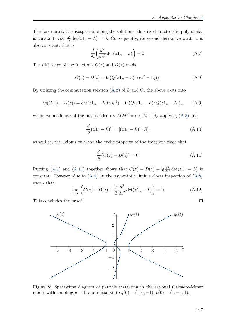
A. Appendix to Chapter 1
The Lax matrix L is isospectral along the solutions, thus its characteristic polynomial
is constant, viz. ddtdet(z1n − L) = 0. Consequently, its second derivative w.r.t. z is
also constant, that isd
dt
(d2
dz2det(z1n − L)
)= 0. (A.7)
The difference of the functions C(z) and D(z) reads
C(z)−D(z) = tr(Q(z1n − L)∨(vv† − 1n)
). (A.8)
By utilizing the commutation relation (A.2) of L and Q, the above casts into
ig(C(z)−D(z)) = det(z1n − L)tr(Q2)− tr(Q(z1n − L)∨Q(z1n − L)
), (A.9)
where we made use of the matrix identity MM∨ = det(M). By applying (A.3) and
d
dt(z1n − L)∨ = [(z1n − L)∨, B], (A.10)
as well as, the Leibniz rule and the cyclic property of the trace one finds that
d
dt
(C(z)−D(z)
)= 0. (A.11)
Putting (A.7) and (A.11) together shows that C(z) − D(z) + ig2d2
dz2det(z1n − L) is
constant. However, due to (A.4), in the asymptotic limit a closer inspection of (A.8)
shows that
limt→∞
(C(z)−D(z) +
ig
2
d2
dz2det(z1n − L)
)= 0. (A.12)
This concludes the proof.
−5 −4 −3 −2 −1 1 2 3 4 5
−2
−1
1
2
0
q1(t)q2(t)q3(t)
q
t
Figure 8: Space-time diagram of particle scattering in the rational Calogero-Mosermodel with coupling g = 1, and initial state q(0) = (1, 0,−1), p(0) = (1,−1, 1).
167

B Appendices to Chapter 2
B.1 Application of Jacobi’s theorem on complemen-
tary minors
In this appendix, we complete the proof of Lemma 2.7 by a calculation based on
Jacobi’s theorem on complementary minors (e.g. [104]), which will be recalled shortly.
Our reasoning below is adapted from Pusztai [105]. A significant difference is that in
our case we need the strong regularity conditions (2.87) and (2.100) to avoid dividing
by zero during the calculation. In fact, this appendix is presented mainly to explain
the origin of the strong regularity conditions.
For an m ×m matrix M let M(r1 ... rkc1 ... ck
)denote the determinant formed from the
entries lying on the intersection of the rows r1, . . . , rk with the columns c1, . . . , ck of M
(k ≤ m),
M
(r1 . . . rk
c1 . . . ck
)= det(Mri,cj)
ki,j=1.
Theorem B.1 (Jacobi). Let A be an invertible N×N matrix with det(A) = 1 and B =
(A−1)⊤. For a fixed permutation(j1 ... jNk1 ... kN
)of the pairwise distinct indices j1, . . . , jN ∈
1, . . . , N and any 1 ≤ p < N we have
B
(j1 . . . jp
k1 . . . kp
)= sgn
(j1 . . . jN
k1 . . . kN
)A
(jp+1 . . . jN
kp+1 . . . kN
). (B.1)
Applying Jacobi’s theorem to A (2.101) we now derive the two equations (2.103)
and (2.104) for the pair of functions (Wa,Wn+a) for each a = 1, . . . , n, which are defined
by Wk = wkFk with Fk = |Fk|2 (2.93) and wk in (2.102).
Lemma B.2. Fix any strongly regular λ, i.e. λ ∈ Rn for which (2.87) and (2.100) hold,
and use the above notations for (Wa,Wn+a). If A given by (2.101) is a unitary matrix,
then (Wa,Wn+a) satisfies the two equations (2.103) and (2.104) for each a = 1, . . . , n.
Proof. Let B = (A−1)⊤, i.e. Bj,k = Aj,k, j, k ∈ 1, . . . , N and a ∈ 1, . . . , n be a
fixed index. Since det(A) = 1, by Jacobi’s theorem with jb = b, (b ∈ NN) and kc = c,
168

B. Appendices to Chapter 2
(c ∈ NN \ a, n+ a), ka = n+ a, kn+a = a and p = n we have
B
(1 . . . a . . . n
1 . . . n+ a . . . n
)= −A
(n+ 1 . . . n+ a . . . N
n+ 1 . . . a . . . N
). (B.2)
Denote the corresponding n×n submatrices of B and A by ξ and η, respectively. One
can check that
ξ = Ψ− µ− νµ− λa
Ea,a, η = Ξ− µ− νµ+ λa
Ea,a, (B.3)
where Ej,k stands for the n × n elementary matrix (Ej,k)j′,k′ = δj,j′δk,k′ and Ψ and Ξ
are the Cauchy-like matrices
Ψj,k =
2µF jFn+k2µ− λj + λk
, if k 6= a,
2µF jFa2µ− λj − λa
, if k = a,
and Ξj,k =
2µFn+jF k
2µ+ λj − λk, if k 6= a,
2µFn+jF n+a
2µ+ λj + λa, if k = a,
(B.4)
j, k ∈ 1, . . . , n. Expanding det(ξ) and det(η) along the a-th column we obtain the
formulae
det(ξ) = det(Ψ)− µ− νµ− λa
Ca,a, det(η) = det(Ξ)− µ− νµ+ λa
Ca,a, (B.5)
where Ca,a is the cofactor of Ψ associated with entry Ψa,a. Since Ψ and Ξ are both
Cauchy-like matrices we have
det(Ψ) =1
µ− λaDaWa, det(Ξ) =
1
µ+ λaDaWn+a, (B.6)
where
Da =n∏
b=1(b6=a)
F bFn+b
n∏
c,d=1(a6=c 6=d6=a)
λc − λd2µ+ λc − λd
. (B.7)
It can be easily seen that Ca,a = Da, therefore formulae (B.2), (B.5), (B.6) lead to the
equation
(µ+ λa)Wa + (µ− λa)Wn+a − 2(µ− ν) = 0. (B.8)
It should be noticed that in the last step we divided by Da, which is legitimate
since Da is non-vanishing due to the strong-regularity condition given by (2.87) and
(2.100). To see this, assume momentarily that Fi = 0 for some i = 1, . . . , n at some
strongly regular λ. The denominator in (2.101) does not vanish, and the unitarity of
A implies that we must have Ai,i+n = 1 or Ai,i+n = −1. These in turn are equivalent
to
λi = 2µ− ν or λi = ν, (B.9)
169

B. Appendices to Chapter 2
which are excluded by (2.100). One can similarly check that the vanishing of Fn+iwould require
λi = ν − 2µ or λi = −ν, (B.10)
which are also excluded. These remarks pinpoint the origin of the second half of the
conditions imposed in (2.100).
Next, we apply Jacobi’s theorem by setting jb = kb = b, (b ∈ Nn), jn+1 = kn+1 =
n+ a, jn+c = kn+c = n + c− 1, (c ∈ Nn−1) and p = n+ 1. Thus
B
(1 . . . n n+ a
1 . . . n n+ a
)= A
(n + 1 . . . n+ a . . . N
n + 1 . . . n+ a . . . N
), (B.11)
where n + a indicates that the (n+a)-th row and column are omitted. Now denote the
submatrices of size (n+1) and (n− 1) corresponding to the determinants in (B.11) by
X and Y , respectively. From (B.11) and (2.101) it follows that det(X) = det(Y ) = Da
(B.7). The submatrix X can be written in the form
X = Φ− µ− νµ− λa
Ea,n+1 −µ− νµ+ λa
En+1,a, (B.12)
i.e. X is a rank two perturbation of the Cauchy-like matrix Φ having the entries
Φj,k =2µF jFn+k
2µ− λj + λk, Φj,n+1 =
2µF jFa2µ− λj − λa
,
Φn+1,k =2µF n+aFn+k2µ+ λa + λk
, Φn+1,n+1 = F n+aFa,
(B.13)
where j, k ∈ 1, . . . , n. The determinant of Φ is
det(Φ) = − λ2aµ2 − λ2a
DaWaWn+a, (B.14)
which cannot vanish because λ is strongly regular. Since X is a rank two perturbation
of Φ we obtain
det(X) = det(Φ)− (µ− ν)( Ca,n+1
µ− λa+Cn+1,a
µ+ λa
)+ (µ− ν)2Ca,n+1Cn+1,a − Ca,aCn+1,n+1
(µ− λa)(µ+ λa) det(Φ),
(B.15)
where C now is used to denote the cofactors of Φ. By calculating the necessary cofactors
we deriveCa,aCn+1,n+1 = D2
aWaWn+a,
Ca,n+1 = −1
µ+ λaDaWn+a, Cn+1,a = −
1
µ− λaDaWa.
(B.16)
170

B. Appendices to Chapter 2
Equations (B.14)-(B.16) together with det(X) = Da imply
λ2a(WaWn+a − 1)− µ(µ− ν)(Wa +Wn+a − 2) + ν2 = 0. (B.17)
Equations (B.8) and (B.17) coincide with (2.103) and (2.104), respectively.
B.2 HvDl as elementary symmetric function
Fix an arbitrary n ∈ N and l ∈ 0, 1, . . . , n and let el stand for the l-th elementary
symmetric polynomial in n variables x1, . . . , xn, i.e. e0(x1, . . . , xn) = 1 and for l ≥ 1
el(x1, . . . , xn) =∑
1≤j1···<jl≤n
xj1 . . . xjl. (B.18)
At the end of Chapter 2, we referred to the following useful result due to van Diejen
[142, Proposition 2.3]. For convenience, we present it together with a direct proof.
Proposition B.3. By using (2.220) it can be shown that
HvDl (q) = 4lel(sinh
2 q12, . . . , sinh2 qn
2). (B.19)
Proof. First, el has the equivalent form
el(sinh2 q12, . . . , sinh2 qn
2) =
∑
J⊂1,...,n, |J |=l
∏
j∈J
sinh2 qj2. (B.20)
Utilizing the identity sinh2(α/2) = [cosh(α)− 1]/2 casts the right-hand side into
∑
J⊂1,...,n, |J |=l
2−l∏
j∈J
[cosh(qj)− 1] =∑
J⊂1,...,n, |J |=l
2−l∑
K⊂J
(−1)l−|K|∏
k∈K
cosh(qk).
(B.21)
The two sums on the right-hand side can be merged into one, but the multiplicity of
subsets must remain the same. This results in the appearance of a binomial coefficient
∑
J⊂1,...,n, |J |≤l
(−1)l−|J |
2l
(n− |J |l − |J |
)∏
j∈J
cosh(qj) =
=∑
J⊂1,...,n, |J |≤lεj=±1, j∈J
(−1)l−|J |
2l+|J |
(n− |J |l − |J |
)∏
j∈J
cosh(εjqj), (B.22)
where we also used that cosh is an even function and compensated the ‘over-counting’
171

B. Appendices to Chapter 2
of terms. Now, let us simply pull a 4−l factor out of the sum to get
4−l∑
J⊂1,...,n, |J |≤lεj=±1, j∈J
(−2)l−|J |
(n− |J |l − |J |
)∏
j∈J
cosh(εjqj). (B.23)
Recall the following identity for the hyperbolic cosine of the sum of a finite number,
say N , real arguments (see [62, Art. 132] and apply cos(iα) = cosh(α))
cosh
( N∑
k=1
αk
)=
[ N∏
k=1
cosh(αk)
][⌊N2
⌋∑
m=0
e2m(tanh(α1), . . . , tanh(αN ))
], (B.24)
where e2m are now elementary symmetric functions with arguments tanh(αk). Note
that for any m > 0 and set of signs ε there is another one ε′, such that eJ,ε′
2m = −eJ,ε2m,
therefore by using (B.24) we see that (B.23) equals to
4−l∑
J⊂1,...,n, |J |≤lεj=±1, j∈J
(−2)l−|J |
(n− |J |l − |J |
)∏
j∈J
cosh(εjqj)
⌊ |J |2
⌋∑
m=0
sJ,ε2m =
= 4−l∑
J⊂1,...,n, |J |≤lεj=±1, j∈J
(−2)l−|J |
(n− |J |l − |J |
)cosh(qεJ). (B.25)
Applying (2.220) concludes the proof.
172
C Appendices to Chapter 3
C.1 Links to systems of van Diejen and Schneider
Recall that the trigonometric BCn van Diejen system [140] has the Hamiltonian
HvD(λ, θ) =
n∑
j=1
(cosh(θj)Vj(λ)
1/2V−j(λ)
1/2 − [Vj(λ) + V−j(λ)]/2), (C.1)
with V±j (j = 1, . . . , n) defined by
V±j(λ) = w(±λj)n∏
k=1(k 6=j)
v(±λj + λk)v(±λj − λk), (C.2)
and v,w denoting the trigonometric potentials
v(z) =sin(µ+ z)
sin(z)and w(z) =
sin(µ0 + z)
sin(z)
cos(µ1 + z)
cos(z)
sin(µ′0 + z)
sin(z)
cos(µ′1 + z)
cos(z),
(C.3)
where µ, µ0, µ1, µ′0, µ
′1 are arbitrary parameters. By making the substitutions
λj → i(pj +R),
θj → iqj ,∀j and µ→ ig/2,
µ0 → i(g0 +R),
µ′0 → i(g′0 − R),
µ1 → ig1 + π/2,
µ′1 → ig′1 + π/2
(C.4)
the potentials become hyperbolic functions and their R→∞ limit exists, namely
limR→∞
v(±(λj + λk)) = e±g/2, limR→∞
v(±(λj − λk)) =sinh(±g/2 + pj − pk)
sinh(pj − pk), ∀j, k
(C.5)
and
limR→∞
w(±λj) = eg0−g′
0±(g1+g′1)−2pj − e±(g0+g′0+g1+g′
1), ∀j. (C.6)
In the 1-particle case we have V±(λ) = w(±λ), thus HvD takes the following form
HvD(λ, θ) = cosh(θ)w(λ)1/2w(−λ)1/2 − [w(λ) + w(−λ)]/2. (C.7)
173

C. Appendices to Chapter 3
By utilizing (C.6) one obtains
limR→∞
w(λ)1/2w(−λ)1/2 =[1− (e2g0 + e−2g′0)e−2p + e2g0−2g′0−4p
]1/2,
limR→∞
[w(λ) + w(−λ)]/2 =eg0−g
′
0+g1+g′
1 + eg0−g′
0−g1−g′
1
2e−2p − cosh(g0 + g′0 + g1 + g′1).
(C.8)
Equating the R → ∞ limit of HvD(λ, θ) (C.7) with the Hamiltonian H(p, q; x, a, b)
(3.1) yields a system of linear equations involving g0, g1, g′0, g
′1 as unknowns and u, v
as parameters. Actually, four sets of linear equations can be constructed, each with
infinitely many solutions depending on one (real) parameter, but these sets are ‘equiv-
alent’ under the exchanges: g0 ↔ g′0 or g1 ↔ g′1. Therefore it is sufficient to give only
one set of solutions, e.g.
g0 = a, g′0 = 0, g1 = b− g′1, g′1 ∈ R. (C.9)
Setting g = x and g′1 = 0 provides the following special choice of couplings in (C.4)
µ = ix/2, µ0 = i(a +R), µ′0 = −iR, µ1 = ib+ π/2, µ′
1 = π/2, (C.10)
and one finds the following
limR→∞
HvD
(λ(p, R), θ(q)
)= −H(p, q; x, a, b) + cosh(b− a). (C.11)
In the n-particle case, by using (C.5) and (C.6) it can be shown that with (C.10) one
has
limR→∞
HvD
(λ(p, R), θ(q)
)= −H(p, q; x, a, b) +
n∑
j=1
cosh((j − 1)x+ b− a
), (C.12)
i.e., the Hamiltonian H (3.1) is recovered as a singular limit of HvD (C.1).
Consider now the functionH(p, q; x, a, b) and introduce the real parameter σ through
the substitutions
b→ b− 2σ (C.13)
and apply the canonical transformation
pj → −Qj + σ, qj → −Pj, ∀j. (C.14)
Then we have
limσ→∞
H(p(Q, σ), q(P ), x, a, b(σ)) = HSch(Q,P, x, a− b), (C.15)
174

C. Appendices to Chapter 3
with Schneider’s [125] Hamiltonian
HSch(Q,P, x, a− b) =ea−b
2
n∑
j=1
e2Qj −n∑
j=1
cos(Pj)
n∏
k=1(k 6=j)
[1− sinh2
(x2
)
sinh2(Qj −Qk)
]12
. (C.16)
Remark C.1. (i) In (C.4) only two of the four external field couplings µ0, µ′0, µ1, µ
′1 are
scaled with R. However, scaling all four of these parameters also leads to an integrable
Ruijsenaars-Schneider type system with a more general 4-parameter external field. For
details, see [143, Section II.B]. (ii) The connection to Schneider’s Hamiltonian was
mentioned in [86, Remark 7.1] as well, where a singular limit, similar to (C.15) was
taken.
C.2 Proof of Proposition 3.2
In this appendix, we prove Proposition 3.2 that states that the range of the ‘position
variable’ p is contained in the closed thick-walled Weyl chamber Cx (3.58).
Proof of Proposition 3.2. According to (3.57) the matrices e2p and e2p−x1n+sgn(x)epww†ep
are similar and therefore have the same characteristic polynomial. This gives the iden-
tity
n∏
j=1
(e2pj − λ) =n∏
j=1
(e2pj−x − λ) + sgn(x)
n∑
j=1
[e2pj |wj|2
n∏
k=1(k 6=j)
(e2pk−x − λ)], (C.17)
where λ is an arbitrary complex parameter. The constraint on p arises from the fact
that |wm|2 (m = 1, . . . , n) must be non-negative and not all zero, because of the
definition (3.56).
Let us assume for a moment that the components of p are distinct such that p1 >
· · · > pn. This enables us to express |wm|2 for all m ∈ 1, . . . , n from the above
equation by evaluating it at n different values of λ, viz. λ = e2pm−x, m = 1, . . . , n. We
obtain the following
|wm|2 = sgn(x)(1 − e−x)n∏
j=1(j 6=m)
e2pj+x − e2pme2pj − e2pm , m = 1, . . . , n. (C.18)
For x > 0 and any p with p1 > · · · > pn the formula (C.18) implies that |wn|2 > 0 and
for m = 1, . . . , n − 1 we have |wm|2 ≥ 0 if and only if pm − pm+1 ≥ x/2. Similarly,
if x < 0 and p ∈ Rn with p1 > · · · > pn, then (C.18) implies |w1|2 > 0 and for
m = 2, . . . , n we have |wm|2 ≥ 0 if and only if pm−1 − pm ≥ −x/2. In summary, if
175

C. Appendices to Chapter 3
p1 > · · · > pn, then |wm|2 ≥ 0 ∀m implies that p ∈ Cx.Now, let us prove our assumption, that all components of p must be different.
Indirectly, suppose that some (or maybe all) of the pj’s coincide. This can be captured
by a partition of the positive integer
n = k1 + · · ·+ kr, (C.19)
where r < n (or equivalently, at least one integer k1, . . . , kr must be greater than 1)
and the indirect assumption can be written as
p1 = · · · = pk1 , pk1+1 = · · · = pk1+k2, . . . , pk1+···+kr−1+1 = · · · = pk1+···+kr ≡ pn.
(C.20)
Then (C.17) can be reformulated as
r∏
j=1
(∆j−λ)kj =r∏
j=1
(∆je−x−λ)kj+sgn(x)
r∑
m=1
Zm∆m(∆me−x−λ)km−1
r∏
j=1(j 6=m)
(∆je−x−λ)kj ,
(C.21)
where we introduced r distinct variables
∆1 = e2pk1 , ∆2 = e2pk1+k2 , . . . , ∆r = e2pk1+···+kr ≡ e2pn , (C.22)
and r non-negative real variables
Z1 = |w1|2 + · · ·+ |wk1|2, Z2 = |wk1+1|2 + · · ·+ |wk1+k2 |2,. . . , Zr = |wk1+···+kr−1+1|2 + · · ·+ |wn|2.
(C.23)
Notice that Z1 + · · · + Zr = |w|2 = sgn(x)e−x(enx − 1) > 0, therefore at least one of
the Zj’s must be positive. Next, we define the rational function of λ
Q(∆, x, λ) =r∏
j=1
(∆j − λ)kj(∆je−x − λ)kj−1
, (C.24)
and use it to rewrite (C.21) as
Q(∆, x, λ) =r∏
j=1
(∆je−x − λ) + sgn(x)
r∑
m=1
Zm∆m
r∏
j=1(j 6=m)
(∆je−x − λ). (C.25)
The above equation implies that all poles of Q are apparent, i.e., there must be can-
celling factors in its numerator. This observation has a straightforward implication on
the ∆’s.
176

C. Appendices to Chapter 3
(∗) For every index m ∈ 1, . . . , r with km > 1, there exists an index s ∈ 1, . . . , rs.t. ∆s = ∆me
−x and ks ≥ km − 1.
The quantities Zm = Zm(∆, x) can be uniquely determined by evaluating (C.25) at r
different values of the parameter λ, namely λm = ∆me−x (m = 1, . . . , r). However,
there are 3 disjoint cases which are to be handled separately.
Case 1: km = 1 and ∄s ∈ 1, . . . , r: ∆s = ∆me−x. Then we find
Zm = sgn(x)(1− e−x)e(n−1)x
r∏
j=1(j 6=m)
(∆j −∆me
−x
∆j −∆m
)kj> 0. (C.26)
Case 2: km > 1 and ks = km − 1. Then we find
Zm = (−1)km+1 sgn(x)(1 − e−x)e(n−km)xr∏
j=1(j 6=m,s)
(∆j −∆me
−x
∆j −∆m
)kj> 0. (C.27)
Case 3: km = 1 and ∃s ∈ 1, . . . , r: ∆s = ∆me−x or km > 1 and ks > km − 1. Then
we get
Zm = 0. (C.28)
Since there is at least one Zm which is positive, the set of indices belonging to Case 1
or Case 2 must be non-empty. Introduce a real positive parameter ε and associate to
every degenerate configuration (C.20) a continuous family of configurations, denoted
by p(ε), with components p(ε)1, . . . , p(ε)n defined by the formulae
exp(2p(ε)a + aε) = ∆1, a = 1, . . . , k1,
exp(2p(ε)∑j−1m=1 km+a + aε) = ∆j , a = 1, . . . , kj, j = 2, . . . , r.
(C.29)
This way coinciding components of p (C.20) are ‘pulled apart’ to points successively
separated by ε/2. It is clear that with sufficiently small separation the configuration
p(ε) sits in the chamber x ∈ Rn | 0 > x1 > · · · > xn. For such non-degenerate
configurations p(ε), let us consider the expressions
|wℓ(p(ε), x)|2 = sgn(x)(1− e−x)n∏
j=1(j 6=ℓ)
e2p(ε)j+x − e2p(ε)ℓe2p(ε)j − e2p(ε)ℓ , ℓ = 1, . . . , n, (C.30)
which give the unique solution of equation (C.17) at p(ε). The limits limε→0 |wℓ(p(ε), x)|2exist, and do not vanish for ℓ = k1 + · · ·+ km if km belongs to Case 1 or Case 2. For
such ℓ = k1 + · · ·+ km we must have
limε→0|wk1+···+km(p(ε), x)|2 = Zm(∆, x) > 0, (C.31)
177

C. Appendices to Chapter 3
where Zm is given by (C.26) in Case 1 and by (C.27) in Case 2. It can be also seen
that
|wℓ(p(ε), x)|2 ≡ 0 ⇐⇒
ℓ /∈ k1, k1 + k2, . . . , k1 + · · ·+ kror
ℓ = k1 + · · ·+ km with km from Case 3,
(C.32)
i.e. |wℓ(p(ε), x)|2 vanishes identically except for the components in (C.31). Notice that
for a small enough ε some coordinates of p(ε) are separated by less than |x|/2. Thus, as
it was shown at beginning the proof, we have |wℓ(p(ε), x)|2 < 0 for some index ℓ, which
might depend on ε. Moreover, (C.32) implies that the index in question must have the
form ℓ = k1 + · · · + km∗ for some m∗ appearing in (C.31). But since the number of
indices is finite, a monotonically decreasing sequence εN∞N=1 tending to zero can be
chosen such that |wk1+···+km∗ (p(εN), x)|2 < 0 for all N . This together with (C.32) gives
the contradiction
0 ≥ limN→∞
|wk1+···+km∗ (p(εN), x)|2 = Zm∗(∆, x) > 0 (C.33)
proving that all components of p must be distinct. This concludes the proof.
The above proof is a straightforward adaptation of the proofs of [37, Lemma 5.2] and
[38, Theorem 2]. We presented it since it could be awkward to extract the arguments
from those lengthy papers, and also our notations and the ranges of our variables are
different.
C.3 Proof of Lemma 3.6
We here prove the following equivalent formulation of Lemma 3.6.
Lemma C.2. Suppose that π2≥ q1 > · · · > qn > 0 and
[ηL(1) 0n
0n ηL(2)
][cos q i sin q
i sin q cos q
][ηR(1)
−10n
0n ηR(2)−1
]=
[cos q i sin q
i sin q cos q
](C.34)
for ηL, ηR ∈ G+. Then
ηL(1) = ηR(2) = m1, ηL(2) = ηR(1) = m2 (C.35)
with some diagonal matrices m1, m2 ∈ Tn having the form
m1 = diag(a, ξ), m2 = diag(b, ξ), ξ ∈ Tn−1, a, b ∈ T1, det(m1m2) = 1. (C.36)
178

C. Appendices to Chapter 3
If in addition π2> q1, then m1 = m2.
Proof. The block off-diagonal components of the equality (C.34) give
ηL(1) = (sin q)ηR(2)(sin q)−1, ηL(2) = (sin q)ηR(1)(sin q)
−1. (C.37)
Since ηL(1)−1 = ηL(1)†, the first of these relations implies ηR(2) = (sin q)2ηR(2)(sin q)
−2.
As the entries of (sin q) are all different, this entails that ηR(2) is diagonal, and conse-
quently we obtain the relations in (C.35) with some diagonal matrices m1 and m2. On
the other hand, the block-diagonal components of (C.34) require that
cos q = ηL(1)(cos q)ηR(1)−1, cos q = ηL(2)(cos q)ηR(2)
−1. (C.38)
Since cos qk 6= 0 for k = 2, . . . , n, the formula (C.36) follows. If an addition cos q1 6= 0,
then we also obtain from (C.38) that a = b, i.e., m1 = m2 = m with some m ∈ Tn.
C.4 Auxiliary material on Poisson-Lie symmetry
The statements presented here are direct analogues of well-known results [7, 56] about
Hamiltonian group actions with zero Poisson bracket on the symmetry group. They
are surely familiar to experts, although we could not find them in a reference.
Let us consider a Poisson-Lie groupG with dual groupG∗ and a symplectic manifold
P equipped with a left Poisson action of G. Essentially following Lu [80] (cf. Remark
C.6), we say that the G-action admits the momentum map ψ : P → G∗ if for any
X ∈ G, the Lie algebra of G, and any f ∈ C∞(P ) we have
(LXPf)(p) = 〈X, f, ψ(p)ψ(p)−1〉, ∀p ∈ P, (C.39)
where XP is the vector field on P corresponding to X, 〈., .〉 stands for the canonical
pairing between the Lie algebras of G and G∗, and the notation pretends that G∗ is
a matrix group. Using the Hamiltonian vector field Vf defined by LVfh = −f, h(∀h ∈ C∞(P )), we can spell out equation (C.39) equivalently as
(LXPf)(p) = −〈X,
(Dψ(p)Rψ(p)−1
)((Dpψ)(Vf(p))
)〉, ∀p ∈ P, (C.40)
where Dpψ : TpP → Tψ(p)G∗ is the derivative, and Rψ(p)−1 denotes the right-translation
on G∗ by ψ(p)−1. Since the vectors of the form Vf(p) span TpP , we obtain the following
characterization of the Lie algebra of the isotropy subgroup Gp < G of p ∈ P .
Lemma C.3. With the above notations, we have
Lie(Gp) =[(Dψ(p)Rψ(p)−1
)(Im(Dpψ)
)]⊥. (C.41)
179

C. Appendices to Chapter 3
This directly leads to the next statement.
Corollary C.4. An element µ ∈ G∗ is a regular value of the momentum map ψ if and
only if Lie(Gp) = 0 for every p ∈ ψ−1(µ) = p ∈ P | ψ(p) = µ.
Let us further suppose that ψ : P → G∗ is G-equivariant, with respect to the
appropriate dressing action of G on G∗. Then we have
Gp < Gµ, ∀p ∈ ψ−1(µ). (C.42)
Here Gp and Gµ refer to the respective actions of G on P and on G∗. Corollary C.4
and equation (C.42) together imply the following useful result.
Corollary C.5. If Gµ acts locally freely on ψ−1(µ), then µ is a regular value of the
equivariant momentum map ψ. Consequently, ψ−1(µ) is an embedded submanifold of
P .
We finish by a clarifying remark concerning the momentum map.
Remark C.6. Let B be the Poisson tensor on P , for which f, h = B(df, dh) = LVhf .
We can write Vh = B♯(dh) with the corresponding bundle map B♯ : T ∗P → TP .
Any X ∈ G = TeG = (Te′G∗)∗ extends to a unique right-invariant 1-form ϑX on G∗
(e ∈ G and e′ ∈ G∗ are the unit elements). With this at hand, equation (C.39) can be
reformulated as
XP = B♯(ψ∗(ϑX)), (C.43)
which is a slight variation of the defining equation of the momentum map found in [80].
C.5 On the reduced Hamiltonians
In this appendix we prove the claim, made in Section 3.4, that on the momentum
surface Φ−1+ (µ) the Hamiltonians Hj, j ∈ Z∗ (3.190) are linear combinations of hk,
k = 1, . . . , n (3.194). This will be achieved by establishing the form of the integer
powers of the matrix displayed in (3.193), which we denote here by L, i.e.
L =
[e−2v
1n −e−vαe−vα† e2v1n − α†α
]. (C.44)
Lemma C.7. For any positive integer j, the j-th power of the 2n×2n matrix L (C.44)
reads
Lj =[Lj11 Lj12Lj21 Lj22
], (C.45)
180

C. Appendices to Chapter 3
where Lj11,Lj12,Lj21,Lj22 are n× n blocks of the form
Lj11 =j∑
m=1
a(j)m (αα†)j−m, Lj12 = α
j∑
m=1
b(j)m (α†α)j−m,
Lj21 = α†
j∑
m=1
c(j)m (αα†)j−m, Lj22 = (−1)j(α†α)j +
j∑
m=1
d(j)m (α†α)j−m,
(C.46)
with the 4j coefficients a(j)m , b(j)m , c
(j)m , d
(j)m , m = 1, . . . , j depending only on the parameter
v.
Proof. We proceed by induction on j. For j = 1 the statement clearly holds, and
supposing that (C.45)-(C.46) is valid for some fixed integer j > 0 we simply calculate
the (j + 1)-th power Lj+1 = LLj. This proves the statement.
Our claim of linear expressibility follows at once, that is for any positive integer j
we have
Hj = (−1)jhj +j−1∑
k=1
k
j(a
(j)j−k + d
(j)j−k)hk +
n
2j(a
(j)j + d
(j)j ). (C.47)
Incidentally, one also obtains a recursion for the coefficients a(j)m , b(j)m , c
(j)m , d
(j)m from the
proof of Lemma C.7. If they are required, this should enable one to establish the values
of the constants that occur in (C.47).
As for the negative powers of L, one readily checks that the inverse of L is
L−1 =
[e2v1n − αα† e−vα
−e−vα† e−2v1n
], (C.48)
which has essentially the same form as L does, thus the blocks of L−j (j > 0) can
be expressed similarly as in Lemma C.7. In fact, conjugating L−1 with the 2n × 2n
involutory block-matrix
C =
[0n 1n
1n 0n
], (C.49)
leads to the following formula
CL−1C =
[e−2v
1n −e−vα†
e−vα e2v1n − αα†
], (C.50)
which implies that the blocks of L−j are obtained from those of Lj by reversing their or-
der and interchanging the role of α and α†. Furthermore, since tr((αα†)k) = tr((α†α)k)
we get
H−j = −Hj ∀j ∈ Z∗. (C.51)
181

D Appendices to Chapter 4
It is clear that our results on the 2-parameter family of hyperbolic systems (4.5) open
up a plethora of interesting problems. Besides, based on our numerical calculations,
below we also wish to discuss some possible generalizations in two further directions.
D.1 Lax matrix with spectral parameter
First, it is a time-honoured principle that the inclusion of a spectral parameter into
the Lax matrix of an integrable system can greatly enrich the analysis by borrowing
techniques from complex geometry. Bearing this fact in mind, with the aid of the
function
Φ(x | η) = ex coth(η) (coth(x)− coth(η)) (D.1)
depending on the complex variables x and η, over the phase space P (4.2) we define
the matrix valued smooth function L = L(λ, θ;µ, ν | η) with entries
Lk,l =(i sin(µ)FkFl + i sin(µ− ν)Ck,l)
)Φ(iµ + Λj − Λk | η) (k, l ∈ NN). (D.2)
One of the outcomes of our numerical investigations is that for any values of η the
eigenvalues of L provide a family of first integrals in involution for the van Diejen
system (4.5). Thinking of η as a spectral parameter, let us also observe that, in the
limit R ∋ η → ∞, from L we can recover our Lax matrix L (4.34); that is, L → L.
Although the spectral parameter dependent matrix L does not take values in the Lie
group U(n, n) (4.9), we find it interesting that the constituent function Φ (D.1) can
be seen as a hyperbolic limit of the elliptic Lamé function, that plays a prominent role
in the theory of the elliptic CMS and RS systems (see e.g. the papers [76, 112] and
the monograph [11]). Therefore, it is tempting to think that an appropriate elliptic
deformation of L (4.34) may lead to a spectral parameter dependent Lax matrix of the
elliptic van Diejen system with coupling parameters µ and ν.
182

D. Appendices to Chapter 4
D.2 Lax matrix with three couplings
In Chapter 4 we have studied the van Diejen system (4.5) with only two independent
coupling parameters. Though a construction of a Lax matrix for the most general
hyperbolic van Diejen system with five independent coupling parameters still seems
to be out of reach, we can offer a plausible conjecture for a Lax matrix with three
independent coupling constants. Simply by generalizing the formulae appearing in the
theory of the rational BCn RSvD systems [108], with the aid of an additional real
parameter κ let us define the real valued functions α and β for any x > 0 by the
formulae
α(x) =1√2
(1 +
(1 +
sin(κ)2
sinh(2x)2
) 12
) 12
and β(x) =i√2
(−1 +
(1 +
sin(κ)2
sinh(2x)2
) 12
) 12
.
(D.3)
Built upon these functions, let us also introduce the Hermitian N ×N matrix
h(λ) =
[diag(α(λ1), . . . , α(λn)) diag(β(λ1), . . . , β(λn))
−diag(β(λ1), . . . , β(λn)) diag(α(λ1), . . . , α(λn))
]. (D.4)
One can easily show that hCh = C, whence the matrix valued function
L = h−1Lh−1 (D.5)
also takes values in the Lie group U(n, n) (4.9). Notice that the rational limit of matrix
L gives back the Lax matrix of the rational BCn RSvD system, that first appeared in
equation (4.51) of paper [107]. Moreover, upon setting
g = µ, g0 = g1 =ν
2, g′0 = g′1 =
κ
2, (D.6)
for van Diejen’s main Hamiltonian H1 (4.209) we get that
H1 = 2n∑
a=1
cosh(θa)ua
(1 +
sin(κ)2
sinh(2λa)2
) 12
+ 2n∑
a=1
Re
(zasinh(iκ + 2λa)
sinh(2λa)
), (D.7)
with the functions za and ua defined in the equations (4.31) and (4.32), respectively.
The point is that, in complete analogy with (4.215), one can establish the relationship
H1 + 2 cos (ν + κ+ (n− 1)µ)sin(nµ)
sin(µ)= tr(L). (D.8)
Furthermore, based on numerical calculations for small values of n, it appears that
the eigenvalues of L (D.5) provide a commuting family of first integrals for the van
183

D. Appendices to Chapter 4
Diejen system (D.7). To sum up, we have numerous evidences that matrix L (D.5) is
a Lax matrix for the 3-parameter family of van Diejen systems (D.7), if the pertinent
parameters are connected by the relationships displayed in (D.6). As can be seen in
[107], the new parameter κ causes many non-trivial technical difficulties even at the
level of the rational van Diejen system. Part of the difficulties can be traced back to
the fact that for sin(κ) 6= 0 the matrix L (D.5) does not belong to the symmetric space
exp(p) (4.15), whence the diagonalization of L requires a less direct approach than that
provided by the canonical form (4.17). We wish to come back to these problems in
later publications.
184

E Appendix to Chapter 5
E.1 Explicit form of the functions Λyj,ℓ
In this appendix, we display the building blocks (5.81) of the global elliptic Lax matrix
explicitly. Below, ξ varies in the closed simplex Ay associated with a type (i) coupling y
(5.13) for fixed p and M . The function J was defined in (5.80). The trigonometric case
is obtained by simply replacing the s-function (5.72) everywhere by the sine function.
Special components: For 1 ≤ j ≤ n− p
Λyj,j+p(ξ) = − sgn(M) s(y)
[∏n−1m=1(m6=p)
s(∑j+m−1
k=j ξk − y) s(∑j+p+n−m−1
k=j+p ξk + y)]12
∏n−1m=1
[s(∑j+m−1
k=j ξk) s(∑j+p+m−1
k=j+p ξk)]12
.
For n− p < j ≤ n
Λyj,j+p−n(ξ) = sgn(M) s(y)
[∏n−1m=1(m6=p)
s(∑j+m−1
k=j ξk − y) s(∑j+p−m−1
k=j+p−n ξk + y)]12
∏n−1m=1
[s(∑j+m−1
k=j ξk) s(∑j+p−m−1
k=j+p−n ξk)]12
.
Diagonal components: For 1 ≤ j = ℓ ≤ p
Λyj,j(ξ) =[J (|uj|2)J (|uj+n−p|2)
]12
[∏n−1m=1(m6=p)
s(∑j+m−1
k=j ξk − y) s(∑j+n−m−1
k=j ξk + y)]12
∏n−1m=1 s(
∑j+m−1k=j ξk)
.
For p < j = ℓ ≤ n
Λyj,j(ξ) =[J (|uj|2)J (|uj−p|2)
]12
[∏n−1m=1(m6=p)
s(∑j+m−1
k=j ξk − y) s(∑j+n−m−1
k=j ξk + y)]12
∏n−1m=1 s(
∑j+m−1k=j ξk)
.
185

E. Appendix to Chapter 5
Components above the diagonal: For 1 ≤ j < ℓ ≤ p
Λyj,ℓ(ξ) = s(y)[J (|uj|2)J (|uℓ+n−p|2)
]12
[∏n−1m=1
(m6=ℓ−j,p)s(∑j+m−1
k=j ξk − y) s(∑ℓ+n−m−1
k=ℓ ξk + y)]12
∏n−1m=1
[s(∑j+m−1
k=j ξk) s(∑ℓ+m−1
k=ℓ ξk)]12
.
For 1 ≤ j < ℓ ≤ n with p < ℓ and ℓ 6= j + p
Λyj,ℓ(ξ) =s(y)
[J (|uj|2)J (|uℓ−p|2)
]12
sgn(j + p− ℓ)
[∏n−1m=1
(m6=ℓ−j,p)s(∑j+m−1
k=j ξk − y) s(∑ℓ+n−m−1
k=ℓ ξk + y)]12
∏n−1m=1
[s(∑j+m−1
k=j ξk) s(∑ℓ+m−1
k=ℓ ξk)]12
.
Components below the diagonal: For 1 ≤ ℓ < j ≤ n with ℓ ≤ p and ℓ 6= j + p− n
Λyj,ℓ(ξ) =s(y)
[J (|uj|2)J (|uℓ+n−p|2)
]12
sgn(ℓ+ n− j − p)
[∏n−1m=1
(m6=j−ℓ,p)s(∑j+n−m−1
k=j ξk − y) s(∑ℓ+m−1
k=ℓ ξk + y)]12
∏n−1m=1
[s(∑j+m−1
k=j ξk) s(∑ℓ+m−1
k=ℓ ξk)]12
.
For p < ℓ < j ≤ n
Λyj,ℓ(ξ) = s(y)[J (|uj|2)J (|uℓ−p|2)
]12
[∏n−1m=1
(m6=j−ℓ,p)s(∑j+n−m−1
k=j ξk − y) s(∑ℓ+m−1
k=ℓ ξk + y)]12
∏n−1m=1
[s(∑j+m−1
k=j ξk) s(∑ℓ+m−1
k=ℓ ξk)]12
.
186

Summary
Integrable many-body systems in one spatial dimension form an important class of
exactly solvable Hamiltonian systems with their diverse mathematical structure and
widespread applicability in physics [102, 103, 134]. Among these models, the systems
of Calogero-Ruijsenaars type occupy a central position, due to their intimate relation
with soliton theory [114], and since many other interesting models (e.g. Toda lattice)
can be obtained from them by taking various limits and analytic continuations [118].
Calogero-Ruijsenaars systems describe interacting particles moving on a line or circle.
They come in different types called rational (I), hyperbolic (II), trigonometric (III),
and elliptic (IV) depending on the functional form of their Hamiltonian. They exist in
nonrelativistic and relativistic form, and both at the classical and quantum level. This
already means sixteen different models (captured by Figure 3). But there are other
interesting extensions maintaining integrability, as is exemplified by versions attached
to (non-A type) root systems [95] or allowing internal degrees of freedom (spin) [51].
A fascinating aspect of Calogero-Ruijsenaars type systems is their duality relations,
which first appeared in the famous paper [68] by Kazhdan, Kostant, and Sternberg, and
was extensively explored by Ruijsenaars [113]. Here the word duality refers to action-
angle duality, which involves two Liouville integrable many-body Hamiltonian systems
(M,ω,H) and (M, ω, H) with Darboux coordinates q, p and q, p. These are said to be
duals of each other if there is a global symplectomorphism R : M → M of the phase
spaces, which exchanges the canonical coordinates with the action-angle variables for
the Hamiltonians. Practically, this means that H R−1 depends only on q, while H Ronly on q. In more detail, q are the particle positions for H and action variables for H ,
and similarly, q are the positions of particles modelled by the Hamiltonian H and action
variables for H . The idea that dualities can be interpreted in terms of Hamiltonian
reduction can be distilled from [68] and was put forward explicitly in several papers in
the 1990s, e.g. [48, 54].
During the past ten years, Fehér and collaborators undertook the study of these
dualities within the framework of reduction [36, 35, 9, 37, 38, 34, 40]. The list of action-
angle dualities was enlarged by Pusztai [105, 106, 107, 108, 109] to dual pairs associated
with non-A type root systems. The primary aim of the work presented in this thesis
was to further develop these earlier developments. In this effort, our main tool was
187
Summary
the method of Hamiltonian reduction, which belongs to the set of standard toolkits
applicable to study a great variety of problems ranging from geometric mechanics to
field theory and harmonic analysis [84, 31]. It is especially useful in the theory of
integrable Hamiltonian systems [11], where one of the maxims is that one should view
the systems of interests as reductions of obviously solvable ‘free’ systems [98]. This
is often advantageous, for example since the reduction produces global phase spaces
on which the reduced free flows are automatically complete, which is an indispensable
property of any integrable system.
The thesis is divided into two parts. Part I of the thesis takes this reduction
approach to Calogero-Ruijsenaars type systems. Part II collects our work that were
initiated by reduction results, but were obtained using direct methods.
Results
Here we collect the main results of the thesis, going chapter by chapter. In each title,
we cite our related contribution (Publications)
Spectral coordinates of the rational Calogero-Moser system [P6]
Chapter 1 starts by recalling the pivotal work of Kazhdan, Kostant, Sternberg [68].
Subsection 1.1.2 is a recap of their result about the complete integrability and action-
angle duality for the rational Calogero-Moser system in the context of Hamiltonian
reduction. In Section 1.2, we put these ideas into use, when we identify the canonical
variables of [33] in terms of the reduction picture (Lemma 1.1), and prove the relation
conjectured in that paper (Theorem 1.2). We attain Sklyanin’s formula as a corollary
(Corollary 1.3).
Action-angle duality for the trigonometric BCn Calogero-Moser-
Sutherland system [P1, P8, P5]
Chapter 2 is a study on the trigonometric Sutherland system attached to the BCn root
system. We start by providing a physical interpretation of the model in Section 2.1.
This is followed by the preparatory Section 2.2, where the group-theoretic ingredients
of reduction are introduced together with the unreduced Abelian Poisson algebras and
the symplectic reduction to be performed. In Section 2.3, we solve the momentum
equations, hence obtaining the first model of the reduced phase space (Theorem 2.1).
In a nutshell, this first model of the reduced phase space carries the Sutherland Hamil-
tonian as the reduction of the free Hamiltonian governing geodesic motion on the Lie
group U(2n) (Corollary 2.2). The content of this section, and even its quantum ana-
188

Summary
logue, is fairly standard [44]. The heart of the second chapter is Subsection 2.3.2, in
which we first describe the reduced phase space locally (Theorem 2.3), then extend
this construction to a global model (Theorem 2.16). This gives rise to the action-angle
dual of the trigonometric BCn Sutherland system. The main Hamiltonian of the dual
system turns out to be a real form of the rational Ruijsenaars-Schneider Hamiltonian
with three independent couplings. In Section 2.4, we apply our duality map to various
problems, such as finding the equilibrium configuration of the Sutherland model, prov-
ing the maximal superintegrability of the dual model, and connecting the Hamiltonians
of the hyperbolic analogue with a family of Hamiltonians found by van Diejen.
A Poisson-Lie deformation of the trigonometric BCn Calogero-
Moser-Sutherland system [P2, P3]
Chapter 3 generalises certain parts of the previous chapter as it derives a 1-parameter
deformation of the trigonometric BCn Sutherland system by applying Hamiltonian
reduction to the Heisenberg double of the Poisson-Lie group SU(2n). Here, we were
also motivated by the recent work of Marshall [86]. We start in Section 3.1 by defining
the reduction of interest. In Section 3.2, we observe that several technical results of
[37] can be applied for analysing the reduction at hand, and solve the momentum map
constraints by taking advantage of this observation (Proposition 3.2, 3.3). The main
result of this chapter is contained in Section 3.3, where we characterize the reduced
system. In Subsection 3.3.1, we prove that the reduced phase space is smooth (Theorem
3.9). Then in Subsection 3.3.2 we focus on a dense open submanifold on which the
Hamiltonian ‘lives’ (Theorem 3.11). The demonstration of the Liouville integrability
of the reduced free flows is given in Subsection 3.3.3. In particular, we prove the
integrability of the completion of the pertinent system carried by the full reduced
phase space. Our main result in this chapter is Theorem 3.14 (proved in Subsection
3.3.4), which establishes a globally valid model of the reduced phase space. In Section
3.4, we complete (Theorem 3.22) the recent derivation of the hyperbolic analogue by
Marshall [86].
Lax representation of the hyperbolic BCn Ruijsenaars-Schneider-
van Diejen system [P7]
Chapter 4 contains our construction of a Lax pair for the classical hyperbolic van Diejen
system with two independent coupling parameters. In Section 4.1, we start with a short
overview on some relevant group-theoretic facts and fix notation. In Section 4.2, we
define our Lax matrix for the van Diejen system, and also investigate its main algebraic
properties (Proposition 4.1, Lemma 4.2). These results can be used to show that the
189

Summary
dynamics can be solved by a projection method, which in turn allows us to initiate
the study of the scattering properties. This was done by B.G. Pusztai and is included
in Subsections 4.2.2, 4.3.1, 4.3.3, 4.3.4, 4.3.5. In Subsection 4.4.1, we elaborate the
link between our special 2-parameter family of Hamiltonians and the most general 5-
parameter family of hyperbolic van Diejen systems. We affirm the equivalence between
van Diejen’s commuting family of Hamiltonians and the coefficients of the characteristic
polynomial of our Lax matrix (Lemma 4.14). Based on this technical result, we can
infer that the eigenvalues of the proposed Lax matrix provide a commuting family of
first integrals for the Hamiltonian system (Theorem 4.15).
Trigonometric and elliptic Ruijsenaars-Schneider models on the
complex projective space [P4]
Chapter 5 is concerned with the compactified Ruijsenaars-Schneider systems with so-
called type (i) couplings [40]. We reconstruct the corresponding compactification on
CPn−1 using only direct, elementary methods (Proposition 5.1, Theorem 5.5). Such
construction was not known previously except for special type (i) cases. By doing
so, we gain a better understanding of the structure of these trigonometric systems.
This part of the chapter fills Sections 5.1 and 5.2. In Section 5.3, we explain that
the direct method is applicable to obtain type (i) compactifications of the elliptic
Ruijsenaars-Schneider system as well (Theorem 5.7). This new result extends the
remarks of Ruijsenaars [114, 118].
190

Összefoglaló
Bevezetés
Az egydimenziós integrálható sokrészecske modellek széleskörû fizikai alkalmazásaik és
gazdag matematikai hátterük okán az egzaktul megoldható hamiltoni rendszerek fontos
osztályát képezik. A Calogero-Ruijsenaars típusú rendszerek központi helyet foglalnak
el ezek között. Ez egyrészt a szolitonok elméletével való kapcsolatuknak, másrészt
annak köszönhetõ, hogy számos más érdekes modell (pl. a Toda-molekula) származ-
tatható belõlük, határesetekként és analitikus kiterjesztéssel. A Calogero-Ruijsenaars
típusú modellek egyenesen vagy körön mozgó kölcsönható részecskéket írnak le. A köl-
csönhatás jellege szerint négy típust különböztetünk meg. Ezek a racionális (I), a hi-
perbolikus (II), a trigonometrikus (III) és az elliptikus (IV) rendszerek. A modelleknek
létezik nemrelativisztikus és relativisztikus, valamint klasszikus- és kvantummechani-
kai változata is. Integrálható általánosításaik közül kiemelendõk a gyökrendszereken
alapuló és a belsõ szabadsági fokot is megengedõ (spin) modellek.
Tudományos előzmények
Tekintsük az (M,ω,H), (M, ω, H) Liouville integrálható rendszereket. A két rendszer
hatás-szög dualitásáról akkor beszélünk, ha létezik a fázisterek között egy R : M → M
szimplektomorf leképezés, amely az M tér valamely (q, p) kanonikus koordinátáit a
H Hamilton-függvényhez tartozó rendszer hatás-szög változóiba viszi át, és fordítva,
az M térnek léteznek (q, p) kanonikus koordinátái, amelyek a H Hamilton-függvény
rendszerének hatás-szög változói lesznek. Ekkor R az ún. hatás-szög leképezés. Ezáltal
H R−1 kizárólag q-tól, és H R csakis q-tól függ. Mindemellett az általunk vizsgált
rendszerek esetén a H Hamilton-függvény (q, p) koordinátás alakja kölcsönható részecs-
kék egy olyan modelljét adja, amelyben q a részecske-koordináták szerepét játssza, és
hasonlóan, a H függvény a (q, p) változókkal kifejezve q pozíciókba elhelyezett részecs-
kék kölcsönhatását írja le. Ezen különleges kapcsolat jelentõségét mutatja, hogy a
kvantummechanikai tárgyalásban is megjelenik mint a fontos speciális függvényekkel
kifejezett hullámfüggvények bispektrális tulajdonsága [30, 114].
Dualitásban álló sokrészecske rendszereket vizsgált Ruijsenaars [113, 115, 117, 118],
191

Összefoglaló
aki közvetlen úton konstruált hatás-szög leképezéseket az An−1 gyökrendszerhez asszo-
ciált Calogero-Ruijsenaars és Toda típusú integrálható rendszerekhez. Ezen dualitási
relációk redukciós értelmezésérõl számos cikk született az 1990-es években, pl. [48, 54].
Az ezekben felmerült ötleteket továbbfejlesztve és szisztematikusan kidolgozva az el-
múlt évtizedben Fehér és munkatársai ilyen kapcsolatokat vezettek le redukciós keretek
között [36, 35, 9, 37, 38, 34, 40] (ld. Alkalmazott módszerek). Az a természetes vára-
kozás, hogy hasonló dualitások fennállnak másfajta gyökrendszerek esetén is Pusztai
munkájában nyert igazolást [105, 106, 107, 108, 109].
Kutatásunkban során olyan új eredmények elérését tűztük ki célul (ld. Publications),
amelyek ezen korábbi fejleményekhez kapcsolódnak.
Célkitűzések
A disszertációban bemutatott doktori munka céljai az alábbi pontokba foglalhatók
össze:
I. A racionális An−1 Calogero-Moser modell hatás-szög változóira vonatkozó Sklyanin-
formula bizonyítása redukciós módszerrel.
II. A trigonometrikus BCn Sutherland rendszer hatás-szög duálisának részletes ki-
dolgozása hamiltoni redukciós keretek között.
III. Az elõzõ pont eredményeit és Marshall egy korábbi munkáját általánosítva a
trigonometrikus BCn Sutherland modell egy 1-paraméteres integrálható defor-
mációjának megalkotása.
IV. A Lax formalizmus kiterjesztése az egynél több csatolási állandót tartalmazó
általánosított hiperbolikus Ruijsenaars-Schneider rendszerekre.
V. Új elliptikus An−1 Ruijsenaars-Schneider modellek konstruálása az n-dimenziós
komplex projektív téren.
A fenti kutatási elképzeléseket sikeresen valósítottuk meg, sõt további, a kezdeti vára-
kozásokon túlmutató elõrelépéseket is tettünk.
Alkalmazott módszerek
A fenti célok eléréséhez az úgynevezett hamiltoni redukció módszerét, valamint stan-
dard matematikai eszközöket alkalmaztunk.
Dióhéjban összefoglalva, a redukciós eljárás során a levezetendõ rendszerek részecs-
kéinek bonyolult mozgását egy magasabb dimenziós térben mozgó, nagyfokú szimmet-
riával bíró szabad részecske ‘ügyesen’ választott vetületeként nyerjük.
192
Összefoglaló
Pontosabban fogalmazva, a redukció kiindulásaként egy csoportelméleti eredetû fá-
zisteret választunk. Ez lehet egy X mátrix Lie-csoport vagy Lie-algebra P = T ∗X
koérintõnyalábja. A P nyalábon természetes módon megadható Ω szimplektikus for-
ma és egy H : P → R Hamilton-függvény megválasztása egy (P,Ω,H) hamiltoni rend-
szert eredményez. Ha a H Hamilton-függvény kellõen egyszerû alakot ölt, akkor a
mozgásegyenletek explicit módon megoldhatók, sõt akár Hj Poisson kommutáló elsõ
integrálok egy egész serege felírható. Ekkor egy megfelelõen választott G csoport ha-
tása az X (és ezáltal a P ) téren, amelyre nézve a Hj függvények invariánsak, lehetõvé
teszi az asszociált Φ: P → g∗ momentum leképezés felírását. A Φ momentum leképezés
értékének µ ∈ g∗ elemre történõ rögzítése egy Φ−1(µ) szintfelületet jelöl ki a P fázis-
térben. Ez a kényszerfelület a momentum érték Gµ ⊂ G izotrópia-részcsoportjának
pályáiból áll. Ezen pályák alkotják a (Pred, ωred, H) redukált fázistér pontjait. A fen-
ti konstrukciónak köszönhetõen az involúcióban álló Hj mozgásállandók hamiltoni
folyamai invariánsan hagyják a momentum szintfelületet és a Hj függvények állan-
dók Gµ pályái mentén. Következésképpen értelmezhetõk a függvények Hj : Pred → R
redukciói, amelyek Poisson zárójele továbbra eltûnik, és ily módon a származtatott
(Pred, ωred, H) hamiltoni rendszer Liouville értelemben integrálható. A gyakorlatban
jellemzõen a redukált fázisteret a Gµ csoport pályáinak egy S sima szelésével azonosít-
juk. Ilyen szelést a Φ = µ egyenlet megoldásával nyerünk. Két így kapott S, S modell
lehet egymás hatás-szög duálisa.
Új tudományos eredmények
Az alábbiakban röviden ismertetem a disszertációban elért tudományos eredménye-
ket. A kapcsolódó publikációkat a disszertáció végén található Publications lista gyűjti
össze. A közleményekre az azoknak megfelelő tézispontok címében, illetve szükség
esetén a szövegben hivatkozok.
I. A racionális Calogero-Moser rendszer spektrális koordinátái
[P6]
+ A hamiltoni redukció módszerének alkalmazásával azonosítottam a racionális
Calogero-Moser rendszer Falqui és Mencattini [33] által felírt kanonikus koor-
dinátáit.
+ Bizonyítottam egy Falqui és Mencattini [33] által megsejtett összefüggést.
+ Igazoltam Sklyanin [130] formuláját, amely spektrális kanonikus koordinátákat
szolgáltat a racionális Calogero-Moser rendszerhez.
193

Összefoglaló
II. A trigonometrikus BCn Sutherland rendszer hatás-szög duá-
lisa [P1, P8, P5]
+ Hamiltoni redukció útján származtattam a trigonometrikus BCn Sutherland mo-
dell hatás-szög duálisát, amelyben a racionális BCn Ruijsenaars-Schneider rend-
szer egy valós formáját ismertem fel.
+ Bizonyítottam, hogy a duális modell lokális leírásában használt változók kanoni-
kus koordináta-rendszert alkotnak [P8].
+ Felírtam ezen duális rendszer Lax-mátrixát explicit alakban.
+ Megadtam a duális modell fázisterének, valamint Lax-mátrixának globális leírását
[P1].
+ Jellemeztem a trigonometrikus BCn Sutherland modell egyensúlyi konfigurációit
a hatás-szög dualitás segítségével.
+ További alkalmazásként igazoltam, hogy a duális rendszer (n− 1) extra mozgás-
állandóval rendelkezik, következésképp maximálisan szuperintegrálható.
+ Végül bizonyítottam, hogy a hiperbolikus BCn Sutherland modell Pusztai [107]
által konstruált involúcióban álló mozgásállandói és a van Diejen [140] által talált
Poisson kommutáló elsõ integrálok ekvivalensek, azaz ugyanazt az abeli algebrát
generálják [P5]. A két említett függvénycsalád közötti lineáris kapcsolatot explicit
formában felírtam és igazoltam.
III. A trigonometrikus BCn Sutherland rendszer
Poisson-Lie deformációja [P2, P3]
+ Marshall korábbi, hiperbolikus esettel foglalkozó munkáját [86] általánosítva le-
vezettem a trigonometrikus BCn Sutherland rendszer egy 1-paraméteres integrál-
ható deformációját a 2n× 2n-es egységnyi determinánsú unitér mátrixok alkotta
Poisson-Lie csoport Heisenberg duplájának általánosított Marsden-Weinstein re-
dukciójából.
+ Megoldottam a momentum kényszer-egyenletet, visszavezetve azt egy Fehér és
Klimčík [37] által korábban már részletesen vizsgált egyenletre.
+ A fejezet fõ eredményeként globálisan jellemeztem a redukált rendszert [P2]. Iga-
zoltam, hogy a levezetett rendszer Liouville integrálható.
194

Összefoglaló
+ Továbbá megmutattam, hogy a modell miként kapható meg van Diejen [140] öt
csatolási állandót tartalmazó modelljébõl. Ezáltal a levezetett modellt sikerült
beilleszteni a Calogero-Ruijsenaars típusú integrálható rendszerek közé.
+ Végül teljessé tettem a hiperbolikus verzió Marshall [86] által adott származta-
tását [P3].
IV. A hiperbolikus BCn Ruijsenaars-Schneider-van Diejen rend-
szer Lax reprezentációja [P7]
+ Igazoltam, hogy a Lax mátrix eleme az (n, n)-szignatúrájú ‘belsõ szorzással’ de-
finiált pszeudounitér mátrixok Lie-csoportjának.
+ Pusztai korábbi eredményét [106] felhasználva bizonyítottam, hogy a Lax mátrix
pozitív definit.
+ Megmutattam a Pusztai által levezetett szóráselméleti eredmények segítségével,
hogy a Lax mátrixból származó spektrális invariánsok és van Diejen [140] öt
paramétert tartalmazó Poisson kommutáló függvénycsaládjának megfelelõ speci-
alizációja ekvivalensek.
+ Ennek segítségével bebizonyítottam, hogy a Lax mátrix független sajátértékei
Poisson kommutáló mozgásállandók teljes rendszerét alkotják.
V. Trigonometrikus és elliptikus Ruijsenaars-Schneider modellek
a komplex projektív téren [P4]
+ Megvizsgáltam a Fehér és Kluck [40] által korábban felfedezett ún. egyes típusú
csatolási állandóval jellemzett kompaktifikált Ruijsenaars-Schneider modelleket,
és közvetlen, elemi úton megmutattam, hogy a trigonometrikus esetben ezen
rendszerek miként ágyazhatók be a megfelelõ komplex projektív térbe.
+ A trigonometrikus esetben alkalmazott eljárást általánosítottam az elliptikus po-
tenciálok esetére is, ezáltal új elliptikus Ruijsenaars-Schneider modelleket konst-
ruáltam a komplex projektív téren. Ezzel kiterjesztettem Ruijsenaars korábbi
eredményeit [114, 118].
195

Publications
Refereed research papers:
[P1] L. Fehér and T.F. Görbe, Duality between the trigonometric BCn Sutherland
system and a completed rational Ruijsenaars-Schneider-van Diejen system, J. Math.
Phys. 55 (2014) 102704; doi:10.1063/1.4898077; arXiv:1407.2057 [math-ph]
[P2] L. Fehér and T.F. Görbe, On a Poisson-Lie deformation of the BCn Suther-
land system, Nucl. Phys. B 901 (2015) 85-114; doi:10.1016/j.nuclphysb.2015.10.008;
arXiv:1508.04991 [math-ph]
[P3] L. Fehér and T.F. Görbe, The full phase space of a model in the Calogero-
Ruijsenaars family, J. Geom. Phys. (2016); doi:10.1016/j.geomphys.2016.04.018;
arXiv:1603.02877 [math-ph]
[P4] L. Fehér and T.F. Görbe, Trigonometric and elliptic Ruijsenaars-Schneider sys-
tems on the complex projective space, Lett. Math. Phys. 106 (2016) 1429-1449;
doi:10.1007/s11005-016-0877-z; arXiv:1605.09736 [math-ph]
[P5] T.F. Görbe and L. Fehér, Equivalence of two sets of Hamiltonians associated
with the rational BCn Ruijsenaars-Schneider-van Diejen system, Phys. Lett. A 379
(2015) 2685-2689; doi:10.1016/j.physleta.2015.08.014; arXiv:1503.01303 [math-ph]
[P6] T.F. Görbe, A simple proof of Sklyanin’s formula for canonical spectral
coordinates of the rational Calogero-Moser system, SIGMA 12 (2016) 027;
doi:10.3842/SIGMA.2016.027; arXiv:1601.01181 [math-ph]
[P7] B.G. Pusztai and T.F. Görbe, Lax representation of the hyperbolic van Diejen
dynamics with two coupling parameters, to appear in Commun. Math. Phys. (2017);
arXiv:1603.06710 [math-ph]
Research paper in conference proceedings:
[P8] T.F. Görbe, On the derivation of Darboux form for the action-angle dual of
trigonometric BCn Sutherland system, J. Phys.: Conf. Ser. 563 (2014) 012012;
doi:10.1088/1742-6596/563/1/012012; arXiv:1410.0301 [math-ph]
196

Publications
Additional refereed research paper:
[P9] V. Ayadi, L. Fehér, and T.F. Görbe, Superintegrability of rational Ruijsenaars-
Schneider systems and their action-angle duals, J. Geom. Symmetry Phys. 27
(2012) 27-44; doi:10.7546/jgsp-27-2012-27-44; arXiv:1209.1314 [nlin.SI]
Conference posters:
[P10] T.F. Görbe, The trigonometric BCn Sutherland system: action-angle dual-
ity and applications, 3-rd Conference on Finite Dimensional Integrable Systems in
Geometry and Mathematical Physics 2015 (FDIS2015), 12-17 July 2015, Bedlewo
(Poland)
[P11] T.F. Görbe, Lax representation of the hyperbolic van Diejen system with two
coupling parameters, Integrable Systems Conference 2016, 19-24 June 2016, CSF
Ascona (Switzerland)
197

Bibliography
[1] M.J. Ablowitz, D.J. Kaup, A.C. Newell, and H. Segur Method for solv-
ing the sine-Gordon equation, Phys. Rev. Lett. 30 (1973) 1262-1264;
doi:10.1103/PhysRevLett.30.1262
[2] R. Abraham and J.E. Marsden, Foundations of Mechanics, Second Edition, AMS
Chelsea Publishing, Providence, RI, 1978; authors.library.caltech.edu/25029
[3] A.Yu. Alekseev and A.Z. Malkin, Symplectic structures associated to Lie-Poisson
groups, Commun. Math. Phys. 162 (1994) 147-174; doi:10.1007/BF02105190;
arXiv:hep-th/9303038
[4] A.Yu. Alekseev, A.Z. Malkin, and E. Meinrenken, Lie group val-
ued moment maps, J. Differential Geom. 48 (1998) 445-495;
projecteuclid.org/euclid.jdg/1214460860; arXiv:dg-ga/9707021
[5] A. Alexandrov, S. Leurent, Z. Tsuboi, and A. Zabrodin, The master T -operator
for the Gaudin model and the KP hierarchy, Nucl. Phys. B 883 (2014) 173-223;
doi:10.1016/j.nuclphysb.2014.03.008; arXiv:1306.1111 [math-ph]
[6] G. Aminov, S. Arthamonov, A. Smirnov, and A. Zotov, Rational top
and its classical r-matrix, J. Phys. A: Math. Theor. 47 (2014) 305207;
doi:10.1088/1751-8113/47/30/305207; arXiv:1402.3189 [hep-th]
[7] J.M. Arms, J.E. Marsden, and V. Moncrief, Symmetry and bifurca-
tions of momentum mappings, Commun. Math. Phys. 78 (1981) 455-478;
doi:10.1007/BF02046759
[8] M. Audin, Spinning Tops: A Course on Integrable Systems, Cambridge Univer-
sity Press, Cambridge, 1996; ISBN: 9780521779197
[9] V. Ayadi and L. Fehér, On the superintegrability of the rational
Ruijsenaars-Schneider model, Phys. Lett. A 374 (2010) 1913-1916;
doi:10.1016/j.physleta.2010.02.065; arXiv:0909.2753 [math-ph]
198
Bibliography
[10] O. Babelon and D. Bernard, The sine-Gordon solitons as an N-body prob-
lem, Phys. Lett. B 317 (1993) 363-368; doi:10.1016/0370-2693(93)91009-C;
arXiv:hep-th/9309154
[11] O. Babelon, D. Bernard, and M. Talon, Introduction to Classical Integrable
Systems, Cambridge University Press, Cambridge, 2003;
doi:10.1017/cbo9780511535024
[12] A. Ballesteros, A. Enciso, F.J. Herranz, and O. Ragnisco, Superintegrability on N-
dimensional curved spaces: Central potentials, centrifugal terms and monopoles,
Ann. Phys. (NY) 324 (2009) 1219-1233 doi:10.1016/j.aop.2009.03.001;
arXiv:0812.1882 [math-ph]
[13] M. Beketov, A. Liashyk, A. Zabrodin, and A. Zotov, Trigonometric version of
quantum-classical duality in integrable systems, Nucl. Phys. B 903 (2016) 150-
163; doi:10.1016/j.nuclphysb.2015.12.005; arXiv:1510.07509 [math-ph]
[14] O. Blondeau-Fournier, P. Desrosiers, and P. Mathieu, The supersymmet-
ric Ruijsenaars-Schneider model, Phys. Rev. Lett. 114 (2015) 121602;
doi:10.1103/PhysRevLett.114.121602; arXiv:1403.4667 [hep-th]
[15] E. Bogomolny, O. Giraud, and C. Schmit, Random matrix ensem-
bles associated with Lax matrices, Phys. Rev. Lett. 103 (2009) 054103;
doi:10.1103/PhysRevLett.103.054103; arXiv:0904.4898 [nlin.CD]
[16] E. Bogomolny, O. Giraud, and C. Schmit, Integrable random matrix en-
sembles, Nonlinearity 24 (2011) 3179-3213; doi:10.1088/0951-7715/24/11/010;
arXiv:1104.3777 [nlin.CD]
[17] O.I. Bogoyavlensky, On perturbations of the periodic Toda lattice, Comm. Math.
Phys. 51 (1976) 201-209; projecteuclid.org/euclid.cmp/1103900387
[18] F. Bonechi, N. Ciccoli, N. Staffolani, and M. Tarlini, On the integra-
tion of Poisson homogeneous spaces, J. Geom. Phys. 58 (2008) 1519-1529;
doi:10.1016/j.geomphys.2008.07.001; arXiv:0711.0361 [math.SG]
[19] L. Brink, A. Turbiner, and N. Wyllard, Hidden algebras of the (super)
Calogero and Sutherland models, J. Math. Phys. 39 (1998) 1285-1315;
doi:10.1063/1.532380; arXiv:hep-th/9705219
[20] F. Calogero, Solution of a three-body problem in one dimension, J. Math. Phys.
10 (1969) 2191-2196; doi:10.1063/1.1664820
199

Bibliography
[21] F. Calogero, Solution of the one-dimensional N-body problems with quadratic
and/or inversely quadratic pair potentials, J. Math. Phys. 12 (1971) 419-436;
doi:10.1063/1.1665604
[22] F. Calogero, Exactly solvable one-dimensional many-body problems, Lett. Nuovo
Cimento 13 (1975) 411-416; doi:10.1007/BF02790495
[23] F. Calogero, Equilibrium configuration of the one-dimensional n-body problem
with quadratic and inversely quadratic pair potentials, Lett. Nuovo Cimento 20
(1977) 251-253; doi:10.1007/BF02785163
[24] F. Calogero, Classical Many-Body Problems Amenable to Exact Treatments,
Springer, Berlin Heidelberg 2001; doi:10.1007/3-540-44730-x
[25] F. Calogero, Calogero-Moser system, Scholarpedia, 3(8):7216 (2008);
doi:10.4249/scholarpedia.7216
[26] F. Calogero, O. Ragnisco, and C. Marchioro, Exact solution of the classical and
quantal one-dimensional many-body problems with the two-body potential Va(x) =
g2a2/ sinh2(ax), Lett. Nuovo Cim. 13 (1975) 383-387; doi:10.1007/BF02742674
[27] V. Chari and A. Pressley, A Guide to Quantum Groups, Cambridge University
Press, Cambridge, 1994; ISBN: 0-521-55884-0
[28] A. Chenciner, Three-body problem, Scholarpedia 2(10):2111 (2007);
doi:10.4249/scholarpedia.2111
[29] E. Corrigan and R. Sasaki, Quantum versus classical integrabil-
ity in Calogero-Moser systems, J. Phys. A 35 (2002) 7017-7062;
doi:10.1088/0305-4470/35/33/306; arXiv:hep-th/0204039
[30] J.J. Duistermaat and F.A. Grünbaum, Differential equations in the spectral pa-
rameter, Commun. Math. Phys. 103 (1986) 177-240; doi:10.1007/BF01206937
[31] P.I. Etingof, Calogero-Moser Systems and Representation Theory, EMS, Zürich,
2007; doi:10.4171/034
[32] L.D. Faddeev and L.A. Takhtajan, Hamiltonian Methods in the Theory of Soli-
tons, Springer, Berlin Heidelberg, 1987; doi:10.1007/978-3-540-69969-9
[33] G. Falqui and I. Mencattini, Bi-Hamiltonian geometry and canonical spectral
coordinates for the rational Calogero-Moser system, J. Geom. Phys. (2016);
doi:10.1016/j.geomphys.2016.04.023; arXiv:1511.06339 [math-ph]
200

Bibliography
[34] L. Fehér, Action-angle map and duality for the open Toda lattice in the
perspective of Hamiltonian reduction, Phys. Lett. A 377 (2013) 2917-2921;
doi:10.1016/j.physleta.2013.09.008; arXiv:1312.0404 [math-ph]
[35] L. Fehér and V. Ayadi, Trigonometric Sutherland systems and their Rui-
jsenaars duals from symplectic reduction, J. Math. Phys. 51 (2010) 103511;
doi:10.1063/1.3492919; arXiv:1005.4531 [math-ph]
[36] L. Fehér and C. Klimčík, On the duality between the hyperbolic Sutherland and
the rational Ruijsenaars-Schneider models, J. Phys. A: Math. Theor. 42 (2009)
185202; doi:10.1088/1751-8113/42/18/185202; arXiv:0901.1983 [math-ph]
[37] L. Fehér and C. Klimčík, Poisson-Lie interpretation of trigonomet-
ric Ruijsenaars duality, Commun. Math. Phys. 301 (2011) 55-104;
doi:10.1007/s00220-010-1140-6; arXiv:0906.4198 [math-ph]
[38] L. Fehér and C. Klimčík, Self-duality of the compactified Ruijsenaars-Schneider
system from quasi-Hamiltonian reduction, Nucl. Phys. B 860 (2012) 464-515;
doi:10.1016/j.nuclphysb.2012.03.005; arXiv:1101.1759 [math-ph]
[39] L. Fehér and C. Klimčík, On the spectra of the quantized action-variables of the
compactified Ruijsenaars-Schneider system, Theor. Math. Phys. 171 (2012) 704-
714; doi:10.1007/s11232-012-0068-8; arXiv:1203.2864 [math-ph]
[40] L. Fehér and T.J. Kluck, New compact forms of the trigonomet-
ric Ruijsenaars-Schneider system, Nucl. Phys. B 882 (2014) 97-127;
doi:10.1016/j.nuclphysb.2014.02.020; arXiv:1312.0400 [math-ph]
[41] L. Fehér and I. Marshall, The action-angle dual of an integrable Hamiltonian
system of Ruijsenaars-Schneider-van Diejen type, preprint (2017)
[42] L. Fehér and B.G. Pusztai, Spin Calogero models associated with Riemannian
symmetric spaces of negative curvature, Nucl. Phys. B 751 (2006) 436-458;
doi:10.1016/j.nuclphysb.2006.06.029; arXiv:math-ph/0604073
[43] L. Fehér and B.G. Pusztai, A class of Calogero type reductions of free
motion on a simple Lie group, Lett. Math. Phys. 79 (2007) 263-277;
doi:10.1007/s11005-007-0146-2; arXiv:math-ph/0609085
[44] L. Fehér and B.G. Pusztai, Derivations of the trigonometric BCn Sutherland
model by quantum Hamiltonian reduction, Rev. Math. Phys. 22 (2010) 699-732;
doi:10.1142/S0129055X10004065; arXiv:0909.5208 [math-ph]
[45] I.E. Fermi, P. Pasta, S. Ulam, and M. Tsingou, Studies of nonlinear problems I,
Los Alamos, document LA-1940 (1955); doi:10.2172/4376203
201

Bibliography
[46] H. Flashka, The Toda lattice. I. Existence of integrals, Phys. Rev. B 9 (1974)
1924-1925; doi:10.1103/PhysRevB.9.1924
[47] H. Flashka, On the Toda lattice. II. Inverse-scattering solution, Prog. Theor.
Phys. 51 (1974) 703-716; doi:10.1143/PTP.51.703
[48] V. Fock, A. Gorsky, N. Nekrasov, and V. Rubtsov, Duality in integrable systems
and gauge theories, JHEP 07 (2000) 028; doi:10.1088/1126-6708/2000/07/028;
arXiv:hep-th/9906235
[49] Y.V. Fyodorov and O. Giraud, High values of disorder-generated multifractals
and logarithmically correlated processes, Chaos Soliton Fract. 74 (2015) 15-26;
doi:10.1016/j.chaos.2014.11.018; arXiv:1407.4035 [cond-mat.dis-nn]
[50] C.S. Gardner, J.M. Greene, M.D. Kruskal, and R.M. Miura, Method for solv-
ing the Korteweg-de Vries equation, Phys. Rev. Lett. 19 (1967) 1095-1097;
doi:10.1103/PhysRevLett.19.1095
[51] J. Gibbons and T. Hermsen, A generalisation of the Calogero-Moser system,
Physica D 11 (1984) 337-348; doi:10.1016/0167-2789(84)90015-0
[52] G. Gorni and G. Zampieri, A class of integrable Hamiltonian systems in-
cluding scattering of particles on the line with repulsive interactions, Dif-
fer. Integral Equ. 4 (1991) 305-329; projecteuclid.org/euclid.die/1371569616;
arXiv:1204.1713 [nlin.SI]
[53] A. Gorsky, Integrable many-body systems in the field theories, Theor. Math. Phys.
103 (1995) 681-700; doi:10.1007/BF02065867; arXiv:hep-th/9410228
[54] A. Gorsky and N. Nekrasov, Relativistic Calogero-Moser model as gauged WZW
theory, Nucl. Phys. B 436 (1995) 582-608; doi:10.1016/0550-3213(94)00499-5;
arXiv:hep-th/9401017
[55] A. Gorsky, A. Zabrodin, and A. Zotov, Spectrum of quantum trans-
fer matrices via classical many-body systems, JHEP 01 (2014) 070;
doi:10.1007/JHEP01(2014)070; arXiv:1310.6958 [hep-th]
[56] V. Guillemin and S. Sternberg, Convexity properties of the moment mapping,
Invent. math. 67 (1982) 491-513; doi:10.1007/BF01398933
[57] G.J. Heckman and E.M. Opdam, Root systems and hyper-
geometric functions I, Compos. Math. 64 (1987) 329-352;
numdam.org/item?id=CM_1987__64_3_329_0
202

Bibliography
[58] G.J. Heckman, Root systems and hypergeometric functions II, Compos. Math. 64
(1987) 353-373; numdam.org/item?id=CM_1987__64_3_353_0
[59] S. Helgason, Differential Geometry, Lie Groups, and Symmetric Spaces, Aca-
demic Press, New York, NY, 1978; ISBN: 978-0-8218-2848-9
[60] M. Hénon, Integrals of the Toda lattice, Phys. Rev. B 9 (1974) 1921-1923;
doi:10.1103/PhysRevB.9.1921
[61] J.E. Humphreys, Introduction to Lie Algebras and Representation Theory,
Springer, New York, NY, 1972; doi:10.1007/978-1-4612-6398-2
[62] J. Hymers, A Treatise on Trigonometry and on Trigonometrical Tables
and Logarithms Together with a Selection of Problems and Their Solu-
tions, University Press for J. & J.J. Deighton and T. Stevenson, 1841;
books.google.com/books?id=J8EqT_O13qoC
[63] V.I. Inozemtsev and D.V. Meshcheryakov, Extension of the class of integrable
dynamical systems connected with semisimple Lie algebras, Lett. Math. Phys. 9
(1985) 13-18; doi:10.1007/BF00398546
[64] V.I. Inozemtsev, The finite Toda lattices, Commun. Math. Phys. 121 (1989) 629-
638; doi:10.1007/BF01218159
[65] C.G.J. Jacobi, Problema trium corporum mutuis attractionibus cubis distan-
tiarium inverse proportionalibus recta linea se moventium, in C.G.J. Jacobi’s
Gesammelte Werke 4 (ed. K. Weierstrass), pp. 531-539, G. Reimer, Berlin, 1886;
doi:10.1017/CBO9781139567985.019
[66] E.G. Kalnins, J.M. Kress, and W. Miller, Jr., Tools for verifying classical and
quantum superintegrability, SIGMA 6 (2010) 066; doi:10.3842/SIGMA.2010.066;
arXiv:1006.0864 [math-ph]
[67] A. Kapustin and S. Skorik, On the non-relativistic limit of the quantum sine-
Gordon model with integrable boundary condition, Phys. Lett. A 196 (1994) 47-
51; doi:10.1016/0375-9601(94)91042-1; arXiv:hep-th/9409097
[68] D. Kazhdan, B. Kostant, and S. Sternberg, Hamiltonian group actions and dy-
namical systems of Calogero type, Comm. Pure Appl. Math. 31 (1978) 481-507;
doi:10.1002/cpa.3160310405
[69] S.P. Khastgir, A.J. Pocklington, and R. Sasaki, Quantum Calogero-Moser
models: Integrability for all root systems, J. Phys. A 33 (2000) 9033-9064;
doi:10.1088/0305-4470/33/49/303; arXiv:hep-th/0005277
203

Bibliography
[70] S.P. Khastgir and R. Sasaki, Liouville integrability of classical Calogero-Moser
models, Phys. Lett. A 279 (2001) 189-193; doi:10.1016/S0375-9601(00)00842-2;
arXiv:hep-th/0005278
[71] B. Khesin and R. Wendt, The Geometry of Infinite-Dimensional Groups,
Springer, Berlin Heidelberg, 2009; doi:10.1007/978-3-540-77263-7
[72] A.W. Knapp, Lie Groups Beyond an Introduction, Birkhäuser, Boston, MA,
2002; doi:10.1007/978-1-4757-2453-0
[73] D.J. Korteweg and G. de Vries, On the change of form of long waves advancing
in a rectangular canal, and on a new type of long stationary waves, Philosophical
Magazine Series 5 39(240) (1895) 422-443; doi:10.1080/14786449508620739
[74] Y. Kosmann-Schwarzbach, B. Grammaticos, and K.M. Tamizhmani (eds.),
Integrability of Nonlinear Systems, Second Edition, Springer, Berlin Heidelberg,
2004; doi:10.1007/b94605
[75] B. Kostant, The solution to a generalized Toda lattice and representation theory,
Adv. Math. 39 (1979) 195-338; doi:10.1016/0001-8708(79)90057-4
[76] I.M. Krichever, Elliptic solutions of the Kadomtsev-Petviashvili equation
and integrable systems of particles, Funct. Anal. Appl. 14 (1980) 282-290;
doi:10.1007/BF01078304
[77] P.P. Kulish, Factorization of the classical and the quantum S matrix and conser-
vation laws, Theor. Math. Phys. 26 (1976) 132-137; doi:10.1007/BF01079418
[78] P.D. Lax, Integrals of nonlinear equations of evolution and solitary waves, Comm.
Pure Applied Math. 21 (1968) 467-490 doi:10.1002/cpa.3160210503
[79] A. Levin, M. Olshanetsky, and A. Zotov, Relativistic classical integrable tops
and quantum R-matrices, JHEP 07 (2014) 012; doi:10.1007/JHEP07(2014)012;
arXiv:1405.7523 [hep-th]
[80] J-H. Lu, Momentum mappings and reduction of Poisson actions, in Symplectic
Geometry, Groupoids, and Integrable Systems (eds. P. Dazord, A. Weinstein),
pp. 209-226, Springer, New York, NY, 1991; doi:10.1007/978-1-4613-9719-9_15
[81] S.V. Manakov, Complete integrability and stochastization
of discrete dynamical systems, JETP 40 (1975) 269-274;
jetp.ac.ru/cgi-bin/e/index/e/40/2/p269?a=list
[82] C. Marchioro, Solution of a three-body scattering problem in one dimension, J,
Math. Phys. 11 (1970) 2193-2196; doi:10.1063/1.1665378
204

Bibliography
[83] J.E. Marsden, G. Misiołek, J-P. Ortega, M. Perlmutter, and T.S. Ratiu,
Hamiltonian Reduction by Stages, Springer, Berlin Heidelberg, 2007;
doi:10.1007/978-3-540-72470-4
[84] J.E. Marsden and T.S. Ratiu, Introduction to Mechanics and Symmetry: A Basic
Exposition of Classical Mechanical Systems, Second Edition, Springer, New York,
NY, 2002; doi:10.1007/978-0-387-21792-5
[85] J.E. Marsden and A. Weinstein, Reduction of symplectic manifolds with symme-
try, Rep. Math. Phys. 5 (1974) 121-130; doi:10.1016/0034-4877(74)90021-4
[86] I. Marshall, A new model in the Calogero-Ruijsenaars family, Com-
mun. Math. Phys. 338 (2015) 563-587; doi:10.1007/s00220-015-2388-7;
arXiv:1311.4641 [math-ph]
[87] T. Matsuki, Double coset decomposition of reductive Lie groups arising from two
involutions, J. Algebra 197 (1997) 49-91; doi:10.1006/jabr.1997.7123
[88] J. Moser, Three integrable Hamiltonian systems connected with isospectral defor-
mations, Adv. Math. 16 (1975) 197-220; doi:10.1016/0001-8708(75)90151-6
[89] J. Moser, Finitely many mass points on the line under the influence of an ex-
ponential potential – an integrable system, in Dynamical Systems, Theory and
Applications (ed. J. Moser) pp. 467-497, Springer, Berlin Heidelberg, 1975;
doi:10.1007/3-540-07171-7_12
[90] J. Moser, The scattering problem for some particle systems on the line, in Geom-
etry and Topology (eds. J. Palis, M. do Carmo), pp. 441-463, Springer, Berlin,
1977; doi:10.1007/BFb0085371
[91] E. Mukhin, V. Tarasov, and A. Varchenko, Gaudin Hamiltonians generate
the Bethe algebra of a tensor power of the vector representation of glN , St.
Petersburg Math. J. 22 (2011) 463-472; doi:10.1090/S1061-0022-2011-01152-5;
arXiv:0904.2131 [math.QA]
[92] N. Nekrasov, Infinite-dimensional algebras, many-body systems and gauge theo-
ries, in Moscow Seminar in Mathematical Physics (eds. A. Morozov, M.A. Ol-
shanetsky), pp. 263-299, AMS, Providence, RI, 1999; doi:10.1090/trans2/191/09
[93] A.A. Oblomkov and J.V. Stokman, Vector valued spherical functions and
Macdonald-Koornwinder polynomials, Compos. Math. 141 (2005) 1310-1350;
doi:10.1112/S0010437X05001636; arXiv:math/0311512
205

Bibliography
[94] S. Odake and R. Sasaki, Calogero-Sutherland-Moser systems, Ruijsenaars-
Schneider-van Diejen systems and orthogonal polynomials, Prog. Theor. Phys.
114 (2005) 1245-1260; doi:10.1143/PTP.114.1245; arXiv:hep-th/0512155
[95] M.A. Olshanetsky and A.M. Perelomov, Completely integrable Hamiltonian sys-
tems connected with semisimple Lie algebras, Invent. Math. 37 (1976) 93-108;
doi:10.1007/BF01418964
[96] M.A. Olshanetsky and A.M. Perelomov, Explicit solutions of classical generalized
Toda models, Invent. Math. 54 (1979) 261-269; doi:10.1007/BF01390233
[97] M.A. Olshanetsky and A.M. Perelomov, Toda lattice as a reduced system, Theor.
Math. Phys. 45 (1981) 843-854; doi:10.1007/BF01047139
[98] M.A. Olshanetsky and A.M. Perelomov, Classical integrable finite-
dimensional systems related to Lie algebras, Phys. Rep. 71 (1981) 313-400;
doi:10.1016/0370-1573(81)90023-5
[99] M.A. Olshanetsky and A.M. Perelomov, Quantum integrable systems related to
Lie algebras, Phys. Rep. 94 (1983) 313-404; doi:10.1016/0370-1573(83)90018-2
[100] E.M. Opdam, Root systems and hypergeometric functions IV, Compos. Math. 67
(1988) 191-209; numdam.org/item?id=CM_1988__67_2_191_0
[101] J-P. Ortega and T.S. Ratiu, Momentum Maps and Hamiltonian Reduction,
Birkhäuser, Boston, MA, 2004; doi:10.1007/978-1-4757-3811-7
[102] A.M. Perelomov, Integrable Systems of Classical Mechanics and Lie Algebras,
Birkhäuser, Basel, 1990; doi:10.1007/978-3-0348-9257-5
[103] A.P. Polychronakos, The physics and mathematics of Calogero parti-
cles, J. Phys. A 39 (2006) 12793-12846; doi:10.1088/0305-4470/39/41/S07;
arXiv:hep-th/0607033
[104] V.V. Prasolov, Problems and Theorems in Linear Algebra, AMS, Providence, RI,
1994; ISBN: 978-0-8218-0236-6
[105] B.G. Pusztai, On the scattering theory of the classical hyperbolic Cn Suther-
land model, J. Phys. A 44 (2011) 155306; doi:10.1088/1751-8113/44/15/155306;
arXiv:1010.4663 [math-ph]
[106] B.G. Pusztai, Action-angle duality between the Cn-type hyperbolic Sutherland and
the rational Ruijsenaars-Schneider-van Diejen models, Nucl. Phys. B 853 (2011)
139-173; doi:10.1016/j.nuclphysb.2011.07.021; arXiv:1106.2943 [math-ph]
206
Bibliography
[107] B.G. Pusztai, The hyperbolic BCn Sutherland and the rational BCn Ruijsenaars-
Schneider-van Diejen models: Lax matrices and duality, Nucl. Phys. B 856 (2012)
528-551; doi:10.1016/j.nuclphysb.2011.11.015; arXiv:1109.0446 [math-ph]
[108] B.G. Pusztai, Scattering theory of the hyperbolic BCn Sutherland and the rational
BCn Ruijsenaars-Schneider-van Diejen models, Nucl. Phys. B 874 (2013) 647-
662; doi:10.1016/j.nuclphysb.2013.06.007; arXiv:1304.2462 [math-ph]
[109] B.G. Pusztai, On the classical r-matrix structure of the rational BCn
Ruijsenaars-Schneider-van Diejen system, Nucl. Phys. B 900 (2015) 115-146;
doi:10.1016/j.nuclphysb.2015.09.009; arXiv:1508.03556 [math-ph]
[110] N. Reshetikhin, Degenerate integrability of quantum spin Calogero-Moser sys-
tems, Lett. Math. Phys. 107 (2017) 187-200; doi:10.1007/s11005-016-0897-8;
arXiv:1510.00492 [math-ph]
[111] S.N.M. Ruijsenaars and H. Schneider, A new class of integrable sys-
tems and its relation to solitons, Ann. Phys. (NY) 170 (1986) 370-405;
doi:10.1016/0003-4916(86)90097-7
[112] S.N.M. Ruijsenaars, Complete integrability of relativistic Calogero-Moser sys-
tems and elliptic function identities, Commun. Math. Phys. 110 (1987) 191-213;
doi:10.1007/BF01207363
[113] S.N.M. Ruijsenaars, Action-angle maps and scattering theory for some finite-
dimensional integrable systems I. The pure soliton case, Commun. Math. Phys.
115 (1988) 127-165; doi:10.1007/BF01238855
[114] S.N.M. Ruijsenaars, Relativistic Toda systems, Commun. Math. Phys. 133 (1990)
217-247; doi:10.1007/BF02097366
[115] S.N.M. Ruijsenaars, Finite-dimensional soliton systems, in Integrable and Super-
integrable Systems (ed. B. Kupershmidt), pp. 165-206, Singapore, World Scien-
tific, 1990; doi:10.1142/9789812797179_0008
[116] S.N.M. Ruijsenaars, Action-angle maps and scattering theory for some finite di-
mensional integrable systems II. Solitons, antisolitons and their bound states,
Publ. RIMS 30 (1994) 865-1008; doi:10.2977/prims/1195164945
[117] S.N.M. Ruijsenaars, Action-angle maps and scattering theory for some finite-
dimensional integrable systems III. Sutherland type systems and their duals, Publ.
RIMS 31 (1995) 247-353; doi:10.2977/prims/1195164440
207

Bibliography
[118] S.N.M. Ruijsenaars, Systems of Calogero-Moser type, in Particles and Fields
(eds. G. Semenoff, L. Vinet), pp. 251-352, Springer, New York, NY, 1999;
doi:10.1007/978-1-4612-1410-6_7
[119] S.N.M. Ruijsenaars, Calogero-Moser-Sutherland systems of nonrelativistic
and relativistic type, in Encyclopedia of Mathematical Physics 1 (eds. J-
P. Françoise, G.L. Naber, and T.S. Tsun), pp. 403-411, Elsevier, Oxford, 2006;
doi:10.1016/B0-12-512666-2/00185-1
[120] S.N.M. Ruijsenaars, Ruijsenaars-Schneider model, Scholarpedia, 4(5):7760
(2009); doi:10.4249/scholarpedia.7760
[121] S.N.M. Ruijsenaars, Integrable Systems: An Overview, survey (2015) pp. 12;
www1.maths.leeds.ac.uk/∼siru/ISsurv(2015).pdf
[122] J.S. Russell, Report on waves: Made to the Meetings of the British Asso-
ciation in 1842-43, in Report on the 14th meeting of the British Associa-
tion for the Advancement of Science, pp. 311-390, J. Murray, London, 1845;
books.google.com/books?id=994EAAAAYAAJ
[123] R. Sasaki, Quantum Calogero-Moser systems, in Encyclopedia of Mathematical
Physics 4 (eds. J-P. Françoise, G.L. Naber, and T.S. Tsun), pp. 123-129, Elsevier,
Oxford, 2006; doi:10.1016/B0-12-512666-2/00184-X
[124] H. Schlichtkrull, Harmonic analysis on semisimple symmetric spaces, in Har-
monic Analysis and Special Functions on Symmetric Spaces (eds. G. Heck-
man, H. Schlichtkrull), pp. 93-190, Academic Press, San Diego, 1994;
doi:10.1016/B978-012336170-7/50007-1
[125] H. Schneider, Integrable relativistic N-particle systems in an external potential,
Physica D 26 (1987) 203-209; doi:10.1016/0167-2789(87)90224-7
[126] M.A. Semenov-Tian-Shansky, Dressing transformations and Poisson groups ac-
tions, Publ. RIMS 21 (1985) 1237-1260; doi:10.2977/prims/1195178514
[127] B.S. Shastry and B. Sutherland, Super Lax pairs and infinite sym-
metries in the 1/r2 system, Phys. Rev. Lett. 70 (1993) 4029-4033;
doi:10.1103/PhysRevLett.70.4029; arXiv:cond-mat/9212029
[128] K. Simonyi, A Cultural History of Physics, CRC Press, Boca Raton, FL, 2012;
[129] E. Sklyanin, Bispectrality and separation of variables in multiparticle hypergeo-
metric systems, talk given at the ‘Quantum Integrable Discrete Systems’ Work-
shop, held at Cambridge, England, March 23-27, 2009.
208

Bibliography
[130] E. Sklyanin, Bispectrality for the quantum open Toda chain, J. Phys.
A: Math. Theor. 46 (2015) 382001; doi:10.1088/1751-8113/46/38/382001;
arXiv:1306.0454 [nlin.SI]
[131] H. Saleur, S. Skorik, and N.P. Warner, The boundary sine-Gordon the-
ory: classical and semi-classical analysis, Nucl. Phys. B 441 (1995) 421-436;
doi:10.1016/0550-3213(95)00021-J; arXiv:hep-th/9408004
[132] B. Sutherland, Exact results for a quantum many-body problem in one dimension,
Phys. Rev. A 4 (1971) 2019-2021; doi:10.1103/PhysRevA.4.2019
[133] B. Sutherland, Exact results for a quantum many-body problem in one dimension
II, Phys. Rev. A 5 (1972) 1372-1376; doi:10.1103/PhysRevA.5.1372
[134] B. Sutherland, Beautiful Models: 70 Years of Exactly Solved Quantum Many-
Body Problems, World Scientific, Singapore, 2004; doi:10.1142/5552
[135] P. Tempesta, P. Winternitz, et al. (eds.), Superintegrability in Classical and
Quantum Systems, AMS, Providence, RI, 2004; ISBN: 978-0-8218-3329-2
[136] W. Thirring, Classical Mathematical Physics, Third Edition, Springer, New York,
NY, 1997; doi:10.1007/978-1-4612-0681-1
[137] M. Toda, Vibration of a chain with a non-linear interaction, J. Phys. Soc. Japan
22 (1967) 431-436; doi:10.1143/JPSJ.22.431
[138] M. Toda, Theory of Nonlinear Lattices, Second Enlarged Edition, Springer,
Berlin Heidelberg, 1989; doi:10.1007/978-3-642-83219-2
[139] Z. Tsuboi, A. Zabrodin, and A. Zotov, Supersymmetric quantum spin chains and
classical integrable systems, JHEP 05 (2015) 086; doi:10.1007/JHEP05(2015)086;
arXiv:1412.2586 [math-ph]
[140] J.F. van Diejen, Deformations of Calogero-Moser systems and finite Toda
chains, Theor. Math. Phys. 99 (1994) 549-554; doi:10.1007/BF01016137;
arXiv:solv-int/9310001
[141] J.F. van Diejen, Integrability of difference Calogero-Moser systems, J. Math.
Phys. 35 (1994) 2983-3004; doi:10.1063/1.530498
[142] J.F. van Diejen, Commuting difference operators with poly-
nomial eigenfunctions, Compos. Math. 95 (1995) 183-233;
numdam.org/item?id=CM_1995__95_2_183_0; arXiv:funct-an/9306002
209

Bibliography
[143] J.F. van Diejen, Difference Calogero-Moser systems and finite Toda chains, J.
Math. Phys. 36 (1995) 1299-1323; doi:10.1063/1.531122
[144] J.F. van Diejen and E. Emsiz, Orthogonality of Macdonald polynomials with uni-
tary parameters, Math. Z. 276 (2014) 517-542; doi:10.1007/s00209-013-1211-4;
arXiv:1301.1276 [math.RT]
[145] J.F. van Diejen and E. Emsiz, Spectrum and eigenfunctions of the lat-
tice hyperbolic Ruijsenaars-Schneider system with exponential Morse term,
Ann. Henri Poincaré 17 (2016) 1615-1629; doi:10.1007/s00023-015-0434-9;
arXiv:1508.03829 [math-ph]
[146] J.F. van Diejen and L. Vinet, The quantum dynamics of the compactified trigono-
metric Ruijsenaars-Schneider model, Commun. Math. Phys. 197 (1998) 33-74;
doi:10.1007/s002200050442; arXiv:math/9709221
[147] J.F. van Diejen and L. Vinet (eds.), Calogero-Moser-Sutherland Models,
Springer, New York, NY, 2000; doi:10.1007/978-1-4612-1206-5
[148] E.T. Whittaker and G.N. Watson, A Course of Modern Analysis, Fourth Edition,
Cambridge University Press, Cambridge, 1996; doi:10.1017/CBO9780511608759
[149] S. Wojciechowski, Superintegrability of the Calogero-Moser system, Phys. Lett.
A 95 (1983) 279-281; doi:10.1016/0375-9601(83)90018-X
[150] N.J. Zabusky and M.D. Kruskal, Interaction of “solitons” in a collisionless
plasma and the recurrence of initial states, Phys. Rev. Lett. 15 (1965) 240-243;
doi:10.1103/PhysRevLett.15.240
[151] V.E. Zakharov and L.D. Faddeev, Korteweg-de Vries equation: A com-
pletely integrable Hamiltonian system, Funct Anal. Appl. 5 (1971) 280-287;
doi:10.1007/BF01086739
[152] V.E. Zakharov and S.V. Manakov, On the complete integrability of a non-
linear Schrödinger equation, J. Theor. Math. Phys. 19 (1974) 551-559;
doi:10.1007/BF01035568
[153] V.E. Zakharov and A.B. Shabat, Exact theory of two-dimensional self-focusing
and one-dimensional self-modulating waves in nonlinear media, Sov. Phys. JETP
34 (1972) 62-69; jetp.ac.ru/cgi-bin/e/index/e/34/1/p62?a=list
210