tandem-x dem calibration concept and height references08_hueso.pdf · schwerdt, folie 12...

06.06.2008- EUSAR 2008, Friedrichshafen –

CALIBRATION

Microwaves and Radar Institute

TanDEM-X DEM Calibration Conceptand Height References

Jaime Hueso González Markus BachmannHauke Fiedler Gerhard Krieger Manfred Zink

Schwerdt, Folie 2CALIBRATION

Folie 2Microwaves and Radar Institute06.06.2008- EUSAR 2008, Friedrichshafen –

Index

1. Introduction2. Objectives – DEM Calibration3. Phase and Baseline Errors to Height Errors4. DEM Calibration

4.1. Simulation4.2. Error Modeling

5. Height References5.1. Types5.2. ICESat5.3. ICESat Data Application5.4. ESAR Campaign Miesbach5.5. ICESat – ESAR – SRTM Comparison

6. Conclusions Height References6.1. Summary and Fall-back solutions6.2. Other recommendations

7. Outlook



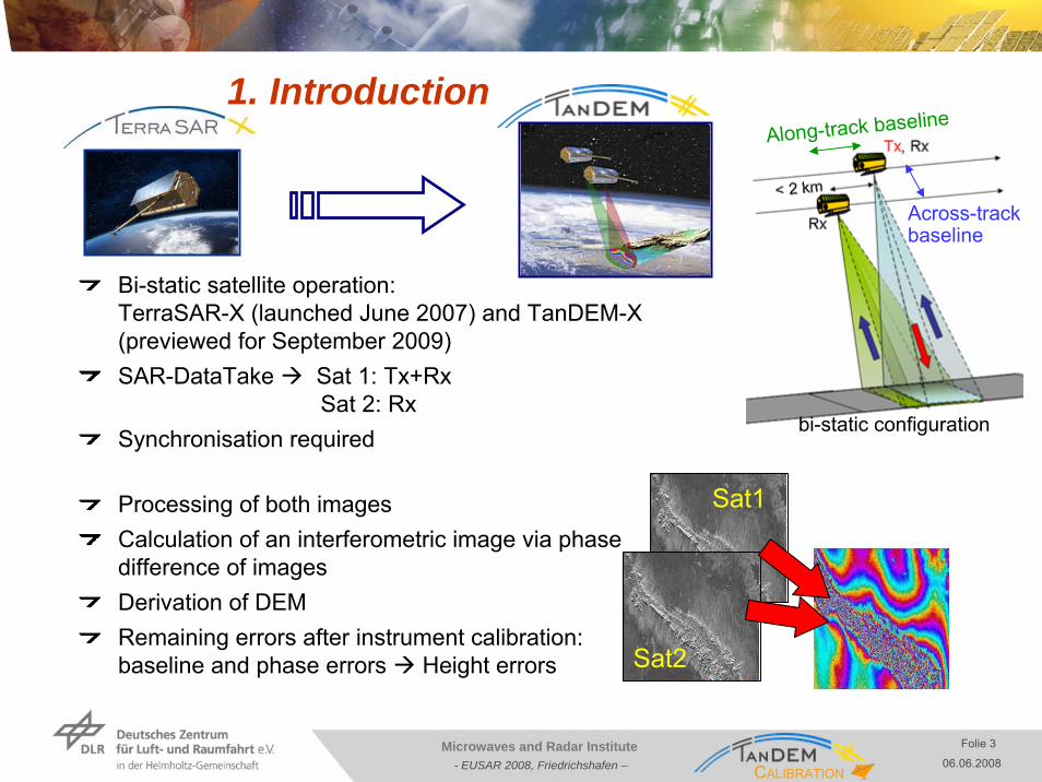
1. Introduction

bi-static configuration

Along-track baseline

Across-trackbaseline

Sat2

Sat1Processing of both imagesCalculation of an interferometric image via phase difference of imagesDerivation of DEMRemaining errors after instrument calibration: baseline and phase errors Height errors

Bi-static satellite operation: TerraSAR-X (launched June 2007) and TanDEM-X (previewed for September 2009)SAR-DataTake Sat 1: Tx+Rx

Sat 2: RxSynchronisation required



2. Objectives – DEM Calibration

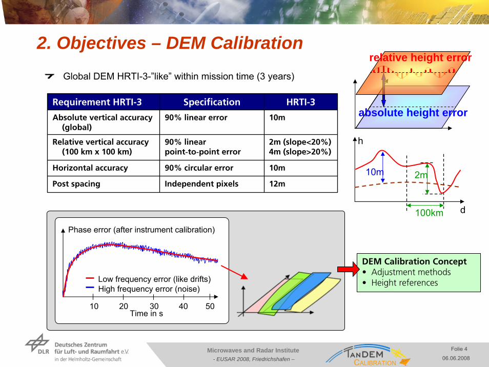
DEM Calibration Concept• Adjustment methods• Height references

Requirement HRTI-3 Specification HRTI-3

Absolute vertical accuracy (global)

90% linear error 10m

Relative vertical accuracy (100 km x 100 km)

90% linear point-to-point error

2m (slope<20%)4m (slope>20%)

Horizontal accuracy 90% circular error 10m

Post spacing Independent pixels 12m

Time in s

Phase error (after instrument calibration)

Low frequency error (like drifts)High frequency error (noise)

10 20 30 40 50

d

h

10m

100km

2m

absolute height error

relative height errorGlobal DEM HRTI-3-”like” within mission time (3 years)



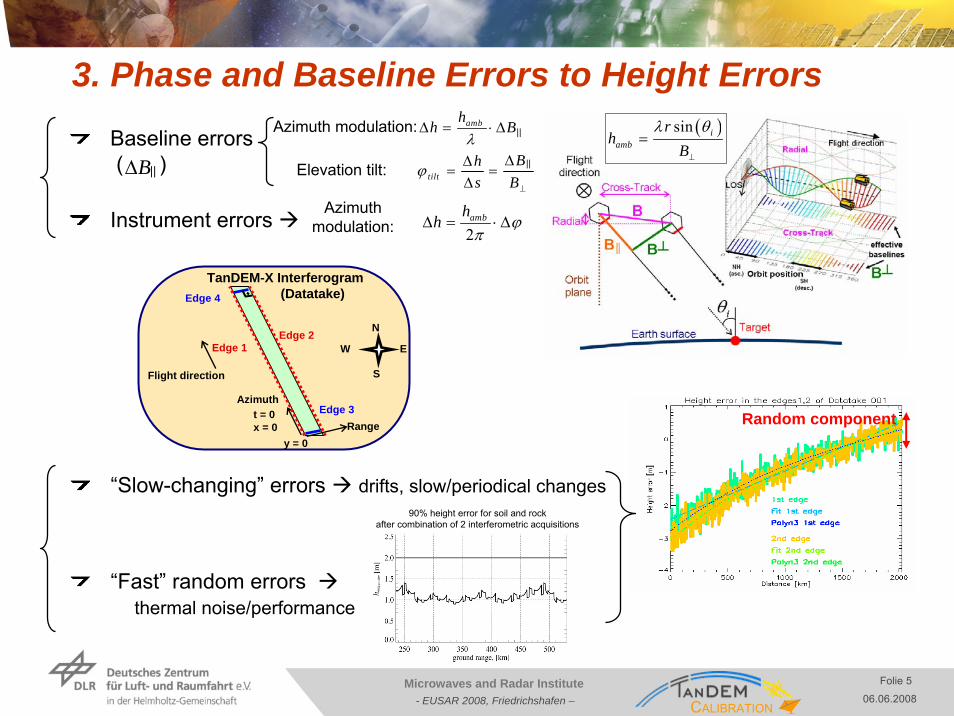
“Slow-changing” errors drifts, slow/periodical changes

“Fast” random errors thermal noise/performance

Baseline errors( )

Instrument errors

3. Phase and Baseline Errors to Height Errors

Random component

( )sin iamb

rh

Bλ θ

⊥

=

2ambh

h ϕπ

Δ = ⋅ Δ

ambhh B

λΔ = ⋅ Δ

BΔ tiltBh

s Bϕ

⊥

ΔΔ= =Δ

90% height error for soil and rockafter combination of 2 interferometric acquisitions

S

W E

N

Edge 3

Edge 1Edge 2

Edge 4

Flight direction

t = 0x = 0

y = 0

Azimuth

Range

TanDEM-X Interferogram(Datatake)

Azimuth modulation:

Elevation tilt:

Azimuth modulation:

||

||

||



Random errors (1.5m) almost exhaust all the relative height error specification (2m)Assumptions:

DEM is calibrated in absolute height (Height references)Processing solves most of the phase unwrapping errors

Rest of the remaining errors have a systematic natureExample:

1 mm ΔB║ height offset of 1.1 m in the datatakeTranslated to specification region (100 km × 100 km) potential non-complianceThe vertical displacement and the tilt in range would also directly follow the time evolution of the parallel baseline error

3. Phase and Baseline Errors to Height Errors (cted.)

Height Errors (for hamb=35m)

ΔB ⎢⎢ = 1mm ΔB ⊥ = 1mm

Δh Δh/Δs (tilt) Δh (h=9km)

30° 260 m 3.8 mm/km 3.5 cm

45° 439 m 2.3 mm/km 2.1 cm1.1 m

Incident Angle

Normal Baseline(hamb=35m)

Necessity of DEM Calibration absolute : height referencesrelative : overlapping regions of DEMs



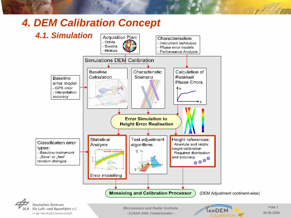
4. DEM Calibration Concept4.1. Simulation

t

Φ

t

Φ

Random componentRandom component

(DEM Adjustment continent-wise)



4. DEM Calibration Concept4.2. Error Modeling

Statistical study of the systematic height error behaviourin different zones (latitudes)

Confirmed assumptions regarding height error evolution (see table)Therefore 2D height error evolution can be approximated

by functional descriptionsStatistical analysis derive coefficients of the following

functional model (to be implemented in the MCP)

Least-squares adjustment with constraintsPrinciple: heights in overlapping areas should be nearly identical

after correction correction parameters can be found independent from terrain types

Height errorevolution

Azimuth Range

Fitting function

3rd order polynomial

linear( ) 2 30 1 2 3 1,g x y a a x a x a x b y k x y= + ⋅ + ⋅ + ⋅ + ⋅ + ⋅ ⋅

Height error in azimuth line Height error in range line

S

W E

N

Edge 3

Edge 1Edge 2

Edge 4

Flight direction

t = 0x = 0

y = 0

Azimuth

Range

TanDEM-X Interferogram(Datatake)



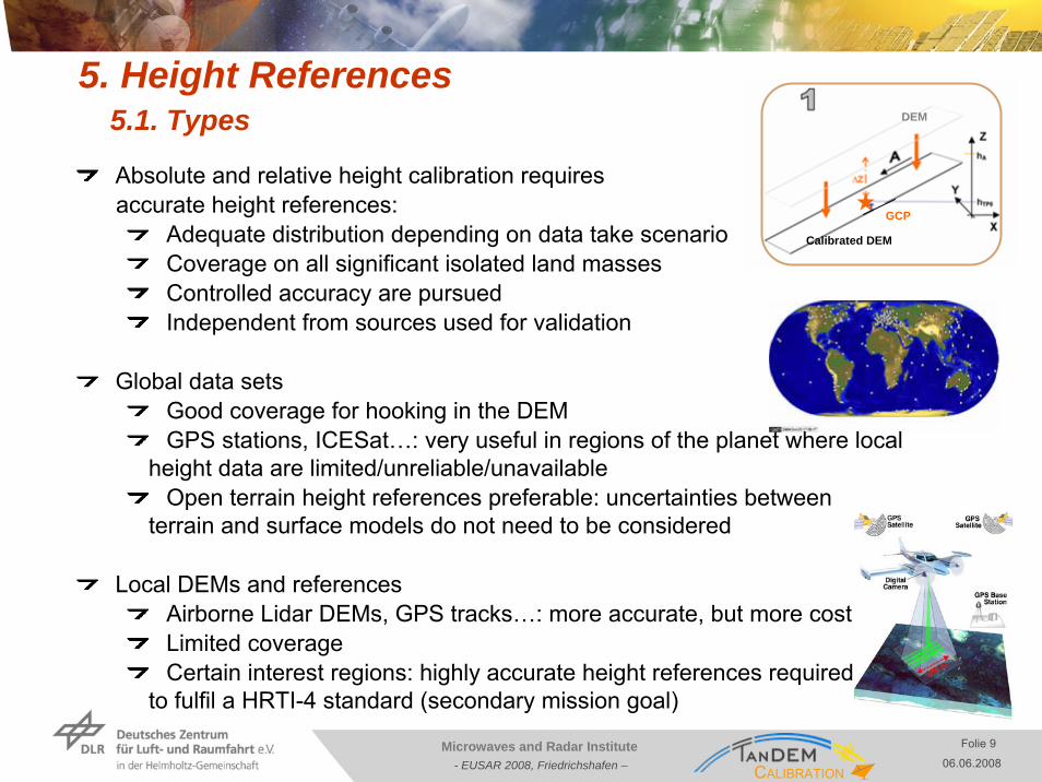
5. Height References5.1. Types

GCP

DEM

Calibrated DEM

Absolute and relative height calibration requiresaccurate height references:

Adequate distribution depending on data take scenarioCoverage on all significant isolated land massesControlled accuracy are pursuedIndependent from sources used for validation

Global data setsGood coverage for hooking in the DEM GPS stations, ICESat…: very useful in regions of the planet where local

height data are limited/unreliable/unavailableOpen terrain height references preferable: uncertainties between

terrain and surface models do not need to be considered

Local DEMs and referencesAirborne Lidar DEMs, GPS tracks…: more accurate, but more costLimited coverageCertain interest regions: highly accurate height references required

to fulfil a HRTI-4 standard (secondary mission goal)



5. Height References5.2. ICESatSatellite with a laser altimeter (GLAS) , Launched in January 2003performing global elevation measurements of land, sea and iceElliptical footprints of 60 m diameter, 170 m in along track distance, 80 km across track separation; 91 day repeat cycleGood absolute accuracy: < 0.5 m (slope < 3 m)

< 1.0 m (slope < 10 m) Slopes determinable from ICESat products

Bibliography:J. Abshire, et al. “Geoscience Laser Altimeter System (GLAS) on the ICESat Mission:

On-orbit measurement performance”, Geophysical Research Letters, Vol. 32, 2005.E. Rodriguez, et al. “An assessment of the SRTM topographic products”,

Technical Report JPL D-31639, Jet Propulsion Laboratory, Pasadena, California, 143 pp.

Improved DEM accuracy as a secondary mission goal (HRTI-4 standard)ICESat database can be applied

Global coverage(actually over 1 billion measurement points)



5. Height References5.3. ICESat Data ApplicationMain height reference source for TanDEM-XElliptical footprints of 60 m diameterPulse characteristics

Decomposed in 6 Gaussians1 peak (flat ground)More peaks (trees, slope,scattering)

ICESat Data Packet Parameters:Evaluation and classification informationfor each measurement point

DEM heightSRTM heightN. PeaksSigma width/saturationSlopeCloud layersSurface propertiesRegion type

Additionally MODIS vegetation coverage data

61 m

47 m

16 Raw DEM pixel



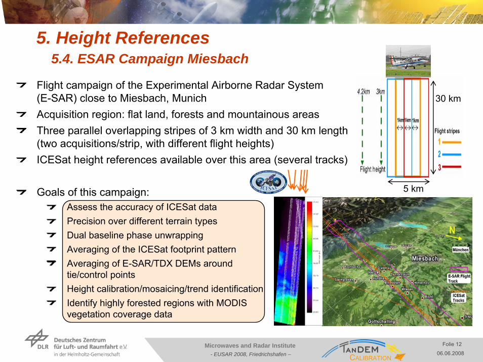
5. Height References5.4. ESAR Campaign Miesbach

Flight campaign of the Experimental Airborne Radar System (E-SAR) close to Miesbach, MunichAcquisition region: flat land, forests and mountainous areasThree parallel overlapping stripes of 3 km width and 30 km length(two acquisitions/strip, with different flight heights)ICESat height references available over this area (several tracks)

Goals of this campaign:Assess the accuracy of ICESat dataPrecision over different terrain typesDual baseline phase unwrappingAveraging of the ICESat footprint patternAveraging of E-SAR/TDX DEMs around tie/control pointsHeight calibration/mosaicing/trend identificationIdentify highly forested regions with MODIS vegetation coverage data

5 km

30 km



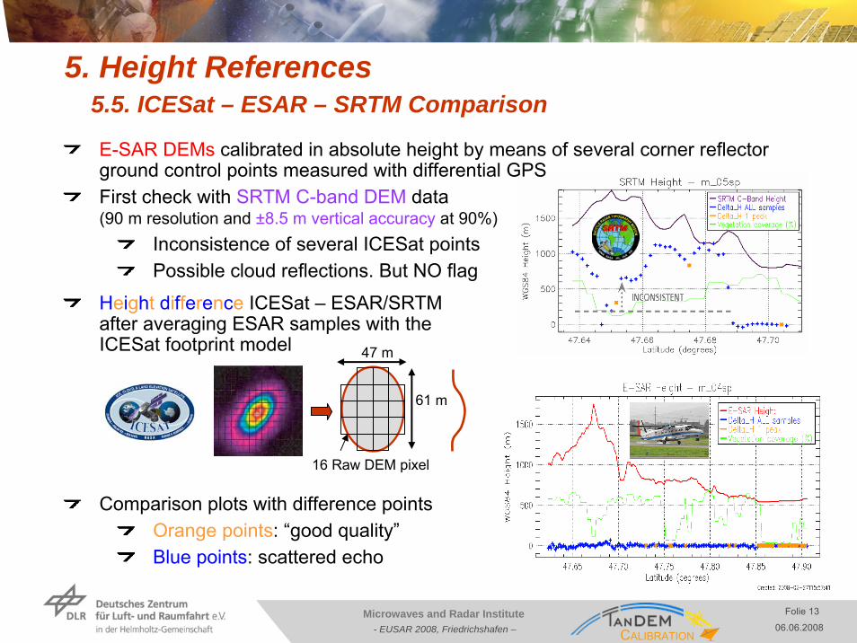
5. Height References5.5. ICESat – ESAR – SRTM Comparison

61 m

47 m

16 Raw DEM pixel

E-SAR DEMs calibrated in absolute height by means of several corner reflector ground control points measured with differential GPSFirst check with SRTM C-band DEM data(90 m resolution and ±8.5 m vertical accuracy at 90%)

Inconsistence of several ICESat pointsPossible cloud reflections. But NO flag

Height difference ICESat – ESAR/SRTMafter averaging ESAR samples with theICESat footprint model

Comparison plots with difference pointsOrange points: “good quality”Blue points: scattered echo



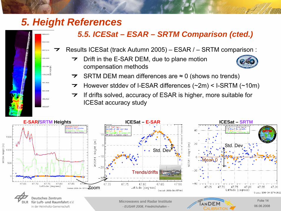
5. Height References5.5. ICESat – ESAR – SRTM Comparison (cted.)

Results ICESat (track Autumn 2005) – ESAR / – SRTM comparison :Drift in the E-SAR DEM, due to plane motion compensation methodsSRTM DEM mean differences are ≈ 0 (shows no trends)However stddev of I-ESAR differences (~2m) < I-SRTM (~10m)If drifts solved, accuracy of ESAR is higher, more suitable for ICESat accuracy study

ICESat – SRTMICESat – E-SARE-SAR/SRTM Heights

Zoom

Std. DevStd. Dev

Mean 0

Trends/drifts



5. Height References5.5. ICESat – ESAR – SRTM Comparison (cted. 2)

Statistic SRTM Differences“Good” points have much better results than scatteredBetter than accuracy specificationsValidates ICESat height values, but not exact accuracy

Selection criteria for ICESat Data:1. Inconsistencies pre-selection with SRTM C-Band;

threshold : 200m difference (Web SRTM Database is more accurate than the parameter in ICESat data package)

2. Only good echoes with 1 peak and narrow sigma (threshold)3. If not enough “good” ICESat height samples available in a certain

region: the best “scattered” samples can be extracted by relaxing the n.peaks and sigma thresholds

4. Vegetation, terrain type, saturation, cloud layer parameters as a quality selection criteria (work ongoing)

Δ ICESat – SRTM C-Band Heights (m)

Reliable points (1pk) All points

Track Mean StdDev (1σ) Mean StdDev (1σ)

All -0.002 3.5 -0.061 10.0



6. Conclusions Height References6.1. Summary and Fall-back solutions

SRTM (C-Band, X-Band) for coarse absolute height offset calibration of the TanDEM-X DEMMain source of height references in the fine DEM Calibration: ICESatFall-back: Ocean-land Transitions, local Lidar DEMsValidation: GPS Tracks

Function GCP source Coverage Accuracy Quality parameters

PRELIMINARYabsolute height calibration

MAIN absolute and relative height calibration

SECONDARY absolute and relative height calibration

VALIDATION

SRTMC-Band: almost Global (56°S-60°N )X-Band: 56°S-60°N , but big gaps

8.5 m ~ surface slope and roughness

ICESat

Height specifications

0.1 m - 1 m (weather/terrain)

Accuracy info/sampleHRTI-3 (even HRTI-4) –after pre-selection

Ocean-land

Global

Global (theory);restricted to optimal along-track distance and no ocean currents

Local

0.5 m TBD

Lidar/Airborne DEM

0.1 m –0.5 m

HRTI-4

SRTM campaigns; selected regions

GPS tracks 0.5 mHeight specificationsHRTI-3



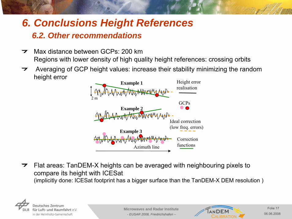
6. Conclusions Height References6.2. Other recommendations

Max distance between GCPs: 200 kmRegions with lower density of high quality height references: crossing orbitsAveraging of GCP height values: increase their stability minimizing the random height error

Flat areas: TanDEM-X heights can be averaged with neighbouring pixels to compare its height with ICESat(implicitly done: ICESat footprint has a bigger surface than the TanDEM-X DEM resolution )

Example 2

Height error realisation

GCPs

Correction functions

Example 3

2 m

Example 1

Azimuth line

Ideal correction (low freq. errors)



7. Outlook

Improvement in the ESAR DEM: more reliable ICESat accuracy studyESAR analysis ICESat selection criteriaOther validation activities related to the ESAR experiment:

Test multi-baseline PUMosaicingTest Mosaicing and Calibration Processor execution chain (functional correction model)Assessment of the X-Band height accuracy over forests.

Laser DEM



End of the presentation

Questions?Suggestions?

tandem-x dem calibration concept and height references08_hueso.pdf · schwerdt, folie 12...

Documents