tangled webs evolutionary dynamics on fitness landscapes ... · pdf filetangled webs...

TANGLED WEBS

Evolutionary Dynamics on Fitness Landscapes with Neutrality

MSc Dissertation

Lionel Barnett ([email protected])

MSc in Evolutionary and Adaptive Systems, Summer, 1997

Supervisor: Inman Harvey ([email protected])

School of Cognitive Sciences

University of East Sussex

Brighton

L. Barnett - Tangled Webs 2

Contents

Abstract

1. Introduction

2. Landscape Structure

2.1. Measuring Neutrality

2.2. The Auto-correlation Function

3. Abstract Landscapes Models with Neutrality

3.1. The NKp Family of Correlated Landscapes with Neutrality

3.2. The RNN Family of Landscapes - Walking the Hypercube

4. Population Dynamics

5. Simulation results

5.1. Population Dynamics on RNN Landscapes

5.2. Population Dynamics on NKp Landscapes

6. Conclusions

Acknowledgements

References

Figures

Appendix A

Appendix B


After a while your adversaries and

competitors will give up trying to think of

alternative hypotheses, or else will grow old

and die, and then your hypothesis will become

accepted. Sounds crazy, we know, but that's

how science works!

- Numerical Recipes in C


Abstract

The bulk of research on the dynamics of populations of genotypes evolving on fitness landscapes hasconcentrated on the rôle of correlation and landscape ruggedness as a putative indicator of thequalitative dynamics. There is, however, a small but growing awareness amongst populationgeneticists (through Motoo Kimura's Neutral Theory of molecular evolution [16, 3]) and molecularbiologists (Eigen, Schuster, et. al.[5, 2, 18]) of the importance of neutral mutation as a significantfactor in evolutionary dynamics. This awareness has thus far not extended to the GA community. Ofparticular interest is the notion of neutral networks of selectively neutral genotypes which percolate afitness landscape - recent work on RNA folding landscapes characterises their structure in terms ofsuch networks [21, 6, 20, 12, 13, 1]. There is at present a lack of computationally tractable abstractmodels demonstrating neutralit y. In this paper we introduce two parametrised families of abstractlandscapes: the NKp landscapes, based on the NK family of abstract landscapes [15], allow tuning ofthe degree of neutralit y whilst leaving invariant the auto-correlation function [24, 23, 15]. The RNN(Random Neutral Network) landscapes, constructed by mutually-avoiding random walks, featurepercolating neutral networks of specifiable size and neutral dimension. The statistical structure ofthese landscapes is examined and related to the characteristic dynamics of populations evolving onthem. Several conjectures regarding the auto-correlation function on NKp landscapes (relevant also toNK landscapes) are raised. Attention is drawn to the very different nature of population dynamics onlandscapes with percolating neutral networks as compared to the dynamics on rugged multi -peakedlandscapes. Qualitative similarities between population dynamics on RNN landscapes and RNAfolding landscapes are highlighted. Finall y, implications for biological research and for theapplication of GA's to optimisation problems are discussed.

1 Introduction

With the introduction of the notion of a fitness landscape by Sewall Wright evolutionary theoryacquired a powerful and intuiti vely appealing metaphor. But a fitness landscape, it must be stressed, isabove all an abstraction. Fitness landscapes do not exist in the world of real biology (or indeed realengineering or real chemistry). The basic idea of the abstraction is that the potential for reproductionof evolving entities can somehow be quantified - that we can attach a number to a genotype and thatthis number specifies, according to some (probably stochastic, iterative) algorithm, the number ofcopies of that genotype that we can expect to find in the next generation of genotypes. But does natureattach numbers to genotypes? Does nature run iterative stochastic algorithms? These questions mayseem frivolous, but they beg serious consideration. How, for instance, are we to attach a "fitness" tothe genotype of a real organism if we cannot possibly take into account the enormous complexity ofthe physical world which will ultimately decide how many offspring that organism really does have?

A common approach to this dilemma deploys what one might term "black box" models - we admitthat we cannot know the inner workings of the real world in all it s stupendous detail , but that on somegross level the criti cal phenomena involved are amenable to a statistical description. This is preciselythe approach taken in statistical mechanics. We don't attempt to describe what every particle in a gasis doing at each moment; we speak, instead, of statistical properties of the ensemble of particles - oftemperature, pressure and entropy. We use the language of probabilit y, of random variables. Likewisein constructing an NK landscape [15], we are saying: "I don't know the precise fitness contribution ofan allele, or the configuration of epistatic linkage, so I'll approximate these things by assigning themat random". The hope is that (perhaps with the Central Limit Theorem on our side) we will t hus endup with a model that reflects at least some characteristics of the real world. The landscape models inthis study are of this nature and should be understood in this spirit.

Another approach, applicable where the physics of the system under investigation is tractable toexperimental analysis, is to construct fitness landscapes and evolutionary algorithms modelled asprecisely as is feasible on the physical system. RNA folding landscapes [22] and flow-reactor models[13, 6] fall into this category.


Ultimately the only resolution of these issues lies in the acceptance of fitness landscapes as abstractmodels that are significant, not in their own right, but only insofar as they assist us in understandingand predicting the world as it reall y is. Like any mathematical model our models may be "interesting"or even "beautiful"; they may acquire a cachet, a li fe of their own in the scientific conciousness, butare they useful? The real space-time continuum is not a Riemannian manifold, real photons are notoperators on a Hilbert space; but these abstractions have been enormously successful in helping usmake sense of the real space-time continuum, of real photons. So may it be with fitness landscapes.

Fitness landscapes suggest a methodology for analysis of the dynamical process that characterises anevolving system: if a fitness landscape is indeed a reasonable abstraction then an evolving system maybe modelled as a quantifiable stochastic process on some abstract landscape. As such, we may expectit to be constrained by the statistical properties of the landscape. The question then arises: whatstatistical features of a fitness landscape are relevant to the dynamics of a population evolving on thatlandscape, and in what manner do they constrain the dynamics?

In attempting to address these questions a picture has become somewhat ingrained in the collectivemind of biologists and GA researchers ali ke, of a fitness landscape as a rugged terrain distinguishedby peaks of relatively high fitness separated by valleys of relatively low fitness [15]. This picture leadsto the view of evolutionary dynamics on such a landscape in terms of the following scenario: selectionpressure will t end to pull a population up the highest hill it chances upon, while genetic operators(mutation, recombination, etc.) counteract this tendency by scattering new genotypes around thelocality of the population.

But this poses a problem which affects both the biologist and the GA speciali st: if selective pressure isstrong enough (relative to the disruptive effects of genetic operators) to drag a population up a hill , itis also li kely to be strong enough to hold it there! How, then, is an evolving population to avoidbecoming "trapped" on a local hillt op? For the GA worker seeking to optimise a multi -peakedfunction this is a practical issue and the literature abounds with schemes to avoid the dilemma [9]. Forthe biologist it is a serious theoretical conundrum, as populations in nature do not seem (in the longrun at least) to suffer this fate [3]. It might be claimed that this can be easil y explained by co-evolutionand environmental change but another possibilit y must be considered - our picture of a fitnesslandscape as a rugged hilly terrain is misleading and in need of an overhaul.

Comparatively recent developments in evolutionary theory and molecular biology have all pointed tothe importance of selective neutralit y as a significant factor in evolutionary dynamics. This workincludes Motoo Kimura's Neutral Theory of molecular evolution [16, 3], Manfred Eigen's analysis ofmolecular "quasispecies" [5, 2, 18] and recent developments in the understanding of RNA evolutionboth in vitro, in simulation and analyticall y [21, 22, 6, 20, 12, 13, 1]. A picture emerges ofpopulations engaged not in hill -climbing but rather drifting along connected networks of neutralgenotypes, with sporadic jumps between networks. These neutral networks are of particularsignificance if they "percolate" the landscape - i.e. they come arbitraril y close to almost every otherneutral network - for this raises the possibilit y that (given enough time) genotypes of almost anypossible fitness value can ultimately be attained by the population. The scenario of a populationtrapped on a local hilltop vanishes.

It is this new paradigm of evolutionary dynamics which we examine in this paper. It has yet to make asignificant impact on the scientific community; it is hoped that the model landscapes, studies ofpopulation dynamics and analytic techniques presented here may assist in gaining insight into thenature of neutral evolution.

At this point we mention several facets of evolution on fitness landscapes which we specificall yexclude from the ambit of this study - not because they are of no importance to a real understanding ofevolution, but rather that they would introduce complexities beyond what could be dealt with here anddistract from the specific issues we attempt to address. For this we offer no apology, merely the hopethat these caveats may be addressed in future studies.

The first issue is that of static vs. dynamic landscapes. In nature, apart from change of environmentover geological time-spans, evolution is almost always co-evolution and any attempt to model


evolution on a static landscape is bound to be unrealistic. It might be argued that static landscapesmay be acceptable models if the time-scale of environmental change is much greater than that ofevolutionary change and co-evolution is not significant. It is not clear whether this is ever the case innature. All model landscapes in this paper are static.

Secondly fitness, as a mediator of selection for reproduction can surely never be precise in nature -real fitness is noisy - this must be considered distinct from any stochasticity present in the selectionmechanism of an evolutionary algorithm. It is often not appreciated that noise may dramaticall y alterthe dynamics of a complex dynamical system. Our landscapes prescribe, and our evolutionaryalgorithm presumes, a precise and pre-ordained fitness value for every genotype.

Thirdly our genotypes are all binary and fixed-length. The binary restriction is arguably not tooinadequate when it comes to modelli ng systems such as RNA folding; it would probably be woefull ydeficient in a model of RNA or DNA protein coding, where the number of alleli c possibiliti es is vast.The fixed-length restriction could possibly be justified on the grounds that length-change mutationseems to be comparatively rare in nature. Our genotypes are, furthermore, rather short (in the regionof 20 loci); this restriction was imposed by time and computational constraints. It is not clear howsome of the phenomena observed might scale to more realistic sequence lengths.

Next we limit our "genetic operators" to mutation alone. Our genotypes are all haploid andreproduction is asexual. This merits some comment. In the GA literature dating back to John Holland[11, 9] there has been a perception of recombination (crossover) as the driving force behindevolutionary search, with mutation taking a back seat as an insurance policy against permanent alleli closs. It is not clear why mutation has been thus relegated, nor that recombination is necessaril yeffective in search. From the biological point of view there are many organisms for whichrecombination rarely or never occurs during reproduction. Molecular biology, furthermore, offersmany scenarios of non-recombinative reproduction.

Finall y we restrict ourselves to a single "fitness-proportional" evolutionary algorithm. Again, theactual mechanics of selection in natural systems tends to be inscrutable [3], so this choice is motivatedmore through being a standard and comparatively well -understood model than by biologicalconsiderations. It may be noted, though, that in the field of GA's in optimisation [9] one is as li kely toencounter rank-based selective schemes, which appear to offer some advantages over fitness-proportional schemes in optimisation applications. The results in this paper cannot be expected toextend mutatis mutandis to other evolutionary algorithms.

Section 2 introduces the tools that will be used to analyse the structure of our landscapes, particularlyas regards neutralit y. Section 3 introduces two rather different parametrised families of landscapeswith "tuneable" neutralit y and investigates their structure. Section 4 presents some methods foranalysing population dynamics on landscapes with neutralit y and Section 5 applies these methods tothe landscape models introduced in Section 3. Section 6 discusses the results and their implications asregards possible application. Areas for further study are also suggested. Appendix A contains somemathematical calculations, while Appendix B contains a source li sting of the LSCAPE program usedto compute all results contained in this paper.

2 Landscape Structure

Much of the literature on fitness landscape structure deals with the concept of ruggedness of alandscape [15, 24]. Intuiti vely this addresses the question: given two "neighbouring" genotypes on alandscape, how similar are their fitness values li kely to be? The main reason for this emphasis seemsto be the perception of a fitness landscape as a vast hill y terrain, on which an evolving population


samples a comparatively tiny fraction of genotypes at any one time for fitter variants. Evolutionarysearch, if it is not to be random, is li kely to be locali sed in a small neighbourhood within thelandscape. It is then natural to inquire what the chances are of finding a better (i.e. higher fitness)genotype than currently exists in the population, by searching the neighbourhood of the currentpopulation. If fitness values can vary wildly even within small neighbourhoods, it is perceived that thesearch, even locall y, is hardly better than random. If, on the other hand, fitness varies only graduallywithin small neighbourhoods, the possibility exists for local hill-climbing.

It has already been mentioned in the Introduction that there are reasons to believe that this picturemay be misleading when there is large-scale neutralit y, which is frequently the case for bothbiological and artificial fitness landscapes. Nor does it address the issue of how a particularevolutionary algorithm actuall y searches, nor indeed whether local hill -climbing is actuall y desirableat all ... Nevertheless it is a de facto standard technique to analyse landscapes in terms of ruggednessand in Section 2.2 below we introduce the most commonly encountered measure of landscaperuggedness, the auto-correlation function. In Section 3.1 we shall see that on some families of fitnesslandscapes this measure possesses some counter-intuiti ve properties and that consequently it may, onits own, be of limited relevance to evolutionary dynamics. Here a variant of the conventional auto-correlation function taking into account landscape neutralit y is suggested. Before that, in Section 2.1we introduce some analytical measures of landscape neutrality.

All fitness landscapes in this paper are based on fixed-length binary bit-string genotypes. Most of theanalysis and actual landscapes, however, generali se quite straightforwardly to the case of multiplealleles. A fitness landscape G of sequence length N is then formally defined to be a mapping f: QN →R where QN denotes the binary N-hypercube and R is the set of real numbers. By abuse of notationwe generall y identify G with the underlying space QN (so |G| = 2N) and refer to the mapping f as thefitness function. The fitness of a genotype g G∈ is then given by f(g). We will often simply refer to a

fitness landscape G, the fitness function f(...) being implicitly assumed.

There is a natural metric, Hamming distance, on QN defined to be the number of loci (bit positions)

at which two genotypes differ. Precisely, h g g g gii

N

i( , ' ) ( , ' )≡=∑ δ

1

where gi denotes the allele (0 or 1)

at the i-th locus of g and δ( , )a bif a b

if a b≡

=≠

1

0 Hamming distance thus introduces a structure of

localit y on a fitness landscape1. Hamming distance is often referred to in terms of mutation. If h(g,g')= d we say that g' is a (d-bit) mutation of g' (and vice-versa, since the relationship is symmetric). Wealso sometimes say that g and g' are (d-bit) neighbours.

A point of confusion worth addressing at this stage is that measures of landscape structure are oftentreated as statistical quantities associated with random variables when they are, in fact, precisely

defined quantities associated with a particular landscape. An example might be the mean fitness f ofa fitness landscape. This is simply a real number associated with a landscape, defined by

fG

f gg G

≡∈∑1

| |( ). It is, however, often treated as the mean, or expected value (in the sense of

probabilit y theory) of a putative random variable, presumably the fitness function f itself! But f is

evidently not a random variable, so f cannot be a mean in the sense of probabilit y theory. There aretwo distinct (and often confused) senses in which f might be treated as a random variable. The first is

that the sum over G in the definition of f may be practicall y impossible to compute, due to the size

(2N) of G. Hence in practice f is estimated by summing over a sample of genotypes in G. This

suggests defining a (discrete) random variable F, say, by setting P( )| |

| |F x

G

G

x

= ≡ where

{ }G g G f g xx ≡ ∈ =| ( ) . In this sense f as defined above is indeed the mean of the random variable F.

1 It is sometimes claimed that if other genetic operators than mutation are being discussed Hamming distance may not be the mostnatural or suitable metric structure for a landscape. This point is, however, open to debate...


However, f is often intended to be something quite different; namely, it is often the case that aparametrised family Γ = { Gλ, λ', λ'', ...} of fitness landscapes is being discussed, where the parametersλ, λ', λ'', ... are themselves (jointly distributed) random variables (which may be discrete orcontinuous). For example the ensemble of all NK landscapes for fixed N and K fall s into thiscategory, where the λ's correspond to the configuration of epistatic links and the fitness table values

(see Section 3.1 below). Then we can consider f to be a random variable over the sample space Γ andits mean, variance, etc. are well -defined. We attempt to maintain this distinction by using angle-

brackets for this latter case - we would thus write not f but < f > or even < f >Γ if we wish to makethe dependence on the parametrised family Γ clear.

2.1 Measuring Neutrality

Given a fitness landscape G we describe a (1-bit) mutation (g,g') as neutral iff f (g) = f(g'). Thisinduces a natural partitioning of G, whereby g and g' are in the same equivalence class iff there is asequence of neutral mutations connecting g and g'; i.e. there are genotypes g ≡ g(0), g(1), g(2), ... g(n) ≡g' such that g(α) is a 1-mutant neighbour of g(α - 1) for α = 1, 2, ... n and f(g) ≡ f(g(0)) = f(g(1)) = f(g(2))= ... = f(g(n)) ≡ f(g'). The neutral networks of the fitness landscape are defined to be the equivalenceclasses of this partitioning. Note that we could define a "coarser" partitioning of G by specifying g andg' to be in the same class iff their fitness values are equal. Under the metric induced by Hammingdistance the neutral networks are just the connected components (in the topological sense) of theequivalence classes of this coarser partitioning2.

A word of caution - the "network" terminology may well be misleading. If the frequency of neutralmutation is low, there are li kely to be very many neutral networks comprising a few, or even singlegenotypes. Even if there is high neutralit y the neutral networks may not resemble networks as muchas large clusters.

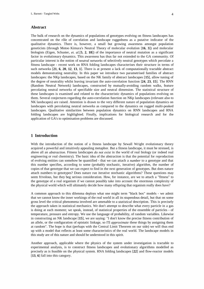
Given a genotype g ∈ G we define the neutral dimension of g to be the number of neutral mutationsof g minus 1. The reason for subtracting 1 is to facilit ate the image of a neutral network of givendimension, where we define the neutral dimension of a neutral network to be the mean of the neutraldimensions of its constituent genotypes (see Figure 2.1.1).

Since the neutral dimensions of the genotypes along a neutral network may vary, we will also beinterested in the variance of neutral dimension over a neutral network. In Section 4 we will see thatneutral dimension turns out to be of particular significance to population dynamics on a landscapewith high neutrality.

We would li ke to quantify the degree to which a neutral network "percolates" the fitness landscape.From the point of view of population dynamics, the question of interest is how many new"phenotypes" or fitness values can be reached within one (or a few) mutations of the network. Thuswe define the percolation index (at distance d) of a neutral network to be the fraction of possiblefitness values attainable within at most d mutations of some genotype on the network.

Precisely, we define the percolation index πH(d) of a neutral network H ⊂ G to be H d

F

( ) where

{ }H d f g g G and g H with h g g d( ) ( ) | ' ( , ' )≡ ∈ ∃ ∈ ≤ and { }F f g g G≡ ∈( ) | . πH(d) is, unfortunately,

expensive to compute in practice as it involves tabulation of all possible fitness values and thetraversal of the entire neutral network. Huynen [12] has defined a stochastic procedure whichmeasures the "innovation rate" along a random walk on a neutral network. The idea is to enumeratenew fitness values or "innovations" encountered (i.e. which are ≤ d mutations away from the current

2 In the RNA folding literature it is sometimes effectively this coarser partitioning that is used to define neutral networks, which thusneed not be connected. In all fitness landscapes encountered in this paper the two partitionings generally "almost" coincide, and wesometimes conveniently confuse them...


genotype) on such a "neutral walk". The number of innovations may then be compared with thenumber of innovations on a random walk of the same length. The ratio of these numbers, whenaveraged over a large number of walks should then be roughly comparable with πH(d) as definedabove3.

In Section 3 we will analyse the neutral network structure of our model landscapes in terms of thedistributions of size, percolation index π(1), mean neutral dimension and neutral dimension varianceamong the neutral networks on the various families of landscapes4. We also calculate theoreticall ywhere possible the probability that an arbitrary mutation is neutral.

2.2 The Auto-correlation Function

The auto-correlation function makes precise the notion of how similar nearby genotypes are in afitness landscape. It is often defined in terms of fitness values at successive steps along random walkson the landscape [24, 15] but, as remarked in [23] "...it seems to be rather contrived to invoke astochastic process in order to characterise a given function [i.e. the fitness function] defined on a finiteset". We thus use the definition below, apparently first proposed in [5].

We first define the mean fitness of the landscape

Eq 2.2.1 fG

f gg G

≡∈∑1

| |( )

the fitness variance

Eq 2.2.2 ( )σ fg G

Gf g f2 21

= −∈∑| |

( )

and for d = 1, 2, ... N the set

Eq 2.2.3 { }G d g g G G h g g d2 ( ) ( , ' ) | ( , ' )≡ ∈ × =

Thus G2(d) is the set of pairs of genotypes in G Hamming distance d apart. Note that

G dN

dG2 ( ) | |=

⋅ since there are

N

d

ways of flipping d loci of a bit-string of length N.

We now define for d = 1, 2, ... N the auto-correlation function to be:

Eq 2.2.4 ρσ

( )( )

( ( ) )( ( ' ) )( , ') ( )

dG d

f g f f g ff g g G d

≡ − −∈∑1

2 22

For consistency we also define ρ(0) ≡ 1. For computational purposes we can estimate f , σf2 and ρ(d)

by sampling subsets of G and G2(d). The basic properties of ρ(d) are that on a flat fitness landscape (f= constant) ρ(d) = 1 for all d (in the limit at least, since the formula yields 0/0 !) while on acompletely uncorrelated landscape ρ(d) will be close to 0. This can be made precise in the followingmanner: introducing the family Γ of landscapes where each G ∈Γ is specified by assigning fitness

3 This should at least be the case if the neutral network is "network-like". If it is more like a "clump" than a network, then neutralwalks are likely to encounter comparatively fewer "innovations" and may not be a good indicator of percolation index as definedhere.4 For these landscapes the genotypes of zero fitness constitute a special case. Thus we generally omit the zero-fitness genotypes fromour analysis of neutral networks.


values independently and uniformly randomly from [0,1] to each genotype, we have <ρ(d)>Γ = 0 (c.f.the closing paragraph in the introduction to this Section).

The auto-correlation function has been quite thoroughly studied for some classes of landscapes [23,24]. In particular, for a large family of "elementary" landscapes [23], the auto-correlation isexponential of the form ρ(d) = a-d for some constant a, and there is thus a natural "correlation length"for the landscape5.

As we shall see in Section 3.1, in the presence of large-scale neutralit y the auto-correlation functionappears to be inadequate on its own as a measure of landscape structure. The effect of neutralit y onthe correlation structure is indeed by no means clear-cut. If a landscape features extensive percolatingnetworks, and particularly if they are of high neutral dimension, then on the one hand it might beexpected that the correlations introduced by neutral mutations would tend to boost the correlation ofneighbouring genotypes - effectively "smoothing" the landscape. On the other hand, percolationsuggests that there is a high li kelihood that genotypes of possibly uncorrelated fitness on differentneutral networks can end up close together, with the effect of increasing ruggedness. In the nextsection we will see evidence that both these effects can occur, and indeed may even appear to "canceleach other out".

Nonetheless, there is evidence from RNA folding landscapes that percolating neutral networks and asignificant correlation structure may well cohabit on a landscape [13, 12]. What seems to be requiredis a refinement of the auto-correlation function which takes neutrality into account.

One possibilit y that suggests itself is that in the definition of ρ(d), rather than averaging over the setG2(d) defined in Eq. 2.2 3, we use instead the "no neutrals" alternative:

Eq 2.2.3a { }G d g g G G h g g d and f g f gnn2 ( ) ( , ' ) | ( , ' ) ( ) ( ' )≡ ∈ × = ≠

Thus we measure correlation of fitness of neighbouring genotypes picked from different neutralnetworks. Preliminary investigation suggests that an auto-correlation function defined in terms of thisset may prove useful in characterising landscape structure, if considered in conjunction with thepercolation index and neutral dimension6.

3 Abstract Landscapes Models with Neutrality

In this Section we introduce the landscape models on which our studies of evolutionary dynamics willbe based.

3.1 The NKp Family of Correlated Landscapes with Neutrality

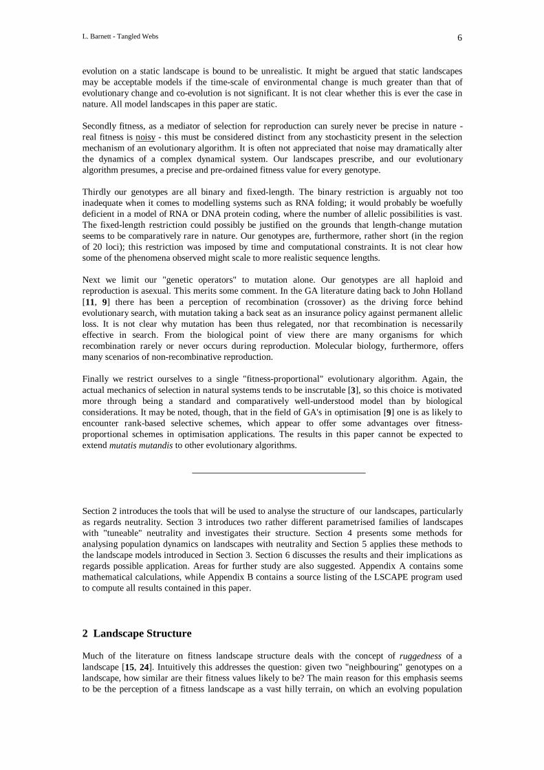
We begin by reviewing the construction of an NK landscape [15]. Let N > 0 be the length of the(binary) genotype and let 0 ≤ K < N. N and K are fixed during the construction. To each locus on thegenotype (corresponding to a position 1 ≤ i ≤ N on the bit-sting) we assign independently and atrandom K distinct loci (excluding the locus under consideration) - these loci are said to beepistatically linked to the locus i. The idea is that a locus i makes a contribution to the total fitness ofthe genotype which depends on the value of the allele (0 or 1) at i and the values of the alleles at eachof the K loci epistaticall y linked to locus i. To each such combination of alleles (there are 2K+1 in all ) afitness contribution is assigned as a real number drawn independently and uniformly at random from

5 Contrary to popular belief the correlation function on NK landscapes is not exponential in form, although it does resemble anexponential for large K values. See Section 3.1 for more on this topic.6 Preliminary tests also demonstrated that this "no neutrals" variant can, unlike the conventional function, distinguish between NKplandscapes (see Section 3.1) with different values of p.


the range [0,1]. We can think of this as the association of a fitness table Fi with each locus i. Giventhe sequence of alleles σ = a1 a2... aK+1 at the loci epistaticall y linked to locus i, the fitness contributionof locus i is then given by Fi(σ). Figure 3.1.1 ill ustrates the situation. Here N = 16, K = 3 and thelocus under consideration is at i = 5. The red arrows indicate epistatic links and a segment of thefitness table for locus 5 is pictured. For the genotype ill ustrated the sequence of alleles for locus 5 is σ= 0110 and the corresponding entry in the fitness table is F5(σ) = 0.305687.

Finall y, to calculate the fitness of an entire genotype the fitness contributions of all l oci are summedand the result divided by N (the genotype length) to scale the fitness to the range [0,1]. In the abovenotation, if g is a genotype and σi(g) the sequence of alleles at the loci epistaticall y linked to locus i ong, its is given by:

Eq 3.1.1 f gN

F gi ii

N

( ) ( ( ))==∑1

1

σ

In summary, an NK landscape is full y specified by N, K, the particular assignment of epistatic linksand the contents of the N fitness tables.

The statistical properties of NK landscapes have been widely studied [15], and in particular the auto-correlation measure for NK landscapes is fairly well understood. The general picture is that for K = 0an NK landscape is highly correlated. As K is increased the correlation drops off until for K = N-1 thelandscape is completely uncorrelated.

It is clear from the construction procedure that there is (almost surely) no neutral mutation on an NKlandscape - for if two genotypes differ at some locus the respective fitness contributions for that locuswill be drawn from different fitness table entries which will (almost surely) be different. There is,however, a "natural" way to introduce neutralit y into the model, via by the following biologicall y-inspired argument: the NK model assumes that every possible combination of alleles at the lociepistaticall y linked to a given locus gives rise to a positi ve contribution to genotype fitness. In nature,however, it seems li kely that many (if not most) combinations of alleles will make no contribution tofitness (or be "lethal"). We could reflect this in the NK model by specifying that the fitness table entrycorresponding to such an alleli c combination be equal to zero. Thus motivated we proceed as follows:a new parameter 0 ≤ p ≤ 1 is introduced to represent the probabilit y that an arbitraril y alleli ccombination makes no contribution to fitness. Explicitl y, when assigning values to the fitness tableswe set each entry to 0 independently with probabilit y p. If an entry is not set to zero it is assigneduniformly randomly from the range [0,1] as before. We refer to the resulting landscape as an NKplandscape. The case p = 0 corresponds to a normal NK landscape, while p = 1 corresponds to acompletely flat landscape (all fitness table entries are zero).

It is evident that the possibilit y of neutral mutation arises in NKp landscapes. A calculation (seeAppendix A.1) yields for the probability that an arbitrary mutation be neutral:

Eq 3.1.2 p pK

Npneutral

N

= −−

−

−2 2

1

11

1( )

For large N (long genotypes) this is well approximated by:

Eq 3.1.2' p p K pneutral e≈ −−2

21( )

Thus the probabilit y of a mutation being neutral is roughly independent of the genotype length forlong genotypes. Figure 3.1.2 plots pneutral (as calculated from Eq 3.1.2) against K and p for N = 30.

We now examine the expected number of neutral mutations per genotype. Since at each genotypethere are N possible 1-bit mutations, the expected number of neutral mutations at each point in thelandscape is Npneutral. The problem is that while this gives us the average number of neutral mutations


per genotype it does not tell us how this quantity is distributed over the landscape, particularly withregard to fitness.

For a genotype g let us set n(g) = number of neutral mutations at g, and ζ(g) = number of loci on gwhich make zero contribution to the fitness of g; i.e. which yield a zero in the i-th fitness table. We

have immediately that f gg

N( )

( ).≤ −1

ζ But for a mutation at i to be neutral g must necessaril y have a

zero in its i-th fitness table. Thus:

Eq 3.1.3 n(g) ≤ ζ(g) ≤ N(1-f(g)).

This implies that genotypes with higher fitness values will have a smaller number of neutralmutations.

Figure 3.1.3 plots the distributions of neutral mutations for genotypes falli ng into fitness bands forNKp landscapes with N = 30, K = 4 and p = 0.9. Note that this graph does not represent the jointdistribution of fitness and neutral mutations. Each "sli ce" (corresponding to genotypes within a givenfitness range) plots the distribution of neutral mutations for genotypes within that fitness range. Thefigures were derived from a sample of 1000 genotypes each from 1000 NKp landscapes.

We see that while the individual distributions are bell -shaped in appearance, the distribution meansfall off roughly linearly with increasing fitness as suggested by Eq 3.1.3. The implication is that the"higher up" the landscape we go, the smaller the number of neutral mutations we are li kely toencounter. Furthermore, for genotypes of high fitness a mutant is very li kely to be a genotype withmore zeros in the fitness tables than its neighbour (particularly with high epistasis), and hence ofdramaticall y smaller fitness. Looked at another way, NKp landscapes become in a sense more ruggedwith increasing p.

Figures 3.1.4a-d give the (non-zero fitness) neutral net statistics for N = 18, K = 4 and p = 0.99,presented as joint distributions over fitness. [For small values of p the neutral networks are small andthere is no percolation]. Results are compiled from averages over 100 landscapes. We see from Figure3.1.4a that the neutral networks fall i nto two groups; there are numerous small networks andcomparatively few large ones. The numbers of both fall off with increasing fitness. There is moderatepercolation, again falli ng off with increasing fitness. Neutral dimension also appears to divide intotwo groups; these are li kely to correspond to the large and small groups of networks. Neutraldimension decreases with increasing fitness. Variance of neutral dimension along networks is quitesmall . A remarkable property of the NKp family of landscapes is the apparent invariance of the auto-correlation function with respect to the p parameter in the following sense: recall that the auto-correlation function ρG(d) for a given fitness landscape G is not a statistical measure (Section 2).However, taking as a sample space all NKp landscapes G for fixed N, K and p we may consider theauto-correlation function as a continuous random variable, which we write as ρ(d), or ρN,K,p(d) if wewish to make the dependence on landscape parameters explicit.

Figure 3.1.5 plots <ρ(d)> [the mean of ρ(d)] for N = 30, K=4 and a range of p values. <ρ(d)> wasestimated as follows: for each of a sample of 1000 landscapes, for each d =1 to 15, a sample of 1000pairs of genotypes Hamming distance d apart was taken to estimate ρ(d) for that landscape. The resultwas then averaged over the sample of landscapes to obtain the mean. As can be seen, there is virtuall yno variation of <ρ(d)> with p - this was verified by a standard χ2 test. The same result was obtainedfor a wide range of N, K, p and d values, including p very close to 1. So far an analytic proof hasproved intractable (see also below), but there is suff icient confidence in the result to state it as aformal conjecture:

Conjecture 3.1.1

The mean (estimated value) <ρN,K,p(d)> of ρN,K,p(d) as defined above is independent of p for 0 ≤ p < 1.


It is also worth remarking that the variance of ρN,K,p(d) with respect to p is very low - i.e. <ρN,K,p(d)>provides an excellent estimate of ρG(d) for any particular NKp landscape G, and indeed for a givenNK landscape.

This result is at first sight paradoxical, as we would suspect that the expected high proportion of pairsof genotypes with equal fitness (particularly for p → 1) would tend to produce higher correlationfigures for increasing p. However, as remarked above, the landscape actuall y appears to become morerugged with increasing p and the effects seem to "cancel" each other. In fact what appears to happenis that the covariance of f(g) with f(g') for genotypes (g,g') Hamming distance d apart scales the sameas the variance of f(g) with respect to the p parameter for fixed N and K. This is made more precise inthe following conjecture: let us define, for an NKp landscape G:

cov ( ) ( ( ) )( ( ' ) )( )

( , ') ( )

G d

g g G d

dG

f g f f g f≡ − −

∈

∑1

where { }G g g G G h g g dd( ) ( , ' ) | ( , ' )≡ ∈ × = and fG

f gg G

≡∈∑1

| |( ) is the landscape mean fitness.

Note that this is again not the usual statistical definition of covariance, but a unique number definedfor a landscape G; as for the auto-correlation function, however, we associate a random variablecov(d) = covN,K,p(d) over the sample space of all NKp landscapes. Note that covG(0) is simply the

fitness variance σ fg G

Gf g f2 21

≡ −∈∑| |

( ( ) ) .

Conjecture 3.1.2

For d = 0,..,N

< > = − +cov ( ) ( )( )( ), , ,N K p N Kd d p pφ 1 1 3

for some function φ N K d, ( ) (which doesn't depend on p) and we have:

< > =ρφφN K p

N K

N K

dd

, ,,

,

( )( )

( )0

The second part of the conjecture follows from the definition of the auto-correlation function (Section2.1). The formula was suggested by Conjecture 3.1.1 and a polynomial data fit.

Figure 3.1.6 plots < >cov ( ), ,N K p d from sampled data and for the formula given in Conjecture 3.1.2

against p for d = 0,..,10 for N = 30 and K = 4. Again a standard χ2 test indicated an excellent fit. Notethat the variance/covariance always peaks at 1/3. Figure 3.1.7 plots the factor φ N K d, ( ) for the same

sample.

Finall y, for a "degenerate" NKp landscape, where only one fitness table entry is non-zero, we canexplicitl y calculate the auto-correlation. The result (surprisingly, since there is no obvious reason tobelieve that such a landscape should yield values close to the statistical expectation) turns out to be an


extremely good fit for < >ρN K p d, , ( ) , and we conjecture that this is indeed the case. The calculation is

somewhat lengthy and can be found in Appendix A.2 - here we just quote the result:

Conjecture 3.1.3

For an NKp landscape (and hence an NK landscape, if Conjecture 3.1.1 holds), the (mean) auto-correlation function is given by:

( ) ( )< > =

− − − +

−

ρα β γ

N K p dP d P d d

P PN

d

, , ( )( ) ( ) ( )

( )

1 2 1

1

2

where

α( )dL

dif d L

otherwise

=

≤

0

β α( ) ( )dN

dd=

−

γ ( ) ( )( , ) ( , )

d PN

d

K

k

L

d kMax d L k Min d K

= −

−

+

−

− ≤ ≤ +∑1

1

1 1

and we have set P = 2K+1 and L = N - K - 1.

Figure 3.1.8 plots < >ρN K p d, , ( ) as calculated according to Conjecture 3.1.3 against sampled data for

N = 30, K = 0,..,10. The sampled data comprised 1000 pairs of genotypes for each of 1000 landscapesfor each value of K. Again a χ2 test indicated an excellent fit.

This concludes our analysis of NKp landscapes. As a test-bed for the study of population dynamicsthey provide an interesting family of landscapes for which the correlation structure and degree ofneutrality may (if Conjecture 3.1.1 holds) be independently varied.

Finally, it is hoped that the conjectures in this sub-section may be proved analytically.

3.2 The RNN Family of Landscapes - Walking the Hypercube

The RNN landscapes were designed as a very basic general model of landscapes with neutralnetworks and hopefull y to reflect some characteristics of RNA secondary structure folding landscapes.There are several reasons for wishing to construct simpli fied models for such landscapes. RNAfolding landscapes provide one of the few examples where abstract landscape theory and computersimulations of population dynamics may be brought to bear on a "real biological" scenario, and onewhich is of great importance in molecular biology. One problem with the analysis of existing RNAfolding landscape models, however, is the high computational cost of fitness evaluation - another isthe sheer complexity of the folding algorithms (and hence of any secondary structure-based fitnessfunction) [22]. These factors conspire against abstract analysis of the features of these landscapes


which may be relevant to their population dynamics. Thus it seems worthwhile to have availablecomputationally cheaper and conceptually simpler models.

Previous work has applied random graph and percolation theory to the construction of landscapeswith percolating neutral networks [21, 6, 20]. While these random graph landscapes appear to capturemany of the structural characteristics of RNA folding landscapes, they do not seem to be very"tuneable" with regard to the dimension, size, number and degree of percolation of neutral networks.The RNN family of landscapes allow specification of these properties, although not quiteindependently. They also have some features in common with so-called "holey" landscapes [7, 8].

Again only binary genotypes are considered (although the construction generali ses to arbitrarynumbers of alleles). The actual construction is as follows: let N be the genotype length, and QN thebinary N-hypercube. There are two parameters: a number R > 0 of neutral networks and a neutraldimension D where 1 ≤ D ≤ N. The basic idea of the construction involves choosing R mutually

disjoint D-1 dimensional (sub)hypercubes H Q for r R with H HrN

r r⊂ = ∩ = ∅ ∀α1,.. , .β We

then allow the R hypercubes to perform "simultaneous" mutually- and self-avoiding random walks inQN. This requires some clarification: a "step" on the random walk for a hypercube H consists of aparallel translation of H - all vertices of H step in the same direction. A hypercube of dimension D-1in QN may be identified with a schema [11, 9] of order N-D+1; i.e. N-D+1 bits are defined - thevertices are represented by those bit-strings obtained by replacing the undefined positions of theschema by all possible combinations of 1's and 0's. Then a step is made by flipping one of the definedbits of the schema. E.g. if H = 0*11**011*1* (here N = 12 and D = 6) we might flip bit 4 to getthe new hypercube H' = 0*10**011*1* which is then one step away from H. Figure 3.2.1 ill ustratesthe process for N = 3, D = 2.

Evidently a D-1 dimensional hypercube has N-D+1 "degrees of freedom" to walk. The walks areperformed "simultaneously" by randomly choosing a hypercube to walk at each step. The randomwalks continue until no further steps are possible for any of the hypercubes - i.e. QN has been "fill edup" as far as possible by the walking hypercubes. To complete the construction, for each r we take theset of genotypes Gr traced out by the vertices of hypercube Hr and independently assign them a fitnessfr chosen randomly and uniformly in the range [0,1]. The remaining genotypes in QN are arbitraril yassigned a fitness of 0. The Gr 's (and the genotypes of zero fitness) thus become the neutral networkson our landscape.

The reason we work with D-1 rather than D, is that we would expect the mean neutral dimension (asdefined in Section 2.2) of each neutral network Gr to be approximately D. It may, in fact, be either lessthan or greater than D: if a walk approaches within one mutation of itself additional neutral mutationswill be introduced, raising the local neutral dimension. Random walk theory could perhaps bedeployed to estimate how often this is li kely to happen. On the other hand, the local neutral dimensionat the "ends" of the random walks will be D-1. If a random walk is short its "ends" will contributesignificantly to the mean neutral dimension - this is li kely to happen if either R or D is large, in whichcase many random walks become quickly "boxed in". In practice the variance turns out to be fairlylow. These effects can be observed in the neutral network statistics for N = 18 displayed overleaf inFigures 3.2.2a-d. Here R = 100 (figs. a and c), R = 500 (figs. b and d), D = 4 (figs. a and b) and D =8 (figs. c and d). The data for each histogram represents an average over 10 RNN landscapes.

The percolation index is, as we might expect, comparatively high for small R. The neutral networks inthis case are extremely "tangled" - every network has a good chance of coming within one mutation ofevery other. As we increase R the percolation index drops off, since on the one hand the size of thenetworks decreases, and in addition there are comparatively more neutral networks to get close to.Increasing D also decreases the size of the networks; furthermore the reduced "co-dimension" ornumber of "degrees of freedom" of the networks (given by N-D), restricts their abilit y to intertwine,and hence get close to each other - the networks are less "tangled" than for small D. [An attractiveanalogy is the fact that a length of string may be knotted in three, but not in two dimensions...]

The mean neutral dimension fall s as R increases. This is due to the effects mentioned previously. Thevariance of neutral dimension along the networks is harder to fathom. In general we would expect the


variance to be high for small networks due to the "end effects". On the other hand large networks areli kely to approach within one mutation of themselves quite frequently, thus also increasing thevariance.

A related issue is to what extent QN is li kely to be fill ed up before the walks grind to a halt. Thiswould seem to be a diff icult question to address analyticall y. There is also the practical possibilit y thatthe construction procedure fall s at the first hurdle - it may be diff icult (or impossible) to find any Rhypercubes that are mutually disjoint for large R or D. Figure 3.2.3 plots the average fraction ν of QN

fill ed by genotypes of non-zero fitness for a range of R and D values for N = 18. Figures are averagesover 10 landscapes. Gaps in the graph represent failure of the algorithm7 to place R initial hypercubesof dimension D-1. We see from the graph that the fraction ν fall s off quite sharply with increasing Dand appears to asymptote at roughly ν = 0.2. There is a slight increase in ν with increasing R. Note

that we would expect the mean neutral network size to be roughly ν⋅2N

R. Comparing the size

histograms of Figures 3.2.2a-d with ν derived from Figure 3.2.3 indicates this to be a goodapproximation.

Finall y, we examine the auto-correlation function for RNN landscapes. Figures 3.2.4a and b plot<ρ(d)> (estimated from a sample of 10,000 pairs of genotypes averaged over 25 RNN landscapes), fora selection of R and D values.

It is to be expected that the only correlation present in RNN landscapes will be the correlation offitnesses between pairs of points on the same neutral networks (since the fitnesses of the neutralnetworks themselves are uniformly distributed and hence entirely uncorrelated). As R increases anarbitraril y chosen pair of genotypes a given Hamming distance apart are more and more li kely to beon different neutral nets and their fitness thus uncorrelated. This effect is evident in Figure 3.2.4a.Conversely, as D increases genotypes close together in Hamming distance are increasingly li kely to beon the same neutral network: consider the case d = 1. Here a 1-bit mutation has, on average, a

probabilit y of roughly D

Nof being neutral. A d-bit mutation thus has a probabilit y of roughly

D

N

d

of

being neutral. Again, this trend is demonstrated in Figure 3.2.4b.

For larger Hamming distances (d >> D) RNN landscapes are virtuall y uncorrelated. It must beremarked, however, that the auto-correlation function would seem to be of limited value on RNNlandscapes (and to some extent on any landscape with extensive percolating neutral networks,particularly where the neutral dimension is high). For when there is a high degree of percolation thengiven a genotype, a neighbouring genotype will either lie on the same neutral network (and becompletely correlated in fitness), or will belong to an arbitrary different neutral network (and thus beof uncorrelated fitness). In this context fitness correlation tends to be "all or nothing".

In the following Sections we shall see that on such landscapes the typical population dynamic is ofsuch a nature as to render auto-correlation virtuall y irrelevant. For "intermediate" degrees ofpercolation the modified auto-correlation measure mooted in Section 2 may be more relevant to thedynamics.

7 The construction algorithm employed to collect sample data for this paper tries to place R randomly chosen hypercubes one at atime, discarding a choice if it intersects an already chosen hypercube. If at some stage it fails after 100⋅R attempts to place ahypercube the entire placement procedure restarts. After 10 restarts the construction algorithm times-out and gives up. Failure of this(rather crude) algorithm does not, of course, imply the impossibilit y of finding R disjoint hypercubes - nevertheless there will , itseems, be a point at which a "regular" (rather than random) arrangement of hypercubes will be enforced. The picture is not clear...


4 Population Dynamics

Up to this stage we have deliberately avoided use of the term "phenotype". The reason for this issimply that the concept does not enter into the formal definition of an abstract fitness landscape. Inthis section we do introduce the term for the principal reason that some standard terminology,particularly in the biological lit erature, is very often phrased in terms of "phenotype". In the context offitness landscapes "phenotype" denotes an intermediate level of mapping between genotype andfitness value. Since our abstract landscapes do not (expli citl y) involve such mappings, the reader maysubstitute "fitness " for "phenotype" wherever abstract landscapes, including the models introducedpreviously in Section 3, are discussed. A caveat is that, of course, the phenotype/fitness distinctioncannot in general be ignored in the literature, so our use of the terminology must be viewed as specificto the abstract scenarios dealt with in this paper.

We start with some formal definitions regarding populations of genotypes. In the following let G be afitness landscape of binary genotypes of sequence length N; i.e. a mapping f: QN → R where QN isthe N-dimensional hypercube. As usual we identify G with the underlying set QN.

(1) A (finite) population P on G is a mapping P: G → N where N is the set of integers 0, 1,2, ... Intuiti vely P(g) is the number of copies of g in P. [By abuse of notation we will

sometimes write g ∈ P to mean P(g) > 0, or we simply say "g is in P"]. The size of P is

P P gg G

≡∈∑ ( )

(2) The genotypic support of P is defined to be { }gsupp( ) | ( )P g G P g≡ ∈ > 0 i.e. gsupp(P) is

the set of all genotypes with at least one copy in P.

(3) The phenotypic support of P is defined as { }fsupp gsupp( ) | ( ) . . ( )P f g P s t f g f≡ ∈ ∃ ∈ =R

i.e. fsupp(P) is the set of all fitness values represented by at least one genotype in P. Thereader is reminded that we use the term "phenotype" and "fitness" interchangeably.

(4) Given a fitness value f, define the population Pf to be the sub-population of P comprising

all genotypes with fitness f ; i.e. P gP g if f g f

otherwisef ( )

( ) ( )≡

=0

(5) The genotypic entropy of P is gentropy PP g

P

P g

Pg P

( )( )

| |log

( )

| |( )

≡ −∈∑

gsupp

. It represents

the degree to which the population is "spread" over the landscape. If the entirepopulation were converged to a single genotype the genotypic entropy would yield zero.At the opposite extreme, if no two genotypes in the population were the same, it wouldattain its maximum of log(|P|).

(6) The phenotypic entropy of P is fentropy PP

P

P

P

f

f P

f

( )| |

| |log

| |

| |( )

≡ −∈∑

fsupp

. It represents the

degree to which the population is spread over the various fitness values. If the entirepopulation had the same fitness the phenotypic entropy would be zero. It attains amaximum when the population is maximally spread over the possible fitness values. Iffsupp(P) < |P| this maximum will be log(|fsupp(P)|), otherwise it will be log(|P|).


(7) The dominant genotype of P is the genotype g* such that P(g*) attains a maximum overall possible genotypes8; i.e. g* is the genotypes value with the most copies in thepopulation.

(8) The dominant phenotype of P is the fitness value f* such that |Pf*| attains a maximumover all possible fitness values; i.e. f* is the fitness value with the most representatives inthe population. We will also write P* to denote Pf* i.e. the sub-population of P withfitness equal to the dominant phenotype. [See also the footnote to (7)].

(9) The centroid of P is a real-valued N-dimensional vector c = cP ∈ RN defined by

cN

P g gi ig P

≡∈∑1

( ))gsupp(

where gi = 0 or 1 is the allele of g at locus i. c may be thought of as

the centre of mass of the population considered as a set of points (weighted by theirmultiplicity in the population) on the hypercube QN embedded in the vector space RN.

(10) An evolutionary algorithm on G is a stochastic process associating a population Pt toeach t = 1, 2, 3, ... Here t represents a (discrete) time parameter measured ingenerations. If |P1| = |P2| =|P3| = ... = M, say, then we say that algorithm has fixedpopulation size M.

Before introducing the measures that will be used to gauge the dynamics of our evolutionary models,the evolutionary algorithm employed is described. We use a very simple tournament-based "fitness-proportional" genetic algorithm acting on a fixed population. The reasons we eschew more complexand possibly reali stic models are twofold. Firstly there is enough complexity inherent in (andcomparatively littl e solid theoretical basis for) the dynamics of even this very basic model; secondlymuch of the existing theory, particularly as regards evolution on the molecular level, is based on verysimilar models, or may be reviewed in similar terms. This includes various "quasispecies" [5, 2],"birth and death" [6] and "flow reactor" [13, 6] models and some common (haploid, asexual) modelsfrom population genetics [3]. The algorithm is as follows:

Given a fitness landscape G, a population P on G and a per-locus mutation rate m, we define atournament to be a stochastic mapping of P to a new population P' defined as follows:

(i) P' starts off as a copy of P.

(ii ) Two parent genotypes g1, g2 and an offspring genotype g3 are chosen independentlyat random and with replacement from P' (thus some, or even all of the g's may bethe same genotype).

(iii ) One parent is selected from g1, g2 with probabilit y proportional to their relativefitness; i.e. if the fitness of gα is fα for α = 1, 2 then the probabilit y that gα is

selected is f

f fα

1 2+. A copy of the selected parent then replaces the offspring g3 in

P'. Note that a genotype may replace itself.

(iv) Each locus of the replaced genotype g3 is mutated (i.e. the bit at that locus isflipped) independently with probability m.

Note that the size of the population P' remains unchanged at M. We now define an evolutionaryalgorithm Pt iteratively by choosing Pt+1 to be the population obtained from Pt by iterating the abovetournament mapping M times9.

8 By this definition g* will not be unique if more than one genotype in the population shares the maximal number of copies. Inpractice for reasonably large populations this is extremely unlikely, so we conveniently ignore the possibility.9 It can be shown that this scheme is similar to Roulette Wheel selection from, and replacement of, the entire population at eachgeneration. A difference lies in the variance of the distribution of number of offspring per genotype, although the mean (expectation)is the same.


With finite populations evolutionary dynamics must be considered as a stochastic process [4, 18]. Dueto the huge number of degrees of freedom present in any reasonably sized population we are forced toseek statistical quantities in order to characterise the dynamics. Below we shall motivate and describethe statistical measures used in this paper. First, however, we digress to discuss a particular aspect ofpopulation dynamics often encountered in the literature, that of a "wild-type" or "master" genotype [5,18]. The idea, it seems, is intimately connected with a single-peaked fitness landscape (or at best aconverged population in the localit y of a single peak of a multi -peaked landscape). On suchlandscapes it is observed and may be analyticall y verified [25], that (for low mutation rates)populations tend to cluster around a predominant "master" genotype of (locall y) optimum fitness10.Selection will t end to reproduce the optimum genotype preferentiall y, thus maintaining itspredominance. As the mutation rate is increased the population is able to maintain a higherproportion of genotypes at small (Hamming) distances from the optimum genotype, so that thepopulation forms a "cloud" around the optimum. At some criti cal mutation rate, the genotypic errorthreshold, selection is no longer able to maintain the optimum genotype, which disappears from thepopulation. The phenomenon known as Muller's Ratchet sets in, whereby mutation drives thepopulation from the optimum more strongly than selection can restore it11. The population now formsa cloud around the fitness peak. Beyond some still higher criti cal mutation rate, which we term theinformation error threshold the population (still i n the form of a "cloud", due to the effects of randomdrift in a finite population) wanders randomly around the landscape, all i nformation about thewhereabouts of the peak having been lost12. This process is now quite well understood, and accurateestimates exist for values of the genotypic error threshold, at least on simple landscapes [18, 25]. Itshould also be stressed that the genotypic error threshold is not a property of a fitness landscape perse, but rather of a landscape's structure in the neighbourhood of a peak.

The problem with this scenario (and certainly with the existing analysis) is that it does not carry overto the situation of large-scale neutralit y. If the local optimum fitness is no longer a peak but a "ridge"or neutral network of equally fit one-mutant neighbours there is no longer a single "master" genotype.Selection acts equally on all genotypes belonging to the neutral network. There is a sense, however, inwhich the genotypes on the locall y optimum neutral network collectively represent a "master" entity ofsorts. In the literature they are sometimes referred to as the "master" or "dominant" phenotype,although this term may, in fact, refer to an actual phenotype (c.f. the discussion at the beginning ofthis Section). By abuse of terminology we shall refer to the "dominant phenotype" of the currentpopulation as defined at the start of this Section, bearing in mind that for our purposes phenotype ≡fitness13. We will also refer to the "dominant neutral network" associated with the dominantphenotype.

The nearest analogue to the single-peaked landscape is a "single ridge" landscape; i.e. there is a singleneutral network of optimum fitness, the remainder of the landscape being genotypes (possibly formingother neutral networks) of lower fitness. The following scenario then pertains: at low mutation ratesthe population drifts as a cloud on the optimum neutral network (corresponding to the dominantphenotype). The rate of drift, or diffusion has been calculated explicitl y for a flat landscape [4]. As themutation rate increases the population maintains a small proportion of genotypes which do not lie onthe neutral network - the cloud "overlaps" the neutral network. There is then a criti cal mutation rate,the phenotypic error threshold [6, 13] at which selective pressure can no longer hold the bulk of thepopulation on the dominant phenotype, and the population forms a cloud around the dominantphenotype. This threshold may be accurately estimated for some simple landscapes [6]. A difference 10 The term "master genotype" is sometimes used to refer to a population "consensus sequence", which is the genotype nearest thecentroid in RN. This genotype may well not, in fact, actually exist in the population. The discussion which follows does not apply tothis usage of the term.11 Strictly speaking Muller's Ratchet considers very long sequence length genotypes and ignores the possibilit y of "back mutation", sothat the population is driven inexorably away from the optimum genotype. With finite populations and/or shorter genotype lengths thepossibility of back mutation cannot be entirely ignored. See [24] for details.12 In "needle in a haystack" models, where the single peak sits in an otherwise flat landscape, the information error threshold willcoincide with the genotypic error threshold, since loss of the "needle" from the population implies loss of all i nformation as to itswhereabouts.13 The "master" or "dominant" phenotype terminology seems to have arisen from the literature on RNA structure evolution, wherethe fitness of a genotype is commonly (and often implicitly) defined as the "distance" of the secondary structure ( ≡ phenotype) froma pre-specified "master" structure [13]. Thus many phenotypes can map to the same fitness value - however the "master phenotype"will still correspond to our "dominant phenotype" presuming that structures at distance zero must coincide.


from the peaked landscape scenario is that the phenotypic error threshold, rather than being aproperty of the landscape structure in the neighbourhood of the entire dominant neutral network, maybe dependent on the particular neighbourhood of the population on the dominant neutral network.This phenomenon is crucial to understanding the dynamics of populations which we shall observe insimulations in the next Section. At a high enough mutation rate an information error threshold isencountered and the population is unable to remain in the localit y of any dominant phenotype at all ,drifting randomly around the landscape. Unlike the peaked landscape case, the phenotypic errorthreshold is li kely to be "fuzzy" due to its dependence on the particular localit y on the dominantneutral network that the population finds itself on. The information error threshold, on the otherhand, appears to be a property of the gross structure of the landscape.

The statistical measures we employ are designed to reflect the dynamical description given above. Inparticular, we want to be able to measure the degree to which the population is spread out - the size ofthe "cloud" - and the rate at which the cloud is "drifting". We also want to be able to detect the onsetof the error thresholds. Most measures are time-dependent; i.e. they are associated with the populationPt at a given generation t. They may be averaged over an evolutionary run and possibly over asequence of runs. We divide them into five categories:

I. Fitness Measures

In this category we monitor the current population mean fitness and highest fitness, and the fitnessvalue of the dominant phenotype. The latter should enable us to identify which neutral network thepopulation is currently clustered around; for very high mutation rates it may fluctuate wildly, asthe population is li kely to be spread more or less randomly over all neutral networks. Fluctuationof the dominant phenotype as we have defined it is thus an indicator of proximity to a phenotypicerror threshold.

II . Phenotypic Error Measures

We define the phenotypic error at generation t to be 1−P

Mt *

. This is the proportion of genotypes

in the population which do not represent the dominant phenotype; i.e. are not on the neutralnetwork associated with the dominant phenotype. It lies between 0 and 1. Again, a high value ( >>0) for the phenotypic error suggests that we are close to a phenotypic error threshold.

We define the phenotypic loss to be the number of times up to the current generation that thedominant phenotype fell i n value. We also define the phenotypic loss rate to be the number oftimes per generation that the dominant phenotype fall s in value. It lies between 0 and but willgenerall y be close to zero. It is also useful in detecting error thresholds. Caution must however beexercised in drawing conclusions from this measure, as its variance (over the course of a run)tends to be high. In practice it must be averaged over many (and/or very long) runs.

III . Entropic measures

The genotypic entropy has been defined at the start of this Section. While it is perhaps morecommon to use the average Hamming distance between genotypes to measure how "spread out" apopulation is, entropy measures rather the amount of "disorder" in the distribution of genotypesamong the population. In practice it often correlates quite closely with average Hamming distanceand is comparatively cheap in computational terms.

The phenotypic entropy measures how spread out the population is over the possible fitnessvalues, or, equivalently, over the neutral networks. In practice it tends to correlate quite closelywith the phenotypic error (see II above).


IV. Diffusion measures

The diffusion coefficient is defined as the square of the (Euclidean) distance (in RN) travelled bythe population centroid c(t) per generation. It measures the rate at which the population "cloud"drifts through the fitness landscape. In practice this quantity tends to fluctuate quite rapidly fromgeneration to generation and is more fruitfull y presented as an average over several generations. Inthe results presented in the next section we calculate a "rolli ng" average of the diffusion coeff icientover the last 100 generations to smooth it out. For flat fitness landscapes the expected value of thediffusion constant may be estimated [4, 13]. For binary genotypes the calculation for a flatlandscape yields14:

Eq 4.1 DNmr

Mm0 1 2=

+

where N = genotype sequence length, m = per-locus mutation rate, M = population size and r isthe "repli cation rate", given by the expected number of offspring per genotype per generation(which will be 1 in our case). This estimate is quite accurate, even for fairly high mutation rates. Itis also stated in [13] that for a non-flat landscape with neutralit y the diffusion coeff icient may beapproximated for low mutation rates by D = λD0 where λ is the mean fraction of neutralmutations [in our terminology λ = (neutral dimension+1)/N]. This gives in our case:

Eq 4.1a Dmr

Mm= +

+( )ν 1

1 2

where ν = (local) neutral dimension (which we calculate as an average over P*). A heuristicargument for this value is as follows: if Eq 4.1 represents a population drifting on a flat landscapewe can, for low mutation rates (where most of the population is confined to the neutral network ofthe dominant phenotype), view our situation as a population of genotypes of sequence length( )ν +1 drifting on a "flat" landscape, since only mutations which keep us "on the neutral network"are significant as regards drift. A plausible refinement of Eq 4.1a is derived by replacing M withthe size of the population actually on the dominant neutral network; i.e. |P*|. This yields:

Eq 4.1b~ ( )

| * |D

mr

P m=

++ν 1

1 2

We refer to D0 as the "flat", D as the "unadjusted theoretical" and~D as the "adjusted theoretical"

diffusion coeff icient. In our simulations in the next section we compute these quantities alongsidethe actual diffusion coefficient for comparison.

While the diffusion rate tell s us about how "fast" the population is wandering about the landscapeit does not actuall y tell us very much about how far it is wandering. For instance, on a singlepeaked landscape at a mutation rate higher than the genotypic error threshold (but not so high asto induce random drift of the population as a whole) the population centroid may move quiterapidly, but remain in the localit y of the dominant genotype. We will be especiall y interested in theactual distances travelled by the centroid when comparing population dynamics on low and highneutralit y landscapes and thus have need for a reliable measure of actual distances travelled by thecentroid. To this end we also compute a "time-lagged" diffusion coeff icient, which we define to bethe square of the distance between the centroid "now" and its position tlag generations previously,where we usually take tlag = 100.

14 The formula given in [13] is for RNA sequences which have four possible allelic values (it also contains an error - the 5 should bereplaced by a 6), and must be adjusted for the binary case. Furthermore, their definition of the centroid works out at twice themagnitude of that given in this paper for the binary case, so we must divide their diffusion coefficient by 2.


IV. Visualisation Techniques

Finall y, to help us get an intuiti ve picture of the dynamical behaviour of the population on thefitness landscape we employ two visualisation techniques based on Principal Components Analysis(PCA) [14].

Firstly we wish to visualise the movement of the population centroid around the landscape. To thisend we perform a PCA of the set of successive position vectors of the centroid and display the firsttwo PC's as a 2-dimensional plot.

Secondly we wish to visualise the configuration of the "cloud" of genotypes representing aconverged population. Here we use a technique from Distance Geometry [10] as described in [13];for each generation t the matrix mαβ ≡ (d0α

2 + d0β2 - dαβ

2) is calculated, where dαβ is the

Hamming distance between genotypes gα and gβ for each gα ∈ gsupp(Pt) and d0α is the distancefrom gα to the centroid c(t). The first two eigenvectors of the matrix mαβ, viewed as vectors in R2,then capture most of the positional variation in the configuration of gα's (considered as vectors inRN). See [10] for a theoretical justification of this method.

In the next Section we apply our statistical analysis tools to GA simulations on RNN and NKplandscapes. We start with RNN landscapes, as they better illustrate the general principles.

5 Simulation Results

5.1 Population Dynamics on RNN Landscapes

Figure 5.1.1 displays the dynamics over 3000 generations of a simulation on an RNN landscape withN = 20, R = 100, D = 6. The population size is 1000 and the mutation rate 0.001. The initialpopulation consisted of 1000 identical genotypes of fitness zero (note that on this landscape about75% of all genotypes have zero fitness). Diffusion coeff icients are rolli ng averages over the previous100 generations. Average figures quoted are means over the last 2500 generations, to allow thedynamics to stabilise.

We see that the population steps up to successively higher fitness levels, represented by the currentdominant neutral network. The phenotypic error is low (less than 5% on average) except where thepopulation steps up to a higher network, indicating that the population is largely confined to thecurrent dominant neutral network. The low phenotypic entropy (which tracks the phenotypic errorclosely) supports this conclusion, while the significant genotypic entropy (average ≈ 2.5, possiblemaximum loge1000 ≈ 6.9) suggests that the population does indeed form a "cloud" on the neutralnetwork. The overall picture strongly supports the scenario described in the previous section. We notethat at this low mutation rate the population does not "slip off" a neutral network once attained -indeed the phenotypic loss rate (not displayed) is always zero - no phenotypic error thresholds arebroached. An intriguing feature evident in this run is that after attaining the last neutral network(around generation 1200) there is a trend towards regions of higher neutral dimension. Thisphenomenon was frequently (but not invariably) observed for a range of mutation rates. The driftingpopulation seems to "seek out" regions of comparatively high neutralit y on its current neutralnetwork. Note that this cannot be due to any relationship between fitness and network structure, as thefitness of a neutral network in an RNN landscape is randomly assigned. Finall y the actual andtheoretical diffusion coeff icients are plotted. In this run the unadjusted theoretical coeff icient (ave.0.00252) is, on average, slightly better than the adjusted (ave. 0.00261); both approximate the actualcoefficient (ave. 0.00251) well, particularly given the substantial variance of the actual coefficient.

Figure 5.1.2 displays the dynamics of a run on the same landscape with identical parameters, exceptthat the mutation rate is now ten times higher, at 0.01. We see a notable difference in the dynamics.


The population still sporadicall y steps up to a higher neutral network, but cannot generall y sustainitself there for long and slips again to a lower network. The phenotypic error is much higher,averaging about 44%, suggesting that somewhat over half the population is resident on the dominantneutral network at any one time; this is reflected in the phenotypic entropy. The genotypic entropy isalso high, suggesting a much more diffused "cloud". An explanation for the overall behaviour is asfollows: on attaining a higher neutral network, the population drifts on the network until it reaches aregion of the network where the phenotypic error threshold drops below the value of the mutation rate(c.f. the discussion in Section 4). The population then slips to a lower network where it drifts untileither slipping again, or encountering a region where selective pressure is again able to hoist it to ahigher network. At about generation 1350 the population attains a neutral network which it appears tobe able to sustain, at least for the remaining duration of the simulation. Note that this is not thehighest network attained during the run. Thus we see that the phenotypic error threshold variesamong and within neutral networks. The phenotypic loss rate was an average of 0.0068 episodes ofphenotypic loss per generation. Again the population seems to "prefer" regions of higher neutraldimension. In this run the adjusted diffusion coeff icient (ave. 0.0070) gives a significantly betterestimate of the actual diffusion coeff icient (ave. 0.0065) than the unadjusted (ave. 0.0038); it can beseen to "track" the actual coefficient to some extent.

In Figure 5.1.3 the mutation rate has been raised to 0.02. Again a qualitative difference is apparent.The population is even less able to sustain itself on high fitness neutral networks. Furthermore, whenit slips off a network the population occasionally loses track of the "higher ground" entirely, and driftsat random among the ∼75% of genotypes of fitness zero (which themselves constitute a neutralnetwork); we are approaching the information error threshold. The phenotypic error is high, falli ngslightly when the population attains a (non-zero-fitness) neutral network. The genotypic entropy isnear the maximum, suggesting that almost every genotype in the population is different. The neutraldimension graph reflects the dimension of the zero-fitness network (about 15) during the episodes ofrandom drift. The theoreticall y calculated diffusion coeff icients are now poor predictors of the actualdiffusion coeff icient, which is closer to the flat landscape rate - the neutral networks have almostrelinquished their influence over the rate of diffusion.

At still higher mutation rates, beyond the information error threshold (results not included), thepopulation drifts randomly about the landscape, unable to attain any higher neutral networks evenmomentaril y. The population carries no information about the landscape structure. The diffusioncoefficient is that of a flat landscape.

Figure 5.1.4 presents a statistical analysis of the dependence of the various dynamical measures on themutation rate. Figures are averages over sets of 20 runs of 5000 generations each, on differentrandomly generated RNN landscapes. Population size is 1000 genotypes initiall y placed at randomand averages are calculated starting at generation 500 to limit the influence of initial transients. Thedata supports our general thesis. There is no clearly defined phenotypic error threshold, although theaverage phenotypic error peaks at about m = 0.026, as does the phenotypic loss rate. This mutationrate could be described as the "mean phenotypic error threshold". The loss rate then drops to zero atabout m = 0.036 as the zero-fitness neutral network becomes completely dominant. The phenotypicentropy peaks at the same value. We might thus describe m = 0.036 as the "mean information errorthreshold". The genotypic entropy asymptotes at its maximum of loge1000 ≈ 6.9. We see that the theadjusted theoretical diffusion coeff icient yields a good approximation to the actual coeff icient for lowmutation rates (up to about m = 0.12).

Finall y, Figure 5.1.5 ill ustrates the trajectory of the centroid of a population of 1500 genotypesevolving on an RNN landscape (N = 20, R = 100, D = 10) over 2500 generations, while Figure 5.1.6is a "snapshot" of the genotypic support for the same run. This Figure is comparable with Fig. 2 in[13] for a population evolving on an RNA folding landscape15, revealing similar clustering (aspredicted in [4] for flat landscapes). Overall , the dynamics exhibit striking similarities to thosedescribed in [13] for RNA structure landscapes based on a folding algorithm.

15 Note that the colour key in our Figure 5.1.6 is not the same as in Fig. 2 in [13].


5.2 Population Dynamics on NKp Landscapes

Figure 5.2.1 presents the dynamics of a simulation run on an NKp landscape with N = 20, K = 4, p =0 and mutation rate 0.001. All other detail s are the same as in Section 5.1. Figure 5.2.2 ill ustrates anidentical run but with p = 0.99. Recall from Section 3.1 that these landscapes will have virtuall yidentical auto-correlation functions.

The p = 0 case is a conventional NK landscape - multi -peaked and somewhat rugged (at K = 4). It isapparent from the fitness plot that the population engages in successive sojourns on local optima,punctuated by hill -climbs to higher optima. There are a few isolated instances where the populationfall s off a peak, but only momentaril y, as we are well below the (genotypic) error threshold for at least"most" optima. The phenotypic error is generall y high - on this landscape phenotype ≡ genotype sinceevery genotype has (almost surely) a unique fitness value - so the phenotypic error here represents thefraction of the population different from the dominant genotype. Similarly, the phenotypic andgenotypic entropies coincide. The neutral dimension (not plotted) is, of course, -1 as there is noneutralit y. The theoretical estimates for the diffusion coeff icient (not plotted) are, for the samereason, of no use.

For p = 0.99 the dynamics are distinctly different. We now have neutral networks, and the picture isnot unli ke the dynamics on RNN landscapes as seen in Section 5.1. A point of interest is that (unli keRNN landscapes) the neutral dimension may be observed to fall as the population climbs to higherneutral networks. This effect is explained by our analysis in Section 3.1, where we noted that neutraldimension fall s as we move higher on an NKp landscape. The theoretical values for the diffusioncoeff icients now provide quite accurate estimates for the actual value. Overall , the picture is strikinglyreminiscent of the RNN run of Figure 5.1.1 (particularly in the latter half of the run, where the neutraldimension is about 7) and quite unlike the p = 0 (NK) case.

Another difference is apparent from Figure 5.2.3 where we plot the lagged diffusion coeff icient (withtlag = 100) for the two runs. Recall that this represents the (squared) distance the population centroidmoves (rather than its rate), here over 100 generations. Values are rolli ng averages, also over 100generations. Peaks in the graphs represent episodes where the population is climbing to a higherhillt op (p = 0) or a higher neutral network (p = 0.99). We observe that between peaks the populationon the p = 0 landscape does not travel very far - it remains in the localit y of the current dominantgenotype - while for the p = 0.99 landscape the population drifts appreciable distances along thedominant neutral network.

Similar runs for different values of K (which alters the correlation) point to the conclusion that in thepresence of percolating neutral networks a landscape's correlation structure is a lesser determiningfactor of population dynamics than its neutral structure.

6 Conclusions

The NKp family of landscapes demonstrates that the correlation structure of a landscape can be oflesser significance than its neutral structure as regards evolutionary dynamics. NKp landscapes alsoill ustrate that correlation can be deceptive and counter-intuiti ve in the presence of percolating neutralnetworks. Analysis and empirical results on the invariance of the auto-correlation function withregard to the p parameter also have potentiall y important implications for (the special case of) NKlandscapes - it is to be hoped that the Conjectures in Section 3.1 may yield to theoretical analysis.

RNN landscapes provide a flexible and conceptually simple model for the analysis of neutral networksin general. It is suggested that they may also be a viable model for the study of evolutionary dynamicson RNA folding landscapes. The model could easil y be extended to more than two alleles and tospecifiable distributions of network size, number and dimension. Because of its relative simplicitypopulation dynamics could perhaps also be analysed using techniques from statistical mechanics as in[17].


The analytic techniques introduced for landscape structure and population dynamics have provenuseful in interpreting simulation results, although more work needs to be done in developing adynamically meaningful measure of correlation for landscapes with neutralit y. Simulation resultssuggest that the theoretical (adjusted) diffusion coeff icient (Eq 4.1b) could be used (for low mutationrates) to estimate the local neutral dimension of neutral networks on landscapes of unknown structure.Future work, perhaps along the lines of [4], is required to extend its usefulness to higher mutationrates. More work is also required to extend the known results on (phenotypic) error thresholds [6] tomore general landscapes. Knowledge of diffusion rates and error thresholds would be of greatimportance for the application of evolutionary techniques in optimisation problems to landscapes withneutralit y. Together they could help predict optimum values for mutation rates, population size, etc. tomaximise search effectiveness by exploiting neutral drift.

The phenomenon observed in Section 5.1, where evolving populations appear to seek out regions ofhigh neutralit y on a neutral network, also begs investigation - the biological implications areparticularly intriguing.

Finall y, the omissions li sted in the Introduction need addressing, in particular the effects of noise,recombination and different selection schemes.

Acknowledgements

The author would li ke to thank Inman Harvey for his direction and encouragement and David Harperfor helpful discussions on statistical procedures.

Lionel Barnett,

August 1997.


References

[1] Baskaran, S., Stadler, P.F. & Schuster, P. (1995). Approximate Scaling Properties of RNAFree Energy Landscapes. Santa Fe Institute Preprint 95-10-083, Santa Fe, NM, USA.

[2] Bonhoeffer, S. & Stadler, P.F. (1993). Error Thresholds on Complex Landscapes. J. Theor.Biol. 164:359-372.

[3] Crow, J.F. & Kimura, M. (1970). An Introduction to Population Genetics Theory. Harper &Row, New York.

[4] Derrida, B. & Peliti, L. (1991). Evolution in a Flat Landscape. Bull. Math. Biol. 53:355-382.

[5] Eigen, M., McCaskill , J. & Schuster, P. (1989). The Molecular Quasispecies. Adv. Chem.Phys. 75:149-263.

[6] Forst, C.V., Reidys, C. & Weber, J. (1995). Neutral Networks as Model-Landscapes for RNASecondary-Structure Folding-Landscapes. Lecture Notes in Artificial Intelli gence, vol.929: Advances in Artificial Life (Morán, F., Moreno, A., Merelo, J.J. & Chacón eds.),Springer-Verlag, Berlin.

[7] Gavrilets, S. (1997). Evolution and Speciation on Holey Adaptive Landscapes. TREE vol. 12(Elsevier Science Ltd.)

[8] Gavrilets, S. & Gravner, J. (1996). Percolation on the Fitness Hypercube and the Evolutionof Reproductive Isolation. J. Theor. Biol. 184:51-64

[9] Goldberg, D.E. (1989). Genetic Algorithms in Search, Optimization and Machine Learning.Addison-Wesley.

[10] Havel, T.F., Kuntz, I.D., & Crippen, G.M. (1983). The Theory and Practice of DistanceGeometry. Bull. Math. Biol. 45:665-720.

[11] Holland, J.H. (1975). Adaptation in Natural and Artificial Systems. MIT Press, USA.

[12] Huynen, M.A (1995). Exploring Phenotype Space through Neutral Evolution. Santa FeInstitute Preprint 95-10-100, Santa Fe, NM, USA.

[13] Huynen, M.A., Stadler, P.F. & Fontana, W. (1996). Smoothness Within Ruggedness: TheRole of Neutrality in Adaptation. Proc. Natl. Acad. Sci. (USA) 93:397-401.

[14] Jain, A.K. & Dubes, R.C. (1988). Algorithms for Clustering Data. Prentice-Hall, New Jersey.

[15] Kauffman, S. A., (1993). The Origins of Order - Self-Organization and Selection inEvolution. Oxford University Press, New York.

[16] Kimura, M. (1983). The Neutral Theory of Molecular Evolution. Cambridge UniversityPress, Cambridge, UK.

[17] van Nimwegen, E., Crutchfield, J.P. & Mitchell , M. (1997). Statistical Dynamics of the RoyalRoad Genetic Algorithm. Santa Fe Institute Preprint 97-04-035, Santa Fe, NM, USA.

[18] Nowak, M. & Schuster, P. (1989). Error Thresholds of Replication in Finite Populations -Mutation Frequencies and the Onset of Muller's Ratchet. J. Theor. Biol. 137:375-395.


[19] Press, W.H., Teukolsky, S.A., Vetterling, W.T. & Flannery, B.P. (1992). Numerical Recipesin C - The Art of Scientific Computing. Cambridge University Press, Cambridge, UK.

[20] Reidys, C.M. & Fraser S.M. (1995). Evolution on Random Structures. Santa Fe InstitutePreprint 95-11-087, Santa Fe, NM, USA

[21] Reidys, C.M., Stadler, P.F. & Schuster, P. (1995). Generic Properties of Combinatory Maps -Neutral Networks of RNA Secondary Structures. Santa Fe Institute Preprint 95-07-058,Santa Fe, NM, USA

[22] Schuster, P., Fontana, W., Stadler, P.F. & Hofacker, I.L. (1994). From Sequences to Shapesand Back - A Case Study in RNA Secondary Structures. Proc. Roy. Soc. (London)B,255:279-284.

[23] Stadler, P.F. (1995). Landscapes and their Correlation Functions. Santa Fe Institute Preprint95-07-067, Santa Fe, NM, USA

[24] Weinberger, E.D. (1990) Correlated and Uncorrelated Fitness Landscapes and How to Tellthe Difference Biol. Cybern. 63:325-336

[25] Woodcock, G. & Higgs, P.G. (1995) Population Evolution in a Single Peak FitnessLandscape - How High are the Clouds? Lecture Notes in Artificial Intelli gence, vol. 929:Advances in Artificial Life (Morán, F., Moreno, A., Merelo, J.J. & Chacón eds.) p148-157, Springer-Verlag, Berlin.


Figure 2.1.1

Schematic diagram illustrating neutral dimension of neutral networks. Dots represent genotypes,labelled with their neutral dimension. Lines represent neutral mutations.

0 0 1 0 1 1 0 1 0 1 1 1 0 1 0 1

Fitness

........

........

........0.305687................................

Links

....

....

....0110................

Figure 3.1.1

Schematic construction of an NK landscape, illustrating epistatic links (red arrows) and the fitnesstable associated with a locus.


00.1

0.20.3

0.40.5

0.60.7

0.80.9

1

0

5

10

15

20

25

0

0.1

0.2

0.3

0.4

0.5

0.6

0.7

0.8

0.9

1

pne

utra

l

p

K

Figure 3.1.2

Calculated probability of neutral mutation in NKp landscapes for N = 30.

0 2 4 6 8 10 12 14 16 18 20 22 24 26 28 300

0.02

0.04

0.06

0.08

0.1

0.12

0.14

0

0.05

0.1

0.15

0.2

0.25

geno

type

freq

uenc

y

neutral mutations per genotype

fitness

Figure 3.1.3

Distributions of neutral mutation for varying fitness in NKp landscapes (N = 30, K = 4, p = 0.9)


02048

40966144

8192

0

0.08

0.16

0

0.01

0.02

0.030.04

0.05

0.06

0.07

0.08

0.09

0.1

frequency

s ize

fitness

(a)

0.00.2

0.40.6

0.8

0

0.08

0.16

0

0.01

0.02

0.030.04

0.05

0.06

0.07

0.08

0.09

0.1

frequency

percolation index

fitness

(b)

03

69

12

0

0.08

0.16

00.01

0.020.03

0.04

0.05

0.06

0.07

0.08

0.09

0.1

frequency

m ean neutr al dim ens ion

fitness

(c)

0.00.3

0.71.0

1.4

0

0.08

0.16

00.010.02

0.030.04

0.050.06

0.07

0.08

0.09

0.1

frequency

neutral dim ens ion var iance

fitness

(d)

Figure 3.1.4a-d

Distribution of (non-zero fitness) neutral network statistics by fitness on NKp landscapes for N = 18, K = 4 and p = 0.99


-0.1

0

0.1

0.2

0.3

0.4

0.5

0.6

0.7

0.8

0.9

1

1 2 3 4 5 6 7 8 9 10 11 12 13 14 15

hamming d istance (d)

<ρ<ρ((d))>>

0

0.1

0.2

0.3

0.4

0.5

0.6

0.7

0.8

0.9

Figure 3.1.5

The (mean) auto-correlation function for NKp landscapes (N = 30, K = 4) for various values of p.

0

0.0005

0.001

0.0015

0.002

0.0025

0.003

0.0035

0.004

0 0.1 0.2 0.3 0.4 0.5 0.6 0.7 0.8 0.9 1

p

<cov(d)>

0 (data)

0 (formula)

1 (data)

1 (formula)

2 (data)

2 (formula)

3 (data)

3 (formula)

4 (data)

4 (formula)

5 (data)

5 (formula)

6 (data)

6 (formula)

7 (data)

7 (formula)

8 (data)

8 (formula)

9 (data)

9 (formula)

10 (data)

10 (formula)

d

Figure 3.1.6

The (mean) variance/covariance for NKp landscapes (N = 30, K = 4) plotted against p for variousvalues of d, for sampled data and for the formula of Conjecture 3.1.2.


-0.0005

0

0.0005

0.001

0.0015

0.002

0.0025

0.003

0 5 10 15 20 25 30

d

φφ (d)

Figure 3.1.7

The factorφ N K d, ( ) for the data from figure 3.1.6. Dotted lines represent ± one standard deviation.

-1

-0.9

-0.8

-0.7

-0.6

-0.5

-0.4

-0.3

-0.2

-0.1

0

0.1

0.2

0.3

0.4

0.5

0.6

0.7

0.8

0.9

1

0 2 4 6 8 10 12 14 16 18 20 22 24 26 28 30

Hamming d istance (d)

<ρρ(d)>

0

1

2

3

4

5

6

7

8

9

10

0'

1'

2'

3'

4'

5'

6'

7'

8'

9'

10'

K (sample)K' (formula)

Figure 3.1.8

The (mean) auto-correlation for NKp landscapes (N = 30, K = 0,..,10) with results from sampled dataplotted alongside corresponding results calculated by the formula in Conjecture 3.1.3


Figure 3.2.1

A 1-dimensional hypercube takes a step in Q3


0

0.05

0.1

0.15

0.2

0.25

0 454 908 1362 1816

s ize

freq

uenc

y

0

0.2

0.4

0.6

0.8

1

0.0 0.2 0.5 0.7 1.0

percolation index

freq

uenc

y0

0.2

0.4

0.6

0.8

1

0 1 2 4 5

m ean neutral dim ens ion

freq

uenc

y

0

0.05

0.1

0.15

0.2

0.25

0.0 0.2 0.4 0.6 0.9


freq

uenc

y

Figure 3.2.2a

Neutral Network Statistics for RNN landscapes: N = 18, R = 100, D = 4

0

0.05

0.1

0.15

0.2

0.25

0 126 252 378 504

s ize

freq

uenc

y

0

0.05

0.1

0.15

0.2

0.25

0.0 0.2 0.4 0.5 0.7

percolation index

freq

uenc

y

0

0.2

0.4

0.6

0.8

1

0 1 3 4 5


freq

uenc

y

0

0.05

0.1

0.15

0.2

0.25

0.0 0.5 0.9 1.4 1.9


freq

uenc

y

Figure 3.2.2b



0

0.05

0.1

0.15

0.2

0.25

0 672 1344 2016 2688

s ize

freq

uenc

y

0

0.05

0.1

0.15

0.2

0.25

0.0 0.2 0.4 0.5 0.7

percolation index

freq

uenc

y0

0.1

0.2

0.3

0.4

0.5

0 2 5 7 9


freq

uenc

y

0

0.1

0.2

0.3

0.4

0.5

0.0 0.3 0.7 1.0 1.3


freq

uenc

y

Figure 3.2.2c


0

0.2

0.4

0.6

0.8

1

0 96 192 288 384

s ize

freq

uenc

y

0

0.1

0.2

0.3

0.4

0.5

0.00 0.05 0.09 0.14 0.18

percolation index

freq

uenc

y

0

0.2

0.4

0.6

0.8

1

0 2 4 6 7


freq

uenc

y

0

0.2

0.4

0.6

0.8

1

0.00 0.06 0.11 0.17 0.22


freq

uenc

y

Figure 3.2.2d



12

34

56

78

910

100200

300400

500

0

0.1

0.2

0.3

0.4

0.5

0.6

0.7

0.8

0.9

1

fraction o f non -zero fitness genotypes

(ν)

dimension (D)

number of neutral networks (R)

Figure 3.2.3

Fraction of RNN landscapes filled by (non-zero fitness) neutral networks for N = 18. Note: gapsindicate that the construction procedure failed (timed-out)

0

0.1

0.2

0.3

0.4

0.5

0.6

0.7

0.8

0.9

1

0 1 2 3 4 5 6


1

2

34

5

678

D

0

0.1

0.2

0.3

0.4

0.5

0.6

0.7

0.8

0.9

1

0 1 2 3 4 5 6


<<ρρ(d)>

50

100

150200250

300

350400450

500

R

<<ρρ(d)>

Figure 3.2.4a Figure 3.2.4b

The (mean) auto-correlation function <ρ(d)> on RNN landscapes for N = 18. Figure 3.2.4a plots<ρ(d)> for D = 8 and R = 50 - 500. Figure 3.2.4b plots <ρ(d)> for R = 250 and D = 1 - 8.


0.8

0.85

0.9

0.95

1

0 1000 2000 3000

mean

best

dominantphenotype

fitness

0

0.1

0.2

0.3

0.4

0.5

0.6

0 1000 2000 3000

phenotypicerror

0

0.5

1

1.5

2

2.5

3

3.5

0 1000 2000 3000

genotypic

phenotypic

entropy

44.5

55.5

66.5

77.5

8

0 1000 2000 3000

neutraldimension

0

0.001

0.002

0.003

0.004

0.005

0.006

0.007

0 1000 2000 3000

actual

theoretical(adjusted)

theoretical(unadjusted)

flat

diffusion coeff icient

Figure 5.1.1

Population dynamics on an RNN Landscape: N = 20, R = 100, D = 6, population = 1000, mutationrate = 0.001 per locus. Abscissa is number of generations. Initial population is 1000 identicalgenotypes of fitness zero.


0.8

0.85

0.9

0.95

1

0 1000 2000 3000

mean

best

dominantphenotype

fitness

0

0.2

0.4

0.6

0.8

1

0 1000 2000 3000

phenotypicerror

0

1

2

3

4

5

6

0 1000 2000 3000

genotypic

phenotypic

entropy

44.5

55.5

66.5

77.5

8

0 1000 2000 3000

neutraldimension

0

0.002

0.004

0.006

0.008

0.01

0.012

0 1000 2000 3000generation

actual



flat


Figure 5.1.2

As Figure 5.1.1 except that the mutation rate is now 0.01.


0

0.2

0.4

0.6

0.8

1

0 1000 2000 3000

phenotypicerror

0

0.2

0.4

0.6

0.8

1

0 1000 2000 3000

mean

best

dominantphenotype

fitness

0

1

2

3

4

5

6

0 1000 2000 3000

genotypic

phenotypic

entropy

02

46

810

1214

16

0 1000 2000 3000

neutraldimension

0

0.005

0.01

0.015

0.02

0.025

0.03

0.035

0 1000 2000 3000

actual



flat


Figure 5.1.3

As Figure 5.1.1 except that the mutation rate is 0.02.


0

0.1

0.2

0.3

0.4

0.5

0.6

0.7

0.8

0 0.01 0.02 0.03 0.04 0.05

phen

otyp

ic e

rror

-0.01

0

0.01

0.02

0.03

0.04

0.05

0 0.01 0.02 0.03 0.04 0.05

phen

otyp

ic lo

ss r

ate

0

0.002

0.004

0.006

0.008

0.01

0.012

0.014

0 0.01 0.02 0.03 0.04 0.05

diffu

sion

coe

ffici

ent

actual

theoretical (adjusted)

theoretical (unadjusted)

flat

0

1

2

3

4

5

6

7

0 0.01 0.02 0.03 0.04 0.05

entr

opy

genotypic

phenotypic

Figure 5.1.4

Dependence of population dynamical measures on mutation rate (abscissa) for RNN landscapes withN = 20, R = 100, D = 6, population 1000. Figures are averages over the last 4500 generations of 20

runs of 5000 generations each. Dotted lines indicate ± 1 standard deviation.


Figure 5.1.5

A Principal Components projection onto two dimensions of the path travelled by the centroid of apopulation evolving on an RNN landscape.

Figure 5.1.6

A Principal Components projection (using the algorithm specified in Section 4 IV) of a "snapshot" ofthe (genotypic) support of a population evolving on an RNN landscape (same run as Figure 5.1.5),ill ustrating clustering. Solid circles represent genotypes on the dominant neutral network, hollowcircles genotypes not on the network. Colours represent the number of instances of genotypes;genotypes are banded by number in ascending order: grey, green, blue, red, black.


0.3

0.4

0.5

0.6

0.7

0.8

0.9

0 1000 2000 3000

mean

best

dominantphenotype

fitness

00.10.20.30.40.50.60.70.80.9

0 1000 2000 3000

phenotypicerror

0

0.5

1

1.5

2

2.5

3

3.5

0 1000 2000 3000

genotypic

phenotypic

entropy

0

0.001

0.002

0.003

0.004

0.005

0.006

0.007

0 1000 2000 3000

actual

f lat


Figure 5.2.1

Population dynamics on an NKp Landscape: N = 20, K = 4, p=0, population = 1000, mutation rate= 0.001 per locus. Abscissa is number of generations. Initial population is 1000 identical genotypes

of fitness ~ zero.


0.03

0.04

0.05

0.06

0.07

0.08

0.09

0.1

0 1000 2000 3000

mean

best

dominantphenotype

fitness

0

0.1

0.2

0.3

0.4

0.5

0.6

0.7

0 1000 2000 3000

phenotypicerror

0

0.5

1

1.5

2

2.5

3

3.5

0 1000 2000 3000

genotypic

phenotypic

entropy

5

7

9

11

13

15

0 1000 2000 3000

neutraldimension

0

0.001

0.002

0.003

0.004

0.005

0.006

0.007

0 1000 2000 3000

actual



flat


Figure 5.2.2

All parameters the same as in Figure 5.2.1, except that here p = 0.99.


0

0.5

1

1.5

2

2.5

3

3.5

0 1000 2000 3000generation

lagg

ed d

iffus

ion

coef

ficie

nt

p = 0.0

p = 0.99

Figure 5.2.3

Comparison of lagged diffusion coefficients for the p = 0 and p = 0.99 runs.


APPENDIX A

A.1 Calculation of the probability that a mutation on an NKp landscape is neutral

Let us introduce the notation i → j to indicate that locus i is epistaticall y linked to locus j [thiscorresponds to a red arrow from locus i to locus j in Figure 3.1.1].

Let an NKp landscape be given and let g and g' be two genotypes differing by a single point mutation.Without loss of generalit y we take g = 000...0 (N zeros) and g' = 100...0 (N-1 zeros). We wishto calculate pneutral ≡ P(f(g) = f(g')). It is clear that:

f(g) = f(g') ⇔ for all loci i σi(g) = σi(g') or Fi(σi(g)) = Fi(σi(g')) = 0.

Note that this equivalence holds "almost surely", and that the "or" is not necessaril y exclusive. Let uscall the i-th condition on the r.h.s. of this statement Ai. It is clear (from the independent assignment ofepistatic links and fitness table entries) that the conditions Ai are independent, so that

p Aneutral ii

N

==

∏P( ).1

Now for i = 1 we always have σ1(g) ≠ σ1(g'), since σ1(g) = 000...0 (K+1

zeros), while σ1(g') = 100...0 (K zeros). Hence P(A1) = P(F1(σ1(g)) = F1(σ1(g')) = 0) = p2. For i ≠ 1we calculate P(A i

C) (where AiC is the complement of A i) as follows: we observe that σi(g) ≠ σi(g') iff

1 → i (otherwise σi(g) and σi(g') both consist entirely of zeros). By the construction of an NKp

landscape we have P(i → j) =K

N −1 for any i, j. Thus P(A i

C) = 1-P(A i) = K

Np

−−

11 2( ). Putting

everything together, we find:

A.1.1 p pK

Npneutral

N

= −−

−

−2 2

1

11

1( )

A.2 Calculation of the auto-correlation function for a "degenerate" NKp landscape

Consider the "degenerate" NKp landscape G where the epistatic links to locus 1 are itself and loci2..(K+1), and where the only non-zero entry in any of the fitness tables is F1(σ0) = f0 where σ0 =000...0 (K+1 zeros).

Let us set M ≡ |G| = 2N and P ≡ 2K+1. Define { }G g G g g gK0 1 2 1 0≡ ∈ = = = =+| ... . We have |G0| =

2N-K-1 = 1

PM and |G0

C| = 11

−

PM where "C" denotes set complement.

We then have:

f g

f

Ng G

g G

( ) =∈

∉

00

00


The mean fitness is given by:

fM

f g

Mf g f g

P

f

N

g G

g G g G

=

= +

=

∈

∈ ∉

∑

∑ ∑

1

1

1

0 0

0

( )

( ) ( )

since the second sum vanishes. We re-write this as:

A.2.1 f PNf0 =

The fitness variance is calculated as:

( )

( ) ( )

( )

σ fg G

g G g G

Mf g f

Mf g f f g f

PPf f

Pf

2 2

2 2

2 2

1

1

11

10 0

= −

= − + −

= − + −

∈

∈ ∉

∑

∑ ∑

( )

( ) ( )

i.e.

A.2.2 σ f P f2 21= −( )

Let us set { }G d g g G G h g g d2 ( ) ( , ' ) | ( , ' )≡ ∈ × = for d = 0,1,2, ... ,N where h( , ) is hamming

distance. Then G d MN

d2 ( ) =

and the auto-correlation at distance d is given by:

( )( )

( )( ) ( )( ) ( )

ρσ

σ

( ) ( ) ( ' )

( ) ( ' ) ( ) ( ' ) ( )

( , ') ( )

( , ') ( ) ( , ') ( ) ( , ') ( )

d

MN

d

f g f f g f

MN

d

f g f f g f f g f f g f f g f

fg g G d

fg g G d G G g g G d G G g g G d G GC C C

=

− −

=

− − + − − + −

∈

∈ ∩ × ∈ ∩ × ∈ ∩ ×

∑

∑ ∑ ∑

1

12

2

2

2

20 0

20 0

20 0

( )f g f

MN

d

P f P f f

fg g G d G G g g G d G G g g G d G GC C C

( ' )

( ) ( )( , ') ( ) ( , ') ( ) ( , ') ( )

−

=

− − − +

∈ ∩ × ∈ ∩ × ∈ ∩ ×∑ ∑ ∑1

1 2 12

2 2 2 2

20 0

20 0

20 0σ

where we have used A.2.1 to express f(g), f(g') in terms of f .


Now let us set:

A.2.3

α

β

γ

( ) ( )

( ) ( )

( ) ( )

dP

MG d G G

dP

MG d G G

dP

MG d G G

C

C C

≡ ∩ ×

≡ ∩ ×

≡ ∩ ×

20 0

20 0

20 0

We then have:

A.2.4( ) ( )

ρα β γ

( )( ) ( ) ( )

( )

dP d P d d

P PN

d

=− − − +

−

1 2 1

1

2

using A.2.2 and it remains to calculate α(d), β(d) and γ(d). Let us set L N K≡ − −1.

It is easy to see that:

A.2.5 α( )dL

dif d L

otherwise

=

≤

0

To calculate β(d) consider the genotype g b b bK

L=+

00 01

1 2� ��

� - i.e. an arbitrary member of G0. For

every element (g,g') of G d G G C20 0( ) ∩ × g' is formed by flipping d bits of such a g in such a way

that the result is in G0C - i.e. at least one of the K+1 zeros must be flipped. We count the number of

ways this can be done. Now we can flip d bits of g in N

d

ways. But of these

L

d

will have been

formed by only flipping the bi's (if d ≤ L), so that the result is still in G0. Thus we find that:

β( )d

N

d

L

dif d L

N

dotherwise

=

−

≤

or

A.2.6 β α( ) ( )dN

dd=

−

To calculate γ(d) consider the genotype g a a a b b bK L= +1 2 1 1 2� � where at least one of the ai's is

non-zero - i.e. an arbitrary member of G0C. For every element (g,g') of G d G GC C2

0 0( ) ∩ × g' is

formed by flipping d bits of such a g, in such a way that the result is in G0C - i.e. at least one of the ai's

must still be non-zero. Again, we count the number of ways this can be done. Consider the case where

exactly k of the ai's in g are non-zero to start with, for k = 1, 2, ... K+1 - there are K

k

+

1such

arrangements. For each of such a genotype there are N

d

ways of flipping d of its bits. But for some


of these, we will end up flipping precisely the k non-zero ai's. This will happen in L

d k−

cases

( ).if 0 ≤ − ≤d k L Thus we find:

γ ( )dK

k

N

d

L

d kd L k d

otherwisek

K

=+

− −

− ≤ ≤

=

+

∑ 1

01

1

or

A.2.7 γ ( ) ( )( , ) ( , )

d PN

d

K

k

L

d kMax d L k Min d K

= −

−

+

−

− ≤ ≤ +∑1

1

1 1

The result is now given by A.2.4, using A.2.5, A.2.6 and A.2.7.

tangled webs evolutionary dynamics on fitness landscapes ... · pdf filetangled webs...

Documents