Target Detection and Characterization from

Electromagnetic Induction Data∗

Habib Ammari† Junqing Chen‡ Zhiming Chen§

Josselin Garnier¶ Darko Volkov∥

September 19, 2012

Abstract

This paper aims to advance the field of nondestructive testing by eddy currents. Itprovides a mathematical and numerical framework for imaging small volume conduc-tive inclusions of arbitrary shapes from electromagnetic induction data. The effect ofmeasurement noise on the localization and characterization approach developed in thispaper is investigated.

Mathematics Subject Classification (MSC2000): 35R30, 35B30

Keywords: eddy current, imaging, induction data, asymptotic formula, detection test, localization, charac-

terization, Hadamard technique, measurement noise

1 Introduction

Nondestructive testing by eddy currents is a technology of choice in the assessment of thestructural integrity of a variety of materials such as, for instance, aircrafts or metal beams,see [10]. In this paper we introduce a new eddy current reconstruction method relying onthe assumption that the objects to be imaged are small. This present study is related to thetheory of small volume perturbations of Maxwell’s equations, see [8]. It is, however, specificto eddy currents and to the particular lengthscales relevant to that case.

We first note that in the eddy current regime a diffusion equation is used for modelingelectromagnetic fields. The characteristic length is the skin depth of the conductive object

∗This work was supported by ERC Advanced Grant Project MULTIMOD–267184.†Department of Mathematics and Applications, Ecole Normale Superieure, 45 Rue d’Ulm, 75005 Paris,

France (habib.ammari@ens.fr).‡Department of Mathematical Sciences, Tsinghua University, Beijing 100084, China. This author was

supported in part by China NSF under the grant 11001150 and 11171040. (jqchen@math.tsinghua.edu.cn).§LSEC, Institute of Computational Mathematics Chinese Academy of Sciences, Beijing 100190, China.

This author was supported in part by National Basic Research Project under the grant 2011CB309700 andChina NSF under the grant 11021101. (zmchen@lsec.cc.ac.cn)

¶Laboratoire de Probabilites et Modeles Aleatoires & Laboratoire Jacques-Louis Lions, Universite ParisVII, 75205 Paris Cedex 13, France (garnier@math.jussieu.fr).

∥Department of Mathematical Sciences, Stratton Hall, 100 Institute Road, Worcester, MA 01609-2280,USA (darko@wpi.edu).

1

to be imaged [10]. We consider the regime where the skin depth is comparable to thecharacteristic size of the conductive inclusion.

Using theE-formulation for the eddy current problem, we first establish energy estimates.We start from integral representation formulas for the electromagnetic fields arising in thepresence of a small conductive inclusion to derive an asymptotic expansion for the magneticpart of the field.

Based on that asymptotic formula we are then able to construct a localization method forthe conductive inclusion. That method involves a response matrix data. A MUSIC (whichstands for MUltiple Signal Classification) imaging functional is proposed for locating thetarget. It uses the projection of onto the image space of the response matrix. Once the loca-tion is found, geometric features of the inclusion can be reconstructed using a least-squaresmethod. These geometric features together with material parameters (electric conductivityand magnetic permeability) are incorporated in polarization tensors.

The so called Hadamard measurement sampling technique is applied in order to reducethe impact of noise in measurements. Finally we provide statistical distributions for thesingular values of the response matrix in the presence of measurement noise and we simulateour localization technique on a test example.

The paper is organized as follows. Section 2 is devoted to a variational formulation ofthe eddy current equations. Section 3 contains the main contributions of this paper. Itprovides a rigorous derivation of the effect of a small conductive inclusion on the magneticfield measured away from the inclusion. Section 4 applies MUSIC-type localization to eddycurrent model. Section 5 discusses the effect of noise on the inclusion detection and proposesa detection test based on the significant eigenvalues of the response matrix. Section 6illustrates numerically on test examples our main findings in this paper. A few concludingremarks are given in the last section.

2 Eddy Current Equations

Suppose that there is an electromagnetic inclusion in R3 of the form Bα = z + αB, whereB ⊂ R3 is a bounded, smooth domain containing the origin. Let Γ and Γα denote theboundary of B and Bα. Let µ0 denote the magnetic permeability of the free space. Letµ∗ and σ∗ denote the permeability and the conductivity of the inclusion which are alsoassumed to be constant. We introduce the piecewise constant magnetic permeability andelectric conductivity

µα(x) =

{µ∗ in Bα,

µ0 in Bcα = R3\Bα,

σα(x) =

{σ∗ in Bα,

0 in Bcα.

Let (Eα,Hα) denote the eddy current fields in the presence of the electromagnetic inclu-sion Bα and a source current J0 located outside the inclusion. Moreover, we suppose thatJ0 has a compact support and is divergence free: ∇ · J0 = 0 in R3. The fields Eα and Hα

are the solutions of the following eddy current equations:∇×Eα = iωµαHα in R3,

∇×Hα = σαEα + J0 in R3,

Eα(x) = O(|x|−1), Hα(x) = O(|x|−1) as |x| → ∞.

(2.1)

2

Eliminate Hα in (2.1) we obtain the following E-formulation of the eddy current problem(2.1):

∇×µ−1α ∇×Eα − iωσαEα = iωJ0 in R3,

∇·Eα = 0 in Bcα,

Eα(x) = O(|x|−1) as |x| → ∞.

(2.2)

We will use the function space

Xα(R3) =

{u :

u√1 + |x|2

∈ L2(R3),∇×u ∈ L2(R3),∇·u = 0 in Bcα

},

and the sesquilinear form on Xα(R3)×Xα(R3)

aα(E,v) = (µ−1α ∇×E,∇×v)R3 − iωσ∗(E,v)Bα ,

where (·, ·)D stands for the L2 inner product on the domain D ⊆ R3. The weak formulationof the E-formulation (2.2) is: Find Eα ∈ Xα(R3) such that

aα(Eα,v) = iω(J0,v)Bcα, ∀v ∈ Xα(R3). (2.3)

The uniqueness and existence of solution of the problem (2.3) is known (cf., e.g., Ammariet al. [1] and Hiptmair [13]).

Let E0 be the solution of the problem∇×µ−1

0 ∇×E0 = iωJ0 in R3,

∇·E0 = 0 in R3,

E0(x) = O(|x|−1) as |x| → ∞.

(2.4)

The field E0 is uniquely existent and satisfies

(µ−10 ∇×E0,∇×v)R3 = iω(J0,v)R3 , ∀v ∈ H−1(curl;R3), (2.5)

where H−1(curl;R3) ={u :

u√1 + |x|2

∈ L2(R3)3,∇×u ∈ L2(R3)3}.

3 Derivation of the Asymptotic Formulas

In this section we will derive the asymptotic formula for Hα when the inclusion is small.Let k = ωµ0σ∗. We are interested in the asymptotic range when α→ 0 and

ν := kα2 (3.1)

is of order one.In eddy current testing the wave equation is converted into the diffusion equation, where

the characteristic length is the skin depth δ, given by δ =√2/k. Hence, in the regime

ν = O(1), the skin depth δ is of order of the characteristic size α of the inclusion.We will always denote C the generic constant which depends possibly on µ∗/µ0, the upper

bound of ωµ0σ∗α2, the domain B, but is independent of ω, σ∗, µ0, µ∗. Let µr = µ∗/µ0.

3

3.1 Energy Estimates

We start with the following estimate.

Lemma 3.1 There exists a constant C such that

∥∇×(Eα −E0)∥L2(R3) +√k∥Eα −E0∥L2(Bα) ≤ Cα3/2(

√k∥E0∥L∞(Bα) + ∥∇×E0∥L∞(Bα)).

Proof. By (2.3) and (2.5), we know that

(µ−1α ∇×(Eα −E0),∇×v)R3 − iω(σα(Eα −E0),v)Bα

= (µ−10 − µ−1

∗ )(∇×E0,∇×v)Bα + iω(σαE0,v)Bα , ∀v ∈ X(R3). (3.2)

Since|(∇×E0,∇×v)Bα | ≤ Cα3/2∥∇×E0∥L∞(Bα)∥∇×v∥L2(Bα)

and|(σαE0,v)| ≤ Cα3/2σ∗∥E0∥L∞(Bα)∥v∥L2(Bα),

by taking v = Eα −E0 ∈ Xα(R3) in (3.2) and multiplying the obtained equation by µ0 wehave that

µ−1r ∥∇×(Eα −E0)∥2L2(R3) + k∥Eα −E0∥2L2(Bα)

≤ Cα3/2(∥∇×E0∥L∞(Bα)∥∇×(Eα −E0)∥L2(Bα) + k∥E0∥L∞(Bα)∥Eα −E0∥L2(Bα)

).

This completes the proof. 2

Let H1(Bα) := {φ ∈ L2(Bα),∇φ ∈ L2(Bα)3}. Let ϕ0 ∈ H1(Bα) be the solution of the

problem

−∆ϕ0 = −∇ · F in Bα, −∂nϕ0 = (E0(x)− F (x)) · n on Γα,

∫Bα

ϕ0 dx = 0, (3.3)

where

F (x) =1

2(∇×E0)(z)× (x− z) +

1

3[D(∇×E0)](z)(x− z)× (x− z). (3.4)

Here D(∇×E0) is the gradient matrix of ∇×E0. Let tr denote the trace. Since tr[D(∇×E0)] = ∇ · (∇×E0) = 0, we know that

∇× F (x) = (∇×E0)(z) + [D(∇×E0)](z)(x− z). (3.5)

Note that since E0 is smooth in Bα we have

∥∇ ×E −∇× F ∥L∞(Bα) ≤ Cα2∥∇ ×E0∥W 2,∞(Bα). (3.6)

Denote by H0 = (iωµ0)−1∇×E0 and introduce w ∈ Xα(R3) as the solution of the

problem

aα(w,v) = iωµ0(µ−10 − µ−1

∗ )(H0(z),∇×v)Bα + iω(σαF ,v)Bα , ∀v ∈ Xα. (3.7)

The following lemma provides a higher-order correction of the error estimate in Lemma 3.1.

4

Lemma 3.2 There exists a constant C such that

∥∇×(Eα −E0 −w)∥L2(R3) ≤ Cα5/2(|1− µ−1r |+ αν)∥∇ ×E0∥W 2,∞(Bα), (3.8)

∥Eα −E0 −∇ϕ0 −w∥L2(Bα) ≤ Cα7/2(|1− µ−1r |+ αν)∥∇ ×E0∥W 2,∞(Bα), (3.9)

where ν = kα2 is defined in (3.1).

Proof. First we notice that by taking v = ∇ψ in (2.3), where ψ ∈ H1(R3) with compactsupport containing Bα such that ψ = 0 on the support of J0,

iω(σαEα,∇ψ)Bα= 0, ∀ψ ∈ H1(Bα).

This yields ∇·Eα = 0 in Bα and Eα · n = 0 on Γα. Similarly, we know from (3.7) thatw · n = −F (x) · n on Γα and ∇·w = −∇ · F in Bα. From (3.3) we also know that∇·(E0 +∇ϕ0) = ∇ · F in Bα and (E0 +∇ϕ0) · n = F (x) · n on Γα. Thus

∇ · (Eα −E0 −∇ϕ0 −w) = 0 in Bα, (Eα −E0 −∇ϕ0 −w) · n = 0 on Γα,

which implies by scaling argument and the embedding theorem that

∥Eα −E0 −∇ϕ0 −w∥L2(Bα) ≤ Cα∥∇ × (Eα −E0 −∇ϕ0 −w) ∥L2(Bα)

= Cα∥∇ × (Eα −E0 −w) ∥L2(Bα),

for some constant C independent of α and σ∗. Therefore, (3.9) follows from (3.8).To show (3.8), we define ϕ0 as the solution of the exterior problem

−∆ϕ0 = 0 in Bcα, ϕ0 = ϕ0 on Γα, ϕ0 → 0 as |x| → ∞.

The existence of ϕ0 in W 1,−1(Bcα) =

{φ :

φ√1 + |x|2

∈ L2(Bcα),∇φ ∈ L2(Bc

α)3}

is known

(cf., e.g., Nedelec [16]).Define Φ0 = ∇ϕ0 in Bα, Φ0 = ∇ϕ0 in Bc

α, then Φ0 ∈ Xα(R3). It follows from (3.2) and(3.7) that

(µ−1α ∇×(Eα −E0 −Φ0 −w),∇×v)R3 − iω(σα(Eα −E0 −Φ0 −w),v)Bα

= iωµ0(µ−10 − µ−1

∗ )(H0 −H0(z),∇×v)Bα + iω(σα(E0 +Φ0 − F ),v)Bα .

Multiply the above equation by µ0 we have then

(µ0µ−1α ∇×(Eα −E0 −Φ0 −w),∇×v)R3 − ik(Eα −E0 −Φ0 −w,v)Bα

= iωµ0(1− µ−1r )(H0(x)−H0(z),∇×v)Bα + ik(E0 +Φ0 − F ,v)Bα . (3.10)

It is easy to check that

|iωµ0(H0 −H0(z),∇×v)Bα | ≤ Cα5/2∥iωµ0H0∥W 1,∞(Bα)∥∇×v∥L2(Bα)

= Cα5/2∥∇ ×E0∥W 1,∞(Bα)∥∇×v∥L2(Bα).

Now taking v = Eα − E0 − Φ0 − w ∈ Xα(R3) in (3.10), since ∇ × Φ0 = 0 in R3 andΦ0 = ∇ϕ0 in Bα, we obtain that

∥∇×(Eα −E0 −w)∥2L2(R3) + k∥Eα −E0 −∇ϕ0 −w∥2L2(Bα)

≤ Cα5/2|1− µ−1r |∥∇ ×E0∥W 1,∞(Bα)∥∇×v∥L2(Bα) + k∥E0 − F +∇ϕ0∥L2(Bα)∥v∥L2(Bα)

≤ Cα5/2(|1− µ−1r |+ αν)∥∇ ×E0∥W 2,∞(Bα)∥∇×v∥L2(Bα),

5

where ν = kα2. Here, we have used

∥E0 − F +∇ϕ0∥L2(Bα) ≤ Cα∥∇ × (E0 − F )∥L2(Bα) ≤ Cα9/2∥∇ ×E0∥W 2,∞(Bα) (3.11)

and ∥v∥L2(Bα) ≤ Cα∥∇ × v∥L2(Bα), since E0 − F + ∇ϕ0 and v are divergence free in Bα

and have vanishing normal traces on Γα. This shows (3.8) and completes the proof. 2

We notice that by Green’s formula,

(µ−10 − µ−1

∗ )(H0(z),∇×v)Bα = (µ−10 − µ−1

∗ )

∫Γα

(H0(z)× n) · v

=

∫Γα

[µ−1α H0(z)× n]Γα · v,

where [·]Γα stands for the jump of the function across Γ. Let w(ξ) = w(z + αξ), we knowfrom (3.7) that, ∀v ∈ X1(R3),

(µ−1∇×w,∇×v)R3−iωα2(σw,v)B = iαωµ0

∫Γ

[µ−1H0(z)×n]Γ ·v+iωα2(σαF (z+αξ),v)B

where µ(x) = µ∗ in B, µ(x) = µ0 in Bc and σ(x) = σ∗ in B, σ(x) = 0 in Bc.This motivates us to define the interface problem

∇×µ−1∇×w0 − iωσα2w0 = iωσα2[α−1F (z + αξ)

]in B ∪Bc,

[w0 × n]Γ = 0, [µ−1∇×w0 × n]Γ = −iω(1− µ−1r )H0(z)× n on Γ,

w0(ξ) = O(|ξ|−1) as |ξ| → ∞.

(3.12)

It is easy to check that w(x) = αw0

(x− z

α

).

The following theorem which is the main result of this section now follows from directlyLemma 3.2.

Theorem 3.1 There exists a constant C such that∥∥∥∇×(Eα −E0 − αw0(

x− z

α))∥∥∥

L2(Bα)≤ Cα5/2(|1− µ−1

r |+ αν)∥∇ ×E0∥W 1,∞(Bα),∥∥∥Eα −E0 −∇ϕ0 − αw0

(x− z

α

)∥∥∥L2(Bα)

≤ Cα7/2(|1− µ−1r |+ αν)∥∇ ×E0∥W 1,∞(Bα).

To conclude this section we remark that

α−1F (z + αξ) = iωµ0

(1

2H0(z)× ξ +

α

3DH0(z)ξ × ξ

)

= iωµ0

1

2

3∑i=1

H0(z)iei × ξ +α

3

3∑i,j=1

DH0(z)ijeieTj ξ × ξ

,(3.13)

where DH0(z)ij is the (i, j)-th element of the matrix DH0(z). Thus

w0(ξ) = iωµ0

1

2

3∑i=1

H0(z)iθi(ξ) +α

3

3∑i,j=1

DH0(z)ijΨij(ξ)

, (3.14)

6

where θi(ξ) is the solution of the following interface problem∇×µ−1∇×θi − iωσα2θi = iωσα2ei × ξ in B ∪Bc,

[θi × n]Γ = 0, [µ−1∇×θi × n]Γ = −[µ−1]Γei × n on Γ,

θi(ξ) = O(|ξ|−1) as |ξ| → ∞,

(3.15)

and Ψij is the solution of∇×µ−1∇×Ψij − iωσα2Ψij = iωσα2ξjei × ξ in B ∪Bc,

[Ψij × n]Γ = 0, [µ−1∇×Ψij × n]Γ = 0,

Ψij(ξ) = O(|ξ|−1) as |ξ| → ∞.

(3.16)

Here ei is unit vector in the xi direction.We impose ∇ · θi = 0 outside B to make the solution θi unique outside B. In this case

by [1, Proposition 3.1] that θi = O(|ξ|−2) and ∇ × θi = O(|ξ|−3) as |ξ| → ∞. Similarly,by imposing ∇ · Ψij = 0 outside B we know that ∇ × Ψij = O(|ξ|−3) which implies byintegrating (3.16) over B that

iωσ∗α2

∫B

(Ψij + ξjei × ξ)d ξ =

∫∂B

n× µ−1∇×Ψijd ξ

=

∫∂BR

n× µ−1∇×Ψijd ξ

→ 0 as R→ +∞,

where BR is a ball of radius R so that B ⊂ BR. Thus we obtain∫B

(Ψij + ξjei × ξ)d ξ = 0. (3.17)

3.2 Integral Representation Formulas

The integral representation is similar to the Stratton-Chu formula for time harmonic Maxwellequations (cf., e.g., Nedelec [16]).

Lemma 3.3 Let D be a bounded domain in R3 with Lipschitz boundary ΓD whose unit outernormal is n. For any E ∈ H−1(curl;R3\D) satisfying ∇×∇×E = 0,∇·E = 0 in R3\D,we have, for any x ∈ R3\D,

E(x) = −∇×∫ΓD

(E × n)G(x,y)−∫ΓD

(∇×E × n)G(x,y)−∇∫ΓD

(E · n)G(x,y),

where G(x,y) = 14π|x−y| is the fundamental solution of the Laplace equation.

Proof. For the sake of completeness we sketch the proof. Since E ∈ H−1(curl;R3\D),for any F such that F = O(|x|−1) as |x| → ∞, we can obtain by integrating by parts, theconditions ∇×∇×E = 0,∇ ·E = 0 in R3\D, and using standard argument that

(E,−∆F )R3\D = (E,∇×∇×F −∇∇·F )R3\D

= −∫ΓD

(E × n) · ∇×F −∫ΓD

∇×E × n · F +

∫ΓD

(E · n)∇·F .

7

Now for x ∈ R3\D,y ∈ ΓD, we choose F = G(x,y)ej and thus −∆F = δ(x,y)ej . Thenwe have

Ej(x)

= −∫ΓD

(E × n) · ∇y × (G(x,y)ej)−∫ΓD

(∇×E × n)jG(x,y) +

∫ΓD

(E · n)∂G(x.y)∂yj

= −(∇×

∫ΓD

(E × n)G(x,y)

)j

−∫ΓD

(∇×E × n)jG(x,y)−∂

∂xj

∫ΓD

(E · n)G(x,y),

where we have used the fact that

(E(y)× n) · ∇x × (G(x,y)ej) = −(∇x × (G(x,y)E(y)× n))j .

This completes the proof. 2

The following lemma will be useful in deriving the asymptotic formula in next subsection.

Recall that Hα =1

iωµα∇×Eα,H0 =

1

iωµ0∇×E0.

Lemma 3.4 Let Hα = Hα −H0. Then we have, for x ∈ Bcα,

Hα(x) =

∫Bα

∇xG(x,y)×∇×Hα(y) dy + (1− µ∗

µ0)

∫Bα

(Hα · ∇y)∇xG(x,y) dy.

Proof. It is easy to check that ∇×Hα = 0 and ∇·Hα = 0 in Bcα. By the representation

formula in Lemma 3.3 we have

Hα(x) = −∇×∫Γα

(H+α × n)G(x,y)−∇

∫Γα

(H+α · n)G(x,y),

where H+α = Hα|Bc

α. Denote H−

α = Hα|Bα . Similar notation applies to E±α . By the

interface condition [Eα × n]Γα = 0, we have

H+α · n =

1

iωµ0∇×E+

α · n−H0 · n =1

iωµ0divΓα(E

+α × n)−H0 · n

=µ∗

µ0H−

α · n−H0 · n.

Then since [Hα × n]Γα = 0, we have

Hα(x) = −∇×∫Γα

(H−α × n)G(x,y)−∇

∫Γα

(µ∗

µ0H−

α · n−H0 · n)G(x,y). (3.18)

For the first term,

−∇×∫Γα

(H−α × n)G(x,y) dy

= ∇×∫Bα

∇y × (Hα(y)G(x,y)) dy

= ∇×∫Bα

(G(x,y)∇×Hα +∇yG(x,y)× Hα(y)) dy

=

∫Bα

(∇xG(x,y)×∇×Hα(y) + (Hα · ∇x)∇yG(x,y)

)dy, (3.19)

8

where we have used the identity

∇×(u× v) = u(∇·v)− (u · ∇)v + (v · ∇)u− v(∇·u),

and the fact that ∇x · ∇yG(x,y) = −∆yG(x,y) = 0. For the second term, we first noticethat

−∇∫Γα

(µ∗

µ0H−

α ·n−H0 ·n)G(x,y) = −µ∗

µ0∇

∫Γα

H−α ·nG(x,y)+(1−µ∗

µ0)

∫Γα

H0 ·nG(x,y).

By integration by parts we have

∇∫Γα

H−α · nG(x,y) = ∇

∫Bα

∇y · (G(x,y)Hα(y)) dy

= ∇∫Bα

∇yG(x,y) · Hα(y) +G(x,y)∇·Hα(y) dy

=

∫Bα

(Hα(y) · ∇y)∇xG(x,y) dy.

Similarly

∇∫Γα

(H0 · n)G(x,y) =∫Bα

(H0(y) · ∇y)∇xG(x,y) dy.

Thus

−∇∫Γα

(µ∗

µ0H−

α · n−H0 · n)G(x,y)

= −µ∗

µ0

∫Bα

(Hα(y) · ∇y)∇xG(x,y) dy

+ (1− µ∗

µ0)

∫Bα

(H0(y) · ∇y)∇xG(x,y) dy. (3.20)

This completes the proof by substituting (3.19)-(3.20) into (3.18). 2

3.3 Asymptotic Formulas

In this subsection we prove the following theorem which is the main result of this section.

Theorem 3.2 Let ν = kα2 be of order one. For x away from the location z of the inclusion,we have

Hα(x)−H0(x) = iνα2

[1

2

3∑i=1

H0(z)i

∫B

∇xG(x, z)× (θi + ei × ξ)dξ

]

+ iνα3

[1

2

3∑i=1

H0(z)i

∫B

D2xG(x, z)ξ × (θi + ei × ξ)dξ

]

+ α3(1− µ0

µ∗

)[3∑

i=1

H0(z)i

∫B

D2xG(x, z)

(ei +

1

2∇× θi

)dξ

]+R,

9

where

|R| ≤ Cνα3|1− µ−1r |∥H0∥W 2,∞(Bα) + Cα4∥H0∥W 2,∞(Bα),

uniformly in x in any compact set away from z.

Proof. The proof starts from the integral representation formula in Lemma 3.4. Wefirst consider the first term in the integral representation in Lemma 3.4. By Theorem 3.1we know that

∥Eα −E0 −∇ϕ0 − αw0(x− z

α)∥L2(Bα) ≤ Cα7/2(|1− µ−1

r |+ αν)∥∇ ×E0∥W 2,∞(Bα).(3.21)

With the help that ∇×H0 = 0 and ∇×Hα = σEα in Bα, we have∫Bα

∇xG(x,y)×∇×Hα(y) dy

= σ∗

∫Bα

∇xG(x,y)×Eα(y) dy

= σ∗

∫Bα

∇xG(x,y)×(Eα(y)−E0(y)−∇ϕ0(y)− αw0(

y − z

α))dy

+ σ∗

∫Bα

∇xG(x,y)× (E0(y) +∇ϕ0(y)− F (y)) dy

+ σ∗

∫Bα

(∇xG(x,y)−∇xG(x, z)−D2xG(x, z)(y − z))×

(F (y) + αw0(

y − z

α))dy

+ σ∗

∫Bα

(∇xG(x,z) +D2xG(x,z)(y − z))×

(F (y) + αw0(

y − z

α))dy

=: I1 + · · ·+ I4.

By (3.21), we have

| I1| ≤ Cα5(|1− µ−1r |+ αν)σ∗∥∇ ×E0∥W 2,∞(Bα)

≤ Ckα5|1− µ−1r |∥H0∥W 2,∞(Bα) + Cα4∥H0∥W 2,∞(Bα).

By (3.13) we have | I2| ≤ Cα6σ∗∥∇ × E0∥W 2,∞(Bα) ≤ Cα4∥H0∥W 2,∞(Bα). Similarly, byusing (3.4) and (3.14) we can show |I3| ≤ Cα4∥H0∥W 2,∞(Bα). For the remaining term wefirst observe that

I4 = iα4σ∗

∫B

(∇xG(x, z) + αD2xG(x, z)ξ)× (α−1F (z + αξ) +w0(ξ)) dξ.

On the other hand,

α−1F (z + αξ) +w0(ξ) = iωµ0

[12

3∑i=1

H0(z)i(ei × ξ + θi)

+α

3

3∑i,j=1

DH0(z)ij(ξjei × ξ +Ψij)],

10

which implies after using (3.17)

I4 = ikα4

[1

2

3∑i=1

H0(z)i

∫B

∇xG(x, z)× (ei × ξ + θi)d ξ

]

+ ikα5

[1

2

3∑i=1

H0(z)i

∫B

D2xG(x,z)ξ × (ei × ξ + θi)d ξ

]+R1,

where |R1| ≤ Cα4∥H0∥W 2,∞(Bα). This shows that∫Bα

∇xG(x,y)×∇× Hα(y)dy

= ikα4

[1

2

3∑i=1

H0(z)i

∫B

∇xG(x,z)× (ei × ξ + θi)d ξ

]

+ ikα5

[1

2

3∑i=1

H0(z)i

∫B

D2xG(x, z)ξ × (ei × ξ + θi)d ξ

]+R2, (3.22)

where |R2| ≤ Ckα5|1− µ−1r |∥H0∥W 2,∞(Bα) + Cα4∥H0∥W 2,∞(Bα).

Now we turn to the second term in Lemma 3.4. From Theorem 3.1 we know that∥∥∥∥Hα − µ0

µ∗H0 −

α

iωµ∗∇x ×w0(

x− z

α)

∥∥∥∥L2(Bα)

≤ Cα5/2∥H0∥W 2,∞(Bα). (3.23)

Let H∗0 (ξ) =

1

iωµ0∇ξ ×w0(ξ). Then∫Bα

(Hα · ∇y)∇xG(x,y) dy

= −∫Bα

D2xG(x,y)Hα(y) dy

= −∫Bα

D2xG(x,y)

(Hα(y)−

µ0

µ∗H0(y)−

µ0

µ∗H∗

0 (y − z

α)

)dy

−µ0

µ∗

∫Bα

(D2xG(x,y)−D2

x(x, z))(H0(y) +H∗0 (

y − z

α)) dy

−µ0

µ∗

∫Bα

D2xG(x, z)(H0(y)−H0(z)) dy

−µ0

µ∗

∫Bα

D2xG(x, z)(H0(z) +H∗

0 (y − z

α)) dy

=: II1 + · · ·+ II4.

It is easy to see from (3.23) that | II1| ≤ Cα4∥H0∥W 1,∞(Bα). By (3.14) we know that

∥H∗0 (

y − z

α)∥L2(Bα) ≤ Cα3/2∥H0∥W 2,∞(Bα),

11

which implies | II2| ≤ Cα4∥H0∥W 2,∞(Bα). Similarly, we have | II3| ≤ Cα4∥H0∥W 1,∞(Bα).Finally, by (3.14), we have

II4 = −µ0

µ∗α3

3∑i=1

H0(z)i

∫B

D2xG(x, z)

(ei +

1

2∇× θi

)d ξ +R3,

where |R3| ≤ Cα4∥H0∥W 2,∞(Bα). Therefore,∫Bα

(Hα · ∇y)∇xG(x,y) dy

= −µ0

µ∗α3

3∑i=1

H0(z)i

∫B

D2xG(x, z)

(ei +

1

2∇× θi

)d ξ +R4 (3.24)

with |R4| ≤ Cα4∥H0∥W 2,∞(Bα). This completes the proof by substituting (3.24) and (3.22)into the integral representation formula in Lemma 3.4. 2

Assume that µ0 = µ∗. Similar argument leading to (3.17) yields from (3.15) that∫B(θi+

ei × ξ)d ξ = 0. Thus the asymptotic formula derived in Theorem 3.2 reduces in this case to

Hα(x)−H0(x) ≃ ikα5

[1

2

3∑i=1

H0(z)i

∫B

D2xG(x, z)ξ × (ei × ξ + θi)d ξ

]= ikα5D2

xG(x, z)MTH0(z). (3.25)

The remainder now satisfies |R| ≤ Cα4∥H0∥W 2,∞(Bα). Here M is the 3 × 3 matrix whose

column vectors are 12

∫Bξ×(θ1+e1×ξ)dξ, 1

2

∫Bξ×(θ2+e2×ξ)dξ, and 1

2

∫Bξ×(θ3+e3×ξ)dξ.

Now we assume that J0 is a dipole source whose position is denoted by s

J0(x) = ∇×(pG(x, s)

), (3.26)

where the unit vector p is the direction of the magnetic dipole. In the absence of anyinclusion, the magnetic field H0 due to J0(x) is given by

H0(x) = ∇×∇×(pG(x, s)) = D2xG(x, s)p. (3.27)

The asymptotic formula (3.25) can be rewritten as

q · (Hα −H0)(x) ≃ ikα5(D2

xG(x,z)q)T MT

(D2

xG(z, s)p). (3.28)

On the other hand, MT is a complex tensor. Writing

MT = ℜeMT + iℑmMT ,

we obtain

ℜe(q · (Hα −H0)(x)) ≃ −kα5(D2

xG(x, z)q)T

(ℑmMT )(D2

xG(z, s)p),

andℑm(q · (Hα −H0)(x)) ≃ kα5

(D2

xG(x, z)q)T

(ℜeMT )(D2

xG(z, s)p).

12

4 Localization and Characterization

Let the N ×M response matrix A = (Anm)n=1,...,N,m=1,...,M be defined by

Anm :=(H(m)

α (rn)−H(m)0 (rn)

)· q.

We assume that N ≥ P , i.e., there are more receivers than sources. As in [4], in order tolocate the conductive inclusion z+αB we can use the MUSIC imaging functional. We focuson formula (3.28) and define the MUSIC imaging functional for a search point zS by

IMU(zS) :=

1∑3l=1 ∥ (IN −Pimag) (D2

xG(r1, zs)q · el, . . . , D2

xG(rN , z)q · el)T ∥,

wherePimag is the orthogonal projection on the image ofA and (e1, e2, e3) is an orthonormalbasis of R3.

Once the inclusion is located we can compute from the response matrix A the tensor Massociated with the inclusion by a least-square method. Given the location of the inclusion,we minimize the discrepancy between the computed and the measured response matrices.

5 Noisy Measurements

In this section we consider that there are M sources and N receivers. The measures arenoisy, which means that the magnetic field measured by a receiver is corrupted by an additivenoise that can be described in terms of a complex Gaussian random variable with mean zeroand variance 2σ2

n (in other words, the real and imaginary parts of the measurement noiseare independent and follow a Gaussian distribution with mean zero and variance σ2

n). Therecorded noises are independent from each other.

5.1 Hadamard Technique

Standard acquisition. In the standard acquisition scheme, the response matrix is mea-sured during a sequence of M experiments. In the mth experience, m = 1, . . . ,M , the mth

source (located at sm) generates the magnetic dipole J(m)0 (r) = ∇ × (pG(r, sm)) and the

N receivers (located at rn, n = 1, . . . , N) record the magnetic field in the q direction whichmeans that they measure

Ameas,nm = A0,nm +Wnm, n = 1, . . . , N, m = 1, . . . ,M,

which gives the matrixAmeas = A0 +W, (5.1)

where A0 is the unperturbed response matrix

A0nm :=(H(m)

α (rn)−H(m)0 (rn)

)· q,

andWnm are independent Gaussian random variables with mean zero and variance σ2n. Here,

H(m)α (rn) and H

(m)0 (rn) are the magnetic fields generated by a magnetic dipole at sm and

measured at the receiver rn, respectively in the presence and absence of the inclusion.The Hadamard technique is a noise reduction technique in the presence of additive noise

that uses the structure of Hadamard matrices.

13

Definition 5.1 A Hadamard matrix H of order M is a M ×M matrix whose elements are−1 or +1 and such that HTH =MI. Here I is the 3× 3 identity matrix.

Hadamard matrices do not exist for all M . A necessary condition for the existence is thatM = 1, 2 or a multiple of 4. A sufficient condition is that M is a power of two. Explicitexamples are known for all M multiple of 4 up to M = 664 [19].Hadamard acquisition. In the Hadamard acquisition scheme, the response matrix ismeasured during a sequence of M experiments. In the mth experience, m = 1, . . . ,M , all

sources generate magnetic dipoles, the m′ source generating Hmm′J(m′)0 (r). This means

that we use all sources to their maximal emission capacity with a specific coding of theirsigns. The N receivers record the magnetic field in the q direction, which means that theymeasure

Bmeas,nm =

M∑m′=1

Hmm′A0,nm′+Wnm = (A0HT )nm+Wnm, n = 1, . . . , N, m = 1, . . . ,M,

which gives the matrixBmeas = A0H

T +W,

where A0 is the unperturbed response matrix and Wnm are independent Gaussian randomvariables with mean zero and variance σ2

n. The measured response matrix Ameas is obtainedby right multiplying the matrix Bmeas by the matrix 1

MH:

Ameas :=1

MBmeasH =

1

MA0H

TH+1

MWH,

which gives

Ameas = A0 + W, W =1

MWH. (5.2)

The interest of the Hadamard technique is that the new noise matrix W has independententries with Gaussian statistics, mean zero, and variance σ2

n/M :

E[WnmWn′m′

]=

1

M2

M∑q,q′=1

HqmHq′m′E[WnqWn′q′ ] =σ2n

M2

M∑q,q′=1

HqmHq′m′δnn′δqq′

=σ2n

M2

M∑q=1

Hqm(HT )m′qδnn′σ2n

M2(HTH)m′mδnn′

=σ2n

Mδmm′δnn′ ,

where E stands for the expectation and δmn is the Kronecker delta symbol. This gain of afactor M in the signal-to-noise ratio is called the Hadamard advantage.

5.2 Singular Values of a Noisy Matrix

We consider here the situation in which the measured response matrix consists of indepen-dent noise coefficients with mean zero and variance σ2

n/M and the number of receivers islarger than the number of sources N ≥ M . This is the case when the response matrix isacquired with the Hadamard technique and there is no inclusion in the medium.

14

We denote by σ(M)1 ≥ σ

(M)2 ≥ σ

(M)3 ≥ · · · ≥ σ

(M)M the singular values of the response

matrix A sorted by decreasing order and by Λ(M) the corresponding integrated density ofstates defined by

Λ(M)([a, b]) :=1

MCard

{l = 1, . . . ,M , σ

(M)l ∈ [a, b]

}, for any a < b.

Λ(M) is a counting measure which consists of a sum of Dirac masses:

Λ(M) =1

M

M∑j=1

δσ(M)j

.

For large N and M with N/M = γ ≥ 1 fixed we have the following results.

Proposition 5.1 a) The random measure Λ(M) almost surely converges to the determin-istic absolutely continuous measure Λ with compact support:

Λ([σu, σv]) =

∫ σv

σu

1

σnργ

( σ

σn

)dσ, 0 ≤ σu ≤ σv (5.3)

where ργ is the deformed quarter-circle law given by

ργ(σ)

{1

πσ

√((γ1/2 + 1)2 − σ2

)(σ2 − (γ1/2 − 1)2

)if γ1/2 − 1 < σ ≤ γ1/2 + 1,

0 otherwise.(5.4)

b) The normalized l2-norm of the singular values satisfies

M[ 1

M

M∑j=1

(σ(M)j )2 − γσ2

n

]M→∞−→

√2γσ2

nZ in distribution, (5.5)

where Z follows a Gaussian distribution with mean zero and variance one.

c) The maximal singular value satisfies

σ(M)1 ≃ σn

[γ1/2 + 1 +

1

2M2/3

(1 + γ−1/2

)1/3Z1 + o(

1

M2/3)]in distribution, (5.6)

where Z1 follows a type-1 Tracy Widom distribution.

The type-1 Tracy-Widom distribution has the pdf pTW1:

P(Z1 ≤ z) =

∫ z

−∞pTW1(x)dx = exp

(− 1

2

∫ ∞

z

φ(x) + (x− z)φ2(x)dx),

where φ is the solution of the Painleve equation

φ′′(x) = xφ(x) + 2φ(x)3, φ(x)x→+∞≃ Ai(x), (5.7)

Ai being the Airy function. The expectation of Z1 is E[Z1] ≃ −1.21 and its variance isVar(Z1) ≃ 1.61.

15

Proof. Point a) is Marcenko-Pastur result [15]. Point b) follows from the expression ofthe normalized l2-norm of the singular values in terms of the entries of the matrix:

1

M

M∑j=1

(σ(M)j )2 =

1

Mtr(ATA

)=

1

M

N∑n=1

M∑m=1

A2nm,

and from the application of the central limit theorem in the regime M ≫ 1. The third pointfollows from [14]. 2

5.3 Singular Values of the Unperturbed Response Matrix

We consider here the situation in which there is one conductive inclusion in the medium andthere is no measurement noise. The response matrix is then the N ×M matrix A0 definedby

(A0)nm = ikα5(D2

xG(rn, z)q)TMT

(D2

xG(z, sm)q). (5.8)

Let us introduce the singular value decomposition of the symmetric 3× 3 matrix ℜeMT :

ℜeMT = (VM)TΣMVM,

where ΣM is a diagonal matrix with singular values σM1 ≥ σM

2 ≥ σM3 > 0. The matrix ℑmA0

possesses three nonzero singular values given by

σA0j = kα5σM

j

[ M∑m=1

∣∣∣(VM(D2xG(z, sm)q

))j

∣∣∣2]1/2×[ N∑n=1

∣∣∣(VM(D2xG(rn, z)q

))j

∣∣∣2]1/2, j = 1, 2, 3.

A similar conclusion holds for ℜeA0.

5.4 Singular Values of the Perturbed Response Matrix

The response matrix using the Hadamard technique in the presence of an inclusion and inthe presence of measurement noise is

A = A0 +W, (5.9)

where A0 is given by (5.8) and W has independent random entries with Gaussian statistics,mean zero and variance σ2

n/M .We consider the critical regime in which the singular values of the unperturbed matrix

are of the same order as the singular values of the noise, that is to say, σA01 , the first singular

value of ℜeA0, is of the same order of magnitude as σn. We will say a few words about thecases σA0

1 much larger or much smaller than σn after the analysis of the critical regime.

Proposition 5.2 a) The normalized l2-norm of the singular values satisfies

M[ 1

M

M∑j=1

(σ(M)j )2 − γσ2

n

]M→∞−→ (σA0

0 )2 +√

2γσ2nZ in distribution, (5.10)

16

where Z follows a Gaussian distribution with mean zero and variance one and

σA00 =

[ 3∑j=1

(σA0j )2

]1/2. (5.11)

b1) If σA01 < γ1/4σn, then the maximal singular value satisfies

σ(M)1 ≃ σn

[γ1/2 + 1 +

1

2M2/3

(1 + γ−1/2

)1/3Z1 + o(

1

M2/3)]in distribution, (5.12)

where Z1 follows a type-1 Tracy Widom distribution.

b2) If σA01 > γ1/4σn, then

σ(M)1 = σA0

1

(α+O(

1

M1/2))in probability, (5.13)

where

α =

(1 + (1 + γ)

σ2n

(σA01 )2

+ γσ4n

(σA01 )4

)1/2

.

If, additionally, σA01 > σA0

2 , then the maximal singular value in the regime M ≫ 1has Gaussian distribution with the mean and variance given by

E[σ(M)1

]= σA0

1

(α+ o(

1

M1/2)), (5.14)

Var(σ(M)1

)=

σ2n

M

(β + o(1)

), (5.15)

where

β =1− γ

σ2n

(σA01 )2(

1 + (1 + γ)σ2n

(σA01 )2

+ γσ4n

(σA01 )4

)1/2.

Proof. Point a follows again from the explicit expression of the l2-norm of the singularvalues in terms of the entries of the matrix. Point b in the case N =M is addressed in [11]and the extension to N ≥M is only technical. Note that, in the item b2, if σA0

1 σA02 ≥ σA0

3 ,then the fluctuations are not Gaussian anymore, but they can be characterized as shownin [11]. 2

5.5 Detection Test

We focus again on formulas (3.28). We consider the response matrix in the presence ofmeasurement noise:

A = A0 +W,

where A0 is zero in the absence of a conductive inclusion and equal to (5.8) when there is aninclusion. The matrix W models additive measurement noise and its entries are independentand identically distributed with Gaussian statistics, mean zero and variance σ2

n/M .

17

The objective is to propose a detection test for the conductive inclusion. Since we knowthat the presence of an inclusion is characterized by the existence of three significant singularvalues for ℑmA0 (there are three significant values for ℜeA0 but of lower order), we proposeto use a test of the form R > r for the alarm corresponding to the presence of a conductiveinclusion. Here R is the quantity obtained from the measured response matrix defined by

R =σ(M)1[

1M−3(1+γ−1/2)2

∑Mj=4(σ

(M)j )2

]1/2 , (5.16)

and the threshold value r has to be chosen by the user. This choice follows from Neyman-Pearson theory as we explain below. It requires the knowledge of the statistical distributionof R which we give in the following proposition.

Proposition 5.3 In the asymptotic regime M ≫ 1 the following statements hold.

a) In absence of a conductive inclusion we have

R ≃ 1 + γ−1/2 +1

2M2/3γ−1/2

(1 + γ−1/2

)1/3Z1 + o(

1

M2/3), (5.17)

where Z1 follows a type-1 Tracy Widom distribution.

b) In presence of a conductive inclusion:

b1) If σA01 > γ1/4σn, then we have

R ≃ σA01

γ1/2σnα+

1

γ1/2M1/2β1/2Z0, (5.18)

where Z0 follows a Gaussian distribution with mean zero and variance one.

b2) If σA01 < γ1/4σn, then we have (5.17).

Proof. In absence of a conductive inclusion, we have on the one hand that the truncatednormalized l2-norm of the singular values satisfies

M[ 1

M − 3(1 + γ−1/2)2

M∑j=4

(σ(M)j )2 − γσ2

n

]M→∞−→

√2γσ2

nZ in distribution,

where Z follows a Gaussian distribution with mean zero and variance one, which impliesthat [ 1

M − 3(1 + γ−1/2)2

M∑j=4

(σ(M)j )2

]1/2= γ1/2σn + o(

1

M2/3) in probability, (5.19)

and on the other hand the maximal singular value satisfies (5.6) in distribution. UsingSlutsky’s theorem, we find the first item of the proposition.

In presence of a conductive inclusion, we have on the one hand that the truncated nor-malized l2-norm of the singular values satisfies (5.19). On the other hand the maximalsingular value is described by Proposition 5.2 which gives the desired result by Slutsky’s

18

theorem. 2

The data (i.e. the measured response matrix) gives the value of the ratio R. We proposeto use a test of the form R > r for the alarm corresponding to the presence of a conductiveinclusion. The quality of this test can be quantified by two coefficients:- The false alarm rate (FAR) is the probability to sound the alarm while there is no inclusion:

FAR = P(R > rδ| no inclusion ).

- The probability of detection (POD) is the probability to sound the alarm when there is aninclusion:

POD = P(R > rδ| inclusion ).

It is not possible to find a test that minimizes the FAR and maximizes the POD. However,by the Neyman-Pearson lemma, the decision rule of sounding the alarm if and only if R > rδmaximizes the POD for a given FAR λ with the threshold

rδ = 1 + γ−1/2 +1

2M2/3γ−1/2

(1 + γ−1/2

)1/3Φ−1

TW1(1− δ), (5.20)

where ΦTW1 is the cumulative distribution function of the Tracy-Widom distribution oftype 1. The computation of the threshold rδ is easy since it depends only on the number ofsensors N and M and on the FAR δ. Note that we should use a Tracy-Widom distributiontable. We have, for instance, Φ−1

TW1(0.9) ≃ 0.45, Φ−1TW1(0.95) ≃ 0.98 and Φ−1

TW1(0.99) ≃ 2.02.The POD of this optimal test (optimal amongst all tests with the FAR δ) depends on

the value σA01 and on the noise level σn. Here we find that the POD is

POD = Φ

(√M

σA01

σnα− γ1/2rδ

β1/2

),

where Φ is the cumulative distribution function of the normal distribution with mean zeroand variance one. The theoretical test performance improves very rapidly with M onceσA01 > γ1/4σn. This result is indeed valid as long as σA0

1 > γ1/4σn. When σA01 < γ1/4σn,

so that the inclusion is buried in noise (more exactly, the singular values corresponding tothe inclusion are buried into the deformed quarter-circle distribution of the other singularvalues), then we have POD = 1 − ΦTW1

(Φ−1

TW1(1 − δ))= δ. Therefore the probability of

detection is given by

POD = max

{Φ

(√M

σA01

σnα− γ1/2rδ

β1/2

), δ

}(5.21)

Remark: The previous results were obtained by an asymptotic analysis assuming thatM is large and σA0

1 and σn are of the same order. In the case in which σA01 is much larger

than σn, then the proposed test has a POD of 100%. In the case in which σA01 is much

smaller than σn, then it is not possible to detect the inclusion from the singular values ofthe response matrix and the proposed test has a POD equal to the FAR (as shown above,this is the case as soon as σA0

1 < γ1/4σn).

19

6 Numerical Experiments

In this section, we will give some numerical examples to demonstrate the detecting algorithm.The unperturbed measurement is acquired synthetically by asymptotic formula (3.25) andnoisy measurements are given by (5.9). Assume that Bα is an ellipsoid described by equation

(x− x0)2 + (y − y0)

2 +(z − z0)

2

4= α2

where α is characteristic length of the inclusion measured in meters. Then the domain B ischaracterized by letting α = 1 and (x0, y0, z0) be origin. We assume that the inclusion Bα

is also located at origin, α = 0.01, µ∗ = µ0 = 1.2566 × 10−6 H/m and σ = 5.96 × 107S/m.Letting ω = 133.5 to make kα2 = 1, then (5.8) is of order α3. We compute the polarizationtensor M by an edge element code for (3.15). In this situation, the numerical tensor M is

M =

2.6185 + 0.3501i 0.0000 + 0.0000i 0.0001 + 0.0000i0.0000 + 0.0000i 2.6180 + 0.3500i −0.0001− 0.0000i0.0001 + 0.0000i −0.0001− 0.0000i 1.6403 + 0.1930i

We remark here that the polarization tensor M is computed numerically, one can imagineM is a diagonal matrix for an ellipsoidal inclusion.

The configuration of the detecting system includes coincident transmitter and receiverarrays uniformly distributed on the square [−2, 2]× [−2, 2]× 1, both consisting of 256(M =N = 162) vertical dipoles (p = q = e3) emitting or receiving with unit amplitude. Thesearching domain is a box [−0.5, 0.5]3 below the arrays. It is worth to be mentioned herethat the number of transducers should be a multiple of 4 in order to mimic the Hadamardtechnique in realistic situation.

Mentioned that H0 is real, after we acquired the multistatic response A0, we first takeits imaginary part to get rid of H0 as we won’t compute the incoming field without theinclusion. Then in what follows, we denote A0 the imaginary part of unperturbed MSRmatrix computed by (3.25).

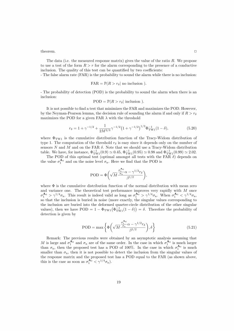
In the above setting, we calculate the SVD of the unperturbed MSR matrix A0. Figure1 displays logarithmic scale plot of the singular values of A0. It has a good accordance withthe previous theoretical analysis: each inclusion according to three singular values. Thenwe can construct the projection Pimag with the first three singular vectors correspondingto the first three significant singular values. In the right part of Figure 1, we also plot themagnitude of IMU on cross section z = 0, which shows that the MUSIC algorithm can detectthe inclusion very well.

We test the influence of the noisy measurements by adding a Gaussian noisy matrixwith mean zero and variance σ2

n/M to unperturbed MSR matrix A0. In our tests, theGaussian noise is generated by MATLAB function randn. The imaging results shown inFigure 2 indicate that with the decreasing of noise level the imaging results become moreand more sharp. Then we show the validity of (5.21). Noticing that M = N makes γ = 1in our setting. By the analysis in Section 5, for given FAR δ, POD depends on the ratioσA01 /σn. Here we only consider the critical regime in which σA0

1 is of the same order of σn(specially σA0

1 > σn). Fixing FAR δ, for each ratio σA01 /σn, we generate 1000 Gaussian noisy

matrices with mean zero and variance σ2n/M and add them to A0 to get according noisy

MSR matrices A. We compute R with the help of SVD for each A and count the times forR > rδ to get the numerical POD. Figure 3 shows the comparisons between numerical POD

20

100

101

102

103

10−25

10−20

10−15

10−10

10−5

σn=0

−0.5

0

0.5

−0.5

0

0.50

50

100

150

magnitude of imaging functional on cross section z=0.

Figure 1: Distribution of singular values of A0 with M = N = 256 and the magnitude ofIMU on plane z = 0.0.

and (5.21) for each δ. We can conclude that the numerical results have a good accordancewith (5.21) and the accordance is better when σA0

1 /σn becomes bigger.

7 Concluding Remarks

In this paper we have provided an asymptotic expansion for the perturbations of the mag-netic field due to the presence of a small conductive inclusion. The characteristic size of theinclusion is of order the depth skin. Our asymptotic expansion is valid for arbitrary shapedinclusions. Based on it, a detection test and a localization method have been provided andtested. It would be very interesting to use our results in this paper for real-time targetidentification in eddy current imaging using dictionary matching. We also plan to use themfor target tracking from induction data. Another interesting problem is to quantitativelyestimate the resolution of the direct localization from induction data in the presence of noise.This would be the subject of a forthcoming publication.

References

[1] H. Ammari, A. Buffa, and J.C. Nedelec, A justification of eddy currents model for theMaxwell equations, SIAM J. Appl. Math., 60 (2000), 1805–1823.

[2] H. Ammari, J. Garnier, H. Kang, W.-K. Park, and K. Sølna, Imaging schemes forperfectly conducting cracks, SIAM J. Appl. Math., 71 (2011), 68–91.

[3] H. Ammari, J. Garnier, and K. Sølna, A statistical approach to target detection andlocalization in the presence of noise, Waves Random Complex Media, 22 (2012), 40–65.

[4] H. Ammari, E. Iakovleva, D. Lesselier, and G. Perrusson, A MUSIC-type electromagnet-ic imaging of a collection of small three-dimensional inclusions, SIAM J. Sci. Comput.,29 (2007), 674–709.

[5] H. Ammari and H. Kang, Reconstruction of small inhomogeneities from boundary mea-surements, vol. 1846, Lecture Notes in Mathematics, Springer-Verlag, Berlin, 2004.

21

detecting results on plane z=0.

−0.5 0 0.5

−0.5

−0.4

−0.3

−0.2

−0.1

0

0.1

0.2

0.3

0.4

0.5

detecting results on plane z=0.

−0.5 0 0.5

−0.5

−0.4

−0.3

−0.2

−0.1

0

0.1

0.2

0.3

0.4

0.5

detecting results on plane z=0.

−0.5 0 0.5

−0.5

−0.4

−0.3

−0.2

−0.1

0

0.1

0.2

0.3

0.4

0.5

detecting results on plane x=0.

−0.5 0 0.5

−0.5

−0.4

−0.3

−0.2

−0.1

0

0.1

0.2

0.3

0.4

0.5

detecting results on plane x=0.

−0.5 0 0.5

−0.5

−0.4

−0.3

−0.2

−0.1

0

0.1

0.2

0.3

0.4

0.5

detecting results on plane x=0.

−0.5 0 0.5

−0.5

−0.4

−0.3

−0.2

−0.1

0

0.1

0.2

0.3

0.4

0.5

Figure 2: Detecting results on cross sectional plane z = 0(top) and x = 0(bottom) fordifferent noise level σn. σ

A01 /σn = 10, 20, 30 from left to right.

1 1.1 1.2 1.3 1.4 1.50

0.5

1

1.5

σA0

1/σ

n

PO

D

δ=0.01

numerical resultstheoretic results

1 1.1 1.2 1.3 1.4 1.50

0.5

1

1.5

σA0

1/σ

n

PO

D

δ=0.05

numerical resultstheoretic results

1 1.1 1.2 1.3 1.4 1.50

0.5

1

1.5

σA0

1/σ

n

PO

D

δ=0.10

numerical resultstheoretic results

Figure 3: POD with respect to σA01 /σn for different δ, δ = 0.01, 0.05, 0.10 from left to right.

22

[6] H. Ammari and H. Kang, Polarization and Moment Tensors: with Applications toInverse Problems and Effective Medium Theory, Applied Mathematical Sciences, Vol.162, Springer-Verlag, New York, 2007.

[7] H. Ammari and A. Khelifi, Electromagnetic scattering by small dielectric inhomo-geneities, J. Math. Pures Appl., 82 (2003), 749–842.

[8] H. Ammari, M. Vogelius, and D. Volkov, Asymptotic formulas for perturbations in theelectromagnetic fields due to the presence of inhomogeneities of small diameter II. Thefull Maxwell equations, J. Math. Pures Appl., 80 (2001), 769–814.

[9] H. Ammari and D. Volkov, The leading-order term in the asymptotic expansion of thescattering amplitude of a collection of Finite Number of dielectric inhomogeneities ofsmall diameter, Int. J. Mult. Comput. Eng., 3 (2005), 149–160.

[10] B. A. Auld and J. C. Moulder, Review of advances in quantitative eddy current non-destructive evaluation, J. Nondest. Eval., 18 (1999), 3–36.

[11] M. Capitaine, C. Donati-Martin, and D. Feral, Central limit theorems for eigenvaluesof deformations of Wigner matrices, arXiv:0903.4740.

[12] D.J. Cedio-Fengya, S. Moskow, and M.S. Vogelius, Identification of conductivity im-perfections of small diameter by boundary measurements: Continuous dependence andcomputational reconstruction, Inverse Problems, 14 (1998), 553–595.

[13] R. Hiptmair, Symmetric coupling for eddy current problems, SIAM J. Numer. Anal. 40(2002), 41-65.

[14] I. M. Johnstone, On the distrbution of the largest eigenvalue in principal componentsanalysis, Ann. Statist., 29 (2001), 295–327.

[15] V. A. Marcenko and L. A. Pastur, Distributions of eigenvalues of some sets of randommatrices, Math. USSR-Sb., 1 (1967), 507–536.

[16] J.C. Nedelec, Acoustic and Electromagnetic Equations: Integral Representations forHarmonic Problems, Springer, 2001.

[17] S. J. Norton and I. J. Won, Identification of buried unexploded ordnance from broad-band electromagnetic induction data, IEEE Trans. Geoscience Remote Sensing, 39(2001), 2253–2261.

[18] J. Rosell, R. Casanas, and H. Scharfetter, Sensitivity maps and system requirements formagnetic induction tomography using a planar gradiometer, Physiol. Meas., 22 (2001),212–130.

[19] J. Seberry, B. J. Wysocki, and T. A. Wysocki, On some applications of Hadamardmatrices, Metrika, 62 (2005), 221–239.

23